System Identification, Time Series Analysis and … · ii Captain Toolbox CAPTAIN is a MATLAB ® compatible toolbox for non stationary time series analysis, system identification,

System Identification, Time Series Analysis and Forecasting. The Captain Toolbox.

Handbook v2.0 February 2007

D. J. Pedregal, C. J. Taylor and P. C. Young

Copyright (c) 2007

Centre for Research on Environmental Systems and Statistics (CRES), Lancaster University, Lancaster, LA1 4YQ, United Kingdom.

Web www.es.lancs.ac.uk/cres/captain

Email [email protected]

ii

Captain Toolbox

CAPTAIN is a MATLAB® compatible toolbox for non stationary time series analysis, system identification, signal processing and forecasting, using unobserved components models, time variable parameter models, state dependent parameter models and multiple input transfer function models. CAPTAIN also includes functions for true digital control.

Toolbox Authors by Department

Department of Environmental Science, Faculty of Science and Technology, Lancaster University, Lancaster, LA1 4YQ, United Kingdom –

Prof. Peter C. Young [email protected] Dr. Wlodek Tych [email protected]

Engineering Department, Faculty of Science and Technology, Lancaster University, Lancaster, LA1 4YR, United Kingdom –

Dr. C. James Taylor [email protected]

Escuela Técnica Superior de Ingenieros Industriales, Edificio Politécnico, Campus Universitario s/n, 13071 Ciudad Real, Spain –

Dr. Diego J. Pedregal [email protected]

Additional Contributors

Dr Paul McKenna, Department of Environmental Science, Lancaster University

Dr Renata Romanowicz, Department of Environmental Science, Lancaster University

iii

Toolbox Installation

CAPTAIN is usually distributed as a mixture of pre-parsed MATLAB® pseudo-code (P-files) and conventional M-files. The following installation instructions assume MATLAB® itself is already installed.

1 Copy all the M- and P-files to a directory where you want the toolbox to reside, such as Program Files\Matlab\Toolbox\Captain or similar.

2 Start MATLAB® and add the above location of the toolbox to your path. You can use the standard addpath function or the graphical user interface to do this. Refer to your MATLAB® documentation for more information.

3 Once installed, typing captdemo in the MATLAB® Command Window starts a simple graphical user interface for access to the on-line demos. If this does not work, then check that you have correctly added the toolbox location to your MATLAB® path.

4 To obtain a full list of CAPTAIN functions, type help captain in the MATLAB® Command Window, replacing captain with the name of the installation directory chosen in item 1 above.

To uninstall CAPTAIN, simply delete the files and remove the associated path.

Conditions of use

The CAPTAIN software package may be freely used for scientific or educational purposes. However, if you publish any results using CAPTAIN you should state clearly that you used the tools. The full reference is:

Young, P.C., Taylor, C.J., Tych, W. and Pedregal, D.J. (2007) The Captain Toolbox. Centre for Research on Environmental Systems and Statistics, Lancaster University, UK. Internet: www.es.lancs.ac.uk/cres/captain

For commercial applications, permission is required from the authors.

The Toolbox is provided without formal support, although questions and bug reports can be emailed to the authors.

Version Tracking

Recent versions of CAPTAIN are developed for MATLAB® v7.0 (R14) onwards.

The examples in the handbook were originally developed with CAPTAIN v5.2 and MATLAB® v6.5 (R13) on a Windows PC. They have subsequently been tested for CAPTAIN v6.0 and MATLAB® v7.3 (R2006b). However, updates to the optimisation routines and default values may yield different numerical results in some cases.

Please check the on-line help for the latest function calling syntax and default values.

iv

Contents

Preface

Chapter 1 Introduction 1

Chapter 2 State Space models 18

Chapter 3 Unobserved Components models 42

Chapter 4 Time Variable Parameter models 70

Chapter 5 State Dependent Parameter models 93

Chapter 6 Discrete-Time Transfer Function models 110

Chapter 7 Continuous-Time Transfer Function models 143

Chapter 8 True Digital Control 156

Bibliography 166

Appendix 1 Reference Guide 173

Appendix 2 Data Sets, Functions and Abbreviations 269

v

Examples

1.1 Interpolation of advertising data using DLR adv.dat 111.2 Transfer function model estimation using RIV vent.dat 132.1 Estimation of a trend for the air passenger series air.dat 232.2 Hyper-parameter estimation for the air passenger series air.dat 302.3 Interpolation and variance intervention for steel consumption steel.dat 332.4 Time variable mean estimation for volume in the Nile river nile.dat 383.1 Analysis of the Mauna Loa CO2 data using DHR co2.dat 543.2 Modelling the US GDP using Trend + AR models usgdp.dat 593.3 Steel consumption in the UK revisited steel.dat 633.4 Car drivers killed and seriously injured cars.dat 664.1 Initial Evaluation of the River Cam data using DLR cam.dat 724.2 Analysis of a signal with changing frequency using DAR sdar.dat 784.3 River Cam Data analysed using DARX cam.dat 824.4 Comparison of DARX and DTFM for simulated data sdtfm1.dat 905.1 Analysis of a simulated SDARX model - 985.2 Final parameter estimates for the model in Example 5.1 - 1025.3 Analysis of squid data squid.dat 1045.4 Hydraulic Actuator - 1066.1 Simulation showing the bias of the LS parameter estimates - 1146.2 Simulation experiment using the IV algorithm - 1216.3 Simulation comparing the SRIV, RIV and ML estimates - 1256.4 Gas furnace gas.dat 1336.5 Unemployment rate in the USA usemp.dat 1376.6 Ventilation data re-visited vent.dat 1417.1 Model identification for the WG Example swg01.dat 1507.2 Parameter Estimation for the WG Example swg01.dat 1517.3 Analysis of winding pilot plant data wind.dat 1538.1 Non-minimal state space form for the ventilation model - 1578.2 Pole assignment design for the ventilation mode - 1608.3 Optimal design for the ventilation model - 161

CAPTAIN is a MATLAB® compatible toolbox for non-stationary time series analysis and forecasting. Based around a powerful state space framework, CAPTAIN extends MATLAB® to allow, in the most general case, for the identification of Unobserved Components (UC) models. Here, the time series is assumed to be composed of an additive or multiplicative combination of different components that have defined statistical characteristics but which cannot be observed directly. With Maximum Likelihood estimation of most models and the inclusion of several popular model forms, such as the Basic Structural Model of Harvey (1989) and the Dynamic Linear Model of West and Harrison (1989), together with a standard set of data pre-processing, system identification and model validation tools, CAPTAIN is a wide-ranging package for signal processing and general time series analysis.

Uniquely, however, CAPTAIN focuses on Time Variable Parameter (TVP) models, where the stochastic evolution of each parameter is assumed to be described by a generalised random walk process (Jakeman and Young, 1981). In this regard, the state space formulation utilised is particularly well suited to estimation based on optimal recursive estimation, in which the time variable parameters are estimated sequentially whilst working through the data in temporal order. In the off-line situation, where all the time series data are available for analysis, this Kalman filtering operation (Kalman, 1960) is accompanied by optimal recursive smoothing. Here the estimates obtained from the forward pass filtering algorithm are updated sequentially whilst working through the data in reverse temporal order using a backwards-recursive Fixed Interval Smoothing (FIS) algorithm (Bryson and Ho, 1969).

In this manner, CAPTAIN provides novel tools for TVP analysis, allowing for the optimal estimation of dynamic regression models, including linear regression, auto-regression (Young, 1998b) and harmonic regression (Young et al., 1999). Furthermore, a closely related algorithm for state dependent parameter estimation provides for the non-parametric identification and forecasting of a very wide class of nonlinear systems, including chaotic systems. The identification stage in this process again exploits the recursive FIS algorithms, combined with special data re-ordering and ‘back-fitting’ procedures, to obtain estimates of any state dependent parameter variations (Young, 2000).

CHAPTER 1

INTRODUCTION

Chapter 1 Introduction

CAPTAIN handbook – D. J. Pedregal, C. J. Taylor and P. C. Young – page 2

Of course, in many cases, specifying time invariant parameters for the model yields the equivalent, conventional, stationary model. In this regard, one model that has received special treatment in the toolbox is the multiple-input, single-output Transfer Function (TF) model. CAPTAIN includes functions for robust unbiased identification and estimation of both discrete- time (Young, 1984, 1985) and continuous- time (Young, 2002) TF models. One advantage of the TF model is its simplicity and ability to characterise the dominant modal behaviour of a dynamic system. This makes such a model an ideal basis for control system design.

In the latter regard, the toolbox includes a set of functions for True Digital Control (TDC), based on the Proportional-Integral-Plus (PIP) control system design methodology (Young et al., 1987; Taylor et al. 1998, 2000). The underlying philosophy of the approach is that the entire design procedure, from the identification and estimation of a suitable model through to the practical implementation of the final control algorithm, is carried out in discrete time. This differs from many conventional digital controllers, where an inherently continuous time algorithm is digitised for implementation purposes. Indeed, CAPTAIN has been successfully utilised for the design of practical PIP control systems for many years (e.g. Young et al., 1994; Gu et al., 2003; Taylor et al., 2004; Taylor and Shaban, 2006).

As demonstrated by the numerous publications and examples below, the CAPTAIN package is useful for system identification, signal extraction, interpolation, backcasting, forecasting and Data-Based Mechanistic (DBM) analysis of a wide range of linear and non-linear stochastic systems. In the latter case, the resulting DBM model is only considered fully acceptable if, in addition to explaining the data well, it also provides a description that has relevance to the physical reality of the system under study (e.g. Young, 1998b).

Some of the estimation algorithms considered here were developed originally in the 1960/1970/1980’s for the CAPTAIN and microCAPTAIN time series analysis and forecasting packages (MS-DOS based). The associated optimisation algorithms were developed in the 1980/1990’s and are used in the latest version of microCAPTAIN (Young and Benner, 1991). However, the MATLAB® implementation is much more flexible than microCAPTAIN and includes the latest innovations and improvements to the algorithms. Note that the present text refers exclusively to this CAPTAIN Toolbox for Time Series Analysis and Forecasting using MATLAB® (Taylor et al., 2007).

1.1 Modelling Philosophy

As we look around us, we perceive complexity in all directions: environmental, biological and ecological systems, socio-economic systems, and some of the more complex engineering systems - they all appear to be complicated assemblages of interacting



processes, many of which are inherently nonlinear dynamic systems, often with considerable uncertainty about both their nature and their interconnections. It is not too surprising, therefore, that the mathematical models of such systems, as constructed by scientists, social scientists and engineers, are often similarly complex. What is perhaps surprising, however, is the apparently widespread belief that such systems can be described very well, if not exactly, by deterministic mathematical equations, with little or no quantification of the associated uncertainty. Such deterministic reductionism leads inexorably to large, nonlinear simulation models which reflect the popular view that complex systems must be described by similarly complex models.

The CAPTAIN toolbox has evolved from a different DBM modelling philosophy, developed by the present third author and colleagues, which is almost the antithesis of deterministic reductionism. DBM models are obtained initially from the analysis of observational time-series but are only considered credible if they can be interpreted in physically meaningful terms. It is a philosophy that emphasises the importance of parametrically efficient, low order, dominant mode models, as well as the development of stochastic methods and the associated statistical analysis required for the identification and estimation of such models. Furthermore, it stresses the importance of explicitly acknowledging the basic uncertainty that is essential to any characterisation of physical, chemical, biological and socio-economic processes.

Previous publications map the evolution of the DBM philosophy and its methodological underpinning. Such publications utilise the approach for the analysis of numerous natural and man-made systems. An incomplete list includes: Beck and Young (1975); Jarvis et al. (1999); Parkinson and Young (1998); Price et al. (1999, 2000, 2001); Shackley et al. (1998); Tych et al. (1999); Ye et al. (1998); Young (1978, 1981; 1983, 1984; 1985; 1993a, 1993b; 1994; 1998a, 1998b, 1999a, 1999b, 2000a, 2000b, 2000c, 2001a, 2001b, 2002); Young and Beven (1994); Young and Lees (1993); Young and Minchin (1991); Young and Pedregal (1996; 1997; 1998, 1999a, 1999b); Young et al. (1996, 1997, 1999, 2000).

Naturally, these publications introduce a wide range of modelling tools, encompassing various model structures and identification algorithms. However, they can be broadly categorised into the four closely related and overlapping themes below.

1. Many of the tools that underpin the DBM modelling philosophy can be unified in terms of the discrete-time UC model. Here, the components may include a trend or low frequency component, a seasonal component (e.g. annual seasonality), additional sustained cyclical or quasi-cyclical components, stochastic perturbations, a component to capture the influence of exogenous input signals and so on. CAPTAIN allows for a wide range of such components, as discussed throughout the text.



2. Nonstationary and nonlinear signal processing based on the identification and estimation of stochastic models with time varying parameters. In this case, the term ‘nonstationarity’ is assumed to mean that the statistical properties of the signal, as defined by the parameters in an associated stochastic model, are changing over time at a rate which is ‘slow’ in relation to the rates of change of the stochastic state variables in the system under study. Although such nonstationary systems exhibit nonlinear behaviour, this can often be approximated well by TVP (or piece-wise linear) models, the parameters of which are recursively estimated.

3. Further to item 2. above, if the changes in the parameters are functions of the state or input variables (i.e. they actually constitute stochastic state variables), then the system is truly nonlinear and likely to exhibit severe nonlinear behaviour. Normally, this cannot be approximated in a simple TVP manner; in which case, recourse must be made to alternative, and more powerful in this context State Dependent Parameter (SDP) modelling methods.

4. Finally, if the essential small perturbation behaviour of the system can be approximated by linearised TF models, then robust unbiased, Refined Instrumental Variable (RIV) and Simplified Refined Instrumental Variable (SRIV) algorithms are employed. Here, either discrete-time TF models represented in terms of the backward shift operator (often denoted in the statistical and engineering literature by either 1−z , q, B or L, where the latter is utilised in the present text) or continuous-time TF models based on the Laplace Transform s-operator are identified and estimated.

1.2 Toolbox Overview

MATLAB® is a high performance language published by The MathWorks, Inc., integrating computation, visualisation and programming in a single environment (MathWorks, 2001). CAPTAIN is a collection of MATLAB® functions for the estimation of UC, TVP, SDP and TF models. By also including a number of tools for data pre-processing, system identification and model validation, CAPTAIN provides a powerful all round package for the analysis of complex stochastic systems. The following subsections introduce these main areas of functionality.

Unobserved Components models

CAPTAIN includes a range of UC models, a number of which are unique to this toolbox. In particular, the Dynamic Harmonic Regression (DHR) model, estimated using the function dhr, is very useful for signal extraction and forecasting of periodic or quasi-periodic series. This function provides smoothed estimates of the series, as well as all its components (trend, fundamental frequency and harmonic components), together with the estimated



changing amplitude and phase of the latter. Typical applications are for the analysis of periodic environmental and economic time-series; restoration of noisy signals with gaps or other aberrations; and the evaluation of temporal changes in environmental data etc. Furthermore, the same function allows for the estimation of the well-known Basic Structural Models (BSM) of Harvey (1989).

It should be pointed out that, while it is sometimes convenient to categorise the functionality of the toolbox, there is considerable overlap between the methodological areas chosen. For example, the DHR model is a particular case of the general stochastic TVP model discussed in the following subsection. In this regard, the hyper-parameters of the model, which define the statistical properties of the time variable parameters, need to be estimated in some manner. CAPTAIN provides three approaches, all through the function dhropt, namely: Maximum Likelihood (ML) based on prediction error decomposition; minimisation of the multiple-steps-ahead forecasting errors; and a special frequency domain optimisation, based on fitting the model pseudo-spectrum to the logarithm of the Auto-Regression (AR) spectrum.

An alternative to dhr/dhropt is provided by the pair univ/univopt, which allow for the estimation of various additional UC model forms. Here, the trend is extracted from the time series and a peturbational component about the trend is modelled as a pure AR component. Although they may also be utilised for modelling seasonal series, univ/univopt are particularly useful in cases where the periodic behaviour of the perturbation about the trend is not very marked. In this case, the models are estimated using either standard statistical methods or a sequential spectral decomposition approach that has been developed for the toolbox in order to avoid identifiably problems.

Time Variable Parameter models

The class of TVP, or ‘dynamic’, regression models, includes: Dynamic Linear Regression (DLR), Dynamic Harmonic Regression (DHR), Dynamic Auto-Regression (DAR), Dynamic Auto-Regression with eXogenous variables (DARX) and the closely related Dynamic Transfer Function (DTF) model. It should be noted that the term ‘dynamic’, which is used to differentiate time variable parameter regression models from their standard constant parameter relatives, is somewhat misleading, since not all of these models are inherently dynamic in a systems sense. However, it is a common term in certain areas of statistics (e.g. West and Harrison, 1989 and the references therein) and is retained for this reason.

CAPTAIN provides functions that allow for the optimal estimation of all these dynamic regression models. In each case, Fixed Interval Smoothing (FIS) estimates of the TVPs are



obtained, under the assumption that the parameters vary as one of a family of generalised random walks (see Chapter 2), namely: Random Walk (RW); Integrated Random Walk (IRW); Smoothed Random Walk (SRW); and Local Linear Trend (LLT). The associated filtering and FIS algorithms are accessible via shells, namely the functions dlr, dhr, dar, darx and dtfm. Since the regressors are freely defined by the user, the most flexible toolbox function for TVP analysis is dlr, which can include all the remaining models as special cases. The other functions all restrict the model to the most commonly used forms. For example, dhr automatically constrains the regressors to model harmonic components. As one of the key tools for estimating UC models, it has already been discussed above.

At this juncture, it is worth pointing out that CAPTAIN includes the functions mar and arspec for Auto-Regression (AR) model and spectrum estimation. However, in the context of dynamic regression, dar and darsp are instead useful for evaluating changing signal spectra and time-frequency analysis based on DAR models, since they provide the AR spectrum at each point in time based on the locally optimum time variable AR parameters.

Further to this, darx is an extension of the DAR model to include measured eXogeneous or input time series that are thought to affect the output, while dtfm augments the model in order to allow for coloured noise in the output signal. The latter function employs instrumental variables in the solution to ensure that the parameter estimates are unbiased (see below and Chapter 4). In this manner, the functions darx and dtfm are truly dynamic in a systems sense and form a link between the dynamic regression analysis considered here and the dedicated TF modelling component of the toolbox discussed below.

In the case of dlr, dar, darx and dtfm, the Noise Variance Ratio (NVR) and other hyper-parameters, which define the statistical properties of the TVP’s, are optimised via ML based on prediction error decomposition. The relevant toolbox functions are dlropt, daropt, darxopt and dtfmopt. In comparison with most other algorithms for TVP estimation, the main innovations in CAPTAIN are this automatic hyper-parameter optimisation, the provision of FIS rather than the filtered TVP estimates and the various special uses outlined above.

State Dependent Parameter models

The approach to TVP estimation discussed above works very well in situations where the parameters are slowly varying when compared to the observed temporal variation in the measured system inputs and outputs. Although such models are nonlinear systems, since the same inputs, injected at different times, will elicit quite different output responses, the resultant nonlinearity is fairly mild. It is only when the parameters are varying at a rate commensurate with that of the system variables themselves that the model behaves in a



heavily nonlinear or even chaotic manner. For such cases, CAPTAIN includes a novel algorithm for state dependent parameter estimation, sdp, allowing for the non-parametric identification and forecasting of a very wide class of nonlinear systems.

Multi-Input Transfer Function models

There are numerous algorithms for estimating TF models. However, the primary technique employed in CAPTAIN, is the least squares- based instrumental variable approach. Here, an adaptive auxiliary model is introduced into the solution in order to avoid parameter bias and to optimally filter the data, so making the estimation more statistically efficient.

In particular, CAPTAIN provides the recursive and en-block RIV and SRIV algorithms, as well as more conventional least squares based approaches, primarily through the functions riv (for discrete-time systems) and rivc (continuous-time). Both these functions return the modelling results in the form of a special matrix from which the various parameters and standard errors may be extracted using getpar. Such parameters may subsequently be utilised for simulation and forecasting through conventional MATLAB® commands like filter, or by using SIMULINK® (MathWorks, 2001).

For a given physical system, an appropriate structure first needs to be identified, i.e. the most appropriate values for the time delay and the orders of the numerator and denominator polynomials in the TF. In this regard, CAPTAIN utilises two functions, namely rivid (discrete-time) and rivcid (continuous-time), which provide numerous statistical diagnostics associated with the model. These include the Coefficient of Determination 2

TR , based on the response error, which is a simple measure of model fit; and the more sophisticated Young Identification Criterion (YIC), which provides a combined measure of fit and parametric efficiency.

True Digital Control

Following the identification of a suitable discrete-time time TF model, PIP control systems are determined using either the pip or pipopt functions, for pole assignment or Linear Quadratic (LQ) optimal design respectively. PIP control with command input anticipation is implemented using pipcom. Finally, gains and pipcl are used to analyse the closed-loop system. The above functions are for the single input, single output (SISO) case, while mfdform, mfd2nmss, mpipqr and mpipinit are used for multivariable PIP control. Finally, dlrqri provides the iterative linear quadratic regulator solution for either the SISO or multivariable cases; while piplib is the associated Simulink® library for various PIP control structures, including the conventional feedback form and an alternative forward path approach.



Conventional Models, Identification Tools and Auxiliary functions

As pointed out above, specifying time invariant parameters in CAPTAIN usually yields the equivalent stationary time series model. In this manner, many of the functions above may be utilised to estimate either the well known conventional model or the more sophisticated TVP version, depending on the input arguments chosen.

Similarly, system identification is inherent to the modelling approach utilised by most of the functions already discussed. However, identification tools not yet mentioned, include: acf to determine the sample and partial autocorrelation function; ccf for the sample cross-correlation; period to estimate the periodogram; and statist for some sample descriptive statistics. Additional statistical diagnostics include: boxcox, cusum and histon.

Finally, del generates a matrix of delayed variables; fcast may be employed to prepare data for forecasting and interpolation; irwsm for smoothing, decimation or for fitting a simple trend to a time series; prepz to prepare data for TF modelling (e.g. baseline removal and input scaling); scaleb to rescale the estimated TF model numerator polynomial following initial prepz use; stand to standardise or de-standardise a matrix by columns; and reconst to reconstruct a time series by removing any dramatic jumps in the trend.

1.3 Getting Started

Installation instructions and conditions of use are given in the preface. Since CAPTAIN is largely a command line toolbox, it is assumed that the reader is already familiar with basic MATLAB® usage, such as loading data, plotting graphs and writing simple M-files. Introductory guides to the package include Etter (1993) and Biran and Breiner (1995). For example, to plot the well known airline passenger series (e.g. Box and Jenkins, 1970), enter the following text at the MATLAB® Command Window prompt,

>> load air.dat >> plot(air) >> title(‘thousands of passengers per month (1949-1960)’)

These data are included with CAPTAIN for demonstration purposes, in a standard text file. If an error occurs, then check that you have correctly added the toolbox location to your MATLAB® path. Note that the Courier New font is used to indicate such worked examples throughout the text. Another convention employed here, is that function and variable names referred to in the body of the text, such as plot, are highlighted in bold notation.



Getting Help

On-line help information follows MATLAB® conventions. For example, to obtain a full list of functions, type help captain in the Command Window, where captain is the name of the installation directory. Similarly, the brief calling syntax for each function is obtained by entering its name without any input arguments, while more information is provided using the standard help command, as illustrated below.

>> irwsm IRWSM Integrated Random Walk smoothing and decimation [t,deriv,err,filt,h,w,y0]=irwsm(y,TVP,nvr,Int,dt) >> help irwsm IRWSM Integrated Random Walk smoothing and decimation [t,deriv,err,filt,h,w,y0]=irwsm(y,TVP,nvr,Int,dt) y: Time series (*) TVP: Model type (RW=0, IRW=1, DIRW=2) (1) nvr: NVR hyper-parameter (1605*(1/(2*dt))^4) Int: Vector of variance intervention points (0) dt: Sampling (1) t: Decimated (or simply smoothed if dt=1) series deriv: Derivatives err: Standard error filt: Filter frequency response h: Frequency response w: Frequency axis for plots y0: Interpolated data See also IRWSMOPT, FCAST, STAND, DHR, DHROPT, SDP

In the latter case, each input argument is described in turn, followed by the output arguments and any other information. Note that the default values for any optional inputs are given in brackets, whilst any necessary inputs, such as the data vector y above, are listed with an asterix. In this case, the default TVP = 1 implies the following model based on an IRW plus noise,

ttt eTy += (1.1)

tttt TTT η+−= −− 212 (1.2)

where ty is the time series, tT is the smoothed signal at sample t, returned by irwsm as the first output argument, and 1−tT and 2−tT are their values at the two previous samples, respectively. Here, tT is effectively a time variable parameter, whose stochastic evolution in the form of an IRW is described by equation (1.2). Finally, tη and et are independent



zero mean white noise sequences with variance 2q and σ 2 , representing the system disturbances and measurement noise respectively.

It should be pointed out that the on-line help messages in CAPTAIN are kept deliberately concise, so that the experienced user can find information quickly (some of the more advanced functions can have ten or more input arguments). For new users, the Reference Guide in Chapter 8 provides more descriptive information about each of the options, whilst the various models implemented in the toolbox are defined in Chapters 2 to 7.

Empty variables [] may be used to indicate default values when a mixture of defaults and user specified arguments are required. For example, a smoothed trend may be fitted to the airline passengers series as follows,

>> load air.dat >> t = irwsm(air, [], 0.0001); % equivalent to t = irwsm(air, 1, 0.0001) >> plot([air t])

In Chapter 2, the ‘IRW plus noise’ model is developed within a state space framework, based on the definition of suitable observation (1.1) and state (1.2) equations. Note that the 3rd input argument to irwsm specifies the associated Noise Variance Ratio (NVR) hyper-parameter. Defined here as 0001.022 =σq , this variable is closely related to the bandwidth of the filter, as discussed in Example 2.1 (Chapter 2).

Demonstrations

The following command initialises the standard MATLAB® Demo Window for access to the on-line demonstrations,

>> captdemo

This simple graphical user interface provides basic background information about CAPTAIN, slideshows and numerous Command Line demos. The latter demos utilise the MATLAB® Command Window for input and output, as well as generating graphs in a separate figure window, so make sure the command window is visible while you run these.

Experience suggests that one of the most effective ways to get started with CAPTAIN, is to examine each Command Line Demo in turn and then to personally adapt them for each new data set. The following examples are based on two of these demos. The intention is to provide a brief illustration of toolbox functionality for users already familiar with the methodology, or at least to introduce some of the ideas to the open minded reader who is not. In this regard, it should be pointed out that formal stochastic descriptions of the models are withheld until later chapters. For brevity, note that the straightforward MATLAB® code to label the plots, set the axis limits etc. is not necessarily shown.



0 10 20 30 40 50 60 70 80 90

0

0.1

0.2

0.3

0.4

Resp

onse

0 10 20 30 40 50 60 70 80 90

0

200

400

600

800

Expe

nditu

re

Time (sample number)

Figure 1.1 Scaled advertising data plotted against an arbitrary fixed sampling rate. Top: response to advertising. Bottom: expenditure on advertising.

Example 1.1 Interpolation of advertising data using DLR

Dynamic Linear Regression or DLR provides an excellent vehicle for the analysis of data in areas such as economic, business and social data, where regression analysis is a popular method of modelling relationships between variables and where these relationships may change over time. In this regard, consider the following straightforward demonstration from the Toolbox, which examines the relationship between a particular company’s expenditure on advertising and their measure of the public’s response to this expenditure, as illustrated in Figure 1.1.

For the purposes of the example, these confidential data have been scaled in an arbitrary manner, so no units are given in the plots. The output data are in the range 0-1, where a larger number implies a more successful response to the advertising. It is clear that the response data contain missing values, represented in MATLAB® by special Not-a-Number or nan values and forming gaps in the top plot of Figure 1.1. The filtering and smoothing algorithms implemented in CAPTAIN automatically account for these.

For a preliminary analysis of these data, we will utilise the following model,



90...,,2,1 =++= teubTy ttttt (1.3)

where yt is the response and tu is the expenditure, while tT and tb are the time variable parameters. Finally, et is a serially uncorrelated and normally distributed Gaussian sequence with zero mean value and variance σ 2 . Note that a full description of the general DLR methodology is given in Chapter 4.

For constant parameters TTt = and bbt = , equation (1.3) takes the form of a conventional regression model based on the equation of a straight line. However, here we utilise dlropt to determine if the optimal values of the parameters, in a Maximum Likelihood sense, in fact vary over time. In this regard, assuming a default random walk model for each of the parameters, the associated NVR hyper-parameters are estimated as follows,

>> load adv.dat >> u = adv(:, 1); % expenditure >> y = adv(:, 2); % response >> z = [ones(size(u)) u]; % regressors >> nvr = dlropt(y, z) nvr = 0.0078 0.0000

While dlropt is running, a window will briefly appear on screen indicating the optimisation algorithm being utilised, together with an update of the Log-Likelihood. If the solution fails to converge the optimisation may be terminated by pressing the STOP button, although this should not prove necessary in the present case.

It should be pointed out that default values for the Toolbox have been carefully chosen, in order to be as widely applicable as possible. In the present case, the default initial conditions and optimisation settings converge to a solution without any problem, hence only the first two input arguments are required.

From this analysis, it appears that the tT level or trend parameter varies significantly over time (NVR = 0.0078), while the tb slope parameter is relatively time invariant and has a NVR value close to zero. To determine the fit and parameters,

>> [fit, fitse, par] = dlr(y, z, [], nvr);

By default, dlr assumes NVR’s of zero, so the 4th input argument above is necessary to specify the previously optimised values. The 3rd input argument selects the model type: in this case, empty brackets imply the default random walk model again. Examination of the parameters, returned as the first and second columns of par, show how these evolve gradually over time.



0 10 20 30 40 50 60 70 80 90

0

0.1

0.2

0.3

0.4

Resp

onse

Time (sample number)

Figure 1.2 Scaled response to advertising plotted against an arbitrary fixed sampling rate. Data (circles), DLR fit (solid) and standard errors (dashed).

The model fit and associated standard errors are shown in Figure 1.2, which is obtained using the code below,

>> plot(y, 'o') >> hold on >> plot(fit) >> plot(fit+2*fitse, ':') >> plot(fit-2*fitse, ':')

It is clear from Figure 1.2 that the data all lie within the standard error bounds. Note also that no user intervention was required to interpolate over the missing response data: both fit and par apply over the entire time series. Refer to Chapter 8 for a full list of optimisation settings and output arguments. For example, dlr can return the interpolated output y0, consisting of the original series with any missing data replaced by the model fit.

Example 1.2 Transfer function model estimation using RIV

Many control systems, both classical and modern, are analysed by means of TF models. Indeed, CAPTAIN has been successfully utilised for the design of control systems for many years, particularly with regards to the development of Proportional-Integral-Plus (PIP) control methods (Young et al., 1987; Taylor et al., 2000). One recent practical application is concerned with forced ventilation in animal houses (Taylor et al., 2003). Here, uncontrolled data are first collected in order to identify the dominant dynamics of the fan.

For a particular test installation at the Katholieke Universiteit Leuven, the SRIV algorithm, combined with the 2

TR and YIC identification criteria (Chapter 6), reveal that a first order model with 6 seconds time delay provides the best estimated model and most optimum fit to the data across a wide range of operating conditions. In a typical experiment, based on a 2 second sampling rate, the SRIV algorithm yields the following difference equation,



31 8.79438.0 −− += ttt uyy (1.4)

where ty is the airflow rate (m3/h) and tu is the applied voltage to the fan expressed as a percentage. Equation (1.4) shows that the output variable ty , is a simple linear function of it’s value at the previous sample and the delayed input variable. Equation (1.4) may alternatively be represented in terms of the backward shift operator L, i.e. jtt

j yyL −= , by the following discrete-time TF model,

tt uL

Ly438.018.79 3

−= (1.5)

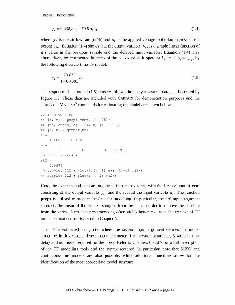
The response of the model (1.5) closely follows the noisy measured data, as illustrated by Figure 1.3. These data are included with CAPTAIN for demonstration purposes and the associated MATLAB® commands for estimating the model are shown below.

>> load vent.dat >> [z, m] = prepz(vent, [], 25); >> [th, stats, e] = riv(z, [1 1 3 0]); >> [a, b] = getpar(th) a = 1.0000 -0.4381 b = 0 0 0 79.7835 >> rt2 = stats(3) rt2 =

0.9873 >> subplot(211); plot([z(:, 1) z(:, 1)-e]+m(1)) >> subplot(212); plot(z(:, 2)+m(2))

Here, the experimental data are organised into matrix form, with the first column of vent consisting of the output variable ty , and the second the input variable tu . The function prepz is utilised to prepare the data for modelling. In particular, the 3rd input argument subtracts the mean of the first 25 samples from the data in order to remove the baseline from the series. Such data pre-processing often yields better results in the context of TF model estimation, as discussed in Chapter 6.

The TF is estimated using riv, where the second input argument defines the model structure: in this case, 1 denominator parameter, 1 numerator parameter, 3 samples time delay and no model required for the noise. Refer to Chapters 6 and 7 for a full description of the TF modelling tools and the syntax required. In particular, note that MISO and continuous-time models are also possible, while additional functions allow for the identification of the most appropriate model structure.



0 50 100 150 2002200

2400

2600

2800

3000

3200

m3 /

hour

0 50 100 150 20028

30

32

34

36

Time (2 second samples)

%

Figure 1.3 Top: ventilation rate (m3/h) and response of the identified TF model (thick trace)

Bottom: applied voltage to the control fan expressed as a percentage.

The first riv output argument, th, is a matrix containing information about the TF model structure, the estimated parameters and their estimated accuracy. In this case, getpar is utilised to extract the required parameter estimates for later control system design. Note that these parameter vectors include the leading unity of the TF denominator, and that the time delays are represented as zero valued elements in the numerator. The second riv output argument, stats, lists nine statistical diagnostics associated with the model, including 9873.02 =TR , implying that the model describes nearly 99% of the variation in the data. Finally, the modelling errors are returned as the variable e and are used in the code above to compare the TF response with the original data, as shown in Figure 1.3. In this graph, the baseline is returned to the series.

Note that the built-in MATLAB® function filter may also be employed to simulate the TF response using these parameter vectors. As discussed in Chapter 6, filter can be useful for simulation and (if estimates of the future input variable are available) forecasting purposes.

1.4 How to use this book

This publication is primarily intended as a tutorial guide to the data-based mechanistic modelling philosophy developed by Peter Young and colleagues over many years. In this



regard, the chapter headings follow a logical structured progress through the relevant methodology, using worked examples throughout the text.

Time variable parameter modelling is introduced in Chapter 2. Here, the filtering algorithm, smoothing algorithm, generalised random walk model and hyper-parameter optimisation routines are formally described. This chapter presents the models in their most general state space form, while the following three chapters introduce the various special cases, namely: unobserved component models (Chapter 3); dynamic regression models (Chapter 4); and state dependent parameter models (Chapter 5). Next, discrete-time (Chapter 6) and continuous-time (Chapter 7) transfer function models are considered, followed by a chapter on control system design (Chapter 8).

Finally, Appendix 1 lists each CAPTAIN function in alphabetical order, showing the calling syntax, together with a brief description of the associated input and output arguments. Appendix 1 is designed to augment the concise on-line help messages. To learn about a particular model, turn to Table A2 for the appropriate function name, then to Appendix 1 for its description. The See Also section for each entry in Appendix 1 lists the relevant worked examples from the text.

Some of the algorithms discussed here have been in constant use for over 20 years. The present authors hope that the CAPTAIN toolbox for MATLAB® will allow interested researchers to add to the ever expanding list of successful applications, which already includes time series analysis, forecasting and control of numerous biological, engineering, environmental and socio-economic processes (see references above).

Documents

System Identification, Time Series Analysis and … · ii Captain Toolbox CAPTAIN is a MATLAB ® compatible toolbox for non stationary time series analysis, system identification,