Embed Size (px)
Citation preview
System Level Design, Performance, Cost and Economic Assessment – Tacoma Narrows Washington Tidal In-Stream
Power Plant
Project: EPRI North American Tidal In Stream Power Feasibility Demonstration Project Phase: 1 – Project Definition Study Report: EPRI – TP – 006 WA Author: Brian Polagye and Mirko Previsic Contributors: George Hagerman and Roger Bedard Date: June 10, 2006

System Level Design, Performance and Cost of Tacoma Narrows Tidal Power Plant
2
DISCLAIMER OF WARRANTIES AND LIMITATION OF LIABILITIES This document was prepared by the organizations named below as an account of work sponsored or cosponsored by the Electric Power Research Institute Inc. (EPRI). Neither EPRI, any member of EPRI, any cosponsor, the organization (s) below, nor any person acting on behalf of any of them. (A) Makes any warranty or representation whatsoever, express or implied, (I) with respect to the use of any information, apparatus, method, process or similar item disclosed in this document, including merchantability and fitness for a particular purpose, or (II) that such use does not infringe on or interfere with privately owned rights, including any party’s intellectual property, or (III) that this document is suitable to any particular user’s circumstance; or (B) Assumes responsibility for any damages or other liability whatsoever (including any consequential damages, even if EPRI or any EPRI representative has been advised of the possibility of such damages) resulting for your selection or use of this document or any other information, apparatus, method, process or similar item disclosed in this document. Organization(s) that prepared this document Electricity Innovation Institute Global Energy Partners LLC Virginia Polytechnic Institute and State University Mirko Previsic Consulting Brian Polagye1 Consulting
1 PhD Student, Department of Mechanical Engineering, University of Washington

System Level Design, Performance and Cost of Tacoma Narrows Tidal Power Plan
1
Table of Contents
1. Introduction and Summary.......................................................................................... 6 2. Site Selection............................................................................................................. 11
2.1. Tidal Energy Resource ........................................................................................... 13 2.2. Grid Interconnection Options................................................................................. 18 2.3. Nearby Port Facilities............................................................................................. 19 2.4. Bathymetry ............................................................................................................. 20 2.5. Seabed Composition............................................................................................... 21 2.6. Navigational Clearance .......................................................................................... 24 2.7. Other Site Specific Considerations ........................................................................ 24
3. Marine Current Turbines........................................................................................... 26
3.1. Device Performance ............................................................................................... 27 3.2. Device Specification .............................................................................................. 29 3.3. MCT Device Evolution .......................................................................................... 30 3.4. Monopile Foundations............................................................................................ 33 3.5. Pile Installation....................................................................................................... 34 3.6. Operational and Maintenance Activities ................................................................ 38
4. Electrical Interconnection ......................................................................................... 41
4.1. Subsea Cabling....................................................................................................... 42 4.2. Onshore Cabling and Grid Interconnection ........................................................... 44
5. System Design – Pilot Plant ...................................................................................... 45 6. System Design - Commercial Plant........................................................................... 49
6.1. Array Layout .......................................................................................................... 49 6.2. Electrical Interconnection ...................................................................................... 52 6.3. Array Performance ................................................................................................. 54 6.4. Site Specific Issues................................................................................................. 58
7. Cost Assessment – Pilot Plant ................................................................................... 60 8. Cost Assessment – Commercial Plant....................................................................... 61 9. Cost of Electricity Assessments ................................................................................ 65 10. Sensitivity Studies ..................................................................................................... 71
10.1. Array Size...................................................................................................... 71 10.2. Array Availability ......................................................................................... 73 10.3. Current Velocity ............................................................................................ 73 10.4. Design Velocity............................................................................................. 75 10.5. Financial Assumptions .................................................................................. 75
System Level Design, Performance and Cost of Tacoma Narrows Tidal Power Plant
2
11. Conclusions ............................................................................................................... 77 11.1. Pilot In-Stream Tidal Power Plant ................................................................ 77 11.2. Techno-economic Challenges ....................................................................... 78 11.3. General Conclusions ..................................................................................... 79 11.4. Recommendations ......................................................................................... 82
12. References ................................................................................................................. 85 13. Appendix ................................................................................................................... 87
13.1. Validity of Pt. Evans Velocity Predictions for Commercial Array............... 87 13.2. Irrelevance of Flow Decay Concerns ............................................................ 88 13.3. Hub-height Velocity Approximation ............................................................ 89 13.4. Utility Generator Cost of Electricity Worksheet........................................... 93 13.5. Non Utility Generator Internal Rate of Return Worksheet ......................... 100 13.6. Municipal Utility Generator Cost of Electricity Worksheet ....................... 105
System Level Design, Performance and Cost of Tacoma Narrows Tidal Power Plant
3
Table of Figures Figure 1 – Tacoma Narrows [5] ............................................................................................ 11 Figure 2 – Tacoma Narrows NOAA Current Stations [5,7].................................................. 14 Figure 3 – Tidal Cycle Velocity Variation at Pt. Evans (February 1st-14th, 2005) ............... 15 Figure 4 –Tidal Current Histogram for Pt. Evans ................................................................. 15 Figure 5 – Depth Profile of Tacoma Narrows in vicinity of Pt. Evans ................................. 16 Figure 6 – Daily Channel Power Variation at Pt. Evans (February 9th, 2005)...................... 17 Figure 7 – Tidal Cycle Channel Power Variation at Pt. Evans (February 1st-14th, 2005)..... 18 Figure 8 – Monthly Average Channel Power at Pt. Evans (2005)........................................ 18 Figure 9 – Interconnection Infrastructure near Pt. Evans [5]................................................ 19 Figure 10 – Aerial Photograph of Port of Tacoma [5] .......................................................... 20 Figure 11 – Tacoma Narrows Bathymetry ............................................................................ 21 Figure 12 – Tacoma Narrows Seabed Composition [9] ........................................................ 22 Figure 13 – Seabed Composition, Tacoma Narrows Bridge (1939) [13] ............................. 23 Figure 14 – MCT SeaGen (courtesy of MCT) ...................................................................... 26 Figure 15 – Comparison of Flow and Electric Power at Pt. Evans....................................... 29 Figure 16 – Daily Variation of Flow and Electric Power at Pt. Evans (February 9th, 2005) 29 Figure 17 – MCT SeaFlow Test Unit (courtesy of MCT)..................................................... 31 Figure 18 - Conceptual MCT deep water configuration (courtesy of MCT) ........................ 32 Figure 19 - Simulation of pile-soil interaction subject to lateral load [23]........................... 33 Figure 20 - Pile Weight as a function of design velocity for different sediment types......... 34 Figure 21 – Pile Installed in Bedrock (courtesy of Seacore Ltd.) ......................................... 35 Figure 22 - Manson Construction 600 ton Derrick Barge WOTAN operating offshore (courtesy of Manson Construction)....................................................................................... 36 Figure 23 - Typical Rigid Inflatable Boat (RIB)................................................................... 39 Figure 24 – Generalized interconnection for turbine array ................................................... 41 Figure 25 – Armored submarine cables ................................................................................ 43 Figure 26 – Pt. Evans Pilot Plant Layout .............................................................................. 46 Figure 27 - Conceptual Electrical Design for a single TISEC Unit ...................................... 47 Figure 28 – Pilot Plant Interconnection................................................................................. 48 Figure 29 – Pt. Evans Commercial Array Layout ................................................................. 49 Figure 30 – Turbine Size and Spacing .................................................................................. 51 Figure 31 – Pile Installation Depth Distribution ................................................................... 52 Figure 32 – Commercial Plant Interconnection .................................................................... 54 Figure 33 – Daily Array Power Output (February 9th, 2005)................................................ 55 Figure 34 – Tidal Cycle Array Power Output (February 1st-14th, 2005)............................... 56 Figure 35 – Daily Average Array Power (2005)................................................................... 56 Figure 36 – Monthly Average Array Power Output (2005).................................................. 57 Figure 37 – MCT SeaFlow (courtesy of MCT)..................................................................... 59 Figure 38 – Sensitivity of COE to number of turbines installed........................................... 71 Figure 39 – Sensitivity of Capital Cost elements to number of installed turbines................ 72 Figure 40 – Sensitivity of annual O&M cost to number of installed turbines ...................... 72 Figure 41 – Sensitivity of COE to array availability............................................................. 73 Figure 42 – Sensitivity of COE to average velocity.............................................................. 74 Figure 43 – Sensitivity of COE to average power flux ......................................................... 74

System Level Design, Performance and Cost of Tacoma Narrows Tidal Power Plant
4
Figure 44 – Sensitivity of COE to design speed ................................................................... 75 Figure 45 – Sensitivity of COE to debt financing rate.......................................................... 76 Figure 46 – Sensitivity of COE to production credits........................................................... 76 Figure 47 – PRISM Model Predictions for Tacoma Narrows............................................... 87 Figure 48 – Representative Numerical Integration ............................................................... 91
System Level Design, Performance and Cost of Tacoma Narrows Tidal Power Plant
5
List of Tables Table 1 - Relevant Site Design Parameters ........................................................................... 13 Table 2 – Tacoma Narrows NOAA Current Stations Predicted Velocity and Power Flux .. 14 Table 3 – Channel and Extractable Power at Pt. Evans ........................................................ 17 Table 4 – Device Performance at Pt. Evans .......................................................................... 28 Table 5 – SeaGen Device Specification for Target Site........................................................ 30 Table 6 – Pilot Grid Interconnection..................................................................................... 48 Table 7 – Pt. Evans Transect MVA Ratings ......................................................................... 52 Table 8 – Pt. Evans Commercial Array Grid Interconnection .............................................. 54 Table 9 – Pt. Evans Array Performance ................................................................................ 55 Table 10 – Pilot Plant Cost Breakdown ................................................................................ 60 Table 11 - Commercial Plant Cost Breakdown..................................................................... 63 Table 12 - COE for Alternative Energy Technologies: 2010................................................ 68 Table 13 – Approximation Variance as Function of Hub Height ......................................... 91
System Level Design, Performance and Cost of Tacoma Narrows Tidal Power Plant
6
1. Introduction and Summary This document describes the results of a system level design, performance and cost study
for both a feasibility demonstration pilot plant and a commercial size in-stream tidal power
plant installed in Tacoma Narrows. For purposes of this design study, the Washington
(WA) stakeholders selected the Marine Current Turbine (MCT) tidal in-stream energy
conversion (TISEC) device for deployment at Point Evans. The study was carried out using
the methodology and standards established in the Design Methodology Report [4], the
Power Production Performance Methodology Report [1] and the Cost Estimate and
Economics Assessment Methodology Report [2].
This study evaluates a MCT SeaGen device consisting of two horizontal-axis rotors and
power trains (gearbox, generator) attached to a supporting monopile by a cross-arm. The
monopile is surface piercing and includes an integrated lifting mechanism to pull the rotors
and power trains out of the water without the intervention of specialized marine craft. The
pilot would cost $4.2M to build and produced an estimated 2010 MWh per year (716 kW
rated electric power). This cost reflects only the capital needed to purchase a SeaGen unit,
install it on site, and connect it to the grid. Therefore, it represents the installed capital cost
required to evaluate and test a SeaGen TISEC system, but does not include detailed design,
permitting and construction financing, yearly O&M or test and evaluation costs.
A commercial scale tidal power plant at the same location was also evaluated to establish a
base case from which economic comparisons to other renewable and non renewable energy
systems could be made. Unlike the pilot scale turbine, commercial turbines will not be
surface piercing. This serves to reduce the visual impact of the array and avoid multiple-use
conflicts with deep draft container traffic passing through the Narrows en route to the port
of Olympia. The cost assessment for a commercial array is predicated on the assumption
that costs for a fully submerged MCT device will be in line with the surface piercing
SeaGen. This fully submerged variant would incorporate the same power train and
foundation as the SeaGen on a different support structure. At this point, that support

System Level Design, Performance and Cost of Tacoma Narrows Tidal Power Plant
7
structure and lifting mechanism are conceptual and create significant technical and
economic uncertainty that must be eliminated prior to the installation of a commercial array.
For the proposed commercial plant of sixty-four dual-rotor turbines, the yearly electrical
energy produced and delivered to bus bar is estimated to be 120,000 MWh/year. These
turbines will, on average, extract 16MW of kinetic power from the tidal stream – 15% of the
total kinetic energy in the flow at Point Evans. Turbines could be arranged in five rows of
twelve to thirteen devices. The elements of cost and economics (in 2005$) are:
• Total Plant Investment = $103 million
• Annual O&M Cost = $3.8 million
• Utility Generator (UG) Levelized Cost of Electricity (COE)2 = 9.0 (Real) – 10.6
(Nominal) cents/kWh with renewable energy incentives equal to those that the
government provides for renewable wind energy technology
• Non Utility Generator (NUG) Levelized Cost of Electricity (IRR) = N/A (low
avoided cost of electricity in WA)
• Municipal Generator (MG) Levelized Cost of Electricity (COE) = 7.2 (Real) – 8.4
(Nominal) cents/kWh with renewable energy incentives equal to those that the
government provides for renewable wind energy technology
While not competitive with fossil generation in the near term, this is lower than the cost of
energy for wind or solar installations possible in the Puget Sound area and, as such,
represents a low cost local renewable power option for the city of Tacoma.
Tacoma Narrows has the potential of being a good location for siting an in-stream tidal
power plant. Strong currents occur four times each day, embodying, on average, over
100MW of kinetic energy. Both sides of Tacoma Narrows have significant electrical
infrastructure and power take-off cables may be readily brought ashore at Pt. Evans using
existing utility easements. Tacoma Narrows is in close proximity to the Port of Tacoma – a
major port facility which could serve as a base of operations for both installation and
maintenance.
System Level Design, Performance and Cost of Tacoma Narrows Tidal Power Plant
8
A pilot demonstration tidal plant in the Tacoma Narrows is recommended to help address
the issues such as:
• Reliability and availability
• Most cost effective type of technology and optimum size for individual turbines
• Uncertainty in project costs, particularly installation and O&M costs
• Dispatcher ability to make use of a predictable, though varying resource
• Regulatory willingness to permit TISEC installations
• Political and public acceptance
In-stream tidal energy is a potential important energy source and should be evaluated for
addition to Tacoma’s energy supply portfolio. A balanced and diversified portfolio of
energy supply options is the foundation of a reliable and robust electric grid. TISEC offers
an opportunity for Tacoma to expand its supply portfolio with a resource that is:
• Local – providing long-term energy security and keeping development dollars in
the region
• Sustainable and green-house gas emission free
• Cost competitive compared to other options for expanding and balancing the
region’s supply portfolio
Except for a few large tidal energy resource sites, such as Minas Passage, TISEC is in the
grey zone between central and distributed power applications. Typical distributed
generation (DG) motivations are:
• Delay transmission and distribution (T&D) infrastructure upgrade
• Provide voltage stability
• Displace diesel fuel in off-grid applications
• Provide guaranteed power
2 For the 45.7 MW, 20 year plant life, 10 years of PTC at 0.18 cents/kWh for a taxable entity, a REPI credit at 0.015 cents/kWh for a non taxable MG, and other assumptions documented in [2].
System Level Design, Performance and Cost of Tacoma Narrows Tidal Power Plant
9
In order to promote development of TISEC, EPRI recommends that stakeholders build
collaboration within Washington and with other State/Federal Government agencies by
forming a state electricity stakeholder group and joining TISEC Working Group to be formed
by EPRI. Additional, EPRI encourages the stakeholders to support related R&D activities at a
state and federal level and at universities in the region. This would include:
• Implement a national ocean tidal energy program at DOE
• Operate a national offshore ocean tidal energy test facility
• Promote development of industry standards
• Continue membership in the IEA Ocean Energy Program
• Clarify and streamline federal permitting processes
• Study provisions for tax incentives and subsidies
• Ensure that the public receives a fair return from the use of ocean tidal energy
resources
• Ensure that development rights in state waters are allocated through a fair and
transparent process that takes into account state, local, and public concerns.
As Tacoma Power has already applied for and received a preliminary permit from FERC for
a pilot feasibility demonstration plant at Pt. Evans in Tacoma Narrows, we recommend that
Tacoma Power progress forward with other Phase II (Detailed Design and Permitting
Project) tasks including:
• Velocity profiling survey (ADCP with CFD)
• High resolution bottom bathymetry survey
• Geotechnical survey
• Detailed engineering design using above data
• Environmental impact report
• Public outreach
• Implementation planning for Phase III (Construction)
• Financing/incentive requirements study four Phase III and IV (Operation)
System Level Design, Performance and Cost of Tacoma Narrows Tidal Power Plant
10
In order to facilitate planning for a commercial plant, we recommend that Tacoma Power
develop and support intellectual capital required for effective deployment of large TISEC
arrays. This would include activities such as:
• Modeling effect of turbines on current flows throughout Puget Sound. This
would serve to justify the expected low impact of TISEC. Additionally, this
model could be used to understand the impact of further development of tidal
energy upstream of Tacoma Narrows (e.g. Admiralty Inlet).
• Understanding array spacing limitations. In order to minimize the array footprint
and take advantage of the most energetic water it will be imperative to cluster
turbines as closely as possible without allowing the wake of one turbine to
degrade the performance of another.
This intellectual capital will take some time to develop and may be strongly site dependent.
Each of the above points represents a significant unknown in the deployment of
commercial-scale tidal in-stream energy.
System Level Design, Performance and Cost of Tacoma Narrows Tidal Power Plant
11
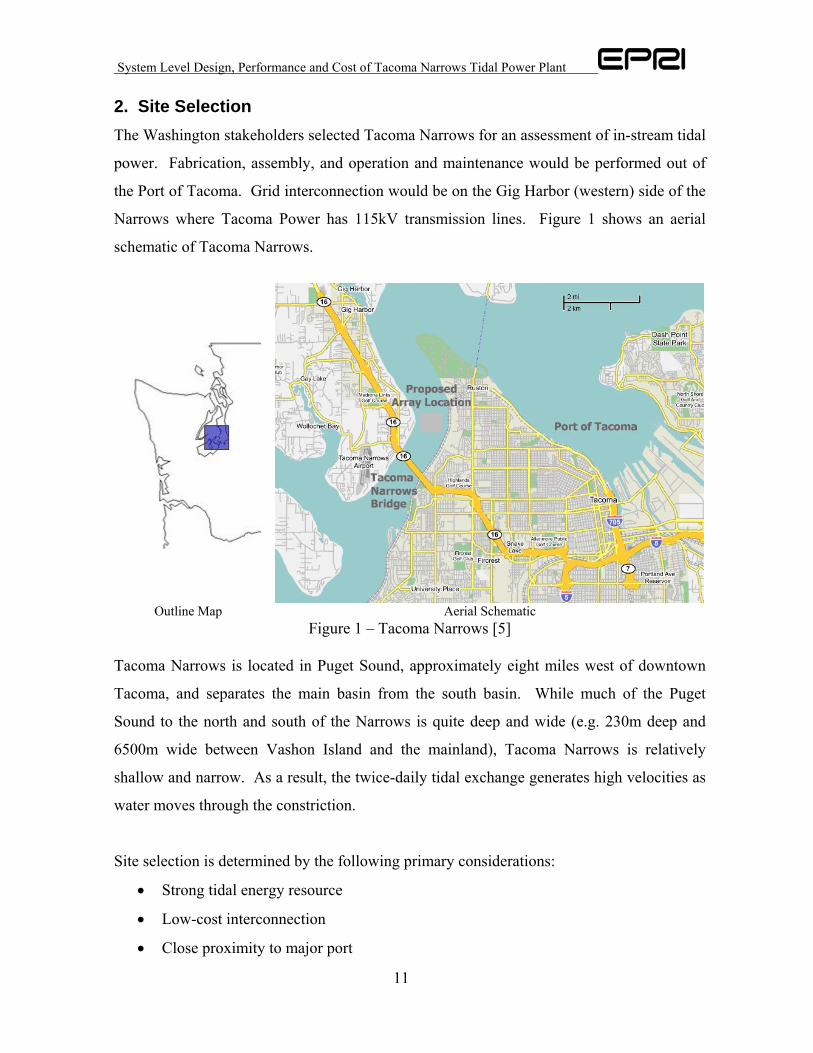
2. Site Selection The Washington stakeholders selected Tacoma Narrows for an assessment of in-stream tidal
power. Fabrication, assembly, and operation and maintenance would be performed out of
the Port of Tacoma. Grid interconnection would be on the Gig Harbor (western) side of the
Narrows where Tacoma Power has 115kV transmission lines. Figure 1 shows an aerial
schematic of Tacoma Narrows.
Outline Map Aerial Schematic Figure 1 – Tacoma Narrows [5]
Tacoma Narrows is located in Puget Sound, approximately eight miles west of downtown
Tacoma, and separates the main basin from the south basin. While much of the Puget
Sound to the north and south of the Narrows is quite deep and wide (e.g. 230m deep and
6500m wide between Vashon Island and the mainland), Tacoma Narrows is relatively
shallow and narrow. As a result, the twice-daily tidal exchange generates high velocities as
water moves through the constriction.
Site selection is determined by the following primary considerations:
• Strong tidal energy resource
• Low-cost interconnection
• Close proximity to major port

System Level Design, Performance and Cost of Tacoma Narrows Tidal Power Plant
12
The Pt. Evans site satisfies all these criteria. Tidal currents at Pt. Evans are the strongest
reported in the Narrows – 1.2 m/s average speed. This translates to a depth averaged power
flux of 1.7 kW/m2 using the methodology described in [1]. The channel at Pt. Evans has a
substantial average cross-section (63,000 m2), yielding an average flow power of 106 MW.
Tacoma Power has high voltage electrical transmission lines (115 kV) crossing at Pt. Evans
which could accommodate the power generated by a commercial array. Tacoma Narrows is
in close proximity to the Port of Tacoma, a major port annually handling over $29B in trade
goods [6]. In short – the site is optimal for TISEC device deployment.
In addition to issues driving the general siting decision, other factors are important to take
into account in the design process:
• Bathymetry: relatively flat seafloor preferred
• Seadbed composition: bearing capacity and type will determine foundation design
• Navigational clearance: turbines may need to share waterway with shipping traffic
• Site specific issues: turbine interaction with marine life, etc.
These issues, as well as those discussed above are considered in more detail in the following
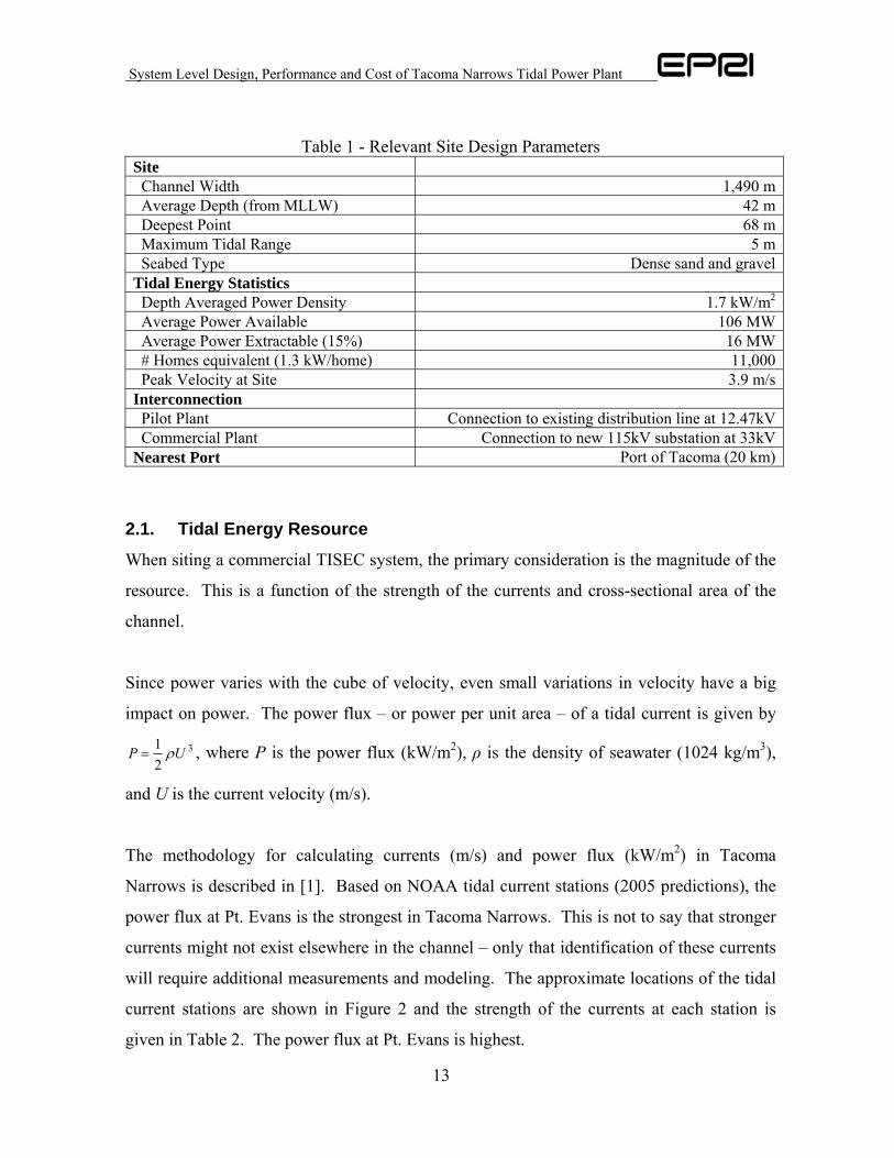
sections. Site parameters are summarized in Table 1.
System Level Design, Performance and Cost of Tacoma Narrows Tidal Power Plant
13
Table 1 - Relevant Site Design Parameters Site Channel Width 1,490 m Average Depth (from MLLW) 42 m Deepest Point 68 m Maximum Tidal Range 5 m Seabed Type Dense sand and gravelTidal Energy Statistics Depth Averaged Power Density 1.7 kW/m2
Average Power Available 106 MW Average Power Extractable (15%) 16 MW # Homes equivalent (1.3 kW/home) 11,000 Peak Velocity at Site 3.9 m/sInterconnection Pilot Plant Connection to existing distribution line at 12.47kV Commercial Plant Connection to new 115kV substation at 33kVNearest Port Port of Tacoma (20 km)
2.1. Tidal Energy Resource
When siting a commercial TISEC system, the primary consideration is the magnitude of the
resource. This is a function of the strength of the currents and cross-sectional area of the
channel.
Since power varies with the cube of velocity, even small variations in velocity have a big
impact on power. The power flux – or power per unit area – of a tidal current is given by
3
21 UP ρ= , where P is the power flux (kW/m2), ρ is the density of seawater (1024 kg/m3),
and U is the current velocity (m/s).
The methodology for calculating currents (m/s) and power flux (kW/m2) in Tacoma
Narrows is described in [1]. Based on NOAA tidal current stations (2005 predictions), the
power flux at Pt. Evans is the strongest in Tacoma Narrows. This is not to say that stronger
currents might not exist elsewhere in the channel – only that identification of these currents
will require additional measurements and modeling. The approximate locations of the tidal
current stations are shown in Figure 2 and the strength of the currents at each station is
given in Table 2. The power flux at Pt. Evans is highest.

System Level Design, Performance and Cost of Tacoma Narrows Tidal Power Plant
14
Figure 2 – Tacoma Narrows NOAA Current Stations [5,7]
Table 2 – Tacoma Narrows NOAA Current Stations Predicted Velocity and Power Flux
Station Depth Averaged Velocity (m/s)
Depth Averaged Power Flux
(kW/m2) North End (east) 1.08 1.47 North End (midstream) 0.90 0.86 North End (west) 0.60 0.40 Pt. Evans 1.12 1.70 South End (midstream) 1.03 1.33
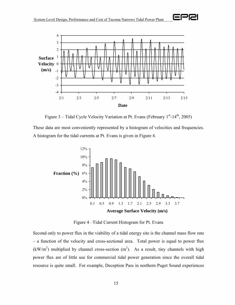
Variations in surface currents over a representative tidal cycle are shown in Figure 3. Tides
in Puget Sound exhibit a high degree of diurnality – a strong tide is often followed by a
much weaker one. This diurnality is not unique to Tacoma Narrows and is, in fact, present
at other current stations throughout Puget Sound, including Admiralty Inlet at the northern
end. At Pt. Evans, the flood tide is stronger than the ebb (average maximum flood = 2.2
m/s, average maximum ebb = 1.7 m/s). The tides are effectively bi-directional, with ebb
and flood offset by 178o (180o for perfectly bi-directional) [7].
System Level Design, Performance and Cost of Tacoma Narrows Tidal Power Plant
15
-4
-3
-2
-1
0
1
2
3
4
2/1 2/3 2/5 2/7 2/9 2/11 2/13 2/15
Date
Surface Velocity
(m/s)
Figure 3 – Tidal Cycle Velocity Variation at Pt. Evans (February 1st-14th, 2005)
These data are most conveniently represented by a histogram of velocities and frequencies.
A histogram for the tidal currents at Pt. Evans is given in Figure 4.
0%
2%
4%
6%
8%
10%
12%
0.1 0.5 0.9 1.3 1.7 2.1 2.5 2.9 3.3 3.7
Average Surface Velocity (m/s)
Fraction (%)
Figure 4 –Tidal Current Histogram for Pt. Evans
Second only to power flux in the viability of a tidal energy site is the channel mass flow rate
– a function of the velocity and cross-sectional area. Total power is equal to power flux
(kW/m2) multiplied by channel cross-section (m2). As a result, tiny channels with high
power flux are of little use for commercial tidal power generation since the overall tidal
resource is quite small. For example, Deception Pass in northern Puget Sound experiences
System Level Design, Performance and Cost of Tacoma Narrows Tidal Power Plant
16
high velocities, but has a very small cross-sectional area and, therefore, could not support a
commercial TISEC array.
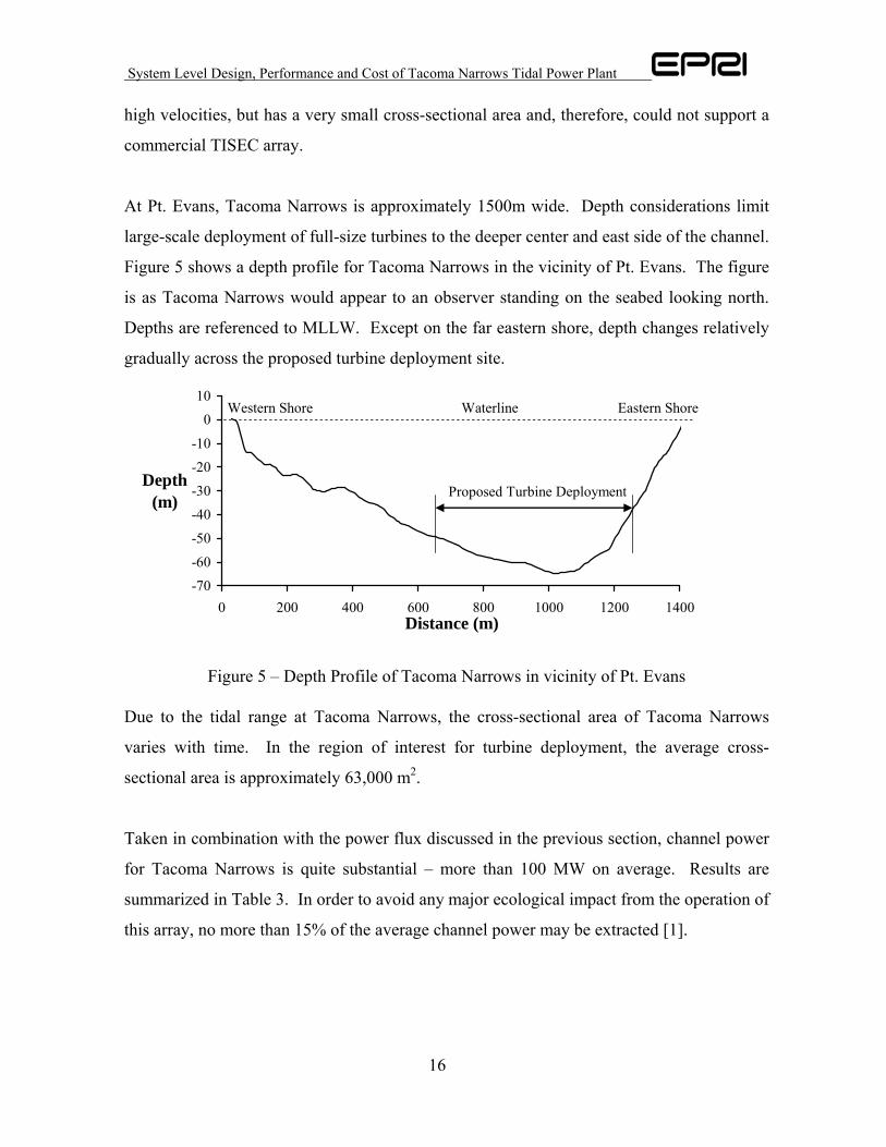
At Pt. Evans, Tacoma Narrows is approximately 1500m wide. Depth considerations limit
large-scale deployment of full-size turbines to the deeper center and east side of the channel.
Figure 5 shows a depth profile for Tacoma Narrows in the vicinity of Pt. Evans. The figure
is as Tacoma Narrows would appear to an observer standing on the seabed looking north.
Depths are referenced to MLLW. Except on the far eastern shore, depth changes relatively
gradually across the proposed turbine deployment site.
-70-60
-50
-40-30
-20-10
010
0 200 400 600 800 1000 1200 1400Distance (m)
Depth (m)
Waterline
Proposed Turbine Deployment
Eastern ShoreWestern Shore
Figure 5 – Depth Profile of Tacoma Narrows in vicinity of Pt. Evans
Due to the tidal range at Tacoma Narrows, the cross-sectional area of Tacoma Narrows
varies with time. In the region of interest for turbine deployment, the average cross-
sectional area is approximately 63,000 m2.
Taken in combination with the power flux discussed in the previous section, channel power
for Tacoma Narrows is quite substantial – more than 100 MW on average. Results are
summarized in Table 3. In order to avoid any major ecological impact from the operation of
this array, no more than 15% of the average channel power may be extracted [1].
System Level Design, Performance and Cost of Tacoma Narrows Tidal Power Plant
17
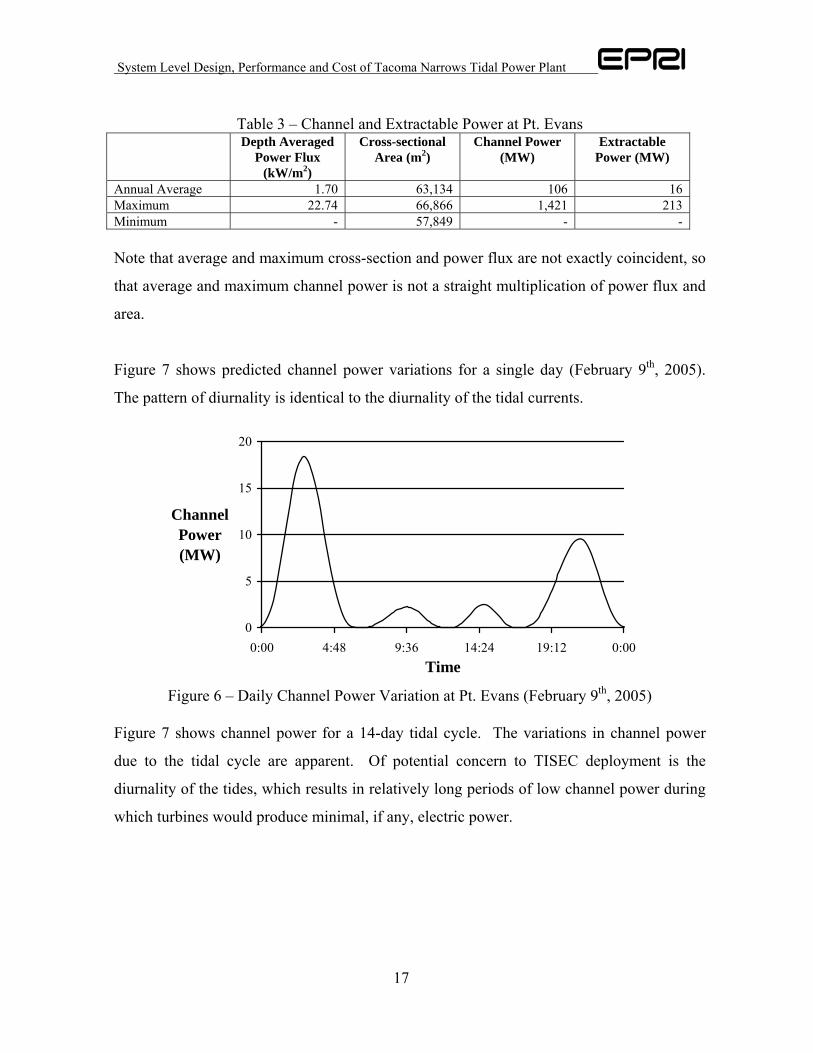
Table 3 – Channel and Extractable Power at Pt. Evans
Depth Averaged Power Flux
(kW/m2)
Cross-sectional Area (m2)
Channel Power (MW)
Extractable Power (MW)
Annual Average 1.70 63,134 106 16 Maximum 22.74 66,866 1,421 213 Minimum - 57,849 - - Note that average and maximum cross-section and power flux are not exactly coincident, so
that average and maximum channel power is not a straight multiplication of power flux and
area.
Figure 7 shows predicted channel power variations for a single day (February 9th, 2005).
The pattern of diurnality is identical to the diurnality of the tidal currents.
0
5
10
15
20
0:00 4:48 9:36 14:24 19:12 0:00Time
Channel Power (MW)
Figure 6 – Daily Channel Power Variation at Pt. Evans (February 9th, 2005)
Figure 7 shows channel power for a 14-day tidal cycle. The variations in channel power
due to the tidal cycle are apparent. Of potential concern to TISEC deployment is the
diurnality of the tides, which results in relatively long periods of low channel power during
which turbines would produce minimal, if any, electric power.
System Level Design, Performance and Cost of Tacoma Narrows Tidal Power Plant
18
0
200
400
600
800
1000
1200
1400
2/1 2/3 2/5 2/7 2/9 2/11 2/13 2/15Day
Channel Power (MW)
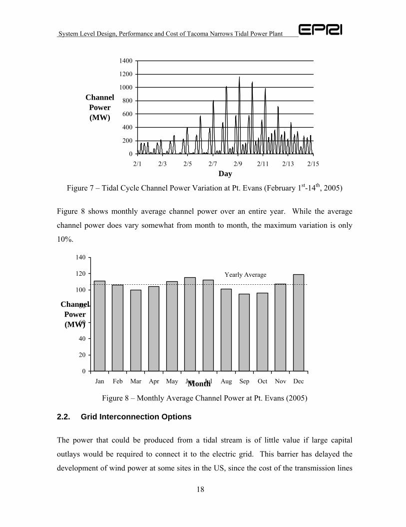
Figure 7 – Tidal Cycle Channel Power Variation at Pt. Evans (February 1st-14th, 2005)
Figure 8 shows monthly average channel power over an entire year. While the average
channel power does vary somewhat from month to month, the maximum variation is only
10%.
0
20
40
60
80
100
120
140
Jan Feb Mar Apr May Jun Jul Aug Sep Oct Nov DecMonth
Channel Power (MW)
Yearly Average
Figure 8 – Monthly Average Channel Power at Pt. Evans (2005)
2.2. Grid Interconnection Options
The power that could be produced from a tidal stream is of little value if large capital
outlays would be required to connect it to the electric grid. This barrier has delayed the
development of wind power at some sites in the US, since the cost of the transmission lines
System Level Design, Performance and Cost of Tacoma Narrows Tidal Power Plant
19
to bring the power to market may be on the same order as the cost to construct the wind
farm. Fortunately, this is not the case at Tacoma Narrows.
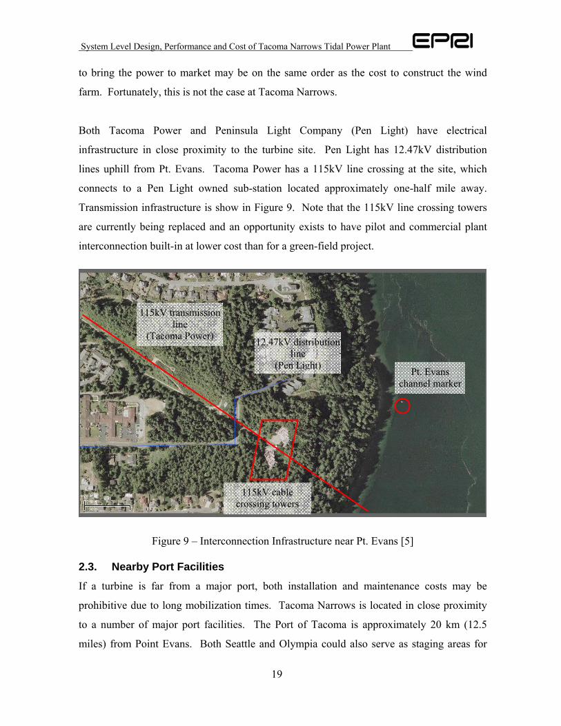
Both Tacoma Power and Peninsula Light Company (Pen Light) have electrical
infrastructure in close proximity to the turbine site. Pen Light has 12.47kV distribution
lines uphill from Pt. Evans. Tacoma Power has a 115kV line crossing at the site, which
connects to a Pen Light owned sub-station located approximately one-half mile away.
Transmission infrastructure is show in Figure 9. Note that the 115kV line crossing towers
are currently being replaced and an opportunity exists to have pilot and commercial plant
interconnection built-in at lower cost than for a green-field project.
Figure 9 – Interconnection Infrastructure near Pt. Evans [5]
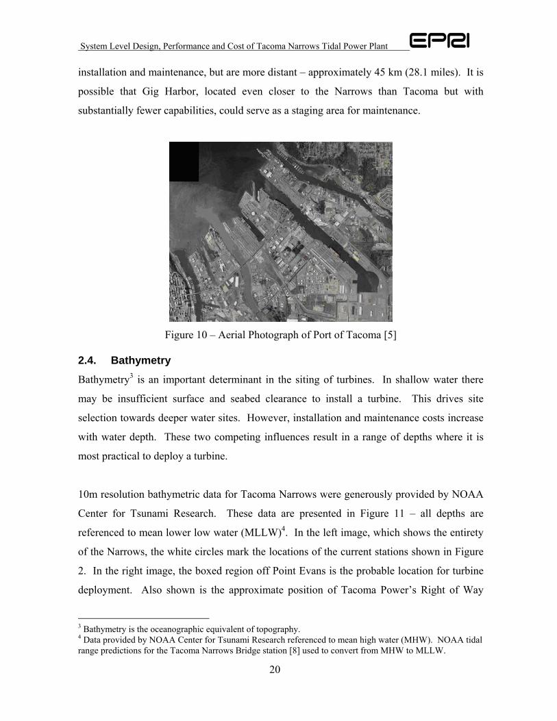
2.3. Nearby Port Facilities
If a turbine is far from a major port, both installation and maintenance costs may be
prohibitive due to long mobilization times. Tacoma Narrows is located in close proximity
to a number of major port facilities. The Port of Tacoma is approximately 20 km (12.5
miles) from Point Evans. Both Seattle and Olympia could also serve as staging areas for
Pt. Evans channel marker
115kV cable crossing towers
115kV transmission line
(Tacoma Power) 12.47kV distribution line
(Pen Light)
System Level Design, Performance and Cost of Tacoma Narrows Tidal Power Plant
20
installation and maintenance, but are more distant – approximately 45 km (28.1 miles). It is
possible that Gig Harbor, located even closer to the Narrows than Tacoma but with
substantially fewer capabilities, could serve as a staging area for maintenance.
Figure 10 – Aerial Photograph of Port of Tacoma [5]
2.4. Bathymetry
Bathymetry3 is an important determinant in the siting of turbines. In shallow water there
may be insufficient surface and seabed clearance to install a turbine. This drives site
selection towards deeper water sites. However, installation and maintenance costs increase
with water depth. These two competing influences result in a range of depths where it is
most practical to deploy a turbine.
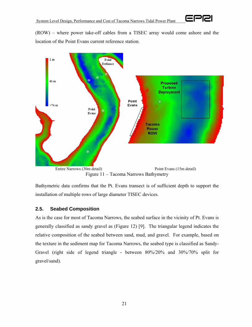
10m resolution bathymetric data for Tacoma Narrows were generously provided by NOAA
Center for Tsunami Research. These data are presented in Figure 11 – all depths are
referenced to mean lower low water (MLLW)4. In the left image, which shows the entirety
of the Narrows, the white circles mark the locations of the current stations shown in Figure
2. In the right image, the boxed region off Point Evans is the probable location for turbine
deployment. Also shown is the approximate position of Tacoma Power’s Right of Way
3 Bathymetry is the oceanographic equivalent of topography. 4 Data provided by NOAA Center for Tsunami Research referenced to mean high water (MHW). NOAA tidal range predictions for the Tacoma Narrows Bridge station [8] used to convert from MHW to MLLW.
System Level Design, Performance and Cost of Tacoma Narrows Tidal Power Plant
21
(ROW) – where power take-off cables from a TISEC array would come ashore and the
location of the Point Evans current reference station.
Entire Narrows (30m detail) Point Evans (15m detail) Figure 11 – Tacoma Narrows Bathymetry
Bathymetric data confirms that the Pt. Evans transect is of sufficient depth to support the
installation of multiple rows of large diameter TISEC devices.
2.5. Seabed Composition
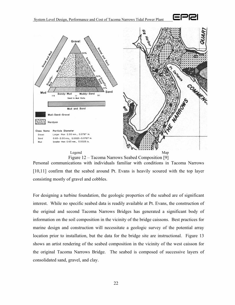
As is the case for most of Tacoma Narrows, the seabed surface in the vicinity of Pt. Evans is
generally classified as sandy gravel as (Figure 12) [9]. The triangular legend indicates the
relative composition of the seabed between sand, mud, and gravel. For example, based on
the texture in the sediment map for Tacoma Narrows, the seabed type is classified as Sandy-
Gravel (right side of legend triangle - between 80%/20% and 30%/70% split for
gravel/sand).
System Level Design, Performance and Cost of Tacoma Narrows Tidal Power Plant
22
Legend Map Figure 12 – Tacoma Narrows Seabed Composition [9]
Personal communications with individuals familiar with conditions in Tacoma Narrows
[10,11] confirm that the seabed around Pt. Evans is heavily scoured with the top layer
consisting mostly of gravel and cobbles.
For designing a turbine foundation, the geologic properties of the seabed are of significant
interest. While no specific seabed data is readily available at Pt. Evans, the construction of
the original and second Tacoma Narrows Bridges has generated a significant body of
information on the soil composition in the vicinity of the bridge caissons. Best practices for
marine design and construction will necessitate a geologic survey of the potential array
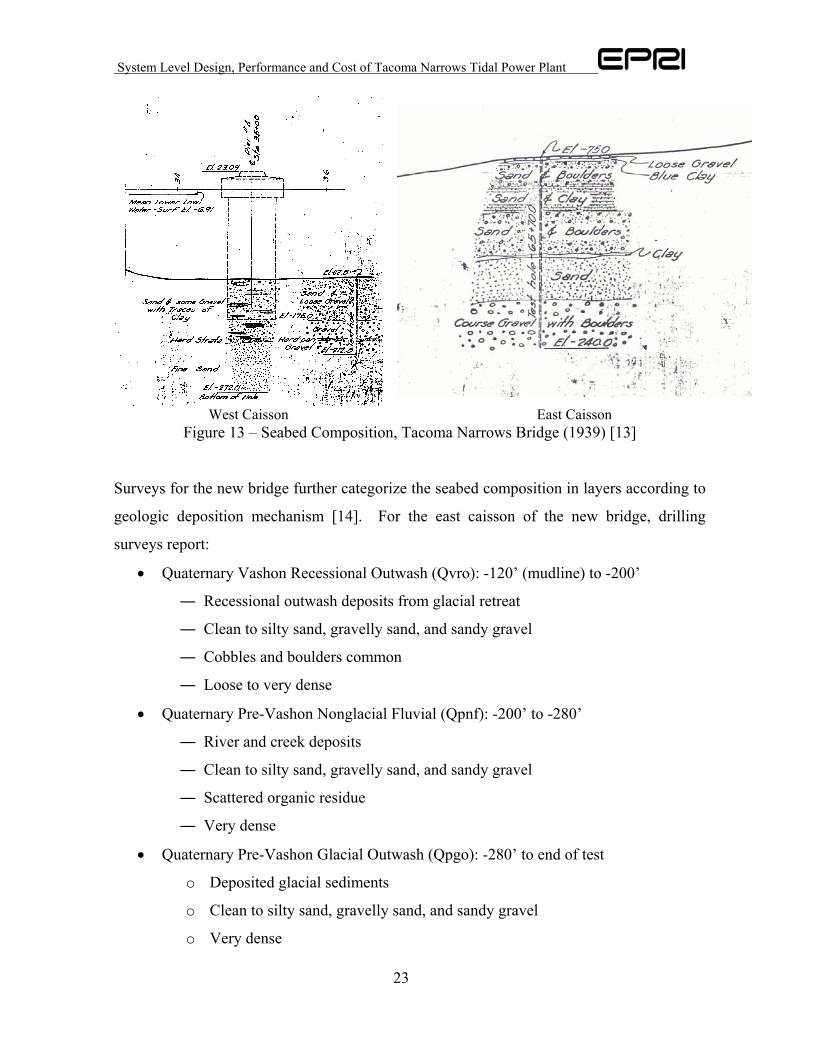
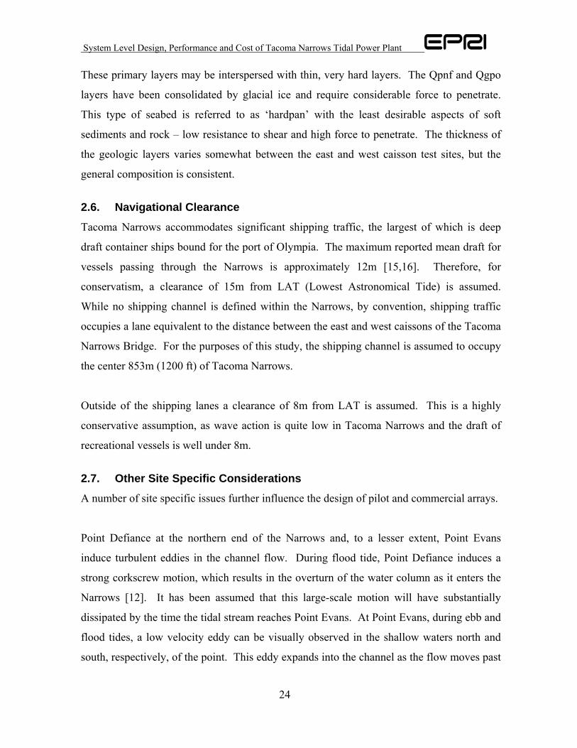
location prior to installation, but the data for the bridge site are instructional. Figure 13
shows an artist rendering of the seabed composition in the vicinity of the west caisson for
the original Tacoma Narrows Bridge. The seabed is composed of successive layers of
consolidated sand, gravel, and clay.
System Level Design, Performance and Cost of Tacoma Narrows Tidal Power Plant
23
West Caisson East Caisson Figure 13 – Seabed Composition, Tacoma Narrows Bridge (1939) [13]
Surveys for the new bridge further categorize the seabed composition in layers according to
geologic deposition mechanism [14]. For the east caisson of the new bridge, drilling
surveys report:
• Quaternary Vashon Recessional Outwash (Qvro): -120’ (mudline) to -200’
― Recessional outwash deposits from glacial retreat
― Clean to silty sand, gravelly sand, and sandy gravel
― Cobbles and boulders common
― Loose to very dense
• Quaternary Pre-Vashon Nonglacial Fluvial (Qpnf): -200’ to -280’
― River and creek deposits
― Clean to silty sand, gravelly sand, and sandy gravel
― Scattered organic residue
― Very dense
• Quaternary Pre-Vashon Glacial Outwash (Qpgo): -280’ to end of test
o Deposited glacial sediments
o Clean to silty sand, gravelly sand, and sandy gravel
o Very dense
System Level Design, Performance and Cost of Tacoma Narrows Tidal Power Plant
24
These primary layers may be interspersed with thin, very hard layers. The Qpnf and Qgpo
layers have been consolidated by glacial ice and require considerable force to penetrate.
This type of seabed is referred to as ‘hardpan’ with the least desirable aspects of soft
sediments and rock – low resistance to shear and high force to penetrate. The thickness of
the geologic layers varies somewhat between the east and west caisson test sites, but the
general composition is consistent.
2.6. Navigational Clearance
Tacoma Narrows accommodates significant shipping traffic, the largest of which is deep
draft container ships bound for the port of Olympia. The maximum reported mean draft for
vessels passing through the Narrows is approximately 12m [15,16]. Therefore, for
conservatism, a clearance of 15m from LAT (Lowest Astronomical Tide) is assumed.
While no shipping channel is defined within the Narrows, by convention, shipping traffic
occupies a lane equivalent to the distance between the east and west caissons of the Tacoma
Narrows Bridge. For the purposes of this study, the shipping channel is assumed to occupy
the center 853m (1200 ft) of Tacoma Narrows.
Outside of the shipping lanes a clearance of 8m from LAT is assumed. This is a highly
conservative assumption, as wave action is quite low in Tacoma Narrows and the draft of
recreational vessels is well under 8m.
2.7. Other Site Specific Considerations
A number of site specific issues further influence the design of pilot and commercial arrays.
Point Defiance at the northern end of the Narrows and, to a lesser extent, Point Evans
induce turbulent eddies in the channel flow. During flood tide, Point Defiance induces a
strong corkscrew motion, which results in the overturn of the water column as it enters the
Narrows [12]. It has been assumed that this large-scale motion will have substantially
dissipated by the time the tidal stream reaches Point Evans. At Point Evans, during ebb and
flood tides, a low velocity eddy can be visually observed in the shallow waters north and
south, respectively, of the point. This eddy expands into the channel as the flow moves past

System Level Design, Performance and Cost of Tacoma Narrows Tidal Power Plant
25
the point and is visually identified by reversing flows and small, standing waves. Turbines
should not be installed in eddies as the flow velocity will be much lower than in the
undisturbed flow. Furthermore, extreme turbulence is likely to accelerate blade fatigue and
reducing operating lifetime.
Tacoma Narrows is a biologically active region. Two types of kelp grow along the
shoreline of Tacoma Narrows – floating and understory. As its name suggest, floating kelp
is positively buoyant and floats on the surface. Understory kelp is fixed to the seabed.
Broken understory or floating kelp may be carried downstream in the middle of the water
column (prior to settling on the bottom or floating to the surface) and could tangle turbine
rotors. Kelp grows fastest during spring and summer, so any bio-fouling due to kelp would
be worst during these seasons [10,11]. In addition to kelp, large barnacles will rapidly grow
on submerged surfaces in Tacoma Narrows [10]. Any turbine installed in the Narrows will
require safeguards against bio-fouling. Anti-fouling paints are the standard method for
protecting marine structures, though with some paints there are environmental concerns
regarding the leaching of paint toxins into the water over the structure’s lifetime.
Some construction techniques (dredging, water jetting, pile driving) disturb sediments.
Sediment dispersion into the water column has two negative impacts: an increase in the
opacity of the water (reducing available light) and the potential re-introduction of toxic
materials that have settled out of the water column. Tacoma Narrows has been purposely
excluded from Washington Department of Ecology sediment contaminant studies [11] since
the generally scoured and cobbled nature of the seabed is incompatible with standard
sampling equipment. While sediment composition may be inferred from measurements
north and south of the Narrows [17], a more rigorous study may be required prior to
approval of construction permits.
System Level Design, Performance and Cost of Tacoma Narrows Tidal Power Plant
26
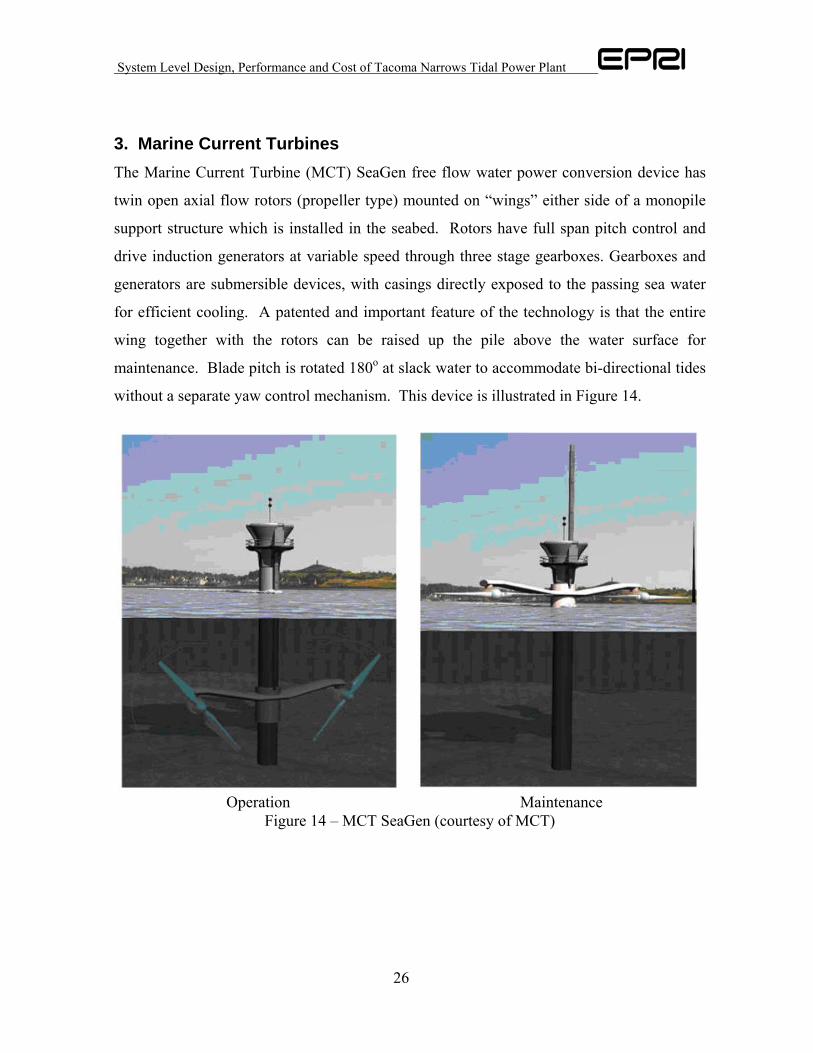
3. Marine Current Turbines The Marine Current Turbine (MCT) SeaGen free flow water power conversion device has
twin open axial flow rotors (propeller type) mounted on “wings” either side of a monopile
support structure which is installed in the seabed. Rotors have full span pitch control and
drive induction generators at variable speed through three stage gearboxes. Gearboxes and
generators are submersible devices, with casings directly exposed to the passing sea water
for efficient cooling. A patented and important feature of the technology is that the entire
wing together with the rotors can be raised up the pile above the water surface for
maintenance. Blade pitch is rotated 180o at slack water to accommodate bi-directional tides
without a separate yaw control mechanism. This device is illustrated in Figure 14.
Operation Maintenance
Figure 14 – MCT SeaGen (courtesy of MCT)
System Level Design, Performance and Cost of Tacoma Narrows Tidal Power Plant
27
3.1. Device Performance
Given a velocity distribution for a site, the calculation of extracted and electrical power is
discussed in [4]. Site surface velocity distributions have been adjusted to hub height
velocity assuming a 1/10th power law, consistent with turbulent flow.
The overall efficiency of the MCT SeaGen is the product of:
• Rotor: constant efficiency = 45%
• Gearbox: maximum efficiency = 96%
• Generator: maximum efficiency = 98%
The efficiency of the gearbox and generator (together termed balance of system efficiency)
is a function of the load on the turbine (% load). Power take off (PTO) efficiency is
assumed to follow the same form as for a conventional wind turbine drive train – which is
approximated by ( ) ( )Load %89.33Load %1467.0 7426.08337.0 −−= eePTOη [18]
This function is capped at 94% - the product of maximum gearbox and generator efficiency.
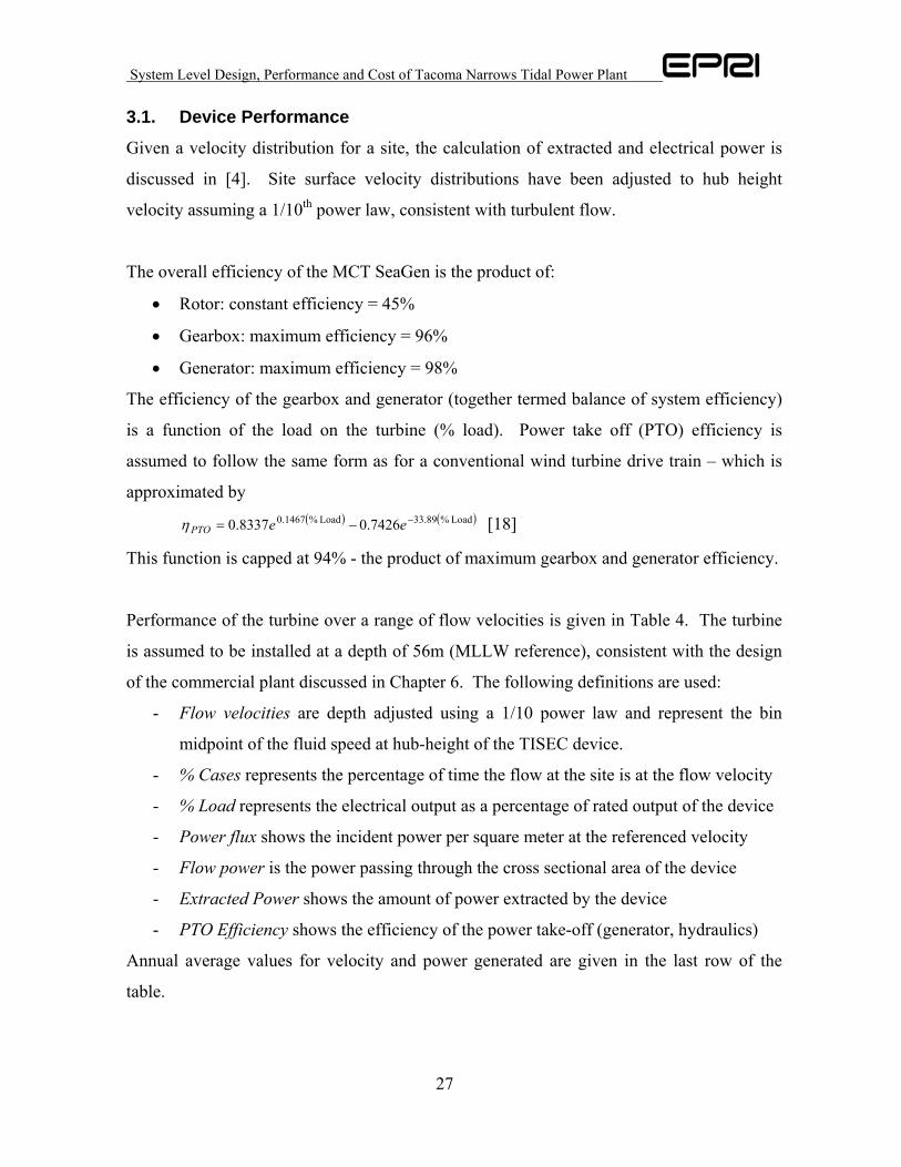
Performance of the turbine over a range of flow velocities is given in Table 4. The turbine
is assumed to be installed at a depth of 56m (MLLW reference), consistent with the design
of the commercial plant discussed in Chapter 6. The following definitions are used:
- Flow velocities are depth adjusted using a 1/10 power law and represent the bin
midpoint of the fluid speed at hub-height of the TISEC device.
- % Cases represents the percentage of time the flow at the site is at the flow velocity
- % Load represents the electrical output as a percentage of rated output of the device
- Power flux shows the incident power per square meter at the referenced velocity
- Flow power is the power passing through the cross sectional area of the device
- Extracted Power shows the amount of power extracted by the device
- PTO Efficiency shows the efficiency of the power take-off (generator, hydraulics)
Annual average values for velocity and power generated are given in the last row of the
table.
System Level Design, Performance and Cost of Tacoma Narrows Tidal Power Plant
28
Table 4 – Device Performance at Pt. Evans
Flow Velocity
% Cases % Load Power Flux
Flow Power
Extracted Power
PTO Efficiency
Electric Power
(m/s) (kW/m2) (kW) (kW) (kW) 0.09 7.41% 0.0% 0.00 0 0 9.38% 00.27 8.29% 0.3% 0.01 5 0 16.13% 00.44 8.73% 1.3% 0.04 23 0 36.54% 00.62 9.56% 3.7% 0.12 63 0 62.66% 00.80 9.57% 7.9% 0.26 133 60 79.18% 470.98 9.28% 14.4% 0.48 243 109 84.58% 921.15 8.62% 23.7% 0.79 401 181 86.30% 1561.33 7.47% 36.4% 1.21 616 277 87.95% 2441.51 7.09% 53.1% 1.76 897 404 90.12% 3641.69 6.39% 74.1% 2.46 1252 564 92.94% 5241.87 5.19% 100.0% 3.32 1691 761 94.08% 7162.04 4.08% 100.0% 4.37 2222 761 94.08% 7162.22 3.10% 100.0% 5.61 2853 761 94.08% 7162.40 2.07% 100.0% 7.06 3594 761 94.08% 7162.58 1.37% 100.0% 8.75 4453 761 94.08% 7162.75 0.85% 100.0% 10.69 5440 761 94.08% 7162.93 0.49% 100.0% 12.89 6562 761 94.08% 7163.11 0.29% 100.0% 15.38 7829 761 94.08% 7163.29 0.13% 100.0% 18.17 9249 761 94.08% 7163.46 0.01% 100.0% 21.28 10831 761 94.08% 7163.64 0.00% 100.0% 24.73 12585 761 94.08% 7163.82 0.00% 100.0% 28.53 14517 761 94.08% 7164.00 0.00% 100.0% 32.69 16639 761 94.08% 7164.17 0.00% 100.0% 37.25 18957 761 94.08% 7164.35 0.00% 100.0% 42.21 21482 761 94.08% 716
Average 1.09 1.54 785 251 230
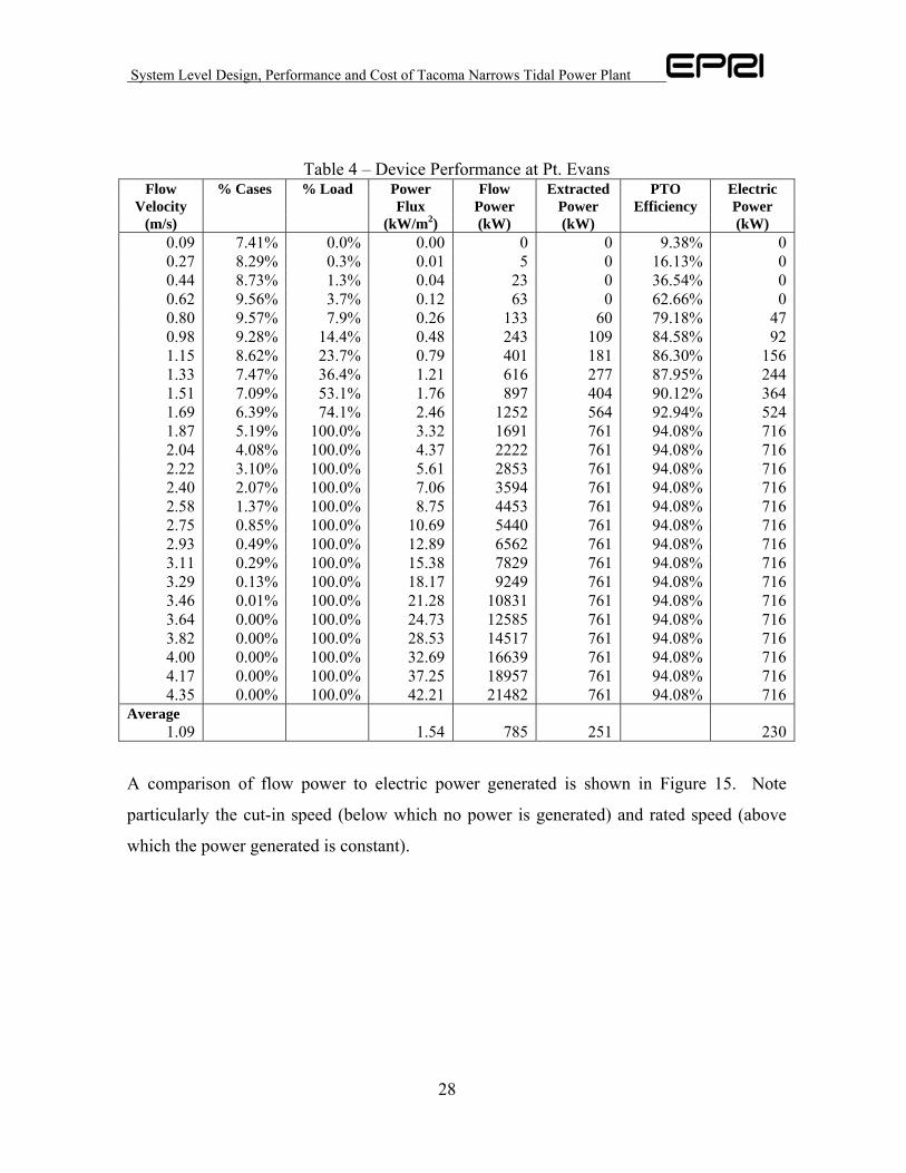
A comparison of flow power to electric power generated is shown in Figure 15. Note
particularly the cut-in speed (below which no power is generated) and rated speed (above
which the power generated is constant).
System Level Design, Performance and Cost of Tacoma Narrows Tidal Power Plant
29
0200400600800
100012001400
0 1 2 3 4 5
Flow Velocity (m/s)
Power (kW)
Fluid PowerElectric Power
Rated Power
Cut-in
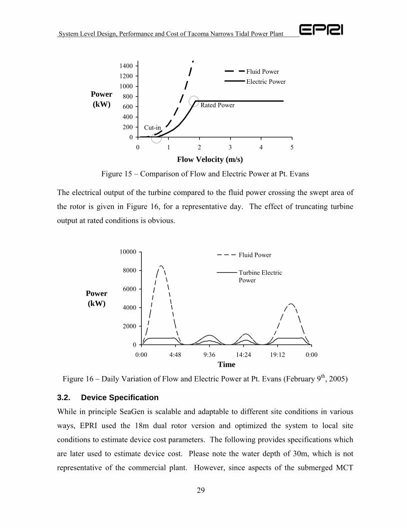
Figure 15 – Comparison of Flow and Electric Power at Pt. Evans
The electrical output of the turbine compared to the fluid power crossing the swept area of
the rotor is given in Figure 16, for a representative day. The effect of truncating turbine
output at rated conditions is obvious.
0
2000
4000
6000
8000
10000
0:00 4:48 9:36 14:24 19:12 0:00Time
Power (kW)
Fluid Power
Turbine ElectricPower
Figure 16 – Daily Variation of Flow and Electric Power at Pt. Evans (February 9th, 2005)
3.2. Device Specification
While in principle SeaGen is scalable and adaptable to different site conditions in various
ways, EPRI used the 18m dual rotor version and optimized the system to local site
conditions to estimate device cost parameters. The following provides specifications which
are later used to estimate device cost. Please note the water depth of 30m, which is not
representative of the commercial plant. However, since aspects of the submerged MCT
System Level Design, Performance and Cost of Tacoma Narrows Tidal Power Plant
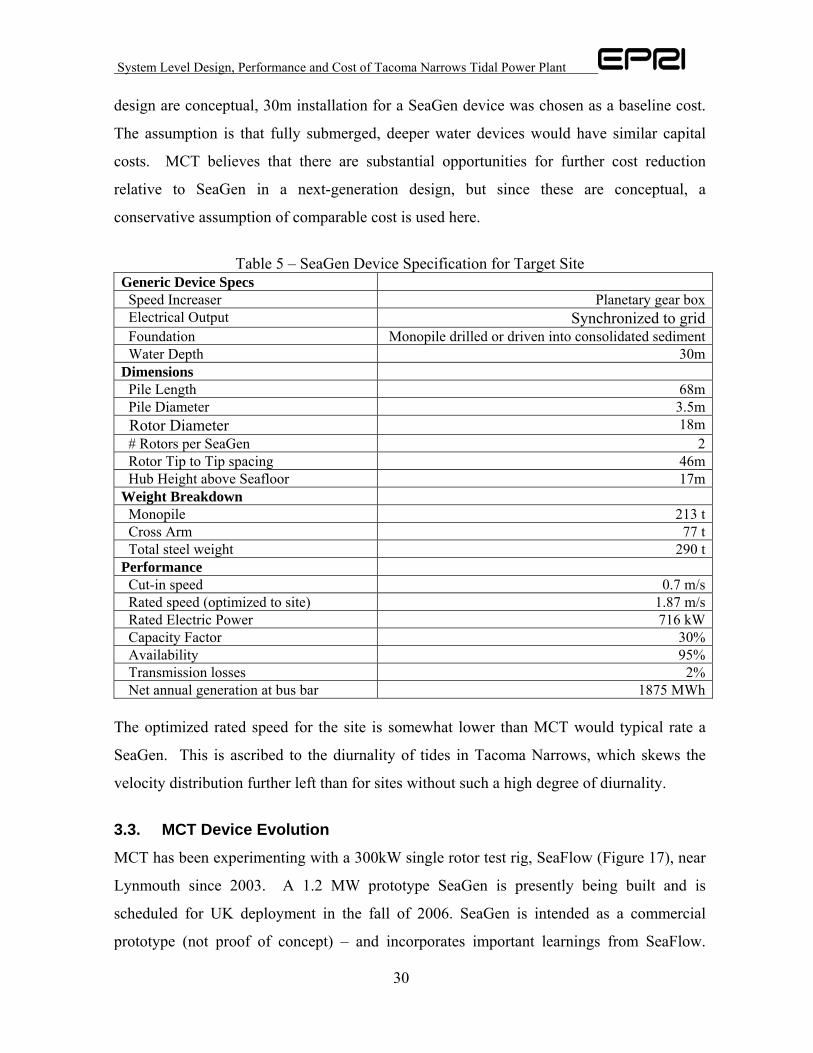
30
design are conceptual, 30m installation for a SeaGen device was chosen as a baseline cost.
The assumption is that fully submerged, deeper water devices would have similar capital
costs. MCT believes that there are substantial opportunities for further cost reduction
relative to SeaGen in a next-generation design, but since these are conceptual, a
conservative assumption of comparable cost is used here.
Table 5 – SeaGen Device Specification for Target Site
Generic Device Specs Speed Increaser Planetary gear box Electrical Output Synchronized to grid Foundation Monopile drilled or driven into consolidated sediment Water Depth 30mDimensions Pile Length 68m Pile Diameter 3.5m Rotor Diameter 18m # Rotors per SeaGen 2 Rotor Tip to Tip spacing 46m Hub Height above Seafloor 17mWeight Breakdown Monopile 213 t Cross Arm 77 t Total steel weight 290 tPerformance Cut-in speed 0.7 m/s Rated speed (optimized to site) 1.87 m/s Rated Electric Power 716 kW Capacity Factor 30% Availability 95% Transmission losses 2% Net annual generation at bus bar 1875 MWh
The optimized rated speed for the site is somewhat lower than MCT would typical rate a
SeaGen. This is ascribed to the diurnality of tides in Tacoma Narrows, which skews the
velocity distribution further left than for sites without such a high degree of diurnality.
3.3. MCT Device Evolution
MCT has been experimenting with a 300kW single rotor test rig, SeaFlow (Figure 17), near
Lynmouth since 2003. A 1.2 MW prototype SeaGen is presently being built and is
scheduled for UK deployment in the fall of 2006. SeaGen is intended as a commercial
prototype (not proof of concept) – and incorporates important learnings from SeaFlow.
System Level Design, Performance and Cost of Tacoma Narrows Tidal Power Plant
31
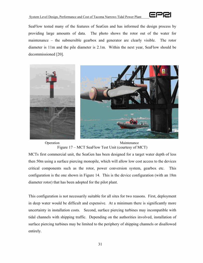
SeaFlow tested many of the features of SeaGen and has informed the design process by
providing large amounts of data. The photo shows the rotor out of the water for
maintenance – the submersible gearbox and generator are clearly visible. The rotor
diameter is 11m and the pile diameter is 2.1m. Within the next year, SeaFlow should be
decommissioned [20].
Operation Maintenance
Figure 17 – MCT SeaFlow Test Unit (courtesy of MCT)
MCTs first commercial unit, the SeaGen has been designed for a target water depth of less
then 50m using a surface piercing monopile, which will allow low cost access to the devices
critical components such as the rotor, power conversion system, gearbox etc. This
configuration is the one shown in Figure 14. This is the device configuration (with an 18m
diameter rotor) that has been adopted for the pilot plant.
This configuration is not necessarily suitable for all sites for two reasons. First, deployment
in deep water would be difficult and expensive. At a minimum there is significantly more
uncertainty in installation costs. Second, surface piercing turbines may incompatible with
tidal channels with shipping traffic. Depending on the authorities involved, installation of
surface piercing turbines may be limited to the periphery of shipping channels or disallowed
entirely.
System Level Design, Performance and Cost of Tacoma Narrows Tidal Power Plant
32
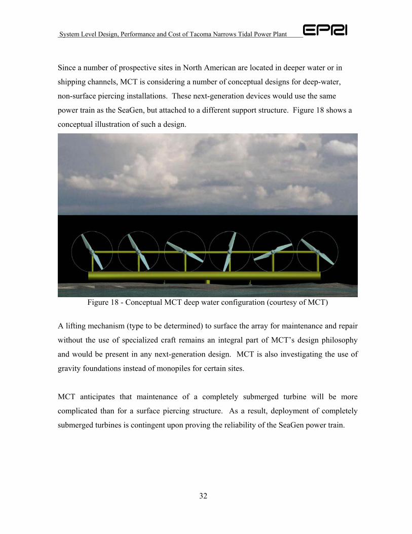
Since a number of prospective sites in North American are located in deeper water or in
shipping channels, MCT is considering a number of conceptual designs for deep-water,
non-surface piercing installations. These next-generation devices would use the same
power train as the SeaGen, but attached to a different support structure. Figure 18 shows a
conceptual illustration of such a design.
Figure 18 - Conceptual MCT deep water configuration (courtesy of MCT)
A lifting mechanism (type to be determined) to surface the array for maintenance and repair
without the use of specialized craft remains an integral part of MCT’s design philosophy
and would be present in any next-generation design. MCT is also investigating the use of
gravity foundations instead of monopiles for certain sites.
MCT anticipates that maintenance of a completely submerged turbine will be more
complicated than for a surface piercing structure. As a result, deployment of completely
submerged turbines is contingent upon proving the reliability of the SeaGen power train.
System Level Design, Performance and Cost of Tacoma Narrows Tidal Power Plant
33
3.4. Monopile Foundations
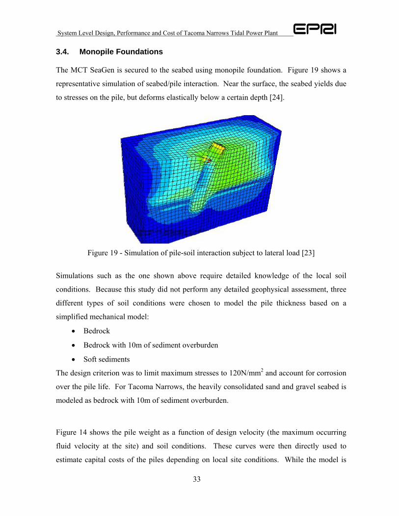
The MCT SeaGen is secured to the seabed using monopile foundation. Figure 19 shows a
representative simulation of seabed/pile interaction. Near the surface, the seabed yields due
to stresses on the pile, but deforms elastically below a certain depth [24].
Figure 19 - Simulation of pile-soil interaction subject to lateral load [23]
Simulations such as the one shown above require detailed knowledge of the local soil
conditions. Because this study did not perform any detailed geophysical assessment, three
different types of soil conditions were chosen to model the pile thickness based on a
simplified mechanical model:
• Bedrock
• Bedrock with 10m of sediment overburden
• Soft sediments
The design criterion was to limit maximum stresses to 120N/mm2 and account for corrosion
over the pile life. For Tacoma Narrows, the heavily consolidated sand and gravel seabed is
modeled as bedrock with 10m of sediment overburden.
Figure 14 shows the pile weight as a function of design velocity (the maximum occurring
fluid velocity at the site) and soil conditions. These curves were then directly used to
estimate capital costs of the piles depending on local site conditions. While the model is
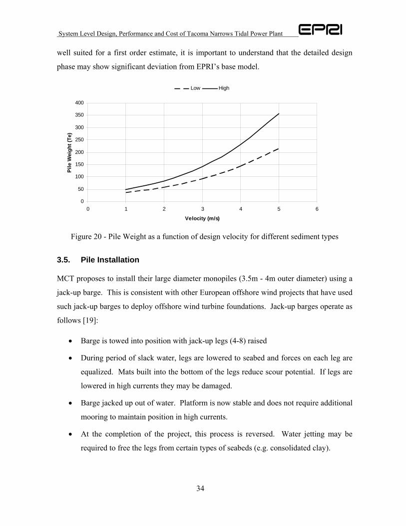
System Level Design, Performance and Cost of Tacoma Narrows Tidal Power Plant
34
well suited for a first order estimate, it is important to understand that the detailed design
phase may show significant deviation from EPRI’s base model.
0
50
100
150
200
250
300
350
400
0 1 2 3 4 5 6
Velocity (m/s)
Pile
Wei
ght (
Te)
Low High
Figure 20 - Pile Weight as a function of design velocity for different sediment types
3.5. Pile Installation
MCT proposes to install their large diameter monopiles (3.5m - 4m outer diameter) using a
jack-up barge. This is consistent with other European offshore wind projects that have used
such jack-up barges to deploy offshore wind turbine foundations. Jack-up barges operate as
follows [19]:
• Barge is towed into position with jack-up legs (4-8) raised
• During period of slack water, legs are lowered to seabed and forces on each leg are
equalized. Mats built into the bottom of the legs reduce scour potential. If legs are
lowered in high currents they may be damaged.
• Barge jacked up out of water. Platform is now stable and does not require additional
mooring to maintain position in high currents.
• At the completion of the project, this process is reversed. Water jetting may be
required to free the legs from certain types of seabeds (e.g. consolidated clay).
System Level Design, Performance and Cost of Tacoma Narrows Tidal Power Plant
35
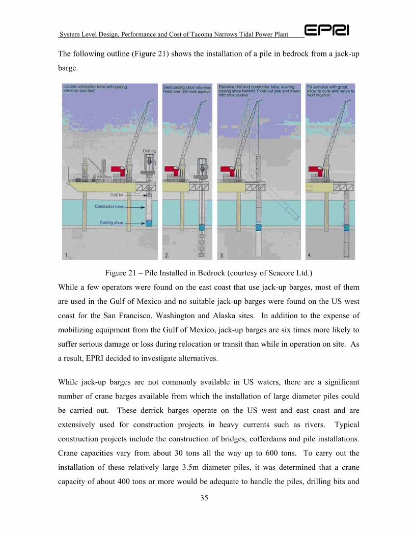
The following outline (Figure 21) shows the installation of a pile in bedrock from a jack-up
barge.
Figure 21 – Pile Installed in Bedrock (courtesy of Seacore Ltd.)
While a few operators were found on the east coast that use jack-up barges, most of them
are used in the Gulf of Mexico and no suitable jack-up barges were found on the US west
coast for the San Francisco, Washington and Alaska sites. In addition to the expense of
mobilizing equipment from the Gulf of Mexico, jack-up barges are six times more likely to
suffer serious damage or loss during relocation or transit than while in operation on site. As
a result, EPRI decided to investigate alternatives.
While jack-up barges are not commonly available in US waters, there are a significant
number of crane barges available from which the installation of large diameter piles could
be carried out. These derrick barges operate on the US west and east coast and are
extensively used for construction projects in heavy currents such as rivers. Typical
construction projects include the construction of bridges, cofferdams and pile installations.
Crane capacities vary from about 30 tons all the way up to 600 tons. To carry out the
installation of these relatively large 3.5m diameter piles, it was determined that a crane
capacity of about 400 tons or more would be adequate to handle the piles, drilling bits and

System Level Design, Performance and Cost of Tacoma Narrows Tidal Power Plant
36
vibratory hammers. Figure 22 shows Manson Construction’s 600 ton derrick barge
WOTAN doing construction work on an offshore drilling rig. Two tug boats are used for
positioning the derrick barge and set moorings if required.
Figure 22 - Manson Construction 600 ton Derrick Barge WOTAN operating offshore
(courtesy of Manson Construction)
In heavy currents these barges use a mooring spread that allows them to keep on station and
accurately reposition themselves continuously using hydraulic winches controlled by the
operator. This is in contrast to the fixed anchoring function of a jack-up barge leg.
Working from a barge, rather then from a jack-up platform does not set hard limits on the
water depth in which piles can be installed (in a jack-up the length of the legs sets the limit
on installation depth). In the offshore industry, piles are oftentimes used as mooring points
for offshore structures. Installation of driven piles in water depths of more then 300m is not
uncommon. It is, however, clear that pile installation in deeper waters becomes more costly
and presents a limiting factor to their viability (e.g. a long follower between pile and
hammer might be needed in deep water).

System Level Design, Performance and Cost of Tacoma Narrows Tidal Power Plant
37
While monopile foundations are used extensively in US waterways for the construction of
bridges and piers, installation of piles in Tacoma Narrows would be under relatively
challenging conditions. Several options exist for installing piles in hardpan, but it is
important to stress that west coast marine construction companies have limited experience
with such methods in deep, high current waters. Potential construction methods include:
• Driving piles using a hydraulic hammer
• Combination of water jetting and vibratory hammer
• Drill and socket a sleeve, then grout pile in place
Each of these methods has advantages and disadvantages.
The force required to drive a large diameter pile into hardpan using a hydraulic hammer is
quite high, and could involve mobilization of a suitably powerful hammer (>1,000,000 ft-
lbs/blow) from Europe [21]. Driving a pile with this much force could induce significant
fatigue and compromise structural integrity [20]. One potential installation procedure might
consist of driving the pile to refusal5, cleaning out the inside of the pile can, and driving
again until a suitable depth has been reached. It may also be necessary to break up the
hardpan around the pile perimeter using water jets if exterior skin friction leads to refusal
[19, 21]. Driven pile supports for the tower foundations of the new Tacoma Narrows
Bridge were considered during the design phase, but rejected in favor of caissons due to
concerns over installation equipment availability [14].
Since hardpan readily breaks up under water jetting, a combination of water jetting and
vibratory hammering could be lower cost option to hammering alone since a suitable
hammer could be mobilized at lower cost. Installation procedure would consist of water
jetting to break up sediments, driving the pile, additional jetting, etc. Once the pile reaches
specified depth, the hammer would act on the pile for a number of additional strikes,
helping to reconsolidate the disrupted sediments [19]. However, environmental regulation
may restrict the use of water jetting since it results in significant sediment disruption [21].
5 Refusal is defined as 1000 blows/meter penetration or 800 blows for 0.3meter penetration.
System Level Design, Performance and Cost of Tacoma Narrows Tidal Power Plant
38
A drilled pile installation would involve drilling into the consolidated sediments and
stabilizing the walls of the drill hole with a metal sleeve. Once the hole has been drilled to a
suitable depth, the pile is inserted and grouted into place. This method of installation is
preferred by MCT to limit excessive pile fatigue during the installation process [20] and
equipment for drilling could be mobilized from Europe. Marine Construction companies
contacted in Puget Sound agreed that such an installation would be possible, though
challenging in Tacoma Narrows [21, 22]. Drilled piles were also considered for the new
bridge tower foundations, but rejected due to the depth of drilling required and concerns
over installation equipment availability [14].
For the purposes of this feasibility study, it is assumed that pile installation would be by
drilling. A detailed design which incorporates the findings of a site-specific geotechnical
survey will be required to determine the most economic option.
3.6. Operational and Maintenance Activities
The guiding philosophy behind the MCT design is to provide low cost access to critical
turbine systems. MCT feels this is especially important since the majority of unplanned
interventions during the SeaFlow demonstration involved minor problems or false alarms
[20]. Since the integrated lifting mechanism on the pile can lift the rotor and all mechanical
subsystems out of the water, general maintenance activities do not require specialized ships
or personnel (e.g. divers). Furthermore, for major repairs or scheduled refits, a barge can be
positioned under the power train for relatively simple dismounting.
The overall design philosophy appears to be that the risks associated with long-term
underwater operation are best offset by minimizing the cost of scheduled and unscheduled
maintenance tasks. The only activities that could require use of divers or ROVs would be
repairs to the lifting mechanism or inspection of the outer surface of the monopile, none of
which are likely to be required over the project life.
Annual inspection and maintenance activities are carried out using a small crew of 2-3
technicians on the device itself. Tasks involved in this annual maintenance cycle include
System Level Design, Performance and Cost of Tacoma Narrows Tidal Power Plant
39
activities such as replacement of gearbox oil, applying bearing grease and changing oil
filters. In addition, all electrical equipment can be checked during this inspection cycle and
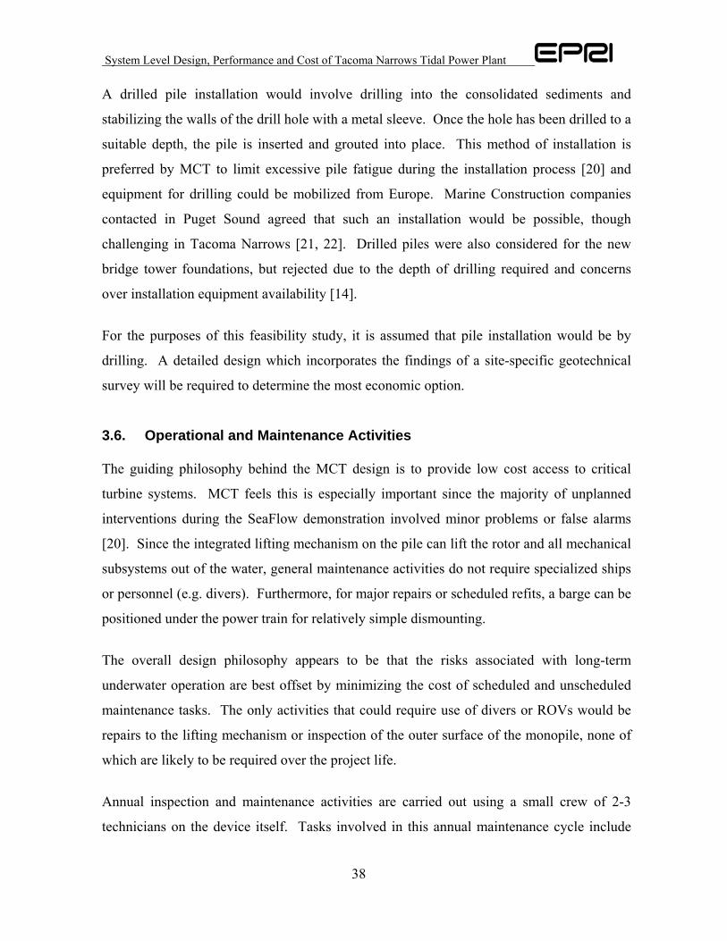
repairs carried out if required. Access to the main structure can be carried out safely using a
small craft such as a RIB (Rigid Inflatable Boat) in most sea conditions. Since Tacoma
Narrows experiences little wave action, maintenance intervention should be feasible year-
round.
Figure 23 - Typical Rigid Inflatable Boat (RIB)
For repairs on larger subsystems such as the gearbox, the individual components can be
hoisted out with a crane or winch and placed onto a motorized barge which is a relatively
low cost vessel. The barge can then convey the systems ashore for overhaul, repair or
replacement. For the purpose of modeling O&M costs, the mean time to failure was
estimated for each component to determine the resulting annual operational and replacement
cost. Based on wind-turbine data, the most critical component is the gearbox which shows
an average mean time to failure of 10.8 years.
For the next generation design for a completely submerged turbine (assumed for
commercial plant) major intervention could require the use of a crane barge to dismount the
power train from the support structure. Since the lifting mechanism would also be
subsurface, a failsafe retrieval method (e.g. retrieval hook) would be required in the case of
a failure of the lifting mechanism. MCT does not anticipate the added complexity of full

System Level Design, Performance and Cost of Tacoma Narrows Tidal Power Plant
40
submergence to greatly increase maintenance costs, because deployment of a fully
submerged device is contingent on proving power train reliability [20].
Barges for major maintenance activities could be mobilized from any of the area ports –
Tacoma, Seattle, or Olympia. For minor maintenance, small craft could be launched
directly from a beach along the Narrows or mobilized from Gig Harbor.
System Level Design, Performance and Cost of Tacoma Narrows Tidal Power Plant
41
4. Electrical Interconnection
Each TISEC device houses a step-up transformer to increase the voltage from generator
voltage to a suitable array interconnection voltage. The choice of the voltage level of this
energy collector system is driven by the grid interconnection requirements and the array
electrical interconnection design but is typically between 12kV and 40kV. For the pilot
scale, 12kV systems are anticipated – depending on local interconnection voltages. This
will allow the device interconnection on the distribution level. For commercial scale arrays,
voltage levels of 33kV are used. This allows the interconnection of an array with a rated
capacity of up to about 40MW on a single cable. While there is little incremental cost in
increasing turbine output voltage from 12 to 40kV (different step-up transformer required),
above 40kV the cost of circuit breakers, interconnection, overvoltage protection, etc.
increase dramatically. As a result, it is not feasible to step-up turbine generator voltage to
transmission line voltage levels (115 kV) at the turbine. However, once commercial array
cables have been brought ashore, they may be readily stepped up to transmission line
voltages.
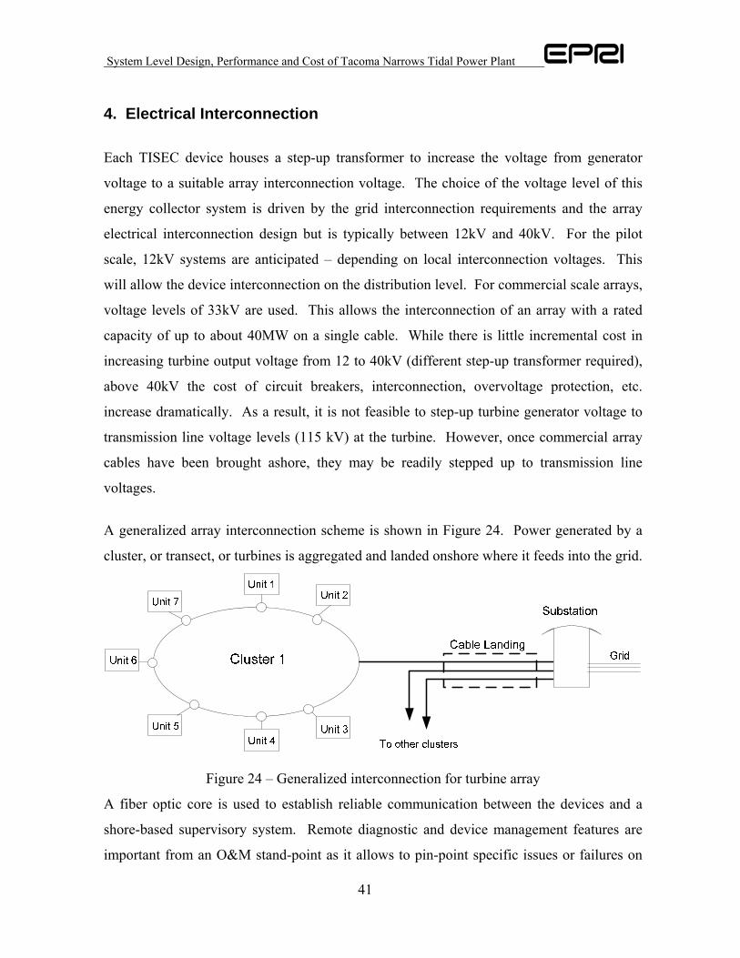
A generalized array interconnection scheme is shown in Figure 24. Power generated by a
cluster, or transect, or turbines is aggregated and landed onshore where it feeds into the grid.
Figure 24 – Generalized interconnection for turbine array
A fiber optic core is used to establish reliable communication between the devices and a
shore-based supervisory system. Remote diagnostic and device management features are
important from an O&M stand-point as it allows to pin-point specific issues or failures on
System Level Design, Performance and Cost of Tacoma Narrows Tidal Power Plant
42
each unit, reducing the physical intervention requirements on the device and optimizing
operational activities. Operational activities offshore are expensive and minimizing such
interventions is a critical component of any operational strategy in this harsh environment.
For the surface piercing MCT SeaGen device (pilot plant), most electrical components are
located inside the top of the monopole, where they are well protected and easily accessible
for operation and maintenance activities. No sub sea connectors or junction boxes are
required to interconnect the device to the electrical grid. A fully submersed MCT device
(commercial plant) would not require a junction box either, but would require a J-tube to
guide the subsea cable up to the power train.
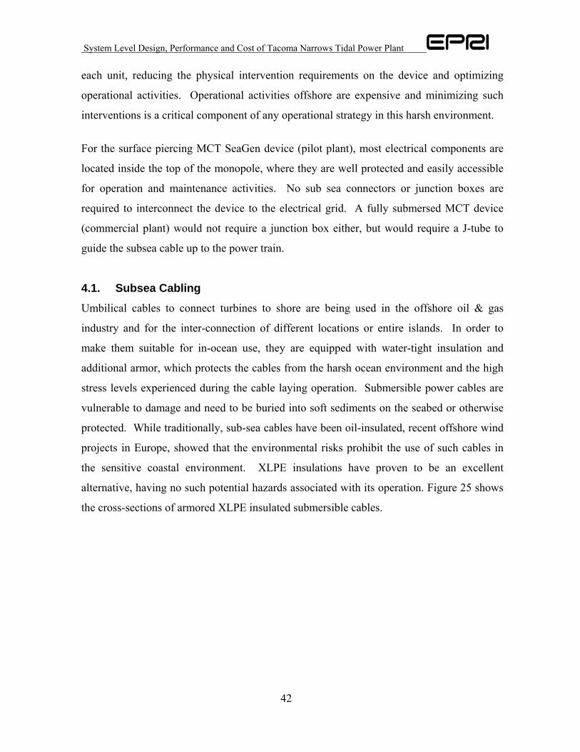
4.1. Subsea Cabling
Umbilical cables to connect turbines to shore are being used in the offshore oil & gas
industry and for the inter-connection of different locations or entire islands. In order to
make them suitable for in-ocean use, they are equipped with water-tight insulation and
additional armor, which protects the cables from the harsh ocean environment and the high
stress levels experienced during the cable laying operation. Submersible power cables are
vulnerable to damage and need to be buried into soft sediments on the seabed or otherwise
protected. While traditionally, sub-sea cables have been oil-insulated, recent offshore wind
projects in Europe, showed that the environmental risks prohibit the use of such cables in
the sensitive coastal environment. XLPE insulations have proven to be an excellent
alternative, having no such potential hazards associated with its operation. Figure 25 shows
the cross-sections of armored XLPE insulated submersible cables.

System Level Design, Performance and Cost of Tacoma Narrows Tidal Power Plant
43
Figure 25 – Armored submarine cables
For this project, 3 phase cables with double armor and a fiber core are being used. The fiber
core allows data transmission between the units and an operator station on shore. In order
to protect the cable properly from damage such as an anchor of a fishing boat, the cable
must either be trenched into the seabed or shielded. In general, a trench is carved in the
seabed, the cable is laid down, and this channel is then back-filled with rocks. Various
trenching technologies exist such as the use of a plough in soft sediments, use of a subsea
rock-saw in rock (if going through hard-rock) or the use of water jets in consolidated
sediments. All of these cable laying operations can be carried out from a derrick barge that
is properly outfitted for the particular job. The choice of technology best suited for getting
the job done depends largely on the outcome of detailed geophysical assessments along the
cable route. For this study, the EPRI team assessed both the use of a trenching rock saw as
well as a plough.
An important part of bringing power back to shore is the cable landing. Existing easements
should be used wherever possible to drive down costs and avoid permitting issues. If they
do not exist, directional drilling is the method with the least impact on the environment.
Directional drilling is a well established method to land such cables from the shoreline into
the ocean and has been used quite extensively to land fiber optic cables on shore. Given
some of the deployment location proximity to shore, detailed engineering might even reveal
that directional drilling directly to the deployment site is possible. This would reduce
environmental construction impacts at the site, while reducing overall cost.

System Level Design, Performance and Cost of Tacoma Narrows Tidal Power Plant
44
4.2. Onshore Cabling and Grid Interconnection
Traditional overland transmission is used to transmit power from the shoreline to a suitable
grid interconnection point. Grid interconnection requirements are driven by local utility
requirements. At the very least, circuit breakers need to be installed to protect the grid
infrastructure from system faults. VAR compensation and other measures might be
introduced based on particular requirements. The peak power output of the plant will
determine the appropriate grid interconnection voltage.
System Level Design, Performance and Cost of Tacoma Narrows Tidal Power Plant
45
5. System Design – Pilot Plant
The purpose of a pilot plant is first, and foremost, to demonstrate the viability of a particular
technology. Pilot plants are, in general, not expected to produce cost competitive electricity
and often incorporate instrumentation absent from a commercial device. The pilot plant is
assumed to consist of a single MCT SeaGen installed in 35m water off Point Evans. While
a true pilot should use the same technology as a commercial plant, this will not be possible
for a turbine installed in the immediate term since (as discussed in Chapter 6) a commercial
plant would have to be fully submerged due to shipping considerations. However, provided
that a fully submerged next-generation MCT device would incorporate the same rotor and
power train as a SeaGen and the support structure would continue to use pile foundations,
there is significant value in deploying a SeaGen pilot. For the commercial plant, it is
assumed that fully submerged turbines at Point Evans would not be the first ever worldwide
installation (much as a SeaGen at Point Evans would not be the first installation of that
device). As a result, the hope would be that regulatory concerns associated with the use of a
different support structure could be satisfied without a second full-scale pilot test. The
selection of a SeaGen for the pilot is intended to balance the competing interests of large-
scale site deployment against a desire to deploy a pilot turbine in the immediate term.
For the pilot TISEC plant, the following should be successfully demonstrated prior to
installation of a commercial array:
• Turbine output meets predictions for site.
• Installation according to design plan with no significant problems.
• Turbine operates reliably, without excessive maintenance intervention.
• No significant environmental impacts for both installation as well as operational
aspects.
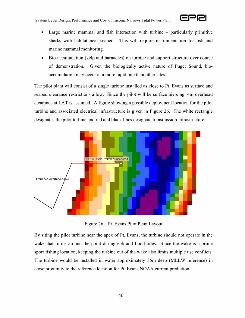
For the pilot plant at Tacoma Narrows, the following issues deserve particular attention and
should be an integral part of the pilot testing plan:
System Level Design, Performance and Cost of Tacoma Narrows Tidal Power Plant
46
• Large marine mammal and fish interaction with turbine – particularly primitive
sharks with habitat near seabed. This will require instrumentation for fish and
marine mammal monitoring.
• Bio-accumulation (kelp and barnacles) on turbine and support structure over course
of demonstration. Given the biologically active nature of Puget Sound, bio-
accumulation may occur at a more rapid rate than other sites.
The pilot plant will consist of a single turbine installed as close to Pt. Evans as surface and
seabed clearance restrictions allow. Since the pilot will be surface piercing, 4m overhead
clearance at LAT is assumed. A figure showing a possible deployment location for the pilot
turbine and associated electrical infrastructure is given in Figure 26. The white rectangle
designates the pilot turbine and red and black lines designate transmission infrastructure.
Figure 26 – Pt. Evans Pilot Plant Layout By siting the pilot turbine near the apex of Pt. Evans, the turbine should not operate in the
wake that forms around the point during ebb and flood tides. Since the wake is a prime
sport fishing location, keeping the turbine out of the wake also limits multiple use conflicts.
The turbine would be installed in water approximately 35m deep (MLLW reference) in
close proximity to the reference location for Pt. Evans NOAA current prediction.
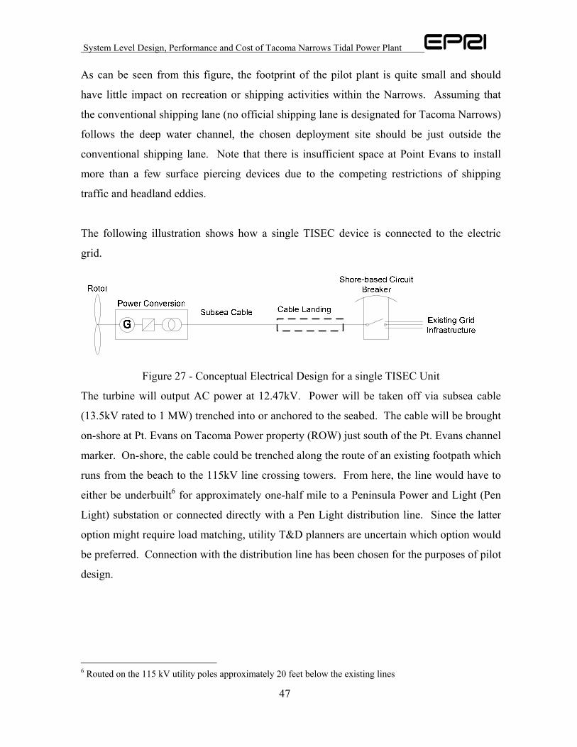
System Level Design, Performance and Cost of Tacoma Narrows Tidal Power Plant
47
As can be seen from this figure, the footprint of the pilot plant is quite small and should
have little impact on recreation or shipping activities within the Narrows. Assuming that
the conventional shipping lane (no official shipping lane is designated for Tacoma Narrows)
follows the deep water channel, the chosen deployment site should be just outside the
conventional shipping lane. Note that there is insufficient space at Point Evans to install
more than a few surface piercing devices due to the competing restrictions of shipping
traffic and headland eddies.
The following illustration shows how a single TISEC device is connected to the electric
grid.
Figure 27 - Conceptual Electrical Design for a single TISEC Unit
The turbine will output AC power at 12.47kV. Power will be taken off via subsea cable
(13.5kV rated to 1 MW) trenched into or anchored to the seabed. The cable will be brought
on-shore at Pt. Evans on Tacoma Power property (ROW) just south of the Pt. Evans channel
marker. On-shore, the cable could be trenched along the route of an existing footpath which
runs from the beach to the 115kV line crossing towers. From here, the line would have to
either be underbuilt6 for approximately one-half mile to a Peninsula Power and Light (Pen
Light) substation or connected directly with a Pen Light distribution line. Since the latter
option might require load matching, utility T&D planners are uncertain which option would
be preferred. Connection with the distribution line has been chosen for the purposes of pilot
design.
6 Routed on the 115 kV utility poles approximately 20 feet below the existing lines
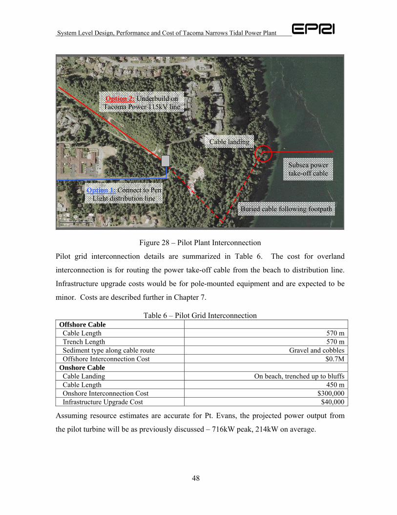
System Level Design, Performance and Cost of Tacoma Narrows Tidal Power Plant
48
Figure 28 – Pilot Plant Interconnection
Pilot grid interconnection details are summarized in Table 6. The cost for overland
interconnection is for routing the power take-off cable from the beach to distribution line.
Infrastructure upgrade costs would be for pole-mounted equipment and are expected to be
minor. Costs are described further in Chapter 7.
Table 6 – Pilot Grid Interconnection Offshore Cable Cable Length 570 m Trench Length 570 m Sediment type along cable route Gravel and cobbles Offshore Interconnection Cost $0.7MOnshore Cable Cable Landing On beach, trenched up to bluffs Cable Length 450 m Onshore Interconnection Cost $300,000 Infrastructure Upgrade Cost $40,000
Assuming resource estimates are accurate for Pt. Evans, the projected power output from
the pilot turbine will be as previously discussed – 716kW peak, 214kW on average.
Option 2: Underbuild on Tacoma Power 115kV line
Option 1: Connect to Pen Light distribution line
Subsea power take-off cable
Buried cable following footpath
Cable landing
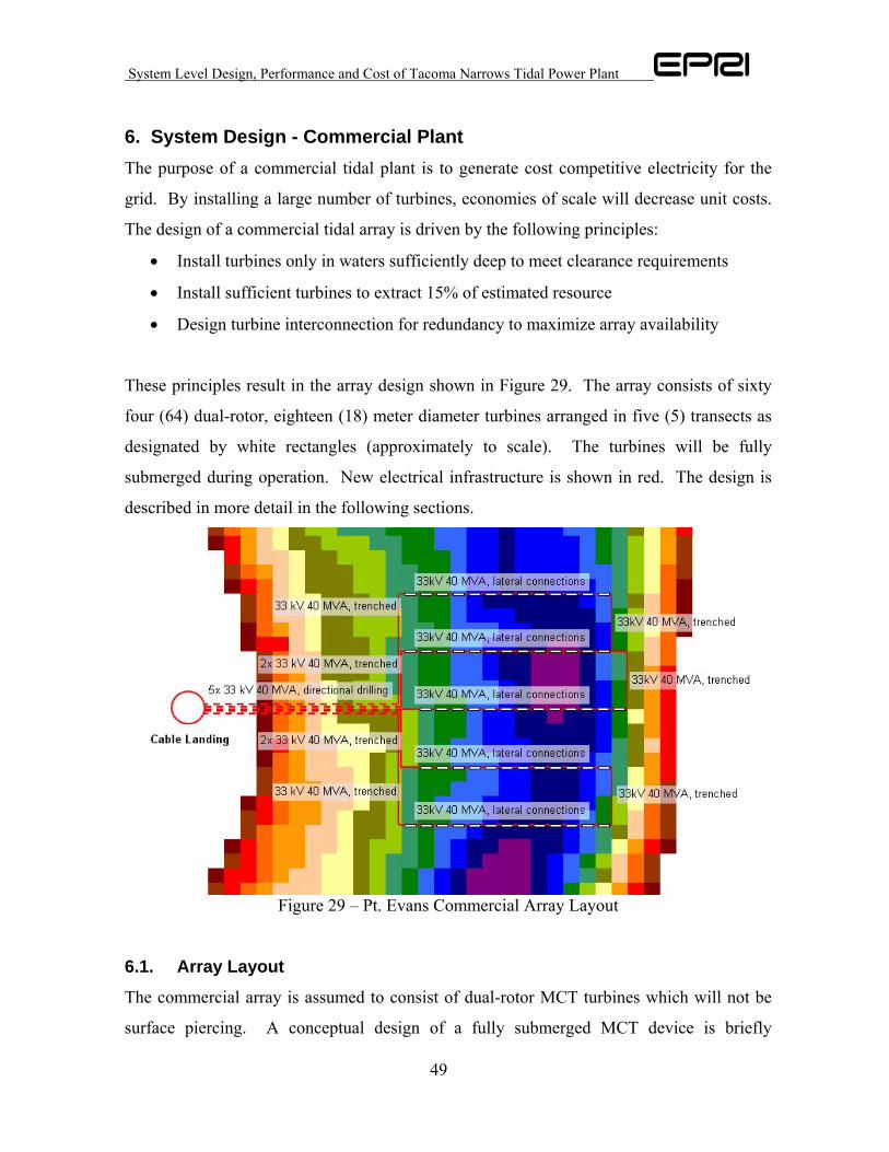
System Level Design, Performance and Cost of Tacoma Narrows Tidal Power Plant
49
6. System Design - Commercial Plant The purpose of a commercial tidal plant is to generate cost competitive electricity for the
grid. By installing a large number of turbines, economies of scale will decrease unit costs.
The design of a commercial tidal array is driven by the following principles:
• Install turbines only in waters sufficiently deep to meet clearance requirements
• Install sufficient turbines to extract 15% of estimated resource
• Design turbine interconnection for redundancy to maximize array availability
These principles result in the array design shown in Figure 29. The array consists of sixty
four (64) dual-rotor, eighteen (18) meter diameter turbines arranged in five (5) transects as
designated by white rectangles (approximately to scale). The turbines will be fully
submerged during operation. New electrical infrastructure is shown in red. The design is
described in more detail in the following sections.
Figure 29 – Pt. Evans Commercial Array Layout
6.1. Array Layout
The commercial array is assumed to consist of dual-rotor MCT turbines which will not be
surface piercing. A conceptual design of a fully submerged MCT device is briefly
System Level Design, Performance and Cost of Tacoma Narrows Tidal Power Plant
50
discussed in Chapter 3. Note that the array layout here is consistent with the dimensions of
a fully submerged SeaGen with two rotors and power trains per foundation pile. While
straight-line transects are used here, it is worth remembering that based on detailed site
velocity data, arrays might be laid out along curves of constant power flux [20].
The layout of the turbine array is governed by the following spacing rules:
• 8m clearance between rotor tip and seabed to prevent cyclic blade stresses due to
operation in the boundary layer.
• In shipping channel, 15m clearance between rotor tip and surface to accommodate
shipping traffic. Shipping lane is assumed to be the distance between east and west
caissons of the Tacoma Narrows Bridge (2800 ft) and is centered on the deep water
channel [15].
• Outside the shipping lane, 8m clearance between rotor tip and surface to
accommodate pleasure craft.
• 9m clearance between each turbine to prevent lateral interaction between rotors [25].
• 180m (10 turbine diameters) downstream spacing between array transects to allow
turbulent dissipation of rotor wake [27].
Note that these spacing rules have been developed based on analogues to wind-turbine array
layouts, and require additional modeling and testing to verify.
Since the next-generation, fully submerged turbine is conceptual at this stage, the following
assumptions have been made in for design and costing purposes:
• Fully submerged in operation
• Integrated lifting mechanism to bring turbine to surface for maintenance and
inspection without use of specialty craft
• Monopile foundation
• Two rotors per supporting foundation (dual-rotor turbine)
• Equipment and installation costs for next-generation MCT turbines in-line with
equipment and installation costs for SeaGen type device
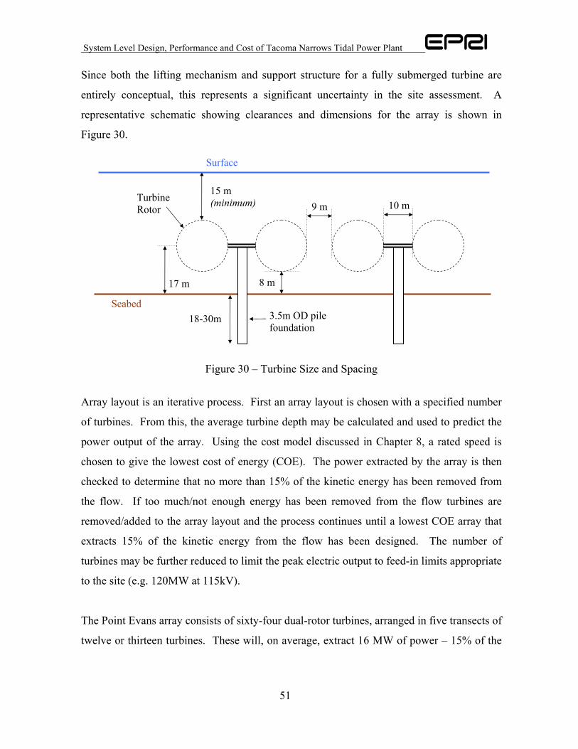
System Level Design, Performance and Cost of Tacoma Narrows Tidal Power Plant
51
Since both the lifting mechanism and support structure for a fully submerged turbine are
entirely conceptual, this represents a significant uncertainty in the site assessment. A
representative schematic showing clearances and dimensions for the array is shown in
Figure 30.
Figure 30 – Turbine Size and Spacing
Array layout is an iterative process. First an array layout is chosen with a specified number
of turbines. From this, the average turbine depth may be calculated and used to predict the
power output of the array. Using the cost model discussed in Chapter 8, a rated speed is
chosen to give the lowest cost of energy (COE). The power extracted by the array is then
checked to determine that no more than 15% of the kinetic energy has been removed from
the flow. If too much/not enough energy has been removed from the flow turbines are
removed/added to the array layout and the process continues until a lowest COE array that
extracts 15% of the kinetic energy from the flow has been designed. The number of
turbines may be further reduced to limit the peak electric output to feed-in limits appropriate
to the site (e.g. 120MW at 115kV).
The Point Evans array consists of sixty-four dual-rotor turbines, arranged in five transects of
twelve or thirteen turbines. These will, on average, extract 16 MW of power – 15% of the
8 m 17 m
Seabed
18 m
Turbine Rotor 9 m
15 m (minimum)
Surface
10 m
3.5m OD pile foundation
18-30m
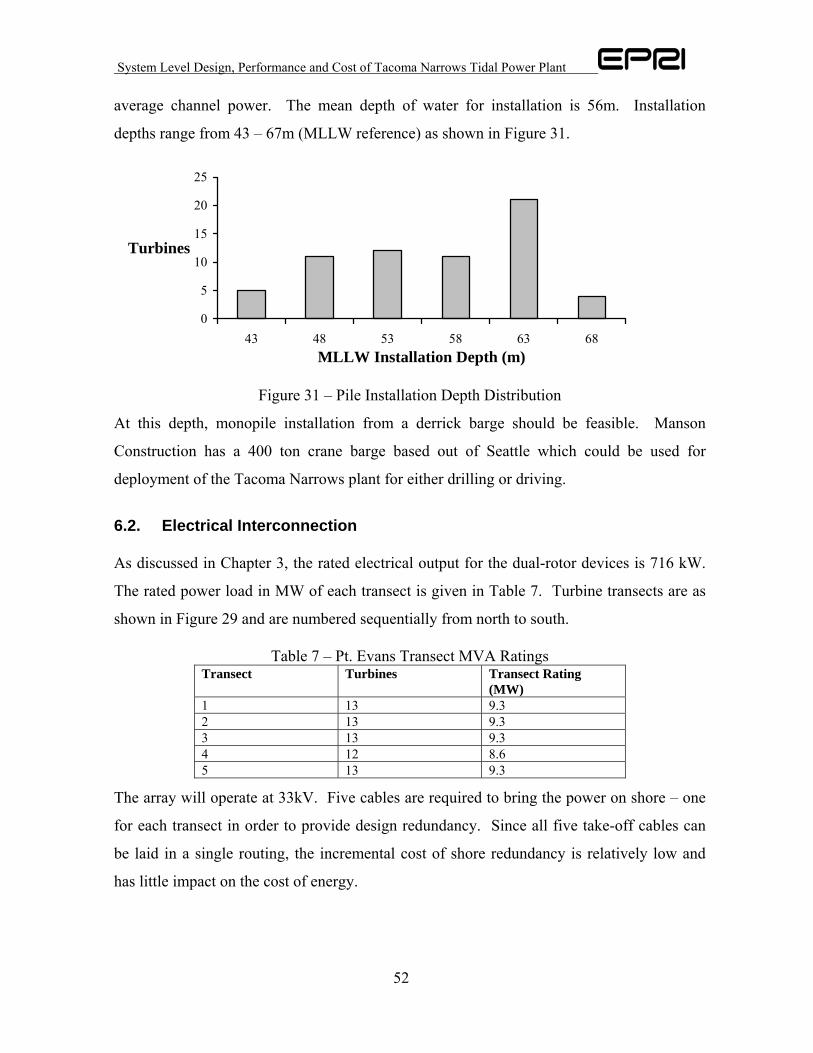
System Level Design, Performance and Cost of Tacoma Narrows Tidal Power Plant
52
average channel power. The mean depth of water for installation is 56m. Installation
depths range from 43 – 67m (MLLW reference) as shown in Figure 31.
0
5
10
15
20
25
43 48 53 58 63 68MLLW Installation Depth (m)
Turbines
Figure 31 – Pile Installation Depth Distribution
At this depth, monopile installation from a derrick barge should be feasible. Manson
Construction has a 400 ton crane barge based out of Seattle which could be used for
deployment of the Tacoma Narrows plant for either drilling or driving.
6.2. Electrical Interconnection
As discussed in Chapter 3, the rated electrical output for the dual-rotor devices is 716 kW.
The rated power load in MW of each transect is given in Table 7. Turbine transects are as
shown in Figure 29 and are numbered sequentially from north to south.
Table 7 – Pt. Evans Transect MVA Ratings Transect Turbines Transect Rating
(MW) 1 13 9.3 2 13 9.3 3 13 9.3 4 12 8.6 5 13 9.3
The array will operate at 33kV. Five cables are required to bring the power on shore – one
for each transect in order to provide design redundancy. Since all five take-off cables can
be laid in a single routing, the incremental cost of shore redundancy is relatively low and
has little impact on the cost of energy.
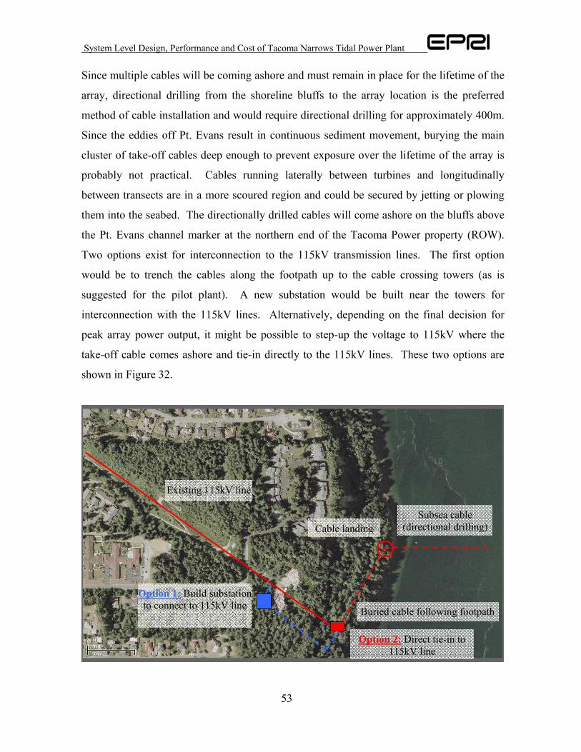
System Level Design, Performance and Cost of Tacoma Narrows Tidal Power Plant
53
Since multiple cables will be coming ashore and must remain in place for the lifetime of the
array, directional drilling from the shoreline bluffs to the array location is the preferred
method of cable installation and would require directional drilling for approximately 400m.
Since the eddies off Pt. Evans result in continuous sediment movement, burying the main
cluster of take-off cables deep enough to prevent exposure over the lifetime of the array is
probably not practical. Cables running laterally between turbines and longitudinally
between transects are in a more scoured region and could be secured by jetting or plowing
them into the seabed. The directionally drilled cables will come ashore on the bluffs above
the Pt. Evans channel marker at the northern end of the Tacoma Power property (ROW).
Two options exist for interconnection to the 115kV transmission lines. The first option
would be to trench the cables along the footpath up to the cable crossing towers (as is
suggested for the pilot plant). A new substation would be built near the towers for
interconnection with the 115kV lines. Alternatively, depending on the final decision for
peak array power output, it might be possible to step-up the voltage to 115kV where the
take-off cable comes ashore and tie-in directly to the 115kV lines. These two options are
shown in Figure 32.
Option 2: Direct tie-in to 115kV line
Option 1: Build substation to connect to 115kV line
Subsea cable (directional drilling)
Buried cable following footpath
Cable landing
Existing 115kV line
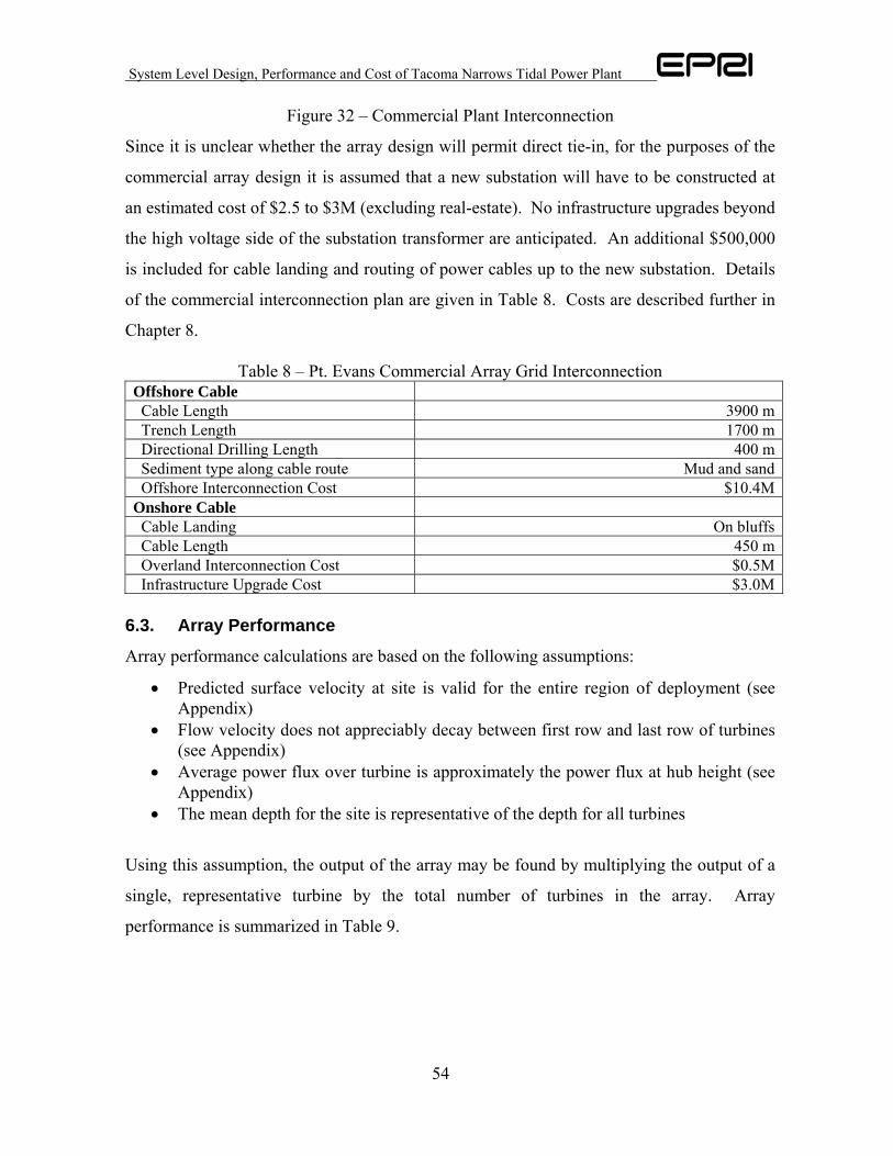
System Level Design, Performance and Cost of Tacoma Narrows Tidal Power Plant
54
Figure 32 – Commercial Plant Interconnection
Since it is unclear whether the array design will permit direct tie-in, for the purposes of the
commercial array design it is assumed that a new substation will have to be constructed at
an estimated cost of $2.5 to $3M (excluding real-estate). No infrastructure upgrades beyond
the high voltage side of the substation transformer are anticipated. An additional $500,000
is included for cable landing and routing of power cables up to the new substation. Details
of the commercial interconnection plan are given in Table 8. Costs are described further in
Chapter 8.
Table 8 – Pt. Evans Commercial Array Grid Interconnection Offshore Cable Cable Length 3900 m Trench Length 1700 m Directional Drilling Length 400 m Sediment type along cable route Mud and sand Offshore Interconnection Cost $10.4MOnshore Cable Cable Landing On bluffs Cable Length 450 m Overland Interconnection Cost $0.5M Infrastructure Upgrade Cost $3.0M
6.3. Array Performance
Array performance calculations are based on the following assumptions:
• Predicted surface velocity at site is valid for the entire region of deployment (see Appendix)
• Flow velocity does not appreciably decay between first row and last row of turbines (see Appendix)
• Average power flux over turbine is approximately the power flux at hub height (see Appendix)
• The mean depth for the site is representative of the depth for all turbines
Using this assumption, the output of the array may be found by multiplying the output of a
single, representative turbine by the total number of turbines in the array. Array
performance is summarized in Table 9.
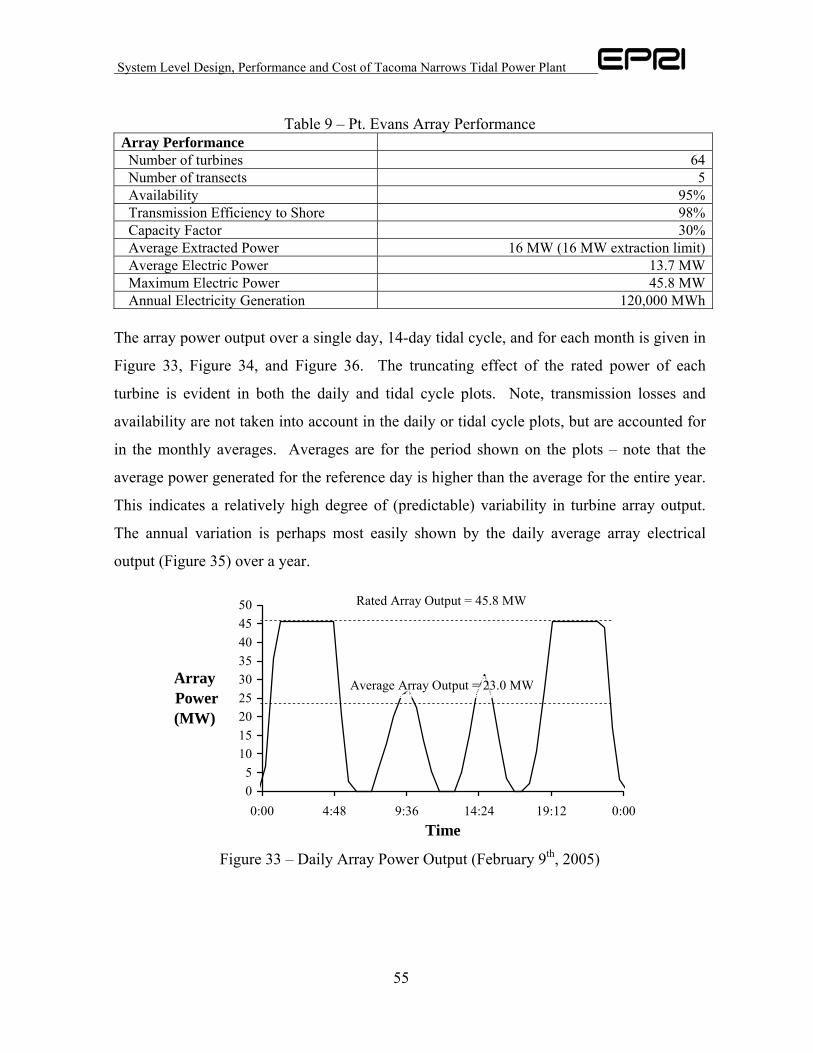
System Level Design, Performance and Cost of Tacoma Narrows Tidal Power Plant
55
Table 9 – Pt. Evans Array Performance
Array Performance Number of turbines 64 Number of transects 5 Availability 95% Transmission Efficiency to Shore 98% Capacity Factor 30% Average Extracted Power 16 MW (16 MW extraction limit) Average Electric Power 13.7 MW Maximum Electric Power 45.8 MW Annual Electricity Generation 120,000 MWh
The array power output over a single day, 14-day tidal cycle, and for each month is given in
Figure 33, Figure 34, and Figure 36. The truncating effect of the rated power of each
turbine is evident in both the daily and tidal cycle plots. Note, transmission losses and
availability are not taken into account in the daily or tidal cycle plots, but are accounted for
in the monthly averages. Averages are for the period shown on the plots – note that the
average power generated for the reference day is higher than the average for the entire year.
This indicates a relatively high degree of (predictable) variability in turbine array output.
The annual variation is perhaps most easily shown by the daily average array electrical
output (Figure 35) over a year.
05
101520253035404550
0:00 4:48 9:36 14:24 19:12 0:00Time
Array Power (MW)
Rated Array Output = 45.8 MW
Average Array Output = 23.0 MW
Figure 33 – Daily Array Power Output (February 9th, 2005)
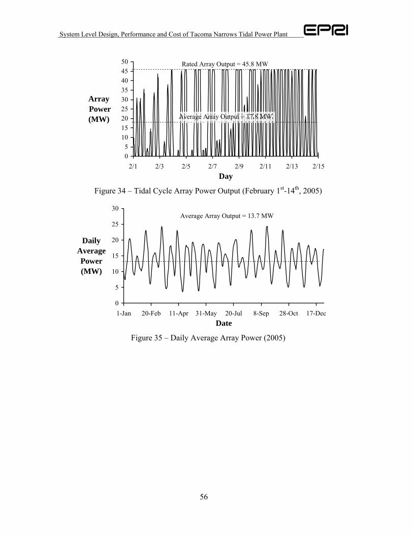
System Level Design, Performance and Cost of Tacoma Narrows Tidal Power Plant
56
05
101520253035404550
2/1 2/3 2/5 2/7 2/9 2/11 2/13 2/15Day
Array Power (MW)
Rated Array Output = 45.8 MW
Average Array Output = 17.8 MW
Figure 34 – Tidal Cycle Array Power Output (February 1st-14th, 2005)
0
5
10
15
20
25
30
1-Jan 20-Feb 11-Apr 31-May 20-Jul 8-Sep 28-Oct 17-DecDate
Daily Average Power (MW)
Average Array Output = 13.7 MW
Figure 35 – Daily Average Array Power (2005)
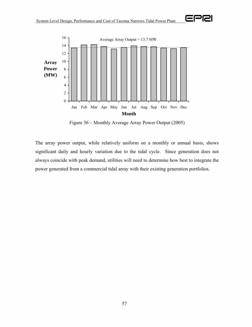
System Level Design, Performance and Cost of Tacoma Narrows Tidal Power Plant
57
0
2
4
6
8
10
12
14
16
Jan Feb Mar Apr May Jun Jul Aug Sep Oct Nov Dec
Month
Array Power (MW)
Average Array Output = 13.7 MW
Figure 36 – Monthly Average Array Power Output (2005)
The array power output, while relatively uniform on a monthly or annual basis, shows
significant daily and hourly variation due to the tidal cycle. Since generation does not
always coincide with peak demand, utilities will need to determine how best to integrate the
power generated from a commercial tidal array with their existing generation portfolios.

System Level Design, Performance and Cost of Tacoma Narrows Tidal Power Plant
58
6.4. Site Specific Issues
Eddies: Turbines should be sufficiently far from Pt. Evans to be unaffected by ebb and flood
eddies off the point.
Shipping: Operation of a fully submerged array of turbines with 15m overhead clearance at
LAT should in no way restrict shipping traffic in Tacoma Narrows. Installation and
maintenance plans should be structured as to minimize interference with shipping. The
Marine Exchange of Puget Sound [16] maintains detailed records of shipping traffic in
Puget Sound and would be an excellent starting point in modeling shipping traffic patterns.
Multiple Use: If, for safety reasons, no recreational boating, diving, or fishing would be able
to take place within the turbine deployment area for safety reasons, the array would require
an exclusion area of approximately 1 km2, 8% of the total surface area of Tacoma Narrows
(12.9 km2). The turbines and cabling occupy an even smaller footprint. This indicates that
even if multiple-use restrictions are necessary commercial scale array turbine installation
should be compatible with continued recreational use of most of Tacoma Narrows. MCT
expects that sport fishing would pose no threat to turbine operation, but net fishing is a
greater concern since nets could tangle and damage turbine rotors [20].
Bio-fouling: MCT expects neither kelp nor barnacles to pose any issue to turbine operation.
The site of the SeaFlow pilot is also a biologically active marine environment. However,
after three years of operation, there has been no substantial bio-accumulation on either rotor
or support structure, as shown in Figure 37.
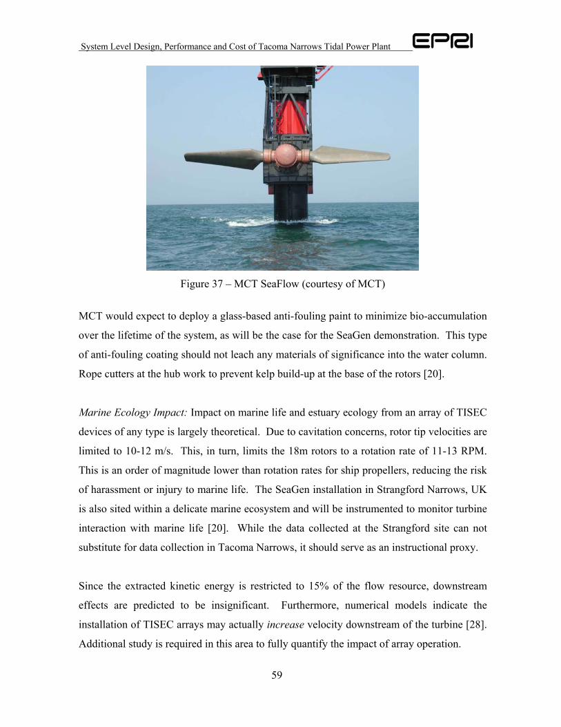
System Level Design, Performance and Cost of Tacoma Narrows Tidal Power Plant
59
Figure 37 – MCT SeaFlow (courtesy of MCT)
MCT would expect to deploy a glass-based anti-fouling paint to minimize bio-accumulation
over the lifetime of the system, as will be the case for the SeaGen demonstration. This type
of anti-fouling coating should not leach any materials of significance into the water column.
Rope cutters at the hub work to prevent kelp build-up at the base of the rotors [20].
Marine Ecology Impact: Impact on marine life and estuary ecology from an array of TISEC
devices of any type is largely theoretical. Due to cavitation concerns, rotor tip velocities are
limited to 10-12 m/s. This, in turn, limits the 18m rotors to a rotation rate of 11-13 RPM.
This is an order of magnitude lower than rotation rates for ship propellers, reducing the risk
of harassment or injury to marine life. The SeaGen installation in Strangford Narrows, UK
is also sited within a delicate marine ecosystem and will be instrumented to monitor turbine
interaction with marine life [20]. While the data collected at the Strangford site can not
substitute for data collection in Tacoma Narrows, it should serve as an instructional proxy.
Since the extracted kinetic energy is restricted to 15% of the flow resource, downstream
effects are predicted to be insignificant. Furthermore, numerical models indicate the
installation of TISEC arrays may actually increase velocity downstream of the turbine [28].
Additional study is required in this area to fully quantify the impact of array operation.

System Level Design, Performance and Cost of Tacoma Narrows Tidal Power Plant
60
7. Cost Assessment – Pilot Plant
The cost assessment of the demonstration plant was carried out by taking manufacturer
specifications for their devices, assessing principal loads on the structure and scaling the
devices to the design velocity at the deployment site. While all costing models were
developed internally, MCT provided data and support to calibrate the models, which was an
important step in developing meaningful and accurate cost models. Installation and
operational costs were evaluated by creating detailed cost build-ups for these aspects taking
into considerations equipment availability at North American rates. A high-level capital
cost breakdown relevant to the deployment site is shown in the table below. Note that the
costs in this table do not include any specialty instrumentation or measurement equipment
that may be deployed over the course of the pilot to satisfy regulatory requirements for a
commercial array.
Table 10 – Pilot Plant Cost Breakdown $/kW $/Turbine %
Power Conversion System $1,428 $1,022,050 24.6% Structural Steel Elements $922 $659,710 15.9% Subsea Cable Cost $25 $18,240 0.4% Turbine Installation $2,014 $1,442,000 34.7% Subsea Cable Installation $944 $675,842 16.3% Onshore Electric Grid Interconnection
$475 $340,000 8.2%
Total Installed Cost $5,808 $4,157,842 100%
A single unit will cost significantly more then subsequent units installed at the site.
Installation costs are dominated by mobilization charges. Additional, the first unit
equipment costs will always be higher then subsequent ones due to learning scale. The
assessment of operational and maintenance cost for the pilot was not part of the scope of
this study.
It is, however, important to understand that the purpose of the pilot plant is not to provide
low cost electricity, but to reduce risks associated with a commercial array. Risks include
technological uncertainty in device performance, operation and maintenance requirements,
validation of structural integrity, and environmental impact associated with the interaction
of the natural habitat with the TISEC device.
System Level Design, Performance and Cost of Tacoma Narrows Tidal Power Plant
61
8. Cost Assessment – Commercial Plant
Costs for the commercial plant are, as for most renewable energy generating technologies,
heavily weighted towards up-front capital. In order to determine the major cost centers of
the commercial plant, detailed cost build-ups were created in order to assess them properly
in the context of the given site conditions. The major influences on cost for a particular site
are discussed below:
Design Current Speed: The design current speed is the maximum velocity of the water
expected to occur at the site. Structural loads (and related structural cost) on a structure
increase with the square of the fluid velocity. Given the velocity distribution at the site, the
design velocity can be well above the velocity at which it is economically useful to extract
power. In other words, the design velocity can have a major influence on the cost of the
structural elements. During normal operating conditions, the loads on the structure will
peak near the rated turbine velocity and decrease thereafter as the turbine blades are pitched
to maintain constant power output, decreasing the thrust coefficient on the rotor blades. For
conservatism, the design velocity is set to the site peak, rather than device rating, in order to
simulate the loads experienced during runaway operation in the event of pitch control
failure.
Velocity Distribution: The velocity distribution at the site is outlined in Chapter 2 of this
report. As the rated velocity of the device increases, so do power train costs. Since the
velocity distribution tails off at higher velocities, the capital cost for equipment to extract
incrementally more flow power at high velocities may not be “paid back” by the additional
power generated. Rather than make assumptions as to appropriate rated velocities of TISEC
devices, an iterative approach was chosen to determine the rated speed of the machine
which yields the lowest cost of electricity at the particular site.
Seabed Composition: The seabed composition at the site has a major impact on the
foundation design of the TISEC device. For a monopile foundation, the seabed composition
determines the installation procedure (i.e. drilling and grouting or pile driving). The soil-

System Level Design, Performance and Cost of Tacoma Narrows Tidal Power Plant
62
type will also impact the cost of the monopile. Typically, soft soils yield higher monopile
cost then rock foundations.
Number of installed units: The number of TISEC devices deployed has a major influence
on the resulting cost of energy. In general a larger number of units will result in lower cost
of electricity due to economies of scale. There are several reasons for this which are
outlined below:
• Infrastructure cost required to interconnect the devices to the electric grid can be
shared and therefore their cost per unit of electricity produced is lower.
• Installation cost per turbine is lower because mobilization cost can be shared
between multiple devices. It is also apparent that the installation of the first unit is
more expensive then subsequent units as the installation contractor is able to
increase their operational efficiency.
• Capital cost per turbine is lower because manufacturing of multiple devices will
result in reduction of cost. The cost of manufactured steel as an example is very
labor intensive. The cost of hot rolled steel plates as of July 2005 was $650 per ton.
The final product can however cost as much as $4500 per manufactured ton of steel.
With other words there is significant potential to reduce capital cost by introducing
more efficient manufacturing processes and engineering a structure in such a way
that it can be manufactured cost effectively. The capital cost for all other equipment
and parts is very similar.
Device Reliability and O&M procedures: The device component reliability directly impacts
to operation and maintenance cost of a device. It is important to understand that it is not
only the component that needs to be replaced, but that the actual operation required to
recover the component can dominate the cost. Additional cost of the failure is incurred by
the downtime of the device and its inability to generate revenues by producing electricity.
In order to determine these operational costs, the failure rate on a per component basis was
estimated. Then operational procedures were outlined to replace these components and
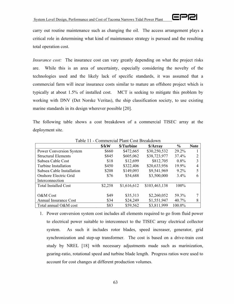
System Level Design, Performance and Cost of Tacoma Narrows Tidal Power Plant
63
carry out routine maintenance such as changing the oil. The access arrangement plays a
critical role in determining what kind of maintenance strategy is pursued and the resulting
total operation cost.
Insurance cost: The insurance cost can vary greatly depending on what the project risks
are. While this is an area of uncertainty, especially considering the novelty of the
technologies used and the likely lack of specific standards, it was assumed that a
commercial farm will incur insurance costs similar to mature an offshore project which is
typically at about 1.5% of installed cost. MCT is seeking to mitigate this problem by
working with DNV (Det Norske Veritas), the ship classification society, to use existing
marine standards in its design wherever possible [20].
The following table shows a cost breakdown of a commercial TISEC array at the
deployment site.
Table 11 - Commercial Plant Cost Breakdown $/kW $/Turbine $/Array % Note
Power Conversion System $660 $472,665 $30,250,532 29.2% 1Structural Elements $845 $605,062 $38,723,977 37.4% 2Subsea Cable Cost $18 $12,699 $812,705 0.8% 3Turbine Installation $450 $322,406 $20,633,956 19.9% 4Subsea Cable Installation $208 $149,093 $9,541,969 9.2% 5Onshore Electric Grid Interconnection
$76 $54,688 $3,500,000 3.4% 6
Total Installed Cost $2,258 $1,616,612 $103,463,138 100% O&M Cost $49 $35,313 $2,260,052 59.3% 7Annual Insurance Cost $34 $24,249 $1,551,947 40.7% 8Total annual O&M cost $83 $59,562 $3,811,999 100.0%
1. Power conversion system cost includes all elements required to go from fluid power
to electrical power suitable to interconnect to the TISEC array electrical collector
system. As such it includes rotor blades, speed increaser, generator, grid
synchronization and step-up transformer. The cost is based on a drive-train cost
study by NREL [18] with necessary adjustments made such as marinization,
gearing-ratio, rotational speed and turbine blade length. Progress ratios were used to
account for cost changes at different production volumes.

System Level Design, Performance and Cost of Tacoma Narrows Tidal Power Plant
64
2. Structural steel elements include all elements required to hold the turbine in place.
In the case of MCT, this is the monopile and cross arm. In order to determine the
amount of steel required, the manufacturer’s data was scaled based on the estimated
loads on the structure. Only principal loads based on the fluid velocity were
considered and it was assumed that they are the driving factor. While this approach
is well suited for a conceptual study, it must be stressed that other loading conditions
such as wave loads, resonance conditions, pile driving forces, or seismic activity can
significantly influence the design and will need to be taken into consideration in a
detailed design phase.
3. Subsea cable cost includes the cable cost to collect the electricity from the turbines
and bring the electricity to shore at a suitable location.
4. Turbine installation cost includes all cost components to install the turbines.
Detailed models were developed to outline the deployment procedures using heavy
offshore equipment such as crane barges, tugs, supply vessels, drilling equipment,
mobilization charges and crew cost. Discussions with experienced contractors and
offshore engineers were used to solidify costs.
5. Subsea cable installation cost includes, trenching, cable laying, and trench back-fill
using a derrick barge. It also includes cable landing costs. If existing easements
such as pipes or existing pier or bridge structures are in place, the cable can be
landed on shore using these easements. If not, it was assumed that directional
drilling is used to bring the cable to shore.
6. Onshore electrical grid interconnection includes all cost components required to
bring the power to the next substation. Cost components required to build-out the
capabilities of the substation or upgrade the transmission capacity of the electric grid
are excluded from cost of energy calculations as these are born by the project but
paid back as a wires charge over its life.

System Level Design, Performance and Cost of Tacoma Narrows Tidal Power Plant
65
9. Cost of Electricity Assessments
To evaluate the economics of tidal in-stream power plants, three standard economic
assessment methodologies have been used:
1. Utility Generator (UG),
2. Municipal Generator (MG)
3. Non-Utility Generator (NUG) or Independent Power Producer (IPP).
Taxable regulated utilities (independently owned utilities) are permitted to set electricity
rates (i.e., collect revenue) that will cover operating costs and provide an opportunity to
earn a reasonable rate of return on the property devoted to the business. This return must
enable the UG to maintain its financial credit as well as to attract whatever capital may be
required in the future for replacement, expansion and technological innovation and must be
comparable to that earned by other businesses with corresponding risk.
Non taxable municipal utilities also set electricity rates that will cover operating costs,
however, utility projects are financed by issuing tax-exempt bonds, enabling local
governments to access some of the lowest interest rates available
Because the risks associated with private ownership are generally considered to be greater
than utility ownership, the return on equity must be potentially higher in order to justify the
investment. However, it is important to understand that there is no single right method to
model an independently owned and operated NUG or IPP renewable power plant.
Considerations such as an organization’s access to capital, project risks, and power purchase
and contract terms determine project risks and therefore the cost of money.
These regulated UG and MG methodologies are based on a levelized cost approach using
both real (constant) and nominal (current) dollars with 2005 as the reference year and a 20-
year book life. The purpose of these standard methodologies is to provide a consistent,
verifiable and replicable basis for computing the cost of electricity (COE) of a tidal energy

System Level Design, Performance and Cost of Tacoma Narrows Tidal Power Plant
66
generation project (i.e., a project to engineer, permit, procure, construct, operate and
maintain a tidal energy power plant).
The NUG methodology is based on a cash flow analysis and projections of market
electricity prices. This allows a NUG to estimate how quickly an initial investment is
recovered and how returns change over time.
The results of this economic evaluation will help government policy makers determine the
public benefit of investing public funds into building the experience base of tidal energy to
transform the market to the point where private investment will take over and sustain the
market. Such technology support is typically done through funding R&D and through
incentives for the deployment of targeted renewable technologies.
If the economics of the notional commercial scale tidal in-stream power plant is favorable
with respect to alternative renewable generation options, a case can be made for pursuing
the development of tidal flow energy conversion technology. If, however, even with the
most optimistic assumptions, the economics of a commercial size tidal flow power plant is
not favorable and cannot economically compete with the alternatives, a case can be made
for not pursuing tidal flow energy conversion technology development.
The methodology is described in detail in [2].
The yearly electrical energy produced and delivered to bus bar by the commercial TISEC
plant described in sections 6 and 8 is estimated to be 120,000 MWh/year for an array
consisting of sixty-four dual-rotor turbines. These turbines will, on average, extract 16MW
of kinetic power from the tidal stream – 15% of the total kinetic energy in the flow at Pt.
Evans. Turbines will be arranged in five rows of twelve to thirteen devices. The elements
of cost and economics (in 2005$) are:
• Total Plant Investment = $103 million
• Annual O&M Cost = $3.8 million
System Level Design, Performance and Cost of Tacoma Narrows Tidal Power Plant
67
• Utility Generator (UG) Levelized Cost of Electricity (COE)7 = 9.0 (Real) – 10.6
(Nominal) cents/kWh with renewable energy incentives equal to those that the
government provides for renewable wind energy technology
• Non Utility Generator (NUG) Levelized Cost of Electricity (IRR) = N/A
• Municipal Generator (MG) Levelized Cost of Electricity (COE) = 7.2 (Real) – 8.4
(Nominal) cents/kWh with renewable energy incentives equal to those that the
government provides for renewable wind energy technology
The detailed worksheets including financial assumptions used to calculate these COEs and
IRR are contained in Appendices (sections 13.4 through 13.6)
The COE for a Municipal Generator such as Tacoma Power is in the range of other
renewable and non renewable energy supply options. Washington does not provide an
internal rate of return (IRR) for a Non-Utility Generator as the avoided cost (average
industrial wholesale rate is used as a proxy for avoided cost) is low (3.86 cents/kWh).
TISEC technology is very similar to wind technology and has benefited from the learning
curve of wind technology, both on shore and off shore. Therefore, the entry point for a
TISEC plant is much less than that of wind technology back in the late 1970s and early
1980s (i.e., over 20 cents/kWh). Additional cost reductions will certainly be realized
through value engineering and economies of scale.
Except for the Minas Passage in Nova Scotia which clearly has the size to be considered
central power, all other sites studied in the U.S. and Canada fall in between the definition of
distributed generation (DG) and central power generation.
We use the term distributed generation (DG) or distributed resources (DR) to describe an
electric generation plant located in close proximity to the load that it is supplying and is
either connected to the electric grid at distribution level voltages or connected directly to the
7 For the 45.7 MW 20 year life plant, 10 years of PTC at 0.18 cents/kWh for a taxable entity, a REPI credit at $0.015 cents/kWh for a non taxable MG and other assumptions documented in [2].

System Level Design, Performance and Cost of Tacoma Narrows Tidal Power Plant
68
load. Examples of DG/DR (DR when some form of storage is included) are rooftop
photovoltaic systems, natural gas micro turbines and small wind turbines. Large wind
projects and traditional fossil and nuclear plants are examples of central generation where
the electricity delivers power into the grid at transmission voltage levels.
DG types of systems traditionally find applications in niche markets because of unique
market drivers such as:
• Delay or defer an upgrade to T&D infrastructure that would otherwise have been
necessary to bring power generated away from a load center to that load center
• Voltage stability support
• Displace diesel fuel in off grid applications
• Satisfy local citizens desires to have control of their own power source
A realistic comparison to equitably evaluate the cost of deferring T&D expenses with the
cost of installing DG/DR is complex and requires considering depreciation and tax benefits,
property tax and insurance for both options, maintenance and fuel costs of operating the
DG/DR and employing discounted cash flow methods. This comparison must be made on a
case-by-case basis.
EPRI, in collaboration with DOER, NJBPU and CEC, and funded by NASEO, is studying
political and financial mechanisms for win-win DG/DR solutions for both the distribution
utility and the end user.
Economic assessments of a commercial scale tidal power plant and other renewable and non
renewable energy systems were made. The current comparative costs of several different
central power generation technologies are given in Table 12 below for 2010. Capital costs
are given in $/kW. They have wide ranges that depend on the size of the plant and other
conditions such as environmental controls for coal and quality of the resource for
geothermal. We are using generally accepted average numbers and ranges from EPRI
sources [26].
Table 12 - COE for Alternative Energy Technologies: 2010
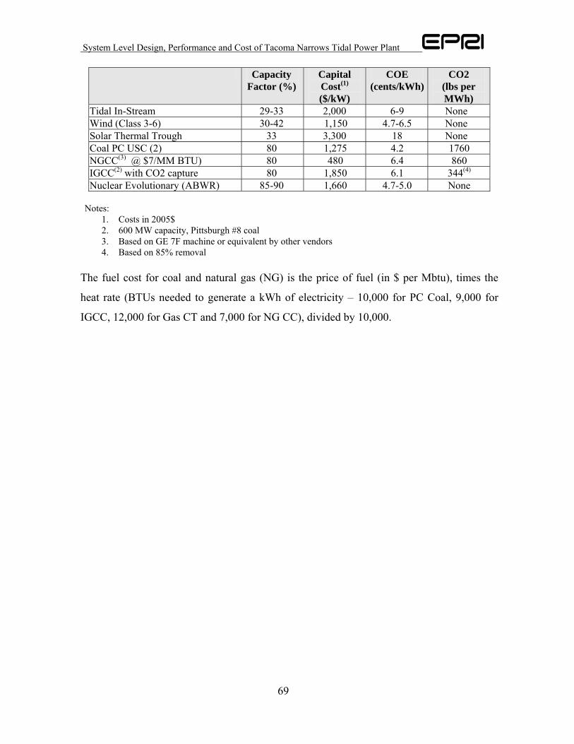
System Level Design, Performance and Cost of Tacoma Narrows Tidal Power Plant
69
Capacity Factor (%)
Capital Cost(1) ($/kW)
COE (cents/kWh)
CO2 (lbs per MWh)
Tidal In-Stream 29-33 2,000 6-9 None Wind (Class 3-6) 30-42 1,150 4.7-6.5 None Solar Thermal Trough 33 3,300 18 None Coal PC USC (2) 80 1,275 4.2 1760 NGCC(3) @ $7/MM BTU) 80 480 6.4 860 IGCC(2) with CO2 capture 80 1,850 6.1 344(4) Nuclear Evolutionary (ABWR) 85-90 1,660 4.7-5.0 None
Notes:
1. Costs in 2005$ 2. 600 MW capacity, Pittsburgh #8 coal 3. Based on GE 7F machine or equivalent by other vendors 4. Based on 85% removal
The fuel cost for coal and natural gas (NG) is the price of fuel (in $ per Mbtu), times the
heat rate (BTUs needed to generate a kWh of electricity – 10,000 for PC Coal, 9,000 for
IGCC, 12,000 for Gas CT and 7,000 for NG CC), divided by 10,000.
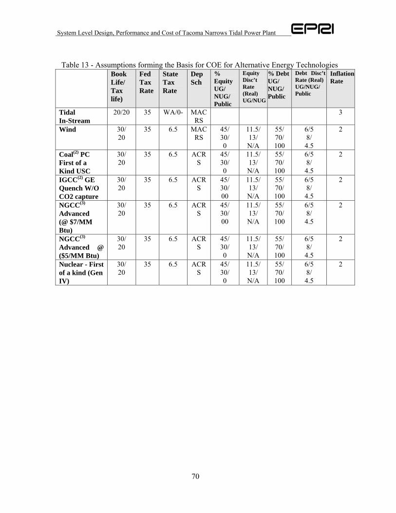
System Level Design, Performance and Cost of Tacoma Narrows Tidal Power Plant
70
Table 13 - Assumptions forming the Basis for COE for Alternative Energy Technologies Book
Life/ Tax life)
Fed Tax Rate
State Tax Rate
Dep Sch
% Equity UG/ NUG/ Public
Equity Disc’t Rate (Real) UG/NUG
% Debt UG/ NUG/ Public
Debt Disc’t Rate (Real)UG/NUG/ Public
InflationRate
Tidal In-Stream
20/20 35 WA/0- MACRS
3
Wind 30/ 20
35 6.5 MACRS
45/ 30/ 0
11.5/ 13/ N/A
55/ 70/ 100
6/5 8/ 4.5
2
Coal(2) PC First of a Kind USC
30/ 20
35 6.5 ACRS
45/ 30/ 0
11.5/ 13/ N/A
55/ 70/ 100
6/5 8/ 4.5
2
IGCC(2) GE Quench W/O CO2 capture
30/ 20
35 6.5 ACRS
45/ 30/ 00
11.5/ 13/ N/A
55/ 70/ 100
6/5 8/ 4.5
2
NGCC(3) Advanced (@ $7/MM Btu)
30/ 20
35 6.5 ACRS
45/ 30/ 00
11.5/ 13/ N/A
55/ 70/ 100
6/5 8/ 4.5
2
NGCC(3) Advanced @ ($5/MM Btu)
30/ 20
35 6.5 ACRS
45/ 30/ 0
11.5/ 13/ N/A
55/ 70/ 100
6/5 8/ 4.5
2
Nuclear - First of a kind (Gen IV)
30/ 20
35 6.5 ACRS
45/ 30/ 0
11.5/ 13/ N/A
55/ 70/ 100
6/5 8/ 4.5
2
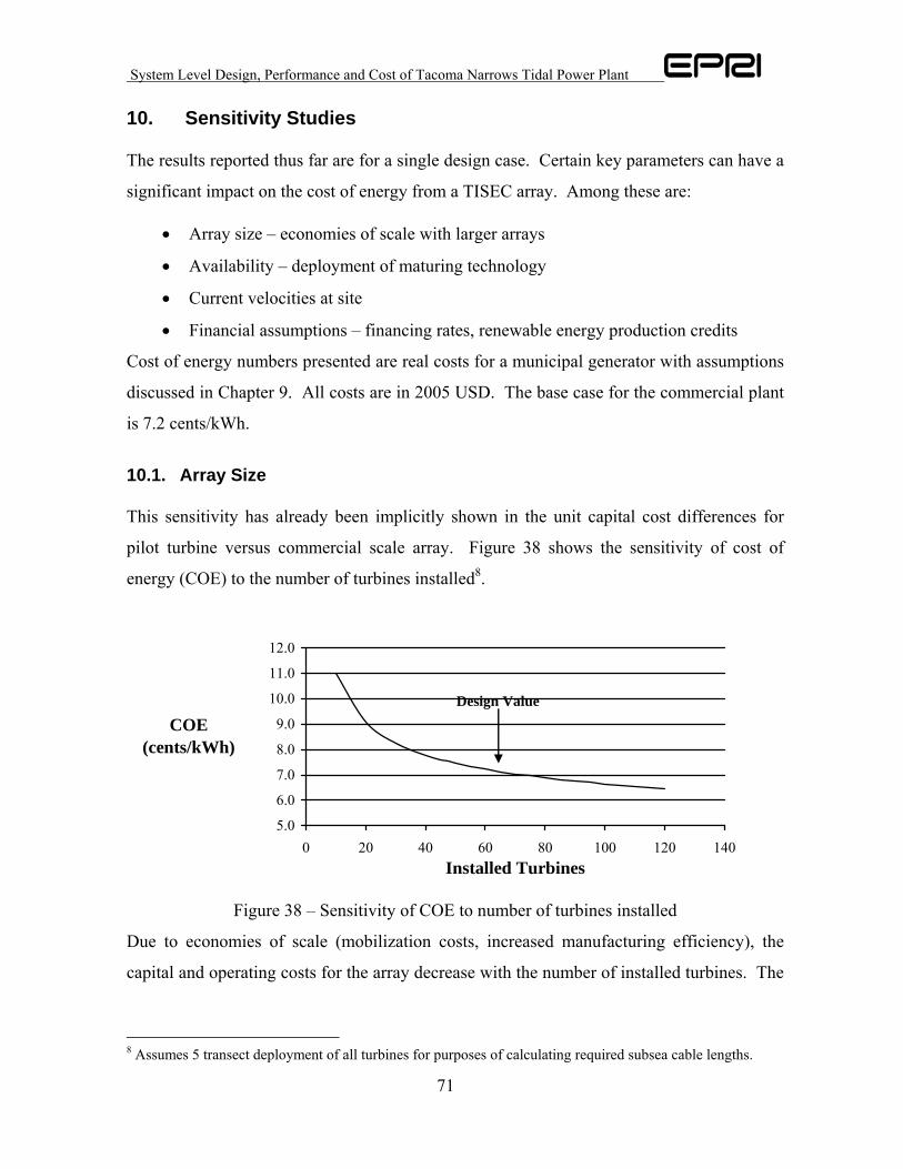
System Level Design, Performance and Cost of Tacoma Narrows Tidal Power Plant
71
10. Sensitivity Studies
The results reported thus far are for a single design case. Certain key parameters can have a
significant impact on the cost of energy from a TISEC array. Among these are:
• Array size – economies of scale with larger arrays
• Availability – deployment of maturing technology
• Current velocities at site
• Financial assumptions – financing rates, renewable energy production credits
Cost of energy numbers presented are real costs for a municipal generator with assumptions
discussed in Chapter 9. All costs are in 2005 USD. The base case for the commercial plant
is 7.2 cents/kWh.
10.1. Array Size
This sensitivity has already been implicitly shown in the unit capital cost differences for
pilot turbine versus commercial scale array. Figure 38 shows the sensitivity of cost of
energy (COE) to the number of turbines installed8.
5.0
6.0
7.0
8.0
9.0
10.0
11.0
12.0
0 20 40 60 80 100 120 140Installed Turbines
COE (cents/kWh)
Design Value
Figure 38 – Sensitivity of COE to number of turbines installed
Due to economies of scale (mobilization costs, increased manufacturing efficiency), the
capital and operating costs for the array decrease with the number of installed turbines. The
8 Assumes 5 transect deployment of all turbines for purposes of calculating required subsea cable lengths.
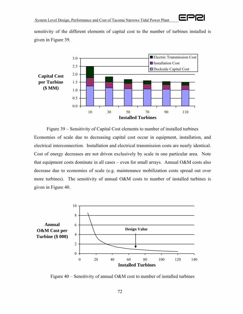
System Level Design, Performance and Cost of Tacoma Narrows Tidal Power Plant
72
sensitivity of the different elements of capital cost to the number of turbines installed is
given in Figure 39.
0.0
0.5
1.0
1.5
2.0
2.5
3.0
10 30 50 70 90 110Installed Turbines
Capital Cost per Turbine
($ MM)
Electric Transmission CostInstallation CostDockside Capital Cost
Figure 39 – Sensitivity of Capital Cost elements to number of installed turbines
Economies of scale due to decreasing capital cost occur in equipment, installation, and
electrical interconnection. Installation and electrical transmission costs are nearly identical.
Cost of energy decreases are not driven exclusively by scale in one particular area. Note
that equipment costs dominate in all cases – even for small arrays. Annual O&M costs also
decrease due to economies of scale (e.g. maintenance mobilization costs spread out over
more turbines). The sensitivity of annual O&M costs to number of installed turbines is
given in Figure 40.
0
2
4
6
8
10
0 20 40 60 80 100 120 140Installed Turbines
Annual O&M Cost per Turbine ($ 000)
Design Value
Figure 40 – Sensitivity of annual O&M cost to number of installed turbines
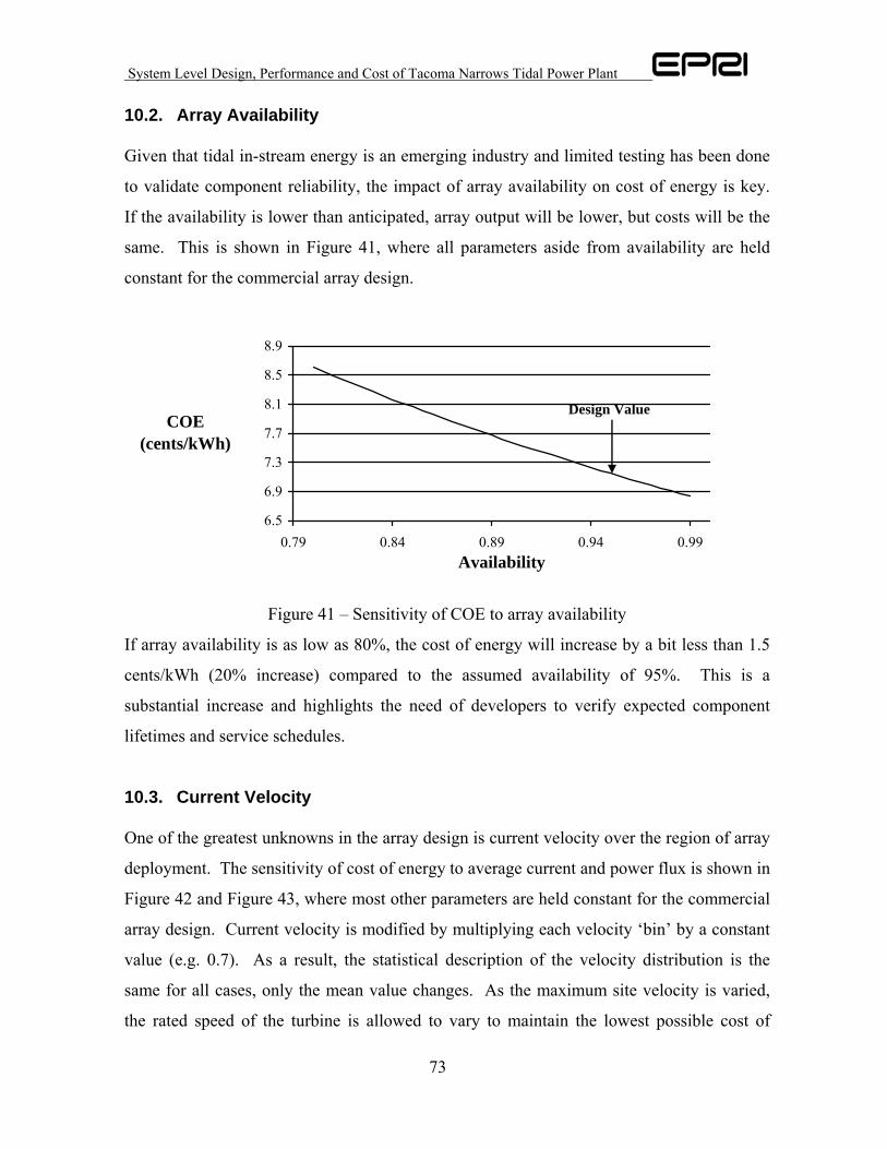
System Level Design, Performance and Cost of Tacoma Narrows Tidal Power Plant
73
10.2. Array Availability
Given that tidal in-stream energy is an emerging industry and limited testing has been done
to validate component reliability, the impact of array availability on cost of energy is key.
If the availability is lower than anticipated, array output will be lower, but costs will be the
same. This is shown in Figure 41, where all parameters aside from availability are held
constant for the commercial array design.
6.5
6.9
7.3
7.7
8.1
8.5
8.9
0.79 0.84 0.89 0.94 0.99Availability
COE (cents/kWh)
Design Value
Figure 41 – Sensitivity of COE to array availability
If array availability is as low as 80%, the cost of energy will increase by a bit less than 1.5
cents/kWh (20% increase) compared to the assumed availability of 95%. This is a
substantial increase and highlights the need of developers to verify expected component
lifetimes and service schedules.
10.3. Current Velocity
One of the greatest unknowns in the array design is current velocity over the region of array
deployment. The sensitivity of cost of energy to average current and power flux is shown in
Figure 42 and Figure 43, where most other parameters are held constant for the commercial
array design. Current velocity is modified by multiplying each velocity ‘bin’ by a constant
value (e.g. 0.7). As a result, the statistical description of the velocity distribution is the
same for all cases, only the mean value changes. As the maximum site velocity is varied,
the rated speed of the turbine is allowed to vary to maintain the lowest possible cost of
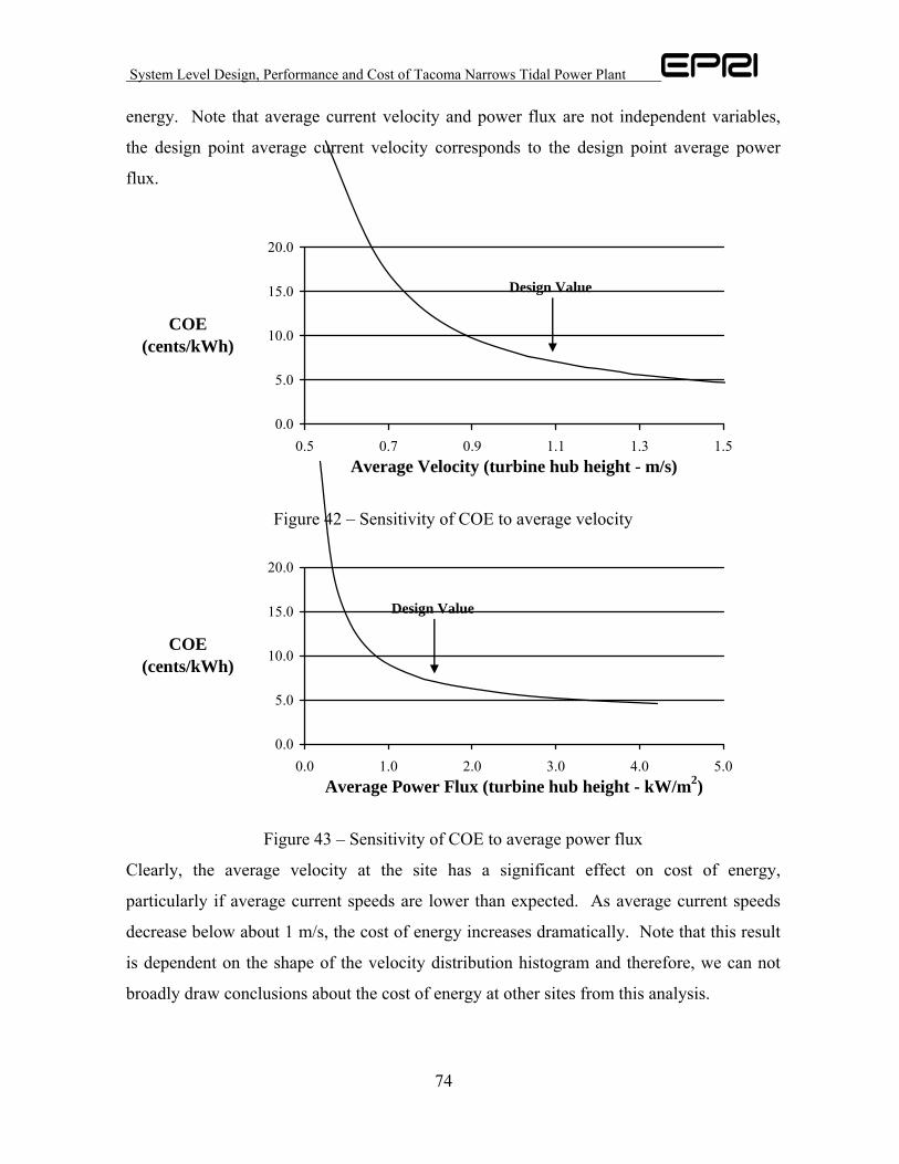
System Level Design, Performance and Cost of Tacoma Narrows Tidal Power Plant
74
energy. Note that average current velocity and power flux are not independent variables,
the design point average current velocity corresponds to the design point average power
flux.
0.0
5.0
10.0
15.0
20.0
0.5 0.7 0.9 1.1 1.3 1.5Average Velocity (turbine hub height - m/s)
COE (cents/kWh)
Design Value
Figure 42 – Sensitivity of COE to average velocity
0.0
5.0
10.0
15.0
20.0
0.0 1.0 2.0 3.0 4.0 5.0Average Power Flux (turbine hub height - kW/m2)
COE (cents/kWh)
Design Value
Figure 43 – Sensitivity of COE to average power flux
Clearly, the average velocity at the site has a significant effect on cost of energy,
particularly if average current speeds are lower than expected. As average current speeds
decrease below about 1 m/s, the cost of energy increases dramatically. Note that this result
is dependent on the shape of the velocity distribution histogram and therefore, we can not
broadly draw conclusions about the cost of energy at other sites from this analysis.
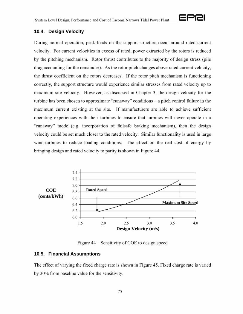
System Level Design, Performance and Cost of Tacoma Narrows Tidal Power Plant
75
10.4. Design Velocity
During normal operation, peak loads on the support structure occur around rated current
velocity. For current velocities in excess of rated, power extracted by the rotors is reduced
by the pitching mechanism. Rotor thrust contributes to the majority of design stress (pile
drag accounting for the remainder). As the rotor pitch changes above rated current velocity,
the thrust coefficient on the rotors decreases. If the rotor pitch mechanism is functioning
correctly, the support structure would experience similar stresses from rated velocity up to
maximum site velocity. However, as discussed in Chapter 3, the design velocity for the
turbine has been chosen to approximate “runaway” conditions – a pitch control failure in the
maximum current existing at the site. If manufacturers are able to achieve sufficient
operating experiences with their turbines to ensure that turbines will never operate in a
“runaway” mode (e.g. incorporation of failsafe braking mechanism), then the design
velocity could be set much closer to the rated velocity. Similar functionality is used in large
wind-turbines to reduce loading conditions. The effect on the real cost of energy by
bringing design and rated velocity to parity is shown in Figure 44.
6.06.26.46.66.87.07.27.4
1.5 2.0 2.5 3.0 3.5 4.0Design Velocity (m/s)
COE (cents/kWh)
Rated Speed
Maximum Site Speed
Figure 44 – Sensitivity of COE to design speed
10.5. Financial Assumptions
The effect of varying the fixed charge rate is shown in Figure 45. Fixed charge rate is varied
by 30% from baseline value for the sensitivity.
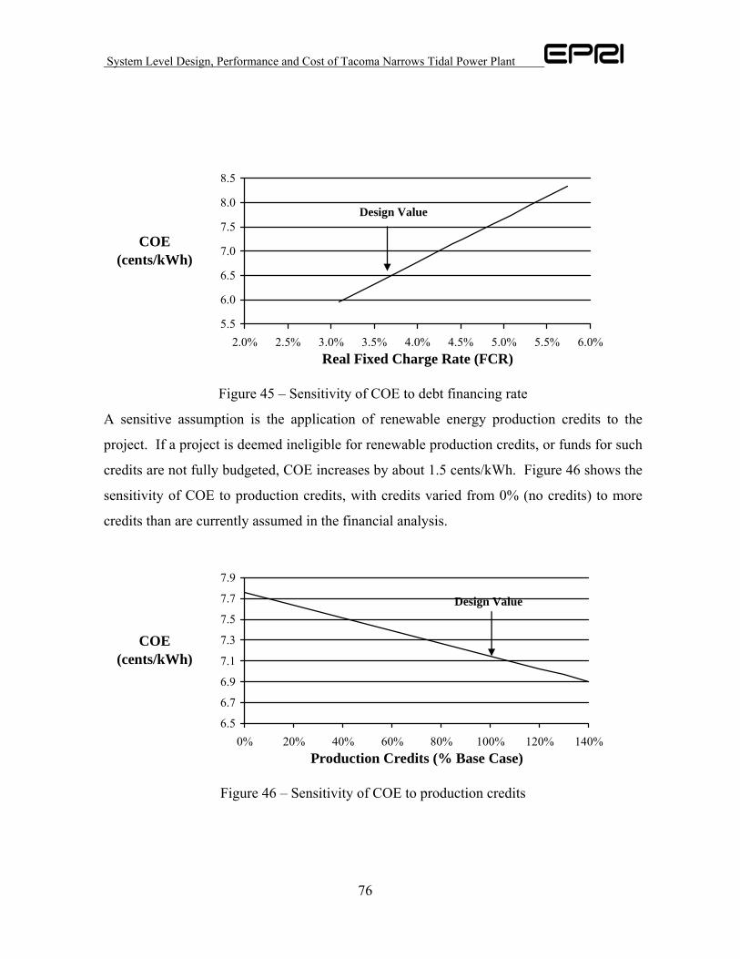
System Level Design, Performance and Cost of Tacoma Narrows Tidal Power Plant
76
5.5
6.0
6.5
7.0
7.5
8.0
8.5
2.0% 2.5% 3.0% 3.5% 4.0% 4.5% 5.0% 5.5% 6.0%Real Fixed Charge Rate (FCR)
COE (cents/kWh)
Design Value
Figure 45 – Sensitivity of COE to debt financing rate
A sensitive assumption is the application of renewable energy production credits to the
project. If a project is deemed ineligible for renewable production credits, or funds for such
credits are not fully budgeted, COE increases by about 1.5 cents/kWh. Figure 46 shows the
sensitivity of COE to production credits, with credits varied from 0% (no credits) to more
credits than are currently assumed in the financial analysis.
6.5
6.7
6.9
7.1
7.3
7.5
7.7
7.9
0% 20% 40% 60% 80% 100% 120% 140%Production Credits (% Base Case)
COE (cents/kWh)
Design Value
Figure 46 – Sensitivity of COE to production credits
System Level Design, Performance and Cost of Tacoma Narrows Tidal Power Plant
77
11. Conclusions
For the single point commercial scale design chosen for feasibility assessment by EPRI in
this study (based on the MCT SeaGen commercial prototype machine), Point Evans is a
reasonably good location for the installation of a pilot tidal in-stream power plant. The
predicted resource is strong, interconnection is easily managed, and the site is served by a
major port facility in close proximity. The pilot will be surface-piercing and may fall inside
the conventional shipping lanes for Tacoma Narrows. The purpose of the pilot is to
demonstrate the potential for a commercial array, verify reliability, availability, low
environmental impact and cost estimates, and generally build towards regulatory acceptance
of an array of similar devices. Since the commercial plant will be fully submerged, the
support structure for the commercial plant will vary from the pilot and may require some
additional on-site testing prior to deployment.
11.1. Pilot In-Stream Tidal Power Plant
A pilot scale tidal power plant rated at 716kW, using an MCT commercial prototype
SeaGen device would cost about $4.2M to build and will produce an estimated 2010 MWh
per year. This cost reflects only the capital needed to purchase a SeaGen unit, install it on
site, and connect it to the grid. Therefore, it represents the installed capital cost required to
evaluate and test a SeaGen TISEC system, but does not include detailed design, permitting
and construction financing, yearly O&M or test and evaluation costs.
11.2. Commercial In-Stream Tidal Power Plant
A commercial scale tidal power plant at the same location was also evaluated to establish a
base case from which economic comparisons to other renewable and non renewable energy
systems could be made. The yearly electrical energy produced and delivered to bus bar is
estimated to be 120,000 MWh/year for an array consisting of sixty-four dual-rotor turbines.
These turbines will, on average, extract 16MW of kinetic power from the tidal stream –
15% of the total kinetic energy in the flow at Pt. Evans. The elements of cost and economics
(in 2005$) are:
System Level Design, Performance and Cost of Tacoma Narrows Tidal Power Plant
78
• Total Plant Investment = $103 million
• Annual O&M Cost = $3.8 million
• Utility Generator (UG) Levelized Cost of Electricity (COE)9 = 9.0 (Real) – 10.6
(Nominal) cents/kWh with renewable energy incentives equal to those that the
government provides for renewable wind energy technology
• Non Utility Generator (NUG) Levelized Cost of Electricity (IRR) = N/A due to low
avoided cost of energy.
• Municipal Generator (MG) Levelized Cost of Electricity (COE) = 7.2 (Real) – 8.4
(Nominal) cents/kWh with renewable energy incentives equal to those that the
government provides for renewable wind energy technology
Pt. Evans is a strong candidate site for the installation of a commercial tidal in-stream plant.
The predicted resource is sufficient to generate a meaningful level of electric power
(>10MW on average) with nearby high voltage transmission lines. Through the use of fully
submerged next-generation devices, multiple turbine transects could be sited in the vicinity
of Point Evans without impeding shipping traffic. Installation and operation of the array
would occupy a relatively small area of the Narrows (<10%). For public safety reasons, it
may be necessary to set up a recreation (e.g. diving) exclusion zone within this area.
Since the commercial array design incorporates features that are largely conceptual, there is
significant economic and technical uncertainty in the deployment of a commercial array at
Pt. Evans. If the cost and performance of a fully submerged design is in-line with SeaGen,
then the results of this study show that an in-stream tidal power plant may provide favorable
economics in terms of COE for a UG or MG in comparison to other locally available
renewable energy production options. This is a technology worth pursuing.
11.3. Techno-economic Challenges
The cost for the first tidal plant leverages the learnings gained from wind energy. Rather
than seeing a sharp reduction in unit cost in early production, a substantial decrease might
9 For the 45.7 MW 20 year life plant, 10 years of PTC at 0.18 cents/kWh for a taxable entity, a REPI credit at $0.015 cents/kWh for a non taxable MG and other assumptions documented in [2].
System Level Design, Performance and Cost of Tacoma Narrows Tidal Power Plant
79
require another 40,000 MW of installed capacity (double the end of 2004 wind production
volume). Device manufacturers are pursuing value engineering and novel approaches to
array-scale installations. The economic analysis presented in this report is based on first-
generation device economics. The assumption implicit in this analysis is that while next-
generation devices will enable turbine deployment at a wider range of sites (e.g. deep water)
and with greater versatility (e.g. integrated lift without surface piercing pile) the cost of
installing and operating next-generation turbines will be similar to first-generation devices.
O&M costs are particularly uncertain since no tidal current turbine has been in service for
extended periods of time. Assumptions regarding intervention frequencies, refit costs, and
component lifetimes will not be completely borne out for at least a decade.
Sensitivities show that the cost of energy is highly dependent on the currents (and power
flux) at the deployment site. This highlights the need for detailed site velocity
measurements. Sensitivities also show that the cost of energy is sensitive to the number of
turbines installed, since for larger arrays fixed mobilization costs are spread over a greater
number of turbines. Therefore, a long-term phased installation of the array (e.g. 10
turbines/year for 6 years) would substantially increase the cost of energy for the entire
project. A regulatory approach that requires a long-term phased installation plan to study
the impact of turbine deployment should be discouraged if the project will not be
compensated for the increased cost.
11.4. General Conclusions
In-stream tidal current energy shows significant promise for Tacoma Narrows and
represents a way to make sustainable use of a local renewable resource without the visual
distractions that delay so many other energy projects. The installation of a TISEC array at
Tacoma Narrows would provide valuable benefits to the local economy and further reduce
Puget Sound’s dependence on environmentally problematic fossil energy resources.
In-stream tidal energy electricity generation is a new and emerging technology. Many
important questions about the application of in stream tidal energy to electricity generation
remain to be answered, such as:

System Level Design, Performance and Cost of Tacoma Narrows Tidal Power Plant
80
• There is not a single in-stream power technology. There is a wide range of in stream
tidal power technologies and power conversion machines which are currently under
development. It is unclear at present what type of technology will yield optimal
economics. Not all devices are equally suitable for deployment in all depths and
currents.
• It is also unclear at present at which size these technologies will yield optimal
economics. Tidal power devices are typically tuned to prevailing conditions at the
deployment site. Wind turbines for example have grown in size from less then
100kW per unit to over 3MW in order to drive down cost.
• Will the predictability of in stream energy earn capacity payments for its ability to
be dispatched for electricity generation?
• How soon will developers be ready to offer large-scale, fully submerged, deep water
devices?
• Will the installed cost of in-stream tidal energy conversion devices realize their
potential of being much less expensive per COE than solar or wind (because a tidal
machine is converting a much more concentrated form of energy than a solar or
wind machine)?
• Will the O&M cost of in-stream tidal energy conversion devices be as high as
predicted in this study and remain much higher than the O&M cost of solar or wind
(because of the more remote and harsher environment in which it operates and must
be maintained)?
• Will the performance, reliability and cost projections be realized in practice once in
stream tidal energy devices are deployed and tested?
And in particular for Tacoma Narrows:
• Detailed velocity measurements will be necessary around Point Evans prior to the
deployment of even a pilot plant. Will the actual power flux experienced at the site
meet the predictions made in this study? Sensitivity analysis clearly shows that if
the power flux is much lower than expected, the cost of energy will increase
substantially.
System Level Design, Performance and Cost of Tacoma Narrows Tidal Power Plant
81
• How far out into the channel do the eddies around Point Evans extend? How close
to Pt. Evans can turbines be sited without performance being degraded by eddies?
• Are assumptions related to turbine spacing (both laterally and downstream)
reasonable? Could the array be packed even closer together (further reducing its
footprint) without degrading individual turbine performance?
• Is extracting 15% of the kinetic energy resource a reasonable target? Could more of
the resource be extracted without degrading the marine environment? If so, the cost
of energy for the project could be further reduced by increasing the size of the array.
• What regulatory concerns need to be addressed prior to the granting of a permit for a
commercial plant, and how can the pilot plant best address them? What additional
regulatory concerns would need to be addressed for the commercial plant since
aspects of the device will change from pilot to commercial?
In-stream tidal energy is a potential important energy source and should be evaluated for
adding to Tacoma’s energy supply portfolio. A balanced and diversified portfolio of energy
supply options is the foundation of a reliable and robust electric grid. TISEC offers an
opportunity for Tacoma to expand its supply portfolio with a resource that is:
• Local – providing long-term energy security and keeping development dollars in
the region
• Sustainable and green-house gas emission free
• Cost competitive compared to other options for expanding and balancing the
region’s supply portfolio
Except for a few large tidal energy resource sites, such as Minas Passage, TISEC is in the
grey zone between central and distributed power applications. Typical distributed
generation (DG) motivations are:
• Delay transmission and distribution (T&D) infrastructure upgrade
• Provide voltage stability
• Displace diesel fuel in off-grid applications
• Provide guaranteed power

System Level Design, Performance and Cost of Tacoma Narrows Tidal Power Plant
82
11.5. Recommendations
EPRI makes the following recommendations to the State of Washington Electricity
stakeholders:
General
Build collaboration within the state of Washington and with other states and the Federal
Government with common goals. In order to accelerate the growth and development of
an ocean energy industry in the United States and to address and answer the many
techno-economic challenges, a technology roadmap is needed which can most effectively
be accomplished through leadership at the national level. The development of ocean
energy technology and the deployment of this clean renewable energy technology would
be greatly accelerated if the Federal Government was financially committed to
supporting the development.
Join a working group to be established by EPRI (to be called “OceanFleet”) for existing
and potential owners, buyers and developers of tidal in stream energy including the
development of a permanent in stream tidal energy testing facility in the U.S. For this
group EPRI will track and regularly report on:
• Potential funding sources
• In-stream tidal energy test and evaluation projects overseas (primarily in the UK)
and in the U.S (Verdant RITE project, etc)
• Status and efforts of the permitting process for new in stream tidal projects
• Newly announced in-stream tidal energy devices
Encourage R&D at universities - potentially in partnership with pilot plant device
developers.
Encourage State and Federal government support of RD&D
• Implement a national ocean tidal energy program at DOE

System Level Design, Performance and Cost of Tacoma Narrows Tidal Power Plant
83
• Operate a national offshore ocean tidal energy test facility
• Promote development of industry standards
• Continue membership in the IEA Ocean Energy Program
• Clarify and streamline federal permitting processes
• Study provisions for tax incentives and subsidies
• Ensure that the public receives a fair return from the use of ocean tidal energy
resources
• Ensure that development rights in state waters are allocated through a fair and
transparent process that takes into account state, local, and public concerns
Pilot Demonstration
As Tacoma Power has already applied for and received a preliminary permit from FERC
for a pilot feasibility demonstration plant at Pt. Evans in Tacoma Narrows, we
recommend that Tacoma Power progress forward with other Phase II tasks including:
• Velocity profiling survey (ADCP with CFD). It is recommended that this consist
of acoustic Doppler current profiling (ADCP) of the waters off Point Evans in a
series of transects and data collection over a 14 day cycle at the selected pilot site.
Computational fluid dynamic (CFD) modeling of tidal flows in the Narrows could
help focus this work on the most promising areas, as well as identifying turbulent
eddies which could degrade turbine performance.
• High resolution bottom bathymetry survey
• Geotechnical seabed survey
• Detailed engineering design using above data
• Environmental impact report
• Public outreach
• Implementation planning for Phase III – Construction
• Financing/incentive requirements study four Phase III and IV (Operation)

System Level Design, Performance and Cost of Tacoma Narrows Tidal Power Plant
84
The replacement of the 115 kV line crossing towers at Tacoma Narrows represents a
potential benefit to the project, since steps could be taken now to reduce the future cost
of interconnection for the pilot or commercial plants.
Additionally, the project developer should look for opportunities to win public support
for the demonstration. For example, as part of the onshore cable laying for
interconnection, the primitive path to the beach at Point Evans could be improved to
allow for greater public access. Pierce County Parks has an interest in extending the
existing trail network to the beach. In addition to the recreational benefit, this would also
allow the public easy access to view the turbine in operation.
Commercial Plant
In order to facilitate planning for a commercial plant, we recommend that Tacoma Power
begin to develop and support intellectual capital related to the deployment of large arrays
of TISEC devices. This would include activities such as:
• Modeling effect of turbines on current flows throughout Puget Sound. This
would serve to justify the expected low impact of extraction. Additionally, this
model could be used to understand the impact of further development of tidal
energy upstream of Tacoma Narrows (e.g. Admiralty Inlet)
• Understanding array spacing limitations. In order to minimize the array
footprint and take advantage of the most energetic water it will be imperative to
cluster turbines as closely as possible without allowing the wake of one turbine
to degrade the performance of another.

System Level Design, Performance and Cost of Tacoma Narrows Tidal Power Plant
85
References 1 EPRI TP-001-NA Guidelines for Preliminary Estimation of Power Production 2 EPRI TP-002-NA Economic Assessment Methodology 3 EPRI TP-004-NA Survey and Characterization of TISEC Devices 4 EPRI TP-005-NA Methodology for Conceptual Level Design of TISEC Plant 5 Google Maps. http://maps.google.com/ 6 Port of Tacoma. http://www.portoftacoma.com/ 7 NOAA Tidal Current Predictions 2005. http://www.tidesandcurrents.noaa.gov/ 8 NOAA Tidal Range Predictions 2005. http://www.tidesandcurrents.noaa.gov/ 9 Roberts, Richard. Surface Sediments (series of 12 maps). University of Washington, Department of Oceanography. 1979 10 Paulson, Wayne. Personal Communication. Washington Department of Fish and Wildlife. 2006. 11 Dutch, Maggie. Personal Communication. Washington Department of Ecology. 2006. 12 McCready, Parker. Lecture to ME 426: Sustainable Energy. 2005. 13 Tacoma Narrows Bridge Geological Cross-Section. Washington Toll Bridge Authority. 1939. 14 Shannon and Wilson Inc., Preliminary Design Report for Tacoma Narrows Bridge. 2001. 15 Washington Coast Guard. Personal Communication. 2005. 16 Marine Exchange of Puget Sound. Personal Communication. 2005. 17 Long, E., M. Dutch, S. Aasen, K. Welch, Sediment Quality in Puget Sound: Year 3, Southern Puget Sound. 2002. 18 Bywaters G, John V, Lynch J, Mattila P, Norton G, Stowell J, Salata M, Labath O, Chertok A, Hablanian D. Northern Power Systems WindPACT Drive Train Alternative Design Study Report. 2005. Available through: http://www.osti.gov/ 19 Gerwick, B. Construction of Marine and Offshore Structures. CRC Press, Boca Raton,

System Level Design, Performance and Cost of Tacoma Narrows Tidal Power Plant
86
FL. 2000. 20 Marine Current Turbines. Personal Communication with Martin Wright and Peter Frankel. 2006. 21 Reller, Rob. Personal Communication. Manson Construction. Seattle, WA. 2006. 22 Quigg, John. Personal Communication. Quigg Brothers Construction. Aberdeen, WA. 2006. 23 Kellezi L, Hansen P, Static and dynamic analysis of an offshore mono-pile windmill foundation, Danish Geotechnical Institute, Lyngby, Denmark 24 Dawson, T. Simplified Analysis of Offshore Piles Under Cyclic Lateral Loads. Ocean Engineering 7;553-562. 1980. 25 Frankel, Peter. Marine Current Turbines. Personal Communication. 2005. 26 EPRI 2005 Summer Seminar. August 2005. 27 Myers L, Bahaj A. Simulated electrical power potential harnessed by marine current turbine arrays in the Alderney Race, Renewable Energy 30:11;1713-1731. 28 Bryden I, Couch J. ME1—marine energy extraction: tidal resource analysis, Renewable Energy 31:2;133-139.
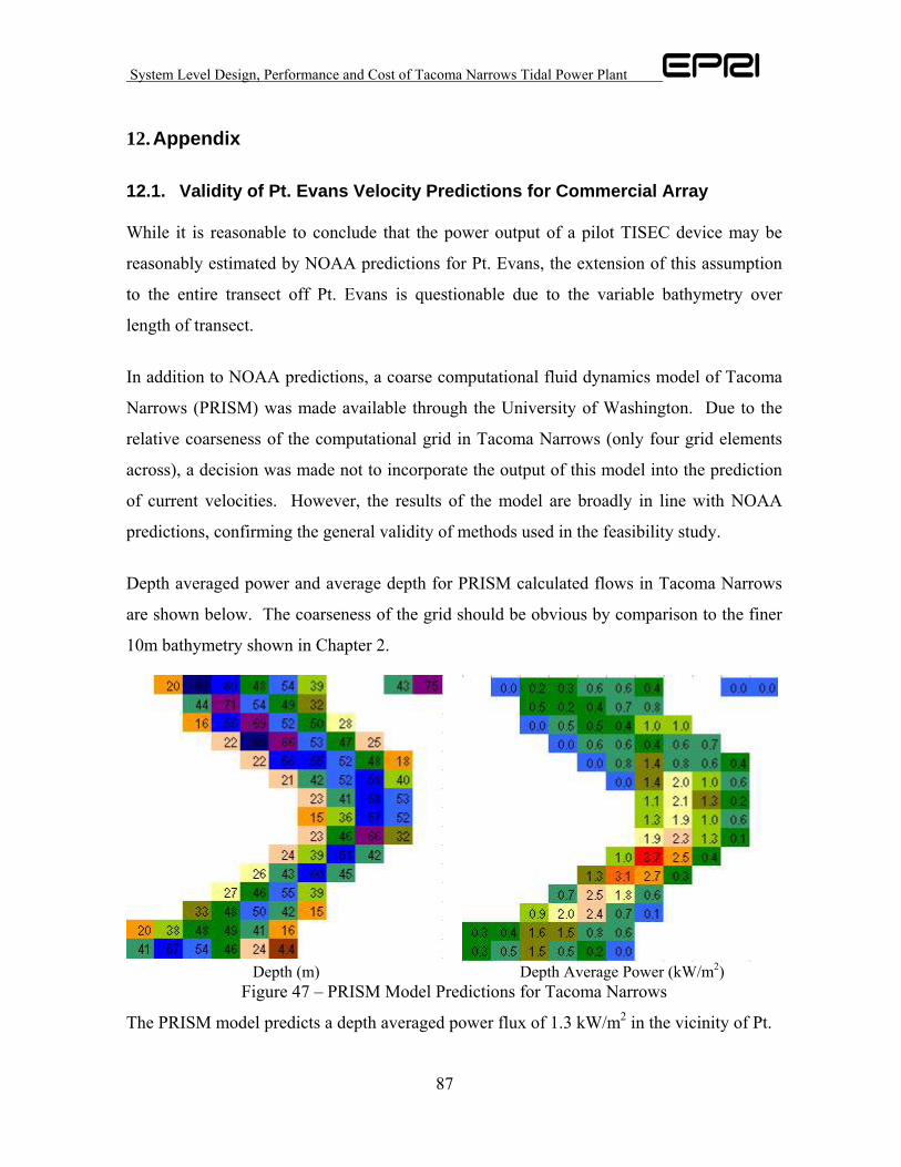
System Level Design, Performance and Cost of Tacoma Narrows Tidal Power Plant
87
12. Appendix
12.1. Validity of Pt. Evans Velocity Predictions for Commercial Array
While it is reasonable to conclude that the power output of a pilot TISEC device may be
reasonably estimated by NOAA predictions for Pt. Evans, the extension of this assumption
to the entire transect off Pt. Evans is questionable due to the variable bathymetry over
length of transect.
In addition to NOAA predictions, a coarse computational fluid dynamics model of Tacoma
Narrows (PRISM) was made available through the University of Washington. Due to the
relative coarseness of the computational grid in Tacoma Narrows (only four grid elements
across), a decision was made not to incorporate the output of this model into the prediction
of current velocities. However, the results of the model are broadly in line with NOAA
predictions, confirming the general validity of methods used in the feasibility study.
Depth averaged power and average depth for PRISM calculated flows in Tacoma Narrows
are shown below. The coarseness of the grid should be obvious by comparison to the finer
10m bathymetry shown in Chapter 2.
Depth (m) Depth Average Power (kW/m2)
Figure 47 – PRISM Model Predictions for Tacoma Narrows
The PRISM model predicts a depth averaged power flux of 1.3 kW/m2 in the vicinity of Pt.
System Level Design, Performance and Cost of Tacoma Narrows Tidal Power Plant
88
Evans, in comparison to 1.7 kW/m2 for the NOAA current station. Power flux is lower on
the east side of the channel than the west. Peak power flux is predicted to occur a bit further
south, closer to the bridge transect. Since the coarseness of the grid omits many of the
significant bathymetric features of the Narrows, the validity of the output to this project is
questionable. These predictions also do not show a known high power point on the east side
of the channel near Point Defiance.
Due to the coarseness of the grid, channel cross-sectional area varies considerably from the
real channel and so channel power as calculated by the model can not be used a priori.
Since the primary purpose of the model is hindcasting circulation in Puget Sound, the model
has better resolution near the surface to incorporate wind effects. Therefore, the model also
can not be used to verify the 1/10th velocity profile assumed for this study. Follow-on work
for this project could involve refinement to the model in Tacoma Narrows for improved
resolution and understanding of the impact of deploying a commercial turbine array. It is
worth noting that any refinement to the model will be highly computationally and storage
intensive. For example, the coarse output shown above involves averaging of one year of
data over the fifteen depth levels. One year of current and velocity data for even this
relatively small area requires almost 2 GB of storage.
Conversations with Devine Tarbell and a driver with the department of fish and wildlife
[10] indicate that flows may be stronger on the east side of the channel than at the reference
station. A footnote in the NOAA tables contradicts this assertion and at the northern end of
the channel, the deeper water region on the west side of the channel has a much lower
power flux (Figure 2). Without the use of ADCP measurements, supplemented by CFD
modeling, a final determination of flow velocity on the east side of the Pt. Evans transects is
mere guesswork. As such, the assumption that surface velocity is uniform across the entire
channel is no worse than any other assumption.
12.2. Irrelevance of Flow Decay Concerns
A concern established by some other researchers, particularly Bahaj and Myers [27] is that
the power available in a tidal stream is reduced for each subsequent transect of turbines.
System Level Design, Performance and Cost of Tacoma Narrows Tidal Power Plant
89
Their results point to a substantial reduction in flow power, and degraded array
performance, for arrays with more than a few transects.
This analysis is, however, in error as it violates mass conservation for tidal channels by
assuming that the cross-sectional area of the channel is constant along the entire array. If
the velocity of the flow is decreasing over each transect, then the area of the channel would
have to increase to maintain conservation of mass.
However, the fuller picture is considerably more counter-intuitive. The total power in a
tidal stream is the summation of the kinetic energy due to its velocity and the potential
energy due to its height. For representative tidal channels, if the height of the water was to
increase to satisfy mass conservation, the potential energy of the stream would also
increase. In fact, this increase in potential energy would actually exceed the decrease of
kinetic energy due to the presence of turbines and the total power in the channel would
increase after each transect. Since this rationale violates conservation of energy it is also,
clearly, incorrect. In order to satisfy both conservation of mass and energy, after each
transect, the height of the water decreases and velocity increases. The net effect is a
decrease in channel power, but from a kinetic energy standpoint, the presence of upstream
turbines actually should improve the performance of those downstream. This effect is
described in detail for an ideal channel in Bryden and Couch [28].
However, without detailed information about cross-channel flow both upstream and
downstream of the proposed turbine array it is not possible to model the potential
performance enhancement. As a result, any such transect-to-transect enhancement is
omitted from the model. However, it would appear that concerns related to flow
degradation have little scientific basis.
12.3. Hub-height Velocity Approximation
In order to simply calculations, it has been assumed that the power flux over the swept area
of the turbine may be approximated by the power flux at the hub height. Assuming the

System Level Design, Performance and Cost of Tacoma Narrows Tidal Power Plant
90
velocity profile in the channel varies with a 1/10th power law, the average power flux over
the area of the turbine is given by the following integral:
∫ ∫
∫ ∫ ⎟⎟⎠
⎞⎜⎜⎝
⎛ +
= π
π
θ
θθ
ρ
2
0 0
2
0 0
103
3 sin21
R
R
o
hubo
rdrd
rdrdz
zru
P
where P is the average power flux, R is the radius of the turbine, uo is the surface current
velocity, zo is the depth of the water, and zhub is the hub height.
This integral is not readily evaluated by analytical methods, but may be approached
numerically. This is done by approximating the rotor as a series of rectangles with height
Δz and width Δx. The power flux for the rectangles is calculated, and an area-weighted
average taken to find the average power flux over the rotor. A representation of this method
is shown in Figure 48.

System Level Design, Performance and Cost of Tacoma Narrows Tidal Power Plant
91
Figure 48 – Representative Numerical Integration
The result of this calculation is independent of water depth and velocity, but is dependent on
hub height above the seabed. The variance from midpoint power flux (defined as ΔP/Phub
height) is tabulated in Table 13.
Table 13 – Approximation Variance as Function of Hub Height
Hub Height (m) Variance 10 -2.7% 15 -1.0% 20 -0.6% 30 -0.3%
A hub height of 17m (as assumed for the purposes of this feasibility study) introduces an
error of -0.8% ― that is, the actual power extracted by a turbine when approximating the
power flux as the midpoint power flux is approximately 1% less than would be extracted by
x
z
Seabed
zhub

System Level Design, Performance and Cost of Tacoma Narrows Tidal Power Plant
92
a turbine operating in water with a 1/10th power velocity profile. For the purposes of a
feasibility study, this approximation is reasonable.

System Level Design, Performance and Cost of Tacoma Narrows Tidal Power Plant
93
12.4. Utility Generator Cost of Electricity Worksheet
INSTRUCTIONS
Indicates Input Cell (either input or use default values)Indicates a Calculated Cell (do not input any values)
Sheet 1. TPC/TPI (Total Plant Cost/Total Plant Investment)a) Enter Component Unit Cost and No. of Units per Systemb) Worksheet sums component costs to get TPC c) Adds the value of the construction loan payments to get TPId) Enter Annual O&M Type including annualized overhaul and refit costc) Worksheet Calculates insurance cost and Total Annual O&M Cost
Sheet 2. Assumptions (Financial)a) Enter project and financial assumptions or leave default values
Sheet 3. NPV (Net Present Value)A Gross Book Value = TPIB Annual Book Depreciation = Gross Book Value/Book LifeC Cumulative DepreciationD MACRS 5 Year Depreciation Tax Schedule AssumptionE Deferred Taxes = (Gross Book Value X MACRS Rate - Annual
Book Depreciation) X Debt Financing RateF Net Book Value = Previous Year Net Book Value - Annual Book
Depreciation - Deferred Tax for that YearSheet 4. CRR (Capital Revenue Requirements)
A Net Book Value for Column F of NPV WorksheetB Common Equity = Net Book X Common Equity Financing
Share X Common Equity Financing RateC Preferred Equity = Net Book X Preferred Equity Financing
Share X Preferred Equity Financing RateD Debt = Net Book X Debt Financing Share X Debt Financing RateE Annual Book Depreciation = Gross Book Value/Book LifeF Income Taxes = (Return on Common Equity + Return of Preferred Equity -
Interest on Debt + Deferred Taxes) X (Comp Tax Rate/(1-Comp Tax Rate))G Property Taxes and Insurance Expense = H Calculates Investment and Production Tax Credit RevenuesI Capital Revenue Req'ts = Sum of Columns B through G
Sheet 5. FCR (Fixed Charge Rate)A Nominal Rates Capital Revenue Req'ts from Columnn H of Previous WorksheetB Nominal Rate Present Worth Factor = 1 / (1 + After Tax Discount Rate)C Nominal Rate Product of Columns A and B = A * BD Real Rates Capital Revenue Req'ts from Columnn H of Previous WorksheetE Real Rates Present Worth Factor = 1 / (1 + After Tax Discount Rate - Inflation Rate)F Real Rates Product of Columns A and B = A * B
Sheet 6. Calculates COE (Cost of Electricity)COE = ((TPI * FCR) + AO&M ) / AEPIn other words…The Cost of Electricity =
The Sum of the Levelized Plant Investment + Annual O&M Cost including Levelized Overhaul and Replacement Cost Divided by the Annual Electric Energy Consumption

System Level Design, Performance and Cost of Tacoma Narrows Tidal Power Plant
94
TOTAL PLANT COST (TPC) - 2005$
Procurement Power Conversion System 64 $472,665 $30,250,532 Structural Elements 64 $605,062 $38,723,977 Subsea Cables Lot $812,705 $812,705 Turbine Installation 64 $322,406 $20,633,956 Subsea Cable Installation Lot $9,541,969 $9,541,969 Onshore Grid Interconnection Lot $3,500,000 $3,500,000
TOTAL $103,463,138
TOTAL PLANT INVESTMENT (TPI) - 2005$
End of Year
Total Cash Expended TPC
(2005$)
Before Tax Construction Loan Cost at
Debt Financing
Rate
2005 Value of Construction
Loan Payments
TOTAL PLANT INVESTMENT
2005$2007 $51,731,569 $3,879,868 $3,163,220 $54,894,7902008 $51,731,569 $3,879,868 $2,856,181 $54,587,750Total $103,463,138 $7,759,735 $6,019,401 $109,482,540
ANNUAL OPERATING AND MAINTENANCE COST (AO&M) - 2005$
Costs Yrly Cost AmountLabor and Parts $2,260,052 $2,260,052Insurance (1.5% of TPC) $1,551,947 $1,551,947
Total $3,811,999
TPC Component Unit Unit Cost Total Cost (2005$)
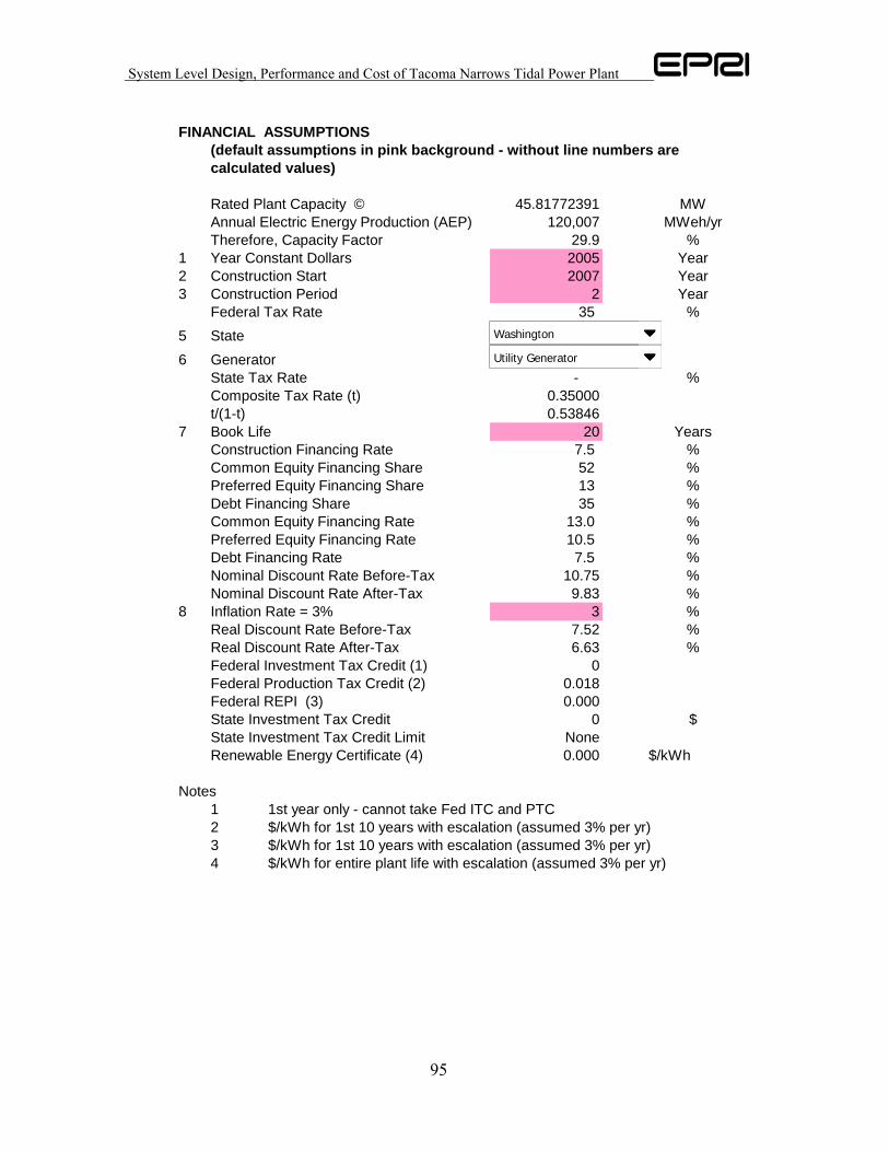
System Level Design, Performance and Cost of Tacoma Narrows Tidal Power Plant
95
FINANCIAL ASSUMPTIONS (default assumptions in pink background - without line numbers are calculated values)
Rated Plant Capacity © 45.81772391 MWAnnual Electric Energy Production (AEP) 120,007 MWeh/yrTherefore, Capacity Factor 29.9 %
1 Year Constant Dollars 2005 Year2 Construction Start 2007 Year3 Construction Period 2 Year
Federal Tax Rate 35 %5 State 16 Generator 2
State Tax Rate - %Composite Tax Rate (t) 0.35000t/(1-t) 0.53846
7 Book Life 20 YearsConstruction Financing Rate 7.5 %Common Equity Financing Share 52 %Preferred Equity Financing Share 13 %Debt Financing Share 35 %Common Equity Financing Rate 13.0 %Preferred Equity Financing Rate 10.5 %Debt Financing Rate 7.5 %Nominal Discount Rate Before-Tax 10.75 %Nominal Discount Rate After-Tax 9.83 %
8 Inflation Rate = 3% 3 %Real Discount Rate Before-Tax 7.52 %Real Discount Rate After-Tax 6.63 %Federal Investment Tax Credit (1) 0Federal Production Tax Credit (2) 0.018Federal REPI (3) 0.000State Investment Tax Credit 0 $State Investment Tax Credit Limit NoneRenewable Energy Certificate (4) 0.000 $/kWh
Notes1 1st year only - cannot take Fed ITC and PTC2 $/kWh for 1st 10 years with escalation (assumed 3% per yr)3 $/kWh for 1st 10 years with escalation (assumed 3% per yr)4 $/kWh for entire plant life with escalation (assumed 3% per yr)
Washington
Utility Generator
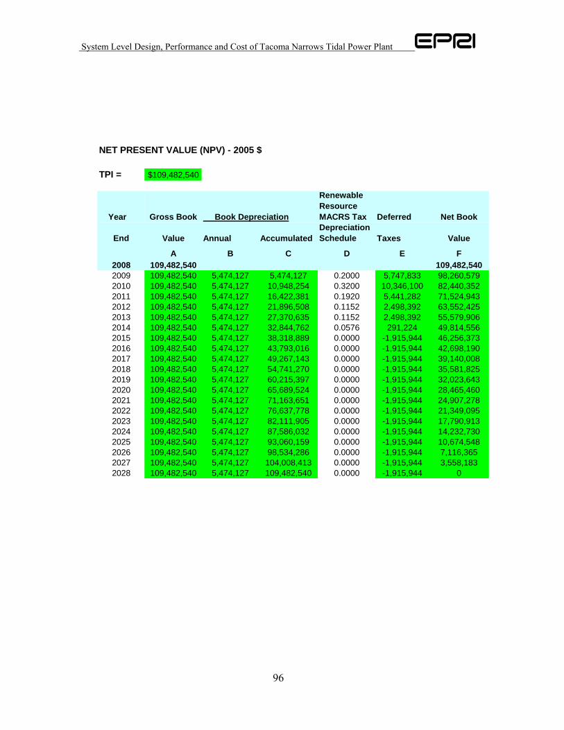
System Level Design, Performance and Cost of Tacoma Narrows Tidal Power Plant
96
NET PRESENT VALUE (NPV) - 2005 $
TPI = $109,482,540
Year Gross Book Book Depreciation
Renewable Resource MACRS Tax Deferred Net Book
End Value Annual AccumulatedDepreciation Schedule Taxes Value
A B C D E F2008 109,482,540 109,482,5402009 109,482,540 5,474,127 5,474,127 0.2000 5,747,833 98,260,5792010 109,482,540 5,474,127 10,948,254 0.3200 10,346,100 82,440,3522011 109,482,540 5,474,127 16,422,381 0.1920 5,441,282 71,524,9432012 109,482,540 5,474,127 21,896,508 0.1152 2,498,392 63,552,4252013 109,482,540 5,474,127 27,370,635 0.1152 2,498,392 55,579,9062014 109,482,540 5,474,127 32,844,762 0.0576 291,224 49,814,5562015 109,482,540 5,474,127 38,318,889 0.0000 -1,915,944 46,256,3732016 109,482,540 5,474,127 43,793,016 0.0000 -1,915,944 42,698,1902017 109,482,540 5,474,127 49,267,143 0.0000 -1,915,944 39,140,0082018 109,482,540 5,474,127 54,741,270 0.0000 -1,915,944 35,581,8252019 109,482,540 5,474,127 60,215,397 0.0000 -1,915,944 32,023,6432020 109,482,540 5,474,127 65,689,524 0.0000 -1,915,944 28,465,4602021 109,482,540 5,474,127 71,163,651 0.0000 -1,915,944 24,907,2782022 109,482,540 5,474,127 76,637,778 0.0000 -1,915,944 21,349,0952023 109,482,540 5,474,127 82,111,905 0.0000 -1,915,944 17,790,9132024 109,482,540 5,474,127 87,586,032 0.0000 -1,915,944 14,232,7302025 109,482,540 5,474,127 93,060,159 0.0000 -1,915,944 10,674,5482026 109,482,540 5,474,127 98,534,286 0.0000 -1,915,944 7,116,3652027 109,482,540 5,474,127 104,008,413 0.0000 -1,915,944 3,558,1832028 109,482,540 5,474,127 109,482,540 0.0000 -1,915,944 0
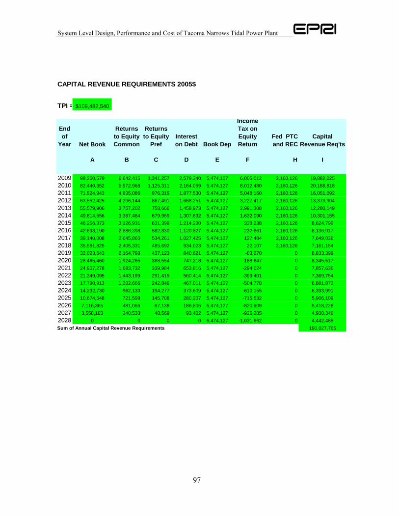
System Level Design, Performance and Cost of Tacoma Narrows Tidal Power Plant
97
CAPITAL REVENUE REQUIREMENTS 2005$
TPI = $109,482,540
End of
Year Net Book
Returns to Equity Common
Returns to Equity
PrefInterest on Debt Book Dep
Income Tax on Equity Return
Fed PTC and REC
Capital Revenue Req'ts
A B C D E F H I
2009 98,260,579 6,642,415 1,341,257 2,579,340 5,474,127 6,005,012 2,160,126 19,882,0252010 82,440,352 5,572,968 1,125,311 2,164,059 5,474,127 8,012,480 2,160,126 20,188,8182011 71,524,943 4,835,086 976,315 1,877,530 5,474,127 5,048,160 2,160,126 16,051,0922012 63,552,425 4,296,144 867,491 1,668,251 5,474,127 3,227,417 2,160,126 13,373,3042013 55,579,906 3,757,202 758,666 1,458,973 5,474,127 2,991,308 2,160,126 12,280,1492014 49,814,556 3,367,464 679,969 1,307,632 5,474,127 1,632,090 2,160,126 10,301,1552015 46,256,373 3,126,931 631,399 1,214,230 5,474,127 338,238 2,160,126 8,624,7992016 42,698,190 2,886,398 582,830 1,120,827 5,474,127 232,861 2,160,126 8,136,9172017 39,140,008 2,645,865 534,261 1,027,425 5,474,127 127,484 2,160,126 7,649,0362018 35,581,825 2,405,331 485,692 934,023 5,474,127 22,107 2,160,126 7,161,1542019 32,023,643 2,164,798 437,123 840,621 5,474,127 -83,270 0 8,833,3992020 28,465,460 1,924,265 388,554 747,218 5,474,127 -188,647 0 8,345,5172021 24,907,278 1,683,732 339,984 653,816 5,474,127 -294,024 0 7,857,6362022 21,349,095 1,443,199 291,415 560,414 5,474,127 -399,401 0 7,369,7542023 17,790,913 1,202,666 242,846 467,011 5,474,127 -504,778 0 6,881,8722024 14,232,730 962,133 194,277 373,609 5,474,127 -610,155 0 6,393,9912025 10,674,548 721,599 145,708 280,207 5,474,127 -715,532 0 5,906,1092026 7,116,365 481,066 97,138 186,805 5,474,127 -820,909 0 5,418,2282027 3,558,183 240,533 48,569 93,402 5,474,127 -926,285 0 4,930,3462028 0 0 0 0 5,474,127 -1,031,662 0 4,442,465Sum of Annual Capital Revenue Requirements 190,027,765

System Level Design, Performance and Cost of Tacoma Narrows Tidal Power Plant
98
FIXED CHARGE RATE (FCR) - NOMINAL AND REAL LEVELIZED - 2005$
TPI = $109,482,540
End of
Capital Revenue
Req'tsPresent
Worth Factor
Product of Columns A
and B
Capital Revenue
Req'ts
Present Worth Factor
Product of Columns D
and EYear Nominal Nominal Real Real
A B C D E F
2009 19,882,025 0.6872 13,663,341 17,664,922 0.7735 13,663,3412010 20,188,818 0.6257 12,632,266 17,415,052 0.7254 12,632,2662011 16,051,092 0.5697 9,144,270 13,442,537 0.6802 9,144,2702012 13,373,304 0.5187 6,936,769 10,873,720 0.6379 6,936,7692013 12,280,149 0.4723 5,799,576 9,694,063 0.5983 5,799,5762014 10,301,155 0.4300 4,429,479 7,894,978 0.5611 4,429,4792015 8,624,799 0.3915 3,376,678 6,417,660 0.5262 3,376,6782016 8,136,917 0.3565 2,900,512 5,878,282 0.4934 2,900,5122017 7,649,036 0.3246 2,482,536 5,364,880 0.4627 2,482,5362018 7,161,154 0.2955 2,116,148 4,876,397 0.4340 2,116,1482019 8,833,399 0.2691 2,376,648 5,839,917 0.4070 2,376,6482020 8,345,517 0.2450 2,044,393 5,356,670 0.3817 2,044,3932021 7,857,636 0.2230 1,752,577 4,896,619 0.3579 1,752,5772022 7,369,754 0.2031 1,496,622 4,458,822 0.3357 1,496,6222023 6,881,872 0.1849 1,272,448 4,042,375 0.3148 1,272,4482024 6,393,991 0.1683 1,076,414 3,646,404 0.2952 1,076,4142025 5,906,109 0.1533 905,280 3,270,070 0.2768 905,2802026 5,418,228 0.1396 756,158 2,912,564 0.2596 756,1582027 4,930,346 0.1271 626,480 2,573,111 0.2435 626,4802028 4,442,465 0.1157 513,958 2,250,960 0.2283 513,958
190,027,765 76,302,552 138,770,001 76,302,552
Nominal $ Real $
76,302,552 76,302,5523% 3%
9.83% 6.63%
0.116109617 0.091712273
8,859,460 6,997,881109,482,540 109,482,540
0.0809 0.0639
1. The present value is at the beginning of 2006 and results from the sum of the products of the annual present value factors times the annual requirements
3. After Tax Discount Rate = i
5. The levelized annual charges (end of year) = Present Value (Item 1) * Capital Recovery Factor (Item 4)
7. The levelized annual fixed charge rate (levelized annual charges divided by the booked cost)
6. Booked Cost
2. Escalation Rate
4. Capital recovery factor value = i(1+i)n/(1+i)n-1 where book life = n and discount rate = i
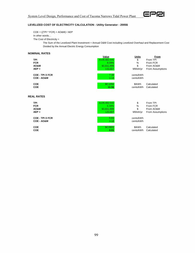
System Level Design, Performance and Cost of Tacoma Narrows Tidal Power Plant
99
LEVELIZED COST OF ELECTRICITY CALCULATION - Utility Generator - 2005$
COE = ((TPI * FCR) + AO&M) / AEPIn other words…The Cost of Electricity =
The Sum of the Levelized Plant Investment + Annual O&M Cost including Levelized Overhaul and Replacement CostDivided by the Annual Electric Energy Consumption
NOMINAL RATESValue Units From
TPI $109,482,540 $ From TPIFCR 8.09% % From FCRAO&M $3,811,999 $ From AO&MAEP = 120,007 MWeh/yr From Assumptions
COE - TPI X FCR 7.38 cents/kWhCOE - AO&M 3.18 cents/kWh
COE $0.1056 $/kWh CalculatedCOE 10.56 cents/kWh Calculated
REAL RATES
TPI $109,482,540 $ From TPIFCR 6.39% % From FCRAO&M $3,811,999 $ From AO&MAEP = 120,007 MWeh/yr From Assumptions
COE - TPI X FCR 5.83 cents/kWhCOE - AO&M 3.18 cents/kWh
COE $0.0901 $/kWh CalculatedCOE 9.01 cents/kWh Calculated

System Level Design, Performance and Cost of Tacoma Narrows Tidal Power Plant
100
12.5. Non Utility Generator Internal Rate of Return Worksheet
INSTRUCTIONS
Fill in first four worksheets (or use default values) - the last two worksheets are automatically
calculated. Refer to EPRI Economic Methodology Report 002
Indicates Input Cell (either input or use default values)
Indicates a Calculated Cell (do not input any values)Sheet 1. Total Plant Cost/Total Plant Investment (TPC/TPI) - 2005$
1 Enter Component Unit Cost and No. of Units per System2 Worksheet sums component costs to get TPC 3 Worksheet adds the value of the construction loan payments to get TPI
Sheet 2. AO&M (Annual Operation and Maintenance Cost) - 2005$1 Enter Labor Hrs and Cost by O&M Type)2 Enter Parts and Supplies Cost by O&M Type)3 Worksheet Calculates Total Annual O&M Cost
Sheet 3. O&R ( Overhaul and Replacement Cost) - 2005$1 Enter Year of Cost and O&R Cost per Item2 Worksheet calculates inflation to the year of the cost of the O&R
Sheet 4. Assumptions (Project, Financial and Others)1 Enter project, financial and other assumptions or leave default values
Sheet 5. Income Statement - Assuming no capacity factor income - Current $1 2008 1st Year Energy payments = AEP X 2005 wholesale price X 97.18% (to adjust price
from 2005 to 2008 (an 2.82% decline) X Inflation from 2005 to 20082009-2011 Energy payments = AEP X Previous Year Elec Price X Annual Price
de-escalation of -1.42% X Inflation2012-2025 Energy payments = AEP X Previous Year Elec Price X 0.72% Price
escalation X Inflation2 Calculates State Investment and Prodution tax credit3 Calculates Federal Investment and Production Tax Credit 4 Scheduled O&M from TPC worksheet with inflation5 Scheduled O&R from TPC worksheet with inflation8 Earnings before EBITDA = total revenues less total operating costs9 Tax Depreciation = Assumed MACRS rate X TPI10 Interest paid = Annual interest given assumed debt interest rate and life of loan11 Taxable earnings = Tax Depreciation + Interest Paid12 State Tax = Taxable Earnings x state tax rate13 Federal Tax = (Taxable earnings - State Tax) X Federal tax rate14 Total Tax Obligation = Total State + Federal Tax
Sheet 6. Cash Flow Statement - Current $1 EBITDA2 Taxes Paid3 Cash Flow From Operations = EBITDA - Taxes Paid4 Debt Service = Principal + Interest paid on the debt loan5 Net Cash Flow after Tax
Year of Start of Ops minus 1 = Equity amountYear of Start of Ops = Cash flow from ops - debt serviceYear of Start of Ops Plus 1 to N = Cash flow from ops - debt service
6 Cum Net Cash Flow After Taxes = previous year net cash flow + current year net cash flow7 Cum IRR on net cash Flow After Taxes = discount rate that sets the present worth
of the net cash flows over the book life equal to the equity investment at the commercial operations
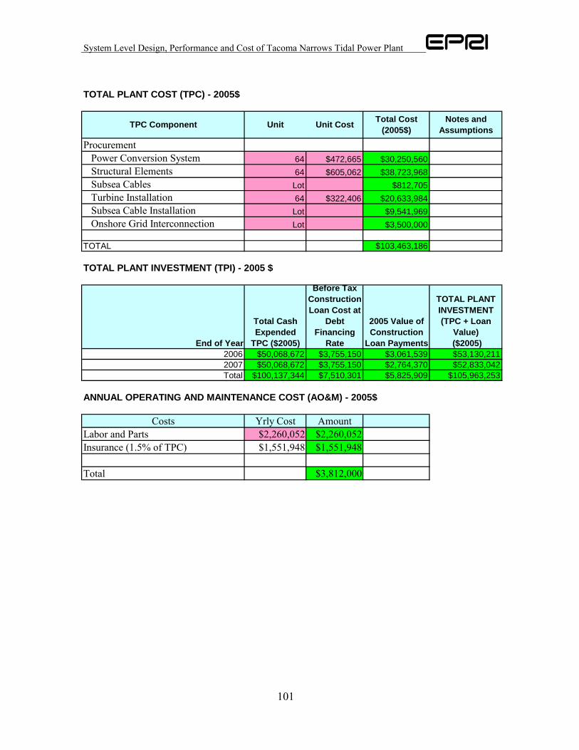
System Level Design, Performance and Cost of Tacoma Narrows Tidal Power Plant
101
TOTAL PLANT COST (TPC) - 2005$
Procurement Power Conversion System 64 $472,665 $30,250,560 Structural Elements 64 $605,062 $38,723,968 Subsea Cables Lot $812,705 Turbine Installation 64 $322,406 $20,633,984 Subsea Cable Installation Lot $9,541,969 Onshore Grid Interconnection Lot $3,500,000
TOTAL $103,463,186
TOTAL PLANT INVESTMENT (TPI) - 2005 $
End of Year
Total Cash Expended
TPC ($2005)
Before Tax Construction Loan Cost at
Debt Financing
Rate
2005 Value of Construction
Loan Payments
TOTAL PLANT INVESTMENT(TPC + Loan
Value) ($2005)
2006 $50,068,672 $3,755,150 $3,061,539 $53,130,2112007 $50,068,672 $3,755,150 $2,764,370 $52,833,042Total $100,137,344 $7,510,301 $5,825,909 $105,963,253
ANNUAL OPERATING AND MAINTENANCE COST (AO&M) - 2005$
Costs Yrly Cost AmountLabor and Parts $2,260,052 $2,260,052Insurance (1.5% of TPC) $1,551,948 $1,551,948
Total $3,812,000
TPC Component Notes and AssumptionsUnit Unit Cost Total Cost
(2005$)
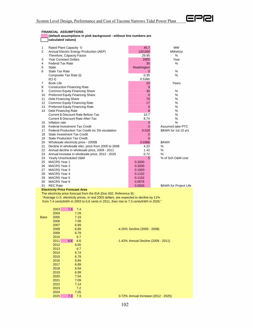
System Level Design, Performance and Cost of Tacoma Narrows Tidal Power Plant
102
FINANCIAL ASSUMPTIONS (default assumptions in pink background - without line numbers are calculated values)
1 Rated Plant Capacity © 45.7 MW2 Annual Electric Energy Production (AEP) 120,000 MWeh/yr
Therefore, Capacity Factor 29.95 %3 Year Constant Dollars 2005 Year4 Federal Tax Rate 35 %5 State Washington6 State Tax Rate 0 %
Composite Tax Rate (t) 0.35 %t/(1-t) 0.5385
7 Book Life 20 Years8 Construction Financing Rate 99 Common Equity Financing Share 30 %10 Preferred Equity Financing Share 0 %11 Debt Financing Share 70 %12 Common Equity Financing Rate 17 %13 Preferred Equity Financing Rate 0 %14 Debt Financing Rate 8 %
Current $ Discount Rate Before-Tax 10.7 %Current $ Discount Rate After-Tax 8.74 %
15 Inflation rate 3 %16 Federal Investment Tax Credit 0 Assumed take PTC17 Federal Production Tax Credit inc 3% escalation 0.018 $/kWh for 1st 10 yrs18 State Investment Tax Credit 019 State Production Tax Credit 020 Wholesale electricity price - 2005$ 0.0386 $/kWh21 Decline in wholesale elec. price from 2005 to 2008 4.20 %22 Annual decline in wholesale price, 2009 - 2011 1.42 %23 Annual increase in wholesale price, 2012 - 2025 0.72 %24 Yearly Unscheduled O&M 5 % of Sch O&M cost25 MACRS Year 1 0.200026 MACRS Year 2 0.320027 MACRS Year 3 0.192028 MACRS Year 4 0.115229 MACRS Year 5 0.115230 MACRS Year 6 0.057631 REC Rate 0.0000 $/kWh for Project LifeElectricity Price Forecast AreaThe electricity price forecast from the EIA (Doc 002, Reference 8): "Average U.S. electricity prices, in real 2003 dollars, are expected to decline by 11% from 7.4 cents/kWh in 2003 to 6.6 cents in 2011, then rise to 7.3 cents/kWh in 2025.”
2003 7.4 7.42004 7.29
Base 2005 7.192006 7.092007 6.992008 6.89 -4.20% Decline (2005 - 2008)2009 6.792010 6.72011 6.6 6.6 -1.42% Annual Decline (2009 - 2011)2012 6.652013 6.72014 6.742015 6.792016 6.842017 6.892018 6.942019 6.992020 7.042021 7.092022 7.142023 7.22024 7.252025 7.3 7.3 0.72% Annual Increase (2012 - 2025)
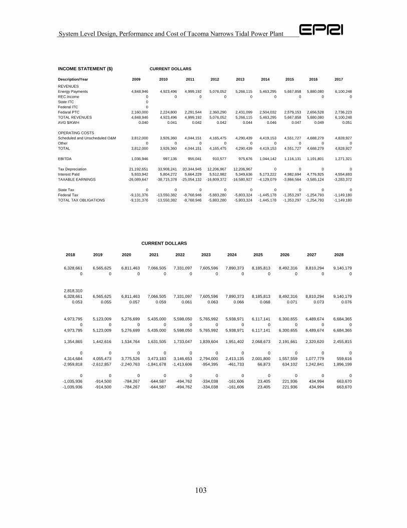
System Level Design, Performance and Cost of Tacoma Narrows Tidal Power Plant
103
INCOME STATEMENT ($) CURRENT DOLLARS
Description/Year 2009 2010 2011 2012 2013 2014 2015 2016 2017
REVENUESEnergy Payments 4,848,946 4,923,496 4,999,192 5,076,052 5,266,115 5,463,295 5,667,858 5,880,080 6,100,248REC income 0 0 0 0 0 0 0 0 0State ITC 0Federal ITC 0Fedaral PTC 2,160,000 2,224,800 2,291,544 2,360,290 2,431,099 2,504,032 2,579,153 2,656,528 2,736,223TOTAL REVENUES 4,848,946 4,923,496 4,999,192 5,076,052 5,266,115 5,463,295 5,667,858 5,880,080 6,100,248AVG $/KWH 0.040 0.041 0.042 0.042 0.044 0.046 0.047 0.049 0.051
OPERATING COSTSScheduled and Unscheduled O&M 3,812,000 3,926,360 4,044,151 4,165,475 4,290,439 4,419,153 4,551,727 4,688,279 4,828,927Other 0 0 0 0 0 0 0 0 0TOTAL 3,812,000 3,926,360 4,044,151 4,165,475 4,290,439 4,419,153 4,551,727 4,688,279 4,828,927
EBITDA 1,036,946 997,136 955,041 910,577 975,676 1,044,142 1,116,131 1,191,801 1,271,321
Tax Depreciation 21,192,651 33,908,241 20,344,945 12,206,967 12,206,967 0 0 0 0Interest PaId 5,933,942 5,804,272 5,664,229 5,512,982 5,349,636 5,173,222 4,982,694 4,776,925 4,554,693TAXABLE EARNINGS -26,089,647 -38,715,378 -25,054,132 -16,809,372 -16,580,927 -4,129,079 -3,866,564 -3,585,124 -3,283,372
State Tax 0 0 0 0 0 0 0 0 0Federal Tax -9,131,376 -13,550,382 -8,768,946 -5,883,280 -5,803,324 -1,445,178 -1,353,297 -1,254,793 -1,149,180TOTAL TAX OBLIGATIONS -9,131,376 -13,550,382 -8,768,946 -5,883,280 -5,803,324 -1,445,178 -1,353,297 -1,254,793 -1,149,180
CURRENT DOLLARS
2018 2019 2020 2021 2022 2023 2024 2025 2026 2027 2028
6,328,661 6,565,625 6,811,463 7,066,505 7,331,097 7,605,596 7,890,373 8,185,813 8,492,316 8,810,294 9,140,1790 0 0 0 0 0 0 0 0 0 0
2,818,3106,328,661 6,565,625 6,811,463 7,066,505 7,331,097 7,605,596 7,890,373 8,185,813 8,492,316 8,810,294 9,140,179
0.053 0.055 0.057 0.059 0.061 0.063 0.066 0.068 0.071 0.073 0.076
4,973,795 5,123,009 5,276,699 5,435,000 5,598,050 5,765,992 5,938,971 6,117,141 6,300,655 6,489,674 6,684,3650 0 0 0 0 0 0 0 0 0 0
4,973,795 5,123,009 5,276,699 5,435,000 5,598,050 5,765,992 5,938,971 6,117,141 6,300,655 6,489,674 6,684,365
1,354,865 1,442,616 1,534,764 1,631,505 1,733,047 1,839,604 1,951,402 2,068,673 2,191,661 2,320,620 2,455,815
0 0 0 0 0 0 0 0 0 0 04,314,684 4,055,473 3,775,526 3,473,183 3,146,653 2,794,000 2,413,135 2,001,800 1,557,559 1,077,779 559,616
-2,959,818 -2,612,857 -2,240,763 -1,841,678 -1,413,606 -954,395 -461,733 66,873 634,102 1,242,841 1,896,199
0 0 0 0 0 0 0 0 0 0 0-1,035,936 -914,500 -784,267 -644,587 -494,762 -334,038 -161,606 23,405 221,936 434,994 663,670-1,035,936 -914,500 -784,267 -644,587 -494,762 -334,038 -161,606 23,405 221,936 434,994 663,670
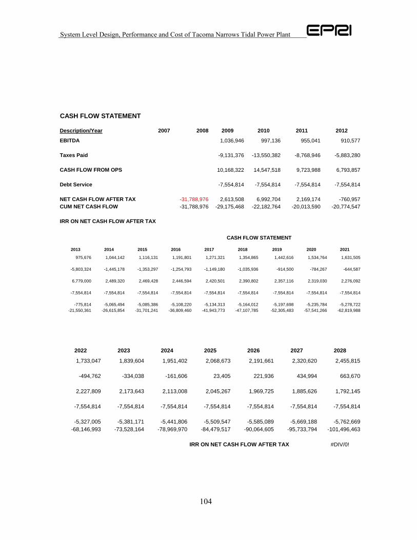
System Level Design, Performance and Cost of Tacoma Narrows Tidal Power Plant
104
CASH FLOW STATEMENT
Description/Year 2007 2008 2009 2010 2011 2012
EBITDA 1,036,946 997,136 955,041 910,577
Taxes Paid -9,131,376 -13,550,382 -8,768,946 -5,883,280
CASH FLOW FROM OPS 10,168,322 14,547,518 9,723,988 6,793,857
Debt Service -7,554,814 -7,554,814 -7,554,814 -7,554,814
NET CASH FLOW AFTER TAX -31,788,976 2,613,508 6,992,704 2,169,174 -760,957CUM NET CASH FLOW -31,788,976 -29,175,468 -22,182,764 -20,013,590 -20,774,547
IRR ON NET CASH FLOW AFTER TAX
CASH FLOW STATEMENT
2013 2014 2015 2016 2017 2018 2019 2020 2021
975,676 1,044,142 1,116,131 1,191,801 1,271,321 1,354,865 1,442,616 1,534,764 1,631,505
-5,803,324 -1,445,178 -1,353,297 -1,254,793 -1,149,180 -1,035,936 -914,500 -784,267 -644,587
6,779,000 2,489,320 2,469,428 2,446,594 2,420,501 2,390,802 2,357,116 2,319,030 2,276,092
-7,554,814 -7,554,814 -7,554,814 -7,554,814 -7,554,814 -7,554,814 -7,554,814 -7,554,814 -7,554,814
-775,814 -5,065,494 -5,085,386 -5,108,220 -5,134,313 -5,164,012 -5,197,698 -5,235,784 -5,278,722-21,550,361 -26,615,854 -31,701,241 -36,809,460 -41,943,773 -47,107,785 -52,305,483 -57,541,266 -62,819,988
2022 2023 2024 2025 2026 2027 2028
1,733,047 1,839,604 1,951,402 2,068,673 2,191,661 2,320,620 2,455,815
-494,762 -334,038 -161,606 23,405 221,936 434,994 663,670
2,227,809 2,173,643 2,113,008 2,045,267 1,969,725 1,885,626 1,792,145
-7,554,814 -7,554,814 -7,554,814 -7,554,814 -7,554,814 -7,554,814 -7,554,814
-5,327,005 -5,381,171 -5,441,806 -5,509,547 -5,585,089 -5,669,188 -5,762,669-68,146,993 -73,528,164 -78,969,970 -84,479,517 -90,064,605 -95,733,794 -101,496,463
IRR ON NET CASH FLOW AFTER TAX #DIV/0!
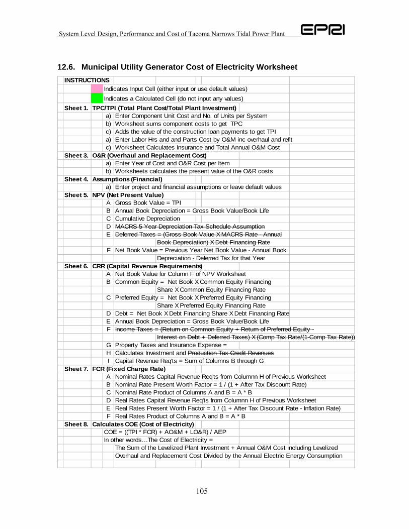
System Level Design, Performance and Cost of Tacoma Narrows Tidal Power Plant
105
12.6. Municipal Utility Generator Cost of Electricity Worksheet INSTRUCTIONS
Indicates Input Cell (either input or use default values)Indicates a Calculated Cell (do not input any values)
Sheet 1. TPC/TPI (Total Plant Cost/Total Plant Investment)a) Enter Component Unit Cost and No. of Units per Systemb) Worksheet sums component costs to get TPC c) Adds the value of the construction loan payments to get TPIa) Enter Labor Hrs and and Parts Cost by O&M inc overhaul and refitc) Worksheet Calculates Insurance and Total Annual O&M Cost
Sheet 3. O&R (Overhaul and Replacement Cost)a) Enter Year of Cost and O&R Cost per Itemb) Worksheets calculates the present value of the O&R costs
Sheet 4. Assumptions (Financial)a) Enter project and financial assumptions or leave default values
Sheet 5. NPV (Net Present Value)A Gross Book Value = TPIB Annual Book Depreciation = Gross Book Value/Book LifeC Cumulative DepreciationD MACRS 5 Year Depreciation Tax Schedule AssumptionE Deferred Taxes = (Gross Book Value X MACRS Rate - Annual
Book Depreciation) X Debt Financing RateF Net Book Value = Previous Year Net Book Value - Annual Book
Depreciation - Deferred Tax for that YearSheet 6. CRR (Capital Revenue Requirements)
A Net Book Value for Column F of NPV WorksheetB Common Equity = Net Book X Common Equity Financing
Share X Common Equity Financing RateC Preferred Equity = Net Book X Preferred Equity Financing
Share X Preferred Equity Financing RateD Debt = Net Book X Debt Financing Share X Debt Financing RateE Annual Book Depreciation = Gross Book Value/Book LifeF Income Taxes = (Return on Common Equity + Return of Preferred Equity -
Interest on Debt + Deferred Taxes) X (Comp Tax Rate/(1-Comp Tax Rate))G Property Taxes and Insurance Expense = H Calculates Investment and Production Tax Credit RevenuesI Capital Revenue Req'ts = Sum of Columns B through G
Sheet 7. FCR (Fixed Charge Rate)A Nominal Rates Capital Revenue Req'ts from Columnn H of Previous WorksheetB Nominal Rate Present Worth Factor = 1 / (1 + After Tax Discount Rate)C Nominal Rate Product of Columns A and B = A * BD Real Rates Capital Revenue Req'ts from Columnn H of Previous WorksheetE Real Rates Present Worth Factor = 1 / (1 + After Tax Discount Rate - Inflation Rate)F Real Rates Product of Columns A and B = A * B
Sheet 8. Calculates COE (Cost of Electricity)COE = ((TPI * FCR) + AO&M + LO&R) / AEPIn other words…The Cost of Electricity =
The Sum of the Levelized Plant Investment + Annual O&M Cost including Levelized Overhaul and Replacement Cost Divided by the Annual Electric Energy Consumption
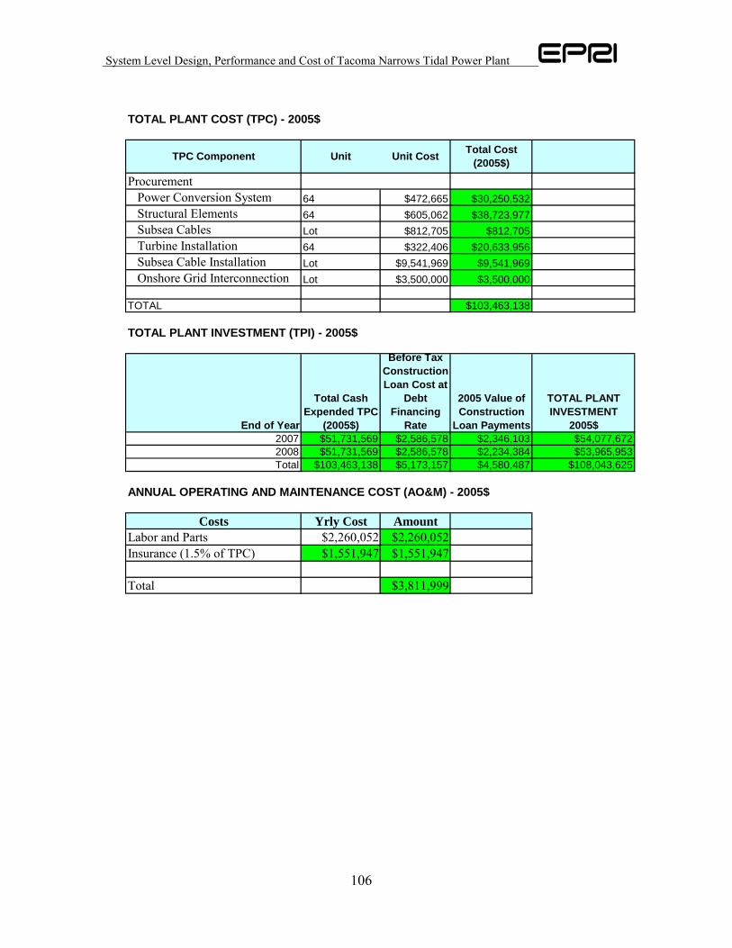
System Level Design, Performance and Cost of Tacoma Narrows Tidal Power Plant
106
TOTAL PLANT COST (TPC) - 2005$
Procurement Power Conversion System 64 $472,665 $30,250,532 Structural Elements 64 $605,062 $38,723,977 Subsea Cables Lot $812,705 $812,705 Turbine Installation 64 $322,406 $20,633,956 Subsea Cable Installation Lot $9,541,969 $9,541,969 Onshore Grid Interconnection Lot $3,500,000 $3,500,000
TOTAL $103,463,138
TOTAL PLANT INVESTMENT (TPI) - 2005$
End of Year
Total Cash Expended TPC
(2005$)
Before Tax Construction Loan Cost at
Debt Financing
Rate
2005 Value of Construction
Loan Payments
TOTAL PLANT INVESTMENT
2005$2007 $51,731,569 $2,586,578 $2,346,103 $54,077,6722008 $51,731,569 $2,586,578 $2,234,384 $53,965,953Total $103,463,138 $5,173,157 $4,580,487 $108,043,625
ANNUAL OPERATING AND MAINTENANCE COST (AO&M) - 2005$
Costs Yrly Cost AmountLabor and Parts $2,260,052 $2,260,052Insurance (1.5% of TPC) $1,551,947 $1,551,947
Total $3,811,999
TPC Component Unit Unit Cost Total Cost (2005$)
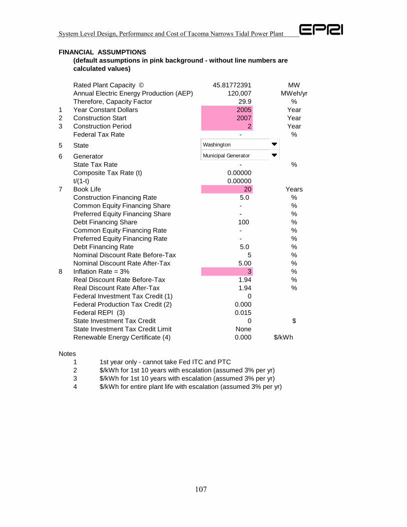
System Level Design, Performance and Cost of Tacoma Narrows Tidal Power Plant
107
FINANCIAL ASSUMPTIONS (default assumptions in pink background - without line numbers are calculated values)
Rated Plant Capacity © 45.81772391 MWAnnual Electric Energy Production (AEP) 120,007 MWeh/yrTherefore, Capacity Factor 29.9 %
1 Year Constant Dollars 2005 Year2 Construction Start 2007 Year3 Construction Period 2 Year
Federal Tax Rate - %5 State 16 Generator 1
State Tax Rate - %Composite Tax Rate (t) 0.00000t/(1-t) 0.00000
7 Book Life 20 YearsConstruction Financing Rate 5.0 %Common Equity Financing Share - %Preferred Equity Financing Share - %Debt Financing Share 100 %Common Equity Financing Rate - %Preferred Equity Financing Rate - %Debt Financing Rate 5.0 %Nominal Discount Rate Before-Tax 5 %Nominal Discount Rate After-Tax 5.00 %
8 Inflation Rate = 3% 3 %Real Discount Rate Before-Tax 1.94 %Real Discount Rate After-Tax 1.94 %Federal Investment Tax Credit (1) 0Federal Production Tax Credit (2) 0.000Federal REPI (3) 0.015State Investment Tax Credit 0 $State Investment Tax Credit Limit NoneRenewable Energy Certificate (4) 0.000 $/kWh
Notes1 1st year only - cannot take Fed ITC and PTC2 $/kWh for 1st 10 years with escalation (assumed 3% per yr)3 $/kWh for 1st 10 years with escalation (assumed 3% per yr)4 $/kWh for entire plant life with escalation (assumed 3% per yr)
Washington
Municipal Generator
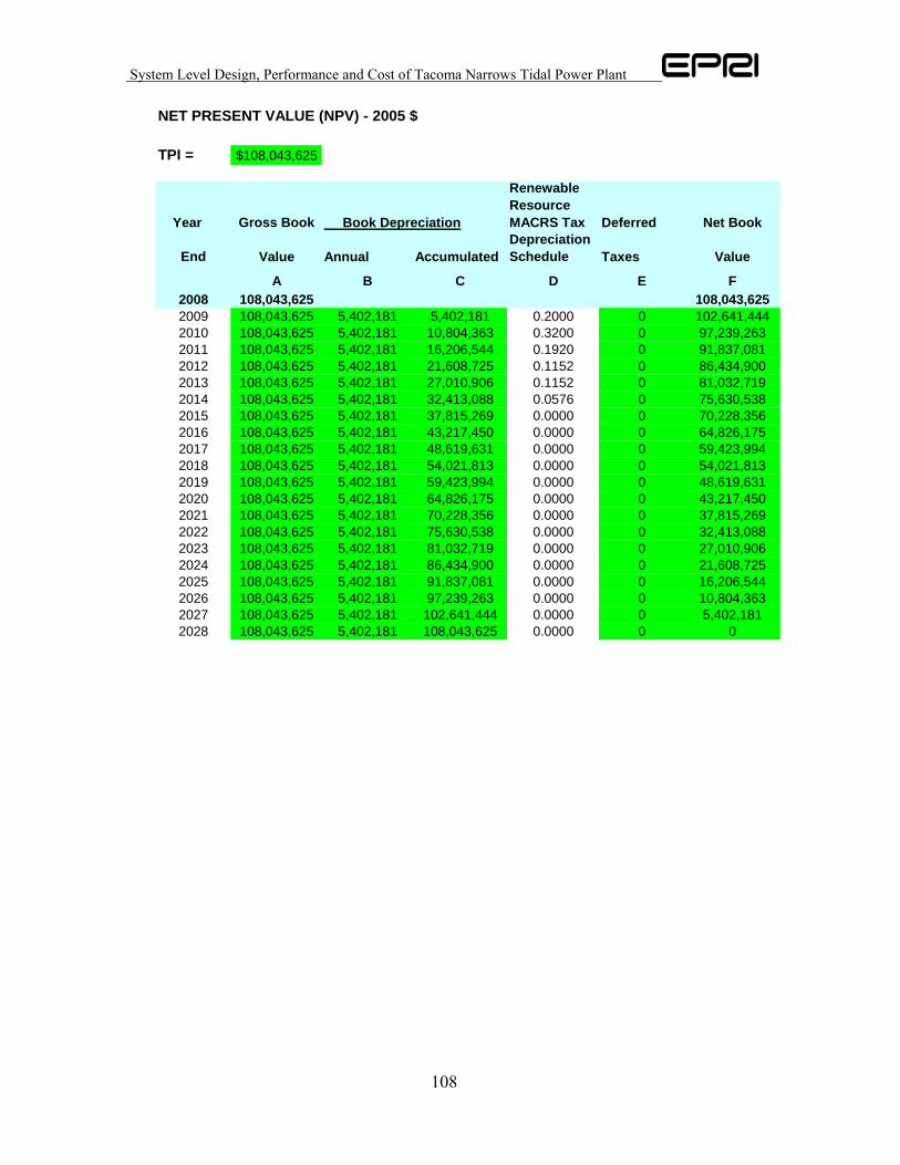
System Level Design, Performance and Cost of Tacoma Narrows Tidal Power Plant
108
NET PRESENT VALUE (NPV) - 2005 $
TPI = $108,043,625
Year Gross Book Book Depreciation
Renewable Resource MACRS Tax Deferred Net Book
End Value Annual AccumulatedDepreciation Schedule Taxes Value
A B C D E F2008 108,043,625 108,043,6252009 108,043,625 5,402,181 5,402,181 0.2000 0 102,641,4442010 108,043,625 5,402,181 10,804,363 0.3200 0 97,239,2632011 108,043,625 5,402,181 16,206,544 0.1920 0 91,837,0812012 108,043,625 5,402,181 21,608,725 0.1152 0 86,434,9002013 108,043,625 5,402,181 27,010,906 0.1152 0 81,032,7192014 108,043,625 5,402,181 32,413,088 0.0576 0 75,630,5382015 108,043,625 5,402,181 37,815,269 0.0000 0 70,228,3562016 108,043,625 5,402,181 43,217,450 0.0000 0 64,826,1752017 108,043,625 5,402,181 48,619,631 0.0000 0 59,423,9942018 108,043,625 5,402,181 54,021,813 0.0000 0 54,021,8132019 108,043,625 5,402,181 59,423,994 0.0000 0 48,619,6312020 108,043,625 5,402,181 64,826,175 0.0000 0 43,217,4502021 108,043,625 5,402,181 70,228,356 0.0000 0 37,815,2692022 108,043,625 5,402,181 75,630,538 0.0000 0 32,413,0882023 108,043,625 5,402,181 81,032,719 0.0000 0 27,010,9062024 108,043,625 5,402,181 86,434,900 0.0000 0 21,608,7252025 108,043,625 5,402,181 91,837,081 0.0000 0 16,206,5442026 108,043,625 5,402,181 97,239,263 0.0000 0 10,804,3632027 108,043,625 5,402,181 102,641,444 0.0000 0 5,402,1812028 108,043,625 5,402,181 108,043,625 0.0000 0 0

System Level Design, Performance and Cost of Tacoma Narrows Tidal Power Plant
109
CAPITAL REVENUE REQUIREMENTS 2005$
TPI = $108,043,625
End of
Year Net Book
Returns to Equity Common
Returns to Equity
PrefInterest on Debt Book Dep
Income Tax on Equity Return
Fed PTC and REC
Capital Revenue Req'ts
A B C D E F H I
2009 102,641,444 0 0 5,132,072 5,402,181 0 1,800,105 8,734,1482010 97,239,263 0 0 4,861,963 5,402,181 0 1,800,105 8,464,0392011 91,837,081 0 0 4,591,854 5,402,181 0 1,800,105 8,193,9302012 86,434,900 0 0 4,321,745 5,402,181 0 1,800,105 7,923,8212013 81,032,719 0 0 4,051,636 5,402,181 0 1,800,105 7,653,7122014 75,630,538 0 0 3,781,527 5,402,181 0 1,800,105 7,383,6032015 70,228,356 0 0 3,511,418 5,402,181 0 1,800,105 7,113,4942016 64,826,175 0 0 3,241,309 5,402,181 0 1,800,105 6,843,3852017 59,423,994 0 0 2,971,200 5,402,181 0 1,800,105 6,573,2762018 54,021,813 0 0 2,701,091 5,402,181 0 1,800,105 6,303,1672019 48,619,631 0 0 2,430,982 5,402,181 0 0 7,833,1632020 43,217,450 0 0 2,160,873 5,402,181 0 0 7,563,0542021 37,815,269 0 0 1,890,763 5,402,181 0 0 7,292,9452022 32,413,088 0 0 1,620,654 5,402,181 0 0 7,022,8362023 27,010,906 0 0 1,350,545 5,402,181 0 0 6,752,7272024 21,608,725 0 0 1,080,436 5,402,181 0 0 6,482,6182025 16,206,544 0 0 810,327 5,402,181 0 0 6,212,5082026 10,804,363 0 0 540,218 5,402,181 0 0 5,942,3992027 5,402,181 0 0 270,109 5,402,181 0 0 5,672,2902028 0 0 0 0 5,402,181 0 0 5,402,181Sum of Annual Capital Revenue Requirements 141,363,295
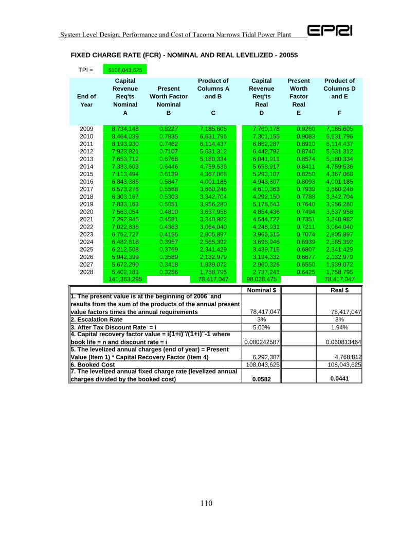
System Level Design, Performance and Cost of Tacoma Narrows Tidal Power Plant
110
FIXED CHARGE RATE (FCR) - NOMINAL AND REAL LEVELIZED - 2005$
TPI = $108,043,625
End of
Capital Revenue
Req'tsPresent
Worth Factor
Product of Columns A
and B
Capital Revenue
Req'ts
Present Worth Factor
Product of Columns D
and EYear Nominal Nominal Real Real
A B C D E F
2009 8,734,148 0.8227 7,185,605 7,760,178 0.9260 7,185,6052010 8,464,039 0.7835 6,631,796 7,301,155 0.9083 6,631,7962011 8,193,930 0.7462 6,114,437 6,862,287 0.8910 6,114,4372012 7,923,821 0.7107 5,631,312 6,442,792 0.8740 5,631,3122013 7,653,712 0.6768 5,180,334 6,041,911 0.8574 5,180,3342014 7,383,603 0.6446 4,759,536 5,658,917 0.8411 4,759,5362015 7,113,494 0.6139 4,367,068 5,293,107 0.8250 4,367,0682016 6,843,385 0.5847 4,001,185 4,943,807 0.8093 4,001,1852017 6,573,276 0.5568 3,660,246 4,610,363 0.7939 3,660,2462018 6,303,167 0.5303 3,342,704 4,292,150 0.7788 3,342,7042019 7,833,163 0.5051 3,956,280 5,178,643 0.7640 3,956,2802020 7,563,054 0.4810 3,637,958 4,854,436 0.7494 3,637,9582021 7,292,945 0.4581 3,340,982 4,544,722 0.7351 3,340,9822022 7,022,836 0.4363 3,064,040 4,248,931 0.7211 3,064,0402023 6,752,727 0.4155 2,805,897 3,966,515 0.7074 2,805,8972024 6,482,618 0.3957 2,565,392 3,696,946 0.6939 2,565,3922025 6,212,508 0.3769 2,341,429 3,439,715 0.6807 2,341,4292026 5,942,399 0.3589 2,132,979 3,194,332 0.6677 2,132,9792027 5,672,290 0.3418 1,939,072 2,960,326 0.6550 1,939,0722028 5,402,181 0.3256 1,758,795 2,737,241 0.6425 1,758,795
141,363,295 78,417,047 98,028,475 78,417,047
Nominal $ Real $
78,417,047 78,417,0473% 3%
5.00% 1.94%
0.080242587 0.060813464
6,292,387 4,768,812108,043,625 108,043,625
0.0582 0.0441
1. The present value is at the beginning of 2006 and results from the sum of the products of the annual present value factors times the annual requirements
3. After Tax Discount Rate = i
5. The levelized annual charges (end of year) = Present Value (Item 1) * Capital Recovery Factor (Item 4)
7. The levelized annual fixed charge rate (levelized annual charges divided by the booked cost)
6. Booked Cost
2. Escalation Rate
4. Capital recovery factor value = i(1+i)n/(1+i)n-1 where book life = n and discount rate = i

System Level Design, Performance and Cost of Tacoma Narrows Tidal Power Plant
111
LEVELIZED COST OF ELECTRICITY CALCULATION - Municipal Generator - 2005$
COE = ((TPI * FCR) + AO&M) / AEPIn other words…The Cost of Electricity =
The Sum of the Levelized Plant Investment + Annual O&M Cost including Levelized Overhaul and Replacement CostDivided by the Annual Electric Energy Consumption
NOMINAL RATESValue Units From
TPI $108,043,625 $ From TPIFCR 5.82% % From FCRAO&M $3,811,999 $ From AO&MAEP = 120,007 MWeh/yr From Assumptions
COE - TPI X FCR 5.24 cents/kWhCOE - AO&M 3.18 cents/kWh
COE $0.0842 $/kWh CalculatedCOE 8.42 cents/kWh Calculated
REAL RATES
TPI $108,043,625 $ From TPIFCR 4.41% % From FCRAO&M $3,811,999 $ From AO&MAEP = 120,007 MWeh/yr From Assumptions
COE - TPI X FCR 3.97 cents/kWhCOE - AO&M 3.18 cents/kWh
COE $0.0715 $/kWh CalculatedCOE 7.15 cents/kWh Calculated