System modelling and evaluation of main battle tank fire

IN DEGREE PROJECT VEHICLE ENGINEERING,SECOND CYCLE, 30 CREDITS

, STOCKHOLM SWEDEN 2021

System modelling and evaluation of main battle tank fire precision

VIKTOR HALLBECK

KTH ROYAL INSTITUTE OF TECHNOLOGYSCHOOL OF ENGINEERING SCIENCES

System modelling and evaluation of main battle tank fire precision

Viktor Hallbeck Master of Science in Engineering Master programme in Vehicle Engineering KTH Royal Institute of Technology Supervisor at (FOI): Ekaterina Fedina Supervisor at KTH: Prof. Mikael Nybacka Examiner at KTH: Prof. Mikael Nybacka Date of presentation: 10/9-2021 TRITA-SCI-GRU 2021:286 KTH Royal Institute of Technology School of Engineering Sciences KTH SCI SE-100 44 Stockholm, Sweden URL: http://www.kth.se/sci

AbstractThis master thesis describes a study of the main battle tankdynamics in order to investigate the fire precision when atank is driving in terrain. A model has been developed tosimulate the dynamic interaction between the tank’s hulland the ground irregularity in MATLAB and SIMULINKthrough the modelling of the tank’s dynamics. Two differ-ent models of suspension system have been analysed. Onelinear model and one hydro-pneumatic model. Further thecontribution from the cannon’s recoil has been modelledto investigate its contribution to the dynamics of the vehi-cle. The models developed are on system level and is to beimplemented in a larger model. Therefore are the modelssimplified and the thesis investigates to what degree of sim-plification the models will accurately predict the movementof the tank.

Sammanfattning

Denna examensarbete beskriver en studie pa stridsvagns-dynamik for att undersoka precision av maltraff nar strids-vagnen framfors i terrang. En modell har utvecklats foratt simulera hur stridsvagnar paverkas av underlagets va-riation i MATLAB och SIMULINK genom att modellerastridsvagnens dynamik. Tva olika former av stotdamparehar undersokts, en linjar modell samt en hydro-pneumatiskmodell. Aven bidraget fran kanonen’s avfyrning har mo-dellerats for att se hur rekylens bidrag paverkar rorelsenav stridsvagnen. Malet med studien var att ta fram en saforenklad modell som mojligt. Flera modeller har darforutvecklats for att jamfora forenklingsgraden.

Acknowledgement

I would like to say a really big thank you to Ekaterina Fedina for all the supportduring this thesis and being an excellent supervisor for the project. I would alsolike to thank Arvid Carlstedt and Mikael Lyth for all the good discussions and helpwith the progress of the thesis. Last but not least I would like to thank NiclasStensback, Anders Lindstrom and Mikael Nybacka for the good discussions regard-ing the thesis.

Viktor Hallbeck

v

Contents

Contents vi

1 Introduction 51.1 Background . . . . . . . . . . . . . . . . . . . . . . . . . . . . . . . . 51.2 Problem formulation . . . . . . . . . . . . . . . . . . . . . . . . . . . 61.3 Purpose and goal . . . . . . . . . . . . . . . . . . . . . . . . . . . . . 61.4 Delimitations and ethics . . . . . . . . . . . . . . . . . . . . . . . . . 6

2 Background and theory 92.1 Dynamics of tracked vehicles . . . . . . . . . . . . . . . . . . . . . . 10

2.1.1 Mathematical representation of half-plane suspension exclud-ing track . . . . . . . . . . . . . . . . . . . . . . . . . . . . . 11

2.1.2 Mathematical representation of half-plane suspension includ-ing track . . . . . . . . . . . . . . . . . . . . . . . . . . . . . 14

2.1.3 Mathematical representation full vehicle suspension . . . . . 152.1.4 Hydro-gas suspension . . . . . . . . . . . . . . . . . . . . . . 17

2.2 Firing of cannon . . . . . . . . . . . . . . . . . . . . . . . . . . . . . 202.2.1 Firing sequence from a force perspective . . . . . . . . . . . . 212.2.2 Accuracy depending on barrel movement . . . . . . . . . . . 22

3 Modelling and simulations 253.1 Half tank model . . . . . . . . . . . . . . . . . . . . . . . . . . . . . 25

3.1.1 9 Degrees of freedom . . . . . . . . . . . . . . . . . . . . . . . 253.1.2 16 Degrees of freedom . . . . . . . . . . . . . . . . . . . . . . 273.1.3 HGS model . . . . . . . . . . . . . . . . . . . . . . . . . . . . 29

3.2 Full vehicle model . . . . . . . . . . . . . . . . . . . . . . . . . . . . 323.3 Firing sequence implementation . . . . . . . . . . . . . . . . . . . . . 36

4 Results and analysis 394.1 Model comparison . . . . . . . . . . . . . . . . . . . . . . . . . . . . 39

4.1.1 Damper model performance comparison . . . . . . . . . . . . 394.1.2 Firing accuracy . . . . . . . . . . . . . . . . . . . . . . . . . . 43

5 Conclusions and future work 45

vi

5.1 Conclusions and discussion . . . . . . . . . . . . . . . . . . . . . . . 455.2 Limitations . . . . . . . . . . . . . . . . . . . . . . . . . . . . . . . . 465.3 Future work . . . . . . . . . . . . . . . . . . . . . . . . . . . . . . . . 47

Bibliography 49

List of Figures

2.1 Visual representation of the torsion-bar suspension implementation inthe chassis of the tank. . . . . . . . . . . . . . . . . . . . . . . . . . . . . 11

2.2 The respective axes and the rotation notation. . . . . . . . . . . . . . . 122.3 Visual representation of the simplified half-vehicle model. . . . . . . . . 132.4 Visiual representation of the extended half-vehicle model. . . . . . . . . 152.5 Visual representation of full vehicle model. . . . . . . . . . . . . . . . . 172.6 The construction of the HGS unit. . . . . . . . . . . . . . . . . . . . . . 182.7 A simplified schematic of the principle of the HGS systems. The nitrogen

chamber on top, in between the nitrogen chamber and the piston is thefluid chambers connected by the orifice and below is the piston, whichis connected to the road-wheel via a linkage. . . . . . . . . . . . . . . . 19

2.8 A visual representation of firing accuracy. . . . . . . . . . . . . . . . . . 23

3.1 The vibration course track profile. . . . . . . . . . . . . . . . . . . . . . 263.2 Test 1, comparing the vertical deviation of each of the tank’s 7 wheels

between the 9 and the 16 DoF model. . . . . . . . . . . . . . . . . . . . 283.3 Test 1, comparison of the hull vertical displacement and the pitch angle

between the 9 and the 16 DoF model. . . . . . . . . . . . . . . . . . . . 283.4 Test 2, comparison of the hull vertical displacement and the pitch angle

between the 9 and the 16 DoF model. . . . . . . . . . . . . . . . . . . . 293.5 Spring force in relation to wheel displacement. . . . . . . . . . . . . . . 303.6 Damping force in relation to wheel speed. . . . . . . . . . . . . . . . . . 313.7 Damper model with linearised high speed compared to the original model. 323.8 HGS-unit force in relation to speed and distance for 0.1 Hz sinusoidal

excitation with amplitudes between 0.1 and 0.45 m from equilibriumposition. . . . . . . . . . . . . . . . . . . . . . . . . . . . . . . . . . . . . 35

3.9 HGS-unit force in relation to speed and distance for 1 Hz sinusoidalexcitation with amplitudes between 0.1 and 0.45 m from equilibriumposition. . . . . . . . . . . . . . . . . . . . . . . . . . . . . . . . . . . . . 35

3.10 The force from the recoil acting on the barrel attachment-point. . . . . 363.11 Visual representation of the recoil acting-point. . . . . . . . . . . . . . . 363.12 The hull pitch angle and pitch acceleration due to firing of the cannon. . 37

viii

4.1 Comparison of the vertical deviation for test 1 between the linear modeland the 2 HGS models. . . . . . . . . . . . . . . . . . . . . . . . . . . . 40

4.2 Comparison of the pitch angle for test 1 between the linear model andthe 2 HGS models. . . . . . . . . . . . . . . . . . . . . . . . . . . . . . . 40





4.7 Aim-point displacement. . . . . . . . . . . . . . . . . . . . . . . . . . . . 43

Abbreviations

MBT - Main Battle TankHGS - Hydro-Gas SuspensionCoG - Centre of GravityIFV - Infantry Fighting Vehicle

1

Variable declaration

Table 0.1: Variable declaration.

Variable Explanation of variable Unitz Vertical displacement of the hull mz Vertical speed of the hull m s−1

z Vertical acceleration of the hull m s−2

zti Vertical displacement of respective tyre mzli Vertical displacement of respective track component mzg Vertical displacement of ground mϕ Pitch angle of the hull radϕ Pitch speed of the hull rad s−1

ϕ Pitch acceleration of the hull rad s−2

γ Roll angle of hull radγ Roll speed of hull rad s−1

γ Roll acceleration of hull rad s−2

xi Wheel position wrt CoG myi Wheel position wrt CoG (width) mm Mass of the vehicle kgmti Mass of the wheel kgmli Mass of the track component kg

Jxx, Jyy Moment of inertia kg m2

Jxy Moment of deviation kg m2

i Index −N Quantity of wheels/track components −kd Spring stiffness of main spring N m−1

kt Spring stiffness of wheel to track N m−1

kl Spring stiffness of track to ground N m−1

cd Damping coefficient main damper N s m−1

ct Damping coefficient of wheel N s m−1

cl Damping coefficient track to ground N s m−1

Pi Pressure of nitrogen chamber PaVi Volume of nitrogen chamber m3

P0 Initial nitrogen pressure PaV0 Initial nitrogen chamber volume m3

n Polytropic index −

3

Q Volume flow rate m3 s−1

K Piston position mK Piston speed m s−1

Ap Piston area m2

Ao Orifice area m2

Cd Discharge coefficient −ρ Density kg m−3

Chapter 1

Introduction

This chapter starts of with an introduction to the thesis. First the background to theproblem formulation is discussed then the problem description is given and defined.Further the purpose of the thesis is described and what the goals of the project are.Last the delimitations of the thesis are presented and the ethical considerations arementioned.

1.1 BackgroundWhen designing tanks many factors need to be taken into consideration. More oftenthan not the tank will need to operate under varying circumstances and hence beable to work well in multiple different scenarios. Urban areas can in some casesfacilitate the movement of a tank where good roads are available, but can also belimiting if the tank will not be able to drive up narrow alleys and have a limited lineof sight. It is not uncommon for tanks to be deployed in multiple different parts ofthe world with a large variations in terrain and temperature. Even locally may thecircumstances change rapidly as for example heavy rain may drastically change soilproperties of the ground. In order to utilize the tank as effectively as possible meansusing the terrain to an advantage, taking routes that gives added protection fromthe enemy. This demands a good understanding of the tanks ability and limitationsin a large span of different terrains and also how to maneuver the terrain given theconditions that are present.

The development of the MBT is affected by the changes in operational environ-ment, the changing threats and the development of technology. Tanks will continueto face more advanced threats in the future and hence will need to be updatedand improved in order to continue to be the best vehicle that the military has inits arsenal. The next generation of tanks are currently in design and with moreadvanced features than ever before. But in order to do the correct design decisionsa proper understanding of the fundamentals of the tank is necessary.

5

Overall are there three major areas to consider when studying tanks. The tanksprotection, its mobility and its firepower, the sum of which can be used to estimatethe tank’s ability to accomplish missions in given scenarios [1].

This thesis will primarily focus on the mobility of the tank. How to model andevaluate the mobility of the tank in order to get a better understanding of thedynamic behaviour of the tank and also its interaction with the environment. Thethesis will also investigate how the mobility can affect the firing precision of the tank.

The models that are to be developed are on system level and therefore the modelsdo not need to be modelled in every detail. A large part of factors that contributeto the dynamics of the tank on detail level will not noticeably change the generalbehaviour of the model. To what degree of detail the model will need to be in orderto predict the movement of the tank is to be investigated in the thesis.

1.2 Problem formulationTo what degree of simplification can a model of a MBT reasonably accurately pre-dict the movement and firing accuracy of a main battle tank in a range of drivingscenarios?

1.3 Purpose and goalThe purpose of this thesis is to gain understanding of an MBT’s dynamic behaviourin running condition. To investigate how the ground that the tank drives on affectsthe movement of the hull and the barrel of the tank in order to be able to evaluatethe tanks performance.

The goal is to create a dynamic system model of a modern tank in MATLAB/SIMULINKthat given a road profile and a speed will approximate the movement of the tank’shull, i.e chassis, turret and barrel. Given this, the firing accuracy of the tank whiledriving will be investigated.

1.4 Delimitations and ethicsThe ground will be considered as a rigid non-moveable object. The model can befurther developed with the addition of terramechanics but this will not be consid-ered. Further, the model will be a simplified model of the real tank hence details ofthe tank that can be considered as not relevant or not giving a substantial impacton the results will be neglected as this is a part of the goals of the thesis.

The tank is a military vehicle and hence a lot of ethical discussion could be doneregarding the warfare part but this is an entirely different subject in itself. Since

this thesis is done only working with a model of a tank the ethical aspects of war arenot considered in this report. The intent of the model is only to evaluate the tank’smobility performance and the results from the model will only be used to predictoutcomes of the mobility of the tank and its accuracy. As a parable a similar modelcould be used to predict the movement and vibrations of a camera mounted on aframe on a car or other vehicle.

Chapter 2

Background and theory

A MBT is a tracked vehicle made for the purpose of combat. The purpose of thetank is to have the best protection, the best mobility and the best firepower possi-ble. The targets are most often ground targets or other tanks. The tank consist ofthe chassis which is housing the drive-train and most of the crew, the turret whichis placed on top of the chassis which can be either manned or unmanned and thecannon which is attached to the turret. In order for the tank to have the best pro-tection the tank is fitted with heavy armour and active anti tank countermeasures.The best mobility is given by the very powerful engine upwards of 1500 horsepowerthat the tank is equipped with giving the tank a high top-speed and the ability totraverse difficult terrain. The best firepower is given by its main armament, whichis a cannon of around 120 mm in diameter. The combination of all these factorsmakes the tank a very fearsome vehicle.

The chapter starts with providing some background on last generations damper sys-tems will be presented since the topic in focus is the mobility of the tank. Thereafterthe mathematics of the half vehicle are introduced. Staying in the half-plane thehalf vehicle model is then extended to more degrees of freedom (DoF) to investigatethe tracks added DoF influence. This is followed by introducing mathematical rep-resentation of the full vehicle model. Given the theory of the movement of the fulltank the dampers are investigated further and the nonlinear hydrogassystem (HGS)is presented, which gives the possibility to improve the ride dynamics of the vehicle.Proceeding, the parts affected by the dynamics of the tank’s hull is investigated.This includes the motion of the turret and barrel assembly. Last the contributionof firing of the tanks cannon is shown and how the tanks firing accuracy is affectedby the motion of the tank.

9

2.1 Dynamics of tracked vehiclesThe design of the suspension will affect the mobility of the tank. The main purposeof the suspension system on a tank is to give the crew of the tank a tolerable rideminimizing fatigue. A proper tuned suspension will also give minimal vibrations,which gives the added benefit of needing less control input on order to stabilize theturret in the move, improving the accuracy of the cannon in a dynamic scenario. Inworst case scenario a tank that is unable to move is an easy target and a unwantedoccurrence, as the tank will need support and rescue from other units to get movingagain. Hence a well working and well tuned suspension system is of great impor-tance for the tanks mobility and ultimately its survivability [2].

Tanks are very heavy vehicles overall. They can weigh upwards of 70 tons andabove. This is largely due to the tank’s armour that needs to be very thick in orderto protect the vehicle from threats. Adding to the weight of the tank is also themain armament of the tank which, in itself can weigh multiple tons. This also meansthat the tank needs a heavy and powerful engine to give the tank fast accelerationand have the ability to climb steep gradients. The suspension and track layout oftanks are usually different in configuration compared to other tracked vehicles suchas in agriculture since the tank needs to be able to run at higher speeds over roughground. The engine power and weight also greatly affect the overall agility of thetank [3].

Looking back at the last generation of tanks, the most commonly used a torsion-barsuspension. The torsion-bar is a very simple type of suspension where a long bar ofmetal creates a spring force through a twisting motion of the bar. The torsion-baracts as the spring for the running wheels in contact with the tracks. On the tank,the first and last pair of wheels are fitted with a damper in order to improve the ridebut the wheels in between only have the torsion bar and hence no specific damper inorder to smooth the motion. Because the tanks substantial weight, the torsion-barneeds to be quite large in order to accommodate the large forces that a tank wouldexperience during manoeuvring. The construction would protrude though the hullof the vehicle taking up a substantial amount of space. Figure 2.1 gives a visualrepresentation of how the torsion-bar suspension is fitted to the chassis of the tank.The benefits of running a torsion-bar suspension is the simplicity of the system andthe absence of maintenance requirements since there are very few moving parts inthe construction.

Figure 2.1: Visual representation of the torsion-bar suspension implementation inthe chassis of the tank.

However, with increasing demands on the ability to go faster over rough terrain andhave overall better mobility the trend is to go towards more advanced suspensionsystems such as a hydro-gas suspension. This because they tend to be lighter, morecompact, improve ride quality for the crew and be more versatile [4].

2.1.1 Mathematical representation of half-plane suspension excludingtrack

The simplest way of modelling the motion of a vehicle is the Quarter-car model. Thismodel represents the vehicle by looking at one quarter of the vehicle i.e one wheel of acar. This model has very few degrees of freedom and will not give much informationabout the motion of the tank as only the bounce motion can be observed. To startas simple as possible with representing the motion i.e. vertical displacement of thetank the half-car model is used. The half-car model effectively cuts the vehicle inhalf and observes one side of the vehicle in a 2D plane as can be seen in figure 2.3.The torsion bar suspension from the last generation of tanks produces a force fromthe twisting motion of the bar as formerly described. The force from the twistingmotion is not precisely linear but quite close [5]. The tank’s suspension systemcan be modelled as a combination of masses, springs and dampers. The motionof a, simplified in plane, traditional suspension can be described mathematicallyby Lagrange equations [5]. As a simplification the tracks contribution has beenneglected. Figure 2.2 shows the notations of the respective rotation roll, pitch andyaw around the axes, bounce is denoted Z and is a displacement.

Figure 2.2: The respective axes and the rotation notation.

d

dt(δEk

δq)− δEk

δq+ δEd

δq+ δEp

δq= F (t) (2.1)

Where the respective terms are the following: Ek - kinetic energy, Ep - potentialenergy, Ed - dissipation energy, q - generalized coordinates, F (t) - generalized forcesdepending on time.

The equations of motion are derived using Lagrange equation and the result is asecond order linear differential equation as follows.

mz + cz + kz = F (t) (2.2)

Where the constants are: m - mass, c - damping coefficient, k - spring stiffness.

As the suspension system of a tracked vehicle is a combination of many wheel-pairs the equation for the motion of the hull can be written as the sum of all forcesacting on the hull of the vehicle. The mathematical description of the motion canbe written as equation 2.3 and equation 2.4 for bounce and pitch motion of the hull.The respective variables and units can be seen in Table 0.1.

The vertical deviation for the hull is described by equation 2.3.

mz +N∑

i=1kd(z + xiϕ− zti) +

N∑i=1

cd(z + xiϕ− zti) = 0 (2.3)

The pitch motion of the hull can in a similar way be described with equation 2.4

Jyyϕ+N∑

i=1kdxi(z + xiϕ− zti) +

N∑i=1

cdxi(z + xiϕ− zti) = 0 (2.4)

The equation of motion for each independent wheel is described with equation 2.5.

mtizti − kd(z + xiϕ− zti)− cd(z + xiϕ− zti) + kt(zti − zg) = 0 (2.5)

Where: z - Vertical displacement of the hull, z - Vertical speed of the hull, z -Vertical acceleration of the hull, zti - Vertical displacement of respective tyre, zg

- Vertical displacement of ground, ϕ - Pitch angle of the hull, ϕ - Pitch speed ofthe hull, ϕ - Pitch acceleration of the hull, xi - Wheel position wrt CoG, m - Massof the vehicle, mti - Mass of the wheel, Jyy - Moment of inertia, Jxy - Moment ofdeviation, i - Index, N - Quantity of wheels/track components, kd - Spring stiffnessof main spring, kt - Spring stiffness of wheel to track, cd - Damping coefficient maindamper, ct - Damping coefficient of wheel.

A visual representation of the simplified model can be seen in figure 2.3. The figuregives a general representation of the system, a damper is represented on each wheelbut this might not always be the case depending on how the suspension is configured.

Figure 2.3: Visual representation of the simplified half-vehicle model.

2.1.2 Mathematical representation of half-plane suspension includingtrack

In order to understand how the contribution of the tracks affects the dynamics ofthe tank the tracks are included into the model. Because the track is not behavinglinearly along the length of the track some different methods of modelling the track’scontribution have been made. One way of modelling the track is to introduce animaginary running-wheel between the actual physical wheels of the tank as done by[6]. According to the author this seems to be a viable way of modelling the tracksbut the results seems to deviate somewhat from the actual measured data in thereport.

In this thesis the method for modelling track involves the vertical movement ofthe track and hence the horizontal stiffness is neglected. The equations of motionfor the half-plane model with the track component included are derived in equations2.6 to 2.9 where each track component is represented by a mass, spring and damper.

The equations for bounce and pitch seen in equations 2.6 and 2.7 are very simi-lar to the simplified model.

mz +N∑

i=1kd(z − zti + ϕxi) +

N∑i=1

cd(z − zti + ϕxi) = 0 (2.6)

Jϕ+N∑

i=1kdxi(z − zti + ϕxi) +

N∑i=1

cdxi(z − zti + ϕxi) = 0 (2.7)

The equation of motion for each individual wheel can be seen in equation 2.8.

mtizti = kd(z + xiϕ− zti) + cd(z + xiϕ− zti)− kt(zti − zl)− ct(zti − zl) (2.8)

And last the equation of motion for the track component can be seen in 2.9.

mlizli = kt(zti − zli) + ct(zti − zli)− kl(zgi − zli)− cl(zgi − zl) (2.9)

Where: zli - Vertical displacement of respective track component, mli - Mass of thetrack component, kl - Spring stiffness of track to ground, cl - Damping coefficienttrack to ground.

A general visiual representation of the model can be seen in figure 2.4.

Figure 2.4: Visiual representation of the extended half-vehicle model.

2.1.3 Mathematical representation full vehicle suspensionThe half-plane model only accommodates the bounce and pitch motion of the hullbut since the goal is to simulate the firing precision a full vehicle model is necessaryin order to be able to include the horizontal deviation due to roll and yaw. Inthe same way that the Lagrange equation is used in equation 2.1 to describe thein-plane motion of the tank, the same equation can be used in order to describe thefull vehicle motion [7].

Applying equation 2.1 to the full vehicle it can be seen that.

Ek = 12(mz2 + Jykϕ

2 + Jxkγ2 − 2Jxyϕγ) (2.10)

Ep = 12

N∑i=1

ki(z − xiϕ+ yiγ − zt)2 (2.11)

Ed = 12

N∑i=1

ci(z − xiϕ+ yiγ − zt)2 (2.12)

Given the above equations the full vehicle model can be derived as the following:

Mz + Cz + Kz = Fw (2.13)

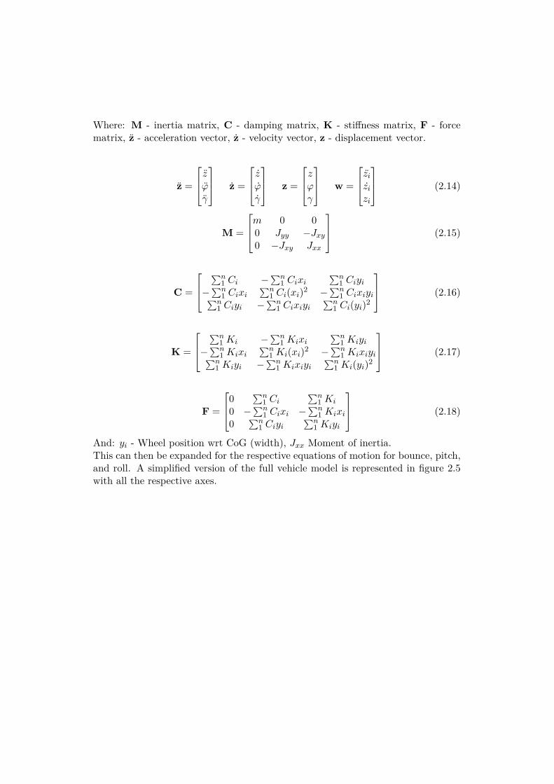
Where: M - inertia matrix, C - damping matrix, K - stiffness matrix, F - forcematrix, z - acceleration vector, z - velocity vector, z - displacement vector.

z =

zϕγ

z =

zϕγ

z =

zϕγ

w =

zi

zi

zi

(2.14)

M =

m 0 00 Jyy −Jxy

0 −Jxy Jxx

(2.15)

C =

∑n

1 Ci −∑n

1 Cixi∑n

1 Ciyi

−∑n

1 Cixi∑n

1 Ci(xi)2 −∑n

1 Cixiyi∑n1 Ciyi −

∑n1 Cixiyi

∑n1 Ci(yi)2

(2.16)

K =

∑n

1 Ki −∑n

1 Kixi∑n

1 Kiyi

−∑n

1 Kixi∑n

1 Ki(xi)2 −∑n

1 Kixiyi∑n1 Kiyi −

∑n1 Kixiyi

∑n1 Ki(yi)2

(2.17)

F =

0 ∑n1 Ci

∑n1 Ki

0 −∑n

1 Cixi −∑n

1 Kixi

0 ∑n1 Ciyi

∑n1 Kiyi

(2.18)

And: yi - Wheel position wrt CoG (width), Jxx Moment of inertia.This can then be expanded for the respective equations of motion for bounce, pitch,and roll. A simplified version of the full vehicle model is represented in figure 2.5with all the respective axes.

Figure 2.5: Visual representation of full vehicle model.

2.1.4 Hydro-gas suspensionIn order to improve the ride comfort and the motion of the tank, a so called hydro-gas suspension system (HGS), seen in figure 2.6, can be implemented. The HGSis similar to an advanced shock absorber on a road going vehicle in that it has ad-justable high and low speed compression and rebound. But instead of a traditionalcoil spring, the system relies on compression of a gas to act as the spring element.Also, the suspension system is more compact than the conventional torsion-bar sus-pension and the HGS units can be mounted outside of the hull freeing up space inthe hull. As each independent wheel will be fitted with an HGS module the tankreceives full damping on each independent wheel. The spring element of the HGSsystem have lower spring rate at lower wheel displacement and stiffer spring rate athigh displacement giving a better ride for the crew and preventing hitting a hardstop at maximum travel in compression [8]. The HGS also has the possibility togive the vehicle road levelling capabilities [4]. With the possibility to adjust thelevel of each individual wheel height comes also the ability to adjust the tension inthe track as well as the ground clearance of the vehicle. The tension in the trackhas been shown to have a significant effect on the vehicles mobility over soft soil [9].

Figure 2.6: The construction of the HGS unit.

The unit is constructed of a nitrogen chamber with a given preset pressure andvolume shown as the top part in figure 2.7. The nitrogen chamber is connectedto a fluid chamber, with a floating piston in between. The fluid chamber has asmall orifice that is restricting the flow of fluid from below to above. When thewheel of the tank moves the lower piston moves displacing the fluid forcing it toflow though the orifice to the other chamber where the floating piston is locatedand compresses the nitrogen gas. In order to control the flow and have the pressuredue to the movement of the wheel not exceed to high pressures, a bleed valve islocated parallel to the orifice. The bleed valve can be designed in different ways butthe main purpose is to allow increased flow between the chambers regulating thepressure differential.

The principle of HGS unit is working on can be seen in figure 2.7.

Figure 2.7: A simplified schematic of the principle of the HGS systems. The nitro-gen chamber on top, in between the nitrogen chamber and the piston is the fluidchambers connected by the orifice and below is the piston, which is connected tothe road-wheel via a linkage.

There are two parts adding to the force of the suspension unit. The first part acts asa spring when the nitrogen chamber is compressed. The second part is the viscousdamping given by the fluid passing through the orifice and the bleed valve. Thisgives the non linear spring-damper action and with the adjustable bleed valve thecharacteristics of the damper can be changed in order to get the best performance[10].

The following equations explain the relation between the motion of the piston andthe reacting force of the HGS unit. Starting of with the compression of the nitro-gen gas. The gas of the chamber is considered to be an ideal gas undergoing anpolytropic process hence the relation between the pressure and volume is given byequation 2.19 [11].

The process of compressing the nitrogen gas is assumed to be an adiabatic pro-cess meaning that no heat exchange is occurring since the process of compressionand expansion is quite rapid. The adiabatic index n is depending on temperatureand pressure. From [11, 4] the adiabatic index can be seen as in proximity of 1.3to 1.4 in temperatures around 20 degrees Celsius and pressures below 200 bar. Pi

represents the instantaneous pressure of the nitrogen chamber and Vi is the in-stantaneous volume of the gas and P0 and V0 is the initial pressure and volume.

P0Vn

0 = PiVn

i ⇒ Pi = P0Vn

0V n

i

(2.19)

The instantaneous volume of the nitrogen chamber is only depending on the dis-

placed volume of the piston, assuming that the fluid is incompressible. Thereforethe volume of the nitrogen chamber can be written as equation 2.20 where K is theposition of the lower piston and Ap is the piston area.

Vi = V0 −ApK (2.20)

The volumetric flow rate Q though the orifice can be seen in equation 2.21 andoriginates from Bernoulli’s equation. Cd is the discharge coefficient and describesthe losses in the orifice plate. The value for the coefficient is usually between 0.6and 0.85 and is affected by geometry of the orifice [12]. Ao is the orifice area, ρ isthe density of the oil and ∆P is the pressure difference between the oil chambers.

Q = CdAo

√2∆Pρ

(2.21)

Since the only component that is inducing any flow though the orifice is the move-ment of the piston the flow rate of can also be written as a function of the pistonspeed.

Q = ApK (2.22)

Solving for the pressure differential between the two chambers gives the followingexpression.

(2.21) & (2.22)⇒ ∆P =ρA2

pK2

2C2dA

2o

(2.23)

Last, the two component of force can be derived. The spring force from the nitrogencompression denoted Fs and the damper force from the pressure difference denotedFd.

Fs = PiAp (2.24)

Fd = Ap∆P (2.25)

Each wheel of the tank is fitted with an individual HGS unit. The force fromequation 2.24 and 2.25 is from a single unit and hence the total force from thecombined system with multiple units will be the sum of all the forces that the unitsproduce.

2.2 Firing of cannonThe tank must be able to fire its cannon while moving. In order to make this possiblethe cannon will need to be controlled and stabilized in order to be able to aim ata given target. The control part will not considered in the thesis. The firing of thecannon will impose a large force on the turret and the hull of the tank during ashort timespan and will affect the entire vehicle. The magnitude and duration of the

force from the cannon’s recoil is depending on the bore of the cannon and the typeof ammunition used. The orientation will also affect how the force is transmitted tothe vehicle. As the firing of the tank’s cannon is a common procedure the recoil’scontribution to the dynamics of the tank’s hull will be investigated.

2.2.1 Firing sequence from a force perspectiveThe main armament of modern tank is usually a cannon with a calibre of approxi-mately 120 mm. The force experienced from the recoil of the cannon is large enoughto affect the entire vehicle. Because of this, tanks are fitted with a recoil mechanismin order to relieve some of the force from the hull and insure that the large impulse ofthe cannon will not permanently damage the vehicle. The recoil mechanism worksby enabling the cannon to move in its axial direction. When the cannon is firedit moves backwards and compresses either a set of springs or containers of air toabsorb some of the force [13].

The firing sequence is a very complex process to model in detail. The generalbehaviour of the recoil force is as follows. The cannon is fired and the projectileleaves the barrel, during that time the tank experiences a large increase in force,which decays in about the same time as the force was generated. The entire eventis over within around one tenth of a second. As the purpose of the thesis is toinvestigate the tank’s dynamics on a system level, a simplified model of the recoilforce is utilized. Vallier’s formula is used for calculating the recoil and is valid underthe assumption that the force from the recoil acting on the vehicle is a rectangularimpulse of a set time [13].

R = 0.5M0U2max

Lmax − Lk + Umaxtp(2.26)

Umax = Mp + βmm

M0U0 (2.27)

β =(700 + U0

U0

)1.1(2.28)

Where: R - recoil force resistance, Umax - maximum velocity of the free recoil, Lmax

- maximum recoil path, Lk – free recoil path (at R = 0), tp – duration of gunpowdergases exhaust activity, Mp – projectile mass, U0 – initial velocity of the projectile,mm – mass of propellant charge, M0 – mass of recoiling assembly, β – activity ofgunpowder gases factor.

With data from the a given cannon and its ammunition a recoil force can be calcu-lated. A few examples of force and recoil time can be seen in Table 2.1.

Table 2.1: Tank main armament recoil force [13, 14].

Cannon Recoil force [kN] Duration [ms]2A46, 125 mm 524 56L44, 120 mm 411 58L7A3 105 mm 460 432A28, 73 mm 126 123

The whole course of firing the cannon is over within milliseconds. The forces in-volved are extremely high as the projectile is often approximately 10 kg in mass andis accelerated during the length of the barrel, often below 8 meters, to a muzzle-velocity of 700 to 1700 m s−1. In order to evaluate if the values for the recoil forceare reasonable a simplified check is done. Assuming constant acceleration of theprojectile, the acceleration to a muzzle velocity of 1 km s−1 over the course of a 8 mbarrel, the acceleration would be 62 km s−2. With Newton’s second law, the forcerequired to achieve this constant acceleration would be in the order of hundredthsof kN with a projectile of above 1.6 kg which, would be much lower than the massof the projectiles seen normally. And according to Newton’s third law every actionthere is an equal and opposite reaction, the tank would experience a recoil force ofthe roughly same magnitude.

2.2.2 Accuracy depending on barrel movementThe accuracy of the tank’s cannon is influenced by the movement of the entiretank. That is the performance of the firing control system and the stabilization ofthe barrel among other things. If the control of the tank’s cannon is neglected andthe cannon is stationary relative to the turret and hull, then the accuracy of thetank will mainly be influenced by the motion depending on the surface the tank isrunning on. The pure movement at the muzzle is a good indicator of what perfor-mance the control system will need in order to stabilize the barrel.

The vertical displacement from the target aim point is given by the following equa-tions [15]. A visual representation can be seen in figure 2.8.

Z +H ≤ Y (2.29)

Where: Y- Half height of target, Z - contribution of vertical deviation at target areadistance L away from the cannon. Z is given at the time the shell leaves the barreland is affected by the entire movement of the tank, i.e pitch motion of the vehicle.H - the deviation contribution at the target, which is given by the movement of thebarrel itself.

Z = ϕuzL+ ϕuzlzL

V0(2.30)

H = ϕuhL+ ϕuhlhL

V0(2.31)

Where: ϕuz - angle deviation of the tank, ϕuz - angular velocity of the tank, L -direct distance to target, lz - length between the cannons CoG and the muzzle, V0- projectile muzzle velocity, ϕuh - angle deviation of cannon, ϕuh - angular velocityof cannon, lh - length between the recoiling parts’ CoG and the muzzle.

Given the displacement of the projectile impact-point to the original aim-point onthe target is it possible to use this information to calculate the probability of hittingthe target given the above mentioned assumptions.

Figure 2.8: A visual representation of firing accuracy.

Chapter 3

Modelling and simulations

This chapter will go though the different models and its implementations. Due todifficulties obtaiming open research data for model validation the model is developedaiming at producing comparable behaviour to the available research data [4] [8] [10].One of the goals when designing the suspension system is to have minimal vibrationstransferred to the hull and hence this goal will be taken into consideration whencomparing the models.

3.1 Half tank model

3.1.1 9 Degrees of freedomThe first model to be designed is the simplified model of the tank. The tank isrepresented by a half car model without the track link. The hull is represented asa mass with two degrees of freedom, and the track and running wheels of the tankare also represented as a mass with one degree of freedom each. The model is con-structed in SIMULINK and consists of simple blocks such as gain and integrators.

The road is considered as stiff and the reason for this is that a road profile, consid-ering road damping or terramechanics, is adding a damping factor to the motion ofthe tank and could hence give the model a better performance than if the road isstiff, since all of the vibration from the ground are transferred into the hull of thetank.

Some different variations of road profile are considered. First a step impulse of100 millimeter in order to check that the model is settling in a correct way and thatthe response of the hull is behaving in a reasonable manner. Further a periodic roadwith amplitude of 60 millimeter and a few different frequencies. Finally a vibrationcourse seen in figure 3.1, with is represented of bumps of varying size and distance istested in order to compare the performance of the models in a mobility challengingscenario more like the real driving conditions that the tank will encounter. The

25

track is roughly 150 m long with bumps in sizes of 0.3, 0.15, 0.12 and 0.075 m witha length of 7.6, 6.1, 0.9 and 0.6 m.

Figure 3.1: The vibration course track profile.

The parameters used for the tank are presented in Table 3.1. The tank is equippedwith seven running-wheels with a wheelbase of 5.7 m and equally spaced wheels.

Table 3.1: Half vehicle 9 DOF parameters.

m 25000 kgmt 875 kgJyy 200000 kg m2

kd 280 kN m−1

cd 39.2 kN s m−1

kt 613 kN m−1

The reasoning for choosing the variables in table 3.1 comes from a comparison ofthe first un-damped eigenfrequency of the sprung mass. Since no data on MBTmodels where found where data from infantry fighting vehicles (IFV) used as itis available in public articles [4] [6][10]. Knowing the mass of the vehicle and thespring constant of the model one can calculate the first undamped eigenfrequencyof the model with the following equation.

ω =√k

m(3.1)

By calculating the first frequency from other models in articles the spring constantcould be determined for a tank model such that the first eigenfrequency would bewithin proximity of the article models. The relation between spring stiffness anddamping coefficient was also checked and determined for the model in a similar way.

The stiffness of the wheels was also chosen with data from the articles. The reason-ing for the chosen value where that the stiffness is the metal wheel should be verystiff and the damping is more or less absent.

3.1.2 16 Degrees of freedomTo investigate the influence of adding more degrees of freedom on the tank model,the tank tracks are put into the model. The tracks are represented in the same wayas the wheels with a mass and with one degree of freedom each. This simplificationdoes not take into account the tracks horizontal impact on the dynamics but willgive valuable information regarding if the extra degrees of freedom will add anyessential information before developing the full vehicle model. The parameters usedin the extended half vehicle model can be seen in table 3.2.

Table 3.2: Half vehicle sixteen DOF parameters.

m 25000 kgmt 875 kgml 285 kgJyy 200000 kg m2

kd 280 kN m−1

cd 39.2 kN s m−1

kt 613 kN m−1

ct 2 kN s m−1

kl 8000 kN m−1

cl 0 kN s m−1

The same parameters are used for the main springs in the 16 DoF model as the 9DoF model. The tracks are given a value for stiffness of at least ten times higherthan the wheels because the tracks are mainly composed of steel and hard rubberplates and would most likely not deflect at all. The wheels are given a small dampingpart in an attempt to include some damping that might be present in the wheelassembly. Both models are simulated with a road profile step of 100 mm denotedtest 1 as well as a periodic road profile of 60 mm and frequency of 1 Hz denoted test2 as seen in figures 3.2 to 3.4. It can be observed that more frequencies are presentat the tracks but that there is no major impact on the dynamics of the hull. Thisresult is to be expected as the added degrees of freedom will result in further detailin the motion of the wheels but the lower frequencies corresponding to the motionof ground will be dominating and the higher frequencies will not add to the motionof the hull.

Figure 3.2: Test 1, comparing the vertical deviation of each of the tank’s 7 wheelsbetween the 9 and the 16 DoF model.

Figure 3.3: Test 1, comparison of the hull vertical displacement and the pitch anglebetween the 9 and the 16 DoF model.

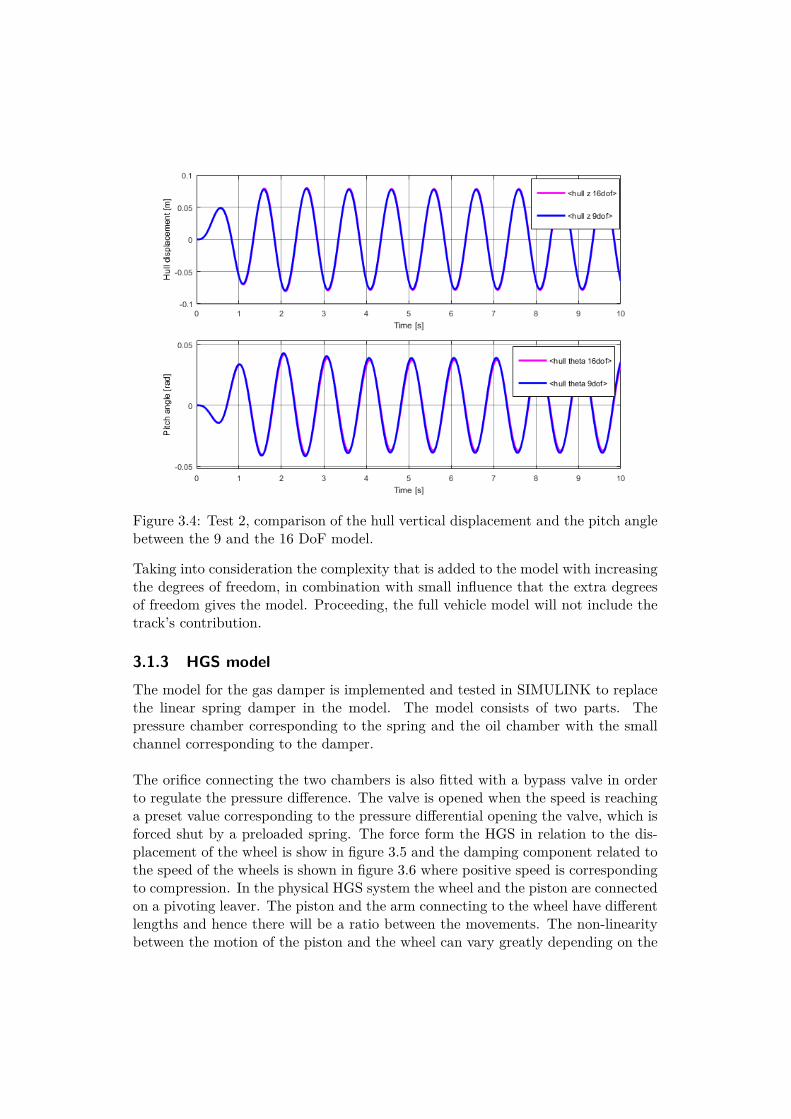
Figure 3.4: Test 2, comparison of the hull vertical displacement and the pitch anglebetween the 9 and the 16 DoF model.

Taking into consideration the complexity that is added to the model with increasingthe degrees of freedom, in combination with small influence that the extra degreesof freedom gives the model. Proceeding, the full vehicle model will not include thetrack’s contribution.

3.1.3 HGS modelThe model for the gas damper is implemented and tested in SIMULINK to replacethe linear spring damper in the model. The model consists of two parts. Thepressure chamber corresponding to the spring and the oil chamber with the smallchannel corresponding to the damper.

The orifice connecting the two chambers is also fitted with a bypass valve in orderto regulate the pressure difference. The valve is opened when the speed is reachinga preset value corresponding to the pressure differential opening the valve, which isforced shut by a preloaded spring. The force form the HGS in relation to the dis-placement of the wheel is show in figure 3.5 and the damping component related tothe speed of the wheels is shown in figure 3.6 where positive speed is correspondingto compression. In the physical HGS system the wheel and the piston are connectedon a pivoting leaver. The piston and the arm connecting to the wheel have differentlengths and hence there will be a ratio between the movements. The non-linearitybetween the motion of the piston and the wheel can vary greatly depending on the

geometry of the HGS system. Attempting to keep the model as simple as possibleas well as the lack of data to confirm the model against, the relation between thepiston and wheel was set to a constant value of 0.2 corresponding to having thewheels rotating on a leaver of 750 mm length and the piston on a leaver of 150 mm.The arm lengths of 500 mm and 137 mm is seen in [8] and [10] corresponding to aratio of 0.25 but as the geometric relation will give a reduction in force the slightlysmaller ratio selected.

Figure 3.5: Spring force in relation to wheel displacement.

Two models of the dampers are implemented. The first model seen in figure 3.6 isbased on an increase of the area that the fluid can flow through after a set value.The area will increase linearly in relation to the speed of the piston up to a setmaximum combined opening of the canal.

Figure 3.6: Damping force in relation to wheel speed.

As can be seen in figure 3.6 the bypass valve is opening on the compression andrebound stroke taking down the force from the damper by increasing the area thatthe oil can flow through.

The second model of the damper is based on the same force build-up in the lowspeed region. The high speed on the other hand is set to be linear in relation to thepiston speed. The result of the linearised damper can be seen in figure 3.7

Figure 3.7: Damper model with linearised high speed compared to the originalmodel.

3.2 Full vehicle modelThe half car model is expanded to a full vehicle model in order to accommodate moredegrees of freedom of the tank and give a more complete picture of the movement.The second pair of wheels are added and with this the roll axle is also introduced.The second pair of tracks is given its own road profile input that can be given atime delay. This gives the possibility to have the tracks se the same road profile andhence little to no roll should be present, or have the tracks experience completelydifferent profiles depending on what kind of excitation one want to test. The tankhas the same placement of the wheels in longitudinal direction and the respectivewheel-set are located 1.525 m from the CoG. The additional data used for the fullvehicle model can be seen in table 3.3

Table 3.3: Full vehicle model parameters.

m 53370 kgmt 875 kgml 285 kgJyy 200130 kg m2

Jxx 224093 kg m2

kd 280 kN m−1

cd 39.2 kN s m−1

kt 613 kN m−1

ct 0 kN s m−1

The HGS dampers are introduced into a separate model and replace the linearsprings and dampers. The equations of motion change as can be seen in equations3.2 to 3.4 due to the fact that the force now comes from the HGS unit.

mz = −∑

FHGS (3.2)

Jyyϕ = −∑

FHGS(xiϕ) (3.3)

Jxxγ = −∑

FHGS(yiγ) (3.4)

Where FHGS is the reacting force from the HGS unit.

The value for the precharged pressure was set according to commonly used pres-sured of either 11.4 MPa or 13 MPa [10]. The volume for the nitrogen chamber ispreferably as small as possible. There are some physical constraint that needs to betaken into consideration that the model might not take into account. The volumeof the nitrogen pressure chamber is in relation to the piston position and it’s area(see equation 2.20), hence the volume need to be large enough such that the volumecan not be less than or equal to zero as a result of the movement of any wheel. Alsothe area of the orifice needs to be significantly smaller than the area of the piston.

Simulations were made for different combinations of areas and volume with lowfrequency and high displacement of the wheels as well as the opposite in order toverify that the force from the HGS model was producing combinations of force inrelation to speed and distance. The resulting parameters used for the HGS modelcan be seen in table 3.4.

Table 3.4: HGS parameters.

P0 11.4 MPaV0 30.4 · 10−5 m3

Ap 1.3 · 10−3 m2

A0 2.8 · 10−6 m2

ρ 850 kg m−3

Cd 0.73n 1.35

The combined damper unit was simulated with a periodic ground excitation using atwo frequencies of 0.1 and 1 hertz and increasing amplitudes between 0.1 and 0.45 min order to make sure that the simulation would produce creditable resulting forcesas can be seen in figure 3.8 and 3.9. The behaviour from the 0.1 hertz test in figure3.8 is corresponding with what is to be expected from the HGS unit. With the lowfrequency excitation of the ground, the force is dominated by the gas spring with asmall contribution from the damper giving the exponential behaviour of the forcein relation to distance. The force in relation to speed seems reasonable with peakforce at maximum force at where the damper goes from compression to rebound i.e.at zero speed. The behaviour in the 1 hertz ground excitation seen in figure 3.9,shows the same behaviour as the 0.1 hertz but more force from the damper presentdue to the higher ground disturbance speed. The force in relation to speed have aslight tilt as to be expected with the larger contribution of force from the damper’swith the behaviour seen in 3.6.

Figure 3.8: HGS-unit force in relation to speed and distance for 0.1 Hz sinusoidalexcitation with amplitudes between 0.1 and 0.45 m from equilibrium position.

Figure 3.9: HGS-unit force in relation to speed and distance for 1 Hz sinusoidalexcitation with amplitudes between 0.1 and 0.45 m from equilibrium position.

3.3 Firing sequence implementationThe force from the recoil is calculated and implemented into the SIMULINK model.The force is set to act on the attachment point where the barrel pivots. The imple-mentation of the force from the recoil can be seen in figure 3.10. The recoil force iscalculated using data from a kinetic energy penetrator round fired from a 120 mmcannon and the time that the impulse is active for is set to 70 ms corresponding tothe average impulse duration of the example ammunition seen in table 2.1.

Figure 3.10: The force from the recoil acting on the barrel attachment-point.

A visual representation of the implementation can be seen in figure 3.11.

Figure 3.11: Visual representation of the recoil acting-point.

The implementation is tested on the linear half vehicle model. Assuming the cannonis oriented straight forward the contribution from the recoil will exclusivity affectthe pitch axis of the tank and therefore the pitch axis is observed. The pitch axis willalso be the main contributor to the firing accuracy as most of the cases when drivingthe pitch axis will have the largest deviations in movement. The pitch accelerationand angle can be seen in figure 3.12. As can be seen the impulse from the forceof the recoil gives a high acceleration impulse in pitch, which decays quickly. Thepitch angle is relatively small as can be expected because even though the forceis very high the time the force is acting on the hull is low and hence the totalenergy transferred is low. Also the leaver arm that the force from the recoil hascorresponding to the distance between the attachment point of the barrel and theCoG of the tank is not very large. This means that the large force that is produceddoes not give as large of a torque rotating the hull.

Figure 3.12: The hull pitch angle and pitch acceleration due to firing of the cannon.

Chapter 4

Results and analysis

In this chapter the results from the modelling are presented. The different modelsare compared to each other and the results from running the simulated tank. Theinfluence of the recoil while driving is investigated and the performance gains fromintroducing the HGS system are analysed. Also the possibility to simplify the HGSmodel is investigated. Lastly the relation between the movement of the tank andit’s line of sight is analysed.

4.1 Model comparisonThree standard scenarios are tested on the tank as follows.

• test 1: 100 mm step,• test 2: 60 mm 1 Hz sinusoidal road excitation,• test 3: vibration course.

All the above mentioned scenarios where simulated for multiple speeds. The speedshown in all the following figures 4.1 to 4.7b are 40 km h−1. A small time delayof 0.1 s was added on the left set of tracks in order to excite roll behaviour. Fireaccuracy was only observed on the vibration course.

4.1.1 Damper model performance comparisonThe fist test of 100 mm step was simulated with three models tested: The linearmodel, the full HGS system and a simplified HGS model where the high speedcompression and rebound force was set to a linear behaviour. The result of thesimulations can be seen in figures 4.1 to 4.6.

39

Figure 4.1: Comparison of the vertical deviation for test 1 between the linear modeland the 2 HGS models.

Figure 4.2: Comparison of the pitch angle for test 1 between the linear model andthe 2 HGS models.

As can be seen from the peaks are lower in both of the pneumatic models comparedto the linear model both in bounce and pitch. A somewhat over-damped behaviouris also seen in the HGS system especially the linearized version as the overshootof the step is more or less absent. Test 2 can be seen in the following figures 4.3

to 4.4 showing the pitch angle and the vertical deviation for the periodic groundirregularity. An improvement in both vertical deviation and pitch angle can be seenfor the HGS models in comparison to the linear model.



Last, test 3, the vibration course can be seen in the following figures 4.5 to 4.6. Inorder to evaluate the impact that the recoil has on the tank the simulation is setto fire at 7,5 s as at this point the tank is on its way up one of the larger obstacles.The results are showing that in comparison to the other obstacles of the same sizeno major change in either pitch nor bounce can be observed. This indicates that

the suspension is handling the recoil very well since the firing of the cannon is notaffecting the hull in any significant way.



Another thing that can be observed from the vibration course is that the linearizedHGS model deviates from the non-linearized HGS model during high frequencymovement of the wheels but not during low frequency movement to the same degree.This is to be expected as the force produced from the HGS models deviates fromeach other in the higher speeds hence the observed outcome.

4.1.2 Firing accuracyTranslating the movement from the hull of the tank to the aim-point displacementis of interest. It will give an indication on what performance requirements that thecontrol system for the barrel and turret will need to achieve.

The aim-point displacement is simulated both for the linear model as well as theHGS model in order to be able to compare the influence of the different dampercharacteristic on the deviation at the target. As the information from the test isto translate into performance requirements of the control system the test scenarioused for generating the aim-point displacement is the vibration track. The reasonfor this is that the vibration track includes a wide variety of frequencies similar tothe regular operation of the vehicle.

The model is given a small variation between the two tracks in order to excitesome roll behaviour as well. The aim-point displacement for the linear model canbe seen in figure 4.7a. The HGS model of the full vehicle is given the same inputfor the tracks. The aim-point displacement can be seen in figure 4.7b.

(a) The aim-point displacement of the linearmodel.

(b) The aim-point displacement of the HGSmodel.

Figure 4.7: Aim-point displacement.

Observing the behaviour of the aim-point displacement of the tank it can be seenthat the HGS system has a more composed behaviour compared to the linear modeland more of the time is spent in the area of 10 by 10 meters from the centre point,in figure 4.7b shown as 0 m in x and 0 m in y. To draw conclusions from the be-haviour of the aim-point displacement one could assume that the more composedbehaviour of the HGS would indicate that a less advanced control system would beneeded or less effort for a given control-system to control the barrel of the tank asthe movement is more predictable.

Looking at the overall behaviour of the different models we se that using a non-lineardamper model gives benefits in terms of performance. The peaks i.e. maximum dis-

tance from centre are in general lower which is desirable. Especially in the pitchaxis the improvements are more noticeable with the peaks almost 15 m lower thanthe linear model, which is a great improvement.

The reason for the right leaning bias of the results are due to the left tracks alwaysbeing small amount before the right tracks and hence the excitation of roll is morebiased to the right.

The linearized HGS model is showing promising results. Observing the pitch axis infigure 4.6 one can see a very similar results between the HGS models and only thepeaks differ a small amount. The major difference between the full HGS model andthe linearized model can be seen in bounce at very high frequency ground excita-tion. This would most likely not be a very common occurrence for the real systemand hence the simplified model can be used in most situations. The advantage ofthe linearized model is that adjustments to the linear part of the damper is verysimple to set whereas the full model needs understanding on how the orifice andbleed valve opening changes the behaviour of the damper.

Chapter 5

Conclusions and future work

In this chapter the conclusions of the work are discussed. What the limiting factorsare and what improvements can be made in order to further develop the model.

5.1 Conclusions and discussionIn order to gain understanding of the dynamic behaviour of a MBT two half-vehiclemodels with different DoF and three full-vehicle models with different suspensionsystems where developed in MATLAB/SIMULINK. The models are all based on theequations of motion describing the dynamics of the system. Through the dynamicsof the tank the motion is then connected to the barrel in order to investigate the fireprecision of the tank. In order to evaluate the performance three different modelsfor dampers are developed and compared to see the influence the suspension systemhas on the entire tank.

From the half-vehicle models can it be observed that adding more degrees of free-dom corresponding to the tracks does not significantly change the behaviour of thehull for the preset conditions. The linear model is used as a representation for lastgeneration of tanks fitted with torsion-bar suspension and dampers on a select fewwheels. Although the linear model will not perfectly represent the last generation oftanks as the torsion bar is not completely linear in its behaviour it is only used as areference of comparison. Also some damping will be present in the torsion bar butit will in comparison to the stiffness be low and hence is neglected. The HGS systemcommonly seen on modern tanks can be observed to have increased performancewith lower average disturbance in all axes compared to the linear model.

Comparing the aim-point displacement of the tank with the different damper config-urations significant changes in behaviour are observed. The behaviour of the linearsystem is showing a larger spread in aim-point. Where the pneumatic system onthe other hand does still have the same tendencies but the spread is more composedin nature.

45

The results can be separated into two different parts. The first part is how thedifferent suspension systems affects the performance of the tank. This is the aimaccuracy of the tank which is the main focus of this thesis. The results are measuringthe performance of the tank and will be used to determine minimum performancerequirements of the control system for the barrel stabilization.

The next part, which is equally as important, is the transmission of vibrationsto the crew of the tank, which is not investigated in this thesis. This is a subjectthat include the question of how long the crew can withstand operating the tank.Minimizing the transmission of vibrations is of great importance as to not make thecrew motion sick or having the crew experience fatigue due to the operation of thetank to name a few examples.

The parameters for both the linear and the non-linear models are produced bycomparison to models of other tracked vehicles and simulations of multiple settings.Both models are passive suspension and none of these are in any way optimized.This means that the result of the simulations are in no way optimal and couldpossibly be either better or worse than the real vehicle.

5.2 LimitationsThe main limitation of the model is that it is not verified against the tank thatis modelled. This fact makes the results of the tank model estimates. It is there-fore uncertain how accurately the tank model correlates to the actual system. Themodel can be used comparatively to see tendencies of how changes to the tank de-sign or environment will affect the tank but it is only an estimate and should notbe considered as equal to the real system.

The model is assuming a few things regarding the world. The first one regard-ing the ground of which the tank is running. Assuming that the ground is infinitelystiff will give a good indication of the dynamics of the tank but the tank will mostlikely never run in such conditions. This would mean that the tank would receivesome damping from the ground and hence the motion would be smother than whatthe model would indicate. Also the model is feed the terrain profile but can notsay anything about the tanks ability to overcome the terrain at all. This wouldmodelling of the contact between the surface and the tank tracks and also wouldneed to have information about the ground of, which the tank is moving on.

Further, the model is an idealized model. There are many parts that could betaken into consideration if one is trying to model the tank as accurately as possible.To name a few of the main areas that will add to the dynamics: more contributingvibration sources, structural dynamics, terramechanics, viscous and flow properties,

and changes due to external influences such as climate, wear and more.

5.3 Future workThe models produced is a relatively simple model and has many areas that couldbe improved on to better represent the tank as a complete system if that is whatis desired. The most important thing that the model needs is verification. All theparameters the model is based on are chosen to the best knowledge and ability, butcan not confirm or accurately represent the movement with any certainty of thetank if not verified and tuned according to the real system. Other parts that couldhelp improve are if data became available for subsystems such as dampers.

Further, the only part that excites movement is the road profile. The real tank hasmore sources of vibrations that could introduce movement or disturbances. Thereare many parts that can be of interest to add in order to evaluate if the contributionaffects the motion of the tank. This could include, for instance an extended modelof the tracks. The tracks themselves have both the loaded part in contact with theground as well as the unloaded parts above the wheels. The section of unloadedtracks could very possibly induce vibrations as the mass of the tracks is quite largeand in the unloaded state can most certainly come into eigen-frequency if underthe right circumstances. Further, the tanks engine is a big vibration source. Theengine can both come in to eigen-frequencies with the drive-train and also inducedisturbances for the control system of the turret.

The HGS also introduces the possibility to add a control system to further increasethe performance. Controlling the pressure in real time to minimize the accelerationof the hull could be a interesting area to investigate. There are some differentapproaches that might be considered. The model produced has the same pressureon all the HGS units so it would be interesting to investigate if there would be aperformance gain to give individual units different pressures i.e. varying the springstiffness across the length of the tank. Depending on how the unit is constructedif there is possibility to control in real time both the pressure of the spring as wellas the damping with control of the bypass valves restriction of flow in the damper.There are different ways of approaching the minimization of the disturbance seenby the hull, some simpler and some more advanced. Depending on the constructionand possibilities the given system will bring to the table it could be interesting tose how large of a decrease in vibrations that could be realistically implemented.Last, there are some simplifications done to the model but it could most probablybe further simplified. A part could be to see how many of the wheel pairs thatare needed and how the model is impacted by reducing the contact points with theground.

Bibliography

[1] P. Bull L. Back J. Eklund K. Heilert H. Liwang P. Stensson C-G. Svantesson N.Bruzelius, editor. Larobok i Militarteknik. Forsvarshogskolan, Stockholm, 2010.

[2] S. Kciuk A. Mezyk. Modelling of tracked vehicle dynamics. Journal of KONESPowertrain and Transport, 17(1):223–232, 2010.

[3] J.Y Wong, editor. Theory of ground vehicles. Wiley, New York, 2001.

[4] H.A. Hammad A.M. Salem I. Mostafa I.A. Elsherifo. Modeling of hydrogas unitfor tracked vehicle suspension. International Conference on Aerospace Sciencesand Aviation Technology, 16(9):1–12, 2015.

[5] S. Cornak M. Sojka. Mathematical model of suspension of tracked vehicles.2017 International Conference on Military Technologies (ICMT), pages 111–114, 2017.

[6] C. Padmanabhan I. Mahalingam. Planar multi-body dynamics of a trackedvehicle using imaginary wheel model for tracks. Defence Science Journal,67(4):460–464, 2017.

[7] K.M. Paplinski. Mathematical model of the main battle tank with stabilizedturret and gun. Journal of KONES Powertrain and Transport, 16(1):387–395,2009.

[8] C. Padmanabhan U. Solomon. Hydro-gas suspension system for a trackedvehicle: Modeling and analysis. Journal of Terramechanics, 48:125–137, 2011.

[9] J.Y. Wong. Dynamics of tracked vehicles. Vehicle System Dynamics, 28(2-3):197–219, 1997.

[10] R. Krishnakumar S. Banerjee, V. Balamurugan. Ride dynamics mathemat-ical model for a single station representation of tracked vehicle. Journal ofTerramechanics, 53:47–58, 2014.

[11] M. Oscarsson. A hydropneumatic suspension parameter study on heavy multi-axle vehicle handling. Master’s thesis, KTH Royal Institute of Technology,2015.

49

[12] Wikipedia. Orifice plate. https://en.wikipedia.org/wiki/Orifice_plate,2021. [Online; accessed 20-July-2021].

[13] W. Borkowski J. Figurski J. Walentynowicz Z. Hryciow. The impact of the can-non on the combat vehicle chasis during firing. Journal of KONES Powertrainand Transport, 14(1):49–61, 2007.

[14] P. Rybak A. Wisniewski, Z. Hryciow. Numerical investigation of dynamic loadsof vehicle hull during firing. AIP Conference Proceedings, 2078:020064, 2019.

[15] M. Gullerova J. Tvarozek. Increasing firing accuracy of 2a46 tank cannonbuilt-in t-72 mbt. American International Journal of Contemporary Research,2(9):140–156, 2012.

https://en.wikipedia.org/wiki/Orifice_plate

TRITA -SCI-GRU 2021:286

www.kth.se

Documents

System modelling and evaluation of main battle tank fire