Embed Size (px)
Citation preview

SystemC Analog/Mixed-Signal User’s Guide
User Perspective on IEEE Std. 1666.1-2016
Accellera SystemC AMS Working Group
January 2020
Copyright © 2020 Accellera Systems Initiative. All rights reserved.Accellera Systems Initiative, 8698 Elk Grove Blvd. Suite 1, #114, Elk Grove, CA 95624, USA

Notices
Accellera Systems Initiative Standards documents are developed within Accellera Systems Initiative(Accellera) and its Technical Committee. Accellera develops its standards through a consensus developmentprocess, approved by its members and board of directors, which brings together volunteers representing variedviewpoints and interests to achieve the final product. Volunteers are not necessarily members of Accellera andserve without compensation. While Accellera administers the process and establishes rules to promote fairnessin the consensus development process, Accellera does not independently evaluate, test, or verify the accuracyof any of the information contained in its standards.
Use of an Accellera Standard is wholly voluntary. Accellera disclaims liability for any personal injury, propertyor other damage, of any nature whatsoever, whether special, indirect, consequential, or compensatory, directlyor indirectly resulting from the publication, use of, or reliance upon this, or any other Accellera Standarddocument.
Accellera does not warrant or represent the accuracy or content of the material contained herein, and expresslydisclaims any express or implied warranty, including any implied warranty of merchantability or suitability fora specific purpose, or that the use of the material contained herein is free from patent infringement. AccelleraStandards documents are supplied “AS IS.”
The existence of an Accellera Standard does not imply that there are no other ways to produce, test,measure, purchase, market, or provide other goods and services related to the scope of an Accellera Standard.Furthermore, the viewpoint expressed at the time a standard is approved and issued is subject to change dueto developments in the state of the art and comments received from users of the standard. Every AccelleraStandard is subjected to review periodically for revision and update. Users are cautioned to check to determinethat they have the latest edition of any Accellera Standard.
In publishing and making this document available, Accellera is not suggesting or rendering professional orother services for, or on behalf of, any person or entity. Nor is Accellera undertaking to perform any dutyowed by any other person or entity to another. Any person utilizing this, and any other Accellera Standardsdocument, should rely upon the advice of a competent professional in determining the exercise of reasonablecare in any given circumstances.
Interpretations: Occasionally questions may arise regarding the meaning of portions of standards as they relateto specific applications. When the need for interpretations is brought to the attention of Accellera, Accellera willinitiate reasonable action to prepare appropriate responses. Since Accellera Standards represent a consensusof concerned interests, it is important to ensure that any interpretation has also received the concurrence ofa balance of interests. For this reason, Accellera and the members of its Technical Committee and WorkingGroups are not able to provide an instant response to interpretation requests except in those cases where thematter has previously received formal consideration.
Comments for revision of Accellera Standards are welcome from any interested party, regardless ofmembership affiliation with Accellera. Suggestions for changes in documents should be in the form of aproposed change of text, together with appropriate supporting comments. Comments on standards and requestsfor interpretations should be addressed to:
Accellera Systems Initiative 8698 Elk Grove Blvd. Suite 1, #114 Elk Grove, CA 95624 USA
Note: Attention is called to the possibility that implementation of this standard may require use of subject mattercovered by patent rights. By publication of this standard, no position is taken with respect to the existence orvalidity of any patent rights in connection therewith. Accellera shall not be responsible for identifying patents
iiCopyright © 2020 Accellera Systems Initiative. All rights reserved.

for which a license may be required by an Accellera Standard or for conducting inquiries into the legal validityor scope of those patents that are brought to its attention.
Accellera is the sole entity that may authorize the use of Accellera-owned certification marks and/or trademarksto indicate compliance with the materials set forth herein.
Authorization to photocopy portions of any individual standard for internal or personal use must be grantedby Accellera, provided that permission is obtained from and any required fee, if any, is paid to Accellera.Permission to photocopy portions of any individual standard for educational classroom use can also be obtainedfrom Accellera. To arrange for authorization please contact Lynn Garibaldi, Executive Director, AccelleraSystems Initiative, 8698 Elk Grove Blvd. Suite 1, #114, Elk Grove, CA 95624, phone (916) 760-1056, [email protected].
Suggestions for improvements to the SystemC AMS User’s Guide are welcome. They can be sent to theAccellera SystemC AMS forum:
https://forums.accellera.org/forum/13-systemc-ams-analogmixed-signal/
The current Accellera SystemC AMS Working Group web page is:
https://accellera.org/activities/working-groups/systemc-ams
iiiCopyright © 2020 Accellera Systems Initiative. All rights reserved.

Contributors
The following people contributed to the creation of this user’s guide:
Sumit Adhikari, NXP SemiconductorsMartin Barnasconi, NXP SemiconductorsMarkus Damm, Fraunhofer IESEKarsten Einwich, COSEDA TechnologiesPaul FloydDaniela Genius, Sorbonne Université, CNRS, LIP6Christoph Grimm, Technische Universität KaiserslauternMarie-Minerve Louërat, Sorbonne Université, CNRS, LIP6Torsten Maehne, Bern University of Applied SciencesFrançois Pecheux, Sorbonne Université, CNRS, LIP6Alain Vachoux, Ecole Polytechnique Fédérale de Lausanne (EPFL)
ivCopyright © 2020 Accellera Systems Initiative. All rights reserved.

Preface
This user’s guide is meant as an introductory guide for electronic system-level engineers and architects whowould like to use the SystemC™1 analog/mixed-signal (AMS) extensions for their system-level design andverification tasks. The main aim is to provide a self-learning guide on how to use the SystemC AMS extensionsby explaining the modeling fundamentals and giving examples on how to start with AMS system-level designat higher levels of abstraction. It assumes that the user has some prior knowledge on SystemC modeling andsimulation and C++ in general and is familiar with analog/mixed-signal design and modeling.
After going through this guide, the reader should be in a position to start using the SystemC AMS extensions,and should be able to:
— Get insight into the applicable use cases and requirements of the SystemC AMS extensions.— Understand the introduced models of computation and associated execution semantics.— Use the language constructs to create discrete-time and continuous-time models at different levels of
abstraction.— Combine SystemC and the AMS extensions to design a mixed-signal system.— Perform time- and frequency-domain analysis and tracing of AMS signals.
The AMS design methodology, modeling style, and examples given in this user’s guide are based on IEEEStd. 1666™-20112,3, IEEE Std. 1666.1™-2016 and the C++ programming language defined in ISO/IEC14882:20034. Any simulator implementation compatible with this standard can be used to build and executethese examples5.
This document is an informative guide, intended to clarify the usage and intended behavior of the SystemCAMS extensions. The precise and complete definition of the SystemC AMS extensions is standardized in IEEEStd. 1666.1™-2016.
1 SystemC™ is a registered trademark of the Accellera Systems Initiative.2 The IEEE standards or products referred to in this user’s guide are trademarks of The Institute of Electrical and Electronics Engineers,
Inc.3 IEEE publications are available from the Institute of Electrical and Electronics Engineers, Inc., 445 Hoes Lane, P.O. Box 1331,
Piscataway, NJ 08855-1331, USA (https://standards.ieee.org/).4 ISO/IEC publications are available from the ISO Central Secretariat, Case Postale 56, 1 rue de Varembé, CH-1211, Genève 20,
Switzerland/Suisse (https://www.iso.org/). ISO/IEC publications are also available in the United States from Global EngineeringDocuments, 15 Inverness Way East, Englewood, Colorado 80112, USA (https://global.ihs.com/). Electronic copies are available in theUnited States from the American National Standards Institute, 25 West 43rd Street, 4th Floor, New York, NY 10036, USA (https://www.ansi.org/).
5 More information on simulation environments can be found at https://www.accellera.org/community/systemc/about-systemc-ams/.
vCopyright © 2020 Accellera Systems Initiative. All rights reserved.

Contents
1. Introduction............................................................................................................................................. 1
1.1 Motivation....................................................................................................................................11.2 SystemC AMS extensions...........................................................................................................1
1.2.1 Use cases and requirements............................................................................................. 21.2.2 Model abstractions........................................................................................................... 31.2.3 Modeling formalisms....................................................................................................... 41.2.4 Time-domain and frequency-domain analysis................................................................. 41.2.5 Language architecture...................................................................................................... 5
2. Timed Data Flow modeling....................................................................................................................6
2.1 Modeling fundamentals............................................................................................................... 62.1.1 TDF module and port attributes.......................................................................................62.1.2 Static and dynamic modes of operation...........................................................................72.1.3 TDF model topologies......................................................................................................92.1.4 Time step assignment and propagation..........................................................................122.1.5 Multiple schedules or clusters........................................................................................142.1.6 Signal processing behavior of TDF models...................................................................15
2.2 Language constructs.................................................................................................................. 162.2.1 TDF modules.................................................................................................................. 162.2.2 TDF ports........................................................................................................................202.2.3 TDF signals.................................................................................................................... 26
2.3 Modeling discrete-time and continuous-time behavior.............................................................262.3.1 Discrete-time modeling.................................................................................................. 262.3.2 Continuous-time modeling............................................................................................. 272.3.3 Structural composition of TDF modules........................................................................332.3.4 Multirate behavior.......................................................................................................... 352.3.5 Introducing delays.......................................................................................................... 36
2.4 Interaction between TDF and discrete-event domain............................................................... 372.4.1 Reading from the discrete-event domain....................................................................... 372.4.2 Writing to the discrete-event domain.............................................................................392.4.3 Using discrete-event control signals.............................................................................. 40
2.5 TDF execution semantics.......................................................................................................... 42
3. Linear Signal Flow modeling...............................................................................................................44
3.1 Modeling fundamentals............................................................................................................. 443.1.1 Setup of the LSF equation system.................................................................................443.1.2 Time step assignment and propagation..........................................................................45
3.2 Language constructs.................................................................................................................. 453.2.1 LSF modules...................................................................................................................45
viCopyright © 2020 Accellera Systems Initiative. All rights reserved.

3.2.2 LSF ports........................................................................................................................ 473.2.3 LSF signals..................................................................................................................... 47
3.3 Modeling continuous-time behavior......................................................................................... 483.3.1 Structural composition of LSF modules........................................................................ 483.3.2 Continuous-time modeling............................................................................................. 49
3.4 Interaction between LSF and discrete-event or TDF models................................................... 503.4.1 Reading from and writing to discrete-event models......................................................513.4.2 Reading from and writing to TDF models.................................................................... 513.4.3 Using discrete-event or TDF control signals.................................................................523.4.4 LSF model encapsulation...............................................................................................53
3.5 LSF execution semantics...........................................................................................................54
4. Electrical Linear Networks modeling...................................................................................................56
4.1 Modeling fundamentals............................................................................................................. 564.1.1 Setup of the equation system.........................................................................................564.1.2 Time step assignment and propagation..........................................................................57
4.2 Language constructs.................................................................................................................. 574.2.1 ELN modules.................................................................................................................. 574.2.2 ELN terminals.................................................................................................................594.2.3 ELN nodes...................................................................................................................... 59
4.3 Modeling continuous-time behavior......................................................................................... 604.3.1 Structural composition of ELN modules....................................................................... 604.3.2 Continuous-time modeling............................................................................................. 61
4.4 Interaction between ELN and discrete-event or TDF models...................................................624.4.1 Reading from and writing to discrete-event models......................................................624.4.2 Reading from and writing to TDF models.................................................................... 634.4.3 ELN model encapsulation in TDF models.................................................................... 654.4.4 Non-linear modeling using TDF encapsulation in ELN................................................66
4.5 ELN execution semantics.......................................................................................................... 68
5. Small-signal frequency-domain analyses............................................................................................. 70
5.1 Modeling fundamentals............................................................................................................. 705.1.1 Setup of the equation system.........................................................................................705.1.2 Analysis methods........................................................................................................... 71
5.2 Language constructs.................................................................................................................. 715.2.1 Small-signal frequency-domain description in TDF modules....................................... 715.2.2 Port access...................................................................................................................... 72
5.3 Utility functions.........................................................................................................................725.3.1 Frequency-domain delay................................................................................................ 725.3.2 Laplace transfer functions.............................................................................................. 735.3.3 S-domain definitions...................................................................................................... 735.3.4 Z-domain definitions...................................................................................................... 75
viiCopyright © 2020 Accellera Systems Initiative. All rights reserved.

5.3.5 Detection of small-signal frequency-domain analyses.................................................. 765.4 Small-signal frequency-domain analysis with combined TDF, LSF and ELN models.............76
6. Simulation and tracing..........................................................................................................................78
6.1 Simulation control..................................................................................................................... 786.1.1 Time-domain simulation.................................................................................................786.1.2 Small-signal frequency-domain simulation....................................................................79
6.2 Tracing....................................................................................................................................... 806.2.1 Trace files and formats.................................................................................................. 806.2.2 Tracing signals and comments.......................................................................................82
6.3 Testbenches................................................................................................................................ 84
7. Application examples........................................................................................................................... 86
7.1 Binary Amplitude Shift Keying (BASK) example................................................................... 867.1.1 BASK modulator............................................................................................................867.1.2 BASK demodulator........................................................................................................ 887.1.3 TDF simulation of the BASK example......................................................................... 897.1.4 Interfacing the BASK example with SystemC.............................................................. 90
7.2 Proportional–Integral–Derivative (PID) controller example.....................................................927.3 Continuous-time Sigma-Delta (CTSD) modulator example..................................................... 947.4 Plain Old Telephone System (POTS) example.........................................................................957.5 Vibration sensor and sensor frontend example......................................................................... 987.6 DCDC converter example....................................................................................................... 105
8. Modeling strategies.............................................................................................................................113
8.1 Behavioral modeling using the available models of computation.......................................... 1138.1.1 Macromodeling with Electrical Linear Networks........................................................1148.1.2 Behavioral modeling with Linear Signal Flow............................................................1168.1.3 Behavioral and baseband modeling with Timed Data Flow........................................ 117
8.2 Modeling embedded analog/mixed-signal systems.................................................................1208.2.1 Partitioning behavior to different models of computation........................................... 1208.2.2 Modeling of architecture-level properties....................................................................122
8.3 Design refinement and mixed-level modeling........................................................................ 1238.3.1 Mixed-signal, mixed-level simulation..........................................................................1238.3.2 Design refinement and use cases................................................................................. 123
8.4 Modeling and coding style......................................................................................................1258.4.1 Namespaces.................................................................................................................. 1258.4.2 Dynamic memory allocation........................................................................................ 1278.4.3 Module parameters....................................................................................................... 1288.4.4 Separation of module definition and implementation..................................................1308.4.5 Class templates............................................................................................................. 131
viiiCopyright © 2020 Accellera Systems Initiative. All rights reserved.

8.4.6 Public and private class members................................................................................132
Annex A Language reference........................................................................................................................134
A.1 TDF modules........................................................................................................................... 134A.2 TDF ports.................................................................................................................................135A.3 TDF signals..............................................................................................................................136A.4 Embedded Laplace transfer functions.....................................................................................136
A.4.1 sca_tdf::sca_ltf_nd........................................................................................................ 136A.4.2 sca_tdf::sca_ltf_zp........................................................................................................ 136A.4.3 sca_tdf::sca_ss.............................................................................................................. 137
A.5 LSF primitive modules............................................................................................................138A.5.1 sca_lsf::sca_add............................................................................................................ 138A.5.2 sca_lsf::sca_sub............................................................................................................ 139A.5.3 sca_lsf::sca_gain........................................................................................................... 139A.5.4 sca_lsf::sca_dot.............................................................................................................140A.5.5 sca_lsf::sca_integ.......................................................................................................... 141A.5.6 sca_lsf::sca_delay......................................................................................................... 141A.5.7 sca_lsf::sca_source........................................................................................................142A.5.8 sca_lsf::sca_ltf_nd........................................................................................................ 144A.5.9 sca_lsf::sca_ltf_zp.........................................................................................................144A.5.10sca_lsf::sca_ss...............................................................................................................145A.5.11sca_lsf::sca_tdf::sca_gain, sca_lsf::sca_tdf_gain......................................................... 146A.5.12sca_lsf::sca_tdf::sca_source, sca_lsf::sca_tdf_source.................................................. 147A.5.13sca_lsf::sca_tdf::sca_sink, sca_lsf::sca_tdf_sink..........................................................148A.5.14sca_lsf::sca_tdf::sca_mux, sca_lsf::sca_tdf_mux......................................................... 148A.5.15sca_lsf::sca_tdf::sca_demux, sca_lsf::sca_tdf_demux................................................. 149A.5.16sca_lsf::sca_de::sca_gain, sca_lsf::sca_de_gain...........................................................150A.5.17sca_lsf::sca_de::sca_source, sca_lsf::sca_de_source....................................................151A.5.18sca_lsf::sca_de::sca_sink, sca_lsf::sca_de_sink........................................................... 151A.5.19sca_lsf::sca_de::sca_mux, sca_lsf::sca_de_mux.......................................................... 152A.5.20sca_lsf::sca_de::sca_demux, sca_lsf::sca_de_demux...................................................153
A.6 ELN primitive modules...........................................................................................................154A.6.1 sca_eln::sca_r................................................................................................................154A.6.2 sca_eln::sca_c............................................................................................................... 154A.6.3 sca_eln::sca_l................................................................................................................ 155A.6.4 sca_eln::sca_vcvs..........................................................................................................156A.6.5 sca_eln::sca_vccs.......................................................................................................... 157A.6.6 sca_eln::sca_ccvs.......................................................................................................... 157A.6.7 sca_eln::sca_cccs.......................................................................................................... 158A.6.8 sca_eln::sca_nullor........................................................................................................159A.6.9 sca_eln::sca_gyrator......................................................................................................160A.6.10sca_eln::sca_ideal_transformer.....................................................................................160A.6.11sca_eln::sca_transmission_line.....................................................................................161
ixCopyright © 2020 Accellera Systems Initiative. All rights reserved.

A.6.12sca_eln::sca_vsource.....................................................................................................162A.6.13sca_eln::sca_isource......................................................................................................163A.6.14sca_eln::sca_tdf::sca_r, sca_eln::sca_tdf_r...................................................................165A.6.15sca_eln::sca_tdf::sca_l, sca_eln::sca_tdf_l................................................................... 165A.6.16sca_eln::sca_tdf::sca_c, sca_eln::sca_tdf_c..................................................................166A.6.17sca_eln::sca_tdf::sca_rswitch, sca_eln::sca_tdf_rswitch..............................................167A.6.18sca_eln::sca_tdf::sca_vsource, sca_eln::sca_tdf_vsource.............................................168A.6.19sca_eln::sca_tdf::sca_isource, sca_eln::sca_tdf_isource.............................................. 169A.6.20sca_eln::sca_tdf::sca_vsink, sca_eln::sca_tdf_vsink.................................................... 170A.6.21sca_eln::sca_tdf::sca_isink, sca_eln::sca_tdf_isink......................................................170A.6.22sca_eln::sca_de::sca_r, sca_eln::sca_de_r.................................................................... 171A.6.23sca_eln::sca_de::sca_l, sca_eln::sca_de_l.................................................................... 172A.6.24sca_eln::sca_de::sca_c, sca_eln::sca_de_c................................................................... 173A.6.25sca_eln::sca_de::sca_rswitch, sca_eln::sca_de_rswitch............................................... 174A.6.26sca_eln::sca_de::sca_vsource, sca_eln::sca_de_vsource..............................................174A.6.27sca_eln::sca_de::sca_isource, sca_eln::sca_de_isource................................................175A.6.28sca_eln::sca_de::sca_vsink, sca_eln::sca_de_vsink..................................................... 176A.6.29sca_eln::sca_de::sca_isink, sca_eln::sca_de_isink....................................................... 177
Annex B Symbols and graphical representations..........................................................................................178
Annex C Glossary..........................................................................................................................................179
Index...............................................................................................................................................................181
xCopyright © 2020 Accellera Systems Initiative. All rights reserved.

1. Introduction
1.1 Motivation
There is a growing trend for tighter interaction between embedded hardware/software (HW/SW) systems andtheir analog physical environment. This leads to systems, in which digital HW/SW is functionally interwovenwith analog and mixed-signal blocks such as RF interfaces, power electronics, sensors, and actuators, as shownfor example by the communication system in Figure 1.1. Such systems are called Heterogeneous AMS/HW/SWsystems. Examples are cognitive radios, sensor networks or systems for image sensing. A challenge for thedevelopment of these heterogeneous systems is to understand the interaction between HW/SW and the analogand mixed-signal subsystems at the architectural level. This requires new means to model and simulate theinteracting analog/mixed-signal subsystems and HW/SW subsystems at the functional and architectural levels.
Figure 1.1—A Communication System, exampleof an heterogeneous AMS/HW/SW architecture
SystemC supports the refinement of HW/SW systems down to cycle-accurate behavior by providing a discrete-event simulation framework. A methodology for generalized modeling of communication and synchronizationbuilt upon this framework is also available: Transaction Level Modeling (TLM). It allows designers to performabstract modeling, simulation, and design of HW/SW system architectures. However, the SystemC simulationkernel has not been designed to handle the modeling and simulation of analog/continuous-time systems andlacks the support of a refinement methodology to describe analog behavior from a functional level down tothe implementation level.
In response to the needs from telecommunication, automotive, and semiconductor industries, AMS extensionsare introduced based on SystemC, to provide a uniform and standardized methodology for modelingheterogeneous AMS/HW/SW systems.
1.2 SystemC AMS extensions
The SystemC AMS extensions are built on top of the SystemC language standard IEEE Std. 1666-2011 anddefine additional language constructs, which introduce new execution semantics and system-level modelingmethodologies to design and verify mixed-signal systems.
The class definitions provided by the AMS language standard form the foundation for the creation of a C++class library implementation, which can be used in combination with an IEEE Std. 1666-2011 compatibleSystemC implementation. Such an implementation can be used to create AMS system-level models to build anexecutable specification, to validate and optimize the AMS system architecture, to explore various algorithms,and to provide the software development team with an operational virtual prototype of an entire AMS system,
1Copyright © 2020 Accellera Systems Initiative. All rights reserved.

SystemC Analog/Mixed-Signal User’s GuideUser Perspective on IEEE Std. 1666.1-2016
including also the analog functionality. To support these use cases, the SystemC AMS extensions define thenecessary modeling formalisms to model AMS system-level behavior at different levels of abstraction.
1.2.1 Use cases and requirements
As depicted in Figure 1.2, the SystemC AMS extensions can be used for a wide variety of use cases such as:— Executable specification;— Virtual prototyping;— Architecture exploration, and— Integration validation.
Figure 1.2—Use cases, model abstractions, and modeling formalisms
1.2.1.1 Executable specification
An executable specification is made to verify the correctness of the system requirement specification bycreating an executable description of the system by using simulation. For this use case, models at a high level ofabstraction are created, which do not necessarily need to relate to the physical architecture or implementationof the system. The models are, therefore, called functional or algorithmic models.
SystemC and the AMS extensions define both the system-level modeling language and their executionsemantics for simulation purposes. They are entirely implemented in the form of C++ libraries, which arelinked to the compiled AMS models to create an executable description of the system. This entirely C++-basedmodeling approach offers unique flexibility as it allows, e.g., the easy integration of embedded software, 3rdparty libraries, and legacy code into the system models.
1.2.1.2 Virtual prototyping
The virtual prototyping use case aims at providing software developers with a high-level untimed ortimed model, that represents the hardware architecture, and provides high simulation speed. Especially forHeterogeneous AMS + HW/SW systems, where software or firmware is interacting directly with AMShardware, interoperability using SystemC Transaction-Level Modeling (TLM) extensions is important.
2Copyright © 2020 Accellera Systems Initiative. All rights reserved.

SystemC Analog/Mixed-Signal User’s GuideUser Perspective on IEEE Std. 1666.1-2016
The usage of Timed Data Flow modeling for (over)sampled continuous-time and signal processing behaviorprovides high simulation speed with appropriate accuracy. In this way, the AMS subsystem can become partof the virtual prototype for further development of the HW/SW subsystem.
1.2.1.3 Architecture exploration
The architecture exploration use case will evaluate if and how the ideal functions and algorithms defined duringthe executable specification phase can be mapped onto the envisioned system architecture. The key propertiesof the system architecture are defined and should match with the actual functionality required.
Architecture exploration is structured in two phases: In the first phase, the executable specification is refinedby adding the non-ideal properties of an implementation to get a better understanding of their impact on theoverall system behavior. In the second phase, the architecture’s structure and interfaces are refined to get amore accurate model by introducing architectural elements and communication between these elements.
1.2.1.4 Integration validation
After the architecture definition and design of the analog and digital HW/SW components, these componentsare integrated and their correctness is verified within the overall system. For the integration validation usecase, the interfaces of all subsystems must be modeled accurately. The interfaces and data types used in themodels should match the physical implementation where applicable. For analog circuits this relates to electricalnodes. For digital circuits, this relates to pin accurate buses. For HW/SW systems, TLM interfaces might beappropriate.
1.2.2 Model abstractions
The SystemC AMS extensions add new abstraction methods for system-level modeling and simulationof AMS systems to the existing SystemC framework. The model abstractions supported by the SystemCAMS extensions are based on well-known methods for abstracting analog and mixed-signal behavior. Asshown in Figure 1.2, the abstraction levels distinguish discrete-time from continuous-time behavior and non-conservative from conservative descriptions. Chapter 8 will present the available abstraction methods in moredetail.
1.2.2.1 Discrete-time vs. continuous-time descriptions
Discrete-time modeling abstracts signals (e.g., audio or video streams) or physical quantities (e.g., voltages,currents, and forces) as sequences of values only defined at discrete time points. Values may be eitherreal values or discrete values (e.g., integer or logic values). Values between time points are formally notdefined, although it is common to consider them as constant. Behaviors are then abstracted as proceduralassignments involving sampled signals. The description of static (algebraic) non-linear behaviors (e.g., usingpolynomials) is supported. Discrete-time modeling is particularly suited for describing signal-processing-dominated behaviors, for which signals are naturally (over)sampled. It can be also used for describingcontinuous-time behaviors, provided that the discrete abstraction produces reasonable approximations.
Continuous-time modeling gets closer to the physical world, as signals and physical quantities are abstracted asreal-valued functions of time. The time is now considered as a continuous value. Behaviors are then describedusing mathematical equations that can include time-domain derivatives of any order (so-called differentialalgebraic equations (DAEs) or ordinary differential equations (ODEs)). Equations must be solved by usinga dedicated linear or non-linear solver, which usually requires complex numerical or symbolic algorithms.Continuous-time modeling is particularly suited for describing physical behaviors, as it can naturally accountfor dynamic effects.
3Copyright © 2020 Accellera Systems Initiative. All rights reserved.

SystemC Analog/Mixed-Signal User’s GuideUser Perspective on IEEE Std. 1666.1-2016
1.2.2.2 Non-conservative vs. conservative descriptions
Continuous-time models can be divided into two classes: non-conservative and conservative models.
Non-conservative models express behaviors as directed flows of continuous-time signals or quantities, onwhich processing functions such as filtering or integration are applied. Non-linear dynamic effects can beproperly described, but mutual effects and interactions between AMS blocks, such as impedances or loads,are not naturally supported.
Conservative models provide a formalism for satisfying the energy conservation laws as defined by Kirchhoff'slaws for the electrical domain.
1.2.3 Modeling formalisms
The SystemC AMS extensions define the essential modeling formalisms required to support AMS behavioralmodeling at different levels of abstraction. These modeling formalisms are implemented by using differentmodels of computation: Timed Data Flow (TDF), Linear Signal Flow (LSF), and Electrical Linear Networks(ELN).
1.2.3.1 Timed Data Flow (TDF)
The execution semantics based on TDF introduce discrete-time modeling and simulation without the overheadof the dynamic scheduling imposed by the discrete-event kernel of SystemC. Simulation is accelerated bydefining a static schedule for the connected TDF modules, forming a TDF cluster. This schedule defines theexecution order of the TDF modules’ processing member function according to the stream direction of thedataflow and the configured number of samples to be read from and written to each TDF port. The staticschedule is computed before simulation starts and may be modified at the end of the execution of the schedule.The sampled, discrete-time signals, which propagate through the TDF modules may represent any C++ type. If,e.g., a real-valued type such as double is used, the TDF signal can represent a voltage or current at a given pointin time. Complex values can be used to represent an equivalent baseband signal. TDF modeling is presentedin Chapter 2.
1.2.3.2 Linear Signal Flow (LSF)
The Linear Signal Flow formalism supports the modeling of continuous-time behavior by offering a consistentset of primitive modules such as addition, multiplication, integration, or delay. The LSF formalism permits thedescription of any linear DAE (Differential Algebraic Equation) system. An LSF model is made up from aconnection of such primitives through real-valued time-domain signals, representing any kind of continuous-time quantity. An LSF model defines a system of linear equations that is solved by a linear DAE solver. LSFmodeling is presented in Chapter 3.
1.2.3.3 Electrical Linear Networks (ELN)
Modeling of electrical networks is supported by instantiating predefined linear network primitives such asresistors or capacitors, which are used as macro models for describing the continuous-time relations betweenvoltages and currents. A restricted set of linear primitives and switches is available to model the electricalenergy conserving behavior. The provided ELN primitives permit also the description of any linear DAEsystem. ELN modeling is presented in Chapter 4.
1.2.4 Time-domain and frequency-domain analysis
The SystemC AMS extensions support both time-domain (transient) and small-signal frequency-domain (AC)analysis, by introducing new execution semantics and additional functions for simulation control.
4Copyright © 2020 Accellera Systems Initiative. All rights reserved.
SystemC Analog/Mixed-Signal User’s GuideUser Perspective on IEEE Std. 1666.1-2016
Time-domain simulation can be applied to descriptions made using the TDF, LSF, or ELN models ofcomputation. The analysis computes the time-domain behavior of the overall system, possibly composed bydifferent models of computation and could even include descriptions defined in the discrete-event domain. Theexecution semantics for time-domain simulation of TDF, LSF, and ELN models are described in Chapter 2,Chapter 3, and Chapter 4, respectively.
Frequency-domain simulation can be applied to the same descriptions, combining different models ofcomputation, where the analysis computes the small-signal frequency-domain behavior of the overallsystem. Besides small-signal frequency-domain analysis, small-signal frequency-domain noise analysis is alsoavailable. Chapter 5 will describe both analysis methods in more detail.
The simulation control and signal tracing techniques for time-domain and frequency-domain simulation arepresented in Chapter 6. Also the creation and basic structure of test benches is explained in this chapter.
1.2.5 Language architecture
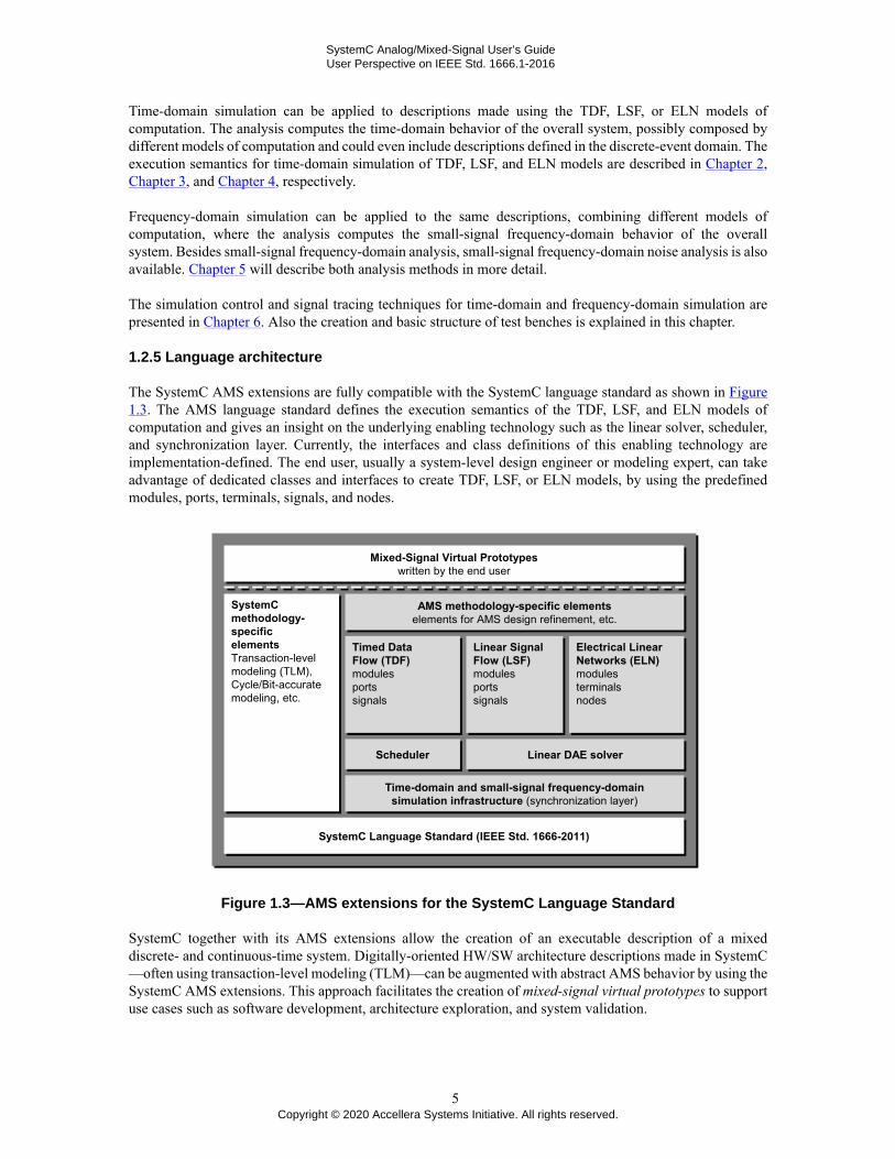
The SystemC AMS extensions are fully compatible with the SystemC language standard as shown in Figure1.3. The AMS language standard defines the execution semantics of the TDF, LSF, and ELN models ofcomputation and gives an insight on the underlying enabling technology such as the linear solver, scheduler,and synchronization layer. Currently, the interfaces and class definitions of this enabling technology areimplementation-defined. The end user, usually a system-level design engineer or modeling expert, can takeadvantage of dedicated classes and interfaces to create TDF, LSF, or ELN models, by using the predefinedmodules, ports, terminals, signals, and nodes.
Figure 1.3—AMS extensions for the SystemC Language Standard
SystemC together with its AMS extensions allow the creation of an executable description of a mixeddiscrete- and continuous-time system. Digitally-oriented HW/SW architecture descriptions made in SystemC—often using transaction-level modeling (TLM)—can be augmented with abstract AMS behavior by using theSystemC AMS extensions. This approach facilitates the creation of mixed-signal virtual prototypes to supportuse cases such as software development, architecture exploration, and system validation.
5Copyright © 2020 Accellera Systems Initiative. All rights reserved.

SystemC Analog/Mixed-Signal User’s GuideUser Perspective on IEEE Std. 1666.1-2016
2. Timed Data Flow modeling
2.1 Modeling fundamentals
The Timed Data Flow (TDF) model of computation is based on the Cyclo-static Synchronous Data Flow(CSDF) modeling formalism. Unlike the untimed CSDF model of computation, TDF is a discrete-timemodeling style, which considers data as signals sampled in time. These signals are tagged at discrete points intime and carry discrete or continuous values like amplitudes.
Figure 2.1 shows the basic principle of the Timed Data Flow modeling. In this figure, there are threecommunicating TDF modules called A, B, and C. A TDF model is composed of a set of connectedTDF modules, which form a directed graph called TDF cluster. TDF modules are the vertices of the graph,and TDF signals correspond to its edges. A TDF module may have several input and output TDF ports. ATDF module containing only output ports is also called a producer (source), while a TDF module with onlyinput ports is a consumer (sink). TDF signals are used to connect ports of different modules together.
Each TDF module contains a C++ method that computes an arbitrary function f (i.e., fA, fB, and fC), whichdepends on its direct inputs and possible internal states. The overall behavior of the cluster is therefore definedas the mathematical composition of the functions of the involved TDF modules in the appropriate order, fC (fB(fA (...))), indicated with schedule {A→B→C} in Figure 2.1.
Figure 2.1—A basic TDF model with 3 TDF modules and 2 TDF signals
A given function is processed (or ‘fired’ according to the SDF formalism) if there are enough samples availableat the input ports. In this case, the input samples are read by the TDF module, where the function usesthese values to compute one or more resultants, which are written to the appropriate output ports. During theexecution of a schedule, the number of samples read from or written to the module ports is fixed, where thenumber of read and written samples by a TDF module are not necessarily equal. The number of samples readfrom or written to the module ports can be changed during the simulation after the execution of each schedule.A time stamp is associated to each sample using the local TDF module time. The interval between two samplesis called the time step.
2.1.1 TDF module and port attributes
The flexibility and expressiveness of TDF modeling comes from the ability to define the attributes of eachTDF module and of each of its TDF ports. In TDF, it is possible:
— To assign a particular time step to a TDF module. The module time step defines the time intervalbetween each module activation. Figure 2.2a shows a TDF module A with a module time step (Tm)of 20 µs.
— To assign a particular maximum time step to a TDF module. The maximum time step enforces themodule activation if this time period is reached. Figure 2.2a shows a TDF module A with a moduletime step (Tm,max) of 1 second.
6Copyright © 2020 Accellera Systems Initiative. All rights reserved.

SystemC Analog/Mixed-Signal User’s GuideUser Perspective on IEEE Std. 1666.1-2016
— To assign a particular time step to a given port of a TDF module belonging to the cluster. The time stepdefines the time interval between two consecutive samples which are written to or read from the port.Figure 2.2b shows a TDF module B with a TDF input port time step (Tp) of 10 µs.
— To assign a particular maximum time step to a given port of a TDF module belonging to the cluster.The maximum time step defines the maximum allowed time interval between two consecutive sampleswhich are written to or read from the port. Figure 2.2b shows a TDF module B with a TDF inputmaximum port time step (Tp,max) of 1 second.
— To assign a particular rate to a given port of a module belonging to the cluster. Figure 2.2b shows aTDF module B, where at each module activation 2 samples are read (input port rate R set to 2, indicatedwith R:2).
— To assign a particular delay to a given port of a module belonging to the cluster. Figure 2.2c shows aTDF module C, where at each module activation, the sample corresponding to the previous time stepis written (output port delay D set to 1 sample, indicated with D:1).
— To assign a particular continuous-time delay to a given decoupling port of a module belonging to thecluster. Figure 2.2d shows a TDF module D, where at each module activation, the sample is written tothe output port with a continuous-time delay of 0.8 µs.
Figure 2.2—TDF module and port attributes
Provided that the attribute assignment on the ports and modules of a TDF model are compatible, the orderof activation of the TDF modules in a cluster and the number of samples they read (consume) and write(produce) can be statically determined before simulation starts and may be changed after the execution ofeach schedule. Thus, and more formally, a TDF cluster can be defined as the set of connected TDF modules,which belong to the same static schedule. The latter may change over time in terms of order and number ofactivations of each TDF module, but no new TDF modules can be added to a cluster nor TDF modules can beremoved from the cluster during simulation. If the attribute assignments are not compatible, the static schedulecannot be established and the TDF cluster is said to be not schedulable (see also Section 2.1.4). Therefore,after the required TDF cluster consistency check, the schedule defines a sequence, in which the algorithmicor procedural description of each TDF module is executed.
The main advantage of using a static schedule is that the execution of TDF models does not rely on the evaluate/update mechanism of SystemC’s discrete-event kernel, resulting in more efficient and thus faster simulations.TDF models are processed independently, using a local time annotation mechanism. Interactions betweenTDF models and pure SystemC models are supported through specific converter ports, as discussed in Section2.4.
2.1.2 Static and dynamic modes of operation
The TDF model of computation supports two modes of operation, which defines the way how changes of theTDF attributes (time step, rate or delay) are handled while executing the schedule.
— Static: in this case, TDF module attributes are not changed during simulation. Attributes are onlydefined prior to simulation and remain fixed during simulation.
7Copyright © 2020 Accellera Systems Initiative. All rights reserved.

SystemC Analog/Mixed-Signal User’s GuideUser Perspective on IEEE Std. 1666.1-2016
— Dynamic: in this case, the TDF model attributes are changed during simulation. Attributes can beredefined, and will be evaluated at the end of the execution of the schedule, and–if valid–will becomeeffective in the next execution of the schedule.
An application may switch between the static and dynamic modes of operation during simulation. The mode ofoperation will be based on the properties of each individual TDF module in a cluster. To this end, the applicationcan mark each TDF module to accept or reject attribute changes, and to do or not do attribute changes itself.
By default, a TDF module does not accept attribute changes and also does not make attribute changes itself,which will enforce a static mode of operation. This means that in order to use TDF modules in a dynamic modeof operation, each individual TDF module in a cluster shall define explicitly that changes to the TDF attributesare supported.
Figure 2.3 shows a TDF cluster with three TDF modules for the static mode of operation. TDF module Ahas no specific settings defined on how to deal with TDF attributes. It relies on the default settings, whichmeans it will reject attribute changes from other TDF modules in the cluster and it does not change attributesitself. TDF module B explicitly defines that it will accept attribute changes from other TDF modules. Bydefault, TDF module B does not change attributes itself, similar as module A. TDF module C explicitly definesthat it does not change attributes itself. By default, TDF module C will reject attribute changes from otherTDF modules in the cluster. Even though TDF module B accepts attribute changes, none of the modules doesmake changes to the attributes. As a result, the TDF cluster operates under the static mode of operation.
Figure 2.3—TDF modules and their settings resulting in a static mode of operation
Figure 2.4 shows a TDF cluster with three TDF modules for the dynamic mode of operation. The TDF modulesA, B, and C accept attribute changes from other TDF modules in the cluster. TDF module B does change theTDF attributes, whereas module A and C by default do not change attributes.
Figure 2.4—TDF modules and their settings resulting in a dynamic mode of operation
If some TDF modules in a cluster define attributes for dynamic mode of operation and other TDF modules inthe same cluster specify attributes for static mode of operation, then an inconsistent set of attributes is specified.For example, Figure 2.5 shows TDF module B, and C which both accept attribute changes. As TDF module
8Copyright © 2020 Accellera Systems Initiative. All rights reserved.

SystemC Analog/Mixed-Signal User’s GuideUser Perspective on IEEE Std. 1666.1-2016
B does make attribute changes, it enforces the dynamic mode of operation. However, TDF module A rejectsattribute changes (by default). This results in an inconsistency in the cluster attributes, which will cause anerror in simulation.
Figure 2.5—TDF modules attributes settings resulting in an inconsistency in the cluster.
2.1.3 TDF model topologies
Figure 2.6 shows an example of a TDF model with multirate characteristics. A port rate assignment withrate value 2 (R:2) has been performed on the output port of TDF module A. Ports with no rate attribute areconsidered to have a rate of 1 (not graphically represented). When module A is activated, 2 samples are written.Since both modules, B and C, read one sample at each activation, a possible schedule for this TDF cluster is{A→B→C→B→C}.
Figure 2.6—Multirate TDF model using port rate assignment
In order to handle TDF models containing loops, it is compulsory to introduce a delay on a module portbelonging to one of the modules of the loop. This port delay has to be defined during elaboration of thesimulation, to make the static scheduling feasible. A simple example is given in Figure 2.7, without loop, thatshows a module A with a delay of one sample associated to the output port (D:1). One possible schedule is{A→B}. Schedule {B→A} is also possible since when module B first activated its input port will read thesample already available thanks to the assigned delay defined in the elaboration phase.
Figure 2.7—TDF model with port delay
The initial value of the sample of a port with a delay is determined by the constructor of the correspondingdata types. The user is advised to set the values of the initial samples if port delays are used, because the valuewill be undefined for C++ fundamental types due to the lack of a default constructor.
9Copyright © 2020 Accellera Systems Initiative. All rights reserved.

SystemC Analog/Mixed-Signal User’s GuideUser Perspective on IEEE Std. 1666.1-2016
Figure 2.8 shows an example of a TDF model containing a loop, a quite common situation when dealingwith signal processing with feedback. A mandatory port delay assignment with delay value 1 (D:1) has beenperformed on the output port of TDF module C. Assigning a delay to the output port of module C, allowsmodule B to be ‘fired’ when the first sample of module A becomes available on input in0 of module B. Apossible schedule for this TDF model is {A→B→C}.
Figure 2.8—TDF model with loop, and port delay assignment
Figure 2.9 shows a more complex example mixing multirate and delay. A possible cluster schedule is{A→B→B→C→D}. Module B is executed twice because of the port rate (R:2) assignments performed on thetwo connected ports (output port of module A and input port of module C). The port delay assignment on theoutput port of module D (D:1) is required for the schedule to be computed properly.
Figure 2.9—Multirate TDF model with loop
Another prerequisite for a proper schedule is that the sum of samples produced at the output ports withina loop must be equal to the sum of samples consumed by the input ports within the loop. Otherwise, anyfinite schedule would accumulate surplus samples somewhere in the cluster when executing it repeatedly. Forexample, in the case the rate of the input port of module C in Figure 2.9 were changed from 2 to 1, the schedule{A→B→C→D→B→C→D} would result in one extra sample at the output of module D after executing theschedule once (see Figure 2.10).
10Copyright © 2020 Accellera Systems Initiative. All rights reserved.

SystemC Analog/Mixed-Signal User’s GuideUser Perspective on IEEE Std. 1666.1-2016
Figure 2.10—Multirate TDF model containing a loop with incompatible rates, resultingin accumulation of samples in the cluster yielding to an infinite (broken) schedule
Figure 2.11 shows how it is possible to connect a TDF model with the discrete-event domain, by means ofTDF converter ports (indicated with ). For example, a discrete-event signal is available at the TDF converterport of TDF module A. Module D has a TDF converter input port, reading a discrete-event control signal.Special care should be taken with the interaction between the TDF and discrete-event domain. This is describedin Section 2.4.
Figure 2.11—TDF model interfacing with discrete-event domain
Another special case is when a TDF model becomes part of a closed loop, which includes a path throughthe discrete-event domain, as shown in Figure 2.12. The TDF cluster itself contains no loop, so there is noport delay assignment necessary to calculate a valid schedule. Module A reads a sample from the discrete-event domain at the first delta cycle of the time point associated to the sample using a TDF converter inputport. Module C writes a sample to the discrete-event domain in the same delta cycle, using a TDF converteroutput port. Note that TDF samples read from module C and passed through the discrete-event module D tothe input of module A will be delayed by one TDF time step due to the evaluate/update mechanism of theSystemC kernel.
More details on the interaction between the TDF and discrete-event domain is described in Section 2.1.5 andSection 2.4.
11Copyright © 2020 Accellera Systems Initiative. All rights reserved.
SystemC Analog/Mixed-Signal User’s GuideUser Perspective on IEEE Std. 1666.1-2016
Figure 2.12—TDF model with loop via the discrete-event domain
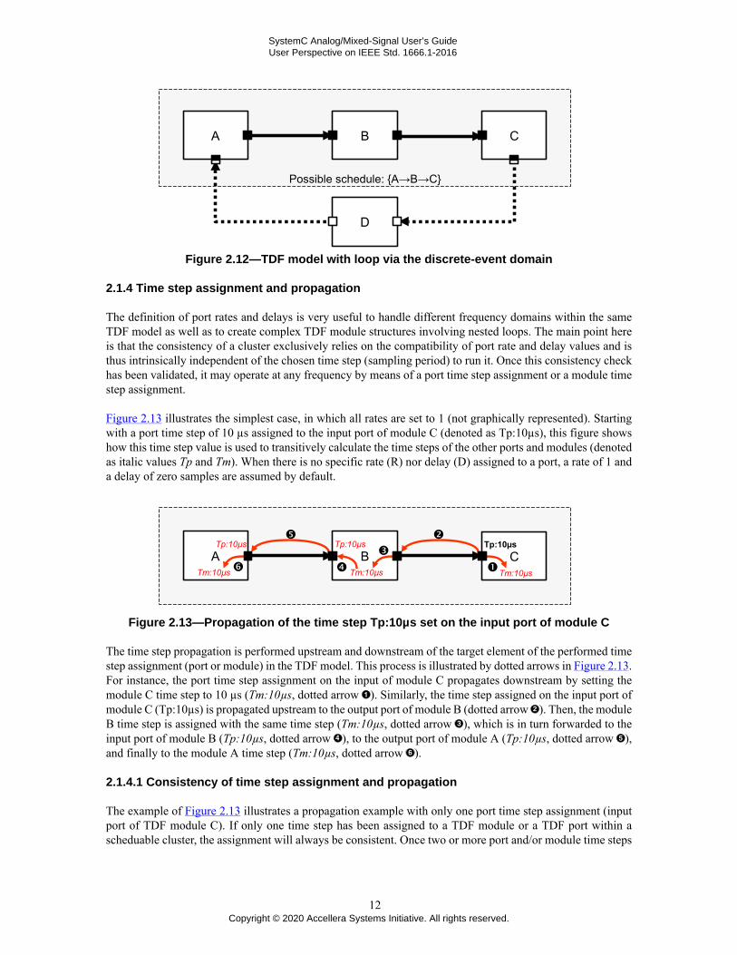
2.1.4 Time step assignment and propagation
The definition of port rates and delays is very useful to handle different frequency domains within the sameTDF model as well as to create complex TDF module structures involving nested loops. The main point hereis that the consistency of a cluster exclusively relies on the compatibility of port rate and delay values and isthus intrinsically independent of the chosen time step (sampling period) to run it. Once this consistency checkhas been validated, it may operate at any frequency by means of a port time step assignment or a module timestep assignment.
Figure 2.13 illustrates the simplest case, in which all rates are set to 1 (not graphically represented). Startingwith a port time step of 10 µs assigned to the input port of module C (denoted as Tp:10µs), this figure showshow this time step value is used to transitively calculate the time steps of the other ports and modules (denotedas italic values Tp and Tm). When there is no specific rate (R) nor delay (D) assigned to a port, a rate of 1 anda delay of zero samples are assumed by default.
Figure 2.13—Propagation of the time step Tp:10µs set on the input port of module C
The time step propagation is performed upstream and downstream of the target element of the performed timestep assignment (port or module) in the TDF model. This process is illustrated by dotted arrows in Figure 2.13.For instance, the port time step assignment on the input of module C propagates downstream by setting themodule C time step to 10 µs (Tm:10µs, dotted arrow ). Similarly, the time step assigned on the input port ofmodule C (Tp:10µs) is propagated upstream to the output port of module B (dotted arrow ). Then, the moduleB time step is assigned with the same time step (Tm:10µs, dotted arrow ), which is in turn forwarded to theinput port of module B (Tp:10µs, dotted arrow ), to the output port of module A (Tp:10µs, dotted arrow ),and finally to the module A time step (Tm:10µs, dotted arrow ).
2.1.4.1 Consistency of time step assignment and propagation
The example of Figure 2.13 illustrates a propagation example with only one port time step assignment (inputport of TDF module C). If only one time step has been assigned to a TDF module or a TDF port within ascheduable cluster, the assignment will always be consistent. Once two or more port and/or module time steps
12Copyright © 2020 Accellera Systems Initiative. All rights reserved.

SystemC Analog/Mixed-Signal User’s GuideUser Perspective on IEEE Std. 1666.1-2016
have been assigned in a TDF cluster, a consistency check has to be made to ensure their compatibility withthe propagated time steps, depending on the port rates.
Figure 2.14 shows a module, where the input port time step is set to 10 µs (Tp:10µs) with a rate of 2 (R:2),and the module time step is set to 20 µs (Tm:20µs). As the output port rate is not set, it will use the defaultrate of 1, resulting in an output port time step of 20 µs.
Figure 2.14—Port time step, port rate, and module time step should be consistent
The module time step should be consistent with the rate and time step of any port within a module. The relationbetween these time steps and rates becomes:
(2.1)
In the example of Figure 2.14, the following relation is checked: 20 µs = 10 µs · 2 = 20 µs · 1.
In the example of Figure 2.15, multiple modules form a cluster, where two time steps are set by the user: thetime step of module A is set to 20 µs (Tm:20µs ) and the input port time step of module C is set to 10 µs(Tp:10µs ). Furthermore, the user has set the rate of the output port of module A to 2 (R:2). Therefore, moduleA is activated two times less frequently than modules B and C, as module A writes 2 samples per activation,see Figure 2.6.
The specified port time step at the input of module C (Tp:10µs ) propagates downstream to module C thussetting its time step to 10 µs (Tm:10µs, dotted arrow ). Similarly, the time step assigned to the input portof module C (Tp:10µs ) is propagated upstream to the output port of module B (dotted arrow ). Then, themodule B time step is assigned with the same time step (Tm:10µs, dotted arrow ), which in turn is forwardedto input port of module B (Tp:10µs, dotted arrow ), and propagated upstream to the output port of moduleA (Tp:10µs, dotted arrow ). Since the output port rate of module A is 2, the propagated module time stepshould become 20 µs (Tm:20µs, dotted arrow ), which matches with the user-specified time step of moduleA (Tm:20µs ).
Figure 2.15—Time step propagation for a multirate TDF modelwith consistent time step assignments done by the user
Figure 2.16 shows the same TDF model with an incompatible time step propagation, which leads to aninconsistent time step assignment. The expected module A time step resulting from propagation is 20 µs(Tm:20µs, dotted arrow ), which is different from the assigned module time step of module A (Tm:10µs ).Therefore, no consistent time steps can be assigned and an error will be reported.
13Copyright © 2020 Accellera Systems Initiative. All rights reserved.

SystemC Analog/Mixed-Signal User’s GuideUser Perspective on IEEE Std. 1666.1-2016
Figure 2.16—Time step propagation for a multirate TDF modelwith inconsistent time step assignments done by the user
2.1.4.2 Maximum time step assignment and propagation
The optional maximum time step attribute can be defined to guarantee that sufficient time points areavailable for the calculation of continuous-time descriptions (e.g., Laplace transfer functions). Assignmentand propagation of the maximum time step for a TDF module or TDF port follows the same mechanism asexplained in Section 2.1.4. In the case where multiple TDF modules in the same cluster define the maximumtime step, the maximum time step will be calculated by taking the smallest propagated maximum time step ofthe TDF modules in the cluster. This maximum time step should always be greater than or equal to the resolvedtime step for each TDF module and TDF port. In the case where a maximum time step is set within the cluster,the regular time step assignment as explained in Section 2.1.4 is not mandatory since the minimum value of thepropagated max time step assignments will be used. If a regular time step has been assigned somewhere in thecluster using member function set_timestep, this time step will be used as long as it is less than or equal to thepropagated maximum time step. If the propagated regular time step is greater than the propagated maximumtime step an error will be reported.
2.1.5 Multiple schedules or clusters
It is possible to have more than one TDF cluster within the same application. In this case, each TDF clusterhas its own data flow characteristics (sampling rate, sampling period, etc.), scheduling, and execution order.This is especially useful in applications where the time steps or (data) rates between the various connectedsubsystems are different.
Specialized TDF decoupling output ports are available to decouple TDF clusters. Two types of TDF decouplingoutput ports are available:
— A continuous-time decoupling port, which uses the default or user-defined interpolation mechanism.— A discrete-time decoupling port, which follows a sample-and-hold regime.
Figure 2.17 shows an example, in which a continuous-time TDF decoupling port (indicated with ) is usedto explicitly split a cluster. The first cluster will use a module time step of 10 µs and will deliver samples atthe output of module B each 10 µs. The second cluster will consume samples at the input of module C each8 µs. For the continuous-time TDF decoupling port, a delay of at least one sample needs to be specified, tofacilitate interpolation.
Figure 2.17—Use of a continuous-time TDF decouplingport to explicitly split a cluster in two independent ones
14Copyright © 2020 Accellera Systems Initiative. All rights reserved.

SystemC Analog/Mixed-Signal User’s GuideUser Perspective on IEEE Std. 1666.1-2016
Note that in between the two clusters, a TDF signal is used to connect module B with module C. As there onlyexist TDF decoupling output ports, the input to the second cluster (module C) is a regular TDF input port.
Alternatively, the discrete-time TDF decoupling output port can be used, which will provide a static outputsignal during the interval of two samples. As such, the decoupling port performs a sample-and-hold function.When using such discrete-time TDF decoupling output port, there is no delay required, because there is nointerpolation necessary. Unlike the continuous-time decoupling port, the discrete-time decoupling port requiresno sample delay. However, due to the evaluation/update semantic of the discrete-event solver, a read at thesame time point like the corresponding write will deliver the previous value. Figure 2.18 shows the usage ofthis discrete-time TDF decoupling port (indicated with ).
Figure 2.18—Use of a discrete-time TDF decoupling outputport to split a cluster using a sample-and-hold mechanism
2.1.6 Signal processing behavior of TDF models
Figure 2.19 illustrates how a cluster of TDF modules processes signals by repetitively activating the processingfunctions of the contained modules in the order of the derived schedule. It generates samples for each moduleas a function of time. Because the rates are all set to 1, the processing is obvious: Module A writes a sample attime 0 µs, which is read by module B at time 0 µs, and module B writes a sample at time 0 µs, which is readby module C at time 0 µs. From the perspective of the generated samples, it is important to notice that it is thewrite operation of the sample produced by module A that actually enables module B to be fired. Respectively,the generation of a sample by module B triggers module C.
The output of module A produces a continuous-value signal (Vin), whose values are only available at discretetime points. The time step between these samples is equidistant, and defined by the time step of the outputport of module A (Tp:10µs). Signal Vin is fed into module B, which in this example is assumed to be a simpleamplifier with a constant gain. The samples of the amplified output signal (Vout) become available at the outputof module B at the same time steps as they were written by module A.
Figure 2.19—TDF module activation (processing) with read and written samples
15Copyright © 2020 Accellera Systems Initiative. All rights reserved.
SystemC Analog/Mixed-Signal User’s GuideUser Perspective on IEEE Std. 1666.1-2016
Besides using TDF modules to describe discrete-time behavior, a TDF module can be used to encapsulatecontinuous-time behavior. Section 2.3 will explain the usage of TDF to model discrete-time and continuous-time behavior.
2.2 Language constructs
2.2.1 TDF modules
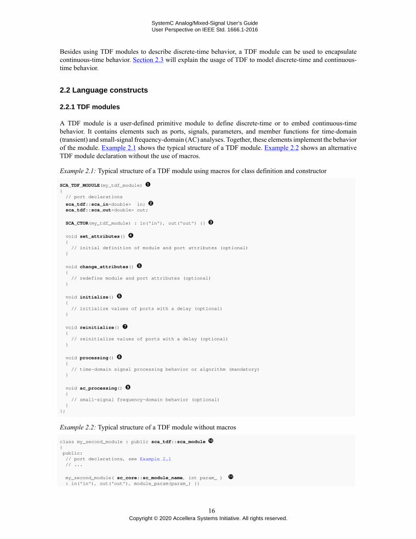
A TDF module is a user-defined primitive module to define discrete-time or to embed continuous-timebehavior. It contains elements such as ports, signals, parameters, and member functions for time-domain(transient) and small-signal frequency-domain (AC) analyses. Together, these elements implement the behaviorof the module. Example 2.1 shows the typical structure of a TDF module. Example 2.2 shows an alternativeTDF module declaration without the use of macros.
Example 2.1: Typical structure of a TDF module using macros for class definition and constructor
SCA_TDF_MODULE(my_tdf_module) { // port declarations
sca_tdf::sca_in<double> in; sca_tdf::sca_out<double> out;
SCA_CTOR(my_tdf_module) : in("in"), out("out") {}
void set_attributes() { // initial definition of module and port attributes (optional) }
void change_attributes() { // redefine module and port attributes (optional) }
void initialize() { // initialize values of ports with a delay (optional) }
void reinitialize() { // reinitialize values of ports with a delay (optional) }
void processing() { // time-domain signal processing behavior or algorithm (mandatory) }
void ac_processing() { // small-signal frequency-domain behavior (optional) } };
Example 2.2: Typical structure of a TDF module without macros
class my_second_module : public sca_tdf::sca_module { public: // port declarations, see Example 2.1 // ...
my_second_module( sc_core::sc_module_name, int param_ ) : in("in"), out("out"), module_param(param_) {}
16Copyright © 2020 Accellera Systems Initiative. All rights reserved.

SystemC Analog/Mixed-Signal User’s GuideUser Perspective on IEEE Std. 1666.1-2016
// definition of the TDF member functions as done in Example 2.1 // ...
private: int module_param; // user-defined module parameter};
Primitive module declaration facilitated by the macro SCA_TDF_MODULE to define a new classpublicly derived from class sca_tdf::sca_module.A TDF module can have multiple input and output ports. Only TDF ports should be instantiated, seeSection 2.2.2.Mandatory constructor definition facilitated by the predefined macro SCA_CTOR, which requiresthe specification of the TDF module name as argument. It is a good practice to assign the names tothe instantiated ports and signals in the constructors’ initializer list.Optional member function set_attributes, in which TDF module and port attributes can be defined.The user is not allowed to call this member function directly. It is called by the simulation kernelduring elaboration.Optional member function change_attributes, in which TDF module and port attributes can beredefined. The user is not allowed to call this member function directly. It is called by the simulationkernel, at the end of the execution of each schedule.Optional member function initialize to initialize data members representing the module state andespecially the initial samples of ports with assigned delays. The user is not allowed to call this memberfunction directly. It is called by the simulation kernel at the end of elaboration, just before transientsimulation starts.Optional member function reinitialize to reinitialize data members. In case of an attribute change,this member function can be used to reassign delay values. The user is not allowed to call thismember function directly. It is called by the simulation kernel after calling the member functionchange_attributes and having advanced the time to the moment of the next cluster activation.Mandatory member function processing, which encapsulates the actual signal processing function.The user is not allowed to call this member function directly. It is called by the simulation kernel aspart of time-domain (transient) simulation, where each module activation advances the local moduletime by the assigned or derived module time step.Optional member function ac_processing, which encapsulates the small-signal frequency-domain(AC) and small-signal frequency-domain noise behavior. The user is not allowed to call this memberfunction directly. It is called by the simulation kernel while executing small-signal frequency-domainanalyses (see Chapter 5).Alternative TDF module declaration by creating a new class publicly derived from classsca_tdf::sca_module.Mandatory constructor definition for a TDF module, which requires the mandatory module name (oftype sc_core::sc_module_name) as first argument. The regular C++ constructor should be used topass and initialize parameters for the TDF module. It is a good practice to initialize port names, signalsnames and other user-defined parameter values in the constructors’ initializer list.
2.2.1.1 Module attributes
Module and port attributes such as sampling rate, delay, and time step should be defined in the member functionset_attributes and may be changed subsequently in the member function change_attributes. The memberfunction may use any legal C++ statement in addition to the definition of module or port attributes. The memberfunction set_attributes is called at elaboration time, whereas the member function change_attributes is calledafter the execution of each schedule (see Section 2.5).
The following member functions are available for TDF modules to set and get the attributes:
17Copyright © 2020 Accellera Systems Initiative. All rights reserved.

SystemC Analog/Mixed-Signal User’s GuideUser Perspective on IEEE Std. 1666.1-2016
— The member functions set_timestep and get_timestep will set and return, respectively, the moduletime step, which is defined as the time step between two consecutive module activations. The moduletime step should be less than the maximum time step defined.
— The member functions set_max_timestep and get_max_timestep will set and return, respectively, themaximum time step between two consecutive module activations. If the maximum time step is notdefined by the application, the time step is set to sca_core::sca_max_time.
— The member function request_next_activation will request a next module activation based on a timestep, event, or event-list given as argument. In the case where multiple TDF modules, which belong tothe same cluster, request a next module activation, the requests are or-concatenated. In consequence,the request with the earliest point in time will be used and the other requests will be ignored.
— The member function get_last_timestep will return the last non-zero module time step of the lastmodule activation or before. For the first module activation, the member function will return thepropagated time step.
In addition to these member functions to change the TDF module attributes, dedicated member functions areavailable to define whether changes to these TDF attributes are allowed or not. The user can define whetherthe TDF model of computation uses the static or dynamic mode of operation (see Section 2.1.2):
— The member functions does_attribute_changes and does_no_attribute_changes are used to mark aTDF module to allow or disallow making attribute changes itself, respectively. Before a module canmake changes to its attributes, it has to call does_attribute_changes first. By default, a TDF moduleis not allowed to make changes to its attributes.
— The member functions accept_attribute_changes and reject_attribute_changes are used to marka TDF module to accept or reject attribute changes caused by other TDF modules in the samecluster, respectively. By default, a TDF module will reject attribute changes. The member functionreject_attribute_changes is especially relevant when a DSP functionality, in which variable time stepsare not allowed, is modeled by using TDF modules.
In Example 2.3, the initial module time step is set to 10 ms in the callback set_attributes. In thismember function, the module is also marked to allow making changes to its TDF attributes by callingdoes_attribute_changes. Note that the member function accept_attribute_changes is not called, whichmeans that the module would not allow any attribute changes done by other TDF modules in the cluster and thusthis module will be guaranteed the only module in the cluster which is allowed to make changes to attributes.The callback change_attributes is used to actually change the attributes. In this example, the time step willchange to 20 ms after 50 ms.
Example 2.3: TDF member functions set_attributes and change_attributes
void set_attributes() { set_timestep(10.0, sc_core::SC_MS); // module time step assignment of a of 10 ms does_attribute_changes(); // module is allowed to make attribute changes} void change_attributes(){ if ( get_time() > sca_core::sca_time(50.0, sc_core::SC_MS) ) set_timestep(20.0, sc_core::SC_MS); // module time step changed to 20 ms after 50 ms}
2.2.1.2 Module initialization
The member function initialize is primarily used to initialize the delay samples of TDF ports that havebeen assigned a delay and to initialize module state variables, which depend in some way on the assignedTDF attributes. To this end, all TDF attributes (rate, delay, and time steps) can be read in the context of thiscallback. This member function is executed only once, just before the actual module activation starts (see next
18Copyright © 2020 Accellera Systems Initiative. All rights reserved.

SystemC Analog/Mixed-Signal User’s GuideUser Perspective on IEEE Std. 1666.1-2016
section). Example 2.4 shows the initialization of an internal state variable t and the use of the port memberfunction get_timestep and initialize. The available port member functions are explained in Section 2.2.2.
Example 2.4: TDF member function initialize
void initialize() {
t = get_timestep();
std::cout << out.name() << ": Time step = " << out.get_timestep() << std::endl;
out.initialize(1.23); }
Set local state variable t. In this example, t is a private data member of type sca_core::sca_time tostore the module time step.Get time step of output port out.Initialize the first sample of output port out of type double with value 1.23.
How to use port initialization inside this member function is explained in Section 2.2.2.
2.2.1.3 Module reinitialization
The member function reinitialize can be used to reinitialize ports with a delay or to readjust module statevariables based on the new TDF attributes. This member function is executed before each execution of thecluster except the first time where initialize is executed. Example 2.5 shows the reset of all delay values of anoutput port in case the time step has changed.
Example 2.5: TDF module reinitialization using member function reinitialize
void reinitialize() { int delay_buffer_size = out.get_delay(); for (int i = 0; i < delay_buffer_size; i++) out.initialize(0.0, i); // reinitialize new delay value to zero}
2.2.1.4 Module activation (processing)
The member function processing is the only mandatory function that needs to be overridden in anyTDF module, since it actually defines the discrete-time or continuous-time behavior of the TDF module. Thismember function is executed at each module activation (see Section 2.3). Example 2.6 shows a very simplecase, in which the value of an internal data member val is written to an output port.
Example 2.6: TDF module activation using member function processing
void processing(){ out.write(val); // writes value to output port out}
2.2.1.5 Module local time
The member function get_time can be used within the processing function to obtain the actual, localmodule time. It returns the time of the first input sample of the current module activation, as atype of class sca_core::sca_time. At elaboration, the actual module time returned by get_time is zero(sc_core::SC_ZERO_TIME). In the context of the member function initialize and reinitialize, the actualmodule time corresponds to the first activation time of the module in the next schedule execution of theTDF cluster. Example 2.7 shows how the local module time can be obtained.
19Copyright © 2020 Accellera Systems Initiative. All rights reserved.

SystemC Analog/Mixed-Signal User’s GuideUser Perspective on IEEE Std. 1666.1-2016
Example 2.7: Get local time of a TDF module
void processing() { sca_core::sca_time local_time; local_time = get_time(); // get actual, local module time}
For multirate TDF models, the local time of the individual TDF modules can differ. Furthermore, there maybe time offsets between the local TDF module time and the SystemC kernel time. Therefore, the functionget_time should be used inside a TDF module as a replacement for sc_core::sc_time_stamp.
2.2.1.6 Module constructor
The macro SCA_CTOR helps to define the standard constructor of a module of class sca_tdf::sca_module. Ithas only one mandatory argument, which is the module name. In the case where parameters need to be passedvia the constructor, the user may define a regular constructor with an arbitrary number of additional parameters.
Member data should be initialized in the initialization list of the constructor, so that all members are properlyinitialized before the constructor of my_tdf_module is called. This also concerns the instantiated TDF ports,which should receive their respective names as constructor argument in the initialization list.
Example 2.8: TDF module constructor
my_tdf_module( sc_core::sc_module_name nm, int param_ ): in("in"), out("out"), module_param(param_) {}
2.2.1.7 Constraints on usage
A TDF module is a primitive of the TDF model of computation. Therefore, it cannot instantiate submodules.The structural composition of TDF modules is possible by defining classes derived from the regular SystemCclass sc_core::sc_module, or using the equivalent macro SC_MODULE. This is discussed in Section 2.3.3.
The member functions set_attributes, change_attributes, initialize, reinitialize, processing, andac_processing should not be called directly by the user. These member functions are called as part of theexecution semantics for time-domain simulation (Section 2.5) or small-signal frequency-domain analyses(Chapter 5).
SystemC functions that describe discrete-event behavior such as creating methods and threads, specifyingsensitivity, waiting for events, and so on are not allowed to be called in a TDF module. Otherwise, the executionsemantics for SystemC discrete-event processing could interfere with the execution of the TDF modules.This means member functions and macros like SC_HAS_PROCESS, SC_METHOD, SC_THREAD, wait,next_trigger, sensitive should not be used in a TDF module.
As the local time of a TDF module is calculated independently from the time in the discrete-event domain(SystemC kernel time), the function sc_core::sc_time_stamp should not be used inside a TDF module.Instead, the member function get_time should be used.
In the case where SystemC signals are needed for processing in a TDF module, specialized converter portshave to be used, as described in Section 2.4.
2.2.2 TDF ports
A TDF port is an object that provides a TDF module with a means to communicate with other connectedmodules. Due to the nature of the TDF modeling formalism, a TDF port can be either an input port or an outputport, but not inout (which is available in SystemC). TDF ports can be declared for any data type defined byC++, SystemC, the SystemC AMS extensions, a third-party library, or the user.
20Copyright © 2020 Accellera Systems Initiative. All rights reserved.

SystemC Analog/Mixed-Signal User’s GuideUser Perspective on IEEE Std. 1666.1-2016
There are currently six classes of TDF ports:— TDF ports of class sca_tdf::sca_in<T> (input port) or sca_tdf::sca_out<T> (output port).— TDF converter ports of class sca_tdf::sca_de::sca_in<T> (converter input port) and
sca_tdf::sca_de::sca_out<T> (converter output port).— TDF decoupling ports of class sca_tdf::sca_out<T, sca_tdf::SCA_CT_CUT> (continuous-
time decoupling output port) and sca_tdf::sca_out<T, sca_tdf::SCA_DT_CUT> (discrete-timedecoupling output port).
TDF ports are used to connect TDF modules using signals of class sca_tdf::sca_signal<T>. TDF converterports allow TDF modules to interact with discrete-event signals of class sc_core::sc_signal<T> orsc_core::sc_buffer. This is explained in Section 2.4. The TDF decoupling output ports can be used to decoupleTDF clusters if a system partitioning requires clusters of different time step or sample rates (see Section 2.1.5).
The port template classes allow the use of different data types, e.g., double, int or bool. The data type doubleis often used to represent the amplitude of a continuous-value signal. Example 2.9 shows the instantiation ofthe six available TDF port classes.
Example 2.9: TDF port instantiations
SCA_TDF_MODULE(my_tdf_module){
sca_tdf::sca_in<double> in;
sca_tdf::sca_out<double> out;
sca_tdf::sca_de::sca_in<bool> inp;
sca_tdf::sca_de::sca_out< sc_dt::sc_logic > outp;
sca_tdf::sca_out<double, sca_tdf::SCA_CT_CUT> out_ct;
sca_tdf::sca_out<double, sca_tdf::SCA_DT_CUT> out_dt; // rest of module not shown};
TDF input port that carries a continuous-value (real) signal.TDF output port that carries a continuous-value (real) signal.TDF input converter port from the discrete-event domain, using a Boolean signal.TDF output converter port to the discrete-event domain, using a SystemC logic signal.TDF output decoupling port which treats the signal as continuous in time and uses an interpolationmechanism in case intermediate values are requested.TDF output decoupling port which treats the signal as discrete in time and uses a sample-and-holdmechanism in case intermediate values are requested.
2.2.2.1 Port attributes
A number of attributes can be assigned to TDF ports. They are used to control the evaluation and execution ofthe TDF cluster, to which the TDF module belongs. TDF port attributes have to be set in the member functionsset_attributes or change_attributes of the TDF module, in which the port is declared (see Section 2.2.1). Thefollowing member functions are available for TDF ports to set or get the attributes:
— The member functions set_timestep and get_timestep will set and return, respectively, the time step(sampling period) between two consecutive samples.
— The member functions set_max_timestep and get_max_timestep will set and return, respectively, themaximum time step (sampling period) between two consecutive samples.
— The member function get_last_timestep will return the last non-zero time step (sampling period)between two consecutive samples preceding the sample which index is given as argument.
21Copyright © 2020 Accellera Systems Initiative. All rights reserved.

SystemC Analog/Mixed-Signal User’s GuideUser Perspective on IEEE Std. 1666.1-2016
— The member functions set_rate and get_rate will set and return, respectively, the number of samplesthat have to be read or written to the port per module execution. The default rate is 1 (single-rate port).
— The member functions set_delay and get_delay will set and return, respectively, the number of samples,which are inserted before reading or writing the first time to the port. The default value depends on thedefault constructor of the data type. For C++ fundamental types like bool, int, long, float, and double,the initial value could be undefined. Therefore, it is recommended to initialize the port with an initialvalue, if a delay has been specified for a port (see Section 2.2.2.2).
— The member functions set_ct_delay and get_ct_delay will be only available for ports of classsca_tdf::sca_out<T, sca_tdf::SCA_CT_CUT> and sca_tdf::sca_out<T, sca_tdf::SCA_DT_CUT>.These member functions will set and return, respectively a continuous time delay which will be addedto the sample based delay (defined with set_delay). Thus the member function set_ct_delay permitssetting a delay, which is independent from the current time step and thus constant also for the casewhere variable time steps are used. The default continuous time delay is sc_core::SC_ZERO_TIME.
Example 2.10 shows the use of these member functions.
Example 2.10: TDF port attribute member functions
void set_attributes(){ out.set_timestep(0.01, sc_core::SC_US); // set time step of port out out.set_max_timestep(0.02, sc_core::SC_US); // set maximum time step of port out out.set_rate(1); // set rate of port out to 1 out.set_delay(2); // set delay of port out to 2 samples
out_ct.set_ct_delay(0.1, sc_core::SC_MS); // set continuous time delay of port out to 0.1ms} void initialize(){ out.get_rate(); // return the rate of port out out.get_delay(); // return the delay of port out out.get_timestep(); // return actual time step of port out out.get_max_timestep(); // return the maximum time step of port out out.get_last_timestep(); // return the previous time step of port out
out_ct.get_ct_delay(); // return the continuous time delay of port out_ct}
2.2.2.2 Port initialization
The initial values of TDF ports with a specified delay have to be specified in the member function initializeof the corresponding TDF module. Example 2.11 shows the initialization of port out, which delay has beenset to 2 samples.
Example 2.11: TDF port initialization
void initialize() // use initialize method of TDM module to initialize ports{ // initialize port out (which has a delay attribute of 2) out.initialize(1.23); // initialize first sample with value 1.23 or out.initialize(1.23,0); // initialize first sample with value 1.23 out.initialize(4.56,1); // initialize second sample with value 4.56}
2.2.2.3 Port read and write access
Samples can be read from a TDF input port by calling its member function read from within the memberfunction processing of the corresponding TDF module. For a multirate port, the sample index can be passedas an argument to read.
In the case of a single rate TDF input port, reading from this port is done as follows:
22Copyright © 2020 Accellera Systems Initiative. All rights reserved.

SystemC Analog/Mixed-Signal User’s GuideUser Perspective on IEEE Std. 1666.1-2016
Example 2.12: Reading a value from a single-rate TDF port
SCA_TDF_MODULE(my_tdf_sink){ sca_tdf::sca_in<double> in;
SCA_CTOR(my_tdf_sink) : in("in") {}
void processing() { // local variable double val; // variable to store value read from port in
val = in.read(); // reading first sample from the input port }};
Consecutive read accesses during the same module activation returns the same value, i.e., the input sample isnot consumed by the read access.
In the case of a multirate TDF input port, reading from this port is done as follows:
Example 2.13: Reading values from a multi-rate TDF port
SCA_TDF_MODULE(my_multi_rate_sink){ sca_tdf::sca_in<double> in;
SCA_CTOR(my_multi_rate_sink) : in("in") {}
void set_attributes() { in.set_rate(2); // two samples read per module activation }
void processing() { // local variable double val; // variable to store values read from port in
val = in.read(); // read first sample val = in.read(0); // same method with index for first sample val = in.read(1); // same method with index for second sample }};
The rate attribute of the input port defines the number of samples available per module activation. In Example2.13, the port rate of 2 gives access to 2 samples with respective index 0 and 1. As for single rate ports,consecutive read accesses during the same module activation return the same value.
Samples can be written to a TDF output port by passing the sample value as argument to the member functionwrite from within the member function processing of the corresponding TDF module. For a multirate port,the sample index can be passed along with the sample value as an argument to write.
In the case of a single rate TDF output port, writing to this port is done as shown in Example 2.14.
Example 2.14: Writing a value to a single-rate TDF port
SCA_TDF_MODULE(my_const_source){ sca_tdf::sca_out<double> out;
my_const_source( sc_core::sc_module_name, double val_ = 1.0 ) : out("out"), val( val_ ) {}
void processing() { out.write( val ); // writes val as a new sample to the port out }
23Copyright © 2020 Accellera Systems Initiative. All rights reserved.

SystemC Analog/Mixed-Signal User’s GuideUser Perspective on IEEE Std. 1666.1-2016
private: double val; // value to be written to the port out};
Consecutive write accesses during the same module evaluation overwrite the sample value, i.e., only the lastwritten output sample is emitted.
In the case of a multirate TDF output port, writing to this port is done as shown in Example 2.15.
Example 2.15: Writing values to a multi-rate TDF port
SCA_TDF_MODULE(my_multi_rate_const_source){ sca_tdf::sca_out<double> out;
my_multi_rate_const_source(sc_core::sc_module_name, double val_ = 1.0 ) : out("out"), val( val_ ) {}
void set_attributes() { out.set_rate(2); // 2 samples written per module activation } void processing() { out.write(val); // writes val as the first sample to the port out out.write(val,0); // writes val as the first sample to the port out by specifying the index 0 out.write(val,1); // writes val as the second sample to the port out by specifying the index 1 }
private: double val; // value to be written to the port out};
The rate attribute of the output port defines the number of samples, which can be written to the port per moduleactivation. In Example 2.15, the port rate of 2 gives write access to two samples with respective index 0 and 1.As for single rate ports, consecutive write accesses during the same module activation overwrite the previoussample value.
Read and write access to SystemC discrete-event signals is done using so called converter ports ofclass sca_tdf::sca_de::sca_in<T> or sca_tdf::sca_de::sca_out<T>. The usage of these converter ports isdiscussed in Section 2.4.
It is mandatory to write all samples at each module activation, otherwise the values read by the connectedmodules are undefined.
2.2.2.4 Port event detection
The TDF converter input port sca_tdf::sca_de::sca_in offers additional member functions for discrete-event detection and time step changes in the context of a TDF module, by means of the member functionsdefault_event and value_changed_event. In addition, the member function event is available to checkwhether an event has occurred or not.
The specialized ports sca_tdf::sca_de::sca_in<bool> and sca_tdf::sca_de::sca_in<sc_dt::sc_logic> alsosupport event detection of a positive or negative edge by means of the member functions posedge_event andnegedge_event, respectively. To detect whether the signal made a transition at the positive or negative edge,the member functions posedge and negedge can be used.
Example 2.16 shows the use of a TDF converter input port to define the next module activation based on avalue change at the connected discrete-event signal of type sc_core::sc_signal to this port. It uses the member
24Copyright © 2020 Accellera Systems Initiative. All rights reserved.

SystemC Analog/Mixed-Signal User’s GuideUser Perspective on IEEE Std. 1666.1-2016
function request_next_activation with the input port inp as argument. In this case, the member functiondefault_event of the converter port will generate an event as soon as the value changes. Note that the memberfunction does_attribute_changes should be called in the set_attributes callback, to mark the TDF moduleto allow it to make attribute changes.
Example 2.16: TDF module activation and time step follows value change at discrete-event input port
SCA_TDF_MODULE(my_event_detection){ sca_tdf::sca_de::sca_in<double> inp;
SCA_CTOR(my_event_detection) {}
void set_attributes() { does_attribute_changes(); set_timestep(1.0, sc_core::SC_MS); }
void processing() { // time-domain signal processing behavior or algorithm } void change_attributes() { request_next_activation(inp); }};
2.2.2.5 Port and sample time
The member function get_time can only be used after elaboration is finished, i.e., in the TDF module’s memberfunctions initialize and processing, to obtain the actual time of the requested sample at an input or outputport. In the case where no argument is specified, it returns the time of the first sample, which has been readfrom or written to a port. An argument can be passed to this function to specify the sample index, where 0indicates the first sample.
Example 2.17: Get time of a TDF port
void processing(){ sca_core::sca_time t; t = out.get_time(); // return time of the first sample of port out t = out.get_time(0); // same method, the first sample has index 0
t = in.get_time(1); // return time of second sample of port in, with index 1}
2.2.2.6 Constraints on usage
The TDF port member functions set_timestep, set_delay, and set_rate for TDF converter ports can only becalled in the TDF module member function set_attributes, as this information is required for the elaborationphase.
The TDF port member functions get_timestep, get_delay, get_rate and get_time and for TDF converterports can only be called after elaboration is finished, i.e., in the TDF module member function initialize orprocessing.
25Copyright © 2020 Accellera Systems Initiative. All rights reserved.

SystemC Analog/Mixed-Signal User’s GuideUser Perspective on IEEE Std. 1666.1-2016
2.2.3 TDF signals
TDF signals are used to connect TDF ports of different primitive TDF modules together. TDF signals carrythe samples of a signal, while TDF ports determine the direction of the signals from one TDF module toanother. TDF signals are declared using the template class sca_tdf::sca_signal<T>. The data type of the signalis passed as a template argument to this class. For example, a continuous-value signal can be represented byusing the data type double:
Example 2.18: TDF signal
// signal declaration within a module (e.g sca_tdf::sca_module or sc_core::sc_module)sca_tdf::sca_signal<double> sig; // continuous-value signal
Unlike SystemC signals, the TDF signals of the AMS extensions do not provide member functions to directlyread to or write from the channel. Instead, the member functions read and write are defined for TDF input andTDF output ports, respectively, as already described in Section 2.2.2.
As in SystemC, the constructor initialization of the parent module can be used to assign a user-defined nameto a signal:
Example 2.19: Assigning a name to a TDF signal in the constructor of a module
// assign the name "sig" to a TDF signal instance called sig in the constructor initialization listSC_CTOR(my_module) : sig("sig") {}
Inside the main program (sc_main) the user-defined name to a signal can be declared in its instantiation:
Example 2.20: Assigning a name to a TDF signal in sc_main
// signal declaration with its name within the sc_main functionsca_tdf::sca_signal<double> sig("sig"); // continuous-value signal
Section 2.3.3 will describe the structural composition of TDF modules in more detail and will show examplesof assigning user-defined names to ports and signals.
2.3 Modeling discrete-time and continuous-time behavior
A TDF module is the basic structural building block for describing discrete-time and continuous-time behavior.It is a class that implements a TDF behavioral description, and may not instantiate other modules. TDF modulesact as primitive modules.
2.3.1 Discrete-time modeling
Discrete-time behavior can be defined in the member function processing. In this member function, a purealgorithmic or procedural description in C++ can be given, which is executed at each module activation. Themodule activation time is defined by the module time step, which can be either user-specified with the memberfunction set_timestep or derived by time step propagation (see Section 2.1.4).
In Figure 2.20, an example is given for a 1 kHz sinusoidal source. By defining a module time step of 0.125ms,the actual output signal will be oversampled with a factor of 8.
26Copyright © 2020 Accellera Systems Initiative. All rights reserved.

SystemC Analog/Mixed-Signal User’s GuideUser Perspective on IEEE Std. 1666.1-2016
Figure 2.20—TDF primitive module implementing a sinusoidal source
The corresponding C++ source code is given in Example 2.21. The constructor has parameters with defaultvalues, which define the amplitude, frequency and sampling period (in this case equal to the module time step)of the sine wave to be generated by the source. The module time step is usually set in the member functionset_attributes. The sine function sin, which is part of the C++ math library, is used in the member functionprocessing. To write the samples to the output port, the port member function write is used.
Example 2.21: TDF module of a sinusoidal source
#include <cmath> // for std::sin and M_PI
SCA_TDF_MODULE(sin_src){ sca_tdf::sca_out<double> out; // output port sin_src( sc_core::sc_module_name nm, double ampl_= 1.0, double freq_ = 1.0e3, sca_core::sca_time Tm_ = sca_core::sca_time(0.125, sc_core::SC_MS) ) : out("out"), ampl(ampl_), freq(freq_), Tm(Tm_) {}
void set_attributes() { set_timestep(Tm); }
void processing() { double t = get_time().to_seconds(); // actual time out.write( ampl * std::sin( 2.0 * M_PI * freq * t ) ); }
private: double ampl; // amplitude double freq; // frequency sca_core::sca_time Tm; // module time step};
2.3.2 Continuous-time modeling
A TDF module can be used to embed linear dynamic equations in the form of linear transfer functions inthe Laplace domain or state-space equations. Although the TDF model of computation processes the samplesat discrete time steps, the equations of these embedded functions will be solved by considering the inputsamples as continuous-time signals. The result of the embedded linear dynamic equations system, which isalso continuous in time and value, is sampled into a signal using a time step which corresponds to the timestep of the port, in which the samples are written.
Figure 2.21 shows the corresponding signal flow when embedding a Laplace transfer function (LTF) in aTDF module. The input signal represents a sampled step function. This discrete-time signal is interpreted bythe LTF function as a continuous-time signal. The filtered, continuous-time signal is written to the output port.During this write operation, the continuous-time signal is being sampled into a discrete-time signal using theoutput port attributes.
27Copyright © 2020 Accellera Systems Initiative. All rights reserved.

SystemC Analog/Mixed-Signal User’s GuideUser Perspective on IEEE Std. 1666.1-2016
Figure 2.21—TDF primitive module embedding acontinuous-time Laplace transfer function (LTF)
2.3.2.1 Laplace transfer functions
A Laplace transfer function (LTF) can be used in the numerator-denominator or zero-pole form.
The class sca_tdf::sca_ltf_nd implements a scaled continuous-time linear transfer function of the Laplace-domain variable s in the numerator-denominator form:
(2.2)
where k is the constant gain of the transfer function, M and N are the number of numerator and denominatorcoefficients, respectively, and numi and deni are real-valued coefficients of the numerator and denominator,respectively. The coefficients must be declared as objects of class sca_util::sca_vector with data type double.The parameter delay is the time continuous delay applied to the values available at the input.
Example 2.22 implements a first-order low-pass filter using the following Laplace transfer function:
(2.3)
where H0 is the DC gain and fc is the filter cut-off frequency in Hz. The filter implementation is using the classsca_tdf::sca_ltf_nd, which instantiates the corresponding equation system. The numerator and denominatorcoefficients are calculated from the user-specified gain and cut-off frequency.
Example 2.22: TDF module of a filter using a Laplace transfer function in numerator-denominator form
SCA_TDF_MODULE(ltf_nd_filter){ sca_tdf::sca_in<double> in; sca_tdf::sca_out<double> out;
ltf_nd_filter( sc_core::sc_module_name nm, double fc_, double h0_ = 1.0 ) : in("in"), out("out"), fc(fc_), h0(h0_) {}
void initialize() { num(0) = 1.0; den(0) = 1.0; den(1) = 1.0 /( 2.0 * M_PI * fc ); }
void processing() { out.write( ltf_nd( num, den, in.read(), h0 ) ); }
private: sca_tdf::sca_ltf_nd ltf_nd; // Laplace transfer function sca_util::sca_vector<double> num, den; // numerator and denominator coefficients
28Copyright © 2020 Accellera Systems Initiative. All rights reserved.

SystemC Analog/Mixed-Signal User’s GuideUser Perspective on IEEE Std. 1666.1-2016
double fc; // 3dB cut-off frequency in Hz double h0; // DC gain};
Example 2.23 shows the same filter, but now implemented as zero-pole description, using the classsca_tdf::sca_ltf_zp.
The class sca_tdf::sca_ltf_zp implements a scaled continuous-time linear transfer function of the Laplace-domain variable s in the zero-pole form:
(2.4)
where k is the constant gain of the transfer function, M and N are the number of zeros and poles, respectively,and zerosi and polesi are complex-valued zeros and poles, respectively. If M or N is zero, the correspondingnumerator or denominator term shall be the constant 1. The parameter delay is the time continuous delayapplied to the values available at the input. The resulting numerator and denominator must be real.
The zeros and poles must be declared as objects of class sca_util::sca_vector with a complex data type ofclass sca_util::sca_complex.
For a first-order low-pass filter, the zero-pole respresentation becomes:
(2.5)
This filter does not require any zeros to be defined. The poles and k-value of the filter are calculated from theuser-defined DC gain H0 and cut-off frequency fc.
Example 2.23: TDF module of a filter using a Laplace transfer function in zero-pole form
SCA_TDF_MODULE(ltf_zp_filter){ sca_tdf::sca_in<double> in; sca_tdf::sca_out<double> out;
ltf_zp_filter( sc_core::sc_module_name nm, double fc_, double h0_ = 1.0 ) : in("in"), out("out"), fc(fc_), h0(h0_) {} void initialize() { // filter requires no zeros to be defined poles(0) = sca_util::sca_complex( -2.0 * M_PI * fc, 0.0 ); k = h0 * 2.0 * M_PI * fc; }
void processing() { out.write( ltf_zp( zeros, poles, in.read(), k ) ); }
private: double k; // filter gain sca_tdf::sca_ltf_zp ltf_zp; // Laplace transfer function sca_util::sca_vector<sca_util::sca_complex > poles, zeros; // poles and zeros as complex values double fc; // 3dB cut-off frequency in Hz double h0; // DC gain};
29Copyright © 2020 Accellera Systems Initiative. All rights reserved.

SystemC Analog/Mixed-Signal User’s GuideUser Perspective on IEEE Std. 1666.1-2016
The numerator and denominator coefficients or zero-pole values do not need to be static. Their values maychange during simulation.
2.3.2.2 State-space equations
The class sca_tdf::sca_ss implements a continuous-time system, which behavior is defined by the followingstate-space equations:
(2.6)
where s(t) is the state vector, x(t) is the input vector, and y(t) is the output vector. The parameter delay is thetime continuous delay applied to the values available at the input. A, B, C, and D are matrices having thefollowing characteristics:
— A is a n-by-n matrix, where n is the number of states.— B is a n-by-m matrix, where m is the number of inputs.— C is a r-by-n matrix, where r is the number of outputs.— D is a r-by-m matrix.
The matrices A, B, C, and D must be declared as objects of class sca_util::sca_matrix with data type double.
Example 2.24 shows the same low-pass filter, but now implemented as state-space equation, using the classsca_tdf::sca_ss.
Example 2.24: TDF module of a low-pass filter using a state-space equation
SCA_TDF_MODULE(statespace_eqn){ sca_tdf::sca_in<double> in; sca_tdf::sca_out<double> out;
statespace_eqn( sc_core::sc_module_name nm, double fc_, double h0_ = 1.0 ) : in("in"), out("out"), fc(fc_), h0(h0_) {}
void initialize() { double r_val = 1e3; double c_val = 1.0 / ( 2.0 * M_PI * fc * r_val);
a(0,0) = -1.0 / ( c_val * r_val ); b(0,0) = 1.0 / r_val; c(0,0) = h0 / c_val; d(0,0) = 0.0; }
void processing() { sca_util::sca_vector<double> x; x(0) = in.read(); sca_util::sca_vector<double> y = state_space1( a, b, c, d, s, x ); out.write(y(0)); }
private: sca_tdf::sca_ss state_space1; // state-space equation sca_util::sca_matrix<double> a, b, c, d; // state-space matrices sca_util::sca_vector<double> s; // state vector double fc; // 3dB cut-off frequency in Hz double h0; // DC gain};
30Copyright © 2020 Accellera Systems Initiative. All rights reserved.

SystemC Analog/Mixed-Signal User’s GuideUser Perspective on IEEE Std. 1666.1-2016
2.3.2.3 Using the state vector
If a coefficient (thus a parameter) in a Laplace transfer function or state-space equation haschanged, the corresponding equation system will be reinitialized. A user-defined vector of classsca_util::sca_vector<double> can be used to store the state of the equation system. If not specified, an internalstate vector is used, which is not accessible to the user. The user-defined state vector is not changed duringreinitialization, but only the default internal state is reset to zero. A user defined state vector will keep the statevalues during re-initialization. Additionally, this allows the creation of filters with different parameters, e.g.,to realize a switch with different cut-off frequencies, by defining multiple LTF instances using the same statevector, which prevents time consuming repeatedly re-initializations of the equation system. The behavior aftera coefficient change and thus the state vector interpretation is for the Laplace transfer functions implementationdefined and for the state-space system given by the equations. Example 2.25 shows how to model such a switch.
Example 2.25: TDF module showing the use of the state vector
SCA_TDF_MODULE(ltf_switch){ sca_tdf::sca_in<double> in; sca_tdf::sca_out<double> out; sca_tdf::sca_de::sca_in<bool> fc_high; // control signal from the discrete-event domain ltf_switch( sc_core::sc_module_name nm, double fc0_, double fc1_, double h0_ = 1.0 ) : in("in"), out("out"), fc_high("fc_high"), fc0(fc0_), fc1(fc1_), h0(h0_) {}
void initialize() { num(0) = 1.0; den0(0) = den1(0) = 1.0; den0(1) = 1.0 /( 2.0 * M_PI * fc0 ); den1(1) = 1.0 /( 2.0 * M_PI * fc1 ); }
void processing() { if ( fc_high.read() ) out.write( ltf1( num, den1, state, in.read(), h0 ) ); else out.write( ltf0( num, den0, state, in.read(), h0 ) ); }
private: sca_tdf::sca_ltf_nd ltf0, ltf1; sca_util::sca_vector<double> num, den0, den1;
sca_util::sca_vector<double> state; double fc0, fc1; double h0;};
The user-defined state vector is kept constant during reinitalization of the LTF function.Declaration of user-defined state vector to store the state of the system during reinitalization of theLTF function.
2.3.2.4 Using Laplace transfer functions or state-space equations in multirate applications
The Laplace transfer functions or state-space equation examples shown so far use the read method of an inputport to retrieve a single value, and use the write method to write a single value to an output port.
Laplace transfer function or state-space equations can also be embedded in multirate applications, where, forexample, the input signal has a higher rate than the output signal, as shown in Figure 2.22. In this example,the TDF module needs to read two input values at each module activation, which then need to be passed tothe embedded function.
31Copyright © 2020 Accellera Systems Initiative. All rights reserved.

SystemC Analog/Mixed-Signal User’s GuideUser Perspective on IEEE Std. 1666.1-2016
Figure 2.22—Laplace transfer function used for combined filtering and decimation
In order to pass all available samples at the input port directly to the LTF function, not the values, but thereference to the port itself is passed as argument to the LTF function, as shown in Example 2.26.
Example 2.26: TDF module implementing a low-pass filter with multi-rate input port
SCA_TDF_MODULE(ltf_multirate_filter){ sca_tdf::sca_in<double> in; sca_tdf::sca_out<double> out;
tf_multirate_filter( sc_core::sc_module_name nm, double fc_, double h0_ = 1.0 ) : in("in"), out("out"), fc(fc_), h0(h0_) {}
set_attributes() { set_timestep(2.0, sc_core::SC_MS); in.set_rate(2); }
void initialize() { num(0) = 1.0; den(0) = 1.0; den(1) = 1.0 /( 2.0 * M_PI * fc ); }
void processing() {
out.write( filter( num, den, in, h0 ) ); }
private: sca_tdf::sca_ltf_nd filter; sca_util::sca_vector<double> num, den; double fc; double h0;};
The argument in directly passes the reference to the input port to the LTF function. Note that in theprevious cases, the input port member read is used, which returns a value of type double, which ispassed to the LTF function.
In a similar way, TDF modules with embedded Laplace transfer functions or state-space equations can bedesigned using output ports with a rate higher than 1. Writing multiple samples to an output port is facilitatedby the port write method, which can access the continuous-time values from a Laplace transfer or state-spacefunction, and write the complete set of output samples to an output port. There is no different language constructneeded to make use of this feature.
Special care has to be taken in the case where the number of output samples is higher than the number of inputsamples. For example, in a TDF module with an output port rate of 3 and an input port rate of 2, there is 1sample missing at the first module activation to write the required samples (3) to the output. To resolve this,a time continuous delay to the input signal should be specified as additional parameter delay, which is oneof the function parameters.
32Copyright © 2020 Accellera Systems Initiative. All rights reserved.
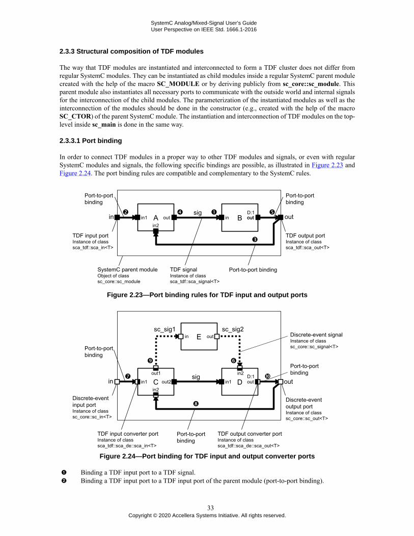
SystemC Analog/Mixed-Signal User’s GuideUser Perspective on IEEE Std. 1666.1-2016
2.3.3 Structural composition of TDF modules
The way that TDF modules are instantiated and interconnected to form a TDF cluster does not differ fromregular SystemC modules. They can be instantiated as child modules inside a regular SystemC parent modulecreated with the help of the macro SC_MODULE or by deriving publicly from sc_core::sc_module. Thisparent module also instantiates all necessary ports to communicate with the outside world and internal signalsfor the interconnection of the child modules. The parameterization of the instantiated modules as well as theinterconnection of the modules should be done in the constructor (e.g., created with the help of the macroSC_CTOR) of the parent SystemC module. The instantiation and interconnection of TDF modules on the top-level inside sc_main is done in the same way.
2.3.3.1 Port binding
In order to connect TDF modules in a proper way to other TDF modules and signals, or even with regularSystemC modules and signals, the following specific bindings are possible, as illustrated in Figure 2.23 andFigure 2.24. The port binding rules are compatible and complementary to the SystemC rules.
Figure 2.23—Port binding rules for TDF input and output ports
Figure 2.24—Port binding for TDF input and output converter ports
Binding a TDF input port to a TDF signal.Binding a TDF input port to a TDF input port of the parent module (port-to-port binding).
33Copyright © 2020 Accellera Systems Initiative. All rights reserved.

SystemC Analog/Mixed-Signal User’s GuideUser Perspective on IEEE Std. 1666.1-2016
Binding a TDF input port to a TDF output port of the parent module (port-to-port binding).Binding a TDF output port to a TDF signal.Binding a TDF output port to a TDF output port of the parent module (port-to-port binding).Binding a TDF input converter port to a discrete-event input signal.Binding a TDF input converter port to a discrete-event input port of the parent module (port-to-portbinding).Binding a TDF input converter port to a discrete-event output port of the parent module (port-to-portbinding).Binding a TDF output converter port to a discrete-event output signal.Binding a TDF output converter port to a discrete-event output port of the parent module (port-to-port binding).
Furthermore, a TDF input port or TDF output port should be bound to exactly one TDF signal throughout thewhole hierarchy. A TDF signal should be bound to exactly one TDF output port of a primitive TDF module,and may be bound to TDF input ports of primitive modules throughout the whole hierarchy. This is shownin Figure 2.25.
Figure 2.25—Port binding in a module hierarchy
Example 2.27 shows the implementation of the structural composition of Figure 2.23.
Example 2.27: Structural composition of TDF modules in a SystemC hierarchical module
SC_MODULE(my_structural_module) {
sca_tdf::sca_in<double> in; sca_tdf::sca_out<double> out;
mod_a a; mod_b b;
SC_CTOR(my_structural_module)
: in("in"), out("out"), a("a"), b("b"), sig("sig") {
a.in1(in); a.in2(out); a.out(sig); b.in(sig); b.out(out); }
private:
sca_tdf::sca_signal<double> sig; };
34Copyright © 2020 Accellera Systems Initiative. All rights reserved.

SystemC Analog/Mixed-Signal User’s GuideUser Perspective on IEEE Std. 1666.1-2016
The TDF input and output ports declared inside this module of class sc_core::sc_module becomepart of the structural composition.The child TDF modules are declared within the parent module. The declaration of these child modulesshould be known prior to the declaration in this context, e.g., by including them via their header files.The initialization-list in the parent module’s constructor propagates the necessary configurationparameters to the TDF ports, TDF signals, and child modules.Port binding is done inside the constructor.Internal TDF signals are used to connect the TDF ports and child modules. These signal are declaredto be private, as they should not be accessible from outside the module.
Example 2.28 shows the implementation of the structural composition of Figure 2.24.
Example 2.28: Structural composition of mixed TDF and SystemC modules
SC_MODULE(my_mixed_module){ sc_core::sc_in<double> in; sc_core::sc_out<double> out;
mod_c c; // TDF primitive module mod_d d; // TDF primitive module mod_e e; // SystemC module SC_CTOR(my_mixed_module) : in("in"), out("out"), c("c"), d("d"), e("e"), sig("sig"), sc_sig1("sc_sig1"), sc_sig2("sc_sig2") { c.in1(in); c.in2(out); c.out1(sc_sig1); c.out2(sig); d.in1(sig); d.in2(sc_sig2); d.out(out); e.in(sc_sig1); e.out(sc_sig2); }
private: sca_tdf::sca_signal<double> sig; sc_core::sc_signal<bool> sc_sig1; sc_core::sc_signal<bool> sc_sig2; };
2.3.4 Multirate behavior
To implement multirate behavior in a TDF module, the TDF port member function set_rate can be used. Asshown in Figure 2.26 and Example 2.29, the rate of the output port is set to 2. For each module activation,one sample is read from the input port, and two samples are written to the output port. This results in anoversampled signal at the output, with a rate equal to the rate of the output port.
Figure 2.26—Multirate example: 2 times oversampling by inserting zeros
As already discussed in Section 2.1.4, the time step of the TDF input port, output port and module shouldbe consistent. As the module time step is set to 20 μs (Tm:20μs), with an input port rate of 1, the samples atthe input port are read each 20 μs. The samples at the output port are written with a time step of 10 μs. This
35Copyright © 2020 Accellera Systems Initiative. All rights reserved.
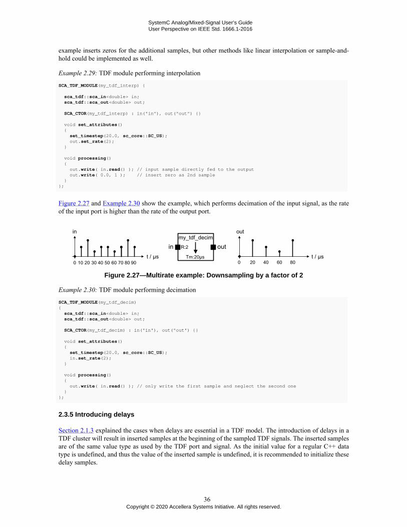
SystemC Analog/Mixed-Signal User’s GuideUser Perspective on IEEE Std. 1666.1-2016
example inserts zeros for the additional samples, but other methods like linear interpolation or sample-and-hold could be implemented as well.
Example 2.29: TDF module performing interpolation
SCA_TDF_MODULE(my_tdf_interp) { sca_tdf::sca_in<double> in; sca_tdf::sca_out<double> out;
SCA_CTOR(my_tdf_interp) : in("in"), out("out") {} void set_attributes() { set_timestep(20.0, sc_core::SC_US); out.set_rate(2); } void processing() { out.write( in.read() ); // input sample directly fed to the output out.write( 0.0, 1 ); // insert zero as 2nd sample }};
Figure 2.27 and Example 2.30 show the example, which performs decimation of the input signal, as the rateof the input port is higher than the rate of the output port.
Figure 2.27—Multirate example: Downsampling by a factor of 2
Example 2.30: TDF module performing decimation
SCA_TDF_MODULE(my_tdf_decim) { sca_tdf::sca_in<double> in; sca_tdf::sca_out<double> out;
SCA_CTOR(my_tdf_decim) : in("in"), out("out") {} void set_attributes() { set_timestep(20.0, sc_core::SC_US); in.set_rate(2); } void processing() { out.write( in.read() ); // only write the first sample and neglect the second one }};
2.3.5 Introducing delays
Section 2.1.3 explained the cases when delays are essential in a TDF model. The introduction of delays in aTDF cluster will result in inserted samples at the beginning of the sampled TDF signals. The inserted samplesare of the same value type as used by the TDF port and signal. As the initial value for a regular C++ datatype is undefined, and thus the value of the inserted sample is undefined, it is recommended to initialize thesedelay samples.
36Copyright © 2020 Accellera Systems Initiative. All rights reserved.

SystemC Analog/Mixed-Signal User’s GuideUser Perspective on IEEE Std. 1666.1-2016
Figure 2.28 shows a basic TDF module, in which a delay of one sample is introduced at the output port.
Figure 2.28—TDF module introducing a delay of one sample
The implementation of this delay is given in Example 2.31. It can be seen in the code, that the delay value isalso initialized with a default value of 1.1.
Example 2.31: TDF module with one sample delay at it output port
SCA_TDF_MODULE(my_tdf_delay) { sca_tdf::sca_in<double> in; sca_tdf::sca_out<double> out;
SCA_CTOR(my_tdf_delay) : in("in"), out("out") {} void set_attributes() { set_timestep(20.0, sc_core::SC_US); out.set_delay(1); }
void initialize() { out.initialize(1.1); } void processing() { out.write( in.read() ); // directly write the input sample to the output (incl the delay) }};
2.4 Interaction between TDF and discrete-event domain
As explained in Section 2.1, the TDF model of computation has its own mechanisms for time annotation, whichcould result in time differences between the local time of each TDF module and the time in the discrete-eventdomain (SystemC kernel time). Therefore, special care should be taken in synchronizing TDF signals with thediscrete-event domain of SystemC in both directions (i.e., reading from and writing to discrete-event signals).
To maintain a high simulation efficiency despite the presence of TDF and discrete-event domain interactions,a loosely-coupled synchronization mechanism can be used, which is called data synchronization. In the caseof data synchronization, the time at which the discrete events occur will not be used for the activation andexecution of TDF modules. Alternatively, the dynamic TDF features now also allow time synchronization,where the activation of TDF modules is driven by the discrete events. Both scenarios are explained in thissection.
2.4.1 Reading from the discrete-event domain
To read from a channel coming from the discrete-event domain, a TDF input converter port ofclass sca_tdf::sca_de::sca_in<T> has to be used, see Figure 2.29. For convenience, the shorter namesca_tdf::sc_in<T> can be used, which class name sc_in indicates the interface to the SystemC discrete-eventdomain. When applying data synchronization, the availability of a discrete-event signal at the TDF inputconverter ports will not activate (‘fire’) module execution. Instead, the TDF module activation order (schedule)
37Copyright © 2020 Accellera Systems Initiative. All rights reserved.

SystemC Analog/Mixed-Signal User’s GuideUser Perspective on IEEE Std. 1666.1-2016
is determined independently at its individual port time step in accordance with the converter port rate and theTDF module time step.
A converter input port will read the value from the bound interface of type sc_core::sc_signal_in_if<T> usingthe member function read during the first delta cycle of the corresponding time. A converter output port willwrite the value to the bound interface of type sc_core::sc_signal_inout_if<T> using the member functionwrite in the first delta cycle of the corresponding time. In the case a channel of type sc_core::sc_signal<T>(which implements the sc_core::sc_signal_in_if<T> and sc_core::sc_signal_inout_if<T> interfaces) is used,the new value written by a converter output port will be read in the second delta cycle of the correspondingtime step following the evaluate-update paradigm of SystemC. Thus, if a converter output port is connected toa converter input port by using a channel of type sc_core::sc_signal<T>, a delay of one time step will occur,as the converter input port will read the value in the first delta cycle of the corresponding time and the newvalue will be available in the second delta cycle.
Example 2.32 shows the data synchronization concept by using one TDF module, which reads the values fromthe discrete-event for further TDF signal processing and writes them to a TDF output port each millisecond.
Figure 2.29—TDF module converting discrete-event signal to TDF signal using data synchronization
Example 2.32: TDF module reading values from the SystemC (discrete-event) domain
SCA_TDF_MODULE(my_de2tdf){ sca_tdf::sca_de::sca_in<double> inp; // TDF input converter port sca_tdf::sca_out<double> out; // TDF output port
SCA_CTOR(my_de2tdf) : inp("inp"), out("out") {}
void set_attributes() { set_timestep(1.0, sc_core::SC_MS); }
void processing() { out.write( inp.read() ); }};
A conversion from the discrete-event and TDF domain using time synchronization is shown inExample 2.33 . The member function change_attributes is used, which embeds the member functionrequest_next_activation to act upon a signal change. The argument of this member function uses thedefault_event mechanism of the converter port to detect the signal change, which is used to set the next moduleactivation. In the case where the elapsed time becomes equal to the maximum time step, because the signalfrom the SystemC discrete-event domain has not changed, the next module activation is equal to the maximumtime step. The maximum time step is defined in the set_attributes callback. As this module makes changes tothe TDF attributes during simulation, it should explicitly call the member function does_attribute_changes.Calling request_next_activation overrules the time step setting defined by member function set_timestepuntil the next activation, however, not the maximum time step defined by member function set_max_timestep.
38Copyright © 2020 Accellera Systems Initiative. All rights reserved.

SystemC Analog/Mixed-Signal User’s GuideUser Perspective on IEEE Std. 1666.1-2016
Figure 2.30—TDF module converting discrete-event signal to TDF signal using time synchronization
Example 2.33: TDF module reading values and synchronizing the time step with the incoming event
SCA_TDF_MODULE(my_de2tdf_dynamic){ sca_tdf::sca_de::sca_in<double> inp; // TDF input converter port sca_tdf::sca_out<double> out; // TDF output port
SCA_CTOR(my_de2tdf_dynamic) : inp("inp"), out("out") {}
void set_attributes() { does_attribute_changes(); set_timestep(1.0, sc_core::SC_MS); set_max_timestep(1.0, sc_core::SC_MS); }
void processing() { out.write( inp.read() ); } void change_attributes() { request_next_activation(inp.default_event()); // next activation when control signal changes }};
2.4.2 Writing to the discrete-event domain
To write to a channel in the discrete-event domain, a TDF output converter port of classsca_tdf::sca_de::sca_out<T> should be used, see Figure 2.31. For convenience, the shorter namesca_tdf::sc_out<T> can be used, which class name sc_out directly indicates the interface to the SystemCdiscrete-event domain. The time step assigned to the output converter port defines at which time point andtime interval a value is written to the discrete-event domain.
A converter output port will write a value to the bound interface of type sc_core::sc_signal_inout_if<T>using the member function write in the first delta cycle of the corresponding time. If the converter output portis bound to a channel of class sc_core::sc_signal<T>, there is only an event generated in case of a signalchange, as indicated with the events e1, e2, and e3. If the converter output port is bound to a channel of classsc_core::sc_buffer<T>, all samples written to the port will generate an event, as indicated with the additionalsamples e11, e12, e13, etc.
39Copyright © 2020 Accellera Systems Initiative. All rights reserved.

SystemC Analog/Mixed-Signal User’s GuideUser Perspective on IEEE Std. 1666.1-2016
Figure 2.31—TDF module with a converter port as output
Example 2.34 shows the implementation of a TDF module, which writes samples to the discrete-event domain.
Example 2.34: TDF module writing values to the SystemC (discrete-event) domain
SCA_TDF_MODULE(my_tdf2de){ sca_tdf::sca_in<double> in; // TDF input port sca_tdf::sca_de::sca_out<double> outp; // TDF output converter port
SCA_CTOR(my_tdf2de) : in("in"), outp("outp") {}
void set_attributes() { set_timestep(1.0, sc_core::SC_MS); }
void processing() { outp.write( in.read() ); }};
2.4.3 Using discrete-event control signals
Example 2.35 shows a simple digitally controlled gain amplifier, in which the gain is defined by an externalcontrol signal from the discrete-event domain. The execution frequency of the member function processing isdefined by the module time step, which is set to 1 ms. Each time the processing function is called, the controlsignal from the discrete-event domain is read.
Figure 2.32—TDF module with a converter port used as control input
40Copyright © 2020 Accellera Systems Initiative. All rights reserved.

SystemC Analog/Mixed-Signal User’s GuideUser Perspective on IEEE Std. 1666.1-2016
Example 2.35: Digitally controlled gain amplifier with discrete-event control input
SCA_TDF_MODULE(my_dga){ sca_tdf::sca_in<double> in; // input port sca_tdf::sca_out<double> out; // output port
// control signal from the discrete-event domain sca_tdf::sca_de::sca_in<bool> high_gain_state; // input converter port
SCA_CTOR(my_dga) : in("in"), out("out"), high_gain_state("high_gain_state"), high_gain(100.0), low_gain(1.0) {}
void set_attributes() { set_timestep(1.0, sc_core::SC_MS); }
void processing() { double gain = high_gain_state.read() ? high_gain : low_gain; out.write( gain * in.read() ); }
private: double high_gain, low_gain; };
In Example 2.35, the value of the control signal was read during the processing callback each millisecond,which means that the exact time of a control signal change gets lost. When using the dynamic TDF features, thetime at which the digital control signal changes can be used to activate the member function processing in theTDF module. For this, the member function change_attributes is introduced, in which the member functionrequest_next_activation is used to act upon a signal change (caused by an event) at the converter input portand use the time at which the event occurred for the next module activation. Furthermore, the TDF moduleshould explicitly define that it will change attributes, by calling the member function does_attribute_changesin the set_attributes callback.
In order to allow changing attributes caused by other TDF modules in the same cluster, the member functionaccept_attribute_changes is called in the same callback. The member function set_max_timestep is essentialto guarantee that the module time step does not become greater than 1 ms. Example 2.36 shows the digitallycontrolled gain amplifier using the dynamic TDF execution semantics.
Example 2.36: Digitally controlled gain amplifier with time step synchronization
SCA_TDF_MODULE(my_dga_dynamic){ sca_tdf::sca_in<double> in; // input port sca_tdf::sca_out<double> out; // output port
// control signal from the discrete-event domain sca_tdf::sca_de::sca_in<bool> high_gain_state; // input converter port
SCA_CTOR(my_dga_dynamic) : in("in"), out("out"), high_gain_state("high_gain_state"), high_gain(100.0), low_gain(1.0) {}
void set_attributes() { accept_attribute_changes(); // module accepts changing attribute // caused by other TDF modules does_attribute_changes(); // module actively changes attributes set_timestep(1.0, sc_core::SC_MS); set_max_timestep(1.0, sc_core::SC_MS); // bound maximum time step to 1ms }
void processing() { double gain = high_gain_state.read() ? high_gain : low_gain; out.write( gain * in.read() );
41Copyright © 2020 Accellera Systems Initiative. All rights reserved.

SystemC Analog/Mixed-Signal User’s GuideUser Perspective on IEEE Std. 1666.1-2016
}
void change_attributes() { request_next_activation(high_gain_state); // next module activation when control signal changes }
private: double high_gain, low_gain;};
2.5 TDF execution semantics
In addition to the elaboration and simulation phases as defined in SystemC language standard IEEE Std.1666-2011, specific functionality is implemented for the elaboration and execution of TDF models. Theessential TDF module member functions for time-domain simulation are set_attributes, initialize, processing,change_attributes, and reinitialize. A user should override these member functions to implement the actualbehavior of the TDF modules. It is not allowed to call these member functions directly.
As depicted in Figure 2.33, the elaboration phase includes the following steps:— TDF module attribute settings: Execute the (optional) member function set_attributes of all
TDF modules.— TDF time step calculation and propagation: Propagate and calculate unassigned port and module time
steps based on the assigned time steps and port rates. (see Section 2.1.4).— TDF cluster computability check: Define and check the cluster schedule.
The steps for the simulation phase are:— TDF module initialization: Execute the (optional) member function initialize of all TDF modules. Prior
to the execution of this member function, the simulation time advances using the calculated time step.— TDF module activation and processing: Execute the member function processing of all TDF modules
which belong to the same cluster.— Change TDF module attribute settings:: Execute the (optional) member functions change_attributes
of all TDF modules. These member functions are called at the end of the cluster execution period.— TDF time step calculation and propagation: Again propagate and calculate unassigned port and module
time steps based on the assigned time steps and port rates, because they could have changed in thechange_attributes callback.
— TDF cluster computability check: Again check the cluster schedule after potential attribute changesmade in the change_attributes callback.
— TDF module reinitialization: Execute the (optional) member function reinitialize of all TDF modules.Prior to the execution of this member function, the simulation time advances using the calculated timestep.
42Copyright © 2020 Accellera Systems Initiative. All rights reserved.

SystemC Analog/Mixed-Signal User’s GuideUser Perspective on IEEE Std. 1666.1-2016
Figure 2.33—TDF elaboration and simulation phases
The elaboration and simulation phases are executed by starting a time-domain simulation using the functionsc_core::sc_start. This is explained in Section 6.1.1. As soon as the simulation time is equal to the specifiedtime, which is defined as argument in the function sc_core::sc_start, the function will return. A call tothe function sc_core::sc_stop will finish the simulation. When the function sc_core::sc_stop is called, thecallback end_of_simulation of all TDF modules is executed. Note that these functions and callback are notpart of the SystemC AMS extensions, but are inherited from the SystemC module base class.
43Copyright © 2020 Accellera Systems Initiative. All rights reserved.
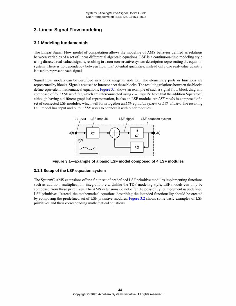
SystemC Analog/Mixed-Signal User’s GuideUser Perspective on IEEE Std. 1666.1-2016
3. Linear Signal Flow modeling
3.1 Modeling fundamentals
The Linear Signal Flow model of computation allows the modeling of AMS behavior defined as relationsbetween variables of a set of linear differential algebraic equations. LSF is a continuous-time modeling styleusing directed real-valued signals, resulting in a non-conservative system description representing the equationsystem. There is no dependency between flow and potential quantities; instead only one real-value quantityis used to represent each signal.
Signal flow models can be described in a block diagram notation. The elementary parts or functions arerepresented by blocks. Signals are used to interconnect these blocks. The resulting relations between the blocksdefine equivalent mathematical equations. Figure 3.1 shows an example of such a signal flow block diagram,composed of four LSF modules, which are interconnected using LSF signals. Note that the addition ‘operator’,although having a different graphical representation, is also an LSF module. An LSF model is composed of aset of connected LSF modules, which will form together an LSF equation system or LSF cluster. The resultingLSF model has input and output LSF ports to connect it with other modules.
Figure 3.1—Example of a basic LSF model composed of 4 LSF modules
3.1.1 Setup of the LSF equation system
The SystemC AMS extensions offer a finite set of predefined LSF primitive modules implementing functionssuch as addition, multiplication, integration, etc. Unlike the TDF modeling style, LSF models can only becomposed from these primitives. The AMS extensions do not offer the possibility to implement user-definedLSF primitives. Instead, the mathematical equations describing the intended functionality should be createdby composing the predefined set of LSF primitive modules. Figure 3.2 shows some basic examples of LSFprimitives and their corresponding mathematical equations.
44Copyright © 2020 Accellera Systems Initiative. All rights reserved.

SystemC Analog/Mixed-Signal User’s GuideUser Perspective on IEEE Std. 1666.1-2016
Figure 3.2—Examples of some basic LSF primitivesand their corresponding mathematical equations
When creating an LSF model (block diagram), the mathematical equations for each block and theirinterconnection will be used to compose the overall equation system. For example, the LSF model presentedin Figure 3.1 will result in the following equation system based on the contributed equations of each primitiveas shown in Figure 3.2:
(3.1)
Note that the scale coefficients of the addition and the first-order time derivative block are set to 1. Instead,additional multiplication blocks k1 and k2 are used for this example.
3.1.2 Time step assignment and propagation
Similar as for a TDF module, a time step can be assigned to an LSF module directly or can be assignedautomatically using the propagation mechanism of the time step within an LSF cluster. In the case where anLSF model is connected to a TDF model, the time step from the connected TDF port(s) is propagated to theLSF model. Consistency between locally defined LSF module time step and propagated time step is essential.Otherwise, the time points for the solution of the LSF equation system or communication with the connectedTDF model cannot be defined properly (see also Section 2.1.4). The time step should be defined at least atone location in the entire system.
During simulation, the LSF equation system is solved numerically with appropriate time steps, which couldbe less than the assigned time step. The solver will at least provide results at the time points calculated fromthe assigned time steps.
3.2 Language constructs
3.2.1 LSF modules
A Linear Signal Flow module is a predefined primitive module to represent a particular function ormathematical relation, which will become part of an overall equation system. The available predefined LSFprimitive modules are listed in Table 3.1. Annex A gives the details for each LSF module.
Table 3.1—LSF primitive modules
LSF module name Descriptionsca_lsf::sca_add Weighted addition of two LSF signals.
45Copyright © 2020 Accellera Systems Initiative. All rights reserved.

SystemC Analog/Mixed-Signal User’s GuideUser Perspective on IEEE Std. 1666.1-2016
LSF module name Descriptionsca_lsf::sca_sub Weighted subtraction of two LSF signals.sca_lsf::sca_gain Multiplication of an LSF signal by a constant gain.sca_lsf::sca_dot Scaled first-order time derivative of an LSF signal.sca_lsf::sca_integ Scaled time-domain integration of an LSF signal.sca_lsf::sca_delay Scaled time-delayed version of an LSF signal.sca_lsf::sca_source LSF source.sca_lsf::sca_ltf_nd Scaled Laplace transfer function in the time-domain in the numerator-
denominator form.sca_lsf::sca_ltf_zp Scaled Laplace transfer function in the time-domain in the zero-pole
form.sca_lsf::sca_ss Single-input single-output state-space equation.sca_lsf::sca_tdf::sca_gain,sca_lsf::sca_tdf_gain
Scaled multiplication of a TDF input signal with an LSF input signal.
sca_lsf::sca_tdf::sca_source,sca_lsf::sca_tdf_source
Scaled conversion of a TDF input signal to an LSF output signal.
sca_lsf::sca_tdf::sca_sink,sca_lsf::sca_tdf_sink
Scaled conversion from an LSF input signal to a TDF output signal.
sca_lsf::sca_tdf::sca_mux,sca_lsf::sca_tdf_mux
Selection of one of two LSF input signals by a TDF control signal(multiplexer).
sca_lsf::sca_tdf::sca_demux,sca_lsf::sca_tdf_demux
Routing of an LSF input signal to either one of two LSF output signalscontrolled by a TDF signal (demultiplexer).
sca_lsf::sca_de::sca_gain,sca_lsf::sca_de_gain
Scaled multiplication of a discrete-event input signal by an LSF inputsignal.
sca_lsf::sca_de::sca_source,sca_lsf::sca_de_source
Scaled conversion of a discrete-event input signal to an LSF outputsignal.
sca_lsf::sca_de::sca_sink,sca_lsf::sca_de_sink
Scaled conversion from an LSF input signal to a discrete-event outputsignal.
sca_lsf::sca_de::sca_mux,sca_lsf::sca_de_mux
Selection of one of two LSF input signals by a discrete-event controlsignal (multiplexer).
sca_lsf::sca_de::sca_demux,sca_lsf::sca_de_demux
Routing of an LSF input signal to either one of two LSF output signalscontrolled by a discrete-event signal (demultiplexer).
3.2.1.1 Module time step
In order to solve the LSF equation system, a time step has to be associated to the set of connected LSF modulesas part of the elaboration phase. This can be done with the LSF module member function set_timestep.Alternatively, the LSF model can rely on the time step propagation mechanism, which passes the time stepfrom module to module via its ports across the TDF, LSF, and ELN models of computation. So in the casewhere an LSF model is connected to a TDF model, the time step from the connected port, if available, ispropagated to the LSF model. The consistency between propagated time steps and user-defined time steps iscompulsory, as described in Section 2.1.4.
The module time step can be assigned by calling the member function set_timestep of the instantiated objectwithin the constructor of the parent module, and passing a double value and the time unit or an object of typesca_core::sca_time, as shown in Example 3.1.
Example 3.1: SystemC hierarchical module instantiating an LSF source with time step assignment
SC_MODULE(my_lsf_source){ // port declaration sca_lsf::sca_out y;
46Copyright © 2020 Accellera Systems Initiative. All rights reserved.

SystemC Analog/Mixed-Signal User’s GuideUser Perspective on IEEE Std. 1666.1-2016
// child module declaration sca_lsf::sca_source src; SC_CTOR(my_lsf_source) : y("y"), src("src", 0.0, 0.0, 1.0e-3, 1.0e3) // 1 kHz sinusoidal source with an amplitude of 1e-3 { src.set_timestep(0.5, sc_core::SC_MS); // set module time step of source to 0.5 ms src.y(y); }};
3.2.2 LSF ports
An LSF port is an object that can be used to connect several LSF models together using LSF signals whichare bound to this port. Due to the nature of the LSF modeling formalism, an LSF port can be either an inputport or an output port, but not inout. LSF ports are used to connect LSF modules using signals of classsca_lsf::sca_signal. As LSF ports are always hierarchical ports inside a parent module, they can be used toconnect to the LSF child modules directly, following the port-to-port binding rule (see Section 3.3.1). LSFports have a predefined data type, also called signal flow nature, which prevents the usage of user-defineddata types.
There are currently two classes of LSF ports:— LSF input ports of class sca_lsf::sca_in.— LSF output ports of class sca_lsf::sca_out.
Example 3.2 shows how LSF ports are used within an LSF structural model.
Example 3.2: LSF structural model with ports
SC_MODULE(my_lsf_model){ // port declarations
sca_lsf::sca_in x;
sca_lsf::sca_out y;
SC_CTOR(my_lsf_model) : x("x"), y("y") { // LSF primitives instantiated here }};
LSF input port that carries a continuous-time and continuous-value signal x(t).LSF output port that carries a continuous-time and continuous-value signal y(t).Using the constructor initialization-list to assign the names “x” and “y” to the input and output ports,respectively.
There are no converter ports available for LSF. Instead, specialized converter modules are provided to connectto the TDF or discrete-event domain. This is explained in Section 3.4. Unlike TDF ports, the LSF ports do notprovide member functions to directly read to or write from the channel.
3.2.3 LSF signals
LSF signals are used to connect LSF primitive modules together. LSF signals represent a variable of the timeand value continuous equation system, while LSF ports determine the direction of the signals from one LSFmodule to another. Therefore, the LSF signals are not defined as a template class and should be used accordingto Example 3.3.
47Copyright © 2020 Accellera Systems Initiative. All rights reserved.

SystemC Analog/Mixed-Signal User’s GuideUser Perspective on IEEE Std. 1666.1-2016
Example 3.3: LSF signal
// signal declaration sca_lsf::sca_signal sig; // LSF signal
As in SystemC, the constructor initialization-list of the parent module can be used to assign a user-definedname to a signal:
Example 3.4: Assigning names to LSF signals using the SystemC constructor
// assign the names of LSF signal instance in the constructor initialization-list SC_CTOR(my_module) : sig("sig") {}
Section 3.3 will describe the creation of structural LSF models and will show examples of assigning user-defined names to ports and signals.
3.3 Modeling continuous-time behavior
LSF models can be used to implement linear dynamic, continuous-time behavior. LSF models can only becomposed using LSF primitive modules. Therefore an LSF model is always a structural model.
3.3.1 Structural composition of LSF modules
LSF modules should be instantiated as child modules inside a regular SystemC parent module createdwith the help of the macro SC_MODULE or by deriving publicly from sc_core::sc_module. This parentmodule also instantiates all necessary ports to communicate with the outside world and internal signals forthe interconnection of the child modules. The parameterization of the instantiated modules as well as theinterconnection of the modules should be done in the constructor (e.g., created with the help of the macroSC_CTOR) of the parent SystemC module.
3.3.1.1 Port binding
In order to connect LSF modules in a proper way to other LSF modules and signals, the following specificbindings are possible, illustrated in Figure 3.3. The port binding rules are compatible and complementary tothe SystemC and TDF rules (see also Section 2.3.3).
Figure 3.3—Port binding rules for LSF input and output ports
Binding an LSF input port to an LSF signal.Binding an LSF input port to an LSF input port of the parent module (port-to-port binding).Binding an LSF input port to an LSF output port of the parent module (port-to-port binding).Binding an LSF output port to an LSF signal.Binding an LSF output port to an LSF output port of the parent module (port-to-port binding).
48Copyright © 2020 Accellera Systems Initiative. All rights reserved.
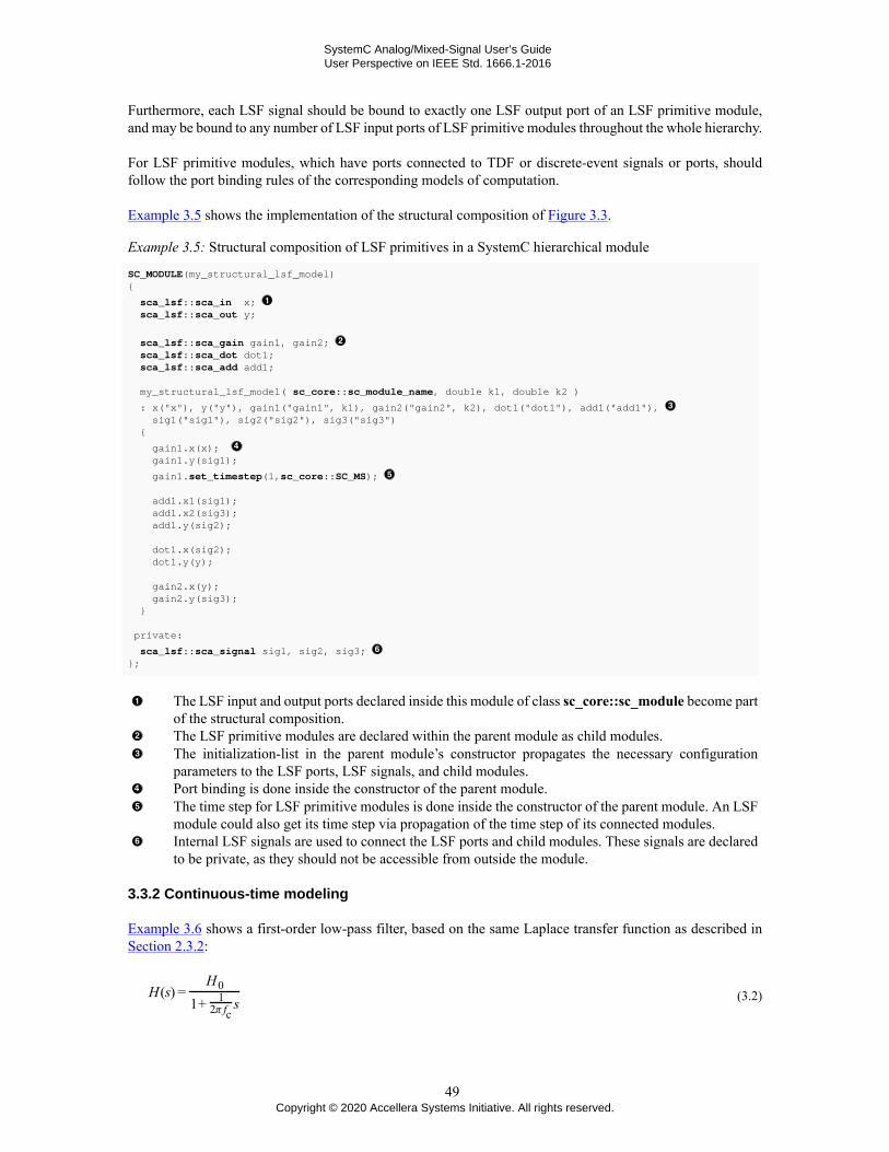
SystemC Analog/Mixed-Signal User’s GuideUser Perspective on IEEE Std. 1666.1-2016
Furthermore, each LSF signal should be bound to exactly one LSF output port of an LSF primitive module,and may be bound to any number of LSF input ports of LSF primitive modules throughout the whole hierarchy.
For LSF primitive modules, which have ports connected to TDF or discrete-event signals or ports, shouldfollow the port binding rules of the corresponding models of computation.
Example 3.5 shows the implementation of the structural composition of Figure 3.3.
Example 3.5: Structural composition of LSF primitives in a SystemC hierarchical module
SC_MODULE(my_structural_lsf_model){
sca_lsf::sca_in x; sca_lsf::sca_out y;
sca_lsf::sca_gain gain1, gain2; sca_lsf::sca_dot dot1; sca_lsf::sca_add add1; my_structural_lsf_model( sc_core::sc_module_name, double k1, double k2 )
: x("x"), y("y"), gain1("gain1", k1), gain2("gain2", k2), dot1("dot1"), add1("add1"), sig1("sig1"), sig2("sig2"), sig3("sig3") {
gain1.x(x); gain1.y(sig1);
gain1.set_timestep(1,sc_core::SC_MS); add1.x1(sig1); add1.x2(sig3); add1.y(sig2);
dot1.x(sig2); dot1.y(y);
gain2.x(y); gain2.y(sig3); } private:
sca_lsf::sca_signal sig1, sig2, sig3; };
The LSF input and output ports declared inside this module of class sc_core::sc_module become partof the structural composition.The LSF primitive modules are declared within the parent module as child modules.The initialization-list in the parent module’s constructor propagates the necessary configurationparameters to the LSF ports, LSF signals, and child modules.Port binding is done inside the constructor of the parent module.The time step for LSF primitive modules is done inside the constructor of the parent module. An LSFmodule could also get its time step via propagation of the time step of its connected modules.Internal LSF signals are used to connect the LSF ports and child modules. These signals are declaredto be private, as they should not be accessible from outside the module.
3.3.2 Continuous-time modeling
Example 3.6 shows a first-order low-pass filter, based on the same Laplace transfer function as described inSection 2.3.2:
(3.2)
49Copyright © 2020 Accellera Systems Initiative. All rights reserved.

SystemC Analog/Mixed-Signal User’s GuideUser Perspective on IEEE Std. 1666.1-2016
where H0 is the DC gain and fc is the filter cut-off frequency in Hz. The Laplace transfer function can berewritten for an LSF implementation into:
(3.3)
The block diagram notation and code implementation is given in Figure 3.4, where the scaling coefficients ofthe LSF primitive modules are used to implement the DC gain H0 and the filter cut-off frequency fc.
Figure 3.4—Example of an LSF model implementing a first-order low-pass filter
Example 3.6: LSF model implementing a first-order low-pass filter
SC_MODULE(my_lsf_filter){ sca_lsf::sca_in x; sca_lsf::sca_out y; sca_lsf::sca_sub sub1; sca_lsf::sca_dot dot1; my_lsf_filter( sc_core::sc_module_name, double h0 = 1.0, double fc = 1.0e3 ) : x("x"), y("y"), sub1("sub1", h0), dot1("dot1", 1.0/(2.0*M_PI*fc) ), sig("sig") { sub1.x1(x); sub1.x2(sig); sub1.y(y);
dot1.x(y); dot1.y(sig); } private: sca_lsf::sca_signal sig;};
The gain coefficient h0 for the input signal is passed via the constructor to the instance sub1 and the frequencyfc is passed via the constructor to the instance dot1.
3.4 Interaction between LSF and discrete-event or TDF models
The LSF model of computation will setup and solve an equation system to simulate the modeled continuous-time behavior, based on the basic set of LSF primitive modules described in Section 3.2.1. Any ‘external’ inputvalue, e.g., from a discrete-event signal or TDF sample, needs to be contributed to the equation system via oneof these LSF primitive modules. Therefore, specialized LSF primitive modules with ports to the discrete-eventdomain and TDF models of computation are available, which are called converter modules. Main purpose ofthese modules is to establish an interface to convert and transfer data from one model of computation to theother.
50Copyright © 2020 Accellera Systems Initiative. All rights reserved.

SystemC Analog/Mixed-Signal User’s GuideUser Perspective on IEEE Std. 1666.1-2016
3.4.1 Reading from and writing to discrete-event models
In order to connect LSF models with discrete-event models, the LSF converter modules with an internal portof class sc_core::sc_in or sc_core::sc_out should be used.
Figure 3.5 shows the LSF primitive module sca_lsf::sca_de::sca_source reading from a discrete-event signaland writing to an LSF signal. In this example a module time step of 1 ms is assigned to the LSF convertermodule. The LSF model continuously reads values from the input at the time points, which are calculated fromthe assigned time steps. The input value is assumed constant until the next value is read. The input values areinterpreted to form a continuous-time signal, which is made available at the output of the converter module(read input samples shown as a dotted signal).
Figure 3.5—LSF converter module reading from a discrete-event input signal and writing to an LSF output signal
Figure 3.6 shows the LSF primitive module sca_lsf::sca_de::sca_sink, which reads an LSF signal and writesthe equivalent value to the discrete-event signal. The values at the output port are written at the time points,which are calculated from the assigned module time step of 1 ms.
Figure 3.6—LSF converter module reading from an LSFinput signal and writing to a discrete-event output signal
3.4.2 Reading from and writing to TDF models
In a similar way, LSF models can be connected to TDF models using converter modules with an internal portof class sca_tdf::sca_in or sca_tdf::sca_out.
Figure 3.7 shows the LSF primitive module sca_lsf::sca_tdf::sca_source reading from a TDF signal andwriting to an LSF signal. In this example a module time step of 1 ms is assigned to the LSF converter module.The LSF model continuously reads the samples from the TDF input. The input samples are interpreted to forma continuous-time signal, available at the output of the converter module (input samples shown as a dottedsignal).
51Copyright © 2020 Accellera Systems Initiative. All rights reserved.

SystemC Analog/Mixed-Signal User’s GuideUser Perspective on IEEE Std. 1666.1-2016
Figure 3.7—LSF converter module reading from aTDF input signal and writing to an LSF output signal
Figure 3.8 shows the LSF primitive module sca_lsf::sca_tdf::sca_sink reading an LSF signal and writing theequivalent values to a TDF signal. The samples at the output port are written at the time points, which arecalculated from the assigned module time step of 1 ms.
Figure 3.8—LSF converter module reading from anLSF input signal and writing to a TDF output signal
3.4.3 Using discrete-event or TDF control signals
Although not fundamentally different from the LSF converter modules described in the previoustwo sections, additional LSF primitives are available to control or scale variables or signalswithin an LSF equation system. The LSF primitives used for control can be identified byhaving an input port of class sc_core::sc_in or sca_tdf::sca_in of data type bool. Examplesare the multiplexers (sca_lsf::sca_de::sca_mux and sca_lsf::sca_tdf::sca_mux) and demultiplexers(sca_lsf::sca_de::sca_demux and sca_lsf::sca_tdf::sca_demux). The primitives, which can scale variablesor signals make use of the same ports, but using data type double. Examples are the multiplication primitives(sca_lsf::sca_de::sca_gain, and sca_lsf::sca_tdf::sca_gain). Note that if a parameter of an LSF module haschanged, the corresponding LSF equation system will be reinitialized.
Figure 3.9 shows an example how LSF primitives can be used in a structural model to control or scale signals.
52Copyright © 2020 Accellera Systems Initiative. All rights reserved.

SystemC Analog/Mixed-Signal User’s GuideUser Perspective on IEEE Std. 1666.1-2016
Figure 3.9—LSF model using discrete-event and TDF control signals
Similar as for the LSF converter modules described in Section 3.4, the discrete-event or TDF control signalsare read with a fixed time step, which corresponds to the module time step. Only then the LSF equation systemwill be updated.
3.4.4 LSF model encapsulation
The converter modules described in the previous sections can be used to encapsulate an LSF model withina different model of computation. Figure 3.10 shows an example on how to use converter modules to andfrom the TDF model of computation to encapsulate LSF behavior. In this case, access to and from the LSFequation system use discrete-time signals following the TDF semantics, whereas the internal LSF signals andcomputations are continuous-time. This approach gives another possibility to embed continuous-time behaviorin the TDF model of computation, besides the embedded linear dynamic equations for TDF modules describedin Section 2.3.2.
Figure 3.10—LSF equation system encapsulated for inclusion intoa structural TDF model description by using converter modules
Example 3.7 shows the implementation of Figure 3.10.
Example 3.7: SystemC hierarchical module with TDF input and output port encapsulating LSF behavior
SC_MODULE(lsf_in_tdf){ sca_tdf::sca_in<double> in; sca_tdf::sca_out<double> out;
53Copyright © 2020 Accellera Systems Initiative. All rights reserved.
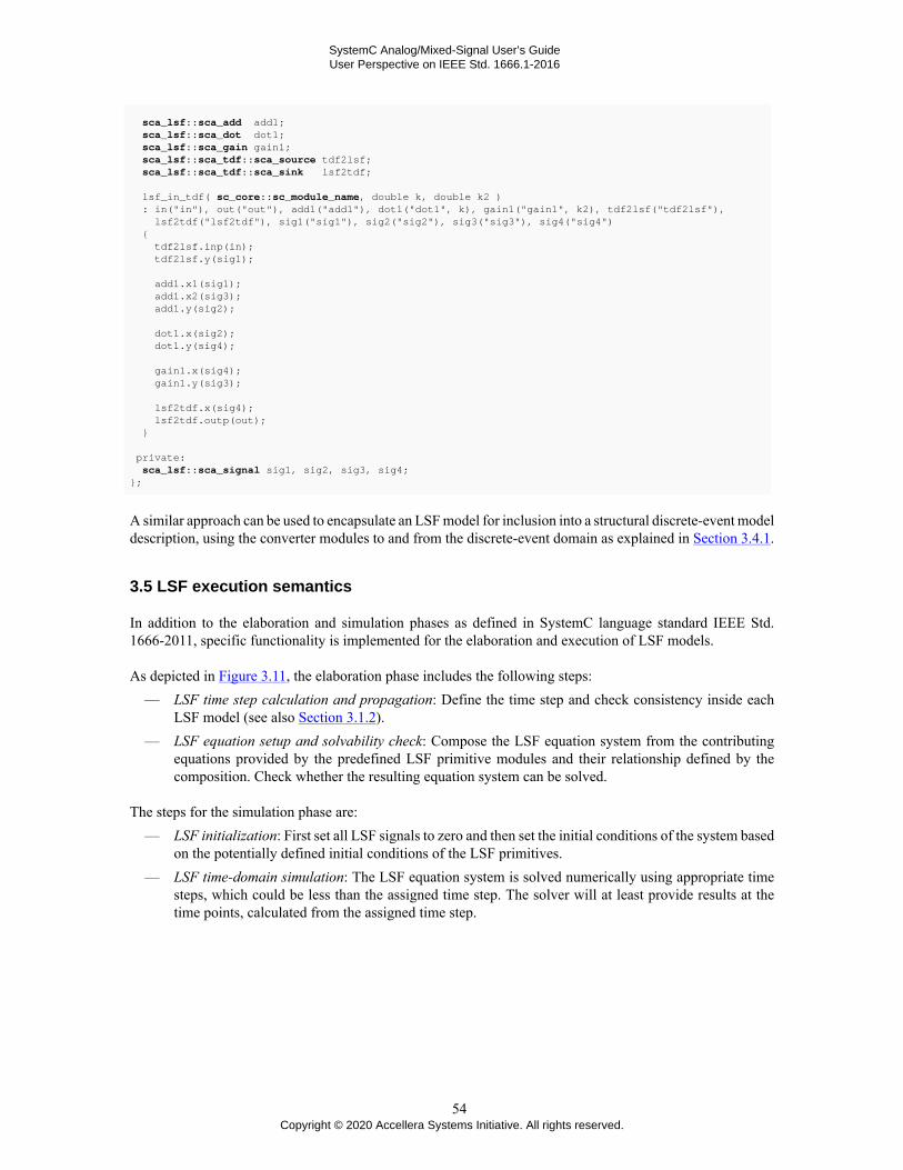
SystemC Analog/Mixed-Signal User’s GuideUser Perspective on IEEE Std. 1666.1-2016
sca_lsf::sca_add add1; sca_lsf::sca_dot dot1; sca_lsf::sca_gain gain1; sca_lsf::sca_tdf::sca_source tdf2lsf; sca_lsf::sca_tdf::sca_sink lsf2tdf; lsf_in_tdf( sc_core::sc_module_name, double k, double k2 ) : in("in"), out("out"), add1("add1"), dot1("dot1", k), gain1("gain1", k2), tdf2lsf("tdf2lsf"), lsf2tdf("lsf2tdf"), sig1("sig1"), sig2("sig2"), sig3("sig3"), sig4("sig4") { tdf2lsf.inp(in); tdf2lsf.y(sig1);
add1.x1(sig1); add1.x2(sig3); add1.y(sig2); dot1.x(sig2); dot1.y(sig4);
gain1.x(sig4); gain1.y(sig3);
lsf2tdf.x(sig4); lsf2tdf.outp(out); } private: sca_lsf::sca_signal sig1, sig2, sig3, sig4;};
A similar approach can be used to encapsulate an LSF model for inclusion into a structural discrete-event modeldescription, using the converter modules to and from the discrete-event domain as explained in Section 3.4.1.
3.5 LSF execution semantics
In addition to the elaboration and simulation phases as defined in SystemC language standard IEEE Std.1666-2011, specific functionality is implemented for the elaboration and execution of LSF models.
As depicted in Figure 3.11, the elaboration phase includes the following steps:— LSF time step calculation and propagation: Define the time step and check consistency inside each
LSF model (see also Section 3.1.2).— LSF equation setup and solvability check: Compose the LSF equation system from the contributing
equations provided by the predefined LSF primitive modules and their relationship defined by thecomposition. Check whether the resulting equation system can be solved.
The steps for the simulation phase are:— LSF initialization: First set all LSF signals to zero and then set the initial conditions of the system based
on the potentially defined initial conditions of the LSF primitives.— LSF time-domain simulation: The LSF equation system is solved numerically using appropriate time
steps, which could be less than the assigned time step. The solver will at least provide results at thetime points, calculated from the assigned time step.
54Copyright © 2020 Accellera Systems Initiative. All rights reserved.

SystemC Analog/Mixed-Signal User’s GuideUser Perspective on IEEE Std. 1666.1-2016
Figure 3.11—LSF elaboration and simulation phases
The elaboration and simulation phase are executed by starting a time-domain simulation using the functionsc_core::sc_start. This is explained in Section 6.1.1.
55Copyright © 2020 Accellera Systems Initiative. All rights reserved.

SystemC Analog/Mixed-Signal User’s GuideUser Perspective on IEEE Std. 1666.1-2016
4. Electrical Linear Networks modeling
4.1 Modeling fundamentals
The Electrical Linear Networks model of computation introduces the use of electrical primitives and theirinterconnections to model conservative, continuous-time behavior. The ELN modeling style allows theinstantiation of electrical primitives, which can be connected together using electrical nodes, to form anelectrical network. The mathematical relations between the electrical primitives are defined at each node inthe network, where both the potential (voltage) and flow (current) quantities are used according to Kirchhoff’svoltage law (KVL) and Kirchhoff’s current law (KCL). As such, the electrical network is represented by aset of differential algebraic equations, which will be resolved during simulation to determine the actual circuitbehavior.
Figure 4.1 shows an example of an electrical network, with two resistors, a capacitor, and a current source.Such a network is called an ELN model and is composed of a set of connected ELN primitive modules, whichwill form together an ELN equation system or cluster. Each ELN primitive module can have one or moreELN terminals. The ELN primitive modules are interconnected via their terminals using ELN nodes. Thereference or ground node, which always has a voltage of zero, is called ELN reference node. ELN terminalsare also used as an interface to connect the ELN model with other ELN models.
Figure 4.1—Example of a basic ELN model representing an electrical network
4.1.1 Setup of the equation system
The SystemC AMS extensions offer a finite set of ELN primitive modules such as sources (voltage or current),linear lumped elements (resistors, capacitors, inductors), linear distributed elements (transmission lines), idealamplifier (nullor), ideal transformer, linear gyrator, and ideal switches. Similar to the LSF modeling style,ELN models can only be composed from these primitives, as there is no possibility to implement user-definedelectrical primitives. Figure 4.2 shows some ELN lumped elements and their corresponding mathematicalequations.
ip,n(t) = C ·d(vp,n(t) +
q0C )
dt vp,n(t) = L ·d(ip,n(t) +
psi0L )
dtvp,n(t) = ip,n(t) · R
Figure 4.2—Examples of the basic ELN lumped elements: resistor (R), capacitor(C), and inductor (L) with their corresponding mathematical equations
When creating an ELN model (electrical network), the mathematical equations for each primitive and theirrelationship defined at each node will be used to compose the overall equation system. For example, theELN model presented in Figure 4.1 will result in an ELN equation system for node A and B by following
56Copyright © 2020 Accellera Systems Initiative. All rights reserved.
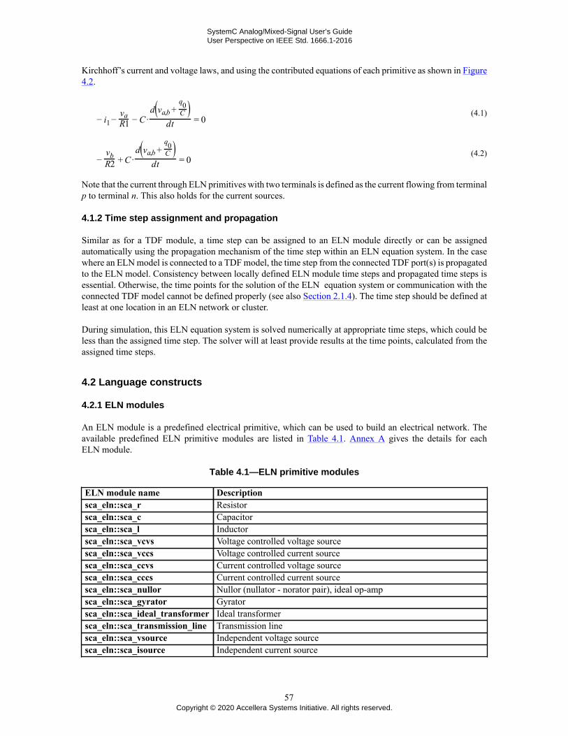
SystemC Analog/Mixed-Signal User’s GuideUser Perspective on IEEE Std. 1666.1-2016
Kirchhoff’s current and voltage laws, and using the contributed equations of each primitive as shown in Figure4.2.
(4.1)
(4.2)
Note that the current through ELN primitives with two terminals is defined as the current flowing from terminalp to terminal n. This also holds for the current sources.
4.1.2 Time step assignment and propagation
Similar as for a TDF module, a time step can be assigned to an ELN module directly or can be assignedautomatically using the propagation mechanism of the time step within an ELN equation system. In the casewhere an ELN model is connected to a TDF model, the time step from the connected TDF port(s) is propagatedto the ELN model. Consistency between locally defined ELN module time steps and propagated time steps isessential. Otherwise, the time points for the solution of the ELN equation system or communication with theconnected TDF model cannot be defined properly (see also Section 2.1.4). The time step should be defined atleast at one location in an ELN network or cluster.
During simulation, this ELN equation system is solved numerically at appropriate time steps, which could beless than the assigned time step. The solver will at least provide results at the time points, calculated from theassigned time steps.
4.2 Language constructs
4.2.1 ELN modules
An ELN module is a predefined electrical primitive, which can be used to build an electrical network. Theavailable predefined ELN primitive modules are listed in Table 4.1. Annex A gives the details for eachELN module.
Table 4.1—ELN primitive modules
ELN module name Descriptionsca_eln::sca_r Resistorsca_eln::sca_c Capacitorsca_eln::sca_l Inductorsca_eln::sca_vcvs Voltage controlled voltage sourcesca_eln::sca_vccs Voltage controlled current sourcesca_eln::sca_ccvs Current controlled voltage sourcesca_eln::sca_cccs Current controlled current sourcesca_eln::sca_nullor Nullor (nullator - norator pair), ideal op-ampsca_eln::sca_gyrator Gyratorsca_eln::sca_ideal_transformer Ideal transformersca_eln::sca_transmission_line Transmission linesca_eln::sca_vsource Independent voltage sourcesca_eln::sca_isource Independent current source
57Copyright © 2020 Accellera Systems Initiative. All rights reserved.

SystemC Analog/Mixed-Signal User’s GuideUser Perspective on IEEE Std. 1666.1-2016
ELN module name Descriptionsca_eln::sca_tdf::sca_r,sca_eln::sca_tdf_r
Variable resistor controlled by a TDF input signal
sca_eln::sca_tdf::sca_c,sca_eln::sca_tdf_c
Variable capacitor controlled by a TDF input signal
sca_eln::sca_tdf::sca_l,sca_eln::sca_tdf_l
Variable inductor controlled by a TDF input signal
sca_eln::sca_tdf::sca_rswitch,sca_eln::sca_tdf_rswitch
Switch controlled by a TDF input signal
sca_eln::sca_tdf::sca_vsource,sca_eln::sca_tdf_vsource
Voltage source driven by a TDF input signal
sca_eln::sca_tdf::sca_isource,sca_eln::sca_tdf_isource
Current source driven by a TDF input signal
sca_eln::sca_tdf::sca_vsink,sca_eln::sca_tdf_vsink
Converts voltage to a TDF output signal
sca_eln::sca_tdf::sca_isink,sca_eln::sca_tdf_isink
Converts current to a TDF output signal
sca_eln::sca_de::sca_r,sca_eln::sca_de_r
Variable resistor controlled by a discrete-event input signal
sca_eln::sca_de::sca_c,sca_eln::sca_de_c
Variable capacitor controlled by a discrete-event input signal
sca_eln::sca_de::sca_l,sca_eln::sca_de_l
Variable inductor controlled by a discrete-event input signal
sca_eln::sca_de::sca_rswitch,sca_eln::sca_de_rswitch
Switch controlled by a discrete-event input signal
sca_eln::sca_de::sca_vsource,sca_eln::sca_de_vsource
Voltage source driven by a discrete-event input signal
sca_eln::sca_de::sca_isource,sca_eln::sca_de_isource
Current source driven by a discrete-event input signal
sca_eln::sca_de::sca_vsink,sca_eln::sca_de_vsink
Converts voltage to a discrete-event output signal
sca_eln::sca_de::sca_isink,sca_eln::sca_de_isink
Converts current to a discrete-event output signal
4.2.1.1 Module time step
In order to solve the ELN equation system, a time step should be associated to the set of connectedELN modules as part of the elaboration phase. This can be done with the ELN module member functionset_timestep. Alternatively, the ELN model can rely on the time step propagation mechanism, which passesthe time step from module to module via its ports across the TDF, LSF, and ELN models of computation. So inthe case where an ELN model is connected to a TDF model, the time step from the connected port, if available,is propagated to the ELN model. Consistency between the propagated time steps and user-defined time stepsis compulsory, as described in Section 2.1.4.
The module time step can be assigned by calling the member function set_timestep of the instantiated objectwithin the constructor of the parent module, and passing a double value and the time unit or an object of typesca_core::sca_time, as shown in Example 4.1.
Example 4.1: SystemC module instantiating ELN voltage source with time step assignment
SC_MODULE(my_eln_source){ // terminal declaration sca_eln::sca_terminal p;
58Copyright © 2020 Accellera Systems Initiative. All rights reserved.

SystemC Analog/Mixed-Signal User’s GuideUser Perspective on IEEE Std. 1666.1-2016
// child module declaration sca_eln::sca_vsource v_src; SC_CTOR(my_eln_source) : p("p"), v_src("v_src", 0.0, 0.0, 1.0e-3, 1.0e3), // 1 kHz sinusoidal source with an amplitude of 1 mV gnd("gnd") { v_src.set_timestep(0.25, sc_core::SC_MS); // set module time step to 0.25 ms v_src.p(p); v_src.n(gnd); } private: sca_eln::sca_node_ref gnd;};
4.2.2 ELN terminals
An ELN terminal is an object that can be used to connect several ELN models together, using ELN nodes whichare bound to this terminal. Due to the conservative nature of the ELN modeling formalism, an ELN terminal isnot defined as an input or output port; instead, these terminal are used to allow making connections with nodesof class sca_eln::sca_node or sca_eln::sca_node_ref (see Section 4.2.3). As ELN terminals are always usedin a structural (parent) module, they can also be used to connect to the ELN child modules directly, followingthe port-to-port binding rule (see Section 4.3.1). ELN terminals make use of an internal data type, also calledelectrical nature, which prevents the usage of user-defined data types.
Example 4.2 shows how ELN terminals are used within an ELN structural model.
Example 4.2: ELN structural model with terminals
SC_MODULE(my_eln_model){ // terminal declarations
sca_eln::sca_terminal p; sca_eln::sca_terminal n;
SC_CTOR(my_eln_model) : p("p"), n("n") { // ELN primitives instantiated here }};
ELN positive (p) and negative (n) terminal that carries a continuous-time and -value signal.Using the constructor initialization-list to assign the names “p” and “n” to the p and n terminals,respectively.
Specialized converter modules are available to connect ELN modules to the TDF or discrete-event domain.This is explained in Section 4.4. ELN terminals do not provide read or write access methods.
4.2.3 ELN nodes
ELN nodes are used to connect ELN primitive modules together. In this case, multiple ELN primitives sharethe same node (also called net). There are two classes of ELN nodes:
— ELN node of class sca_eln::sca_node.— ELN reference node (ground) of class sca_eln::sca_node_ref.
The ELN nodes and reference nodes are used to set up the overall equation system. Example 4.3 shows howto use ELN nodes and ELN reference nodes.
59Copyright © 2020 Accellera Systems Initiative. All rights reserved.

SystemC Analog/Mixed-Signal User’s GuideUser Perspective on IEEE Std. 1666.1-2016
Example 4.3: ELN nodes and ELN reference nodes
// node declarations sca_eln::sca_node net1; // ELN node (called "net1") sca_eln::sca_node_ref gnd; // ELN reference node (called ground, "gnd")
As in SystemC, the constructor initialization-list of the parent module can be used to assign a user-definedname to a node:
Example 4.4: Assigning names to ELN nodes using the SystemC constructor
// using the constructor initialization-list to assign the names to the declared ELN nodes SC_CTOR(my_eln_module) : net1("net1"), gnd("gnd") {}
Section 4.3 will describe the creation of structural ELN models and will show examples of assigning user-defined names to terminals and nodes.
4.3 Modeling continuous-time behavior
ELN models can be used to implement linear dynamic, continuous-time, conservative behavior. ELN modelscan only be composed using ELN primitive modules. Therefore an ELN model is always a structural model.
4.3.1 Structural composition of ELN modules
ELN modules should be instantiated as child modules inside a regular SystemC parent module createdwith the help of the macro SC_MODULE or by deriving publicly from sc_core::sc_module. This parentmodule also instantiates all necessary terminals to communicate with the outside world and internal nodesfor the interconnection of the child modules. The parameterization of the instantiated modules as well as theinterconnection of the modules should be done in the constructor (e.g., created with the help of the macroSC_CTOR) of the parent SystemC module.
4.3.1.1 Port (terminal) binding
In order to connect ELN modules in a proper way to other ELN modules and nodes, the following specificbindings are possible, as shown in Figure 4.3. The port binding rules are compatible and complementary tothe SystemC rules.
Figure 4.3—Port binding rules for ELN terminals
Binding an ELN terminal to an ELN node.Binding an ELN terminal to an ELN reference node.Binding an ELN terminal to an ELN terminal of the parent module (port-to-port binding).
60Copyright © 2020 Accellera Systems Initiative. All rights reserved.

SystemC Analog/Mixed-Signal User’s GuideUser Perspective on IEEE Std. 1666.1-2016
Furthermore, an ELN terminal should be bound to exactly one ELN node or reference node throughout thewhole hierarchy. An ELN node or ELN reference node should be bound to one or more ELN terminalsthroughout the whole hierarchy.
ELN primitive modules, which have ports to connect to TDF or discrete-event signals or ports, should followthe port binding rules of the corresponding models of computation.
Example 4.5 shows the implementation of the structural composition of Figure 4.3.
Example 4.5: Structural composition of ELN primitives in a SystemC hierarchical module
SC_MODULE(my_structural_eln_model){
sca_eln::sca_terminal a; sca_eln::sca_terminal b;
sca_eln::sca_r r1, r2; sca_eln::sca_c c1; SC_CTOR(my_structural_eln_model)
: a("a"), b("b"), r1("r1", 10e3), r2("r2", 100.0), c1("c1", 100e-6), net1("net1"), gnd("gnd") {
r1.p(a); r1.n(b);
r2.p(a); r2.n(net1);
c1.p(net1); c1.n(gnd); } private:
sca_eln::sca_node net1; sca_eln::sca_node_ref gnd;};
The ELN terminals declared inside this module of class sc_core::sc_module become part of thestructural composition.The ELN primitive modules are declared within the parent module as child modules.The initialization-list in the parent module’s constructor propagates the necessary configurationparameters to the ELN terminals, ELN nodes, and child modules.Port (terminal) binding is done inside the constructor of the parent module.Internal ELN nodes are used to connect the ELN terminals and child modules. These nodes aredeclared in the private space, as they should not be accessible from outside the module.
4.3.2 Continuous-time modeling
Example 4.6 shows a first-order low-pass filter, based on the same Laplace transfer function as described inSection 2.3.2. The cut-off frequency of the filter is defined by the time constant of the filter, which is theproduct of the resistance and capacitance value:
(4.3)
The circuit implementation of this filter is rather simple, as shown in Figure 4.4.
61Copyright © 2020 Accellera Systems Initiative. All rights reserved.

SystemC Analog/Mixed-Signal User’s GuideUser Perspective on IEEE Std. 1666.1-2016
Figure 4.4—ELN circuit implementation of a first-order low-pass filter
The code implementation for the first-order low-pass filter, implemented as RC network is shown in Example4.6.
Example 4.6: ELN model of a low-pass filter
SC_MODULE(my_eln_filter){ sca_eln::sca_terminal a; sca_eln::sca_terminal b; sca_eln::sca_r r1; sca_eln::sca_c c1; my_eln_filter( sc_core::sc_module_name, double r1_value, double c1_value ) : a("a"), b("b"), r1("r1", r1_value), c1("c1", c1_value), gnd("gnd"), { r1.n(a); r1.p(b);
c1.n(b); c1.p(gnd); } private: sca_eln::sca_node_ref gnd;};
Note that the time step for this network has not been defined in this ELN module. This means that this modelrelies on the time step propagation mechanism.
4.4 Interaction between ELN and discrete-event or TDF models
The ELN model of computation will setup and solve an equation system to simulate the modeled continuous-time behavior, based on the basic set of ELN primitive modules described in Section 4.2.1. Any ‘external’input value, e.g., from a discrete-event signal or TDF sample, needs to be contributed to the equation systemvia one of these ELN primitive modules. Therefore, specialized ELN primitive modules with ports to thediscrete-event domain and TDF models of computation are available, which are called converter modules.The main purpose of these modules is to establish an interface to convert and transfer data from one modelof computation to the other.
4.4.1 Reading from and writing to discrete-event models
In order to connect ELN models with discrete-event models, the ELN converter modules with an internal portof class sc_core::sc_in or sc_core::sc_out should be used.
Figure 4.5 shows the ELN primitive modules sca_eln::sca_de::sca_vsource andsca_eln::sca_de::sca_isource, which read a discrete-event signal representing a real value and converting thisvalue to an electrical voltage or current respectively. In this example a module time step of 1 ms is assignedto the ELN converter module. The ELN model continuously reads values from the input at the time points,
62Copyright © 2020 Accellera Systems Initiative. All rights reserved.
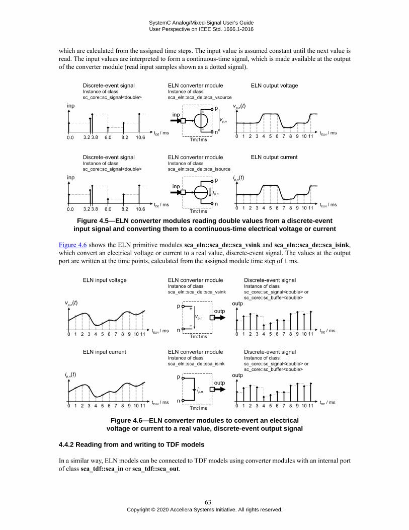
SystemC Analog/Mixed-Signal User’s GuideUser Perspective on IEEE Std. 1666.1-2016
which are calculated from the assigned time steps. The input value is assumed constant until the next value isread. The input values are interpreted to form a continuous-time signal, which is made available at the outputof the converter module (read input samples shown as a dotted signal).
Figure 4.5—ELN converter modules reading double values from a discrete-eventinput signal and converting them to a continuous-time electrical voltage or current
Figure 4.6 shows the ELN primitive modules sca_eln::sca_de::sca_vsink and sca_eln::sca_de::sca_isink,which convert an electrical voltage or current to a real value, discrete-event signal. The values at the outputport are written at the time points, calculated from the assigned module time step of 1 ms.
Figure 4.6—ELN converter modules to convert an electricalvoltage or current to a real value, discrete-event output signal
4.4.2 Reading from and writing to TDF models
In a similar way, ELN models can be connected to TDF models using converter modules with an internal portof class sca_tdf::sca_in or sca_tdf::sca_out.
63Copyright © 2020 Accellera Systems Initiative. All rights reserved.

SystemC Analog/Mixed-Signal User’s GuideUser Perspective on IEEE Std. 1666.1-2016
Figure 4.7 shows the ELN primitive modules sca_eln::sca_tdf::sca_vsource andsca_eln::sca_tdf::sca_isource, which read a value from a TDF signal and convert this value to an electricalvoltage or current, respectively. In this example a module time step of 1 ms is assigned to the ELN convertermodule. The ELN model continuously reads the samples from the TDF input. The input samples are interpretedto form a continuous-time signal, which is made available at the output of the converter module (input samplesshown as a dotted signal).
Figure 4.7—ELN converter modules reading double values from a TDF inputsignal and converting them to a continuous-time electrical voltage or current
Figure 4.8 shows the ELN primitive modules sca_eln::sca_tdf::sca_vsink and sca_eln::sca_tdf::sca_isink,which will convert an electrical voltage or current to a TDF signal. The samples at the output port are writtenat the calculated time points, which correspond to the assigned module time step of 1 ms.
Figure 4.8—ELN converter modules convert anelectrical voltage or current to a TDF output signal
64Copyright © 2020 Accellera Systems Initiative. All rights reserved.

SystemC Analog/Mixed-Signal User’s GuideUser Perspective on IEEE Std. 1666.1-2016
4.4.3 ELN model encapsulation in TDF models
The converter modules described in the previous sections can be used to encapsulate an ELN model withina different model of computation. Figure 4.9 shows an example on how to use converter modules to andfrom the TDF model of computation to encapsulate ELN behavior. In this case, access to and from theELN equation system use discrete-time signals following the TDF semantics, whereas the internal ELN signalsand computations are continuous-time.
Figure 4.9—ELN equation system encapsulated for inclusion intoa structural TDF model description by using converter modules
Example 4.7 shows the implementation of Figure 4.9.
Example 4.7: SystemC hierarchical module with TDF input and output port encapsulating ELN behavior
SC_MODULE(eln_in_tdf){ sca_tdf::sca_in<double> in; sca_tdf::sca_out<double> out; sca_eln::sca_tdf::sca_vsource vin; sca_eln::sca_tdf::sca_vsink vout; sca_eln::sca_r r; sca_eln::sca_c c; eln_in_tdf( sc_core::sc_module_name, double r_val, double c_val ) : in("in"), out("out"), vin("vin"), vout("vout"), r("r", r_val), c("c", c_val), n1("n1"), n2("n2"), gnd("gnd") { vin.inp(in); vin.p(n1); vin.n(gnd); r.p(n1); r.n(n2); c.p(n2); c.n(gnd); vout.p(n2); vout.n(gnd); vout.outp(out); } private: sca_eln::sca_node n1, n2; sca_eln::sca_node_ref gnd;};
65Copyright © 2020 Accellera Systems Initiative. All rights reserved.

SystemC Analog/Mixed-Signal User’s GuideUser Perspective on IEEE Std. 1666.1-2016
A similar approach can be used to encapsulate an ELN model for inclusion into a structural discrete-eventmodel description, using the converter modules to and from the discrete-event domain as explained in Section4.4.1.
4.4.4 Non-linear modeling using TDF encapsulation in ELN
The encapsulation method explained in the previous section can also be applied in the ‘reverse’ order, whereTDF models are encapsulated in ELN models. Especially in the case where the predefined set of ELN primitivemodels (see Annex A) are not sufficient to model continuous-time behavior, inclusion of TDF models offersa very powerful approach to make advanced continuous-time models.
Figure 4.10 shows a combination of ELN and TDF models to create a non-linear model for a diode. In thisexample, the diode is modeled by means of a TDF controlled voltage source of type sca_eln::sca_tdf_vsourcein series with a variable resistor of type sca_eln::sca_tdf::sca_r, which is controlled by a TDF inputsignal. The input voltage across the terminals p and n (Vp,n) is measured using the ELN primitive of typesca_eln::sca_tdf_vsink. The voltage source is used to model the threshold voltage (Vth). If the input voltageis above the threshold voltage in the forward direction (Vth_p), the diode starts conducting (the ON state) and itwill follow the I-V slope according to its ON-resistance Ron. If the input voltage remains below this thresholdvoltage, the diode will not conduct (the OFF state) and the series resistor gets a high impedance, defined byRoff. As soon as the input voltage is below the breakdown voltage (Vth_n), the diode will start conducting inthe reverse direction. A conventional diode will be destroyed due to the high reverse current caused by theavalanche effect. The rectifier functionality to calculate the threshold voltage and the ON or OFF resistanceis implemented in a TDF model.
The same topology can be used to model a zener diode. The characteristics of a zener diode are equivalent tothe diode as described above, except that such diode is designed to operate at the (zener) breakdown voltage.As such, a zener diode is normally used in reverse current operation.
Figure 4.10—Model of a non-linear element (diode) using TDF encapsulation in ELN
Example 4.8 shows the implementation of the diode.
Example 4.8: ELN model of a diode
SC_MODULE(diode){ sca_eln::sca_terminal p; sca_eln::sca_terminal n;
diode( sc_core::sc_module_name, double vth_p_ = 0.7, double vth_n_ = -53.0, double ron_ = 1e-3, double roff_ = 1e8 ) : p("p"), n("n"), vth_p(vth_p_), vth_n(vth_n_), ron(ron_), roff(roff_),
66Copyright © 2020 Accellera Systems Initiative. All rights reserved.

SystemC Analog/Mixed-Signal User’s GuideUser Perspective on IEEE Std. 1666.1-2016
vth("vth"), rrect("rrect"), vrect("vrect"), rctrl("rctrl"), s_vin("s_vin"), s_rout("s_rout"), s_vth("s_vth"), n1("n1") { rctrl.vin(s_vin); rctrl.rout(s_rout); rctrl.vth(s_vth);
vth.p(n1); vth.n(n); vth.inp(s_vth);
rrect.p(p); rrect.n(n1); rrect.inp(s_rout);
vrect.p(p); vrect.n(n); vrect.outp(s_vin); } private: double vth_p; double vth_n; double ron; double roff; sca_eln::sca_tdf_vsource vth; sca_eln::sca_tdf::sca_r rrect; sca_eln::sca_tdf_vsink vrect; rectifier rctrl;
sca_tdf::sca_signal<double> s_vin; sca_tdf::sca_signal<double> s_rout; sca_tdf::sca_signal<double> s_vth;
sca_eln::sca_node n1; };
Within the diode model, the rectifier functionality is implemented as TDF module, as shown in Example 4.9.The TDF module calculates whether a state change (from ON to OFF or OFF to ON state) has occurred. Incase the state changed, the calculated time step was not correct, as the resistor and voltage source hold thevalues of the previous state. Therefore the TDF module has to provide the corresponding values for the newstate and initiates a repetition of the time step. This is done by requesting a time step of zero seconds. If azero time step is scheduled for an ELN network, the equation solver resets to the previous state and repeatsthe time step with the new values.
Example 4.9: TDF model of the rectifier
SCA_TDF_MODULE(rectifier){ sca_tdf::sca_in<double> vin; sca_tdf::sca_out<double> rout; sca_tdf::sca_out<double> vth;
SCA_CTOR(rectifier) : vin("vin"), rout("rout"), vth("vth") {}
double ron, roff, vth_p, vth_n;
void set_attributes() { rout.set_delay(1); vth.set_delay(1); vth_p = 0.7; // threshold voltage vth_n = -53.0; // breakdown voltage ron = 1e-3; // on resistance roff = 1e8; // off resistance does_attribute_changes(); }
void initialize() { rout.initialize(roff); vth.initialize(0.0);
67Copyright © 2020 Accellera Systems Initiative. All rights reserved.

SystemC Analog/Mixed-Signal User’s GuideUser Perspective on IEEE Std. 1666.1-2016
ron_state=true; recalculate = 0; activations = 0; iterations = 0; max_iterations = 0; }
void change_attributes() { activations++; if(recalculate > 0) { request_next_activation(sc_core::SC_ZERO_TIME); // repeat last time step if(recalculate > 10) SC_REPORT_ERROR("dtdf_rectifier_ctrl","Convergence failed. Simulation will terminate.");
iterations++; if(recalculate > max_iterations) max_iterations = iterations; } }
void processing() { double vin_tmp = vin.read(); if(ron_state) { if((vin_tmp > vth_p)||(vin_tmp < vth_n)) // hysteresis, as curves do not fit exactly recalculate = 0; else { recalculate++; ron_state=false; } } else { if((vin_tmp > vth_p)||(vin_tmp < vth_n)) { recalculate++; ron_state=true; } else recalculate = 0; } if(ron_state) { rout.write(ron); // set resistance and threshold in dependency of the state if(vin_tmp > vth_p) vth.write(vth_p); else vth.write(vth_n); } else { rout.write(roff); vth.write(0.0); } }
private: bool ron_state; unsigned long recalculate, iterations, activations, max_iterations;};
4.5 ELN execution semantics
In addition to the elaboration and simulation phases as defined in SystemC language standard IEEE Std.1666-2011, specific functionality is implemented for the elaboration and execution of ELN models. Theseadditions are similar to the ones in LSF.
As depicted in Figure 4.11, the elaboration phase includes the following steps:— ELN time step calculation and propagation: Define the time step and check consistency inside each
ELN model (see also Section 4.1.2).— ELN equation setup and solvability check: Compose the ELN equation system from the contributing
equations provided by the predefined ELN primitive modules and their relationship defined by thecomposition. Check whether the resulting equation system can be solved.
The steps for the simulation phase are:
68Copyright © 2020 Accellera Systems Initiative. All rights reserved.

SystemC Analog/Mixed-Signal User’s GuideUser Perspective on IEEE Std. 1666.1-2016
— ELN initialization: At time zero, a static equation system to determine the initial condition has tobe setup and solved. Therefore all capacitors with a defined initial charge are replaced by a voltagesource with a voltage v = q0 / C and all inductors with a defined initial linked flux are replacedby a current source with a current I = psi0 / L. In the case where a capacitor has an initial chargeof sca_util::SCA_UNDEFINED, the capacitor is removed from the initial condition calculation.Consequently, the initial charge of this capacitor is calculated using the voltage across the removedcapacitor (determined by the initial condition calculation without the capacitor), q0 = C · v0. In the casewhere an inductor has an initial linked flux of sca_util::SCA_UNDEFINED, the inductor is replacedby a short for the initial condition calculation. Consequently, the initial linked flux of this inductor iscalculated using the current flowing through the short, psi0 = L · i0.
— ELN time-domain simulation: The ELN equation system is solved numerically using appropriate timesteps, which could be less than the assigned time step. The solver will at least provide results at thetime points, calculated from the assigned time step.
Figure 4.11—ELN elaboration and simulation phases
The elaboration and simulation phase are executed by starting a time-domain simulation using the functionsc_core::sc_start. This is explained in Section 6.1.1.
69Copyright © 2020 Accellera Systems Initiative. All rights reserved.

SystemC Analog/Mixed-Signal User’s GuideUser Perspective on IEEE Std. 1666.1-2016
5. Small-signal frequency-domain analyses
5.1 Modeling fundamentals
To analyze the frequency-domain behavior of an analog/mixed-signal system, varying small signals, calledalternating-current (AC) signals, at different frequencies are used to stimulate and analyze the steady-stateresponse of the circuit. Either small-signal sinusoidal sources or noise sources are used, and applied to thecircuit, which is being linearized around a given direct-current (DC) operating-point. This means that large-signal behavior, such as non-linearities causing distortion, are not captured during small-signal frequency-domain analyses.
These AC-domain analysis methods can compute the small-signal frequency-domain behavior of the entireanalog/mixed-signal system, which can be composed of modules from the available models of computation.TDF modules can embed a user-defined small-signal frequency-domain description. For LSF and ELNprimitive modules, the small-signal frequency-domain behavior is implicitly part of the primitive’s description.Figure 5.1 shows an example of a mixed-signal system containing TDF, LSF and ELN models. The moduleslabeled with ‘AC’ have, besides their time-domain description, a small-signal frequency-domain representationassociated with it. Based on the structural composition, a linear complex equation is extracted.
Figure 5.1—Small-signal frequency-domain description using TDF, LSF and ELN modules
5.1.1 Setup of the equation system
The linear complex equation system will make use of the TDF cluster as well as the LSF and ELN equationsystems, which are initially defined for time-domain simulation. Transformation of LSF and ELN equationsystems from the time-domain representation into the small-signal frequency-domain representation is doneusing the Laplace transform rules. Generally, for a given function f(t), the following substitutions will beapplied to the time-domain-oriented ELN and LSF equation systems:
— A derivation d/dt is substituted by jω.— An integration is substituted by 1/jω.— A delay f(t-delay) is substituted by e–jω · delay
Substitution will result in the frequency-domain function F(jω) for the LSF and ELN contributions.
TDF modules allow the definition of user-defined small-signal frequency-domain behavior as part of theprimitive definition. There is no mechanism available to derive an ‘AC representation’. It is entirely theresponsibility of the user to ensure the consistency of the defined frequency-domain and time-domainrepresentations. How to implement small-signal frequency-domain behavior in TDF modules is discussed inSection 5.2.1.
70Copyright © 2020 Accellera Systems Initiative. All rights reserved.

SystemC Analog/Mixed-Signal User’s GuideUser Perspective on IEEE Std. 1666.1-2016
5.1.2 Analysis methods
Two types of analyses are supported:— Small-signal frequency-domain analysis: Solves for each frequency point the linear complex equation
system, including all small-signal frequency-domain source contributions.— Small-signal frequency-domain noise analysis: Solves the linear complex equation system for each
frequency point and each small-signal frequency-domain noise source contribution, whereby allcontributions of small-signal frequency-domain sources and small-signal frequency-domain noisesources, except the currently activated noise source, are set to zero.
The result of a small-signal frequency-domain or noise analysis is the steady-state response or transfer functionof the circuit, described from the input port to the output port of the overall system. During analysis, theresulting linear complex equation system is solved for the given frequency points.
5.2 Language constructs
5.2.1 Small-signal frequency-domain description in TDF modules
The small-signal frequency-domain behavior of a TDF module can be defined in the member functionac_processing. This member function describes the contribution of the module to the overall complex equationsystem. The description should be written in the form of a linear complex transfer function, capturing thebehavior from the TDF input port to the TDF output port. Different functions are available to define the linearcomplex transfer function, as presented in the next sections. For these calculations, a data container of typesca_util::sca_complex should be used.
Example 5.1 shows the implementation of a transfer function H(s) = 1. The intermediate result is stored in avariable res of type sca_util::sca_complex, which is assigned to the TDF output port. More details on the portaccess methods are given in the next section.
Example 5.1: Small-signal frequency-domain description of the function H(s) = 1
SCA_TDF_MODULE(flat_response){ sca_tdf::sca_in<double> in; sca_tdf::sca_out<double> out;
SCA_CTOR(flat_response) {}
void processing() { out.write( in.read() ); }
void ac_processing() { double h = 1.0; // flat frequency response H(s) = 1 sca_util::sca_complex res; res = h * sca_ac_analysis::sca_ac(in); sca_ac_analysis::sca_ac(out) = res; } };
In the case where a small-signal frequency-domain analysis is performed, but no member functionac_processing is defined, or if no complex value is assigned to one or more TDF output ports, all related portvalues are set to zero, independently from the available value(s) at the input ports.
Note that there is no automatic consistency check between the time- and frequency-domain descriptions, asthese definitions are used-defined.
71Copyright © 2020 Accellera Systems Initiative. All rights reserved.

SystemC Analog/Mixed-Signal User’s GuideUser Perspective on IEEE Std. 1666.1-2016
5.2.2 Port access
For small-signal frequency-domain analysis, the complex value of all TDF ports, excluding the converterports, can be accessed by using the function sca_ac_analysis::sca_ac with as argument the port instances,as shown in the previous example. This access method is independent from the port type required in time-domain simulation.
For input ports, the function sca_ac_analysis::sca_ac returns a constant reference to a value of typesca_util::sca_complex, which means that no value can be assigned to a TDF input port. For output ports,the function returns a reference to a value of type sca_util::sca_complex, allowing the assignment of acontribution for small-signal frequency-domain analysis.
For small-signal frequency-domain noise analysis, a noise source independent from the input port values, canbe assigned to a TDF output port using the function sca_ac_analysis::sca_ac_noise.
Note that the values returned from the functions sca_ac_analysis::sca_ac and sca_ac_analysis::sca_ac_noiseare implementation-defined and have no physical interpretation. These values can only be used todescribe the complex linear relation between the input and output ports, accessed using these portaccess functions. Consequently, the values read during simulation from the input ports using the functionsca_ac_analysis::sca_ac does not represent a result for this port for the current frequency point.
5.3 Utility functions
The SystemC AMS extensions offer a set of utility functions, which can be used within the member functionac_processing to define the small-signal frequency-domain behavior. Note that these functions cannot be usedin the time-domain processing method processing.
5.3.1 Frequency-domain delay
The function sca_ac_analysis::sca_ac_delay can be used to implement a continuous-time delay, defined ase–jω · delay. Example 5.2 shows the extension of the TDF delay example presented in Section 2.3.5. The delay isnow a module parameter, and used to initialize the delay samples to 0.0 for the time-domain simulation. Notethat the delay parameter is an integer value, reflecting the number of samples which will be inserted for time-domain simulation, using a discrete time step. The member function ac_processing implements the frequency-domain behavior of this delay. First, the delay is translated into a continuous-time variant, using the memberfunction get_timestep multiplied with the number of delayed samples. This value of type sca_core::sca_timeis passed as argument to the function sca_ac_analysis::sca_ac_delay, which defines the delay in the frequencydomain.
Example 5.2: Small-signal frequency-domain description of a continuous-time delay
SCA_TDF_MODULE(my_tdf_ac_delay){ sca_tdf::sca_in<double> in; sca_tdf::sca_out<double> out;
my_tdf_ac_delay( sc_core::sc_module_name, unsigned long delay_ ) : in("in"), out("out"), delay(delay_) {} void set_attributes() { out.set_delay(delay); }
void initialize() // time-domain initialization { for( unsigned long i = 0; i < delay; i++ ) out.initialize( 0.0, i ); }
72Copyright © 2020 Accellera Systems Initiative. All rights reserved.

SystemC Analog/Mixed-Signal User’s GuideUser Perspective on IEEE Std. 1666.1-2016
void processing() // time-domain implementation { out.write( in.read() ); } void ac_processing() // frequency-domain implementation { sca_core::sca_time ct_delay = out.get_timestep() * delay; // calculate continuous-time delay sca_ac_analysis::sca_ac(out) = sca_ac_analysis::sca_ac(in) * sca_ac_analysis::sca_ac_delay( ct_delay ); }
private: unsigned long delay;};
5.3.2 Laplace transfer functions
The frequency-domain descriptions of the Laplace transfer functions in the numerator-denominatorand zero-pole form are available, using the utility functions sca_ac_analysis::sca_ac_ltf_nd orsca_ac_analysis::sca_ac_ltf_zp, respectively. They can be used in combination with the time-domainrepresentation, as shown in Example 5.3.
Example 5.3: TDF model with embedded Laplace transfer function in the time- and frequency-domain filter
SCA_TDF_MODULE(ltf_filter_ac){ sca_tdf::sca_in<double> in; sca_tdf::sca_out<double> out;
ltf_filter_ac( sc_core::sc_module_name nm, double fc_, double h0_ = 1.0 ) : in("in"), out("out"), fc(fc_), h0(h0_) {}
void initialize() { num(0) = 1.0; den(0) = 1.0; den(1) = 1.0 / ( 2.0 * M_PI * fc ); }
void processing() // time-domain implementation { out.write( ltf_nd( num, den, in.read(), h0 ) ); }
void ac_processing() // frequency-domain implementation { sca_ac_analysis::sca_ac(out) = sca_ac_analysis::sca_ac_ltf_nd( num, den, sca_ac_analysis::sca_ac(in), h0 ); }
private: sca_tdf::sca_ltf_nd ltf_nd; // Laplace transfer function sca_util::sca_vector<double> num, den; // numerator and denominator coefficients double fc; // 3dB cutoff frequency in Hz double h0; // DC gain};
5.3.3 S-domain definitions
The function sca_ac_analysis::sca_ac_s supports frequency-domain representations defined in the s-domain,by using the Laplace operator sn = (jω)n.
Figure 5.2 and Example 5.4 show the definition and frequency response H(s) and implementation of a secondorder low-pass filter, implemented in the time- and frequency-domain.
73Copyright © 2020 Accellera Systems Initiative. All rights reserved.

SystemC Analog/Mixed-Signal User’s GuideUser Perspective on IEEE Std. 1666.1-2016
Figure 5.2—Frequency response of second orderlow-pass filter implemented in the s-domain
Example 5.4: TDF model of a second order low-pass filter in the time- and frequency-domain
SCA_TDF_MODULE(lp_filter_ac_s){ sca_tdf::sca_in<double> in; sca_tdf::sca_out<double> out;
SCA_CTOR(lp_filter_ac_s) : in("in"), out("out") {} void initialize() { num(0) = 1.0; den(0) = 1.0; den(1) = 1.0; den(2) = 1.0; }
void processing() // time-domain implementation { out.write( ltf_nd( num, den, in.read(), 1.0 ) ); }
void ac_processing() // frequency-domain implementation { sca_util::sca_complex h = 1.0 / ( sca_ac_analysis::sca_ac_s(2) + sca_ac_analysis::sca_ac_s(1) + 1.0 );
sca_ac_analysis::sca_ac(out) = h * sca_ac_analysis::sca_ac(in); }
private: sca_tdf::sca_ltf_nd ltf_nd; sca_util::sca_vector<double> num, den;};
Alternatively, the frequency-domain behavior can be implemented using the relation s = jω. The memberfunction ac_processing from the previous example can be replaced with an implementation which uses thefunction sca_ac_analysis::sca_ac_w, which returns the current angular frequency in radians/seconds:
Example 5.5: Small-signal frequency-domain implementation using s = jω
void ac_processing(){ sca_util::sca_complex s = sca_util::SCA_COMPLEX_J * sca_ac_analysis::sca_ac_w(); sca_util::sca_complex h = 1.0 / ( s * s + s + 1.0 );
sca_ac_analysis::sca_ac(out) = h * sca_ac_analysis::sca_ac(in);}
According to the relation ω = 2πf, the frequency term can be used as well. The implementation using thefunction sca_ac_analysis::sca_ac_f, which returns the current frequency in Hertz, becomes:
Example 5.6: Small-signal frequency-domain implementation using s = j2πf
void ac_processing() { sca_util::sca_complex s = sca_util::SCA_COMPLEX_J * 2.0 * M_PI * sca_ac_analysis::sca_ac_f(); sca_util::sca_complex h = 1.0 / ( s * s + s + 1.0 );
sca_ac_analysis::sca_ac(out) = h * sca_ac_analysis::sca_ac(in);
74Copyright © 2020 Accellera Systems Initiative. All rights reserved.

SystemC Analog/Mixed-Signal User’s GuideUser Perspective on IEEE Std. 1666.1-2016
}
5.3.4 Z-domain definitions
The function sca_ac_analysis::sca_ac_z supports frequency-domain representations defined in the z-domain,by using the operator zn( = e jω · n · tstep). Where n is an integer defining the delay, and tstep is the time stepbetween the delays. If the tstep argument is not used, tstep will be defined as the time step returned by themember function get_timestep.
Figure 5.3 shows the definition and frequency response H(z) of a comb-filter.
Figure 5.3—Frequency response of a comb-filter implemented in the z-domain
For the frequency-domain implementation, the function sca_ac_analysis::sca_ac_z is used, as shown inExample 5.7.
Example 5.7: TDF model of a comb-filter in the time- and frequency-domain
SCA_TDF_MODULE(comb_filter){ sca_tdf::sca_in<bool> in; sca_tdf::sca_out<sc_dt::sc_int<28> > out;
comb_filter( sc_core::sc_module_name, int k_ = 64, int n_ = 3 ) : in("in"), out("out"), k(k_), n(n_) {}
void set_attributes() { in.set_rate(k); out.set_rate(1); } void ac_processing() // frequency-domain implementation { // complex transfer function sca_util::sca_complex h = pow( ( 1.0 - sca_ac_analysis::sca_ac_z(-k) ) / ( 1.0 - sca_ac_analysis::sca_ac_z(-1) ), n );
sca_ac_analysis::sca_ac(out) = h * sca_ac_analysis::sca_ac(in) ; }
void processing() // time-domain implementation { int x, y, i; for( i = 0; i < k; i++) { x = in.read(i); ... } out.write(y); } private: int k; // decimation factor int n; // order of filter };
75Copyright © 2020 Accellera Systems Initiative. All rights reserved.

SystemC Analog/Mixed-Signal User’s GuideUser Perspective on IEEE Std. 1666.1-2016
5.3.5 Detection of small-signal frequency-domain analyses
The utility functions sca_ac_analysis::sca_ac_is_running and sca_ac_analysis::sca_ac_noise_is_runningcan be used within the member function processing or ac_processing of a TDF module, to implement specificbehavior, which depends on the type of analysis running.
The function sca_ac_analysis::sca_ac_is_running returns true when a small-signal frequency-domain ornoise analysis is running. The function sca_ac_analysis::sca_ac_noise_is_running only returns true if asmall-signal frequency-domain noise analysis is running.
Example 5.8 shows the implementation of a sinusoidal source, which can be used in time-domain andfrequency-domain simulations.
Example 5.8: TDF model of a sinusoidal source in the time- and frequency-domain
SCA_TDF_MODULE(sin_src){ sca_tdf::sca_out<double> out; sin_src( sc_core::sc_module_name nm, double offset_= 0.0, double ampl_= 1.0, double noise_ampl_= 0.1, double freq_ = 1.0e3, sca_core::sca_time Tm_ = sca_core::sca_time(0.125, sc_core::SC_MS) ) : out("out"), offset(offset_), ampl(ampl_), noise_ampl(noise_ampl_), freq(freq_), Tm(Tm_) {}
void set_attributes() { set_timestep(Tm); }
void processing() { double t = get_time().to_seconds(); // actual time out.write( offset + ampl * std::sin( 2.0*M_PI*freq*t ) ); } void ac_processing() {
if( sca_ac_analysis::sca_ac_noise_is_running() ) sca_ac_analysis::sca_ac_noise(out) = noise_ampl; else sca_ac_analysis::sca_ac(out) = ampl; } private: double offset, ampl, noise_ampl, freq; sca_core::sca_time Tm;};
Only for small-signal frequency-domain noise analysis, the functionsca_ac_analysis::sca_ac_noise_is_running returns true. In this case, the noise amplitude of thesource is set.
5.4 Small-signal frequency-domain analysis with combined TDF, LSF and ELNmodels
As already stated in the introduction of this chapter, the small-signal frequency-domain analysis is able toextract the frequency behavior of the entire analog/mixed-signal system. The frequency response of the entiresystem can be analyzed by using TDF modules, which have their frequency-domain behavior defined in theirmember function ac_processing, plus the frequency-domain description of LSF and ELN primitive modules,which is extracted from the LSF and ELN equation system during elaboration.
76Copyright © 2020 Accellera Systems Initiative. All rights reserved.
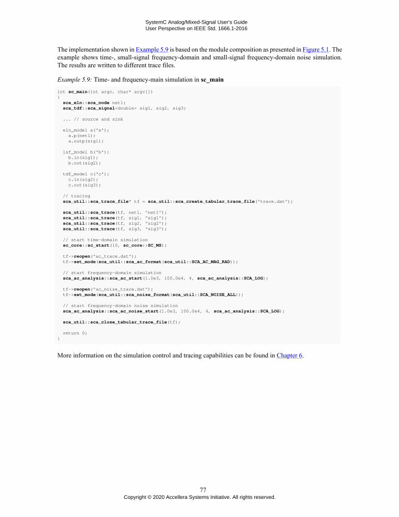
SystemC Analog/Mixed-Signal User’s GuideUser Perspective on IEEE Std. 1666.1-2016
The implementation shown in Example 5.9 is based on the module composition as presented in Figure 5.1. Theexample shows time-, small-signal frequency-domain and small-signal frequency-domain noise simulation.The results are written to different trace files.
Example 5.9: Time- and frequency-main simulation in sc_main
int sc_main(int argc, char* argv[]){ sca_eln::sca_node net1; sca_tdf::sca_signal<double> sig1, sig2, sig3; ... // source and sink
eln_model a("a"); a.p(net1); a.outp(sig1); lsf_model b("b"); b.in(sig1); b.out(sig2);
tdf_model c("c"); c.in(sig2); c.out(sig3);
// tracing sca_util::sca_trace_file* tf = sca_util::sca_create_tabular_trace_file("trace.dat"); sca_util::sca_trace(tf, net1, "net1"); sca_util::sca_trace(tf, sig1, "sig1"); sca_util::sca_trace(tf, sig2, "sig2"); sca_util::sca_trace(tf, sig3, "sig3"); // start time-domain simulation sc_core::sc_start(10, sc_core::SC_MS);
tf->reopen("ac_trace.dat"); tf->set_mode(sca_util::sca_ac_format(sca_util::SCA_AC_MAG_RAD));
// start frequency-domain simulation sca_ac_analysis::sca_ac_start(1.0e3, 100.0e4, 4, sca_ac_analysis::SCA_LOG);
tf->reopen("ac_noise_trace.dat"); tf->set_mode(sca_util::sca_noise_format(sca_util::SCA_NOISE_ALL));
// start frequency-domain noise simulation sca_ac_analysis::sca_ac_noise_start(1.0e3, 100.0e4, 4, sca_ac_analysis::SCA_LOG);
sca_util::sca_close_tabular_trace_file(tf);
return 0;}
More information on the simulation control and tracing capabilities can be found in Chapter 6.
77Copyright © 2020 Accellera Systems Initiative. All rights reserved.

SystemC Analog/Mixed-Signal User’s GuideUser Perspective on IEEE Std. 1666.1-2016
6. Simulation and tracing
The AMS extensions use the SystemC functions to start and stop time-domain simulations. New functions areavailable for frequency-domain simulation. Advanced tracing mechanism are available to enable or disabletime-domain or frequency-domain tracing while running simulations.
6.1 Simulation control
6.1.1 Time-domain simulation
Time-domain (transient) simulation is started by calling sc_core::sc_start from within the function sc_main,as shown in Example 6.1.
Example 6.1: Time-domain (transient) simulation in sc_main
#include <systemc-ams>
#include "my_source.h"#include "my_control.h"#include "my_dut.h"#include "my_sink.h"
int sc_main(int argc, char* argv[]){ sc_core::sc_set_time_resolution(1.0, sc_core::SC_FS); sca_tdf::sca_signal<double> sig1, sig2; sc_core::sc_signal<bool> sc_sig; my_source i_my_source("i_my_source"); i_my_source.out(sig1);
my_control i_my_ctrl("i_my_ctrl"); i_my_ctrl.out(sc_sig);
my_dut i_my_dut("i_my_dut"); i_my_dut.in(sig1); i_my_dut.ctrl(sc_sig); i_my_dut.out(sig2);
my_sink i_my_sink("i_my_sink"); i_my_sink.in(sig2);
sc_core::sc_start(10.0, sc_core::SC_MS); return 0;}
6.1.1.1 Program arguments
The function sc_main acts as main program, and has the same signature of arguments and return value asC++’s usual program entry function int main(int argc, char* argv[]). The argument argc specifies thenumber of arguments passed to the main routine. The argument argv[] is a field of pointers to the differentstring arguments, where argv[0] is the program name.
Note that implementations or simulators, which support SystemC and the AMS extensions may use differentmechanisms to define the main program body or even use an alternative approach to sc_main.
6.1.1.2 Time resolution
For AMS simulations, it is recommended to use the smallest time resolution possible covering the requiredsimulation time using the function sc_core::sc_set_time_resolution. It is recommended to add this function asthe first statement in the sc_main function. For time-domain simulation, a time resolution of 1 femtosecond (fs)
78Copyright © 2020 Accellera Systems Initiative. All rights reserved.

SystemC Analog/Mixed-Signal User’s GuideUser Perspective on IEEE Std. 1666.1-2016
is recommended, which is the smallest time resolution possible allowing a maximum simulation time of 264 fs,which is approximately 5 hours. In the case where longer simulation times are needed, the time resolutionshould be increased resulting in a coarser time grid and in possible rounding errors.
6.1.1.3 Simulation arguments
The function sc_core::sc_start without arguments will result in a simulation that runs until the last event hasbeen processed, which might be forever. To simulate for a limited amount of time, the to-be-simulated-timecan be specified as a double value together with the time unit, or as an object of class sc_core::sc_time. Thefunction sc_core::sc_start can be called multiple times, as shown in Example 6.2.
Example 6.2: Time-domain simulation calling sc_core::sc_start multiple times
int sc_main(int argc, char* argv[]){ // instantiate design and testbench, setup tracing, ... ...
sc_core::sc_start(10.0, sc_core::SC_MS); ... sc_core::sc_time sim_time(10.0, sc_core::SC_MS);
sc_core::sc_start(sim_time); ...
sc_core::sc_start(); return 0;}
Start transient analysis, where the simulation time is specified with two arguments. The first argumentis the time of type double. The second argument is the time unit, which is an object of classsc_core::sc_time_unit.Start transient analysis, where the simulation time is specified with a single argument, which is anobject of class sc_core::sc_time.In this case, no simulation time is specified. Transient analysis will run till the event queue is empty.
6.1.2 Small-signal frequency-domain simulation
Frequency domain simulations are also started from within the function sc_main, usingsca_ac_analysis::sca_ac_start for a small-signal (AC) simulation and sca_ac_analysis::sca_ac_noise_startfor a small-signal frequency-domain noise simulation. In the case that the model description has not beenelaborated, because sc_core::sc_start has not yet been called, this will be automatically done before the firstfrequency-domain simulation starts.
It is possible to subsequently call the frequency-domain and time-domain analyses start functions in any orderinside the function sc_main, to analyze the system description under different operating points or digital states.
Example 6.3 shows the usage of the functions sca_ac_analysis::sca_ac_start andsca_ac_analysis::sca_ac_noise_start, which take as arguments the start frequency, stop frequency,number of frequency points, and whether a linear (sca_ac_analysis::SCA_LIN) or logarithmic(sca_ac_analysis::SCA_LOG) frequency scale should be used.
Example 6.3: Small-signal frequency-domain simulation
// frequency-domain simulations from 1kHz to 10kHz with 100 points on a linear scale:sca_ac_analysis::sca_ac_start(1.0e3, 10.0e3, 100, sca_ac_analysis::SCA_LIN); sca_ac_analysis::sca_ac_noise_start(1.0e3, 10.0e3, 100, sca_ac_analysis::SCA_LIN); // frequency-domain simulations from 1Hz to 1MHz with 1001 points on a logarithmic scale:sca_ac_analysis::sca_ac_start(1.0, 1.0e6, 1001, sca_ac_analysis::SCA_LOG); sca_ac_analysis::sca_ac_noise_start(1.0, 1.0e6, 1001, sca_ac_analysis::SCA_LOG);
79Copyright © 2020 Accellera Systems Initiative. All rights reserved.

SystemC Analog/Mixed-Signal User’s GuideUser Perspective on IEEE Std. 1666.1-2016
6.2 Tracing
The SystemC AMS extensions provide utility functions to record the simulation results (waveforms) into tracefiles, using the Value Change Dump (VCD) format or tabular format. The VCD format has limited capabilitiesto trace AMS signals, nodes, ports, terminals, or variables. Besides the tracing of regular SystemC variablesand signals, it only supports tracing for time-domain simulations. The tabular format can be used to recordboth time-domain and frequency-domain traces.
The trace file is usually created at the top-level (e.g., inside sc_main) after all modules andsignals have been instantiated, and just before starting the actual simulation using sc_core::sc_start,sca_ac_analysis::sca_ac_start, or sca_ac_analysis::sca_ac_noise_start.
6.2.1 Trace files and formats
6.2.1.1 Tracing to a VCD file
For tracing waveforms using the VCD format, the trace file is created by calling the functionsca_util::sca_create_vcd_trace_file with the name of the file as an argument. This function returns apointer to a data structure that is used for tracing. Closing the trace file is done using the functionsca_util::sca_close_vcd_trace_file with as argument the pointer to the same data structure.
Example 6.4: Tracing to a VCD file
// open trace file in VCD formatsca_util::sca_trace_file* atf = sca_util::sca_create_vcd_trace_file( "my_trace.vcd" );
...
// close the trace filesca_util::sca_close_vcd_trace_file( atf );
6.2.1.2 Tracing to a tabular file
For tracing waveforms using the tabular format, the trace file is created by calling the functionsca_util::sca_create_tabular_trace_file with the name of the file as an argument. The function returnsa pointer to a data structure that is used for tracing. Closing the trace file is done using the functionsca_util::sca_close_tabular_trace_file with as argument the pointer to the same data structure, as shown inExample 6.5.
Example 6.5: Tracing to a tabular file
// open trace file in tabular formatsca_util::sca_trace_file* atf = sca_util::sca_create_tabular_trace_file( "my_trace.dat" );
... // close the trace filesca_util::sca_close_tabular_trace_file( atf );
6.2.1.3 Tracing to a tabular stream
As tracing of analog signals could result in very big trace files, the AMS tracing functionality has been extendedto trace to an output stream, so there is no file generated. This allows direct processing of the AMS signalsavailable in the output stream derived from std::ostream, for example to immediately display the results or tocompact the results into an archive file.
For tracing waveforms to an output stream, the trace file is created by calling the functionsca_util::sca_create_tabular_trace_file with the output stream object as an argument. The function returns
80Copyright © 2020 Accellera Systems Initiative. All rights reserved.

SystemC Analog/Mixed-Signal User’s GuideUser Perspective on IEEE Std. 1666.1-2016
a pointer to an object of class sca_util::sca_trace_file, which references the stream and is used to manage thesignal tracing to it. Closing the trace file is done using the function sca_util::sca_close_tabular_trace_filewith as argument the pointer to the same output stream, as shown in Example 6.6.
Example 6.6: Tracing to a tabular stream
// trace in tabular format to the shellsca_util::sca_trace_file* atfs = sca_util::sca_create_tabular_trace_file(std::cout);
...
// close the trace file handle, the stream is automatically closed once the scope of os is left.sca_util::sca_close_tabular_trace_file(atfs);
6.2.1.4 Trace file control
As tracing of AMS signals could result in very large and unmanageable waveform files, additional functionalityis available to control the recording of trace files. The following trace file control methods are available forclass sca_util::sca_trace_file:
a) The member function enable will start tracing at the simulation time where this method is called.b) The member function disable will stop tracing at the simulation time where this method is called.c) The member function reopen will close the existing trace file (if it was open), and will continue tracing
in a new trace file at the simulation time where this method is called.d) The member function set_mode will change the mode of the trace file at the simulation time where
this method is called. The following modi are available:1) The time step (sampling) between samples can be set by using the function
sca_util::sca_sampling, where the first argument is the time step and the second argumentis the time offset. Both arguments should be an object of class sca_core::sca_time.
2) The function sca_util::sca_decimation, with argument n, will only write the n-th sampleto the trace file.
3) The function sca_util::sca_multirate defines which signal value should bewritten to the trace file if no actual value is available. This can occurwhile tracing signals with different rates and time steps. Available argumentsare to interpolate (sca_util::SCA_INTERPOLATE), to use the last availablevalue (sca_util::SCA_HOLD_SAMPLE), or to not write a value at all(sca_util::SCA_DONT_INTERPOLATE). In the latter case, the symbol ‘*’ is writtento the trace file.
4) For small-signal frequency-domain tracing, the function sca_util::sca_ac_formatdefines the format, in which the signals are written. Available functionarguments are: real/imaginary (sca_util::SCA_AC_REAL_IMAG) and amplitude/phase in magnitude/radians (sca_util::SCA_AC_MAG_RAD) or dB/degrees(sca_util::SCA_AC_DB_DEG).
5) For small-signal frequency-domain tracing, the function sca_noise_format defines howthe noise contribution is written to the trace file. If sca_util::SCA_NOISE_ALLis passed, each individual noise contribution is written to the trace file. Ifsca_util::SCA_NOISE_SUM is passed, the sum of all noise contributions is written tothe trace file..
The following sections give some examples on how to use trace file control in combination with simulationcontrol.
81Copyright © 2020 Accellera Systems Initiative. All rights reserved.
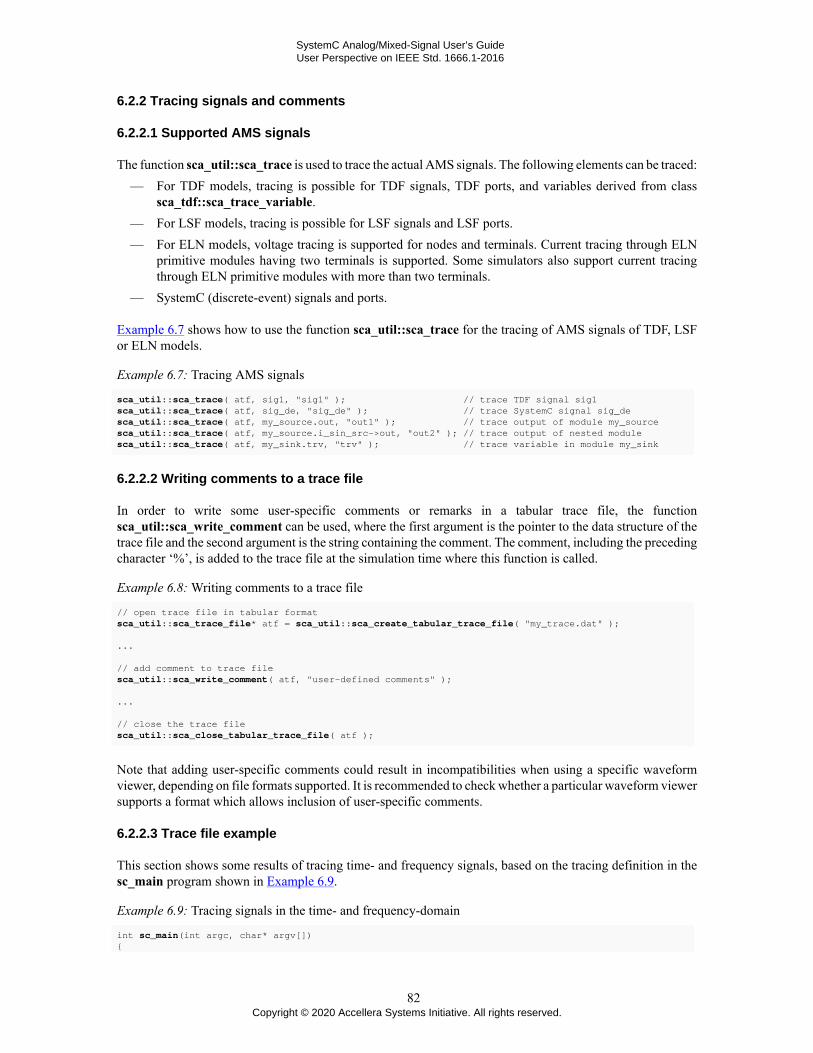
SystemC Analog/Mixed-Signal User’s GuideUser Perspective on IEEE Std. 1666.1-2016
6.2.2 Tracing signals and comments
6.2.2.1 Supported AMS signals
The function sca_util::sca_trace is used to trace the actual AMS signals. The following elements can be traced:— For TDF models, tracing is possible for TDF signals, TDF ports, and variables derived from class
sca_tdf::sca_trace_variable.— For LSF models, tracing is possible for LSF signals and LSF ports.— For ELN models, voltage tracing is supported for nodes and terminals. Current tracing through ELN
primitive modules having two terminals is supported. Some simulators also support current tracingthrough ELN primitive modules with more than two terminals.
— SystemC (discrete-event) signals and ports.
Example 6.7 shows how to use the function sca_util::sca_trace for the tracing of AMS signals of TDF, LSFor ELN models.
Example 6.7: Tracing AMS signals
sca_util::sca_trace( atf, sig1, "sig1" ); // trace TDF signal sig1sca_util::sca_trace( atf, sig_de, "sig_de" ); // trace SystemC signal sig_desca_util::sca_trace( atf, my_source.out, "out1" ); // trace output of module my_sourcesca_util::sca_trace( atf, my_source.i_sin_src->out, "out2" ); // trace output of nested modulesca_util::sca_trace( atf, my_sink.trv, "trv" ); // trace variable in module my_sink
6.2.2.2 Writing comments to a trace file
In order to write some user-specific comments or remarks in a tabular trace file, the functionsca_util::sca_write_comment can be used, where the first argument is the pointer to the data structure of thetrace file and the second argument is the string containing the comment. The comment, including the precedingcharacter ‘%’, is added to the trace file at the simulation time where this function is called.
Example 6.8: Writing comments to a trace file
// open trace file in tabular formatsca_util::sca_trace_file* atf = sca_util::sca_create_tabular_trace_file( "my_trace.dat" );
...
// add comment to trace filesca_util::sca_write_comment( atf, "user-defined comments" );
...
// close the trace filesca_util::sca_close_tabular_trace_file( atf );
Note that adding user-specific comments could result in incompatibilities when using a specific waveformviewer, depending on file formats supported. It is recommended to check whether a particular waveform viewersupports a format which allows inclusion of user-specific comments.
6.2.2.3 Trace file example
This section shows some results of tracing time- and frequency signals, based on the tracing definition in thesc_main program shown in Example 6.9.
Example 6.9: Tracing signals in the time- and frequency-domain
int sc_main(int argc, char* argv[]){
82Copyright © 2020 Accellera Systems Initiative. All rights reserved.

SystemC Analog/Mixed-Signal User’s GuideUser Perspective on IEEE Std. 1666.1-2016
... // instantiate design and testbench
sca_util::sca_trace_file* tf = sca_util::sca_create_tabular_trace_file("trace.dat");
sca_util::sca_trace(tf, sig1, "sig1"); sca_util::sca_trace(tf, sig2, "sig2");
sc_core::sc_start(2.0, sc_core::SC_MS);
tf->reopen("ac_trace.dat");
tf->set_mode(sca_util::sca_ac_format(sca_util::SCA_AC_MAG_RAD));
sca_ac_analysis::sca_ac_start(1.0e3, 1.0e6, 4, sca_ac_analysis::SCA_LOG);
tf->reopen("trace.dat", std::ios_base::app);
sc_core::sc_start(10, sc_core::SC_MS);
tf->reopen("ac2_trace.dat");
sca_ac_analysis::sca_ac_start(1.0e3, 1.0e6, 4, sca_ac_analysis::SCA_LOG);
sca_util::sca_close_tabular_trace_file(tf);
...}
Trace AMS signals to a file in tabular format using the tracing functionality of the AMS extensions.Define which signals to trace.Execute time-domain simulation for 2 ms. Signals sig1 and sig2 will be traced.Close the current trace file and start tracing to a new file for the first AC analysis.Definition to trace the amplitude and phase of the signals in magnitude and radians.Execute AC simulation at the operating point at the current time. AC analysis is done from 1 kHz to1 MHz with 4 points on a logarithmic scale.Re-open time-domain trace file and continue tracing (append).Continue time-domain simulation for 10 ms.Open new trace file for next AC simulation.Execute AC simulation at the operating point at the current time.Close the trace file.
The file trace.dat is shown in Example 6.10. The %time in the first line indicates that this file was createdduring time-domain simulation, and shows the signal names, which are traced. Each line shows the time inseconds and signal values at that point in time. The values are separated by one or more spaces.
Example 6.10: Tabular trace file of time-domain simulation
%time sig1 sig20 0 00.0005 1 1e-60.001 2 1.5e-60.0015 3 2e-60.002 4 2.5e-5
Example 6.11 shows the result of the small-signal frequency-domain tracing in ac_trace.dat. The file startswith %frequency in the header. The format of the AC signals is set to amplitude (the magnitude) and phase (inradians) indicated with .mag and .rad suffixes to the signal names, respectively.
Example 6.11: Tabular trace file of small-signal frequency-domain simulation
%frequency sig1.mag sig1.rad sig2.mag sig2.rad1000 1 0 2.53302962314e-08 -3.1414334986410000 1 0 2.53302959138e-10 -3.1415767381
83Copyright © 2020 Accellera Systems Initiative. All rights reserved.

SystemC Analog/Mixed-Signal User’s GuideUser Perspective on IEEE Std. 1666.1-2016
100000 1 0 2.53302959106e-12 -3.141591062041000000 1 0 2.53302959106e-14 -3.14159249443
6.3 Testbenches
Testbenches are used to provide stimulus to a device under test (DUT) and check the results or response of theDUT. Very often the DUT is put into a certain state, using an external control. A typical testbench structureis given in Figure 6.1.
Figure 6.1—Testbench containing stimulus, control, checker, and device under test
A testbench can be implemented in various ways:— The stimulus and controller can be embedded in the main program and the results is checked in another
module. In this way, the main program acts as the testbench.— The stimulus, controller, and checker are part of a dedicated module, which is instantiated in the main
program. Such a module is often called a verification component, which basically acts as the testbench.— The stimulus and controller are separate modules, both instantiated in the main program. The checker
is embedded in the main program, which acts as the testbench.
Besides the examples listed above, there are other possibilities to create a testbench. Obviously, there is nosingle ‘right’ way to create a testbench; it depends on the application.
Example 6.12 shows the main program in which the stimuli my_source, the control my_control and the sinkmy_sink are instantiated as objects. Together with the tracing implemented as inline code, they form thetestbench. The device under test my_dut is instantiated as a module and is connected to the modules of thetestbench.
Example 6.12: Simple test bench in sc_main
#include <systemc-ams>
#include "my_source.h"#include "my_control.h"#include "my_dut.h"#include "my_sink.h"
int sc_main(int argc, char* argv[]){ sc_core::sc_set_time_resolution(1.0, sc_core::SC_FS);
sca_tdf::sca_signal<double> sig1, sig2; sc_core::sc_signal<bool> sc_sig; my_source i_my_source("i_my_source");
84Copyright © 2020 Accellera Systems Initiative. All rights reserved.

SystemC Analog/Mixed-Signal User’s GuideUser Perspective on IEEE Std. 1666.1-2016
i_my_source.out(sig1);
my_control i_my_ctrl("i_my_ctrl"); i_my_ctrl.out(sc_sig);
my_dut i_my_dut("i_my_dut"); i_my_dut.in(sig1); i_my_dut.ctrl(sc_sig); i_my_dut.out(sig2);
my_sink i_my_sink("i_my_sink"); i_my_sink.in(sig2);
sc_core::sc_trace_file* tf = sc_core::sc_create_vcd_trace_file("my_sc_trace"); sc_core::sc_trace(tf, sc_sig ,"sc_sig");
sca_util::sca_trace_file* atf1 = sca_util::sca_create_vcd_trace_file("ams_vcd_trace.vcd"); sca_util::sca_trace(atf1, sig1 ,"sig1");
sca_util::sca_trace_file* atf2 = sca_util::sca_create_tabular_trace_file("ams_trace.dat"); sca_util::sca_trace(atf2, sig2 ,"sig2");
sc_core::sc_start(2.0, sc_core::SC_MS);
atf2->reopen("ams_trace2.dat"); sc_core::sc_start(2.0, sc_core::SC_MS);
atf2->disable(); sc_core::sc_start(2.0, sc_core::SC_MS);
atf2->enable(); atf2->set_mode( sca_util::sca_decimation(2) ); sc_core::sc_start(2.0, sc_core::SC_MS);
atf2->reopen("ams_trace3.dat");
sca_core::sca_time tstep(1.0, sc_core::SC_MS); atf2->set_mode( sca_util::sca_sampling( tstep, sc_core::SC_ZERO_TIME ) ); sc_core::sc_start(10.0, sc_core::SC_MS);
sc_core::sc_close_vcd_trace_file(tf); sca_util::sca_close_vcd_trace_file(atf1); sca_util::sca_close_tabular_trace_file(atf2);
return 0;}
Trace signals using SystemC’s standard tracing facility.Trace AMS signals to a file in VCD format using the tracing functionality of the AMS extensions.Trace AMS signals to a file in tabular format using the tracing functionality of the AMS extensions.Start time-domain simulation. Signals sig1 and sig2 will be traced.Close the current trace file and start tracing to a new file.Disable tracing to atf2 to not record the next 2 ms.Re-enable tracing to atf2, but with a different sample period defined by a decimation factor of 2 (skipone sample).Close the current trace file of atf2 and start tracing to a new file using a different time step.Define how samples are written to the trace file. Sample every 1 ms starting from 0 ms.Close all trace files.
85Copyright © 2020 Accellera Systems Initiative. All rights reserved.

SystemC Analog/Mixed-Signal User’s GuideUser Perspective on IEEE Std. 1666.1-2016
7. Application examples
This chapter shows concrete application examples using the different models of computation offered by theSystemC AMS extensions. These application examples are also made available for download6.
7.1 Binary Amplitude Shift Keying (BASK) example
This section shows a Binary Amplitude Shift Keying (BASK) modulator and demodulator application example.It demonstrates the use of the TDF model of computation and its multirate capabilities. Especially, theinteraction of time steps and data rates will play an important role here. The reader is encouraged to reproducethe computations regarding data rates and time steps of the examples in this section in order to grasp theconcepts of Timed Data Flow modeling.
7.1.1 BASK modulator
This example considers Binary Amplitude Shift Keying (BASK) modulation, where a sinusoidal carrier ismodulated by a binary signal. A BASK modulator consists of the carrier signal source (sin_src) and a mixer(mixer), which basically multiplies a binary baseband signal (bit_src) with segments of the carrier signal.Figure 7.1 shows a structural composition of the BASK modulator. The signals in this figure illustrate theconcept of Binary Amplitude Shift Keying.
Figure 7.1—BASK modulator
The module sin_src is already described in Section 2.3.1. The mixer reads 40 carrier samples per basebandsample. Example 7.1 shows the implementation.
Example 7.1: TDF model of a mixer
SCA_TDF_MODULE(mixer) { sca_tdf::sca_in<bool> in_bin; // input port baseband signal sca_tdf::sca_in<double> in_wav; // input port carrier signal sca_tdf::sca_out<double> out; // output port modulated signal
SCA_CTOR(mixer) : in_bin("in_bin"), in_wav("in_wav"), out("out"), rate(40) {} // use a carrier data rate of 40 void set_attributes() { in_wav.set_rate(rate); out.set_rate(rate); }
6 Application examples are available for download at the Accellera Systems Initiative SystemC community pages https://www.accellera.org/community/systemc/about-systemc-ams/.
86Copyright © 2020 Accellera Systems Initiative. All rights reserved.

SystemC Analog/Mixed-Signal User’s GuideUser Perspective on IEEE Std. 1666.1-2016
void processing() { for(unsigned long i = 0; i < rate; i++) { if ( in_bin.read() ) out.write( in_wav.read(i), i ); else out.write( 0.0, i ); } }
private: unsigned long rate;};
This is obviously more sensible than up-sampling the binary signal first to a data rate of 40 such that boththe carrier signal and the base band signal fit to a mixer with both input ports set to a data rate of 1. Example7.2 shows how the two modules can be combined to form a BASK modulator module. Note that a regularSC_MODULE is used in this case, in which the two TDF primitive modules are instantiated.
Example 7.2: TDF model of the BASK modulator
SC_MODULE(bask_mod){ sca_tdf::sca_in<bool> in; sca_tdf::sca_out<double> out;
sin_src sine; mixer mix;
SC_CTOR(bask_mod) : in("in"), out("out"), sine("sine", 1.0, 1.0e7, sca_core::sca_time( 5.0, sc_core::SC_NS ) ), mix("mix") { sine.out(carrier); mix.in_wav(carrier); mix.in_bin(in); mix.out(out); }
private: sca_tdf::sca_signal<double> carrier;};
Note that the carrier frequency of 10 MHz is set by passing a parameter to the module sin_src, while thebaseband frequency is determined indirectly by the data rate of the module mixer, and the time step set atthe output of module sin_src. The port in_wav of the module mixer has the same time step as the output ofmodule sin_src (namely 5 ns), but a data rate of 40. Therefore, the port in_bin of the module mixer, whichhas a data rate of 1, gets a time step of 200 ns. This results in a baseband frequency of 5 MHz, which is exactlythe situation depicted in Figure 7.1.
The code of the binary baseband source, which produces a random binary signal is given in Example 7.3.
Example 7.3: TDF model of the source generating random bits
SCA_TDF_MODULE(bit_src){ sca_tdf::sca_out<bool> out; // output port SCA_CTOR(bit_src) : out("out") {}
void processing() { out.write( (bool)(std::rand()%2) ); }};
87Copyright © 2020 Accellera Systems Initiative. All rights reserved.

SystemC Analog/Mixed-Signal User’s GuideUser Perspective on IEEE Std. 1666.1-2016
7.1.2 BASK demodulator
The demodulation of a BASK modulated signal is done by first using a rectifier (which takes the absolute valueof the signal), followed by a low-pass filter, which can be implemented as described in Section 2.3.2 with themodule ltf_nd_filter. Example 7.4 shows the implementation of the rectifier.
Example 7.4: TDF model of the rectifier
SCA_TDF_MODULE(rectifier) { sca_tdf::sca_in<double> in; sca_tdf::sca_out<double> out; SCA_CTOR(rectifier) : in("in"), out("out") {} void processing() { out.write( std::abs(in.read()) ); }};
The output signal of the low-pass filter is a signal of type double, which contains 40 samples per 200 ns, andneeds to get sampled down to 1 sample per 200 ns (see Figure 7.2).
Figure 7.2—BASK demodulator
Example 7.5 shows an implementation of the sampler. It has an input data rate of 40. Therefore, it reads exactlythe number of samples, which are associated to one specific bit in the baseband signal. It only uses one sampleat a fixed sampling position within the second half of the sample stream read per module execution. The ideabehind this is that the output of the low-pass filter can be expected to be settled by that time. If the valueof a sample is greather than the threshold value, the output of the sampler is true, and false otherwise. Thiseffectively models a 1-bit A/D converter, which samples its input every 200 ns.
Example 7.5: TDF model of the sampler
SCA_TDF_MODULE(sampler){ sca_tdf::sca_in<double> in; // input port sca_tdf::sca_out<bool> out; // output port
SCA_CTOR(sampler) : in("in"), out("out"), rate(40), threshold(0.2) {}
void set_attributes() { in.set_rate(rate); sample_pos = (unsigned long)std::ceil( 2.0 * (double)rate/3.0 ); }
void processing() { if( in.read(sample_pos) > threshold ) out.write(true); else out.write(false);
88Copyright © 2020 Accellera Systems Initiative. All rights reserved.

SystemC Analog/Mixed-Signal User’s GuideUser Perspective on IEEE Std. 1666.1-2016
} private: unsigned long rate; double threshold; unsigned long sample_pos;};
Note that the above code bears a certain causal looseness, which can occur if the rate of the input port isgreater than 1: The value of the output sample is computed based on an input sample, which has a time stampgreater than the output token. Therefore, regarding the simulation time of the TDF model of computation, effectprecedes cause. This irregularity can easily be resolved by introducing a delay, for example with a set_delay(1)at the output port. However, this is not really necessary since serious problems (i.e. paradoxes) could occuronly if a produced output value would be fed into a feedback loop. But in this case, a delay has to be introducedanyway (see Section 2.1.3), which resolves the problem automatically.
Example 7.6 shows how the three modules are combined for the overall BASK demodulator module. Notethat no time step is explicitly set here, since we expect it to be set in the part of the model which providesthe modulated signal.
Example 7.6: TDF model of the BASK demodulator
SC_MODULE(bask_demod){ sca_tdf::sca_in<double> in; sca_tdf::sca_out<bool> out;
rectifier rc; ltf_nd_filter lp; sampler sp;
SC_CTOR(bask_demod) : in("in"), out("out"), rc("rc"), lp("lp", 3.3e6), sp("sp"), rc_out("rc_out"), lp_out("lp_out") { rc.in(in); rc.out(rc_out);
lp.in(rc_out); lp.out(lp_out);
sp.in(lp_out); sp.out(out); }
private: sca_tdf::sca_signal<double> rc_out, lp_out;};
7.1.3 TDF simulation of the BASK example
The implementation of the complete BASK application is done in the sc_main program, see Example 7.7.Within the program body, the bit source module bit_src, BASK modulator module bask_mod and BASKdemodulator module bask_demod are instantiated. These TDF modules are interconnected using TDF signals.
Example 7.7: BASK application main program
int sc_main(int argc, char* argv[]){ sc_core::sc_set_time_resolution(1.0, sc_core::SC_FS); sca_tdf::sca_signal<bool> in_bits, out_bits; sca_tdf::sca_signal<double> wave; bit_src bs("bs"); // random bit source bs.out(in_bits); bask_mod mod("mod"); // modulator
89Copyright © 2020 Accellera Systems Initiative. All rights reserved.

SystemC Analog/Mixed-Signal User’s GuideUser Perspective on IEEE Std. 1666.1-2016
mod.in(in_bits); mod.out(wave); bask_demod demod("demod"); // demodulator demod.in(wave); demod.out(out_bits); sca_util::sca_trace_file* atf = sca_util::sca_create_vcd_trace_file( "tr.vcd" );
sca_util::sca_trace( atf, in_bits, "in_bits" ); sca_util::sca_trace( atf, wave, "wave" ); sca_util::sca_trace( atf, out_bits, "out_bits" ); sc_core::sc_start(1, sc_core::SC_US);
sca_util::sca_close_vcd_trace_file( atf ); return 0;}
More information on the simulation control and tracing capabilities can be found in Chapter 6.
7.1.4 Interfacing the BASK example with SystemC
As shown by Figure 7.1, the components instantiated in the BASK example are all TDF modules that belongto the same TDF cluster. In particular, the random binary signal at the data input of the mixer is generated bythe pure TDF module bit_src.
In practice, this binary signal is more likely to be produced by a digital component that follows thediscrete-event domain rules, resulting in a true heterogeneous system composed of two digital parts (therandom data generator and the data drain) and one AMS TDF part (the BASK modulator and demodulator).Figure 7.3 shows the major modification induced by this design: the data input of the BASK modulator(respectively, the data output of the BASK demodulator) should now be a SystemC sc_core::sc_in<T> port(resp. sc_core::sc_out<T> port) carrying Boolean values. From the TDF perspective, a converter port is thusrequired to read from the channel (resp. to write to the channel) corresponding to the discrete-event domainport. Such ports are indicated by the symbol in this Figure.
Figure 7.3—BASK modulator, mixing discrete-event and TDF domain
The code shown in Example 7.8 is pure SystemC. Thanks to the infinite loop in a SystemC SC_THREADconstruct, this new version of the bit source, now called bit_src_de, generates a new random Boolean valueon its output port out every 200 ns.
Example 7.8: SystemC discrete-event model of the source generating random bits
SC_MODULE(bit_src_de){ sc_core::sc_out<bool> out;
90Copyright © 2020 Accellera Systems Initiative. All rights reserved.

SystemC Analog/Mixed-Signal User’s GuideUser Perspective on IEEE Std. 1666.1-2016
SC_CTOR(bit_src_de): out("out") { SC_THREAD(bit_gen_thread); }
void bit_gen_thread() { while(true) { bool var = (bool)(std::rand()%2); out.write(var); sc_core::wait( 200, sc_core::SC_NS ); } }};
The TDF mixer module has now a digital input in_bin connected to the output of the bit_src_de SystemCmodule. The mixer source code as shown in Example 7.9 does not differ too much from the one shown inExample 7.1; the major modification being the introduction of the discrete-event converter input port.
Example 7.9: TDF model of a mixer with an input port from the discrete-event domain
SCA_TDF_MODULE(mixer_de){ sca_tdf::sca_de::sca_in<bool> in_bin; // TDF converter input port from discrete-event domain sca_tdf::sca_in<double> in_wav; sca_tdf::sca_out<double> out;
SCA_CTOR(mixer_de) : in_bin("in_bin"), in_wav("in_wav"), out("out"), rate(40) {}
void set_attributes() { in_wav.set_rate(rate); out.set_rate(rate); }
void processing() { for(unsigned long i = 0; i < rate; i++) { if(in_bin.read()) out.write( in_wav.read(i), i ); else out.write( 0.0, i ); } }
private: unsigned long rate;};
Accordingly, the source code for the BASK modulator, shown in Example 7.10, details the minor changeneeded: the data input is now a discrete-event input port.
Example 7.10: SystemC hierarchical model of the BASK modulator
SC_MODULE(bask_mod_de){ sc_core::sc_in<bool> in; // data input is now digital sca_tdf::sca_out<double> out;
sin_src sine; mixer_de mix; // use mixer with discrete-event input
SC_CTOR(bask_mod_de) : in("in"), out("out"), sine("sine", 1.0, 1.0e7, sca_core::sca_time( 5.0, sc_core::SC_NS ) ), mix("mix"), carrier("carrier") { sine.out(carrier); mix.in_wav(carrier);
91Copyright © 2020 Accellera Systems Initiative. All rights reserved.

SystemC Analog/Mixed-Signal User’s GuideUser Perspective on IEEE Std. 1666.1-2016
mix.in_bin(in); mix.out(out); }
private: sca_tdf::sca_signal<double> carrier;};
For completeness, the source code for the BASK sampler in the demodulator is given in Example 7.11. Thedata output out is now a converter output port. The corresponding port in the demodulator which instantiatesthe sampler is declared as a traditional SystemC output port.
Example 7.11: TDF model of the BASK sampler
SCA_TDF_MODULE(sampler_de){ sca_tdf::sca_in<double> in; // input port sca_tdf::sca_de::sca_out<bool> out; // TDF converter output port to discrete-event domain
SCA_CTOR(sampler_de) : in("in"), out("out"), rate(40), threshold(0.2) {}
void set_attributes() { in.set_rate(rate); sample_pos = (unsigned long)std::ceil( 2.0 * (double)rate/3.0 ); }
void processing() { if( in.read(sample_pos) > threshold ) out.write(true); else out.write(false); } private: unsigned long rate; double threshold; unsigned long sample_pos;};
7.2 Proportional–Integral–Derivative (PID) controller example
The Linear Signal Flow modeling formalism is very suitable to model control systems. An example of sucha control system is shown in Figure 7.4. This example shows the use of a Proportional–Integral–Derivative(PID) controller, which is part of a control loop. The input of the PID controller is an error signal e(t), which isthe difference between a measured output value y(t) of a certain device and the desired reference input y0. Thecontrol output u(t) generated by the PID controller, which regulates the behavior of the device under control,will be such that the error signal will be minimized. The responsiveness and behavior of the PID controllerto an error, either caused by a (sudden) change of the reference input or output value, depends on the PIDcontroller characteristics defined by the parameters Kp, Ki, and Kd.
92Copyright © 2020 Accellera Systems Initiative. All rights reserved.

SystemC Analog/Mixed-Signal User’s GuideUser Perspective on IEEE Std. 1666.1-2016
Figure 7.4—Block diagram of a PID controller within a control loop
The parameters Kp, Ki, and Kd are used within the PID controller to set the proportional, integral, and derivativeterms, which are then summed to calculate the control output. The equation system of the PID controller, inwhich e(t) is the error input signal and u(t) is the controller output, then becomes:
(7.1)
The PID controller can be implemented by using LSF primitive modules in a parent module as shown inExample 7.12.
Example 7.12: LSF model of the PID controller
SC_MODULE(pid_controller){ sca_lsf::sca_in e; sca_lsf::sca_out u; sca_lsf::sca_gain gain1; sca_lsf::sca_integ integ1; sca_lsf::sca_dot dot1;
sca_lsf::sca_add add1, add2;
pid_controller( sc_core::sc_module_name, double kp, double ki, double kd ) : e("e"), u("u"), gain1("gain1", kp), integ1("integ1", ki), dot1("dot1", kd), add1("add1"), add2("add2"), sig_p("sig_p"), sig_i("sig_i"), sig_d("sig_d"), sig_pi("sig_pi") { gain1.x(e); gain1.y(sig_p);
integ1.x(e); integ1.y(sig_i);
dot1.x(e); dot1.y(sig_d);
add1.x1(sig_p); add1.x2(sig_i); add1.y(sig_pi);
add2.x1(sig_pi); add2.x2(sig_d); add2.y(u); } private: sca_lsf::sca_signal sig_p, sig_i, sig_d, sig_pi;};
93Copyright © 2020 Accellera Systems Initiative. All rights reserved.

SystemC Analog/Mixed-Signal User’s GuideUser Perspective on IEEE Std. 1666.1-2016
In order to sum the proportional, integral, and derivative terms, two adders are used, as each primitiveadder module has only two inputs.The parameters for the PID controller can be assigned via the constructor, which allows their settingfrom the parent module (or sc_main function) in which the PID controller is instantiated.
7.3 Continuous-time Sigma-Delta (CTSD) modulator example
Figure 7.5 shows the application of a continuous-time sigma-delta (CTSD) modulator architecture, containinga loop filter H(s), a quantizer and a digital to analog converter (DAC) in the feedback path. The loop filter isimplemented using LSF primitives. The quantizer and DAC are implemented as TDF modules. LSF convertermodules to and from the TDF model of computation are used, to be able to sample the continuous-time filteroutput signal U(s) to a discrete-time domain signal V(z), and to convert the discrete-time DAC output signalW(z) to a continuous-time feedback signal T(s).
Figure 7.5—Block diagram of a continuous-time sigma-delta (CTSD) modulator
A 3rd-order loop filter is implemented using three integrators, which are cascaded and summed with weightingsfactors k1, k2, and k3. The corresponding transfer function H(s) for this loop filter then becomes:
(7.2)
The loop filter can be implemented by using LSF primitive modules in a parent module as shown in Example7.13.
Example 7.13: LSF model implementing a loop filter
SC_MODULE(ctsd_loop_filter){ sca_lsf::sca_in x; sca_tdf::sca_out<double> v; sca_tdf::sca_in<double> w; sca_lsf::sca_tdf::sca_source tdf2lsf; sca_lsf::sca_sub sub1; sca_lsf::sca_integ integ1, integ2, integ3; sca_lsf::sca_gain gain2, gain3; sca_lsf::sca_add add1, add2; sca_lsf::sca_tdf::sca_sink lsf2tdf; ctsd_loop_filter( sc_core::sc_module_name, double k1, double k2, double k3 ) : x("x"), v("v"), w("w"), tdf2lsf("tdf2lsf"), sub1("sub1"), integ1("integ1", k1), integ2("integ2"), integ3("integ3"), gain2("gain2", k2), gain3("gain3", k3), add1("add1"), add2("add2"), lsf2tdf("lsf2tdf"), sig_t("sig_t"), sig_i("sig_1"), sig_i1("sig_i1"), sig_i2("sig_i2"),
94Copyright © 2020 Accellera Systems Initiative. All rights reserved.

SystemC Analog/Mixed-Signal User’s GuideUser Perspective on IEEE Std. 1666.1-2016
sig_i3("sig_i3"), sig_a1("sig_a1"), sig_a2("sig_a2"), sig_a3("sig_a3"), sig_u("sig_u") { tdf2lsf.inp(w); tdf2lsf.y(sig_t);
sub1.x1(x); sub1.x2(sig_t); sub1.y(sig_i);
integ3.x(sig_i); integ3.y(sig_i3);
integ2.x(sig_i3); integ2.y(sig_i2);
integ1.x(sig_i2); integ1.y(sig_i1);
gain3.x(sig_i3); gain3.y(sig_a1);
gain2.x(sig_i2); gain2.y(sig_a2);
add1.x1(sig_a1); add1.x2(sig_a2); add1.y(sig_a3);
add2.x1(sig_a3); add2.x2(sig_i1); add2.y(sig_u);
lsf2tdf.x(sig_u); lsf2tdf.outp(v); } private: sca_lsf::sca_signal sig_t, sig_i, sig_i1, sig_i2, sig_i3; sca_lsf::sca_signal sig_a1, sig_a2, sig_a3, sig_u;};
7.4 Plain Old Telephone System (POTS) example
The Plain Old Telephone System (POTS) front-end is depicted in Figure 7.6. It consists of a phone, transmissionline, a protection circuit and a subscriber line interface circuit (SLIC), which can be modeled naturally usingELN primitives. The interface from and to the POTS front-end are based on TDF or discrete-event signals.
Figure 7.6—The Plain Old Telephone System (POTS) front-end
The implementation of the phone, protection circuit and subscriber line interface circuit (SLIC) are given inExample 7.14, Example 7.15, and Example 7.16, respectively.
95Copyright © 2020 Accellera Systems Initiative. All rights reserved.

SystemC Analog/Mixed-Signal User’s GuideUser Perspective on IEEE Std. 1666.1-2016
Example 7.14: SystemC hierarchical model of the phone
SC_MODULE(phone){ // terminals and ports sca_eln::sca_terminal tip; sca_eln::sca_terminal ring; sca_tdf::sca_in<double> voice; sc_core::sc_in<bool> hook;
// electrical primitives sca_eln::sca_de::sca_rswitch sw1; sca_eln::sca_de::sca_rswitch sw2; sca_eln::sca_c cr, cp; sca_eln::sca_r rr, rs, rp; sca_eln::sca_tdf::sca_vsource mic;
phone( sc_core::sc_module_name nm, double cr_val = 1.0e-6, double rr_val = 1.0e3, double rs_val = 220.0, double cp_val = 115.0e-9, double rp_val = 820.0 ) : tip("tip"), ring("ring"), voice("voice"), hook("hook"), sw1("sw1"), sw2("sw2"), cr("cr", cr_val), cp("cp", cp_val), rr("rr", rr_val), rs("rs", rs_val), rp("rp", rp_val), mic("mic"), w_offhook("w_offhook"), w_onhook("w_onhook"), w1("w1"), w2("w2"), wring("wring") { // architecture sw1.p(tip); sw1.n(w_onhook); sw1.ctrl(hook); sw1.off_state = true;
sw2.p(tip); sw2.n(w_offhook); sw2.ctrl(hook);
cr.p(wring); cr.n(w_onhook);
rr.p(wring); rr.n(ring);
rs.p(w1); rs.n(w2);
cp.p(w1); cp.n(w_offhook);
rp.p(w_offhook); rp.n(w1);
mic.p(w2); mic.n(ring); mic.inp(voice); } private: // nodes sca_eln::sca_node w_offhook, w_onhook, w1, w2, wring;};
Example 7.15: SystemC hierarchical model of the protection circuit
SC_MODULE(protection_circuit){ // terminals sca_eln::sca_terminal tip_slic; sca_eln::sca_terminal ring_slic; sca_eln::sca_terminal tip; sca_eln::sca_terminal ring;
// electrical primitives sca_eln::sca_r rprot1, rprot2, rprot3, rprot4; sca_eln::sca_c cprot1, cprot2;
protection_circuit( sc_core::sc_module_name, double rprot1_val = 20.0, double rprot2_val = 20.0, double rprot3_val = 20.0, double rprot4_val = 20.0,
96Copyright © 2020 Accellera Systems Initiative. All rights reserved.

SystemC Analog/Mixed-Signal User’s GuideUser Perspective on IEEE Std. 1666.1-2016
double cprot1_val = 18.0e-9, double cprot2_val = 18.0e-9 ) : tip_slic("tip_slic"), ring_slic("ring_slic"), tip("tip"), ring("ring"), rprot1("rprot1", rprot1_val), rprot2("rprot2", rprot2_val), rprot3("rprot3", rprot3_val), rprot4("rprot4", rprot4_val), cprot1("cprot1", cprot1_val), cprot2("cprot2", cprot2_val), n_tip("n_tip"), n_ring("n_ring"), gnd("gnd") { // architecture rprot1.p(tip); rprot1.n(n_tip); rprot2.p(tip_slic); rprot2.n(n_tip);
cprot1.p(n_tip); cprot1.n(gnd);
rprot3.p(ring); rprot3.n(n_ring); rprot4.p(ring_slic); rprot4.n(n_ring);
cprot2.p(n_ring); cprot2.n(gnd); }
private: // nodes sca_eln::sca_node n_tip, n_ring; sca_eln::sca_node_ref gnd;};
Example 7.16: SystemC hierarchical model of the subscriber line interface circuit
SC_MODULE(slic){ // terminals and ports sca_eln::sca_terminal tip; sca_eln::sca_terminal ring; sca_tdf::sca_in<double> v2w; sca_tdf::sca_out<double> i_trans;
// electrical primitives sca_eln::sca_tdf::sca_vsource driver1, driver2; sca_eln::sca_tdf::sca_vsink itr_meas; sca_eln::sca_cccs mirror1, mirror2; sca_eln::sca_r rtr; slic( sc_core::sc_module_name, double scale_v_tr = 1.0, double scale_i_tr = 1.0 ) : tip("tip"), ring("ring"), v2w("v2w"), i_trans("i_trans"), driver1("driver1", scale_v_tr/2.0), driver2("driver2", scale_v_tr/2.0), itr_meas("itr_meas", scale_i_tr), mirror1("mirror1", 0.5), mirror2("mirror2", -0.5), rtr("rtr", 1.0), n_tr_i("n_tr_i"), n_tip_gnd("n_tip_gnd"), n_ring_gnd("n_ring_gnd"), gnd("gnd") { // architecture driver1.inp(v2w); driver1.p(tip); driver1.n(n_tip_gnd);
driver2.inp(v2w); driver2.p(ring); driver2.n(n_ring_gnd);
mirror1.ncp(n_tip_gnd); mirror1.ncn(gnd); mirror1.np(n_tr_i); mirror1.nn(gnd);
mirror2.ncp(n_ring_gnd); mirror2.ncn(gnd); mirror2.np(n_tr_i); mirror2.nn(gnd);
97Copyright © 2020 Accellera Systems Initiative. All rights reserved.

SystemC Analog/Mixed-Signal User’s GuideUser Perspective on IEEE Std. 1666.1-2016
rtr.p(n_tr_i); rtr.n(gnd);
itr_meas.p(n_tr_i); itr_meas.n(gnd); itr_meas.outp(i_trans); } private: // nodes sca_eln::sca_node n_tr_i, n_tip_gnd, n_ring_gnd; sca_eln::sca_node_ref gnd;};
The implementation of the POTS front-end is done in the function sc_main, which is the main program, seeExample 7.17. Only the instantiation and structural composition is shown.
Example 7.17: POTS front-end main program
int sc_main(int argc,char* argv[]){ sca_eln::sca_node n_slic_tip, n_slic_ring; sca_eln::sca_node n_tip_a1, n_tip_a2, n_ring_b1, n_ring_b2; sca_tdf::sca_signal<double> s_v_in; sca_tdf::sca_signal<double> s_i_trans;
sca_tdf::sca_signal<double> s_voice; sc_core::sc_signal<bool> s_hook;
// testbench modules ... slic i_slic("i_slic"); i_slic.tip(n_slic_tip); i_slic.ring(n_slic_ring); i_slic.v2w(s_v_in); i_slic.i_trans(s_i_trans);
protection_circuit i_protection_circuit("i_protection_circuit"); i_protection_circuit.tip_slic(n_slic_tip); i_protection_circuit.ring_slic(n_slic_ring); i_protection_circuit.tip(n_tip_a2); i_protection_circuit.ring(n_ring_b2);
sca_eln::sca_transmission_line i_transmission_line("i_transmission_line", 50.0, sc_core::SC_ZERO_TIME, 0.0); i_transmission_line.a1(n_tip_a1); i_transmission_line.b1(n_ring_b1); i_transmission_line.a2(n_tip_a2); i_transmission_line.b2(n_ring_b2); phone i_phone("i_phone"); i_phone.tip(n_tip_a1); i_phone.ring(n_ring_b1); i_phone.voice(s_voice); i_phone.hook(s_hook);
...};
7.5 Vibration sensor and sensor frontend example
The model of the vibration sensor and sensor frontend is shown in Figure 7.7. The vibration sensor outputsignal is fed through a programmable gain amplifier (PGA) and digitized using an analog-to-digital converter(ADC). To make optimal use of the ADC dynamic range, the sensor frontend contains a feedback loop tocontrol the PGA.
98Copyright © 2020 Accellera Systems Initiative. All rights reserved.
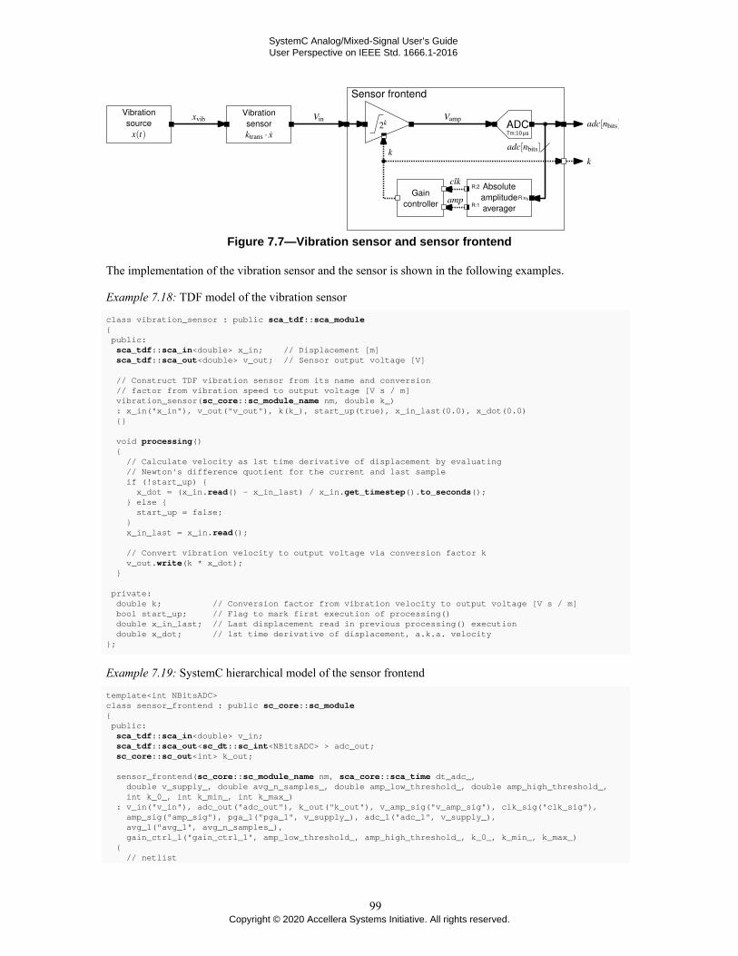
SystemC Analog/Mixed-Signal User’s GuideUser Perspective on IEEE Std. 1666.1-2016
Figure 7.7—Vibration sensor and sensor frontend
The implementation of the vibration sensor and the sensor is shown in the following examples.
Example 7.18: TDF model of the vibration sensor
class vibration_sensor : public sca_tdf::sca_module{ public: sca_tdf::sca_in<double> x_in; // Displacement [m] sca_tdf::sca_out<double> v_out; // Sensor output voltage [V]
// Construct TDF vibration sensor from its name and conversion // factor from vibration speed to output voltage [V s / m] vibration_sensor(sc_core::sc_module_name nm, double k_) : x_in("x_in"), v_out("v_out"), k(k_), start_up(true), x_in_last(0.0), x_dot(0.0) {}
void processing() { // Calculate velocity as 1st time derivative of displacement by evaluating // Newton's difference quotient for the current and last sample if (!start_up) { x_dot = (x_in.read() - x_in_last) / x_in.get_timestep().to_seconds(); } else { start_up = false; } x_in_last = x_in.read();
// Convert vibration velocity to output voltage via conversion factor k v_out.write(k * x_dot); }
private: double k; // Conversion factor from vibration velocity to output voltage [V s / m] bool start_up; // Flag to mark first execution of processing() double x_in_last; // Last displacement read in previous processing() execution double x_dot; // 1st time derivative of displacement, a.k.a. velocity};
Example 7.19: SystemC hierarchical model of the sensor frontend
template<int NBitsADC>class sensor_frontend : public sc_core::sc_module{ public: sca_tdf::sca_in<double> v_in; sca_tdf::sca_out<sc_dt::sc_int<NBitsADC> > adc_out; sc_core::sc_out<int> k_out;
sensor_frontend(sc_core::sc_module_name nm, sca_core::sca_time dt_adc_, double v_supply_, double avg_n_samples_, double amp_low_threshold_, double amp_high_threshold_, int k_0_, int k_min_, int k_max_) : v_in("v_in"), adc_out("adc_out"), k_out("k_out"), v_amp_sig("v_amp_sig"), clk_sig("clk_sig"), amp_sig("amp_sig"), pga_1("pga_1", v_supply_), adc_1("adc_1", v_supply_), avg_1("avg_1", avg_n_samples_), gain_ctrl_1("gain_ctrl_1", amp_low_threshold_, amp_high_threshold_, k_0_, k_min_, k_max_) { // netlist
99Copyright © 2020 Accellera Systems Initiative. All rights reserved.

SystemC Analog/Mixed-Signal User’s GuideUser Perspective on IEEE Std. 1666.1-2016
pga_1.in(v_in); pga_1.k_in(k_out); pga_1.out(v_amp_sig);
adc_1.set_timestep(dt_adc_); adc_1.in(v_amp_sig); adc_1.out(adc_out);
avg_1.in(adc_out); avg_1.clk(clk_sig); avg_1.out(amp_sig);
gain_ctrl_1.clk(clk_sig); gain_ctrl_1.amp_in(amp_sig); gain_ctrl_1.k_out(k_out); }
private: sca_tdf::sca_signal<double> v_amp_sig; sc_core::sc_signal<bool> clk_sig; sc_core::sc_signal<sc_dt::sc_int<NBitsADC> > amp_sig;
programmable_gain_amplifier pga_1; ad_converter<NBitsADC> adc_1; abs_amplitude_averager<NBitsADC> avg_1; gain_controller<NBitsADC> gain_ctrl_1;};
Example 7.20: TDF model of the programmable gain amplifier
class programmable_gain_amplifier : public sca_tdf::sca_module{ public: sca_tdf::sca_in<double> in; sca_tdf::sca_de::sca_in<int> k_in; sca_tdf::sca_out<double> out;
programmable_gain_amplifier(sc_core::sc_module_name nm, double v_supply_) : in("in"), k_in("k_in"), out("out"), v_supply(v_supply_) { sc_assert(v_supply > 0.0); }
void processing() { double k = k_in.read(); // Amplify input value to output value double val = std::pow(2.0, k) * in.read(); // Test if output saturates. if (val > v_supply) { out.write(v_supply); } else if (val < -v_supply) { out.write(-v_supply); } else { out.write(val); } }
private: const double v_supply; // Supply voltage limiting output};
Example 7.21: TDF model of the A/D converter
template<int NBits>class ad_converter : public sca_tdf::sca_module{ public: sca_tdf::sca_in<double> in; sca_tdf::sca_out<sc_dt::sc_int<NBits> > out;
ad_converter(sc_core::sc_module_name nm, double v_max_) : in("in"), out("out"), v_max(v_max_)
100Copyright © 2020 Accellera Systems Initiative. All rights reserved.

SystemC Analog/Mixed-Signal User’s GuideUser Perspective on IEEE Std. 1666.1-2016
{ sc_assert((2 <= NBits) && (NBits <= 64)); sc_assert(v_max_ > 0.0); }
void processing() { using namespace std; double v_in = in.read(); if (v_in < -v_max) { out.write(-((1 << (NBits - 1)) - 1)); } else if (v_in > v_max) { out.write((1 << (NBits - 1)) - 1); } else { sc_dt::sc_int<NBits> q_v_in = lround((v_in / v_max) * ((1 << (NBits - 1)) - 1)); out.write(q_v_in); } }
private: const double v_max;};
Example 7.22: TDF model of the absolute amplitude averager
template<int NBits>class abs_amplitude_averager : public sca_tdf::sca_module{ public: sca_tdf::sca_in<sc_dt::sc_int<NBits> > in; sca_tdf::sca_de::sca_out<bool> clk; sca_tdf::sca_de::sca_out<sc_dt::sc_int<NBits> > out;
explicit abs_amplitude_averager(sc_core::sc_module_name nm, long n_samples_) : in("in"), clk("clk"), out("out"), n_samples(n_samples_) { sc_assert((NBits >= 2) && (NBits <= 64)); sc_assert(n_samples_ > 0); }
void set_attributes() { in.set_rate(n_samples); clk.set_rate(2); clk.set_delay(2); out.set_rate(1); out.set_delay(1); }
void initialize() { clk.initialize(true, 0); clk.initialize(false, 1); out.initialize(0); }
void processing() { // Generate clock signal clk.write(true, 0); clk.write(false, 1); // Calculate and output average of absolute amplitudes long sum = 0; for (long i = 0; i < n_samples; ++i) { sum += std::labs(in.read(i)); } long avg = sum / n_samples; out.write(avg); }
private: const long n_samples; // Number of averaged samples
101Copyright © 2020 Accellera Systems Initiative. All rights reserved.

SystemC Analog/Mixed-Signal User’s GuideUser Perspective on IEEE Std. 1666.1-2016
};
The gain controller implements a finite state machine (FSM) as shown in Figure 7.8. A regular SystemCmodule is used for the implementation of the FSM, see Example 7.23.
Figure 7.8—Gain controller finite state machine (FSM)
Example 7.23: SystemC hierarchical model of the gain controller
template<int NBits>class gain_controller : public sc_core::sc_module{ public: sc_core::sc_in<bool> clk; sc_core::sc_in<sc_dt::sc_int<NBits> > amp_in; sc_core::sc_out<int> k_out;
SC_HAS_PROCESS(gain_controller); explicit gain_controller(sc_core::sc_module_name nm, int low_threshold_ = 0.2 * ((1 << (NBits - 1)) - 1), int high_threshold_ = 0.8 * ((1 << (NBits - 1)) - 1), int k_0_ = 0, int k_min_ = 0, int k_max_ = 16) : clk("clk"), amp_in("amp_in"), k_out("k_out"), low_threshold(low_threshold_), high_threshold(high_threshold_), k_min(k_min_), k_max(k_max_), state(KEEP_GAIN), k(k_0_) { sc_assert(low_threshold_ > 0); sc_assert(low_threshold_ < high_threshold_); sc_assert(high_threshold_ < ((1 << (NBits - 1)) - 1)); sc_assert(k_min_ < k_max_); sc_assert(k_min_ <= k_0_ && k_0_ <= k_max_);
SC_METHOD(gain_fsm); sensitive << clk.pos(); }
void gain_fsm() { switch (state) { case KEEP_GAIN: if (amp_in.read() < low_threshold) { state = INCREASE_GAIN; ++k; } else if (amp_in.read() >= high_threshold) { state = DECREASE_GAIN; --k; } break; case INCREASE_GAIN: if (amp_in.read() < high_threshold) { ++k; } else { state = DECREASE_GAIN; --k; } break; case DECREASE_GAIN: if (amp_in.read() < high_threshold) { state = KEEP_GAIN; } else { --k; }
102Copyright © 2020 Accellera Systems Initiative. All rights reserved.

SystemC Analog/Mixed-Signal User’s GuideUser Perspective on IEEE Std. 1666.1-2016
break; default: SC_REPORT_ERROR("/vibration_sensor/gain_controller", "Unexpected state."); } // Limit and set new gain if (k < k_min) { k = k_min; } if (k > k_max) { k = k_max; } k_out.write(k); }
private: const int low_threshold; // Low threshold for amplitude to increase gain const int high_threshold; // High threshold for amplitude to lower gain const double k_min; // Minimum gain power const double k_max; // Maximum gain power
enum state_type {KEEP_GAIN, INCREASE_GAIN, DECREASE_GAIN}; state_type state; // Current state int k; // Current gain power};
Example 7.24: TDF model of the vibration source
class vibration_source : public sca_tdf::sca_module{ public: sca_tdf::sca_out<double> out;
// Construct sinusoidal wavelets waveform generator vibration_source(sc_core::sc_module_name nm, double offset_, double amplitude_, double f_0_, int n_period_ = 1, int n_harmonic_ = 3) : out("out"), offset(offset_), amplitude(amplitude_), f_0(f_0_), n_period(n_period_), n_harmonic(n_harmonic_), T_0(1.0 / f_0_), T_period(n_period * T_0) { sc_assert(f_0_ > 0.0); sc_assert(n_period_ >= 1); sc_assert(n_harmonic_ >= 0); }
// Calculate and output value of waveform at time t void processing () { double t = this->get_time().to_seconds(); double t_pos = fmod(t, T_period); int harmonic = static_cast<int>(floor(t / T_period)) % (n_harmonic + 1); double val = offset; val += amplitude * sin(2.0 * M_PI * pow(2.0, harmonic) * f_0 * t_pos); out.write(val); }
private: const double offset; // Offset of the sine wave const double amplitude; // Amplitude of the sine wave const double f_0; // Base frequency of the sine wave const int n_period; // Number of periods for one wavelet with f_0_ const int n_harmonic; // Number of harmonics in the wavelet sequence const double T_0; // Period of sine wave with f_0_ const double T_period; // Period of a sine wavelet};
The testbench of the vibration sensor is implemented in the function sc_main.
Example 7.25: Vibration sensor main program
int sc_main(int argc, char* argv[]){ using namespace sc_core; using namespace sca_util;
// vibration sensor transducer constant for transformation of speed into voltage
103Copyright © 2020 Accellera Systems Initiative. All rights reserved.

SystemC Analog/Mixed-Signal User’s GuideUser Perspective on IEEE Std. 1666.1-2016
const double k_trans = 1.0; // V s / m
// Resolution of the ADC const int NBitsADC = 5; // ADC sampling period (equal to TDF time step) const sc_time dt_adc(10.0, SC_US);
// Absolute amplitude averager parameters const long avg_n_samples = 50;
// Gain controller parameters const int amp_low_threshold = 0.2 * ((1 << (NBitsADC - 1)) - 1); const int amp_high_threshold = 0.66 * ((1 << (NBitsADC - 1)) - 1); const int k_0 = 8; const int k_min = 0; const int k_max = 16;
// Supply voltages for pre-amplifier and ADC const double v_supply = 5.0; // V
// Vibration test signal const double x_offset = -8.0e-6; // m const double x_amplitude = 4.0e-6; // m const double x_f_0 = 2.0e3; // Hz const int x_n_period = 8; const int x_n_harmonic = 2;
// Simulation stop time const sc_time t_stop(25.0, SC_MS);
// Signals sca_tdf::sca_signal<double> x_sig("x_sig"), v_sig("v_sig"); sca_tdf::sca_signal<sc_dt::sc_int<NBitsADC> > adc_sig("adc_sig"); sc_core::sc_signal<int> k_sig("k_sig");
// Mechanical vibration source x(t) vibration_source vib_src("vib_src", x_offset, x_amplitude, x_f_0, x_n_period, x_n_harmonic); vib_src.out(x_sig);
// Vibration sensor with displacement input and velocity proportional voltage output vibration_sensor vib_sensor("vib_sensor", k_trans); vib_sensor.x_in(x_sig); vib_sensor.v_out(v_sig);
// Sensor frontend with PGA and gain controller to use fully the dynamic range of its ADC sensor_frontend<NBitsADC> frontend("frontend", dt_adc, v_supply, avg_n_samples, amp_low_threshold, amp_high_threshold, k_0, k_min, k_max); frontend.v_in(v_sig); frontend.adc_out(adc_sig); frontend.k_out(k_sig);
// Tracing sca_trace_file *tfp = sca_create_tabular_trace_file("vibration_sensor_tb"); sca_trace(tfp, x_sig, x_sig.name()); sca_trace(tfp, v_sig, v_sig.name()); sca_trace(tfp, adc_sig, "adc_sig"); sca_trace(tfp, k_sig, "k_sig");
// Simulation sc_start(t_stop);
// Close and save trace file sca_close_tabular_trace_file(tfp);
sc_stop(); return 0;}
The waveforms of the vibration sensor example are shown below.
104Copyright © 2020 Accellera Systems Initiative. All rights reserved.

SystemC Analog/Mixed-Signal User’s GuideUser Perspective on IEEE Std. 1666.1-2016
Figure 7.9—Simulation results of the vibration sensor example
7.6 DCDC converter example
Figure 7.10 shows a switching regulator circuit implemented in the form of a step-down (buck) converter.The output power is regulated using pulse-width modulation (PWM) to change the duty cycle of the controlsignal to the switch.
Figure 7.10—DCDC converter
105Copyright © 2020 Accellera Systems Initiative. All rights reserved.

SystemC Analog/Mixed-Signal User’s GuideUser Perspective on IEEE Std. 1666.1-2016
The implementation of the DCDC converter is shown in the examples below.
Example 7.26: SystemC hierarchical model of the DCDC converter
SC_MODULE(dcdc_converter){ // terminals and ports sca_eln::sca_terminal vout; sca_tdf::sca_in<double> vsupply; sca_tdf::sca_in<double> vref;
// parameters double l_value; double c_value; sca_core::sca_time sample_time;
compensator i_compensator; sca_eln::sca_tdf_vsource i_vsupply; sca_eln::sca_tdf_rswitch i_switch; sca_eln::sca_l i_sca_l; sca_eln::sca_c i_sca_c; sca_eln::sca_tdf_vsink i_sca_tdf_vsink; dcdc_pwm i_dcdc_pwm; diode i_diode;
dcdc_converter( sc_core::sc_module_name nm, double l_val_ = 6.5e-3, double c_val_ = 6e-6, sc_core::sc_time sample_time_ = sc_core::SC_ZERO_TIME ) : vout("vout"), vsupply("vsupply"), vref("vref"), l_value(l_val_), c_value(c_val_), sample_time(sample_time_), i_compensator("i_compensator", 806.0/2.0, 806.0/2.0, 7.5e3, 531.0e3, 100.0), i_vsupply("i_vsupply", 1.0), i_switch("i_switch", 1e-3, 1e9, false), i_sca_l("i_sca_l", l_value, 0.0), i_sca_c("i_sca_c", c_value, 0.0), i_sca_tdf_vsink("i_sca_tdf_vsink", 1.0), i_dcdc_pwm("i_dcdc_pwm", sc_core::sc_time(40.0, sc_core::SC_US), 2.5, sample_time_), i_diode("i_diode", 0.7, 1e-3, 1e9), rsw("rsw"), ctrl("ctrl"), s_vout("s_vout"), gnd("gnd"), vx("vx"), n_supply("n_supply") { // netlist i_compensator.inp(s_vout); i_compensator.ref(vref); i_compensator.outp(ctrl);
i_vsupply.p(n_supply); i_vsupply.n(gnd); i_vsupply.inp(vsupply);
i_switch.p(n_supply); i_switch.n(vx); i_switch.ctrl(rsw);
i_sca_l.p(vx); i_sca_l.n(vout);
i_sca_c.p(gnd); i_sca_c.n(vout);
i_sca_tdf_vsink.p(vout); i_sca_tdf_vsink.n(gnd); i_sca_tdf_vsink.outp(s_vout);
i_dcdc_pwm.inp(ctrl); i_dcdc_pwm.outp(rsw);
i_diode.np(gnd); i_diode.nn(vx); }
private: // nodes and signals sca_tdf::sca_signal<bool> rsw; sca_tdf::sca_signal<double> ctrl;
106Copyright © 2020 Accellera Systems Initiative. All rights reserved.

SystemC Analog/Mixed-Signal User’s GuideUser Perspective on IEEE Std. 1666.1-2016
sca_tdf::sca_signal<double> s_vout; sca_eln::sca_node_ref gnd; sca_eln::sca_node vx; sca_eln::sca_node n_supply;};
Example 7.27: TDF model of the compensator
SCA_TDF_MODULE(compensator){ // ports sca_tdf::sca_in<double > inp; sca_tdf::sca_in<double> ref; sca_tdf::sca_out<double> outp;
// parameters double fz1, fz2, fp1, fp2, gain; void initialize() { // linear transfer function - zeros coefficients zeros(0) = -2.0 * M_PI * fz1; zeros(1) = -2.0 * M_PI * fz2;
// linear transfer function - poles coefficients poles(0) = -2.0 * M_PI * fp1; poles(1) = -2.0 * M_PI * fp2; poles(2) = 0.0;
// scale due SystemC zp uses (s-k) like Matlab and Verilog-AMS (1-s/k) scale = fp1 * fp2 / fz1 / fz2 * gain; }
void processing() { outp = -scale * ltfzp(zeros, poles, inp - ref); }
compensator( sc_core::sc_module_name nm, double fz1_ = 806.0/2.0, double fz2_ = 806.0/2.0, double fp1_ = 7.5e3, double fp2_ = 531.0e3, double gain_ = 100.0 ) : inp("inp"), ref("ref"), outp("outp"), fz1(fz1_), fz2(fz2_), fp1(fp1_), fp2(fp2_), gain(gain_) { accept_attribute_changes(); }
private: sca_util::sca_vector<sca_util::sca_complex> zeros, poles; double scale; sca_tdf::sca_ltf_zp ltfzp;};
Example 7.28: TDF model of the pulse-width modulator
SCA_TDF_MODULE(dcdc_pwm){ // ports sca_tdf::sca_in<double > inp; sca_tdf::sca_out<bool> outp;
// parameters sc_core::sc_time clk_period; double sawtooth_amp; sca_core::sca_time sample_time;
void initialize() { outp.initialize(false); }
void processing() { //do not iterate - use first result if (this->get_timestep() > sc_core::SC_ZERO_TIME)
107Copyright © 2020 Accellera Systems Initiative. All rights reserved.

SystemC Analog/Mixed-Signal User’s GuideUser Perspective on IEEE Std. 1666.1-2016
{ // generate sawtooth double freq = 1.0 / clk_period.to_seconds();
// circular integration between -pi and pi double increment = freq * (this->get_timestep()).to_seconds();
if (sum + increment > 1.0) { sum = sum + increment - 1.0; } else if (sum + increment < 0.0) //at time zero { sum = 0.0; } else { sum += increment; }
sawtooth = sawtooth_amp * sum;
// calculate switch output rswitch = (sawtooth > inp.read()) ? false : true; }
outp.write(rswitch); }
void set_attributes() { if (sample_time != sc_core::SC_ZERO_TIME) { set_timestep(sample_time); } outp.set_delay(1); }
dcdc_pwm( sc_core::sc_module_name nm, sc_core::sc_time clk_period_ = sc_core::sc_time(25.0, SC_US), double sawtooth_amp_ = 2.5, sca_core::sca_time sample_time_ = sc_core::SC_ZERO_TIME ) : inp("inp"), outp("outp"), clk_period(clk_period_), sawtooth_amp(sawtooth_amp_), sample_time(sample_time_) { accept_attribute_changes();
// initial values sum = 0.0; sawtooth=0.0; rswitch=false; }
private: double sum; double sawtooth; bool rswitch;};
Example 7.29: SystemC hierarchical model of a diode
SC_MODULE(diode){ // terminals sca_eln::sca_terminal np; sca_eln::sca_terminal nn;
// parameters diode_dtdf i_diode_characteristic; sca_eln::sca_tdf_vsource i_vth; sca_eln::sca_tdf_vsink i_vdiode2tdf; sca_eln::sca_tdf_r i_rdiode;
diode(sc_core::sc_module_name nm, double vth_p_ = 0.7, double ron_ = 1e-3, double roff_ = 1e9) : np("np"), nn("nn"), i_diode_characteristic("i_diode_characteristic", ron_, roff_, vth_p_), i_vth("i_vth", 1.0), i_vdiode2tdf("i_vdiode2tdf", 1.0), i_rdiode("i_rdiode", 1.0), s_rout("s_rout"), s_vth("s_vth"),
108Copyright © 2020 Accellera Systems Initiative. All rights reserved.

SystemC Analog/Mixed-Signal User’s GuideUser Perspective on IEEE Std. 1666.1-2016
n_rdiode("n_rdiode"), s_vdiode("s_vdiode") { // netlist i_diode_characteristic.vin(s_vdiode); i_diode_characteristic.vth(s_vth); i_diode_characteristic.rout(s_rout);
i_vth.p(np); i_vth.n(n_rdiode); i_vth.inp(s_vth);
i_vdiode2tdf.p(np); i_vdiode2tdf.n(nn); i_vdiode2tdf.outp(s_vdiode);
i_rdiode.p(nn); i_rdiode.n(n_rdiode); i_rdiode.inp(s_rout); }
private: // nodes and signals sca_tdf::sca_signal<double> s_rout; sca_tdf::sca_signal<double> s_vth; sca_eln::sca_node n_rdiode; sca_tdf::sca_signal<double> s_vdiode;};
Example 7.30: TDF model implementing the diode characteristic
SCA_TDF_MODULE(diode_dtdf){ // ports sca_tdf::sca_in<double > vin; sca_tdf::sca_out<double> vth; sca_tdf::sca_out<double> rout;
// parameters double ron; double roff; double vth_p;
void initialize() { // iteration at time zero is possible rout.initialize(roff); vth.initialize(0.0); ron_state = true;
recalculate = 0; activations = 0; iterations = 0; max_iterations = 0; timestep_cnt = 0; }
void processing() { double vin_tmp = vin.read();
if (this->get_timestep() > sc_core::SC_ZERO_TIME) timestep_cnt++;
// switch between states if (ron_state) { // hysteresis due curves do not fit exactly if (vin_tmp > vth_p) { recalculate = 0; } else { recalculate++; ron_state = false; } } else { if (vin_tmp < vth_p) {
109Copyright © 2020 Accellera Systems Initiative. All rights reserved.

SystemC Analog/Mixed-Signal User’s GuideUser Perspective on IEEE Std. 1666.1-2016
recalculate = 0; } else { recalculate++; ron_state = true; } }
// set resistance and threshold in dependency of the state if (ron_state) { rout.write(ron); vth.write(vth_p); } else { rout.write(roff); vth.write(0.0); } }
void end_of_simulation() { std::ostringstream str;
str << "Repeat timestep requests: " << iterations << " from: " << timestep_cnt << " valid timesteps "; str << " overall timesteps: " << activations; str << " maximum repeat of a timestep: " << max_iterations; SC_REPORT_INFO("diode_dtdf", str.str().c_str()); } void set_attributes() { vth.set_delay(1); rout.set_delay(1); }
void change_attributes() { activations++;
if (recalculate > 0) { // invalid, repeat last timestep request_next_activation(sc_core::SC_ZERO_TIME);
if (recalculate > 30) { SC_REPORT_ERROR("diode_dtdf", "Convergence failed"); }
iterations++; if (recalculate > max_iterations) max_iterations = recalculate; } }
diode_dtdf( sc_core::sc_module_name nm, double ron_ = 1e-3, double roff_ = 1e9, double vth_p_ = 0.7 ) : vin("vin"), vth("vth"), rout("rout"), ron(ron_), roff(roff_), vth_p(vth_p_) { accept_attribute_changes(); does_attribute_changes(); }
private: bool ron_state; long recalculate; long activations; long iterations; long max_iterations; long timestep_cnt;};
Example 7.31: TDF model implementing a constant source
SCA_TDF_MODULE(const_src){ sca_tdf::sca_out<double> outp;
110Copyright © 2020 Accellera Systems Initiative. All rights reserved.

SystemC Analog/Mixed-Signal User’s GuideUser Perspective on IEEE Std. 1666.1-2016
void processing() { outp.write(value); }
SCA_CTOR(const_src) : outp("outp") { accept_attribute_changes(); value=0.0; }
double value;};
The testbench of the DCDC converter is shown below.
Example 7.32: DCDC converter main program
int sc_main(int argc, char* argv[]){ using namespace sc_core; using namespace sca_util; sc_set_time_resolution(1.0, SC_FS);
sca_tdf::sca_signal<double> input_s("input_s"); sca_tdf::sca_signal<double> vsupply_s("vsupply_s"); sca_tdf::sca_signal<double> vref_s("vref_s"); sca_tdf::sca_signal<double> vout_s("vout_s"); sc_core::sc_signal<double> rload_s("rload_s"); sca_eln::sca_node n_out("n_out"); sca_eln::sca_node_ref gnd("gnd");
const_src i_const_vsupp("i_const_vsupp"); i_const_vsupp.value = 42.0; i_const_vsupp.outp(vsupply_s);
const_src i_const_vref("i_const_vref"); i_const_vref.value = 4.8; i_const_vref.outp(vref_s); //output port
dcdc_converter dut("dut", 5.0e-3, 10.0e-6, sca_core::sca_time(0.7777, SC_US)); dut.vref(vref_s); dut.vsupply(vsupply_s); dut.vout(n_out);
sca_eln::sca_de_r i_sca_de_rload("i_sca_de_rload"); i_sca_de_rload.scale = 1.0; i_sca_de_rload.p(n_out); i_sca_de_rload.n(gnd); i_sca_de_rload.inp(rload_s);
// tracing sca_trace_file *tf = sca_create_tabular_trace_file( "dcdc_converter_trace.dat"); sca_trace(tf, n_out, "vout"); sca_trace(tf, i_sca_de_rload, "iout"); sca_trace(tf, vsupply_s, "vsupply"); sca_trace(tf, vref_s, "vref");
// set load resistance to 2.4 Ohm rload_s.write(2.4);
// run 25 ms sc_start(25.0, SC_MS);
// set load resistance to 5 Ohm rload_s.write(5.0);
// run 15 ms sc_start(15.0, SC_MS);
// close trace file sca_close_tabular_trace_file(tf);
111Copyright © 2020 Accellera Systems Initiative. All rights reserved.

SystemC Analog/Mixed-Signal User’s GuideUser Perspective on IEEE Std. 1666.1-2016
// stop simulation to print statistics sc_stop();
std::ostringstream str; str << sc_core::sc_time_stamp() << " time domain simulation finished"; SC_REPORT_INFO("sc_main", str.str().c_str());
return 0;}
The waveforms of the DCDC converter example are shown below.
Figure 7.11—Simulation results of the DCDC converter example
112Copyright © 2020 Accellera Systems Initiative. All rights reserved.

SystemC Analog/Mixed-Signal User’s GuideUser Perspective on IEEE Std. 1666.1-2016
8. Modeling strategies
The SystemC AMS extensions provide designers with powerful tools for modeling analog/mixed-signalsystems. The extensions cover the use cases described in Chapter 1, by providing the models of computationTimed Data Flow, Linear Signal Flow, and Electrical Linear Networks, in addition to the discrete-event andTransaction Level Modeling approaches of SystemC. This chapter gives additional advice on how to use andcombine these models of computation in an efficient way. The presented strategies are not mandatory, andsometimes there might be other or better approaches. They are provided in order to guide an inexperienceduser in creating understandable models, to achieve high simulation performance, and to increase productivitywhen designing mixed analog/digital systems.
8.1 Behavioral modeling using the available models of computation
The models of computation provided by the SystemC AMS extensions are primarily intended to facilitate thebehavioral modeling of analog circuits, as well as of signal processing functions (no matter whether they willbe implemented in the analog or digital domain). Depending on the abstraction required, a suitable modelof computation for behavioral modeling has to be selected. Figure 8.1 gives an overview of the availablemodels of computation and the abstractions imposed by them, considering the aspects behavior, structure,communication, and time/frequency.
Figure 8.1—Abstractions imposed by the AMS models of computation
The most important abstractions imposed by the models of computation are:— Linearization of non-linear behavior due to the focus on linear behavior in the models of computation
that require the solving of equation systems (LSF, ELN).— Structural abstraction of circuits (conservative systems) to functional blocks (non-conservative
systems) with directed signals in the models of computation LSF and TDF. This abstraction replacesthe physical quantities (i(t), u(t)) with abstract quantities x(t).
— Sampling of continuous-time signals to discrete-time signals for the TDF model of computation. Fixedtime step and dynamic time step are supported when using the TDF static mode of operation or dynamicmode of operation, respectively (see Section 2.1.2).
Figure 8.2 shows the impact of abstraction and sampling to non-conservative behavior of a signal in anelectrical network.
113Copyright © 2020 Accellera Systems Initiative. All rights reserved.
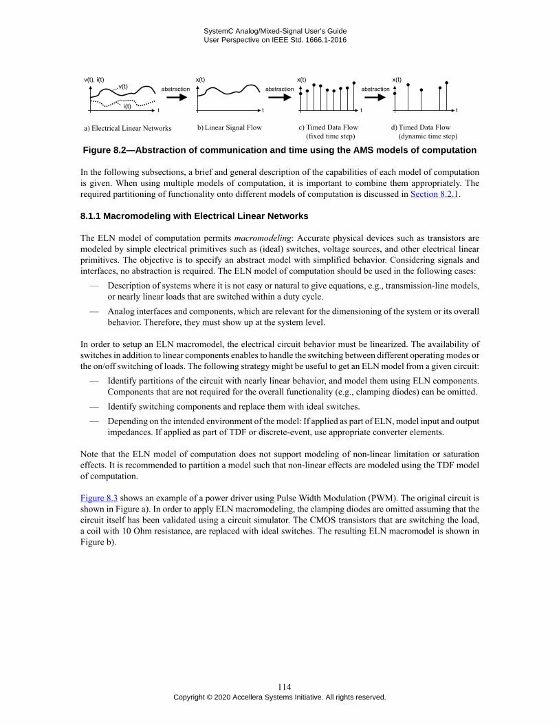
SystemC Analog/Mixed-Signal User’s GuideUser Perspective on IEEE Std. 1666.1-2016
Figure 8.2—Abstraction of communication and time using the AMS models of computation
In the following subsections, a brief and general description of the capabilities of each model of computationis given. When using multiple models of computation, it is important to combine them appropriately. Therequired partitioning of functionality onto different models of computation is discussed in Section 8.2.1.
8.1.1 Macromodeling with Electrical Linear Networks
The ELN model of computation permits macromodeling: Accurate physical devices such as transistors aremodeled by simple electrical primitives such as (ideal) switches, voltage sources, and other electrical linearprimitives. The objective is to specify an abstract model with simplified behavior. Considering signals andinterfaces, no abstraction is required. The ELN model of computation should be used in the following cases:
— Description of systems where it is not easy or natural to give equations, e.g., transmission-line models,or nearly linear loads that are switched within a duty cycle.
— Analog interfaces and components, which are relevant for the dimensioning of the system or its overallbehavior. Therefore, they must show up at the system level.
In order to setup an ELN macromodel, the electrical circuit behavior must be linearized. The availability ofswitches in addition to linear components enables to handle the switching between different operating modes orthe on/off switching of loads. The following strategy might be useful to get an ELN model from a given circuit:
— Identify partitions of the circuit with nearly linear behavior, and model them using ELN components.Components that are not required for the overall functionality (e.g., clamping diodes) can be omitted.
— Identify switching components and replace them with ideal switches.— Depending on the intended environment of the model: If applied as part of ELN, model input and output
impedances. If applied as part of TDF or discrete-event, use appropriate converter elements.
Note that the ELN model of computation does not support modeling of non-linear limitation or saturationeffects. It is recommended to partition a model such that non-linear effects are modeled using the TDF modelof computation.
Figure 8.3 shows an example of a power driver using Pulse Width Modulation (PWM). The original circuit isshown in Figure a). In order to apply ELN macromodeling, the clamping diodes are omitted assuming that thecircuit itself has been validated using a circuit simulator. The CMOS transistors that are switching the load,a coil with 10 Ohm resistance, are replaced with ideal switches. The resulting ELN macromodel is shown inFigure b).
114Copyright © 2020 Accellera Systems Initiative. All rights reserved.

SystemC Analog/Mixed-Signal User’s GuideUser Perspective on IEEE Std. 1666.1-2016
Figure 8.3—Abstraction of PWM power driver into an ELN macromodel
The PWM driver together with its load has the behavior of a low pass filter for the load current IL(t). As such, itcould also be modeled as a functional block. However, the load itself is usually an external part, and thus mightbe changed by the user. Therefore, it makes sense to provide an electrical terminal, and a (linear) macromodelof the load. Example 8.1 shows the ELN model of the PWM driver.
Example 8.1: ELN model of a PWM driver
SC_MODULE(pwm_driver){ sc_core::sc_in<bool> in; sca_eln::sca_terminal out; sca_eln::sca_vsource vcc; // voltage source sca_eln::sca_de::sca_rswitch highside, lowside; // two switches pwm_driver( sc_core::sc_module_name nm, double vcc_ = 5.0) : in("in"), out("out"), vcc("vcc"), highside("highside"), lowside("lowside"), node("node"), gnd("gnd") { vcc.offset = vcc_; // usage as constant voltage source vcc.p(node); vcc.n(gnd);
highside.ctrl(in); // 1st switch highside.p(node); highside.n(out);
lowside.ctrl(in); // 2nd switch... lowside.p(out); lowside.n(gnd); lowside.off_state = true; // ...is inverted }
private: sca_eln::sca_node node; sca_eln::sca_node_ref gnd;};
The load can also be described easily using linear primitives, in the most simple case, a coil with some resistancemight be sufficient:
Example 8.2: ELN model of the load
SC_MODULE(load){ sca_eln::sca_terminal p, n; sca_eln::sca_r r; sca_eln::sca_l l; load( sc_core::sc_module_name nm,
115Copyright © 2020 Accellera Systems Initiative. All rights reserved.

SystemC Analog/Mixed-Signal User’s GuideUser Perspective on IEEE Std. 1666.1-2016
double res_ = 500.0, double ind_ = 0.000001 ) : p("p"), n("n"), r("r", res_ ), l("l", ind_ ), node("node") { r.p(p); r.n(node);
l.p(node); l.n(n); }
private: sca_eln::sca_node node;};
8.1.2 Behavioral modeling with Linear Signal Flow
The LSF model of computation permits the description of block diagrams for the computation of lineardifferential equations. Compared to transfer functions, LSF allows to specify the order of computations and toaccess intermediate results or coefficients. In particular, LSF is useful to:
— Model filters with a given structure that has, e.g., impact on noise.— Model continuous-time control systems, in particular those that require access to coefficients from
other models of computation.
For LSF, an abstraction of physical signals is required as described in Chapter 3. Most notably, this also requiresthe abstraction of communication towards directed signals. Considering the structure and behavior, functionalblocks have to be identified, and their behavior has to be described by instantiating the pre-defined functionalprimitives. Considering time, no abstraction is required.
Note that LSF does not provide means to specify non-linear limitation or saturation. It is recommended topartition a model in a way that non-linear effects, if needed, are specified using the TDF model of computation.A typical application example where LSF is useful is shown in Figure 8.4 and Example 8.3. It is a PID controllerthat can be part of a closed loop control system model. Its coefficients can be adjusted from a TDF model.In order to model a closed-loop control system without delay, the device itself must also be modeled usingthe LSF model of computation. Using any other model of computation (ELN, TDF) will introduce a delayin the control loop.
Figure 8.4—LSF model of a PID controller with adjustable coefficients
Example 8.3: LSF model of a PID controller with adjustable coefficients
SC_MODULE(lsf_pid_external_control){ sca_lsf::sca_in in; sca_lsf::sca_out out;
sca_tdf::sca_in<double> p, i, d; // adjustable coefficients
116Copyright © 2020 Accellera Systems Initiative. All rights reserved.

SystemC Analog/Mixed-Signal User’s GuideUser Perspective on IEEE Std. 1666.1-2016
sca_lsf::sca_tdf::sca_gain gain_p, gain_i, gain_d; // coefficients used to scale the gain sca_lsf::sca_integ integ; sca_lsf::sca_dot dot; sca_lsf::sca_add add1, add2;
lsf_pid_external_control( sc_core::sc_module_name name ) : in("in"), out("out"), p("p"), i("i"), d("d"), gain_p("gain_p"), gain_i("gain_i"), gain_d("gain_d"), integ("integ"), dot("dot"), add1("add1"), add2("add2"), sig_gain("sig_gain"), sig_integ1("sig_integ1"), sig_integ2("sig_integ2"), sig_dot1("sig_dot1"), sig_dot2("sig_dot2"), sig_add("sig_add") { gain_p.x(in); gain_p.y(sig_gain); gain_p.inp(p);
gain_i.x(in); gain_i.y(sig_integ1); gain_i.inp(i);
gain_d.x(in); gain_d.y(sig_dot1); gain_d.inp(d);
integ.x(sig_integ1); integ.y(sig_integ2); dot.x(sig_dot1); dot.y(sig_dot2);
add1.x1(sig_gain); add1.x2(sig_integ2); add1.y(sig_add);
add2.x1(sig_add); add2.x2(sig_dot2); add2.y(out); } private: sca_lsf::sca_signal sig_gain, sig_integ1, sig_integ2, sig_dot1, sig_dot2, sig_add;};
8.1.3 Behavioral and baseband modeling with Timed Data Flow
The TDF model of computation permits the modeling of analog systems at a high level of abstraction, as wellas the modeling of signal processing functions.
For modeling analog behavior, the TDF model of computation requires a discrete-time approximation ofthe continuous-time analog signals. However, TDF permits, in contrast to LSF and ELN, the modeling ofstatic non-linear behavior. The discrete-time approximation reduces the continuous-time signal to a sequenceof discrete samples. The time-distance between the samples can be constant (fixed time step) or controlleddynamically, triggered by events from the discrete-event domain or by requested activations in TDF modules(see Section 2.1.2).
The imposed data flow modeling style avoids the need for solving (non-linear) equations, or delta iterations,and thus improves simulation performance. Besides the discretization, the TDF model of computation alsorequires the breaking of cyclic dependencies (also known as algebraic loops) by inserting delays (see Section2.1.3).
Taking advantage of these abstractions, TDF models permit describing the processing of streams of samples inan arbitrary, algorithmic way with the help of the member function processing. In particular, also non-lineartransfer functions (i.e., for modeling limitation) or look-up tables can be implemented easily. Furthermore,the specification of signal processing methods in terms of transfer functions H(s), H(z), or state spacerepresentations is supported in TDF (see Section 2.3.2).
117Copyright © 2020 Accellera Systems Initiative. All rights reserved.

SystemC Analog/Mixed-Signal User’s GuideUser Perspective on IEEE Std. 1666.1-2016
The following abstractions are introduced by TDF:— Like in LSF, a block diagram structure has to be defined. Unlike in LSF, there is virtually no restriction
to the behavior of single blocks.— The sampling frequency, or time/event of the next cluster activation must be defined.— The TDF model requires acyclic structures to ensure schedulability. The acyclic structure can be
achieved by introducing a delay into the cycle (Section 2.1.3). Note that most control loops use digitalcontrollers that introduce delays. The location of the digital controller might be a good location forintroducing such a delay.
8.1.3.1 Definition and propagation of time steps and rates
The time steps and rates in TDF must be selected carefully to match the modeling problem. It is alsorecommended to carefully select the places where time steps and rates are defined.
For modeling analog behavior, it is recommended to ensure a sufficiently high sample frequency. The samplingfrequency must be significantly higher than twice the frequency defined by the lowest time constant in thesystem. If in doubt, a factor 10 is recommended. Selecting a higher rate or smaller time steps results in a higheraccuracy at high frequencies at the cost of simulation performance. An appropriate place to define the timestep might be the test bench.
Systems with time constants that differ by orders of magnitudes (stiff systems) are a particular problem. Werecommend partitioning such systems into parts with low time constants, and parts with higher time constants.Then, different rates of the TDF model of computation can be used to define different sample frequencies ineach partition.
Note that for digital signal processing (DSP) methods (e.g., using H(z), or state space representations of digitalfilters), there is a dependency between functionality and the selected time step. For DSP methods that areintended for use at a particular sample frequency, it is therefore recommended to define a time step in themodule itself (or at its ports respectively). Then, a test bench can still define time steps. However, an error willbe reported if the consistency check after propagation of time steps fails (see Section 2.5).
The ability to use non-equidistant time steps available since SystemC AMS version 2.0 enables very powerfulmodeling strategies that permit solving a number of challenging modeling issues, such as:
— Modeling change of rates in adaptive radio,— Modeling jitter in implementation of discrete-time systems, or— Modeling discrete-time systems where pulses of variable length are used, like in PWM (digitally
controlled length), or PLL (continuously controlled length).
8.1.3.2 Behavioral modeling with TDF
Section 7.1 shows an application example demonstrating behavioral modeling using the TDF model ofcomputation. Note that the SystemC AMS extensions permit to write arbitrary C++ code into the TDF modulemember function processing. This allows combining ideal signal processing functions (usually found in blocklibraries) such as amplification, multiplication, or transfer functions in a very easy and effective way with non-ideal behavior. An amplifier, for example, can be modeled by combining the following features:
— Large-signal behavior (e.g., saturation, non-linearity) can be modeled by using functions in C++.— The frequency-domain behavior can be modeled using a Laplace transfer function, as discussed in
Section 2.3.2. Poles and zeros can be identified easily using circuit simulation, or using the Bode plot.
Example 8.4: TDF model of an amplifier
SCA_TDF_MODULE(amplifier)
118Copyright © 2020 Accellera Systems Initiative. All rights reserved.

SystemC Analog/Mixed-Signal User’s GuideUser Perspective on IEEE Std. 1666.1-2016
{ sca_tdf::sca_in<double> in; sca_tdf::sca_out<double> out; amplifier( sc_core::sc_module_name, double gain_ = 100.0, double dom_pole_ = 5.0e8, double limit_ = 5.0 ) : in("in"), out("out"), gain(gain_), dom_pole(dom_pole_), limit(limit_) {} void initialize() { // filter requires no zeros to be defined poles(0) = sca_util::sca_complex( -2.0 * M_PI * dom_pole, 0.0 ); k = gain * 2.0 * M_PI * dom_pole; } void processing() { // time-domain implementation of amplifier behavior as function of frequency double internal = ltf_zp( zeros, poles, state, in.read(), k );
// limiting the signal if (internal > limit) internal = limit; else if (internal < -limit) internal = -limit;
out.write(internal); } private: double gain; // DC gain double dom_pole; // 3dB cutoff frequency in Hz double limit; // limiter value double k; // filter gain sca_tdf::sca_ltf_zp ltf_zp; // Laplace transfer function sca_util::sca_vector<sca_util::sca_complex > poles, zeros; // poles and zeros as complex values sca_util::sca_vector<double> state; // state vector};
8.1.3.3 Baseband modeling with TDF
When modeling radio frequency (RF) systems with high carrier frequencies, a significant speed-up ofsimulation can be achieved by applying baseband modeling. This modeling strategy is based on the fact thatdigital modulation techniques use the amplitude r and the phase ϕ to transmit information. The informationitself is then independent from the (usually high) carrier frequency. The idea of baseband modeling is to mapthe RF carrier frequency to zero, as shown in Figure 8.5. The required sampling rate then only depends onthe bandwidth of the modulated signal.
Figure 8.5—Passband (a) and baseband (b)representation of signals in the frequency domain
Formally, the modulated carrier signal x(t) can be described as:
(8.1)
119Copyright © 2020 Accellera Systems Initiative. All rights reserved.

SystemC Analog/Mixed-Signal User’s GuideUser Perspective on IEEE Std. 1666.1-2016
where r(t) is the modulating signal, ϕ(t) the modulating phase and fc the carrier frequency. The term, whichincludes the carrier frequency fc, can be separated from the signal part, which contains the transmittedinformation. The signal v(t), which contains the information, is independent from the carrier frequency fc:
(8.2)
This signal is called the complex low-pass equivalent or the complex envelope. For the baseband signal, thecarrier frequency fc is set to zero. With si = r cos(ϕ) and sq = r sin(ϕ), the resulting baseband signal becomes:
(8.3)
where si represents the in-phase term of the baseband signal, and sq represents the quadrature term. Theamplitude and phase of the carrier signal can be computed from these signals at each point in time.
To implement baseband modeling using the SystemC AMS extensions, the C++ data type specializationstd::complex<double> can be used to represent complex numbers. This data type offers arithmetic andassociated C++ operators for calculations supporting complex numbers. Example 8.5 shows a simple basebandamplifier with an input and output port supporting complex envelope signals.
Example 8.5: TDF model of an amplifier using baseband modeling
#include <complex>
SCA_TDF_MODULE(baseband_amplifier){ sca_tdf::sca_in<std::complex<double > > in; sca_tdf::sca_out<std::complex<double > > out;
baseband_amplifier( sc_core::sc_module_name nm, double gain_ = 1.0 ) : in("in"), out("out"), c1( gain_ ) {}
void processing() { out.write( c1 * in.read() ); } private: double c1; };
The limitation of using std::complex<double> as data type is that it only describes the complex envelope ofthe modulated signal, and that the carrier frequency information is lost. Due to this, effects like harmonics ofthe carrier or intermodulation products are not represented. The solution to this is to create a user-defined datatype supporting multi-carrier equivalent baseband computations.
8.2 Modeling embedded analog/mixed-signal systems
Behavioral modeling using a single model of computation imposes a number of restrictions as shown in Section8.1. They can be overcome by combining (the strengths of) different models of computation. The followingsubsections describe how to partition the functional behavior onto the different models of computation. Then,a number of simple modeling guidelines is given, how to model architecture-level properties of analog circuits.
8.2.1 Partitioning behavior to different models of computation
A simple, but general strategy that allows beginners to distribute a block diagram like specification to thedifferent models of computation provided by the SystemC AMS extensions is shown by Figure 8.6. It can beapplied for each block successively.
120Copyright © 2020 Accellera Systems Initiative. All rights reserved.

SystemC Analog/Mixed-Signal User’s GuideUser Perspective on IEEE Std. 1666.1-2016
Figure 8.6—Partitioning of behavior to different models of computation
In the first two steps (see and ), the functionality to be modeled should be investigated to select themost appropriate language. The SystemC AMS extensions are a good choice for modeling signal processingfunctions and electrical (conservative) networks (see ). Note that signal processing functions implementedin analog, digital or software can be modeled very efficiently using the SystemC AMS extensions at thefunctional level. For the modeling of digital hardware/software systems (e.g., microcontrollers and processors),interconnect and communication protocols, SystemC and transaction-level modeling approaches are mostsuitable.
The decomposition of each function is evaluated in the steps labelled to . Here, the most efficient andapplicable model of computation is selected. The Timed Data Flow model of computation can be used tomodel static non-linear behavior (see ). Note that in some cases delays should be introduced in the modelsto facilitate interpolation or to resolve cyclic dependencies in the static TDF schedule (see ). Dynamic linearsystems can be modeled efficiently using the Linear Signal Flow model of computation, enabling a blockdiagram notation to represent the function (see ).
Another good reason to use the SystemC AMS extensions would be the need for having analog terminalsand/or physical quantities such as current available, e.g., for modeling external loads or analog behavior ofcommunication lines. For this purpose, the Electrical Linear Network model of computation offers the mostnatural modeling approach to include electrical primitives and to capture conservative behavior. In addition,piecewise linear approximation techniques using a combination of TDF and ELN models can be applied tomodel non-linear behavior. For strong non-linear systems, it is recommended to incorporate (or cosimulatewith) a non-linear solver like SPICE (see ).
When the TDF MoC is considered to model the AMS subsystem, different approaches are available to abstractthe signal in time (see ). In the most straight forward way, a signal can be sampled or even oversampledin equidistant time steps. In this case, the TDF static mode of operation is used, resulting in fixed time stepsduring the entire simulation. The TDF model of computation can also be used if the size of the time stepsshould be determined by events, by time outs, or by other computations. In this case, the TDF dynamic modeof operation can be used, which enable changing TDF attributes such as time steps, delays, or rates during
121Copyright © 2020 Accellera Systems Initiative. All rights reserved.

SystemC Analog/Mixed-Signal User’s GuideUser Perspective on IEEE Std. 1666.1-2016
simulation. Alternatively, regular SystemC discrete-event models can be created to become event-driven andcycle-accurate, but such approach is less efficient due to the additional simulation overhead imposed by thedynamic scheduling mechanism of SystemC for each evaluate/update cycle.
8.2.2 Modeling of architecture-level properties
In order to evaluate feasibility and performance of different architectures, the functional model can be usedand refined by adding specific properties. These properties include: noise, attenuation, distortions, limitation,jitter, delays, quantization, sampling frequencies, and many other. In the following, some simple guidelinesfor handling these effects during architecture exploration are given.
8.2.2.1 Modeling distortions, limitation, and quantization
In order to study the impact of distortions and limitations on the overall system functionality, analog modulesshould be split into linear dynamic behavior and nonlinear static behavior. Linear dynamic behavior can bespecified, e.g., using transfer functions in TDF (see Section 2.3.2). Non-linear behavior such as distortionsand limitation can be modeled easily using C++ functions in the TDF module’s member function processing(see Section 8.1.3).
8.2.2.2 Modeling noise in the time domain
Noise in the TDF model of computation can be modeled by adding Gaussian distributed random numbersto a TDF signal. Example 8.6 demonstrates a simple model for (white) noise and attenuation in a wirelesscommunication link. For this purpose, a function gauss_rand is used that generates Gaussian distributedrandom numbers.
Example 8.6: Modeling Gaussian noise
// the gauss_rand() function returns a Gaussian distributed// random number with variance "variance", centered around 0, using the Marsaglia polar method
#include <cstdlib> // for std::rand#include <cmath> // for std::sqrt and std::log
double gauss_rand(double variance){ double rnd1, rnd2, Q, Q1, Q2; do { rnd1 = ((double)std::rand()) / ((double)RAND_MAX) ; rnd2 = ((double)std::rand()) / ((double)RAND_MAX) ; Q1 = 2.0 * rnd1 - 1.0 ; Q2 = 2.0 * rnd2 - 1.0 ; Q = Q1 * Q1 + Q2 * Q2 ; } while (Q > 1.0) ; return ( std::sqrt(variance) *( std::sqrt( - 2.0 * std::log(Q) / Q) * Q1) );} SCA_TDF_MODULE(air_channel_with_noise) { sca_tdf::sca_in<double> in; sca_tdf::sca_out<double> out;
void processing() { out.write( in.read() * attenuation + gauss_rand(variance) ); } air_channel_with_noise( sc_core::sc_module_name nm, double attenuation_, double variance_ ) : in("in"), out("out"), attenuation(attenuation_), variance(variance_) {}
122Copyright © 2020 Accellera Systems Initiative. All rights reserved.
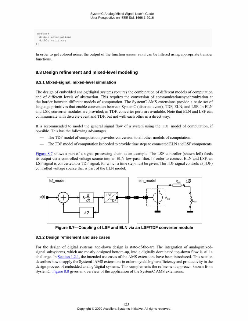
SystemC Analog/Mixed-Signal User’s GuideUser Perspective on IEEE Std. 1666.1-2016
private: double attenuation; double variance;};
In order to get colored noise, the output of the function gauss_rand can be filtered using appropriate transferfunctions.
8.3 Design refinement and mixed-level modeling
8.3.1 Mixed-signal, mixed-level simulation
The design of embedded analog/digital systems requires the combination of different models of computationand of different levels of abstraction. This requires the conversion of communication/synchronization atthe border between different models of computation. The SystemC AMS extensions provide a basic set oflanguage primitives that enable conversion between SystemC (discrete-event), TDF, ELN, and LSF. In ELNand LSF, converter modules are provided; in TDF, converter ports are available. Note that ELN and LSF cancommunicate with discrete-event and TDF, but not with each other in a direct way.
It is recommended to model the general signal flow of a system using the TDF model of computation, ifpossible. This has the following advantages:
— The TDF model of computation provides conversion to all other models of computation.— The TDF model of computation is needed to provide time steps to connected ELN and LSF components.
Figure 8.7 shows a part of a signal processing chain as an example: The LSF controller (shown left) feedsits output via a controlled voltage source into an ELN low-pass filter. In order to connect ELN and LSF, anLSF signal is converted to a TDF signal, for which a time step must be given. The TDF signal controls a (TDF)controlled voltage source that is part of the ELN model.
Figure 8.7—Coupling of LSF and ELN via an LSF/TDF converter module
8.3.2 Design refinement and use cases
For the design of digital systems, top-down design is state-of-the-art. The integration of analog/mixed-signal subsystems, which are mostly designed bottom-up, into a digitally dominated top-down flow is still achallenge. In Section 1.2.1, the intended use cases of the AMS extensions have been introduced. This sectiondescribes how to apply the SystemC AMS extensions in order to yield higher efficiency and productivity in thedesign process of embedded analog/digital systems. This complements the refinement approach known fromSystemC. Figure 8.8 gives an overview of the application of the SystemC AMS extensions.
123Copyright © 2020 Accellera Systems Initiative. All rights reserved.

SystemC Analog/Mixed-Signal User’s GuideUser Perspective on IEEE Std. 1666.1-2016
Figure 8.8—Use cases for the SystemC AMS extensions within top-down refinement
In the ideal case, top-down refinement begins with an executable specification of the intended behavior atsystem level. Usually, the TDF model of computation is suitable to develop a functional model for this purpose.Refinement of the executable specification is part of the architecture exploration use case. The refinementprocess consists of a stepwise approach of replacing the blocks in the system with more accurate (less abstract)models.
Architecture exploration distinguishes three separate aspects, each one being the opposite of one of theabstractions in Figure 8.1:
— Refinement of behavior.— Refinement of structure.— Refinement of communication/interfaces.
Behavioral refinement augments the functional model used for the executable specification with specificproperties of an architecture (implementation). This permits the evaluation of the feasibility and performance ofdifferent architectures (implementations). Properties that can easily be included in a functional model include:noise, attenuation, distortions, limitation, jitter, delays, quantization, sampling frequencies, and many other.
As an example, Figure 8.9 shows an ideal (linear) and non-linear power amplifier, where the linear gain (c1)and non-linear third-order term (c3) are approximated by using a Taylor series.
Figure 8.9—Refinement of behavior of a power amplifier
Example 8.7 shows the implementation of the power amplifier. The function std::pow(x,y) from the C++standard library cmath is used, which computes x raised to the power of y.
Example 8.7: TDF modeling of a non-linear power amplifier
#include <cmath>
SCA_TDF_MODULE(non_linear_amplifier){
124Copyright © 2020 Accellera Systems Initiative. All rights reserved.

SystemC Analog/Mixed-Signal User’s GuideUser Perspective on IEEE Std. 1666.1-2016
sca_tdf::sca_in<double> in; sca_tdf::sca_out<double> out;
non_linear_amplifier( sc_core::sc_module_name nm, double pow_gain_db_ = 10.0, double iip3_dbm_ = 10.0, double zref_ = 50.0 ) : in("in"), out("out") { a1 = std::pow(10.0, pow_gain_db_ / 10.0); double iip3_lin = std::sqrt(std::pow(10.0, (iip3_dbm_-30.0)/10.0) * 2.0 * zref_); a3 = (4.0 * a1)/(3.0 * std::pow(iip3_lin, 2.0)); }
void processing() { out.write( a1 * in.read() - a3 * std::pow(in.read(),3) ); } private: double a1, a3;};
Refinement of structure repartitions the (usually block-diagram-like) system, used for executable specification,with a structure of functional blocks that each represent a circuit or processor to be designed. Note that alsothe model of computation changes depending on the intended domain of implementation.
Figure 8.10—Structural refinement of a filter
In order to make the refinement of a model easier, the namespace concept allows to re-use a large part of existingmodeling infrastructure such as module and port declarations. However, behavior and (refined) structure haveto be written from scratch.
Refinement of communication/interfaces replaces the abstract communication used within the TDF model ofcomputation with concrete signals, e.g., electrical voltages and currents or digital (discrete-event) SystemCsignals. This requires to add also converter ports or modules to the models. Conversion between the modelsof computation is discussed in Section 8.3.1. In order to support the refinement of communication/interfaces,it is recommended to create adapter/converter classes as known from SystemC TLM extensions.
8.4 Modeling and coding style
8.4.1 Namespaces
The SystemC AMS extensions make extensive use of C++ namespaces to be able to clearly identify theavailable models of computation and use the available primitive modules within the right context. Thenamespaces sca_tdf, sca_lsf and sca_eln are reserved names for the language constructs used for the TDF,LSF and ELN model of computation, respectively. Other reserved namespaces are sca_util for utility classesand functions, and sca_ac_analysis for small-signal frequency-domain analyses. The user should not add newdefinitions in these namespaces. Instead, it is recommended to declare user-defined modules belonging to thesame model of computation to a unique user-defined namespace, as shown in Example 8.8.
125Copyright © 2020 Accellera Systems Initiative. All rights reserved.

SystemC Analog/Mixed-Signal User’s GuideUser Perspective on IEEE Std. 1666.1-2016
Example 8.8: Defining a namespace
namespace my_tdf_library {
SCA_TDF_MODULE(my_source) { ... }
}; // namespace my_tdf_library
Instantiation of this object will look like this:
Example 8.9: Instantiation of a module from a specific namespace
SC_MODULE(analog_top){ ... my_tdf_library::my_source i_my_source("i_my_source"); ...}
8.4.1.1 Header files and naming conventions
The header file systemc-ams does not import the reserved namespaces sca_tdf, sca_lsf, sca_eln, sca_util,and sca_ac_analysis into the scope of the program. This means the user has to explicitly add the namespaceidentifier to each element, when instantiating or declaring such an object. Although the names are a bit longerto write, it will result in a clear naming convention, where the user can recognize immediately whether theobject belongs to a particular class library of the SystemC AMS extensions, or whether the object is part of auser-defined library. Example 8.10 and all other examples in this user’s guide follow this naming convention.
Example 8.10: Usage of header file systemc-ams
#include <systemc-ams>
#include "my_source.h"
int sc_main(int argc, char* argv[]){ sc_core::sc_set_time_resolution(1.0, sc_core::SC_FS);
sca_tdf::sca_signal<double> sig1;
// instantiate user-defined module from user-defined 'my_tdf_library' namespace my_tdf_library::my_source i_my_source("i_my_source"); i_my_source.out(sig1);
// instantiate other modules ...
// tracing AMS signals sca_util::sca_trace_file* tf = sca_util::sca_create_tabular_trace_file("trace.dat"); sca_util::sca_trace(tf, sig1 ,"sig1"); sc_core::sc_start(10.0, sc_core::SC_MS);
tf->set_mode(sca_util::sca_ac_format(sca_util::SCA_AC_MAG_RAD)); sca_ac_analysis::sca_ac_start(1.0e3, 1.0e6, 4, sca_ac_analysis::SCA_LOG); sca_util::sca_close_tabular_trace_file(tf); return 0;}
When using the header file systemc-ams.h, all elements, which belong to the namespace sca_core, sca_utiland sca_ac_analysis, are imported into the scope of the program. This means the user can omit to prefixthe elements in these namespaces. Note that the namespace for the different models of computation are not
126Copyright © 2020 Accellera Systems Initiative. All rights reserved.

SystemC Analog/Mixed-Signal User’s GuideUser Perspective on IEEE Std. 1666.1-2016
declared, so even in this case, the user has to explicitly use the namespace to create TDF, LSF, and ELN models.Example 8.11 shows the use of the header file systemc-ams.h.
Example 8.11: Usage of header systemc-ams.h
#include <systemc-ams.h>
#include "my_source.h"
int sc_main(int argc, char* argv[]){ sc_set_time_resolution(1.0, sc_core::SC_FS);
sca_tdf::sca_signal<double> sig1;
// instantiate user-defined module from user-defined 'my_tdf' namespace my_tdf::my_source i_my_source("i_my_source"); i_my_source.out(sig1);
// instantiate other modules ...
// tracing AMS signals sca_trace_file* tf = sca_create_tabular_trace_file("trace.dat"); sca_trace(tf, sig1 ,"sig1"); sc_start(10.0, SC_MS);
tf->reopen("ac_trace.dat"); tf->set_mode( sca_ac_format(SCA_AC_MAG_RAD) ); sca_ac_start(1.0e3, 1.0e6, 4, SCA_LOG); sca_close_tabular_trace_file(tf); return 0;}
It is recommended to use the header file systemc-ams, resulting in a naming convention reflecting the fullnames of classes and functions.
8.4.1.2 Using directive
The using directive of C++ allows the elements in a namespace to be used without explicitly adding thenamespace identifier to each element. It should only be used in a module implementation, not in the moduledeclaration (e.g., definition in a header file). It is recommended to apply the using directive only within thelocal scope, e.g., as part of the implementation of a class member function. Example 8.12 shows how thisconcept can be applied for a frequency-domain description as described in Section 5.3.3.
Example 8.12: Using directive
void ac_processing(){ using namespace sca_util; using namespace sca_ac_analysis; sca_complex s = SCA_COMPLEX_J * sca_ac_w(); sca_complex h = 1.0 / ( s * s + s + 1.0 );
sca_ac(out) = h * sca_ac(in);}
8.4.2 Dynamic memory allocation
Most of the examples shown in this user’s guide use objects (e.g., primitive modules), which are directlyinstantiated in a function body, and thus are allocated automatically on the stack. In the case of big designs using
127Copyright © 2020 Accellera Systems Initiative. All rights reserved.

SystemC Analog/Mixed-Signal User’s GuideUser Perspective on IEEE Std. 1666.1-2016
many modules in a complex hierarchy, this approach is not the most efficient way as it can lead to an overflowof the stack for automatic variables. The instantiated objects are referenced by pointers so that they do not needto reside anymore in a consecutive memory area, which can lead to resource allocation problems. Furthermore,it allows the instantiation of an arbitrary number of modules determined at runtime, which are referenced froma dynamically created array of module pointers, and which constructors can be called individually to vary theparameterization of each object.
The C++ operator new is used to dynamically allocate memory on the heap to store the objects. As allocationreturns the address to the newly allocated memory, access to the object’s member functions is done using apointer. Any memory dynamically allocated with the operator new must be released (deallocated) using theoperator delete. This operator is usually called for each dynamically created member object in the destructorof the class.
Example 8.13 shows the use of dynamic memory allocation and deallocation for the BASK demodulator similaras described in Section 7.1.2.
Example 8.13: Dynamic memory allocation
SC_MODULE(bask_demod){ sca_tdf::sca_in<double> in; sca_tdf::sca_out<bool> out;
rectifier* rc; ltf_nd_filter* lp; sampler* sp;
SC_CTOR(bask_demod) : in("in"), out("out"), rc_out("rc_out"), lp_out("lp_out") { rc = new rectifier("rc"); rc->in(in); rc->out(rc_out);
lp = new ltf_nd_filter("lp", 3.3e6); lp->in(rc_out); lp->out(lp_out);
sp = new sampler("sp"); sp->in(lp_out); sp->out(out); }
~bask_demod() { delete(rc); delete(lp); delete(sp); }
private: sca_tdf::sca_signal<double> rc_out, lp_out;};
8.4.3 Module parameters
Modules need to be flexible to be reusable, i.e., their behavior and internal structure must be parameterizedto a reasonable degree to allow their adoption to varying specifications. This is especially interesting for theearly design stages of architecture exploration and successive refinement of the system structure.
In Section 7.1.1, a BASK modulator model is presented with hard coded design parameters, like the carrierfrequency of 70 MHz. With respect to this carrier frequency, the time step values and the data rates werehard coded, such that the resulting signal was sufficiently sampled. Such ‘magic numbers’, hard coded portrates, delays, and time steps, are typical signs of an inflexible implementation. If, for example, the carrier
128Copyright © 2020 Accellera Systems Initiative. All rights reserved.

SystemC Analog/Mixed-Signal User’s GuideUser Perspective on IEEE Std. 1666.1-2016
frequency would be increased without changing the time step, the model might not work properly becauseof undersampling.
A more flexible approach is to derive time step and data rate values from the functional module parameters. Inthis section it is shown how to make a parameterized version of the BASK modulator from Section 7.1.1, withadjustable carrier-frequency and baseband frequency, and how to derive data rates and time steps automaticallyfrom that. Firstly, a mixer with parameterized data rate is needed:
Example 8.14: TDF module of a mixer with parameterized data rate
SCA_TDF_MODULE(mixer) { sca_tdf::sca_in<bool> in_bin; // input port baseband signal sca_tdf::sca_in<double> in_wav; // input port carrier signal sca_tdf::sca_out<double> out; // output port modulated signal mixer( sc_core::sc_module_name nm, unsigned long rate_ ) : in_bin("in_bin"), in_wav("in_wav"), out("out"), rate(rate_) { using namespace sc_core; sc_assert(rate_ > 0); } void set_attributes() { in_wav.set_rate(rate); out.set_rate(rate); }
void processing() { for(unsigned long i = 0; i < rate; i++) { if( in_bin.read() ) out.write( in_wav.read(i), i ); else out.write( 0.0 , i ); } }
private: unsigned long rate;};
If parameters are used which are computed elsewhere, it is always a good idea to make plausibility checks.Therefore, the mixers’ constructor contains the line sc_assert(rate_ > 0) to check if the rate parameter is atleast 1.
Using this mixer, and the parameterized sinusoidal source already used in Section 7.1.1, a parameterized BASKmodulator can be implemented as follows:
Example 8.15: Parameterized TDF module of the BASK modulator
SC_MODULE(bask_mod){ sca_tdf::sca_in<bool> in; sca_tdf::sca_out<double> out; sin_src sine; mixer mix;
bask_mod( sc_core::sc_module_name nm, double baseband_freq, double carrier_freq, double carrier_ampl = 1.0, unsigned long samples_per_period = 20 ) : in("in"), out("out"), sine("sine", carrier_ampl, carrier_freq, sca_core::sca_time( (1.0 / (samples_per_period * carrier_freq) ), sc_core::SC_SEC) ),
129Copyright © 2020 Accellera Systems Initiative. All rights reserved.

SystemC Analog/Mixed-Signal User’s GuideUser Perspective on IEEE Std. 1666.1-2016
mix("mix", (int)std::ceil( static_cast<double>(samples_per_period) * carrier_freq / baseband_freq ) ), carrier("carrier") { using namespace sc_core; // Plausibility checks sc_assert(carrier_freq > baseband_freq); // wouldn't make sense otherwise! sc_assert(samples_per_period > 2); // Nyquist criterion satisfied? sc_assert(carrier_ampl > 0.0); // Otherwise the output is 0 all the way! sine.out(carrier); mix.in_wav(carrier); mix.in_bin(in); mix.out(out); }
private: sca_tdf::sca_signal<double> carrier;};
The BASK modulator above can be configured with the following parameters:— baseband_freq is the frequency of the binary signal.— carrier_freq is the frequency of the carrier signal.— carrier_ampl is the amplitude of the carrier signal, which defaults to 1.— samples_per_period is the number of samples used for one period of the sinusoidal carrier signal. The
default of 20 ensures sufficient sampling.
From these parameters, the appropriate parameters for the constructors of sin_src and mixer are computed.Again, the constructor contains some plausibility checks using sc_assert. The time step of sin_src is thereverse of the product of the carrier frequency and the samples per sinus period used. For example, if the carrierfrequency is 10 MHz, and 20 samples per period are used, the overall sampling frequency becomes 200 MHz,which results in a time step of 5 ns. The rate of the port in_wav of the mixer has to be the ratio of the product ofsamples per period and carrier frequency to the baseband frequency. Assuming the latter to be 2 MHz, and againa 10 MHz carrier frequency with 20 samples per period, this would result in a data rate of 100. Note that theceiling operation in the modulator code might result in a slightly higher samples per period rate than intended.
8.4.4 Separation of module definition and implementation
The condensed examples shown so far have implemented the behavior or structural composition directly insidethe class definition. It is recommended to separate the module definition from the actual implementation, intoa header file (with .h or .hpp extension) and an implementation file (with .cpp extension), as it is common C++coding practice. Thus, only the information necessary to use the module is exposed to other files including theheader and not its implementation details. Duplicated code generation is avoided reducing overall compilationtime. Only for template classes declaration and implementation need to be both kept in the header files, as theC++ compiler needs to be able to specialize the implementation to the passed template parameters.
Example 8.16 and Example 8.17 show the BASK demodulator example from Section 7.1.2, where the structuralcomposition is implemented in a separate implementation file, as part of the module constructor. The classdefinition is put in a header file, which allows inclusion in other files. Note: if this separation is applied inthe case of a module which is created using a class template, the implementation file must be included intothe header file.
Example 8.16: BASK modulator header definition
// bask_demod.h
#ifndef BASK_DEMOD_H_#define BASK_DEMOD_H_
#include <systemc-ams>
130Copyright © 2020 Accellera Systems Initiative. All rights reserved.

SystemC Analog/Mixed-Signal User’s GuideUser Perspective on IEEE Std. 1666.1-2016
#include "rectifier.h"#include "ltf_nd_filter.h"#include "sampler.h"
SC_MODULE(bask_demod){ sca_tdf::sca_in<double> in; sca_tdf::sca_out<bool> out;
rectifier* rc; ltf_nd_filter* lp; sampler* sp; bask_demod( sc_core::sc_module_name nm );
private: sca_tdf::sca_signal<double> rc_out, lp_out;};
#endif // BASK_DEMOD_H_
The class implementation containing the actual structural composition is stored in a separate file:
Example 8.17: BASK modulator implementation
// bask_demod.cpp
#include "bask_demod.h"
bask_demod::bask_demod(sc_core::sc_module_name nm): in("in"), out("out"), rc_out("rc_out"), lp_out("lp_out"){ rc = new rectifier("rc"); rc->in(in); rc->out(rc_out);
lp = new ltf_nd_filter("lp", 3.3e6); lp->in(rc_out); lp->out(lp_out);
sp = new sampler("sp"); sp->in(lp_out); sp->out(out);}
8.4.5 Class templates
C++ class templates can be used in the case of multiple instances using different data types or sizes areneeded in a design. For example, if a parallel data stream of width N has to be serialized, this can be modeledvery naturally with a TDF module having an input data rate of 1 and an output data rate of N. Figure 8.11and Example 8.18 show the definition of a serializer, implemented as template class with parameter N. Forserialization of a 3 bit vector, the template parameter N is set to 3.
Figure 8.11—Serialization of a 3-bit vector
131Copyright © 2020 Accellera Systems Initiative. All rights reserved.
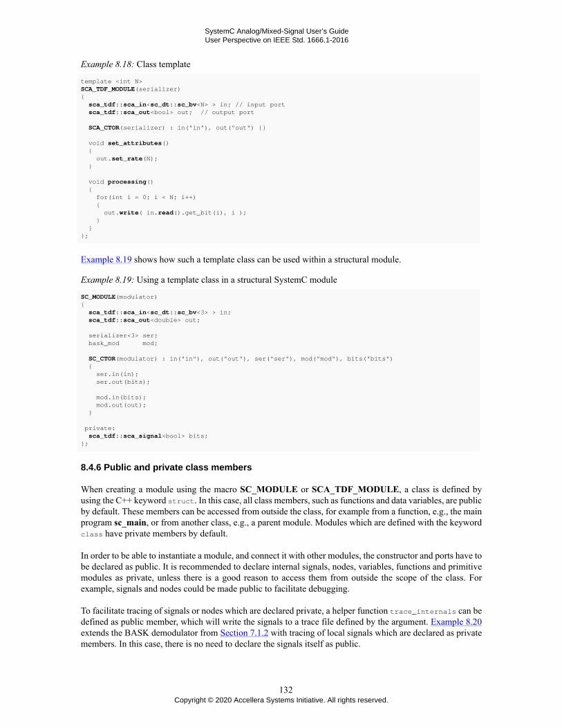
SystemC Analog/Mixed-Signal User’s GuideUser Perspective on IEEE Std. 1666.1-2016
Example 8.18: Class template
template <int N>SCA_TDF_MODULE(serializer){ sca_tdf::sca_in<sc_dt::sc_bv<N> > in; // input port sca_tdf::sca_out<bool> out; // output port
SCA_CTOR(serializer) : in("in"), out("out") {} void set_attributes() { out.set_rate(N); } void processing() { for(int i = 0; i < N; i++) { out.write( in.read().get_bit(i), i ); } }};
Example 8.19 shows how such a template class can be used within a structural module.
Example 8.19: Using a template class in a structural SystemC module
SC_MODULE(modulator){ sca_tdf::sca_in<sc_dt::sc_bv<3> > in; sca_tdf::sca_out<double> out;
serializer<3> ser; bask_mod mod;
SC_CTOR(modulator) : in("in"), out("out"), ser("ser"), mod("mod"), bits("bits") { ser.in(in); ser.out(bits);
mod.in(bits); mod.out(out); }
private: sca_tdf::sca_signal<bool> bits;};
8.4.6 Public and private class members
When creating a module using the macro SC_MODULE or SCA_TDF_MODULE, a class is defined byusing the C++ keyword struct. In this case, all class members, such as functions and data variables, are publicby default. These members can be accessed from outside the class, for example from a function, e.g., the mainprogram sc_main, or from another class, e.g., a parent module. Modules which are defined with the keywordclass have private members by default.
In order to be able to instantiate a module, and connect it with other modules, the constructor and ports have tobe declared as public. It is recommended to declare internal signals, nodes, variables, functions and primitivemodules as private, unless there is a good reason to access them from outside the scope of the class. Forexample, signals and nodes could be made public to facilitate debugging.
To facilitate tracing of signals or nodes which are declared private, a helper function trace_internals can bedefined as public member, which will write the signals to a trace file defined by the argument. Example 8.20extends the BASK demodulator from Section 7.1.2 with tracing of local signals which are declared as privatemembers. In this case, there is no need to declare the signals itself as public.
132Copyright © 2020 Accellera Systems Initiative. All rights reserved.
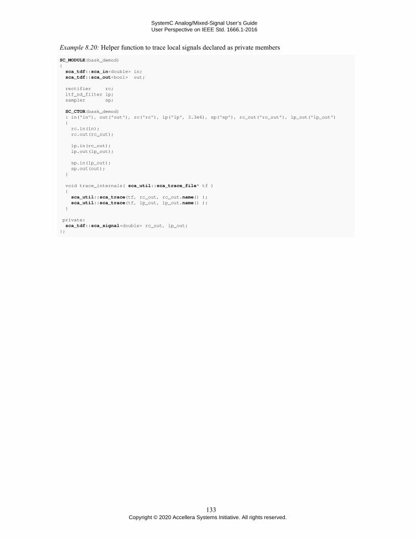
SystemC Analog/Mixed-Signal User’s GuideUser Perspective on IEEE Std. 1666.1-2016
Example 8.20: Helper function to trace local signals declared as private members
SC_MODULE(bask_demod){ sca_tdf::sca_in<double> in; sca_tdf::sca_out<bool> out;
rectifier rc; ltf_nd_filter lp; sampler sp;
SC_CTOR(bask_demod) : in("in"), out("out"), rc("rc"), lp("lp", 3.3e6), sp("sp"), rc_out("rc_out"), lp_out("lp_out") { rc.in(in); rc.out(rc_out);
lp.in(rc_out); lp.out(lp_out);
sp.in(lp_out); sp.out(out); } void trace_internals( sca_util::sca_trace_file* tf ) { sca_util::sca_trace(tf, rc_out, rc_out.name() ); sca_util::sca_trace(tf, lp_out, lp_out.name() ); }
private: sca_tdf::sca_signal<double> rc_out, lp_out;};
133Copyright © 2020 Accellera Systems Initiative. All rights reserved.

SystemC Analog/Mixed-Signal User’s GuideUser Perspective on IEEE Std. 1666.1-2016
Annex A
Language reference
Note: This appendix gives only a list of the basic language definitions for TDF, LSF or ELN primitive modules.The complete list of definitions can be found in the Language Reference Manual of the SystemC AMSextensions as defined in IEEE Std. 1666.1-2016.
If the default value for a parameter is not given in the tables below, then the value has to be provided by theuser and cannot be omitted during construction.
A.1 TDF modules
// Name Type Description// --------------------------------------------------------------------------------------------// T Arbitrary data type (e.g double, sca_util::sca_vector, ... // tstep sca_core::sca_time Time step as object// abstime sca_core::sca_time Time step as object// tstepd double Time step in seconds// tunit sc_core::sc_time_unit Time unit (e.g., sc_core::SC_US, sc_core::SC_MS, ...)// name const char* Module name as string// nm sc_core::sc_module_name Module name as object// --------------------------------------------------------------------------------------------
SCA_TDF_MODULE( name ){ // port declarations sca_tdf::sca_in<T> in; // input port sca_tdf::sca_out<T> out; // output port // Converter ports sca_tdf::sca_de::sca_in<T> inp; // converter port from discrete-event domain sca_tdf::sca_de::sca_out<T> outp; // converter port to discrete-event domain
// Cluster decoupling ports sca_tdf::sca_out<T, sca_tdf::SCA_CT_CUT> out_ct; // decouple using continuous-time semantics sca_tdf::sca_out<T, sca_tdf::SCA_DT_CUT> out_dt; // decouple using discrete-time semantics
// TDF methods, called automatically by the scheduler: void set_attributes() { // initial definition of module and port attributes (optional) }
void change_attributes() { // redefine module and port attributes (optional) }
void initialize() { // initial values of ports with a delay (optional) }
void reinitialize() { // reinitialize values of ports with a delay (optional) }
void processing() { // time-domain signal processing behavior or algorithm (mandatory) } void ac_processing() { // small-signal frequency-domain behavior (optional) }
134Copyright © 2020 Accellera Systems Initiative. All rights reserved.

SystemC Analog/Mixed-Signal User’s GuideUser Perspective on IEEE Std. 1666.1-2016
// module constructor (mandatory) SCA_CTOR( name ) {} // macro, or name( sc_core::sc_module_name nm ) {} // full constructor, can also be used to pass parameters
};
A.2 TDF ports
// Name Type Description// -------------------------------------------------------------------------------------------------// value T Value with arbitrary type (double, sca_util::sca_vector, ...) // sample_id unsigned long Sample ID: 0 for single-rate, 0...(rate-1) for multirate// nsamples unsigned long Number of samples// rate unsigned long Rate of the port// tstep sca_core::sca_time Time step as time object// tstepd double Time step in seconds // ctdelay sca_core::sca_time Continuous-time delay as time object// ctdelayd double Continuous-time delay in seconds// tunit sc_core::sc_time_unit Time unit (e.g., sc_core::SC_US, sc_core::SC_MS, ...)// changed bool Detect if there was an attribute change // -------------------------------------------------------------------------------------------------
sca_tdf::sca_in<T> in; sca_tdf::sca_out<T> out; sca_tdf::sca_out<T, sca_tdf::SCA_CT_CUT> out_ct; sca_tdf::sca_out<T, sca_tdf::SCA_DT_CUT> out_dt; sca_tdf::sca_de::sca_in<T> inp; sca_tdf::sca_de::sca_out<T> outp; out.set_delay( nsamples ); out.set_rate( rate ); out.set_timestep( tstep ); out.set_timestep( tstepd, tunit ); out.set_max_timestep( tstep ); out.set_max_timestep( tstepd, tunit ); out_ct.set_ct_delay( ctdelayd, tunit ); nsamples = out.get_delay(); ctdelay = out_ct.get_ct_delay(); rate = out.get_rate();
abstime = out.get_time(); abstime = out.get_time( sample_id );
tstep = out.get_timestep(); tstep = out.get_timestep( sample_id ); tstepd = out.get_timestep().to_seconds(); tstep = out.get_last_timestep(); tstep = out.get_last_timestep( sample_id ); tstepd = out.get_last_timestep().to_seconds(); tstep = out.get_max_timestep(); tstepd = out.get_max_timestep().to_seconds(); value = out.read_delayed_value(); value = out.read_delayed_value( sample_id ); changed = out.is_timestep_changed(); changed = out.is_timestep_changed( sample_id ); changed = out.is_rate_changed(); changed = out.is_delay_changed();
out.initialize( value, sample_id );
value = in.read(); value = in.read( sample_id );
out.write( value ); out.write( value, sample_id );
135Copyright © 2020 Accellera Systems Initiative. All rights reserved.

SystemC Analog/Mixed-Signal User’s GuideUser Perspective on IEEE Std. 1666.1-2016
A.3 TDF signals
// type T sca_tdf::sca_signal<T> // TDF signal
A.4 Embedded Laplace transfer functions
A.4.1 sca_tdf::sca_ltf_nd
Description
Scaled Laplace transfer function in the time-domain in the numerator-denominator form.
Definition
sca_tdf::sca_ltf_nd( num, den, delay, state, input, k, tstep );
Equation
(A.1)
Parameters
Name Type Default Descriptionnum sca_util::sca_vector<double> Numerator coefficientsden sca_util::sca_vector<double> Denominator coefficientsdelay sca_core::sca_time sc_core::SC_ZERO_TIME Time continuous delay
(optional)state sca_util::sca_vector<double> State vector (optional)input double, sca_tdf::sca_in<double>,
sca_tdf::sca_de::sca_in<double>,sca_util::sca_vector<double>
Input value, or signalfrom port
k double 1.0 Gain coefficient (optional)tstep sca_core::sca_time sc_core::SC_ZERO_TIME Time step
Constraint of usage
The delay shall be greater than or equal to zero.
A.4.2 sca_tdf::sca_ltf_zp
Description
Scaled Laplace transfer function in the time-domain in the zero-pole form.
Definition
sca_tdf::sca_ltf_zp( zeros, poles, delay, state, input, k, tstep );
136Copyright © 2020 Accellera Systems Initiative. All rights reserved.

SystemC Analog/Mixed-Signal User’s GuideUser Perspective on IEEE Std. 1666.1-2016
Equation
(A.2)
Parameters
Name Type Default Descriptionzeros sca_util::sca_vector<
sca_util::sca_complex >Numerator coefficients
poles sca_util::sca_vector<sca_util::sca_complex >
Denominator coefficients
delay sca_core::sca_time sc_core::SC_ZERO_TIME Time continuous delay(optional)
state sca_util::sca_vector<double> State vector (optional)input double, sca_tdf::sca_in<double>,
sca_tdf::sca_de::sca_in<double>,sca_util::sca_vector<double>
Input value, or signalfrom port
k double 1.0 Gain coefficient (optional)tstep sca_core::sca_time sc_core::SC_ZERO_TIME Time step
Constraint of usage
The delay shall be greater than or equal to zero.
A.4.3 sca_tdf::sca_ss
Description
Single-input single-output state-space equation.
Definition
sca_tdf::sca_ss( a, b, c, d, delay, s, x, tstep );
Equation
(A.3)
Parameters
Name Type Default Descriptiona sca_util::sca_matrix<double> Matrix A of size n-by-n (n
= number of states)b sca_util::sca_matrix<double> Matrix B of size n-by-m
(m = number of inputs)c sca_util::sca_matrix<double> Matrix C of size r-by-n (r
= number of outputs)d sca_util::sca_matrix<double> Matrix D of size r-by-m
137Copyright © 2020 Accellera Systems Initiative. All rights reserved.

SystemC Analog/Mixed-Signal User’s GuideUser Perspective on IEEE Std. 1666.1-2016
Name Type Default Descriptiondelay sca_core::sca_time sc_core::SC_ZERO_TIME Time continuous delay
(optional)s sca_util::sca_vector<double> State vector (optional)x sca_util::sca_vector<double>,
sca_util::sca_matrix<double>,sca_tdf::sca_in<double>,sca_tdf::sca_in<sca_util::sca_vector><double>,sca_tdf::sca_de::sca_in<sca_util::sca_vector<double>
Input vector, matrix orsignal from port
tstep sca_core::sca_time sc_core::SC_ZERO_TIME Time step
Constraint of usage
The delay shall be greater than or equal to zero.
A.5 LSF primitive modules
A.5.1 sca_lsf::sca_add
Description
Weighted addition of two LSF signals.
Definition
sca_lsf::sca_add( nm, k1, k2 );
Symbol
Equation
(A.4)
Parameters
Name Type Default Descriptionnm sc_core::sc_module_name Module namek1 double 1.0 Weighting coefficient for LSF signal at port x1k2 double 1.0 Weighting coefficient for LSF signal at port x2
138Copyright © 2020 Accellera Systems Initiative. All rights reserved.
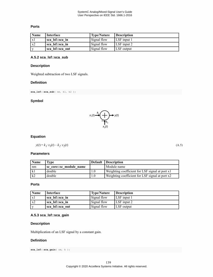
SystemC Analog/Mixed-Signal User’s GuideUser Perspective on IEEE Std. 1666.1-2016
Ports
Name Interface Type/Nature Descriptionx1 sca_lsf::sca_in Signal flow LSF input 1x2 sca_lsf::sca_in Signal flow LSF input 2y sca_lsf::sca_out Signal flow LSF output
A.5.2 sca_lsf::sca_sub
Description
Weighted subtraction of two LSF signals.
Definition
sca_lsf::sca_sub( nm, k1, k2 );
Symbol
Equation
(A.5)
Parameters
Name Type Default Descriptionnm sc_core::sc_module_name Module namek1 double 1.0 Weighting coefficient for LSF signal at port x1k2 double 1.0 Weighting coefficient for LSF signal at port x2
Ports
Name Interface Type/Nature Descriptionx1 sca_lsf::sca_in Signal flow LSF input 1x2 sca_lsf::sca_in Signal flow LSF input 2y sca_lsf::sca_out Signal flow LSF output
A.5.3 sca_lsf::sca_gain
Description
Multiplication of an LSF signal by a constant gain.
Definition
sca_lsf::sca_gain( nm, k );
139Copyright © 2020 Accellera Systems Initiative. All rights reserved.

SystemC Analog/Mixed-Signal User’s GuideUser Perspective on IEEE Std. 1666.1-2016
Symbol
Equation
(A.6)
Parameters
Name Type Default Descriptionnm sc_core::sc_module_name Module namek double 1.0 Gain coefficient
Ports
Name Interface Type/Nature Descriptionx sca_lsf::sca_in Signal flow LSF inputy sca_lsf::sca_out Signal flow LSF output
A.5.4 sca_lsf::sca_dot
Description
Scaled first-order time derivative of an LSF signal.
Definition
sca_lsf::sca_dot( nm, k );
Symbol
Equation
(A.7)
Parameters
Name Type Default Descriptionnm sc_core::sc_module_name Module namek double 1.0 Scale coefficient
140Copyright © 2020 Accellera Systems Initiative. All rights reserved.

SystemC Analog/Mixed-Signal User’s GuideUser Perspective on IEEE Std. 1666.1-2016
Ports
Name Interface Type/Nature Descriptionx sca_lsf::sca_in Signal flow LSF inputy sca_lsf::sca_out Signal flow LSF output
A.5.5 sca_lsf::sca_integ
Description
Scaled time-domain integration of an LSF signal.
Definition
sca_lsf::sca_integ( nm, k, y0 );
Symbol
Equation
(A.8)
Parameters
Name Type Default Descriptionnm sc_core::sc_module_name Module namek double 1.0 Scale coefficienty0 double 0.0 Initial condition at t=0
Ports
Name Interface Type/Nature Descriptionx sca_lsf::sca_in Signal flow LSF inputy sca_lsf::sca_out Signal flow LSF output
Constraint of usage
If y0 is set to sca_util::SCA_UNDEFINED, the primitive contributes the equation y = k · x for the firstcalculation instead of Equation (A.8). In this case, y0 is set to the resulting y value of the first calculation.
A.5.6 sca_lsf::sca_delay
Description
Scaled time-delayed version of an LSF signal.
141Copyright © 2020 Accellera Systems Initiative. All rights reserved.

SystemC Analog/Mixed-Signal User’s GuideUser Perspective on IEEE Std. 1666.1-2016
Definition
sca_lsf::sca_delay( nm, delay, k, y0 );
Symbol
Equation
(A.9)
Parameters
Name Type Default Descriptionnm sc_core::sc_module_name Module namedelay sca_core::sca_time sc_core::SC_ZERO_TIME Time continuous delayk double 1.0 Scale coefficienty0 double 0.0 Output value before delay
is in effect
Ports
Name Interface Type/Nature Descriptionx sca_lsf::sca_in Signal flow LSF inputy sca_lsf::sca_out Signal flow LSF output
Constraint of usage
The delay shall be greater than or equal to zero.
A.5.7 sca_lsf::sca_source
Description
LSF source.
Definition
sca_lsf::sca_source( nm, init_value, offset, amplitude, frequency, phase, delay, ac_amplitude, ac_phase, ac_noise_amplitude );
142Copyright © 2020 Accellera Systems Initiative. All rights reserved.

SystemC Analog/Mixed-Signal User’s GuideUser Perspective on IEEE Std. 1666.1-2016
Symbol
Equation
For time-domain simulation:
(A.10)
For small-signal frequency-domain simulation:
(A.11)
For small-signal frequency-domain noise simulation:
(A.12)
Parameters
Name Type Default Descriptionnm sc_core:: sc_module_name Module nameinit_value double 0.0 Initial valueoffset double 0.0 Offset valueamplitude double 0.0 Source amplitudefrequency double 0.0 Source frequency in hertzphase double 0.0 Source phase in radiandelay sca_core::sca_time sc_core::SC_ZERO_TIME Time continuous delayac_amplitude double 0.0 Small-signal amplitude *)ac_phase double 0.0 Small-signal phase in
radian *)ac_noise_amplitude
double 0.0 Small-signal noiseamplitude **)
*) for small-signal frequency-domain simulation only.
**) for small-signal frequency-domain noise simulation only.
Ports
Name Interface Type/Nature Descriptiony sca_lsf::sca_out Signal flow LSF output
Constraint of usage
The delay shall be greater than or equal to zero.
143Copyright © 2020 Accellera Systems Initiative. All rights reserved.

SystemC Analog/Mixed-Signal User’s GuideUser Perspective on IEEE Std. 1666.1-2016
A.5.8 sca_lsf::sca_ltf_nd
Description
Scaled Laplace transfer function in the time-domain in the numerator-denominator form.
Definition
sca_lsf::sca_ltf_nd( nm, num, den, delay, k );
Symbol
Equation
(A.13)
Parameters
Name Type Default Descriptionnm sc_core::sc_module_name Module namenum sca_util::sca_vector<double> Numerator coefficientsden sca_util::sca_vector<double> Denominator coefficientsdelay sca_core::sca_time sc_core::SC_ZERO_TIME Time continuous delayk double 1.0 Gain coefficient
Ports
Name Interface Type/Nature Descriptionx sca_lsf::sca_in Signal flow LSF outputy sca_lsf::sca_out Signal flow LSF output
Constraint of usage
The delay shall be greater than or equal to zero.
A.5.9 sca_lsf::sca_ltf_zp
Description
Scaled Laplace transfer function in the time-domain in the zero-pole form.
144Copyright © 2020 Accellera Systems Initiative. All rights reserved.

SystemC Analog/Mixed-Signal User’s GuideUser Perspective on IEEE Std. 1666.1-2016
Definition
sca_lsf::sca_ltf_zp( nm, zeros, poles, delay, k );
Symbol
Equation
(A.14)
Parameters
Name Type Default Descriptionnm sc_core::sc_module_name Module namezeros sca_util::sca_vector<
sca_util::sca_complex>Zeros
poles sca_util::sca_vector<sca_util::sca_complex>
Poles
delay sca_core::sca_time sc_core::SC_ZERO_TIME Time continuous delayk double 1.0 Gain coefficient
Ports
Name Interface Type/Nature Descriptionx sca_lsf::sca_in Signal flow LSF outputy sca_lsf::sca_out Signal flow LSF output
Constraint of usage
The expansion of the numerator and the denominator shall result in a real value, respectively. The delay shallbe greater than or equal to zero.
A.5.10 sca_lsf::sca_ss
Description
Single-input single-output state-space equation.
Definition
sca_lsf::sca_ss( nm, a, b, c, d, delay );
145Copyright © 2020 Accellera Systems Initiative. All rights reserved.

SystemC Analog/Mixed-Signal User’s GuideUser Perspective on IEEE Std. 1666.1-2016
Symbol
Equation
(A.15)
(A.16)
Parameters
Name Type Default Descriptionnm sc_core::sc_module_name Module namea sca_util::sca_matrix<double> Matrix A of size n-by-nb sca_util::sca_matrix<double> Matrix B with one column of
size nc sca_util::sca_matrix<double> Matrix C with one row of size
nd sca_util::sca_matrix<double> Matrix D of size 1delay sca_core::sca_time sc_core::SC_ZERO_TIME Time continuous delay
Ports
Name Interface Type/Nature Descriptionx sca_lsf::sca_in Signal flow LSF outputy sca_lsf::sca_out Signal flow LSF output
Constraint of usage
The delay shall be greater than or equal to zero.
A.5.11 sca_lsf::sca_tdf::sca_gain, sca_lsf::sca_tdf_gain
Description
Scaled multiplication of a TDF input signal by an LSF input signal.
Definition
sca_lsf::sca_tdf::sca_gain( nm, scale ); sca_lsf::sca_tdf_gain( nm, scale );
146Copyright © 2020 Accellera Systems Initiative. All rights reserved.

SystemC Analog/Mixed-Signal User’s GuideUser Perspective on IEEE Std. 1666.1-2016
Symbol
Equation
(A.17)
Parameters
Name Type Default Descriptionnm sc_core::sc_module_name Module namescale double 1.0 Scale coefficient
Ports
Name Interface Type/Nature Descriptioninp sca_tdf::sca_in<T> double TDF inputx sca_lsf::sca_in Signal flow LSF outputy sca_lsf::sca_out Signal flow LSF output
A.5.12 sca_lsf::sca_tdf::sca_source, sca_lsf::sca_tdf_source
Description
Scaled conversion of a TDF input signal to an LSF output signal.
Definition
sca_lsf::sca_tdf::sca_source( nm, scale ); sca_lsf::sca_tdf_source( nm, scale );
Symbol
Equation
(A.18)
Parameters
Name Type Default Descriptionnm sc_core::sc_module_name Module name
147Copyright © 2020 Accellera Systems Initiative. All rights reserved.

SystemC Analog/Mixed-Signal User’s GuideUser Perspective on IEEE Std. 1666.1-2016
Name Type Default Descriptionscale double 1.0 Scale coefficient
Ports
Name Interface Type/Nature Descriptioninp sca_tdf::sca_in<T> double TDF inputy sca_lsf::sca_out Signal flow LSF output
A.5.13 sca_lsf::sca_tdf::sca_sink, sca_lsf::sca_tdf_sink
Description
Scaled conversion from an LSF input signal to a TDF output signal.
Definition
sca_lsf::sca_tdf::sca_sink( nm, scale ); sca_lsf::sca_tdf_sink( nm, scale );
Symbol
Equation
There is no equation contributed to the overall equation system for this module.
Parameters
Name Type Default Descriptionnm sc_core::sc_module_name Module namescale double 1.0 Scale coefficient
Ports
Name Interface Type/Nature Descriptionx sca_lsf::sca_in Signal flow LSF inputoutp sca_tdf::sca_out<T> double TDF output
A.5.14 sca_lsf::sca_tdf::sca_mux, sca_lsf::sca_tdf_mux
Description
Selection of one of two LSF input signals by a TDF control signal (multiplexer).
148Copyright © 2020 Accellera Systems Initiative. All rights reserved.

SystemC Analog/Mixed-Signal User’s GuideUser Perspective on IEEE Std. 1666.1-2016
Definition
sca_lsf::sca_tdf::sca_mux( nm ); sca_lsf::sca_tdf_mux( nm );
Symbol
Equation
(A.19)
Parameters
Name Type Default Descriptionnm sc_core::sc_module_name Module name
Ports
Name Interface Type/Nature Descriptionx1 sca_lsf::sca_in Signal flow LSF input 1x2 sca_lsf::sca_in Signal flow LSF input 2ctrl sca_tdf::sca_in<T> bool TDF control inputy sca_lsf::sca_out Signal flow LSF output
A.5.15 sca_lsf::sca_tdf::sca_demux, sca_lsf::sca_tdf_demux
Description
Routing of an LSF input signal to either one of two LSF output signals controlled by a TDF signal(demultiplexer).
Definition
sca_lsf::sca_tdf::sca_demux( nm ); sca_lsf::sca_tdf_demux( nm );
Symbol
149Copyright © 2020 Accellera Systems Initiative. All rights reserved.

SystemC Analog/Mixed-Signal User’s GuideUser Perspective on IEEE Std. 1666.1-2016
Equation
(A.20)
(A.21)
Parameters
Name Type Default Descriptionnm sc_core::sc_module_name Module name
Ports
Name Interface Type/Nature Descriptionx sca_lsf::sca_in Signal flow LSF inputctrl sca_tdf::sca_in<T> bool TDF control inputy1 sca_lsf::sca_out Signal flow LSF output 1y2 sca_lsf::sca_out Signal flow LSF output 2
A.5.16 sca_lsf::sca_de::sca_gain, sca_lsf::sca_de_gain
Description
Scaled multiplication of a discrete-event input signal by an LSF input signal.
Definition
sca_lsf::sca_de::sca_gain( nm, scale ); sca_lsf::sca_de_gain( nm, scale );
Symbol
Equation
(A.22)
Parameters
Name Type Default Descriptionnm sc_core::sc_module_name Module namescale double 1.0 Scale coefficient
150Copyright © 2020 Accellera Systems Initiative. All rights reserved.

SystemC Analog/Mixed-Signal User’s GuideUser Perspective on IEEE Std. 1666.1-2016
Ports
Name Interface Type/Nature Descriptioninp sc_core::sc_in<T> double Discrete-event inputx sca_lsf::sca_in Signal flow LSF outputy sca_lsf::sca_out Signal flow LSF output
A.5.17 sca_lsf::sca_de::sca_source, sca_lsf::sca_de_source
Description
Scaled conversion of a discrete-event input signal to an LSF output signal.
Definition
sca_lsf::sca_de::sca_source( nm, scale ); sca_lsf::sca_de_source( nm, scale );
Symbol
Equation
(A.23)
Parameters
Name Type Default Descriptionnm sc_core::sc_module_name Module namescale double 1.0 Scale coefficient
Ports
Name Interface Type/Nature Descriptioninp sc_core::sc_in<T> double Discrete-event inputy sca_lsf::sca_out Signal flow LSF output
A.5.18 sca_lsf::sca_de::sca_sink, sca_lsf::sca_de_sink
Description
Scaled conversion from an LSF input signal to a discrete-event output signal.
Definition
sca_lsf::sca_de::sca_sink( nm, scale );
151Copyright © 2020 Accellera Systems Initiative. All rights reserved.

SystemC Analog/Mixed-Signal User’s GuideUser Perspective on IEEE Std. 1666.1-2016
sca_lsf::sca_de_sink( nm, scale );
Symbol
Equation
There is no equation contributed to the overall equation system for this module.
Parameters
Name Type Default Descriptionnm sc_core::sc_module_name Module namescale double 1.0 Scale coefficient
Ports
Name Interface Type/Nature Descriptionx sca_lsf::sca_in Signal flow LSF inputoutp sc_core::sc_out<T> double Discrete-event output
A.5.19 sca_lsf::sca_de::sca_mux, sca_lsf::sca_de_mux
Description
Selection of one of two LSF input signals by a discrete-event control signal (multiplexer).
Definition
sca_lsf::sca_de::sca_mux( nm ); sca_lsf::sca_de_mux( nm );
Symbol
Equation
(A.24)
152Copyright © 2020 Accellera Systems Initiative. All rights reserved.

SystemC Analog/Mixed-Signal User’s GuideUser Perspective on IEEE Std. 1666.1-2016
Parameters
Name Type Default Descriptionnm sc_core::sc_module_name Module name
Ports
Name Interface Type/Nature Descriptionx1 sca_lsf::sca_in Signal flow LSF input 1x2 sca_lsf::sca_in Signal flow LSF input 2ctrl sc_core::sc_in<T> bool Discrete-event control inputy sca_lsf::sca_out Signal flow LSF output
A.5.20 sca_lsf::sca_de::sca_demux, sca_lsf::sca_de_demux
Description
Routing of an LSF input signal to either one of two LSF output signals controlled by a discrete-event controlsignal (demultiplexer).
sca_lsf::sca_de::sca_demux( nm ); sca_lsf::sca_de_demux( nm );
Symbol
Equation
(A.25)
(A.26)
Parameters
Name Type Default Descriptionnm sc_core::sc_module_name Module name
Ports
Name Interface Type/Nature Descriptionx sca_lsf::sca_in Signal flow LSF inputctrl sc_core::sc_in<T> bool Discrete-event control inputy1 sca_lsf::sca_out Signal flow LSF output 1y2 sca_lsf::sca_out Signal flow LSF output 2
153Copyright © 2020 Accellera Systems Initiative. All rights reserved.

SystemC Analog/Mixed-Signal User’s GuideUser Perspective on IEEE Std. 1666.1-2016
A.6 ELN primitive modules
A.6.1 sca_eln::sca_r
Description
Resistor.
Definition
sca_eln::sca_r( nm, value );
Symbol
Equation
(A.27)
Parameters
Name Type Default Descriptionnm sc_core::sc_module_name Module namevalue double 1.0 Resistance in ohms
Ports
Name Interface Type/Nature Descriptionp sca_eln::sca_terminal Electrical Positive terminaln sca_eln::sca_terminal Electrical Negative terminal
A.6.2 sca_eln::sca_c
Description
Capacitor.
Definition
sca_eln::sca_c( nm, value, q0 );
Symbol
154Copyright © 2020 Accellera Systems Initiative. All rights reserved.

SystemC Analog/Mixed-Signal User’s GuideUser Perspective on IEEE Std. 1666.1-2016
Equation
(A.28)
Parameters
Name Type Default Descriptionnm sc_core::sc_module_name Module namevalue double 1.0 Capacitance in faradsq0 double 0.0 Initial charge in coulombs
Ports
Name Interface Type/Nature Descriptionp sca_eln::sca_terminal Electrical Positive terminaln sca_eln::sca_terminal Electrical Negative terminal
Constraints of usage
The parameter value shall not be numerically zero.
If the initial charge q0 is set to sca_util::SCA_UNDEFINED, the primitive contributes no equation tothe equation system for the first calculation. In this case, the initial charge q0 is calculated as follows:q0 = value · vp,n0, where vp,n0 is the voltage across the capacitor after the first calculation.
A.6.3 sca_eln::sca_l
Description
Inductor.
Definition
sca_eln::sca_l( nm, value, psi0 );
Symbol
Equation
(A.29)
Parameters
Name Type Default Descriptionnm sc_core::sc_module_name Module name
155Copyright © 2020 Accellera Systems Initiative. All rights reserved.

SystemC Analog/Mixed-Signal User’s GuideUser Perspective on IEEE Std. 1666.1-2016
Name Type Default Descriptionvalue double 1.0 Inductance in henryspsi0 double 0.0 Initial linked flux in webers
Ports
Name Interface Type/Nature Descriptionp sca_eln::sca_terminal Electrical Positive terminaln sca_eln::sca_terminal Electrical Negative terminal
Constraints of usage
The parameter value shall not be numerically zero.
If the initial linked flux psi0 is set to sca_util::SCA_UNDEFINED, the primitive contributes to the equationsystem the equation vp,n = 0 for the first calculation instead of Equation (A.29). In this case, the initial linkedflux psi0 is calculated as follows: psi0 = value · ip,n0, where ip,n0 is the current flowing through the inductorafter the first calculation.
A.6.4 sca_eln::sca_vcvs
Description
Voltage controlled voltage source.
Definition
sca_eln::sca_vcvs( nm, value );
Symbol
Equation
(A.30)
Parameters
Name Type Default Descriptionnm sc_core::sc_module_name Module namevalue double 1.0 Scale coefficient of the control voltage
Ports
Name Interface Type/Nature Descriptionncp sca_eln::sca_terminal Electrical Positive control terminalncn sca_eln::sca_terminal Electrical Negative control terminal
156Copyright © 2020 Accellera Systems Initiative. All rights reserved.
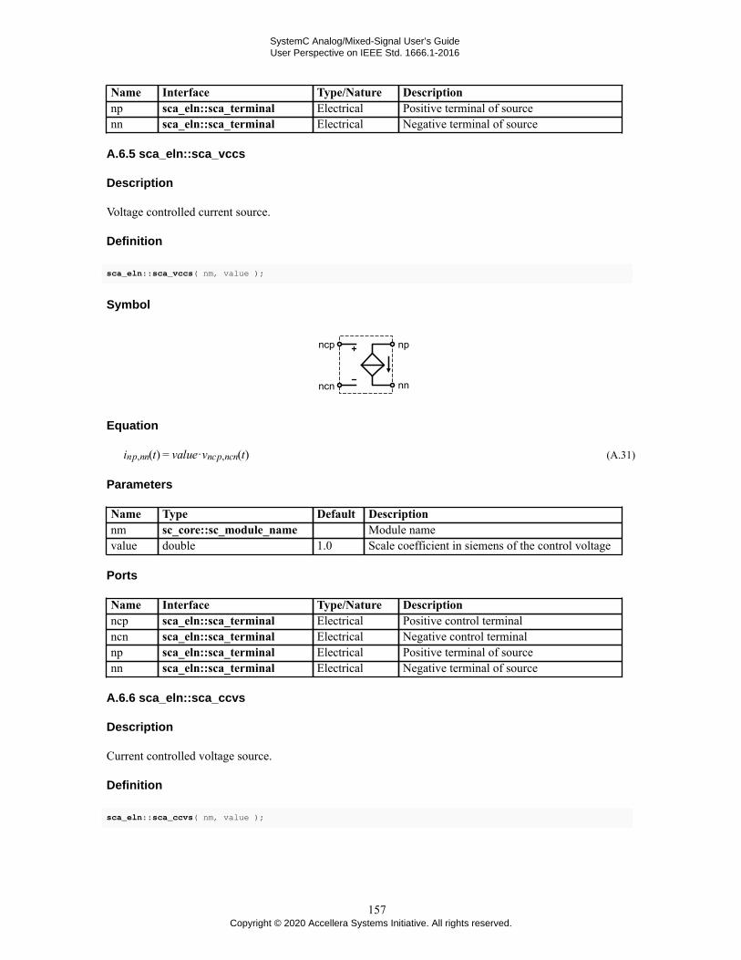
SystemC Analog/Mixed-Signal User’s GuideUser Perspective on IEEE Std. 1666.1-2016
Name Interface Type/Nature Descriptionnp sca_eln::sca_terminal Electrical Positive terminal of sourcenn sca_eln::sca_terminal Electrical Negative terminal of source
A.6.5 sca_eln::sca_vccs
Description
Voltage controlled current source.
Definition
sca_eln::sca_vccs( nm, value );
Symbol
Equation
(A.31)
Parameters
Name Type Default Descriptionnm sc_core::sc_module_name Module namevalue double 1.0 Scale coefficient in siemens of the control voltage
Ports
Name Interface Type/Nature Descriptionncp sca_eln::sca_terminal Electrical Positive control terminalncn sca_eln::sca_terminal Electrical Negative control terminalnp sca_eln::sca_terminal Electrical Positive terminal of sourcenn sca_eln::sca_terminal Electrical Negative terminal of source
A.6.6 sca_eln::sca_ccvs
Description
Current controlled voltage source.
Definition
sca_eln::sca_ccvs( nm, value );
157Copyright © 2020 Accellera Systems Initiative. All rights reserved.
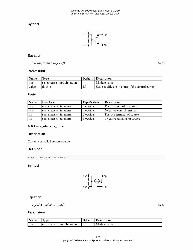
SystemC Analog/Mixed-Signal User’s GuideUser Perspective on IEEE Std. 1666.1-2016
Symbol
Equation
(A.32)
Parameters
Name Type Default Descriptionnm sc_core::sc_module_name Module namevalue double 1.0 Scale coefficient in ohms of the control current
Ports
Name Interface Type/Nature Descriptionncp sca_eln::sca_terminal Electrical Positive control terminalncn sca_eln::sca_terminal Electrical Negative control terminalnp sca_eln::sca_terminal Electrical Positive terminal of sourcenn sca_eln::sca_terminal Electrical Negative terminal of source
A.6.7 sca_eln::sca_cccs
Description
Current controlled current source.
Definition
sca_eln::sca_cccs( nm, value );
Symbol
Equation
(A.33)
Parameters
Name Type Default Descriptionnm sc_core::sc_module_name Module name
158Copyright © 2020 Accellera Systems Initiative. All rights reserved.

SystemC Analog/Mixed-Signal User’s GuideUser Perspective on IEEE Std. 1666.1-2016
Name Type Default Descriptionvalue double 1.0 Scale coefficient of the control current
Ports
Name Interface Type/Nature Descriptionncp sca_eln::sca_terminal Electrical Positive control terminalncn sca_eln::sca_terminal Electrical Negative control terminalnp sca_eln::sca_terminal Electrical Positive terminal of sourcenn sca_eln::sca_terminal Electrical Negative terminal of source
A.6.8 sca_eln::sca_nullor
Description
Nullor (nullator - norator pair), ideal Opamp.
Definition
sca_eln::sca_nullor( nm );
Symbol
Equation
(A.34)
(A.35)
Parameters
Name Type Default Descriptionnm sc_core::sc_module_name Module name
Ports
Name Interface Type/Nature Descriptionnip sca_eln::sca_terminal Electrical Positive terminal of nullatornin sca_eln::sca_terminal Electrical Negative terminal of nullatornop sca_eln::sca_terminal Electrical Positive terminal of noratornon sca_eln::sca_terminal Electrical Negative terminal of norator
159Copyright © 2020 Accellera Systems Initiative. All rights reserved.

SystemC Analog/Mixed-Signal User’s GuideUser Perspective on IEEE Std. 1666.1-2016
A.6.9 sca_eln::sca_gyrator
Description
Gyrator.
Definition
sca_eln::sca_gyrator( nm, g1, g2 );
Symbol
Equation
(A.36)
(A.37)
Parameters
Name Type Default Descriptionnm sc_core::sc_module_name Module nameg1 double 1.0 Gyration conductance in siemensg2 double 1.0 Gyration conductance in siemens
Ports
Name Interface Type/Nature Descriptionp1 sca_eln::sca_terminal Electrical Positive terminal of primary portn1 sca_eln::sca_terminal Electrical Negative terminal of primary portp2 sca_eln::sca_terminal Electrical Positive terminal of secondary portn2 sca_eln::sca_terminal Electrical Negative terminal of secondary port
A.6.10 sca_eln::sca_ideal_transformer
Description
Ideal transformer.
Definition
sca_eln::sca_ideal_transformer( nm, ratio );
160Copyright © 2020 Accellera Systems Initiative. All rights reserved.

SystemC Analog/Mixed-Signal User’s GuideUser Perspective on IEEE Std. 1666.1-2016
Symbol
Equation
(A.38)
(A.39)
Parameters
Name Type Default Descriptionnm sc_core::sc_module_name Module nameratio double 1.0 Transformation ratio
Ports
Name Interface Type/Nature Descriptionp1 sca_eln::sca_terminal Electrical Positive terminal of primary portn1 sca_eln::sca_terminal Electrical Negative terminal of primary portp2 sca_eln::sca_terminal Electrical Positive terminal of secondary portn2 sca_eln::sca_terminal Electrical Negative terminal of secondary port
A.6.11 sca_eln::sca_transmission_line
Description
Transmission line.
Definition
sca_eln::sca_transmission_line( nm, z0, delay, delta0 );
Symbol
161Copyright © 2020 Accellera Systems Initiative. All rights reserved.

SystemC Analog/Mixed-Signal User’s GuideUser Perspective on IEEE Std. 1666.1-2016
Equation
(A.40)
(A.41)
Parameters
Name Type Default Descriptionnm sc_core::sc_module_name Module namez0 double 100.0 Characteristic impedance of
the transmission line in ohmsdelay sca_core::sca_time sc_core::SC_ZERO_TIME Transmission delaydelta0 double 0.0 Dissipation factor in 1/seconds.
Ports
Name Interface Type/Nature Descriptiona1 sca_eln::sca_terminal Electrical Wire A at primary sideb1 sca_eln::sca_terminal Electrical Wire B at primary sidea2 sca_eln::sca_terminal Electrical Wire A at secondary sideb2 sca_eln::sca_terminal Electrical Wire B at secondary side
Constraint of usage
The delay shall be greater than or equal to zero.
A.6.12 sca_eln::sca_vsource
Description
Independent voltage source.
Definition
sca_eln::sca_vsource( nm, init_value, offset, amplitude, frequency, phase, delay, ac_amplitude, ac_phase, ac_noise_amplitude );
Symbol
162Copyright © 2020 Accellera Systems Initiative. All rights reserved.

SystemC Analog/Mixed-Signal User’s GuideUser Perspective on IEEE Std. 1666.1-2016
Equation
For time-domain simulation:
(A.42)
For small-signal frequency-domain simulation:
(A.43)
For small-signal frequency-domain noise simulation:
(A.44)
Parameters
Name Type Default Descriptionnm sc_core:: sc_module_name Module nameinit_value double 0.0 Initial valueoffset double 0.0 Offset valueamplitude double 0.0 Source amplitudefrequency double 0.0 Source frequency in hertzphase double 0.0 Source phase in radiandelay sca_core::sca_time sc_core::SC_ZERO_TIME Time continuous delayac_amplitude double 0.0 Small-signal amplitude *)ac_phase double 0.0 Small-signal phase in
radian *)ac_noise_amplitude
double 0.0 Small-signal noiseamplitude **)
*) for small-signal frequency-domain simulation only.
**) for small-signal frequency-domain noise simulation only.
Ports
Name Interface Type/Nature Descriptionp sca_eln::sca_terminal Electrical Positive terminaln sca_eln::sca_terminal Electrical Negative terminal
Constraint of usage
The delay shall be greater than or equal to zero.
A.6.13 sca_eln::sca_isource
Description
Independent current source.
163Copyright © 2020 Accellera Systems Initiative. All rights reserved.

SystemC Analog/Mixed-Signal User’s GuideUser Perspective on IEEE Std. 1666.1-2016
Definition
sca_eln::sca_isource( nm, init_value, offset, amplitude, frequency, phase, delay, ac_amplitude, ac_phase, ac_noise_amplitude );
Symbol
Equation
For time-domain simulation:
(A.45)
For small-signal frequency-domain simulation:
(A.46)
For small-signal frequency-domain noise simulation:
(A.47)
Parameters
Name Type Default Descriptionnm sc_core:: sc_module_name Module nameinit_value double 0.0 Initial valueoffset double 0.0 Offset valueamplitude double 0.0 Source amplitudefrequency double 0.0 Source frequency in hertzphase double 0.0 Source phase in radiandelay sca_core::sca_time sc_core::SC_ZERO_TIME Time continuous delayac_amplitude double 0.0 Small-signal amplitude *)ac_phase double 0.0 Small-signal phase in
radian *)ac_noise_amplitude
double 0.0 Small-signal noiseamplitude **)
*) for small-signal frequency-domain simulation only.
**) for small-signal frequency-domain noise simulation only.
Ports
Name Interface Type/Nature Descriptionp sca_eln::sca_terminal Electrical Positive terminaln sca_eln::sca_terminal Electrical Negative terminal
164Copyright © 2020 Accellera Systems Initiative. All rights reserved.

SystemC Analog/Mixed-Signal User’s GuideUser Perspective on IEEE Std. 1666.1-2016
Constraint of usage
The delay shall be greater than or equal to zero.
A.6.14 sca_eln::sca_tdf::sca_r, sca_eln::sca_tdf_r
Description
Variable resistor controlled by a TDF input signal.
Definition
sca_eln::sca_tdf::sca_r( nm, scale ); sca_eln::sca_tdf_r( nm, scale );
Symbol
Equation
(A.48)
Parameters
Name Type Default Descriptionnm sc_core::sc_module_name Module namescale double 1.0 Scale coefficient
Ports
Name Interface Type/Nature Descriptionp sca_eln::sca_terminal Electrical Positive terminaln sca_eln::sca_terminal Electrical Negative terminalinp sca_tdf::sca_in<T> double TDF control input
A.6.15 sca_eln::sca_tdf::sca_l, sca_eln::sca_tdf_l
Description
Variable inductor controlled by a TDF input signal.
Definition
sca_eln::sca_tdf::sca_l( nm, scale, psi0 );
sca_eln::sca_tdf_l( nm, scale, psi0 );
165Copyright © 2020 Accellera Systems Initiative. All rights reserved.

SystemC Analog/Mixed-Signal User’s GuideUser Perspective on IEEE Std. 1666.1-2016
Symbol
Equation
(A.49)
Parameters
Name Type Default Descriptionnm sc_core::sc_module_name Module namescale double 1.0 Scale coefficientpsi0 double 0.0 Initial linked flux in webers
Ports
Name Interface Type/Nature Descriptionp sca_eln::sca_terminal Electrical Positive terminaln sca_eln::sca_terminal Electrical Negative terminalinp sca_tdf::sca_in<T> double TDF control input
Constraints of usage
The TDF control input inp shall not be zero.
If the initial linked flux psi0 is set to sca_util::SCA_UNDEFINED, the primitive contributes to the equationsystem the equation vp,n = 0 for the first calculation instead of Equation (A.49). In this case, the initial linkedflux psi0 is calculated as follows: psi0 = value · ip,n0, where ip,n0 is the current flowing through the inductorafter the first calculation.
A.6.16 sca_eln::sca_tdf::sca_c, sca_eln::sca_tdf_c
Description
Variable capacitor controlled by a TDF input signal.
Definition
sca_eln::sca_tdf::sca_c( nm, scale, q0 );
sca_eln::sca_tdf_c( nm, scale, q0 );
166Copyright © 2020 Accellera Systems Initiative. All rights reserved.

SystemC Analog/Mixed-Signal User’s GuideUser Perspective on IEEE Std. 1666.1-2016
Symbol
Equation
(A.50)
Parameters
Name Type Default Descriptionnm sc_core::sc_module_name Module namescale double 1.0 Scale coefficientq0 double 0.0 Initial charge in coulombs
Ports
Name Interface Type/Nature Descriptionp sca_eln::sca_terminal Electrical Positive terminaln sca_eln::sca_terminal Electrical Negative terminalinp sca_tdf::sca_in<T> double TDF control input
Constraints of usage
The TDF control input inp shall not be zero.
If the initial charge q0 is set to sca_util::SCA_UNDEFINED, the primitive contributes no equation tothe equation system for the first calculation. In this case, the initial charge q0 is calculated as follows:q0 = value · vp,n0, where vp,n0 is the voltage across the capacitor after the first calculation.
A.6.17 sca_eln::sca_tdf::sca_rswitch, sca_eln::sca_tdf_rswitch
Description
Switch controlled by a TDF input signal.
Definition
sca_eln::sca_tdf::sca_rswitch( nm, ron, roff, off_state );
sca_eln::sca_tdf_rswitch( nm, ron, roff, off_state );
167Copyright © 2020 Accellera Systems Initiative. All rights reserved.

SystemC Analog/Mixed-Signal User’s GuideUser Perspective on IEEE Std. 1666.1-2016
Symbol
Equation
(A.51)
Parameters
Name Type Default Descriptionnm sc_core::sc_module_name Module nameron double 0.0 On resistance in ohmsroff double sca_util::SCA_INFINITY Off resistance in ohmsoff_state bool false Define which position is the
off-position
Ports
Name Interface Type/Nature Descriptionp sca_eln::sca_terminal Electrical Positive terminaln sca_eln::sca_terminal Electrical Negative terminalctrl sca_tdf::sca_in<T> bool TDF control input
A.6.18 sca_eln::sca_tdf::sca_vsource, sca_eln::sca_tdf_vsource
Description
Voltage source driven by a TDF input signal.
Definition
sca_eln::sca_tdf::sca_vsource( nm, scale );
sca_eln::sca_tdf_vsource( nm, scale );
Symbol
Equation
(A.52)
168Copyright © 2020 Accellera Systems Initiative. All rights reserved.
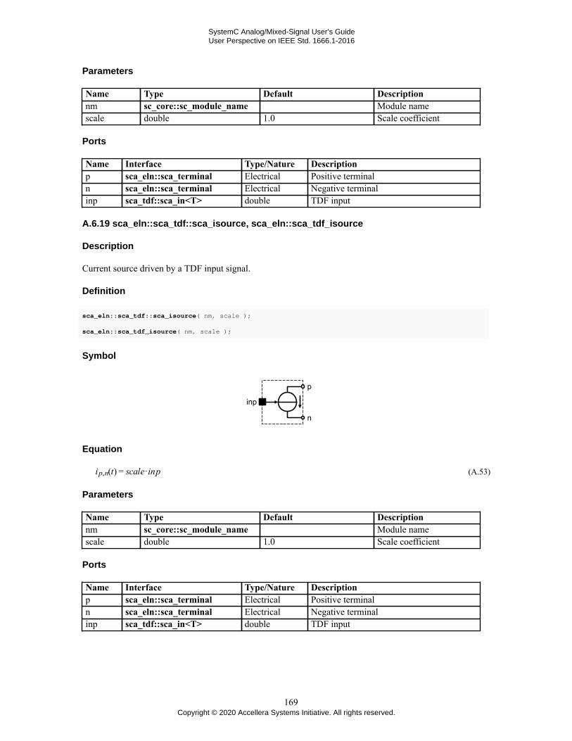
SystemC Analog/Mixed-Signal User’s GuideUser Perspective on IEEE Std. 1666.1-2016
Parameters
Name Type Default Descriptionnm sc_core::sc_module_name Module namescale double 1.0 Scale coefficient
Ports
Name Interface Type/Nature Descriptionp sca_eln::sca_terminal Electrical Positive terminaln sca_eln::sca_terminal Electrical Negative terminalinp sca_tdf::sca_in<T> double TDF input
A.6.19 sca_eln::sca_tdf::sca_isource, sca_eln::sca_tdf_isource
Description
Current source driven by a TDF input signal.
Definition
sca_eln::sca_tdf::sca_isource( nm, scale );
sca_eln::sca_tdf_isource( nm, scale );
Symbol
Equation
(A.53)
Parameters
Name Type Default Descriptionnm sc_core::sc_module_name Module namescale double 1.0 Scale coefficient
Ports
Name Interface Type/Nature Descriptionp sca_eln::sca_terminal Electrical Positive terminaln sca_eln::sca_terminal Electrical Negative terminalinp sca_tdf::sca_in<T> double TDF input
169Copyright © 2020 Accellera Systems Initiative. All rights reserved.

SystemC Analog/Mixed-Signal User’s GuideUser Perspective on IEEE Std. 1666.1-2016
A.6.20 sca_eln::sca_tdf::sca_vsink, sca_eln::sca_tdf_vsink
Description
Converts voltage to a TDF output signal.
Definition
sca_eln::sca_tdf::sca_vsink( nm, scale );
sca_eln::sca_tdf_vsink( nm, scale );
Symbol
Equation
No equation added to the equation system.
Parameters
Name Type Default Descriptionnm sc_core::sc_module_name Module namescale double 1.0 Scale coefficient
Ports
Name Interface Type/Nature Descriptionp sca_eln::sca_terminal Electrical Positive terminaln sca_eln::sca_terminal Electrical Negative terminaloutp sca_tdf::sca_out<T> double TDF output
A.6.21 sca_eln::sca_tdf::sca_isink, sca_eln::sca_tdf_isink
Description
Converts current to a TDF output signal.
Definition
sca_eln::sca_tdf::sca_isink( nm, scale );
sca_eln::sca_tdf_isink( nm, scale );
170Copyright © 2020 Accellera Systems Initiative. All rights reserved.

SystemC Analog/Mixed-Signal User’s GuideUser Perspective on IEEE Std. 1666.1-2016
Symbol
Equation
(A.54)
Parameters
Name Type Default Descriptionnm sc_core::sc_module_name Module namescale double 1.0 Scale coefficient
Ports
Name Interface Type/Nature Descriptionp sca_eln::sca_terminal Electrical Positive terminaln sca_eln::sca_terminal Electrical Negative terminaloutp sca_tdf::sca_out<T> double TDF output
A.6.22 sca_eln::sca_de::sca_r, sca_eln::sca_de_r
Description
Variable resistor controlled by a discrete-event input signal.
Definition
sca_eln::sca_de::sca_r( nm, scale ); sca_eln::sca_de_r( nm, scale );
Symbol
Equation
(A.55)
171Copyright © 2020 Accellera Systems Initiative. All rights reserved.

SystemC Analog/Mixed-Signal User’s GuideUser Perspective on IEEE Std. 1666.1-2016
Parameters
Name Type Default Descriptionnm sc_core::sc_module_name Module namescale double 1.0 Scale coefficient
Ports
Name Interface Type/Nature Descriptionp sca_eln::sca_terminal Electrical Positive terminaln sca_eln::sca_terminal Electrical Negative terminalinp sc_core::sc_in<T> double Discrete-event control input
A.6.23 sca_eln::sca_de::sca_l, sca_eln::sca_de_l
Description
Variable inductor controlled by a discrete-event input signal.
Definition
sca_eln::sca_de::sca_l( nm, scale, psi0 );
sca_eln::sca_de_l( nm, scale, psi0 );
Symbol
Equation
(A.56)
Parameters
Name Type Default Descriptionnm sc_core::sc_module_name Module namescale double 1.0 Scale coefficientpsi0 double 0.0 Initial linked flux in webers
Ports
Name Interface Type/Nature Descriptionp sca_eln::sca_terminal Electrical Positive terminaln sca_eln::sca_terminal Electrical Negative terminalinp sc_core::sc_in<T> double Discrete-event control input
172Copyright © 2020 Accellera Systems Initiative. All rights reserved.

SystemC Analog/Mixed-Signal User’s GuideUser Perspective on IEEE Std. 1666.1-2016
Constraints of usage
The discrete-event control input inp shall not be zero.
If the initial linked flux psi0 is set to sca_util::SCA_UNDEFINED, the primitive contributes to the equationsystem the equation vp,n = 0 for the first calculation instead of Equation (A.56). In this case, the initial linkedflux psi0 is calculated as follows: psi0 = value · ip,n0, where ip,n0 is the current flowing through the inductorafter the first calculation.
A.6.24 sca_eln::sca_de::sca_c, sca_eln::sca_de_c
Description
Variable capacitor controlled by a discrete-event input signal.
Definition
sca_eln::sca_de::sca_c( nm, scale, q0 );
sca_eln::sca_de_c( nm, scale, q0);
Symbol
Equation
(A.57)
Parameters
Name Type Default Descriptionnm sc_core::sc_module_name Module namescale double 1.0 Scale coefficientq0 double 0.0 Initial charge in coulombs
Ports
Name Interface Type/Nature Descriptionp sca_eln::sca_terminal Electrical Positive terminaln sca_eln::sca_terminal Electrical Negative terminalinp sc_core::sc_in<T> double Discrete-event control input
Constraints of usage
The discrete-event control input inp shall not be zero.
173Copyright © 2020 Accellera Systems Initiative. All rights reserved.
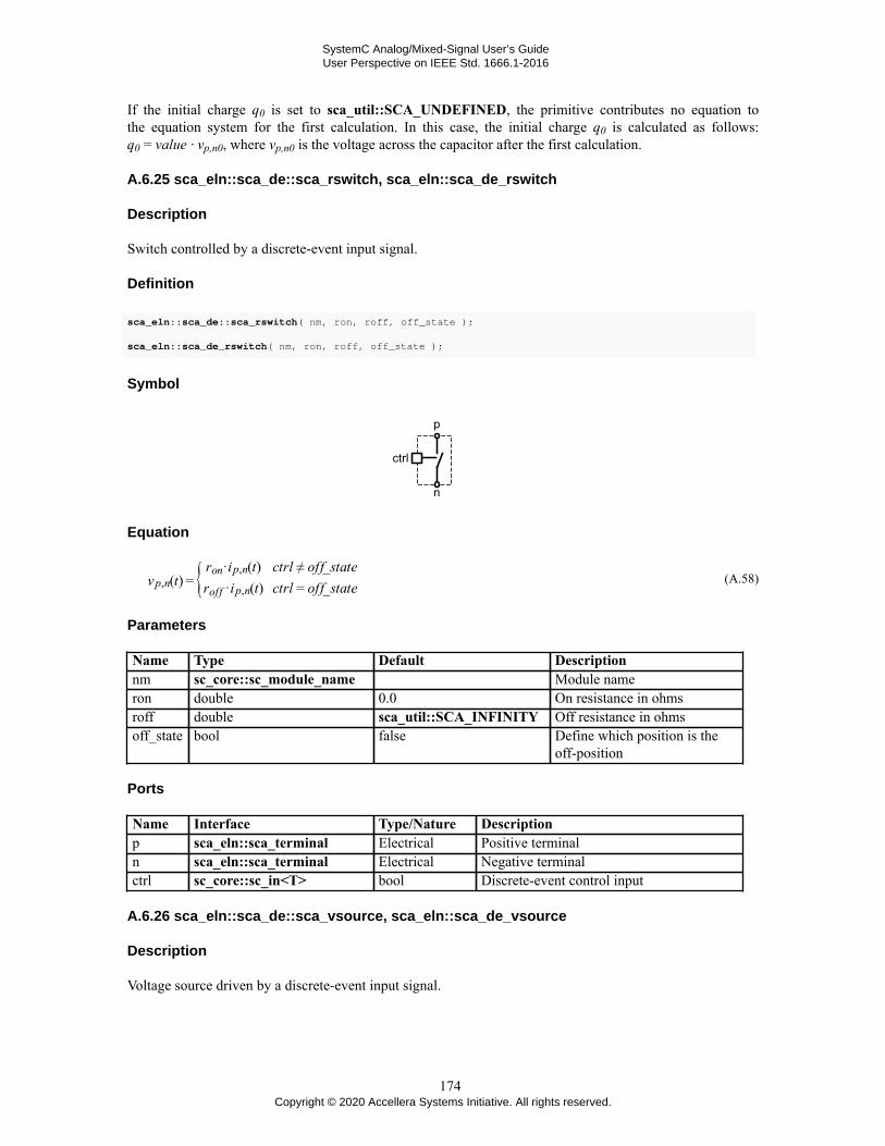
SystemC Analog/Mixed-Signal User’s GuideUser Perspective on IEEE Std. 1666.1-2016
If the initial charge q0 is set to sca_util::SCA_UNDEFINED, the primitive contributes no equation tothe equation system for the first calculation. In this case, the initial charge q0 is calculated as follows:q0 = value · vp,n0, where vp,n0 is the voltage across the capacitor after the first calculation.
A.6.25 sca_eln::sca_de::sca_rswitch, sca_eln::sca_de_rswitch
Description
Switch controlled by a discrete-event input signal.
Definition
sca_eln::sca_de::sca_rswitch( nm, ron, roff, off_state );
sca_eln::sca_de_rswitch( nm, ron, roff, off_state );
Symbol
Equation
(A.58)
Parameters
Name Type Default Descriptionnm sc_core::sc_module_name Module nameron double 0.0 On resistance in ohmsroff double sca_util::SCA_INFINITY Off resistance in ohmsoff_state bool false Define which position is the
off-position
Ports
Name Interface Type/Nature Descriptionp sca_eln::sca_terminal Electrical Positive terminaln sca_eln::sca_terminal Electrical Negative terminalctrl sc_core::sc_in<T> bool Discrete-event control input
A.6.26 sca_eln::sca_de::sca_vsource, sca_eln::sca_de_vsource
Description
Voltage source driven by a discrete-event input signal.
174Copyright © 2020 Accellera Systems Initiative. All rights reserved.

SystemC Analog/Mixed-Signal User’s GuideUser Perspective on IEEE Std. 1666.1-2016
Definition
sca_eln::sca_de::sca_vsource( nm, scale );
sca_eln::sca_de_vsource( nm, scale );
Symbol
Equation
(A.59)
Parameters
Name Type Default Descriptionnm sc_core::sc_module_name Module namescale double 1.0 Scale coefficient
Ports
Name Interface Type/Nature Descriptionp sca_eln::sca_terminal Electrical Positive terminaln sca_eln::sca_terminal Electrical Negative terminalinp sc_core::sc_in<T> double Discrete-event input
A.6.27 sca_eln::sca_de::sca_isource, sca_eln::sca_de_isource
Description
Current source driven by a discrete-event input signal.
Definition
sca_eln::sca_de::sca_isource( nm, scale );
sca_eln::sca_de_isource( nm, scale );
Symbol
175Copyright © 2020 Accellera Systems Initiative. All rights reserved.
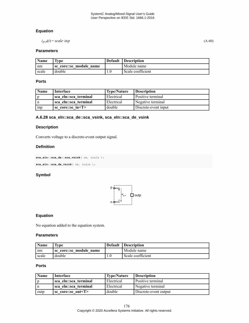
SystemC Analog/Mixed-Signal User’s GuideUser Perspective on IEEE Std. 1666.1-2016
Equation
(A.60)
Parameters
Name Type Default Descriptionnm sc_core::sc_module_name Module namescale double 1.0 Scale coefficient
Ports
Name Interface Type/Nature Descriptionp sca_eln::sca_terminal Electrical Positive terminaln sca_eln::sca_terminal Electrical Negative terminalinp sc_core::sc_in<T> double Discrete-event input
A.6.28 sca_eln::sca_de::sca_vsink, sca_eln::sca_de_vsink
Description
Converts voltage to a discrete-event output signal.
Definition
sca_eln::sca_de::sca_vsink( nm, scale );
sca_eln::sca_de_vsink( nm, scale );
Symbol
Equation
No equation added to the equation system.
Parameters
Name Type Default Descriptionnm sc_core::sc_module_name Module namescale double 1.0 Scale coefficient
Ports
Name Interface Type/Nature Descriptionp sca_eln::sca_terminal Electrical Positive terminaln sca_eln::sca_terminal Electrical Negative terminaloutp sc_core::sc_out<T> double Discrete-event output
176Copyright © 2020 Accellera Systems Initiative. All rights reserved.

SystemC Analog/Mixed-Signal User’s GuideUser Perspective on IEEE Std. 1666.1-2016
A.6.29 sca_eln::sca_de::sca_isink, sca_eln::sca_de_isink
Description
Converts current to a discrete-event output signal.
Definition
sca_eln::sca_de::sca_isink( nm, scale );
sca_eln::sca_de_isink( nm, scale );
Symbol
Equation
(A.61)
Parameters
Name Type Default Descriptionnm sc_core::sc_module_name Module namescale double 1.0 Scale coefficient
Ports
Name Interface Type/Nature Descriptionp sca_eln::sca_terminal Electrical Positive terminaln sca_eln::sca_terminal Electrical Negative terminaloutp sc_core::sc_out<T> double Discrete-event output
177Copyright © 2020 Accellera Systems Initiative. All rights reserved.

SystemC Analog/Mixed-Signal User’s GuideUser Perspective on IEEE Std. 1666.1-2016
Annex B
Symbols and graphical representations
This annex gives an overview of the symbols and graphical representations used in this user’s guide. In the casewhere block diagrams or electrical networks are extracted from this user’s guide, it is strongly recommendedto use these symbols and graphical representations in a consistent manner.
The symbols for the individual LSF and ELN primitives are given in Annex A.
Figure B.1—Symbols and graphical representationsof TDF, LSF, ELN and discrete-event elements.
178Copyright © 2020 Accellera Systems Initiative. All rights reserved.
SystemC Analog/Mixed-Signal User’s GuideUser Perspective on IEEE Std. 1666.1-2016
Annex C
Glossary
This glossary contains brief descriptions for a number of terms used in this user’s guide.
application: A C++ program, written by an end user, that makes use of the classes, functions, macros, and soforth provided by SystemC and the AMS extensions. An application may use as few or as many features ofC++ as is seen fit and as few or as many features of SystemC and the AMS extensions as is seen fit.
cluster: A cluster is a set of connected modules sharing the same model of computation.
continuous-time signal: A continuous-time signal is a piecewise contiguous and differentiable signal, whichmay be represented in approximation by a set of samples at discrete time points. Values between the samplescan be estimated by different interpolation techniques.
discrete-time signal: A discrete-time signal is a signal that has been sampled from a continuous-time signalresulting in a sequence of values at discrete time points. Each value in the sequence is called a sample.
electrical linear networks (ELN): A model of computation providing a formalism for satisfying the energyconservation laws as defined by the Kirchhoff's laws for the electrical domain.
electrical primitive: A primitive module derived from class sca_eln::sca_module.
frequency-domain processing: Frequency-domain processing can be embedded in timed data flowdescriptions for analysis of small-signal frequency-domain behavior. The frequency-domain behavior of amodule instance derived from sca_tdf::sca_module has to be implemented either by overriding its memberfunction sca_tdf::sca_module::ac_processing or by registering an application-defined member functionusing sca_tdf::sca_module::register_ac_processing.
hierarchical port: A port of a parent module.
implementation: A specific concrete implementation of the full SystemC AMS extensions, of which only thepublic shell needs to be exposed to the application (i.e., parts may be pre-compiled and distributed as objectcode by a tool vendor).
linear signal flow (LSF): A model of computation that uses the linear signal flow formalism for calculationsand signal processing.
model of computation (MoC): A model of computation implements a modeling formalism, which is a set ofrules defining the behavior (computation) and interaction (communication) between AMS primitive modulesinstantiated within a module.
numerically singular: Numerically singular describes a situation, in which the solution of an equation systemcannot be calculated.
primitive module: A class that is derived from class sca_core::sca_module and complies to a particular modelof computation. A primitive module cannot be hierarchically decomposed and contains no child modules orchannels.
primitive port: A port of a primitive module.
179Copyright © 2020 Accellera Systems Initiative. All rights reserved.

SystemC Analog/Mixed-Signal User’s GuideUser Perspective on IEEE Std. 1666.1-2016
proxy class: A class, which only purpose is to extend the readability of certain statements that otherwise wouldbe restricted by the semantics of C++. An example is to use the proxy class to represent a continuous-timesignal and to map it to discrete-time signal. Proxy classes are only intended to be used for the temporary valuereturned by a function. A proxy class constructor shall not be called explicitly by an application to create anamed object.
rate: The rate defines the number of samples that have to be read or written at a port of type sca_tdf::sca_in,sca_tdf::sca_out, sca_tdf::sca_de::sca_in, and sca_tdf::sca_de::sca_out during each execution of the time-domain and frequency-domain processing function of its parent module derived from sca_tdf::sca_module.The rate of such a port shall have a positive, nonzero value.
sample: A sample refers to a value at a certain point in time or refers to a set of values with a certain startand end time. sample_id denotes the index of the (data) sample, nsample denotes the number of samples ina set of values.
solver: A solver computes the solution of an equation system (e.g., a set of differential and algebraic equations).
terminal: A terminal is a class derived from the class sca_core::sca_port and is associated with the electricallinear networks model of computation. For electrical primitives with two terminals, the terminal names p andn are defined. Multi-port primitives may use different terminal names.
timed data flow (TDF): A model of computation that uses the timed data flow formalism for scheduling andsignal processing.
time-domain processing: Time-domain processing is done through the repetitive activation of the time-domain processing member functions as part of the timed data flow model of computation. The time-domain processing member function can be either the member function sca_tdf::sca_module::processingor an application-defined member function, which shall be registered using the member functionsca_tdf::sca_module::register_processing.
time step: The time interval between two samples.
untimed model of computation: In an untimed model of computation, the behavioral description(computation) and interaction with other modules and processes (communication) does not have a notion oftime. Only the order of computations or events, and cause and effect of computations or events are relevant.
180Copyright © 2020 Accellera Systems Initiative. All rights reserved.

SystemC Analog/Mixed-Signal User’s GuideUser Perspective on IEEE Std. 1666.1-2016
Index
A
ac_processing, member functionclass sca_tdf::sca_module 134
applicationglossary 179
application examplesbinary amplitude shift keying 86continuous-time sigma-delta modulator 94dcdc converter 105plain old telephone system 95proportional–integral–derivative controller 92vibration sensor 98
attribute changesaccept_attribute_changes, member function 17are_attribute_changes_allowed, member function 17are_attributes_changed, member function 17does_attribute_changes, member function 17does_no_attribute_changes, member function 17is_delay_changed, member function 17is_dynamic, member function 17is_rate_changed, member function 17is_timestep_changed, member function 17reject_attribute_changes, member function 17
attribute settingschange_attributes, member function 17get_last_timestep, member function 17request_next_activation, member function 17set_attributes, member function 17timed data flow 17
B
baseband modelingtimed data flow 117
behavioral modelinglinear signal flow 116models of computation 113timed data flow 117
binding, See port binding
C
change_attributes, member functionclass sca_tdf::sca_module 134
classessca_eln::sca_c 57, 154sca_eln::sca_cccs 57, 158sca_eln::sca_ccvs 57, 157sca_eln::sca_de::sca_c 173sca_eln::sca_de::sca_c, class 57sca_eln::sca_de::sca_isink 57, 177sca_eln::sca_de::sca_isource 57, 175sca_eln::sca_de::sca_l 57, 172sca_eln::sca_de::sca_r 57, 171sca_eln::sca_de::sca_rswitch 57, 174sca_eln::sca_de::sca_vsink 57, 176
sca_eln::sca_de::sca_vsource 57, 174sca_eln::sca_gyrator 57, 160sca_eln::sca_ideal_transformer 57, 160sca_eln::sca_isource 57, 163sca_eln::sca_l 57, 155sca_eln::sca_node 59sca_eln::sca_node_ref 59sca_eln::sca_nullor 57, 159sca_eln::sca_r 57, 154sca_eln::sca_tdf::sca_c 57, 166sca_eln::sca_tdf::sca_isink 57, 170sca_eln::sca_tdf::sca_isource 57, 169sca_eln::sca_tdf::sca_l 57, 165sca_eln::sca_tdf::sca_r 57, 165sca_eln::sca_tdf::sca_rswitch 57, 167sca_eln::sca_tdf::sca_vsink 57, 170sca_eln::sca_tdf::sca_vsource 57, 168sca_eln::sca_terminal 59sca_eln::sca_transmission_line 57, 161sca_eln::sca_vccs 57, 157sca_eln::sca_vcvs 57, 156sca_eln::sca_vsource 57, 162sca_lsf::sca_add 45, 138sca_lsf::sca_de::sca_demux 45, 153sca_lsf::sca_de::sca_gain 45, 150sca_lsf::sca_de::sca_mux 45, 152sca_lsf::sca_de::sca_sink 45, 151sca_lsf::sca_de::sca_source 45, 151sca_lsf::sca_delay 45, 141sca_lsf::sca_dot 45, 140sca_lsf::sca_gain 45, 139sca_lsf::sca_in 47sca_lsf::sca_integ 45, 141sca_lsf::sca_ltf_nd 45, 144sca_lsf::sca_ltf_zp 45, 144sca_lsf::sca_out 47sca_lsf::sca_signal 47sca_lsf::sca_source 45, 142sca_lsf::sca_ss 45, 145sca_lsf::sca_sub 45, 139sca_lsf::sca_tdf::sca_demux 45, 149sca_lsf::sca_tdf::sca_gain 45, 146sca_lsf::sca_tdf::sca_mux 45, 148sca_lsf::sca_tdf::sca_sink 45, 148sca_lsf::sca_tdf::sca_source 45, 147sca_tdf::sca_de::sca_in 20, 135sca_tdf::sca_de::sca_out 20, 135sca_tdf::sca_de::sca_out<T,sca_tdf::SCA_CT_CUT> 20sca_tdf::sca_de::sca_out<T,sca_tdf::SCA_DT_CUT> 20sca_tdf::sca_in 20, 135sca_tdf::sca_ltf_nd 28, 136sca_tdf::sca_ltf_zp 28, 136sca_tdf::sca_module 134sca_tdf::sca_out 20, 135sca_tdf::sca_out<T, sca_tdf::SCA_CT_CUT> 135
181Copyright © 2020 Accellera Systems Initiative. All rights reserved.

SystemC Analog/Mixed-Signal User’s GuideUser Perspective on IEEE Std. 1666.1-2016
sca_tdf::sca_out<T, sca_tdf::SCA_DT_CUT> 135sca_tdf::sca_signal 26sca_tdf::sca_ss 30, 137sca_tdf::sca_trace_variable 82sca_util::sca_trace_file 81
clusterglossary 179multiple clusters 14timed data flow 6
coding style 125complex
constant, sca_util::SCA_COMPLEX_J 74envelope 120low-pass equivalent 120
constantssca_util::SCA_COMPLEX_J 74
constructorSCA_CTOR, macro 20
continuous-time modelingelectrical linear networks 61linear signal flow 49timed data flow 27
continuous-time signal, glossary 179converter modules
electrical linear networks 62linear signal flow 50
converter portstimed data flow 20, 37
D
delayfrequency-domain delay 72get_ct_delay, member function 21get_delay, member function 21set_ct_delay, member function 21set_delay, member function 21, 36timed data flow 36
design refinement 123disable, member function
class sca_util::sca_trace_file 81discrete-time modeling
timed data flow 26discrete-time signal, glossary 179dynamic memory allocation 127
E
electrical linear networkscontinuous-time modeling 61glossary 179language constructs 57macromodeling 114modeling fundamentals 56module time step 58port binding 60set_timestep, member function 58setup equation system 56structural composition of modules 60
time step assignment 57time step propagation 57
electrical primitive, glossary 179ELN, See electrical linear networksembedded equations
Laplace transfer functions 28state-space equations 30
enable, member functionclass sca_util::sca_trace_file 81
examples, See application examplesexecution semantics
electrical linear networks 68linear signal flow 54timed data flow 42
F
frequency-domain processing, glossary 179frequency-domain simulation 79functions
sc_core::sc_ac_noise_start 79sc_core::sc_ac_start 79sc_core::sc_start 78, 79sc_main 78sca_ac_analysis::sca_ac 72sca_ac_analysis::sca_ac_delay 72sca_ac_analysis::sca_ac_f 74sca_ac_analysis::sca_ac_is_running 76sca_ac_analysis::sca_ac_ltf_nd 73sca_ac_analysis::sca_ac_ltf_zp 73sca_ac_analysis::sca_ac_noise 72sca_ac_analysis::sca_ac_noise_is_running 76sca_ac_analysis::sca_ac_s 73sca_ac_analysis::sca_ac_w 74sca_ac_analysis::sca_ac_z 75sca_util::sca_close_tabular_trace_file 80sca_util::sca_close_vcd_trace_file 80sca_util::sca_create_tabular_trace_file 80sca_util::sca_create_vcd_trace_file 80sca_util::sca_decimation 81sca_util::sca_sampling 81sca_util::sca_trace 82sca_util::sca_write_comment 82
G
get_ct_delay, member functionclass sca_tdf::sca_out<T, sca_tdf::SCA_CT_CUT>21, 135class sca_tdf::sca_out<T, sca_tdf::SCA_DT_CUT>21, 135
get_delay, member functionclass sca_tdf::sca_de::sca_in 21, 135class sca_tdf::sca_de::sca_out 21, 135class sca_tdf::sca_in 21, 135class sca_tdf::sca_out 21, 135class sca_tdf::sca_out<T, sca_tdf::SCA_CT_CUT>21
182Copyright © 2020 Accellera Systems Initiative. All rights reserved.

SystemC Analog/Mixed-Signal User’s GuideUser Perspective on IEEE Std. 1666.1-2016
class sca_tdf::sca_out<T, sca_tdf::SCA_DT_CUT>21
get_last_timestep, member functionclass sca_tdf::sca_de::sca_in 21class sca_tdf::sca_de::sca_out 21class sca_tdf::sca_in 21class sca_tdf::sca_module 17class sca_tdf::sca_out 21class sca_tdf::sca_out<T, sca_tdf::SCA_CT_CUT>21class sca_tdf::sca_out<T, sca_tdf::SCA_DT_CUT>21
get_max_timestep, member functionclass sca_tdf::sca_de::sca_in 21class sca_tdf::sca_de::sca_out 21class sca_tdf::sca_in 21class sca_tdf::sca_module 17class sca_tdf::sca_out 21class sca_tdf::sca_out<T, sca_tdf::SCA_CT_CUT>21class sca_tdf::sca_out<T, sca_tdf::SCA_DT_CUT>21
get_rate, member functionclass sca_tdf::sca_de::sca_in 21, 135class sca_tdf::sca_de::sca_out 21, 135class sca_tdf::sca_in 21, 135class sca_tdf::sca_out 21, 135class sca_tdf::sca_out<T, sca_tdf::SCA_CT_CUT>21class sca_tdf::sca_out<T, sca_tdf::SCA_DT_CUT>21
get_timestep, member functionclass sca_tdf::sca_de::sca_in 21, 135class sca_tdf::sca_de::sca_out 21, 135class sca_tdf::sca_in 21, 135class sca_tdf::sca_module 17class sca_tdf::sca_out 21, 135class sca_tdf::sca_out<T, sca_tdf::SCA_CT_CUT>21class sca_tdf::sca_out<T, sca_tdf::SCA_DT_CUT>21
H
header files 126hierarchical port, glossary 179
I
implementationglossary 179
initializationinitialize, member function 18timed data flow modules 18timed data flow ports 22
initialize, member functionclass sca_tdf::sca_de::sca_in 22, 135class sca_tdf::sca_de::sca_out 22, 135class sca_tdf::sca_in 22, 135
class sca_tdf::sca_module 134class sca_tdf::sca_out 22, 135class sca_tdf::sca_out<T, sca_tdf::SCA_CT_CUT>22class sca_tdf::sca_out<T, sca_tdf::SCA_DT_CUT>22
interaction between models of computationelectrical linear networks 62linear signal flow 50timed data flow 37
introductionmotivation 1
L
language architecture 5language constructs
electrical linear networks 57linear signal flow 45small-signal frequency-domain 71, 71timed data flow 16
language reference 134Laplace transfer functions
class sca_lsf::sca_ltf_nd 144class sca_lsf::sca_ltf_zp 144class sca_tdf::sca_ltf_nd 28, 136class sca_tdf::sca_ltf_zp 28, 136function sca_ac_analysis::sca_ac_ltf_nd 73function sca_ac_analysis::sca_ac_ltf_zp 73
linear signal flowbehavioral modeling 116continuous-time modeling 49glossary 179language constructs 45modeling fundamentals 44module time step 46port binding 48set_timestep, member function 46setup equation system 44structural composition of modules 48time step assignment 45time step propagation 45
LSF, See linear signal flowLTF, See Laplace transfer functions
M
macromodeling 114model abstractions
abstraction levels 113conservative descriptions 4continuous-time descriptions 3discrete-time descriptions 3non-conservative descriptions 4
model of computationbehavioral modeling 113electrical linear networks 56glossary 179linear signal flow 44
183Copyright © 2020 Accellera Systems Initiative. All rights reserved.

SystemC Analog/Mixed-Signal User’s GuideUser Perspective on IEEE Std. 1666.1-2016
partitioning behavior 120timed data flow 6untimed, glossary 180
modeling formalismselectrical linear networks 4linear signal flow 4timed data flow 4
modeling style 125module activation
processing, member function 19, 134module local time
get_time, member function 19module time step
get_last_timestep, member function 17get_max_timestep, member function 17get_timestep, member function 17, 18set_max_timestep, member function 17set_timestep, member function 17, 46, 58
modulesclass sca_eln::sca_module 57class sca_lsf::sca_module 45class sca_tdf::sca_module 16, 134definition and implementation 130electrical linear networks 57linear signal flow 45parameters 128timed data flow 16
multirate behaviorget_rate, member function 21, 135set_rate, member function 21, 35, 135timed data flow 35
N
namespaces 125naming conventions 126nodes
class sca_eln::sca_node 59class sca_eln::sca_node_ref 59electrical linear networks 59
noisesmall-signal frequency-domain 71time-domain 122
numerically singular, glossary 179
P
PID controllerapplication example 92with adjustable coefficients 116
port attributesget_ct_delay, member function 21get_delay, member function 21, 135get_last_timestep, member function 21, 135get_max_timestep, member function 135get_rate, member function 21, 135get_timestep, member function 21, 135is_delay_changed, member function 135is_rate_changed, member function 135
is_timestep_changed, member function 135read_delayed_value, member function 135set_ct_delay, member function 21set_delay, member function 21, 135set_rate, member function 21, 135set_timestep, member function 21, 135timed data flow 21, 135
port bindingelectrical linear networks 60linear signal flow 48timed data flow 33
port initializationinitialize, member function 22, 135
port read accessread, member function 22, 135
port timeget_time, member function 24, 25, 135
port time stepget_last_timestep, member function 21, 135get_max_timestep, member function 135get_timestep, member function 21, 135set_timestep, member function 21, 135
port write accesswrite, member function 22, 135
portsclass sca_eln::sca_terminal 59class sca_lsf::sca_in 47class sca_lsf::sca_out 47class sca_tdf::sca_de::sca_in 20, 135class sca_tdf::sca_de::sca_out 20, 135class sca_tdf::sca_in 20, 135class sca_tdf::sca_out 20, 135electrical linear networks terminals 59linear signal flow 47timed data flow 20
primitive modulesclass sca_eln::sca_c 57, 154class sca_eln::sca_cccs 57, 158class sca_eln::sca_ccvs 57, 157class sca_eln::sca_de::sca_c 173class sca_eln::sca_de::sca_c, class 57class sca_eln::sca_de::sca_isink 57, 177class sca_eln::sca_de::sca_isource 57, 175class sca_eln::sca_de::sca_l 57, 172class sca_eln::sca_de::sca_r 57, 171class sca_eln::sca_de::sca_rswitch 57, 174class sca_eln::sca_de::sca_vsink 57, 176class sca_eln::sca_de::sca_vsource 57, 174class sca_eln::sca_gyrator 57, 160class sca_eln::sca_ideal_transformer 57, 160class sca_eln::sca_isource 57, 163class sca_eln::sca_l 57, 155class sca_eln::sca_nullor 57, 159class sca_eln::sca_r 57, 154class sca_eln::sca_tdf::sca_c 57, 166class sca_eln::sca_tdf::sca_isink 57, 170class sca_eln::sca_tdf::sca_isource 57, 169class sca_eln::sca_tdf::sca_l 57, 165class sca_eln::sca_tdf::sca_r 57, 165class sca_eln::sca_tdf::sca_rswitch 57, 167
184Copyright © 2020 Accellera Systems Initiative. All rights reserved.

SystemC Analog/Mixed-Signal User’s GuideUser Perspective on IEEE Std. 1666.1-2016
class sca_eln::sca_tdf::sca_vsink 57, 170class sca_eln::sca_tdf::sca_vsource 57, 168class sca_eln::sca_transmission_line 57, 161class sca_eln::sca_vccs 57, 157class sca_eln::sca_vcvs 57, 156class sca_eln::sca_vsource 57, 162class sca_lsf::sca_add 45, 138class sca_lsf::sca_de::sca_demux 45, 153class sca_lsf::sca_de::sca_gain 45, 150class sca_lsf::sca_de::sca_mux 45, 152class sca_lsf::sca_de::sca_sink 45, 151class sca_lsf::sca_de::sca_source 45, 151class sca_lsf::sca_delay 45, 141class sca_lsf::sca_dot 45, 140class sca_lsf::sca_gain 45, 139class sca_lsf::sca_integ 45, 141class sca_lsf::sca_ltf_nd 45, 144class sca_lsf::sca_ltf_zp 45, 144class sca_lsf::sca_source 45, 142class sca_lsf::sca_ss 45, 145class sca_lsf::sca_sub 45, 139class sca_lsf::sca_tdf::sca_demux 45, 149class sca_lsf::sca_tdf::sca_gain 45, 146class sca_lsf::sca_tdf::sca_mux 45, 148class sca_lsf::sca_tdf::sca_sink 45, 148class sca_lsf::sca_tdf::sca_source 45, 147class sca_tdf::sca_module 16class sca_tdf::sca_ss 137electrical linear networks 57glossary 179linear signal flow 45timed data flow 16
primitive port, glossary 179private class members 132processing, member function
class sca_tdf::sca_module 134proxy class, glossary 180public class members 132
R
rate, glossary 180read, member function
class sca_tdf::sca_de::sca_in 22, 135class sca_tdf::sca_in 22, 135
reinitializationreinitialize, member function 19timed data flow 19
reinitialize, member functionclass sca_tdf::sca_module 134
reopen, member functionclass sca_util::sca_trace_file 81
S
S-domainfunction sca_ac_analysis::sca_ac_s 73
sample, glossary 180sc_core::sc_ac_noise_start, function 79
sc_core::sc_ac_start, function 79sc_core::sc_start, function 78, 79sca_ac_analysis::sca_ac_delay, function 72sca_ac_analysis::sca_ac_f, function 74sca_ac_analysis::sca_ac_is_running, function 76sca_ac_analysis::sca_ac_ltf_nd, function 73sca_ac_analysis::sca_ac_ltf_zp, function 73sca_ac_analysis::sca_ac_noise_is_running, function 76sca_ac_analysis::sca_ac_noise, function 72sca_ac_analysis::sca_ac_s, function 73sca_ac_analysis::sca_ac_w, function 74sca_ac_analysis::sca_ac_z, function 75sca_ac_analysis::sca_ac, function 72sca_eln::sca_c, class 154sca_eln::sca_cccs, class 158sca_eln::sca_ccvs, class 157sca_eln::sca_de_c, typedef
class sca_eln::sca_de::sca_c 173sca_eln::sca_de_isink, typedef
class sca_eln::sca_de::sca_isink 177sca_eln::sca_de_isource, typedef
class sca_eln::sca_de::sca_isource 175sca_eln::sca_de_l, typedef
class sca_eln::sca_de::sca_l 172sca_eln::sca_de_r, typedef
class sca_eln::sca_de::sca_r 171sca_eln::sca_de_rswitch, typedef
class sca_eln::sca_de::sca_rswitch 174sca_eln::sca_de_vsink, typedef
class sca_eln::sca_de::sca_vsink 176sca_eln::sca_de_vsource, typedef
class sca_eln::sca_de::sca_vsource 174sca_eln::sca_de::sca_c, class 173sca_eln::sca_de::sca_isink, class 177sca_eln::sca_de::sca_isource, class 175sca_eln::sca_de::sca_l, class 172sca_eln::sca_de::sca_r, class 171sca_eln::sca_de::sca_rswitch, class 174sca_eln::sca_de::sca_vsink, class 176sca_eln::sca_de::sca_vsource, class 174sca_eln::sca_gyrator, class 160sca_eln::sca_ideal_transformer, class 160sca_eln::sca_isource, class 163sca_eln::sca_l, class 155sca_eln::sca_nullor, class 159sca_eln::sca_r, class 154sca_eln::sca_tdf_c, typedef
class sca_eln::sca_tdf::sca_c 166sca_eln::sca_tdf_isink, typedef
class sca_eln::sca_tdf::sca_isink 170sca_eln::sca_tdf_isource, typedef
class sca_eln::sca_tdf::sca_isource 169sca_eln::sca_tdf_l, typedef
class sca_eln::sca_tdf::sca_l 165sca_eln::sca_tdf_r, typedef
class sca_eln::sca_tdf::sca_r 165sca_eln::sca_tdf_rswitch, typedef
class sca_eln::sca_tdf::sca_rswitch 167sca_eln::sca_tdf_vsink, typedef
class sca_eln::sca_tdf::sca_vsink 170
185Copyright © 2020 Accellera Systems Initiative. All rights reserved.

SystemC Analog/Mixed-Signal User’s GuideUser Perspective on IEEE Std. 1666.1-2016
sca_eln::sca_tdf_vsource, typedefclass sca_eln::sca_tdf::sca_vsource 168
sca_eln::sca_tdf::sca_c, class 166sca_eln::sca_tdf::sca_isink, class 170sca_eln::sca_tdf::sca_isource, class 169sca_eln::sca_tdf::sca_l, class 165sca_eln::sca_tdf::sca_r, class 165sca_eln::sca_tdf::sca_rswitch, class 167sca_eln::sca_tdf::sca_vsink, class 170sca_eln::sca_tdf::sca_vsource, class 168sca_eln::sca_transmission_line, class 161sca_eln::sca_vccs, class 157sca_eln::sca_vcvs, class 156sca_eln::sca_vsource, class 162sca_lsf::sca_add, class 138sca_lsf::sca_de_demux, typedef
class sca_lsf::sca_de::sca_demux 153sca_lsf::sca_de_gain, typedef
class sca_lsf::sca_de::sca_gain 150sca_lsf::sca_de_mux, typedef
class sca_lsf::sca_de::sca_mux 152sca_lsf::sca_de_sink, typedef
class sca_lsf::sca_de::sca_sink 151sca_lsf::sca_de_source, typedef
class sca_lsf::sca_de::sca_source 151sca_lsf::sca_de::sca_demux, class 153sca_lsf::sca_de::sca_gain, class 150sca_lsf::sca_de::sca_mux, class 152sca_lsf::sca_de::sca_sink, class 151sca_lsf::sca_de::sca_source, class 151sca_lsf::sca_delay, class 141sca_lsf::sca_dot, class 140sca_lsf::sca_gain, class 139sca_lsf::sca_integ, class 141sca_lsf::sca_ltf_nd, class 144sca_lsf::sca_ltf_zp, class 144sca_lsf::sca_source, class 142sca_lsf::sca_ss, class 145sca_lsf::sca_sub, class 139sca_lsf::sca_tdf_demux, typedef
class sca_lsf::sca_tdf::sca_demux 149sca_lsf::sca_tdf_gain, typedef
class sca_lsf::sca_tdf::sca_gain 146sca_lsf::sca_tdf_mux, typedef
class sca_lsf::sca_tdf::sca_mux 148sca_lsf::sca_tdf_sink, typedef
class sca_lsf::sca_tdf::sca_sink 148sca_lsf::sca_tdf_source, typedef
class sca_lsf::sca_tdf::sca_source 147sca_lsf::sca_tdf::sca_demux, class 149sca_lsf::sca_tdf::sca_gain, class 146sca_lsf::sca_tdf::sca_mux, class 148sca_lsf::sca_tdf::sca_sink, class 148sca_lsf::sca_tdf::sca_source, class 147SCA_TDF_MODULE, macro
class sca_tdf::sca_module 16sca_tdf::sca_ltf_nd, class 136sca_tdf::sca_ltf_zp, class 136sca_tdf::sca_module, class 134sca_tdf::sca_signal 136
sca_tdf::sca_ss, class 30, 137sca_tdf::sca_trace_variable, class 82sca_util::sca_close_tabular_trace_file, function 80sca_util::sca_close_vcd_trace_file, function 80sca_util::SCA_COMPLEX_J, constant 74sca_util::sca_create_tabular_trace_file, function 80sca_util::sca_create_vcd_trace_file, function 80sca_util::sca_decimation, function 81sca_util::sca_sampling, function 81sca_util::SCA_UNDEFINED 69sca_util::sca_write_comment, function 82set_attributes, member function
class sca_tdf::sca_module 134set_ct_delay, member function
class sca_tdf::sca_out<T, sca_tdf::SCA_CT_CUT>21, 135class sca_tdf::sca_out<T, sca_tdf::SCA_DT_CUT>21, 135
set_delay, member functionclass sca_tdf::sca_de::sca_in 21, 135class sca_tdf::sca_de::sca_out 21, 135class sca_tdf::sca_in 21, 135class sca_tdf::sca_out 21, 135class sca_tdf::sca_out<T, sca_tdf::SCA_CT_CUT>21class sca_tdf::sca_out<T, sca_tdf::SCA_DT_CUT>21
set_max_timestep, member functionclass sca_tdf::sca_de::sca_in 21class sca_tdf::sca_de::sca_out 21class sca_tdf::sca_in 21class sca_tdf::sca_module 17class sca_tdf::sca_out 21class sca_tdf::sca_out<T, sca_tdf::SCA_CT_CUT>21class sca_tdf::sca_out<T, sca_tdf::SCA_DT_CUT>21
set_mode, member functionclass sca_util::sca_trace_file 81
set_rate, member functionclass sca_tdf::sca_de::sca_in 21, 135class sca_tdf::sca_de::sca_out 21, 135class sca_tdf::sca_in 21, 135class sca_tdf::sca_out 21, 135class sca_tdf::sca_out<T, sca_tdf::SCA_CT_CUT>21class sca_tdf::sca_out<T, sca_tdf::SCA_DT_CUT>21
set_timestep, member functionclass sca_eln::sca_module 58class sca_lsf::sca_module 46class sca_tdf::sca_de::sca_in 21, 135class sca_tdf::sca_de::sca_out 21, 135class sca_tdf::sca_in 21, 135class sca_tdf::sca_module 17, 17class sca_tdf::sca_out 21, 135class sca_tdf::sca_out<T, sca_tdf::SCA_CT_CUT>21class sca_tdf::sca_out<T, sca_tdf::SCA_DT_CUT>21
186Copyright © 2020 Accellera Systems Initiative. All rights reserved.

SystemC Analog/Mixed-Signal User’s GuideUser Perspective on IEEE Std. 1666.1-2016
signalsclass sca_eln::sca_node 59class sca_eln::sca_node_ref 59class sca_lsf::sca_signal 47class sca_tdf::sca_signal 26electrical linear networks, nodes 59linear signal flow 47timed data flow 26
simulationarguments 79frequency-domain 79time-domain, transient 78
simulation control 78small-signal frequency-domain
analyses methods 71language constructs 71, 71modeling fundamentals 70setup equation system 70
solver, glossary 180state-space equations
class sca_lsf::sca_ss 145class sca_tdf::sca_ss 30, 137
structural compositionelectrical linear networks 60linear signal flow modules 48timed data flow modules 33
T
TDF, See timed data flowtemplates
class templates 131terminals
class sca_eln::sca_terminal 59electrical linear networks 59glossary 180
testbench 84time step
electrical linear networks modules 58glossary 180linear signal flow modules 46timed data flow modules 17timed data flow ports 20
time step assignment and propagationelectrical linear networks 57linear signal flow 45timed data flow 12
time-domain processing, glossary 180time-domain simulation 78timed data flow
attributes 6baseband modeling 117behavioral modeling 117continuous-time modeling 27discrete-time modeling 26glossary 180language constructs 16Laplace transfer functions 28modeling fundamentals 6module attributes 17
multirate behavior 35port binding 33propagation 118signal processing behavior 15state-space equations 30structural composition of modules 33time step assignment 12, 118time step propagation 12
tracingreopen trace file 81sca_tdf::sca_trace_variable, class 82sca_util::sca_trace, function 82signal types 82to an output stream 80to tabular file 80to VCD file 80trace file control 81trace file mode 81trace variables 82writing comments 82
typedefsca_eln::sca_de_c 173sca_eln::sca_de_isink 177sca_eln::sca_de_isource 175sca_eln::sca_de_l 172sca_eln::sca_de_r 171sca_eln::sca_de_rswitch 174sca_eln::sca_de_vsink 176sca_eln::sca_de_vsource 174sca_eln::sca_tdf_c 166sca_eln::sca_tdf_isink 170sca_eln::sca_tdf_isource 169sca_eln::sca_tdf_l 165sca_eln::sca_tdf_r 165sca_eln::sca_tdf_rswitch 167sca_eln::sca_tdf_vsink 170sca_eln::sca_tdf_vsource 168sca_lsf::sca_de_demux 153sca_lsf::sca_de_gain 150sca_lsf::sca_de_mux 152sca_lsf::sca_de_sink 151sca_lsf::sca_de_source 151sca_lsf::sca_tdf_demux 149sca_lsf::sca_tdf_gain 146sca_lsf::sca_tdf_mux 148sca_lsf::sca_tdf_sink 148sca_lsf::sca_tdf_source 147
U
use casesarchitecture exploration 3executable specification 2integration validation 3virtual prototyping 2
using directive 127
187Copyright © 2020 Accellera Systems Initiative. All rights reserved.

SystemC Analog/Mixed-Signal User’s GuideUser Perspective on IEEE Std. 1666.1-2016
W
write, member functionclass sca_tdf::sca_de::sca_out 22, 135class sca_tdf::sca_out 22, 135class sca_tdf::sca_out<T, sca_tdf::SCA_CT_CUT>22class sca_tdf::sca_out<T, sca_tdf::SCA_DT_CUT>22
Z
z-domainfunction sca_ac_analysis::sca_ac_z 75
188Copyright © 2020 Accellera Systems Initiative. All rights reserved.