Systemic Risk and Stability in Financial Networks∗

Daron Acemoglu† Asuman Ozdaglar‡ Alireza Tahbaz-Salehi§

This version: January 2013First version: December 2011

Abstract

We provide a framework for studying the relationship between the financial network archi-tecture and the likelihood of systemic failures due to contagion of counterparty risk. We showthat financial contagion exhibits a form of phase transition as interbank connections increase: aslong as the magnitude and the number of negative shocks affecting financial institutions are suf-ficiently small, more “complete” interbank claims enhance the stability of the system. However,beyond a certain point, such interconnections start to serve as a mechanism for propagation ofshocks and lead to a more fragile financial system. We also show that, under natural contractingassumptions, financial networks that emerge in equilibrium may be socially inefficient due to thepresence of a network externality: even though banks take the effects of their lending, risk-takingand failure on their immediate creditors into account, they do not internalize the consequencesof their actions on the rest of the network.

Keywords: Contagion, counterparty risk, financial network, systemic risk.JEL Classification: G01, D85.

∗We are grateful to David Brown, Ozan Candogan, Gary Gorton, Ali Jadbabaie, Jean-Charles Rochet, Alp Simsek, AliShourideh and Rakesh Vohra for useful feedback and suggestions. We also thank seminar participants at the 2012 and2013 AEA Conferences, Chicago Booth, MIT, Stanford GSB, and the Systemic Risk conference at the Goethe University.Acemoglu and Ozdaglar gratefully acknowledge financial support from the Army Research Office, Grant MURI W911NF-12-1-0509.†Department of Economics, Massachusetts Institute of Technology.‡Laboratory for Information and Decision Systems, Massachusetts Institute of Technology.§Columbia Business School, Columbia University.

1 Introduction

Since the global financial crisis of 2008, the view that the architecture of the financial system causes,

and shapes the nature of, crises has become conventional wisdom. The intertwined nature of fi-

nancial markets has not only been offered as an explanation for the spread of risk throughout the

system,1 but also motivated much of the policy actions as the crisis unfolded.2 Such views have

even been incorporated into the new regulatory frameworks developed since.3 Yet, the specific role

played by the financial network structure in creating systemic risk and shaping the fragility of the fi-

nancial system remains, at best, imperfectly understood. This is not only due to a lack of conclusive

empirical evidence on the nature of financial contagion, but also due to the absence of a theoretical

framework that can serve to clarify the relevant economic forces.

The current state of uncertainty about the nature and causes of systemic risk is reflected in po-

tentially conflicting views on the relationship between the structure of the financial network and

the extent of financial contagion. Pioneering works by Allen and Gale (2000) and Freixas, Parigi, and

Rochet (2000) suggested that a more equal distribution of interbank claims enhances the resilience

of the system to the insolvency of any individual bank.4 Allen and Gale, for example, argue that in a

more densely interconnected financial network, the losses of a distressed bank are divided among

more creditors, reducing the impact of negative shocks to individual institutions on the rest of the

system. In contrast to this view, however, others have suggested that dense interconnections may

function as a destabilizing force, paving the way to systemic failures. For example, Vivier-Lirimont

(2006) argues that as the number of a bank’s counterparties grows, the likelihood of a systemic col-

lapse increases. This perspective is also shared by Blume et al. (2011) who model interbank conta-

gion as an epidemic.5

In view of the conflicting perspectives noted above, this paper presents a unifying, yet simple

framework for studying the role of the financial system’s architecture in shaping systemic risk. In

particular, by focusing on the relationship between the structure of the financial network and the

extent of contagion via the so-called “domino effects,” we clarify the economic forces that may con-

tribute to the propagation of shocks during the times of crises.6

1See, for example, Plosser (2009) and Financial Crisis Inquiry Commission (2011).2For an account of the policy actions during the crisis, see Sorkin (2009). For a general discussion of the crisis and events

that followed the collapse of Lehman Brothers, see Gorton (2010). Also see Gorton and Metrick (2011) on the spread ofthe crisis from subprime housing assets to the repo market; Stulz (2010) on the CDS market; and Longstaff (2010) oncross-market contagion.

3For example, the provision on “single counterparty exposure limits” in the Dodd-Frank Wall Street Reform and Con-sumer Protection Act is meant to prevent the distress at a single institution from infecting the rest of the system by limitingeach firm’s exposure to any single counterparty (The Economist, 05/12/12).

4Similar ideas are discussed by Kiyotaki and Moore (1997), who study contagion in credit chains amongst lenders andentrepreneurs.

5Along the same lines, Battiston et al. (2012) argue that due to a positive feedback loop resulting from a financial ac-celeration mechanism, more interconnectivity leads to greater fragility in the financial system. Somewhat relatedly, Billioet al. (2012) show that, over the past decade, financial institutions have become highly interrelated, which has led to anincrease in the level of systemic risk in the finance and insurance industries.

6The role played by the network architecture crucially depends on the nature of economic interactions between differ-

1

We focus on an economy consisting of n financial institutions (henceforth banks, for short) that

lasts for three dates. In the initial date, banks borrow funds from one another to invest in projects

that yield returns both in the intermediate and final dates. The liability structure that emerges from

such interbank loans determines the financial network, capturing the pairwise counterparty rela-

tionships between different institutions. Each bank also has to make other payments (such as wages,

taxes or payments to other senior creditors) with claims that are senior to those of other banks. We

assume that the returns at the final date are not pledgeable, so all debts have to be repaid at the

intermediate date. Thus, a bank whose short-term returns are below a certain level may have to

liquidate its project prematurely (i.e., before the final date returns are realized). If the revenues from

the liquidations are insufficient to pay all its debts, the bank defaults. Depending on the structure

of the financial network, this may then trigger a cascade of failures: the default of a bank on its debt

may lead to financial distress of its creditor banks, which in turn may default on their own counter-

parties, and so on.7

We first study the extent of financial contagion while taking the structure of the financial net-

work as given. By generalizing the results of Eisenberg and Noe (2001), we show that a mutually

consistent collection of repayments on interbank loans always exists and is generically unique. We

then show that when the magnitude and the number of negative shocks are below certain thresh-

olds, a result similar to those of Allen and Gale (2000) and Freixas, Parigi, and Rochet (2000) holds:

a more equal distribution of interbank obligations (liabilities) leads to a less fragile financial sys-

tem. In particular, the complete financial network, in which the liabilities of each institution are

equally held by all other banks, is the configuration least prone to contagious defaults. At the op-

posite end of the spectrum, the ring network — a configuration in which all liabilities of a bank are

held by a single counterparty — is the most fragile of all financial network structures. The intuition

underlying these results is that a more equal distribution of interbank liabilities guarantees that the

burden of any potential losses is shared among more counterparties and hence, in the presence of

relatively small shocks, the excess liquidity of the non-distressed banks can be efficiently utilized in

forestalling further defaults.

As our next result, we show that as the magnitude or the number of negative shocks cross cer-

ent entities that constitute the network. For example, focusing on the intersectoral input-output linkages in the real econ-omy, Acemoglu, Carvalho, Ozdaglar, and Tahbaz-Salehi (2012) show that in the presence of linear (or log-linear) economicinteractions, the volatility of aggregate output is independent of the sparseness or denseness of connections. Rather, itdepends on the extent of asymmetry in the interconnections of different entities. Acemoglu, Ozdaglar, and Tahbaz-Salehi(2010) show a similar result for the “systemic” event in which aggregate output falls below a certain threshold. Such conclu-sions, however, do not extend to financial interactions, as the possibility of default (and the presence of debt-like financialinstruments or other non-linearities) create a very different set of economic interactions over the network.

7As this description clarifies, our main focus is on the spread of counterparty risk, which is a specific type of financialnetwork interaction. At least two other types of network interactions are important in practice: (i) fire sales of some assetsby a bank may create distress on other institutions that hold similar assets (represented by the means of the network ofcommon asset holdings); and (ii) withdrawal of liquidity by a bank (for example, by not rolling over a repo agreement orincreasing the haircut on a collateral) may lead to a chain reaction spreading over a particular network structure, perhapsrelated to the network of counterparty relations. In view of the comment in footnote 6, we expect the role of networkarchitecture in these alternative mechanisms, though related, to be different from the one studied in here. The study ofthese alternative propagation mechanisms is beyond the scope of the current paper.

2

tain thresholds, the types of financial networks that are most prone to contagious failures change

dramatically. In particular, more financial interconnections are no longer a guarantee for stability.

Rather, in the presence of large shocks, interbank liabilities facilitate financial contagion and create

a more fragile system. We also show that, in the presence of large shocks, “weakly connected” finan-

cial networks — for example, one consisting of a collection of pairwise connected banks with only

a minimal amount of shared assets and liabilities with the rest of the system — are significantly less

fragile than the more complete networks.8 The intuition underlying such a sharp “phase transition”

is that, with large negative shocks, the excess liquidity of the banking system may no longer be suffi-

cient for absorbing the losses. Under such a scenario, less interbank connections guarantee that the

losses are shared with the senior creditors of the distressed banks, and hence, protecting the rest of

the system.

Our formal results thus confirm a conjecture of Andrew Haldane (2009), the Executive Director

for Financial Stability at the Bank of England, who suggested that highly interconnected financial

networks may be “robust-yet-fragile” in the sense that “within a certain range, connections serve

as shock-absorbers [and] connectivity engenders robustness.” However, beyond a certain range, in-

terconnections start to serve as a mechanism for propagation of shocks, “the system [flips to] the

wrong side of the knife-edge,” and fragility prevails. On a broader level, our results highlight that the

same features that make a financial system more resilient under certain conditions may function as

significant sources of systemic risk and instability under another.

We next endogenize the interbank counterparty relations and use our characterization of finan-

cial contagion to investigate the efficiency of equilibrium financial networks. The key endogeneity

in our model involves the structure and the terms of bilateral interbank agreements. In our analy-

sis, we assume that banks lend to one another through debt contracts with contingency covenants,

which allow lenders to charge different interest rates depending on the risk-taking behavior of the

borrower. The presence of such covenants is both empirically plausible and theoretically central. As

we show, the contingency covenants in the interbank contracts guarantee that bilateral externalities

are internalized. Nevertheless, our key result here is that, despite the covenants, the equilibrium

financial networks are generally inefficient. Our results thus highlight the presence of a novel finan-

cial network externality in the formation of financial networks: even though banks take the effects of

their actions on their immediate creditors into account, they fail to internalize the externalities that

they impose on the rest of the network — such as on their creditors’ creditors and so on. We then

illustrate the implications of this externality for the types of inefficiencies that may arise in the for-

mation of financial networks. In particular, we show that (i) banks may “overlend” in equilibrium,

creating channels over which idiosyncratic shocks can translate into systemic crises via financial

contagion; and (ii) they may not spread their lending sufficiently among the set of potential borrow-

ers, creating insufficiently connected financial networks that are excessively prone to contagion. We

8Such financial networks are somewhat reminiscent of the old-style unit banking system, in which banks within aregion are only weakly connected to the rest of the financial network.

3

also show that banks’ private incentives may lead to the formation of robust-yet-fragile networks

of counterparty relations, which are overly susceptible (from the social planner’s point of view) to

systemic meltdowns with some small probability.

Finally, we relax the assumption of non-pledgeability of the long-term returns and study the na-

ture of contagion within the financial network. With limited pledgeablity of returns, there is room

for renegotiating debts that are due in the intermediate date. We show that when the financial net-

work is connected, there is a threshold of financial distress below which the structural details of the

network become irrelevant and the excess liquidity within the banking system can be efficiently mo-

bilized to forestall all defaults. However, once the size of the negative shock is sufficiently large, our

earlier results become applicable once again and the fragility of the banking system would highly

depend on the structure of the financial network. Thus, limited pledgeability leads to another form

of phase transition in the financial network: below the critical threshold, the banking system suc-

cessfully manages aggregate liquidity provision, whereas above that threshold, the local structural

properties of the financial network dictate the extent of contagion.

Related Literature Our paper is part of a recent but growing literature that focuses on the role

of the architecture of the financial system as an amplification mechanism. Allen and Gale (2000)

and Freixas, Parigi, and Rochet (2000) provided some of the first formal models of contagion over

financial networks. Using a multi-region version of Diamond and Dybvig (1983)’s model, Allen and

Gale show that the interbank relations that emerge to pool region-specific shocks may at the same

time create fragility in response to unanticipated shocks. Dasgupta (2004) studies how the cross-

holdings of deposits motivated by imperfectly correlated regional liquidity shocks can lead to con-

tagious breakdowns. Shin (2008, 2009), on the other hand, constructs an accounting framework of

the financial system as a network of interlinked balance sheets. He shows that securitization enables

credit expansion through higher leverage of the financial system as a whole, driving down lending

standards and hence, enhancing fragility.

More recently, Allen, Babus, and Carletti (2012) show that the pattern of asset commonalities be-

tween different banks determines the extent of information contagion and hence, the likelihood of

a systemic crisis. Also related is the work of Castiglionesi, Feriozzi, and Lorenzoni (2010), who show

that a higher degree of financial integration leads to more stable interbank interest rates in normal

times, but to larger interest rate spikes during crises.9 None of the above papers, however, provide

a comprehensive analysis of the relationship between the architecture of the financial network and

the likelihood of systemic failures due to contagion of counterparty risk.

The paper most closely related to ours is an independent work by Eboli (2012). Even though he

also studies the extent of contagion in some classes of networks and notes the possibility of phase

9Other related contributions include Cifuentes, Ferrucci, and Shin (2005), Leitner (2005), Rotemberg (2011), Zawad-owski (2011), Caballero and Simsek (forthcoming) and Cohen-Cole, Patacchini, and Zenou (2013). For a more detaileddiscussion of the literature, see the survey by Allen and Babus (2009).

4

transitions, his focus and results are quite different from ours. In particular, he develops a differ-

ent analysis based on the network flow problems and provides conditions for the indeterminacy of

interbank payments due to the cyclical entanglement of assets and liabilities.

Two other related, recent studies are the independent works of Elliott, Golub, and Jackson (2013)

and Cabrales, Gottardi, and Vega-Redondo (2013). Even though these papers also study the broad

question of propagation of shocks in a network of firms with financial interdependencies, they focus

on a contagion mechanism different from ours. In particular, unlike our work, these papers study

whether and how cross-holdings of different organizations’ shares or assets may lead to cascading

failures. Elliott et al. (2013) consider a model with cross-ownership of equity shares and show that in

the presence of bankruptcy costs, a firms’ default may induce losses on all firms owning its equity;

hence, triggering a chain reaction. On the other hand, Cabrales et al. (2013) study how securitization

— modeled as exchange of assets among firms — may lead to the instability of the financial system

as a whole. Our work, in contrast, focuses on the likelihood of systemic failures due to contagion of

counterparty risk.

Our analysis of the financial externality is related to a smaller literature on the formation of fi-

nancial networks. Babus (2009) studies a model in which banks form linkages with one another in

order to insure against the risk of contagion. She shows that banks can succeed in forming networks

that are highly resilient to the propagation of shocks. Zawadowski (forthcoming), on the other hand,

shows that banks may choose not to buy default insurance on their counterparties, even though this

may be socially desirable. This differs from our focus, which is to explicitly endogenize the network

of interbank liabilities and study the implications of the financial network externality across institu-

tions.

Finally, our paper is related to the literature that emphasizes the possibility of indirect spillovers

in the financial market. For example, Shleifer and Vishny (1992), Holmstrom and Tirole (1998),

Brunnermeier and Pedersen (2005), Lorenzoni (2008) and Krishnamurthy (2010) study the poten-

tial impacts of firm-level distress on market distress or liquidity shortages. Rather than taking place

through direct contractual relations as in our paper, the amplification mechanisms studied in these

papers work through the endogenous responses of various market participants.10

The rest of the paper is organized as follows. Our model is presented in Section 2. Section 3

contains our results on the relationship between the extent of financial contagion and the financial

network acrhitecture. In Section 4, we endogenize the interbank counterparty relations and study

the financial networks that arise in equilibrium. In Section 5, we show how the possibility and extent

of renegotiations affect the robustness of the financial system to distress. Section 6 concludes. All

proofs are presented in the Appendix.

10For a recent survey of this literature, see Brunnermeier and Oehmke (2012).

5

2 Model

2.1 Banks and Technology

Consider a single good economy, consisting ofn risk-neutral banks denote by {1, 2, . . . , n} and a con-

tinuum of risk-neutral outside financiers of unit mass. We index the representative outside financier

— which may be another financial institution outside of the network of interest — by 0.

The economy lasts for three dates: t = 0, 1, 2. At the initial date, banks borrow funds from one

another or the outside financiers to invest in projects that yield returns at the intermediate and fi-

nal dates. More formally, each bank is endowed with k units of capital at t = 0 and has access to a

project that requires an investment of size k to generate returns in future dates. However, in analogy

to the “coconut” model of Diamond (1982), a bank cannot use its own funds to invest in its project,

and instead, needs to borrow from other banks or the outside financiers. We assume that there are

exogenous constraints on the extent to which banks can borrow from one another. Such restrictions

may be due to liquidity or maturity mismatch across banks, asymmetric costs of peer monitoring,

absence of long-term interbank relationships, or pairwise commitment problems.11 Formally, we

assume that bank j can borrow at most kij units of capital from bank i. This relationship may not

necessarily be symmetric, in the sense that the extent to which bank j can borrow from bank i may

be different from the extent to which the latter can borrow from the former. We define the lend-

ing/borrowing opportunity network as a weighted, directed graph on n vertices, where each ver-

tex corresponds to a bank and a directed edge of weight kij from vertex j to vertex i is present if

bank j has the opportunity to borrow from bank i. The existence of such a borrowing opportunity,

however, does not necessarily imply that the banks would enter into a lending agreement. Rather,

the interbank lending and borrowing decisions are endogenous. Banks may also decide to keep

(“hoard”) their funds, receiving a rate of return normalized to 1 (for example, by purchasing govern-

ment bonds).

Alternatively, each bank can always borrow from the outside financiers, who are assumed to have

sufficient funds at t = 0 with an opportunity cost of r > 1 between dates t = 0 and t = 1 (e.g., they

have access to a linear risk-free technology with return r realized at t = 1).

Once bank i borrows k units of capital at t = 0, it invests in a project with a random short-term

return of zi at t = 1, and if held to maturity, a fixed, non-pledgeable long-term return of A at t = 2.

The bank can liquidate the project prematurely at t = 1, at a loss. In particular, if the project is

liquidated, the bank obtains a return of ζA. For simplicity, throughout the paper, we focus on the

11The assumption that bank i cannot invest its own funds in its project, and can only borrow from some specific banks,is meant to capture, in a simple way, the possibility that the investment opportunity and the funds required for under-taking that investment may not arise simultaneously. Consequently, banks may need to borrow when they have accessto an investment opportunity, and can only do so from banks that have available funds exactly at the same time. As analternative setup with identical implications, one can assume that date t = 0 is itself subdivided to multiple subperiods,in each of which some banks have excess capital while others have investment opportunities. In this alternative setup, thefact that i cannot invest its funds in its own project, for example, can be interpreted as the assumption that the subperiodsin which i has excess capital and the subperiods in which it has an investment opportunity do not coincide.

6

limiting case where ζ → 0. This assumption ensures that liquidation of the project does not generate

enough funds for the bank to meet its obligations.12

Finally, we assume that once a bank undertakes the project, it must also meet an outside obliga-

tion of magnitude v > 0 at t = 1, which is assumed to have seniority relative to the its obligations to

other banks and the outside financiers. These more senior obligations may be senior debts (to other

financial institutions outside the network), wages due to its workers or taxes due to the government.

2.2 Debt Contracts

Interbank lending takes place through debt contracts signed at t = 0.13 We defer the complete de-

scription of the contracts and the process according to which agents enter into lending agreements

to Section 4. For now, we take the amount of interbank borrowing and the interest rates as given. In

particular, if `ij denotes the amount of capital borrowed by bank j from bank i, the face value of j’s

debt to i is equal to yij = Rij`ij , whereRij is the corresponding interest rate. Note that by definition,

`ij ≤ kij . The total debts (liabilities) of bank i at t = 1 is thus equal to yi + v where yi =∑

j 6=i yji.

Given our assumption that the long-term returns are not pledgeable, all debts have to be cleared

at date t = 1. If bank j is unable to meet its t = 1 obligations in full, it defaults and has to liquidate

its project prematurely where the proceeds are distributed among its creditors. We assume that all

junior creditors — that is, other banks and outside financiers — are of equal seniority. Hence, if bank

j can meet its senior obligations, v, but defaults on its debt to the junior creditors, they are repaid

in proportion to the face value of the contracts. On the other hand, if j cannot meet its more senior

outside obligation v, its junior creditors receive nothing.

2.3 Financial Networks

The lending decisions of the banks and the resulting counterparty relations can be equivalently rep-

resented by an (endogenous) interbank network. In particular, we define the financial network cor-

responding to the bilateral debt contracts in the economy as a weighted, directed graph on n ver-

tices, where each vertex corresponds to a bank and a directed edge from vertex j to vertex i is present

if bank i is a creditor of bank j. The weight assigned to this edge is equal to yij , the face value of the

contract between the two banks. By definition, the set of edges of a financial network is necessarily

a subset of the set of edges of the underlying borrowing opportunity network.

A (financial) network is said to be regular, if all banks have identical interbank claims and lia-

bilities; that is,∑

j 6=i yij =∑

j 6=i yji = y for some y and all banks i. Even though the total liabilities

12This assumption can be relaxed without affecting our qualitative results, though this would complicate the expressionsfor the extent of financial contagion and the relevant thresholds.

13Even though we will allow these debt contracts to have covenants making interest rates contingent on the lending/risk-taking decisions of the borrowers, we do not allow general contracts. In a setting with bankruptcy and multiple creditors,general contracts pose certain conceptual problems which are beyond the scope of this paper (for example, obligationscan be arranged so that they are highest when the bank is already bankrupt, thus making the creditor effectively seniorrelative to other creditors or so as to avoid the bankruptcy threshold in certain cases). In practice, the issue of counterpartyrisk is pertinent in the presence of debt contracts which are the norm in interbank markets.

7

and claims of all banks in a regular financial network are equal, the distribution of interbank claims

may not be identical across different banks. Two important regular financial networks which feature

prominently in our analysis are as follows.

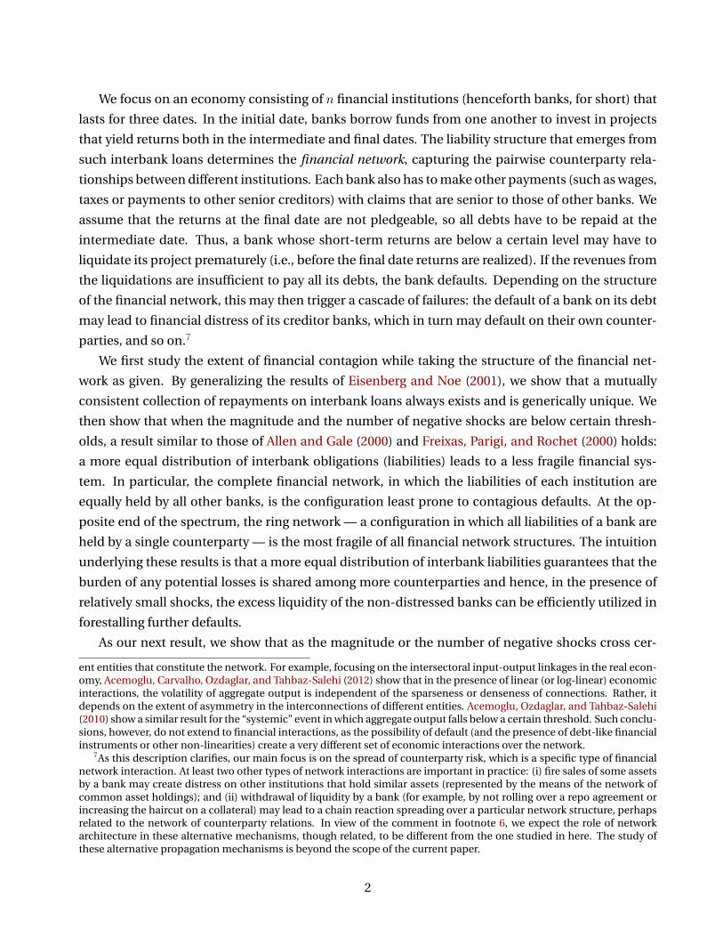
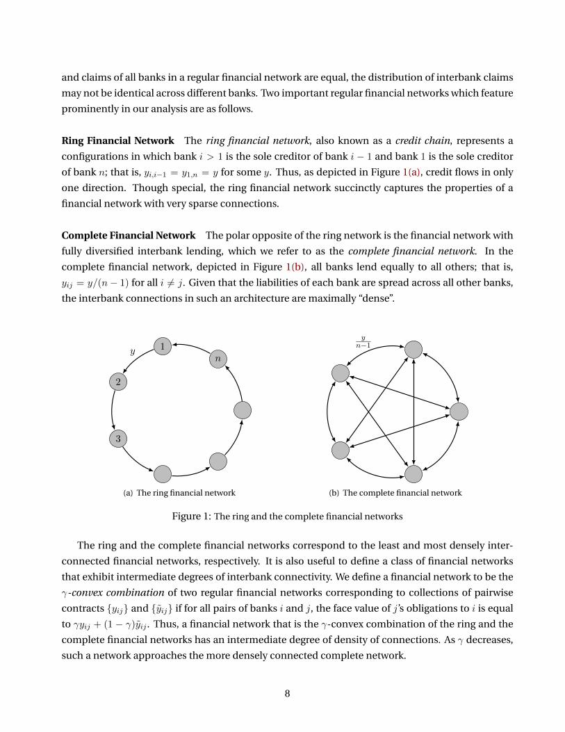
Ring Financial Network The ring financial network, also known as a credit chain, represents a

configurations in which bank i > 1 is the sole creditor of bank i − 1 and bank 1 is the sole creditor

of bank n; that is, yi,i−1 = y1,n = y for some y. Thus, as depicted in Figure 1(a), credit flows in only

one direction. Though special, the ring financial network succinctly captures the properties of a

financial network with very sparse connections.

Complete Financial Network The polar opposite of the ring network is the financial network with

fully diversified interbank lending, which we refer to as the complete financial network. In the

complete financial network, depicted in Figure 1(b), all banks lend equally to all others; that is,

yij = y/(n− 1) for all i 6= j. Given that the liabilities of each bank are spread across all other banks,

the interbank connections in such an architecture are maximally “dense”.

1

2

3

ny

(a) The ring financial network

yn−1

(b) The complete financial network

Figure 1: The ring and the complete financial networks

The ring and the complete financial networks correspond to the least and most densely inter-

connected financial networks, respectively. It is also useful to define a class of financial networks

that exhibit intermediate degrees of interbank connectivity. We define a financial network to be the

γ-convex combination of two regular financial networks corresponding to collections of pairwise

contracts {yij} and {yij} if for all pairs of banks i and j, the face value of j’s obligations to i is equal

to γyij + (1 − γ)yij . Thus, a financial network that is the γ-convex combination of the ring and the

complete financial networks has an intermediate degree of density of connections. As γ decreases,

such a network approaches the more densely connected complete network.

8

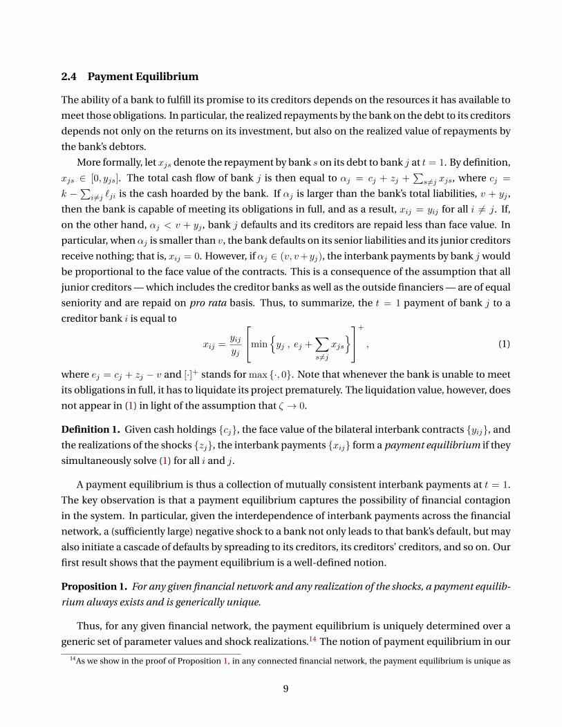
2.4 Payment Equilibrium

The ability of a bank to fulfill its promise to its creditors depends on the resources it has available to

meet those obligations. In particular, the realized repayments by the bank on the debt to its creditors

depends not only on the returns on its investment, but also on the realized value of repayments by

the bank’s debtors.

More formally, let xjs denote the repayment by bank s on its debt to bank j at t = 1. By definition,

xjs ∈ [0, yjs]. The total cash flow of bank j is then equal to αj = cj + zj +∑

s 6=j xjs, where cj =

k −∑

i 6=j `ji is the cash hoarded by the bank. If αj is larger than the bank’s total liabilities, v + yj ,

then the bank is capable of meeting its obligations in full, and as a result, xij = yij for all i 6= j. If,

on the other hand, αj < v + yj , bank j defaults and its creditors are repaid less than face value. In

particular, when αj is smaller than v, the bank defaults on its senior liabilities and its junior creditors

receive nothing; that is, xij = 0. However, if αj ∈ (v, v+yj), the interbank payments by bank j would

be proportional to the face value of the contracts. This is a consequence of the assumption that all

junior creditors — which includes the creditor banks as well as the outside financiers — are of equal

seniority and are repaid on pro rata basis. Thus, to summarize, the t = 1 payment of bank j to a

creditor bank i is equal to

xij =yijyj

min{yj , ej +

∑s 6=j

xjs

}+

, (1)

where ej = cj + zj − v and [·]+ stands for max {·, 0}. Note that whenever the bank is unable to meet

its obligations in full, it has to liquidate its project prematurely. The liquidation value, however, does

not appear in (1) in light of the assumption that ζ → 0.

Definition 1. Given cash holdings {cj}, the face value of the bilateral interbank contracts {yij}, and

the realizations of the shocks {zj}, the interbank payments {xij} form a payment equilibrium if they

simultaneously solve (1) for all i and j.

A payment equilibrium is thus a collection of mutually consistent interbank payments at t = 1.

The key observation is that a payment equilibrium captures the possibility of financial contagion

in the system. In particular, given the interdependence of interbank payments across the financial

network, a (sufficiently large) negative shock to a bank not only leads to that bank’s default, but may

also initiate a cascade of defaults by spreading to its creditors, its creditors’ creditors, and so on. Our

first result shows that the payment equilibrium is a well-defined notion.

Proposition 1. For any given financial network and any realization of the shocks, a payment equilib-

rium always exists and is generically unique.

Thus, for any given financial network, the payment equilibrium is uniquely determined over a

generic set of parameter values and shock realizations.14 The notion of payment equilibrium in our

14As we show in the proof of Proposition 1, in any connected financial network, the payment equilibrium is unique as

9

model is a generalization of the notion of a clearing vector introduced by Eisenberg and Noe (2001)

and utilized by Shin (2008, 2009). Unlike the model of Eisenberg and Noe, the financial obligations

of the banks in our model are of different seniorities.

Finally, for any given financial network and the corresponding payment equilibrium, we define

the (utilitarian) social surplus in the economy as the sum of the returns to all agents; that is,

u = π0 +

n∑i=1

(πi + Ti),

where Ti ≤ v is the transfer from bank i to its senior creditors, πi is the bank’s profit, and π0 denotes

the net return (in excess of their opportunity cost of r per unit of lending) to the outside financiers.

3 Financial Contagion

In this section, we study the repayment of interbank loans and the extent of financial contagion at

t = 1, while taking the interbank debt contracts (signed at t = 0) as given. In particular, we focus

on the properties of the payment equilibrium as a function of the structure of the financial network.

We study the lending decisions of the banks and the formation of the financial network in Section 4.

In order to simplify the presentation, we restrict our attention to regular financial networks in

which banks have no liabilities to outside financiers, and assume that all interbank loans are at the

same interest rate, R.15 Thus, the total interbank claims and liabilities of all banks are equal to y =

Rk. Restricting our attention to regular financial networks enables us to focus on the relationship

between the distributions of interbank liabilities and the extent of contagion, while abstracting away

from effects that are driven by other features of the financial network, such as the asymmetry in the

size of different banks’ assets or liabilities.16

We further assume that the short-term returns on a given bank i’s investment can only take two

values zi ∈ {a, a − ε}, where a > v is the return of the project in the “business as usual” regime and

ε ∈ (a − v, a) corresponds to the magnitude of a negative shock to the project’s returns. Finally, we

assume that the realizations of the short-term returns are independent and identically distributed

across different banks. These simplifying assumptions enable us to provide a meaningful compari-

son between the extent of financial contagion in different financial networks in a tractable manner.

The following lemma characterizes the social surplus under the above assumptions.

long as∑

j(zj + cj) 6= nv. In the non-generic case in which∑

j(zj + cj) = nv, there may exist a continuum of paymentequilibria, in almost all of which banks default due to “coordination failures”. For example, if the economy consists of twobanks with c1 = c2 = v, bilateral contracts of face values y12 = y21 and no shocks, then defaults can occur if banks do notpay one another, even though both are solvent.

15In the full equilibrium of the model described in Section 4, banks may face potentially different (and endogenouslydetermined) interest rates depending on their probability of default.

16For example, Acemoglu et al. (2012) show that asymmetry in the degree of interconnectivity of different industries asinput suppliers in the real economy plays a crucial role in the propagation of shocks.

10

Lemma 1. Conditional on the realization of m negative shocks, the social surplus in the economy is

equal to

u = (n− ]defaults)A+ na−mε.

Hence, the social surplus is simply determined by the number of defaults, which in turn reflects

the extent of financial contagion. It is thus natural to measure the performance of a financial net-

work in terms of the number of banks in default.

Definition 2. Conditional on the realization of m negative shocks,

(i) the stability of a financial network is the inverse of the expected number of defaults.

(ii) The resilience of the financial network is the inverse of the maximum number of possible de-

faults.

Thus, stability and resilience capture the expected and worst-case performances of the financial

network in the presence of m negative shocks, respectively. Clearly, both measures of performance

not only depend on the number (m) and the size (ε) of the realized shocks, but also on the structure

of the financial network. To illustrate the relation between the extent of contagion and the financial

network architecture in the most transparent manner, we initially assume that exactly one bank is

hit with a negative shock. We generalize our results to the case of multiple shocks in Section 3.3.

3.1 Small Shock Regime

We first characterize the fragility of different financial networks when the size of the negative shock

is relatively small.

Proposition 2. Let ε∗ = n(a− v) and suppose that ε < ε∗. Then, there exists y∗ such that for y > y∗,

(a) The ring network is the least resilient and least stable financial network.

(b) The complete network is the most resilient and most stable financial network.

(c) The γ-convex combination of the ring and complete networks becomes less stable and resilient as

γ increases.

The above proposition thus establishes that as long as the size of the negative shock is below a

critical threshold ε∗, the ring is the financial network most prone to financial contagion, whereas the

complete network is the least fragile. Moreover, a more equal distribution of interbank obligations

leads to less fragility.17 Proposition 2 is thus in line with, and generalizes, the observations made by

17It may appear that part (c) of Proposition 2 can be proved by generalizing Lemma 6 of Eisenberg and Noe (2001).However, a closer inspection shows that the statement and the proof of the aforementioned lemma are incorrect (a coun-terexample is available from the authors upon request). We provide a direct proof of Proposition 2 in the Appendix. NeitherEisenberg and Noe (2001) nor any other paper we are aware of proves an equivalent statement.

11

Allen and Gale (2000) and Freixas, Parigi, and Rochet (2000). The underlying intuition is that a more

equal distribution of interbank liabilities implies that the burden of any potential losses is shared

among more banks, creating a more robust system. In particular, in the extreme case of the complete

financial network, the losses of a distressed bank are divided among as many creditors as possible,

guaranteeing that the excess liquidity in the financial system can fully absorb the transmitted losses.

On the other hand, in the ring financial network, the losses of the distressed bank — rather than

being divided up between multiple counterparties — are fully transferred to its immediate creditor,

leading to the creditor’s possible default. A similar mechanism then guarantees that the distress is

passed to a large fraction of the banks through a chain reaction, leading to a highly fragile system.

The condition that ε < ε∗ = n(a − v) requires the size of the negative shock to be less than the

total “excess liquidity” available to the financial network as a whole. Recall that in the absence of

any shock, a− v is the liquidity available to each bank after meeting its senior obligations to outside

the network. Proposition 2 also requires that interbank liabilities (and claims) are above a certain

threshold y∗, which is natural given that for small values of y, no contagion would occur, regardless

of the structure of financial network.

The extreme fragility of the ring financial network established by Proposition 2 is in contrast with

the results of Acemoglu et al. (2010, 2012), who show that if the interactions over the network are

linear (or log linear), the ring is as stable as any other regular network structure. This contrast reflects

the fact that, with linear interactions, negative and positive shocks cancel each other out in exactly

the same way independently of the structure of network. However, the often non-linear nature of

financial interactions (captured in our model by the presence of debt contracts on which banks

may default) implies that the effects of negative and positive shocks are not necessarily averaged

out. Stability and resilience are thus achieved by minimizing the impact of the distress at any given

bank on the rest of the system. The ring financial network is highly fragile precisely because the

adverse effects of a negative shock to any bank are fully transmitted to the bank’s immediate creditor,

triggering maximal financial contagion.

3.2 Large Shock Regime

Proposition 2 shows that as long as the magnitude of the negative shock is below the threshold ε∗,

a more equal distribution of interbank liabilities leads to less fragility. In particular, it shows that

the complete network is the most stable and resilient financial network: except for the bank that

is directly hit with the negative shock, no other bank defaults. Our next result, however, shows that

when the magnitude of the shock is above the critical threshold ε∗, this picture changes dramatically.

A collection of banksM ⊂ N is said to form a δ-component of the financial network if (i) the total

obligations of banks outside of M to any bank in M is at most δ ≥ 0; and (ii) the total obligations

of banks in M to any bank outside of M is no more than δ. Intuitively, for small values of δ, banks

in a δ-component have weak ties to the rest of the financial network. We say a financial network is

δ-connected if it contains a δ-component.

12

Proposition 3. Suppose ε > ε∗ and y > y∗. Then,

(a) The complete and the ring networks are the least stable and least resilient financial networks.

(b) For small enough values of δ, any δ-connected financial network is strictly more stable and re-

silient than the ring and complete financial networks.

Thus, when the magnitude of the negative shock is sufficiently large, the complete network ex-

hibits a form of phase transition: it flips from being the most to the least stable and resilient network,

achieving the same level of fragility as the ring network. In particular, when ε > ε∗, all banks in the

complete network default. The intuition behind this result is simple: given that all banks in the

complete network are creditors of the distressed bank, the adverse effects of the negative shock are

directly transmitted to them. Thus, when the size of the negative shock is large enough, not even the

originally non-distressed banks are capable of paying their debts in full, leading to the default of all

banks.

Not all financial systems are as fragile in the face of large shocks. Instead, as part (b) shows, if

the financial network contains a δ-component for small enough values of δ, then it is strictly more

stable and resilient than both the complete and the ring networks. The presence of such “weakly

connected” components in the network guarantees that the losses — rather than being transmitted

to all other banks — are borne in part by the distressed banks’ senior creditors.

Taken together, Propositions 2 and 3 illustrate the “robust-yet-fragile” property of highly inter-

connected financial networks conjectured by Haldane (2009). They show that more densely inter-

connected financial networks, epitomized by the complete network, are more stable and resilient in

response to a range of shocks. However, once we move outside this range, these dense interconnec-

tions act as a channel through which shocks to a subset of the financial institutions transmit to the

entire system, creating a vehicle for instability and systemic risk.

The intuition behind such a phase transition it related to the presence of two types of “shock

absorbers” in our model, each of which capable of reducing the extent of contagion in the network.

The first absorber is the excess liquidity a − v > 0 of non-distressed banks at t = 1: the impact

of a shock is attenuated once it reaches banks with excess liquidity. This mechanism is utilized

more effectively when the financial network is more “complete”, an observation in line with the

results of Allen and Gale (2000) and Freixas, Parigi, and Rochet (2000). However, the claim v of

senior creditors of the distressed banks also function as a shock absorption mechanism. Rather

than transmitting the shocks to other banks in the system, the senior creditors can be forced to bear

(some of) the losses and hence, limit the extent of contagion. In contrast to the first mechanism, this

shock absorber is best utilized in weakly connected configurations and is the least effective in the

complete financial network. Thus, when the shock is so large that it cannot be fully absorbed by the

excess liquidity in the system — which is exactly when ε > ε∗ — financial networks that significantly

utilize the second absorber are less fragile.

13

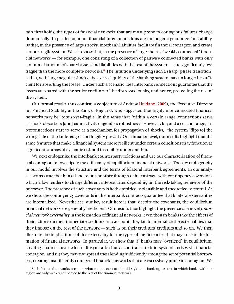
y − δ/2

δ/2

δ/2

y − δ y − δ/2

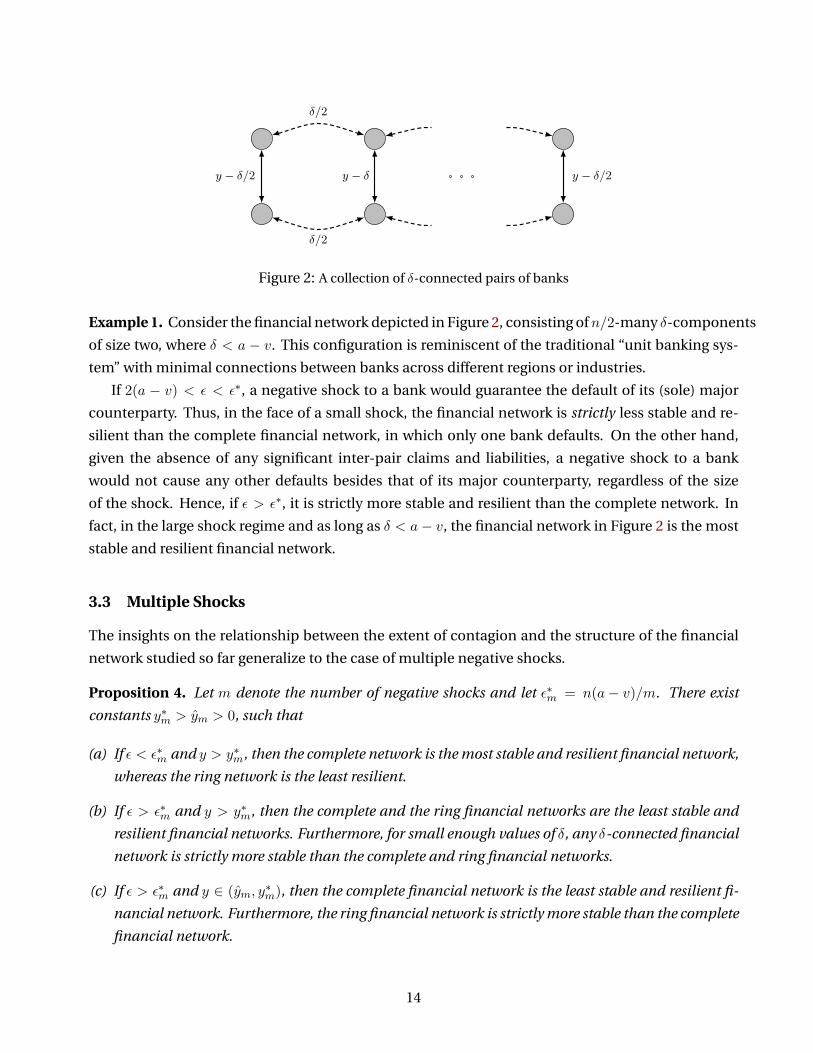
Figure 2: A collection of δ-connected pairs of banks

Example 1. Consider the financial network depicted in Figure 2, consisting ofn/2-many δ-components

of size two, where δ < a − v. This configuration is reminiscent of the traditional “unit banking sys-

tem” with minimal connections between banks across different regions or industries.

If 2(a − v) < ε < ε∗, a negative shock to a bank would guarantee the default of its (sole) major

counterparty. Thus, in the face of a small shock, the financial network is strictly less stable and re-

silient than the complete financial network, in which only one bank defaults. On the other hand,

given the absence of any significant inter-pair claims and liabilities, a negative shock to a bank

would not cause any other defaults besides that of its major counterparty, regardless of the size

of the shock. Hence, if ε > ε∗, it is strictly more stable and resilient than the complete network. In

fact, in the large shock regime and as long as δ < a− v, the financial network in Figure 2 is the most

stable and resilient financial network.

3.3 Multiple Shocks

The insights on the relationship between the extent of contagion and the structure of the financial

network studied so far generalize to the case of multiple negative shocks.

Proposition 4. Let m denote the number of negative shocks and let ε∗m = n(a− v)/m. There exist

constants y∗m > ym > 0, such that

(a) If ε < ε∗m and y > y∗m, then the complete network is the most stable and resilient financial network,

whereas the ring network is the least resilient.

(b) If ε > ε∗m and y > y∗m, then the complete and the ring financial networks are the least stable and

resilient financial networks. Furthermore, for small enough values of δ, any δ-connected financial

network is strictly more stable than the complete and ring financial networks.

(c) If ε > ε∗m and y ∈ (ym, y∗m), then the complete financial network is the least stable and resilient fi-

nancial network. Furthermore, the ring financial network is strictly more stable than the complete

financial network.

14

Parts (a) and (b) generalize the insights of Propositions 2 and 3 to the case of multiple negative

shocks. The key new observation is that the critical threshold ε∗m that defines the boundary of the

small and large shock regimes is a decreasing function of m. Thus, the number of negative shocks

plays a role similar to that of the size of the shocks. More specifically, as long as the magnitude and

the number of negative shocks affecting financial institutions are sufficiently small, more complete

interbank claims enhance the stability and the resilience of the financial system. This is due to the

fact that the more complete the interbank connections are, the better the excess liquidity of non-

distressed banks are utilized in absorbing the shocks. On the other hand, if the magnitude or the

number of shocks are large enough so that the excess liquidity in the financial system is not sufficient

for absorbing the losses, financial interconnections serve as a propagation mechanism, creating a

more fragile financial system. Weakly connected networks ensure that the losses are shared with the

senior creditors of the distressed banks, protecting the rest of the system.

Part (c) of Proposition 4 contains another new result. It shows that in the presence of multiple

shocks, the claims of the senior creditors in the ring financial network are used more effectively as a

shock absorption mechanism than in the ring financial network. In particular, the closer the banks

hit with the negative shocks are to one another in the ring financial network, the larger the loss their

senior creditors are collectively forced to bear. This limits the extent of contagion in the network.

Finally, we remark that even though we illustrated our results by focusing on an environment

in which shocks can take only two values, similar results can be obtained for more general shock

distributions.

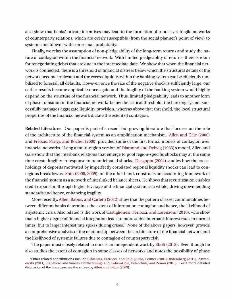
3.4 Illustrative Simulations

We end this section by providing a few simulations, illustrating the performance of different finan-

cial network structures as a function of the size of the negative shock.

We focus on four different financial network configurations consisting of n = 20 banks: (i) the

complete financial network; (ii) the ring financial network; (iii) the γ-convex combination of the

ring and the financial networks for γ = 3/4 ; and (iv) the double-clique financial network which is

a weakly connected network consisting of two 0-components (that is, disconnected components)

of size 10, each of which is complete. We vary the size of the negative shock ε and simulate the

expected number of defaults in each of the above-mentioned financial networks. For the purpose

of the simulations, we let y = 30 and a− v = 1, which implies that the critical threshold is ε∗ = 20.

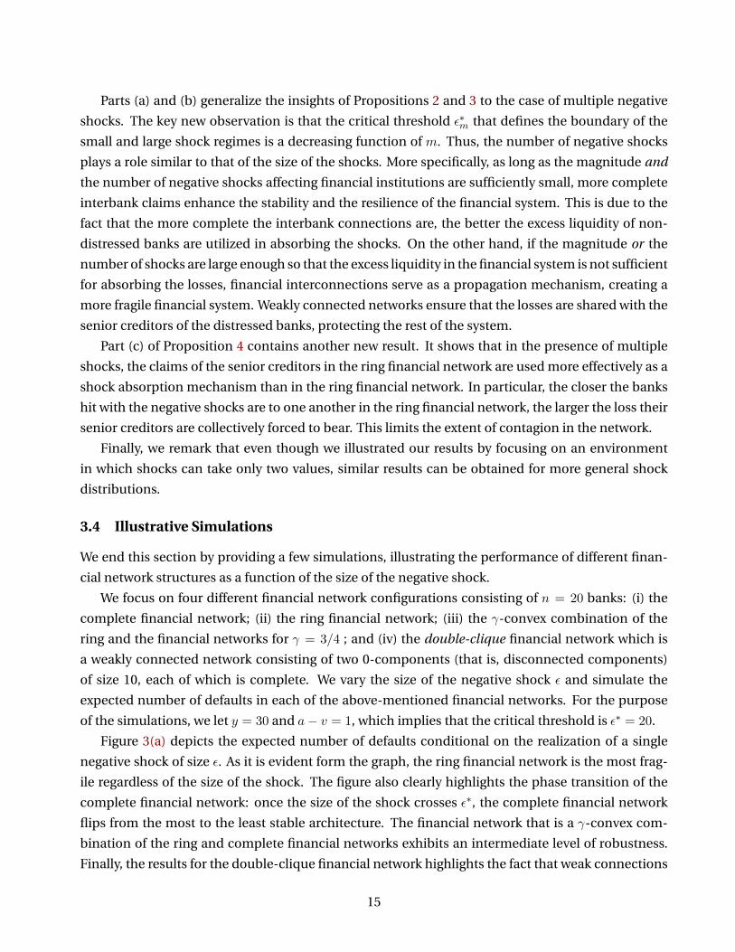
Figure 3(a) depicts the expected number of defaults conditional on the realization of a single

negative shock of size ε. As it is evident form the graph, the ring financial network is the most frag-

ile regardless of the size of the shock. The figure also clearly highlights the phase transition of the

complete financial network: once the size of the shock crosses ε∗, the complete financial network

flips from the most to the least stable architecture. The financial network that is a γ-convex com-

bination of the ring and complete financial networks exhibits an intermediate level of robustness.

Finally, the results for the double-clique financial network highlights the fact that weak connections

15

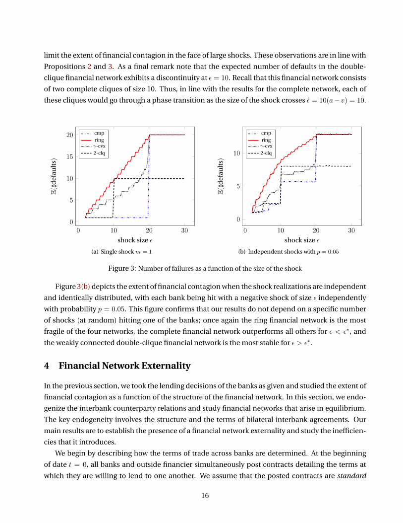
limit the extent of financial contagion in the face of large shocks. These observations are in line with

Propositions 2 and 3. As a final remark note that the expected number of defaults in the double-

clique financial network exhibits a discontinuity at ε = 10. Recall that this financial network consists

of two complete cliques of size 10. Thus, in line with the results for the complete network, each of

these cliques would go through a phase transition as the size of the shock crosses ε = 10(a− v) = 10.

0 10 20 30

0

5

10

15

20

shock size ε

E(]d

efau

lts)

cmpringγ-cvx

2-clq

(a) Single shock m = 1

0 10 20 30

0

5

10

shock size ε

E(]d

efau

lts)

cmpringγ-cvx

2-clq

(b) Independent shocks with p = 0.05

Figure 3: Number of failures as a function of the size of the shock

Figure 3(b) depicts the extent of financial contagion when the shock realizations are independent

and identically distributed, with each bank being hit with a negative shock of size ε independently

with probability p = 0.05. This figure confirms that our results do not depend on a specific number

of shocks (at random) hitting one of the banks; once again the ring financial network is the most

fragile of the four networks, the complete financial network outperforms all others for ε < ε∗, and

the weakly connected double-clique financial network is the most stable for ε > ε∗.

4 Financial Network Externality

In the previous section, we took the lending decisions of the banks as given and studied the extent of

financial contagion as a function of the structure of the financial network. In this section, we endo-

genize the interbank counterparty relations and study financial networks that arise in equilibrium.

The key endogeneity involves the structure and the terms of bilateral interbank agreements. Our

main results are to establish the presence of a financial network externality and study the inefficien-

cies that it introduces.

We begin by describing how the terms of trade across banks are determined. At the beginning

of date t = 0, all banks and outside financier simultaneously post contracts detailing the terms at

which they are willing to lend to one another. We assume that the posted contracts are standard

16

debt contracts with contingency covenants, according to which the lender specifies the interest rates

at which it lends to the borrower as a function of the borrower’s lending behavior. Given the posted

contracts, each bank then decides how much and from whom to borrow, which in turn determines

the interbank interest rates. More formally, the timing of events over date t = 0 is as follows.

1. All agents i ∈ {0, . . . , n} simultaneously post contracts of the form Ri = (Ri1, . . . , Rin), where

Rij is a mapping from the bank j’s lending decision (`j1, . . . , `jn) to the interest rate on bank j’s

debt to i. If i cannot lend to bank j or decides not to do so, then Rij = ∅.

2. After observing the set of posted contracts, each agent can withdraw one or more of its contract

offers if it so wishes. The final set of contracts offered by bank i is thus Ri = (Ri1, . . . , Rin),

where Rij ∈ {Rij ,∅}.18

3. Given the set of contracts (R0, . . . , Rn), each bank j decides on the amount bij that it borrows

from agent i.

By construction, the borrowing decisions of the banks determine the amount of interbank lend-

ing; that is, `ij = bij . This, in turn, pins down the interest rate on bank j’s debt to i at Rij(`j1, . . . , `jn).

Given the large set of possible lending decisions by the banks, the contract Ri posted by bank

i is an infinite dimensional object. In order to simplify the exposition and derivation of our main

results, unless otherwise noted, we restrict the set of interbank borrowings by assuming that bij ∈{0, kij}. That is, if banks i and j enter into a lending agreement, then the borrowing would be equal

to the maximal borrowing capacity. This simplification reduces each borrowing decision to a binary

choice. Consequently, the contract Rij(`j1, . . . , `jn) is reduced to a vector, specifying the interest

rates at which bank i is willing to lend to j as a function of the identities of j’s counterparties. With

some abuse of notation, we use Rij to denote both the contingent debt contract between i and j,

as well as the actual interest rate on j’s debt to i once all the bilateral interbank agreements are

finalized. Also, whenever there is no risk of confusion, we use Rij and Rij interchangeably.

Definition 3. A full (subgame perfect) equilibrium is a collection of contracts posted by the banks

and the outside financiers, given by (R0,R1, . . . ,Rn) and (R0, R1, . . . , Rn), bilateral borrowing deci-

sions {bij}, and interbank repayments {xij} such that,

(a) Given the financial network, the repayments on the loans are determined by the corresponding

payment equilibrium.

18The second stage of the game, in which contract offers can be withdrawn, is introduced in order to rule out certainunnatural equilibria that may arise due to “coordination failures”. In particular, unless bank i can withdraw its postedcontracts, it cannot make its lending decisions contingent on the contract posted by a potential creditor bank s. In otherwords, without the possibility of contract withdrawals, once bank i posts a contractRij , it already commits to lend to bankj regardless of the value of Rsi.

17

(b) Given the posted contracts, the financial network is a Nash equilibrium of the corresponding

subgame.19

(c) Neither the banks nor the outside financiers have an incentive to deviate by withdrawing or

posting a different contract at any stage of the game at time t = 0.

A financial network {yij} is thus part of an equilibrium if (i) taking the interest rates as given,

the banks have no incentive to unilaterally change their counterparties; and (ii) they cannot make

strictly

higher profits by charging different interest rates. Given that the outside financiers are risk neu-

tral and act competitively, the equilibrium contract R0 gives them an expected return equal to their

opportunity cost, r.

The most important feature of our setup is that equilibrium interest rates are determined en-

dogenously. In particular, given that the lending behavior of a bank may expose its creditors to

additional counterparty risks, the presence of covenants that make interest rates contingents on the

borrower’s behavior forces the banks to internalize the impact of their decisions on their immedi-

ate creditors. This feature, as we show in the next subsection, ensures that the most obvious form

of bilateral externalities are internalized, thus providing a useful framework for analyzing financial

network externalities. Throughout, we use a notion of efficiency according to which the social plan-

ner controls the lending decisions, but not the interbank interest rates, which are determined by the

equilibrium behavior of the outside financiers.20

4.1 Bilateral Efficiency: The Three-Chain Financial Network

To show how bilateral financial externalities are internalized thanks to the covenants, we focus on

a special architecture in which no other form of network externalities is present. In particular, we

consider an economy comprising of three banks labeled {1, 2, 3}, each endowed with k units of cap-

ital. In order to invest in their projects, banks 1 and 2 need to borrow k units of capital from banks

2 and 3, respectively. That is, k21 = k32 = k, and kij = 0 otherwise. Bank 3, on the other hand, does

not borrow and simply acts as a (potential) lender to bank 2. The assumption that there are no other

banks or financiers lending to bank 3 rules out the possibility of network externalities.21

19An alternative is to use a solution concept similar to the pairwise stability notion of Jackson and Wolinsky (1996), oftenused in problems of network formation. Given the more specific context here, posting of interest rates combined withsubgame perfection provides a powerful solution concept that is both more transparent and easier to work with. Ourmain results and the insights that follow are robust with respect to the choice of the solution concept.

20If we allow the social planner to also determine the interbank interest rates, she can increase utilitarian social wel-fare by setting all interest rates equal to zero, thus minimizing defaults. Such a framework, clearly, does not constitute areasonable benchmark for comparison.

21This assumption implicitly implies that bank 3 is not subject to default. This has no bearing for the results that follow.To restore symmetry between the three banks, we can alternatively assume that bank 3 also has access to a project it caninvest in and loses an extra amount ofA (due to costly liquidations) if its returns fall below a certain threshold. Proposition5 remains valid under this assumption.

18

Given the above description, if no bank relies on the outside financiers for funding, the three-

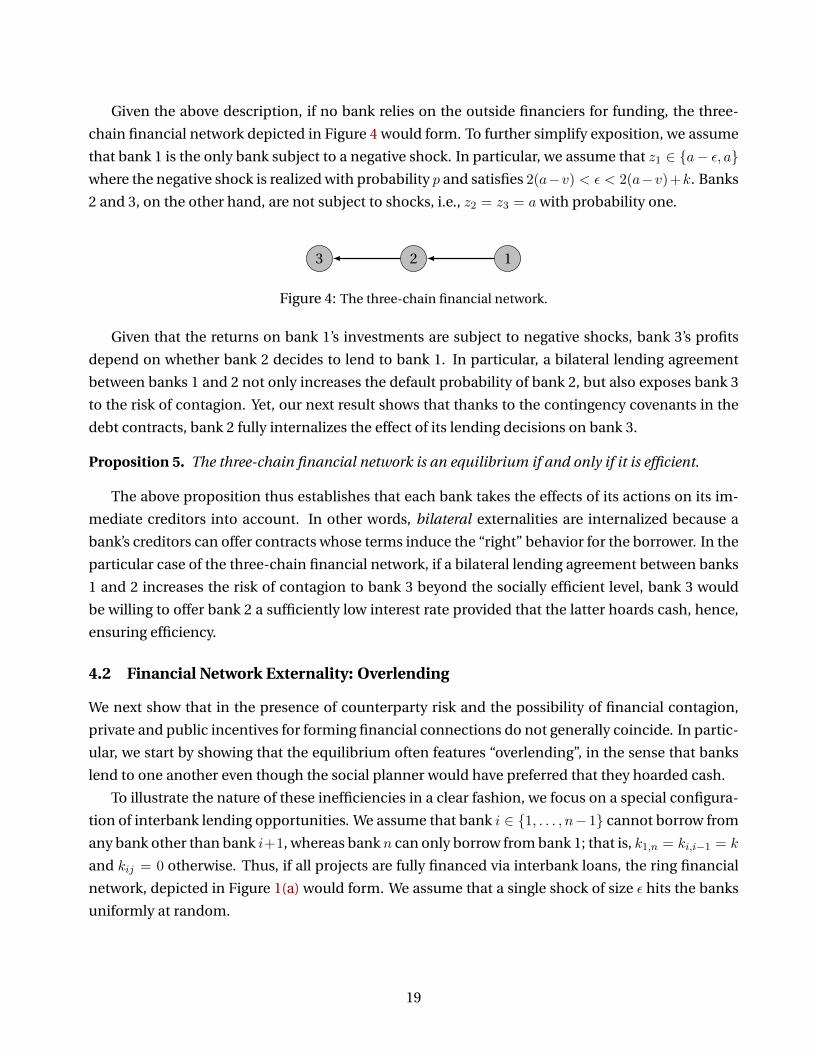
chain financial network depicted in Figure 4 would form. To further simplify exposition, we assume

that bank 1 is the only bank subject to a negative shock. In particular, we assume that z1 ∈ {a− ε, a}where the negative shock is realized with probability p and satisfies 2(a−v) < ε < 2(a−v)+k. Banks

2 and 3, on the other hand, are not subject to shocks, i.e., z2 = z3 = a with probability one.

123

Figure 4: The three-chain financial network.

Given that the returns on bank 1’s investments are subject to negative shocks, bank 3’s profits

depend on whether bank 2 decides to lend to bank 1. In particular, a bilateral lending agreement

between banks 1 and 2 not only increases the default probability of bank 2, but also exposes bank 3

to the risk of contagion. Yet, our next result shows that thanks to the contingency covenants in the

debt contracts, bank 2 fully internalizes the effect of its lending decisions on bank 3.

Proposition 5. The three-chain financial network is an equilibrium if and only if it is efficient.

The above proposition thus establishes that each bank takes the effects of its actions on its im-

mediate creditors into account. In other words, bilateral externalities are internalized because a

bank’s creditors can offer contracts whose terms induce the “right” behavior for the borrower. In the

particular case of the three-chain financial network, if a bilateral lending agreement between banks

1 and 2 increases the risk of contagion to bank 3 beyond the socially efficient level, bank 3 would

be willing to offer bank 2 a sufficiently low interest rate provided that the latter hoards cash, hence,

ensuring efficiency.

4.2 Financial Network Externality: Overlending

We next show that in the presence of counterparty risk and the possibility of financial contagion,

private and public incentives for forming financial connections do not generally coincide. In partic-

ular, we start by showing that the equilibrium often features “overlending”, in the sense that banks

lend to one another even though the social planner would have preferred that they hoarded cash.

To illustrate the nature of these inefficiencies in a clear fashion, we focus on a special configura-

tion of interbank lending opportunities. We assume that bank i ∈ {1, . . . , n− 1} cannot borrow from

any bank other than bank i+1, whereas bank n can only borrow from bank 1; that is, k1,n = ki,i−1 = k

and kij = 0 otherwise. Thus, if all projects are fully financed via interbank loans, the ring financial

network, depicted in Figure 1(a) would form. We assume that a single shock of size ε hits the banks

uniformly at random.

19

Proposition 6. Suppose that ε < ε∗. Then, there exist constants α < α such that,

(a) The ring financial network is part of an equilibrium if αA < (r − 1)k.

(b) The ring financial network is socially inefficient if (r − 1)k < αA.

The ring financial network is thus part of an equilibrium if the interest rates that the banks can

charge when they lend to one another — the benefit of which over hoarding cash is (r−1)k— is large

enough to justify the subsequent increase in the expected cost of a default, which is proportional to

A. On the other hand, the ring financial network would be socially inefficient whenever the costs

associated with the higher risk of financial contagion are high enough so that it is no longer justified

for all banks to lend. The more important consequence of Proposition 6 is that, unlike the case of

the three-chain financial network, the equilibrium and efficiency conditions no longer coincide: as

long as αA < (r − 1)k < αA, the ring financial network is part of an equilibrium, even though it is

inefficiently fragile.

The juxtaposition of Propositions 5 and 6 clarifies that the inefficiency of equilibrium financial

networks is not due to a simple bilateral externality. Rather, it is due to the presence of a finan-

cial network externality: lending by each bank creates a pathway for the translation of idiosyncratic

shocks into financial contagion and systemic crises. Even though, thanks to the covenants, each

bank takes the effect of its actions on itself and its immediate creditors into account, it does not

fully internalize the effects of its decisions on the its creditors’ creditors and so on. For example, in

the case of the ring financial network, despite the fact that the interest rate Ri+1,i faced by bank i

depends on whether it decides to lend or not, the effects of i’s actions on banks other than i + 1 are

not reflected in that interest rate. In particular, neither i nor i + 1 take into account that lending by

bank i may lead to a cascade of defaults of length τ > 2.

The presence of this type of financial network externality implies that financial stability is a pub-

lic good, which cannot be resolved by bilateral contracting and is only inadequately provided in

equilibrium.22

4.3 Financial Network Externality: Insufficiently Dense Networks

We next show that the financial externality identified in the previous subsection may lead to the

formation of insufficiently dense networks, in the sense that, from the social planner’s point of view,

banks may not spread out their lending enough among all potential borrowers.

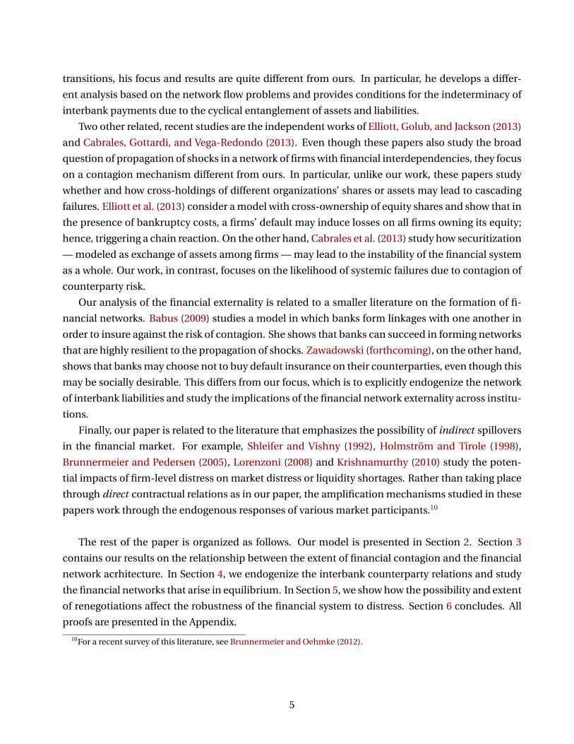
To illustrate this possibility, we focus on an economy in which each bank can lend to two different

borrowers. In particular, consider an n-bank economy (where n is even) in which banks labeled 2i

and 2i − 1 can lend to banks labeled 2i − 2 and 2i − 3; that is, k2i,2i−2 = k2i,2i−3 = k2i−1,2i−2 =

22As noted in the Introduction, this result is related to Zawadowski (forthcoming) who shows that banks may underin-vest in default insurance on their counterparties, partly because they do not internalize the positive spillovers that suchinsurance would create to other banks. Though clearly complementary, the exact mechanism and theoretical analysis inhis paper are quite different from ours.

20

k2i−1,2i−3 = k and kij = 0 otherwise. Thus, if all banks decide to lend equally to their potential

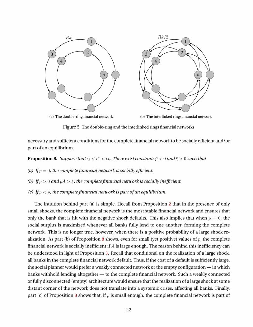
borrowers, the interlinked rings financial network, depicted in Figure 5(b), would form. However,

each bank can also decide to follow an undiversified lending strategy and instead lend to only one

borrower. Following such a strategy by all banks would lead to the formation of the double-ring

financial network depicted in Figure 5(a). We assume that a single shock of size ε hits the banks

uniformly at random.

Proposition 7. Suppose that ε < ε∗/2. Then, the number of defaults in the double-ring financial

network is equal to τ = dε/(a− v)e − 1. Furthermore, there exists α > 0 such that

(a) The double-ring financial network is part of an equilibrium if αA < (r − 1)k.

(b) The double-ring financial network is socially inefficient if τ is even.

Thus, for large enough values of r, the double-ring financial network is part of an equilibrium

even though it is not socially efficient. As in Proposition 6, the assumption that αA < (r − 1)k

guarantees that no bank in the double-ring financial network has an incentive to deviate by hoarding

cash. Unlike the previous example, each bank can also deviate by following a diversified lending

strategy. Yet, as part (a) shows, such a deviation would not be profitable either: for a large enough

value of r, lending to a diversified set of banks would expose the bank (and its immediate creditor)

to a higher level of counterparty risk.

The key observation is that even though no bank finds diversified lending profitable, such a de-

viation imposes a positive externality on the rest of the system. Recall that by Proposition 2, the

extent of financial contagion is reduced the more densely interconnected the financial network is.

Hence, following a diversified lending strategy would benefit other banks as the excess liquidity in

the system is more efficiently utilized in absorbing the shocks. This is the source of inefficiency of

the double-ring financial network established in part (b) of Proposition 7.23

4.4 Robust-Yet-Fragile Financial Networks

We end this section by showing that the the same type of financial externalities can also lead to the

emergence of robust-yet-fragile financial networks, in the sense that the entire financial network

remains (inefficiently) vulnerable to the realization of a rare negative shock.

To this end, we focus on the particular configuration of interbank lending opportunities de-

scribed by kij = k/(n−1) for all i 6= j; that is, if no bank hoards cash, the complete financial network

depicted in Figure 1(b) would form. We once again assume that a single shock hits the banks uni-

formly at random. The shock can take two distinct values εh and ε` with probabilities p and 1 − p,

respectively, where ε` < ε∗ < εh. Thus, for small enough values of p, the two realizations correspond

to “large but rare” and “small but frequent” negative shocks, respectively. Our next result provides

23The requirement that τ is an even number is a simple technical assumption guaranteeing that the extent of financialcontagion in the interlinked rings financial networks is strictly smaller than τ .

21

3

1Rk

2

4

n

(a) The double-ring financial network

3

1Rk/2

2

4

n

(b) The interlinked rings financial network

Figure 5: The double-ring and the interlinked rings financial networks

necessary and sufficient conditions for the complete financial network to be socially efficient and/or

part of an equilibrium.

Proposition 8. Suppose that ε` < ε∗ < εh. There exist constants p > 0 and ξ > 0 such that

(a) If p = 0, the complete financial network is socially efficient.

(b) If p > 0 and pA > ξ, the complete financial network is socially inefficient.

(c) If p < p, the complete financial network is part of an equilibrium.

The intuition behind part (a) is simple. Recall from Proposition 2 that in the presence of only

small shocks, the complete financial network is the most stable financial network and ensures that

only the bank that is hit with the negative shock defaults. This also implies that when p = 0, the

social surplus is maximized whenever all banks fully lend to one another, forming the complete

network. This is no longer true, however, when there is a positive probability of a large shock re-

alization. As part (b) of Proposition 8 shows, even for small (yet positive) values of p, the complete

financial network is socially inefficient if A is large enough. The reason behind this inefficiency can

be understood in light of Proposition 3. Recall that conditional on the realization of a large shock,

all banks in the complete financial network default. Thus, if the cost of a default is sufficiently large,

the social planner would prefer a weakly connected network or the empty configuration — in which

banks withhold lending altogether — to the complete financial network. Such a weakly connected

or fully disconnected (empty) architecture would ensure that the realization of a large shock at some

distant corner of the network does not translate into a systemic crises, affecting all banks. Finally,

part (c) of Proposition 8 shows that, if p is small enough, the complete financial network is part of

22

an equilibrium. This is due to the fact that if the large shock, and hence, financial contagion is fairly

unlikely, the banks find lending more profitable than hoarding cash.

The key insight in Proposition 8 is obtained from comparison of the conditions in the three parts.

Taken together, parts (a) and (c) imply that the complete financial network is part of an efficient

equilibrium whenever the possibility of a large systemic shock is ruled out (because when p = 0,

the complete financial network fully absorbs the shock without any contagion). However, as soon

as there is the slightest possibility of the realization of a large shock, public and private incentives

for interbank lending start to diverge. This can be seen by comparing statements (b) and (c). As

far as an individual bank is concerned, hoarding cash (as opposed to lending to the other banks)

decreases its default probability by p(n − 1)/n. But, hoarding cash by some bank i also protects

the rest of banking system whenever i is hit with the large shock. In fact, from the social planner’s

point of view, hoarding cash by a bank decreases the expected number of defaults by 2p(n − 1)/n.

The presence of the financial network externality thus implies that the possibility of a rare, large

shock may lead to the formation of (inefficiently) robust-yet-fragile financial networks a la Haldane

(2009).24

5 Renegotiations and Financial Contagion

In this section, we relax the assumption that long-term returns are non-pledgeable, thus allowing

banks to pledge at least a fraction of their long-term (date t = 2) returns to their creditors. In

particular, we assume that a fraction κ ∈ [0, 1] of the long-term returns can be pledged at t = 1,

essentially allowing banks to pass the ownership of a fraction κ of their long-term returns to their

creditors.25 Because these returns remain non-pledgeable at t = 0, banks still need to fund their

projects through standard debt contracts that clear at the intermediate date. The difference, how-

ever, arises in the event that a bank is unable to make its debt payments at t = 1, in which case it can

pledge up to κA of its long-term returns.26

In order to formalize the renegotiation stage, we assume that the intermediate date is subdivided

intoM periods (whereM > 2n2) during which banks make renegotiation offers to their counterpar-

ties. In particular, first bank 1 makes renegotiation offers to its creditor banks in a pre-specified

order, followed by renegotiation offers by bank 2 to its own creditors, and so on.27 These renegoti-

24The comparison between statements (b) and (c) of Proposition 8 implies the emergence of the complete financialnetwork as an inefficient equilibrium only if the intersection of the conditions in the two statements is non-empty; thatis, only if p < p and pA > ξ can hold simultaneously. It can be verified that for large enough n, the value of p becomesindependent of A. Hence, for any p ∈ (0, p), there exists a large enough A such that pA > ξ holds.

25We are thus assuming that two banks cannot renegotiate with one another, unless they are counterparties. We alsocontinue to assume that the banks cannot pledge their long-term returns to the outside financiers.

26Equivalent results would be obtained if the initial loans are made with more complex contracts that make paymentsboth at date t = 1 and t = 2. Sticking to the standard debt contracts and allowing renegotiation is just a convenientconvention.

27The same results would obtain with simultaneous renegotiation offers if we pick the best Nash equilibrium of thesimultaneous offer game.

23

ation offers take the form of a bank i pledging some amount Aji ≥ 0 to its creditor j, subject to the

constraint that its pledges do not exceed κA. In exchange, i may request postponement of its debt

repayments or even injection of additional funding from j. The interbank payments are made at the

end of date t = 1 after the renegotiation phase is over. For a given regular financial network, we have

the following result:

Proposition 9. Suppose that the financial network is connected.

(a) If ε < min{ε∗m, κA/m+ a− v}, then no bank defaults.

(b) If ε > min{ε∗m, κA+ a− v}, then at least one bank defaults.

Thus, for large enough values of κ, the possibility of renegotiations by counterparties would pre-

vent all defaults, even if some banks are distressed. On the other hand, if κ is small enough, then

distressed banks cannot avoid costly defaults by renegotiating their obligations to counterparties

in exchange for future payments. In fact, no renegotiations occur throughout the network, all dis-

tressed banks default and financial contagion occurs as if κ = 0. These observations are intuitive.

More interestingly, however, is the case that a single bank is hit with a negative shock. In particular,

if m = 1, Proposition 9 is essentially another phase transition result: there exists a threshold

ε = min{ε∗, κA+ a− v},

such that for ε < ε, the structure of the financial network (beyond connectivity) plays no role whatso-

ever in the extent of contagion. In fact, regardless of the detailed structure of the financial network,

the excess liquidity of the banking system — through a sequence of renegotiations — is utilized to

avoid all bankruptcies. This picture is dramatically different if ε is above the critical threshold ε, in

which case even all the liquidity that can be mobilized is insufficient for preventing defaults. Thus,

failures would occur and local network effects similar to those characterized in the Section 3 would

become the defining factor in the extent of financial contagion.

Note that for the above phase transition result to hold we do not need to assume that a bank

can renegotiate with all other banks. In fact, as long as each bank can renegotiate with its creditors

(and the financial network is connected), the excess liquidity at any part of the banking system can

be diverted to the distressed bank. This is due to the fact that even if a distressed bank’s creditors

do not have enough funds to lend, they can themselves pledge their own long-term returns to their

creditors, and raise the necessary funds to lend to the distressed bank. Such renegotiation chains

guarantee that excess liquidity would be allocated efficiently.

6 Conclusions

The recent financial crisis has rekindled interest in the relationship between the structure of the fi-

nancial network and systemic risk. Two polar views on this relationship have been suggested in the

24

academic literature and the policy world. The first maintains that the “incompleteness” of the finan-

cial network can be a source of instability, as individual banks are overly exposed to the liabilities of

a handful of financial institutions. Thus, according to this argument, a more complete financial

network which limits the exposure of the banks to any one counterparty would be less prone to sys-

temic failures. The second view, in stark contrast, hypothesizes that it is the highly interconnected

nature of the financial system that contributes to its fragility, as it facilitates the spread of financial

distress and solvency problems from one bank to the rest in an epidemic-like fashion.

This paper provides a tractable theoretical framework for the study of the economic forces shap-

ing the relationship between the structure of the financial network and systemic risk. We show that

as long as the magnitude (or the number) of negative shocks is below a critical threshold, a more

equal distribution of interbank obligations leads to less fragility. In particular, all else equal, the

sparsely connected ring financial network (corresponding to a credit chain) is the most fragile of all

configurations, whereas the highly interconnected complete financial network is the configuration

least prone to contagion. In line with the observations made by Allen and Gale (2000), our results

establish that, in the more complete networks, the losses of a distressed bank are passed to a larger

number of counterparties, guaranteeing a more efficient use of the excess liquidity in the system in

forestalling defaults.

We also show that when negative shocks are larger than a certain threshold, the second view on

the relationship between the structure of the financial network and the extent of contagion prevails.

In particular, completeness is no longer a guarantee for stability. Rather, in the face of large shocks,

financial networks in which banks are only weakly connected to one another would be less prone

to systemic failures. Such a “phase transition” is due to the fact that, the senior liabilities of banks,

as well as the excess liquidity within the financial network, can act as shock absorbers. Weak inter-

connections guarantee that the more senior creditors of a distressed bank bear most of the losses

and hence, protect the rest of the system against cascading defaults. Our model thus formalizes the

robust-yet-fragile property of interconnected financial networks conjectured by Haldane (2009). On

a broader level, our results highlight the possibility that the same features that make a financial net-

work structure more stable under certain conditions may function as significant sources of systemic

risk and instability under another.

The paper also provides an analysis of the efficiency of the financial networks that emerge in

equilibrium. We assume that interbank interest rates adjust endogenously in order to reflect the

risk that each bank’s decisions impose on its counterparties. Nevertheless, we show that equilib-

rium financial networks may be excessively prone to the risk of financial contagion. The intuition

underlying this result is that even though banks fully internalize the effects of their lending (and

risk-taking) decisions on their immediate creditors, they do not take into account the fact that their

lending decisions may also put many other banks (such as their creditors’ creditors) at a greater risk

of default. Thus, our results highlight the presence of a financial network externality, which cannot

be internalized via simple bilateral contractual relations, thus providing an example of the view that

25

financial stability is a “public good,” likely to be under-provided in equilibrium. We also show that

the presence of this externality may manifest itself in equilibrium financial networks that (relative

to the socially efficient level) are either too sparsely or too densely connected. The financial network

externality and the consequent inefficiency also imply that there is room for welfare-improving gov-

ernment interventions. We leave the analysis of the optimal policy in this class of models to future

work.

Finally, we establish a second form of phase transition when long-term returns are partially

pledgeable. In particular, we show that if the fraction of the returns that is pledgeable is above a

certain threshold, there are no network effects: the excess liquidity of the baking system can be effi-

ciently reallocated to distressed banks and all defaults are avoided, regardless of the structure of the

financial network. However, if the pledgeable fraction is below this threshold, network effects can-

not be avoided, and the local structure of the financial network plays a defining role in the extent of

financial contagion.

There are several areas of future research highlighted by our paper. First, a more complete anal-

ysis of network formation in the presence of counterparty risks is an obvious area of investigation.

Second, it is important to understand whether and how other forms of financial network interac-

tions (along the lines of those discussed in footnote 7) affect the stability of the system as a whole.

Finally and most importantly, a systematic empirical investigation, informed by the theoretical re-

sults in this paper, would enable us to measure the key components that play a role in financial

stability.

26

A Appendix: Proofs

Denote the fraction of obligations of agent j 6= 0 to agent i by qij = yij/yj . Given that the outside

financiers have no debt obligations (i.e., y0 = 0), we define qi0 > 0 arbitrarily, while assuming that∑ni=0 qi0 = 1. Let Q = [qij ] ∈ R(n+1)×(n+1) and denote the sum of the payments of bank j to the rest

of the banks in the financial network by xj =∑n

i=0 xij . Finally, we define the mapping Φ : H → H as

Φ(x) =[

min {Qx+ e, y}]+,

where H =∏ni=0[0, yi]. We have the following simple lemma.

Lemma A.1. For any x, x ∈ H ,

‖Φ(x)− Φ(x)‖1 ≤ ‖Q(x− x)‖1. (2)

Furthermore, the above inequality is tight only if for all i, either (Qx+e)i, (Qx+e)i ∈ [0, yi] or (Qx)i =

(Qx)i.

Proof. For any pair of real numbers ξ and ξ, it is straightforward to verify |ξ+ − ξ+| ≤ |ξ − ξ|, where

the inequality is tight only if ξ = ξ or ξ, ξ ≥ 0. Therefore,∣∣Φi(x)− Φi(x)∣∣ ≤ |min {(Qx)i + ei, yi} −min {(Qx)i + ei, yi}| . (3)

On the other hand, it is again easy to verify |min{ξ, ζ} −min{ξ, ζ}| ≤ |ξ − ξ| for all real numbers ξ, ξ

and ζ, where the inequality is tight only if ξ = ξ or ξ, ξ ≤ ζ. As a result,

|min {(Qx)i + ei, yi} −min {(Qx)i + ei, yi}| ≤∣∣(Qx)i − (Qx)i

∣∣, (4)

for all i. Combining (3) and (4) establishes (2).

To prove the second statement, note that (2) is tight only if inequalities (3) and (4) are tight for all

i. Inequality (4) is tight only if either (Qx)i = (Qx)i or (Qx)i + ei, (Qx)i + ei ≤ yi. On the other hand,

inequality (3) is tight only if (Qx)i = (Qx)i or (Qx)i + ei, (Qx)i + ei ≥ 0. Combining these completes

the proof.

Proof of Proposition 1

Existence: The mapping Φ : H → H continuously maps a convex and compact subset of the Eu-

clidean space to itself. Therefore, by the Brouwer fixed point theorem, there exists x∗ ∈ H such

that Φ(x∗) = x∗. This immediately implies that the collection of pairwise interbank payment {x∗ij}defined as x∗ij = qijx

∗j simultaneously solves the collection of equations (1) for all i and j, and thus,

corresponds to a payment equilibrium of the financial network.28

28Conversely, any payment equilibrium of the financial network corresponds to a fixed point of Φ.

27

Generic Uniqueness: Without loss of generality, assume that the financial network is connected.29

By Lemma A.1, Φ is a non-expansive operator with respect to the `1-norm. In particular, for any

x, x ∈ H ,

‖Φ(x)− Φ(x)‖1 ≤ ‖Q(x− x)‖1 (5)

≤ ‖Q‖1 · ‖x− x‖1 (6)

= ‖x− x‖1,

where the last equality is due to the fact that the column sums ofQ are equal to one. Therefore, Φ has

two distinct fixed points x and x only if all the inequalities above are tight. By Lemma A.1, inequality

(5) is tight only if for any given bank i, either (Qx)i+ei, (Qx)i+ei ∈ [0, yi] or (Qx)i = (Qx)i. Denoting

the set of banks that satisfy the former by B, we have

ei +

n∑j=0

qijxj = xi

ei +

n∑j=0

qij xj = xi,

for all i ∈ B with the convention that e0 = 0. Subtracting the above two equations from one another

leads to

(Qx)i − (Qx)i = xi − xi ∀i ∈ B,

which in view of the fact that (Qx)i = (Qx)i for all i 6∈ B implies

Q(x− x) =

[xB − xB

0

],

and hence,

‖Q(x− x)‖1 = ‖xB − xB‖1. (7)

Therefore, (6) holds as an equality only if xi = xi for all i 6∈ B, as it would otherwise violate (7).

Hence,

QBB(xB − xB

)= xB − xB, (8)

where QBB is the submatrix of Q corresponding to the banks in B. However, the fact that the finan-

cial network is connected (alongside the assumption that qi0 > 0 for all i) implies thatQ, and hence,

QBB are irreducible matrices.30 Given that x 6= x, equality (8) cannot hold unless Bc is empty. As a

consequence,n∑i=0

xi =

n∑i=1

ei +

n∑i=0

n∑j=0

qijxj

29If the financial network is not connected, the proof can be applied to each connected component separately.30An n×nmatrixQ is said to be reducible, if for some permutation matrix P , the matrix P ′QP is block upper triangular.

If a square matrix is not reducible, it is said to be irreducible. If Q is a non-negative irreducible matrix with unit columnsums, then all eigenvalues of any square submatrix ofQ, say Q, lie within the unit circle, which implies that Qx = x has nosolution. For more on this, see e.g., Berman and Plemmons (1979).

28

which implies∑n

i=1 ei = 0, an equality that holds only for a non-generic set of parameters z1, . . . , zn.

Thus, the fixed points of Φ, and hence the payment equilibria of the model are generically unique.

Proof of Lemma 1

Denote the set of banks that default on their senior debt by F , the set of banks that default but can

meet their senior obligations by D, and the set banks that do not default by S = (D ∪ F )c. For any

bank i ∈ F , we have

πi + Ti = zi +∑j 6=i

xij ,

whereas for i ∈ D,

πi + Ti = v.

On the other hand, for any bank i ∈ S which does not default,

πi + Ti = A+ zi − y +∑j 6=i

xij .

Finally, note that in any regular financial network, the outside financiers do not lend to the banks

and instead, invest their capital in a linear technology with return r, implying that π0 = 0. Therefore,

the social surplus is given by

u = (A− y)|S|+ v|D|+∑i 6∈D

zi +∑i 6∈D

∑j 6=i

xij

= (A− y)|S|+n∑i=1

zi +∑i∈S

∑j 6=i

yij

where the second equality is due to the fact that for i ∈ D we have,∑

j 6=i(xji − xij) = zi − v. Hence,

u = na−mε+A(n− ]defaults).

Two Auxiliary Lemmas

Lemma A.2. The number of bank defaults satisfies

m ≤ ](defaults) <mε

a− v

where m is the number of realizations of negative shocks in the network.

Proof. Given that the total interbank liabilities of each bank is equal to its total interbank claims and

that v > a − ε, any bank that is hit with a negative shock defaults. Hence, the lower bound is trivial.

To obtain the upper bound, note that for any bank i that defaults but can meet its senior obligations

in full, we have

zi +∑j 6=i

xij = v +∑j 6=i

xji.

29

Denoting the set of such banks by D and summing over all i ∈ D imply∑i∈D

zi +∑i∈D

∑j 6=i

xij = v|D|+∑i∈D

∑j 6=i

xji. (9)

On the other hand, for any bank i that defaults on its senior obligations (if such a bank exists), we

have ∑j 6=i

xij + zi < v.

Summing over the set of all such banks, F , implies∑i∈F

∑j 6=i

xij +∑i∈F

zi < v|F |. (10)

Adding (9) and (10) leads to

mε− (a− v)](defaults) ≥∑j 6∈S

∑i∈S

(yij − xij),

where S is the set of banks that do not default. By definition, the right-hand side of the above equal-

ity is strictly positive, proving that the number of defaults is strictly smaller than mε/(a− v).

Lemma A.3. If ε < ε∗m, then at least one bank does not default, where ε∗m = n(a− v)/m. On the other

hand, if ε > ε∗m, then at least one bank defaults on its senior obligations.

Proof. Suppose that ε < ε∗m and that all banks default. Therefore,

zi +∑j 6=i

xij ≤ v +∑j 6=i

xji,

for all banks i. Summing over i implies

na−mε ≤ nv,

which contradicts the assumption that ε < ε∗m.

To prove the second statement, suppose that ε > ε∗m and that no bank defaults on its senior

obligations. Thus,

zi +∑j 6=i

xij ≥ v +∑j 6=i

xji,

for all banks i. Summing over i implies na−mε ≥ nv, leading to a contradiction.

Proof of Proposition 2

Proof of part (a). Without loss of generality assume that bank 1 is hit with the negative shock. By

Lemma A.3, bank n does not default as it is the bank furthest away from the distressed bank. More-

over, as long as y > y∗ = (n−1)(a−v), bank 1 — and consequently all banks — can meet their senior

30

obligations in full. This is due to the fact that y + a − ε > v. Given that the set of banks that default

form a connected chain, say of length τ , the repayment of the last bank in default to its sole creditor

satisfies

xτ+1,τ = y + τ(a− v)− ε.

On the other hand, given that bank τ + 1 does not default, we have

a+ xτ+1,τ > y + v.

As a result, τ ≥ ε/(a − v) − 1, implying that the number of defaults reaches the upper bound estab-

lished in Lemma A.2. Hence, the ring network is the least stable and least resilient financial network.

Proof of part (b). By Lemma A.3, as long as ε < ε∗, there exists at least one bank that does not de-

fault. Given the full symmetry in the complete network, the n − 1 banks that are not hit with the

negative shock can thus meet their obligations in full. Hence, the complete financial network is the

most stable and most resilient regular financial network.

Proof of part (c). Consider the financial network constructed as the γ-convex combination of the

ring and the complete financial networks. Without loss of generality, we assume that bank 1 is hit

with the negative shock. Define γd to be the value at which banks 1 through d− 1 default while bank

d is at the verge of default. At this value of γ, we have

x1 =

(1− γdn− 1

)[(x1 + · · ·+ xd)− x1 + (n− d)y] + γdy + (a− v − ε) (11)

xi =

(1− γdn− 1

)[(x1 + · · ·+ xd)− xi + (n− d)y] + γdxi−1 + (a− v) (12)

for 2 ≤ i ≤ d. Hence,

∆2 = x2 − x1 = γd∆1 −(

1− γdn− 1

)∆2 + ε

∆i = xi − xi−1 = γd∆i−1 −(

1− γdn− 1

)∆i,

where ∆1 = x1 − y. Thus, for all 2 ≤ i ≤ d,

∆i = βi−1(∆1 + ε/γd),

where for notational simplicity we have defined β = (1 + 1−γdn−1 )−1γd. Given that xd = y, the terms ∆i

must add up to zero, that is,

d∑i=1

∆i =

(1− βd

1− β

)∆1 +

(1− βd−1

1− β

)(βε

γd

)= 0,

which immediately implies

∆1 = −(

1− βd−1

1− βd

)(βε

γd

).

31

Therefore,

xi = y +

i∑s=1

∆s = y +

(βd−1 − βi−1

1− βd

)(βε

γd

),

and as a result,d−1∑i=1

xi = (d− 1)y +

[dβd−1(1− β)− (1− βd)

γd(1− β)(1− βd)

]βε.

On the other hand, from (11) and (12), we have

d−1∑i=1

xi = (d− 1)y +d(a− v)− ε

(n− d)(1− γd)/(n− 1).

Equating the above two equalities thus leads to

n(a− v)/ε− 1 =

[βd−1(1− β)

1− βd

](n− d).

Therefore, the value γd at which d− 1 banks default and bank d is at the verge of default must satisfy

the above equality. For a fixed value of d, the right-hand side is increasing in β (and hence in γd).31

As a consequence, in order for the right-hand side to remain equal to the constant on the left-hand

side, d has to decrease with γ. Thus, there will be weakly more defaults as γ increases.

Proof of Proposition 3

Proof of part (a). First consider the complete financial network. By Lemma A.3, the distressed bank

defaults on its senior obligations. Suppose that the remaining n − 1 banks do not default and that

they can all meet their obligations in full.32 This would be the case only if

(n− 2)y

n− 1+ (a− v) ≥ y,

where we are using the fact that the distressed bank does not pay anything to its junior creditors.

The above inequality, however, contradicts the assumption that y > y∗. Hence, all banks default,

implying that the complete network is the least resilient and the least stable financial network.

Now consider the ring financial network and assume without loss of generality that bank 1 is

hit with the negative shock. Once again by Lemma A.3, bank 1 defaults on its senior obligations

and hence, does not pay anything to its more junior creditor, bank 2. Thus, if some bank does not

default, the length of the default cascade, τ , must satisfy

τ(a− v) > y,

31This can be easily verified by noticing that βd−1(1− β) = (1− βd)(1 + β−1 + · · ·+ β−(d−1)

)−1.

32Note that given the symmetric structure of the complete network and the uniqueness of payment equilibrium, eitherall other banks default together or they all meet their obligations fully at the same time.

32

which in light of the assumption that y > y∗ guarantees that τ > n − 1, leading to a contradiction.

Hence, all banks default, implying that the ring financial network is the least stable and resilient fi-

nancial network.

Proof of part (b). By definition, any regular δ-connected financial network contains at least one δ-

component M . Given that the total obligations of banks in M c to any bank i ∈ M is at most δ, the

total obligations of banks in M to i is at least y − δ; that is,∑

j∈M yij > y − δ.

If the negative shock hits a bank outside of M , all banks in M can meet their obligations in full

as long as

y < a− v + mini∈M

{∑j∈M

yij

},

which holds whenever δ < a − v. A similar argument shows that when the shock hits a bank in M ,

all banks in M c can meet their obligations in full. Thus, the financial network is strictly more stable

and resilient than both the complete and the ring networks.

Proof of Proposition 4

Proof of part (a). First consider the complete financial network. If ε < ε∗m, at least one bank does not

default. Given the symmetry, all n − m banks that are not hit with a negative shock do not default

either, implying that the complete network is the most stable and resilient financial network in the

face of small shocks.

Now consider the ring financial network and assume that m consecutive banks, labeled i + 1

through j = i + m, are hit with negative shocks. An immediate observation is that all banks in

default also form a connected chain, say of length τ ≥ m, the last of which is labeled s = i + τ . In

view of Lemma A.3, bank i does not default, as it is the bank furthest away from the realized shocks.

As a result, as long as y > y∗m = (n −m)(a − v), in the unique payment equilibrium of the financial

network, all banks can meet their senior obligations v in full. This can be established by verifying

that bank j — which is the bank facing the most amount of potential distress — can pay its senior

debts. In particular,

xj,j−1 = y + (m− 1)(a− ε− v),

guaranteeing that xj,j−1 + a− ε > v. Given that all banks can meet their senior obligations, we have

xs+1,s = y + τ(a− v)−mε

where s = i+ τ is the index of the last bank on the chain that defaults. On the other hand, given that

s+ 1 does not default, we have y ≤ a− v + xs+1,s. As a result,

τ =

⌈mε

a− v

⌉− 1 ≥ mε

a− v− 1. (13)

33

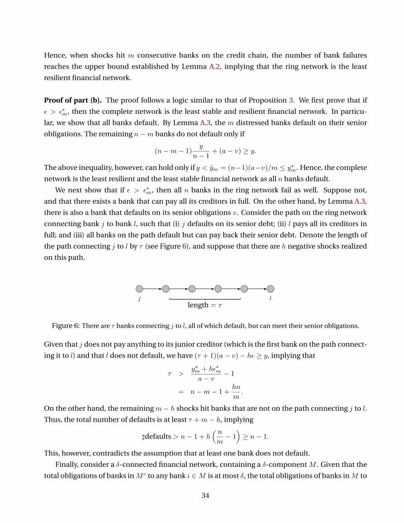
Hence, when shocks hit m consecutive banks on the credit chain, the number of bank failures

reaches the upper bound established by Lemma A.2, implying that the ring network is the least

resilient financial network.

Proof of part (b). The proof follows a logic similar to that of Proposition 3. We first prove that if

ε > ε∗m, then the complete network is the least stable and resilient financial network. In particu-

lar, we show that all banks default. By Lemma A.3, the m distressed banks default on their senior

obligations. The remaining n−m banks do not default only if

(n−m− 1)y

n− 1+ (a− v) ≥ y.

The above inequality, however, can hold only if y < ym = (n−1)(a−v)/m ≤ y∗m. Hence, the complete

network is the least resilient and the least stable financial network as all n banks default.

We next show that if ε > ε∗m, then all n banks in the ring network fail as well. Suppose not,

and that there exists a bank that can pay all its creditors in full. On the other hand, by Lemma A.3,

there is also a bank that defaults on its senior obligations v. Consider the path on the ring network

connecting bank j to bank l, such that (i) j defaults on its senior debt; (ii) l pays all its creditors in

full; and (iii) all banks on the path default but can pay back their senior debt. Denote the length of

the path connecting j to l by τ (see Figure 6), and suppose that there are h negative shocks realized

on this path.

j llength = τ

Figure 6: There are τ banks connecting j to l, all of which default, but can meet their senior obligations.

Given that j does not pay anything to its junior creditor (which is the first bank on the path connect-

ing it to l) and that l does not default, we have (τ + 1)(a− v)− hε ≥ y, implying that

τ >y∗m + hε∗ma− v

− 1

= n−m− 1 +hn

m.

On the other hand, the remaining m− h shocks hit banks that are not on the path connecting j to l.

Thus, the total number of defaults is at least τ +m− h, implying

]defaults > n− 1 + h( nm− 1)≥ n− 1.

This, however, contradicts the assumption that at least one bank does not default.

Finally, consider a δ-connected financial network, containing a δ-component M . Given that the

total obligations of banks inM c to any bank i ∈M is at most δ, the total obligations of banks inM to

34

i is at least y− δ; that is,∑

j∈M yij > y− δ for all i. If the negative shock hits a bank outside ofM and

as long as y < a− v+ mini∈M

{∑j∈M yij

}, all banks inM can meet their obligations in full. Thus, as

long as δ < a − v, the financial network is strictly more stable than both the complete and the ring

networks.

Proof of part (c). An argument similar to the one invoked in the proof of part (b) shows that the when

ε > ε∗m and y > ym, all banks in the complete network default. Therefore, the complete network is

the least stable and resilient financial network.

To prove that the ring financial network is more stable than the complete network, we show that

there exists a realization of the shocks for which at least one bank in the ring network does not

default. In particular, consider the situation in whichm consecutive banks, labeled 1 throughm, are

hit with negative shocks. By Lemma A.3, in the unique payment equilibrium, bank m defaults on its

senior debt. Therefore, the length of the cascade of defaults following bankm, denoted by τ , satisfies

τ(a− v) < y ≤ (τ + 1)(a− v).

Thus, the number of defaults in the whole network is

]defaults = m+ τ

< m+y∗ma− v

= n,

implying that at least one bank does not default. Hence, the ring network is strictly more stable than

the complete network.

Proof of Proposition 5

We first prove that the 3-chain financial network is efficient if and only if

(r − 1)k ≥ pA. (14)

Given that there are only two potential interbank bilateral contracts, there are only four possible

financial networks that can arise. It is easy to show that if banks 2 and 3 lend to banks 1 and 2,

respectively, the social surplus is equal to

u3-chain = 2a− pε+ k + 2(1− p)A,

where 2(1 − p)A captures the fact that a negative shock to bank 1 would lead to the default of (and

hence, costly liquidation by) banks 1 and 2. Furthermore,

u23 = 2a− pε+ 2k − rk + (2− p)A

u12 = 2a− pε+ 2k − rk + 2(1− p)A

uempty = 2a− pε+ 3k − 2rk + (2− p)A,

35

where uij refers to the social surplus in the financial network in which only bank j lends to bank i,

and uempty is the social surplus in the financial network with no interbank borrowings. The above

equalities immediately imply that the 3-chain financial network is efficient if and only if (14) holds.

We next show that (14) is a necessary condition for the 3-chain to be an equilibrium finan-

cial network. Suppose that the 3-chain financial network along with the collection of posted con-

tracts (R0,R2,R3) correspond to an equilibrium.33 Given that the outside financiers are compet-

itive and have to break even, the contract posted by the representative outside financier, R0 =

(R01, (R02, R′02)), satisfies

rk = (1− p)R01k + p(a− v − ε+ k) (15)

rk = (1− p)R02k + p(2(a− v)− ε+ k) (16)

rk = R′02k,

where R02 and R′02 are interest rates faced by bank 2 contingent on its decision whether to lend to

bank 1 or not, respectively. It is also immediate to verify that the equilibrium interest rate offered by

bank 2 to bank 1 has to be equal to the one offered by the outside financiers; that is, R2 = R01. Else,

either bank 1 would have borrowed from the outside financiers, or bank 2 could have increased its

profits by posting a higher interest rate. A similar argument establishes that, as long as bank 2 lends

to bank 1, bank 3 would not charge an interest rate different than what is offered by the outside

financiers. In other words, R3 = (R02, R′32), whereR′32 is the interest rate at which bank 2 can borrow

from bank 3 if it decides not to lend to bank 1. Thus, given the equilibrium interest rates, the profits

of the banks are equal to34

π1 = a− v − (r − 1)k − pε+ (1− p)A

π2 = a− v + (1− p)A

π3 = rk.

Finally, for the 3-chain financial network to be part of an equilibrium, bank 3 should not be able to

make a strictly higher profit by deviating and posting a new contract R3 = (R32, R′32). In particular,

there should not exist an interest rate R′32 for which both banks 2 and 3 would make strictly higher

profits if bank 2 hoards cash. Given that the profits of the banks when bank 2 hoards cash are

π2 = a− v + k − R′32k +A

π3 = R′32k,

such a deviation would be profitable if there exists R′32 such that

k + pA > R′32k > rk

33Note that since bank 1 has no lending opportunity, the contract R1 is not part of the equilibrium definition.34Note that given that hoarding cash by bank 2 is off the equilibrium path, the equilibrium profits of the banks are

independent of the value R′32.

36

as it would guarantee that π2 > π2 and π3 > π3. Thus, if (14) does not hold, the 3-chain financial

network cannot be part of an equilibrium.

The proof is complete once we show that (14) is also a sufficient condition for the 3-chain fi-

nancial network to be part of an equilibrium. In particular, we show that if (14) holds, then the

collection of contracts R0 = (R01, (R02, r)), R2 = R01, and R3 = (R02, r) and the 3-chain financial

network constitute an equilibrium, where R01 and R02 solve equations (15) and (16), respectively.

To this end, first take the posted contracts as given and consider the subgame that follows. Banks 1

and 2 have no unilateral incentives to borrow from the outside financiers, as they would be facing

the same interest rates offered by banks 2 and 3, respectively. Furthermore, bank 2 does not have

an incentive to deny lending to bank 1. In particular, if bank 2 hoards cash, it would make a profit

of π2 = a − v + k + A − rk which is strictly smaller than π2 = a − v + (1 − p)A. Finally, note that

bank 3 does not have an incentive to hoard either. Because, if bank 3 hoards cash, its profit would

be equal to π3 = k, which is strictly smaller than its profits in the 3-chain financial network. Thus,

given (R0,R2,R3), the 3-chain financial network is a Nash equilibrium of the subgame that follows

the posting of the contracts.

Finally, we show that no bank has an incentive to unilaterally deviate by posting a different con-

tract. Given that R0 = (R01, (R02, r)), bank 2 has no incentive to post anything other than R2 = R01.

Similarly, bank 3 cannot make strictly positive profits by posting a contract that offers bank 2 an in-

terest rate other thanR02 if bank 2 does not hoard cash. Thus, the only possible profitable unilateral

deviation would be for bank 3 to post a contract R3 = (R02, R′32) in which R′32 < r. However, as

we showed earlier, as long as (14) holds, such a deviation either (i) is not profitable to bank 3, or (ii)

would not induce bank 2 to hoard cash. Thus, the specified collection of contract and the 3-chain

financial network constitute a subgame perfect Nash equilibrium.

Proof of Proposition 6

Proof of part (a). Define τ = dε/(a− v)e − 1 as the extent of financial contagion in the ring financial

network and let α = 2(τ − 1)/(n − 1). We show that if αA < (r − 1)k, a collection of contracts

of the form Ri = (R,R′) for all i ∈ {0, 1, . . . , n} along with the ring financial network constitute a

symmetric equilibrium, whereR andR′ are the interest rates at which the lender is willing to lend to

the borrower contingent on whether the latter lends or hoards cash, respectively. In particular, we

choose the pair (R,R′) to satisfy the indifference equations of the outside financiers:

rk =

(n− τn

)Rk +

1

n

τ∑s=1

[s(a− v)− ε+Rk

](17)

rk =

(n− 1

n

)R′k +

1

n(a− v − ε+ k). (18)

We first take the pair of interest rates (R,R′) as given, and consider the subsequence subgame. Note

that bank i has an incentive to deny lending to bank i − 1 and hoard cash instead. In particular, if

37

bank i hoards cash, it would face the interest rate R′ and as a result, its profits would be equal to

π = a− v +

(n− 1

n

)A− ε

n− (r − 1)k.

On the other hand, if bank i does not hoard cash, it would make a profit equal to

πring =

(n− τn

)A+ a− v − ε

n, (19)

which is strictly larger that π. Furthermore, bank i has no incentive to deviate in its borrowing be-

havior either, as it would face interest rate R no matter if it borrows from bank i + 1 or the outside

financiers. Therefore, given the collection of contracts Ri = (R,R′), the ring financial network is a

Nash equilibrium of the corresponding subgame.

It is thus sufficient to show that no bank has an incentive to deviate by posting a different con-

tract. Clearly, no bank can make a strictly higher profit by offering an interest rate other than R for

the case that its designated borrower does not hoard cash. Therefore, the only possible profitable

deviation is for a bank i to post Ri = (R, R′) where R′ < R′. For such a deviation to be profitable,

however, there should exist an interest rate R′ such that πi > πring and πi+1 > πring where,

πi =

(n− 1

n

)(a− v + k − R′k +A)

πi+1 =

(n− 2

n

)(a− v + R′k −Rk +A).

Thus, such an interest rate exists only if

k − 1

n− 1(a− v − ε) +

(τ − 1

n− 1

)A > Rk +

1

n− 2(2(a− v)− ε)−

(τ − 2

n− 2

)A,

which implies(τ − 1

n− 1+τ − 2

n− 2

)A+

(1

n− 1+

1

n− 2

)ε > (r − 1)k +

(τ − 1

2n+

1

τ(n− 1)+

2

τ(n− 2)

)ε,

where we are using the fact that τ = dε/(a − v)e − 1. The above inequality, however, contradicts

the assumption that αA < (r − 1)k. Therefore, such a deviation would not be profitable for by i,

completing the proof.

Proof of part (b). Given that the ring financial network is symmetric, there are exactly τ defaults in

the presence of a single negative shock. Therefore, the social surplus is equal to

uring = na− ε+ (n− τ)A.

If, on the other hand, the social planner forces a single bank i to hoard cash instead of lending to

bank i− 1, (that is, by setting `i,i−1 = 0 and `j,j−1 = k for j 6= i) the social surplus would be equal to

uhoard = na− ε+ (n− E[τhoard])A− (r − 1)k,

38

where E[τhoard] is the expected number of defaults. Given that bank i is no longer at the risk of default

due to contagion, the extent of contagion would be strictly smaller than τ if any of the banks indexed

i − τ + 1 through i − 1 are hit by the negative shock, whereas there would be a longer cascade of

defaults, say of length τ ′ ≥ τ , if bank i itself is distressed. This is due to the fact that hoarding cash

implies a smaller return on i’s capital, and hence, a smaller cushion to absorb the shock at t = 1.

Hence,

E[τhoard] =1

n

[(n− τ − 1)τ +

τ∑s=1

s+ τ ′]

≤ τ + 1− τ(τ + 1)

2n,

where the inequality is due to the fact that τ ′ ≤ n. Therefore, as long as

(r − 1)k <(τ(τ + 1)

2n− 1)A,

the social planner can increase the social surplus by forcing bank i not to lend to bank i− 1.

Proof of Proposition 7

Proof of part (b). We establish the inefficiency of the double-ring financial network by showing that

the social surplus is higher in the interlinked rings financial network. Given that there are τ defaults

in the double-ring financial network, the social surplus is equal to

u2-ring = na− ε+ (n− τ)A.

On the other hand, the social surplus in the interlinked rings network is

ulinked = na− ε+ (n− τ)A,

where τ is the number of defaults. Thus, it is sufficient to show that τ < τ . Suppose without loss of

generality that bank n in the interlinked financial network is hit with the negative shock. Hence, if

banks 2q − 1 and 2q default, their total repayments on their obligations are equal to

x2q−1 = x2q = Rk + (q + 1/2)(a− v)− ε/2.

As a result, the total number of defaults in the interlinked rings financial network would be equal to

2s+ 1, where s is the largest integer for which x2s < Rk. Hence,

τ = 2

⌈ε

2(a− v)− 3/2

⌉+ 1.

Given that ε/(a− v) ≤ τ + 1, we have

τ ≤ 2 dτ/2− 1e+ 1 = 2 dτ/2e − 1,

39

which implies that if τ is even, then τ < τ . Hence, the double-ring financial network is socially inef-

ficient.

Proof of part (a). We show that a collection of contracts of the formR = (R,R′) for all i ∈ {0, 1, . . . , n}along with the double-ring financial network constitute a symmetric equilibrium, where R and R′

are the interest rates at which bank i is willing to lend to a borrower contingent on whether the latter

lends to others (regardless of whether it lends to one or two other banks) or hoards cash, respectively.

We choose the pair (R,R′) to satisfy the indifference equations of the outside financiers, determined

by (17) and (18).

Given that in the double-ring financial network each bank effectively belongs to a single credit

chain, the results established in Proposition 6 are applicable. In particular, the double-ring financial

network is a Nash equilibrium of the subgame that follows the posting of contract R by all agents.

Furthermore, no bank has an incentive to deviate and charge an interest rate other than R or R′

when its borrower lends fully or hoards cash, respectively. Therefore, to verify thatR and the double-

ring financial network constitute an equilibrium, it is sufficient to show that no lender bank i + 2

has an incentive to charge an interest rate that would lead the borrower bank i to split its lending

between two counterparties. We establish this statement by showing that if the interest rate is kept

atR, both banks i and i+2 would make strictly smaller profits when bank i splits its lending. Hence,

there is no interest rate at which (i) bank i+2 can induce bank i to split its lending; and (ii) bank i+2

is strictly better off than in the double-ring financial network.

Recall from (19) that the profit of a bank in a credit chain is equal to

πring =

(n− τn

)A+ a− v − ε

n.

On the other hand, if bank i deviates and splits its lending between the two borrower banks (i.e.,

banks i− 2 and i− 1 assuming that i is odd), then it would default on its obligations to bank i+ 2 if

any bank j satisfying i− 2τ + 4 ≤ j ≤ i is hit with the negative shock. Therefore, if the interest rates

are kept constant at R,

πi =

(n− 2τ + 3

n

)A+

(n− τ + 2

n

)(a− v)− ε

n.

A similar argument implies that bank i+ 2 defaults with probability 2τ − 6 and hence,

πi+2 =

(n− 2τ + 6

n

)A+

(n− τ + 5

n

)(a− v)− ε

n.

The above equations immediately imply that if τ > 3, then πi, πi+2 < πring, completing the proof.

Proof of Proposition 8

We first state and prove a simple lemma. Suppose that p = 0 and define Rc as the interest rate at

which the outside financiers break even in a complete financial network when all banks are also

40

lending at rate Rc. In other words, Rc solves

rk =

(n− 1

n

)Rck +

1

n(a− v − ε` +Rck).

Furthermore, for 0 ≤ s ≤ n− 1, defineRs as the interest rate at which the outside financiers are will-

ing to lend to a bank i who deviates from the complete network by only lending to s other banks.35

Lemma A.4. Suppose that p = 0. Then, Rs > Rc for all s < n− 1.

Proof. Suppose that bank i lends to s other banks, where s < n − 1. Also suppose that the outside

financiers break even by charging bank i an interest rate of Rs ≤ Rc. It is easy to verify that bank i

defaults on its obligations with probability at least 1/n. In particular, even ifRs = r, the bank cannot

meet all its obligations, as a− ε` +Rck < v+ rk. Furthermore, given that bank i is lending at rateRc,

the total default repayment of i on its debt to the outside financiers is strictly less thanRck+a−v−ε`.Hence, the expected repayment of bank i on its debt to the outside financiers satisfies

E[x0i] <

(n− 1

n

)Rsk +

1

n(a− v − ε` +Rck) ≤ rk,

which is a contradiction.

Proof of part (a). Given that the shock is of size of ε` with probability one, the social surplus in the

economy is equal to

u = na− ε` + (n− E[τ ])A− (c1 + · · ·+ cn)(r − 1),

where ci is the amount of cash hoarded by bank i and E[τ ] is the expected number of defaults in

the financial network. As the above equality suggests, only the last two terms depend on the struc-

ture of the financial network. Given that r > 1, the last term achieves its maximum value of zero

when no bank hoards cash. Clearly, the complete network satisfies this condition. Furthermore, by

Proposition 2, there is exactly one failure in the complete network regardless of the realization of the

shock, and hence, E[τ ] = 1. Thus, the proof is complete once we show that the expected number

of failures in all symmetric financial networks is at least one. Suppose not. This implies that there

exists a realization of the shocks for which no bank fails. By symmetry, however, this means that

no bank fails in the financial network, and as a result, all banks can borrow at the risk-free interest

rate r. Therefore, the total amount owed to any given bank i is less than or equal to its total debt of

value rk. This however, implies that the bank defaults if it is hit with the negative shock, which is a

contradiction. Thus, the complete network is the most efficient symmetric financial network.

Proof of part (b). It is sufficient to construct a symmetric financial network for which the social

surplus is larger than that of the complete network. First, consider the complete financial network.

35Note that by definition, Rn−1 = Rc.

41

Conditional on the realization of ε` and εh, there are 1 and n defaults, respectively. Therefore, the

social surplus in the economy is

ucomplete = na+ (1− p)(n− 1)A− [(1− p)ε` + pεh].

Next, consider the empty financial network in which banks do not lend to one another at all and

instead, hoard all their cash. In this case, the social surplus in the economy is

uempty = na+ (n− 1)A− [(1− p)ε` + pεh]− nk(r − 1),

where we are using the fact that a bank defaults only if it is hit with (either a small or a large) shock.

Thus, for any given p and n, the complete network is inefficient if

p(n− 1)A ≥ n(r − 1)k,

which completes the proof.

Proof of part (c). We first show that if p = 0, then the complete financial network is part of an

equilibrium. In particular, we show that if all banks and the outside financiers post the contract

R = (R0, . . . , Rn−1), then the complete financial network can be supported as part of an equilibrium,

where Rs is defined above.

As a first step, we show that given R, the complete network is a Nash equilibrium of the subse-

quent subgame. Given that all banks and the outside financiers are posting the same contract, no

bank has an incentive to deviate and borrow from the outside financiers instead of other banks. Fur-

thermore, no bank has an incentive to deviate and lend less either. By Lemma A.4, such a deviation

implies that the bank would face a higher interest rate from its creditors, while getting a smaller rate

of return on its own investment. Therefore, given the contracts, no bank has a profitable unilateral

deviation.

Next, we show that no bank has an incentive to deviate by posting a contract other than R.

Clearly, a given bank cannot make strictly higher profits by charging an interest rate other than Rc

for the case that its borrowers are not hoarding cash. In particular, if the bank chargers an interest

rate higher than Rc, the borrower banks would switch to the outside financiers. Thus, any potential

profitable deviation should involve changing the interest rates that a bank is willing to charge con-

tingent on the borrowers hoarding cash. Note that such deviations would lead to different payoffs

only if the banks do end up hoarding cash in the subsequent subgame. Thus, suppose that a bank i

deviates by posting a contract R 6= R and that at least one bank, say bank j, hoards cash (partially

or fully) in the subgame that follows. Now it is easy to verify that the corresponding element of the

vector of interest rates R cannot be larger thanRc. In particular, if that is the case, then j can simply

stop hoarding cash, and hence, face the smaller interest rate of Rc instead. On the other hand, no

element of R can be smaller than or equal to Rc either. In particular, if bank i charges an interest

rate that is smaller than or equal to Rc, it would be receiving a strictly smaller repayment on its loan

42

to j, regardless of whether j is defaulting or not. Hence, no bank has a profitable unilateral deviation

in posting a contract other than R.

To summarize, we have so far shown that when p = 0, the complete financial network is part

of an equilibrium. More specifically, we showed that any deviation that would lead to a financial

network structure other than the complete network in the subsequent subgame, would lead to a

strictly lower profit for the deviating bank. Therefore, by continuity, there exists a small enough p

such that for p < p, the complete network is part of a subgame perfect Nash equilibrium of the

game.

Proof of Proposition 9

If ε > ε∗m, then there is simply not enough liquidity in the system to forestall all defaults, regardless

of the value of κ. Therefore, throughout the proof, we assume that ε < ε∗m.

Proof of part (a). The argument relies on transforming the pattern of interbank renegotiations into

a network flow problem and invoking the maximum-flow minimum-cut theorem of Ford and Fulk-

erson (1956).36 In particular, consider the multi-source multi-destination network flow problem

defined as follows: (i) each bank i for which zi = a is a source with value of a − v, (ii) each dis-

tressed bank is a sink of value ε+ v − a, and finally, (iii) each vertex in the network has a capacity of

κA whereas all edges have infinite capacity. Note that the capacity of each vertex can alternatively

be represented by “splitting up” that vertex to two adjacent vertices of infinite capacity each and

connecting them with an imaginary edge of capacity κA.

If the above network flow problem has a feasible solution, then there exists a pattern of renegoti-

ations such that all banks would avoid default. In particular, the flow value on the edge connecting

bank i to bank j is exactly the amount that one bank pledges to pay the other at t = 2, in exchange

for a reverse transfer at t = 1. Also note that the assumption that vertex capacities are equal to κA

guarantees that no bank can get a transfer at t = 1 which exceeds the value of its pledgeable assets

at t = 2.

Given the above network flow problem, the max-flow min-cut theorem implies that a feasible

flow exists as long as the value of the minimum cut in the network is larger than the total outgoing

flow to the sinks, i.e.,m(ε+v−a). Since the minimum cut would consists of at least one of the imagi-

nary edges of capacity κA, the theorem implies that a feasible flow exists as long as κA > m(ε+v−a),

completing the proof.

Proof of part (b). Suppose that there exists a pattern of renegotiations which guarantees that no

defaults occur. If all defaults are indeed avoided, any distressed bank i is paid back in full by its

debtors, which means that i would have a total shortfall of v + ε − a on all its debt (to its senior36For a careful treatment of network flow problems, see for example, Cormen, Leiserson, Rivest, and Stein (2001). For

another application of this theory in economics, see Ambrus, Mobius, and Szeidl (2012).

43

creditors and other banks). Bank i would be able to renegotiate this debt only if it can pledge as

much at t = 2; that is, only if κA > v + ε− a. This is, however, in contradiction with the assumption

that ε > min{ε∗m, κA+ a− v}. Thus, at least one bank defaults.

44

References

Acemoglu, Daron, Vasco M. Carvalho, Asuman Ozdaglar, and Alireza Tahbaz-Salehi (2012), “The net-work origins of aggregate fluctuations.” Econometrica, 80, 1977–2016.

Acemoglu, Daron, Asuman Ozdaglar, and Alireza Tahbaz-Salehi (2010), “Cascades in networks andaggregate volatility.” NBER Working Paper 16516.

Allen, Franklin and Ana Babus (2009), “Networks in finance.” In The Network Challenge: Strategy,Profit, and Risk in an Interlinked World (Paul R. Kleindorfer and Yoram (Jerry) Wind, eds.), 367–382, Wharton School Publishing.

Allen, Franklin, Ana Babus, and Elena Carletti (2012), “Asset commonality, debt maturity and sys-temic risk.” Journal of Financial Economics, 104, 519–534.

Allen, Franklin and Douglas Gale (2000), “Financial contagion.” Journal of Political Economy, 108,1–33.

Ambrus, Attila, Markus Mobius, and Adam Szeidl (2012), “Consumption risk-sharing in social net-works.” NBER Working Paper 15719.

Babus, Ana (2009), “The formation of financial networks.” Discussion Paper 06-093, Tinbergen Insti-tute.

Battiston, Stefano, Domenico Delli Gatti, Mauro Gallegati, Bruce Greenwald, and Joseph E. Stiglitz(2012), “Liaisons dangereuses: Increasing connectivity, risk sharing, and systemic risk.” Journal ofEconomic Dynamics and Control, 36, 1121–1141.

Berman, Abraham and Robert J. Plemmons (1979), Nonnegative matrices in the mathematical sci-ences. Academic Press, New York.

Billio, Monica, Mila Getmansky, Andrew W. Lo, and Loriana Pelizzon (2012), “Econometric measuresof connectedness and systemic risk in the finance and insurance sectors.” Journal of FinancialEconomics, 104, 535–559.

Blume, Larry, David Easley, Jon Kleinberg, Robert Kleinberg, and Eva Tardos (2011), “Network for-mation in the presence of contagious risk.” Proceedings of the 12th ACM Conference on ElectronicCommerce.

Brunnermeier, Markus K. and Martin Oehmke (2012), “Bubbles, financial crises, and systemic risk.”In Handbook of the Economics of Finance (George M. Constantinides, Milton Harris, and Rene M.Stulz, eds.), volume 2, North Holland.

Brunnermeier, Markus K. and Lasse Heje Pedersen (2005), “Predatory trading.” The Journal of Fi-nance, 60, 1825–1863.

Caballero, Ricardo J. and Alp Simsek (forthcoming), “Fire sales in a model of complexity.” Journal ofFinance.

Cabrales, Antonio, Piero Gottardi, and Fernando Vega-Redondo (2013), “Risk-sharing and contagionin networks.” Working Paper.

Castiglionesi, Fabio, Fabio Feriozzi, and Guido Lorenzoni (2010), “Financial integration and liquiditycrises.” Working paper.

45

Cifuentes, Rodrigo, Gianluigi Ferrucci, and Hyun Song Shin (2005), “Liquidity risk and contagion.”Journal of the European Economic Association, 3, 556–566.

Cohen-Cole, Ethan, Eleonora Patacchini, and Yves Zenou (2013), “Systemic risk and network forma-tion in the interbank market.” Working Paper.

Cormen, Thomas H., Charles E. Leiserson, Ronald L. Rivest, and Clifford Stein (2001), Introductionto Algorithms. MIT Press, Cambridge, MA.

Dasgupta, Amil (2004), “Financial contagion through capital connections: A model of the origin andspread of bank panics.” Journal of the European Economic Association, 2, 1049–1084.

Diamond, Douglas W. and Philip H. Dybvig (1983), “Bank runs, deposit insurance, and liquidity.”Journal of Political Economy, 91, 401–419.

Diamond, Peter A. (1982), “Aggregate demand management in search equilibrium.” Journal of Polit-ical Economy, 90, 881–894.

Eboli, Mario (2012), “A flow network analysis of direct balance-sheet contagion in financial net-works.” Working paper.

Eisenberg, Larry and Thomas H. Noe (2001), “Systemic risk in financial systems.” Management Sci-ence, 47, 236–249.

Elliott, Matthew, Benjamin Golub, and Matthew O. Jackson (2013), “Financial networks and conta-gion.” Working Paper.

Financial Crisis Inquiry Commission (2011), “The Financial Crisis Inquiry Report: Final Report of theNational Commission on the Causes of the Financial and Economic Crisis in the United States.”U.S. Government Printing Office, Washington, DC.

Ford, Lester Randolph and Delbert Ray Fulkerson (1956), “Maximal flow through a network.” Cana-dian Journal of Mathematics, 8, 399–404.

Freixas, Xavier, Bruno M. Parigi, and Jean-Charles Rochet (2000), “Systemic risk, interbank relations,and liquidity provision by the central bank.” Journal of Money, Credit and Banking, 32, 611–638.

Gorton, Gary and Andrew Metrick (2011), “Securitized banking and the run on repo.” Journal of Fi-nancial Economics (forthcoming).

Gorton, Gary B. (2010), Slapped by the Invisible Hand: The Panic of 2007. Oxford University Press,USA.

Haldane, Andrew G. (2009), “Rethinking the financial network.” Speech delivered at the FinancialStudent Association in Amsterdam, The Netherlands, April 2009.http://www.bankofengland.co.uk/publications/Documents/speeches/2009/speech386.pdf.

Holmstrom, Bengt and Jean Tirole (1998), “Private and public supply of liquidity.” Journal of PoliticalEconomy, 106, 1–40.

Jackson, Matthew O. and Asher Wolinsky (1996), “A strategic model of social and economic net-works.” Journal of Economic Theory, 71, 44 – 74.

Kiyotaki, Nobuhiro and John Moore (1997), “Credit chains.” Working Paper.

46

Krishnamurthy, Arvind (2010), “Amplification mechanisms in liquidity crises.” American EconomicJournal: Macroeconomics, 2, 1–30.

Leitner, Yaron (2005), “Financial networks: Contagion, commitment, and private sector bailouts.”The Journal of Finance, 60, 2925–2953.

Longstaff, Francis A. (2010), “The subprime credit crisis and contagion in financial markets.” Journalof Financial Economics, 97, 436 – 450.

Lorenzoni, Guido (2008), “Inefficient credit booms.” The Review of Economic Studies, 75, 809–833.

Plosser, Charles I. (2009), “Redesigning financial system regulation.” A speech at the New York Uni-versity Conference “Restoring Financial Stability: How to Repair a Failed System”.

Rotemberg, Julio J. (2011), “Minimal settlement assets in economies with interconnected financialobligations.” Journal of Money, Credit and Banking, 43, 81–108.

Shin, Hyun Song (2008), “Risk and liquidity in a system context.” Journal of Financial Intermediation,17, 315 – 329.

Shin, Hyun Song (2009), “Securitisation and financial stability.” The Economic Journal, 119, 309–332.

Shleifer, Andrei and Robert W. Vishny (1992), “Liquidation values and debt capacity: A market equi-librium approach.” The Journal of Finance, 47, 1343–1366.

Sorkin, Andrew Ross (2009), Too Big to Fail: The Inside Story of How Wall Street and WashingtonFought to Save the Financial System—and Themselves. Viking, New York.

Stulz, Rene M. (2010), “Credit default swaps and the credit crisis.” Journal of Economic Perspectives,24, 73–92.

Vivier-Lirimont, Sebastian (2006), “Contagion in interbank debt networks.” Working Paper.

Zawadowski, Adam (2011), “Interwoven lending, uncertainty, and liquidity hoarding.” Working Pa-per.

Zawadowski, Adam (forthcoming), “Entangled financial systems.” The Review of Financial Studies.

47