31545 Medical Imaging systems

Lecture 3: Ultrasound focusing and modeling

Jørgen Arendt Jensen

Department of Electrical Engineering (DTU Elektro)

Biomedical Engineering Group

Technical University of Denmark

September 10, 2018

1

Topic of today: Imaging in ultrasound

Focusing and spatial impulse responses

1. Go through signal processing quiz

2. Repetition and assignment from last

3. Arrays and focusing using delay-and-sum

4. Ultrasound fields and resolution

5. Questions for exercise 1

Reading material: JAJ, ch. 2., p. 24-36

Self-study: CW fields

2

From last lecture: The wave equation

Speed of sound c:

c =

√1

ρκ

Linear wave equation:

∂2p

∂x2− 1

c2∂2p

∂t2= 0

General solutions:

p(t, x) = g(t± xc

)

x

cis time delay

3

Spherical wave

p(t, ~r) =p0

|~r| sin(2πf0(t− |~r|c

))

Propagates radially from a center point.

Used for describing diffraction, focusing, and ultrasound fields.

4

Attenuation of ultrasound

AttenuationTissue dB/[MHz·cm]Liver 0.6 – 0.9Kidney 0.8 – 1.0Spleen 0.5 – 1.0Fat 1.0 – 2.0Blood 0.17 – 0.24Plasma 0.01Bone 16.0 – 23.0

Approximate attenuation values for tissue penetrated for human tissue

Pulse-echo: depth of 10 cm, f0 = 5 MHz, attenuation 0.7 dB/[MHz·cm]:

Attenuation: 2 · 10 · 5 · 0.7 = 70 dB

5

Amplitude attenuation transfer function for a plane wave

|H(f ; z)| = exp(−(β0z + β1fz)), (1)

z - depth in tissuef - frequencyβ0 - frequency-independent attenuationβ1 - frequency-dependent term expressed in Np/[MHz·cm] (Np - Nepers)

Converted to Nepers by dividing with 8.6859

0.7 dB/[MHz·cm] is 0.0806 Np/[MHz·cm].

Frequency dependent term is the major source of attenuation

Frequency independent term is often left out.

6

Effect of attenuation

Down-shift in center frequency: fmean = f0 − (β1B2r f

20 )z

0 2 4 6 8 10 12 14 160

100

200

300

400

Depth in tissue [cm]

Dow

nshift [k

Hz]

Br=0.2

Br=0.1

0 2 4 6 8 10 12 14 160

5

10

15

20

25

Br=0.05

Depth in tissue [cm]

Dow

nshift [k

Hz]

f0 = 3 MHz, β1 = 0.5 dB/[MHz·cm]

f0 Center frequency of transducerc Speed of soundv Blood velocityβ1 Frequency dependent attenuationBr Relative bandwidth of pulse

7

FDA safety limits

Ispta Isppa ImmW/cm2 W/cm2 W/cm2

Use In Situ Water In Situ Water In Situ WaterCardiac 430 730 65 240 160 600Peripheral vessel 720 1500 65 240 160 600Ophthalmic 17 68 28 110 50 200Fetal imaging (a) 46 170 65 240 160 600

Highest known acoustic field emissions for commercial scanners as stated by theUnited States FDA (The use marked (a) also includes intensities for abdominal,

intra-operative, pediatric, and small organ (breast, thyroid, testes, neonatal cephalic,and adult cephalic) scanning)

8

Discussion assignment from last time

B-mode system, 10 cm penetration, 300 λ

Frequency 4.5 MHz, one cycle emission.

Plane wave with an intensity of 730 mW/cm2 (cardiac, water)

z = 1.48 · 106 kg/[m2 s]

Pulse emitted: f0 = 4.5 MHz, M = 1 period, fprf = 7.5 kHz, Tprf = 133µs

Pressure emitted:

Ispta =1

Tprf

∫ M/f0

0Ii(t, ~r)dt =

M/f0

Tprf

P 20

2z

p0 =

√Ispta2zTprfM/f0

=

√0.730 · 104 · 2 · 1.48 · 106 · 133 · 10−6

1/4.5 · 106= 3.60 · 106 Pa = 36.0 atm

The normal atmospheric pressure is 100 kPa.

9

Example continued

The particle velocity is U0 = p0Z = 3.60·106

1.48·106 = 2.43 m/s.

The particle velocity is the derivative of the particle displacement, so

z(t) =∫U0 sin(ω0t− kz)dt =

U0

ω0cos(ω0t− kz).

The displacement is

z0 = U0/ω0 = 2.43/(2π · 4.5 · 106) = 86 nm.

10

How do we use ultrasound arrays?

11

Ultrasound imaging using arrays

• Multi-element transducer arrays are used:– Linear arrays - element width ≈ λ– Phased arrays - element width ≈ λ/2

1. Focused transmit by applying different de-lays on elements

2. Field propagates along beam direction.Echoes scattered back.

3. Received signals are delayed and summed(beamformed). Delays change as a func-tion of time (dynamic delays).

4. The same process is repeated for anotherimage direction.

Active elements

Beam profile

Imagearea

Linear array transducer

}

Beam profile

Active elementsImagearea

}

Phased array transducer

12

Array geometry

• dx - Element pitch. For linear array:

≈ λ = c/f0, for phased array: ≈ λ/2

• w - Width of element

• ke = dx − w - Kerf (gap between ele-

ments)

• D = (Ne−1)dx+w - Size of transducer

• Commercial 7 MHz linear array:

– Elements: Ne = 192 ,

64 active at the same time

– λ = c/f0 = 1540/7 · 106 = 0.22 mm

– Pitch: dx = 0.208 mm

– Width: D = 3.9 cm

– Height: h = 4.5 mm

– Kerf: ke = 0.035 mm13

Beamforming in Modern Scanners

τ1

a1

τ2 a

2

τ3

a3

τN−1

aN−1

τN

aN

Focal point(scatterer)

Array elements Delay lines Apodization coefficients

Adder

s(t) =Nxdc∑

1

aiyi(t− τi)

τi =|~rc − ~rf | − |~ri − ~rf |

c

• ai - Weighting coefficient (apodiza-

tion)

• yi(t) - Received signal

• ~r = [x, y, z]T - Spatial position

• ~ri - Position of transducer element,

• ~rc - Beam reference point

• ~rf - Focal point

• c - Speed of sound 14

Focusing and beamforming

Electronic focusing

t

0

Excitation pulses

Transducerelements

Beam shape

(a)

t

0

Excitation pulses

Transducerelements

Beam shape

Beam steering and focusing

(b)

Time from the center of aperture to field point:

ti =1

c

√(xi − xf)2 + (yi − yf)2 + (zi − zf)2

(xf , yf , zf) - position of the focal point(xi, yi, zi) - center of physical element number i

Reference point on aperture:

tc =1

c

√(xc − xf)2 + (yc − yf)2 + (zc − zf)2

(xc, yc, zc) - reference center point on the aperture.

Delay to use on each element of the array:

∆ti =1

c

(√(xc − xf)2 + (yc − yf)2 + (zc − zf)2 −

√(xi − xf)2 + (yi − yf)2 + (zi − zf)2

)

15

Focusing and apodization time lines

Focusing: From time Focus at0 x1, y1, z1t1 x1, y1, z1t2 x2, y2, z2... ...

Purpose: to maintain a roughly con-stant F-number F# = z

D

Lateral resolution at focus ≈ λF#

Apodization: From time Apodize with0 a1,1, a1,2, · · · a1,Net1 a1,1, a1,2, · · · a1,Net2 a2,1, a2,2, · · · a2,Net3 a3,1, a3,2, · · · a3,Ne... ...

16

Imaging methods

17

Typical transducers

−5 0 5−2

−1.5−1

−0.5

y [mm]

z [m

m]

−20 −10 0 10 20

−5

0

5

x [mm]

y [m

m]

−20 −10 0 10 20−2−1.5−1−0.5

x [mm]

z [m

m]

−20−10

010

20

−50

5

−2−1.5−1−0.5

x [mm]y [mm]

z [m

m]

−5 0 5

−25

−20

−15

−10

−5

y [mm]

z [

mm

]

−20 −10 0 10 20−5

0

5

x [mm]

y [

mm

]

−20 −10 0 10 20

−25

−20

−15

−10

−5

x [mm]

z [

mm

]

−20−10

010

20

−50

5

−25

−20

−15

−10

−5

x [mm]y [mm]

z [

mm

]

Linear or phased array Convex array (curvature exaggerated)

18

PSF Characteristics

Ele

vation

Latera

l

x

z

Axial

y

• The PSF is three dimensional

• The B-mode images are only 2-D

• Displayed on a logarithmic scale

• Maximum taken along z

• Parameters used: FWHM, side-and grating-lobe level

Axia

l dis

tance [m

m]

−8 −6 −4 −2 0 2 4 6 8

58

59

60

61

62

63

64

−10 −8 −6 −4 −2 0 2 4 6 8 10−70

−60

−50

−40

−30

−20

−10

0

Full Width Half Maximum

Sid

e L

obe L

evel

Lateral Distance [mm]

Am

plit

ude L

evel [d

B]

19

System Characterization

A system can be characterized bythe point-spread-function (PSF).The point spread function is:

p(~x, t) = vpe(t) ∗thpe(~r, t).

Examples of PSF withoutapodization:

• A - one focal zone• B - 6 receive focal zones• C - 6 xmt and rcv zones• D - 128 elem, 4 xmt zones,

7 rcv zones• E - 128 elem, 4 xmt zones,

dynamic rcv• F - 128 elem, xmt F# = 4,

rcv F# = 2

Axia

l dis

tance [m

m]

A

Lateral distance [mm]

−10 0 10

10

20

30

40

50

60

70

80

90

100

110

120

B C D E F

20

Sidelobe Reduction

The sidelobes can be improvedby applying apodization.

Examples of PSF with apodiza-tion:

• A - one focal zone• B - 6 receive focal zones• C - 6 xmt and rcv zones• D - 128 elem, 4 xmt zones,

7 rcv zones• E - 128 elem, 4 xmt zones,

dynamic rcv• F - 128 elem, xmt F# = 4,

rcv F# = 2

Axia

l dis

tance [m

m]

A

Lateral distance [mm]

−10 0 10

10

20

30

40

50

60

70

80

90

100

110

120

B C D E F

21

How can we calculate the ultrasound fields?

22

Linear Electrical System

Fully characterized by it’s impulse response

23

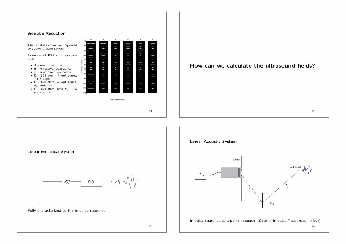
Linear Acoustic System

Impulse response at a point in space - Spatial Impulse Responses - h(~r, t)

24

Huygens’ Principle

Arrival times: t = d/c, summation of spherical waves

Moving the point results in a new impulse response:

Spatial Impulse Responses - h

25

Rayleigh’s Integral

p(~r1, t) =ρ0

2π

∫

S

∂vn(~r2, t− |~r1−~r2|c )

∂t| ~r1 − ~r2 |

d2~r2

| ~r1 − ~r2 | - Distance to field pointvn(~r2, t) - Normal velocity of transducer surface

Summation of spherical waves from each point on the aperture surface

26

Spatial impulse response:

h(~r1, t) =∫

S

δ(t− |~r1−~r2|c )

2π | ~r1 − ~r2 |dS

Emitted field:

p(~r1, t) = ρ0∂v(t)

∂t∗ h(~r1, t)

Pulse echo field:

vr(~r1, t) = vpe(t) ∗ hpe(~r1, t) = vpe(t) ∗ ht(~r1, t) ∗ hr(~r1, t)

27

Ultrasound fields

Emitted field:

p(~r1, t) = ρ0∂v(t)

∂t∗ h(~r1, t)

Pulse echo field:

vr(~r1, t) = vpe(t) ∗ fm(~r1) ∗ hpe(~r1, t)

= vpe(t) ∗ fm(~r1) ∗ ht(~r1, t) ∗ hr(~r1, t)

fm(~r1) =∆ρ(~r1)

ρ0− 2∆c(~r1)

c

Continuous wave fields:

F {p(~r1, t)} , F {vr(~r1, t)}

All fields can be derived from the spatial impulse response.

28

Point spread functions

−8 −6 −4 −2 0 2 4 6 80

1

2

3

4

x 10−6

Lateral displacement [mm]

Tim

e [

s]

Calculated response at z=60 mm with fs = 100 MHz

−8 −6 −4 −2 0 2 4 6 80

1

2

3

4

x 10−6

Lateral displacement [mm]

Tim

e [

s]

Measured response at z=60 mm

Point spread function for concave, focused transducer

Top: simulation top

Bottom: tank measurement (6 dB contour lines)

29

Discussion for next time

What are the focusing delays on an array.

Parameters: 64 element array, 5 MHz center frequency, λ pitch, all ele-

ments used in transmit

Focusing is performed directly down at the array center.

1. Imaging depth of 1 cm: How much should the center element be

delayed?

2. Imaging depth of 10 cm: How much should the center element be

delayed?

30

Learned today

• Focusing of arrays using delay-and-sum beamforming

• Point spread functions

• Calculation of fields using spatial impulse response

Next time: Ch. 2 in JAJ, pages 36-44 on array geometries and their

design

31

Signal processing in ultrasound system - Exercise 1

Transmit/receive

Beamsteering

Time-gaincompensation

Detector

Memory

Control

Imagearea

Sweepingbeam

Display

Scanconverter

Signal processing in a simple ultrasound system with a single element

ultrasound transducer.32

Signal processing

1. Acquire RF data (load from file)

2. Perform Hilbert transform to find envelope:env(n) = |y(n)2 +H{y(n)}2|

3. Compress the dynamic range to 60 dB:log env(n) = 20 log10(env(n))

4. Scale to the color map range (128 gray levels)

5. Make polar to rectangular mapping and interpolation

6. Display the image

7. Load a number of clinical images and make a movie

33

Polar to rectangular mapping and interpolation 1

Two step procedure to set-up tables and then perform the interpolation.

Table setup:

% Function for calculating the different weight tables% for the interpolation. The tables are calculated according% to the parameters in this function and are stored in% the internal C-code.%% Input parameters:%% start_depth - Depth for start of image in meters% image_size - Size of image in meters%% start_of_data - Depth for start of data in meters% delta_r - Sampling interval for data in meters% N_samples - Number of samples in one envelope line%% theta_start - Angle for first line in image% delta_theta - Angle between individual lines% N_lines - Number of acquired lines

34

%% scaling - Scaling factor from envelope to image% Nz - Size of image in pixels% Nx - Size of image in pixels%% Output: Nothing, everything is stored in the C program%% Calling: make_tables (start_depth, image_size, ...% start_of_data, delta_r, N_samples, ...% theta_start, delta_theta, N_lines, ...% scaling, Nz, Nx);%% Version 1.1, 11/9-2001, JAJ: Help text corrected

35

Geometry

x

z

angle

start_anglestart_depth

roc

Relation between the different variables

36

Polar to rectangular mapping and interpolation 2

Perform the actual interpolation:

% Function for making the interpolation of an ultrasound image.% The routine make_tables must have been called previously.%% Input parameters:%% envelope_data - The envelope detected and log-compressed data% as an integer array as 32 bits values (uint32)%% Output: img_data - The final image as 32 bits values%% Calling: img_data = make_interpolation (envelope_data);

37

Resulting image

Lateral position [mm]

Axia

l positio

n [m

m]

−60 −40 −20 0 20 40 60

0

50

100

150

Ultrasound image of portal veins in the liver.

38

Useful Matlab commands

Loading of files:

load ([’in_vivo_data/8820e_B_mode_invivo_frame_no_’,num2str(j)]

Making a movie:

for j=1:66

image(randn(20))colormap(gray(256))axis image

F(j)=getframe;end

% Play the movie 5 times at 22 fr/s

movie(F,5, 22)

39