Plants 2013, 2, 16-49; doi:10.3390/plants2010016

plantsISSN 2223-7747

www.mdpi.com/journal/plants

Review

Systems Modeling at Multiple Levels of Regulation:

Linking Systems and Genetic Networks to Spatially

Explicit Plant Populations

James L. Kitchen and Robin G. Allaby *

School of Life Sciences, University of Warwick, Coventry, CV4 7AL, UK

* Author to whom correspondence should be addressed; E-Mail: r.g.allaby@warwick.ac.uk.

Received: 1 November 2012; in revised form: 21 December 2012 / Accepted: 16 January 2013 /

Published: 25 January 2013

Abstract: Selection and adaptation of individuals to their underlying environments are

highly dynamical processes, encompassing interactions between the individual and its

seasonally changing environment, synergistic or antagonistic interactions between

individuals and interactions amongst the regulatory genes within the individual. Plants are

useful organisms to study within systems modeling because their sedentary nature simplifies

interactions between individuals and the environment, and many important plant processes

such as germination or flowering are dependent on annual cycles which can be disrupted

by climate behavior. Sedentism makes plants relevant candidates for spatially explicit

modeling that is tied in with dynamical environments. We propose that in order to fully

understand the complexities behind plant adaptation, a system that couples aspects from

systems biology with population and landscape genetics is required. A suitable system

could be represented by spatially explicit individual-based models where the virtual

individuals are located within time-variable heterogeneous environments and contain

mutable regulatory gene networks. These networks could directly interact with the

environment, and should provide a useful approach to studying plant adaptation.

Keywords: population genetics; landscape genetics; spatial individual based modeling;

simulation; gene regulatory networks; systems biology

OPEN ACCESS

Plants 2013, 2

17

1. Introduction

There is an increasing awareness of how our climate is changing due to continuing urbanization and

industrialization of our planet, and of the possible conservational, ecological and sociological implications.

With research studies demonstrating that climate change can affect crops on a genotypic [1] and a

phenotypic level [2], it is desirable to improve our understanding for plant adaptation so that it may be

exploited to produce crops more resilient to shifting climates, pests and disease, which in turn can be

grown to produce larger yields. A related field is the study of genotype-by-environment (GxE)

interaction. GxE interactions are widely studied within epidemiological studies [3–5], and are of

particular relevance to agronomy. These studies are concerned with finding significant correlations

between crop genotypes and non-genetic factors, such as climate or environments, in the interests of

increasing crop yield [6–10]. In order for such GxE interaction studies to be performed, a comprehensive

knowledge of genotypes and of polymorphic non-neutral loci is required. Single-nucleotide polymorphism

(SNP) data extracted from using amplified fragment length polymorphisms (AFLPs) are useful markers

for demonstrating such genetic differentiation and AFLPs combined with whole genome-scans [11]

have previously demonstrated adaptation at different environments such as temperature mediated

selection in trees [12]. Mega-bases of sequence data belonging to non-model organisms may now be

obtained from next-generation sequencing (NGS) technologies [13] with such studies having been

used to demonstrate population differentiation [14,15] and adaptation of individuals to different

environments [16,17]. As the environments that organisms reside in are highly dynamic due to regular

events such as seasons, night and day cycles, or due to unexpected events such as droughts or floods, it

is desirable to quantify the differential gene expression of the alleles of interest. Experimental

techniques for accurately identifying protein-DNA interactions such as chromatin-immunoprecipitation

coupled with microarrays (ChIP-chip) [18,19] or in more recent years the use of RNA-Seq [20]

combined with ChIP-Seq [21] has allowed differential expression patterns at different conditions and

the inference of gene-regulatory networks (GRNs) to be determined. Complete GRNs when used in a

predictive capacity will provide a useful tool for agronomists to improve crops [22,23]. In recent years,

there has also been an interest in merging together the different disciplines in order to assess the

differential gene expression data in segregating populations, in the form of eQTL’s [24]. However,

despite the numerous mathematical modeling studies that have developed GRNs from expression data,

and the numerous programs and tools developed for population and landscape genetics used to model

the evolution of individuals with neutral and adaptive loci, to our knowledge no studies have been

made to combine the two disciplines and develop models that contain simulated individuals with

GRNs that can adapt through a landscape. Such models would be capable of simulating a system that

contains the hierarchical levels of regulation that are intricately involved in the adaptation of

organisms to their environment. These levels include the gene, genome, individual, population and

environment, Figure 1. In such models, a gene may interact with other genes and up-regulate or

down-regulate its downstream target genes, eventually inducing a phenotype. The genome accumulates

mutations and recombines its comprising homologous chromosomes to produce new genotypic

variants, some of which may be adaptive or deleterious. The individual undergoes different life

histories, generates gametes, reproduces, and either synergistically or antagonistically interacts with

other individuals. The (sub)population collectively adapts to its local environment and may undergo

Plants 2013, 2

18

range expansions and admixture with other populations within the meta-population, sometimes

outcompeting these populations or forming hybrid zones when speciation events have occurred.

Finally, the environment contains dynamic abiotic and biotic factors that may interact with the

individuals. Abiotic factors include light or temperature that can change cyclically or unexpectedly,

directly impacting on the needs of the individuals (such as facilitating or inhibiting their dispersal for

instance), whereas biotic factors from other organisms interact with the individuals of interest. Plants

are interesting organisms to model due to their sedentary nature. For example, their dispersal is more

limited and often reliant upon environmental features in the case of anemophily and anemochory (wind

dispersal of pollen and seeds), hydrophily and hydrochory (water dispersal) or is reliant upon other

organisms in the case of entomophily and zoochory, or through cultivation by humans. Unlike animals,

they are unable to migrate away from their environments and often exhibit phenotypic plasticity as a

result. Furthermore, many plants are allopolyploids and autopolyploids with the potential for providing

more of an insight into the underlying genetics, although at a greater complexity. In this review, we

discuss previous population and landscape genetics simulation models, including simulations from our

laboratory and current methodologies to simulation GRNs. We then move onto examples where

population genetics models making use of GRNs will be beneficial within evolutionary biology.

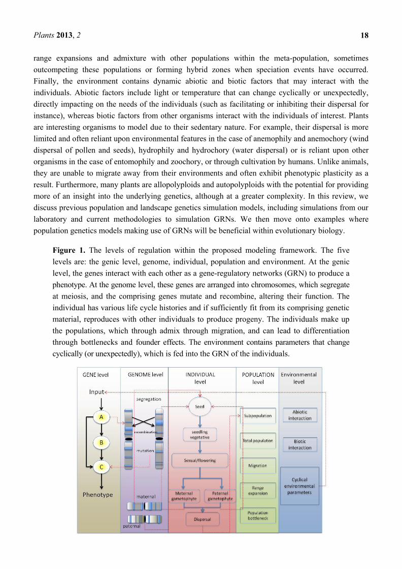
Figure 1. The levels of regulation within the proposed modeling framework. The five

levels are: the genic level, genome, individual, population and environment. At the genic

level, the genes interact with each other as a gene-regulatory networks (GRN) to produce a

phenotype. At the genome level, these genes are arranged into chromosomes, which segregate

at meiosis, and the comprising genes mutate and recombine, altering their function. The

individual has various life cycle histories and if sufficiently fit from its comprising genetic

material, reproduces with other individuals to produce progeny. The individuals make up

the populations, which through admix through migration, and can lead to differentiation

through bottlenecks and founder effects. The environment contains parameters that change

cyclically (or unexpectedly), which is fed into the GRN of the individuals.

Plants 2013, 2

19

2. Current Tools in Evolutionary Biology, Population Genetic and Landscape Genetic

Simulation Models

2.1. Fisherian Population Genetics Models

Simulation models in population genetics classically are based on a number of simplifying

assumptions, such as panmixia, non-overlapping generations and constant population sizes. These

assumptions allow the mathematics behind these principles to be described formally and allows the

simulated populations to behave in computationally tractable and deterministic ways, such as

Hardy-Weinberg equilibria (HWE) [25]. Often these assumptions are biologically reasonable: For

instance, it is not uncommon for plant species to be found exhibiting HWE [26–30], especially when

pollen dispersal may be distributed via entomophily or hydrophily and seed dispersal via zoochory.

Often in these cases, a departure from neutrality can indicate selection. Many population genetics

simulation models are based on genealogical trees with many being backwards-in-time coalescent

simulations. In coalescent simulations, sampled alleles are traced back via the simulation of

gametogenesis until the most recent-common-ancestor (MRCA) has been found [31]. A tree-based

forward-time simulation system, TreeSimJ [32], has also been developed, however. Programs such as

ms [33] and simCoal [34] are coalescent simulation programs able to simulate genealogies and infer

demography and population structure amongst a number of populations. simCoal has three mutation

models, a two-allele finite sites model for simulating RFLP data, a stepwise mutation model for

microsatellite data and several finite-sites models for simulating mutation of DNA sequence data. The

program simCoal has also been further developed to allow for diploid individuals, heterogeneous

recombination rates between adjacent loci, multiple coalescent events per generation [35] and to use

multiple time points as with ancient DNA data [36]. The program ms has been further developed to

process input recombination hotspots [37] and to use elements of a forward time simulator to model

selection at a single diploid locus [38].

2.2. Landscape Genetics

In reality, geographic landmarks such as lakes, mountains and even roads [39] can provide barriers

to gene flow sufficient enough to induce population differentiation, and biotic, climactic and edaphic

factors can induce adaptation of individuals at different geographical locations during range expansions.

Such biogeographic effects concern the developing fields of Landscape Genetics [40,41], which

broadly speaking can be described as a combination of the fields of population genetics and landscape

ecology (the field concerned with the interactions between ecological processes and the underlying

spatial contexts in which these processes reside). MS and simCoal for example are able to take into

account spatial information by the use of migration matrices between subpopulations with either the

stepping-stone or island models. Another notable program, SPLATCHE (SPatiaL And Temporal

Coalescences in Heterogeneous Environments) [42] along with SPLATCHE2 [43] has been developed

in mind to simulate the expansion of a population through an arena comprised of heterogeneous

environments. Each SPLATCHE simulation is comprised of two simulations: The first being a

forward-in-time simulation of the demographic and spatial expansion, and the second step being a

coalescent simulation based on simCoal for reconstructing the genealogies throughout the simulated

Plants 2013, 2

20

subpopulations. Here the input terrain files (input from a ―vegetation‖ and a ―roughness‖ ascii raster

file, the format used in most geographical information systems (GIS)) are used to represent geographic

regions with variable carrying capacities and friction values, a parameter used to represent the

difficulty of migration from one deme to another. SPLATCHE allows dynamic simulations such that

carrying capacities and friction values may change throughout a simulation according to an input file,

and can generate DNA, STR, RFLP and standard genetic data as an output. SPLATCHE has been used

in previous studies on range expansions [44,45]. A number of other simulation studies have included

demic information [46,47] and the use of population units within simulations lends itself conveniently

to the calculation of population-based measures of differentiation, such as Fst. Such simulations could

be described as being spatially implicit and are often biologically reasonable, as populations can be

found within discrete units. For instance Manel et al. gives fish in isolated ponds or birds nesting on

separate islands within archipelagos as examples [40]. However, many populations are found to exhibit

continuous genetic differences across space, as is the case with Arabidopsis thaliana over Eurasia and

North America [48]. When individuals are distributed across an area exhibiting a gradient of a certain

influencing environmental variable, spatial autocorrelations of the genotypes and the variable

magnitude can reveal clinal variation: This has been seen with the flowering times of Barley

latitudinally across Europe [49]. Such high-resolution genetic data may be obtained by the explicit

simulation of individuals rather than populations whose interaction is spatially constrained within a

two or a three dimensional arena. Such simulation models are termed spatially explicit individual-based

models (SIBMs).

2.3. Spatially Explicit Individual-Based Models and Their Use in Simulation Studies

Interest in forward-time individual based-models (IBMs) has arisen in the potential for increased

individual heterogeneity and stochasticity within the system. Within IBMs, the individual becomes the

fundamental modeling unit within the system, unlike mean field models, where populations are

represented as homogenous collections of individuals with identical attributes based on summary

statistics. The various states that the individual may occupy can therefore be modeled explicitly,

allowing for different life histories and other behaviors to be incorporated that may provide more

biological realism to the model. These models are generally less efficient than coalescent models, as

the coalescent will only simulate genealogies from survived offspring that have made it to the present,

and not the entire evolutionary history as with IBMs. However, the greater flexibility posed by

forward-simulation models may make them more desirable in some studies and it has been suggested

that a tradeoff between the two modeling approaches exists in terms of efficiency and flexibility [50,51].

2.3.1. Semi-Spatial Models

A number of software tools using IBMs have been developed. These include EasyPop, a population

genetics simulator to simulate neutral loci datasets under various mating schemes and migration

models [52]; IBDSim, a program for simulating isolation by distance between individuals [53];

QuantiNemo, an individual-based model for simulating quantitative traits amongst individuals within

heterogeneous ―patches‖ [54]; and SimuPop, a flexible simulator that consists of a library of python

functions that are required by the user to be ―glued together‖ within a python script, which again has

Plants 2013, 2

21

various different mating schemes and migration models at the users disposal [55,56]. GenomePop [57]

is an IBM that utilizes Markovian nucleotide or codon models of DNA mutation, such as the Jukes-Cantor

or general time reversible mutation model to generate synonymous and non-synonymous mutations.

GenomePop thus provides an IBM that can simulate more information at the nucleotide level.

GenomePop can also simulate recombination, allow constant or variable population sizes and provides

different migration models such as the Island model and the stepping stone model.

2.3.2. Spatially Explicit Models

The programs listed in [42,43,52–54] have been described as being semi-spatial [58]. However, due

to the flexibility of IBMs they can readily have a fully spatial element incorporated within them to

become spatially explicit. Broadly speaking, spatially-explicit individual-based models (SIBMs)

contain individuals that are distributed across an area, such as a lattice or matrix (although non-lattice

models have been proposed [58]) and may interact with other individuals in a spatially constrained

way rather than purely at random. A number of plant-based SIBMs simulation studies have also

emerged [59–61] in which the spatial element of these models is of particular importance, due to the

sedentary nature of plants. The spatial element is of increased importance in anemophilous crops and

trees due to their limited dispersal, which follows a ―leptokurtic‖ curve [62]. Doligez et al. [59]

compared their simulated plant populations, when permitted to form a uniform distribution throughout

their matrix, with the clumped populations that readily formed through limited dispersal. They found

that the clumped populations exhibited greater spatial genetic structure than the continuously distributed

populations, particularly when selfing was allowed. Kitchen and Allaby [60] developed a plant-based

SIBM to study the effects of spatial extension between individuals upon the heterozygosity of the plant

populations when compared to mean-field HWE expectations. They showed that when plant-mating

systems approximated mean-field assumptions (i.e., the density was such that the individuals were

approximately randomly mating) the observed and expected heterozygosities were largely equivalent.

However, the heterozygosity of individuals decreased from mean-field expectations as sparseness

amongst individuals increased. AMELIE [61] is a SIBM with a rather more direct application towards

food-security and GM crops, and was used to study the amount of introgression from GM forests to

conventional forests. It can also allow various life histories and mating systems and can provide

demographic and environmental stochasticity. These simulations, however, are only simulating neutral

markers and do not attempt to model selection. It is relatively straightforward to take an IBM or SIBM

framework and then hard-code a specific adaptive trait, such as one that may influence selection

through the perturbation of mortality, or reproductive rate, at a di-allelic or perhaps even a multi-allelic

locus if necessary. However, the goal is to be able to account for a possible continuum in the range of

landscape heterogeneity and on the strength of the selection inferred from the landscape. One emergent

approach is to utilize the concept of resistance surfaces [63,64] and modify the surface in such a way

as to produce a ―fitness landscape‖.

2.4. Resistance Surfaces

Resistance surfaces are essentially matrices that contain variables relating to different

environmental or landscape features that may impede or facilitate connectivity between individuals in

Plants 2013, 2

22

the form of migration or gene flow. They can be parameterized through field data as obtained from

GIS systems and are useful for providing hypotheses on the nature of how spatial genetic structure

through migration, introgression and dispersal may have formed. One notable SIBM that utilizes

resistance surfaces is CD-POP (Cost Distance POPulations) that contains cost distance matrices for

representing resistance to movement through the landscape [65]. The program uses gradients of

cumulative cost to impede dispersal between grid cells and can facilitate reproduction according to

four different functions: linear, inverse square, nearest neighbor and random mixing. The initial

version of CD-POP could be used only with neutral loci. However, this was improved upon in an

important follow-up paper where CD-POP made use of a fitness landscape in order to simulate

selection [66]. CD-POP was upgraded to include a di-allelic single or multi-locus system with any

number of neutral loci and up to two unlinked, di-allelic, selective loci (with alleles A, a, B, and b).

Selection is then implemented according to the grid value where generated offspring reside and the

genotypes of the selective loci that they contain. This represents an important step towards providing a

general model for simulating selection. More recently, another study utilizing CD-POP’s selection

model has been used in a study to assess the role of adaptive and neutral markers towards population

differentiation [67]. Another open-source software tool that uses resistance surfaces is Circuitscape,

which is based upon resistance paths that are analogous to those within an electrical circuit [68]. It may

be used to predict dispersal of animals or plants and patterns of genetic differentiation among in

heterogeneous landscapes [69].

These efforts in landscape genetics simulations represent the first stages into relating genotype to

environment and the resulting effects on selection and adaptation. As with CD-POP, different

genotypes of unlinked loci may produce different effects on fitness of an individual according to the

spatial grid point on which it is located. However, in reality genes do not exist in isolation but exist in

networks, and through cis-acting and trans-acting regulatory effects can up-regulate or de-regulate

each other, ultimately affecting the expressed phenotype in a dynamic way. It has therefore been

suggested that in the interest of genotype to phenotype mapping, genes should be considered in the

context of networks [70]. We discuss genes within networks in the next section.

3. GRNs, Network Motifs and Inference

Efforts to ascertain all the interacting genes with regards to the expression of a particular phenotype

is an area of which is highly relevant to most, if not all, disciplines within biology. Such information,

for instance, could provide biologists with potential molecular targets, be they genes, proteins or

metabolites, whose function may be altered through gene silencing, catabolism, or through agonistic or

antagonistic ligands. The identification of GRNs has multiple uses ranging from developing drug

targets in complex disease, understanding stress response (with clear uses in developing drug targets

and in agronomy), decreasing antibiotic, herbicide or pesticide resistance and identifying key

developmental genes. One application of a GRN can be to model transcriptional networks within a

cell, although interactions at the proteomic and metabolomic level and other areas of the ―interactome‖

may also be modeled. Transcription factors (TFs) may behave as transcriptional activators that

up-regulate other TFs or behave as transcriptional repressors that can down-regulate their targets. The

crosstalk between the up- and down-regulation of transcription allows dynamicity to the amount of

Plants 2013, 2

23

protein product that is expressed, which ultimately, will have an effect on the phenotype of the

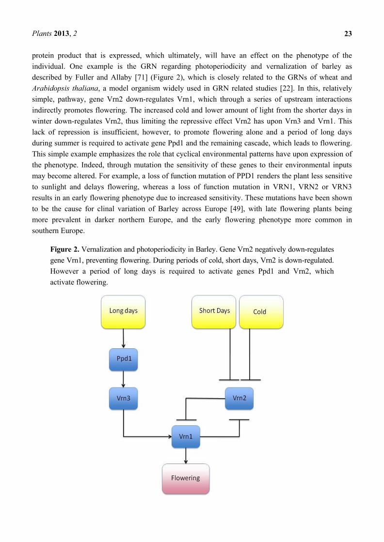
individual. One example is the GRN regarding photoperiodicity and vernalization of barley as

described by Fuller and Allaby [71] (Figure 2), which is closely related to the GRNs of wheat and

Arabidopsis thaliana, a model organism widely used in GRN related studies [22]. In this, relatively

simple, pathway, gene Vrn2 down-regulates Vrn1, which through a series of upstream interactions

indirectly promotes flowering. The increased cold and lower amount of light from the shorter days in

winter down-regulates Vrn2, thus limiting the repressive effect Vrn2 has upon Vrn3 and Vrn1. This

lack of repression is insufficient, however, to promote flowering alone and a period of long days

during summer is required to activate gene Ppd1 and the remaining cascade, which leads to flowering.

This simple example emphasizes the role that cyclical environmental patterns have upon expression of

the phenotype. Indeed, through mutation the sensitivity of these genes to their environmental inputs

may become altered. For example, a loss of function mutation of PPD1 renders the plant less sensitive

to sunlight and delays flowering, whereas a loss of function mutation in VRN1, VRN2 or VRN3

results in an early flowering phenotype due to increased sensitivity. These mutations have been shown

to be the cause for clinal variation of Barley across Europe [49], with late flowering plants being

more prevalent in darker northern Europe, and the early flowering phenotype more common in

southern Europe.

Figure 2. Vernalization and photoperiodicity in Barley. Gene Vrn2 negatively down-regulates

gene Vrn1, preventing flowering. During periods of cold, short days, Vrn2 is down-regulated.

However a period of long days is required to activate genes Ppd1 and Vrn2, which

activate flowering.

Plants 2013, 2

24

3.1. The GRN Topologies Observed in Nature

The genes within a network may be visualized as directed graphs containing a set of nodes,

representing the genes, protein and/or metabolites, connected by a set of edges, which represent the

interactions between these nodes. The number of edges that belongs to a node is its degree, and the

distribution of the number of edges across networks is the degree distribution. Intuitively it may be

assumed that the degree distribution would approximate a Poisson distribution, however, conversely

they tend to approximate a power-law distribution, where most nodes are sparsely connected and a

small number has a much larger degree [72,73]. When auto-regulation of genes is not permitted, the

maximum number of edges within a network of size N must necessarily be N(N-1) edges, however,

many genes do regulate themselves as in single-gene positive or negative feedback loops. Expression

data obtained from technologies such as Yeast 2-Hybrid, ChIP-chip or ChIP-Seq can provide

relationships such as correlative relationships between sets of expression data. The resultant expression

data can be processed by software and mathematical models can be inferred (reviewed in [74,75]). An

interesting paradigm emergent from this data is the existence of common network topologies that are

observed across different taxa and even different types of networks (i.e., non-GRNs). This paradigm

was first observed by Milo et al. [76,77] who generated null distributions of network sub-graphs

through randomizing the edges of networks with the same degrees, and selected motifs that were found

to be in numbers significantly higher than at random [76]. A follow up study used z-scores to calculate

a significance profile for comparison of network local structure when compared with random

structures [77]. Both studies found commonly occurring motifs not only within transcriptional

networks, but also within protein-signaling networks, neuronal networks and non-biological networks,

such as those found in social networks, power-grids and within the World Wide Web. These methods

did receive some criticism, however. For example, it was stated that C. elegans neuronal pathways are

spatially dependent with networks being formed between spatially closer nodes and that these spatial

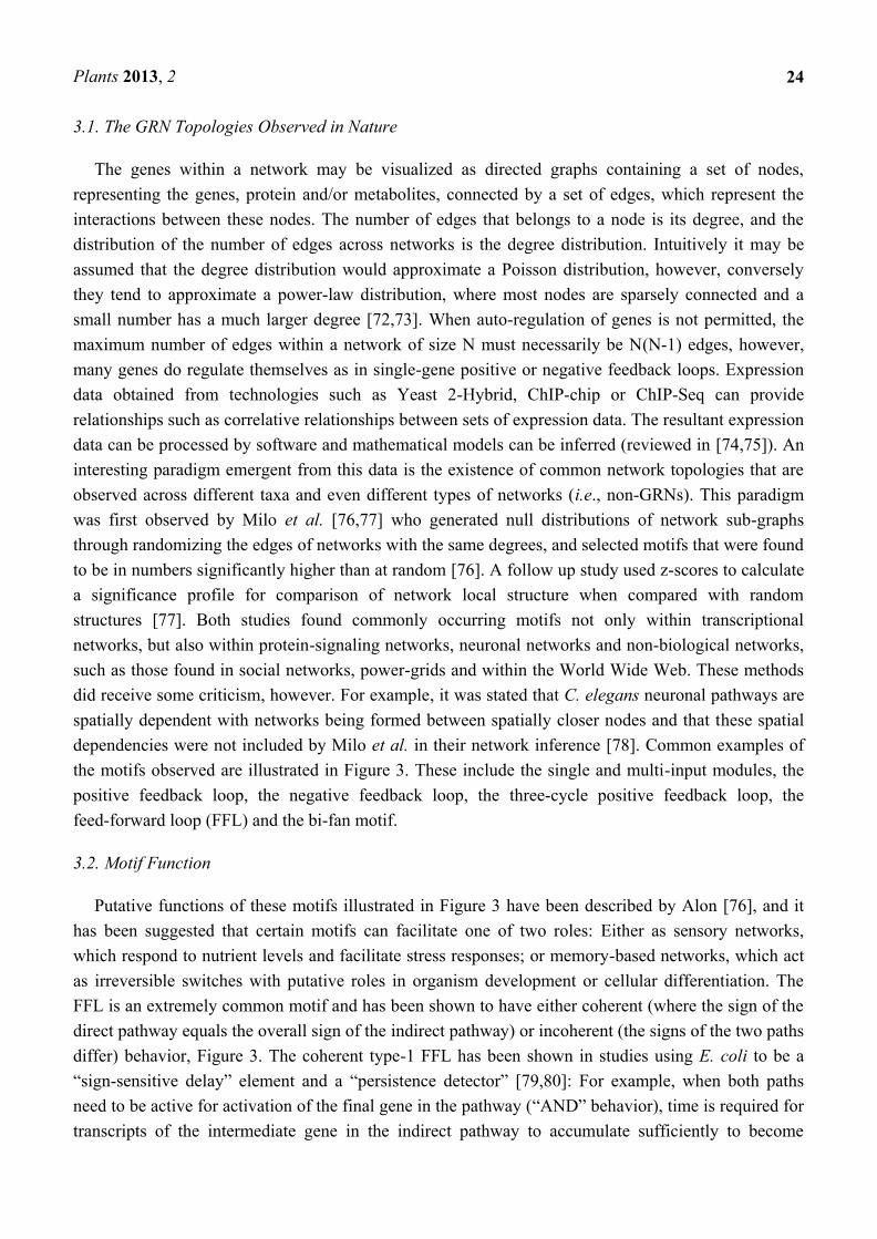
dependencies were not included by Milo et al. in their network inference [78]. Common examples of

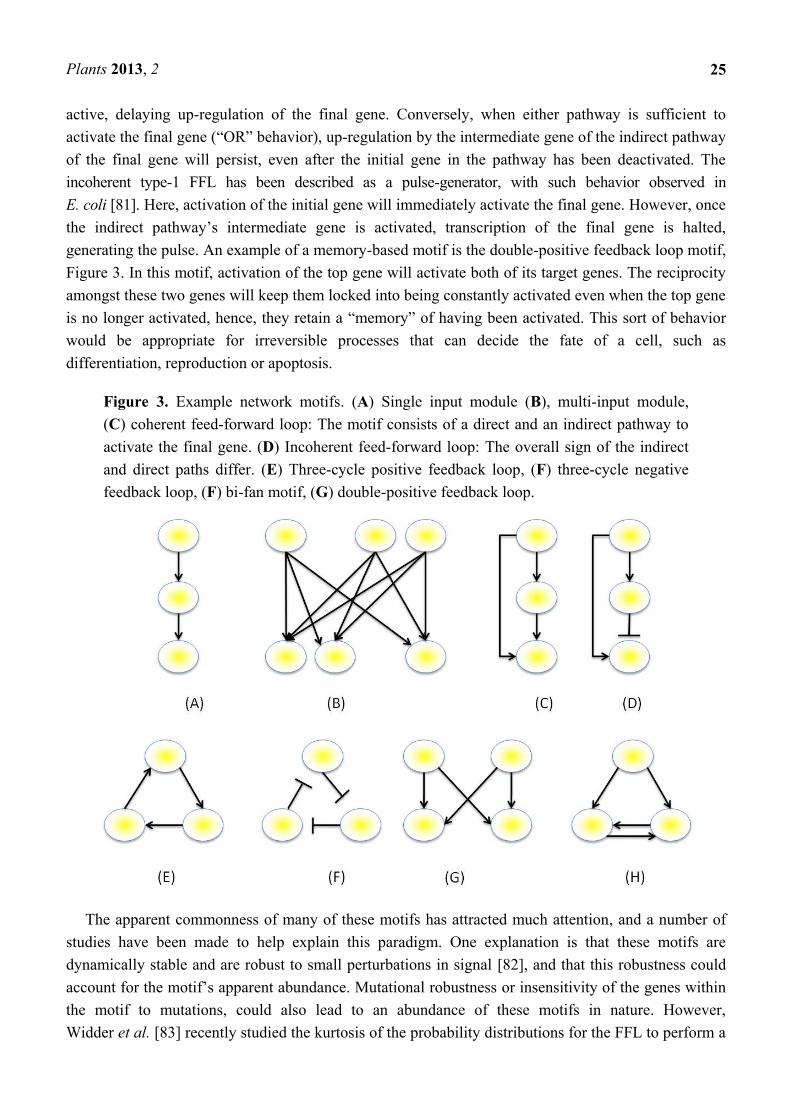
the motifs observed are illustrated in Figure 3. These include the single and multi-input modules, the

positive feedback loop, the negative feedback loop, the three-cycle positive feedback loop, the

feed-forward loop (FFL) and the bi-fan motif.

3.2. Motif Function

Putative functions of these motifs illustrated in Figure 3 have been described by Alon [76], and it

has been suggested that certain motifs can facilitate one of two roles: Either as sensory networks,

which respond to nutrient levels and facilitate stress responses; or memory-based networks, which act

as irreversible switches with putative roles in organism development or cellular differentiation. The

FFL is an extremely common motif and has been shown to have either coherent (where the sign of the

direct pathway equals the overall sign of the indirect pathway) or incoherent (the signs of the two paths

differ) behavior, Figure 3. The coherent type-1 FFL has been shown in studies using E. coli to be a

―sign-sensitive delay‖ element and a ―persistence detector‖ [79,80]: For example, when both paths

need to be active for activation of the final gene in the pathway (―AND‖ behavior), time is required for

transcripts of the intermediate gene in the indirect pathway to accumulate sufficiently to become

Plants 2013, 2

25

active, delaying up-regulation of the final gene. Conversely, when either pathway is sufficient to

activate the final gene (―OR‖ behavior), up-regulation by the intermediate gene of the indirect pathway

of the final gene will persist, even after the initial gene in the pathway has been deactivated. The

incoherent type-1 FFL has been described as a pulse-generator, with such behavior observed in

E. coli [81]. Here, activation of the initial gene will immediately activate the final gene. However, once

the indirect pathway’s intermediate gene is activated, transcription of the final gene is halted,

generating the pulse. An example of a memory-based motif is the double-positive feedback loop motif,

Figure 3. In this motif, activation of the top gene will activate both of its target genes. The reciprocity

amongst these two genes will keep them locked into being constantly activated even when the top gene

is no longer activated, hence, they retain a ―memory‖ of having been activated. This sort of behavior

would be appropriate for irreversible processes that can decide the fate of a cell, such as

differentiation, reproduction or apoptosis.

Figure 3. Example network motifs. (A) Single input module (B), multi-input module,

(C) coherent feed-forward loop: The motif consists of a direct and an indirect pathway to

activate the final gene. (D) Incoherent feed-forward loop: The overall sign of the indirect

and direct paths differ. (E) Three-cycle positive feedback loop, (F) three-cycle negative

feedback loop, (F) bi-fan motif, (G) double-positive feedback loop.

The apparent commonness of many of these motifs has attracted much attention, and a number of

studies have been made to help explain this paradigm. One explanation is that these motifs are

dynamically stable and are robust to small perturbations in signal [82], and that this robustness could

account for the motif’s apparent abundance. Mutational robustness or insensitivity of the genes within

the motif to mutations, could also lead to an abundance of these motifs in nature. However,

Widder et al. [83] recently studied the kurtosis of the probability distributions for the FFL to perform a

Plants 2013, 2

26

range of different functions and computationally studied the effects of repeated mutations to the

functional robustness of the motifs. Their results suggested that the abundance is more influenced by

the plasticity of the FFL in performing a wide-range of functions and that mutational insensitivity was

unlikely to account for the abundance. A wide range in function of the Bi-fan motif has also been

reported [84], with a caution from the authors of the study that the particular structure of a motif

should not necessarily be expected to guarantee a particular function. Furthermore, a study by

Konagurthu and Lesk [85] reported that through their implementation of a random-edge search

algorithm, the frequencies of common motifs within natural networks was similar to those within

random networks. They also noted that random connectivity within a three-node network, such as the

FFL loop or a three-member positive feedback loop (3-cyc) would naturally form an FFL due to the

search space involved (with 23 possible conformations, six will be consistent with FFL architecture,

and two with the 3-cyc) and that the search space may account more for the abundance than

the function.

3.3. Mathematical Modeling of GRNs

Developing GRNs from experimental data is often described as reverse engineering, or network

inference, and comprises a particularly large field within the discipline of systems biology. Although

major advances in experimental techniques and advances in modern computing power have no doubt

assisted efforts in network inference, it still remains a non-trivial task. Ultimately the quality of an

inferred network model is highly dependent upon the quality of the data, and this can come at a

considerable cost with large networks, as the amount of required data is proportional to the number of

network nodes. Perturbation experiments such as generating gene knock-outs, stress experiments or

RNAi experiments can provide an informative insight into the dynamicity of a particular network.

However, the large amount of noise within expression data often requires that experiments be repeated

in order to determine the extent of the noise. Constraints on the GRN can be placed to alleviate the

model’s complexity and data requirements, however. These include limits on the number of nodes in

the inferred network (thereby generating a sparser network) and restricting the model parameters, e.g.,

through connectivity limitations. It is also often desirable when inferring a network to make use of

prior biological knowledge (such as molecule binding sequence motifs, posttranslational modification

sites or molecular interactions), which may assist with model validation or with constraining the model

complexity. A number of online repositories of such information are available such as the Gene

Ontology (GO) or the Kyoto encyclopedia of genes and genomes (KEGG).

3.3.1. Boolean Networks

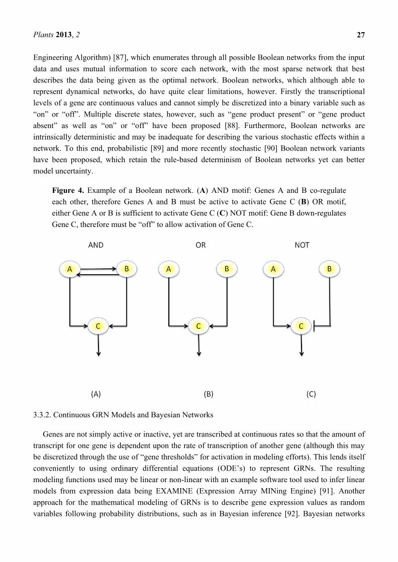
The activation of some genes within a network may hold certain dependencies with the activities of

other genes, such as the ―AND‖ and ―OR‖ behavior described previously. Thus, it is possible to

represent genes in a similar manner to logic gates, where a gene may belong to one of two discrete

states, namely ―ON‖ or ―OFF‖ and hold a set of discrete dependencies in terms of activation with other

genes in the network, such as ―AND‖, ―OR‖ and ―NOT‖ relationships, Figure 4. Boolean

representations of genes were first described by Kauffman [86] and are widely used today. An example

piece of software for inference of Boolean network from experimental data is REVEAL (REVerse

Plants 2013, 2

27

Engineering Algorithm) [87], which enumerates through all possible Boolean networks from the input

data and uses mutual information to score each network, with the most sparse network that best

describes the data being given as the optimal network. Boolean networks, which although able to

represent dynamical networks, do have quite clear limitations, however. Firstly the transcriptional

levels of a gene are continuous values and cannot simply be discretized into a binary variable such as

―on‖ or ―off‖. Multiple discrete states, however, such as ―gene product present‖ or ―gene product

absent‖ as well as ―on‖ or ―off‖ have been proposed [88]. Furthermore, Boolean networks are

intrinsically deterministic and may be inadequate for describing the various stochastic effects within a

network. To this end, probabilistic [89] and more recently stochastic [90] Boolean network variants

have been proposed, which retain the rule-based determinism of Boolean networks yet can better

model uncertainty.

Figure 4. Example of a Boolean network. (A) AND motif: Genes A and B co-regulate

each other, therefore Genes A and B must be active to activate Gene C (B) OR motif,

either Gene A or B is sufficient to activate Gene C (C) NOT motif: Gene B down-regulates

Gene C, therefore must be ―off‖ to allow activation of Gene C.

3.3.2. Continuous GRN Models and Bayesian Networks

Genes are not simply active or inactive, yet are transcribed at continuous rates so that the amount of

transcript for one gene is dependent upon the rate of transcription of another gene (although this may

be discretized through the use of ―gene thresholds‖ for activation in modeling efforts). This lends itself

conveniently to using ordinary differential equations (ODE’s) to represent GRNs. The resulting

modeling functions used may be linear or non-linear with an example software tool used to infer linear

models from expression data being EXAMINE (Expression Array MINing Engine) [91]. Another

approach for the mathematical modeling of GRNs is to describe gene expression values as random

variables following probability distributions, such as in Bayesian inference [92]. Bayesian networks

Plants 2013, 2

28

form a directed-acyclic graph (DAG) and may represent dynamic or static (i.e., representing a GRN

once a steady-state has been reached) networks using continuous or discrete data, and are readily able

to model the randomness and stochastic effects that may exist amongst GRNs. This makes them more

robust in the presence of noise or missing data than Boolean networks. Another benefit of Bayesian

networks is that they provide a framework that allows researchers to incorporate prior knowledge for

network inference. However, caution should be made when little or no information is available, as the

use of uninformative priors (e.g., uniform priors) can make Bayesian network inference inefficient. As

Bayesian networks are formed with a DAG, static networks cannot represent cycles such as in

feedback loops. However, this limitation is not present with dynamic Bayesian networks [93], as they

avoid cyclical representations by using discrete time steps to separate input nodes (e.g., at time t) from

output nodes (e.g., at time t + ∆t). BANJO (BAyesian Networks with Java Objects) is a software tool

that has been developed for the inference of static and dynamic Bayesian networks [94].

4. Synthesis: Spatial Individual-Based Models with Gene Networks: Approaches, Applications to

Plant Science and Potential Pitfalls

Within this review we have discussed theory within the fields of population and landscape genetics

and systems biology, and have described software and approaches to simulating adaptation. We

believe that modeling efforts within evolutionary biology have reached a suitable step where coupling

systems of genes to SIBMs that can interact with the surrounding environment and induce phenotype

in a more complex and perhaps more biologically reasonable way, can now be considered. Ultimately,

a unified approach based upon stochastic elements of GRN evolution, migration and range expansion

could allow emergent paradigms in how phenotype relates to GRN topology and raise questions as to

how this relates to different abiotic and biotic interactions at different spatial locations. Thus, such

systems could direct research into a number of previously unanswered questions in evolutionary

biology and evolutionary systems biology, including:

1. How does a functional (non-neutral) mutation to the sensitivity (as in threshold) or output of a

GRN node affect the expressed phenotype or the fitness of an individual? How do the

phenotypic effects differ from simulating single non-interacting loci?

2. How do perturbations of the edges within a network (such as edge deletion, addition and

rewiring) or node duplications impact on the fitness of an individual within different

environments?

3. How does the conformation of a GRN affect the quantitative trait that is ultimately expressed?

Can population models or SIBMs show that certain motifs may be selected for within different

environments?

4. What role do evolutionary forces such as gene flow and range expansion play on the diversity

of GRN topologies?

5. Considering the effects of gene flow, can certain environments (i.e., abiotic factors) favor

specific GRN topologies? Similarly, can biotic interaction select for certain GRN topologies?

6. Which choice of GRN representations (such as static-edge, Boolean, Bayesian, ODE-based

networks) is a better fit to the system in question?

Plants 2013, 2

29

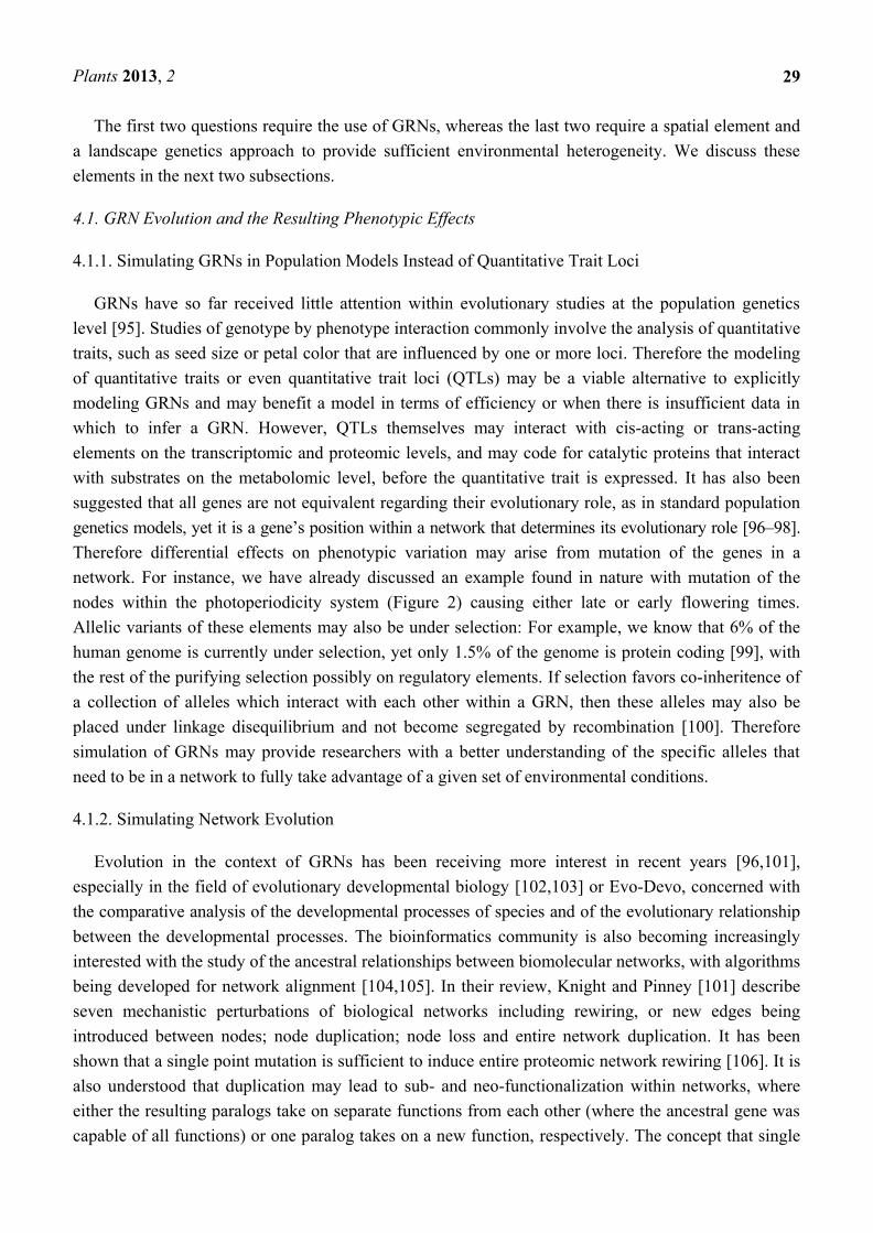
The first two questions require the use of GRNs, whereas the last two require a spatial element and

a landscape genetics approach to provide sufficient environmental heterogeneity. We discuss these

elements in the next two subsections.

4.1. GRN Evolution and the Resulting Phenotypic Effects

4.1.1. Simulating GRNs in Population Models Instead of Quantitative Trait Loci

GRNs have so far received little attention within evolutionary studies at the population genetics

level [95]. Studies of genotype by phenotype interaction commonly involve the analysis of quantitative

traits, such as seed size or petal color that are influenced by one or more loci. Therefore the modeling

of quantitative traits or even quantitative trait loci (QTLs) may be a viable alternative to explicitly

modeling GRNs and may benefit a model in terms of efficiency or when there is insufficient data in

which to infer a GRN. However, QTLs themselves may interact with cis-acting or trans-acting

elements on the transcriptomic and proteomic levels, and may code for catalytic proteins that interact

with substrates on the metabolomic level, before the quantitative trait is expressed. It has also been

suggested that all genes are not equivalent regarding their evolutionary role, as in standard population

genetics models, yet it is a gene’s position within a network that determines its evolutionary role [96–98].

Therefore differential effects on phenotypic variation may arise from mutation of the genes in a

network. For instance, we have already discussed an example found in nature with mutation of the

nodes within the photoperiodicity system (Figure 2) causing either late or early flowering times.

Allelic variants of these elements may also be under selection: For example, we know that 6% of the

human genome is currently under selection, yet only 1.5% of the genome is protein coding [99], with

the rest of the purifying selection possibly on regulatory elements. If selection favors co-inheritence of

a collection of alleles which interact with each other within a GRN, then these alleles may also be

placed under linkage disequilibrium and not become segregated by recombination [100]. Therefore

simulation of GRNs may provide researchers with a better understanding of the specific alleles that

need to be in a network to fully take advantage of a given set of environmental conditions.

4.1.2. Simulating Network Evolution

Evolution in the context of GRNs has been receiving more interest in recent years [96,101],

especially in the field of evolutionary developmental biology [102,103] or Evo-Devo, concerned with

the comparative analysis of the developmental processes of species and of the evolutionary relationship

between the developmental processes. The bioinformatics community is also becoming increasingly

interested with the study of the ancestral relationships between biomolecular networks, with algorithms

being developed for network alignment [104,105]. In their review, Knight and Pinney [101] describe

seven mechanistic perturbations of biological networks including rewiring, or new edges being

introduced between nodes; node duplication; node loss and entire network duplication. It has been

shown that a single point mutation is sufficient to induce entire proteomic network rewiring [106]. It is

also understood that duplication may lead to sub- and neo-functionalization within networks, where

either the resulting paralogs take on separate functions from each other (where the ancestral gene was

capable of all functions) or one paralog takes on a new function, respectively. The concept that single

Plants 2013, 2

30

gene and whole genome duplication could lead to evolutionary diversification has existed for

decades [107] and is still commonly under study [108,109]. We have already discussed the widely

documented examples of network motifs found within biological motifs, their potential roles and how

their structure may relate to function, if at all. Whether the structure of a motif necessarily relates to

function may currently be a topic of debate, however, it is conceivable that selection for a particular

phenotype may require a specific structural motif, and this has been suggested for the positive

feedback loop [110]. There have also been a number of studies of how motif structure may influence

stochastic fluctuations, or noise, from a network motif, and it has been suggested that noise itself can

be placed under selection [111]. Noise may control organism stress-responses such as persistence in

bacteria, where the cell may enter a state of dormancy in harsh environmental conditions at the cost of

cellular growth rate. Through mathematical modeling of the HipBA toxin-antitoxin system in E. coli [112]

Koh and Dunlop showed that by altering the architecture of the network (through removing feedback

and placing the two genes on separate operons), they were able to alter the frequency of persistence, a

trait that could be selected for in different environmental conditions [113]. Interestingly, a study from

Tsong et al. [114] demonstrated that for the two species S. cerevisiae and C. albicans, a particular

network shared by the two species had been reversed in structure (one regulated by a repressor, the

other by an activator). The ―logical output‖ or phenotype, however, remained the same due to several

changes in cis- and trans-regulatory elements. Therefore network evolution may converge to the same

outcome as well as diverge.

4.1.3. Choice of GRN Model within the Context of a Spatially Explicit Individual-Based Model

The GRN reverse engineering approaches described in Section 3.2 can be conceptualized as ―top-down‖

processes, where we begin with a phenotype of an individual (i.e., after subjected to stress or after a

gene knock-out procedure), observe the expression patterns, and infer a genetic model from the data

using statistical and mathematical approaches. However, the inferred networks and the modeling

paradigm used to describe it (such as Boolean or continuous GRNs) could readily be used in a

―bottom-up‖ approach to demonstrate the range in expression and/or the resulting phenotype once

subjected to different environmental inputs. We therefore believe that SIBMs parameterized with

resistance surfaces or landscape patches provide an excellent framework for producing such models.

The GRN could be represented using a Boolean network form or as a continuous form, using linear or

non-linear ODEs, that would take its input from the surrounding environment, interact with the other

nodes in the network and produce a phenotype. Gene threshold parameters could be used to define the

criteria needed for activation, and genes at the top of the network could directly interact with the

environment. Whereas Boolean or ODE-based GRNs would classically represent deterministic

networks, the output on each gene could instead be a random variable generated from a certain

probability distribution, providing a network that may more approximate Bayesian networks. A

potentially interesting study could be: If given genetic network data within a real environmental

system (such as the distribution of flowering times latitudinally across Europe), which GRN model

best explains the data and provides the maximum likelihood?

Plants 2013, 2

31

4.2. Benefit through Using a Spatially-Explicit System

In this review we propose that research should be directed towards looking at the phenotypic effects

of network evolution in the context of populations located within patchy landscapes. The addition of

spatially explicit heterogeneous landscapes will add another layer of complexity to any model, and

adding any intra-annual variation in environmental parameters will increase this complexity. Although

it is not the goal of modeling to accurately represent nature in all of its complexity, we argue that such

extra detail is necessary in order to fully understand how phenotypic variation (through mutation of

GRNs) may emerge and become selected for or against. Firstly we need to adequately model gene

flow, which provides the homogenizing force between subpopulations that would otherwise ultimately

differentiate through a process of mutation and genetic drift. Although the flow of chromosomes

containing genes that may interact with one-another in a GRN may be modeled within a mean-field

system, gene flow itself is often spatially constrained and may be influenced through geographic

landmarks, such as mountains, rivers or roads. Impeding gene flow can lead to increased population

differentiation, which can lead towards speciation. The explicit modeling of space is a convenient way

to allow the simulation of range expansions and the subsequent limiting effects on allelic diversity

through the subsequent founder effects. Incorporating heterogeneous environments into the spatially

explicit arena will also allow abiotic interaction to select for different alleles, and possibly select for

different GRN conformations. For example, the GRN conformations for Barley, wheat and Arabidopsis

have shown to be quite different, despite sharing many of the same components [71,115]. A

particularly fundamental question to be addressed in evolutionary systems biology is why do certain

GRN conformations exist in different environments and why are they favored in some way? One

possible way to answer such a question could be to keep GRN topologies constant and randomize

environmental parameters according to a given prior distributions, as in a Bayesian analysis.

4.2.1. Biotic Interaction

We have described how the resistance surfaces that may be explicitly incorporated into an SIBM

may represent climactic or edaphic factors that can impede dispersal or influence selection of the

simulated individuals. However, in a similar vein, they may also represent biotic interactions from

animals or plants. Biodiversity varies latitudinally across the globe [116], and biotic interaction is

thought to be of particular importance in the tropics [117]. One example of biotic interaction is seed

predation, and this has famously been proposed in what is collectively termed the Janzen-Connel

hypothesis [118,119] to prevent competitive exclusion. Seed predation can be represented in

simulations as probabilities of predation for dispersed seeds, either throughout the entirety of the

simulation or at individual grid-points, for example. It may be difficult in this approach, however, to

simulate the dynamics of predator-prey co-evolution, unless some form of dependency was

incorporated between the modeled individuals and the resistance surfaces. Another approach is to have

multiple classes of individuals within a simulation that could represent ―species‖. Individuals

belonging to different species could then be modeled with different GRNs, as has been seen in nature

with the barley, wheat and the Arabadopsis photoperidocity network. Individuals may then compete

for space (in order to germinate). If the model is specific and growth and nutrient uptake are explicitly

Plants 2013, 2

32

modeled (see Section 4.6.2 on functional-structural plant modeling), then different species could

potentially compete for resources.

4.2.2. Analyzing Past and Future Events on Adaptation

GRNs are dynamic, and therewith comes the necessity of incorporating time-dependent

environmental variation when GRNs are simulated within the context of SIBMs. A natural extension

of this is that it will become convenient to study past shifts in the environment onto the genotypic and

phenotypic characteristics of a population (such as through the effects of bottlenecks and migration, for

example). Hypothesized future effects could also be studied in a similar manner.

4.3. Producing Complex Modeling Systems in a Step-Wise Manner

Complicated models with multiple levels of regulation could be developed within a step-wise

manner, yet there is no one correct path a researcher may take. The model should be validated as each

level of regulation (Figure 1) is added. Deterministic systems based on mean-field assumptions such as

Hardy-Weinberg equilibria may provide a means of model validation. Complex models may require

time-consuming simulations, and if there is much stochasticity in the system, it could become difficult

to interpret their results. Therefore a suitable strategy might be to start with simple models, such as

mean-field models and/or single population models. For example, the initial stage of a modeling study

could be to begin with a population of limited spatial structure, single genes or QTLs and only neutral

non-selective abiotic parameters, where the only source of genetic variation is through mutation and

genetic drift. After validation, extra elements could be added including a more heterogenous

environment and a rudimentary GRN, and so on. If a modeling system is designed in order to be

modular, as in to allow certain features to be enabled or disabled in the model, it may be convenient to

begin with simple systems and prevent the need to develop new models for each step of the study.

The relevant question here is at which level of regulation the modeler begins, which will be highly

influenced by the hypothesis that the researcher intends to address. One possible hypothesis could be

that certain environmental parameters would select for a particular GRN variant, for example, and so a

study might involve analyzing the effects of GRN conformation on individual fitness. GRN

conformation could indicate the shape of its degree distribution, or could simply mean choice of

structural motif, for example. In the first study, simulations could provide data on fitness (in the form

of population growth curves, for example) for different GRN configurations that are kept constant

(i.e., no mutation or rewiring) throughout the simulation. In a subsequent step GRN reconfiguration

could be enabled and the final configuration recorded, to determine whether GRNs have evolved into

an ―optimal‖ configuration. Final simulations could involve allowing populations containing evolving

GRNs expanding throughout a heterogeneous landscape, and spatial genetic structure could be analyzed.

Another study might be to attempt to explain the spatial genetic structure of a population found in

nature, for which GRN data exists, through attempting to recreate data observed in nature (such as

allele frequencies or selection coefficients). Initial simulations could be within mean-field systems,

with non-stochastic migration rates between subpopulations and only single gene nodes or QTLs being

simulated. Subsequent simulations could add spatial explicitness, abiotic and biotic factors and GRNs.

At each step of the study, likelihood densities could be generated to explain which models best explain

Plants 2013, 2

33

the observed data. Our research group has previously applied Approximate Bayesian Computation

(ABC) [120] to our SIBM in our research (currently unpublished). ABC can be a powerful numerical

technique within population genetics. It allows for likelihood densities to be generated from parameter

subsets that can simulate summary statistic data that is sufficiently close to data observed in reality. It

has been widely used within a number of population genetics studies thus far (for example, see [121,122]).

4.4. Adaptive Dynamics

When simulating selection in models it is important to consider the role of evolutionary tradeoffs

and how they may influence the adaptation of a species. Antagonistic pleiotropic effects [123–125] as

first proposed by Williams [123] occur when a mutation with a beneficial change in fitness on one trait

has a detrimental effect upon another trait. This can lead to the emergence of evolutionary fitness

costs [126–133] where increased resource allocation from one function leaves more limited allocation

to another function. One plant example of a trade-offs in the literature is increased transposable

element silencing despite deleterious effects on the expression of nearby genes [129] in Arabidopsis

thaliana. Another study showed that increased investment in female and male reproductive structures

limited the quantity and nitrogen content of clonal propagules, respectively, in Sagittaria latifolia [126].

A further example exists in Arabidopsis thaliana where a mutation in the EMBRYONIC FLOWER

(EMF) genes EMF1 and EMF2 induces very early flowering but also a reduction in seed production [134].

Thus evolutionarily ―perfect‖ organisms are not trivial to obtain. Trade-offs may also exist according

to the ecological characteristics within the geographical area that a population resides within. To give

an example: Selection for increased plant size may increase the rate of depletion of the nutrient

resource within the soil, thus, adaptation of the plant population to its surrounding environment in turn

influences the environment. In order to help study such dynamic genotype by environment interactions,

the 1990s saw the emergence of the field of adaptive dynamics (AD, reviewed in [135,136]), which,

through mathematical modeling allowed the researcher to gain an insight into the long-term dynamics

of the evolutionary and the ecological processes within a given system. AD has developed from

evolutionary game theory and the study of evolutionary stable strategies, which may describe the

payoffs associated with a mutant, m, of strategy A invading a resident population, r, with strategy B. It

makes four assumptions: clonal reproduction, separation of ecological time scales, small mutational

steps and a small initial invading mutant frequency within the monomorphic population r. The

invasion fitness is given as the exponential growth rate of a m within r. Positive values of f indicate

that m will successfully invade and replace r, and negative values indicate that the mutant will be

unsuccessful in invading the resident. Using the invasion fitness function, f, pairwise invasion plots

(PIPs) may be plotted. PIPs are two-dimensional plots where the zero contour line is plotted at the

various quantitative values of the m and r phenotype, allowing potential regions of invasion success

and failure to graphically be identified. Intersection of the isocline at the 45-degree line from the origin

(where m = r) allows identification of possible evolutionary end points at certain values of the resident

phenotype. Using the AD framework, Geritz et al. [137] produced a model to study the evolutionary

dynamics of seed size, which contained a trade-off between seed size and seed number. They were

able to adjust the influence of the seed size on the competitive ability of their seeds (which they called

competitive asymmetry), the resources per germination site and the type of precompetitive

Plants 2013, 2

34

environment in which their seeds resided (a continuum from favorable to unfavorable). They found

that strong competitive asymmetry, high resource levels, and intermediate harshness of the precompetitive

environment favored a polymorphic population containing the coexistence of plants with different seed

sizes, where although a single large seed may outcompete a single small seed, the higher numbers of

smaller seeds was also competitive. Boudsocq et al. [138] presented an AD study that investigated the

trade-off between plant size (due to increased nutrient uptake), where larger plants are fitter, and

increased plant mortality with greater nutrient uptake. The authors set out to determine whether natural

selection could lead to ―evolutionary suicide‖ or Harman’s ―tragedy of the commons‖ where resources

become too depleted to allow plant survival, or whether Tilman’s R* rule, where the plant with the

lowest steady-state resource level is selected for will apply. In their model, Boudsocq et al. found that

evolution leads to a minimization of soil mineral nutrient content, yet the nutrient resource was not

intensely depleted, supporting Tilman’s R* rule.

Simulation of Evolutionary Tradeoffs with GRNs

Such example AD studies have the benefit of allowing researchers to quantify the effects of certain

trade-offs to an evolutionary system. We believe the modeling framework proposed in this study of

coupling GRNs to SIBMs could also allow for such tradeoffs through interactions between one gene

and numerous target genes/traits. When considering complex interconnected networks, it becomes

clear that potential trade-offs could be programmed into the system. For instance, a simple example

may be where mutation of a gene may cause up-regulation of one or more of its target genes with

beneficial fitness effects to trait A, whilst this may indirectly negatively impact the fitness provided by

trait B. However, as with the AD framework, such interactions have to be hypothesized. This may not

be the case, however, if a model is complicated enough to allow for GRN re-wiring. Through

stochastic GRN re-wiring through mutation and movement through a heterogeneous landscape,

emergent trade-offs may be observed that may not have previously been hypothesized. This may

provide opportunities to document such trade-offs and analyze their evolutionary impact.

4.5. Pitfalls

4.5.1. Algorithmic and Programming Complexity

The complexity of SIBMs is not trivial and development of a large simulation software tool may

not be without problems if inadequate care is not put into the development process, or if there is

ambiguity in its function, as this may make the tool difficult to communicate or reproduce. To this end

a few authors have proposed protocols that can be used in the design and development of IBMs [51,139].

SIBMs are generally less efficient than aspatial IBMs due to the processing of spatial distances or

landscape values, if landscape information is incorporated. The use of a quadtree structure [140],

which breaks the two-dimensional space down into nodes and are stored in a hierarchical way (as in a

tree-like data structure) may provide some optimization over brute-force searches when individuals

interact over space. A further approach for optimization in landscape genetics based on the quadtree

was to use a hierarchical system of patches within an irregular grid [141]. Although the efficiency of

developed software tools poses one problem, the implementation of complex systems within a model

Plants 2013, 2

35

can be non-trivial, especially if interacting genes and environmental information are to be

incorporated. Software engineering approaches [142] into the design of a system provide a more

thoroughly planned design-process that will allow a greater transparency of the system specification to

non-developers and may prevent design flaws or other complications during the development phase.

These include the use of process-management models including the waterfall or iterative model,

analysis and design of behavior using data flow diagrams, and the use of diagrams specified within the

unified modeling language (UML) such as class hierarchy diagrams for object design and use-case

diagrams for system interaction analysis and design. Object-oriented programming languages,

including languages such as C++, Java, C# and Python provide a number of concepts such as

object-inheritance, polymorphism, abstraction and interfaces, which can greatly facilitate the design

and implementation of IBMs. For example, classes such as Individual, Gene, Genome, Chromosome

and Patch could be implemented, and a number of individual-based modeling studies have taken

similar object-oriented approaches [54–56,60,141,143]. However, it has been suggested that the use of

certain features within SIBMs, such as environmental or terrain features, may be best not represented

as objects [144]. Furthermore, the implementation of an IBM using an object-oriented approach in

Java and C++ was shown to be less efficient than when implemented with a procedural approach in

Fortran 95 [145]. Inexorably, object generation can be computationally costly, therefore, excessive use

of objects when unnecessary should be cautioned against.

4.5.2. Accurate Representations of GRNs

Arguably the most obvious pitfall with using such models is the high computational cost associated

with the large ranges in scale required, from subcellular processes within the simulated individuals to

the dynamical environment in which they reside. It is generally required that SIBM simulations be run

with thousands of individuals, therefore, large GRNs with large numbers of nodes and large numbers

of edges may become more intractable. Furthermore, sensory based GRNs such as the delay-response

element and the persistence detector mentioned in Section 3.1 may become difficult to implement

within simulated individuals as they represent time-dependent processes at a microscopic-scale, with a

requirement for continuous transcript levels that builds up or breaks down over a period of time. The

level of detail required for such processes could greatly slow down the rest of the simulation at the

individual, population and environmental scales. If the simulation model was also run using discrete

time steps (such as generations or months), a particularly fine-grained time step, such as hours or even

minutes, may realistically be required, confounding the tractability of running the simulation for a

meaningful length of time at the population level (such as 1,000 generations, for example). However,

discrete GRN models such as Boolean networks or discrete Bayesian networks cannot represent these

sorts of sensory networks themselves. GRNs representing memory-based motifs used for cell-fate

determination as previously described, however, may be more suitable as they could guide differentiation

events at the individual-based level. These could act as switches to ensure that individuals change from

one life cycle stage to another, and thus would therefore have important implications to the fitness of

an individual.

Plants 2013, 2

36

4.6. Applications to Plant Science

As previously discussed, selection of individuals for certain traits may occur from a number of

different selection regimes. In some populations, it may be that edaphic or other climactic effects such

as light, as in the case of flowering time, or selection may be facilitated more from biotic interaction

arising from pests or predators. Another example of a selection regime upon plants is crop

domestication, a topic of considerable debate [146], where selection is imposed upon populations of

crops by humans, who provide the biotic interaction. Interestingly, the nature of the human biotic

interaction is so important that crop traits acquired through the domestication process are deleterious in

nature. We believe that the described system of coupling GRNs with SIBMs is equally applicable to

modeling selection as imposed by human cultivators as modeling selection by the wild. This is an

ongoing research effort within our group. For modeling domestication, however, specific models may

be required for simulating cultivator involvement, such as harvesting and sowing of crops, and

removal of pests, for example.

4.6.1. Domestication as a Selection Regime

Domestication represents an important model of evolution where all aforementioned levels of

regulation played a role, including the interactions at the genic level, the population level and the roles

of abiotic and biotic factors (such as local climactic effects on crops and the roles of weeds and pests to

crop yield). Through domestication our crops have developed traits that better serve human needs in

agriculture. These traits include the non-shattering phenotype within cereals, where wind is insufficient

to mediate dispersal of seeds from the ears and human intervention is necessary; increased seed size,

which enables seeds to be sown deeper within the soil due to the larger endosperm, therefore

preventing seeds from blowing away from the farmers field; a loss of hooks and awns, helping to

prevent loss of seed from the field; and enhanced culinary chemistry, allowing superior food products

to be produced (for reviews, see [71,100,147–149]). All of the aforementioned domestication traits are

heavily relied upon today. It is understood that the non-shattering phenotype is a monogenic trait that

occurs within double-recessive homozygotes, whereas the larger seed size phenotype is a polygenic

trait [71]. Understanding how such genes interact and the evolutionary processes behind the selection

of these traits is an area that warrants further study. Intra-annual variation has also played important

roles in the domestication process, as crops were sown and harvested at certain times of the year, and

some crops have since developed a lack of sensitivity to environmental cues for flowering or

germination (hence a loss of dormancy amongst seeds). A meta-analysis conducted by Munguía-Rosa

et al. found that flowering time is still under selection in many plants [150] and increased fitness

amongst populations has been seen to be associated with local alleles of flowering time in Arabidopsis

lyrata [151]. A model for the simulation of vernalization in onion has been developed by Streck [152]

which demonstrated a response in flowering to the temperature and to the duration of vernalization

(in days), using statistical functions. However, this simulation was not at a population or a genetic

level. Developing models that can incorporate a landscape genetics element and a GRN element could

greatly improve our understanding on such phenotypic variation. Dormancy and germination are other

complex plant-processes where regulation exists on a population genetics level, where periods of

Plants 2013, 2

37

dormancy will have important effects on the emergent seedlings fitness, and where regulation exists at

a systems-based level. Dormancy has been described as having a number of categories: morphological,

physiological deep, physiological non-deep and physical dormancy [153]. Morphological dormancy

arises due to an underdeveloped seed embryo that requires time to mature, whereas physical dormancy

involves the development of a water impermeable seed coat that requires scarification. Physiological

dormancy, however, arises due to an imbalance in the ratio of abscissic acid and giberrellins, with

abscissic acid promoting dormancy [154]. Moisture and temperature (specifically thermoinhibition) are

important environmental conditions that may induce germination and hydrothermal models have been

developed (including one from Watt et al. [155]) for simulation of germination at different

environmental conditions. These models lack the population, landscape and genetic elements to

selection, however, which could be simulated with the use of SIBMs and incorporated GRNs.

4.6.2. Simulation Models Accounting for Polyploidy amongst Plants

It is not uncommon for flowering plants to exhibit polyploidy [156]. Examples of triploid plants are

apple and banana, tetraploids include durum and cotton, and bread wheat is an example of a hexaploid.

Polyploidy of many flowering plants are relatively recent events whereas some flowering plants, such

as tetraploid brassicas, are paleopolyploids after ancient genome duplication events [157]. Simulation

models that simulate independent assortment of chromosomes may not be able to accurately reflect the

gametogenesis of allopolyploids, as there is a tendency there for homoeologous chromosomes to

preferentially pair during meiosis. However, a recent simulation model of meiosis developed by

Voorips and Maliepard [158], called PedigreeSim, allows varying degrees of preferential pairing and

the formation of different quadrivalent chromosomal configurations, which can be used for the study

of allotetraploids. Future simulation studies will have to take into account similar approaches if

polyploid plants or other organisms are to be accurately simulated.

4.6.3. Functional-Structural Plant Modeling and Efforts in the Simulation of Plant Growth

and Morphology

Understanding plant growth habit and morphology is of particular importance to agronomic and

ecological studies, as plants react to their environment by adjusting their growth and morphology to

maximize their gained benefits from nutrient acquisition. Thus modeling efforts that take plant growth

and morphology according to simulated environmental conditions could be useful for determining the

impact of changes to the availability of light, temperature or moisture, etc. A currently developing field

within the plant science and computational biology disciplines is the field of functional-structural plant

modeling (FSPM) [159–161]. Modeling efforts within this field are concerned with the acquisition of

nutrients from sources such as light, carbon, water and soil minerals and how this impacts upon the

growth and morphology of the resulting plants. Complex plant architectures comprising organs such as

stalks, leaves and meristems are simulated, often in three dimensions, which take on mass and form

complex morphologies. Widely-used algorithmic concepts behind these models are fractal-like

rewriting systems called L-systems [162], where in the case of plants, the plant architecture is

represented by a text string of components (or phytomers) which represent building blocks that

comprise the plant, such as the stalks, branches, flowers and meristems. This systematic approach

Plants 2013, 2

38

enables virtual plants to be simulated with realistic morphologies that grow and develop new

morphologies over time. Such studies have been used to simulate leaf development according to light

input in Arabidopsis thaliana [163], carbon-water acquisition in orange trees [164], carbon and

nitrogen acquisition [165] and light competition [166] in general virtual plants, and hormone

biosynthesis and photosynthetate of Poplar [167]; where graph-rewriting systems called relational

growth grammars (RGGs) [168] based on L-systems were used to model a metabolic regulatory

network to simulate biosynthesis. The aforementioned studies do not attempt to simulate the

population genetics of these plants. However, a notable study by Buck-Sorlin et al. developed a FSPM

of barley using RGGs, where a GRN of seven genes was used to synthesize giberrellic acid, which

played a role in the growth and morphology of the virtual barley plants [169]. The genes were able to

crossover, therefore sexual reproduction was simulated, allowing the resulting genotypes to influence

the resultant barley phenotypes. Only five individuals were simulated per generation, however.

A follow-up study used simulated rice morphologies, and the model was parameterized with

quantitative trait loci taken from a cultivated population, allowing the phenotypic effects of the

morphologies to be influenced by the input genotypes [170]. Another more recent rice FSPM study

simulated growth rates and was parameterized with different genotypes, with different effects towards

the growth rate [171]. These studies represent important modeling efforts with application towards

G × E interactions. Bornhofen et al. [172] provided an interesting FSPM study that utilized an

evolutionary L-Systems approach that allowed plant strategies to evolve. Their simulations began with

distribution of 1,000 seed individuals throughout a heterogeneous environment (consisting of five

patches) that grew into mature virtual plants according to procurement of biomass from the surrounding

environment. Their individuals contained a mutating genotype that comprised a set of parameters

involved with the life history of the individuals, their dispersal and the system rules concerned with

biomass acquisition and distribution. The individuals were able to reproduce asexually.

Interdisciplinary work involving FSPM and evolutionary biology or landscape genetics is an

interesting avenue of research, although due to the scale required by landscape genetics studies it could

be that computational costs involved may impede development of such models at present, as is a

limitation discussed by Bornhofen. However, assuming that computational power increases in the

future, larger populations of simulated plants within FSPM studies may provide an interesting insight

into the demography and adaptation of a population according to nutrient resource availability. They

may also provide an important way to study biotic interactions from competitors such as weeds.

5. Conclusions

In this review we have covered a number of aspects from the need for plant genetic modeling and

simulation, concepts in population and landscape genetics and network motifs and inference within the

field of systems biology. We believe that modeling systems that could incorporate regulation at the

genic, genome, individual, population and environmental scales would be able to provide flexible

systems for studying adaptation within highly dynamical environments. Population genetics

simulations are often based upon simplifying assumptions that may not necessarily represent the

complexity within a real population. Conversely, the complexities within large inferred GRNs may

often be to such a degree that the noise arising from the numerous nodes may add ambiguity to each of

Plants 2013, 2

39

their roles. By merging the two modeling systems, both could complement each other, as the

complexity of large GRNs could be culled to the minimum set of nodes that is necessary to represent

the system (obtaining this set could be another application of such models), and the GRNs at the

population genetic level will provide an interface for interaction of genetic material with the

environment. We are not describing an unnecessarily complex modeling approach intended to

accurately represent nature in all its detail. Instead we are describing a general approach containing the

requisite components to be able to simulate adaptation of individuals in certain environments through

networks of interacting genes. The genes stimulate or repress each other according to their input and

this invokes expression of a phenotype. This system provides greater dynamicity regarding simulation

of phenotypic expression than by simply simulating QTLs when we consider the role of mutation to

the interacting nodes, and therefore requires a dynamic environment, such as seen throughout the year.

Such a model immediately has application to the simulation of time-dependent processes such as

germination or flowering. Furthermore by coupling GRNs to SIBMs and allowing GRN evolution,

through network rewiring or duplication, for example, we will be given an insight into how networks

evolve as populations expand throughout a landscape, a field that to our knowledge remains largely

unexplored. Simulation of movement of gene networks through heterogenous landscapes combined

with stochastic evolutionary forces such as gene flow, mutation and genetic drift will allow emergent

properties of GRN evolution and phenotypic diversity to be observed. Such observations may be

difficult to achieve without a unified simulation model. This way we envision an approach to modeling

GRN evolution that incorporates all levels of biological organization.

Acknowledgments

This work is supported by the Leverhulme Trust F/00 215/BC.

References

1. Fitzgerald, T.L.; Shapter, F.M.; McDonald, S.; Waters, D.L.; Chivers, I.H.; Drenth, A.; Nevo, E.;

Henry, R.J. Genome diversity in wild grasses under environmental stress. Proc. Natl. Acad. Sci. USA

2011, 108, 21140–21145.

2. Nevo, E.; Fu, Y.B.; Pavlicek, T.; Khalifa, S.; Tavasi, M.; Beiles, A. Evolution of wild cereals

during 28 years of global warming in Israel. Proc. Natl. Acad. Sci. USA 2012, 109, 3412–3415.

3. Aschard, H.; Lutz, S.; Maus, B.; Duell, E.J.; Fingerlin, T.E.; Chatterjee, N.; Kraft, P.; van Steen, K.

Challenges and opportunities in genome-wide environmental interaction (GWEI) studies.

Hum. Genet. 2012, 131, 1591–1613.

4. Amato, R.; Pinelli, M.; D’Andrea, D.; Miele, G.; Nicodemi, M.; Raiconi, G.; Cocozza, S.

A novel approach to simulate gene-environment interactions in complex diseases.

BMC Bioinformatics 2010, 11, 8.

5. Pinelli, M.; Scala, G.; Amato, R.; Cocozza, S.; Miele, G. Simulating gene-gene and

gene-environment interactions in complex diseases: Gene-Environment iNteraction Simulator 2.

BMC Bioinformatics 2012, 13, 132.

Plants 2013, 2

40

6. Gunasekera, C.P.; Martin, L.D.; Siddique, K.H.M.; Walton, G.H. Genotype by environment

interactions of Indian mustard (Brassica juncea L.) and canola (B. napus L.) in Mediterranean-type

environments: 1. Crop growth and seed yield. Eur. J. Agron. 2006, 25, 1–12.

7. Helgadottir, A.; Kristjansdottir, T.A. Simple Approach to the Analysis of Gxe Interactions in a

Multilocational Spaced Plant Trial with Timothy. Euphytica 1991, 54, 65–73.

8. Haji, H.M.; Hunt, L.A. Genotype x environment interactions and underlying environmental

factors for winter wheat in Ontario. Can. J. Plant Sci. 1999, 79, 497–505.

9. DeLacy, I.H.; Kaul, S.; Rana, B.S.; Cooper, M. Genotypic variation for grain and stover yield of

dryland (rabi) sorghum in India: 1. Magnitude of genotype x environment interactions.

Field Crops Res. 2010, 118, 228–235.

10. Kang, M.S. Using genotype-by-environment interaction for crop cultivar development.

Adv. Agron. 1998, 62, 199–252.

11. Holderegger, R.; Herrmann, D.; Poncet, B.; Gugerli, F.; Thuiller, W.; Taberlet, P.; Gielly, L.;

Rioux, D.; Brodbeck, S.; Aubert, S.; et al. Land ahead: Using genome scans to identify molecular

markers of adaptive relevance. Plant Ecol. Div. 2008, 1, 273–283.

12. Cox, K.; Broeck, A.V.; van Calster, H.; Mergeay, J. Temperature-related natural selection in a

wind-pollinated tree across regional and continental scales. Mol. Ecol. 2011, 20, 2724–2738.

13. Schuster, S.C. Next-generation sequencing transforms today’s biology. Nat. Methods 2008, 5,

16–18.

14. Cannon, C.H.; Kua, C.-S.; Zhang, D.; Harting, J.R. Assembly free comparative genomics of

short-read sequence data discovers the needles in the haystack. Mol. Ecol. 2010, 19, 147–161.

15. Whittall, J.B.; Syring, J.; Parks, M.; Buenrostro, J.; Dick, C.; Liston, A.; Cronn, R. Finding a

(pine) needle in a haystack: Chloroplast genome sequence divergence in rare and widespread

pines. Mol. Ecol. 2010, 19, 100–114.

16. Ferguson, L.; Lee, S.F.; Chamberlain, N.; Nadeau, N.; Joron, M.; Baxter, S.; Wilkinson, P.;

Papanicolaou, A.; Kumar, S.; Kee, T.-J.; et al. Characterization of a hotspot for mimicry:

Assembly of a butterfly wing transcriptome to genomic sequence at the HmYb/Sb locus.

Mol. Ecol. 2010, 19, 240–254.

17. Kloch, A.; Babik, W.; Bajer, A.; SiŃSki, E.; Radwan, J. Effects of an MHC-DRB genotype and

allele number on the load of gut parasites in the bank vole Myodes glareolus. Mol. Ecol. 2010,

19, 255–265.

18. Aparicio, O.; Geisberg, J.V.; Struhl, K. Chromatin Immunoprecipitation for Determining the

Association of Proteins with Specific Genomic Sequences in Vivo. Curr. Protoc. Cell Biol. 2004,

23, 17.7.1–17.7.23.

19. Buck, M.J.; Lieb, J.D. ChIP-chip: Considerations for the design, analysis, and application of

genome-wide chromatin immunoprecipitation experiments. Genomics 2004, 83, 349–360.

20. Wang, Z.; Gerstein, M.; Snyder, M. RNA-Seq: A revolutionary tool for transcriptomics.

Nat. Rev. Genet. 2009, 10, 57–63.

21. Park, P.J. ChIP-seq: Advantages and challenges of a maturing technology. Nat. Rev. Genet. 2009,

10, 669–680.

22. Ferrier, T.; Matus, J.T.; Jin, J.; Riechmann, J.L. Arabidopsis paves the way: Genomic and

network analyses in crops. Curr. Opin. Biotechnol. 2011, 22, 260–270.

Plants 2013, 2

41

23. Singh, D.; Singh, P.K.; Chaudhary, S.; Mehla, K.; Kumar, S. Chapter Three—Exome Sequencing

and Advances in Crop Improvement. In Advances in Genetics; Theodore Friedmann, J.C.D.,

Stephen, F.G., Eds.; Academic Press: New York, NY, USA, 2012; Volume 79, pp. 87–121.

24. Jansen, R.C.; Nap, J.P. Genetical genomics: The added value from segregation. Trends Genet.

2001, 17, 388–391.

25. Hardy, G.H. Mendelian Proportions in a Mixed Population. Science 1908, 28, 49–50.

26. Barrett, M.D.; Wallace, M.J.; Anthony, J.M. Characterization and Cross Application of Novel

Microsatellite Markers for a Rare Sedge, Lepidosperma Gibsonii (Cyperaceae). Am. J. Bot. 2012,

99, E14–E16.

27. King, T.L.; Springmann, M.J.; Young, J.A. Tri- and tetra-nucleotide microsatellite DNA markers

for assessing genetic diversity, population structure, and demographics in the Holmgren

milk-vetch (Astragalus holmgreniorum). Conserv. Genet. Resour. 2012, 4, 39–42.

28. Wohrmann, T.; Guicking, D.; Khoshbakht, K.; Weising, K. Genetic variability in wild

populations of Prunus divaricata Ledeb. in northern Iran evaluated by EST-SSR and genomic

SSR marker analysis. Genet. Resour. Crop Evol. 2011, 58, 1157–1167.

29. Millar, M.A.; Byrne, M.; Barbour, E. Characterisation of eleven polymorphic microsatellite

DNA markers for Australian sandalwood (Santalum spicatum) (R.Br.) A.DC. (Santalaceae).

Conserv. Genet. Resour. 2012, 4, 51–53.

30. Muir, K.; Byrne, M.; Barbour, E.; Cox, M.C.; Fox, J.E.D. High levels of outcrossing in a family

trial of Western Australian sandalwood (Santalum spicatum). Silvae Genetica 2007, 56, 222–230.

31. Rosenberg, N.A.; Nordborg, M. Genealogical trees, coalescent theory and the analysis of genetic

polymorphisms. Nat. Rev. Genet. 2002, 3, 380–390.

32. O'fallon, B. TreesimJ: A flexible, forward time population genetic simulator. Bioinformatics

2010, 26, 2200–2201.

33. Hudson, R.R. Generating samples under a Wright-Fisher neutral model of genetic variation.

Bioinformatics 2002, 18, 337–338.

34. Excoffier, L.; Novembre, J.; Schneider, S. SIMCOAL: A general coalescent program for the

simulation of molecular data in interconnected populations with arbitrary demography. J. Hered.

2000, 91, 506–509.

35. Laval, G.; Excoffier, L. SIMCOAL 2.0: A program to simulate genomic diversity over large

recombining regions in a subdivided population with a complex history. Bioinformatics 2004, 20,

2485–2487.

36. Anderson, C.N.K.; Ramakrishnan, U.; Chan, Y.L.; Hadly, E.A. Serial SimCoal: A population

genetics model for data from multiple populations and points in time. Bioinformatics 2005, 21,

1733–1734.

37. Hellenthal, G.; Stephens, M. msHOT: Modifying Hudson’s ms simulator to incorporate

crossover and gene conversion hotspots. Bioinformatics 2007, 23, 520–521.

38. Ewing, G.; Hermisson, J. MSMS: A coalescent simulation program including recombination,

demographic structure and selection at a single locus. Bioinformatics 2010, 26, 2064–2065.

39. Garroway, C.J.; Bowman, J.; Wilson, P.J. Using a genetic network to parameterize a landscape

resistance surface for fishers, Martes pennanti. Mol. Ecol. 2011, 20, 3978–3988.

Plants 2013, 2

42

40. Manel, S.; Schwartz, M.K.; Luikart, G.; Taberlet, P. Landscape genetics: Combining landscape

ecology and population genetics. Trends Ecol. Evol. 2003, 18, 189–197.

41. Segelbacher, G.; Cushman, S.A.; Epperson, B.K.; Fortin, M.-J.; Francois, O.; Hardy, O.J.;

Holderegger, R.; Taberlet, P.; Waits, L.P.; Manel, S. Applications of landscape genetics in

conservation biology: Concepts and challenges. Conserv. Genet. 2010, 11, 375–385.

42. Currat, M.; Ray, N.; Excoffier, L. splatche: A program to simulate genetic diversity taking into

account environmental heterogeneity. Mol. Ecol. Notes 2004, 4, 139–142.

43. Ray, N.; Currat, M.; Foll, M.; Excoffier, L. SPLATCHE2: A spatially explicit simulation

framework for complex demography, genetic admixture and recombination. Bioinformatics

2010, 26, 2993–2994.

44. Hamilton, G.; Currat, M.; Ray, N.; Heckel, G.; Beaumont, M.A.; Excoffier, L. Bayesian

estimation of recent migration rates after a spatial expansion. Genetics 2005, 170, 409–417.

45. Klopfstein, S.; Currat, M.; Excoffier, L. The Fate of Mutations Surfing on the Wave of a Range

Expansion. Mol. Biol. Evol. 2006, 23, 482–490.

46. Van Etten, J.; Hijmans, R.J. A geospatial modelling approach integrating archaeobotany and

genetics to trace the origin and dispersal of domesticated plants. PLoS One 2010, 5, e12060.

47. Itan, Y.; Powell, A.; Beaumont, M.A.; Burger, J.; Thomas, M.G. The Origins of Lactase

Persistence in Europe. PLoS Comput. Biol. 2009, 5, e1000491.

48. Platt, A.; Horton, M.; Huang, Y.S.; Li, Y.; Anastasio, A.E.; Mulyati, N.W.; Agren, J.; Bossdorf, O.;

Byers, D.; Donohue, K.; et al. The scale of population structure in Arabidopsis thaliana.

PLoS Genet. 2010, 6, e1000843.

49. Jones, H.; Leigh, F.J.; Mackay, I.; Bower, M.A.; Smith, L.M.J.; Charles, M.P.; Jones, G.;

Jones, M.K.; Brown, T.A.; Powell, W. Population-Based Resequencing Reveals That the

Flowering Time Adaptation of Cultivated Barley Originated East of the Fertile Crescent.

Mol. Biol. Evol. 2008, 25, 2211–2219.

50. Carvajal-Rodriguez, A. Simulation of genomes: A review. Curr. Genomics 2008, 9, 155–159.

51. Carvajal-Rodriguez, A. Simulation of Genes and Genomes Forward in Time. Curr. Genomics

2010, 11, 58–61.

52. Balloux, F. EASYPOP (version 1.7): A computer program for population genetics simulations.

J. Hered. 2001, 92, 301–302.

53. Leblois, R.; Estoup, A.; Rousset, F. IBDSim: A computer program to simulate genotypic data

under isolation by distance. Mol. Ecol. Resour. 2009, 9, 107–109.

54. Neuenschwander, S.; Hospital, F.; Guillaume, F.; Goudet, J. quantiNemo: An individual-based

program to simulate quantitative traits with explicit genetic architecture in a dynamic

metapopulation. Bioinformatics 2008, 24, 1552–1553.

55. Peng, B.; Amos, C.I. Forward-time simulations of non-random mating populations using

simuPOP. Bioinformatics 2008, 24, 1408–1409.

56. Peng, B.; Kimmel, M. simuPOP: A forward-time population genetics simulation environment.

Bioinformatics 2005, 21, 3686–3687.

57. Carvajal-Rodriguez, A. GENOMEPOP: A program to simulate genomes in populations.

BMC Bioinformatics 2008, 9, 223.

Plants 2013, 2

43

58. Epperson, B.K.; McRae, B.H.; Scribner, K.; Cushman, S.A.; Rosenberg, M.S.; Fortin, M.J.;

James, P.M.; Murphy, M.; Manel, S.; Legendre, P.; et al. Utility of computer simulations in

landscape genetics. Mol. Ecol. 2010, 19, 3549–3564.

59. Doligez, A.; Baril, C.; Joly, H.I. Fine-scale spatial genetic structure with nonuniform distribution

of individuals. Genetics 1998, 148, 905–919.

60. Kitchen, J.L.; Allaby, R.G. The Limits of Mean-Field Heterozygosity Estimates under Spatial

Extension in Simulated Plant Populations. PLoS One 2012, 7, e43254.

61. Kuparinen, A.; Schurr, F.M. A flexible modelling framework linking the spatio-temporal

dynamics of plant genotypes and populations: Application to gene flow from transgenic forests.

Ecol. Modell. 2007, 202, 476–486.

62. Beckie, H.J.; Hall, L.M. Simple to complex: Modelling crop pollen-mediated gene flow.

Plant Sci. 2008, 175, 615–628.

63. McRae, B.H. Isolation by resistance. Evolution 2006, 60, 1551–1561.

64. Spear, S.F.; Balkenhol, N.; Fortin, M.J.; McRae, B.H.; Scribner, K. Use of resistance surfaces for

landscape genetic studies: Considerations for parameterization and analysis. Mol. Ecol. 2010, 19,

3576–3591.

65. Landguth, E.L.; Cushman, S.A. cdpop: A spatially explicit cost distance population genetics

program. Mol. Ecol. Resour. 2010, 10, 156–161.

66. Landguth, E.L.; Cushman, S.A.; Johnson, N.A. Simulating natural selection in landscape

genetics. Mol. Ecol. Resour. 2012, 12, 363–368.

67. Landguth, E.; Balkenhol, N. Relative sensitivity of neutral versus adaptive genetic data for

assessing population differentiation. Conserv. Genet. 2012, 13, 1421–1426.

68. McRae, B.H.; Dickson, B.G.; Keitt, T.H.; Shah, V.B. Using circuit theory to model connectivity

in ecology, evolution, and conservation. Ecology 2008, 89, 2712–2724.

69. Shah, V.; McRae, B. Circuitscape: A Tool for Landscape Ecology. In Proceedings of the 7th

Python in Science Conference (SciPy); Varoquaux, G., Millman, J., Vaught T., Eds.; Pasadena,

CA, USA, 19–24 August 2008; pp. 62–65.

70. Pigliucci, M. Genotype-phenotype mapping and the end of the ―genes as blueprint‖ metaphor.

Philos. Trans. R. Soc. Lond. B Biol. Sci. 2010, 365, 557–566.

71. Fuller, D.Q.; Allaby, R. Seed Dispersal and Crop Domestication: Shattering, Germination and

Seasonality in Evolution under Cultivation. In Annual Plant Reviews, Fruit Development and

Seed Dispersal; Østergaard, L., Ed.; Wiley-Blackwell: Oxford, UK, 2009; Volume 38, pp. 238–295.

72. Jeong, H.; Tombor, B.; Albert, R.; Oltvai, Z.N.; Barabasi, A.L. The large-scale organization of

metabolic networks. Nature 2000, 407, 651–654.

73. Bork, P.; Jensen, L.J.; von Mering, C.; Ramani, A.K.; Lee, I.; Marcotte, E.M. Protein interaction

networks from yeast to human. Curr. Opin. Struct. Biol. 2004, 14, 292–299.

74. Hecker, M.; Lambeck, S.; Toepfer, S.; van Someren, E.; Guthke, R. Gene regulatory network

inference: Data integration in dynamic models—A review. Biosystems 2009, 96, 86–103.

75. Smolen, P.; Baxter, D.A.; Byrne, J.H. Mathematical modeling of gene networks. Neuron 2000,

26, 567–580.

76. Milo, R.; Shen-Orr, S.; Itzkovitz, S.; Kashtan, N.; Chklovskii, D.; Alon, U. Network motifs:

Simple building blocks of complex networks. Science 2002, 298, 824–827.

Plants 2013, 2

44

77. Milo, R.; Itzkovitz, S.; Kashtan, N.; Levitt, R.; Shen-Orr, S.; Ayzenshtat, I.; Sheffer, M.; Alon, U.

Superfamilies of evolved and designed networks. Science 2004, 303, 1538–1542.

78. Artzy-Randrup, Y.; Fleishman, S.J.; Ben-Tal, N.; Stone, L. Comment on ―Network motifs:

Simple building blocks of complex networks‖ and ―Superfamilies of evolved and designed

networks‖. Science 2004, 305, 1107.

79. Mangan, S.; Zaslaver, A.; Alon, U. The Coherent Feedforward Loop Serves as a Sign-sensitive

Delay Element in Transcription Networks. J. Mol. Biol. 2003, 334, 197–204.

80. Kalir, S.; Mangan, S.; Alon, U. A coherent feed-forward loop with a SUM input function

prolongs flagella expression in Escherichia coli. Mol. Syst. Biol. 2005, doi:10.1038/msb4100010.

81. Basu, S.; Mehreja, R.; Thiberge, S.; Chen, M.T.; Weiss, R. Spatiotemporal control of gene

expression with pulse-generating networks. Proc. Natl. Acad. Sci. USA 2004, 101, 6355–6360.

82. Prill, R.J.; Iglesias, P.A.; Levchenko, A. Dynamic properties of network motifs contribute to

biological network organization. PLoS Biol. 2005, 3, e343.

83. Widder, S.; Sole, R.; Macia, J. Evolvability of feed-forward loop architecture biases its

abundance in transcription networks. BMC Syst. Biol. 2012, 6, 7.

84. Ingram, P.J.; Stumpf, M.P.; Stark, J. Network motifs: Structure does not determine function.

BMC Genomics 2006, 7, 108.

85. Konagurthu, A.S.; Lesk, A.M. On the origin of distribution patterns of motifs in biological

networks. BMC Syst. Biol. 2008, 2, 73.

86. Kauffman, S.A. Metabolic stability and epigenesis in randomly constructed genetic nets.

J. Theor. Biol. 1969, 22, 437–467.

87. Liang, S.; Fuhrman, S.; Somogyi, R. Reveal, a general reverse engineering algorithm for

inference of genetic network architectures. Pac. Symp. Biocomput. 1998, 1998, 18–29.

88. Thomas, R. Regulatory networks seen as asynchronous automata: A logical description. J. Theor.

Biol. 1991, 153, 1–23.

89. Shmulevich, I.; Dougherty, E.R.; Kim, S.; Zhang, W. Probabilistic Boolean networks: A rule-based

uncertainty model for gene regulatory networks. Bioinformatics 2002, 18, 261–274.

90. Liang, J.; Han, J. Stochastic Boolean networks: An efficient approach to modeling gene

regulatory networks. BMC Syst. Biol. 2012, 6, 113.

91. Deng, X.; Geng, H.; Ali, H. EXAMINE: A computational approach to reconstructing gene

regulatory networks. Biosystems 2005, 81, 125–136.

92. Friedman, N.; Linial, M.; Nachman, I.; Pe'er, D. Using Bayesian networks to analyze expression

data. In Proceedings of the Fourth Annual International Conference on Computational

Molecular Biology; ACM: Tokyo, Japan, 2000; pp. 127–135.

93. Van Berlo, R.J.P.; van Someren, E.P.; Reinders, M.J.T. Studying the Conditions for Learning

Dynamic Bayesian Networks to Discover Genetic Regulatory Networks. Simulation 2003, 79,

689–702.

94. Hartemink, A.; Gifford, D.; Jaakkola, T.; Young, R. In Using Graphical Models and Genomic

Expression Data to Statistically Validate Models of Genetic Regulatory Networks, Pacific

Symposium on Biocomputing; Altman, R., Dunker, K., Hunker, L., Eds.; World Scientific

Publishing: Stanford, CA, USA, 2001; pp. 422–433.

Plants 2013, 2

45

95. Prud'homme, B.; Gompel, N.; Carroll, S.B. Emerging principles of regulatory evolution.

Proc. Natl. Acad. Sci. USA 2007, 104, 8605–8612.

96. Stumpf, M.P.H.; Kelly, W.P.; Thorne, T.; Wiuf, C. Evolution at the system level: The natural

history of protein interaction networks. Trends Ecol. Evol. 2007, 22, 366–373.

97. Chouard, T. Darwin 200: Beneath the surface. Nature 2008, 456, 300–303.

98. Stern, D.L.; Orgogozo, V. Is genetic evolution predictable? Science 2009, 323, 746–751.

99. Lander, E.S. Initial impact of the sequencing of the human genome. Nature 2011, 470, 187–197.

100. Allaby, R. Integrating the processes in the evolutionary system of domestication. J. Exp. Bot.

2010, 61, 935–944.

101. Knight, C.G.; Pinney, J.W. Making the right connections: Biological networks in the light of

evolution. Bioessays 2009, 31, 1080–1090.

102. Fischer, A.H.; Smith, J. Evo-devo in the era of gene regulatory networks. Integr. Comp. Biol.

2012, 52, 842–849.

103. Muller, G.B. Evo-devo: Extending the evolutionary synthesis. Nat. Rev. Genet. 2007, 8, 943–949.

104. Flannick, J.; Novak, A.; Do, C.B.; Srinivasan, B.S.; Batzoglou, S. Automatic parameter learning

for multiple local network alignment. J. Comput. Biol. 2009, 16, 1001–1022.

105. Kolar, M.; Meier, J.; Mustonen, V.; Lassig, M.; Berg, J. GraphAlignment: Bayesian pairwise

alignment of biological networks. BMC Syst. Biol. 2012, 6, 144.

106. Knight, C.G.; Zitzmann, N.; Prabhakar, S.; Antrobus, R.; Dwek, R.; Hebestreit, H.; Rainey, P.B.

Unraveling adaptive evolution: How a single point mutation affects the protein coregulation

network. Nat. Genet. 2006, 38, 1015–1022.

107. Ohno, S. Evolution by Gene Duplication; Springer: New York, NY, USA, 1970.

108. Farid, N.; Christensen, K. Evolving networks through deletion and duplication. New J. Phys.

2006, 8, 212.

109. Evlampiev, K.; Isambert, H. Modeling protein network evolution under genome duplication and

domain shuffling. BMC Syst. Biol. 2007, 1, 49.

110. Tsai, T.Y.C.; Choi, Y.S.; Ma, W.Z.; Pomerening, J.R.; Tang, C.; Ferrell, J.E. Robust, tunable

biological oscillations from interlinked positive and negative feedback loops. Science 2008, 321,

126–129.

111. Zhang, Z.H.; Qian, W.F.; Zhang, J.Z. Positive selection for elevated gene expression noise in

yeast. Mol. Syst. Biol. 2009, 5, 299.

112. Schumacher, M.A.; Piro, K.M.; Xu, W.; Hansen, S.; Lewis, K.; Brennan, R.G. Molecular

Mechanisms of HipA-Mediated Multidrug Tolerance and Its Neutralization by HipB. Science

2009, 323, 396–401.

113. Koh, R.; Dunlop, M. Modeling suggests that gene circuit architecture controls phenotypic

variability in a bacterial persistence network. BMC Syst. Biol. 2012, 6, 47.

114. Tsong, A.E.; Tuch, B.B.; Li, H.; Johnson, A.D. Evolution of alternative transcriptional circuits

with identical logic. Nature 2006, 443, 415–420.

115. Song, Y.H.; Ito, S.; Imaizumi, T. Similarities in the circadian clock and photoperiodism in plants.

Curr. Opin. Plant Biol. 2010, 13, 594–603.

116. Fischer, A.G. Latitudinal Variations in Organic Diversity. Evolution 1960, 14, 64–81.

Plants 2013, 2

46

117. Schemske, D.W.; Mittelbach, G.G.; Cornell, H.V.; Sobel, J.M.; Roy, K. Is There a Latitudinal

Gradient in the Importance of Biotic Interactions? Annu. Rev. Ecol. Evol. Syst. 2009, 40, 245–269.

118. Connel, J.H. On the role of natural enemies in preventing competitive exclusion in some marine

animals and in rain forest trees. In Dynamics of Population; den Boer, P.J., Gradwell, G.R., Eds.;

Cent. Agric.: Wageningen, The Netherlands, 1971; pp. 298–312.

119. Janzen, D.H. Herbivores and the Number of Tree Species in Tropical Forests. Am. Nat. 1970,

104, 501–528.

120. Beaumont, M.A.; Zhang, W.Y.; Balding, D.J. Approximate Bayesian computation in population

genetics. Genetics 2002, 162, 2025–2035.

121. Estoup, A.; Lombaert, E.; Marin, J.M.; Guillemaud, T.; Pudlo, P.; Robert, C.P.; Cornuet, J.M.

Estimation of demo-genetic model probabilities with Approximate Bayesian Computation using

linear discriminant analysis on summary statistics. Mol. Ecol. Resour. 2012, 12, 846–855.

122. Itan, Y.; Powell, A.; Beaumont, M.A.; Burger, J.; Thomas, M.G. The Origins of Lactase

Persistence in Europe. PLoS Comput. Biol. 2009, 5, e1000491.

123. Williams, G.C. Pleiotropy, Natural-Selection, and the Evolution of Senescence. Evolution 1957,

11, 398–411.

124. Cheverud, J.M. Developmental integration and the evolution of pleiotropy. Am. Zool. 1996, 36,

44–50.

125. Elena, S.F.; Sanjuan, R. Climb every mountain? Science 2003, 302, 2074–2075.

126. Van Drunen, W.E.; Dorken, M.E. Trade-offs between clonal and sexual reproduction in

Sagittaria latifolia (Alismataceae) scale up to affect the fitness of entire clones. New Phytol.

2012, 196, 606–616.

127 Kalske, A.; Muola, A.; Laukkanen, L.; Mutikainen, P.; Leimu, R. Variation and constraints of

local adaptation of a long-lived plant, its pollinators and specialist herbivores. J. Ecol. 2012, 100,

1359–1372.

128. Freitak, D.; Wheat, C.W.; Heckel, D.G.; Vogel, H. Immune system responses and fitness costs

associated with consumption of bacteria in larvae of Trichoplusia ni. BMC Biol. 2007, 5, 56.

129. Hollister, J.D.; Gaut, B.S. Epigenetic silencing of transposable elements: A trade-off between

reduced transposition and deleterious effects on neighboring gene expression. Genome Res.

2009, 19, 1419–1428.

130. Jacobs, M.W.; Sherrard, K.M. Bigger is not always better: Offspring size does not predict growth

or survival for seven ascidian species. Ecology 2010, 91, 3598–3608.

131. Denison, R.F. Past evolutionary tradeoffs represent opportunities for crop genetic improvement

and increased human lifespan. Evol. Appl. 2011, 4, 216–224.

132. Sanchez-Humanes, B.; Sork, V.L.; Espelta, J.M. Trade-offs between vegetative growth and acorn

production in Quercus lobata during a mast year: The relevance of crop size and hierarchical

level within the canopy. Oecologia 2011, 166, 101–110.

133. Friesen, M.L. Widespread fitness alignment in the legume-rhizobium symbiosis. New Phytol.

2012, 194, 1096–1111.

134. Moon, Y.H.; Chen, L.J.; Pan, R.L.; Chang, H.S.; Zhu, T.; Maffeo, D.M.; Sung, Z.R. EMF genes

maintain vegetative development by repressing the flower program in Arabidopsis (vol 15, pg

681, 2003). Plant Cell 2003, 15, 1257–1257.

Plants 2013, 2

47

135. Dieckmann, U. Can adaptive dynamics invade? Trends Ecol. Evol. 1997, 12, 128–131.

136. Geritz, S.A.H.; Gyllenberg, M. Seven answers from adaptive dynamics. J. Evol. Biol. 2005, 18,

1174–1177.

137. Geritz, S.A.H.; van der Meijden, E.; Metz, J.A.J. Evolutionary dynamics of seed size and

seedling competitive ability. Theor. Popul. Biol. 1999, 55, 324–343.

138. Boudsocq, S.; Barot, S.; Loeuille, N. Evolution of nutrient acquisition: When adaptation fills the

gap between contrasting ecological theories. Proc. R. Soc. B Biol. Sci. 2011, 278, 449–457.

139. Grimm, V.; Berger, U.; Bastiansen, F.; Eliassen, S.; Ginot, V.; Giske, J.; Goss-Custard, J.;

Grand, T.; Heinz, S.K.; Huse, G.; et al. A standard protocol for describing individual-based and

agent-based models. Ecol. Modell. 2006, 198, 115–126.

140. Finkel, R.A.; Bentley, J.L. Quad trees: A data structure for retrieval on composite keys.

Acta Informatica 1974, 4, 1–9.

141. Tischendorf, L. Modelling individual movements in heterogeneous landscapes: Potentials of a

new approach. Ecol. Modell. 1997, 103, 33–42.

142. Sommerville, I. Software Engineering, 6th ed.; Addison Wesley: Harlow, UK, 2007.

143. Kool, J.T. An object-oriented, individual-based approach for simulating the dynamics of genes in

subdivided populations. Ecol. Inform. 2009, 4, 136–146.

144. Bian, L. Object-Oriented Representation of Environmental Phenomena: Is Everything Best

Represented as an Object? Ann. Assoc. Am. Geogr. 2007, 97, 267–281.

145. Barnes, D.J.; Hopkins, T.R. The impact of programming paradigms on the efficiency of an

individual-based simulation model. Simul. Modell. Pract. Theory 2003, 11, 557–569.

146. Abbo, S.; Lev-Yadun, S.; Gopher, A. Origin of Near Eastern plant domestication: Homage to

Claude Levi-Strauss and ―La Pensee Sauvage‖. Genet. Resour. Crop Evol. 2011, 58, 175–179.

147. Ross-Ibarra, J.; Morrell, P.L.; Gaut, B.S. Plant domestication, a unique opportunity to identify

the genetic basis of adaptation. Proc. Natl. Acad. Sci. USA 2007, 104, 8641–8648.

148. Fuller, D.Q.; Allaby, R.G.; Stevens, C. Domestication as innovation: The entanglement of

techniques, technology and chance in the domestication of cereal crops. World Archaeol. 2010,

42, 13–28.

149. Brown, T.A.; Jones, M.K.; Powell, W.; Allaby, R.G. The complex origins of domesticated crops

in the Fertile Crescent. Trends Ecol. Evol. 2009, 24, 103–109.

150. Munguía-Rosas, M.A.; Ollerton, J.; Parra-Tabla, V.; de-Nova, J.A. Meta-analysis of phenotypic

selection on flowering phenology suggests that early flowering plants are favoured. Ecol. Lett.

2011, 14, 511–521.

151. Leinonen, P.H.; Remington, D.L.; Leppala, J.; Savolainen, O. Genetic basis of local adaptation

and flowering time variation in Arabidopsis lyrata. Mol. Ecol. 2013, 22, 709–723.

152. Streck, N.A. A vernalization model in onion (Allium cepa L.). Revista Brasileira de Agrociência

2003, 10, 99–105.

153. Finch-Savage, W.E.; Leubner-Metzger, G. Seed dormancy and the control of germination.

New Phytol. 2006, 171, 501–523.

154. White, C.N.; Proebsting, W.M.; Hedden, P.; Rivin, C.J. Gibberellins and seed development in

maize. I. Evidence that gibberellin/abscisic acid balance governs germination versus maturation

pathways. Plant Physiol. 2000, 122, 1081–1088.

Plants 2013, 2

48

155. Watt, M.S.; Bloomberg, M.; Finch-Savage, W.E. Development of a hydrothermal time model

that accurately characterises how thermoinhibition regulates seed germination. Plant Cell

Environ. 2011, 34, 870–876.

156. Meyers, L.A.; Levin, D.A. On the abundance of polyploids in flowering plants. Evolution 2006,

60, 1198–1206.

157. Lysak, M.A.; Cheung, K.; Kitschke, M.; Bures, P. Ancestral chromosomal blocks are triplicated

in Brassiceae species with varying chromosome number and genome size. Plant Physiol. 2007,

145, 402–410.

158. Voorrips, R.; Maliepaard, C. The simulation of meiosis in diploid and tetraploid organisms using

various genetic models. BMC Bioinformatics 2012, 13, 248.

159. Godin, C.; Sinoquet, H. Functional-structural plant modelling. New Phytol. 2005, 166, 705–708.

160. Fourcaud, T.; Zhang, X.; Stokes, A.; Lambers, H.; Körner, C. Plant Growth Modelling and

Applications: The Increasing Importance of Plant Architecture in Growth Models. Ann. Bot.

2008, 101, 1053–1063.

161. Vos, J.; Evers, J.B.; Buck-Sorlin, G.H.; Andrieu, B.; Chelle, M.; de Visser, P.H.B.

Functional-structural plant modelling: A new versatile tool in crop science. J. Exp. Bot. 2010, 61,

2101–2115.

162. Prusinkiewicz, P.; Lindenmayer, A. The Algorithmic Beauty of Plants; Springer-Verlag:

New York, NY, USA, 1990; p. 228.

163. Chenu, K.; Franck, N.; Lecoeur, J. Simulations of virtual plants reveal a role for SERRATE in

the response of leaf development to light in Arabidopsis thaliana. New Phytol. 2007, 175, 472–481.

164. Qu, H.; Wang, Y.; Cai, L.; Wang, T.; Lu, Z. Orange tree simulation under heterogeneous

environment using agent-based model ORASIM. Simul. Modell. Pract. Theory 2012, 23, 19–35.

165. Drouet, J.-L.; Pagès, L. GRAAL-CN: A model of GRowth, Architecture and ALlocation for

Carbon and Nitrogen dynamics within whole plants formalised at the organ level. Ecol. Modell.

2007, 206, 231–249.

166. Clark, B.; Bullock, S. Shedding light on plant competition: Modelling the influence of plant

morphology on light capture (and vice versa). J. Theor. Biol. 2007, 244, 208–217.

167. Buck-Sorlin, G.; Kniemeyer, O.; Kurth, W. A Model of Poplar (Populus sp.) Physiology and

Morphology Based on Relational Growth Grammars Mathematical Modeling of Biological

Systems; Deutsch, A., Parra, R.B.D.L., Boer, R.J.D., Diekmann, O., Jagers, P., Kisdi, E.,

Kretzschmar, M., Lansky, P., Metz, H., Eds.; Birkhäuser: Boston, MA, USA, 2008; Volume II,

pp. 313–322.

168. Kurth, W.; Kniemeyer, O.; Buck-Sorlin, G. Relational Growth Grammars—A Graph Rewriting

Approach to Dynamical Systems with a Dynamical Structure Unconventional Programming

Paradigms. In Unconventional Programming Paradigms; Banâtre, J.-P., Fradet, P., Giavitto, J.-L.,

Michel, O., Eds.; Springer: Berlin/Heidelberg, Germany, 2005; Volume 3566, p. 97.

169. Buck-Sorlin, G.H.; Kniemeyer, O.; Kurth, W. Barley morphology, genetics and hormonal

regulation of internode elongation modelled by a relational growth grammar. New Phytol. 2005,

166, 859–867.

Plants 2013, 2

49

170. Xu, L.; Henke, M.; Zhu, J.; Kurth, W.; Buck-Sorlin, G. A functional-structural model of rice

linking quantitative genetic information with morphological development and physiological

processes. Ann. Bot. 2011, doi:10.1093/aob/mcq264.

171. Luquet, D.; Soulié, J.C.; Rebolledo, M.C.; Rouan, L.; Clément-Vidal, A.; Dingkuhn, M.

Developmental Dynamics and Early Growth Vigour in Rice 2. Modelling Genetic Diversity

Using Ecomeristem. J. Agron. Crop Sci. 2012, 198, 385–398.

172. Bornhofen, S.; Barot, S.; Lattaud, C. The evolution of CSR life-history strategies in a plant

model with explicit physiology and architecture. Ecol. Modell. 2011, 222, 1–10.

© 2013 by the authors; licensee MDPI, Basel, Switzerland. This article is an open access article

distributed under the terms and conditions of the Creative Commons Attribution license

(http://creativecommons.org/licenses/by/3.0/).