1

Systems of ODE Example of system with 2 ODE: 1 11 1 12 2

2 21 1 22 2

y a y a yy a y a y

′ = +′ = +

In general for a system of n ODE

1 11 1 12 2 1

2 21 1 22 2 2

1 1 2 2

n n

n n

n n n nn n

y a y a y a y

y a y a y a y

y a y a y a y

′ = + + +

′ = + + +

′ = + + +

LL

LLLLLLLLLLLLL

Differentiation of matrix: ( ) ( )( ) ( ) ( )

( )1 1

2 2

y t y tt t

y t y t

′ ′= ⇒ = ′

y y

Usually can take the form ( ) ( )( )

11 12 11

21 22 22

a a yy tt A

a a yy t

′ ′ = = = ′

y y

Or in general

11 12 1 1

21 22 2 2

1 2

n

n

n n nn n

a a a y

a a a yA

a a a y

′ = =

y y

LL

M M M M ML

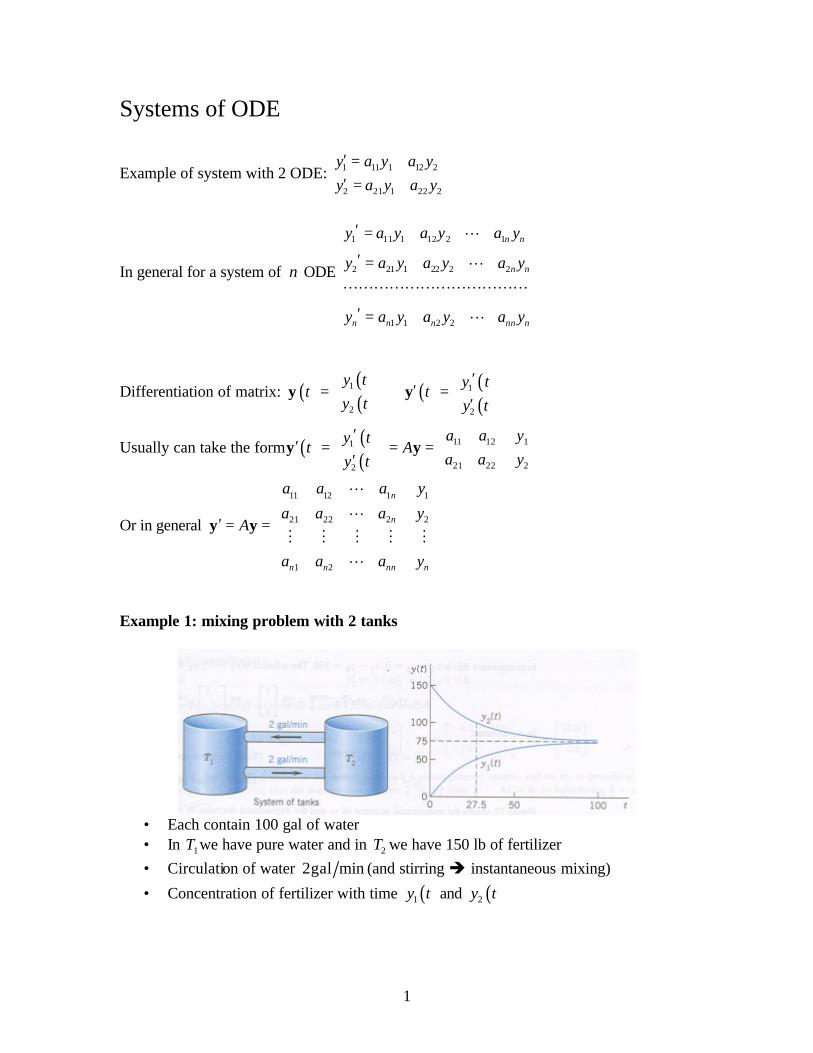
Example 1: mixing problem with 2 tanks

• Each contain 100 gal of water • In 1T we have pure water and in 2T we have 150 lb of fertilizer • Circulation of water 2gal min (and stirring è instantaneous mixing)

• Concentration of fertilizer with time ( )1y t and ( )2y t

2

Model: ( ) inflow outflowmin min

y t′ = −

This gives 2 ODEs: 1 2 1

2 1 2

2 2100 100

2 2100 100

y y y

y y y

′ = −

′ = −

Equivalent to 1 1

2 2

0.02 0.020.02 0.02

y yy y

′ − = ′ −

We try a solution of the form: t t te e A eλ λ λλ′= ⇒ = =y x y x x This is an eigenvalues problem: 0A Aλ λ= ⇒ − =x x x x With nontrivial solution if ( )Det 0A Iλ− =

( ) ( ) ( )2 20.02 0.020.02 0.02 0.04 0

0.02 0.02λ

λ λ λλ

− −⇒ = − − − = + =

− −

Two eigenvalues 1 0λ = and 2 0.04λ = − and two eigenvectors ( )1 11

=

x and ( )2 1

1

= − x

The solution ( ) ( )1 21 2 0.041 2 1 2

1 11 1

t t tc e c e c c eλ λ − = + = + −

y x x where 1c and 2c are arbitrary

constants Initial conditions: ( )1 0 0y = and ( )2 0 150y =

( ) 1 21 2 1 2

1 2

01 1 00 75 and 75

1501 1 150c c

c c c cc c

+ = ⇒ = + = ⇒ ⇒ = = − − =−

y

At what time 1t concentration is ½ that of 2t ? This happens when 1t contains 1/3 of total

amount 0.04 0.041

1 ln(3)75 75 50 27.5min

3 0.04t ty e e t− −⇒ = − = ⇒ = ⇒ = =

3

Example 2 Electric network

We want to know the currents ( )1I t and ( )2I t in the two loops of the above circuit and we assume all currents and charges to be zero at 0t = The model is based on Kirchhoff’s voltage law: In the left loop

• the voltage drops over the inductor [ ]1 1 VLI I′ ′=

• the voltage drops over the resistor ( ) ( )[ ]1 1 2 1 24 VR I I I I− = −

• The sum of voltage must be equal to that of the battery ( )1 1 24 12I I I′ + − = In the right loop

• the voltage drops over the first resistor ( ) ( )[ ]1 2 1 2 14 VR I I I I− = −

• the voltage drops over the resistor [ ]2 2 26 VR I I=

• the voltage drops over the capacitor [ ]2 2

14 VI dt I dt

C=∫ ∫

• The sum must be equal to zero

( )2 2 1 2 2 1 26 4 4 0 or 10 4 4 0I I I I dt I I I dt+ − + = − + =∫ ∫

Dividing by ten and deriving 2 1 20.4 0.4 0I I I′ ′− + =

Replacing by the value of 1I ′ in left loop: ( )( )2 1 2 20.4 12 4 0.4 0I I I I′ − − − + =

2 1 21.6 1.2 4.8I I I′⇒ = − + +

In matrix form 1

2

4.0 4.0 12.01.6 1.2 4.8

IA

I−

′ = + = + − J J g

This is a nonhomogeneous system

4

We first look for a solution of the homogenous system 1

2

4.0 4.01.6 1.2

IA

I−

′ = = − J J

trying t t te e A eλ λ λλ′= ⇒ = =J x J x x

The nontrivial solution ( ) ( )4.0 4.0det 0 0

1.6 1.2A I

λλ

λ

− −− = ⇒ =

− −

2 2.8 1.6 0λ λ⇒ + + = with two eigenvalues 1 2λ = − and 2 0.8λ = −

And two eigenvectors ( )1 21

=

x and ( )2 1

0.8

=

x

Consistent with general homogenous solution

( ) ( )1 22 0.8 2 0.81 2 1 2

2 11 0.8

t t t th c e c e c e c e− − − −

= + = +

J x x

To find a particular solution, we note that since g is a constant we can try a constant

p⇒ =J a such that 1

2

4.0 4.0 12.00

1.6 1.2 4.8a

Aa

− + = ⇒ + −

a g

1 2

1 2

4.0 4.0 12.0 01.6 1.2 4.8 0

a aa a

− + + =− + + = 1 3a⇒ = and 2 0a = or

30

=

a

So the general solution

( ) ( )1 22 0.8 2 0.81 2 1 2

2 1 31 0.8 0

t t t th p c e c e c e c e− − − −

= + = + + = + +

J J J x x a

2 0.81 1 22 3t tI c e c e− −= + + and 2 0.8

2 1 20.8t tI c e c e− −= + Applying the initial conditions

1 1 22 3 0I c c= + + = and 2 1 20.8 0I c c= + = 1 4c⇒ = − and 2 5c =

5

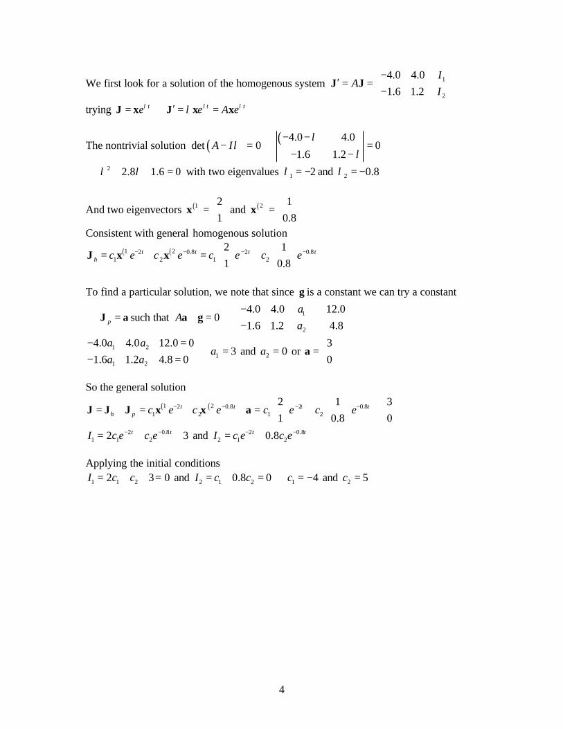
Solution

( ) ( )1 22 0.8 2 0.82 1 34.0 5.0 4.0 5.0

1 0.8 0t t t t

h p e e e e− − − − = + = − + + = − + +

J J J x x a

2 0.81 8.0 5.0 3t tI e e− −= − + + and 2 0.8

2 4.0 4.0t tI e e− −= − +

Solutions shown individually look like two damp vibrations Phase plane Shows the solution using 1I and 2I as degrees of liberty of system (parametric representation) where the arrow shows the sense of variation with time

• The current 2I rises almost linearly in time with 1I both reaching a maximum • But then 2I drops to zero while the current 1I reach a lower constant value below

its maximum

6

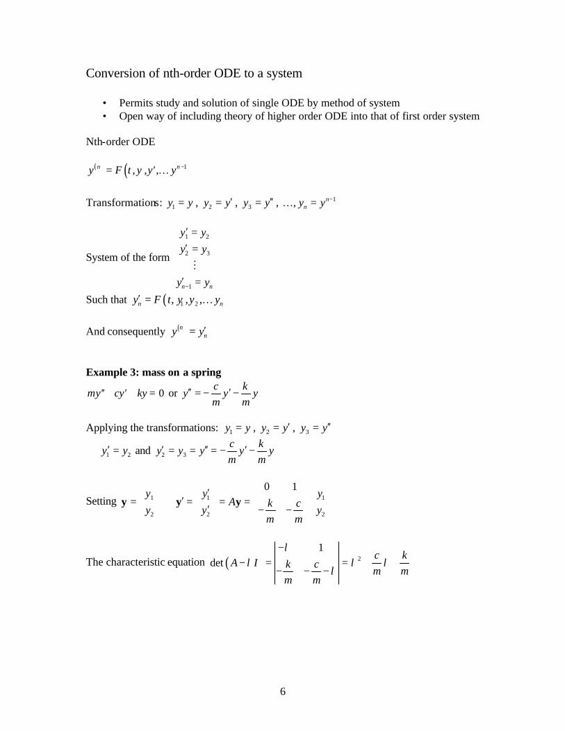
Conversion of nth-order ODE to a system

• Permits study and solution of single ODE by method of system • Open way of including theory of higher order ODE into that of first order system

Nth-order ODE

( ) ( )1, , ,n ny F t y y y −′= …

Transformations: 1y y= , 2y y′= , 3y y′′= , 1, n

ny y −=…

System of the form

1 2

2 3

1n n

y yy y

y y−

′ =′ =

′ =M

Such that ( )1 2, , ,n ny F t y y y′ = … And consequently ( )n

ny y′= Example 3: mass on a spring

0my cy ky′′ ′+ + = or c k

y y ym m

′′ ′= − −

Applying the transformations: 1y y= , 2y y′= , 3y y′′=

1 2y y′⇒ = and 2 3

c ky y y y y

m m′ ′′ ′= = = − −

Setting 1 1 1

2 2 2

0 1y y y

A k cy y y

m m

′ ′= ⇒ = = = ′ − −

y y y

The characteristic equation ( ) 2

1det

c kA I k c

m mm m

λλ λ λ

λ

−− = = + +

− − −

7

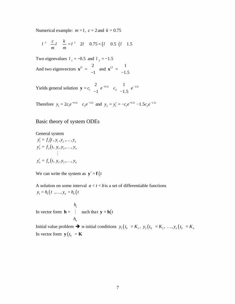
Numerical example: 1m = , 2c = and 0.75k =

( ) ( )2 2 2 0.75 0.5 1.5c km m

λ λ λ λ λ λ⇒ + + = + + = + +

Two eigenvalues 1 0.5λ = − and 2 1.5λ = −

And two eigenvectors ( )1 21

= −

x and ( )2 11.5

= −

x

Yields general solution 0.5 1.51 2

2 11 1.5

t tc e c e− − = + − −

y

Therefore 0.5 1.5

1 1 22 t ty c e c e− −= + and 0.5 1.52 1 1 21.5t ty y c e c e− −′= = − −

Basic theory of system ODEs General system

( )( )

( )

1 1 1 2

2 2 1 2

1 2

, , , ,

, , , ,

, , , ,

n

n

n n n

y f t y y y

y f t y y y

y f t y y y

′ =′ =

′ =

……

M…

We can write the system as ( )t′ =y f A solution on some interval a t b< < is a set of differentiable functions

( ) ( )1 1 , , n ny h t y h t= =…

In vector form 1

n

h

h

=

h M such tha t ( )t=y h

Initial value problem è n- initial conditions ( )1 0 1y t K= , ( )2 0 2y t K= , ( )0, n ny t K=…

In vector form ( )0t =y K

8

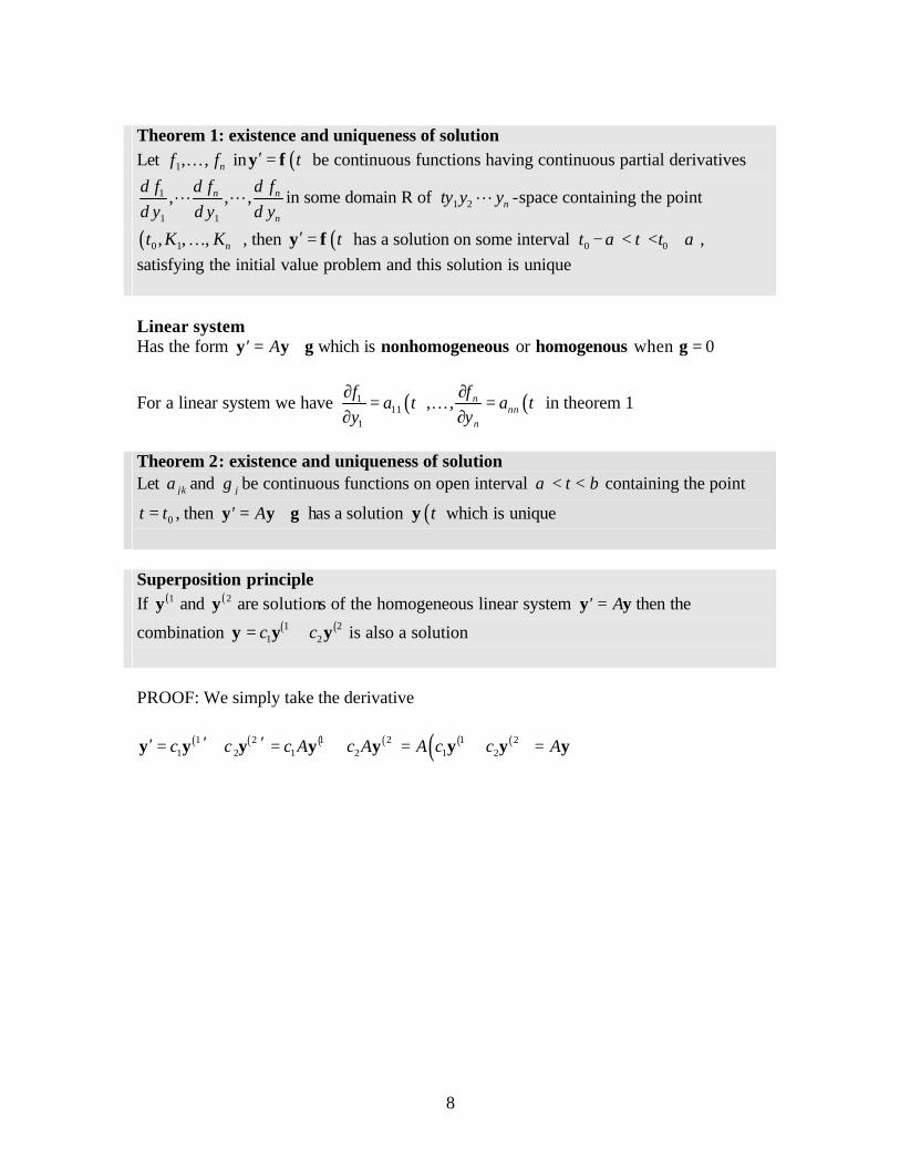
Theorem 1: existence and uniqueness of solution Let 1, , nf f… in ( )t′ =y f be continuous functions having continuous partial derivatives

1

1 1

, , ,n n

n

f ffy y y

δ δδδ δ δ

L L in some domain R of 1 2 nty y yL -space containing the point

( )0 1, , , nt K K… , then ( )t′ =y f has a solution on some interval 0 0t t tα α− < < + , satisfying the initial value problem and this solution is unique Linear system Has the form A′ = +y y g which is nonhomogeneous or homogenous when 0=g

For a linear system we have ( ) ( )111

1

, , nnn

n

ffa t a t

y y∂∂

= =∂ ∂

… in theorem 1

Theorem 2: existence and uniqueness of solution Let jka and jg be continuous functions on open interval tα β< < containing the point

0t t= , then A′ = +y y g has a solution ( )ty which is unique Superposition principle If ( )1y and ( )2y are solutions of the homogeneous linear system A′ =y y then the

combination ( ) ( )1 21 2c c= +y y y is also a solution

PROOF: We simply take the derivative

( ) ( ) ( ) ( ) ( ) ( )( )1 2 1 2 1 21 2 1 2 1 2c c c A c A A c c A′ ′′ = + = + = + =y y y y y y y y

9

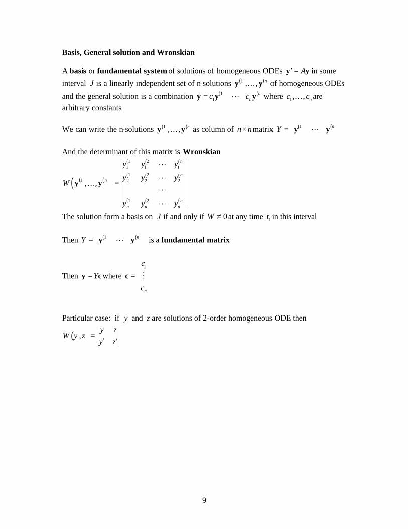
Basis, General solution and Wronskian A basis or fundamental system of solutions of homogeneous ODEs A′ =y y in some

interval J is a linearly independent set of n-solutions ( ) ( )1 , , ny y… of homogeneous ODEs

and the general solution is a combination ( ) ( )11

nnc c= + +y y yL where 1 , , nc c… are

arbitrary constants We can write the n-solutions ( ) ( )1 , , ny y… as column of n n× matrix ( ) ( )1 nY = y yL

And the determinant of this matrix is Wronskian

( ) ( )( )

( ) ( ) ( )

( ) ( ) ( )

( ) ( ) ( )

1 21 1 1

1 21 2 2 2

1 2

, ,

n

nn

nn n n

y y y

y y yW

y y y

=⋅ ⋅ ⋅

y y

LL… LL

The solution form a basis on J if and only if 0W ≠ at any time 1t in this interval

Then ( ) ( )1 nY = y yL is a fundamental matrix

Then Y=y c where 1

n

c

c

=

c M

Particular case: if y and z are solutions of 2-order homogeneous ODE then

( ),y z

W y zy z

=′ ′

10

Constant coefficient systems Assume A′ =y y With constant coefficients n n⇒ × matrix jkA a = all independent of t

Solution K′ =y y using kty ce= t te e Aλ λλ′⇒ = ⇒ = =y x y x y Eigenvalues problem 0A λ− =x x If A has linearly independent set of eigenvalues, example A symmetric ( )kj jka a= or

skew symmetric ( )kj jka a= − or n -different eigenvalues 1, , nλ λ… then we have

( ) ( )1 , , nx x… eigenvectors and a related set of solutions

( ) ( )

( ) ( )

( ) ( )

1

2

1 1

2 2

n

t

t

n n t

e

e

e

λ

λ

λ

=

=

=

y x

y x

y x

M

The Wronskian

( ) ( )( )

( ) ( ) ( )

( ) ( ) ( )

( ) ( ) ( )

( ) ( ) ( )

( ) ( ) ( )

( ) ( ) ( )

1 2

1 2

1 2

1 2

1 2 1 21 1 1 1 1 1

1 2 1 21 2 2 2 2 2 2

1 2 1 2

, ,

n

n

n

n

n ntt t

n ntt tn t t t

n ntt tn n n n n n

x e x e x e x x x

x e x e x e x x xW e

x e x e x e x x x

λλ λ

λλ λλ λ λ

λλ λ

+ + += =⋅ ⋅ ⋅ ⋅ ⋅ ⋅

y y L

L LL L… L LL L

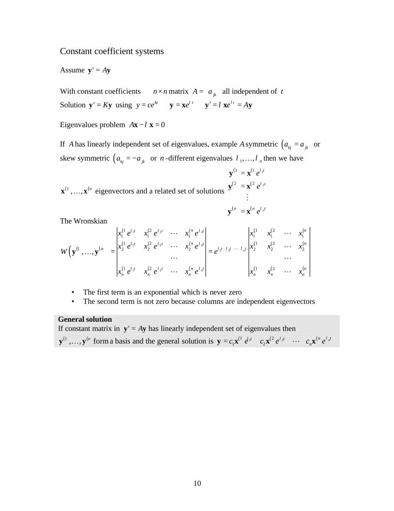
• The first term is an exponential which is never zero • The second term is not zero because columns are independent eigenvectors

General solution If constant matrix in A′ =y y has linearly independent set of eigenvalues then

( ) ( )1 , , ny y… form a basis and the general solution is ( ) ( ) ( )1 21 21 2

nn tt tnc e c e c eλλ λ= + + +y x x xL

11

Phase plane Qualitative method of obtaining general qualitative information on solutions without actually solving ODE or system Created by Henri Poincaré (1854-1912) French mathematician who worked on complex analysis, divergent series, topology and astronomy In physics – phase plane is - - -r mr r mv r p′ = = Consider two ODEs then A′ =y y takes the form

1 11 12 1

2 21 22 2

y a a yy a a y

′ = ′

With solution ( ) ( )( )

1

2

y tt

y t

=

y

which can be graphed as two simple curves, or together in the phase plane 1 2y y The parametric curve in this phase plane is the trajectory

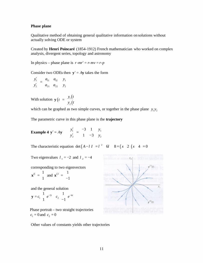
Example 4 1 1

2 2

3 11 3

y yA

y y

′ − ′ = ⇒ = ′ −

y y

The characteristic equation ( ) ( ) ( )2det 6 8 2 4 0A I x xλ λ λ− = + + = + + = Two eigenvalues 1 2λ = − and 2 4λ = − corresponding to two eigenvectors

( )1 11

=

x and ( )2 1

1

= − x

and the general solution

2 41 2

1 11 1

t tc e c e− − = + −

y

Phase portrait – two straight trajectories

1 0c = and 2 0c =

Other values of constants yields other trajectories

12

Critical points In example 4, the point 0 is a critical point = common point for all the trajectories

From A′ =y y we get that 2 2 2 21 1 22 2

1 1 1 11 1 12 2

dy y dt y a y a ydy y d t y a y a y

′ ′ += = =

′ ′ +

This associates with every point ( )1 2,P y y a unique tangent direction 2

1

dydy

of trajectory

passing through P , except at ( )0 0,0P = where 2

1

00

dydy

= which is a critical point

There are 5 different types of critical points:

Improper node

All the trajectories except two have the same limiting direction of the tangent The two exceptional trajectories also have limiting direction of tangent at 0P but they are different The common limiting direction at zero is that of ( ) [ ]1 1 1

T=x because 4te− goes faster to

zero than 2te− The two exceptional directions are

( ) [ ]2 1 1T

= −x and ( ) [ ]2 1 1T

− = −x

Proper node

Every trajectory as limiting direction and for any given direction dat 0P there is a trajectory having das its limiting direction

Unit matrix 1

2

1 00 1

yy

′ =

y

Characteristic equation ( )21 0λ− =

Solution 1 2

1 00 1

t tc e c e

= +

y

Trajectories 1 2 2 1c y c y= (linear)

13

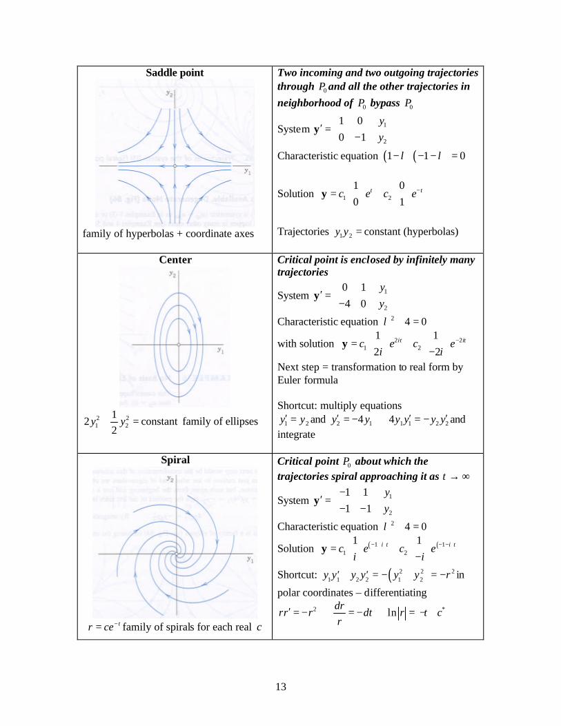
Saddle point

family of hyperbolas + coordinate axes

Two incoming and two outgoing trajectories through 0P and all the other trajectories in neighborhood of 0P bypass 0P

System 1

2

1 00 1

yy

′ = −

y

Characteristic equation ( ) ( )1 1 0λ λ− − − =

Solution 1 2

1 00 1

t tc e c e− = +

y

Trajectories 1 2 constanty y = (hyperbolas)

Center

2 21 2

12 constant

2y y+ = family of ellipses

Critical point is enclosed by infinitely many trajectories

System 1

2

0 14 0

yy

′ = −

y

Characteristic equation 2 4 0λ + =

with solution 2 21 2

1 12 2

it itc e c ei i

− = + −

y

Next step = transformation to real form by Euler formula Shortcut: multiply equations

1 2y y′ = and 2 14y y′ = − 1 1 2 24y y y y′ ′⇒ = − and integrate

Spiral

tr ce−= family of spirals for each real c

Critical point 0P about which the trajectories spiral approaching it as t → ∞

System 1

2

1 11 1

yy

− ′ = − −

y

Characteristic equation 2 4 0λ + =

Solution ( ) ( )1 11 2

1 1i t i tc e c ei i

− + − − = + −

y

Shortcut: ( )2 2 21 1 2 2 1 2y y y y y y r′ ′+ = − + = − in

polar coordinates – differentiating 2rr r′ = − *ln

drdt r t c

r⇒ = − ⇒ = − +

14

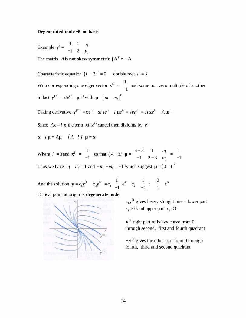
Degenerated node è no basis

Example 1

2

4 11 2

yy

′ = −

y

The matrix A is not skew symmetric ( )T ≠ −A A

Characteristic equation ( )2

3 0λ − = ⇒ double root 3λ =

With corresponding one eigenvector ( )1 11

= −

x and some non zero multiple of another

In fact ( )2 t tte eλ λ= +y x µ with [ ]1 2

Tµ µ=µ

Taking derivative ( ) ( )2 2t t t t te te e A A te A eλ λ λ λ λλ λ′ = + + = = +y x x µ y x µ Since A λ=x x the term tteλλx cancel then dividing by teλ

( )A A Iλ λ+ = ⇒ − =x µ µ µ x

Where 3λ = and ( )1 11

= −

x so that ( ) 1

2

4 3 1 13

1 2 3 1A I

µµ

− − = = − − −

µ

Thus we have 1 2 1µ µ+ = and 1 2 1µ µ− − = − which suggest ( )0 1T

=µ

And the solution ( ) ( )1 2 3 31 2 1 2

1 1 01 1 1

t tc c c e c t e

= + = + + − − y y y

Critical point at origin is degenerate node

( )11c y gives heavy straight line – lower part

1 0c > and upper part 1 0c <

( )2y right part of heavy curve from 0 through second, first and fourth quadrant

( )2−y gives the other part from 0 through fourth, third and second quadrant

15

Critical points vs. stability of solutions Consider an system of homogeneous ODEs with constant coefficients

1 11 12 1

2 21 22 2

y a a yA

y a a y

′ ′ = = = ′

y y

On the phase plane, the solution ( ) ( ) ( )( )1 2

Tt y t y t=y yields trajectories = phase

portrait

With critical point such that 2 2 2 21 1 22 2

1 1 1 11 1 12 2

dy y dt y a y a ydy y d t y a y a y

′ ′ += = =

′ ′ +

The relation between critical point and eigenvalues pass by characteristic equation

( ) ( ) ( )11 12 211 22

21 22

det det 0a a

A I a a Aa a

λλ λ λ

λ−

− = = − + + =−

This is a quadratic equation 2 0p qλ λ− + = with solutions

( )1

12

pλ = + ∆ and ( )2

12

pλ = − ∆

Where

• ( )11 22p a a= + is the trace of A

• ( )11 22 12 21det( )q A a a a a= = −

• 2 4p q∆ = − If we express the solution in terms of product ( ) ( )2

1 2p qλ λ λ λ λ λ− + = − − Then we have

• 1 2p λ λ= + • 1 2q λ λ=

• ( )2

1 2λ λ∆ = − Eigenvalue criteria for critical points

1 2p λ λ= + 1 2q λ λ= ( )2

1 2λ λ∆ = − eigenvalues

Node 0q > 0∆ ≥ Real same sign Saddle point 0q < Real opposite sign

Center 0p = 0q > Pure imaginary Spiral point 0p ≠ 0∆ < Complex, not pure

imaginary

16

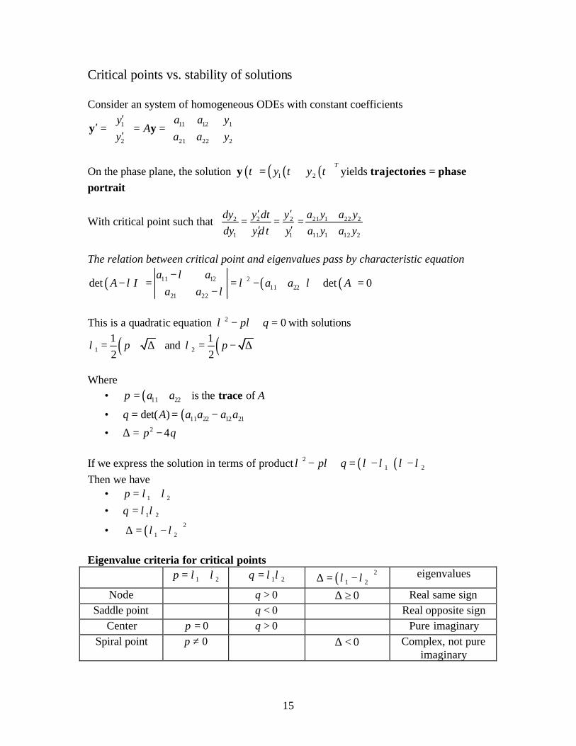
Stability of critical points

• Stable all the trajectories close to 0P remain close to 0P in future

For every disk Dε of radius 0ε > with center 0P , there is a disk Dδ with radius 0δ > and

center 0P such that every trajectory that has point ( )1 1P t in Dδ has all its subsequent

points 1t t≥ in Dε If condition not verified = unstable

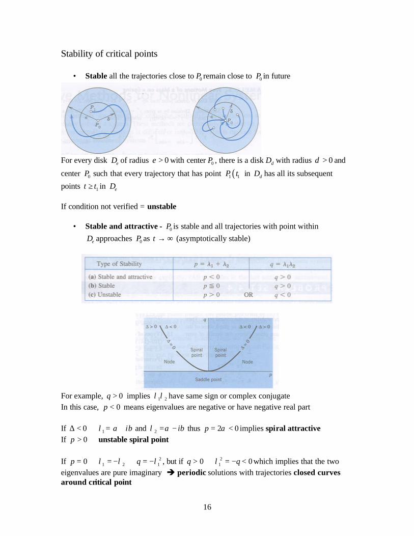
• Stable and attractive - 0P is stable and all trajectories with point within Dε approaches 0P as t → ∞ (asymptotically stable)

For example, 0q > implies 1 2λ λ have same sign or complex conjugate In this case, 0p < means eigenvalues are negative or have negative real part If 10 iλ α β∆ < ⇒ = + and 2 iλ α β= − thus 2 0p α= < implies spiral attractive If 0p > ⇒ unstable spiral point If 2

1 2 10p qλ λ λ= ⇒ = − ⇒ = − , but if 210 0q qλ> ⇒ = − < which implies that the two

eigenvalues are pure imaginary è periodic solutions with trajectories closed curves around critical point

17

Example 5 1 1

2 2

3 11 3

y yA

y y

′ − ′ = ⇒ = ′ −

y y

6p = − , 8q = , 4∆ = è node whish is stable and attractive Example 6 mass on spring

0my cy ky′′ ′+ + = or c k

y y ym m

′′ ′= − −

1

2

0 1y

A k cy

m m

′ = = − −

y y

( ) 2

1det 0

c kA I k c

m mm m

λλ λ λ

λ

−− = = + + =

− − −

cp

m= − ,

kq

m= and

2

4c km m

∆ = −

No damping 0c⇒ = which yields 0p = and 0q > the critical point is a center Underdamping 2 4c mk< which yields 0, 0, 0p q< > ∆ < stable attractive spiral Critical damping 2 4c mk= which yields 0, 0, 0p q< > ∆ = stable attractive node Overdamping 2 4c mk> which yields 0, 0, 0p q< > ∆ > stable attractive node

18

Numerical example: 1m = , 2c = and 0.75k =

( ) ( )2 2 2 0.75 0.5 1.5c km m

λ λ λ λ λ λ⇒ + + = + + = + +

Two eigenvalues 1 0.5λ = − and 2 1.5λ = −

And two eigenvectors ( )1 21

= −

x and ( )2 11.5

= −

x

Yields general solution 0.5 1.51 2

2 11 1.5

t tc e c e− − = + − −

y

Therefore 0.5 1.5

1 1 22 t ty c e c e− −= + and 0.5 1.52 1 1 21.5t ty y c e c e− −′= = − −

19

Non linear systems Solution by analytic method is difficult or impossible

First order non linear systems : ( )′ =y f y and thus ( )( )

1 1 1 2

2 2 1 2

,

,

y f y y

y f y y

′ =

′ =

If system is autonomous (does not depend on t ) extended phase plane methods give characterization of various general properties of solutions

• Advantage over numerical methods, which give only one (approximate) solution at a time (but with higher precision)

If first order nonlinear solution has several critical points

• discuss one after the other each time moving point ( )0 : ,P a b to be discussed at

origin ⇒ applying translation 1 1y y a= −% and 2 2y y b= −% • 0P is isolated – only critical point within sufficiently small circular disk with

center on origin Linearization of nonlinear systems Assume 1f and 2f are continuous and have continuous partial derivatives in neighborhood of 0P

• A linear system approximating ( )′ =y f y have same kind of critical points (with two exceptions)

• Since 0P is critical point ( ) ( )1 20,0 0,0 0f f= =

• Transformation ( )′ = +y Ay h y and thus ( )( )

1 11 1 12 2 1 1 2

2 21 1 22 2 2 1 2

,

,

y a y a y h y y

y a y a y h y y

′ = + +

′ = + +

• If Det 0≠A then the type and stability of 0P is the same as that of critical point of linear system

• ′ =y Ay and thus 1 11 1 12 2

2 21 1 22 2

y a y a yy a y a y

′ = +′ = +

The above assumption on derivatives implies that 1h and 2h are small near 0P Two exceptions : eigenvalues are equal (degenerated) or pure imaginary, then in addition to the type of critical points of linear system the nonlinear system may have a spiral point

20

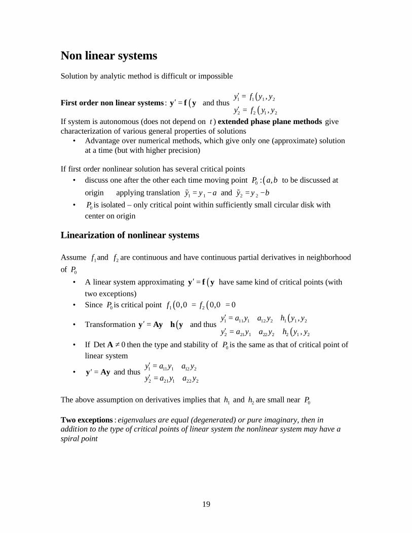
Example 1 – free undamped pendulum

Mathematical model sin 0mL mgθ θ′′ + =

Dividing by mL and writingg

kL

= : sin 0kθ θ′′ + =

This is a nonlinear equation When small value of sinθ θ θ⇒ ∼ and approximate form 0kθ θ′′ + = has solution

cos sinA kt B kt+ Critical points by linearization:

Set 1yθ = and 2yθ ′ = then nonlinear system ( )( )

1 1 1 2 2

2 2 1 2 1

,

, sin

y f y y y

y f y y k y

′ = =

′ = = −

The right side both zero when 2 0y = and 1y nπ= ⇒ infinity of critical points

( ), 0nπ where 0, 1, 2,n = ± ± …

Consider ( )0,0 the McLaurin series 31 1 1 1

1sin

6y y y y= − + − ≈L

Linearized system 0 1

0k ′ = = −

y Ay y and thus 1 2

2 1

y yy ky

′ =′ = −

We need 0p = , q = det ( )0k= >A and 2 4 4p q k∆ = − = − From this we conclude that ( )0,0 is a center always stable

Since 1sin sin yθ = is periodic with period 2π all critical points ( ), 0nπ with 2, 4,n = ± ± … are centers

21

Consider now ( ), 0π ⇒ setting 1yθ π− = and ( ) 2yθ π θ′ ′− = = therefore

( ) 31 1 1 1 1

1sin sin sin

6y y y y yθ π= − = − = − + − + ≈ −L

And linearized system 0 1

0k ′ = =

y Ay y and thus 1 2

2 1

y yy ky

′ =′ =

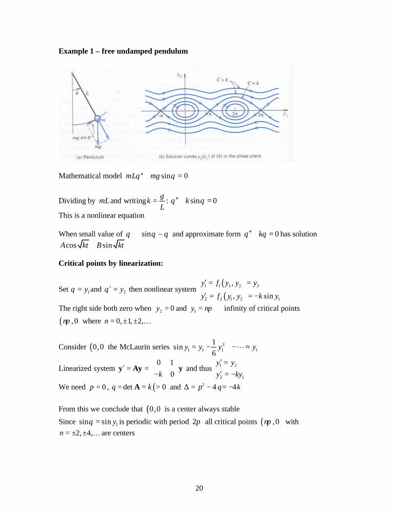
Which yields that 0p = , q = det ( )0k= − <A and 2 4 4p q k∆ = − = From which we conclude that ( ), 0nπ with 1, 3,n = ± ± …are saddle points which are always unstable

22

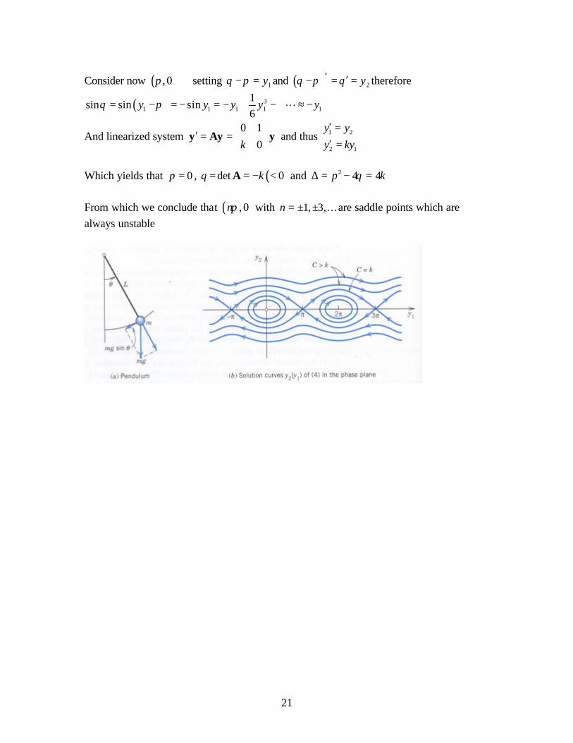
Example 2 –damped pendulum Introduce damping term proportional to velocity

sin 0c kθ θ θ′′ ′+ + =

Linearized system 1 2

2 1 2siny yy k y cy

′ =′ = − −

Critical points at same locations ( ) ( ) ( )0,0 , , 0 , 2 ,0 ,π π± ± …

Consider ( )0,0

0 1k c

′ = = − − y Ay y and 1 2

2 1 2

y yy ky cy

′ =′ = − −

For small damping spiral point For critical point ( ), 0π we have 11 22p a a c= + = − , q = det ( )0k= − <A and

2 24 4p q c k∆ = − = + For 0c > a saddle point Damping = lost of energy – instead of closed trajectories we spiraling ones – no more trajectories connecting critical points

23

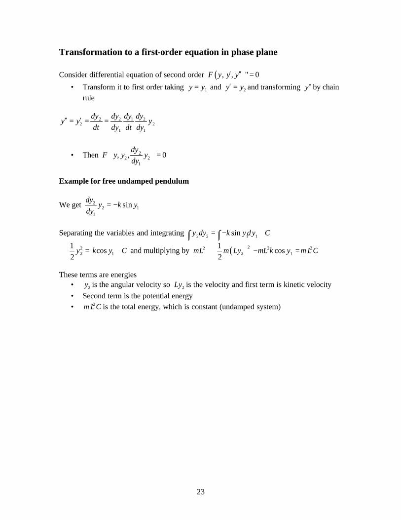
Transformation to a first-order equation in phase plane Consider differential equation of second order ( ), , " 0F y y y′ ′′ =

• Transform it to first order taking 1y y= and 2y y′ = and transforming y′′ by chain rule

2 2 1 2

2 21 1

dy dy dy dyy y y

dt dy dt dy′′ ′= = =

• Then 22 2

1

, , 0dy

F y y ydy

=

Example for free undamped pendulum

We get 22 1

1

sindy

y k ydy

= −

Separating the variables and integrating 2 2 1 1siny dy k y d y C= − +∫ ∫

22 1

1cos

2y k y C⇒ = + and multiplying by 2mL ( )2 2 2

2 1

1cos

2m Ly mL k y m L C⇒ − =

These terms are energies

• 2y is the angular velocity so 2Ly is the velocity and first term is kinetic velocity • Second term is the potential energy • 2m L C is the total energy, which is constant (undamped system)

24

Type of motion depends on C

• Smallest possible C k= − then 2 0y = and 1cos 1y = , the pendulum is at rest • Change of direction of motion 2 0y θ ′= = then 1cos 0k y C+ =

• If 1y π= then 1cos 1y = − and C k= , hence if k C k− < < the pendulum oscillate (closed trajectories)

• If C k> then 2 0y = is impossible and pendulum makes a whirly motion appearing a wavy trajectory

• If C k= correspond to two separating trajectories connecting saddle point

25

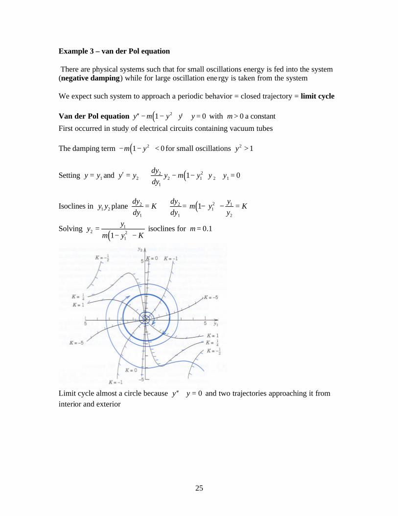
Example 3 – van der Pol equation There are physical systems such that for small oscillations energy is fed into the system (negative damping) while for large oscillation energy is taken from the system We expect such system to approach a periodic behavior = closed trajectory = limit cycle Van der Pol equation ( )21 0y y y yµ′′ ′− − + = with 0µ > a constant

First occurred in study of electrical circuits containing vacuum tubes The damping term ( )21 0yµ− − < for small oscillations 2 1y >

Setting 1y y= and 2y y′ = ( )222 1 2 1

1

1 0dy

y y y ydy

µ⇒ − − + =

Isoclines in 1 2y y plane 2

1

dyK

dy= ( )22 1

11 2

1dy y

y Kdy y

µ⇒ = − − =

Solving ( )

12 2

11y

yy Kµ

=− −

isoclines for 0.1µ =

Limit cycle almost a circle because 0y y′′ + = and two trajectories approaching it from interior and exterior

26

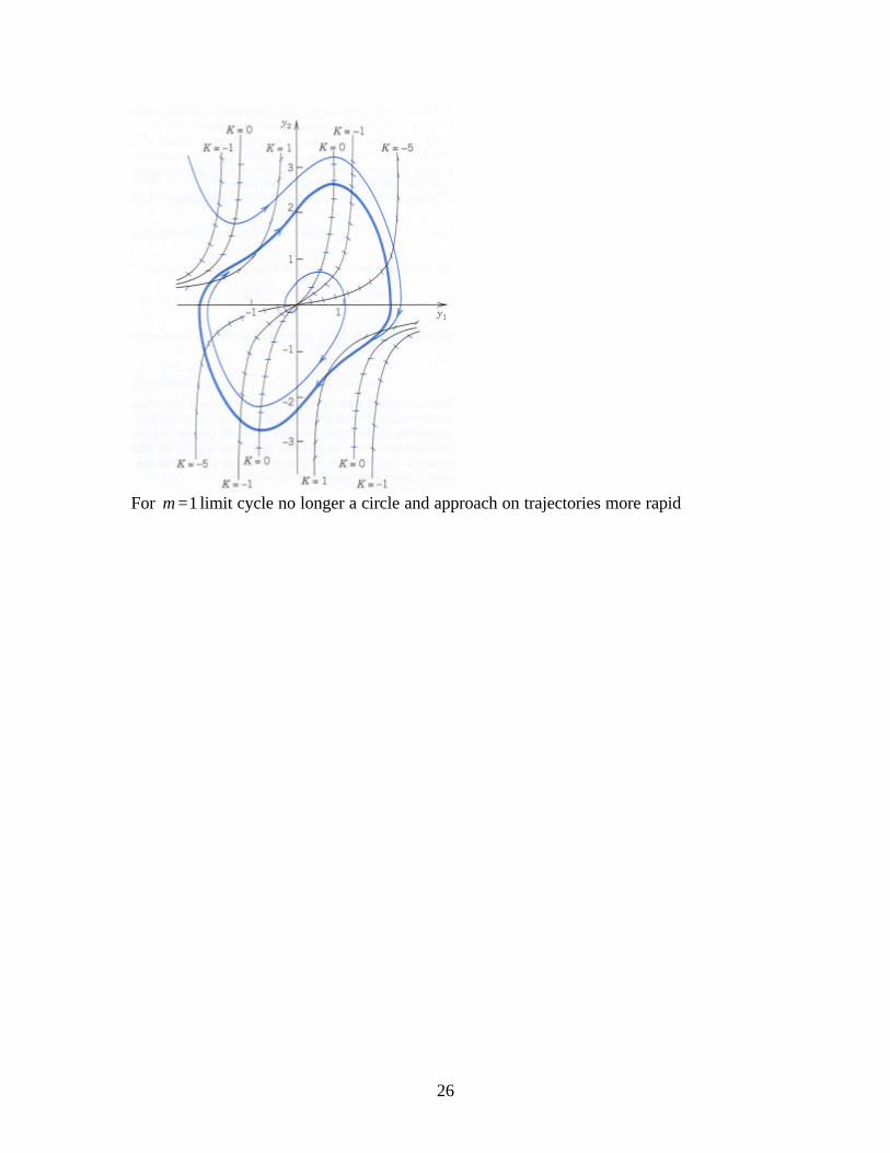
For 1µ = limit cycle no longer a circle and approach on trajectories more rapid

27

Non homogeneous linear systems