Systolic-Type Implementation of Matrix Computations Based on the Faddeev Algorithm

R. Wyrzykowski

Dept. Math. 8~ Computer Science Technical IJniversity of Czestochowa*

Czestochowa, Poland 42-400

Abstract This paper deals with the problem of enhancing

the versatility of V L S I processor arrays without un- due addition of hardware, tinae/control overhead, and software complexity. A promissing approach to this problem is based on matrix computations carried out through the Faddeev algorithm. In th.e paper, we design a fixed-size, linear array architectu.re .with fully lo- cal communications and, rather, straightforward con- trol requirements. This high.-throughput, systolic-type architecture allows us io minirnize both. I /O require- ments a n d the number of processing elements perform- ing complicated operations like diuisions. To derive the array from a formal description of the Faddeev algorithm based on Gaussian elimination with partial pivoting, we use purposive transformations of tAe basic dependenze graph of the algorithm. before its space-time mappings onto array architectures.

1 Introduction Recent, advantages in VLSI technology have

stimulated research in applica.tion-specific architec- tures which are tailored to particular applications. Among these architectures are application-specific processor arrays, which can have a different degree of specialization [I]. Systolic-type arrays [1,2] are examples of such architectures. Using massive paral- lelism/pipelining, these VLSI processor networks ex- ploit the regularity inherent in many algorithms to achieve high performance while keeping local commu- nications and low 1 /0 requirements.

One of the principal problems encountered in designing these arrays is that of providing a suf- ficiently general range of functionality without un- due addition of hardware, time/control overhead, and software complexity. A promissing approach to this problem is based [3,4] on the generality of linear (or matrix algebra), a class of operations whiclie arises in a wide variet,y of application area.s, including signal and image processing, real-time control, modelling and simulation, etc.

In computational linear algebra, the Faddeev algo- rithm [4,5,6,7,8,9] is inherently versatile. It enables one to perform many matrix operations including ad- dition, multiplication, inversion, LU-decomposi tion, solution of linear systems, etc.

J . S. Kanevski, 0. V. Maslennikov

Dept. Computer Science Kiev Polytechnic Institute

Kiev, Ukraine 252-056

Since the underlaying procedure to carry out the Faddeev algorithm is matrix triangularisation, any processor array performing the algorithm should be based [8] on an architecture which can realize trian- gularisation efficiently. The triangular systolic array developed by Kung and Gentleman [lo] is a common platform for two-dimensional (2-D) systolic architec- tures [4, 6, 7, 8, 93. which perform the Faddeev algo- rithm using either Gaussian elimination with neigh- bour pivoting or orthogonal triangularisation. The second approach is numerically stable but it requires relatively complex processing elements (PES). Some of them must perform square root operations, which are not easily implementable for real-time applications. On the other hand, Gaussian elimination architectures employ simple PES. But Sorenson has shown [ll] that the error bound for pairwise pivoting is much worse than that for Gaussian elimination with partial pivot- ing [3], as well as, for orthogonal triangularisation.

This paper deals with the design of linear proces- sor arrays which perform the Faddeev algorithm using Gaussian elimination. Unlike 2-D architectures, these one-dimensional (1-D) arrays allow one [12], firstly, to minimize the amount of 1 / 0 channels because they are connected only with the first or/and the last PE. Secondly, a large structure can be constructed simply by concatenation of smaller arrays. Thirdly, a h e a r array requires memory bandwidth which is indepen- dent of the size of the array. In the paper, we employ partial pivoting instead of neighbour pivoting. When processing time for linear architectures is considered, neighbour pivoting has not any advantage over partial pivoting [13] being much less reliable.

The paper is organized as follows. At first (Section a), we describe the choseii version of the Faddeev algorithm and some applications of it. The next section deals with a basic dependence graph of the algorithm. This graph is then used (Sectiou 4) for the desigil of linear array architectures performing the algorithm. To derive arrays with desired features, some purposive transformations of the basic graph are employed before space-time mappings of graphs onto array architectures. Since the arrays derived in this way feature a strong dependence of their sizes upon sizes of matrices being processed, we show (Section 5) how these architectures should be modified in order to

31 0-8186-6322-7/94 $04.00 0 1994 IEEE

process large size matrices on fixed-size arrays. Sec- tion 6 provides conclusions.

2 Faddeev algorithm and its applica- tions

Starting with N x N , N x R, P x N and P x R input matrices A , B , C and D, respectively, the Faddeev algorithm is intended [5] for solving matrix equations of the type

x = CA-' + D (1)

where the four input matrices form an ( N + P ) x ( N + R) joint matrix F when arranged in the following way:

A B F = [ -C D ]

The essence of the Faddeev algorithm [4, 51 consists in reducing the lower left quadrant of the matrix F (i.e. C-matrix) to zero matrix, while in the lower right quadrant of the matrix F (i.e. in place of D-matrix), the resultant P x R matrix X is formed. To carry out the above-stated operations with A being a non- singular matrix, Gaussian elimination is used. Hence, in the course of computations, t.he joint matrix F is being transformed into the following matrix:

[: :] where R is the upper triangular matrix. A consid- erable degree of versatility of the Faddeev algorithm stems from the fa.ct that Eq. 1 allows us to solve a set of problems. Some of them are listed below:

0 solving a system A X = B of linear algebraic equations with one or more right-hand sides (de- pending upon the number of columns in X), i.e.

X = A - ' B for C = I , D = O

where I is the identity matrix;

0 matrix multiplication X = CB for A = I, D = 0 ;

0 matrix multiply-add operation

0 matrix inversion X = A-' for C = B = I, D = 0.

There are [7, 81 other important modifications of the Faddeev algorithm. As a result, it can be employed, for example, in fast solving of linear programming problems using the Karinarkar algorithm.

To provide numerical stability of t.he Faddeev al- gorithm, we employ Gaussian elimination with partial pivoting within columns [3, 131. As a result, a t the i-th step (i = 1! . . . , N ) of the algorithm, the elimination of elements f j i ( j = i+l, . . . , N + P ) , which belong either

X = CB + D for A =I ;

to the original matrix F = F' (for i = 1) or to the par- tially transformed matrix F' (for i > l), is preceeded by successive comparisons of ffi ( j = i + 1,. . . , N ) with the pivot element fji. If

I ffi I > I fiii I then the i-th and j-tli rows of the matrix Fi are in- terchanged, and a boolean variable vji is set to 1. In the opposite case, the row interchange does not take place, and Vj' is set to 0.

After completing all compafisons and interchanges for a given step, the pivot row f j = [fik] with the pivot element f:i is finally derived, where k = i, . . . , N + R. Then the elimination of elements fjj (j = i+l , . . . , N + P ) starts. It is accompanied by transformations of rows of the matrix F, from the ( i + 1)-st row to the ( N + P)-th row. These transformations consist in the element-by-element summation of each row with the pivot row, whicli is,in advanced multiplied by coeffi- cient m.j; = -fji/f&.

Thus, to provide a correct realization of the algo- rit,hm, the selection of pivot elements as well as cor- responding interchanges are limited only to the upper (corresponding to the matrices A and B ) quadrants of matrices Fi. However, the elimination process is carried out within all quadrants of F'. Naturally, in the N-th step, the element #N. is immediately taken as a pivot, without any comparison.

The described-above version of the Faddeev algo- rithm can be expressed in the following form: f o r i : = i s tep 1 u n t i l N do

{se lect ion of the pivot element u i th in the i - th column) f o r j : = i+i s t e p 1 u n t i l N do begin

if abs(f [ i , i ] ) < abs(f [ j , i ] ) then begin

s : = f [ i , i ] ; f [ i , i ] : = f C j , i l ; f C j , i l :=si v[j , i l : = true;

end

Crow interchanges) f o r k : = i+l step i u n t i l N+R do

i f v [ j , i] = true then begin s:=f [i,k]; f [ i ,k] :=f Cj ,kl ; f Cj ,kI :=s;

end ;

e l s e vCj , i l := f a l s e ;

end j ; {calculation of mult ipl iers m C j , i l l f o r j:= i+ i s tep I u n t i l N+P do i f f C i , i ] = 0 then mCj, i l := 0

e l s e m C j , i J := -f Cj , i l / f C i , i l ; (transformations of rows of the

jo int matrix, from the ( i + l ) - s t row t o the (N+P)-th one)

f o r j:= i+i s tep I u n t i l N+P do for k : = i+i steD i u n t i l N+R do

(2) f [ j ,k] := f C j , k l - + m{j , i l*fCi ,kl

end i

32

3 Basic dependence graph of the Fad- deev algorithm

statements in algorithm (2), the order of execution of its opera- tors is unambigously determined before computations. This allows us to construct 111 its dependence graph (DG) called the basic DG and denoted by G B . It cor- responds to the execution of algorithm (2) in accor- dance with the given lexicographical order. Nodes of GB are distribuJed in nodes of the three-dimensional lattice QB = {A' = ( i , j , k ) : 15 i 5 N, i + 15 j 5 N + P, i 5 IC 5 N + R}. This lattice can be visualized as a truncated pyramid possessing a rectangular base with the size of ( N + R) x ( N + P - 1) nodes. The height of the lattice is N units (or layers).

The graph GB is shown in Fig. 1, where N = 4, R = P = 1. It should be noted that the i-th layer of G B (i = 1 , .. . , N - 1) is composed of two sublayers for which we assume z = 1 or z = 2. We will call these two sublayers pivot or elimination sublayer, respectively. The first sublayer with z = 1 consists of ( N - i) x ( N + R - i + 1) subnodes, and corresponds to the selection of the pivot element within the i-th column of the matrix F', as well as, to the described-above interchanges of its rows, from the i-th row to the N-th row. These interchanges are carried out under the control of boolean variables vJi generated during the selection process, where j = i + 1, . . . , N . The second sublayer with z = 2 consists of ( N + P - i) x ( N + R - i + 1) subnodes, and corresponds to the computation of coefficients mji, where j = i+ 1, . . . , N + P , followed by transformations of rows of the joint matrix, from the (i-t 1)-st row to the ( N + P ) - t h row. The highest, N-th layer of GB is composed of only the elimination sublayer with P x ( R + 1) subnodes.

The data dependencies (or arcs) between nodes of the graph G g are represented by the following vectors: dl = [100]', dz = [O10It, d3 = [ O O l ] ' , de = [110]'and d5 = [0 i - N 01'. Note that dl and d4 correspond to the passing of variables f ; k and f&. , respectively, froin the elimination sublayer of the previous, (i- 1)-st layer ( i # 1) to either the pivot sublayer of the actual, i-th layer, if j 5 N , or to the elimination sublayer of this layer, i f j > N . For i = 1, the elements of the input matrix F are fed into pivot subnodes of the first layer. The selection of the pivot row at the pivot sublayer of a layer, as well as the pipeline propagation of this row between subnodes of the eliminatioii sublayer of the same layer, are described by the vector dz. The vector d3 corresponds to the pipeline propagation of boolean variables uji or coefficients niji between subnodes of a pivot or elimination layer, respectively.

We take particular note of the vector ds, It cor- responds to the transfer of the pivot row f,", finally determined in the pivot sublayer of the i-th layer, to the elimination sublayer of the same layer. While the rest of vectors correspond to local data depen- dencies between nodes of the graph G B , the vec- tor d5 introduces global dependencies in the graph. Besides tBhe above-described data dependencies be- tween nodes of GI, there are also dependencies inside

In spite of using if . . .then . . .else

( N - i ) x ( N + R - i + 1 ) nodesofthe i-th layer. Each of t,hese dependencies origina.tes in the pivot subnode of a node and ends in the elimination subnode of the chosen node. They are produced by passing results of row interchanges, except for a pivot row, from a pivot sublayer to the elimination sublayer.

4 Design of linear arrays for the Fad- deev algorithm

The DG of an algorithm is known [15] to reflect all essential properties of dependencies between its operators. That is why, the above form of parallel algorithm represent,ation is used as a basis in many methods (e.g. [ I , 2, 12, 141) for the design of pro- cessor arrays. According to these methods, the DG is mapped onto structural schemes C =< S,T,O > of processor arrays performing the given algorithm, where S is the directed graph called the array struc- ture, T is the synchronization function, and 0 is the set of P E operation algorithms. For this purpose, the DG, which is determined in an integer lattice, is sub- ject to a set of monotonic and injective mappings F. Each of t.liese mappings, which are usually linear func- tions, contains the processor assignment Fs and the schedule mapping FT, where Fs determines a struc- ture S, FT determines a function T , and both of them determine a set a.

However, these methods can not be regarded as complete ones. For example, they neglect a possibility to generate not a single variant of DG but. a set of them. At the same time, any value of space-time mappings must lie within the domain of such parallel implementations of the algorithm which are allowed by a c.ertain version of its DGs. This version not only de- termines permissible topologies of interprocessor con- nections, but also partly predetermines the execution order for operators of the algorithm. Hence, to obtain a wider set of structural schemes performing the given algorithm, it is desirable to expand this domain by generating a variet,y of DGs for the initial description of the algorithm. Such a generation, which is equiva- lent to transformations of the basic DG, allows us to unfold the inherent properties of the algorithm in OF der to use them for deriving array archilectures with desired features. 4.1 Graph transformations in the design

of arrays for the Faddeev algorithm In the graph GB, the critical paths (paths with a

ma.ximum length) have the length of N ( N + 5)/2 + R+ P - 2 subnodes. It gives the lower hound for the t,ota.l computation t%irne t' required by the algorithm to process a particular matrix F. Consequently, when matrices are processed individually, all 2-D processor arrays will manifest the low processor utilization of v* = W / ( t * f i ) x O(N-'). Here W M O(N3) or A? x O ( N 2 ) is the number of subnodes i n the graph G B or PES in a 2-D structure, respectively.

Before passing on to the design process for 1-D (or linear) arrays, we note that the presence of global de- pendencies in Gg limits the set of array structures S with fully local communications between PES. Indeed,

33

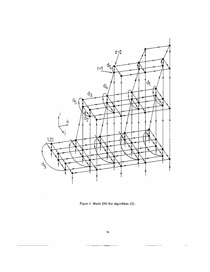
Figure 1: Basic DG for algorithm (2).

34

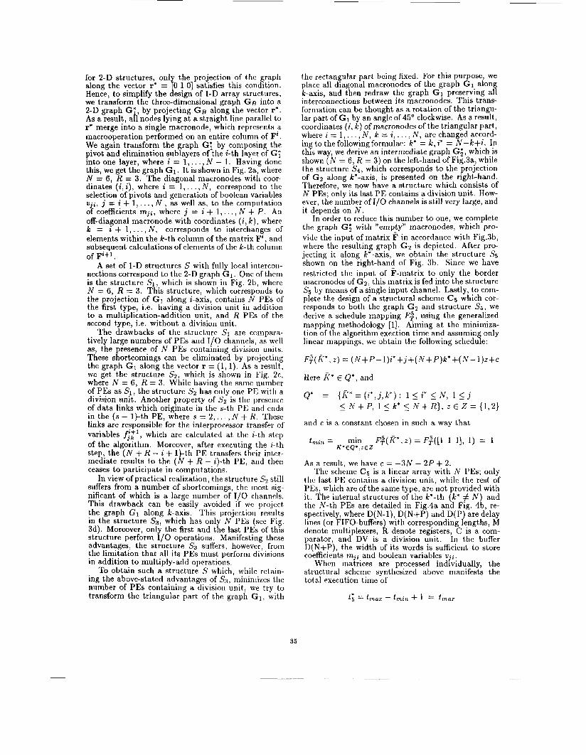
for 2-D structures, on1 the projection of the graph along the vector r* = TO 101 satisfies this condition. Hence, to simplify the design of 1-D array structures, we transform the three-dimensional graph GB into a 2-D graph G*, by projecting G B along the vector r'. As a result, ah nodes lying at a straight line parallel to r* merge into a single macronode, which represents a macrooperation performed on an entire column of F" We again transform the graph G; by composing the pivot and elimination sublayers of the i-th layer of G; into one layer, where i = 1 , . . . , N - 1. Having done this, we get the graph G I . It is shown in Fig. 2a, where N = 6, R = 3. The diagonal macronodes with coor- dinates (i, i), where i = 1 , . . . , N , correspond to the selection of pivots and generation of boolean variables v j i , j = i + 1 , . . . , N , as well as, to the computation of coefficients mji, where j = i + 1 , . . . , N + P . An off-diagonal macronode with coordinates (i, k), where k = i + 1, . . . , N , corresponds to interchanges of elements within the k-th column of the matrix F', and subsequent calculations of elements of the k-th column of Fit'.

A set of 1-D structures S with fully local intercon- nections correspond to the 2-D graph G I . One of them is the structure SI, which is shown in Fig. 2b, where N = 6, R = 3. This structure, which corresponds to the projection of G1 along i-axis, contains N PES of the first type, i.e. having a division unit in addition to a multiplication-addition unit, and R PES of the second type, i.e. without a division unit.

The drawbacks of the structure S1 are compara- tively large numbers of PES and 1 / 0 channels, as well as, the presence of N PES containing division units. These shortcomings can he eliminated by projecting the graph G1 along the vector r = ( 1 , l ) . As a result, we get the structure S2, which is shown in Fig. 2c, where N = 6, R = 3. While having the same number of PES as SI, the structure Sa has only one PE with a division unit. Another property of Sa is the presence of data links which originate in the s-th PE and ends in the (s - 1)-th PE, where s = 2, . . . , N + R. These links are responsible for the interprocessor transfer of variables f!", which are calculated at the i-th step of the algorithm. Moreover, after executing the i-th step, the ( N + R - i + 1)-th PE transfers their inter- mediate results to the ( N + R - i)-th PE, and then ceases to participate in computations.

In view of practical realization, the structure S2 still suffers from a number of shortcomings, the most sig- nificant of which is a large number of 1 / 0 channels. This drawback can be easily avoided if we project the graph GI along k-axis. This projection results in the structure S3, which has only N PES (see Fig. 3d). Moreover, only the first and the last PES of this structure perform 1 / 0 operations. Manifesting these advantages, the structure Ss suffers, however, from the limitation that all its PES must perform divisions in addition to multiply-add operations,

To obtain such a structure S which, while retain- ing the above-stated advantages of &, minimizes the number of PES containing a division unit, we try to transform the triangular part of the graph G1, with

J k

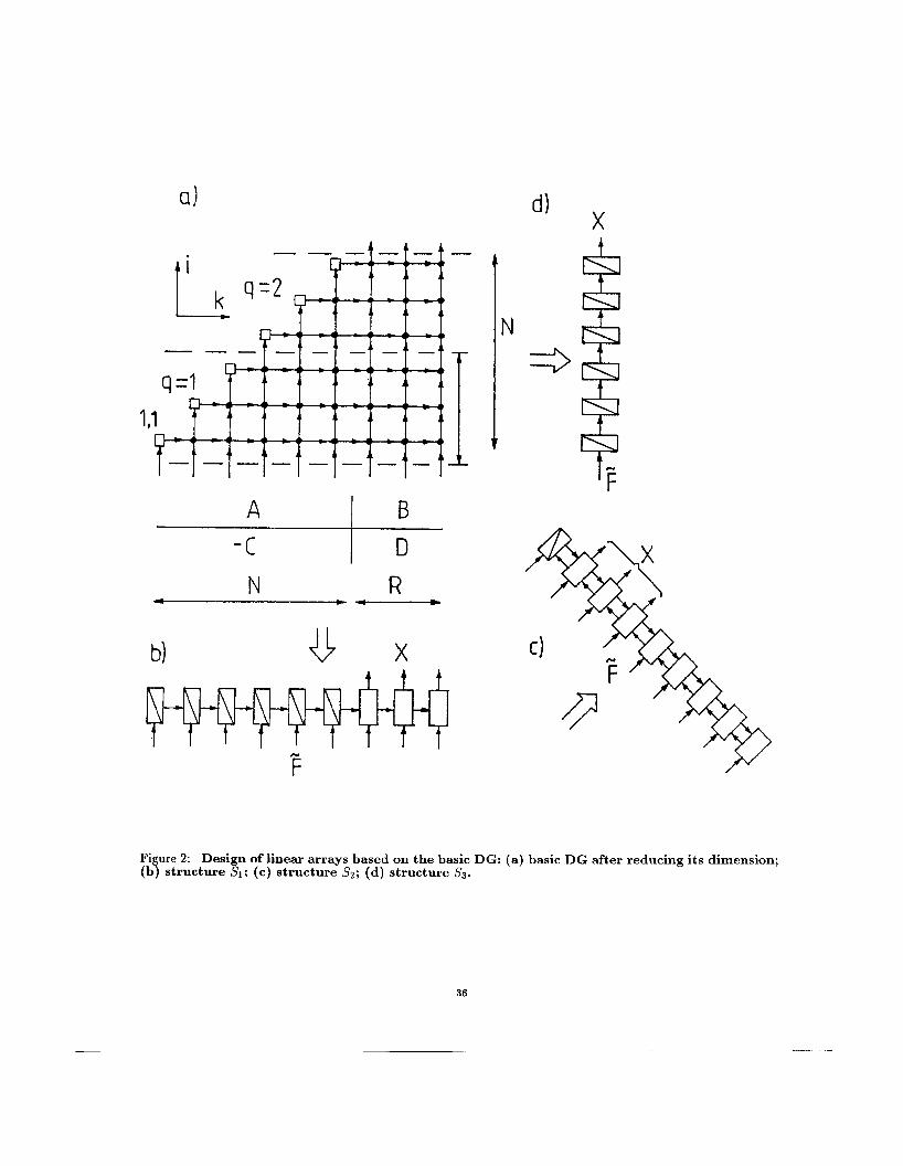
the rectangular part being fixed. For this purpose, we place all diagonal macronodes of the graph G1 along k-axis, and then redraw the graph GI preserving all interconnections between its macronodes. This trans- formation can be thought as a rotation of the triangu- lar part of GI by an angle of 45' clockwise. As a result, coordinates ( i , K ) of macronodes of the triangular part, where i = 1, . . . , N, K = i, . . . , N , are changed accord- ing to the followingformulw: k* = k, i' = N-k+i. In this way, we derive an intermediate graph G;, which is shown ( N = 6, R = 3) on the left-hand of Fig.3a, while the structure Sq, which corresponds to the projection of G2 along k*-axis, is presented on the right-hand. Therefore, we now have a structure which consists of N PES; only its last PE contains a division unit. How- ever, the number of 1 / 0 channels is still very large, and it depends on N .

In order to reduce this number to one, we complete the graph G ; with "empty" macronodes, which pro- vide the input of matrix F in accordance with Fig.3b, where the resulting graph Gz is depicted. After pro- jecting it along k*-axis, we obtain the structure S5 shown on the right-hand of Fig. 3b. Since we have restricted the input of F-matrix to only the border macronodes of G2, this matrix is fed into the structure S5 by means of a single input channel. Lastly, to com- plete the design of a structural scheme C5 which cor- responds to both the graph Gz and structure S5, we derive a schedule mapping F f , using the generalized mapping methodology [l]. Aiming a t the minimiza- tion of the algorithm exection time and assuming only linear mappings, we obtain the following schedule:

F;( I?', z) = ( N + P - l) i* +j+( N + P)k* +( N - l ) z+c

Here I?* E &*, and

Q* = { K * = ( i * , j , k * ) : l < i * < N , 1 s j 5 N + P, 1 5 k* 5 N + R} , z E Z = {1,2}

and c is a constant chosen in such a way that

As a result, we have c = -3N - 2P + 2. The scheme Cs is a linear array with N PES; only

the last PE contains a division unit, while the rest. of PES, which are of the same t,ype, are not provided with

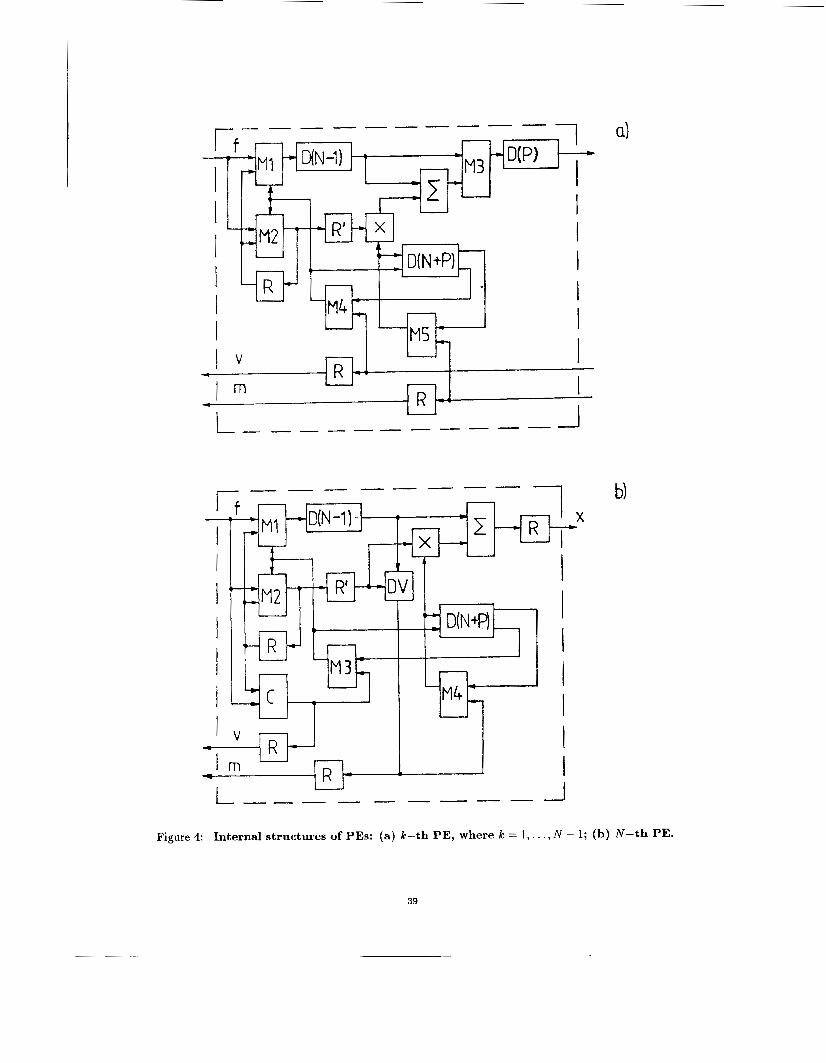
the N-th PES are detailed in Fig.4a and Fig. 4 b , and re- it. The internal structures of the k*-th (IC* # N

spectively, where D(N-l), D(N+P) and D(P) are delay lines (or FIFO-buffers) with corresponding lengths, M denote multiplexers, R denote registers, C is a com- parator, and DV is a division unit. In the buffer D(N+P), the width of its words is sufficient to store coefficients mji and boolean variables vj~j",

When matrices are processed individually, the structural scheme synthesized above manifests the tot.al execution time of

35

a)

I

X d)

N

i

A I B -C I D

i i x

Figure 2: Design of linear arrays based on the basic DG: (a) basic DG after reducing its dimension; (b) structure SI; (c) structure S2; (d) structure Ss.

36

X

D X

i =I b )

A

N I

8

q = l

,-. X F

c )

i =I

-C I D

;J d)

X

kF'

Figure 3: Design of linear arrays, using transformations of the basic DG: (a) intermediate DG and structure S, corresponding to it; (b) resulting DG and structure Ss corresponding to it; (c) DG partitionning for the LPGS scheme; (d) fixed-size linear array for the Faddeev algorithm.

37

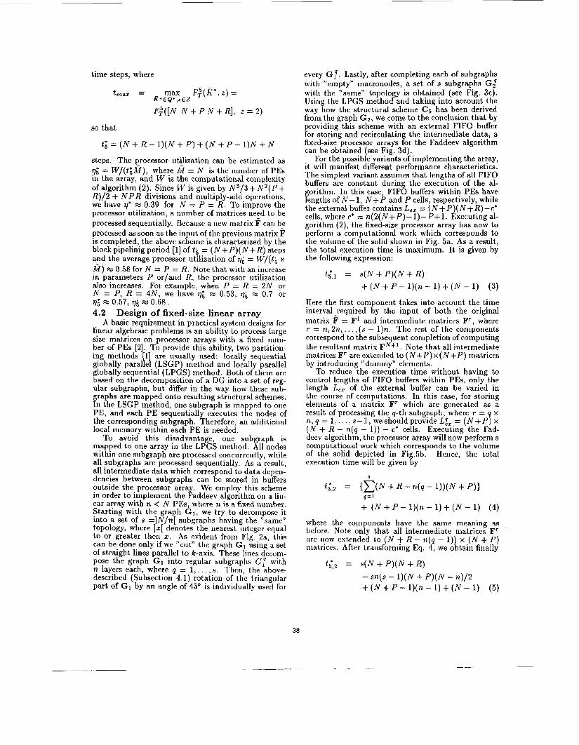
time steps, where

F$([N A'+ P N + RI, z = 2)

so that

t; = ( N + R - 1)(N + P ) + ( N + P - 1)N + N

steps. The processor utilization can be estimated as 17; = W/(tgA?), where M = N is the number of PES in the array, and W is the computational complexity of algorithm (2). Since W is given by N 3 / 3 + N 2 ( P + R)/2 + N P R divisions and multiply-add operations, we have q* R 0.39 for N = P = R. To improve the processor utilization, a number of matrices need to be processed sequentially. Because a new matrix F can b: processed as soon as the input of the previous matrix F is completed, the above scheme is characterized by the block pipelinig period [l] of tt = ( N + P ) ( N + R) steps and the average processor utilization of q; = W/( t ; x &f) R 0.58 for N = P = R. Note that with an increase in parameters P or/and R, the processor utilization also increases. For example, when P = R = 2N or N = P, R = 4N, we have q; M 0.53, 11; M 0.7 or q; x 0.57, q; R 0 .68 . 4.2 Design of fixed-size linear array

A basic requirement in practical system designs for linear algebraic problems is an ability to process large size matrices on processor arrays wi th a fixed nuin- ber of PES [2]. To provide this ability, two partition- ing methods 1 are usually used: locally sequential globally para1 I t e (LSGP) method and locally parallel globally sequential (LPGS) method. Both of them are based on the decomposition of a DG into a set of reg- ular subgraphs, but differ in the way how these sub- graphs are mapped onto resulting structural schemes. In the LSGP method, one subgraph is mapped to one PE, and each PE sequentially executes the nodes of the corresponding subgraph. Therefore, an additional local memory within each PE is needed.

To avoid this disadvantage, one subgraph is mapped to one array in the LPGS method. All nodes within one subgraph are processed concurrently, while all subgraphs are processed sequentially. As a result, all intermediate data which correspond to data depen- dencies between subgraphs can be stored in buffers outside the processor array. We employ this scheme in order to implement the Faddeev algorithm on a lin- ear array with n < N PES, where n is a fixed number. Starting with the graph GI, we try to decompose it into a set of s = N / n [ subgraphs having the "same" topology, where ]x[ denotes the nearest integer equal to or greater then x. As evident from Fig. 2a, this can be done only if we "cut" the graph G I using a set of straight lines parallel to k-axis. These lines decom- pose the graph GI into regular subgraphs GP with n layers each, where q = 1 , . . . ,s. Then, the above- described (Subsection 4.1) rotation of the triangular part of GI by an angle of 45' is individually used for

every GP. Lastly, after completing each of subgraphs with "empty" niacronodes, a set of s subgraphs G t with the "same" topology is obtained (see Fig. 3c). Using the LPGS method and taking into account the way how the structural scheme C5 has been derived from the graph Gz, we come to the conclusion that by providing this scheme with an external FIFO buffer for storing and recirculating the intermediate data, a fixed-size processor arrays for the Faddeev algorithm can be obtained (see Fig. 3d).

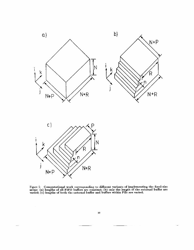
For the possible variants of implementing the array, it will manifest different performance characteristics. The simplest variant assumes that lengths of all FIFO buffers are constant during the execution of the al- gorithm. In this case, FIFO buffers within PES have lengths of N - 1, N + P and P cells, respectively, while the external buffer contains Le, = ( N + P ) ( N + R ) - c ' cells, where c* = n ( 2 ( N + P ) - l ) - P + l . Executing al- gorithm (2), the fixed-size processor array has now to perform a computational work which corresponds to the volume of the solid shown in Fig. 5a. As a result, the total execution time is maximum. It is given by the following expression:

t;,l = s ( N + P ) ( N + R) + ( N + P - l ) (n - 1) + ( N - 1) (3)

Here the first component takes into account the time interval -required by the input of both the original matrix F = F' and intermediate matrices F", where r = n, 2 7 1 , . . . , (s - 1)n. The rest of the components correspond to the subsequent completion of computing the resultant matrix FN+'. Note that all intermediate matrices F" are extended to ( N + P ) x ( N + P ) matrices by introducing "dummy" elements.

To reduce the execution time without having to control lengths of FIFO buffers within PES, only the length Le, of the external buffer can be varied in the course of computations. In this case, for storing elements of a matrix F' which are generated as a result of processing the q-th subgraph, where r = q x n, q = 1,. . . , s-1, we should provide L:! = ( N + P ) x ( N + R - n(q - 1)) - c* cells. Executing the Fad- deev algorithm, the processor array will now perform a computational work which corresponds to the volume of the solid depicted in Fig.5b. Hence, the total execution time will be given by

s

t;,z = { C ( N + R - 4 q - 1))(N + PI1 q = l

+ ( N + P - l ) (n - 1) + ( N - 1) (4)

where the components have the same meaning as before. Note only that all intermediate matrices F' are now extended to ( N + R - n(q - 1)) x ( N + P ) matrices. After transforrniiig Eq. 4, we obtain finally

t;,a = s ( N + P ) ( N + R) - sn(s - l ) ( N + P ) ( N - n)/2 + ( N + P - l ) ( n - l ) + ( N - l ) (5)

38

U I I

- I " I

I U

I

I I U 1 I b R I m

I J I - - - - - - - -

Figure 4: Internal structures of PES: (a) k-th PE, where k = 1,. . . , N - 1; (b) N-th PE.

39

I < I

Figure 5: Computational work corresponding to different variants of implementing the fixed-size array: (a) lengths of all FIFO buffers are constant; (b) only the length of the external buffer are varied; ( c ) lengths of both the external buffer and buffers within PES are varied.

40

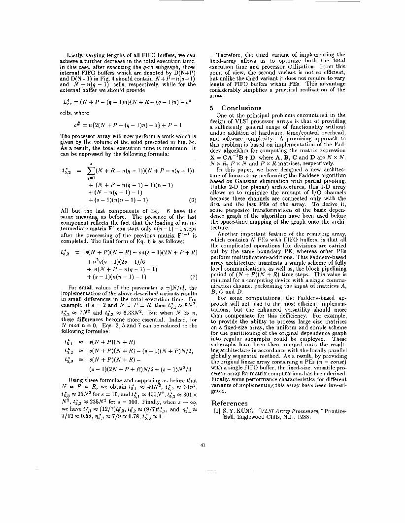
Lastly, varying lengths of all FIFO buffers, we can achieve a further decrease in the total execution time. In this case, after executing the q-th subgraph, those internal FIFO buffers which are denoted by D(N+P) and D( N - 1) in Fi ,4 should contain N + P - n ( q - 1) and N - n q - 17 cells, respectively, while for the

Lzz = ( N + P - ( q - l)n)(N + R - ( q - 1)n) - C#

external bu d er we should provide

cells, where

c# = n{2(N + P - ( q - 1)n) - 1 ) + P - 1

The processor array will now perform a work which is given by the volume of the solid presented in Fig. 5c. As a result, the total execution time is minimum. It can be expressed by the following formula:

3

t;,3 = C ( N + R - n(q - 1))(N + P - n(q - 1)) g=l

+ ( N + P - n(q - 1) - l)(n - 1)

+ ( s - l)(n(n - 1) - 1) + ( N - n(q - 1) - 1)

(6)

All but the last components of Eq. G have the same meaning as before. The presence of the last component reflects the fact that the loadin of an in- termediate matrix F‘ can start only n(n - lf - 1 steps after the processing of the previous matrix Fr-’ is completed. The final form of Eq. 6 is as follows:

t:,3 = s (N + P ) ( N + R) - ST*(S - 1)(2N 4 P + R) + n2s(s - l)(2s - 1)/G + n ( N + P - n(q - 1) - 1 ) + (s - l ) (n(n - 1) - 1) (7)

For small values of the parameter s =IN/??[, tlie implementation of the above-described variants results in small differences in the total execution time. For example, i f s = 2 and N = P = R, t,hen f & = 8N2, t l , 2 x 7N2 and t;,3 G.33N2. But when N >> 1 1 ,

these differences become more essent,ial. Indeed, for N mod n = 0, Eqs- 3, 5 and 7 can be reduced to the following formulae:

t;,l x s ( N + P ) ( N + R) t;,2 “ s ( N + P ) ( N + R) - ( s - 1)(N + P ) N / 2 , t;,3 s ( N + P ) ( N + R) -

(s - 1)(2N + P + R)N/2 + (s - 1)N2/3

Using these formulae and supposing as before that N = P = R, we obtain t;,l x 40N2, t;,2 w 31n2,

25N2 fors = 10, and t<,l x 400N2, f;,2 w 301 x N 2 , w 235N2 for s = 100. Finally, when s -- 00, we have M (12/7)t{,3, 1;,2 w (9/7)t;,,, and v; ,~ = 7/12 x 0.58, )75:2 x 7/9 x 0.78, t5:3 x 1.

Therefore, the third variant of implementing the fixed-array allows us to optimize both the total execution time and processor utilization. From this point of view, the second variant is not so efficient, but unlike the third variant it does not require to vary lengts of FIFO buffers within PES. This advantage considerably simplifies a practical realization of the array.

5 Coiiclusioiis One ot the principal probleiiis encountered in the

design of VLSI processor arrays is that of providing a suficiently general range of functionality without undue addition of hardware, time/control overhead, and software complexity. A promising approach to this problem is based on implementatmion of the Fad- deev algorithm for computing the matrix expression X = CA-lB + D , where A, B, C and D are N x N , N x R, P x N and P x R matrices, respectively.

In this paper, we have designed a new architec- ture of linear array performing the Faddeev algorithm based on Gaussian elimination with partial pivoting. Unlike 2-D (or planar) architectures, this 1-D array allows us to minimize the amount of 1/0 channels because these channels are connected only with the firsl and the last PES of the array. To derive it, some purposive transformations of the basic depen- dence graph of tlie algorithm have been used before the space-time mapping of the graph ont80 the archi- tecture.

Another importmalit feature of the resulting array, which contains N PES with FIFO buffers, is that all the coniplicated operations like divisions are carried out by the same boundary PE, whereas other PES perform multiplication-additions. This Faddeev-based array architecture manifests a simple scheme of fully local communications, as well as, the block pipelining period of ( N + P ) ( N + R) time steps. This value is minimal for a computing device with a single commu- nication channel performing the input of matrices A , B , C and D.

For some computations, the Faddeev-based ap- proach will not lead to the most efkient implemen- tations, but tlie enhanced versatility should more than compensate for this defficiency. For example, to provide the ability to process large size matrices on a fixed-size array, the uniform and simple scheme for the partitioning of the original dependence graph into regular subgraphs could be employed. These subgraphs have been then mapped onto the result- ing architecture in accordance with the locally parallel globally sequential method. As a result, by providing the original linear array containing n PES ( n = const) with a single FIFO buffer, the fixed-size, versatile pro- cessor array for matrix coniputatioiis has been derived. Finally, some performance cliaract<eristics for different variants of implenienting this array have been investi- gated.

References [I] S. Y. KUNG, “VLSI Army Processors, ” Prentice-

Hall, Eiiglewood Cliffs, N . J . , 1988.

41

J. H. MORENO, and T. Lang, “Matrix Compu- tations on Systolic-Type Meshes,” Computer, Vol.

J. RICE, “Matrix Computations and Mathemat- ical Soflware,” McGraw-Hill Book Comp., New York, 1981.

J. G. NASH, and S. HANSEN, “Modified Faddeev Algorithm for Concurrent Execution of Linear Algebraic Operations,’’ IEEE Trans.

D. K. FADDEEV, and V. N. FADDEVA, “Coni- putational Methods of Linear Algebra,” W. H. Freeman and Company, 1963.

H. Y. H. CHUANG, and G. HE, “A Versatile Sys- tolic Array for Matrix Computations,” Ini. Symp. Comput. Archat., pp.315-322, 1985.

H. V. D. LE, and M. A. PERKOWSKI, “A New General Purpose Systolic Architecture for Matrix Computations,” Proc. Int. Conf. on Computing and Information, ICCI’89, Ontario, 1989.

H. V. D. LE, and M. A. PERKOWSKI, “Realiza- tion of Extensions to Faddeev algorithm on Array of SIMD Processors’, Proc. IEEE In!. Synip. Circuits and Syst . , New Orleans, pp.2312-2315, May 1990.

23, NO. 4, pp.32-51, 1990.

Comput., Vol. C-37, pp.129-137, 1988.

[9] M. A. BAYOUMI, P. RAO, and B. ALHALABI, “VLSI Parallel Architectures for Kalman Filter- ing: An Algorithm Specific Approach,” J. VLSI Signal Process., Vol. 4, pp. 147-163, 1992.

[lo] M. GENTLEMAN, and H. T. KUNG, “Matrix Triangularisation by Systolic Arrays,” PFOC. SPIE, Vol. 298, pp. 19-26, 1982.

42

D. SORENSON, “Analysis of Pairwise Pivoting in Gaussian Elimination,” IEEE Tram. Comput,

M. COSNARD, “Designing Parallel Algorithms for Linearly Connected Processors and Systolic Arrays,” Advances in Parallel Computing, Vol. 1,

R. WYRZYKOWSKI, “Processor Arrays for Matrix Triangularisation with Partial Pivoting,” IEE PFOC. E, Compul. Digit. Tech., Vol. 139,

D. I. MOLDOVAN, and J . A. B. FORTES, “Par- titioning and Mapping Algorithms into Fixed- Size Systolic Arrays,” IEEE Trans. Comput. , Vol.

V. V. VOEVODIN, ‘‘Mathematical Models and Methods in Parallel Computing, ” Nauka, Moscow, 1986 (in Russian).

Vol. C-34, pp. 274-278, 1985.

pp. 273-317, 1990.

No.2, pp. 165-169, 1992.

C-35, pp. 1-12, 1986.