Embed Size (px)
DESCRIPTION
The paper describes research on the prediction of horizontal displacements and internal forces in an anchored wall for the protection of an excavation, using standard field and laboratory tests and a finite-element programme with a soil model that can simulate the key aspects of soil behaviour at a construction site.
Citation preview

ACTA GEOTECHNICA SLOVENICA, 2008/1 5.
ADVANCES AND UNCERTAINTIES IN THE DESIGN OF ANCHORED RETAINING WALLS USING NUMERICAL MODELLING
ANTUN SZAVITS NOSSAN
About the author
Antun Szavits NossanUniversity of Zagreb,Faculty of Civil EngineeringKačićeva 26, 10 000 Zagreb, CroatiaE-mail: [email protected]
Abstract
This paper describes research on the prediction of hori-zontal displacements and internal forces in an anchored wall for the protection of an excavation, using standard field and laboratory tests and a finite-element programme with a soil model that can simulate the key aspects of soil behaviour at a construction site. It is important to be acquainted with the constitutive model incorporated in the programme, and the selection of the appropriate soil parameters for the numerical analysis is a crucial part of the modelling. As a result, it is useful to carry out numerical simulations of standard laboratory tests with well-known soil behaviour in order to select the relevant parameters for the simulation of the actual construction process.It is shown in this paper that the measurements of the shear-wave velocities, which can provide the soil’s stiffness at very small strains, can also be useful for determining the static stiffness at a magnitude of the strains relevant for the geotechnical structure under consideration, for both cohesive and noncohesive soils.The research was carried out by a detailed analysis of a case history involving an anchored, reinforced concrete wall supporting the walls of an excavation in a relatively stiff soil. The wall displacements were monitored using an installed inclinometer.The major part of the paper is devoted to an analysis of the selection of parameters, especially the stiffness parameters. The simulation of the triaxial, consolidated, undrained tests was used in order to assess the reduction of the secant stiffness modulus with an increase of the relative mobi-lized shear strength for the hard clay layer according to the published empirical evidence. It is shown that by selecting the appropriate stiffness parameters for the soil model used
in the numerical analysis, it is possible to get an acceptable prediction of the anchored-wall displacements. This is just one example of a successful analysis, but it is encouraging in the way that it shows how it is possible to make reliable predictions based on standard field and laboratory tests and with the use of an available computer programme with a realistic soil model.
Keywords
anchored wall, soil model, shear stiffness, numerical modelling, measured displacements
1 INTRODUCTION
Anchored, retained structures are often used as tempo-rary protection for deep excavations in urban areas. Their role is to ensure the stability of the soil around the excavation and to prevent any damage to surrounding buildings that might be caused by the excavation. The successful design of such structures depends a great deal on a realistic solution to the interaction between the structure, the anchors and the soil, taking into consider-ation the mechanical characteristics of the surrounding soil as well as the manner and the sequence of the construction. Gaba et al. [1] gave an overview of the available numerical methods, together with an assess-ment of their advantages and drawbacks. A detailed solution to the interaction problems is becoming increasingly more accessible with the use of commercial, numerical tools based primarily on the finite-element method, which allows for the use of complex, constitu-tive soil models [2], [3]. There are, however, serious problems with the practical use of these tools. Schweiger [4] describes a detailed benchmarking experiment in which several experts were invited to numerically model the behaviour of an anchored diaphragm wall. The results were scattered over an alarmingly wide range, which is not acceptable in practice, due to the selection of different constitutive models and soil parameters. De Vos and Whenham [5] have shown the results of a survey among a large number of users of geotechnical

ACTA GEOTECHNICA SLOVENICA, 2008/16.
finite-element programmes that show the problems they were encountering. The first item on the list of problems is the determination of soil parameters (23% of answers), followed by the determination of the initial conditions in the soil, the selection of the constitutive soil model, the interpretation of the results, the numeri-cal discretization, the boundary conditions and the selection of the type of analysis. The first three items represent the core of the geotechnical design, supported by numerical modelling, and so they appeared at the top of the list in more than 50% of the answers. Gaba et al. [1] state, among others, the following reasons for these problems: the inadequate constitutive models, where the simple ones are not realistic; the data on soil strength; the stiffness and initial stresses that are not of sufficient quality; the insufficient user experience with the particu-lar programme; and the inadequate modelling of the undrained conditions in cohesive soils. They claim that “Ground movements cannot be predicted accurately. It is essential that optimum use is made of precedent in comparable conditions through the use of good-quality case-history data. Case-history-based empirical methods of prediction are to be preferred to the use of complex analyses, unless such analyses are first calibrated against reliable measurements of well-monitored comparable excavations and wall systems.” In any case, finite-element analyses should be used with caution, but they remain the only tool in cases of unusual structures for which there is no comparable experience.
Studies in which complex numerical models are calibrated against the monitoring data of a case history can be helpful in resolving the above-mentioned prob-lems related to the use of commercial finite-element programmes for geotechnical structures. This paper describes such a case history and the subsequent numerical modelling. The case history comprises an excavation protected by an anchored, retaining struc-ture, of which there are several examples constructed recently in Zagreb, Croatia. Standard geotechnical inves-tigations of average quality were carried out along with measurements of the shear-wave velocities with respect to depth. It was intended to use these measurements for the prediction of the anchored-wall displacements, based on the significance of this aspect of soil behaviour, which has recently gained attention [6], related to the soil-structure interaction [7] and particularly to the interaction of the soil with the anchored walls [8]. Shear-wave velocities provide a direct in-situ measure of the soil stiffness without the necessity to retrieve undisturbed soil samples or use problematic correla-tions. The anchored-wall displacements were monitored during construction, and the excavation was successfully completed. Subsequent numerical analyses were carried
out using the finite-element programme Plaxis V8 [9], which is widely used in Croatia. Its option of small strain was used in order to take advantage of the shear-wave velocity measurements and the resulting soil stiffness at very small strains. It was decided, for practical reasons, to use Plaxis V8, even though sophisticated analyses of anchored walls at small strains have been reported [10], but using a commercially unavailable programme.
Designers in Croatia are familiar with the use of Plaxis for modelling anchored structures. Their predictions of displacements based on the standard recommendations for the selection of soil parameters usually turn out as a significant overestimation in comparison with the measured wall displacements. As a result they use a higher soil stiffness, based on the argument of available data on similar structures in similar soils. This type of reasoning, which is not based on serious studies, makes the use of complex finite-element calculations question-able, because they do not seem to have a significant advantage over, for example, the method of a beam resting on elasto-plastic springs, where the springs’ char-acteristics are determined empirically from displacement measurements on similar anchored walls.
2 THE CASE HISTORY
The excavation, 14.5 m deep, is located in a rapidly expanding commercial area in Zagreb, and is intended for the construction of underground storeys of a commercial building. An existing, old, brick house, sensitive to soil displacements, is located near to the excavation. A 17.5-m-high and 0.6-m-thick wall of reinforced concrete, embedded in the soil 4 m below the bottom of the excavation, provided protection. The wall was cast in place prior to the excavation works.
Three rows of BBR 1860/1660 pre-stressed ground anchors were installed at a horizontal distance of 2.5 m in each row. The upper, first row anchors consist of 4 strands of high-strength steel, 0.6” in diameter. The second and third row anchors consist of 5 strands. Each anchor in the first two rows was pre-stressed to 500 kN, whereas the anchors in the third row were pre-stressed to 650 kN. Inclinometer measurements of the relative horizontal wall displacements were taken during the excavation works. The inclinometer tube was installed in the wall concrete along its whole height at the location of the brick house. The vertical excavation section with the wall and the neighbouring house is shown in Fig. 1.
A. S. NOSSAN: ADVANCES AND UNCERTAINTIES IN THE DESIGN OF ANCHORED RETAINING WALLS USING NUMERICAL MODELLING
ACTA GEOTECHNICA SLOVENICA, 2008/1 7.
Figure 1. Vertical excavation section, reinforced concrete wall with three rows of anchors and the neighbouring brick house.
The ground surface at the location is horizontal and the underlying ground is horizontally layered. The surface layer is around 2 m thick and it consists of medium dense fill and clay underlain by a layer of poorly graduated medium dense gravel down to a depth of 14 m. Below this depth is a thick layer of hard, overcon-solidated clay. The geotechnical field investigation was carried out in several 30-m-deep boreholes. Disturbed and undisturbed samples were retrieved and SPT measurements were taken. The shear-wave velocities were measured in two boreholes using the down-hole method. The underground water level was determined in the gravel layer at 7 m below the ground surface.
Standard classification tests were carried out in the laboratory on disturbed samples, and undisturbed clay samples were used for the triaxial, consolidated, undrained (CIU) and unconsolidated, undrained (UU) tests. The CIU tests were performed with pore-water
pressure measurements in order to determine the effec-tive shear-strength parameters. The undrained shear strength was determined in the UU tests and with the use of a pocket penetrometer. The undisturbed clay samples were also used for oedometer tests. The results of the field and laboratory tests are presented in Fig. 2.
The SPT blow count N was corrected by the standard hammer impact energy of 60% and the normalized vertical effective stress, where pref = 100 kPa, according to Skempton [11]
( )N Np
1 60 60=′
ref
vσ (1)
The full line in Fig. 2 represents the selected character-istic value of the design parameter (N1)60 according to Eurocode 7 [12]. The same characteristic value of
A. S. NOSSAN: ADVANCES AND UNCERTAINTIES IN THE DESIGN OF ANCHORED RETAINING WALLS USING NUMERICAL MODELLING

ACTA GEOTECHNICA SLOVENICA, 2008/18.
this parameter was selected for the gravel for reasons of simplicity, even though a larger value could have been selected for the gravel above the water level. It also seemed reasonable to select a unique value of this parameter for the entire clay layer.
The characteristic value of the shear modulus for very small strains, G0 , was determined from the shear-wave velocity through G v0
2= ρ s , where ρ is the soil density. The distribution of this modulus with depth was assumed according to the following expression
G Gp0 0=′ref v
ref
σ (2)
where G0ref is the reference shear modulus at a verti-
cal effective stress of 100 kPa. Two distinct values of G0
ref were allocated to the entire layers of gravel and clay. No such parameter was allocated to the thin surface layer because it was assumed that its influence on the behaviour of the anchored wall was negligible. The full line in Fig. 2 shows the design characteristic shear-wave velocities, which result from the above assumptions.
The characteristic value of the effective angle of internal friction ′ϕ for the gravel layer was determined through the correlation with ( )N1 60 proposed by Hatanaka and Uchida [13]
′( )= +ϕ 0 01 6020 15 4. ( )N (3)
which gives a characteristic value of ′ =ϕ 350 for ( )N1 60 14= . Even though this correlation was derived for sandy soils, there were no reliable data for gravel available.
The characteristic values of the effective cohesion, ′c , and the effective angle of internal friction for the clay layer were determined by the interpretation of the triaxial CIU tests. The shear-strength parameters were selected at the point where the ratio of the major and minor principal effective stresses reaches a maximum. The test results and the selected values of the shear-strength parameters are shown in Fig. 3. The other characteristic parameter values depend on the selected soil model, and their determination will be described in the next section.
Figure 2. Soil profile with the fines and sand content in the gravel, the water content (w0), the liquid limit (wL) and the plastic limit (wP), the undrained shear strength (cu), the corrected SPT blow count (N1 and (N1)60) and the shear-wave velocity (vs).
A. S. NOSSAN: ADVANCES AND UNCERTAINTIES IN THE DESIGN OF ANCHORED RETAINING WALLS USING NUMERICAL MODELLING

ACTA GEOTECHNICA SLOVENICA, 2008/1 9.
3 THE SOIL MODEL
The hardening-soil model with the option of using the soil stiffness at small strains was selected from the Plaxis V8 programme. This model is described in the programme manual [9] and in much more detail by Schanz et al. [14] and Benz [15]. It is described here only to the extent of explaining the selection of the required parameters. The original hardening model, which did not have the option for small strain stiffness, is described first.
This soil model is of the elasto-plastic isotropic harden-ing type with two hardening laws, each with its own yield surface and plastic potential. It satisfies the Mohr-Coulomb strength criterion with a constant effective cohesion ′c and a constant effective angle of internal friction ′ϕ . The first hardening law is related to shear (S) with a convex yield surface that crosses the Mohr-Coulomb envelope at the point where the deviatoric stress q= 0 . It is used to model irreversible strains due to primary deviatoric loading. The second hardening law is related to the compression (C) and it is used to model irreversible plastic strains due to primary compression in the oedometer loading and the isotropic loading. When the loading phase results in the effective stress path reaching the two yield surfaces, they are “dragged” along with the stress path, thus producing both elastic and plastic strains. The development of the plastic
A. S. NOSSAN: ADVANCES AND UNCERTAINTIES IN THE DESIGN OF ANCHORED RETAINING WALLS USING NUMERICAL MODELLING
Figure 3. Clay shear-strength parameters from the results of the CIU tests and selected characteristic values. The numbers connected to the symbols represent the vertical strains ε1 (%) at the maximum value of ′ ′σ σ1 3 .
Figure 4. Stress path and yield surfaces for the hardening model from Plaxis V8 for a soil going throughits geologic phases of sedimentation, overconsolidation and triaxial undrained shear.
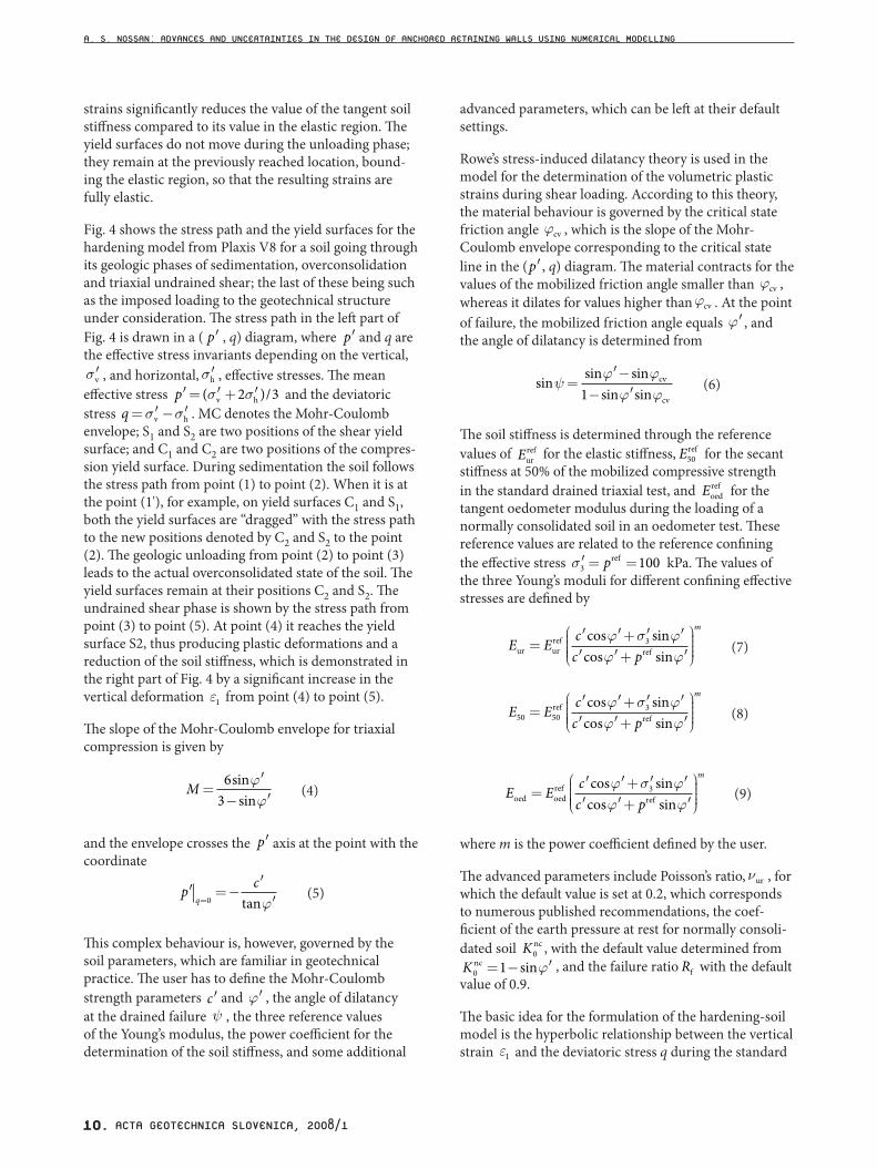
ACTA GEOTECHNICA SLOVENICA, 2008/110.
strains significantly reduces the value of the tangent soil stiffness compared to its value in the elastic region. The yield surfaces do not move during the unloading phase; they remain at the previously reached location, bound-ing the elastic region, so that the resulting strains are fully elastic.
Fig. 4 shows the stress path and the yield surfaces for the hardening model from Plaxis V8 for a soil going through its geologic phases of sedimentation, overconsolidation and triaxial undrained shear; the last of these being such as the imposed loading to the geotechnical structure under consideration. The stress path in the left part of Fig. 4 is drawn in a ( ′p , q) diagram, where ′p and q are the effective stress invariants depending on the vertical, ′σv , and horizontal, ′σh , effective stresses. The mean
effective stress ′ = ′ + ′p ( )/σ σv h2 3 and the deviatoric stress q= ′ − ′σ σv h . MC denotes the Mohr-Coulomb envelope; S1 and S2 are two positions of the shear yield surface; and C1 and C2 are two positions of the compres-sion yield surface. During sedimentation the soil follows the stress path from point (1) to point (2). When it is at the point (1'), for example, on yield surfaces C1 and S1, both the yield surfaces are “dragged” with the stress path to the new positions denoted by C2 and S2 to the point (2). The geologic unloading from point (2) to point (3) leads to the actual overconsolidated state of the soil. The yield surfaces remain at their positions C2 and S2. The undrained shear phase is shown by the stress path from point (3) to point (5). At point (4) it reaches the yield surface S2, thus producing plastic deformations and a reduction of the soil stiffness, which is demonstrated in the right part of Fig. 4 by a significant increase in the vertical deformation ε1 from point (4) to point (5).
The slope of the Mohr-Coulomb envelope for triaxial compression is given by
M =′
− ′6
3sinsin
ϕϕ
(4)
and the envelope crosses the ′p axis at the point with the coordinate
′ =−′′=
p cq 0 tanϕ
(5)
This complex behaviour is, however, governed by the soil parameters, which are familiar in geotechnical practice. The user has to define the Mohr-Coulomb strength parameters ′c and ′ϕ , the angle of dilatancy at the drained failure ψ , the three reference values of the Young’s modulus, the power coefficient for the determination of the soil stiffness, and some additional
advanced parameters, which can be left at their default settings.
Rowe’s stress-induced dilatancy theory is used in the model for the determination of the volumetric plastic strains during shear loading. According to this theory, the material behaviour is governed by the critical state friction angle ϕcv , which is the slope of the Mohr-Coulomb envelope corresponding to the critical state line in the ( ′p , q) diagram. The material contracts for the values of the mobilized friction angle smaller than ϕcv , whereas it dilates for values higher thanϕcv . At the point of failure, the mobilized friction angle equals ′ϕ , and the angle of dilatancy is determined from
sinsin sin
sin sinψ
ϕ ϕϕ ϕ
=′−
− ′cv
cv1 (6)
The soil stiffness is determined through the reference values of Eur
ref for the elastic stiffness, E50ref for the secant
stiffness at 50% of the mobilized compressive strength in the standard drained triaxial test, and Eoed
ref for the tangent oedometer modulus during the loading of a normally consolidated soil in an oedometer test. These reference values are related to the reference confining the effective stress ′ = =σ3 100pref kPa. The values of the three Young’s moduli for different confining effective stresses are defined by
E Ec
c p
m
ur urref
ref=′ ′+ ′ ′′ ′+ ′
⎛
⎝⎜⎜⎜⎜
⎞
⎠⎟⎟⎟⎟
cos sincos sin
ϕ σ ϕϕ ϕ
3 (7)
E Ec
c p
m
50 503=
′ ′+ ′ ′′ ′+ ′
⎛
⎝⎜⎜⎜⎜
⎞
⎠⎟⎟⎟⎟
refref
cos sincos sin
ϕ σ ϕϕ ϕ
(8)
E Ec
c p
m
oed oedref
ref=′ ′+ ′ ′′ ′+ ′
⎛
⎝⎜⎜⎜⎜
⎞
⎠⎟⎟⎟⎟
cos sincos sin
ϕ σ ϕϕ ϕ
3 (9)
where m is the power coefficient defined by the user.
The advanced parameters include Poisson’s ratio, νur , for which the default value is set at 0.2, which corresponds to numerous published recommendations, the coef-ficient of the earth pressure at rest for normally consoli-dated soil K0
nc , with the default value determined fromK0 1nc = − ′sinϕ , and the failure ratio Rf with the default value of 0.9.
The basic idea for the formulation of the hardening-soil model is the hyperbolic relationship between the vertical strain ε1 and the deviatoric stress q during the standard
A. S. NOSSAN: ADVANCES AND UNCERTAINTIES IN THE DESIGN OF ANCHORED RETAINING WALLS USING NUMERICAL MODELLING

ACTA GEOTECHNICA SLOVENICA, 2008/1 11.
isotropically consolidated drained shear, which can be approximated by
ε122 1
≈−
−
RE
qqqa
f
50
(10)
where qa is the asymptotic value of the shear strength, related to the deviatoric stress at failure, qf , throughq q Ra = f f , and the deviatoric stress at failure is defined by
q cf = ′+ ′′
− ′( cot ) sin
sinϕ σ
ϕϕ3
21
(11)
The recently developed new version of the Plaxis programme has the possibility to model the soil stiffness at small strains. This option requires two additional soil parameters, the reference shear modulus at very small strains, G0
ref , and the reference shear strain, γ0 7. . The first parameter serves for a determination of the shear modulus at very small strains G0 through
G Gc
c p
m
01=
′ ′+ ′ ′′ ′+ ′
⎛
⎝⎜⎜⎜⎜
⎞
⎠⎟⎟⎟⎟0
refref
cos sincos sin
ϕ σ ϕϕ ϕ
(12)
The reference shear strain is the value of the shear strain attained when the shear modulus, G0 , reduces to 70% of its initial value. The Plaxis manual recommends the following expression for its determination
γ ϕ σ ϕ0 70
1 01
92 1 2 1 2. ( cos ) ( )sin ’= ′ + ′ + ′ +⎡⎣ ⎤⎦G
c K (13)
where K0 is the coefficient of the earth pressure at rest. K0 and the overconsolidation ratio OCR may be defined by the user in order to define the initial stresses.
4 DETERMINATION OF THE SOIL PARAMETERS AND THE INITIAL STRESS STATE
Due to the complex constitutive relationship used in the numerical modelling, the determination of the soil parameters for the hardening-soil model deserves special attention. The intention in this research was to use those parameters that were readily available, either from tests and measurements performed at the construction site and in the laboratory or from correla-tions published in the literature. It has to be emphasized that the parameters were not adjusted so as to get the best agreement between the measured and the calcu-
lated displacements for a class-C prediction, after the completion of construction, instead, they were selected as if a class-A prediction were to be made prior to the construction.
The determination of the parameters for the hard clay layer is described first, because it required an analysis in both the drained and the undrained conditions, as the two limiting states for the development of the deforma-tions. The undrained conditions are required because of the clay’s low permeability and the high rate at which the excavation proceeded.
For the undrained conditions, the designer can make a total stress analysis with the determined, undrained shear strength, or an effective stress analysis with the requirement that there are no volumetric strains during the excavation. The second approach was chosen for this research because it was estimated that the undrained shear strength of the hard clays, determined in labora-tory tests on undisturbed samples, is not sufficiently reliable because such samples might contain fissures. These fissures lead to an unrealistically fast consolidation and, thus, a too fast transition from the undrained to the drained state. This approach is on the safe side and it represents a cautious estimate of the characteristic values in terms of Eurocode 7 [12].
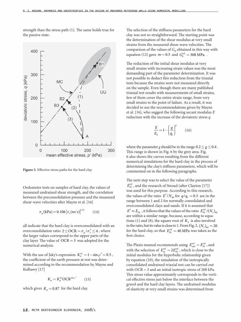
The hardening-soil model is, however, very limited in terms of the choice of the effective stress analysis in undrained conditions. This is especially so for hard, overconsolidated clays, for which the undrained shear strength is larger than the drained shear strength. The soil parameters that successfully model the shear strength and the dilatancy characteristics in drained conditions lead to an unrealistic, extremely large, undrained shear strength. The only way to avoid this is to set the angle of dilatancy ψ= 0 for the hard clay, which ensures that the material volume does not change during the shear loading at the drained failure. The result is a significantly lower undrained shear strength for the numerical model than the one determined from laboratory tests, as shown in Fig. 5. Curve (1) represents the assumed effective stress path in undrained condi-tions from the initial state at point A to failure at point B1 on the Mohr-Coulomb envelope (MC) in the grey area, which shows the range of measured values for the undrained shear strength in the UU tests. Curve (2) is the effective stress path in undrained conditions, from the initial state to the failure at point B2 for the hardening-soil model with an angle of dilatancy ψ= 0 . Curve (3) is the effective stress path in drained condi-tions for the idealized case of Rankine active pressures on the wall. It is obvious from Fig. 5 that the stress path (2) gives a much lower value for the undrained shear
A. S. NOSSAN: ADVANCES AND UNCERTAINTIES IN THE DESIGN OF ANCHORED RETAINING WALLS USING NUMERICAL MODELLING
ACTA GEOTECHNICA SLOVENICA, 2008/112.
strength than the stress path (1). The same holds true for the passive state.
Figure 5. Effective stress paths for the hard clay.
Oedometer tests on samples of hard clay, the values of measured undrained shear strength, and the correlation between the preconsolidation pressure and the measured shear-wave velocities after Mayne et al. [16]
σp skPa( ) . ( / ) .= [ ]0 106 1 47v m s (14)
all indicate that the hard clay is overconsolidated with an overconsolidation ratio 2 4≤ = ′ ≤OCR p vσ σ/ , where the larger values correspond to the upper parts of the clay layer. The value of OCR= 3 was adopted for the numerical analysis.
With the use of Jaky’s expression K0 1 0 5nc = − ′=sin .ϕ , the coefficient of the earth pressure at rest was deter-mined according to the recommendation by Mayne and Kulhawy [17]
K K0 0= ′ncOCRsinϕ (15)
which gives K0 0 87= . for the hard clay.
The selection of the stiffness parameters for the hard clay was not so straightforward. The starting point was the determination of the shear modulus at very small strains from the measured shear-wave velocities. The comparison of the values of G0 obtained in this way with equation (12) gave m= 0 5. and G0 308ref MPa= .
The reduction of the initial shear modulus at very small strains with increasing strain values was the most demanding part of the parameter determination. It was not possible to deduct this reduction from the triaxial tests because the strains were not measured directly on the sample. Even though there are many published triaxial test results with measurements of small strains, few of them cover the entire strain range, from very small strains to the point of failure. As a result, it was decided to use the recommendations given by Mayne et al. [16], who suggest the following secant modulus E reduction with the increase of the deviatoric stress q
EE
g
0
1= −⎛
⎝⎜⎜⎜⎜
⎞
⎠⎟⎟⎟⎟
f
(16)
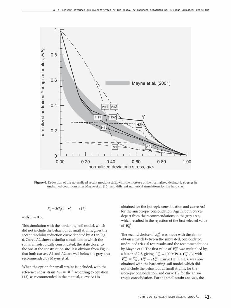
where the parameter g should be in the range 0 2 0 4. .≤ ≤g . This range is shown in Fig. 6 by the grey area. Fig. 6 also shows the curves resulting from the different numerical simulations for the hard clay in the process of determining the clay’s stiffness parameters, which will be commented on in the following paragraphs.
The next step was to select the value of the parameterE50
ref , and the research of Stroud (after Clayton [17]) was used for this purpose. According to this research, the values of the ratio ′E N/ 60 for q q/ .f = 0 5 are in the range between 1 and 2 for normally consolidated and overconsolidated clays and sands. If it is assumed that ′ ≈E E50 , it follows that the values of the ratio E N50 1 60
ref /( ) are within a similar range, because, according to equa-tions (1) and (8), the square root of K0 is also involved in the ratio, but its value is close to 1. From Fig. 2, ( )N1 60 20=for the hard clay, so that E50
ref MPa= 40 was taken as the first choice.
The Plaxis manual recommends using E Eoedref ref= 50 , and
with the selection of E Eurref ref= 2 50 , which is close to the
initial modulus for the hyperbolic relationship given by equation (10), the simulation of the isotropically consolidated undrained triaxial test can be carried out with OCR = 3 and an initial isotropic stress of 200 kPa. This stress value approximately corresponds to the verti-cal effective stress just below the interface between the gravel and the hard clay layers. The undrained modulus of elasticity at very small strains was determined from
A. S. NOSSAN: ADVANCES AND UNCERTAINTIES IN THE DESIGN OF ANCHORED RETAINING WALLS USING NUMERICAL MODELLING
ACTA GEOTECHNICA SLOVENICA, 2008/1 13.
Figure 6. Reduction of the normalized secant modulus E/E0 with the increase of the normalized deviatoric stresses inundrained conditions after Mayne et al. [16], and different numerical simulations for the hard clay.
E G0 02 1= +( )ν (17)
with ν = 0 5. .
This simulation with the hardening-soil model, which did not include the behaviour at small strains, gives the secant modulus reduction curve denoted by A1 in Fig. 6. Curve A2 shows a similar simulation in which the soil is anisotropically consolidated, the state closer to the one at the construction site. It is obvious from Fig. 6 that both curves, A1 and A2, are well below the grey area recommended by Mayne et al.
When the option for small strains is included, with the reference shear strain γ0 7
410. =− according to equation
(13), as recommended in the manual, curve As1 is
obtained for the isotropic consolidation and curve As2 for the anisotropic consolidation. Again, both curves depart from the recommendations in the grey area, which resulted in the rejection of the first selected value of E50
ref .
The second choice of E50ref was made with the aim to
obtain a match between the simulated, consolidated, undrained triaxial test results and the recommendations by Mayne et al. The first value of E50
ref was multiplied by a factor of 2.5, giving E G50 0100 3ref refMPa= ≈ / , withE Eoed
ref ref= 50 , E Eurref ref= 2 50 . Curve H1 in Fig. 6 was now
obtained with the hardening-soil model, which did not include the behaviour at small strains, for the isotropic consolidation, and curve H2 for the aniso-tropic consolidation. For the small strain analysis, the
A. S. NOSSAN: ADVANCES AND UNCERTAINTIES IN THE DESIGN OF ANCHORED RETAINING WALLS USING NUMERICAL MODELLING

ACTA GEOTECHNICA SLOVENICA, 2008/114.
recommended equation (13) was not applied for the determination of the reference shear strain, but a value of γ0 7
52 10. = ⋅ − was chosen instead. Curve Hs1 was the result for the isotropic consolidation and curve Hs2 for the anisotropic consolidation. These two curves provide a much better comparison with the Mayne et al. grey area, particularly the curve for the isotropic consolida-tion.
The deviations of the curve Hs2 from the grey area, with a sharp break at point Y, are the consequences of the characteristics of the hardening-soil model, i.e., the values of q q/ f lower than the one at point Y are below the yield surface S2 in Fig. 4. At point Y, the stress path reaches this yield surface at point (4) from Fig. 4, after which, it was shown, the reduction of stiffness occurs all the way to the point of failure when q q/ f equals 1. Even though similar research could not be found in the literature, it is not likely that the break at point Y reflects the actual soil behaviour. It seems more likely that the real Hs2 curve passes much closer to the grey area. It is interesting to note that a similar approach for the determination of the modulus reduction as a function of q q/ f was adopted by Mayne [19] for the calculation of settlements of spread foundations. They reported good agreement with the observed settlement of the experi-mental foundation.
The additional verification of the validity of the numerical simulations was carried out by comparing calculated vertical strains ε1 with the values measured in laboratory triaxial tests. It was noted that in simulated triaxial tests, where the behaviour at small strains was not included (curves H1 and H2 in Fig. 6), the vertical strains at the point of failure, defined by the maximum value of the ratio ′ ′σ σ1 3/ , differ by a small margin from the results of the simulated triaxial tests with small strains (curves Hs1 and Hs2). This means that the small strain behaviour in the range 0 0 2≤ ≤q q/ .f , where the modulus reduction is most important, does not have a significant influence on the strains close to the point of failure. Even though there are significant differences between curves H1 and H2, on the one hand, and Hs1 and Hs2 on the other, the anisotropic consolidation does not dominate over the isotropic consolidation for strains at the point of failure.
The calculated vertical strains at the point of failure for curves H1, H2, Hs1 and Hs2 are in the range between 2.8% and 3.2%. This is in very good agreement with the measured strains in the laboratory triaxial tests, which were in the range between 2.4% and 4.4% (Fig. 3). This is another indicator that the numerically simulated hard clay behaviour was within the measured values.
The stiffness parameters for the poorly graded gravel were determined in a similar way as for the hard clay, except for the dilatancy during shear, which was not disregarded. The gravel dilatancy was estimated based on the assessment of its critical state friction angle ϕcv
which, in turn, was determined through the round-ness parameter R. For predominantly sub-rounded to rounded grains, 0 5 0 7. .≤ ≤R , and by using the correla-tion suggested by Santamarina and Cho [20]
ϕcv0 042 17( )= − R (18)
With the use of equation (6), the angle of dilation ψ= 60 .
It was also estimated that due to its geologic age in the zone of strong local seismicity (IXth zone of the MCS intensity scale), the gravel would probably exhibit preconsolidation characteristics. It was just assumed that the preconsolidation ratio has a value of OCR = 2. The coefficient of the earth pressure at rest could then be calculated from equation (15) as K0 0 6= . . The effect of the selection of the assumed values was tested, and it turned out that the influence of the value of OCR on the wall displacements was negligible, which was not the case for the hard clay.
G0 226ref MPa= was determined from the measured shear-wave velocity with m = 0.5. The other stiffness parameters were determined using the same equations as for hard clay, E G50 075 3ref refMPa= ≈ / , E Eoed
ref ref= 50 and E Eur
ref50ref= 2 .
Table 1 lists the user-provided gravel and hard-clay parameters for the numerical analysis using the harden-ing-soil model, and Table 2 gives the parameters for the calculation of the initial stresses.
It is interesting to note that for both the gravel and the hard clay, the following two ratios gave approximately the same values
EN
50
1 60
5ref MPa)
MPa(
( )≈ (19)
GN
0
1 60
15ref MPa
MPa( )
( )≈ (20)
Since the top fill layer is of small thickness, it was disre-garded in the analysis in a way that it was assumed that the gravel layer extended from the ground surface.
As for the required parameters for the supporting wall and anchors, the modulus of elasticity of the reinforced
A. S. NOSSAN: ADVANCES AND UNCERTAINTIES IN THE DESIGN OF ANCHORED RETAINING WALLS USING NUMERICAL MODELLING

ACTA GEOTECHNICA SLOVENICA, 2008/1 15.
concrete was taken as Erc MPa= ⋅2 5 104. , and the design concrete section bending resistance at the occur-rence of a plastic hinge as MRd MNm/m= 0 4. accord-ing to Eurocode 7. The anchor modulus of elasticity was taken as Es MPa= ⋅1 95 105. , the stiffness of the anchors with four strands as E As MN= ⋅1 17 102. , and those with five strands as E As MN= ⋅1 46 102. . The design anchor resistance to steel extension was taken as Rad = 0.844 MN for the anchors with four strands and Rad = 1.06 MN for the anchors with five strands.
Table 1. Soil parameters for the analysis with the hardening-soil model.
Parameter Symbol UnitValue
gravel hard clayReference stress pref kPa 100Saturated density ρsat kN/m3 21 21Density above GWL ρunsat MkN/m3 20 21Permeability k m/day 100 10-4
Reference Young’s modulus at 50% mobilized strength E50ref Mpa 75 100
Reference oedometer modulus Eoedref Mpa 75 100
Reference elastic Young’s modulus Eurref Mpa 150 200
Elastic Poisson’s ratio (effective) νur - 0.2 0.2Power coefficient m - 0.5 0.5Effective cohesion ′c kPa 2 25
Effective friction angle ′ϕ degree 35 30
Angle of dilatancy at drained failure ψ degree 6 0
Coefficient of earth pressure at rest (normally consolidated soil) K0nc - 0.426 0.5
Failure ratio Rf - 0.9 0.9Tension cut off - - yes yesReference shear strain γ0 7. - 2 · 10-5 2 · 10-5
Reference small strain shear modulus G0ref Mpa 226 308
Table 2. Soil parameters for the initial stress state.
Parameter Symbol UnitValue
gravel hard clayCoefficient of earth pressure at rest K0 - 0.6 0.87Overconsolidation ratio OCR - 2 3Depth of phreatic surface - m -7 -7
5 SIMULATION OF THE CONSTRUCTION AND THE COMPUTED DISPLACEMENTS
The soil-structure interaction was analysed in phases that simulated the real construction stages. After the calculation of the initial stresses and the pore-water pressures was completed, the excavation was simulated as shown in Table 3. The load of the neighbouring house was estimated to be 720 kN/m, uniformly distributed on strip foundations and acting vertically. Each excavation phase, except for the last one, was subdivided into two parts, the first part comprising the excavation to the
A. S. NOSSAN: ADVANCES AND UNCERTAINTIES IN THE DESIGN OF ANCHORED RETAINING WALLS USING NUMERICAL MODELLING
ACTA GEOTECHNICA SLOVENICA, 2008/116.
selected depth, and the ground-anchor pre-stressing in the second part. Drained conditions were assumed for the gravel layer and undrained conditions were assumed for the hard clay layer in all the construction phases.
As the excavation reached under the underground water level, the water level was lowered to the bottom of the excavation and the pore-water pressures were calculated as
u u u= +0 e (21)
where u0 are the pressures due to seepage and ue are the excess pore pressures developed in undrained condi-tions. For drained conditions in gravel ue = 0 at all times. The last calculation phase consisted of consolida-tion to the fully drained state in all the soil layers. The time development of the consolidation process was not simulated because of the unreliable data on the coeffi-cient of consolidation. No measurements of pore-water pressure in the clay were taken during the construction.
Table 3. Construction calculation phases.
No. PhaseDepth belowground level
m
AnchorsPre-stressing force (kN) Spacing (m)
0 initial state - - -0a load from the adjacent house -1.7 - -1 excavation -5 - -1a anchor pre-stressing -4 500 2.52 excavation -8 - -2a anchor pre-stressing -7.5 500 2.53 aexcavation -12 - -3a anchor pre-stressing -11.5 650 2.54 excavation -14.3 - -5 consolidation - - -
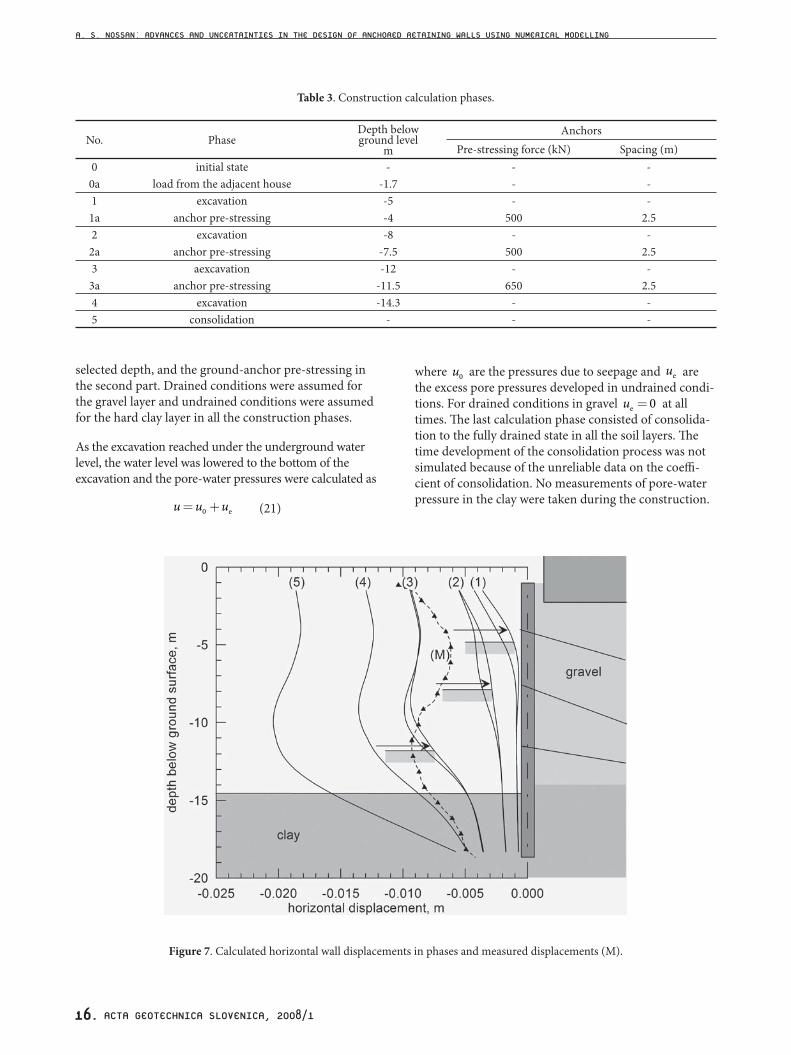
Figure 7. Calculated horizontal wall displacements in phases and measured displacements (M).
A. S. NOSSAN: ADVANCES AND UNCERTAINTIES IN THE DESIGN OF ANCHORED RETAINING WALLS USING NUMERICAL MODELLING

ACTA GEOTECHNICA SLOVENICA, 2008/1 17.
Fig. 7 shows the calculated development of the horizon-tal displacements of the anchored wall in phases denoted by the numbers in the brackets. The analysis was performed with the hardening-soil model and the small strains. The measured relative horizontal wall displace-ments after the last excavation phase are also shown by the curve (M). These displacements are relative because the inclinometer does not record the rigid-body wall translation. Thus, the bottom measured value is attached to curve (4) for undrained conditions after the comple-tion of the excavation because it is assumed that the measured displacements occurred in such conditions.
The calculated displacements in phase 4 deviate signifi-cantly from the measured displacements. However, the calculated shape of the wall bending seems to be well in accordance with the measured one. Also, when the deviations are regarded in the light of the parameter-selection process and the generally negative experience in the prediction of displacements, then the obtained calculation results do seem to be encouraging and, from the point of view of the designer, acceptable. This partic-ularly holds true when the fact that the displacement prediction was simulated on the basis of the available data and literature, and not actually a class-C prediction, is taken into account.
It has, however, to be noted that the measured displace-ments indicate the wall is bending more than the calculations are showing. This means that savings on the reinforcement of the wall should not be made.
Fig. 8 shows the comparison of the wall horizontal displacements calculated with (full lines) and without (dashed lines) small strains near and after the comple-tion of the excavation. The differences between the corresponding curves with and without small strains are not significant, which might appear surprising, but previously described simulations of triaxial, consoli-dated, undrained tests showed that vertical strains at the point of failure do not differ much between the two options, which explains the results in Fig. 8. The gener-alization of these results would lead to the conclusion that for practical purposes it is not necessary to include the soil behaviour at small strains for similar walls and similar ground conditions. However, the shear modulus at very small strains is still the most important param-eter for the determination of other stiffness parameters. If it were not used, the accurate prediction of wall displacements would not have been feasible. This fact emphasizes the importance of measuring the shear-wave velocity in situ.
Figure 8. Comparison of horizontal wall displacements near and after the completion of the excavation with (full lines) and without (dashed lines) small strains.
A. S. NOSSAN: ADVANCES AND UNCERTAINTIES IN THE DESIGN OF ANCHORED RETAINING WALLS USING NUMERICAL MODELLING

ACTA GEOTECHNICA SLOVENICA, 2008/118.
When comparing the wall bending moments with and without small strains, the differences are more signifi-cant, the bending moments being smaller in the analysis with small strains than in the one without small strains. Similar results are obtained for the anchor forces.
Another comparison was made in order to determine the influence of the overconsolidation ratio on the behaviour of the gravel. Fig. 9 shows the results for the overconsolidation ratio of 2 and for normally consoli-dated gravel with OCR = 1 and K K0 0 0= =nc 426. . The full lines correspond to the overconsolidated gravel and the dashed lines to the normally consolidated gravel, all calculated with the option for small strains. It is clear that the differences between the corresponding curves are negligible, so that the overconsolidation ratio for the gravel does not influence its behaviour. The same does not hold true for the hard clay, but this analysis is of minor importance because the overconsolidation ratio for the clay was determined with sufficient certainty.
The stability analysis was also performed using the option of reducing the soil’s strength parameters by a common factor, which can then be taken as the safety factor for the soil. For undrained conditions the safety factor was F ≈1 6. , and for drained conditions F ≈1 3. . It has to be emphasized that the performed analyses
Figure 9. Comparison of horizontal wall displacements near and after the completion of the excavationfor the overconsolidated (full lines) and the normally consolidated (dashed lines) gravel.
lead to the mobilization of the wall resistance, and for the undrained conditions also the mobilization of the anchor steel resistance. While this is not especially important for the wall, due to its ductility, it is of utmost importance for the anchor steel, because it has brittle behaviour, which leads to an annulment of the anchor forces at failure. As a result, it is essential to determine at exactly which point the anchor steel resistance is mobilized. In the undrained conditions, this occurred for a safety factor of a little below 1.6.
6 CONCLUSIONS
The described research of a case history involving the construction of an anchored wall for the protection of an excavation showed that it is possible to adequately predict wall displacements and stability based on standard geotechnical investigations, soil data from the literature and a finite-element computer programme with a realistic soil model. It was shown that it is very important to clearly understand the functioning of the selected soil model. This can be achieved by numerical simulations of a standard laboratory test with stress paths that are relevant for the geotechnical structure under consideration.
A. S. NOSSAN: ADVANCES AND UNCERTAINTIES IN THE DESIGN OF ANCHORED RETAINING WALLS USING NUMERICAL MODELLING
ACTA GEOTECHNICA SLOVENICA, 2008/1 19.
The soil-parameter determination for numerical simula-tions has the most important role in this type of analysis and the most valuable parameter is the shear modulus at very small strains, obtained from field measurements of the shear-wave velocity. The reduction of the shear modulus with increasing strains was obtained by using published evidence. The soil behaviour was analysed with and without the option of small strains. It is clear that it is not necessary to use modelling with small strains in order to get a satisfactory prediction of the wall displacements because the differences in the two types of analysis are within the general uncertainties of modelling. However, the determination of the soil stiff-ness at larger strains has to be very detailed and based on solid arguments, because it greatly influences the results.
This is just one example of an analysis of a case history, but it is encouraging, and further similar research might lead to more reliable and more economic designs. Until then, the prediction of soil behaviour in similar situa-tions will still be a challenge for designers who have to take into consideration that the use of finite-element programmes requires a studious approach.
ACKNOWLEDGEMENTS
This research was conducted with the help of G. Plepelić from Prizma, Zagreb, and I. Sokolić and V. Szavits-Nossan from the Faculty of Civil Engineering of the University of Zagreb, to whom I would like to express my deep gratitude.
REFERENCES
[1] Gaba, , A. R., Simpson, B., Powrie, W. Beadman, D. R. (2003). Embedded retaining walls – guidance for economic design. CIRIA Report C580, London.
[2] Potts, D. M., Zdravkovic, L. (2001). Finite element analysis in geotechnical engineering: Aplication. Thomas Telford, London.
[3] Potts, D., Axelsson, K., Grande, L., Scweiger, H., Long, M. (2002). Guidelines fort he use of advanced numerical analysis. Thomas Telford, London.
[4] Schweiger, F. H. (2002). Benchmarking in geotechnics 1. Report No.CGG_IR006_2002. Computational GeotechnicsG roup, Institute for Soil Mechanics and Foundation Engineering, Graz University of Technology, Austria.
[5] De Vos, M., Whenham, V. (2006). Workpackage 3 – Innovative design methods in geotechnical engi-neering. Bacground document to part 2 of the final WP3 report on the use of finite element and finite
difference methods in geoechnical engineering. Geotechnet (http://www.geotechnet.org)
[6] Burland, J.B. (1989). Small is beautiful-the stiffness of soils at small strains. Canadian Geotechnical Journ., Vol. 26, 499-516.
[7] Jardine, R.J., Potts, D.M., Fourie, A.B. & Burland, J.B. (1986). Studies of the influence of non-linear stress-strain characteristics in soil-structure inter-action. Géotechnique, Vol. 36 (3): 377-396.
[8] Simpson, B. (1992). Retaining structures: Displace-ment and design. Géotechnique, Vol. 42 (4), 541-576.
[9] Brinkgreve, R.B., Broere, W., Waterman, D. (2006). PLAXIS 2D Version 8. Plaxis bv, Delft.
[10] Szavits-Nossan, A., Kovačević, M.S., Szavits-Nossan, V. (1999). Modeling of an anchord diaphragm wall. Proc. Interntl. FLAC Symposium on Numerical Modeling in Geomechanics: FLAC and Numerical Modeling in Geomechanics. Minne-apolis. eds.: Detournay & Hart, Balkema, Rotter-dam, 451-458.
[11] Skempton, A.W. (1986). SPT procedures and the effects in sands of overburden pressure, relative density, particle size, aging, and overconsolidation. Géotechnique, Vol. 36 (3), 425-447.
[12] BSI (2004). BS EN 1997-1:2004; Eurocode 7: Geotech-nical design – Part 1: General rules. British standard.
[13] Hatanaka, M. and Uchida, A. (1996). Empirical correlation between penetraion resistance and effective friction of sandy soil. Soils & Foundations, Vol. 36 (4), 1-9.
[14] Schanz, T., Vermeer, P.A. & Bonnier, P. G. (1999). The hardening soil model - formulation and verification. Plaxis Symposium ‘‘Beyond 2000 in Computational Geomechanics’’, Balkema, Amsterdam, 281–296.
[15] Benz, T. (2007). Small-Strain Stiffness of Soils and its Numerical Consequences. Dr-Ing Thesis. Institute of Geotechnics, University of Stuttgart, Stuttgart.
[16] Mayne, P. W., Christopher, B. R., De Jong, J. (2001). Manual on Subsurface Investigations. National High-way Institute, Publication No. FHWA NHI-01-031, Federal Highway Administration, Washington, DC.
[17] Mayne, P.W. and Kulhawy, F.H. (1982). K0-OCR relationships in soil. Journal of Geotechnical Engi-neering, Vol. 108 (GT6), 851-872.
[18] Clayton, C. R. I. (1995). The Standard Penetration Test (SPT): Methods and Use. Report 143, CIRIA, London.
[19] Mayne, P. W. (2000). Enhanced geotechnical site characterization by seismic piezocone penetration tests. Ivited lecture. Fifth International Geotechnical Conference, Cairo University, Cairo, 95-120.
[20] Santamarina, J. C., Cho, G. C. (2004). Soil behaviour: The role of particle shape. Advances in Geotechnical Engineering: The Skempton Confer-ence. Thomas Telford, London, Vol. 1, 604-617.
A. S. NOSSAN: ADVANCES AND UNCERTAINTIES IN THE DESIGN OF ANCHORED RETAINING WALLS USING NUMERICAL MODELLING


![Procesi te enja u tlu i stijeni str. 1 Vlasta Szavits-Nossan ...1].pdftla je γ = 19 kN/m3, Youngov modul elastinosti E′ = 5 MPa (zadaje se u kPa), a č Poissonov koeficijent ν′](https://img.pdfslide.net/doc/110x75/60a53e57780fe84ab7158363/procesi-te-enja-u-tlu-i-stijeni-str-1-vlasta-szavits-nossan-1pdf-tla-je-.jpg)