T H A M E S V A L L E Y

S E R V I C E S

ARCHAEOLOGICAL

Straighthanger Field, Sonning, Berkshire

Geophysical Survey (Magnetic)

by Tim Dawson

Site Code Geo12/6

(SU 7657 7593)

Straighthanger Field, Sonning, Berkshire

Geophysical Survey (Magnetic) Report

For University of Reading

by Tim Dawson

Thames Valley Archaeological Services Ltd

Site Code Geo12/6

November 2012

i Thames Valley Archaeological Services Ltd, 47–49 De Beauvoir Road, Reading RG1 5NR

Tel. (0118) 926 0552; Fax (0118) 926 0553; email tvas@tvas.co.uk; website: www.tvas.co.uk

Summary

Site name: Straighthanger Field, Sonning, Berkshire Grid reference: SU 76577 75937 Site activity: Magnetometer survey Date and duration of project: 7th - 19th November 2012

Project manager: Steve Ford Site supervisor: Tim Dawson Site code: Geo12/6 Area of site: 8.15ha Summary of results: A wide variety of probable archaeological features were identified by the geophysical survey. Of these, several had already been noted by aerial surveys but the geophysics served to extend and clarify these in addition to plotting previously unknown features. Those identified include a cursus, three rectangular enclosures, a ring ditch and several linear features. Additionally, a probable palaeochannel and several agricultural features and areas of magnetic disturbance were noted. Location of archive: The archive is presently held at Thames Valley Archaeological Services, Reading in accordance with TVAS digital archiving policies. This report may be copied for bona fide research or planning purposes without the explicit permission of the copyright holder. All TVAS unpublished fieldwork reports are available on our website: www.tvas.co.uk/reports/reports.asp. Report edited/checked by: Steve Ford 23.11.12 Andrew Mundin 22.11.12

1

Straighthanger Field, Sonning, Berkshire A Geophysical Survey (Magnetic)

by Tim Dawson

Report Geo12/6

Introduction

This report documents the results of a geophysical survey (magnetic) carried out at Straighthanger Field,

Sonning, Berkshire (SU 76577 75937) (Fig. 1). The work was undertaken as a research project with the

permission of the landowner, the University of Reading, and English Heritage.

The field investigation was carried out to a specification approved by Mr Chris Welch, Inspector of Ancient

Monuments at English Heritage and in accordance with an Ancient Monuments and Archaeological Areas Act

1979 (as amended) under licence to carry out a geophysical survey (Licence No: SL00042648). The fieldwork

was undertaken by Marta Buczek, Aiji Castle and Tim Dawson between 7th and 19th November 2012 and the

site code is Geo12/6.

The archive is presently held at Thames Valley Archaeological Services, Reading in accordance with

TVAS digital archiving policies.

Location, topography and geology

The site is located on agricultural land halfway between the villages of Sonning and Charvil, to the east of

Reading, in eastern Berkshire. The River Thames is located c.750m northwest of the site with the Bath Road

(A4) located c.250m to the southeast (Fig. 1). The site itself is an irregularly-shaped field, currently lying fallow

after a recent harvest with wide overgrown boundaries along all edges except the eastern. Topographically, the

field is on two levels: a plateau c.40m above Ordnance Datum (aOD) in the south-eastern half that falls away to

the edge of the Thames flood plain to the north at c.35m aOD. This reflects the underlying geology with the

upper, south-eastern part of the site being located primarily on Taplow gravel formation with bands of Seaford

chalk and Lambeth group clay along its southern edge while the remainder of the site is on Kempton Park gravel

(BGS 1971).

Ground and weather conditions during the survey were favourable. Ground cover consisted of short wheat

stubble with patches of nettles over a firm, largely level, topsoil while the weather remained largely dry during

the survey period (Plates 1 and 2). There were however, particularly around the edges of the field, rutted, boggy

trackways that were not conducive to the regular pacing required for accurate surveying.

2

Site history and archaeological background

An extensive series of cropmarks have been identified from aerial photography (Slade 1964; Gates 1975 map 19,

and Pl. 11) and the RCHME’s National Mapping Programme. Amongst these a Scheduled Ancient Monument

has been defined warranting preservation due to ‘nationally significant remains being identified’ (SAM

no.1006962). This includes a 35m-wide cursus and rectangular, circular and polygonal enclosures as well as

several intercutting linear features (Ford 1987). Excavations on one of the rectangular enclosures (Slade 1964)

confirmed the presence of archaeological remains of Neolithic date with some Roman activity.

Methodology

Sample interval

Data collection required a temporary grid to be established across the survey area using wooden pegs at 30m

intervals with further subdivision where necessary. Readings were taken at 0.25m intervals along traverses 1m

apart. This provides 3600 sampling points across a full 30m × 30m grid (English Heritage 2008), providing an

appropriate methodology balancing cost and time with resolution. The proposed grid was to extend north and

west to cover the western end of the field from a point at SU 7676 7576, targeting the cropmarks summarised by

Gates and the RCHME. This would have consisted of a total of 125 30m × 30m grid squares. A new hedgerow

had, however, divided the field in two, along the eastern edge of the survey grid, cutting across the proposed

survey area. This obstruction had no effect on the position of the actual grid plan but did prevent the eastern edge

from being surveyed fully. Other obstructions included the rough, boggy ground aforementioned and the strip of

thick undergrowth around three sides of the field, all of which meant that the overall area available for surveying

was somewhat reduced. In total, therefore, 98 grid squares were surveyed (Fig. 2).

The Grad 601-2 has a typical depth of penetration of 0.5m to 1.0m. This would be increased if strongly

magnetic objects have been buried in the site. Under normal operating conditions it can be expected to identify

buried features >0.5m in diameter. Features which can be detected include disturbed soil, such as the fill of a

ditch, structures that have been heated to high temperatures (magnetic thermoremnance) and objects made from

ferro-magnetic materials. The strength of the magnetic field is measured in nano Tesla (nT), equivalent to 10-9

Tesla, the SI unit of magnetic flux density.

3

Equipment

The purpose of the survey was to identify geophysical anomalies that may be archaeological in origin and

compare the resulting plot with that drawn from cropmarks identified through aerial survey. The survey and

report generally follow the recommendations set out by both English Heritage (2008) and the Institute for

Archaeologists (2002).

Magnetometry was chosen as a survey method as it offers the most rapid ground coverage and responds to

a wide range of anomalies caused by past human activity. These properties make it ideal for fast yet detailed

survey of an area.

The detailed magnetometry survey was carried out using a dual sensor Bartington Instruments Grad 601-2

fluxgate gradiometer. The instrument consists of two fluxgates mounted 1m vertically apart with a second set

positioned at 1m horizontal distance. This enables readings to be taken of both the general background magnetic

field and any localised anomalies with the difference being plotted as either positive or negative buried features.

All sensors are calibrated to cancel out the local magnetic field and react only to anomalies above or below this

base line. On this basis, strong magnetic anomalies such as burnt features (kilns and hearths) will give a high

response as will buried ferrous objects. More subtle anomalies such as pits and ditches, can be seem from their

infilling soils containing higher proportions of humic material, rich in ferrous oxides, compared to the

undisturbed subsoil. This will stand out in relation to the background magnetic readings and appear in plan

following the course of a linear feature or within a discrete area.

A Trimble GeoXH 6000 handheld GPS system with sub-decimetre accuracy was used to tie the site grid

into the Ordnance Survey national grid. This unit offers both real-time correction and post-survey processing;

enabling a high level of accuracy to be obtained both in the field and in the final post-processed data.

Data gathered in the field was processed using the ArcheoSurveyorLite software package. This allows the

survey data to be collated and manipulated to enhance the visibility of anomalies, particularly those likely to be

of archaeological origin. The table below lists the processes applied to this survey, full survey and data

information is recorded in Appendix 1.

Process Effect Clip from -7.00 to 7.00 nT Enhance the contrast of the image to improve the

appearance of possible archaeological anomalies.

De-stripe: sensors, median, all grids Corrects for the striping effect caused by differences in calibration between the two sets of sensors.

De-spike: threshold 1, window size 3×3, all grids Softens extreme values, enhancing the clarity of possible archaeological features.

De-stagger: out- and in-bound, by: -1 intervals Shifts the results for each traverse 0.25m north or south

4

(0.25m), all grids to correct for changes in pace.

Clip from -1.70 to 2.00 nT Final enhancement of the contrast of the image to improve visibility of possible archaeological anomalies.

Once processed, the results are presented as a greyscale plot shown in relation to the site (Fig. 4), followed

by a second plan to present the abstraction and interpretation of the magnetic anomalies (Fig. 5). Anomalies are

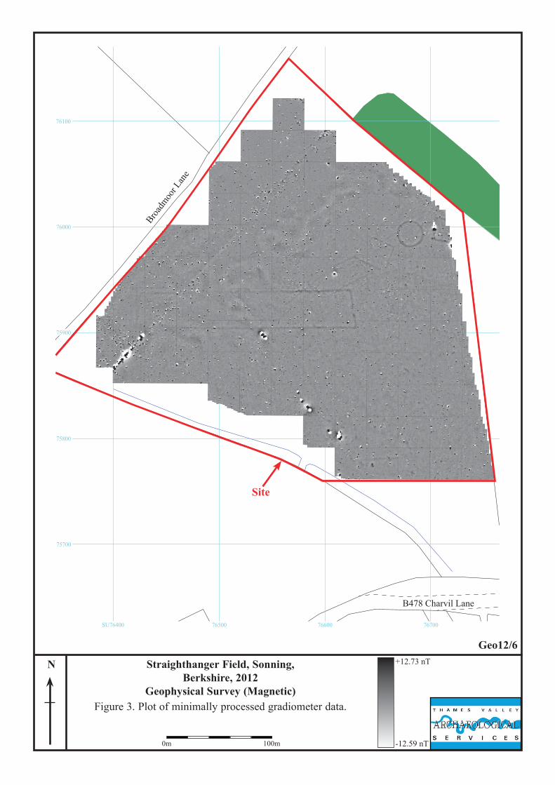
shown as colour-coded lines, points and polygons. A minimally processed version of the greyscale results plot is

presented in Figure 3 for comparison purposes. The grid layout and georeferencing information (Fig. 2) is

prepared in EasyCAD v.7.22.01, producing a .FC7 file format, and printed as a .PDF for inclusion in the final

report.

The greyscale plot of the processed data is exported from ArcheoSurveyorLite in portable network graphics

(.PNG) format, a raster image format chosen for its lossless data compression and support for transparent pixels,

enabling it to easily be overlaid onto an existing site plan. The data plot is rotated to orientate it to north and

combined with grid and site plans in Adobe InDesign CS5.5, creating .INDD file formats. Once the figures are

finalised they are exported in .PDF format for inclusion within the finished report.

Results

A wide range of magnetic anomalies are present across the majority of the site. These are described below

grouped according to the type of anomaly.

Certain and possible archaeological features

Several substantial positive magnetic anomalies cross the centre of the site on a southwest-northeast axis.

The cursus

The most obvious anomaly is a very elongated rectangular enclosure with an opening at its eastern end (Figs. 3-

5); most likely a Neolithic cursus monument as originally identified from aerial views of the cropmarks it created

(Gates 1975, Slade 1964, RCHME) (Fig. 2). It is worth noting that although the aerial photographs allowed for

the plotting of the cursus’ eastern end and the majority of the side ditches, the western end and therefore the

extent of the monument was previously unknown. The west end now appears to have been identified and which

shows it to be rectilinear without an entrance. The cursus can now be shown to be 200 m long and 35m wide.

5

Ring ditch

The strongest of these positive anomalies is the circular feature, most likely a ring ditch, which is c.26m in

diameter and, as with the cursus, was originally identified through its cropmarks (Fig. 2).

Rectangular enclosures

Two certain and one probable rectangular enclosures with the ring ditch extend on a north-easterly axis from the

eastern end of the cursus. Either side of the ring ditch are two rectangular enclosures both recorded as cropmarks

The westernmost (E2) is 25m by 32m aligned northwest - southeast. On the geophysical plot (Fig. 3) the north-

western element is hardly visible, but is clearer on the aerial photograph. The eastern enclosure (E1) is 22m by

28m also aligned northwest - southeast. It is bisected by the modern hedgerow which formed the eastern

boundary of the survey area and could not be fully surveyed. However, it was the latter that was excavated by

Slade (1964) and considered to be a Neolithic mortuary enclosure. A Roman ditch partly overlying this enclosure

can be seen on the aerial photographs but lies beyond the boundary of the geophysical survey.

The third rectangular enclosure (E3) is closest to the cursus and is aligned on a southwest-northeast axis. It

was not previously identified on the aerial photographs but with hindsight might now be faintly visible. It is c.

25m x 20m across. The northwest and south east elements seem well defined (Fig. 3) but the north-eastern and

south-western elements are ill-defined with further obscurity caused by a ferrous spike in the west. The

relationship with Enclosure 2 is unclear.

Linear features

Several linear positive anomalies cut across the enclosures and cursus monument. These are all aligned roughly

southwest-northeast with, in two places, two such features running parallel to each other giving the appearance

of a trackway. Only a few of these anomalies have been previously identified through their cropmark signatures

with the majority being newly discovered. A second set of linear positive anomalies is located in the

southeastern corner of the survey site and approach the cursus before turning through a right angle. They are

possibly old field boundaries.

Two linear negative anomalies run almost parallel to each other in a south-westerly direction from the ring

ditch and across the eastern end of the cursus. While these may represent archaeological features it is possible

that they just signify the presence of old field boundaries.

6

Polygonal enclosure?

Cropmarks interpreted as a polygonal enclosure are represented on the aerial photographs lying at the southern

end of the survey area (Gates 1975 map 19). The geophysical survey has identified the elements forming this

feature perhaps extending the recorded lengths of linear features and adding a few new components.

Anomalies of probable geological origin

A large section of the low-lying area of the site is characterised by a meandering line of slightly positive and

negative magnetic anomalies. Due to the organic appearance of the anomalies they most likely represent a palaeo

stream channel.

Anomalies of post-medieval origin

Two positive anomalies on the western edge of the site can be interpreted as being part of the relatively modern

agricultural landscape as, not only do they extend at right-angles from the current field boundary, they also

appear as field boundaries on historic Ordnance Survey maps of the area.

Magnetic scatters, disturbance and ferrous spikes

The entire site is scattered with areas of strong magnetic disturbance (Fig. 3). Of particular note is the scatter in

the western-most tip of the site that coincides with the heavily rutted modern field entrance, in the surface of

which patches of brick and rubble were seen. This cuts across a strong positive linear anomaly with associated

negative response which runs parallel to the modern field boundary and represents a modern buried cable. This

linear feature becomes weaker and to the north but can be confidently matched with a field boundary that

appears on historic Ordnance Survey maps. Several other very strong dipolar anomalies were plotted in the

southern area of the site and most likely represent buried ferrous objects. Slightly smaller dipolar anomalies are

present around the enclosures in the north-eastern corner of the field with one in particular probably being

associated with the backfill of Slade’s excavations. Many smaller dipolar responses are scattered across the

entire site, the most prominent of these are marked on Figure 5 and may represent buried ferrous debris or

thermoremnant material.

Conclusion

The geophysical survey of the Straighthanger Field site has successfully identified all of the cropmark

features previously plotted from aerial photographs and has served to clarify and extend these. It has,

7

additionally, identified further features of archaeological potential. The most notable observations are the

discovery of the full extent of the cursus and the plotting of a possible third rectangular enclosure.

References BGS, 1971, British Geological Survey, 1 Inch Series, Sheet 268, Drift Edition, Keyworth English Heritage, 2008, Geophysical Survey in Archaeological Field Evaluation, English Heritage, Portsmouth

(2nd edn) Ford, S, 1987, East Berkshire Archaeological Survey, Department of Highways and Planning Occasional Paper

1, Reading Gates, T, 1975, The Middle Thames Valley: An archaeological survey of the river gravels, Berkshire

Archaeological Committee Publication 1, Reading IFA, 2002, The Use of Geophysical Techniques in Archaeological Evaluation, IFA Paper No. 6, Reading Slade, C F, 1964, ‘A late Neolithic enclosure at Sonning, Berkshire’, Berkshire Archaeological Journal 61, 4-19

8

Appendix 1. Survey and data information

Raw data SITE: Name: Straighthanger, Sonning Location: Straighthanger Field, Sonning COMPOSITE: Filename: Nov 16.xcp Instrument Type: Bartington (Gradiometer) Units: nT Surveyed by: Marta Buczek, Aiji Castle, Tim Dawson on

19/11/2012 Assembled by: Tim Dawson on 19/11/2012 Direction of 1st Traverse: 0 deg Collection Method: ZigZag Sensors: 2 @ 1.00 m spacing. Dummy Value: 32000 Dimensions Composite Size (readings): 1440 x 390 Survey Size (meters): 360 m x 390 m Grid Size: 30 m x 30 m X Interval: 0.25 m Y Interval: 1 m Stats Max: 12.73 Min: -12.59 Std Dev: 1.77 Mean: 0.06 Median: 0.00 Composite Area: 14.04 ha Surveyed Area: 8.1468 ha Source Grids: 98 1 Col:0 Row:8 grids\e35.xgd 2 Col:0 Row:9 grids\d25.xgd 3 Col:0 Row:10 grids\d15.xgd 4 Col:0 Row:11 grids\d06.xgd 5 Col:0 Row:12 grids\d01.xgd 6 Col:1 Row:7 grids\f45.xgd 7 Col:1 Row:8 grids\e36.xgd 8 Col:1 Row:9 grids\d26.xgd 9 Col:1 Row:10 grids\d16.xgd 10 Col:1 Row:11 grids\d07.xgd 11 Col:1 Row:12 grids\d02.xgd 12 Col:2 Row:4 grids\h74.xgd 13 Col:2 Row:5 grids\g65.xgd 14 Col:2 Row:6 grids\f55.xgd 15 Col:2 Row:7 grids\f46.xgd 16 Col:2 Row:8 grids\e37.xgd 17 Col:2 Row:9 grids\d27.xgd 18 Col:2 Row:10 grids\d17.xgd 19 Col:2 Row:11 grids\d08.xgd 20 Col:2 Row:12 grids\d03.xgd 21 Col:3 Row:0 grids\i96.xgd 22 Col:3 Row:1 grids\i92.xgd 23 Col:3 Row:2 grids\i87.xgd 24 Col:3 Row:3 grids\h82.xgd 25 Col:3 Row:4 grids\h75.xgd 26 Col:3 Row:5 grids\g66.xgd 27 Col:3 Row:6 grids\f56.xgd 28 Col:3 Row:7 grids\f47.xgd 29 Col:3 Row:8 grids\e38.xgd 30 Col:3 Row:9 grids\d28.xgd 31 Col:3 Row:10 grids\d18.xgd 32 Col:3 Row:11 grids\d09.xgd 33 Col:3 Row:12 grids\d04.xgd 34 Col:4 Row:0 grids\i97.xgd 35 Col:4 Row:1 grids\i93.xgd 36 Col:4 Row:2 grids\i88.xgd 37 Col:4 Row:3 grids\h83.xgd 38 Col:4 Row:4 grids\h76.xgd

39 Col:4 Row:5 grids\g67.xgd 40 Col:4 Row:6 grids\f57.xgd 41 Col:4 Row:7 grids\f48.xgd 42 Col:4 Row:8 grids\e39.xgd 43 Col:4 Row:9 grids\d29.xgd 44 Col:4 Row:10 grids\d19.xgd 45 Col:4 Row:11 grids\d10.xgd 46 Col:4 Row:12 grids\d05.xgd 47 Col:5 Row:0 grids\i98.xgd 48 Col:5 Row:1 grids\i94.xgd 49 Col:5 Row:2 grids\i89.xgd 50 Col:5 Row:3 grids\h84.xgd 51 Col:5 Row:4 grids\h77.xgd 52 Col:5 Row:5 grids\g68.xgd 53 Col:5 Row:6 grids\f58.xgd 54 Col:5 Row:7 grids\f49.xgd 55 Col:5 Row:8 grids\e40.xgd 56 Col:5 Row:9 grids\d30.xgd 57 Col:5 Row:10 grids\d20.xgd 58 Col:5 Row:11 grids\d11.xgd 59 Col:6 Row:1 grids\i95.xgd 60 Col:6 Row:2 grids\i90.xgd 61 Col:6 Row:3 grids\h85.xgd 62 Col:6 Row:4 grids\h78.xgd 63 Col:6 Row:5 grids\g69.xgd 64 Col:6 Row:6 grids\f59.xgd 65 Col:6 Row:7 grids\f50.xgd 66 Col:6 Row:8 grids\e41.xgd 67 Col:6 Row:9 grids\d31.xgd 68 Col:6 Row:10 grids\d21.xgd 69 Col:6 Row:11 grids\d12.xgd 70 Col:7 Row:2 grids\i91.xgd 71 Col:7 Row:3 grids\h86.xgd 72 Col:7 Row:4 grids\h79.xgd 73 Col:7 Row:5 grids\g70.xgd 74 Col:7 Row:6 grids\f60.xgd 75 Col:7 Row:7 grids\f51.xgd 76 Col:7 Row:8 grids\e42.xgd 77 Col:7 Row:9 grids\d32.xgd 78 Col:7 Row:10 grids\d22.xgd 79 Col:7 Row:11 grids\d13.xgd 80 Col:8 Row:4 grids\h80.xgd 81 Col:8 Row:5 grids\g71.xgd 82 Col:8 Row:6 grids\g61.xgd 83 Col:8 Row:7 grids\f52.xgd 84 Col:8 Row:8 grids\f43.xgd 85 Col:8 Row:9 grids\d33.xgd 86 Col:8 Row:10 grids\d23.xgd 87 Col:8 Row:11 grids\d14.xgd 88 Col:9 Row:4 grids\h81.xgd 89 Col:9 Row:5 grids\g72.xgd 90 Col:9 Row:6 grids\g62.xgd 91 Col:9 Row:7 grids\f53.xgd 92 Col:9 Row:8 grids\f44.xgd 93 Col:9 Row:9 grids\e34.xgd 94 Col:9 Row:10 grids\d24.xgd 95 Col:10 Row:5 grids\g73.xgd 96 Col:10 Row:6 grids\g63.xgd 97 Col:10 Row:7 grids\f54.xgd 98 Col:11 Row:6 grids\g64.xgd Processes: 4 1 Base Layer 2 DeStripe Median Sensors: All 3 De Stagger: Grids: All Mode: Both By: -1 intervals 4 Clip at 3.00 SD PROGRAMME: Name: ArcheoSurveyor Version: 2.5.19.6

9

Processed data COMPOSITE Filename: Nov 16 processed.xcp Stats Max: 2.00 Min: -1.70 Std Dev: 0.70 Mean: 0.03 Median: 0.00 Composite Area: 14.04 ha Surveyed Area: 8.1468 ha Processes: 13 1 Base Layer 2 Clip from -7.00 to 7.00 nT 3 DeStripe Median Sensors: All 4 Clip from -4.00 to 6.00 nT 5 Despike Threshold: 1 Window size: 3x3 6 De Stagger: Grids: All Mode: Both By: -1 intervals 7 Clip from -3.90 to 6.00 nT 8 Clip from -3.00 to 3.00 nT 9 Clip from -2.00 to 2.00 nT 10 De Stagger: Grids: f57.xgd f58.xgd Mode: Outbound By: -1

intervals 11 Clip from -1.70 to 2.00 nT 12 De Stagger: Grids: f57.xgd Mode: Outbound By: 2 intervals 13 Clip from -1.70 to 2.00 nT

75000

76000

77000

SU76000 77000

Survey area

SITE

Newbury

READING

Hungerford

Wokingham

Bracknell

Windsor

Maidenhead

Slough

Straighthanger Field, Sonning,Berkshire, 2012

Geophysical Survey (Magnetic)Figure 1. Location of survey area within Sonning and

Berkshire and in relation to cropmarks and SAM.

Geo12/6

Reproduced from Ordnance Survey Explorer 159 at 1:12500Ordnance Survey Licence 100025880

SAM

Geo12/6

Figure 2. Plan of the site showing survey gridsshowing cropmark plot in brown (after RCHME).

Straighthanger Field, Sonning,Berkshire, 2012

Geophysical Survey (Magnetic)

0 125m

N

SU76400

75700

1

2

3

4

5

6

7

8

9

10

11

12

13

14

15

16

17

18

19

20

21

22

23

24

25

26

27

28

29

30

31

32

33

34

35

36

37

38

39

40

41

42

43

44

45

46

47

48

49

50

51

52

53

54

55

56

57

58

59

60

61

62

63

64

65

66

67

68

69

70

71

72

73

74

75

76

77

78

79

80

81

82

83

84

85

86

87

88

89

90

92

93

94

96

91

95

97

98

SITE

75800

75900

76000

76100

76500 76600 76700

E 476729N 175909

E 476459N 175910

Excavated(Slade 1964)

Broadm

oor L

ane

B478 Charvil Lane

SU76400

75700

75800

75900

76000

76100

76500 76600 76700

Geo12/6

Straighthanger Field, Sonning,Berkshire, 2012

Geophysical Survey (Magnetic)Figure 3. Plot of minimally processed gradiometer data.

+12.73 nT

-12.59 nT

N

Site

B478 Charvil Lane

0m 100m

Broadm

oor L

ane

SU76400

75700

75800

75900

76000

76100

76500 76600 76700

Geo12/6

Straighthanger Field, Sonning,Berkshire, 2012

Geophysical Survey (Magnetic)Figure 4. Plot of processed gradiometer data.

+2 nT

-1.7 nT

N

Site

B478 Charvil Lane

0m 100m

Broadm

oor L

ane

SU76400

75700

75800

75900

76000

76100

76500 76600 76700

Geo12/6

Straighthanger Field, Sonning,Berkshire, 2012

Geophysical Survey (Magnetic)Figure 5. Interpretation of processed gradiometer data.

N

Site

B478 Charvil Lane

0m 100m

Broadm

oor L

ane

Ringditch

E1

E2

E3

Palaeochannel

Cursus

Polygonal enclosure

LegendPositive anomaly - possible cut feature (archaeology)

Negative anomaly - possible earthwork (archaeology)

Ferrous spike - probable ferrous objectMagnetic disturbance caused by nearby metal objects/services

Weak positive anomaly - possible cut feature

Positive anomaly - probably of geological originPositive anomaly - probably of agricultural origin

Scattered ferromagnetic debris

Plate 1. Straighthanger Field, looking north.

Plate 2. Straighthanger Field, looking northeast.

Plates 1 and 2.

Geo12/6

Straighthanger Field, Sonning,Berkshire, 2012

Geophysical Survey (Magnetic)

TIME CHART

Calendar Years

Modern AD 1901

Victorian AD 1837

Post Medieval AD 1500

Medieval AD 1066

Saxon AD 410

Roman AD 43BC/AD

Iron Age 750 BC

Bronze Age: Late 1300 BC

Bronze Age: Middle 1700 BC

Bronze Age: Early 2100 BC

Neolithic: Late 3300 BC

Neolithic: Early 4300 BC

Mesolithic: Late 6000 BC

Mesolithic: Early 10000 BC

Palaeolithic: Upper 30000 BC

Palaeolithic: Middle 70000 BC

Palaeolithic: Lower 2,000,000 BC

Thames Valley Archaeological Services Ltd,47-49 De Beauvoir Road, Reading,

Berkshire, RG1 5NR

Tel: 0118 9260552Fax: 0118 9260553

Email: tvas@tvas.co.ukWeb: www.tvas.co.uk