Embed Size (px)
Citation preview
非平衡界面成長モデルとランダム行列
T. Sasamoto
(Based on collaborations with H. Spohn, T. Imamura)
21 Feb 2012 @ 立教大学
References: arxiv:1002.1883, 1108.2118, 1111.4634
1

1. Introduction: 1D surface growth
• Paper combustion, bacteria colony, crystal
growth, liquid crystal turbulence
• Growing interface between two regions
• Non-equilibrium statistical mechanics
• Integrable systems
Where is matrix model?
2

Basics: Simulation models
Ex: ballistic deposition model, Eden model
A!
!!A
B!
!B
0
20
40
60
80
100
0 10 20 30 40 50 60 70 80 90 100
"ht10.dat""ht50.dat"
"ht100.dat"
3
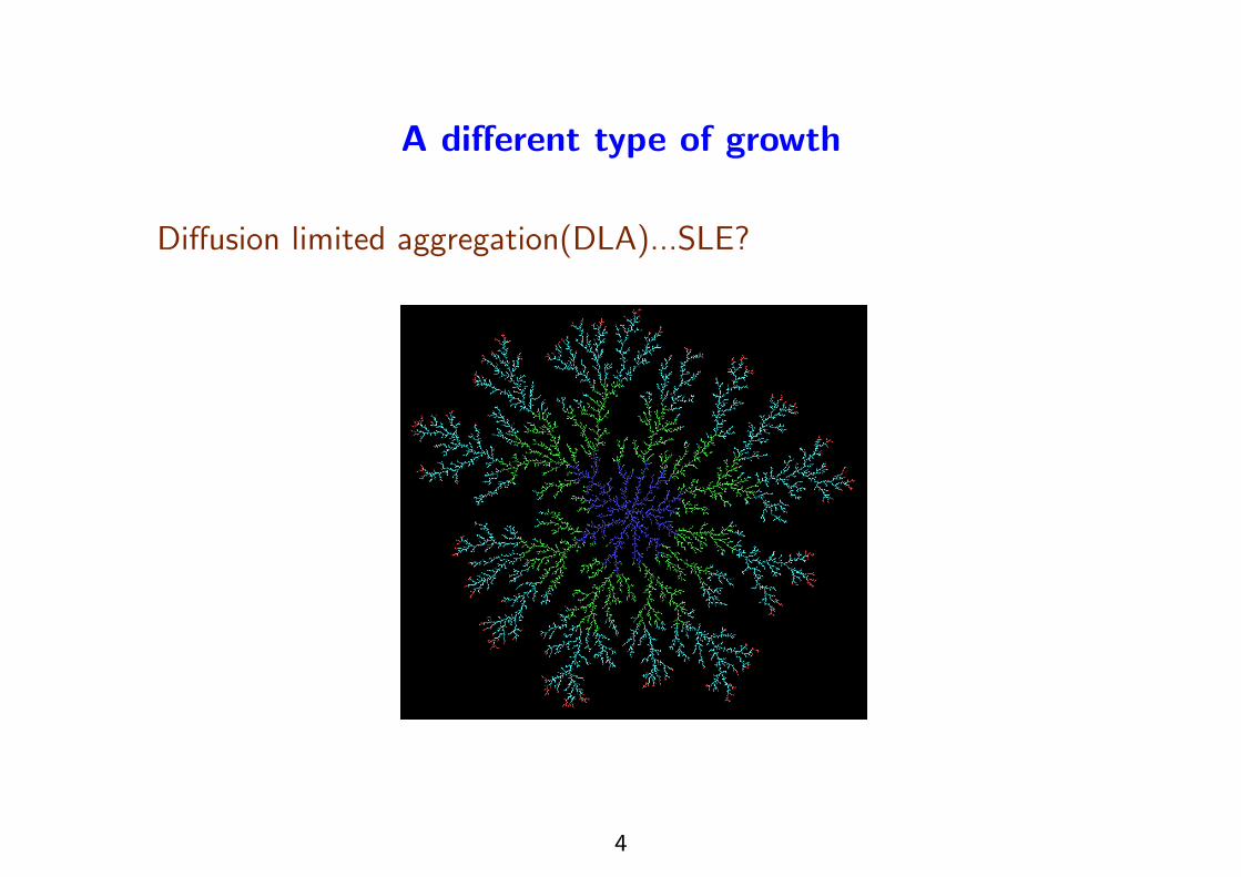
A di!erent type of growth
Di!usion limited aggregation(DLA)...SLE?
4
Scaling
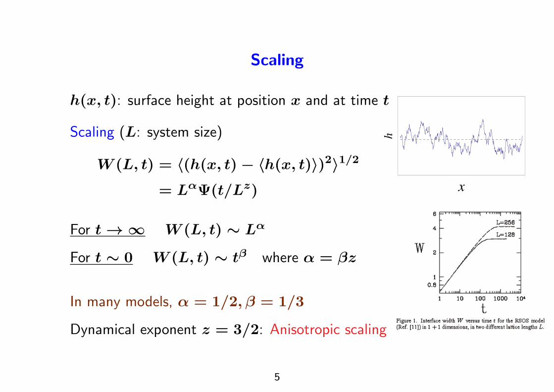
h(x, t): surface height at position x and at time t
Scaling (L: system size)
W (L, t) = "(h(x, t) # "h(x, t)$)2$1/2
= L!!(t/Lz) x
h
For t % & W (L, t) ' L!
For t ' 0 W (L, t) ' t" where ! = "z
In many models, ! = 1/2," = 1/3
Dynamical exponent z = 3/2: Anisotropic scaling
5

KPZ equation
1986 Kardar Parisi Zhang (not Knizhnik-Polyakov-Zamolodchikov)
#th(x, t) = 12$(#xh(x, t))
2 + %#2xh(x, t) +(D&(x, t)
where & is the Gaussian noise with covariance
"&(x, t)&(x!, t!)$ = '(x # x!)'(t # t!)
• Dynamical RG analysis: h(x = 0, t) ) vt + c(t1/3
KPZ universality class
• The Brownian motion is stationary.
• The issue of well-definedness.
• Now revival: New analytic and experimental developments
6
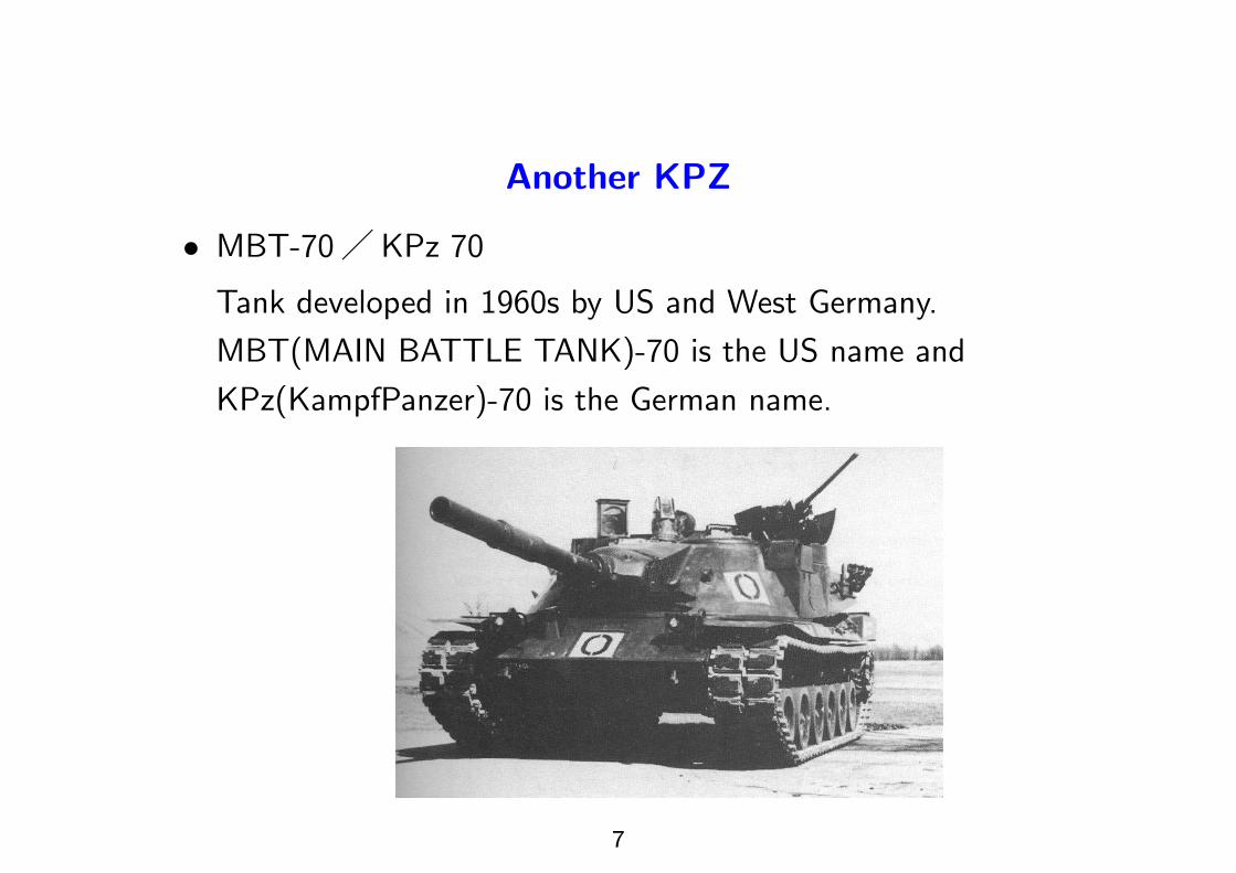
Another KPZ
• MBT-70/ KPz 70
Tank developed in 1960s by US and West Germany.
MBT(MAIN BATTLE TANK)-70 is the US name and
KPz(KampfPanzer)-70 is the German name.
7
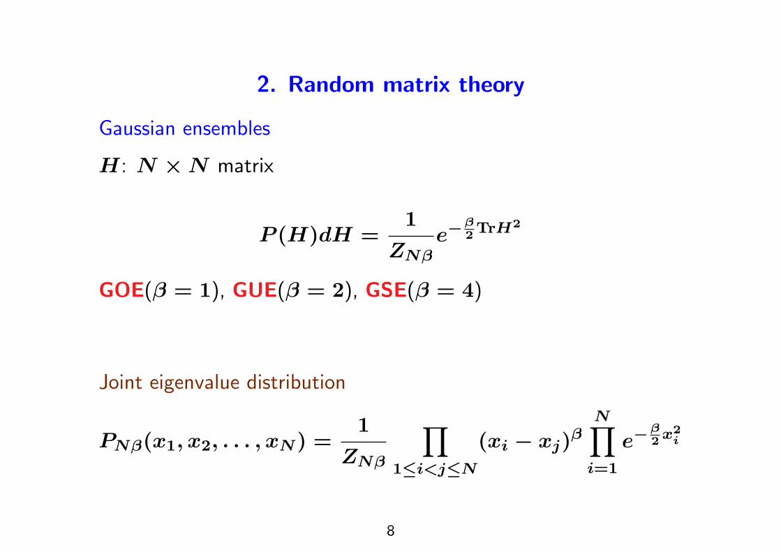
2. Random matrix theory
Gaussian ensembles
H: N * N matrix
P (H)dH =1
ZN"e"
!2TrH2
GOE(" = 1), GUE(" = 2), GSE(" = 4)
Joint eigenvalue distribution
PN"(x1, x2, . . . , xN) =1
ZN"
!
1#i<j#N
(xi # xj)"
N!
i=1
e"!2x2
i
8
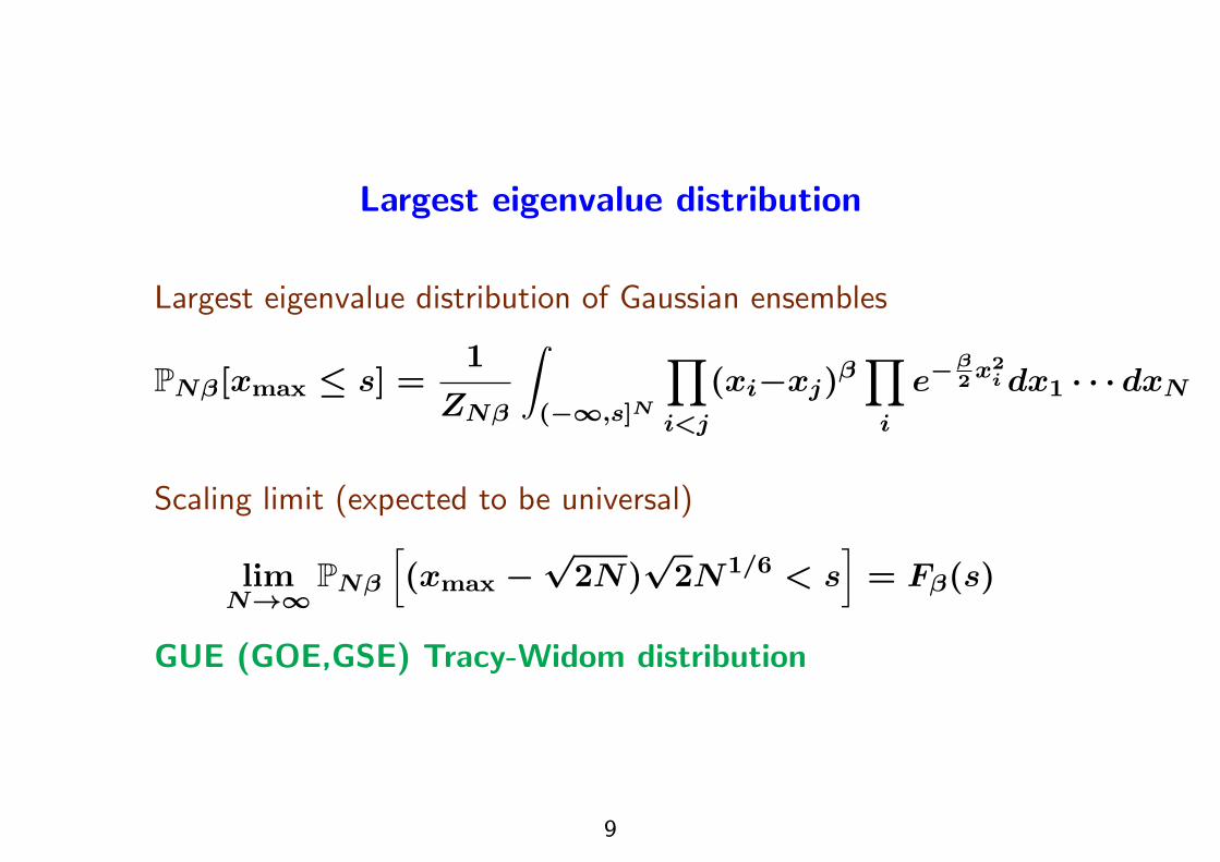
Largest eigenvalue distribution
Largest eigenvalue distribution of Gaussian ensembles
PN"[xmax + s] =1
ZN"
"
("$,s]N
!
i<j
(xi#xj)"!
i
e"!2x2
i dx1 · · · dxN
Scaling limit (expected to be universal)
limN%$
PN"
#(xmax #
(2N)
(2N1/6 < s
$= F"(s)
GUE (GOE,GSE) Tracy-Widom distribution
9
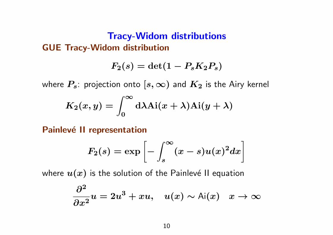
Tracy-Widom distributionsGUE Tracy-Widom distribution
F2(s) = det(1 # PsK2Ps)
where Ps: projection onto [s,&) and K2 is the Airy kernel
K2(x, y) =
" $
0d$Ai(x + $)Ai(y + $)
Painleve II representation
F2(s) = exp
%#" $
s(x # s)u(x)2dx
&
where u(x) is the solution of the Painleve II equation
#2
#x2u = 2u3 + xu, u(x) ' Ai(x) x % &
10

GOE Tracy-Widom distribution
F1(s) = exp
%#
1
2
" $
su(x)dx
&(F2(s))
1/2
GSE Tracy-Widom distribution
F4(s) = cosh
%#
1
2
" $
su(x)dx
&(F2(s))
1/2
Figures for Tracy-Widom distributions
11
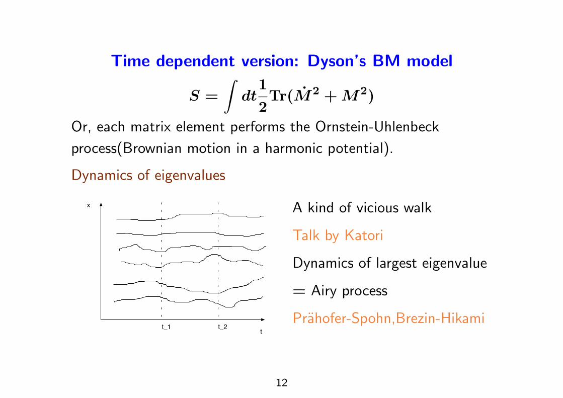
Time dependent version: Dyson’s BM model
S =
"dt
1
2Tr(M2 + M2)
Or, each matrix element performs the Ornstein-Uhlenbeck
process(Brownian motion in a harmonic potential).
Dynamics of eigenvalues
t
x
t_1 t_2
A kind of vicious walk
Talk by Katori
Dynamics of largest eigenvalue
= Airy process
Prahofer-Spohn,Brezin-Hikami
12
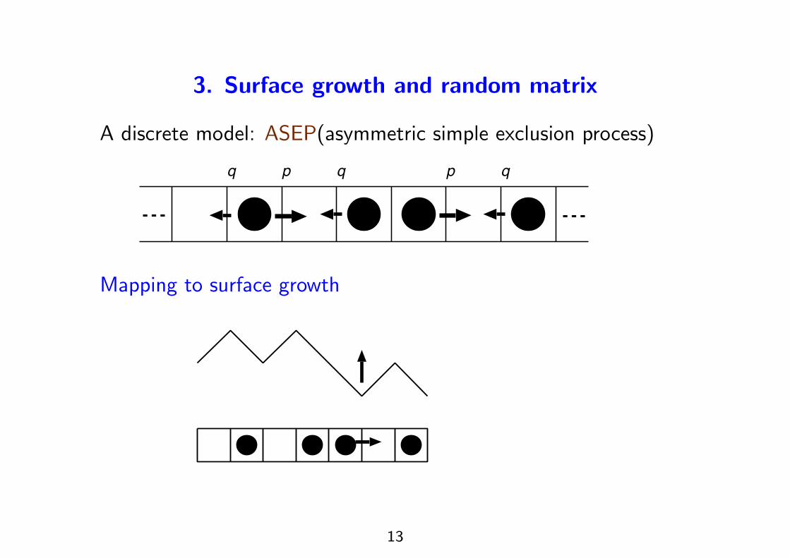
3. Surface growth and random matrix
A discrete model: ASEP(asymmetric simple exclusion process)
q p q p q
Mapping to surface growth
13
A few comments on ASEP
• Some applications
– Tra"c flow
– Ionic conductor
– Ribosome on mRNA, Molecular motor
• A standard model in nonequilibrium statistical physics
– A system far from equilibrium
– Shock wave
– Boundary induced phase transitions
– Exactly solvable
14

Stationary measure
ASEP · · · Bernoulli measure: each site is independent and
occupied with prob. ) (0 < ) < 1). Current is )(1 # )).
· · · ) ) ) ) ) ) ) · · ·
-3 -2 -1 0 1 2 3
Surface growth · · · Random walk height profile
15
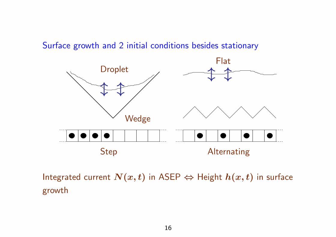
Surface growth and 2 initial conditions besides stationary
Step
Droplet
Wedge
, ,
Alternating
Flat
, ,
Integrated current N(x, t) in ASEP - Height h(x, t) in surface
growth
16

Connection to random matrix: JohanssonTASEP(Totally ASEP, hop only in one direction)Step initial condition (t = 0)
· · ·
-3 -2 -1 0 1 2 3
N(t): Number of particles which crossed (0,1) up to time t
P[N(t) . N ] =1
ZN
"
[0,t]N
!
i<j
(xi#xj)2!
i
e"xidx1 · · · dxN
(cf. chiral GUE)
17

Zero temperature directed polymer• Time at which N th particle arrives at the origin
= maxup-right paths from(1,1)to(N,N)
'(
)*
(i,j) on a path
wi,j
+,
-
!
"
(1, 1)
(N,N)
· · ·
...
i
j
wij on (i, j): exponentially distributed
waiting time of ith hop of jth particle
• RSK algorithm / Combinatorics of Young tableaux
(cf. Schur measure % Plancherel measure % Gross-Witten)
18

Dynamics on Gelfand-Zetlin Cone
Blocking and pushing dynamics
x11
x21 x2
2
x31 x3
2 x33
. .. ...
. . .
xn1 xn
2 xn3 . . . xn
n"1 xnn
19

Current distributions for ASEP with wedge initial conditions
2000 Johansson (TASEP) 2008 Tracy-Widom (ASEP)
N(0, t/(q # p)) ) 14t # 2"4/3t1/3(TW
Here N(x = 0, t) is the integrated current of ASEP at the origin
and (TW obeys the GUE Tracy-Widom distributions;
FTW(s) = P[(TW + s] = det(1 # PsKAiPs)
where KAi is the Airy kernel
KAi(x, y) =
" $
0d$Ai(x + $)Ai(y + $) !6 !4 !2 0 2
0.0
0.1
0.2
0.3
0.4
0.5
s
20
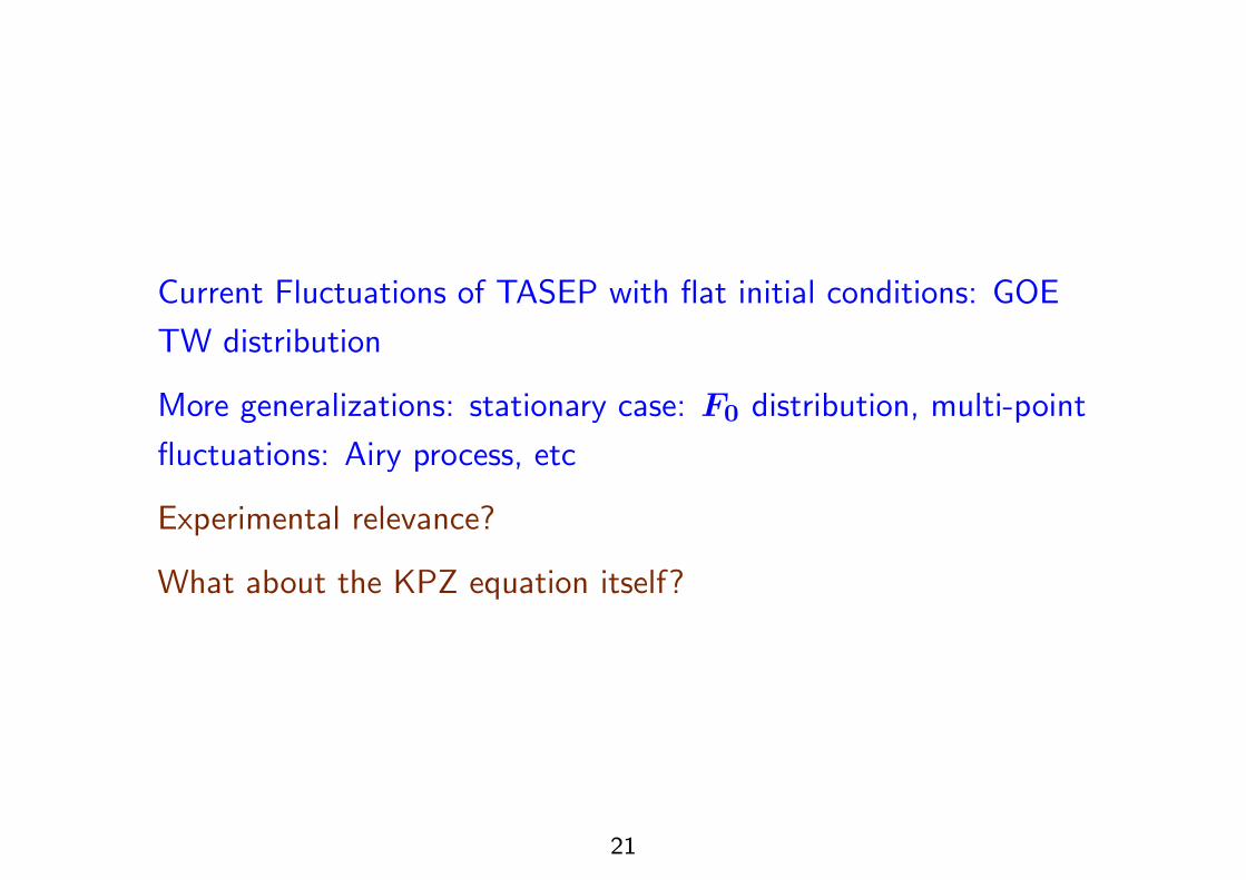
Current Fluctuations of TASEP with flat initial conditions: GOE
TW distribution
More generalizations: stationary case: F0 distribution, multi-point
fluctuations: Airy process, etc
Experimental relevance?
What about the KPZ equation itself?
21

4. Experiments by liquid crystal turbulence
2010-2011 Takeuchi Sano
22
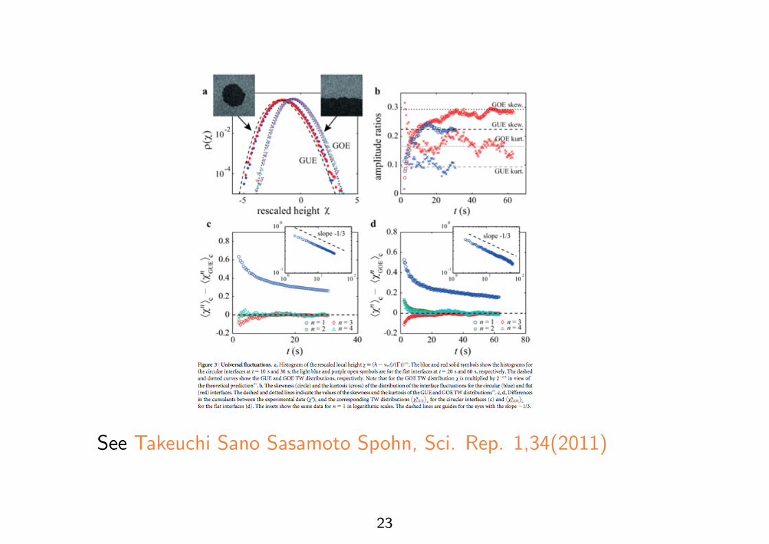
See Takeuchi Sano Sasamoto Spohn, Sci. Rep. 1,34(2011)
23
5. The narrow wedge KPZ equation
Remember the KPZ equation
#th(x, t) = 12$(#xh(x, t))
2 + %#2xh(x, t) +(D&(x, t)
2010 Sasamoto Spohn, Amir Corwin Quastel
• Narrow wedge initial condition
• Based on (i) the fact that the weakly ASEP is KPZ equation
(1997 Bertini Giacomin) and (ii) a formula for step ASEP by
2009 Tracy Widom
• The explicit distribution function for finite t
• The KPZ equation is in the KPZ universality class
24
Narrow wedge initial condition
Scalingsx % !2x, t % 2%!4t, h %
$
2%h
where ! = (2%)"3/2$D1/2.
We can and will do set % = 12 ,$ = D = 1.
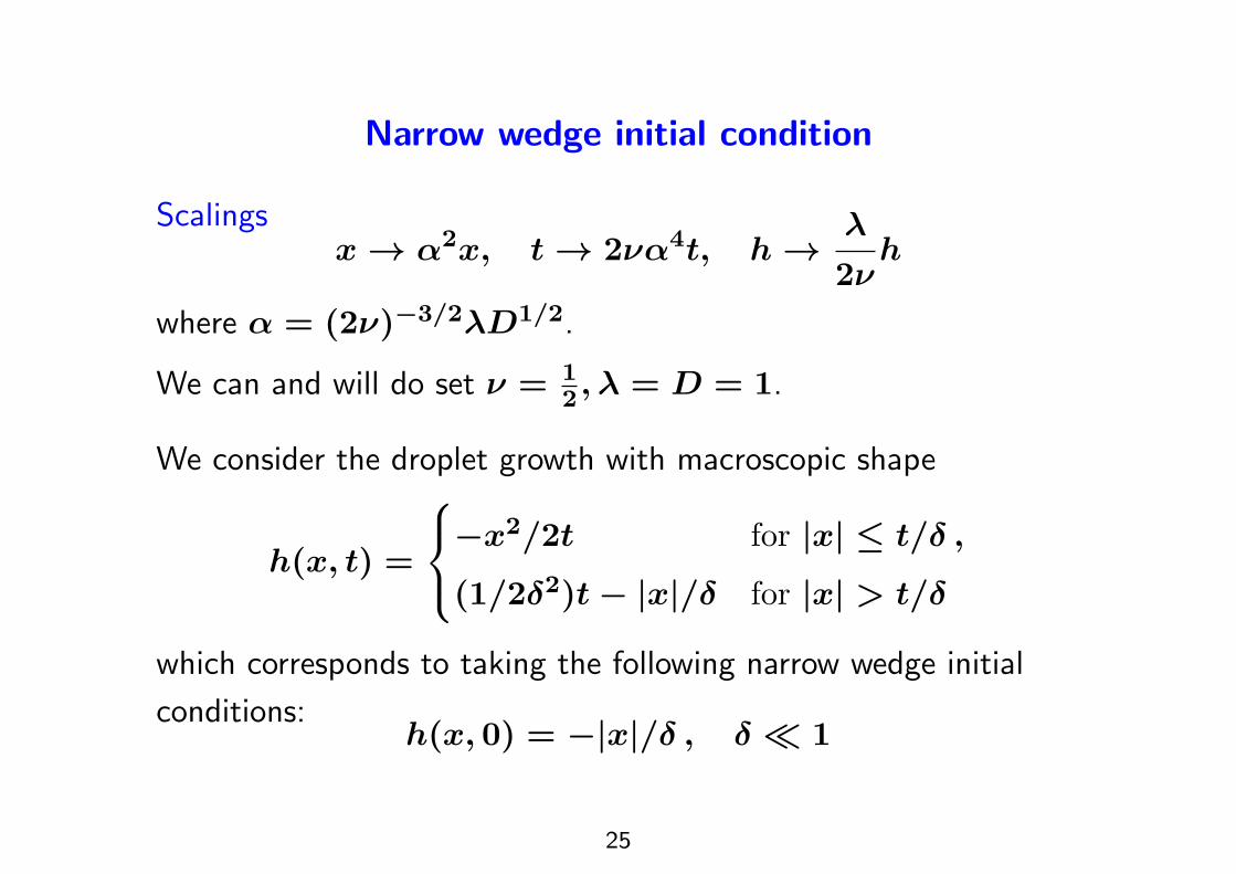
We consider the droplet growth with macroscopic shape
h(x, t) =
'(
)#x2/2t for |x| + t/' ,
(1/2'2)t # |x|/' for |x| > t/'
which corresponds to taking the following narrow wedge initial
conditions:h(x, 0) = #|x|/' , ' 0 1
25

2λt/δx
h(x,t)
26
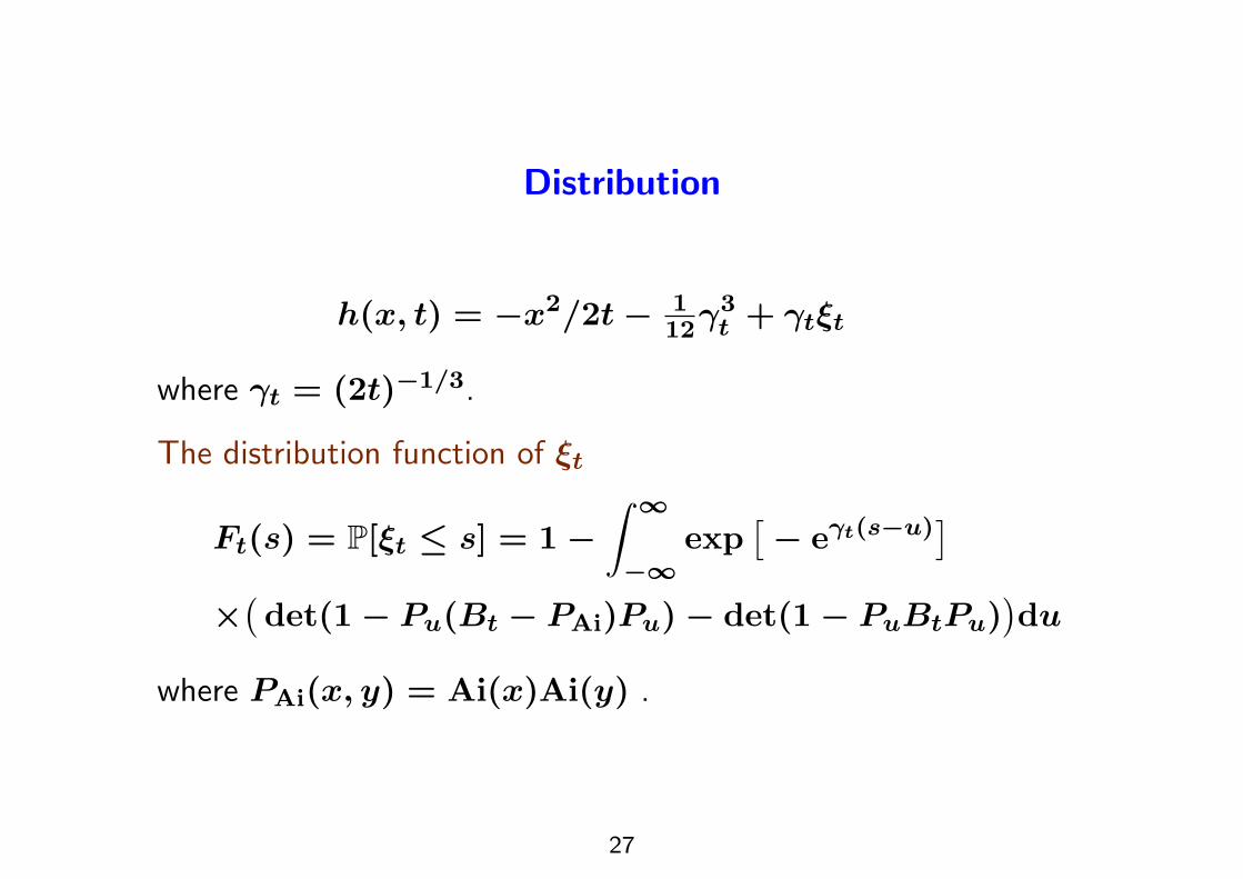
Distribution
h(x, t) = #x2/2t # 112*
3t + *t(t
where *t = (2t)"1/3.
The distribution function of (t
Ft(s) = P[(t + s] = 1 #" $
"$exp
.# e#t(s"u)
/
*0det(1 # Pu(Bt # PAi)Pu) # det(1 # PuBtPu)
1du
where PAi(x, y) = Ai(x)Ai(y) .
27

Pu is the projection onto [u,&) and the kernel Bt is
Bt(x, y) = KAi(x, y) +
" $
0d$(e#t$ # 1)"1
*0Ai(x + $)Ai(y + $) # Ai(x # $)Ai(y # $)
1.
A question: Random matrix interpretation?
28
Developments
• 2010 Calabrese Le Doussal Rosso, Dotsenko Replica
• 2010 Corwin Quastel Half-BM by step Bernoulli ASEP
• 2010 O’Connell A directed polymer model related to quantum
Toda lattice
• 2010 Prolhac Spohn Multi-point distributions by replica
• 2011 Calabrese Le Dossal Flat case by replica
• 2011 Corwin et al Tropical RSK for inverse gamma polymer
• 2011 Borodin Corwin Macdonald process
• 2011 Imamura Sasamoto Half-BM and stationary case by
replica
29
6. Stationary case
• Narrow wedge is technically the simplest.
• Flat case is a well-studied case in surface growth
• Stationary case is important for stochastic process and
nonequilibrium statistical mechanics
– Two-point correlation function
– Experiments: Scattering, direct observation
– A lot of approximate methods (renormalization,
mode-coupling, etc.) have been applied to this case.
– Nonequilibrium steady state(NESS): No principle.
Dynamics is even harder.
30
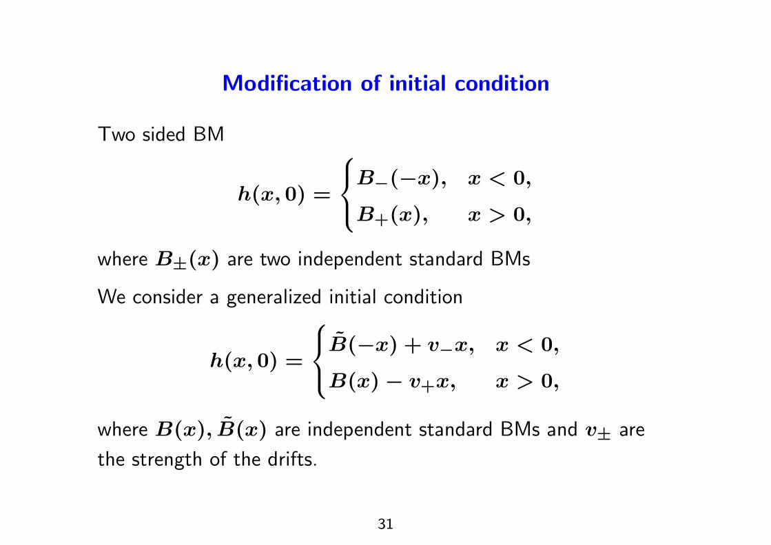
Modification of initial condition
Two sided BM
h(x, 0) =
'(
)B"(#x), x < 0,
B+(x), x > 0,
where B±(x) are two independent standard BMs
We consider a generalized initial condition
h(x, 0) =
'(
)B(#x) + v"x, x < 0,
B(x) # v+x, x > 0,
where B(x), B(x) are independent standard BMs and v± are
the strength of the drifts.
31

Result
For the generalized initial condition with v±
Fv±,t(s) := Prob.h(x, t) + *3t /12 + *ts
/
="(v+ + v")
"(v+ + v" + *"1t d/ds)
%1 #
" $
"$due"e"t(s!u)
%v±,t(u)
&
Here %v±,t(u) is expressed as a di!erence of two Fredholm
determinants,
%v±,t(u) = det01 # Pu(B
!t # P!
Ai)Pu1# det
01 # PuB
!t Pu
1,
where Ps represents the projection onto (s,&),
P!Ai((1, (2) = Ai!!
2(1,
1
*t, v", v+
3Ai!!
2(2,
1
*t, v+, v"
3
32
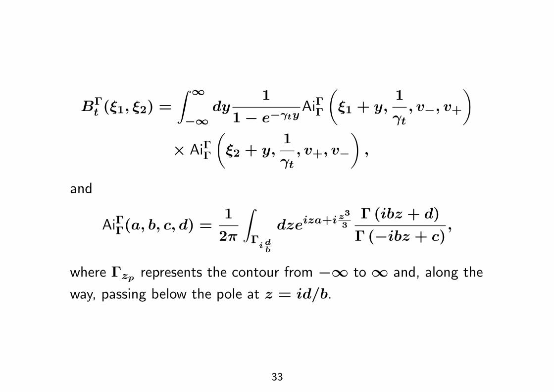
B!t ((1, (2) =
" $
"$dy
1
1 # e"#tyAi!!
2(1 + y,
1
*t, v", v+
3
* Ai!!
2(2 + y,
1
*t, v+, v"
3,
and
Ai!!(a, b, c, d) =1
2+
"
!i db
dzeiza+iz3
3" (ibz + d)
" (#ibz + c),
where "zp represents the contour from #& to & and, along the
way, passing below the pole at z = id/b.
33
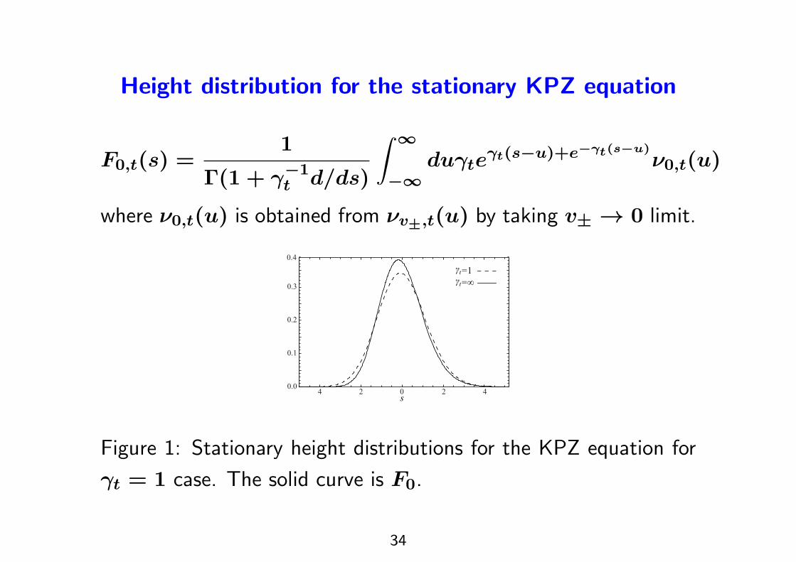
Height distribution for the stationary KPZ equation
F0,t(s) =1
"(1 + *"1t d/ds)
" $
"$du*te
#t(s"u)+e!"t(s!u)%0,t(u)
where %0,t(u) is obtained from %v±,t(u) by taking v± % 0 limit.
4 2 0 2 40.0
0.1
0.2
0.3
0.4
!t=1!t=!
s
Figure 1: Stationary height distributions for the KPZ equation for
*t = 1 case. The solid curve is F0.
34
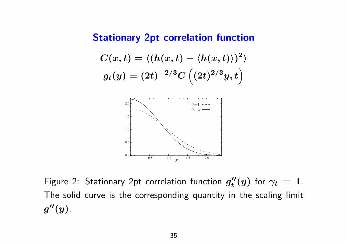
Stationary 2pt correlation function
C(x, t) = "(h(x, t) # "h(x, t)$)2$
gt(y) = (2t)"2/3C4(2t)2/3y, t
5
0.5 1.0 1.5 2.00.0
0.5
1.0
1.5
2.0
y
!t=1!t=!
Figure 2: Stationary 2pt correlation function g!!t (y) for *t = 1.
The solid curve is the corresponding quantity in the scaling limit
g!!(y).
35
Derivation
Cole-Hopf transformation
1997 Bertini and Giacomin
h(x, t) = log (Z(x, t))
Z(x, t) is the solution of the stochastic heat equation,
#Z(x, t)
#t=
1
2
#2Z(x, t)
#x2+ &(x, t)Z(x, t).
and can be considered as directed polymer in random potential &.
cf. Hairer Well-posedness of KPZ equation without Cole-Hopf
36
Feynmann-Kac and Generating function
Feynmann-Kac expression for the partition function,
Z(x, t) = Ex
2exp
%" t
0& (b(s), t # s) ds
&Z(b(t), 0)
3
We consider the N th replica partition function "ZN(x, t)$ and
compute their generating function Gt(s) defined as
Gt(s) =$*
N=0
0#e"#ts
1N
N !
6ZN(0, t)
7eN
"3t
12
with *t = (t/2)1/3.
37
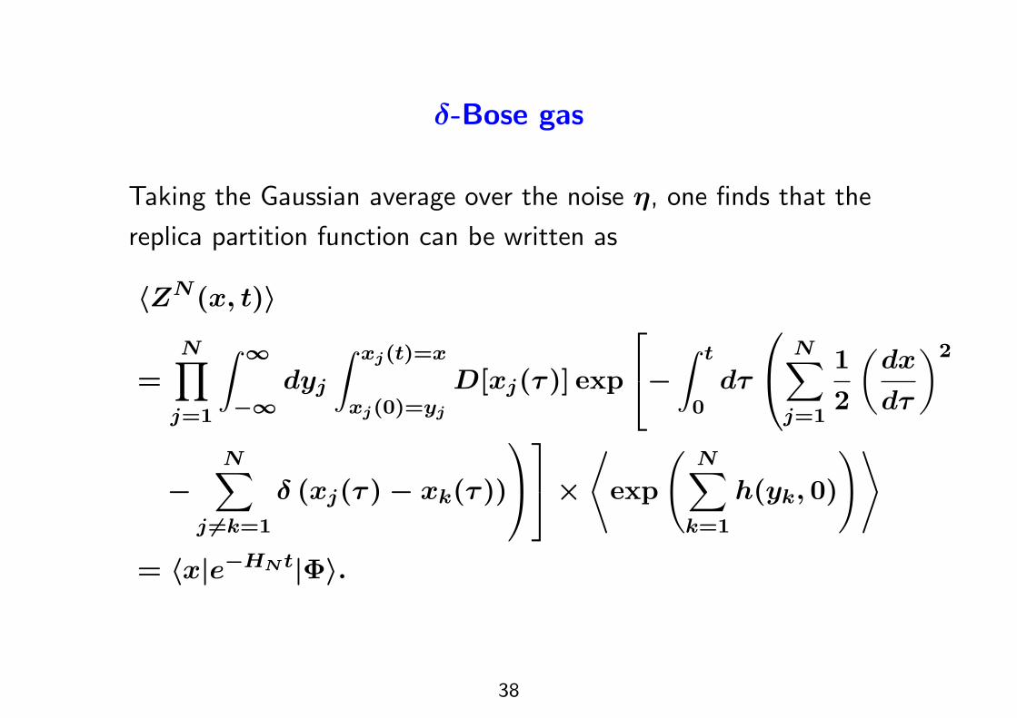
'-Bose gas
Taking the Gaussian average over the noise &, one finds that the
replica partition function can be written as
"ZN(x, t)$
=N!
j=1
" $
"$dyj
" xj(t)=x
xj(0)=yj
D[xj(, )] exp
8
9#" t
0d,
:
;N*
j=1
1
2
2dx
d,
32
#N*
j &=k=1
' (xj(, ) # xk(, ))
<
=
>
?*@exp
AN*
k=1
h(yk, 0)
BC
= "x|e"HN t|#$.
38

HN is the Hamiltonian of the '-Bose gas,
HN = #1
2
N*
j=1
#2
#x2j
#1
2
N*
j &=k
'(xj # xk),
|#$ represents the state corresponding to the initial condition. We
compute "ZN(x, t)$ by expanding in terms of the eigenstates of
HN ,
"Z(x, t)N$ =*
z
"x|!z$"!z|#$e"Ezt
where Ez and |!z$ are the eigenvalue and the eigenfunction of
HN : HN |!z$ = Ez|!z$.
39
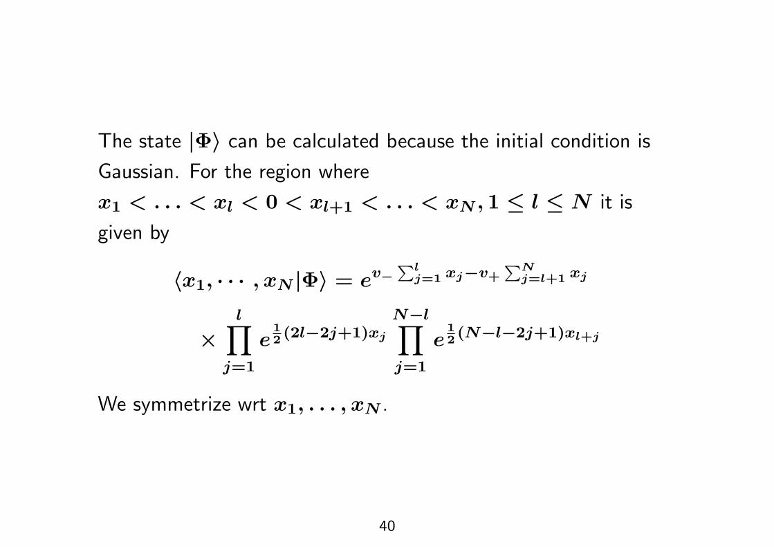
The state |#$ can be calculated because the initial condition is
Gaussian. For the region where
x1 < . . . < xl < 0 < xl+1 < . . . < xN , 1 + l + N it is
given by
"x1, · · · , xN |#$ = ev!!l
j=1 xj"v+!N
j=l+1 xj
*l!
j=1
e12 (2l"2j+1)xj
N"l!
j=1
e12 (N"l"2j+1)xl+j
We symmetrize wrt x1, . . . , xN .
40

Bethe statesBy the Bethe ansatz, the eigenfunction is given as
"x1, · · · , xN |!z$ = Cz
*
P'SN
sgnP
*!
1#j<k#N
0zP (j) # zP (k) + isgn(xj # xk)
1exp
Ai
N*
l=1
zP (l)xl
B
N momenta zj (1 + j + N) are parametrized as
zj = q! #i
2(n! + 1 # 2r!) , for j =
!"1*
"=1
n" + r!.
(1 + ! + M and 1 + r! + n!). They are divided into M
groups where 1 + M + N and the !th group consists of n!
quasimomenta z!js which shares the common real part q!.
41
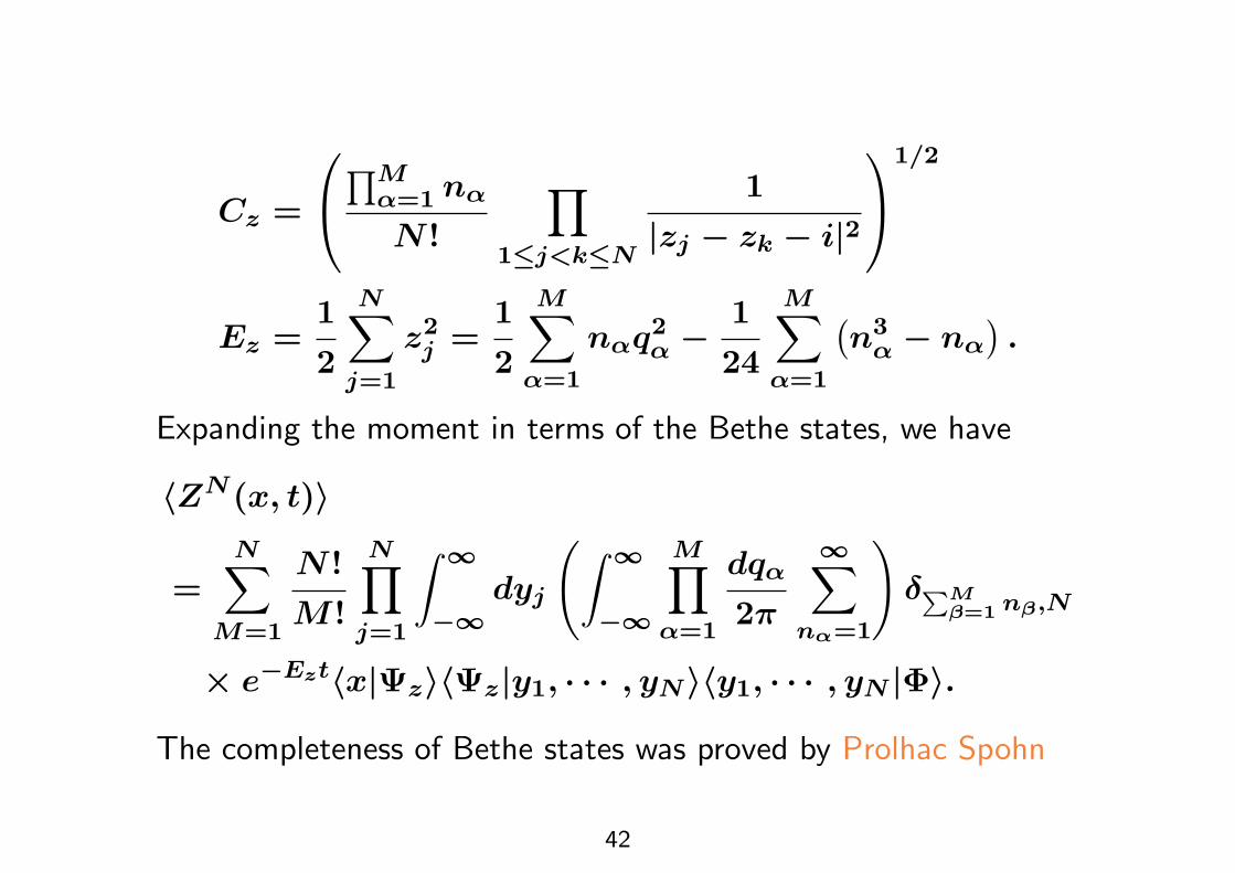
Cz =
:
;DM
!=1 n!
N !
!
1#j<k#N
1
|zj # zk # i|2
<
=1/2
Ez =1
2
N*
j=1
z2j =
1
2
M*
!=1
n!q2! #
1
24
M*
!=1
0n3! # n!
1.
Expanding the moment in terms of the Bethe states, we have
"ZN(x, t)$
=N*
M=1
N !
M !
N!
j=1
" $
"$dyj
A" $
"$
M!
!=1
dq!
2+
$*
n#=1
B'!M
!=1 n!,N
* e"Ezt"x|!z$"!z|y1, · · · , yN$"y1, · · · , yN |#$.
The completeness of Bethe states was proved by Prolhac Spohn
42

We see
"!z|#$ = N !Cz
*
P'SN
sgnP!
1#j<k#N
4z(P (j) # z(
P (k) + i5
*N*
l=0
(#1)ll!
m=1
1Em
j=1(#iz(Pj
+ v") # m2/2
*N"l!
m=1
1EN
j=N"m+1(#iz(Pj
# v+) + m2/2.
43

Combinatorial identities
(1)*
P'SN
sgnP!
1#j<k#N
0wP (j) # wP (k) + if(j, k)
1
= N !!
1#j<k#N
(wj # wk)
44
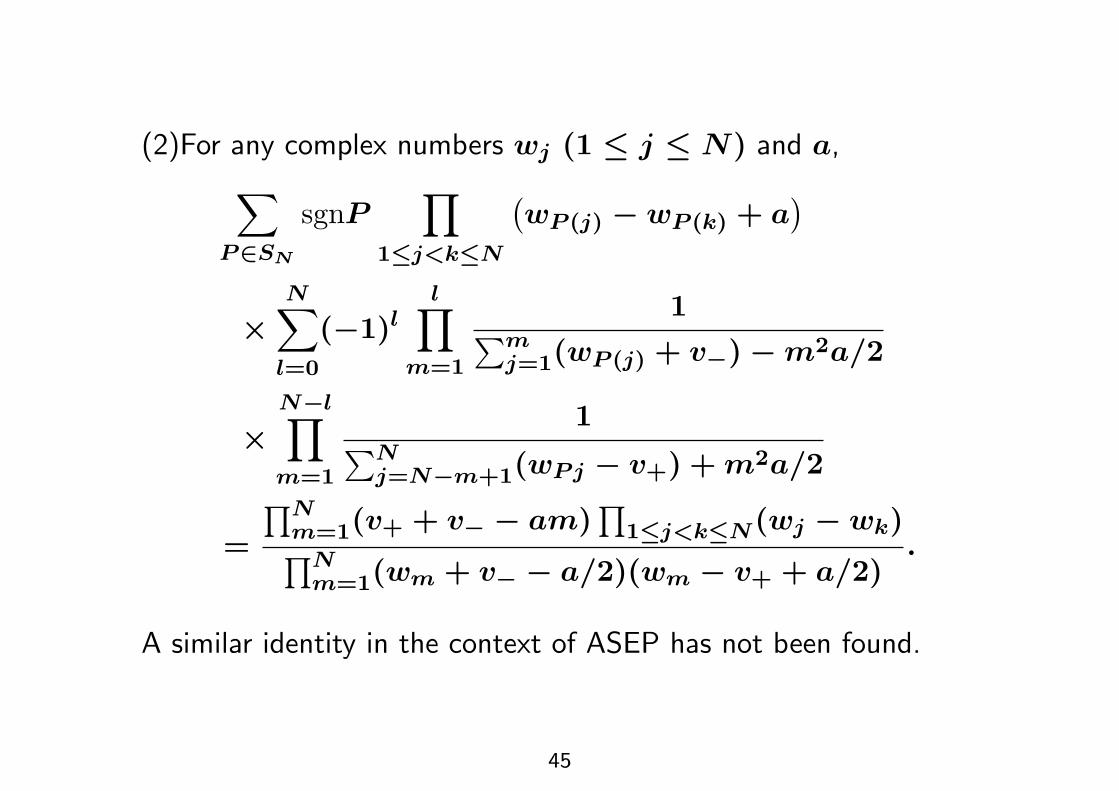
(2)For any complex numbers wj (1 + j + N) and a,*
P'SN
sgnP!
1#j<k#N
0wP (j) # wP (k) + a
1
*N*
l=0
(#1)ll!
m=1
1Em
j=1(wP (j) + v") # m2a/2
*N"l!
m=1
1EN
j=N"m+1(wPj # v+) + m2a/2
=
DNm=1(v+ + v" # am)
D1#j<k#N(wj # wk)
DNm=1(wm + v" # a/2)(wm # v+ + a/2)
.
A similar identity in the context of ASEP has not been found.
45
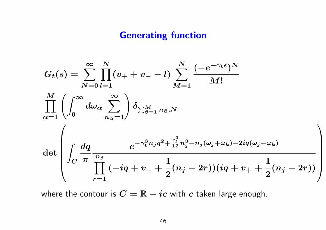
Generating function
Gt(s) =$*
N=0
N!
l=1
(v+ + v" # l)N*
M=1
(#e"#ts)N
M !
M!
!=1
A" $
0d-!
$*
n#=1
B'!M
!=1 n!,N
det
:
FFFFF;
"
C
dq
+
e"#3t njq2+
"3t
12 n3j"nj(%j+%k)"2iq(%j"%k)
nj!
r=1
(#iq + v" +1
2(nj # 2r))(iq + v+ +
1
2(nj # 2r))
<
GGGGG=
where the contour is C = R # ic with c taken large enough.
46

This generating function itself is not a Fredholm determinant due
to the novel factorDN
l=1(v+ + v" # l).
We consider a further generalized initial condition in which the
initial overall height . obeys a certain probability distribution.
h = h + .
where h is the original height for which h(0, 0) = 0. Therandom variable . is taken to be independent of h.
Moments "eNh$ = "eNh$"eN&$.We postulate that . is distributed as the inverse gamma
distribution with parameter v+ + v", i.e., if 1/. obeys the
gamma distribution with the same parameter. Its N th moment is
1/DN
l=1(v+ + v" # l) which compensates the extra factor.
47

Distributions
F (s) =1
/(*"1t
dds)
F (s),
where F (s) = Prob[h(0, t) + *ts],F (s) = Prob[h(0, t) + *ts] and / is the Laplace transform of
the pdf of .. For the inverse gamma distribution,
/(() = "(v + ()/"(v), by which we get the formula for the
generating function.
48

Summary
• Some surface growth models are related to random matrix.
• The developments in the last 12 years allow us to study also
the KPZ equation.
• We have presented some formulas for the height distributions
and stationary two point correlation functions.
49