t00-058

Dynamic analysis for laterally loaded piles anddynamic p–y curves

M. Hesham El Naggar and Kevin J. Bentley

Abstract: Pile foundations are often subjected to lateral dynamic loading due to forces on the supported structure. Inthis study, a simple two-dimensional analysis was developed to accurately model the pile response to dynamic loads.The proposed model incorporates the staticp–y curve approach (wherep is the static soil reaction andy is the pile de-flection) and the plane strain assumptions to represent the soil reactions within the frame of a Winkler model. Thep–ycurves are used to relate pile deflections to the nonlinear soil reactions. Wave propagation and energy dissipation arealso accounted for along with discontinuity conditions at the pile–soil interface. The inclusion of damping with thestatic unit transfer curves results in increased soil resistance, thus producing “dynamicp–y curves.” The dynamicp–ycurves are a function of the staticp–y curve and velocity of the soil particles at a given depth and frequency of load-ing. The proposed model was used to analyze the pile response to the lateral Statnamic load test, and the predicted re-sponse compared well with the measured response. Closed-form solutions for dynamicp–y curves were established bycurve fitting the dynamic soil reactions for a range of soil types and loading frequencies. These solutions can be usedto model soil reactions for pile vibration problems in readily available finite element analysis (FEA) and dynamicstructural analysis packages. A simple spring and dashpot model was also proposed to be used in equivalent linearanalyses of transient pile response. The proposed models were incorporated into an FEA program (ANSYS) which wasused to compute the response of a laterally loaded pile. The computed responses compared well with the predictions ofthe two-dimensional analysis.

Key words: dynamic, transient, lateral, piles,p–y curves, inertial interaction.

Résumé: Les fondations sur pieux sont souvent soumises à un chargement dynamique latéral dû à des forcesappliquées sur la structure portée. Dans cette étude, une analyse unidimensionnelle simple a été développée pourmodéliser avec précision la réaction du pieu aux charges dynamiques. Le modèle proposé incorpore l’approche de lacourbe statiquep–y et les hypothèses de déformation plane pour représenter les réactions du sol dans le cadre d’unmodèle de Winkler. Les courbesp–y sont utilisées pour faire une corrélation entre les déflexions du pieu et lesréactions non linéaires du sol. La propagation d’ondes et la dissipation d’énergie sont également prises en compte enmême temps que les conditions de discontinuité à l’interface pieu-sol. L’inclusion de l’amortissement avec les courbesde transfert d’unité statique résulte en un accroissement de la résistance du sol, produisant ainsi des « courbesp–ydynamiques ». Les courbesp–y dynamiques sont une fonction de la courbe statiquep–y et de la vélocité des particulesde sol à une profondeur et à une fréquence de chargement données. Le modèle proposé a été utilisé pour analyser laréponse du pieu à l’essai de chargement statnamique, et la réponse prédite se comparaît bien à la réponse mesurée. Lessolutions exactes pour les courbesp–y dynamiques ont été établies par lissage des courbes des réactions dynamiquesdu sol pour une plage de types de sol et de fréquences de chargement. Ces solutions peuvent être utilisées pourmodéliser les réactions du sol pour les problèmes de vibration de pieux dans les progiciels FEA et d’analysestructurale dynamique couramment disponibles. Un modèle comprenant un simple ressort avec pot amortisseur a aussiété proposé pour être utilisé dans des analyses linéaires équivalentes de la réponse transitoire d’un pieu. Les modèlesproposés ont été incorporés dans un programme FEA (ANSYS) qui a été utilisé pour évaluer la réponse d’un pieuchargé latéralement. Les réponses calculées se comparaîent bien avec les prédictions de l’analyse bidimensionnelle.

Mots clés: dynamique, transitoire, latéral, pieux, courbesp–y, interaction inertielle.

[Traduit par la Rédaction] El Naggar and Bentley 1183

Introduction

Pile foundations are often subjected to lateral loading dueto forces on the supported structure. The horizontal loads atthe pile head can be the governing design constraint for sin-

gle piles and pile groups supporting different types of struc-tures in many situations including environmental loading(wind, water, and earthquakes) and machine loading onstructures such as buildings, bridges, and offshore platforms.

Most building and bridge codes use factored static loadsto account for the dynamic effects of pile foundations. Al-though very low frequency vibrations may be accuratelymodeled using factored loads, the introduction of non-linearity, damping, and pile–soil interaction during transientloading may significantly alter the response. The typical fre-quencyranges of interest are 0–10 Hz for earthquakes,

Can. Geotech. J.37: 1166–1183 (2000) © 2000 NRC Canada

1166

Received May 5, 1999. Accepted April 28, 2000. Publishedon the NRC Research Press website on December 5, 2000.

M.H. El Naggar and K.J. Bentley. Geotechnical ResearchCentre, The University of Western Ontario, London, ONN6A 5B9, Canada.

I:\cgj\Cgj37\Cgj06\T00-058.vpThursday, November 30, 2000 11:48:21 AM

Color profile: Generic CMYK printer profileComposite Default screen

0–1 Hz for offshore environmental loading, and 5–200 Hzfor machine foundations. The emphasis in the current studyis on the seismic loading case.

Novak et al. (1978) developed a frequency-dependentpile–soil interaction model; however, it assumes strictly lin-ear or equivalent linear soil properties. Gazetas and Dobry(1984) introduced a simplified linear method to predictfixed-head pile response accounting for both material and ra-diation damping and using available static stiffness (derivedfrom a finite element or any other accepted method). Thismethod is not suitable for the seismic response analysis be-cause of the linearity assumptions. In general, there is muchcontroversy over advanced linear solutions (frequency do-main), as they do not account for permanent deformation orgapping at the pile–soil interface.

Nogami et al. (1992) developed a time-domain analysismethod for single piles and pile groups by integrating planestrain solutions with a nonlinear zone around each pile usingp–y curves, (wherep is the static soil reaction andy is thepile deflection). El Naggar and Novak (1995, 1996) also de-veloped a computationally efficient model for evaluating thelateral response of piles and pile groups based on theWinkler hypothesis, accounting for nonlinearity using a hy-perbolic stress–strain relationship and slippage and gappingat the pile–soil interface. The model also accounts for thepropagation of waves away from the pile and energy dissipa-tion through both material and geometric damping.

The p–y curves (unit load transfer curves) approach is awidely accepted method for predicting pile response understatic loads because of its simplicity and practical accuracy.In the present study, the model proposed by El Naggar andNovak (1996) is modified to utilize existing or developed cy-clic or staticp–y curves to represent the nonlinear behaviourof the soil adjacent to the pile. The model uses unit loadtransfer curves in the time domain to model nonlinearity andincorporates both material and radiation damping to generatedynamicp–y curves.

Model description

Pile modelThe pile is assumed to be vertical and flexible with circu-

lar cross section. Noncylindrical piles are represented by cy-lindrical piles with equivalent radius to accommodate anypier–pile configurations. The pile and surrounding soil aresubdivided inton segments, with pile nodes correspondingto soil nodes at the same elevation. The standard bendingstiffness matrix of beam elements models the structural stiff-ness matrix for each pile element. The pile global stiffnessmatrix is then assembled from the element stiffness matricesand is condensed to give horizontal translations at each layerand the rotational degree of freedom at the pile head.

Soil model: hyperbolic stress–strain relationshipThe soil is divided into n layers with different soil proper-

ties assigned to each layer according to the soil profile con-sidered. Within each layer, the soil medium is divided intotwo annular regions as shown in Fig. 1. The first region is aninner zone adjacent to the pile and accounts for the soilnonlinearity. The second region is the outer zone that allowsfor wave propagation away from the pile and provides for

the radiation damping in the soil medium. The soil reactionsand the pile–soil interface conditions are modeled separatelyon both sides of the pile to account for slippage, gappingand state of stress as the load direction changes.

Inner field elementThe inner field is modeled with a nonlinear spring to rep-

resent the stiffness and a dashpot to simulate material(hysteretic) damping. The stiffness is calculated assumingplane strain conditions, the inner field is a homogeneous iso-tropic viscoelastic massless medium, the pile is rigid and cir-cular, there is no separation at the pile–soil interface, anddisplacements are small. Novak and Sheta (1980) obtainedthe stiffnesskNL under these conditions as

[1] k

G v vrr

rr

NL

mo

o

=

− −

+

8 1 3 4 11

2

1

π ( )( )

+ −

+

2

2

1

2

3 4 1( ) lnvrr

rr

o 1

o

−1

wherero is the pile radius,r1 is the outer radius of the innerzone, andν is Poisson’s ratio of the soil stratum. The ratior1/ro depends on the extent of nonlinearity, which dependson the level of loading, and on the size of the pile. A para-metric study showed that a ratio of 1.1–2.0 yielded goodagreement between the stiffness of a composite medium (in-ner zone and outer zone) and that of a homogeneous me-dium (no inner zone) under small strain (linear) conditions.Gm is the modified shear modulus of the soil and is approxi-mated, according to the strain level, by a hyperbolic law as

[2] G Gm = −+

max

11

ηη

where Gmax is the maximum shear modulus (small strainmodulus) of the soil according to laboratory or field tests. Inthe absence of actual measurements, maximum shear modu-lus for any soil layer can be calculated in this model by(Hardin and Black 1968)

© 2000 NRC Canada

El Naggar and Bentley 1167

Fig. 1. Element representation of the proposed model. m1, m2

represent the mass of the inner field lumped at two nodes; half(m1) at the node adjacent to the pile, and the other half (m2) atthe node adjacent to the outer field.



[3] Ge

emax

)= −+

3230(2.97o0.5

2

1σ

wheree is the void ratio, andσo is the mean principal effec-tive stress (in kN/m2) at the soil layer. The parameterη =P/Pu is the ratio of the horizontal soil reaction in the soilspring,P, to the ultimate resistance of the soil element,Pu.The ultimate resistance of the soil element is calculated us-ing standard relations given by the American Petroleum In-stitute (1991). For clay, the ultimate resistance is given as aforce per unit length of soil by

[4] Pu = 3cud + γXd + JcuX

[5] Pu = 9cud

where Pu is the minimum of the resistances calculated byeqs. [4] and [5],cu is the undrained shear strength,d is thediameter of the pile,γ is the effective unit weight of the soil,X is the depth below the surface, andJ is an empirical coef-ficient dependent on the shear strength. A value ofJ = 0.5was used for soft clays (Matlock 1970) andJ = 1.5 for stiffclays (Bhushan et al. 1979).

The corresponding criteria for the ultimate lateral resis-tance of sands at shallow depthsPu1 or at large depthsPu2are as follows (American Petroleum Institute 1991):

[6] P A XK X

ucos

10=

−

+

−γ φ β

β φ αβ

β φtan sin

tan( )tan

tan( )

× + +( tan tan ) tan (tan sind X K Xβ α β φ β0

− −

tan )α K da

[7] P A Xd K Ku a28

041= − +γ β φ β[ (tan ) tan tan ]

whereA is an empirical adjustment factor dependent on thedepth from the soil surface,K0 is the earth pressure coeffi-cient at rest,φ is the effective friction angle of the sand,β =φ /2 + 45°,α = φ /2, andKa is the Rankine minimum activeearth pressure coefficient defined asKa = tan2(45 – φ /2).

In the derivation of eq. [1], the inner field was assumed tobe massless (Novak and Sheta 1980). Therefore, the mass ofthe inner field is lumped equally at two nodes on each sideof the pile: node 1 adjacent to the pile, and node 2 adjacentto the outer field, as shown in Fig. 1.

Far-field elementThe outer field is modeled with a linear spring in parallel

with a dashpot to represent the linear stiffness and damping(mainly radiation damping). The outer zone allows for thepropagation of waves to infinity. Novak et al. (1978) devel-oped explicit solutions for the soil reactions expressed interms of complex stiffness,K, of a unit length of a cylinderembedded in a linear viscoelastic medium given by

[8] K = Gmax[Su1(ao, ν, D) + iSu2(ao, ν, D)]

whereao = ωr1/Vs is the dimensionless frequency,ω is thefrequency of loading,Vs is the shear wave velocity of thesoil layer, i is the imaginary unit (= −1 ), andD is the ma-terial damping constant of the soil layer. Figure 2 shows thegeneral variations ofSu1 andSu2 with Poisson’s ratio and ma-terial damping. Rewriting eq. [8], the complex stiffness,K,can be represented by a spring coefficient,kL, and a dampingcoefficient,cL, as

[9] K = kL + iaocL

Figure 2 shows that for the dimensionless frequency rangebetween 0.05 and 1.5,Su1 maintains a constant value andSu2increases linearly with an increase inao. The majority of dy-namic loading on foundations falls within this frequencyrange, including destructive earthquake loading. Therefore,for the purpose of the time-domain analysis, the spring anddashpot constants,Su1 and Su2, respectively, are consideredfrequency independent and depend only on Poisson’s ratioand are given as follows:

[10] kL = GmaxSu1(ν)

[11] cG r

VS a vL

1

su2 o 0.5= =

2 max ( , )

© 2000 NRC Canada

1168 Can. Geotech. J. Vol. 37, 2000

Fig. 2. Envelope of variations of horizontal stiffness and damping stiffness parameters betweenν = 0.25 andν = 0.4 (after Novak etal. 1978).



Pile–soil interfaceThe pile–soil interface is modeled separately on each side

of the pile, thus allowing gapping and slippage to occur oneach side independently. The soil and pile nodes in eachlayer are connected using a no-tension spring, that is, thepile and soil will remain connected and will have equal dis-placement for compressive stresses. The spring is discon-nected if tensile stress is detected in the soil spring to allowa gap to develop. This separation or gapping results in per-manent displacement of the soil node dependent on the mag-nitude of the load. The development of such gaps is oftenobserved in experiments, during offshore loading, and afterearthquake excitation in clays. These gaps eventually fill inagain over time until the next episode of lateral dynamicloading. The pile–soil interface for sands does not allow forgap formation, but instead the sand caves in, resulting in thevirtual backfilling of sand particles around the pile duringrepeated dynamic loading. When the pile is unloaded, thesand on the tension side of the pile follows the pile with zerostiffness instead of remaining permanently displaced as inthe clay model. In the unloading phase, the stiffness of theinner field spring is assumed to be linear in both the clayand sand models.

Soil model: p–y curve approachThe soil reaction to transient loading comprises stiffness

and damping. The stiffness is established using thep–ycurve approach and the damping is established from analyti-cal solutions that account for wave propagation. A similarapproach was suggested by Nogami et al. (1992) usingp–ycurves.

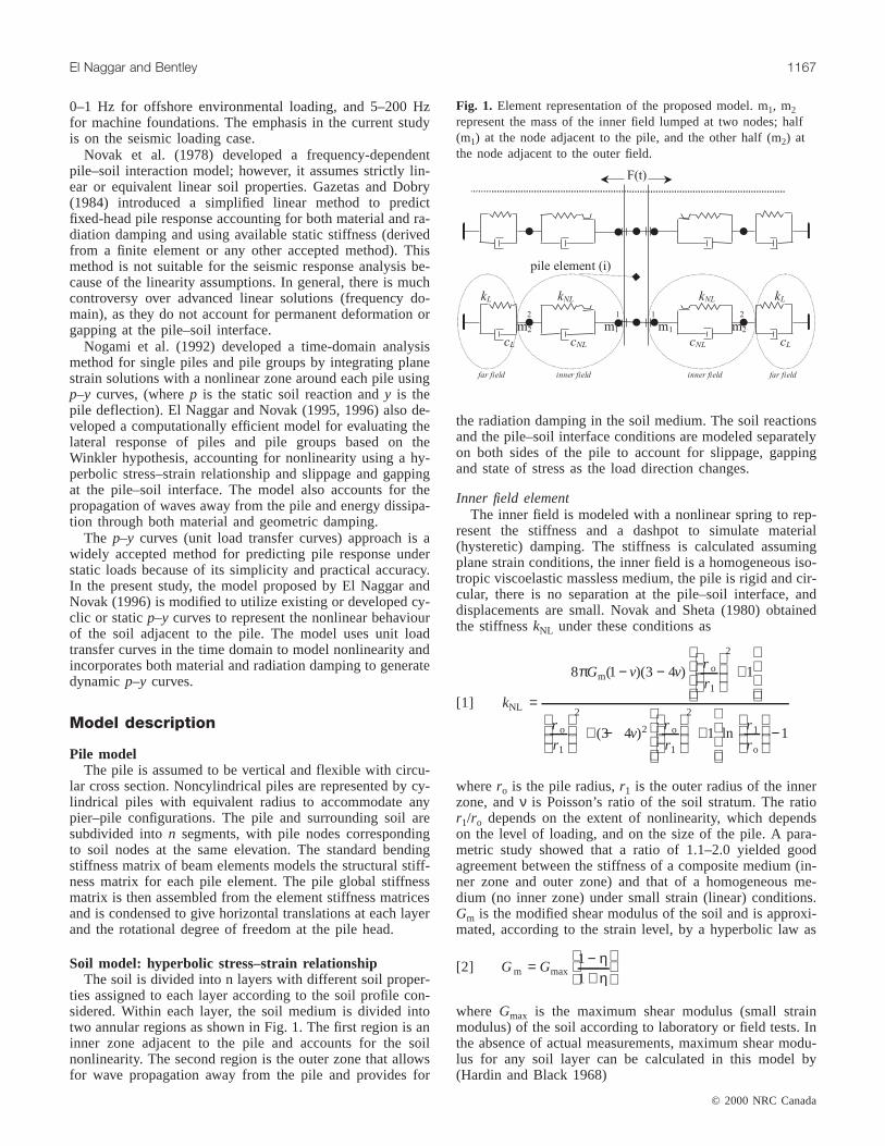
Based on model tests,p–y curves relate pile deflections tothe corresponding soil reaction at any depth (element) belowthe ground surface. Thep–y curve represents the total soilreaction to the pile motion (i.e., the reactions of the innerand outer zones combined). The total stiffness,kpy, derivedfrom the p–y curve is equivalent to the true stiffness (realpart of the complex stiffness) of the soil medium. Thus, re-ferring to the hyperbolic law model, the combined innerzone stiffness (kNL) and outer zone stiffness (kL) can be re-placed by a unified equivalent stiffness zone (kpy) as shownin Fig. 3a. Hence, to ensure that the true stiffness is thesame for the two soil models, the flexibility of the two mod-els is equated, i.e.,

[12]1 1 1

k k kpy

= +L NL

The stiffness of the nonlinear strength is then calculatedas

[13] kk k

k kpy

pyNL

L

L

=−

The constant of the linear elastic spring,kL, is establishedfrom the plane strain solution (i.e., eq. [10]). The static soilstiffness,kpy represents the relationship between the staticsoil reaction,p, and the pile deflection,y, for a givenp–ycurve at a specific load level. Thep–y curves are establishedusing empirical equations (Matlock 1970; Reese and Welch1975; Reese et al. 1975) or curve fit to measured strain datausing an accepted method such as the modified Ramberg-Osgood model (Desai and Wu 1976). In the present study,internally generated staticp–y curves are established basedon commonly used empirical correlations for a range of soiltypes.

DampingThe damping (imaginary part of the complex stiffness) is

incorporated into both thep–y approach and the hyperbolicmodel to allow for energy dissipation throughout the soil.The nonlinearity in the vicinity of the pile, however, drasti-cally reduces the geometric damping in the inner field.Therefore, both material and geometric (radiation) dampingare modeled in the outer field. A dashpot is connected inparallel to the far-field spring, and its constant is derivedfrom eq. [11]. If the material damping in the inner zone is tobe considered, a parallel dashpot with a constantcNL, coeffi-cient of material damping in the inner zone, to be suitablychosen may be added as shown in Fig. 3b. The addition ofthe damping resistance to static resistance represented by thestatic unit load transfer (thep–y curve) tends to increase thetotal resistance as shown in Fig. 4.

Static p–y curve generation for clayThe general procedure for computingp–y curves in clays

both above and below the groundwater table and correspond-ing parameters are recommended by Matlock (1970) andBhushan et al. (1979), respectively. Thep–y relationship wasbased on the following equation:

[14]pP

yy

n

u

0.5=

50

wherep is the soil resistance,y is the deflection correspond-ing to p, Pu is the ultimate soil resistance from eqs. [4] and[5], n is a constant relating soil resistance to pier–pile de-flection, andy50 is the corrected deflection at one-half theultimate soil reaction determined from laboratory tests. Thetangent stiffness constant,kpy, of any soil element at timestep t + ∆t is given by the slope of the tangent to thep–ycurve at the specific load level as shown in Fig. 4. This slopeis established from the soil deflections at time stepst andt –∆t and the corresponding soil reactions calculated fromeq. [14], i.e.,

© 2000 NRC Canada


Fig. 3. Soil model: (a) composite medium andp–y curve, and(b) inclusion of damping.



[15] kp p

y ypy t t

t t t

t t t( )+

−

−=

−−∆

∆

∆

Therefore, eqs. [10] and [15] can be substituted intoeq. [13] to obtain the nonlinear stiffness representing the in-ner field element in the analysis. Thus, the linear and nonlin-ear qualities of the unit load transfer curves have beenlogically incorporated into the outer and inner zones, respec-tively.

Static p–y curve generation for sandSeveral methods have been used to experimentally obtain

p–y curves for sandy soils. Abendroth and Greimann (1990)performed 11 scaled pile tests and used a modifiedRamberg-Osgood model to approximate the nonlinear soilresistance and displacement behaviour for loose and densesand. The most commonly used criteria for development ofp–y curves for sand were proposed by Reese et al. (1974)but tend to give very conservative results. Bhushan et al.(1981) and Bhushan and Askari (1984) used a different pro-cedure based on full-scale load test results to obtain nonlin-ear p–y curves for saturated and unsaturated sand. A step-by-step procedure for developingp–y curves in sands(Bhushan and Haley 1980; Bhushan et al. 1981) was used toestimate the static unit load transfer curves for differentsands below and above the water table. The procedure usedto generatep–y curves for sand differs from that suggestedfor clays. The secant modulus approach is used to approxi-mate soil reactions at specified lateral displacements. Thesoil resistance in the staticp–y curve model can be calcu-lated using the following equation:

[16] p = (k)(x)(y)(F1)(F2)

wherek is a constant that depends on the lateral deflectiony(i.e., k decreases asy increases) and relates the secant modu-lus of soil for a given value ofy to depth (Es = kx); x is thedepth at which thep–y curve is being generated; and F1 andF2 are density and groundwater (saturated or unsaturated)factors, respectively, and can be determined from Meyer andReese (1979). The main factors affectingk are the relativedensity of the sand (loose or dense) and the level of lateraldisplacement. The secant modulus decreases with increasing

displacement and thus the nonlinearity of the sand can bemodeled accurately. This analysis assumes a linear increaseof the soil modulus with an increase in depth (but variesnonlinearly with displacement at each depth) which is typi-cal for many sands.

Equation [16] was used to establish thep–y curve at agiven depth. The tangent stiffnesskpy (needed in the time-domain analysis), which represents the tangent to thep–ycurve at the specific load level, was then calculated usingeq. [15] based on calculated soil reactions from the corre-sponding pile displacements for two consecutive time steps(using eq. [16]).

Degradation of soil stiffnessTransient loading, especially cyclic loading, may result in

a buildup of pore-water pressures and (or) a change of thesoil structure that causes the shear strain amplitudes of thesoil to increase with an increasing number of cycles (Idrisset al. 1978). Idriss et al. (1978) reported that the shear stressamplitude decreased with an increasing number of cycles forharmonically loaded clay and saturated sand specimens un-der strain-controlled, undrained conditions. These studiessuggest that repeated cyclic loading results in the degrada-tion of the soil stiffness. For cohesive soils, the value of theshear modulus afterN cycles,GN, can be related to its valuein the first cycle,Gmax, by

[17] GN = δ Gmax

where the degradation index,δ, is given byδ = N –t, and t isthe degradation parameter defined by Idriss et al. (1978).This is incorporated into the proposed model by updatingthe nonlinear stiffness,kNL, by an appropriate factor in eachloading cycle.

Time-domain analysis and equations ofmotion

The time-domain analysis was used to include all aspectsof nonlinearity and examine the transient response logicallyand realistically. The governing equation of motion is givenby

© 2000 NRC Canada


Fig. 4. Determination of stiffness (kpy) from an internally generated staticp–y curve to produce a dynamicp–y curve (including damping).



[18] [ ]{ &&} [ ]{ &} [ ]{ } { ( )}M u C u K u F t+ + =

where [M], [C], and [K] are the global mass, damping, andstiffness matrices, respectively; and{&&}, { &}, { }u u u, and F(t) areacceleration, velocity, displacement, and external load vec-tors, respectively. Referring to Fig. 1, the equations of mo-tion at node 1 (adjacent to the inner field) and node 2(adjacent to the outer field) are

[19] m u c u u k u u F1 1 1 2 1 2 1&& (& & ) ( )+ − + − =NL NL

[20] m u c u u k u u F2 2 1 2 1 2 2&& (& & ) ( )− − − − =NL NL

whereu1 andu2 are displacements of nodes 1 and 2, respec-tively; F1 is the force in the nonlinear spring including theconfining pressure; andF2 is the soil resistance at node 2.The equation of motion for the outer field is written as

[21] cu k u F&&2 2 2+ = −L

Assuming compatibility and equilibrium at the interfacebetween the inner and outer zones leads to the followingequation, which is valid for both sides of the pile:

[22]F1

0

=

Am B c c k

k Bc

k Bc

k Am B c c1

2

+ + +− −

− −+ + +

( )

(L NL NL

NL NL

NL NL

NL L NL L) +

k

×

+

−

−

u

uF

F

i

i

1

2

11

21

where F i1

1− and F i2

1− are the sums of inertia forces and soilreactions at nodes 1 and 2, respectively; andA and B areconstants of numerical integration for inertia and damping,respectively.

The linear acceleration assumption was used and theNewmarkβ method was implemented for direct time integra-tion of the equations of motion. The modified Newton-Raphson iteration scheme was used to solve the nonlinearequilibrium equations.

© 2000 NRC Canada


Fig. 5. Soil modulus variation for profiles considered in the analysis.d, pile diameter;L, pile depth;z, depth below the surface.

Fig. 6. Calculated dynamic soil reactions at 1.0 m depth (for a prescribed harmonic displacement at the pile head with amplitude0.03d = 0.015 m,L/d = 30).



Verification of the analytical model

Verification of clay modelDifferent soil profiles were considered in the analysis.

Figure 5 shows the typical pile–soil system and the soil pro-files considered including linear and parabolic soil profiles.The p–y model was first verified against the hyperbolicmodel (El Naggar and Novak 1996). Figures 6 and 7 com-pare the dynamic soil reaction and pile head response forboth the hyperbolic andp–y curve models for a single rein-forced concrete pile in soft clay. A 0.5 m diameter, 15 mlong pile was used with an elastic modulus (Ep ) equal to 35GPa. A parabolic soil profile with the ratioEp /Es = 1000 atthe pile base was assumed. The undrained shear strength ofthe clay was assumed to be 25 kPa. Figure 6 shows the cal-culated dynamic soil reactions for a prescribed harmonicdisplacement of a single amplitude equal to 0.03d (0.015 m)at a frequency of 2 Hz at the pile head. Figure 6 shows thatthe soil reactions obtained from the two models are verysimilar and approach stability after five cycles. The patternshown in Fig. 6 is also similar to that obtained by Nogami etal. (1992) showing an increasing gap and stability after ap-proximately five cycles. Figure 7 shows the displacement–time history of the pile head installed in the same soil pro-file. A harmonic load with single amplitude equal to 10 kNwas applied at the pile head. The hyperbolic andp–y curvemodels show very similar responses at the pile head andboth stabilize after approximately five cycles.

The dynamic soil reactions are, in general, larger than thestatic reactions because of the contribution from damping.Employing the same definition used for staticp–y curves,dynamicp–y curves can be established to relate pile deflec-tions to the corresponding dynamic soil reaction at any depthbelow the ground surface. The proposed dynamicp–y curvesare frequency dependent. These dynamicp–y curves can beused in other static analyses that are based on thep–y curveapproach to approximately account for the dynamic effectson the soil reactions to transient loading.

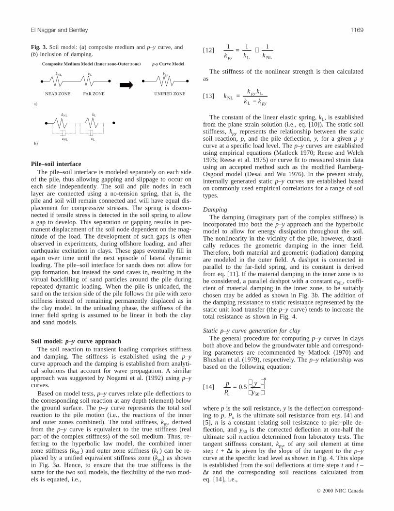
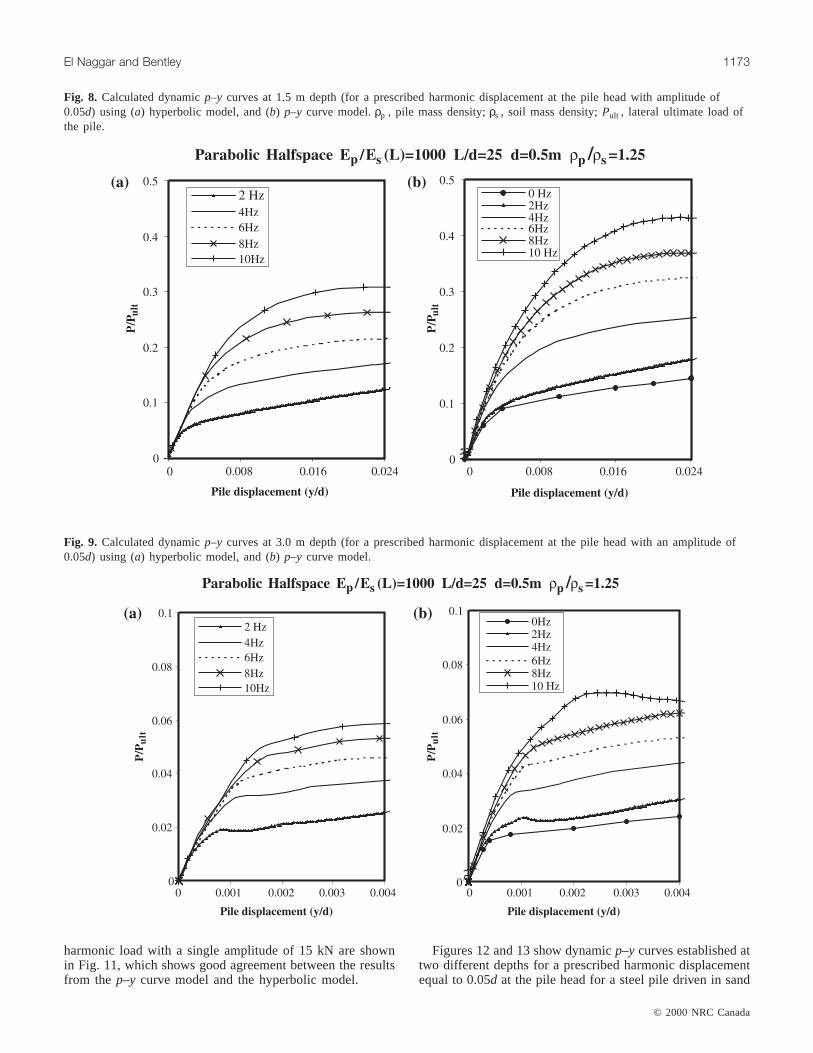
Figures 8 and 9 show dynamicp–y curves established attwo different clay depths for a prescribed harmonic displace-ment at the pile head with single amplitude equal to 0.05d,for a frequency range from 0 to 10 Hz. The shear modulus

of the soil was assumed to increase parabolically along thepile length. A concrete pile 12.5 m in length and 0.5 m in di-ameter was considered in the analysis. The elastic modulusof the pile material was assumed to be 35 GPa and the ratioEp /Es = 1000 (at the pile base). Both thep–y curve and hy-perbolic models were used to analyze the pile response. Thedynamic soil reaction (normalized by the ultimate pile ca-pacity, Pult) obtained from thep–y curve model comparedwell with that obtained from the hyperbolic relationshipmodel, especially for lower frequencies, as shown in Figs. 8and 9, which also show that the soil reaction increased as thefrequency increased. This increase was more evident in theresults obtained from thep–y curve model.

Verification of sand modelThe p–y curve and hyperbolic models were used to ana-

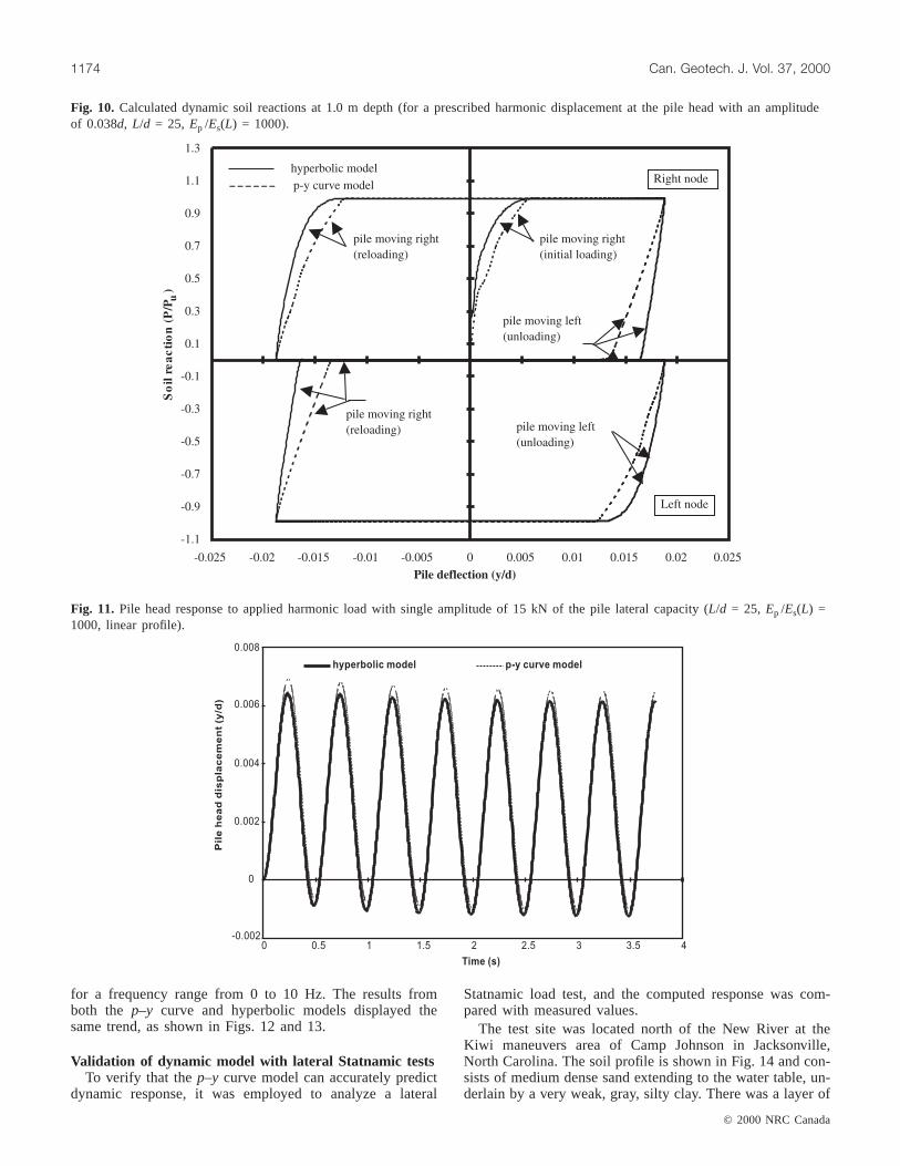
lyze the response of piles installed in sand. The sand was as-sumed to be unsaturated and a linear soil modulus profilewas adopted. The pile used in the previous case was consid-ered. Figure 10 shows the calculated dynamic soil reactionsat 1 m depth for a prescribed harmonic displacement with anamplitude equal to 0.038d at the pile head with a frequencyof 2 Hz. The two models feature very similar dynamic soilreactions. It should be noted that the soil reactions at bothsides of the pile are traced independently. The upper part ofthe curve in Fig. 10 represents the reactions for the soil ele-ment adjacent to the right face of the pile, when it is loadedfrom the left. The lower part represents the reactions of thesoil element adjacent to the left face of the pile as it isloaded from the right. Both elements offer zero resistance tothe pile movement when tensile stresses are detected in thenonlinear soil spring during unloading of the soil element oneither side. However, the soil nodes remain attached to thepile node at the same level, allowing the sand to “cave in”and fill the gap. Observations from field and laboratory piletesting confirmed that, unlike clays, sands usually do notexperience gapping during harmonic loading. Thus bothanalyses model the physical behaviour of the soil realisti-cally and logically.

The pile head displacement–time histories obtained fromthe p–y curve and hyperbolic models for a pile installed in asand with linearly varying elastic modulus due to an applied

© 2000 NRC Canada


Fig. 7. Pile head response under applied harmonic load with single amplitude equal to 10 kN (L/d = 30, Ep /Es(L) = 1000, linear profile).



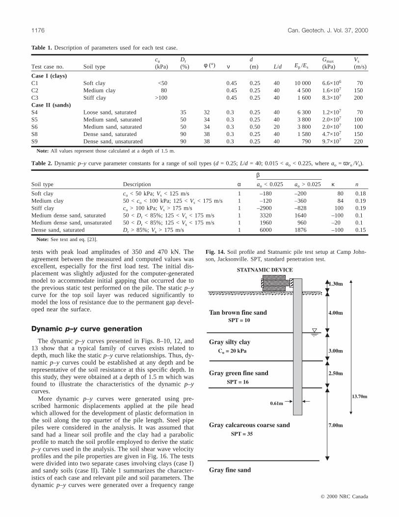
harmonic load with a single amplitude of 15 kN are shownin Fig. 11, which shows good agreement between the resultsfrom the p–y curve model and the hyperbolic model.

Figures 12 and 13 show dynamicp–y curves established attwo different depths for a prescribed harmonic displacementequal to 0.05d at the pile head for a steel pile driven in sand

© 2000 NRC Canada


Fig. 9. Calculated dynamicp–y curves at 3.0 m depth (for a prescribed harmonic displacement at the pile head with an amplitude of0.05d) using (a) hyperbolic model, and (b) p–y curve model.

Fig. 8. Calculated dynamicp–y curves at 1.5 m depth (for a prescribed harmonic displacement at the pile head with amplitude of0.05d) using (a) hyperbolic model, and (b) p–y curve model.ρp , pile mass density;ρs , soil mass density;Pult , lateral ultimate load ofthe pile.



for a frequency range from 0 to 10 Hz. The results fromboth the p–y curve and hyperbolic models displayed thesame trend, as shown in Figs. 12 and 13.

Validation of dynamic model with lateral Statnamic testsTo verify that thep–y curve model can accurately predict

dynamic response, it was employed to analyze a lateral

Statnamic load test, and the computed response was com-pared with measured values.

The test site was located north of the New River at theKiwi maneuvers area of Camp Johnson in Jacksonville,North Carolina. The soil profile is shown in Fig. 14 and con-sists of medium dense sand extending to the water table, un-derlain by a very weak, gray, silty clay. There was a layer of

© 2000 NRC Canada


Fig. 10. Calculated dynamic soil reactions at 1.0 m depth (for a prescribed harmonic displacement at the pile head with an amplitudeof 0.038d, L/d = 25, Ep /Es(L) = 1000).

Fig. 11. Pile head response to applied harmonic load with single amplitude of 15 kN of the pile lateral capacity (L/d = 25, Ep /Es(L) =1000, linear profile).



gray sand at a depth of 7 m and a calcified sand stratum be-low the gray sand. The pile tested at this site was a cast-in-place reinforced concrete shaft with a steel casing having anouter diameter of 0.61 m and a casing wall thickness of13 mm. More details on the soil and pile properties and theloading procedure can be found in El Naggar (1998).

Statnamic testing was conducted on the pile 2 weeks afterlateral static testing was performed. Statnamic loading testswere performed by M. Janes and P. Bermingham, both ofBerminghammer Foundation Equipment, Hamilton, Ontario.

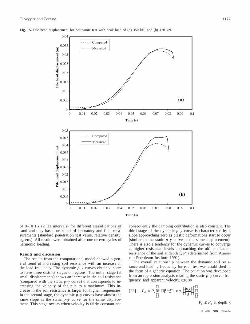
The computed lateral response of the pile head is com-pared with the measured response in Fig. 15 for two separate

© 2000 NRC Canada






tests with peak load amplitudes of 350 and 470 kN. Theagreement between the measured and computed values wasexcellent, especially for the first load test. The initial dis-placement was slightly adjusted for the computer-generatedmodel to accommodate initial gapping that occurred due tothe previous static test performed on the pile. The staticp–ycurve for the top soil layer was reduced significantly tomodel the loss of resistance due to the permanent gap devel-oped near the surface.

Dynamic p–y curve generation

The dynamicp–y curves presented in Figs. 8–10, 12, and13 show that a typical family of curves exists related todepth, much like the staticp–y curve relationships. Thus, dy-namic p–y curves could be established at any depth and berepresentative of the soil resistance at this specific depth. Inthis study, they were obtained at a depth of 1.5 m which wasfound to illustrate the characteristics of the dynamicp–ycurves.

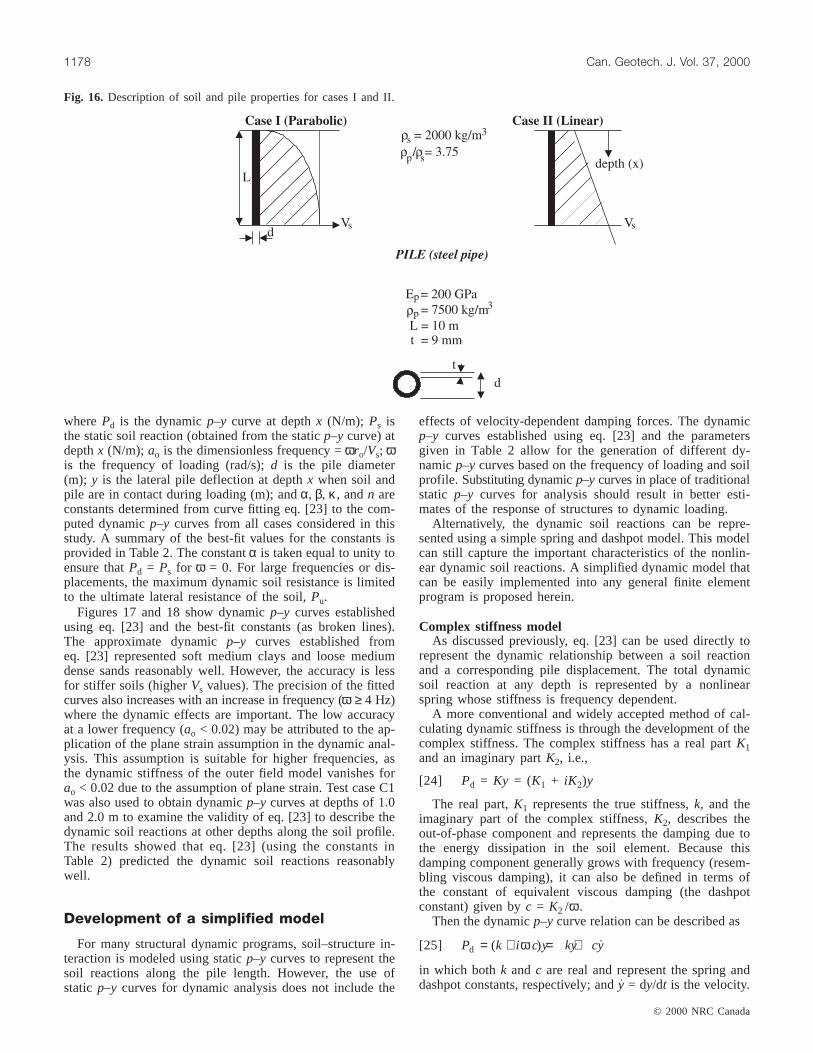
More dynamic p–y curves were generated using pre-scribed harmonic displacements applied at the pile headwhich allowed for the development of plastic deformation inthe soil along the top quarter of the pile length. Steel pipepiles were considered in the analysis. It was assumed thatsand had a linear soil profile and the clay had a parabolicprofile to match the soil profile employed to derive the staticp–y curves used in the analysis. The soil shear wave velocityprofiles and the pile properties are given in Fig. 16. The testswere divided into two separate cases involving clays (case I)and sandy soils (case II). Table 1 summarizes the character-istics of each case and relevant pile and soil parameters. Thedynamicp–y curves were generated over a frequency range

© 2000 NRC Canada


Fig. 14. Soil profile and Statnamic pile test setup at Camp John-son, Jacksonville. SPT, standard penetration test.

Test case no. Soil typecu

(kPa)Dr

(%) φ (°) νd(m) L/d Ep /Es

Gmax

(kPa)Vs

(m/s)

Case I (clays)C1 Soft clay <50 0.45 0.25 40 10 000 6.6×106 70C2 Medium clay 80 0.45 0.25 40 4 500 1.6×107 150C3 Stiff clay >100 0.45 0.25 40 1 600 8.3×107 200Case II (sands)S4 Loose sand, saturated 35 32 0.3 0.25 40 6 300 1.2×107 70S5 Medium sand, saturated 50 34 0.3 0.25 40 3 800 2.0×107 100S6 Medium sand, saturated 50 34 0.3 0.50 20 3 800 2.0×107 100S8 Dense sand, saturated 90 38 0.3 0.25 40 1 580 4.7×107 150S9 Dense sand, unsaturated 90 38 0.3 0.25 40 790 9.7×107 220

Note: All values represent those calculated at a depth of 1.5 m.

Table 1. Description of parameters used for each test case.

βSoil type Description α ao < 0.025 ao > 0.025 κ n

Soft clay cu < 50 kPa;Vs < 125 m/s 1 –180 –200 80 0.18Medium clay 50 <cu < 100 kPa; 125 <Vs < 175 m/s 1 –120 –360 84 0.19Stiff clay cu > 100 kPa;Vs > 175 m/s 1 –2900 –828 100 0.19Medium dense sand, saturated 50 <Dr < 85%; 125 <Vs < 175 m/s 1 3320 1640 –100 0.1Medium dense sand, unsaturated 50 <Dr < 85%; 125 <Vs < 175 m/s 1 1960 960 –20 0.1Dense sand, saturated Dr > 85%; Vs > 175 m/s 1 6000 1876 –100 0.15

Note: See text and eq. [23].

Table 2. Dynamicp–y curve parameter constants for a range of soil types (d = 0.25; L/d = 40; 0.015 <ao < 0.225, whereao = ωro /Vs).



of 0–10 Hz (2 Hz intervals) for different classifications ofsand and clay based on standard laboratory and field mea-surements (standard penetration test value, relative density,cu, etc.). All results were obtained after one or two cycles ofharmonic loading.

Results and discussionThe results from the computational model showed a gen-

eral trend of increasing soil resistance with an increase inthe load frequency. The dynamicp–y curves obtained seemto have three distinct stages or regions. The initial stage (atsmall displacements) shows an increase in the soil resistance(compared with the staticp–y curve) that corresponds to in-creasing the velocity of the pile to a maximum. This in-crease in the soil resistance is larger for higher frequencies.In the second stage, the dynamicp–y curves have almost thesame slope as the staticp–y curve for the same displace-ment. This stage occurs when velocity is fairly constant and

consequently the damping contribution is also constant. Thethird stage of the dynamicp–y curve is characterized by aslope approaching zero as plastic deformations start to occur(similar to the staticp–y curve at the same displacement).There is also a tendency for the dynamic curves to convergeat higher resistance levels approaching the ultimate lateralresistance of the soil at depthx, Pu (determined from Ameri-can Petroleum Institute 1991).

The overall relationship between the dynamic soil resis-tance and loading frequency for each test was established inthe form of a generic equation. The equation was developedfrom an regression analysis relating the staticp–y curve, fre-quency, and apparent velocity,ωy, so

[23] P P a ay

d

n

d s o2

o= + +

α β κ ω,

P P xd u at depth≤

© 2000 NRC Canada


Fig. 15. Pile head displacement for Statnamic test with peak load of (a) 350 kN, and (b) 470 kN.



wherePd is the dynamicp–y curve at depthx (N/m); Ps isthe static soil reaction (obtained from the staticp–y curve) atdepthx (N/m); ao is the dimensionless frequency =ωro/Vs; ωis the frequency of loading (rad/s);d is the pile diameter(m); y is the lateral pile deflection at depthx when soil andpile are in contact during loading (m); andα, β, κ, andn areconstants determined from curve fitting eq. [23] to the com-puted dynamicp–y curves from all cases considered in thisstudy. A summary of the best-fit values for the constants isprovided in Table 2. The constantα is taken equal to unity toensure thatPd = Ps for ω = 0. For large frequencies or dis-placements, the maximum dynamic soil resistance is limitedto the ultimate lateral resistance of the soil,Pu.

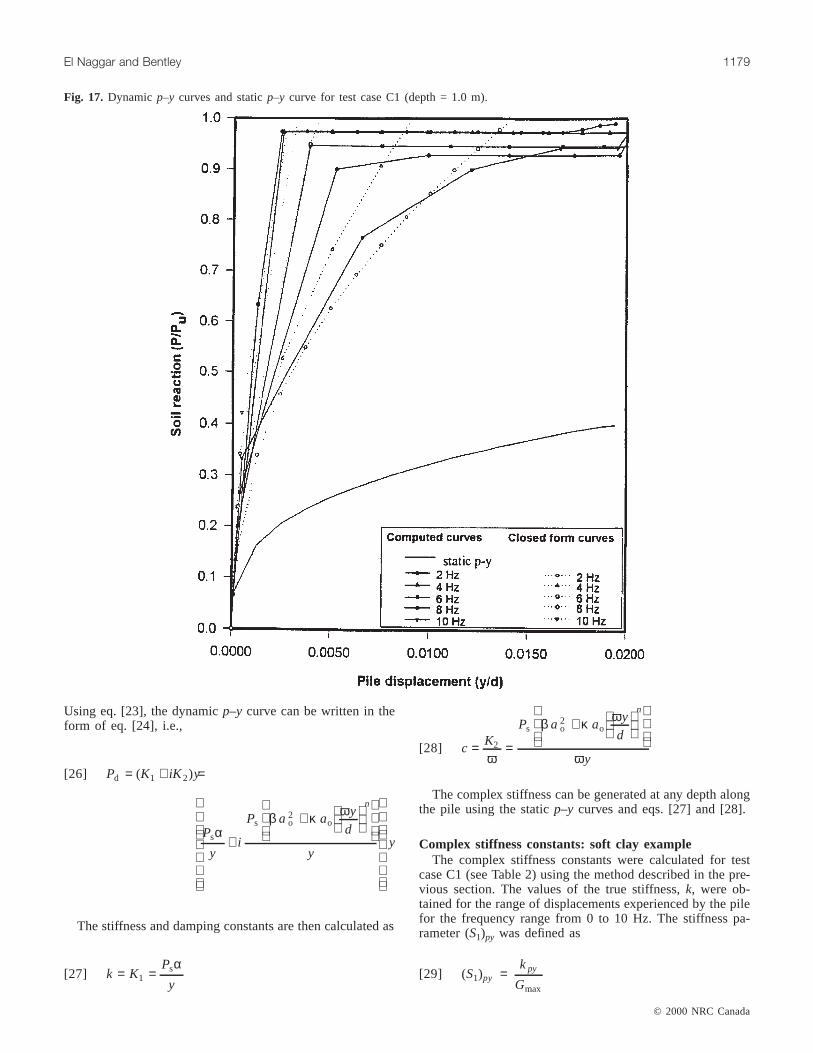
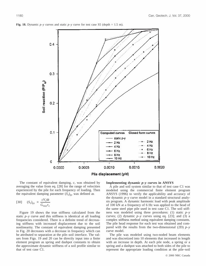
Figures 17 and 18 show dynamicp–y curves establishedusing eq. [23] and the best-fit constants (as broken lines).The approximate dynamicp–y curves established fromeq. [23] represented soft medium clays and loose mediumdense sands reasonably well. However, the accuracy is lessfor stiffer soils (higherVs values). The precision of the fittedcurves also increases with an increase in frequency (ω ≥ 4 Hz)where the dynamic effects are important. The low accuracyat a lower frequency (ao < 0.02) may be attributed to the ap-plication of the plane strain assumption in the dynamic anal-ysis. This assumption is suitable for higher frequencies, asthe dynamic stiffness of the outer field model vanishes forao < 0.02 due to the assumption of plane strain. Test case C1was also used to obtain dynamicp–y curves at depths of 1.0and 2.0 m to examine the validity of eq. [23] to describe thedynamic soil reactions at other depths along the soil profile.The results showed that eq. [23] (using the constants inTable 2) predicted the dynamic soil reactions reasonablywell.

Development of a simplified model

For many structural dynamic programs, soil–structure in-teraction is modeled using staticp–y curves to represent thesoil reactions along the pile length. However, the use ofstatic p–y curves for dynamic analysis does not include the

effects of velocity-dependent damping forces. The dynamicp–y curves established using eq. [23] and the parametersgiven in Table 2 allow for the generation of different dy-namicp–y curves based on the frequency of loading and soilprofile. Substituting dynamicp–y curves in place oftraditionalstatic p–y curves for analysis should result in better esti-mates of the response of structures to dynamic loading.

Alternatively, the dynamic soil reactions can be repre-sented using a simple spring and dashpot model. This modelcan still capture the important characteristics of the nonlin-ear dynamic soil reactions. A simplified dynamic model thatcan be easily implemented into any general finite elementprogram is proposed herein.

Complex stiffness modelAs discussed previously, eq. [23] can be used directly to

represent the dynamic relationship between a soil reactionand a corresponding pile displacement. The total dynamicsoil reaction at any depth is represented by a nonlinearspring whose stiffness is frequency dependent.

A more conventional and widely accepted method of cal-culating dynamic stiffness is through the development of thecomplex stiffness. The complex stiffness has a real partK1and an imaginary partK2, i.e.,

[24] Pd = Ky = (K1 + iK2)y

The real part,K1 represents the true stiffness,k, and theimaginary part of the complex stiffness,K2, describes theout-of-phase component and represents the damping due tothe energy dissipation in the soil element. Because thisdamping component generally grows with frequency (resem-bling viscous damping), it can also be defined in terms ofthe constant of equivalent viscous damping (the dashpotconstant) given byc = K2 /ω .

Then the dynamicp–y curve relation can be described as

[25] P k i c y ky cyd = + = +( ) &ω

in which bothk and c are real and represent the spring anddashpot constants, respectively; and&y = dy/dt is the velocity.

© 2000 NRC Canada


Fig. 16. Description of soil and pile properties for cases I and II.



Using eq. [23], the dynamicp–y curve can be written in theform of eq. [24], i.e.,

[26] P K iK yd = + =( )1 2

P

yi

P a ay

d

y

n

s

s o2

oα

β κ ω

+

+

y

The stiffness and damping constants are then calculated as

[27] k KP

y= =1

sα

[28] cK

P a ay

d

y

n

= =

+

2

ω

β κ ω

ω

s o2

o

The complex stiffness can be generated at any depth alongthe pile using the staticp–y curves and eqs. [27] and [28].

Complex stiffness constants: soft clay exampleThe complex stiffness constants were calculated for test

case C1 (see Table 2) using the method described in the pre-vious section. The values of the true stiffness,k, were ob-tained for the range of displacements experienced by the pilefor the frequency range from 0 to 10 Hz. The stiffness pa-rameter (S1)py was defined as

[29] (S1)py =k

Gpy

max

© 2000 NRC Canada


Fig. 17. Dynamic p–y curves and staticp–y curve for test case C1 (depth = 1.0 m).



The constant of equivalent damping,c, was obtained byaveraging the value from eq. [28] for the range of velocitiesexperienced by the pile for each frequency of loading. Thenthe equivalent damping parameter (S2)py was defined as

[30] (S2)py =cV

G rs

o

ω

max

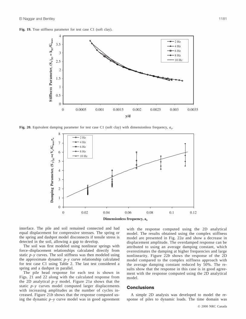
Figure 19 shows the true stiffness calculated from thestatic p–y curve and this stiffness is identical at all loadingfrequencies considered. There is a definite trend of decreas-ing stiffness with increased displacement due to the soilnonlinearity. The constant of equivalent damping presentedin Fig. 20 decreases with a decrease in frequency which canbe attributed to separation at the pile–soil interface. The val-ues from Figs. 19 and 20 can be directly input into a finiteelement program as spring and dashpot constants to obtainthe approximate dynamic stiffness of a soil profile similar tothat of test case C1.

Implementing dynamic p–y curves in ANSYSA pile and soil system similar to that of test case C1 was

modeled using the commercial finite element programANSYS (1996) to verify the applicability and accuracy ofthe dynamicp–y curve model in a standard structural analy-sis program. A dynamic harmonic load with peak amplitudeof 100 kN at a frequency of 6 Hz was applied to the head ofthe same steel pipe pile used in test case C1. The soil stiff-ness was modeled using three procedures: (1) staticp–ycurves; (2) dynamicp–y curves using eq. [23]; and (3) acomplex stiffness method using equivalent dampingconstants.The pile head response for each test was obtained and com-pared with the results from the two-dimensional (2D)p–ycurve model.

The pile was modeled using two-noded beam elementsand was discretized into 10 elements that increased in lengthwith an increase in depth. At each pile node, a spring or aspring and a dashpot was attached to both sides of the pile torepresent the appropriate loading condition at the pile–soil

© 2000 NRC Canada


Fig. 18. Dynamic p–y curves and staticp–y curve for test case S5 (depth = 1.5 m).



interface. The pile and soil remained connected and hadequal displacement for compressive stresses. The spring orthe spring and dashpot model disconnects if tensile stress isdetected in the soil, allowing a gap to develop.

The soil was first modeled using nonlinear springs withforce–displacement relationships calculated directly fromstaticp–y curves. The soil stiffness was then modeled usingthe approximate dynamicp–y curve relationship calculatedfor test case C1 using Table 2. The last test considered aspring and a dashpot in parallel.

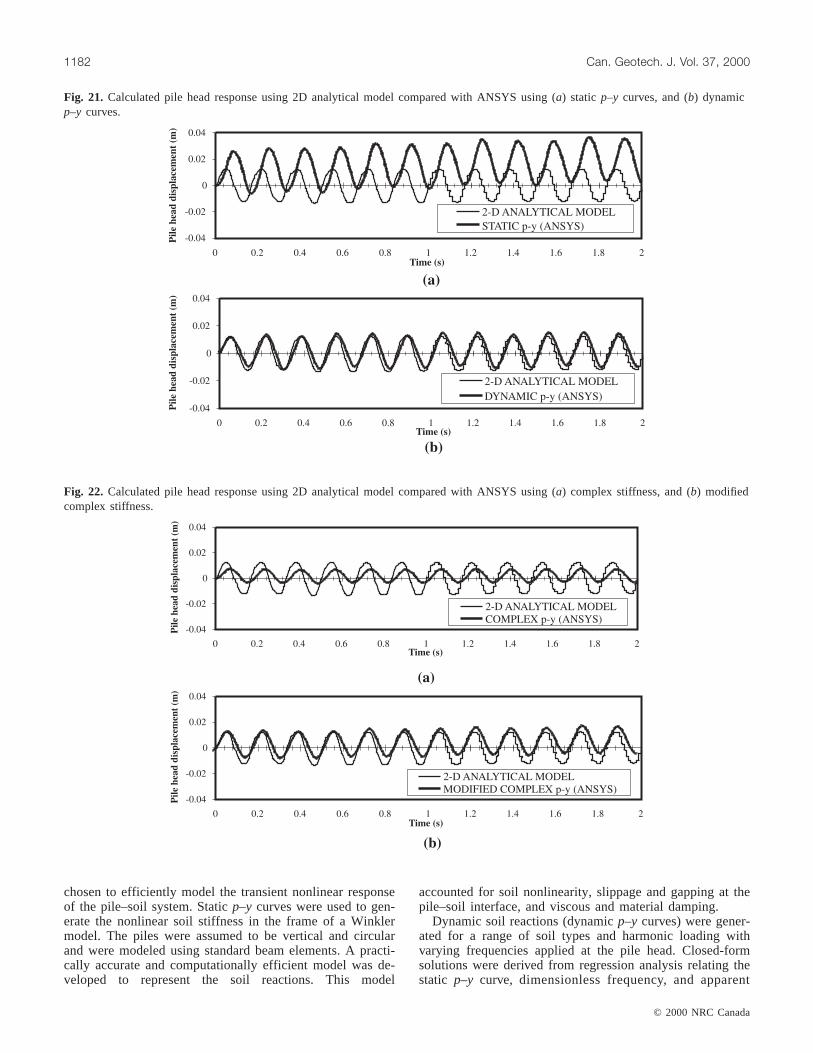
The pile head response for each test is shown inFigs. 21 and 22 along with the calculated response fromthe 2D analyticalp–y model. Figure 21a shows that thestatic p–y curves model computed larger displacementswith increasing amplitudes as the number of cycles in-creased. Figure 21b shows that the response computed us-ing the dynamicp–y curve model was in good agreement

with the response computed using the 2D analyticalmodel. The results obtained using the complex stiffnessmodel are presented in Fig. 22a and show a decrease indisplacement amplitude. The overdamped response can beattributed to using an average damping constant, whichoverestimates the damping at higher frequencies and largenonlinearity. Figure 22b shows the response of the 2Dmodel compared to the complex stiffness approach withthe average damping constant reduced by 50%. The re-sults show that the response in this case is in good agree-ment with the response computed using the 2D analyticalmodel.

Conclusions

A simple 2D analysis was developed to model the re-sponse of piles to dynamic loads. The time domain was

© 2000 NRC Canada


Fig. 20. Equivalent damping parameter for test case C1 (soft clay) with dimensionless frequency,ao.

Fig. 19. True stiffness parameter for test case C1 (soft clay).



chosen to efficiently model the transient nonlinear responseof the pile–soil system. Staticp–y curves were used to gen-erate the nonlinear soil stiffness in the frame of a Winklermodel. The piles were assumed to be vertical and circularand were modeled using standard beam elements. A practi-cally accurate and computationally efficient model was de-veloped to represent the soil reactions. This model

accounted for soil nonlinearity, slippage and gapping at thepile–soil interface, and viscous and material damping.

Dynamic soil reactions (dynamicp–y curves) were gener-ated for a range of soil types and harmonic loading withvarying frequencies applied at the pile head. Closed-formsolutions were derived from regression analysis relating thestatic p–y curve, dimensionless frequency, and apparent

© 2000 NRC Canada


Fig. 21. Calculated pile head response using 2D analytical model compared with ANSYS using (a) static p–y curves, and (b) dynamicp–y curves.

Fig. 22. Calculated pile head response using 2D analytical model compared with ANSYS using (a) complex stiffness, and (b) modifiedcomplex stiffness.



© 2000 NRC Canada


velocity of the soil particles. A simple spring and dashpotmodel was also proposed whose constants were establishedby splitting the dynamicp–y curves into real (stiffness) andimaginary (damping) components. This model could be usedin equivalent linear analysis for harmonic loading at the pilehead. The proposed dynamicp–y curves and the spring anddashpot model were incorporated into a commercial finiteelement program, ANSYS, that was used to compute the re-sponse of a laterally loaded pile. The computed responsescompared well with the predictions of the 2D analysis.

The following conclusions were drawn from the study:(1) The developed pile–soil model is capable of analyzing

the response of piles to lateral transient loading accountingfor the nonlinear behaviour of the soil and energy dissipa-tion.

(2) The soil resistance to the pile motion increases withthe frequency of the pile head loading (inertial loading) forsingle piles.

(3) The developed dynamicp–y curve can represent thedynamic soil reactions using a predefined staticp–y curve.

(4) The pile head response under harmonic loading can beapproximately modeled using dynamicp–y curve functionsin most of the available structural analysis programs.

(5) The implementation of the dynamicp–y curves intime-domain analyses to model the soil reactions is preferredbecause it accounts for the variation in damping with thedisplacement level. The damping constant in the complexstiffness model must be chosen accounting for the level ofnonlinearity expected.

Acknowledgements

This research was supported by a grant from the NaturalSciences and Engineering Research Council of Canada(NSERC) to the first author and research contract 24-9 fromthe National Cooperative Highway Research Program(NCHRP). Both sources of support are greatly appreciated.

References

Abendroth, R.E., and Greimann, L.F. 1990. Pile behavior estab-lished from model tests. Journal of Geotechnical Engineering,ASCE, 116(4): 571–588.

American Petroleum Institute. 1991. Recommended practice forplanning, designing and constructing fixed offshore platforms.API Recommended Practice 2A (RP 2A). 19th ed. American Pe-troleum Institute, Washington, D.C., pp. 47–55.

ANSYS Inc. 1996. General finite element analysis program. Ver-sion 5.4. ANSYS Inc., Canonsburg, Pa.

Bhushan, K., and Askari, S. 1984. Lateral load tests on drilled pierfoundations for solar plant heliostats.In Laterally loaded piles.Edited byJ.A. Langer. American Society for Testing and Mate-rials, Special Technical Publication STP 835, pp. 141–155.

Bhushan, K., and Haley, S.C. 1980. Development of computer pro-gram usingP–y data from load test results for lateral load de-sign of drilled piers. Woodward-Clyde Consultants ProfessionalDevelopment Committee, San Francisco, Calif.

Bhushan, K., Haley, S.C., and Fong, P.T. 1979. Lateral load testson drilled piers in stiff clays. Journal of the Geotechnical Engi-neering Division, ASCE,105(GT8): 969–985.

Bhushan, K., Lee, L.J., and Grime, D.B. 1981. Lateral load tests ondrilled piers in sand.In Proceedings of a Session on DrilledPiers and Caissons, Geotechnical Engineering Division, Ameri-can Society of Civil Engineers, National Convention, St. Louis,Mo., pp. 131–143.

Desai, C.S., and Wu, T.H. 1976. A general function for stress–strain curves.In Proceedings of the 2nd International Confer-ence on Numerical Methods in Geomechanics, American Soci-ety of Civil Engineers, Blacksburg, Vol. 1, pp. 306–318.

El Naggar, M.H. 1998. Interpretation of lateral statnamic load testresults. Geotechnical Testing Journal,21(3): 169–179.

El Naggar, M.H., and Novak, M. 1995. Nonlinear lateral interac-tion in pile dynamics. Journal of Soil Dynamics and EarthquakeEngineering,14(3): 141–157.

El Naggar, M.H., and Novak, M. 1996. Nonlinear analysis for dy-namic lateral pile response. Journal of Soil Dynamics and Earth-quake Engineering,15(4): 233–244.

Gazetas, G., and Dobry, R. 1984. Horizontal response of piles inlayered soils. Journal of Geotechnical Engineering, ASCE,110(1): 20–40.

Hardin, B.O., and Black, W.L. 1968. Vibration modulus of nor-mally consolidated clay. Journal of the Soil Mechanics andFoundations Division, ASCE,94(SM2): 353–369.

Idriss, I.M., Dobry, R., and Singh, R.D. 1978. Nonlinear behaviorof soft clays during cyclic loading. Journal of the GeotechnicalEngineering Division, ASCE,104(GT12): 1427–1447.

Matlock, H. 1970. Correlations for design of laterally loaded pilesin soft clay. In Proceedings of the 2nd Offshore TechnologyConference, Houston, Tex., Vol. 1, pp. 577–588.

Meyer, B.J., and Reese, L.C. 1979. Analysis of single piles underlateral loading. Preliminary Review Copy, Research Report 244-1, Center for Highway Research, The University of Texas atAustin, Austin, Tex., pp. 1–145.

Nogami, T., Konagai, K., Otani, J., and Chen, H.L. 1992. Nonlin-ear soil–pile interaction model for dynamic lateral motion. Jour-nal of Geotechnical Engineering, ASCE,118(1): 106–116.

Novak, M., and Sheta, M. 1980. Approximate approach to contacteffects of piles.In Proceedings of a Speciality Conference onDynamic Response of Pile Foundations: Analytical Aspects,American Society of Civil Engineers, Hollywood, Fla., pp. 53–79.

Novak, M., Nogami, T., and Aboul-Ella, F. 1978. Dynamic soil re-actions for plane strain case. Journal of the Engineering Me-chanics Division, ASCE,104: 953–959.

Reese, L.C., and Welch, R.C. 1975. Lateral loading of deep foun-dations in stiff clay. Journal of the Geotechnical Engineering Di-vision, ASCE,101(GT7): 633–649.

Reese, L.C., Cox, W.R., and Koop, F.D. 1974. Analysis of laterallyloaded piles in sand.In Proceedings of the 6th Annual OffshoreTechnology Conference, Houston, Tex., Vol. 2, Paper OTC2080, pp. 473–483.

Reese, L.C., Cox, W.R., and Koop, F.D. 1975. Field testing andanalysis of laterally loaded piles in stiff clay.In Proceedings ofthe 7th Annual Offshore Technology Conference, Houston, Tex.,Vol. 2, pp. 671–690.



Documents

t00-058