Embed Size (px)
Citation preview

TA202A - Manufacturing Processes II
Mechanics of Machining
Lecture 4
Niraj Sinha
Department of Mechanical Engineering
IIT Kanpur

Machining Processes
2
Example part to be made on a mill-turn center
Sequence of operations
Process Planning For A Component

3
Most machining operations are geometrically complex and 3D
https://www.youtube.com/watch?v=JoVQAn7Suto
Machining Processes
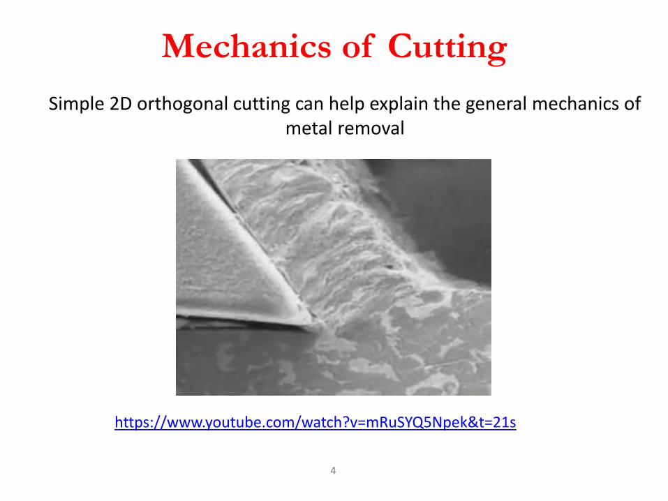
Mechanics of Cutting
4
Simple 2D orthogonal cutting can help explain the general mechanics of metal removal
https://www.youtube.com/watch?v=mRuSYQ5Npek&t=21s

Tensile Testing
5
@ ACMS, IITK

Milling
MachiningParameters

Work Material Cutting Tool Machining Conditions
Machine Tool
Cutting Process
Product
Measurements
Determinations
Metal type Purity BCC, FCC, HCP Predeformation(work hardening prior to machining)

Machining Conditions
Cutting parameters • Depth of cut • Speed • Feed
Environment • Lubricant
(cutting fluid) • Oxygen • Temperature
Workholder• Fixtures • Jigs • Chucks • Collets
Cutting speed (v) – primary motion
The speed at which the work moves with respect to the tool
Feed (f) – secondary motion
Depth of cut (d) – penetration of tool below original work surface

Machining Conditions in Turning
Feed Rate - fr
f = feed per rev
Depth of Cut - d
Machining Time - Tm
L = length of cut
Material Removal Rate - MRRoDπ
vN
Spindle Speed - N
v = cutting speed
Do = outer diameter
fNf r
2fo DD
d
r
mf
LT
dfvM R R

Selecting Depth of Cut
Depth of cut is often predetermined by workpiece
geometry and operation sequence
– In roughing, depth is made as large as possible to maximize
material removal rate, subject to limitations of
horsepower, machine tool and setup rigidity, and strength
of cutting tool
– In finishing, depth is set to achieve final part dimensions

Determining Feed
• In general: feed first, speed second
• Determining feed rate depends on:
– Tooling – harder tool materials require lower feeds
– Roughing or finishing - Roughing means high feeds,
finishing means low feeds
– Constraints on feed in roughing - Limits imposed by cutting
forces, setup rigidity, and sometimes horsepower
– Surface finish requirements in finishing – select feed to
produce desired finish

Optimizing Cutting Speed
• Select speed to achieve a balance between high
metal removal rate and suitably long tool life
• Mathematical formulas are available to determine
optimal speed
• Two alternative objectives in these formulas:
1. Maximum production rate
2. Minimum unit cost

Maximum Production Rate
• Maximizing production rate = minimizing cutting time per unit
• In turning, total production cycle time for one part consists of:
1. Part handling time per part = Th
2. Machining time per part = Tm
3. Tool change time per part = Tt/np , where np = number of pieces cut in one tool life
Total time per unit product for operation:
Tc = Th + Tm + Tt/np
Cycle time Tc is a function of cutting speed

Cycle Time vs. Cutting Speed

Minimizing Cost per Unit
In turning, total production cycle cost for one part consists of:
1. Cost of part handling time = CoTh , where Co = cost rate for operator and machine
2. Cost of machining time = CoTm
3. Cost of tool change time = CoTt/np
4. Tooling cost = Ct/np , where Ct = cost per cutting edge
Total cost per unit product for operation:
Cc = CoTh + CoTm + CoTt/np + Ct/np
Again, unit cost is a function of cutting speed, just as Tc is a function of v
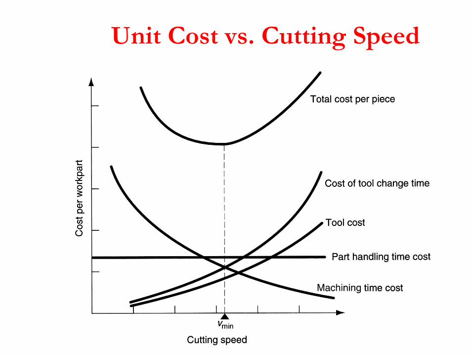
Unit Cost vs. Cutting Speed

Cutting Fluids
Any liquid or gas applied directly to machining operation to
improve cutting performance
• Two main problems addressed by cutting fluids:
1. Heat generation at shear zone and friction zone
2. Friction at the tool-chip and tool-work interfaces
• Other functions and benefits:
– Wash away chips (e.g., grinding and milling)
– Reduce temperature of workpart for easier handling
– Improve dimensional stability of workpart

Cutting Fluid Functions
Cutting fluids can be classified according to function:
– Coolants - designed to reduce effects of heat in machining
– Lubricants - designed to reduce tool-chip and tool-work friction
• Water used as base in coolant-type cutting fluids
• Most effective at high cutting speeds where heat generation and high
temperatures are problems
• Most effective on tool materials that are most susceptible to
temperature failures (e.g., HSS)
• Usually oil-based fluids
• Most effective at lower cutting speeds
• Also reduces temperature in the operation
Coolants
Lubricants

Work Material Cutting Tool Machining Conditions
Machine Tool
Cutting Process
Product
Measurements
Determinations

Cutting Tool Classification
1. Single-Point Tools– One dominant cutting edge
– Point is usually rounded to form a nose radius
– Turning uses single point tools
2. Multiple Cutting Edge Tools– More than one cutting edge
– Motion relative to work achieved by rotating
– Drilling and milling use rotating multiple cutting edge tools

Figure: (a) Seven elements of single-point tool geometry; and (b) the tool
signature convention that defines the seven elements
Single-Point Tool Geometry

Tool MaterialsTool failure modes identify the important properties that a tool material should possess:
– Toughness - to avoid fracture failure
– Hot hardness - ability to retain hardness at high temperatures
– Wear resistance - hardness is the most important property to resist abrasive wear
High speed steel (HSS) Cemented carbides Cermets Coated carbides Ceramics Synthetic diamonds Cubic boron nitride

Failure of Cutting Tools and Tool Wear
• Fracture failure
– Cutting force becomes excessive and/or dynamic, leading to brittle fracture
• Temperature failure
– Cutting temperature is too high for the tool material
• Gradual wear
– Gradual wearing of the cutting tool
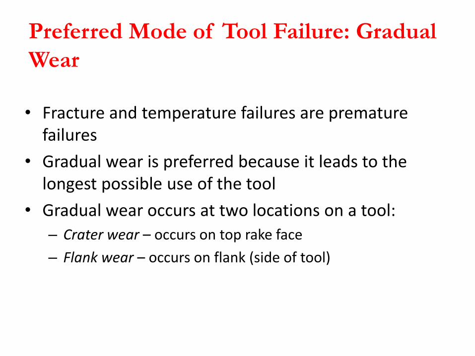
Preferred Mode of Tool Failure: Gradual
Wear
• Fracture and temperature failures are premature failures
• Gradual wear is preferred because it leads to the longest possible use of the tool
• Gradual wear occurs at two locations on a tool:
– Crater wear – occurs on top rake face
– Flank wear – occurs on flank (side of tool)

Figure - Diagram of worn cutting tool, showing the principal
locations and types of wear that occur

Figure -
(a) Crater wear, and
(b) flank wear on a cemented carbide tool, as seen through a toolmaker's microscope
(Source: Manufacturing Technology Laboratory, Lehigh University, photo by J. C. Keefe)
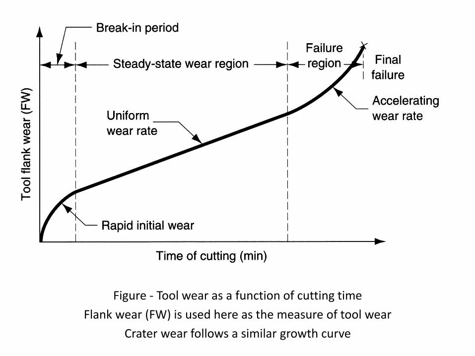
Figure - Tool wear as a function of cutting time
Flank wear (FW) is used here as the measure of tool wear
Crater wear follows a similar growth curve

Figure - Effect of cutting speed on tool flank wear (FW) for three cutting speeds, using a tool life criterion of 0.50 mm flank wear

Figure - Natural log-log plot of cutting speed vs tool life

Taylor Tool Life Equation
This relationship is credited to F. W. Taylor (~1900)
CvT n
where v = cutting speed; T = tool life; and n and C are parameters that
depend on feed, depth of cut, work material, tooling material, and the
tool life criterion used
• n is the slope of the plot
• C is the intercept on the speed axis

Variables Affecting Tool Life
Cutting conditions.
Tool geometry.
Tool material.
Work material.
Cutting fluid.
Vibration behavior of the machine-tool work system.
Built-up edge.

Work Material Cutting Tool Machining Conditions
Machine Tool
Cutting Process
Product
Measurements
Determinations
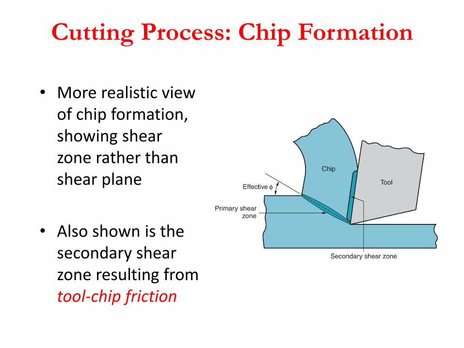
Cutting Process: Chip Formation
• More realistic view of chip formation, showing shear zone rather than shear plane
• Also shown is the secondary shear zone resulting from tool-chip friction

Four Basic Types of Chip in Machining
1. Discontinuous chip
2. Continuous chip
3. Continuous chip with Built-up Edge (BUE)
4. Serrated chip
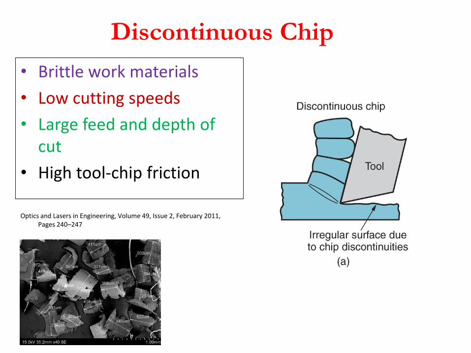
• Brittle work materials
• Low cutting speeds
• Large feed and depth of cut
• High tool-chip friction
Optics and Lasers in Engineering, Volume 49, Issue 2, February 2011, Pages 240–247
Discontinuous Chip

• Ductile work materials
• High cutting speeds
• Small feeds and depths
• Sharp cutting edge
• Low tool-chip friction
Journal of Materials Processing Technology, Volume 121, Issues 2–3, 28 February 2002, Pages 363–372
Continuous Chip

• Ductile materials
• Low-to-medium cutting speeds
• Tool-chip friction causes portions of chip to adhere to rake face
• BUE forms, then breaks off, cyclically
Springerimages.com
Continuous with BUE

• Semi-continuous - saw-tooth appearance
• Cyclical chip forms with alternating high shear strain then low shear strain
• Associated with difficult-to-machine metals at high cutting speeds
Springerimages.com
Serrated Chip
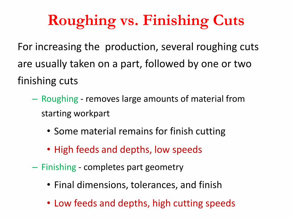
Roughing vs. Finishing Cuts
For increasing the production, several roughing cuts
are usually taken on a part, followed by one or two
finishing cuts
– Roughing - removes large amounts of material from
starting workpart
• Some material remains for finish cutting
• High feeds and depths, low speeds
– Finishing - completes part geometry
• Final dimensions, tolerances, and finish
• Low feeds and depths, high cutting speeds

Orthogonal Cutting Geometry
73
Assumptions:1. Cutting edge is perfectly sharp2. Uncut chip thickness is constant
and << than width3. Width of tool > width of
workpiece4. Continuous chip with no built up-
edge5. Uniform cutting along edge6. 2D plane strain deformation7. No side spreading of material8. Uniform stress distribution on
shear plane9. Forces primarily in directions of
velocity and uncut chip thickness

Orthogonal Cutting Geometry
74
Primary shear zone:Material ahead of tool is sheared to form a chip
Secondary shear zone:Sheared material (chip) partially deforms and moves along the rake face
Tertiary zone:Flank of tool rubs the newly machined surface
Simple 2D orthogonal cutting can help explain the general mechanics of metal removal
Tool
Workpiece
Chip

Primary Shearing Zone
75
𝐹𝑡𝑐
𝐹𝑓𝑐
𝐹𝑛
𝐹𝑠
𝐹𝑣
∅𝑐
𝐹𝑠 = 𝐹𝑡𝑐 cos𝜙𝑐 − 𝐹𝑓𝑐 sin𝜙𝑐 ;
𝐹𝑛 = 𝐹𝑡𝑐 sin 𝜙𝑐 + 𝐹𝑓𝑐 cos𝜙𝑐 ;𝐹𝑠𝐹𝑛
=cos𝜙𝑐 −sin𝜙𝑐
sin 𝜙𝑐 cos𝜙𝑐
𝐹𝑡𝑐𝐹𝑓𝑐
Force components in primary shear zone
𝐹𝑢
𝛼𝑟 𝛼𝑟- rake angle; 𝜙𝑐 - shear angle𝐹𝑡𝑐 - tangential force/cutting force;𝐹𝑓𝑐 - feed force/thrust force
𝐹𝑠 - force acting along the shear plane𝐹𝑛 - normal force acting on the shear plane𝐹𝑣 - force acting on the rake face𝐹𝑢 - frictional force
• Forces acting on the tool that can be measured: Cutting force Ftc and Thrust force Ffc
• Other forces cannot be directly measured

Chip ratios – basic characteristics
76
sin𝜙𝑐 =ℎ
𝑙𝜙
ℎ
ℎ𝑐
∅𝑐
𝛼𝑟
∅𝑐 − 𝛼𝑟
𝑙𝜙
cos 𝜙𝑐 − 𝛼𝑟 =ℎ𝑐𝑙𝜙
ℎ = 𝑙𝜙sin𝜙𝑐 ℎ𝑐 = 𝑙𝜙cos 𝜙𝑐 − 𝛼𝑟
𝑟𝑐 =ℎ
ℎ𝑐=
sin𝜙𝑐
cos 𝜙𝑐 − 𝛼𝑟
&
&
Chip thickness ratio
From mass (volume flow rate) conservation, chip thickness ratio ≅ chip length ratio
𝑟𝑐 =ℎ
ℎ𝑐=𝑙𝑐𝑙= 𝑟𝑙 No side spreading assumption, 𝑟𝑤 = 1
𝜙𝑐 = tan−1𝑟𝑐 cos 𝛼𝑟
1 − 𝑟𝑐sin 𝛼𝑟

Velocity Relations
80
𝑉𝑠 = 𝑉cos 𝛼𝑟
cos 𝜙𝑐 − 𝛼𝑟
𝑉𝑠
𝑉
𝑉𝑐
𝑉𝑠𝑉𝑐
𝑉
𝛼𝑟
𝜙𝑐
𝜙𝑐 − 𝛼𝑟
𝛼𝑟
𝜙𝑐
𝜙𝑐 − 𝛼𝑟Chip velocity, 𝑉𝑐 (acknowledging conservation of volume-flow rate):
𝑉𝑐𝑉=𝑙𝑐/∆𝑡
𝑙/∆𝑡= 𝑟𝑙 ⇒ 𝑉𝑐 = 𝑟𝑙𝑉
𝑟𝑐 = 𝑟𝑙 =sin𝜙𝑐
cos 𝜙𝑐 − 𝛼𝑟
𝑉𝑐 =sin𝜙𝑐
cos 𝜙𝑐 − 𝛼𝑟𝑉
Shear velocity, 𝑉𝑠 is vector sum of 𝑉𝑐 and 𝑉

Shear Strain and Material Movement
81
Undeformed chip section 𝐴0𝐵𝑜𝐴1𝐵1moves with velocity 𝑉
When one element traverses the shear plane in time ∆𝑡:
point 𝐴1 moves to point 𝐴2, point 𝐴0 moves to point 𝐴1
point 𝐵1 moves to point 𝐵2, point 𝐵0 moves to point 𝐵1
Undeformed chip section 𝐴0𝐵𝑜𝐴1𝐵1hence becomes deformed chip with section 𝐴1𝐵1𝐴2𝐵2
Hence chip is shifted from expected position of 𝐵2′ 𝐴2
′ to 𝐵2𝐴2 because of shearing

Shear Strain and Shear Strain Rate
82
∆𝑥
𝑦
𝛾
tan 𝛾 =∆𝑥
𝑦𝛾 =
∆𝑥
𝑦𝛾 =
∆𝑠
∆𝑑=𝐴2𝐴2
′
𝐴1𝐶=𝐴2
′𝐶
𝐴1𝐶+𝐶𝐴2𝐴1𝐶
= cot𝜙𝑐 + tan 𝜙𝑐 − 𝛼𝑟Smallangles
Shear strain rate
ሶ𝛾 =𝛾
∆𝑡
Assuming shear zone increment is ∆𝑠 and the thickness of the shear deformation zone is ∆𝑑
𝛾 =∆𝑠
∆𝑑𝑉𝑠 =
∆𝑠
∆𝑡ሶ𝛾 =
𝑉𝑠∆𝑑
= 𝑉cos𝛼𝑟
∆𝑑 cos 𝜙𝑐 − 𝛼𝑟
∆𝑑 → 0 → thin shear plane → very large strain rates

Primary Shearing Zone
83
Endres, Adv. Mcing processes
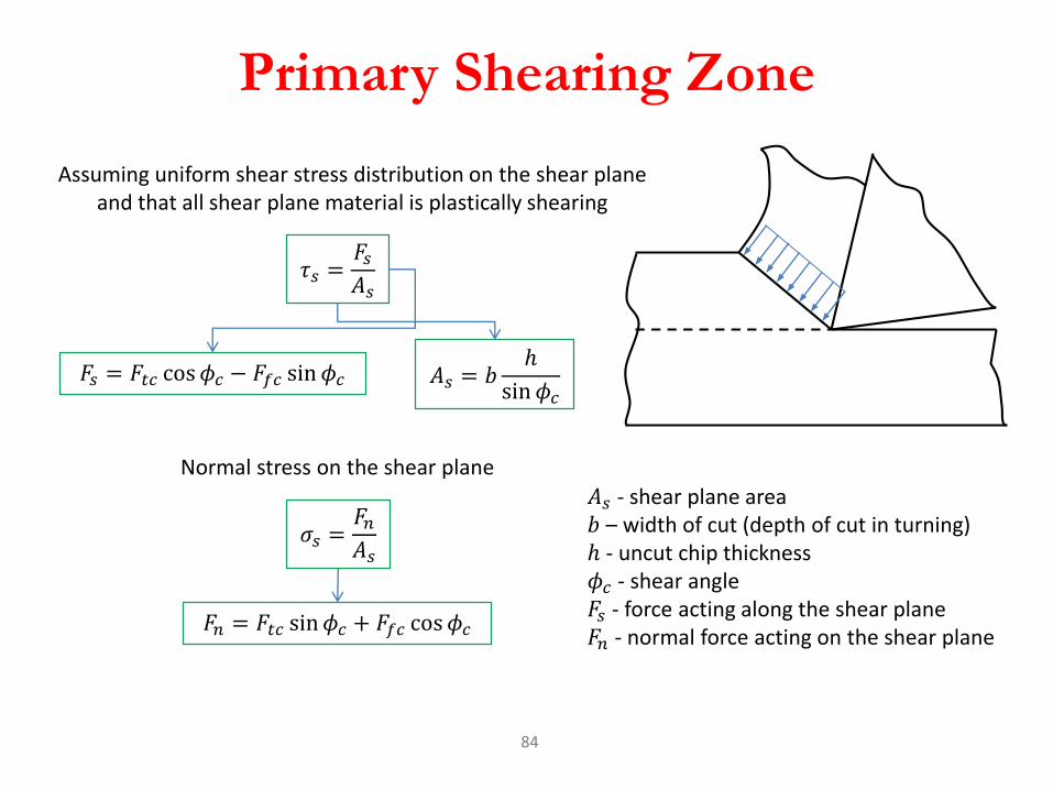
84
Assuming uniform shear stress distribution on the shear plane and that all shear plane material is plastically shearing
𝜏𝑠 =𝐹𝑠𝐴𝑠
𝐴𝑠 = 𝑏ℎ
sin𝜙𝑐
𝐹𝑠 = 𝐹𝑡𝑐 cos𝜙𝑐 − 𝐹𝑓𝑐 sin𝜙𝑐
𝐴𝑠 - shear plane area𝑏 – width of cut (depth of cut in turning)ℎ - uncut chip thickness 𝜙𝑐 - shear angle𝐹𝑠 - force acting along the shear plane𝐹𝑛 - normal force acting on the shear plane
Normal stress on the shear plane
𝜎𝑠 =𝐹𝑛𝐴𝑠
𝐹𝑛 = 𝐹𝑡𝑐 sin𝜙𝑐 + 𝐹𝑓𝑐 cos𝜙𝑐
Primary Shearing Zone

Orthogonal Cutting Geometry
85
Primary shear zone:Material ahead of tool is sheared to form a chip
Secondary shear zone:Sheared material (chip) partially deforms and moves along the rake face
Tertiary zone:Flank of tool rubs the newly machined surface

Secondary Shear Zone
86
𝐹𝑣 = 𝐹𝑡𝑐 cos𝛼𝑟 − 𝐹𝑓𝑐 sin 𝛼𝑟 ;
𝐹𝑢 = 𝐹𝑡𝑐 sin 𝛼𝑟 + 𝐹𝑓𝑐 cos 𝛼𝑟 ;𝐹𝑣𝐹𝑢
=cos𝛼𝑟 −sin 𝛼𝑟sin 𝛼𝑟 cos 𝛼𝑟
𝐹𝑡𝑐𝐹𝑓𝑐
Force components in secondary shear zone
𝜇𝑎 = tan𝛽𝑎 =𝐹𝑢𝐹𝑣
Average friction coeff on rake face:

Force Circle Diagram
87
Tool
𝐹𝑡𝑐
𝐹𝑓𝑐
𝐹𝑛
𝐹𝑠
𝐹𝑣
∅𝑐
𝐹𝑢
𝛼𝑟∅𝑐𝐹𝑐
𝛽𝑎 − 𝛼𝑟
𝛼𝑟
𝛽𝑎 − 𝛼𝑟 𝛽𝑎

88
Tool
𝐹𝑡𝑐
𝐹𝑓𝑐
𝐹𝑛
𝐹𝑠
𝐹𝑣
∅𝑐
𝐹𝑢
𝛼𝑟∅𝑐
𝛽𝑎 − 𝛼𝑟
𝛼𝑟
𝛽𝑎 − 𝛼𝑟 𝛽𝑎
𝐹𝑠 = 𝐹𝑡𝑐 cos𝜙𝑐 − 𝐹𝑓𝑐 sin𝜙𝑐 ;
𝐹𝑛 = 𝐹𝑡𝑐 sin𝜙𝑐 + 𝐹𝑓𝑐 cos𝜙𝑐 ;
Force components in primary shear zone
Force components in primary shear zoneusing the force circle diagram
𝐹𝑠 = 𝐹𝑐 cos 𝜙𝑐 + 𝛽𝑎 − 𝛼𝑟 ;𝐹𝑛 = 𝐹𝑐 sin 𝜙𝑐 + 𝛽𝑎 − 𝛼𝑟 ;
𝐹𝑐
Force components in secondary shear zone using the force circle diagram
𝐹𝑣 =? ; 𝐹𝑢 =?
Force Circle Diagram

Total Power Consumed in Cutting
89
𝑃𝑡𝑐 = 𝑃𝑠 + 𝑃𝑢
𝑃𝑡𝑐 = 𝐹𝑠𝑉𝑠 + 𝐹𝑢𝑉𝑐
𝑉𝑠 = 𝑉cos 𝛼𝑟
cos 𝜙𝑐 − 𝛼𝑟
Total power consumed in cutting is sum of energy spent in shear and friction zones
𝐹𝑢 = 𝐹𝑡𝑐 sin 𝛼𝑟 + 𝐹𝑓𝑐 cos 𝛼𝑟𝐹𝑠 = 𝐹𝑡𝑐 cos𝜙𝑐 − 𝐹𝑓𝑐 sin 𝜙𝑐
𝜙𝑐 - shear angle?𝐹𝑠 - force acting along the shear plane?𝐹𝑢 - frictional force?
𝑉𝑐 = 𝑉sin𝜙𝑐
cos 𝜙𝑐 − 𝛼𝑟

Force Prediction for Power Consumption
90
𝑃𝑡𝑐 = 𝐹𝑠𝑉𝑠 + 𝐹𝑢𝑉𝑐
𝐹𝑠 = 𝐹𝑡𝑐 cos𝜙𝑐 − 𝐹𝑓𝑐 sin𝜙𝑐 𝐹𝑠 = 𝐹𝑐 cos 𝜙𝑐 + 𝛽𝑎 − 𝛼𝑟
𝐹𝑠 = 𝜏𝑠𝐴𝑠 = 𝜏𝑠 𝑏ℎ
sin 𝜙𝑐
Total power consumed in cutting is sum of energy spent in shear and friction zones
Primary chip generation mechanism is shearing
𝑃𝑠 = 𝐹𝑠𝑉𝑠
𝑉𝑠 = 𝑉cos 𝛼𝑟
cos 𝜙𝑐 − 𝛼𝑟
Shear force can also be expressed as
Resultant cutting force can be now be expressed in terms of shear stress, friction and shear angles, width of cut, and feed rate as follows:
𝐹𝑐 =𝐹𝑠
cos 𝜙𝑐 + 𝛽𝑎 − 𝛼𝑟= 𝜏𝑠 𝑏ℎ
1
sin𝜙𝑐 cos 𝜙𝑐 + 𝛽𝑎 − 𝛼𝑟Know everything but for 𝜙𝑐

91
Resultant cutting force can be now be expressed in terms of shear stress, friction and shear angles, width of cut, and feed rate as follows:
𝐹𝑐 =𝐹𝑠
cos 𝜙𝑐 + 𝛽𝑎 − 𝛼𝑟= 𝜏𝑠 𝑏ℎ
1
sin𝜙𝑐 cos 𝜙𝑐 + 𝛽𝑎 − 𝛼𝑟
Nature always takes the path of least resistance, so during cutting 𝜙𝑐 takes a value such that least amount of energy is consumed, i.e. since 𝜏𝑠, 𝑏, ℎ, and 𝛽𝑎 and 𝛼𝑟 are given and do not
change, power consumed becomes:
𝐹𝑡𝑐 = 𝐹𝑐 cos 𝛽𝑎 − 𝛼𝑟 = 𝜏𝑠 𝑏ℎcos 𝛽𝑎 − 𝛼𝑟
sin𝜙𝑐 cos 𝜙𝑐 + 𝛽𝑎 − 𝛼𝑟
𝑃𝑡𝑐 = 𝑉𝐹𝑡𝑐
Recalling the FCD
Power consumed during cutting:
𝑃𝑡𝑐 𝜙𝑐 =𝑐𝑜𝑛𝑠𝑡𝑎𝑛𝑡
sin 𝜙𝑐 cos 𝜙𝑐 + 𝛽𝑎 − 𝛼𝑟
Shear Angle – from Merchant’s Energy Principle

Shear Angle – from Merchant’s Energy Principle
92
Nature always takes the path of least resistance, so during cutting , 𝜙𝑐 takes a value such that least amount of energy is consumed, i.e. since 𝜏𝑠, 𝑏, ℎ, and 𝛽𝑎 and 𝛼𝑟 are given and do not
change, power consumed becomes:
𝑃𝑡𝑐 𝜙𝑐 =𝑐𝑜𝑛𝑠𝑡𝑎𝑛𝑡
sin𝜙𝑐 cos 𝜙𝑐 + 𝛽𝑎 − 𝛼𝑟
𝑃𝑡𝑐 𝜙𝑐 will be a minimum when the denominator is a maximum, hence differentiate denominator w.r.t 𝜙𝑐 and equate it to zero:
cos𝜙𝑐 cos 𝜙𝑐 + 𝛽𝑎 − 𝛼𝑟 − sin𝜙𝑐 sin 𝜙𝑐 + 𝛽𝑎 − 𝛼𝑟 = 0
cos 2𝜙𝑐 + 𝛽𝑎 − 𝛼𝑟 = 0
2𝜙𝑐 + 𝛽𝑎 − 𝛼𝑟 =𝜋
2 𝜙𝑐 =𝜋
4−𝛽𝑎 − 𝛼𝑟
2

Force Prediction
93
𝐹𝑡𝑐 = 𝐹𝑐 cos 𝛽𝑎 − 𝛼𝑟 = 𝜏𝑠 𝑏ℎcos 𝛽𝑎 − 𝛼𝑟
sin𝜙𝑐 cos 𝜙𝑐 + 𝛽𝑎 − 𝛼𝑟𝑃𝑡𝑐 = 𝑉𝐹𝑡𝑐
𝜙𝑐 =𝜋
4−𝛽𝑎 − 𝛼𝑟
2
Shear angle using Merchant’s minimum energy principle
Force prediction Power consumed
• Shear angle prediction with these and other such models are not very accurate
• However, they provide important relationships between tool geometry and shear
angle – which is important for tool design
• To increase shear plane angle ₋ Increase the rake angle ₋ Reduce the friction angle (or reduce the coefficient of friction)
• Higher shear plane angle means smaller shear plane which means lower shear force, cutting forces, power, and temperature

94
• Contact mechanics between flank face and finished surface depends on
tool wear, preparation of cutting edge and friction characteristics of tool
and workpiece
• Assume total friction force on flank face is 𝐹𝑓𝑓
• And force normal to flank face in 𝐹𝑓𝑛
• Assume pressure (𝜎𝑓) on the flank face to be uniform (a gross
oversimplification)
𝐹𝑓𝑓
𝐹𝑓𝑛
𝛾𝑓
Tertiary Deformation Zone

Tertiary Deformation Zone
95
𝐹𝑡𝑒 = 𝐹𝑓𝑛 sin 𝛾𝑓 + 𝐹𝑓𝑓 cos 𝛾𝑓 ;
𝐹𝑓𝑒 = 𝐹𝑓𝑛 cos 𝛾𝑓 + 𝐹𝑓𝑓 sin 𝛾𝑓;
𝐹𝑓𝑛 = 𝜎𝑓𝑉𝐵𝑏
𝑉𝐵
𝛾𝑓
𝜇𝑓 = 𝐹𝑓𝑓/𝐹𝑓𝑛
Normal force on the flank face
Because the tool rubs on the finished surface, there is friction
Resolving contact forces into tangentialand feed directions
Any measured forces will include forces due to shearing and tothe tertiary deformation process, i.e. rubbing/ploughing at theflank of the cutting edge
𝐹𝑡 = 𝐹𝑡𝑐 + 𝐹𝑡𝑒;𝐹𝑓 = 𝐹𝑓𝑐 + 𝐹𝑓𝑒;
All cutting force expressions presented up until now were only for shearing, but in reality, edge forces also exist, hence edge forces must be subtracted from measured tangential and feed
forces before applying laws of orthogonal cutting mechanics

Orthogonal and Oblique Cutting Geometry
96
Cutting velocity is inclined at an acute angle 𝑖 to the cutting edge
Cutting velocity is perpendicular to cutting edge
Altintas, Mfg. Automation
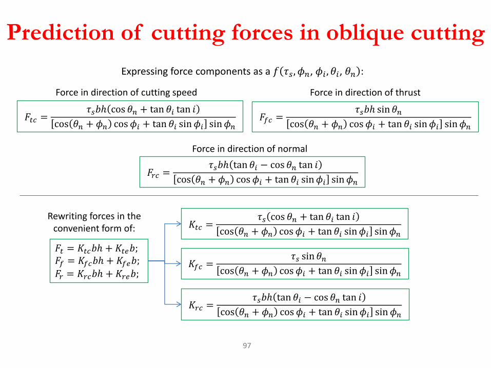
Prediction of cutting forces in oblique cutting
97
𝐹𝑡 = 𝐾𝑡𝑐𝑏ℎ + 𝐾𝑡𝑒𝑏;𝐹𝑓 = 𝐾𝑓𝑐𝑏ℎ + 𝐾𝑓𝑒𝑏;
𝐹𝑟 = 𝐾𝑟𝑐𝑏ℎ + 𝐾𝑟𝑒𝑏;
𝐾𝑡𝑐 =𝜏𝑠 cos 𝜃𝑛 + tan 𝜃𝑖 tan 𝑖
cos 𝜃𝑛 + 𝜙𝑛 cos 𝜙𝑖 + tan 𝜃𝑖 sin𝜙𝑖 sin𝜙𝑛
𝐾𝑓𝑐 =𝜏𝑠 sin 𝜃𝑛
cos 𝜃𝑛 + 𝜙𝑛 cos 𝜙𝑖 + tan 𝜃𝑖 sin𝜙𝑖 sin𝜙𝑛
𝐾𝑟𝑐 =𝜏𝑠𝑏ℎ tan 𝜃𝑖 − cos 𝜃𝑛 tan 𝑖
cos 𝜃𝑛 + 𝜙𝑛 cos 𝜙𝑖 + tan 𝜃𝑖 sin𝜙𝑖 sin 𝜙𝑛
𝐹𝑟𝑐 =𝜏𝑠𝑏ℎ tan 𝜃𝑖 − cos 𝜃𝑛 tan 𝑖
cos 𝜃𝑛 + 𝜙𝑛 cos 𝜙𝑖 + tan 𝜃𝑖 sin𝜙𝑖 sin𝜙𝑛
𝐹𝑡𝑐 =𝜏𝑠𝑏ℎ cos 𝜃𝑛 + tan 𝜃𝑖 tan 𝑖
cos 𝜃𝑛 + 𝜙𝑛 cos 𝜙𝑖 + tan 𝜃𝑖 sin𝜙𝑖 sin𝜙𝑛𝐹𝑓𝑐 =
𝜏𝑠𝑏ℎ sin 𝜃𝑛cos 𝜃𝑛 + 𝜙𝑛 cos 𝜙𝑖 + tan 𝜃𝑖 sin𝜙𝑖 sin𝜙𝑛
Force in direction of cutting speed
Expressing force components as a 𝑓 𝜏𝑠, 𝜙𝑛, 𝜙𝑖 , 𝜃𝑖, 𝜃𝑛 :
Force in direction of thrust
Force in direction of normal
Rewriting forces in the convenient form of:

Cutting Temperature
• Approximately 98% of the energy in machining is
converted into heat
• This can cause temperatures to be very high at the
tool-chip
• The remaining energy (about 2%) is retained as
elastic energy in the chip

Cutting Temperatures are Important
High cutting temperatures
1. reduce tool life
2. produce hot chips that pose safety hazards to the
machine operator
3. can cause inaccuracies in part dimensions due to
thermal expansion of work material
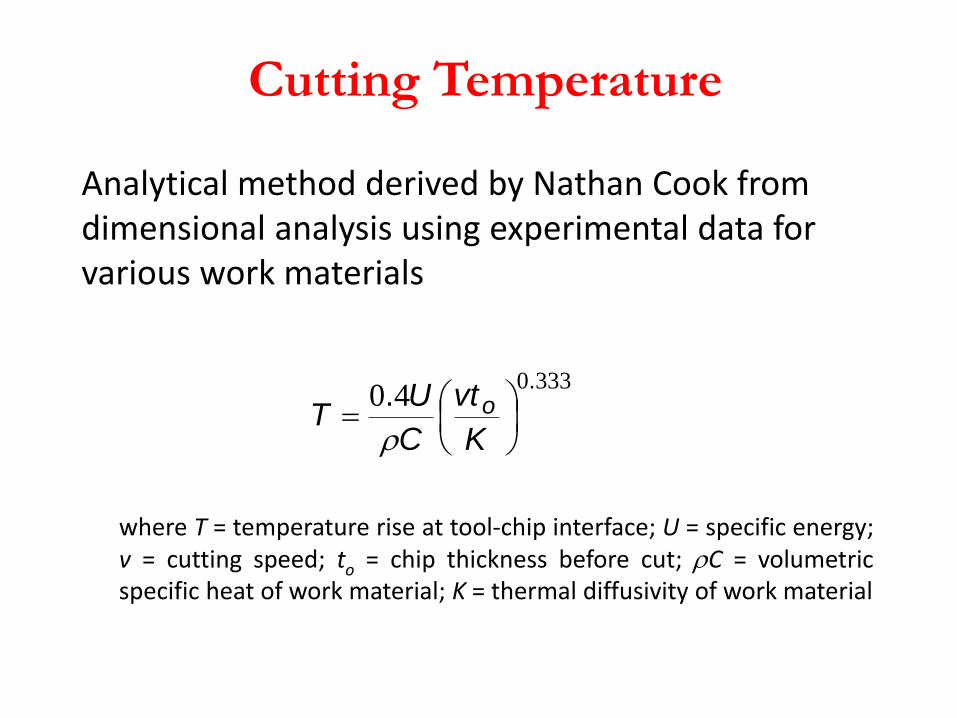
Cutting Temperature
Analytical method derived by Nathan Cook from dimensional analysis using experimental data for various work materials
where T = temperature rise at tool-chip interface; U = specific energy;v = cutting speed; to = chip thickness before cut; C = volumetricspecific heat of work material; K = thermal diffusivity of work material
333040
..
K
vt
C
UT o

• Experimental methods can be used to measure
temperatures in machining
– Most frequently used technique is the tool-chip
thermocouple
• Using this method, Ken Trigger determined the
speed-temperature relationship to be of the form:
T = K vm
where T = measured tool-chip interface temperature,
and v = cutting speed
Cutting Temperature

Example
Consider a turning operation performed on steel whose hardness = 225 HB at a speed = 3.0 m/s, feed = 0.25 mm, and depth = 4.0 mm. Using values of thermal properties and the appropriate specific energy value from tables, compute an estimate of cutting temperature using the Cook equation. Assume ambient temperature = 20C.
Solution: From Table, U = 2.2 N-m/mm3 = 2.2 J/mm3
From Table, = 7.87 g/cm3 = 7.87(10-3) g/mm3
From Table, C = 0.11 Cal/g-C. From note “a” at the bottom of the table, 1 cal = 4.186 J.
From Table, thermal conductivity k = 0.046 J/s-mm-C
Thus, C = 0.11(4.186) = 0.460 J/ g-C
C = (7.87 g/cm3)(0.46 J/g-C) = 3.62(10-3) J/mm3-C
Also, thermal diffusivity K = k/C
K = 0.046 J/s-mm-C /[(7.87 x 10-3 g/mm3)(0.46 J/g-C)] = 12.7 mm2/s
Using Cook’s equation, to = f = 0.25 mm
T = (0.4(2.2)/3.62(10-3))[3(103)(0.25)/12.7]0.333 = 0.2428(103)(59.06)0.333
= 242.8(3.89) = 944.4 C
Final temperature, taking ambient temperature in account T = 20 + 944 = 964C