Embed Size (px)
Citation preview

460
2.3.17 Food-matrices Exterior Time-temperature Simulations: Gradual Heating 56oC
Table 313. Assessment of individual model fit for strains following gradual heating at 56oC.
Strain Challenge Type RMSE R2adjusted D-value
12662 ST-257, CC-257 Gradual Heat (Un-chilled) 0.430 0.817 10.180
12662 ST-257, CC-257 Gradual Heat (Pre-chilled) 0.364 0.906 12.850
13126 (ST-21, CC-21) Gradual Heat (Un-chilled) 0.515 0.865 9.640
13126 (ST-21, CC-21) Gradual Heat (Pre-chilled) 0.357 0.807 10.560
13136 (ST-45, CC-45) Gradual Heat (Un-chilled) 0.326 0.856 10.950
13136 (ST-45, CC-45) Gradual Heat (Pre-chilled) 0.448 0.759 7.090
Table 314. Mixed Weibull distribution model incorporating an asymptotic function for survival of
strain 12662 (ST-257, CC-257) following gradual heating at 56oC.
Parameters Estimates Standard Error
α 2.355 0.301
δ1 10.184 0.709
p 5.359 2.186
N0 5.730 0.254
δ2 27.180 5.993
Table 315. Weibull model incorporating an asymptotic function for survival of strain 12662 (ST-257,
CC-257) following prior chilling and gradual heating at 56oC.
Parameters Estimates Standard Error
Nres 3.032 0.105
δ 12.839 0.560
p 7.242 2.788
N0 5.678 0.192
Table 316. Mixed Weibull distribution model for survival of strain 13126 (ST-21, CC-21) following
exposure to gradual direct heating at 56oC.
Parameters Estimates Standard Error
α 1.685 0.248
δ1 9.643 0.515
p 6.000 4.987
N0 4.167 0.172
δ2 22.930 1.692
461
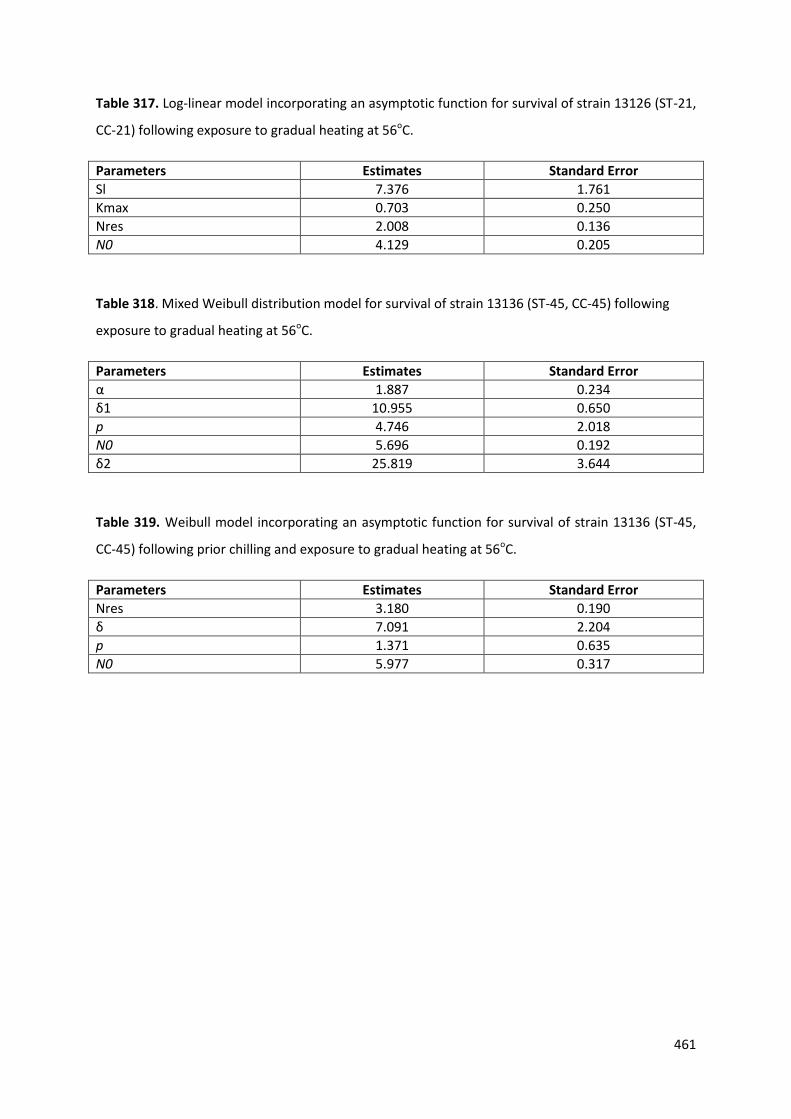
Table 317. Log-linear model incorporating an asymptotic function for survival of strain 13126 (ST-21,
CC-21) following exposure to gradual heating at 56oC.
Parameters Estimates Standard Error
Sl 7.376 1.761
Kmax 0.703 0.250
Nres 2.008 0.136
N0 4.129 0.205
Table 318. Mixed Weibull distribution model for survival of strain 13136 (ST-45, CC-45) following
exposure to gradual heating at 56oC.
Parameters Estimates Standard Error
α 1.887 0.234
δ1 10.955 0.650
p 4.746 2.018
N0 5.696 0.192
δ2 25.819 3.644
Table 319. Weibull model incorporating an asymptotic function for survival of strain 13136 (ST-45,
CC-45) following prior chilling and exposure to gradual heating at 56oC.
Parameters Estimates Standard Error
Nres 3.180 0.190
δ 7.091 2.204
p 1.371 0.635
N0 5.977 0.317
462
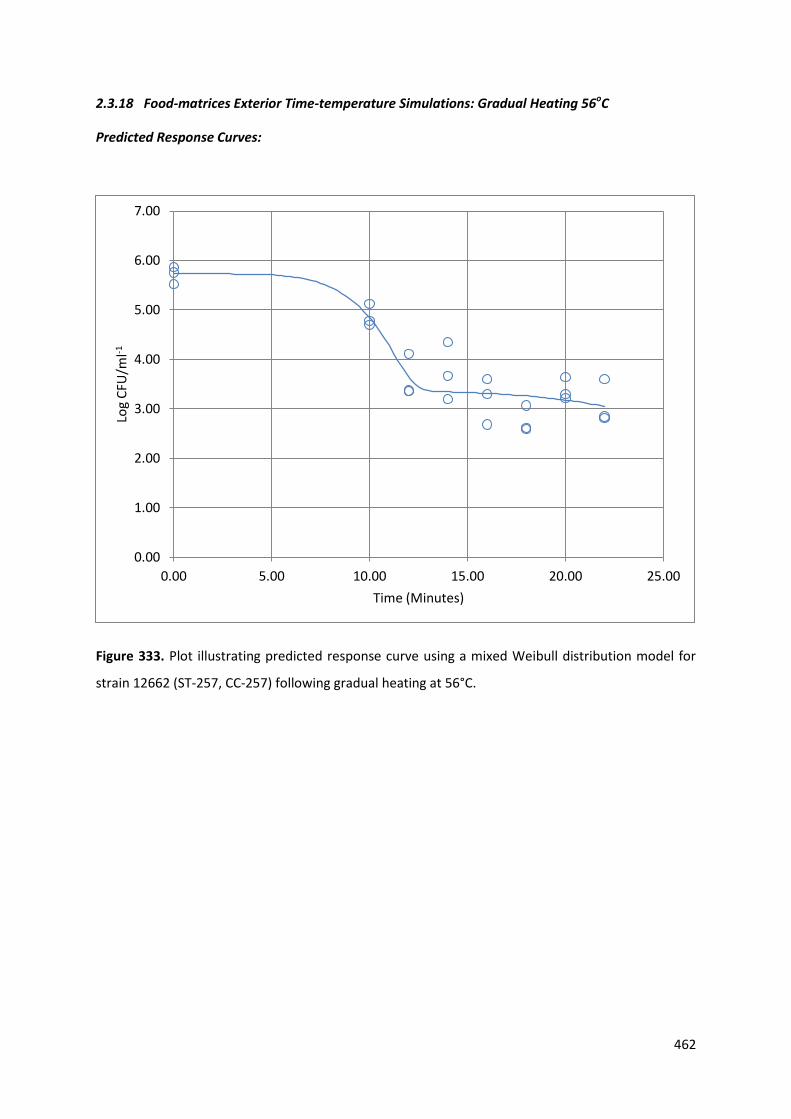
2.3.18 Food-matrices Exterior Time-temperature Simulations: Gradual Heating 56oC
Predicted Response Curves:
Figure 333. Plot illustrating predicted response curve using a mixed Weibull distribution model for
strain 12662 (ST-257, CC-257) following gradual heating at 56°C.
0.00
1.00
2.00
3.00
4.00
5.00
6.00
7.00
0.00 5.00 10.00 15.00 20.00 25.00
Log
CFU
/ml-1
Time (Minutes)
463
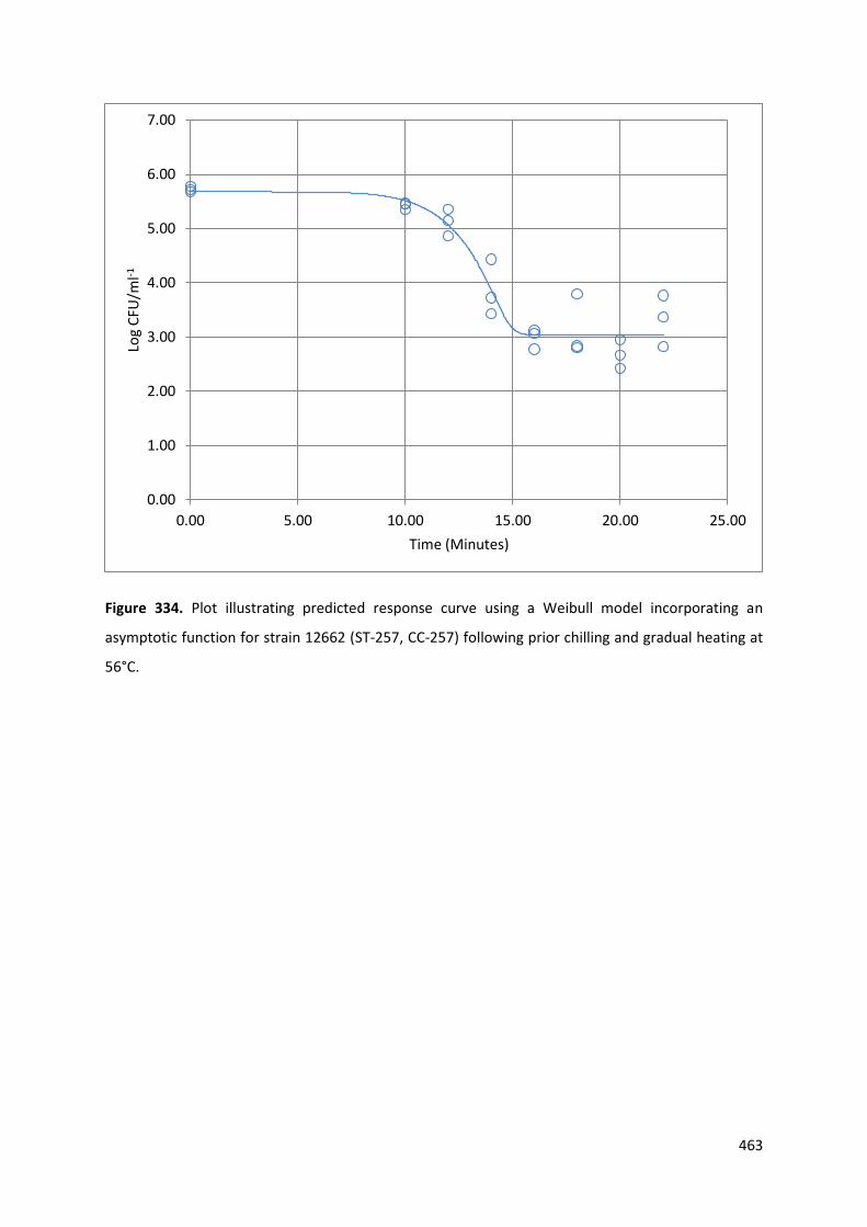
Figure 334. Plot illustrating predicted response curve using a Weibull model incorporating an
asymptotic function for strain 12662 (ST-257, CC-257) following prior chilling and gradual heating at
56°C.
0.00
1.00
2.00
3.00
4.00
5.00
6.00
7.00
0.00 5.00 10.00 15.00 20.00 25.00
Log
CFU
/ml-1
Time (Minutes)
464
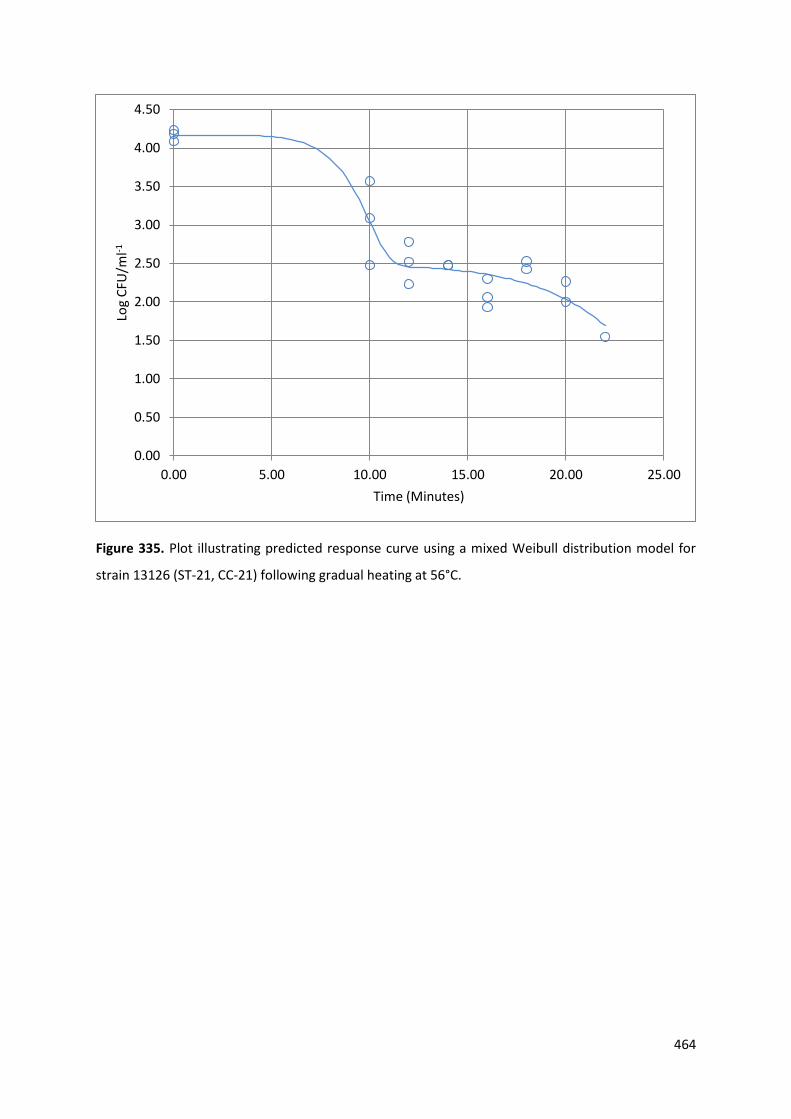
Figure 335. Plot illustrating predicted response curve using a mixed Weibull distribution model for
strain 13126 (ST-21, CC-21) following gradual heating at 56°C.
0.00
0.50
1.00
1.50
2.00
2.50
3.00
3.50
4.00
4.50
0.00 5.00 10.00 15.00 20.00 25.00
Log
CFU
/ml-1
Time (Minutes)
465
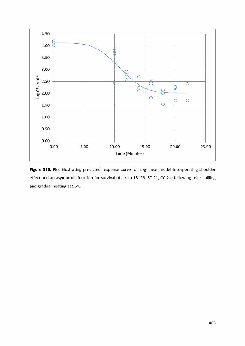
Figure 336. Plot illustrating predicted response curve for Log-linear model incorporating shoulder
effect and an asymptotic function for survival of strain 13126 (ST-21, CC-21) following prior chilling
and gradual heating at 56oC.
0.00
0.50
1.00
1.50
2.00
2.50
3.00
3.50
4.00
4.50
0.00 5.00 10.00 15.00 20.00 25.00
Log
CFU
/ml-1
Time (Minutes)
466
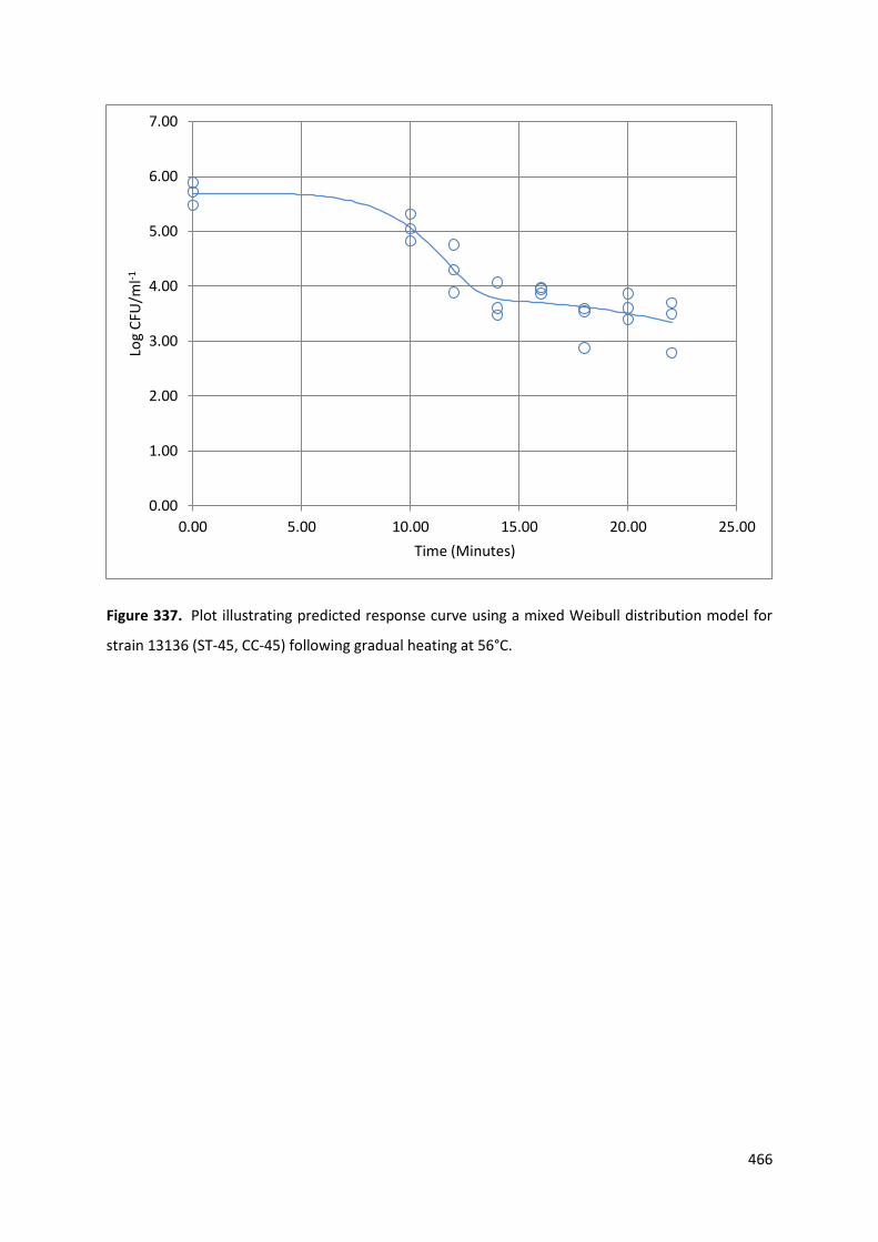
Figure 337. Plot illustrating predicted response curve using a mixed Weibull distribution model for
strain 13136 (ST-45, CC-45) following gradual heating at 56°C.
0.00
1.00
2.00
3.00
4.00
5.00
6.00
7.00
0.00 5.00 10.00 15.00 20.00 25.00
Log
CFU
/ml-1
Time (Minutes)
467
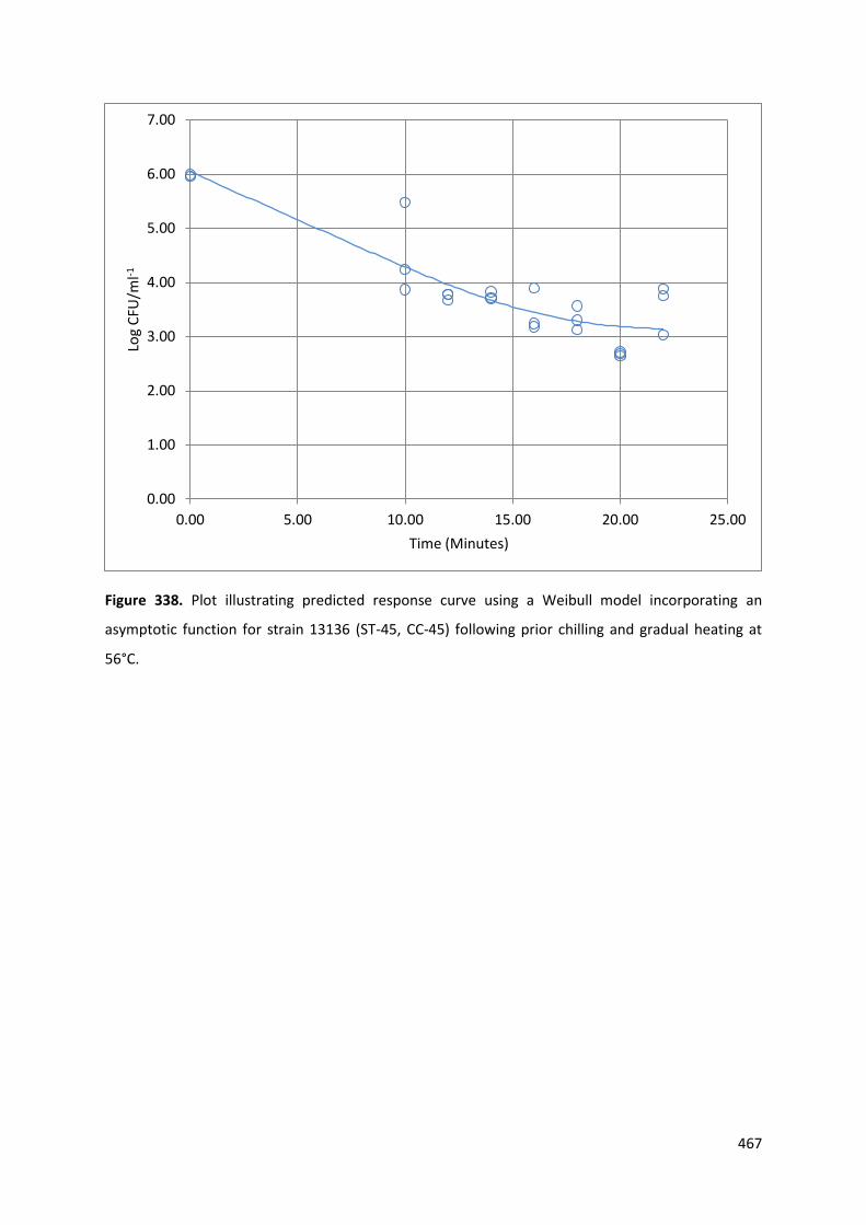
Figure 338. Plot illustrating predicted response curve using a Weibull model incorporating an
asymptotic function for strain 13136 (ST-45, CC-45) following prior chilling and gradual heating at
56°C.
0.00
1.00
2.00
3.00
4.00
5.00
6.00
7.00
0.00 5.00 10.00 15.00 20.00 25.00
Log
CFU
/ml-1
Time (Minutes)
468
2.3.19 Food-matrices Exterior Time-temperature Simulations: Gradual Heating 70oC
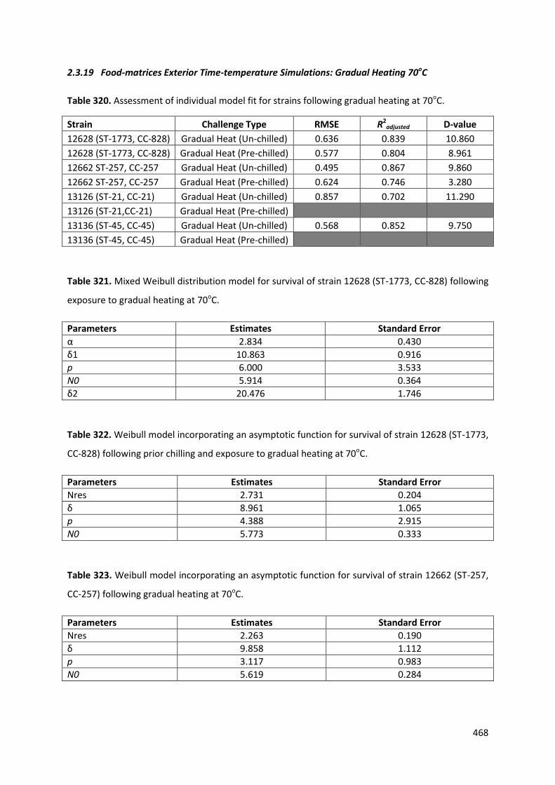
Table 320. Assessment of individual model fit for strains following gradual heating at 70oC.
Strain Challenge Type RMSE R2adjusted D-value
12628 (ST-1773, CC-828) Gradual Heat (Un-chilled) 0.636 0.839 10.860
12628 (ST-1773, CC-828) Gradual Heat (Pre-chilled) 0.577 0.804 8.961
12662 ST-257, CC-257 Gradual Heat (Un-chilled) 0.495 0.867 9.860
12662 ST-257, CC-257 Gradual Heat (Pre-chilled) 0.624 0.746 3.280
13126 (ST-21, CC-21) Gradual Heat (Un-chilled) 0.857 0.702 11.290
13126 (ST-21,CC-21) Gradual Heat (Pre-chilled)
13136 (ST-45, CC-45) Gradual Heat (Un-chilled) 0.568 0.852 9.750
13136 (ST-45, CC-45) Gradual Heat (Pre-chilled)
Table 321. Mixed Weibull distribution model for survival of strain 12628 (ST-1773, CC-828) following
exposure to gradual heating at 70oC.
Parameters Estimates Standard Error
α 2.834 0.430
δ1 10.863 0.916
p 6.000 3.533
N0 5.914 0.364
δ2 20.476 1.746
Table 322. Weibull model incorporating an asymptotic function for survival of strain 12628 (ST-1773,
CC-828) following prior chilling and exposure to gradual heating at 70oC.
Parameters Estimates Standard Error
Nres 2.731 0.204
δ 8.961 1.065
p 4.388 2.915
N0 5.773 0.333
Table 323. Weibull model incorporating an asymptotic function for survival of strain 12662 (ST-257,
CC-257) following gradual heating at 70oC.
Parameters Estimates Standard Error
Nres 2.263 0.190
δ 9.858 1.112
p 3.117 0.983
N0 5.619 0.284
469
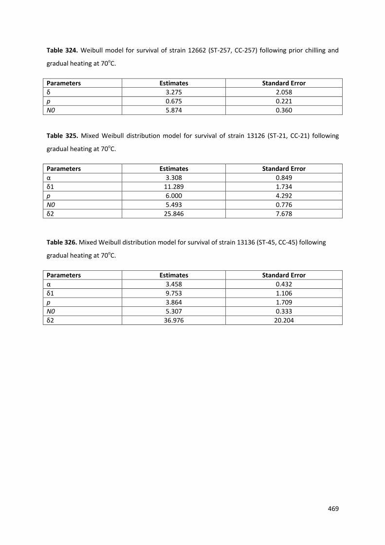
Table 324. Weibull model for survival of strain 12662 (ST-257, CC-257) following prior chilling and
gradual heating at 70oC.
Parameters Estimates Standard Error
δ 3.275 2.058
p 0.675 0.221
N0 5.874 0.360
Table 325. Mixed Weibull distribution model for survival of strain 13126 (ST-21, CC-21) following
gradual heating at 70oC.
Parameters Estimates Standard Error
α 3.308 0.849
δ1 11.289 1.734
p 6.000 4.292
N0 5.493 0.776
δ2 25.846 7.678
Table 326. Mixed Weibull distribution model for survival of strain 13136 (ST-45, CC-45) following
gradual heating at 70oC.
Parameters Estimates Standard Error
α 3.458 0.432
δ1 9.753 1.106
p 3.864 1.709
N0 5.307 0.333
δ2 36.976 20.204
470
2.3.20 Food-matrices Exterior Time-temperature Simulations: Gradual Heating 70oC
Predicted Response Curves:
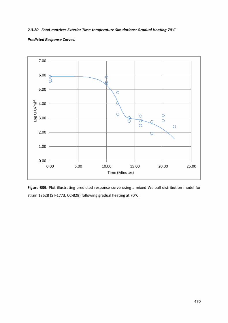
Figure 339. Plot illustrating predicted response curve using a mixed Weibull distribution model for
strain 12628 (ST-1773, CC-828) following gradual heating at 70°C.
0.00
1.00
2.00
3.00
4.00
5.00
6.00
7.00
0.00 5.00 10.00 15.00 20.00 25.00
Log
CFU
/ml-1
Time (Minutes)
471
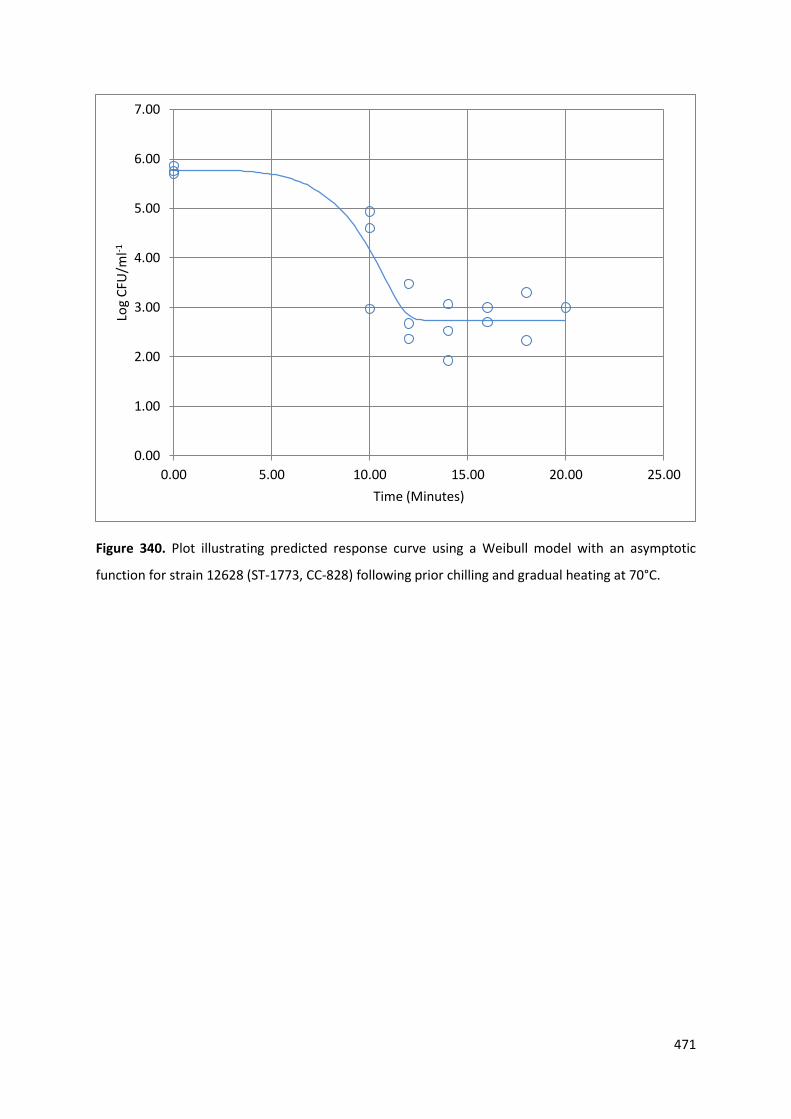
Figure 340. Plot illustrating predicted response curve using a Weibull model with an asymptotic
function for strain 12628 (ST-1773, CC-828) following prior chilling and gradual heating at 70°C.
0.00
1.00
2.00
3.00
4.00
5.00
6.00
7.00
0.00 5.00 10.00 15.00 20.00 25.00
Log
CFU
/ml-1
Time (Minutes)
472
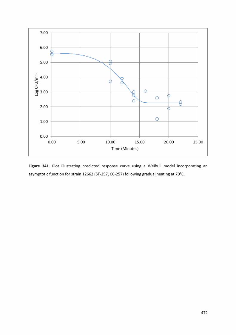
Figure 341. Plot illustrating predicted response curve using a Weibull model incorporating an
asymptotic function for strain 12662 (ST-257, CC-257) following gradual heating at 70°C.
0.00
1.00
2.00
3.00
4.00
5.00
6.00
7.00
0.00 5.00 10.00 15.00 20.00 25.00
Log
CFU
/ml-1
Time (Minutes)
473
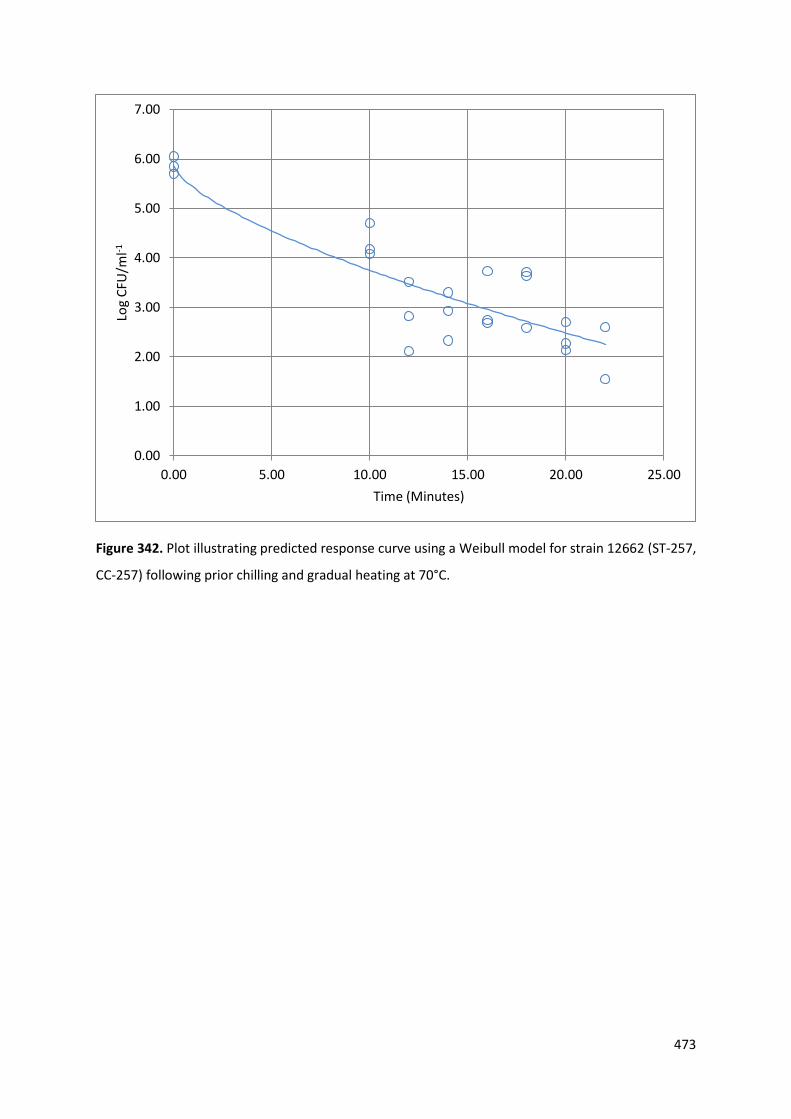
Figure 342. Plot illustrating predicted response curve using a Weibull model for strain 12662 (ST-257,
CC-257) following prior chilling and gradual heating at 70°C.
0.00
1.00
2.00
3.00
4.00
5.00
6.00
7.00
0.00 5.00 10.00 15.00 20.00 25.00
Log
CFU
/ml-1
Time (Minutes)
474
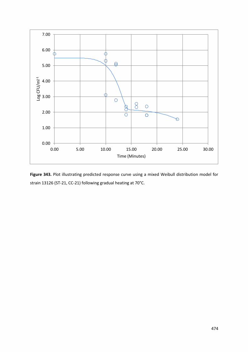
Figure 343. Plot illustrating predicted response curve using a mixed Weibull distribution model for
strain 13126 (ST-21, CC-21) following gradual heating at 70°C.
0.00
1.00
2.00
3.00
4.00
5.00
6.00
7.00
0.00 5.00 10.00 15.00 20.00 25.00 30.00
Log
CFU
/ml-1
Time (Minutes)
475
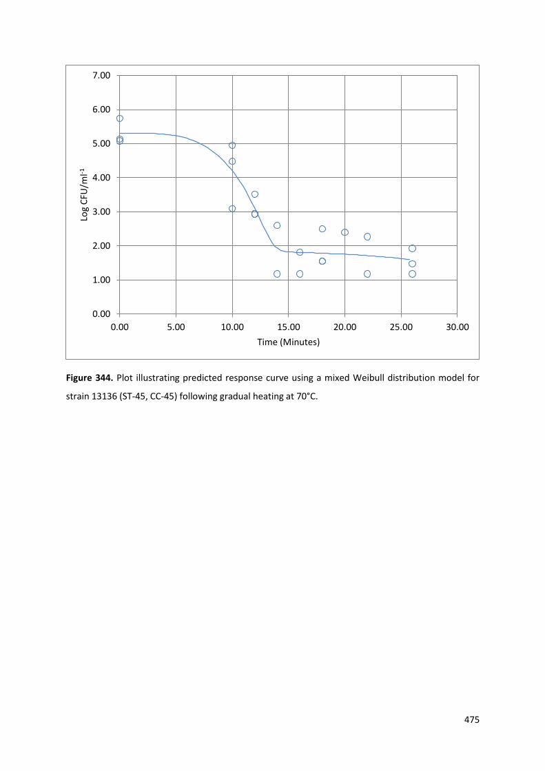
Figure 344. Plot illustrating predicted response curve using a mixed Weibull distribution model for
strain 13136 (ST-45, CC-45) following gradual heating at 70°C.
0.00
1.00
2.00
3.00
4.00
5.00
6.00
7.00
0.00 5.00 10.00 15.00 20.00 25.00 30.00
Log
CFU
/ml-1
Time (Minutes)
476
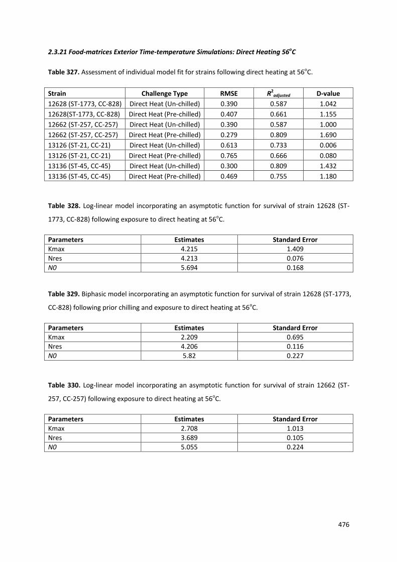
2.3.21 Food-matrices Exterior Time-temperature Simulations: Direct Heating 56oC
Table 327. Assessment of individual model fit for strains following direct heating at 56oC.
Strain Challenge Type RMSE R2adjusted D-value
12628 (ST-1773, CC-828) Direct Heat (Un-chilled) 0.390 0.587 1.042
12628(ST-1773, CC-828) Direct Heat (Pre-chilled) 0.407 0.661 1.155
12662 (ST-257, CC-257) Direct Heat (Un-chilled) 0.390 0.587 1.000
12662 (ST-257, CC-257) Direct Heat (Pre-chilled) 0.279 0.809 1.690
13126 (ST-21, CC-21) Direct Heat (Un-chilled) 0.613 0.733 0.006
13126 (ST-21, CC-21) Direct Heat (Pre-chilled) 0.765 0.666 0.080
13136 (ST-45, CC-45) Direct Heat (Un-chilled) 0.300 0.809 1.432
13136 (ST-45, CC-45) Direct Heat (Pre-chilled) 0.469 0.755 1.180
Table 328. Log-linear model incorporating an asymptotic function for survival of strain 12628 (ST-
1773, CC-828) following exposure to direct heating at 56oC.
Parameters Estimates Standard Error
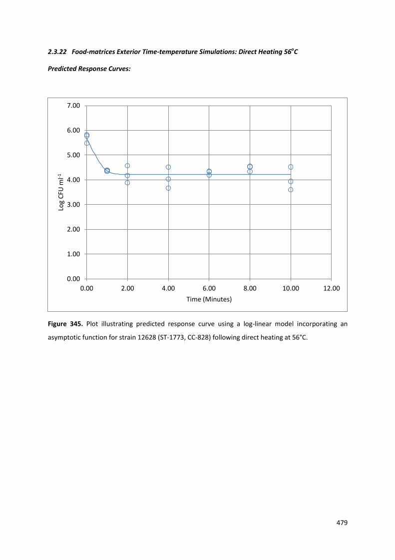
Kmax 4.215 1.409
Nres 4.213 0.076
N0 5.694 0.168
Table 329. Biphasic model incorporating an asymptotic function for survival of strain 12628 (ST-1773,
CC-828) following prior chilling and exposure to direct heating at 56oC.
Parameters Estimates Standard Error
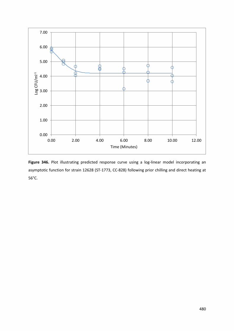
Kmax 2.209 0.695
Nres 4.206 0.116
N0 5.82 0.227
Table 330. Log-linear model incorporating an asymptotic function for survival of strain 12662 (ST-
257, CC-257) following exposure to direct heating at 56oC.
Parameters Estimates Standard Error
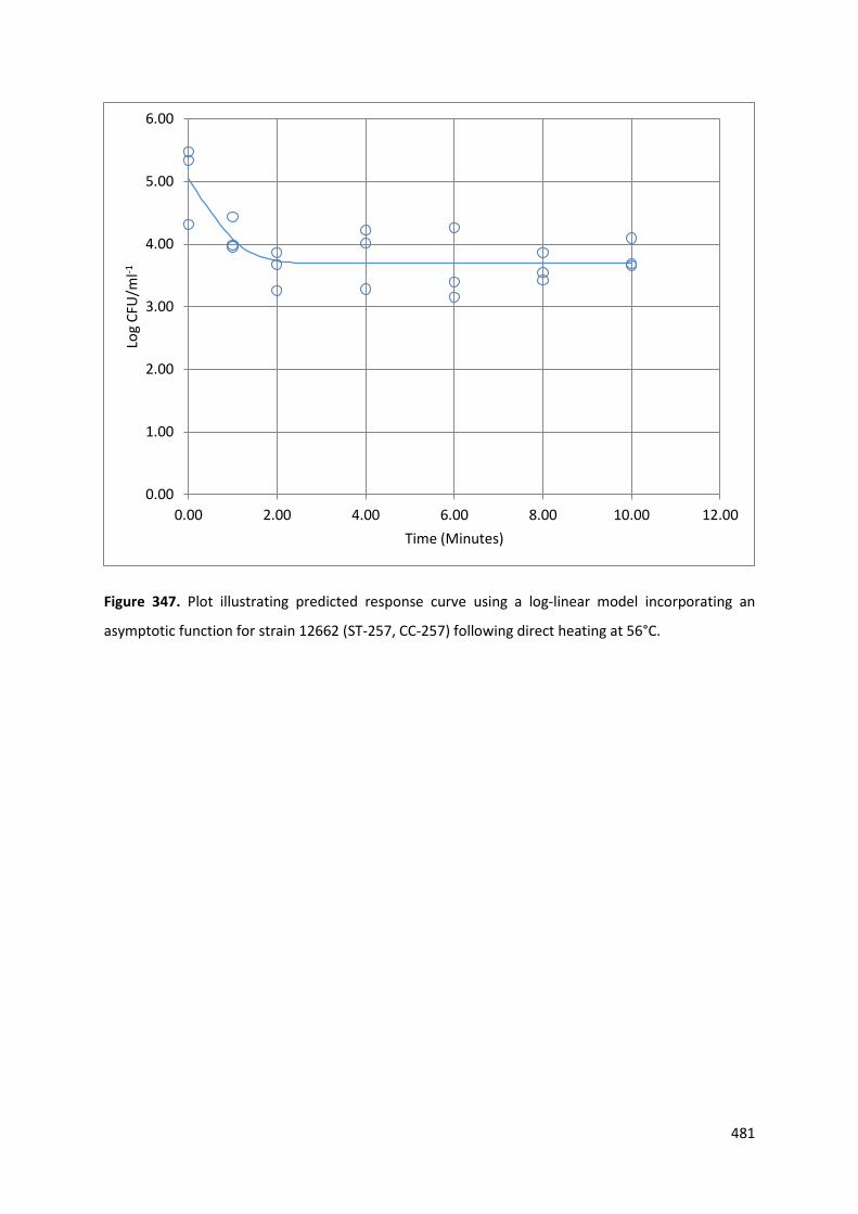
Kmax 2.708 1.013
Nres 3.689 0.105
N0 5.055 0.224
477
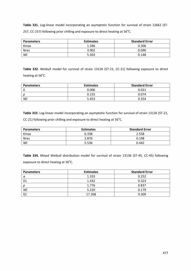
Table 331. Log-linear model incorporating an asymptotic function for survival of strain 12662 (ST-
257, CC-257) following prior chilling and exposure to direct heating at 56oC.
Parameters Estimates Standard Error
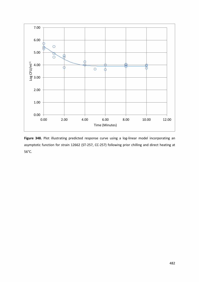
Kmax 1.346 0.306
Nres 3.902 0.090
N0 5.503 0.148
Table 332. Weibull model for survival of strain 13126 (ST-21, CC-21) following exposure to direct
heating at 56oC.
Parameters Estimates Standard Error
δ 0.006 0.021
p 0.155 0.074
N0 5.453 0.354
Table 333. Log-linear model incorporating an asymptotic function for survival of strain 13126 (ST-21,
CC-21) following prior chilling and exposure to direct heating at 56oC.
Parameters Estimates Standard Error
Kmax 6.338 2.558
Nres 2.876 0.198
N0 5.536 0.442
Table 334. Mixed Weibull distribution model for survival of strain 13136 (ST-45, CC-45) following
exposure to direct heating at 56oC.
Parameters Estimates Standard Error
α 1.333 0.252
δ1 1.432 0.323
p 1.776 0.837
N0 5.220 0.179
δ2 17.268 9.309
478
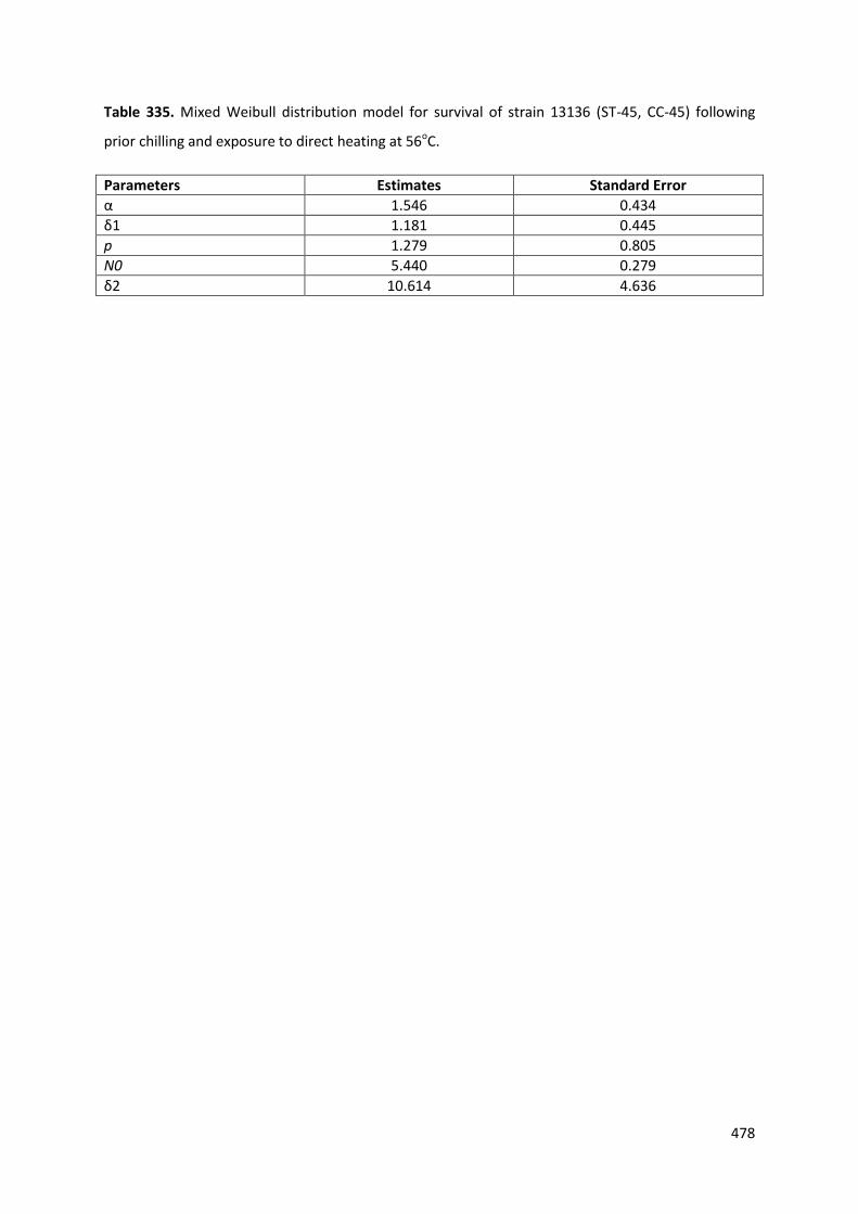
Table 335. Mixed Weibull distribution model for survival of strain 13136 (ST-45, CC-45) following
prior chilling and exposure to direct heating at 56oC.
Parameters Estimates Standard Error
α 1.546 0.434
δ1 1.181 0.445
p 1.279 0.805
N0 5.440 0.279
δ2 10.614 4.636
479
2.3.22 Food-matrices Exterior Time-temperature Simulations: Direct Heating 56oC
Predicted Response Curves:
Figure 345. Plot illustrating predicted response curve using a log-linear model incorporating an
asymptotic function for strain 12628 (ST-1773, CC-828) following direct heating at 56°C.
0.00
1.00
2.00
3.00
4.00
5.00
6.00
7.00
0.00 2.00 4.00 6.00 8.00 10.00 12.00
Log
CFU
ml-1
Time (Minutes)
480
Figure 346. Plot illustrating predicted response curve using a log-linear model incorporating an
asymptotic function for strain 12628 (ST-1773, CC-828) following prior chilling and direct heating at
56°C.
0.00
1.00
2.00
3.00
4.00
5.00
6.00
7.00
0.00 2.00 4.00 6.00 8.00 10.00 12.00
Log
CFU
/ml-1
Time (Minutes)
481
Figure 347. Plot illustrating predicted response curve using a log-linear model incorporating an
asymptotic function for strain 12662 (ST-257, CC-257) following direct heating at 56°C.
0.00
1.00
2.00
3.00
4.00
5.00
6.00
0.00 2.00 4.00 6.00 8.00 10.00 12.00
Log
CFU
/ml-1
Time (Minutes)
482
Figure 348. Plot illustrating predicted response curve using a log-linear model incorporating an
asymptotic function for strain 12662 (ST-257, CC-257) following prior chilling and direct heating at
56°C.
0.00
1.00
2.00
3.00
4.00
5.00
6.00
7.00
0.00 2.00 4.00 6.00 8.00 10.00 12.00
Log
CFU
/ml-1
Time (Minutes)

483
Figure 349. Plot illustrating predicted response curve using a Weibull model for strain 13126 (ST-21,
CC-21) following direct heating at 56°C.
0.00
1.00
2.00
3.00
4.00
5.00
6.00
7.00
0.00 2.00 4.00 6.00 8.00 10.00 12.00
Log
CFU
/ml-1
Time (Minutes)
484
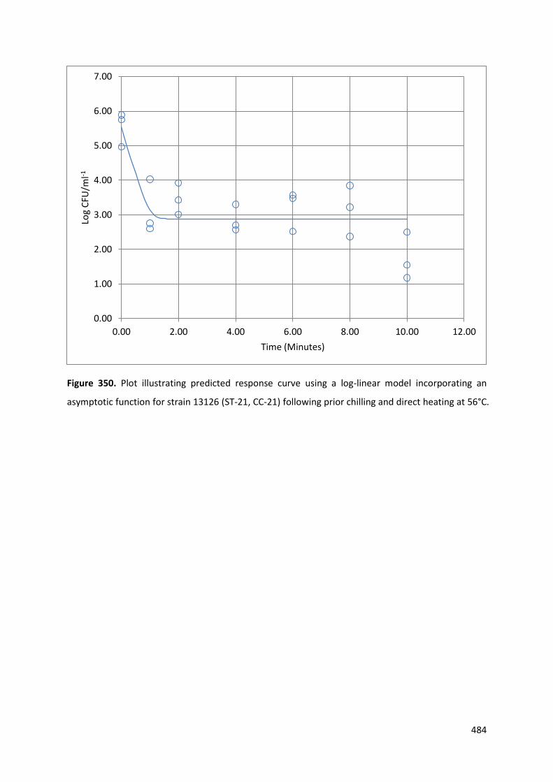
Figure 350. Plot illustrating predicted response curve using a log-linear model incorporating an
asymptotic function for strain 13126 (ST-21, CC-21) following prior chilling and direct heating at 56°C.
0.00
1.00
2.00
3.00
4.00
5.00
6.00
7.00
0.00 2.00 4.00 6.00 8.00 10.00 12.00
Log
CFU
/ml-1
Time (Minutes)

485
Figure 351. Plot illustrating predicted response curve using a mixed Weibull distribution model for
strain 13136 (ST-45, CC-45) following direct heating at 56°C.
0.00
1.00
2.00
3.00
4.00
5.00
6.00
0.00 2.00 4.00 6.00 8.00 10.00 12.00
Log
CFU
/ml-1
Time (Minutes)
486
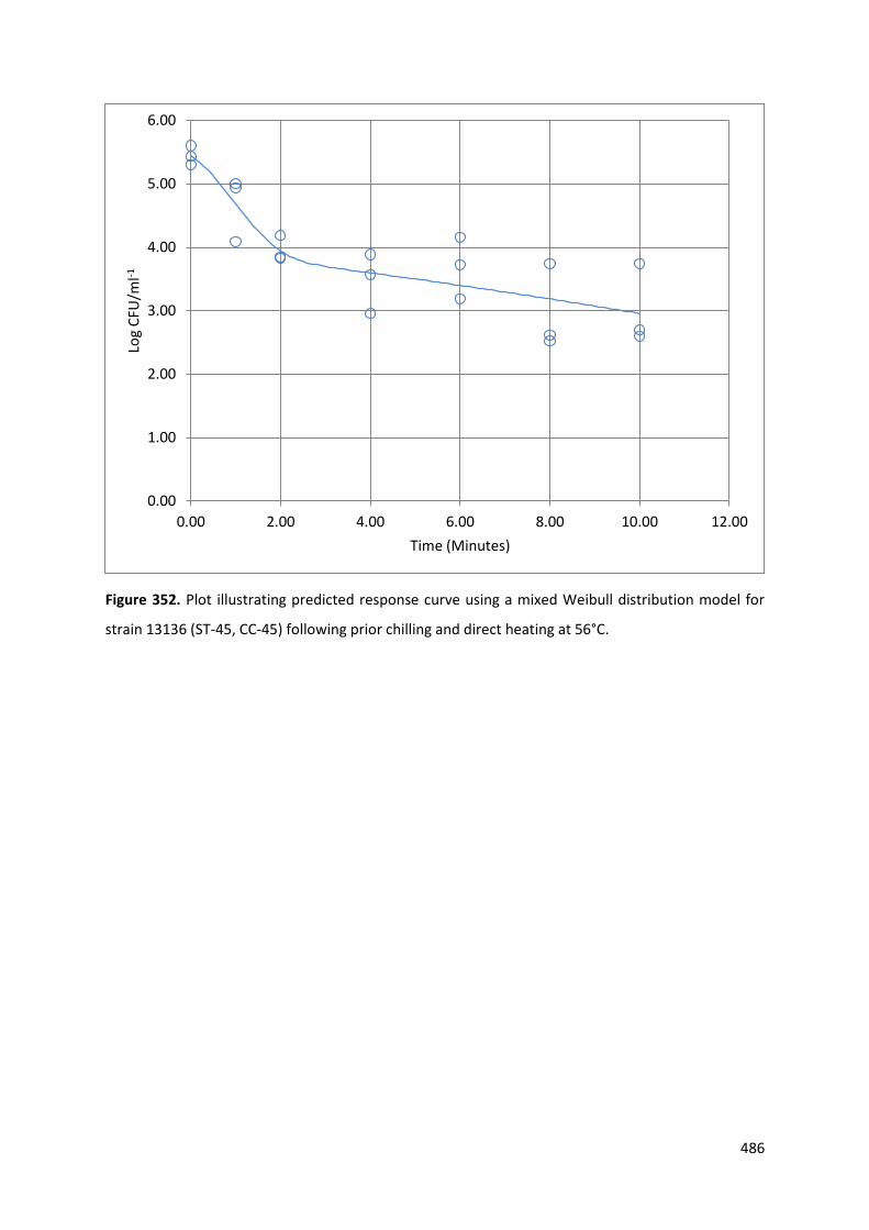
Figure 352. Plot illustrating predicted response curve using a mixed Weibull distribution model for
strain 13136 (ST-45, CC-45) following prior chilling and direct heating at 56°C.
0.00
1.00
2.00
3.00
4.00
5.00
6.00
0.00 2.00 4.00 6.00 8.00 10.00 12.00
Log
CFU
/ml-1
Time (Minutes)
487
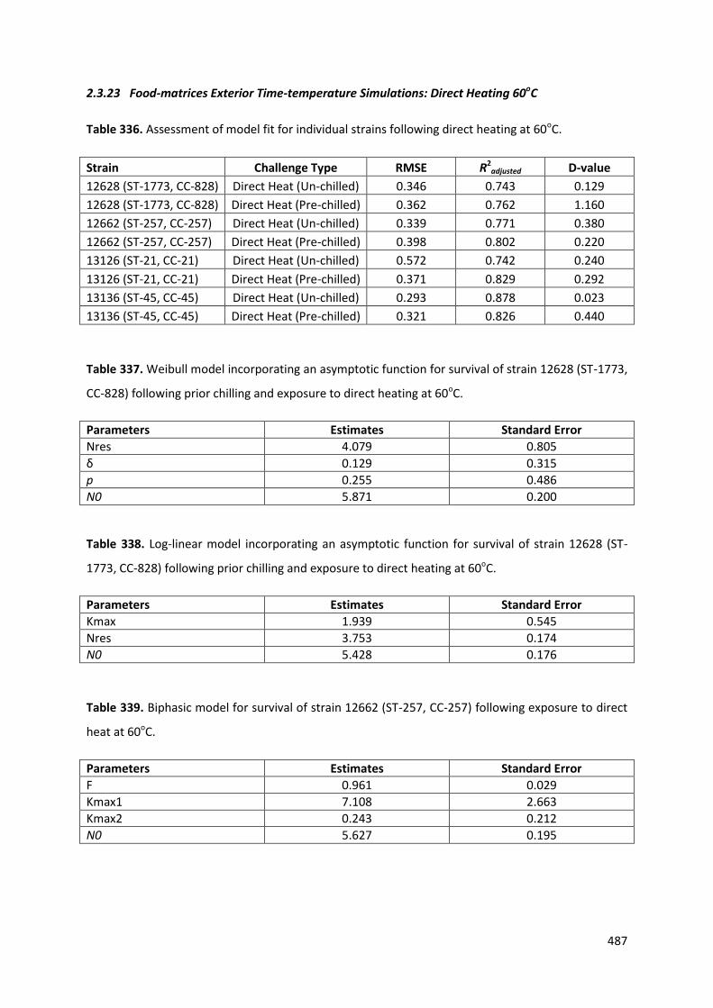
2.3.23 Food-matrices Exterior Time-temperature Simulations: Direct Heating 60oC
Table 336. Assessment of model fit for individual strains following direct heating at 60oC.
Strain Challenge Type RMSE R2adjusted D-value
12628 (ST-1773, CC-828) Direct Heat (Un-chilled) 0.346 0.743 0.129
12628 (ST-1773, CC-828) Direct Heat (Pre-chilled) 0.362 0.762 1.160
12662 (ST-257, CC-257) Direct Heat (Un-chilled) 0.339 0.771 0.380
12662 (ST-257, CC-257) Direct Heat (Pre-chilled) 0.398 0.802 0.220
13126 (ST-21, CC-21) Direct Heat (Un-chilled) 0.572 0.742 0.240
13126 (ST-21, CC-21) Direct Heat (Pre-chilled) 0.371 0.829 0.292
13136 (ST-45, CC-45) Direct Heat (Un-chilled) 0.293 0.878 0.023
13136 (ST-45, CC-45) Direct Heat (Pre-chilled) 0.321 0.826 0.440
Table 337. Weibull model incorporating an asymptotic function for survival of strain 12628 (ST-1773,
CC-828) following prior chilling and exposure to direct heating at 60oC.
Parameters Estimates Standard Error
Nres 4.079 0.805
δ 0.129 0.315
p 0.255 0.486
N0 5.871 0.200
Table 338. Log-linear model incorporating an asymptotic function for survival of strain 12628 (ST-
1773, CC-828) following prior chilling and exposure to direct heating at 60oC.
Parameters Estimates Standard Error
Kmax 1.939 0.545
Nres 3.753 0.174
N0 5.428 0.176
Table 339. Biphasic model for survival of strain 12662 (ST-257, CC-257) following exposure to direct
heat at 60oC.
Parameters Estimates Standard Error
F 0.961 0.029
Kmax1 7.108 2.663
Kmax2 0.243 0.212
N0 5.627 0.195
488
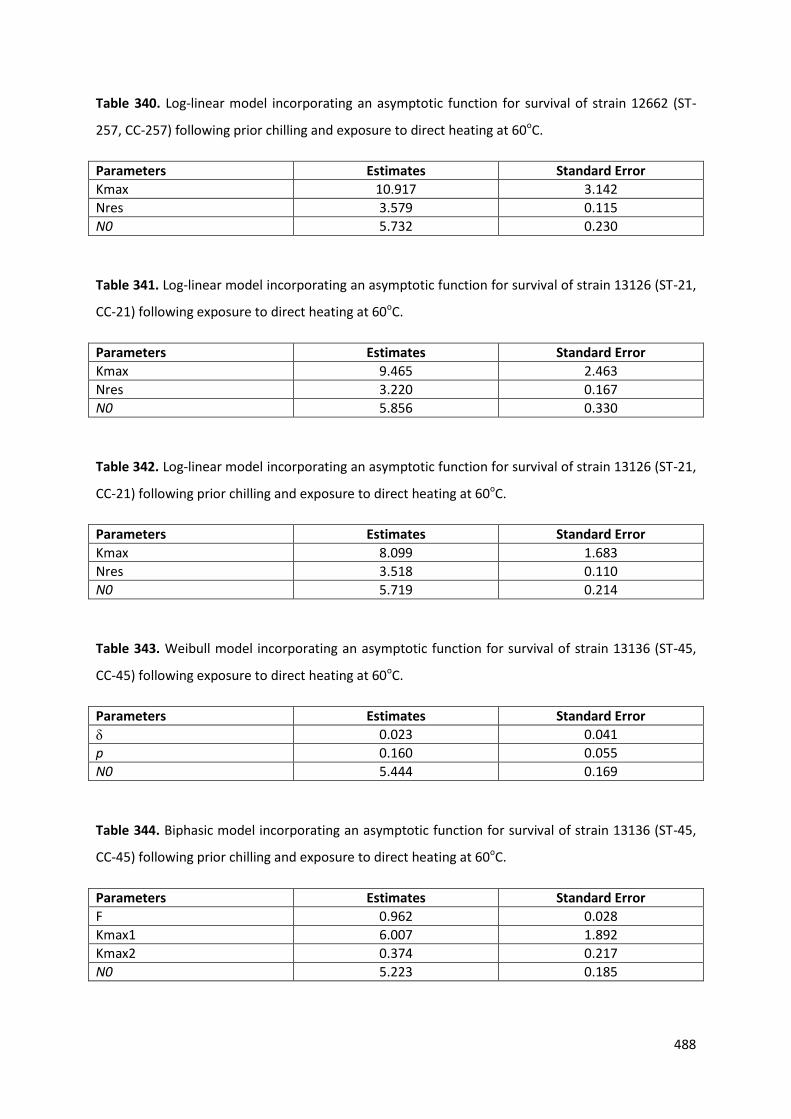
Table 340. Log-linear model incorporating an asymptotic function for survival of strain 12662 (ST-
257, CC-257) following prior chilling and exposure to direct heating at 60oC.
Parameters Estimates Standard Error
Kmax 10.917 3.142
Nres 3.579 0.115
N0 5.732 0.230
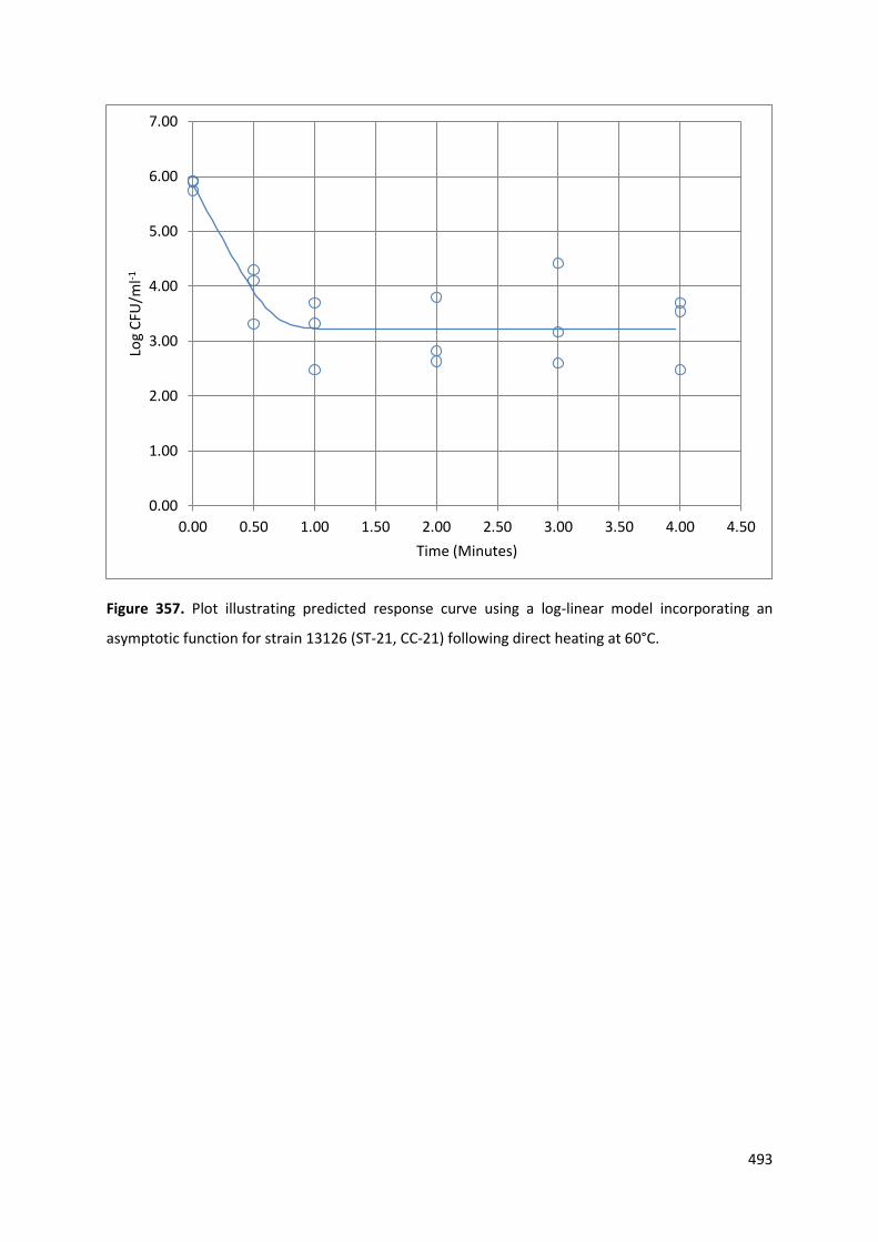
Table 341. Log-linear model incorporating an asymptotic function for survival of strain 13126 (ST-21,
CC-21) following exposure to direct heating at 60oC.
Parameters Estimates Standard Error
Kmax 9.465 2.463
Nres 3.220 0.167
N0 5.856 0.330
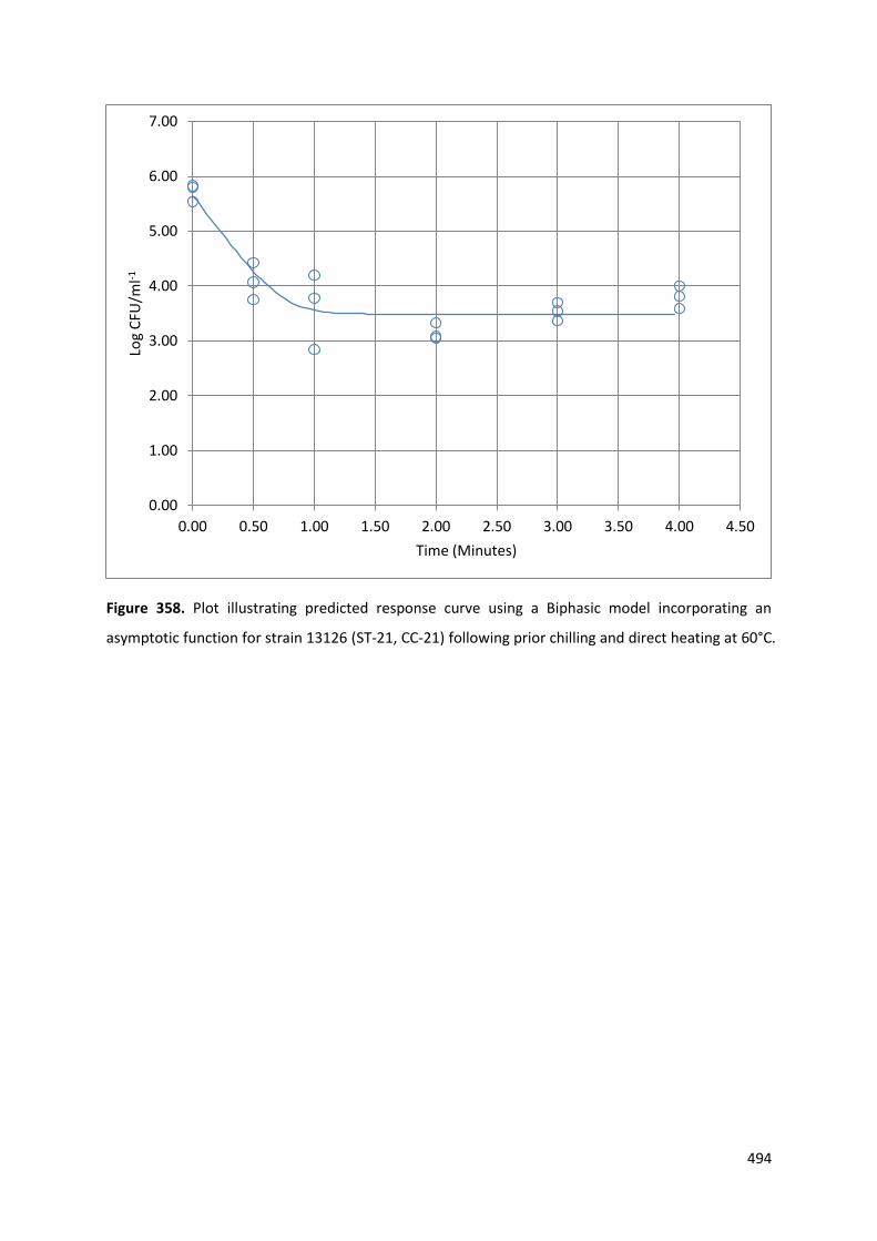
Table 342. Log-linear model incorporating an asymptotic function for survival of strain 13126 (ST-21,
CC-21) following prior chilling and exposure to direct heating at 60oC.
Parameters Estimates Standard Error
Kmax 8.099 1.683
Nres 3.518 0.110
N0 5.719 0.214
Table 343. Weibull model incorporating an asymptotic function for survival of strain 13136 (ST-45,
CC-45) following exposure to direct heating at 60oC.
Parameters Estimates Standard Error
δ 0.023 0.041
p 0.160 0.055
N0 5.444 0.169
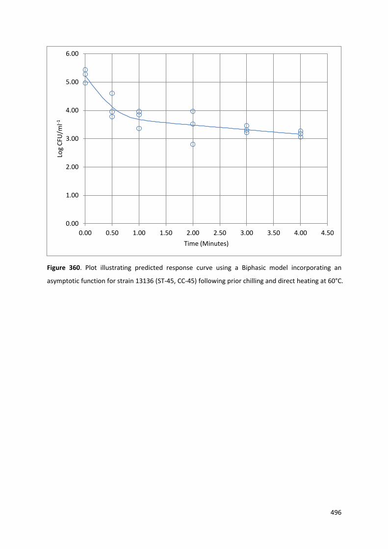
Table 344. Biphasic model incorporating an asymptotic function for survival of strain 13136 (ST-45,
CC-45) following prior chilling and exposure to direct heating at 60oC.
Parameters Estimates Standard Error
F 0.962 0.028
Kmax1 6.007 1.892
Kmax2 0.374 0.217
N0 5.223 0.185
489
2.3.24 Predicted Response Curves: Food Matrix Exterior Time-Temperature Profile Direct Heating
60oC
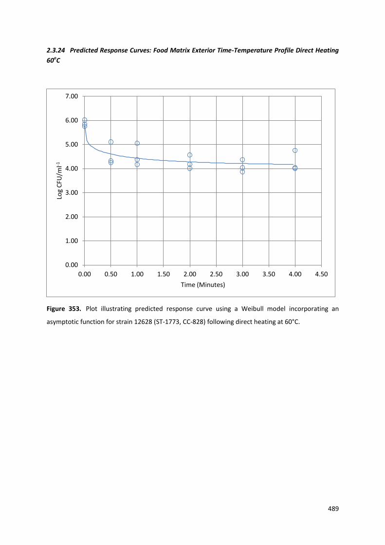
Figure 353. Plot illustrating predicted response curve using a Weibull model incorporating an
asymptotic function for strain 12628 (ST-1773, CC-828) following direct heating at 60°C.
0.00
1.00
2.00
3.00
4.00
5.00
6.00
7.00
0.00 0.50 1.00 1.50 2.00 2.50 3.00 3.50 4.00 4.50
Log
CFU
/ml-1
Time (Minutes)
490
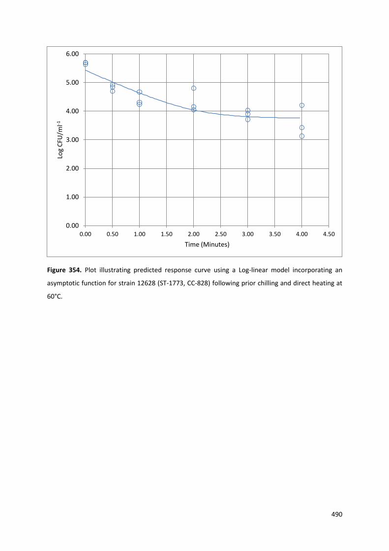
Figure 354. Plot illustrating predicted response curve using a Log-linear model incorporating an
asymptotic function for strain 12628 (ST-1773, CC-828) following prior chilling and direct heating at
60°C.
0.00
1.00
2.00
3.00
4.00
5.00
6.00
0.00 0.50 1.00 1.50 2.00 2.50 3.00 3.50 4.00 4.50
Log
CFU
/ml-1
Time (Minutes)
491
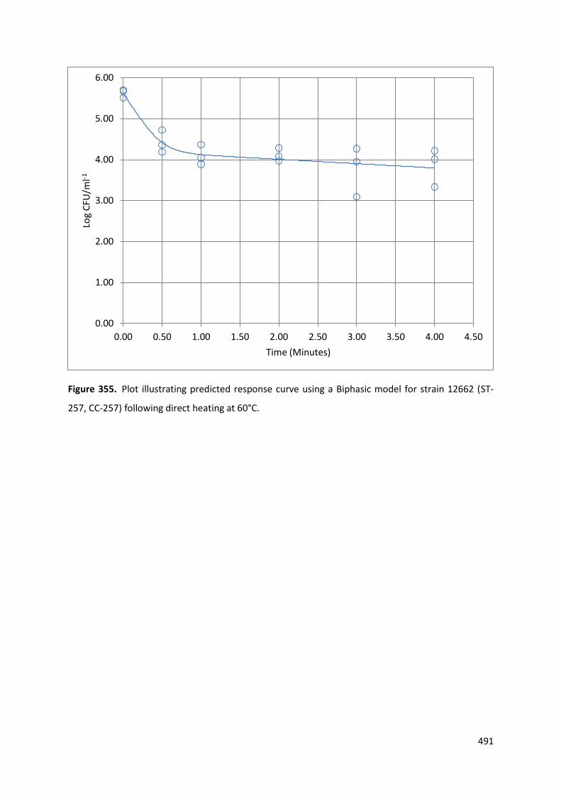
Figure 355. Plot illustrating predicted response curve using a Biphasic model for strain 12662 (ST-
257, CC-257) following direct heating at 60°C.
0.00
1.00
2.00
3.00
4.00
5.00
6.00
0.00 0.50 1.00 1.50 2.00 2.50 3.00 3.50 4.00 4.50
Log
CFU
/ml-1
Time (Minutes)
492
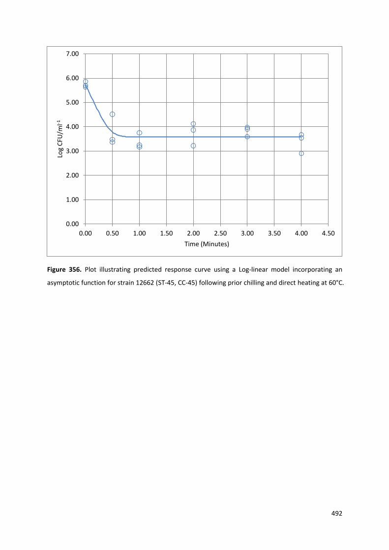
Figure 356. Plot illustrating predicted response curve using a Log-linear model incorporating an
asymptotic function for strain 12662 (ST-45, CC-45) following prior chilling and direct heating at 60°C.
0.00
1.00
2.00
3.00
4.00
5.00
6.00
7.00
0.00 0.50 1.00 1.50 2.00 2.50 3.00 3.50 4.00 4.50
Log
CFU
/ml-1
Time (Minutes)
493
Figure 357. Plot illustrating predicted response curve using a log-linear model incorporating an
asymptotic function for strain 13126 (ST-21, CC-21) following direct heating at 60°C.
0.00
1.00
2.00
3.00
4.00
5.00
6.00
7.00
0.00 0.50 1.00 1.50 2.00 2.50 3.00 3.50 4.00 4.50
Log
CFU
/ml-1
Time (Minutes)
494
Figure 358. Plot illustrating predicted response curve using a Biphasic model incorporating an
asymptotic function for strain 13126 (ST-21, CC-21) following prior chilling and direct heating at 60°C.
0.00
1.00
2.00
3.00
4.00
5.00
6.00
7.00
0.00 0.50 1.00 1.50 2.00 2.50 3.00 3.50 4.00 4.50
Log
CFU
/ml-1
Time (Minutes)

495
Figure 359. Plot illustrating predicted response curve using a Weibull model for strain 13136 (ST-45,
CC-45) following direct heating at 60°C.
0.00
1.00
2.00
3.00
4.00
5.00
6.00
0.00 0.50 1.00 1.50 2.00 2.50 3.00 3.50 4.00 4.50
Log
CFU
/ml-1
Time (Minutes)
496
Figure 360. Plot illustrating predicted response curve using a Biphasic model incorporating an
asymptotic function for strain 13136 (ST-45, CC-45) following prior chilling and direct heating at 60°C.
0.00
1.00
2.00
3.00
4.00
5.00
6.00
0.00 0.50 1.00 1.50 2.00 2.50 3.00 3.50 4.00 4.50
Log
CFU
/ml-1
Time (Minutes)

497
2.3.25 Food-matrices Exterior Time-temperature Simulations: Direct Heating 64oC
Table 345. Assessment of model fit for individual strains following direct heating at 64oC.
Strain Challenge Type RMSE R2adjusted D-value
12662 ST-257, CC-257 Direct Heat (Un-chilled) 0.384 0.935 0.230
12662 ST-257, CC-257 Direct Heat (Pre-chilled) 0.375 0.876 0.140
13126 (ST-21, CC-21) Direct Heat (Un-chilled) 0.515 0.880 0.130
13126 (ST-21, CC-21) Direct Heat (Pre-chilled) 0.375 0.947 0.033
13136 (ST-45, CC-45) Direct Heat (Un-chilled) 0.606 0.797 0.056
13136 (ST-45, CC-45) Direct Heat (Pre-chilled) 0.623 0.799 0.001
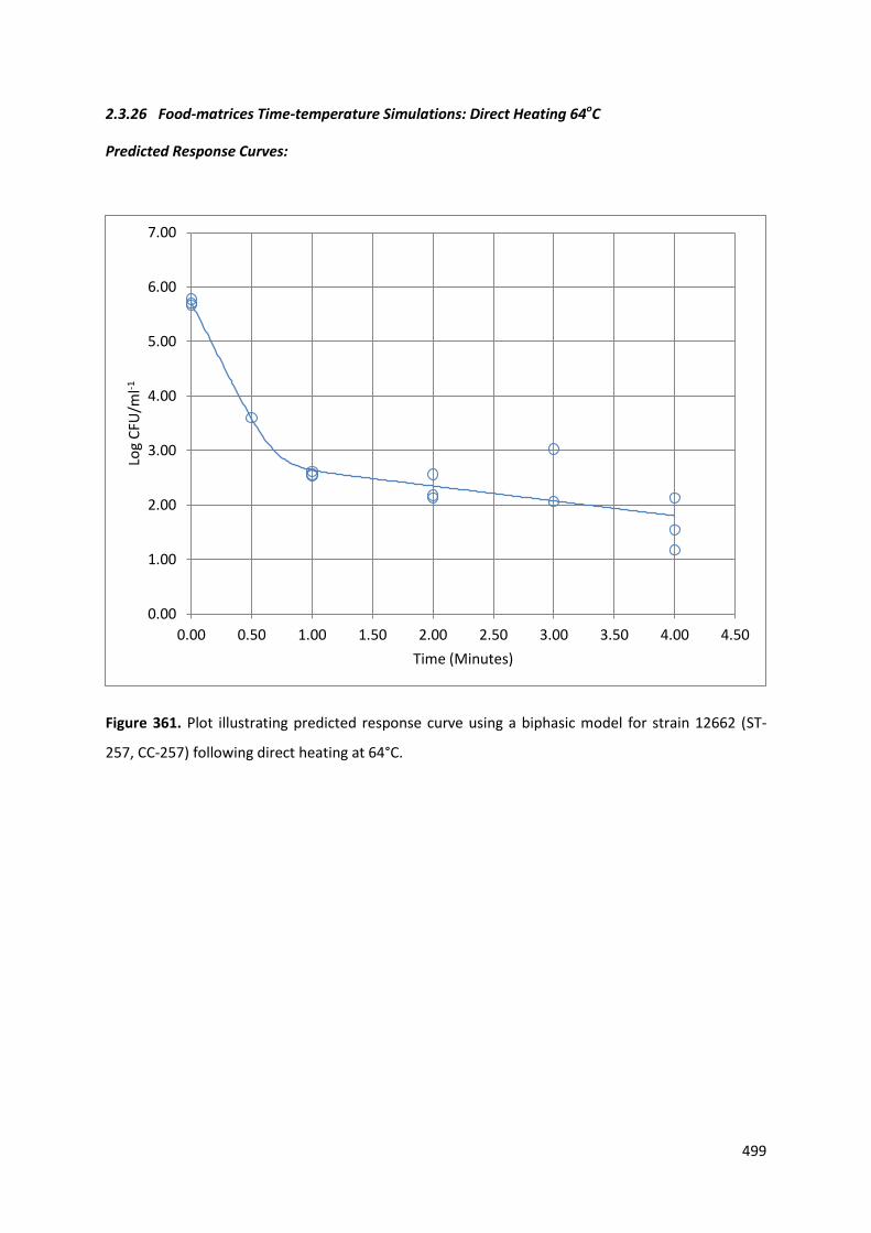
Table 346. Biphasic model incorporating an asymptotic function for survival of strain 12662 (ST-257,
CC-257) following direct heating at 64oC.
Parameters Estimates Standard Error
F 0.999 0.001
Kmax1 10.176 2.342
Kmax2 0.628 0.239
N0 5.719 0.221
Table 347. Log-linear model incorporating an asymptotic function for survival of strain 12662 (ST-
257, CC-257) following prior chilling and direct heating at 64oC.
Parameters Estimates Standard Error
Kmax 16.035 4.184
Nres 2.487 0.138
N0 5.647 0.264
Table 348. Log-linear model incorporating an asymptotic function for survival of strain 13126 (ST-21,
CC-21) following direct heating at 64oC.
Parameters Estimates Standard Error
Kmax 17.298 4.174
Nres 2.094 0.163
N0 5.614 0.297

498
Table 349. Weibull model incorporating an asymptotic function for survival of strain 13126 (ST-21,
CC-21) following prior chilling and direct heating at 64oC.
Parameters Estimates Standard Error
Nres 1.761 0.233
δ 0.013 0.033
p 0.310 0.199
N0 5.715 0.216
Table 350. Weibull model incorporating an asymptotic function for survival of strain 13136 (ST-45,
CC-45) following direct heating at 64oC.
Parameters Estimates Standard Error
Nres 1.828 0.893
δ 0.056 0.109
p 0.329 0.213
N0 5.461 0.350
Table 351. Weibull model for survival of strain 13136 (ST-45, CC-45) following prior chilling and
direct heating at 64oC.
Parameters Estimates Standard Error
δ 0.001 0.004
p 0.148 0.084
N0 5.701 0.360
499
2.3.26 Food-matrices Time-temperature Simulations: Direct Heating 64oC
Predicted Response Curves:
Figure 361. Plot illustrating predicted response curve using a biphasic model for strain 12662 (ST-
257, CC-257) following direct heating at 64°C.
0.00
1.00
2.00
3.00
4.00
5.00
6.00
7.00
0.00 0.50 1.00 1.50 2.00 2.50 3.00 3.50 4.00 4.50
Log
CFU
/ml-1
Time (Minutes)
500
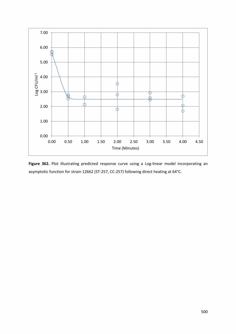
Figure 362. Plot illustrating predicted response curve using a Log-linear model incorporating an
asymptotic function for strain 12662 (ST-257, CC-257) following direct heating at 64°C.
0.00
1.00
2.00
3.00
4.00
5.00
6.00
7.00
0.00 0.50 1.00 1.50 2.00 2.50 3.00 3.50 4.00 4.50
Log
CFU
/ml-1
Time (Minutes)
501
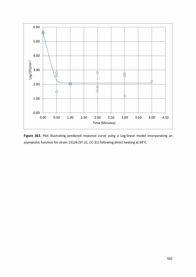
Figure 363. Plot illustrating predicted response curve using a Log-linear model incorporating an
asymptotic function for strain 13126 (ST-21, CC-21) following direct heating at 64°C.
0.00
1.00
2.00
3.00
4.00
5.00
6.00
0.00 0.50 1.00 1.50 2.00 2.50 3.00 3.50 4.00 4.50
Log
CFU
/ml-1
Time (Minutes)

502
Figure 364. Plot illustrating predicted response curve using a Weibull model incorporating an
asymptotic function for strain 13126 (ST-21, CC-21) following prior chilling and direct heating at 64°C.
0.00
1.00
2.00
3.00
4.00
5.00
6.00
7.00
0.00 0.50 1.00 1.50 2.00 2.50 3.00 3.50 4.00 4.50
Log
CFU
/ml-1
Time (Minutes)

503
Figure 365. Plot illustrating predicted response curve using a Weibull model incorporating an
asymptotic function for strain 13136 (ST-45, CC-45) following direct heating at 64°C.
0.00
1.00
2.00
3.00
4.00
5.00
6.00
0.00 0.50 1.00 1.50 2.00 2.50 3.00 3.50 4.00 4.50
Lo C
FU/m
l-1
Time (Minutes)

504
Figure 366. Plot illustrating predicted response curve using a Weibull model for strain 13136 (ST-45,
CC-45) following prior chilling and direct heating at 64°C.
0.00
1.00
2.00
3.00
4.00
5.00
6.00
7.00
0.00 0.50 1.00 1.50 2.00 2.50 3.00 3.50 4.00 4.50
Log
CFU
/ml-1
Time (Minutes)
505
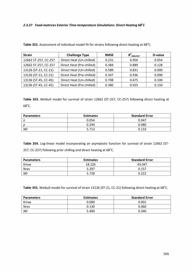
2.3.27 Food-matrices Exterior Time-temperature Simulations: Direct Heating 68oC
Table 352. Assessment of individual model fit for strains following direct heating at 68oC.
Strain Challenge Type RMSE R2adjusted D-value
12662 ST-257, CC-257 Direct Heat (Un-chilled) 0.231 0.956 0.054
12662 ST-257, CC-257 Direct Heat (Pre-chilled) 0.384 0.889 0.128
13126 (ST-21, CC-21) Direct Heat (Un-chilled) 0.589 0.831 0.000
13126 (ST-21, CC-21) Direct Heat (Pre-chilled) 0.347 0.936 0.090
13136 (ST-45, CC-45) Direct Heat (Un-chilled) 0.708 0.675 0.100
13136 (ST-45, CC-45) Direct Heat (Pre-chilled) 0.380 0.925 0.150
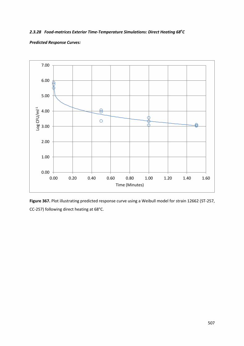
Table 353. Weibull model for survival of strain 12662 (ST-257, CC-257) following direct heating at
68oC.
Parameters Estimates Standard Error
δ 0.054 0.047
p 0.294 0.080
N0 5.713 0.133
Table 354. Log-linear model incorporating an asymptotic function for survival of strain 12662 (ST-
257, CC-257) following prior chilling and direct heating at 68oC.
Parameters Estimates Standard Error
Kmax 18.226 43.047
Nres 3.297 0.157
N0 5.728 0.222
Table 355. Weibull model for survival of strain 13126 (ST-21, CC-21) following direct heating at 68oC.
Parameters Estimates Standard Error
Kmax 0.000 0.001
Nres 0.130 0.060
N0 5.400 0.340
506
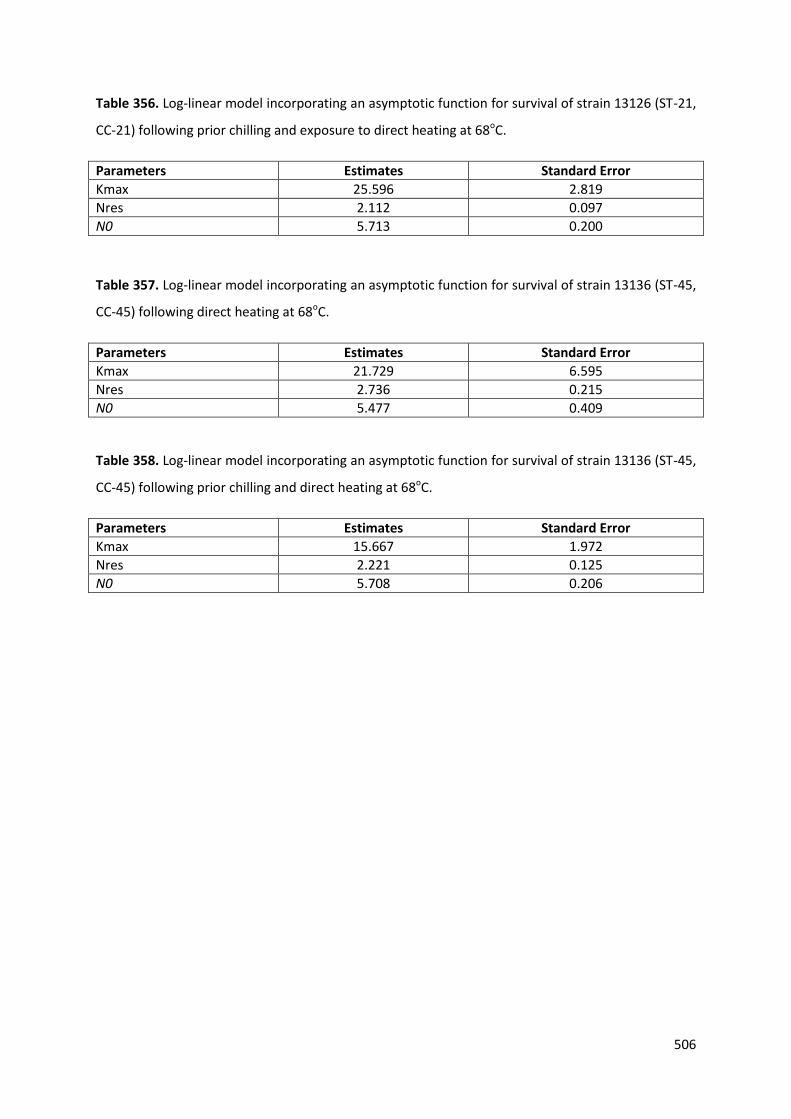
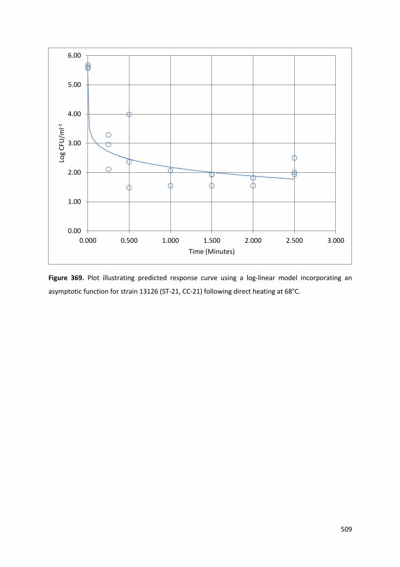
Table 356. Log-linear model incorporating an asymptotic function for survival of strain 13126 (ST-21,
CC-21) following prior chilling and exposure to direct heating at 68oC.
Parameters Estimates Standard Error
Kmax 25.596 2.819
Nres 2.112 0.097
N0 5.713 0.200
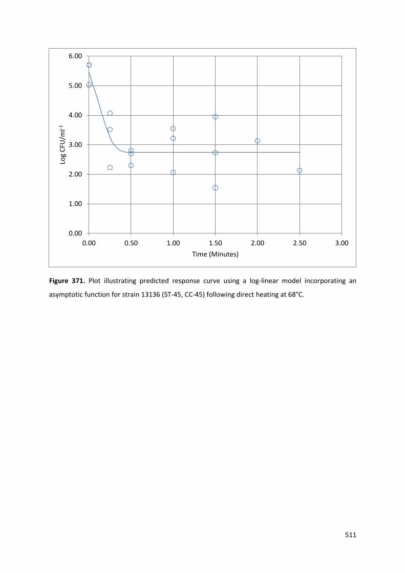
Table 357. Log-linear model incorporating an asymptotic function for survival of strain 13136 (ST-45,
CC-45) following direct heating at 68oC.
Parameters Estimates Standard Error
Kmax 21.729 6.595
Nres 2.736 0.215
N0 5.477 0.409
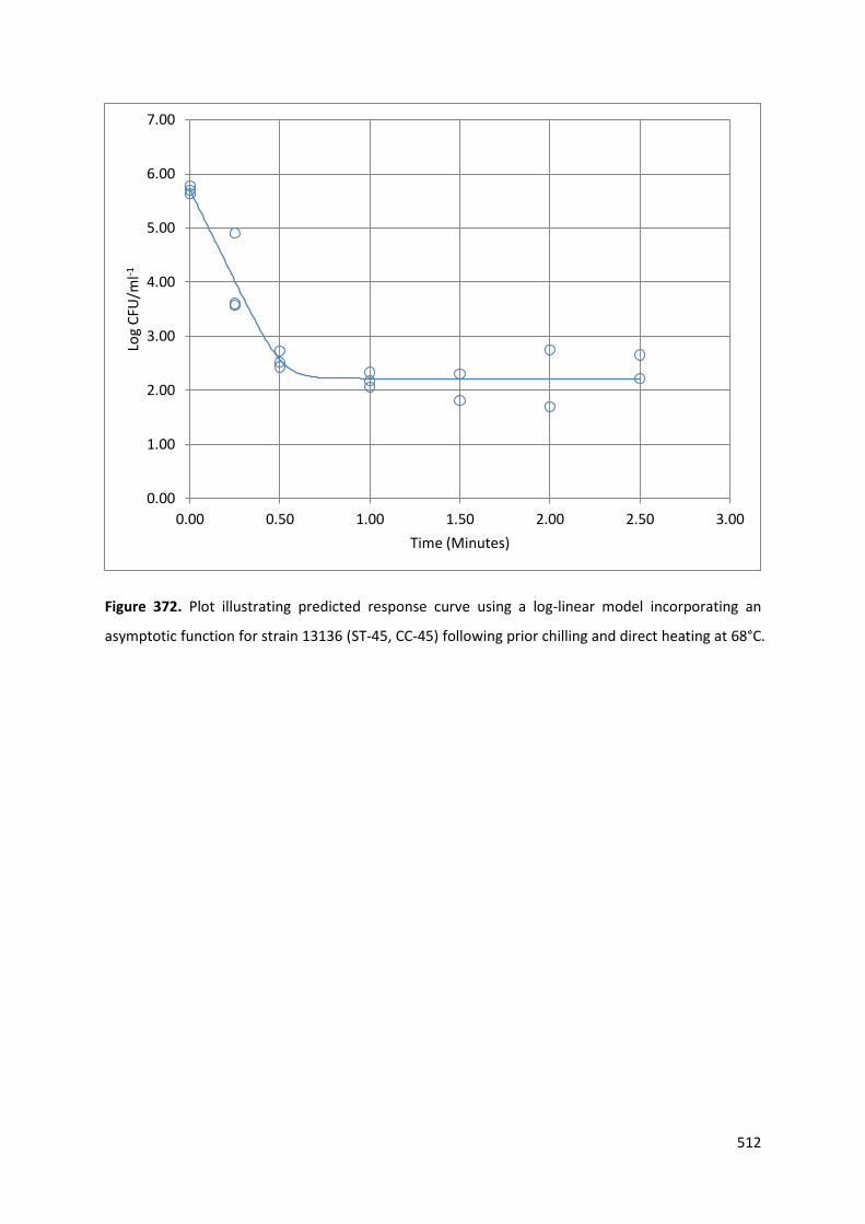
Table 358. Log-linear model incorporating an asymptotic function for survival of strain 13136 (ST-45,
CC-45) following prior chilling and direct heating at 68oC.
Parameters Estimates Standard Error
Kmax 15.667 1.972
Nres 2.221 0.125
N0 5.708 0.206
507
2.3.28 Food-matrices Exterior Time-Temperature Simulations: Direct Heating 68oC
Predicted Response Curves:
Figure 367. Plot illustrating predicted response curve using a Weibull model for strain 12662 (ST-257,
CC-257) following direct heating at 68°C.
0.00
1.00
2.00
3.00
4.00
5.00
6.00
7.00
0.00 0.20 0.40 0.60 0.80 1.00 1.20 1.40 1.60
Log
CFU
/ml-1
Time (Minutes)

508
Figure 368. Plot illustrating predicted response curve using a Log-linear model incorporating an
asymptotic function for strain 12662 (ST-257, CC-257) following prior chilling and direct heating at
68°C.
0.00
1.00
2.00
3.00
4.00
5.00
6.00
7.00
0.00 0.20 0.40 0.60 0.80 1.00 1.20 1.40 1.60
Log
CFU
/ml-1
Time (Minutes)
509
Figure 369. Plot illustrating predicted response curve using a log-linear model incorporating an
asymptotic function for strain 13126 (ST-21, CC-21) following direct heating at 68°C.
0.00
1.00
2.00
3.00
4.00
5.00
6.00
0.000 0.500 1.000 1.500 2.000 2.500 3.000
Log
CFU
/ml-1
Time (Minutes)

510
Figure 370. Plot illustrating predicted response curve using a log-linear model incorporating an
asymptotic function for strain 13126 (ST-21, CC-21) following prior chilling and direct heating at 68°C.
0.00
1.00
2.00
3.00
4.00
5.00
6.00
7.00
0.00 0.50 1.00 1.50 2.00 2.50 3.00
Log
CFU
/ml-1
Time (Minutes)
511
Figure 371. Plot illustrating predicted response curve using a log-linear model incorporating an
asymptotic function for strain 13136 (ST-45, CC-45) following direct heating at 68°C.
0.00
1.00
2.00
3.00
4.00
5.00
6.00
0.00 0.50 1.00 1.50 2.00 2.50 3.00
Log
CFU
/ml-1
Time (Minutes)
512
Figure 372. Plot illustrating predicted response curve using a log-linear model incorporating an
asymptotic function for strain 13136 (ST-45, CC-45) following prior chilling and direct heating at 68°C.
0.00
1.00
2.00
3.00
4.00
5.00
6.00
7.00
0.00 0.50 1.00 1.50 2.00 2.50 3.00
Log
CFU
/ml-1
Time (Minutes)
513
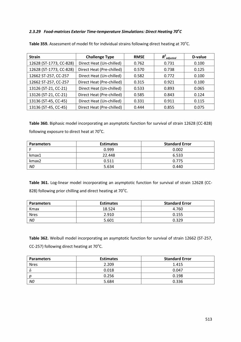
2.3.29 Food-matrices Exterior Time-temperature Simulations: Direct Heating 70oC
Table 359. Assessment of model fit for individual strains following direct heating at 70oC.
Strain Challenge Type RMSE R2adjusted D-value
12628 (ST-1773, CC-828) Direct Heat (Un-chilled) 0.762 0.731 0.100
12628 (ST-1773, CC-828) Direct Heat (Pre-chilled) 0.570 0.738 0.125
12662 ST-257, CC-257 Direct Heat (Un-chilled) 0.582 0.772 0.100
12662 ST-257, CC-257 Direct Heat (Pre-chilled) 0.315 0.921 0.100
13126 (ST-21, CC-21) Direct Heat (Un-chilled) 0.533 0.893 0.065
13126 (ST-21, CC-21) Direct Heat (Pre-chilled) 0.585 0.843 0.124
13136 (ST-45, CC-45) Direct Heat (Un-chilled) 0.331 0.911 0.115
13136 (ST-45, CC-45) Direct Heat (Pre-chilled) 0.444 0.855 0.075
Table 360. Biphasic model incorporating an asymptotic function for survival of strain 12628 (CC-828)
following exposure to direct heat at 70oC.
Parameters Estimates Standard Error
F 0.999 0.002
kmax1 22.448 6.533
kmax2 0.511 0.775
N0 5.634 0.440
Table 361. Log-linear model incorporating an asymptotic function for survival of strain 12628 (CC-
828) following prior chilling and direct heating at 70oC.
Parameters Estimates Standard Error
Kmax 18.524 4.760
Nres 2.910 0.155
N0 5.601 0.329
Table 362. Weibull model incorporating an asymptotic function for survival of strain 12662 (ST-257,
CC-257) following direct heating at 70oC.
Parameters Estimates Standard Error
Nres 2.209 1.415
δ 0.018 0.047
p 0.256 0.198
N0 5.684 0.336

514
Table 363. Log-linear model incorporating an asymptotic function for survival of strain 12662 (ST-
257, CC-257) following prior chilling and direct heating at 70oC.
Parameters Estimates Standard Error
Kmax 24.512 2.986
Nres 2.652 0.084
N0 5.654 0.182
Table 364. Log-linear model incorporating an asymptotic function for survival of strain 13126 (ST-21,
CC-21) following direct heating at 70oC.
Parameters Estimates Standard Error
Kmax 18.643 3.198
Nres 1.600 0.182
N0 5.465 0.295
Table 365. Log-linear model incorporating an asymptotic function for survival of strain 13126 (ST-21,
CC-21) following prior chilling and direct heating at 70oC.
Parameters Estimates Standard Error
Kmax 21.021 4.436
Nres 2.051 0.174
N0 5.648 0.337
Table 366. Biphasic model incorporating an asymptotic function for survival of strain 13136 (ST-45,
CC-45) following direct heating at 70oC.
Parameters Estimates Standard Error
F 0.998 0.002
kmax1 20.292 3.007
kmax2 0.468 0.288
N0 5.532 0.191
Table 367. Biphasic model incorporating an asymptotic function for survival of strain 13136 (ST-45,
CC-45) following prior chilling and direct heating at 70oC.
Parameters Estimates Standard Error
F 0.997 0.003
kmax1 31.273 24.254
kmax2 0.636 0.416
N0 5.524 0.256
515
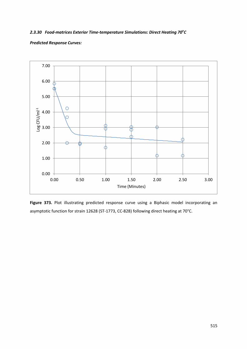
2.3.30 Food-matrices Exterior Time-temperature Simulations: Direct Heating 70oC
Predicted Response Curves:
Figure 373. Plot illustrating predicted response curve using a Biphasic model incorporating an
asymptotic function for strain 12628 (ST-1773, CC-828) following direct heating at 70°C.
0.00
1.00
2.00
3.00
4.00
5.00
6.00
7.00
0.00 0.50 1.00 1.50 2.00 2.50 3.00
Log
CFU
/ml-1
Time (Minutes)
516
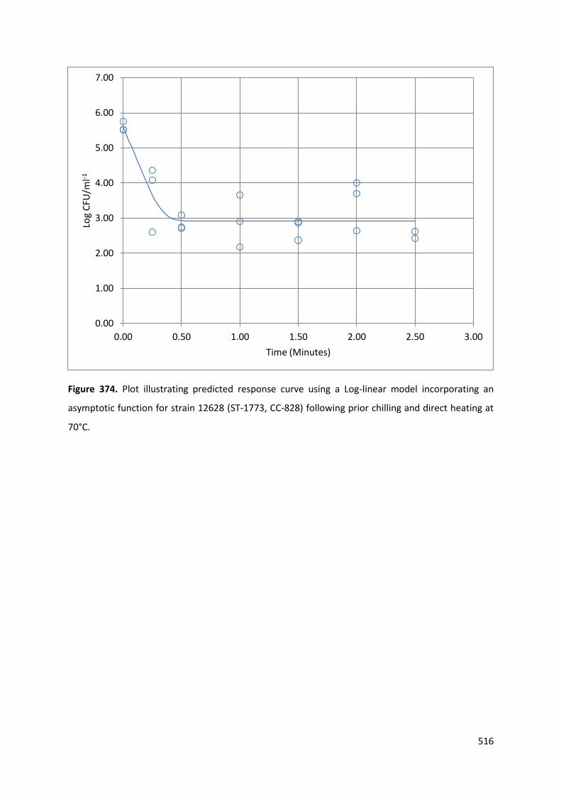
Figure 374. Plot illustrating predicted response curve using a Log-linear model incorporating an
asymptotic function for strain 12628 (ST-1773, CC-828) following prior chilling and direct heating at
70°C.
0.00
1.00
2.00
3.00
4.00
5.00
6.00
7.00
0.00 0.50 1.00 1.50 2.00 2.50 3.00
Log
CFU
/ml-1
Time (Minutes)
517
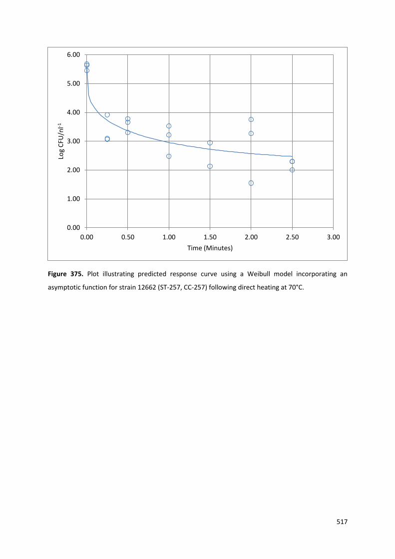
Figure 375. Plot illustrating predicted response curve using a Weibull model incorporating an
asymptotic function for strain 12662 (ST-257, CC-257) following direct heating at 70°C.
0.00
1.00
2.00
3.00
4.00
5.00
6.00
0.00 0.50 1.00 1.50 2.00 2.50 3.00
Log
CFU
/nl-1
Time (Minutes)
518
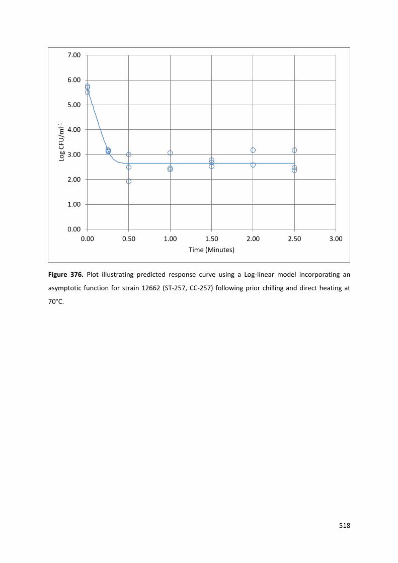
Figure 376. Plot illustrating predicted response curve using a Log-linear model incorporating an
asymptotic function for strain 12662 (ST-257, CC-257) following prior chilling and direct heating at
70°C.
0.00
1.00
2.00
3.00
4.00
5.00
6.00
7.00
0.00 0.50 1.00 1.50 2.00 2.50 3.00
Log
CFU
/ml-1
Time (Minutes)
519
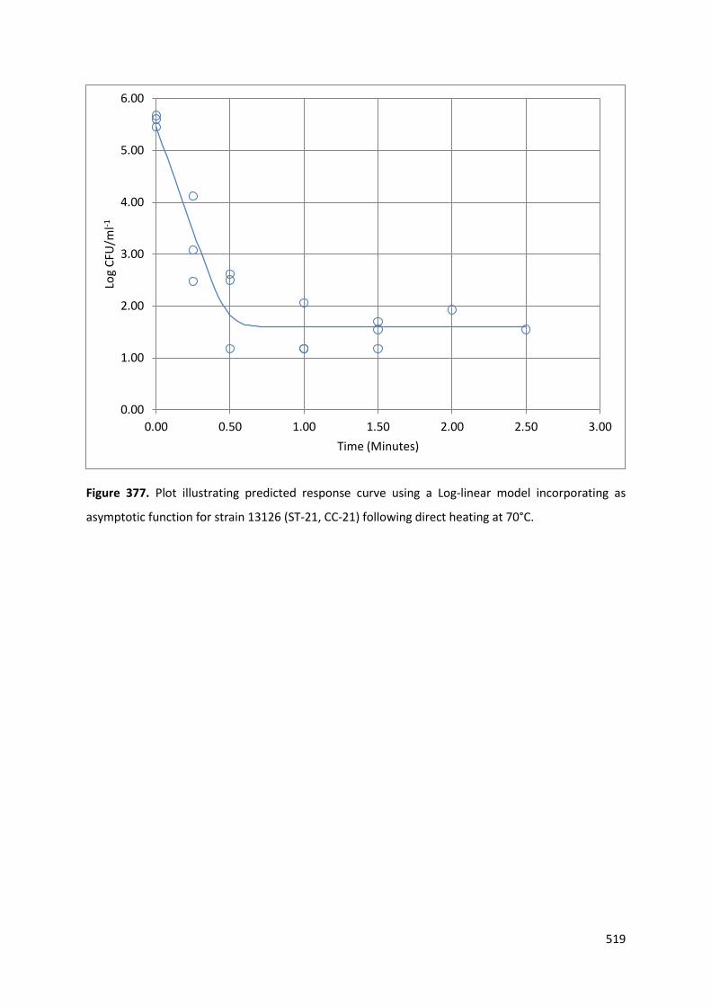
Figure 377. Plot illustrating predicted response curve using a Log-linear model incorporating as
asymptotic function for strain 13126 (ST-21, CC-21) following direct heating at 70°C.
0.00
1.00
2.00
3.00
4.00
5.00
6.00
0.00 0.50 1.00 1.50 2.00 2.50 3.00
Log
CFU
/ml-1
Time (Minutes)

520
Figure 378. Plot illustrating predicted response curve using a Log-linear model incorporating an
asymptotic function for strain 13126 (ST-21, CC-21) following prior chilling and direct heating at 70°C.
0.00
1.00
2.00
3.00
4.00
5.00
6.00
7.00
0.00 0.50 1.00 1.50 2.00 2.50 3.00
Log
CFU
/ml-1
Time (Minutes)
521
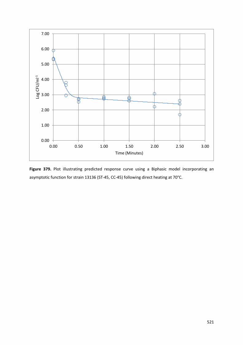
Figure 379. Plot illustrating predicted response curve using a Biphasic model incorporating an
asymptotic function for strain 13136 (ST-45, CC-45) following direct heating at 70°C.
0.00
1.00
2.00
3.00
4.00
5.00
6.00
7.00
0.00 0.50 1.00 1.50 2.00 2.50 3.00
Log
CFU
/ml-1
Time (Minutes)

522
Figure 380. Plot illustrating predicted response curve using a Biphasic model incorporating an
asymptotic function for strain 13136 (ST-45, CC-45) following prior chilling and direct heating at 70°C.
0.00
1.00
2.00
3.00
4.00
5.00
6.00
7.00
0.00 0.50 1.00 1.50 2.00 2.50 3.00
Log
CFU
/ml-1
Time (Minutes)
523
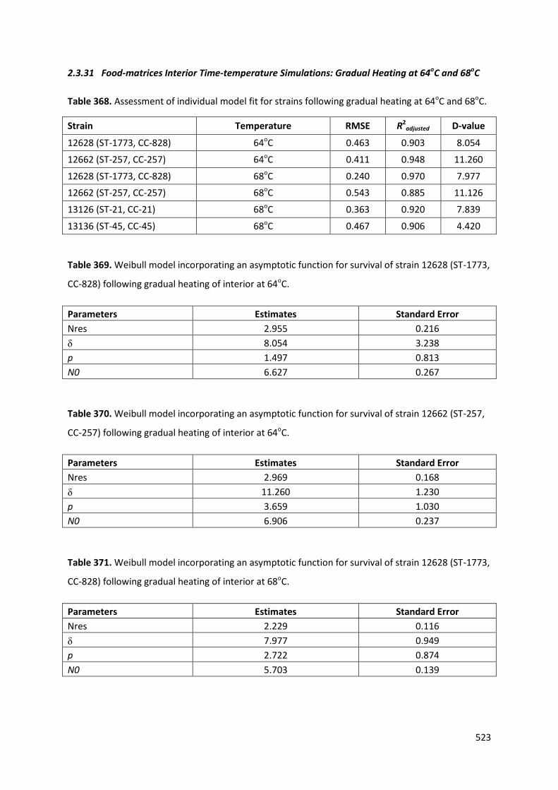
2.3.31 Food-matrices Interior Time-temperature Simulations: Gradual Heating at 64oC and 68oC
Table 368. Assessment of individual model fit for strains following gradual heating at 64oC and 68oC.
Strain Temperature RMSE R2adjusted D-value
12628 (ST-1773, CC-828) 64oC 0.463 0.903 8.054
12662 (ST-257, CC-257) 64oC 0.411 0.948 11.260
12628 (ST-1773, CC-828) 68oC 0.240 0.970 7.977
12662 (ST-257, CC-257) 68oC 0.543 0.885 11.126
13126 (ST-21, CC-21) 68oC 0.363 0.920 7.839
13136 (ST-45, CC-45) 68oC 0.467 0.906 4.420
Table 369. Weibull model incorporating an asymptotic function for survival of strain 12628 (ST-1773,
CC-828) following gradual heating of interior at 64oC.
Parameters Estimates Standard Error
Nres 2.955 0.216
δ 8.054 3.238
p 1.497 0.813
N0 6.627 0.267
Table 370. Weibull model incorporating an asymptotic function for survival of strain 12662 (ST-257,
CC-257) following gradual heating of interior at 64oC.
Parameters Estimates Standard Error
Nres 2.969 0.168
δ 11.260 1.230
p 3.659 1.030
N0 6.906 0.237
Table 371. Weibull model incorporating an asymptotic function for survival of strain 12628 (ST-1773,
CC-828) following gradual heating of interior at 68oC.
Parameters Estimates Standard Error
Nres 2.229 0.116
δ 7.977 0.949
p 2.722 0.874
N0 5.703 0.139
524
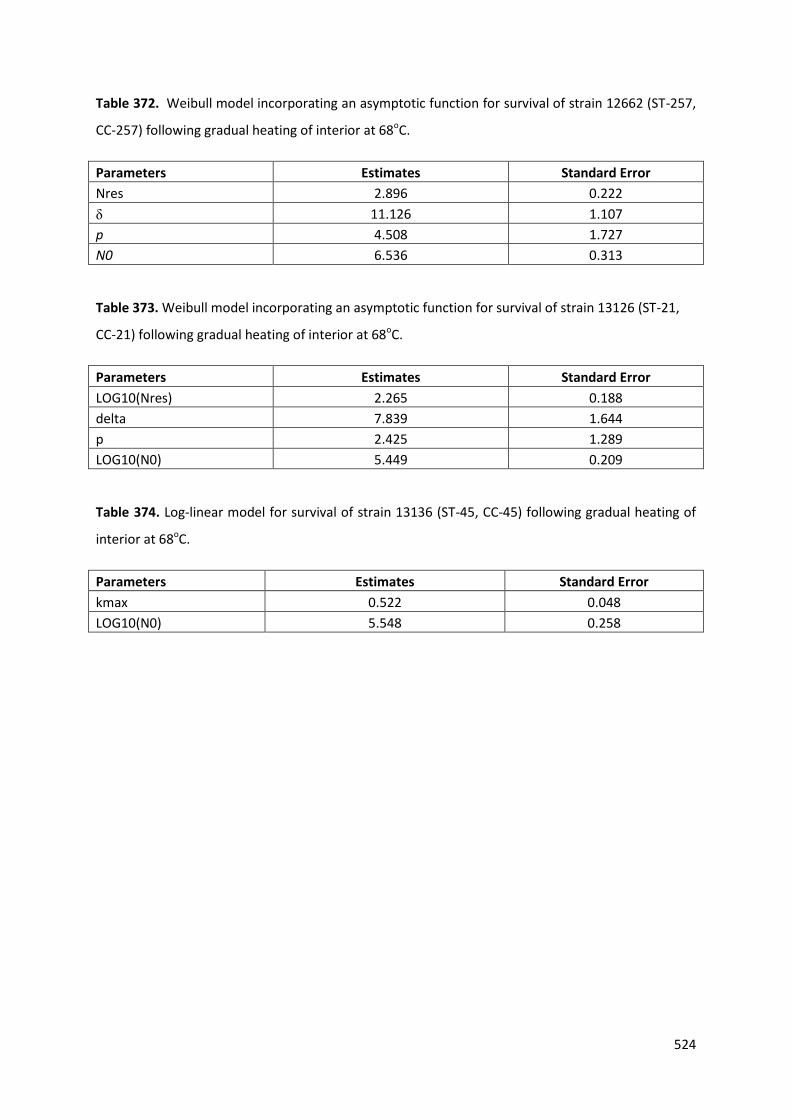
Table 372. Weibull model incorporating an asymptotic function for survival of strain 12662 (ST-257,
CC-257) following gradual heating of interior at 68oC.
Parameters Estimates Standard Error
Nres 2.896 0.222
δ 11.126 1.107
p 4.508 1.727
N0 6.536 0.313
Table 373. Weibull model incorporating an asymptotic function for survival of strain 13126 (ST-21,
CC-21) following gradual heating of interior at 68oC.
Parameters Estimates Standard Error
LOG10(Nres) 2.265 0.188
delta 7.839 1.644
p 2.425 1.289
LOG10(N0) 5.449 0.209
Table 374. Log-linear model for survival of strain 13136 (ST-45, CC-45) following gradual heating of
interior at 68oC.
Parameters Estimates Standard Error
kmax 0.522 0.048
LOG10(N0) 5.548 0.258
525
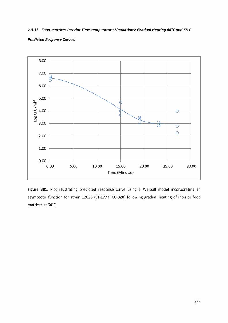
2.3.32 Food-matrices Interior Time-temperature Simulations: Gradual Heating 64oC and 68oC
Predicted Response Curves:
Figure 381. Plot illustrating predicted response curve using a Weibull model incorporating an
asymptotic function for strain 12628 (ST-1773, CC-828) following gradual heating of interior food
matrices at 64°C.
0.00
1.00
2.00
3.00
4.00
5.00
6.00
7.00
8.00
0.00 5.00 10.00 15.00 20.00 25.00 30.00
Log
CFU
/ml-1
Time (Minutes)
526
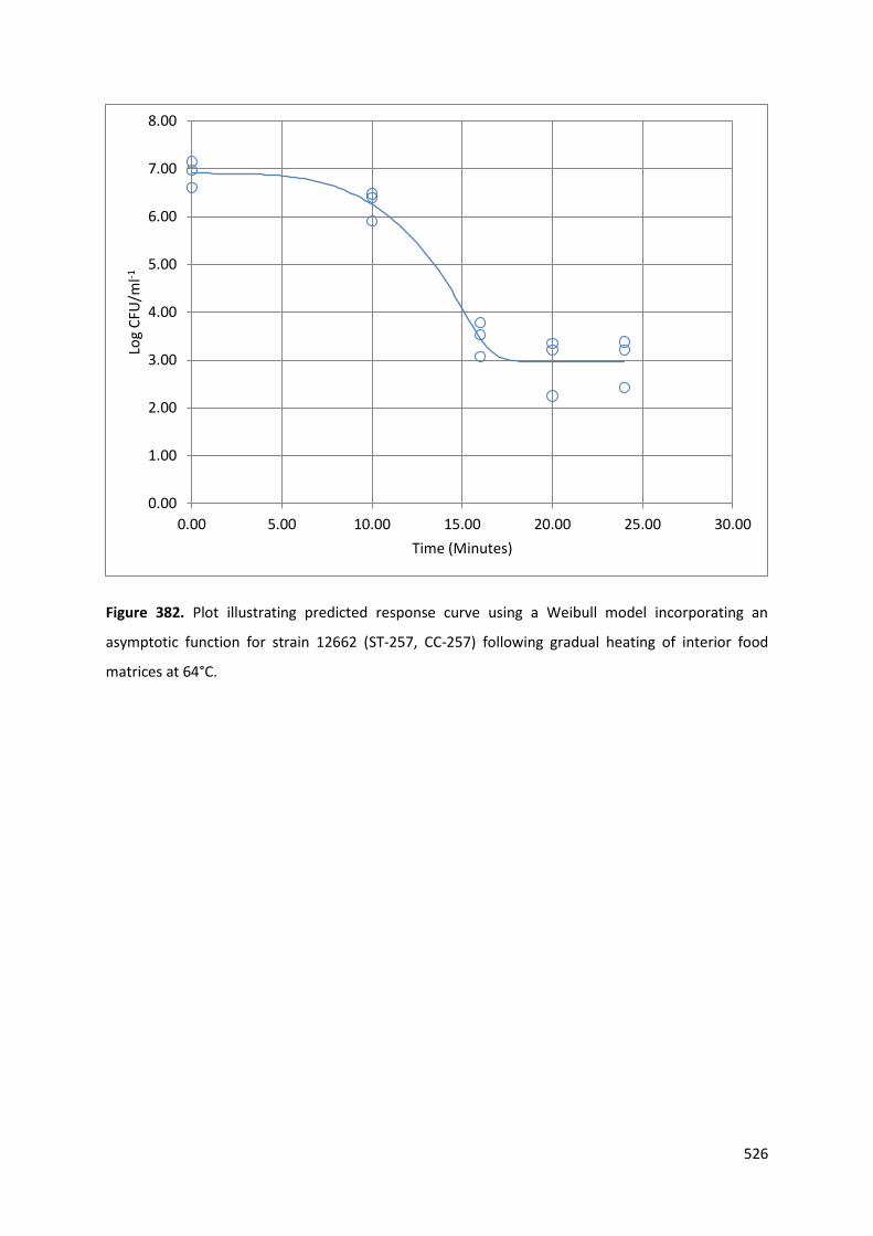
Figure 382. Plot illustrating predicted response curve using a Weibull model incorporating an
asymptotic function for strain 12662 (ST-257, CC-257) following gradual heating of interior food
matrices at 64°C.
0.00
1.00
2.00
3.00
4.00
5.00
6.00
7.00
8.00
0.00 5.00 10.00 15.00 20.00 25.00 30.00
Log
CFU
/ml-1
Time (Minutes)
527
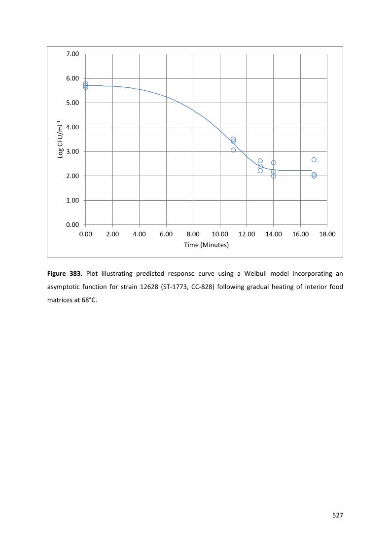
Figure 383. Plot illustrating predicted response curve using a Weibull model incorporating an
asymptotic function for strain 12628 (ST-1773, CC-828) following gradual heating of interior food
matrices at 68°C.
0.00
1.00
2.00
3.00
4.00
5.00
6.00
7.00
0.00 2.00 4.00 6.00 8.00 10.00 12.00 14.00 16.00 18.00
Log
CFU
/ml-1
Time (Minutes)
528
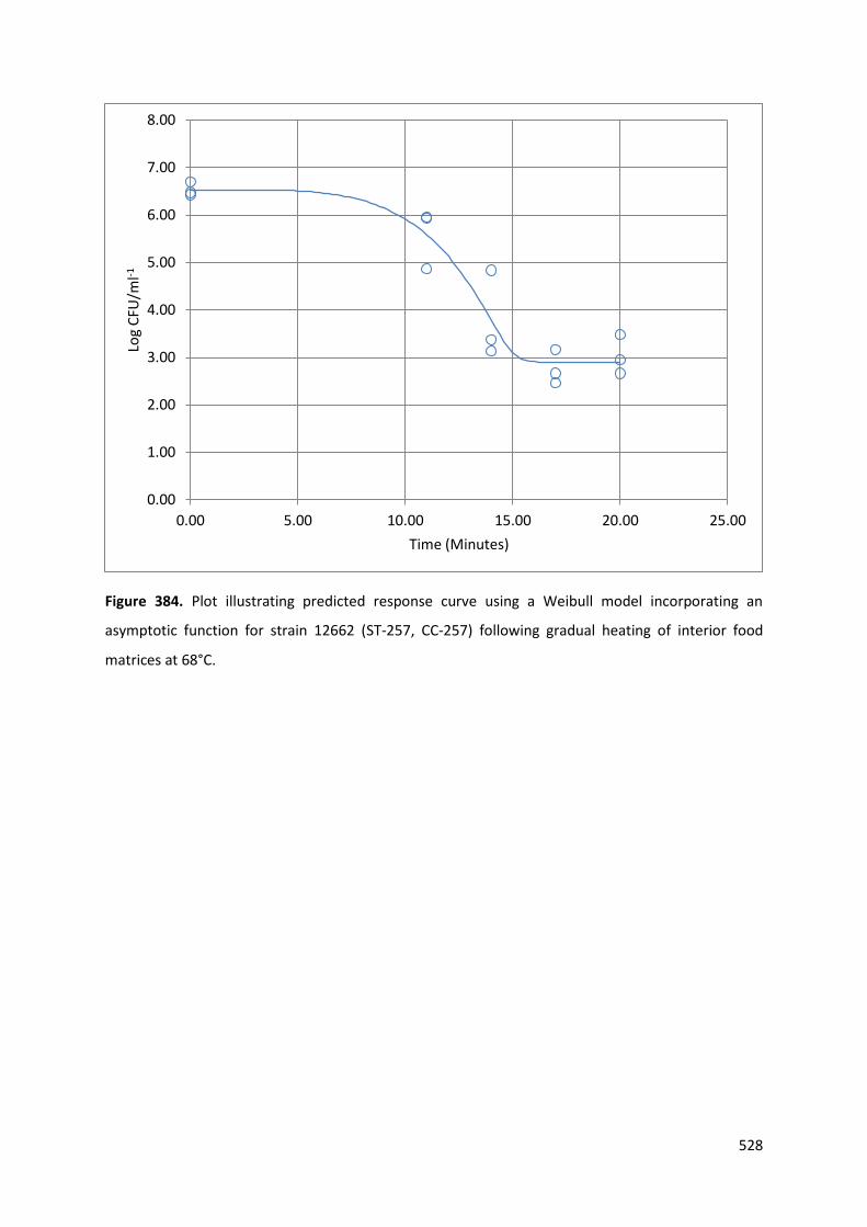
Figure 384. Plot illustrating predicted response curve using a Weibull model incorporating an
asymptotic function for strain 12662 (ST-257, CC-257) following gradual heating of interior food
matrices at 68°C.
0.00
1.00
2.00
3.00
4.00
5.00
6.00
7.00
8.00
0.00 5.00 10.00 15.00 20.00 25.00
Log
CFU
/ml-1
Time (Minutes)

529
Figure 385. Plot illustrating predicted response curve using a Weibull model incorporating an
asymptotic function for strain 13126 (ST-21, CC-21) following gradual heating of interior food
matrices at 68°C.
0.00
1.00
2.00
3.00
4.00
5.00
6.00
7.00
0.00 2.00 4.00 6.00 8.00 10.00 12.00 14.00 16.00 18.00
Log
CFU
/ml-1
Time (Minutes)
530
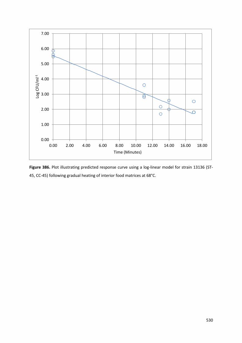
Figure 386. Plot illustrating predicted response curve using a log-linear model for strain 13136 (ST-
45, CC-45) following gradual heating of interior food matrices at 68°C.
0.00
1.00
2.00
3.00
4.00
5.00
6.00
7.00
0.00 2.00 4.00 6.00 8.00 10.00 12.00 14.00 16.00 18.00
Log
CFU
/ml-1
Time (Minutes)
531
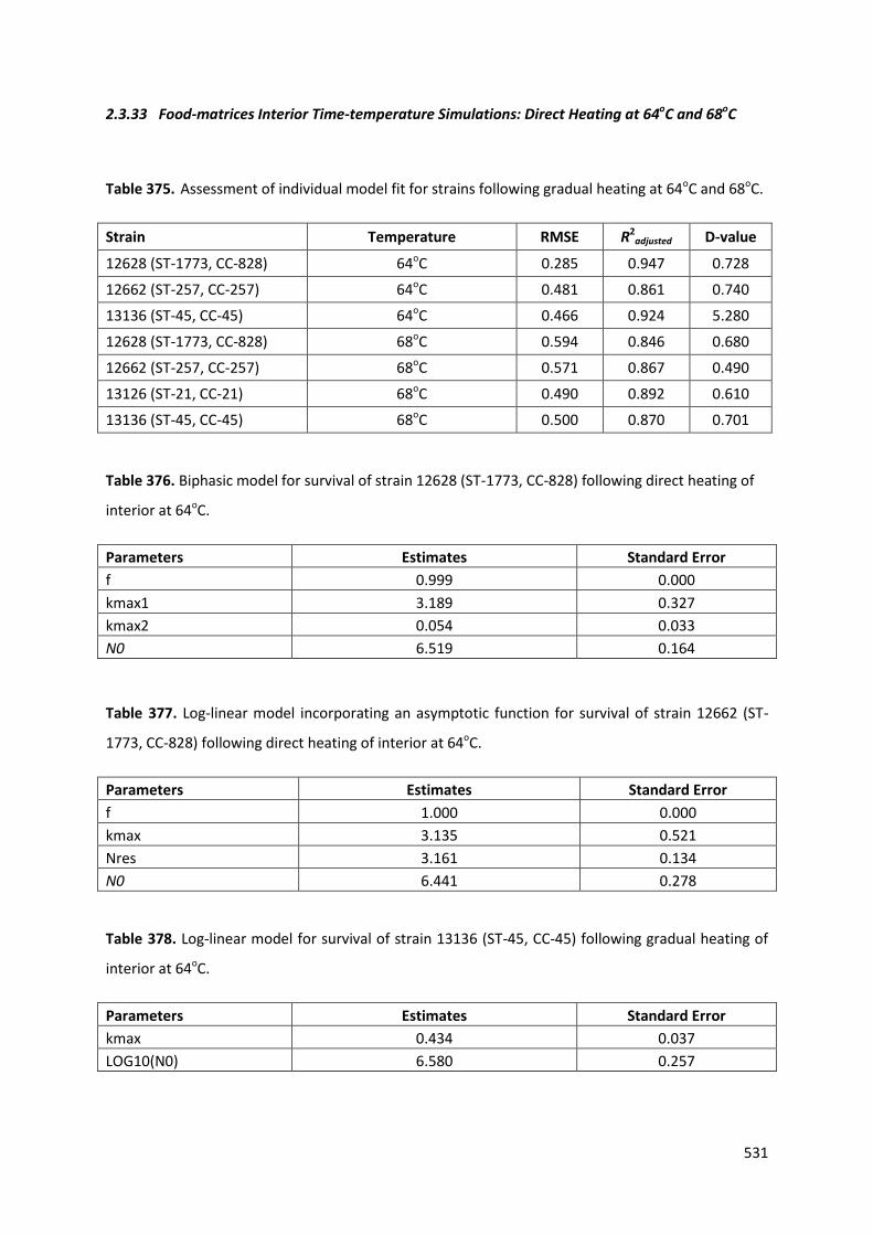
2.3.33 Food-matrices Interior Time-temperature Simulations: Direct Heating at 64oC and 68oC
Table 375. Assessment of individual model fit for strains following gradual heating at 64oC and 68oC.
Strain Temperature RMSE R2adjusted D-value
12628 (ST-1773, CC-828) 64oC 0.285 0.947 0.728
12662 (ST-257, CC-257) 64oC 0.481 0.861 0.740
13136 (ST-45, CC-45) 64oC 0.466 0.924 5.280
12628 (ST-1773, CC-828) 68oC 0.594 0.846 0.680
12662 (ST-257, CC-257) 68oC 0.571 0.867 0.490
13126 (ST-21, CC-21) 68oC 0.490 0.892 0.610
13136 (ST-45, CC-45) 68oC 0.500 0.870 0.701
Table 376. Biphasic model for survival of strain 12628 (ST-1773, CC-828) following direct heating of
interior at 64oC.
Parameters Estimates Standard Error
f 0.999 0.000
kmax1 3.189 0.327
kmax2 0.054 0.033
N0 6.519 0.164
Table 377. Log-linear model incorporating an asymptotic function for survival of strain 12662 (ST-
1773, CC-828) following direct heating of interior at 64oC.
Parameters Estimates Standard Error
f 1.000 0.000
kmax 3.135 0.521
Nres 3.161 0.134
N0 6.441 0.278
Table 378. Log-linear model for survival of strain 13136 (ST-45, CC-45) following gradual heating of
interior at 64oC.
Parameters Estimates Standard Error
kmax 0.434 0.037
LOG10(N0) 6.580 0.257
532
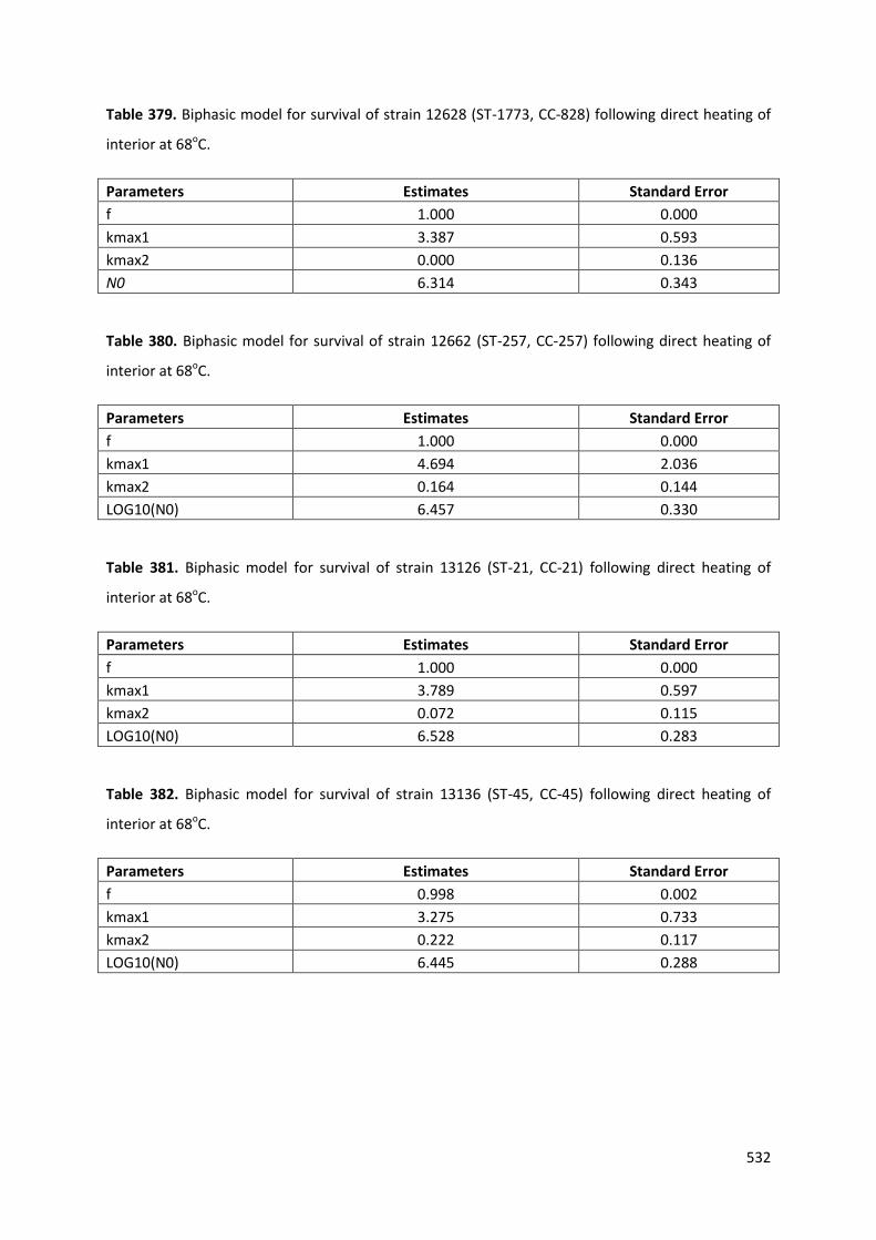
Table 379. Biphasic model for survival of strain 12628 (ST-1773, CC-828) following direct heating of
interior at 68oC.
Parameters Estimates Standard Error
f 1.000 0.000
kmax1 3.387 0.593
kmax2 0.000 0.136
N0 6.314 0.343
Table 380. Biphasic model for survival of strain 12662 (ST-257, CC-257) following direct heating of
interior at 68oC.
Parameters Estimates Standard Error
f 1.000 0.000
kmax1 4.694 2.036
kmax2 0.164 0.144
LOG10(N0) 6.457 0.330
Table 381. Biphasic model for survival of strain 13126 (ST-21, CC-21) following direct heating of
interior at 68oC.
Parameters Estimates Standard Error
f 1.000 0.000
kmax1 3.789 0.597
kmax2 0.072 0.115
LOG10(N0) 6.528 0.283
Table 382. Biphasic model for survival of strain 13136 (ST-45, CC-45) following direct heating of
interior at 68oC.
Parameters Estimates Standard Error
f 0.998 0.002
kmax1 3.275 0.733
kmax2 0.222 0.117
LOG10(N0) 6.445 0.288

533
2.3.34 Food-matrices Interior Time-temperature Simulations: Direct Heating 64oC and 68oC
Predicted Response Curves:
Figure 387. Plot illustrating predicted response curve using a Biphasic model incorporating an
asymptotic function for strain 12628 (ST-1773, CC-828) following extended direct heating of interior
food matrices at 64°C.
0.00
1.00
2.00
3.00
4.00
5.00
6.00
7.00
0.00 5.00 10.00 15.00 20.00
Log
CFU
/ml-1
Time (Minutes)
534
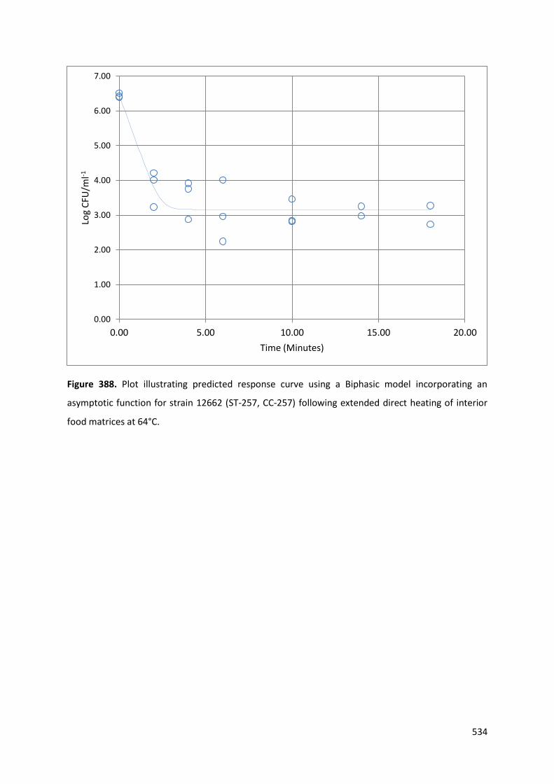
Figure 388. Plot illustrating predicted response curve using a Biphasic model incorporating an
asymptotic function for strain 12662 (ST-257, CC-257) following extended direct heating of interior
food matrices at 64°C.
0.00
1.00
2.00
3.00
4.00
5.00
6.00
7.00
0.00 5.00 10.00 15.00 20.00
Log
CFU
/ml-1
Time (Minutes)
535
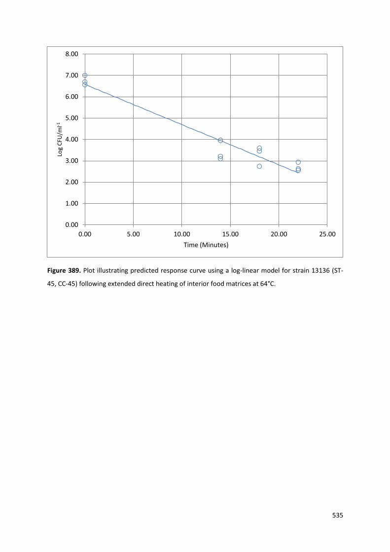
Figure 389. Plot illustrating predicted response curve using a log-linear model for strain 13136 (ST-
45, CC-45) following extended direct heating of interior food matrices at 64°C.
0.00
1.00
2.00
3.00
4.00
5.00
6.00
7.00
8.00
0.00 5.00 10.00 15.00 20.00 25.00
Log
CFU
/ml-1
Time (Minutes)
536
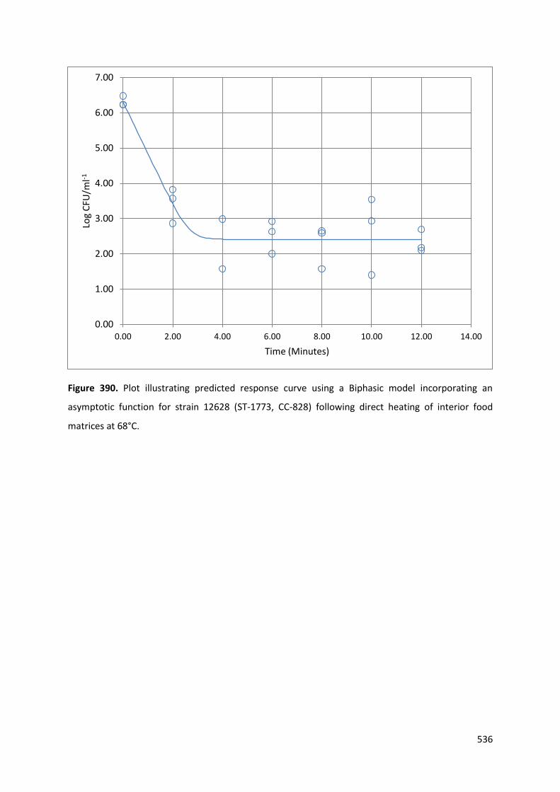
Figure 390. Plot illustrating predicted response curve using a Biphasic model incorporating an
asymptotic function for strain 12628 (ST-1773, CC-828) following direct heating of interior food
matrices at 68°C.
0.00
1.00
2.00
3.00
4.00
5.00
6.00
7.00
0.00 2.00 4.00 6.00 8.00 10.00 12.00 14.00
Log
CFU
/ml-1
Time (Minutes)
537
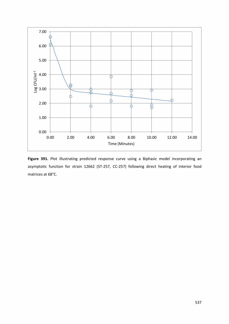
Figure 391. Plot illustrating predicted response curve using a Biphasic model incorporating an
asymptotic function for strain 12662 (ST-257, CC-257) following direct heating of interior food
matrices at 68°C.
0.00
1.00
2.00
3.00
4.00
5.00
6.00
7.00
0.00 2.00 4.00 6.00 8.00 10.00 12.00 14.00
Log
CFU
/ml-1
Time (Minutes)
538
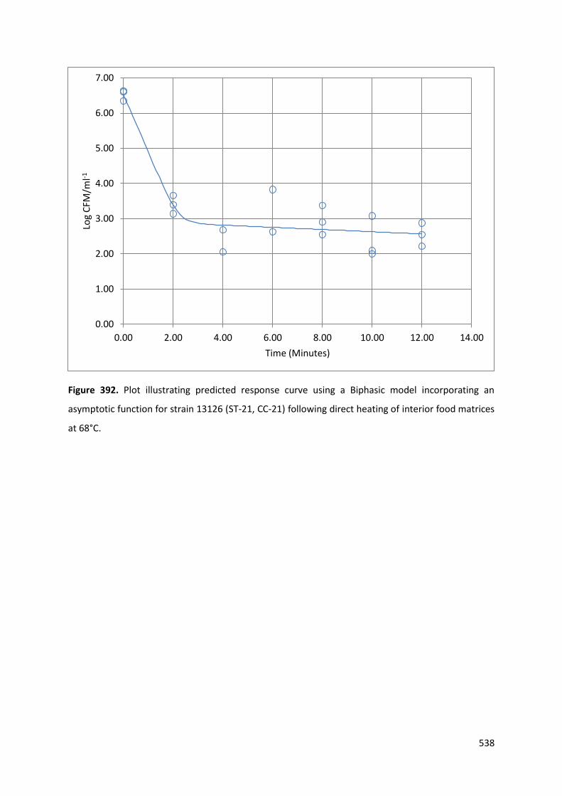
Figure 392. Plot illustrating predicted response curve using a Biphasic model incorporating an
asymptotic function for strain 13126 (ST-21, CC-21) following direct heating of interior food matrices
at 68°C.
0.00
1.00
2.00
3.00
4.00
5.00
6.00
7.00
0.00 2.00 4.00 6.00 8.00 10.00 12.00 14.00
Log
CFM
/ml-1
Time (Minutes)

539
Figure 393. Plot illustrating predicted response curve using a Biphasic model incorporating an
asymptotic function for strain 13136 (ST-45, CC-45) following direct heating of interior food matrices
at 68°C.
0.00
1.00
2.00
3.00
4.00
5.00
6.00
7.00
0.00 2.00 4.00 6.00 8.00 10.00 12.00 14.00
Log
CFU
/ml-1
Time (Minutes)
540
2.4 DISCUSSION
2.4.1 Time-temperature Simulations
The overall fit of models to data varied according to strain and the magnitude of bi-physical stress.
This variation may be due to increased levels of experimental heterogeneity encountered during the
recovery and observation phase of simulation, where the numbers of cells recovered during is more
variable at later sampling points (See Figure 236). In general, the underlying response of strains
differed in accordance with exposure to temperature. For instance, models incorporating a shoulder
effect and asymptote, or models that generated combined concave response curves were fit to data
for simulations undertaken at 56oC.
For simulations undertaken at 60oC, a combination of first-order kinetics models, Weibull
and mixed Weibull distribution models were used to generate predicted response curves. In
comparison to predicted response curves for simulations at 56oC, the survival of each strain was
characterised by a reduced shoulder effect followed by a gradual decline in survival through time. By
contrast, biphasic and log-linear first-order kinetics models were used exclusively to generate
predicted response curves for time-temperature simulations undertaken at 64oC. These models
generated predicted response curves that demonstrate a rapid decrease in survival of an initial
subpopulation followed by either a gradual decrease in survival of an additional subpopulation, or
asymptote effect indicating an ability to resist biophysical stress at higher temperatures. The overall
fit of models generated to describe the survival of strains at 56oC was greater than the fit of models
for simulations undertaken at 60oC and 64oC. Similarly, survival of strains appeared to decline from
simulations undertaken at 60oC in comparison to those at 64oC.
This evaluation is supported by comparing the time to first decimal reduction (D-value) for
each time-temperature simulation. We used a Generalized Least Squares (GLS) approach to assess
differences in the time taken to achieve a one-log reduction in the counts of cells. There was a
significant difference between in D-value between Simulations undertaken at 56oC and those
undertaken at 60oC and 64oC, indicating that initial resistance to bio-physical stress declined
accordance with an increase in temperature.
2.4.2 pH and Time-temperature Simulations
The fit of models to data generated by combined pH and time-temperature simulations data varied
according to strain and the magnitude of the bi-physical and bio-chemical challenge. Comparatively,
overall model fit was greater for predicted response curves generated form combined pH and time-
temperature simulations following exposure to heating at 56oC. Model fit subsequently declined for
541
combined pH and time-temperature simulations undertaken at 60oC and 64oC. The decrease in
model fit may be due to increased experimental heterogeneity and may be particularly relevant for
simulations undertaken at 64oC. There was broad similarity in types of models used to generate
predicted response curves for combined pH and temperature simulations undertaken at 56oC. The
first-order kinetic biphasic model was used to generate predicted response curves for all strains at
pH 4.5. The underlying response of strains at pH 5.5 – pH 8.5 were similar insofar as predicted
response curves were generated using broad class of Weibull models, namely Weibull model,
Weibull model incorporating asymptotic function and the mixed Weibull distribution model. In the
first instance, predicted response curves generated using the biphasic model indicate that
Campylobacter strains are susceptible to bio-chemical stress. In contrast, the class Weibull models,
and the mixed Weibull model in particular, was used to generate single or double concave predicted
response curves for simulations undertaken at pH 5.5 – pH 8.5. This may suggest that initial
subpopulations within strains may exhibit enhanced capacity to resist biochemical stress.
The biphasic and log-linear first-order kinetics models were predominantly used to generate
predicted response curves for survival of strains at pH 4.5 and pH 8.5 following heating at 60oC,
indicating that strains were susceptible to combined and multiplicative effects of increased bio-
physical and bio-chemical stress. By contrast, the mixed Weibull distribution model was used
predominantly used to generate predicted response curves for simulations undertaken between pH
5.5 – pH7.5. However, two exceptions were noted; the Weibull model was used to generated
predicted response curves for strain 13136 (ST-45, CC-45) for simulations undertaken at pH 4.5 and
pH 8.5, whereas the mixed Weibull model was used throughout all combined pH simulations for
strain 13126 (ST-21, C-21).
The classes of models used to generate predictive response curves for combined simulations
undertaken at 64oC varied according to pH and strain. Variants of the Weibull class of models were
used in conjunctions with first-order kinetics models to generate both concave and convex predicted
response curves. Concave response curves were typically generated for simulations at pH 4.5 and pH
8.5, whereas convex response curves were generated for survival of strains at pH 5.5 – pH 7.5. A
general pattern emerged throughout this particular phase of the study whereby variants of the class
of Weibull models were used to generate convex survival curves for simulations at pH 5.5 and pH 6.5
and in some instances, pH 7.5. The presence of a lag, or shoulder effect indicated that these acidic
conditions may be optimal for the survival of Campylobacter. This evaluation was supported when
we examined the time to first decimal reduction for each combined pH and time-temperature
simulation.
542
We used Generalized Least Squares to examine potential differences between estimated D-
values for each combined pH and temperature simulation. In general, results indicate that estimated
D-values, and therefore resistance to stress, decline following combined exposure to acidic stress
and high temperature. Average estimated D-values at 56oC were significantly higher in comparison
to those estimated at 60oC and 64oC. Estimated D-values at 56oC were also significantly higher at pH
5.5 – pH 8.5 when compared to pH 4.5. Significant reductions in estimated D-values were also
observed between each individual pH and time-temperature simulation. For instance, the D-value
estimated at 60oC for pH 5.5 was significantly lower than the corresponding value estimated at 56oC
for pH 5.5. The pattern of significant reductions in estimated D-values was observed for pH 5.5 – pH
8.5 for simulations undertaken at 60oC and for all pH simulations undertaken at 64oC.
However, there was also variation in estimated D-values within each combined pH and time-
temperature simulation. The time to first log reduction in counts of cells is highest at 56oC for pH 5.5
– pH 6.5. There was also marked differences in estimated D-values within each temperature group
where higher values were estimated for pH 5.5 – pH7.5. This finding is indicative of an enhanced
capability to resist acidic stress.
2.4.3.1 Food-matrices Exterior Time-temperature Simulations
For gradual heating simulations undertaken at 56oC strains demonstrated similar survival convex
curves with evidence of a tailing-effect at later observation points. The first-order-kinetics log-linear
model incorporating a shoulder effect, the Weibull model and the mixed Weibull distribution model
were all used to generate concave predicted response curves. In contrast, the Weibull and mixed
Weibull distribution models were used exclusively to generate convex predicted response curves for
gradual heating simulations undertaken at 70oC.
An assessment of goodness-of-fit indices suggests that the fit of models to data from gradual
hating experiments was largely dependent on strain and the temperature used during simulations.
Model fit was generally good for simulations undertaken at 56oC. In comparison, overall fit declined
during gradual heating simulations undertaken at 70oC and may be due to considerable
heterogeneity in observed counts of cells. There was insufficient data to generate models to
examine the effects of pre-chilling of food-matrices prior to heating. The log-linear first order
kinetics model, incorporating an asymptote function, and the mixed Weibull distribution model were
used to generate predicted response curves for direct heating simulations of chilled and un-chilled
meat at 56oC. Predicted response curves for these simulations were primarily concave with
543
elongated tails, indicating that strains were able to persist on tissue surfaces for an extended period
of time. There was no appreciable difference in overall model fit between chilled and un-chilled
simulations.
Models used to generate predicted response curves for remaining direct heating simulations
undertaken at 60oC, 64oC, 68oC and 70oC all demonstrated a similar response to those described at
56oC. Biphasic and log-linear first order kinetics models and the Weibull model incorporating an
asymptotic function were used to generate predicted response curves, whereby individual strains
demonstrated an initial susceptibility to increased temperature followed by a period of enhanced
resistance demonstrated by the tailing effect.
An evaluation of the estimated D-values for direct heating simulations indicates that the
time to first log-reduction in numbers of cells significantly declines as temperature increases. We did
not find a significant difference in the estimated D-value relating to pre-treatment effects of chilled
and un-chilled tissue. The Weibull models and first-order kinetic biphasic and log-linear models used
to generate predicted response curves reflect differences in the resistance of Campylobacter strains
within food-matrices. In general, the Weibull models fit to these data describe convex survival
curves that demonstrate a reduction in survival towards zero. Conversely, first-order kinetic models
data generate predicted response curves with an initial log-linear decrease in survival followed by a
noticeable tailing effect that remains continuous through a significant proportion of the
experimental simulation. For instance, the predictive models used to generate survival curves for
food-matrices simulations undertaken at 56oC demonstrated an elongated tailing effect from 2:00 –
10:00 minutes (see Figure 343) indicating enhanced survival characteristics and resistance to stress
at lower temperature. The magnitude of the resistance to stress for strain 12662 (ST-257, CC-257)
was described by tailing effect at 60oC was 1:00 – 4:00 minutes (see Figure 356). A similar degree of
resistance was observed for simulations undertaken at 64oC where evidence of increased resistance
was observed within strains from 0:50 – 4:00 minutes, for example strain 12662 (ST-257, CC-257)
(Figure 362). For simulations undertaken at 68oC enhanced resistance was observed for strain 12662
(ST-257, CC-257) from 0:50 – 2:50 minutes (Figure 368). However, it is important to remember that
the length of the tailing effects also reflects the respective reduction in the duration of the
observation periods for each increase in temperature. Nevertheless, such inherent resistance to heat
may have implications for food-processing industry and the control and management of
Campylobacter in the food chain.
544
2.4.3.2 Food-matrices Interior Time-temperature Simulations
The survival of Campylobacter within food-matrix interiors following gradual heating simulations
undertaken using at 64oC and 68oC were primarily analysed using Weibull models incorporating an
asymptotic function. The predicted response curves were convex in shape with evidence of tailing
effect in excess of 20 minutes. This indicates Campylobacter can survive for extended periods of time
within food tissue. The underlying survival response curves for strains following direct heating
simulations undertaken using at 64oC and 68oC were evaluated using biphasic and log-linear first-
order kinetics models incorporating an asymptotic function. The predicted response curves were
concave in shape and show an initial and rapid decline in survival before demonstrating an
elongated tailing effect indicative of enhanced survival between 5.00 – 20.00 minutes for direct
heating simulations undertaken at 64oC and between 4.00 – 12.00 minutes for direct heating
simulations undertaken at 68oC. By contrast, the first-order log-linear model was used to describe
the response of strain 13136 (ST-45, CC-45). The predicted response curves generated by this model
infer a linear decline in survival through time. Attempts to generate a predicted response curve for
this strain using other types of models failed. However, this does not imply that the mechanistic
response for this particular combination of strain and time-temperature simulation is purely linear.
In actuality, the log-linear response may be an artefact of insufficient observations between the
initial counts obtained at 0 minutes and the subsequent counts obtained at 11 minutes, rather than
an accurate reflection of the underlying mechanism of the strain in response to heating.
Complications are also faced in the interpretation of the time until first log-reduction. Estimated D-
values for direct heating simulation at 64oC ranged from 0.728 – 5.280. The later value was
estimated for strain 13136. It is likely that this estimate may also be a consequence of the model
used rather than a reflection of the underlying process. On reflection, an increase in the frequency
of observations during this type of experimental simulation would improve model selection and
determining the response of strains to bio-physical and bio-chemical challenge.