Embed Size (px)
Citation preview
1
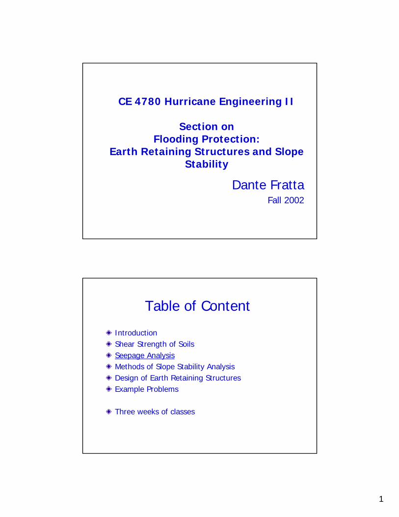
CE 4780 Hurricane Engineering II
Section onFlooding Protection:
Earth Retaining Structures and Slope Stability
Dante FrattaFall 2002
Table of Content
IntroductionShear Strength of SoilsSeepage Analysis Methods of Slope Stability Analysis Design of Earth Retaining Structures Example Problems
Three weeks of classes
2
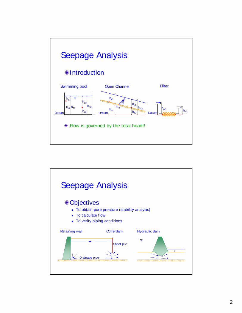
Seepage Analysis
Introduction
Flow is governed by the total head!!
Swimming pool
Datum
hz1
hp1
hT1
hp2
hz2
hT2
Datumhz1
hp1
hp2
hz2
hT2hT1
Open Channel Filter
Datumhp2
hp2
Seepage Analysis
ObjectivesTo obtain pore pressure (stability analysis)To calculate flowTo verify piping conditions
Retaining wall Cofferdam
Sheet pile
Drainage pipe
Hydraulic dam
3
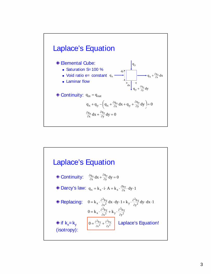
Laplace’s Equation
Elemental Cube:Saturation S=100 %Void ratio e= constantLaminar flow
Continuity:
0dyqdxqqq yq
yxq
xyxyx =⎟
⎠⎞⎜
⎝⎛ +++−+ ∂
∂∂∂
0dydx yq
xq yx =+ ∂
∂∂∂
outin qq =
xq dxq xq
xx
∂∂+
dyq yq
yy
∂∂
+
yq
dx
dy
Laplace’s Equation
Continuity:
Darcy’s law:
Replacing:
if kx=ky Laplace’s Equation!(isotropy):
0dydx yq
xq yx =+ ∂
∂∂∂
1dykAikq xh
xxxT ⋅⋅⋅=⋅⋅= ∂
∂
1dxdyk1dydxk0 2T
2
2T
2
yh
yxh
x ⋅⋅⋅+⋅⋅⋅=∂
∂
∂
∂
2T
2
2T
2
yh
yxh
x kk0∂
∂
∂
∂ ⋅+⋅=
2T
2
2T
2
yh
xh0
∂
∂
∂
∂ +=

4
Laplace’s Equation
Typical cases1 Dimensional:
linear variation!!
2-Dimensional:
3-Dimensional:
2T
2
xh0
∂
∂=
ittancons xhT == ∂∂
xbahT ⋅+=
2T
2
2T
2
yh
xh0
∂
∂
∂
∂ +=
2T
2
2T
2
2T
2
zh
yh
xh0
∂
∂
∂
∂
∂
∂ ++=
Laplace’s Equation Solutions
Exact solutions (for simple B.C.’s) Physical models (scaling problems)Graphical solutions: flow netsAnalogies: heat flow and electrical flowNumerical solutions: finite differencesApproximate solutions: method of fragments
5
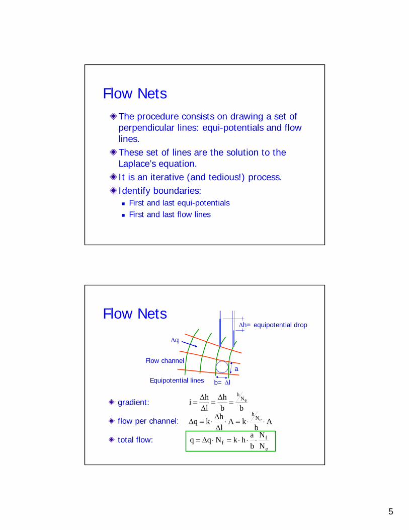
Flow NetsThe procedure consists on drawing a set of perpendicular lines: equi-potentials and flow lines.These set of lines are the solution to the Laplace’s equation.It is an iterative (and tedious!) process.Identify boundaries:
First and last equi-potentialsFirst and last flow lines
Flow Nets
gradient:
flow per channel:
total flow:
Flow channel
Equipotential lines b= ∆l
a
∆q
∆h= equipotential drop
bbh
lhi eN
h=∆=
∆∆=
Ab
kAlhkq eN
h⋅⋅=⋅
∆∆⋅=∆
e
ff N
NbahkNqq ⋅⋅⋅=⋅∆=
6
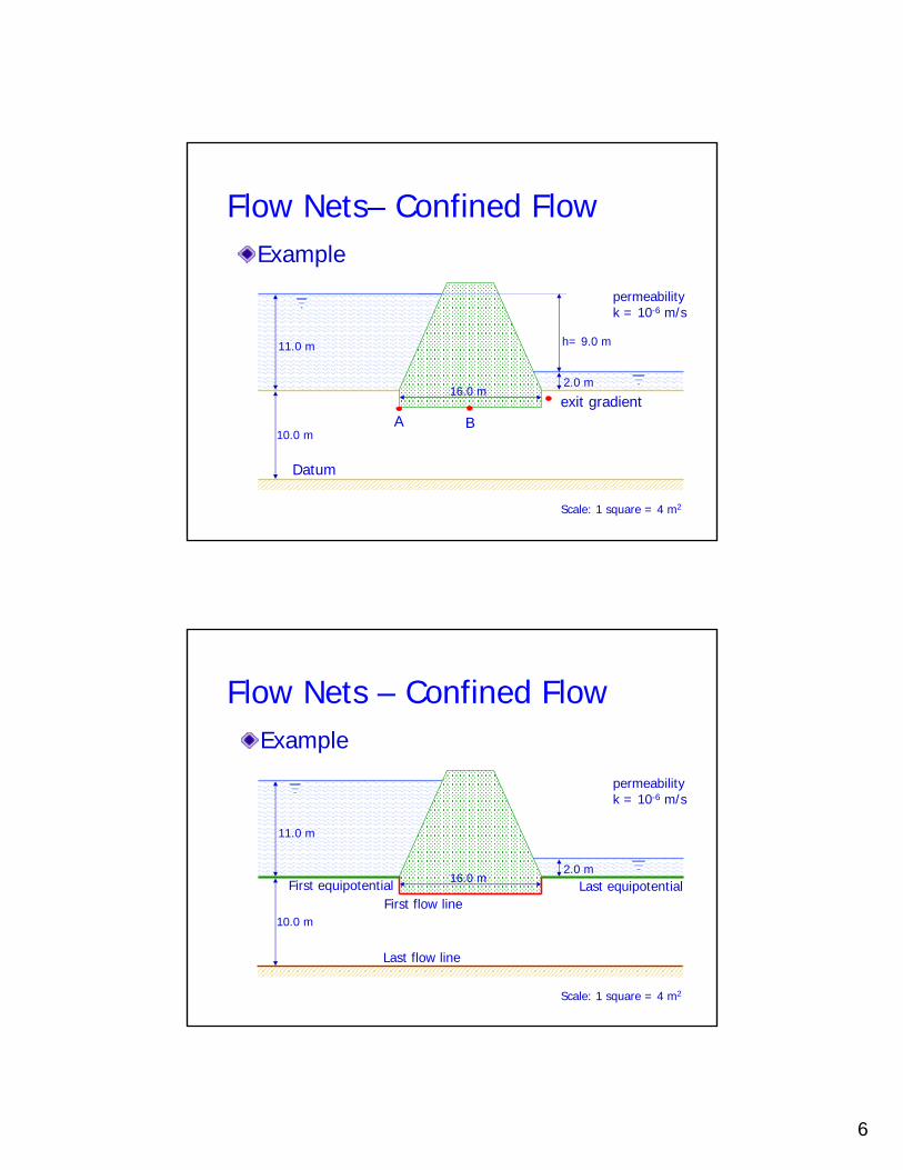
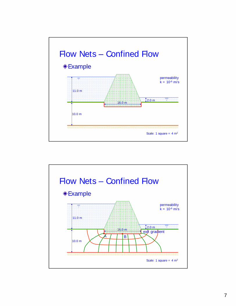
Flow Nets– Confined FlowExample
Scale: 1 square = 4 m2
A B
11.0 m
10.0 m
2.0 m16.0 m
permeabilityk = 10-6 m/s
h= 9.0 m
exit gradient
Datum
Flow Nets – Confined FlowExample
11.0 m
10.0 m
2.0 m16.0 m
Scale: 1 square = 4 m2
permeabilityk = 10-6 m/s
Last flow line
First flow lineFirst equipotential Last equipotential
7
Flow Nets – Confined FlowExample
11.0 m
10.0 m
2.0 m16.0 m
Scale: 1 square = 4 m2
permeabilityk = 10-6 m/s
11.0 m
Flow Nets – Confined FlowExample
A B10.0 m
16.0 m
Scale: 1 square = 4 m2
permeabilityk = 10-6 m/s
2.0 mexit gradient
8
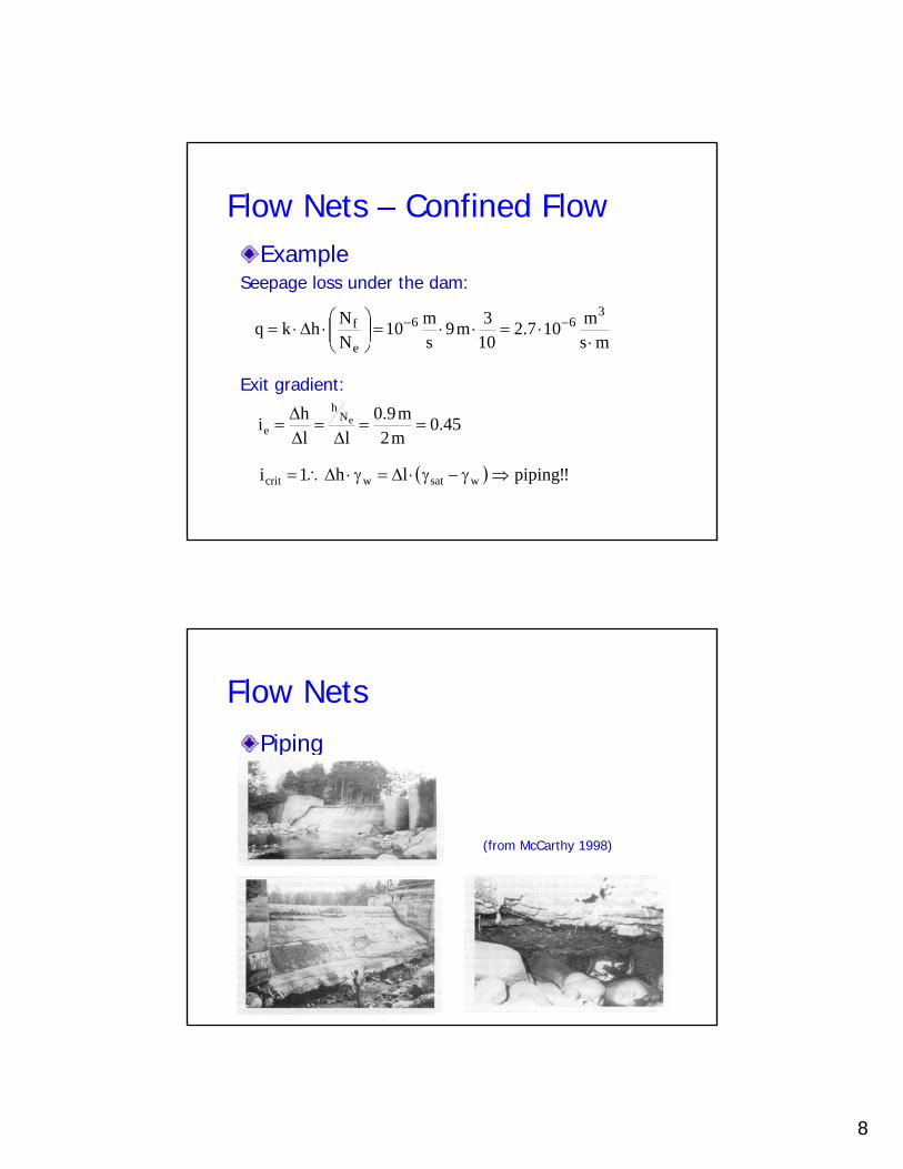
Flow Nets – Confined FlowExample
Seepage loss under the dam:
Exit gradient:
msm107.2
103m9
sm10
NNhkq
366
e
f⋅
⋅=⋅⋅=⎟⎟⎠
⎞⎜⎜⎝
⎛⋅∆⋅= −−
45.0m2m9.0
llhi eN
h
e ==∆
=∆∆
=
( ) !!pipinglh1i wsatwcrit ⇒γ−γ⋅∆=γ⋅∆∴=
Flow NetsPiping
(from McCarthy 1998)
9
Flow NetsExample
Total head at points A and B:
Pressure head at points A and B:
kPa121m1.12m8m1.20hhh zATAPA ⇒≈=−=−=
m1.20101m9m21
NNhhh
f
AToTA =⋅−=⋅−=
m5.16105m9m21
NNhhh
f
BToTB =⋅−=⋅−=
kPa85m5.8m8m5.16hhh zBTBPB ⇒≈=−=−=
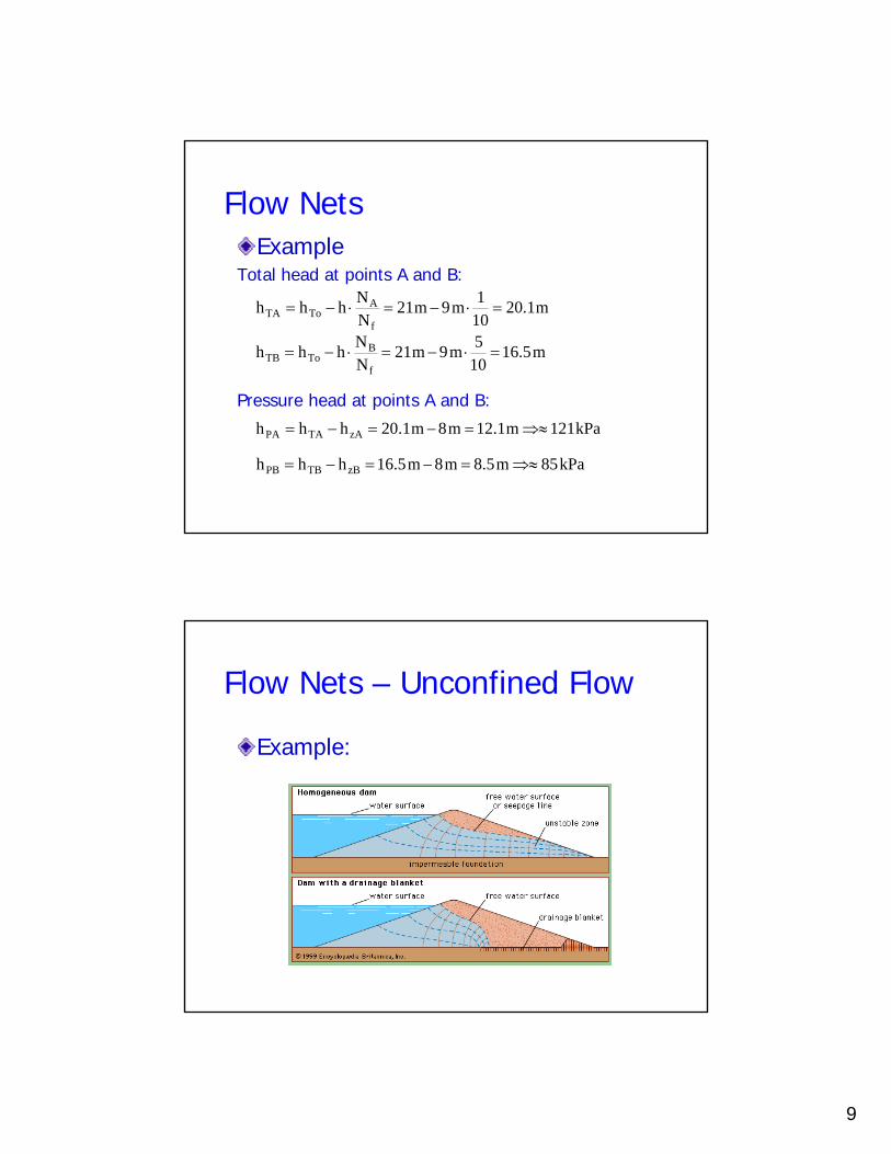
Flow Nets – Unconfined Flow
Example:
10
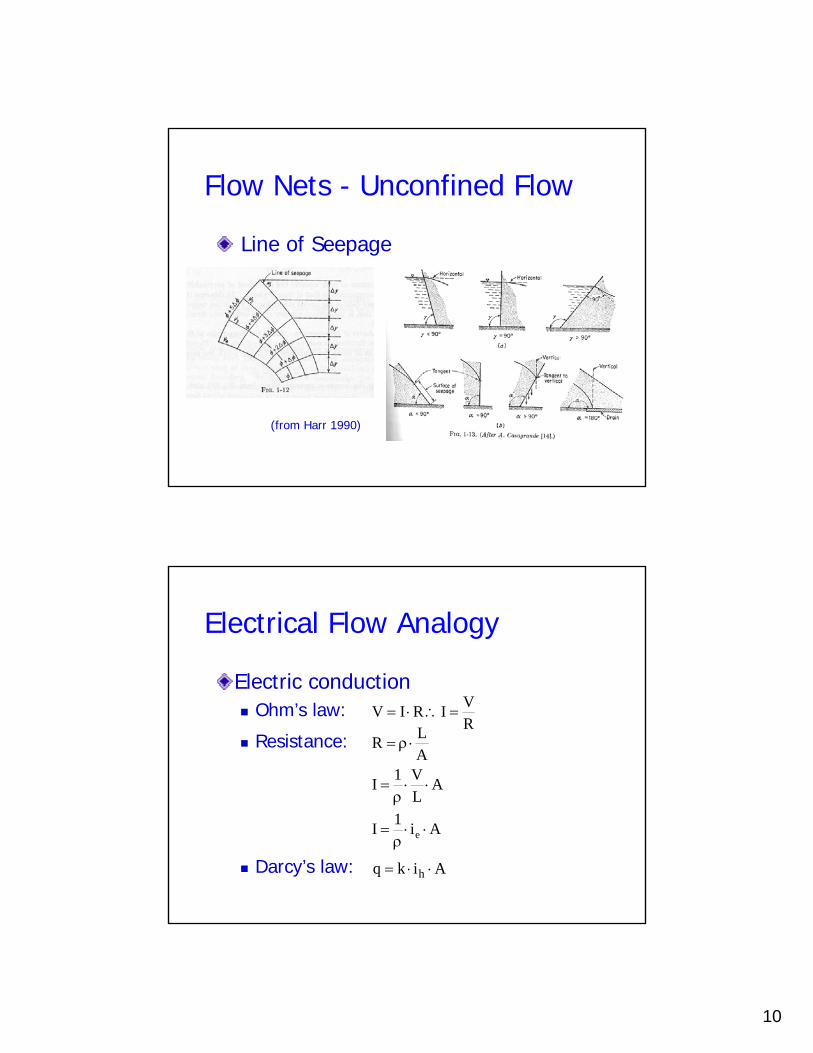
Flow Nets - Unconfined Flow
Line of Seepage
(from Harr 1990)
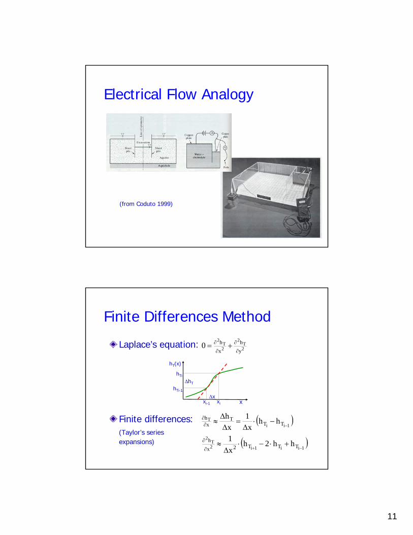
Electrical Flow Analogy
Electric conductionOhm’s law:
Resistance:
Darcy’s law:
RVIRIV =∴⋅=
ALR ⋅ρ=
ALV1I ⋅⋅
ρ=
Aikq h ⋅⋅=
Ai1I e ⋅⋅ρ
=
11
Electrical Flow Analogy
(from Coduto 1999)
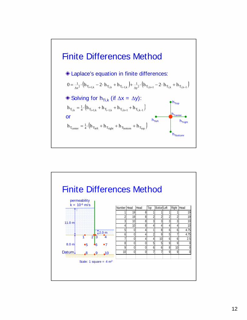
Finite Differences Method
Laplace’s equation:
Finite differences:(Taylor’s series expansions)
2T
2
2T
2
yh
xh0
∂
∂
∂
∂ +=
( )1ii
TTT
Tx
h hhx
1x
h−
−⋅∆
=∆∆≈∂
∂
x
hT(x)
∆x
∆hT
xi-1 xi
hTi-1
hTi
( )1ii1i2
T2
TTT2xh hh2h
x1
−++⋅−⋅
∆≈
∂
∂
12
Finite Differences Method
Laplace’s equation in finite differences:
Solving for hTi,k (if ∆x = ∆y):
or
( )1k,i1k,ik,1ik,1ik,i TTTT4
1T hhhhh
−+−++++⋅=
( )topbottomrightleftcenter TTTT4
1T hhhhh +++⋅=
( ) ( )1k,ik,i1k,i2k,1ik,ik,1i2 TTTy
1TTTx
1 hh2hhh2h0−+−+
+⋅−⋅++⋅−⋅=∆∆
hTcenter
hTbottomr
hTtop
hTleft hTright
Finite Differences Method
11.0 m
8.0 m
2.0 m
Scale: 1 square = 4 m2
permeabilityk = 10-6 m/s
Datum
1 2 3
5
8
6
4
10
7
9
Number Head Head Top BottomLeft Right Head1 19 8 1 1 1 1 192 19 8 2 2 2 2 193 10 8 3 3 3 3 104 10 8 4 4 4 4 105 0 4 1 8 6 6 4.756 0 4 2 9 5 7 4.757 0 4 4 10 6 6 2.58 0 0 5 5 9 9 09 0 0 6 6 8 10 0
10 0 0 7 7 9 9 0

13
Finite Differences MethodExample (solution by Wes Sherrod)
0 500 1000 150010-15
10-10
10-5
100Iteration balance
iteration [ ]
sum
of t
otal
hea
d [m
]
0 10 20 30
-5
0
5
10
15
Total head distribution
x-coordinate [m]
y-co
ordi
nate
[m]
0 10 20 30
-5
0
5
10
15
Elevation head distribution
x-coordinate [m]
y-co
ordi
nate
[m]
0 10 20 30
-5
0
5
10
15
Pressure head distribution
x-coordinate [m]
y-co
ordi
nate
[m]
Finite Differences MethodExample (solution by Wes Sherrod - GTREP)
0 5 10 15 20 25 30 35
0
5
10
15
20
Total head distribution
x-coordinate [m]
y-co
ordi
nate
[m] 11.0 m
2.0 m

14
Method of FragmentsThe fundamental assumption in the method of fragments is that the problem can be divided in segments with flow characterized by vertical equipotential lines (Harr 1990).
(after Holtz and Kovacks 1981)
Fragment 1 Fragment 2 Fragment 3
Method of FragmentsThe flow through a fragment m is computed as (Harr 1990)
Where k is the hydraulic conductivity, ∆htm is the total head drop in segment m, and Φm is the dimensionless form factor
m
tmhkqΦ∆⋅=
15
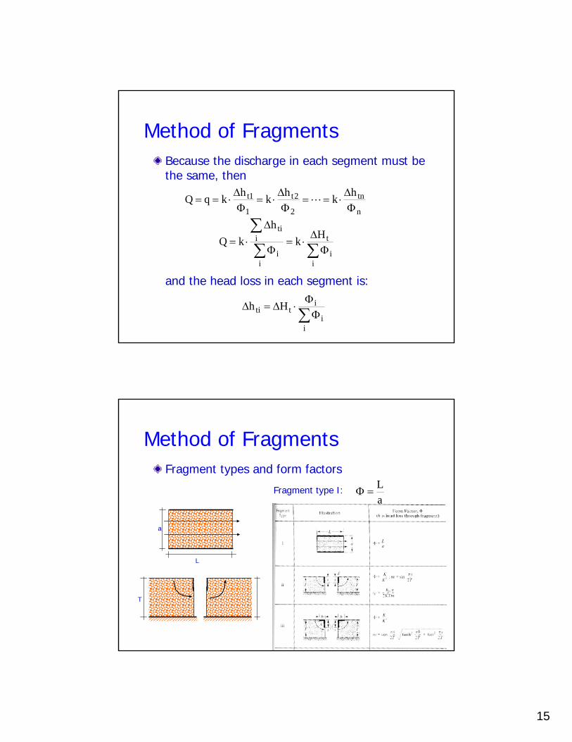
Method of FragmentsBecause the discharge in each segment must be the same, then
and the head loss in each segment is:
n
tn
2
2t
1
1t hkhkhkqQΦ∆⋅==
Φ∆⋅=
Φ∆⋅== L
∑∑∑
Φ∆
⋅=Φ
∆⋅=
ii
t
ii
iti Hk
hkQ
∑ΦΦ
⋅∆=∆
ii
itti Hh
Method of FragmentsFragment types and form factors
a
L
aL
=ΦFragment type I:
T
16
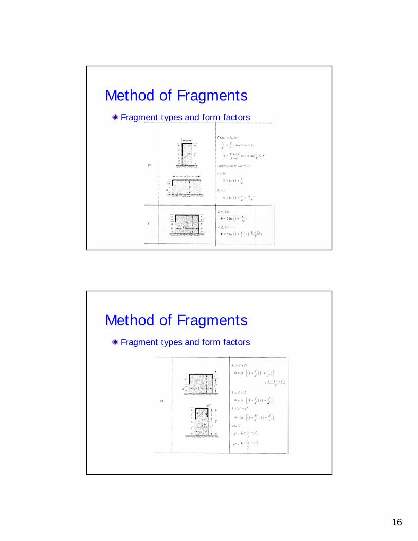
Method of FragmentsFragment types and form factors
Method of FragmentsFragment types and form factors
17
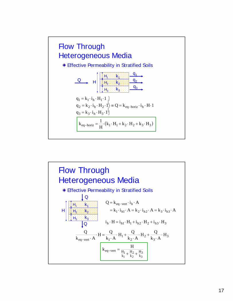
Flow Through Heterogeneous Media
Effective Permeability in Stratified Soils
Qq1
q2
q3
k1
k2
k3
1HikQ1Hikq1Hikq
1Hikq
hhorizeq
3h33
2h22
1h11
⋅⋅⋅=≡⎪⎭
⎪⎬
⎫
⋅⋅⋅=⋅⋅⋅=⋅⋅⋅=
−
H1
H2
H3
H
( )332211horizeq HkHkHkH1k ⋅+⋅+⋅⋅=−
Flow Through Heterogeneous Media
Effective Permeability in Stratified Soils
33h22h11hh HiHiHiHi ⋅+⋅+⋅=⋅Q
k1
k2
k3
H1
H2
H3
H
Q
AikAikAik
AikQ
3h32h21h1
hverteq
⋅⋅=⋅⋅=⋅⋅=
⋅⋅= −
33
22
11verteq
HAk
QHAk
QHAk
QHAk
Q⋅
⋅+⋅
⋅+⋅
⋅=⋅
⋅−
33
22
11
kH
kH
kHverteq
Hk++
=−

18
Flow Through Heterogeneous Media
Effective Permeability in Stratified Soils
33h22h11hh HiHiHiHi ⋅+⋅+⋅=⋅Q
k1
k2
k3
H1
H2
H3
H
Q
AikAikAik
AikQ
3h32h21h1
hverteq
⋅⋅=⋅⋅=⋅⋅=
⋅⋅= −
3AkQ
2AkQ
1AkQ
AkQ HHHH
321verteq⋅+⋅+⋅=⋅ ⋅⋅⋅⋅−
33
22
11
kH
kH
kHverteq
Hk++
=−
Flow Through Heterogeneous Media
Zones of different hydraulic conductivities
( ) ( )1blhk1b
lhkq 2
221
11 ⋅⋅
∆⋅=⋅⋅
∆⋅=∆
1
1
2
2
2
1bl
lb
kk
⋅=
(Das 1983)

19
Flow Through Heterogeneous Media
Zones of different hydraulic conductivities
( ) ( )( ) ( )( ) ( )( ) ( )222
111
222
111
sinACcosACbsinACcosACbcosABsinABl
cosABsinABl
α⋅=θ⋅=α⋅=θ⋅=α⋅=θ⋅=α⋅=θ⋅=
then( )( )
( )( ) ( )
( )111
1
1
1
1
1 tantan
1cossin
sincos
lb
α=θ
=αα
=θθ
=
( )( )
( )( ) ( )
( )222
2
2
2
2
2 tantan
1cossin
sincos
lb
α=θ
=αα
=θθ
=
Flow Through Heterogeneous Media
Zones of different hydraulic conductivities
( )( )
( )( )1
2
2
1
2
1tantan
tantan
kk
αα
=θθ
=
Examples:
(Das 1983)
20
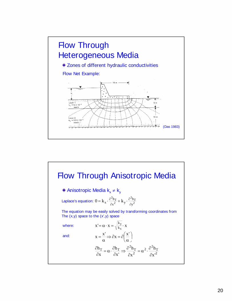
Flow Through Heterogeneous Media
Zones of different hydraulic conductivities
Flow Net Example:
(Das 1983)
Flow Through Anisotropic Media
Anisotropic Media kx ≠ ky
Laplace’s equation: 2T
2
2T
2
yh
yxh
x kk0∂
∂
∂
∂ ⋅+⋅=
where: xx'xxy
kk⋅=⋅α=
The equation may be easily solved by transforming coordinates fromThe (x,y) space to the (x’,y) space
and: ⎟⎠⎞
⎜⎝⎛α
∂=∂⇒α
='xx'xx
2T
22
2T
2TT
'xh
xh
'xh
xh
∂∂⋅α=
∂∂
⇒∂∂⋅α=
∂∂

21
Anisotropic Media kx ≠ ky
Replacing into Laplace’s equation:
2T
2
2T
2
xy
2T
2
2T
2
yh
y'xh
kk
x
yh
y'xh2
x
kk
kk0
∂
∂
∂
∂
∂
∂
∂
∂
⋅+⋅⎟⎠⎞⎜
⎝⎛⋅=
⋅+⋅α⋅=
And that is: 2T
2
2T
2
yh
'xh0
∂
∂
∂
∂ +=
The problem may then be solved using flow nets by redrawing the cross-section using x’=x⋅√(ky/kx)…
Flow Through Anisotropic Media
Flow Through Anisotropic Media
Anisotropic Media kx ≠ ky
The flow in an anisotropic media: y
hyy
heq
TT kxkxQ ∂∂
∂∂ ⋅⋅=⋅⋅⋅α=
yxeq kkk ⋅=
yeqy
yyeq kk
kk
kk =⋅⇒=⋅α
Transformed permeability:
Q
x
y ky
Q
α⋅x
y ky

22
Coupled FlowCoupled Phenomena
It is justify by: Le Chaterlier’s Principle & Energy Conservation
Example: Electrosmosis
(Das 1983)
Seepage Control - Filters
Seepage: Cut-off wallsImpervious blankets
Erosion and piping: FiltersRequirements
Piping: D15(filter) =< 5 D85 (soil)Permeability: D15(filter) >= 5 D15 (soil)Uniformity: D50(filter) =< 25 D50 (soil)

23
BibliographyCoduto, D. (1999). Geotechnical Engineering. Principles and Practice. Prentice-Hall. Craig, R. F. (1987). Soil Mechanics. Chapman & Hall.Das, B. (1983). Advanced Soil Mechanics.Encyclopædia Britannica (2000). http://www.encyclopedia.com.Frost, J. D. (1996). Earth Retaining Structures Class Notes. Georgia Institute of Technology. Atlanta, Georgia.Harr, M. (1990) Groundwater and Seepage. Dover PublicationsHoltz, R. and Kovaks, D. (1981). An Introduction to Geotechnical Engineering. Prentice-Hall. Matyas, E. (1994). Earth Retaining Structures Class Notes. University of Waterloo. Waterloo, Canada. McCarthy, D. (1998). Essential of Soil Mechanics and Foundation. Prentice-Hall.Powrie, W. (1997). Soils Mechanics. E&FN SPON.Santamarina, J. C. (1999). Geotechnical Engineering I Class Notes. Georgia Institute of Technology. Atlanta, Georgia.