Embed Size (px)
Citation preview

Chapter Based Lecture Notes
CO 353: Computational Discrete Optimization
Prepared by: Calvin KENTwww.student.math.uwaterloo.ca/~c2kent/
Instructor: Ricardo FUKASAWATerm: Winter 2020
Last revised: 7 March 2020 Page
Table of Contents i
Preface and Notation iii
1 Algorithm Runtime, Big-O Notn. and Graph Theory 1
1.1 Algorithm Running Time . . . . . . . . . . . . . . . . . . . . . . . . . . . . . . . 1Finding an Estimate of Runtime (big-O Notation) . . . . . . . . . . . . . . . . . . . 1Arithmetic Model . . . . . . . . . . . . . . . . . . . . . . . . . . . . . . . . . . . . . . 2
1.2 Graph Theory . . . . . . . . . . . . . . . . . . . . . . . . . . . . . . . . . . . . . . . 3Minimum Spanning Tree (MST) . . . . . . . . . . . . . . . . . . . . . . . . . . . . . 6
MST Problem . . . . . . . . . . . . . . . . . . . . . . . . . . . . . . . . . . . . 6
2 Greedy Algorithms and Matroids 11
2.1 Kruskal’s Algorithm . . . . . . . . . . . . . . . . . . . . . . . . . . . . . . . . . . . 11Implementation of Kruskal’s Algorithm . . . . . . . . . . . . . . . . . . . . . . . . . . 12Validating Kruskal’s Algorithm with Linear Programming . . . . . . . . . . . . . . . 13
2.2 Greedy Algorithms . . . . . . . . . . . . . . . . . . . . . . . . . . . . . . . . . . . . 17Maximum Cost Forest Problem . . . . . . . . . . . . . . . . . . . . . . . . . . . . . . 18
Using Kruskal’s Algorithm for Max. Cost Forest . . . . . . . . . . . . . . . . . . . 18Properties of Forests . . . . . . . . . . . . . . . . . . . . . . . . . . . . . . . . . 19
2.3 Matroids . . . . . . . . . . . . . . . . . . . . . . . . . . . . . . . . . . . . . . . . . . 20Independence Systems and Independent Sets . . . . . . . . . . . . . . . . . . . . . . 20Solving Maximum Weighted Independent Set Problem with Greedy Algorithm . . . . 22Matroid Constructions . . . . . . . . . . . . . . . . . . . . . . . . . . . . . . . . . . . 24
3 Dynamic Programming 29
3.1 Weighted Interval Scheduling . . . . . . . . . . . . . . . . . . . . . . . . . . . . . 29Dynamic Programming Overview . . . . . . . . . . . . . . . . . . . . . . . . . . . . . 32Knapsack Problem . . . . . . . . . . . . . . . . . . . . . . . . . . . . . . . . . . . . . 32Shortest Paths . . . . . . . . . . . . . . . . . . . . . . . . . . . . . . . . . . . . . . . 33
Dijkstra’s Algorithm . . . . . . . . . . . . . . . . . . . . . . . . . . . . . . . . . 34Shortest Paths Without Negative Cycles . . . . . . . . . . . . . . . . . . . . . . . 36
4 Complexity Theory 39
4.1 Polytime Reductions . . . . . . . . . . . . . . . . . . . . . . . . . . . . . . . . . . 39
i
ii
Examples of Polytime Reducible Problems . . . . . . . . . . . . . . . . . . . . . . . . 39Classes of P and NP . . . . . . . . . . . . . . . . . . . . . . . . . . . . . . . . . . . . 45NP-Completeness . . . . . . . . . . . . . . . . . . . . . . . . . . . . . . . . . . . . . . 46NP-Hardness . . . . . . . . . . . . . . . . . . . . . . . . . . . . . . . . . . . . . . . . 47
Index 47
Preface and Notation
This PDF document includes lecture notes for CO 353 - Computational Discrete Optimizationtaught by Ricardo FUKASAWA in Winter 2020.
For any questions contact me at c2kent(at)uwaterloo(dot)ca.Thanks to Taric Ali and Caleb Nicholas Chappell for providing me the notes for the classes I missed.
Notation
Course outline and relevant info: https://piazza.com/uwaterloo.ca/winter2020/co353
Throughout the course and the notes, unless otherwise is explicitly stated, we adopt the follow-ing conventions and notations.
• Algorithms use the same counter as definitions, theorems, examples etc.
• The university logo is used as a place holder.
Calvin KENT
iii
Chapter 1. Algorithm Runtime, Big-O Notn. and Graph Theory 1
Chapter 1 – Algorithm Runtime, Big-O Notn. and GraphTheory
1.1 Algorithm Running Time
We want to formally see which algorithms are more efficient. To compare algorithms, we measureruntime (number of steps) of an algorithm as a function of the input.
Definition 1.1.1: Size of an input is the number of bits needed to encode it. /
Example 1.1.2: Consider a list of positive integers a1, a2, . . . , an where ai ∈ Z+ for i = 1, . . . , n.For each integer ai, we need dlog aie bits. Hence, the number of bits needed to represent the inputis∑n
i=1dlog aie. /
1.1.1 Finding an Estimate of Runtime (big-O Notation)
Definition 1.1.3: Let f, g : Z+ → R+ be two functions. We say f is O(g), read as big-O of g, if∃ c ∈ R+ and ∃ n′ ∈ Z+ such that ∀ n ≥ n′ we have f(n) ≤ cg(n). /
Example 1.1.4: Let f(n) = 5 log n and show f(n) is O(n). Let g(n) = n and c = 5. Since for alln ≥ 1 we have log n < n. Then, for n ≥ 1 we have f(n) ≤ 5n. So, f(n) ≤ cg(n). Hence, f(n) isO(g) = O(n). /
Example 1.1.5: Let f(n) = 2n2 + 3n log n and show f(n) is O(n2).We have
f(n) = 2n2 + 3n log n ≤ 5n2,
so it follows that f(n) is O(n2). /
Remark 1.1.6: We make the following remarks for polynomials, logarithms and exponentials.
1d∑
k=0
αknk where αk ∈ R and αd > 0 is O(nd). i.e. polynomials are dominated by their leading
term.
2 logb n where b > 1 and c > 0 is O(nc). i.e. logarithms are dominated by polynomials.
a We recall logarithm rules. We have
logb n =log2 n
log2 b=
(1
log2 b
)log2 n.
So big-O does not get affected by log base. In this course we will use log base 2.
3 nc where b > 1 and c > 0 is O(bn). i.e. polynomials are dominated by exponentials. /
Theorem 1.1.7 (Properties of big-O): Let f, g, h, fi, gi : Z+ → R+ be functions for i = 1, . . . ,m.
1 (Transitivity) If f is O(g) and g is O(h) then f is O(h).
Winter 2020 CO 353 1
Chapter 1. Algorithm Runtime, Big-O Notn. and Graph Theory 2
2 If f, g are O(h) then f + g is O(h).
3 If fi is O(gi) for all i = 1, . . . ,m, then f1 · · · fm is O(g1 · · · gm).
Proof: Exercise. /
Definition 1.1.8: Let f, g : Z+ → R+ be two functions. We say f is Ω(g), read as omega of g(or big-omega of g), if ∃ c ∈ R+ and ∃ n′ ∈ Z+ such that ∀ n ≥ n′, we have f(n) ≥ cg(n).
We say f is Θ(g), read as theta of g (or big-theta of g), if f is O(g) and Ω(g). /
Definition 1.1.9: Operations involving a combination of basic arithmetic (+,−,×,÷) operations,comparisons, if-then-else statements and assignments are called basic operations (sometimes re-ferred as elementary operations).
We say an algorithm has runtime p(n) if the algorithm executes p(n) basic operations on inputsof size n. /
1.1.2 Arithmetic Model
Definition 1.1.10: Consider an algorithm with runtime of p(n). If p(n) isO(g) for some polynomialfunction g(n), then the algorithm said to be in polynomial time . In short, we refer these algorithmsas polytime algorithms and they are also called efficient algorithms. /
Remark 1.1.11: In practice, big-O does not always shows which algorithms are more efficient.
1 Big-O analysis provides an upper bound (i.e. worst case) for an algorithm. For example, inlinear programming simplex algorithm is widely used and considered to be efficient but it hasbig-O of exponential.
2 Big-O hides constants. Depending on the input, an exponential algorithm can be more efficientthat an polytime algorithm. For example, for small numbers for n, the exponential algorithmwith runtime 1.0001n is more efficient than the polytime algorithm with runtime 1020n100. /
We recall Example 1.1.2. Given integers a1, . . . , an ∈ Z+, we want to find an efficient algorithmthat sorts these integers. We have the size of input as
∑ni=1dlog2 aie. It becomes tricky to express
runtime as a function of input size. So we pick some parameters that are at most a polynomial ofactual input size.
If the input size is k, then we want to pick parameters n so that we have n is poly(k).
Example 1.1.12: We refer back to our example. We have
• n as the number of integers,
• amax as the largest integer (does not have to be unique unless specified).
So, if we find algorithms in time poly(n, log amax), then time is polynomial in input size. Now,consider the following example:
Given distinct integers a1, . . . , an ∈ Z+ find the largest integer. We know the algorithm is polytime
Winter 2020 CO 353 2
Chapter 1. Algorithm Runtime, Big-O Notn. and Graph Theory 3
in terms of n, log amax. Consider the following algorithm.
Algorithm 1.1.13: Finding largest integer
Input : a1, . . . , an (distinct)Output: amax (such that amax ≥ ai for i = 1, . . . , n)
1 largest ← a1
2 for i = 1, . . . , n do3 if ai >largest then O(1)
O(n)
4 largest ← ai O(1)
5 return largest
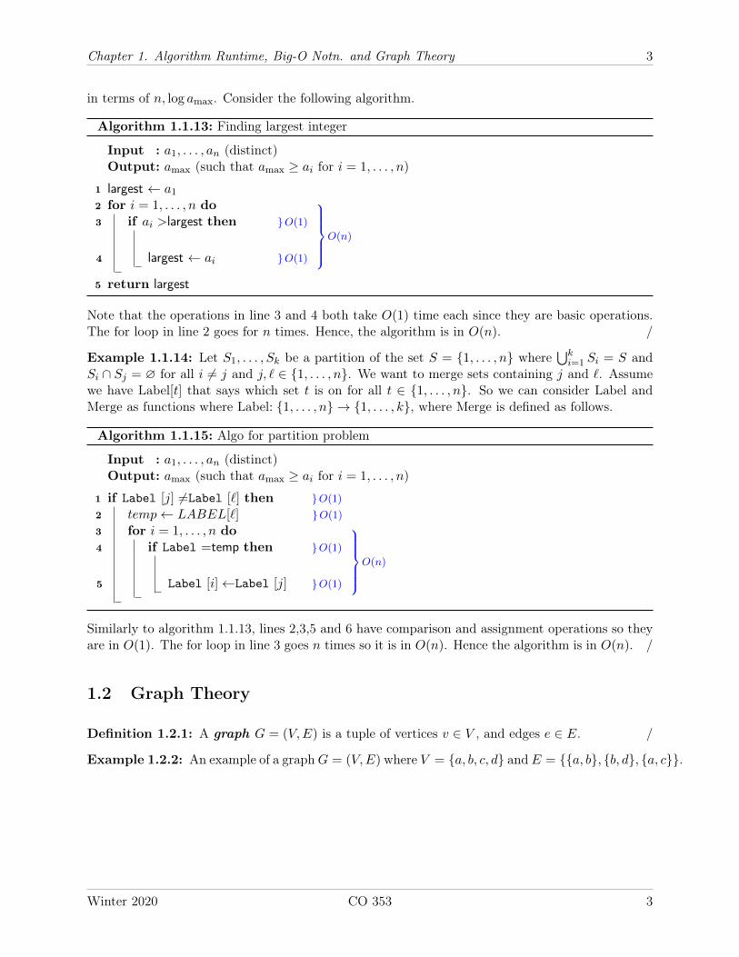
Note that the operations in line 3 and 4 both take O(1) time each since they are basic operations.The for loop in line 2 goes for n times. Hence, the algorithm is in O(n). /
Example 1.1.14: Let S1, . . . , Sk be a partition of the set S = 1, . . . , n where⋃ki=1 Si = S and
Si ∩ Sj = ∅ for all i 6= j and j, ` ∈ 1, . . . , n. We want to merge sets containing j and `. Assumewe have Label[t] that says which set t is on for all t ∈ 1, . . . , n. So we can consider Label andMerge as functions where Label: 1, . . . , n → 1, . . . , k, where Merge is defined as follows.
Algorithm 1.1.15: Algo for partition problem
Input : a1, . . . , an (distinct)Output: amax (such that amax ≥ ai for i = 1, . . . , n)
1 if Label [j] 6=Label [`] then O(1)
2 temp← LABEL[`] O(1)
3 for i = 1, . . . , n do4 if Label =temp then O(1)
O(n)
5 Label [i]←Label [j] O(1)
Similarly to algorithm 1.1.13, lines 2,3,5 and 6 have comparison and assignment operations so theyare in O(1). The for loop in line 3 goes n times so it is in O(n). Hence the algorithm is in O(n). /
1.2 Graph Theory
Definition 1.2.1: A graph G = (V,E) is a tuple of vertices v ∈ V , and edges e ∈ E. /
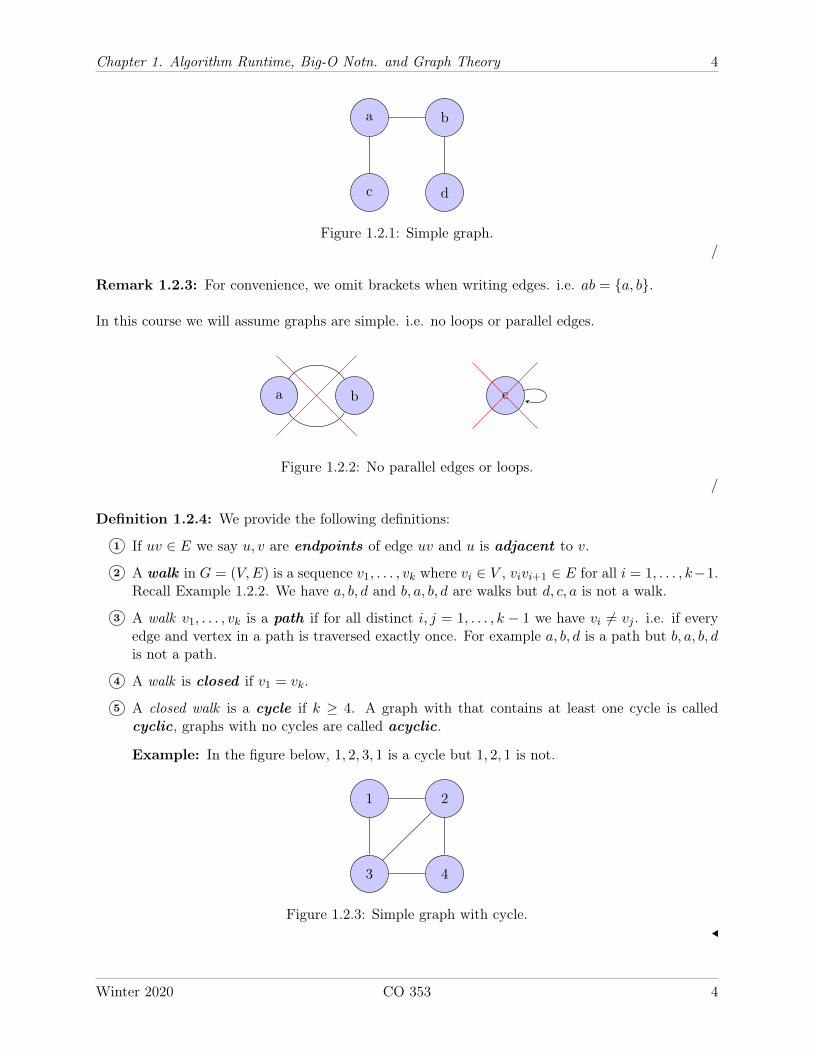
Example 1.2.2: An example of a graphG = (V,E) where V = a, b, c, d andE = a, b, b, d, a, c.
Winter 2020 CO 353 3
Chapter 1. Algorithm Runtime, Big-O Notn. and Graph Theory 4
c
a b
d
Figure 1.2.1: Simple graph./
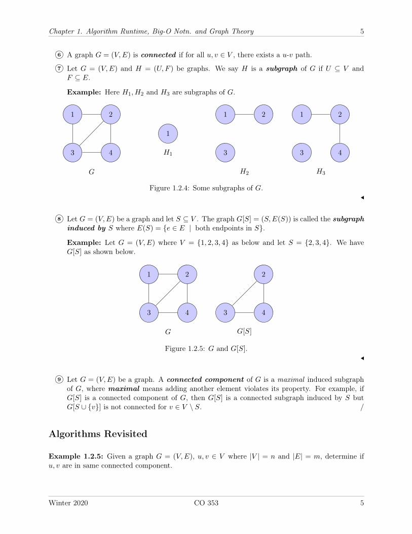
Remark 1.2.3: For convenience, we omit brackets when writing edges. i.e. ab = a, b.
In this course we will assume graphs are simple. i.e. no loops or parallel edges.
a b c
Figure 1.2.2: No parallel edges or loops./
Definition 1.2.4: We provide the following definitions:
1 If uv ∈ E we say u, v are endpoints of edge uv and u is adjacent to v.
2 A walk in G = (V,E) is a sequence v1, . . . , vk where vi ∈ V , vivi+1 ∈ E for all i = 1, . . . , k−1.Recall Example 1.2.2. We have a, b, d and b, a, b, d are walks but d, c, a is not a walk.
3 A walk v1, . . . , vk is a path if for all distinct i, j = 1, . . . , k − 1 we have vi 6= vj . i.e. if everyedge and vertex in a path is traversed exactly once. For example a, b, d is a path but b, a, b, dis not a path.
4 A walk is closed if v1 = vk.
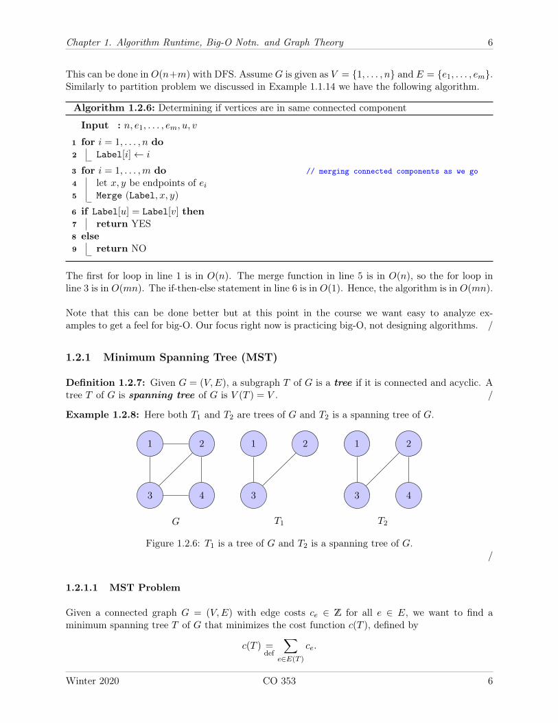
5 A closed walk is a cycle if k ≥ 4. A graph with that contains at least one cycle is calledcyclic, graphs with no cycles are called acyclic.
Example: In the figure below, 1, 2, 3, 1 is a cycle but 1, 2, 1 is not.
3
1 2
4
Figure 1.2.3: Simple graph with cycle.
Winter 2020 CO 353 4
Chapter 1. Algorithm Runtime, Big-O Notn. and Graph Theory 5
6 A graph G = (V,E) is connected if for all u, v ∈ V , there exists a u-v path.
7 Let G = (V,E) and H = (U,F ) be graphs. We say H is a subgraph of G if U ⊆ V andF ⊆ E.
Example: Here H1, H2 and H3 are subgraphs of G.
3
1 2
4
G
1
H1 3
1 2
H2
3
1 2
4
H3
Figure 1.2.4: Some subgraphs of G.
8 Let G = (V,E) be a graph and let S ⊆ V . The graph G[S] = (S,E(S)) is called the subgraphinduced by S where E(S) = e ∈ E | both endpoints in S.
Example: Let G = (V,E) where V = 1, 2, 3, 4 as below and let S = 2, 3, 4. We haveG[S] as shown below.
3
1 2
4
G
3
2
4
G[S]
Figure 1.2.5: G and G[S].
9 Let G = (V,E) be a graph. A connected component of G is a maximal induced subgraphof G, where maximal means adding another element violates its property. For example, ifG[S] is a connected component of G, then G[S] is a connected subgraph induced by S butG[S ∪ v] is not connected for v ∈ V \ S. /
Algorithms Revisited
Example 1.2.5: Given a graph G = (V,E), u, v ∈ V where |V | = n and |E| = m, determine ifu, v are in same connected component.
Winter 2020 CO 353 5
Chapter 1. Algorithm Runtime, Big-O Notn. and Graph Theory 6
This can be done in O(n+m) with DFS. Assume G is given as V = 1, . . . , n and E = e1, . . . , em.Similarly to partition problem we discussed in Example 1.1.14 we have the following algorithm.
Algorithm 1.2.6: Determining if vertices are in same connected component
Input : n, e1, . . . , em, u, v
1 for i = 1, . . . , n do2 Label[i]← i
3 for i = 1, . . . ,m do // merging connected components as we go
4 let x, y be endpoints of ei5 Merge (Label, x, y)
6 if Label[u] = Label[v] then7 return YES8 else9 return NO
The first for loop in line 1 is in O(n). The merge function in line 5 is in O(n), so the for loop inline 3 is in O(mn). The if-then-else statement in line 6 is in O(1). Hence, the algorithm is in O(mn).
Note that this can be done better but at this point in the course we want easy to analyze ex-amples to get a feel for big-O. Our focus right now is practicing big-O, not designing algorithms. /
1.2.1 Minimum Spanning Tree (MST)
Definition 1.2.7: Given G = (V,E), a subgraph T of G is a tree if it is connected and acyclic. Atree T of G is spanning tree of G is V (T ) = V . /
Example 1.2.8: Here both T1 and T2 are trees of G and T2 is a spanning tree of G.
3
1 2
4
G
3
1 2
T1
3
1 2
4
T2
Figure 1.2.6: T1 is a tree of G and T2 is a spanning tree of G./
1.2.1.1 MST Problem
Given a connected graph G = (V,E) with edge costs ce ∈ Z for all e ∈ E, we want to find aminimum spanning tree T of G that minimizes the cost function c(T ), defined by
c(T ) =def
∑e∈E(T )
ce.
Winter 2020 CO 353 6
Chapter 1. Algorithm Runtime, Big-O Notn. and Graph Theory 7
Theorem 1.2.9 (Properties of Spanning Trees): Let T be a spanning tree of G = (V,E). Thenthe following are true.
1 For all u, v ∈ V , there exists a unique u-v path in T (call Tuv).
2 T is minimally connected.
3 T is maximally acyclic.
4 T is spanning tree if and only if T is connected and has n− 1 edges.
Proof:
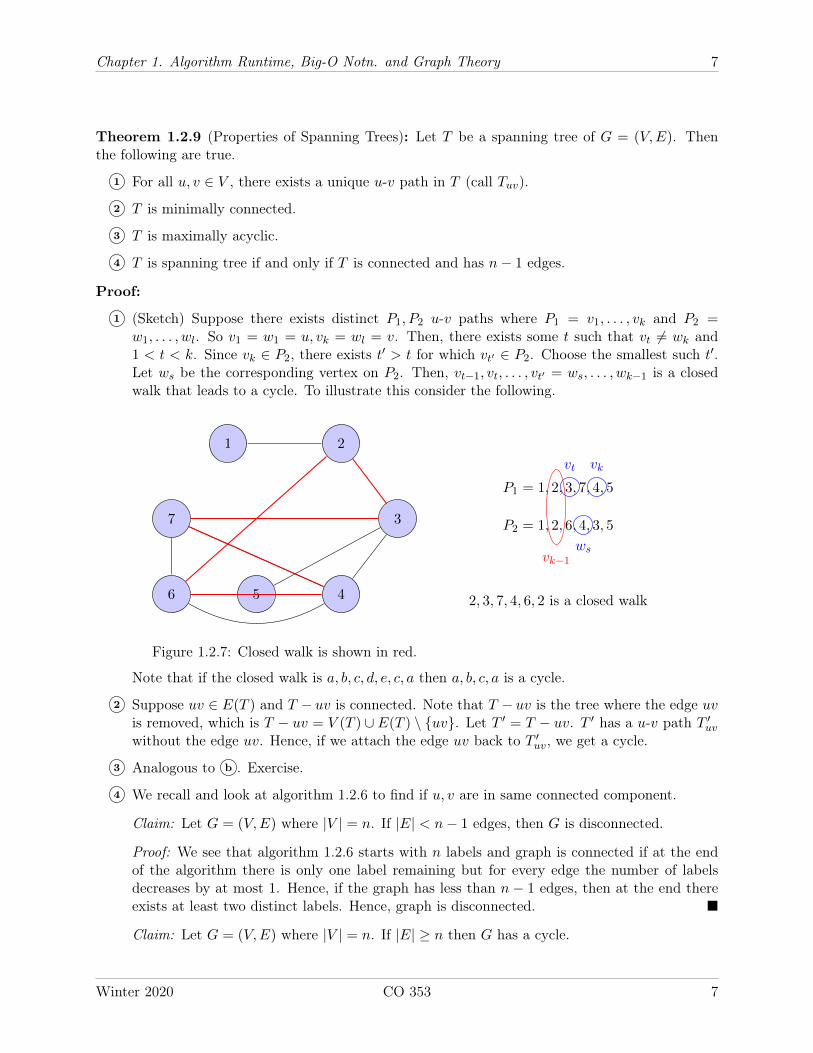
1 (Sketch) Suppose there exists distinct P1, P2 u-v paths where P1 = v1, . . . , vk and P2 =w1, . . . , wl. So v1 = w1 = u, vk = wl = v. Then, there exists some t such that vt 6= wk and1 < t < k. Since vk ∈ P2, there exists t′ > t for which vt′ ∈ P2. Choose the smallest such t′.Let ws be the corresponding vertex on P2. Then, vt−1, vt, . . . , vt′ = ws, . . . , wk−1 is a closedwalk that leads to a cycle. To illustrate this consider the following.
1 2
3
456
7
Figure 1.2.7: Closed walk is shown in red.
P1 = 1, 2, 3, 7, 4, 5
P2 = 1, 2, 6, 4, 3, 5
2, 3, 7, 4, 6, 2 is a closed walk
vkvt
wsvk−1
Note that if the closed walk is a, b, c, d, e, c, a then a, b, c, a is a cycle.
2 Suppose uv ∈ E(T ) and T − uv is connected. Note that T − uv is the tree where the edge uvis removed, which is T − uv = V (T ) ∪ E(T ) \ uv. Let T ′ = T − uv. T ′ has a u-v path T ′uvwithout the edge uv. Hence, if we attach the edge uv back to T ′uv, we get a cycle.
3 Analogous to b . Exercise.
4 We recall and look at algorithm 1.2.6 to find if u, v are in same connected component.
Claim: Let G = (V,E) where |V | = n. If |E| < n− 1 edges, then G is disconnected.
Proof: We see that algorithm 1.2.6 starts with n labels and graph is connected if at the endof the algorithm there is only one label remaining but for every edge the number of labelsdecreases by at most 1. Hence, if the graph has less than n − 1 edges, then at the end thereexists at least two distinct labels. Hence, graph is disconnected.
Claim: Let G = (V,E) where |V | = n. If |E| ≥ n then G has a cycle.
Winter 2020 CO 353 7
Chapter 1. Algorithm Runtime, Big-O Notn. and Graph Theory 8
Proof: Since |E| ≥ n, then ∃ e = uv ∈ E for which the algorithm does not decrease numberof labels. Hence, there exists a u-v path P that does not use uv. Hence, P +uv is a cycle.
Hence, it follows that spanning trees are connected with n − 1 edges. Reverse argument isalso analogous (exercise)
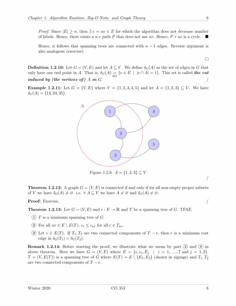
Definition 1.2.10: Let G = (V,E) and let A ⊆ V . We define δG(A) as the set of edges in G thatonly have one end point in A. That is, δG(A) =
defe ∈ E | |e ∩A| = 1. This set is called the cut
induced by (the vertices of) A in G. /
Example 1.2.11: Let G = V,E where V = 1, 2, 3, 4, 5 and let A = 1, 2, 3 ⊆ V . We haveδG(A) = 14, 24, 35.
1
2
3
4
5
A
Figure 1.2.8: A = 1, 2, 3 ⊆ V/
Theorem 1.2.12: A graph G = (V,E) is connected if and only if for all non-empty proper subsetsof V we have δG(A) 6= ∅. i.e. ∀ A ( V we have A 6= ∅ and δG(A) 6= ∅.
Proof: Exercise. /
Theorem 1.2.13: Let G = (V,E) and c : E → R and T be a spanning tree of G. TFAE.
1 T is a minimum spanning tree of G.
2 For all uv ∈ E \ E(T ), ce ≤ cuv for all e ∈ Tuv.
3 Let e ∈ E(T ). If T1, T2 are two connected components of T − e, then e is a minimum costedge in δG(T1) = δG(T2).
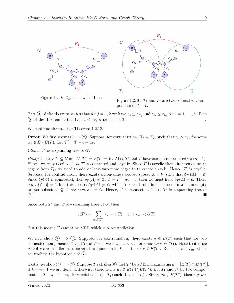
Remark 1.2.14: Before starting the proof, we illustrate what we mean by part 2 and 3 inabove theorem. Here we have G = (V,E) where E = e, ei, Ej | i = 1, . . . , 7 and j = 1, 2.T = (V,E(T )) is a spanning tree of G where E(T ) = E \ E1, E2 (shown in zigzags) and T1, T2
are two connected components of T − e.
Winter 2020 CO 353 8
Chapter 1. Algorithm Runtime, Big-O Notn. and Graph Theory 9
u v
s t
G
e1
e5
e2
e6
E2
e
e7
e3
e4
E1
Figure 1.2.9: Tuv is shown in blue.
u v
s t
G
T1 T2
e1
e5
e2
e6
E2
e
e7
e3
e4
E1
Figure 1.2.10: T1 and T2 are two connected com-ponents of T − e.
Part 2 of the theorem states that for j = 1, 2 we have ce ≤ cEj and cei ≤ cEj for i = 1, . . . , 5. Part3 of the theorem states that ce ≤ cEj where j = 1, 2. /
We continue the proof of Theorem 1.2.13.
Proof: We first show 1 =⇒ 2 . Suppose, for contradiction, ∃ e ∈ Tuv such that ce > cuv for someuv ∈ E \ E(T ). Let T ′ = T − e+ uv.
Claim: T ′ is a spanning tree of G.
Proof: Clearly T ′ ⊆ G and V (T ′) = V (T ) = V . Also, T ′ and T have same number of edges (n− 1).Hence, we only need to show T ′ is connected and acyclic. Since T is acyclic then after removing anedge e from Tuv we need to add at least two more edges to to create a cycle. Hence, T ′ is acyclic.Suppose, for contradiction, there exists a non-empty proper subset A ( V such that δT ′(A) = ∅.Since δT (A) is connected, then δT (A) 6= ∅. T = T − uv + e, then we must have δT (A) = e. Then,|u, v ∩A| = 1 but this means δT ′(A) 6= ∅ which is a contradiction. Hence, for all non-emptyproper subsets A ( V , we have δT ′ = ∅. Hence, T ′ is connected. Thus, T ′ is a spanning tree ofG.
Since both T ′ and T are spanning trees of G, then
c(T ′) =∑
e∈E(T )′
ce = c(T )− ce + cuv < c(T ).
But this means T cannot be MST which is a contradiction.
We now show 2 =⇒ 3 . Suppose, for contradiction, there exists e ∈ E(T ) such that for twoconnected components T1 and T2 of T − e, we have ce < cuv for some uv ∈ δG(T1). Note that sinceu and v are in different connected components of T − e then uv /∈ E(T ). But then e ∈ Tuv whichcontradicts the hypothesis of 2 .
Lastly, we show 3 =⇒ 1 . Suppose T satisfies 3 . Let T ∗ be a MSTmaximizing k = |E(T ) ∩ E(T ∗)|.If k = n− 1 we are done. Otherwise, there exists uv ∈ E(T ) \E(T ∗). Let T1 and T2 be two compo-nents of T − uv. Then, there exists e ∈ δT ∗(T1) such that e ∈ T ∗uv. Since, uv /∈ E(T ∗), then e 6= uv.
Winter 2020 CO 353 9
Chapter 2. Greedy Algorithms and Matroids 10
From the hypothesis of 3 , we have cuv ≤ ce. Let T ′ = T ∗− e+ uv then |E(T ′)| = n− 1. From theproof of 1 =⇒ 2 , we have that T ′ is also connected and T ′ is a spanning tree of G. Hence,
c(T ′) = c(T ∗)− ce + cuv ≤ c(T ∗).
Then c(T ′) is a MST but this gives us |E(T ) ∩ E(T ′)| > |E(T ) ∩ E(T ∗)| which contradicts thechoice of T ∗.
Winter 2020 CO 353 10
Chapter 2. Greedy Algorithms and Matroids 11
Chapter 2 – Greedy Algorithms and Matroids
2.1 Kruskal’s Algorithm
Kruskal’s algorithm takes a connected graph G = (V,E) and edge costs as inputs and gives a MSTof G as output. It operates as follows.
Algorithm 2.1.1: Kruskal’s algorithm (idea)
Input : G = (V,E) (connected), c : E → R
Output: MST T .Init : T = (V,∅).
1 while T is not a spanning tree do2 Let e be the cheapest edge whose end points are different connected components of T .3 Add e to T .
4 return T
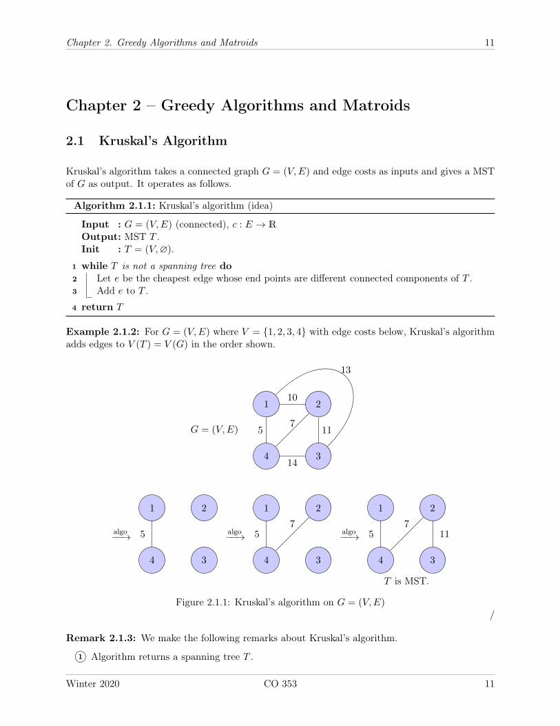
Example 2.1.2: For G = (V,E) where V = 1, 2, 3, 4 with edge costs below, Kruskal’s algorithmadds edges to V (T ) = V (G) in the order shown.
1 2
34
G = (V,E)
10
13
5 117
14
algo−−→
1 2
34
algo−−→5
1 2
34
algo−−→57
1 2
34
T is MST.
57
11
Figure 2.1.1: Kruskal’s algorithm on G = (V,E)/
Remark 2.1.3: We make the following remarks about Kruskal’s algorithm.
1 Algorithm returns a spanning tree T .
Winter 2020 CO 353 11
Chapter 2. Greedy Algorithms and Matroids 12
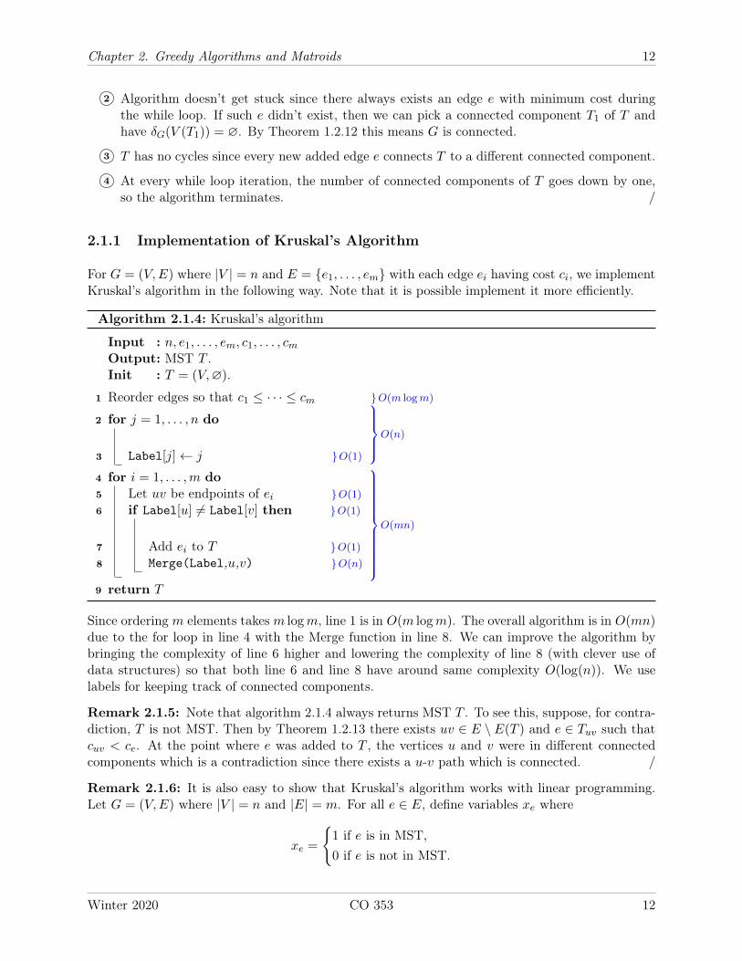
2 Algorithm doesn’t get stuck since there always exists an edge e with minimum cost duringthe while loop. If such e didn’t exist, then we can pick a connected component T1 of T andhave δG(V (T1)) = ∅. By Theorem 1.2.12 this means G is connected.
3 T has no cycles since every new added edge e connects T to a different connected component.
4 At every while loop iteration, the number of connected components of T goes down by one,so the algorithm terminates. /
2.1.1 Implementation of Kruskal’s Algorithm
For G = (V,E) where |V | = n and E = e1, . . . , em with each edge ei having cost ci, we implementKruskal’s algorithm in the following way. Note that it is possible implement it more efficiently.
Algorithm 2.1.4: Kruskal’s algorithm
Input : n, e1, . . . , em, c1, . . . , cmOutput: MST T .Init : T = (V,∅).
1 Reorder edges so that c1 ≤ · · · ≤ cm O(m logm)
2 for j = 1, . . . , n doO(n)
3 Label[j]← j O(1)
4 for i = 1, . . . ,m do5 Let uv be endpoints of ei O(1)
6 if Label[u] 6= Label[v] then O(1)
O(mn)
7 Add ei to T O(1)
8 Merge(Label,u,v) O(n)
9 return T
Since ordering m elements takes m logm, line 1 is in O(m logm). The overall algorithm is in O(mn)due to the for loop in line 4 with the Merge function in line 8. We can improve the algorithm bybringing the complexity of line 6 higher and lowering the complexity of line 8 (with clever use ofdata structures) so that both line 6 and line 8 have around same complexity O(log(n)). We uselabels for keeping track of connected components.
Remark 2.1.5: Note that algorithm 2.1.4 always returns MST T . To see this, suppose, for contra-diction, T is not MST. Then by Theorem 1.2.13 there exists uv ∈ E \ E(T ) and e ∈ Tuv such thatcuv < ce. At the point where e was added to T , the vertices u and v were in different connectedcomponents which is a contradiction since there exists a u-v path which is connected. /
Remark 2.1.6: It is also easy to show that Kruskal’s algorithm works with linear programming.Let G = (V,E) where |V | = n and |E| = m. For all e ∈ E, define variables xe where
xe =
1 if e is in MST,0 if e is not in MST.
Winter 2020 CO 353 12
Chapter 2. Greedy Algorithms and Matroids 13
We have
(Pst) : min∑e∈E
cexe,
subject to∑e∈E
xe = n− 1,∑e∈F
xe ≤ n− κ(F ), ∀ F ⊆ E,
with 0 ≤ xe ≤ 1.
Here κ(F ), kappa of F , is the number of connected components of (V, F ). /
2.1.2 Validating Kruskal’s Algorithm with Linear Programming
Recall MST problem we introduced in subsubsection 1.2.1.1. Given G = (V,E) and c : E → R, wewant to find a spanning tree of G of minimum cost.
Definition 2.1.7: A graph is called a forest if it is acyclic (contains no cycles). /
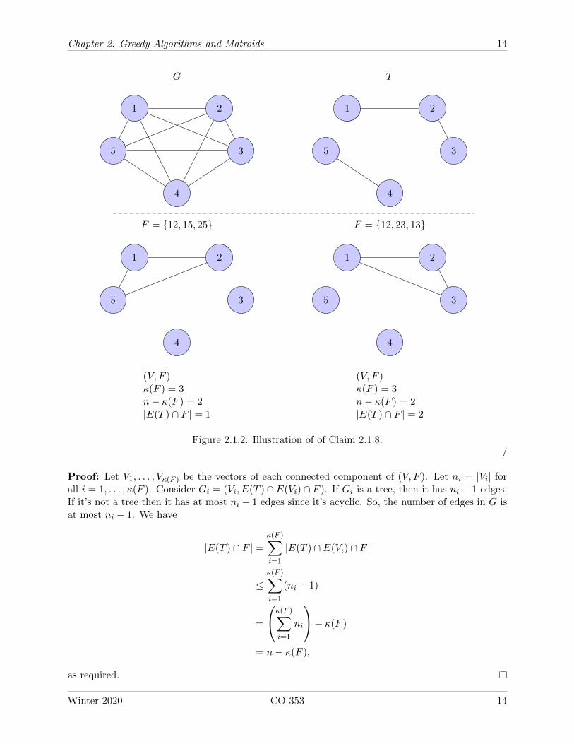
Claim 2.1.8: If T is a forest of G = (V,E) with V (T ) = V , then for all F ⊆ E, T has at mostn− κ(F ) edges of F .
Example 2.1.9:
Winter 2020 CO 353 13
Chapter 2. Greedy Algorithms and Matroids 14
1 2
3
4
5
G
F = 12, 15, 25
1 2
3
4
5
(V, F )κ(F ) = 3n− κ(F ) = 2|E(T ) ∩ F | = 1
1 2
3
4
5
T
F = 12, 23, 13
1 2
3
4
5
(V, F )κ(F ) = 3n− κ(F ) = 2|E(T ) ∩ F | = 2
Figure 2.1.2: Illustration of of Claim 2.1.8./
Proof: Let V1, . . . , Vκ(F ) be the vectors of each connected component of (V, F ). Let ni = |Vi| forall i = 1, . . . , κ(F ). Consider Gi = (Vi, E(T ) ∩E(Vi) ∩ F ). If Gi is a tree, then it has ni − 1 edges.If it’s not a tree then it has at most ni − 1 edges since it’s acyclic. So, the number of edges in G isat most ni − 1. We have
|E(T ) ∩ F | =κ(F )∑i=1
|E(T ) ∩ E(Vi) ∩ F |
≤κ(F )∑i=1
(ni − 1)
=
κ(F )∑i=1
ni
− κ(F )
= n− κ(F ),
as required.
Winter 2020 CO 353 14
Chapter 2. Greedy Algorithms and Matroids 15
Remark 2.1.10: Given a spanning tree T , let x> be its characteristic vector . i.e.
x>e =
1 if e ∈ E(T ),
0 if e /∈ E(T ).
x> is feasible for (Pst). Thus, the optimal solution of (Pst) is at most equal to the cost of MST.
Note that by convention, χ is used to denote characteristic vector. In this course we’ll use x. /
Theorem 2.1.11: Let T be the tree returned by Kruskal’s algorithm. Then x> is optimal for (Pst).
Proof: We have the linear program (Pst) as follows.
(Pst) : min c>x,
subject to∑e∈F
xe ≤ n− κ(F ), ∀ F ( E,∑e∈F
xe = n− 1,
with xe ≥ 0.
We have the dual of (Pst) as (Dst) where
(Dst) : max∑∀ F⊆E
(n− κ(F ))yF ,
subject to∑F :e∈F
yF ≤ ce, ∀ e ∈ E,
with yF ≤ 0, F ( E,
yE free.
We illustrate what we mean by above in the following example.
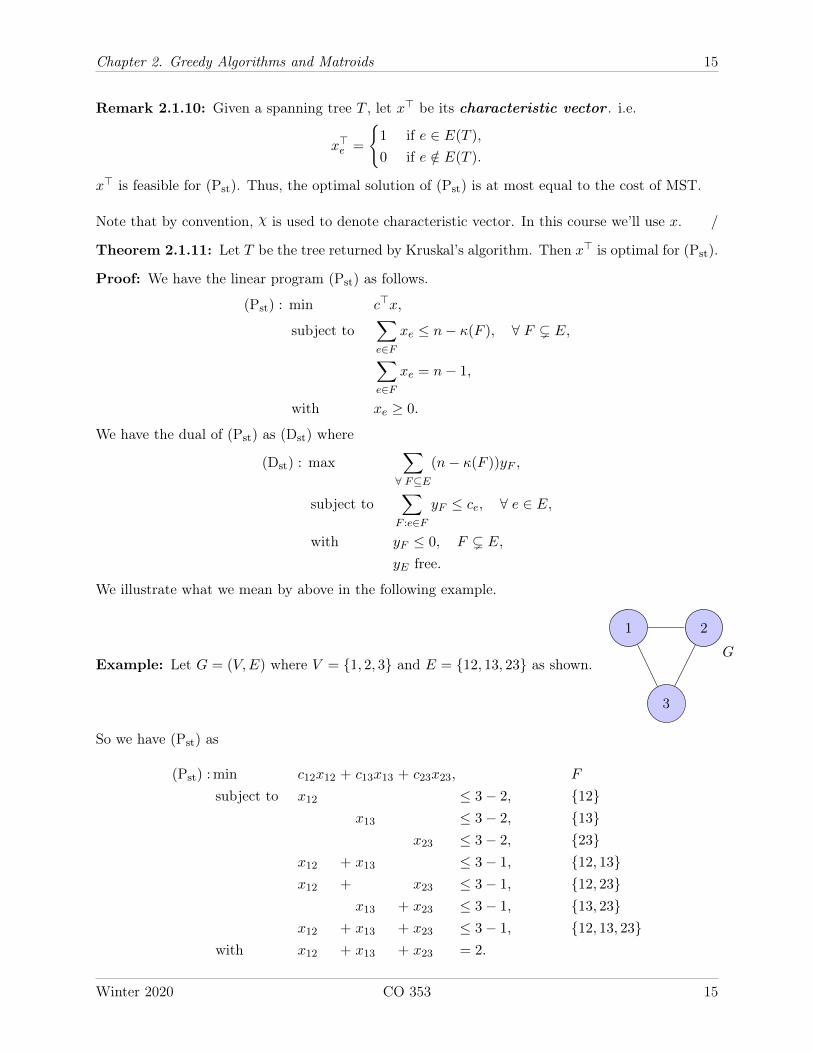
Example: Let G = (V,E) where V = 1, 2, 3 and E = 12, 13, 23 as shown.
3
1 2
G
So we have (Pst) as
(Pst) : min c12x12 + c13x13 + c23x23, F
subject to x12 ≤ 3− 2, 12x13 ≤ 3− 2, 13
x23 ≤ 3− 2, 23x12 + x13 ≤ 3− 1, 12, 13x12 + x23 ≤ 3− 1, 12, 23
x13 + x23 ≤ 3− 1, 13, 23x12 + x13 + x23 ≤ 3− 1, 12, 13, 23
with x12 + x13 + x23 = 2.
Winter 2020 CO 353 15
Chapter 2. Greedy Algorithms and Matroids 16
We have (Dst) as
(Dst) : max y12 + y13 + y23 + 2y12,13 + 2y12,23 + 2y13,23 + 2y12,13,23
subject to y12 + y12,13 + y12,23 + y12,13,23 ≤ c12
y13 + y12,13 + y13,23 + 2y12,13,23 ≤ c13
y23 + y12,23 + y13,23 + 2y12,13,23 ≤ c23,
with all y’s ≤ 0 except for y12,13,23. /
We now letE = e1, . . . , em with ce1 ≤ · · · ≤ cem ,Ei := e1, . . . , ei,yEi
= cei − cei+1 ≤ 0, ∀ i = 1, . . . ,m− 1,
yE = cem ,
yF = 0, for all other F ⊆ E.
Claim 2.1.12: y is feasible for (Dst).
Proof: We immediately see that the sign restrictions are satisfied. Consider edge ek. We have∑F :ek∈F
yF =
m∑i=k
yEi=
(m∑i=k
cei − cei+1
)+ cem = cek .
We see that the dual constraints are tight.
Complementary-Slackness conditions state the following.
1 If primal variable is non-zero, then corresponding dual constraint is tight.
2 If dual variable is non-zero, then corresponding primal constraint is tight.
Clearly 1 holds since by the proof of above claim, every dual constraint is tight. To show 2 istrue, we make the following claims.
Claim: For all F ⊆ E, if T is a maximal forest of (V, F ) (that is, if any more edges are added to Tit’s no longer a forest), then |E(T ) ∩ F | = n− κ(F ).
Proof: Exercise.
Claim: At every step of Kruskal’s algorithm we have a maximal forest of Ei = e1, . . . , ei.
Proof: Suppose T is a forest constructed after edges in Ei and suppose, for contradiction, T is nota maximal forest of (V,Ei). Then, there exists ek ∈ Ei \ E(T ) such that T + ek is a forest. Then,when Kruskal’s algorithm is at step k ≤ i, we had constructed (V,E(T )∩Ek) and ek was not added.But that means adding ek would have created a cycle and this a contradiction since T is a tree andT + ek is acyclic.
Hence, by above claims we have∑e∈F
x>e n− κ(Ei), ∀ i = 1, . . . ,m.
Hence, x> and y satisfy the Complementary-Slackness (C-S) conditions.
Winter 2020 CO 353 16
Chapter 2. Greedy Algorithms and Matroids 17
Remark 2.1.13: The tight inequality we found in the proof of Claim 2.1.12 provides a certificatethat verifies the MST obtained from Kruskal’s algorithm is correct. /
2.2 Greedy Algorithms
Definition 2.2.1: In every step, Kruskal’s algorithm picks the locally best option since it takes thecheapest edge that keeps the solution feasible. The algorithms that prioritize locally best optionsare called greedy algorithms.
This greedy approach doesn’t work on some problems. /
Definition 2.2.2: A cycle that goes through every edge exactly once is called a Hamiltoniancycle . /
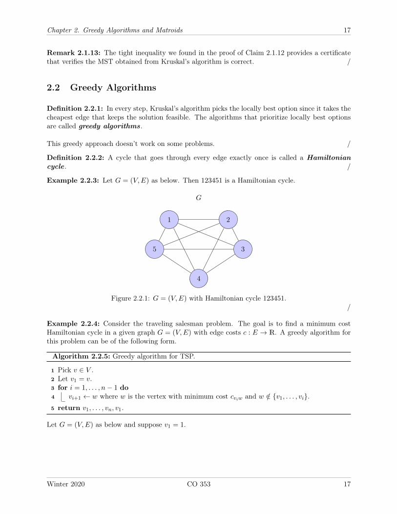
Example 2.2.3: Let G = (V,E) as below. Then 123451 is a Hamiltonian cycle.
1 2
3
4
5
G
Figure 2.2.1: G = (V,E) with Hamiltonian cycle 123451./
Example 2.2.4: Consider the traveling salesman problem. The goal is to find a minimum costHamiltonian cycle in a given graph G = (V,E) with edge costs c : E → R. A greedy algorithm forthis problem can be of the following form.
Algorithm 2.2.5: Greedy algorithm for TSP.
1 Pick v ∈ V .2 Let v1 = v.3 for i = 1, . . . , n− 1 do4 vi+1 ← w where w is the vertex with minimum cost cviw and w /∈ v1, . . . , vi.5 return v1, . . . , vn, v1.
Let G = (V,E) as below and suppose v1 = 1.
Winter 2020 CO 353 17
Chapter 2. Greedy Algorithms and Matroids 18
1 2
34
G
100
1
0 0
5
0
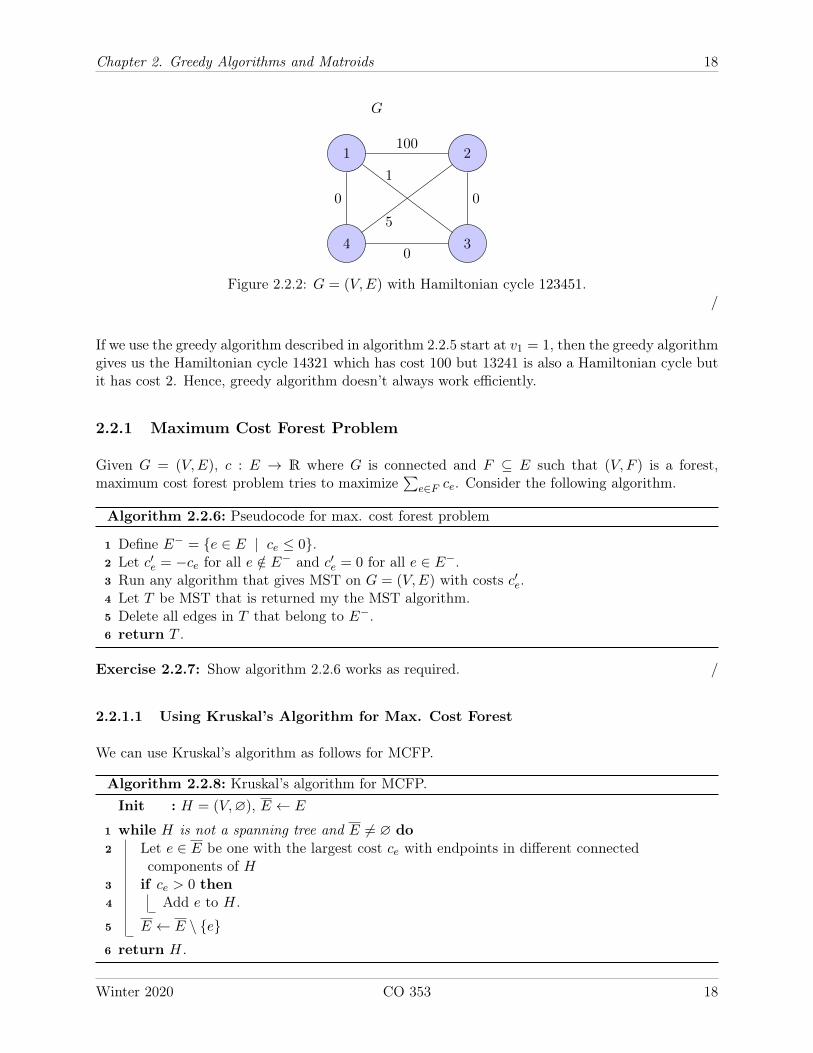
Figure 2.2.2: G = (V,E) with Hamiltonian cycle 123451./
If we use the greedy algorithm described in algorithm 2.2.5 start at v1 = 1, then the greedy algorithmgives us the Hamiltonian cycle 14321 which has cost 100 but 13241 is also a Hamiltonian cycle butit has cost 2. Hence, greedy algorithm doesn’t always work efficiently.
2.2.1 Maximum Cost Forest Problem
Given G = (V,E), c : E → R where G is connected and F ⊆ E such that (V, F ) is a forest,maximum cost forest problem tries to maximize
∑e∈F ce. Consider the following algorithm.
Algorithm 2.2.6: Pseudocode for max. cost forest problem
1 Define E− = e ∈ E | ce ≤ 0.2 Let c′e = −ce for all e /∈ E− and c′e = 0 for all e ∈ E−.3 Run any algorithm that gives MST on G = (V,E) with costs c′e.4 Let T be MST that is returned my the MST algorithm.5 Delete all edges in T that belong to E−.6 return T .
Exercise 2.2.7: Show algorithm 2.2.6 works as required. /
2.2.1.1 Using Kruskal’s Algorithm for Max. Cost Forest
We can use Kruskal’s algorithm as follows for MCFP.
Algorithm 2.2.8: Kruskal’s algorithm for MCFP.Init : H = (V,∅), E ← E
1 while H is not a spanning tree and E 6= ∅ do2 Let e ∈ E be one with the largest cost ce with endpoints in different connected
components of H3 if ce > 0 then4 Add e to H.
5 E ← E \ e6 return H.
Winter 2020 CO 353 18
Chapter 2. Greedy Algorithms and Matroids 19
The rough idea behind this algorithm is as follows.
1 while There exists an edge e such that ce > 0 with endpoints of e in different connectedcomponents, do
2 Choose ce that is largest.3 Add e to H.
4 return H.
Exercise 2.2.9: Prove algorithm 2.2.8 works. /
2.2.1.2 Properties of Forests
We will refer forests by their edge sets. Forests have the following properties.
1 The empty set is a forest.
2 If F is a forest and if F ′ ⊆ F , then F ′ is a forest.
3 If A ⊆ E, then every inclusion-wise maximal forest F ⊆ A, has the same cardinality.
Note that these properties coincide with the definition of matroids which will be explained later.
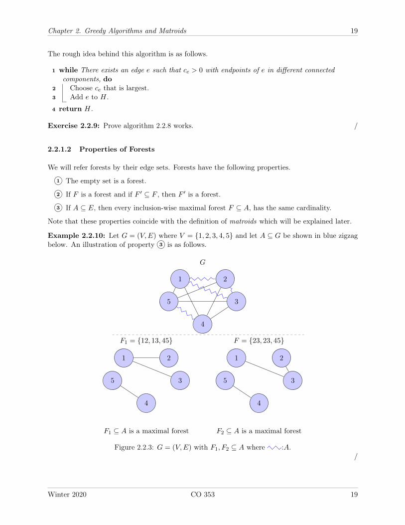
Example 2.2.10: Let G = (V,E) where V = 1, 2, 3, 4, 5 and let A ⊆ G be shown in blue zigzagbelow. An illustration of property 3 is as follows.
1 2
3
4
5
G
F1 = 12, 13, 45
1 2
3
4
5
F1 ⊆ A is a maximal forest
F = 23, 23, 45
1 2
3
4
5
F2 ⊆ A is a maximal forest
Figure 2.2.3: G = (V,E) with F1, F2 ⊆ A where :A./
Winter 2020 CO 353 19
Chapter 2. Greedy Algorithms and Matroids 20
Note that F1, F2 ⊆ A are maximal forests since if any edge where added to F1 or F2, they no longerare subset forests of A.
Remark 2.2.11: We proved property 3 in MST problem with |F | = n− κ(A). /
2.3 Matroids
We introduce the abstract notion of matroids. We will focus on how greedy algorithms work onmatroids.
2.3.1 Independence Systems and Independent Sets
Definition 2.3.1: Let S be a finite set and let I ⊆ P(S) = 2S . Here P(S) is the power set of S,which is the collection of all subsets of S. So, I is a collection of subsets of S. If I satisfies
M1 I 3 ∅, and
M2 if I1 ∈ I and I2 ⊆ I1, then I2 ∈ I,
then the pair (S, I) is called an independence system and the elements I ∈ I are calledindependent sets. This property is known as the hereditary property and it is equivalent tosaying every subset of an independent set is independent. If (S, I) is an independence systemand if it also satisfies
M3 for all A ⊆ S, every inclusion-wise maximal element of I contained in A has same cardinality,
then the pair M = (S, I) is called a matroid , where S is a finite set (which is called theground set) and I is a collection of subsets of the ground set. This property is known as theaugmentation property or (independent set) exchange property. /
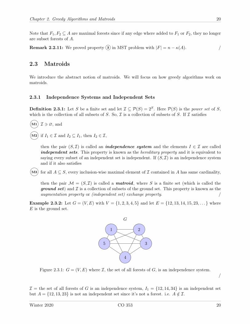
Example 2.3.2: Let G = (V,E) with V = 1, 2, 3, 4, 5 and let E = 12, 13, 14, 15, 23, . . . whereE is the ground set.
1 2
3
4
5
G
Figure 2.3.1: G = (V,E) where I, the set of all forests of G, is an independence system./
I = the set of all forests of G is an independence system, I1 = 12, 14, 34 is an independent setbut A = 12, 13, 23 is not an independent set since it’s not a forest. i.e. A /∈ I.
Winter 2020 CO 353 20
Chapter 2. Greedy Algorithms and Matroids 21
Example 2.3.3: Let S = 1, . . . ,m and k ∈ Z+. Let I = U ⊆ S | |U | ≤ k. Since |∅| = 0,then ∅ ∈ I and it is clear that for all I1 ∈ I, if I2 ⊆ I1, then I2 ∈ I. So, I is an independencesystem. I also satisfies property M3 . To see this, let A ⊆ S with |A| ≤ k. Then, in this case theonly maximal element of I in A is A. If |A| > k and I ∈ I with I ⊆ A and |I| < k, then thereexists e ∈ S such that I ∪ e ∈ I. i.e. I is not maximal. Hence, every maximal element of I hascardinality of 5. Hence, the pair (S, I) is a matroid. /
Example 2.3.4: Let S = 1, 2, 3, 4 and I = ∅, 1, 2, 3, 4, 1, 2. It is easy to see thatM1 and M2 hold. Let A = 1, 2, 3 ⊆ S. We have
1, 2 ⊆ A, and 1, 2 ⊆ I,3 ⊆ A, and 3 ⊆ I.
Clearly 1, 2 and 3 are maximal but |1, 2| 6= |3|. So, M3 doesn’t hold. Hence, the pair(S, I) is not a matroid but I is an independence system. /
Remark 2.3.5: We will show that greedy algorithms for independence systems I ⊆ 2S give optimalsolution if and only if the pair (S, I) =M is a matroid. /
Definition 2.3.6: Let (S, I) be an independence system. Given A ⊆ S, a basis of A is a maximalindependent set contained in A. If A = S whereM = (S, I), then a basis of A is a basis ofM. /
Example 2.3.7: Consider the matrix B below.
B =
1 2 3 4 5 1 -1 0 0 12 -2 0 1 44 1 1 0 2
.
Let S = 1, 2, 3, 4, 5 (column indices) and let I be defined as follows.
I = A ⊆ S | corresponding columns are linearly independent.
Since M1 , M2 and M3 are satisfied, (S, I) =M is a matroid. Any matroid of the formM = (S, I)
where the ground set S is column (row) indices and I is the set of linearly independent columns(rows) is called a linear matroid . Basis ofM are the bases of the vector space generated by thecorresponding columns. /
Remark 2.3.8: We can characterize the necessary matroid condition as follows.
M3 : ∀ A ⊆ S, every inclusion-wise maximal
element of I contained in A has cardinality⇐⇒
∀ A ⊆ S, all bases of A havethe same cardinality.
/
Definition 2.3.9: Let (S, I) = M be an independence system and let A ⊆ S. The rank of A,r(A), is the largest basis of A. That is,
r(A) =def
max|J | | J ⊆ A and J ∈ I. /
If A = S, then r(A) = r(S) = r(M).
Winter 2020 CO 353 21
Chapter 2. Greedy Algorithms and Matroids 22
Remark 2.3.10: It is easy to see that r(A) = |A| if and only if A ∈ I. Consider the graphG = (V,E). Let S = E and I = A ⊆ S | (V,A) is a forest. The pair (S, I) of this form is calleda graphic (forest) matroid . We have
r(A) = n− κ(A),
where κ(A) is the number of connected connected components of A. /
2.3.2 Solving Maximum Weighted Independent Set Problem with Greedy Al-gorithm
GivenM = (S, I) independence system and costs ce for all e ∈ S, consider the problem of findingA ∈ I maximizing
∑e∈A ce. This problem is called maximum weighted independent set problem.
Consider the greedy algorithm below.
Algorithm 2.3.11: Greedy Algorithm for Max Weighted Independent Set Problem1 J ← ∅2 while ∃ e ∈ S \ J such that ce > 0 and J ∪ e ∈ I do3 Let e be such element of largest ce,4 J ← J ∪ e5 return J
Let S′ = e ∈ S | ce > 0. Define I ′ = A ⊆ S′ | A ∈ I. So,M′ = (S′, I ′) is an independence
system. In fact, if M is a matroid (that is, if M satisfies M3 ) then so is M′. Hence, solvingmaximum weighted independent set overM′ solves the problem overM. Note that since our goalis to maximize the sum of costs, we may assume that ce′ > 0 for all e′ ∈ S′.
Theorem 2.3.12 (Rado ‘57, Edmonds ‘71): Let M = (S, I) be a matroid and let c : S → R+.Then, greedy algorithm in algorithm 2.3.11 finds maximum weighted independent set.
Proof: Exercise. /
Theorem 2.3.13: LetM = (S, I) be an independence system. Greedy algorithm finds a maximumweighted independent set for all c ∈ RS if and only ifM is a matroid.
Proof: For forward direction we will use contrapositive. Suppose M is not a matroid. Then, Mdoes not satisfy 3 . Let A ⊆ S such that A1, A2 are two bases of A with |A1| < |A2|. Note thatsuch two bases exists by Remark 2.3.8. Let
ce =
1 + ε if e ∈ A1,
1 if e ∈ A2,
0 otherwise.
Hence, in this case greedy algorithm in algorithm 2.3.11 outputs A where∑e∈A1
ce = (1 + ε)|A1|.
But we also have∑
e∈A2ce = |A2|. So if we choose ε small enough where
ε <|A2||A1|
− 1,
Winter 2020 CO 353 22
Chapter 2. Greedy Algorithms and Matroids 23
then A1 is not a maximum weighted independent set which proves the contrapositive. The converseimmediately follows from Theorem 2.3.12.
Remark 2.3.14 (Runtime of Greedy Algorithm): Consider the greedy algorithm in algorithm 2.3.11.We see that the main loop is executed O(|S|) times. Hence if the process of checking J ∈ I can bedone in poly(|S|), then greedy algorithm can run in polytime in |S|. /
Definition 2.3.15: LetM = (S, I) be an independence system and let A ⊆ S.
ρ(A) =def
min|B| | B is a basis of A.
Note thatM = (S, I) is a matroid if and only if ρ(A) = rank(A) for all A ⊆ S. /
Definition 2.3.16: Let M = (S, I) be an independence system. The rank quotient of M,q(S, I), is defined as
q(S, I) =def
minA⊆S
ρ(A)
RankA.
Note that we always have q(S, I) ≤ 1 and it follows thatM is a matroid if and only if q(S, I) = 1. /
Theorem 2.3.17 (Jenkyns ‘76): Let M = (S, I) be an independence system. Let GRS,I be thetotal weight of solution found by the greedy algorithm in algorithm 2.3.11. Let OPTS,I be weightof optimal solution. Then
GRS,I ≥ q(S, I)OPTS,I .
Note that this implies ifM is a matroid then greedy algorithm in algorithm 2.3.11 finds an optimalsolution.
Proof: We prove Theorem 2.3.17 as follows. Let S = e1, . . . , em with ce1 ≥ · · · ≥ cem and letSj = e1, . . . , ej for all j = 1, . . . ,m. Let G be the solution obtained by the greedy algorithm andlet σ be the optimal solution. So, G, σ ⊆ S. Let Gj = G ∩ Sj and σj = σ ∩ Sj . Let G0 = ∅ = σ0.We have
c(G) =∑ej∈G
cej =m∑j=1
(|Gj | − |Gj−1|︸ ︷︷ ︸
(?)
)cej =
m−1∑j=1
|Gj |(cej − cej+1
)+ cem |Gm| =
m∑j=1
|Gj |(cej − cej+1︸ ︷︷ ︸
∆j≥0
),
where cem+1 = 0. Note that
(?) =
= 1 if ei ∈ G,= 0 otherwise.
At step j, Gj is a basis of Sj . Hence, |Gj | ≥ ρ(Sj). Thus,
c(G) ≥m∑j=1
ρ(Sj)∆j ≥m∑j=1
q(S, I)r(Sj)∆j ≥ q(S, I)m∑j=1
|σj |∆j︸ ︷︷ ︸c(σ)
.
Corollary 2.3.18: IfM is a matroid, then the greedy algorithm in algorithm 2.3.11 computes theoptimal solution.
Theorem 2.3.19: IfM = (S, I) is an independent system then
M3 : ∀ A ⊆ S, every inclusion-wise maximal
element of I contained in A has cardinality⇐⇒
M3’ : ∀ X,Y ∈ I such that |X| < |Y |,
∃ e ∈ Y \X such that X ∪ e ∈ I.
Winter 2020 CO 353 23
Chapter 2. Greedy Algorithms and Matroids 24
Proof: Skipped, exercise. /
Example 2.3.20: Let S = 1, 2, 3, 4 and I = ∅, 1, 2, 3, 4, 1, 2, 3, 4. Clearly M1
and M2 are satisfied but since 1, 2, 3 ∈ I and 3 ∪ e /∈ I for any e ∈ 1, 2 \ 3, then
M3’ is not satisfied. Hence, (S, I) is an independence system but not a matroid. /
Remark 2.3.21: We can fully specify an independence system or a matroid by listing its bases. Inthe above example, the set of bases of (S, I) is B = 1, 2, 3, 4. /
Theorem 2.3.22: Let S be a finite set and let B ⊆ P(S) = 2S . Then B is the set of bases of amatroid if and only if
1 B 6= ∅,
2 For all B1, B2 ∈ B and x ∈ B1 \B2, there exists y ∈ B2 \B1 such that (B1 \ x) ∪ y ∈ B.
Proof: Exercise. /
Remark 2.3.23: Note that by this theorem, the set B = 1, 2, 3, 4 in above example cannotbe a set of basis of a matroid.
M = (S, I) = ∅ is a matroid and set of bases B = ∅ = I 6= ∅. /
2.3.3 Matroid Constructions
Given a matroidM, we can construct other matroids by using some operations.
Remark 2.3.24: Let M = (S, I) be a matroid. By using the following we can construct othermatroids.
1 Deletion: If J ⊆ S thenM\J = S′, I ′ is a matroid where S′ = S\J and I ′ = A ⊆ S′ | A ∈ I.
We use backslash, (\), to denote deletion of J from matroidM. Some sources use M − Jnotation for deletion which is objectively better.
2 Truncation: Given k ∈ Z+ define I ′ = A ∈ I | |A| ≤ k. Then,M′ = (S, I ′) is a matroid.
3 Dual: Let I∗ = A ⊆ S | S \ A has a basis ofM. Equivalently, r(S \ A) = r(S). We callM∗ = (S, I∗) the dual matroid of M. Note that (M∗)∗ =M
We will prove thatM∗ is a matroid and rM∗(A) = |A|+ rM (S \A)− rM (S).
4 Contraction: If J ⊆ S and if B is a basis of J , then M/J = (S′, I ′) is a matroid whereS′ = S \ J and I ′ = A ⊆ S′ | A ∪ B ∈ I.
We use forward slash, (/), to denote deletion of J from matroidM.
5 Disjoint Union:1LetMi = (Si, Ii) be matroids. If Si are distinct for all i = 1, . . . , k then theunion of these matroids is a direct sum and
⊕ki=1Mi =M1 ⊕ · · · ⊕Mk =M = (S′, I ′) is a
Winter 2020 CO 353 24
Chapter 2. Greedy Algorithms and Matroids 25
matroid where
S′ =
k⋃i=1
Si, I ′ =k⋃i=1
Ii and A ∈ I ′ ⇐⇒ A =
k⋃i=1
Ai where Ai ∈ Ii for i = 1, . . . , k. /
Exercise 2.3.25: Show that duality operation on matroids is an involution. i.e. M = (M∗)∗. /
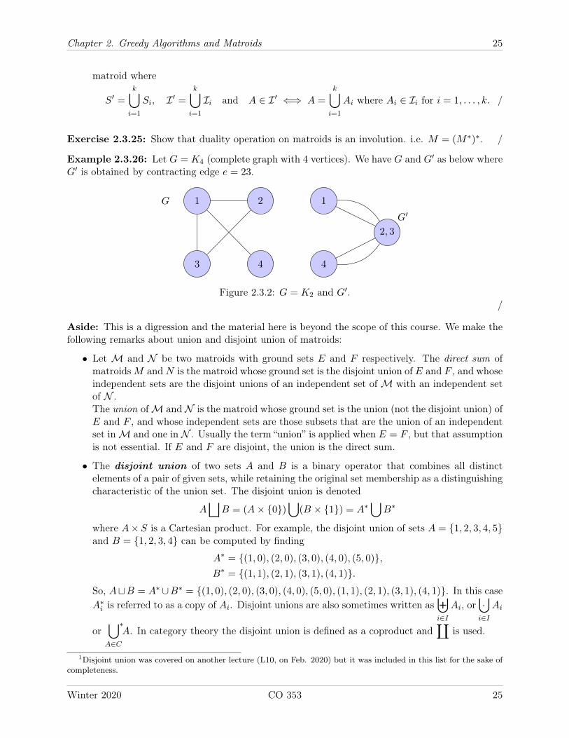
Example 2.3.26: Let G = K4 (complete graph with 4 vertices). We have G and G′ as below whereG′ is obtained by contracting edge e = 23.
1 2
3 4
G 1
2, 3
4
G′
Figure 2.3.2: G = K2 and G′./
Aside: This is a digression and the material here is beyond the scope of this course. We make thefollowing remarks about union and disjoint union of matroids:
• Let M and N be two matroids with ground sets E and F respectively. The direct sum ofmatroidsM andN is the matroid whose ground set is the disjoint union of E and F , and whoseindependent sets are the disjoint unions of an independent set ofM with an independent setof N .The union ofM and N is the matroid whose ground set is the union (not the disjoint union) ofE and F , and whose independent sets are those subsets that are the union of an independentset inM and one in N . Usually the term “union” is applied when E = F , but that assumptionis not essential. If E and F are disjoint, the union is the direct sum.
• The disjoint union of two sets A and B is a binary operator that combines all distinctelements of a pair of given sets, while retaining the original set membership as a distinguishingcharacteristic of the union set. The disjoint union is denoted
A⊔B = (A× 0)
⋃(B × 1) = A∗
⋃B∗
where A× S is a Cartesian product. For example, the disjoint union of sets A = 1, 2, 3, 4, 5and B = 1, 2, 3, 4 can be computed by finding
A∗ = (1, 0), (2, 0), (3, 0), (4, 0), (5, 0),B∗ = (1, 1), (2, 1), (3, 1), (4, 1).
So, AtB = A∗ ∪B∗ = (1, 0), (2, 0), (3, 0), (4, 0), (5, 0), (1, 1), (2, 1), (3, 1), (4, 1). In this caseA∗i is referred to as a copy of Ai. Disjoint unions are also sometimes written as
⊎i∈I
Ai, or ·⋃i∈I
Ai
or⋃∗A∈C
A. In category theory the disjoint union is defined as a coproduct and∐
is used.
1Disjoint union was covered on another lecture (L10, on Feb. 2020) but it was included in this list for the sake ofcompleteness.
Winter 2020 CO 353 25
Chapter 2. Greedy Algorithms and Matroids 26
• Some authors use ∨ to denote matroid union. /
Remark 2.3.27: We verify that using operations of deletion, truncation, taking the dual andcontraction on a matroid gives a matroid. Let (S, I) =M be a matroid.
1 Deletion: Recall that we have if J ⊆ S thenM\ J = S′, I ′. We want to show (S′, I ′) is amatroid where S′ = S \ J and I ′ = A ⊆ S′ | A ∈ I.
For any J ⊆ S, we have ∅ ⊆ S \ J . So, ∅ ∈ I ′. Let I ∈ I ′ and K ⊆ I. Since I ∈ I,then K ∈ I and since I ⊆ S′ then so is K. Hence, hereditary property holds. Let X,Y ∈ I ′with |X| < |Y |. Then, X,Y ∈ I since M is a matroid. Then, there exists x ∈ Y \ X suchthat X ∪ x ∈ I but X ∪ x ⊆ S′. Hence, X ∪ x ∈ I ′. So, (S, I ′) is a matroid.
2 Truncation: Recall that given k ∈ Z+ we define I ′ = A ∈ I | |A| ≤ k. We will show,M′ = (S, I ′) is a matroid.
Since ∅ ∈ I and since |∅| = 0 ≤ k then ∅ ∈ I ′. Let A ⊆ I ′ and B ⊆ A. Since B ∈ I and since|B| ≤ |A| ≤ k, then B ∈ I ′. So, hereditary property holds. Let X,Y ∈ I ′ with |X| < |Y |.Then, X,Y ∈ I and X ∪ x ∈ I where x ∈ Y \X. Since |X ∪ x| = |X|+ 1 ≤ |Y | ≤ k,then X ∪ x ∈ I ′. Hence, (S, I ′) is a matroid.
3 Dual: Recall that we let I∗ = A ⊆ S | S \ A has a basis ofM. Equivalently, r(S \ A) =r(S). We will showM∗ = (S, I∗) is a matroid.
Since r(S\∅) = r(S), then ∅ ∈ I∗. Let A ∈ I∗ and B ⊆ A. Note that we have r(S\A) = r(S)if and only if deleting A from S still leaves us with an M-basis of S. Hence, S \ B still hasan M-basis of A. Hence, B ∈ I∗, which means hereditary property holds. So (S, I∗) is anindependence system. Now, consider any subset A ⊆ S. All M∗ bases of A have the samecardinality. Let J ⊆ A be anM∗-basis of A. Let B be anM-basis of S \A. Extend it to B′,anM-basis of S \ J . So, |B′| = r(S \ J) = r(S).
Claim 2.3.28: A \ J ⊆ B′.
Proof: Suppose, for contradiction, there exists e ∈ A \ J such that e /∈ B′. Since we haveB′ ⊆ S \ (J ∪e), then J ∪e ∈ I∗ which is a contradiction since J is anM∗-basis of A.
We know |J | = |A| − |A \ J | and B′ = (A \ J) ∪B and that |B′| = |A \ J |+ |B|. Hence,∣∣B′∣∣ = rM (S) = |A \ J | = rM (S \A).
Then, |J | = |A| − rM (S) + rM (S \A). So sizes of allM∗-bases of A are the same.
Remark 2.3.29: The dual matrix (S, I∗) =M∗ has the rank function
rM∗(A) = |A| − rM (S) + rM (S \A). /
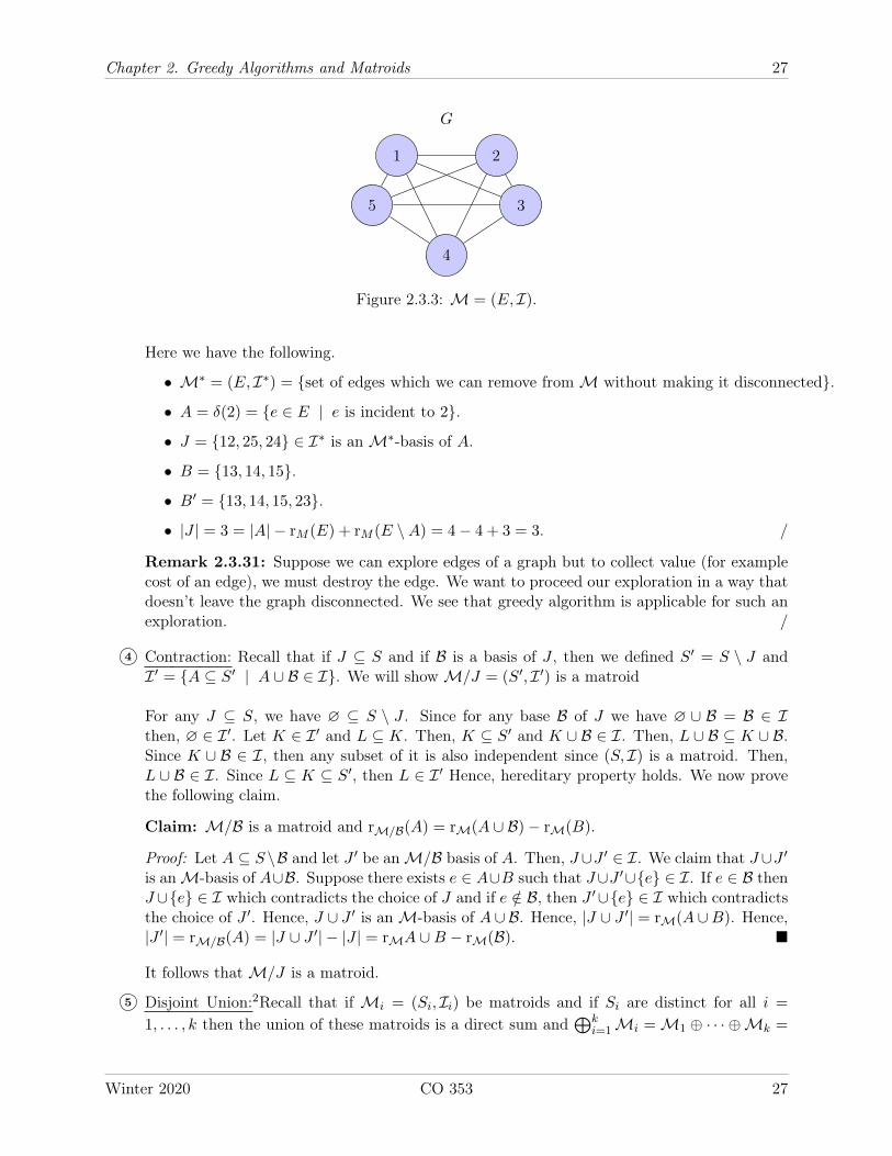
Example 2.3.30: Consider the graphical matroidM = (E, I) presented by G below.
Winter 2020 CO 353 26
Chapter 2. Greedy Algorithms and Matroids 27
1 2
3
4
5
G
Figure 2.3.3: M = (E, I).
Here we have the following.
• M∗ = (E, I∗) = set of edges which we can remove fromM without making it disconnected.
• A = δ(2) = e ∈ E | e is incident to 2.
• J = 12, 25, 24 ∈ I∗ is anM∗-basis of A.
• B = 13, 14, 15.
• B′ = 13, 14, 15, 23.
• |J | = 3 = |A| − rM (E) + rM (E \A) = 4− 4 + 3 = 3. /
Remark 2.3.31: Suppose we can explore edges of a graph but to collect value (for examplecost of an edge), we must destroy the edge. We want to proceed our exploration in a way thatdoesn’t leave the graph disconnected. We see that greedy algorithm is applicable for such anexploration. /
4 Contraction: Recall that if J ⊆ S and if B is a basis of J , then we defined S′ = S \ J andI ′ = A ⊆ S′ | A ∪ B ∈ I. We will showM/J = (S′, I ′) is a matroid
For any J ⊆ S, we have ∅ ⊆ S \ J . Since for any base B of J we have ∅ ∪ B = B ∈ Ithen, ∅ ∈ I ′. Let K ∈ I ′ and L ⊆ K. Then, K ⊆ S′ and K ∪ B ∈ I. Then, L ∪ B ⊆ K ∪ B.Since K ∪ B ∈ I, then any subset of it is also independent since (S, I) is a matroid. Then,L ∪ B ∈ I. Since L ⊆ K ⊆ S′, then L ∈ I ′ Hence, hereditary property holds. We now provethe following claim.
Claim: M/B is a matroid and rM/B(A) = rM(A ∪ B)− rM(B).
Proof: Let A ⊆ S \B and let J ′ be anM/B basis of A. Then, J∪J ′ ∈ I. We claim that J∪J ′is anM-basis of A∪B. Suppose there exists e ∈ A∪B such that J∪J ′∪e ∈ I. If e ∈ B thenJ ∪e ∈ I which contradicts the choice of J and if e /∈ B, then J ′∪e ∈ I which contradictsthe choice of J ′. Hence, J ∪ J ′ is anM-basis of A ∪ B. Hence, |J ∪ J ′| = rM(A ∪B). Hence,|J ′| = rM/B(A) = |J ∪ J ′| − |J | = rMA ∪B − rM(B).
It follows thatM/J is a matroid.
5 Disjoint Union:2Recall that if Mi = (Si, Ii) be matroids and if Si are distinct for all i =
1, . . . , k then the union of these matroids is a direct sum and⊕k
i=1Mi =M1 ⊕ · · · ⊕Mk =
Winter 2020 CO 353 27
Chapter 3. Dynamic Programming 28
M = (S, I). We will show thatM is a matroid where
S =k⋃i=1
Si, I =k⋃i=1
Ii and A ∈ I ′ ⇐⇒ A =k⋃i=1
Ai where Ai ∈ Ii for i = 1, . . . , k.
Exercise 2.3.32: ShowM = (S, I) is an independence system. /
Let A ⊆ S. Consider a basis B inM =M1 ⊕ · · · ⊕Mk of A. We have Bj = B ∪ Sj ∈ Ij . Bjis a basis of A ∩ Sj inMj . Since if Bj isn’t maximal, then there exists e ∈ (A ∩ Sj) \ Bj suchthat Bj ∪ e ∈ Ij which implies B ∪ e ∈ I but this contradicts the maximality of B. Wehave
B =k∑j=1
|Bj | =k∑j=1
r(A ∩ Sj).
Hence, every basis of A inM has same size. Hence,M is a matroid. /
2The part about disjoint union was covered in another lecture (L10, on Feb. 2020) but it was included in this listfor the sake of completeness.
Winter 2020 CO 353 28
Chapter 3. Dynamic Programming 29
Chapter 3 – Dynamic Programming
3.1 Weighted Interval Scheduling
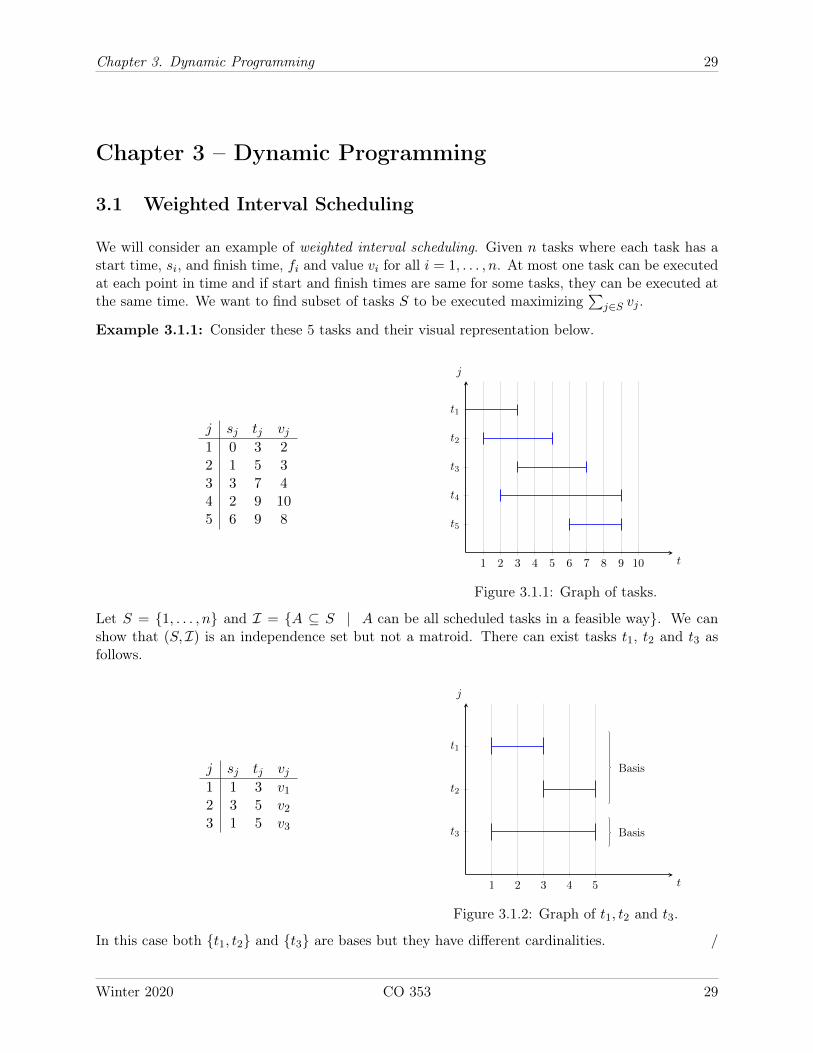
We will consider an example of weighted interval scheduling. Given n tasks where each task has astart time, si, and finish time, fi and value vi for all i = 1, . . . , n. At most one task can be executedat each point in time and if start and finish times are same for some tasks, they can be executed atthe same time. We want to find subset of tasks S to be executed maximizing
∑j∈S vj .
Example 3.1.1: Consider these 5 tasks and their visual representation below.
j sj tj vj1 0 3 22 1 5 33 3 7 44 2 9 105 6 9 8
1 2 3 4 5 6 7 8 9 10
t5
t4
t3
t2
t1
t
j
Figure 3.1.1: Graph of tasks.
Let S = 1, . . . , n and I = A ⊆ S | A can be all scheduled tasks in a feasible way. We canshow that (S, I) is an independence set but not a matroid. There can exist tasks t1, t2 and t3 asfollows.
j sj tj vj1 1 3 v1
2 3 5 v2
3 1 5 v3
1 2 3 4 5
t3
t2
t1
Basis
Basis
t
j
Figure 3.1.2: Graph of t1, t2 and t3.
In this case both t1, t2 and t3 are bases but they have different cardinalities. /
Winter 2020 CO 353 29
Chapter 3. Dynamic Programming 30
To solve this problem, we first assume the tasks are sorted with respecting to their finishing timein ascending order. If they were not ordered, we can order them in n log n time. We have n tasksordered in a way so that
f1 ≤ · · · ≤ fn.
Let
p(j) =
maxi < j | fi ≤ sj,0 if none exists for all j = 1, . . . , n.
So, p(j) is the last job that can be possibly scheduled with task j. In the above example we have
p(1) = 0, p(2) = 0, p(3) = 1, p(4) = 0, p(5) = 2.
We see that in an optimal solution, either we perform task n or we don’t. This is a very obviousobservation but it helps us construct algorithms to solve this problem.
Suppose we use task n. Then, we cannot use tasks p(n) + 1, . . . , n − 1 and we can use tasks1, . . . , p(n) since for all k = 1, . . . , p(n), we have fk ≤ fn−1 ≤ sn. So in this example, if we use task5, then we cannot use task 3 and task 4 but we can use tasks 1 and 2.
Let OPT(j) be the optimal value (not the optimal solution) for instance with tasks 1, . . . , j. Wehave
OPT(n) = vn + OPT(p(n)).
If we don’t use task n, then we have OPT(n− 1) = OPT(n). This approach allows us to break upthe problem into smaller problems. In general, when we implement the algorithm we have
OPT(0) = 0,
OPT(j) = maxvj + OPT(p(j)),OPT(j − 1).
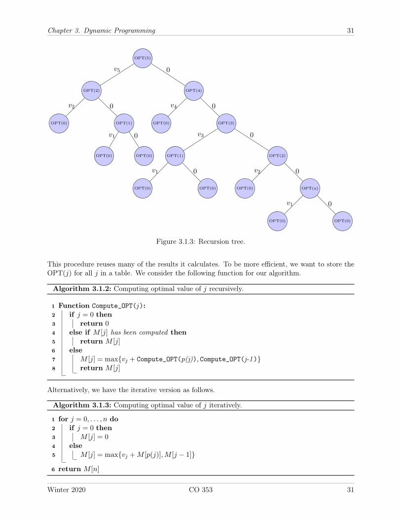
Using this approach we can compute a recursive OPT function with the following recursion tree.
Winter 2020 CO 353 30
Chapter 3. Dynamic Programming 31
OPT(5)
OPT(2) OPT(4)
OPT(0) OPT(1) OPT(0) OPT(3)
OPT(0) OPT(0) OPT(1) OPT(2)
OPT(0) OPT(0) OPT(0) OPT(x)
OPT(0) OPT(0)
v5 0
v2 0 v4 0
v1 0 v3 0
v1 0 v2 0
v1 0
Figure 3.1.3: Recursion tree.
This procedure reuses many of the results it calculates. To be more efficient, we want to store theOPT(j) for all j in a table. We consider the following function for our algorithm.
Algorithm 3.1.2: Computing optimal value of j recursively.
1 Function Compute_OPT(j):2 if j = 0 then3 return 04 else if M [j] has been computed then5 return M [j]6 else7 M [j] = maxvj + Compute_OPT(p(j)), Compute_OPT(j-1)8 return M [j]
Alternatively, we have the iterative version as follows.
Algorithm 3.1.3: Computing optimal value of j iteratively.
1 for j = 0, . . . , n do2 if j = 0 then3 M [j] = 04 else5 M [j] = maxvj +M [p(j)],M [j − 1]
6 return M [n]
Winter 2020 CO 353 31
Chapter 3. Dynamic Programming 32
This clearly runs in O(n). So we have a polytime algorithm to solve the problem. This process ofremembering (caching) results is called memoization . This algorithm gives optimal value. To getthe optimal solution, we store the decision algorithm made in S[j] as follows.
0 if vj +M [p(j)] > M [j − 1],
0 otherwise.
This gives us the following function algorithm.
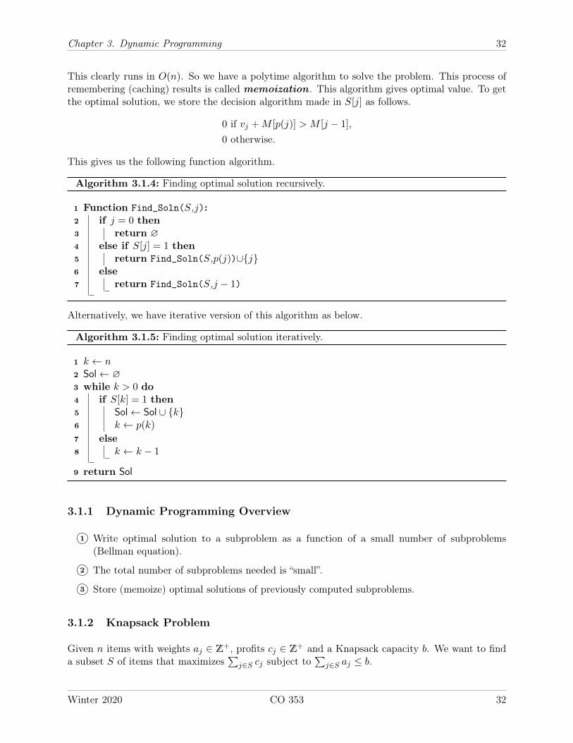
Algorithm 3.1.4: Finding optimal solution recursively.
1 Function Find_Soln(S,j):2 if j = 0 then3 return ∅4 else if S[j] = 1 then5 return Find_Soln(S,p(j))∪j6 else7 return Find_Soln(S,j − 1)
Alternatively, we have iterative version of this algorithm as below.
Algorithm 3.1.5: Finding optimal solution iteratively.
1 k ← n2 Sol← ∅3 while k > 0 do4 if S[k] = 1 then5 Sol← Sol ∪ k6 k ← p(k)
7 else8 k ← k − 1
9 return Sol
3.1.1 Dynamic Programming Overview
1 Write optimal solution to a subproblem as a function of a small number of subproblems(Bellman equation).
2 The total number of subproblems needed is “small”.
3 Store (memoize) optimal solutions of previously computed subproblems.
3.1.2 Knapsack Problem
Given n items with weights aj ∈ Z+, profits cj ∈ Z+ and a Knapsack capacity b. We want to finda subset S of items that maximizes
∑j∈S cj subject to
∑j∈S aj ≤ b.
Winter 2020 CO 353 32
Chapter 3. Dynamic Programming 33
WLOG, we order items 1, . . . , n and let OPT(i, w) be the optimal solution using items 1, . . . , iand backpack (knapsack) capacity w. We want to find OPT(n, b).
Case 1: OPT(i, w) uses i. Then, OPT(i, w) = OPT(i− 1, w − ai) + ci.Case 2: OPT(i, w) does not use i. Then, OPT(i, w) = OPT(i− 1, w).
• if i > 1 and ai ≤ w, then OPT(i, w) = maxOPT(i− 1, w − ai) + ci,OPT(i− 1, w),
• if i > 1 and 0 ≤ w ≤ ai, then OPT(i, w) = OPT(i− 1, w),
• if i = 1 and a1 ≤ w then OPT(i, w) = c1,
• otherwise, OPT(i, w) = 0.
Note that case 2 leads us to the following recursive definition
OPT(i, w) = max
max
OPT(i− 1, w − a1) + ci,
OPT(i− 1, w)
if i > 1 and ai ≤ w,
OPT(i− 1, w) if i > 1 and 0 ≤ w ≤ ai,ci if i = 1 and a1 ≤ w,0 otherwise.
Remark 3.1.6: OPT(i, w) has O(nb) entries and it takes O(1) time to compute. Hence, the run-time is O(nb).
We have 1 ≤ i ≤ n and 1 ≤ w ≤ b. This is not polytime since input size is measured in log b,not b. If b ∈ O(nk) for some fixed k, then the algorithm above is a pseudo-polytime algorithm. /
Definition 3.1.7: If a numeric algorithm runs in polytime in the numeric value of the input (thelargest integer present in the input) but not necessarily in the length of the input (the number ofbits to represent it) then it runs in pseudo-polynomial time (pseudo-polytime for short). /
One perspective on dynamic programming is that we have a memoization table to compute andeach table entry defines a state. Each state is determined by optimal solutions to some previousstates. Imparts a partial order on states.
Example 3.1.8: Consider the Knapsack problem with 3 items and capacity 5. Let
a1 = 2, c1 = 3,
a2 = 1, c2 = 2,
a3 = 5, c3 = 4.
We can construct a directed graph for this problem. Solution to our dynamic program can be foundby computing the longest path from s to t (or shortest path if we multiply costs by −1). /
3.1.3 Shortest Paths
Definition 3.1.9: A directed graph or digraph is an ordered pair D = (V,A) where V is a setof vertices and A is a set of ordered pairs of vertices, called arcs, directed edges or arrows.
Winter 2020 CO 353 33
Chapter 3. Dynamic Programming 34
An arc a = (x, y) is considered to be directed from x to y and
• x is called the tail of the arc and x is said to be a direct predecessor of y,
• y is called the head of the arc and y is said to be a direct successor of y and y is reachablefrom x. /
Given a directed graph D = (V,A) with non-negative arc costs ca for all a ∈ A and vertices s, t ∈ V .We want to find an s-t path P which minimizes
∑a∈A(P ) ca.
Definition 3.1.10: Let D = (V,A) be a directed graph. Let ∅ ⊆ S ⊆ V . We define
δ+(S) = (u, v) ∈ A | u ∈ S, v /∈ S (the set of arcs leaving S),
δ−(S) = (u, v) ∈ A | u /∈ S, v ∈ S (the set of arcs entering S).
The set δ(S) is called the cut induced by S. We have δ(S) = δ+(S) ∪ δ−(S). /
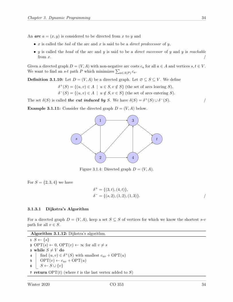
Example 3.1.11: Consider the directed graph D = (V,A) below.
s
1
2
3
4
t
Figure 3.1.4: Directed graph D = (V,A).
For S = 2, 3, 4 we have
δ+ = (3, t), (4, t),δ− = (s, 2), (1, 2), (1, 3). /
3.1.3.1 Dijkstra’s Algorithm
For a directed graph D = (V,A), keep a set S ⊆ S of vertices for which we know the shortest s-vpath for all v ∈ S.
Algorithm 3.1.12: Dijkstra’s algorithm.1 S ← s2 OPT(s)← 0, OPT(v)←∞ for all v 6= s3 while S 6= V do4 find (u, v) ∈ δ+(S) with smallest cuv + OPT(u)5 OPT(v)← cuv + OPT(u)6 S ← S ∪ v7 return OPT(t) (where t is the last vertex added to S)
Winter 2020 CO 353 34
Chapter 3. Dynamic Programming 35
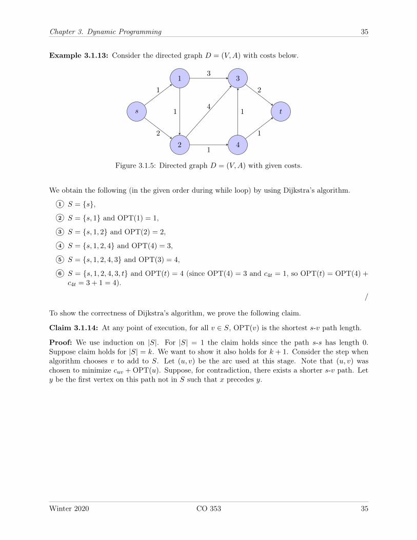
Example 3.1.13: Consider the directed graph D = (V,A) with costs below.
s
1
2
3
4
t
1
2
1
3
4
1
1
2
1
Figure 3.1.5: Directed graph D = (V,A) with given costs.
We obtain the following (in the given order during while loop) by using Dijkstra’s algorithm.
1 S = s,
2 S = s, 1 and OPT(1) = 1,
3 S = s, 1, 2 and OPT(2) = 2,
4 S = s, 1, 2, 4 and OPT(4) = 3,
5 S = s, 1, 2, 4, 3 and OPT(3) = 4,
6 S = s, 1, 2, 4, 3, t and OPT(t) = 4 (since OPT(4) = 3 and c4t = 1, so OPT(t) = OPT(4) +c4t = 3 + 1 = 4).
/
To show the correctness of Dijkstra’s algorithm, we prove the following claim.
Claim 3.1.14: At any point of execution, for all v ∈ S, OPT(v) is the shortest s-v path length.
Proof: We use induction on |S|. For |S| = 1 the claim holds since the path s-s has length 0.Suppose claim holds for |S| = k. We want to show it also holds for k + 1. Consider the step whenalgorithm chooses v to add to S. Let (u, v) be the arc used at this stage. Note that (u, v) waschosen to minimize cuv + OPT(u). Suppose, for contradiction, there exists a shorter s-v path. Lety be the first vertex on this path not in S such that x precedes y.
Winter 2020 CO 353 35
Chapter 3. Dynamic Programming 36
s
u
x
S
v
y
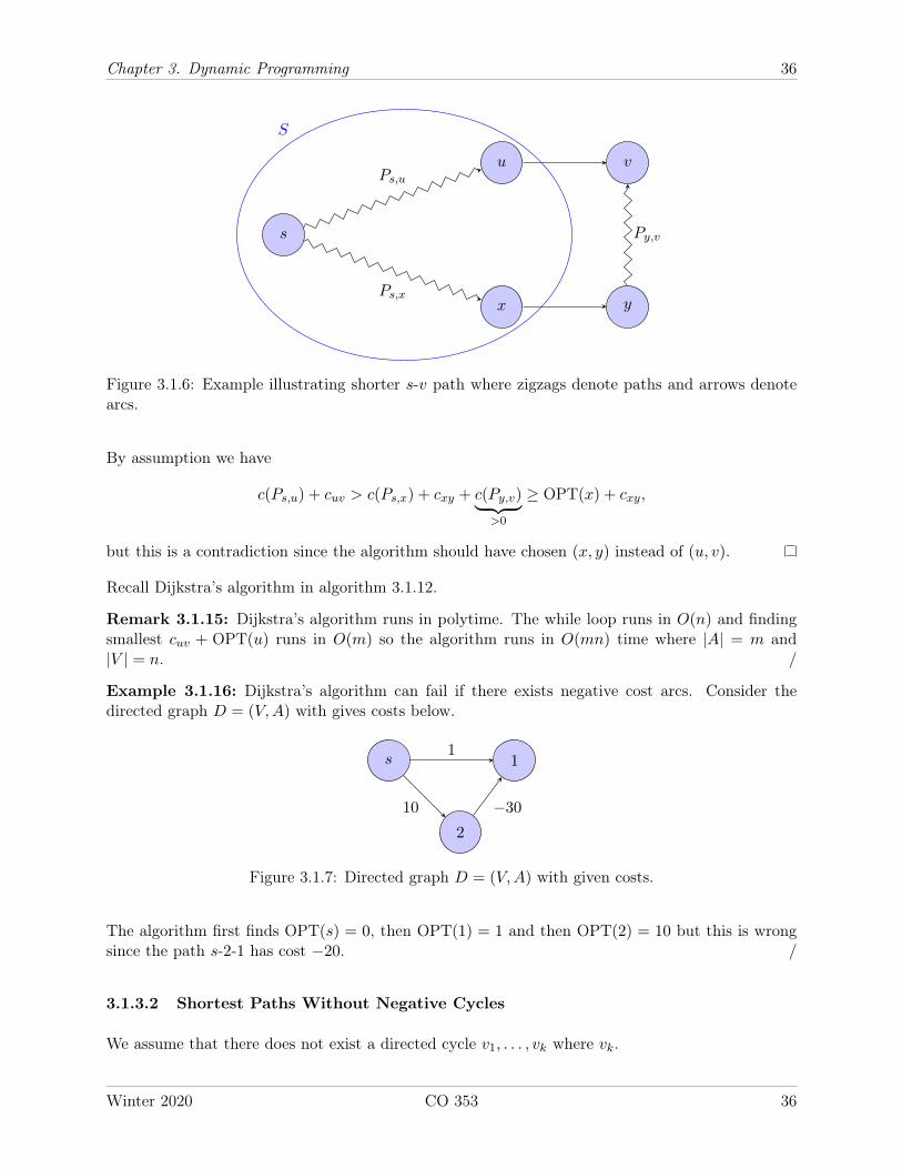
Ps,u
Ps,x
Py,v
Figure 3.1.6: Example illustrating shorter s-v path where zigzags denote paths and arrows denotearcs.
By assumption we have
c(Ps,u) + cuv > c(Ps,x) + cxy + c(Py,v)︸ ︷︷ ︸>0
≥ OPT(x) + cxy,
but this is a contradiction since the algorithm should have chosen (x, y) instead of (u, v).
Recall Dijkstra’s algorithm in algorithm 3.1.12.
Remark 3.1.15: Dijkstra’s algorithm runs in polytime. The while loop runs in O(n) and findingsmallest cuv + OPT(u) runs in O(m) so the algorithm runs in O(mn) time where |A| = m and|V | = n. /
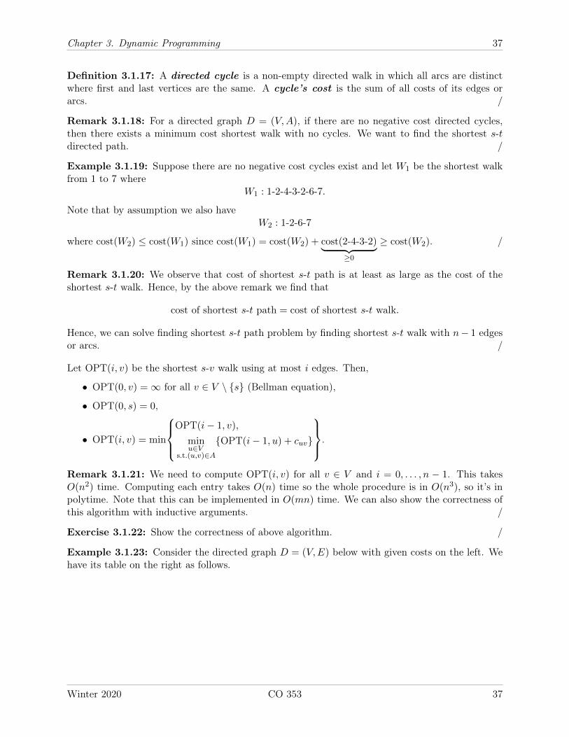
Example 3.1.16: Dijkstra’s algorithm can fail if there exists negative cost arcs. Consider thedirected graph D = (V,A) with gives costs below.
s 1
2
1
10 −30
Figure 3.1.7: Directed graph D = (V,A) with given costs.
The algorithm first finds OPT(s) = 0, then OPT(1) = 1 and then OPT(2) = 10 but this is wrongsince the path s-2-1 has cost −20. /
3.1.3.2 Shortest Paths Without Negative Cycles
We assume that there does not exist a directed cycle v1, . . . , vk where vk.
Winter 2020 CO 353 36
Chapter 3. Dynamic Programming 37
Definition 3.1.17: A directed cycle is a non-empty directed walk in which all arcs are distinctwhere first and last vertices are the same. A cycle’s cost is the sum of all costs of its edges orarcs. /
Remark 3.1.18: For a directed graph D = (V,A), if there are no negative cost directed cycles,then there exists a minimum cost shortest walk with no cycles. We want to find the shortest s-tdirected path. /
Example 3.1.19: Suppose there are no negative cost cycles exist and let W1 be the shortest walkfrom 1 to 7 where
W1 : 1-2-4-3-2-6-7.
Note that by assumption we also haveW2 : 1-2-6-7
where cost(W2) ≤ cost(W1) since cost(W1) = cost(W2) + cost(2-4-3-2)︸ ︷︷ ︸≥0
≥ cost(W2). /
Remark 3.1.20: We observe that cost of shortest s-t path is at least as large as the cost of theshortest s-t walk. Hence, by the above remark we find that
cost of shortest s-t path = cost of shortest s-t walk.
Hence, we can solve finding shortest s-t path problem by finding shortest s-t walk with n− 1 edgesor arcs. /
Let OPT(i, v) be the shortest s-v walk using at most i edges. Then,
• OPT(0, v) =∞ for all v ∈ V \ s (Bellman equation),
• OPT(0, s) = 0,
• OPT(i, v) = min
OPT(i− 1, v),
minu∈V
s.t.(u,v)∈A
OPT(i− 1, u) + cuv
.
Remark 3.1.21: We need to compute OPT(i, v) for all v ∈ V and i = 0, . . . , n − 1. This takesO(n2) time. Computing each entry takes O(n) time so the whole procedure is in O(n3), so it’s inpolytime. Note that this can be implemented in O(mn) time. We can also show the correctness ofthis algorithm with inductive arguments. /
Exercise 3.1.22: Show the correctness of above algorithm. /
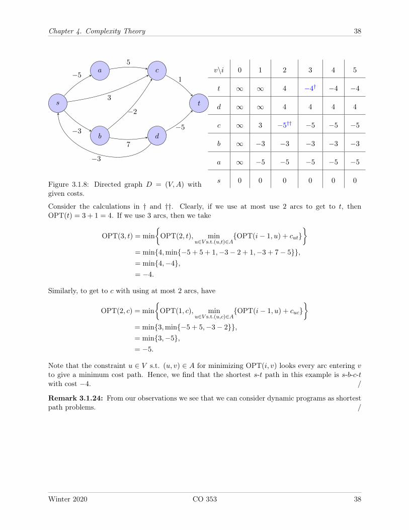
Example 3.1.23: Consider the directed graph D = (V,E) below with given costs on the left. Wehave its table on the right as follows.
Winter 2020 CO 353 37
Chapter 4. Complexity Theory 38
s
a
b
c
d
t
−5
−3
3
−3
5
−2
7
1
−5
Figure 3.1.8: Directed graph D = (V,A) withgiven costs.
v\i 0 1 2 3 4 5
t ∞ ∞ 4 −4† −4 −4
d ∞ ∞ 4 4 4 4
c ∞ 3 −5†† −5 −5 −5
b ∞ −3 −3 −3 −3 −3
a ∞ −5 −5 −5 −5 −5
s 0 0 0 0 0 0
Consider the calculations in † and ††. Clearly, if we use at most use 2 arcs to get to t, thenOPT(t) = 3 + 1 = 4. If we use 3 arcs, then we take
OPT(3, t) = min
OPT(2, t), min
u∈V s.t.(u,t)∈AOPT(i− 1, u) + cut
= min4,min−5 + 5 + 1,−3− 2 + 1,−3 + 7− 5,= min4,−4,= −4.
Similarly, to get to c with using at most 2 arcs, have
OPT(2, c) = min
OPT(1, c), min
u∈V s.t.(u,c)∈AOPT(i− 1, u) + cuc
= min3,min−5 + 5,−3− 2,= min3,−5,= −5.
Note that the constraint u ∈ V s.t. (u, v) ∈ A for minimizing OPT(i, v) looks every arc entering vto give a minimum cost path. Hence, we find that the shortest s-t path in this example is s-b-c-twith cost −4. /
Remark 3.1.24: From our observations we see that we can consider dynamic programs as shortestpath problems. /
Winter 2020 CO 353 38
Chapter 4. Complexity Theory 39
Chapter 4 – Complexity Theory
Complexity theory tries to address the question of if there exists a polytime algorithm to solve aproblem of interest.
4.1 Polytime Reductions
Definition 4.1.1: Given two problems X and Y , we say Y is polytime reducible to X, denotedby Y ≤p X, if there exists an algorithm to solve instances of Y of input size n that does
1 poly(n) basic operations,
2 poly(n) many calls to an algorithm that solves problem X. /
Example 4.1.2: We have seen that
finding maximum cost forest ≤p MST problem, andMST problem ≤p finding maximum cost forest.
/
Remark 4.1.3: If there exists a polytime algorithm to solve X and Y ≤p X, then there exists apolytime algorithm to solve Y . Conversely, if there does not exist a polytime algorithm to solve Yand if Y ≤p X, then there does not exist a polytime algorithm to solve X.
This definition implies that input to solving problem X must be poly(k) in time. /
4.1.1 Examples of Polytime Reducible Problems
Definition 4.1.4: Let G = (V,E) be a graph. An independent set S ⊆ V in G is a set suchthat for all u, v ∈ S, we have uv /∈ E. That is, there are no edges that connects any two vertices inS. /
Definition 4.1.5: Let G = (V,E) be a graph. A clique S ⊆ V in G is a set such that for alldistinct u, v ∈ S, we have uv ∈ S. That is, every vertex in S is connected. /
Example 4.1.6: Consider the graph G = (V,E) below.
Winter 2020 CO 353 39
Chapter 4. Complexity Theory 40
1 2
3 4
5
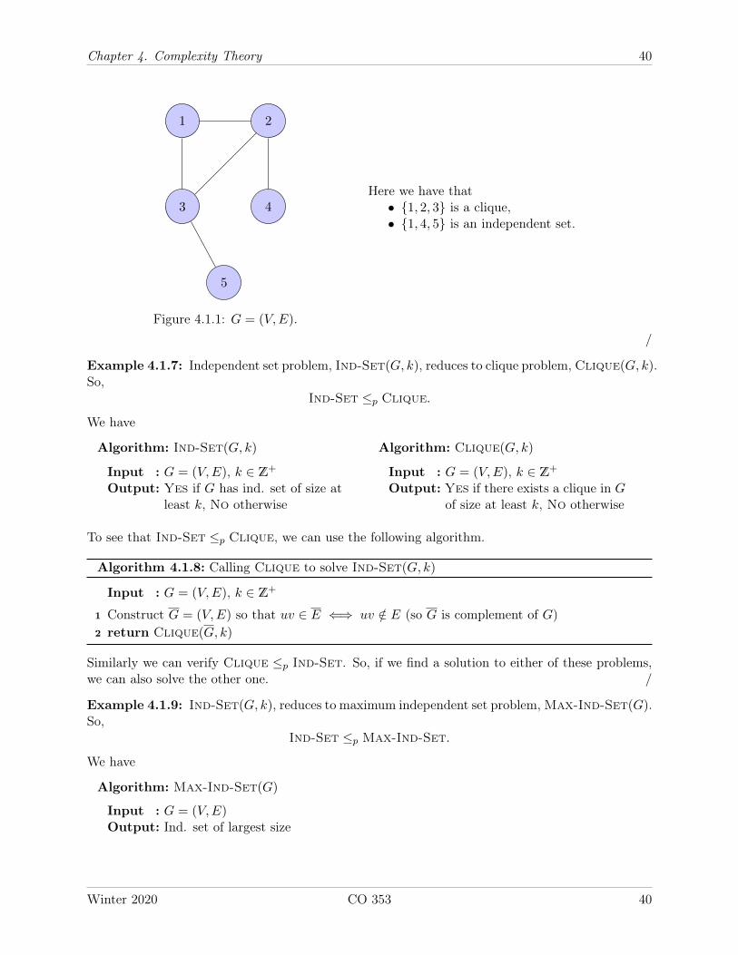
Figure 4.1.1: G = (V,E).
Here we have that• 1, 2, 3 is a clique,• 1, 4, 5 is an independent set.
/
Example 4.1.7: Independent set problem, Ind-Set(G, k), reduces to clique problem, Clique(G, k).So,
Ind-Set ≤p Clique.
We have
Algorithm: Ind-Set(G, k)
Input : G = (V,E), k ∈ Z+
Output: Yes if G has ind. set of size atleast k, No otherwise
Algorithm: Clique(G, k)
Input : G = (V,E), k ∈ Z+
Output: Yes if there exists a clique in Gof size at least k, No otherwise
To see that Ind-Set ≤p Clique, we can use the following algorithm.
Algorithm 4.1.8: Calling Clique to solve Ind-Set(G, k)
Input : G = (V,E), k ∈ Z+
1 Construct G = (V,E) so that uv ∈ E ⇐⇒ uv /∈ E (so G is complement of G)2 return Clique(G, k)
Similarly we can verify Clique ≤p Ind-Set. So, if we find a solution to either of these problems,we can also solve the other one. /
Example 4.1.9: Ind-Set(G, k), reduces to maximum independent set problem, Max-Ind-Set(G).So,
Ind-Set ≤p Max-Ind-Set.
We have
Algorithm: Max-Ind-Set(G)
Input : G = (V,E)Output: Ind. set of largest size
Winter 2020 CO 353 40
Chapter 4. Complexity Theory 41
To see that Ind-Set ≤p Max-Ind-Set, we can use the following algorithm.
Algorithm 4.1.10: Calling Max-Ind-Set to solve Ind-Set(G, k)
Input : G = (V,E), k ∈ Z+
1 S ←Max-Ind-Set(G)2 return Yes ⇐⇒ |S| ≥ k
/
Definition 4.1.11: Let G = (V,E) be a graph. A vertex cover S ⊆ V of G is a set such thatfor all e ∈ E, we have |e ∩ S| ≥ 1. That is, every edge of G has an end point in S. /
Example 4.1.12: Consider the graph G = (V,E) below.
1 2
3 4
5
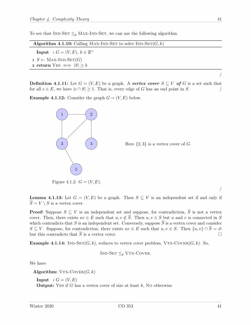
Figure 4.1.2: G = (V,E).
Here 2, 3 is a vertex cover of G.
/
Lemma 4.1.13: Let G = (V,E) be a graph. Then S ⊆ V is an independent set if and only ifS = V \ S is a vertex cover.
Proof: Suppose S ⊆ V is an independent set and suppose, for contradiction, S is not a vertexcover. Then, there exists uv ∈ E such that u, v /∈ S. Then u, v ∈ S but u and v is connected in Swhich contradicts that S is an independent set. Conversely, suppose S is a vertex cover and considerS ⊆ V . Suppose, for contradiction, there exists uv ∈ E such that u, v ∈ S. Then u, v ∩ S = ∅but this contradicts that S is a vertex cover.
Example 4.1.14: Ind-Set(G, k), reduces to vertex cover problem, Vtx-Cover(G, k). So,
Ind-Set ≤p Vtx-Cover.
We have
Algorithm: Vtx-Cover(G, k)
Input : G = (V,E)Output: Yes if G has a vertex cover of size at least k, No otherwise
Winter 2020 CO 353 41
Chapter 4. Complexity Theory 42
To see that Ind-Set ≤p Vtx-Cover, we can use the following algorithm.
Algorithm 4.1.15: Calling Vtx-Cover to solve Ind-Set(G, k)
Input : G = (V,E), k ∈ Z+
1 Call Vtx-Cover(G,n− k) where |V | = n2 return Vtx-Cover(G,n− k)
/
Definition 4.1.16: Let U = 1, . . . , n be a finite set and let C be a collection of subsets of U . Wesay C is a set cover of U if
⋃S∈C S = U . Given a collection subsets S1, . . . , Sm ⊆ U = 1, . . . , n,
the set cover problem tries to find the smallest set cover I of U such that⋃i∈I Si = U . /
Example 4.1.17: Vtx-Cover(G, k), reduces to set cover problem, Set-Cover(x). So,
Vtx-Cover ≤p Set-Cover.
We have
Algorithm: Set-Cover(U, S1, . . . , Sm, k)
Input : U, S1, . . . , Sm, k ∈ Z+ where U = 1, . . . , n and Si ⊆ U for i = 1, . . . ,mOutput: Yes if I ⊆ 1, . . . ,m such that
⋃i∈I Si = U and |I| ≤ k, No otherwise
To see that Vtx-Cover ≤p Set-Cover, we can use the following algorithm.
Algorithm 4.1.18: Calling Set-Cover to solve Vtx-Cover(G, k)
Input : G = (V,E), k ∈ Z+
1 U ← E2 Sv ← e ∈ E | e ∈ δ(v), that is, Sv is the set of edges that are incident to v for all v ∈ V3 Call Set-Cover(U, Svv∈V , k)4 return Set-Cover(U, Svv∈V , k)
Since Ind-Set ≤p Vtx-Cover and Vtx-Cover ≤p Set-Cover then Ind-Set ≤p Set-Cover./
Definition 4.1.19: A clause c is a finite disjunction of terms ti where each term ti is either xjor its complement, xj . i.e. each term is a literal . We say the clause c is satisfied if given anassignment of values t1, . . . , t` at least one of ti is true where
c = t1 ∨ · · · ∨ t`.
A satisfying assignment in a problem with clauses c1, . . . , cm is an assignment that satisfies allci for i = 1, . . . ,m. /
Example 4.1.20: Consider literals x1, x2, x3, x4 and clauses
c1 = x1 ∨ x2,
c2 = x1 ∨ x3 ∨ x4,
c3 = x3 ∨ x4.
The assignment x = (1, 0, 0, 1) is not a satisfying assignment because it
Winter 2020 CO 353 42
Chapter 4. Complexity Theory 43
• satisfies c1 since 1 ∨ 1 = 1,
• satisfies c2 since 0 ∨ 1 ∨ 1 = 1,
• does not satisfy c3 since 0 ∨ 0 = 0.
The assignment x = (1, 0, 1, 1) is a satisfying assignment since it satisfies c1, c2 and c3. /
Example 4.1.21: 3-Sat problem reduces to Ind-Set. So,
3-Sat ≤p Ind-Set.
We have
Algorithm: 3-Sat(x1, . . . , xn, c1, . . . , cm) where
Input : x1, . . . , xn (literals) and c1, . . . , cm clauses of length 3.Output: Yes if there exists a satisfying assignment for all ci for i = 1, . . . ,m, No otherwise
Before verifying this, we show an example of converting a 3-Sat problem into an independent setproblem. /
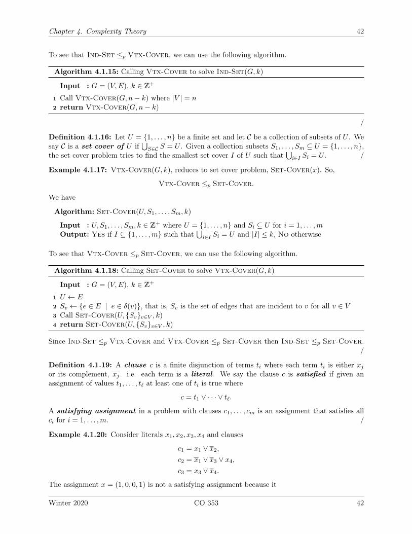
Example 4.1.22: Let x1, . . . , x5 be literals with clauses of length 3 as follows.
c1 = x1 ∨ x2 ∨ x3,
c2 = x2 ∨ x4 ∨ x5,
c3 = x1 ∨ x2 ∨ x5.
Here each clause has length 3, so each clause has 3 terms (literals). For each j-th literal in eachclause ci, we put a vertex vij and connect vertices that belong to same clause with an edge asfollows.
v11
v12 v13
v21
v22 v23
v31
v32 v33
Figure 4.1.3: Constructing a graph from SAT problem.
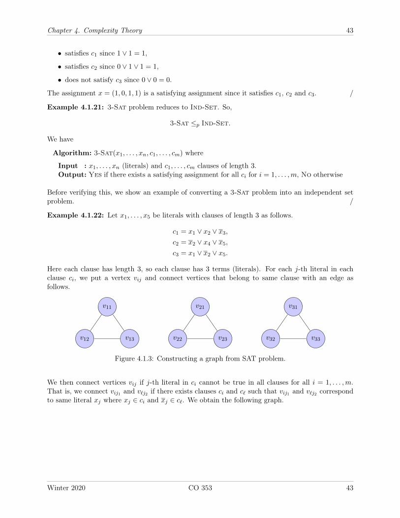
We then connect vertices vij if j-th literal in ci cannot be true in all clauses for all i = 1, . . . ,m.That is, we connect vij1 and v`j2 if there exists clauses ci and c` such that vij1 and v`j2 correspondto same literal xj where xj ∈ ci and xj ∈ c`. We obtain the following graph.
Winter 2020 CO 353 43
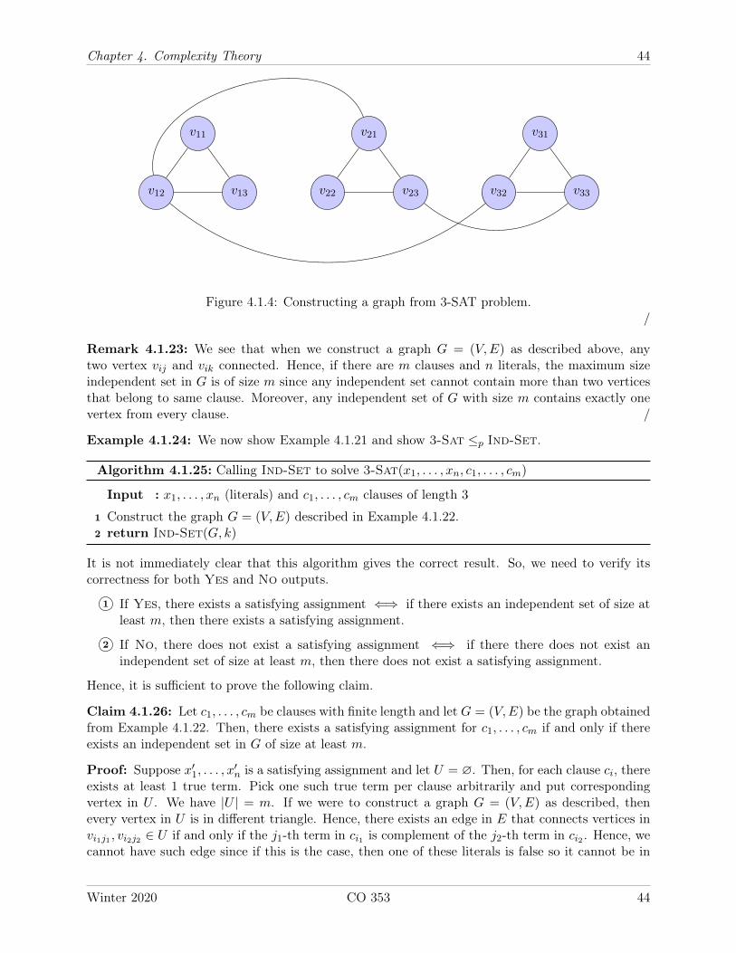
Chapter 4. Complexity Theory 44
v11
v12 v13
v21
v22 v23
v31
v32 v33
Figure 4.1.4: Constructing a graph from 3-SAT problem./
Remark 4.1.23: We see that when we construct a graph G = (V,E) as described above, anytwo vertex vij and vik connected. Hence, if there are m clauses and n literals, the maximum sizeindependent set in G is of size m since any independent set cannot contain more than two verticesthat belong to same clause. Moreover, any independent set of G with size m contains exactly onevertex from every clause. /
Example 4.1.24: We now show Example 4.1.21 and show 3-Sat ≤p Ind-Set.
Algorithm 4.1.25: Calling Ind-Set to solve 3-Sat(x1, . . . , xn, c1, . . . , cm)
Input : x1, . . . , xn (literals) and c1, . . . , cm clauses of length 3
1 Construct the graph G = (V,E) described in Example 4.1.22.2 return Ind-Set(G, k)
It is not immediately clear that this algorithm gives the correct result. So, we need to verify itscorrectness for both Yes and No outputs.
1 If Yes, there exists a satisfying assignment ⇐⇒ if there exists an independent set of size atleast m, then there exists a satisfying assignment.
2 If No, there does not exist a satisfying assignment ⇐⇒ if there there does not exist anindependent set of size at least m, then there does not exist a satisfying assignment.
Hence, it is sufficient to prove the following claim.
Claim 4.1.26: Let c1, . . . , cm be clauses with finite length and let G = (V,E) be the graph obtainedfrom Example 4.1.22. Then, there exists a satisfying assignment for c1, . . . , cm if and only if thereexists an independent set in G of size at least m.
Proof: Suppose x′1, . . . , x′n is a satisfying assignment and let U = ∅. Then, for each clause ci, thereexists at least 1 true term. Pick one such true term per clause arbitrarily and put correspondingvertex in U . We have |U | = m. If we were to construct a graph G = (V,E) as described, thenevery vertex in U is in different triangle. Hence, there exists an edge in E that connects vertices invi1j1 , vi2j2 ∈ U if and only if the j1-th term in ci1 is complement of the j2-th term in ci2 . Hence, wecannot have such edge since if this is the case, then one of these literals is false so it cannot be in
Winter 2020 CO 353 44
Chapter 4. Complexity Theory 45
U . Hence, U is an independent set in G of size m.
Conversely, let U ⊆ V be an independent set in G of size m. Then, U contains exactly one vertexfrom each clause and there does not exist an edge that connects any two vertices in U . Hence, nopair of vertices in U can correspond to xj and xj for any literal xj . Note that any independent setI in G of size less than m cannot contain one vertex from each clause since there are m clauses.Consider the assignment x′1, . . . , x′n obtained by setting terms corresponding to vertices in U as trueand other terms as false. This is a satisfying assignment since every vertex in U corresponds todifferent clause and since |U | = m, then each clause is satisfied. Moreover, we cannot have set bothxj and xj to true at the same time since if there exists a vertex corresponding to xj , say u1 ∈ U ,then there does not exists u2 ∈ U that correspond to xj because there exists an edge in E thatconnects u1 and u2 in G and U is an independent set.
Hence, by the claim above, 3-Sat ≤p Ind-Set. /
4.1.2 Classes of P and NP
Definition 4.1.27: A problem X is called a decision problem if its outputs are Yes or No. Theset (or class) of all decision problems for that are solvable in polytime is called P. /
Example 4.1.28: The problems 3-Sat, Ind-Set, Vtx-Cover, Set-Cover etc. are all decisionproblems. MST problem (that gives MST of a graph) is not a decision problem but the decisionversion of the MST problem (that answers if there exists a spanning tree of cost at most k ∈ Z) isa decision problem.
Decision-MST and Decision-Max-Cost-Forest are problems in P but it is not known if Ind-Set is in P. /
Definition 4.1.29: A certifier C(s, t) for a decision problem X is an algorithm that for everyinput s to X,
X(s) is Yes ⇐⇒ there exists t such that C(s, t) returns Yes.
In this case, t is called a Yes certificate . /
Example 4.1.30: Consider the decision problem Ind-Set(G, k). If the answer for this problemis yes for given a graph G = (V,E) and k ∈ Z+, then one way to validate this answer is toprovide U ⊆ V such that |U | ≥ k and U is independent. In this case, U is a Yes certificate. For3-Sat(x1, . . . , xn, c1, . . . , cm), a Yes certificate is a satisfying assignment x′1, . . . , x′n. /
Definition 4.1.31: A certifier C(s, t) for a decision problem X is called a polytime certifier if
1 size of t is polynomial in size of s and
2 C(s, t) does polynomially many basic operations in size of s. /
Definition 4.1.32: Let X be a decision problem. We say X is in non-deterministic polytime ifthere exists a polytime certifier for X. The set (or class) of algorithms that are in non-deterministicpolytime is called NP. Equivalently, X ∈ NP if there exists a polytime non-deterministic algorithmthat solves X.
Winter 2020 CO 353 45
Chapter 4. Complexity Theory 46
A non-deterministic algorithm is an algorithm that, even for the same input, can exhibit differ-ent behaviors on different runs, as opposed to a deterministic algorithm. An algorithm that solvesa problem in non-deterministic polynomial time can run in polynomial time or exponential timedepending on the choices it makes during execution. The non-deterministic algorithms are oftenused to find an approximation to a solution, when the exact solution would be too costly to obtainusing a deterministic one. /
Remark 4.1.33: Let X be a decision problem. If X ∈ P, then X is solvable in polytime. Hence,its certifier is also in polytime (we can just take its certifier as itself). Hence X ∈ NP. Hence,P ⊆ NP. It is not known if NP ⊆ P but the consensus is NP 6⊆ P. /
4.1.3 NP-Completeness
Definition 4.1.34: A decision problem X is called NP-complete if
1 X ∈ NP, and
2 for all Y ∈ NP, Y ≤p X (so X is at least as hard as any problem in NP-class). /
Theorem 4.1.35: Let X be NP-complete. There exists a polytime algorithm to solve X if andonly if P = NP.
Proof: Suppose X is a polytime algorithm. Since for all Y ∈ NP we have Y ≤p X, then we canuse the polytime algorithm which we use to solve X to solve Y in polytime. Hence, NP ⊆ P. SoP = NP. Conversely, suppose P = NP. Since X ∈ NP then X ∈ P.
Theorem 4.1.36 (Cook-Levin ’71): Circuit-Sat problem is NP-complete.
Proof: Proof is beyond the scope of this course. We provide this theorem to show existence ofNP-complete problems. /
Theorem 4.1.37: Let X and Y be decision problems. If Y is NP-complete and if
1 X ∈ NP and
2 Y ≤p X (that is, we can solve Y using X as a subroutine),
then X is NP-complete.
Proof: Let Z ∈ NP be arbitrary. Since Y is NP-complete then Z ≤p Y . Since Y ≤p X, then wehave Z ≤p Y ≤p X for any Z ∈ NP and since X ∈ NP, then X is NP-complete.
Remark 4.1.38: Without proof, we state Circuit-Sat ≤p 3-Sat. This shows 3-Sat is NP-complete since
1 Circuit-Sat is NP-complete by Cook-Levin ’71 theorem,
2 3-Sat ∈ NP. Let x′1, . . . , x′n be a certificate for 3-Sat. For each clause ci, we can check if ci issatisfied by checking each term in ci. Since each ci has length 3 and since there are m clauses,then the certifier for 3-Sat is in polytime. /
Remark 4.1.39: Note that when showing Y ≤p X, we need to show reduction is correct in bothYes and No outputs. /
Winter 2020 CO 353 46
Chapter 4. Complexity Theory 47
Example 4.1.40: Subset-Sum is NP-complete. — This example is long and will be writtenlater. /
4.1.4 NP-Hardness
Winter 2020 CO 353 47
Index
Aacyclic, 4arc, 33
Bbasic operations, 2basis
of a matroid, 21big-O, 1Big-omega, 2Big-theta, 2
Ccertifier, 45
polytime, 45characteristic vector, 15clause, 42
satisfies, 42clique, 39cut induced by a vertex set, 8cycle, 4
cost of, 37directed, 37Hamiltonian, 17
cyclic, 4
Ddecision problems, 45
set of, 45disjoint union, 25
Eedge, 3
Ggraph, 3
connected, 4connected component, 5directed, 33forest, 13
greedy algorithm, 17ground set, 20
Iindependence system, 20independent set, 20
independent set (graph theory), 39
Lliteral, 42
Mmatroid, 20
graphic, 22linear, 21
maximal, 5memoization, 31
Ppath, 4polytime algorithm, 2
pseudo, 33polytime reducible problems, 39
Rrank
of a matroid, 21rank quotient, 23runtime of an algorithm, 2
Sset cover, 42size of input, 1subgraph, 5
induced by, 5
Ttree, 6
spanning, 6
Vvertex, 3
adjacent, 4endpoints, 4
vertex cover, 41
Wwalk, 4
closed, 4
YYes certifier, 45
48