Embed Size (px)
Citation preview
Groundwater Vistas Version 3 Page 1
TABLE OF CONTENTS Introduction ....................................................................................................................... 1
What is Groundwater Vistas?.......................................................................................... 1 Package Contents and Installation................................................................................... 3
What Comes with GV? ............................................................................................... 3 Installing GV............................................................................................................... 3 Uninstalling Groundwater Vistas ................................................................................ 4
Licensing ......................................................................................................................... 4 Special Considerations for Windows 2000 and NT.................................................... 4
What’s New in Version 3? .............................................................................................. 4 How to Use This Manual ................................................................................................ 5 Technical Support & Updates ......................................................................................... 6
Concepts ............................................................................................................................. 7 Introduction ..................................................................................................................... 7 GV Files .......................................................................................................................... 7 The Finite-Difference Grid.............................................................................................. 7 Coordinate Systems....................................................................................................... 10 Digitized Maps .............................................................................................................. 11 Boundary Conditions..................................................................................................... 12
Constant Head Boundaries ........................................................................................ 12 Constant Flux Boundaries ......................................................................................... 12 Head-dependent Flux Boundaries ............................................................................. 12 Grid-Independent Boundaries ................................................................................... 13 Use of Boundary Conditions ..................................................................................... 13
Transient Modeling ....................................................................................................... 14 Zone Concept for Aquifer Properties ............................................................................ 14 Using Variable Layer Elevations .................................................................................. 17 Calibration Targets........................................................................................................ 19
Tutorial............................................................................................................................. 21 Introduction ................................................................................................................... 21 Starting a New Model ................................................................................................... 21 Adding Rows & Columns ............................................................................................. 24 Adding Boundary Conditions ....................................................................................... 25 Creating MODFLOW Datasets..................................................................................... 27 Other Types of Plots...................................................................................................... 29 Particle-Tracking in GV................................................................................................ 31 Model Calibration with GV........................................................................................... 34 Automated Calibration .................................................................................................. 36 Editing Aquifer Properties ............................................................................................ 42 Setting Up a Transient Model ....................................................................................... 44 Transport Modeling with MT3D................................................................................... 47 Stochastic MODFLOW................................................................................................. 50
Stochastic MODFLOW............................................................................................. 51 Stochastic MODPATH.............................................................................................. 54 Stochastic MT3D....................................................................................................... 55

Groundwater Vistas Version 3 Page 2
Constructing a 3D Model with Sloping Layers............................................................. 59 Additional Tutorials ...................................................................................................... 61
Designing Models ............................................................................................................ 63 Introduction ................................................................................................................... 63 General Steps to Apply GV........................................................................................... 63
Beginning A New Model Design .............................................................................. 63 Digitized Map Files................................................................................................... 67
Designing The Finite-Difference Grid .......................................................................... 68 Concepts .................................................................................................................... 68 Working with Rows and Columns ............................................................................ 68 Automating Grid Design ........................................................................................... 70 Working with Layers................................................................................................. 71 Using Variable Layer Elevations .............................................................................. 71 Specifying Exact Layer Elevations ........................................................................... 73
Assigning Boundary Conditions ................................................................................... 75 Concepts .................................................................................................................... 75 Choice of Boundary Condition Type ........................................................................ 76 Displaying Boundary Cells ....................................................................................... 77 Inserting Boundary Cells........................................................................................... 77 Deleting Boundary Conditions.................................................................................. 80 Editing Boundary Conditions.................................................................................... 80 Importing Boundary Conditions from a File............................................................. 81 Grid-Independent Boundary Conditions ................................................................... 82
Defining Aquifer Properties .......................................................................................... 84 Concepts .................................................................................................................... 84 Specifying Zone Values ............................................................................................ 85 Assigning Zone Numbers to Cells ............................................................................ 87 Importing Properties from Files ................................................................................ 88
Saving The Model Design............................................................................................. 93 Running Simulations....................................................................................................... 95
Introduction ................................................................................................................... 95 Model-Specific Preprocessing....................................................................................... 95 Creating Data Sets......................................................................................................... 95
MODFLOW .............................................................................................................. 96 MODFLOW2000 ...................................................................................................... 98 MODFLOWT............................................................................................................ 99 MODFLOW-SURFACT........................................................................................... 99 MODPATH ............................................................................................................. 100 MT3D...................................................................................................................... 100 PATH3D.................................................................................................................. 101
Running Simulations ................................................................................................... 101 Assumptions Used in Creating Data Files .................................................................. 102
MODFLOW and MODFLOW2000........................................................................ 102 MODPATH ............................................................................................................. 105 MT3D...................................................................................................................... 106 RT3D....................................................................................................................... 107
Groundwater Vistas Version 3 Page 3
Processing Simulation Results ..................................................................................... 109 Introduction ................................................................................................................. 109 Importing Model Results............................................................................................. 109
MODFLOW and MT3D.......................................................................................... 109 Importing MODPATH Pathlines ............................................................................ 112 Importing PATH3D Pathlines................................................................................. 112
The Cross-Section View.............................................................................................. 112 Contour Maps.............................................................................................................. 112 Color Floods................................................................................................................ 114 Velocity Vectors.......................................................................................................... 115 Particle Traces ............................................................................................................. 115 Mass Balance Analysis................................................................................................ 116
Required Data Files................................................................................................. 116 Displaying Mass Balance Data ............................................................................... 117 Digitize Feature ....................................................................................................... 118
Hydrographs ................................................................................................................ 119 Profiles ........................................................................................................................ 119 Charts in Groundwater Vistas ..................................................................................... 120 Legends ....................................................................................................................... 122 Printing Graphics......................................................................................................... 123
Plan View ................................................................................................................ 123 Cross-Section View................................................................................................. 124 Creating a Plot Border............................................................................................. 124 Charts ...................................................................................................................... 127
Matrix Calculator ........................................................................................................ 127 Exporting Data ............................................................................................................ 129 File Operations ............................................................................................................ 129 Graphics for Calibration.............................................................................................. 131
Model Calibration ......................................................................................................... 133 Introduction ................................................................................................................. 133 Calibration Targets...................................................................................................... 133
Adding Targets........................................................................................................ 133 Importing Targets.................................................................................................... 134
Computing Calibration Statistics ................................................................................ 135 Plotting Calibration Results ........................................................................................ 136
Scatter Plots............................................................................................................. 136 Posting Residuals .................................................................................................... 138
Sensitivity Analysis..................................................................................................... 139 Single Sensitivity Run............................................................................................. 140 Automated Sensitivity Analysis .............................................................................. 140 Cleaning Up After a Sensitivity Run ...................................................................... 144
Automatic Calibration Procedure................................................................................ 144 Using the Automatic Calibration in GV.................................................................. 144 Specifying Parameters to Calibrate (Estimate) ....................................................... 145 Calibration Options ................................................................................................. 145 Starting and Ending the Calibration ........................................................................ 146
Groundwater Vistas Version 3 Page 4
Viewing the Calibration Results ............................................................................. 146 Using PEST................................................................................................................. 147
Setting up a PEST Run............................................................................................ 147 Running PEST......................................................................................................... 150 PEST Parameters..................................................................................................... 150 Advanced PEST Features........................................................................................ 151
Using UCODE............................................................................................................. 151 Setting up a UCODE Run ....................................................................................... 152 UCODE Parameters ................................................................................................ 156 UCODE Graphics.................................................................................................... 157
Calibrating with MODFLOW2000 ............................................................................. 158 Converting from MODFLOW to MODFLOW2000............................................... 159
Calibration Tutorial ..................................................................................................... 161 Optimization Models..................................................................................................... 175
Using Brute Force ....................................................................................................... 175 The Brute Force Procedure ..................................................................................... 176 Evaluating Brute Force Results............................................................................... 180
Using MODOFC ......................................................................................................... 180 Constraints............................................................................................................... 180 Candidate Wells ...................................................................................................... 184 Run Options............................................................................................................. 185 Well Options ........................................................................................................... 186 Recharge Balance.................................................................................................... 186 Pumping Constraints ............................................................................................... 187 Running MODOFC................................................................................................. 188
Using SOMOS ............................................................................................................ 188 Optimization Tutorial.................................................................................................. 188
MODOFC Problem I: CONTAIN.......................................................................... 189 MODOFC Problem II: DEWATER....................................................................... 196 MODOFC Problem III: SUPPLY .......................................................................... 200 Using Brute Force Optimization ............................................................................. 202
Using ArcView with GV ............................................................................................... 205 A Simple ArcView Project.......................................................................................... 205
The View Document ............................................................................................... 206 Other Document Types ........................................................................................... 209 Groundwater Vistas................................................................................................. 212
Importing Shapefiles into Groundwater Vistas........................................................... 217 Exporting Shapefiles from Groundwater Vistas ......................................................... 228
Model Results.......................................................................................................... 228 Analytic Features – Calibration Targets.................................................................. 229 Boundary Conditions............................................................................................... 230 Finite-difference Grid.............................................................................................. 230 Aquifer Properties ................................................................................................... 230
Creating Layouts in ArcView ..................................................................................... 231 Digitized Maps............................................................................................................... 237
Digitized Map File Format.......................................................................................... 237

Groundwater Vistas Version 3 Page 5
DXF Translator ........................................................................................................... 239 References ...................................................................................................................... 241
Introduction ................................................................................................................. 241 References ................................................................................................................... 241

Groundwater Vistas Version 3 Page 1
Introduction
What is Groundwater Vistas?
Groundwater Vistas (GV) is a unique groundwater modeling environment for Microsoft Windows that couples a powerful model design system with comprehensive graphical analysis tools. GV is a graphical design system for MODFLOW and other similar models, such as MODPATH and MT3D. GV displays the model design in both plan and cross-sectional views using a split window (both views are visible at the same time). Model results are presented using contours, shaded (color flood) contours, velocity vectors, and detailed mass balance analyses. MODPATH particle traces are also displayed in both plan and cross-sectional views. Another unique aspect of GV is its use of grid independent boundary conditions. Grid-independent boundaries do not change position as the grid is modified. This allows you to make major changes to the mesh without wasting time repairing the location of boundaries.
GV is designed to be a model-independent system. This means that you only need to learn one software program in order to use a wide range of groundwater models. In the current release, GV supports the following models:
MODFLOW, a three-dimensional groundwater flow model published originally by the USGS (MODFLOWwin32 comes with GV),
MODFLOW2000, the latest version of MODFLOW from the USGS incorporating an inverse model for parameter estimation (MODFLOW2000win32 comes with GV),
MODFLOW-SURFACT, a new version of MODFLOW from HydroGeoLogic, Inc. that includes variably-saturated flow, a sophisticated well-bore model, a radial flow model, an improved recharge package including seepage faces, an improved PCG solver, and a contaminant transport model that incorporates the new TVD solution scheme. TVD allows you to simulate sharp contaminant fronts without the mass-balance problems associated with particle-tracking codes. MODFLOW-SURFACT does not come with Groundwater Vistas but can be purchased separately from ESI.
MT3D, a three-dimensional contaminant transport model distributed by the U.S. EPA (public domain version) and by S.S. Papadopulos & Associates (latest commercial version). GV supports the latest version of MT3D, called MT3D ’99 and the latest public version called MT3DMS.
MODFLOWT, a new version of MODFLOW that includes contaminant transport. MODFLOWT was developed by GeoTrans, Inc. and may be purchased from ESI. GV does not come with MODFLOWT.
MODPATH, a three-dimensional particle-tracking model that works with MODFLOW. MODPATH was developed by the USGS. The initial release of MODPATH supported only steady-state MODFLOW models. The most recent version, however, has been enhanced to include transient simulations. GV supports both versions. ESI has developed a windows interface for MODPATH Version 3.2 (called MODPATHwin32).
PATH3D, a three-dimensional particle-tracking model that works with MODFLOW. PATH3D is sold commercially by S.S. Papadopulos & Associates.
PEST, a model-independent calibration tool from Watermark Computing. PEST uses nonlinear least-squares techniques to calibrate virtually any type of model. Special software is included with GV to interface PEST with all models supported by GV. The latest version of PEST is called PEST-ASP and is provided at no extra charge with Groundwater Vistas.
RT3D, a public version of MT3D that simulates natural attenuation reactions. A command-line version called RT3DV1 is provided with Groundwater Vistas.
Groundwater Vistas Version 3 Page 2
Stochastic MODFLOW/MODPATH/MT3D, monte carlo versions of these popular models. These models are ideal for addressing and evaluating model uncertainty and are available at an extra cost as part of the Advanced Version of Groundwater Vistas.
SWIFT, a 3D flow and transport model incorporating density-dependent flow and heat transport. SWIFT is not provided with GV but is supported by the Advanced Version of GV.
All of the supported models may be run from within the GV environment. That means that you simply click a button to create data sets, run the model, and display the results. No other software offers you as seamless an interface to such a wide variety of models!
GV imports a wide variety of files to make model building a quick and painless process! Types of files that may be imported include the following:
MODFLOW data sets. GV can import existing MODFLOW data files that you may already be working on. This allows you to quickly get started with GV.
ModelCad386 files. GV was written by the same author as ModelCad and can thus read any ModelCad design file.
Digitized map files. GV imports AutoCAD DXF files, ArcView Shapefiles, and SURFER BLN (blanking) files. These files are automatically converted to the GV map file format. No auxiliary software is required.
Calibration target data. Calibration targets are point measurements of head, concentration, drawdown, or water flux that are compared against model-computed values during model calibration. These data may be imported from ASCII files for both steady-state and transient targets.
Boundary condition data. GV imports boundary condition data from delimited ASCII files for any boundary type.
Aquifer property data. GV imports both SURFER grid files and delimited ASCII files (X,Y,Z format) to set any aquifer property (e.g., hydraulic conductivity, layer elevations, etc.)
GV offers a wide variety of analysis techniques for viewing the results of model simulations, including the following:
• Head, Drawdown, Concentration, Flux contours
• Head, Drawdown, Concentration, Flux color floods
• Velocity Vectors
• Pathline and travel times from MODPATH and PATH3D
• Mass Balance Bar Charts
• Plot head, drawdown, concentration versus time at monitoring wells
• Parameter Sensitivity Plots
• Head, Drawdown, Concentration, Flux Profiles along
a cross-section
• Calibration target scatter plots
• Calibration target hydrographs
• Calibration statistics for head, concentration, flux
A unique and powerful model calibration feature is the new automatic calibration procedure which is part of the GV interface. GV is the only modeling interface to offer a nonlinear least-squares parameter estimation technique right in the interface. This makes calibration a lot easier in many cases. GV also supports three other inverse models, including PEST-ASP, UCODE, and MODFLOW2000. All of these inverse models are provided at no extra charge with GV.

Groundwater Vistas Version 3 Page 3
GV offers another unique capability which is a detailed parameter sensitivity analysis. You select the parameter type (e.g., vertical hydraulic conductivity or boundary condition conductance,etc. ), the number of simulations, and the parameter value for each simulation. GV then runs the model automatically and extracts both calibration and head-change information. (Note: automatic sensitivity analyses are only supported using ESI’s MODFLOWwin32).
GV produces report-quality graphics using any Windows device driver. Output may also be exported to a wide variety of file types, including SURFER, ArcView, EVS, EarthVision, Windows Metafiles, and AutoCAD-compatible DXF files.
Package Contents and Installation
What Comes with GV? Your GV system is distributed with a lot more than just GV! You receive MODFLOW2000win32 and MODFLOWwin32, ESI’s versions for Windows, MT3DMSwin32 (our windows interface version of MT3D), MODPATHwin32 (our windows interface for MODPATH), and much more. Here is a complete list of models and software provided with Groundwater Vistas: Models with Windows Interfaces:
MODFLOWwin32 – MODFLOW88 from USGS MODFLOW2000win32 – MODFLOW2000 from the USGS MODPATHwin32 – MODPATH version 3.2 from the USGS MT3DMSwin32 – latest public version of MT3D
Models with Command Line Interfaces MODPATH – older steady-state version of MODPATH MODPATH version 3.2 MT3DMS RT3D Version 1 SEAWAT4 – special version of MODFLOW & MT3D for seawater intrusion modeling
Calibration Models PEST-ASP UCODE MODFLOW2000win32
Optimization Models MODOFC – developed by David Ahlfeld and Guy Riefler (http://www.ecs.umass.edu/modofc/) Brute Force – ESI’s own creation for optimizing pump & treat systems
Advanced Version contains: Stochastic MODFLOW Stochastic MT3DMS Stochastic MODPATH Support for SWIFT
You also receive full, context-sensitive help with GV and an extensive tutorial that will help you get started. We also offer free technical support and updates are distributed through our Internet ftp site or from our web site (http://www.groundwatermodels.com).
Installing GV
GV is distributed on CD-ROM and uses an installation program that is similar to other Windows products. Normally, setup will start as soon as you put the CD-ROM into your computer. If not, simply run setup.exe from the Program Manager File menu or the Run option on the Windows Start menu and follow the directions as the installation proceeds.
A dialog prompts for the hard disk drive letter and directory where the GV files will be stored. The default is c:\gwv3. Enter a new path for GV if you would like to place the files in a different directory. Click the OK button when you are done (you may also press the Enter key to accept the drive and directory). Select
Groundwater Vistas Version 3 Page 4
CANCEL at any time to terminate the installation process. NOTE: If you have a copy of Groundwater Vistas Version 1 or Version 2, do not install Version 3 in the same directory!
Next you decide how much stuff to install. The choices include: Groundwater Vistas Optimization Models (MODOFC and Brute Force) Calibration Tools (UCODE and PEST-ASP) Help Files for GV and MODFLOW Electronic Manuals (this takes up a lot of room!)
A dialog will now appear allowing you to name the Program Manager Group for the GV icons. The default name is GWVistas 3. To change the group name, you may select from an existing group listed in the dialog or name a new one. Select OK to accept your choice.
Finally, a dialog box appears telling you to restart your computer to complete the installation.
Uninstalling Groundwater Vistas You uninstall Groundwater Vistas like any other Windows program. Double-click My Computer in the upper left corner of the desktop. Double-click the Control Panel and then double-click the Add/Remove Programs icon. Select Groundwater Vistas from the list of programs and click the Add/Remove button on the dialog. Just follow the prompts from the uninstall wizard from there.
Licensing Groundwater Vistas Version 3 is distributed by default with a hardware lock or dongle. This little gadget goes on the parallel port and allows you to move GV to any computer you like. GV will only run on the computer that has the dongle. If you do not like dongles, you may return it to ESI and get a software code.
If you decide to use a software code instead of a dongle, this is a three-step process. The first step is to select Help->About Groundwater Vistas then click Register. The dialog will display a System Code, which can be copied to the clipboard (you do this by highlighting the system code and pressing Ctrl-C) and pasted into an email to be sent to [email protected]. We will reply with a security code that you paste or enter into the Security Code field in the same dialog. Alternatively, you can call ESI at (703) 834-3054 to get a security code; however, it is strongly recommended that the transaction be done via email since the codes are rather long.
If the security code is invalid or expired or if the dongle does not work, Groundwater Vistas will run as a demo which cannot export data or print.
Special Considerations for Windows 2000 and NT When you install GV for Windows 2000 or NT, you must take the following steps before you can use the program with your dongle: Log in as the System Administrator Open a DOS window Go to the GV directory (e.g., type cd \gwv3) Type hldinst –install and hit the enter key
These four steps are necessary to install the drivers for our hardware locks. You could run the hldinst program from the Start menu but you would not see any error messages. Thus, it is safer to use the old DOS command line.
What’s New in Version 3? Groundwater Vistas Version 3 is not dramatically different from Version 2 in terms of the interface and basic operations. There are a lot of new capabilities, though, which are listed below:
Groundwater Vistas Version 3 Page 5
New Models:
MODFLOW2000 MT3D'99 SWIFT (Duke Engineering's SWIFT II and GeoTrans' SWIFT for Windows) GFLOW - 2D steady-state analytic element model
Optimization Models for Wellfield & Pump and Treat Design
Brute Force – ESI’s own creation pump & treat optimization MODOFC - free optimizer from University of Massachusetts SOMOL (used to be REMAX) - Richard Peralta's code which is quite advanced and available at
extra cost
New Calibration Features
Support for PEST-ASP, including pilot points and regularisation GV now generates autosensitivity analysis script files MODFLOW2000 contains an inverse model that is supported by GV
New Windows Interfaces on Supported Models
MT3DMS MODPATH Version 3.2 MODFLOW2000
Other New Features
Export EVS UCD format files Support for SURFER Version 7 files New MODFLOW Lake3 Package supported in MODFLOW2000 GV automatically senses when the working directory and map files have moved and prompts for
new ones
How to Use This Manual You should start learning about Groundwater Vistas by working through the tutorial in the next chapter. You should also read the chapter entitled “GV Concepts” to learn about the primary assumptions that GV uses in constructing models. After you have read through these two chapters, you are ready to start constructing your own models or importing your existing models into GV.
As you start designing your models, you may consult the following chapters:
Designing Models
Running Simulations
Analyzing Results
Model Calibration
These chapters were designed to parallel the modeling process. Each chapter now contains mini-tutorials that illustrate important concepts in each chapter.
You start by designing the model grid, assigning boundary conditions, and specifying aquifer properties. These aspects are all part of “Designing Models”.
Once your model is constructed, you will begin to run simulations. “Running Simulations” involves selecting the proper model, setting options related to each specific model, and executing the model code from within Groundwater Vistas.
Groundwater Vistas Version 3 Page 6
Following each simulation, you will want to display the results of the simulation. GV provides you with a wide variety of maps, graphs, and analysis techniques that aid in “Analyzing Results”.
The last and most time-consuming phase of modeling is “Model Calibration”. Calibration is the process of matching the simulated heads, concentrations, and fluxes to those measured in the field. GV has been specifically designed to assist you in calibrating your model by quickly computing calibration statistics, automatically running sensitivity analyses, and creating data sets for the PEST calibration software.
Technical Support & Updates At times, you will have questions about a particular menu item or dialog in GV. If you cannot find the answer to your question, try looking at the index or search through the GV help file. Still puzzled? Call us at (703) 834-3054 or send email to [email protected]. Our technical support is always free!
We have a very active development schedule for Groundwater Vistas 3 just like we did for versions 1 and 2. The easiest way to stay current is to download updates from Internet. The updates are accessed from our web site (www.groundwatermodels.com). Look for the Groundwater Vistas page and then scroll to the bottom. There should be a link there to the update. If you have trouble getting it, you can get the update via anonymous ftp from ftp://ftp.groundwatermodels.com/gv3update.EXE.

Groundwater Vistas Version 3 Page 7
Concepts
Introduction The application of a numerical model to the solution of a ground-water problem is a creative process. There are many different techniques that can be applied to solve the same problem and each modeler has developed preferred ways of approaching a model design. GV facilitates the use of complex three-dimensional ground-water models through a flexible user interface that allows the modeler to create a model in a variety of ways. However, no software package can be totally flexible and GV is no exception. There are several important concepts and assumptions built into GV that will effect the way you construct a ground-water model. The following chapter discusses these major concepts and, as such, it is one of the most important parts of the GV documentation.
GV Files There are two important files which GV uses to define each problem. These include a GV input file (hereafter called a grid file) and a digitized map file. The grid file is the actual input file for GV. This file maintains all finite-difference data in a model-independent format. Grid files use the default extension ".gwv". You should use this naming convention to be consistent with the tutorial and manual descriptions
The digitized map file is used as an overlay for the finite-difference grid during design work. The map file is optional, however, it is extremely useful on site-specific problems. The default map file extension is ".map". For more information on creating map files, see the chapter entitled “Digitized Maps”.
GV also creates several other files that may be of use during model design, including the following: A graphics output file can be created to depict the finite-difference grid, property zones, boundary
conditions, etc. The output file formats include Drawing Interchange Format (DXF) for CAD programs (such as AutoCAD), SURFER grid and blanking (BLN) files, ArcView Shapefiles for GIS, EVS field and UCD format files, files for EarthVision, and delimited ASCII files of model computed values.
Model data sets are collections of files that are used by specific models, such as MODFLOW, to run your simulation. All of the models currently supported by GV require numerous input files, which GV creates, and produce several output files which GV interprets or plots.
An error file is generated by GV each time new model data sets are created. The error file contains a listing of all warnings and errors identified by the translator. This file is a DOS text file that can be imported into an editor or word processor or can be listed to any printer. Error file names are created using the name of the model with a ".err" extension. For example, the error file created for MODFLOW files is called "modflow.err".
The Finite-Difference Grid GV allows modelers to interactively design generic finite-difference ground-water flow and contaminant transport models. The model design is generic because it can be used to create data sets for a variety of specific model codes, such as MODFLOW, MT3D, and MODPATH. While each of these specific models has its own data input format, they all have key features in common. The most important features in common are the physical layout of the grid or mesh, the specification of boundary conditions, and the definition of hydraulic properties.
A finite-difference model is constructed by dividing the model domain into square or rectangular regions called blocks or cells. Head or concentration is computed at discrete points within the model called nodes. The network of cells and nodes is called the grid or mesh. These terms are used throughout the GV documentation.

Groundwater Vistas Version 3 Page 8
There are two main types of finite-difference techniques, known as block-centered and mesh-centered. The name of the technique refers to the relationship of the node to the grid lines. Head is computed at the center of the rectangular cell in the block-centered approach. Conversely, head is computed at the intersection of grid lines (the mesh) in the mesh-centered technique. The figure below illustrates this concept graphically.

Groundwater Vistas Version 3 Page 9
You should note in this figure that the dependent variable (head or concentration) is computed at the center of cells in the block-centered technique but may be offset from the center in the mesh-centered approach. In each technique, the head and all physical properties are assumed to be constant throughout the cell region surrounding the node. In either case, the model grid is designed in GV by manipulating the grid lines and not the rectangular cells. However, all models currently supported by GV are block-centered.
The finite-difference grid is designed by manipulating rows, columns, and layers of cells. A series of cells oriented parallel to the x-direction is called a row. A series of cells along the y-direction is called a column. A horizontal two-dimensional network of cells is called a layer. This terminology is shown in the preceeding figure. Cells are designated using the row and column coordinates, with the origin in the upper left corner of the mesh. That is, the upper left cell is called (row 1, column 1). The upper layer is layer 1 and layers increase in number downward.
The finite-difference grid is created in GV by first specifying the number of rows, columns, and layers. The user also provides the initial row and column widths or spacings. GV then creates a mesh with uniform row and column widths. This is called a regular mesh. While the regular mesh represents the most accurate form of the finite-difference solution (Anderson and Woessner 1992), it is often necessary or desirable to refine the mesh in areas of interest. In this manner, more accuracy is achieved in key areas at the expense of lower accuracy at the edges of the model grid.
GV provides the user with the ability of inserting, deleting, and moving rows, columns, and layers. Rows and columns are manipulated using the horizontal and vertical grid lines, not the rectangular cells. Therefore, when you insert a row, you are actually inserting a new horizontal grid line which splits one row into two new rows. Columns are manipulated in an analogous manner.

Groundwater Vistas Version 3 Page 10
Coordinate Systems Two different coordinate systems are used throughout the GV documentation. These are the finite-difference (model) coordinates and site (map) coordinates. The finite-difference coordinates are shown on the status bar and are relative to the lower left corner of the finite-difference grid. That is, the origin (0,0) is in the lower left corner of the grid. This is opposite of the grid numbering convention, in which the origin (row #1, column #1) is located in the upper left corner of the grid.
Site or map coordinates are used to define the digitized base map, as described in the next section. Site coordinates are commonly used at most commercial facilities or may be state or UTM coordinate systems. In any case, this coordinate system is used in defining such things as well locations, highway intersections, etc. The site coordinate system may or may not be the same as the model grid coordinate system. Usually, they are different. The distinction between the two systems is shown in the next figure. When the offsets and rotation are all equal to zero, the site and grid coordinates are the same.

Groundwater Vistas Version 3 Page 11
When digitized data, such as the base map or well coordinates, are used in the design of the model grid, they are first transformed (offset and rotated) to the new finite-difference grid coordinate system. This transformation is done automatically by GV, but you must be aware of the differences in coordinate systems when preparing the model dataset and base map.
The sign conventions for angles and offsets are important. Negative angles indicate that the grid has been rotated in a clockwise direction relative to the base map coordinate system. The angle shown in the figure above would be expressed as a negative angle. The x- and y-offset values are the site coordinates which represent the origin of the model grid. Thus, the offsets in the above figure would both be positive values.
It is important to note that data imported into GV may be in either coordinate system. You must tell GV which coordinate system will be used, however, when importing data from external files (e.g. SURFER grid files). GV will make the coordinate transformation to finite-difference grid coordinates based upon the offset and rotation if the data are entered in site coordinates.
Digitized Maps GV plots digitized base maps over the finite-difference grid to give the modeler a frame of reference. These digitized maps serve no other function in the model design process. Data cannot be imported directly from the map; the map is simply a graphical feature. There is no set limit on the size of any map.
GV imports CAD files in DXF format, ArcView shapefile format, or SURFER blanking (BLN) file format. After importing one of these files, GV creates a new map in GV map format. This newly created map file

Groundwater Vistas Version 3 Page 12
is then used in all future model design with GV. This transformation is done because the GV map file format is often more compact and faster to manipulate.
The digitized map contains coordinates of lines and text entities (the actual format of the map file is described in a later chapter). The coordinates are called "site" coordinates in GV terminology. "Grid" coordinates, on the other hand, refer to the finite-difference grid where the X-axis is parallel to the row direction, the Y-direction is parallel to columns, and the origin (0,0) is in the lower left corner of the grid. In many cases, the "site" coordinates will not be identical to the "grid" coordinate system. In this case, the finite-difference grid is said to be offset and/or rotated relative to the base map. GV provides a way to interactively position the finite-difference grid on the map and to rotate the map if necessary.
GV stores the digitized map in a temporary binary file on disk. For this reason, there is no limit on the size of displayed maps.
Boundary Conditions Boundary conditions fall into one of five categories: specified head or Dirichlet, specified flux or Neumann, mixed or Cauchy boundary conditions, free surface boundary, and seepage face (Franke et al. 1987). GV supports the use of the first three types, specified head, specified flux, and mixed type boundary conditions. Specified head boundary cells are called constant head cells. Specified flux boundary cells are represented using no-flow, wells, or recharge. The latter flux is actually defined as a parameter and is discussed under parameter zones in the next section. Mixed-type boundary conditions are called rivers, drains, general-head boundaries, streams, or evapotranspiration. The latter is treated like recharge as a property.
The terminology used to describe boundary conditions is consistent with the MODFLOW usage (McDonald and Harbaugh 1988). Most other models will support similar boundary types; however, different names may be used.
Constant Head Boundaries Constant head boundary conditions are assigned a head and/or concentration that does not vary throughout the simulation. GV allows you to specify whether a constant head cell refers to head, concentration, or both.
Constant Flux Boundaries Constant flux boundary conditions are called wells in GV. You will specify a constant flux in a cell by entering the volumetric flow rate (e.g. ft3/d) that the model (e.g. MODFLOW) will extract or inject into that cell. The sign of the flow rate (positive or negative) depends upon the model. For example, MODFLOW assumes that negative flow rates indicate pumping and positive refers to injection. Recharge is a form of constant flux boundary conditions; however, it is normally distributed over large areas of the model and is thus categorized as a parameter in GV.
No-Flow boundary conditions, a form of constant flux boundaries, are applied to cells that are outside the computational domain of the model. These are termed inactive cells in MODFLOW (IBOUND = 0). Head and concentration are not computed in cells designated as no-flow.
Head-dependent Flux Boundaries GV supports the use of four types of mixed-type or head-dependent flux boundary conditions, including drain, river, general-head, and stream. Evapotranspiration is another form of head-dependent flux boundary condition, but it treated like recharge as a property zone. Many models, such as MOC, support the use of only one type of head-dependent boundary condition. In these cases, you should use the general-head boundary condition because it is the most generic of the four types. In all four head-dependent boundary types, you specify a boundary head and a conductance term at a minimum. In most models, the flux of water into or out of the cell is then computed as follows:

Groundwater Vistas Version 3 Page 13
Q = C(Hb - Hm)
where: Q = flux into or out of boundary cell (L3/T),
Hb = boundary head (L),
Hm = head computed by model (L), and
C = boundary conductance (L2/T).
The conductance term is a coefficient that is usually computed using an equation similar to the following:
C = Kb A / B
where: Kb = hydraulic conductivity of the boundary material (L/T),
A = area of the boundary (L2), and
B = thickness or width of boundary (L).
For example, the conductance term for the MODFLOW river boundary type is computed using the hydraulic conductivity of the river bed material, the area of the river bottom within the finite-difference cell, and the thickness of the river bottom (McDonald and Harbaugh 1988).
The generic form of the head-dependent flux boundary condition (general-head boundary in GV and MODFLOW) computes the flux of water into or out of the model and assigns that flux to the cell. The other types of head-dependent boundary conditions (drains, rivers, and streams) modify this flux term depending upon the relationship of boundary head to model-computed head in the cell. The drain boundary condition will only allow water to be removed from the system; if the head computed by the model is less than the head in the boundary (drain), the boundary condition is turned off. The river boundary condition also limits the amount of water injected into the aquifer if the aquifer head drops below the bottom of the river (McDonald and Harbaugh 1988). The stream boundary is a special case of the river boundary in which the amount of water injected into the aquifer is further limited by the available water flow in the stream (Prudic 1989).
Grid-Independent Boundaries Grid-independent boundary conditions are those defined by spatial coordinates rather than row-column-layer coordinates. These boundary conditions are assigned to model nodes (row, column, layer) when model data sets are created. The advantage to these types of boundary conditions is that they do not change when you insert or delete row and column grid lines.
Grid-independent boundaries are added to the model using the Add menu and are referred to as “Analytic Elements” in many of the GV menus. This term was adopted to be consistent with other ESI software such as WinFlow. The analytic elements that are supported by GV include (1) wells, (2) line boundaries, and (3) circular boundaries.
Wells are always defined as constant flux boundary conditions or may be defined as “Fracture Wells” for use in MODFLOW-SURFACT. Line and circle boundaries may be constant head, constant flux, or any of the head-dependent boundaries except for streams.
Use of Boundary Conditions It is desirable to include only natural hydrologic boundaries as boundary conditions in the model. Most numerical models, however, employ a grid that must end somewhere. Thus, it is often unavoidable to specify artificial boundaries at the edges of the model. When these grid boundaries are sufficiently remote from the area of interest, the artificial conditions on the grid boundary do not significantly impact the predictive capabilities of the model. However, the impact of artificial boundaries should always be tested and thoroughly documented in the model report. The model grid should be expanded to include more farfield conditions until the effect of these boundaries on the domain of interest is insignificant. This manual is not intended as a tutorial on the proper use of boundary conditions. If you are interested in more

Groundwater Vistas Version 3 Page 14
information on boundary conditions, Anderson and Woessner (1992), Franke et al (1987), and Franke and Reilly (1987) provide excellent explanations of boundary condition usage.
Transient Modeling Many ground-water flow models neglect the change in head over time and are called steady-state models. Models which simulate the changes in head with time are called transient models. In many cases, transient models are created by varying boundary conditions over time. For example, a pumping well may only pump during a few months of the year or the rate may change seasonally. In this case, the well pumping rate varies with time.
Each boundary condition in GV has an associated starting and ending stress period number. A stress period represents a period of time during which all boundary conditions are constant. The “stress period” terminology is adopted from MODFLOW, which breaks up a transient simulation into stress periods and time steps. Multiple time steps are computed for each stress period. Boundary conditions change value at the beginning of each new stress period.
When you are designing a transient model, you must first decide how many stress periods will be simulated. As you add boundary conditions, you must then decide how that boundary condition will vary with time. Those boundary conditions that are constant through time may be designated “steady-state” boundaries. For example, if a well is pumping at a constant rate throughout the entire simulation, you may simply call it a “steady-state” well. Boundaries that change with time must be provided with transient data. These data elements include the starting and ending stress period number (an integer number) and the boundary head or pumping rate.
Zone Concept for Aquifer Properties "Zoning" is one of the fundamental concepts employed by GV in assigning aquifer properties and some boundary conditions to model grid cells. All ground-water flow and contaminant transport models require the modeler to assign values of hydraulic properties (hydraulic conductivity and storage, for example) to each cell in the model. This requirement implies that each cell may have a distinct or unique value for each parameter. Unfortunately, our knowledge (lack of knowledge, really) of subsurface conditions seldom allows us to assign properties with any degree of certainty. For this reason, most models are constructed using a limited number of material properties. Each of these material types is called a zone and each zone is identified by an integer number in GV.
GV requires that each model parameter be defined in terms of zones. Each parameter may have its own zone pattern and zone values. The figure below illustrates an example of a finite-difference grid with hydraulic conductivity zones identified. This is similar to how zones appear in GV. The number of property zones is theoretically limited only by the amount of memory in your computer. As a practical matter, however, the number of zones is usually less than 100.

Groundwater Vistas Version 3 Page 15
Groundwater Vistas Version 3 Page 16
GV defines several different parameters that can be defined in zones. Many of these parameters are hydraulic or transport properties, including the following: hydraulic conductivity (x-, y-, and z-directions), storage coefficient (storage, specific yield, and porosity), vertical leakance coefficient (VCONT in MODFLOW terminology), layer bottom elevation, layer top elevation, dispersivity (longitudinal, transverse, vertical), chemical reactions (Kd or distribution coefficient, aquifer bulk density, and contaminant half-life), and diffusion/soil decay (diffusion, half-life of contaminant on soil, exponent for nonlinear rate reaction).
Other types of parameters include boundary conditions and initial conditions, as follows: recharge (rate, concentration, and ponding elevation), evapotranspiration (rate and extinction depth), and
Groundwater Vistas Version 3 Page 17
initial concentrations.
There are several key points to keep in mind when using GV to define these parameter zones, as described below: (1) Each cell in the model is initially assigned a zone value of 1 for each parameter type. This implies that
the model is homogeneous in each of the parameters. To create a parameter distribution containing heterogeneities, you must change the zone numbers for some of the cells and then assign property values to each zone number. For example, hydraulic conductivity zone #1 may represent a value of 10 ft/d while zone #2 represents 100 ft/d.
(2) Each parameter type has its own distribution of zones. For example, the model cell at (row 1, column 1, layer 1) may have a hydraulic conductivity zone number 1, a leakance zone value defined by zone 2, and a recharge zone 4.
(3) You will enter zone values into a table called the database. Each zone number is assigned a value. For example, hydraulic conductivity zone 1 may be assigned 10 ft/d and zone 2 100 ft/d. The zone numbers do not refer in any way to layers! Many first-time users of GV mistakenly assume that the zone numbers refer to layer numbers; that is, zone 1 is assigned to layer 1 and zone 2 to layer 2, etc. You may choose to assign zone numbers in this manner, but it not required nor is this situation the default case.
GV requires that you specify hydraulic conductivity for each cell rather than transmissivity. You must also specify the bottom elevation for each cell. Top elevations are optional, except for layer 1. The top elevation must be set in layer 1 so that the cross-sectional view may be drawn properly. In all other layers, the bottom of one layer is assumed to be the top of the underlying layer.
Many ground-water flow models require only transmissivity for confined layers and do not require you to enter the thickness or elevations of layer tops and bottoms. However, if you intend to use the model for particle-tracking analyses (using MODPATH or PATH3D, for example) or for contaminant transport modeling (using MT3D), you will need to define the elevations of layers. In addition, GV needs the layer elevations in order to draw the cross-sectional view. Therefore, GV requires you to always set up the model using layer bottom elevations and hydraulic conductivity (rather than transmissivity). In this way, you will always be ready to perform particle-tracking and transport analyses if the need arises.
Another good practice is to define the vertical hydraulic conductivity for each model cell rather than the leakance coefficient. This should be done for a couple of reasons. First, MODFLOW is one of the only ground-water flow models that requires the user to compute a vertical leakance or VCONT coefficient. Most other flow models require vertical permeability as input and vertical conductances are computed by the code. Second, GV will accurately compute the leakance term for MODFLOW using layer elevations and vertical hydraulic conductivity. Therefore, there is no need to perform this computation yourself.
Using Variable Layer Elevations The zone concept works quite well for hydraulic properties where we have limited field measurements. Layer bottom elevation is the only parameter where we commonly have significant amounts of field data. Even with a large database of layer elevation values the zone concept can work quite well. The following procedure should be used when you want to have layer elevation vary within a layer (i.e., the layers are not flat).
Step 1. You should first determine the minimum and maximum elevations required for your model. This does not mean the minimum and maximum for a given layer but for all layers in the model from the bottom of the aquifer to the top or land surface. As an example to follow through this procedure we will assume that the lowest bottom elevation for our model is 600 feet below sea level or –600 ft msl. We will also assume that the highest elevation in the model is land surface and is 100 feet above sea level or +100 ft msl.
Step 2. You must now decide the precision assigned to layer bottom elevations. That is, should the layer elevations be rounded to the nearest foot, the nearest tenth of a foot, or some other value? When deciding this, there are a couple of points to keep in mind. First, if you have ever logged a well or boring, even if it was cored, you probably realize that the contacts you determine are only accurate to about one foot. Second, you can have thousands of zones without impacting the memory requirements of your model.

Groundwater Vistas Version 3 Page 18
Given these two facts, we usually recommend a precision of 1 foot for layer elevations. Even if you have thousands of feet of relief in your model, the precision of one foot will not harm the performance of your model or its memory requirements. In our example, we would need 700 zones to achieve a 1 foot precision or 7,000 zones for a precision of 0.1 ft.
Step 3. Reset the database to the number of zones determined in Step 2. You do this by selecting Props->Bottom Elevations and then selecting Props->Property Values->Database. Enter the number of zones at the top of the dialog as shown below.
After entering the number of zones, click the Update button and then click OK. You do not need to enter the new elevations yet.
Step 4. Now we use a shortcut to set up the database. Select Props->Property Values->Auto Zone Setup. The dialog is shown below. Enter a 1 for the starting zone number (i.e., the beginning of the database) and 700 for the ending zone number. The starting value is the lowest elevation in your model and the increment is the precision you chose in Step 2 above. In our example, we will use a precision of 1 foot. Click OK when done.
Step 5. You can now import a variety of files to set layer elevations or use the any of the other methods to define zones (individual cells, gradient fill, window, etc.). See the Menu chapter under Props and Import for more information on importing property data from external files.
You should also repeat this procedure if you would like to vary top elevations in your model. Keep in mind that you only need to define the top of layer 1. GV assumes that the tops of lower layers are the same as the bottom of the overlying layer. For example, the top of layer 2 is assumed to be the same as the bottom of layer 1. Even the top of layer 1 does not need to be defined accurately unless you are using a MODFLOW layer type of 3 or if you are using the evapotranspiration package.
Groundwater Vistas Version 3 Page 19
The only time you would need to define the top elevations of lower layers is if there are gaps between layers. Gaps would normally represent aquitards that are not explicitly modeled; this is called quasi-three-dimensional modeling. Quasi three-dimensional models used to be common in resource modeling but are not used as often anymore. You should never use the quasi-three-dimensional approach if you are going to model the transport of contaminants.
Calibration Targets GV allows you to specify calibration targets within the model. A calibration target is a field-measured value that you will attempt to match with model-computed values. Matching the model results to field measurements is called calibration. GV supports four types of calibration targets, including head, drawdown, concentration, and flux. Head targets are usually ground-water levels measured in monitoring wells or piezometers. Drawdowns may be more convenient when trying to match the results of a pumping test. Concentration targets are usually contaminant concentrations measured in water samples collected from monitoring wells. Flux targets are often base flow measurements in surface streams.
Calibration targets are provided in GV because inverse, or automatic-calibration, codes are becoming more readily available. For example, the PEST calibration software (supported by GV) uses calibration targets to compute statistics that guide the selection of aquifer property values. In addition, GV computes these statistics for you and displays a variety of plots that will assist you in calibrating your model. For a good discussion of calibration targets, see Anderson and Woessner (1992).

Groundwater Vistas Version 3 Page 20
Groundwater Vistas Version 3 Page 21
Tutorial
Introduction The GV exercise, described below, introduces you to most of the important features of this software in a step-by-step example. You will be given very specific instructions to show how to use GV to design finite-difference models for MODFLOW. In a graphical user environment such as Windows, it is difficult to tell you exactly what to do during each step because many of the steps involve using the mouse. This demonstration provides several snap-shots of the GV screens to show you what your screen should look like, however, in case you miss a step. This tutorial also assumes that you are using ESI’s MODFLOWwin32 and MODFLOW2000win32.
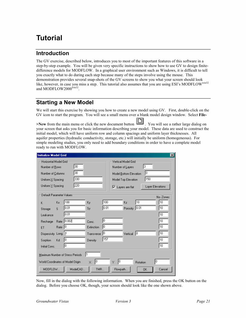
Starting a New Model We will start this exercise by showing you how to create a new model using GV. First, double-click on the GV icon to start the program. You will see a small menu over a blank model design window. Select File-
>New from the main menu or click the new document button . You will see a rather large dialog on your screen that asks you for basic information describing your model. These data are used to construct the initial model, which will have uniform row and column spacings and uniform layer thicknesses. All aquifer properties (hydraulic conductivity, storage, etc.) will initially be uniform (homogeneous). For simple modeling studies, you only need to add boundary conditions in order to have a complete model ready to run with MODFLOW.
Now, fill in the dialog with the following information. When you are finished, press the OK button on the dialog. Before you choose OK, though, your screen should look like the one shown above.

Groundwater Vistas Version 3 Page 22
Number of Rows 30
Number of Columns 30
X Spacing 330 ft
Y Spacing 220 ft
Number of Layers 3
Bottom Elevation 0.0 ft
Top Elevation 150.0 ft
Number of Stress Periods 1
Change Kz to 10.0 ft/d
Change Recharge rate to 0.002 ft/d
Check the box labeled “Layers are flat”
If you were familiar with Groundwater Vistas Version 2, you will notice some differences on the initialization dialog. You now enter a top elevation instead of a uniform layer thickness. The top of the model for most models will be land surface. You can also click the Layer Elevations button to edit the default layer bottom elevation for each layer. Layers will initially be flat regardless of whether the Layers are flat option is checked. The latter is checked to simplify the layer elevation database. If you check this option, GV will provide one elevation zone per layer, making it simpler to modify later. If you know that your model will have sloping layers (usually by importing SURFER or other format files), then leave the Layers are flat option unchecked.
You will also notice that you can supply the world X and Y coordinates of the model origin (lower left corner) and an angle of rotation. This makes it easier to import map files if you know in advance where the model should be placed on these maps.
The only other difference between Version 3 and Version 2 is when you click the MODFLOW button to import an existing model. There will now be a checkbox on the MODFLOW import dialog to tell GV that the MODFLOW files are in MODFLOW96 format. This does two things: (1) GV will look for the name file instead of the BASIC package to determine what files to import, and (2) GV will look to see if the files are in the new FREE format. You should check this option only if you have a MODFLOW name file for your simulation. You do not need to click the MODFLOW button now because we are starting a new model but the MODFLOW import dialog is shown below for your reference:
There are two other differences to point out here. First, there is an option to have one property zone per cell. This option effects K, storage, leakance (VCONT), and layer elevation databases. You should only check this option if you are trying to quickly import a huge model. A very large model (over 1,000,000 nodes) can often take many hours for GV to import because of the time to set up complex zone databases.

Groundwater Vistas Version 3 Page 23
The “one zone per cell” option makes it much faster but will use a lot more memory. The second difference between Groundwater Vistas 3 and Version 2 is the default vertical anisotropy (Kx/Kz). Quite often models use a uniform vertical anisotropy. Even though GV will correctly use the leakance already in the MODFLOW data files, it is often more convenient to recompute leakance as the model evolves. This can only be done if Kz is in the hydraulic conductivity database.
Now back to our initial model. After clicking the OK button, your screen should be similar to the one shown below. The model has uniform row and column spacings and the rows and columns are labeled.
Now, let’s change the font size used for the row and column labels. All text used to annotate the GV model may be modified in terms of font style and size. To change the font for the row and column labels, select Grid->Options and click the font button. Change the font size to 8 points and click OK to return to the Grid Options dialog. Click OK again to return to the GV menu.
You will now import a base map to display with the model. Select File->Map->GW Vistas. A file open dialog will be displayed. Choose the map called t2.map, which can be found in the GV tutorial directory (default: c:\gwv3\tutorial). After importing the map, select View->Full->Screen to fit everything back in the GV window. Your screen should now look similar to the one shown below.

Groundwater Vistas Version 3 Page 24
Adding Rows & Columns GV has four different modes when designing the model. These include Analytic Elements, Grid, Boundary condition, and Property zones. The design operation that you may perform is determined on the Edit menu. Select Edit from the main menu. At the bottom of the pulldown menu you will see selections entitled Grid, Aquifer Properties, Boundary Conditions, and Analytic Elements. A check mark appears next to the option
that is the current selection and the appropriate button is pushed down on the toolbar. The button
represents Analytic Elements, represents Boundary Conditions, stands for Property Zones, and
represents Grid operations. The Grid option allows you to add, delete, and move rows, columns, and layers. Aquifer Properties refers to assigning physical properties (e.g., hydraulic conductivity) to each cell in the model. Analytic Elements refers to the grid-independent boundary conditions in GV as well as annotation and calibration targets. You will see the buttons on the right side of the toolbar change depending upon which button is pressed down. This customization provides you with the most commonly used commands for each mode.
GV gives you the ability to insert, move, and delete rows, columns, and layers. In order to perform these operations, you must be in grid mode. This is accomplished by selecting Edit->Grid from the main menu
or by pressing the button on the toolbar. The word grid will appear in one of the panes of the status bar at the bottom of the GV window.
Once in grid mode, the cursor behaves differently than in other modes. When you are close to a row or column grid line, the cursor changes shape to either a left-right or up-down arrow. Pressing the left mouse button when this cursor appears allows you to slide the row or column line to a new position. You may not slide it beyond the adjacent row or column, however.
You may insert or delete rows, columns, and layers using the menu commands. These are fairly straightforward. Select the command (Grid->Insert->Row for example), move the cursor on the screen, and click the left mouse button. When deleting a row or column, the row or column closest to the cursor is deleted. Layers may be added above or below the current layer (the current layer is displayed as L:1,2,3,... on the status bar).
Groundwater Vistas Version 3 Page 25
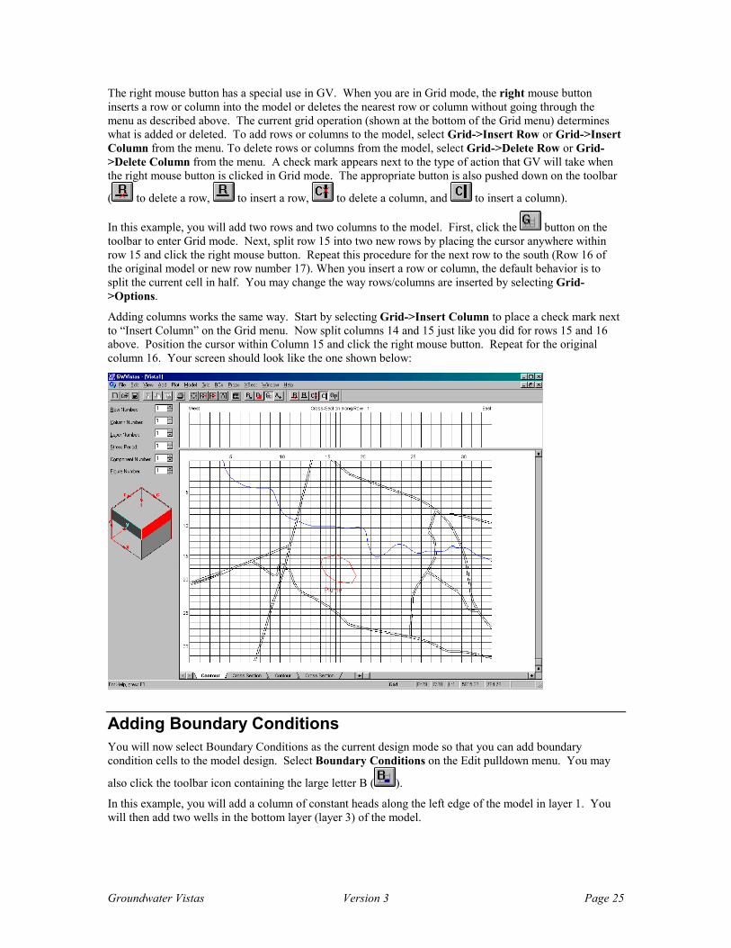
The right mouse button has a special use in GV. When you are in Grid mode, the right mouse button inserts a row or column into the model or deletes the nearest row or column without going through the menu as described above. The current grid operation (shown at the bottom of the Grid menu) determines what is added or deleted. To add rows or columns to the model, select Grid->Insert Row or Grid->Insert Column from the menu. To delete rows or columns from the model, select Grid->Delete Row or Grid->Delete Column from the menu. A check mark appears next to the type of action that GV will take when the right mouse button is clicked in Grid mode. The appropriate button is also pushed down on the toolbar
( to delete a row, to insert a row, to delete a column, and to insert a column).
In this example, you will add two rows and two columns to the model. First, click the button on the toolbar to enter Grid mode. Next, split row 15 into two new rows by placing the cursor anywhere within row 15 and click the right mouse button. Repeat this procedure for the next row to the south (Row 16 of the original model or new row number 17). When you insert a row or column, the default behavior is to split the current cell in half. You may change the way rows/columns are inserted by selecting Grid->Options.
Adding columns works the same way. Start by selecting Grid->Insert Column to place a check mark next to “Insert Column” on the Grid menu. Now split columns 14 and 15 just like you did for rows 15 and 16 above. Position the cursor within Column 15 and click the right mouse button. Repeat for the original column 16. Your screen should look like the one shown below:
Adding Boundary Conditions You will now select Boundary Conditions as the current design mode so that you can add boundary condition cells to the model design. Select Boundary Conditions on the Edit pulldown menu. You may
also click the toolbar icon containing the large letter B ( ).
In this example, you will add a column of constant heads along the left edge of the model in layer 1. You will then add two wells in the bottom layer (layer 3) of the model.

Groundwater Vistas Version 3 Page 26
The easiest way to set a large number of boundary conditions is to use the Window command. Select BCs-
>Insert->Window from the main menu (or from the toolbar). The cursor will change shape and appear like a mini-finite-difference grid. Move the cursor to the upper left corner of the model (row 1, column 1) and press the left mouse button. Make sure the cursor is inside the grid before pressing the left mouse button. Hold the mouse button down and move the cursor to the lower left corner (row 32, column 1). Release the mouse button and a dialog appears to confirm the coordinates of the window that you just created. Simply press the OK button to accept these coordinates. Next, a constant head dialog appears. The only item that must be changed is the value of constant head. Change this value to 150 ft. A common mistake here is to forget to reset the head to 150 from the default of 0.0. This results in constant head values below the layer bottom and the whole model goes dry!
Notice that the boundary condition is steady-state. This means that the boundary cells will be active during the entire simulation. In MODFLOW, constant heads are active for the entire simulation and cannot be changed. Your screen should now look like the one shown below.
Now, move to layer 3 of the model. The easiest way to change layers is by clicking the “+” button next to “Layer” on the 3D cube (called the Reference Cube) that is on the left side of the screen. Click the “+” button twice to get to Layer 3. The model will be redrawn and the constant head cells will disappear. This happens because these constant head cells were defined in layer 1 (the top layer) and we are now viewing the bottom layer of the model. You should still see one constant head in the upper left corner of the cross-section view however.
Select BCs->Well from the main menu. This places a check mark next to the word “Well” indicating that we are now editing wells. Next, select BCs->Insert->Single Cell. Move the cursor to row 16, column 15 and click the left mouse button. (You could also add a well by simply moving the cursor to row 16, column 15 and clicking the right mouse button.) You will notice that as you move the cursor on the screen, the status bar at the bottom of the screen updates the current row and column. When you are at row 16, column 15 the status bar should read “R:16 C:15”. After clicking the mouse button, a well edit dialog will appear. (Note that in MODFLOW, negative flow rates are used for production and postive rates for injection). Enter a flow rate of -30000 ft3/d. GV assumes that units of length and time are consistent for all parameters. In this example, all length units are in feet and all time units in days. Therefore, hydraulic conductivity is in ft/d, well flow rates are in ft3/d, recharge is in ft/d, etc.

Groundwater Vistas Version 3 Page 27
Add another well at row 8, column 16. This time, enter a flow rate of -40000. Use the same sequence of events that you used to insert the first well. Your screen should not look like the one below.
Creating MODFLOW Datasets The example model is now complete. The aquifer properties have already been set from the initialization dialog because we are using a homogeneous system. You will now create a MODFLOW data set, run the simulation, and analyze the results.
The preprocessing of model-specific options is accomplished using the Model selection on the main menu. Select Model and you will see options including MODFLOW, MODPATH, MT3D, etc. Select MODFLOW from the dropdown menu to reveal another menu with numerous selections. You will select several of these options before creating the data files.
First, select Model->MODFLOW->Packages. The dialog displays all of the MODFLOW packages and allows you to create only the ones necessary for the current model. The default selections do not normally need to be changed. The only change you need to make is the root file name. Change this parameter to t2. This means that the MODFLOW data files will be named T2.BAS for the BASIC package, T2.WEL for the well package, etc. Those of you familiar with Groundwater Vistas Version 2 will notice a slight change to this dialog. There is now a MODFLOW version selection at the top. The default is Original (88/96) which should be used for ESI’s MODFLOWwin32. There are also selections for MODFLOW-SURFACT and MODFLOWT, as well as MODFLOW2000. For now, leave this option at the default and select OK when you are finished.
Choose Model->MODFLOW->BCF Package to edit the layer types in the Block-Centered-Flow (BCF) Package. Change layers 2 and 3 from type 3 to type 0 (confined) layers. It is normally a good idea to make layers confined if you know that the water table will not drop into those layers. This speeds model convergence and can help avoid problems such as cells drying out. In this example, we know that the water table will always be in layer 1 so we make the lower layers confined. Click OK when you are done. One final change will be to the solver. Select Model->MODFLOW->Solver Package and change the number of iterations from 100 to 300. At this point, all of the model options have been selected. You will now run the model and view the results.

Groundwater Vistas Version 3 Page 28
One last thing to change before we actually run the model is to reset the Working Directory. This directory is where GV will create the MODFLOW data files. It is also where MODFLOW will write the model results. By default, the working directory is the directory where GV was launched from (default: c:\gwv3). It is a good idea to have a special directory for your model runs that is separate from the GV program directory and from the GV file (*.gwv). In this example, we will use c:\gwv3\tutorial\work. If you installed GV in another location, then the directory will be tutorial\work under your GV directory. To change the working directory, select Model->Paths to Models. The working directory is the last item on the dialog. After changing it, click OK.
This is a good time to save your work. Choose File->Save As from the main menu. Use the file name T2.GWV for this first example.
You are now ready to create data files for a MODFLOW simulation. The simplest way to create data sets and run the model is to click the calculator button on the toolbar. A progress dialog will be displayed briefly as the files are created. You will then be asked if you want to view the error file. Choose Cancel for this example as there should be no errors to view. After clicking Cancel, MODFLOWwin32 will start to run.
When MODFLOW is finished, a dialog will be displayed notifying you that the simulation is done and asks if you want to process the results. Choose YES to start the post-processing session. You will next see a dialog that allows you to specify what model results to analyze (the dialog is shown below). The default settings allow you to read the head file from the MODFLOW run. We will also look at the mass balance results so place a check mark next to Cell-by-Cell Flow as shown on the example dialog below. Click OK when you are done.
GV automatically contours the head results for the current layer and cross-section views. The resulting contours for layer 3 and for the cross-section along row 1 are shown below. Your screen should look similar, unless you have changed to another layer.
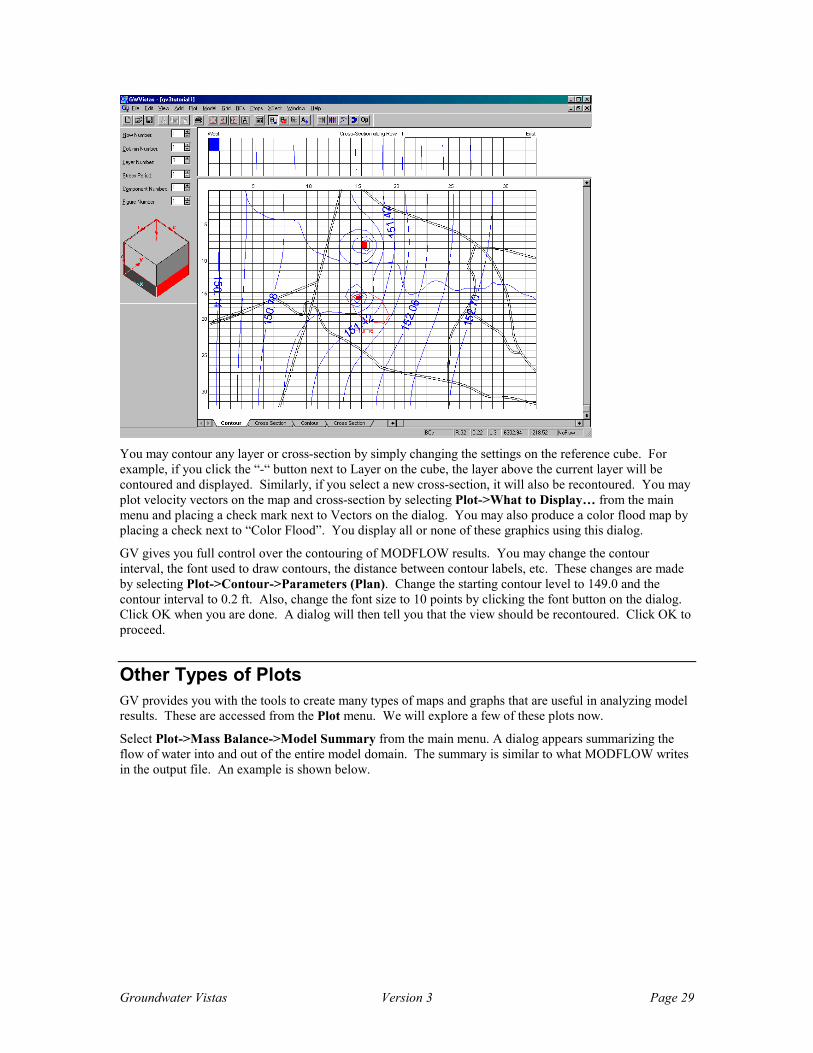
Groundwater Vistas Version 3 Page 29
You may contour any layer or cross-section by simply changing the settings on the reference cube. For example, if you click the “-“ button next to Layer on the cube, the layer above the current layer will be contoured and displayed. Similarly, if you select a new cross-section, it will also be recontoured. You may plot velocity vectors on the map and cross-section by selecting Plot->What to Display… from the main menu and placing a check mark next to Vectors on the dialog. You may also produce a color flood map by placing a check next to “Color Flood”. You display all or none of these graphics using this dialog.
GV gives you full control over the contouring of MODFLOW results. You may change the contour interval, the font used to draw contours, the distance between contour labels, etc. These changes are made by selecting Plot->Contour->Parameters (Plan). Change the starting contour level to 149.0 and the contour interval to 0.2 ft. Also, change the font size to 10 points by clicking the font button on the dialog. Click OK when you are done. A dialog will then tell you that the view should be recontoured. Click OK to proceed.
Other Types of Plots GV provides you with the tools to create many types of maps and graphs that are useful in analyzing model results. These are accessed from the Plot menu. We will explore a few of these plots now.
Select Plot->Mass Balance->Model Summary from the main menu. A dialog appears summarizing the flow of water into and out of the entire model domain. The summary is similar to what MODFLOW writes in the output file. An example is shown below.

Groundwater Vistas Version 3 Page 30
You may produce a bar chart of the mass balance results by simply clicking on the Graph button on the dialog. An example is shown below. Another useful mass balance feature of GV is that the flux rate of water into or out of a boundary cell is displayed on the status bar when the cursor moves over a boundary cell. Try this feature by moving the cursor over a constant-head cell in layer 1. The flow rate into the constant head for Row 1, Column 1 should be about -1561 ft3/d (NOTE: You must be in Boundary Condition mode to view fluxes; press the “B” button on the tool bar to enter BC mode). The negative sign is the MODFLOW convention for water being removed from the aquifer.
Another graph that shows head relationships between different layers of the model is the “profile” plot. A profile is simply a graph of head, concentration, drawdown, or water flux plotted versus distance along the current cross-section. Select Plot->Profile->Head from the main menu to display a profile of head in your

Groundwater Vistas Version 3 Page 31
example model. An example profile plot through Row 15 is shown below. To make this plot, click the “+” button next to Row on the reference cube until the number 15 appears. This changes the cross-section view to the row you specify and also determines which row or column will be plotted using the profile command. This plot shows the head relationships around a pumping well.
Groundwater Vistas uses two charting packages to make the mass balance and profile plots shown above. The default package is called First Impression. GV also supports ChartFX’98. To use the latter package, select View->Use ChartFX. You will notice that there is no menu bar on the First Impression graphs. To print, export, or modify the chart, simply right-click on the graph. A context menu allows you to work with the chart and data.
Particle-Tracking in GV GV provides pre- and post-processing of particle tracking results for MODPATH (both the steady-state and transient versions) and for PATH3D. In the following example, we will use MODPATHwin32. In Groundwater Vistas Versions 1 and 2, the modpath programs were DOS command line programs. We have now created a Windows interface for MODPATH to allow GV better control of particle tracking simulations. MODPATHwin32 is the same as the USGS MODPATH Version 3.2 but with a nicer interface. This version works with both MODFLOWwin32 and MODFLOW2000win32.
Particle tracking is a form of transport modeling in which only the bulk movement of groundwater is investigated. Particle tracking neglects the effects of chemical reactions, dispersion, and diffusion. The results of a particle tracking simulation are displayed by plotting pathlines through the aquifer system. Travel times are often labeled on the pathlines.
You start the particle tracking analysis by adding particle starting locations to the model. Particle traces are then drawn either downgradient (forward tracking) or upgradient (reverse tracking) from these starting locations. First, move to layer 1 by clicking the “-“ button next to layer on the cube until the number 1 appears in the Layer field. Select Add->Particle->Line from the GV main menu. Move the cursor to the upper right corner of the model (north-east corner). Click the left mouse button and drag a line to the lower right corner. Make sure the line of particles is within the bounds of the finite-difference grid. If the particles are outside the grid, they will not be tracked. Release the left mouse button to display a dialog. Change the number of particles along the line to 20 and click OK.
MODPATH has options just like MODFLOW only not as many. Select Model->Modpath->Packages and change the root file name for the MODPATH run to t2mp. It is not a good idea to use the same root name as MODFLOW because MODPATH uses some of the same file types with a slightly different format. Also, make sure that the MODPATH version is 3. Click OK when you are done.
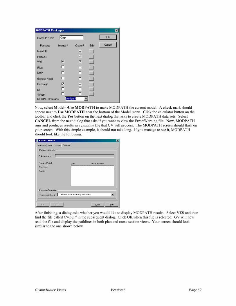
Groundwater Vistas Version 3 Page 32
Now, select Model->Use MODPATH to make MODPATH the current model. A check mark should appear next to Use MODPATH near the bottom of the Model menu. Click the calculator button on the toolbar and click the Yes button on the next dialog that asks to create MODPATH data sets. Select CANCEL from the next dialog that asks if you want to view the Error/Warning file. Now, MODPATH runs and produces results in a pathline file that GV will process. The MODPATH screen should flash on your screen. With this simple example, it should not take long. If you manage to see it, MODPATH should look like the following.
After finishing, a dialog asks whether you would like to display MODPATH results. Select YES and then find the file called t2mp.ptl in the subsequent dialog. Click OK when this file is selected. GV will now read the file and display the pathlines in both plan and cross-section views. Your screen should look similar to the one shown below.

Groundwater Vistas Version 3 Page 33
There are many options that can be used to modify the particle trace display. Usually you will want arrows on the traces. Most display options in Groundwater Vistas are found on the Plot menu. Select Plot->Particles->Arrows and change the distance between arrows to 500 ft and the size of the arrows to 100 ft (these are both in model units of length). Also, check the box to display the arrows.
This method puts an arrow at a constant distance along the trace. Another method places the arrows at a constant time along the trace. Select Plot->Particles->Time Posting. Keep the default interval of 365 days but change the precision from 2 to 0 and change the multiplier from 1 to 0.00274. This will display an arrow every 365 days but the label will be in years (1/365 = 0.00274). Check the box to display time postings and click the font button. Change the font to 8 or 10 points.
Now GV will redraw the traces with arrows spaced at equal time intervals instead of distance intervals. This is handy for looking at capture zones around wells for different time intervals.

Groundwater Vistas Version 3 Page 34
Model Calibration with GV Calibration is one of the most complex parts of applying groundwater models. GV assists model calibration in three ways: (1) calculation of calibration statistics for head, drawdown, concentration, or flux, (2) automated parameter sensitivity analysis, (3) automatic model calibration using a nonlinear least-squares technique built right into the GV interface or using external inverse models such as PEST, UCODE, and MODFLOW2000. All of these inverse models are included at no extra charge with Groundwater Vistas. You start by adding calibration targets to the model. A calibration target is a point in the aquifer where a measurement of head, drawdown, concentration, or flux has been made. Calibration targets may be either steady-state or transient. When you run the model to compare against the target values, GV reads the model results and interpolates the model result in both space and time to compute an error or residual. Analysis of residual statistics is a powerful way of determining calibration quality and guiding further refinements to the model. The following exercise will illustrate the calculation of calibration statistics and automatic sensitivity analysis. We will then use the inverse model MODFLOW2000 to calibrate the model.
We will start by defining 16 head target locations in our example model. Rather than type in the data manually, you will import a text file containing the target data. GV provides many data import features for calibration targets, boundary conditions, aquifer properties, and base maps. Select Add->Import->Targets from the main menu. Find the file called targets.dat, which should be in the tutorial directory (default is c:\gwv3\tutorial). Click OK when you have found it.
A dialog now prompts for the format of the file. The data in this file can be in any order as long as the data are delimited (separated by commas, spaces, or tabs) and each target contains the same number of data values. In this case, the default values on this dialog are fine so just click OK.
GV will report the number of targets successfully imported. In this example, there should be 16. The targets will appear on the plan view as small blue dots. Targets are only displayed for the layer in which they are defined. You should see 6 in layer 1, 5 in layer 2, and 5 in layer 3. You may edit target information by double-clicking on a target symbol (You must be in Analytic Element mode, however;
click the button on the tool bar to edit targets in this manner).
You will need to import model results again in order to compute the calibration statistics. Select Plot->Import Results and click OK on the dialog. All of the options should be set properly from the last run you made. You may view the calibration statistics by selecting Plot->Calibration->Statistics/Plots… A dialog is displayed that allows you to select the type of targets to use in the calculation (head, concentration, drawdown, or flux). You may also plot only selected ranges of layers. To view the statistics for this model, click the Statistics button. The residual sum of squares should be about 39.4 ft2. Click OK
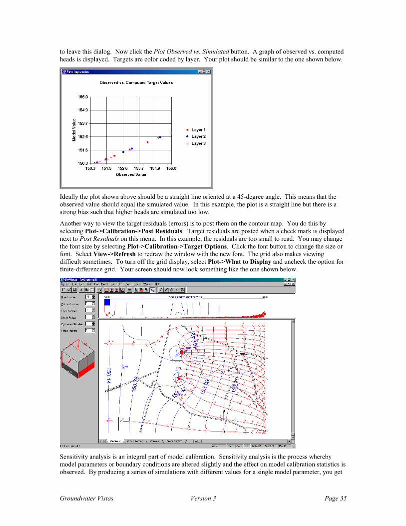
Groundwater Vistas Version 3 Page 35
to leave this dialog. Now click the Plot Observed vs. Simulated button. A graph of observed vs. computed heads is displayed. Targets are color coded by layer. Your plot should be similar to the one shown below.
Ideally the plot shown above should be a straight line oriented at a 45-degree angle. This means that the observed value should equal the simulated value. In this example, the plot is a straight line but there is a strong bias such that higher heads are simulated too low.
Another way to view the target residuals (errors) is to post them on the contour map. You do this by selecting Plot->Calibration->Post Residuals. Target residuals are posted when a check mark is displayed next to Post Residuals on this menu. In this example, the residuals are too small to read. You may change the font size by selecting Plot->Calibration->Target Options. Click the font button to change the size or font. Select View->Refresh to redraw the window with the new font. The grid also makes viewing difficult sometimes. To turn off the grid display, select Plot->What to Display and uncheck the option for finite-difference grid. Your screen should now look something like the one shown below.
Sensitivity analysis is an integral part of model calibration. Sensitivity analysis is the process whereby model parameters or boundary conditions are altered slightly and the effect on model calibration statistics is observed. By producing a series of simulations with different values for a single model parameter, you get

Groundwater Vistas Version 3 Page 36
a feel for how a parameter may be modified in order to achieve a better calibration. This is a tedious process because many simulations are required for each parameter and there are often many parameters to analyze. GV provides you with an automated way of performing a sensitivity analysis that greatly improves the efficiency of the process. You simply choose a parameter type, the number of simulations, and a parameter multiplier for each simulation. GV then runs MODFLOW the desired number of times and produces a sensitivity plot. For each simulation, GV multiplies your initial parameter value by the multiplier you specify. After all of the simulations are finished, GV plots calibration statistics versus parameter multiplier to visually show the results of the analysis.
You start a sensitivity analysis by selecting Model->Sensitivity Setup. Select Kx as the parameter to vary. Keep the default of Zone number 1 and 5 simulations. Click on the “Multipliers” button. Enter the values 0.2, 0.5, 1.0, 1.5, and 2.0 for simulations 1 through 5, respectively. Click OK when you are done and click OK on the main dialog. Running the analysis is as simple as selecting Models->Run Sensitivity from the main menu. You will see MODFLOW flash on your screen five times and after the last simulation a dialog will ask whether you would like to see the results. Select “Yes” and you are asked to choose a variable to plot for each run. The choices include sum of squared residuals, residual mean, residual standard deviation, average drawdown, and total flux to a designated boundary condition reach. A plot of residual sum of squares vs. multiplier is displayed below for this example. Your graph should look similar to this one.
Note that a Kx value of half the current value gives a much better calibration because it has a lower sum of squared residuals than the current model (multiplier of 1.0 is the current value). If we were trying to achieve a better calibration in this model, we would probably want to lower the K value. We will explore this more in the next section.
By producing a series of sensitivity plots, you can quickly determine the optimum parameter values to assign in your calibrated model. Of course, these parameters should be reasonable values given your knowledge of the aquifer system.
Automated Calibration Groundwater Vistas offers several ways of automating the calibration process. GV has a very simple and easy-to-use automated calibration procedure (called inverse modeling) built into the GV interface. GV also supports PEST, UCODE, and MODFLOW2000. In this tutorial, we will show you how to use the inverse model built into GV. We will then use MODFLOW2000.
The Groundwater Vistas calibration options are listed under the Model->GV Calibration menu. To use the auto-calibration in GV, you first select the parameters that you would like to estimate. Obviously there

Groundwater Vistas Version 3 Page 37
are lots of parameters in most models but the goal is to find the most sensitive ones and only estimate those. Also, if you are confident that a parameter value is already accurate then do not estimate it. In this example, we will estimate horizontal hydraulic conductivity in zone 1 (which is the whole model in this case). Select Model->GV Calibration->Parameters and enter the data shown on the following dialog.
GV actually estimates a multiplier on the parameter value so the multiplier of 1.0 in column 4 above means that we will start with our initial guess (in this case 100 ft/d). The minimum and maximum values in the last 2 columns are used to constrain the parameter value. These are also multipliers.
Now select Model->GV Calibration->Options and change the number of iterations from 25 to 5. Normally the calibration will converge within several iterations. Your screen should look like the following dialog.
The rest of the data on this dialog are explained in later sections of this manual. For now, just click OK after changing the number of iterations to 5.
GV is now ready to calibrate the model. Select Model->GV Calibration->Start Calibration. GV will run MODFLOW a number of times and display progress on the status bar to let you know how far it has gotten. After the calibration run is finished, GV will ask you if you want to display the results. GV writes the results to a text file for later viewing. Select OK to view the file. Scroll down to the end of the file. You should see the following data just before the residual summary:
-------------------------------------------- | Parameter Summary for Iteration: 5 |
--------------------------------------------
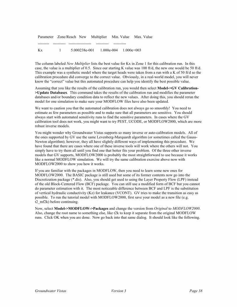
Groundwater Vistas Version 3 Page 38
Parameter Zone/Reach New Multiplier Min. Value Max. Value
--------- ---------- ------------------ ---------- ----------
Kx 1 5.000238e-001 1.000e-004 1.000e+003
The column labeled New Multiplier lists the best value for Kx in Zone 1 for this calibration run. In this case, the value is a multiplier of 0.5. Since our starting K value was 100 ft/d, the new one would be 50 ft/d. This example was a synthetic model where the target heads were taken from a run with a K of 50 ft/d so the calibration procedure did converge to the correct value. Obviously, in a real-world model, you will never know the “correct” value but this automated procedure can help you identify the best possible value.
Assuming that you like the results of the calibration run, you would then select Model->GV Calibration->Update Databases. This command takes the results of the calibration run and modifies the parameter databases and/or boundary condition data to reflect the new values. After doing this, you should rerun the model for one simulation to make sure your MODFLOW files have also been updated.
We want to caution you that the automated calibration does not always go so smoothly! You need to estimate as few parameters as possible and to make sure that all parameters are sensitive. You should always start with automated sensitivity runs to find the sensitive parameters. In cases where the GV calibration tool does not work, you might want to try PEST, UCODE, or MODFLOW2000, which are more robust inverse models.
You might wonder why Groundwater Vistas supports so many inverse or auto-calibration models. All of the ones supported by GV use the same Levenberg-Marquardt algorithm (or sometimes called the Gauss-Newton algorithm); however, they all have slightly different ways of implementing this procedure. We have found that there are cases where one of these inverse tools will work where the others will not. You simply have to try them all until you find one that better fits your problem. Of the three other inverse models that GV supports, MODFLOW2000 is probably the most straightforward to use because it works like a normal MODFLOW simulation. We will try the same calibration exercise above now with MODFLOW2000 to show you how it works.
If you are familiar with the packages in MODFLOW, then you need to learn some new ones for MODFLOW2000. The BASIC package is still used but some of its former contents now go into the Discretization package (*.dis). Also, you should get used to using the Layer Property Flow (LPF) instead of the old Block-Centered Flow (BCF) package. You can still use a modified form of BCF but you cannot do parameter estimation with it. The most noticeable difference between BCF and LPF is the substitution of vertical hydraulic conductivity (Kz) for leakance (VCONT). GV tries to make the transition as easy as possible. To run the tutorial model with MODFLOW2000, first save your model as a new file (e.g. t2_mf2k) before continuing.
Now, select Model->MODFLOW->Packages and change the version from Original to MODFLOW2000. Also, change the root name to something else, like t2k to keep it separate from the original MODFLOW runs. Click OK when you are done. Now go back into that same dialog. It should look like the following.
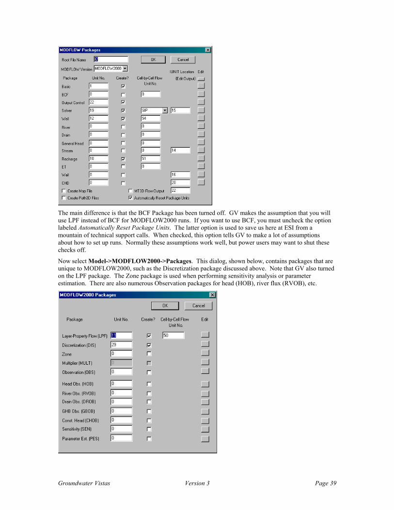
Groundwater Vistas Version 3 Page 39
The main difference is that the BCF Package has been turned off. GV makes the assumption that you will use LPF instead of BCF for MODFLOW2000 runs. If you want to use BCF, you must uncheck the option labeled Automatically Reset Package Units. The latter option is used to save us here at ESI from a mountain of technical support calls. When checked, this option tells GV to make a lot of assumptions about how to set up runs. Normally these assumptions work well, but power users may want to shut these checks off.
Now select Model->MODFLOW2000->Packages. This dialog, shown below, contains packages that are unique to MODFLOW2000, such as the Discretization package discussed above. Note that GV also turned on the LPF package. The Zone package is used when performing sensitivity analysis or parameter estimation. There are also numerous Observation packages for head (HOB), river flux (RVOB), etc.
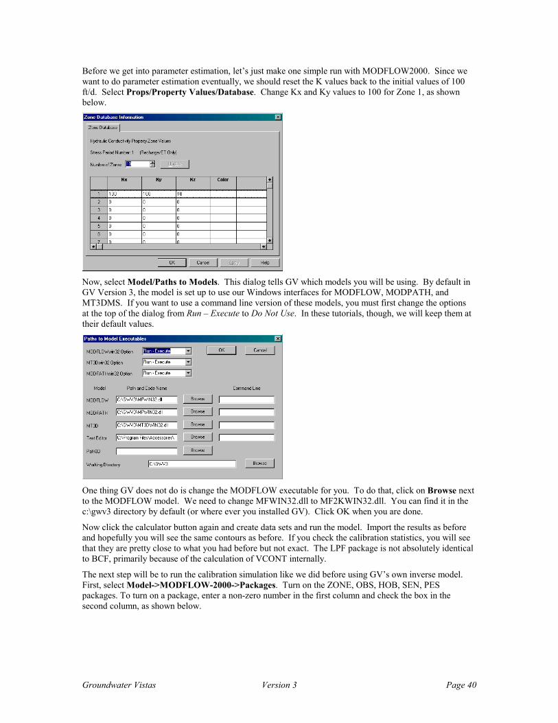
Groundwater Vistas Version 3 Page 40
Before we get into parameter estimation, let’s just make one simple run with MODFLOW2000. Since we want to do parameter estimation eventually, we should reset the K values back to the initial values of 100 ft/d. Select Props/Property Values/Database. Change Kx and Ky values to 100 for Zone 1, as shown below.
Now, select Model/Paths to Models. This dialog tells GV which models you will be using. By default in GV Version 3, the model is set up to use our Windows interfaces for MODFLOW, MODPATH, and MT3DMS. If you want to use a command line version of these models, you must first change the options at the top of the dialog from Run – Execute to Do Not Use. In these tutorials, though, we will keep them at their default values.
One thing GV does not do is change the MODFLOW executable for you. To do that, click on Browse next to the MODFLOW model. We need to change MFWIN32.dll to MF2KWIN32.dll. You can find it in the c:\gwv3 directory by default (or where ever you installed GV). Click OK when you are done.
Now click the calculator button again and create data sets and run the model. Import the results as before and hopefully you will see the same contours as before. If you check the calibration statistics, you will see that they are pretty close to what you had before but not exact. The LPF package is not absolutely identical to BCF, primarily because of the calculation of VCONT internally.
The next step will be to run the calibration simulation like we did before using GV’s own inverse model. First, select Model->MODFLOW-2000->Packages. Turn on the ZONE, OBS, HOB, SEN, PES packages. To turn on a package, enter a non-zero number in the first column and check the box in the second column, as shown below.
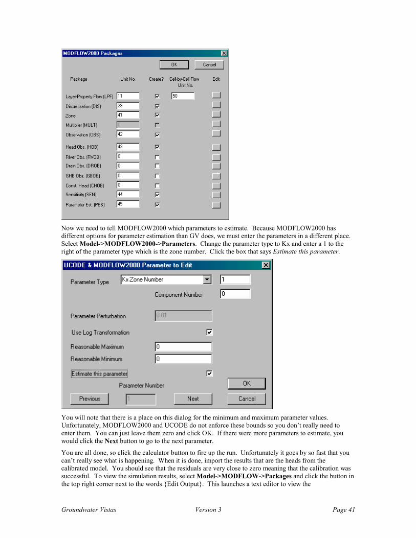
Groundwater Vistas Version 3 Page 41
Now we need to tell MODFLOW2000 which parameters to estimate. Because MODFLOW2000 has different options for parameter estimation than GV does, we must enter the parameters in a different place. Select Model->MODFLOW2000->Parameters. Change the parameter type to Kx and enter a 1 to the right of the parameter type which is the zone number. Click the box that says Estimate this parameter.
You will note that there is a place on this dialog for the minimum and maximum parameter values. Unfortunately, MODFLOW2000 and UCODE do not enforce these bounds so you don’t really need to enter them. You can just leave them zero and click OK. If there were more parameters to estimate, you would click the Next button to go to the next parameter.
You are all done, so click the calculator button to fire up the run. Unfortunately it goes by so fast that you can’t really see what is happening. When it is done, import the results that are the heads from the calibrated model. You should see that the residuals are very close to zero meaning that the calibration was successful. To view the simulation results, select Model->MODFLOW->Packages and click the button in the top right corner next to the words {Edit Output}. This launches a text editor to view the
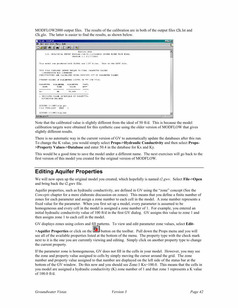
Groundwater Vistas Version 3 Page 42
MODFLOW2000 output files. The results of the calibration are in both of the output files t2k.lst and t2k.glo. The latter is easier to find the results, as shown below.
Note that the calibrated value is slightly different from the ideal of 50 ft/d. This is because the model calibration targets were obtained for this synthetic case using the older version of MODFLOW that gives slightly different results.
There is no automatic way in the current version of GV to automatically update the databases after this run. To change the K value, you would simply select Props->Hydraulic Conductivity and then select Props->Property Values->Database and enter 50.4 in the database for Kx and Ky.
This would be a good time to save the model under a different name. The next exercises will go back to the first version of this model you created for the original version of MODFLOW.
Editing Aquifer Properties We will now open up the original model you created, which hopefully is named t2.gwv. Select File->Open and bring back the t2.gwv file.
Aquifer properties, such as hydraulic conductivity, are defined in GV using the “zone” concept (See the Concepts chapter for a more elaborate discussion on zones). This means that you define a finite number of zones for each parameter and assign a zone number to each cell in the model. A zone number represents a fixed value for the parameter. When you first set up a model, every parameter is assumed to be homogeneous and every cell in the model is assigned a zone number of 1. For example, you entered an initial hydraulic conductivity value of 100 ft/d in the first GV dialog. GV assigns this value to zone 1 and then assigns zone 1 to each cell in the model.
GV displays zones using colors and fill patterns. To view and edit parameter zone values, select Edit-
>Aquifer Properties or click on the button on the toolbar. Pull down the Props menu and you will see all of the available properties listed at the bottom of the menu. The property type with the check mark next to it is the one you are currently viewing and editing. Simply click on another property type to change the current property.
If the parameter zone is homogeneous, GV does not fill in the cells in your model. However, you may see the zone and property value assigned to cells by simply moving the cursor around the grid. The zone number and property value assigned to that number are displayed on the left side of the status bar at the bottom of the GV window. Do this now and you should see Zone:1 Kx=100.0. This means that the cells in you model are assigned a hydraulic conductivity (K) zone number of 1 and that zone 1 represents a K value of 100.0 ft/d.

Groundwater Vistas Version 3 Page 43
We will now change the distribution of hydraulic conductivity in your model by first defining another zone value and then assigning this new zone to some cells in your model. The first step is to modify the database of zone numbers for hydraulic conductivity. Select Props->Property Values->Database or press
on the toolbar. You will see a dialog that lists zone numbers on the left (NOTE: these are NOT layer numbers). There are three columns labeled Kx, Ky, and Kz. These are the three directional values of hydraulic conductivity. You should also see that zone 1 has been assigned values of 100.0, 100.0, and 10.0 for these three parameters, respectively. All other zone numbers in the database have values of zero. Now, change the Kx, Ky, and Kz values for zone 2 to 25.0, 25.0, and 2.5. Also, double-click the color next to zone 2 and make it blue. Your dialog should look like the following. Click OK to save these values.
By changing the value of the property assigned to zone 2, you have not changed the model at all because no cells are currently assigned zone 2! You have simply allowed for the possibility that a value of 25.0 ft/d may be assigned for hydraulic conductivity. To actually change certain cells to this new property value, select Props->Set Zone Numbers->Window. Now move the cursor to a location within the model and drag a rectangle on the screen. Release the left mouse button and you will see a dialog asking for the zone number to assign to this region. Enter a value of 2 and click the OK button (or simply hit the Enter key). The screen will now be redrawn and you should see blue cells for the region covered by zone 2. Your screen should look similar to the one below except you may have defined a different location for the window. If you now move the cursor over the blue area, you should see the new K values on the status bar.

Groundwater Vistas Version 3 Page 44
Setting Up a Transient Model Before starting this next session, save your current design as T3.GWV. Select File->Save As and enter T3 as the file name. Now, select File->Close to end this model. We will now load the previous model that you saved as T2.GWV. Select File->Open and select the T2.GWV file.
You will now set up a model to evaluate the recovery of the aquifer after the pumping wells are shut off. The key aspects of this session will be to delete the 2 wells in layer 3 and set accurate initial conditions from the previous head-save file. First, to make sure that the proper head-save file exists we will rerun the
T2 model. Simply click the calculator button , create the MODFLOW data sets, and run the model. You do not need to import the results after the simulation.
We will start by deleting the wells in layer 3. Click the + button next to “Layer” on the Reference Cube until you are in layer 3. Now, select BCs->Well to edit the wells. Move the cursor over one of the two wells (they are red squares on the screen). Click the right mouse button to delete the well. Repeat this for the other well.
The next step is to set up MODFLOW options to make a transient run. Select Model->MODFLOW->Packages and change the root file name to T3. Now select Model->MODFLOW->BASIC Package and uncheck the option labeled Steady State Simulation. The latter is the first step in setting up a transient model. The second step in creating any transient run is to set up the MODFLOW stress periods and time steps. Select Model->MODFLOW->Stress Period Setup and change the stress period length to 60.0 days for stress period 1. Change the number of time steps to 30.

Groundwater Vistas Version 3 Page 45
Steady-state models do not require accurate starting heads, however, transient simulations must start with accurate heads in all cells. The easiest way is to use the heads from a steady-state simulation. In this example, we will use the heads from the T2 simulation. Select Model->MODFLOW->Initial Heads. Place a check mark next to Set Initial Heads from Head-Save File and enter t2.hds next to file name for the head-save file.
Transient runs require storage coefficients for each cell in the model. This has already been set when you set up the first run. Each cell in the model is assigned a storage value of 0.01. You can confirm this by
selecting Props->Storage. Next click the database button on the toolbar . Zone 1 should have specific yield and storage coefficient values of 0.01. Click OK when you are done.
GV allows you to monitor head, drawdown, and concentration over time during a transient simulation.
You must first add observation wells, though to record the heads. Select from the toolbar to enter Analytic Element mode. You add observation wells by selecting Add->Well. Move the cursor to Row 7, Column 15 and click the left mouse button. Make sure to change the pumping rate to 0.0 and place a check mark next to Monitor Head/Concentration vs. Time. Enter a 1 next to both Top of Screen and Bottom of Screen. Click the Name button and enter MW-1 for the name of this monitoring well. Click OK when you are done.
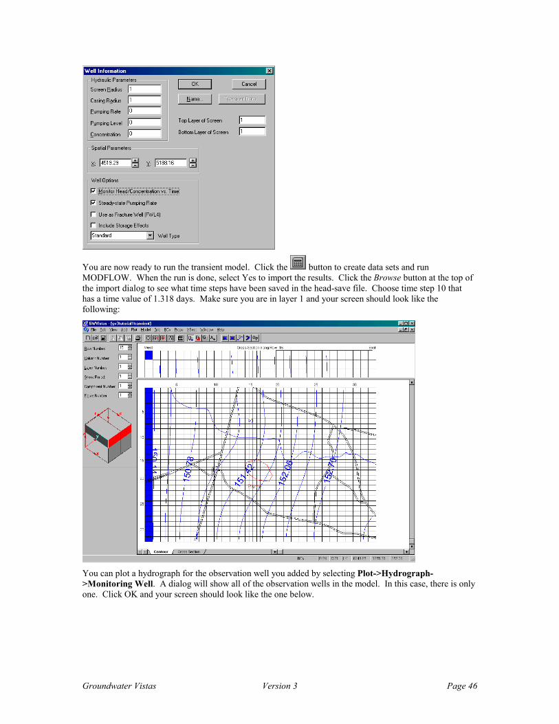
Groundwater Vistas Version 3 Page 46
You are now ready to run the transient model. Click the button to create data sets and run MODFLOW. When the run is done, select Yes to import the results. Click the Browse button at the top of the import dialog to see what time steps have been saved in the head-save file. Choose time step 10 that has a time value of 1.318 days. Make sure you are in layer 1 and your screen should look like the following:
You can plot a hydrograph for the observation well you added by selecting Plot->Hydrograph->Monitoring Well. A dialog will show all of the observation wells in the model. In this case, there is only one. Click OK and your screen should look like the one below.

Groundwater Vistas Version 3 Page 47
This ends the transient simulation. Save this file for later use by selecting File->Save As. Enter the file name TR.GWV.
Transport Modeling with MT3D We will now introduce you to transport modeling using MT3D. Groundwater Vistas comes with the public domain version of MT3D that has been compiled specifically to work with GV. We will use the new version called MT3DMS but we will just refer to it as MT3D in the following discussion.
MT3D simulations start with a MODFLOW simulation. MODFLOW creates a special flow file (similar to a cell-by-cell flow file) that MT3D uses to compute velocities and flow rates into or out of boundary cells. We will start by going back to the original T2 steady-state run. Close any open models in GV and select File->Open. Select the T2.GWV file.
We will now add a source of contamination in the transport model using a special recharge zone. This is a handy way to introduce a source of contamination and is appropriate for leaching of contaminants from the unsaturated zone or from a leachfield. Select Props->Recharge and then select Props->Property Values->Database. Enter a recharge rate of 0.002 in zone 2 and a concentration of 1000.0. Change the color to a nice red!
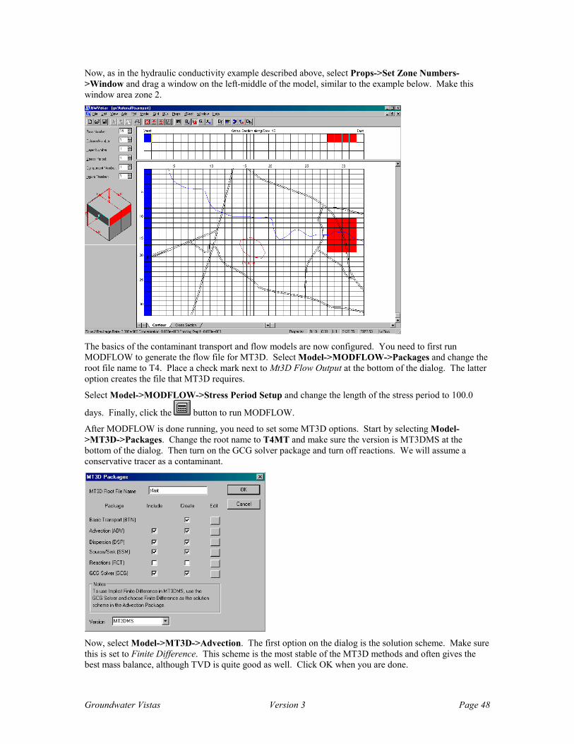
Groundwater Vistas Version 3 Page 48
Now, as in the hydraulic conductivity example described above, select Props->Set Zone Numbers->Window and drag a window on the left-middle of the model, similar to the example below. Make this window area zone 2.
The basics of the contaminant transport and flow models are now configured. You need to first run MODFLOW to generate the flow file for MT3D. Select Model->MODFLOW->Packages and change the root file name to T4. Place a check mark next to Mt3D Flow Output at the bottom of the dialog. The latter option creates the file that MT3D requires.
Select Model->MODFLOW->Stress Period Setup and change the length of the stress period to 100.0
days. Finally, click the button to run MODFLOW.
After MODFLOW is done running, you need to set some MT3D options. Start by selecting Model->MT3D->Packages. Change the root name to T4MT and make sure the version is MT3DMS at the bottom of the dialog. Then turn on the GCG solver package and turn off reactions. We will assume a conservative tracer as a contaminant.
Now, select Model->MT3D->Advection. The first option on the dialog is the solution scheme. Make sure this is set to Finite Difference. This scheme is the most stable of the MT3D methods and often gives the best mass balance, although TVD is quite good as well. Click OK when you are done.

Groundwater Vistas Version 3 Page 49
Next, select Model->MT3D->Printing Results. Place a check mark next to the item labeled Save Concentration in Binary File. Change the frequency of output to Every N Time Steps and the number to 2. Click OK when you are finished. Select Model->MT3D->Time Stepping. Confirm that the initial time step size is 0.1 with a maximum step size of 5 days and a multiplier of 1.2.
You are now ready to run MT3D and contour the concentrations. Select Model->Use MT3D. Now, when
you click the button, GV runs the MT3D model. Do this now. If MT3D does not run, select Model->Path to Models and confirm that the MT3D model is MT3DWIN32.dll.
After MT3D is done running, import the results. When the import results dialog is on the screen, click the Browse button next to the transport time step. This shows all of the times that concentration was saved. Choose the last time step at 100 days (should be step number 37). Click OK and GV will read heads and concentrations.
By default GV contours heads. To contour concentrations, select Plot->What to Display. Change the variable to contour from Head to Concentration. Click OK and GV will contour concentrations.
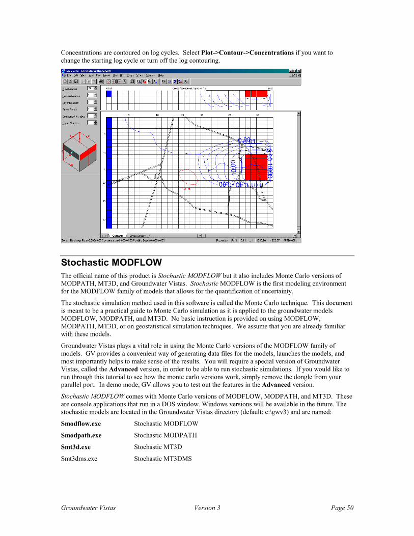
Groundwater Vistas Version 3 Page 50
Concentrations are contoured on log cycles. Select Plot->Contour->Concentrations if you want to change the starting log cycle or turn off the log contouring.
Stochastic MODFLOW The official name of this product is Stochastic MODFLOW but it also includes Monte Carlo versions of MODPATH, MT3D, and Groundwater Vistas. Stochastic MODFLOW is the first modeling environment for the MODFLOW family of models that allows for the quantification of uncertainty.
The stochastic simulation method used in this software is called the Monte Carlo technique. This document is meant to be a practical guide to Monte Carlo simulation as it is applied to the groundwater models MODFLOW, MODPATH, and MT3D. No basic instruction is provided on using MODFLOW, MODPATH, MT3D, or on geostatistical simulation techniques. We assume that you are already familiar with these models.
Groundwater Vistas plays a vital role in using the Monte Carlo versions of the MODFLOW family of models. GV provides a convenient way of generating data files for the models, launches the models, and most importantly helps to make sense of the results. You will require a special version of Groundwater Vistas, called the Advanced version, in order to be able to run stochastic simulations. If you would like to run through this tutorial to see how the monte carlo versions work, simply remove the dongle from your parallel port. In demo mode, GV allows you to test out the features in the Advanced version.
Stochastic MODFLOW comes with Monte Carlo versions of MODFLOW, MODPATH, and MT3D. These are console applications that run in a DOS window. Windows versions will be available in the future. The stochastic models are located in the Groundwater Vistas directory (default: c:\gwv3) and are named:
Smodflow.exe Stochastic MODFLOW
Smodpath.exe Stochastic MODPATH
Smt3d.exe Stochastic MT3D
Smt3dms.exe Stochastic MT3DMS

Groundwater Vistas Version 3 Page 51
This tutorial covers the basic operation of the Monte Carlo versions of MODFLOW, MODPATH, and MT3D. The tutorial assumes that you are already familiar with Groundwater Vistas and have run the general GV tutorial in the previous sections of this chapter.
You should first start Groundwater Vistas and open the GV file called stutor.gwv in the tutorial directory (default: c:\gwv3\tutorial). The following sections show how to configure the simulation, run the Monte Carlo versions of MODFLOW, MODPATH, and MT3D, and analyze the results.
You need to confirm that the working directory is set up correctly. Select Model/Paths to Models and make sure that the working directory (c:\gwv3\tutorial) exists. If this directory does not exist, please change it to one that is valid.
Stochastic MODFLOW In a deterministic model, you have a fixed set of parameters and boundary conditions, usually from a calibrated model. When making predictions, you simply change the stresses in the model to simulate what will happen to the groundwater system in the future. You make one run and present the result in a report. In some cases, you may bracket the deterministic solution with a best and worst case. While this approach is generally accepted in our industry, it does not really address the issue of uncertainty in parameters distributions in the model and how that uncertainty effects our predictions.
In monte carlo modeling, on the other hand, you can make key model parameters uncertain by specifying a distribution type and associated statistical characteristics. Instead of making one simulation, you make hundreds or thousands of simulations. In each simulation, a different value is selected for the uncertain parameters. When processing the results of a monte carlo simulation, you look at the probability that something will happen by evaluating all of the hundreds or thousands of simulations. GV helps you perform this evaluation by organizing and summarizing the monte carlo simulations.
We will start this example by selecting the parameter that will be uncertain. In this case, we will just use horizontal hydraulic conductivity in Zone 1. Select Model/Stochastic/Parameters. Select Kx as the parameter type. Use a normal distribution, zone number 1, standard deviation of 30.0 ft/d, minimum value of 10.0 ft/d, and maximum of 500.0 ft/d. Your screen should look like the following dialog.
Next, select Model/Stochastic/MODFLOW Options. Use an output file name of smod.out and 100 realizations. In the jargon of monte carlo simulations, a realization is one MODFLOW run. An ensemble is the collection of all realizations, 100 in this case. Before running the model, change the root file name to t2s. This is done by selecting Model/MODFLOW/Packages.
We have now selected the parameters that will vary with each realization and how they will vary. In this case, Stochastic MODFLOW will use a normal distribution for sampling of K values and will limit the range to between 10 and 500 ft/d. We will also run 100 realizations and each realization will use a homogeneous K distribution.
Now run the simulation by selecting Model/Stochastic/Create MODFLOW Datasets and then Model/Stochastic/Run Stochastic MODFLOW. If Stochastic MODFLOW does not run, check Model/Stochastic/Paths to be sure that you have smodflow.exe for the Stochastic MODFLOW program and it is pointing to no directory or the directory containing the program (c:\gwv3 by default).
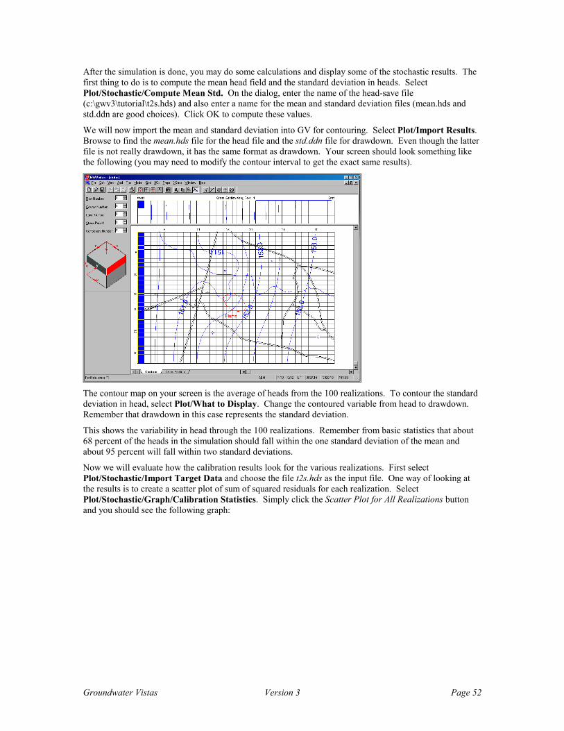
Groundwater Vistas Version 3 Page 52
After the simulation is done, you may do some calculations and display some of the stochastic results. The first thing to do is to compute the mean head field and the standard deviation in heads. Select Plot/Stochastic/Compute Mean Std. On the dialog, enter the name of the head-save file (c:\gwv3\tutorial\t2s.hds) and also enter a name for the mean and standard deviation files (mean.hds and std.ddn are good choices). Click OK to compute these values.
We will now import the mean and standard deviation into GV for contouring. Select Plot/Import Results. Browse to find the mean.hds file for the head file and the std.ddn file for drawdown. Even though the latter file is not really drawdown, it has the same format as drawdown. Your screen should look something like the following (you may need to modify the contour interval to get the exact same results).
The contour map on your screen is the average of heads from the 100 realizations. To contour the standard deviation in head, select Plot/What to Display. Change the contoured variable from head to drawdown. Remember that drawdown in this case represents the standard deviation.
This shows the variability in head through the 100 realizations. Remember from basic statistics that about 68 percent of the heads in the simulation should fall within the one standard deviation of the mean and about 95 percent will fall within two standard deviations.
Now we will evaluate how the calibration results look for the various realizations. First select Plot/Stochastic/Import Target Data and choose the file t2s.hds as the input file. One way of looking at the results is to create a scatter plot of sum of squared residuals for each realization. Select Plot/Stochastic/Graph/Calibration Statistics. Simply click the Scatter Plot for All Realizations button and you should see the following graph:
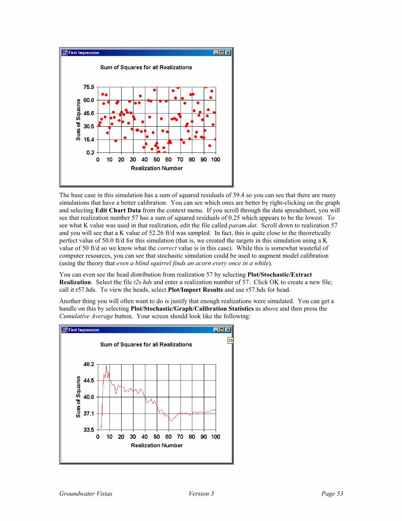
Groundwater Vistas Version 3 Page 53
The base case in this simulation has a sum of squared residuals of 39.4 so you can see that there are many simulations that have a better calibration. You can see which ones are better by right-clicking on the graph and selecting Edit Chart Data from the context menu. If you scroll through the data spreadsheet, you will see that realization number 57 has a sum of squared residuals of 0.25 which appears to be the lowest. To see what K value was used in that realization, edit the file called param.dat. Scroll down to realization 57 and you will see that a K value of 52.26 ft/d was sampled. In fact, this is quite close to the theoretically perfect value of 50.0 ft/d for this simulation (that is, we created the targets in this simulation using a K value of 50 ft/d so we know what the correct value is in this case). While this is somewhat wasteful of computer resources, you can see that stochastic simulation could be used to augment model calibration (using the theory that even a blind squirrel finds an acorn every once in a while).
You can even see the head distribution from realization 57 by selecting Plot/Stochastic/Extract Realization. Select the file t2s.hds and enter a realization number of 57. Click OK to create a new file; call it r57.hds. To view the heads, select Plot/Import Results and use r57.hds for head.
Another thing you will often want to do is justify that enough realizations were simulated. You can get a handle on this by selecting Plot/Stochastic/Graph/Calibration Statistics as above and then press the Cumulative Average button. Your screen should look like the following:
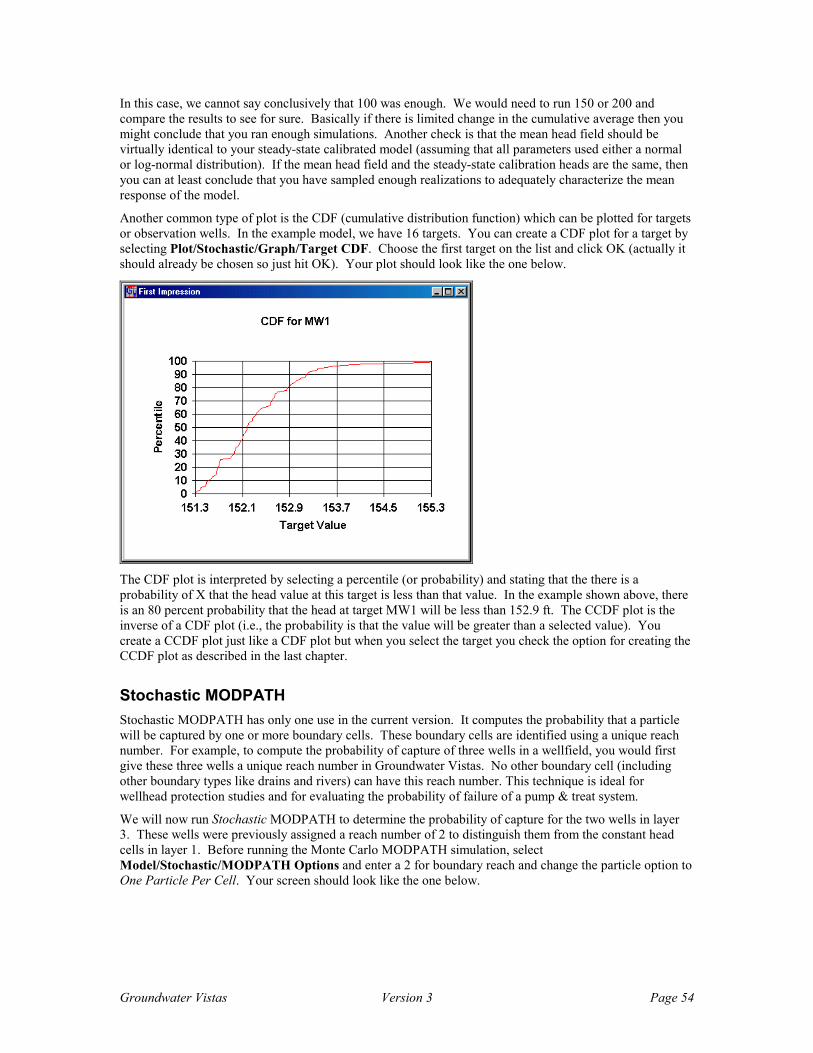
Groundwater Vistas Version 3 Page 54
In this case, we cannot say conclusively that 100 was enough. We would need to run 150 or 200 and compare the results to see for sure. Basically if there is limited change in the cumulative average then you might conclude that you ran enough simulations. Another check is that the mean head field should be virtually identical to your steady-state calibrated model (assuming that all parameters used either a normal or log-normal distribution). If the mean head field and the steady-state calibration heads are the same, then you can at least conclude that you have sampled enough realizations to adequately characterize the mean response of the model.
Another common type of plot is the CDF (cumulative distribution function) which can be plotted for targets or observation wells. In the example model, we have 16 targets. You can create a CDF plot for a target by selecting Plot/Stochastic/Graph/Target CDF. Choose the first target on the list and click OK (actually it should already be chosen so just hit OK). Your plot should look like the one below.
The CDF plot is interpreted by selecting a percentile (or probability) and stating that the there is a probability of X that the head value at this target is less than that value. In the example shown above, there is an 80 percent probability that the head at target MW1 will be less than 152.9 ft. The CCDF plot is the inverse of a CDF plot (i.e., the probability is that the value will be greater than a selected value). You create a CCDF plot just like a CDF plot but when you select the target you check the option for creating the CCDF plot as described in the last chapter.
Stochastic MODPATH Stochastic MODPATH has only one use in the current version. It computes the probability that a particle will be captured by one or more boundary cells. These boundary cells are identified using a unique reach number. For example, to compute the probability of capture of three wells in a wellfield, you would first give these three wells a unique reach number in Groundwater Vistas. No other boundary cell (including other boundary types like drains and rivers) can have this reach number. This technique is ideal for wellhead protection studies and for evaluating the probability of failure of a pump & treat system.
We will now run Stochastic MODPATH to determine the probability of capture for the two wells in layer 3. These wells were previously assigned a reach number of 2 to distinguish them from the constant head cells in layer 1. Before running the Monte Carlo MODPATH simulation, select Model/Stochastic/MODPATH Options and enter a 2 for boundary reach and change the particle option to One Particle Per Cell. Your screen should look like the one below.

Groundwater Vistas Version 3 Page 55
When you run Stochastic MODPATH, the probability of capture for each particle will be written to the file smpath.cap. After clicking OK on this dialog, select Model/Stochastic/Create MODPATH Data Sets. Now run the model by selecting Model/Stochastic/Run Stochastic MODPATH.
After MODPATH is done with the 100 realizations, select Plot/Stochastic/Convert Capture to HDS. First you identify the capture file (default is c:\gwv3\tutorial\work\smpath.cap but you may need to browse to the correct directory) in a standard file open dialog. Next, you will see a file save dialog where you enter the name of the head-save format file that will contain capture probability. Enter capture.hds here. Now select Plot/Import Results and browse to find capture.hds for the head file. Your screen should look like the one below.
This plot is not very interesting because there is not a lot of variability in the capture probability for this model. The example does, however, show how you can get a capture probability map for any problem. Another useful technique is to use the color flood option (Plot/What to Display) for capture probability. Your might try it in this case just to see how it is done.
Stochastic MT3D The third Monte Carlo model we will explore is MT3D. The example model has been configured with a second recharge zone that injects contaminant in the recharge water. This is supposed to simulate a leaking landfill or impoundment. We will add this parameter to the list of uncertain variables and then run Stochastic MT3D. Start by selecting Model/Stochastic/Parameters. Enter a second parameter as recharge concentration with a log normal distribution, a standard deviation of 1.0 (e.g., one order of magnitude), a
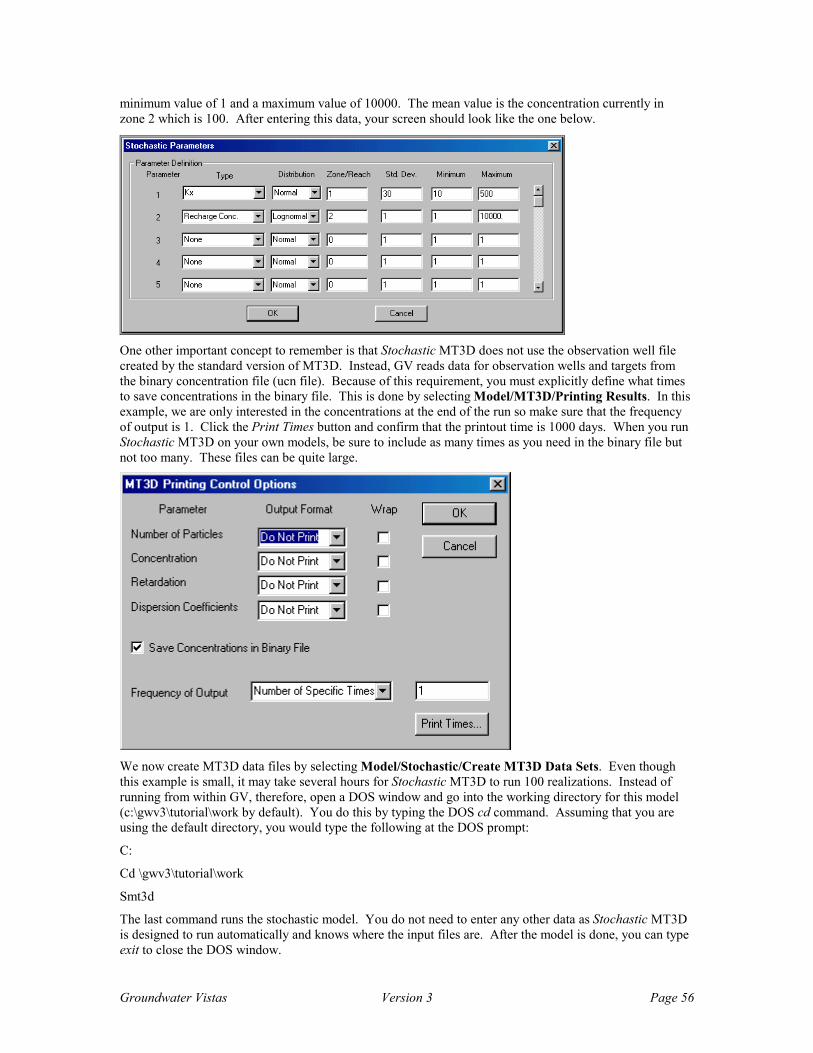
Groundwater Vistas Version 3 Page 56
minimum value of 1 and a maximum value of 10000. The mean value is the concentration currently in zone 2 which is 100. After entering this data, your screen should look like the one below.
One other important concept to remember is that Stochastic MT3D does not use the observation well file created by the standard version of MT3D. Instead, GV reads data for observation wells and targets from the binary concentration file (ucn file). Because of this requirement, you must explicitly define what times to save concentrations in the binary file. This is done by selecting Model/MT3D/Printing Results. In this example, we are only interested in the concentrations at the end of the run so make sure that the frequency of output is 1. Click the Print Times button and confirm that the printout time is 1000 days. When you run Stochastic MT3D on your own models, be sure to include as many times as you need in the binary file but not too many. These files can be quite large.
We now create MT3D data files by selecting Model/Stochastic/Create MT3D Data Sets. Even though this example is small, it may take several hours for Stochastic MT3D to run 100 realizations. Instead of running from within GV, therefore, open a DOS window and go into the working directory for this model (c:\gwv3\tutorial\work by default). You do this by typing the DOS cd command. Assuming that you are using the default directory, you would type the following at the DOS prompt:
C:
Cd \gwv3\tutorial\work
Smt3d
The last command runs the stochastic model. You do not need to enter any other data as Stochastic MT3D is designed to run automatically and knows where the input files are. After the model is done, you can type exit to close the DOS window.

Groundwater Vistas Version 3 Page 57
Processing the results is similar to Stochastic MODFLOW. First, compute the mean and standard deviation for concentration at 1000 days. Select Plot/Stochastic/Compute Mean & Std. Fill in the dialog as shown below.
Be sure to specify the transport time of 1000 and that the file type is an MT3D Concentration file. You can now import the mean concentration and mean heads by selecting Plot/Import Results. The mean contaminant plume should look like the one shown below.
One common plot you will want to make is a CCDF plot showing the probability that concentrations will exceed a certain value in a receptor well. First, we will add an observation well near the southern-most pumping well in layer 3. Make sure you are viewing layer 3 and that the A button (analytic elements) is pushed down on the toolbar and then select Add/Well. Move the cursor to the southern well and click the left mouse button. On the dialog, check the option to Monitor Head/Concentration and set the pumping rate to zero. You must also set the top and bottom screen layers to 3. Your dialog should look like the one shown below.
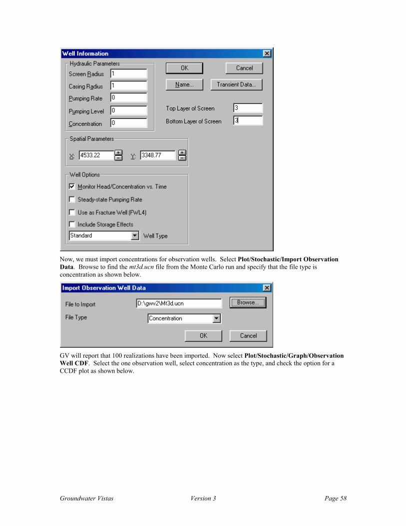
Groundwater Vistas Version 3 Page 58
Now, we must import concentrations for observation wells. Select Plot/Stochastic/Import Observation Data. Browse to find the mt3d.ucn file from the Monte Carlo run and specify that the file type is concentration as shown below.
GV will report that 100 realizations have been imported. Now select Plot/Stochastic/Graph/Observation Well CDF. Select the one observation well, select concentration as the type, and check the option for a CCDF plot as shown below.
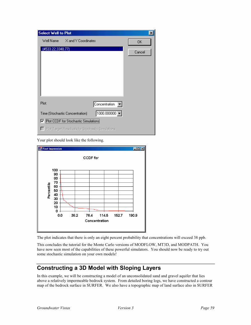
Groundwater Vistas Version 3 Page 59
Your plot should look like the following.
The plot indicates that there is only an eight percent probability that concentrations will exceed 38 ppb.
This concludes the tutorial for the Monte Carlo versions of MODFLOW, MT3D, and MODPATH. You have now seen most of the capabilities of these powerful simulators. You should now be ready to try out some stochastic simulation on your own models!
Constructing a 3D Model with Sloping Layers In this example, we will be constructing a model of an unconsolidated sand and gravel aquifer that lies above a relatively impermeable bedrock system. From detailed boring logs, we have constructed a contour map of the bedrock surface in SURFER. We also have a topographic map of land surface also in SURFER

Groundwater Vistas Version 3 Page 60
format. The goal of this exercise is to show the best way of defining layer topography in Groundwater Vistas.
The following is the land surface topography. It is contained within a file called surface.grd and is in SURFER format. The surface topography ranges in elevation from 1000 ft msl to 1210 ft msl.
455000.00 460000.00 465000.00 470000.00 475000.00 480000.00
885000.00
890000.00
895000.00
900000.00
The bedrock topography is shown below from a SURFER file called bedrock.grd. The bedrock elevations range from 431 ft msl to 1104 ft msl.
455000.00 460000.00 465000.00 470000.00 475000.00 480000.00
885000.00
890000.00
895000.00
900000.00
Now we will start a new GV model. Click the new document button or select File/New. Use 50 rows, 50 columns and 1 layer (we will start with 1 layer and then add another layer after importing layer topography). Enter the X spacing as 564.4 ft and Y spacing is 447.7 ft. Enter the base of the model as an elevation of 420 ft. and the top elevation of 1,220 ft. Click OK when you are done.
Now, import a base map so that the coordinates in the SURFER grid files can be mapped to actual site coordinates. Select File->Map->GWVistas. The map file is called 3d.map and is in the gwv3\tutorial directory. You will probably not see anything on your screen because the map is just a box that surrounds the grid. GV automatically offsets the model so that it lies at the minimum coordinates of the map. The model is now in the proper coordinate system.

Groundwater Vistas Version 3 Page 61
We will start by configuring the top of the model (layer 1). Select Props->Top Elevation. Click the database button on the toolbar or select Props->Property Values->Database. You will see that there are 100 zones and an elevation increment of 10 ft. We are going to change the database so that there are zone values going from a low of 990 ft msl in increments of 1 ft. The philosophy here is that our elevation data is only accurate to about 1 ft (given errors in gridding, size of model cells, surveying problems, etc.). Change the number of zones from 100 to 250 and click OK.
Now select Props->Property Values->Automatic Zone Setup. In the first (top) row of data, enter a starting value of 990 and an increment of 1.0. Click OK when you are done. Now go back to the database and you should see that zone 1 has a top elevation value of 990 ft msl and each zone is 1 ft. higher than the previous zone. We are now ready to import the SURFER file containing the surface topography.
Select Props->Import->Surfer. Check the box labeled Surfer File in Site Coordinates and browse to find the file called surface.grd. Click OK when you are done and the surface of the model is now sloping in the cross-section view.
We will do the same thing with bottom elevation. Select Props->Bottom Elevation. Click the database button and change the number of zones from 100 to 800. Click OK when you are done. Now select Props->Property Values->Automatic Zone Setup. In the first (top) row of data, enter a starting value of 400.0 and an increment of 1.0. Click OK when you are done. Now go back to the database and you should see that zone 1 has a bottom elevation value of 400 ft msl and each zone is 1 ft. higher than the previous zone. We are now ready to import the SURFER file containing the bedrock topography.
Select Props->Import->Surfer. Check the box labeled Surfer File in Site Coordinates and browse to find the file called bedrock.grd. Click OK when you are done and the bottom of the model is now sloping in the cross-section view subparallel to the top of the model.
This procedure sets the bounds of our model. Now we will insert a layer to make the model three-dimensional. Select Grid->Insert->Layer Below. This will split our one-layer model into 2 layers. A dialog prompts for the way in which to split the layer. You may make the new layer a constant thickness or a percentage of the current layer thickness (the default). The default is usually the best when the model layer changes in thickness like this one does. Keep the defaults and click the OK button. You should now see 2 layers in the cross-section view and at each row/column location the layers are the same thickness (+/- 1 ft).
Another way we could have split this layer is to have a SURFER file for each layer bottom. If we took this approach, we would have specified the number of layers we wanted to model in the initialization dialog instead of inserting them later. Otherwise, setting up the database and importing the files would have been identical to the way you did it above.
We are not going to run this model. The purpose was to show you how to construct the 3D grid. You might try adding boundary conditions, though, and see if the model will run.
Additional Tutorials This manual contains other tutorials including how to use ArcView Shapefiles and using optimization models with GV. These supplementary tutorials are provided in the remaining chapters of this manual.

Groundwater Vistas Version 3 Page 62

Groundwater Vistas Version 3 Page 63
Designing Models
Introduction The following chapter describes how to design the row, column, and layer configuration for a finite-difference model, assign boundary conditions to the model, and define aquifer properties.
There are generally six steps to follow when using GV to design a model: (1) design the finite-difference grid network (i.e., the number and spacing of rows, columns, and layers), (2) specify the location and type of boundary conditions, (3) define appropriate aquifer property zones for each cell, and (4) translate the model design into a data set for a particular model such as MODFLOW, (5) run the model, and (6) analyze and plot the results. These steps should generally be performed in the order presented above; however, there is often iteration in these steps as the model is constructed and calibrated. This chapter describes the first three steps in the model design process: grid design, boundary conditions, and aquifer properties.
General Steps to Apply GV
Beginning A New Model Design
Use the File->New menu selection to start a new model. You may also use the toolbar or press Ctrl-N. You select New even when you are importing a model from MODFLOW datasets or from an existing ModelCad grid file.
A dialog is displayed (shown below) that includes all of the parameters to define a new model. These include the number of rows, columns, and layers, the number of stress periods, row, column, and layer spacings, and default values for all properties. Fill out the table as completely as possible. You may always add or delete rows, columns, and layers later. You may also change the property values. You will see that this dialog is different from previous versions of GV. Most notable is the specification of the world coordinates of the model origin. If you know about where the model origin lies in world coordinates, it is better to specify them here. This will make importing maps easier.

Groundwater Vistas Version 3 Page 64
For simple models that have uniform aquifer properties and a uniform grid spacing, filling out this table gets you most of the way to a complete model. The only thing missing is the definition of boundary conditions, which determine where groundwater enters and exits the model.
A common question is whether the initialization dialog can be displayed later during model design. The answer is no. You may change all of the parameters associated with this dialog but they are done individually in other menus and dialogs. The initialization process just gets you started.
Do not try to run a model without specifying boundary conditions because it will simply “bomb”. This happens because most models, including MODFLOW, assume that the lateral and vertical edges of the model are no-flow boundaries unless you define another type of boundary. While this may seem obvious, beginning modelers often are confused by the notion of boundary conditions. These are described later in this chapter.
For a new model that you are designing from scratch, simply fill in the initialization dialog and click the OK button. You may also use this dialog to import an existing model from MODFLOW data files or from a ModelCad386 file. These import options are described below.
You may import a MODFLOW dataset by clicking the MODFLOW button. A dialog is displayed where you must enter the following information:
Option to automatically set number of zones for each parameter
Import MODFLOW-SURFACT files
Import Wells as Analytic Elements (instead of BC wells)
GHB Conductance Based on Saturated Thickness (usually only necessary for South Florida Water Management District files)
Import the MODFLOW files using MODFLOW96 formatting
Default vertical anisotropy ratio
Path to MODFLOW files
Root file name for MODFLOW dataset.
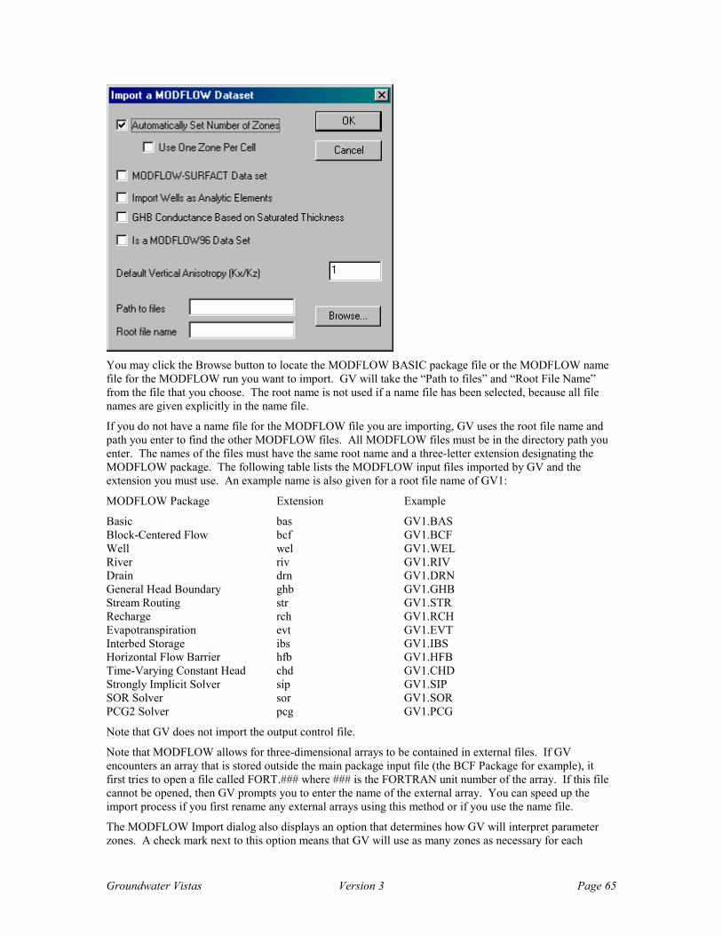
Groundwater Vistas Version 3 Page 65
You may click the Browse button to locate the MODFLOW BASIC package file or the MODFLOW name file for the MODFLOW run you want to import. GV will take the “Path to files” and “Root File Name” from the file that you choose. The root name is not used if a name file has been selected, because all file names are given explicitly in the name file.
If you do not have a name file for the MODFLOW file you are importing, GV uses the root file name and path you enter to find the other MODFLOW files. All MODFLOW files must be in the directory path you enter. The names of the files must have the same root name and a three-letter extension designating the MODFLOW package. The following table lists the MODFLOW input files imported by GV and the extension you must use. An example name is also given for a root file name of GV1:
MODFLOW Package Extension Example
Basic bas GV1.BAS Block-Centered Flow bcf GV1.BCF Well wel GV1.WEL River riv GV1.RIV Drain drn GV1.DRN General Head Boundary ghb GV1.GHB Stream Routing str GV1.STR Recharge rch GV1.RCH Evapotranspiration evt GV1.EVT Interbed Storage ibs GV1.IBS Horizontal Flow Barrier hfb GV1.HFB Time-Varying Constant Head chd GV1.CHD Strongly Implicit Solver sip GV1.SIP SOR Solver sor GV1.SOR PCG2 Solver pcg GV1.PCG
Note that GV does not import the output control file.
Note that MODFLOW allows for three-dimensional arrays to be contained in external files. If GV encounters an array that is stored outside the main package input file (the BCF Package for example), it first tries to open a file called FORT.### where ### is the FORTRAN unit number of the array. If this file cannot be opened, then GV prompts you to enter the name of the external array. You can speed up the import process if you first rename any external arrays using this method or if you use the name file.
The MODFLOW Import dialog also displays an option that determines how GV will interpret parameter zones. A check mark next to this option means that GV will use as many zones as necessary for each
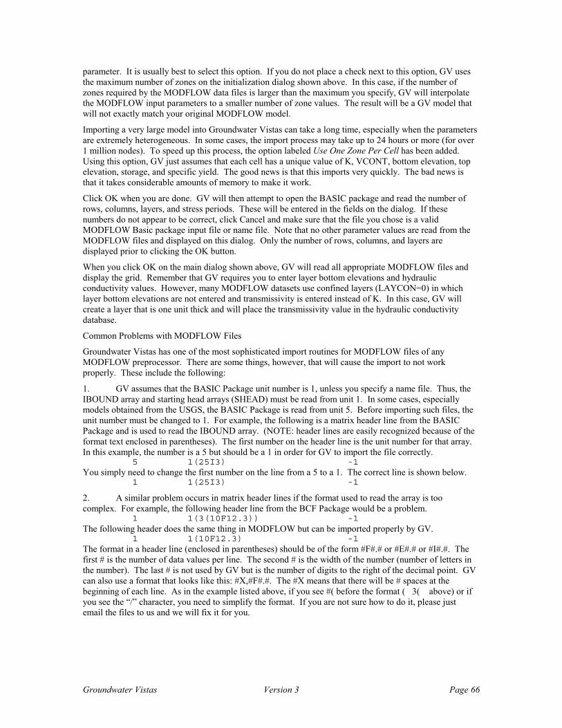
Groundwater Vistas Version 3 Page 66
parameter. It is usually best to select this option. If you do not place a check next to this option, GV uses the maximum number of zones on the initialization dialog shown above. In this case, if the number of zones required by the MODFLOW data files is larger than the maximum you specify, GV will interpolate the MODFLOW input parameters to a smaller number of zone values. The result will be a GV model that will not exactly match your original MODFLOW model.
Importing a very large model into Groundwater Vistas can take a long time, especially when the parameters are extremely heterogeneous. In some cases, the import process may take up to 24 hours or more (for over 1 million nodes). To speed up this process, the option labeled Use One Zone Per Cell has been added. Using this option, GV just assumes that each cell has a unique value of K, VCONT, bottom elevation, top elevation, storage, and specific yield. The good news is that this imports very quickly. The bad news is that it takes considerable amounts of memory to make it work.
Click OK when you are done. GV will then attempt to open the BASIC package and read the number of rows, columns, layers, and stress periods. These will be entered in the fields on the dialog. If these numbers do not appear to be correct, click Cancel and make sure that the file you chose is a valid MODFLOW Basic package input file or name file. Note that no other parameter values are read from the MODFLOW files and displayed on this dialog. Only the number of rows, columns, and layers are displayed prior to clicking the OK button.
When you click OK on the main dialog shown above, GV will read all appropriate MODFLOW files and display the grid. Remember that GV requires you to enter layer bottom elevations and hydraulic conductivity values. However, many MODFLOW datasets use confined layers (LAYCON=0) in which layer bottom elevations are not entered and transmissivity is entered instead of K. In this case, GV will create a layer that is one unit thick and will place the transmissivity value in the hydraulic conductivity database.
Common Problems with MODFLOW Files
Groundwater Vistas has one of the most sophisticated import routines for MODFLOW files of any MODFLOW preprocessor. There are some things, however, that will cause the import to not work properly. These include the following:
1. GV assumes that the BASIC Package unit number is 1, unless you specify a name file. Thus, the IBOUND array and starting head arrays (SHEAD) must be read from unit 1. In some cases, especially models obtained from the USGS, the BASIC Package is read from unit 5. Before importing such files, the unit number must be changed to 1. For example, the following is a matrix header line from the BASIC Package and is used to read the IBOUND array. (NOTE: header lines are easily recognized because of the format text enclosed in parentheses). The first number on the header line is the unit number for that array. In this example, the number is a 5 but should be a 1 in order for GV to import the file correctly. 5 1(25I3) -1 You simply need to change the first number on the line from a 5 to a 1. The correct line is shown below. 1 1(25I3) -1
2. A similar problem occurs in matrix header lines if the format used to read the array is too complex. For example, the following header line from the BCF Package would be a problem. 1 1(3(10F12.3)) -1 The following header does the same thing in MODFLOW but can be imported properly by GV. 1 1(10F12.3) -1 The format in a header line (enclosed in parentheses) should be of the form #F#.# or #E#.# or #I#.#. The first # is the number of data values per line. The second # is the width of the number (number of letters in the number). The last # is not used by GV but is the number of digits to the right of the decimal point. GV can also use a format that looks like this: #X,#F#.#. The #X means that there will be # spaces at the beginning of each line. As in the example listed above, if you see #( before the format ( 3( above) or if you see the “/” character, you need to simplify the format. If you are not sure how to do it, please just email the files to us and we will fix it for you.

Groundwater Vistas Version 3 Page 67
Digitized Map Files After you start your new model or import an old one, you may want to display a base map with the model grid. GV plots digitized base maps over the finite-difference grid to give the modeler a frame of reference. These digitized maps serve no other function in the model design process. Data cannot be imported directly from the map; the map is simply a graphical feature. There is no set limit on the size of a map. GV reads a base map and stores the data in a temporary file on your hard disk. This is saves memory and allows you to use maps that are quite large.
Digitized base maps may be in one of four formats, (1) GV format, (2) ArcView shapefile format, (3) DXF format, and (4) SURFER BLN (blanking file) format. These map options are displayed on a dropdown menu after you select Map from the File menu.
The DXF file is a generic format supported by most CAD software packages (such as AutoCAD). The SURFER BLN format is used by the popular SURFER contouring software to draw base maps and to create blank regions in contour maps. The BLN format is limited to only one color for all map entities and you will be presented with a dialog to choose the color assigned to the BLN map you import. The Chapter entitled Digitized Maps provides details regarding the GV map format, which is identical to the QuickFlow and ModelCad map formats. ArcView shapefiles are geographic information system (GIS) files used by many GIS applications like ArcView. Shapefiles can also be imported with attributes to set boundary conditions and properties. In the context of this section, though, they are only used for displaying maps.
By default GV assumes that the coordinate systems for the map and model are identical. That is, the origin (x=0.0 and y=0.0) of both map and model coincide with the lower left corner of the model grid. GV will check, however, to see if the map and model are completely separated (e.g., they do not overlap) when you import the map. If the map and model do not overlap, GV will automatically offset the model grid such that the origin of the model is moved to the minimum X and Y coordinates on the map. You may move the model grid further by selecting Grid->Offset as described after the discussion on DXF files.
DXF Files
After choosing DXF from the Map menu, a standard Windows file selection dialog will then be displayed where you select the file to import. For DXF files, a second file dialog appears because the DXF file is translated into a GV map file. The second dialog prompts for the name of the GV map file to be created. Once you import a DXF file, you do not need it again because GV will subsequently use the GV map that is created. To quickly determine the distance between two points, select Add->Line Boundary. Drag a line between two points and the subsequent dialog showsthe distance. Select Cancel to delete the line you just inserted.
After specifying the GV map file name that will be created, GV displays a dialog for the DXF multiplication factor. This is a scaling factor used to modify the coordinates in the DXF file. Often, the DXF file will contain coordinates in inches. You would then enter a multiplication factor of 0.08333 to convert inches to feet. It is difficult to know in advance what coordinates are in the DXF file, so some experimentation may be required. After importing the DXF file, move the cursor around on the screen and check the coordinates of key points on the map. Use these coordinates to determine distances. If these distances are not correct, simply import the DXF map again and use a multiplier to change the scale of the DXF file.
Another common problem with DXF files is that many drafters use “blocks” to define items on the map. A block is a special entity used by AutoCAD (and other CAD systems, too) to group multiple entities (e.g., lines and circles) into one item. GV does not properly interpret blocks. If you see that GV has not imported all items on your DXF map, go back to the CAD software and perform a function called “explode all blocks”. This breaks down the blocks into individual entities that can then be exported in the DXF file so that GV will recognize them.
Moving the Grid on the Map
GV will now read the map file and try to display it on the screen. Remember, the lower left corner of the finite difference grid is placed at the map origin (X=0, Y=0). In some cases, the map origin may be located far from the area covered by the map. This is especially true when using State Plane coordinates or UTM coordinates. In this case, GV will automatically move the grid so that the grid origin (lower left corner)

Groundwater Vistas Version 3 Page 68
lies at the minimum X and Y coordinates on the map. To move the finite-difference grid to another location on the map, use the following procedure:
(1) Select View->Full->Grid to place the full grid on the screen. The finite-difference grid will take up most of the screen. You want want to zoom out (View->Zoom Out) to see more of the map.
(2) Select Grid -> Offset.
(3) Move the cursor to the point on the map where you want the lower left corner of the finite-difference grid to be. Click the left mouse button or press the Enter key.
(4) A dialog appears showing you the coordinates that you chose. Click the OK button to accept these coordinates (or change the values if you like).
The finite-difference grid will be drawn over the map using the new offset coordinates.
You may also rotate the finite-difference grid. The Grid->Rotate command actually rotates the map under the finite-difference grid. The grid is always shown with rows and columns parallel to the edge of your screen. Enter the rotation angle in degrees. Negative angles indicate that the grid will be rotated in a clockwise direction relative to the map.
The X and Y coordinates of the cursor are always displayed on the status bar at the bottom of the GV window. By default, these coordinates are grid coordinates with the origin at the lower left corner of the grid. You may change these coordinates to map coordinates by selecting Grid->Options.
Designing The Finite-Difference Grid
Concepts The finite-difference grid is created in GV by first specifying the number of rows, columns, and layers as described in a previous section. GV creates a mesh with uniform row and column widths that you specify on the initialization dialog. This is called a regular mesh. While the regular mesh represents the most accurate form of the finite-difference solution (Anderson and Woessner 1992), it is often necessary or desirable to refine the mesh in areas of interest. In this manner, more accuracy is achieved in key areas at the expense of less accuracy at the edges.
GV provides you with the ability to insert, delete, and move rows, columns, and layers. Rows and columns are manipulated using the horizontal and vertical grid lines, not the rectangular cells. In essence, inserting a new row splits the previous row into two new rows. Columns are manipulated in an analogous manner.
Inserting and deleting grid lines causes boundary conditions to be disrupted in the new mesh. GV places the boundary condition in one of the two new cells caused by inserting a row or column. While this preserves the basic model design, some repairs are necessary after modifying the grid layout. For this reason, the spacing of rows and columns should be determined prior to specifying boundary conditions.
Inserting rows and columns does not affect the grid-independent boundary types (wells, line boundaries, boundaries), calibration targets, and titles. These items are placed in the model using X and Y coordinates rather than row and column locations.
There is no limit to the number of rows, columns, and layers you may add to the model. GV automatically adjusts the memory requirements of the model as you expand the grid. You may reach a physical limit on model size due to the amount of memory in your computer, however.
Working with Rows and Columns The rows and columns refer to the horizontal and vertical grid lines in the model. Layers are approximately horizontal networks of rows and columns. Layers are numbered from top to bottom, with layer 1 being the uppermost layer. Rows are numbered from the top of your screen to the bottom. Row 1 is the top-most row. Columns are numbered from left to right.
Groundwater Vistas Version 3 Page 69
The finite-difference grid is designed and edited using the Grid menu. You must also be in Grid mode to
make changes to the grid layout. Select Edit->Grid or click on the button on the toolbar. When the
button is depressed on the toolbar, you are in Grid mode.
You may insert, delete, and move rows and columns. Each command on the Grid menu alters the position of the grid lines and not the rectangular regions called cells. The Insert command adds a row or column grid line to the mesh. Delete is used to remove a row or column grid line from the mesh. Move shifts the position of a row or column grid line. Uniform changes all row or column spacings to a uniform value.
Click the button on the toolbar to quickly get to the Grid options dialog.
The Insert menu allows you to insert rows, columns, and layers into your model design. The Insert menu contains four options, Row, Column, Layer Below, and Layer Above. When you select Row, the cursor changes shape to resemble a row grid line (a horizontal line). Move the cursor to the location for the new row and click the left mouse button. GV determines where to place the new row depending upon the option labeled “Option for Adding New Rows/Columns” on the Grid->Options dialog. The default is to split the current cell in half. Using this option, you do not need to have accurate placement of the cursor when you click the mouse button. GV will simply split the cell containing the cursor into two equal rows. Inserting columns works the same way.
Other options for inserting rows and columns include “Set cell spacing”, “Percent current spacing”, and “Insert at the cursor”. With the “Set cell spacing” option, you enter a given row and column spacing. When you click the left mouse button, GV attempts to make the row or column that exact spacing. This is a useful option for adding new rows or columns beyond the edges of the current grid. The “Percent cell spacing” option splits the current cell using a proportion you enter on the Grid Options dialog. The “Insert at the cursor” option simply adds the new row or column grid line where ever you click the left mouse button.
You may add as many rows, columns, and layers to the model as you choose (as long as you have enough memory!). GV automatically compensates for the added memory requirements.
The Delete menu contains three selections, Row, Column, and Layer. Selecting Row or Column allows you to move the cursor to a location on the screen, click the left mouse button, and delete the row or column grid line nearest to the cursor. When you select Layer, the current layer is deleted (along with all boundary conditions in this layer).
GV uses the right mouse button to quickly insert or delete rows and columns when in grid mode. The function of the right mouse button depends upon which button is depressed on the right side of the toolbar. The choices are:
Delete Column
Insert Column
Delete Row
Insert Row
For example, to insert a row click on the button, move the cursor to the desired location and press the right mouse button. A new row grid line is inserted using whichever option is selected on the Grid Options
dialog as described above. You may insert as many rows as you like while the button is depressed. Columns are inserted in an analogous manner.
You may slide row and column grid lines around on the screen when you are in Grid mode. This is done by placing the cursor near a row or column grid line. The cursor will change to either a (left-right)

Groundwater Vistas Version 3 Page 70
cursor for moving columns or a (up-down) cursor for moving rows. You may now press and hold the left mouse button down and move the cursor to slide the row or column grid line. You may not move it beyond the adjacent row or column grid lines, however.
You may manually change row and column spacings by selecting Grid->Edit->Row Spacings or Grid->Edit->Column Spacings. You will see a scrolling list of spacings that you can modify.
The Grid->Edit menu also allows you to automatically change row and column spacings using an initial spacing and a multiplier. When you select Grid->Edit->Row Auto Setup or Grid->Edit->Column Auto Setup, you will see a dialog with four parameters, including:
Starting row/column number Ending row/column number Initial spacing assigned to starting row/column Multiplier
The automatic setup starts by changing the spacing of the starting row/column to the initial value. The next row/column spacing is assigned a value equal to the intial spacing times the multiplier. The procedure continues until the ending row/column is reached. You may also specify a starting row/column number that is larger than the starting number so that you can go in either direction.
Row and column spacings may also be reset to a uniform value by selecting Grid->Uniform->Row Spacing or Grid->Uniform->Column Spacing. You simply enter a new spacing value and all rows or columns are set to that value.
Automating Grid Design Groundwater Vistas offers two additional ways to quickly modify the grid. The first is grid smoothing which takes out large jumps in grid spacing. The second is grid refinement (not the same as telescopic mesh refinement) which allows you to specify an area where a uniform grid will be established and the remaining grid spacings will be automatically smoothed.
The Smooth Grid option rearranges grid spacings so that adjacent cells vary by no more than a user-specified amount. The following dialog is displayed when selecting this option.
The grid smoothing option is very different from the one in Visual MODFLOW which some users may be familiar with. In Visual MODFLOW, the grid is smoothed but no rows or columns are added. This can result in a very different looking grid after smoothing. The approach used in GV tries to minimize the impact on grid spacings by adding rows or columns where necessary to achieve the maximum ratio.
A similar option is the Refine Grid command. After selecting this option, you drag a window on the screen. GV will set cell widths in this window to a constant value that you select on the following dialog.

Groundwater Vistas Version 3 Page 71
The Maximum Grid Change Ratio is then used to smooth around the edges of the new refined area as described in the last paragraph for grid smoothing. This option should be used with caution as boundary conditions and aquifer property zones may change significantly after refinement. The refine grid command is best used before boundaries or properties are defined in detail.
Working with Layers Layers are approximately horizontal collections of rows and columns. Each layer contains the same number of rows and columns. By default, layers are horizontal with uniform top and bottom elevations. You may offset the elevation of any cell, however, using the Property menu as described later in this chapter.
You have two options for inserting layers into the model. You may insert a layer above the current layer or insert a layer below the current layer. The current layer is displayed on the status bar as L: and on the Reference Cube. These options are selected using Grid->Insert->Layer Above and Grid->Insert->Layer Below commands.
Selecting Layer Below adds a new layer below the current layer. The current layer is shown two places, on the reference cube (usually on the left side of the screen) and on the status bar (e.g., L:1 for layer 1). Layer Above adds a new layer above the current layer.
When adding a layer, you will see the dialog below. There are two options for setting the thickness of the new layer. It can either be half the thickness of the current layer or a percentage of the current layer. In all cases, your new model will have the same thickness as the old model because the current layer will decrease in thickness to accommodate the additional layer.
You may add as many rows, columns, and layers to the model as you choose (as long as you have enough memory!). GV automatically compensates for the added memory requirements.
It is also easy to delete an entire layer. Simply select Grid->Delete->Layer. The current layer is deleted from the model. GV also deletes any boundary conditions that were in that layer.
Using Variable Layer Elevations The zone concept works quite well for hydraulic properties where we have limited field measurements. Layer bottom elevation is the only parameter where we commonly have significant amounts of field data. Even with a large database of layer elevation values the zone concept can work quite well. The following procedure should be used when you want to have layer elevation vary within a layer (i.e., the layers are not flat).
Step 1. You should first determine the minimum and maximum elevations required for your model. This does not mean the minimum and maximum for a given layer but for all layers in the model from the bottom of the aquifer to the top or land surface. As an example to follow through this procedure we will assume that the lowest bottom elevation for our model is 600 feet below sea level or –600 ft msl. We will also assume that the highest elevation in the model is land surface and is 100 feet above sea level or +100 ft msl.
Step 2. You must now decide the precision assigned to layer bottom elevations. That is, should the layer elevations be rounded to the nearest foot, the nearest tenth of a foot, or some other value? When deciding

Groundwater Vistas Version 3 Page 72
this, there are a couple of points to keep in mind. First, if you have ever logged a well or boring, even if it was cored, you probably realize that the contacts you determine are only accurate to about one foot. Second, you can have thousands of zones without impacting the memory requirements of your model. Given these two facts, we usually recommend a precision of 1 foot for layer elevations. Even if you have thousands of feet of relief in your model, the precision of one foot will not harm the performance of your model or its memory requirements. In our example, we would need 700 zones to achieve a 1 foot precision or 7,000 zones for a precision of 0.1 ft.
Step 3. Reset the database to the number of zones determined in Step 2. You do this by selecting Props->Bottom Elevations and then selecting Props->Property Values->Database. Enter the number of zones at the top of the dialog as shown below.
After entering the number of zones, click the Update button and then click OK. You do not need to enter the new elevations yet.
Step 4. Now we use a shortcut to set up the database. Select Props->Property Values->Auto Zone Setup. The dialog is shown below. Enter a 1 for the starting zone number (i.e., the beginning of the database) and 700 for the ending zone number. The starting value is the lowest elevation in your model and the increment is the precision you chose in Step 2 above. In our example, we will use a precision of 1 foot. Click OK when done.
Step 5. You can now import a variety of files to set layer elevations or use the any of the other methods to define zones (individual cells, gradient fill, window, etc.). See the Menu chapter under Props and Import for more information on importing property data from external files.
You should also repeat this procedure if you would like to vary top elevations in your model. Keep in mind that you only need to define the top of layer 1. GV assumes that the tops of lower layers are the same as
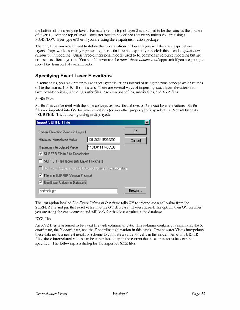
Groundwater Vistas Version 3 Page 73
the bottom of the overlying layer. For example, the top of layer 2 is assumed to be the same as the bottom of layer 1. Even the top of layer 1 does not need to be defined accurately unless you are using a MODFLOW layer type of 3 or if you are using the evapotranspiration package.
The only time you would need to define the top elevations of lower layers is if there are gaps between layers. Gaps would normally represent aquitards that are not explicitly modeled; this is called quasi-three-dimensional modeling. Quasi three-dimensional models used to be common in resource modeling but are not used as often anymore. You should never use the quasi-three-dimensional approach if you are going to model the transport of contaminants.
Specifying Exact Layer Elevations In some cases, you may prefer to use exact layer elevations instead of using the zone concept which rounds off to the nearest 1 or 0.1 ft (or meter). There are several ways of importing exact layer elevations into Groundwater Vistas, including surfer files, ArcView shapefiles, matrix files, and XYZ files.
Surfer Files
Surfer files can be used with the zone concept, as described above, or for exact layer elevations. Surfer files are imported into GV for layer elevations (or any other property too) by selecting Props->Import->SURFER. The following dialog is displayed:
The last option labeled Use Exact Values in Database tells GV to interpolate a cell value from the SURFER file and put that exact value into the GV database. If you uncheck this option, then GV assumes you are using the zone concept and will look for the closest value in the database.
XYZ files
An XYZ files is assumed to be a text file with columns of data. The columns contain, at a minimum, the X coordinate, the Y coordinate, and the Z coordinate (elevation in this case). Groundwater Vistas interpolates these data using a nearest neighbor scheme to compute a value for cells in the model. As with SURFER files, these interpolated values can be either looked up in the current database or exact values can be specified. The following is a dialog for the import of XYZ files.

Groundwater Vistas Version 3 Page 74
To use exact interpolated values in the database, check the last box labeled Append Data to Database. If you want to totally start over with the database, you may also check the box labeled Automatically Reset Database. This option must be used in conjunction with the append data option. If both of these options are unchecked, then GV looks up the closest value in the database. See the section on defining aquifer properties for a discussion of the nearest neighbor algorithm for interpolation in GV.
Matrix File
In some cases, you may want to use another application to define the elevations of layers and store them in a simple matrix. The matrix is assumed to contain one value for each cell in the model or in a single layer. The order of the numbers is layer, row, column (just like MODFLOW reads them). The numbers must be separated by a comma, tab, or space.
The last option defines how the values in the matrix are used. If you select Append to Database, GV will put the exact values in the database. Selecting Find Nearest in Database will use the zone concept and find the closest value in the database.
ArcView Shapefile

Groundwater Vistas Version 3 Page 75
There are three types of shapefiles that can be imported from ArcView for layer elevation (or any other property for that matter). A point shapefile is treated just like an XYZ file above. A line shapefile is assumed to represent contours. In this case, GV will extract the vertices of the lines (contours) and then use them as a collection of points. For a polygon shapefile, GV looks for cells within each polygon and simply sets the property associated with that polygon.
The dialog for a point or line shapefile is shown below:
You first select the attribute field for the bottom elevation (BOTTOM_LAY in the example above). You then determine whether you want to interpolate or not. Usually for points and lines you would use interpolation. If you don’t interpolate, GV will only change the bottom elevation of cells containing points or vertices of lines. You then have the option of using exact values or check the box to Find Nearest Value in Existing Database. The dialog for a polygon shapefile is the same but you cannot choose to interpolate values.
Assigning Boundary Conditions
Concepts GV supports the use of three types of boundary conditions, specified head/concentration, specified flux, and mixed type boundary conditions. Specified head boundary cells are called constant head cells. GV calls these cells constant head, but you may make the cell constant head, constant concentration, or both constant head and concentration. Specified flux boundary cells are represented using no-flow, wells, or recharge. Mixed-type boundary conditions are called rivers, drains, general-head boundaries, streams, or evapotranspiration. Recharge and ET are treated as properties because they are distributed to every cell in the top layer in the model. These are discussed under parameter zones in the next section.
The terminology used to describe boundary conditions is consistent with the MODFLOW usage (McDonald and Harbaugh 1988). Most other models will support similar boundary types; however, different names may be used.

Groundwater Vistas Version 3 Page 76
In the following discussion, the phrases boundary values or boundary condition parameters are often used. These terms refer to the set of data values entered for each boundary condition cell. Each boundary type (except no-flow) has its own set of values that are displayed on the boundary condition dialog. Values common to all boundary types include the following:
• Head or flux (stage for rivers, drain elevation, pumping rate for wells),
• row, column, layer of cell containing the boundary condition,
• reach number,
• option for steady-state or transient condition, and
• color
Head-dependent flux boundary types (rivers, drains, general-head boundary, streams) also include a set of parameters for the conductance term. GV takes these parameters and computes the conductance term, as described below. Rivers also require the elevation of the river bottom. Streams require additional information related to surface flow. No data are entered for no-flow cells.
Boundary conditions may be inserted in the model individually, in a window, along a digitized line, or within a digitized polygon region. You are limited to one boundary condition per cell.
In addition to boundary conditions that are defined for specific cells in the model, GV includes grid-independent boundary conditions, called analytic elements. The analytic element boundaries include wells, line boundaries, and circular boundaries. Wells are used exclusively for pumping or injection wells (constant flux) while line and circle boundaries may represent constant head, river, drain, or general head boundary types.
Choice of Boundary Condition Type GV supports all of the boundary condition types in MODFLOW, including constant head, well, river, drain, general head, and stream. In addition, the horizontal flow barrier package is supported by GV using a special boundary type called a wall. The choice of what boundary type to use for a given hydrologic condition is one of the most complex decisions you will make in designing your model. There is no right answer to this decision.
Boundary conditions determine where water enters or leaves the model domain and in what quantity. In order to make an informed decision about boundaries, you must have a good understanding of water budgets in the physical system. Ideally, your boundaries should represent real physical boundaries such as surface water bodies and regional groundwater divides.
Use the following information to guide your decision:
Constant Head
A constant head, by definition, is a boundary where the head and/or concentration does not change during the simulation. You should use these types of boundaries with caution as they imply an infinite supply of water to the aquifer. Constant head boundaries should be used for major sources of water that fully penetrate the model layer where they are defined. Good candidates for constant head boundaries include major surface water bodies (rivers, lakes, ocean). The most common mistake in modeling is to place constant heads completely surrounding a model layer. While there are occasions where this may be warranted (modeling an island for example), normally this procedure should not be done. By fixing the head around the layer, the model is constrained and can often be calibrated with virtually any value for hydraulic conductivity.
Constant Flux (well)
A constant flux is analogous to a constant head except that the flow of water into or out of the aquifer is fixed. Constant flux boundaries normally represent wells or drains where the pumping rates are known or can be estimated with some certainty.
Groundwater Vistas Version 3 Page 77
Special types of constant flux boundary conditions include recharge and the no-flow boundary. Recharge is the rate at which infiltrating water reaches the water table and is expressed in units of L/T (e.g., ft/d). Recharge is implemented in GV as a property because it applies to all cells in the top model layer. A no-flow boundary is an area where the flow of groundwater is zero. By default, all outer edges of the model grid are assumed to be no-flow in most models, including MODFLOW. No-flow boundaries may also be used to represent bedrock areas in an unconsolidated aquifer where the bedrock yields negligible amounts of water to the system.
River
Rivers are special forms of the head-dependent boundary condition. In a head-dependent boundary, the model computes the difference in head between the boundary and the model cell where the boundary is defined. The head difference is then multiplied by a conductance term to get the amount of water flowing into or out of the aquifer. In a river boundary, MODFLOW performs an additional check before computing flow rates. If the head in the model cell is below the bottom elevation of the river boundary, the difference in head is computed as the river stage minus the river bottom elevation. This causes flow rates to reach a maximum value when an unsaturated zone exists beneath the river.
River boundaries should be used where a surface water feature partially penetrates a layer and can both remove water from the aquifer and infiltrate water into the aquifer. River boundaries should not be used if the flow in the river can go to zero under losing conditions. In this case, a drain or stream boundary should be used.
Drain
Drains are similar to rivers except that drains will only remove water from the model. If the head in the model cell drops below the drain elevation, the drain will not inject water into the model. Under these conditions, the drain becomes inactive.
Streams
A stream is a special form of river boundary in which simple surface water modeling is also performed. The surface flow rate is provided to the model and is monitored by MODFLOW during a simulation. If the stream loses water to the aquifer and the infiltration rate exceeds the amount of flow in the stream, MODFLOW sets infiltration to zero in that cell and all downstream cells.
General Head Boundary
A general head boundary (or GHB) is a generic form of the head-dependent boundary condition. GHBs are normally used along the edge of the model to allow groundwater to flow into or out of the model under a regional gradient.
Displaying Boundary Cells GV normally displays boundary conditions by filling the cell containing a boundary condition with a solid color. GV also has the capability of displaying a small symbol centered in the cell to represent boundary conditions. By default, GV will display all boundary cells even if you are not in BC mode. You may change this so that GV only displays boundary cells when you are in boundary model. All boundary
condition options, like the ones described here, are edited by selecting BCs->Options or .
Inserting Boundary Cells The Insert menu provides options to add boundary conditions to the model individually (Single Cell), in a rectangular region (Window), interpolated along a digitized line (Digitize Polyline), or within a digitized region (Digitize Polygon). The currently selected boundary condition type is inserted using these commands. The current type is the one listed at the bottom of the BCs menu with a check mark next to it.
To insert a single boundary cell, select Insert->Single Cell, move the cursor to the cell where you want to add the boundary condition, and click the left mouse button. A dialog is displayed containing several data fields. A quick way to insert a boundary cell is to move the mouse cursor to that cell and click the right
Groundwater Vistas Version 3 Page 78
mouse button. Be careful, though, because clicking the right mouse button over an existing boundary condition deletes that boundary cell.
Each boundary condition type has its own dialog, but they all have common fields. These common data include:
Row number Column number Layer number Reach number Steady-state Boundary check box Transient Data button Color button
Row, column, and layer determine the position of the boundary condition within the model. The reach number is used to group boundary condition cells. Boundary conditions may be deleted, modified, and calibrated by reach number. You may also obtain a mass balance summary for each boundary reach and the flux for a specified reach may be recorded in the automatic sensitivity analysis.
The steady-state boundary option should be checked if the boundary is active for the entire simulation at a constant value. Uncheck the steady-state option to change the values of head, flow rate, and/or concentration during a transient simulation. After you uncheck the steady-state option, click the “Transient Data” button. A spreadsheet is displayed with five columns, including
Starting the starting stress period number Ending the ending stress period number Head (Q for wells) the boundary head (river stage, etc.) or flow rate for wells Concentration only used for transport simulations Flow this is the flow in the surface water body for Streams
The starting and ending stress period determine the period of time when the specified head, concentration, or flow data are active. Important Note: the starting and ending stress period numbers are integers from 1 to the maximum number of stress periods. You may not enter the time values in days here. You may enter as many of these groups of transient data as you wish up to the maximum number of stress periods. The maximum number of stress periods is entered when you initialize the model and may be changed using the BCs->Options dialog.
On the right side of the dialog are data describing the hydraulic impact of the boundary condition. These data are unique to each boundary type. The river boundary condition is a good example, however, since it has most of the available data types. An example river boundary dialog is shown below. Note that GV will compute the conductance of head-dependent boundary conditions (river, drain, general head, stream). You enter the length (L), width (W), hydraulic conductivity (K), and thickness (T) parameters and GV computes conductance using the following equation:
C = K L W/T
When you enter boundary conditions in a window, GV automatically selects the length parameter as the maximum cell dimension (the maximum of the column and row width). For digitized polygons, GV automatically sets the length and width parameters to the cell dimensions, i.e., the area term (LW above) is the area of the cell.
For digitized polylines, GV uses the column or row width as the length of the boundary condition in that cell. GV determines which dimension to use based upon the orientation of the line. If the digitized line is longer in the X direction than in Y, GV uses the width of the cell in X (column width) for the length term in the conductance calculation.
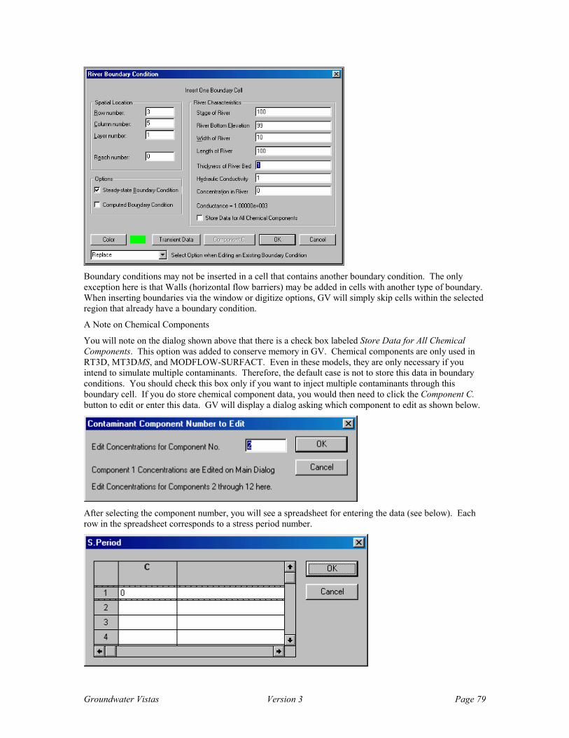
Groundwater Vistas Version 3 Page 79
Boundary conditions may not be inserted in a cell that contains another boundary condition. The only exception here is that Walls (horizontal flow barriers) may be added in cells with another type of boundary. When inserting boundaries via the window or digitize options, GV will simply skip cells within the selected region that already have a boundary condition.
A Note on Chemical Components
You will note on the dialog shown above that there is a check box labeled Store Data for All Chemical Components. This option was added to conserve memory in GV. Chemical components are only used in RT3D, MT3DMS, and MODFLOW-SURFACT. Even in these models, they are only necessary if you intend to simulate multiple contaminants. Therefore, the default case is not to store this data in boundary conditions. You should check this box only if you want to inject multiple contaminants through this boundary cell. If you do store chemical component data, you would then need to click the Component C. button to edit or enter this data. GV will display a dialog asking which component to edit as shown below.
After selecting the component number, you will see a spreadsheet for entering the data (see below). Each row in the spreadsheet corresponds to a stress period number.
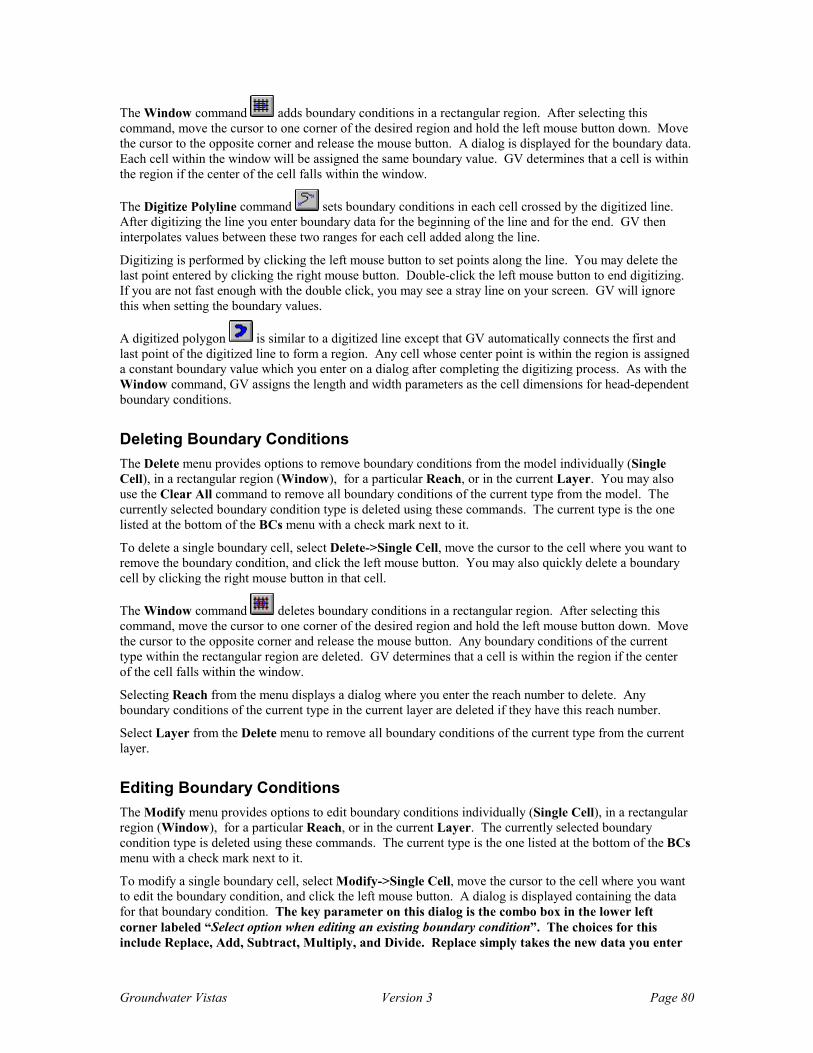
Groundwater Vistas Version 3 Page 80
The Window command adds boundary conditions in a rectangular region. After selecting this command, move the cursor to one corner of the desired region and hold the left mouse button down. Move the cursor to the opposite corner and release the mouse button. A dialog is displayed for the boundary data. Each cell within the window will be assigned the same boundary value. GV determines that a cell is within the region if the center of the cell falls within the window.
The Digitize Polyline command sets boundary conditions in each cell crossed by the digitized line. After digitizing the line you enter boundary data for the beginning of the line and for the end. GV then interpolates values between these two ranges for each cell added along the line.
Digitizing is performed by clicking the left mouse button to set points along the line. You may delete the last point entered by clicking the right mouse button. Double-click the left mouse button to end digitizing. If you are not fast enough with the double click, you may see a stray line on your screen. GV will ignore this when setting the boundary values.
A digitized polygon is similar to a digitized line except that GV automatically connects the first and last point of the digitized line to form a region. Any cell whose center point is within the region is assigned a constant boundary value which you enter on a dialog after completing the digitizing process. As with the Window command, GV assigns the length and width parameters as the cell dimensions for head-dependent boundary conditions.
Deleting Boundary Conditions The Delete menu provides options to remove boundary conditions from the model individually (Single Cell), in a rectangular region (Window), for a particular Reach, or in the current Layer. You may also use the Clear All command to remove all boundary conditions of the current type from the model. The currently selected boundary condition type is deleted using these commands. The current type is the one listed at the bottom of the BCs menu with a check mark next to it.
To delete a single boundary cell, select Delete->Single Cell, move the cursor to the cell where you want to remove the boundary condition, and click the left mouse button. You may also quickly delete a boundary cell by clicking the right mouse button in that cell.
The Window command deletes boundary conditions in a rectangular region. After selecting this command, move the cursor to one corner of the desired region and hold the left mouse button down. Move the cursor to the opposite corner and release the mouse button. Any boundary conditions of the current type within the rectangular region are deleted. GV determines that a cell is within the region if the center of the cell falls within the window.
Selecting Reach from the menu displays a dialog where you enter the reach number to delete. Any boundary conditions of the current type in the current layer are deleted if they have this reach number.
Select Layer from the Delete menu to remove all boundary conditions of the current type from the current layer.
Editing Boundary Conditions The Modify menu provides options to edit boundary conditions individually (Single Cell), in a rectangular region (Window), for a particular Reach, or in the current Layer. The currently selected boundary condition type is deleted using these commands. The current type is the one listed at the bottom of the BCs menu with a check mark next to it.
To modify a single boundary cell, select Modify->Single Cell, move the cursor to the cell where you want to edit the boundary condition, and click the left mouse button. A dialog is displayed containing the data for that boundary condition. The key parameter on this dialog is the combo box in the lower left corner labeled “Select option when editing an existing boundary condition”. The choices for this include Replace, Add, Subtract, Multiply, and Divide. Replace simply takes the new data you enter

Groundwater Vistas Version 3 Page 81
for the boundary condition. The other options either add, subtract, multiply, or divide the data in the current boundary condition by the data you enter on this dialog. All of the data except for the row, column, layer, color, and reach values are effected by what you enter. When using the multiply or divide options, make sure to enter the number 1.0 for fields that you do not want to change. Enter a zero for those values that you do not want to modify when using the add or subtract options.
You may also edit a single boundary condition by double-clicking the left mouse button on that cell.
The Window command modifies boundary conditions in a rectangular region. After selecting this command, move the cursor to one corner of the desired region and hold the left mouse button down. Move the cursor to the opposite corner and release the mouse button. GV finds the first occurrence of the current boundary type within the region and displays a dialog for editing. Any boundary conditions of the current type within the rectangular region are modified using the data you enter on this dialog. GV determines that a cell is within the region if the center of the cell falls within the window.
Selecting Reach from the menu displays a dialog where you enter the reach number to modify. GV then finds the first occurrence of the current boundary type with the specified reach number and displays a dialog for editing. Any boundary conditions of the current type in the current layer are modified if they have this reach number.
Select Layer from the Modify menu to modify all boundary conditions of the current type in the current layer. GV then finds the first occurrence of the current boundary type in the current layer and displays a dialog for editing. Any boundary conditions of the current type in the current layer are modified.
The Copy command allows you to copy boundary conditions of the current type form another layer to the current layer. A dialog is displayed where you enter the layer number to copy the boundary conditions from. You may not copy boundary conditions of another type.
Importing Boundary Conditions from a File The Import feature provides a way of reading boundary conditions from ASCII (DOS text) files. These files may be created from spreadsheets, text editors, or customized programs. Even MODFLOW boundary condition files may be read using this option.
Data in the import file may be in any order but the structure of the file must conform to the following specifications:
there may be any number of lines at the top of the file to label the information. You will tell GV how many lines to skip in this header record.
all data beneath the header lines must be in columns, separated by spaces, tabs, and or commas. Each line of the file must contain data for one boundary condition and each line must contain the same number of columns of information.
there can be no extraneous information after the columns of data.
data are imported for the current boundary condition type.
You enter the name of the file on the Import dialog (a browse button is provided so that you can locate the file), the number of lines to skip at the top of the file, and whether the coordinates in the file are in site coordinates. Site coordinates refer to the coordinates of the base map. Uncheck this option if the coordinates are model grid coordinates, with the origin being the lower left corner of the grid.
Beneath these data are three buttons labeled “Coordinate Data”, “Boundary Data”, and “Conductance Data”. You should click each button to edit the information pertaining to these categories of information. On each dialog you enter the column number containing the specific data items. If the data are not contained in the file, enter a zero for the column number. In some cases, you may also enter default data for a particular variable. In this case, if the data are not in the file, the default value is assigned to each boundary condition imported.
Coordinate Data
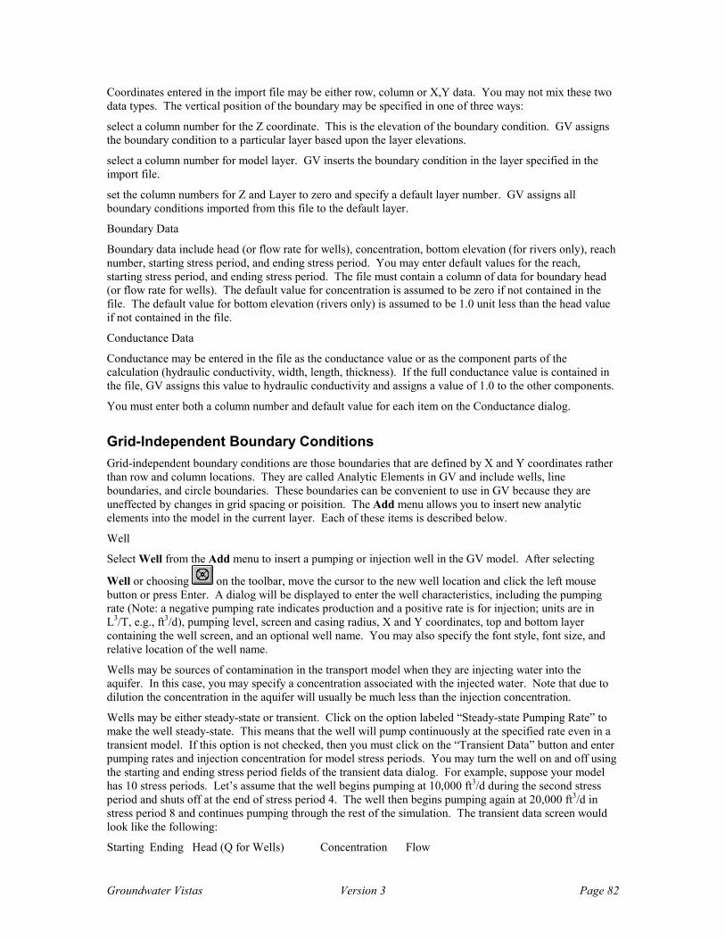
Groundwater Vistas Version 3 Page 82
Coordinates entered in the import file may be either row, column or X,Y data. You may not mix these two data types. The vertical position of the boundary may be specified in one of three ways:
select a column number for the Z coordinate. This is the elevation of the boundary condition. GV assigns the boundary condition to a particular layer based upon the layer elevations.
select a column number for model layer. GV inserts the boundary condition in the layer specified in the import file.
set the column numbers for Z and Layer to zero and specify a default layer number. GV assigns all boundary conditions imported from this file to the default layer.
Boundary Data
Boundary data include head (or flow rate for wells), concentration, bottom elevation (for rivers only), reach number, starting stress period, and ending stress period. You may enter default values for the reach, starting stress period, and ending stress period. The file must contain a column of data for boundary head (or flow rate for wells). The default value for concentration is assumed to be zero if not contained in the file. The default value for bottom elevation (rivers only) is assumed to be 1.0 unit less than the head value if not contained in the file.
Conductance Data
Conductance may be entered in the file as the conductance value or as the component parts of the calculation (hydraulic conductivity, width, length, thickness). If the full conductance value is contained in the file, GV assigns this value to hydraulic conductivity and assigns a value of 1.0 to the other components.
You must enter both a column number and default value for each item on the Conductance dialog.
Grid-Independent Boundary Conditions Grid-independent boundary conditions are those boundaries that are defined by X and Y coordinates rather than row and column locations. They are called Analytic Elements in GV and include wells, line boundaries, and circle boundaries. These boundaries can be convenient to use in GV because they are uneffected by changes in grid spacing or poisition. The Add menu allows you to insert new analytic elements into the model in the current layer. Each of these items is described below.
Well
Select Well from the Add menu to insert a pumping or injection well in the GV model. After selecting
Well or choosing on the toolbar, move the cursor to the new well location and click the left mouse button or press Enter. A dialog will be displayed to enter the well characteristics, including the pumping rate (Note: a negative pumping rate indicates production and a positive rate is for injection; units are in L3/T, e.g., ft3/d), pumping level, screen and casing radius, X and Y coordinates, top and bottom layer containing the well screen, and an optional well name. You may also specify the font style, font size, and relative location of the well name.
Wells may be sources of contamination in the transport model when they are injecting water into the aquifer. In this case, you may specify a concentration associated with the injected water. Note that due to dilution the concentration in the aquifer will usually be much less than the injection concentration.
Wells may be either steady-state or transient. Click on the option labeled “Steady-state Pumping Rate” to make the well steady-state. This means that the well will pump continuously at the specified rate even in a transient model. If this option is not checked, then you must click on the “Transient Data” button and enter pumping rates and injection concentration for model stress periods. You may turn the well on and off using the starting and ending stress period fields of the transient data dialog. For example, suppose your model has 10 stress periods. Let’s assume that the well begins pumping at 10,000 ft3/d during the second stress period and shuts off at the end of stress period 4. The well then begins pumping again at 20,000 ft3/d in stress period 8 and continues pumping through the rest of the simulation. The transient data screen would look like the following:
Starting Ending Head (Q for Wells) Concentration Flow
Groundwater Vistas Version 3 Page 83
2 4 10000.0 0.0 0.0
8 10 20000.0 0.0 0.0
Another well option is labeled “Monitor Head/Conc vs. Time”. Click this option to record head, drawdown, and/or concentrations at each time step. These data may be plotted or exported to files for processing in another program. The export file format is a delimited ASCII file that can be imported into a variety of other applications, such as Microsoft's Excel spreadsheet.
Fracture Wells
GV supports the new Fracture Well Package in MODFLOW-SURFACT. MODFLOW-SURFACT is an advanced version of MODFLOW developed by HydroGeoLogic, Inc. (send email to [email protected] or call 703.478.5186). The fracture well package has the following characteristics:
well pumping rates are automatically allocated between the layers penetrated by the well screen (top and bottom screen layers).
when the level in the well drops below the bottom of a layer, the pumping rates are automatically reallocated to lower layers.
if the water level drops below the pumping level, the flow rate is decreased until the pumping level is maintained.
well-bore storage effects may be simulated by clicking on the “Include Storage Effects” option. You must also enter values for the Screen Radius and Casing Radius on the GV dialog to use this option.
Select “Use as Fracture Well (FWL4)” to make the well a fracture well for use with MODFLOW-SURFACT.
Allocating Well Rates
If you do not specify the well as a Fracture Well, GV will allocate pumping rates between the model layers based upon the transmissivity of the layers. Note that screen radius, casing radius, and pumping level do not have any effect if you are not using MODFLOW-SURFACT.
Line Boundaries
Line boundaries are linear features that are analogous to drains, river reaches, or trenches. After selecting
Line Boundary ( on the toolbar) from the menu, you move the cursor to one end of the new line, click the left mouse button and drag the cursor to the other end of the line. Release the mouse button when you are finished. A dialog will then prompt for the data defining the line boundary characteristics. These data include the head or flux rate (Note: a negative flux rate specifies discharge and a positive rate represents recharge or injection), boundary conductance data, type of boundary condition, coordinates for the endpoints of the line, and an optional name for the line. You may also specify the font style, font size, and relative location for the line name.
Line Boundaries may represent constant head, constant flux (well), river, drain, or general head boundary conditions. These boundary conditions are created when you create model data sets (e.g., for MODFLOW). GV determines what cells are crossed by the line and assigns the boundary condition you select. When two or more line or circle boundaries cross the same cell, only the first feature entered is used. The order of entry may be determined by selecting Edit->Analytic Element List. A dialog will display the grid-independent boundary conditions in the order entered in the model.
GV computes the conductance term for line boundaries that represent head-dependent flux boundary conditions (river, drain, or general head). The conductance term is computed using the following equation:
C = K W L/T
where C is conductance (L2/T; e.g., ft2/d), K is hydraulic conductivity of the boundary (L/T; e.g., ft/d), W is the width of the boundary condition, L is the length of the boundary condition within the cell, and T is the thickness of the sediments lining the boundary condition. You enter all of the data on the dialog except for

Groundwater Vistas Version 3 Page 84
the length of the boundary within the cell. GV computes the length of the boundary that passes through each cell and computes the conductance term from the equation listed above.
For constant flux line boundaries, GV computes the length of the line within each cell that it passes through and multiplies the length by the flux per unit length entered on dialog to come up with the total flow rate.
Line boundaries may also be sources of contamination. You may enter a concentration value in the dialog. If the line is recharging the aquifer (injecting water), the concentration is applied to the injected water just like an injection well described above.
Circle Boundaries
Circle boundaries are circular regions that may be defined as constant head, constant flux (well), river,
drain, or general head boundaries. Select Circle Boundary from the Add menu or from the toolbar. Now, move the cursor to the center of the circular region and click the left mouse button. Hold the left mouse button down and drag the cursor to the desired size of the circular area. Release the mouse button when you are done. A dialog then asks for data relating to the circle boundary. These data include the head or recharge rate (positive for production and negative for injection with units of L/T, e.g., ft/d), the radius of the circle, the coordinates of the center of the circle, and an optional name for the boundary. You may also specify the font style, font size, and relative location for the name.
GV computes the conductance term for circle boundaries that represent head-dependent flux boundary conditions (river, drain, or general head). The conductance term is computed using the following equation:
C = K A/T
where C is conductance (L2/T; e.g., ft2/d), K is hydraulic conductivity of the boundary (L/T; e.g., ft/d), A is the area of the boundary in the cell, and T is the thickness of the sediments lining the boundary condition. You enter all of the data on the dialog except for the area of the boundary within the cell. GV computes the area of the boundary that passes through each cell and computes the conductance term from the equation listed above.
For constant flux line boundaries, GV computes the area of the circle within each cell that it passes through and multiplies the area by the flux per unit area entered on dialog to come up with the total flow rate.
Circle boundaries may be sources of contamination if a concentration value is entered in the dialog. Only infiltrating boundaries may be contaminant sources.
Defining Aquifer Properties
Concepts GV defines eleven different properties that are represented in the model in zones or equal value. Many of these parameters are hydraulic or transport properties, including the following:
• hydraulic conductivity ,
• storage coefficient (including specific yield and porosity),
• vertical leakance coefficient,
• layer bottom elevation,
• layer top elevation,
• dispersivity (longitudinal, transverse, retardation coefficient),
• chemical reactions,
• diffusion/half-life on soil,
• interbed storage parameters, and

Groundwater Vistas Version 3 Page 85
• hydrostratigraphy.
Other types of parameters include boundary conditions and initial conditions, as follows:
• recharge,
• evapotranspiration, and
• initial concentrations.
You must perform two functions when defining a property in GV. The first step is to assign a property value to each zone number that will be used in the model. This step is performed each time you select Database from the property menu. The second step is to assign a zone number to each cell in the model. Each cell is automatically set to zone #1 when you start a new model and the parameters assigned to zone #1 are defined on the initialization dialog.
There are several key points to keep in mind when using GV to define these parameter zones, as described below:
(1) The only parameters that are required by the model are hydraulic conductivity and layer bottom elevation.
(2) Each cell in the model is initially assigned a zone value of 1 for each parameter type. This implies that the model is homogeneous in each of the parameters. To create a parameter distribution containing heterogeneities, you must change the zone numbers for some of the cells.
(3) Each parameter type has its own distribution of zones. For example, the model cell at (row 1, column 1, layer 1) may have a hydraulic conductivity zone number 1, a leakance zone value defined by zone 2, and a recharge zone 4.
(4) You will enter zone values into a table. Each zone number is assigned a value. For example, hydraulic conductivity zone 1 may be assigned 10 ft/d and zone 2 100 ft/d. The zone numbers do not refer in any way to layers! Many first-time users of GV mistakenly assume that the zone numbers refer to layer numbers; that is, zone 1 is assigned to layer 1 and zone 2 to layer 2, etc. You may choose to assign zone numbers in this manner, but it not required nor is this situation the default case.
Many ground-water flow models require only transmissivity for confined layers and do not require you to enter the thickness or elevations of layer tops and bottoms. However, if you intend to use the model for particle-tracking analyses (using MODPATH or PATH3D, for example) or for contaminant transport modeling (using MT3D), you will need to define the elevations of layers. Therefore, GV requires that each layer be defined in terms of its bottom elevation. GV will compute transmissivity for confined layers by multiplying hydraulic conductivity by layer thickness.
Another good practice is to define the vertical hydraulic conductivity for each model cell rather than the leakance coefficient (VCONT in MODFLOW terminology). This should be done for a couple of reasons. First, MODFLOW is one of the only ground-water flow models that requires the user to compute a vertical leakance coefficient. Most other flow models require vertical permeability as input and vertical conductances are computed by the code. Second, GV will accurately compute the leakance term for MODFLOW using layer elevations and vertical hydraulic conductivity. Therefore, there is no need to compute the leakance coefficient yourself.
Specifying Zone Values Zone numbers are assigned to each cell in the model for each property type. The zone number corresponds to a property value in a simple database.
The Property Values menu operates on the database of parameter values. The database contains a property value assigned to each zone number used in the model. The database contains from one to three parameter values for each property. The properties and their associated parameter values are shown below:
Property Parameters

Groundwater Vistas Version 3 Page 86
Hydraulic Conductivity Kx, Ky, Kz Storage S, Sy, Porosity Leakance Leakance (VCONT) Recharge rate, concentration, ponding elevation ET ET rate, ET extinction depth Top layer top elevation Bottom layer bottom elevation Dispersivity longitudinal, transverse, vertical Chemical Reactions Kd, bulk density, contaminant half-life Initial Concentrations concentration Diffusion diffusion, half-life on soil, Kd exponent Interbed Storage elastic and inelastic storage
Select Database from the menu to edit the parameter values for the current property type. The current property type is the one checked at the bottom of the Props menu. A spreadsheet is displayed with zone numbers along the left side and three columns for the parameter values. Some properties only have one parameter value (e.g., Bottom elevation). In this case, you can ignore the other two columns.
Most properties have only one database of values corresponding to zone numbers. Recharge and ET, on the other hand, have a unique database of values for each stress period. The pattern of zone numbers assigned to model cells remains the same for each stress period, but the parameter values assigned to those
zone numbers may change by stress period. When you select Database for Recharge and ET, GV displays the database for the current stress period. The current stress period may be changed by selecting Props->Rech/ET Stress Period.
Chemical reaction and diffusion parameters are similar in concept to recharge and ET. In this case, however, a different database is provided for up to 5 chemical components. Select Props->Current Chemical Component to enter the component value. All subsequent editing of the databases for these two properties corresponds to the current component. Use of multiple components only applies to the MODFLOW-SURFACT transport model at this time.
The Sort Zones command sorts the database from lowest parameter value to highest. GV uses the first parameter value (e.g., Kx for hydraulic conductivity or Recharge rate for Recharge) to perform the sort. The sort command also changes the zone numbers assigned to cells so that the cells contain the same property value as they did before the sort.
The Automatic Zone Setup command provides a quick way of setting up the database. You enter the starting and ending zone numbers to modify, the initial property value for each of the three parameters, and the increment for each parameter. GV then resets the database within the range of zones specified. Note that some properties have less than three parameters. In this case, you can ignore the unused parameters on the dialog. For Recharge and ET, the auto zone setup command works on the current stress period. The current stress period may be changed by selecting Props->Rech/ET Stress Period.
The Copy Transient Data command allows you to copy the database for recharge or evapotranspiration from one stress period to another. The current property type must be either Recharge or ET. These are the only two properties that have a different database for each stress period. The pattern of zone numbers may also be different for each stress period. The copy transient data command makes it easy to set up a transient run.
GV assigns zone colors using a standard spectrum where blue is assigned to zone 1 and red is assigned to the highest zone number. You may redefine the color assigned to any zone using the Edit Zone Colors command. The dialog presents a scrolling list of zone numbers with a color button and a hatch pattern button. The default hatch pattern is solid color fill. There are several other patterns that may be chosen, however.
The Default Zone Pattern dialog changes the hatch pattern for all zones. Use the Edit Zone Colors command described above to change patterns for individual zone numbers.
The Reset Colors command resets the colors back to a standard spectrum and to a solid fill pattern.

Groundwater Vistas Version 3 Page 87
Assigning Zone Numbers to Cells All property zone numbers for all properties in all cells are initially set to a value of 1 when you initialize the model. Property zones are modified in the model using the Set Zone Number option on the Props menu, which has several options for assigning zone numbers to cells. These include the following:
Single Cell
After selecting this option, move the cursor to the desired grid location and click the left mouse button. A dialog then appears where you enter the new zone number for the cell. You may also click the right mouse button in a cell to change that cell to the current default zone number. You set the default zone number by
selecting Props->Default Zone No. . It is a good idea to turn off the automatic refresh on the view menu while using the right mouse button, otherwise, GV will repaint the screen after each right mouse click.
Window
The Window command changes the zone number of all cells in a rectangular region. After selecting this command, move the cursor to one corner of the desired region and hold the left mouse button down. Move the cursor to the opposite corner and release the mouse button. GVdisplays a dialog where you enter the new zone number. All cells within this region are changed to the new zone number. GV determines that a cell is within the region if the center of the cell falls within the window.
Digitize
The Digitize command sets a new zone number in each cell contained within the digitized region. After digitizing the polygon region, you enter a new zone number. GV then finds each cell within the polygon and changes the zone number to the one you specify.
Digitizing is performed by clicking the left mouse button to set points along the line. You may delete the last point entered by clicking the right mouse button. Double-click the left mouse button to end digitizing. If you are not fast enough with the double click, you may see a stray line on your screen. GV will ignore this when zone numbers. GV automatically closes the polygon by connecting the first and last points digitized.
Transpose
The Transpose command changes all cells with a given zone number in the current layer to another zone number. A dialog prompts for the zone number to change and the new zone number. Only cells in the current layer are affected.
Clear
Select Clear to change all cells in the current layer to a constant zone number. A dialog prompts for the new zone number.
Gradient Fill
The Gradient Fill option was designed to make it easy to slope the elevation of a layer, but may be applied to any property type. You enter the row and column number of a know property value and the slope and direction of the property. The known value is fixed during the calculations. The slope is computed as change in parameter value divided by change in distance. For top and bottom elevation, the slope is expressed as change in elevation divided by change in distance. The direction is an angle in degrees, where east is 0.0 and north is 90.0. You may also confine the calculations to a range of row and column locations.
The gradient fill calculation assumes that the property database contains a wide range of values that are entered in order from lowest value to highest. When you initially set up the model in GV, several hundred zones are created for bottom and top elevation. Thus, you may apply the gradient fill to layer elevation without performing any special operations on the database. For other properties, you may need to modify the structure of the database before applying the gradient fill. Key options to look at are Auto Zone Setup
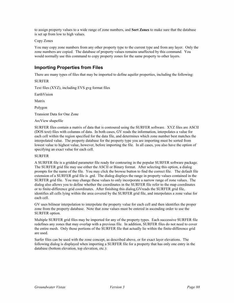
Groundwater Vistas Version 3 Page 88
to assign property values to a wide range of zone numbers, and Sort Zones to make sure that the database is set up from low to high values.
Copy Zones
You may copy zone numbers from any other property type to the current type and from any layer. Only the zone numbers are copied. The database of property values remains unaffected by this command. You would normally use this command to copy property zones for the same property to other layers.
Importing Properties from Files There are many types of files that may be imported to define aquifer properties, including the following:
SURFER
Text files (XYZ), including EVS gvg format files
EarthVision
Matrix
Polygon
Transient Data for One Zone
ArcView shapefile
SURFER files contain a matrix of data that is contoured using the SURFER software. XYZ files are ASCII (DOS text) files with columns of data. In both cases, GV reads the information, interpolates a value for each cell within the region specified for the data file, and determines which zone number best matches the interpolated value. The property database for the property type you are importing must be sorted from lowest value to highest value, however, before importing the file. In all cases, you also have the option of specifying an exact value for each cell.
SURFER
A SURFER file is a gridded parameter file ready for contouring in the popular SURFER software package. The SURFER grid file may use either the ASCII or Binary format. After selecting this option, a dialog prompts for the name of the file. You may click the browse button to find the correct file. The default file extension of a SURFER grid file is .grd. The dialog displays the range in property values contained in the SURFER grid file. You may change these values to only incorporate a narrow range of zone values. The dialog also allows you to define whether the coordinates in the SURFER file refer to the map coordinates or to finite-difference grid coordinates. After finishing this dialog,GVreads the SURFER grid file, identifies all cells lying within the area covered by the SURFER grid file, and interpolates a zone value for each cell.
GV uses bilinear interpolation to interpolate the property value for each cell and then identifies the proper zone from the property database. Note that zone values must be entered in ascending order to use the SURFER option.
Multiple SURFER grid files may be imported for any of the property types. Each successive SURFER file redefines any zones that may overlap with a previous file. In addition, SURFER files do not need to cover the entire mesh. Only those portions of the SURFER file that actually lie within the finite-difference grid are used.
Surfer files can be used with the zone concept, as described above, or for exact layer elevations. The following dialog is displayed when importing a SURFER file for a property that has only one entry in the database (bottom elevation, top elevation, etc.):
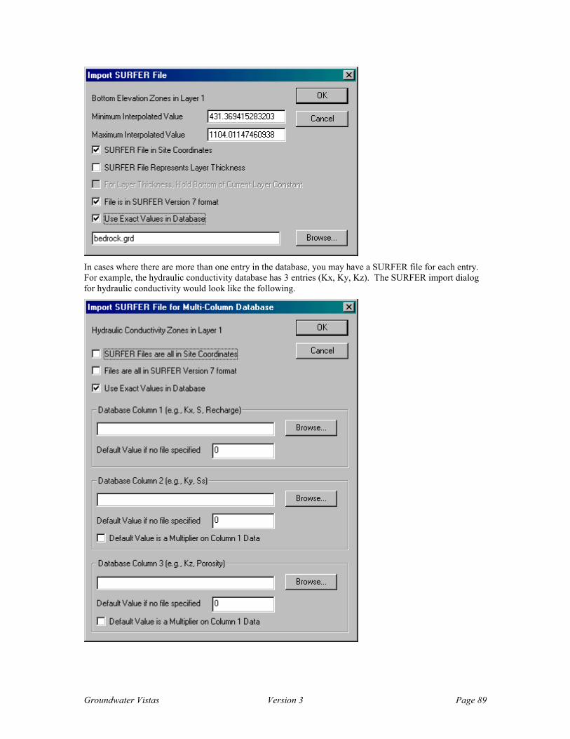
Groundwater Vistas Version 3 Page 89
In cases where there are more than one entry in the database, you may have a SURFER file for each entry. For example, the hydraulic conductivity database has 3 entries (Kx, Ky, Kz). The SURFER import dialog for hydraulic conductivity would look like the following.

Groundwater Vistas Version 3 Page 90
The last option labeled Use Exact Values in Database tells GV to interpolate a cell value from the SURFER file and put that exact value into the GV database. If you uncheck this option, then GV assumes you are using the zone concept and will look for the closest value in the database.
XYZ files
Importing property zone values from an ASCII file is similar to the procedure for boundary conditions, except that you may interpolate cell values from the random XYZ data. This process is identical to the distance-squared interpolation method in SURFER. You also have the option, however, of importing the ASCII data directly into individual cells without interpolation.
Selecting Import->XYZ from the pull-down menu displays a dialog. The first item is the file name with an associated browse button to make it easy to find the proper file. You also enter the number of lines to skip in the data file. This allows you to have header information in the file. The next three data items identify the column in the file containing the X coordinate, the Y coordinate, and the Z (property) value.
Data in the import file may be in any order but the structure of the file must conform to the following specifications:
there may be any number of lines at the top of the file to label the information. You will tell GV how many lines to skip in this header record.
all data beneath the header lines must be in columns, separated by spaces, tabs, and or commas. Each line of the file must contain data for one boundary condition and each line must contain the same number of columns of information.
there can be no extraneous information after the columns of data.
data are imported for the current boundary condition type.
You enter the name of the file on the Import dialog (a browse button is provided so that you can locate the file), the number of lines to skip at the top of the file, and whether the coordinates in the file are in site coordinates. Site coordinates refer to the coordinates of the base map. Uncheck this option if the coordinates are model grid coordinates, with the origin being the lower left corner of the grid.
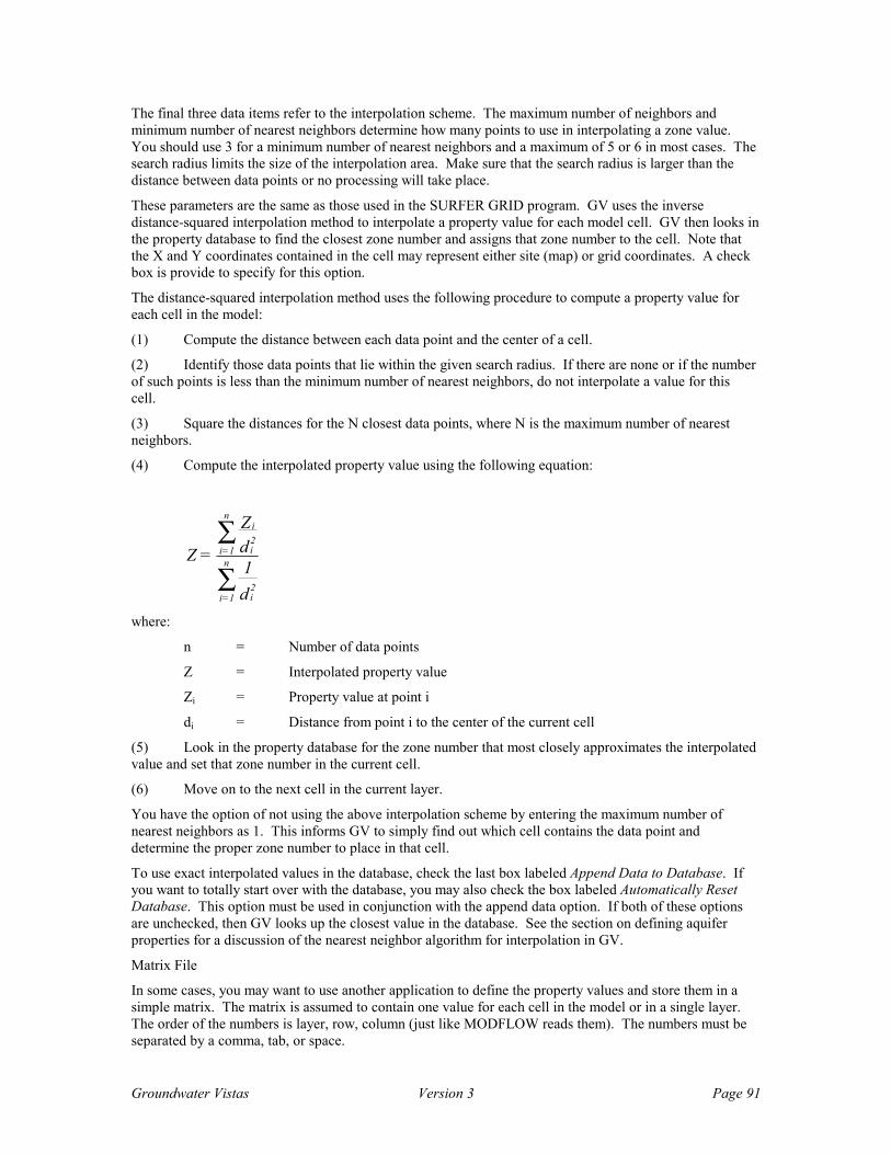
Groundwater Vistas Version 3 Page 91
The final three data items refer to the interpolation scheme. The maximum number of neighbors and minimum number of nearest neighbors determine how many points to use in interpolating a zone value. You should use 3 for a minimum number of nearest neighbors and a maximum of 5 or 6 in most cases. The search radius limits the size of the interpolation area. Make sure that the search radius is larger than the distance between data points or no processing will take place.
These parameters are the same as those used in the SURFER GRID program. GV uses the inverse distance-squared interpolation method to interpolate a property value for each model cell. GV then looks in the property database to find the closest zone number and assigns that zone number to the cell. Note that the X and Y coordinates contained in the cell may represent either site (map) or grid coordinates. A check box is provide to specify for this option.
The distance-squared interpolation method uses the following procedure to compute a property value for each cell in the model:
(1) Compute the distance between each data point and the center of a cell.
(2) Identify those data points that lie within the given search radius. If there are none or if the number of such points is less than the minimum number of nearest neighbors, do not interpolate a value for this cell.
(3) Square the distances for the N closest data points, where N is the maximum number of nearest neighbors.
(4) Compute the interpolated property value using the following equation:
Z =
Zd1d
i=1
ni
i2
i=1
n
i2
∑
∑
where:
n = Number of data points
Z = Interpolated property value
Zi = Property value at point i
di = Distance from point i to the center of the current cell
(5) Look in the property database for the zone number that most closely approximates the interpolated value and set that zone number in the current cell.
(6) Move on to the next cell in the current layer.
You have the option of not using the above interpolation scheme by entering the maximum number of nearest neighbors as 1. This informs GV to simply find out which cell contains the data point and determine the proper zone number to place in that cell.
To use exact interpolated values in the database, check the last box labeled Append Data to Database. If you want to totally start over with the database, you may also check the box labeled Automatically Reset Database. This option must be used in conjunction with the append data option. If both of these options are unchecked, then GV looks up the closest value in the database. See the section on defining aquifer properties for a discussion of the nearest neighbor algorithm for interpolation in GV.
Matrix File
In some cases, you may want to use another application to define the property values and store them in a simple matrix. The matrix is assumed to contain one value for each cell in the model or in a single layer. The order of the numbers is layer, row, column (just like MODFLOW reads them). The numbers must be separated by a comma, tab, or space.
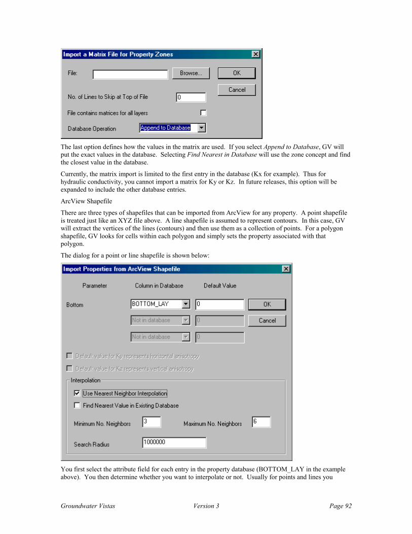
Groundwater Vistas Version 3 Page 92
The last option defines how the values in the matrix are used. If you select Append to Database, GV will put the exact values in the database. Selecting Find Nearest in Database will use the zone concept and find the closest value in the database.
Currently, the matrix import is limited to the first entry in the database (Kx for example). Thus for hydraulic conductivity, you cannot import a matrix for Ky or Kz. In future releases, this option will be expanded to include the other database entries.
ArcView Shapefile
There are three types of shapefiles that can be imported from ArcView for any property. A point shapefile is treated just like an XYZ file above. A line shapefile is assumed to represent contours. In this case, GV will extract the vertices of the lines (contours) and then use them as a collection of points. For a polygon shapefile, GV looks for cells within each polygon and simply sets the property associated with that polygon.
The dialog for a point or line shapefile is shown below:
You first select the attribute field for each entry in the property database (BOTTOM_LAY in the example above). You then determine whether you want to interpolate or not. Usually for points and lines you

Groundwater Vistas Version 3 Page 93
would use interpolation. If you don’t interpolate, GV will only change the bottom elevation of cells containing points or vertices of lines. You then have the option of using exact values or check the box to Find Nearest Value in Existing Database. The dialog for a polygon shapefile is the same but you cannot choose to interpolate values.
Saving The Model Design You have three ways to save the design in a GV grid file. You may save the design at any time by selecting the File->Save or Save As menu options from the main menu. You may then go back to the design menu to continue making changes. We recommend that you save the design periodically in case of power outages or in case you do something (like clear all boundary conditions) that you did not intend to do. In this way, you can recover without too much lost time.
You will also be given the opportunity to save the model design before exiting GV. To exit GV, select Exit from the File menu. A screen will appear asking if you want to save the current GV design.

Groundwater Vistas Version 3 Page 94

Groundwater Vistas Version 3 Page 95
Running Simulations
Introduction Running model simulations with GV involves three steps following the design of a groundwater model. These steps include (1) edit options that are specific to the particular model being used (e.g., MODFLOW), (2) create input files for the model, and (3) run the model. Models supported in this release of Groundwater Vistas include MODFLOW, MODFLOW2000, MODFLOWT, MODFLOW-SURFACT, MT3D (all versions including MT3D’99), MODPATH, Path3D. There are also specialized models for calibration (PEST, UCODE) and for optimization (MODOFC, Brute Force, SOMOS) but they are discussed in subsequent chapters of this manual. The following chapter describes how these models are interfaced to GV, how to create data files for each model, and the assumptions that GV makes when running these models.
Model-Specific Preprocessing Once you have designed the model grid, added boundary conditions, and assigned aquifer properties to each cell, you are ready to run a simulation. The first step in the simulation process is to set the various options for the model you will be using. These options are edited using the Model menu. At the top of this menu are the names of the models supported by GV. These include:
MODFLOW MODFLOW2000 MODFLOWT MODFLOW-SURFACT MODPATH MT3D PATH3D Selecting any of these models from the Model menu displays another menu with the various options. In order to use these menus successfully, you need to be familiar with the data input requirements of each model you will use. Use of GV is not a substitute for learning the intricacies of a particular model. GV is designed to make model simulation easier, but does not replace the documentation for each model. Manuals for most of these models are provided in electronic format when you install GV. Contact us for details if you cannot find a particular manual.
Normally, you should scan through all of the menu options for each model when you first start a simulation. Afterward, you will only need to visit key dialogs to fine-tune simulation options.
In addition to scanning through the various dialogs for the model you are using, you should also browse through the MODFLOW menu. Most of the models supported by GV are either derivatives of MODFLOW (i.e., MODFLOWT and MODFLOW-SURFACT) or are simulators that use the results of a MODFLOW run such as MT3D, PATH3D, and MODPATH. Each of these models use key information from the MODFLOW run and hence the MODFLOW dialogs. Of particular interest are the stress period data (Model->MODFLOW->Stress Period Setup) and the layer type (LAYCON) assigned to each model layer (Model->MODFLOW->BCF Package).
Creating Data Sets Model data sets are the collection of input files that a particular model will read during a simulation. All of the models supported by GV use numerous input files and generate a variety of output files. GV aids you in managing all of this information by naming the files with a root file name and a three-letter extension that designates the particular input file or output file. For example, by using a root file name of “run1”, the MODFLOW Basic Package would be called “run1.bas” and the MODFLOW head output file (head-save file) would be called “run1.hds”.
Groundwater Vistas Version 3 Page 96
You create data sets for each model using two methods. The first is to select a menu option labeled Create Datasets at the bottom of each model menu (e.g., Model->MODFLOW->Create Datasets). The second
method is to simply click the calculator button, . GV first asks whether you want to create data sets. Click the Yes button to create these files. Next, GV will run the model. The model that is run is the one with a check mark next to it at the bottom of the Model menu. The default model is MODFLOW.
GV creates the model files and then displays a dialog that asks whether you would like to view the error file. GV looks for potential problems while creating model datasets. These are categorized as Warnings and Errors. Warnings are potential problems with the model while errors generally mean that the model will not run. Select Yes on this dialog and GV will attempt to run the Windows application Notepad. If notepad cannot be found, an error will be displayed. Notepad must be in the path in order for GV to find it, however.
How does GV know what files to create? This is a common question. You control what files are created by using the Packages menu selection for each model. Package is the term used in the MODFLOW manual to describe each feature of the model that requires a separate data input file. GV attempts to make an educated guess about which packages are required the first time you view the Packages dialog for each model. You should confirm that there are no packages missing and that extraneous packages are not included. The following discussion should help in making this determination.
MODFLOW Selecting Packages from the MODFLOW menu displays a dialog where you decide what MODFLOW packages will be created and what the packages will be called. A package is a separate data file in a MODFLOW simulation. The following packages are displayed on this dialog:
Basic BASIC Package containing starting heads, constant heads, stress period definition, and some options (.bas)
BCF Block Centered Flow Package containing aquifer property data and grid spacings (.bcf)
Output Control Determines what model results to print and save to files during the simulation (.oc)
Solver There are several solver packages (SIP, SOR, PCG2) that are used to solve the partial differential equations in MODFLOW (.sip or .sor or .pcg)
Well Well boundary conditions (.wel)
River River boundary conditions (.riv)
Drain Drain boundary conditions (.drn)
General Head General Head Boundary conditions (.ghb)
Stream Stream Routing Package (Prudic 1989) (.str)
Recharge Recharge boundary condition (.rch)
ET Evapotranspiration boundary condition (.evt)
Wall Horizontal Flow Barrier (HFB) or slurry wall package (.hfb)
CHD Time-variant Constant Head package (.chd)
The first field on the dialog is labeled Root File Name. All MODFLOW files in a simulation have the same file name with an extension that describes the package name. For example, if the root file name is “sim1”, then the Basic package is called sim1.bas, the Well package is called sim1.wel, etc. The file extensions used for each package are listed above.
There are up to four columns of information to the right of each package name. The first column to the right of the package name is labeled Unit No. This refers to the FORTRAN unit number assigned to each package. You may assign any number between 1 and 100, but all numbers must be unique (i.e., do not duplicate a number in two or more packages!). Also, the Basic Package unit number should always be 1.

Groundwater Vistas Version 3 Page 97
(Note: GV will check for duplicate unit numbers and will reassign those that are duplicates when you create MODFLOW datasets).
Only place a unit number next to a Package that is part of your simulation. Every simulation must have a BASIC Package, BCF Package, an Output Control Pacakge, and a solver Package (SIP, SOR, or PCG2). Place a zero next to Packages you are not using. For example, if you do not have any rivers in your simulation make sure that a zero is next to River in the Unit No. column.
The second column is labeled Create? and may be checked or unchecked. A check mark in this column means that GV will create this package. If you have already created a certain package and nothing has changed, you may remove the check mark. You may want to do this if one package takes a long time for GV to create or if you have modified the file outside of GV. Make sure that the Unit No. field contains a non-zero number if the Create column contains a check mark.
The third column is labeled Cell-by-Cell Flow Unit No. Like the package unit numbers described above, the Cell-by-Cell unit numbers refer to MODFLOW files. In this case, the Cell-by-Cell files are output files containing groundwater mass balance information. Place a non-zero number is this column if you want MODFLOW to save the mass balance data. To plot velocity vectors, you must save Cell-by-Cell flow data for the BCF Package. To get a complete mass balance analysis in GV, you must specify a cell-by-cell unit number for each package listed in column 3 that is part of the simulation. These numbers must not be the same as those in column 1 and must usually be unique. If you are using the new version of MODPATH, however, you should save mass balance information in the same file. In this case, you would specify the same unit number for all packages. (Note: GV will check that the required cell-by-cell flow files exist when you create MODPATH data files. GV will also check to see that the unit numbers are properly assigned in the preceding MODFLOW run.)
You will see that there is a combo box field in column 3 next to the Solver package. This determines what type of solver to use. The original solvers in MODFLOW are the Strongly Implicit Procedure (SIP) and the Successive Over-Relaxation (SOR) packages. A newer solver is the PCG2 package. You may choose any of these 3 solvers. Please note that PCG4 is reserved for MODFLOW-SURFACT and is not available for other MODFLOW versions.
The fourth and last column on the dialog is labeled IUNIT Location. This is the location in the IUNIT array in MODFLOW that represents the particular package. The only reason these data are listed on this dialog is to maintain consistency with other MODFLOW versions. The values that show up as defaults are consistent with ESI’s MODFLOWwin32. If you are using any other version, you may need to modify these values. Contact your vendor if you are not sure. Please note that the IUNIT Location for the Solver Package is only used for the PCG2 package. The SIP and SOR solvers have standard IUNIT array locations.
At the bottom of the Package dialog are three additional options related to the creation of data files. Place a check next to Create Map File to write a new GV map file that has been offset and rotated using your current model settings. The name of the map will be the root name and a .map extension, e.g., sim1.map. Placing a check next to Create Path3D Files creates MODFLOW files compatible with the Path3D particle tracking model. Placing a check next to MT3D Flow Output causes MODFLOW to save flow information for a subsequent MT3D transport simulation. The IUNIT Location number to the right of this option is consistent with most versions of MODFLOW and need not be changed.
The following is a summary of the MODFLOW input and output files describing the extension used by GV.
Package Extension
Input files
Basic bas Block-Centered Flow bcf Output Control oc Strongly Implicit Package sip Successive Overrelaxation sor Preconditioned Conjugate Gradient 2 pcg

Groundwater Vistas Version 3 Page 98
Well wel River riv Drain drn General Head Boundary ghb Stream Routing str Recharge rch Evapotranspiration evt Horizontal Flow Barrier (wall) hfb Time-variant Constant Head chd Interbed Storage (compaction) ibs
Output files
Main output file out Head-save file hds Drawdown ddn
Cell-by-cell for BCF cbb Cell-by-cell for Wells cbw Cell-by-cell for Rivers crv Cell-by-cell for Drains cbd Cell-by-cell for General Heads cbg Cell-by-cell for Streams cst Cell-by-cell for Streams (surface flow) st2 Cell-by-cell for Recharge crc Cell-by-cell for ET cbe MT3D flow file mt3
MODFLOW2000 MODFLOW2000 uses the same packages as listed above for the standard version of MODFLOW and adds some new ones, primarily related to parameter estimation. These new packages and their default extensions are listed below:
Package Extension
Input files
Layer Property Flow lpf Discretization dis Zone zone Multiplier mult Observation Process obs Head Observations hob River Observations rvob Drain Observations drob GHB Observations gbob Constant Head Observations chob Sensitivity Process sen Parameter Estimation Process pes
Output Files
Global output file glo Listing file lst
MODFLOW2000 is described in more detail in the chapter on model calibration. MODFLOW2000 is the latest version of MODFLOW produced by the USGS. It is recommended that you read the
Groundwater Vistas Version 3 Page 99
MODFLOW2000 manual before attempting to use this new version.
MODFLOWT MODFLOWT uses the same packages as listed above for the standard version of MODFLOW and adds new ones related to transport, a new solver, and a new output control package. These new packages and their default extensions are listed below:
Package Extension
Input files
Block-Centered Transport bct Basic Transport bst Orthomin Solver for Flow omn Orthomin Solver for Transport omt Output Control for Transport oct Observation Nodes obs Recharge for Transport rct Evapotranspiration for Transport (not supported) SOR Solver for Transport sot
Output files
Concentrations cnc Observation nodes obh
There are other output files created by MODFLOWT, but the ones listed above are the only ones processed by GV.
MODFLOW-SURFACT MODFLOW-SURFACT uses the same packages as listed above for the standard version of MODFLOW and adds new ones related to several enhancements to the flow model, a new solver, new output control, and a contaminant transport package. These new packages and their default extensions are listed below:
Packages Extension
BCF4 bcf Recharge 4 rch Fracture Well fwl Automatic Time Stepping ato PCG4 Solver pcg Transport Package btn Prescribed concentrations pcn Concentrations at constant heads hcn
The MODFLOW-SURFACT BCF4 package adds a variably saturated flow option to MODFLOW for improved simulation of water table layers. You implement the BCF4 package by selecting MODFLOW-SURFACT->Packages and adding a unit number (default should be 11) next to BCF4 and checking the box to create this package. You implement the variably saturated option by selecting MODFLOW->BCF Package. There is a check box at the bottom of the dialog labeled “Variably Saturated”. Note that only confined (type 0) and unconfined (type 3) layers are supported by the BCF4 package. If you try to set a type 1 or 2 layer, GV will automatically change them to type 3.
Fracture wells (FWL4 Package) are implemented in GV using analytic wells. You add a fracture well to the model by selecting Add->Well (see the Menu Chapter for more information).

Groundwater Vistas Version 3 Page 100
The new recharge package (RCH4 Package) contains two enhancements. These include the ponding depth and seepage face nodes. The ponding depth is a parameter in the Recharge database and seepage face nodes are implemented by checking the appropriate option for drain boundary conditions.
MODPATH MODPATH data files are very similar to MODFLOW data files, especially for the boundary conditions (e.g., rivers, drains, etc.). GV assigns the same extensions to these common files for both MODPATH and MODFLOW. Therefore, you should use a different root file name for MODPATH simulations. A good practice is to append the letters “mp” to the MODFLOW root name. Thus, if your MODFLOW run is called “sim1” the MODPATH run will be “sim1mp”. This is a convenient way to keep similar runs together in the same directory without getting too confused.
The following are the MODPATH files created by GV and their default extensions:
Package Extension or File Name
Input files
File names for simulation modpath.dat Main file dat Particle starting locations ptr Well wel River riv Drain drn General Head Boundary ghb Recharge rch ET evt
Output files
Pathlines ptl
MODPATH creates more output files that the one listed above, but only the pathline file is processed by GV. The pathline file contains the coordinates and travel times for each particle. GV uses this file to display the particle traces in plan and cross-sectional views. If there is a problem with the MODPATH simulation, the file called summary.pth contains the error messages. You can view this file in a text editor such as Notepad.
You must create a MODPATH file for each of the boundary files that you use in the preceding MODFLOW simulation. For example, if you use the well package in MODFLOW, you need the well package in MODPATH. MODPATH also requires the cell-by-cell flow output file for the BCF Package and for each of the head-dependent flow boundary conditions. These include rivers, drains, general head boundaries, and evapotranspiration. When using the older version of MODPATH (mpath.exe distributed with GV), you need to tell MODFLOW to write the cell-by-cell output to separate files. This means that you must use a different unit number for each file. In the case of the new MODPATH version for transient simulations (mpath3.exe distributed with GV), these cell-by-cell flows must be written to the same file! This means that the unit number for the cell-by-cell output files must all be the same value.
MT3D MT3D has relatively few packages compared to the other models listed above. GV uses the same root file name as for MODFLOW when creating MT3D datasets. The MT3D files and their default extensions are listed below:
Package Extension
Basic Transport btn Advection adv Dispersion dsp

Groundwater Vistas Version 3 Page 101
Source & Sink Mixing ssm Chemical Reactions rct
Output files
Concentration file mt3d.ucn Observation file mt3d.obs
In order to run MT3D after a MODFLOW simulation, you must tell MODFLOW to save flow data for MT3D. This is accomplished by checking the option labeled “MT3D Flow Output” on the MODFLOW Packages dialog.
PATH3D PATH3D uses the same files as MODFLOW does with two additions. First, you must check the box labeled “Create PATH3D files” on the MODFLOW Packages dialog. This causes GV to write additional information into the BCF Package input file. GV also writes the PATH3D main data file to a file with a ptr extension and the same root file name as the MODFLOW run.
PATH3D creates a file that is called p3dplot.dat. This is the file used by GV to display the particle traces.
Running Simulations GV is designed to run each of the supported models from within GV and subsequently to process the results. GV works best with ESI’s MODFLOWwin32 or with MODFLOW2000win32 but can also use any other version of MODFLOW. The only problem will be the passing of file names to these other versions. GV automatically passes file names to MODFLOWwin32, MODFLOW2000win32 , MODFLOWT, and MODFLOW-SURFACT. This means that you do not need to type in any file names when these programs run. If you are using a version of MODFLOW other than the four mentioned above, you will probably need to enter file names in response to prompts from MODFLOW.
One other potential problem is related to the format of binary files. GV requires that output files from each model be true binary files. Most models from other vendors produce files that are called “unformatted” files. These are not compatible with GV. This topic is covered in greater detail in the next chapter. If you get errors when importing the binary files, you may run a program called UNF2BIN.EXE from the DOS prompt to manually convert unformatted files to binary ones.
Features that are exclusive to ESI’s own version of MODFLOW include the automatic sensitivity analysis and the automatic calibration procedure. Only MODFLOWwin32 and MODFLOW2000win32 can be used for these two techniques! The reason is that all of the other versions of MODFLOW are DOS programs. GV can run these models for single runs, but cannot control a succession of runs because GV does not know when the run finishes. MODFLOWwin32, on the other hand, sends a message through Windows to GV informing the software that a simulation is finished. This allows you to do multi-tasking while a sensitivity analysis is in progress.
Running simulations from within GV is a two-step process once you have designed the model and set the appropriate options for the particular model you are using. You first select Model->Paths to Models. A dialog is displayed where you enter the path to the models you will be using. By default, GV is set up to use MODFLOWwin32. In this case, the MODFLOW path should be set to mfwin32.dll (for MODFLOW88) or mf2kwin32.dll (for MODFLOW2000). If you are using another version of MODFLOW, such as MODFLOW-SURFACT, you must first select do not use as the option labeled MODFLOWwin32. Next, enter the path to your version of MODFLOW. A browse button is provided to help you find the file.
You must also enter the paths to MODPATH, MT3D, and PATH3D on this dialog. MODPATH and MT3D also now have user interfaces like MODFLOWwin32. There are also options for using the dll’s or for using dos applications just like MODFLOW.
At the bottom of the dialog is a field labeled Working Directory. This is the directory containing your data files. A browse button is provided for you to select such a directory. Simply select any file within the directory and click OK. GV strips off the file name leaving the path to the directory.
Groundwater Vistas Version 3 Page 102
The second step in running a model is to simply select Run “model” from either the MODFLOW, MODFLOWT, MODFLOW-SURFACT, MT3D, or PATH3D menus. Most of the models you use are DOS programs. Therefore, your screen may turn black as Windows shells out to DOS to run the model. If you are using MODFLOWwin32 this does not happen.
After the simulation is over, GV asks whether you would like to process the results. Select Yes to read the output files and begin analyzing the simulation. Analysis techniques are discussed in the next chapter. You do not need to import the results right away. You may select Plot->Import Results to view the output at a later time.
You may also click the calculator button, , on the toolbar as a short-cut to creating data sets and running the model. A dialog is first displayed asking whether you want to create the files for the run. GV then runs the model automatically. The model with a check mark next to its name at the bottom of the Model menu is the one that is used by GV.
Assumptions Used in Creating Data Files Groundwater Vistas makes a variety of assumptions in turning your model design into files that are read by the various models. You must be familiar with these assumptions and with the data input requirements of each model in order to be confident that your simulations are correct. Please take the time to read this section and to study the documentation for each model you use.
MODFLOW and MODFLOW2000 Parameter Zones
GV uses seven of the available property types in creating MODFLOW data files. These include the following:
• hydraulic conductivity,
• storage coefficient and specific yield (transient simulations only),
• vertical leakance coefficient (optional),
• layer bottom elevation,
• layer top elevation (only if needed as discussed below),
• recharge, and
• evapotranspiration.
None of the transport parameters (dispersivity, diffusion, chemical reactions, initial concentrations) are used in MODFLOW.
Layer Elevations
GV assumes by default that the bottom of a layer also represents the top of the underlying layer. In some cases, the top of layer 1 is required; this happens when you use the ET package and when you define layer 1 to be of type 3 (See McDonald and Harbaugh, 1988, page 5-39). GV defines the top of layer 1 when you initialize your model design and uses this default value unless you modify the top elevation database.
You only need to use the top elevation property when you need a detailed depiction of surface topography for the ET package or when there are gaps between model layers. These gaps usually represent aquitard layers that are not being simulated explicitly. This is called quasi-three-dimensional modeling. In this case, you would define top elevation zones for each layer in the model. You must check the options labeled “Use top elevation zones” on the BCF Package dialog (select Model->MODFLOW->BCF Package) if there are gaps between model layers.

Groundwater Vistas Version 3 Page 103
It is very important to recognize that if you choose the option to Use top elevation zones on the BCF Package dialog that you MUST define the top elevation of each layer! If you only need to define the top of layer 1 then you do not need to set the BCF option to use top elevation zones. GV always assumes that you need to define the top of layer 1.
Layer Types
When you first translate the model design into MODFLOW data sets, GV makes an initial guess regarding the layer types used to represent each model layer. MODFLOW defines four layer types as follows (See McDonald and Harbaugh, 1988, page 5-39):
Layer Code (LAYCON) Description
0 Confined layer; enter transmissivity and storage coefficient.
1 Unconfined layer (layer 1 only); enter hydraulic conductivity, bottom elevation, and specific yield as the primary storage coefficient.
2 Confined/unconfined layer; enter transmissivity, bottom and top elevations, and two storage coefficients (storage & specific yield).
3 Confined/unconfined layer; enter hydraulic conductivity, bottom and top elevations, and two storage coefficients (storage & specific yield).
You can use any of the LAYCON layer types described above. GV will compute transmissivity from hydraulic conductivity and layer elevations for confined layers.
Calculation of the Leakance Coefficient
Groundwater Vistas provides one of the most comprehensive leakance calculators of any modeling preprocessor. GV uses several methods to define vertical leakance (VCONT in MODFLOW terminology) including the following:
GV will automatically compute leakance from vertical hydraulic conductivity contained in the hydraulic conductivity database. This is the default case and the one you should most often use. To use this option, the option labeled “Compute Leakance” should be checked on the BCF dialog and the leakance option should be set to “leakance”.
You define leakance zones for all but the bottom layer. Values for each zone represent leakance coefficients that you compute by hand using vertical hydraulic conductivity and layer thicknesses. GV simply copies these zone values into the VCONT array of the Block-Centered-Flow (BCF) Package (See McDonald and Harbaugh, 1988, page 5-37). To use this option make sure that the option labeled “Compute leakance” is unchecked on the BCF Package dialog and that the leakance option is set to “Leakance”.
You define leakance zones for all layers, with the leakance values actually representing vertical hydraulic conductivity. You then set the Leakance option on the BCF Package dialog to “Kz of Layer” and check Compute Leakance. GV will then compute leakance from layer elevations and the vertical hydraulic conductivity values defined in the leakance zone array. GV will ignore whatever value of Kz you have defined in the hydraulic conductivity database. You should only do this when the pattern of Kz zones differs from horizontal conductivity.
You define leakance zones for layers that have an underlying aquitard that is not being simulated in your model (i.e., quasi-three-dimensional model). The leakance value in the database represents the vertical hydraulic conductivity of this underlying aquitard. You set the Leakance option on the BCF Package dialog to “Kz of aquitard”. GV performs the rigorous VCONT calculation in this case using the Kz parameter in the hydraulic conductivity database for aquifer layers and the leakance value for the Kz of the aquitard. GV gets the thickness of the aquitard from the thickness of the gap between layers. If there is no gap (i.e., the bottom of the overlying layer and the top of the underlying layer are the same), GV does not use the Kz value in the leakance database.
Groundwater Vistas Version 3 Page 104
Leakance represents the vertical anisotropy of the layer. In this case, GV gets the Kz for each cell by dividing the Kx value by the data in the leakance database. You specify this option by setting the leakance option on the BCF Package dialog to “vertical anisotropy”.
One other thing to keep in mind is how GV computes the thickness of a cell. For Type 1 and 3 layers (unconfined), GV first compares the starting heads to the top of a layer. If the starting heads are below the top of the layer, GV uses the saturated thickness in computing leakance.
A good practice is to define the vertical hydraulic conductivity for each model cell rather than the leakance coefficient. This should be done for a couple of reasons. First, MODFLOW is one of the only ground-water flow models that requires the user to compute a vertical leakance coefficient. Most other flow models require vertical permeability as input and vertical conductances are computed by the code. Second, GV will accurately compute the leakance term for MODFLOW using layer elevations and vertical hydraulic conductivity (See McDonald and Harbaugh, 1988, page 5-11 for formulas used in computing vertical leakance).
Now that MODFLOW2000 has been released, you can begin to forget about VCONT or leakance. When using MODFLOW2000 with the new Layer Property Flow (LPF) package, you specify Kz for each cell instead of VCONT. You may also continue to use the older BCF package with MODFLOW2000; however, you may not use the parameter estimation features of MODFLOW2000 with the BCF package.
Defining Stress Periods
MODFLOW breaks up a transient simulation into stress periods and time steps. Within a stress period, all boundary conditions are constant. When you define a boundary cell in GV, you have the option of specifying the boundary as either steady-state or transient. Steady-state boundary conditions are active during the entire simulation. If you are running a transient simulation, steady-state boundary conditions are active during all stress periods.
You enter the starting stress period, ending stress period, and boundary head and concentration for each transient boundary condition. When writing out boundary data for each MODFLOW stress period, GV scans through each boundary condition to see if it is active during that stress period.
You specify the length of each stress period by selecting Model->MODFLOW->Stress Period Setup.
A new feature in MODFLOW2000 is that each stress period can be either steady-state or transient. In the older versions of MODFLOW, all stress periods were either steady-state or transient but you could not mix them up. You specify the type of stress period for MODFLOW2000 by selecting Model->MODFLOW2000->Stress Period Types->Edit Stress Period Types.
Density Correction for Boundary Heads
GV can compute equivalent fresh-water heads for constant head or any other boundary condition. The computation is based upon the concentration specified for each boundary cell, the fractional increase in brine density at the maximum brine concentration (entered on the Model->MODFLOW->Density Correction dialog), and the maximum brine concentration (also entered on the Density Correction dialog). The equation used to compute the equivalent head is specified below:
∆ ∆H = CC
(h - z )ii iρ
max1
where:
∆H = head correction added to boundary head
∆ρ = fractional increase in brine density
hi = boundary head at cell i
zi = elevation at the center of cell i
Ci = concentration at cell i
Groundwater Vistas Version 3 Page 105
Cmax = maximum brine concentration
The fractional increase in brine density (∆ρ ) would be 0.025 for standard seawater. The concentration at the cell is the concentration specified for the boundary condition. Normally you should use a concentration of 0.0 for freshwater and 1.0 for seawater.
MODPATH Parameter Zones
GV uses 5 of the property types in creating MODPATH data files. These include the following:
• porosity from the storage property database (REQUIRED!!!),
• layer bottom elevation,
• layer top elevation,
• recharge, and
• evapotranspiration.
None of the transport parameters, hydraulic conductivity, or leakance are used in MODPATH.
Vertical Geometry
When you first translate the model design into MODFLOW data sets, GV makes an initial guess regarding the layer types used to represent each model layer. MODFLOW defines four layer types as follows (See McDonald and Harbaugh, 1988, page 5-39):
Layer Code (LAYCON) Description
0 Confined layer; enter transmissivity and storage coefficient.
1 Unconfined layer (layer 1 only); enter hydraulic conductivity, bottom elevation, and specific yield as the primary storage coefficient.
2 Confined/unconfined layer; enter transmissivity, bottom and top elevations, and two storage coefficients (storage & specific yield).
3 Confined/unconfined layer; enter hydraulic conductivity, bottom and top elevations, and storage coefficient.
You can use any of the LAYCON layer types described above.
GV assumes that the bottom of a layer also represents the top of the underlying layer. In some cases, the top of layer 1 is required; this happens when you use the ET package and when you define layer 1 to be of type 3 (See McDonald and Harbaugh, 1988, page 5-39). GV defines the top of layer 1 when you initialize your model design and uses this default value unless you modify the top elevation database.
You only need to use the top elevation property when you need a detailed depiction of surface topography for the ET package or when there are gaps between model layers. These gaps usually represent aquitard layers that are not being simulated explicitly. This is called quasi-three-dimensional modeling. In this case, you would define top elevation zones for each layer in the model. You must also check the options labeled “Use top elevation zones” on the BCF Package dialog (select Model->MODFLOW->BCF Package).
You must define the same layer types as those used in the MODFLOW run that precedes the MODPATH run
Defining Stress Periods
MODPATH uses the same stress period information as MODFLOW.
Cell-by-Cell Flow Files

Groundwater Vistas Version 3 Page 106
MODPATH requires that the preceeding MODFLOW simulation create a head-save file (hds), the cell-by-cell flow output file for the BCF Package (cbb), and for each of the head-dependent flow boundary conditions. These include rivers, drains, general head boundaries, and evapotranspiration. When using the older version of MODPATH (mpath.exe distributed with GV), you need to tell MODFLOW to write the cell-by-cell output to separate files. This means that you must use a different unit number for each cell-by-cell flow file. In the case of the new MODPATH version for transient simulations (mpath3.exe distributed with GV), these cell-by-cell flows must be written to the same file! This means that the unit number for the cell-by-cell output files must all be the same value.
GV checks cell-by-cell flow unit numbers in the MODFLOW run when you create MODPATH data files. You can find out if there is an error by checking the MODPATH error file after creating the data files. GV will also check to see that each required cell-by-cell flow file actually exists before running MODPATH. Since invalid unit numbers and non-existent files are the two most common problems when running MODPATH, GV helps solve these problems before you make the simulation.
MT3D Packages
There are five packages in MT3D, including the Basic Transport (btn), Advection (adv), Dispersion (dsp), Source & Sink Mixing (ssm), and Chemical Reaction (rct). For MT3DMS and MT3D’99, there is a sixth package now, called the GCG Solver Package. The MT3D packages dialog includes check options to create and include the packages in an MT3D simulation. Place a check mark in the Include column next to each package you need in the simulation. Place a check mark in the Create column for packages you want GV to write. If you have made changes outside of GV, you may not want to recreate these files because you will lose your changes.
Each MT3D simulation requires the Basic Transport, Advection, and Source & Sink Mixing packages. If you do not want to simulate dispersion, do not include the Dispersion package in your simulation. You do not need the chemical reactions package if the contaminant you are simulating is conservative (no decay and no retardation).
Required MODFLOW Files
MT3D requires that you make a MODFLOW simulation and create the MT3D flow file before each MT3D run. The MT3D flow file is created by checking the option at the bottom of the MODFLOW Packages dialog. The default name of this file is root.mt3, where root is the root file name displayed on the MODFLOW Packages dialog.
There are two versions of the MT3D flow link file. ESI’s MODFLOWwin32 can create both versions. You must first select the version of MT3D you will be using on the Model->MT3D/RT3D->Packages dialog. You then check the option on the MODFLOW Packages dialog to create the MT3D flow link file. Finally, you create MODFLOW files and rerun the flow model.
MT3D’96, MT3DMS, MT3D’99
The newer versions of MT3D (MT3DMS, MT3D’96, and MT3D’99) are all supported by GV. Options specific to the new version are found by selecting Model->MT3D->MT3D’96 and MT3DMS. By default, GV creates data files compatible with MT3DMS.
The most significant change in the newer MT3D files is the definition of chemical reaction parameters on a cell-by-cell basis. The older MT3D versions defined chemical reaction parameters as homogeneous by layer. To use the new MT3D approach, you must check the option labeled Write chemical reaction coefficients cell-by-cell. The only thing to watch for is that the second sorption parameter MT3D’96 is defined using the Kd Exponent parameter in the Diffusion database. The second sorption parameter in the older MT3D format is taken from the chemical reactions dialog (Model->MT3D->Chemical Reactions).

Groundwater Vistas Version 3 Page 107
RT3D Groundwater Vistas now supports the RT3D model as a special subset of MT3D simulations. The RT3D program is not distributed with GV at this time because it is still under development; however, you can download the program at no charge from the Battelle Pacific Northwest Laboratory home page. A link is provided on our web page (www.groundwatermodels.com).
RT3D is used just like the DOD version of MT3D with the exception of the reaction package options and some other aspects described below. To run RT3D, just select Model->MT3D/RT3D->Packages and choose RT3D as the version at the bottom of the packages dialog. You then select Model->MT3D/RT3D->RT3D Options to select the reaction model and other options.
RT3D supports seven specialized reaction models, all of which use multiple chemical components. These components affect boundary conditions, recharge concentrations, initial concentrations, and chemical reaction parameter databases in Groundwater Vistas. The RT3D Options dialog is shown below and referenced in the following discussion of how each aspect of RT3D is implemented in Groundwater Vistas.
Boundary Conditions. Each boundary condition may have an associated concentration just like in MT3D and the other supported transport models. In addition, however, RT3D allows you to specify concentrations for each mobile component. To do this, you need to check the box labeled Store data for all chemical components. When you check this option, the button labeled "Component C." becomes active and you can enter concentrations for other components. Components are numbered from 1 through MCOMP components (see RT3D documentation). The first component is the normal one entered on the boundary condition dialog or by pressing the "Transient Data" button on the boundary condition dialog. Components 2 through MCOMP are entered by pressing the "Component C." button. The default condition is that these additional component concentrations are not stored. This saves a tremendous amount of memory. You should only store component concentrations when necessary and not on a routine basis.
A special feature is also available for the constant concentration boundary conditions. You have the option of having all component concentrations constant or only component number 1. RT3D is more general than this, allowing you to set any of the components constant. The current version of GV only allows one or all components to be constant.
Each component is referenced by a number. The components are numbered in order as they appear in the RT3D manual (and the dialog shown above) for each reaction model. To confirm the component numbers, select Model/MT3D/RT3D Options.

Groundwater Vistas Version 3 Page 108
Recharge Concentration. You may specify the concentration for any mobile component that will be infiltrated with recharge. By default, however, this option is disabled to save memory. To activate the use of more than one component with recharge, choose Model/MT3D/RT3D Options and check the box at the top of the dialog labeled Store Component Recharge Concentrations. To edit the component recharge concentrations, you first select Props/Recharge to edit his property. Next, select Props/Current Component and enter the number of the chemical component you wish to edit. Finally, select Props/Property Values/Database and enter the concentration for that component in the third column of the database. All components must use the same pattern of recharge zones but may have different concentrations in the database corresponding to each zone number.
Each component is referred to by a number. The components are numbered in order as they appear in the RT3D manual for each reaction model. To confirm the component numbers, select Model/MT3D/RT3D Options.
Initial Concentrations. GV assumes that, by default, only the first chemical component will have non-zero initial concentrations. To enter initial concentrations for other components, select Model/MT3D/RT3D Options and check the box at the top of the dialog labeled Store Component Initial Concentrations. To edit the component initial concentrations, you first select Props/Initial Concentrations to edit his property. Next, select Props/Current Component and enter the number of the chemical component you wish to edit. Finally, select Props/Property Values/Database and enter the concentration for that component in the first column of the database. Each component may have a different pattern of zones and a different database.
Choosing a Reaction Model. The first seven reaction models are supported by GV. You select the model for your simulation by selecting Model/MT3D/RT3D Options. You first check the box labeled "Create RT3D Datasets". This option tells GV to create RT3D files the next time MT3D datasets are created. The reaction model is selected from a pulldown combobox on this dialog. As you select the specific model, the lower portion of the dialog displays component names, values for RTOL and ATOL variables, and reaction constants. Be sure to confirm that the reaction constants are correct before running the model! This is especially true for the decay rates, which have default values of one year (assuming that you are using time units of days). Note also that the decay constants on this dialog must be computed as the natural log of 2.0 divided by the half-life of the contaminant. GV does not compute this for you.
Postprocessing. When you import results from RT3D, you will need to use the *.CON files. You will see several of these, one for each component. If your root file name was RT, then you will see files names RT001.CON, RT002.CON, etc. You will also see RT001.UCN, etc. These files are not in the proper format for GV to process. You must use the *.CON files.
Limitations. There are certain limitations to the number of RT3D features supported by GV. These are summarized below:
1. All reaction constants are assumed to be constant (e.g. NVRXNDATA is always 0)
2. In a constant concentration boundary condition, you may have component #1 constant or all components constant.
3. Only reaction models 1 through 7 are currently supported.
4. All chemical components use the same pattern of zones in the Recharge property.
5. Results for only one component may be contoured at any one time.

Groundwater Vistas Version 3 Page 109
Processing Simulation Results
Introduction GV offers a wide variety of analysis techniques and graphics for viewing the results of model simulations. These range from contours of various model output to velocity vector maps and charts. Contours, velocity vector maps, and particle traces may be plotted in both plan view and cross-sectional view simultaneously. The charts in GV are provided through the use of a package called First Impression or Chart/FX. The following is a summary of the different plots that can be created with GV:
• Head, Drawdown, Concentration, Flux contours
• Head, Drawdown, Concentration, Flux color floods
• Velocity Vectors
• Pathline and travel times from MODPATH/PATH3D
• Local Mass Balance Bar Charts
• Plot head, drawdown, concentration versus time
• Parameter Sensitivity Plots
• Head, Drawdown, Concentration, Flux Profiles along
a cross-section
• Calibration target scatter plots
• Calibration target hydrographs
• Calibration statistics for head, concentration, flux
The following chapter describes the various plots, graphs, and analysis techniques available in GV to help you evaluate your model simulations.
Importing Model Results
MODFLOW and MT3D The first step in processing the results of a MODFLOW or MT3D simulation is to import the data from one or more output files into GV. GV reads the results of model simulations in two ways. The first method is to manually import the results by selecting Plot->Import Results for head, concentration, drawdown, and/or cell-by-cell flow data. You may select Plot->Import MODPATH or Import->PATH3D to read the results of a particle-tracking simulation. The second method happens right after a simulation, when GV asks you whether you would like to process the results of the model run. You may select Yes to read the results immediately or No to import the results later.
Selecting Plot->Import Results displays a dialog where you provide the file names to process, the time step and stress period to import, and the format of the files. This dialog is shown below:
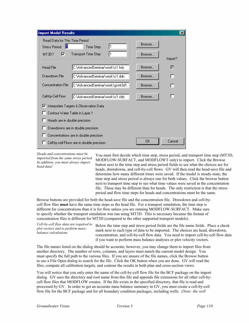
Groundwater Vistas Version 3 Page 110
Heads and concentrations must be imported from the same stress period. In addition, you must always import head data!
You must first decide which time step, stress period, and transport time step (MT3D, MODFLOW-SURFACT, and MODFLOWT only) to import. Click the Browse button next to the time step and stress period fields to see what the choices are for heads, drawdowns, and cell-by-cell flows. GV will then read the head-save file and determine how many different times were saved. If the model is steady-state, the time step and stress period is always one for both values. Click the browse button next to transport time step to see what time values were saved in the concentration file. These may be different than for heads. The only restriction is that the stress period and flow time steps for heads and concentrations must be the same.
Browse buttons are provided for both the head-save file and the concentration file. Drawdown and cell-by-cell flow files must have the same time steps as the head file. For a transport simulation, the time step is different for concentrations than it is for flow unless you are running MODFLOW-SURFACT. Make sure to specify whether the transport simulation was run using MT3D. This is necessary because the format of concentration files is different for MT3D (compared to the other supported transport models). Cell-by-cell flow data are required to plot vectors and to perform mass-balance calculations
Below the time step and stress period fields are the file name fields. Place a check mark next to each type of data to be imported. The choices are head, drawdown, concentration, and cell-by-cell flow data. You need to import cell-by-cell flow data if you want to perform mass balance analyses or plot velocity vectors.
The file names listed on the dialog should be accurate; however, you may change them to import files from another directory. The number of rows, columns, and layers must match the current model design. You must specify the full path to the various files. If you are unsure of the file names, click the Browse button to use a File Open dialog to search for the file. Click the OK button when you are done. GV will read the files, compute all calibration targets, and contour the results in both plan and cross-section views.
You will notice that you only enter the name of the cell-by-cell flow file for the BCF package on the import dialog. GV uses the directory and root name from this file and appends file extensions for all other cell-by-cell flow files that MODFLOW creates. If the file exists in the specified directory, that file is read and processed by GV. In order to get an accurate mass balance summary in GV, you must create a cell-by-cell flow file for the BCF package and for all boundary condition packages, including wells. (Note: the well
Groundwater Vistas Version 3 Page 111
cell-by-cell file is not absolutely necessary as long as all wells in the model are simulated and no cells containing wells go dry during the simulation).
When importing cell-by-cell flows, GV does not necessarily need a cell-by-cell flow file for recharge. However, for a large model, you may notice a delay between the reading of the results and the contouring of the information. This is caused by GV assembling recharge rates internally. If you notice a long wait before contouring happens, the best solution is to select Model->MODFLOW->Packages and place a non-zero number in the 3rd column next to Recharge. This tells MODFLOW to save cell-by-cell flow terms for the recharge package.
In some cases, GV may not be able to properly read the binary (unformatted) files. If you get errors trying to import unformatted files, you must run a program called UNF2BIN.EXE at the DOS prompt. When running UNF2BIN, you are first prompted for the file type to convert (0=Head-save or Drawdown, 1 = cell-by-cell flow, 2 = MT3D UCN file, and 3 = quit). You will next enter the name of the unformatted file and finally the name of the binary file to create. The latter file is the one you will import into GV.
You do not need to convert binary files if you are using the following models:
MODFLOWwin32 MODFLOW2000win32 MODFLOWT from GeoTrans MODFLOW-SURFACT from HydroGeoLogic MT3D versions supplied with GV RT3D supplied with GV
Import of Cell-by-Cell Flow Data. Prior to GV Version 1.74, fluxes read from the BCF Package cell-by-cell flow file were contoured without any modification. The units on these flux terms are L3/T (e.g., ft3/d). The problem with this approach is that for a nonuniform grid, the flux term is partially dependent on the size of the grid cell and this makes interpretation of the contours misleading. Consequently, GV now divides all flux terms by the cross-sectional area perpendicular to the orientation of the flux term. For example, the flow terms in the Z (layer) direction are divided by the area of the cell. This makes them analogous to a recharge term.
Contouring Starting Heads. MODFLOW does not save the starting heads (initial conditions) to the head-save file so GV cannot contour them. The Import Results dialog has been changed, however, so that you may import heads from the BASIC Package for contouring. Simply substitute the BASIC Package file name for the Head-Save File name on the “head” line of the Import Results dialog.
Water Table Contouring. In a multi-layer water table simulation, the water table surface may span more than one layer. For example, the water table may drop into layer 2 causing layer 1 cells to become dry. Normally, GV will contour the heads in one layer at a time. There is an option on the Import Results dialog that will allow contouring the continuous water table surface. Check the box labeled “Contour Water Table in Layer 1” prior to importing heads. When you contour Layer 1, GV will use heads in lower layers if the upper layers are dry. This will give you a continuous water table map when the water table spans more than one layer. You should make sure, however, that the value assigned to dry cells is different than the head value assigned to no-flow cells. You can change the dry cell head value by selecting Model->MODFLOW->Resaturation Data. You set the no-flow value of head by selecting Model->MODFLOW->Basic Package.
Interpolation of target and observation well data. When this option is checked, GV uses bilinear interpolation to estimate a target or observation well value from the MODFLOW results. This is done by default because the targets and observation wells are often not located at the center of a cell and are thus some combination of the four surrounding nodes. You may uncheck this option to use the data computed by MODFLOW (or other model) without any modification. In the latter case, GV just determines the cell containing the well and uses the value directly from the binary file. There is also a subtle difference in how GV uses concentrations from MT3D. When you choose to interpolate target and observation well data, GV uses concentration data from the binary concentration file (*.ucn). If you do not interpolate target and observation well data, GV uses data directly from the observation well file created by MT3D (default is mt3d.obs).
Groundwater Vistas Version 3 Page 112
Importing MODPATH Pathlines The Import MODPATH selection on the Plot menu reads the results of a MODPATH simulation. A File Open dialog prompts for the name of the file to import. Most MODPATH versions create a file called PATHLINE. The command line versions of MODPATH distributed by ESI with GV create a file called PATHLINE.PTL. Enter the appropriate file name in the dialog and click OK. If you are using the new Windows DLL version of MODPATH, however, the name of the pathline file is root.ptl, where root is the root file name for MODPATH defined under Model->Modpath->Packages. GV reads the results and displays the pathlines in both plan and section views.
Importing PATH3D Pathlines The Import PATH3D option works just like the one for MODPATH listed above. The only difference is that Path3D creates a file called p3dplot.dat. Find this file and click OK to process and display the particle traces.
The Cross-Section View The cross-section view is displayed above the plan view on your screen. In the current release of GV, it is only a view. GV will not respond to mouse clicks in the cross-section view, although the coordinates of the cursor and any property or boundary condition data will be displayed on the status bar.
You may expand or decrease the size of the cross-section view by sliding the border between the section and plan views up or down. Slide the border to the toolbar to get rid of the section view entirely. The vertical exaggeration of the cross-section automatically adapts to the size of the available window. In addition, the section is always the same horizontal scale as the plan view.
You may change the current section being displayed by clicking the + or - buttons next to row or column on the Reference Cube or by selecting Xsect->Select. The cross-section view is also printed from the Xsect menu.
In Groundwater Vistas Version 3, there is also a tab at the bottom of the GV screen for display of the cross-section in its own window. This tab view is a functional cross-section where some design functions can take place. At this time, you may add titles to the tab cross-section view and you may add a vertical scale bar.
Contour Maps GV contours head, concentration, drawdown, and flow in the X-, Y-, and Z- directions. Contours are created in both plan and cross-section views. As you change the current layer and section number using the reference cube, GV automatically recomputes and redraws the contours. Only one variable (e.g., head, concentration, etc.) may be contoured at one time. The same variable is contoured in both map view and section view.
By default GV contours heads when you import a model run for the first time. You may change the type of contours by selecting Plot->What to Display. The following dialog is displayed:

Groundwater Vistas Version 3 Page 113
This dialog controls not just contouring but velocity vectors, particle traces, color floods, and how the base map is displayed. A check mark next to any option means that the selected item will be displayed or the option is in effect. You may overlay any or all of these graphics on the screen through these check boxes.
The contour and color flood options also contain combo-boxes that have the following options (1) head, (2) drawdown, (3) concentration, (4) flow in the X-direction, (5) flow in the Y-direction, (6) flow in the Z-direction, (7) velocity (Darcy flux divided by porosity), and (8) four user-defined variables. You may contour one variable type and flood another using a combination of these options. In addition to the seven predefined variables described above, you may also define four user variables. These user variables are computed using matrix calculations.
The Plot->Contour menu is used to modify how GV draws contours. There are four options on the menu, including Window, Parameters (Plan), Parameters (Section), and Concentration.
The contour window is the area contoured within the model grid. By default this is the entire model domain. You may resize the window to contour a subregion within the model. Selecting Window will allow you to resize the contour area. Move the mouse to one corner of the new contour window and press the left mouse button. Hold the left button down, drag the cursor to the opposite corner of the window, and release the button. A dialog will then be displayed to confirm the window coordinates. Press OK to accept the new contour window or Cancel to keep the existing one. This also resizes the section contour map to the same area as the plan view.
Choosing Parameters (Plan) from the Contour menu displays a dialog that allows you to change the resolution of the contour matrix and the look of the contour map. You may change the minimum contour level, the contour interval, the number of nodes in the contour matrix, and format of the labeling. This dialog is shown below:
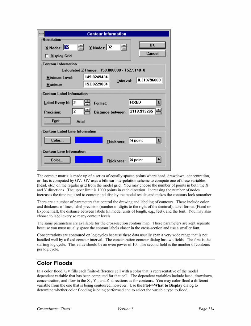
Groundwater Vistas Version 3 Page 114
The contour matrix is made up of a series of equally spaced points where head, drawdown, concentration, or flux is computed by GV. GV uses a bilinear interpolation scheme to compute one of these variables (head, etc.) on the regular grid from the model grid. You may choose the number of points in both the X and Y directions. The upper limit is 1000 points in each direction. Increasing the number of nodes increases the time required to contour and display the model results and makes the contours look smoother.
There are a number of parameters that control the drawing and labeling of contours. These include color and thickness of lines, label precision (number of digits to the right of the decimal), label format (Fixed or Exponential), the distance between labels (in model units of length, e.g., feet), and the font. You may also choose to label every so many contour levels.
The same parameters are available for the cross-section contour map. These parameters are kept separate because you must usually space the contour labels closer in the cross-section and use a smaller font.
Concentrations are contoured on log cycles because these data usually span a very wide range that is not handled well by a fixed contour interval. The concentration contour dialog has two fields. The first is the starting log cycle. This value should be an even power of 10. The second field is the number of contours per log cycle.
Color Floods In a color flood, GV fills each finite-difference cell with a color that is representative of the model dependent variable that has been computed for that cell. The dependent variables include head, drawdown, concentration, and flow in the X-, Y-, and Z- directions as for contours. You may color flood a different variable from the one that is being contoured, however. Use the Plot->What to Display dialog to determine whether color flooding is being performed and to select the variable type to flood.

Groundwater Vistas Version 3 Page 115
GV scales the colors from blue for the lowest value in the model domain to red for the highest values. You can change how the colors are mapped by selecting Plot->Color Flood Options. GV maps blue to the minimum value you enter on the dialog and red to the highest. You may also scale the colors logarithmically and you may display a color bar legend next to the model grid.
GV uses 24-bit color values to create color flood plots. In order to get the full effect of this technique, you must configure your Windows display device to show more than 256 colors. In Windows 95, you simply click the right mouse button on your desktop (not on an active application window!). A small menu is displayed. Choose Properties and a tab dialog is displayed. Click the Settings tab to see your current resolution and number of colors. You should choose either High Color (16 bit) or True Color (24 bit) to get the best visual effect from using GV.
Velocity Vectors Velocity vectors are simply arrows that are drawn in the direction of groundwater flow. The length of the arrow is proportional to the velocity or to the logarithm of the velocity. The following is an example of a vector map with contours:
In order to plot vectors, you must import cell-by-cell flow data for at least the BCF package. MODFLOW saves cell-by-cell values for the BCF Package when you place a nonzero number in the CBC column on the MODFLOW Packages dialog. If you create a new model in GV (as opposed to importing an existing one), GV automatically assigns a unit number of 50 to the cell-by-cell flow file for the BCF package. GV also automatically tells MODFLOW to save this data.
You may modify how vectors are drawn by selecting Plot->Vector Options. A dialog is displayed which controls vectors in both plan and cross-section views. The options include the minimum velocity to plot (default is zero), the maximum vector length in model length units (e.g., feet), an option to scale vectors logarithmically, and the color of upward and downward vectors. The determination of whether a vector is upward or downward is based upon the flow direction of water at the top of the layer. Thus, for the top layer, the direction is usually downward from recharge. For other layers, the vertical direction of flow is determined based upon the head relationships between adjacent layers.
Particle Traces Particle traces are computed using either MODPATH or PATH3D. Both the steady-state and transient versions of MODPATH are supported by GV. The Import MODPATH option on the Plot menu reads the

Groundwater Vistas Version 3 Page 116
results of a MODPATH simulation. A File Open dialog prompts for the name of the file to import. Most MODPATH versions create a file called PATHLINE. The MODPATH programs distributed by ESI with GV create a file called PATHLINE.PTL. Enter the appropriate file name in the dialog and click OK. GV reads the results and displays the pathlines in both plan and section views.
The Import PATH3D option works just like the one for MODPATH listed above. The only difference is that Path3D creates a file called p3dplot.dat. Find this file and click OK to process and display the particle traces.
GV reads the pathline data and displays the traces in both plan and section views. By default neither travel times nor arrow heads are plotted on the traces; however, you may select Plot->Particles to change these options. The Particles menu contains a dropdown menu with three selections, including Arrows, Time Posting, and Options.
The Arrows option controls the appearance of arrowheads on particle traces. A dialog prompts for three values, the distance between arrows, the size of each arrow-head, and a check-box which determines whether the arrows are displayed. The size of arrows and distance between successive arrows are entered in model units of length (e.g., feet).
The Time Posting selection controls the appearance of time values posted along particle traces. The dialog asks for several data values, including the time interval between successive postings, the precision (decimal digits) of the posting, a time multiplier value, the font to use for the posting, and a check-box which determines whether postings are displayed. The multiplier is used to change the time units of the posting. For example, to convert model units of days to years for the posting, multiply by 365.
The Options menu selection controls the way in which particles are displayed. A dialog is displayed prompting for the maximum tracking time and the direction (forward or reverse) of tracking. The maximum travel time determines how much of the particle trace is displayed. This allows you to truncate particle traces from a MODPATH or Path3D run. For example, to compute the 10 year travel time around a production well, set this value to 3650 days (if your model time units are days). The direction of tracking is used to control the direction that arrows are displayed.
Mass Balance Analysis GV provides several different types of mass balance analysis techniques for the entire model, a single layer, or for a subregion of the model (either a window or irregular polygon). In the current release, only flow mass balances for MODFLOW, MODFLOWT, and MODFLOW-SURFACT are supported. Contaminant mass balance will be supported in a later release.
Required Data Files Mass balance is a method of looking at the amount of water that enters or leaves the model plus any change in storage within the model. Adding these three major components together should yield zero. However, there will always be some error and hopefully it is small. If you import all of the components of the cell-by-cell flow terms computed by MODFLOW, GV will compute the error for the whole model, for a single layer, or for a window. In order to save all of the necessary cell-by-cell flow data, you must place a nonzero number in the CBC field of the MODFLOW Packages dialog for all of the following packages:
Cell-by-cell for BCF cbb Cell-by-cell for Wells cbw Cell-by-cell for Rivers crv Cell-by-cell for Drains cbd Cell-by-cell for General Heads cbg Cell-by-cell for Streams cst Cell-by-cell for Recharge crc Cell-by-cell for ET cbe You must always create the cell-by-cell flow file for the BCF Package and any other boundary conditions that are in your model. You may ignore the well cell-by-cell flow file in most cases, however, because GV

Groundwater Vistas Version 3 Page 117
knows these values. You only specify the cell-by-cell flow file for the BCF package on the Import Results dialog; however, GV looks for the other files in the same directory as the BCF cell-by-cell file and uses the default extensions for the file names as shown above.
Displaying Mass Balance Data Selecting Mass Balance from the Plot menu displays a dropdown menu with several options, (1) Window, (2) Layer Summary, (3) Model Summary, (4) Boundary Reach, (5) Digitize, and (6) Graph Setup. The first three options summarize the flow of water into and out of an arbitrary window, the entire model, or the current layer, respectively. The boundary reach option adds the flows to every boundary condition with a specified reach number. The resulting dialog displays the total flow broken down by boundary type. The digitize option allows you to digitize a polygon region where flow data will be summarized. You may even save the digitized region to a file for later processing. The last option is used to configure the bar chart that may be plotted when summarizing the mass balance in one of the first three options.
After choosing Window from the Mass Balance menu, move the cursor to one corner of the area you are interested in. Click and hold the left mouse button, move the cursor to the opposite corner of the rectangular area and release the mouse button. You will then see a dialog to confirm the coordinates you just entered. Click OK and another dialog is displayed to show the mass balance summary. An example is shown below:
The Model and Layer summary options will display the same dialog with the mass balance summary. The units on all mass balance numbers are L3/T (e.g., ft3/d). This summary should match the one printed in the MODFLOW output file.
These numbers may not match the mass balance summary in MODFLOW because the MODFLOW mass balance numbers in the first column of the MODFLOW output file have been multiplied by the time step size. Thus, the MODFLOW mass balance numbers are in units of L3. (NOTE: the right side of the MODFLOW output file for mass balance should match the GV numbers; only the left side of the printout in MODFLOW has been multiplied by time step size).

Groundwater Vistas Version 3 Page 118
Mass balance data for individual boundary conditions is available as you move the mouse on the screen. Moving the mouse over a boundary cell displays the flux into (+) or out of (-) the model at that cell location. The flux value is displayed on the status bar as “F=” with units of L3/T. You must be in boundary condition mode, however, for these flux values to be displayed.
The mass balance summary dialog contains a buttons labeled Graph and Export. The export button prompts for a file name where GV will write the data used to create the mass balance summary. This file is an ASCII comma-delimited file that can be imported to just about any spreadsheet program (like Excel). Click the Graph button to display a bar graph of inflows (positive numbers) and outflows (negative numbers). The chart displayed by GV is generated using the First Impression software. An example is shown below:
Choosing Graph Setup from the dropdown menu displays a dialog with options for displaying the mass balance summary bar chart. These options include:
Display only nonzero flux values Minimum flux on Y-Axis Maximum flux on Y-Axis Distance between Y-Axis labels Number of decimals in Y-axis labels
When you choose the option to display only non-zero flux values, GV will only display bars for boundary conditions or faces of the cube (or model or layer) that have non-zero fluxes. This limits the amount of information on the chart and makes it easier to compare the differences between flux values.
Digitize Feature GV has a powerful digitize feature for analyzing mass balance information. The Digitize option allows you to digitize a polygon with the mouse. GV then provides you with a mass balance summary for this irregular region. There are several digitize options for mass balance: (1) New Polygon, (2) Last Polygon, (3) Export Polygon, (4) Import Polygon, and (5) Display Polygon. After selecting New Polygon, you digitize the polygon by moving the mouse and clicking the left mouse button. The right mouse button deletes the last point digitized. Double-click the left mouse button to end digitizing and close the polygon. GV will then shade each cell within the polygon. GV decides that a cell is within the polygon if the center
Groundwater Vistas Version 3 Page 119
of the cell lies within the digitized region. Last Polygon uses the last polygon you digitized in this GV session (NOTE: polygons are not automatically saved when you exit GV). You may import and export the last polygon you digitized. The final option is a check menu item. When checked, the Display Polygon option keeps the mass balance polygon shaded. This will also print to any Windows output device.
Hydrographs Hydrographs are plots of a model dependent variable with time on an arithmetic graph. Hydrographs may be plotted for head, drawdown, and/or concentration at either calibration target locations or for monitoring wells.
Monitoring wells are added to the model by selecting Add->Well from the main menu. After selecting
Well or choosing on the toolbar, move the cursor to the new well location and click the left mouse button or press Enter. A dialog will be displayed to enter the well characteristics. Click the box labeled “Monitor head/concentration vs. Time”. If the well is used strictly for monitoring, make sure that the flow rate is set to zero. Also, monitoring well must be defined in only one layer. Multi-layer monitoring wells will only display hydrographs for the upper layer containing the well.
You may plot hydrographs for observation wells or for calibration targets by selecting Plot->Hydrographs->Target or Plot->Hydrographs->Monitoring Well, respectively. In each case a dialog is displayed with a list of available targets or monitoring wells. Click on the well you would like to plot and a graph is displayed. For monitoring wells, you must also select the variable to plot. You may plot head, drawdown, or concentration.
You also may set plot options for each plot type (Target or Monitoring Well) by selecting Plot->Hydrographs->Plot Options. A dialog is displayed with options for the Time (X) axis and the Model Value (Y) axis. The options include the minimum and maximum values to plot, the distance between axis labels, and the number of decimal places in the axis labels.
Hydrograph data are read from the model output files when these files are imported, as discussed in the first section of this chapter. If you add targets or monitoring wells after importing the results of a simulation, you must import the results again so that GV records the information.
Hydrograph data generally comes from either the head, drawdown, or concentration files. GV plots data for each time step found in these files. If only a few time steps were saved, the plots may not look very smooth. You may fix this by saving more time steps. The exception to this is MT3D, which saves concentration in an observation file (called MT3D.OBS). GV reads this file directly to get concentration hydrograph data.
Profiles Profiles are graphs of a model variable versus distance along a cross-section. The model variables may be head, drawdown, concentration, flow in the X-direction (Qx), flow in the Y-direction (Qy), or flow in the Z-direction (Qz). To plot a head profile for the current cross-section (the one that is displayed above the plan view on your screen), select Plot->Profiles->Head. Similar menu choices are available for the other variables. The following is an example head profile:
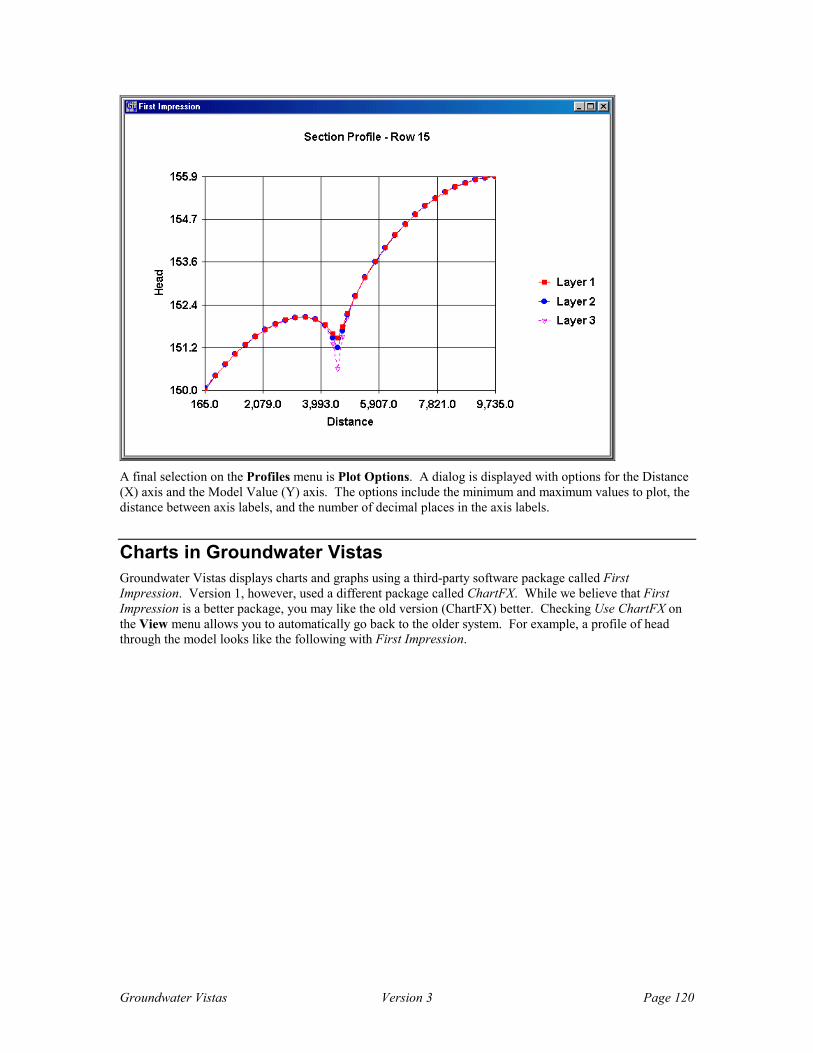
Groundwater Vistas Version 3 Page 120
A final selection on the Profiles menu is Plot Options. A dialog is displayed with options for the Distance (X) axis and the Model Value (Y) axis. The options include the minimum and maximum values to plot, the distance between axis labels, and the number of decimal places in the axis labels.
Charts in Groundwater Vistas Groundwater Vistas displays charts and graphs using a third-party software package called First Impression. Version 1, however, used a different package called ChartFX. While we believe that First Impression is a better package, you may like the old version (ChartFX) better. Checking Use ChartFX on the View menu allows you to automatically go back to the older system. For example, a profile of head through the model looks like the following with First Impression.

Groundwater Vistas Version 3 Page 121
The same graph in ChartFX looks like the following:
The biggest difference you will see right away is the lack of a menu on the First Impression graph. You can export data, set options, and print the chart, however, by right-clicking on the graph. This brings up a context menu with the following options.
Chart Designer Edit Chart Data Wizard Open Save As Print Copy Paste
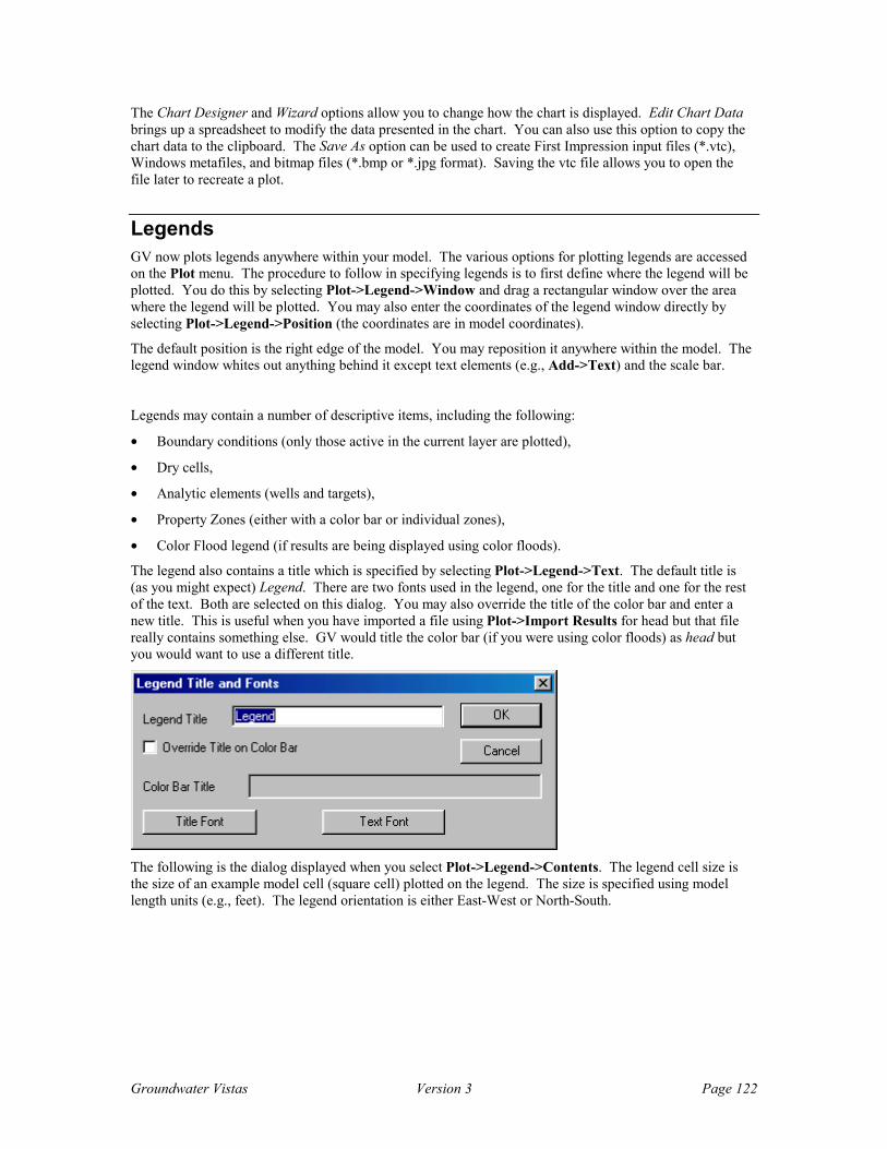
Groundwater Vistas Version 3 Page 122
The Chart Designer and Wizard options allow you to change how the chart is displayed. Edit Chart Data brings up a spreadsheet to modify the data presented in the chart. You can also use this option to copy the chart data to the clipboard. The Save As option can be used to create First Impression input files (*.vtc), Windows metafiles, and bitmap files (*.bmp or *.jpg format). Saving the vtc file allows you to open the file later to recreate a plot.
Legends GV now plots legends anywhere within your model. The various options for plotting legends are accessed on the Plot menu. The procedure to follow in specifying legends is to first define where the legend will be plotted. You do this by selecting Plot->Legend->Window and drag a rectangular window over the area where the legend will be plotted. You may also enter the coordinates of the legend window directly by selecting Plot->Legend->Position (the coordinates are in model coordinates).
The default position is the right edge of the model. You may reposition it anywhere within the model. The legend window whites out anything behind it except text elements (e.g., Add->Text) and the scale bar.
Legends may contain a number of descriptive items, including the following:
• Boundary conditions (only those active in the current layer are plotted),
• Dry cells,
• Analytic elements (wells and targets),
• Property Zones (either with a color bar or individual zones),
• Color Flood legend (if results are being displayed using color floods).
The legend also contains a title which is specified by selecting Plot->Legend->Text. The default title is (as you might expect) Legend. There are two fonts used in the legend, one for the title and one for the rest of the text. Both are selected on this dialog. You may also override the title of the color bar and enter a new title. This is useful when you have imported a file using Plot->Import Results for head but that file really contains something else. GV would title the color bar (if you were using color floods) as head but you would want to use a different title.
The following is the dialog displayed when you select Plot->Legend->Contents. The legend cell size is the size of an example model cell (square cell) plotted on the legend. The size is specified using model length units (e.g., feet). The legend orientation is either East-West or North-South.
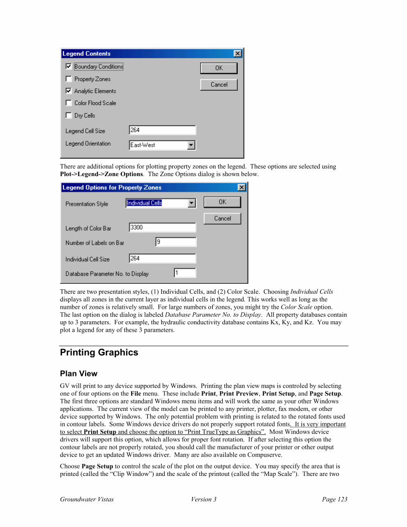
Groundwater Vistas Version 3 Page 123
There are additional options for plotting property zones on the legend. These options are selected using Plot->Legend->Zone Options. The Zone Options dialog is shown below.
There are two presentation styles, (1) Individual Cells, and (2) Color Scale. Choosing Individual Cells displays all zones in the current layer as individual cells in the legend. This works well as long as the number of zones is relatively small. For large numbers of zones, you might try the Color Scale option. The last option on the dialog is labeled Database Parameter No. to Display. All property databases contain up to 3 parameters. For example, the hydraulic conductivity database contains Kx, Ky, and Kz. You may plot a legend for any of these 3 parameters.
Printing Graphics
Plan View GV will print to any device supported by Windows. Printing the plan view maps is controled by selecting one of four options on the File menu. These include Print, Print Preview, Print Setup, and Page Setup. The first three options are standard Windows menu items and will work the same as your other Windows applications. The current view of the model can be printed to any printer, plotter, fax modem, or other device supported by Windows. The only potential problem with printing is related to the rotated fonts used in contour labels. Some Windows device drivers do not properly support rotated fonts. It is very important to select Print Setup and choose the option to “Print TrueType as Graphics”. Most Windows device drivers will support this option, which allows for proper font rotation. If after selecting this option the contour labels are not properly rotated, you should call the manufacturer of your printer or other output device to get an updated Windows driver. Many are also available on Compuserve.
Choose Page Setup to control the scale of the plot on the output device. You may specify the area that is printed (called the “Clip Window”) and the scale of the printout (called the “Map Scale”). There are two
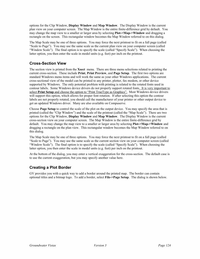
Groundwater Vistas Version 3 Page 124
options for the Clip Window, Display Window and Map Window. The Display Window is the current plan view on your computer screen. The Map Window is the entire finite-difference grid by default. You may change the map view to a smaller or larger area by selecting Plot->Map->Window and dragging a rectangle on the screen. This rectangular window becomes the Map Window referred to on this dialog.
The Map Scale may be one of three options. You may force the next printout to fit on a full page (called “Scale to Page”). You may use the same scale as the current plan view on your computer screen (called “Window Scale”). The final option is to specify the scale (called “Specify Scale”). When choosing the latter option, you then enter the scale in model units (e.g. feet) per inch on the printout.
Cross-Section View The section view is printed from the Xsect menu. There are three menu selections related to printing the current cross-section. These include Print, Print Preview, and Page Setup. The first two options are standard Windows menu items and will work the same as your other Windows applications. The current cross-sectional view of the model can be printed to any printer, plotter, fax modem, or other device supported by Windows. The only potential problem with printing is related to the rotated fonts used in contour labels. Some Windows device drivers do not properly support rotated fonts. It is very important to select Print Setup and choose the option to “Print TrueType as Graphics”. Most Windows device drivers will support this option, which allows for proper font rotation. If after selecting this option the contour labels are not properly rotated, you should call the manufacturer of your printer or other output device to get an updated Windows driver. Many are also available on Compuserve.
Choose Page Setup to control the scale of the plot on the output device. You may specify the area that is printed (called the “Clip Window”) and the scale of the printout (called the “Map Scale”). There are two options for the Clip Window, Display Window and Map Window. The Display Window is the current cross-section view on your computer screen. The Map Window is the entire finite-difference grid by default. You may change the map view to a smaller or larger area by selecting Plot->Map->Window and dragging a rectangle on the plan view. This rectangular window becomes the Map Window referred to on this dialog.
The Map Scale may be one of three options. You may force the next printout to fit on a full page (called “Scale to Page”). You may use the same scale as the current section view on your computer screen (called “Window Scale”). The final option is to specify the scale (called “Specify Scale”). When choosing the latter option, you then enter the scale in model units (e.g. feet) per inch on the printout.
At the bottom of the dialog, you may enter a vertical exaggeration for the cross-section. The default case is to use the current exaggeration, but you may specify another value here.
Creating a Plot Border GV provides you with a quick way to add a border around the printed map. The border can contain optional titles and a bitmap logo. To add a border, select File->Page Setup. The dialog is shown below.

Groundwater Vistas Version 3 Page 125
The Display Border option draws a rectangular line around the plot. Select Footer Line to place a title and logo at the bottom of the plot or select Header Line to put the title and logo at the top of the page. When turning on the footer or header line, you must also change None to Default next to header or footer in the center of the dialog.
Click the Maps tab to determine the scale of the plot and how much of the model to plot. This tab is shown below.

Groundwater Vistas Version 3 Page 126
You use this tab to set the scale and to determine what part of the model is clipped. The Display Window clipping option means that the plot will show whatever is on your screen. The Map Window, on the other hand, may be larger or smaller than what is currently displayed. The map window is defined by default as the whole model. You may change it, though, by selecting Plot->Map->Window and drag a rectangle to define the map window.
The Default Header/Footer tab allows you to import a bitmap for a logo. This tab is shown below.

Groundwater Vistas Version 3 Page 127
You may also define up to four lines of text along with fonts.
Charts Charts, such as the mass balance bar chart shown above, are printed by right-clicking on the chart. A print option is displayed on the context menu that appears over the chart. If you are using ChartFX (check mark placed next to Use ChartFX on the View menu), printing is done from the File menu on the chart.
Matrix Calculator The Matrix Calculator gives you the flexibility to compute and display your own variables which are mathematical functions of model results and/or parameters. For example, you can create a user-defined variable called transmissivity to contour transmissivity in the model. You may select Plot->Matrix Calculator->Variable Names to give the matrix a logical name. In this example, you would type transmissivity for user variable 1 as shown below.
You would next define how the transmissivity is computed. There are two types of calculations. The first is a true three-dimensional calculation. Use the 3D matrix computation if all cells in every layer are treated

Groundwater Vistas Version 3 Page 128
the same way. In this example, you would select Plot->Matrix Calculator->Compute (3D) and enter the calculation data for user variable 1 as shown below:
To activate an equation, simply place a check to the left of the definition for that equation. In this example, we are making only one calculation. You then select the variables to use in the calculation and how they are combined (add, subtract, multiply, divide, or square root). If you use a constant, you would enter this below the word constant in the equation.
The equations are processed when you click OK on this dialog. The equations are also processed in the order they appear on the dialog. The two-dimensional calculation works the same way but you also assign layer numbers to each variable in the equation. The 2D matrix math would be useful for computing the head difference between two layers, for example.
Once a user-defined variable has been computed, you can contour and color flood the data just like heads or drawdown from a MODFLOW simulation. Select Plot->What to Display. The combo box next to contour and color flood will contain the user variable names.
You can also export the user variables to head-save files for later use. Select Plot->Matrix Calculator->Export and specify the variable name and file name to contain the data as shown below.
These can also be imported back into GV by selecting Plot->Matrix Calculator->Import. The same type of dialog is displayed. Just tell GV what variable will contain the imported data and the file name.
Groundwater Vistas Version 3 Page 129
Exporting Data Data and graphics are exported from GV primarily from the File menu, although some dialogs (such as the Mass Balance dialog) offer their own data export options. The Export feature on the File menu provides you with a way to transfer GV graphics and data to other software packages. Supported file formats include the following:
• SURFER (ASCII and binary grid files, XYLINE files, and Posting files),
• DXF (*.dxf),
• Windows Metafiles (*.wmf),
• ASCII XYZ (*.dat),
• Observation Well Data (*.dat)
• ArcView shapefile (*.shp)
• ArcView Spatial Analyst ASCII Raster
• EVS field file
• EVS UCD file
GV supports both ASCII and binary SURFER grid files. The grid files contain the matrix of head, concentration, or flux values currently contoured in plan view by GV for recontouring in SURFER. GV can also export the digitized map file as a SURFER XYLINE file. Text values (time postings, map titles, etc.) are exported to SURFER Posting files. You may also export SURFER grid files for the cross-section view by selecting Xsect->Export.
GV exports model graphics (contours, digitized map, etc.) to either a DXF file or a Windows Metafile. DXF is a generic format supported by most CAD software, including AutoCAD. A Windows Metafile (.wmf) is a fairly generic format supported by most Windows programs. Many of these applications, however, do not support the rotated text required for the contour labels.
A Windows Metafile (.wmf) is a fairly generic format supported by most Windows programs. The metafile retains the proper text font and colors in your plot. The metafile contains everything displayed on your screen. In Microsoft Word Version 6.0, however, you may need to insert a frame around the graphic after importing into Word.
The XYZ format is a simple DOS text file that lists each head, concentration, drawdown, flux, or velocity computed by GV and its X and Y locations. One data point is listed on each line of the file. After clicking OK on the file save dialog, you will be presented with another dialog to specify the options for XYZ export. These include (1) data type (head, drawdown, concentration, flux in the x-, y-, and z-directions, and horizontal velocities), (2) dimensions (3D or 2D), and (3) data format (X, Y, Z or Row, Column, Layer). In order to export these data, you must first import them from the previous model run.
File Operations GV now provides a convenient way to view what is contained in a binary file. You select Plot->File Operations->View Contents and the following dialog is displayed.

Groundwater Vistas Version 3 Page 130
Select the file name and type at the bottom of the dialog and then click the View button. GV will scan through the file and display all time steps, stress periods, transport time steps (if appropriate), and the title of the variables stored in the file.
The second option on the File Operations menu compares the contents of two files. This is convenient for determining the difference between two runs or as a QA/QC step to make sure an imported model is producing the same results as the original one. The file comparison dialog is shown below.
Select the two files to compare and give a file name that would contain the differences for later processing. Also select the file type at the bottom of the dialog. Click the View button to perform the comparison and create the Results file. The maximum difference is displayed at the top of the dialog for each matrix in the file.

Groundwater Vistas Version 3 Page 131
Graphics for Calibration There are several types of plots that are used to evaluate model calibration. These include the scatter plot of measured vs. Observed heads, drawdowns, and concentrations, posting residuals on contour maps, and the sensitivity plots. These are all covered in the next chapter on model Calibration.

Groundwater Vistas Version 3 Page 132

Groundwater Vistas Version 3 Page 133
Model Calibration
Introduction In most modeling studies, the calibration phase requires the most effort and is the most difficult to accomplish. Groundwater Vistas helps streamline the calibration process by offering one of the most comprehensive suites of calibration tools of any groundwater modeling system. These tools include calculation of residuals and residual statistics for head, drawdown, concentration, and flux targets, running individual sensitivity simulations, an automated sensitivity analysis, running multiple automatic sensitivity analyses in batch mode, an automatic calibration procedure built into the GV interface, and support for the PEST, UCODE, and MODFLOW2000 calibration (inverse) models. Each of these capabilities are described in the following chapter.
Calibration Targets A calibration target is a point in space and time where one of the model dependent variables has been measured. Calibration targets provide a means of assessing calibration quality because an error term, called a residual, is computed for each target location. A residual is computed as the field measurement minus the model-computed value. The range of errors helps you determine whether the quality of the calibration is adequate for your purposes. GV assists you in this determination by computing a wide variety of target statistics and by creating several different types of calibration maps and plots.
Calibration targets may be measurements of head, concentration, drawdown, or groundwater flow (called flux in the following discussion). Targets may be steady-state or may have an associated time value (called transient targets). One limitation is that flux targets must be steady-state. Head, drawdown, and concentration targets may be either steady-state or transient.
A new type of target has been added recently. These are gradient targets and are composed of three normal calibration targets. The three targets form a triangle that can be used to assess the error in the direction and magnitude of the hydraulic gradient.
Adding Targets Targets are added to the model by selecting Add->Target from the menu or by pressing the target button,
, on the toolbar. You must be in analytic element mode in order to add targets (i.e., press the button on the toolbar. Move the mouse to the target location and click the left mouse button. A dialog prompts for the target type, target value, layer number, X- and Y- coordinates, and an optional target name. You may also choose the font style, font size, and relative location of the target name. The target dialog is shown below.
Targets may be either steady-state or transient (NOTE: transient flux targets are not supported in GV but they may be used with Pest, UCODE, and MODFLOW2000). If you enter a steady-state target in a transient model, the target value will not be used by GV. Similarly, transient targets are ignored when the model is steady-state.
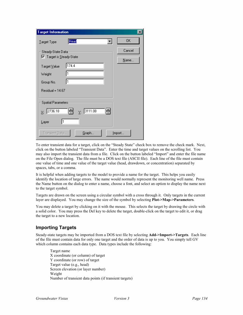
Groundwater Vistas Version 3 Page 134
To enter transient data for a target, click on the “Steady State” check box to remove the check mark. Next, click on the button labeled “Transient Data”. Enter the time and target values on the scrolling list. You may also import the transient data from a file. Click on the button labeled “Import” and enter the file name on the File Open dialog. The file must be a DOS text file (ASCII file). Each line of the file must contain one value of time and one value of the target value (head, drawdown, or concentration) separated by spaces, tabs, or a comma.
It is helpful when adding targets to the model to provide a name for the target. This helps you easily identify the location of large errors. The name would normally represent the monitoring well name. Press the Name button on the dialog to enter a name, choose a font, and select an option to display the name next to the target symbol.
Targets are drawn on the screen using a circular symbol with a cross through it. Only targets in the current layer are displayed. You may change the size of the symbol by selecting Plot->Map->Parameters.
You may delete a target by clicking on it with the mouse. This selects the target by drawing the circle with a solid color. You may press the Del key to delete the target, double-click on the target to edit it, or drag the target to a new location.
Importing Targets Steady-state targets may be imported from a DOS text file by selecting Add->Import->Targets. Each line of the file must contain data for only one target and the order of data is up to you. You simply tell GV which column contains each data type. Data types include the following:
Target name X coordinate (or column) of target Y coordinate (or row) of target Target value (e.g., head) Screen elevation (or layer number) Weight Number of transient data points (if transient targets)

Groundwater Vistas Version 3 Page 135
Items must be separated by a comma, spaces, or a tab. For transient targets, enter one line to define the target and include a column that has the number of time-target pairs. Immediately after the target definition line enter the time and target values (in that order and delimited as described above).
Computing Calibration Statistics Calibration statistics are computed by first calculating the error associated with each target and then calculating simple statistics on the population of targets. The error is called a residual and is computed by subtracting the model-computed value (head, drawdown, concentration, or flux) from the target value. Negative residuals indicate that the model is calculating the dependent value too high and a positive residual is where the model value is too low.
Prior to computing calibration statistics or plotting residuals, you must run the model and import results. If you add a target to the model after importing the results of a simulation, you must import the results again so that GV can compute the target residuals. Calculation of residuals is done only when you import results.
Select Plot->Calibration->Statistics/Plot to display a dialog that controls calculation and display of target residuals. You may select the type of target to compute (head, drawdown, concentration, or flux) and the range of layers to use in the calculation. Click on the “Statistics” button to display a summary of residual statistics and a listing of the residual values. The types of statistics computed include the following:
Sum of squared residuals Residual mean Residual standard deviation Absolute residual mean Residual standard deviation divided by range in target value

Groundwater Vistas Version 3 Page 136
The sum of squared residuals is computed by squaring all residuals and adding them together. This statistic is meaningless by itself but is useful to plot on sensitivity curves or when judging several different simulations. The sum of squared residuals is used by inverse models in the automated calibration process.
The residual mean is computed by dividing the sum of residuals by the number of residuals. Because both positive and negative residuals are used in the calculation, this value should be close to zero for a good calibration. In other words, the positive and negative errors should balance each other. The absolute residual mean, on the other hand, is calculated using the absolute value of the error (only positive values) and is a measure of the average error in the model.
The residual standard deviation is a measure of the overall spread of residuals. Think of it as a ± value. The residual standard deviation can be compared to the overall range in target value (e.g., head) as a further comparison. For head targets, this value shows how the errors relate to the overall gradient across the model. Normally, this value should be less than 10 to 15 percent for a good calibration.
You may compute your own calibration statistics by exporting the target information to a DOS text file. Simply click the “Export” button on the calibration statistics dialog and specify a file name. Data exported include the target name, target value, model computed value, and residual. Times are also exported for transient models.
Plotting Calibration Results
Scatter Plots Three types of plots are useful in assessing the quality of calibration simulations. The first is the scatter plot where observed target values (measurements) are plotted versus the values computed by the model. In an ideal calibration, the points will fall on a straight line with a 45 degree slope; i.e., that the computed value equals the measured value. The degree of scatter about this theoretical line is a measure of overall calibration quality.
Scatter plots are displayed by clicking the Plot Observed vs. Simulated button on the target statistics dialog. A different symbol type and color is used for residuals in each model layer to help you identify calibration problems, as shown below.
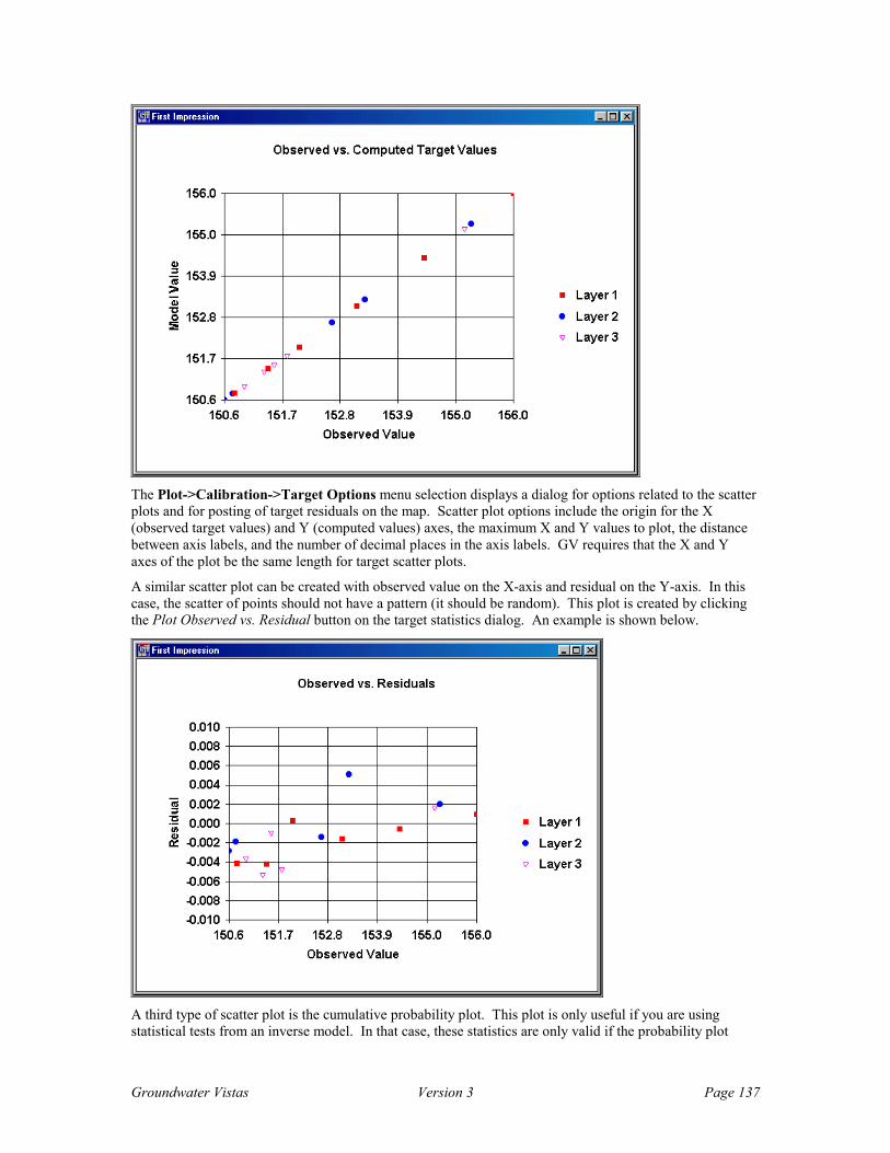
Groundwater Vistas Version 3 Page 137
The Plot->Calibration->Target Options menu selection displays a dialog for options related to the scatter plots and for posting of target residuals on the map. Scatter plot options include the origin for the X (observed target values) and Y (computed values) axes, the maximum X and Y values to plot, the distance between axis labels, and the number of decimal places in the axis labels. GV requires that the X and Y axes of the plot be the same length for target scatter plots.
A similar scatter plot can be created with observed value on the X-axis and residual on the Y-axis. In this case, the scatter of points should not have a pattern (it should be random). This plot is created by clicking the Plot Observed vs. Residual button on the target statistics dialog. An example is shown below.
A third type of scatter plot is the cumulative probability plot. This plot is only useful if you are using statistical tests from an inverse model. In that case, these statistics are only valid if the probability plot

Groundwater Vistas Version 3 Page 138
forms a straight line. For example, PEST computes the 95% confidence limits on estimated parameters values. You can only use these limits if the errors are randomly distributed, which is indicated by a straight line on probability plots, as shown below.
Posting Residuals Another type of plot that is useful in assessing calibration quality is a contour map of the model dependent variable (e.g., head) with residuals posted on the contours. To display the target residuals, place a check mark next to the Post Residual selection on the Calibration menu.
The Plot->Calibration->Target Options menu selection displays a dialog for options related to the posting of target residuals on the map. Target posting options control the way that residuals are posted on the plan view of the model. These options include justification (left, right, center), format of the residual (fixed or exponential), precision of the label (number of significant digits), time index (for transient models), dX and dY (these are offsets from the target symbol), the font, and color.
GV only posts residuals for the layer containing the target. These residual posting maps are useful in pointing out spatial bias in the distribution of errors. You should look for areas where residuals are all too high or too low. This indicates that something is incorrect about your conceptual model or model parameters. Even when the calibration statistics look good, you can have significant spatial bias in the distribution of residuals. The following is an example of a residual posting plot. Note that most of the residuals are negative indicating spatial bias in this part of the model.

Groundwater Vistas Version 3 Page 139
A similar option is the residual circle option. In cases when you have many targets, it is sometimes difficult to read the individual residuals on the map. A circle can be drawn around the target, though, with the size of the circle proportional to the magnitude of the error. The color of the circle indicates whether the residual is positive or negative. You can turn on display of residual circles using Plot->Calibration->Post Residual Circles. Select Plot->Calibration->Residual Circle Options to modify how these circles are drawn, as shown below.
Sensitivity Analysis Sensitivity analysis is the process of identifying the model parameters that have the most effect on model calibration or on model predictions. Model calibration is the focus of this chapter, so sensitivity analysis evaluates the effect of a change in a model parameter or boundary condition on the calibration statistics. GV has two methods of performing a sensitivity analysis, (1) single sensitivity runs, and (2) an automated sensitivity analysis.
In the current release of GV, only MODFLOW simulations are used in the two types of sensitivity analysis. For the automated sensitivity analysis, you must use ESI’s MODFLOWwin32 or MODFLOW2000win32.

Groundwater Vistas Version 3 Page 140
Single Sensitivity Run In an individual sensitivity run, you change one parameter or boundary condition by a small amount and evaluate the change in calibration statistics. A sensitive parameter is one that changes these statistics by a large amount. By identifying the most sensitive parameters in a model, you can streamline the calibration process by focusing your efforts on the most important aspects of the model.
A single sensitivity run is performed by selecting Model->MODFLOW->Sensitivity Analysis. The sensitivity analysis dialog is used to make a single sensitivity run by multiplying a single parameter zone by a given multiplication factor. This is not the same as the automatic sensitivity analysis discussed below in which several runs are made by GV. The advantage of the single sensitivity run is that you may modify a parameter value but not change the value in the database.
You select a parameter type (Kx, Ky, Kz, Leakance, Storage, Specific Yield, Recharge rate, ET rate, or ET extinction depth), the zone number to modify, and the multiplication factor. The parameter value in the database for the specified zone is then multiplied by the factor before being written to the data set.
You now create a new set of model files, run the model, import results, and evaluate calibration statistics. The single sensitivity run works with any version of MODFLOW.
Automated Sensitivity Analysis In an automated sensitivity analysis, GV runs MODFLOW several times and computes calibration statistics for each simulation. After the analysis is finished, you may plot key statistics versus model parameter value. The automated sensitivity analysis only works with ESI’s MODFLOWwin32.
Setting Up the Run
The automatic sensitivity analysis procedure is a powerful calibration tool offered by GV. Running the sensitivity analysis is a two step procedure. You start by selecting Model->Auto Sensitivity Setup. A dialog is displayed as shown below:
The dialog contains four items:
parameter type to modify zone or reach number to modify

Groundwater Vistas Version 3 Page 141
number of simulations boundary condition reach to monitor list of multiplication factors (one for each simulation)
Parameters include the following:
Kx = Ky Kz Leakance Storage coefficient Specific Yield Recharge rate ET rate ET extinction depth River conductance Drain conductance GHB conductance Stream conductance Well discharge (Q) HFB conductance River stage Drain elevation GHB head Stream stage Constant Head
The first eight parameters are Properties and the last eleven are boundary conditions. For the properties, you enter a zone number from the GV database. For boundary conditions, you enter a reach number, which is a number used to segregate boundary cells into groups.
Click the Multipliers button to display a scrolling list of multiplication factors for each run, as shown below. The multipliers are used to scale the property value or boundary conductance for each run in the sensitivity analysis. GV takes the parameter value in the database or the conductance you entered in the boundary condition dialog and multiplies it by the multiplication factor. GV then creates a new MODFLOW data file when you start the run.
Automating the Automatic Sensitivity Analysis! Just when you thought it was automatic enough, we added yet another automated procedure. You can now create a script (text) file for any number of automatic sensitivity analyses and have GV run it. This is great to check the sensitivity of every model parameter in one large batch run (best done over night!).
The first step is to create a sensitivity analysis script file in any text editor or word processor. In GV Version 3, you can also use the buttons on the side of the dialog (see example above) to create the script file, add to the script file, or load the script file into a text editor. The file consists of blocks of data for each sensitivity run corresponding to one parameter type. You may append as many of these blocks as you like to form a series of analyses. Each block of data has the following format:

Groundwater Vistas Version 3 Page 142
Type Zone NumRuns Reach
X(1)
.
.
X(NumRuns)
Where: Type is the parameter type (see the following table for numeric parameter type codes), Zone is the parameter zone number or boundary condition reach number, NumRuns is the number of simulations in the current analysis, and Reach is the boundary reach number for summarizing effects on boundary fluxes. These data are listed on one line of the file. The numbers should be separated by spaces, commas, or tabs. Following this line is one line for each parameter multiplier value.
Parameter Type Integer Code
Kx 0
Kz 1
Leakance 2
Storage Coefficient 3
Specific Yield 4
Recharge Rate 5
ET Rate 6
ET Extinction Depth 7
River Conductance 8
Drain Conductance 9
GHB Conductance 10
Stream Conductance 11
Well Flow Rate 12
HFB Conductance 13
River Stage 14
Drain elevation 15
GHB head 16
Stream Stage 17
Constant Head 18
For example, the following block of data would perform a sensitivity analysis on Recharge Zone number 3 with 7 simulations:
5 3 7 0
0.7
0.8
0.9
1.0
1.1
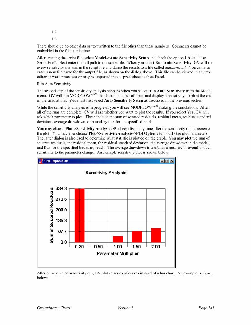
Groundwater Vistas Version 3 Page 143
1.2
1.3
There should be no other data or text written to the file other than these numbers. Comments cannot be embedded in the file at this time.
After creating the script file, select Model->Auto Sensitivity Setup and check the option labeled “Use Script File”. Next enter the full path to the script file. When you select Run Auto Sensitivity, GV will run every sensitivity analysis in the script file and dump the results to a file called autosens.out. You can also enter a new file name for the output file, as shown on the dialog above. This file can be viewed in any text editor or word processor or may be imported into a spreadsheet such as Excel.
Run Auto Sensitivity
The second step of the sensitivity analysis happens when you select Run Auto Sensitivity from the Model menu. GV will run MODFLOWwin32 the desired number of times and display a sensitivity graph at the end of the simulations. You must first select Auto Sensitivity Setup as discussed in the previous section.
While the sensitivity analysis is in progress, you will see MODFLOWwin32 making the simulations. After all of the runs are complete, GV will ask whether you want to plot the results. If you select Yes, GV will ask which parameter to plot. These include the sum of squared residuals, residual mean, residual standard deviation, average drawdown, or boundary flux for the specified reach.
You may choose Plot->Sensitivity Analysis->Plot results at any time after the sensitivity run to recreate the plot. You may also choose Plot->SensitivityAnalysis->Plot Options to modify the plot parameters. The latter dialog is also used to determine what statistic is plotted on the graph. You may plot the sum of squared residuals, the residual mean, the residual standard deviation, the average drawdown in the model, and flux for the specified boundary reach. The average drawdown is useful as a measure of overall model sensitivity to the parameter change. An example sensitivity plot is shown below:
After an automated sensitivity run, GV plots a series of curves instead of a bar chart. An example is shown below:

Groundwater Vistas Version 3 Page 144
8
58
108
158
208
258
308
358
408
458
0.5 0.6 0.7 0.8 0.9 1.0 1.1 1.2 1.3 1.4 1.5Multiplier
Kx1Kx2Recharge2River Cond1
Sensitivity Analysis
You can replot the results of a previous sensitivity run by selecting Plot->Sensitivity Analysis->Plot Results or Plot->Sensitivity Analysis->Plot Scripted Results.
Cleaning Up After a Sensitivity Run Keep in mind that the last MODFLOW run on your computer’s disk is now the last sensitivity run. It is a good idea to run MODFLOW one more time without any sensitivity analysis to make certain that all of your data files reflect your current design and that all output files are consistent with your GV design. Simply click the calculator button on the toolbar to make this final run.
Automatic Calibration Procedure GV now incorporates an automatic calibration procedure right in the interface. The term “automatic calibration” is overly optimistic; however, the new calibration feature in Groundwater Vistas can significantly speed the calibration of groundwater flow models. GV’s calibration procedure employs Marquardt’s modification to the Gauss-Newton nonlinear least-squares parameter estimation technique. This is the same technique used in other inverse models such as MODFLOW2000, UCODE, and PEST. GV’s version of this technique is somewhat simplified over these other codes which makes it easier to use.
Using the Automatic Calibration in GV The GV calibration procedure is an extension of the automated sensitivity analysis. Like the sensitivity analysis, GV runs MODFLOW numerous times to compute new estimates for each parameter. The calibration procedure is also like the automated sensitivity analysis in that it only works with ESI’s MODFLOWwin32.
The general procedure for performing calibration runs in GV includes several steps, as outline below:
The first step is to run the model one time using the normal methods (e.g., click the calculator button) and import heads to be contoured. This step sets up the memory required for calibration and also ensures that

Groundwater Vistas Version 3 Page 145
the model is running properly. You will note that the Start Calibration command is not accessible until you make a model run and import the results.
The second step is to specify which parameters will be estimated in the calibration procedure. You should limit the number of parameters to as few as possible. Each chosen parameter should also be a sensitive parameter. That is, changing the value of the parameter does effect the sum of squared residuals for the calibration targets. Trying to estimate insensitive parameters will usually render the calibration run worthless.
The third step is to set the calibration Options, primarily the number of iterations and whether you want to pause after each iteration. The options are described in more detail below.
Once these first three steps are done, you select Model->GV Calibration->Start Calibration and go get a cup of coffee or lunch. Depending upon how quickly your model runs, it may be a while until the simulation is finished. After the simulation is done, you should view the results of the calibration and decide whether the estimates for the parameter values are meaningful and whether there was any significant improvement in the overall quality of the calibration.
If you like the results, select Model->GV Calibration->Update Databases to apply the new parameter estimates to your model. If the results do not look very good, try using a different set of parameters. You should also use the automatic sensitivity analysis to find the most important parameters. Trying to estimate a parameter that is not very sensitive can throw off the entire procedure.
Specifying Parameters to Calibrate (Estimate) Selecting Parameters from the GV Calibration menu displays a dialog as shown above. You specify all of the model parameters and boundary conditions that you want to estimate using the calibration procedure. There is a limit of 50 calibration parameters, but you should try to keep the number of estimated parameters to a minimum and those parameters that are estimated should be the most sensitive in your model. Trying to estimate an insensitive parameter will not work very well.
For each parameter, you specify the parameter type (e.g., Kx ), whether the parameter is to be estimated (On?), the zone number (or reach number for boundary conditions), the initial multiplier, and the upper and lower bounds on the multiplier. Note that even if the “On?” column is not checked (meaning that the parameter is not being estimated), the multiplier for that parameter is applied to each simulation.
GV actually estimates a multiplier on the parameter value. For example, if you are estimating Kx Zone Number 1 as shown in the dialog on the previous page and GV computes a new estimate for the parameter of 3.5, then you would multiply the Kx value in Zone 1 by 3.5 to get the actual parameter value.
Calibration Options The Options dialog controls how many calibration iterations will be simulated. Usually no more than 3 to 5 are necessary to either improve the calibration or find out that it cannot be improved with these parameters. You may also check the option to pause after each iteration. This is a convenient way to keep
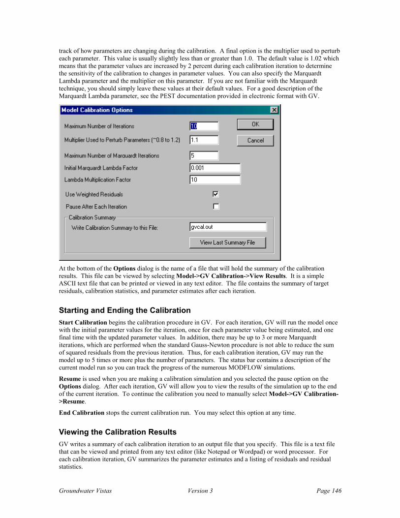
Groundwater Vistas Version 3 Page 146
track of how parameters are changing during the calibration. A final option is the multiplier used to perturb each parameter. This value is usually slightly less than or greater than 1.0. The default value is 1.02 which means that the parameter values are increased by 2 percent during each calibration iteration to determine the sensitivity of the calibration to changes in parameter values. You can also specify the Marquardt Lambda parameter and the multiplier on this parameter. If you are not familiar with the Marquardt technique, you should simply leave these values at their default values. For a good description of the Marquardt Lambda parameter, see the PEST documentation provided in electronic format with GV.
At the bottom of the Options dialog is the name of a file that will hold the summary of the calibration results. This file can be viewed by selecting Model->GV Calibration->View Results. It is a simple ASCII text file that can be printed or viewed in any text editor. The file contains the summary of target residuals, calibration statistics, and parameter estimates after each iteration.
Starting and Ending the Calibration Start Calibration begins the calibration procedure in GV. For each iteration, GV will run the model once with the initial parameter values for the iteration, once for each parameter value being estimated, and one final time with the updated parameter values. In addition, there may be up to 3 or more Marquardt iterations, which are performed when the standard Gauss-Newton procedure is not able to reduce the sum of squared residuals from the previous iteration. Thus, for each calibration iteration, GV may run the model up to 5 times or more plus the number of parameters. The status bar contains a description of the current model run so you can track the progress of the numerous MODFLOW simulations.
Resume is used when you are making a calibration simulation and you selected the pause option on the Options dialog. After each iteration, GV will allow you to view the results of the simulation up to the end of the current iteration. To continue the calibration you need to manually select Model->GV Calibration->Resume.
End Calibration stops the current calibration run. You may select this option at any time.
Viewing the Calibration Results GV writes a summary of each calibration iteration to an output file that you specify. This file is a text file that can be viewed and printed from any text editor (like Notepad or Wordpad) or word processor. For each calibration iteration, GV summarizes the parameter estimates and a listing of residuals and residual statistics.
Groundwater Vistas Version 3 Page 147
When viewing results, you should look to see if the calibration is actually improving and whether the new parameter estimates make sense. If you see that a parameter reaches its minimum or maximum value, there may be a problem with that parameter. In many cases, this indicates an insensitive parameter. You should remove this parameter from the calibration in most cases.
View Results displays the calibration output file (see Options dialog above) in the Windows Notepad application. If you are not able to view the results, it probably means that Notepad is not available on your system. You may then view the file (default: gvcal.out) in any word processor or text editor.
Update Databases should be used with caution. This command takes the parameter multipliers from the Parameters dialog and modifies the property database or the conductance values for boundary conditions. GV then resets the multipliers in the Parameters dialog to 1.0. You should only use this command if you are satisfied with the results of the calibration simulations.
Using PEST PEST is a calibration tool, developed by John Doherty of Watermark Computing, that works with all types of models that use one or more input files and produce one or more output files. PEST has been successfully used with MODFLOW and MT3D and is supported by Groundwater Vistas. PEST is a DOS application and can be run from within GV.
The current version of PEST is called PEST-ASP and is supplied at no extra charge with GV. PEST-ASP is quite sophisticated so you should be sure to read the PEST manuals before using it. All PEST manuals are supplied in electronic format with GV.
PEST works with several types of files including a control file, a template file, and an instruction file. GV creates all of these files for you, although the instruction file must be used with GV’s software called targpest.exe. Targpest reads MODFLOW binary files and reformats the output so that PEST can compute the target statistics.
Most of the data on the GV dialogs are related to the PEST control file. The remaining data define the model parameters that will be estimated by PEST. You should read the following sections so that you can relate the information on the GV dialogs to the variables described in the PEST manual. The following is not a substitute for the PEST manual.
Setting up a PEST Run There are several steps you should follow when running PEST to calibrate your model. The first is to make sure your model runs properly and that GV can calculate calibration statistics for your model. It is also advisable that you do some sensitivity analysis prior to running PEST so that you can properly select parameters to estimate. For example, attempting to estimate a non-sensitive parameter can limit the usefulness of the PEST simulation.
After you have made several successful simulations with MODFLOW, you should make a list of the parameters and boundary conditions that you want to estimate. If you are using PEST-Lite, you are limited to four parameters per simulation. Next, select Model->PEST->Basic Control Data. A dialog prompts for information describing the simulation, as discussed below.
The Basic Control Data dialog prompts for information contained in the PEST control file. You first define the number of parameters that will be estimated by PEST (NPAR) and determine whether the parameters should be grouped during estimation. If you check the latter, GV groups the parameters into the following categories:
Horizontal K Vertical K Leakance (VCONT) Horizontal Anisotropy Storage/Specific Yield Recharge
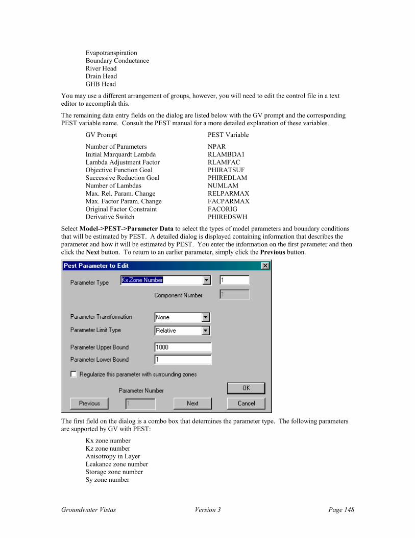
Groundwater Vistas Version 3 Page 148
Evapotranspiration Boundary Conductance River Head Drain Head GHB Head
You may use a different arrangement of groups, however, you will need to edit the control file in a text editor to accomplish this.
The remaining data entry fields on the dialog are listed below with the GV prompt and the corresponding PEST variable name. Consult the PEST manual for a more detailed explanation of these variables.
GV Prompt PEST Variable
Number of Parameters NPAR Initial Marquardt Lambda RLAMBDA1 Lambda Adjustment Factor RLAMFAC Objective Function Goal PHIRATSUF Successive Reduction Goal PHIREDLAM Number of Lambdas NUMLAM Max. Rel. Param. Change RELPARMAX Max. Factor Param. Change FACPARMAX Original Factor Constraint FACORIG Derivative Switch PHIREDSWH
Select Model->PEST->Parameter Data to select the types of model parameters and boundary conditions that will be estimated by PEST. A detailed dialog is displayed containing information that describes the parameter and how it will be estimated by PEST. You enter the information on the first parameter and then click the Next button. To return to an earlier parameter, simply click the Previous button.
The first field on the dialog is a combo box that determines the parameter type. The following parameters are supported by GV with PEST:
Kx zone number Kz zone number Anisotropy in Layer Leakance zone number Storage zone number Sy zone number
Groundwater Vistas Version 3 Page 149
Recharge zone number ET Rate zone number ET Extinction Depth zone number Well discharge for reach River conductance for reach Drain conductance for reach GHB conductance for reach Stream conductance for reach
To the right of the parameter type combo box is the zone number or reach number of the parameter. For anisotropy, this value is the layer number to estimate. The following data are also entered on this dialog for each parameter:
GV Prompt PEST Variable
Parameter Transformation PARTRANS Parameter Limit Type PARCHGLIM Parameter Upper Bound PARUBND Parameter Lower Bound PARLBND
The parameter’s initial value (PARVAL1) is taken from the GV database or boundary condition definition (i.e., the information you entered when setting up the model). The SCALE and OFFSET variables are fixed by GV at values of 1.0 and 0.0, respectively.
PEST has an option of assigning parameters to groups. If you choose to group the parameters in your simulation, you should select Model->PEST->Group Data to enter options related to each group. Consult the PEST manual for more information on groups.
Parameter group data are entered in the same manner as parameter types. You first enter the parameter group that you would like to edit. Next, a dialog is displayed where you enter the data for the specified group. These data include the following:
GV Prompt PEST Variable
Increment Type INCTYP Parameter Increment DERINC Parameter Increment Lower Bound DERINCLB Derivative Type FORCEN Derivative Increment Multiplier DERINCMUL Derivative Method DERMTHD
Select Model->PEST->Run Termination Options to edit options related to how PEST ends a simulation. PEST offers a multitude of options to use in determining when a parameter estimation run is finished. These are described in the PEST manual. The following are contained on the Run Termination Options dialog in GV:
GV Prompt PEST Variable
Maximum Optimization Iterations NOPTMAX Objective Function Criterion PHIREDSTP Maximum PHIREDSTP Iterations NPHISTP Max. Rel. Param. Change RELPARSTP Maximum RELPARSTP Iterations NRELPAR Maximum Failed Iterations NPHINORED
The Print Options dialog (Model->PEST->Print Options) contains three options for the printing of matrices. These include the covariance matrix (ICOV), the correlation coefficient matrix (ICOR), and the eigenvector matrix (IEIG).
Finally, select Model->Pest->Create Datasets to write the files required for the PEST simulation. PEST also needs the MODFLOW files from you last model run. This menu selection only creates the PEST
Groundwater Vistas Version 3 Page 150
control file, the template file(s), and the instruction file. Note also that GV will not run PEST due to the long simulation times. It is better to open a DOS window and run PEST manually.
Running PEST The easiest way to run PEST is to simply select Model->PEST->Run PEST. You can also run it from the command line. Refer to the PEST manual for the proper commands.
A good practice is to check the PEST input file for errors before trying to run PEST. PEST comes with a program called pestchek which does this for you. Simply type the following at the DOS prompt:
PESTCHEK root.pst
If there were any errors, PESTCHEK will display them on the screen. You can either correct the problem in a text editor or go back into GV to fix the error.
PEST creates an output file in DOS text format. The name of the file is root.rec where root is your root file name for MODFLOW simulations. You should print or view this file in an editor to review the results of the simulation. The PEST manual provides information on how to interpret the results of a simulation. Essentially, you should be looking for new parameter values that improve the calibration statistics in your model. If these new values appear to be reasonable, you should open your model in GV and change the parameter values in the database. In the case of boundary conditions, you would change the conductance data for the reach you were estimating.
PEST Parameters PEST works by using a template file that is a copy of the MODFLOW file containing parameters to be estimated. The parameters are replaced by a special code that tells PEST where to get the parameters. This means that the parameters to be estimated must be the ones written to the MODFLOW file (usually the BCF Package file or boundary condition files). This presents some problems that you need to be aware of.
Transmissivity of Confined Layers
The first problem is transmissivity in confined layers. GV uses hydraulic conductivity and layer thickness to compute transmissivity. When you try to estimate horizontal hydraulic conductivity with PEST, the layer thickness within a particular conductivity zone may not be constant and therefore the transmissivity will not be constant. PEST will assume, however, the parameter is constant. To overcome this problem, you must use a layer type of 3 (unconfined) instead of 0 (confined). In this manner, the hydraulic conductivity values are written to the MODFLOW BCF file.
Another way around this problem is to write the BCF information to an external file. GV will then run a preprocessor before the PEST run that will compute transmissivity and VCONT (see the next section). To turn on this option, select Model->PEST->Basic Control Data.

Groundwater Vistas Version 3 Page 151
The last option on this dialog (Write BCF Arrays as External Files) allows you to estimate K of a confined layer without having to convert from Type 0 to Type 3.
Vertical Hydraulic Conductivity
GV provides you the option of estimating vertical hydraulic conductivity; however, MODFLOW does not use this parameter. Rather, a vertical conductance term called VCONT (leakance in GV) is used by the BCF package. The VCONT term is computed from vertical hydraulic conductivity, and like transmissivity, is not a constant value when layer thickness changes.
When you try to estimate vertical hydraulic conductivity, GV places the appropriate PEST code in the VCONT array. This will only work if the leakance value is constant within the Kz zone being estimated. It is better while calibrating the model to use the Leakance parameter in GV. This approach allows PEST to estimate the leakance values directly.
One way around this problem is to use external arrays as described above for hydraulic conductivity.
Boundary Conductance
GV allows you to estimate boundary conductance within a given reach for a specific boundary type. In order to work properly with PEST, however, the conductance term must be constant within the reach being estimated. There is currently no work-around for this limitation.
Advanced PEST Features PEST-ASP has many advanced features such as pilot points, regularisation, and conversion of MODFLOW2000 data sets. These features are described later in a tutorial.
Using UCODE UCODE is a calibration tool, developed by the USGS, that works just like PEST. UCODE can utilize all types of models that use one or more input files and produce one or more output files. UCODE has been

Groundwater Vistas Version 3 Page 152
successfully used with MODFLOW and MT3D and is supported by Groundwater Vistas. UCODE is a DOS application but can be run from within GV.
UCODE works with several types of files including a universal file (*.uni), a prepare file (*.pre) that describes the parameters to be calibrated, an extract file (*.ext) that describes how to read the model output, a template file (*.tpl) that mimics the MODFLOW Package input file and shows where the various parameters go, and a function file (*.fnc) that GV uses for heterogeneous boundary condition reaches. GV creates all of these files for you, although the extract file must be used with GV’s software called targpest.exe. Targpest reads MODFLOW binary files and reformats the output so that UCODE can compute the target statistics.
Most of the data on the GV dialogs are related to the UCODE universal and prepare files. The remaining data define the model parameters that will be estimated by UCODE. You might want to read through the UCODE manual that is provided in electronic format (ucode.pdf) to compare the options on the Groundwater Vistas dialogs.
Setting up a UCODE Run There are several steps you should follow when running UCODE to calibrate your model. The first is to make sure your model runs properly and that GV can calculate calibration statistics for your model. It is also advisable that you do some sensitivity analysis prior to running UCODE so that you can properly select parameters to estimate. For example, attempting to estimate a non-sensitive parameter can limit the usefulness of the UCODE simulation.
After you have made several successful simulations with MODFLOW, you should make a list of the parameters and boundary conditions that you want to estimate. Next, select Model->UCODE->Universal Input. A dialog prompts for information describing the simulation, as discussed below.

Groundwater Vistas Version 3 Page 153
UCODE performs several types of simulations, called PHASES. Phase 1 is just a single run for testing purposes. Phase 2 or 22 is for evaluating parameter sensitivity. Phase 3 is what you really want to do – calibrate the model or perform a regression. Most of the other parameters on this dialog can be left at their default values until you have a better feel for how UCODE works. Consult the UCODE documentation (ucode.pdf) for the definitions of these parameters (see page 24 in the UCODE manual).
It is a good idea to set everything up for a UCODE run and then choose PHASE 1 just to make sure everything works. Then you can go on to PHASE 2 to make sure your parametes are sensitive. Finally, use PHASE 3 for calibration.
Select Model->UCODE->Parameters to select the types of model parameters and boundary conditions that will be estimated by UCODE. The dialog that is displayed is shown below:

Groundwater Vistas Version 3 Page 154
The dialog is for one parameter. Hit the Next and Previous buttons to go from one parameter to another. Essentially you just choose the parameter type and zone or reach number. The perturbation factor is added to 1.0 and then multiplied by the parameter value during regression to compute parameter sensitivities. With UCODE, it is always a good idea to estimate the log value of the parameter, so check this option. While you can enter reasonable upper and lower bounds for the parameters, UCODE does not enforce these bounds. Because UCODE does not enforce the parameter limits, values can become negative. If hydraulic conductivity becomes negative, MODFLOW will bomb. Estimating log parameter values eliminates this concern. Finally, click the “Estimate this parameter” check-box to have UCODE calibrate on this property or boundary condition. If you do not check the Estimate this parameter option, UCODE will not calibrate a new value for the parameter.
UCODE can use a variety of target types. Select Model->UCODE->Target Types to tell UCODE which ones you want to use.
The trickiest thing about this dialog is the use of weights. Weights in Groundwater Vistas are simply multipliers on the residuals. Thus, if a head target has a residual of 2.5 ft and the weight is 0.1, then the
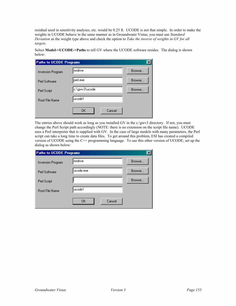
Groundwater Vistas Version 3 Page 155
residual used in sensitivity analyses, etc. would be 0.25 ft. UCODE is not that simple. In order to make the weights in UCODE behave in the same manner as in Groundwater Vistas, you must use Standard Deviation as the weight type above and check the option to Take the inverse of weights in GV for all targets.
Select Model->UCODE->Paths to tell GV where the UCODE software resides. The dialog is shown below:
The entries above should work as long as you installed GV in the c:\gwv3 directory. If not, you must change the Perl Script path accordingly (NOTE: there is no extension on the script file name). UCODE uses a Perl interpreter that is supplied with GV. In the case of large models with many parameters, the Perl script can take a long time to create data files. To get around this problem, ESI has created a compiled version of UCODE using the C++ programming language. To use this other version of UCODE, set up the dialog as shown below:
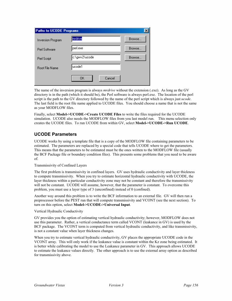
Groundwater Vistas Version 3 Page 156
The name of the inversion program is always mrdrive without the extension (.exe). As long as the GV directory is in the path (which it should be), the Perl software is always perl.exe. The location of the perl script is the path to the GV directory followed by the name of the perl script which is always just ucode. The last field is the root file name applied to UCODE files. You should choose a name that is not the same as your MODFLOW files.
Finally, select Model->UCODE->Create UCODE Files to write the files required for the UCODE simulation. UCODE also needs the MODFLOW files from you last model run. This menu selection only creates the UCODE files. To run UCODE from within GV, select Model->UCODE->Run UCODE.
UCODE Parameters UCODE works by using a template file that is a copy of the MODFLOW file containing parameters to be estimated. The parameters are replaced by a special code that tells UCODE where to get the parameters. This means that the parameters to be estimated must be the ones written to the MODFLOW file (usually the BCF Package file or boundary condition files). This presents some problems that you need to be aware of.
Transmissivity of Confined Layers
The first problem is transmissivity in confined layers. GV uses hydraulic conductivity and layer thickness to compute transmissivity. When you try to estimate horizontal hydraulic conductivity with UCODE, the layer thickness within a particular conductivity zone may not be constant and therefore the transmissivity will not be constant. UCODE will assume, however, that the parameter is constant. To overcome this problem, you must use a layer type of 3 (unconfined) instead of 0 (confined).
Another way around this problem is to write the BCF information to an external file. GV will then run a preprocessor before the PEST run that will compute transmissivity and VCONT (see the next section). To turn on this option, select Model->UCODE->Universal Input.
Vertical Hydraulic Conductivity
GV provides you the option of estimating vertical hydraulic conductivity; however, MODFLOW does not use this parameter. Rather, a vertical conductance term called VCONT (leakance in GV) is used by the BCF package. The VCONT term is computed from vertical hydraulic conductivity, and like transmissivity, is not a constant value when layer thickness changes.
When you try to estimate vertical hydraulic conductivity, GV places the appropriate UCODE code in the VCONT array. This will only work if the leakance value is constant within the Kz zone being estimated. It is better while calibrating the model to use the Leakance parameter in GV. This approach allows UCODE to estimate the leakance values directly. The other approach is to use the external array option as described for transmissivity above.

Groundwater Vistas Version 3 Page 157
UCODE Graphics UCODE creates a variety of files for producing graphical output. GV supports some of these files by selecting Plot->Calibration->UCODE. The menu contains three choices:
Parameter Summary
Scatter Plots
Sensitivity Plot
The Parameter Summary option scans through the UCODE output file (root._ot) and then plots the relative change in sum of squared residuals and parameter value for each parameter versus iteration number. An example plot is shown below. This is a handy feature to see how parameters and calibration quality changed throughout the UCODE run.
The Scatter Plots option allows you to plot a variety of graphs that are similar to the ones available in GV under Plot->Calibration->Stats. After selecting the Scatter Plots menu item, a File Open dialog is displayed showing you the types of graphs you can plot. Browse to find the correct UCODE file and then click OK. GV plots the graph, as shown below:

Groundwater Vistas Version 3 Page 158
The Sensitivity Plot creates a bar chart where the height of each bar is proportional to the composite scaled sensitivity coefficient computed by UCODE in the last run. The sensitivity coefficients are useful in identifying those parameters that are insensitive. Insensitive parameters should not be estimated during model calibration. The value of the sensitivity coefficient is not important, only the relative sensitivities of all parameters.
Calibrating with MODFLOW2000 The primary change in MODFLOW2000 over previous versions of MODFLOW is the ability to estimate parameters using nonlinear least-squares regression. It uses the same algorithm as UCODE but instead of computing parameter sensitivities using perturbation, MODFLOW2000 computes sensitivities analytically. The main advantage of MODFLOW2000 over UCODE is that it runs as one model and is therefore somewhat easier to use.
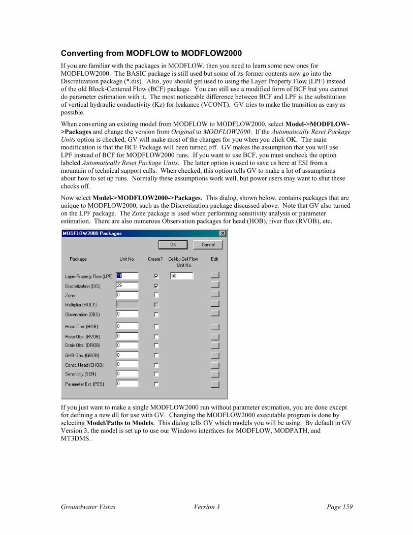
Groundwater Vistas Version 3 Page 159
Converting from MODFLOW to MODFLOW2000 If you are familiar with the packages in MODFLOW, then you need to learn some new ones for MODFLOW2000. The BASIC package is still used but some of its former contents now go into the Discretization package (*.dis). Also, you should get used to using the Layer Property Flow (LPF) instead of the old Block-Centered Flow (BCF) package. You can still use a modified form of BCF but you cannot do parameter estimation with it. The most noticeable difference between BCF and LPF is the substitution of vertical hydraulic conductivity (Kz) for leakance (VCONT). GV tries to make the transition as easy as possible.
When converting an existing model from MODFLOW to MODFLOW2000, select Model->MODFLOW->Packages and change the version from Original to MODFLOW2000. If the Automatically Reset Package Units option is checked, GV will make most of the changes for you when you click OK. The main modification is that the BCF Package will been turned off. GV makes the assumption that you will use LPF instead of BCF for MODFLOW2000 runs. If you want to use BCF, you must uncheck the option labeled Automatically Reset Package Units. The latter option is used to save us here at ESI from a mountain of technical support calls. When checked, this option tells GV to make a lot of assumptions about how to set up runs. Normally these assumptions work well, but power users may want to shut these checks off.
Now select Model->MODFLOW2000->Packages. This dialog, shown below, contains packages that are unique to MODFLOW2000, such as the Discretization package discussed above. Note that GV also turned on the LPF package. The Zone package is used when performing sensitivity analysis or parameter estimation. There are also numerous Observation packages for head (HOB), river flux (RVOB), etc.
If you just want to make a single MODFLOW2000 run without parameter estimation, you are done except for defining a new dll for use with GV. Changing the MODFLOW2000 executable program is done by selecting Model/Paths to Models. This dialog tells GV which models you will be using. By default in GV Version 3, the model is set up to use our Windows interfaces for MODFLOW, MODPATH, and MT3DMS.

Groundwater Vistas Version 3 Page 160
One thing GV does not do is change the MODFLOW executable for you. To do that, click on Browse next to the MODFLOW model. We need to change MFWIN32.dll to MF2KWIN32.dll. You can find it in the c:\gwv3 directory by default (or where ever you installed GV). Click OK when you are done. (Note: you need to change the file type from *.exe to *.dll to see these files). After changing the program, you are ready to make a single run just like the original version of MODFLOW.
When making a calibration run with MODFLOW2000, you need to turn on a few more packages by selecting Model->MODFLOW-2000->Packages. Turn on the ZONE, OBS, HOB, SEN, PES packages. These are the minimum you need for parameter estimation. If you have flux targets, you will also turn on the appropriate flux observation files. To turn on a package, enter a non-zero number in the first column and check the box in the second column, as shown below.
Next, you need to tell MODFLOW2000 which parameters to estimate. Select Model->MODFLOW2000->Parameters. The parameter definition dialog is the same as for UCODE so you can refer to the previous section.
You will note that there is a place on this dialog for the minimum and maximum parameter values. Unfortunately, MODFLOW2000 and UCODE do not enforce these bounds so you don’t really need to enter them. You can just leave them zero and click OK. If there were more parameters to estimate, you would click the Next button to go to the next parameter.

Groundwater Vistas Version 3 Page 161
To view the simulation results, select Model->MODFLOW->Packages and click the button in the top right corner next to the words {Edit Output}. This launches a text editor to view the MODFLOW2000 output files. The results of the calibration are in both of the output files root.lst and root.glo. The latter is easier to find the results, as shown below.
There is no automatic way in the current version of GV to automatically update the databases after this run. To change a K value, for example, you would simply select Props->Hydraulic Conductivity and then select Props->Property Values->Database and enter the new value in the database for Kx and Ky.
Calibration Tutorial The following tutorial focuses on Groundwater Vistas’ tools for model calibration and uses a synthetic model developed to illustrate the following concepts:
Automatic Sensitivity Analysis in Groundwater Vistas
Inverse modeling with Groundwater Vistas, MODFLOW2000, UCODE, and PEST
Run Groundwater Vistas Version 3 and open the file CalEx1.gwv. This model should be in the c:\gwv3\tutorial directory. Your screen should look like the following:
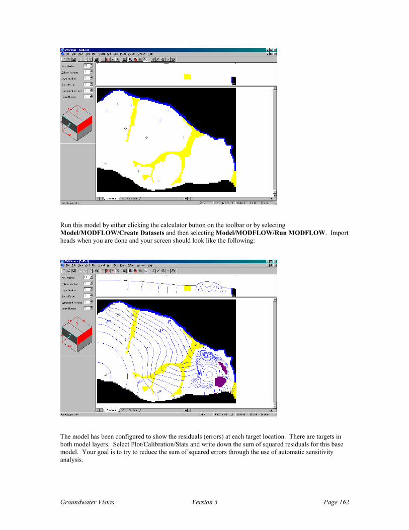
Groundwater Vistas Version 3 Page 162
Run this model by either clicking the calculator button on the toolbar or by selecting Model/MODFLOW/Create Datasets and then selecting Model/MODFLOW/Run MODFLOW. Import heads when you are done and your screen should look like the following:
The model has been configured to show the residuals (errors) at each target location. There are targets in both model layers. Select Plot/Calibration/Stats and write down the sum of squared residuals for this base model. Your goal is to try to reduce the sum of squared errors through the use of automatic sensitivity analysis.
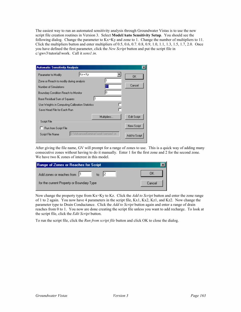
Groundwater Vistas Version 3 Page 163
The easiest way to run an automated sensitivity analysis through Groundwater Vistas is to use the new script file creation routines in Version 3. Select Model/Auto Sensitivity Setup. You should see the following dialog. Change the parameter to Kx=Ky and zone to 1. Change the number of multipliers to 11. Click the multipliers button and enter multipliers of 0.5, 0.6, 0.7. 0.8, 0.9, 1.0, 1.1, 1.3, 1.5, 1.7, 2.0. Once you have defined the first parameter, click the New Script button and put the script file in c:\gwv3\tutorial\work. Call it sens1.in.
After giving the file name, GV will prompt for a range of zones to use. This is a quick way of adding many consecutive zones without having to do it manually. Enter 1 for the first zone and 2 for the second zone. We have two K zones of interest in this model.
Now change the property type from Kx=Ky to Kz. Click the Add to Script button and enter the zone range of 1 to 2 again. You now have 4 parameters in the script file, Kx1, Kx2, Kz1, and Kz2. Now change the parameter type to Drain Conductance. Click the Add to Script button again and enter a range of drain reaches from 0 to 1. You now are done creating the script file unless you want to add recharge. To look at the script file, click the Edit Script button.
To run the script file, click the Run from script file button and click OK to close the dialog.

Groundwater Vistas Version 3 Page 164
Now, start the sensitivity analysis by selecting Model/Run Auto Sensitivity. The model will run 66 times, which should not be too long since this is a relatively simple model.
When the model is done running, you will be asked if you want to create a plot. Select Yes, and then just click OK on the next dialog that prompts for the file name. GV automatically creates a file called autosens.out when running the script file. Next click OK on the dialog asking which statistic to plot. Although you may choose from a variety of statistics, the sum of squared errors is the best one to use. Your first plot should look like the following:
This curve shows that reducing Kx1 by a factor of 0.5 would substantially reduce the sum of squared errors and therefore improve the quality of the calibration. Make that change now by selecting Props/Property Values/Database. After making the change, run the model one time to confirm the results and make another pass through the automatic sensitivity analysis. Do this a few times and see how much you can improve the calibration.
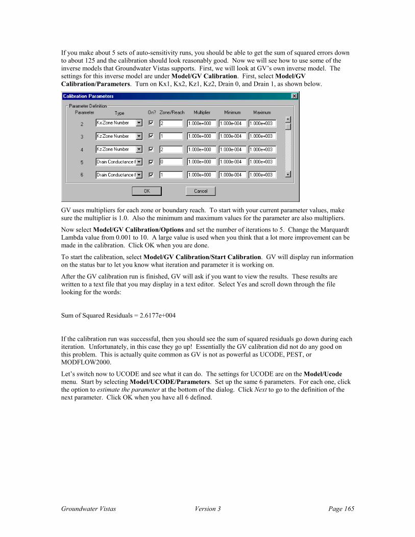
Groundwater Vistas Version 3 Page 165
If you make about 5 sets of auto-sensitivity runs, you should be able to get the sum of squared errors down to about 125 and the calibration should look reasonably good. Now we will see how to use some of the inverse models that Groundwater Vistas supports. First, we will look at GV’s own inverse model. The settings for this inverse model are under Model/GV Calibration. First, select Model/GV Calibration/Parameters. Turn on Kx1, Kx2, Kz1, Kz2, Drain 0, and Drain 1, as shown below.
GV uses multipliers for each zone or boundary reach. To start with your current parameter values, make sure the multiplier is 1.0. Also the minimum and maximum values for the parameter are also multipliers.
Now select Model/GV Calibration/Options and set the number of iterations to 5. Change the Marquardt Lambda value from 0.001 to 10. A large value is used when you think that a lot more improvement can be made in the calibration. Click OK when you are done.
To start the calibration, select Model/GV Calibration/Start Calibration. GV will display run information on the status bar to let you know what iteration and parameter it is working on.
After the GV calibration run is finished, GV will ask if you want to view the results. These results are written to a text file that you may display in a text editor. Select Yes and scroll down through the file looking for the words:
Sum of Squared Residuals = 2.6177e+004
If the calibration run was successful, then you should see the sum of squared residuals go down during each iteration. Unfortunately, in this case they go up! Essentially the GV calibration did not do any good on this problem. This is actually quite common as GV is not as powerful as UCODE, PEST, or MODFLOW2000.
Let’s switch now to UCODE and see what it can do. The settings for UCODE are on the Model/Ucode menu. Start by selecting Model/UCODE/Parameters. Set up the same 6 parameters. For each one, click the option to estimate the parameter at the bottom of the dialog. Click Next to go to the definition of the next parameter. Click OK when you have all 6 defined.
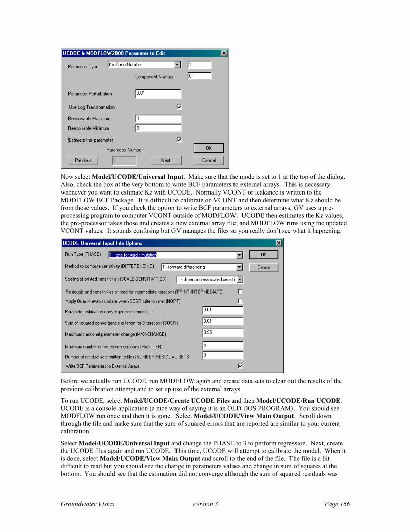
Groundwater Vistas Version 3 Page 166
Now select Model/UCODE/Universal Input. Make sure that the mode is set to 1 at the top of the dialog. Also, check the box at the very bottom to write BCF parameters to external arrays. This is necessary whenever you want to estimate Kz with UCODE. Normally VCONT or leakance is written to the MODFLOW BCF Package. It is difficult to calibrate on VCONT and then determine what Kz should be from those values. If you check the option to write BCF parameters to external arrays, GV uses a pre-processing program to computer VCONT outside of MODFLOW. UCODE then estimates the Kz values, the pre-processor takes those and creates a new external array file, and MODFLOW runs using the updated VCONT values. It sounds confusing but GV manages the files so you really don’t see what it happening.
Before we actually run UCODE, run MODFLOW again and create data sets to clear out the results of the previous calibration attempt and to set up use of the external arrays.
To run UCODE, select Model/UCODE/Create UCODE Files and then Model/UCODE/Run UCODE. UCODE is a console application (a nice way of saying it is an OLD DOS PROGRAM). You should see MODFLOW run once and then it is gone. Select Model/UCODE/View Main Output. Scroll down through the file and make sure that the sum of squared errors that are reported are similar to your current calibration.
Select Model/UCODE/Universal Input and change the PHASE to 3 to perform regression. Next, create the UCODE files again and run UCODE. This time, UCODE will attempt to calibrate the model. When it is done, select Model/UCODE/View Main Output and scroll to the end of the file. The file is a bit difficult to read but you should see the change in parameters values and change in sum of squares at the bottom. You should see that the estimation did not converge although the sum of squared residuals was

Groundwater Vistas Version 3 Page 167
decreasing. Select Model/UCODE/Universal Input and increase the number of parameter estimation iterations from 5 to 10 and try again. If this model took a long time to run, it would probably be good to update parameter values and then run again. You could do it either way in this case since the model runs quickly.
After running UCODE again, you should see something like the following at the end of the main UCODE output file:
PARAMETER VALUES AND STATISTICS FOR ALL ITERATIONS
PARAMETER NAMES
Kx1 Kx2 Lk1 Lk2
Dr0 Dr1
INITIAL PARAMETER VALUES
1.75 0.200 0.500 0.250E-02
0.133E+04 30.9
LEAST SQUARES
OBJ OBJ FNC
FUNC W/PRIOR MAX-CHG PARAM MARQRDT
.12E+03 .12E+03 -.95 Lk1 0.00
iteration # 1
1.73 0.200 0.250E-01 0.233E-02
0.141E+04 32.6
.10E+03 .10E+03 -.95 Lk1 0.00
iteration # 2
1.71 0.200 0.125E-02 0.287E-02
0.116E+04 39.3
95. 95. 0.95 Lk2 0.00
iteration # 3
1.69 0.200 0.128E-02 0.559E-02
688. 47.6
76. 76. 0.95 Lk2 0.00
iteration # 4
1.67 0.200 0.131E-02 0.109E-01
456. 59.5
67. 67. 0.95 Lk2 0.00
iteration # 5
1.66 0.200 0.153E-02 0.213E-01
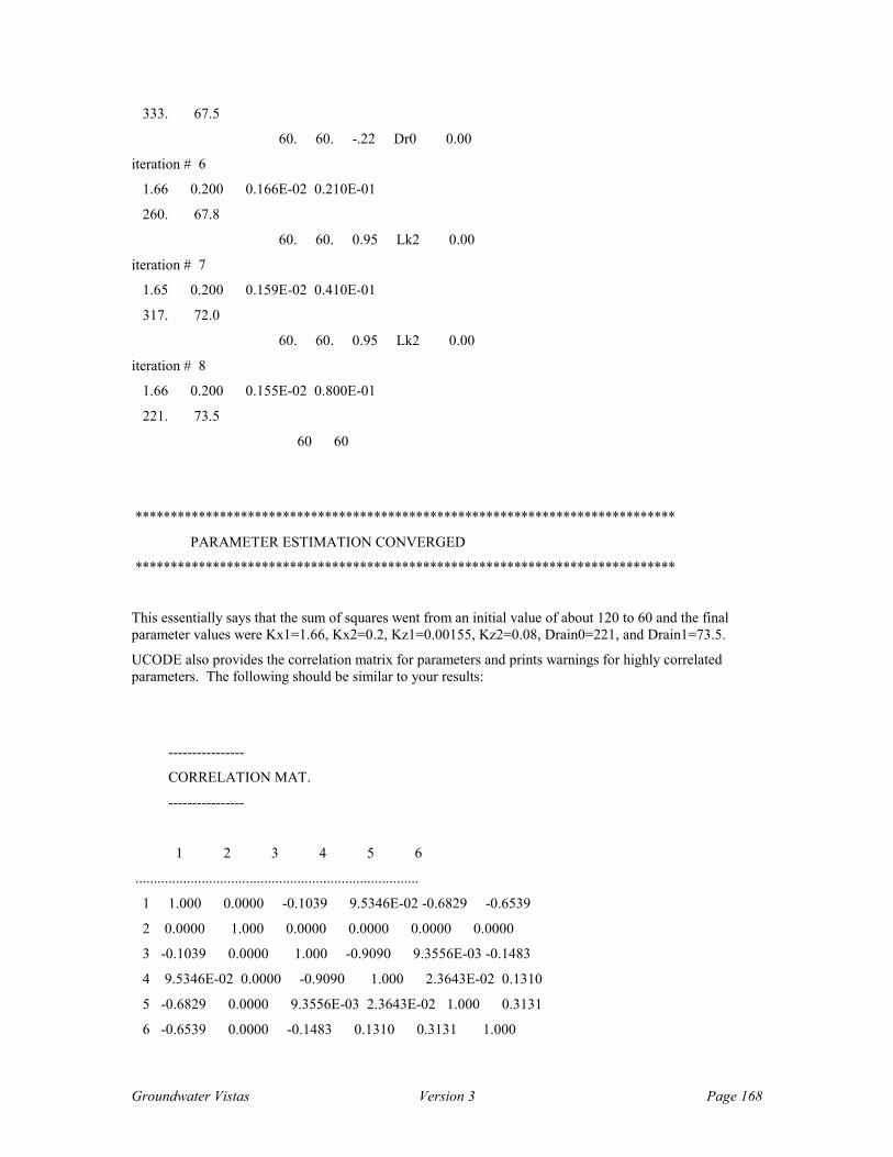
Groundwater Vistas Version 3 Page 168
333. 67.5
60. 60. -.22 Dr0 0.00
iteration # 6
1.66 0.200 0.166E-02 0.210E-01
260. 67.8
60. 60. 0.95 Lk2 0.00
iteration # 7
1.65 0.200 0.159E-02 0.410E-01
317. 72.0
60. 60. 0.95 Lk2 0.00
iteration # 8
1.66 0.200 0.155E-02 0.800E-01
221. 73.5
60 60
*****************************************************************************
PARAMETER ESTIMATION CONVERGED
*****************************************************************************
This essentially says that the sum of squares went from an initial value of about 120 to 60 and the final parameter values were Kx1=1.66, Kx2=0.2, Kz1=0.00155, Kz2=0.08, Drain0=221, and Drain1=73.5.
UCODE also provides the correlation matrix for parameters and prints warnings for highly correlated parameters. The following should be similar to your results:
----------------
CORRELATION MAT.
----------------
1 2 3 4 5 6
.............................................................................
1 1.000 0.0000 -0.1039 9.5346E-02 -0.6829 -0.6539
2 0.0000 1.000 0.0000 0.0000 0.0000 0.0000
3 -0.1039 0.0000 1.000 -0.9090 9.3556E-03 -0.1483
4 9.5346E-02 0.0000 -0.9090 1.000 2.3643E-02 0.1310
5 -0.6829 0.0000 9.3556E-03 2.3643E-02 1.000 0.3131
6 -0.6539 0.0000 -0.1483 0.1310 0.3131 1.000

Groundwater Vistas Version 3 Page 169
THE CORRELATION OF THE FOLLOWING PARAMETER PAIRS >= .95
PARAMETER # ID # ID CORRELATION
THE CORRELATION OF THE FOLLOWING PARAMETER PAIRS IS BETWEEN .90 AND .95
PARAMETER # ID # ID CORRELATION
3 Lk1 4 Lk2 -0.91
THE CORRELATION OF THE FOLLOWING PARAMETER PAIRS IS BETWEEN .85 AND .90
PARAMETER # ID # ID CORRELATION
This says that the two vertical hydraulic conductivity zones are correlated. Normally when this happens, you should only try to estimate one of the parameters.
Another useful thing that UCODE does is compute a composite scaled sensitivity coefficient so you can see which parameters are sensitive. For this simulation, the sensitivity coefficients are:
COMPOSITE SCALED SENSITIVITIES
((SUM OF THE SQUARED VALUES)/ND)**.5
PARAMETER #: 1 2 3 4 5 6
PARAMETER ID: Kx1 Kx2 Lk1 Lk2 Dr0 Dr1
6.24 0.000 15.2 0.112 1.34 1.80
This information says that Kx2 and Kz2 (labeled as Lk2) are much lower than the other parameters. Normally when this happens, the estimation may not have worked as well as it might have. Since the two vertical K zones are correlated and the second one is not sensitive, it would be good to not estimate Kz2. Try a run with UCODE turning off estimation of Kx2 and Kz2 parameters. Select Model/UCODE/Parameters and scroll through the list until you come to these two and simply uncheck the box at the bottom of the dialog that says estimate. Then rewrite the UCODE files and rerun UCODE.
You will probably see that this really did not improve things very much. Let’s move on to MODFLOW2000 and see what it can do. There are several steps involved in moving to MODFLOW2000. First, select Model/MODFLOW/Packages. Change the version of MODFLOW at the top of the dialog from Original (88/96) to MODFLOW2000. Click OK when done. Now get back into the same dialog. You should see that GV has automatically turned off the BCF Package. Select Model/MODFLOW2000/Packages. You should see here that the discretization, zone, and LPF packages are turned on, as shown below:

Groundwater Vistas Version 3 Page 170
This run is now roughly equivalent to the original MODFLOW run we had been working on. We could make it virtually identical by keeping the BCF package but then we could not use parameter estimation.
The one remaining thing to change is the model program. Select Model/Paths to Models. Click the browse button next to MODFLOW and find the file MF2KWIN32.dll which should be in c:\gwv3. Click OK when you are done.
Now run the model in the usual way and import results. Make sure you are getting about the same value for sum of squared residuals when selecting Plot/Calibration/Stats.
To turn on the parameter estimation process in MODFLOW2000, select Model/MODFLOW2000/Packages. You need to enter non-zero numbers in the first column next to the OBS, HOB, SEN, and PES packages. A short-cut is to simply enter a non-zero number next to the PES package and check the box to create the file. Then click OK. GV will fix the other ones. Go back to this dialog to confirm that it was done as shown below:
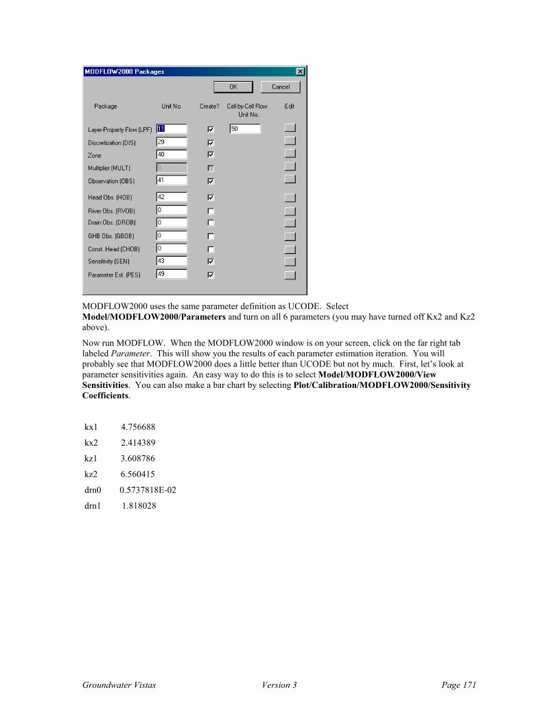
Groundwater Vistas Version 3 Page 171
MODFLOW2000 uses the same parameter definition as UCODE. Select Model/MODFLOW2000/Parameters and turn on all 6 parameters (you may have turned off Kx2 and Kz2 above).
Now run MODFLOW. When the MODFLOW2000 window is on your screen, click on the far right tab labeled Parameter. This will show you the results of each parameter estimation iteration. You will probably see that MODFLOW2000 does a little better than UCODE but not by much. First, let’s look at parameter sensitivities again. An easy way to do this is to select Model/MODFLOW2000/View Sensitivities. You can also make a bar chart by selecting Plot/Calibration/MODFLOW2000/Sensitivity Coefficients.
kx1 4.756688
kx2 2.414389
kz1 3.608786
kz2 6.560415
drn0 0.5737818E-02
drn1 1.818028

Groundwater Vistas Version 3 Page 172
Note that the sensitivity coefficients computed by MODFLOW2000 are much different from UCODE. MODFLOW2000 indicates that Drain reach 0 has almost no sensitivity. Turn off drain reach 0 and rerun MODFLOW2000 to see what happens.
Now you should see dramatically better results with MODFLOW2000 dropping the sum of squared residuals below a value of 1.0. To see how parameter and sum of squares changed during the run, select Plot/Calibration/MODFLOW2000/Parameters Changes:
You can also see the numerical values by selecting Model/MODFLOW2000/View Estimated Parameters.
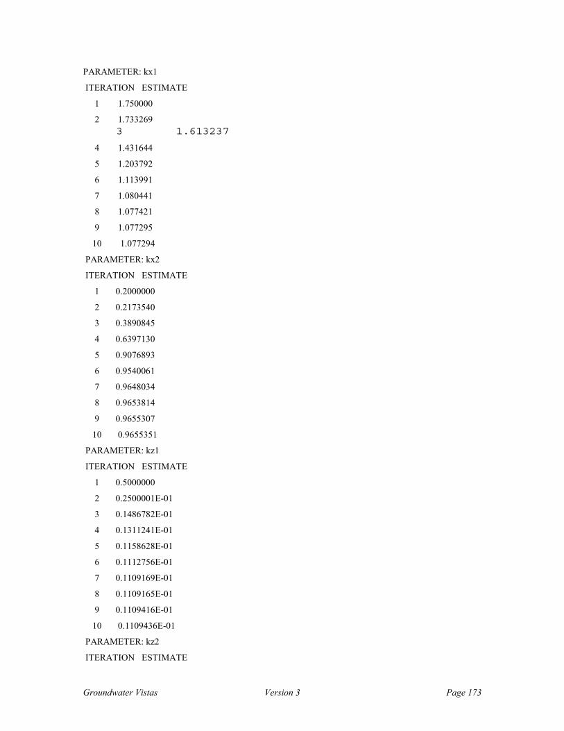
Groundwater Vistas Version 3 Page 173
PARAMETER: kx1
ITERATION ESTIMATE
1 1.750000
2 1.733269 3 1.613237
4 1.431644
5 1.203792
6 1.113991
7 1.080441
8 1.077421
9 1.077295
10 1.077294
PARAMETER: kx2
ITERATION ESTIMATE
1 0.2000000
2 0.2173540
3 0.3890845
4 0.6397130
5 0.9076893
6 0.9540061
7 0.9648034
8 0.9653814
9 0.9655307
10 0.9655351
PARAMETER: kz1
ITERATION ESTIMATE
1 0.5000000
2 0.2500001E-01
3 0.1486782E-01
4 0.1311241E-01
5 0.1158628E-01
6 0.1112756E-01
7 0.1109169E-01
8 0.1109165E-01
9 0.1109416E-01
10 0.1109436E-01
PARAMETER: kz2
ITERATION ESTIMATE

Groundwater Vistas Version 3 Page 174
1 0.2500000E-02
2 0.2744052E-02
3 0.5350901E-02
4 0.1043426E-01
5 0.2034681E-01
6 0.2748325E-01
7 0.3153307E-01
8 0.3229839E-01
9 0.3230623E-01
10 0.3230164E-01
PARAMETER: drn1
ITERATION ESTIMATE
1 30.85000
2 31.47860
3 36.80551
4 50.62363
5 98.13686
6 191.3668
7 373.1654
8 503.6739
9 524.0244
10 524.4166
In this example, MODFLOW2000 was the best inverse model but it does not always work out that way. That is why Groundwater Vistas supports such a wide variety of inverse models. If one does not work for your calibration, simply try another.
The next example is a real model that you should try to calibrate using the techniques described during the first session.
Groundwater Vistas Version 3 Page 175
Optimization Models One of the new changes in Groundwater Vistas Version 3 is the addition of optimization models. Optimization is a technique for minimizing or maximizing groundwater pumping under a series of constraints. For example, you might want to contain a contaminant plume while pumping as little water as possible. Another example for water supply would be to maximize the volume of water extracted while minimizing the impact on surrounding wetlands. There are a lot of optimization models available now and GV supports several of them. These models include:
Brute Force – a model developed by ESI to optimize pump & treat systems. The model uses MODFLOW and MODPATH in a new particle-tracking technique to minimize the pumping while containing a contaminant plume. Brute Force is provided with GV.
MODOFC – a model developed by David Ahlfeld and Guy Reifler (http://www.ecs.umass.edu/modofc/) that incorporates optimization technology right into MODFLOW. MODOFC is self-contained, requiring no other software to run. While not as sophisticated as some other optimizing models, it is very easy to use. MODOFC is provided with GV or can be downloaded from the author’s web page shown above.
SOMOS (formerly known as Remax) – a model developed by Richard Peralta at Utah State University. SOMOS is one of the most sophisticated optimizing models available. SOMOS is not included with GV but can be purchased separately.
This chapter is not designed to serve as a text on optimization. Rather, we are just going to show how to use these models with GV. We recommend the book Optimal Management of Groundwater Systems by David Ahlfeld and Ann Mulligan for more information on the subject.
Using Brute Force The BruteForce optimization technique is a new way of optimizing pump & treat systems. Unlike more classical techniques (e.g. SOMOS, MODOFC, or MODMAN), BruteForce uses particle tracking to determine whether a system is successful. Other optimizing software uses head, drawdown, or gradient constraints to design the system. The problem with these more classical techniques is that defining the gradient constraints is difficult and often the resulting system is poorly designed. The benefit of using particle tracking is that it is intuitive - the particles are either captured or they are not. The BruteForce routine continues until all particles are captured in the plume area. This makes interpreting the results very straightforward. The disadvantage of BruteForce is that it requires more simulations than many of the other optimizers.
BruteForce operates in two modes. In Mode 1, the user enters all possible well locations for the pump & treat system. BruteForce then selects the best wells from this list in constructing the pump & treat system. Only pumping wells may be used in Mode 1.
In Mode 2, the user enters a pattern of wells that serves as a template for designing the system. Normally, Mode 2 is used when a configuration of pumping and injecting wells is desired (e.g., a five-spot pattern). The user also defines which cells in the model are legitimate locations for adding the pattern of wells. BruteForce then operates as in Mode 1 but adds wells in the same pattern as defined by the user and in the best location within the pump & treat zone.
Groundwater Vistas serves as the pre-processor for BruteForce. You simply set up the model with particles and potential well locations. You then set a number of BruteForce options, generate the BruteForce data files, and run BruteForce. In the current release, BruteForce is implemented in a DOS C program that is external to Groundwater Vistas. The program is called brute.exe. MODFLOW and MODPATH are run from the BruteForce program. These are also DOS executables called brutemod.exe and mpbrute.exe. In future releases, the BruteForce procedure will be incorporated in Groundwater Vistas.

Groundwater Vistas Version 3 Page 176
The Brute Force Procedure Step 1. Set up the model in Groundwater Vistas by placing particles in the area that must be captured. Remember, BruteForce optimization continues until a given percentage of particles have been captured (the default is 100 percent capture). Capture is achieved when particles terminate at a well in the pump & treat system or at another legitimate boundary cell defined by you. Capture is also time dependent. Each particle has a maximum travel time defined within GV. Therefore, the particles are only captured if they terminate at a legitimate capture cell and within a specified period of time.
To facilitate the placement of particles within a contaminant plume, GV has been modified for digitizing a polygon of particles. Any model cell within the digitized polygon will have a particle placed at the cell center. To digitize a polygon of particles, select Add/Particles/Digitize.
A typical particle dialog is shown below for a single particle:
The last two fields have been added for BruteForce. The weight is used when determining the ranking for each potential well. BruteForce makes one simulation for each potential well (or pattern location in Mode 2) and sums up the number of particles captured by each well. The particle weight is the value summed when that particle is captured. For example, if a particle has a weight of 10, then the value 10 is added to the cumulative particle count when that particle is captured by a potential well. The maximum travel time is used to determine particle capture. Even if a particle is captured by a potential well, BruteForce will not acknowledge the capture unless the travel time is less than the maximum travel time for that particle.
Another particle feature has been added for use with Brute Force Version 2.1. You may define particles using property zone numbers. The Interbed Storage package is used for particles, because compaction is seldom simulated by most users. You should define different zones based on travel time or weight of the particles. The first column in the Interbed Storage database is the particle weight and the second column is the particle travel time. One particle is placed at the center of the cell when running Brute Force. Select Model/Brute Force/Particle Options to turn this option on. The following dialog will appear.

Groundwater Vistas Version 3 Page 177
Compaction zones refers to the Interbed Storage property. You then give a sequence of zones to use for particle starting locations. Note that in Brute Force Version 2.1, particles can be excluded from capture using negative weights. The size of particles in Brute Force Output maps refers to map files created at each iteration to show the particles captured by the pumping system. The size is in model units of length (e.g. feet). These output maps are described later in this documentation.
You must also define the location of every possible pumping well location for the capture system (Mode 1) or a pattern of wells for the system (Mode 2). You must use Boundary Condition wells (BCs menu in GV) and you must give them a unique (or series of unique) reach numbers. Some new fields have been added to the dialog for Boundary wells, as shown below:
The new fields are enclosed in the box entitled Optimization for Managed Pumping. The unit stimulus is the starting pumping rate for the well and is used by BruteForce during the well ranking phase. BruteForce does not use the well radius. The upper and lower bounds are the maximum and minimum pumping rates that BruteForce can use for that well. BruteForce checks the maximum drawdown during the polishing phase of the simulations. If the maximum drawdown is exceeded, BruteForce will reduce the pumping rate for that well. The weight is used in a similar manner to the weight for particles. After determining the number of particles (more properly the sum of particle weights for all particles captured by the well) captured by the well, BruteForce multiplies by the well weight to determine final ranking among potential wells.
There are several options that control the BruteForce simulation. These are entered by selecting Model/BruteForce/Options. The BF options dialog is shown below:
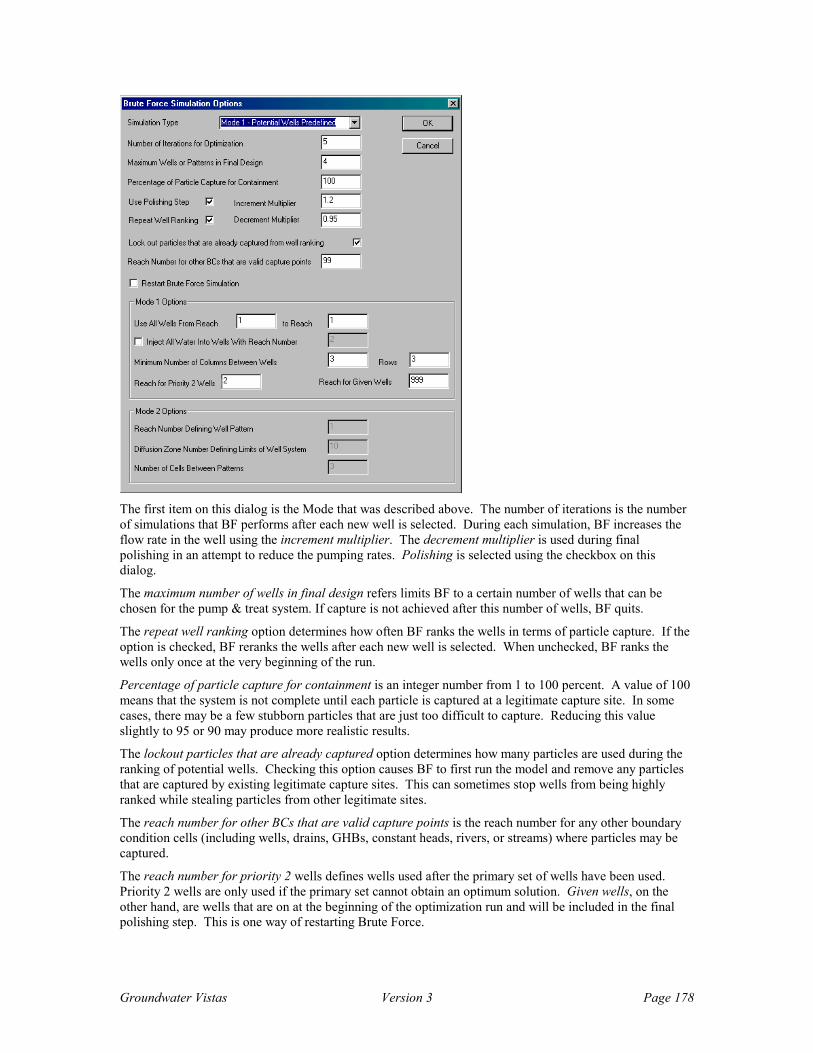
Groundwater Vistas Version 3 Page 178
The first item on this dialog is the Mode that was described above. The number of iterations is the number of simulations that BF performs after each new well is selected. During each simulation, BF increases the flow rate in the well using the increment multiplier. The decrement multiplier is used during final polishing in an attempt to reduce the pumping rates. Polishing is selected using the checkbox on this dialog.
The maximum number of wells in final design refers limits BF to a certain number of wells that can be chosen for the pump & treat system. If capture is not achieved after this number of wells, BF quits.
The repeat well ranking option determines how often BF ranks the wells in terms of particle capture. If the option is checked, BF reranks the wells after each new well is selected. When unchecked, BF ranks the wells only once at the very beginning of the run.
Percentage of particle capture for containment is an integer number from 1 to 100 percent. A value of 100 means that the system is not complete until each particle is captured at a legitimate capture site. In some cases, there may be a few stubborn particles that are just too difficult to capture. Reducing this value slightly to 95 or 90 may produce more realistic results.
The lockout particles that are already captured option determines how many particles are used during the ranking of potential wells. Checking this option causes BF to first run the model and remove any particles that are captured by existing legitimate capture sites. This can sometimes stop wells from being highly ranked while stealing particles from other legitimate sites.
The reach number for other BCs that are valid capture points is the reach number for any other boundary condition cells (including wells, drains, GHBs, constant heads, rivers, or streams) where particles may be captured.
The reach number for priority 2 wells defines wells used after the primary set of wells have been used. Priority 2 wells are only used if the primary set cannot obtain an optimum solution. Given wells, on the other hand, are wells that are on at the beginning of the optimization run and will be included in the final polishing step. This is one way of restarting Brute Force.
Groundwater Vistas Version 3 Page 179
Another way of restarting Brute Force from a previous run is to simply check the restart option on the dialog shown above. Make sure to increase the maximum allowable number of wells in the optimum design. A restart file (bf.rst) is always written at the end of a Brute Force simulation.
Mode 1 options are only available for editing when Mode 1 is selected at the top of the dialog. Potential pumping wells are chosen by a range of reach numbers entered in this area of the dialog. There is also an option to have all pumped water reinjected. If the latter is checked, you also enter a reach number for a set of existing well(s) where the water will be injected. BF takes the total amount pumped from the system and divides it evenly between all wells in the injection reach. The minimum number of columns or rows between wells determines how close wells can be. After selecting a well for the system, BF will invalidate any other well that lies within this many rows and columns of the chosen well.
Mode 2 options include the reach number of the well pattern. You only set a representative pattern of pumping and injection wells. You should also place this pattern of wells in the first spot you want BF to check. The number of cells between patterns defines a buffer zone around each chosen pattern location. The diffusion zone number defining limits of well system defines where potential well patterns can exist. Select Props/Diffusion and then set zone 10 (default – you may change it on this dialog) for the areas where you want to design the pump & treat system. Each chosen well pattern must fit totally within this area.
The final task in GV is to produce the BF input file. Select Model/Brute Force/Create Input Files. GV will then create a file called brutefrc.dat. BruteForce (brute.exe) requires that a file called brutefrc.dat be placed in the working directory. This file contains all options for the simulation, including all potential well locations and valid particle capture locations. The format of the input file is documented within the brutefrc.dat file using comment lines that begin with the “#” character. All data entered into the brutefrc.dat file are assumed to be in FORTRAN list-directed or free format. That is, each number must be separated by a space, comma, or tab.
Step 2. Run MODFLOW and MODPATH for the base case without any pumping from the potential remediation well locations. Right now, BF only works for steady-state models so be sure to use MODPATH Version 2 (mpath.exe). Also, do NOT save cell-by-cell flow terms for the Well Package. This step makes sure that the model is working and all the necessary files have been created.
Step 3. Open a DOS Window and change to the working directory. Make sure all the BruteForce program files are in the working directory. These include the following:
Brute.exe The BruteForce program
Brutemod.exe Version of MODFLOW that works with BF
Mpbrute.exe Version of MODPATH that works with BF
Step 4. Run Brute.exe. Just type brute at the DOS prompt and hit the enter key. As MODFLOW runs it displays a message near the top of the screen to show you what simulation it is working on. BF makes one run for each potential well location; this is called Stage 1. After selecting the well that captures the most particles, BF then starts to increment the pumping rate in order to maximize capture; this is called Stage 2. This process is repeated for each new well added to the capture system up to the maximum number of wells specified by the user or until the desired degree of particle capture is attained.
Step 5. Review the Results. BF creates a file called brutefrc.out that contains a summary of the optimization process. This is an ASCII file that can be viewed in a text editor or word processor and printed.

Groundwater Vistas Version 3 Page 180
Evaluating Brute Force Results Brute Force creates several output files. The main output file is called brutefrc.out. You may view this file by selecting Model->Brute Force->View Output File. There is also a file called BruteSummary.out which contains the number of wells selected and their pumping rates for each iteration. You may view this file by selecting Model->Brute Force->View Summary File.
Assuming that you like the results of the Brute Force run, you may import a MODFLOW well file with the optimized wells and rates. This file is called Brute.wel. You must first, though, delete all wells from the reaches that you optimized. You can do this by selecting BCs->Well and then BCs->Delete->Reach. You need to do this because GV will not import the brute wells over top of existing wells.
There are also several other files you should look at:
Particle Capture Maps – After each new well is selected, a file will be created that can be imported into GWV showing in green the particles that have been captured within the specified constraints and in red those particles still requiring capture. These files are written for each layer and are named as follows:
Iteration#_layer#.map
Where # is the iteration and number of wells. These maps can be displayed in Groundwater Vistas using File/Map/GW Vistas. A green “#” means that the particle was captured. A red “O” means the particle was not captured.
Water-level Elevations and Drawdowns – Similar to particle capture, after each new well is selected, files are created that can be imported into GWV to show the cumulative effects of each new well on the groundwater flow regime. These files are called Iteration#.hds and Iteration#.ddn where # is the number of wells.
Simple Plot File – data concerning the cumulative pumping rate and number of particles captured for each well added are recorded and used to produce plots of number of wells verses particles captured, number of wells verses cumulative pumping rate, and cumulative pumping rate verses particles captured. It is assumed these plots would actually be done in another program like Excel or Lotus. This files is called BFSummary.plt.
Using MODOFC MODOFC works very differently from Brute Force and is also more general than Brute Force. MODOFC can be used to optimize containment but can also be used to optimize pumping systems for dewatering and water supply. We are not going to try to describe MODOFC in detail here. For more information on MODOFC, you should look at the documentation (modofc.pdf) supplied with GV.
There are several steps to follow when using MODOFC. The first is to get your model running properly without simulating the wells you are trying to optimize. Once the model is running and the heads look reasonable, you need to turn off all binary output. MODOFC does not like use of the output control file. Select Model->MODFLOW->Packages and enter a zero in the first column next to Output Control and remove the checkmark in the second column. Next, make sure that all numbers in the third column on this dialog under the heading Cell-by-cell Unit No. are set to zero.
Constraints The second step is to define a set of constraints for the optimization problem. Constraints include the following:
• Maximum head
• Minimum head
• Head difference in X, Y, or Z directions
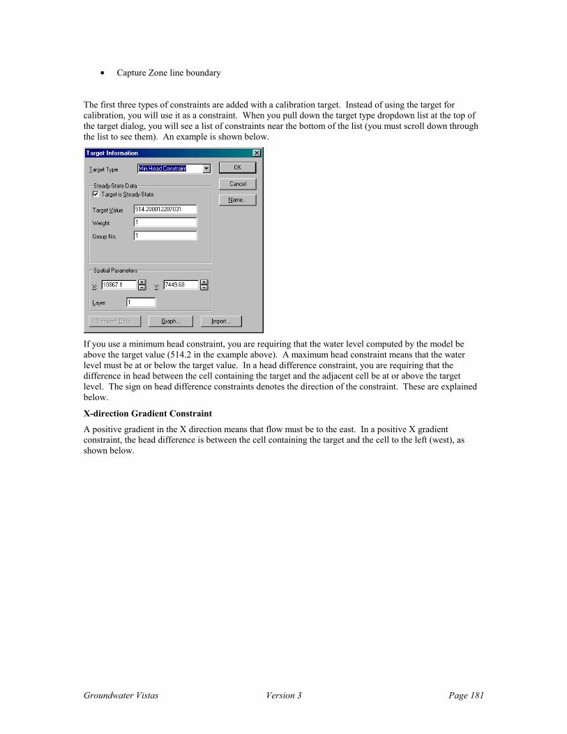
Groundwater Vistas Version 3 Page 181
• Capture Zone line boundary
The first three types of constraints are added with a calibration target. Instead of using the target for calibration, you will use it as a constraint. When you pull down the target type dropdown list at the top of the target dialog, you will see a list of constraints near the bottom of the list (you must scroll down through the list to see them). An example is shown below.
If you use a minimum head constraint, you are requiring that the water level computed by the model be above the target value (514.2 in the example above). A maximum head constraint means that the water level must be at or below the target value. In a head difference constraint, you are requiring that the difference in head between the cell containing the target and the adjacent cell be at or above the target level. The sign on head difference constraints denotes the direction of the constraint. These are explained below.
X-direction Gradient Constraint
A positive gradient in the X direction means that flow must be to the east. In a positive X gradient constraint, the head difference is between the cell containing the target and the cell to the left (west), as shown below.

Groundwater Vistas Version 3 Page 182
Y-direction Gradient Constraint
A positive gradient in the Y direction means that flow must be to the north. In a positive Y gradient constraint, the head difference is between the cell containing the target and the cell to the south, as shown below.
Z-direction Gradient Constraint
A positive gradient in the Z direction means that flow must be upward. In a positive Z direction constraint, the head difference is computed between the cell containing the target and the layer below. In the figure below, the three cells are layers (i.e., a cross-sectional view).

Groundwater Vistas Version 3 Page 183
Capture Zone Constraint
MODOFC has a unique feature for defining a capture zone. You may define a series of lines outlining the area to be contained. You assign a head difference constraint to these lines and MODOFC turns them into lateral gradient constraints when it runs. This makes setting up head difference constraints easier for pump & treat systems. In Groundwater Vistas, you use a line boundary (Add->Line Boundary). Instead of being a boundary, however, you select the type as Capture Zone Constraint, as shown on the example below.
The only data you need to fill in the line boundary dialog is the Head or Flow rate per unit length which in this case is actually a head difference. In the example above the head difference is 0.01 ft. You also must enter a capture zone number and a sequence number. If there are several line segments outlining your
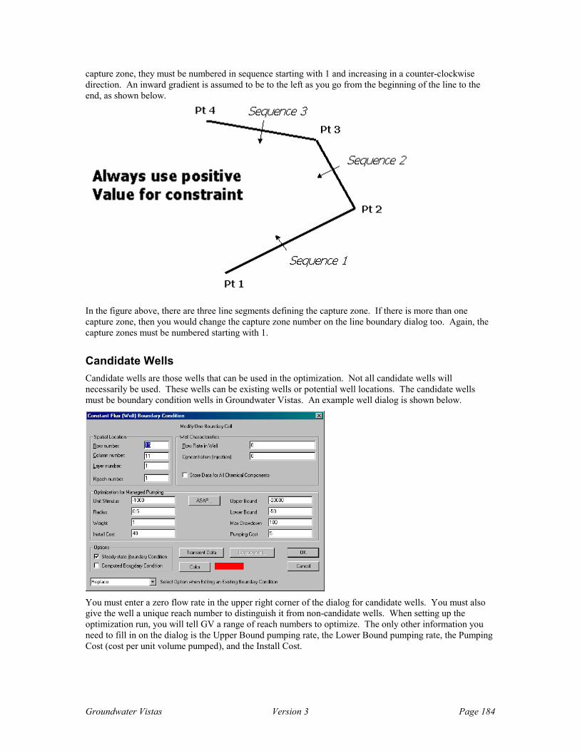
Groundwater Vistas Version 3 Page 184
capture zone, they must be numbered in sequence starting with 1 and increasing in a counter-clockwise direction. An inward gradient is assumed to be to the left as you go from the beginning of the line to the end, as shown below.
In the figure above, there are three line segments defining the capture zone. If there is more than one capture zone, then you would change the capture zone number on the line boundary dialog too. Again, the capture zones must be numbered starting with 1.
Candidate Wells Candidate wells are those wells that can be used in the optimization. Not all candidate wells will necessarily be used. These wells can be existing wells or potential well locations. The candidate wells must be boundary condition wells in Groundwater Vistas. An example well dialog is shown below.
You must enter a zero flow rate in the upper right corner of the dialog for candidate wells. You must also give the well a unique reach number to distinguish it from non-candidate wells. When setting up the optimization run, you will tell GV a range of reach numbers to optimize. The only other information you need to fill in on the dialog is the Upper Bound pumping rate, the Lower Bound pumping rate, the Pumping Cost (cost per unit volume pumped), and the Install Cost.
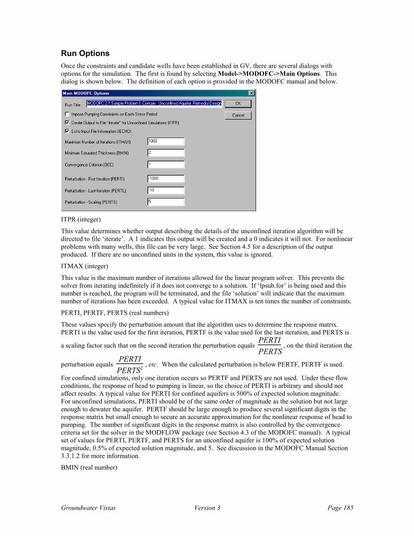
Groundwater Vistas Version 3 Page 185
Run Options Once the constraints and candidate wells have been established in GV, there are several dialogs with options for the simulation. The first is found by selecting Model->MODOFC->Main Options. This dialog is shown below. The definition of each option is provided in the MODOFC manual and below.
ITPR (integer)
This value determines whether output describing the details of the unconfined iteration algorithm will be directed to file ‘iterate’. A 1 indicates this output will be created and a 0 indicates it will not. For nonlinear problems with many wells, this file can be very large. See Section 4.5 for a description of the output produced. If there are no unconfined units in the system, this value is ignored.
ITMAX (integer)
This value is the maximum number of iterations allowed for the linear program solver. This prevents the solver from iterating indefinitely if it does not converge to a solution. If ‘lpsub.for’ is being used and this number is reached, the program will be terminated, and the file ‘solution’ will indicate that the maximum number of iterations has been exceeded. A typical value for ITMAX is ten times the number of constraints.
PERTI, PERTF, PERTS (real numbers)
These values specify the perturbation amount that the algorithm uses to determine the response matrix. PERTI is the value used for the first iteration, PERTF is the value used for the last iteration, and PERTS is
a scaling factor such that on the second iteration the perturbation equals PERTIPERTS
, on the third iteration the
perturbation equals PERTIPERTS2 , etc. When the calculated perturbation is below PERTF, PERTF is used.
For confined simulations, only one iteration occurs so PERTF and PERTS are not used. Under these flow conditions, the response of head to pumping is linear, so the choice of PERTI is arbitrary and should not affect results. A typical value for PERTI for confined aquifers is 500% of expected solution magnitude. For unconfined simulations, PERTI should be of the same order of magnitude as the solution but not large enough to dewater the aquifer. PERTF should be large enough to produce several significant digits in the response matrix but small enough to secure an accurate approximation for the nonlinear response of head to pumping. The number of significant digits in the response matrix is also controlled by the convergence criteria set for the solver in the MODFLOW package (see Section 4.3 of the MODOFC manual). A typical set of values for PERTI, PERTF, and PERTS for an unconfined aquifer is 100% of expected solution magnitude, 0.5% of expected solution magnitude, and 5. See discussion in the MODOFC Manual Section 3.3.1.2 for more information.
BMIN (real number)

Groundwater Vistas Version 3 Page 186
This value indicates the minimum saturated thickness allowed in unconfined units. It is necessary to avoid dewatering portions of the unconfined units. This value is used to automatically set lower head bound constraints at all extraction wells in unconfined units. These constraints are named ‘b’ plus the corresponding well name. If there are no unconfined units in the system, this value is ignored. A typical value for BMIN is 15% of the saturated thickness.
OCC (real number)
This value indicates the convergence criteria for solving unconfined problems. Iteration stops when the maximum difference in pumping rates between the previous iteration and the current iteration is below OCC. If there are no unconfined units in the system, this value is ignored. This value is typically set at the precision desired for the pumping solution.
IECHO (integer)
IECHO determines whether the input read by MODOFC from file ‘opt.in’ will be echoed to file ‘setup’. A 1 indicates that input will be echoed, a 0 that input will not be echoed.
Well Options The Well Options dialog defines which wells are going to be used by MODOFC as candidate wells. This is done using a range of reach numbers at the top of the dialog. The other variables are defined below.
INCST (integer)
This flag determines whether binary variables are to be included in the optimization problem. The use of binary variables complicates the solution procedure, but enables incorporation of installation costs and constraints on the number of wells selected (NWMIN, NWMAX) and on minimum pumping rates (PMN). If INCST equals 0, binary variables are not included. If INCST equals 1, binary variables are included. Sample Problem II in the tutorial (later in this chapter) demonstrates the inclusion of binary variables.
INPR (integer)
This value determines whether output describing the details of the brand and bound algorithm for solving mixed binary problems will be directed to file ‘iterate’. A 1 indicates this output will be created and a 0 indicates it will not. For problems with many wells, this file can be very large. This value is not used if INCST equals zero. See section 4.5 in the MODOFC manual for a description of the output produced.
NWMIN, NWMAX (integers)
These values set the minimum and maximum number of wells the solution can use, Nl in (15) and Nu in (14). These values are not used if INCST equals zero. Setting NWMIN equal to zero and NWMAX equal to NUMWELS eliminates restrictions on the number of wells.
Recharge Balance The recharge balance constraints produce both upper and lower bounds on the ratio of extraction and injection, and are imposed for each stress period in which any well is available. Note that these constraints will take the form of a specified ratio between extraction and injection, if the coefficients are defined so

Groundwater Vistas Version 3 Page 187
that b a= 1 . The constraints will be consistent with each other as long as ab ≤ 1. Input values should appear in the following order:
A (real number)
This value indicates the fraction of total injection which total extraction must exceed, a in equation (9). If A equals zero, the constraint is not imposed.
B (real number)
This value indicates the fraction of total injection which total extraction must exceed, b in equation (10). If B equals zero, the constraint is not imposed.
Pumping Constraints The first column in the pumping constraint dialog is the MINP variable in the MODOFC manual. This indicates the minimum total pumping that will be required for the stress period, Qt
l in equation (8) in the MODOFC manual. Extraction is defined as positive pumping and injection as negative pumping. Thus, MINP can be viewed as the minimum total extraction allowed or -MINP as the maximum total injection allowed. MAXP must be greater than or equal to MINP.
The second column is the MAXP variable which indicates the maximum total pumping that will be required for the stress period, Qt
u in equation (7) in the MODOFC manual. Extraction is defined as positive pumping and injection as negative pumping. Thus, MAXP can be viewed as the maximum total extraction allowed or -MAXP as the minimum total injection allowed. MAXP must be greater than or equal to MINP.
These constraints are defined in each stress period. The current dialog has room for 12 stress periods. In a future release this dialog will be a spreadsheet.

Groundwater Vistas Version 3 Page 188
Running MODOFC Before running MODOFC, be sure to create the MODFLOW files using Model->MODFLOW->Create Data Sets. MODOFC is then run by first creating the MODOFC input file, called opt.in. Select Model->MODOFC->Create Input File to create the opt.in file. After this is done, select Model->MODOFC->Run MODOFC to run the model.
Using SOMOS SOMOS is under active development in GV. The documentation of interfacing GV with SOMOS will be completed in the near future.
Optimization Tutorial We will explore MODOFC and Brute Force in the following tutorial session. Both are included with GV Version 3.
MODOFC is probably the simplest of the classical optimizers to use. By classical, we mean that the optimization is done using linear programming techniques originally developed for management science. Classical optimizers include MODOFC, SOMOS, MODMAN (developed for U.S. EPA by GeoTrans), AQMAN (old USGS model), etc. The nice thing about MODOFC (other than it’s free!) is that it is totally self-contained. Many other optimizers, like MODMAN, require additional software. That adds cost and complexity to the whole process. With MODOFC, the optimizer is included within the MODFLOW software and runs as one application.
The MODOFC manual contains three simple examples to illustrate how to use the code for common applications. We have put those examples into Groundwater Vistas to get you started. Work through these examples to familiarize yourself with how MODOFC works.
Sample Problem I demonstrates a groundwater containment scenario in which head bounds, head difference constraints, and a capture zone are used. In this problem, wells are screened over multiple intervals and unconfined units. Sample Problem II demonstrates a construction dewatering project in which head bounds are used with construction costs in a confined aquifer. Binary variables and the branch and bound algorithm are used for this problem. Sample Problem III demonstrates a water supply problem

Groundwater Vistas Version 3 Page 189
in which drawdown and minimum total extraction is constrained. In this problem, the simulations use multiple stress periods.
MODOFC Problem I: CONTAIN This sample problem represents a hazardous waste site in which contaminated groundwater must be contained. The sample problem has two layers, an upper unconfined unit above a lower confined unit with lengths of 600 feet and widths of 400 feet. Both layers have no flow boundary conditions along the top and bottom boundaries, fixed heads of 50 feet along the left boundary, and fixed heads of 45 feet along the right boundary. The layers are horizontally homogenous and isotropic with a vertical conductance between the two of 0.05 1/day. The upper unconfined unit has a hydraulic conductivity of 5 ft/day, a bottom elevation of 30 feet, and a uniform recharge of 0.002 ft/day. The lower confined unit has a transmissivity of 800 ft2/day. Each layer is divided into 600 square block centered nodes each 20 ft by 20 ft. A production well is located in the lower unit at grid point (13,20,2) pumping at 10,000 ft3/day. The grids for these layers are shown in the figures below.
It is assumed that an area in the upper layer of the model domain has been contaminated. From a design standpoint, at steady state, all contaminated water must be contained within a capture zone, while the production well continues to operate. Mounding above the ground surface cannot occur at injection wells (assumed at 65 feet), and the upper unit cannot be dewatered. Due to surface features at the site, there are only 6 possible well locations as shown in Figure 1 and well 5 is screened in both units. These design criteria can be converted into linear programming constraints, using head difference constraints and head constraints. First, a capture zone of three line segments has been defined around the contaminated area with a required gradient of 0.01 ft/ft. MODOFC will convert this into 23 head difference constraints. In addition, head difference constraints requiring a head difference of 0.01 ft have been defined in the source area to ensure upward vertical gradients and prevent contaminated water from leaking into the lower unit. A fixed head constraint has been used at the candidate injection well requiring that head remain below 65 feet. Finally, a minimum hydraulic thickness of 2 feet was allowed in the unconfined aquifer. It was assumed that extraction costs 5 times more than injection due to treatment costs.
This sample problem demonstrates several features of MODOFC. First, all possible head constraints are employed: head constraints, head difference constraints, and capture zones. Note the coordinates of the capture zone, which use the MODFLOW system of the origin at the upper left location of the grid, down is the positive Y-direction, and to the right is the positive X-direction. Because lower heads are required on the right side of the capture zone line, the first node is defined near Well 1. MODFLOW input file distances are used, for this case each cell is 20 ft by 20 ft. This problem also has an unconfined layer in it, so the solution will be determined through iteration, and care must be given to defining the first perturbation (PERTI), last perturbation (PERTF), perturbation scaling (PERTS), minimum aquifer thickness (BMIN), iteration convergence criteria (OCC), and whether iterations should be printed (ITPR). Also, repeated optimizations are not possible (ICOM = 1) and inclusion of binary variables is not recommended (INCST = 0) with unconfined problems. Because INCST = 0, values for installation costs (ICST), minimum pumping rates (PMN), and minimum (NWMIN) and maximum (NWMAX) number of wells to install are ignored. Wells 2 and 4 are screened over multiple units in this problem. Note the syntax for Wells 2 and 4, i.e. NL = 0 and extra rows are provided to set the pumping ratios for each screened layer.

Groundwater Vistas Version 3 Page 190
1 2010 30
Head = 50 ft Head = 45 ft
400 ft
600 ft2 3 4 5 6 7 8 9 11 12 13 14 15 16 17 18 19 21 22 23 24 25 26 27 28 29
1
20
10
2
3
4
5
6
7
8
9
11
12
13
14
15
16
17
18
19
Figure 1Layer 1 of Sample Problem I
1
3
4
5
6
1
6
candidate extraction well
candidate injection well
capture zone
vertical head difference constraints
KEY:
+
+
+
+++
++
+
+
+2
1 2010 30
Head = 50 ft Head = 45 ft
400 ft
600 ft2 3 4 5 6 7 8 9 11 12 13 14 15 16 17 18 19 21 22 23 24 25 26 27 28 29
1
20
10
2
3
4
5
6
7
8
9
11
12
13
14
15
16
17
18
19
Figure 2Layer 2 of Sample Problem I
production well
KEY:
Run Groundwater Vistas Version 3 and open the file modofc_contain.gwv in the c:\gwv3\tutorial directory. Your screen should look like the one below:

Groundwater Vistas Version 3 Page 191
You will probably notice that the capture zone lines do not match the figure from the MODOFC manual. This is not an optical illusion, the data sets that come with MODOFC do not match the picture in the manual. The problem will only run with the capture zone as defined in the data files and as shown in your GV model.
The first thing you need to do when running MODOFC is to shut off the output control file. For some reason, MODOFC does not like the saving of binary head, drawdown, and cell-by-cell flow files. Select Model/MODFLOW/Packages and confirm that the output control file is off:
Also, make sure that all cell-by-cell flow unit numbers are zero, as shown above. MODOFC is a MODFLOW96 version, so also make sure that the MODFLOW version is set to Original (88/96).

Groundwater Vistas Version 3 Page 192
Now, double-click on one of the targets on the screen. Groundwater Vistas uses calibration targets as optimization constraints. The definition of the northern-most target is shown in the following dialog:
Notice that the target type is not head or drawdown but is changed to Z Gradient Constraint. If you pull down the target type list you will see there are several other types of constraints as well. The target value in this case is the constraint value for MODOFC. The weight is not used. One important thing to remember is that you MUST give the target a name.
The other type of constraint in this problem is the capture zone. MODOFC allows you to simplify the definition of constraints through the use of capture zone lines. Groundwater Vistas supports this option through the use of analytic line boundaries. Double-click on the southern-most line boundary and your dialog should look like the one below:
Note that the boundary condition type is Capture Zone Constraint. This type of line boundary is only used with MODOFC and is not supported by any of the other optimizing models in GV. There are several

Groundwater Vistas Version 3 Page 193
important things to remember when defining a capture zone for MODOFC. First, the area that you want to capture is on the left as you drag the line from its beginning point to its end point. You must also give the capture zone a number, called Capture Zone Number. Since a capture zone may have more than one line, you also give it a sequence number starting with 1. The one above is the first line for Capture Zone 1. You must start numbering capture zones at 1. The only other thing to remember is that the Head or Flow rate here represents a change in head used to construct head difference constraints by MODOFC.
Now look at the wells defined in GV. Select BCs/Well and then double-click on the well in the southwest corner of the capture zone. Your dialog should look like the following:
You may have wells in your model that are always on and those that are used in the optimization process. These are distinguished from one another by the reach number. You should use special reach numbers for those wells that are part of the optimization. In this example, all wells with reach 1 are part of the optimization. You must also enter a zero pumping rate for these wells. You will see a special section of the well dialog that is labeled Optimization for Managed Pumping. Not all of this information is used by MODOFC. The things that are used include the Upper Bound, Lower Bound, Install Cost, and Pumping Cost.
Now you have defined the problem except for MODOFC options. The model design has constraints and candidate wells. Fortunately, MODOFC has relatively few options. While this somewhat limits power users, it is nice for those of us who are not optimization experts! First, look at the general MODOFC options by selecting Model/MODOFC/Main Options:

Groundwater Vistas Version 3 Page 194
Probably the most important information on this dialog are the perturbation values. The first perturbation (PERTI) in unconfined aquifers is the pumping rate used in the first iteration. It should be about what you expect the pumping rate to be in the final solution. If you specify a value that is too large, the aquifer can be dewatered. If the value is too low, the aquifer response is not large enough for MODOFC to determine optimal rates. In confined systems, the last perturbation value (PERTL) and scaling factor (PERTS) are not used. In unconfined aquifers, iteration is required and these parameters determine how the perturbation factor is reduced during iteration. The author, David Ahlfeld, recommends that PERTL be 0.5 percent of PERTI and PERTS be set to 5. I have found that some experimentation if usually required for these values.
The other value to consider is the convergence criterion (OCC). For unconfined systems, OCC is the change in pumping rate that must occur for the iterations to stop. In this synthetic example, it is quite low. In practice, you may need to make this a much bigger number.
Now, select Model/MODOFC/Well Options and look at the following dialog:
The first option on the dialog defines which wells in your model are going to be part of the optimization. In this case, only wells with a reach number of 1 are going to be used. The other important option is INCST, which includes or excludes integer variables. If you include integer variables, then MODOFC will constrain the solution using specified minimum pumping rates, well pumping/installation costs, and minimum/maximum number of wells. Without integer variables, these factors are not considered. Given that choice, why not always include integer variables? Unfortunately, using integer variables in unconfined aquifers often does not work. In this example, we will not include integer variables.
Now let’s run MODOFC. The first step once you have defined constraints, candidate wells, and options, is to create MODFLOW files. Select Model/MODFLOW/Create datasets. Next, select Model/MODOFC/Create Input File. MODOFC always looks for a file called opt.in, which is created when you select this menu item. If everything was set correctly, you should be able to choose Model/MODOFC/Run MODOFC.
When it is finished, select Model/MODOFC/View Solution to see the results. The first part of the file is the important stuff:
MODOFC VERSION 2.1 - SOLUTION OUTPUT FILE
MODOFC 2.1 Sample Problem I: Contain - Unconfined Aquifer, Remedial Desi
++++++++++++++++++++++++++++++++++++++++++++++++++++++++++++++++++++++
MODOFC Version 2.1 Optimization Results
++++++++++++++++++++++++++++++++++++++++++++++++++++++++++++++++++++++
Optimal Solution Found

Groundwater Vistas Version 3 Page 195
++++++++++++++++++++++++++++++++++++++++++++++++++++++++++++++++++++++
PROBLEM SOLUTION
++++++++++++++++++++++++++++++++++++++++++++++++++++++++++++++++++++++
Objective Function Value 2.2435E+04
Pumping Rates Listed For Each Well
Name Stress periods Extraction Injection
----------------------------------------------------------------------
well1 1 1.5250E+03
well2 1 1.2747E+03
well3 1 2.7335E+02
well4 1 8.0558E+02
well5 1 5.3112E+02
well6 1 7.7213E+01
----------------------------------------------------------------------
Total Rates 3.9558E+03 5.3112E+02
++++++++++++++++++++++++++++++++++++++++++++++++++++++++++++++++++++++
The results are almost identical to the example output that is included with MODOFC. Note that all wells are needed, even though wells 1 and 2 pump most of the water. This happens because we could not include integer variables to throw out wells unless they have a certain minimum pumping rate.
Try turning on the integer variables and see what happens (Model/MODOFC/Well Options). You will probably get the same answer. That is because our minimum flow rate for the wells was 50 ft3/d. Edit all of the wells in layer 1 except the far eastern one which is the injection well. Change the minimum flow rate from –50 to –500. Now run it. In this case, you probably get the common error Problem infeasible.

Groundwater Vistas Version 3 Page 196
MODOFC Problem II: DEWATER This sample problem represents a dewatering problem for a construction site. The sample problem has one confined layer with a length of 3,000 feet and a width of 2,000 feet. The layer has boundary conditions of no flow along the top and bottom boundaries, fixed head of 80 feet along the left boundary, and fixed head of 60 feet along the right boundary. The layer is homogenous and isotropic with a transmissivity of 50 ft2/day. The aquifer is divided into 600 square block centered nodes each 100 ft by 100 ft. The grid is shown in Figure 3.
In this problem, the groundwater needs to be lowered to a depth of 50 feet so that footings can be installed in the region shown on Figure 3. This design criteria can be imposed by defining 10 upper bound head constraints as shown in Figure 3. Seven candidate well locations are selected with minimum pumping rates of 100 ft3/day, maximum pumping rates of 10,000 ft3/day, pumping costs for the construction period of 10 $ day/ft3, and construction costs of $2000 per well. To improve reliability, at least three wells must be installed.
This sample problem primarily demonstrates the use of binary variables. To include the cost for well installation, binary variables must be used, thus INCST = 1. This enables several other constraints, so meaningful values must be provided for installation costs (ICST), minimum pumping rates (PMN), and minimum (NWMIN) and maximum (NWMAX) number of wells to install. Also, if the user wants to record branch and bound algorithm solution steps, INPR must be set to 1.
1 2010 30
Head = 80 ft Head = 60 ft
2,000 ft
3,000 ft2 3 4 5 6 7 8 9 11 12 13 14 15 16 17 18 19 21 22 23 24 25 26 27 28 29
1
20
10
2
3
4
5
6
7
8
9
11
12
13
14
15
16
17
18
19
Figure 3Sample Problem II
candidate extraction wellKEY:
head constraintconstruction area
* * *
* *
* **
**
*
1
3
5
2
4
6
7
5
We have constructed this example as GV file modofc_dewater.gwv. Open up this design and it should look like the following:

Groundwater Vistas Version 3 Page 197
The main difference in this example is in the constraints. Instead of requiring an inward and upward gradient, we want a certain amount of drawdown for dewatering. Edit one of the targets (constraints) and you will see that the target type is Max Head Constraint.
This means that the wells will be optimized so that the water level is at or below this value. The head value is defined as the target value, 50 in this case.
The wells for this example are similar to the previous one except that we are now entering cost information.

Groundwater Vistas Version 3 Page 198
Go ahead and run this example. Your answer should be the same as the following:
MODOFC VERSION 2.1 - SOLUTION OUTPUT FILE
MODOFC Problem
++++++++++++++++++++++++++++++++++++++++++++++++++++++++++++++++++++++
MODOFC Version 2.1 Optimization Results
++++++++++++++++++++++++++++++++++++++++++++++++++++++++++++++++++++++
Optimal Solution Found
++++++++++++++++++++++++++++++++++++++++++++++++++++++++++++++++++++++
PROBLEM SOLUTION
++++++++++++++++++++++++++++++++++++++++++++++++++++++++++++++++++++++
Objective Function Value 3.4799E+04
Pumping Rates Listed For Each Well
Name Stress periods Extraction Injection
----------------------------------------------------------------------
well1 1 1.2425E+03
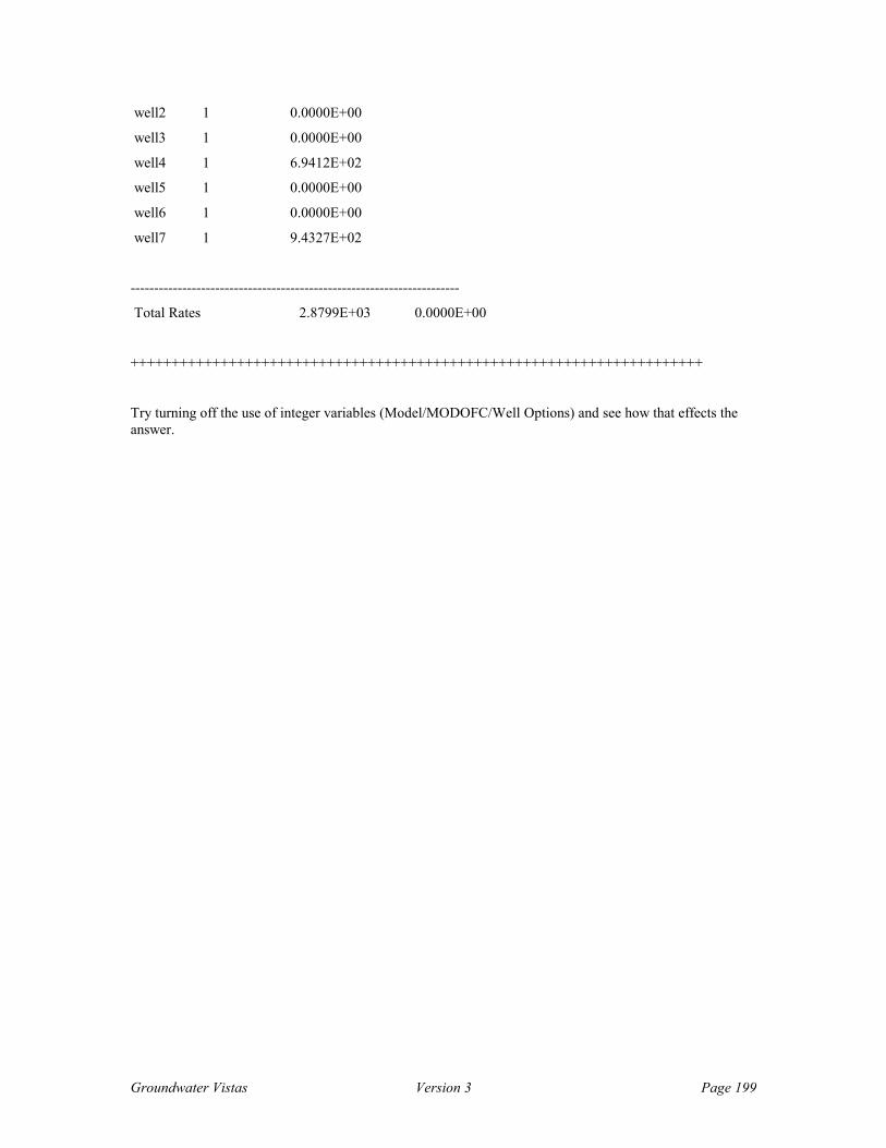
Groundwater Vistas Version 3 Page 199
well2 1 0.0000E+00
well3 1 0.0000E+00
well4 1 6.9412E+02
well5 1 0.0000E+00
well6 1 0.0000E+00
well7 1 9.4327E+02
----------------------------------------------------------------------
Total Rates 2.8799E+03 0.0000E+00
++++++++++++++++++++++++++++++++++++++++++++++++++++++++++++++++++++++
Try turning off the use of integer variables (Model/MODOFC/Well Options) and see how that effects the answer.
Groundwater Vistas Version 3 Page 200
MODOFC Problem III: SUPPLY This sample problem represents a water supply problem in which limited drawdown is allowed near a river. The sample problem has one confined layer, 6,000 feet by 5,000 feet, with a river running through the center of it. The layer has boundary conditions of no flow along the left and right boundaries, fixed heads along the top boundary which vary from 100 feet to 86 feet, and fixed heads along the bottom boundary which vary from 80 feet to 66 feet. The layer is homogenous and isotropic with a transmissivity of 5000 ft2/day and a storativity of 0.05. The aquifer is divided into 750 square block centered nodes each 200 ft by 200 ft. The stream flows from left to right with summer heads which vary from 50 feet to 32 feet along its length. The fall and winter heads are 1 foot higher and the spring heads are 2 feet higher. During summer the average stream depth is 3 feet. The stream is approximately 10 feet wide with a bed conductance of 500 ft2/day. Recharge also varies throughout the year: 0.0005 ft/yr in winter, 0.002 ft/yr in spring, 0 ft/yr in summer, and 0.001 ft/yr in fall. The grid and stream are shown in Figure 4.
In this problem, the objective is to maximum groundwater extraction over a three-year period (12 seasons) while maintaining a certain level of water in the stream. This design criteria can be imposed by defining upper head constraints in the groundwater at locations under the stream, as shown in Figure 4. In addition, there are limits on the maximum (80,000 ft3/day) and minimum (30,000 ft3/day in the first year and 25,000 ft3/day in the second and third year) total rates of water extracted in a three-month period. These values define the total pumping constraints. Four possible well locations are shown in Figure 4 with maximum pumping rates at each well of 50,000 ft3/day and pumping costs of -0.001 $ /ft3/day (i.e., each 1000 cubic foot of water pumped is worth $1). The wells and constraints are only active for various stress periods as shown in the opt.in file.
This sample problem primarily demonstrates optimization of groundwater problems with multiple stress periods. Because the recharge and streamflows vary with the season, a transient groundwater model is required to properly depict the site. It may be advantageous to have wells pump at different rates for each season. This is exhibited in Well 2 which is required to have one pump rate for winter (stress periods 1, 5, and 9), another for spring (stress periods 2, 6, and 10), another for summer (stress periods 3, 7, and 11) and another for fall (stress periods 4, 8, and 12). Well 1 on the other hand is required to have the same pump rate for the entire 3 years (stress periods 1-12). Well 3 will only be pumping in year 2 (stress periods 5-8) and Well 4 can only pump in spring (stress periods 2, 6, and 10) and fall (stress periods 4, 8, and 12). Similarly, constraints are only active for certain stress periods: b-01 and b-03 for the entire 3 years (stress periods 1-12) and b-03 and b-04 for summer (stress periods 3, 7, and 11) and fall (stress periods 4, 8, and 12).

Groundwater Vistas Version 3 Page 201
1 2010 30
5,0 00 ft
6,000 ft2 3 4 5 6 7 8 9 11 12 13 14 15 16 17 18 19 21 22 23 24 25 26 27 28 29
1
20
10
2
3
4
5
6
7
8
9
11
12
13
14
15
16
17
18
19
Figure 4Sample Problem III
1
3
4
1 candidate extraction well
river
head constraints
KEY:
2
21
22
23
24
25
* ***
*
This example illustrates some very complex use of when wells can pump during a transient run. Groundwater Vistas right now cannot handle this degree of complexity, so you will need to edit the opt.in file in a text editor to complete it. First, load modofc_supply.gwv into Groundwater Vistas. Create the MODFLOW files and then the MODOFC file. Find the file c:\gwv3\tutorial\work\opt.in and edit it in Notepad, Wordpad, or something else. Look for the following lines in the file:
well1 t 11 22 1 1 e 100.000000 50000.000000 0.000000 2000.000000 '1,12'
well2 t 12 11 1 1 e 100.000000 50000.000000 0.000000 2000.000000 '1,12'
well3 t 14 25 1 1 e 100.000000 50000.000000 0.000000 2000.000000 '1,12'
well4 t 16 17 1 1 e 100.000000 50000.000000 0.000000 2000.000000 '1,12'
And change them to:
well1 t 11 22 1 1 e 100.000000 50000.000000 0.000000 2000.000000 '5-8'
well2 t 12 11 1 1 e 100.000000 50000.000000 0.000000 2000.000000 '1-12'
well3 t 14 25 1 1 e 100.000000 50000.000000 0.000000 2000.000000 '2,6,10:4,8,12'
well4 t 16 17 1 1 e 100.000000 50000.000000 0.000000 2000.00 '1,5,9:2,6,10:3,7,11:4,8,12'
Likewise, find the Bounds on Head section and change the following:
h-1 t 14 14 1 > 67.000000 '1-12'

Groundwater Vistas Version 3 Page 202
h-2 t 13 20 1 > 64.000000 '1-12'
h-3 t 13 23 1 > 62.000000 '1-12'
h-4 t 15 26 1 > 60.000000 '1-12'
To:
h-1 t 14 14 1 > 67.000000 '1-12'
h-2 t 13 20 1 > 64.000000 '3,4,7,8,11,12'
h-3 t 13 23 1 > 62.000000 '1-12'
h-4 t 15 26 1 > 60.000000 '3,4,7,8,11,12'
Save these changes and run MODOFC.
Using Brute Force Optimization The Brute Force optimization technique is a new way of optimizing pump & treat systems. Unlike more MODOFC, Brute Force uses particle tracking to determine whether a system is successful. Other optimizing software uses head, drawdown, or gradient constraints to design the system as we saw with our MODOFC examples. The problem with these more classical techniques is that defining the gradient constraints is difficult and often the optimization is not successful. The benefit of using particle tracking is that the particles are either captured or they are not. The Brute Force routine continues until all particles, or a specified percentage of particles, are captured in the plume area. This makes interpreting the results very straightforward. The disadvantage of Brute Force is that it requires more simulations than many of the other optimizers.
We have created a simple BF example that you can compare with MODOFC. Open the file modofc_contain_noInject2_brute.gwv. This is a modified version of the first MODOFC example problem with one layer and no injection. The model looks like the following:

Groundwater Vistas Version 3 Page 203
You can see the lines defining the capture zone and potential wells that are similar to the first MODOFC example. You also see a bunch of particles within the capture zone. These are for use with BF. The first thing to do is run one MODFLOW and one MODPATH simulation. These files form the basis for the next BF run. After running MODFLOW and MODPATH, your screen should look like the following:
We are starting with no pumping so the particles just go east to the constant head boundary. Now, let’s look at the Brute Force options. Select Model/Brute Force/Options. The dialog is shown below:
Probably the most critical option for BF is the number of iterations for optimization (7 in this case) and the increment multiplier (1.25). Also important is the unit stimulus for the pumping wells, which is –1,000 ft3/d in this case. BF will use the –1,000 pumping rate to rank the wells so it is important that this rate be large enough to actually capture particles. BF will then select the best well and run 7 simulations multiplying the pumping rate (-1,000 initially) by 1.25 until it hits either 7 simulations or the maximum

Groundwater Vistas Version 3 Page 204
pumping rate defined for that well (-20,000 in this example). You need to make sure that BF can test the whole range from unit stimulus to max. pumping rate during the number of iterations specified.
Now, select Model/Brute Force/Create Input Files. GV will create the main BF input file (brutefrc.dat) and a new well file and particle file. To run BF, select Model/Brute Force/Run Brute Force.
This run goes pretty fast. Select Model/Brute Force/View Output File and you should see at the end of the file that BF came up with 1 well (row 10, column 17) pumping –2,441 ft3/d to contain this plume. Plug this pumping rate in and rerun MODFLOW/MODPATH to confirm it. Your results should be similar to those below:
Try running the MODOFC version of this model – modofc_contain_noInject2.gwv. How do the results compare?
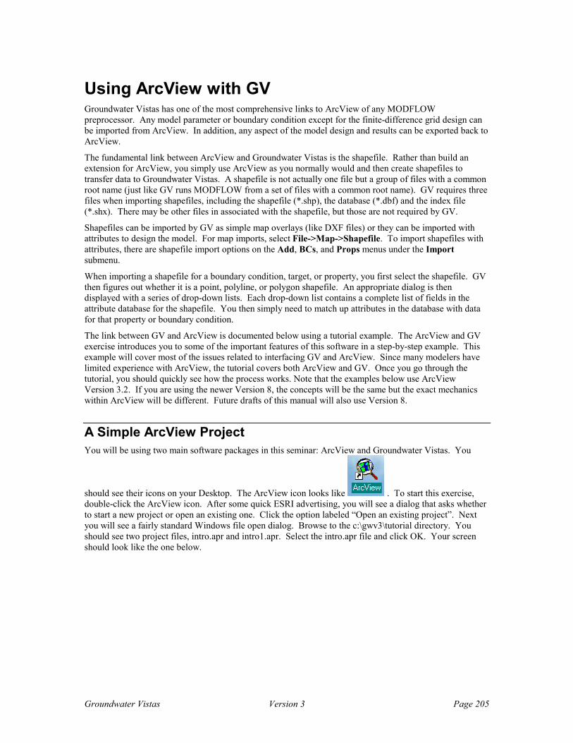
Groundwater Vistas Version 3 Page 205
Using ArcView with GV Groundwater Vistas has one of the most comprehensive links to ArcView of any MODFLOW preprocessor. Any model parameter or boundary condition except for the finite-difference grid design can be imported from ArcView. In addition, any aspect of the model design and results can be exported back to ArcView.
The fundamental link between ArcView and Groundwater Vistas is the shapefile. Rather than build an extension for ArcView, you simply use ArcView as you normally would and then create shapefiles to transfer data to Groundwater Vistas. A shapefile is not actually one file but a group of files with a common root name (just like GV runs MODFLOW from a set of files with a common root name). GV requires three files when importing shapefiles, including the shapefile (*.shp), the database (*.dbf) and the index file (*.shx). There may be other files in associated with the shapefile, but those are not required by GV.
Shapefiles can be imported by GV as simple map overlays (like DXF files) or they can be imported with attributes to design the model. For map imports, select File->Map->Shapefile. To import shapefiles with attributes, there are shapefile import options on the Add, BCs, and Props menus under the Import submenu.
When importing a shapefile for a boundary condition, target, or property, you first select the shapefile. GV then figures out whether it is a point, polyline, or polygon shapefile. An appropriate dialog is then displayed with a series of drop-down lists. Each drop-down list contains a complete list of fields in the attribute database for the shapefile. You then simply need to match up attributes in the database with data for that property or boundary condition.
The link between GV and ArcView is documented below using a tutorial example. The ArcView and GV exercise introduces you to some of the important features of this software in a step-by-step example. This example will cover most of the issues related to interfacing GV and ArcView. Since many modelers have limited experience with ArcView, the tutorial covers both ArcView and GV. Once you go through the tutorial, you should quickly see how the process works. Note that the examples below use ArcView Version 3.2. If you are using the newer Version 8, the concepts will be the same but the exact mechanics within ArcView will be different. Future drafts of this manual will also use Version 8.
A Simple ArcView Project You will be using two main software packages in this seminar: ArcView and Groundwater Vistas. You
should see their icons on your Desktop. The ArcView icon looks like . To start this exercise, double-click the ArcView icon. After some quick ESRI advertising, you will see a dialog that asks whether to start a new project or open an existing one. Click the option labeled “Open an existing project”. Next you will see a fairly standard Windows file open dialog. Browse to the c:\gwv3\tutorial directory. You should see two project files, intro.apr and intro1.apr. Select the intro.apr file and click OK. Your screen should look like the one below.

Groundwater Vistas Version 3 Page 206
The View Document You are looking at the main workspace in ArcView called the view, which is one type of ArcView document. A view contains one or more themes that are usually (but not always) shapefiles. The project you are looking at is a simple one in which several features of a Groundwater Vistas model have been imported into ArcView. You see the finite-difference grid, constant head boundary cells on the west, a DXF base map, and target well locations (targets are used in model calibration).
The main thing to keep in mind is that if you want to import these themes into Groundwater Vistas, they must first be converted to shapefiles. As an example, the first theme is called map.dxf. This is not a shapefile; it is an AutoCAD map. You can convert this map to a shapefile by clicking near the word Map.dxf to make this the active theme. You should see a raised box around the theme just like the picture above where Targets is the active theme.
Now that Map.dxf is the active theme, you can convert it to a shapefile. Select Theme/Convert to Shapefile. ArcView prompts you to enter a name for the new shapefile. Just name it map.shp. After clicking OK, ArcView asks whether to add the shapefile as a theme to the view. Select yes and you will see it added to the top of your list of themes. Notice that it is not checked so it is not visible yet. You can delete the old theme by highlighting it (Map.dxf) and then selecting Edit/Delete Themes. ArcView does not actually delete any of the files, it just removes it as a theme from the current view. Now, click on the little box next to map.shp and the map will be redrawn.
OK, so now you’re probably wondering why we bothered converting a DXF file to a shapefile. Well, there are two reasons you might want to do this. First, shapefiles are easier for Groundwater Vistas to convert to base maps than DXF files. Second, you may have contours of layer elevation or some other property in the DXF file. Often the contour lines are annotated with the elevation. If you convert the DXF file to a shapefile and the elevation of the contour line is preserved as a field in the shapefile database, then GV can import that for a property (like bottom elevation).

Groundwater Vistas Version 3 Page 207
Converting themes to shapefiles works with most things that can be displayed as themes, including ArcInfo coverages. We will not be using ArcInfo in this course but if you have questions about ArcInfo, feel free to ask one of the instructors.
You might notice that ArcView gave your new base map a different color. ArcView sort of randomly selects colors for new themes. This is easy to change. Double-click on the map.shp theme and you get the Legend Editor that looks like the following:
There are many ways to display the data in themes. For a polyline map like this one, the easiest way is Single Symbol which draws everything in the theme with one color and symbol (in this case they are lines so symbol is not really a good word). To change the color, double-click on the line displayed under the word Symbol. You should now see a small dialog that ArcView uses to change colors, line styles, symbols, etc. Click on the paintbrush icon and you will see a color palette as shown below:
Click on another color on the palette and then click Apply on the legend editor. To close the dialog, click the x in the upper right corner of the dialog. Notice that the palette hangs around. This is a handy little feature if you are doing lots of editing. Just put it somewhere on your desktop or click x to close it.

Groundwater Vistas Version 3 Page 208
Now we will explore some more features of the ArcView interface. Click next to Targets on the legend to make that the active theme. You will notice two rows of buttons under the menu at the top of the screen. The first row of buttons is called the Button Bar. When these buttons are pressed, something generally
happens right away. For example, press the button and ArcView opens the database table for the active theme. Assuming that you made Targets your active theme, you should now see the following table:
The data in this table are attributes of the Targets theme. These attributes include the name of the well, the layer in the model, the measured water level (targetvalu), the water level computed by the model, and the residual (calibration error). Go ahead and close the table by clicking the x in the upper right corner of the table.
The bottom row of buttons below the menu is called the tool bar. Tools are usually reserved for actions
that require you to move the mouse and click. For example, press the button and then click on one of the target wells. You will get all of the information on that well that is contained in the shapefile database. You should see a window similar to the following:
Now select the tool. This allows you to select features in the active theme (in this case Targets). Click on one of the target wells and it should change to a yellow color. Hold down the shift key and click another one. Now you should have 2 yellow target wells. Now open the database as you did above by clicking the
button. Notice that the two wells you selected are highlighted in the table.
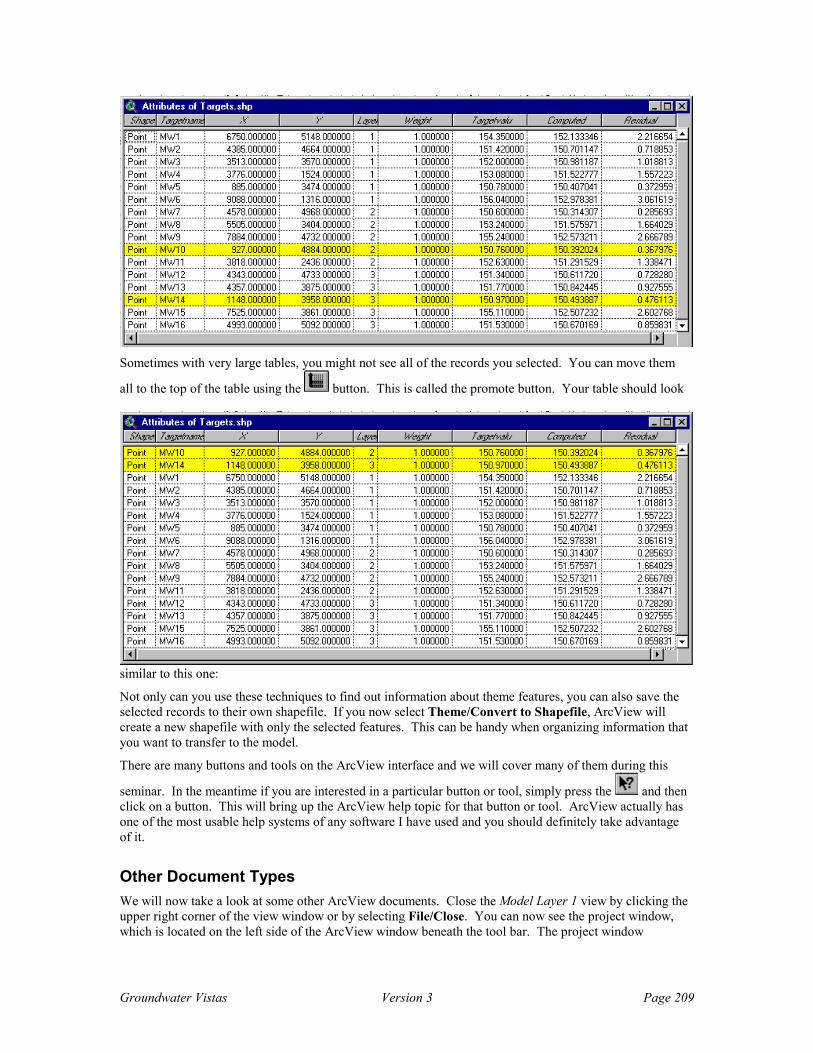
Groundwater Vistas Version 3 Page 209
Sometimes with very large tables, you might not see all of the records you selected. You can move them
all to the top of the table using the button. This is called the promote button. Your table should look
similar to this one:
Not only can you use these techniques to find out information about theme features, you can also save the selected records to their own shapefile. If you now select Theme/Convert to Shapefile, ArcView will create a new shapefile with only the selected features. This can be handy when organizing information that you want to transfer to the model.
There are many buttons and tools on the ArcView interface and we will cover many of them during this
seminar. In the meantime if you are interested in a particular button or tool, simply press the and then click on a button. This will bring up the ArcView help topic for that button or tool. ArcView actually has one of the most usable help systems of any software I have used and you should definitely take advantage of it.
Other Document Types We will now take a look at some other ArcView documents. Close the Model Layer 1 view by clicking the upper right corner of the view window or by selecting File/Close. You can now see the project window, which is located on the left side of the ArcView window beneath the tool bar. The project window
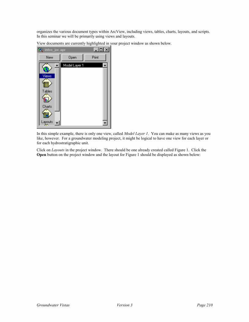
Groundwater Vistas Version 3 Page 210
organizes the various document types within ArcView, including views, tables, charts, layouts, and scripts. In this seminar we will be primarily using views and layouts.
View documents are currently highlighted in your project window as shown below.
In this simple example, there is only one view, called Model Layer 1. You can make as many views as you like, however. For a groundwater modeling project, it might be logical to have one view for each layer or for each hydrostratigraphic unit.
Click on Layouts in the project window. There should be one already created called Figure 1. Click the Open button on the project window and the layout for Figure 1 should be displayed as shown below:

Groundwater Vistas Version 3 Page 211
Layouts are where you can create report illustrations. You can add one or more views, charts, legends, graphics, a scale bar, and a north arrow. You may also draw on the layout and add text. While not as versatile as a drafting program like AutoCAD, it is a lot easier to work with. We will cover layouts in much greater detail later in the seminar.
Now take a look at charts. You should have a chart open on your screen now in the lower left corner of the ArcView window as shown below:

Groundwater Vistas Version 3 Page 212
You can probably tell by looking at this chart that charting is not one of ArcView’s strong points. ArcView charts are very basic but you can get around this by importing graphics on the layouts. We will take a look at this feature in a while.
Groundwater Vistas We will now take a look at Groundwater Vistas (GV) to introduce how ArcView can work with a groundwater model. Double-click the GV icon. Select File/Open and find the file c:\gwv3\tutorial\intro.gwv. Your GV screen should look like the following:
This model should look pretty familiar since it is the same one we just saw in ArcView. This model is ready to run except we removed the constant head cells in layer 1. The first step is to import them from one of the ArcView themes we saw before. To do this, select BCs/Import/ArcView Shapefile. Browse to find the file c:\gwv3\tutorial\bcs.shp. Click the OK button and the following dialog is displayed.
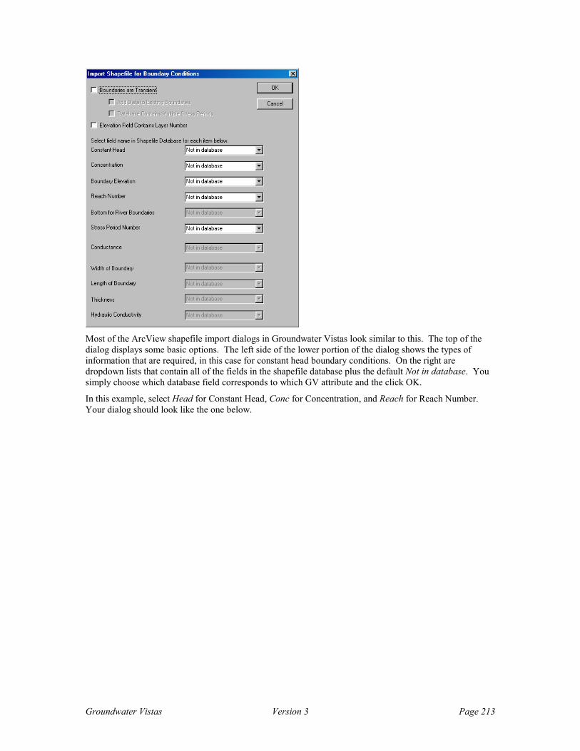
Groundwater Vistas Version 3 Page 213
Most of the ArcView shapefile import dialogs in Groundwater Vistas look similar to this. The top of the dialog displays some basic options. The left side of the lower portion of the dialog shows the types of information that are required, in this case for constant head boundary conditions. On the right are dropdown lists that contain all of the fields in the shapefile database plus the default Not in database. You simply choose which database field corresponds to which GV attribute and the click OK.
In this example, select Head for Constant Head, Conc for Concentration, and Reach for Reach Number. Your dialog should look like the one below.

Groundwater Vistas Version 3 Page 214
Click OK and your Groundwater Vistas screen should show a column of blue cells on the left side of the screen like below.
Run the model by clicking the calculator button ( ) on the GV tool bar. Select OK to create the MODFLOW data files, then Cancel because you don’t need to look at the error file. The model will run quickly and then ask if you want to process the results. Select Yes and you should see the import results dialog.
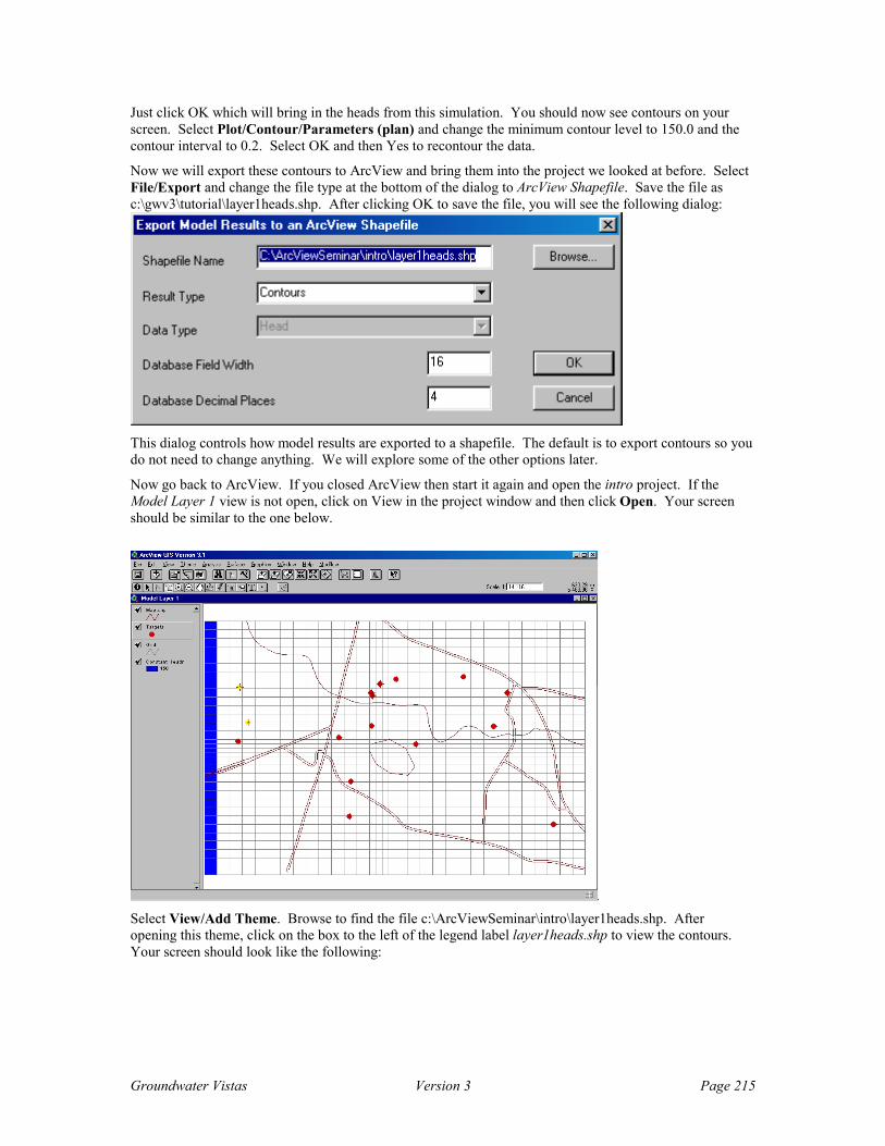
Groundwater Vistas Version 3 Page 215
Just click OK which will bring in the heads from this simulation. You should now see contours on your screen. Select Plot/Contour/Parameters (plan) and change the minimum contour level to 150.0 and the contour interval to 0.2. Select OK and then Yes to recontour the data.
Now we will export these contours to ArcView and bring them into the project we looked at before. Select File/Export and change the file type at the bottom of the dialog to ArcView Shapefile. Save the file as c:\gwv3\tutorial\layer1heads.shp. After clicking OK to save the file, you will see the following dialog:
This dialog controls how model results are exported to a shapefile. The default is to export contours so you do not need to change anything. We will explore some of the other options later.
Now go back to ArcView. If you closed ArcView then start it again and open the intro project. If the Model Layer 1 view is not open, click on View in the project window and then click Open. Your screen should be similar to the one below.
Select View/Add Theme. Browse to find the file c:\ArcViewSeminar\intro\layer1heads.shp. After opening this theme, click on the box to the left of the legend label layer1heads.shp to view the contours. Your screen should look like the following:
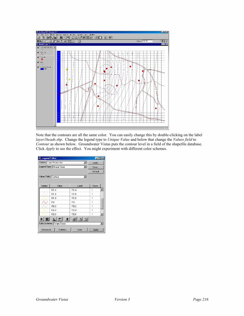
Groundwater Vistas Version 3 Page 216
Note that the contours are all the same color. You can easily change this by double-clicking on the label layer1heads.shp. Change the legend type to Unique Value and below that change the Values field to Contour as shown below. Groundwater Vistas puts the contour level in a field of the shapefile database. Click Apply to see the effect. You might experiment with different color schemes.

Groundwater Vistas Version 3 Page 217
Importing Shapefiles into Groundwater Vistas In the second computer session for the ArcView & Groundwater Vistas tutorial, we will build a conceptual model in ArcView and then import everything but the grid into Groundwater Vistas. The advantage of this approach is that you can redesign the grid at any time in Groundwater Vistas and then just reload the shapefiles that represent the boundaries, properties, wells, and calibration targets. The model you will be building is a real superfund site in Ohio. The last section of this manual contains a description of the site if you are interested.
First, start ArcView and accept the default of creating a new project with a new view. Next, answer Yes to add data to the view. Change the Data Source Type to image data source. In the directory c:\gwv3\tutorial is a file called catlettsburg.tif which is a scanned USGS topographic map. Select this file and then click OK. Once in ArcView, turn on the base map and zoom in. Your screen should look similar to the one below.
Before getting too far into this GIS, select File/Set Work Directory and enter c:\gwv3\tutorial. Also, select File/Extensions and put a check mark next to the MODFLOW Data Reader, the SDTS Grid Import, and the Spatial Analyst Extensions, as shown below. Click OK when you are done. We will need these extensions later on. If you do not have these extensions, then skip this step.

Groundwater Vistas Version 3 Page 218
Now, select View/Properties and change the name of the view to South Point. Also, set the map units to meters and the distance units to meters. Since the map we are using is not in latitude-longitude, we need to set the units directly. The map was downloaded from the web in UTM meters so those are the units we will use for this model. Your screen should look like the one below.
Now, close the South Point view and you should see the project document on the left side of the ArcView window. We first are going to add a couple of text files (comma-delimited Excel csv files) to our ArcView project containing pumping well information and calibration targets for average 1989 conditions. These files have already been prepared for you.
Click on Tables and then click on the Add button. Change the file type to delimited text and find the file wells_m.txt. This file contains the well information in metric units. Repeat this step to add the file targets_m.txt. This one is for calibration targets (monitoring wells). Open these tables to see what they contain.

Groundwater Vistas Version 3 Page 219
Now, click on Views and Open to get back to our topo map. Notice the tables we added before are not showing up anywhere. We need to add them to the view as what ArcView calls an event theme. Select View/Add Event Theme and ArcView displays a dialog where you select the table that contains the information for the theme. Select either the Targets or Wells table. The X field is called X (m) and the Y field is called Y (m). Your dialog should look like the one below. Click OK when you are done.
This is an easy way to get point information into ArcView. As long as the data are in columns separated by commas and there are columns for the X and Y coordinates, the procedure is very straightforward. Repeat this procedure for the other table.
One important thing to keep in mind at this point is that an event theme is not a shapefile and cannot be imported into GV (well, that’s not really true, GV can import comma-delimited files, but shapefiles are easier). It is a good idea to convert the event themes to shapefiles. To do this, simply select Theme/Convert to Shapefile. Now so you don’t get confused, delete the old event themes. Click on each one to make it the active theme and then select Edit/Delete Theme.
The default symbols that ArcView uses are small dots for the wells. To make them more legible, double-click on the wells and targets shapefiles and use the legend editor to make the symbols larger and use a different symbol and color. Your view should then look like the one below.

Groundwater Vistas Version 3 Page 220
Now we want to add two fields to the shapefile database for wells. Click on the wells theme in the legend
and then click the button to open the theme table for wells. To modify the table, select Table/Start Editing. Select Edit/Add Field. We will add a field to the table for the type of pumping well. There are 3 types of wells in this model, municipal supply wells (labeled SPMU), interceptor wells (SPIS-1,5,6,8,9,10), and plant supply wells (the rest). Add a field called type that is a string and 14 characters long as shown below.
Add a second field called Reach which is a number, 4 characters wide with no decimal places. Groundwater Vistas segregates boundary conditions based on a reach number. This number is not used by MODFLOW but can come in handy during model calibration, sensitivity analysis, and editing. We will make the municipal supply wells reach 1, the interceptor wells reach 2, and the plant supply wells reach 3.
Fill in the table like the one below by first clicking on the edit tool ( ) and then entering data in the table. Select Table/Stop Editing when you are done.
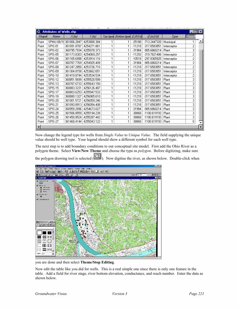
Groundwater Vistas Version 3 Page 221
Now change the legend type for wells from Single Value to Unique Value. The field supplying the unique value should be well type. Your legend should show a different symbol for each well type.
The next step is to add boundary conditions to our conceptual site model. First add the Ohio River as a polygon theme. Select View/New Theme and choose the type as polygon. Before digitizing, make sure
the polygon drawing tool is selected ( ). Now digitise the river, as shown below. Double-click when
you are done and then select Theme/Stop Editing.
Now edit the table like you did for wells. This is a real simple one since there is only one feature in the table. Add a field for river stage, river bottom elevation, conductance, and reach number. Enter the data as shown below.
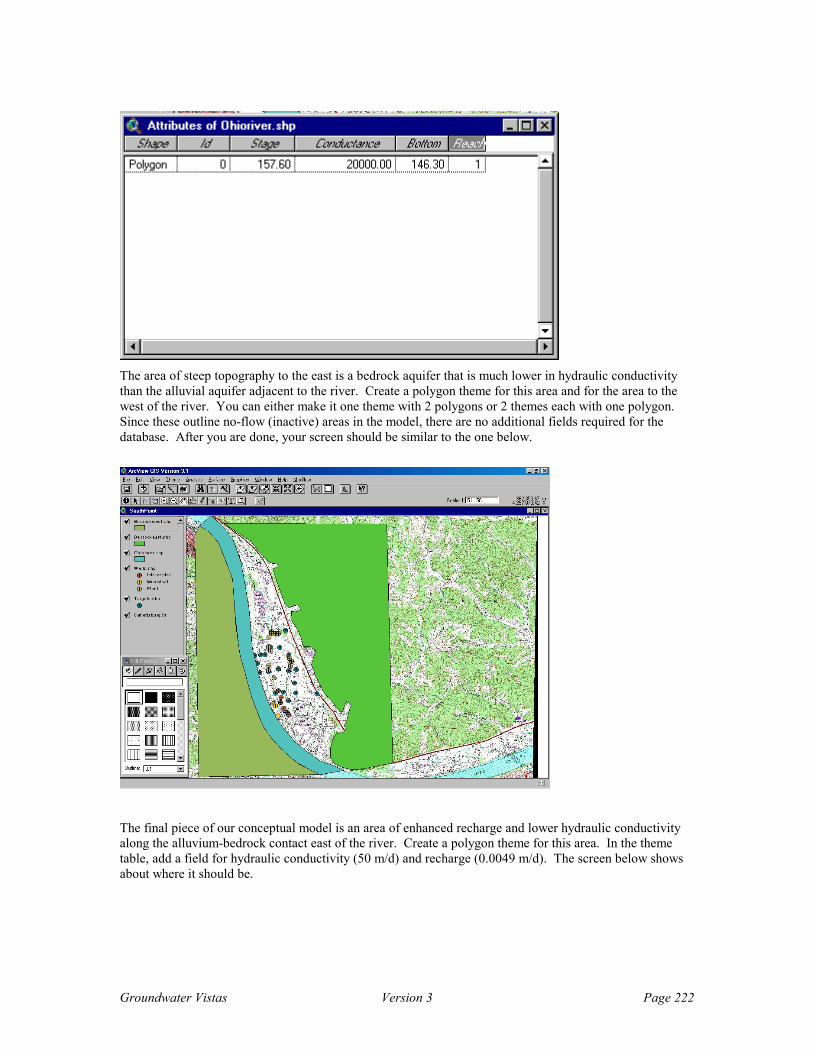
Groundwater Vistas Version 3 Page 222
The area of steep topography to the east is a bedrock aquifer that is much lower in hydraulic conductivity than the alluvial aquifer adjacent to the river. Create a polygon theme for this area and for the area to the west of the river. You can either make it one theme with 2 polygons or 2 themes each with one polygon. Since these outline no-flow (inactive) areas in the model, there are no additional fields required for the database. After you are done, your screen should be similar to the one below.
The final piece of our conceptual model is an area of enhanced recharge and lower hydraulic conductivity along the alluvium-bedrock contact east of the river. Create a polygon theme for this area. In the theme table, add a field for hydraulic conductivity (50 m/d) and recharge (0.0049 m/d). The screen below shows about where it should be.

Groundwater Vistas Version 3 Page 223
That completes the development of the conceptual model in ArcView for now. Save the project and exit ArcView.
You will see that transfering the data we just entered in those ArcView themes to Groundwater Vistas is very simple. Start Groundwater Vistas and select File/New. Make the following changes to the initialization dialog:
Rows 245
Columns 125
Row spacing 30 m
Column spacing 30 m
Bottom elevation 146 m
Top elevation 171 m
Recharge rate 0.00049 m/d
Click OK when you are finished.
The first step when importing data from ArcView is to make sure the coordinate systems (site coordinates in GV) match. The easiest way to do this is to import some of the shapefile themes from ArcView as map overlays in Groundwater Vistas. We will import the bedrock areas and the river. For each of these themes, select File/Map/Shapefile and find the theme. After clicking OK on the file open dialog, GV prompts for a map file name. GV translates the shapefile into a format that GV uses for all map overlays. Enter a name with a *.map extension. After saving the map, GV asks what color to use for this theme.
Depending upon how you digitized the various polygons, you might have to move the finite-difference grid. To realign the grid, select Grid/Offset and click on the screen where you want the lower left corner of the grid to go. If you know the coordinates already, you just click anywhere and then enter the X and Y coordinates on the next dialog.
After the grid is aligned, select BCs/No-Flow so we are editing no-flow boundaries or inactive cells. Select BCs/Import/ArcView Shapefile and browse to find your bedrock theme. If you used two separate themes, you will have to repeat this procedure. After you are done, your model should look similar to the one below.
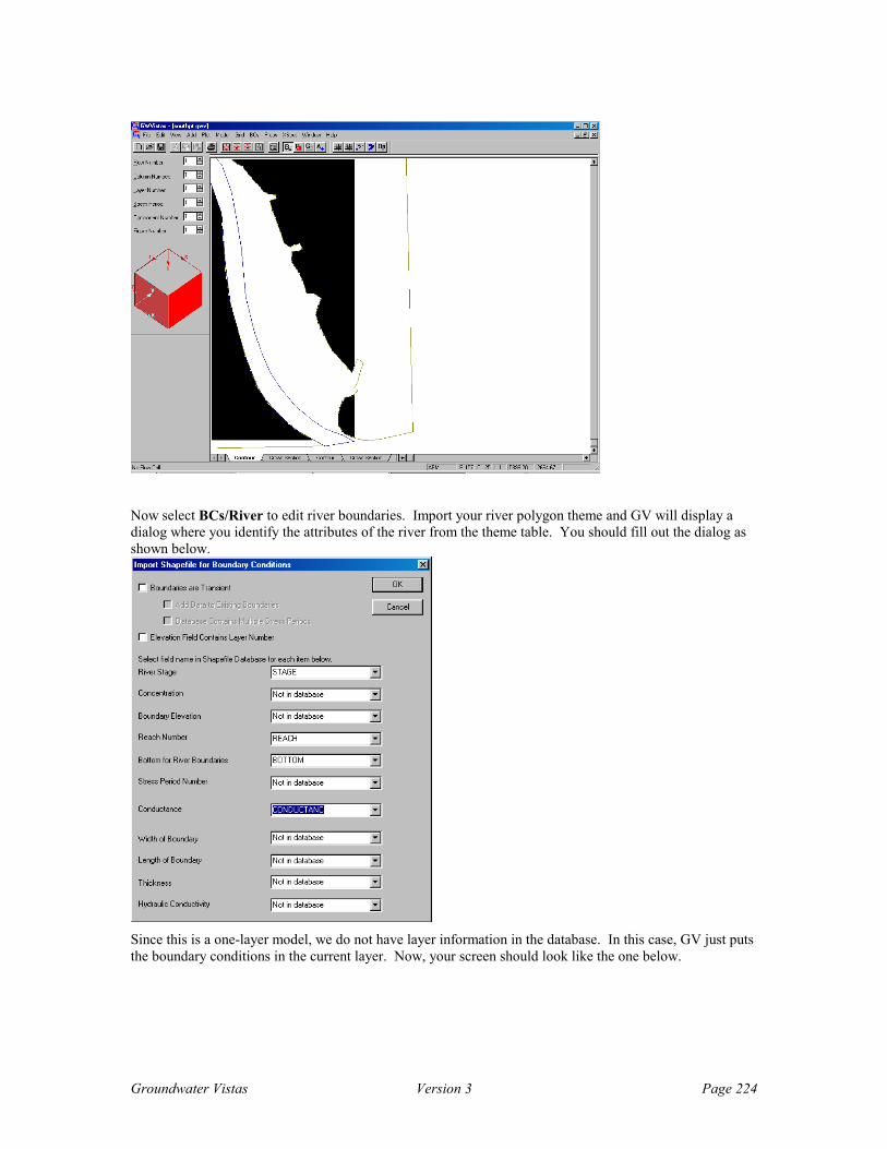
Groundwater Vistas Version 3 Page 224
Now select BCs/River to edit river boundaries. Import your river polygon theme and GV will display a dialog where you identify the attributes of the river from the theme table. You should fill out the dialog as shown below.
Since this is a one-layer model, we do not have layer information in the database. In this case, GV just puts the boundary conditions in the current layer. Now, your screen should look like the one below.

Groundwater Vistas Version 3 Page 225
The final boundary condition is for the wells. Select BCs/Wells and import the well theme from ArcView. Be sure to use the pumping field that is labeled Q_M3_D. Also, use the reach number you put in the theme table.
The boundary conditions are now done. The next things to import are the calibration targets. Select Add/Import/ArcView Shapefile. Browse to find the target theme and select the appropriate name, target value, and weight fields. Note that there are target values in both feet and meters above sea level. Be sure to use the one in meters.
Now we move on to the aquifer properties. Select Props/Hydraulic Conductivity and then select Props/Import/ArcView Shapefile. Browse to find the last theme you created with a narrow K and recharge zone. Since we only have a field for Kx, enter default values for Ky and Kz of 1.0 and check the options that set the anisotropy ratios equal to the default values for these two parameters. Your dialog should look like the one below. Since this is a polygon shapefile, there is no interpolation. GV simply takes the value from the shapefile and puts it into the GV database directly.

Groundwater Vistas Version 3 Page 226
After you are done, you should see a dark blue K zone along the river and a light blue K zone along the bedrock. If you click the Db button at the end of the GV toolbar, you should see that zone 1 is 100 m/d and zone 2 is 50 m/d.
Repeat this procedure for recharge. You should again see two zones of recharge.
The model is just about complete. There are just a couple of administrative things to do. Select Model/MODFLOW/Packages and change the root file name from the default of gvmod to something like sp1. Also change the solver from SIP to PCG2. Finally, enter a 51 next to River under the heading Cell-by-Cell Flow Unit No. to save flux data for the river nodes.
We need to modify the solver parameters slightly. Select Model/MODFLOW/Solver Package and change the number of inner iterations from 5 to 30. Click OK when you are done.
Now save your work by selecting File/Save As. To run the model simply click the calculator button on the
toolbar . Click the Yes button to create the datafiles for MODFLOW and Cancel because you don’t really need to see the errors/warnings file. After the model runs, select Yes to import results and then OK on the Import Results dialog (the defaults are fine for now). Your water-table contours should be similar to the ones below.

Groundwater Vistas Version 3 Page 227
Hopefully you see how simple it is to set up almost entirely from ArcView themes. If you have time, go back to ArcView and digitize the smaller streams that feed into the Ohio River. Use polyline themes and have fields that represent stages at the beginning and end of polylines. You should be able to get stage information from the topo maps.
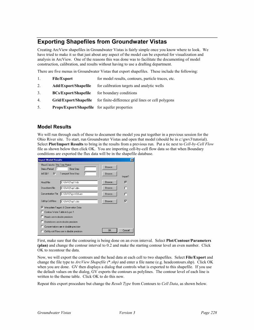
Groundwater Vistas Version 3 Page 228
Exporting Shapefiles from Groundwater Vistas Creating ArcView shapefiles in Groundwater Vistas is fairly simple once you know where to look. We have tried to make it so that just about any aspect of the model can be exported for visualization and analysis in ArcView. One of the reasons this was done was to facilitate the documenting of model construction, calibration, and results without having to use a drafting department.
There are five menus in Groundwater Vistas that export shapefiles. These include the following:
1. File/Export for model results, contours, particle traces, etc.
2. Add/Export/Shapefile for calibration targets and analytic wells
3. BCs/Export/Shapefile for boundary conditions
4. Grid/Export/Shapefile for finite-difference grid lines or cell polygons
5. Props/Export/Shapefile for aquifer properties
Model Results We will run through each of these to document the model you put together in a previous session for the Ohio River site. To start, run Groundwater Vistas and open that model (should be in c:\gwv3\tutorial). Select Plot/Import Results to bring in the results from a previous run. Put a tic next to Cell-by-Cell Flow file as shown below then click OK. You are importing cell-by-cell flow data so that when Boundary conditions are exported the flux data will be in the shapefile database.
First, make sure that the contouring is being done on an even interval. Select Plot/Contour/Parameters (plan) and change the contour interval to 0.2 and make the starting contour level an even number. Click OK to recontour the data.
Now, we will export the contours and the head data at each cell to two shapefiles. Select File/Export and change the file type to ArcView Shapefile (*.shp) and enter a file name (e.g. headcontours.shp). Click OK when you are done. GV then displays a dialog that controls what is exported to this shapefile. If you use the default values on the dialog, GV exports the contours as polylines. The contour level of each line is written to the theme table. Click OK to do this now.
Repeat this export procedure but change the Result Type from Contours to Cell Data, as shown below.

Groundwater Vistas Version 3 Page 229
Cell data means that heads at each active model cell in the current layer will be exported as rectangular polygons to a shapefile. You can also export drawdown, concentration, flux data, and the four user variables. The latter are used in the matrix calculator. You can also export Nodal Data in which case GV exports heads at each model cell but the shape is a point instead of a polygon. You might try each one to see the difference in ArcView.
Analytic Features – Calibration Targets The second export type for shapefiles is for analytic features – wells and targets. We have calibration targets in this model and of course there is already a shapefile in the ArcView project that contains these targets. The additional information that you get, though, when you export targets back out to another shapefile is the simulated head value and the error (residual) are placed in the theme table. This is also why we wanted to import the model results before exporting the targets so we would have this information (in fact, GV will not allow you to export targets to a shapefile without first importing model results).
Export the targets out of this model by selecting Add/Export/Target Shapefile. The dialog is shown below. Enter a file name and keep the other default settings. If this were a multi-layer model you could just export targets from the current layer or you could export them all. There will be a layer number field in the theme table so you could then segregate them in ArcView. If you choose to export transient targets, there will be fields in the theme table for each time, target value, and error. You should be careful using this feature when you have a lot of transient data for targets as the theme table could be quite large.
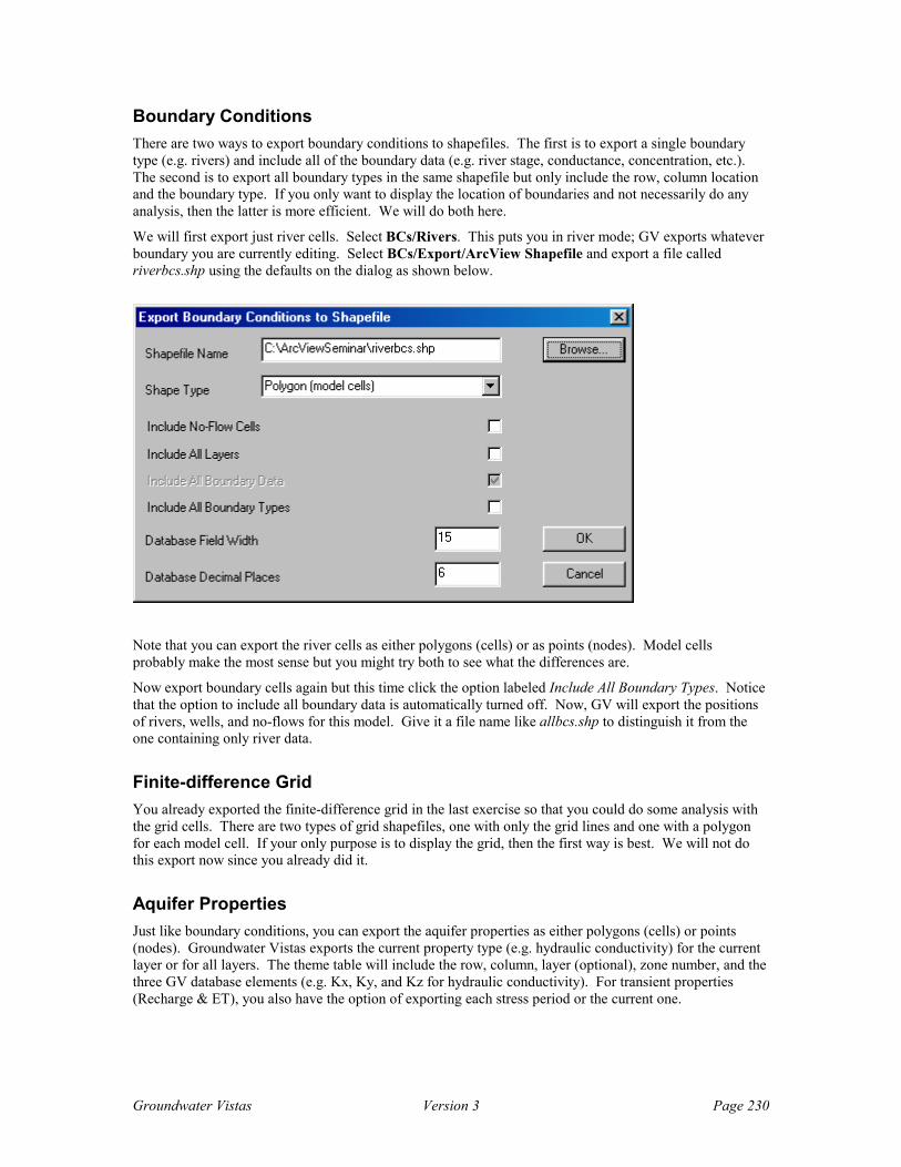
Groundwater Vistas Version 3 Page 230
Boundary Conditions There are two ways to export boundary conditions to shapefiles. The first is to export a single boundary type (e.g. rivers) and include all of the boundary data (e.g. river stage, conductance, concentration, etc.). The second is to export all boundary types in the same shapefile but only include the row, column location and the boundary type. If you only want to display the location of boundaries and not necessarily do any analysis, then the latter is more efficient. We will do both here.
We will first export just river cells. Select BCs/Rivers. This puts you in river mode; GV exports whatever boundary you are currently editing. Select BCs/Export/ArcView Shapefile and export a file called riverbcs.shp using the defaults on the dialog as shown below.
Note that you can export the river cells as either polygons (cells) or as points (nodes). Model cells probably make the most sense but you might try both to see what the differences are.
Now export boundary cells again but this time click the option labeled Include All Boundary Types. Notice that the option to include all boundary data is automatically turned off. Now, GV will export the positions of rivers, wells, and no-flows for this model. Give it a file name like allbcs.shp to distinguish it from the one containing only river data.
Finite-difference Grid You already exported the finite-difference grid in the last exercise so that you could do some analysis with the grid cells. There are two types of grid shapefiles, one with only the grid lines and one with a polygon for each model cell. If your only purpose is to display the grid, then the first way is best. We will not do this export now since you already did it.
Aquifer Properties Just like boundary conditions, you can export the aquifer properties as either polygons (cells) or points (nodes). Groundwater Vistas exports the current property type (e.g. hydraulic conductivity) for the current layer or for all layers. The theme table will include the row, column, layer (optional), zone number, and the three GV database elements (e.g. Kx, Ky, and Kz for hydraulic conductivity). For transient properties (Recharge & ET), you also have the option of exporting each stress period or the current one.

Groundwater Vistas Version 3 Page 231
In this example, select Props/Hydraulic Conductivity and then Props/Export/ArcView Shapefile. Enter a file name that makes sense and keep all the defaults. Note that you can export cells containing no-flow boundaries (inactive cells in MODFLOW) or not. In this case, just export the active cells.
That’s it for exporting shapefiles from Groundwater Vistas. You should now go back into your ArcView project and import these shapefiles. Instead of adding them to the current view you set up for the conceptual model, create a new view and load them into it along with the USGS topographic map. You should spend some time experimenting with the various ways of displaying this information in ArcView before moving on to the layout tools.
Creating Layouts in ArcView You should now have at least two views in your ArcView project, one for the conceptual model that was imported to Groundwater Vistas and another for the numerical model that was exported out of Groundwater Vistas. Close or minimize these views so you can see the project window. Click on Layouts and then click the Add button to create a new layout. Select Layout/Page Setup and choose landscape view. Your screen should look like the following.
The layout is basically a piece of paper where you place frames. A frame holds an ArcView document (e.g. views and charts), legends, north arrows, scale bars, etc. You decide which frame to add to the layout using the frame tool located at or near the right end of the toolbar. If you click the left mouse button on the frame tool and hold it down, you will see the following selections:

Groundwater Vistas Version 3 Page 232
These tools are used to enter (from top to bottom) views, legends, scale bars, north arrows, charts, tables, and graphics. Select the view frame tool and make sure the button is pushed down. Go to the layout and drag a window for the frame. After you are done dragging the frame, a dialog is displayed that prompts for what information will be displayed.
Choose the view that you would like to draw here and change the Display option to Always. You can also specify the scale here but the easiest thing to do is simply have the scale be automatic and the view fill the frame. The Live Link option means that if you subsequently do anything to the view it will be reflected in the layout. If you uncheck this option, the view will be displayed as it appears right now but subsequent changes to the view will not effect the layout. You should now have a layout page with one of your views, similar to the one below.
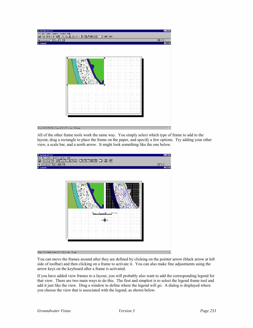
Groundwater Vistas Version 3 Page 233
All of the other frame tools work the same way. You simply select which type of frame to add to the layout, drag a rectangle to place the frame on the paper, and specify a few options. Try adding your other view, a scale bar, and a north arrow. It might look something like the one below.
You can move the frames around after they are defined by clicking on the pointer arrow (black arrow at left side of toolbar) and then clicking on a frame to activate it. You can also make fine adjustments using the arrow keys on the keyboard after a frame is activated.
If you have added view frames to a layout, you will probably also want to add the corresponding legend for that view. There are two main ways to do this. The first and simplest is to select the legend frame tool and add it just like the view. Drag a window to define where the legend will go. A dialog is displayed where you choose the view that is associated with the legend, as shown below.
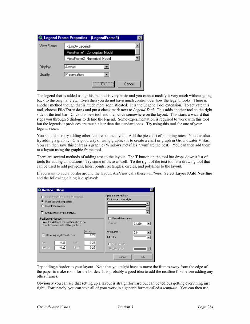
Groundwater Vistas Version 3 Page 234
The legend that is added using this method is very basic and you cannot modify it very much without going back to the original view. Even then you do not have much control over how the legend looks. There is another method though that is much more sophisticated. It is the Legend Tool extension. To activate this tool, choose File/Extensions and put a check mark next to Legend Tool. This adds another tool to the right side of the tool bar. Click this new tool and then click somewhere on the layout. This starts a wizard that steps you through 5 dialogs to define the legend. Some experimentation is required to work with this tool but the legends it produces are much nicer than the standard ones. Try using this tool for one of your legend views.
You should also try adding other features to the layout. Add the pie chart of pumping rates. You can also try adding a graphic. One good way of using graphics is to create a chart or graph in Groundwater Vistas. You can then save this chart as a graphic (Windows metafiles *.wmf are the best). You can then add them to a layout using the graphic frame tool.
There are several methods of adding text to the layout. The T button on the tool bar drops down a list of tools for adding annotations. Try some of these as well. To the right of the text tool is a drawing tool that can be used to add polygons, lines, points, rectangles, circles, and polylines to the layout.
If you want to add a border around the layout, ArcView calls these neatlines. Select Layout/Add Neatline and the following dialog is displayed:
Try adding a border to your layout. Note that you might have to move the frames away from the edge of the paper to make room for the border. It is probably a good idea to add the neatline first before adding any other frames.
Obviously you can see that setting up a layout is straightforward but can be tedious getting everything just right. Fortunately, you can save all of your work in a generic format called a template. You can then use
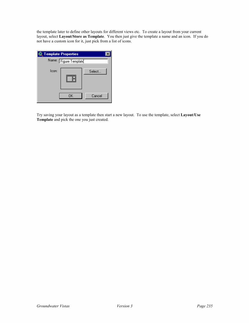
Groundwater Vistas Version 3 Page 235
the template later to define other layouts for different views etc. To create a layout from your current layout, select Layout/Store as Template. You then just give the template a name and an icon. If you do not have a custom icon for it, just pick from a list of icons.
Try saving your layout as a template then start a new layout. To use the template, select Layout/Use Template and pick the one you just created.

Groundwater Vistas Version 3 Page 236

Groundwater Vistas Version 3 Page 237
Digitized Maps
Digitized Map File Format Digitized base maps increase the efficiency of site-specific modeling by placing the modeling results in context with the area to be modeled. As shown in the tutorial, GV overlays the base map on head contours and streamlines, making it easier to interpret the results.
GV uses a very simple file format for the digitized base map, as shown in Table 1. The file is made up of two sections. The first defines a series of line segments, while the second set of data defines a series of text strings. Each line segment requires the following data (1) the beginning and ending X and Y coordinates, (2) the line style, e.g., dashed or solid, and (3) the line color. The data for each line segment should appear on one line and be separated by at least one space between each data item. Commas may not be used to separate data items.
The following data items are required for each text item (1) X and Y coordinates of the lower left corner of the text, (2) angle of rotation of the text string, (3) height of the text, (4) color, and (5) a text string. The first four data items are entered on one line separated by at least one space between each data item. The text string is located on the following line and the height of the text string is in map coordinates (not in inches!).
Line and text colors are defined as integer numbers from 0 through 15. Each integer defines a unique color. The possible colors are shown in Table 2. These colors are all displayed on VGA color displays.
The digitized map file is a simple ASCII file that may be created in any text editor. You may also find it advantageous to write a simple program to convert files from your digitizing software to the GV format. GV also has the ability to convert DXF files directly. Simply choose File from the main menu and Map from the pull-down menu. Next select DXF from the menu. Specify the DXF file name and a conversion factor, which is explained below. The DXF file format is a relatively standard file format for CAD packages, such as AutoCad.

Groundwater Vistas Version 3 Page 238
Table 1 File Format for Digitized Maps.
Line 1 NLS, NTEXT NLS = Number of line segments in map NTEXT = Number of Text Strings in map Lines 2 to NLS+1 (Enter one line for each line segment) X1, Y1, X2, Y2, NDASH, NCOLOR X1, Y1 = Beginning line coordinates X2, Y2 = Ending line coordinates NDASH = Positive integer for solid line, negative for dashed NCOLOR = Color index (integer) Lines NLS+2 to end (Enter one set per text item) X1, Y1, ANGLE, HEIGHT, NCOLOR TEXT X1, Y1 = Coordinates of left side of text string ANGLE = Angle of text string HEIGHT = Height of text string NCOLOR = Color index of text string TEXT = Text string
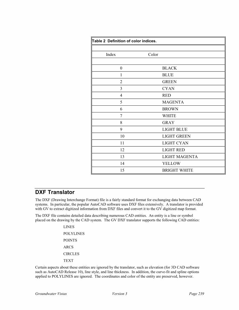
Groundwater Vistas Version 3 Page 239
Table 2 Definition of color indices.
Index Color 0 BLACK 1 BLUE 2 GREEN 3 CYAN 4 RED 5 MAGENTA 6 BROWN 7 WHITE 8 GRAY 9 LIGHT BLUE 10 LIGHT GREEN 11 LIGHT CYAN 12 LIGHT RED 13 LIGHT MAGENTA 14 YELLOW 15 BRIGHT WHITE
DXF Translator The DXF (Drawing Interchange Format) file is a fairly standard format for exchanging data between CAD systems. In particular, the popular AutoCAD software uses DXF files extensively. A translator is provided with GV to extract digitized information from DXF files and convert it to the GV digitized map format.
The DXF file contains detailed data describing numerous CAD entities. An entity is a line or symbol placed on the drawing by the CAD system. The GV DXF translator supports the following CAD entities:
LINES
POLYLINES
POINTS
ARCS
CIRCLES
TEXT
Certain aspects about these entities are ignored by the translator, such as elevation (for 3D CAD software such as AutoCAD Release 10), line style, and line thickness. In addition, the curve-fit and spline options applied to POLYLINES are ignored. The coordinates and color of the entity are preserved, however.
Groundwater Vistas Version 3 Page 240
Many CAD drawings contain entities called BLOCKS, which are a collection of other entities (e.g., lines, circles, text, etc.). GV will not interpret BLOCKS properly, so make sure that these are converted to other entities before creating the DXF file in your CAD package. In AutoCAD terminology, this is called “exploding” the blocks.
The DXF translator is activated from the File menu, as described above. Next, specify the DXF file name and a Map file name using standard Windows file dialogs. You only have to answer one additional prompt after starting the DXF translator -- a conversion factor for the translation. Normally, a conversion factor of 1.0 will work; however, sometimes your CAD software will store coordinates in the DXF file in units of inches. If this happens, use a conversion factor of 0.0833333 (1.0/12.0). Each coordinate in the DXF file is multiplied by the conversion factor before being written to the GV map file.
After all entities are processed in the DXF file, the digitized map file is created. A message to that effect is displayed at the bottom of the screen. After the translation is finished, the map file is imported into the model and displayed on your screen.

Groundwater Vistas Version 3 Page 241
References
Introduction The following are papers, books, and other publications referenced in the Groundwater Vistas manual.
References
Anderson, M.P. and W.W. Woessner, 1992, Applied Groundwater Modeling: Simulation of Flow and Advective Transport, Academic Press, Inc., New York, 381 pp.
Franke, O.L. and T.E. Reilly, 1987, The effects of boundary conditions on the steady-state response of three hypothetical ground-water systems - results and implications of numerical experiments, U.S. Geological Survey Water Supply Paper 2315, 19 pp.
Franke, O.L., T.E. Reilly, and G.D. Bennett, 1987, Definition of boundary and initial conditions in the analysis of saturated ground-water flow systems - an introduction, U.S. Geological Survey, Techniques of Water Resources Investigations, Book 3, Chapter B5, 15 pp.
Goode, D.J. and L.F. Konikow, 1989, Modification of a method-of-characteristics solute transport model to incorporate decay and equilibrium-controlled sorption or ion exchange, USGS WRI Report 89-4030, 65 pp.
Hill, M.C., 1992, A computer program (MODFLOWP) for estimating parameters of a transient, three-dimensional, ground-water flow model using nonlinear regression, USGS Open File Report 91-484, 358 pp.
Konikow, L.F. and J.D. Bredehoeft, 1978, Computer model of two-dimensional solute transport and dispersion in ground water, USGS TWRI, Chapter C2, Book 7, 89 pp.
Kuiper, L.K., 1987, Computer program for solving ground-water flow equations by the preconditioned conjugate gradient method, USGS WRI Report 87-4091, 33 pp.
McDonald, M.G. and A.W. Harbaugh, 1988, A modular three-dimensional finite-difference ground-water flow model, USGS TWRI Chapter 6-A1, 586 pp.
McDonald, M.G., A.W. Harbaugh, B.R. Orr, and D.J. Ackerman, 1991, A method of converting no-flow cells to variable-head cells for the USGS modular, finite-difference ground-water flow model, USGS Open File Report 91-536, 99 pp.

Groundwater Vistas Version 3 Page 242
Pollock, D.W., 1989, Documentation of computer programs to compute and display pathlines using results from the U.S. Geological Survey modular three-dimensional finite-difference ground-water flow model, USGS Open File Report 89-391, 188 pp.
Prudic, D.E., 1989, Documentation of a computer program to simulate stream-aquifer relations using a modular, finite-difference ground-water flow model, USGS Open-File Report 88-729, 113 pp.
Rumbaugh, J.O. and L.L. Ruskauff, 1993, Geraghty & Miller Modeling Survey: Analysis of May 1992 Survey Results, Geraghty & Miller, Inc., Reston, Virginia, 20 pp.
Zheng, C., 1989, PATH3D: A ground-water path and travel-time simulator, S.S. Papadopulos & Associates, Inc., Rockville, Maryland,
Zheng, C., 1990, MT3D: A modular three-dimensional transport model for simulation of advection, dispersion and chemical reactions of contaminants in ground-water systems, U.S. EPA, R.S. Kerr Environmental Research Laboratory, Ada, Oklahoma.