Table of Contents Preface PLCs in a glance 07

Basic PLC Operation 07 1- Processor Operating Cycle 07 2- Input modules 08

3- Output modules 08 4- Programming device 08 Ladder Diagrams 09

Hard-wired Control 10

Replacing hard-wired control with a PLC 11

The advantage of using a PLC as a controller 11

Different PLC models made by Siemens 12

1- SIMATIC S5 12

2-SIMATIC S7 12

3-LOGO! 13

MicroLogix 1500 PLC 13

Number system – decimal & binary 14

Logic 0, Logic 1 15

Actuator 16

Discrete Inputs 16 Analog Inputs 18

Discrete Outputs 18 Analog outputs 18 CPU (Central Processing Unit) 19

Programming Languages 19 Ladder Logic programming 20

Reading Ladder Logic Diagrams 21

Function Block Diagrams (FBD) 22

Hardware 23

PLC memory size 23 1- RAM/ ROM / EPROM / Firmware 23

2- Memory structure 24 3- Program space 24 4- Data space 24 Software 25

Cables 26

S7-200 & A-B MicroLogix 1500 PLCs 26 PLC models 27

Optional cartridge 28

Expansion modules 28 Understanding Controller Status indicators 28 Using a DIN rail to Install PLC and Expansion units 29

External power supplies 30 I/O numbering 31

Inputs / Outputs 32

Super Capacitor 32

PLC Display and HMI units 32 Siemens TD200 33

Computer network 33 PROFIBUS connection 33

Powerful AS-Interface connection 33

Contact & coil symbols (Ladder format) 34

Input/Output & contact programming examples 36

Functions mostly used in PLC programming 38

1- AND function 38 2- OR function 39

3- Latch function 40

4- Inverse function 40

FBD (Function Block Diagram) programming language 41

STL (Statement List) programming language 41

Normally Open (NO) & Closed Contacts (NC) 42

Boolean Algebra PLC programming 43

Status Function 45

Force Function 46

Sequence 47 3 phase motor starter program 48

Wiring motor Starter circuit with PLC 50

Expanding the previous problem 51 Introduction to Analog signals 53 Analog Output signals 54

Introduction to A-B & Siemens S7-200 Timers 55

Hard-wired time Delay relay 56 A-B MicroLogix 1500 & SIMATIC S7-200 Timers 56

1-Timer On-Delay (TON) 56 2- Timer Off-Delay (TOF) 56 3- Timer Retentive On-Delay Timer (RTO) 56 An On-Delay timer programming examples & application 57 A-B Off-Delay timer 57 An Off-Delay (TOF) application example 58 A-B Retentive On-Delay Timer programming 59 SIEMENS SIMATIC S7-200 timers 60

1- SIMATIC On-Delay timer application example 61

2-How to calculate PT? 61

3- S7-200 Off-Delay timer (ladder Logic symbol and functions) 61

4- S7-200 Retentive On-Delay timer (ladder Logic symbol and functions) 62 A-B SLC & Siemens S7-200 Counters 63

1-Up-counter (CTU) definition, symbol & an application example 64 2- Down-counter (CTD) definition and symbol& and application example 66 SIEMENS SIMATIC S7-200 Counters 66

1-Regular Counters 66 A- CTUD ~ Count Up/Down counter 66 B-CTU ~ Count Up counter 66 C- CTD ~ Count Down counter 66 2- High-Speed Counters 66 Sample problem 68 Pulse Train Output (PTO) function 69

Pulse Width Modulation (PWM) function 70

Transmit function 71

Introduction to Network Communication 72

AS-Interface (AS-i) the Actuator Sensor Interface 72

2

PLCs in a glance

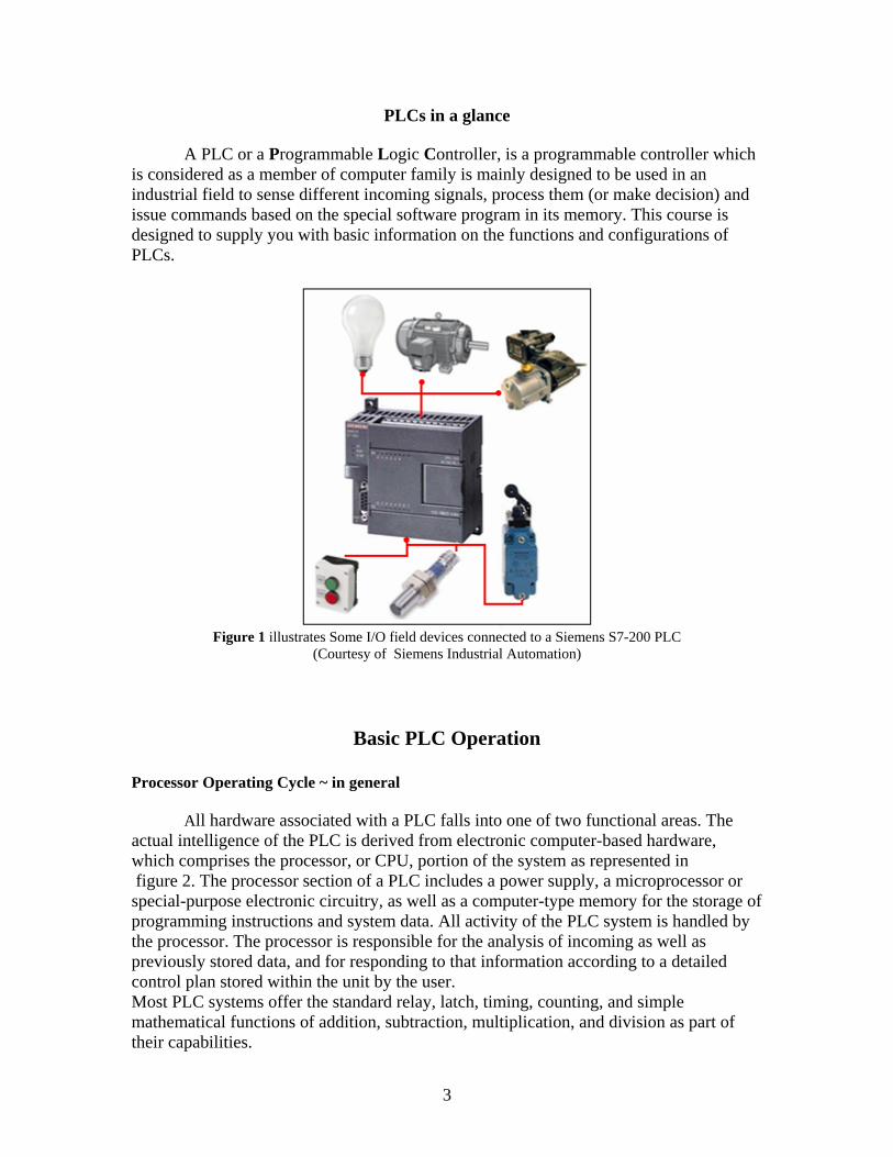
A PLC or a Programmable Logic Controller, is a programmable controller which is considered as a member of computer family is mainly designed to be used in an industrial field to sense different incoming signals, process them (or make decision) and issue commands based on the special software program in its memory. This course is designed to supply you with basic information on the functions and configurations of PLCs.

Figure 1 illustrates Some I/O field devices connected to a Siemens S7-200 PLC

(Courtesy of Siemens Industrial Automation)

Basic PLC Operation

Processor Operating Cycle ~ in general

All hardware associated with a PLC falls into one of two functional areas. The actual intelligence of the PLC is derived from electronic computer-based hardware, which comprises the processor, or CPU, portion of the system as represented in figure 2. The processor section of a PLC includes a power supply, a microprocessor or special-purpose electronic circuitry, as well as a computer-type memory for the storage of programming instructions and system data. All activity of the PLC system is handled by the processor. The processor is responsible for the analysis of incoming as well as previously stored data, and for responding to that information according to a detailed control plan stored within the unit by the user. Most PLC systems offer the standard relay, latch, timing, counting, and simple mathematical functions of addition, subtraction, multiplication, and division as part of their capabilities.

3

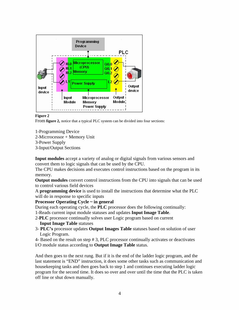
Figure 2 From figure 2, notice that a typical PLC system can be divided into four sections: 1-Programming Device 2-Micrrocessor + Memory Unit 3-Power Supply 3-Input/Output Sections Input modules accept a variety of analog or digital signals from various sensors and convert them to logic signals that can be used by the CPU. The CPU makes decisions and executes control instructions based on the program in its memory. Output modules convert control instructions from the CPU into signals that can be used to control various field devices A programming device is used to install the instructions that determine what the PLC will do in response to specific inputs Processor Operating Cycle ~ in general During each operating cycle, the PLC processor does the following continually: 1-Reads current input module statuses and updates Input Image Table. 2-PLC processor continually solves user Logic program based on current Input Image Table statuses 3- PLC’s processor updates Output Images Table statuses based on solution of user Logic Program. 4- Based on the result on step # 3, PLC processor continually activates or deactivates I/O module status according to Output Image Table status. And then goes to the next rung. But if it is the end of the ladder logic program, and the last statement is “END” instruction, it does some other tasks such as communication and housekeeping tasks and then goes back to step 1 and continues executing ladder logic program for the second time. It does so over and over until the time that the PLC is taken off line or shut down manually.

4

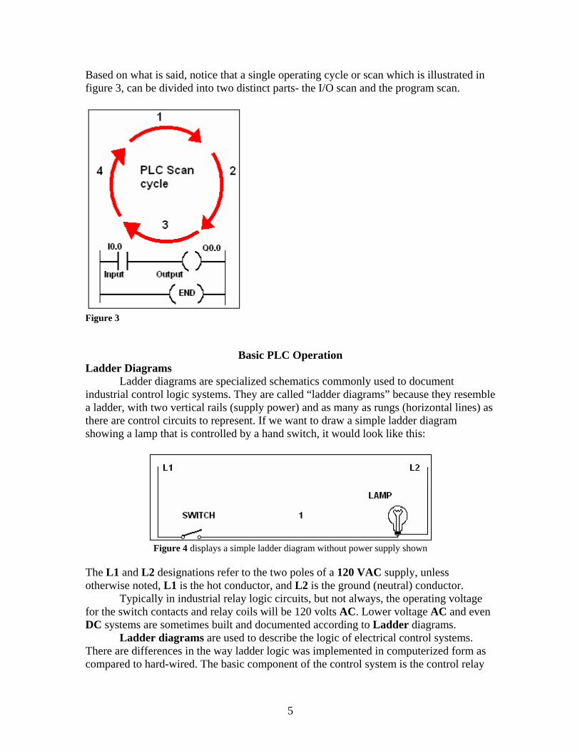
Based on what is said, notice that a single operating cycle or scan which is illustrated in figure 3, can be divided into two distinct parts- the I/O scan and the program scan.

Figure 3

Basic PLC Operation Ladder Diagrams

Ladder diagrams are specialized schematics commonly used to document industrial control logic systems. They are called “ladder diagrams” because they resemble a ladder, with two vertical rails (supply power) and as many as rungs (horizontal lines) as there are control circuits to represent. If we want to draw a simple ladder diagram showing a lamp that is controlled by a hand switch, it would look like this:

Figure 4 displays a simple ladder diagram without power supply shown

The L1 and L2 designations refer to the two poles of a 120 VAC supply, unless otherwise noted, L1 is the hot conductor, and L2 is the ground (neutral) conductor.

Typically in industrial relay logic circuits, but not always, the operating voltage for the switch contacts and relay coils will be 120 volts AC. Lower voltage AC and even DC systems are sometimes built and documented according to Ladder diagrams.

Ladder diagrams are used to describe the logic of electrical control systems. There are differences in the way ladder logic was implemented in computerized form as compared to hard-wired. The basic component of the control system is the control relay

5

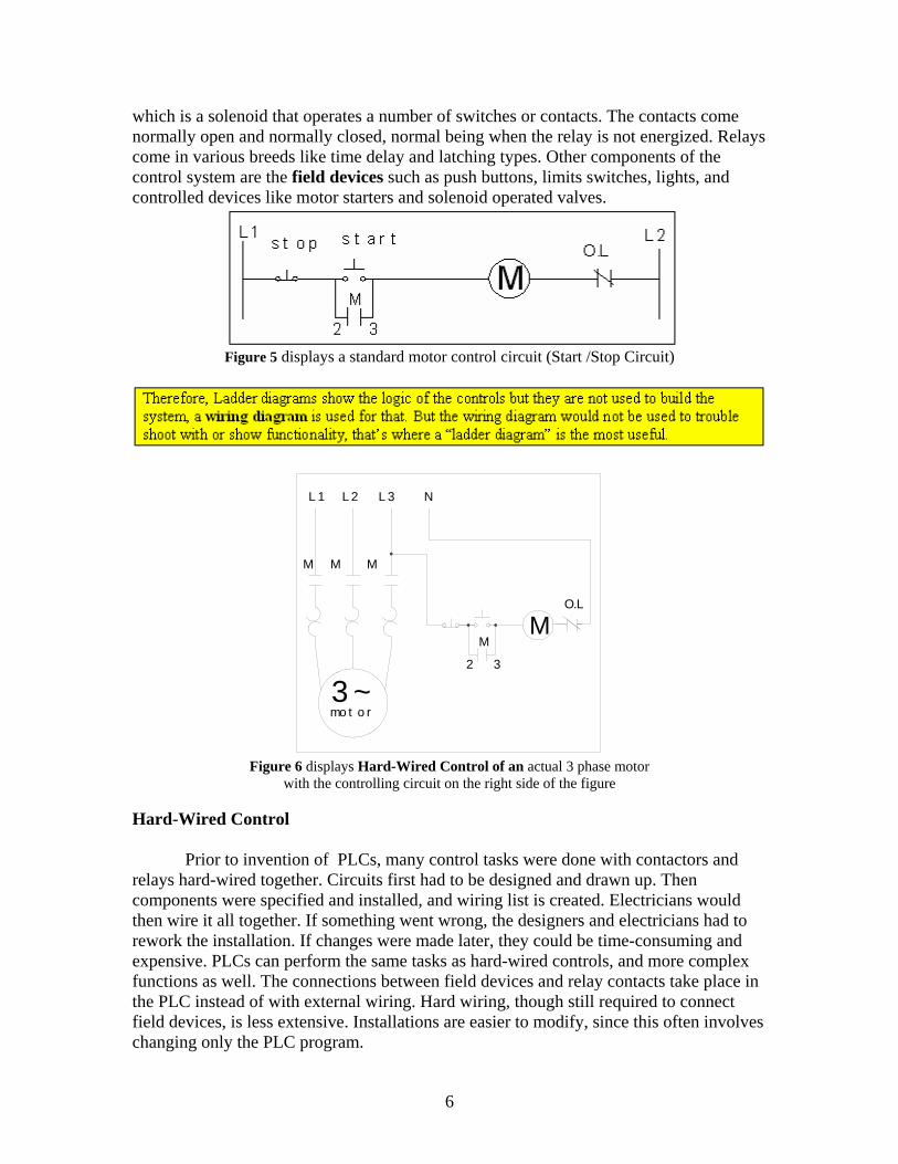
which is a solenoid that operates a number of switches or contacts. The contacts come normally open and normally closed, normal being when the relay is not energized. Relays come in various breeds like time delay and latching types. Other components of the control system are the field devices such as push buttons, limits switches, lights, and controlled devices like motor starters and solenoid operated valves.

Figure 5 displays a standard motor control circuit (Start /Stop Circuit)

O.L

MM

2 3

3 ~mo t o r

L 1 L 2 L 3 N

M M M

Figure 6 displays Hard-Wired Control of an actual 3 phase motor

with the controlling circuit on the right side of the figure Hard-Wired Control

Prior to invention of PLCs, many control tasks were done with contactors and relays hard-wired together. Circuits first had to be designed and drawn up. Then components were specified and installed, and wiring list is created. Electricians would then wire it all together. If something went wrong, the designers and electricians had to rework the installation. If changes were made later, they could be time-consuming and expensive. PLCs can perform the same tasks as hard-wired controls, and more complex functions as well. The connections between field devices and relay contacts take place in the PLC instead of with external wiring. Hard wiring, though still required to connect field devices, is less extensive. Installations are easier to modify, since this often involves changing only the PLC program.

6

Replacing hard-wired control with a PLC

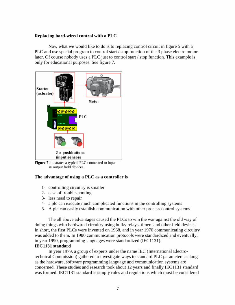
Now what we would like to do is to replacing control circuit in figure 5 with a PLC and use special program to control start / stop function of the 3 phase electro motor later. Of course nobody uses a PLC just to control start / stop function. This example is only for educational purposes. See figure 7.

Figure 7 illustrates a typical PLC connected to input & output field devices. The advantage of using a PLC as a controller is

1- controlling circuitry is smaller 2- ease of troubleshooting 3- less need to repair 4- a plc can execute much complicated functions in the controlling systems 5- A plc can easily establish communication with other process control systems The all above advantages caused the PLCs to win the war against the old way of

doing things with hardwired circuitry using bulky relays, timers and other field devices. In short, the first PLCs were invented on 1968, and in year 1970 communicating circuitry was added to them. In 1980 communication protocols were standardized and eventually, in year 1990, programming languages were standardized (IEC1131). IEC1131 standard

In year 1979, a group of experts under the name IEC (International Electro-technical Commission) gathered to investigate ways to standard PLC parameters as long as the hardware, software programming language and communication systems are concerned. These studies and research took about 12 years and finally IEC1131 standard was formed. IEC1131 standard is simply rules and regulations which must be considered

7

by PLC manufactures and cover different aspects of PLCs. IEC1131 suggests the specifications set forward as long as the hardware design, programming language, troubleshooting of hardware, installation and testing is concerned. Different PLC models made by Siemens

Siemens categorizes its range of PLCs under the name SIMATIC ®. Some of these PLCs are built in Compact form meaning the PLC box contains power supply, CPU, input and output models. All these different part are located in plc box and considered as a unit. On the other hand, the second model of PLC is built in Modular form. In this form of application, the end user can choose which model he needs for his particular need. SIMATIC S5

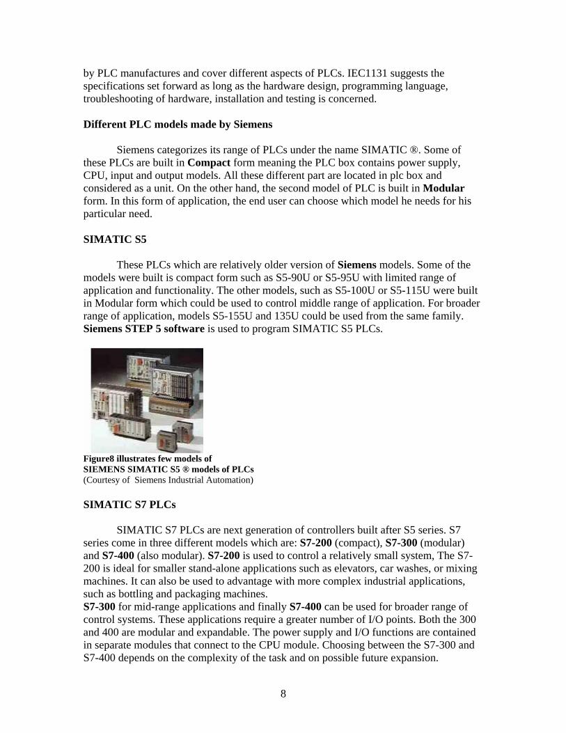
These PLCs which are relatively older version of Siemens models. Some of the models were built is compact form such as S5-90U or S5-95U with limited range of application and functionality. The other models, such as S5-100U or S5-115U were built in Modular form which could be used to control middle range of application. For broader range of application, models S5-155U and 135U could be used from the same family. Siemens STEP 5 software is used to program SIMATIC S5 PLCs.

Figure8 illustrates few models of SIEMENS SIMATIC S5 ® models of PLCs (Courtesy of Siemens Industrial Automation) SIMATIC S7 PLCs

SIMATIC S7 PLCs are next generation of controllers built after S5 series. S7 series come in three different models which are: S7-200 (compact), S7-300 (modular) and S7-400 (also modular). S7-200 is used to control a relatively small system, The S7-200 is ideal for smaller stand-alone applications such as elevators, car washes, or mixing machines. It can also be used to advantage with more complex industrial applications, such as bottling and packaging machines. S7-300 for mid-range applications and finally S7-400 can be used for broader range of control systems. These applications require a greater number of I/O points. Both the 300 and 400 are modular and expandable. The power supply and I/O functions are contained in separate modules that connect to the CPU module. Choosing between the S7-300 and S7-400 depends on the complexity of the task and on possible future expansion.

8

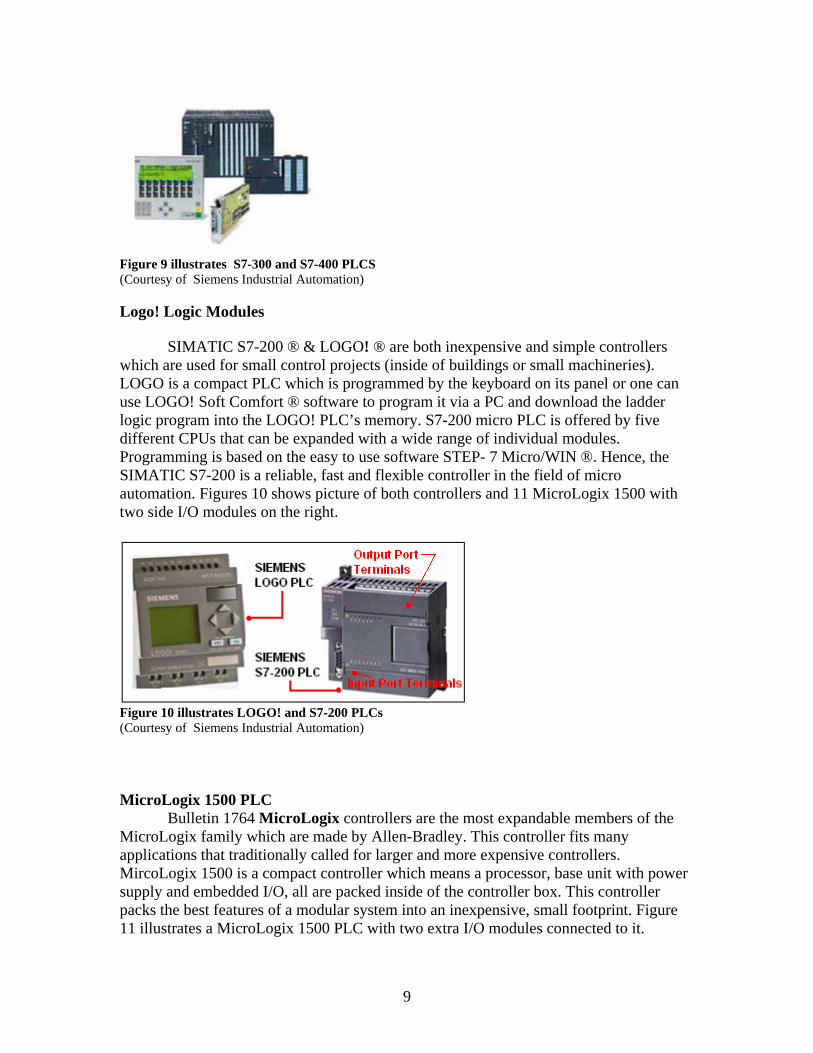
Figure 9 illustrates S7-300 and S7-400 PLCS (Courtesy of Siemens Industrial Automation) Logo! Logic Modules

SIMATIC S7-200 ® & LOGO! ® are both inexpensive and simple controllers which are used for small control projects (inside of buildings or small machineries). LOGO is a compact PLC which is programmed by the keyboard on its panel or one can use LOGO! Soft Comfort ® software to program it via a PC and download the ladder logic program into the LOGO! PLC’s memory. S7-200 micro PLC is offered by five different CPUs that can be expanded with a wide range of individual modules. Programming is based on the easy to use software STEP- 7 Micro/WIN ®. Hence, the SIMATIC S7-200 is a reliable, fast and flexible controller in the field of micro automation. Figures 10 shows picture of both controllers and 11 MicroLogix 1500 with two side I/O modules on the right.

Figure 10 illustrates LOGO! and S7-200 PLCs (Courtesy of Siemens Industrial Automation) MicroLogix 1500 PLC

Bulletin 1764 MicroLogix controllers are the most expandable members of the MicroLogix family which are made by Allen-Bradley. This controller fits many applications that traditionally called for larger and more expensive controllers. MircoLogix 1500 is a compact controller which means a processor, base unit with power supply and embedded I/O, all are packed inside of the controller box. This controller packs the best features of a modular system into an inexpensive, small footprint. Figure 11 illustrates a MicroLogix 1500 PLC with two extra I/O modules connected to it.

9

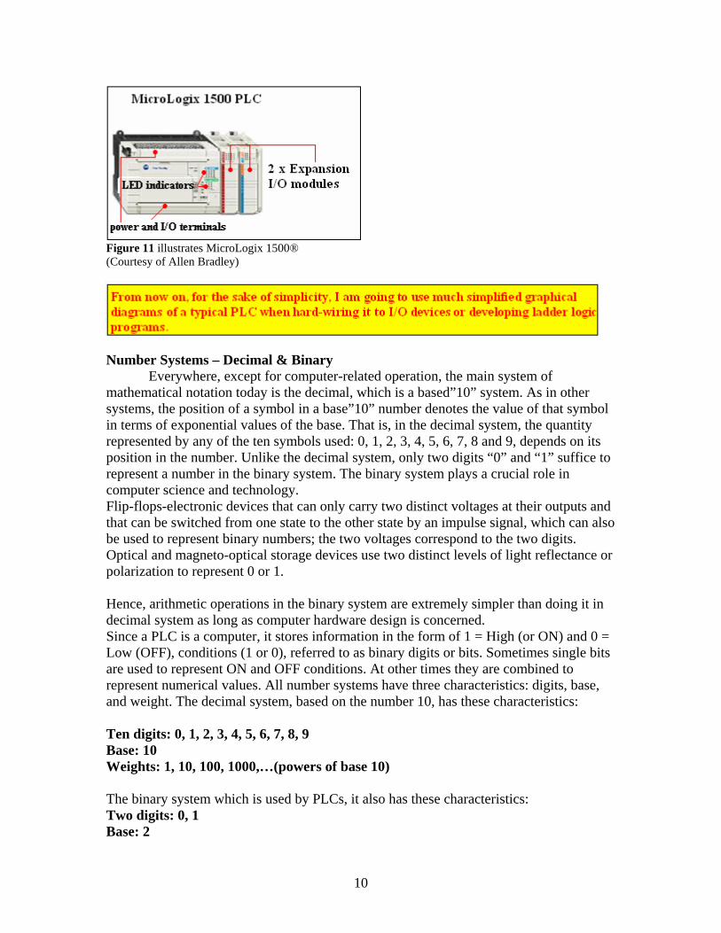
Figure 11 illustrates MicroLogix 1500® (Courtesy of Allen Bradley)

Number Systems – Decimal & Binary Everywhere, except for computer-related operation, the main system of mathematical notation today is the decimal, which is a based”10” system. As in other systems, the position of a symbol in a base”10” number denotes the value of that symbol in terms of exponential values of the base. That is, in the decimal system, the quantity represented by any of the ten symbols used: 0, 1, 2, 3, 4, 5, 6, 7, 8 and 9, depends on its position in the number. Unlike the decimal system, only two digits “0” and “1” suffice to represent a number in the binary system. The binary system plays a crucial role in computer science and technology. Flip-flops-electronic devices that can only carry two distinct voltages at their outputs and that can be switched from one state to the other state by an impulse signal, which can also be used to represent binary numbers; the two voltages correspond to the two digits. Optical and magneto-optical storage devices use two distinct levels of light reflectance or polarization to represent 0 or 1. Hence, arithmetic operations in the binary system are extremely simpler than doing it in decimal system as long as computer hardware design is concerned. Since a PLC is a computer, it stores information in the form of 1 = High (or ON) and 0 = Low (OFF), conditions (1 or 0), referred to as binary digits or bits. Sometimes single bits are used to represent ON and OFF conditions. At other times they are combined to represent numerical values. All number systems have three characteristics: digits, base, and weight. The decimal system, based on the number 10, has these characteristics: Ten digits: 0, 1, 2, 3, 4, 5, 6, 7, 8, 9 Base: 10 Weights: 1, 10, 100, 1000,…(powers of base 10) The binary system which is used by PLCs, it also has these characteristics: Two digits: 0, 1 Base: 2

10

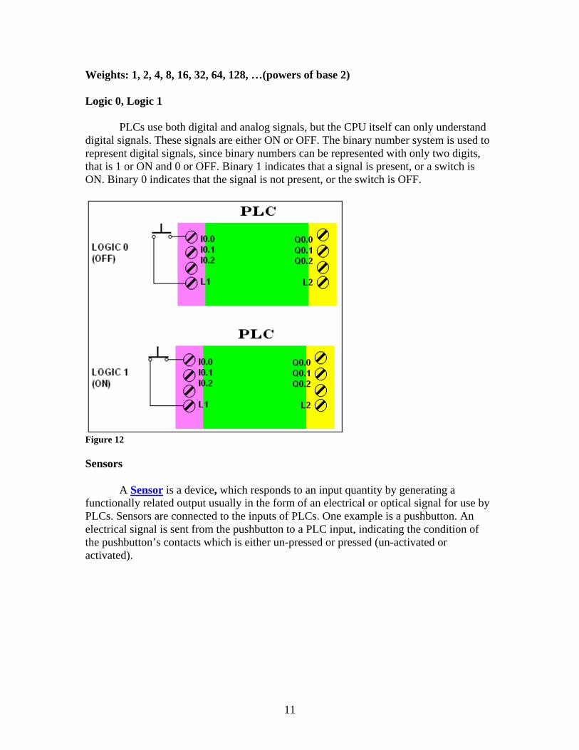
Weights: 1, 2, 4, 8, 16, 32, 64, 128, …(powers of base 2) Logic 0, Logic 1 PLCs use both digital and analog signals, but the CPU itself can only understand digital signals. These signals are either ON or OFF. The binary number system is used to represent digital signals, since binary numbers can be represented with only two digits, that is 1 or ON and 0 or OFF. Binary 1 indicates that a signal is present, or a switch is ON. Binary 0 indicates that the signal is not present, or the switch is OFF.

Figure 12 Sensors

A Sensor is a device, which responds to an input quantity by generating a functionally related output usually in the form of an electrical or optical signal for use by PLCs. Sensors are connected to the inputs of PLCs. One example is a pushbutton. An electrical signal is sent from the pushbutton to a PLC input, indicating the condition of the pushbutton’s contacts which is either un-pressed or pressed (un-activated or activated).

11

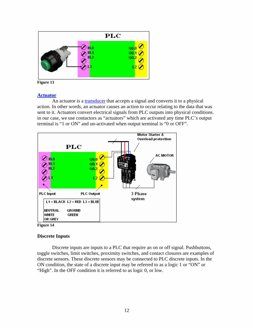
Figure 13

Actuator An actuator is a transducer that accepts a signal and converts it to a physical action. In other words, an actuator causes an action to occur relating to the data that was sent to it. Actuators convert electrical signals from PLC outputs into physical conditions. in our case, we use contactors as “actuators” which are activated any time PLC’s output terminal is “1 or ON” and un-activated when output terminal is “0 or OFF”.

Figure 14 Discrete Inputs Discrete inputs are inputs to a PLC that require an on or off signal. Pushbuttons, toggle switches, limit switches, proximity switches, and contact closures are examples of discrete sensors. These discrete sensors may be connected to PLC discrete inputs. In the ON condition, the state of a discrete input may be referred to as a logic 1 or “ON” or “High”. In the OFF condition it is referred to as logic 0, or low.

12

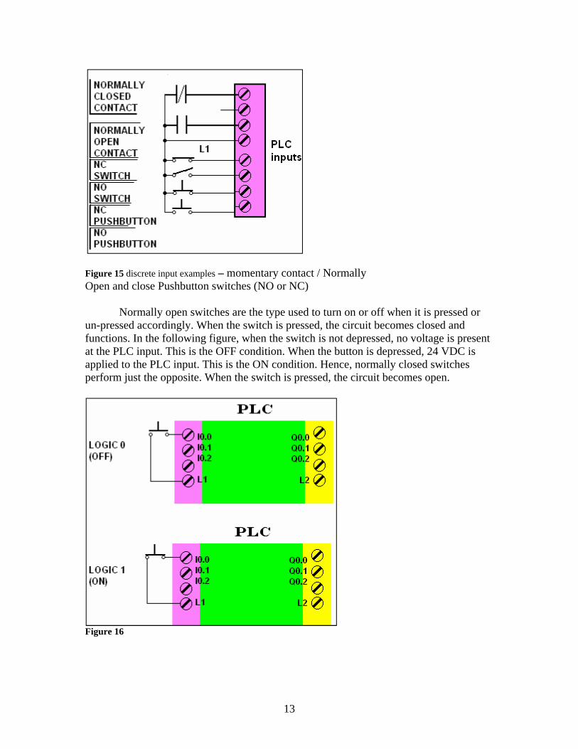
Figure 15 discrete input examples – momentary contact / Normally Open and close Pushbutton switches (NO or NC) Normally open switches are the type used to turn on or off when it is pressed or un-pressed accordingly. When the switch is pressed, the circuit becomes closed and functions. In the following figure, when the switch is not depressed, no voltage is present at the PLC input. This is the OFF condition. When the button is depressed, 24 VDC is applied to the PLC input. This is the ON condition. Hence, normally closed switches perform just the opposite. When the switch is pressed, the circuit becomes open.

Figure 16

13

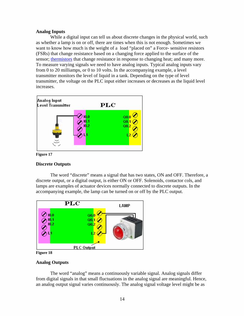
Analog Inputs While a digital input can tell us about discrete changes in the physical world, such

as whether a lamp is on or off, there are times when this is not enough. Sometimes we want to know how much is the weight of a load “placed on” a Force- sensitive resistors (FSRs) that change resistance based on a changing force applied to the surface of the sensor; thermistors that change resistance in response to changing heat; and many more. To measure varying signals we need to have analog inputs. Typical analog inputs vary from 0 to 20 milliamps, or 0 to 10 volts. In the accompanying example, a level transmitter monitors the level of liquid in a tank. Depending on the type of level transmitter, the voltage on the PLC input either increases or decreases as the liquid level increases.

Figure 17 Discrete Outputs

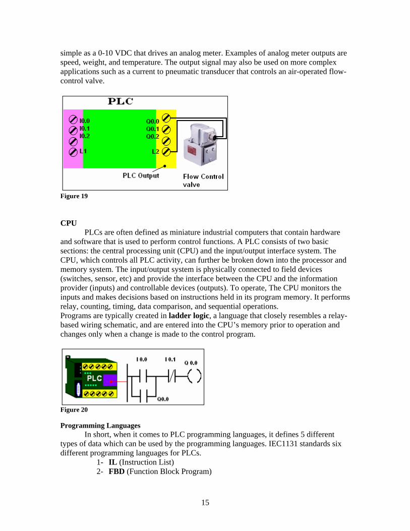
The word “discrete” means a signal that has two states, ON and OFF. Therefore, a discrete output, or a digital output, is either ON or OFF. Solenoids, contactor cols, and lamps are examples of actuator devices normally connected to discrete outputs. In the accompanying example, the lamp can be turned on or off by the PLC output.

Figure 18 Analog Outputs

The word “analog” means a continuously variable signal. Analog signals differ from digital signals in that small fluctuations in the analog signal are meaningful. Hence, an analog output signal varies continuously. The analog signal voltage level might be as

14

simple as a 0-10 VDC that drives an analog meter. Examples of analog meter outputs are speed, weight, and temperature. The output signal may also be used on more complex applications such as a current to pneumatic transducer that controls an air-operated flow-control valve.

Figure 19 CPU

PLCs are often defined as miniature industrial computers that contain hardware and software that is used to perform control functions. A PLC consists of two basic sections: the central processing unit (CPU) and the input/output interface system. The CPU, which controls all PLC activity, can further be broken down into the processor and memory system. The input/output system is physically connected to field devices (switches, sensor, etc) and provide the interface between the CPU and the information provider (inputs) and controllable devices (outputs). To operate, The CPU monitors the inputs and makes decisions based on instructions held in its program memory. It performs relay, counting, timing, data comparison, and sequential operations. Programs are typically created in ladder logic, a language that closely resembles a relay-based wiring schematic, and are entered into the CPU’s memory prior to operation and changes only when a change is made to the control program.

Figure 20 Programming Languages

In short, when it comes to PLC programming languages, it defines 5 different types of data which can be used by the programming languages. IEC1131 standards six different programming languages for PLCs.

1- IL (Instruction List) 2- FBD (Function Block Program)

15

3- LD (Ladder Diagram) 4- ST (Structured Text) 5- SFC (Sequential Function Control) 6- CFC (Continuous Function Chart)

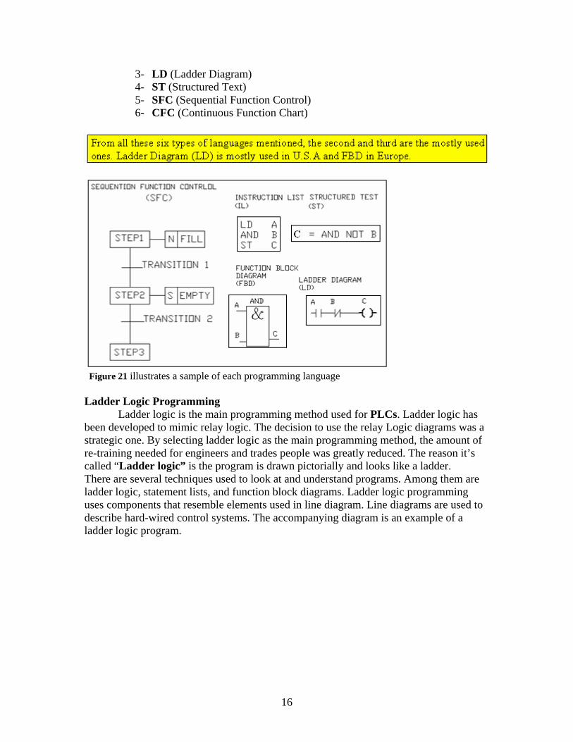
Figure 21 illustrates a sample of each programming language Ladder Logic Programming Ladder logic is the main programming method used for PLCs. Ladder logic has been developed to mimic relay logic. The decision to use the relay Logic diagrams was a strategic one. By selecting ladder logic as the main programming method, the amount of re-training needed for engineers and trades people was greatly reduced. The reason it’s called “Ladder logic” is the program is drawn pictorially and looks like a ladder. There are several techniques used to look at and understand programs. Among them are ladder logic, statement lists, and function block diagrams. Ladder logic programming uses components that resemble elements used in line diagram. Line diagrams are used to describe hard-wired control systems. The accompanying diagram is an example of a ladder logic program.

16

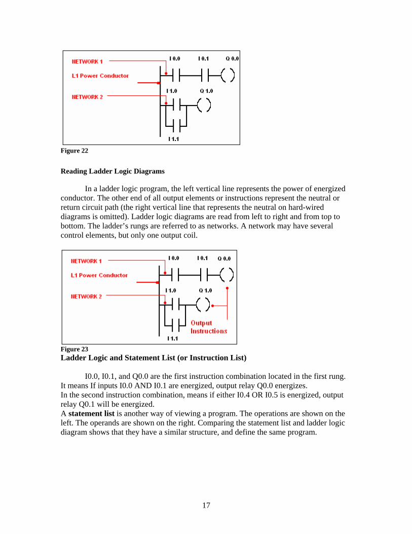
Figure 22

Reading Ladder Logic Diagrams

In a ladder logic program, the left vertical line represents the power of energized conductor. The other end of all output elements or instructions represent the neutral or return circuit path (the right vertical line that represents the neutral on hard-wired diagrams is omitted). Ladder logic diagrams are read from left to right and from top to bottom. The ladder’s rungs are referred to as networks. A network may have several control elements, but only one output coil.

Figure 23 Ladder Logic and Statement List (or Instruction List)

I0.0, I0.1, and Q0.0 are the first instruction combination located in the first rung. It means If inputs I0.0 AND I0.1 are energized, output relay Q0.0 energizes. In the second instruction combination, means if either I0.4 OR I0.5 is energized, output relay Q0.1 will be energized. A statement list is another way of viewing a program. The operations are shown on the left. The operands are shown on the right. Comparing the statement list and ladder logic diagram shows that they have a similar structure, and define the same program.

17

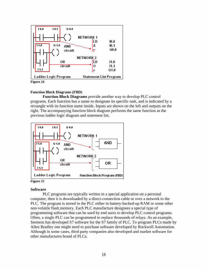
Figure 24

Function Block Diagrams (FBD)

Function Block Diagrams provide another way to develop PLC control programs. Each function has a name to designate its specific task, and is indicated by a rectangle with its function name inside. Inputs are shown on the left and outputs on the right. The accompanying function block diagram performs the same function as the previous ladder logic diagram and statement list.

Figure 25 Software

PLC programs are typically written in a special application on a personal computer, then it is downloaded by a direct-connection cable or over a network to the PLC. The program is stored in the PLC either in battery-backed-up RAM or some other non-volatile flash memory. Each PLC manufacture designees a special type of programming software that can be used by end users to develop PLC control programs. Often, a single PLC can be programmed to replace thousands of relays. As an example, Siemens has developed S7 software for the S7 family of PLC. To program PLCs made by Allen Bradley one might need to purchase software developed by Rockwell Automation. Although in some cases, third party companies also developed and market software for other manufactures brand of PLCs.

18

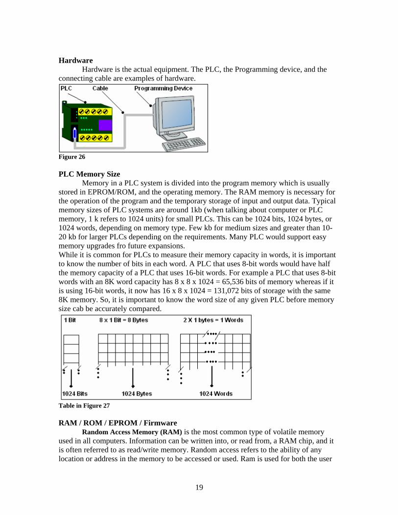
Hardware Hardware is the actual equipment. The PLC, the Programming device, and the connecting cable are examples of hardware.

Figure 26 PLC Memory Size

Memory in a PLC system is divided into the program memory which is usually stored in EPROM/ROM, and the operating memory. The RAM memory is necessary for the operation of the program and the temporary storage of input and output data. Typical memory sizes of PLC systems are around 1kb (when talking about computer or PLC memory, 1 k refers to 1024 units) for small PLCs. This can be 1024 bits, 1024 bytes, or 1024 words, depending on memory type. Few kb for medium sizes and greater than 10-20 kb for larger PLCs depending on the requirements. Many PLC would support easy memory upgrades fro future expansions. While it is common for PLCs to measure their memory capacity in words, it is important to know the number of bits in each word. A PLC that uses 8-bit words would have half the memory capacity of a PLC that uses 16-bit words. For example a PLC that uses 8-bit words with an 8K word capacity has 8 x 8 x 1024 = 65,536 bits of memory whereas if it is using 16-bit words, it now has 16 x 8 x 1024 = 131,072 bits of storage with the same 8K memory. So, it is important to know the word size of any given PLC before memory size cab be accurately compared.

Table in Figure 27 RAM / ROM / EPROM / Firmware

Random Access Memory (RAM) is the most common type of volatile memory used in all computers. Information can be written into, or read from, a RAM chip, and it is often referred to as read/write memory. Random access refers to the ability of any location or address in the memory to be accessed or used. Ram is used for both the user

19

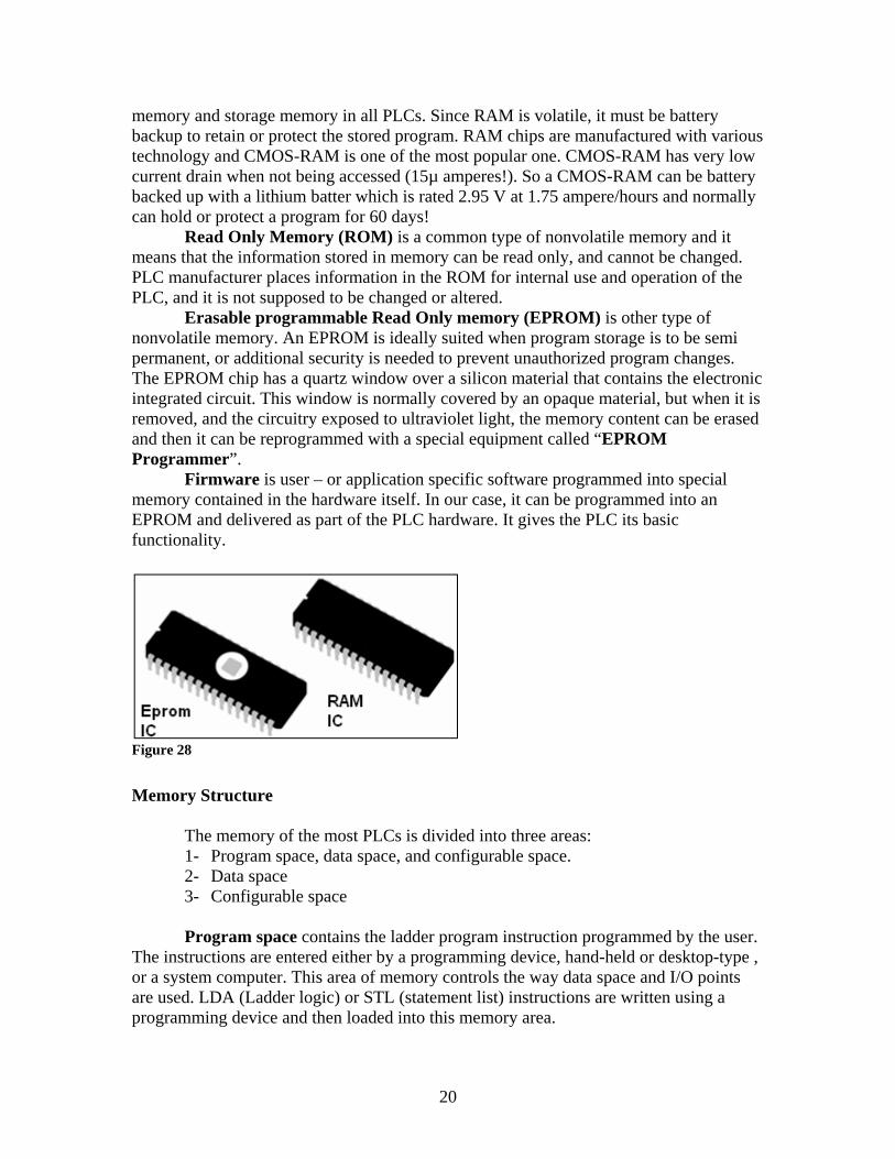
memory and storage memory in all PLCs. Since RAM is volatile, it must be battery backup to retain or protect the stored program. RAM chips are manufactured with various technology and CMOS-RAM is one of the most popular one. CMOS-RAM has very low current drain when not being accessed (15µ amperes!). So a CMOS-RAM can be battery backed up with a lithium batter which is rated 2.95 V at 1.75 ampere/hours and normally can hold or protect a program for 60 days! Read Only Memory (ROM) is a common type of nonvolatile memory and it means that the information stored in memory can be read only, and cannot be changed. PLC manufacturer places information in the ROM for internal use and operation of the PLC, and it is not supposed to be changed or altered. Erasable programmable Read Only memory (EPROM) is other type of nonvolatile memory. An EPROM is ideally suited when program storage is to be semi permanent, or additional security is needed to prevent unauthorized program changes. The EPROM chip has a quartz window over a silicon material that contains the electronic integrated circuit. This window is normally covered by an opaque material, but when it is removed, and the circuitry exposed to ultraviolet light, the memory content can be erased and then it can be reprogrammed with a special equipment called “EPROM Programmer”. Firmware is user – or application specific software programmed into special memory contained in the hardware itself. In our case, it can be programmed into an EPROM and delivered as part of the PLC hardware. It gives the PLC its basic functionality.

Figure 28

Memory Structure

The memory of the most PLCs is divided into three areas: 1- Program space, data space, and configurable space. 2- Data space 3- Configurable space

Program space contains the ladder program instruction programmed by the user. The instructions are entered either by a programming device, hand-held or desktop-type , or a system computer. This area of memory controls the way data space and I/O points are used. LDA (Ladder logic) or STL (statement list) instructions are written using a programming device and then loaded into this memory area.

20

Data space is where the status (ON or OFF) of all input and output devices is stored. Numeric values timers and counters (preset and accumulated), numeric values for arithmetic instruction, and the status of internal relays also are stored in this area of memory. Configurable parameter space stores either the default or modified configuration parameters.

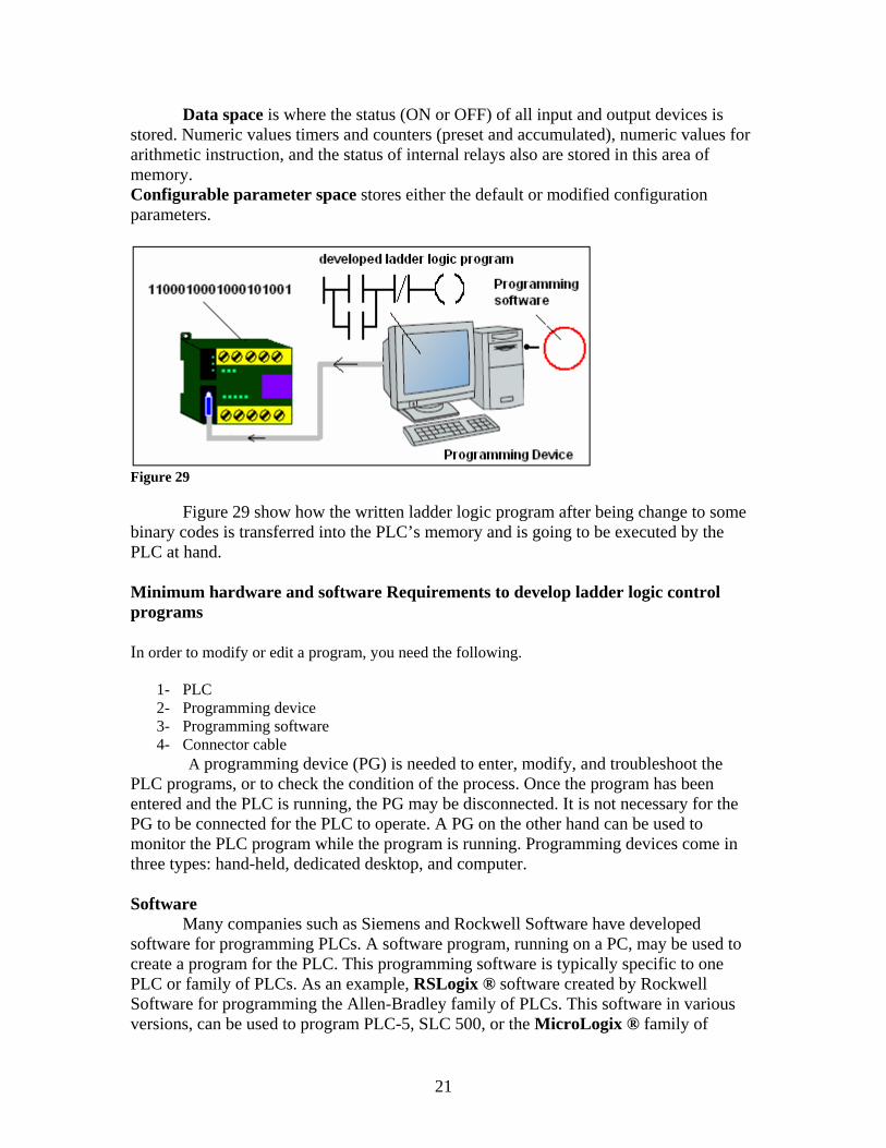
Figure 29

Figure 29 show how the written ladder logic program after being change to some binary codes is transferred into the PLC’s memory and is going to be executed by the PLC at hand. Minimum hardware and software Requirements to develop ladder logic control programs In order to modify or edit a program, you need the following.

1- PLC 2- Programming device 3- Programming software 4- Connector cable A programming device (PG) is needed to enter, modify, and troubleshoot the

PLC programs, or to check the condition of the process. Once the program has been entered and the PLC is running, the PG may be disconnected. It is not necessary for the PG to be connected for the PLC to operate. A PG on the other hand can be used to monitor the PLC program while the program is running. Programming devices come in three types: hand-held, dedicated desktop, and computer. Software Many companies such as Siemens and Rockwell Software have developed software for programming PLCs. A software program, running on a PC, may be used to create a program for the PLC. This programming software is typically specific to one PLC or family of PLCs. As an example, RSLogix ® software created by Rockwell Software for programming the Allen-Bradley family of PLCs. This software in various versions, can be used to program PLC-5, SLC 500, or the MicroLogix ® family of

21

processors. It is Microsoft Window ® based and very user friendly. The S7-200 also uses a windows-based program called step 7-micro/Win32 ®, which may be installed on a PC in the same way as any computer software. Cables

A special cable is needed when a personal computer is used as the programming device to download the developed programs into the PLC’s memory. This cable, called a PC/PPI cable, allows the serial interface of the PLC to communicate with the serial interface of a PC. Some of these connecting cables have DIP switches on the PC/PPI to select the appropriate speed (baud rate) for passing information between the PLC and computer. The S7-200 and Allen-Bradley MicroLogix 1500 Micro PLCs

Examples of basic programming techniques of typical PLCs are discussed and illustrated in this section of this manual. For the sake of educational purposes, Many of the examples used in the text are based on the Allen-Bradley MicroLogix as well as the S7-200 micro PLC which the smallest member of the SIMATIC family of programmable controllers . These two manufacturers are considered to have a large share of U.S.A and Europe PLC market accordingly. In both controllers, the CPUs are integral to the motherboards and inputs and outputs connect them to the system being controlled. The inputs monitor field devices, such as switches and sensors. Outputs control devices such as contactors, signal lamps or pumps. The programming port is used to connect to the programming device.

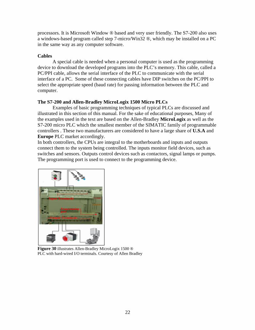
Figure 30 illustrates Allen-Bradley MicroLogix 1500 ® PLC with hard-wired I/O terminals. Courtesy of Allen Bradley

22

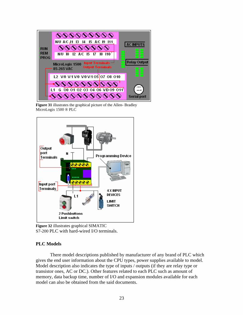
Figure 31 illustrates the graphical picture of the Allen- Bradley MicroLogix 1500 ® PLC

Figure 32 illustrates graphical SIMATIC S7-200 PLC with hard-wired I/O terminals. PLC Models

There model descriptions published by manufacturer of any brand of PLC which gives the end user information about the CPU types, power supplies available to model. Model description also indicates the type of inputs / outputs (if they are relay type or transistor ones, AC or DC.). Other features related to each PLC such as amount of memory, data backup time, number of I/O and expansion modules available for each model can also be obtained from the said documents.

23

Optional Cartridge

The S7-200 provides a super capacitor that maintains the integrity of the RAM after power has been removed. Depending on the model of the S7-200, the super capacitor can maintain the RAM for several days. The S7-200 also supports an optional cartridge that extends the amount of time the RAM can be maintained after power has been removed from the S7-200. The battery cartridge provides power only after the super capacitor has been drained. Expansion modules

S7-200 PLCs are expandable and various expansion modules are designed to give these PLCs extra capacity to add additional digital/analog inputs, outputs and other functions such as protecting over-voltage analog input modules. Expansion modules are connected to the base unit with a ribbon connector. The number of expansion modules that one can connect it to a PLC also depends on the model of that particular PLC. For example for S7-200 CPU 224 the limit is maximum number of 7 units and even then one needs to check the power budget to be sure he does not overload the CPU power output. Check specification sheets when it comes to expansion modules. Understanding controller Status Indicators

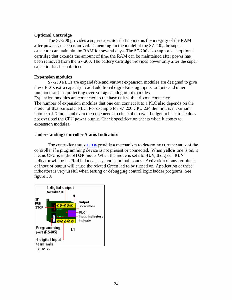
The controller status LEDs provide a mechanism to determine current status of the controller if a programming device is not present or connected. When yellow one is on, it means CPU is in the STOP mode. When the mode is set t to RUN, the green RUN indicator will be lit. Red led means system is in fault status. Activation of any terminals of input or output will cause the related Green led to be turned on. Application of these indicators is very useful when testing or debugging control logic ladder programs. See figure 33.

Figure 33

24

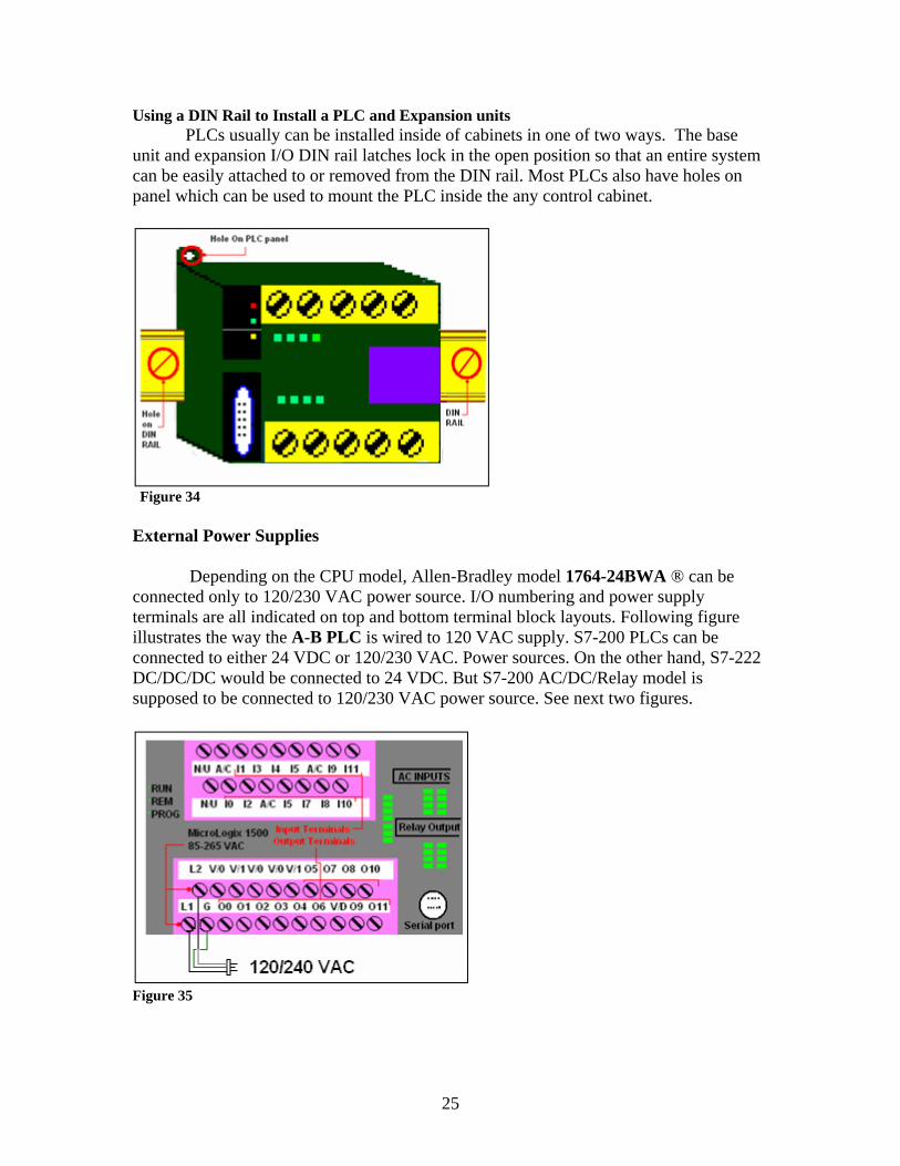
Using a DIN Rail to Install a PLC and Expansion units PLCs usually can be installed inside of cabinets in one of two ways. The base

unit and expansion I/O DIN rail latches lock in the open position so that an entire system can be easily attached to or removed from the DIN rail. Most PLCs also have holes on panel which can be used to mount the PLC inside the any control cabinet.

Figure 34 External Power Supplies

Depending on the CPU model, Allen-Bradley model 1764-24BWA ® can be connected only to 120/230 VAC power source. I/O numbering and power supply terminals are all indicated on top and bottom terminal block layouts. Following figure illustrates the way the A-B PLC is wired to 120 VAC supply. S7-200 PLCs can be connected to either 24 VDC or 120/230 VAC. Power sources. On the other hand, S7-222 DC/DC/DC would be connected to 24 VDC. But S7-200 AC/DC/Relay model is supposed to be connected to 120/230 VAC power source. See next two figures.

Figure 35

25

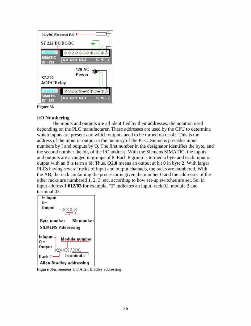
Figure 36 I/O Numbering

The inputs and outputs are all identified by their addresses, the notation used depending on the PLC manufacturer. These addresses are used by the CPU to determine which inputs are present and which outputs need to be turned on or off. This is the address of the input or output in the memory of the PLC. Siemens precedes input numbers by I and outputs by Q. The first number in the designator identifies the byte, and the second number the bit, of the I/O address. With the Siemens SIMATIC, the inputs and outputs are arranged in groups of 8. Each 8 group is termed a byte and each input or output with an 8 is term a bit Thus, Q2.0 means an output at bit 0 in byte 2. With larger PLCs having several racks of input and output channels, the racks are numbered. With the AB, the rack containing the processor is given the number 0 and the addresses of the other racks are numbered 1, 2, 3, etc. according to how set-up switches are set. So, in input address I:012/03 for example, “I” indicates an input, rack 01, module 2 and terminal 03.

Figure 36a, Siemens and Allen Bradley addressing

26

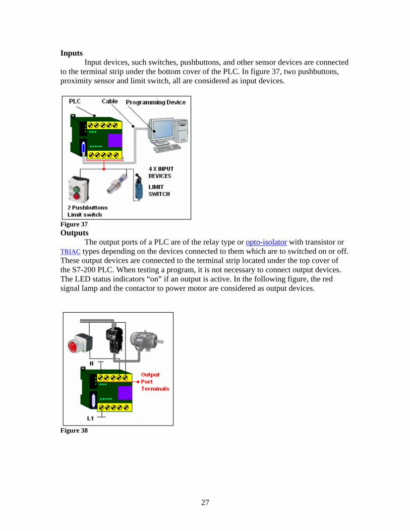
Inputs Input devices, such switches, pushbuttons, and other sensor devices are connected

to the terminal strip under the bottom cover of the PLC. In figure 37, two pushbuttons, proximity sensor and limit switch, all are considered as input devices.

Figure 37 Outputs

The output ports of a PLC are of the relay type or opto-isolator with transistor or TRIAC types depending on the devices connected to them which are to switched on or off. These output devices are connected to the terminal strip located under the top cover of the S7-200 PLC. When testing a program, it is not necessary to connect output devices. The LED status indicators “on” if an output is active. In the following figure, the red signal lamp and the contactor to power motor are considered as output devices.

Figure 38

27

Super Capacitor

The Super capacitor is an electrochemical energy storage applied in “power” industries. Compared with battery, a super Capacitor has one-tenth of energy, but delivers over 10 times power due to ultra low ESR (Equivalent Series Resistance). They also have a much higher power density than batteries or fuel cells. These capacitors can provide backup power for maintaining charge for a long period of time and protect data stored in PLC’s RAM during power losses. The RAM is typically backed up for 50 hours on the S7-221 and 222, and for 72 hours on the S7-224 and 226. PLC Reference Manuals

A reference manual is a document often organized aphetically, designed as a quick reference for experience users. A reference manual typically contains the most frequently referenced subset of information including basic setup instructions, troubleshooting for the most commonly encountered problems, and or prominent features. Both Siemens and AB have lot’s of information in their websites regarding their line of products. www.ab.com ab.rockwellautomation.com/Programmable-Controllers www.siemens.com/ www.automation.siemens.com/_en/s7-200/index.htm www.automation.siemens.com/.../simatic-s7.../s7-200/.../Default.aspx PLC Display and HMI (human-machine interaction) Units

A user interface is a system by which people (users) interact with a machine. The user interface includes hardware (physical) and software (logical) components. User interfaces exist for various systems, and provide a means of: 1- Input, allowing the users to manipulate a system 2- Output, allowing the system to indicate the effects of the users manipulation. Generally, the goal of human-machine interaction engineering is to produce a user interface which makes it easy, efficient, and enjoyable to operate a machine in the way which produces the desired result. This generally means that the operator needs to provide minimal input to achieve the desired output, and also that the machine minimizes undesired outputs to the human. Usually PLCs are designed such that could be used to communicate with a variety of external devices such as HMI devices. HMI devices can display messages read from the PLCs connected to and allow for adjustment of program variables, provides forcing ability, and permits setting of time and date. The summarized description of few HMI devices made by Rockwell Automation and Siemens is mentioned here for your information. Mfr. Part Number: 1760-DUB made by Rockwell Automation. Description: Allen Bradley 1760-DUB multi-function Pico GFX-70 Display unit with Keypad, displays text, date, and time, as well as custom bitmaps. Mfr. Part number 20-HIM-C3 S/A made by Rockwell Automation Allen Bradley 20-HIM-A3 PwerFlex Architecture Class Hand-Held Human Interface Module, LCD Display, Full Numeric Keypad, Series C

28

Allen Bradley 2711-B5A2 PanelView 550 monochrome Terminal 5.5 inch, Keypad & touch screen, DH-485 communication Ports, AC power, Series F. combination for convenient and flexible operator input: RS232 printer port, alarms, alarm lists, triggered messages, and triggered states of a multi state indicator, field-replaceable backlights. AB 1201-HJ2 programming terminal LCD Display Siemens LOGO! Text display 6ED1 055-4MH00-0BA0 The new LOGO! TD text display panel provides an affordable HMI for equipment builders and their customers, even on the simplest relay control systems. By having a display panel with built-in operator functions and diagnostic messages customized for their process, end users can now make quick adjustment or easy troubleshoot…. Siemens TD200

The Siemens TD 200 is the proven HMI device for the SIMATIC S7-200. In addition to the display of alarm texts, it enables interventions in the control program (e.g. set point value changes) or the setting of inputs and outputs. The TD 200 is suitable for simple operation tasks with the SIMATIC S7-200 PLC. The focus is on the display of alarm texts. The low total height and device depth make it the unit of choice even in cramped space conditions. Computer network

A computer network is a collection of hardware components and computers interconnected by communication channels that allow sharing of resources and information. The SIMATIC S7-200 micro PLC provides a full range of communication capabilities. The integrated RS485 interfaces can be operated at data transmission rages from 1.2 to 187.5 k. baud. A total of 31 units can be interconnected using a communication cable. PROFIBUS connection

All CPUs from 222 upwards can be run via the EM277 communications modules as a norm slave on a PROFIBUS DP network with a transmission rate of up to 12 Mbit/s. the open feature of the S7-200 to higher level PROFIBUS DP control levels ensures you can integrate individual machines into your production line. With the EM277 expansion module, you can implement PROFIBUS capability of individual machines equipped with S7-200. Powerful AS-Interface connection

The CP 243-2 turns all CPUs from 222 upwards into powerful masters on the AS-interface network. According to the new AS-interface specification v 2.1, you can connect up to 62 stations, making even analog sensors easy to integrate. With AS-interface, you can connect up to 62 stations, making even analog sensors easy to integrate. With AS-interface, you can connect up to 248 DIs + 186 DOs in the maximum configuration. The max, number of 62 stations can include up to 31 analog modules. The configuration of the slaves and reading/writing of data is supported by the handy AS-interface Wizard.

29

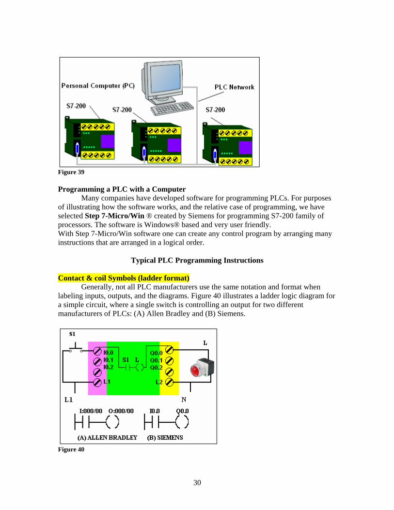
Figure 39 Programming a PLC with a Computer

Many companies have developed software for programming PLCs. For purposes of illustrating how the software works, and the relative case of programming, we have selected Step 7-Micro/Win ® created by Siemens for programming S7-200 family of processors. The software is Windows® based and very user friendly. With Step 7-Micro/Win software one can create any control program by arranging many instructions that are arranged in a logical order.

Typical PLC Programming Instructions Contact & coil Symbols (ladder format)

Generally, not all PLC manufacturers use the same notation and format when labeling inputs, outputs, and the diagrams. Figure 40 illustrates a ladder logic diagram for a simple circuit, where a single switch is controlling an output for two different manufacturers of PLCs: (A) Allen Bradley and (B) Siemens.

Figure 40

30

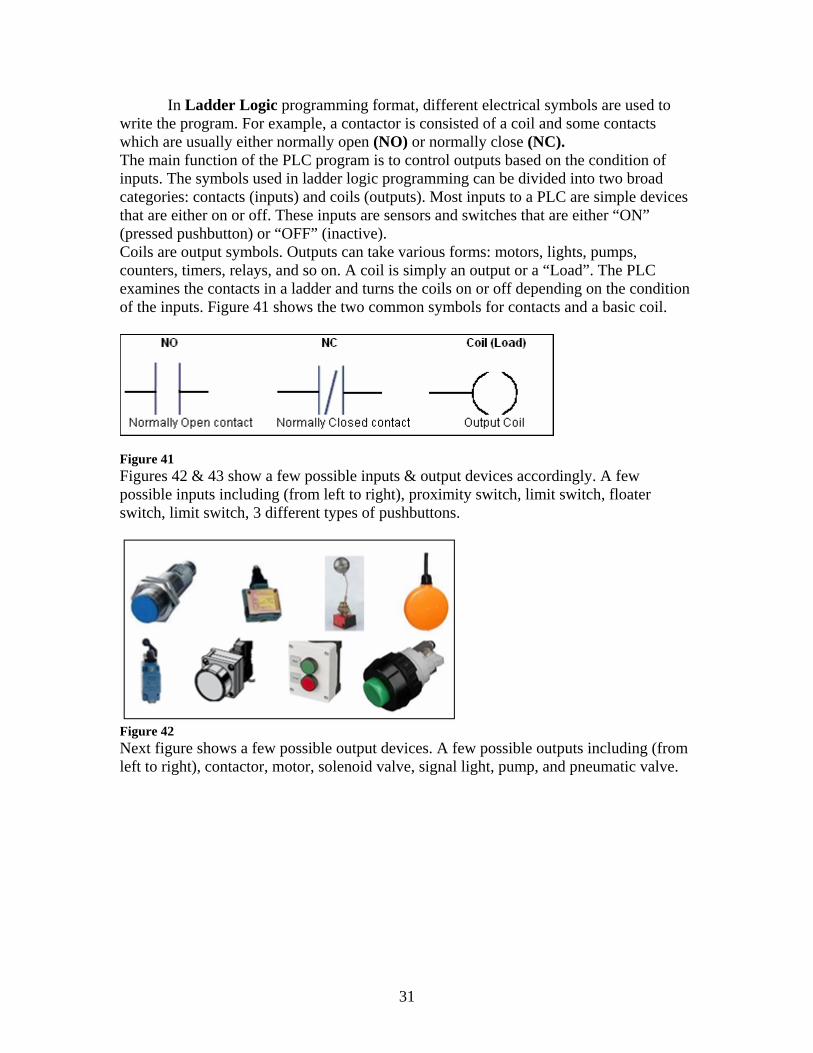
In Ladder Logic programming format, different electrical symbols are used to write the program. For example, a contactor is consisted of a coil and some contacts which are usually either normally open (NO) or normally close (NC). The main function of the PLC program is to control outputs based on the condition of inputs. The symbols used in ladder logic programming can be divided into two broad categories: contacts (inputs) and coils (outputs). Most inputs to a PLC are simple devices that are either on or off. These inputs are sensors and switches that are either “ON” (pressed pushbutton) or “OFF” (inactive). Coils are output symbols. Outputs can take various forms: motors, lights, pumps, counters, timers, relays, and so on. A coil is simply an output or a “Load”. The PLC examines the contacts in a ladder and turns the coils on or off depending on the condition of the inputs. Figure 41 shows the two common symbols for contacts and a basic coil.

Figure 41 Figures 42 & 43 show a few possible inputs & output devices accordingly. A few possible inputs including (from left to right), proximity switch, limit switch, floater switch, limit switch, 3 different types of pushbuttons.

Figure 42 Next figure shows a few possible output devices. A few possible outputs including (from left to right), contactor, motor, solenoid valve, signal light, pump, and pneumatic valve.

31

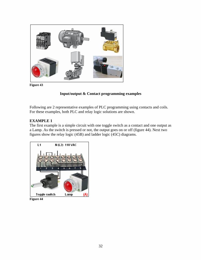
Figure 43

Input/output & Contact programming examples

Following are 2 representative examples of PLC programming using contacts and coils. For these examples, both PLC and relay logic solutions are shown. EXAMPLE 1 The first example is a simple circuit with one toggle switch as a contact and one output as a Lamp. As the switch is pressed or not, the output goes on or off (figure 44). Next two figures show the relay logic (45B) and ladder logic (45C) diagrams.

Figure 44

32

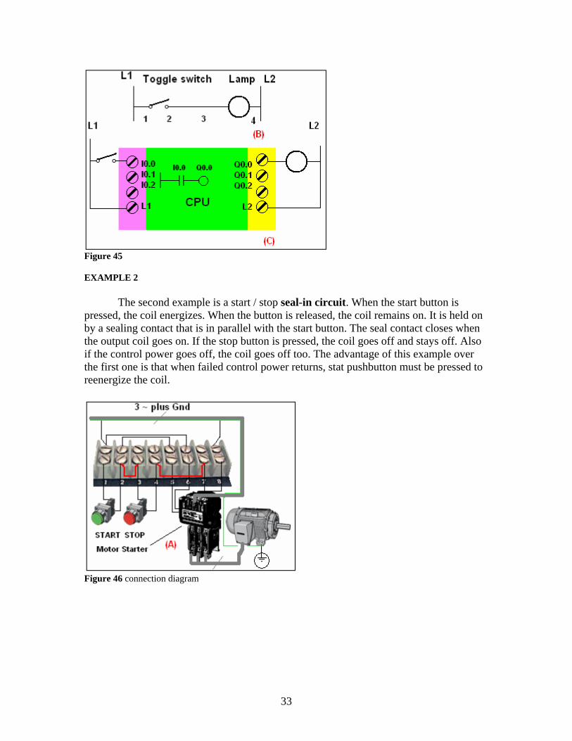
Figure 45 EXAMPLE 2

The second example is a start / stop seal-in circuit. When the start button is pressed, the coil energizes. When the button is released, the coil remains on. It is held on by a sealing contact that is in parallel with the start button. The seal contact closes when the output coil goes on. If the stop button is pressed, the coil goes off and stays off. Also if the control power goes off, the coil goes off too. The advantage of this example over the first one is that when failed control power returns, stat pushbutton must be pressed to reenergize the coil.

Figure 46 connection diagram

33

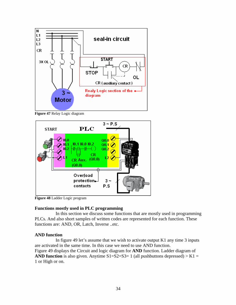
Figure 47 Relay Logic diagram

Figure 48 Ladder Logic program Functions mostly used in PLC programming In this section we discuss some functions that are mostly used in programming PLCs. And also short samples of written codes are represented for each function. These functions are: AND, OR, Latch, Inverse ..etc. AND function In figure 49 let’s assume that we wish to activate output K1 any time 3 inputs are activated in the same time. In this case we need to use AND function. Figure 49 displays the Circuit and logic diagram for AND function. Ladder diagram of AND function is also given. Anytime S1=S2=S3= 1 (all pushbuttons depressed) > K1 = 1 or High or on.

34

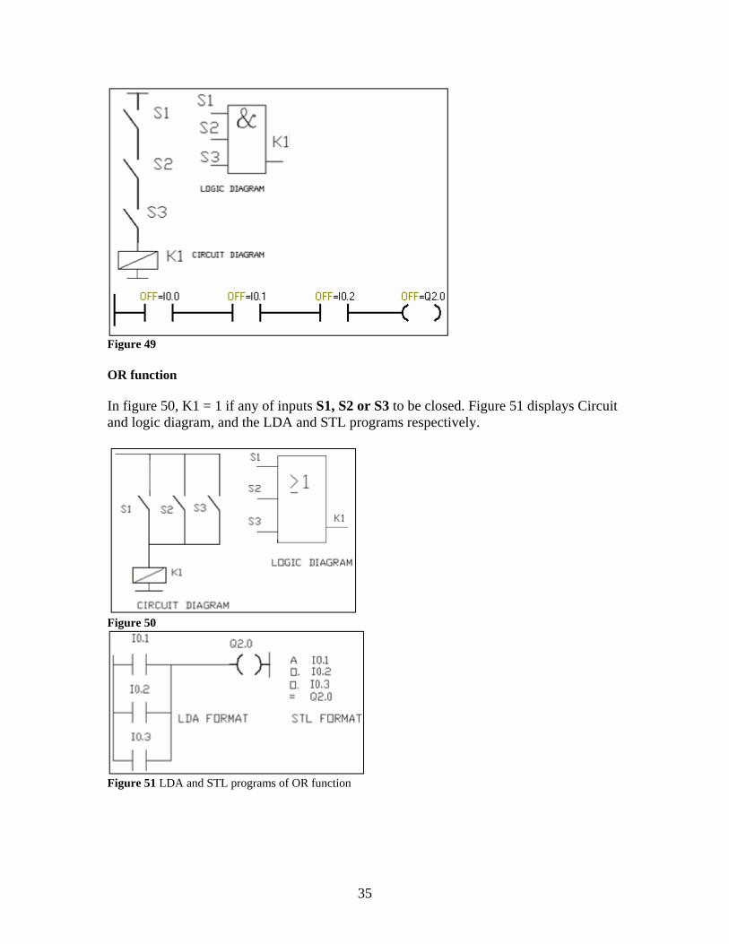
Figure 49 OR function In figure 50, K1 = 1 if any of inputs S1, S2 or S3 to be closed. Figure 51 displays Circuit and logic diagram, and the LDA and STL programs respectively.

Figure 50

Figure 51 LDA and STL programs of OR function

35

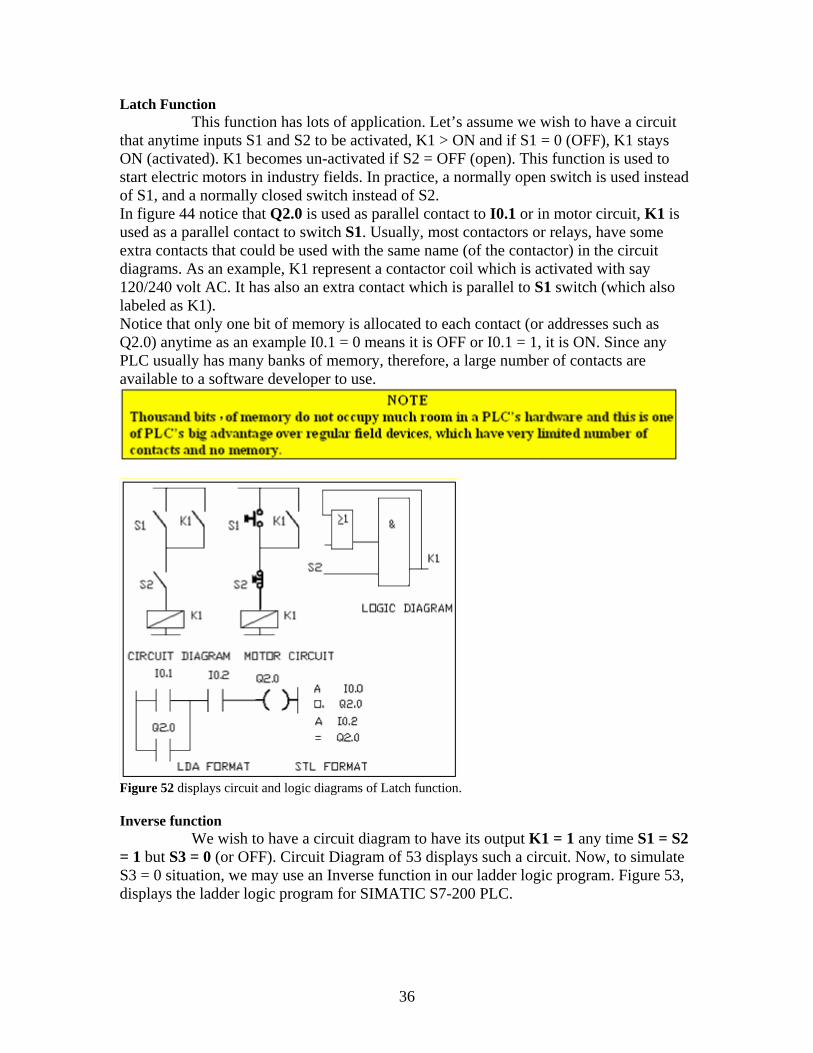
Latch Function This function has lots of application. Let’s assume we wish to have a circuit that anytime inputs S1 and S2 to be activated, K1 > ON and if S1 = 0 (OFF), K1 stays ON (activated). K1 becomes un-activated if S2 = OFF (open). This function is used to start electric motors in industry fields. In practice, a normally open switch is used instead of S1, and a normally closed switch instead of S2. In figure 44 notice that Q2.0 is used as parallel contact to I0.1 or in motor circuit, K1 is used as a parallel contact to switch S1. Usually, most contactors or relays, have some extra contacts that could be used with the same name (of the contactor) in the circuit diagrams. As an example, K1 represent a contactor coil which is activated with say 120/240 volt AC. It has also an extra contact which is parallel to S1 switch (which also labeled as K1). Notice that only one bit of memory is allocated to each contact (or addresses such as Q2.0) anytime as an example I0.1 = 0 means it is OFF or I0.1 = 1, it is ON. Since any PLC usually has many banks of memory, therefore, a large number of contacts are available to a software developer to use.

Figure 52 displays circuit and logic diagrams of Latch function. Inverse function We wish to have a circuit diagram to have its output K1 = 1 any time S1 = S2 = 1 but S3 = 0 (or OFF). Circuit Diagram of 53 displays such a circuit. Now, to simulate S3 = 0 situation, we may use an Inverse function in our ladder logic program. Figure 53, displays the ladder logic program for SIMATIC S7-200 PLC.

36

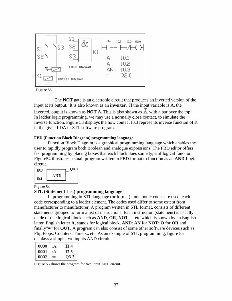
Figure 53 The NOT gate is an electronic circuit that produces an inverted version of the input at its output. It is also known as an inverter. If the input variable is A, the inverted, output is known as NOT A. This is also shown as with a bar over the top. In ladder logic programming, we may use a normally close contact, to simulate the Inverse function. Figure 53 displays the how contact I0.3 represents inverse function of K in the given LDA or STL software program. FBD (Function Block Diagram) programming language Function Block Diagram is a graphical programming language which enables the user to rapidly program both Boolean and analogue expressions. The FBD editor offers fast programming by placing boxes that each block does some type of logical function. Figure54 illustrates a small program written in FBD format to function as an AND Logic circuit.

Figure 54 STL (Statement List) programming language In programming in STL language (or format), mnemonic codes are used, each code corresponding to a ladder element. The codes used differ to some extent from manufacturer to manufacturer. A program written in STL format, consists of different statements grouped to form a list of instructions. Each instruction (statement) is usually made of one logical block such as AND, OR, NOT … etc which is shown by an English letter. English letter A, stands for logical block, AND: AN for NOT: O for OR and finally”=” for OUT. A program can also consist of some other software devices such as Flip Flops, Counters, Timers.. etc. As an example of STL programming, figure 55 displays a simple two inputs AND circuit.

Figure 55 shows the program for two input AND circuit

37

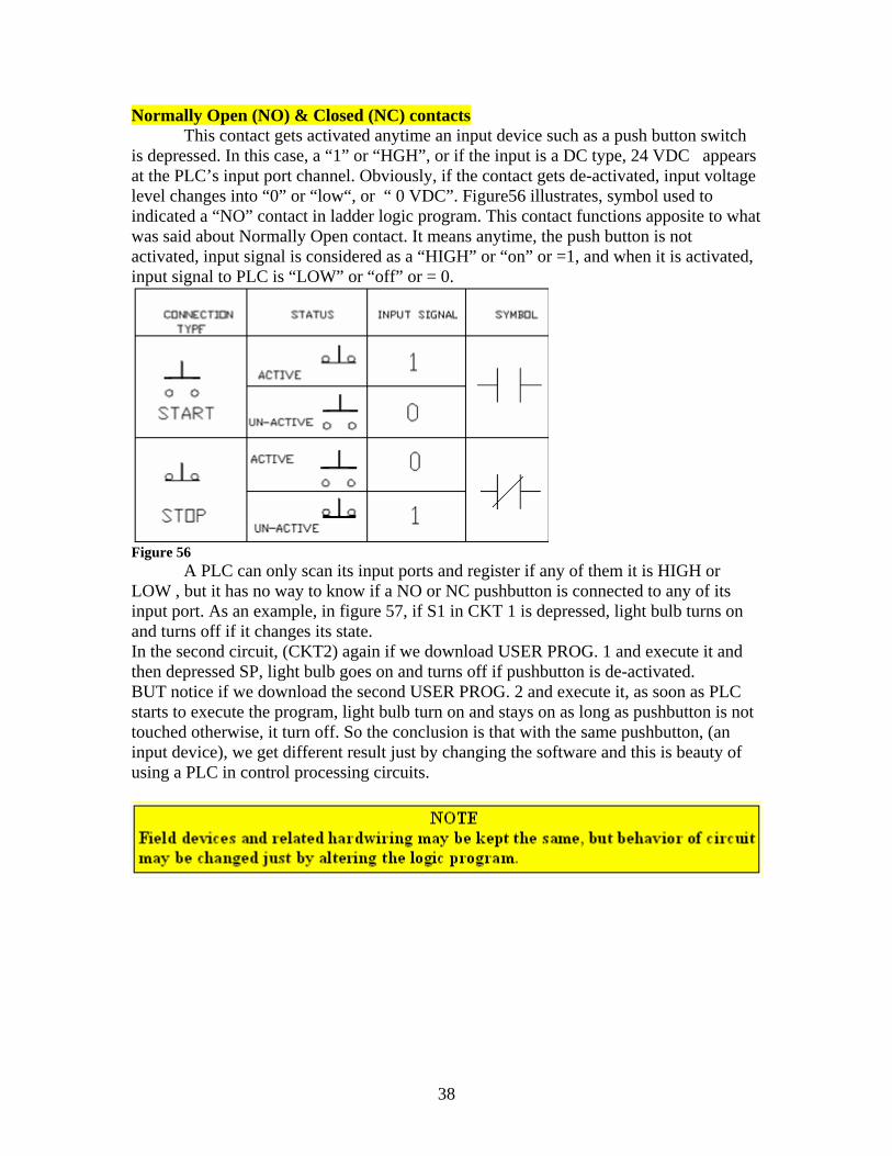
Normally Open (NO) & Closed (NC) contacts This contact gets activated anytime an input device such as a push button switch

is depressed. In this case, a “1” or “HGH”, or if the input is a DC type, 24 VDC appears at the PLC’s input port channel. Obviously, if the contact gets de-activated, input voltage level changes into “0” or “low“, or “ 0 VDC”. Figure56 illustrates, symbol used to indicated a “NO” contact in ladder logic program. This contact functions apposite to what was said about Normally Open contact. It means anytime, the push button is not activated, input signal is considered as a “HIGH” or “on” or =1, and when it is activated, input signal to PLC is “LOW” or “off” or = 0.

Figure 56 A PLC can only scan its input ports and register if any of them it is HIGH or LOW , but it has no way to know if a NO or NC pushbutton is connected to any of its input port. As an example, in figure 57, if S1 in CKT 1 is depressed, light bulb turns on and turns off if it changes its state. In the second circuit, (CKT2) again if we download USER PROG. 1 and execute it and then depressed SP, light bulb goes on and turns off if pushbutton is de-activated. BUT notice if we download the second USER PROG. 2 and execute it, as soon as PLC starts to execute the program, light bulb turn on and stays on as long as pushbutton is not touched otherwise, it turn off. So the conclusion is that with the same pushbutton, (an input device), we get different result just by changing the software and this is beauty of using a PLC in control processing circuits.

38

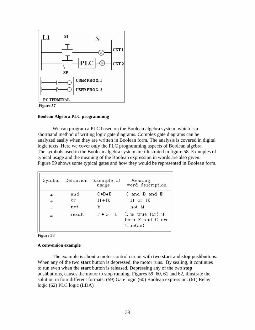
Figure 57 Boolean Algebra PLC programming

We can program a PLC based on the Boolean algebra system, which is a shorthand method of writing logic gate diagrams. Complex gate diagrams can be analyzed easily when they are written in Boolean form. The analysis is covered in digital logic texts. Here we cover only the PLC programming aspects of Boolean algebra. The symbols used in the Boolean algebra system are illustrated in figure 58. Examples of typical usage and the meaning of the Boolean expression in words are also given. Figure 59 shows some typical gates and how they would be represented in Boolean form.

Figure 58 A conversion example

The example is about a motor control circuit with two start and stop pushbuttons. When any of the two start button is depressed, the motor runs. By sealing, it continues to run even when the start button is released. Depressing any of the two stop pushbuttons, causes the motor to stop running. Figures 59, 60, 61 and 62, illustrate the solution in four different formats: (59) Gate logic (60) Boolean expression. (61) Relay logic (62) PLC logic (LDA)

39

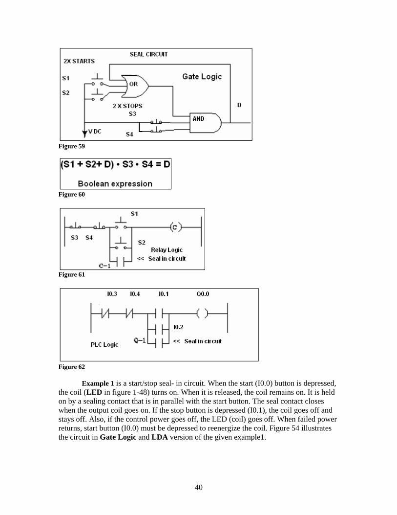
Figure 59

Figure 60

Figure 61

Figure 62 Example 1 is a start/stop seal- in circuit. When the start (I0.0) button is depressed, the coil (LED in figure 1-48) turns on. When it is released, the coil remains on. It is held on by a sealing contact that is in parallel with the start button. The seal contact closes when the output coil goes on. If the stop button is depressed (I0.1), the coil goes off and stays off. Also, if the control power goes off, the LED (coil) goes off. When failed power returns, start button (I0.0) must be depressed to reenergize the coil. Figure 54 illustrates the circuit in Gate Logic and LDA version of the given example1.

40

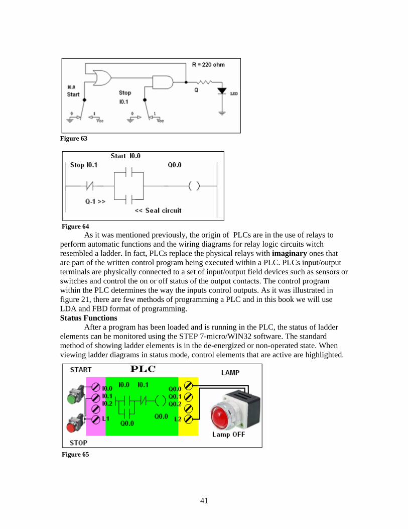
Figure 63

Figure 64 As it was mentioned previously, the origin of PLCs are in the use of relays to perform automatic functions and the wiring diagrams for relay logic circuits witch resembled a ladder. In fact, PLCs replace the physical relays with imaginary ones that are part of the written control program being executed within a PLC. PLCs input/output terminals are physically connected to a set of input/output field devices such as sensors or switches and control the on or off status of the output contacts. The control program within the PLC determines the way the inputs control outputs. As it was illustrated in figure 21, there are few methods of programming a PLC and in this book we will use LDA and FBD format of programming. Status Functions

After a program has been loaded and is running in the PLC, the status of ladder elements can be monitored using the STEP 7-micro/WIN32 software. The standard method of showing ladder elements is in the de-energized or non-operated state. When viewing ladder diagrams in status mode, control elements that are active are highlighted.

Figure 65

41

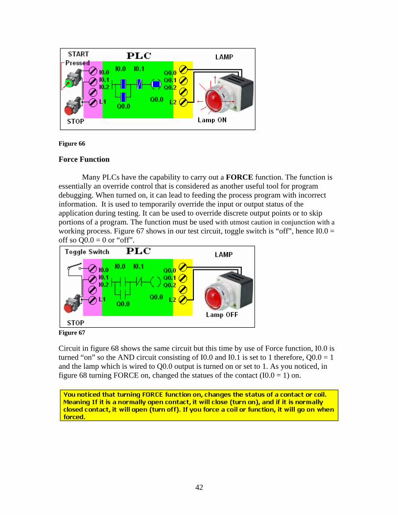
Figure 66 Force Function

Many PLCs have the capability to carry out a FORCE function. The function is essentially an override control that is considered as another useful tool for program debugging. When turned on, it can lead to feeding the process program with incorrect information. It is used to temporarily override the input or output status of the application during testing. It can be used to override discrete output points or to skip portions of a program. The function must be used with utmost caution in conjunction with a working process. Figure 67 shows in our test circuit, toggle switch is “off”, hence I0.0 = off so Q0.0 = 0 or “off”.

Figure 67 Circuit in figure 68 shows the same circuit but this time by use of Force function, I0.0 is turned “on” so the AND circuit consisting of I0.0 and I0.1 is set to 1 therefore, Q0.0 = 1 and the lamp which is wired to Q0.0 output is turned on or set to 1. As you noticed, in figure 68 turning FORCE on, changed the statues of the contact (I0.0 = 1) on.

42

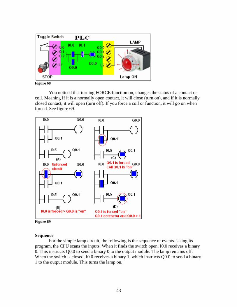
Figure 68 You noticed that turning FORCE function on, changes the status of a contact or coil. Meaning If it is a normally open contact, it will close (turn on), and if it is normally closed contact, it will open (turn off). If you force a coil or function, it will go on when forced. See figure 69.

Figure 69 Sequence

For the simple lamp circuit, the following is the sequence of events. Using its program, the CPU scans the inputs. When it finds the switch open, I0.0 receives a binary 0. This instructs Q0.0 to send a binary 0 to the output module. The lamp remains off. When the switch is closed, I0.0 receives a binary 1, which instructs Q0.0 to send a binary 1 to the output module. This turns the lamp on.

43

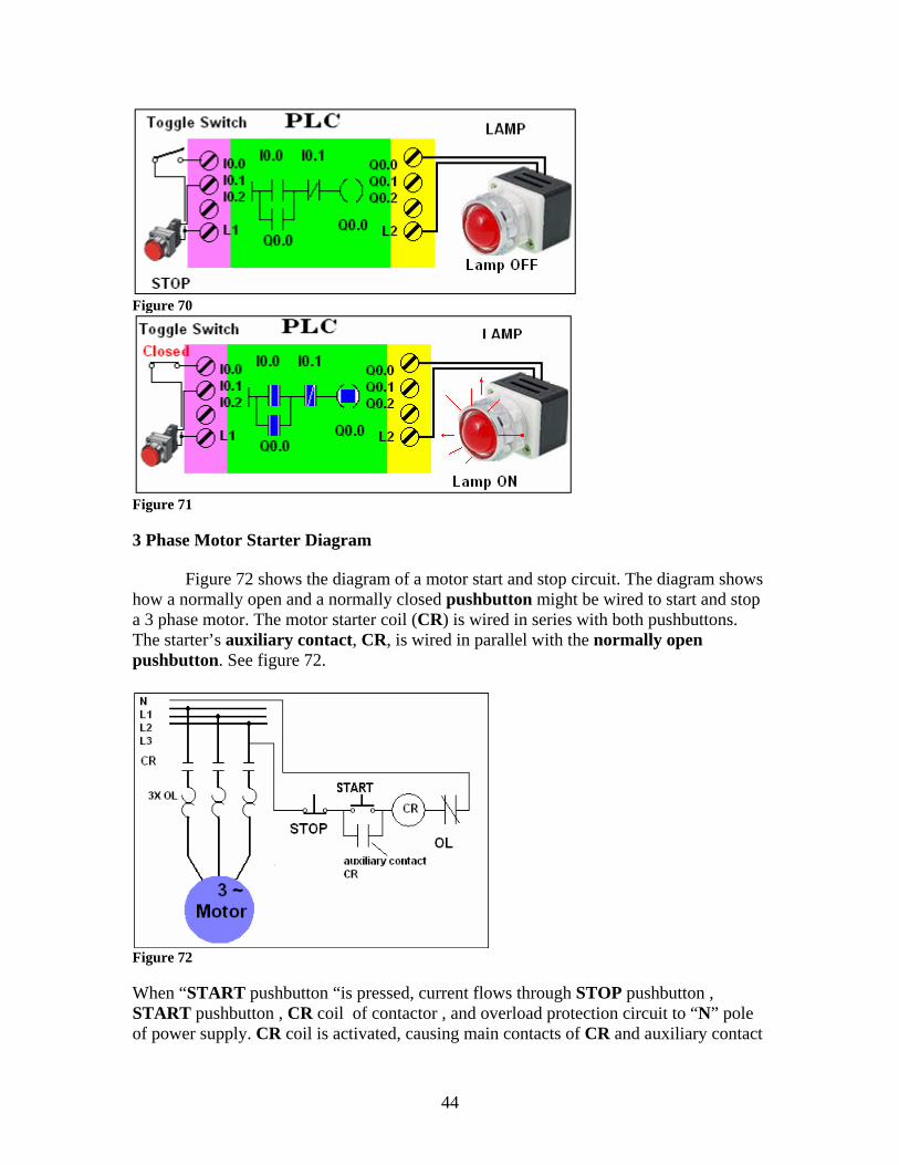
Figure 70

Figure 71 3 Phase Motor Starter Diagram

Figure 72 shows the diagram of a motor start and stop circuit. The diagram shows how a normally open and a normally closed pushbutton might be wired to start and stop a 3 phase motor. The motor starter coil (CR) is wired in series with both pushbuttons. The starter’s auxiliary contact, CR, is wired in parallel with the normally open pushbutton. See figure 72.

Figure 72 When “START pushbutton “is pressed, current flows through STOP pushbutton , START pushbutton , CR coil of contactor , and overload protection circuit to “N” pole of power supply. CR coil is activated, causing main contacts of CR and auxiliary contact

44

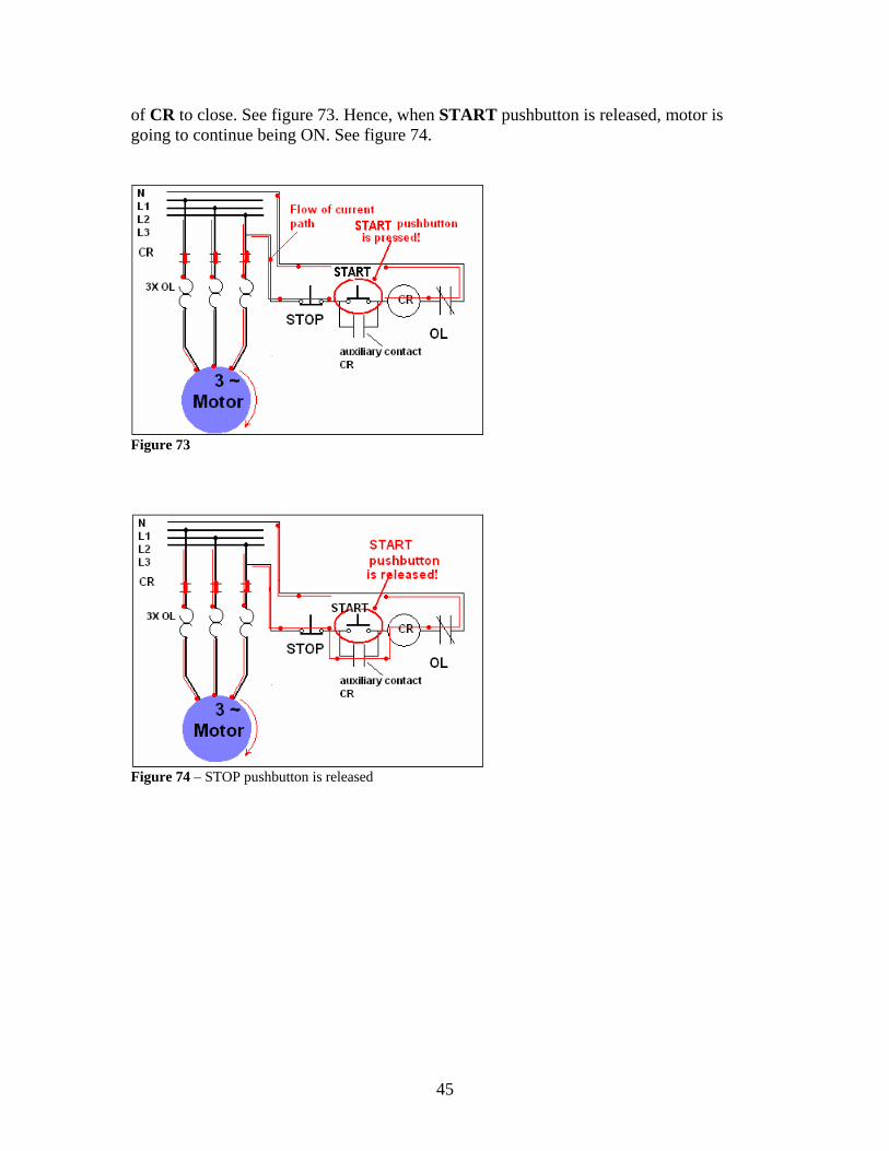
of CR to close. See figure 73. Hence, when START pushbutton is released, motor is going to continue being ON. See figure 74.

Figure 73

Figure 74 – STOP pushbutton is released

45

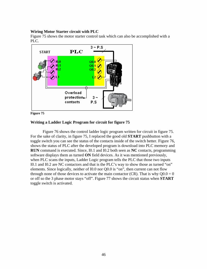
Wiring Motor Starter circuit with PLC Figure 75 shows the motor starter control task which can also be accomplished with a PLC.

Figure 75 Writing a Ladder Logic Program for circuit for figure 75

Figure 76 shows the control ladder logic program written for circuit in figure 75. For the sake of clarity, in figure 75, I replaced the good old START pushbutton with a toggle switch you can see the status of the contacts inside of the switch better. Figure 76, shows the status of PLC after the developed program is download into PLC memory and RUN command is executed. Since, I0.1 and I0.2 both seen as NC contacts, programming software displays them as turned ON field devices. As it was mentioned previously, when PLC scans the inputs, Ladder Logic program tells the PLC that those two inputs I0.1 and I0.2 are NC contactors and that is the PLC’s way to show those as turned “on” elements. Since logically, neither of I0.0 nor Q0.0 is “on”, then current can not flow through none of those devices to activate the main contactor (CR). That is why Q0.0 = 0 or off so the 3 phase motor stays “off”. Figure 77 shows the circuit status when START toggle switch is activated.

46

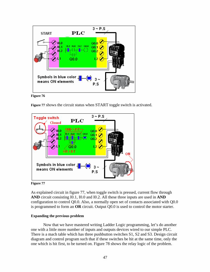
Figure 76 Figure 77 shows the circuit status when START toggle switch is activated.

Figure 77 As explained circuit in figure 77, when toggle switch is pressed, current flow through AND circuit consisting I0.1, I0.0 and I0.2. All these three inputs are used in AND configuration to control Q0.0. Also, a normally open set of contacts associated with Q0.0 is programmed to form an OR circuit. Output Q0.0 is used to control the motor starter. Expanding the previous problem

Now that we have mastered writing Ladder Logic programming, let’s do another one with a little more number of inputs and outputs devices wired to our simple PLC. There is a mach table which has three pushbutton switches S1, S2 and S3. Design circuit diagram and control program such that if these switches be hit at the same time, only the one which is hit first, to be turned on. Figure 78 shows the relay logic of the problem.

47

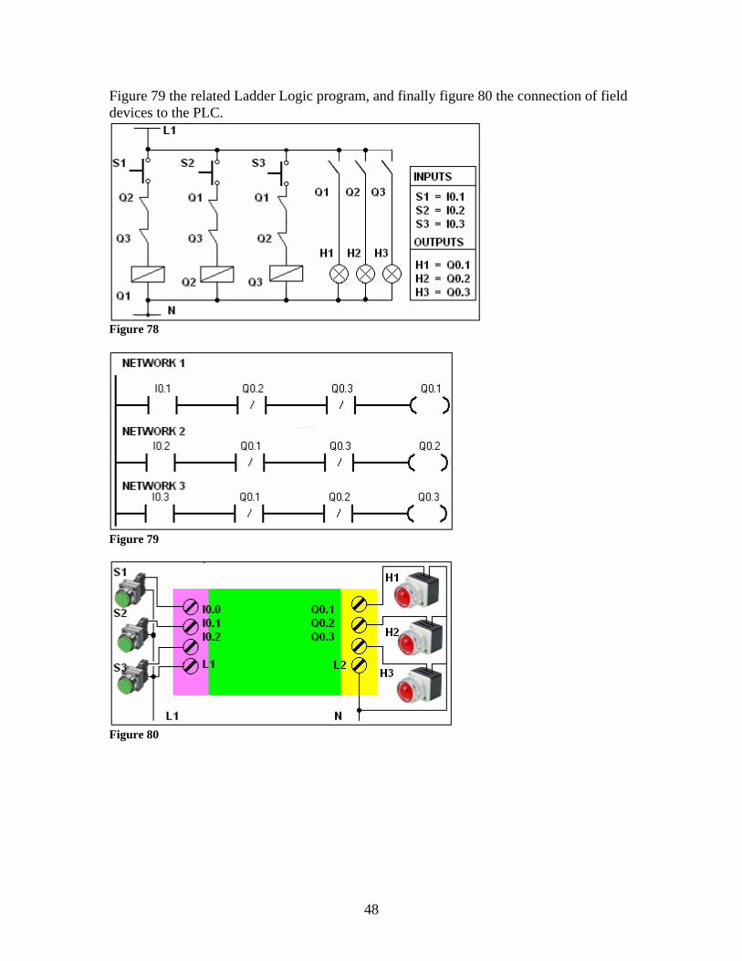
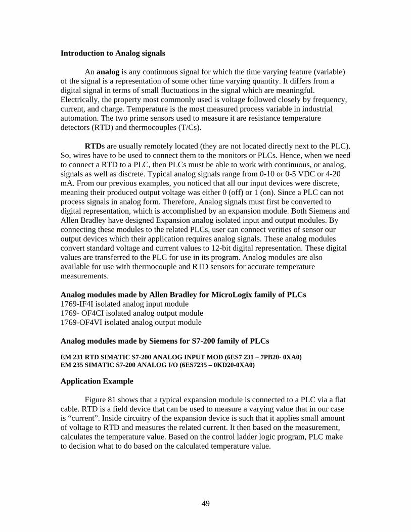
Figure 79 the related Ladder Logic program, and finally figure 80 the connection of field devices to the PLC.

Figure 78

Figure 79

Figure 80

48

Introduction to Analog signals

An analog is any continuous signal for which the time varying feature (variable) of the signal is a representation of some other time varying quantity. It differs from a digital signal in terms of small fluctuations in the signal which are meaningful. Electrically, the property most commonly used is voltage followed closely by frequency, current, and charge. Temperature is the most measured process variable in industrial automation. The two prime sensors used to measure it are resistance temperature detectors (RTD) and thermocouples (T/Cs).

RTDs are usually remotely located (they are not located directly next to the PLC). So, wires have to be used to connect them to the monitors or PLCs. Hence, when we need to connect a RTD to a PLC, then PLCs must be able to work with continuous, or analog, signals as well as discrete. Typical analog signals range from 0-10 or 0-5 VDC or 4-20 mA. From our previous examples, you noticed that all our input devices were discrete, meaning their produced output voltage was either 0 (off) or 1 (on). Since a PLC can not process signals in analog form. Therefore, Analog signals must first be converted to digital representation, which is accomplished by an expansion module. Both Siemens and Allen Bradley have designed Expansion analog isolated input and output modules. By connecting these modules to the related PLCs, user can connect verities of sensor our output devices which their application requires analog signals. These analog modules convert standard voltage and current values to 12-bit digital representation. These digital values are transferred to the PLC for use in its program. Analog modules are also available for use with thermocouple and RTD sensors for accurate temperature measurements.

Analog modules made by Allen Bradley for MicroLogix family of PLCs 1769-IF4I isolated analog input module 1769- OF4CI isolated analog output module 1769-OF4VI isolated analog output module Analog modules made by Siemens for S7-200 family of PLCs EM 231 RTD SIMATIC S7-200 ANALOG INPUT MOD (6ES7 231 – 7PB20- 0XA0) EM 235 SIMATIC S7-200 ANALOG I/O (6ES7235 – 0KD20-0XA0) Application Example

Figure 81 shows that a typical expansion module is connected to a PLC via a flat cable. RTD is a field device that can be used to measure a varying value that in our case is “current”. Inside circuitry of the expansion device is such that it applies small amount of voltage to RTD and measures the related current. It then based on the measurement, calculates the temperature value. Based on the control ladder logic program, PLC make to decision what to do based on the calculated temperature value.

49

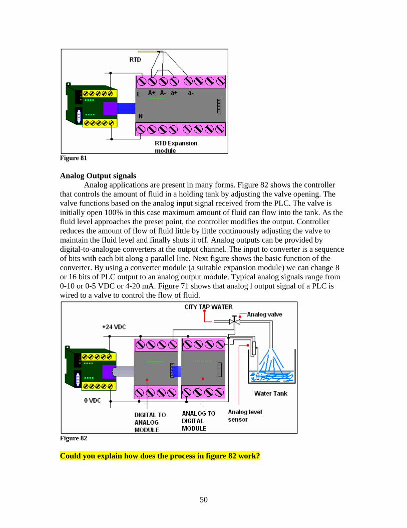
Figure 81 Analog Output signals

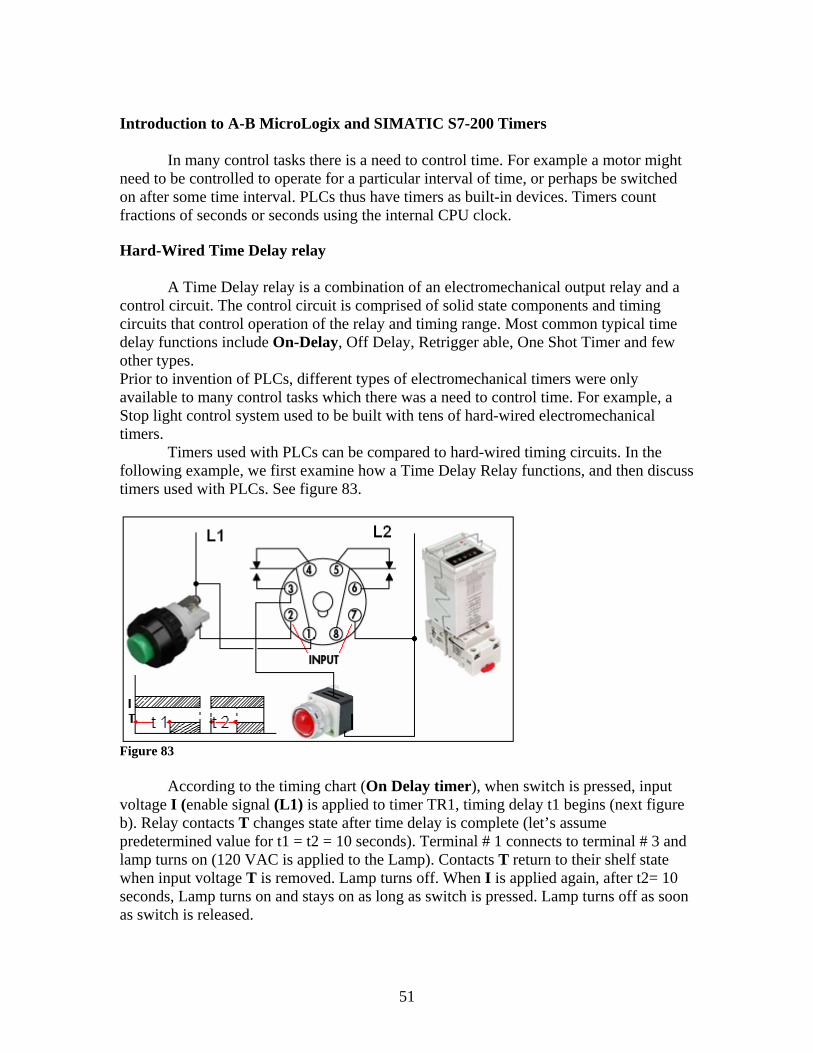
Analog applications are present in many forms. Figure 82 shows the controller that controls the amount of fluid in a holding tank by adjusting the valve opening. The valve functions based on the analog input signal received from the PLC. The valve is initially open 100% in this case maximum amount of fluid can flow into the tank. As the fluid level approaches the preset point, the controller modifies the output. Controller reduces the amount of flow of fluid little by little continuously adjusting the valve to maintain the fluid level and finally shuts it off. Analog outputs can be provided by digital-to-analogue converters at the output channel. The input to converter is a sequence of bits with each bit along a parallel line. Next figure shows the basic function of the converter. By using a converter module (a suitable expansion module) we can change 8 or 16 bits of PLC output to an analog output module. Typical analog signals range from 0-10 or 0-5 VDC or 4-20 mA. Figure 71 shows that analog l output signal of a PLC is wired to a valve to control the flow of fluid.

Figure 82 Could you explain how does the process in figure 82 work?

50

Introduction to A-B MicroLogix and SIMATIC S7-200 Timers

In many control tasks there is a need to control time. For example a motor might need to be controlled to operate for a particular interval of time, or perhaps be switched on after some time interval. PLCs thus have timers as built-in devices. Timers count fractions of seconds or seconds using the internal CPU clock. Hard-Wired Time Delay relay

A Time Delay relay is a combination of an electromechanical output relay and a control circuit. The control circuit is comprised of solid state components and timing circuits that control operation of the relay and timing range. Most common typical time delay functions include On-Delay, Off Delay, Retrigger able, One Shot Timer and few other types. Prior to invention of PLCs, different types of electromechanical timers were only available to many control tasks which there was a need to control time. For example, a Stop light control system used to be built with tens of hard-wired electromechanical timers. Timers used with PLCs can be compared to hard-wired timing circuits. In the following example, we first examine how a Time Delay Relay functions, and then discuss timers used with PLCs. See figure 83.

Figure 83

According to the timing chart (On Delay timer), when switch is pressed, input voltage I (enable signal (L1) is applied to timer TR1, timing delay t1 begins (next figure b). Relay contacts T changes state after time delay is complete (let’s assume predetermined value for t1 = t2 = 10 seconds). Terminal # 1 connects to terminal # 3 and lamp turns on (120 VAC is applied to the Lamp). Contacts T return to their shelf state when input voltage T is removed. Lamp turns off. When I is applied again, after t2= 10 seconds, Lamp turns on and stays on as long as switch is pressed. Lamp turns off as soon as switch is released.

51

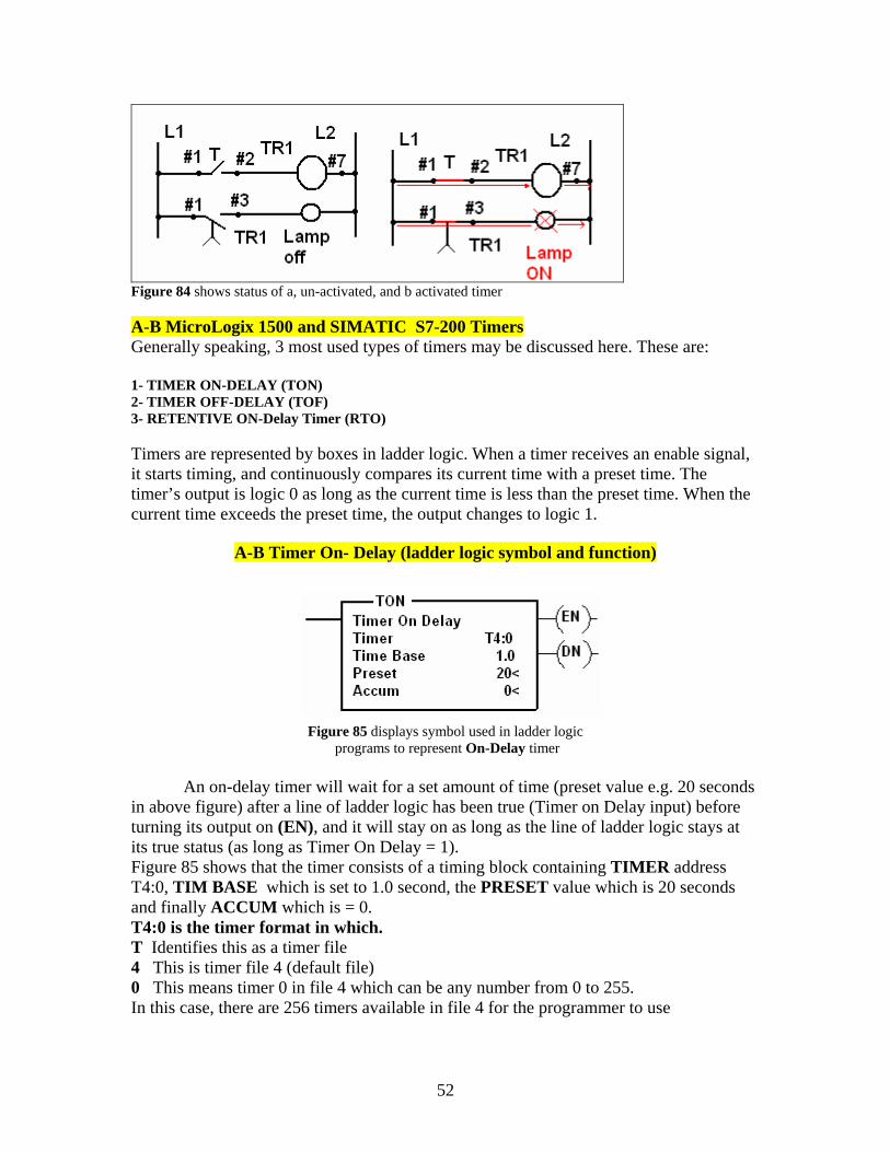
Figure 84 shows status of a, un-activated, and b activated timer A-B MicroLogix 1500 and SIMATIC S7-200 Timers Generally speaking, 3 most used types of timers may be discussed here. These are: 1- TIMER ON-DELAY (TON) 2- TIMER OFF-DELAY (TOF) 3- RETENTIVE ON-Delay Timer (RTO) Timers are represented by boxes in ladder logic. When a timer receives an enable signal, it starts timing, and continuously compares its current time with a preset time. The timer’s output is logic 0 as long as the current time is less than the preset time. When the current time exceeds the preset time, the output changes to logic 1.

A-B Timer On- Delay (ladder logic symbol and function)

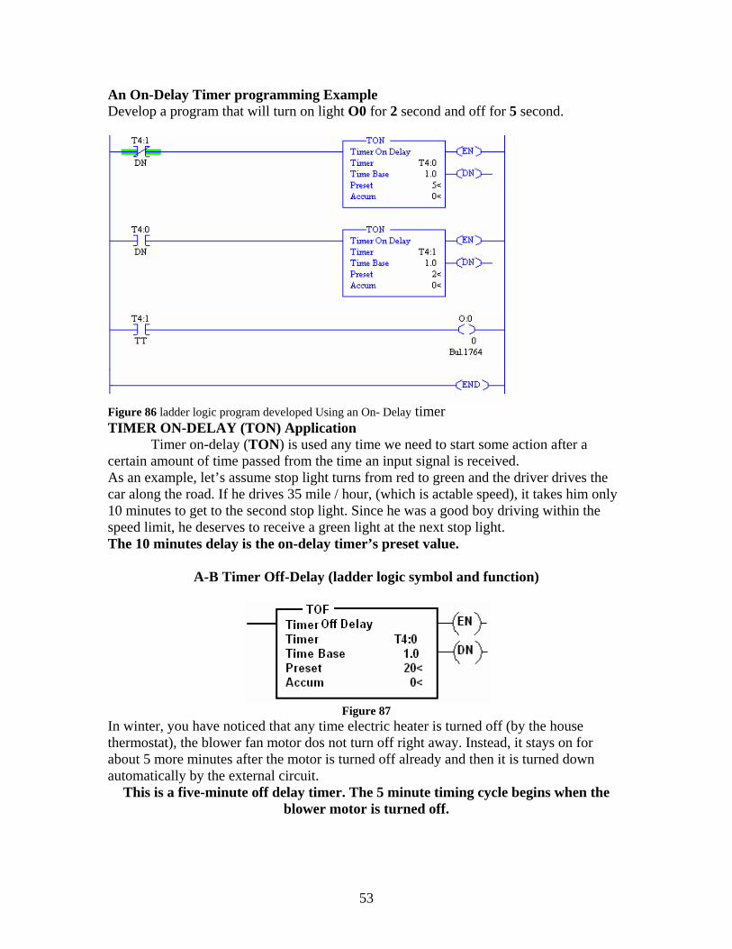
Figure 85 displays symbol used in ladder logic programs to represent On-Delay timer

An on-delay timer will wait for a set amount of time (preset value e.g. 20 seconds

in above figure) after a line of ladder logic has been true (Timer on Delay input) before turning its output on (EN), and it will stay on as long as the line of ladder logic stays at its true status (as long as Timer On Delay = 1). Figure 85 shows that the timer consists of a timing block containing TIMER address T4:0, TIM BASE which is set to 1.0 second, the PRESET value which is 20 seconds and finally ACCUM which is = 0. T4:0 is the timer format in which. T Identifies this as a timer file 4 This is timer file 4 (default file) 0 This means timer 0 in file 4 which can be any number from 0 to 255. In this case, there are 256 timers available in file 4 for the programmer to use

52

An On-Delay Timer programming Example Develop a program that will turn on light O0 for 2 second and off for 5 second.

Figure 86 ladder logic program developed Using an On- Delay timer TIMER ON-DELAY (TON) Application

Timer on-delay (TON) is used any time we need to start some action after a certain amount of time passed from the time an input signal is received. As an example, let’s assume stop light turns from red to green and the driver drives the car along the road. If he drives 35 mile / hour, (which is actable speed), it takes him only 10 minutes to get to the second stop light. Since he was a good boy driving within the speed limit, he deserves to receive a green light at the next stop light. The 10 minutes delay is the on-delay timer’s preset value.

A-B Timer Off-Delay (ladder logic symbol and function)

Figure 87

In winter, you have noticed that any time electric heater is turned off (by the house thermostat), the blower fan motor dos not turn off right away. Instead, it stays on for about 5 more minutes after the motor is turned off already and then it is turned down automatically by the external circuit.

This is a five-minute off delay timer. The 5 minute timing cycle begins when the blower motor is turned off.

53

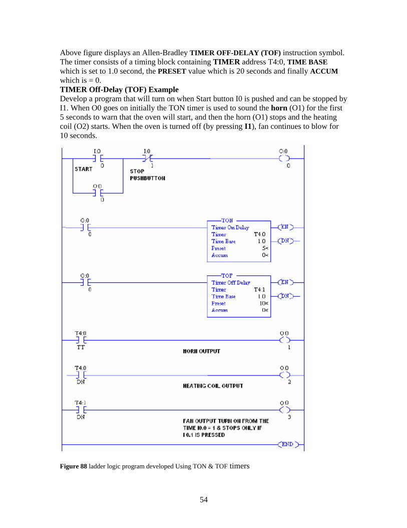
Above figure displays an Allen-Bradley TIMER OFF-DELAY (TOF) instruction symbol. The timer consists of a timing block containing TIMER address T4:0, TIME BASE which is set to 1.0 second, the PRESET value which is 20 seconds and finally ACCUM which is = 0. TIMER Off-Delay (TOF) Example Develop a program that will turn on when Start button I0 is pushed and can be stopped by I1. When O0 goes on initially the TON timer is used to sound the horn (O1) for the first 5 seconds to warn that the oven will start, and then the horn (O1) stops and the heating coil (O2) starts. When the oven is turned off (by pressing I1), fan continues to blow for 10 seconds.

Figure 88 ladder logic program developed Using TON & TOF timers

54

AB Retentive On- Delay Timer (ladder logic symbol and function)

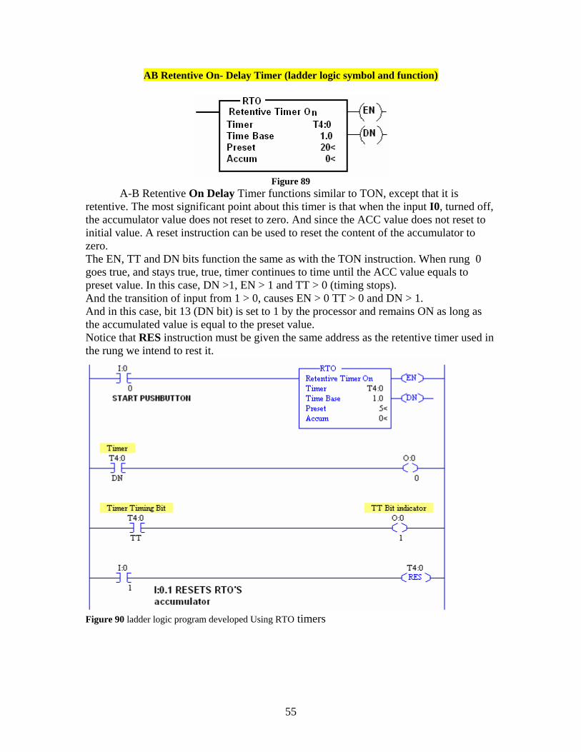
Figure 89

A-B Retentive On Delay Timer functions similar to TON, except that it is retentive. The most significant point about this timer is that when the input I0, turned off, the accumulator value does not reset to zero. And since the ACC value does not reset to initial value. A reset instruction can be used to reset the content of the accumulator to zero. The EN, TT and DN bits function the same as with the TON instruction. When rung 0 goes true, and stays true, true, timer continues to time until the ACC value equals to preset value. In this case, DN >1, EN > 1 and TT > 0 (timing stops). And the transition of input from 1 > 0, causes EN > 0 TT > 0 and DN > 1. And in this case, bit 13 (DN bit) is set to 1 by the processor and remains ON as long as the accumulated value is equal to the preset value. Notice that RES instruction must be given the same address as the retentive timer used in the rung we intend to rest it.

Figure 90 ladder logic program developed Using RTO timers

55

SIEMENS SIMATIC S7-200 TIMERS

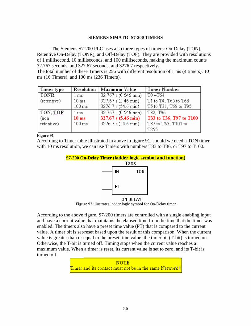
The Siemens S7-200 PLC uses also three types of timers: On-Delay (TON),

Retentive On-Delay (TONR), and Off-Delay (TOF). They are provided with resolutions of 1 millisecond, 10 milliseconds, and 100 milliseconds, making the maximum counts 32.767 seconds, and 327.67 seconds, and 3276.7 respectively. The total number of these Timers is 256 with different resolution of 1 ms (4 timers), 10 ms (16 Timers), and 100 ms (236 Timers).

Figure 91 According to Timer table illustrated in above in figure 91, should we need a TON timer with 10 ms resolution, we can use Timers with numbers T33 to T36, or T97 to T100.

S7-200 On-Delay Timer (ladder logic symbol and function)

Figure 92 illustrates ladder logic symbol for On-Delay timer

According to the above figure, S7-200 timers are controlled with a single enabling input and have a current value that maintains the elapsed time from the time that the timer was enabled. The timers also have a preset time value (PT) that is compared to the current value. A timer bit is set/reset based upon the result of this comparison. When the current value is greater than or equal to the preset time value, the timer bit (T-bit) is turned on. Otherwise, the T-bit is turned off. Timing stops when the current value reaches a maximum value. When a timer is reset, its current value is set to zero, and its T-bit is turned off.

56

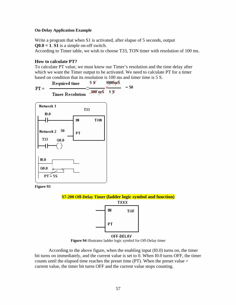
On-Delay Application Example Write a program that when S1 is activated, after elapse of 5 seconds, output Q0.0 = 1. S1 is a simple on-off switch. According to Timer table, we wish to choose T33, TON timer with resolution of 100 ms. How to calculate PT? To calculate PT value, we must know our Timer’s resolution and the time delay after which we want the Timer output to be activated. We need to calculate PT for a timer based on condition that its resolution is 100 ms and timer time is 5 S.

Figure 93

S7-200 Off-Delay Timer (ladder logic symbol and function)

Figure 94 illustrates ladder logic symbol for Off-Delay timer

According to the above figure, when the enabling input (I0.0) turns on, the timer

bit turns on immediately, and the current value is set to 0. When I0.0 turns OFF, the timer counts until the elapsed time reaches the preset time (PT). When the preset value = current value, the timer bit turns OFF and the current value stops counting.

57

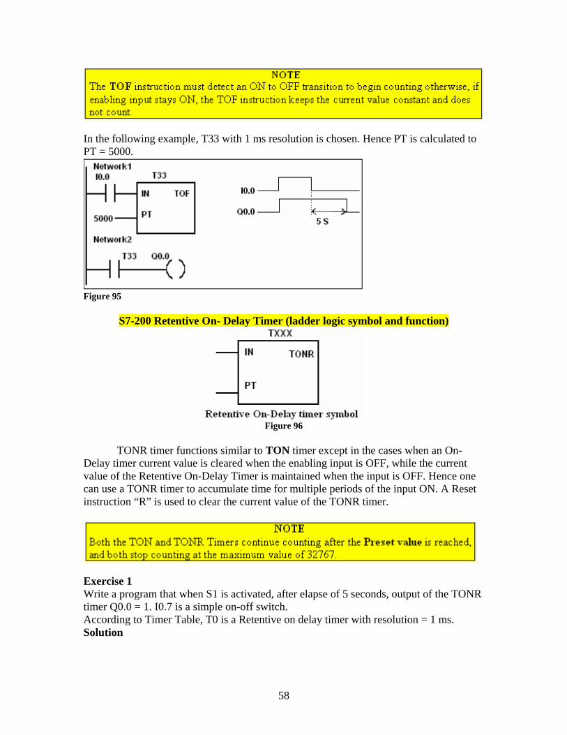
In the following example, T33 with 1 ms resolution is chosen. Hence PT is calculated to PT = 5000.

Figure 95

S7-200 Retentive On- Delay Timer (ladder logic symbol and function)

Figure 96

TONR timer functions similar to TON timer except in the cases when an On-

Delay timer current value is cleared when the enabling input is OFF, while the current value of the Retentive On-Delay Timer is maintained when the input is OFF. Hence one can use a TONR timer to accumulate time for multiple periods of the input ON. A Reset instruction “R” is used to clear the current value of the TONR timer.

Exercise 1 Write a program that when S1 is activated, after elapse of 5 seconds, output of the TONR timer Q0.0 = 1. I0.7 is a simple on-off switch. According to Timer Table, T0 is a Retentive on delay timer with resolution = 1 ms. Solution

58

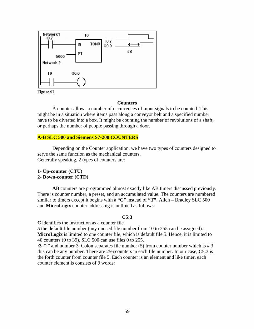
Figure 97

Counters A counter allows a number of occurrences of input signals to be counted. This

might be in a situation where items pass along a conveyor belt and a specified number have to be diverted into a box. It might be counting the number of revolutions of a shaft, or perhaps the number of people passing through a door. A-B SLC 500 and Siemens S7-200 COUNTERS

Depending on the Counter application, we have two types of counters designed to

serve the same function as the mechanical counters. Generally speaking, 2 types of counters are: 1- Up-counter (CTU) 2- Down-counter (CTD)

AB counters are programmed almost exactly like AB timers discussed previously. There is counter number, a preset, and an accumulated value. The counters are numbered similar to timers except it begins with a “C” instead of “T”. Allen – Bradley SLC 500 and MicroLogix counter addressing is outlined as follows:

C5:3 C identifies the instruction as a counter file 5 the default file number (any unused file number from 10 to 255 can be assigned). MicroLogix is limited to one counter file, which is default file 5. Hence, it is limited to 40 counters (0 to 39). SLC 500 can use files 0 to 255. :3 “:” and number 3. Colon separates file number (5) from counter number which is # 3 this can be any number. There are 256 counters in each file number. In our case, C5:3 is the forth counter from counter file 5. Each counter is an element and like timer, each counter element is consists of 3 words:

59

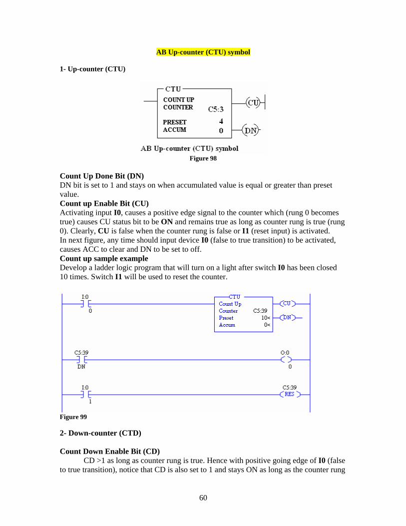
AB Up-counter (CTU) symbol 1- Up-counter (CTU)

Figure 98

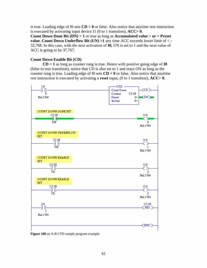
Count Up Done Bit (DN) DN bit is set to 1 and stays on when accumulated value is equal or greater than preset value. Count up Enable Bit (CU) Activating input I0, causes a positive edge signal to the counter which (rung 0 becomes true) causes CU status bit to be ON and remains true as long as counter rung is true (rung 0). Clearly, CU is false when the counter rung is false or I1 (reset input) is activated. In next figure, any time should input device I0 (false to true transition) to be activated, causes ACC to clear and DN to be set to off. Count up sample example Develop a ladder logic program that will turn on a light after switch I0 has been closed 10 times. Switch I1 will be used to reset the counter.

Figure 99 2- Down-counter (CTD) Count Down Enable Bit (CD)

CD >1 as long as counter rung is true. Hence with positive going edge of I0 (false to true transition), notice that CD is also set to 1 and stays ON as long as the counter rung

60

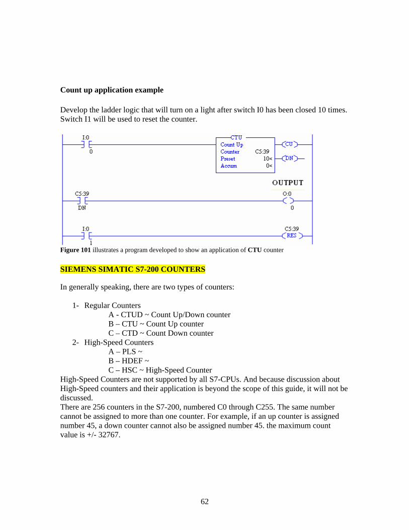
is true. Leading edge of I0 sets CD > 0 or false. Also notice that anytime rest instruction is executed by activating input device I1 (0 to 1 transition), ACC> 0. Count Down Done Bit (DN) > 1 or true as long as Accumulated value > or = Preset value. Count Down Underflow Bit (UN) >1 any time ACC exceeds lower limit of < -32,768. In this case, with the next activation of I0, UN is set to 1 and the next value of ACC is going to be 37,767. Count Down Enable Bit (CD)

CD > 1 as long as counter rung is true. Hence with positive going edge of I0 (false to true transition), notice that CD is also set to 1 and stays ON as long as the counter rung is true. Leading edge of I0 sets CD > 0 or false. Also notice that anytime rest instruction is executed by activating a reset input, (0 to 1 transition), ACC> 0.

Figure 100 an A-B CTD sample program example

61

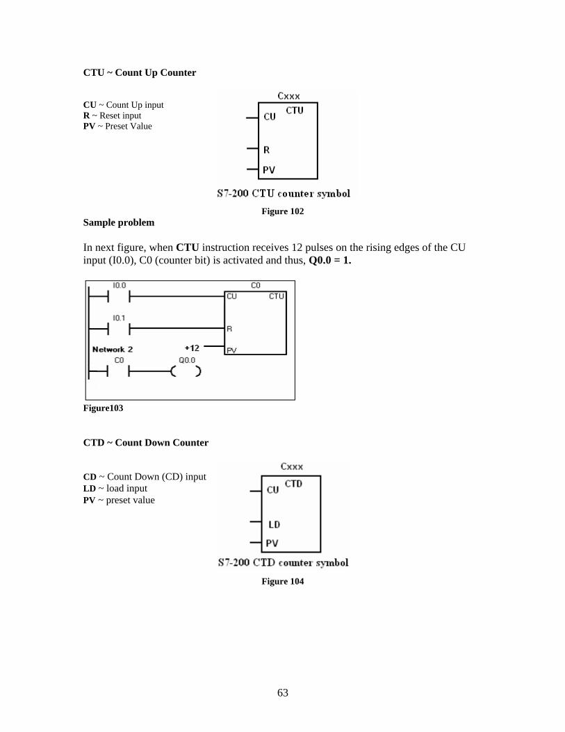
Count up application example Develop the ladder logic that will turn on a light after switch I0 has been closed 10 times. Switch I1 will be used to reset the counter.

Figure 101 illustrates a program developed to show an application of CTU counter SIEMENS SIMATIC S7-200 COUNTERS In generally speaking, there are two types of counters:

1- Regular Counters A - CTUD ~ Count Up/Down counter B – CTU ~ Count Up counter C – CTD ~ Count Down counter

2- High-Speed Counters A – PLS ~ B – HDEF ~ C – HSC ~ High-Speed Counter

High-Speed Counters are not supported by all S7-CPUs. And because discussion about High-Speed counters and their application is beyond the scope of this guide, it will not be discussed. There are 256 counters in the S7-200, numbered C0 through C255. The same number cannot be assigned to more than one counter. For example, if an up counter is assigned number 45, a down counter cannot also be assigned number 45. the maximum count value is +/- 32767.

62

CTU ~ Count Up Counter

CU ~ Count Up input R ~ Reset input PV ~ Preset Value

Figure 102 Sample problem In next figure, when CTU instruction receives 12 pulses on the rising edges of the CU input (I0.0), C0 (counter bit) is activated and thus, Q0.0 = 1.

Figure103 CTD ~ Count Down Counter CD ~ Count Down (CD) input LD ~ load input PV ~ preset value

Figure 104

63

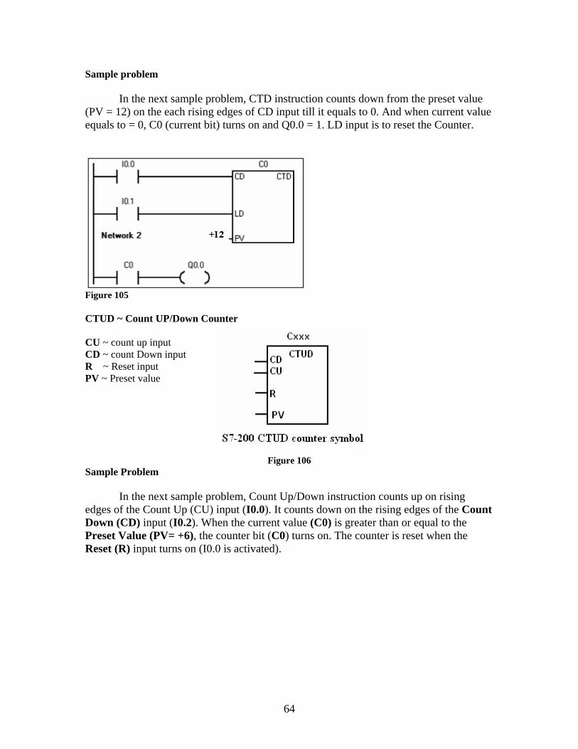
Sample problem

In the next sample problem, CTD instruction counts down from the preset value (PV = 12) on the each rising edges of CD input till it equals to 0. And when current value equals to = 0, C0 (current bit) turns on and Q0.0 = 1. LD input is to reset the Counter.

Figure 105 CTUD ~ Count UP/Down Counter CU ~ count up input CD ~ count Down input R ~ Reset input PV ~ Preset value

Figure 106

Sample Problem In the next sample problem, Count Up/Down instruction counts up on rising edges of the Count Up (CU) input (I0.0). It counts down on the rising edges of the Count Down (CD) input (I0.2). When the current value (C0) is greater than or equal to the Preset Value (PV= +6), the counter bit (C0) turns on. The counter is reset when the Reset (R) input turns on (I0.0 is activated).

64

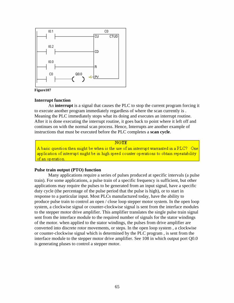
Figure107 Interrupt function

An interrupt is a signal that causes the PLC to stop the current program forcing it to execute another program immediately regardless of where the scan currently is . Meaning the PLC immediately stops what its doing and executes an interrupt routine. After it is done executing the interrupt routine, it goes back to point where it left off and continues on with the normal scan process. Hence, Interrupts are another example of instructions that must be executed before the PLC completes a scan cycle.

Pulse train output (PTO) function

Many applications require a series of pulses produced at specific intervals (a pulse train). For some applications, a pulse train of a specific frequency is sufficient, but other applications may require the pulses to be generated from an input signal, have a specific duty cycle (the percentage of the pulse period that the pulse is high), or to start in response to a particular input. Most PLCs manufactured today, have the ability to produce pulse train to control an open / close loop stepper motor system. In the open loop system, a clockwise signal or counter-clockwise signal is sent from the interface modules to the stepper motor drive amplifier. This amplifier translates the single pulse train signal sent from the interface module to the required number of signals for the stator windings of the motor. when applied to the stator windings, the pulses from drive amplifier are converted into discrete rotor movements, or steps. In the open loop system , a clockwise or counter-clockwise signal which is determined by the PLC program , is sent from the interface module to the stepper motor drive amplifier. See 108 in which output port Q0.0 is generating pluses to control a stepper motor.

65

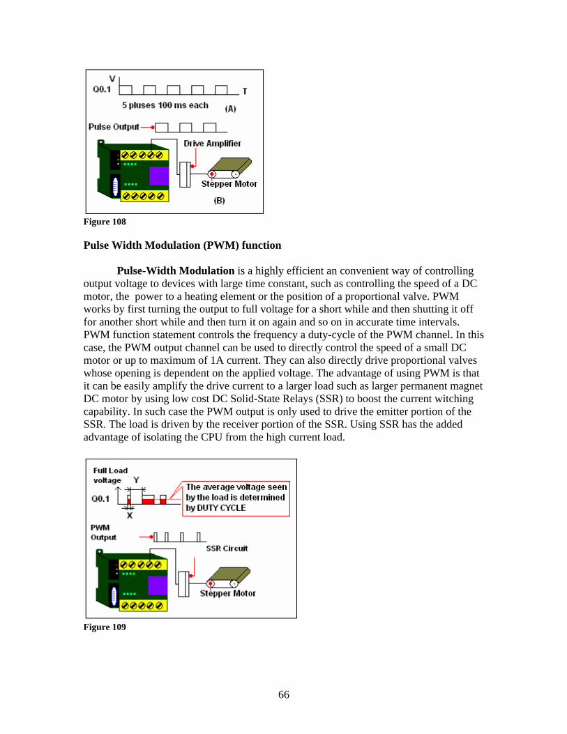
Figure 108 Pulse Width Modulation (PWM) function

Pulse-Width Modulation is a highly efficient an convenient way of controlling output voltage to devices with large time constant, such as controlling the speed of a DC motor, the power to a heating element or the position of a proportional valve. PWM works by first turning the output to full voltage for a short while and then shutting it off for another short while and then turn it on again and so on in accurate time intervals. PWM function statement controls the frequency a duty-cycle of the PWM channel. In this case, the PWM output channel can be used to directly control the speed of a small DC motor or up to maximum of 1A current. They can also directly drive proportional valves whose opening is dependent on the applied voltage. The advantage of using PWM is that it can be easily amplify the drive current to a larger load such as larger permanent magnet DC motor by using low cost DC Solid-State Relays (SSR) to boost the current witching capability. In such case the PWM output is only used to drive the emitter portion of the SSR. The load is driven by the receiver portion of the SSR. Using SSR has the added advantage of isolating the CPU from the high current load.

Figure 109

66

In figure 109, top shows the average voltage applied to the Load with the shown duty cycle. In the bottom, it shows how the output Q0.1 PWM voltage is amplified and applied to the DC motor. Figure110 illustrates the equations to calculate the Average voltage, duty cycle, period, and frequency.

Figure 110 Voltage of 110 VAC @ 60 HZ is with duty cycle of 20% is applied to a resistive load. Calculate the average voltage and period of the voltage applied to the load. Average voltage is = (20/100) 110 = 2/10 x 110 = 22 Volt F = 1/Period 60 cycle /Second = 1/period Period = 1/60 second = 1000 ms/60 = ~ 16.66 ms Transmit function

The Transmit blocks send Modbus messages from a "master" PLC to multiple slave PLCs or sends ASCII character strings from the PLC’s Modbus slave port to ASCII printers and terminals. The function can send these messages over telephone dialup modems, radio modems, or simply direct connections. The Transmit blocks perform general ASCII input functions in the communication mode including simple ASCII and terminated ASCII. You may import and export ASCII or binary data into your PLC. The block has built in diagnostics that checks to make sure no other Transmit blocks are active in the PLC on the same port. Within the Transmit blocks, control inputs allows you to control the communications link between the PLC and DCE (Data Communication Equipment) devices attached to Modbus ports of the PLC. The Transmit blocks do NOT activate the port LED when transmitting data. Transmit allows communication with external devices, such as modems, printers, and computers, via the serial interface.

Modbus is a serial communications protocol published by Modicon in 1979 for use with its PLCs. Simple and robust, it has since become one of the de facto standard communications protocols in the industry, and it is now amongst the most commonly available means of connecting industrial electronic devices.

http://www.alamedaelectric.com/Modicon http://kernow.curtin.edu.au/www/plc/3STANDAR.HTM

67

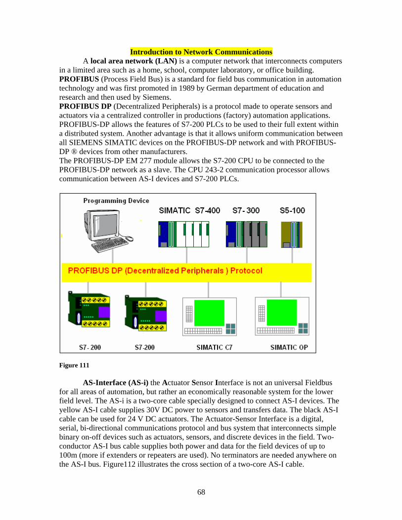
Introduction to Network Communications A local area network (LAN) is a computer network that interconnects computers

in a limited area such as a home, school, computer laboratory, or office building. PROFIBUS (Process Field Bus) is a standard for field bus communication in automation technology and was first promoted in 1989 by German department of education and research and then used by Siemens. PROFIBUS DP (Decentralized Peripherals) is a protocol made to operate sensors and actuators via a centralized controller in productions (factory) automation applications. PROFIBUS-DP allows the features of S7-200 PLCs to be used to their full extent within a distributed system. Another advantage is that it allows uniform communication between all SIEMENS SIMATIC devices on the PROFIBUS-DP network and with PROFIBUS-DP ® devices from other manufacturers. The PROFIBUS-DP EM 277 module allows the S7-200 CPU to be connected to the PROFIBUS-DP network as a slave. The CPU 243-2 communication processor allows communication between AS-I devices and S7-200 PLCs.

Figure 111

AS-Interface (AS-i) the Actuator Sensor Interface is not an universal Fieldbus for all areas of automation, but rather an economically reasonable system for the lower field level. The AS-i is a two-core cable specially designed to connect AS-I devices. The yellow AS-I cable supplies 30V DC power to sensors and transfers data. The black AS-I cable can be used for 24 V DC actuators. The Actuator-Sensor Interface is a digital, serial, bi-directional communications protocol and bus system that interconnects simple binary on-off devices such as actuators, sensors, and discrete devices in the field. Two-conductor AS-I bus cable supplies both power and data for the field devices of up to 100m (more if extenders or repeaters are used). No terminators are needed anywhere on the AS-I bus. Figure112 illustrates the cross section of a two-core AS-I cable.

68

Figure 112

SIMATIC S7-200 from CPU 222 upwards has functionality as AS- interface master via AS-interface module (AS-Interface master CP 243-2 max. 2 modules). Figure 113 illustrates an AS-I network of S7-200 PLC participating as a master module.

Figure 113 A thermistor is a type of resistor whose resistance varies significantly with temperature, more so than in standard resistors. Thermistors are widely used as inrush current limiters, temperature sensors, self-resetting over current protectors, and self-regulating heating elements. Thermistors differ from resistance temperature detectors (RTD) in that the material used in a thermistor is generally a ceramic or polymer, while RTDs use pure metals. The temperature response is also different. RTDs are usfeful over larger temperature ranges, while thermistors typically achieve a higher precision within a limited temperature range typically -90 ºC to 130 ºC

69

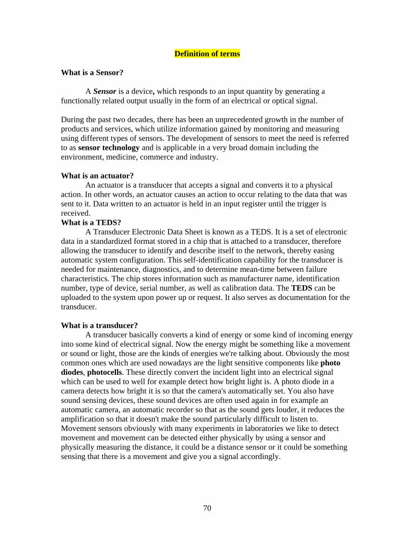
Definition of terms

What is a Sensor?

A Sensor is a device, which responds to an input quantity by generating a functionally related output usually in the form of an electrical or optical signal.

During the past two decades, there has been an unprecedented growth in the number of products and services, which utilize information gained by monitoring and measuring using different types of sensors. The development of sensors to meet the need is referred to as sensor technology and is applicable in a very broad domain including the environment, medicine, commerce and industry. What is an actuator? An actuator is a transducer that accepts a signal and converts it to a physical action. In other words, an actuator causes an action to occur relating to the data that was sent to it. Data written to an actuator is held in an input register until the trigger is received. What is a TEDS? A Transducer Electronic Data Sheet is known as a TEDS. It is a set of electronic data in a standardized format stored in a chip that is attached to a transducer, therefore allowing the transducer to identify and describe itself to the network, thereby easing automatic system configuration. This self-identification capability for the transducer is needed for maintenance, diagnostics, and to determine mean-time between failure characteristics. The chip stores information such as manufacturer name, identification number, type of device, serial number, as well as calibration data. The TEDS can be uploaded to the system upon power up or request. It also serves as documentation for the transducer. What is a transducer? A transducer basically converts a kind of energy or some kind of incoming energy into some kind of electrical signal. Now the energy might be something like a movement or sound or light, those are the kinds of energies we're talking about. Obviously the most common ones which are used nowadays are the light sensitive components like photo diodes, photocells. These directly convert the incident light into an electrical signal which can be used to well for example detect how bright light is. A photo diode in a camera detects how bright it is so that the camera's automatically set. You also have sound sensing devices, these sound devices are often used again in for example an automatic camera, an automatic recorder so that as the sound gets louder, it reduces the amplification so that it doesn't make the sound particularly difficult to listen to. Movement sensors obviously with many experiments in laboratories we like to detect movement and movement can be detected either physically by using a sensor and physically measuring the distance, it could be a distance sensor or it could be something sensing that there is a movement and give you a signal accordingly.

70

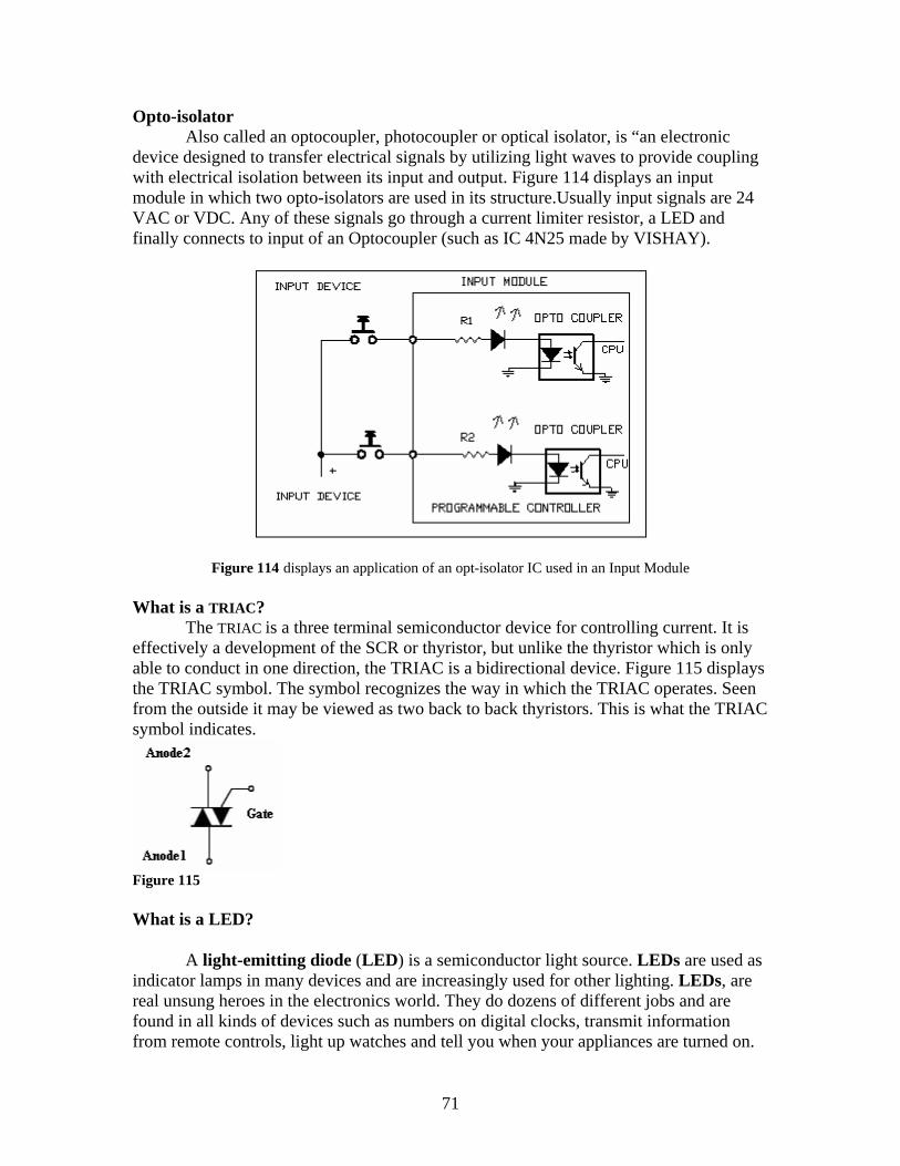
Opto-isolator Also called an optocoupler, photocoupler or optical isolator, is “an electronic device designed to transfer electrical signals by utilizing light waves to provide coupling with electrical isolation between its input and output. Figure 114 displays an input module in which two opto-isolators are used in its structure. Usually input signals are 24 VAC or VDC. Any of these signals go through a current limiter resistor, a LED and finally connects to input of an Optocoupler (such as IC 4N25 made by VISHAY).

Figure 114 displays an application of an opt-isolator IC used in an Input Module What is a TRIAC? The TRIAC is a three terminal semiconductor device for controlling current. It is effectively a development of the SCR or thyristor, but unlike the thyristor which is only able to conduct in one direction, the TRIAC is a bidirectional device. Figure 115 displays the TRIAC symbol. The symbol recognizes the way in which the TRIAC operates. Seen from the outside it may be viewed as two back to back thyristors. This is what the TRIAC symbol indicates.

Figure 115 What is a LED?

A light-emitting diode (LED) is a semiconductor light source. LEDs are used as indicator lamps in many devices and are increasingly used for other lighting. LEDs, are real unsung heroes in the electronics world. They do dozens of different jobs and are found in all kinds of devices such as numbers on digital clocks, transmit information from remote controls, light up watches and tell you when your appliances are turned on.

71

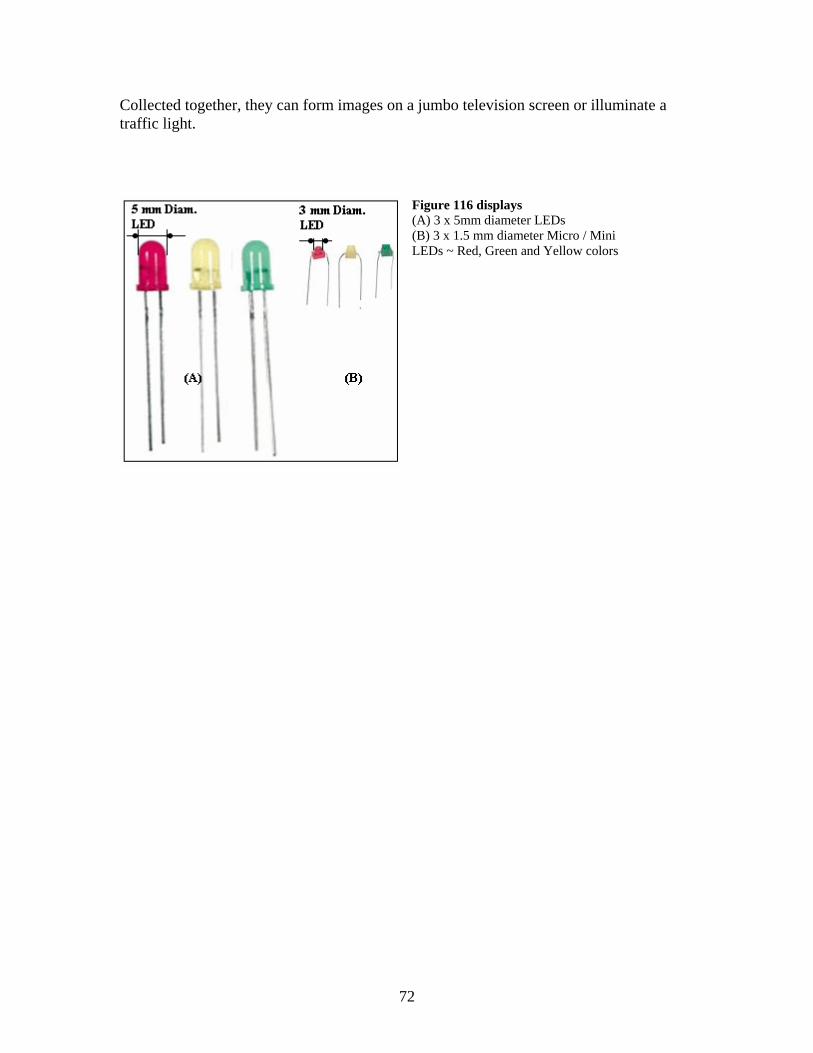
Collected together, they can form images on a jumbo television screen or illuminate a traffic light.

Figure 116 displays (A) 3 x 5mm diameter LEDs (B) 3 x 1.5 mm diameter Micro / Mini LEDs ~ Red, Green and Yellow colors

72