Embed Size (px)
Citation preview

Strategic, Tactical and Real‐Time Planning of Locomotives at Norfolk Southern
Using Approximate Dynamic Programming
Warren B. Powell [email protected]
(609)273‐0218
Belgacem Bouzaiene‐Ayari [email protected]
Department of Operations Research and Financial Engineering
Sherrerd Hall Princeton University Princeton, NJ 08544
Coleman Lawrence [email protected]
Clark Cheng
Sourav Das [email protected]
Ricardo Fiorillo
Norfolk Southern Corporation
1200 Peachtree St. NE , Box 12‐117 Atlanta GA 30309
March 9, 2012

Abstract
Locomotive planning has been a popular application of classical optimization models for decades, but with very few success stories. There are a host of complex rules governing how locomotives should be used. In addition, it is necessary to simultaneously manage locomotive inventories by balancing the need for holding power against the need for power at other yards. At the same time, we have to plan the need to return foreign power, and move power to maintenance facilities for scheduled FRA appointments. An additional complication arises as a result of the high level of uncertainty in transit times and delays due to yard processing, and as a result we may have to plan additional inventories in order to move outbound trains on time despite inbound delays. We describe a novel modeling and algorithmic strategy known as approximate dynamic programming, which can also be described as a form of “optimizing simulator” which uses feedback learning to plan locomotive movements in a way that closely mimics how humans plan real‐world operations. This strategy can be used for strategic and tactical planning, and can also be adapted to real‐time operations. We describe the strategy, and summarize experiences at Norfolk Southern with a strategic planning system.

Page 1
1
Locomotive planning is one of the most complex operational problems in freight transportation.
Planners have to take into consideration a host of operational characteristics that describe a locomotive
to best utilize the fleet to meet the service requirements of the trains. Locomotive fleets can represent
billions of dollars in investments, and as a result railroads have every incentive to manage this
investment as efficiently as possible. The complexity of the problem has put it well past the capabilities
of even today’s advanced optimization solvers. Completely overlooked in these models are the
important sources of uncertainty such as transit time delays, the dynamics of scheduling commodities
such as coal and grain, and the ever present problem of equipment failures and maintenance.
Railroads face three classes of planning problems when managing railroads:
Strategic planning – The major question here is fleet size and mix, but other questions can
include understanding the impact of improvements in transit time reliability, the effect of
changes in train plans and changes in interchange policies with other railroads.
Tactical planning and operational forecasting – Here the horizon is 1‐7 days, and the
question is whether there will be significant shortages of power that might require
additional repositioning, short‐term modifications in leasing decisions and perhaps the
decision to retain locomotives that belong to other railroads (known as “foreign power”)
and incur additional per diem charges.
Real‐time planning – The decision here is the assignment of specific locomotives to specific
trains that are departing over the immediate horizon (typically the next 12 hours).
A large railroad may have billions invested in their fleet of locomotives. Too many locomotives mean
that hundreds of millions are invested in equipment that is not yielding a return. However, a failure to
maintain a sufficiently large fleet translates to delayed trains and service failures that can seriously
impact revenue. Despite the scale of this investment, it is not unusual for a large railroad to plan their
locomotive fleets using a simple linear regression that relates operating statistics such as forecasted
tonnage and operating speeds to the amount of power required to run the railroad.
Given the size of the investment, railroads have tried for decades to tap the power of optimization tools
to manage their fleets more effectively. Booler (1980) presents a very early attempt at using linear
programming to solve a scheduling model. Chih (1986) and Chih et al. (1990) describe an
implementation of an integer programming model for locomotive scheduling at the Burlington Northern
Sante Fe Railroad (see also Forbes (1990)). This early work struggled with the limitation of integer
programming algorithms, despite using highly simplified models of locomotive operations. A number of
advances have been made in the design of specialized algorithms to solve integer programming
formulations locomotive scheduling. Ziarati (1999) presents a new branch and cuct algorithm. Ahuja et
al (2005) describe a heuristic based on very large scale neighborhoods to find near‐optimal schedules for
locomotives which considers consist breakups and the desire for weekly patterns in the flows of
locomotives. Vaidyanathan et al. (2008a) provides a detailed model of the locomotive routing problem
capturing a number of operational constraints with an adaptation of their large neighborhood search
strategy (see also Vaidyanathan et al. (2008b) for additional experimental work). Cordeau et a. (2000,
2001) describe the use of Benders decomposition for the simultaneous assignment of cars and

Page 2
2
locomotives. At the same time, it is important to recognize major advances to general purpose integer
programming solvers such as Cplex and Gurobi that have occurred since 2005. Below, we report on
experiments with Cplex 12 running on a multithreaded machine.
This paper describes a multiyear effort to develop a family of locomotive planning models for Norfolk
Southern Railroad. The result is the Princeton Locomotive And Shop MAnagement system (PLASMA),
which can be used for strategic planning, short term operational forecasting, and real‐time operations.
PLASMA has been imbedded in a larger information system developed at Norfolk Southern called the
Locomotive Assignment and Routing System (LARS). As of this writing, the system has been used for
strategic fleet sizing for several years and has become an integral part of the company’s network and
resource planning processes. The operational forecasting system has been undergoing extensive user
acceptance testing while Norfolk Southern has been upgrading its information systems to improve the
accuracy of some of the data. We then provide an indication of how the system can be implemented as
a real‐time, interactive system.
LocomotiveoperationsLocomotives are described by a host of attributes including horsepower and tractive effort, the owning
railroad, its maintenance status (e.g. days until the next federally mandated maintenance appointment),
and equipment details such as communications gear (for coordinating multiple locomotives).
Locomotives typically need to be bundled together into consists of one to perhaps five locomotives
which are needed to pull a particular train. The process of connecting locomotives is time‐consuming,
requiring the connecting and testing of cables that allow the set of locomotives to work as a single unit.
Trains often arrive from a neighboring railroad using locomotives owned by that railroad (known as
“foreign power”). Normally foreign locomotives are returned to the owning railroad, but it is possible to
use these locomotives, but only within negotiated limits If the locomotive is returned, this has to be
handled through pre‐defined exchange points.
The trains themselves also have numerous attributes. The number of locomotives needed to pull a train
depends on the weight of the train, the speed requirements (merchandise trains need to move more
quickly than coal and grain trains), and the steepest grade that the train has to navigate. Trains have
different service priorities, and a scheduler has to consider if there are not enough locomotives to move
all the trains on time.
Shop routing (getting the locomotive to a maintenance shop) is one of the most complex issues facing a
locomotive manager. Locomotives need to have regular maintenance reviews on a periodic schedule
(typically every 90 days). If a locomotive does not make its shop appointment on time, it has to be
turned off and “towed” to the shop. Of course, on some trains it is possible to simply add a locomotive
as an extra locomotive and move it to its shop appointment, but it is better to use the locomotive
productively. At the same time, the scheduler has to balance getting the locomotive to shop early
(which costs productivity) or risk that it may arrive late (for example, by missing a critical connection).
On top of this, there may be multiple shop locations that can service a locomotive. It is necessary to
anticipate the number of locomotives that are scheduled at each shop in order to balance the loads and
maintain a steady flow of work.

Page 3
3
A separate issue that is widely discussed but rarely solved concerns the different types of uncertainty
that plague locomotive operations. These include:
Transit time delays – These can be as long as six to 12 hours for the shorter movements
of an Eastern railroad, to more than a day for the long movements of the western
railroads.
Dynamic schedule changes ‐ Planners also have to deal with the pattern of scheduling
additional trains for commodities such as coal and grain, with as little as one or two days
advance notice.
Shop delays – Maintenance managers will provide estimates of when a locomotive will
be ready to leave a shop, but these are just estimates and frequent calls to a
maintenance facility are often needed to determine if a locomotive will be ready for a
particular train.
Equipment failures – Locomotives may fail unexpectedly, and this represents an
additional source of uncertainty.
The model presented in this paper is designed to handle uncertainty, but production applications of the
model have yet to exploit this capability.
DeterministicoptimizationmodelsThe most common strategy for modeling locomotives as an optimization problem is to use the
framework of multicommodity flows over a time‐space network, depicted in figure 1. Mathematically,
such a model can be written in a generic format using
Figure 1‐ Illustration of multicommodity network flow problem over a time‐space network.

Page 4
4
1 1
minT K
k kx ij tij
t k
c x (1)
subject to
1 1k k k kt t t t tA x B x R (2)
t t tD x u (3)
0 and integer.ktijx (4)
Here, ktijx represents the flow of locomotives of type k moving from yard i to yard j departing at time t.
Equation (2) captures flow conservation for locomotives of each type. Equation (3) captures the number
of locomotives needed to move a train (summing across different types of locomotives). Equation (4)
requires that the flow variables be integer.
This basic model has to be adjusted to allow for the following:
If a train requires three locomotives to meet speed and grade requirements, we can still use the
train to pull more locomotives if we need to reposition power from one yard to another.
One or more locomotives can be moved from one yard to another without pulling a train, an
operation known as a “light engine move.” Light engine moves incur crew costs and as a result
need to be carefully managed.
There is a cost for coupling locomotives together into a consist to pull a single train, as well as a
cost for decoupling the locomotives. This operation also takes time which has to be built into
the dynamics.
Locomotives that need to be routed to shop have to be modeled.
A particularly difficult challenge is the modeling of train delay. The most common assumption is to use a
time‐space network as shown in figure 1, but to then replicate train movements over multiple time
periods. Since the same train cannot move at different points in time, they are linked by a bundle
constraint that ensures that only one “copy” of the train can move, as shown in figure 2.
Figure 2‐Time‐space representation of trains with multiple departure times.

Page 5
5
Our experience with this strategy was that it introduced discretization errors that were unacceptable to
the railroad. If we use a one‐hour time step, the network simply explodes. However, if we use a slightly
more manageable four‐hour time step (which still increases the size of the problem dramatically), we
encounter situations where a locomotive may arrive 20 minutes too late to serve a train, but this then
forces us to impose a four hour delay. This was felt to be an unacceptable distortion, and it dramatically
inflated train delay.
We avoid this problem by using a classic “task graph” formulation, where a train is modeled as a task
which is characterized by an initial time of availability. The basic idea is illustrated in figure 3.
Locomotives are modeled as arriving in continuous time. Dashed assignment arcs can join a locomotive
at any point in time to a specific train. The departure time of the train is governed by the latest
locomotive that is actually assigned to the train, which allows us to model train delays of any length.
Deterministic models are extremely hard to solve over long planning horizons, especially when modeling
the ability to delay trains. Figure 4 shows the run times as the horizon is extended for the Norfolk
Southern fleet. Note the exceptionally fast execution time for the single‐day horizon. For this problem,
locomotives are being assigned to at most a single train. As the horizon grows, we have to model the
cascading of train delays in the task graph. With a horizon of as little as four days, the run times are
already exceeding 50 hours.
Figure 4 ‐ Execution times for increasing planning horizons for the full fleet of locomotives.
Figure 3‐Task graph representation of trains and locomotive arrivals.

Page 6
6
AnapproximatedynamicprogrammingmodelandalgorithmApproximate dynamic programming is a modeling and algorithmic strategy that decomposes decisions
over time (see Powell (2011) for an introduction using the concepts and notation in this paper;
approximate dynamic programming is closely related to the field of reinforcement learning, see Sutton
and Barto (1998)). It was originally developed to handle problems which involve uncertainty. Our own
work, however, has focused on its ability to decompose large deterministic problems, overcoming the
dramatic increase in CPU times documented in figure 4. In fact, all of the production applications of ADP
at Norfolk Southern have been conducted using a deterministic model. In this paper, we report on some
recent experiments using ADP to improve the robustness of the solution in the presence of uncertainty
in transit times.
This paper will not attempt to present a complete mathematical model. Instead, we provide a sketch of
how approximate dynamic programming approaches the problem. The basic idea in an ADP approach is
to set up a subproblem where we assign locomotives to trains over a relatively short horizon (perhaps 4‐
6 hours). We could start by maximizing the contribution we earn now, ignoring the impact of decisions
now on the future. In such a model, let
tS The state of our system, including the status of current and inbound trains, and the
outbound schedule of trains that we know of at time t.
tx A vector of assignments of current and possibly inbound locomotives to outbound trains
over a specific horizon (such as 4‐6 hours).
( , )t tC S x Contribution earned if we are in state tS and make decision tx . This would include
bonuses for moving trains (which reflect the priority of the train), costs for forming or
breaking consists, and any costs that are incurred implementing the decision.
If we are willing to ignore the future, we would make decisions using a myopic policy defined by
( ) arg max ( , ).t
Mt x t tX S C S x X
This means we find the set of assignments that produces the highest contribution now. Such a policy
would never reposition power for use in the future. Furthermore, we might use power now on a low
priority train, ignoring the very high priority train that has to leave, say, 10 hours from now. A policy
that overcomes this limitation looks like
1 1( ) arg max ( , ) ( ) |t
Mt x t t t t tX S C S x V S S X (5)
where 1 1( , , )Mt t t tS S S x W is the state at the next time period (typically four hours from now) given
that we are in state tS right now (this specifies the available locomotives and trains), we make decision
tx (this determines which locomotives are assigned to each train, and which locomotives are held), and
where 1tW captures the random information such as train delays, schedule changes and equipment
Page 7
7
problems that were not known at time t. In a deterministic implementation, the variable 1tW does not
contain anything (no trains are delayed, no schedule changes are made, and no equipment fails). The
expectation in equation (5) generally cannot be computed, but we can get around this (for stochastic
problems) by using the concept of the post‐decision state variable. While this arises in different forms,
in this setting it is easiest to think of it as that the state that we would land in if the random information
1tW is what we expect it to be (say, the average travel time, or assuming that there are no changes in
the schedule and no equipment failures). Let , 1t tW be a forecast of 1tW given what we know at time t.
We can write the post decision state xtS using
, 1( , , ).x Mt t t t tS S S x W
We can then replace equation (5) with
( ) arg max ( , ) ( ).t
V x xt x t t t tX S C S x V S X (6)
Finally, we will never be able to calculate the value function ( )x xt tV S exactly, so we replace it with an
approximation that we write as ( ) ( )x x xt t tV S V S . The challenge then is to design an approximation
( )xtV S that is easy to estimate, allows equation (6) to be solved fairly easily, and works well.
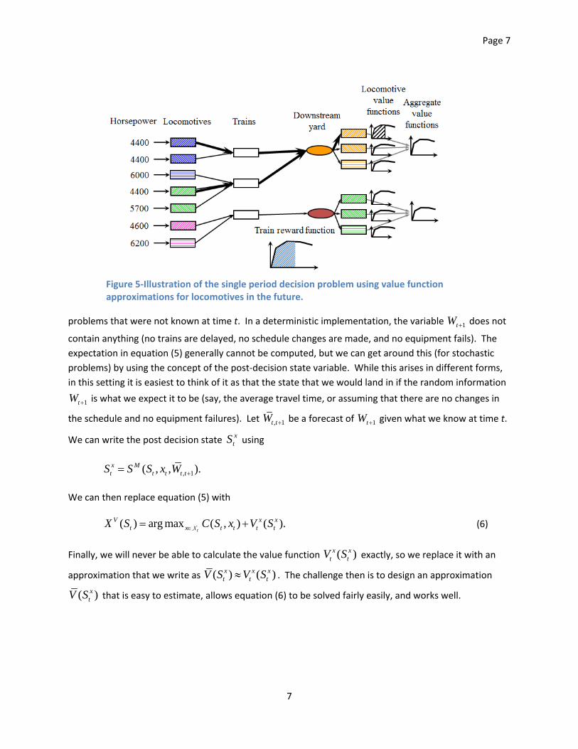
Figure 5‐Illustration of the single period decision problem using value function approximations for locomotives in the future.

Page 8
8
Recall that the state variable consists of locomotives and trains. We have found that an approximation
strategy that works well ignores the value of trains in the future , and uses a piecewise linear function to
approximate the value of the major classes of locomotive (low/high adhesion, low/high horsepower).
Capturing the value of trains in the future contributes to better decisions only when trains are delayed,
which happens fairly infrequently. This produces an optimization problem that is depicted in figure 5. In
the figure, we see the initial assignment of locomotives to trains. We also use a piecewise linear
function (identified as the “train reward function”) to capture the value of putting power on the train.
Each train has a critical point, below which the train cannot move. We then model the fact that there
may be value in adding power above the critical point, but only up to a specified goal horsepower. We
can continue to add power because it is needed at a downstream yard, but there is a cost to doing so
(the positive contribution is reduced). Finally, we model the value of each type of locomotive at the
destination location using piecewise linear value functions. This is done at two levels of aggregation: the
value of each of the major types of locomotive at a location, and the value of the total amount of power
at a yard. This helps the model learn both the right mix of power, as well as the right amount of power
in aggregate.
The policy in equation (6) (and depicted in figure 5) is an integer program, but with a very small horizon.
As a result, it can be solved in a few seconds. The value function approximations will not be known in
advance. These are learned adaptively by computing the marginal value of each type of locomotive at
each yard, at each time period. There is by now a fairly extensive literature on these methods, and we
refer the determined reader to Powell (2011) (chapter 13). The basic idea, then, is to start with a value
function 1( )n
tV s which determines our policy (basically, the decision function in equation (6)). We step
through time simulating the policy, as depicted in figure 7, and use the information to produce an
updated value function approximation ( )ntV s . If we want to capture uncertainty, we use Monte Carlo
simulation to sample train delays, schedule changes and equipment failures in the information variable
1 2, ,..., ,...tW W W However, if we are using a deterministic model, we just simulate the average transit
time, and ignore schedule changes and equipment failures. This way, we can solve large deterministic
Figure 6‐Illustration of the process of stepping forward through time, solving sequences of small locomotive assignment problems with value function approximations.

Page 9
9
problems using a sequence of very small integer programming problems. The price is that we have to
run these simulations iteratively to learn the value function.
The improvement in the objective function as a result of the adaptive learning is shown in figure 7. Note
that the jump in the objective function after 10 iterations is due to an algorithmic strategy where no
trains are allowed to be delayed for the first 10 iterations, a strategy that helps to stabilize the value
functions. We found that 50 iterations gave good solutions.
A major feature of this strategy, completely separate from the ability to handle uncertainty, is that we
can model individual locomotives and trains at a very high level of detail. If we try to simultaneously
optimize the problem over a long horizon using a single deterministic formulation, it is essential that the
problem be simplified, such as grouping locomotives into a small number of classes (known as
“commodities”) and discretizing time fairly coarsely. Our strategy makes it possible to handle the
different attributes that are required for a truly realistic model. For example, we can capture that a
particular locomotive needs to get to shop. During the simulations where we sweep forward in time, we
can calculate the time that would be required to get to each shop location, and use this when we solve
the problem in equation (5).
This adaptive learning strategy can be used for strategic, tactical and real‐time planning. The biggest
challenge, however, was calibrating the model so that we could be confident that it was accurately
capturing real‐world operations.
ModelcalibrationandvalidationThe model went through several years of careful calibration against historical performance. This
required the painstaking examination of detailed assignments, along with the comparison of high level
performance metrics. The process involved the iterative identification and correction of data errors, as
well as enhancements in the model and, from time to time, improvements in the basic algorithm. For
example, it was through this process that we identified the need to use two layers of aggregation in the
value function approximations as shown in figure 5. The most common data problems arose in the
initial location of locomotives, and the representation of the train schedule and tonnage requirements.
10000000
10500000
11000000
11500000
12000000
12500000
13000000
13500000
14000000
14500000
15000000
1 4 7 10 13 16 19 22 25 28 31 34 37 40 43 46 49 52 55 58
Iterations
Figure 7‐Growth in objective function due to iterative learning

Page 10
10
Examples of modeling problems included changes required in the handling of foreign power and the
rules for consist formation.
In addition to the careful examination of individual assignments, Norfolk Southern focused on train
delay as the most important metric of overall performance. Matching train delay at a system level is an
extremely difficult target because it requires that the model match locomotive productivity almost
perfectly. For example, it is important that we accurately capture the costs and time required for
breaking up locomotive consists. If we ignore this component, we would over‐represent the ability to
use power to move trains, which in turn would underestimate train delay.
In the early stages of the calibration process, the model would produce delays that were an order of
magnitude larger than history, largely as a result of data errors that had locomotives hopelessly out of
position. It is not possible to match historical performance simply by tuning parameters within the
model. It was essential that the detailed assignments pass the examination of experienced schedulers.
This process was simplified by a powerful diagnostic tool called Pilotview (figure 8) that we developed
for complex resource allocation problems such as this.
We proceeded by creating a curve from estimates of total train delay as a function of the fleet size.
After finally getting the model to closely match historical performance, we repeated the exercise with an
entirely new dataset. The result is the curve shown in figure 9, which shows a very close match between
the curve and the historical delay at the current effective fleet size. Also note that the relationship
between fleet size and train delay is smooth and predictable. Achieving this behavior with a model that
captures this level of detail is actually quite hard, as it requires that we have the ability to model train
delays continuously.
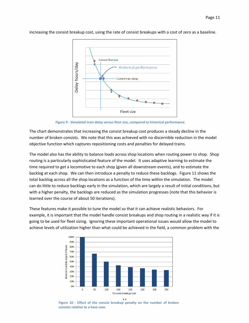
Other forms of model validation involved testing the sensitivity of the model to key input parameters.
One such test evaluated the effect of increasing the consist breakup cost to determine its impact on
both the number of consists being broken and overall solution quality. Figure 10 shows the effect of
Figure 8 ‐ Snapshot of Pilotview, showing assignments of individual locomotives to trains.
Page 11
11
increasing the consist breakup cost, using the rate of consist breakups with a cost of zero as a baseline.
The chart demonstrates that increasing the consist breakup cost produces a steady decline in the
number of broken consists. We note that this was achieved with no discernible reduction in the model
objective function which captures repositioning costs and penalties for delayed trains.
The model also has the ability to balance loads across shop locations when routing power to shop. Shop
routing is a particularly sophisticated feature of the model. It uses adaptive learning to estimate the
time required to get a locomotive to each shop (given all downstream events), and to estimate the
backlog at each shop. We can then introduce a penalty to reduce these backlogs. Figure 11 shows the
total backlog across all the shop locations as a function of the time within the simulation. The model
can do little to reduce backlogs early in the simulation, which are largely a result of initial conditions, but
with a higher penalty, the backlogs are reduced as the simulation progresses (note that this behavior is
learned over the course of about 50 iterations).
These features make it possible to tune the model so that it can achieve realistic behaviors. For
example, it is important that the model handle consist breakups and shop routing in a realistic way if it is
going to be used for fleet sizing. Ignoring these important operational issues would allow the model to
achieve levels of utilization higher than what could be achieved in the field, a common problem with the
Figure 10 ‐ Effect of the consist breakup penalty on the number of brokenconsists relative to a base case.
Figure 9 ‐ Simulated train delay versus fleet size, compared to historical performance.

Page 12
12
use of optimization models. In addition, these features mean that it is possible to perform strategic
planning studies that are realistic to railroad operations.
At this point, we concluded that the model was calibrated, and responded in a smooth and consistent
way to changes in the input parameters.
StrategicplanningThe most important strategic planning question at Norfolk Southern involved estimating the appropriate
fleet size and mix given a projected train schedule. NS had used a simple regression model to estimate
fleet size, but management came to feel that inefficiencies were baked into this model. The
development of PLASMA was motivated by the desire to have an engineering solution that could adapt
in a realistic way to assumptions about train schedules, fleet size and mix, and network performance.
When the model is used for strategic planning, all locomotives start in a “super source” node. We do
not have to specify where locomotives are initially, and we do not even have to specify the fleet mix,
although we are allowed to do so. The model then figures out where to first position each locomotive at
the beginning of the planning horizon. After this decision is made, the adaptive learning logic assigns
power to trains over a planning period (typically a month). The use of an optimization‐based modeling
strategy means that the model simulates a well‐trained group of locomotive planners.
Figure 12 illustrates how the model is used to estimate fleet size. The model is first used to create a
train delay curve (total delay as a function of fleet size) for the current year. Then, a projected train
schedule is created for some period in the future, after which the model is used to create a new delay
curve. If we would like to maintain the same level of train delay, we can simply pick off the required
number of locomotives. If we do not constrain the model to a fixed proportion of different locomotive
types, the model will also specify the fleet mix.
The model can also be used to perform different types of policy studies. Figure 13 illustrates an analysis
of the effect of changes in average train speed. Train delay curves were generated for a base case, and
then for six scenarios where the average train speed was varied. We note that the curves are quite
consistent and well‐behaved, simplifying the task of identifying the correct fleet size.
Figure 11‐Total shop backlog over the course of a simulation, with and without a congestion penalty.

Page 13
13
While Norfolk Southern has primarily used the model for fleet sizing studies, it can be used for other
questions such as quantifying the effect of changes to the train schedule, changes in interchange points
to foreign railroads, and changes in the size and location of maintenance shops.
ExtensionsWe close with a discussion of several significant ways in which the model can be extended. These
include: managing uncertainty, using the model for short term operational forecasting, and finally, using
the model for real‐time operational planning.
ManaginguncertaintyLocomotives have to be managed in the presence of a significant level of uncertainty. The most
important is the variability in transit times due primarily to the need for lower priority trains to sit on
Figure 13‐ Train delay curves for different variations of average train speed.
Figure 12 ‐ Delay curves based on current and forecasted schedules, showing the fleet size needed to maintain the same level of train delay.

Page 14
14
sidings to allow higher priority trains to pass. Other sources of uncertainty arise as a result of yard
delays, changes in the train schedule (e.g. scheduling new coal and grain trains), and equipment
problems.
Approximate dynamic programming makes it extremely easy to handle uncertainty. The algorithm
requires that we step forward through time repeatedly as we learn the value of locomotives in the
future. If we want to incorporate uncertainty, all we have to do is to sample from distributions
describing transit times, yard delays and equipment failures. The effect can be quickly seen in the value
functions. Figure 14(a) illustrates what a value function might look like if trained on deterministic data.
The value rises as a function of the number of locomotives, but there is clearly a point where additional
locomotives are just not needed. Figure 14(b) illustrates what the same value function might look like if
trained in the presence of uncertainty. Here, the value function continues to rise, because situations
might arise where an inbound train is delayed, and as a result there is value in holding additional
locomotives.
When we use stochastically trained value functions, there is value to holding additional power in a yard.
This reflects the tendency of terminal managers to hold onto a few extra locomotives, just in case of
problems. Of course, every yard manager would like to hold onto a few more locomotives, creating the
widely recognized problem where the railroad appears to need more locomotives than it has. The logic
will create the highest values (in the form of higher slopes) at the yards which truly need the additional
power the most. At the same time, just because there is value to holding more locomotives does not
mean that a yard will be allowed to keep additional locomotives. Instead of simplistic rules to hold a
particular number of locomotives at specific yards, the value functions provide a flexible policy that
adapts to the general availability of locomotives. For example, each railroad experiences a time every
week when power inventories are at their tightest. This is the point where yards simply cannot hold
onto buffer inventories. By contrast, at other times there are yards which really benefit from holding
onto power to protect against inbound delays or equipment failures.
Figure 15 shows train delay over 150 simulations of random transit times, using deterministically and
stochastically trained value functions. Note that the stochastically trained value functions not only
produce smaller delays, but also much more stable results. Given the effect of randomness on the value
functions (depicted in figure 14), we would expect that the stochastically trained value functions should
Figure 14(a) ‐ Value function trained on deterministic data.
Figure 14(b) ‐ Value function trained on stochastic data.

Page 15
15
be more inclined to hold power in inventory. Figure 16 shows that this hypothesis is accurate. When
aggregated across the railroad, the stochastically trained VFAs show consistently higher inventories,
although the difference varies by time reflecting, we believe, the changing ability of the network to hold
power.
This is the first reported solution of a stochastic formulation of the locomotive management problem.
The methods presented are based on a mathematically rigorous formulation, but they are also quite
intuitive and practical.
OperationalforecastingAn operational forecasting model produces a plan over perhaps a five to seven day horizon. The model
is used to identify surpluses and deficits of power, and to anticipate locomotive repositioning and light
engine moves (moving power without a train). Such a model requires that we know where the
locomotives are initially. Thus, while the strategic planning model has to figure out where each
Figure 15 ‐ Train delay over multiple simulations using deterministically and stochastically trained value function approximations.
Figure 16‐Aggregate power inventories over the course of a simulation using stochastically and deterministically trained value function approximations.

Page 16
16
locomotive should be at the beginning of the simulation, the operational forecasting model works from
a live snapshot.
The operational forecasting model at NS runs in a production setting. After each forward sweep (over,
say, a seven day horizon), the model would refresh the locomotive snapshot, as well as capture any
changes to the train schedule. This process should repeat itself approximately once each minute (for a
network comparable to that of Norfolk Southern). In the process, the model is constantly refining the
value function approximations.
The operational forecasting model requires that the train schedule and locomotive snapshot be accurate
(the strategic planning model does not require a locomotive snapshot). This is not a small request for a
railroad. Norfolk Southern has been extensively testing and validating the operational forecasting
model, but in the meantime the process has helped to identify areas where data reporting needs to be
more accurate. This will be realized through upgrades to the information systems and improved
reporting procedures. A byproduct of this implementation has sparked a major revision of their data
collection and reporting process for locomotives. This is a familiar experience, where the process of
implementing advanced decision support systems has the effect of raising the bar on the quality of
information systems.
Real‐timeplanningThe last and arguably most ambitious use of optimization would be the real‐time assignment of
locomotives to trains. Real‐time assignment models have been used for years for truckload trucking
with tremendous success, and several railroads use real‐time optimization to assign cars to orders.
PLASMA can easily be adapted to perform real‐time operational planning for locomotives. Assuming
that the operational forecasting model is running in production, we have access to the value function
approximations. A real‐time operational model requires that instead of solving a sequence of decision
problems (depicted in figure 5) over time (as illustrated in figure 6), we only have to solve a single
problem, reflecting what is known now. Such a model can be solved from scratch in a matter of
seconds, but it can be solved even more quickly by holding the solution live in memory.
The challenge of any real‐time model is that human planners always have access to information that will
simply not be available in the computer. For example, often the first source of updated information
about the status of a locomotive comes from an inspector talking on a cell phone to a planner. As a
result, regardless of the sophistication of a model or the quality of a database, there will always be
instances when a human will simply disagree (and in some cases, correctly) with the recommendation of
a model. This is not a problem if the planner is allowed to override the model, and if the model can then
be updated extremely quickly (which is to say in a second or two). The speed with which the model
needs to be updated is not related to the rate at which updates come in from the railroad. The main
constraint is the speed with which planners make decisions.
Real‐time operational model pose additional demands on the quality of data, over and above what is
required for a tactical model. However, we believe that a fully interactive model can be robust, adding
value even in the presence of imperfect information.

Page 17
17
ConclusionsApproximate dynamic programming offers a novel modeling and algorithmic strategy that combines the
realism of simulation with the intelligence of optimization. Classical optimization models have offered
the promise of better decisions, but the technology has required the use of major simplifying
assumptions. As a result, the “savings” produced by such models are often a by‐product of simplified
models rather than intelligent decisions.
PLASMA has been shown to produce high quality, accurate solutions to strategic and tactical planning
problems at Norfolk Southern. Furthermore, it has shown very promising results for operational
forecasting and has high potential for real‐time locomotive assignments. It is the first optimization‐
based model that calibrates accurately against history, making it useful as a tool for fleet sizing, one of
the most demanding strategic planning problems. The technology allows locomotives and trains to be
modeled at an extremely high level of detail. Train delays can be modeled down to the minute. The
model can simultaneously handle consist breakups and shop routing, while also planning the empty
repositioning of power. In addition, it can handle uncertainties in transit times, yard delays and
equipment failures in a simple and intuitive way. The entire methodology is based on first principles,
and as a result avoids the need for heuristic rules that have to be retuned as the data changes.
Acknowledgements: We would like to thank the following people who have made significant
contributions to this project: Don Grabb, Ed Courney, Junxia Chang, Brian Wilker, and Jermaine
Wilkinson. The early stages of this project were managed by Ajith Wijeratne (who was the first to use
the train delay curves), and the first author would like to thank the very early support of Roger Baugher
who recognized the potential of approximate dynamic programming for rail operations. The research
behind this work has been supported over the years by the Air Force Office of Scientific Research and
the National Science Foundation.

Page 18
18
References
Ahuja, R. K., Liu, J., Orlin, J. B., Sharma, D., & Shughart, L. A. (2005). Solving real‐life locomotive‐scheduling problems. Transportation Science, 39, 503‐517..
Booler, J. (1980). The solution of a railway locomotive scheduling problem.Journal of the Operational Research Society, 31(10), 943–948. Pergamon Press. Retrieved from http://www.jstor.org/stable/2581584
Chih, K., Hornung, M., Rothenberg, M., & Kornhauser, A. (1990). Implementation of a real time locomotive distribution system. Computer Applications in Railway Planning and Management (pp. 39–49). Computational Mechanics Publications, Southampton, UK.
Chih, K. C.‐K. (1986). A Real Time Dynamic Optimal Freight Car Management Simulation Model of the Multiple Railroad, Multicommodity Temporal Spatial Network Flow Problem. Princeton University.
Cordeau, J. F., Soumis, F., &Desrosiers, J. (2000).A Benders decomposition approach for the locomotive and car assignment problem. Transportation Science, 34, 133‐149.
Cordeau, J. F., Soumis, F., &Desrosiers, J. (2001). Simultaneous assignment of locomotives and cars to passenger trains. Operations Research, 49, 531‐548.
Forbes, M., Holt, J., & Watts, A. (1991).Exact solution of locomotive scheduling problems.Journal of the Operational Research Society, 825–831.
Powell, W.B. (2011) Approximate Dynamic Programming: Solving the curses of dimensionality, 2nd edition, John Wiley and Sons, Hoboken, NJ.
Rouillon, S., Desaulniers, G., &Soumis, F. (2006).An extended branch‐and‐bound method for locomotive assignment.Transportation Research Part B: Methodological, 40(5), 404‐423. doi:10.1016/j.trb.2005.05.005
Sutton, R. and A. Barto, (1998) Reinforcement Learning, MIT Press, Cambridge, MA. Vaidyanathan, B., Ahuja, R. K., & Orlin, J. B. (2008a). The Locomotive Routing Problem. Transportation
Science, 42(4), 492‐507. doi:10.1287/trsc.1080.0244 Vaidyanathan, B., & Ahuja, R. K. (2008b). Real‐life locomotive planning : New formulations and
computational results. Transportation Research B, 42, 147‐168. Ziarati, K., Soumis, F., Desrosiers, J., Gelinas, S., &Saintonge, A. (1997). Locomotive assignment with
heterogeneous consists at CN North America. European journal of operational research, 97, 281‐292.Elsevier.
Ziarati, K., Soumis, F., Desrosiers, J., & Solomon, M. (1999).A branch‐first, cut‐second approach for locomotive assignment.Management Science, 45, 1156‐1168.