Embed Size (px)
Citation preview
HAL Id: tel-01719523https://tel.archives-ouvertes.fr/tel-01719523
Submitted on 28 Feb 2018
HAL is a multi-disciplinary open accessarchive for the deposit and dissemination of sci-entific research documents, whether they are pub-lished or not. The documents may come fromteaching and research institutions in France orabroad, or from public or private research centers.
L’archive ouverte pluridisciplinaire HAL, estdestinée au dépôt et à la diffusion de documentsscientifiques de niveau recherche, publiés ou non,émanant des établissements d’enseignement et derecherche français ou étrangers, des laboratoirespublics ou privés.
Tactical production planning for physical and financialflows for supply chain in a multi-site context
Yuan Bian
To cite this version:Yuan Bian. Tactical production planning for physical and financial flows for supply chain in a multi-site context. Operations Research [cs.RO]. Ecole nationale supérieure Mines-Télécom Atlantique,2017. English. �NNT : 2017IMTA0064�. �tel-01719523�
Thèse de Doctorat
Yuan BIANMémoire présenté en vue de l’obtention dugrade de Docteur de l’École nationale supérieure Mines-Télécom Atlantique Bretagne Pays de la
Loiresous le sceau de l’Université Bretagne Loire
École doctorale : MathSTIC
Spécialité : InformatiqueUnité de recherche : Laboratoire des Sciences de Numérique de Nantes (LS2N)
Soutenue le 19 décembre 2017Thèse n° : 2017IMTA0064
Tactical production planning for physical andfinancial flows for supply chain in a multi-site
context
JURY
Rapporteurs : Mme Safia KEDAD-SIDHOUM, Maître de conférences HDR, Université Pierre et Marie CurieM. Pierre FÉNIES, Professeur des universités, Université Paris NanterreM. Stefan HELBER, Professeur des universités, Leibniz Universität Hannover, Allemagne
Examinateurs : M. Alexandre DOLGUI, Professeur, IMT Atlantique campus de NantesM. Jean-Laurent VIVIANI, Professeur des universités, Université de Rennes 1
Invités : M. David LEMOINE, Maître assistant, IMT Atlantique campus de NantesM. Thomas G. YEUNG, Maître assistant, IMT Atlantique campus de Nantes
Directrice de thèse : Mme Nathalie BOSTEL, Professeur des Universités, Université de Nantes


Acknowledgement
First and foremost, I would like to express my sincere gratitude to my supervisors, Prof. NathalieBOSTEL, David LEMOINE and Thomas YEUNG for all their contributions of time, ideas, andfunding to make my Ph.D. experience productive and stimulating. Their continuous support, advice,caring, and trust throughout the past three and a half years was contagious and motivational for me,even during tough times in the Ph.D. pursuit. During my master internship and my Ph.D. program,I have benefited enormously from their valuable comments, their innovative approaches and seriousattitude regarding research. I am also thankful for the excellent example they have provided as aresearcher in Operations recherches that will guide and encourage me for my future career.
Special thanks goes to Prof. Safia KEDAD-SIDHOUM (Université Pierre Marie CURIE (Paris6)), who teached me during my master program, supervised my master internship and whom becameone of my thesis reviewers. Also a thank-you to Prof. Stefan HELBER (Leibniz Universität Han-nover) for being part of my Generals committee, a thesis reviewer, and who provides many profoundadvises during an international workshop. And thank you to Prof. Pierre FENIES (Université ParisOuest Nanterre La Défense) for his insightful comments from a financial point of view after reviewingmy thesis. I am also grateful to other members of the defense committee, Prof. Alexandre DOLGUI(IMT Atlantique) and Prof. Jean-Laurent VIVIANI (Université de Rennes 1) for letting my defensebe an enjoyable moment, and for your brilliant comments and suggestions that inspired me in manyways.
Our research works took part of the project RCSM which is financed by the French Competi-tiveness Cluster. In the context of this project, the collaboration with Prof. Jean-Laurent VIVIANIand Prof. Vincent HOVELAQUE (IGR-IAE of Rennes I) made our works possible and ensured itsfinancial coherence with their knowledge and expertise in finance. I am grateful for all comments,advises and suggestions that I received for this thesis and I hope many success for the followingproject on this topic.
During the stay at IMT Altantique, the members of the team SLP of LS2N have contributedimmensely to my personal and professional time. The team has been a source of friendships as well asgood advice and collaboration. I would like to thank Fabien LEHUEDE, Prof. Olivier PETON, OdileMORINEAU, Naly RAKOTO, Guillaume MASSONNET, Laurent TRUFFET, Chams LAHLOU,Nadjib BRAHIMI for their helps, constructive discussions and considerations for the conviviality inthe laboratory and to improve my research works. I am especially grateful to Axel GRIMAULTand Fabrice GAYRAUD who were always willing to provide their kind helps with my researchand with my daily life. My gratitude also goes to Juliette MEDINA, Alex KOSGODA, QuentinTONNEAU, Clément FAUVEL, Thomas VINCENT, Tanguy LAPEGUE, Agnès LE ROUX, Jean-Guillaume FAGES, Aleksandr PIROGOV, Oussama BEN-AMMAR, Olivier BACHOLLET, GillesSIMONIN, Hélène COULLON for their kindness and sharing great time at IMTA and in Nantes.In addition, my dear Chinese friends, Mi ZHANG, Yier WU, Yulong ZHAO, Ning GUO, JiuchunGAO, Xiao YANG, Junle WANG, Jing Li, Xing YAJING, Yuwei ZHU, Ka Yu LEE, Tianyu WANG,Zheng CHENG, Zhewei YU, Letian CHEN, He YUN who made the three years unforgettable. I amvery much grateful for our friendships. I also recognize the support and assistance from Dominique
3
4
MOREL, Isabelle LAINE and Anita NIEBROJ for the administrative procedures as well as fromDelphine TURLIER of the Doctoral school of IMTA. For the non-scientific side of my thesis, I thankmy teammates of basketball for the time playing together.
Last but not least, I owe my deepest gratitude to my dear family, especially, my grand parents,my mother and father, for their continuous encouragement, unconditional love and support as alwaysin my life. They raised me with a love of science and supported me in all my pursuits. During myten-year study in France, they gave up many things for me, cherished with me every great momentand supported me whenever I needed it. Also for my loving, supportive, encouraging, and patientbeloved Ye whose faithful support during the final stages of this Ph.D. is so appreciated.

5
Tian dao chou qin- BIAN Jiawen

Contents
1 General introduction 11
General Introduction 11
2 Research background, context and problem statement 152.1 Notion of supply chain and supply chain management . . . . . . . . . . . . . . . . . . 152.2 Supply chain described by flows . . . . . . . . . . . . . . . . . . . . . . . . . . . . . . 17
2.2.1 Physical flow . . . . . . . . . . . . . . . . . . . . . . . . . . . . . . . . . . . . 172.2.2 Financial flow . . . . . . . . . . . . . . . . . . . . . . . . . . . . . . . . . . . . 182.2.3 Information flow . . . . . . . . . . . . . . . . . . . . . . . . . . . . . . . . . . 18
2.3 Supply chain management and tactical planning . . . . . . . . . . . . . . . . . . . . . 192.3.1 Planning decisions in supply chain management . . . . . . . . . . . . . . . . . 202.3.2 Tactical planning, multi-site context and coordinations . . . . . . . . . . . . . 21
2.4 Financial supply chain . . . . . . . . . . . . . . . . . . . . . . . . . . . . . . . . . . . 272.4.1 Introduction to financial supply chain . . . . . . . . . . . . . . . . . . . . . . . 272.4.2 WCR: link between physical and financial flows . . . . . . . . . . . . . . . . . 29
2.5 Project "Risk, Credit and Supply Chain Management" . . . . . . . . . . . . . . . . . . 332.6 Problematic and contribution . . . . . . . . . . . . . . . . . . . . . . . . . . . . . . . 34
3 Integration of working capital requirement financing cost in EOQ model 373.1 Introduction . . . . . . . . . . . . . . . . . . . . . . . . . . . . . . . . . . . . . . . . . 373.2 The Economic Order Quantity model . . . . . . . . . . . . . . . . . . . . . . . . . . . 37
3.2.1 The EOQ model . . . . . . . . . . . . . . . . . . . . . . . . . . . . . . . . . . 373.2.2 Financial aspects considered in the literature . . . . . . . . . . . . . . . . . . . 393.2.3 Positioning the work of this chapter . . . . . . . . . . . . . . . . . . . . . . . . 43
3.3 EOQ based profit maximization model, EOQP (WCR) . . . . . . . . . . . . . . . . . . 433.3.1 OWCR modeling . . . . . . . . . . . . . . . . . . . . . . . . . . . . . . . . . . 433.3.2 Assumptions . . . . . . . . . . . . . . . . . . . . . . . . . . . . . . . . . . . . . 443.3.3 Parameters et decision variables . . . . . . . . . . . . . . . . . . . . . . . . . . 443.3.4 OWCR formulation . . . . . . . . . . . . . . . . . . . . . . . . . . . . . . . . . 443.3.5 Objective function . . . . . . . . . . . . . . . . . . . . . . . . . . . . . . . . . 46
3.4 Optimal solution and structural properties . . . . . . . . . . . . . . . . . . . . . . . . 473.4.1 Optimal solution . . . . . . . . . . . . . . . . . . . . . . . . . . . . . . . . . . 473.4.2 Comparison with classic EOQ based-formula with the cost of capital . . . . . 53
3.5 Numerical analysis . . . . . . . . . . . . . . . . . . . . . . . . . . . . . . . . . . . . . 563.5.1 Comparison betweens results obtained by the proposed model and the classic
EOQ model . . . . . . . . . . . . . . . . . . . . . . . . . . . . . . . . . . . . . 573.5.2 Illustration of the trade-off between costs . . . . . . . . . . . . . . . . . . . . . 573.5.3 Sensitivity of Q∗ to varying parameters in the classic and proposed EOQ models 58
3.6 Conclusions . . . . . . . . . . . . . . . . . . . . . . . . . . . . . . . . . . . . . . . . . 58
7

8 CONTENTS
4 Dynamic lot-sizing based discounted model considering the financing cost of work-ing capital requirement 614.1 Introduction . . . . . . . . . . . . . . . . . . . . . . . . . . . . . . . . . . . . . . . . . 614.2 Dynamic lot sizing models . . . . . . . . . . . . . . . . . . . . . . . . . . . . . . . . . 61
4.2.1 The uncapacitated Lot-Sizing (ULS) model and mathematical formulations . . 624.3 The discounted cash flow model of the DLS problem . . . . . . . . . . . . . . . . . . 65
4.3.1 Mathematical Formulation of the discounted cash flow model for DSL problems 664.3.2 Literature review of discounted cash flow model for the DLS problem . . . . . 67
4.4 ULS-based profit maximization DCF model . . . . . . . . . . . . . . . . . . . . . . . 684.4.1 OWCR modeling . . . . . . . . . . . . . . . . . . . . . . . . . . . . . . . . . . 684.4.2 Assumptions . . . . . . . . . . . . . . . . . . . . . . . . . . . . . . . . . . . . . 694.4.3 Physical and financial flows illustration . . . . . . . . . . . . . . . . . . . . . . 694.4.4 Parameters et decision variables . . . . . . . . . . . . . . . . . . . . . . . . . . 714.4.5 Mathematical formulation . . . . . . . . . . . . . . . . . . . . . . . . . . . . . 714.4.6 Objective function . . . . . . . . . . . . . . . . . . . . . . . . . . . . . . . . . 734.4.7 ULSP (WCR) model . . . . . . . . . . . . . . . . . . . . . . . . . . . . . . . . . 73
4.5 Solution method . . . . . . . . . . . . . . . . . . . . . . . . . . . . . . . . . . . . . . 744.5.1 Zero-Inventory-Ordering property . . . . . . . . . . . . . . . . . . . . . . . . . 744.5.2 Proof of Theorem . . . . . . . . . . . . . . . . . . . . . . . . . . . . . . . . . . 744.5.3 Algorithm description . . . . . . . . . . . . . . . . . . . . . . . . . . . . . . . 80
4.6 Numerical analysis . . . . . . . . . . . . . . . . . . . . . . . . . . . . . . . . . . . . . 814.6.1 Production program comparisons . . . . . . . . . . . . . . . . . . . . . . . . . 824.6.2 Production program evolution with different rates of discount and interest . . 834.6.3 Production and financial cost comparisons . . . . . . . . . . . . . . . . . . . . 844.6.4 Program evaluation with different purchasing costs and delays in payment to
supplier . . . . . . . . . . . . . . . . . . . . . . . . . . . . . . . . . . . . . . . 844.6.5 Program evaluation with different production unit costs . . . . . . . . . . . . . 854.6.6 Program evaluation with different delays in payment from client . . . . . . . . 86
4.7 Conclusions . . . . . . . . . . . . . . . . . . . . . . . . . . . . . . . . . . . . . . . . . 86
5 Multi-level uncapacitated lot sizing based discounted model considering the fi-nancing cost of working capital requirement 875.1 Introduction . . . . . . . . . . . . . . . . . . . . . . . . . . . . . . . . . . . . . . . . . 875.2 The multi-level uncapacitated lot sizing-based models . . . . . . . . . . . . . . . . . . 87
5.2.1 MRP and the multi-level lot-sizing problem . . . . . . . . . . . . . . . . . . . 875.2.2 The description of the MLLP problem and associated mathematical formulation 885.2.3 Review of the multi-level problem . . . . . . . . . . . . . . . . . . . . . . . . . 90
5.3 Two-level discounted models with WCR costs . . . . . . . . . . . . . . . . . . . . . . 925.3.1 Problem description . . . . . . . . . . . . . . . . . . . . . . . . . . . . . . . . 925.3.2 OWCR model in two-level case . . . . . . . . . . . . . . . . . . . . . . . . . . 94
5.4 Proposed approaches . . . . . . . . . . . . . . . . . . . . . . . . . . . . . . . . . . . . 965.4.1 Mathematical formulation . . . . . . . . . . . . . . . . . . . . . . . . . . . . . 965.4.2 Sequential approach . . . . . . . . . . . . . . . . . . . . . . . . . . . . . . . . 975.4.3 Centralized approach . . . . . . . . . . . . . . . . . . . . . . . . . . . . . . . . 97
5.5 Numerical tests for the 2ULSP (WCR) model . . . . . . . . . . . . . . . . . . . . . . . . 1115.5.1 Test 1: production program comparisons . . . . . . . . . . . . . . . . . . . . . 1125.5.2 Test2: production program evolution with different ratios between two-level
discount rates . . . . . . . . . . . . . . . . . . . . . . . . . . . . . . . . . . . . 1145.5.3 Test3: program comparisons with different payment delays . . . . . . . . . . . 1155.5.4 Production program evolution with different unit selling prices of the supplier 119

CONTENTS 9
5.6 Generalization to multi-level problem . . . . . . . . . . . . . . . . . . . . . . . . . . . 1205.6.1 MLLPPWCR model and centralized approach . . . . . . . . . . . . . . . . . . 1215.6.2 WCR model in multi-level . . . . . . . . . . . . . . . . . . . . . . . . . . . . . 121
5.7 Conclusions . . . . . . . . . . . . . . . . . . . . . . . . . . . . . . . . . . . . . . . . . 124
6 Conclusion and future directions 127
Conclusion and future directions 127
7 Résumé en français 131
Résumé en français 131
List of tables 137
List of figures 140
Bibliography 150


1General introduction
Since the 1980s, supply chain management (SCM) has supplanted the traditional production andlogistics management problems which are based on a single entity. Subcontracting and outsourcing,mergers, acquisitions and alliances among companies entail a considerable complication at both intra-and inter-organizational levels for all companies. Understanding the optimal mechanism within theentities involved in the chain and ensuring an overall performance are recognized as the ultimate andideal goal that is extremely difficult to reach, but still be pursued by the academics and practitionersover decades.
There are various study fields of the SCM, such as the fields of classic logistics, operationalresearch, management control, information technology, or even law. The SCM issues always fallwithin a global hierarchical problems. Indeed, in the literature, the SCM is described by three levels:strategic, tactical and operational levels. Our problem focuses on the study of tactical productionplanning problems in the SCM.
Traditionally, tactical production planning aims at determining the production quantity over theplanning horizon during each period. It is often known for its significant influence on the customerservice quality and production-related operation costs. Two main classes of the model distinguishthe problem based on continuous or discrete time, for instance, Economic Order Quantity (EOQ)model of Harris (1913) for constant demand over continuous time and Uncapacitated Lot-Sizingmodel (ULS) of Wagner & Whitin (1958) for time-varying demand over discrete time. However,the traditional production planning is determined following the well-known Manufacturing ResourcePlanning (MRP II) logic for medium-term objectives that only consider the physical flow of goods.This decision fails to reflect the Net Present Value (NPV) of cash flow due to planned operations inthe real world market system as indicated by Helber (1998). Therefore, financial aspects should beintegrated in the traditional production planning model.
This thesis mainly focuses on the integration of the Working Capital Requirement (WCR) aspectin the production planning process. Recently, the WCR management draws an increasing attentionin the finance department of companies, especially since the financial crisis. In the context of thefinancial crisis, companies need more free cash flow to efficiently react against all uncertainties toensure solvency. According to the Ernst & Young annual Working Capital Management (WCM)report of 2012 devoted to the leading 1000 US companies in 2011, on average, Net Working Capital(NWC) of $330 billion dollars is unnecessarily immobilized (see in Ernst (2012)). This range of cashopportunities corresponds to their aggregate sales of 3% and 6% respectively. Buchmann et al. (2008)also stress that savings on the WCR as a potential source of cash to fund company’s growth is oftenneglected in practice. Suboptimal WCM not only reduces potential gains, but also raises company’s
11

12 CHAPTER 1. GENERAL INTRODUCTION
risk. A company should carefully manage its WCR in order to ensure financial liquidity or reduce theinsolvency risk. Finally, optimal WCM can unlock internal capital and provide financial resourcesfor financially-constrained firms. Especially during the last financial crisis period, bank loans wereextremely difficult to be obtained by companies especially those in the development phase (see inWu et al. (2016)). Many companies suffer from lack of credit and insufficient working capital. Smallsuppliers have to accept unfavorable payment terms from their customers, which exacerbates theirfinancial situation. Moreover, tight or unavailable bank credit reduces the working capital level ofthese companies. As a result, some companies have to suspend their operations which can disruptthe whole supply chain as reported in Benito et al. (2010) and Ernst (2010).
In spite of its importance for the firm (and more generally the supply chain) performance andsurvival, the WCM has been neglected by the literature on production planning. More generally,as stated by Birge (2014), "operations management models typically only consider the level andorganization of a firm’s transformation activities without considering the financial implications ofthose activities". The separation of operational decisions (minimizing operational costs or maximizingoperational profits) and financial decisions (minimizing financial costs or maximizing financial profit)was theoretically grounded on the famous Modigliani & Miller (1958) theorem and practically bythe functional organization of companies. However, in recent years, the literature on operation andsupply chain management, following the original work of Babich & Sobel (2004), became aware of thefact that financing and operational problems are imbricated and that optimizing the two dimensionsglobally can improve the global performance of the company as shown in Chen et al. (2014). Arecent review of the literature based on a risk management framework has been proposed by Zhao& Huchzermeier (2015). Nevertheless, in the production planning field majority of models typicallyignore the financial consequences of production planning decisions. In an attempt to fill this gap,the aim of the paper is to explicitly introduce the WCR dimension in a tactical production planningmodel.
The general structure of the manuscript is presented as follows:The first chapter gives a detailed analysis of concepts on the supply chain in the literature,
classifications and challenges. It allows us to understand the complexity of the supply chain. Then,financial supply chain management and its main approaches are presented. Furthermore, the thirdpart will focus on the working capital and working capital requirement management, while the fourthpart will describe our problematic within the context of the RCSM project (Risk, Credit and Supplychain Management) and the main contributions of this thesis.
In the second chapter, we tackle the single-level problem considering the financial cost of the WCRin the EOQ context. A state of the art of financial aspects which have been integrated into the EOQmodel in the literature is first provided. This review shows that only few works have considered theworking capital requirement in the past and absence of consideration of working capital requirementin the tactical production planning context. Secondly, we focus on establishing a suitable modelof the WCR in single-level, single-product and for constant demand over continuous-time planninghorizon case. We further integrate it into the classic EOQ model. Analytical analysis are executedat the end of the chapter.
In the third chapter, we consider the financing cost of the WCR based on the dynamic lot-sizing (DLS) model for time-varying demand. Firstly, a review of the DLS models in the productionplanning literature is given. Then, a generic modeling of WCR is established in the ULS contextwhich allows us to follow the evolution of the WCR during the planning horizon. Second, a ULS-baseddiscounted cash flow model is built considering the financing cost of the WCR in single level, singleproduct, with infinite production capacity and constant parameter values. Inspired by the classicULS, the Zero-Inventory-Ordering (ZIO) property is proven to be valid in this problem. With thisproperty, a dynamic programming-based algorithm is constructed. A numerical analysis is preformedand shows the difference between the classic ULS model and the proposed model in terms of theoptimal production program. Moreover, the sensitivity of the proposed model to the variation of
13
financial parameters is also investigated.In the fourth chapter, we first extend the previous single-level model to a two-level (supplier-
customer) model and further generalize it to a multi-level case based on the Multi-level Lot-sizingmodel (MLLP). The WCR model is modified to adapt this multi-level scenario. Considering theOWCR cost in the multi-level case, sequential and centralized approaches are proposed to solveboth the two-level and the multi-level problems with a serial chain structure. The ZIO propertystill naturally stands in the sequential approach. It is further proven to be valid in centralizedapproach. The property equally allows us to establish a dynamic programming-based algorithm.Finally, the differences in optimal solutions obtained by the sequential and the centralized approachesare analyzed.


2Research background, context andproblem statement
Since the 1990s, supply chain management has been largely addressed by scholars and practi-tioners. Related literature is significantly rich and diversified on its conception, optimization andapplication. This chapter is dedicated to positioning our tactical planning problem within the recenttrends of supply chain management.
This chapter is divided into four parts: the first part is devoted to the analysis of concepts of thesupply chain in the literature, classifications and challenges. It allows us to understand the complexityof the supply chain. The second part will then present financial supply chain management and itsmain approaches. The third part will focus on working capital and working capital requirementmanagement, while the fourth part will describe our problem within the context of the RCSM project(Risk, Credit and Supply chain Management) and the main contributions of this thesis.
2.1 Notion of supply chain and supply chain managementDevelopment of industry, growth of product complexity and the globalization have led to the sup-
ply chain being more sophisticated to manage which requires more investment and special expertisein supply chain management (SCM). It involves the trend of outsourcing for logistics services, whichwere initially carry on by the company itself, to external service providers since 1980s. Furthermore,the lean management approach, imported from the USA and Asia to Europe, encouraged companiesto focus on their core competencies and to seek service providers for downstream processes, includ-ing logistic activities. Therefore, the organizational structure for the logistic activities in the 1990stended to an external integration scheme. However, this evolution in logistics brought a reflectionfacing a more complex chain to manage with an inter-organizational consideration.
In literature, many definitions of supply chain management are proposed (Christopher (1992);Lee & Billington (1993); Ganeshan & Harrison (1995); Genin (2003)). For example, Cooper et al.(1997) defined it as "a key management, integrated business processes from original suppliers toultimate user, that provides products, associates services, and information that creates additionalvalue for customers and other stakeholders." More recently, the Council of Supply Chain ManagementProfessionals provided the official definition of SCM:" Supply chain management encompasses theplanning and management of all activities involved in sourcing and procurement, conversion, and alllogistics management activities. Importantly, it also includes coordination and collaboration with
15

16 CHAPTER 2. RESEARCH BACKGROUND, CONTEXT AND PROBLEM STATEMENT
channel partners, which can be suppliers, intermediaries, third party service providers, and customers.In essence, supply chain management integrates supply and demand management within and acrosscompanies."
Moreover, Féniès (2006) defined it as "an open set crossed by flows, composed of entities andvarious autonomous actors who use limited resources (capital, time, equipment, raw materials ...)and who coordinate their actions through an integrated logistics process in order to improve theircollective performance (satisfaction of the final customer, global optimization of the supply chainfunctioning) as well as their individual performance (profit maximization of an entity). This definitionshows that a supply chain can be described with the three different sets:
— a network composed of physical entities (factories, workshops, warehouses, distributors, whole-salers, retailers, etc.) and autonomous organizations (firms, subsidiaries , ...);
— an open set crossed by flows (financial, material, information, ...);— a set of activities regrouped in an integrated logistics process, the layout of which constitutes
an intra and inter-organizational value chain.Following this definition, the logistics chain can first be described as a network of physical en-
tities and autonomous organizations. Thus, Lee & Billington (1993) define the supply chain as "anetwork composed by production sites and distribution sites that procure raw materials, processand distribute them to the consumer". Moreover, both service and production entities exist in thesupply chain. Genin (2003) thus proposes that: "A supply chain is a network of geographically dis-persed organizations or functions on several cooperating sites to reduce costs and increase the speedof processes and activities between suppliers and customers." There are two different criteria thatdifferentiate the way of describing the supply chain with entities. First, some consider each productas a chain and associated infrastructures (see in Pimor (2001)). Thus, Rota et al. (2001) define thesupply chain of a product as the set of all entities from the first supplier to the ultimate customerof that product. The second distinguishes logistic chains according to the legal aspects related totheir entities. Consequently, Colin (2004) proposes that the supply chain can be separated into aninternal supply chain and an external supply chain. In the same way, Genin (2003) indicates boththe inter and intra-organizational supply chain. In the case of legally linked entities, they form an"intra-organizational" supply chain that involves a single legal entity, mono or multi-site. Otherwise,the supply chain is considered as "inter-organizational". The difference between these types of supplychains essentially lies in the decision-making process. Thus, the management of "inter-organizational"supply chains cannot ignore the complexity associated with the need for collaboration between differ-ent actors, contrary to an intra-organizational supply chain where it is easy to assume a centralizeddecision-making mode.
The logistics chain can also be defined by the activities and processes that it generates and whichit supports. The definition of Fenies et al. (2004) describes the logistics chain from a set of activitiesgrouped together in an integrated logistics process, the arrangement of which constitutes an intra andinter-organizational value chain. The definition of logistics chains by the process approach consistsin describing the activities between firms and in the company that satisfy the end customer (Lee& Billington (1993), Beamon (1998) and New & Payne (1995)). Tchernev (1997) thus presents anextension of the logistics process concept for any logistics system and defines the logistics process asa set of ordered activities with the objective of controlling and managing material flows through thelogistic system. Then, it allocates resources in the logistics system in order to ensure best level ofservices at the lowest cost. As given in Vowles (1995), the activities in the logistic process includes:
— Ordering— Purchasing— Production— Control— Conditioning— Inventory holding
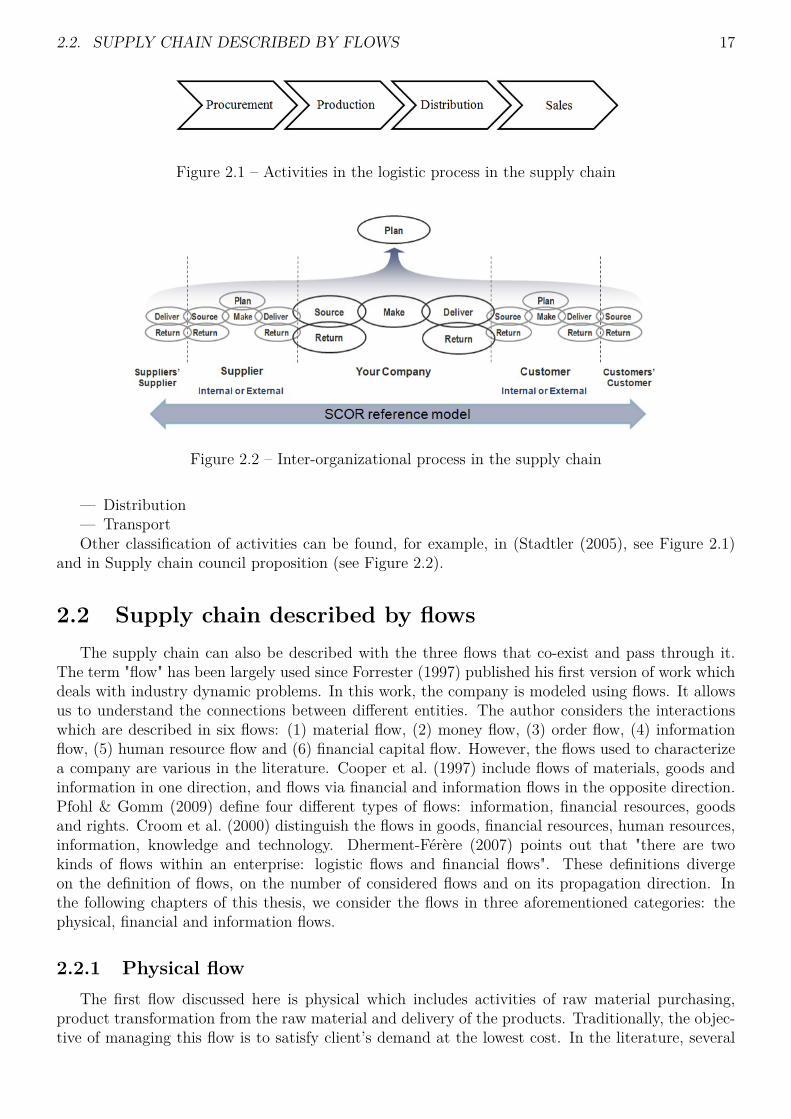
2.2. SUPPLY CHAIN DESCRIBED BY FLOWS 17
Figure 2.1 – Activities in the logistic process in the supply chain
Figure 2.2 – Inter-organizational process in the supply chain
— Distribution— TransportOther classification of activities can be found, for example, in (Stadtler (2005), see Figure 2.1)
and in Supply chain council proposition (see Figure 2.2).
2.2 Supply chain described by flowsThe supply chain can also be described with the three flows that co-exist and pass through it.
The term "flow" has been largely used since Forrester (1997) published his first version of work whichdeals with industry dynamic problems. In this work, the company is modeled using flows. It allowsus to understand the connections between different entities. The author considers the interactionswhich are described in six flows: (1) material flow, (2) money flow, (3) order flow, (4) informationflow, (5) human resource flow and (6) financial capital flow. However, the flows used to characterizea company are various in the literature. Cooper et al. (1997) include flows of materials, goods andinformation in one direction, and flows via financial and information flows in the opposite direction.Pfohl & Gomm (2009) define four different types of flows: information, financial resources, goodsand rights. Croom et al. (2000) distinguish the flows in goods, financial resources, human resources,information, knowledge and technology. Dherment-Férère (2007) points out that "there are twokinds of flows within an enterprise: logistic flows and financial flows". These definitions divergeon the definition of flows, on the number of considered flows and on its propagation direction. Inthe following chapters of this thesis, we consider the flows in three aforementioned categories: thephysical, financial and information flows.
2.2.1 Physical flowThe first flow discussed here is physical which includes activities of raw material purchasing,
product transformation from the raw material and delivery of the products. Traditionally, the objec-tive of managing this flow is to satisfy client’s demand at the lowest cost. In the literature, several

18 CHAPTER 2. RESEARCH BACKGROUND, CONTEXT AND PROBLEM STATEMENT
definition are proposed in different points of view.— "A physical flow in industrial production is a movement, in time and space, of material ele-
ments, from the reception of the raw materials or semi-finished products, until the delivery tothe customer for satisfying its demand" Biteau & Biteau (2003);
— "The physical flow is tangible and material contrasting with the flow of services that is intan-gible and immaterial" (Dherment-Férère (2007));
— "The physical flow can be described as a set of units circulating in space, on a surface, on aplane, on a curve, or on a straight line according to a precise law. The processes durationfor processing these flows allows to plan the productivity of a system, while the connectionbetween quantity and time describes the productivity of the system related to this physicalflow" (Tchernev (1997)).
2.2.2 Financial flowThe financial flow, consisting of the cash flows of the supply chain, aims to satisfy the actors
who contribute to the functioning of the supply chain (legal entities, human resources, shareholders,banks, etc.). It is the monetary counterpart of physical flow. This flow is also known as "cashflow". It is always generated by the same activities that generate physical flows, such as production,transport, storage or recycling. Financial flows are thus not independent. It is often correlated withphysical flows because it is the reception of the goods that triggers payment. However, it can also benot correlated to the physical flow, for example, with the payment of a deposit. With regard to thesupply chain, the financial flow is mainly unidirectional, i.e. from the final customer to the supplierof the highest rank. Nevertheless, at company level, the flow is bi-directional including incoming (e.g.revenue) and outgoing (e.g. cost) cash flow. Different cash flow optimization objectives are addressedin the literature. Cash flow optimization may allow, a priori, to reach shareholders’ satisfaction forentities in the supply chain and to improve its overall functioning (Shapiro (2006)). Dematerializedpayment impacts the cash flow for accomplishing long-term objectives of shareholders in entitiesof the supply chain, the medium-term customer credit policy and short term cash flow schedulingaccording to Lysons & Farrington (2006).
Some limits of managing the financial flow are identified by Hohmann (2004) because it doesnot reflect the problematic in a coherent way. Féniès (2006) indicates that, even if using monetaryunits, analytic accounting models produce information on the levels of profits and costs generatedby the activity of the physical flow, but do not allow to measure the associated cash flow level. It isbecause they do not take into account the specification of the calculated charges and products nor thepayment deadlines. A cash balance or a financing plan is more suitable for financial flow management.Thus, financial flows have a dynamic aspect, which can not be captured by the traditional accountingapproaches, which certainly allow to have a precise vision of the economic reality of a structure butat a given and fixed moment. In contrast, the cash flow principle is to ensure the availability of allpayments (see in Cooper et al. (1997)). Also, when we use the term of financial flows, we mainly referthe flows related to the exploitation cycle. Non-operating financial flows have a lesser occurrence infirms, following strategic level decisions, with relatively high predictability. Physical and financialflows are jointly linked thanks to an information flow whose quality guarantees their translation.Thus, financial flows are only the tangible representation and final result of the intellectual andphysical action of the employees.
2.2.3 Information flowThe information flow represents all transfers or exchanges of data between the various actors in
the supply chain, so that they can respond to the needs expressed by the order of the final customer.The information flow is bidirectional and can possibly be linked to the physical and financial flow.
2.3. SUPPLY CHAIN MANAGEMENT AND TACTICAL PLANNING 19
Fawcett & Magnan (2001) indicate that information flows "coordinate physical and financial flowsbetween each node of the supply chain network and thus allow a global coordination. Kyriakopoulos& De Ruyter (2004) propose the notion of internal and external information flow to characterizethe origin of the flow. Moreover, the information flow can be horizontal, vertical, or a combinationof both. "Vertical flows of information correspond to hierarchical planning. Horizontal informationflows can exist between two entities who easily and quickly use local information, for example tocontrol the effects of a machine failure" (Meyers & Tucker (1989)).
Information flows must be reliable and traceable in order to ensure the intelligibility of theircontent and avoid any form of distortion. Reliability refers to the fact that information does notsuffer from any failure: it should be accurate, correct, up-to-date and controllable. The problemsof inherent quality of the information flow and its propagation within the supply chain have beenlargely investigated in the literature. Entitled "the Bullwhip effect", it refers to the phenomenon ofinformation distortion which is propagated along the supply chain by expanding and resulting ininstability in trade and economic losses according to Lee et al. (1997).
Regardless of the hierarchical level of the logistics system, the information flows contain necessarydata for the planning and management of all the activities. The following information must beavailable:
— clear information on resources for executing this activity (the state of these resources, thenecessary knowledge and data for associated operations, the local rules for their steering);
— information on the status of activities that depend on this activity;— information on the status of this activity concerning all dependent activities;— information on the status of this activity concerning the management system of the flexible
production / storage unit or feedback;— the global rules for the steering and management of all activities related to the considered
activity.
2.3 Supply chain management and tactical planningThe works of Stadtler (2005) and Kilger et al. (2015) present a clear understanding and summarize
the essential knowledge on SCM resulting from the very rich and wide-ranging operations researchfield. Stadtler (2005) defines SCM as "an approach that allows the integration of organizational unitsalong a supply chain and the coordination of physical, financial and information flows in order tosatisfy the final consumer and improve the competitiveness of supply chain". The author proposes toconsolidate the necessary methods and tools for the success of an SCM approach within the SupplyChain Management house as presented in Figure 2.3.
— The roof of the SCM house is the objective of SCM approach, that includes both the finalcustomer’s satisfaction and the competitiveness improvement of the Supply Chain. Thesetwo objectives are held on two pillars: supply chain members integration and the processescoordination;
— The first pillar of supply chain members integration consists of three "blocks". They include theintegration of partners selection, the supply chain network organization/inter-organizationalcollaboration and the leadership situation in the supply chain;
— The second pillar consists of the coordination between three approaches. The use of informa-tion/communication technology accelerates the exchange between partners and restrain thebull-whip effect. Process management tears down the barriers between business function andorganizations. Lastly, advanced planning reinforces the strength of transactional enterpriseresource planning (ERP) in planning area.
— These two pillars are based on conceptual and academic foundations from several fields (lo-gistics, operations research, marketing, organizational theory, etc.).

20 CHAPTER 2. RESEARCH BACKGROUND, CONTEXT AND PROBLEM STATEMENT
Figure 2.3 – House of supply chain management (Stadtler, 2005)
Figure 2.4 – Software modules covering the supply chain planning matrix (Meyr et al. (2008))
2.3.1 Planning decisions in supply chain managementVarious decisions of activities planning in supply chain concern improving supply chain perfor-
mance and efficiency. Proposed as a solid reinforcement of ERP system, advanced planning (oradvanced planning and scheduling (APS)) system provides analysis and planning of logistics andmanufacturing. Meyr et al. present a two-dimension classification of these plannings in the "supplychain matrix" (see Figure 2.4):
— the level of the managerial decision making involved and the time during which the decisionwill have an impact on the future development of the supply chain. Following the principlesof hierarchical production planning, three planning levels are used: "long-term/strategic","mid-term/tactical" and "short-term/operational",
— the supply chain process involved. Four different processes are identified: procurement, pro-duction, distribution and sales.
Similar classification of levels is also illustrated in Genin (2003) as three levels of planning. In-dustrial planning have been recognized as a major problem existing at all three levels. It aims atdelivering ordered products to customers at the right time, at the lowest cost and to the right place.In other words, the challenge is to find a trade-off between customer satisfaction rate and differentcosts generated by production-related activities (production, storage, etc.). As it is integrated inproduction management, the industrial planning is thus divided into these three hierarchical levels.

2.3. SUPPLY CHAIN MANAGEMENT AND TACTICAL PLANNING 21
Subsequently, long-term and short-term level decisions and plannings will be briefly presented. Then,the problematic at the tactical level will be discussed in detail in the following sub-chapter.
- Strategic level:Strategic decisions always concern the general company management over the long term horizon
(conventionally, more than 18 months) in order to make decisions on the company’s major policy.It thus implies a decision on its portfolio of activities which will involve necessary and stable re-sources to ensure the achievement of these decisions. The stable resources include machines as wellas manpower. The decisions may concern their purchases or hiring, replacements, discard or lay-off, transfers, locations, etc. It may also concern production information (formalized managementprocedures, technical databases, etc.). All these decisions will then be implemented at lower levels.
Strategic planning aims to satisfy the market as a whole within the framework of the generalstrategy of the company. More specifically, it seeks to determine its growth, development and prof-itability objectives. Its primary responsibility is to find a global strategy to achieve long-term ob-jectives through substantial changes in production capacities (new production units, new locations,adoption of new technologies, etc.).
- Operational level:Operational decisions should respect decisions at the tactical level and further ensure necessary
daily flexibility to handle expected demand fluctuations and resource availability based on forecasting.Therefore, implementation at the operational level requires a complete disaggregation of the plandefined at a higher hierarchical level. Regarding production management, operational decisionsinclude:
— Inventory management, which ensures the availability of raw materials and components;— Scheduling, which consists of a detailed programming of the mobilized resources (operators,
equipments and tools) for execution of necessary operations for basic production of goods orservices over a horizon of no more than a few days, within a time framework of minutes.
The operational planning is always determined over a daily or weekly horizon. It closely monitorsand controls physical flow in order to ensure the availability of the products at each line according tothe conditions defined at the tactical level. This thus involves production scheduling on a day-to-weekbasis which means determining the starting time of tasks of different resources in order to guaranteepunctuality of the production and the accurate quantity of products decided at the tactical level. Forthis reason, this approach is traditionally called "planning by timing". The associated problematicsat the operational level are traditionally addressed in the scheduling area.
2.3.2 Tactical planning, multi-site context and coordinations
The tactical level connects the strategic and operational levels. The decisions at this level aremade for a medium term horizon (6 to 18 months). As indicated in Tchernev (1997), three types ofplanning problematics exist at this level which are procurement planning in upstream, productionplanning in the production unit and transport planning in downstream. It is important to noticethat all these decisions should fulfill the global framework defined by the strategic decisions.
The production planning aims at determining the quantities of products to be manufactured overa medium- or short-term horizon (priority planning) and to decide the amount of resources to beassigned (capacity planning) in order to meet the operational objectives in the best quality, volume,location, duration and cost. The capacity of facilities is limited and will not be significantly improvedover the planning period. Therefore, the only available solution left to the manager is to optimize theproduction quantities using available or additional production resources (e.g. overtime, temporaryhiring...), the variation of resource quantities, or searching external recourse.
22 CHAPTER 2. RESEARCH BACKGROUND, CONTEXT AND PROBLEM STATEMENT
Practical approaches
In the literature, tactical planning is considered as hierarchical approach as proposed by Vollmannet al. (1997). The authors decompose tactical planning into three levels :
— Sales and Operations planning (S&OP).— Master production schedule (MPS)— Material Requirement Planning (MRP)First, the objective of S&OP is to transform the business plan into a forecasting production
volume for each major product family of the company. It is carried out not only based on salesforecasts, but also based on markets and economic situation. It will be updated at least every monthby the various managers of the company (sales, production, supply chain, marketing, R&D ...). Itintegrates plans of all sectors of the company. Indeed, the S&OP is always used to coordinate arounda common axis the different strategies of company’s services. Nevertheless, S&OP reflects what thecompany wants to produce and not the full capacity of production.
Since the time required for the implementation of the S&OP decisions is generally long, itselaboration is therefore based on sales forecasts and its horizon is 12 to 18 months. The traditionalelaboration is based on graphic methods or linear programming models e.g., in Giard (2003), Herzer(1996), Lamouri & Thomas (1999) and Baglin et al. (2005). The graphic methods are easy tounderstand and to use. They proceed by successive cost evaluation calculations and allow to identifydifferent integrated plans that are valid but whose costs are not necessarily the lowest. However, itsquality is often based on experience and common sense. On the contrary, the linear models optimallymanage the strategies for a set of parameter inputs. Although, the user should be concise of the"forecasting" nature of these parameters because it may lead to a biased result that is far from theoptimum and even influence the optimal strategy. Regarding the importance of S&OP decision, itsrobustness should take priority over its optimization.
Therefore, the S&OP provides a capacity and sales planning which leads to the next level oftactical planning to define a master production schedule (MPS). Generally, MPS is established everymonth over a period of time from three to six months for the key product, commonly the finishedproduct. It determines the quantities to manufacture for each period of the horizon (day) by eachplant with precise planning of required resources available in the plant. Compared with planningobtained by S&OP, planning of MPS is established with a smaller time unit, e.g. day. Furthermore,the MPS planning focus on allocation of critical resources in the system for a local objective.
The primary objective of the MPS is therefore to ensure the on-time delivery of customer orders.The second is the optimal resource allocation. The MPS evaluates the product availability for client’sdemands. It thus plays a major role in the functioning of an integrated planning and control systemfor production and inventories, since it establishes at each period the balance between the company’sresources and the demands to meet. Thus, Tchernev (2003) considers that "the MPS is at the centerof tensions generated by disruptions in the company, such as production delays or in its externalenvironment, such as demand changes".
Different from the MPS that considers only one level planning, the MRP allows a multi-levelmanufacturing planning of finished products and its components over the same planning horizon.The bill of material(BOM) represents the product structure and is introduced in the MRP method.According to the BOM, The resource required of each component are calculated from the bottomlevel of the BOM to the level of the component considering the associated coefficients. In addition toplanning, the MRP is also used for system control to manage manufacturing processes and indicate"directions" for resource allocations. Ultimately, the MRP determines necessary components or rawmaterials to prepare in order to accomplish the MPS, item quantities to purchase and manufactureregarding the inventory level and the cycle and quantities of orders as well as the staring time ofproduction.
During the planning elaboration with MRP, the delivery delay, production lead time and assemblyduration are taken into account. The quantities determined by the MRP are strongly correlated
2.3. SUPPLY CHAIN MANAGEMENT AND TACTICAL PLANNING 23
with the MPS decisions. Even small inaccuracies in MPS planning may be significantly amplifiedthrough the MRP system. Even though MRP principle is easy to understand, the difficulties alwaysappear during its implementation in an industrial environment. The reason is that, in practice, aconsiderable number of calculations based on a complex product BOM will be generated. It thusgenerates thousands of manufacturing and purchasing orders that must be precisely controlled andpursued. In fact, when quantities and timings of production and control activities are fixed, it isthen possible to schedule the activities. Thus, the MRP is considered as the interface of detailedoperation planning and scheduling.
Initially, the MRP did not take account the external constraints and planned the needs only onthe basis of demand or demand forecast considering:
— an unlimited production capacity always capable of supplying,— no uncertainties (breakdowns, delays of delivery ...)In 1971, Orlicky defined the MRP I method, which takes into account finite capacities. Then, in
1984, Wight launched the foundation of the MRP II (Manufacturing Resource Planning) method byextending the concept to management resources planning and the integration of financial and logisti-cal data (Wight (1995)). In MRP II framework, the capacities of production, supply, subcontracting,storage, distribution and also financial resources are taken into account Genin (2003).
Multi-site tactical planning
The previous hierarchical structure is limited to a single-site description of tactical planning. Insupply chain management, tactical planning attempts to further ensure a "horizontal synchronization"of the chain. At the MPS level, the synchronization is achieved by a process called DistributionRequirement Planning (DRP). This method is used in business administration for planning orderswithin a supply chain. DRP enables the user to set certain inventory control parameters (like a safetystock) and calculate the time-phased inventory requirements. Its approach based on the burstingof the "BOM" of the distribution system is similar to an MRP which uses the "BOM" of product.Vollmann et al. position the DRP close to the marketplace and presents that "DRP is a link betweenthe marketplace, demand management and MPS". The authors indicate the role of DRP is "toprovide the necessary date for matching customer demand with the supply of products at variousstages in the physical distribution system and products being produced by manufacturing."
The limit of DRP is caused by the fact that horizontal integration is necessarily limited to a fewentities in the supply chain. Indeed, in the case of short-term customer demands, the upstream needswill
— either generate needs prior to the current date (cases of desynchronization and thus cases ofout of stock)
— or can be absorbed by one or more stocks upstream of the chain (where the order is fulfilled).Crama et al. (2001) recall the limits of this system which sometimes are caused by a desynchro-
nization of production plans. Thus, the application of a DRP at the lower level of tactical planningonly remains for short-term use. It is indeed necessary to already ensure a horizontal synchroniza-tion at the S&OP level in order to predict a load/capacity adequacy on all the sites as well as theirsynchronization.
The synchronization is carried out by considering the material need and the components generatedby the product BOM. It brings a much more complex tactical planning problem, which consists notonly in generating production plans for the entities but in ensuring their synchronization. Thesemodels are therefore called multi-level. Synchronization will then be ensured by considering thebalance of stocks that bind each entity in the chain.
As mentioned above, the understanding of multi-level planning problems can be achieved byassuming two approaches:
— A centralized approach
24 CHAPTER 2. RESEARCH BACKGROUND, CONTEXT AND PROBLEM STATEMENT
— A decentralized approachThe centralized approach assumes that whatever the nature of the links between the component
entities in the supply chain, it is possible to consider a master supply chain manager (or mediator)that has all the information and power to generate a synchronized planning of the supply chain.Certainly, this assumption assumes that there is a full collaboration between all the entities in thesupply chain. This is why this hypothesis should be set rather for the case considering only theentities of a company than the cases including an external partner of the supply chain.
However, the literature mainly assumes that the centralized approach is not enough realistic.Therefore, numerous researchers suppose a decentralized approach where the actors in the supplychain share a certain amount of information but generate their planning independently. Féniès(2006) proposes to synthesize the processes of tactical planning by adopting the work of Simatupang& Sridharan (2002) based on the notion of Collaborative Planning Forecasting and Replenishment. Alot of work has compared these two approaches. Thierry et al. (1994) demonstrates, on a case study,the interest of centralizing the decision to obtain an optimal solution. The centralized approachprovides better solutions than those obtained through a decentralized approach. These conclusionslead many authors to study the relevance of information sharing at the heart of supply chains inorder to improve their performance.
A vast literature has addressed the tactical planning problems. However, mosts of the workshave focused on the mathematical model development of these problems and the elaboration ofmethods dedicated to these models which are called "Lot Sizing Problems". They are dedicated tothe development of the different production plans (S&OP, MPS and MRP).
Mathematical model families of Lot-sizing problem
Kuik et al. (1994) defined the lot-sizing problem as "the clustering of items for transportationor manufacturing processing at the same time". This problem arises whenever we need to decidethe timing of productions as well as the quantity to produce each time. On one hand, the setuptimes or setup costs generated by these productions should be taken into account that may involvemany different operations such as cleaning, preheating, machine adjustments, calibration, inspection,test runs or change in tooling, etc. Setup costs or changeover costs can be caused by a additionalworkforce needed to prepare the equipment or by the consumption of resources during the setupoperations. Overall, in order to reduce the times of launching setups for efficiently utilizing theproduction resources, the production lot size should be reasonably large. On the other hand, theseproductions may generate products that need to be held in the inventory and deliver in a laterperiod because the production may not be exactly synchronized with the received demand for a costoptimization objective. Inventory holding costs is thus incurred for tied up capital, product valuedepreciation and storing cost (warehousing, handling, shrinkage and insurance...).
The classic objective of lot-sizing problem is to determine an optimal/good production programthat minimizes the sum of the setup costs and the inventory holding costs generated by this program.Essentially, an optimal/good trade-off between setup costs and inventory holding costs is what weneed to reach for this objective and for satisfying customer demand. Consequently, finding this trade-off is critical to improve the production performance that strongly influences the competitiveness ofthe company in the modern global market.
Since lot-sizing is always being recognized as a difficult optimization problem, considerable effortson this problematic can be found in the lot-sizing literature for over a century. Different problematicsare dedicated for problems in different contexts of the supply chain such as mono-site, multi-site orthe entire supply chain. The criteria considered the most discriminating are presented as followswhich are indeed not exhaustive, but provides a general overview of the classification: models andits extensions or characteristics such as:
— Nature of data (deterministic or stochastic),

2.3. SUPPLY CHAIN MANAGEMENT AND TACTICAL PLANNING 25
— Type of supply chain structure (single- or multi-site (plant)),— Model of demand (constant or variable),— Type of bill of material (single- or multi-level),— Capacity constraints (with or without),— Length of production periods (small or big bucket), etc.First of all, even though most of the lot-sizing literature focuses on problems dealing with deter-
ministic demand, the data considered here can also be stochastic for more realistic cases. In practice,production planning decision are very often made with forecasts in which errors may be hidden.This fact could strongly affect the solution procedure to apply. For similar reason, other parametersconsidered in this problem may also be stochastic, as surveyed in Brahimi et al. (2017).
Secondly, both single- and multi-site problematics appear in the lot-sizing literature. Obviously,the multi-site model is established for supply chain tactical planning in a more practical way. Thereplenishment and distribution problem between plants are also sometimes taken into account.
Thirdly, the type of deterministic demand in a lot-sizing problem can be further distinguished bythe demand rate. Constant demand is evenly distributed over the horizon. Otherwise, it is calledvariable. Even though the objectives of these models are both to minimize production cost and tomeet customers’ demand, the fundamental difference of these models are in their purpose:
— Constant demand models aim at determining an optimal production cycle that is reproducibleover the horizon. For example, the EOQ problem.
— Variable demand models determine optimal quantities to produce in all predefined periods ofthe discrete-time planning horizon.
Fourthly, the way in which the bill of material (BOM) is taken into account: the tactical planningproblems consist of not only the planning for finished products but also for their components. Thesecan be treated in two different ways:
— single-level: following the logic of MRP, the planning is executed level by level. It consists ofcomputing the requirement of components from the finished products (called external demand)which are found at top of the BOM. This thus defines a level-by-level planning. It is thereforepossible to use single-level models with which the quantity determined at the higher level ofthe BOM generates the (internal) demand at the current level. The limit of this approach isthat there is no guarantee to provide feasible plannings due to the lack of consideration of theproduction capacity in the planning process.
— multi-level: multi-level models link the BOM levels by introducing the structure of BOMand expressing the internal and external demand. Such models ensure the feasibility of thesolution. They also allow us to consider lead time between the levels.
Fifthly, capacity constraints are also an important aspect to be considered. Considering a capacityconstraint significantly increases the computation complexity for determining an optimal solution,even for the most simple case.
Lastly, for variable demand models, lot-sizing models can also be distinguished based on theirsize of the production period, i.e., bucket. Both "small bucket" and "big bucket" models exists inthe literature. On the one hand, for "small bucket" models, we assume that only one productcan be produced during a micro period which can be short as hours. They aim at determiningboth production quantities and sequence of production. Obviously, the horizon length is reducedcompared to the one in "big bucket" model. On the other hand, "big bucket" models are thus usedto deal with problems with larger length horizon. In this case, several products can be planned in asame period, called a macro period, e.g. week or month.
In Figure 2.5, the classification of deterministic models of lot-sizing problems presented in Comelliet al. (2008) is given. In the single-level context, the main models are:
— Capacitated Lot-Sizing Problem (CLSP): A multi-item problem for satisfying dynamic demandwith capacity constraints. This big bucket model is proven as a NP-Hard problem in Bitran& Yanasse (1982);

26 CHAPTER 2. RESEARCH BACKGROUND, CONTEXT AND PROBLEM STATEMENT
Figure 2.5 – Classification of lot-sizing models (Comelli et al. (2008))
— Lot Sizing Problem (LSP): when capacity constraints are not taken into account, the CLSPbecomes polynomial (Wagner & Whitin (1958)). In this thesis, we adopt the name used inPochet & Wolsey (2006), which is ULS for "Uncapacitated Lot-Sizing Problem";
— Economic Order Quantity (EOQ), Economic Lot Scheduling Problem (ELSP): The EOQ andthe ELSP are single-item problems with constant demand. The time is continuous (notdivided in the periods) and the planning horizon is infinite. The EOQ does not assumecapacity constraints which make it polynomial thanks to Wilson’s formulas contrary to theELSP which is NP-Hard;
— Discrete Lot Sizing Problem (DLSP): The NP-hard problem DLSP is a small bucket model. Itassumes that only one item may be produced by period, using the full capacity of the system.This is called the "all or nothing" assumption;
— Continuous Setup Lot sizing Problem (CSLP): In this small bucket model, contrary to theDLSP, The "all or nothing" assumption does not exist anymore. Thus, the capacity of periodsmay be not fully used;
— Proportional Lot Sizing Problem (PLSP): the main idea of the PLSP is to use this remainingcapacity left by the CSLP model for scheduling a second item in the particular period;
— General Lot sizing and Scheduling Problem (GLSP): this one integrates lot sizing and schedul-ing of several products on a single capacitated machine. Continuous lot sizes are determinedand scheduled. By this way, this model generalizes models using restricted time structures.
About multi-level context, models with similar hypothesis are considered. Therefore, their namesare quite similar to the single level ones (with adjunction on ML prefix).
More classification is referred to the Lang (2010) and Brahimi et al. (2017).The extensions of the standard lot-sizing problem include backlogging, perishable inventory, lost
sales, time windows, multi-facilities, inventory capacity, setup carry over and remanufacturing, etc,which are not be considered in this thesis. The interested reader can refer to Brahimi et al. (2017)for further details.
In this thesis, we only consider three models without a capacity constraint. Using the aforemen-

2.4. FINANCIAL SUPPLY CHAIN 27
tioned classification, the three models are respectively:— single-product, single-level and for constant demand that is same case as in the EOQ model;— single-product, single-level, big bucket and for variable demand that is same case as in the
ULS model;— multi-level, big bucket and for variable demand that is same case as in the MLLP model;
2.4 Financial supply chain
2.4.1 Introduction to financial supply chainAs defined by Dalmia (2008), the supply chain can be categorized into the physical and the
financial supply chain. The former consists of processes involved in the physical movement of goods,e.g. inventory management. The latter includes the movements of funds resulting from the physicalsupply chain, (see Figure 2.6). Supply chain management and the optimization of physical flows havereceived more attention than optimizing financial flows between the different supply chain partners.However, this situation seems to be evolving with the advent of the Financial Supply Chain (FSC).The term Financial Supply Chain Management mirrors the concept of Supply Chain Management. Itrecognizes that there is a chain of dependent events that has an impact on the working capital of anorganization. On the buy-side, the timing of purchases, inventory, payment terms with suppliers anddiscount arrangements all impact working capital. The management of that chain of events (in so faras finance can influence them) is part of Financial Supply Chain Management (FSCM). More andmore firms engage in advanced methods of managing financial flows along their supply chains (seeFigure 2.7). FSCM thus requires the internal coordination between financial managers and supplychain managers of the company, as well as the external collaboration with service providers (e.g.banks), suppliers, and customers. Traditionally, financial flow management focuses on optimizing asingle firm’s cash flow. However, FSCM extends the scope to the entire supply chain (see Wuttkeet al. (2013)). The authors provide a summary of recent FSCM methods which involves many diversefundamental elements of FSCM:
— Buyer credit: Term financing provided to finance suppliers (e.g. advance payments or deposits)( Chauffour & Farole (2009); Thangam (2012))
— Inventory/work-in-progress financing: Buyer provides loan to supplier to finance work-in-progress (Chauffour & Farole (2009))
— Reverse factoring: The supplier obtains a credit from a bank and pays the interest accordingto the buyer’s interest rate. The buyer pays the loan principal to payment terms (Tanriseveret al. (2012); Klapper (2006))
— Supply chain finance: An automated solution that enables buying firms to use reverse factoringwith their entire supplier base, often providing flexibility and transparency of the paymentprocess ( Shang et al. (2009); Demica (2007))
— Electronic platforms: Systems offered by third parties to electronically connect trading part-ners with financial institutions to automate payment processes (Sadlovska (2007))
— Letters of credit: A financial institution provides guarantee to exporters by replacing theimporter’s risk with its own default risk (Amiti & Weinstein (2011))
— Open account credit: A buying firm receives credit from suppliers without formally offeringsecurities or involving third-party security (Malouche & Chauffour (2011); Chauffour & Farole(2009))
— Bank loan for financing the supply chain: Short-term or medium-term financing providedfrom a bank involving working capital and pre-export finance (Chauffour & Farole (2009))
Due to its high practical relevance, analytical research has recently shown significant improve-ment potential of inventory models if financial flows are taken into consideration(e.g. Babich & Sobel(2004); Gupta & Wang (2009)).

28 CHAPTER 2. RESEARCH BACKGROUND, CONTEXT AND PROBLEM STATEMENT
Figure 2.6 – Physical and financial supply chain
Financial status of companyIn accounting, three documents are established to measure the company’s financial statues, i.e.financial asset position, financial performance and cash flows level. They are :
— Profit & loss (P&L) statement: a financial statement that summarizes the revenues, costsand expenses incurred during a specific period of time, usually a fiscal quarter or year. Theserecords provide information about a company’s ability or lack to generate profit by increasingrevenue, reducing costs, or both. The P&L statement is also referred to as "statement of profitand loss", "income statement," "statement of operations," "statement of financial results," and"income and expense statement." A key concept of the P&L statement is the gross operatingsurplus (GOS), which represents the surplus created by the operation of the company afterremuneration for the labor input factor and the taxes linked to production. The GOS ismeasured before the depreciation decisions and financial charges arising from the company’sfinancing choices. It appears to be the balance between operating revenues that have resultedor will result in a cash inflow and, on the other hand, operating expenses that are disbursedor are expected to be disbursed. This is a potential monetary surplus and therefore allows tomeasure the capacity of the company to generate cash resources from its exploitation. In thissense, the GOS is both an operating balance and a measure of gross cash flow.
— Balance sheet: a financial statement that summarizes a company’s assets, liabilities and share-holders’ equity at a specific point in time. These three balance sheet segments give investorsan idea as to what the company owns and owes, as well as the amount invested by share-holders. The balance sheet is built based on the main functions of the company: investment(which represents stable resources), financing (which comes from stable resources) and oper-ating (which translates into liabilities and short-term assets: Inventories, trade receivables,trade payables). Cash flows arising from operating activities are reflected in the balance sheetin the form of receivables or debts. The outcome of these three cycles results in an impact oncash flow with either a surplus or an insufficiency.
— Cash-flow statement: The cash-flow statement (CFS) is a mandatory part of a company’s

2.4. FINANCIAL SUPPLY CHAIN 29
Figure 2.7 – Increasing number of firms using supply chain finance method in Germany (Wuttkeet al. (2016))
financial reports since 1987 - records the amount of cash and cash equivalents entering andleaving a company. The CFS allows investors to understand how a company’s operations arerunning, where its money is coming from, and how it is being spent. Treasury is a leadingindicator for financial management and analysis. This statement provides the evaluation ofcompanies on their ability to generate liquidity and meet their commitments. It has theadvantage of providing an objective indicator, cash, which is commonly used in the companyvaluation. Cash is also fundamental to evaluate the failure risk rate.
2.4.2 Working capital requirement: link between physical and financialflows
"Cash is king" - despite the fact that the cash has its own costs. Cash is the most liquid assetand is presented commonly on the balance sheet as the first item. Management of cash is of greatimportance for a company. If adequate cash is not available when it is needed, the situation lead tobankruptcy. Management of cash and liquidity involves providing sufficient funds to the business formeeting various requirements at the right time, such as repayment of bank loans, payment of taxes,payment of wages, purchases of raw materials and inventory etc. Moreover, holding the cash entailsa precautionary motive in order to meet unforeseen events. Therefore, the cash must be managedproperly and provided for arising contingencies. In the following section, we present the currenteconomic and financial context. Next, we explain the direct link between the cash and workingcapital requirement(WCR) which is chosen as the financial aspect considered in tactical planning.Then, we describe the main concept of the WCR and how it links the physical and financial flows.
Economic context
Over the past few years, the succession of economic and financial crises has constantly jeopardizedthe competitiveness and even the life of companies. The Credit Crunch, in other words, the slowdownin credit lending by financial institutions, is one of the main causes of this situation. According toa recent study of the Organization for Economic Cooperation and Development (OECD), 115,813companies, mostly small and medium-sized enterprises (SMEs), have closed down in France in 2009and 2010. The number of these bankruptcies is increasing in 2012. According to Coface and the
30 CHAPTER 2. RESEARCH BACKGROUND, CONTEXT AND PROBLEM STATEMENT
Altarès consulting, the forecast of bankruptcies in the crisis of 2012 arises to 63,500 and of jobsaving plan (plans sociaux) is more than 317,000. At the same time, financing constraints which arereinforced by the difficulties of the banking sector and the new regulations strongly penalize growth(10 to 15% of turnover loss in the industrial sector) and operational performance (20 to 25% loss inproductivity) for all involved actors (suppliers, subcontractors, payers).
Especially, in early 2012, potential instabilities in France, Greece, and in other European countriesafter the elections have been considered as the cause that may further worsen the economic andfinancial situation in Europe in the Euro debt crisis period. The major European banks were fearedto be heavily stroked and began hoarding cash in large quantities since the end of 2011. Until theend of March 2012, the top 10 European banks deposit cash at the central bank of different countriesaround the world totaled nearly 1.2 trillion US dollars, an increase of 128 billion dollars comparedwith the amount at the end of the fourth quarter 2011, equivalent to a 12% increase. If we compareit with the end of 2010, the amount increases 66%. Therefore, the top 10 European banks no longerlend money to customers, or for other purposes, in order to ensure a large number stored into thecentral bank, as their self-protection and self-help. If the expansion of the European debt crisis leadsto a worse credit crunch, financing will become more difficult. Moreover, if their credit levels weredowngraded, it may promote a large number of divestment of their clients. Storing sufficient cashallows them ensure the source of funds for all emergency events. The top 10 banks kept 440 billiondollar in total in the central banks from the end of September 2011 to the end of March 2012, mostof which came from the recent three-year low-profit refinancing operations launched by the EuropeanCentral Bank. The measure was intended to quell the liquidity crisis of the financial system causedby the European debt crisis and hopes to drive banks to expand lending and to buy governmentbonds and then thus alleviate European economic and financial problems. The top 10 Europeanbanks includes Banco Santander, BBVA, Deutsche Bank, UBS, Credit Suisse, BNP Paribas, SocieteGenerale, Barclays, Lloyds Banking and Royal Bank of Scotland Group.
The liquidity and financing needs of the operating cycle (purchasing, production and inventories)of SME/SMIs have become the fatal weakness of the "Supply Chain" and the competitiveness ofindustrial sectors. Paradoxically, companies are demanding billions of aid from banks and publicauthorities to finance their Working Capital Requirement (WCR), even though almost one-thirdof these needs result from a lack of collaboration between customers and suppliers, and the weaksynchronization between operational flows and financial flows. An Ernst & Young study on theWCR performance indicates almost 100 billion euros in excess needs among a panel of 130 Frenchcompanies in 2010.
Definition of Working capital and Working capital requirement
Coordination between physical flows and financial flows is essential to ensure economic profitabil-ity, customer satisfaction and to ensure the sustainability of the company. In practice, both academicsand practitioners agree that the consolidation of the physical and financial supply chain enhance thecash flow predictability, reduce risk-related costs, improve working capital and cash flow level as pre-sented in Zeballos et al. (2013). However, it can be very difficult to achieve this transversal subjectconcerning specific objectives which may be in conflict with each other. Decisions of operation aremade from an operational point of view considering inventory, service levels and capacities whichdrive the results on profit, working capital requirement (WCR) and return on investment (ROI).
In this thesis, we adopt the francophone expressions of working capital and working capitalrequirement :
— Working capital: Corresponds to the difference between permanent capital and immobilizedassets. It allows a company to verify if the long-term resources are able to cover the immo-bilized assets. When positive, it is a surplus of resources to finance part of the company’sshort-term business. Negative, it can reveal a detrimental financial imbalance, especially if

2.4. FINANCIAL SUPPLY CHAIN 31
the company is in the growth phase.— Working capital requirement: The measurement of the financial resources that an enterprise
must use to cover the financial need arising from cash flow mismatch. This mismatch is be-tween the disbursements (expenses and operating revenues required for production) and cashreceipts (selling goods and services) which are linked to its operating activity.
The concept of Working capital requirements
The WCR has two components: operating working capital requirements (OWCR) and non-operating working capital requirements (NOWCR). The NOWCR is generated by the time mismatchof cash flows which are related to non-operating operations (debt on investment, dividends to becollected or to be disbursed, exceptional events ...). Given its marginal importance, the NOWCRhas no particular economic significance. Furthermore, the NOWCR is difficult to predict and analyzeand sometime event-based, contrary to the OWCR which is recurrent. Therefore, we only considerOWCR in this thesis which will be referred as WCR.
The operating cycle corresponds to the regular and recurring activity of the company. This regu-larity entails permanent financial consequences because they are commonly renewed. Considerationof this dynamic in financial analysis is ensured by the notion of financing need for operating or work-ing capital requirements. The WCR is thus analyzed as a financial need linked to the company’sactivities which requires a financial resource to cover.
The WCR finds its justification in very simple principles:— A receivable (or payable), although acquired and certain, is not usually paid immediately by
the customer (to the supplier);— A stock is not sold immediately and products remain in stock for a period before being sold.These different gaps will generate a financial need for the company, which will have to be financed
either by the settlement period negotiated with the suppliers, by the working capital or by thetreasury. Consequently, the WCR can be expressed by the following formula :
WCR = Account receivable + Inventory value - Account payable
The operating WCR is characteristic of the sector according to their activities pattern. However,the WCR is usually positive. The concept of WCR thus highlights the fact that companies sometimedo not finance all their operating jobs (stock requirements and customer loans) with resources comingfrom the operating cycle but by additional funds from working capital or free cash flow. The free cashflow is calculated as the difference between the working capital and the working capital requirement.It represents the cash remaining after financing the operating cycle of the company. Therefore, therelation between these elements is formulated as follows:
Working capital = Working capital requirement + Free cash flow
Thus, the lower the working capital requirement, the greater the cash position, which shows a strongrelation and a solid financial structure between these two terms.
The WCR results from the existence of the time mismatch between the operating flows (expenses/ income) and cash flows (receipts / disbursements). These differences are of different origins:
— They first originate from the production process itself, where exists a production lead-timewhich already separates the exit of raw material from inventory and the entry of finishedproduct into inventory;
— Second, the storage duration of finished products represents the time of immobilizing theproduct value before its sale;
— Third, the delay in payment from the client settled by negotiation which delays the paymentcollection;
32 CHAPTER 2. RESEARCH BACKGROUND, CONTEXT AND PROBLEM STATEMENT
— Finally, the company benefits from the payment delay granted by its own suppliers, which isconsidered as a financial resource.
Generally, firms with negative WCR and firms with a positive WCR can be distinguished:— Positive WCR:
The positive WCR is characteristic of general industrial firms whose operating cycle includesa major production phase. The operating cycle of an industrial enterprise includes purchasingthe raw material, intermediate and finished product production, storage of these items, andselling the finished product. For example, the suppliers of raw materials grant an average creditof 6 weeks, the manufacturing costs are settled on average 3 weeks after their commitment.The company gives its customers a settlement period of around 4 weeks, which means thatcompanies pay almost all the expenses incurred in the production process before the productsare sold.The WCR is thus equal to the financing requirement of the operating activities plus the needdue to the credits granted to the customers and less the resources coming from the creditsgranted by the suppliers.
— Negative WCR:A negative WCR is characteristic of retail, hospitality and e-commerce sectors. In the caseof large retailers, and hotel and restaurant customers, customers pay in advance or with asignificantly small delay, supplier payment delays are high (on average 60 days in France)and inventory turnover is often rapid (around 15 days in the case of a prominent retailer).Similarly, the e-commerce sector (Amazon, other e-shops...), benefits from a negative WCRbecause customers pay for the product before the delivery which is deferred and sometime ina great delay of a month and the supplier delays are also significant.This negative financing requirement therefore constitutes a financing resource. These short-term resources are stable because they are due to the market structure and the operation ofthe sector and can therefore finance capital investments.
In some sectors, seasonality is also a factor to be taken into account. In highly seasonal sectors(e.g. textiles, coats and swim-wear production, ice-cream production, etc.), the working capitalrequirements may be very different between two periods. An aforementioned static analysis of theWCR is limited to an aggregated situation by the end of the considered period. It can therefore bevery far from the economic and financial reality of the company. Thus, this type of business mayexperience an important demand at a time of year, which will result in a high turnover of stock. It istherefore necessary for the company to have a minimum security inventory level throughout the year,but it must also be able to predict these fluctuations so that it can finance the operating cycles withhigh production activity to avoid out-of-stock situations. In these cases, it is interesting to analyzethe evolution of this indicator during the year.
Working capital requirement: link between the physical and financial flows
In practice, the WCR is known as a key indicator to monitor and control the financial situationof a company. The WCR is the minimum amount of financial resources to cover the logistic costbefore receiving the clients’ payment. As we mentioned in previous paragraphs, the level of cashflow is remaining cash after covering the WCR by using working capital. Optimizing the WCRgenerates additional cash flow that will allow efficiently allocating resources (for paying suppliers,employees... ) and to continue business development (for mergers and acquisitions, etc.). By thisdirect link with cash flow, the WCR increasingly draws attention of finance departments especially ineconomic crisis when funding is difficult to obtain. On the other hand, financial managers are alwayslimited by operational performance concerning levels of desired financial performance . A trade-offis generally difficult to reach in practice since the outcome of a decision on both the financial and

2.5. PROJECT "RISK, CREDIT AND SUPPLY CHAIN MANAGEMENT" 33
operational side is not always predictable. For example, improving the working capital positionmight lead to counterproductive outcomes: supplier prices will be increased due to an exaggerateddecrease of accounts payable which may consequently increase the WCR. Thereby, complexities inboth theoretical and implementational levels should be carefully considered.
In this thesis, we consider WCR as the link between the physical and financial flows by integratingthe financial cost of the WCR in the classic lot-sizing that only minimizes the total logistic cost. Thenew models thus take into account the financial consequences involved by the operation decisionsin order to obtain new optimal production plans. The main reason of combing the WCR financialcost and the logistic cost is that the annual average inventory value is involved in the accountingformula of the WCR. Fundamentally, the inventory level is the key factor we optimize with tacticalplanning model. However, in accounting, the WCR is calculated using information provided by theProfit & loss (P&L) statement and balance sheet. All this information only represents an aggregatedsituation by the end of the financial year. For this reason, we can not directly adopt the traditionalcalculation of the WCR and new generic models of the WCR are proposed in following chapters.
2.5 Project "Risk, Credit and Supply Chain Management"
This thesis is financed by the project "Risk, Credit and Supply chain Management" (RCSM).In an economic and financial context, the credit crisis has led to the emergence of new solidaritypractices based on the pooling of excess cash between companies. For example, the Airbus groupplayed the banker for some of its subcontractors who were in cash shortage. Airbus has mobilized 1billion Euros for this purpose. In the same spirit, the shipbuilder STX France of Saint-Nazaire, withits 4,000 suppliers and subcontractors, proposes to consolidate and pool the financing of shipbuildingprojects (projects based on operating cycles of 18-24 months and are very risky and very demandingin financing) for shipowners who refuse to pay any down payment and pay almost only on thedelivery day. For this purpose, STX France has recruited specialized teams in financial engineeringto facilitate the implementation of financing for these shipbuilding projects. Even if the actual casesare very few, such approaches to pool financial needs and excess cash motivate the establishment ofthe RCSM project.
Therefore, the RCSM project aims at developing a pooled and consolidated cash flow and workingcapital requirement financing platform within the supply chain for industrial sectors (see Figure 2.8).
The objectives are as follows:— Reducing excess WCR (stocks and payment delays) at the sector level through better collab-
oration between clients, their networks of multi-ranked SME / SMI suppliers, and fundingagencies;
— Free up financing capacities (and thus free up growth potential) for SMEs / SMIs, by poolingand smoothing the financial needs and cash surpluses between the actors in the supply chain;
— Reduce the financing cost and the cost of risks (operational, financial) for all supply chainactors, thereby improving the competitiveness of industrial sectors;
— Accelerate cash flow in the supply chain by synchronizing payment flows and physical flowsacross the supply chain and by optimizing the management of inter-company loans;
— Secure and improve the performance of the financial Supply Chain through risk pooling andsupervision.
This project is fonded by both the industrial partner like Weave Consulting, Kyriba Corporation,People’s Bank of the Alps, Marsh group, and academic institutions like IGR-IAE of Rennes, Lip 6,Armines (IMTA Nantes) and INSA of Rouen.

34 CHAPTER 2. RESEARCH BACKGROUND, CONTEXT AND PROBLEM STATEMENT
Figure 2.8 – Project RCSM
2.6 Problematic and contribution
This thesis is positioned in the main part of the RCSM project and its objective is to developtactical planning models based on the classical lot-sizing models considering the financial cost ofWCR. In other words, we consider not only the classic logistic costs (purchasing, setup, productionand inventory costs), but also the financial cost to cover the production-related costs before the receiptof the customer’s payment. This integration of the WCR cost reveals the financial consequences ofthe operation decisions that can not be directly derived from the classic lot-sizing models. In thisthesis, we assume that the financial needs of the supply chain members are covered by one andonly one financial resource (e.g., a bank or its own working capital). Thus, the associated portfolioproblem as addressed in Serrano et al. (2017) is not considered in this thesis.
The main contributions of this thesis are summarized as follows:— Chapter 2: Study of the constant demand case with infinite capacity.
— Proposition of WCR model (for this continuous time case);— Integration of WCR financing cost in the classic Economic Order Quantity (EOQ) model;— Formulation of optimal quantities in different cases with analytical solutions;— Comparison with the classic model;— Numerical illustrations.
— Chapter 3: Study of a single-level, time-varying demand case with infinite capacity— Proposition of WCR modeling (for this discrete time case);— Integration of the WCR financing cost in the classic Uncapacitated Lot-Sizing (ULS)
model;— Proof of the Zero-Inventory-Ordering (ZIO) property;— Proposition of a polynomial algorithm to solve the problem;— Comparison with the classic model and sensitivity analysis of the new parameters.
— Chapter 4: Study of a multi-level case with time-varying demand and infinite capacity— Proposition of WCR modeling (for two-level "supplier-client" case);
2.6. PROBLEMATIC AND CONTRIBUTION 35
— Integration of the WCR financing cost in the classical two-Level Lot-sizing (2ULS) model;— Proof of the Zero-Inventory-Ordering (ZIO) property;— Proposition of a polynomial algorithm to solve the problem;— Comparison with the classic model and sensitivity analysis of the new parameters;— Generalization to multi-level case;

3Integration of working capitalrequirement financing cost in EOQ model
3.1 IntroductionAt the beginning of our work, we are interested in problematics of single-level, single-product
planning. In this chapter, we firstly provide a state of the art of financial aspects which have beenintegrated into the Economic-Ordering-Quantity (EOQ) model in the literature. This investigationshows that only a few studies have involved the working capital requirement in the past and absenceof consideration of working capital requirement in the tactical production planning context. Secondly,we focus on establishing a suitable model of the working capital requirement (WCR) in single-level,single product, and for constant demand over continuous-time planning horizon case. It is furtherintegrated into the classic EOQ model.
3.2 The Economic Order Quantity modelIn daily business, operations managers deal with the question of quantities to produce or buy
for satisfying external (e.g., customer demand) or internal needs of some products. This decisionshould be carefully made due to its significant consequences in both operational and financial aspects.As indicated by Schwarz (2008), the fundamental decision about the "order-quantity" is to identify"the circumstances under which the choice of the order-quantity makes a lot of overall differences"comparing with current policy. Since it is simple to implement the EOQ model which is able toprovide an optimal ordering quantity with assumptions. It deserves a great deal of managementattention and thoughtful judgments if a significant overall difference is revealed by the result of theEOQ model. For this reason, as the creator of the EOQ model Harris (1913) suggests that using theWilson’s formula "as a check for a trained judgment, is at least warranted".
3.2.1 The EOQ modelThis model focuses on to a problem concerning management of a single-product production over
an infinite horizon under the following hypotheses:— the demand is constant and intervenes uniformly over time, when d pieces being withdrawn
from the stock at each unit of time;
37

38 CHAPTER 3. EOQ BASED MODEL
— at each production, a fixed cost, K ≥ 0, must be paid, as well as a variable cost a ·Q that isproportional to number of produced units, Q (a ≥ 0);
— production is immediately executed (which means that no lead time of production is consid-ered);
— backlogging is not allowed;— for each unit of time and each product in the stock, a constant unit cost of storage, h ≥ 0, is
to be paid (that is proportional to product value).In the EOQ model, three types of costs, namely unit purchase cost, inventory holding cost and
the fixed order costs, are taken into accounts. First, the unit purchase cost a, measured in dollarsper unit, is assumed to be fixed and independent of the order (manufacturing) quantity. Although,the order quantity-related discounts exists in the literature. Second, the inventory-holding cost his considered in this model as a product value depreciation . It may be caused, for example, bythe deterioration of products, holding costs for storage, taxes or insurance fees and time value ofmoney during a holding period. h is measured in dollars per (unit × time). In real world scenarios,the value of h is approximately accounted between 25% and 50% of product value. Besides, it alsodepends on the company’s profitability (i.e. cost of capital) and the product’s risk of obsolescence.However, determining the exact value of this cost is generally difficult for numerous aspects thatare to be considered, which may also vary over time. Third, the fixed order cost is denoted as sand measured in dollars in the EOQ model. Therefore, it is independent of the order quantity andrepresents all the costs for placing an order excluding the cost of units themselves. For example,s may include any administrative cost of placing and/or receiving an order (e.g., paperwork andinspection); or, in a production scenario, it represents the cost of machine setup for the productionof demand. In practice, fixed order costs are always very significant costs. As stated in Schwarz(2008), "a set-up (i.e., equipment changeover) in pharmaceutical manufacturing, for example, canshut down production and engage dozens of workers for weeks at a time; thereby costing thousandsof dollars." For the similar reason for h, determining the exact dollar value of s is also challenging.
The objective of the EOQ model is to determine the optimal ordering quantity, Q∗, that minimizesthe sum of up-mentioned costs in the function of Q over the considered horizon. The result representsan ordering/production cycle that repeats over the infinite time horizon. The overall cost is denotedas C(Q) that is in function of Q. Mathematically, this total cost includes average unit cost, averageinventory holding cost and average fixed ordering cost, as written as follows:
C(Q) = a×D + h× Q
2 + s× D
Q(3.1)
Detailed explanation of this equation is presented in Schwarz (2008) for each term.Trade-off between costs: Since the unit cost is independent of the order quantity and other terms
vary inversely following the variation of Q, we essentially look for a trade-off between the inventoryholding cost and the fixed order cost, as shown in Figure 3.1. This trade-off that minimizes the sumof these costs is obtained when the derivative of (3.1) is equal to zero:
dC(Q)dQ
= h
2 −sD
Q2 = 0 (3.2)
Therefore, the optimal ordering quantity, Q∗, is obtained when h2 = sD
Q2 . Named as Wilson’s formula,Q∗ can thus be expressed as follows:
Q∗ =√
2Dsh
(3.3)
A formal sensitivity analysis can be found in Lowe & Schwarz (1983) for different managementscenarios.

3.2. THE ECONOMIC ORDER QUANTITY MODEL 39
Figure 3.1 – Illustration of trade-off between costs in basic EOQ model
Classification: During a century of evolution from Harris’s basic EOQ model, this problem hascontinuously attracted researchers’ attention. In the review of Andriolo et al. (2014), the authorsanalyze 219 papers selected from 1913 to 2012 which can be immediately classified into three majorsub-systems by the type of input data: deterministic, stochastic and fuzzy models. In Figure 3.2,Andriolo et al. (2014) illustrate the historical evolution of the EOQ model according to the chrono-logical appearance of new aspects and assumptions being considered based on the reviewed papers.Then, the authors further propose a detailed classification of these three types of models based ontheir extensions. For instance, the extensions of the deterministic model exist for integrating aspectsof time-varying demand, backlogging, quantity discounts, trade credit, deteriorating items, imperfectquality items, inflation effect, remanufacturing, finite production rate, sustainability into the classicEOQ model. Some other extensions of the classic EOQ model are discussed in Schwarz (2008).
This thesis focuses on the integrating financial aspects in tactical production planning problem.In the following paragraphs, we thus only discuss the financial aspects considered in the literature ofEOQ problems.
3.2.2 Financial aspects considered in the literatureAs shown in the classification of Andriolo et al. (2014) and after reviewing other articles in
inventory management literature, it is indicated that four financial aspects are mainly considered:— Trade credit;— Time value of money;— Inflation;— Cost of capital.
Trade credit
Trade credit is an agreement that is determined between two companies, where a customer candelay payment in cash to the supplier after receiving purchased goods. In practice, trade creditis usually given for a fixed number of days, such as 30, 60 or 90 days. Its main purpose is tostimulate the firm’s sales and it is considered as a financial effort to strengthen the relationshipwith its customers. It is commonly used as a source of short-term financing for the purchase ofgoods and services. Essentially, trade credit terms offer firms contractual solutions to informationalasymmetries between buyers and sellers. The credit period allows buyers to reduce uncertainties
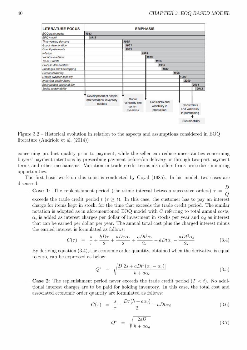
40 CHAPTER 3. EOQ BASED MODEL
Figure 3.2 – Historical evolution in relation to the aspects and assumptions considered in EOQliterature (Andriolo et al. (2014))
concerning product quality prior to payment, while the seller can reduce uncertainties concerningbuyers’ payment intentions by prescribing payment before/on delivery or through two-part paymentterms and other mechanisms. Variation in trade credit terms also offers firms price-discriminatingopportunities.
The first basic work on this topic is conducted by Goyal (1985). In his model, two cases arediscussed:
— Case 1: The replenishment period (the stime interval between successive orders) τ = D
Qexceeds the trade credit period t (τ ≥ t). In this case, the customer has to pay an interestcharge for items kept in stock, for the time that exceeds the trade credit period. The similarnotation is adopted as in aforementioned EOQ model with C referring to total annual costs,αc is added as interest charges per dollar of investment in stocks per year and αd as interestthat can be earned per dollar per year. The annual total cost plus the charged interest minusthe earned interest is formulated as follows:
C(τ) = s
τ+ hDτ
2 + aDταc2 + aDt2αc
2τ − aDtαc −aDt2αd
2τ (3.4)
By deriving equation (3.4), the economic order quantity, obtained when the derivative is equalto zero, can be expressed as below:
Q∗ =√D[2s+ aDt2(αc − αd)]
h+ aαc(3.5)
— Case 2: The replenishment period never exceeds the trade credit period (T < t). No addi-tional interest charges are to be paid for holding inventory. In this case, the total cost andassociated economic order quantity are formulated as follows:
C(τ) = s
τ+ Dτ(h+ aαd)
2 − aDtαd (3.6)
Q∗ =√
2sDh+ aαd
(3.7)

3.2. THE ECONOMIC ORDER QUANTITY MODEL 41
In tactical planning, the aspect of trade credit has been largely investigated in the EOQ model.Jaggi et al. (2008) develop a new inventory model under two levels of trade credit policy with credit-linked demand to reflect real-life situations. Chang et al. (2009) discuss the effects of the inflationrate, the deterioration rate and delay in payment in determining the optimal payment period andthe replenishment cycle. Chang et al. (2010) propose an inventory model for deteriorating itemswith two kind of possible trade credits on the order quantity. Furthermore, Kouvelis & Zhao (2011)compare short-term debt with supplier-financed trade credit via a newsvendor model and studythe interplay between operations and finance. In recent studies, the classical EOQ model has beenfurther developed considering deteriorating items under a two-level trade credit policy. Min et al.(2010) establish a lot-sizing model for deteriorating items with a current-stock-dependent demandand delays in payment in order to maximize a retailer’s average profit per unit time. Mo et al. (2014)extend the previous model to a multi-item inventory model for perishable items. The work of Seifertet al. (2013) is referred for the detailed review of trade credit terms that are considered with theEOQ model.
Time value of money and inflation
The time value of money (TVM) indicates the fact that money values more at the present timethan the same amount in the future for its potential earning capacity over time. The TVM isalso referred as present discounted value or net present value (NPV). Essentially, money has timevalue because of the following reasons: first, since risk and uncertainties exist in the future and areextremely difficult to be predicted. A common preference for present consumption generally existswhich may result from urgent financial needs and it is to avoid payment in the future. Second,sufficient money at present ensures the availability when facing better investment opportunities.Thus, payment in the future generates an extra opportunity cost. Last, in an inflationary economy,the money received today, has stronger purchasing power than the money to be received in future.
Inflation refers to a continuous increase in the price level and is an index of the prices of allgoods in the economic aspect. Actually, inflation occurs when the government creates money at afaster rate than the economy growth. The government should print enough money to fuel economicgrowth but not too much money that may destroy the value of money. Even though money canpotentially generate more money, inflation itself will devalue money that you earn in the future interms of purchase power. For example, prices for many consumer goods are twice higher than thatof 20 years ago.
The TVM and inflation are the first two financial aspects integrated into the EOQmodel accordingto Andriolo et al. (2014). A present value formulation based on the EOQ model is proposed in theearly work of Trippi & Lewin (1974). As presented by Andriolo et al. (2014), this inflation effect isnot considered before the study of Buzacott (1975) who considers both the inflation and time valueof money in a lot-sizing problem. The author examines the influence of inflation on different typesof pricing policies in order to study how TVM impacts inventory decisions. In the work of Trippi &Lewin (1974), the authors regard the inventory as a form of investment that serves as part of firms’financial structure and is discounted by a continuous-time interest rate, αnpv. After substitutingthe Taylor series expansion, an expression of the optimal order quantity is obtained. The authorsthen illustrate the insensitivity of the discount cost to the error in the expression. As a result, anear-optimal formulation of the optimal quantity can be written as below:
Q∗ =√
2Dsαnpva
(3.8)
In the work of Buzacott (1975), the near-optimal formula considering the inflation is provided usingthe same up-mentioned reasoning:
Q∗ =√
2Ds(αnpv − γ)a,where, γ is the inflation rate (3.9)

42 CHAPTER 3. EOQ BASED MODEL
Other formulations can be found in Jesse et al. (1983).— without inflation
Q∗ =√
2Ds(h+ αnpv)a
(3.10)
— under inflation
Q∗ =√
2Ds[h+ (αnpv − γ)]a (3.11)
During last three decades, this topic is largely investigated in the EOQ literature for more re-alistic cases. More related works are referred to the review of Andriolo et al. (2014), Taleizadeh &Nematollahi (2014) and Martínez-Costa et al. (2014). In this work, production planning is executedin a medium-term horizon that the TVM and the inflation effect can thus be neglected.
Cost of capital
The cost of capital is the rate of return on a portfolio company’s existing securities. It is oftenused to compute the net present value of the cash flows in a proposed investment. Besides, it is alsoconsidered to be the minimum after-tax internal rate of return to be earned by new investments.The cost of capital is specific to each particular type of capital that a company uses. At the highestlevel, they are the cost of equity and the cost of debt, but each class of shares, each class of debtsecurities, and each loan will have its own cost. The Weighted Average Cost of Capital (WACC)combines all these into a single number for a company’s cost of capital.
WACC : The weighted average cost of capital (WACC) normalizes the cost of capital by combiningthe interest rates being incurred from both debt and equity. The cost of debt refers to the effectiverate that a company pays on its current debt.
Ratedebt = IE
De(3.12)
, where IEt represents interest expenses while De is the value of total debt.The cost of equity is the return that stockholders require for their investment in a company.
Rateequity = Ratefree + β(Ratemarket −Ratefree) (3.13)
, where Ratefree is the risk-free rate of interest, Ratemarket is the expected market return, β is tomeasure the sensitivity of the stock to the market evolution, namely the stock beta , and Ratemarket−Ratefree is the expected risk premium of the stock market. (see in Brealey (2001))
The tax-adjusted formulation can be written as:
WACC = RateequityE
E +De+Ratedebt
De
E +De(1− Tc) (3.14)
, where E represents the value of equity, Tc is the corporate tax rate. A firm’s WACC increasesas β and the rate of return on equity increase, when an increase in the WACC denotes a decrease invaluation and an increase in risk. A common practice in business admits that the financial part ofinventory holding cost is the WACC of the firm (around 12%) as presented in Serrano et al. (2017).
When defining the cost of capital, it is useful to frame it from either the borrower’s point of view(i.e. the organization) or the lender’s point of view (the investor). For the organization borrowingthe capital, while the cost of capital is the cumulative rate of interest (usually derived as an averagerate, combining all capital inputs) applied to the borrowed capital to fund a project. From theinvestor’s point of view, the cost of capital is the relative required return rate considering the risk ofthe investment being made.

3.3. EOQ BASED PROFIT MAXIMIZATION MODEL, EOQP (WCR) 43
3.2.3 Positioning the work of this chapterThis thesis is relatively close to the literature which involves the cost of capital in operational
decision, especially with EOQ-based models. As shown in Zipkin (2000), the cost of capital is addedin the Wilson’s formula alongside the inventory holding cost. However, it is not frequently consideredby the inventory planner as stated by Rumyantsev & Netessine (2007). Therefore, the authors providean empirical investigation using the data panel that contains 722 public US companies for the periodfrom 1992 to 2002. Their study shows that classical inventory models continue to provide goodpolicies in an aggregated way at the firm level. Even though the authors prove the influence of thedemand uncertainty, company size and margin on the inventory level. No relations can be foundbetween the inventory and the cost of capital since it is affected by the time trend inclusion. Thisinconclusiveness joins the finding of Lai (2006) which indicates the need of finding new calculationof the cost of capital for operations models will be helpful in the future research. Recent effortof Hoberg et al. (2017) reveals the interplay between a firm’s financial situation and its inventoryownership from single- and two-firm perspectives. In their empirical study, the authors proposea refined formulation of the cost of capital and points out that higher costs of capital are weaklyassociated with lower inventories. Other related studies using the classical way to consider the costof capital are conducted by Serrano et al. (2009) and Serrano et al. (2017). The former presents theinfluence of operational decisions on the shareholders’ cost of capital. The latter addresses how thecost of capital is more precisely measured when the financial risk depends on the inventory decisionmade in place of using the WACC.
However, to the best of our knowledge, in the EOQ literature, only a few studies involve theaspect of working capital. Zeballos et al. (2013) explain the evolution of the Modigliani and Millertheorem in the field of inventory management and propose a single-product, finite horizon model tostudy how different sources of financing and how long-term and short-term debts affect the optimalordering policy considering the financial aspects of working capital constraints, payment delays andlead times. Although, this model is not exactly based on the EOQ model.
In this work, the financial consequences of the production decision on the production policy areaddressed considering the cost of working capital requirement based on the classic EOQ model. Thefinancial cost of the WCR is to cover all costs of production-related operations in medium-termlevel. It is generated by the time mismatch of paying for the operations and receiving the customer’spayment after the payment delay. Since, in the framework of the project RCSM, the planning horizonis defined at the medium-term level, there is thus no NPV and inflation effects being considered inthe proposed model.
3.3 EOQ based profit maximization model, EOQP (WCR)
3.3.1 OWCR modelingWe propose a generic OWCR formulation adapted for the EOQ-based model integrating the
financial costs linked to operational decisions (i.e., the financing cost of OWCR). Both the delay inpayment to supplier and from client are taken into account in this formulation. To establish themodel, we adopt the cash to cash cycle methodology presented in Theodore Farris & Hutchison(2002) and Hofmann & Kotzab (2010) where the OWCR for producing a unit of product depends onthe amount invested into the related operations (e.g., purchasing, setup, production and inventoryholding) and the financing duration of these investments before recovering from corresponding sales.However, we first assume that using the profit portion of the sales revenue to cover the OWCR is notallowed. Since the profit margin of the company has never been required, it does not correspond tothe OWCR definition. Furthermore, this assumption supposes that the company does not prioritizeits profit allocation to WCR financing. Profit can be allocated to any of a number of objectives for
44 CHAPTER 3. EOQ BASED MODEL
the firm including debt reduction, internal or external investment, or dividend payments. Since wedo not designate the allocation of profit (to WCR financing or others objectives), our model is thusa partial model for company. Moreover, following the Modigliani Miller Theorem, a company shouldnot affect a specific financial resource (here profit) to a specific object (here WCR financing). Inconsequence, we adopt the scheme that the WCR generated by producing a product is only effectivelyrecovered when that product is sold. Thus, we progressively and uniformly receive all productionrelated cost from the sales revenue of products over time.
3.3.2 AssumptionsIn this section, we present an EOQ-based model with a profit maximization objective considering
the financing cost of OWCR. The OWCR formulation and the corresponding profit maximizationmodel proposed in this paper are built under the following assumptions :
— Production:— Demand is constant and uniform during the planning horizon;— For each production lot, all purchasing, setup, production and inventory holding costs
must be financed;— Production capacity is infinite;— No backlogging is allowed;— Only inventory of final product is considered;— Initial and final stocks are defined as zero;— No delivery delay of material and production is immediate.
— Financial:— Production, inventory and setup costs should be paid instantaneously (but may be fi-
nanced);— The profit margin from selling products is not be used for financing the WCR in the
OWCR calculation;— The fixed setup cost is earned back uniformly and progressively by selling products of the
same production lot.As previously discussed, we only consider the cost portion in revenue (not the profit margin)
for financing the OWCR because the margin may be reinvested in another operation cycle. Withthis assumption, we do not need to consider the opportunity cost of using the margin to finance theOWCR. Moreover, we consider that the OWCR is generated due to the timing mismatch betweenrevenue and costs to finance. Therefore, we set the last assumption in the list in order to preciselycalculate the setup cost in revenue of selling each product. More specifically, all products in the sameproduction lot share the fixed setup cost equally and it will be refunded progressively by selling theproducts.
3.3.3 Parameters et decision variablesNotation is defined for the single-site, single-level, single-product with infinite capacity case in Ta-
ble 3.1. These parameters are all assumed to be nonnegative. The decision variable is the productionlot size, denoted as Q. Accordingly, Q∗ represents the optimal production lot size.
3.3.4 OWCR formulationFollowing the concept of the cash conversion cycle methodology, we propose a generic OWCR
formulation for purchasing, setup, production and holding inventory by taking into account theinterest accrued by financing the OWCR during the planning horizon.
In the EOQ model, a uniform time division is established in which, for each cycle, a quantity Qis instantly supplied at the beginning of the cycle and uniformly consumed over the cycle. Thus, for
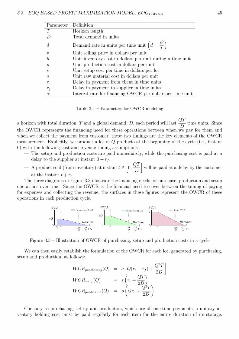
3.3. EOQ BASED PROFIT MAXIMIZATION MODEL, EOQP (WCR) 45
Parameter DefinitionT Horizon lengthD Total demand in unitsd Demand rate in units per time unit
(d = D
T
)v Unit selling price in dollars per unith Unit inventory cost in dollars per unit during a time unitp Unit production cost in dollars per units Unit setup cost per time in dollars per lota Unit raw material cost in dollars per unitrc Delay in payment from client in time unitsrf Delay in payment to supplier in time unitsα Interest rate for financing OWCR per dollar per time unit
Table 3.1 – Parameters for OWCR modeling
a horizon with total duration, T and a global demand, D, each period will last QTD
time units. Sincethe OWCR represents the financing need for these operations between when we pay for them andwhen we collect the payment from customer, these two timings are the key elements of the OWCRmeasurement. Explicitly, we product a lot of Q products at the beginning of the cycle (i.e., instant0) with the following cost and revenue timing assumptions:
— The setup and production costs are paid immediately, while the purchasing cost is paid at adelay to the supplier at instant 0 + rf .
— A product sold (from inventory) at instant t ∈[0, QT
D
]will be paid at a delay by the customer
at the instant t+ rc.The three diagrams in Figure 3.3 illustrate the financing needs for purchase, production and setup
operations over time. Since the OWCR is the financial need to cover between the timing of payingfor expenses and collecting the revenue, the surfaces in these figures represent the OWCR of theseoperations in each production cycle.
Figure 3.3 – Illustration of OWCR of purchasing, setup and production costs in a cycle
We can then easily establish the formulation of the OWCR for each lot, generated by purchasing,setup and production, as follows:
WCRpurchasing(Q) = a
[Q(rc − rf ) + Q2T
2D
]WCRsetup(Q) = s
(rc + QT
2D
)WCRproduction(Q) = p
(Qrc + Q2T
2D
)
Contrary to purchasing, set-up and production, which are all one-time payments, a unitary in-ventory holding cost must be paid regularly for each item for the entire duration of its storage.

46 CHAPTER 3. EOQ BASED MODEL
Therefore, there is a cumulative effect in financing the inventory holding costs. More precisely, forone product sold at t ∈
[0, QT
D
], we must pay its inventory holding costs generated in all instants
over the entire duration from 0 to t. Thus, all these costs must be financed from the instant whenthey occur (instant 0) until the arrival of client’s payment at t+ rc, as presented in Figure 3.4.
Figure 3.4 – Illustration of the OWCR calculation for inventory holding cost
Consider an item that is sold at insant t, where t ∈[0, QT
D
]) and one of its inventory payment
which occurs at τ ∈ [0, t]. This cost must be financed until the customer pays the product at t+ rc.Therefore, the financing duration will be t+ rc − τ . Consequently, the OWCR for inventory holdingcost in a production cycle is formulated as follows:
WCRinventory(Q) =∫ QT
D
0
∫ t
0hQT
D(t+ rc − τ) dτdt
= h(Q3T 2
6D2 + rcQ2T
2D )
(3.15)
Following the above formulations of OWCR, the total OWCR for a production cycle can beexpressed as follows:
WCR(Q) = WCRpurchasing +WCRsetup +WCRproduction +WCRinventory
= h(Q3T 2
6D2 + rcQ2T
2D ) + a
[Q(rc − rf ) + Q2T
2D
]+ p(rcQ+ Q2T
2D ) + s(rc + QT
2D )
= hT 2
6D2Q3 + T
2D (hrc + a+ p)Q2 +[a(rc − rf ) + prc + sT
2D
]Q+ src
Accordingly, the total WCR is formulated as follows:
WCRtotal = D
Q×WCR(Q) = hT 2
6D Q2 + T
2 (hrc + a+ p)Q+D[a(rc − rf ) + prc + sT
2D
]+srcD 1
Q
3.3.5 Objective functionThe aim of our contribution is to maximize the profit by satisfying constant demands. According
to the profit definition proposed by Chen & Teng (2015), the profit can be defined as the differencebetween sales revenue and all expenses including logistic costs and interests to pay. In our case, theinterest is the cost of financing the OWCR. The formulations of these components are
— The sales revenue (denoted as R): R = vD;
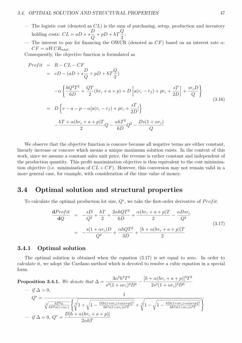
3.4. OPTIMAL SOLUTION AND STRUCTURAL PROPERTIES 47
— The logistic cost (denoted as CL) is the sum of purchasing, setup, production and inventoryholding costs: CL = aD + s
D
Q+ pD + hT
Q
2 ;— The interest to pay for financing the OWCR (denoted as CF ) based on an interest rate α:
CF = αWCRtotal.Consequently, the objective function is formulated as
Profit = R− CL− CF
= vD − (aD + sD
Q+ pD + hT
Q
2 )
−α{hQ2T 2
6D + QT
2 (hrc + a+ p) +D[a(rc − rf ) + prc + sT
2D
]+ srcD
Q
}
= D{v − a− p− α[a(rc − rf ) + prc + sT
2D ]}
−hT + α(hrc + a+ p)T2 Q− αhT 2
6D Q2 − Ds(1 + αrc)Q
(3.16)
We observe that the objective function is concave because all negative terms are either constant,linearly increase or concave which means a unique maximum solution exists. In the context of thiswork, since we assume a constant sales unit price, the revenue is rather constant and independent ofthe production quantity. This profit maximization objective is thus equivalent to the cost minimiza-tion objective (i.e. minimization of CL+ CF ). However, this conversion may not remain valid in amore general case, for example, with consideration of the time value of money.
3.4 Optimal solution and structural propertiesTo calculate the optimal production lot size, Q∗, we take the first-order derivative of Profit.
dProfitdQ
= −sDQ2 + hT
2 + 2αhQT 2
6D + α(hrc + a+ p)T2 − αDsrc
Q2
= −s(1 + αrc)DQ2 + αhQT 2
3D + [h+ α(hrc + a+ p)]T2
(3.17)
3.4.1 Optimal solutionThe optimal solution is obtained when the equation (3.17) is set equal to zero. In order to
calculate it, we adopt the Cardano method which is devoted to resolve a cubic equation in a specialform.
Proposition 3.4.1. We denote that ∆ = 3α2h2T 4
s2(1 + αrc)2D4 −[h+ α(hrc + a+ p)]3T 3
2s3(1 + αrc)3D3
— if ∆ > 0,Q∗ = 1
3√
hT 2α6D2s(1+αrc)
{3
√1 +
√1− D[h(1+αrc)+α(a+p)]3
6h2s(1+αrc)α2T+ 3
√1−
√1− D[h(1+αrc)+α(a+p)]3
6h2s(1+αrc)α2T
}
— if ∆ = 0, Q∗ = D[h+ α(hrc + a+ p)]2αhT

48 CHAPTER 3. EOQ BASED MODEL
— if ∆ < 0,Q∗ = 1
2√
[h(1 + αrc) + α(a+ p)]T6Ds(1 + αrc)
cos
13 arccos
√√√√ 6h2s(1 + αrc)α2T
[h(1 + αrc) + α(a+ p)]3D
Proof. We seek to maximize the objective function given by:
Profit = D{v − a− p− α[a(rc − rf ) + prc + sT
2D ]}− hT + α(hrc + a+ p)T
2 Q
−αhT2
6D Q2 − Ds(1 + αrc)Q
The objective function is strictly concave as a sum of concave functions and a strictly concavefunction (Q > 0). Thus, if there is a maximum, it will be unique and will occur when function (3.17)will be equal to zero. Thus,
dProfitdQ
= 0 ⇔ −s(1 + αrc)DQ2 + αhQT 2
3D + [h+ α(hrc + a+ p)]T2 = 0
(Q ∈ R∗+) ⇔ −s(1 + αrc)DQ3 + [h+ α(hrc + a+ p)]T
2Q + αhT 2
3D = 0
(X = 1Q
) ⇔ s(1 + αrc)DX3 − [h+ α(hrc + a+ p)]T2 X − αhT 2
3D = 0
(s(1 + αrc)D > 0) ⇔ X3 − [h+ α(hrc + a+ p)]T2s(1 + αrc)D
X − αhT 2
3s(1 + αrc)D2 = 0
We compute the discriminant of this cubic equation. According to Cardano’s method, for acubic equation, x3 + px + q = 0, the discriminant ∆ = 4p3 + 27q2. Therefore, for our case, p =− [h+ α(hrc + a+ p)]T
2s(1 + αrc)Dand q = − αhT 2
3s(1 + αrc)D2 . Consequently,
∆ = −4{
[h+ α(hrc + a+ p)]T2s(1 + αrc)D
}3
+ 27[− αhT 2
3s(1 + αrc)D2
]2
Three cases must be considered:— ∆ > 0: In this case, there is only one real root given by:
X∗ = 13
3
√√√√√√ 27αhT 2
3s(1 + αrc)D2 + 27√
∆
2 +3
√√√√√√ 27αhT 2
3s(1 + αrc)D2 − 27√
∆
2
Thus,Q∗ = 1
X∗= 1
3
√hT 2α
6D2s(1 + αrc)
×
3
√√√√1 +√
1− D[h(1 + αrc) + α(a+ p)]36h2s(1 + αrc)α2T
+ 3
√√√√1−√
1− D[h(1 + αrc) + α(a+ p)]36h2s(1 + αrc)α2T
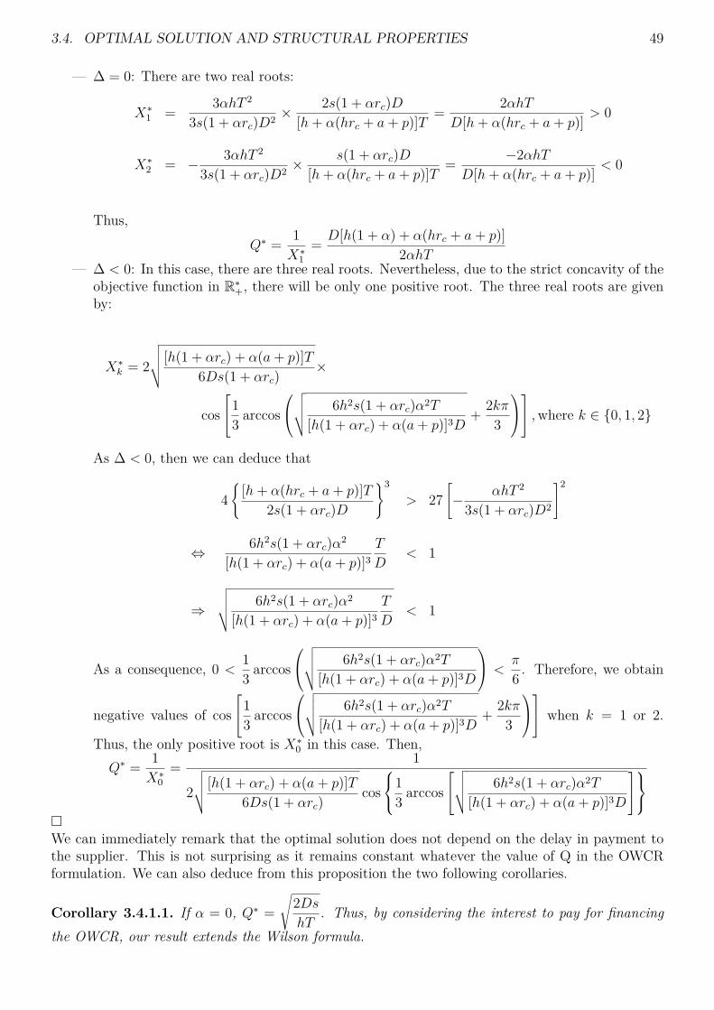
3.4. OPTIMAL SOLUTION AND STRUCTURAL PROPERTIES 49
— ∆ = 0: There are two real roots:
X∗1 = 3αhT 2
3s(1 + αrc)D2 ×2s(1 + αrc)D
[h+ α(hrc + a+ p)]T = 2αhTD[h+ α(hrc + a+ p)] > 0
X∗2 = − 3αhT 2
3s(1 + αrc)D2 ×s(1 + αrc)D
[h+ α(hrc + a+ p)]T = −2αhTD[h+ α(hrc + a+ p)] < 0
Thus,Q∗ = 1
X∗1= D[h(1 + α) + α(hrc + a+ p)]
2αhT— ∆ < 0: In this case, there are three real roots. Nevertheless, due to the strict concavity of the
objective function in R∗+, there will be only one positive root. The three real roots are givenby:
X∗k = 2
√√√√ [h(1 + αrc) + α(a+ p)]T6Ds(1 + αrc)
×
cos1
3 arccos√√√√ 6h2s(1 + αrc)α2T
[h(1 + αrc) + α(a+ p)]3D + 2kπ3
,where k ∈ {0, 1, 2}As ∆ < 0, then we can deduce that
4{
[h+ α(hrc + a+ p)]T2s(1 + αrc)D
}3
> 27[− αhT 2
3s(1 + αrc)D2
]2
⇔ 6h2s(1 + αrc)α2
[h(1 + αrc) + α(a+ p)]3T
D< 1
⇒
√√√√ 6h2s(1 + αrc)α2
[h(1 + αrc) + α(a+ p)]3T
D< 1
As a consequence, 0 <13 arccos
√√√√ 6h2s(1 + αrc)α2T
[h(1 + αrc) + α(a+ p)]3D
<π
6 . Therefore, we obtain
negative values of cos1
3 arccos√√√√ 6h2s(1 + αrc)α2T
[h(1 + αrc) + α(a+ p)]3D + 2kπ3
when k = 1 or 2.
Thus, the only positive root is X∗0 in this case. Then,Q∗ = 1
X∗0= 1
2
√√√√ [h(1 + αrc) + α(a+ p)]T6Ds(1 + αrc)
cos
13 arccos
√√√√ 6h2s(1 + αrc)α2T
[h(1 + αrc) + α(a+ p)]3D
�We can immediately remark that the optimal solution does not depend on the delay in payment tothe supplier. This is not surprising as it remains constant whatever the value of Q in the OWCRformulation. We can also deduce from this proposition the two following corollaries.
Corollary 3.4.1.1. If α = 0, Q∗ =√
2DshT
. Thus, by considering the interest to pay for financingthe OWCR, our result extends the Wilson formula.
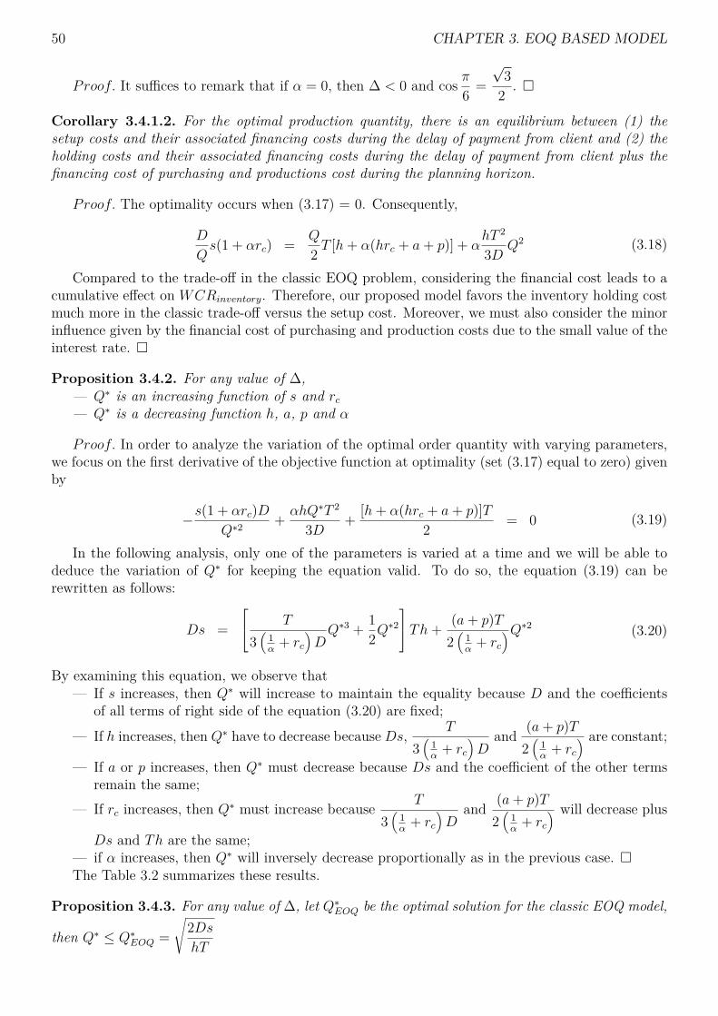
50 CHAPTER 3. EOQ BASED MODEL
Proof. It suffices to remark that if α = 0, then ∆ < 0 and cos π6 =√
32 . �
Corollary 3.4.1.2. For the optimal production quantity, there is an equilibrium between (1) thesetup costs and their associated financing costs during the delay of payment from client and (2) theholding costs and their associated financing costs during the delay of payment from client plus thefinancing cost of purchasing and productions cost during the planning horizon.
Proof. The optimality occurs when (3.17) = 0. Consequently,
D
Qs(1 + αrc) = Q
2 T [h+ α(hrc + a+ p)] + αhT 2
3D Q2 (3.18)
Compared to the trade-off in the classic EOQ problem, considering the financial cost leads to acumulative effect on WCRinventory. Therefore, our proposed model favors the inventory holding costmuch more in the classic trade-off versus the setup cost. Moreover, we must also consider the minorinfluence given by the financial cost of purchasing and production costs due to the small value of theinterest rate. �
Proposition 3.4.2. For any value of ∆,— Q∗ is an increasing function of s and rc— Q∗ is a decreasing function h, a, p and α
Proof. In order to analyze the variation of the optimal order quantity with varying parameters,we focus on the first derivative of the objective function at optimality (set (3.17) equal to zero) givenby
−s(1 + αrc)DQ∗2
+ αhQ∗T 2
3D + [h+ α(hrc + a+ p)]T2 = 0 (3.19)
In the following analysis, only one of the parameters is varied at a time and we will be able todeduce the variation of Q∗ for keeping the equation valid. To do so, the equation (3.19) can berewritten as follows:
Ds = T
3(
1α
+ rc)DQ∗3 + 1
2Q∗2
Th+ (a+ p)T2(
1α
+ rc)Q∗2 (3.20)
By examining this equation, we observe that— If s increases, then Q∗ will increase to maintain the equality because D and the coefficients
of all terms of right side of the equation (3.20) are fixed;
— If h increases, then Q∗ have to decrease becauseDs, T
3(
1α
+ rc)D
and (a+ p)T2(
1α
+ rc) are constant;
— If a or p increases, then Q∗ must decrease because Ds and the coefficient of the other termsremain the same;
— If rc increases, then Q∗ must increase because T
3(
1α
+ rc)D
and (a+ p)T2(
1α
+ rc) will decrease plus
Ds and Th are the same;— if α increases, then Q∗ will inversely decrease proportionally as in the previous case. �The Table 3.2 summarizes these results.
Proposition 3.4.3. For any value of ∆, let Q∗EOQ be the optimal solution for the classic EOQ model,
then Q∗ ≤ Q∗EOQ =√
2DshT

3.4. OPTIMAL SOLUTION AND STRUCTURAL PROPERTIES 51
Parameter Variation Influence on Q*s ↗ ↗rc ↗ ↗h ↗ ↘a ↗ ↘p ↗ ↘α ↗ ↘
Table 3.2 – Analysis of influences of varying parameters on optimal batch size
Proof. In order to compare between the optimal solutions of this model and of the classic EOQmodel (Denoted as Q∗EOQ), the equation (3.20) is reformulated as follows.
Ds = T
3(
1α
+ rc)DQ∗3 + 1
2Q∗2
Th+ (a+ p)T2(
1α
+ rc)Q∗2
⇔ Ds =hT
2 + hT 2Q∗
3(
1α
+ rc)D
+ (a+ p)T2(
1α
+ rc)Q∗2
⇔ Q∗ =√√√√√√√√
2Ds
hT + 2hT 2Q∗
3( 1α
+ rc
)D
+ (a+ p)T( 1α
+ rc
)
(3.21)
Since 2hT 2Q∗
3(
1α
+ rc)D
+ (a+ p)T(1α
+ rc) can only be a positive value, we are able to obtain that Q∗ ≤√
2DshT
= Q∗EOQ. This proposition shows that taking into account the interest generated by financ-ing the OWCR during the planning horizon always leads to a decrease of the optimum batch sizecompared with the classical Economic Order Quantity.
Corollary 3.4.3.1. The optimal production quantity obtained by the proposed model is less sensitiveto variation of the fixed setup cost and of the inventory holding unit cost compared with the optimalquantity of classic EOQ model
Proof. In Corollary 3.4.3.1, we study the sensibility of the optimal production quantities withvarying parameter of fixed setup cost and inventory holding unit cost. In order to compare to EOQmodel, we set the values of purchasing and production unit cost at zero. Then, we focus on thetrade-offs in this problem and the EOQ problem which are respectively presented as follows:
— In the EOQP (WCR) problem, the trade-off is obtained when the equation is equal to zero.Thus,
s(1 + αrc)DQ∗2
= αhT 2Q∗
3D + hT (1 + αrc)2
sD = hTQ∗2
2 + αhT 2Q∗3
3D(1 + αrc)(3.22)
— In EOQ problem, the trade-off can be formulated as follows:
sD = hTQ∗2
2(3.23)

52 CHAPTER 3. EOQ BASED MODEL
Let denote that Q∗ and Q∗EOQ are the optimal quantities obtained by EOQP (WCR) model andEOQ model. With zero purchasing and production unit cost, the equation (3.21) is expressed asfollow:
Q∗ =√√√√√√√√
2Ds
hT + 2hT 2Q∗
3( 1α
+ rc
)D
⇔ Q∗ =√√√√√√
2Ds
hT
[1 + 2αTQ∗
3D(1 + αrc)
]
Since Q∗EOQ =√
2DshT
, then
Q∗2EOQQ∗2
=
√2DshT√√√√√√2Ds
hT
[1 + 2αTQ∗
3D(1 + αrc)
]
2
= 1 + 2αTQ∗3D(1 + αrc)
> 1
(3.24)
This equation shows the relation between optimal quantity of these models with same set ofinstance. Next, with the same value of parameters expect for s, we denote that Q∗1 (Q∗2) and Q∗EOQ1(Q∗EOQ2) are the optimal quantities with s1 (s2, where s2 > s1). According to the proposition 3.4.2,the optimal quantities in our problem will increase following the increase of s, i.e. Q∗1 < Q∗2. Samerelation can be found in EOQ problem, i.e. Q∗EOQ1 < Q∗EOQ2. We express the relation between theseoptimal quantity in these two cases:
Q∗2EOQ1
Q∗21= 1 + 2αTQ∗1
3D(1 + αrc)(3.25)
Q∗2EOQ2
Q∗22= 1 + 2αTQ∗2
3D(1 + αrc)(3.26)
Since Q∗1 < Q∗2, we have2αTQ∗1
3D(1 + αrc)<
2αTQ∗23D(1 + αrc)
. We can thus deduce thatQ∗EOQ1
Q∗1<Q∗EOQ2
Q∗2.
Then, we assume that X = Q∗EOQ1Q∗2Q∗1
. According to the proposition 3.4.3, Q∗1 < Q∗EOQ1 and we get:
X −Q∗EOQ1
Q∗2 −Q∗1=
Q∗EOQ1
Q∗1
Q∗2Q∗1− 1
Q∗2Q∗1− 1
> 1 (3.27)
Thus, X −Q∗EOQ1 > Q∗2 −Q∗1. Furthermore, we study the relation between Q∗EOQ2 and X. Because

3.4. OPTIMAL SOLUTION AND STRUCTURAL PROPERTIES 53
we haveQ∗EOQ1
Q∗1<Q∗EOQ2
Q∗2which means Q∗EOQ2Q
∗1 > Q∗EOQ1Q
∗2, we obtain that
Q∗EOQ2 −X = Q∗EOQ2 −Q∗EOQ1Q∗2Q∗1
=Q∗EOQ2Q
∗1 −Q∗EOQ1Q
∗2
Q∗1> 0
(3.28)
To conclude, Q∗EOQ2−Q∗EOQ1 > Q∗2−Q∗1. It signifies that with the same increase of the fixed setupcost, the optimal quantity in EOQ model will increase more than in our model which represents thatit is more sensible to the s in our model than in EOQ model.
Similar argument can be found for the inventory holding unit cost, h. The difference is, accordingto the proposition 3.4.2, when h increases, the optimal quantity will decrease in our model (same inEOQ model). In this case, we fix all parameters expect for h (in place of s in the previous case).Therefore, the relations between up-mentioned optimal quantities are Q∗EOQ1 > Q∗EOQ2 and Q∗1 > Q∗2.
Comparing between the equation (3.25) and (3.26), we obtainQ∗EOQ1
Q∗1>Q∗EOQ2
Q∗2because Q∗1 > Q∗2.
We execute similar approach as in the previous case of s. We assume that X = Q∗EOQ1Q∗2Q∗1
. Accordingto proposition 3.4.3, we have Q∗EOQ1 > Q∗EOQ2. Then, we get:
Q∗EOQ1 −XQ∗1 −Q∗2
=Q∗EOQ1
Q∗1
1−Q∗2Q∗1
1−Q∗2Q∗1
> 1 (3.29)
Thus, Q∗EOQ1−X > Q∗1−Q∗2. Subsequently, we compare the relation between X and Q∗EOQ2 with
the relationQ∗EOQ1
Q∗1>Q∗EOQ2
Q∗2.
X −Q∗EOQ2 = Q∗EOQ1Q∗2Q∗1−Q∗EOQ2
=Q∗EOQ1Q
∗2 −Q∗EOQ2Q
∗1
Q∗1> 0
(3.30)
Therefore, Q∗EOQ1−Q∗EOQ2 > Q∗1−Q∗2. We thus obtain similar result that the optimal quantity, Q∗,is less sensible to the h than Q∗EOQ. �
3.4.2 Comparison with classic EOQ based-formula with the cost of cap-ital
In the literature and in practice, a traditional way to consider the cost of capital is to add italongside the holding cost in Wilson’s formula. For instance, as Jesse et al. (1983) proposes, inan inventory management context, the near-optimal formula considering the cost of capital can be
written as Q∗j =√
2DshT + αcV T
where V represents unitary product value (unit cost in their work)and αc as the cost of capital. As is customary in the EOQ literature, the unit cost is the sum of

54 CHAPTER 3. EOQ BASED MODEL
operation costs including purchasing raw material and production which is V = a+ p. The setup isnot included in the unit cost (Harris (1913)). Therefore, the approximate formula can be rewrittenas :
Q∗j =√
2Ds[h+ αc(a+ p)]T
(3.31)
Note that if we take equation (4.37) and set rc = 0 and remove the last term containing thequadratic variables we will obtain the approximation in exact same form as given in (3.31) (i.e. αin place of αc). We then seek to compare this approximation with our fully derived formula takinginto account WCR financing from Proposition 3.4.1 without client payment delay as given in thefollowing proposition.
Proposition 3.4.4. When rc = 0, the ratio between optimal production quantities obtained with ourformula (proposition 3.4.1), denoted as Q∗, and with classic EOQ-based formula considering cost ofcapital, denoted as Q∗j , can be expressed in different cases as follows :
— if ∆ > 0, 0 < Q∗
Q∗j<
√3
2 .
— if ∆ = 0, Q∗
Q∗j=√
32
— if ∆ < 0,√
32 <
Q∗
Q∗j< 1.
Proof.We compare the ratio between the optimal production quantities obtained by two formula with
rc = 0 in three cases. These cases value of ∆. Knowing that ∆ = −4{
[h+ α(a+ p)]T2sD
}3
+
27[−αhT
2
3sD2
]2
, the three cases are discussed in the following paragraphs.
— When ∆ > 0, the ratio can be expressed as follows :
Q∗
Q∗j=√
3 6
√D[h+ α(a+ p)]3
6α2h2sT×
1
3
√√√√1 +√
1− D[h+ α(a+ p)]36α2h2sT
+ 3
√√√√1−√
1− D[h+ α(a+ p)]36α2h2sT
Denote that X = D[h+ α(a+ p)]36α2h2sT
where 0 < X < 1 since ∆ > 0. Consequently, Q∗
Q∗j=
√3F (X) =
√3 6√X
3√
1 +√
1−X + 3√
1−√
1−X. Then, we search the extreme value of this equa-
tion by calculating the derivate of F (X).

3.4. OPTIMAL SOLUTION AND STRUCTURAL PROPERTIES 55
[F (X)]X
= 1
6(
3√√
1−X + 1 + 3√
1−√
1−X)x
56
−
(1
6(1−√
1−X)23√1−X
− 1
6(√1−X+1)23√1−X
)6√X(
3√√
1−X + 1 + 3√
1−√
1−X)2
=
√1−X − 3
√X(
3√√
1−X + 1− 3√
1−√
1−X)
6(
3√√
1−X + 1 + 3√
1−√
1−X)X
56√
1−X
(3.32)
Since we have 0 < X < 1, we attempt to determinate the sign of the derivate. First, thedenominator of (3.32) is greater than zero with 0 < X < 1. Second, for the nominator, welet Y =
√1−X where 0 < Y < 1. Therefore, the nominator of (.11) can be rewritten as
N(Y ) = Y − 3√
1− Y 2(
3√
1 + Y − 3√
1− Y). Its derivate is calculated as follows:
N(Y )Y
=2Y
(3√Y + 1− 3
√1− Y
)3 (1− Y 2)
23
− 3√
1− Y 2
13 (Y + 1)
23
+ 13 (1− Y )
23
+ 1 (3.33)
In order to determinate the sign of N(Y )Y
, we denote that A = 3√
1 + Y and B = 3√
1− Y .With this notation, (3.33) can be reformulate as follows:
N(Y )Y
= (A3 −B3) (A−B)3A2B2 − AB
( 13A2 + 1
3B2
)+ 1
= (A−B)2(A2 + AB +B2)− AB(A2 +B2) + 3A2B2
3A2B2
= (A−B)2(A2 + AB +B2)− AB(A−B)2 + A2B2
3A2B2
= (A−B)2(A2 +B2) + A2B2
3A2B2 > 0
(3.34)
With positive nominator and denominator, (3.32) is always positive. Furthermore, N(0) = 1.
Consequently, N(Y ) > 0 with 0 < Y < 1. Therefore, [F (X)]X
> 0. Since we have that
0 < X < 1, the derivate of F (X) is always positive in corresponding interval and F (1) =√
32 ,
we deduct that 0 < Q∗
Q∗j<
√3
2 .
— if ∆ = 0, Q∗
Q∗j=√
32
√D[h+ α(a+ p)]3
6α2h2sT=√
32 = 0.86
— if ∆ < 0, Q∗
Q∗j=
√3
2 cos
13 arccos
√√√√ 6α2h2sT
[h+ α(a+ p)]3D
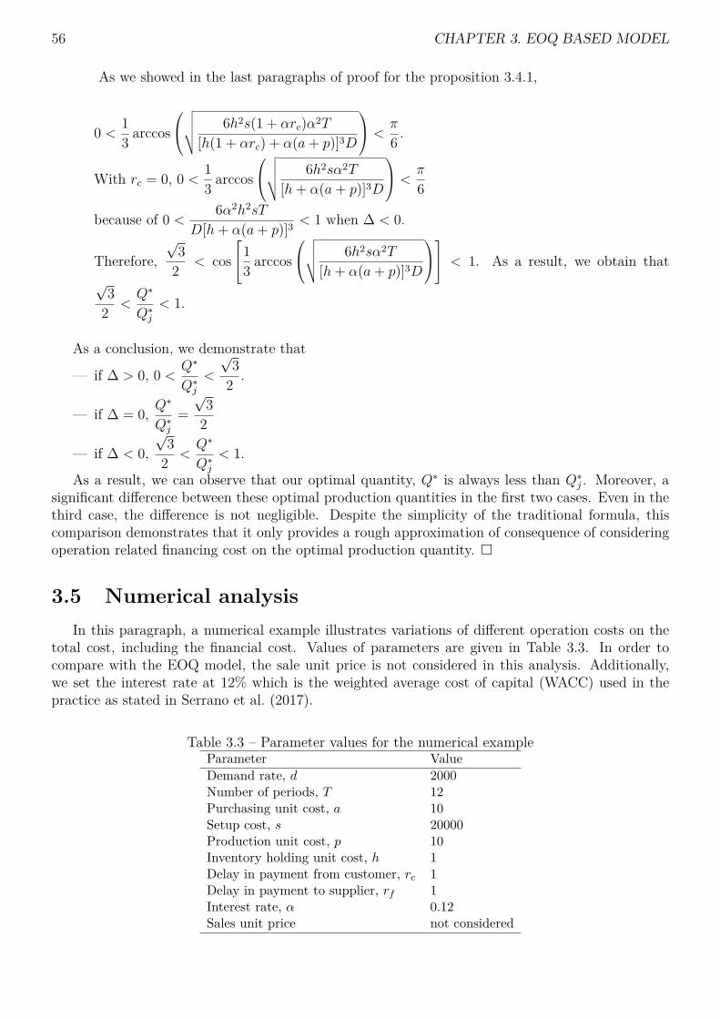
56 CHAPTER 3. EOQ BASED MODEL
As we showed in the last paragraphs of proof for the proposition 3.4.1,
0 < 13 arccos
√√√√ 6h2s(1 + αrc)α2T
[h(1 + αrc) + α(a+ p)]3D
<π
6 .
With rc = 0, 0 < 13 arccos
√√√√ 6h2sα2T
[h+ α(a+ p)]3D
<π
6
because of 0 < 6α2h2sT
D[h+ α(a+ p)]3 < 1 when ∆ < 0.
Therefore,√
32 < cos
13 arccos
√√√√ 6h2sα2T
[h+ α(a+ p)]3D
< 1. As a result, we obtain that√
32 <
Q∗
Q∗j< 1.
As a conclusion, we demonstrate that
— if ∆ > 0, 0 < Q∗
Q∗j<
√3
2 .
— if ∆ = 0, Q∗
Q∗j=√
32
— if ∆ < 0,√
32 <
Q∗
Q∗j< 1.
As a result, we can observe that our optimal quantity, Q∗ is always less than Q∗j . Moreover, asignificant difference between these optimal production quantities in the first two cases. Even in thethird case, the difference is not negligible. Despite the simplicity of the traditional formula, thiscomparison demonstrates that it only provides a rough approximation of consequence of consideringoperation related financing cost on the optimal production quantity. �
3.5 Numerical analysisIn this paragraph, a numerical example illustrates variations of different operation costs on the
total cost, including the financial cost. Values of parameters are given in Table 3.3. In order tocompare with the EOQ model, the sale unit price is not considered in this analysis. Additionally,we set the interest rate at 12% which is the weighted average cost of capital (WACC) used in thepractice as stated in Serrano et al. (2017).
Table 3.3 – Parameter values for the numerical exampleParameter ValueDemand rate, d 2000Number of periods, T 12Purchasing unit cost, a 10Setup cost, s 20000Production unit cost, p 10Inventory holding unit cost, h 1Delay in payment from customer, rc 1Delay in payment to supplier, rf 1Interest rate, α 0.12Sales unit price not considered

3.5. NUMERICAL ANALYSIS 57
3.5.1 Comparison betweens results obtained by the proposed model andthe classic EOQ model
We first compute the optimal production quantity with the proposed model and the classic EOQmodel. By applying the formula presented in Proposition 3.4.1, we obtain that Q∗ = 5507 for the
values in Table 3.3. Moreover, the optimal quantity with the EOQ model is Q∗EOQ =√
2DshT
= 8944.These results verify Proposition 3.4.3. In figure 3.5, we illustrate the total costs calculated by thesetwo models. We denote that CWCR represents the total cost in EOQP (WCR) model including thelogistic cost CL and financial cost CF (i.e.CWCR = CL + CF , as presented in equation (3.16)).CEOQ is the total cost in the EOQ model which is mathematically formulated as CEOQ = D(a +p) + sD
Q+ hTQ
2 which is equal to CL in EOQP (WCR) model. Moreover, the optimal quantities areindicated in the figure which verifies the proposition 3.4.3.
0.5 1 1.5 2·104
0.5
1
1.5
·106
Batch size
TotalC
osts
CWCR
CEOQ
Q∗ Q∗EOQ
Figure 3.5 – Comparison of total cost between the EOQ and proposed model
Next, we measure the increase of total cost (CL + CF ) by using our proposed model in placeof the EOQ model. To do so, we compare between the optimal total cost C∗WCR with Q∗ andthe total cost with C∗WCR(Q∗EOQ) introducing Q∗EOQ. As a result, we obtains that ∆C∗WCR =C∗WCR(Q∗EOQ)− C∗WCR
C∗WCR
= 2.5% which indicates a 2.5% increase in profit with our proposed modelthat considers the financing cost of OWCR versus the classic EOQ model.
3.5.2 Illustration of the trade-off between costsAs mentioned in Corollary 3.4.1.2, there exists a trade-off between the setup related costs and
all other costs. In Figure 3.6, we illustrate the trade-off with the given instance. Knowing that onlythe terms in function of Q are involved in the trade-off, the mathematical formulation of the setuprelated cost, Cs, and other costs, Co are thus presented as follows:
Cs = (1 + αrc)DsQ
= 768000000Q
Co = αhT 2
6D Q2 + hT + α(hrc + a+ p)T2 Q = 0.00012Q2 + 21.12Q

58 CHAPTER 3. EOQ BASED MODEL
0.5 1 1.5 2·104
2
4
6
·105
QCosts
Cs Co Total
Figure 3.6 – Trade-off between batch size related costs
3.5.3 Sensitivity of Q∗ to varying parameters in the classic and proposedEOQ models
In Figures 3.7 and 3.8, we illustrate the sensitivity of the optimal quantities of both models withvarying setup cost and inventory holding costs as shown in Corollary 4.3.1. In these tests, we onlyconsider the fixed setup cost and unit inventory holding cost which appear as parameters in bothmodels. The purchasing and production unit costs are set to zero. As a result, we observe that theoptimal batch size of the proposed model varies less than the one of the EOQ model. By introducingthe financial cost, the optimal production lot size of our propposed model is less sensitive than inthe classic model to changes in s and h as we state in Corollary 3.4.3.1.
0 2 4 6 80.4
0.6
0.8
1
1.2
·104
Inventory holding unit cost
Optim
alba
tchsiz
e Q∗ Q∗EOQ
Figure 3.7 – Variations of optimal batchsizes to s with both models
0 2 4·104
0.5
1
1.5 ·104
fixed setup cost
Optim
alba
tchsiz
e Q∗ Q∗EOQ
Figure 3.8 – Variations of optimal batchsizes with varying s with the models
3.6 ConclusionsIn this chapter, a new generic model of operations-related working capital requirements in the
EOQ context is presented. Such a model allows us to measure the evolution of the WCR overthe continuous-time planning horizon. Furthermore, an EOQ-based profit maximization model isdeveloped considering the financing cost of the WCR. The analytical formula of the optimal EOQ isderived and associated analysis are provided to highlight some managerial insights. It is shown that

3.6. CONCLUSIONS 59
an increase in purchasing, production unit costs or the interest rate reduces the optimal production lotsize in order to obtain the maximum profit. Moreover, it is demonstrated that the economic quantityproposed by our model is always smaller than the optimal quantity of the traditional EOQ model.Thus, it is desirable to launch more frequent production with smaller lots in this joint managementcase in order to reduce inventory levels and their associated holding costs. Additionally, a comparisonwith the approximation of Jesse et al. (1983) demonstrates that our model provides a more coherentand accurate measure of the optimal production quantity for a profit maximization objective whenconsidering financial aspects. Finally, the numerical example illustrates the reduced sensitivity ofour model to several parameters when compared with the classic EOQ model.
As we reveal for this problem, there is a complex trade-off between the multitudes of differentoperational and financial costs in order to maximize the profit. For future research, we may firstbenefit from this trade-off to verify if the Zero-Inventory-Property is still valid in the dynamic lot-sizing problem with time-varying demand. Second,Based on this trade-off, it could be interesting toestablish heuristics for the capacitated lot-sizing problem considering OWCR financing costs. Thisis inspired by the way how the trade-off in the EOQ problem is used for the capacitated lot-sizingmodel proposed by Silver & Meal (1973), the Least Unit Cost heuristic proposed by Gorham (1968)and the Part Period Balancing heuristic proposed by DeMatteis (1968). Lastly, it is shown that thedelay in payment to the supplier has no influence on the optimal production quantity. However,it would be interesting to look into a two-echelon, supplier-customer relationship because, in thiscontext, the delay in payment to supplier (accounts payable for the customer) would simultaneouslyinfluence the accounts receivable for the supplier. Thus, the customer’s production policy wouldrestrict the policy of the supplier and the delay in payment to supplier would no longer be negligible.


4Dynamic lot-sizing based discountedmodel considering the financing cost ofworking capital requirement
4.1 IntroductionIn the first chapter, we take into consideration the financing cost of working capital requirements
in the classic EOQ model in which the constant demand is assumed. To relax this assumption ofconstant demand to a more realistic time-varying demand, models of the dynamic lot-sizing problem(DLS) are proposed in the production planning literature. Hence, the objective here is to integratethe financing cost of WCR into the DLS models. We studies the case of Uncapacitated Lot-SizingProblem (ULS) which is the case of single-level, single-product, constant parameter context and withinfinite production capacity. First, a generic modeling of WCR is established in the ULS contextthat allows us to trace the evolution of WCR during the planning horizon. Second, a discounted cashflow model on the basis of the classic ULS model is built considering the financing cost of WCR.Subsequently, inspired by the classic Uncapacitated Lot-Sizing Problem (ULS), the Zero-Inventory-Ordering (ZIO) property is proven valid in this problem. With possession of this property, a dynamicprogramming-based algorithm is constructed which resolves the problem in O(T 4). A numericalanalysis is effectuated that shows the difference between the classic ULS model and the proposedmodel in term of optimal production program. Moreover, the sensitivity analysis are performed withvarying parameters.
4.2 Dynamic lot sizing modelsAfter inquiring into the problem over continuous-time horizon with constant demand, the focus of
this chapter is on the integration the financial cost of the WCR into the dynamic lot-sizing problem(DLS). In an Advanced Planning System (APS), DLS models are involved in the production planningas presented in Figure 2.4 of chapter 1. Thus, DLS models are close to the short term machinescheduling topic as well as sales planning as a Capable-To-Promise (CTP) logic (Fleischmann (2005))to verify the fulfillment of client’s demands. Additionally, supplier selection and capacity planningare frequently taken into consideration in DLS models and a large amount of literature is dedicatedto the production planning problem by using DLS models. "This is due to the ubiquity of lot-sizing
61

62 CHAPTER 4. ULS BASED MODEL
and scheduling decision problems in manufacturing firms and the large variety of production typesin these firms, which often require specialized models" (Lang (2010)).
Early seminal work of Wagner & Whitin (1958) is deemed as the initial effort to deal withthis problem that extends the EOQ problem over discrete time horizon and handles time-varyingdemand. Similar to the EOQ problem, the DLS problem consist in determining production planningwith setups periods and production quantities. The planned setup periods consequently derives theinventory holding level as well as the associated holding costs. Thus, the objective of DLS is todetermine the best trade-off that minimizes the sum of production, setup and inventory holdingcosts. The main feature of the ULS models and the classification are given in Section 2.3.2. In thefollowing paragraph, we will mainly focus on the ULS model.
4.2.1 The uncapacitated Lot-Sizing (ULS) model and mathematical for-mulations
As stated above, single-level, multi-product production planning problem with infinite productioncapacity can be solvable in polynomial time because it can be reduced to N polynomial single produc-tion planning problems. Nevertheless, the problem becomes more difficult to handle with capacityconstraints. NP-hardness is proven for both single- and multi-product cases with the productioncapacity in work of Bitran & Yanasse (1982). In this chapter, we consider the financial cost of WCRin the single-site, single-product, big bucket and with infinite capacity case, i.e. the proposed modelis based on ULS model. The motivation of considering this case is mainly based on two points:
— With the above-presented classification, it is reasonable to start the study with the most basicproblem.
— In studies of capacitated single-product or multi-product problems, the ULS problem is oftenconsidered as a sub-problems to tackle. Examples can be found in the application of theLagrangian relaxation (e.g. Thizy & Van Wassenhove (1983)) to CLSP and column generation(Cattrysse et al. (1990)) to DLSP.
ULS model and aggregate formulation
The ULS problem is described as follows and the associated formulation are given as well. First,the ULS model aims at satisfying time-varying demand over a planning horizon of T periods anddetermining timing of setups and production lot size Qt in these periods. Such a planning shouldminimize the sum of the up-mentioned costs which includes:
— unit production cost pt (where t = 1, .., T is the period);— setup cost st, a fixed cost incurred when a production is planned in a period t,— unit inventory holding cost ht per period.The assumptions of this problem are:— No replenishment and production delays as they are negligible compared to the period dura-
tion;— Demand should be met on time (no backlogging);— Only inventory of final product is considered;— Initial and final stocks are set to zero;— One unit of finished product is manufactured using one unit of raw material.In the DLS literature, Mixed Integer Programming (MIP) formulation is not directly adopted for
solving the ULS problem as the case of Wagner & Whitin (1958) and as stated by Brahimi et al.(2017). However, as above-mentioned, the ULS problem is often considered as a subproblem ofmore complex DLS problem for which the MIP formulation is built for solution procedure. In thefollowing, different MIP formulations of the ULS problem are presented in the following paragraphsand the associated parameters are summarized below.

4.2. DYNAMIC LOT SIZING MODELS 63
Parameter DefinitionT Horizon lengthdt Demand in period tdtk Sum of demands from period t to period kht Unit inventory cost in period tpt Unit production cost in period tst Fixed setup cost in period t
Table 4.1 – Parameters
Variable DefinitionQt Total production quantity in period tXtk Production quantity in period t for satisfying (a part of) demand in period kIt Product quantity held in inventory in period tYt Binary variable which indicates whether a setup occurs in period t or not
Table 4.2 – Decision variables
A natural formulation of the ULS problem is the aggregate formulation provided as below. In thisformulation, products manufactured in a same period t are aggregated as Qt which aims to satisfydemand(s) of following period(s).
MinT∑t=1
(stYt + ptQt + htIt) (4.1)
s.t. It−1 +Qt = dt + It ∀t (4.2)dtTYt −Qt ≥ 0 ∀t (4.3)Qt, It ≥ 0 ∀t (4.4)Yt = 0 or 1 ∀t (4.5)
The objective function (4.1) minimizes the sum of setup, production and inventory holding costsover the entire horizon. Constraints (4.2) are the inventory balance equations. They express thatthe entering stock It−1 added to the current period production Qt is used to satisfy the demand dtand the remains is kept in stock at the end of the period It. Constraints (4.3) ensure that a setuponly occurs when a production planned in period t. Constraints (4.4) and (4.5) relate the continuousproduction variables Qt to the binary setup variables Yt.
Reformulations of the ULS model
Three reformulations of the ULS model are presented in this section. The first two reformulationsare based on the fact that:
— Constraints (4.2) balance the inventory by the difference between the remaining in the in-ventory plus the new production and the consumption of inventory for satisfying demands.The first reformulation combines the unit production costs with the holding costs in order toreplace the variable of inventory quantity.
— The second reformulation disaggregates the production variable, Qt because it merely repre-sents all products manufactured in a certain period without knowing for which demand theyare produced. Therefore, a disaggregate formulation can be formulated, namely, the facilitylocation-based (FAL) formulation.
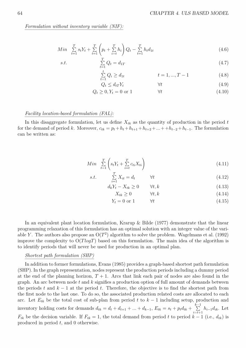
64 CHAPTER 4. ULS BASED MODEL
Formulation without inventory variable (NIF):
MinT∑t=1
stYt +T∑t=1
(pt +
T∑i=thi
)Qt −
T∑t=1
htd1t (4.6)
s.t.T∑t=1
Qt = d1T (4.7)t∑t=1
Qi ≥ d1t t = 1, ..., T − 1 (4.8)
Qt ≤ dtTYt ∀t (4.9)Qt ≥ 0, Yt = 0 or 1 ∀t (4.10)
Facility location-based formulation (FAL):
In this disaggregate formulation, let us define Xtk as the quantity of production in the period tfor the demand of period k. Moreover, ctk = pt+ht+ht+1 +ht+2 + ...++ht−2 +ht−1. The formulationcan be written as:
MinT∑t=1
(stYt +
T∑i=tctiXti
)(4.11)
s.t.T∑i=1
Xit = dt ∀t (4.12)
dkYt −Xtk ≥ 0 ∀t, k (4.13)Xtk ≥ 0 ∀t, k (4.14)
Yt = 0 or 1 ∀t (4.15)
In an equivalent plant location formulation, Krarup & Bilde (1977) demonstrate that the linearprogramming relaxation of this formulation has an optimal solution with an integer value of the vari-able Y . The authors also propose an O(T 2) algorithm to solve the problem. Wagelmans et al. (1992)improve the complexity to O(T logT ) based on this formulation. The main idea of the algorithm isto identify periods that will never be used for production in an optimal plan.
Shortest path formulation (SHP)
In addition to former formulations, Evans (1985) provides a graph-based shortest path formulation(SHP). In the graph representation, nodes represent the production periods including a dummy periodat the end of the planning horizon, T + 1. Arcs that link each pair of nodes are also found in thegraph. An arc between node t and k signifies a production option of full amount of demands betweenthe periods t and k − 1 at the period t. Therefore, the objective is to find the shortest path fromthe first node to the last one. To do so, the associated production related costs are allocated to eacharc. Let Etk be the total cost of sub-plan from period t to k − 1 including setup, production andinventory holding costs for demands dtk = dt + dt+1 + ...+ dk−1, Etk = st + ptdtk +
k−1∑i=t+1
hi−1dik. LetFtk be the decision variable. If Ftk = 1, the total demand from period t to period k − 1 (i.e., dtk) isproduced in period t, and 0 otherwise.

4.3. THE DISCOUNTED CASH FLOW MODEL OF THE DLS PROBLEM 65
MinT∑t=1
(stYt +T+1∑k=t+1
EtkFtk) (4.16)
s.t.T∑i=1
F1i = 1 (4.17)t−1∑i=1
Fit =T+1∑i=t+1
Fti t = 2, ..., T (4.18)
T+1∑i=t+1
Fti ≤ Yt ∀t (4.19)
Ftk ≥ 0 ∀t, k (4.20)Yt = 0 or 1 ∀t (4.21)
Constraints (4.17) ensure that no more than one arc outgoing from the node 1. Constraints (4.18)ensure that the flow balance is not violated at nodes 2, ..., T + 1. Constraints (4.19) force the setupbinary variable Yt to be one whenever there is production in period t. The linear relaxation of thisformulation has an optimal solution with integer variables Y (constraints (4.21)).
A comparison of the last two formulations is given in work of Gao et al. (2008) on the effective-ness of solving MIP formulation with tight LP relaxations by establishing specialized primal-dualalgorithms . A research timeline with different formulations is also provided.
Solution procedure
The first exact algorithm for this problem has been proposed by Wagner & Whitin (1958) basedon dynamic programming (DP) which solve the problem in O(T 2). This kind of method explores thesolution space of a problem by implicit enumeration to find its optimal solution. The authors proveda strong structural property of the optimal planning.
Theorem 4.2.1. There exists an optimal solution with QtIt−1=0 for all t, where It represents theinventory level, which means the production will only occur with no product held in inventory.
Using dynamic programming with the above property, the search space can be significantly re-duced to at most T (T+1)
2 . Another interpretation of this property is, in the optimal planning, theproduction quantities can only be the sum of demand(s) in following consecutive period(s). In thisliterature, this problem draw many attention as studied in Zabel (1964), Eppen et al. (1969) andLundin & Morton (1975). However, the complexity of the WW algorithm is further improved byrespective efforts of Wagelmans et al. (1992), Aggarwal & Park (1993) and Federgruen & Tzur (1991).Reviewing literature of this problem, we notice that the DP technique has been largely consideredwhich will be further discussed in the next section.
4.3 The discounted cash flow model of the DLS problemThe DLS models are always built based on given or estimated demand for short-term or medium-
term production planning problems. Thus, in the lot-sizing literature, the traditional planningmodel implicitly assumes that all the investment is financed by equity without debt and the financialbudget limitations in expansions for incapacity are often neglected. It is rarely the case in real worldbecause operational and financial decisions are interrelated for reaching the maximum profitabilityand performance of the company in an extremely competitive economic context. Consequently, acompany may raise its capital from profits, external loans, or bonds and the financial decisions ofstrategic capacity development are usually set for a large planning horizon. Therefore, the time valueof money should be considered for its significant impact on investment decision.
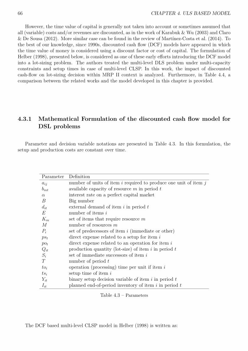
66 CHAPTER 4. ULS BASED MODEL
However, the time value of capital is generally not taken into account or sometimes assumed thatall (variable) costs and/or revenues are discounted, as in the work of Karabuk & Wu (2003) and Claro& De Sousa (2012). More similar case can be found in the review of Martínez-Costa et al. (2014). Tothe best of our knowledge, since 1990s, discounted cash flow (DCF) models have appeared in whichthe time value of money is considered using a discount factor or cost of capital. The formulation ofHelber (1998), presented below, is considered as one of these early efforts introducing the DCF modelinto a lot-sizing problem. The authors treated the multi-level DLS problem under multi-capacityconstraints and setup times in case of multi-level CLSP. In this work, the impact of discountedcash-flow on lot-sizing decision within MRP II context is analyzed. Furthermore, in Table 4.4, acomparison between the related works and the model developed in this chapter is provided.
4.3.1 Mathematical Formulation of the discounted cash flow model forDSL problems
Parameter and decision variable notations are presented in Table 4.3. In this formulation, thesetup and production costs are constant over time.
Parameter Definitionaij number of units of item i required to produce one unit of item jbmt available capacity of resource m in period tα interest rate on a perfect capital marketB Big numberdit external demand of item i in period tE number of items iKm set of items that require resource mM number of resources mPi set of predecessors of item i (immediate or other)pst direct expense related to a setup for item ipot direct expense related to an operation for item iQit production quantity (lot-size) of item i in period tSi set of immediate successors of item iT number of period ttoi operation (processing) time per unit if item itsi setup time of item iYit binary setup decision variable of item i in period tIit planned end-of-period inventory of item i in period t
Table 4.3 – Parameters
The DCF based multi-level CLSP model in Helber (1998) is written as:
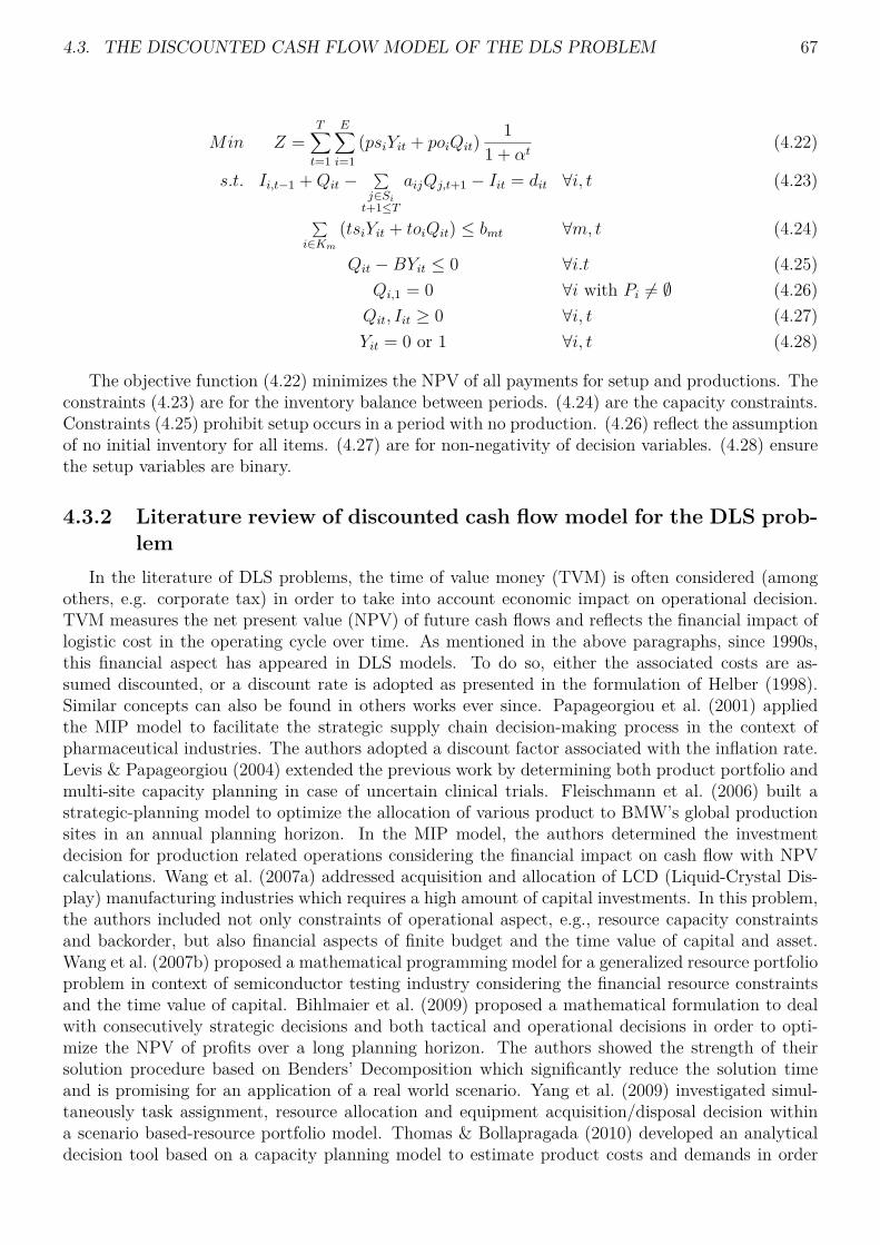
4.3. THE DISCOUNTED CASH FLOW MODEL OF THE DLS PROBLEM 67
Min Z =T∑t=1
E∑i=1
(psiYit + poiQit)1
1 + αt(4.22)
s.t. Ii,t−1 +Qit −∑j∈Sit+1≤T
aijQj,t+1 − Iit = dit ∀i, t (4.23)
∑i∈Km
(tsiYit + toiQit) ≤ bmt ∀m, t (4.24)
Qit −BYit ≤ 0 ∀i.t (4.25)Qi,1 = 0 ∀i with Pi 6= ∅ (4.26)Qit, Iit ≥ 0 ∀i, t (4.27)Yit = 0 or 1 ∀i, t (4.28)
The objective function (4.22) minimizes the NPV of all payments for setup and productions. Theconstraints (4.23) are for the inventory balance between periods. (4.24) are the capacity constraints.Constraints (4.25) prohibit setup occurs in a period with no production. (4.26) reflect the assumptionof no initial inventory for all items. (4.27) are for non-negativity of decision variables. (4.28) ensurethe setup variables are binary.
4.3.2 Literature review of discounted cash flow model for the DLS prob-lem
In the literature of DLS problems, the time of value money (TVM) is often considered (amongothers, e.g. corporate tax) in order to take into account economic impact on operational decision.TVM measures the net present value (NPV) of future cash flows and reflects the financial impact oflogistic cost in the operating cycle over time. As mentioned in the above paragraphs, since 1990s,this financial aspect has appeared in DLS models. To do so, either the associated costs are as-sumed discounted, or a discount rate is adopted as presented in the formulation of Helber (1998).Similar concepts can also be found in others works ever since. Papageorgiou et al. (2001) appliedthe MIP model to facilitate the strategic supply chain decision-making process in the context ofpharmaceutical industries. The authors adopted a discount factor associated with the inflation rate.Levis & Papageorgiou (2004) extended the previous work by determining both product portfolio andmulti-site capacity planning in case of uncertain clinical trials. Fleischmann et al. (2006) built astrategic-planning model to optimize the allocation of various product to BMW’s global productionsites in an annual planning horizon. In the MIP model, the authors determined the investmentdecision for production related operations considering the financial impact on cash flow with NPVcalculations. Wang et al. (2007a) addressed acquisition and allocation of LCD (Liquid-Crystal Dis-play) manufacturing industries which requires a high amount of capital investments. In this problem,the authors included not only constraints of operational aspect, e.g., resource capacity constraintsand backorder, but also financial aspects of finite budget and the time value of capital and asset.Wang et al. (2007b) proposed a mathematical programming model for a generalized resource portfolioproblem in context of semiconductor testing industry considering the financial resource constraintsand the time value of capital. Bihlmaier et al. (2009) proposed a mathematical formulation to dealwith consecutively strategic decisions and both tactical and operational decisions in order to opti-mize the NPV of profits over a long planning horizon. The authors showed the strength of theirsolution procedure based on Benders’ Decomposition which significantly reduce the solution timeand is promising for an application of a real world scenario. Yang et al. (2009) investigated simul-taneously task assignment, resource allocation and equipment acquisition/disposal decision withina scenario based-resource portfolio model. Thomas & Bollapragada (2010) developed an analyticaldecision tool based on a capacity planning model to estimate product costs and demands in order

68 CHAPTER 4. ULS BASED MODEL
to maximize the NPV of profit for General Electric. More related works are referred in You et al.(2010), Lim et al. (2013a), Lim et al. (2013b) and Mitra et al. (2014) in various industry contexts.A comparison between these works and our research is presented in Table 4.4.
Authors SC Nb of Finite Time value Inflation Delay of WCR Objective3structure1 products2 budget of money payment
Helber (1998) S M√
MinCPapageorgiou et al. (2001) S M
√ √MaxP
Levis & Papageorgiou (2004) M M√ √
MaxPFleischmann et al. (2006) M M
√ √MinC
Wang et al. (2007a) S M√ √
MaxPWang et al. (2007b) S M
√ √MaxP
Bihlmaier et al. (2009) M M√
MinCYang et al. (2009) S M
√ √MaxP
Thomas & Bollapragada (2010) S√ √
MaxPYou et al. (2010) M M
√MaxP
Lim et al. (2013a) S M√
MaxPLim et al. (2013b) M M
√MaxP
Mitra et al. (2014) S M√
MinCThis work S S
√ √ √ √MaxP
1 S: single-site; M: multi-site.2 S: single-product; M: multi-product.3 MinC: cost minimization; MaxP: profit maximization.
Table 4.4 – Brief literature review
In the context of the project RCSM, we investigate the consolidation of financial needs of all actorsof supply chain. We assume the budget is no longer a constraint. Therefore, we rather consider theintegration of the financing cost of WCR in the ULS model. We choose the profit maximizationobjective because the WCR is presumed covered by the cost part of sales revenue. The detailedexplanation is given in the following section. Compared to the related literature, we consequentlytake into account the delay in payment because the WCR is generated by the timing mismatchbetween receivables and payables.
4.4 ULS-based profit maximization DCF model
4.4.1 OWCR modelingThe discounted cash flows method explicitly takes into account the time difference between the
cash flows but it does not take into account the financial borrowing costs because, in traditionalmodels, these costs have supposedly no influence on thee optimal operational decision. As we chal-lenge this assumption, we want to integrate only the financial costs linked to operational decisionsin the cash flows (i.e., financing cost of OWCR). To do so, we propose a generic OWCR formulationin a tactical planning context. In this formulation, both the delay in payment to supplier and fromclient are taken into account and the time value of money is considered in order to calculate presentvalues of incoming and outgoing cash flows. Furthermore, the level of inventory should be able tobe precisely measured over the planning horizon with this OWCR formulation as inventory holdingcosts make up a substantial portion of the OWCR.
Therefore, we adopt the cash to cash cycle methodology presented in Theodore Farris & Hutchison(2002) and Hofmann & Kotzab (2010) where the OWCR for producing a unit of product depends onthe amount invested into the related operations (e.g., purchasing, setup, production and inventoryholding) and the number of periods to finance these investments before recovering from correspondingsales. However, we firstly consider that the profit portion of the sales revenue are not available to coverthe OWCR. This is because the profit margin of the company does not correspond to the definition of

4.4. ULS-BASED PROFIT MAXIMIZATION DCF MODEL 69
working capital requirement since it has never been required. Furthermore, this assumption supposesthat the company does not prioritize its profit allocation to WCR financing. Profit can be allocatedto any of a number of objectives for the firm including debt reduction, internal or external investment,or dividend payments. Our model is a partial model of the company and we do not assume thatallocation of profit to WCR financing rather than to other objectives (e.g., new investments) isoptimal. Moreover, following the Modigliani Miller Theorem, a company should not affect a specificfinancial resource (here profit) to a specific object (here WCR financing). In consequence, we adoptthe scheme that the WCR generated by producing a product is only effectively recovered when thatproduct is sold.
This assumption complicates the calculation of the financing duration of setup costs because it ispaid in its entirety at a single point in time for the entire production lot. Thus, we must progressivelyand uniformly recover the setup cost from the sales revenue of all products in the same productionlot. Therefore, these products share the fixed setup cost equally as the invested amount and thenumber of periods to finance is the time difference between the period where the setup occurs andthe period of sale of each product.
4.4.2 Assumptions
Since this model is built in context of the ULS (Uncapacitated Lot-Sizing) problem, the OWCRformulation and the corresponding profit maximization model proposed in this section are under thefollowing assumptions:
— Production:— No replenishment and production delays as they are negligible compared to period dura-
tion;— Demand should be met on time (no backlogging);— Only inventory of final product is considered;— Initial and final stocks are defined as zero;— One unit of finished product is manufactured using one unit of raw material.
— Financial:— All logistic and financial costs are paid in the beginning of periods;— The profit from selling products is not used for financing the OWCR;— The fixed setup cost of a given lot is progressively and uniformly recovered over the different
periods during which the products of the corresponding lot are sold;— All holding costs paid for a product for all periods it remains in inventory are not recovered
until its sale.
4.4.3 Physical and financial flows illustration
With the aforementioned assumptions, we express in detail, in Figure 4.1, the physical andfinancial flows generated by a production in period 1 for the demand of period 3. In this case, weassume the delays in payment from client and to supplier are both one period.
— Physical flows are presented in the first bloc. They are generated by the decision made in theoperating cycle, such as purchase, production, inventory holding and delivery. Therefore, thephysical flows link all decisions in the graphic with the single line arrow.
— As financial flow, first, the logistic costs are immediately generated by the physical activitiespresented by small squares in the second bloc. Meanwhile, the WCR financing costs are alsoto be paid from the same period of corresponding logistic costs until the reception of revenue.These financial costs are presented with the double line arrow.

70 CHAPTER 4. ULS BASED MODEL
Period 1 Period 2 Period 3 Period 4
Decision
Fina
ncialfl
ow
Pu.
Pr.
I.H. I.H. De.
Pr. C
I.H. C
Pu. C
I.H. C
Revenue
Pay
mentdelayr f
Payment delay rc
Graph legend
XDecision X
Physical flow generatedby the decision X
X CCost generated bythe decision X
Financing periods ofthe cost
Pu. (Purchasing)/Pr. (Production)/I.H. (Inventory holding)/De. (Delivery)
Figure 4.1 – Physical and financial flows illustration
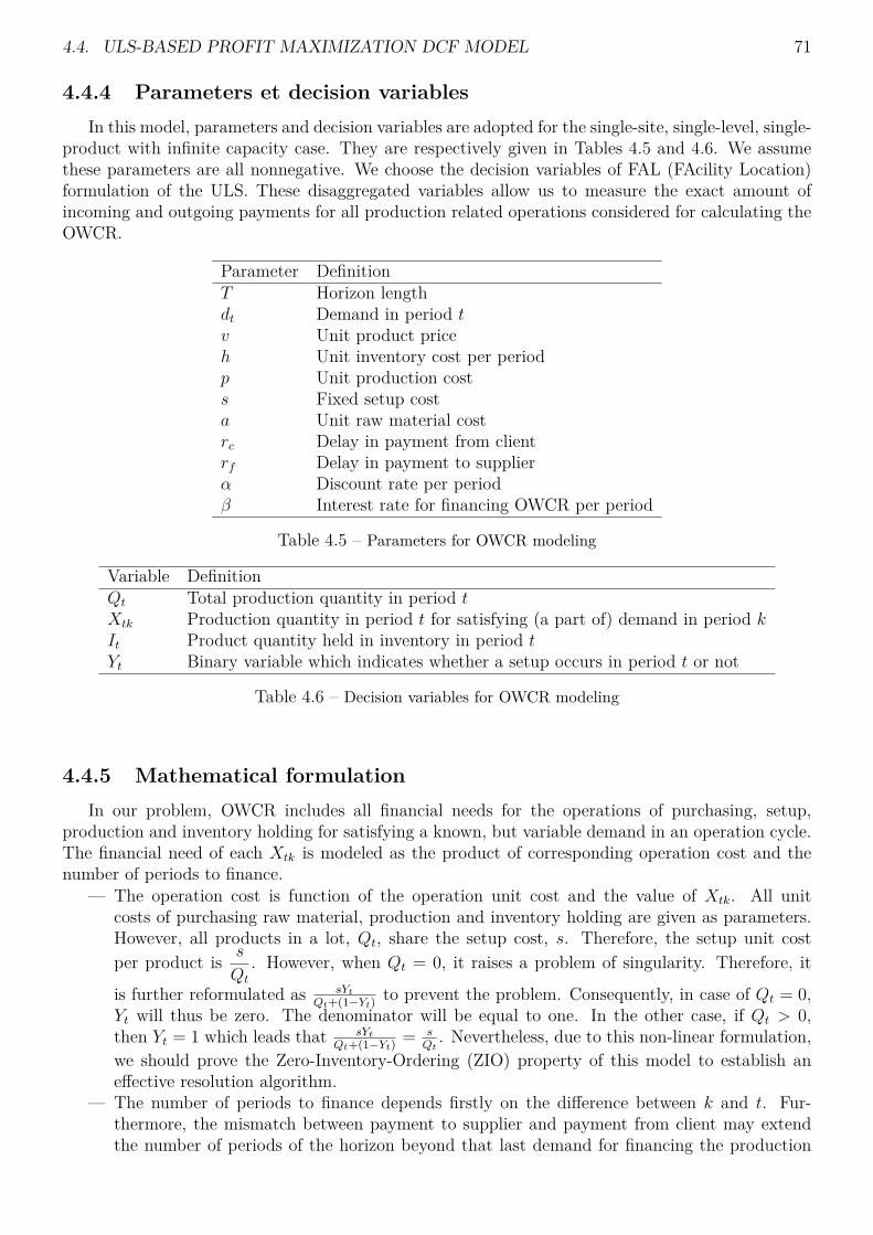
4.4. ULS-BASED PROFIT MAXIMIZATION DCF MODEL 71
4.4.4 Parameters et decision variablesIn this model, parameters and decision variables are adopted for the single-site, single-level, single-
product with infinite capacity case. They are respectively given in Tables 4.5 and 4.6. We assumethese parameters are all nonnegative. We choose the decision variables of FAL (FAcility Location)formulation of the ULS. These disaggregated variables allow us to measure the exact amount ofincoming and outgoing payments for all production related operations considered for calculating theOWCR.
Parameter DefinitionT Horizon lengthdt Demand in period tv Unit product priceh Unit inventory cost per periodp Unit production costs Fixed setup costa Unit raw material costrc Delay in payment from clientrf Delay in payment to supplierα Discount rate per periodβ Interest rate for financing OWCR per period
Table 4.5 – Parameters for OWCR modeling
Variable DefinitionQt Total production quantity in period tXtk Production quantity in period t for satisfying (a part of) demand in period kIt Product quantity held in inventory in period tYt Binary variable which indicates whether a setup occurs in period t or not
Table 4.6 – Decision variables for OWCR modeling
4.4.5 Mathematical formulationIn our problem, OWCR includes all financial needs for the operations of purchasing, setup,
production and inventory holding for satisfying a known, but variable demand in an operation cycle.The financial need of each Xtk is modeled as the product of corresponding operation cost and thenumber of periods to finance.
— The operation cost is function of the operation unit cost and the value of Xtk. All unitcosts of purchasing raw material, production and inventory holding are given as parameters.However, all products in a lot, Qt, share the setup cost, s. Therefore, the setup unit costper product is s
Qt
. However, when Qt = 0, it raises a problem of singularity. Therefore, it
is further reformulated as sYt
Qt+(1−Yt) to prevent the problem. Consequently, in case of Qt = 0,Yt will thus be zero. The denominator will be equal to one. In the other case, if Qt > 0,then Yt = 1 which leads that sYt
Qt+(1−Yt) = sQt. Nevertheless, due to this non-linear formulation,
we should prove the Zero-Inventory-Ordering (ZIO) property of this model to establish aneffective resolution algorithm.
— The number of periods to finance depends firstly on the difference between k and t. Fur-thermore, the mismatch between payment to supplier and payment from client may extendthe number of periods of the horizon beyond that last demand for financing the production

72 CHAPTER 4. ULS BASED MODEL
related costs. The delays in payment (i.e., rc and rf ) are introduced as parameters in orderto quantify this mismatch. With these parameters, we define the beginning period to financethe corresponding production related cost as well as the end period as presented in table 4.7.
Operation cost Periods to finance
Operations Unit cost × Quantity from( the period ofoutgoing payment
)until
( the period ofincoming payment
)Purchasing a × Xtk from (t+ rf ) until (k + rc − 1)
Setup sYtQt + (1− Yt)
× Xtk from t until (k + rc − 1)
Production p × Xtk from t until (k + rc − 1)Inventory holding h × Xtk Financing periods (FP)
Table 4.7 – Formulation of OWCR components
Although the costs of purchasing, set-up and production are all one-time payments for eachproduction lot, the inventory holding cost is regularly paid in all periods where the stock is heldin inventory. For this reason, there is a cumulative effect of financing the inventory holding costs.Assuming that a production lot covers all demands from period t to period k, which means that theproduction occurs in period t at the latest. A unit of product of the demand in period k will besold in period k and the client’s payment will arrive in period k + rc. Therefore, we should pay theinventory holding cost for this item from period t until period k − 1 (noted as "OWCRinv series").The first of these payments occurs in period t and must be financed until period k + rc − 1 (beforethe arrival of client’s payment, so k+ rc− t periods have to be financed in total.). The second is paidin period t+ 1 until the same period of k+ rc− 1 (in total, k+ rc− (t+ 1) periods to finance.), etc.
Consequently, for each Xtk, the financing period is 1 + (k − t)2 (k − t) + rc(k − t) periods including
all periods to finance before and after the demand delivery.Following this formulation of OWCR, the OWCR at the period t, noted Ot, can be expressed as
follows:
Ot = at−rf∑j=1
T∑l=t−rc+1
Xj,l + pt∑
j=1
T∑l=t−rc+1
Xj,l + st∑
j=1
T∑l=t−rc+1
YjQj + (1− Yj)
Xj,l
+ht∑
j=1
T∑l=t−rc+1
Xj,l(min {l, t+ 1} − j) (4.29)
The formulationt−rf∑j=1
T∑l=t−rc−1
Xj,l represents all products for which we still need to finance theirproduction related operations at period t considering the delays in payment. Especially for measuringthe total amount of inventory holding cost to finance at period t, we need to count the number ofcompleted payments in the OWCRinv series until period t for each Xj,l. However, we must considerwhether we have sold the products of Xj,l or not before reception of the client’s payment (in otherwords, if Xtk is still in inventory or not). min {l, t+ 1} − j precisely represents the total number ofall payments for these two possible cases. The difference between these two cases as presented informulation (4.29) is :
— If we have sold Xtk at period t (i.e. l ≤ t < l + rc), then the total amount to finance forinventory holding will not change during the periods before the arrival of client’s payment.This is because we no longer need to pay the inventory holding cost for Xtk in theses periods.Thus, no additional inventory holding cost must be financed which means the total amountis a function of l − j.
— On the contrary, if the Xtk is still in inventory (i.e. j ≤ t < l), then the total amount ofinventory holding costs to finance depends on t+ 1− j.

4.4. ULS-BASED PROFIT MAXIMIZATION DCF MODEL 73
This formulation of OWCR allows us to follow the variation of OWCR over time in the planninghorizon. It will be used in the following section for calculating the financing cost of OWCR.
4.4.6 Objective functionThe objective of this problem is to maximize the NPV of the profit (denoted by Profit) by
satisfying variable demand. To simplify the problem, the NPV of profit is defined as the differencebetween the NPV of revenue and the NPV of expenses. In our model, the revenue per period is afunction of constant unit sales prices and demand quantity. The expenses include the productioncosts and the OWCR financing costs. The production cost is the sum of the costs for raw materialpurchasing, machine setup, production and inventory holding. The OWCR financing cost dependson the interest rate and the OWCR for satisfying all the demand on-time. Considering the delays ofpayment, the planning horizon must be extended to the period where the last incoming or outgoingcash flow is occurred. Mathematically, this accounting horizon is presented as T + max {rf , rc}. Forreason of simplification, T denotes the accounting horizon in this section. Since the time value ofmoney is considered in this model, both cash inflow (i.e., revenues) and outflow (i.e., expenses) arepresented in NPV as follows :
— NPV of revenue in period t, Rt : Because of the delay of the client’s payment, we onlyreceive the client’s payment of demand of period t− rc in period t. Thus, Rt = 1
(1+α)tvDt−rc .— NPV of logistic cost in period t, LCt : All expenses of the production related operations
must be immediately paid when they occur except for the purchasing cost which can bedelayed rf periods according to the supplier agreement. Therefore, LCt = 1
(1+α)t (aQt−rf+
pQt + sYt + hIt) with Qt =T∑k=t
Xtk and It =t∑l=1
T∑k=t+1
Xlk.— NPV of OWCR financing cost in period t, FCt : The OWCR financing cost only
depends on the interest rate per period and the amount of financial need (i.e., Ot) to cover inperiod t. FCt = 1
(1+α)tβOt.By summing over all periods of the accounting horizon, the objective function is formulated as
follows :
Profit =T∑t=1
(Rt − LCt − FCt)
4.4.7 ULSP (WCR) modelA mixed-integer model of the profit maximization problem, ULSP (WCR), is formulated as follows
:
Max Profit (4.30)s.t. Qt = ∑T
k=tXtk ∀t (4.31)dkYt −Xtk ≥ 0 ∀t, k (4.32)Yt −Qt ≤ 0 ∀t (4.33)k∑t=1
Xtk = dk ∀k (4.34)
Xtk ≥ 0, Yt ∈ {0, 1} ∀t, k (4.35)The objective function is to maximize the NPV of total profit (4.30). Then, constraints are
similar to those of the FAL formulation of the ULS. Constraints (4.31) indicate that Qt is the totalquantity of production that occurs in period t. Constraints (4.32) ensure that a setup is executedbefore production. Constraints (4.33) prevent a setup from occurring in a period with no production.Finally, constraints (4.34) assure all demands are satisfied.
74 CHAPTER 4. ULS BASED MODEL
4.5 Solution methodIn order to solve effectively the ULSP (WCR) problem, we propose an algorithm which avoids the
difficulty of the non-linear formulation of the setup cost in the OWCR calculation. This algorithm issimilar to the algorithm which is based on the Zero-Inventory-Ordering (ZIO) property establishedfor the ULS problem with infinite capacity by Wagner & Whitin (1958) as mentioned in section 4.2.1.
4.5.1 Zero-Inventory-Ordering propertyIn a ZIO-type planning, production would only be planned when there is no product remaining
in inventory. We demonstrate that an optimal solution can always be found within all possible plansthat respects the ZIO property. Moreover, since only ZIO type plans need to be investigated infinding the optimal solution, the number of feasible solutions to investigate is significantly reduced.The ZIO property can be expressed as follows:
Theorem 4.5.1. There exists an optimal production plan in which It−1 ×Qt = 0 for all t (where Itis the inventory at the end of the period t) in ULSP (BFR) problem.
The proof is presented in the below sub-section. The main idea is to demonstrate that we canalways improve the objective value by eliminating violation(s) of the property by transforming aproduction plan which does not comply with the ZIO property to a ZIO-type plan. Eventually, wecan prove the ZIO-type production program provides the optimal objective value.
4.5.2 Proof of Theorem
Firstly, we denote that :— XULSP (W CR) represents all feasible solution in term of Xtk;— P is a production plan;— Profit(P ) stands for the objective value in the proposed model with P .
Definition 1. A production planning is complying with the ZIO property if and only if the productionis only planned when the inventory level drops to zero. With our notation, it can mathematically canbe expressed as
Qt ×[t−1∑k=1
(T∑l=t
Xk,l
)]= 0 ∀t ∈ [2, T ]
In other words, it can be written as :{Qt > 0 ⇒ Xk,l = 0 ∀(k, l) ∈ [1, t− 1]× [t, T ]Xk,l > 0 ⇒ Qt = 0 ∀t ∈ [k + 1, l]
Conjecture 4.5.2. There is a plan P ∗ ∈ X(ULSP (BF R)) which verifies the ZIO property while
Profit(P ∗) = maxP∈X(ULSP (BF R))
Profit(P )
Let (P ) ∈ X(ULSP (BF R)) be a planning which does not complies with the ZIO property. Note that(t,m, n) ∈ [1, T ]3 is a triplet with m < t ≤ n and a violation of the property can be presented asQt ×Xm,n > 0. Then, we assume that several violations can be found in P .
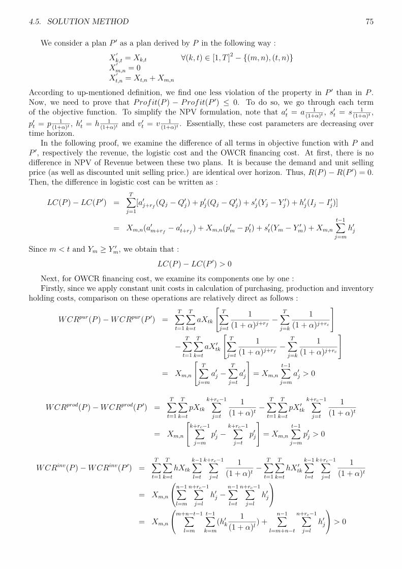
4.5. SOLUTION METHOD 75
We consider a plan P ′ as a plan derived by P in the following way :
X′k,t = Xk,t ∀(k, t) ∈ [1, T ]2 − {(m,n), (t, n)}
X′m,n = 0
X′t,n = Xt,n +Xm,n
According to up-mentioned definition, we find one less violation of the property in P ′ than in P .Now, we need to prove that Profit(P ) − Profit(P ′) ≤ 0. To do so, we go through each termof the objective function. To simplify the NPV formulation, note that a′t = a 1
(1+α)t , s′t = s 1(1+α)t ,
p′t = p 1(1+α)t , h′t = h 1
(1+α)t and v′t = v 1(1+α)t . Essentially, these cost parameters are decreasing over
time horizon.In the following proof, we examine the difference of all terms in objective function with P and
P ′, respectively the revenue, the logistic cost and the OWCR financing cost. At first, there is nodifference in NPV of Revenue between these two plans. It is because the demand and unit sellingprice (as well as discounted unit selling price.) are identical over horizon. Thus, R(P )−R(P ′) = 0.Then, the difference in logistic cost can be written as :
LC(P )− LC(P ′) =T∑j=1
[a′j+rf(Qj −Q′j) + p′j(Qj −Q′j) + s′j(Yj − Y ′j ) + h′j(Ij − I ′j)]
= Xm,n(a′m+rf− a′t+rf
) +Xm,n(p′m − p′t) + s′t(Ym − Y ′m) +Xm,n
t−1∑j=m
h′j
Since m < t and Ym ≥ Y ′m, we obtain that :
LC(P )− LC(P ′) > 0
Next, for OWCR financing cost, we examine its components one by one :Firstly, since we apply constant unit costs in calculation of purchasing, production and inventory
holding costs, comparison on these operations are relatively direct as follows :
WCRpur(P )−WCRpur(P ′) =T∑t=1
T∑k=t
aXtk
T∑j=t
1(1 + α)j+rf
−T∑j=k
1(1 + α)j+rc
−
T∑t=1
T∑k=t
aX ′tk
T∑j=t
1(1 + α)j+rf
−T∑j=k
1(1 + α)j+rc
= Xm,n
T∑j=m
a′j −T∑j=t
a′j
= Xm,n
t−1∑j=m
a′j > 0
WCRprod(P )−WCRprod(P ′) =T∑t=1
T∑k=t
pXtk
k+rc−1∑j=t
1(1 + α)t −
T∑t=1
T∑k=t
pX ′tk
k+rc−1∑j=t
1(1 + α)t
= Xm,n
k+rc−1∑j=m
p′j −k+rc−1∑j=t
p′j
= Xm,n
t−1∑j=m
p′j > 0
WCRinv(P )−WCRinv(P ′) =T∑t=1
T∑k=t
hXtk
k−1∑l=t
k+rc−1∑j=l
1(1 + α)t −
T∑t=1
T∑k=t
hX ′tk
k−1∑l=t
k+rc−1∑j=l
1(1 + α)t
= Xm,n
n−1∑l=m
n+rc−1∑j=l
h′j −n−1∑l=t
n+rc−1∑j=l
h′j
= Xm,n
m+n−t−1∑l=m
t−1∑k=m
(h′k1
(1 + α)l ) +n−1∑
l=m+n−t
n+rc−1∑j=l
h′j
> 0

76 CHAPTER 4. ULS BASED MODEL
Since the cost parameters are all positive, we confirm that the OWCR of these three operationsis greater with P than the OWCR with P ′.
At last, we focus on the difference in OWCR of set-up. The difficulty comes from the fact thatthe shared set-up cost per product (in period m and t) changes with the quantity of Xtk :
WCRset(P )−WCRset(P ′) =T∑t=1
T∑k=t
sYtXtk
Qt + (1− Yt)Xtk
k+rc−1∑j=t
1(1 + α)t
−T∑t=1
T∑k=t
sYtXtk
Qt + (1− Yt)Xtk
k+rc−1∑j=t
1(1 + α)t
=T∑
k=mXm,k
k+rc−1∑j=m
s′jYm
Qm + (1− Ym) +T∑k=t
Xtk
k+rc−1∑j=t
s′jYt
Qt + (1− Yt)
−T∑
k=mX ′m,k
k+rc−1∑j=m
s′jY′m
Q′m + (1− Y ′m) −T∑k=t
X ′tk
k+rc−1∑j=t
s′jY′t
Q′t + (1− Y ′t )
=T∑
k=m
Xm,k
k+rc−1∑j=m
s′jYm
Qm + (1− Ym) −X′m,k
k+rc−1∑j=m
s′jY′m
Q′m + (1− Y ′m)
︸ ︷︷ ︸
Part1
+T∑k=t
Xtk
k+rc−1∑j=t
s′jYt
Qt + (1− Yt)−X ′tk
k+rc−1∑j=t
s′jY′t
Q′t + (1− Y ′t )
︸ ︷︷ ︸
Part2
Next, we evaluate the part 1. Two possible cases are discussed in the following paragraphs :Case 1: Q′
m = 0. In this case,
Part 1 =T∑
k=mXm,k
k+rc−1∑j=m
s′jYm
Qm + (1− Ym) =T∑
k=mXm,k
k+rc−1∑j=m
s′jQm
> 0
Case 2: Q′m > 0. In this case,
Part 1 =T∑
k=m
Xm,k
k+rc−1∑j=m
s′jYm
Qm + (1− Ym) −X′m,k
k+rc−1∑j=m
s′jY′m
Q′m + (1− Y ′m)
=
T∑k=m
Xm,k
k+rc−1∑j=m
s′jQm
−X ′m,kk+rc−1∑j=m
s′jQ′m
= 1
QmQ′m
T∑k=m
k+rc−1∑j=m
s′j(Xm,kQ
′
m −X′
m,kQm
)
= 1QmQ
′m
n+rc−1∑j=m
s′jXm,nQ′
m +T∑
k=m,k 6=n
k+rc−1∑j=m
s′j(X
′
m,kQ′
m −X′
m,kQm
)

4.5. SOLUTION METHOD 77
= 1QmQ
′m
n+rc−1∑j=m
s′jXm,nQ′
m +T∑
k=m,k 6=n
k+rc−1∑j=m
s′j(X
′
m,kQ′
m −X′
m,k(Q′
m +Xm,n))
= 1QmQ
′m
n+rc−1∑j=m
s′jXm,nQ′
m −T∑
k=m,k 6=n
k+rc−1∑j=m
s′jX′m,kXm,n
= Xm,n
QmQ′m
n+rc−1∑j=m
s′jQ′
m −T∑
k=m,k 6=n
k+rc−1∑j=m
s′jX′m,k
= Xm,n
QmQ′m
n+rc−1∑j=m
s′j
t−1∑k=m
X ′m,k −t−1∑k=m
k+rc−1∑j=m
s′jX′m,k
= Xm,n
QmQ′m
t−1∑k=m
Xm,k(n+rc−1∑j=m
s′j −k+rc−1∑j=m
s′j)
= Xm,n
QmQ′m
t−1∑k=m
Xm,k
n+rc−1∑j=k+rc−1
s′j > 0
Thus, the part 1 is always positive in all cases. Then, we go through the part 2:
Part 2 =T∑k=t
Xtk
k+rc−1∑j=t
s′jYt
Qt + (1− Yt)−X ′tk
k+rc−1∑j=t
s′jY′t
Q′t + (1− Y ′t )
=
T∑k=t
Xtk
Qt
k+rc−1∑j=t
s′j −X ′tkQ′t
k+rc−1∑j=t
s′j
= 1
QtQ′t
T∑k=t
XtkQ′t
k+rc−1∑j=t
s′j −X ′tkQt
k+rc−1∑j=t
s′j
= 1
QtQ′t
T∑k=t
Xtk(Qt +Xm,n)k+rc−1∑j=t
s′j −X ′tkQt
k+rc−1∑j=t
s′j
= 1
QtQ′t
T∑k=t
XtkXm,n
k+rc−1∑j=t
s′j −Qt(Xtk −X ′tk)k+rc−1∑j=t
s′j
= 1QtQ
′t
T∑k=t
XtkXm,n
k+rc−1∑j=t
s′j −QtXm,n
n+rc−1∑j=t
s′j
The element which clearly causes a problem in the different cases is Xm,n
Q′t
n+rc−1∑j=t
s′j. Two possibil-ities are to examine:
Case A : Q′t ≥ Qm. We have
Xm,n
Q′t
n+rc−1∑j=n
s′j <Xm,n
Qm
n+rc−1∑j=n
s′j
Then, we attempt to compare this element with the part 1 :

78 CHAPTER 4. ULS BASED MODEL
Case A-1: Q′m = 0. In this case,
Part 1 =T∑
k=m
Xm,k
Qm
k+rc−1∑j=m
s′j
=T∑
k=m,k 6=n
Xm,k
Qm
k+rc−1∑j=m
s′j + Xm,n
Qm
n+rc−1∑j=n
s′j
≥ Xm,n
Qm
n+rc−1∑j=n
s′jq
≥ Xm,n
Qm
n+rc−1∑j=n
s′j
Then, Part 1 + Part 2 ≥ Xm,n
Qm
n+rc−1∑j=n
s′j −Xm,n
Q′t
n+rc−1∑j=n
s′j (4.36)
≥ (Xm,n
Q′t− Xm,n
Q′t)n+rc−1∑j=n
s′j > 0 with Q′
t ≥ Qm
Case A-2: Q′m > 0. In this case,
Part 1 = Xm,n
QmQ′m
t−1∑k=m
Xm,k
n+rc−1∑j=k+rc−1
s′j
= Xm,n
QmQ′m
t−1∑k=m
Xm,k(n+rc−1∑j=m
s′j −k+rc−1∑j=m
s′j)
≥ Xm,n
QmQ′m
t−1∑k=m
Xm,k(n+rc−1∑j=m
s′j −t+rc−1∑j=m
s′j)
≥ Xm,n
Qm
(n+rc−1∑j=m
s′j −t+rc−1∑j=m
s′j)
≥ Xm,n
Q′t(n+rc−1∑j=m
s′j −t+rc−1∑j=m
s′j)
= Xm,n
Q′t
n+rc−1∑j=t+rc−1
s′j (4.37)
Moreover, we have :
1QtQ
′t
T∑k=t
XtkXm,n
k+rc−1∑j=t
s′j ≥
Xm,n
QtQ′t
T∑k=t
Xtk
k+rc−1∑j=t
s′j ≥
Xm,n
QtQ′t
T∑k=t
Xtk
t+rc−1∑j=t
s′j ≥
Xm,n
QtQ′t
t+rc−1∑j=t
s′j
T∑k=t
Xtk ≥
Xm,n
Q′t
t+rc−1∑j=t
s′j (4.38)
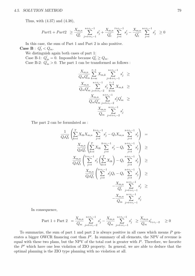
4.5. SOLUTION METHOD 79
Thus, with (4.37) and (4.38),
Part1 + Part2 ≥ Xm,n
Q′t
n+rc−1∑j=t+rc−1
s′j + Xm,n
Q′t
t+rc−1∑j=t
s′j −Xm,n
Q′t
n+rc−1∑j=t
s′j ≥ 0
In this case, the sum of Part 1 and Part 2 is also positive.Case B : Q′
t < Qm.We distinguish again both cases of part 1:Case B-1: Q′
m = 0. Impossible because Q′t ≥ Qm.
Case B-2: Q′m > 0. The part 1 can be transformed as follows :
Xm,n
QmQ′m
t−1∑k=m
Xm,k
n+rc−1∑j=k+rc−1
s′j ≥
Xm,n
QmQ′m
n+rc−1∑j=t+rc−2
s′j
t−1∑k=m
Xm,k ≥
Xm,n
QmQ′m
n+rc−1∑j=t+rc−2
s′jQ′
m ≥
Xm,n
Qm
n+rc−1∑j=t+rc−2
s′j
The part 2 can be formulated as :
1QtQ
′t
T∑k=t
XtkXm,n
k+rc−1∑j=t
s′j −QtXm,n
n+rc−1∑j=t
s′j
=
Xm,n
QtQ′t
T∑k=t
Xtk
k+rc−1∑j=t
s′j −Qt
n+rc−1∑j=t
s′j
≥
Xm,n
QtQ′t
t+rc−1∑j=t
s′j
(T∑k=t
Xtk
)−Qt
n+rc−1∑j=t
s′j
≥
Xm,n
QtQ′t
t+rc−1∑j=t
s′jQt −Qt
n+rc−1∑j=t
s′j
≥
−Xm,n
Q′t
n+rc−1∑j=t+rc−1
s′j ≥
−Xm,n
Qm
n+rc−1∑j=t+rc−1
s′j
In consequence,
Part 1 + Part 2 = Xm,n
Qm
n+rc−1∑j=t+rc−2
s′j −Xm,n
Qm
n+rc−1∑j=t+rc−1
s′j ≥Xm,n
Qm
s′t+rc−2 ≥ 0
To summarize, the sum of part 1 and part 2 is always positive in all cases which means P gen-erates a bigger OWCR financing cost than P ′. In summary of all elements, the NPV of revenue isequal with these two plans, but the NPV of the total cost is greater with P . Therefore, we favoritethe P ′ which have one less violation of ZIO property. In general, we are able to deduce that theoptimal planning is the ZIO type planning with no violation at all.
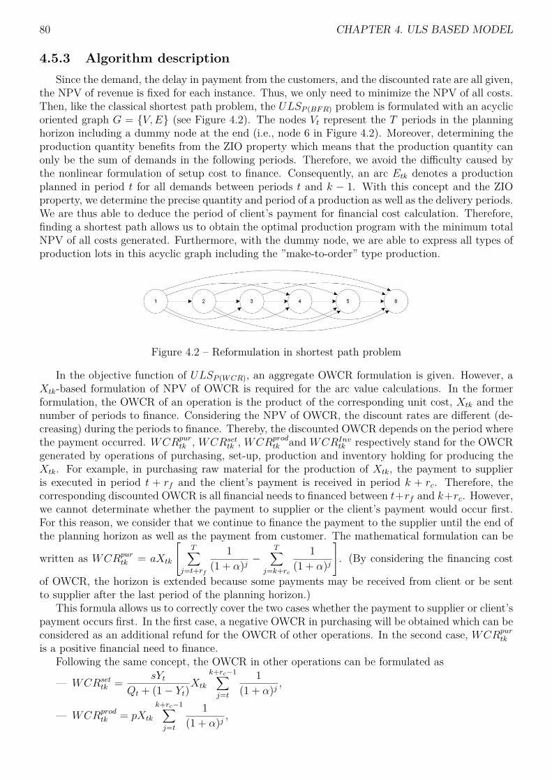
80 CHAPTER 4. ULS BASED MODEL
4.5.3 Algorithm descriptionSince the demand, the delay in payment from the customers, and the discounted rate are all given,
the NPV of revenue is fixed for each instance. Thus, we only need to minimize the NPV of all costs.Then, like the classical shortest path problem, the ULSP (BFR) problem is formulated with an acyclicoriented graph G = {V,E} (see Figure 4.2). The nodes Vt represent the T periods in the planninghorizon including a dummy node at the end (i.e., node 6 in Figure 4.2). Moreover, determining theproduction quantity benefits from the ZIO property which means that the production quantity canonly be the sum of demands in the following periods. Therefore, we avoid the difficulty caused bythe nonlinear formulation of setup cost to finance. Consequently, an arc Etk denotes a productionplanned in period t for all demands between periods t and k − 1. With this concept and the ZIOproperty, we determine the precise quantity and period of a production as well as the delivery periods.We are thus able to deduce the period of client’s payment for financial cost calculation. Therefore,finding a shortest path allows us to obtain the optimal production program with the minimum totalNPV of all costs generated. Furthermore, with the dummy node, we are able to express all types ofproduction lots in this acyclic graph including the ”make-to-order” type production.
Figure 4.2 – Reformulation in shortest path problem
In the objective function of ULSP (WCR), an aggregate OWCR formulation is given. However, aXtk-based formulation of NPV of OWCR is required for the arc value calculations. In the formerformulation, the OWCR of an operation is the product of the corresponding unit cost, Xtk and thenumber of periods to finance. Considering the NPV of OWCR, the discount rates are different (de-creasing) during the periods to finance. Thereby, the discounted OWCR depends on the period wherethe payment occurred. WCRpur
tk , WCRsettk , WCRprod
tk and WCRInvtk respectively stand for the OWCR
generated by operations of purchasing, set-up, production and inventory holding for producing theXtk. For example, in purchasing raw material for the production of Xtk, the payment to supplieris executed in period t + rf and the client’s payment is received in period k + rc. Therefore, thecorresponding discounted OWCR is all financial needs to financed between t+rf and k+rc. However,we cannot determinate whether the payment to supplier or the client’s payment would occur first.For this reason, we consider that we continue to finance the payment to the supplier until the end ofthe planning horizon as well as the payment from customer. The mathematical formulation can be
written as WCRpurtk = aXtk
T∑j=t+rf
1(1 + α)j −
T∑j=k+rc
1(1 + α)j
. (By considering the financing cost
of OWCR, the horizon is extended because some payments may be received from client or be sentto supplier after the last period of the planning horizon.)
This formula allows us to correctly cover the two cases whether the payment to supplier or client’spayment occurs first. In the first case, a negative OWCR in purchasing will be obtained which can beconsidered as an additional refund for the OWCR of other operations. In the second case, WCRpur
tk
is a positive financial need to finance.Following the same concept, the OWCR in other operations can be formulated as
— WCRsettk = sYt
Qt + (1− Yt)Xtk
k+rc−1∑j=t
1(1 + α)j ,
— WCRprodtk = pXtk
k+rc−1∑j=t
1(1 + α)j ,

4.6. NUMERICAL ANALYSIS 81
— and WCRInvtk = hXtk
k−1∑l=t
k+rc−1∑j=l
1(1 + α)j .
For WCR of inventory holding, if k = t (i.e., Xtk is produced for demand in the same period),then there is no inventory holding cost. Combining all these components, the total OWCR for allXtk, denoted as WCRtotal, can be written as follows :
WCRtotal =T∑t=1
T∑k=1
(WCRpurtk +WCRset
tk +WCRprodtk +WCRInv
tk )
To simplify the NPV formulation, note that a′t = a 1(1+α)t , s′t = s 1
(1+α)t , p′t = p 1(1+α)t and h′t =
h 1(1+α)t . With the ZIO property, the arc values are presented as follows (with LCtk representing all
the production-related costs):
Etk = LCtk + βk−1∑l=t
(WCRpur
tk +WCRsettk +WCRprod
tk +WCRInvtk
)
= (a′t+rf+ p′t)
k−1∑l=t
dl + s′t +k−1∑l=t
dll−1∑i=t
h′i
+βk−1∑l=t
dl
T∑j=t
a′j+rf−
T∑j=l
a′j+rc
+l+rc−1∑j=t
p′j +l+rc−1∑j=t
s′jk−1∑i=t
di
+l−1∑i=t
l+rc−1∑j=i
h′j
(4.39)
The computation of Etk is done in O(T 2). The objective of this algorithm is to find the shortestpath to the last node. To do so, we need to progressively locate the shortest path to other nodes.Thereby, we examine all possible paths to each node from all its predecessors through the arc inbetween. This can be realized by the recursive function presented as follows :
Cost[t] = minj∈[1,t−1]
{Cost[j] + Ejt}
with Cost[t] the minimal total cost to finance to satisfy all demands until period t. Therefore, adynamic programming algorithm is established as presented in Algorithm 1. The complexity of thealgorithm is O(T 4), thus the ULSP (WCR) problem can be solved in polynomial time.
Algorithm 1 Solving ULSP (WCR)
Require: All parameter valuesfor i = 1 to T dofor j = 1 to i− 1 doif Cost[i] > Cost[j] + Eji thenCost[i] = Cost[j] + Eji
end ifend for
end for
4.6 Numerical analysisThrough the following numerical tests, we reveal differences between optimal production plans
for profit maximization or costs minimization objectives. These tests illustrate the influence ofconsidering the financing cost of OWCR on an optimal production program. With the proven ZIO

82 CHAPTER 4. ULS BASED MODEL
property, the optimal program of profit maximization problem is calculated and denoted as P optwcr.
Moreover, the optimal program of the traditional ULS model is denoted as P optuls . The tests are
organized as follows:— Firstly, a comparison between P opt
wcr and Poptuls with a same set of parameter values is provided
to show the differences in the production programs;— Secondly, the evolution of a production program following the variation of discount and interest
rates is presented as well as the change of average inventory level;— Thirdly, we compare the objective value of ULS and ULSP (WCR) models by applying respec-
tively P optuls and P opt
wcr in both models.For the following tests, we adopt the demand of the instance of Trigeiro et al. (1989) (G-72,
demand 7). Values of other parameters are set to adapt the ULS concept which considers only setupand inventory holding costs (see Table 4.8):
— Since the purchasing and production cost are not considered in traditional ULS model, theseunit costs are given as zero in order to compare the optimal programs in the same conditions.Accordingly, the delay in payment to the supplier involved only in purchasing is irrelevant indetermining the production planning. Thus, a = p = rf = 0;
— The setup cost, s, is given as 600 and the unit cost of inventory holding per period, h, is fixedto 1;
— The delay in payments from customer, rc is set to 5 periods;— The unit selling price will not be considered as it is a constant parameter and will not impact
the production program. However, it should be taken into account for the periodic OWCRmaximization objective.
Table 4.8 – Numerical example parameter valuesParameter ValuePurchasing unit cost, a 0Setup cost, s 600Production unit cost, p 0Inventory holding unit cost per period, h 1Delay in payment from customer, rc 5Delay in payment to supplier, rf 0Unit sales price not considered
4.6.1 Production program comparisonsWe compare optimal programs separately calculated by these two models with α = 0.08 and
β = 0.1. P optwcr and P
optuls are illustrated in figure 4.3. We observe that
— The production programs are different. The ULS model can not always provide the optimalsolution for maximizing the profit;
— The production lots of P optwcr are smaller with a profit maximization objective compared to the
ones in P optuls . More setups are planned in P opt
wcr that results in a lower average inventory levels;This difference in production plans is mainly caused by the cumulative effect of financing the
inventory holding costs. In ULSP (WCR) model, all purchasing, setup, production and inventoryholding costs have a financial consequence by considering the financial cost to cover them beforereceiving customer’s payment. As shown in Table 4.7, the duration to be financed is much moregreater for inventory holding cost compared to the one for setup cost. It means that the financialcost of inventory holding cost varies more rapidly than the one of setup cost. Therefore, when weare looking for a trade-off between the setup related and inventory holding related costs, we would
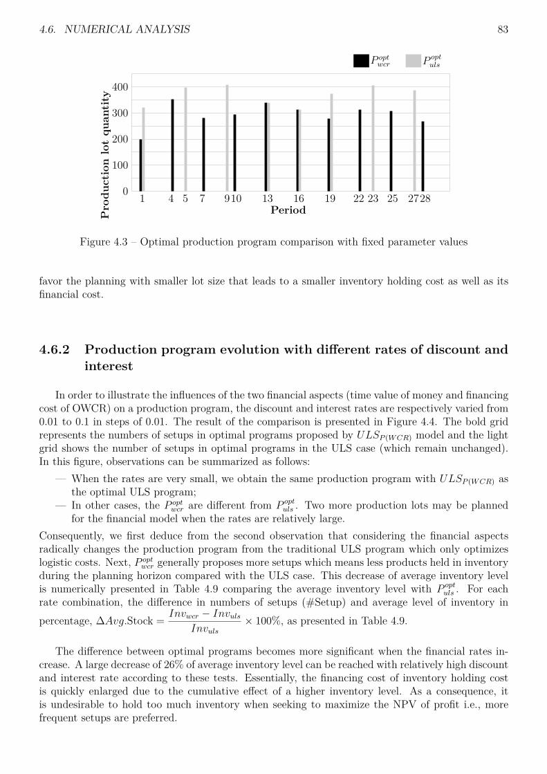
4.6. NUMERICAL ANALYSIS 83
1 4 7 10 13 16 19 22 25 285 9 23 27
400
300
200
100
0PeriodP
rodu
ctionlotqu
antity
P optulsP opt
wcr
Figure 4.3 – Optimal production program comparison with fixed parameter values
favor the planning with smaller lot size that leads to a smaller inventory holding cost as well as itsfinancial cost.
4.6.2 Production program evolution with different rates of discount andinterest
In order to illustrate the influences of the two financial aspects (time value of money and financingcost of OWCR) on a production program, the discount and interest rates are respectively varied from0.01 to 0.1 in steps of 0.01. The result of the comparison is presented in Figure 4.4. The bold gridrepresents the numbers of setups in optimal programs proposed by ULSP (WCR) model and the lightgrid shows the number of setups in optimal programs in the ULS case (which remain unchanged).In this figure, observations can be summarized as follows:
— When the rates are very small, we obtain the same production program with ULSP (WCR) asthe optimal ULS program;
— In other cases, the P optwcr are different from P opt
uls . Two more production lots may be plannedfor the financial model when the rates are relatively large.
Consequently, we first deduce from the second observation that considering the financial aspectsradically changes the production program from the traditional ULS program which only optimizeslogistic costs. Next, P opt
wcr generally proposes more setups which means less products held in inventoryduring the planning horizon compared with the ULS case. This decrease of average inventory levelis numerically presented in Table 4.9 comparing the average inventory level with P opt
uls . For eachrate combination, the difference in numbers of setups (#Setup) and average level of inventory inpercentage, ∆Avg.Stock = Invwcr − Invuls
Invuls× 100%, as presented in Table 4.9.
The difference between optimal programs becomes more significant when the financial rates in-crease. A large decrease of 26% of average inventory level can be reached with relatively high discountand interest rate according to these tests. Essentially, the financing cost of inventory holding costis quickly enlarged due to the cumulative effect of a higher inventory level. As a consequence, itis undesirable to hold too much inventory when seeking to maximize the NPV of profit i.e., morefrequent setups are preferred.

84 CHAPTER 4. ULS BASED MODEL
Figure 4.4 – Comparison of number of setups between optimal plans with different interest rates
Table 4.9 – Differences in number of setups and average inventory level between optimal programsof ULSP (WCR) and ULS
Parameter β = 0.01 β = 0.02 β = 0.08 β = 0.1
α = 0.01#Setup = = +1 +1
∆Avg.Stock 0 0 -14.2% -14.2%
α = 0.02#Setup = +1 +1 +1
∆Avg.Stock 0 -14.2% -14.2% -14.2%
α = 0.08#Setup +1 +1 +1 +2
∆Avg.Stock -14.08% -14.08% -14.08% -26.7%
α = 0.1#Setup +1 +1 +2 +2
∆Avg.Stock -14.08% -14.08% -26.32% -26.32%
4.6.3 Production and financial cost comparisonsWithin these tests, we find 3 cases where P opt
uls and P optwcr are identical when the rates are small.
For other cases, we compare the NPV of total costs including the financing cost of OWCR gen-erated by P opt
uls and P optwcr, denoted respectively as NPVuls and NPVwcr. Since P opt
wcr generates aminimum NPV of total cost, the increase of NPV in applying the P opt
uls is computed as ∆NPVULS =NPVuls −NPVwcr
NPVwcr× 100%. The result is presented in Figure 4.5 (∆NPVULSP (WCR) represents the
minimum NPV of total cost with P optwcr). P
optuls generates a lower NPV of total cost by at most 3%
compared to the NPV obtained by P optuls .
On the other hand, because the production cost generated by ULS model, denoted as Logulsis already optimal, the production cost generated by applying P opt
wcr (denoted as Logwcr) is logicallyhigher. The increase is calculated as ∆LOGULSP (WCR) = Logwcr − Loguls
Loguls× 100% and presented
in Figure 4.6.
4.6.4 Program evaluation with different purchasing costs and delays inpayment to supplier
Considering the delay in payment to supplier only affects the purchasing cost, we thus combinethe tests of these two parameters, see Figure 4.7. In these tests, we set the purchasing unit costvarying between 0 to 90 in step of 10. Moreover, the delay in payment to supplier varies from 0 to20 in step of 2. Moreover, the rates are fixed at 3%. First, we observe that following the increase

4.6. NUMERICAL ANALYSIS 85
Figure 4.5 – Difference in NPV of total costincluding the financing cost
Figure 4.6 – Difference in logistic cost
of purchasing unit cost and with a fixed delay, more production lots are launched which signifiesless products held in inventory. The reason is when the purchasing cost is more expensive, we areinterested to launch the production later considering the discount effect which makes early activitiesmore costly in term of NPV. Second, with a fixed purchasing unit cost and an increasing delay tosupplier, the production size will generally increase for keeping more NPV of inventory value in thesystem and cash back to the supplier as last as possible.
Figure 4.7 – Production plan compari-son with varying purchasing unit cost anddownstream delay Figure 4.8 – Variation of number of setups
with varying production unit cost
4.6.5 Program evaluation with different production unit costs
Based on the parameter value given in Table 4.8, we set the production unit cost at 5 and therates at 3%. The result is presented in Figure 4.8. The production lot size will decrease withan increasing production unit cost. It is because when the production cost increase, we have lessinterest to significantly advance the production in an early period considering the discount effort andincreased number of periods to finance.
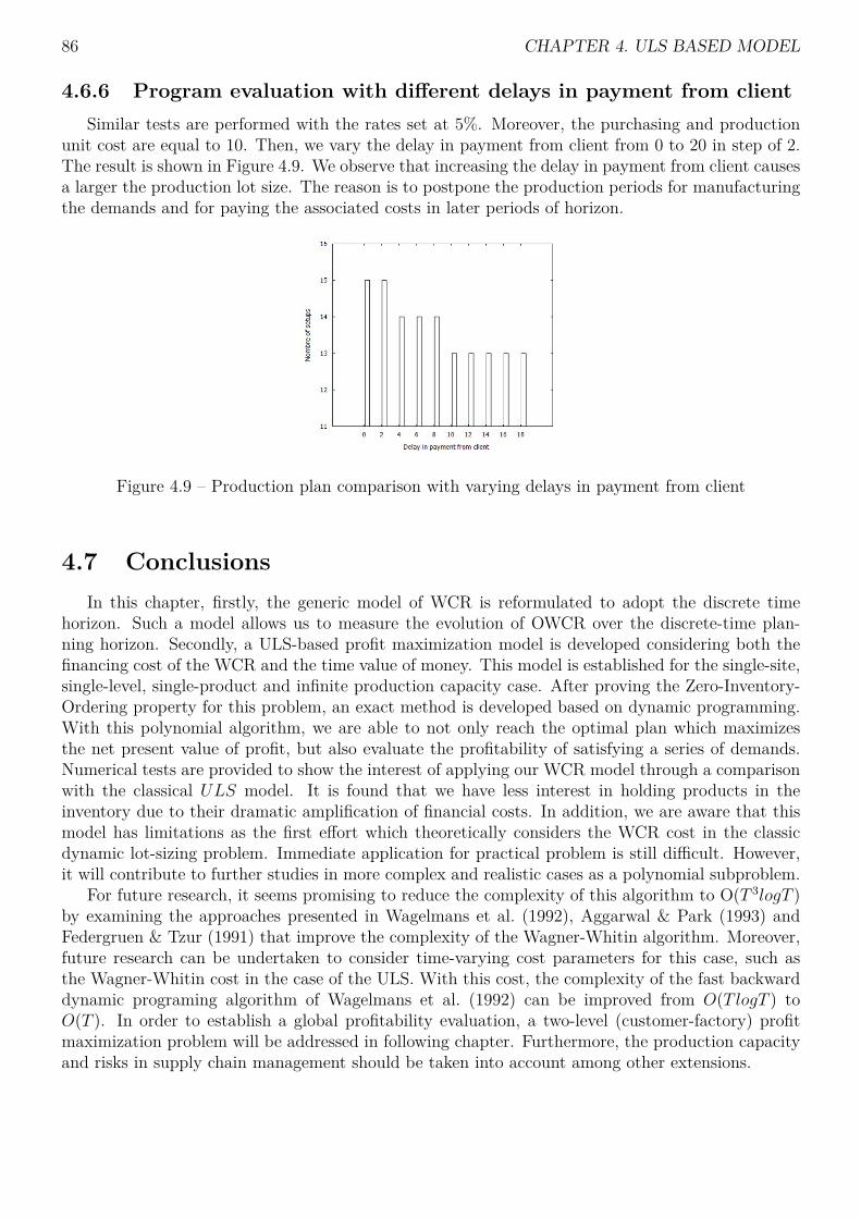
86 CHAPTER 4. ULS BASED MODEL
4.6.6 Program evaluation with different delays in payment from clientSimilar tests are performed with the rates set at 5%. Moreover, the purchasing and production
unit cost are equal to 10. Then, we vary the delay in payment from client from 0 to 20 in step of 2.The result is shown in Figure 4.9. We observe that increasing the delay in payment from client causesa larger the production lot size. The reason is to postpone the production periods for manufacturingthe demands and for paying the associated costs in later periods of horizon.
Figure 4.9 – Production plan comparison with varying delays in payment from client
4.7 ConclusionsIn this chapter, firstly, the generic model of WCR is reformulated to adopt the discrete time
horizon. Such a model allows us to measure the evolution of OWCR over the discrete-time plan-ning horizon. Secondly, a ULS-based profit maximization model is developed considering both thefinancing cost of the WCR and the time value of money. This model is established for the single-site,single-level, single-product and infinite production capacity case. After proving the Zero-Inventory-Ordering property for this problem, an exact method is developed based on dynamic programming.With this polynomial algorithm, we are able to not only reach the optimal plan which maximizesthe net present value of profit, but also evaluate the profitability of satisfying a series of demands.Numerical tests are provided to show the interest of applying our WCR model through a comparisonwith the classical ULS model. It is found that we have less interest in holding products in theinventory due to their dramatic amplification of financial costs. In addition, we are aware that thismodel has limitations as the first effort which theoretically considers the WCR cost in the classicdynamic lot-sizing problem. Immediate application for practical problem is still difficult. However,it will contribute to further studies in more complex and realistic cases as a polynomial subproblem.
For future research, it seems promising to reduce the complexity of this algorithm to O(T 3logT )by examining the approaches presented in Wagelmans et al. (1992), Aggarwal & Park (1993) andFedergruen & Tzur (1991) that improve the complexity of the Wagner-Whitin algorithm. Moreover,future research can be undertaken to consider time-varying cost parameters for this case, such asthe Wagner-Whitin cost in the case of the ULS. With this cost, the complexity of the fast backwarddynamic programing algorithm of Wagelmans et al. (1992) can be improved from O(T logT ) toO(T ). In order to establish a global profitability evaluation, a two-level (customer-factory) profitmaximization problem will be addressed in following chapter. Furthermore, the production capacityand risks in supply chain management should be taken into account among other extensions.
5Multi-level uncapacitated lot sizing baseddiscounted model considering thefinancing cost of working capitalrequirement
5.1 IntroductionIn this chapter, firstly, we extend the aforementioned single-level model to a two-level (supplier-
customer) model and further generalize it to a multi-level case based on the Multi-level Lot-sizing(MLLP) model. The OWCR model is then modified for adapting to this multi-level scenario. Con-sidering the OWCR cost in multi-level case, we propose sequential and centralized approaches tosolve both the two-level and the multi-level problem with a serial chain structure. The ZIO propertystill unaffectedly stands in the sequential approach and is further proven valid in the centralizedapproach. The property allows us to establish a dynamic programming algorithm which solves theproblem in O(NT 6) (where, L represents the number of level in the considered supply chain). Fi-nally, we analyze the disparities in the optimal solutions obtained by both the sequential and thecentralized approaches.
5.2 The multi-level uncapacitated lot sizing-based models
5.2.1 MRP and the multi-level lot-sizing problemSince the introduction of materials requirement planning (MRP) in the late 1960’s, companies
have rapidly implemented it when facing increasing customer needs (Davis (1975)). This situationrequires manufacturing production systems to deal with larger and more complex product structures.This evolution has magnificently revealed the significance of the MLLP problem in the MRP process.The principal concept is to translate the production program of a finished item into the programs ofits components. Those programs are calculated on the basis of the bill-of-material (BOM) and lead-time information. Nevertheless, several difficulties and limits of the MRP are revealed in practicethat restricts the use of MRP setting:
— No capacity constraints considered is MRP planning.
87
88 CHAPTER 5. MLLP BASED MODEL
— Unpredictable demands of finished items and production lead times deeply affect the accuracyof the planning with MRP.
— Integrity of the data considerably impacts the accuracy of the result.First, in the fundamental concept of the MRP system, capacity constraints are not considered.
No limit of production quantity restraints the planning at all levels. Consequantly, the feasibilityof the result obtained by the MRP system can thus not be guaranteed. Moreover, the leeway ofoperation capacity can also be used for reallocation at the practical level via the shop floor based oninitial plan obtained by MRP.
Second, demand uncertainty causes the difficulty of accurately estimating customer demands inthe years to come. This problem leads to a significant challenge of inventory control and management.Indeed, uncertain demands may result from a variety of reasons. For instance, demands of seasonalmerchandises may significantly fluctuate over time and sometimes strongly correlate with a particularevent. Moreover, changes in trade credit terms and customer’s needs, and alteration in technologydevelopment and situation of competitors can influence the demands as well. The bull-whip effect isa common result of the demand fluctuation resulting in an important adjustment especially requiredin the upstream of the supply chain.
Furthermore, in a tactical production planning context, the longer the lead time, the higher thelevel of total inventory. The lead time, computed in days, is typically the sum of the supply delay,that is to say, the time delay between placing order and demand delivery incorporating the transittime, and the reordering delay, which is the time until an ordering opportunity arises again.
Third, if there exists any errors in the inventory data, the bill of materials (commonly referredto as ’BOM’) data, or the master production schedule, the output data will then be incorrect.
Despite all this restrictions, the MRP yet have been largely implemented for the productionplanning. However, for a direct application of the MRP planning, all calculations should be repeatedfor each adjustment in accordance with demand or lead time changes. To meet the requirement,simple "heuristic" solutions have been developed. In this chapter, we address the multi-site lot sizingproblem with a serial supply chain structure while taking into account the financing cost of theOWCR. In this problem, we exclusively consider the transport delay, without the consideration ofthe transport cost. According to the comparison provided in Lemoine (2008), the multi-level modelscan be applied in our case where the transport aspect is overlooked. In the following paragraph, theproblem description, mathematical model and solution procedure are put forward.
5.2.2 The description of the MLLP problem and associated mathemat-ical formulation
The problem of the multi-level production planning considers products made from several othercomponents. Specifically, finished products require components for which it is also necessary todetermine the corresponding production plans. These components may also have subcomponents,etc. Meaning that different levels of BOM are taken into account, hence the term "multi-level". Inthese models, we thus find the two types of demand (external and internal) and the internal demandis deduced from the external demand according to the BOM structure.
Generally speaking, the BOM is represented by an acyclic graph (as in Bookbinder & Koch(1990)) where the nodes represent the products (or its components) and the arcs stand for the linksbetween the different nodes. For each finished product i, one can list all the products j directlyinvolved in its manufacture and the technical coefficient rij is defined as the quantity of product idirectly used to manufacture a unit of product j. The valued graph is named "graph gozinto". Theacyclic character of the graph allows it to be split into several levels. By convention and based onthe definition of the product BOM, the products of level 0 are the finished products. However, theymerely represent the external demand. If a product i is at level n, all products directly involvedin its manufacture will be at level n + 1. This graph can also be formulated using a square matrix

5.2. THE MULTI-LEVEL UNCAPACITATED LOT SIZING-BASED MODELS 89
Figure 5.1 – Four product BOM structures
called the "gozinto matrix". Its dimensions are equal to the number of products to be planned forproduction, and where each element rij represents the number of products i directly involved in themanufacture of the product j. Since the graph is acyclic, the matrix can be represented in a lowertriangular form with a diagonal of zero.
In the literature, there are four types of structure (gozinto graphs) illustrated in Figure 5.1:— the structure in series: each product has at most a predecessor and at most one successor,— the assembly structure: each product has at most one successor,— the arborescent/tree structure: each product has at most a predecessor,— the general structure where there is no limitation on the number of all predecessors and
successors.In the literature, the MLLP model is built for the multi-level, big bucket and infinite capacity
case to satisfy time-varying demand. The mathematical formulation can be found in Steinberg &Napier (1980) and Clark & Armentano (1995) and the latter is presented below. The parametersand decision variables are given in Table 5.1 and 5.2.
Parameter DefinitionN number of levels,T number of periods,S(i) the set of all immediate successor components to component i,P (i) the set of immediate predecessors of component i; if P(i)= ∅, then i
is called end item,rij the number of units of i required for production of one unit of component
j ∈ S(i).dit, the independent demand for component i in period t,pit the unit production cost of component i in period t,sit the fixed setup cost occurred if component i is produced in period t,hit the unit holding cost of component i at the end of period t,M upper bound of possible production lot-size,L(i) the production lead time of component i, in unit of periods, to ensure the
lot Qit is available for consumption only at the beginning of period t+ L(i),T (i) + 1 the period in which, on a rolling horizon basis, the planning of component i
starts over the T periods from T (i) + 1 to T (i) + T in order to synchronize itsproduction with that of the other components, in particular with that ofthe finished item.
Table 5.1 – Parameters
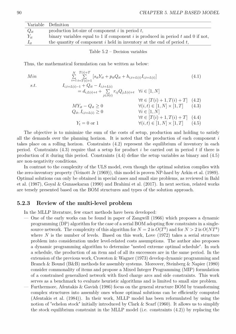
90 CHAPTER 5. MLLP BASED MODEL
Variable DefinitionQit production lot-size of component i in period t,Yit binary variables equal to 1 if component i is produced in period t and 0 if not,Iit the quantity of component i held in inventory at the end of period t,
Table 5.2 – Decision variables
Thus, the mathematical formulation can be written as below:
MinN∑i=1
T (i)+T∑t=T (i)+1
[sitYit + pitQit + hi,t+L(i)Ii,t+L(i)] (4.1)
s.t. Ii,t+L(i)−1 +Qit − Ii,t+L(i)= di,L(i)+t + ∑
j∈S(i)rijQj,L(i)+t ∀i ∈ [1, N ]
∀t ∈ [T (i) + 1, T (i) + T ] (4.2)MYit −Qit ≥ 0 ∀(i, t) ∈ [1, N ]× [1, T ] (4.3)Qit, Ii,t+L(i) ≥ 0 ∀i ∈ [1, N ]
∀t ∈ [T (i) + 1, T (i) + T ] (4.4)Yt = 0 or 1 ∀(i, t) ∈ [1, N ]× [1, T ] (4.5)
The objective is to minimize the sum of the costs of setup, production and holding to satisfyall the demands over the planning horizon. It is noted that the production of each component itakes place on a rolling horizon. Constraints (4.2) represent the equilibrium of inventory in eachperiod. Constraints (4.3) require that a setup for product i be carried out in period t if there isproduction of it during this period. Constraints (4.4) define the setup variables as binary and (4.5)are non-negativity conditions.
In contrast to the complexity of the ULS model, even though the optimal solution complies withthe zero-inventory property (Veinott Jr (1969)), this model is proven NP-hard by Arkin et al. (1989).Optimal solutions can only be obtained in special cases and small size problems, as reviewed in Bahlet al. (1987), Goyal & Gunasekaran (1990) and Brahimi et al. (2017). In next section, related worksare tersely presented based on the BOM structures and types of the solution approach.
5.2.3 Review of the multi-level problemIn the MLLP literature, few exact methods have been developed:— One of the early works can be found in paper of Zangwill (1966) which proposes a dynamic
programming (DP) algorithm for the case of a serial BOM adopting flow constraints in a single-source network. The complexity of this algorithm for N = 2 is O(T 3) and for N > 2 is O(NT 4)where N is the number of levels. Based on this work, Love (1972) takes a serial structureproblem into consideration under level-related costs assumptions. The author also proposesa dynamic programming algorithm to determine "nested extreme optimal schedule". In sucha schedule, the production of an item and of all its successors are in the same period. In theextension of the previous work, Crowston &Wagner (1973) develop dynamic programming andBranch & Bound (B&B) methods for assembly systems. Moreover, Steinberg & Napier (1980)consider commonality of items and propose a Mixed Integer Programming (MIP) formulationof a constrained generalized network with fixed charge arcs and side constraints. This workserves as a benchmark to evaluate heuristic algorithms and is limited to small size problem.
— Furthermore, Afentakis & Gavish (1986) focus on the general structure BOM by transformingcomplex structures into assembly ones whose optimal solutions can be efficiently computed(Afentakis et al. (1984)). In their work, MLLP model has been reformulated by using thenotion of "echelon stock" initially introduced by Clark & Scarf (1960). It allows us to simplifythe stock equilibrium constraint in the MLLP model (i.e. constraints (4.2)) by replacing the
5.2. THE MULTI-LEVEL UNCAPACITATED LOT SIZING-BASED MODELS 91
terms of internal demand. This reformulation makes the constraint in a similar form to theones of the single-level models and allows us to build a strong single-item relaxation whichleads the authors to an efficient B&B algorithm using Lagrangian relaxation. More relevantearly works are summarized in Dellaert & Jeunet (2003) and Pochet & Wolsey (2006).
— Recently, Van Hoesel et al. (2005) give a DP algorithm for two-level and multi-level problemsin which constant capacity constraint merely exists in the initial production level. Melo &Wolsey (2010) consider the uncapacitated two-level problem with serial structure and developa DP algorithm that runs in O(T 2logT ) using the approach of Eppen & Martin (1987).For the same model but with intermediate independent demand, Zhang et al. (2012) give apartial description of the convex hull of solutions in the original variable space. Besides, theauthors develop a polynomial-time dynamic programming algorithm, which leads to a tightand compact extended formulation.
In addition to those exact methods, considerable efforts have been continuously invested fordeveloping heuristic and meta-heuristic methods over decades in order to tackle the computationaldifficulty. In the literature, these methods can be classified into three main types:
— Sequential approach, which determines the production program level by level following theMRP logic.
— Simultaneous (centralized) approach, with a global optimization objective including simulta-neously all levels.
— Decentralized or distributed approach, which considers an interaction between the actors ofthe supply chain.
The sequential approach is the one of the first methods developed for the multi-level problem in theMRP framework which decomposed the multi-level problem into polynomial single-level problems,for instance, with the Wagner-Whitin algorithm (Veral & LaForge (1985)). States of the art onvarious related methods are provided in Bahl et al. (1987) and Gupta & Keung (1990). The basicidea of this approach is to consider the optimal production program calculated for the upper level asthe demand to satisfy for the adjacent lower level. The direct application of the single-level methodafter the decomposition in case of complex product structure may induce unnecessary high setupand holding costs because the interdependence between levels has been ignored. In the literature,cost modification (revision) is proposed for taking into account some degree of interdependenceof demands between levels. This demand interdependence stems from the fact that planning aproduction of item i would possibly trigger the production of its components that may cause anadditional setup cost. In some work, the cost modification also contains the holding cost. In theserevisited costs, the single-level method is used to each item in the product structure. Blackburn& Millen (1982) compare five types of modifications for setup and inventory holding costs in caseof the single end-item assembly system. Bookbinder & Koch (1990) later extend this cost revisiontype method for more general product structure cases. Recent work of Dellaert & Jeunet (2003)pursue ideas of early cost modification methods and give a randomized MLLP heuristic for generalproduct structure. Two main contributions of this work are considering time-varying setup cost andrandomizing their algorithm multiplying the modification term with Monte Carlo simulation. Morerelated methods are also reviewed in this paper.
The simultaneous (centralized) approach, often based on metaheuristic algorithms, has emergedmuch more recently. Its performance are reported for providing highly cost-efficient solutions witha reasonable computation effort. Kuik & Salomon (1990) implement simulated annealing for sixneighborhood systems and compare their effectiveness. Dellaert & Jeunet (2000) and Dellaert et al.(2000) propose a hybrid genetic algorithm (HGA) for this problem with a general product struc-ture. In those works, a competitive strategy is introduced to mix five operators in the chromosomeevolutions between consecutive generations. Tang (2004) raises a novel neighborhood system basedon a property called "Inner corner" and develop a simulated annealing algorithm to handle serialstructure problems. Jeunet & Jonard (2005) also propose a simulated annealing based on solution

92 CHAPTER 5. MLLP BASED MODEL
coding, the two best performing neighborhood systems given by Kuik & Salomon (1990) and threenew neighborhood systems. Homberger (2008) present a parallel genetic algorithm (PGA) with anempirical policy for subpopulations migrations. This method benefits from sharing calculation loadover multiple processors. Other metaheuristics algorithms, such as the particle swarm optimization(PSO) algorithm by Han et al. (2009) and Deroussi & Lemoine (2009), the ant colony optimization(ACO) system by Pitakaso et al. (2007) and Homberger & Gehring (2009), the segmentation-basedsoft optimization approach (SOA) by Kaku et al. (2010) and variable neighborhood search (VNS)by Xiao et al. (2014), have been proposed for solving the MLLP problems.
Third, in the MLLP model, we implicitly assume that only one decision maker who decides theproduction planning for all items with all necessary information on cost parameters exists. Thisassumption is normally fulfilled within a single company. Nevertheless, in practice and in a globalsupply chain, the components are often supplied by different independent companies (Christopher(1999)). Hence, this assumption is not practicable in some cases (Dudek & Stadtler (2005), Straube& Beyer (2006)), i.e. no decision maker is authorized to make production decisions for the entiresupply chain. Distributed (Decentralized) approaches are developed to fill this gap in MLLP context,for instance, in the recent work of Homberger (2010), Buer et al. (2013) and Homberger et al. (2015)with different negotiation mechanisms.
In addition, the NPV principle has been identified as a natural approach to reveal the economicconsequences in MRP theory in the early work of Grubbström (1967). The author shows that cashflows can be immediately transformed by exchanging the Laplace frequency for the continuous interestrate. The author and his colleagues have made an significant contribution to the MRP theory in viewof economic aspect while using NPV approach, input-output analysis and Laplace transform witha continuous-time model. Related works are referred to Grubbström (1998), Grubbström (1999),Bogataj & Grubbström (2012) and other works in its references. Furthermore, discrete-time modelswith consideration of the NPV have also been developed in the literature. Helber (1998) treats themulti-level problem in the framework of Manufacturing Resource Planning (MRP II) with multiplecapacity constraints and setup times in a discrete-time horizon. Grubbström & Wang (2003) presenta model of multi-level capacity-constrained system with a stochastic external demand and a constantlead time for maximizing expected NPV of profit. A dynamic programming procedure is applied tosolve the problem. Based on the previous work, Grubbström & Huynh (2006) establish a similarmodel with deterministic demand and extend the model for any non-zero lead time. Other modelconsidering the NPV approach also exists in multi-site models which are reviewed in Martínez-Costaet al. (2014).
In this chapter, we extend our single-level model to two-level, and then to multi-level with aserial chain structure. The corresponding OWCR model is presented for multi-level case and theassociated non-linear Mix Integer Programming (MIP) formulation with an objective to maximizethe NPV of profit is given. To study the structural property of optimal planning, we first provethe Zero-Inventory-Ordering (ZIO) property in the two-level case, and then we generalize it to themulti-level problem. With this property, dynamic programming algorithms are developed for bothcases. The financial consequences of the operation decisions on the production programs are analyzedthrough numerical tests.
5.3 Two-level MLLP discounted models considering OWCRfinancing cost
5.3.1 Problem descriptionThis problem is named as 2ULSP (WCR) problem in which we consider a supply chain composed
of two sites which extends the previous single-level model. In this system, the supplier purchases

5.3. TWO-LEVEL DISCOUNTED MODELS WITH WCR COSTS 93
and process the raw material to produce intermediate goods in site S0. These goods are delivered tothe manufacturer for further processing in site S1 in order to satisfy the external demand. Only onetype of item is manufactured in each site which are respectively denoted as P0 in S0 and P1 in S1.More assumptions are presented in the paragraphs below.
Each site is characterized by:— logistic costs: purchasing costs (noted ai, i ∈ {0, 1}), setup costs (noted si, i ∈ {0, 1}), produc-
tion costs (noted pi, i ∈ {0, 1}) and inventory holding costs (noted hi, i ∈ {0, 1}). Accordingto common sense, the purchasing unit cost of the manufacturer should be higher than thetotal unit cost for its production in supplier (i.e. including all four type of costs);
— term of payment: one of the differences compared to the single-level case is found in thepayment delay between the site i − 1 and site i (denoted as ri). In this two-level case, thesupplier will receive the payment from the manufacturer after L1 + r1 periods which includesboth the delivery and payment delays between these sites. Furthermore, no particular indexis given for the final customer who command the external demand and the tier 2 supplier whoprovides the raw material. The payment delay from the final customer to the manufactureris denoted as r2 and the payment from the supplier to the tier 2 supplier is denoted as r0.Moreover, the delivery delays of raw martial and finished product are not considered in thisproblem, i.e. L0 = L2 = 0.
— financial aspects: the same financial aspects (discount and interest rate) as in the previoussingle-level model are considered in this case. The discount rate is denoted as αi, i ∈ {0, 1}and the interest rate (the rate of financing the WCR) are denoted as βi, i ∈ {0, 1}.
r2
r1Payment after
delivery reception
r0
Intermediate goodsdelivery with L1
End customer: external demand
Tier 2 supplier: raw materials
S1
S0
site S1
site S0
Caption
(delay)Physical flow
(delay)Financing flowManufacturer
Supplier
Figure 5.2 – Supply chain and delay
According to Hofmann et al. (2011) (chapter5, pp64), buying company often has a lower capitalcost rate than its supplier resulted from a shortened cash-to-cash cycle. Moreover, in practice, theunit sales price of supplier (i.e. the unit purchasing cost of manufacturer) is usually greater thanaverage cost per product including all logistic and financial cost in order to gain profit. Furthermore,"The supplier frequently has a lower inventory carrying rate since its goods are warehoused in largequantities and scaling effects are achieved." (Hofmann et al. (2011), chapter5, pp63). Thus, theinventory holding cost is greater in S1 than in S0 (i.e. h0 < h1). In addition, we assume the r1 ≥ r2for this problem which is the case where the manufacturer take the dominant plan in the chain. Wealso assume that the interest rates are equal in the centralized approach. To conclude, the two-levelmodel is established under the following assumptions:
— Production aspects:— No replenishment and production delays as they are negligible compared to the period
duration;

94 CHAPTER 5. MLLP BASED MODEL
— Demand should be met on time (no backlogging);— Initial and final stock of all items are defined as zero;— One unit of item is manufactured using one unit of component or raw material;— Delivery delays of raw material and finished product are not considered;— Intermediate goods are only held in the inventory of the supplier;— Inventory holding unit cost is greater in the manufacturer level than the one in the supplier
level.— Financial aspects:
— The payment of the manufacturer to the supplier for the intermediate goods is executedafter receipt of the goods;
— Payments of all logistic and financial costs are made at the beginning of periods;— The margin resulting from the sale of selling products will not be used for financing the
WCR;— Products in the same lot uniformly share the setup cost. However, the inventory holding
cost is measured for each product according to its total holding time in the inventory;— The purchasing unit cost of one level should be higher than the unit cost for producing
one unit at the lower (adjacent) level;— The discount rate is greater at the supplier level than the one of the manufacturer level;— The payment delay from the manufacturer is shorter or equal to the one from the supplier;— The interest rates of the two levels are assumed equal in the centralized approach.
5.3.2 OWCR model in two-level caseThe notations of parameters and decision variables are similar to the single-level model and
adapted for the two-level case, see Table 5.3 and 5.4. In the two-level case, i can take three values,0 for the supplier and 1 for the manufacturer (2 for the external customer).
Parameter DefinitionT Horizon lengthdit Demand in period t for site ivi Unit selling pricehi Unit inventory cost per periodpi Unit production costsi Fixed setup costai Unit purchasing costri Delay in payment from site i to site i− 1Li Delivery lead time of intermediate goods from site i− 1 to site iαi Discount rate per period of site iβi Interest rate for financing OWCR per period of site i
Table 5.3 – Parameters for OWCR modeling in two-level case
Variable DefinitionQit Total production quantity in period t of site iXitk Production quantity in period t for satisfying (a part of) demand in period k of site iIit Product quantity held in inventory in period t of site iYit Binary variable which indicates whether a setup occurs in period t or not in site i
Table 5.4 – Decision variables for OWCR modeling in two-level case
At each period, the WCR is composed of the same terms as the single-level case, for coveringthe purchasing (purch), setup (setup), production (prod) and inventory holding (inv) costs. The

5.3. TWO-LEVEL DISCOUNTED MODELS WITH WCR COSTS 95
formulation of the WCR in this case is similar to the previous case for covering the different logisticcosts associated to the disaggregated production quantity, Xitk (where i ∈ {0, 1}, t ∈ [0, T ] andk ∈ [t, T ]). For instance, WCRpurch
itk represents the WCR for financing the purchasing cost relatedto Xitk. In the general formulation proposed thereafter, we consider the beginning of the supplier’sproduction as the beginning of the global planning horizon. For this reason, the delivery delay to sitei will postpone its planning in the global planning horizon and add additional discount effects to theincoming and outgoing cash flows of site i. Therefore, for instance, the first term in the formulationof the manufacturer’s WCR, 1
(1+αi)L1 reflects the discount effect of this backward shifting of planninghorizon for L1 periods. The WCR of the supplier and of the manufacturer are respectively formulatedwith the following equations, where i ∈ {0, 1}, t ∈ [0, T ] and k ∈ [t, T ].
Supplier’s WCRs are written as:
WCRpurch0tk = a0 ·X0tk ·
T∑j=t+r0
1(1 + α0)j
−T∑
j=k+L1+r1
1(1 + α0)j
(5.1)
WCRprod0tk = p0 ·X0tk ·
k+L1+r1−1∑j=t
1(1 + α0)j
(5.2)
WCRsetup0tk = s0 · Y0t
Q0t + 1− Y0t·X0tk ·
k+L1+r1−1∑j=t
1(1 + α0)j
(5.3)
WCRinv0tk = h0 ·X0tk ·
k−1∑w=t
k+L1+r1−1∑j=w
1(1 + α0)j
(5.4)
Manufacturer’s WCRs are formulated as:
WCRpurch1tk = 1
(1 + α1)L1· a1 ·X1tk ·
T∑j=t+r1
1(1 + α1)j
−T∑
j=k+r2
1(1 + α1)j
(5.5)
WCRprod1tk = 1
(1 + α1)L1· p1 ·X1tk ·
k+r2−1∑j=t
1(1 + α1)j
(5.6)
WCRsetup1tk = 1
(1 + α1)L1· s1 · Y1t
Q1t + 1− Y1t·X1tk ·
k+r2−1∑j=t
1(1 + α1)j
(5.7)
WCRinv1tk = 1
(1 + α1)L1· h1 ·X1tk ·
k−1∑w=t
k+r2−1∑j=w
1(1 + α1)j
(5.8)
Combining all these terms, the total WCR for the site i ∈ {0, 1} is given by the eq. (5.9)
WCRi =T∑t=1
T∑k=t
(WCRpurch
itk +WCRproditk +WCRsetup
itk +WCRinvitk
)(5.9)
and the financing cost of WCRi is thus βi ×WCRi.

96 CHAPTER 5. MLLP BASED MODEL
5.4 Proposed approachesWith the WCR model for the two-level problem, we develop the two traditional approaches as
presented in the Section 5.2.3: the sequential and the centralized approaches:1. A sequential approach based on the resolution of two independent single-level problems with
a MRP-like logic and the maximization of the manufacturer’s profit is tackled as a matter ofpriority;
2. A centralized approach that consists to solve the global problem that maximizes the sum ofprofits of both sites;
Since the constraints in these two approaches are the same as those adopted from the classicalMLLP model presented in the Section 5.2.2 . The only difference is on the objective functionformulated as in the Section 5.4.1.
5.4.1 Mathematical formulation of objective functions in sequential andcentralized approaches
The objective functions of theses approaches mainly depend on the total logistic and financialcosts and the profit of each site. They can be written in a similar form as in the single-level problem.The formulations of the logistic cost for each site are composed of four components over the entirehorizon computed with the following equations. For the supplier,
LCpurch0 = a0
T∑t=1
Q0t
(1 + α0)t+r0(5.10)
LCprod0 = p0 ·
T∑t=1
Q0t
(1 + α0)t(5.11)
LCsetup0 = s0 ·
T∑t=1
Y0t
(1 + α0)t(5.12)
LCinv0 = h0 ·
T∑t=1
T∑k=t
k−1∑q=t
X0tk
(1 + α0)q (5.13)
For the manufacturer,
LCpurch1 = 1
(1 + α1)L1· a1
T∑t=1
Q1t
(1 + α1)t+r1(5.14)
LCprod1 = 1
(1 + α1)L1· p1 ·
T∑t=1
Q1t
(1 + α1)t(5.15)
LCsetup1 = 1
(1 + α1)L1· s1 ·
T∑t=1
Y1t
(1 + α1)t(5.16)
LCinv1 = 1
(1 + α1)L1· h1 ·
T∑t=1
T∑k=t
k−1∑q=t
X1tk
(1 + α1)q (5.17)
In total, we denote that LCi = LCpurchi +LCprod
i +LCsetupi +LCinv
i . The overall revenue of sellingthe intermediate goods and the finished products are respectively Ri =
T∑t=1
vi · dit where i ∈ {0, 1}. Itshould notice that d0t = Q1,t+L1 , with ∀t and d1t is the external demand. Consequently, the objective
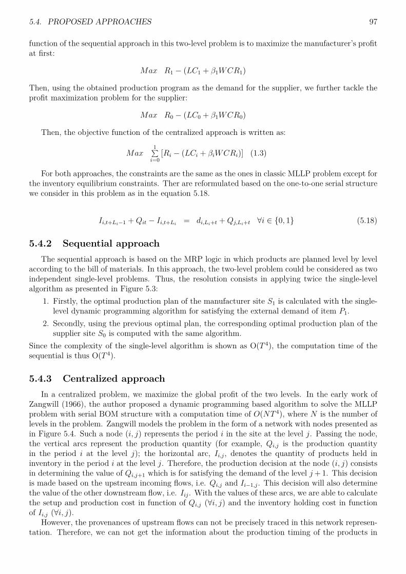
5.4. PROPOSED APPROACHES 97
function of the sequential approach in this two-level problem is to maximize the manufacturer’s profitat first:
Max R1 − (LC1 + β1WCR1)
Then, using the obtained production program as the demand for the supplier, we further tackle theprofit maximization problem for the supplier:
Max R0 − (LC0 + β1WCR0)
Then, the objective function of the centralized approach is written as:
Max1∑i=0
[Ri − (LCi + βiWCRi)] (1.3)
For both approaches, the constraints are the same as the ones in classic MLLP problem except forthe inventory equilibrium constraints. Ther are reformulated based on the one-to-one serial structurewe consider in this problem as in the equation 5.18.
Ii,t+Li−1 +Qit − Ii,t+Li= di,Li+t +Qj,Li+t ∀i ∈ {0, 1} (5.18)
5.4.2 Sequential approachThe sequential approach is based on the MRP logic in which products are planned level by level
according to the bill of materials. In this approach, the two-level problem could be considered as twoindependent single-level problems. Thus, the resolution consists in applying twice the single-levelalgorithm as presented in Figure 5.3:
1. Firstly, the optimal production plan of the manufacturer site S1 is calculated with the single-level dynamic programming algorithm for satisfying the external demand of item P1.
2. Secondly, using the previous optimal plan, the corresponding optimal production plan of thesupplier site S0 is computed with the same algorithm.
Since the complexity of the single-level algorithm is shown as O(T 4), the computation time of thesequential is thus O(T 4).
5.4.3 Centralized approachIn a centralized problem, we maximize the global profit of the two levels. In the early work of
Zangwill (1966), the author proposed a dynamic programming based algorithm to solve the MLLPproblem with serial BOM structure with a computation time of O(NT 4), where N is the number oflevels in the problem. Zangwill models the problem in the form of a network with nodes presented asin Figure 5.4. Such a node (i, j) represents the period i in the site at the level j. Passing the node,the vertical arcs represent the production quantity (for example, Qi,j is the production quantityin the period i at the level j); the horizontal arc, Ii,j, denotes the quantity of products held ininventory in the period i at the level j. Therefore, the production decision at the node (i, j) consistsin determining the value of Qi,j+1 which is for satisfying the demand of the level j+ 1. This decisionis made based on the upstream incoming flows, i.e. Qi,j and Ii−1,j. This decision will also determinethe value of the other downstream flow, i.e. Iij. With the values of these arcs, we are able to calculatethe setup and production cost in function of Qi,j (∀i, j) and the inventory holding cost in functionof Ii,j (∀i, j).
However, the provenances of upstream flows can not be precisely traced in this network represen-tation. Therefore, we can not get the information about the production timing of the products in

98 CHAPTER 5. MLLP BASED MODEL
Site S1
Dynamic programming algorithm: ULSP (W CR)
Site S0
Dynamic programming algorithm: ULSP (W CR)
External demand
Production planof site S1
Production planof site S0
1 2 3 4 5
1 2 3 4 5
Figure 5.3 – Sequential approach
(i, j)
Qi,j
Qi,j+1
Ii,jIi−1,j
Figure 5.4 – A node and associated arcs in the Zangwill’s network presentation of the multi-levelproblem

5.4. PROPOSED APPROACHES 99
Ii−1,j. Consequently, the associated WCR can not be correctly measured. For this reason, Zangwill’salgorithm can not be directly applied for this problem. As a consequence, a new concept is requiredto tackle this problem. To do so, we first prove the ZIO property remains valid for this two-levelproblem. Then, the new concept will be explicitly described in the following. In this centralizedproblem, the delivery delay is not considered because it will significantly amplify the discount effecton the cost of the manufacturer when the delivery delay is theoretically great. It makes the NPV ofthe costs and the revenues of the manufacturer negligible and has no impact in the optimization oftwo-level plans. To avoid this unrealistic situation, the delivery is not considered in this approach.Theorem 5.4.1. There exists a set of optimal production plans of the supplier and the manufacturerin which Ii,t−1 ×Qit = 0 for all t and i ∈ {0, 1} (where Iit is the inventory of site i at the end of theperiod t) in 2ULSP (BFR) problem with associated assumptions in section 5.3.1.
Proof of the ZIO property in centralized approach for 2ULSP (WCR) problem
In the single-level case, the NPV of revenue is fixed by the deterministic demand that will not varyduring the planning process. However, in two-level case, the revenue NPV of the supplier depends onthe production program of the manufacturer. This program is not fixed a priori and is determinedwith a centralized optimization objective. Therefore, the revenue NPV of the supplier may varyaccording to the manufacturer’s production plan and needs to be considered in the optimizationprocedure. However, the revenue NPV of the manufacturer is still fixed by the known externaldemands which do not vary in the planning process. It is omitted in the following proof.
The basic idea of this proof is similar to the previous one for single-level problem. The details ofthe proof are described as follows:
Firstly, we denote that :— X(2ULSP (W CR)) represents all feasible solutions fro the two sites;— P denotes a set of feasible production plans of both sites;— Profit(P ) stands for the objective value in the proposed model with the set of plans P .
Definition 2. A production planning is complied with the ZIO property if and only if the productionis only planned when the inventory level drops to zero. With the notation of the two-level problem, itcan mathematically be expressed as
Qit ×[t−1∑k=1
(T∑l=t
Xilk
)]= 0 ∀t ∈ [2, T ] , i ∈ {0, 1}
In other words, it can be written as :{Qit > 0 ⇒ Xikl = 0 ∀(k, l) ∈ [1, t− 1]× [t, T ]Xikl > 0 ⇒ Qit = 0 ∀t ∈ [k + 1, l] , i ∈ {0, 1}
Then, we denote that there is the optimal plan set P ∗ ∈ X(2ULSP (W CR)), where
Profit(P ∗) = maxP∈X(2ULSP (BF R))
Profit(P )
.Let Pi (with i ∈ {0, 1}) be a feasible planning which does not comply with the ZIO property.
Note that (t,m, n) ∈ [1, T ]3 is a triplet with m < t ≤ n. Thus, a violation of the property can bepresented as Qt ×Xm,n > 0. Then, we assume that at least one violation can be found in Pi.
We consider a plan P ′i as a plan derived from Pi in the following way and the ZIO structure canthus be found in P ′i :
X′ikt = Xikt ∀(k, t) ∈ [1, T ]2 − {(m,n), (t, n)} , i ∈ {0, 1}
X′imn = 0
X′itn = Xitn +Ximn

100 CHAPTER 5. MLLP BASED MODEL
The violation can be found in the planning of either level. Therefore, we examine the objectivevalue variations in the two following cases. In each case, we have a feasible plan at one level and weeliminate a violation of the ZIO property at the other level:
— case 1: Compare P = {P0, P ′′1 } with P ′ ={P ′0, P ′′1 }, where P ′′1 is any feasible plan of themanufacturer;
— case 2: Compare P = {P ′′0 , P1} with P ′ ={P ′′0 , P ′1}, where P ′′0 is any feasible plan of thesupplier;
To simplify the NPV formulation, denote that ajit = ai1
(1 + αj)t, sjit = si
1(1 + αj)t
, pjit =
pi1
(1 + αj)t, hjit = hi
1(1 + αj)t
and vjit = vi1
(1 + αj)t.
Case 1 :In this case, we change one period of the supplier’s planning into ZIO structure. The change atsupplier level will not impact the profit of the manufacturer. For this reason, this case can be consid-ered as a single-level problem. According to the ZIO property in the single-level problem, changinginto P ′0 decreases the total cost and increases the profit of supplier. In other word, eliminating ZIOviolation globally improves the profit of the chain in this case.
Case 2 :In case 2, we move backward the production of X1mn in S1 from the period m to the period t in orderto ensure a ZIO structure in the period t at manufacturer level. It delays the delivery from S0 whichincreases the NPV of the inventory holding cost and of the financial costs of supplier. The latter isdue to the delayed payments of manufacturer. However, it will simultaneously decrease the NPV ofall logistic and financial costs of the manufacturer. All NPV variations due to this transformationare summarized in Table 5.5.
Variation of revenueSupplier ↘
Manufacturer =Variation of LC Purchasing Setup Production Holding
Supplier = = = ↗Manufacturer ↘ ↘ or = ↘ ↘
Variation of WCR WCRpur WCRset WCRprod WCRinv
Supplier ↗ ↗ ↗ ↗Manufacturer ↘ ↘ ↘ ↘
Table 5.5 – Variations due to the transformation for moving X1mn
Thus, we examine the objective value and express the mathematical formulation of these variationsat two levels.
Firstly, at supplier level, we calculate the difference in logistic costs, LC0. Obviously, since theplanning of S0 remains the same, the only difference can be found in inventory holding cost.
∆LC0 = LC0(P0, P1)− LC0(P0, P′1) = ∆LCinv
0 = −X1mn
t−1∑j=m
h00j < 0
Next, we examine the variation of the financial cost through all its components. All of them

5.4. PROPOSED APPROACHES 101
increase because the delayed delivery of X1mn extends the time length of financing these expenses.
∆WCRpur0 = WCRpur
0 (P0, P1)−WCRpur0 (P0, P
′1)
=T∑t=1
T∑k=t
a0X0tk
T∑j=t+r0
1(1 + α0)j −
T∑j=k+r1
1(1 + α0)j
−
T∑t=1
T∑k=t
a0X′0tk
T∑j=t+r0
1(1 + α0)j −
T∑j=k+r1
1(1 + α0)j
= −X1mn
T∑j=m
a00j −
T∑j=t
a00j
= −X1mn
t−1∑j=m
a00j < 0
∆WCRprod0 = WCRprod
0 (P0, P1)−WCRprod0 (P0, P
′1)
=T∑t=1
T∑k=t
p0X0tk
k+r1−1∑j=t
1(1 + α)t −
T∑t=1
T∑k=t
p0X′0tk
k+r1−1∑j=t
1(1 + α)t
= −X1mn
k+r1−1∑j=m
p0j −
k+r1−1∑j=t
p0j
= −X1mn
t−1∑j=m
p00j < 0
∆WCRinv0 = WCRinv
0 (P0, P1)−WCRinv0 (P0, P
′1)
=T∑t=1
T∑k=t
h0X0tk
k−1∑l=t
k+r1−1∑j=l
1(1 + α)t −
T∑t=1
T∑k=t
h0X′0tk
k−1∑l=t
k+r1−1∑j=l
1(1 + α)t
= X1mn
n−t−1∑l=0
t−1∑k=m
h00,k+l +
n−1∑l=m+n−t
n+r2−1∑j=l
h00j
= −X1mn
n−t−1∑l=0
t−1∑k=m
h00,k+l +
n−1∑l=m+n−t
n+r1−1∑j=l
h00j
< 0
(5.19)
∆WCRset0 = WCRset
0 (P0, P1)−WCRset0 (P0, P
′1)
=T∑t=1
T∑k=t
s0tY0tX0tk
Q0t + (1− Y0t)
k+r1−1∑j=t
1(1 + α)t
−
T∑t=1
T∑k=t
s0tY0tX′0tk
Q′0t + (1− Y0t)
k+r1−1∑j=t
1(1 + α)t
= −X1mn
Q0m
t−1∑j=m
s00j < 0
(5.20)
The NPV changes of the supplier’s revenue can be expressed as ∆R0 = X1mn(v00,m+r1 − v
00,t++r1) > 0
because the X1mn will be paid in a later period due to this transformation and the payment is furtherdiscounted over time.
Secondly, we calculate the differences at manufacturer level : By transforming from P1 to P ′1, the

102 CHAPTER 5. MLLP BASED MODEL
production of X1mn is delayed from the period m to t. The difference of the logistic cost is thus :
∆LC1 = LC1(P0, P1)− LC1(P0, P′1)
= X1mn
(a11,m+r1 − a
11,t+r1) + (p1
1m − p11t) +
t−1∑j=m
h11j
+ (s1mY1m − s1
mY′
1m)
(5.21)
We need to separate the purchasing cost and inventory holding cost from the others. Thus, thevariation of
— the purchasing cost of the manufacturer: ∆LCpur1 = X1mn(a1
1,m+r1 − a11,t+r1) > 0
— the inventory holding cost of the manufacturer: ∆LCinv1 = X1mn
∑t−1j=m h
11j > 0
— the setup and production of the manufacturer:
X1mn(p11m − p1
1t) + (s1mY1m − s1
mY′
1m)> 0 with Y1m ≥ Y ′1m and Y1t = Y ′1t = 1 (5.22)
For the financial cost, the relation of WCR1(P ) > WCR1(P ′) has been proved in the single-levelcase. However, we need to evaluate the difference on the purchasing WCR cost which is in a formsimilar to the ones at supplier level:
∆WCRpur1 = WCRpur
1 (P0, P1)−WCRpur1 (P0, P
′1)
=T∑t=1
T∑k=t
a1X1tk
T∑j=t+r1
1(1 + α)j −
T∑j=k+r2
1(1 + α)j
−
T∑t=1
T∑k=t
a1X′1tk
T∑j=t+r1
1(1 + α)j −
T∑j=k+r2
1(1 + α)j
= X1mn
T∑j=m
a11j −
T∑j=t
a11j
= X1mn
t−1∑j=m
a11j > 0
∆WCRprod1 = X1mn
t−1∑j=m
p11j > 0
∆WCRinv1 = X1mn
n−t−1∑l=0
t−1∑k=m
h11,k+l +
n−1∑l=m+n−t
n+r2−1∑j=l
h11j
> 0
(5.23)
The change in WCR for the setup cost at the manufacturer level is positive as proven in the single-level case:
∆WCRset1 =
T∑t=1
T∑k=t
sY1tX1tk
X1t + (1− Y1t)
k+r2−1∑j=t
1(1 + α)t
−
T∑t=1
T∑k=t
sY1tX′1tk
X ′1t + (1− Y1t)
k+r2−1∑j=t
1(1 + α)t
> 0
(5.24)
Once expressed all variations of NPVs of the related revenue and costs, we combine them tocalculate the global difference due to this transformation in following order:

5.4. PROPOSED APPROACHES 103
1. The variation of revenue NPV of the supplier minus the variation of purchasing cost NPV ofthe manufacturer;
2. The sum of the NPV variations of inventory holding costs of both levels;
3. The sum of the WCR variations of purchasing cost of the manufacturer and all WCR of thesupplier excluding the WCR of inventory holding cost;
4. The sum of the WCR variations of inventory holding cost of both levels.
First, the variation of purchasing cost NPV of the manufacturer minus the variation of revenueNPV of the supplier is calculated as below:
∆LCpur1 −∆R0 = X1mn(a1
1,m+r1 − a11,t+r1)−X1mn(v0
0,m+r1 − v00,t+r1) (5.25)
As assumed, α1 < α0, we thus have 11 + α1
>1
1 + α0. Since v0 = a1, a1
1,i = a11
(1 + α1)i =
v01
(1 + α1)i > v01
(1 + α0)i = v00,i. Therefore, ∆R0 − Pur1 < 0
Second, since we assume h0 < h1, the sum of the NPV variations of inventory holding costs ofboth levels is positive:
∆LCinv0 + ∆LCinv
1
= X1mnt−1∑j=m
(h11j − h0
0j)
> X1mnt−1∑j=m
(h01j − h0
0j)
> X1mnt−1∑j=m
(h00j − h0
0j) = 0 (5.26)
Third, in practice, the unit sales price of supplier (i.e. the unit purchasing cost of manufacturer)is usually greater than average cost per intermediate product including all logistic and financial costin order to gain profit for the supplier site. Therefore, we adopt a simplified formulation to expressthe relation between a1 and all cost parameters of the supplier that a1 ≥ a0 + s̄0 + p0 + h0 (where,s̄0 = max
t∈T and Q0t 6=0{ s0
Q0t}). For this reason, we could obtain that
∆WCRpur1 + ∆WCRpur
0 + ∆WCRprod0 + ∆WCRset
0
= X1mn
t−1∑j=m
a11j −X1mn
t−1∑j=m
a00j −X1mn
t−1∑j=m
p00j −
X1mn
Q0m
t−1∑j=m
s00j
> X1mn
t−1∑j=m
a01j −X1mn
t−1∑j=m
a00j −X1mn
t−1∑j=m
p00j −
X1mn
Q0m
t−1∑j=m
s00j
> X1mn
t−1∑j=m
(a00 + s̄0
0 + p00)−X1mn
t−1∑j=m
a00j −X1mn
t−1∑j=m
p00j −
X1mn
Q0m
t−1∑j=m
s00j > 0
(5.27)
Last, we assume the r1 ≥ r2. In addition, we have h0 < h1 and α1 < α0. Consequently, h11,i > h0
0,i.Therefore,

104 CHAPTER 5. MLLP BASED MODEL
∆WCRinv0 + ∆WCRinv
1
= X1mn
(n−t−1∑l=0
t−1∑k=m
h11,k+l +
n−1∑l=m+n−t
n+r2−1∑j=l
h11j
)
−X1mn
(n−t−1∑l=0
t−1∑k=m
h00,k+l +
n−1∑l=m+n−t
n+r1−1∑j=l
h00j
)> 0 (5.28)
In summary, combining the equation (5.22), (5.25), (5.26), (5.27) and (5.28), the sum of total logisticand financial cost minus the difference in revenue NPV of the supplier is positive. This means thatthe total cost will be reduced by changing P1 to P ′1. Thus, we favor the ZIO type planning whichimproves the global profit.
To conclude, as proven above, the ZIO property remains valid in this two-level problem. It allowsus to established a dynamic programming-based algorithm considering the financial cost of the WCRand the interdependency between levels.
Description of the centralized approach
Production planning forboth the manufacturer
and the supplier
Site S0
Dynamic programming algorithm
Mas
ter
prob
lem
subp
robl
ems
One
ofth
e
1 2 3 4 5
Planning of intermediategoods production for
d2, d3 and d4
Site S1
Dynamic programming algorithm
2 3 4 5
E025
E1235
Figure 5.5 – Centralized approach for 2ULSP (WCR)
For this centralized approach, we propose a reformulation in the form of two-level shortest pathswhich represents the two-level supply chain as shown in Figure 5.5. In the reformulation, for bothlevels, the nodes represent the planning periods with a dummy period at the end. As the ZIOproperty have been proven valid and the one-to-one production assumption, passing an arc, E, fromthe period t to k represents a production of corresponding products (semi-finished at the supplierlevel or finished at the manufacturer level) for all external demands between periods t and k − 1at the period t in site Si with i ∈ {0, 1}. We firstly consider a master problem to determine theshortest path at the supplier level. In order to take into account the interdependency between thesetwo levels, the value of the arc at the supplier level includes not only the NPV of the revenue andall logistic and financial cost of the supplier, but also the NPV of all costs of the manufacturer. Tocalculate these costs and revenue associated to an arc E0
tk at supplier level from t to k,— on the one hand, we first calculate the discounted costs of the supplier for such a production
that do not depend on the manufacturer’s plan. To do so, since we have all intermediateproducts made in the period t at the supplier level, we can directly compute the discountedcosts of the supplier including:— purchasing cost;

5.4. PROPOSED APPROACHES 105
— setup cost;— production cost.
— on the other hand, we should also add all the costs and the revenue that depend on themanufacturer’s plan that includes the NPV of— the inventory holding cost of the supplier;— the WCR financial cost of the supplier;— the revenue of the supplier;— all logistic and financial costs of the manufacturer between period t to k.These terms are computed by solving a sub-problem which determines the optimal plan of themanufacturer that minimizes the sum of these costs minus the revenue of the supplier, forsatisfying the external demands from t to k − 1, denoted as dtk =
k−1∑i=t
di.
For the E0tk of the master problem and the associated sub-problem, the productions at both levels
are only organized for satisfying dtk in order to comply with the ZIO property at both levels. Itmeans that, firstly, the intermediate product for dj with j > k would not be produced between theperiods t and k − 1 in the supplier because there is another production planned in the period k;secondly, the final product for dj with j > k would not be produced between the period t and k − 1because the corresponding intermediate product have not be prepared at the supplier level duringthese periods.
Therefore, in the sub-problem of E0tk, the arc E1
tt′k′ , with t ≤ t′, k′ ≤ k, of the sub-problemat manufacturer level represents a production for dt′k′ at the period t′. For this production, allintermediate products have been manufactured at the period t by the supplier and delivered to themanufacturer at the period t′. Therefore, we are able to calculate the value of the arc E1
tt′k′ thatconsists of:
— the inventory holding cost of the supplier for holding the intermediate products for the externaldemands between the period t′ and k′−1 (denoted as dt′k′) during the periods from t to t′−1;
— the WCR financial cost to cover all operations costs associated to the intermediate goods pro-duction for dtk of the supplier until the correspondent payment arrived from the manufacturerin the period t′ + r1;
— the revenue of the supplier of selling the intermediate goods for dt′k′ that will be received inthe period t′ + r1.
— All logistic and financial costs for a production of dt′k′ at the period t′ by the manufacturer.The manufacturer would receive the payment from the external customer according to itsdemand and the payment delay, r2.
After formulating the problem in the form of a two-level shortest paths, both the master problemand sub-problem can be solved by a dynamic programming algorithm similar to the single-level one(whose complexity is O(T 4)). Since there are O(T 2) sub-problems to be dealt with and each one iscomputed at worst in O(T 4), the complexity of this centralized approach is thus O(T 6). The detailof the algorithm is presented in the following section. The optimality of this approach is ensured bythe fact that this approach enumerates all possible combinations of production plans of both levelscomplying with the ZIO property.
As we state in the introduction of the decentralized approach, the application of the centralizedapproach may not be applicable in a supply chain with independent companies. However, in thecontext of the RCSM project, the optimization platform provides a global management for all mem-bers of the supply chain and financial solutions for cover their WCRs which are gathered in a WCRpooling. It is still reasonable to employ the centralized approach. Furthermore, we assume that thesemembers benefit from a same interest rate for financing the pooled WCR.
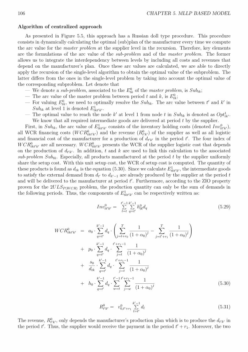
106 CHAPTER 5. MLLP BASED MODEL
Algorithm of centralized approach
As presented in Figure 5.5, this approach has a Russian doll type procedure. This procedureconsists in dynamically calculating the optimal (sub)plan of the manufacturer every time we computethe arc value for the master problem at the supplier level in the recursion. Therefore, key elementsare the formulations of the arc value of the sub-problem and of the master problem. The formerallows us to integrate the interdependency between levels by including all costs and revenues thatdepend on the manufacturer’s plan. Once these arc values are calculated, we are able to directlyapply the recursion of the single-level algorithm to obtain the optimal value of the subproblem. Thelatter differs from the ones in the single-level problem by taking into account the optimal value ofthe corresponding subproblem. Let denote that
— We denote a sub-problem, associated to the E0tk of the master problem, is Subtk;
— The arc value of the master problem between period t and k, is E0tk;
— For valuing E0tk, we need to optimally resolve the Subtk. The arc value between t′ and k′ in
Subtk at level 1 is denoted E1tkt′k′ .
— The optimal value to reach the node k′ at level 1 from node t in Subtk is denoted as Opt1tk′ .We know that all required intermediate goods are delivered at period t by the supplier.
First, in Subtk, the arc value of E1tkt′k′ consists of the inventory holding costs (denoted Inv0
tt′k′),all WCR financing costs (WCR0
tkt′k′) and the revenue (R0t′k′) of the supplier as well as all logistic
and financial cost of the manufacturer for a production of dt′k′ in the period t′. The four index ofWCR0
tkt′k′ are all necessary. WCR0tkt′k′ presents the WCR of the supplier logistic cost that depends
on the production of dt′k′ . In addition, t and k are used to link this calculation to the associatedsub-problem Subtk. Especially, all products manufactured at the period t by the supplier uniformlyshare the setup cost. With this unit setup cost, the WCR of setup cost is computed. The quantity ofthese products is found as dtk is the equation (5.30). Since we calculate E1
tkt′k′ , the intermediate goodsto satisfy the external demand from dt′ to dk′−1 are already produced by the supplier at the period tand will be delivered to the manufacturer at period t′. Furthermore, according to the ZIO propertyproven for the 2ULSP (WCR) problem, the production quantity can only be the sum of demands inthe following periods. Thus, the components of E1
tkt′k′ can be respectively written as:
Inv0tt′k′ =
t′−1∑l=t
k′−1∑q=t′
h00ldq (5.29)
WCR0tkt′k′ = a0 ·
k′−1∑q=t′
dq ·
T∑j=t+r0
1(1 + α0)j
−T∑
j=t′+r1
1(1 + α0)j
+ p0 ·
k′−1∑q=t′
dq ·t′+r1−1∑j=t
1(1 + α0)j
+ s0
dtk·k′−1∑q=t′
dq ·t′+r1−1∑j=t
1(1 + α0)j
+ h0 ·k′−1∑q=t′
dq ·t′−1∑w=t
t′+r1−1∑j=w
1(1 + α0)j
(5.30)
R0t′k′ = v0
0,t′+r1
k′−1∑l=t′
dl (5.31)
The revenue, R0t′k′ , only depends the manufacturer’s production plan which is to produce the dt′k′ in
the period t′. Thus, the supplier would receive the payment in the period t′ + r1. Moreover, the two
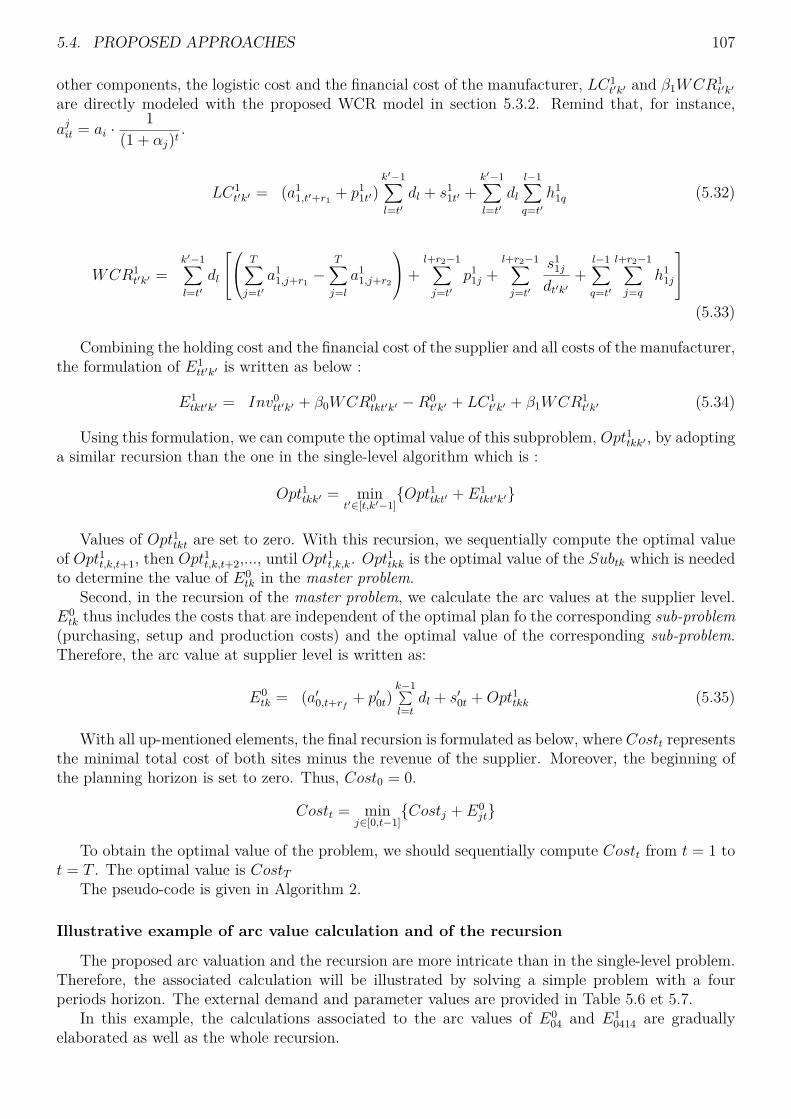
5.4. PROPOSED APPROACHES 107
other components, the logistic cost and the financial cost of the manufacturer, LC1t′k′ and β1WCR1
t′k′
are directly modeled with the proposed WCR model in section 5.3.2. Remind that, for instance,ajit = ai ·
1(1 + αj)t
.
LC1t′k′ = (a1
1,t′+r1 + p11t′)
k′−1∑l=t′
dl + s11t′ +
k′−1∑l=t′
dll−1∑q=t′
h11q (5.32)
WCR1t′k′ =
k′−1∑l=t′
dl
T∑j=t′
a11,j+r1 −
T∑j=l
a11,j+r2
+l+r2−1∑j=t′
p11j +
l+r2−1∑j=t′
s11j
dt′k′+
l−1∑q=t′
l+r2−1∑j=q
h11j
(5.33)
Combining the holding cost and the financial cost of the supplier and all costs of the manufacturer,the formulation of E1
tt′k′ is written as below :
E1tkt′k′ = Inv0
tt′k′ + β0WCR0tkt′k′ −R0
t′k′ + LC1t′k′ + β1WCR1
t′k′ (5.34)
Using this formulation, we can compute the optimal value of this subproblem, Opt1tkk′ , by adoptinga similar recursion than the one in the single-level algorithm which is :
Opt1tkk′ = mint′∈[t,k′−1]
{Opt1tkt′ + E1tkt′k′}
Values of Opt1tkt are set to zero. With this recursion, we sequentially compute the optimal valueof Opt1t,k,t+1, then Opt1t,k,t+2,..., until Opt1t,k,k. Opt1tkk is the optimal value of the Subtk which is neededto determine the value of E0
tk in the master problem.Second, in the recursion of the master problem, we calculate the arc values at the supplier level.
E0tk thus includes the costs that are independent of the optimal plan fo the corresponding sub-problem
(purchasing, setup and production costs) and the optimal value of the corresponding sub-problem.Therefore, the arc value at supplier level is written as:
E0tk = (a′0,t+rf
+ p′0t)k−1∑l=t
dl + s′0t +Opt1tkk (5.35)
With all up-mentioned elements, the final recursion is formulated as below, where Costt representsthe minimal total cost of both sites minus the revenue of the supplier. Moreover, the beginning ofthe planning horizon is set to zero. Thus, Cost0 = 0.
Costt = minj∈[0,t−1]
{Costj + E0jt}
To obtain the optimal value of the problem, we should sequentially compute Costt from t = 1 tot = T . The optimal value is CostT
The pseudo-code is given in Algorithm 2.
Illustrative example of arc value calculation and of the recursion
The proposed arc valuation and the recursion are more intricate than in the single-level problem.Therefore, the associated calculation will be illustrated by solving a simple problem with a fourperiods horizon. The external demand and parameter values are provided in Table 5.6 et 5.7.
In this example, the calculations associated to the arc values of E004 and E1
0414 are graduallyelaborated as well as the whole recursion.
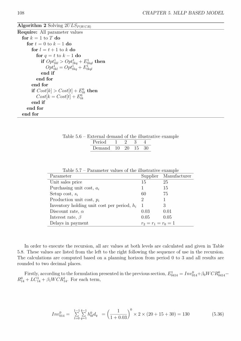
108 CHAPTER 5. MLLP BASED MODEL
Algorithm 2 Solving 2ULSP (WCR)
Require: All parameter valuesfor k = 1 to T dofor t = 0 to k − 1 dofor l = t+ 1 to k dofor q = t to k − 1 doif Opt1tkl > Opt1tkq + E1
tkql thenOpt1tkl = Opt1tkq + E1
tkql
end ifend for
end forif Cost[k] > Cost[t] + E0
tk thenCost[k = Cost[t] + E0
tk
end ifend for
end for
Table 5.6 – External demand of the illustrative examplePeriod 1 2 3 4Demand 10 20 15 30
Table 5.7 – Parameter values of the illustrative exampleParameter Supplier ManufacturerUnit sales price 15 25Purchasing unit cost, ai 1 15Setup cost, si 60 75Production unit cost, pi 2 1Inventory holding unit cost per period, hi 1 3Discount rate, α 0.03 0.01Interest rate, β 0.05 0.05Delays in payment r2 = r1 = r0 = 1
In order to execute the recursion, all arc values at both levels are calculated and given in Table5.8. These values are listed from the left to the right following the sequence of use in the recursion.The calculations are computed based on a planning horizon from period 0 to 3 and all results arerounded to two decimal places.
Firstly, according to the formulation presented in the previous section, E10414 = Inv0
014+β0WCR00414−
R014 + LC1
14 + β1WCR114. For each term,
Inv0014 =
1−1∑l=0
4−1∑q=1
h00ldq =
( 11 + 0.03
)0× 2× (20 + 15 + 30) = 130 (5.36)

5.4. PROPOSED APPROACHES 109
Table 5.8 – Arc values of both levelsE0
01 185.84 E002 358.31 E0
03 550.41 E004 995.64
E10101 96.13 E1
0201 94.13 E10301 93.80 E1
0401 93.53 E10423 179.03
E10202 209.19 E1
0302 208.19 E10402 207.39 E1
0404 780.30E1
0212 162.87 E10312 161.55 E1
0412 160.50 E10414 657.35
E10303 356.72 E1
0403 355.51 E10424 505.43
E10313 286.57 E1
0413 284.73 E10434 360.31
E10323 180.20
E012 230.87 E0
13 361.99 E014 730.86 E0
23 207.92 E024 473.31
E11212 114.93 E1
1312 113.68 E11412 112.91 E1
2323 109.36 E12423 107.47
E11313 202.79 E1
1413 201.44 E12424 290.74
E11323 143.15 E1
1423 142.01 E12434 212.42
E11414 502.67
E11424 394.37
E11434 283.69
E034 281.59
E13434 145.12
WCR00414 = a0 ·
4−1∑q=1
dq ·
T∑j=0+r0
1(0 + α0)j
−T∑
j=1+r1
1(0 + α0)j
+ p0 ·
4−1∑q=1
dq ·1+r1−1∑j=1
1(1 + α0)j
+ s0
d04·
4−1∑q=1
dq ·1+r1−1∑j=0
1(1 + α0)j
+ h0 ·4−1∑q=1
dq ·1−1∑w=0
1+r1−1∑j=w
1(1 + α0)j
=( 1
1 + 0.03
)× 1× (20 + 15 + 30)
+[( 1
1 + 0.03
)0+ 1
1 + 0.03
]× 2× (20 + 15 + 30)
+[( 1
1 + 0.03
)0+ 1
1 + 0.03
]× 60
75 × (20 + 15 + 30)
+[( 1
1 + 0.03
)0+ 1
1 + 0.03
]× 2× (20 + 15 + 30)
= 63.11 + 256.21 + 102.49 + 256.21= 678.02 (5.37)
R014 = v0
0,1+r1
4−1∑l=1
dl =( 1
1 + 0.03
)2× 15× (20 + 15 + 30) = 919.03 (5.38)
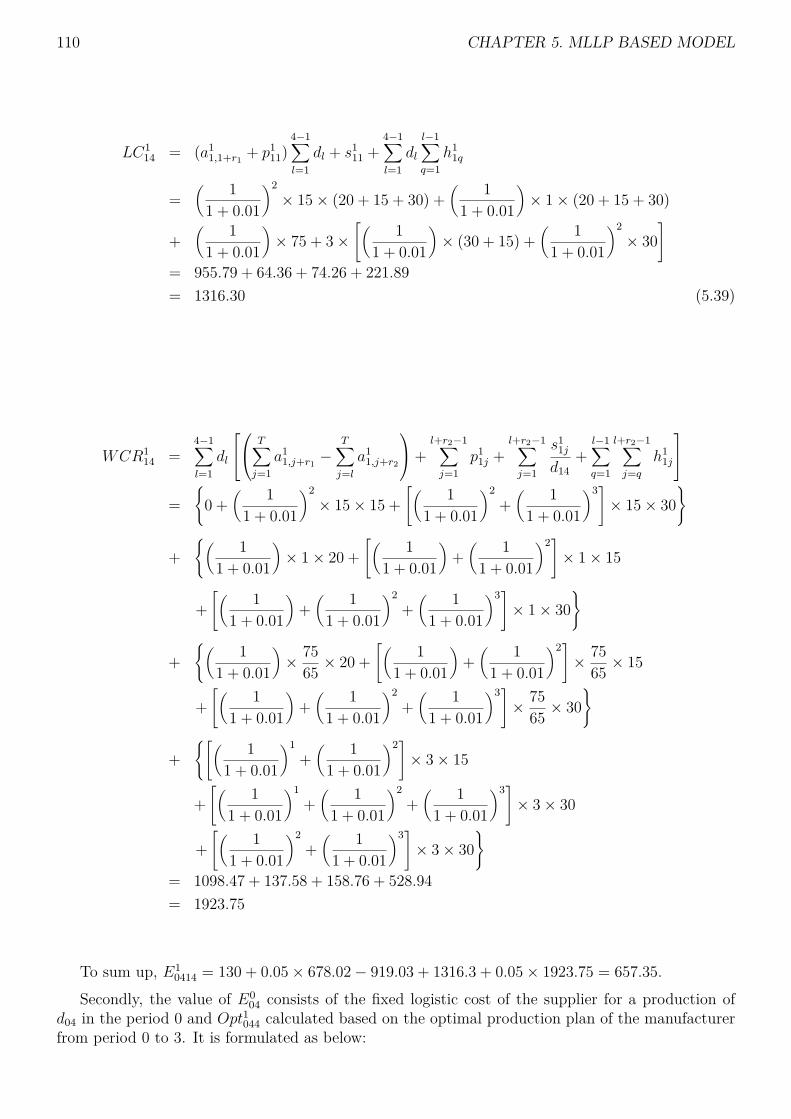
110 CHAPTER 5. MLLP BASED MODEL
LC114 = (a1
1,1+r1 + p111)
4−1∑l=1
dl + s111 +
4−1∑l=1
dll−1∑q=1
h11q
=( 1
1 + 0.01
)2× 15× (20 + 15 + 30) +
( 11 + 0.01
)× 1× (20 + 15 + 30)
+( 1
1 + 0.01
)× 75 + 3×
[( 11 + 0.01
)× (30 + 15) +
( 11 + 0.01
)2× 30
]= 955.79 + 64.36 + 74.26 + 221.89= 1316.30 (5.39)
WCR114 =
4−1∑l=1
dl
T∑j=1
a11,j+r1 −
T∑j=l
a11,j+r2
+l+r2−1∑j=1
p11j +
l+r2−1∑j=1
s11j
d14+
l−1∑q=1
l+r2−1∑j=q
h11j
=
{0 +
( 11 + 0.01
)2× 15× 15 +
[( 11 + 0.01
)2+( 1
1 + 0.01
)3]× 15× 30
}
+{( 1
1 + 0.01
)× 1× 20 +
[( 11 + 0.01
)+( 1
1 + 0.01
)2]× 1× 15
+[( 1
1 + 0.01
)+( 1
1 + 0.01
)2+( 1
1 + 0.01
)3]× 1× 30
}
+{( 1
1 + 0.01
)× 75
65 × 20 +[( 1
1 + 0.01
)+( 1
1 + 0.01
)2]× 75
65 × 15
+[( 1
1 + 0.01
)+( 1
1 + 0.01
)2+( 1
1 + 0.01
)3]× 75
65 × 30}
+{[( 1
1 + 0.01
)1+( 1
1 + 0.01
)2]× 3× 15
+[( 1
1 + 0.01
)1+( 1
1 + 0.01
)2+( 1
1 + 0.01
)3]× 3× 30
+[( 1
1 + 0.01
)2+( 1
1 + 0.01
)3]× 3× 30
}= 1098.47 + 137.58 + 158.76 + 528.94= 1923.75
To sum up, E10414 = 130 + 0.05× 678.02− 919.03 + 1316.3 + 0.05× 1923.75 = 657.35.
Secondly, the value of E004 consists of the fixed logistic cost of the supplier for a production of
d04 in the period 0 and Opt1044 calculated based on the optimal production plan of the manufacturerfrom period 0 to 3. It is formulated as below:

5.5. NUMERICAL TESTS FOR THE 2ULSP (WCR) MODEL 111
E004 = (a′0,0+rf
+ p′0t)4−1∑l=0
dl + s′00 +Opt1044
=[( 1
1 + 0.03
)1+( 1
1 + 0.03
)0]× 1× (10 + 20 + 15 + 30)
+( 1
1 + 0.03
)0× 60 +Opt1044
= 282.82 +Opt1044 (5.40)
In order to obtain the value of Opt1044, we should sequentially compute the Opt104k′ from k′ = 1 tok′ = 4 using the recursion (5.4.3). These calculations are presented as follows:
Opt1041 = Opt1040 + E10401 = 0+ 93.53 = 93.53
Opt1042 = min{Opt1040 + E10402, Opt
1041 + E1
0412}= min{0+207.39, 93.53 + 160.50} = 207.39
Opt1043 = min{Opt1040 + E10403, Opt
1041 + E1
0413, Opt1042 + E1
0423}= min{0+355.52, 93.53 + 284.73, 207.39 + 179.03} = 355.52
Opt1044 = min{Opt1040 + E10404, Opt
1041 + E1
0414, Opt1042 + E1
0424, Opt1043 + E1
0434}= min{780.30, 93.53 + 657.35,207.39+505.43, 355.52 + 360.31} = 712.82 (5.41)
With this value, we obtain that E004 = 282.82 + 712.82 = 995.64.
Once we obtain all values of E0tk where t ∈ {0, T − 1} and t < k ≤ T as given in Table 5.8, the
optimal value of the problem CostT can be calculated as follows:
Cost1 = Cost0 + E001 = 0+ 185.84 = 185.84
Cost2 = min{Cost0 + E002, Cost1 + E0
12}= min{0+358.31, 185.84 + 230.87} = 358.31
Cost3 = min{Cost0 + E003, Cost1 + E0
13, Cost2 + E023}
= min{0 + 550.41,185.84+361.99, 358.31 + 207.92} = 547.83
Cost4 = min{Cost0 + E004, Cost1 + E0
14, Cost2 + E024, Cost3 + E0
34}= min{0 + 995.64, 185.84 + 730.86, 358.31 + 473.31,547.83+281.59} = 829.42(5.42)
To summarize, the optimal value of this problem is 829.42. The corresponding optimal plansof the two levels are also obtained as shown in Table 5.9. To remain that the fixed revenue of themanufacturer is not considered in the optimization.
5.5 Numerical tests for the 2ULSP (WCR) modelIn this section, we show differences between results (optimal production plans and different costs)
obtained by classicMLLP model, 2ULSP (WCR) model with sequential approach and with centralized
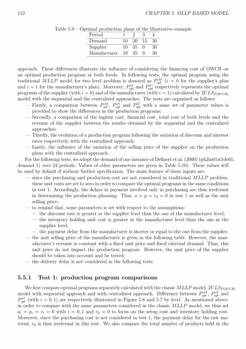
112 CHAPTER 5. MLLP BASED MODEL
Table 5.9 – Optimal production plans of the illustrative examplePeriod 1 2 3 4Demand 10 20 15 30Supplier 10 35 0 30Manufacturer 10 35 0 30
approach. These differences illustrate the influence of considering the financing cost of OWCR onan optimal production program at both levels. In following tests, the optimal program using thetraditional MLLP model for two level problem is denoted as P iM
opt (i = 0 for the supplier’s planand i = 1 for the manufacturer’s plan). Moreover, P iS
opt and P iCopt respectively represents the optimal
programs of the supplier (with i = 0) and of the manufacturer (with i = 1) calculated by 2ULSP (WCR)model with the sequential and the centralized approaches. The tests are organized as follows:
— Firstly, a comparison between P iMopt , P iS
opt and P iCopt with a same set of parameter values is
provided to show the differences in the production programs;— Secondly, a comparison of the logistic cost, financial cost, total cost of both levels and the
revenue of the supplier between the results obtained by the sequential and the centralizedapproaches;
— Thirdly, the evolution of a production program following the variation of discount and interestrates respectively with the centralized approach;
— Lastly, the influence of the variation of the selling price of the supplier on the productionplans with the centralized approach.
For the following tests, we adopt the demand of one instance of Dellaert et al. (2000) (ph2in01st1de01,demand 1) over 24 periods. Values of other parameters are given in Table 5.10). These values willbe used by default if without further specification. The main feature of these inputs are:
— since the purchasing and production cost are not considered in traditional MLLP problem,these unit costs are set to zero in order to compare the optimal programs in the same conditionsin test 1. Accordingly, the delays in payment involved only in purchasing are thus irrelevantin determining the production planning. Thus, a = p = r0 = 0 in test 1 as well as the unitselling price;
— to remind that, some parameters is set with respect to the assumptions:— the discount rate is greater at the supplier level than the one of the manufacturer level;— the inventory holding unit cost is greater at the manufacturer level than the one at the
supplier level;— the payment delay from the manufacturer is shorter or equal to the one from the supplier.
— the unit selling price of the manufacturer is given in the following table. However, the man-ufacturer’s revenue is constant with a fixed unit price and fixed external demand. Thus, thisunit price do not impact the production program. However, the unit price of the suppliershould be taken into account and be tested;
— the delivery delay is not considered in the following tests.
5.5.1 Test 1: production program comparisonsWe first compare optimal programs separately calculated with the classicMLLP model, 2ULSP (WCR)
model with sequential approach and with centralized approach. Difference between P iMopt , P iS
opt andP iCopt (with i = 0, 1) are respectively illustrated in Figure 5.6 and 5.7 by level. As mentioned above,
in order to compare with the same parameters considered in the classic MLLP model, we thus setai = pi = vi = 0 with i = 0, 1 and r0 = 0 to focus on the setup cost and inventory holding cost.Moreover, since the purchasing cost is not considered in test 1, the payment delay for the raw ma-terial, r0 is thus irrelevant in this test. We also compare the total number of products held in the
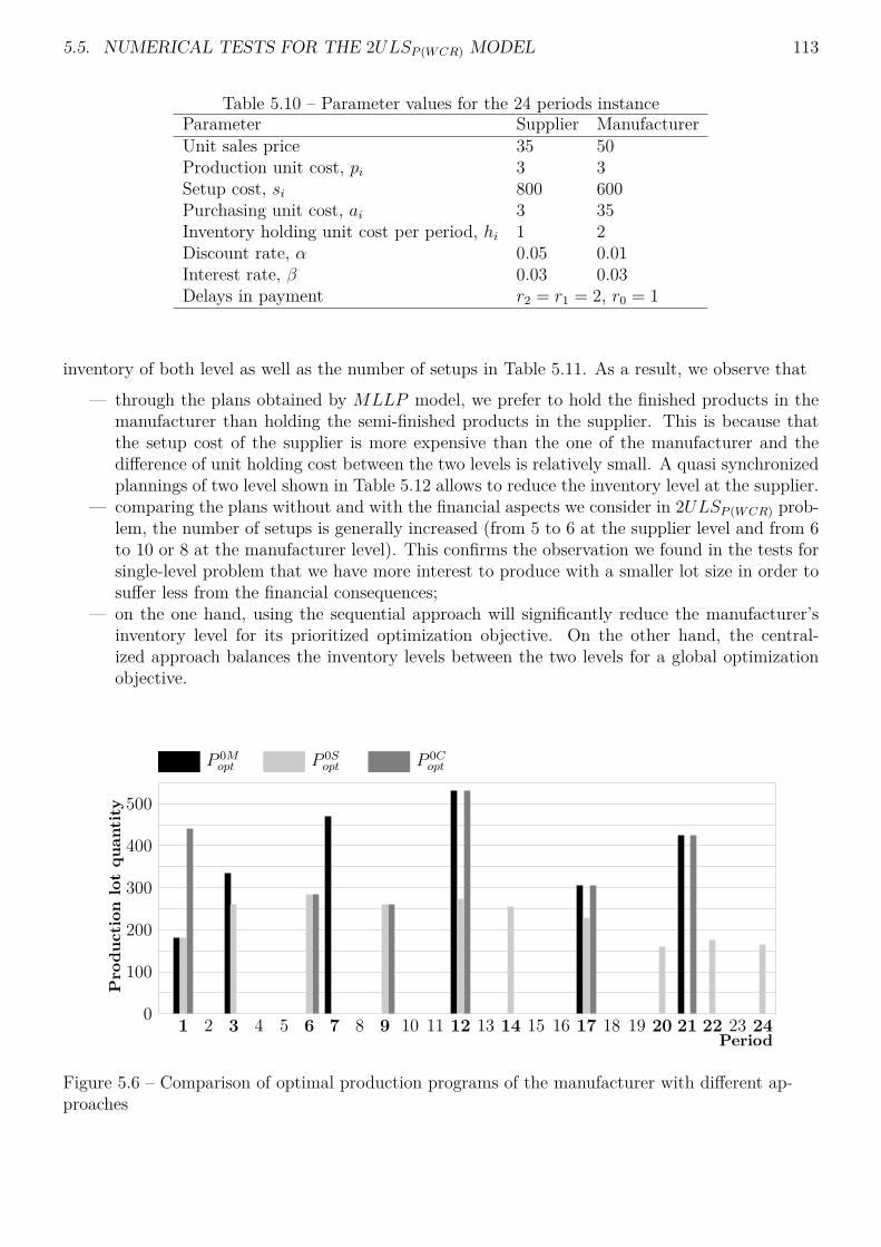
5.5. NUMERICAL TESTS FOR THE 2ULSP (WCR) MODEL 113
Table 5.10 – Parameter values for the 24 periods instanceParameter Supplier ManufacturerUnit sales price 35 50Production unit cost, pi 3 3Setup cost, si 800 600Purchasing unit cost, ai 3 35Inventory holding unit cost per period, hi 1 2Discount rate, α 0.05 0.01Interest rate, β 0.03 0.03Delays in payment r2 = r1 = 2, r0 = 1
inventory of both level as well as the number of setups in Table 5.11. As a result, we observe that— through the plans obtained by MLLP model, we prefer to hold the finished products in the
manufacturer than holding the semi-finished products in the supplier. This is because thatthe setup cost of the supplier is more expensive than the one of the manufacturer and thedifference of unit holding cost between the two levels is relatively small. A quasi synchronizedplannings of two level shown in Table 5.12 allows to reduce the inventory level at the supplier.
— comparing the plans without and with the financial aspects we consider in 2ULSP (WCR) prob-lem, the number of setups is generally increased (from 5 to 6 at the supplier level and from 6to 10 or 8 at the manufacturer level). This confirms the observation we found in the tests forsingle-level problem that we have more interest to produce with a smaller lot size in order tosuffer less from the financial consequences;
— on the one hand, using the sequential approach will significantly reduce the manufacturer’sinventory level for its prioritized optimization objective. On the other hand, the central-ized approach balances the inventory levels between the two levels for a global optimizationobjective.
1 2 3 4 5 6 7 8 9 10 11 12 13 14 15 16 17 18 19 20 21 22 23 24
500
400
300
200
100
0Period
Pro
duct
ion
lot
quan
tity
P 0Mopt P 0S
opt P 0Copt
Figure 5.6 – Comparison of optimal production programs of the manufacturer with different ap-proaches

114 CHAPTER 5. MLLP BASED MODEL
1 2 3 4 5 6 7 8 9 10 11 12 13 14 15 16 17 18 19 20 21 22 23 24
500
400
300
200
100
0Period
Pro
duct
ion
lot
quan
tity
P 0Mopt P 0S
opt P 0Copt
Figure 5.7 – Comparison of optimal production programs of the supplier with different approaches
Table 5.11 – Comparison of total products held in inventory over time and of the number of setupsApproaches Supplier Manufacturer
Total products held (in unit/period)MLLP 670 3085Sequential 1840 1230Centralized 1005 2065
Number of setupsMLLP 5 6Sequential 6 10Centralized 6 8
Table 5.12 – Setup timings comparison between optimal programsPeriod 1 2 3 4 5 6 7 8 9 10 11 12 13 14 15 16 17 18 19 20 21 22 23 24P 1Mopt 1 1 1 1 1 1P 0Mopt 1 1 1 1 1
P 1Sopt 1 1 1 1 1 1 1 1 1 1P 0Sopt 1 1 1 1 1 1
P 1Copt 1 1 1 1 1 1 1 1P 0Copt 1 1 1 1 1 1
1, represents Yit = 1 which means that a setup is occurred in the period t at the level i
5.5.2 Test2: production program evolution with different ratios betweentwo-level discount rates
In previous test for the single-level problem, we have tested the production program evolutionrespectively following the variations of the discount rate and the interest rate. Generally, comparingwith the optimal program with the classicMLLP model, we would naturally obtain the optimal pro-grams with equal or small lot size using either the sequential or the centralized approach. Therefore,in following test, we rather focus on the influence of the variation of the discount rate ratio betweenlevels. Since we assume that α1 < α0 in the chapter, we set the α1 at 0.01 and vary the α0 from 0.01

5.5. NUMERICAL TESTS FOR THE 2ULSP (WCR) MODEL 115
to 0.09 in step of 0.02. Values of other parameters are the same as in test 1. We show the resultof comparisons between the two approaches in Figure 5.8 and 5.9. Firstly, we compare the numberof setups of the optimal program of both levels respectively with the two approaches. Observationscan be summarized as follows:
— With the sequential approach, the manufacturer’s plan remains the same since α1 is fixed.Then, the setups are more frequent when α1 is sufficiently greater. This complies with theobservation we made in the test of the single-level problem.
— Moreover, using the centralized approach, the plans of the two levels synchronize when α0 =α1 = 0.01. However, when α0 increases, the change of plan occurs not necessarily at thesupplier’s level as shown in Figure 5.8. In this test, the lot size of the manufacturer decreaseswhen the discount rate of the supplier increases for a centralized objective.
— Nevertheless, when α0 reaches 0.09, its influence is expanded to both levels that we generallyproduce with smaller lots at both levels.
Figure 5.8 – Comparison of number of setups between optimal plans with different α0
Secondly, we focus on the difference of the cumulative inventory (denoted as CI) of both levels(i.e. total products held in inventory over the horizon, in "item/period") following the increase of α0.We observe that:
— there is not too many to state with the sequential approach. Only decrease of the CI level ofthe supplier is caused by the increase of the number of the setup following the increase of theα0.
— in the result with the centralized approach shown in 5.9, we find that, when α0 = 0.01, theCI level benefits from the synchronized plans and remains at zero over the planning horizon.With an increasing α0, the manufacture no longer advances too much its productions and letthe semi-finished items stay longer in the supplier’s inventory because the NPV of all costsof the supplier is smaller with an increased α0. Therefore, the supplier is interested to sharethe inventory stress from the manufacturer for a centralized objective. This trend continuesuntil the α0 is greater enough (α = 0.09), then the production of both levels are completelyreorganized.
5.5.3 Test3: program comparisons with different payment delaysIn following test, we focus on the influence of all payment delays on the two level plans with the
two approaches:
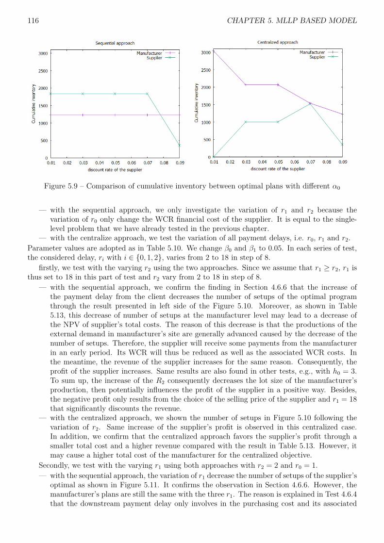
116 CHAPTER 5. MLLP BASED MODEL
Figure 5.9 – Comparison of cumulative inventory between optimal plans with different α0
— with the sequential approach, we only investigate the variation of r1 and r2 because thevariation of r0 only change the WCR financial cost of the supplier. It is equal to the single-level problem that we have already tested in the previous chapter.
— with the centralize approach, we test the variation of all payment delays, i.e. r0, r1 and r2.Parameter values are adopted as in Table 5.10. We change β0 and β1 to 0.05. In each series of test,the considered delay, ri with i ∈ {0, 1, 2}, varies from 2 to 18 in step of 8.
firstly, we test with the varying r2 using the two approaches. Since we assume that r1 ≥ r2, r1 isthus set to 18 in this part of test and r2 vary from 2 to 18 in step of 8.
— with the sequential approach, we confirm the finding in Section 4.6.6 that the increase ofthe payment delay from the client decreases the number of setups of the optimal programthrough the result presented in left side of the Figure 5.10. Moreover, as shown in Table5.13, this decrease of number of setups at the manufacturer level may lead to a decrease ofthe NPV of supplier’s total costs. The reason of this decrease is that the productions of theexternal demand in manufacturer’s site are generally advanced caused by the decrease of thenumber of setups. Therefore, the supplier will receive some payments from the manufacturerin an early period. Its WCR will thus be reduced as well as the associated WCR costs. Inthe meantime, the revenue of the supplier increases for the same reason. Consequently, theprofit of the supplier increases. Same results are also found in other tests, e.g., with h0 = 3.To sum up, the increase of the R2 consequently decreases the lot size of the manufacturer’sproduction, then potentially influences the profit of the supplier in a positive way. Besides,the negative profit only results from the choice of the selling price of the supplier and r1 = 18that significantly discounts the revenue.
— with the centralized approach, we shown the number of setups in Figure 5.10 following thevariation of r2. Same increase of the supplier’s profit is observed in this centralized case.In addition, we confirm that the centralized approach favors the supplier’s profit through asmaller total cost and a higher revenue compared with the result in Table 5.13. However, itmay cause a higher total cost of the manufacturer for the centralized objective.
Secondly, we test with the varying r1 using both approaches with r2 = 2 and r0 = 1.— with the sequential approach, the variation of r1 decrease the number of setups of the supplier’s
optimal as shown in Figure 5.11. It confirms the observation in Section 4.6.6. However, themanufacturer’s plans are still the same with the three r1. The reason is explained in Test 4.6.4that the downstream payment delay only involves in the purchasing cost and its associated

5.5. NUMERICAL TESTS FOR THE 2ULSP (WCR) MODEL 117
Figure 5.10 – Production plan comparison with varying r2
Table 5.13 – Comparison of NPVs of financial terms with different r2 using the sequential approachSupplier Manufacturer
r2 Total costs Revenue Profit Total cost2 21530.7 20156.5 -1374.2 23465.410 21530.7 20156.5 -1374.2 54918.818 21290.1 20307.4 -982.7 83908
Table 5.14 – Comparison of NPVs of financial terms with different r2 using the centralized ap-proach
Supplier Manufacturerr2 Total costs Revenue Profit Total cost2 19462.3 20749.4 1287.1 24943.810 18904.5 20954.5 2050 56904.818 18904.5 20954.5 2050 85686.5
WCR financial cost that has only a small impact on the optimal plan.— similar changes are found using the centralized approach. Moreover, a significant decrease of
the supplier’s profit are found with both approaches as presented in Table 5.15 and 5.16. Itis mainly due to the enlarged payment delay from the manufacturer (i.e. r1).
Table 5.15 – Comparison of NPVs of financial terms with different r1 using the sequential approachSupplier Manufacturer
r1 Total costs Revenue Profit Total cost2 14691.5 43999 29307.5 85056.610 18817.5 29780.3 10962.8 53035.918 21530.7 20156.5 -1374.2 23465.4
Lastly, r0 is varied from 2 to 18 and other parameters are adopted from the Table 5.10. As illus-trated in Figure 5.12, the small impact of the downstream payment delay do not change the optimalplans in the three cases. However, it still decreases the total cost of the supplier because it shortensthe financing duration for its logistic costs and decrease the WCR financial cost. Consequently, the

118 CHAPTER 5. MLLP BASED MODEL
Figure 5.11 – Production plan comparison with varying r1
Table 5.16 – Comparison of NPVs of financial terms with different r1 using the centralized ap-proach
Supplier Manufacturerr1 Total costs Revenue Profit Total cost2 13136.9 45293.3 32156.4 86848.210 16937.6 30656.3 13718.7 54664.718 19462.3 20749.4 1287.1 24943.8
supplier’s profit increases.
Figure 5.12 – Production plan comparison with varying r0
Furthermore, focusing on the centralized approach, a comparison of the supplier’s profit (Profit0),the manufacturer’s total cost (TC1) and the objective value (OV ) changes between ri = 2 and ri = 18(i ∈ {0, 1, 2}) is given in Table 5.19. For example, ∆Profit0 = Profit0(ri = 18)− Profit0(ri = 2).To remind that OV represent the sum of the logistic costs and the WCR financial costs of bothlevels minus the supplier’s revenue. Since we attempt to minimize the OV , it is obvious that r2should be shorten as much as possible in order to reduce the unnecessary WCR financial cost of themanufacturer. Moreover, it is beneficial to lengthen r1 and r0 that may further decrease the OV.
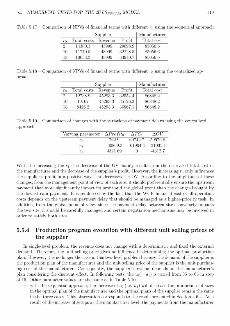
5.5. NUMERICAL TESTS FOR THE 2ULSP (WCR) MODEL 119
Table 5.17 – Comparison of NPVs of financial terms with different r0 using the sequential approachSupplier Manufacturer
r0 Total costs Revenue Profit Total cost2 14300.1 43999 29698.9 85056.610 11770.5 43999 32228.5 85056.618 10058.3 43999 33940.7 85056.6
Table 5.18 – Comparison of NPVs of financial terms with different r0 using the centralized ap-proach
Supplier Manufacturerr0 Total costs Revenue Profit Total cost2 12738.9 45293.3 32554.4 86848.210 10167 45293.3 35126.3 86848.218 8426.2 45293.3 36867.1 86848.2
Table 5.19 – Comparison of changes with the variations of payment delays using the centralizedapproach
Varying parameter ∆Profit0 ∆TC1 ∆OVr2 762.9 60742.7 59979.8r1 -30869.3 -61904.4 -31035.1r0 4321.69 0 -4312.7
With the increasing the r1, the decrease of the OV mainly results from the decreased total cost ofthe manufacturer and the decrease of the supplier’s profit. However, the increasing r0 only influencesthe supplier’s profit in a positive way that decreases the OV. According to the amplitude of thesechanges, from the management point of view of each site, it should preferentially ensure the upstreampayment that more significantly impact its profit and the global profit than the changes brought bythe downstream payment. It is reinforced by the fact that the WCR financial cost of all operationcosts depends on the upstream payment delay that should be managed as a higher-priority task. Inaddition, from the global point of view, since the payment delay between sites conversely impactsthe two site, it should be carefully managed and certain negotiation mechanisms may be involved inorder to satisfy both sites.
5.5.4 Production program evolution with different unit selling prices ofthe supplier
In single-level problem, the revenue does not change with a deterministic and fixed the externaldemand. Therefore, the unit selling price gives no influence in determining the optimal productionplan. However, it is no longer the case in this two-level problem because the demand of the supplier isthe production plan of the manufacturer and the unit selling price of the supplier is the unit purchas-ing cost of the manufacturer. Consequently, the supplier’s revenue depends on the manufacturer’splan considering the discount effect. In following tests, the v0(= a1) is varied from 35 to 65 in stepof 15. Other parameter values are the same as in Table 5.10.
— with the sequential approach, the increase of v0 (i.e. a1) will decrease the production lot sizesin the optimal plan of the manufacturer and the optimal plans of the supplier remain the samein the three cases. This observation corresponds to the result presented in Section 4.6.4. As aresult of the increase of setups at the manufacturer level, the payments from the manufacturer

120 CHAPTER 5. MLLP BASED MODEL
to the supplier are postponed. This delay leads to a increase of the WCR financial cost of thesupplier.
— subsequently, the influence of the increase of v0 on the optimal plans within the centralizedapproach is tested. The optimal plans of both levels are presented in Figure 5.13 and 5.14.Generally, an increase of the number of setups is found on both levels. The increase ofsetups of the manufacturer’s level confirms the finding in Section 4.6.4. As a consequence ofthe centralized objective, the increase of the selling price will thus decrease the productionquantities of the supplier. As shown in Table 5.20, the increase of v0 will obviously increasethe supplier’s profit but more significantly increase the total cost of the manufacturer thatglobally increase the objective value. Therefore, pricing problem for the supplier should alsoconsider the consequences at the manufacturer level with the centralized objective.
Table 5.20 – Comparison of the profit of the supplier, the total cost of the manufacturer and theobjective value with different selling prices using the centralized approach
Varying parameter Profit0 TC1 OVv0 = 35 32156.4 86848.2 54691.8v0 = 50 51065.9 117431 66364.6v0 = 65 68431.2 146412 77981.1
1 2 3 4 5 6 7 8 9 10 11 12 13 14 15 16 17 18 19 20 21 22 23 24
500
400
300
200
100
0Period
Pro
duct
ion
lot
quan
tity
v0 = 35 v0 = 50 v0 = 65
Figure 5.13 – Comparison of optimal production programs of the manufacturer with different sell-ing prices of the supplier
5.6 Generalization to multi-level problem
In this section, the two-level problem is generalized to multi-level, namelyMLLPP (WCR) problem.Since the sequential approach can be naturally extended to multi-level, we here focus on the central-ized approach. To do so, first, the WCR model in multi-level case will be firstly given. Secondly, theZIO property will be further examined for multi-level case. In the end of this section, the algorithmfor 2ULSP (WCR) will be extended to the multi-level case.
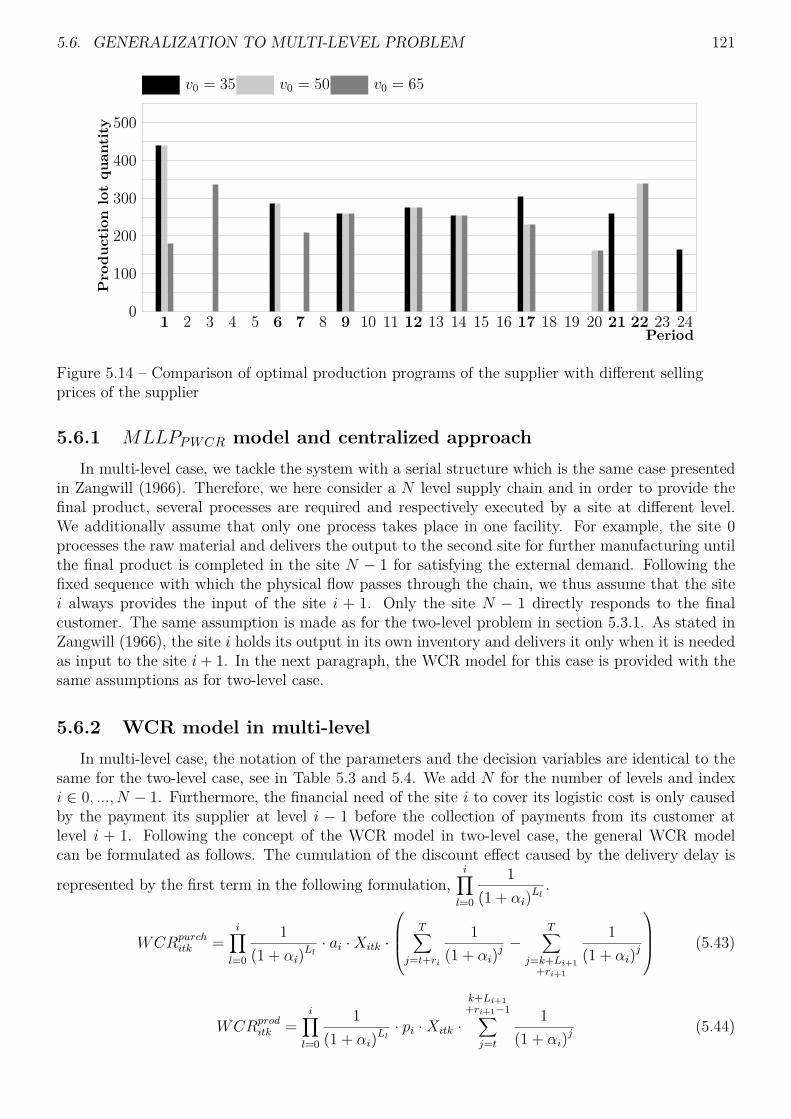
5.6. GENERALIZATION TO MULTI-LEVEL PROBLEM 121
1 2 3 4 5 6 7 8 9 10 11 12 13 14 15 16 17 18 19 20 21 22 23 24
500
400
300
200
100
0Period
Pro
duct
ion
lot
quan
tity
v0 = 35 v0 = 50 v0 = 65
Figure 5.14 – Comparison of optimal production programs of the supplier with different sellingprices of the supplier
5.6.1 MLLPPWCR model and centralized approachIn multi-level case, we tackle the system with a serial structure which is the same case presented
in Zangwill (1966). Therefore, we here consider a N level supply chain and in order to provide thefinal product, several processes are required and respectively executed by a site at different level.We additionally assume that only one process takes place in one facility. For example, the site 0processes the raw material and delivers the output to the second site for further manufacturing untilthe final product is completed in the site N − 1 for satisfying the external demand. Following thefixed sequence with which the physical flow passes through the chain, we thus assume that the sitei always provides the input of the site i + 1. Only the site N − 1 directly responds to the finalcustomer. The same assumption is made as for the two-level problem in section 5.3.1. As stated inZangwill (1966), the site i holds its output in its own inventory and delivers it only when it is neededas input to the site i+ 1. In the next paragraph, the WCR model for this case is provided with thesame assumptions as for two-level case.
5.6.2 WCR model in multi-levelIn multi-level case, the notation of the parameters and the decision variables are identical to the
same for the two-level case, see in Table 5.3 and 5.4. We add N for the number of levels and indexi ∈ 0, ..., N − 1. Furthermore, the financial need of the site i to cover its logistic cost is only causedby the payment its supplier at level i − 1 before the collection of payments from its customer atlevel i + 1. Following the concept of the WCR model in two-level case, the general WCR modelcan be formulated as follows. The cumulation of the discount effect caused by the delivery delay is
represented by the first term in the following formulation,i∏l=0
1(1 + αi)Ll
.
WCRpurchitk =
i∏l=0
1(1 + αi)Ll
· ai ·Xitk ·
T∑j=t+ri
1(1 + αi)j
−T∑
j=k+Li+1+ri+1
1(1 + αi)j
(5.43)
WCRproditk =
i∏l=0
1(1 + αi)Ll
· pi ·Xitk ·
k+Li+1+ri+1−1∑j=t
1(1 + αi)j
(5.44)
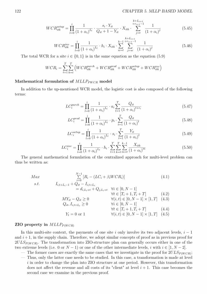
122 CHAPTER 5. MLLP BASED MODEL
WCRsetupitk =
i∏l=0
1(1 + αi)Ll
· si · YitQit + 1− Yit
·Xitk ·
k+Li+1+ri+1−1∑j=t
1(1 + αi)j
(5.45)
WCRinvitk =
i∏l=0
1(1 + αi)Ll
· hi ·Xitk ·k−1∑w=t
k+Li+1+ri+1−1∑j=w
1(1 + αi)j
(5.46)
The total WCR for a site i ∈ {0, 1} is in the same equation as the equation (5.9)
WCRi =T∑t=1
T∑k=t
(WCRpurch
itk +WCRproditk +WCRsetup
itk +WCRinvitk
)
Mathematical formulation of MLLPPWCR model
In addition to the up-mentioned WCR model, the logistic cost is also composed of the followingterms:
LCpurchi =
i∏l=0
1(1 + αi)Ll
· aiT∑t=1
Qit
(1 + αi)t+ri(5.47)
LCprodi =
i∏l=0
1(1 + αi)Ll
· pi ·T∑t=1
Qit
(1 + αi)t(5.48)
LCsetupi =
i∏l=0
1(1 + αi)Ll
· si ·T∑t=1
Yit
(1 + αi)t(5.49)
LCinvi =
i∏l=0
1(1 + αi)Ll
· hi ·T∑t=1
T∑k=t
k−1∑m=t
Xitk
(1 + αi)m(5.50)
The general mathematical formulation of the centralized approach for multi-level problem canthus be written as:
MaxN−1∑i=0
[Ri − (LCi + βiWCRi)] (4.1)s.t. Ii,t+Li−1 +Qit − Ii,t+Li
= di,Li+t +Qj,Li+t ∀i ∈ [0, N − 1]∀t ∈ [Ti + 1, Ti + T ] (4.2)
MYit −Qit ≥ 0 ∀(i, t) ∈ [0, N − 1]× [1, T ] (4.3)Qit, Ii,t+Li
≥ 0 ∀i ∈ [0, N − 1]∀t ∈ [Ti + 1, Ti + T ] (4.4)
Yt = 0 or 1 ∀(i, t) ∈ [0, N − 1]× [1, T ] (4.5)
ZIO property in MLLPP (WCR)
In this multi-site context, the payments of one site i only involve its two adjacent levels, i − 1and i+ 1, in the supply chain. Therefore, we adopt similar concepts of proof as in previous proof for2ULSP (WCR). The transformation into ZIO-structure plan can generally occurs either in one of thetwo extreme levels (i.e. 0 or N − 1) or one of the other intermediate levels, i with i ∈ [1, N − 2].
— The former cases are exactly the same cases that we investigate in the proof for 2ULSP (WCR);— Thus, only the latter case needs to be studied. In this case, a transformation is made at level
i in order to change the plan into ZIO structure at one period. However, this transformationdoes not affect the revenue and all costs of its "client" at level i + 1. This case becomes thesecond case we examine in the previous proof.
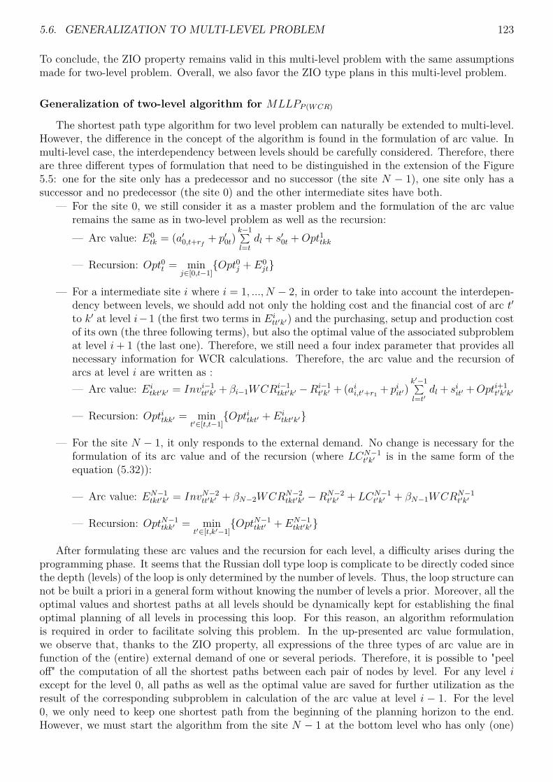
5.6. GENERALIZATION TO MULTI-LEVEL PROBLEM 123
To conclude, the ZIO property remains valid in this multi-level problem with the same assumptionsmade for two-level problem. Overall, we also favor the ZIO type plans in this multi-level problem.
Generalization of two-level algorithm for MLLPP (WCR)
The shortest path type algorithm for two level problem can naturally be extended to multi-level.However, the difference in the concept of the algorithm is found in the formulation of arc value. Inmulti-level case, the interdependency between levels should be carefully considered. Therefore, thereare three different types of formulation that need to be distinguished in the extension of the Figure5.5: one for the site only has a predecessor and no successor (the site N − 1), one site only has asuccessor and no predecessor (the site 0) and the other intermediate sites have both.
— For the site 0, we still consider it as a master problem and the formulation of the arc valueremains the same as in two-level problem as well as the recursion:— Arc value: E0
tk = (a′0,t+rf+ p′0t)
k−1∑l=t
dl + s′0t +Opt1tkk
— Recursion: Opt0t = minj∈[0,t−1]
{Opt0j + E0jt}
— For a intermediate site i where i = 1, ..., N − 2, in order to take into account the interdepen-dency between levels, we should add not only the holding cost and the financial cost of arc t′to k′ at level i−1 (the first two terms in Ei
tt′k′) and the purchasing, setup and production costof its own (the three following terms), but also the optimal value of the associated subproblemat level i+ 1 (the last one). Therefore, we still need a four index parameter that provides allnecessary information for WCR calculations. Therefore, the arc value and the recursion ofarcs at level i are written as :— Arc value: Ei
tkt′k′ = Invi−1tt′k′ + βi−1WCRi−1
tkt′k′ −Ri−1t′k′ + (aii,t′+r1 + piit′)
k′−1∑l=t′
dl + siit′ +Opti+1t′k′k′
— Recursion: Optitkk′ = mint′∈[t,t−1]
{Optitkt′ + Eitkt′k′}
— For the site N − 1, it only responds to the external demand. No change is necessary for theformulation of its arc value and of the recursion (where LCN−1
t′k′ is in the same form of theequation (5.32)):
— Arc value: EN−1tkt′k′ = InvN−2
tt′k′ + βN−2WCRN−2tkt′k′ −RN−2
t′k′ + LCN−1t′k′ + βN−1WCRN−1
t′k′
— Recursion: OptN−1tkk′ = min
t′∈[t,k′−1]{OptN−1
tkt′ + EN−1tkt′k′}
After formulating these arc values and the recursion for each level, a difficulty arises during theprogramming phase. It seems that the Russian doll type loop is complicate to be directly coded sincethe depth (levels) of the loop is only determined by the number of levels. Thus, the loop structure cannot be built a priori in a general form without knowing the number of levels a prior. Moreover, all theoptimal values and shortest paths at all levels should be dynamically kept for establishing the finaloptimal planning of all levels in processing this loop. For this reason, an algorithm reformulationis required in order to facilitate solving this problem. In the up-presented arc value formulation,we observe that, thanks to the ZIO property, all expressions of the three types of arc value are infunction of the (entire) external demand of one or several periods. Therefore, it is possible to "peeloff" the computation of all the shortest paths between each pair of nodes by level. For any level iexcept for the level 0, all paths as well as the optimal value are saved for further utilization as theresult of the corresponding subproblem in calculation of the arc value at level i − 1. For the level0, we only need to keep one shortest path from the beginning of the planning horizon to the end.However, we must start the algorithm from the site N − 1 at the bottom level who has only (one)

124 CHAPTER 5. MLLP BASED MODEL
predecessor.The pseudo-code is presented as follows:
Algorithm 3 Solving MLLPP (WCR)
Require: All parameter valuesLevel=N-1;while Level ≥ 0 dofor k = 1 to T dofor t = 0 to k − 1 doif Level 6= 0 thenfor l = t+ 1 to k dofor q = t to l doif OptLeveltll > OptLeveltlq + ELevel
tlql thenOptLeveltll = OptLeveltlq + ELevel
tlql
end ifend for
end forelse {Level = 0}if Opt0t > Opt0k + E0
kt thenOpt0t = Opt0k + E0
kt
end ifend if
end forend forLevel = Level − 1;
end while
The loops t and k are for:— generating all possible pairs of nodes for any level except for the level 0;— the recursion of dynamic programming for the level 0.Then, the loops l and q are the recursion of the dynamic programming for other levels than
level 0. In total, for each of these levels (other than 0), there are O(T 2) pairs of nodes and eachpossible shortest path between one pair of nodes is determined in O(T 4) because it is based on thesingle-level type algorithm. Besides, the resolution at level 0 takes O(T 2) for one shortest path tosolve. Globally, for this N level problem, the overall complexity is O(NT 6).
5.7 ConclusionsIn this chapter, firstly, we extend the previous single-level problem to a supplier-manufacturer
two-level problem with a serial chain structure. following similar steps in the previous chapter,after establishing the associated WCR model for this case, the corresponding mathematical modelof this problem is established considering the WCR financial cost of the two levels. For the solutionprocedure, both the sequential approach, that prioritizes the maximization of manufacturer’s profitthan the supplier’s, and the centralized approaches with a global profit maximization objective areproposed. For on thing, the sequential approach indeed consists in a direct application of the single-level algorithm at two levels. For another, it is proved that the ZIO property remains valid withcertain assumptions for the centralized approach. This property allows us to develop a reviseddynamic programming-based algorithm, in which the interdependency between levels is consideredby the arc valuation. Through the numerical tests, the observations obtained in the tests of thesingle-level problem are confirmed. Moreover, other observations are related to the interdependency
5.7. CONCLUSIONS 125
between levels. We found that the upstream payment delay and the selling price of the suppliershould be preferentially managed.
Secondly, the generalization from the two-level problem to the multi-level problem is addressed.The mathematical model and the associated WCR model are further extended to the multi-level caseas well as the two approaches and the proof of the ZIO property. In order to solve this multi-levelproblem with the centralized approach, the dynamic programming algorithm is modified to avoidthe Russian doll type structure that is difficult to program. The new algorithm tackles the problemlevel by level and the final complexity of the algorithm is O(NT 6) where N represents the numberof levels of the considered supply chain.
For future research, a generalization of the chain structure seems imperative. The first setupcan focus on the assembly structure and then the general structure. Moreover, the developmentof heuristic or meta-heuristic algorithms helps us to solve problems with a more realistic size andwith fewer assumptions. Furthermore, in addition to the two approaches proposed in this thesis,the decentralized approach has drawn increasing attention since the work of the Homberger (2010).The problem concerning the relation (domination) between supply chain members will thus be ad-dressed that involves more negotiation mechanisms and game theory techniques as studied in workof Hovelaque et al. (2015).

6Conclusion and future directions
ConclusionIn this thesis, we introduce a first link between tactical planning models and the financial aspects
of working capital requirements (WCR). Moreover, new generic WCR models are respectively pro-posed based on the EOQ, ULS and MLLP models. After integrating the WCR financial cost intothese classic models, the financial consequences of the traditional logistic costs on the productionplanning are analyzed for each case.
In the first chapter, the research background and the motivation of our work are provided. Westress that the joint consideration of the physical and financial flows in the supply chain ensures abetter alignment with the global objective of the company and improve the competitiveness in theincreasing global market.
In this second chapter, to begin with, a new generic model of operations-related working capitalrequirements in the EOQ context is presented. Such a model allows us to measure the evolution ofthe WCR over the entire planning horizon. Furthermore, an EOQ-based profit maximization modelis developed considering the financing cost of the WCR. The analytical formula of the optimal EOQis derived and associated analysis are provided to highlight some managerial insights. It is shown thatan increase in purchasing, production unit costs or the interest rate reduces the optimal production lotsize in order to obtain the maximum profit. Moreover, it is demonstrated that the economic quantityproposed by our model is always smaller than the optimal quantity of the traditional EOQ model.Thus, it is desirable to launch more frequent production with smaller lots in this joint managementcase in order to reduce inventory levels and their associated holding costs. Additionally, a comparisonwith the approximation of Jesse et al. (1983) demonstrates that our model provides a more coherentand accurate measure of the optimal production quantity for a profit maximization objective whenconsidering financial aspects. Finally, the numerical example illustrates the reduced sensitivity ofour model to several parameters when compared with the classic EOQ model.
In the third chapter, firstly, the generic model of WCR is reformulated to adopt the discretetime horizon. Secondly, a ULS-based profit maximization model is developed considering both thefinancing cost of the WCR and the time value of money. This model is established for the single-site,single-level, single-product and infinite production capacity case. After proving the Zero-Inventory-Ordering property for this problem, an exact method is developed based on dynamic programming.With this polynomial algorithm, we are able to not only reach the optimal plan which maximizesthe net present value of profit, but also evaluate the profitability of satisfying a series of demands.
127

128 CHAPTER 6. CONCLUSION AND FUTURE DIRECTIONS
Numerical tests are provided to show the interest of applying our WCR model through a comparisonwith the classical ULS model. It is found that we have less interest in holding products in theinventory due to their dramatic amplification of financial costs.
In the fourth chapter, firstly, we extend the previous single-level problem to a supplier-manufacturertwo-level problem with a serial chain structure. following similar steps in the previous chapter, afterestablishing the associated WCR model for this case, the corresponding mathematical model of thisproblem is established considering the WCR financial cost of the two levels. For the solution proce-dure, both the sequential approach, that prioritizes the maximization of manufacturer’s profit thanthe supplier’s, and the centralized approaches with a global profit maximization objective are pro-posed. For on thing, the sequential approach indeed consists in a direct application of the single-levelalgorithm at two levels. For another, it is proved that the ZIO property remains valid with certainassumptions for the centralized approach. This property allows us to develop a revised dynamicprogramming-based algorithm, in which the interdependency between levels is considered by the arcvaluation. Through the numerical tests, the observations obtained in the tests of the single-levelproblem are confirmed. Moreover, other observations are related to the interdependency betweenlevels. We found that the upstream payment delay and the selling price of the supplier should bepreferentially managed.
Secondly, the generalization from the two-level problem to the multi-level problem is addressed.The mathematical model and the associated WCR model are further extended to the multi-level caseas well as the two approaches and the proof of the ZIO property. In order to solve this multi-levelproblem with the centralized approach, the dynamic programming algorithm is modified to avoidthe Russian doll type structure that is difficult to program. The new algorithm tackles the problemlevel by level and the final complexity of the algorithm is O(NT 6) where N represents the numberof levels of the considered supply chain.
Besides, we are aware that this paper has some limitations as the first effort that theoreticallyconsiders the WCR cost in the classic dynamic lot-sizing problem. Immediate application for practicalproblem is still difficult. However, it will contribute to further studies in more complex and realisticcases as polynomial subproblems.
Future directionsIn this thesis, an infinite production capacity and the constant value of parameters are assumed.
Therefore, future works may naturally be extended to the case with varying parameter values andinvestigate whether the ZIO property is still valid for dynamic lot-sizing cases. Moreover, the con-sideration of the production capacity constraint is also an unavoidable extension of our work. Acomplexity analysis that reveals both its computational difficulty and some polynomial cases shouldbe preformed. The classification proposed by Bitran & Yanasse (1982) can be adopted to identifyspecial cases. In addition, the financial capacity of the company is not considered in this thesisand a global financial resource is assumed to cover the WCR in the context of the project RSCM.Thus, the financial capacity can be taken into account as a model constraint. This financial capacityrepresents its cash flow reserve (free cash flow) for covering the production-related operation costs.Furthermore, this reserve can be provided by the debt holder (e.g., a bank) or by its own workingcapital (from its shareholders). Consequently, it raises a selection problem among all available finan-cial resources as well as a problem of valuing their associated risks. Readers are referred to the workof Serrano et al. (2017) that considers the risk of different financial resources in the EOQ contextand the work of Lusa et al. (2012) which involves the maximum amount of credit that can be bor-rowed as a financial constraint of a dynamic lot-sizing model. In addition, all extensions consideredfor the classic lot-sizing model, such as backlogging, perishable inventory and others mentioned inMartínez-Costa et al. (2014) and Brahimi et al. (2017), are all potential directions that can enrichour model.
129
For the three classic models proposed in this work, some specific extensions may be respectivelystudied:
— for EOQP (WCR) model: as we reveal for this problem, there is a complex trade-off betweenthe multitudes of different operational and financial costs in order to maximize the profit.Based on this trade-off, it could be interesting to establish heuristics for the capacitatedlot-sizing problem considering OWCR financing costs. This is inspired by the way how thetrade-off in the EOQ problem is used for the capacitated lot-sizing model proposed by Silver& Meal (1973), the Least Unit Cost heuristic proposed by Gorham (1968) and the Part PeriodBalancing heuristic proposed by DeMatteis (1968).
— for ULSP (WCR) model: it seems promising to reduce the complexity of this algorithm toO(n3logn) by examining the approaches presented in Wagelmans et al. (1992), Aggarwal& Park (1993) and Federgruen & Tzur (1991) that improve the complexity of the Wagner-Whitin algorithm. Moreover, future research can be undertaken to consider time-varying costparameters for this case, such as the Wagner-Whitin cost in the case of the ULS. With thiscost, the complexity of the fast backward dynamic programing algorithm of Wagelmans et al.(1992) can be improved from O(T logT ) to O(T ).
— for MLLPP (WCR) model: for future research, a generalization of the chain structure seemsimperative. The first setup can focus on the assembly structure and then the general struc-ture. Moreover, the development of heuristic or meta-heuristic algorithms helps us to solveproblems with a more realistic size and with fewer assumptions. Furthermore, in addition tothe two approaches proposed in this thesis, the decentralized approach has drawn increasingattention since the work of the Homberger (2010). The problem concerning the relation (dom-ination) between supply chain members will thus be addressed that involves more negotiationmechanisms and game theory techniques as studied in work of Hovelaque et al. (2015).

7Résumé en français
Introduction généraleEn période de crise financière, les entreprises ont besoin de trésorerie pour réagir efficacement aux
aléas et assurer leur solvabilité. Cette thèse se focalise sur l’intégration de la gestion des opérationset de la finance d’entreprise. Pour ce faire, nous développons des modèles de planification tactiquegérant simultanément les flux physiques et financiers. Le coût de financement des opérations basé surle besoin en fonds de roulement (BFR) est intégré comme un nouvel aspect financier jamais considérédans la littérature des problèmes de lot-sizing.
Le besoin en fonds de roulement (BFR) correspond au niveau de fonds nécessaire pour financerles activités d’exploitation d’une entreprise, c’est-à-dire pour acheter les matières premières, payer lesfournisseurs, configurer et faire tourner les machines, etc. En bref, le besoin en fonds de roulement estgénéré par les créances des clients et les investissements réalisés à la production, et est réduit par lesdettes dues aux fournisseurs. Pendant ces dernières années, la gestion du besoin en fonds de roulementattire de plus en plus l’attention des entreprises en raison de la crise financière. En effet les liquiditéssont le fluide vital de toute entreprise et aucune entreprise ne peut survivre sans liquidités. Mêmesi une entreprise réalise des profits substantiels, elle ne peut jamais garantir qu’il reste suffisammentde liquidités disponibles pour répondre aux créances impayées après impôts, dépenses en capitalet allocation de dividendes. Donc, dans la pratique, le profit n’est pas automatiquement égal àla trésorerie, et la manière dont une entreprise gère son besoin en fonds de roulement dans unenvironnement en croissance peut affecter significativement son flux de trésorerie.
Dans cette thèse, cette problèmatique est étudiée dans trois différents cas. Nous proposonsd’abord une extension du modèle EOQ intégrant les coûts de financement du BFR, l’objectif etantla maximisation du profit. Une quantité de production optimale est obtenue analytiquement, puisnous proposons l’analyse de la sensibilité du modèle. De plus, les comparaisons avec le modèleEOQ et un modèle qui considère le coût du capital sont étudiées. Ensuite, nous travaillons surun modèle à demande dynamique. La propriété ZIO est démontrée, elle permet l’utilisation d’unalgorithme en temps polynomial. Enfin le cas multi-niveau à capacité infini est étudié avec uneapproche séquentielle puis centralisée. La propriété ZIO est prouvée pour les deux approches. Desalgorithmes de programmation dynamique sont utilisés pour obtenir une solution optimale. Cettethèse peut être considérée comme un premier, mais significatif, travail combinant la planification deproduction et la gestion du besoin en fond de roulement. Nous montrons que les aspects financiersont un impact important sur les plans de production. Les cas étudiés dans cette thèse peuvent être
131
132 CHAPTER 7. RÉSUMÉ EN FRANÇAIS
considérés comme des sous-problèmes dans l’étude de problèmes plus réalistes.
Intégration du coût de financement du BFR dans le modèlede l’EOQ
Dans ce chapitre, nous établissons un nouveau modèle de maximization du profit basé sur lemodèle classique de l’"Economic Order Quantity" (EOQ) en considérant le coût de financement duBFR. Depuis la création du modèle EOQ, il a été largement étudié pour des problèmes de gestiondes stocks et est adapté aux cas de plus en plus réalistes. Dans la littérature récente, la valeuractuelle nette et le crédit commercial sont souvent considérés comme un aspect financier intégré dansle modèle EOQ (voir Taleizadeh & Nematollahi (2014) et Martínez-Costa et al. (2014)). Cependant,aucun de ces modèles ne considère le financement du besoin en fonds de roulement comme nous lefaisons. Attendu que le BFR est d’une importance critique car il est directement lié à la solvabilitéde l’entreprise et peut générer des coûts financiers importants, ce travail vise à intégrer le coût definancement du BFR dans le modèle classique de l’EOQ. Dans ce cas, nous considérons la planificationde la production tactique pour un horizon annuel. Ainsi, l’effet actualisation est négligeable et n’estpas intégrée dans le modèle proposé.
Par conséquent, ce travail introduit une gestion conjointe des flux physiques et financiers enutilisant ce nouveau modèle. Nous nous concentrons sur le problème de la maximisation du profit entenant compte des coûts opérationnels classiques (achats, configuration, production et détention destocks) et du coût de financement du BFR associé (par exemple, intérêts sur les prêts). Dans cetteétude, seul le BFR lié à l’exploitation (Operating Working Capital Requirement) est pris en comptedans le calcul du coût de financement du BFR. Les taxes, par exemple, ne seront pas prises en compte.Le OWCR est principalement généré par un décalage entre les coûts des activités liées à la productionet les revenus de la vente de produits. Dans cette thèse, le BFR est donc le besoin financier pourcouvrir les coûts logistiques jusqu’à l’encaissement de paiement du client. La modélisation du BFRdans cette thèse suit le concept du cycle "cash-to-cash". Elle nous permet de suivre la traçabilitédes investissements dans le cycle d’exploitation. Pour cette raison, des hypothèses sont prises afinde simplifier et standardiser la modélisation du BFR et surtout pour garantir la traçabilité:
— Les coûts de setup, production et stockage sont payés immédiatement;— Le BFR n’est financé que par la partie "coût" du revenu;— Le coût de setup est uniformément reparti sur les produits d’un même lot.
Nous supposons que les paramètres de coût sont constants sur l’horizon dans cette thèse. Unetelle modélisation générique nous permet de mesurer l’évolution du BFR sur l’horizon continu deplanification. Enfin, le coût de financement du BFR est calculé en multipliant le BFR par le tauxd’intérêt.
Après avoir intégré ce coût de financement, le modèle de maximisation du profit basé sur lemodèle de l’EOQ est établi. Le profit est défini comme le revenu moins l’ensemble du coût logistiqueet du coût de financement du BFR. Afin de mettre en évidence l’influence de l’intégration des coûtsfinanciers, la formule analytique de l’EOQ optimale est dérivée avec la méthode Cardan et l’analyseassociée est fournie dans ce chapitre. Le résultat démontre qu’une augmentation des coûts unitairesde production et d’achat ou du taux d’intérêt réduit la taille optimale du lot de production lorsde la maximisation du profit. De plus, il est démontré que la quantité économique proposée parnotre modèle est toujours inférieure à la quantité optimale du modèle EOQ traditionnel. Ainsi, ilest profitable de lancer une production plus fréquente de lots plus petits afin de réduire les niveauxde stock, leurs coûts de détention associés et le BFR engendré. De plus, une comparaison avecl’approximation de Jesse et al. (1983) démontre que notre modèle fournit une mesure plus cohérenteet plus précise de la quantité de production optimale pour un objectif de maximisation du profit

133
intégrant des aspects financiers. Enfin, l’exemple numérique illustre la sensibilité réduite de notremodèle à plusieurs paramètres par rapport au modèle EOQ classique.
Un des résultats importants obtenus avec ce modèle concerne le compromis entre les coûts quimaximise le profit. Pour de futures recherches, ce compromis pourra être utilisé pour établir desheuristiques pour le problème de taille de lot à capacité finie en tenant compte des coûts de fi-nancement d’OWCR. Ceci est inspiré de la façon dont le compromis dans le problème EOQ estutilisé pour le modèle de dimensionnement par lot proposé par Silver & Meal (1973), l’heuristique dumoindre coût unitaire proposée par Gorham (1968) et l’heuristique Part Period Balancing proposépar DeMatteis (1968). Enfin, il est démontré que le retard de paiement au fournisseur n’a aucuneinfluence sur la quantité de production optimale. Cependant, il serait intéressant de se penchersur une relation fournisseur-client à deux échelons car, dans ce contexte, le retard de paiement aufournisseur (comptes créditeurs pour le client) influencerait simultanément les comptes débiteurs dufournisseur. Ainsi, la politique de production du client limiterait la politique du fournisseur et leretard de paiement au fournisseur ne serait plus négligeable.
Modèle de lot-sizing dynamique considérant l’actualisationdes coûts et le financement du BFR
Dans le deuxième chapitre, nous étudions le cas plus realiste à demande variable sur l’horizonde planification en intégrant le coût de financement du BFR. Plus précisément, nous considéronsdans ce chapitre le cas mono-site, mono-niveau, big backet et à capacité infinie. Dans la littératuredu lot-sizing, ce problème est résolu par le modèle de lot-sizing dynamique, appelé "uncapacitatedlot-sizing" (ULS).
Tout d’abord, le modélisation du BFR est modifiée et adaptée au cas discret en fonction devariables désagrégés. Ce type de variable est utilisé dans la formulation "Facility-Location" (FAL) dumodèle ULS dans la littérature classique. Ces variables ont été sélectionnées car elles nous permettentd’indiquer les périodes de début et de fin de financement du BFR. Une fois la modélisation définie,elle est intégrée dans le modèle classique de l’ULS avec des contraintes similaires à celles de l’ULSFAL.
L’expression du coût de setup et du BFR induit rend le modèle non-liéaire. En effet, le coût desetup est partagé par tous les produits fabriqués dans un même lot. Ainsi, les méthodes de résolutionclassiques ne peuvent plus être appliquées pour ce nouveau problème. Afin d’établir une méthodeefficace, la propriété Zéro-stock (ZIO) a été prouvée valide pour ce problème. Cette propriété estimportante car elle nous permet de réduire significativement le nombre de plans à évaluer parmilesquels le plan optimal se trouvera. L’idée de la preuve est de montrer que nous arrivons toujoursà améliorer la valeur de la fonction objectif d’un plan qui ne respecte pas de propriété ZIO en letransformant à un plan de type ZIO. Grâce à cette propriété, nous sommes capables de reformulerce problème sous la forme d’un problème de plus court chemin. Le nœud, Vt, représente la périodet de planification avec un noeud fictif à la fin de l’horizon. L’arc, Etk, représente une production del’ensemble des demandes entre la période t et k−1. Après avoir reformulé le problème, un algorithmede programmation dynamique est construit en s’inspirant de celui de Wagner et Whitin. La valeurd’un arc peut être calculé au pire en O(T 2) où T est le longueur de l’horizon. Puis, la récursion estréalisable en O(T 2). Ainsi, ce problème peut être résolu en O(T 4).
Enfin, des tests numériques sont effectués afin de démontrer l’influence de l’intégration du coûtde financement du BFR dans le modèle classique de l’ULS et l’impact de la valeur des différentsparamètres financiers sur le plan optimal de production. Ces tests est réalisés sur une instance baséesur une instance de Trigeiro. Premièrement, le résultat montre que la taille de productions du planoptimal du nouveau problème est généralement plus petite par rapport celle du plan optimal de l’ULS.Cela signifie que nous avons moins intérêt à stocker des produits afin de réduire le coût financement

134 CHAPTER 7. RÉSUMÉ EN FRANÇAIS
du BFR. Deuxièmement, l’impact de variations des paramètres financiers est testé et les résultatsconfirment ce que nous avons obtenu dans le chapitre précédent à l’exception de l’augmentation dudélai de paiement au fournisseur qui a maintenant un impact sur le plan optimale. Ceci est dû àl’intégration de de l’actualisation des coûts.
Pour de futures recherches, il semble prometteur de réduire la complexité de cet algorithmeà O(T 3logT ) en examinant les approches présentées dans Wagelmans et al. (1992), Aggarwal &Park (1993) et Federgruen & Tzur (1991) qui améliorent la complexité de l’algorithme de Wagner-Whitin. Enfin, de futures recherches peuvent s’intéresser à des paramètres de coûts variables dansle temps cmome les coûts de Wagner-Whitin dans le cas de l’ULS. Avec ce coût, la complexité del’algorithme de programmation dynamique backward rapide de Wagelmans et al. (1992) peut êtreaméliorée de O(T logT ) à O(T ). Afin d’établir une évaluation de la rentabilité globale, un problèmede maximisation du profit à deux niveaux (fournisseur-fabricant) sera étudié dans le chapitre suivant.De plus, la capacité de production et la gestion des risques dans la chaîne logistique devraient êtrepris en compte parmi les autres extensions.
Modèle multi-niveau en considérant le coût de financementdu BFR et l’actualisation pour une chaîne logistique en série
Après avoir étudié les problèmes mono-niveau, nous considérons une chaîne logistique à deuxacteurs en série: un fournisseur et un fabricant. Ce dernier organise ses productions pour satisfaireles demandes externes dt, t ∈ T . Pour ce faire, il commande des produits semi-finis auprès dufournisseur. Le fournisseur gère ses activités en respectant les commandes du fabricant, la livraisonest soumise à un délai noté L. Nous supposons qu’aucun produit semi-fini n’est stocké chez lefabricant. Autrement dit, le fournisseur ne livre les produits semi-finis qu’à la période où le fabricanten a besoin. Chaque transaction est soumise à son propre délai de paiement. Le client final ne paie lefabricant qu’après un délai de paiement qui s’ajoute au délai de livraison, idem entre le fabricant et lefournisseur et entre le fournisseur et son fournisseur en matière première. De plus, dans ce problème,nous considérons également des aspects financiers tels que l’actualisation et le financement du BFR.
La modélisation du BFR est adaptée au cas à deux niveaux. Sachant que l’encaissement despaiements du fabricant au fournisseur est déterminé par le plan de production du fabricant. Parconséquent, le BFR du fournisseur dépend fortement du plan du fabricant. En revanche, les plans deproduction des deux niveaux peuvent être déduit selon l’objectif prédéfini. Dans cette thèse, deuxapproches de résolution sont présentées. Premièrement, une approche séquentielle qui représentele cas où le fabricant satisfait la demande externe à profit maximum et le fournisseur organise sonactivité de production selon le plan optimal de production du fabricant et une approche centraliséequi détermine des plans de production optimaux de chaque niveau en maximisant le profit total dela chaîne.
— Approche séquentielle:Dans ce cas, nous considérons la planification des deux niveaux comme deux sous-problèmesséparés. Donc, deux étapes de calcul s’effectuent dans cette approche : d’abord, le planoptimal du fabricant peut être calculé en utilisant l’algorithme ULSP (BFR) proposé pour leproblème mono-niveau qui est en O(T 4). Le plan de production ainsi obtenu sera la demandedu fournisseur. Une seconde application de l’algorithme nous permet de calculer le planoptimal du fournisseur pour satisfaire les demandes du fabricant. Par conséquent, dans le cas,le complexité du problème est de O(T 4).
— Approche centraliséeLe problème avec un objectif centralisé a été traité dans la littérature du lot-sizing avec le

135
modèle "Multi-Level Lot-sizing Problem" (MLLP). Initialement, il a été étudié par Zangwill(1966) sur un problème avec une nomenclature en série. Pour le résoudre, l’auteur a proposéun algorithme de programmation dynamique. Cependant, cet algorithme ne peut pas êtredirectement appliqué à notre problème. C’est parce que le concept du réseau du flot nepermet pas d’identifier précisément les périodes de début et de fin de financement du BFR.Donc, après avoir prouvé la propriété "zéro-stock" (ZIO) pour ce problème et sous certainshypothèses, nous proposons également un algorithme de programmation dynamique pour lerésoudre en O(T 6). Le principe de l’algorithme est le suivant :— reformuler le problème sous forme de problème plus court chemin à chaque niveau ;— considérer le problème au niveau fournisseur comme un problème maître ;— pour calculer la valeur d’arc au niveau fournisseur, il faut résoudre préalablement un sous-
problème au niveau fabricant. Ce sous-problème est entre les mêmes périodes que l’arcconsidéré au niveau fournisseur. La valeur d’arc du sous-problème comporte non seulementle profit et l’ensemble des coûts logistiques et financiers du fabricant, mais aussi les coûtsdu fournisseur qui dépendent du plan de production du fabricant (le coût de stockage etle coût de financement du BFR).
— la récursion du problème maître et de chaque sous-problème est similaire que celui dualgorithme mono-niveau.
Le calcul du sous-problème est réalisé au pire en O(T 4) et la récursion du problème maître seréalise en O(T 2). Ainsi, la complexité du algorithme centralisé est en O(T 6).Les tests numériques sont réalisés afin d’illustrer d’abord l’influence des coûts de financementdu BFR sur le plan de production de chaque niveau. La taille de lot de production obtenueavec les deux approches est généralement plus petite que celle obtenue avec le modèle MLLPclassique. Puis, l’importance du délai de paiement entre les acteurs sur le profit total estidentifiée avec l’approche centralisée. Ensuite, le prix unitaire de vente n’impacte pas le plande production dans le problème mono-niveau. En revanche, nous montrons que le prix unitairede vente du fournisseur a une influence non négligeable car il est aussi le coût unitaire d’achatdu fabricant.Dans la dernière partie de la thèse, le problème à deux niveau est généralisé àN niveau en série.La modélisation du BFR, le modèle mathématique et les deux approches sont généralisés aucas multi-niveau avec une nomenclature en série. Les complexités sont respectivement O(NT 4)et O(NT 6) où N est le nombre de niveaux de la chaîne. Pour l’approche centralisée, troistypes de valeur d’arc sont formulés afin de prendre en compte l’interdépendance entre lesniveaux.Comme perspectives, la généralisation de la structure de la chaîne nous permet de traiter leproblème plus réaliste. Puis, l’interaction entre les acteurs devrait également être considéréeà travers les mécanismes de négociation.


List of Tables
3.1 Parameters for OWCR modeling . . . . . . . . . . . . . . . . . . . . . . . . . . . . . . . 453.2 Analysis of influences of varying parameters on optimal batch size . . . . . . . . . . . 513.3 Parameter values for the numerical example . . . . . . . . . . . . . . . . . . . . . . . 56
4.1 Parameters . . . . . . . . . . . . . . . . . . . . . . . . . . . . . . . . . . . . . . . . . 634.2 Decision variables . . . . . . . . . . . . . . . . . . . . . . . . . . . . . . . . . . . . . . 634.3 Parameters . . . . . . . . . . . . . . . . . . . . . . . . . . . . . . . . . . . . . . . . . . 664.4 Brief literature review . . . . . . . . . . . . . . . . . . . . . . . . . . . . . . . . . . . 684.5 Parameters for OWCR modeling . . . . . . . . . . . . . . . . . . . . . . . . . . . . . . . 714.6 Decision variables for OWCR modeling . . . . . . . . . . . . . . . . . . . . . . . . . . . 714.7 Formulation of OWCR components . . . . . . . . . . . . . . . . . . . . . . . . . . . . 724.8 Numerical example parameter values . . . . . . . . . . . . . . . . . . . . . . . . . . . 824.9 Differences in number of setups and average inventory level between optimal programs
of ULSP (WCR) and ULS . . . . . . . . . . . . . . . . . . . . . . . . . . . . . . . . . . 84
5.1 Parameters . . . . . . . . . . . . . . . . . . . . . . . . . . . . . . . . . . . . . . . . . . 895.2 Decision variables . . . . . . . . . . . . . . . . . . . . . . . . . . . . . . . . . . . . . . 905.3 Parameters for OWCR modeling in two-level case . . . . . . . . . . . . . . . . . . . . . . 945.4 Decision variables for OWCR modeling in two-level case . . . . . . . . . . . . . . . . . . . 945.5 Variations due to the transformation for moving X1mn . . . . . . . . . . . . . . . . . . 1005.6 External demand of the illustrative example . . . . . . . . . . . . . . . . . . . . . . . 1085.7 Parameter values of the illustrative example . . . . . . . . . . . . . . . . . . . . . . . 1085.8 Arc values of both levels . . . . . . . . . . . . . . . . . . . . . . . . . . . . . . . . . . 1095.9 Optimal production plans of the illustrative example . . . . . . . . . . . . . . . . . . 1125.10 Parameter values for the 24 periods instance . . . . . . . . . . . . . . . . . . . . . . . 1135.11 Comparison of total products held in inventory over time and of the number of setups 1145.12 Setup timings comparison between optimal programs . . . . . . . . . . . . . . . . . . 1145.13 Comparison of NPVs of financial terms with different r2 using the sequential approach 1175.14 Comparison of NPVs of financial terms with different r2 using the centralized approach1175.15 Comparison of NPVs of financial terms with different r1 using the sequential approach 1175.16 Comparison of NPVs of financial terms with different r1 using the centralized approach1185.17 Comparison of NPVs of financial terms with different r0 using the sequential approach 1195.18 Comparison of NPVs of financial terms with different r0 using the centralized approach1195.19 Comparison of changes with the variations of payment delays using the centralized
approach . . . . . . . . . . . . . . . . . . . . . . . . . . . . . . . . . . . . . . . . . . . 1195.20 Comparison of the profit of the supplier, the total cost of the manufacturer and the
objective value with different selling prices using the centralized approach . . . . . . . 120
137


List of Figures
2.1 Activities in the logistic process in the supply chain . . . . . . . . . . . . . . . . . . . 172.2 Inter-organizational process in the supply chain . . . . . . . . . . . . . . . . . . . . . 172.3 House of supply chain management (Stadtler, 2005) . . . . . . . . . . . . . . . . . . . 202.4 Software modules covering the supply chain planning matrix (Meyr et al. (2008)) . . . 202.5 Classification of lot-sizing models (Comelli et al. (2008)) . . . . . . . . . . . . . . . . 262.6 Physical and financial supply chain . . . . . . . . . . . . . . . . . . . . . . . . . . . . 282.7 Increasing number of firms using supply chain finance method in Germany (Wuttke
et al. (2016)) . . . . . . . . . . . . . . . . . . . . . . . . . . . . . . . . . . . . . . . . 292.8 Project RCSM . . . . . . . . . . . . . . . . . . . . . . . . . . . . . . . . . . . . . . . . 34
3.1 Illustration of trade-off between costs in basic EOQ model . . . . . . . . . . . . . . . 393.2 Historical evolution in relation to the aspects and assumptions considered in EOQ
literature (Andriolo et al. (2014)) . . . . . . . . . . . . . . . . . . . . . . . . . . . . . 403.3 Illustration of OWCR of purchasing, setup and production costs in a cycle . . . . . . 453.4 Illustration of the OWCR calculation for inventory holding cost . . . . . . . . . . . . 463.5 Comparison of total cost between the EOQ and proposed model . . . . . . . . . . . . 573.6 Trade-off between batch size related costs . . . . . . . . . . . . . . . . . . . . . . . . . 583.7 Variations of optimal batch sizes to s with both models . . . . . . . . . . . . . . . . . 583.8 Variations of optimal batch sizes with varying s with the models . . . . . . . . . . . . 58
4.1 Physical and financial flows illustration . . . . . . . . . . . . . . . . . . . . . . . . . . 704.2 Reformulation in shortest path problem . . . . . . . . . . . . . . . . . . . . . . . . . . 804.3 Optimal production program comparison with fixed parameter values . . . . . . . . . 834.4 Comparison of number of setups between optimal plans with different interest rates . 844.5 Difference in NPV of total cost including the financing cost . . . . . . . . . . . . . . . 854.6 Difference in logistic cost . . . . . . . . . . . . . . . . . . . . . . . . . . . . . . . . . . 854.7 Production plan comparison with varying purchasing unit cost and downstream delay 854.8 Variation of number of setups with varying production unit cost . . . . . . . . . . . . 854.9 Production plan comparison with varying delays in payment from client . . . . . . . . 86
5.1 Four product BOM structures . . . . . . . . . . . . . . . . . . . . . . . . . . . . . . . 895.2 Supply chain and delay . . . . . . . . . . . . . . . . . . . . . . . . . . . . . . . . . . . 935.3 Sequential approach . . . . . . . . . . . . . . . . . . . . . . . . . . . . . . . . . . . . . 985.4 A node and associated arcs in the Zangwill’s network presentation of the multi-level
problem . . . . . . . . . . . . . . . . . . . . . . . . . . . . . . . . . . . . . . . . . . . 985.5 Centralized approach for 2ULSP (WCR) . . . . . . . . . . . . . . . . . . . . . . . . . . 1045.6 Comparison of optimal production programs of the manufacturer with different
approaches . . . . . . . . . . . . . . . . . . . . . . . . . . . . . . . . . . . . . . . . . . 1135.7 Comparison of optimal production programs of the supplier with different approaches 1145.8 Comparison of number of setups between optimal plans with different α0 . . . . . . . 1155.9 Comparison of cumulative inventory between optimal plans with different α0 . . . . . 116
139

140 LIST OF FIGURES
5.10 Production plan comparison with varying r2 . . . . . . . . . . . . . . . . . . . . . . . 1175.11 Production plan comparison with varying r1 . . . . . . . . . . . . . . . . . . . . . . . 1185.12 Production plan comparison with varying r0 . . . . . . . . . . . . . . . . . . . . . . . 1185.13 Comparison of optimal production programs of the manufacturer with different selling
prices of the supplier . . . . . . . . . . . . . . . . . . . . . . . . . . . . . . . . . . . . 1205.14 Comparison of optimal production programs of the supplier with different selling
prices of the supplier . . . . . . . . . . . . . . . . . . . . . . . . . . . . . . . . . . . . 121
Bibliography
Afentakis, P. & Gavish, B. (1986), ‘Optimal lot-sizing algorithms for complex product structures’,Operations research 34(2), 237–249. 90
Afentakis, P., Gavish, B. & Karmarkar, U. (1984), ‘Computationally efficient optimal solutions tothe lot-sizing problem in multistage assembly systems’, Management Science 30(2), 222–239.90
Aggarwal, A. & Park, J. K. (1993), ‘Improved algorithms for economic lot size problems’, Operationsresearch 41(3), 549–571. 65, 86, 129, 134
Amiti, M. & Weinstein, D. E. (2011), ‘Exports and financial shocks’, The Quarterly Journal ofEconomics 126(4), 1841–1877. 27
Andriolo, A., Battini, D., Grubbström, R. W., Persona, A. & Sgarbossa, F. (2014), ‘A century ofevolution from harris’ s basic lot size model: Survey and research agenda’, International Journalof Production Economics 155, 16–38. 39, 40, 41, 42, 139
Arkin, E., Joneja, D. & Roundy, R. (1989), ‘Computational complexity of uncapacitated multi-echelon production planning problems’, Operations research letters 8(2), 61–66. 90
Babich, V. & Sobel, M. J. (2004), ‘Pre-ipo operational and financial decisions’, Management Science50(7), 935–948. 12, 27
Baglin, G., Bruel, O., Garreau, A., Greif, M., Kerbache, L. & van Delft, C. (2005), ‘Managementindustriel et logistique: conception et pilotage de la supply chain (4 ème édition)’, Economica,Paris . 22
Bahl, H. C., Ritzman, L. P. & Gupta, J. N. (1987), ‘Or practice: Determining lot sizes and resourcerequirements: A review’, Operations Research 35(3), 329–345. 90, 91
Beamon, B. M. (1998), ‘Supply chain design and analysis:: Models and methods’, Internationaljournal of production economics 55(3), 281–294. 16
Benito, A., Neiss, K. S., Price, S. & Rachel, L. (2010), ‘The impact of the financial crisis on supply’,Bank of England Quarterly Bulletin p. Q2. 12
Bihlmaier, R., Koberstein, A. & Obst, R. (2009), ‘Modeling and optimizing of strategic and tacticalproduction planning in the automotive industry under uncertainty’, OR spectrum 31(2), 311–336. 67, 68
Birge, J. R. (2014), ‘Om forum - operations and finance interactions’, Manufacturing & ServiceOperations Management 17(1), 4–15. 12
Biteau, R. & Biteau, S. (2003), La maîtrise des flux industriels, Éditions d’Organisation. 18Bitran, G. R. & Yanasse, H. H. (1982), ‘Computational complexity of the capacitated lot size prob-
lem’, Management Science 28(10), 1174–1186. 25, 62, 128Blackburn, J. D. & Millen, R. A. (1982), ‘Improved heuristics for multi-stage requirements planning
systems’, Management Science 28(1), 44–56. 91Bogataj, M. & Grubbström, R. W. (2012), ‘On the representation of timing for different structures
within mrp theory’, International Journal of Production Economics 140(2), 749–755. 92
141
142 BIBLIOGRAPHY
Bookbinder, J. H. & Koch, L. A. (1990), ‘Production planning for mixed assembly/arborescentsystems’, Journal of Operations Management 9(1), 7–23. 88, 91
Brahimi, N., Absi, N., Dauzère-Pérès, S. & Nordli, A. (2017), ‘Single-item dynamic lot-sizing prob-lems: An updated survey’, European Journal of Operational Research . 25, 26, 62, 90, 128
Brealey, M. (2001), ‘Marcus. 2007. fundamentals of corporate finance’, International Edition p. 435.42
Buchmann, P., Roos, A., Jung, U. & Martin, A. (2008), ‘Cash for growth: The neglected power ofworking-capital management’, BCG Opportunities for Actions. Available Online: http://www.bcg. com. cn/en/files/publications/articles_pdf/Cash_for_Growth_May_2008. pdf [AccessedMai 18 2014] . 11
Buer, T., Homberger, J. & Gehring, H. (2013), ‘A collaborative ant colony metaheuristic for dis-tributed multi-level uncapacitated lot-sizing’, International Journal of Production Research51(17), 5253–5270. 92
Buzacott, J. (1975), ‘Economic order quantities with inflation’, Operational research quarterlypp. 553–558. 41
Cattrysse, D., Maes, J. & Van Wassenhove, L. N. (1990), ‘Set partitioning and column genera-tion heuristics for capacitated dynamic lotsizing’, European Journal of Operational Research46(1), 38–47. 62
Chang, C.-T., Ouyang, L.-Y., Teng, J.-T. & Cheng, M.-C. (2010), ‘Optimal ordering policies fordeteriorating items using a discounted cash-flow analysis when a trade credit is linked to orderquantity’, Computers & Industrial Engineering 59(4), 770–777. 41
Chang, C.-T., Wu, S.-J. & Chen, L.-C. (2009), ‘Optimal payment time with deteriorating itemsunder inflation and permissible delay in payments’, International Journal of Systems Science40(10), 985–993. 41
Chauffour, J.-P. & Farole, T. (2009), ‘Trade finance in crisis: market adjustment or market failure?’.27
Chen, S.-C. & Teng, J.-T. (2015), ‘Inventory and credit decisions for time-varying deterioratingitems with up-stream and down-stream trade credit financing by discounted cash flow analysis’,European Journal of Operational Research 243(2), 566–575. 46
Chen, T.-L., Lin, J. T. & Wu, C.-H. (2014), ‘Coordinated capacity planning in two-stage thin-film-transistor liquid-crystal-display (tft-lcd) production networks’, Omega 42(1), 141–156. 12
Christopher, M. (1992), Logistics & supply chain management, Pitman Publishing, London. 15Christopher, M. (1999), ‘Logistics and supply chain management: Strategies for reducing cost and
improving service financial times: Pitman publishing. london, 1998 isbn 0 273 63049 0 (hardback)294+ 1× pp.’. 92
Clark, A. J. & Scarf, H. (1960), ‘Optimal policies for a multi-echelon inventory problem’, Managementscience 6(4), 475–490. 90
Clark, A. R. & Armentano, V. A. (1995), ‘The application of valid inequalities to the multi-stagelot-sizing problem’, Computers & operations research 22(7), 669–680. 89
Claro, J. & De Sousa, J. P. (2012), ‘A multiobjective metaheuristic for a mean-risk multistage capacityinvestment problem with process flexibility’, Computers & Operations Research 39(4), 838–849.66
Colin, J. (2004), ‘La logistique du point de vue des sciences de gestion’, La logistique, entremanagement et optimisation, LIÈVRE, P., TCHERNEV, N.,(sous la direction de), Lavoisier,Paris pp. 34–43. 16
BIBLIOGRAPHY 143
Comelli, M., Gourgand, M. & Lemoine, D. (2008), ‘A review of tactical planning models’, Journalof Systems Science and Systems Engineering 17(2), 204–229. 25, 26, 139
Cooper, M. C., Lambert, D. M. & Pagh, J. D. (1997), ‘Supply chain management: more than a newname for logistics’, The international journal of logistics management 8(1), 1–14. 15, 17, 18
Crama, Y., Pochet, Y., Wera, Y. et al. (2001), ‘A discussion of production planning approaches inthe process industry’. 23
Croom, S., Romano, P. & Giannakis, M. (2000), ‘Supply chain management: an analytical frameworkfor critical literature review’, European journal of purchasing & supply management 6(1), 67–83.17
Crowston, W. B. & Wagner, M. H. (1973), ‘Dynamic lot size models for multi-stage assembly sys-tems’, Management Science 20(1), 14–21. 90
Dalmia, S. (2008), Financial Supply Chain, Tata McGraw-Hill Education. 27Davis, E. W. (1975), ‘A look at the use of production-inventory techniques: past and present’,
Production and Inventory management 16(4), 1–19. 87Dellaert, N. & Jeunet, J. (2000), ‘Solving large unconstrained multilevel lot-sizing problems using a
hybrid genetic algorithm’, International Journal of Production Research 38(5), 1083–1099. 91Dellaert, N., Jeunet, J. & Jonard, N. (2000), ‘A genetic algorithm to solve the general multi-level
lot-sizing problem with time-varying costs’, International Journal of Production Economics68(3), 241–257. 91, 112
Dellaert, N. P. & Jeunet, J. (2003), ‘Randomized multi-level lot-sizing heuristics for general productstructures’, European Journal of Operational Research 148(1), 211–228. 91
DeMatteis, J. J. (1968), ‘An economic lot-sizing technique, i: The part-period algorithm’, IBMsystems Journal 7(1), 30–38. 59, 129, 133
Demica, S. S. (2007), ‘Steady supplu: The growing role of supply chain finance in a changing world’,Demica Report Series . 27
Deroussi, L. & Lemoine, D. (2009), A particle swarm approach for the mllp, in ‘Computers &Industrial Engineering, 2009. CIE 2009. International Conference on’, IEEE, pp. 12–17. 92
Dherment-Férère, I. (2007), Maîtrise d’ouvrage et ERP, processus logistiques, comptables etfinanciers, édition Lavoisier, Paris. 17, 18
Dudek, G. & Stadtler, H. (2005), ‘Negotiation-based collaborative planning between supply chainspartners’, European Journal of Operational Research 163(3), 668–687. 92
Eppen, G. D., Gould, F. & Pashigian, B. P. (1969), ‘Extensions of the planning horizon theorem inthe dynamic lot size model’, Management Science 15(5), 268–277. 65
Eppen, G. D. & Martin, R. K. (1987), ‘Solving multi-item capacitated lot-sizing problems usingvariable redefinition’, Operations Research 35(6), 832–848. 91
Ernst, Y. (2010), ‘All tied up’, White paper, working capital management report . 12Ernst, Y. (2012), ‘All tied up’, White paper, working capital management report . 11Evans, J. R. (1985), ‘An efficient implementation of the wagner-whitin algorithm for dynamic lot-
sizing’, Journal of Operations Management 5(2), 229–235. 64Fawcett, S. E. & Magnan, G. M. (2001), Achieving world-class supply chain alignment: benefits,
barriers, and bridges, Center for Advanced Purchasing Studies Tempe, AZ. 19Federgruen, A. & Tzur, M. (1991), ‘A simple forward algorithm to solve general dynamic lot sizing
models with n periods in 0 (n log n) or 0 (n) time’, Management Science 37(8), 909–925. 65,86, 129, 134
144 BIBLIOGRAPHY
Féniès, P. (2006), Une méthodologie de modélisation par processus multiples et incrémentiels: ap-plication pour l’évaluation des performances de la Supply Chain, PhD thesis, Université BlaisePascal-Clermont-Ferrand II. 16, 18, 24
Fenies, P., Gourgand, M. & Tchernev, N. (2004), A framework for supply chain performance evalu-ation, in ‘Congresso Internacional de pesquisa em logistica’, Vol. 87, pp. 1–12. 16
Fleischmann, B. (2005), ‘Distribution and transport planning’, Supply chain management andadvanced planning pp. 229–244. 61
Fleischmann, B., Ferber, S. & Henrich, P. (2006), ‘Strategic planning of bmw’s global productionnetwork’, Interfaces 36(3), 194–208. 67, 68
Forrester, J. W. (1997), ‘Industrial dynamics’, Journal of the Operational Research Society48(10), 1037–1041. 17
Ganeshan, R. & Harrison, T. P. (1995), ‘An introduction to supply chain management’, Departmentof Management Science and Information Systems, Penn State University pp. 1–7. 15
Gao, L.-L., Altay, N. & Robinson, E. P. (2008), ‘A comparative study of modeling and solutionapproaches for the coordinated lot-size problem with dynamic demand’, Mathematical andComputer Modelling 47(11), 1254–1263. 65
Genin, P. (2003), ‘Planification tactique robuste avec usage d’un aps. proposition d’un mode degestion par plan de référence’, Mémoire de thèse, Ecole des Mines de Paris, France . 15, 16, 20,23
Giard, V. (2003), Gestion de la production et des flux: avec CD livre électronique+ Logiciels+Animations, Economica. 22
Gorham, T. (1968), ‘Dynamic order quantities’, Production and Inventory Management 9(1), 75–81.59, 129, 133
Goyal, S. K. (1985), ‘Economic order quantity under conditions of permissible delay in payments’,Journal of the operational research society pp. 335–338. 40
Goyal, S. K. & Gunasekaran, A. (1990), ‘Multi-stage production-inventory systems’, EuropeanJournal of Operational Research 46(1), 1–20. 90
Grubbström, R. W. (1967), ‘On the application of the laplace transform to certain economic prob-lems’, Management Science 13(7), 558–567. 92
Grubbström, R. W. (1998), ‘A net present value approach to safety stocks in planned production’,International Journal of Production Economics 56, 213–229. 92
Grubbström, R. W. (1999), ‘A net present value approach to safety stocks in a multi-level mrpsystem’, International Journal of Production Economics 59(1), 361–375. 92
Grubbström, R. W. & Huynh, T. T. T. (2006), ‘Multi-level, multi-stage capacity-constrainedproduction–inventory systems in discrete time with non-zero lead times using mrp theory’,International Journal of Production Economics 101(1), 53–62. 92
Grubbström, R. W. & Wang, Z. (2003), ‘A stochastic model of multi-level/multi-stage capacity-constrained production–inventory systems’, International Journal of Production Economics81, 483–494. 92
Gupta, D. & Wang, L. (2009), ‘A stochastic inventory model with trade credit’, Manufacturing &Service Operations Management 11(1), 4–18. 27
Gupta, Y. P. & Keung, Y. (1990), ‘A review of multi-stage lot-sizing models’, International Journalof Operations & Production Management 10(9), 57–73. 91
Han, Y., Tang, J., Kaku, I. & Mu, L. (2009), ‘Solving uncapacitated multilevel lot-sizing problemsusing a particle swarm optimization with flexible inertial weight’, Computers & Mathematicswith Applications 57(11), 1748–1755. 92

BIBLIOGRAPHY 145
Harris, F. W. (1913), ‘How many parts to make at once’, Operations Research 38(6), 947–950. 11,37, 54
Helber, S. (1998), Cash-flow oriented lot sizing in mrp ii systems, in ‘Beyond Manufacturing ResourcePlanning (MRP II)’, Springer, pp. 147–183. 11, 66, 67, 68, 92
Herzer, J. (1996), ‘Production and operations management-strategic and tactical decisions’. 22Hoberg, K., Protopappa-Sieke, M. & Steinker, S. (2017), ‘How do financial constraints and financing
costs affect inventories? an empirical supply chain perspective’, International Journal of PhysicalDistribution & Logistics Management 47(6). 43
Hofmann, E. & Kotzab, H. (2010), ‘A supply chain-oriented approach of working capital manage-ment’, Journal of Business Logistics 31(2), 305–330. 43, 68
Hofmann, E., Maucher, D., Piesker, S. & Richter, P. (2011), Measures for strengthening internalfinancing power from a supply chain viewpoint, in ‘Ways Out of the Working Capital Trap’,Springer, pp. 55–73. 93
Hohmann, C. (2004), Audit combiné qualité/supply chain: sécuriser ses relations clients-fournisseurs,Ed. d’Organisation. 18
Homberger, J. (2008), ‘A parallel genetic algorithm for the multilevel unconstrained lot-sizing prob-lem’, INFORMS Journal on Computing 20(1), 124–132. 92
Homberger, J. (2010), ‘Decentralized multi-level uncapacitated lot-sizing by automated negotiation’,4OR 8(2), 155–180. 92, 125, 129
Homberger, J. & Gehring, H. (2009), An ant colony optimization approach for the multi-level un-constrained lot-sizing problem, in ‘System Sciences, 2009. HICSS’09. 42nd Hawaii InternationalConference on’, IEEE, pp. 1–7. 92
Homberger, J., Gehring, H. & Buer, T. (2015), Integrating side payments into collaborative planningfor the distributed multi-level unconstrained lot sizing problem, in ‘System Sciences (HICSS),2015 48th Hawaii International Conference on’, IEEE, pp. 1068–1077. 92
Hovelaque, V., Viviani, J.-L. & Mansour, M. A. (2015), ‘Chaine logistique sous contrainte budgétaire’,CIGI . 125, 129
Jaggi, C. K., Goyal, S. & Goel, S. K. (2008), ‘Retailer’s optimal replenishment decisions with credit-linked demand under permissible delay in payments’, European Journal of Operational Research190(1), 130–135. 41
Jesse, R. R., Mitra, A. & Cox, J. F. (1983), ‘Eoq formula: Is it valid under inflationary conditions?’,Decision Sciences 14(3), 370–374. 42, 53, 59, 127, 132
Jeunet, J. & Jonard, N. (2005), ‘Single-point stochastic search algorithms for the multi-level lot-sizingproblem’, Computers & operations research 32(4), 985–1006. 91
Kaku, I., Li, Z. & Xu, C. (2010), ‘Solving large multilevel lot-sizing problems with a simple heuristicalgorithm based on segmentation’, International Journal of Innovative Computing, Informationand Control 6(3), 817–827. 92
Karabuk, S. & Wu, S. D. (2003), ‘Coordinating strategic capacity planning in the semiconductorindustry’, Operations Research 51(6), 839–849. 66
Kilger, C., Meyr, H. & Stadtler, H. (2015), Supply chain management and advanced planning:concepts, models, software, and case studies, Springer. 19
Klapper, L. (2006), ‘The role of factoring for financing small and medium enterprises’, Journal ofBanking & Finance 30(11), 3111–3130. 27
Kouvelis, P. & Zhao, W. (2011), ‘The newsvendor problem and price-only contract when bankruptcycosts exist’, Production and Operations Management 20(6), 921–936. 41
146 BIBLIOGRAPHY
Krarup, J. & Bilde, O. (1977), ‘Plant location, set covering and economic lot size: an o (mn)-algorithmfor structured problems’, Numerische methoden bei optimierungsaufgaben 3, 155–180. 64
Kuik, R. & Salomon, M. (1990), ‘Multi-level lot-sizing problem: Evaluation of a simulated-annealingheuristic’, European Journal of Operational Research 45(1), 25–37. 91, 92
Kuik, R., Salomon, M. & Van Wassenhove, L. N. (1994), ‘Batching decisions: structure and models’,European journal of operational research 75(2), 243–263. 24
Kyriakopoulos, K. & De Ruyter, K. (2004), ‘Knowledge stocks and information flows in new productdevelopment’, Journal of Management Studies 41(8), 1469–1498. 19
Lai, R. K. (2006), ‘Inventory and the stock market’, Working paper, Harvard University . 43Lamouri, S. & Thomas, A. (1999), Optimization of the process of development of the sop, in ‘Inter-
national Conference (CPI’99), Tanger, Maroc’, pp. 328–338. 22Lang, J. C. (2010), Production and operations management: Models and algorithms, Springer. 26,
62Lee, H. L. & Billington, C. (1993), ‘Material management in decentralized supply chains’, Operations
research 41(5), 835–847. 15, 16Lee, H. L., Padmanabhan, V. & Whang, S. (1997), ‘Information distortion in a supply chain: The
bullwhip effect’, Management science 43(4), 546–558. 19Lemoine, D. (2008), Modèles génériques et méthodes de résolution pour la planification tactique
mono-site et multi-site, PhD thesis, Université Blaise Pascal-Clermont-Ferrand II. 88Levis, A. A. & Papageorgiou, L. G. (2004), ‘A hierarchical solution approach for multi-site capacity
planning under uncertainty in the pharmaceutical industry’, Computers & Chemical Engineering28(5), 707–725. 67, 68
Lim, J. S., Abdul Manan, Z., Hashim, H. & Wan Alwi, S. R. (2013b), ‘Optimal multi-site re-source allocation and utility planning for integrated rice mill complex’, Industrial & EngineeringChemistry Research 52(10), 3816–3831. 68
Lim, J. S., Manan, Z. A., Alwi, S. R. W. & Hashim, H. (2013a), ‘A multi-period model for opti-mal planning of an integrated, resource-efficient rice mill’, Computers & Chemical Engineering52, 77–89. 68
Love, S. F. (1972), ‘A facilities in series inventory model with nested schedules’, Management Science18(5-part-1), 327–338. 90
Lowe, T. J. & Schwarz, L. B. (1983), ‘Parameter estimation for the eoq lot-size model: Minimax andexpected value choices’, Naval Research Logistics (NRL) 30(2), 367–376. 38
Lundin, R. A. & Morton, T. E. (1975), ‘Planning horizons for the dynamic lot size model: Zabel vs.protective procedures and computational results’, Operations Research 23(4), 711–734. 65
Lusa, A., Martínez-Costa, C. & Mas-Machuca, M. (2012), ‘An integral planning model that includesproduction, selling price, cash flow management and flexible capacity’, International Journal ofProduction Research 50(6), 1568–1581. 128
Lysons, K. & Farrington, B. (2006), Purchasing and supply chain management, Pearson Education.18
Malouche, M. & Chauffour, J.-P. (2011), Trade finance during the great trade collapse, World BankPublications. 27
Martínez-Costa, C., Mas-Machuca, M., Benedito, E. & Corominas, A. (2014), ‘A review of math-ematical programming models for strategic capacity planning in manufacturing’, InternationalJournal of Production Economics 153, 66–85. 42, 66, 92, 128, 132
Melo, R. A. & Wolsey, L. A. (2010), ‘Uncapacitated two-level lot-sizing’, Operations Research Letters38(4), 241–245. 91

BIBLIOGRAPHY 147
Meyers, P. W. & Tucker, F. G. (1989), ‘Defining roles for logistics during routine and radical tech-nological innovation’, Journal of the Academy of Marketing Science 17(1), 73–82. 19
Meyr, H., Wagner, M. & Rohde, J. (2008), Structure of advanced planning systems, in ‘Supply chainmanagement and advanced planning’, Springer, pp. 109–115. 20, 139
Min, J., Zhou, Y.-W. & Zhao, J. (2010), ‘An inventory model for deteriorating items under stock-dependent demand and two-level trade credit’, Applied Mathematical Modelling 34(11), 3273–3285. 41
Mitra, S., Pinto, J. M. & Grossmann, I. E. (2014), ‘Optimal multi-scale capacity planning for power-intensive continuous processes under time-sensitive electricity prices and demand uncertainty.part i: Modeling’, Computers & Chemical Engineering 65, 89–101. 68
Mo, J., Guimei, C., Ting, F. & Hong, M. (2014), ‘Optimal ordering policies for perishable multi-itemunder stock-dependent demand and two-level trade credit’, Applied Mathematical Modelling38(9), 2522–2532. 41
Modigliani, F. & Miller, M. H. (1958), ‘The cost of capital, corporation finance and the theory ofinvestment’, The American economic review 48(3), 261–297. 12
New, S. J. & Payne, P. (1995), ‘Research frameworks in logistics: three models, seven dinners and asurvey’, International Journal of Physical Distribution & Logistics Management 25(10), 60–77.16
Papageorgiou, L. G., Rotstein, G. E. & Shah, N. (2001), ‘Strategic supply chain optimization for thepharmaceutical industries’, Industrial & Engineering Chemistry Research 40(1), 275–286. 67,68
Pfohl, H.-C. & Gomm, M. (2009), ‘Supply chain finance: optimizing financial flows in supply chains’,Logistics research 1(3-4), 149–161. 17
Pimor, Y. (2001), Logistique: techniques et mise en œuvre, Dunod. 16Pitakaso, R., Almeder, C., Doerner, K. F. & Hartl, R. F. (2007), ‘A max-min ant system for uncon-
strained multi-level lot-sizing problems’, Computers & Operations Research 34(9), 2533–2552.92
Pochet, Y. & Wolsey, L. A. (2006), Production planning by mixed integer programming, SpringerScience & Business Media. 26, 91
Rota, K., Thierry, C. & Bel, G. (2001), ‘La maîtrise des flux (coordonateur: Jp campagne): Chapitre5" gestion des flux dans les chaînes logistiques (supply chain management)", ouvrage hermès:Traité systèmes pour l’ingénieur’, Hermès . 16
Rumyantsev, S. & Netessine, S. (2007), ‘What can be learned from classical inventory models?a cross-industry exploratory investigation’, Manufacturing & Service Operations Management9(4), 409–429. 43
Sadlovska, V. (2007), ‘The 2008 state of the market in supply chain finance’. 27Schwarz, L. B. (2008), The economic order-quantity (EOQ) model, In: Building Intuition, Springer.
37, 38, 39Seifert, D., Seifert, R. W. & Protopappa-Sieke, M. (2013), ‘A review of trade credit literature: Oppor-
tunities for research in operations’, European Journal of Operational Research 231(2), 245–256.41
Serrano, A., Kraiselburd, S. & Oliva, R. (2009), ‘Ordering decisions, cost of capital, and the value ofthe firm’, Working paper . 43
Serrano, A., Oliva, R. & Kraiselburd, S. (2017), ‘On the cost of capital in inventory models withdeterministic demand’, International Journal of Production Economics 183, 14–20. 34, 42, 43,56, 128

148 BIBLIOGRAPHY
Shang, K. H., Song, J.-S. & Zipkin, P. H. (2009), ‘Coordination mechanisms in decentralized serialinventory systems with batch ordering’, Management Science 55(4), 685–695. 27
Shapiro, J. (2006), Modeling the supply chain, Nelson Education. 18Silver, E. A. & Meal, H. C. (1973), ‘A heuristic for selecting lot size quantities for the case of a de-
terministic time-varying demand rate and discrete opportunities for replenishment’, Productionand inventory management 14(2), 64–74. 59, 129, 133
Simatupang, T. M. & Sridharan, R. (2002), ‘The collaborative supply chain’, The internationaljournal of logistics management 13(1), 15–30. 24
Stadtler, H. (2005), ‘Supply chain management and advanced planning—-basics, overview and chal-lenges’, European journal of operational research 163(3), 575–588. 17, 19
Steinberg, E. & Napier, H. A. (1980), ‘Optimal multi-level lot sizing for requirements planningsystems’, Management Science 26(12), 1258–1271. 89, 90
Straube, F. & Beyer, I. (2006), Decentralized planning in global and local networks–coordination ofinter-and intraorganizational networks at tactical level, in ‘Proceedings of IFSAM VIIIth WorldCongress’, pp. 28–30. 92
Taleizadeh, A. A. & Nematollahi, M. (2014), ‘An inventory control problem for deteriorating itemswith back-ordering and financial considerations’, Applied Mathematical Modelling 38(1), 93–109. 42, 132
Tang, O. (2004), ‘Simulated annealing in lot sizing problems’, International Journal of ProductionEconomics 88(2), 173–181. 91
Tanrisever, F., Cetinay, H., Reindorp, M. & Fransoo, J. (2012), ‘Value of reverse factoring in multi-stage supply chains’, Available at SSRN: 2183991. 27
Tchernev, N. (1997), Modélisation du processus logistique dans les systèmes flexibles de production,PhD thesis. 16, 18, 21
Tchernev, N. (2003), ‘Approvisionnement et logistique’, Manuel de l’étudiant, Institut UniversitaireProfessionnalisé Management et gestion des entreprises, Université d’Auvergne . 22
Thangam, A. (2012), ‘Optimal price discounting and lot-sizing policies for perishable items in a supplychain under advance payment scheme and two-echelon trade credits’, International Journal ofProduction Economics 139(2), 459–472. 27
Theodore Farris, M. & Hutchison, P. D. (2002), ‘Cash-to-cash: the new supply chain managementmetric’, International Journal of Physical Distribution & Logistics Management 32(4), 288–298.43, 68
Thierry, C., Le Page, P., Chapeaublanc, N. & Bel, G. (1994), Multi-site planning: A centralizedor a distributed approach?, in ‘11th International Conference on Analysis and Optimization ofSystems Discrete Event Systems’, Springer, pp. 609–615. 24
Thizy, J. & Van Wassenhove, L. (1983), ‘A subgradient algorithm for the multi-item capacitatedlot-sizing problem’, IIE Transactions. 18 pp. 114–123. 62
Thomas, B. G. & Bollapragada, S. (2010), ‘General electric uses an integrated framework for productcosting, demand forecasting, and capacity planning of new photovoltaic technology products’,Interfaces 40(5), 353–367. 67, 68
Trigeiro, W. W., Thomas, L. J. & McClain, J. O. (1989), ‘Capacitated lot sizing with setup times’,Management science 35(3), 353–366. 82
Trippi, R. R. & Lewin, D. E. (1974), ‘A present value formulation of the classical eoq problem’,Decision Sciences 5(1), 30–35. 41
Van Hoesel, S., Romeijn, H. E., Morales, D. R. & Wagelmans, A. P. (2005), ‘Integrated lot sizing inserial supply chains with production capacities’, Management science 51(11), 1706–1719. 91

BIBLIOGRAPHY 149
Veinott Jr, A. F. (1969), ‘Minimum concave-cost solution of leontief substitution models of multi-facility inventory systems’, Operations Research 17(2), 262–291. 90
Veral, E. A. & LaForge, R. L. (1985), ‘The performance of a simple incremental lot-sizing rule in amultilevel inventory environment’, Decision Sciences 16(1), 57–72. 91
Vollmann, T. E., Berry, W. L. & Whybark, D. C. (1997), Manufacturing planning and controlsystems, Irwin/McGraw-Hill. 22
Vowles, A. (1995), ‘Chain of demand’, CMA Magazine 69(7), 15–19. 16Wagelmans, A., Van Hoesel, S. & Kolen, A. (1992), ‘Economic lot sizing: an o (n log n) algorithm that
runs in linear time in the wagner-whitin case’, Operations Research 40(1-supplement-1), S145–S156. 64, 65, 86, 129, 134
Wagner, H. M. & Whitin, T. M. (1958), ‘Dynamic version of the economic lot size model’,Management science 5(1), 89–96. 11, 26, 62, 65, 74
Wang, K.-J., Wang, S.-M. & Yang, S.-J. (2007b), ‘A resource portfolio model for equipment in-vestment and allocation of semiconductor testing industry’, European Journal of OperationalResearch 179(2), 390–403. 67, 68
Wang, S., Chen, J. & Wang, K.-J. (2007a), ‘Resource portfolio planning of make-to-stock productsusing a constraint programming-based genetic algorithm’, Omega 35(2), 237–246. 67, 68
Wight, O. (1995), Manufacturing resource planning: MRP II: unlocking America’s productivitypotential, John Wiley & Sons. 23
Wu, J., Al-Khateeb, F. B., Teng, J.-T. & Cárdenas-Barrón, L. E. (2016), ‘Inventory models fordeteriorating items with maximum lifetime under downstream partial trade credits to credit-risk customers by discounted cash-flow analysis’, International Journal of Production Economics171, 105–115. 12
Wuttke, D. A., Blome, C., Heese, H. S. & Protopappa-Sieke, M. (2016), ‘Supply chain finance:Optimal introduction and adoption decisions’, International Journal of Production Economics178, 72–81. 29, 139
Wuttke, D. A., Blome, C. & Henke, M. (2013), ‘Focusing the financial flow of supply chains: An em-pirical investigation of financial supply chain management’, International Journal of ProductionEconomics 145(2), 773–789. 27
Xiao, Y., Zhang, R., Zhao, Q., Kaku, I. & Xu, Y. (2014), ‘A variable neighborhood search withan effective local search for uncapacitated multilevel lot-sizing problems’, European Journal ofOperational Research 235(1), 102–114. 92
Yang, S.-J. S., Yang, F.-C., Wang, K.-J. & Chandra, Y. (2009), ‘Optimising resource portfolio plan-ning for capital-intensive industries under process-technology progress’, International Journal ofProduction Research 47(10), 2625–2648. 67, 68
You, F., Grossmann, I. E. & Wassick, J. M. (2010), ‘Multi-site capacity, production, and distribu-tion planning with reactor modifications: Milp model, bilevel decomposition algorithm versuslagrangean decomposition scheme’, Industrial & Engineering Chemistry Research 50(9), 4831–4849. 68
Zabel, E. (1964), ‘Some generalizations of an inventory planning horizon theorem’, ManagementScience 10(3), 465–471. 65
Zangwill, W. I. (1966), ‘A deterministic multiproduct, multi-facility production and inventory model’,Operations Research 14(3), 486–507. 90, 97, 121, 135
Zeballos, A. C., Seifert, R. W. & Protopappa-Sieke, M. (2013), ‘Single product, finite horizon, peri-odic review inventory model with working capital requirements and short-term debt’, Computers& Operations Research 40(12), 2940–2949. 30, 43

150 BIBLIOGRAPHY
Zhang, M., Küçükyavuz, S. & Yaman, H. (2012), ‘A polyhedral study of multiechelon lot sizing withintermediate demands’, Operations Research 60(4), 918–935. 91
Zhao, L. & Huchzermeier, A. (2015), ‘Operations–finance interface models: A literature review andframework’, European Journal of Operational Research 244(3), 905–917. 12
Zipkin, P. H. (2000), Foundations of inventory management. 43


Thèse de Doctorat
Yuan BIAN
Planification tactique de production des flux physiques et financiers d’unechaîne logistique multi-site
Tactical production planning for physical and financial flows for supply chain ina multi-site context
Résumé
En période de crise financière, les entreprises ont be-soin de trésorerie pour réagir efficacement aux aléaset assurer leur solvabilité. Cette thèse se situe à l’in-tersection entre l’opérationnel et la finance pour déve-lopper des modèles de planification tactique gérant si-multanément les flux physiques et financiers. Le coûtde financement des opérations basé sur le besoin enfond de roulement (BFR) est intégré comme un nou-vel aspect financier jamais considéré dans la littératuredes problèmes de lot-sizing. Nous proposons une ex-tension du modèle EOQ intégrant les coûts de finance-ment du BFR, l’objectif etant la maximisation du profit.Une quantité de production optimale est obtenue ana-lytiquement, puis nous proposons l’analyse de la sensi-bilité du modèle. De plus, les comparaisons avec le mo-dèle EOQ et un modèle qui considère le coût du capitalsont étudiées. Ensuite, nous travaillons sur un modèleà demande dynamique. La propriété ZIO est démon-trée, elle permet l’utilisation d’un algorithme en tempspolynomial. Enfin le cas multi-niveau à capacité infiniest étudié avec une approche séquentielle puis centra-lisée. La propriété ZIO est prouvée dans ces deux cas.Des algorithmes de programmation dynamique sontutilisés pour obtenir une solution optimale. Cette thèsepeut être considérée comme un premier, mais signifi-catif, travail combinant la planification de production etla gestion du besoin en fond de roulement. Nous mon-trons que les aspects financiers ont un impact impor-tant sur les plans de production. Les cas étudiés danscette thèse peuvent être considérés comme des sous-problèmes dans l’étude de problèmes plus réalistes.
Abstract
In financial crisis, companies always need free cashflow to efficiently react to any uncertainties to ensuresolvency. Thus, this thesis serves as an interface be-tween operations and finance to develop tactical pro-duction planning models for joint management of phys-ical and financial flows in the supply chain. In thesemodels, the financing cost of operation-based workingcapital requirement (WCR) is integrated as a new fi-nancial aspect never before considered in the lot-sizingliterature. We first focus on extending the classic EOQmodel by considering the financing cost of WCR with aprofit maximization objective. The optimal analytic pro-duction quantity formula is derived as well as sensitiv-ity analysis of this model. Moreover, a comparison withthe EOQ model and with the formula which considersthe cost of capital are discussed. Secondly, a dynamiclot-sizing-based, discounted cash flow model is estab-lished based on Uncapacitated lot-sizing model. Thezero-inventory ordering property is proven valid for thiscase and a polynomial-time algorithm can thus be es-tablished. Thirdly, multi-level and infinite capacity sce-nario is investigated with both sequential and central-ized approaches. The ZIO property is demonstratedvalid in both cases. Dynamic-programming based al-gorithms are constructed in order to obtain an optimalsolution. This thesis should be considered as a first,but significant setup of combining production planningand working capital management. It is shown the sig-nificant financial consequences of lot-sizing decisionon production planning. The cases investigated in thisthesis may be tackled as subproblems in the study ofmore realistic scenarios.
Mots clésLot-sizing, Besoin en Fond de Roulement, Fluxde trésorerie actualisés, Maximisation du profit.
Key WordsLot-sizing , Working Capital Requirement,Discounted cash flow, Profit maximization.
L’UNIVERSITÉ NANTES ANGERS LE MANS