NBER WORKING PAPER SERIES

TAIL RISK AND ASSET PRICES

Bryan KellyHao Jiang

Working Paper 19375http://www.nber.org/papers/w19375

NATIONAL BUREAU OF ECONOMIC RESEARCH1050 Massachusetts Avenue

Cambridge, MA 02138August 2013

Kelly thanks his thesis committee, Robert Engle (chair), Xavier Gabaix, Alexander Ljungqvist andStijn Van Nieuwerburgh for many valuable discussions. We also thank Andrew Ang, Joseph Chen(WFA discussant), Mikhail Chernov, John Cochrane, Itamar Drechsler, Phil Dybvig, Marcin Kacperczyk,Andrew Karolyi, Ralph Koijen, Toby Moskowitz, Lubos Pastor, Seth Pruitt, Ken Singleton, Ivan Shaliastovich,Adrien Verdelhan, Jessica Wachter, and Amir Yaron for comments, as well as seminar participantsat Berkeley, Chicago, Columbia, Cornell, Dartmouth, Duke, Federal Reserve Board, Harvard, MIT,New York Federal Reserve, NYU, Northwestern, Notre Dame, Ohio State, Q Group, Rochester, Stanford,UBC, UCLA, Washington University, and Wharton. We thank Mete Karakaya for sharing option returndata. This paper is based in on Kelly's doctoral thesis and was previously circulated under the title"Risk Premia and the Conditional Tails of Stock Returns." The views expressed herein are those ofthe authors and do not necessarily reflect the views of the National Bureau of Economic Research.

NBER working papers are circulated for discussion and comment purposes. They have not been peer-reviewed or been subject to the review by the NBER Board of Directors that accompanies officialNBER publications.

© 2013 by Bryan Kelly and Hao Jiang. All rights reserved. Short sections of text, not to exceed twoparagraphs, may be quoted without explicit permission provided that full credit, including © notice,is given to the source.

Tail Risk and Asset PricesBryan Kelly and Hao JiangNBER Working Paper No. 19375August 2013JEL No. G01,G12,G13,G17

ABSTRACT

We propose a new measure of time-varying tail risk that is directly estimable from the cross sectionof returns. We exploit firm-level price crashes every month to identify common fluctuations in tailrisk across stocks. Our tail measure is significantly correlated with tail risk measures extracted fromS&P 500 index options, but is available for a longer sample since it is calculated from equity data.We show that tail risk has strong predictive power for aggregate market returns: A one standard deviationincrease in tail risk forecasts an increase in excess market returns of 4.5% over the following year.Cross-sectionally, stocks with high loadings on past tail risk earn an annual three-factor alpha 5.4%higher than stocks with low tail risk loadings. These findings are consistent with asset pricing theoriesthat relate equity risk premia to rare disasters or other forms of tail risk.

Bryan KellyUniversity of ChicagoBooth School of Business5807 S. Woodlawn AvenueChicago, IL 60637and NBERbryan.kelly@chicagobooth.edu

Hao JiangDepartment of FinanceMcCombs School of BusinessUniversity of Texas at Austin2110 Speedway; B6600Austin, TX 78712-1276and Department of FinanceErasmus Universityhao.jiang77@gmail.com

1 Introduction

Recent models of time-varying disasters in output or consumption offer a theoretical solution

to a range of asset pricing puzzles. They show that the mere potential for infrequent events

of extreme magnitude can have important effects on economic activity and asset prices.

Since at least Mandelbrot (1963) and Fama (1963) a separate literature has developed

arguing that unconditional return distributions are heavy-tailed and aptly described by a

power law. More recent empirical work suggests that the return tail distribution varies over

time.1 We show that empirical studies of fat-tailed stock return behavior and theoretical

models of tail risk in the “real” economy are closely linked.

Our primary goal is to investigate the effects of time-varying extreme event risk in asset

markets. The chief obstacle to this investigation is a viable measure of tail risk over time.

Ideally, one would directly construct a measure of aggregate tail risk dynamics from the time

series of, say, market returns or GDP growth rates, in analogy to dynamic volatility estimated

from a GARCH model. But dynamic tail risk estimates are infeasible in a univariate time

series model due to the infrequent nature of extreme events.

To overcome this problem, we devise a panel estimation approach that captures common

variation in the tail risks of individual firms. If firm-level tail distributions possess similar

dynamics, then the cross section of crash events for individual firms can be used to identify

the common component of tail risk at each point in time.

Our empirical framework centers on a reduced form description for the tail distribution

of returns. The time t lower tail distribution is defined as the set of return events falling

below some extreme negative threshold ut. We assume that the lower tail of asset return i

1A seminal paper documenting variation in the power law tail of returns is Quintos, Fan and Phillips(2001), with additional evidence presented in Galbraith and Zernov (2004), Werner and Upper (2004), andWagner (2003).

1

behaves according to

P (Ri,t+1 < r∣∣ Ri,t+1 < ut and Ft) =

(r

ut

)−ai/λt, (1)

where r < ut < 0. Equation (1) states that extreme return events obey a power law. The

key parameter of the model, ai/λt, determines the shape of the tail and is referred to as the

tail exponent. Because r < ut < 0, r/ut > 1. This implies that ai/λt > 0 to ensure that the

probability (r/ut)−ai/λt always lies between zero and one. High values of λt correspond to

“fat” tails and high probabilities of extreme returns.2

In contrast to past power law research, Equation (1) is a model of the conditional return

tail. The 1/λt term in the exponent may vary with the conditioning information set Ft.

Although different assets can have different levels of tail risk (determined by the constant

ai), dynamics are the same for all assets because they are driven by the common process

λt. Thus we refer to λt as “tail risk,” and we refer to the tail structure in (1) as a dynamic

power law.

We build a tail risk measure from the dynamic power law structure (1). The identifying

assumption is that tail risks of individual assets share similar dynamics. Therefore, in a

sufficiently large cross section, enough stocks will experience individual tail events each

period to provide accurate information about the prevailing level of tail risk. Applying Hill’s

(1975) power law estimator to the time t cross section recovers an estimate of λt.3

We find that the time-varying tail exponent is highly persistent. We estimate λt separately

each month, so there is no mechanical persistence in this series, yet we find a monthly AR(1)

coefficient of 0.927. Thus, λt has strong predictive power for future extreme returns of

individual stocks, offering a first indication that λt is a potentially important determinant

2A convenient heuristic for the tail fatness of a power law is the following. The mth moment of a powerlaw variable diverges if m ≥ ai/λt.

3This allows us to isolate common fluctuations in individual firms’ tails over time. This procedure avoidshaving to accumulate years of tail observations from the aggregate series in order to estimate tail risk, andtherefore avoids using stale observations that carry little information about current tail risk.

2

of asset prices. We also find a high degree of comovement among the tail risks of disjoint

sets of firms, supporting our assumption of common firm-level tail dynamics. For example,

when we estimate separate tail risk series for each industry, we find time series correlations

in their tail risks ranging from 57% to 87%.

We find strong predictive power of tail risk for market portfolio returns and individual

stock returns. First, we test the hypothesis that tail risk forecasts aggregate stock market

returns. Predictive regressions show that a one standard deviation increase in tail risk

forecasts an increase in annualized excess market returns of 4.5%, 4.0%, 3.7% and 3.2%

at the one month, one year, three year and five year horizons, respectively. These are all

statistically significant with t-statistics of 2.1, 2.0, 2.4 and 2.7, based on Hodrick’s (1992)

standard error correction. These results are robust out-of-sample, achieving a 4.5% R2 at

the annual frequency, compared to 6.1% in-sample. The forecasting power of tail risk is also

robust to controlling for a broad set of alternative predictors, outperforming the dividend-

price ratio and other common predictors surveyed by Goyal and Welch (2008).

The tail exponent also has substantial predictive power for the cross section of aver-

age returns. We run predictive regressions for each stock, then sort stocks based on their

predictive tail risk exposures. Stocks in the highest quintile earn annual value-weighted

three-factor alphas 5.4% higher than stocks in the lowest quintile over the subsequent year.

This tail risk premium is robust to controlling for other priced factors and characteristics,

including momentum (Carhart (1997)), liquidity (Pastor and Stambaugh (2003)), individual

stock volatility (Ang, Hodrick, Xing and Zhang (2006)) and downside beta (Ang, Chen and

Xing (2006)). We also find a strong association between our tail risk measure and the crash

insurance premium on deep out-of-the-money equity put options.

We then investigate the mechanism linking tail risk to equity premia. Model (1) is a

description of tail distributions for individual firms. Since discount rates are determined by

aggregate risk exposure, why might individual return tail distributions be tied to equity risk

3

premia? We propose two reasons why aggregate risks (and therefore risk premia) are linked

to the common component in firm-level tail risks.

First, power law distributions are stable under aggregation: A sum of idiosyncratic power

law shocks inherits the tail behavior of the individual shocks.4 This implies that firm-level

tail distributions are informative about the likelihood of market-wide extremes. Aggregate

tail risks, which we expect to have important pricing implications, are thus linked to common

dynamics in idiosyncratic tails. Because direct estimation of tail dynamics for univariate se-

ries is infeasible, our approach jointly models individual tails to indirectly infer the aggregate

tail.

A second link between individual firm risks and aggregate effects arises from the impact

of uncertainty shocks on real outcomes. Bloom (2009) argues that, due to capital and labor

adjustment costs, an increase in uncertainty raises the value of a firm’s “real options,” such

as the option to postpone investment decisions. In his framework, idiosyncratic uncertainty

fluctuates in concert across all firms. Thus a rise in uncertainty depresses aggregate eco-

nomic activity by inducing all firms to simultaneously reduce investment and hiring. While

Bloom focuses on uncertainty in the form of volatility, his rationale also implies that com-

mon changes in firm-level tail risk can have important aggregate real effects.5 Because we

find common fluctuations in tail risk across firms, firm-level tail uncertainty shocks may be

transmitted to aggregate real outcomes, representing a second potential channel through

which tail risk impacts equity premia.

We explore both of these mechanisms empirically. Because it is built from individual

stock data, it is important to investigate whether our tail estimator also describes the tail

risk of the market portfolio. Options data, though only available for the last twenty years,

4Gabaix (2009) provides a summary of aggregation properties for variables with power law tails. Powerlaw tails are conserved under addition, multiplication, polynomial transformation, min, and max. Furtherdetails and derivations are found in Jessen and Mikosch (2006).

5Gourio (2012) presents a theoretical model showing that shocks to aggregate tail risk induce qualitativelysimilar business fluctuations as the volatility uncertainty studied in Bloom (2009). Our focus is instead onfirm-level tail risks.

4

provide an opportunity to compare our measure to option-implied tail risk for the S&P 500

index. We find that our tail measure has significant correlation of 33% with option-implied

kurtosis and −30% with option-implied skewness, suggesting that our measure is closely

associated with lower tail risks perceived by option market participants. Furthermore, our

tail risk series has significant predictive power for future risk-neutral skewness and kurtosis

even after controlling for their own lags. Thus, options data corroborate the power law ag-

gregation property that firm-level tail distributions contain information about the likelihood

of aggregate extreme events.

Motivated by the uncertainty shocks argument, we investigate whether there is evidence of

time-varying tail risk in firms’ fundamentals. We apply our estimation approach to the panel

of firm-level sales growth and show that dynamics in stock return tails share a significant

correlation of 31% with fluctuations in the tail distribution of cash flows (p-value of 0.008).

Furthermore, we find that economic activity is highly sensitive to tail risk shocks. Aggregate

investment, output and employment drop significantly following an increase in tail risk.

These facts provide a bridge between empirical studies of fat-tailed stock return behavior

and theoretical models of tail risk in the “real” economy.

Our research question draws on several literatures. Recently, researchers have hypothe-

sized that heavy-tailed shocks to economic fundamentals help explain certain asset pricing

behavior that has proved otherwise difficult to reconcile with traditional macro-finance the-

ory. Examples include the Rietz (1988) and Barro (2006) rare disaster hypothesis and its

extensions to dynamic settings by Gabaix (2011), Gourio (2012) and Wachter (2013), as

well as extensions of Bansal and Yaron’s (2004) long run risks model that incorporate fat-

tailed endowment shocks (Eraker and Shaliastovich (2008), Bansal and Shaliastovich (2010,

2011), and Drechsler and Yaron (2011)).6 Model calibrations show that this class of mod-

els matches a number of focal asset pricing moments. Ours is the first paper to directly

6These long run risks extensions build on a large literature that models extreme events with jump pro-cesses, most notably the widely used affine class of Duffie, Pan and Singleton (2000).

5

document time-varying tail risk in fundamentals. We also provide direct estimates of the

association between tail risk and risk premia (as opposed to model calibrations). There are

two key equity premium implications from this class of models, and we find that tail risk

significantly relates return data in the manner predicted. First, tail risk positively forecasts

excess returns. Because investors are tail risk averse, increases in tail risk raise the return

required by investors to hold the market, thereby inducing a positive predictive relationship

between tail risk and future returns. The second implication applies to the cross section of

expected returns. High tail risk is associated with bad states of the world and high marginal

utility. Hence, assets that hedge tail risk are more valuable (have lower expected returns)

than those that are adversely exposed to tail risk.

There are two extant approaches to measuring tail risk dynamics for stock returns: One

based on option price data and another on high frequency return data. Examples of the

option-based approach include Bakshi, Kapadia and Madan (2003) who study risk-neutral

skewness and kurtosis, Bollerslev, Tauchen and Zhou (2009) who examine how the variance

risk premium relates to the equity premium, and Backus, Chernov and Martin (2012) who

infer disaster risk premia from index options. Tail estimation from high-frequency data is

exemplified by Bollerslev and Todorov (2012). These approaches are powerful but subject to

data limitations (a sample horizon of at most 20 years). Also, they are not generalizable to

direct estimation of cash flow tails. In contrast, our tail risk series is estimated using returns

and sales growth data since 1963, and may be used in any setting where a large cross section

is available.7

7 The cross section procedure that we propose has subsequently been adopted as a measure of systemicbanking sector risk by Allen, Bali, and Tang (2011).

6

2 Empirical Methodology

2.1 The Tail Distribution of Returns

We posit that returns obey the dynamic power law structure in Equation (1). An extensive

literature in finance, statistics and physics has thoroughly documented power law tail behav-

ior of equity returns.8 Evidence suggests that the key parameter of this power law may vary

over time (Quintos, Fan and Phillips (2001)). We propose a novel specification for equity

returns in which the tail distribution obeys a potentially time-varying power law. Modeling

dynamic tail risk is challenging because observations that are informative about tails occur

rarely by definition. To overcome this challenge, our approach relies on commonality in the

tail risks of individual assets, which in turn exploits the comparatively rich information about

tail risk in the cross section of returns. We allow for a different level of firm-specific tail risk

across assets, but assume that tail risk fluctuations for all assets are governed by a single

process. This structure implies that firms have different unconditional tail risks, but their

tail risk dynamics are similar (we provide evidence below that supports this assumption).

As described in Kelly (2011), this mechanism is convenient for modeling common tail risk

variation even when the true tails possess some additional idiosyncratic dynamics.

Conditional upon exceeding some extreme lower “tail threshold,” ut, and given informa-

tion Ft, we assume that an asset’s return obeys the tail probability distribution

P (Ri,t+1 < r∣∣ Ri,t+1 < ut,Ft) =

(r

ut

)−ai/λt,

where r < ut < 0.9

8See, for example, Mandelbrot (1963), Fama (1963, 1965), Officer (1972), Blattberg and Gonedes (1974),Akgiray and Booth (1988), Hols and de Vries (1991), Jansen and de Vries (1991), Kearns and Pagan (1997),Gopikrishnan et al. (1999), and Gabaix et al. (2006).

9This specification is motivated by the Pickands-Balkema-de Haan limit theorem, which states that for awide class of heavy-tailed distributions for Ri,t+1, P (Ri,t+1 < r

∣∣ Ri,t+1 < ut) will converge to a generalizedpower law distribution as ut approaches the support boundary of Ri,t+1. To operationalize this limit result,we follow the extreme value statistics literature and treat the power law specification as an exact relationship.

7

The tail distribution’s shape is governed by the power law exponent. As ai/λt falls, the

tail of the return distribution becomes fatter. The threshold parameter ut is chosen by the

econometrician and defines where the center of the distribution ends and the tail begins. It

represents a suitably extreme quantile of the return distribution such that any observations

below this cutoff are well described by the specified tail distribution. In practice, we fix the

threshold at the 5th percentile of the cross section distribution period-by-period, following

standard practice in the extreme value literature. As a result, the threshold varies as the

cross section distribution fans out and compresses over time, which mitigates undue effects

of volatility on tail risk estimates. We discuss volatility considerations further in Appendix

A.

The common time-varying component of return tails, λt, may be a general function of

time t information. Kelly (2011) specifies λt as an autoregressive process updated by recent

extreme return observations, and develops the properties of maximum likelihood estimation

under this assumption. For purposes of the asset pricing tests presented in this paper, we use

a simpler and more transparent estimation approach that produces the same qualitative (and

nearly identical quantitative) results as the more sophisticated estimator. In particular, we

estimate the tail exponent month-by-month by applying Hill’s (1975) power law estimator

to the set of daily return observations for all stocks in month t. Applied to the pooled cross

section each month, it takes the form10

λHillt =1

Kt

Kt∑k=1

lnRk,t

ut

where Rk,t is the kth daily return that falls below ut during month t and Kt is the total

number of such exceedences within month t.11 The extreme value approach constructs Hill’s

10For simplicity, the Hill formula is written as though the cross-sectional u-exceedences are the first Kt

elements of Rt. This is without loss of generality because the elements of Rt are exchangeable from theperspective of the estimator.

11We work with arithmetic returns, but the estimator may also be applied if R is a log return. At thedaily frequency, this distinction is trivial because even extreme returns are typically small enough magnitude

8

measure using only those observations that exceed the tail threshold (observations such that

Ri,t/ut > 1, referred to as “u-exceedences”) and discards non-exceedences. To understand

why this is a sensible estimate of the exponent, first note that non-exceedences are part of

the non-tail domain, thus they need not obey a power law and are appropriately omitted

from tail estimates. Next, because u-exceedences obey a power law with exponent ai/λt, log

exceedences are exponentially distributed with scale parameter ai/λt. By the properties of

an exponential random variable, Et−1[ln(Ri,t/ut)] = λt/ai. When all stocks have the same ex

ante probability of experiencing a threshold exceedence, the expected value of λHillt becomes

the cross-sectional harmonic average tail exponent:12

Et−1

[1

Kt

Kt∑k=1

lnRk,t

ut| λt, Rk,t < ut

]= λt

1

a, where

1

a≡ 1

n

n∑i=1

1

ai. (2)

Equation (2) states that, in expectation, the Hill estimator is equal to the true common

tail risk component λt times a constant multiplicative bias term. Thus, expected value of

period-by-period Hill estimates is perfectly correlated with λt.

2.2 Other Empirical Considerations

A potential empirical concern is contamination of tail estimates due to dependence arising,

for example, from a common factor structure in returns. This can be mitigated by first

removing common return factors, then estimating the tail process from return residuals. We

implement this strategy by removing common return factors with Fama and French (1993)

that the approximation ln(1 + x) ≈ x is highly accurate. We find nearly identical quantitative results withlog returns.

12In Appendix A we consider the case in which different stocks have different ex ante probabilities ofexperiencing threshold exceedence. The left hand side of Equation (2) is an average over the entire pooledcross section due to the fact that the identities of the Kt exceedences are unknown at time t− 1. Althoughthe identities of the exceedences are unknown, the number of exceedences is known because the tail is definedby a fixed fraction of the pool size (the most extreme 5% of observations that month). In different periods,different stocks will experience tail realizations, which will affect period-by-period tail measurement due toheterogeneity in the set of ai coefficients entering the tail calculation over time. However, the conditionalexpectation of the Hill measure is unaffected by this heterogeneity because ex ante it is unknown whichstocks will be in the tail.

9

three-factor model regressions and then estimating tail risk from the residuals.13

Next, because the tail threshold varies over time, common time-variation in volatility

is largely taken into account in the construction of our tail estimates. This mitigates the

potential contamination of the tail risk time series by volatility dynamics. The threshold ut

is selected as a fixed q% quantile of the cross section,

ut(q) = infi

{R(i),t ∈ Rt :

q

100≤ (i)

n

}

where (i) denotes the ith order statistic of the (n×1) vector Rt. Thus, the threshold expands

and contracts with volatility so that a fixed fraction of the most extreme observations is

used for estimation each period, helping to nullify the effect of volatility dynamics on tail

estimates. Our estimates use q = 5.14

In Appendix A we discuss additional potentially confounding issues that can arise when

estimating tail risk. We show via simulation that Hill estimates appear consistent amid com-

mon forms of dependence and heterogeneity known to exist in return data, including factor

structures and cross-sectional differences in volatilities and tail exponents. The simulations

corroborate theoretical results from the extreme value literature (see Hill (2010)).

2.3 Hypotheses

Our hypothesis is that investors’ marginal utility (and hence the stochastic discount factor)

is increasing in tail risk and that tail risk is persistent. These hypotheses have two testable

13These results are very similar to tail estimates based on raw returns.14Threshold choice can have important effects on results. An inappropriately mild threshold will contam-

inate tail exponent estimates by using data from the center of the distribution, whose behavior can varymarkedly from tail data. A very extreme threshold can result in noisy estimates resulting from too few datapoints. Although sophisticated methods for threshold selection have been developed (Dupuis (1999) andMatthys and Beirlant (2000), among others), these often require estimation of additional parameters. Inlight of this fact, Gabaix et al. (2006) advocate a simple rule that fixes the u-exceedence probability at 5%for unconditional power law estimation. We follow these authors by applying a similar simple rule in thedynamic setting. Unreported estimates suggest that ranging q between 1 and 5 produces similar empiricalresults.

10

asset pricing implications. The first applies to the equity premium time series. Because

investors are averse to tail risk, a positive tail risk shock increases the return required by

investors to hold any tail risky portfolio, including the market portfolio. Tail risk persistence

is a necessary condition for time series effects because investors will only dynamically adjust

their portfolio positions (or, equivalently, their discount rates) in response to shocks that

are informative about future levels of risk. Empirically, we test whether tail risk positively

forecasts market returns.

Second, assets that hedge tail risk will command a relatively high price and earn low

expected returns, whereas assets that are particularly susceptible to tail risk shocks will

be more heavily discounted and earn higher expected returns. This implication may be

tested in the cross section by comparing average returns of stocks to their estimated tail risk

sensitivities.

Marginal utility and discount rates are determined by aggregate risk exposure. The key

question is therefore how our estimated tail risk series, which describes tail distributions for

individual firms, is tied to aggregate risk. A variety of models can potentially generate the

hypothesized association between tail risk and risk premia. Rather than specifying a detailed

model of preferences and fundamentals, we discuss two general mechanisms that give rise to

asset pricing effects of tail risk. We then provide a simple example that illustrates both of

these mechanisms.

A first link comes from the fact that power law distributions are stable under aggregation.

A sum of idiosyncratic power law shocks inherits the tail behavior of the individual shocks. If

the summands have different power law exponents, the heaviest-tailed summand determines

the tail of the sum. Jessen and Mikosch (2006) show that this so-called “inheritance mecha-

nism,” employed by Gabaix (2006, 2009) among others, is quite general and also applies to

weighted sums, products, order statistics and in some cases even infinite sums of power law

variables. These aggregation properties offer an approach to inferring aggregate tail risk by

11

understanding the common tail behavior of the individuals that comprise the aggregate. It

implies that the tail distribution of shocks to the market return share similar dynamics to

tails of firm-level shocks.

The real business cycle literature suggests a second channel by which shifts in idiosyncratic

risk impact investors’ marginal utility and therefore asset prices. Bloom (2009) argues that an

increase in uncertainty raises the value of a firm’s “real options.” Because firms face capital

and labor adjustment costs, higher uncertainty makes the option to postpone investment

more valuable. This can produce aggregate effects if uncertainty at the firm-level tends to

rise and fall in unison across firms. Bloom (2009) focuses on uncertainty in the form of

volatility, and Bloom et al. (2012) provide evidence that firm-level volatility tends to rise

for many firms during economic downturns, depressing aggregate investment, hiring and

output. If investors are unable to smooth consumption across waves of high idiosyncratic

uncertainty and falling output, idiosyncratic risk can impact investors’ marginal utility via

the uncertainty shock channel.

An additional implication of the uncertainty shock channel is that tail risk should be

associated not only with equity premia, but also with aggregate economic activity. We

test this implication by estimating the response of macroeconomic activity such as output,

investment, and employment to a shock to tail risk (while controlling for other potential

sources of uncertainty shocks as in Bloom (2009)).

2.3.1 Example

To bolster the intuition behind these hypotheses, we consider a highly stylized example econ-

omy. It emphasizes the roles of power law aggregation and uncertainty shocks to illustrate

how idiosyncratic tail risk can have effects on risk premia and aggregate economic activity.

There are N ex ante identical firms with capital endowment K that have access to two

production technologies. The first is a risky constant returns to scale technology that yields

12

output Ai per unit of investment. Investment in the risky technology, denoted I, incurs

a standard quadratic adjustment cost, 0.5(I/K)2K. The firm also has a risk-free storage

technology with return 1 − δ. All output is consumed at the end of the period, and at the

start of the period the firm maximizes its value.

The first key feature of this economy is that all production shocks Ai obey a power law

and are completely idiosyncratic (i.i.d.). In particular,

P (Ai < a) = a1/λ, with λ ∈ (0, 1) and Ai ∈ [0, 1]. (3)

Ai is a multiplicative productivity shock and is therefore bounded below by zero. This

distribution embeds precisely the same slow probability decay for extreme downside events

as a standard power law with infinite support, except that in this case extreme events are

those approaching zero (when invested capital is wiped out).

A representative agent’s consumption growth depends on the aggregation of firm-level

shocks, N−1∑

iAi. With standard preferences, power law aggregation implies that the

stochastic discount factor shock inherits Ai’s power law for low output realizations. Instead

of modeling consumer preferences, we directly specify the discount factor as M = A−1. We

assume that A follows the same power law as Ai in order to mimic the economy’s aggregation

of firm-level shocks, while the functional form of M is motivated by log utility.15 We assume

(conditional on knowing the level of tail risk) that A is independent of each Ai, which

emphasizes the pricing effects of tail risk even when firms’ shocks are purely idiosyncratic.

The distribution in (3) implies that

E[Ai|λ] =1

1 + λand E[M |λ] =

1

1− λ.

15We follow Berk et al. (1999) and Zhang (2005) in our use of an analytically tractable discount factor thatis exogenously specified yet economically motivated. This allows us to obtain closed form pricing expressionssince the precise distribution of

∑iAi is not generally known when Ai is a power law. While we cannot

exactly characterize the distribution of the sum, our specification is motivated by the fact that the lower tailof the sum is approximated by a power law with the same exponent as Ai.

13

The second key feature of this economy is uncertainty about the distribution of the tail

parameter. This is the tail analogue of Bloom’s (2009) volatility uncertainty model.16 We

assume the tail parameter takes one of two values λCH or λCL with equal probability, where

CH and CL are constants that satisfy 1 > CH > CL > 0. The baseline tail risk value, λ, is

known. This structure for tail risk uncertainty is meant to resemble persistence in tail risk.

As λ increases, the high and low possible tail risk values both increase.17

Consider the return on risky investment excluding adjustment costs, defined as Ri =

AiI/E[MAiI]. The associated risk premium E[Ri]/Rf , which captures how steeply investors

discount the future output shock under the risk-neutral measure relative to its objective

expectation, may be written as

E[M ]E[Ai]

E[MAi]=

1

2

[1 +

2− 2λ2CLCH2− λ2(C2

L + C2H)

]. (4)

This equation highlights the role of investors’ uncertainty about future tail risk. If the tail

distribution is perfectly known, then CL = CH and the risk premium is simply one. If there

is any uncertainty about the tail distribution, then the risk premium rises above one.18

We can also see how changes in the baseline level of tail risk λ impact the equity premium:

∂

∂λ

(E[M ]E[Ai]

E[MAi]

)=

2λ(CH − CL)2

(2− λ2(CH − CL)2)2> 0

This captures the intuition behind return predicability on the basis of tail risk: When tail risk

is high, future expected returns are also high. Again, the key to this result is that investors

have some ex ante uncertainty about tail risk. Panel A of Figure 1 plots the equity premium

16It also shares similar logic as the production-based rare disaster economy of Gourio (2012), who arguesthat shocks to the probability of a disaster produce business cycle effects. Our setting differs in that we arerelying on purely idiosyncratic shocks to generate pricing and production effects, but similar in our focus onextreme event risk.

17We require λ ∈ (0, 1) for productivity shocks to have well-defined first moments. The assumption thatAi < 1 is for convenience and easily generalized.

18We have C2L + C2

H > 2CLCH since (CH − CL)2 > 0.

14

for the firm’s total return as a function of λ.19 It is straightforward to extend this setting

to incorporate heterogeneity in tail risk across firms, for example in the form of firm-level

tails being described by λ/ai. This has the intuitive implication that firms with higher tail

risk have higher sensitivity to tail risk uncertainty, producing cross sectional differences in

expected returns (and aligning with Equation (1)).

In this economy, a rise in tail risk also impacts investment. The standard solution to the

firm’s problem is 1− δ+ IK

= E[MAi]E[M ]

. The expression for investment implies that investment

is decreasing in tail risk.20 Panel B of Figure 1 plots this association at various parameter

values.

This highly stylized example is meant to capture the economic effects of heavy-tailed

shocks. Tail risk can impact a firm’s equity risk premium and investment even when firm

shocks are purely idiosyncratic. For this to be the case, two conditions must be met. First,

aggregate and idiosyncratic tail risks must have similar dynamics. We expect this to be

the case by the properties of power law aggregation as long as firm-level tails risks com-

move (we document this commovement in Section 3). Second, investors must possess some

uncertainty about future tails, which introduces higher-order dependence between the SDF

and idiosyncratic shock and generates a risk premium. If λ is persistent so that information

about today’s tail distribution is informative about future tails, then λ will predict future

returns with a positive sign. Value-maximizing behavior of managers leads to an impact of

19The equity premium corresponding to the total return incorporates not only the return on risky in-vestment but also adjustment costs, depreciation of stored capital, and the ex ante value of stored capital.Its behavior is qualitatively the same as the risky investment risk premium though with more complicatedexpressions.

20The risk free storage technology is important for this result since investors have precautionary savingsmotives. Without the risk-free technology, investors are forced to invest more in the risky technology tomeet their demand for precautionary savings. The solution for investment per unit of capital is

I

K=

1/(2(C2Hλ

2 − 1)) + 1/(2(C2Lλ

2 − 1))

1/(2(CHλ− 1)) + 1/(2(CLλ− 1))+ δ − 1

and its derivative with respect to tail risk is

∂I/K

∂λ= − (CH + CL)(C3

HCLλ4 + C2

Hλ2 + CHC

3Lλ

4 − 6CHCLλ2 + C2

Lλ2 + 2)

(CHλ+ 1)2(CLλ+ 1)2(CHλ+ CLλ− 2)2< 0.

15

tail risk uncertainty on investment decisions. Common tail fluctuations in the cross section

imply that firms’ investment will rise and fall in unison, leading to aggregate fluctuations in

investment, hiring and output.

3 Empirical Results

3.1 Tail Risk Estimates

We estimate the dynamic power law exponent using daily CRSP data from January 1963 to

December 2010 for NYSE/AMEX/NASDAQ stocks with share codes 10 and 11. Large data

sets are crucial to the accuracy of extreme value estimates since only a small fraction of data

are informative about the tail distribution. Because our approach to estimating the dynamic

power law exponent relies on the cross section of returns, we require a large panel of stocks

in order to gather sufficient information about the tail at each point in time. The number

of stocks in CRSP varies dramatically over time.21 We focus on the 1963–2010 sample due

to the cross section expansion of CRSP beginning in August 1962.22 To further increase the

sample size and reduce sampling noise we estimate the tail exponent monthly, pooling all

daily observations within the month.

Figure 2 plots the estimated tail risk series alongside the market return over the sub-

sequent three-year period (both series scaled for comparison). The tail risk series appears

countercyclical. Our sample begins just after a 28% drop in the aggregate US stock market

during the first half of 1962. This major market decline was the first in the post-war era. Es-

timated tail risk is high at this starting point, but begins to decline steadily until December

1968, when it reaches its lowest level in the sample. This tail risk minimum corresponds to

21The period-wise Hill approach to the dynamic power law in Section 2 naturally accommodates changesin cross section size over time.

22The sample begins with just under 500 stocks in 1926 and has fewer than 1,000 stocks for the next 25years. In July 1962, the sample size roughly doubles to nearly 2,000 stocks with the addition of AMEX, thenin December 1972 NASDAQ stocks enter the sample raising the stock count above 5,000.

16

a late 1960’s bull market peak, the level of which is not reached again until the mid-1970’s.

Tail risk rises throughout the 1970’s, accelerating its ascent during the oil crisis. It fluctuates

above its mean for several years. Tail risk recedes in the four bull market years leading up to

1987, rising quickly in the months following the October crash. During the technology boom,

tail risk retreats sharply but briefly, rising to its highest post-2000 level amid the early 2003

market trough. At this time the value-weighted index was down 49% from its 2000 high and

NASDAQ was 78% off its peak. During the last half of the decade, tail risk hovers close to

its mean, and is roughly flat through the 2007-2009 financial crisis and recession. The ab-

sence of an increase in measured tail risk during the recent financial crisis may be surprising

prima facie, but is potentially consistent with the account of the recent financial crisis in

Brownlees, Engle and Kelly (2011). They argue that the financial crisis was characterized by

soaring volatility, but that this volatility was predictable over short horizons using standard

volatility forecasting models and that volatility-adjusted residuals do not appear extreme

compared to their historical distribution. This argument is also consistent with Figure 3,

which plots the cross section tail threshold series ut (in absolute value) alongside monthly

realized volatility of the CRSP value-weighted index. The lower tail threshold has a 60%

correlation with market volatility. During the crisis period, the threshold, which measures

the dispersion of the cross section distribution, spikes drastically along with market volatility.

A fixed percentile is used to define the tail region for exactly this reason. If volatility rises

dramatically but the shape of return tails is unchanged, then a widening of the threshold will

absorb the effect of volatility changes and leave estimates of the tail exponent unaffected.

The tail series is highly persistent, possessing a monthly AR(1) coefficient of 0.927. Be-

cause the Hill measure is estimated month-by-month with non-overlapping data, this auto-

correlation is strong evidence that the severity of extreme returns is highly predictable.23

23Tail risk estimates are inherently noisy. The AR(1) coefficient is thus likely to be downward biased dueto the fact that estimation noise presumably mean reverts more quickly than the true tail process. This alsohelps explain significant return predictability at multi-year horizons despite mean reversion in the measuredtail series.

17

That is, a high tail risk estimate in month t significantly forecasts relatively severe tail risk

in stock returns in month t + 1. The estimated persistence in tail risk is on par with that

of equity volatility. Because tail shocks are persistent, they have the potential to weigh

significantly on equilibrium prices.

Our hypotheses rely on a close association between tail risk dynamics estimated from

individual stock returns and tail risk of the aggregate market portfolio. Validating this

association is a challenge because the latter is difficult (if not infeasible) to estimate from

the time series of market returns alone, which is the original motivation for our panel-based

estimator. S&P 500 index options present one potential way to measure aggregate market

tail risk directly, albeit for a comparatively short sample (only beginning in 1996) and under

the risk neutral rather than physical measure.

In Table 1, we compare our tail risk estimates to various options-based measures of

tail risk during the 15 year subsample in which options are available. First, we compare

against risk-neutral skewness and kurtosis estimated from S&P 500 index options, following

Bakshi, Kapadia and Madan (2003).24 We find correlations of −30% and 33%, respectively,

indicating that when tail risk rises the risk-neutral market return distribution also becomes

more negatively skewed and more leptokurtic (p-value of 0.02 and 0.01, respectively, based

on Newey-West (1987) standard errors with twelve lags).25

Next, we compare our tail risk time series to the slope of the implied volatility smirk for

out-of-the-money S&P 500 put options. We estimate the slope in a regression of OTM put-

implied volatility on option moneyness (strike over spot) using options with Black-Scholes

delta greater than −0.5 and one month to maturity. A more negative slope of the smirk

24We only use options with positive open interest when calculating risk neutral skewness and kurtosis andthe smirk slope. Each of these measures is estimated separately for two sets of options with maturities closestto 30 days (one set for the maturity just greater than 30 days, and one set for the maturity just less than 30days), then the estimates are linearly interpolated to arrive at a measure with constant 30-day maturity.

25We also find that our tail risk series forecasts risk-neutral skewness and kurtosis one month ahead aftercontrolling for lagged skewness and kurtosis. Forecast coefficients on tail risk are significant with p-values of0.06 and 0.04, respectively.

18

means that OTM puts are especially expensive relative to ATM puts and indicates that

investors are willing to pay more to insure against downside market risk. Tail risk has

a significant correlation of −17% with the slope of the smirk indicating that OTM puts

become especially expensive when tail risk is high (though this estimate is insignificant with

Newey-West p-value of 0.15). Finally, we compare tail risk against the CBOE put/call

ratio (Pan and Poteshman (2006)). This ratio measures the number of new put contracts

purchased by non-market makers relative to new calls purchases, which depends in part on

crash risk perceived by investors. We find a correlation of 42% (p-value of 0.01) between tail

risk and the put/call ratio, indicating that high tail risk is associated with above average

purchases of puts.26

Collectively, the strong correlation between our tail risk series and a range of S&P 500

option-based tail risk proxies suggest that our measure is closely associated with aggregate

market crash risk perceived by option market participants.

The key feature of our tail specification in Equation (1) is that the tail risk of all assets

share a common factor. This is motivated by the empirical fact that dynamic tail risk

estimates are highly correlated across firms. We demonstrate this fact by splitting the

sample of CRSP stocks into non-overlapping subsets and applying cross-sectional tail risk

estimator to each subset.

Because our estimation approach requires a large cross section, we split stocks into rea-

sonably large subsets. First, we group stocks into five industries according to the SIC code

classification of Fama and French. Within each industry we calculate the cross section lower

tail Hill estimate pooling daily observations within a month, as in our main tail series con-

struction above. Table 2, Panel A shows that industry-level tail risks are highly correlated

over time, ranging between 57% and 87%. Panel B conducts the same test but instead

26We use daily put/call ratios from 1996 to 2010 are for all option contracts traded on the Chicago Boardof Options Exchange and compute monthly averages. Data are available at http://www.cboe.com/data/

PutCallRatio.aspx. Put/call ratios for the S&P 500 index are also available, but the series only begin in2010.

19

groups stocks into equally-spaced size (market equity) quintiles each month. Time series

correlations of size quintile tails range between 38% and 86%. All correlation estimates in

Table 2 are highly statistically significant (p < 0.001). In summary, dynamic tails estimated

from entirely distinct subsets of CRSP data display a high degree of comovement, providing

empirical support for the specification in Equation (1).

3.2 Predicting Stock Market Returns

We first test the hypothesis that tail risk forecasts returns of the aggregate market portfolio.

Because our tail risk series is persistent, it has the potential to impact returns at both short

and long horizons. A preliminary visual inspection of Figure 2 shows that the monthly

tail risk series possesses very similar dynamics to the the compounded market return over

the subsequent three-year period, highlighting a close correspondence between tail risk and

realized future returns.

To investigate this hypothesis we estimate a series of predictive regressions for market

returns based on the estimated tail risk series. All regressions are conducted at the monthly

frequency, meaning that observations are overlapping for the one, three and five year analyses.

We conduct inference using the Hodrick (1992) standard error correction for overlapping

data.27

The dependent variable is the return on the CRSP value-weighted index at frequencies

of one month, one year, three years and five years. To illustrate economic magnitudes, all

reported predictive coefficients are scaled to be interpreted as the effect of a one standard

deviation increase in the regressor on future annualized returns. Table 3 shows that tail risk

27Richardson and Smith (1991), Hodrick (1992) and Boudoukh and Richardson (1993) (among others) havenoted the inferential problems concomitant with overlapping horizon predictive regressions. Overlappingreturn observations induce a moving average structure in prediction errors, distorting the size of tests basedon OLS, and even Newey-West (1987), standard errors. Ang and Bekaert (2007) demonstrate in a MonteCarlo study that the standard error correction of Hodrick (1992) provides the most conservative test statisticsrelative to other commonly employed procedures, maintaining appropriate test size over horizons as long asfive years. We also find that Hodrick’s correction produces the most conservative results in our analysis.

20

has large, significant forecasting power over all horizons. A one standard deviation increase

in lower tail risk predicts an increase in future excess returns of 4.5%, 4.0%, 3.7% and

3.2% per annum, based on data for one month, one year, three year and five year horizons,

respectively. The corresponding Hodrick t-statistics are 2.1, 2.0, 2.4 and 2.7.28

Table 3 compares the forecasting power of tail risk with a large set of alternative forecast-

ing variables studied in a survey by Goyal and Welch (2008).29 Tail risk forecasts returns

strongly and consistently over all horizons, with performance comparable to the aggregate

dividend-price ratio. The long term bond return strongly predicts one month returns, but

its effect dies out at longer horizons. The long term yield is successful at long horizons, but

has weak short horizon predictability.

We next run bivariate regressions using lower tail risk alongside each Goyal and Welch

variable to assess the robustness of tail risk’s return forecasts after controlling for alternative

predictors. Table 4 presents these results. Conclusions regarding the predictive ability of tail

risk are unaffected by including alternative regressors. For one month forecasts, the tail risk

predictive coefficient remains above 4% when combined with each of the Goyal and Welch

variables, with a t-statistic above 1.8 in all cases. At longer horizons, the performance of

tail risk relative to alternatives becomes stronger. At the five year horizon, the t-statistic is

always above 2.2, except when included with the long term yield when it is 1.74. Tail risk,

when combined with the dividend-price ratio, achieves impressive levels of predictability,

reaching R2 values of 38% at three years and 54% at five years.

We also investigate the out-of-sample predictive ability of tail risk. Using data only

through month t (beginning at t = 120 to allow for a sufficiently large initial estimation

period), we run univariate predictive regressions of market returns on tail risk. This coeffi-

cient is used to forecast the t + 1 return. The estimation window is then extended by one

28We find that Goyal and Welch (2008) bootstrap standard errors produce even stronger statistical resultsthan those based on the Hodrick correction.

29We thank Amit Goyal for providing the data from Goyal and Welch (2008), updated through 2010.

21

month to obtain a new predictive coefficient, and an out-of-sample forecast of the following

month’s return is constructed. This procedure is repeated until the full sample has been

exhausted. Because coefficients are based only on data through t, this procedure mimics the

information set an investor would work with in real-time. Using the forecast errors from this

approach, we calculate the out-of-sample R2 as 1−∑

t(rm,t+1− rm,t+1|t)2/∑

t(rm,t+1− rm,t)2,

where rm,t+1|t is the out-of-sample forecast of the t+ 1 return based only on data through t,

and rm,t is the historical average market return through t. A negative R2 implies that the

predictor performs worse than setting forecasts equal to the historical mean. This recursive

out-of-sample forecast approach is also performed using each of the alternative predictors

considered in the preceding tables.30 The results from this analysis are reported in Table 5.

Tail risk forecasts demonstrate similar predictive success out-of-sample. At the one month,

one year, three year and five year horizons, the tail risk out-of-sample R2 is 0.3%, 4.5%,

15.7% and 20.1%, versus 0.7%, 6.1%, 16.6% and 20.9% in-sample. We conduct tests of out-

of-sample predictive power based on Clark and McCracken (2001), which is the benchmark

out-of-sample predictive test in the forecasting literature. According to this test, only tail

risk and the long term yield demonstrate statistically significant out-of-sample performance

at multiple horizons (at the 5% significance level or better).

In summary, predictive regressions suggest that tail risk is positively and significantly

related to market discount rates.

3.3 Tail Risk and the Cross Section of Expected Stock Returns

We next test the hypothesis that tail risk helps explain differences in expected returns across

stocks, consistent with the priced tail risk hypothesis. If investors are averse to tail risk,

stocks with high predictive loadings on tail risk will be discounted more steeply and thus

have higher expected returns going forward. On the other hand, stocks with low or negative

30Due to the short time series for the variance risk premium, out-of-sample forecasts based on VRP areinfeasible and thus omitted.

22

tail risk loadings serve as effective hedges and therefore will have comparatively higher prices

and lower expected returns.

In line with the aggregate predictive analysis above, we estimate tail risk sensitivities of

individual stocks with regressions of the form Et[ri,t+1] = µi + βiλt. Consistent with the

intuition from aggregate tail risk predictive regressions, stocks with high values of βi are

those that are most sensitive to tail risk, and thus are deeply discounted when tail risk

is high and have high expected returns going forward. On the other hand, stocks with

low or negative βi are good tail risk hedges because, when tail risk rises, their prices rise

contemporaneously and their expected future returns fall. Each month, we estimate the tail

loading for each stock in regressions that use the most recent 120 months of data.31 Stocks

are then sorted into quintile portfolios based on their estimated tail risk loadings. We track

twelve month post-formation value-weighted and equal-weighted quintile portfolio returns,

which are reported in Panel A of Table 6. Portfolio returns are truly out-of-sample; there

is no overlap between data used for loading estimation and the post-formation performance

period.

Stocks in the highest tail risk loading quintile earn value-weighted average annual returns

4.2% higher than stocks in the lowest quintile, with a t-statistic of 2.2 based on Newey-West

standard errors using twelve lags. The equal-weighted high minus low tail risk portfolio

average return is 4.0% per annum (t=2.5). Average portfolios’ returns demonstrate a stable

monotonic pattern that is increasing in tail risk.

We next test if the high average return for the long/short tail risk portfolio is robust to

considering alternative priced factors. Panel A reports alphas from regressions of portfolio

returns on the three Fama-French factors, alphas with respect to the Fama-French-Carhart

four factor momentum model, and alphas with respect to the Fama-French-Carhart model

plus the Pastor and Stambaugh (2003) traded liquidity factor as a fifth control. Alphas of

31This analysis uses all NYSE/AMEX/NASDAQ stocks with CRSP share codes 10 and 11 and at least 36months out of 120 with non-missing returns. Portfolios are reconstituted each month.

23

the value-weighted high minus low tail risk portfolio are large and statistically significant for

each of these models. For the three-factor model the alpha is 5.4% per annum (t=3.0). On an

equal-weighted basis, the high minus low tail risk portfolio alpha is 4.0% for the three-factor

model (t=2.9). Portfolio alphas retain the same stable monotonicity that was observed for

average portfolio returns.

Panel B reports one-month post-formation returns. These results show that short horizon

portfolio returns have the same qualitative behavior as annual returns. The value-weighted

three-factor alpha for the high minus low tail risk portfolio is 5.5% annualized (t=2.6),

whereas the equal-weighted three-factor alpha is 3.6% annualized (t=2.2).

We also examine the robustness of tail risk’s cross section return explanatory power to

controlling for other individual stock characteristics that are potentially associated with

return tails. We test whether the return spread between high and low tail risk portfolios

is robust to controlling for three alternative firm characteristics. The first characteristic we

examine is firm size, measured as equity market value at the time of portfolio formation,

which may be an important driver of tail risk if smaller firms are particularly susceptible to

tail risk shocks. Next, because our tail measure is derived from tail events among individual

firms, we explore its association with the idiosyncratic volatility effect of Ang, Hodrick,

Xing and Zhang (2006). We measure firm volatility as the standard deviation of daily

residuals from the Fama-French three factor model in the month prior to portfolio formation.

The results are qualitatively unchanged if we use raw returns rather than factor model

residuals or different window lengths to calculate firms’ volatility. Lastly, because our tail

risk measure captures an asymmetric downside risk, we investigate how tail risk interacts

with the downside beta of Ang, Chen and Xing (2006). Downside beta is estimated as the

regression coefficient of firm returns on market returns based only on months in which the

market return was negative, using the most recent 120 months of data prior to portfolio

formation.

24

Results from independent two-way portfolio sorts are reported in Table 7. We report

annual four-factor post-formation alphas. Within each alternative characteristic quartile we

calculate the average returns on the high minus low tail risk portfolio and the corresponding

Newey-West t-statistic with twelve lags. Results are broadly consistent with findings reported

thus far. Value-weighted spreads within size quartiles range are above 3.6% per annum for

all but the smallest stocks, are between 2.2% and 5.4% within volatility quartiles, and are

between 2.4% and 4.0% within downside beta quartiles.

3.4 Crash Insurance

The preceding analysis shows that stocks with low tail risk exposure have low average returns,

consistent with the view that investors value the ability of such stocks to hedge against

fluctuations in tail risk. We next examine the relative values of contracts explicitly designed

to hedge against tail risk. We form portfolios of individual equity put options on the basis of

option moneyness following the approach of Frazzini and Pedersen (2012).32 Moneyness is

defined as absolute value of the Black-Scholes delta of an option, and the five portfolios are

deep out-of-the-money (DOTM, |∆| < 0.20), out-of-the-money (OTM, 0.20 ≤ |∆| < 0.40),

at-the-money (ATM, 0.40 ≤ |∆| < 0.60), in-the-money (ITM, 0.60 ≤ |∆| < 0.80) and deep-

in-the-money (DITM, 0.80 ≤ |∆|). Portfolios are rebalanced corresponding to the monthly

expiration schedule for exchange-listed options (the Saturday immediately following the third

Friday of the month). Our option sample covers 1996 to 2010.

We compute the return of selling a put with one month to maturity on the first trading

day following each expiration date and holding it to the next month’s expiration. Each put

position is delta-hedged daily. We use the standard put return calculation, incorporating the

change in option value, the profit or loss from the delta hedge, and interest on the margin

32We use data from OptionMetrics and apply data filters that include dropping all observations for whichthe bid-ask spread is smaller than the minimum tick size, the bid is zero, open interest is zero, embeddedleverage is in the top or bottom 1% of the distribution, or time value is below 5%. The time value filtercontrols for the American exercise feature as discussed in Frazzini and Pedersen (2012).

25

account. We recalculate our monthly tail risk measure to correspond to the expiration

schedule, so there is no timing overlap between tail risk in month t and option portfolio

returns in t+1. We then estimate a predictive regression of each portfolio’s return on lagged

tail risk. Due to the relatively short sample for options data we estimate a single in-sample

predictive coefficient for each portfolio.

Panel A of Table 8 reports predictive tail betas and average monthly returns on delta-

hedged put option portfolios. An investor that is willing to sell crash protection in the form

of DOTM puts earns a massive insurance premium. The average DOTM return is 19.5% per

month and falls monotonically with moneyness. The difference between DOTM and DITM

short put returns is 16.7% per month (t=3.6), and cannot be accounted for by standard risk

factors. The exposure of option portfolios to tail risk is also monotonically decreasing in

moneyness. The difference in tail risk coefficients for the DOTM portfolio versus DITM is

7.2 (t=2.4), meaning that a one standard deviation increase in tail risk predicts an increase

in the expected return spread (DOTM−DITM) of over 7% in the next month.33 The far

right column reports the correlation between tail beta and portfolio alpha across the five

portfolios. There is a 94% correlation between exposures and average portfolio returns.

Equity positions can be levered as much as twenty times using out-of-the-money options.

Frazzini and Pedersen (2012) argue that much of the spread in Panel A is due to a premium

that financially constrained investors are willing to pay to hold implicitly levered positions.

To remove this “embedded leverage” effect from our analysis, we modify weights in our

portfolio construction to equalize the embedded leverage of each portfolio. This procedure,

described in Karakaya (2013), is a direct extension of the Frazzini-Pedersen portfolio ap-

proach that additionally scales positions by the elasticity of an option’s price with respect

to the underlying price. Since embedded leverage also magnifies risk exposure and expected

returns, de-leveraged return magnitudes are more easily compared to our earlier equity port-

33In all regressions, tail risk is first standardized to have unit variance for ease of interpreting the estimatedcoefficients.

26

folio results.

Panel B reports leverage-adjusted average returns and tail exposures for short put portfo-

lios. The DOTM portfolio returns 1.6% per month, exceeding returns on the DITM portfolio

by 1.1% per month (t=2.4). Portfolio returns and tail risk exposures decrease monotonically

with moneyness. The difference in DOTM and DITM coefficients corresponds to a predicted

increase in the return spread of 0.8% (t=2.4) in the following month for a one standard de-

viation increase in tail risk. The correlation between tail risk exposures and average returns

across portfolios is 81%.

These results suggest that a large portion of the premium for stock market crash insurance

is associated with the ability of these contracts to hedge fluctuations in tail risk, and cannot

be explained by exposures to standard risk factors or differences in embedded leverage alone.

4 Tail Risk Shocks and the Real Economy

In Section 2.3 we discuss two mechanisms that can give rise to asset pricing effects of tail

risk. The first mechanism is the stability of power law distributions under aggregation, which

is supported by a high degree of correlation between options-based measures of tail risk and

our panel-based estimates.

The second channel derives from the real business cycle literature, which suggests that

shifts in idiosyncratic risk can impact aggregate real activity. The discussion and example

in Section 2.3 imply that tail risk should manifest itself not only in returns, but also in

firms’ fundamental growth rate shocks. We check this implication directly by testing for

comovement between tail risk in firm-level sales growth and tail risk measured from stock

returns. We estimate sales growth tail risk by applying our cross section Hill estimator

approach to the panel of quarterly sales growth data from Compustat. To ensure a sufficiently

large cross section, we pool all reported sales data that occur within the same calendar

27

quarter and use data beginning in 1975.34

Figure 4 reports correlations between stock return tail risk in quarter t, and sales growth

tail risk in quarters t − 4 to t + 4. Despite the coarseness of quarterly sales data, we still

find that fundamental cash flow tail risk shares a significant contemporaneous correlation

of 23% with the stock return tails (Newey-West p-value of 0.024). Return tails are most

strongly correlated with sales growth tails one quarter ahead (31%, p = 0.008), and remains

significantly correlated up to three quarters ahead. The notion that return tail risk leads

tail risk measured from sales growth is perhaps unsurprising given the comparatively rapid

response of market prices to news and the infrequent reporting of accounting data.

To have pricing effects via the uncertainty shocks channel outlined in Section 2.3, tail risk

measured from the cross section must ultimately be associated with aggregate real economic

outcomes. Bloom (2009) provides a useful framework to gauge the influence of uncertainty

on economic activity and shows that the evolution of uncertainty (measured by stock market

volatility) has a large influence on industrial production and employment.

We examine the impact of time-varying tail risk on macroeconomic aggregates in a

monthly vector autoregression (VAR) that extends Bloom’s (2009) econometric model to

include tail risk. In our VAR ordering, stock market volatility is first, followed by tail risk,

the Federal Funds Rate, log average hourly earnings, the log consumer price index, hours,

log employment, and log industrial production. The resulting impulse responses, however,

are robust to different orderings of the variables. Since our sample period coincides largely

with Bloom (2009), we estimate the VAR using monthly data from July 1963 to June 2008

(as available from Bloom) so that we can quantify the incremental impact of tail risk relative

to volatility.

The left-hand plot in Panel A of Figure 5 shows the response of industrial production to

34Due to the quarterly nature of sales data, we are forced to use a substantially smaller number of obser-vations to estimate the tail risk series. To increase the number of observation we define the sales growth tailthreshold as the 7.5th percentile of the cross section distribution each year. Quarterly stock return tails arecalculated as an average of the monthly tail risk series within each calendar quarter.

28

a one-standard deviation shock to tail risk.35 It indicates that industrial production displays

an immediate decline of 0.6% within one year of the shock, with a subsequent recovery that

peaks at two years. For comparison, the right plot in Panel A shows that a volatility shock

produces a decline in industrial production of 1.4% with a similar pattern to that of tail

risk.36 These are distinct effects, however, as tail risk and volatility are weakly negatively

correlated and included side-by-side in the VAR. Panel B estimates the impulse response for

employment. These plots indicate that a shock to tail risk produces the same effect that it

does for production, declining in the first year by just over 0.6% then rebounding at around

two years.

Investment decisions play a central role in the production-based asset pricing example in

Section 2.3. Unlike production and employment, investment is only available quarterly (and

thus was omitted from Bloom’s (2009) analysis). We estimate a quarterly trivariate VAR that

includes stock market volatility, tail risk, and aggregate investment. We measure investment

as either quarterly gross private domestic or private nonresidential fixed investment (as

in Cochrane (1991, 1996)). Panels C and D indicate that, following a shock to tail risk,

investment displays an immediate drop of 2.5% to 4% in the subsequent year, followed with

a recovery by year three. The investment impact arising due to a volatility shock is smaller in

magnitude (1.5% to 2.5%) than that arising from a tail risk shock. The response of investment

to tail risk is larger in magnitude than the response of production or employment but is less

precisely estimated (indicated by the relatively wide standard error bands), perhaps due to

having one third as many observations as the monthly series.

35Because industrial production and employment are only calculated for the manufacturing sector, theVARs in Panels A and B use tail risk estimated from the cross section of manufacturing firms. The resultsare nearly identical when tails are estimated including non-manufacturing firms.

36Volatility produces a comparatively large effect due to our use of the volatility indicator constructed byBloom (2009). It equals one when the peak of HP detrended volatility is more than 1.65 standard deviationsabove the mean. A “shock” is defined as a movement of this variable from zero to one, and thus representsan extreme shift in volatility. If instead we use raw stock market volatility in the VAR (to be more closelycomparable to the tail risk measure that we use), the effect of a one standard deviation volatility shock isqualitatively similar, but quantitatively much smaller, producing a decline in IP growth of 0.4% after oneyear, while the effect of a tail risk shock is effectively identical to that reported in Figure 5.

29

In summary, after controlling for the impact of the volatility shocks as emphasized in

the previous literature, we find that a positive shock to tail risk precedes an immediate and

prolonged contraction in economic activity in the subsequent year. These effects on the real

economy, coupled with the effects of tail risk on expected stock returns, suggest that tail risk

plays an important role in the marginal utility of investors and in determining equilibrium

asset prices.

5 Conclusion

A measure of extreme event risk is crucial for evaluating modern theoretical asset pricing

paradigms. Estimates based on the univariate time series of aggregate market returns are

incapable of accurately tracking conditional tail risk. We present a new dynamic tail risk

measure that overcomes this difficulty. It uses the cross section of individual stock returns

to estimate conditional tail risk at each point in time.

We provide evidence that tail risk has large predictive power for aggregate stock market

returns over horizons of one month to five years, performing as well as the most successful

alternative predictors considered in the literature. Furthermore, tail risk has substantial

explanatory power for the cross section of stock and put option returns. Stocks that are

effective tail risk hedges earn annual three-factor alphas that are 5.4% lower than their high

tail risk counterparts.

These results can be understood from the perspective of structural models with heavy-

tailed firm-level shock distributions that are preserved under aggregation. In this case,

common fluctuations in tail risk across firms can lead them to simultaneously disinvest, which

impairs aggregate economic activity even when firms’ productivity shocks are idiosyncratic.

Both power law aggregation and the real effects of uncertainty shocks represent channels

through which firm-level tail risk can influence asset prices.

30

Internet Appendix

A Tail Estimation Amid Heterogeneous and Depen-

dent Data

This subsection briefly addresses certain issues that can arise when estimating tail risk. Recentresearch in extreme value statistics shows that the Hill (1975) estimator is consistent in the presenceof dependent and heterogeneously distributed observations. Implicit in our cross section applicationof the Hill estimator is an assumption that daily equity returns satisfy the conditions of consistencytheorems in Hill (2010), Resnick and Starica (1995) or Rootzen et al. (1998). Simulations providedin Appendix A support this assumption by showing that Hill estimates appear consistent amidforms of dependence and heterogeneity known to exist in return data, including factor structuresand cross-sectional differences in volatilities and tail exponents.

Heterogeneity in individual stock volatilities affects the likelihood that a particular stock willexceed the tail threshold ut and thus be included in the Hill estimate. To see this, let X be apower law variable such that P (X < u) = bu−λ. Now consider a volatility rescaled version of this

variable, Y = σX. The exceedence probability of Y equals b(uσ

)−λ, different than that of X. When

σ > 1, Y has a higher exceedence probability than X. However, the shape of Y ’s u-exceedencedistribution, and hence its power law exponent, is identical to that of X.

A reinterpretation of the estimator that allows for heterogeneous volatilities is easily established.Let each stock have unique u-exceedence probability pi, and consider the effect of this heterogeneityon the expectation of the tail estimate. In this case, the expectation is no longer the harmonicaverage tail exponent, but is instead the exceedence probability-weighted average exponent,

Et−1

[1

Kt

Kt∑k=1

lnRk,tut|λt, Rk,t < ut

]= λt

n∑i=1

ωiai, (5)

where stock i’s weight in the average is ωi = pi/∑

j pj . The entire estimation approach and con-sistency argument outlined above proceeds identically after establishing this point. The ultimateresult is that the fitted λt series is no longer an estimate of the equal-weighted average exponent,but becomes a volatility-weighted average due to the effect that volatility has on the probability ofexceeding threshold ut.

In our setup, stocks are also allowed to have different levels of unconditional tail risk arisingfrom heterogeneity in ai coefficients. Because different subsets of stocks land in the cross sectiontail each period, differences in the cross-sectional tail shape from one period to the next may arisethat are unrelated to fluctuations in λt. This sampling randomness introduces measurement noise,and may potentially bias our empirics against finding an effect of tail risk on prices. When thecross section is large, this noise becomes less severe. To ensure that a large number of thresholdexceedences are entering the Hill estimate each period, we calculate the tail measure monthly bypooling all stocks’ daily returns within that month.

An alternative way to address heterogeneity is to transform the data with a preliminary esti-mation step. Substantial measurement-related problems arise with this approach. First, at theindividual stock level, variance standardization involves dividing returns by an estimate of volatil-ity. Volatility-standardized returns can be extremely sensitive to estimation error in the divisor.For example, if sampling variation produces too low an estimate of volatility, volatility scaling canexcessively inflate returns, making them appear as tail observations when they are not. The reverseis also true – volatility estimates can be substantially influenced by tail risk. If a stock experiences

31

a tail event, this mechanically inflates its measured volatility, in which case scaling can over-shrinkprecisely those observations that are most informative about the tail distribution. Thus both over-and underestimating volatility is a genuine concern that can exacerbate measurement error in tailestimates.

This discussion and the simulations below suggest that avoiding preliminary data transforma-tions may prove a less costly choice than attempting to volatility standardize returns.

A.1 Monte Carlo Analysis: Hill Estimates with Dependent andHeterogeneous Data

Econometric theory (e.g. Hill (2010), Resnick and Starica (1995) and Rootzen et al. (1998)) provesthat Hill’s (1975) estimator may be applied to samples of dependent and heterogeneous data, butthe conditions under which consistency obtains may be difficult to verify. The goal of this sectionis to demonstrate that our estimation procedure is accurate amid the forms of dependence andheterogeneity typically present in equity return data.

To show that dependence in returns has a small effect on estimates of the tail exponent, weperform a Monte Carlo experiment as follows. We generate data according to Y = bX + e, whereY , b and e are n × 1 vectors and X is a scalar factor. We assume that X and e are Student tdistributed with equal degrees of freedom, m. The volatility of e is set equal to 0.03, or nearly50% per year. Note that a Student t variable with m degrees of freedom has a tail distributionthat is approximately power law with exponent equal to −m. Simulations are performed underthree factor structures. The first, independence, fixes b = 0. The second, equi-dependence, gives allelements of Y the same non-zero loading, b = 1. Third, we allow for heterogeneous dependence byassuming that for each element bi ∈ b, bi ∼ N(1, 1). Therefore, some elements will have near-zeroor negative correlations with the factor (and with other members of the cross section), while otherelements will be highly correlated. Note also that heterogeneity in b introduces heterogeneity intothe variance of returns. We vary n and m to inspect how different sample sizes and tail weightsaffect estimates in the presence of dependence. In all cases we estimate the tail using data in thelowest 5 percent of the simulated return distribution.37

Results are shown in Panel A of Table A1. The way to read this table is to compare estimatesunder the “Equi-Dependence” and “Hetero-Dependence” cases to the “None” case in the samecolumn.38 Mean estimates under dependence are very close to the independent case. Estimatesare hardly affected under equi-dependence, with the largest deviation from independence occurringwhen degrees of freedom equal two and the sample size is 500. In this case, the independentmean estimate is 2.64, while the equi-dependent mean estimate is 2.68. Deviations are marginallylarger under hetero-dependence, with the largest deviation being 4.78 versus the mean independentestimate of 4.66 (when degrees of freedom are four and the sample size is 500).

The dependence concepts used in the two types of dependent simulations are substantial, andresult in high average correlations among realizations.39 Nonetheless, the Hill estimator is littleaffected, and for intuitive reasons. In the equi-dependent case, it is as though a constant valuebX is added to each element of the error vector e. As a result, the distribution of Y is just ahorizontally shifted version of e, without further distortion. When the 5% threshold is found, thedistribution is re-centered and estimation essentially reverts to the independent setting. On the

37Note, the reported values of n are the pre-truncation sample sizes. The actual number of observationsused to calculate the tail is approximately 0.05n.

38Exponents are reported in absolute value in order drop minus signs from all estimates in the table.39Correlation between variables Y1 and Y2, generated as described above, is equal to b1b2√

(b21+1)(b22+1), or 0.5

when b1 = b2 = 1.

32

other hand, when there is variety among loadings, data come closer to having a mixing character,and the consistency theorems mentioned above begin to take effect.

Next we consider the effects of heterogeneous volatility. Heterogeneity in volatility can affectselection of an appropriate threshold or the composition of firms that end up in the tail sample.The next Monte Carlo experiment is designed to examine how λ estimates can be affected bymoderate to large differences in volatility across stocks and proceeds as follows. The vector e isagain n× 1 with m degrees of freedom, and this is transformed to Y = b� e, where b is n× 1 and� denotes element-wise multiplication. Three levels of volatility heterogeneity are considered: 1)no heterogeneity (fixing b = 1), 2) moderate heterogeneity (bi ∼ U [0.5, 1.5]), which allows stocks tohave up to three times the volatility (nine times the variance) of other stocks in the cross section,and 3) severe heterogeneity (bi ∼ U [0.1, 1.9]), in which case the volatility ratio between stocksreaches as high as 19 (variance ratio of 361). Panel B of Table A1 shows that under moderatecross sectional variance dispersion, the Hill estimator is little affected. Even when heterogeneityis extreme, the estimator performs reasonably well. Some deterioration is detected as degrees offreedom increase: as tails become thinner, the estimator becomes more susceptible to confoundingeffects of cross sectional volatility dispersion. When tails are very fat, the extremity of eventsdominates differences in volatility among observations. The worst performance occurs when tailsare thinnest (degrees of freedom are four) and the sample is smallest (n = 500), in which case themean estimate under severe volatility heterogeneity is 4.33, versus 4.63 for the homogeneous case.

In light of the model in Equation 1, perhaps the most relevant dimension of heterogeneity is thatof the tail exponent. The third Monte Carlo explores how tail estimates are affected when datacontains observations with heterogeneous tail exponents. An n× 1 vector of Student t variates aregenerated under three scenarios for cross sectional variation in degrees of freedom, m. These are 1)no heterogeneity (m the same for all observations), 2) moderate heterogeneity (m ∼ N(m, 0.252)),and 3) severe heterogeneity (m ∼ N(m, 0.502)). Simulation results in Panel C of Table A1 showthat the Hill method accurately estimates the average tail exponent. Estimates under moderateheterogeneity are essentially unperturbed relative to the homogeneous case. Amid severe exponentheterogeneity, Hill estimates suffer most when tails are fattest (mean estimate of 2.57 under severeheterogeneity versus the 2.91 under homogeneity when degrees of freedom are three and n = 500).Nonetheless, mean estimates under all heterogeneity scenarios remain well within one standarderror of the homogeneous estimate.

The conclusion from Table A1 is that the Hill estimator provides robust estimation of the

(average) tail exponent under a variety of specifications, including rather extreme heterogeneity

and dependence, and corroborates the theoretical results of Hill (2010). The scenarios that produce

bias are those that use far fewer observations (only 500) than what we obtain from the CRSP cross

section.

33

Tab

leA

1:Sim

ulated

HillEst

imatesforDependentand

HeterogeneousData

Pan

elA

:C

ross

Sec

tion

alD

epen

den

ceP

anel

B:

Vol

atil

ity

Het

erog

enei

tyP

an

elC

:T

ail

Exp

onen

tH

eter

ogen

eity

d.o

.f.

Typ

en

=50

010

00500

0d

.o.f

.T

yp

en

=50

010

0050

00d

.o.f

.T

yp

en

=500

1000

5000

2N

one

2.64

2.22

2.01

2N

one

2.60

2.21

2.00

3N

on

e3.8

03.1

92.9

1

(1.9

)(1

.0)

(0.4

)(1

.9)

(1.0

)(0

.4)

(2.8

)(1

.3)

(0.5

)

2E

qu

i-D

ep.

2.68

2.24

1.9

92

Mod

erat

e2.

662.

222.

003

Mod

erate

3.7

53.1

92.8

9

(2.4

)(1

.1)

(0.4

)(2

.0)

(1.0

)(0

.4)

(2.7

)(1

.4)

(0.5

)

2H

eter

o-D

ep.

2.69

2.23

2.02

2S

ever

e2.

592.

211.

993

Sev

ere

3.4

72.8

92.5

7

(2.4

)(1

.1)

(0.4

)(1

.9)

(1.0

)(0

.4)

(2.7

)(1

.3)

(0.5

)

3N

one

3.74

3.21

2.9

13

Non

e3.

783.

192.

904

Non

e4.6

83.9

83.6

6

(2.7

)(1

.4)

(0.5

)(2

.9)

(1.4

)(0

.5)

(3.3

)(1

.6)

(0.7

)

3E

qu

i-D

ep.

3.73

3.17

2.9

03

Mod

erat

e3.

643.

142.

884

Mod

erate

4.6

23.9

73.6

6

(2.8

)(1

.5)

(0.6

)(2

.7)

(1.3

)(0

.5)

(3.2

)(1

.7)

(0.7

)

3H

eter

o-D

ep.

3.81

3.24

2.93

3S

ever

e3.

593.

082.

844

Sev

ere

4.4

63.8

13.4

9

(3.0

)(1

.5)

(0.7

)(2

.5)

(1.3

)(0

.5)

(3.2

)(1

.6)

(0.6

)

4N

one

4.66

4.00

3.6

74

Non

e4.

633.

973.

665

Non

e5.3

04.6

24.2

7

(3.4

)(1

.7)

(0.7

)(3

.2)

(1.6

)(0

.7)

(3.8

)(1

.9)

(0.7

)

4E

qu

i-D

ep.

4.66

3.98

3.6

44

Mod

erat

e4.

503.

853.

565

Mod

erate

5.3

44.6

14.2

8

(3.5

)(1

.8)

(0.8

)(3

.9)

(1.6

)(0

.6)

(3.8

)(1

.9)

(0.8

)

4H

eter

o-D

ep.

4.78

4.04

3.72

4S

ever

e4.

333.

753.

485

Sev

ere

5.2

64.4

94.1

7

(4.4

)(1

.8)

(0.9

)(3

.1)

(1.5

)(0

.6)

(3.9

)(1

.8)

(0.7

)

Notes:

Th

eta

ble

rep

ort

sth

em

ean

an

dst

an

dard

dev

iati

on

(in

pare

nth

eses

)of

Hill

esti

mate

sfo

rth

eta

ilex

pon

ent

un

der

vari

ou

sfo

rms

dep

end

ence

an

dh

eter

ogen

eity

.P

an

elA

show

sre

sult

su

nd

erfa

ctor

stru

ctu

red

epen

den

ce.

Data

are

gen

erate

dacc

ord

ing

toY

=b

X+

e,w

her

eY

,b

an

de

are

n×

1vec

tors

an

dX

isa

scala

rfa

ctor.

We

ass

um

eth

at

Xan

de

are

ind

epen

den

tan

dS

tud

ent

td

istr

ibu

ted

wit

heq

ual

deg

rees

of

free

dom

.S

imu

lati

on

sare

per

form

edu

nd

erth

ree

fact

or

stru

ctu

res.

Th

efi

rst,

ind

epen

den

ce,

fixes

b=

0.

Th

ese

con

d,

equ

i-d

epen

den

ce,

giv

esall

elem

ents

of

Yth

esa

me

load

ing,

b=

1.

Th

eth

ird

allow

sfo

rh

eter

ogen

eou

sd

epen

den

ceby

ass

um

ing

that

elem

ents

of

bare

norm

all

yd

istr

ibu

ted

wit

ha

mea

nan

dvari

an

ceof

on

e.P

an

elB

pre

sents

resu

lts

base

don

het

erogen

eou

svola

tility

am

on

gob

serv

ati

on

s.In

this

case

,d

ata

isgen

erate

dacc

ord

ing

toY

=b·e

,w

her

eY

,b

an

de

are

n×

1vec

tors

an

d·d

enote

sel

emen

t-w

ise

mu

ltip

lica

tion

.W

eass

um

eth

at

eis

Stu

den

tt

dis

trib

ute

d,

an

dsi

mu

lati

on

sare

per

form

edu

nd

erth

ree

diff

eren

tle

vel

sof

vola

tility

het

erogen

eity

:1)

no

het

erogen

eity

(fixin

gb

=1),

2)

mod

erate

het

erogen

eity

(b∼

U[0

.5,1

.5])

,an

d3)

sever

eh

eter

ogen

eity

(b∼

U[0

.1,1

.9])

.P

an

elC

pre

sents

resu

lts

base

don

het

erogen

eity

am

on

gta

ilex

pon

ents

.A

nn×

1vec

tor

of

Stu

den

tt

vari

ate

sis

gen

erate

du

nd

erth

ree

scen

ari

os

for

cross

sect

ion

al

vari

ati

on

ind

egre

esof

free

dom

.T

hes

eare

1)

no

het

erogen

eity

(d.o

.fth

esa

me

for

all

ob

serv

ati

on

s),

2)

mod

erate

het

erogen

eity

(d.o

.f.i∼

N(d

.o.f

.,0.2

5))

,an

d3)

sever

eh

eter

ogen

eity

(d.o

.f.i∼

N(d

.o.f

.,0.5

0))

.S

imu

lati

on

sare

per

form

edco

nsi

der

ing

vary

ing

deg

rees

of

tail

thic

kn

ess

(d.o

.f)

an

dcr

oss

sect

ion

size

(n).

Inall

case

sw

ees

tim

ate

the

tail

ind

exch

oosi

ng

the

2.5

%of

data

inth

eu

pp

erta

ilof

Y(t

her

efore

,th

enu

mb

erof

ob

serv

ati

on

su

sed

inca

lcu

lati

ng

this

isap

pro

xim

ate

ly0.0

25n

).

34

References

Akgiray, V., and G.G. Booth. 1988. “The stable-law model of stock returns.” Journal ofBusiness & Economic Statistics, 51–57.

Allen, Linda, Turan G Bali, and Yi Tang. 2012. “Does Systemic Risk in the Financial SectorPredict Future Economic Downturns?” Review of Financial Studies, 25(10): 3000–3036.

Ang, A., and G. Bekaert. 2007. “Stock return predictability: Is it there?” Review ofFinancial Studies, 20(3): 651.

Ang, A., J. Chen, and Y. Xing. 2006. “Downside Risk.” The Review of Financial Studies,19(4).

Ang, A., R.J. Hodrick, Y. Xing, and X. Zhang. 2006. “The cross-section of volatility andexpected returns.” The Journal of Finance, 61(1): 259–299.

Backus, David, Mikhail Chernov, and Ian Martin. 2011. “Disasters implied by equity indexoptions.” The journal of finance, 66(6): 1969–2012.

Bakshi, G., N. Kapadia, and D. Madan. 2003. “Stock return characteristics, skew laws,and the differential pricing of individual equity options.” Review of Financial Studies,16(1): 101.

Bansal, R., and A. Yaron. 2004. “Risks for the long run: A potential resolution of assetpricing puzzles.” Journal of Finance, 1481–1509.

Bansal, R., and I. Shaliastovich. 2010. “Confidence Risk and Asset Prices.” The AmericanEconomic Review: Papers and Proceedings, 100(2): 537–541.

Bansal, R., and I. Shaliastovich. 2011. “Learning and Asset-Price Jumps.” Review of Fi-nancial Studies.

Barro, R. 2006. “Rare disasters and asset markets in the twentieth century.” The QuarterlyJournal of Economics, 121(3): 823–866.

Beirlant, J. 2004. Statistics of extremes: theory and applications. John Wiley & Sons Inc.

Berk, J., R. Green, and V. Naik. 1999. “Optimal investment, growth options, and securityreturns.” The Journal of Finance, 54(5): 1553–1607.

Blattberg, R.C., and N.J. Gonedes. 1974. “A comparison of the stable and student distribu-tions as statistical models for stock prices.” The Journal of Business, 47(2): 244–280.

Bollerslev, T., G. Tauchen, and H. Zhou. 2009. “Expected stock returns and variance riskpremia.” Review of Financial Studies, 22(11): 4463–4492.

Bollerslev, Tim, and Viktor Todorov. 2011. “Tails, fears, and risk premia.” The Journal ofFinance, 66(6): 2165–2211.

Boudoukh, J., and M. Richardson. 1993. “Stock returns and inflation: A long-horizonperspective.” The American Economic Review, 83(5): 1346–1355.

35

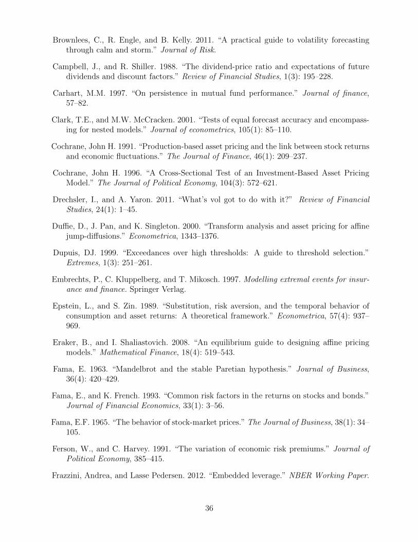
Brownlees, C., R. Engle, and B. Kelly. 2011. “A practical guide to volatility forecastingthrough calm and storm.” Journal of Risk.

Campbell, J., and R. Shiller. 1988. “The dividend-price ratio and expectations of futuredividends and discount factors.” Review of Financial Studies, 1(3): 195–228.

Carhart, M.M. 1997. “On persistence in mutual fund performance.” Journal of finance,57–82.

Clark, T.E., and M.W. McCracken. 2001. “Tests of equal forecast accuracy and encompass-ing for nested models.” Journal of econometrics, 105(1): 85–110.

Cochrane, John H. 1991. “Production-based asset pricing and the link between stock returnsand economic fluctuations.” The Journal of Finance, 46(1): 209–237.

Cochrane, John H. 1996. “A Cross-Sectional Test of an Investment-Based Asset PricingModel.” The Journal of Political Economy, 104(3): 572–621.

Drechsler, I., and A. Yaron. 2011. “What’s vol got to do with it?” Review of FinancialStudies, 24(1): 1–45.

Duffie, D., J. Pan, and K. Singleton. 2000. “Transform analysis and asset pricing for affinejump-diffusions.” Econometrica, 1343–1376.

Dupuis, DJ. 1999. “Exceedances over high thresholds: A guide to threshold selection.”Extremes, 1(3): 251–261.

Embrechts, P., C. Kluppelberg, and T. Mikosch. 1997. Modelling extremal events for insur-ance and finance. Springer Verlag.

Epstein, L., and S. Zin. 1989. “Substitution, risk aversion, and the temporal behavior ofconsumption and asset returns: A theoretical framework.” Econometrica, 57(4): 937–969.

Eraker, B., and I. Shaliastovich. 2008. “An equilibrium guide to designing affine pricingmodels.” Mathematical Finance, 18(4): 519–543.

Fama, E. 1963. “Mandelbrot and the stable Paretian hypothesis.” Journal of Business,36(4): 420–429.

Fama, E., and K. French. 1993. “Common risk factors in the returns on stocks and bonds.”Journal of Financial Economics, 33(1): 3–56.

Fama, E.F. 1965. “The behavior of stock-market prices.” The Journal of Business, 38(1): 34–105.

Ferson, W., and C. Harvey. 1991. “The variation of economic risk premiums.” Journal ofPolitical Economy, 385–415.

Frazzini, Andrea, and Lasse Pedersen. 2012. “Embedded leverage.” NBER Working Paper.

36

Gabaix, X. 2009. “Power laws in economics and finance.” Annual Review of Economics,1(1).

Gabaix, X., P. Gopikrishnan, V. Plerou, and H. Stanley. 2006. “Institutional investors andstock market volatility.” Quarterly Journal of Economics, 121(2): 461–504.

Gabaix, Xavier. 2012. “Variable rare disasters: An exactly solved framework for ten puzzlesin macro-finance.” The Quarterly Journal of Economics, 127(2): 645–700.

Galbraith, J.W., and S. Zernov. 2004. “Circuit breakers and the tail index of equity returns.”Journal of Financial Econometrics, 2(1): 109–129.

Gnedenko, B., and A. Kolmogorov. 1968. Limit distributions for sums of independent randomvariables. Addison-Wesley.

Gopikrishnan, P., V. Plerou, L.A.N. Amaral, M. Meyer, and H.E. Stanley. 1999. “Scal-ing of the distribution of fluctuations of financial market indices.” Physical Review E,60(5): 5305.

Goyal, A., and I. Welch. 2008. “A comprehensive look at the empirical performance of equitypremium prediction.” Review of Financial Studies, 21(4): 1455–1508.

Hill, B. 1975. “A simple general approach to inference about the tail of a distribution.” TheAnnals of Statistics, 3: 1163–1174.

Hill, J.B. 2010. “On tail index estimation for dependent, heterogeneous data.” EconometricTheory, 26(05): 1398–1436.

Hodrick, R. 1992. “Dividend yields and expected stock returns: Alternative procedures forinference and measurement.” Review of Financial Studies, 5(3): 357–386.

Hols, M.C.A.B., and C.G. De Vries. 1991. “The limiting distribution of extremal exchangerate returns.” Journal of Applied Econometrics, 6(3): 287–302.

Jansen, D.W., and C.G. De Vries. 1991. “On the frequency of large stock returns: puttingbooms and busts into perspective.” The Review of Economics and Statistics, 18–24.

Karakaya, Mete. 2013. “Expected returns, volatility, and other characteristics in individualequity option markets.” University of Chicago Working Paper.

Kearns, P., and A. Pagan. 1997. “Estimating the density tail index for financial time series.”Review of Economics and Statistics, 79(2): 171–175.

Kelly, B. 2011. “The dynamic power law model.” Chicago Booth Working Paper.

Koijen, R., H. Lustig, and S. Van Nieuwerburgh. 2010. “The Cross-Section and Time-Seriesof Stock and Bond Returns.” Chicago Booth Working Paper.

Krasker, W. 1980. “The “peso problem” in testing the efficiency of forward exchange mar-kets.” Journal of Monetary Economics, 6(2): 269–276.

37

Lettau, M., and S. Ludvigson. 2001a. “Consumption, aggregate wealth, and expected stockreturns.” Journal of Finance, 815–849.

Lettau, M., and S. Ludvigson. 2001b. “Resurrecting the (C) CAPM: A cross-sectional testwhen risk premia are time-varying.” Journal of Political Economy, 109(6): 1238–1287.

Lustig, H., and S. Van Nieuwerburgh. 2005. “Housing collateral, consumption insurance,and risk premia: An empirical perspective.” The Journal of Finance, 60(3): 1167–1219.

Mandelbrot, B. 1963. “The variation of certain speculative prices.” Journal of business,36(4): 394.

Matthys, G., and J. Beirlant. 2000. “Adaptive threshold selection in tail index estimation.”Extremes and Integrated Risk Management, 37–49.

Newey, W., and K. West. 1987. “A simple, positive semi-definite, heteroskedasticity andautocorrelation consistent covariance matrix.” Econometrica, 55: 703–708.

Officer, R.R. 1972. “The distribution of stock returns.” Journal of the American StatisticalAssociation, 807–812.

Pan, J., and A. Poteshman. 2006. “The information in option volume for future stockprices.” Review of Financial Studies, 871–908.

Pastor, L., and R. Stambaugh. 2003. “Liquidity risk and expected stock returns.” Journalof Political Economy, 111(3).

Quintos, C., Z. Fan, and P.C.B. Philips. 2001. “Structural change tests in tail behaviourand the Asian crisis.” Review of Economic Studies, 68(3): 633–663.

Resnick, S., and C. Starica. 1995. “Consistency of Hill’s estimator for dependent data.”Journal of Applied Probability, 139–167.

Richardson, M., and T. Smith. 1991. “Tests of financial models in the presence of overlappingobservations.” Review of Financial Studies, 227–254.

Rietz, T. 1988. “The equity risk premium: A solution.” Journal of Monetary Economics,22(1): 117–131.

Rootzen, H., M.R. Leadbetter, and L. Haan. 1998. “On the distribution of tail array sumsfor strongly mixing stationary sequences.” The Annals of Applied Probability, 8(3): 868–885.

Wachter, Jessica A. 2013. “Can Time-Varying Risk of Rare Disasters Explain AggregateStock Market Volatility?” The Journal of Finance, 68(3): 987–1035.

Wagner, N. 2003. “Estimating financial risk under time-varying extremal return behavior.”OR Spectrum, 25(3): 317–328.

Werner, T., and C. Upper. 2004. “Time variation in the tail behavior of Bund futurereturns.” Journal of Futures Markets, 24(4): 387–398.

Zhang, Lu. 2005. “The value premium.” The Journal of Finance, 60(1): 67–103.

38

Figure 1: Risk Premium, Investment and Tail Risk

Panel A: Equity Risk Premium Panel B: Investment

0.5 0.55 0.6 0.65 0.7 0.75 0.8 0.85 0.9 0.95

0.1

0.2

0.3

0.4

0.5

0.6

λ

E[R

i]/Rf −

1 (

%)

λ ± 0.01λ ± 0.02λ ± 0.03λ ± 0.04

0.5 0.55 0.6 0.65 0.7 0.75 0.8 0.85 0.9 0.95

0.22

0.24

0.26

0.28

0.3

0.32

0.34

0.36

λ

I/K

λ ± 0.01λ ± 0.02λ ± 0.03λ ± 0.04

Notes: The figure plots the equilibrium equity risk premium (Panel A) and investment per unit of capital(Panel B) as a function of initial tail risk for the example economy presented in Section 2.3.

Figure 2: Tail Exponent Estimates and Subsequent Market Returns

1963 1967 1971 1975 1979 1983 1987 1991 1995 1999 2003 2007 2010−4

−3

−2

−1

0

1

2

3

Tail

Next 3−Year Return

Notes: Plotted is the monthly estimated tail risk time series. Tail estimates are calculated each month bypooling daily returns of NYSE/AMEX/NASDAQ stocks. Also plotted in each month t is the realized marketreturn over the three years following month t. To emphasize comparison, both series have been scaled tohave mean zero and variance one.

39

Figure 3: Tail Threshold and Aggregate Market Volatility

1963 1967 1971 1975 1979 1983 1987 1991 1995 1999 2003 2007 2010−3

−2

−1

0

1

2

3

4

5

6

Realized Market VolatilityTail Threshold

Notes: Plotted is the monthly tail threshold series. The threshold is the absolute value of the fifth percentileof monthly pooled daily returns of NYSE/AMEX/NASDAQ stocks. Also plotted is the (annualized) monthlyrealized volatility of the CRSP value-weighted index. To emphasize comparison, both series have been scaledto have the mean zero and variance one.

Figure 4: Correlogram: Sales Growth Tails and Stock Return Tails

−4 −3 −2 −1 0 1 2 3 4 0

5

10

15

20

25

30

35

j

Co

rrela

tio

n (

%)

Notes: The figure shows the correlogram of the estimated return tail series in quarter t with the sales growthtail series in quarter t + j for j = −4, ..., 4. Correlation estimates are reported in percentages and testsare conducted using Newey-West standard errors with four quarters of lags. Black and gray bars denotesignificant correlation at the 1% and 2.5% level, respectively.

40

Fig

ure

5:Tail

Risk

Impulse

Resp

onse

Functions

Pan

elA

:In

du

stri

alP

rod

uct

ion

Pan

elB

:E

mp

loym

ent

-1-.50.51

% Impact on Industrial Production

06

1218

2430

36M

onth

s af

ter t

he ta

il ris

k sh

ock

-2-1012

% Impact on Industrial Production0

612

1824

3036

Mon

ths

afte

r the

vol

atili

ty s

hock

-1-.50.5

% Impact on Employment

06

1218

2430

36M

onth

s af

ter t

he ta

il ris

k sh

ock

-2-101

% Impact on Employment

06

1218

2430

36M

onth

s af

ter t

he v

olat

ility

sho

ck

Pan

elC

:G

ross

Pri

vate

Dom

esti

cIn

vest

men

tP

anel

D:

Pri

vate

Non

resi

den

tial

Fix

edIn

vest

men

t

-4-2024

% Impact on Private Non-Residential Fixed Investment

01

23

45

67

89

1011

12Q

uarte

rs a

fter t

he ta

il ris

k sh

ock

-3-2-10

% Impact on Private Non-Residential Fixed Investment

01

23

45

67

89

1011

12Q

uarte

rs a

fter t

he v

olat

ility

sho

ck

-6-4-2024

% Impact on Gross Domestic Private Investment

01

23

45

67

89

1011

12Q

uarte

rs a

fter t

he ta

il ris

k sh

ock

-4-3-2-101

% Impact on Gross Domestic Private Investment

01

23

45

67

89

1011

12Q

uarte

rs a

fter t

he v

olat

ility

sho

ck

Notes:

Th

efi

gure

plo

tsth

ees

tim

ated

imp

act

ofu

nce

rtai

nty

shock

son

ind

ust

rial

pro

du

ctio

n(P

anel

A),

emp

loym

ent

(Pan

elB

),gr

oss

pri

vate

dom

esti

cin

vest

men

ts(P

anel

C)

an

dp

riva

ten

onre

sid

enti

alfi

xed

inves

tmen

ts(P

anel

D).

Wit

hin

each

pan

el,

the

imp

uls

ere

spon

sefo

ra

one

stan

dard

dev

iati

on

shock

tota

ilri

skon

the

left

and

for

aon

est

and

ard

dev

iati

onsh

ock

tovo

lati

lity

onth

eri

ght.

For

ind

ust

rial

pro

du

ctio

nan

dem

plo

ym

ent

we

esti

mate

am

onth

lyV

AR

that

incl

ud

esst

ock

mar

ket

vola

tili

ty,

tail

risk

,F

eder

alF

un

ds

Rat

e,lo

gav

erag

eh

ourl

yea

rnin

gs,

the

log

con

sum

erp

rice

ind

ex,

hou

rs,

log

emp

loym

ent,

and

log

ind

ust

rial

pro

du

ctio

nov

erth

ep

erio

dJu

ly19

63to

Ju

ne

2008

.B

ecau

sein

ves

tmen

tis

only

avai

lab

lequ

arte

rly,

Pan

els

Can

dD

are

for

qu

arte

rly

triv

aria

teV

AR

sth

atin

clu

des

stock

mar

ket

vola

tili

ty,

tail

risk

,an

dag

greg

ate

inve

stm

ent

over

the

per

iod

1963

Q3

to2008

Q2.

Bec

au

sein

du

stri

alp

rod

uct

ion

and

emp

loym

ent

are

only

calc

ula

ted

for

the

man

ufa

ctu

rin

gse

ctor

,th

eV

AR

sin

Pan

els

Aan

dB

use

tail

risk

esti

mate

dfr

om

the

cros

sse

ctio

nof

man

ufa

ctu

rin

gfirm

s.D

ash

edli

nes

are

1st

and

ard

-err

orb

and

s.

41

Table 1: Correlations With Risk Measures Based on S&P 500 Index Options

(1) (2) (3) (4) (5) (6)

Tail (1) 1.00

-

R.N. Skewness (2) -0.30 1.00

0.02 -

R.N. Kurtosis (3) 0.33 -0.92 1.00

0.01 <0.01 -

Put/Call Ratio (4) 0.42 -0.49 0.38 1.00

0.01 <0.01 0.01 -

OTM Put IV Slope (5) -0.17 0.22 -0.25 0.00 1.00

0.15 0.06 0.05 0.97 -

Variance Risk Premium (6) 0.04 0.10 -0.17 -0.22 -0.10 1.00

0.67 0.13 0.02 0.03 0.41 -

Notes: The table reports monthly correlations between tail risk estimated from the cross section ofreturns on NYSE/AMEX/NASDAQ stocks, and various options-based risk measures derived fromprices of S&P 500 index options from 1996 to 2010. Below each correlation estimate we report itsp-value in italics (based on Newey-West (1987) standard errors with 12 lags). Risk-neutral skewnessand kurtosis are estimated following Bakshi, Kapadia and Madan (2003). The slope of the impliedvolatility smirk for out-of-the-money S&P 500 put options is estimated from a regression of put-implied volatility on option moneyness (strike over spot) using options with Black-Scholes deltagreater than −0.5 and one month to maturity. The put/call ratio measures the number of newput contracts purchased by non-market makers relative to new calls purchases and comes from theCBOE. The variance risk premium is the difference between the squared VIX and realized varianceof the S&P 500 index and comes from Hao Zhou’s website. Risk neutral moments and the IV slopeonly use options with positive open interest. These three measures are estimated separately for twosets of options with maturities closest to 30 days (one set for the maturity just greater than 30 days,and one set for the maturity just less than 30 days), then the estimates are linearly interpolated toarrive at a daily measure with constant 30-day maturity. Finally, all daily measures are averagedwithin the month to arrive at a monthly time series.

42

Table 2: Correlation of Dynamic Tail Risk Estimates Among Subgroups

Panel A: By Industry (1) (2) (3) (4) (5)

Consumer (1) 1.00

Manufacturing (2) 0.85 1.00

Technology (3) 0.81 0.75 1.00

Healthcare (4) 0.67 0.58 0.69 1.00

Other (5) 0.86 0.87 0.77 0.57 1.00

Panel B: By Size (1) (2) (3) (4) (5)

Small (1) 1.00

(2) 0.71 1.00

(3) 0.59 0.77 1.00

(4) 0.47 0.66 0.76 1.00

Big (5) 0.38 0.56 0.67 0.86 1.00

Notes: The table reports time series correlation between monthly tail risk series estimated from the crosssection of stocks in each of the five Fama-French industry SIC classifications (Panel A) and in each sizequintile (Panel B) for 1963 to 2010.

43

Tab

le3:

MarketReturnPredictability:UnivariatePredictorPerformance

On

em

onth

hor

izon

On

eye

arh

oriz

onT

hre

eye

ar

hori

zon

Fiv

eye

ar

hori

zon

Coeff

.t -stat.

R2

Coeff

.t-stat.

R2

Coeff

.t-stat.

R2

Coeff

.t-stat.

R2

Tai

l4.

542.08

0.7

4.02

2.04

6.1

3.65

2.40

16.6

3.1

62.65

20.9

Book

-to-

mar

ket

2.49

1.14

0.2

3.12

1.34

3.7

2.26

1.12

6.3

2.7

61.82

15.5

Def

ault

retu

rnsp

read

2.96

1.36

0.3

0.43

0.57

0.1

0.28

1.22

0.1

0.0

20.18

0.0

Def

ault

yie

ldsp

read

2.82

1.29

0.3

2.93

1.63

3.2

1.90

1.19

4.5

3.0

42.80

14.8

Div

iden

dp

ayou

tra

tio

0.79

0.36

0.0

1.55

0.90

0.9

1.90

1.38

4.4

3.5

53.68

10.4

Div

iden

dp

rice

rati

o4.

241.94

0.7

4.75

2.07

8.5

4.34

2.56

23.1

4.1

93.60

36.5

Ear

nin

gsp

rice

rati

o3.

231.48

0.4

3.16

1.48

3.8

2.54

1.65

8.0

3.7

52.90

21.5

Infl

atio

n-5

.07

-2.33

0.9

-1.6

7-1.09

1.1

0.40

0.40

0.2

0.8

10.71

1.2

Lon

gte

rmre

turn

5.40

2.48

1.1

1.83

3.04

1.3

0.56

2.16

0.4

0.6

82.69

0.9

Lon

gte

rmyie

ld1.

950.89

0.1

3.72

1.70

5.2

4.26

3.48

21.9

4.5

95.17

40.5

Net

equ

ity

exp

ansi

on-0

.71

-0.33

0.0

-0.0

3-0.01

0.0

0.44

0.27

0.2

-0.1

4-0.13

0.0

Sto

ckvol

atilit

y-6

.24

-2.87

1.4

0.61

0.50

0.1

0.07

0.13

0.0

0.0

10.03

0.0

Ter

mS

pre

ad2.

281.04

0.2

2.57

1.35

2.5

2.53

1.69

7.7

2.1

81.72

9.1

Tre

asu

ryb

ill

rate

0.44

0.20

0.0

1.78

0.80

1.2

2.33

1.48

6.3

3.0

02.56

15.6

Var

.R

isk

Pre

m.*

11.2

23.45

4.5

3.32

2.18

3.5

0.63

0.33

0.3

-1.2

4-1.90

1.1

R.N

.S

kew

nes

s*-0

.74

-0.17

0.0

-1.1

3-0.34

0.3

-0.3

5-0.18

0.1

-0.3

2-0.37

0.4

R.N

.K

urt

osis

*-1

.82

-0.43

0.1

1.56

0.53

0.6

1.16

0.48

1.0

0.5

60.59

1.1

Notes:

Th

eta

ble

rep

orts

resu

lts

from

mon

thly

pre

dic

tive

regr

essi

ons

ofC

RS

Pva

lue-

wei

ghte

dm

arket

ind

exre

turn

sov

eron

em

onth

,on

eye

ar,

thre

eyea

ran

dfi

veyea

rh

oriz

ons.

Th

efi

rst

row

rep

ort

sfo

reca

stin

gre

sult

sb

ased

onou

res

tim

ated

tail

risk

tim

ese

ries

.N

ext

are

resu

lts

from

pre

dic

tors

stu

die

din

the

surv

eyof

Goy

alan

dW

elch

(2008

)(d

ata

from

Am

itG

oyal

’sw

ebsi

te),

asw

ell

asth

eva

rian

ceri

skp

rem

ium

(Bol

lers

lev,

Tau

chen

an

dZ

hou

(2009),

dat

afr

omH

aoZ

hou

’sw

ebsi

te)

and

risk

neu

tral

skew

nes

san

dku

rtos

isb

ased

onS

&P

500

ind

exop

tion

s.(∗

)d

enot

esth

ata

vari

able

isav

ail

ab

lefo

ra

tru

nca

ted

sam

ple

:T

he

vari

ance

risk

pre

miu

mis

only

avai

lab

leb

egin

nin

gin

1990

and

risk

neu

tral

mom

ents

are

only

avai

lab

leb

egin

nin

gin

1996.

Bec

au

seov

erla

pp

ing

month

lyob

serv

atio

ns

are

use

d,

test

stat

isti

csar

eca

lcu

late

du

sin

gH

od

rick

’s(1

992)

stan

dar

der

ror

corr

ecti

onfo

rov

erla

pp

ing

data

wit

hla

gle

ngt

heq

ual

toth

enu

mb

erof

mon

ths

inea

chh

oriz

on.

For

com

par

ison

,re

por

ted

pre

dic

tive

coeffi

cien

tsar

esc

aled

tob

ein

terp

rete

das

the

per

centa

ge

chan

gein

exp

ecte

dan

nu

alm

arket

retu

rns

resu

ltin

gfr

oma

one

stan

dar

dd

evia

tion

incr

ease

inea

chp

red

icto

rva

riab

le.

44

Table 4: Market Return Predictability: Bivariate Predictor Performance

One month horizon One year horizon

Tail Tail Tail Tail

Coeff. t-stat. Coeff. t-stat. R2 Coeff. t-stat. Coeff. t-stat. R2

Book-to-market 4.68 2.15 2.73 1.25 1.0 4.19 2.27 3.34 1.49 10.3

Default return spread 4.57 2.10 3.01 1.38 1.1 4.02 2.05 0.46 0.61 6.2

Default yield spread 4.32 1.97 2.42 1.10 1.0 3.78 2.01 2.58 1.51 8.6

Dividend payout ratio 4.67 2.13 1.26 0.58 0.8 4.22 2.19 1.98 1.14 7.6

Dividend price ratio 4.32 1.98 4.00 1.84 1.3 3.77 2.07 4.54 2.03 13.8

Earnings price ratio 4.22 1.92 2.73 1.25 1.0 3.70 1.92 2.72 1.31 8.9

Inflation 4.12 1.89 -4.70 -2.16 1.5 3.90 2.01 -1.32 -0.88 6.7

Long term return 4.04 1.85 5.00 2.29 1.6 3.88 1.99 1.44 2.82 6.9

Long term yield 4.34 1.91 0.71 0.31 0.8 3.22 1.54 2.80 1.23 8.8

Net equity expansion 4.86 2.10 0.93 0.40 0.8 4.53 2.31 1.51 0.53 6.9

Stock volatility 4.04 1.86 -5.90 -2.71 2.0 4.10 2.07 0.95 0.77 6.4

Term Spread 4.27 1.83 0.80 0.34 0.8 3.56 1.74 1.33 0.67 6.7

Treasury bill rate 4.53 2.07 0.18 0.08 0.8 3.93 1.99 1.55 0.74 7.0

Three year horizon Five year horizon

Tail Tail Tail Tail

Coeff. t-stat. Coeff. t-stat. R2 Coeff. t-stat. Coeff. t-stat. R2

Book-to-market 3.77 2.56 2.44 1.40 24.0 3.31 2.55 2.92 2.31 38.4

Default return spread 3.66 2.40 0.34 1.61 16.7 3.16 2.65 0.04 0.39 20.9

Default yield spread 3.51 2.25 1.57 1.14 19.6 2.83 2.28 2.57 2.79 31.2

Dividend payout ratio 3.86 2.57 2.27 1.72 22.8 3.36 2.80 3.97 4.55 33.9

Dividend price ratio 3.40 2.47 4.13 2.65 37.5 2.88 2.47 3.99 3.66 53.8

Earnings price ratio 3.40 2.28 2.14 1.54 22.2 2.84 2.21 3.38 2.77 38.2

Inflation 3.72 2.47 0.73 0.83 17.2 3.30 2.61 1.25 1.26 23.6

Long term return 3.63 2.38 0.18 0.85 16.6 3.13 2.63 0.28 1.74 21.1

Long term yield 2.63 1.72 3.46 2.53 29.7 1.99 1.74 3.94 4.68 48.0

Net equity expansion 4.31 2.68 1.91 1.14 20.6 3.73 2.71 1.62 1.49 24.4

Stock volatility 3.69 2.41 0.38 0.67 16.8 3.17 2.66 0.24 0.66 21.0

Term Spread 3.17 2.03 1.41 1.06 18.7 2.77 2.46 1.11 0.99 23.0

Treasury bill rate 3.51 2.43 2.07 1.45 21.6 2.98 2.28 2.77 2.75 34.2

Notes: The table reports results from monthly predictive regressions of CRSP value-weighted market indexreturns over one month, one year, three year and five year horizons. The table repeats the analysis of Table3, but instead reports bivariate regressions that include each alternative predictor alongside the estimatedtail risk process. For each horizon, the first two columns are the coefficient estimate and t-statistic for thetail risk process, while the third and fourth columns are the coefficient and t-statistic for the alternativepredictor. Because overlapping monthly observations are used, test statistics are calculated using Hodrick’s(1992) standard error correction for overlapping data with lag length equal to the number of months ineach horizon. For comparison, reported predictive coefficients are scaled to be interpreted as the percentagechange in expected annual market returns resulting from a one standard deviation increase in each predictorvariable.

45

Table 5: Market Return Predictability: Out-of-Sample R2 (%)

One One Three Five

Month Year Years Years

Tail 0.3 4.5∗ 15.7∗ 20.1∗

Book-to-market -1.6 -9.9 -14.5 -34.0

Default return spread -0.9 -0.6 -0.4 -0.3

Default yield spread -0.6 -0.5 -9.2 3.0

Dividend payout ratio -1.7 -23.6 -13.7 -46.4

Dividend price ratio -1.3 -6.5 -4.4 15.8∗

Earnings price ratio -1.8 -15.6 -9.3 1.3

Inflation -0.4 -4.0 -3.1 -11.4

Long term return -0.1 0.9 -0.2 0.8

Long term yield -0.9 -4.6 20.6∗ 10.2∗

Net equity expansion -0.8 -10.6 -6.6 -9.0

Stock volatility -2.5 -25.0 -28.1 -22.1

Term Spread -0.6 -2.9 -7.1 7.0

Treasury bill rate -1.3 -9.2 5.8 -14.4

Notes: The table reports the out-of-sample forecasting R2 in percent from predictive regressions of CRSPvalue-weighted market index returns over one month, one year, three year and five year horizons. In eachmonth t (beginning at t = 120 to allow for a sufficiently large initial estimation period), we estimate rollingunivariate forecasting regressions of monthly market returns on the estimated tail risk series and alternativepredictors. Predictive coefficient estimates only use data through date t, which are then used to forecastreturns at t + 1. The out-of-sample R2 is calculated as 1 −

∑t(rm,t+1 − rm,t+1|t)

2/∑

t(rm,t+1 − rm,t)2,

where rm,t+1|t is the out-of-sample forecast of the t+ 1 return based only on data through t, and rm,t is thehistorical average market return through t. A negative R2 implies that the predictor performs worse thansetting forecasts equal to the sample mean. Due to the short time series for the variance risk premium out-of-sample forecasts are infeasible. A star (∗) beside an estimate denotes that it is statistically significant at the5% level or better based on the Clark and McCracken (2001) ENC-NEW test of out-of-sample predictability.

46

Table 6: Tail Beta-Sorted Portfolio Returns

Low 2 3 4 High High-Low t-stat

Panel A: Twelve Month Returns

Equal-Weighted

Average Return 1.14 1.24 1.31 1.39 1.48 0.33 2.48

CAPM Alpha 0.10 0.31 0.4 0.47 0.49 0.38 2.63

FF Alpha -0.13 0.01 0.09 0.17 0.20 0.33 2.85

FF + Mom Alpha 0.04 0.10 0.15 0.22 0.26 0.21 2.15

FF + Mom + Liq Alpha 0.02 0.10 0.17 0.24 0.27 0.25 2.54

Value-Weighted

Average Return 0.86 0.99 1.03 1.14 1.21 0.35 2.15

CAPM Alpha -0.17 0.05 0.12 0.20 0.18 0.35 2.10

FF Alpha -0.20 -0.02 0.08 0.19 0.25 0.45 3.00

FF + Mom Alpha -0.02 0.07 0.11 0.18 0.32 0.34 2.24

FF + Mom + Liq Alpha -0.08 0.08 0.14 0.21 0.35 0.43 2.93

Panel B: One Month Returns

Equal-Weighted

Average Return 1.14 1.24 1.28 1.4 1.45 0.31 2.12

CAPM Alpha 0.10 0.31 0.37 0.48 0.47 0.37 2.52

FF Alpha -0.11 0.02 0.09 0.19 0.19 0.30 2.22

FF + Mom Alpha -0.06 0.06 0.11 0.22 0.24 0.29 2.14

FF + Mom + Liq Alpha -0.08 0.06 0.12 0.24 0.26 0.34 2.50

Value-Weighted

Average Return 0.84 0.96 0.98 1.18 1.20 0.36 2.00

CAPM Alpha -0.19 0.03 0.08 0.25 0.18 0.37 2.08

FF Alpha -0.19 -0.04 0.05 0.22 0.27 0.46 2.58

FF + Mom Alpha -0.16 -0.03 0.03 0.18 0.30 0.45 2.22

FF + Mom + Liq Alpha -0.21 -0.03 0.05 0.21 0.35 0.55 2.78

Notes: The table reports monthly return statistics for portfolios formed on the basis of tail risk beta.Each month stocks are sorted into quintile portfolios based on predictive tail loadings that are estimatedfrom monthly data over the previous ten years. Portfolios are based on NYSE/AMEX/NASDAQ stockswith CRSP share codes 10 and 11. Panel A reports equal- and value-weighted average out-of-sample twelvemonth holding period portfolio returns and Panel B reports out-of-sample one month holding period portfolioreturns. The table also reports portfolio alphas from regressions of portfolio returns using the Fama-Frenchthree-factor model as well as extended four and five-factor models controlling for momentum and liquidity(Pastor and Stambaugh (2003)) factors. The right-most columns report results for the high minus low zeronet investment portfolio that is long quintile portfolio five and short quintile one and associated t-statistics.For twelve month returns, t-statistics use Newey-West (1987) standard errors based on twelve lags. Stockswith prices below $5 at the portfolio formation date are excluded.

47

Table 7: Double-Sorted Portfolio Returns

Low 2 3 High High-Low t-stat

Panel A: Firm Size and Tail Risk BetaEqual-Weighted

Small 0.10 0.16 0.26 0.15 0.05 0.372 -0.07 0.09 0.24 0.23 0.30 2.543 -0.07 0.11 0.15 0.24 0.31 2.11Large -0.08 0.03 0.08 0.27 0.35 1.94

Value-WeightedSmall 0.08 0.10 0.19 0.10 0.01 0.102 -0.07 0.06 0.23 0.24 0.31 2.573 -0.07 0.10 0.16 0.23 0.30 2.03Large -0.14 0.01 0.09 0.20 0.34 1.69

Panel B: Idiosyncratic Volatility and Tail Risk BetaEqual-Weighted

Low IV 0.15 0.16 0.22 0.30 0.15 1.522 0.10 0.17 0.25 0.33 0.22 2.333 0.11 0.13 0.24 0.30 0.19 2.02High IV -0.10 -0.01 0.08 0.11 0.21 2.02

Value-WeightedLow IV 0.12 0.11 0.14 0.30 0.18 1.532 -0.01 0.09 0.16 0.30 0.30 2.253 -0.05 0.07 0.18 0.30 0.36 2.32High IV -0.17 -0.09 0.11 0.28 0.45 2.61

Panel C: Downside Beta and Tail Risk BetaEqual-Weighted

Low Down Beta 0.20 0.18 0.25 0.28 0.08 0.762 0.08 0.12 0.20 0.29 0.21 1.923 0.06 0.13 0.21 0.29 0.24 2.43High Down Beta -0.04 0.06 0.08 0.17 0.21 1.97

Value-WeightedLow Down Beta 0.07 0.11 0.14 0.40 0.33 2.152 0.11 0.14 0.19 0.40 0.29 1.723 -0.15 0.01 0.03 0.16 0.31 2.26High Down Beta -0.04 -0.04 0.25 0.16 0.20 0.94

Notes: The table reports monthly 4-factor (Fama-French and momentum) alphas for double-sorted port-folios that are formed on the basis of tail risk loadings and size (Panel A), idiosyncratic volatility (PanelB), or downside beta (Panel C). Each month stocks are independently sorted into four quartile portfoliosbased each of these characteristics, and four quartiles along another dimension based on predictive tailloadings. Loading are estimated from monthly data over the previous ten years. Portfolios are based onNYSE/AMEX/NASDAQ stocks with CRSP share codes 10 and 11. The right-most columns report resultsfor the high minus low zero net investment portfolio that is long quartile portfolio four and short quartileone. The portfolios are held for one year t-statistics use the Newey-West (1987) standard errors based ontwelve lags. Stocks with prices below $5 at the portfolio formation date are excluded.

48

Table 8: Moneyness-Sorted Short Put Portfolios

DOTM OTM ATM ITM DITM DOTM−DITM t-stat R2

Panel A: Delta-hedged

Tail Risk Beta 7.17 4.20 2.89 1.07 0.01 7.17 2.39 -

Average Return 19.46 16.64 10.21 5.31 2.80 16.66 3.55 94.10

CAPM Alpha 18.50 15.88 9.74 5.01 2.53 15.96 3.43 93.91

FF Alpha 18.05 15.28 9.52 4.90 2.51 15.54 3.31 94.54

FF + Mom Alpha 17.87 15.21 9.51 4.96 2.62 15.25 3.18 94.36

FF + Mom + Liq Alpha 15.83 14.17 9.17 4.94 2.68 13.15 2.82 92.27

Panel B: Delta-hedged and Leverage-adjusted

Tail Risk Beta 0.79 0.46 0.25 0.08 0.00 0.79 2.43 -

Average Return 1.63 1.57 1.28 0.99 0.56 1.07 2.43 79.15

CAPM Alpha 1.55 1.49 1.22 0.94 0.50 1.05 2.29 77.79

FF Alpha 1.55 1.44 1.20 0.91 0.50 1.04 2.28 80.79

FF + Mom Alpha 1.54 1.43 1.22 0.93 0.54 1.00 2.07 80.51

FF + Mom + Liq Alpha 1.29 1.32 1.16 0.94 0.56 0.73 1.54 65.97

Notes: We form portfolios of individual equity put options on the basis of option moneyness following theapproach of Frazzini and Pedersen (2012) over 1996 to 2010. Moneyness is defined as absolute value of theBlack-Scholes delta of an option, and the five portfolios are deep out-of-the-money (DOTM, |∆| < 0.20),out-of-the-money (OTM, 0.20 ≤ |∆| < 0.40), at-the-money (ATM, 0.40 ≤ |∆| < 0.60), in-the-money (ITM,0.60 ≤ |∆| < 0.80) and deep-in-the-money (DITM, 0.80 ≤ |∆|). We also report results from the differencebetween the DOTM and DITM portfolios. Portfolio rebalancing dates and one month holding periodscorrespond to the monthly expiration schedule. We compute the return of selling an put with one monthto maturity on the first trading day following the an expiration date and holding it to the next month’sexpiration. Each put position is delta-hedged daily. Tail betas are estimated from a predictive regression ofeach portfolio’s return on lagged tail risk (which is recalculated to correspond to the option portfolio formationschedule and variance standardized). Due to the relatively short sample for options data we estimate a singlein-sample predictive coefficient for each portfolio. The far right column reports the correlation between tailbeta and portfolio alpha across the five portfolios. Panel A reports results for monthly returns on delta-hedged short put option portfolios. Panel B reports results for leverage-adjusted versions of these portfoliosfollowing the procedure in Karakaya (2013).

49