Embed Size (px)
Citation preview

Laboratório de Modelagem, Análise e Controle de Sistemas Não-Lineares
Departamento de Engenharia Eletrônica
Universidade Federal de Minas Gerais
Av. Antônio Carlos 6627, 31270-901 Belo Horizonte, MG Brasil
Fone: +55 31 3409-3470
Takagi-Sugeno Models in a TensorProduct Approach
Exploiting the representation
Víctor Costa da Silva Campos
Advisor: Prof. Dr. Leonardo Antônio Borges TôrresCo-Advisor: Prof. Dr. Reinaldo Martinez Palhares
Belo Horizonte, July 24, 2015


Laboratório de Modelagem, Análise e Controle de Sistemas Não-Lineares
Departamento de Engenharia Eletrônica
Universidade Federal de Minas Gerais
Av. Antônio Carlos 6627, 31270-901 Belo Horizonte, MG Brasil
Fone: +55 31 3409-3470
Takagi-Sugeno Models in a TensorProduct Approach
Exploiting the representation
Thesis presented to the Graduate Pro-gram in Electrical Engineering (PPGEE) ofthe Universidade Federal de Minas Gerais(UFMG) as a partial requirement to obtain-ing the degree of Doctor in Electrial Engi-neering
Víctor Costa da Silva Campos
Advisor: Prof. Dr. Leonardo Antônio Borges TôrresCo-Advisor: Prof. Dr. Reinaldo Martinez Palhares
UNIVERSIDADE FEDERAL DE MINAS GERAISESCOLA DE ENGENHARIA
PROGRAMA DE PÓS-GRADUAÇÃO EM ENGENHARIA ELÉTRICA
Belo HorizonteJuly 24, 2015


Acknowledgements
These were four long years, and I thoroughly enjoyed all that I’ve learned and the life I’ve lead duringthem. And because of that I’m very grateful.
I’m grateful to god for this wonderful opportunity.To Léo and Reinaldo for putting up with me through all of these 6 and a half years. I’m pretty sure I
wasn’t the model graduate student an advisor would wish for (given all the random stuff I do), but yousure made me feel like it! I couldn’t have asked for better advisors.
To CNPq for the funding while I was here at UFMG, and CAPES for the funding while I was abroad(specially for the people responsible for my grant while I was abroad due to my sandwich internship notbeing like the usuals).
To Thierry and João for agreeing to advise me while I was in each of their labs. This experience wasamazing, and I only bring good memories from both of them.
To my dear family, for all the love, support and tenderness even while I was away. All of you meanthe world to me. I couldn’t write this without specially thanking those that went out of their way tomake me feel loved and at home, specially when I was abroad. So I’d like to take this moment andthank Jacqueline, Tio Júlio, Tia Ana Maria and Tio Fábio for meeting me in Europe and my parentsAmália and José, my brothers Matheus and Marcos and my soon-to-be sister-in-law Júlia for meetingme in the US!
To my dear old time friends, who are always there, even when I’m not: Mairon, Rafael, Raul, Elvis,Daniel, Augusto, Carol, André.
To my dear (now also old time) friends from UFMG, for making me feel at home wherever we are.Specially, Tales, Cristina, Wendy, Dimas, Leandro, Luciano, Thales, Vitinho, Vinicius, Grazi, Fernanda,Tiago, Jullierme, Rogério, Johnathas, Thiago, Rodrigo, Marcus, Ana e Petrus.
Here’s a shoutout to “beberrões” - I’ll forever be indebted to you guys for making me company,even when I was far away.
To my dancing friends, Ana (too bad it didn’t work out between us), Paulinho, Kleinny and every-one else for reminding me that there’s more to life than just the university.
To all the friends I’ve made while I was in France, in special everyone from LAMIH - AnhTu, Victor,Raymundo, Miguel, Antonio, Rémi - it was a pleasure meeting you all.
To all the friends I’ve made while I was in the US, specially those from CCDC and the SBDC, Hen-rique, Becky, Ya, Michelle, Kunihisa, Masashi, Hari, Kyriakos, Noor. You guys made my life over theresomething memorable that I’ll always cherish.


“A lesson without pain is
meaningless. That’s because no
one can gain without
sacrificing something. But by
enduring that pain and
overcoming it...
...he shall obtain a powerful,
unmatched heart.
A fullmetal heart.”
Edward Elric, FullMetalAchemist Brotherhood


Abstract
Takagi-Sugeno (TS) fuzzy analysis and control techniques extend several results from linear robust con-trol theory to nonlinear systems. However, in many cases, the conditions used do not explore the mem-bership functions’ information aside from the fact that they belong to the standard unit simplex. Inaddition, since we are dealing with nonlinear systems, the use of quadratic Lyapunov functions carriesa certain conservatism.
In this work, we propose different ways to exploit the membership functions’ information in pa-rameter dependent Linear Matrix Inequalities (LMIs) as well as new classes of candidate Lyapunovfunctions that cover other existing classes in the literature.
Asymptotically necessary conditions for parameter dependent LMIs are proposed based on parti-tioning the membership functions’ image space. Such partitions are also used to propose a switchedcontrol law and we present ways to modify the conditions of this controller such that a continuouscontroller can be recovered.
An alternative way to reduce the number of rules of a given Takagi-Sugeno model, based on theHigher Order Singular Value Decomposition (HOSVD), is presented as well as how to model the uncer-tainty introduced by this rule reduction scheme.
We propose the use of local transformations of the membership functions in conjunction with piece-wise fuzzy Lyapunov functions so as to find more relaxed stability conditions than others available inthe literature.
A novel way to deal with the time derivative of the membership functions, in cases where theyare functions of the states, is proposed. This new proposition avoids the use of direct bounds over themembership functions time-derivative, and new stability and stabilization conditions are presented.
Finally, we propose new LMI synthesis conditions based on piecewise-like Lyapunov functions.This class of Lyapunov functions behaves similarly to piecewise functions (in the sense that we can un-derstand that a different function is valid for each region) while using a fuzzy formulation. By adaptingrecent conditions to deal with bounds on the Lyapunov function’s membership functions time deriva-tive, new synthesis conditions are presented to guarantee local stabilization.
v


Resumo
As técnicas de análise e controle de sistemas Takagi-Sugeno (TS) estendem vários resultados de controlerobusto de sistemas lineares para sistemas não-lineares. Entretanto, em muitos dos casos, as condiçõesutilizadas não exploram a informação das funções de pertinência do sistema, com exceção do fato deelas pertencerem ao simplex unitário padrão. Além disso, por se tratarem de sistemas não-lineares, ouso de funções de Lyapunov quadráticas carrega consigo um certo conservadorismo.
Neste trabalho são propostas algumas formas diferentes de se explorar a informação das funções depertinência nas Desigualdades Matriciais Lineares (LMIs) dependentes de parâmetros bem como novasclasses de funções de Lyapunov candidatas que cobrem outras classes existentes na literatura.
São propostas condições assintoticamente necessárias para LMIs dependentes de parâmetros baseadasem partições do espaço imagem das funções de pertinência. Tais partições são também utilizadas parase propor uma lei de controle chaveada de acordo com tais partições e como modificar as condiçõesdessa lei de controle chaveada para que se possa recuperar um controlador contínuo.
Uma maneira alternativa, baseada na Decomposição de Valores Singulares de Alta Ordem (HOSVD)para a redução do número de regras de modelos TS é proposta, bem como formas de se modelar aincerteza introduzida pelo procedimento de redução de regras proposto.
É proposto o uso de transformações locais das funções de pertinência em conjunto com funções deLyapunov fuzzy por partes de modo a se encontrar condições de estabilidade mais relaxadas do queoutras apresentadas na literatura.
Uma nova forma de lidar com a derivada temporal das funções de pertinência é proposta paraos casos em que as funções de pertinência são funções das variáveis de estado somente. Esta novaproposição evita o uso de limitantes sobre as derivadas temporais das funções de pertinência, e novascondições de estabilidade e estabilização são apresentadas.
Finalmente, são apresentadas novas condições LMI de síntese baseadas em funções de Lyapunovquase-por-partes. Esta classe de funções de Lyapunov se comporta de maneira similar às funções porpartes (no sentido de que pode-se entender que uma função diferente é válida para cada região) e faz usode uma formulação fuzzy. Adaptando-se condições recentes na literatura sobre limitantes superiores nasderivadas temporais das funções de pertinência da função de Lyapunov, novas condições de síntese sãopropostas para garantir a estabilização local.
vii


Contents
List of Figures xi
List of Tables xiii
Notation xv
List of Acronyms xvii
1 Introduction 1
1.1 Motivation . . . . . . . . . . . . . . . . . . . . . . . . . . . . . . . . . . . . . . . . . . . . . 1
1.2 Objectives . . . . . . . . . . . . . . . . . . . . . . . . . . . . . . . . . . . . . . . . . . . . . 2
1.3 Outline . . . . . . . . . . . . . . . . . . . . . . . . . . . . . . . . . . . . . . . . . . . . . . . 2
2 Theoretical Foundation 5
2.1 Takagi-Sugeno Fuzzy Models . . . . . . . . . . . . . . . . . . . . . . . . . . . . . . . . . . 5
2.2 Fuzzy Summations . . . . . . . . . . . . . . . . . . . . . . . . . . . . . . . . . . . . . . . . 6
2.3 Function Approximation . . . . . . . . . . . . . . . . . . . . . . . . . . . . . . . . . . . . . 9
2.4 Tensor Product Model Transformation . . . . . . . . . . . . . . . . . . . . . . . . . . . . . 12
2.5 Membership Functions Transformations . . . . . . . . . . . . . . . . . . . . . . . . . . . . 29
2.6 Usual Uncertainty Representations . . . . . . . . . . . . . . . . . . . . . . . . . . . . . . . 32
I Premise variables are free 35
3 Exploiting the membership functions 37
3.1 Asymptotically necessary conditions . . . . . . . . . . . . . . . . . . . . . . . . . . . . . . 37
3.2 Switched representation . . . . . . . . . . . . . . . . . . . . . . . . . . . . . . . . . . . . . 48
3.3 Examples . . . . . . . . . . . . . . . . . . . . . . . . . . . . . . . . . . . . . . . . . . . . . . 50
4 Rule Reduction 75
4.1 Rule reduction by means of tensor approximation . . . . . . . . . . . . . . . . . . . . . . 75
4.2 Uncertainty transformation . . . . . . . . . . . . . . . . . . . . . . . . . . . . . . . . . . . 78
4.3 Numerical Example . . . . . . . . . . . . . . . . . . . . . . . . . . . . . . . . . . . . . . . . 83
ix
CONTENTS CONTENTS
II Premise variables are state variables 87
5 New stability analysis conditions 895.1 Introduction . . . . . . . . . . . . . . . . . . . . . . . . . . . . . . . . . . . . . . . . . . . . 895.2 Local Transformation Matrices . . . . . . . . . . . . . . . . . . . . . . . . . . . . . . . . . . 905.3 Relaxed Stability Conditions . . . . . . . . . . . . . . . . . . . . . . . . . . . . . . . . . . . 925.4 Example . . . . . . . . . . . . . . . . . . . . . . . . . . . . . . . . . . . . . . . . . . . . . . 101
6 Nonquadratic Lyapunov functions 1096.1 Introduction . . . . . . . . . . . . . . . . . . . . . . . . . . . . . . . . . . . . . . . . . . . . 1096.2 Considerations and special notation . . . . . . . . . . . . . . . . . . . . . . . . . . . . . . 1106.3 Stability Conditions . . . . . . . . . . . . . . . . . . . . . . . . . . . . . . . . . . . . . . . . 1136.4 Stabilization Conditions . . . . . . . . . . . . . . . . . . . . . . . . . . . . . . . . . . . . . 119
7 LMI synthesis conditions 1277.1 Problem definition . . . . . . . . . . . . . . . . . . . . . . . . . . . . . . . . . . . . . . . . 1277.2 Solution proposed . . . . . . . . . . . . . . . . . . . . . . . . . . . . . . . . . . . . . . . . . 1287.3 LMI conditions - generic membership functions . . . . . . . . . . . . . . . . . . . . . . . 1307.4 Choice of the membership functions . . . . . . . . . . . . . . . . . . . . . . . . . . . . . . 1337.5 LMI conditions - optimal membership functions . . . . . . . . . . . . . . . . . . . . . . . 1377.6 Example . . . . . . . . . . . . . . . . . . . . . . . . . . . . . . . . . . . . . . . . . . . . . . 139
IIIConclusions 141
8 Discussion and Future Directions 1438.1 Discussion . . . . . . . . . . . . . . . . . . . . . . . . . . . . . . . . . . . . . . . . . . . . . 1438.2 Future Directions . . . . . . . . . . . . . . . . . . . . . . . . . . . . . . . . . . . . . . . . . 146
Bibliography 147
x

List of Figures
2.1 Example of a piecewise constant approximation . . . . . . . . . . . . . . . . . . . . . . . . . . 102.2 f (x, y) = xy(1 + sin(x) cos(y)), used in example 2.3. . . . . . . . . . . . . . . . . . . . . . . . 172.3 weighting functions from example 2.4. . . . . . . . . . . . . . . . . . . . . . . . . . . . . . . . 182.4 SN-NN weighting functions obtained in example 2.5. . . . . . . . . . . . . . . . . . . . . . . . 202.5 CNO weighting functions obtained in example 2.6. . . . . . . . . . . . . . . . . . . . . . . . . 222.6 RNO-INO weighting functions obtained in example 2.7. . . . . . . . . . . . . . . . . . . . . . 232.7 Squared approximation error when using the weight functions from example 2.7. . . . . . . 242.8 Illustration of possible weighting functions, λ
(n)j (xn) . . . . . . . . . . . . . . . . . . . . . . . 25
2.9 Different weighting functions obtained in example 2.8. . . . . . . . . . . . . . . . . . . . . . . 29
3.1 Standard simplex partition using (Kruszewski et al. 2009) . . . . . . . . . . . . . . . . . . . . 383.2 Conservativeness of (Kruszewski et al. 2009) . . . . . . . . . . . . . . . . . . . . . . . . . . . . 383.3 Example of a partition that satisfy the proposed condition. . . . . . . . . . . . . . . . . . . . . 393.4 Steps from strategy Divinding and Discarding . . . . . . . . . . . . . . . . . . . . . . . . . . . . 423.5 Steps from strategy Grouping the membership points . . . . . . . . . . . . . . . . . . . . . . . . 433.6 Approximation of the membership functions by piecewise constant functions . . . . . . . . 453.7 Partition generated by the Divinding and Discarding strategy . . . . . . . . . . . . . . . . . . . 523.8 Partition generated by the Grouping the membership points strategy . . . . . . . . . . . . . . . 533.9 Maximum feasible b versus number of rows of LMIs for (Sala and Ariño 2007) . . . . . . . . 563.10 Maximum feasible b versus number of rows of LMIs for (Kruszewski et al. 2009) . . . . . . . 573.11 Maximum feasible b versus number of rows of LMIs for (Sala and Ariño 2007) and (Kruszewski
et al. 2009) when using (Sala and Ariño 2008) . . . . . . . . . . . . . . . . . . . . . . . . . . . 583.12 Maximum feasible b versus number of rows of LMIs for the Dividing and Discarding partition
strategy . . . . . . . . . . . . . . . . . . . . . . . . . . . . . . . . . . . . . . . . . . . . . . . . . 593.13 Maximum feasible b versus number of rows of LMIs for the Dividing and Discarding partition
strategy when using (Sala and Ariño 2008) . . . . . . . . . . . . . . . . . . . . . . . . . . . . . 603.14 Maximum feasible b versus number of rows of LMIs for the Grouping the membership points
partition strategy for a PDC control law . . . . . . . . . . . . . . . . . . . . . . . . . . . . . . . 613.15 Maximum feasible b versus number of rows of LMIs for the Grouping the membership points
partition strategy for a linear/switched control law . . . . . . . . . . . . . . . . . . . . . . . . 623.16 Maximum feasible b versus number of rows of LMIs for the Grouping the membership points
partition strategy for a PDC control law using (Sala and Ariño 2008) . . . . . . . . . . . . . . 633.17 Maximum feasible b versus number of rows of LMIs for the Grouping the membership points
partition strategy for a linear/switched control law . . . . . . . . . . . . . . . . . . . . . . . . 643.18 Linear stabilizing controller’s phase plane . . . . . . . . . . . . . . . . . . . . . . . . . . . . . 66
xi
List of Figures LIST OF FIGURES
3.19 PDC stabilizing controller’s phase plane . . . . . . . . . . . . . . . . . . . . . . . . . . . . . . 673.20 Stabilizing switched controller’s phase plan . . . . . . . . . . . . . . . . . . . . . . . . . . . . 683.21 Controller’s membership functions . . . . . . . . . . . . . . . . . . . . . . . . . . . . . . . . . 693.22 Stabilizing fuzzy controller’s phase plan . . . . . . . . . . . . . . . . . . . . . . . . . . . . . . 703.23 GuaranteedH∞ norm vs number of simplices . . . . . . . . . . . . . . . . . . . . . . . . . . . 723.24 Membership functions found in Example 3.2 . . . . . . . . . . . . . . . . . . . . . . . . . . . . 733.25 System’s disturbance rejection in Example 3.2 . . . . . . . . . . . . . . . . . . . . . . . . . . . 74
4.1 reduced membership functions for the TORA system . . . . . . . . . . . . . . . . . . . . . . . 844.2 Time evolution of the states of the TORA system . . . . . . . . . . . . . . . . . . . . . . . . . 85
5.1 Feasibility space for Theorem 5.1 + (Bernal, Guerra, and Kruszewski 2009) . . . . . . . . . . 1065.2 Feasibility space for Theorem 5.2 + (Bernal, Guerra, and Kruszewski 2009) . . . . . . . . . . 1075.3 Feasibility space for Theorem 2 from (Bernal, Guerra, and Kruszewski 2009) . . . . . . . . . 1075.4 Feasibility space for Theorem 5.1 . . . . . . . . . . . . . . . . . . . . . . . . . . . . . . . . . . . 1085.5 Feasibility space for Theorem 5.2 . . . . . . . . . . . . . . . . . . . . . . . . . . . . . . . . . . . 108
6.1 Domain of attraction using Theorem 6.1 with q = 1 . . . . . . . . . . . . . . . . . . . . . . . . 1176.2 Domain of attraction using Theorem 6.1 with q = 2 . . . . . . . . . . . . . . . . . . . . . . . . 1186.3 Comparing the domain of attraction with the one found with (Lee, Joo, and Tak 2014) and
(Lee and Kim 2014) . . . . . . . . . . . . . . . . . . . . . . . . . . . . . . . . . . . . . . . . . . 1186.4 Domain of attraction found using Theorem 6.2 with q = 2, µ = 1.4 and Lemma 6.3 . . . . . . 1246.5 Domain of attraction found using Theorem 6.2 with q = 2, q = 4 and q = 6 . . . . . . . . . . 125
7.1 Optimal membership functions . . . . . . . . . . . . . . . . . . . . . . . . . . . . . . . . . . . 1367.2 Alternative optimal membership functions . . . . . . . . . . . . . . . . . . . . . . . . . . . . . 1377.3 Closed loop phase plane - example 7.1 . . . . . . . . . . . . . . . . . . . . . . . . . . . . . . . 1397.4 Closed loop domain of attraction - example 7.1 . . . . . . . . . . . . . . . . . . . . . . . . . . 140
xii

List of Tables
3.1 Comparison of different methods of sum relaxation for a Parallel Distributed Compensation(PDC) control law in example 3.1 (minimum number of rows of Linear Matrix Inequalities(LMIs) required to find a stabilizing control law) . . . . . . . . . . . . . . . . . . . . . . . . . 54
3.2 Comparison of different methods of sum relaxation for a linear control law in example 3.1(minimum number of rows of LMIs required to find a stabilizing control law) . . . . . . . . 55
3.3 Comparison of different methods of sum relaxation for a switched control law in example3.1 (minimum number of rows of LMIs required to find a stabilizing control law) . . . . . . 55
3.4 Complexity analysis for the different methods of sum relaxation used in example 3.1. . . . . 65
5.1 Maximum feasible values for b for the derivative independent conditions . . . . . . . . . . . 1055.2 Maximum feasible values for b for the derivative dependent conditions . . . . . . . . . . . . 105
xiii

Notation
a Scalara VectorA MatrixA Tensorai i-th column vector of matrix Aaij Element from row i, column j of matrix Aai1i2 ...iN Element from position (i1, i2, . . . , iN) of tensor AA(n) n-mode matrix of tensor AA⊗ B Kronecker product between matrices A and B〈·, ·〉 Scalar (dot) product operator×n n-mode product operator between a tensor and a matrix‖ · ‖ Norm operator
S N×n=1
U(n) Short notation for S ×1 U(1) ×2 U(2) · · · ×N U(N)
1 Vector whose components are all equal to oneAT Transpose of matrix A∗ Transpose elements inside of a symmetric matrixP > 0 Denotes that matrix P is positive definiteP ≥ 0 Denotes that matrix P is positive semi-definiteP < 0 Denotes that matrix P is negative definiteP ≤ 0 Denotes that matrix P is negative semi-definiteP 0 Denotes that all elements of matrix P are positiveP 0 Denotes that all elements of matrix P are non-negativeP ≺ 0 Denotes that all elements of matrix P are negativeP 0 Denotes that all elements of matrix P are non-positive
xv


List of Acronyms
BMI Bilinear Matrix Inequality
CNO Close to Normalized
CNPq Conselho Nacional de Desenvolvimento Científico e Tecnológico
HOOI Higher Order Orthogonal Iteration
HOSVD Higher Order Singular Value Decomposition
INO Inverse Normalized
LMI Linear Matrix Inequality
LPV Linear Parameter Varying
NN Non Negative
NO Normalized
PDC Parallel Distributed Compensation
PDVA Grupo de Pesquisa e Desenvolvimento de Veículos Autônomos
qLPV quasi-Linear Parameter Varying
RNO Relaxed Normalized
SN Sum Normalized
TS Takagi-Sugeno
xvii


1 Introduction
Takagi-Sugeno (TS) fuzzy models (Takagi and Sugeno 1985) are capable of representing nonlinear dynamical sys-tems as a convex combination of linear models (or in some cases affine models - Campos et al. 2013; Johansson,Rantzer, and Arzen 1999; Wang and Yang 2013). This representation allows that some of these systems’ analysisand synthesis conditions be written as optimization problems subject to LMIs (Boyd et al. 1994; Teixeira and As-sunção 2007).
However, most of the conditions presented in the literature do not make much use of the membership functionsinformation, aside from the fact that they belong to the standard unit simplex (i.e. they add up one and are allbigger than or equal to zero) (Sala 2009). Such conditions are, therefore, conservative since they are valid for alarger family of systems than the one we wish to analyze/control. Since we are dealing with nonlinear systems,another source of conservatism comes from the family of candidate Lyapunov functions used in the conditions.
1.1 Motivation
Takagi-Sugeno models with a Tensor Product (TP) structure (Ariño 2007; Ariño and Sala 2007) (alsoknown as multisimplex structure - Tognetti, Oliveira, and Peres 2011; Tognetti, Oliveira, and Peres 2012)are models whose membership functions can be written as the product of one-variable membershipfunctions, and are really common in the literature (Bernal and Guerra 2010; Campos et al. 2013; Guerraet al. 2012; Mozelli, Palhares, and Avellar 2009; Rhee and Won 2006). This class of models covers thosefound using the well-known sector nonlinearity approach (Tanaka and Wang 2001), as well as thosefound using the Tensor Product model transformation (Baranyi 2004; Baranyi et al. 2003).
Examples of use of this class of TS models in the literature include:
• Less conservative sufficient conditions for double fuzzy summations (Ariño and Sala 2007);
• A fuzzy Lyapunov function whose stability analysis conditions do not depend on the time deriva-tives of the membership functions (Rhee and Won 2006);
• Replacing the time derivative of the membership function by partial derivatives regarding thestates and considering local analysis/synthesis conditions instead of global ones (Bernal andGuerra 2010; Guerra et al. 2012).
Another advantage of this TP representation, little explored in the literature, is the fact that thisrepresentation allows the decomposition of the image space of the membership functions into the ten-sor product of the image spaces of the one-variable membership functions. These decomposed image
1

OBJECTIVES INTRODUCTION
spaces are simpler, and can, for example, be approximated by a finite number of samples from the func-tions and an approximation error (that can be calculated by means of the Mean Value Theorem). Theseapproximations, in turn, allow the study of the membership functions’ “shape” to be carried in a finitedimensional space.
When studying this “shape” information, it might be useful to split the image space into regions.In cases where the premise variables are all state variables, one can map these regions to regions in thesystem’s state space. In these cases, an interesting approach is to employ a different Lyapunov functionfor each region, or a “fuzzy blending” of them.
A different problem for these systems’ analysis and synthesis conditions, unrelated to their conser-vativeness, is that they become computationally intractable for models with a high number of rules.Due to the nature of the conditions, it is not always easy to develop conditions that scale well with thenumber of rules. A simple workaround to this problem is to employ an uncertain simpler model with asmaller number of rules.
1.2 Objectives
This work aims to present forms of incorporating the membership functions’ “shape” information (ad-ditional information aside from the usual one that they belong to the standard unit simplex) into theLMI conditions, as well as alternative ways of reducing the number of rules of a TS model (and how tomodel the error introduced by this reduction as an uncertainty).
Specifically, we aim to:
• Present sufficient and asymptotically necessary conditions for LMIs with a fuzzy summation,taking into consideration the shape of the membership functions;
• Propose new control laws for TS systems whose synthesis conditions make use of the membershipfunctions’ shape;
• Propose novel families of candidate Lyapunov functions whose analysis/synthesis conditionsmake better use of the membership functions’ shape;
• Propose alternative ways of reducing the number of rules of TS models in a way that the reducedmodel’s behaviour is “close” to the original, and how to use the error between the models togenerate an uncertain model;
1.3 Outline
This work aims to study different ways of exploiting the knowledge of TS systems’ membership func-tions, whether for obtaining less conservative analysis/synthesis conditions, or reducing the numberof rules of a given TS model. Some of the results presented here may be applied to TS models withany sort of membership functions, whereas others can only be applied in cases where the membershipfunctions are only allowed to be functions of the state variables. To that end, the remainder of this thesisis structured as follows1:
Chapter 2 presents definitions and results used throughout all of the work.
1note that, even though the text was structured in this order, it does not reflect the chronologicalorder. If the chapters were presented in chronological order, after chapter 2, the order would be: 5, 3, 4,6, and 7
2

INTRODUCTION OUTLINE
Part I groups the results that are independent of which variables are used as premise variables inthe TS model. Chapter 3 presents ways of exploring the membership functions’ shape. And chapter 4presents an alternative way of reducing the number of rules of a given TS model based on techniquesfrom the Tensor Product Model Transformation, as well as how to model the error introduced by thisrule reduction as different forms of uncertainty.
Part II groups the results that assume that the TS model’s premise variables are state variables (orfunctions of them). Chapter 5 presents two novel families of piecewise fuzzy Lyapunov functions foraffine TS models, as well as their stability analysis conditions. Chapter 6 presents a novel way to dealwith the membership functions’ time derivative when making use of fuzzy Lyapunov functions (sharingthe same membership functions as the TS system). Chapter 7 presents a family of fuzzy Lyapunovfunctions whose membership functions are different from the TS system, but that give conditions similarto those one would expect to get for piecewise Lyapunov functions.
Part III is composed only of chapter 8, that summarizes, discusses and presents conclusions regard-ing this thesis.
3


2 Theoretical Foundation
2.1 Takagi-Sugeno Fuzzy Models
Throughout this work, we consider, in a general way, two distinct types of TS fuzzy models (Takagi andSugeno 1985): those whose premise variables might be any signal, and those whose premise variablesare state variables.
Free premise variables
A representative model, in this work, for cases in which the premise variables might be any signal is:
Rule i: If v1 ∈ Mαi11 and . . . and v` ∈ Mαi`
` ,then x = Aix + Biu
in which x ∈ Rn is the state vector; u ∈ Rm is the control input vector; v ∈ R` is the premise variablesvector (vi is the i-th element of vector v); Ai ∈ Rn×n and Bi ∈ Rn×m are matrices describing the dynam-ical behaviour of the system; i represents the rule number;Mαij
j represents the fuzzy sets related to thepremise variable vj; αij is an index that relates each fuzzy set of the premise variable vj with rule i (i.e.an index α21 = 3 indicates that the third fuzzy set of the premise variable v1 is used on the second rule);and 1 ≤ αij ≤ rj with rj the number of fuzzy sets related to the premise vj.
Considering that each fuzzy setMαijj has a corresponding membership function ω
αijj (vj) with
0 ≤ ωαijj (vj) ≤ 1.
A normalized membership function can be obtained from ωαijj (xj), by
µαijj (vj) =
ωαijj (vj)
∑rjαij=1 ω
αijj (vj)
.
These normalized functions have the properties
µαijj (vj) ≥ 0;
rj
∑αij=1
µαijj (vj) = 1. (2.1)
Such properties endow the inferred TS membership functions with the properties
Property 2.1: Membership functions decomposition
hi(v) =`
∏j=1
µαijj (vj), (2.2)
5

FUZZY SUMMATIONS THEORETICAL FOUNDATION
Property 2.2: convex sum property
hi(v) ≥ 0,r
∑i=1
hi(v) = 1,r
∑i=1
hi(v) = 0. (2.3)
where r =`
∏j=1
rj is the TS model’s total rule number.
The second property may also be seen as imposing that the membership function take values in thestandard (r− 1)-dimensional simplex whose vertices are given by the standard unit vectors of Rr.
Making use of the membership functions (2.2), the inferred TS model can be written in a compactway as:
x =r
∑i=1
hi(v) (Aix + Biu) . (2.4)
Premises are state variables
The only difference in the case where the premises variables are restricted to being state variables is thatthe premise vector is substituted by the state vector (or a subset of the state vector). However, in chapter5, we’ll also deal with affine TS models. A representative model in this case is given by (Campos et al.2013):
Rule i: If x1 ∈ Mαi11 and . . . and xn ∈ Mαin
n ,then x = Aix + ai
in which x ∈ Rn is the state vector; Ai ∈ Rn×n and ai ∈ Rn×1 are matrices and column vectors describ-ing the dynamical behaviour of the system (and ai is zero for every rule that is active at the origin); irepresents the rule number; Mαij
j represents the fuzzy sets related to the premise variable xj; αij is anindex that relates each fuzzy set of the premise variable xj with rule i; and 1 ≤ αij ≤ rj with rj thenumber of fuzzy sets related to the premise xj.
It is worth noting that relations (2.1), (2.2) and (2.3) are also valid for this model (just substitute v byx), and, in this case, the inferred model can be compactly written as:
x =r
∑i=1
hi(x)Aix, (2.5)
in which
x =
[x1
], Ai =
[Ai ai
0 0
].
From this point forward, whenever it will not cause confusion we will the drop the dependence ofthe membership functions hi(x) or hi(v) and simply present them as hi.
2.2 Fuzzy Summations
Many of the analysis and synthesis conditions for TS systems may be expressed as matrix inequalitiesinvolving fuzzy sums.
6

THEORETICAL FOUNDATION FUZZY SUMMATIONS
Some of these conditions, specially those related to the analysis of TS systems, may be written asr
∑i=1
hiQi > 0, (2.6)
in which Qi are matrices containing parameters describing the systems and the decision variables of theoptimization problem. In some parts of this work, expression (2.6) will be referred as a “single fuzzysummation”.
Other conditions, like many of the synthesis conditions for TS systems available in the literature,may be written as
r
∑i=1
r
∑j=1
hihjQij > 0, (2.7)
in which Qij are matrices containing parameters describing the systems and the decision variables of theoptimization problem. In some parts of this work, expression (2.7) will be referred as a “double fuzzysummation”.
Useful Results
In order to guarantee that condition (2.7) is valid, several sufficient conditions have been proposed inthe literature. Some examples of these conditions are presented below:
Lemma 2.1: (Tanaka and Wang 2001)
A sufficient condition for expression (2.7) to be valid, with i, j ∈ 1, . . . , r, is
Qii > 0,
Qij + Qji > 0, j > i.
Proof. Note thatr
∑i=1
r
∑j=1
hihjQij
=r
∑i=1
h2i Qii +
r−1
∑i=1
r
∑j=i+1
hihj(Qij + Qji
)
Therefore the conditions on the lemma are sufficient for expression (2.7).
Lemma 2.2: Theorem 2.2 - 1 in (Tuan et al. 2001)
A sufficient condition for expression (2.7) to be valid, with i, j ∈ 1, . . . , r, is
Qii > 0,2
r− 1Qii + Qij + Qji > 0, j 6= i.
Proof. Note thatr
∑i=1
r
∑j=1
hihjQij
=r
∑i=1
r−1
∑j=i+1
[1
r− 1h2
i Qii +1
r− 1h2
j Qjj + hihj(Qij + Qji
)]
7

FUZZY SUMMATIONS THEORETICAL FOUNDATION
Therefore the conditions on the lemma are sufficient for expression (2.7).
Lemma 2.3: Adapted from Theorem 2 in (Xiaodong and Qingling 2003)
A sufficient condition for expression (2.7) to be valid, with i, j ∈ 1, . . . , r, is that there exist matricesΘij = ΘT
ji such that
Qii > Θii,
Qij + Qji > Θij + Θji, j > i,
Θ =
Θ11 . . . Θ1r...
. . ....
Θr1 . . . Θrr
> 0.
Proof. Note that the first two conditions of the lemma imply in
r
∑i=1
r
∑j=1
hihjQij
≥r
∑i=1
r
∑j=1
hihjΘij
=
h1 I...
hr I
T
Θ11 . . . Θ1r...
. . ....
Θr1 . . . Θrr
h1 I...
hr I
and the last condition implies that this expression is positive definite, therefore the conditions on thelemma are sufficient for (2.7).
Remark 2.1
Despite having presented three different sets of sufficient conditions, for simplicity, this work makesuse of the conditions presented in Lemma 2.1. Note, however, that any of the other two conditionscould be used without problems.
If we are working with multiple fuzzy summations instead of a double summation, the followingLemma (which is a generalization of Lemma 2.1 ) will be employed in this work
Lemma 2.4: (Sala and Ariño 2007)
A sufficient condition forr
∑i1=1· · ·
r
∑iq=1
(q
∏`=1
hi`
)Li1 ...iq > 0,
is that, for every combination of (i1, i2, . . . , iq) with i` ∈ 1, 2, . . . , r, the sum of its permutations is positivedefinite.
Example 2.1. Consider that we have a condition of the form
2
∑i1=1
2
∑i2=1
2
∑i3=1
hi1 hi2 hi3 Li1i2i3 > 0,
8

THEORETICAL FOUNDATION FUNCTION APPROXIMATION
the possible combinations of (i1, i2, i3) are (1, 1, 1), (1, 2, 1), (1, 2, 2) and (2, 2, 2) and the use of Lemma2.4 says that sufficient conditions for the LMIs are
L111 > 0,
L112 + L121 + L211 > 0,
L122 + L212 + L221 > 0,
L222 > 0.
These conditions can easily be seen to be sufficient because the initial condition can be rewritten as
h31L111 + h2
1h2 (L112 + L121 + L211) + h1h22 (L122 + L212 + L221) + h3
2L222 > 0.
In addition to these fuzzy sum relaxations, the following two lemmas (modified from Bernal, Guerra,and Kruszewski 2009) will be useful throughout this work.
Lemma 2.5: Adapted from Lemma 1 in (Bernal, Guerra, and Kruszewski 2009)
Consider the normalized membership functions hi, with i ∈ 1 . . . r, and hj, with j ∈ 1 . . . r, belong-ing to the standard simplex of dimension r − 1. Consider also the vectors h, formed by grouping the hi
membership functions, and h formed by grouping the hj membership functions. Given a matrix G ∈ Rr×r
describing a transformation from h to h, h = Gh:
r
∑i=1
hiQi > 0⇔r
∑j=1
hj
(r
∑i=1
gijQi
)> 0,
with gij the element of row i and column j of matrix G.
Lemma 2.6: Adapted from Lemma 2 in (Bernal, Guerra, and Kruszewski 2009)
Consider the normalized membership functions hi, with i ∈ 1 . . . r, and hj, with j ∈ 1 . . . r, belong-ing to the standard simplex of dimension r − 1. Consider also the vectors h, formed by grouping the hi
membership functions, and h formed by grouping the hj membership functions. Given a matrix G ∈ Rr×r
describing a transformation from h to h, h = Gh:
r
∑i=1
r
∑j=1
hihjQij > 0⇔
r
∑k=1
r
∑l=1
hk hl
(r
∑i=1
r
∑j=1
gikgjlQij
)> 0,
with gij the element of row i and column j of matrix G.
2.3 Function Approximation
Under certain circumstances, the use of function approximations might simplify, or even allow, certaindevelopments that would otherwise be too complex with the original function. Throughout this work,zero order interpolations (that generate piecewise constant functions) have a fundamental part and en-able developments that would otherwise be too complex.
9

FUNCTION APPROXIMATION THEORETICAL FOUNDATION
−5 −4.5 −4 −3.5 −3 −2.5 −2 −1.5 −1 −0.5 0
0
0.5
1
x
Figure 2.1: Example of a piecewise constant approximation
In that regard, this section aims to present, in a quick fashion, a way to consider these approxima-tions and how to calculate an upper bound for the error between the original and the approximatedfunction.
Zero order interpolation - piecewise constant functions
Consider a vector function of one variable f(x) in the interval x ∈ [x, x] and n samples equally spaced,which is equivalent to a sampling step of
h =x− xn− 1
A possible approximation for function f(x) is given by
f(x) =
f(x), x ≤ x < x + h2
f(x + ih), x + (2i−1)h2 ≤ x < x + (2i+1)h
2
f(x), x− h2 ≤ x ≤ x
with
i ∈ N such that 1 ≤ i < n
Figure 2.1 presents an example of this approximation.
10

THEORETICAL FOUNDATION FUNCTION APPROXIMATION
Error polytope
Assuming that f(x) is continuously differentiable, for each function fk(x) composing vector f(x), wemay employ the Mean Value Theorem (Mean Value Theorem 2012)
fk(x)− fk(x− δ) = δ f ′k(y), y ∈ [x− δ, x]
fk(x + δ)− fk(x) = δ f ′k(y), y ∈ [x, x + δ]
⇓
| fk(x)− fk(y)| ≤h2
maxz| f ′k(z)|, y ∈
[x− h
2, x +
h2
], z ∈
[x− h
2, x +
h2
]
⇓
| fk(x)− fk(x)| ≤ h2
maxy| f ′k(y)|, y ∈
[x− h
2, x +
h2
]
Using this relationship for each element of function f(x) separately, we can find an upper bound forthe error in each component ζk and use it to build an error polytope around each sample.
This polytope will have 2κ components, in which κ is the number of components of vector f(x), andits vertices will be given by the combinations of fk(x) + ζk and fk(x)− ζk for each component.
Error maximum 2-norm
In case of the error 2-norm, we may make use of the generalization of the Mean Value Theorem forvector functions (Mean Value Theorem 2012)
||f(x)− f(x)||2 ≤h2
maxy|| ∂
∂xf(y)||2, y ∈
[x− h
2, x +
h2
]
in which ∂∂x f(z) is the Jacobian vector of function f(x) evaluated at z.
Several variables function - tensor product
In order to calculate the error bounds, we assume that the functions to be approximated have the fol-lowing form
f(x) = f1(x1)⊗ f2(x2)⊗ · · · ⊗ fn(xn).
Therefore, the approximation will have the form
f(x) = f1(x1)⊗ f2(x2)⊗ · · · ⊗ fn(xn).
Error calculation in several variables - tensor product
As shown in the following, for the polytopic error representation, it suffices to take the tensor product(Kronecker product) of the matrices representing the polytope.
11

TENSOR PRODUCT MODEL TRANSFORMATION THEORETICAL FOUNDATION
µi ∈ Polytopei
⇒ µi =ni
∑j=1
αijp
ij, αi
j ≥ 0ni
∑j=1
αij = 1
pij are vertices of Polytopei
Pi =[pi
1 pi2 . . . pi
ni
], matrix representing Polytopei
If h = µ1 ⊗ µ2 ⊗ · · · ⊗ µm
⇒ h =
(n1
∑j1=1
α1j1 p1
j1
)(n2
∑j2=1
α2j2 p2
j2
). . .
(nm
∑jm=1
αmjm pm
jm
)
h =n1
∑j1=1
n2
∑j2=1· · ·
nm
∑jm=1
(m
∏i=1
αiji
)(m
∏i=1
piji
)
h =n
∑j=1
αjpj, by reordering the indices with n =m
∏i=1
ni
αjis given by the product of αiji with the indices according to the reordering
pjis given by the product of piji with the indices according to the reordering
⇒ h ∈ Polytope
P =[pi
1 pi2 . . . pi
ni
], matrix that represents the Polytope
P = P1 ⊗ P2 ⊗ · · · ⊗ Pm
Unfortunately, a simple way to propagate the bound on the 2-norm of the error was not found. Twodifferent alternatives in this case are: using the Mean Value Theorem for several variables and recalculatethe bound (it can be rather troublesome in some cases), or finding the smallest ball that contains the errorpolytope (since the center is known, it suffices to find the farthest vertex from the center and use thatdistance as radius. This approach is simple but at the same time might be conservative).
2.4 Tensor Product Model Transformation
The tensor product model transformation (Baranyi 2004; Baranyi et al. 2003) is a numerical techniquethat, given a quasi-Linear Parameter Varying (qLPV) system representation, finds an equivalent convexrepresentation. It has interesting applications in numerically obtaining a TS model of a system, as wellas reducing the number of rules of a given model.
In order to ease the presentation, initially we present some multilinear algebra concepts and thesingular value decomposition generalization Higher Order Singular Value Decomposition (HOSVD).Afterwards, the tensor product model transformation is presented. Finally, we present an exampleapplying the technique to a dynamical system.
The following presentation was based on the master’s dissertation (Campos 2011), which in turnwas based on (Baranyi 2004; De Lathauwer, De Moor, and Vandewalle 2000a).
12

THEORETICAL FOUNDATION TENSOR PRODUCT MODEL TRANSFORMATION
Preliminary Concepts
The key point of the tensor product model transformation is using the HOSVD to find, among all thesampled values, those that really carry information (think of something similar to finding a base oflinearly independent vectors for a subspace). However, in order to enunciate the theorem that definesthis decomposition, some definitions are necessary.
The first of them, called n-mode matrix or unfolding matrix of a tensor, is a matrix representation ofhigh order tensors that allow some tensor operations to be represented as matrix operations.
Definition 2.1: n-mode matrix of a tensor
Consider an N-th order tensor A ∈ RI1×I2×···×IN . Its n-mode matrix, A(n) ∈ RIn×J , with J =N
∏k=1k 6=n
Ik,
is a possible matrix representation of the tensor. This matrix contain the tensor’s element ai1i2 ...iN inrow in and column
(in+1 − 1)In+2 In+3 . . . IN I1 I2 . . . In−1 + (in+2 − 1)In+3 In+4 . . . IN I1 I2 . . . In−1 + . . .+(iN − 1)I1 I2 . . . In−1 + (i1 − 1)I2 I3 . . . In−1 + (i2 − 1)I3 I4 . . . In−1 + · · ·+ in−1.
In other words, this definition shows that the n-mode unfolding will be such that:
• The n-th index of each element indicates in which row it will be on the n-mode matrix.
• The columns are “unfolded” on the following order: first the (n− 1)-th element, followed by the(n− 2)-th element and so on in a circular fashion.
Example 2.2. Given a tensor A ∈ R2×2×2, its unfolding is done as described above.
In the case of the 1-mode matrix, the first index indicates the elements row and the columns are“unfolded” first by the third index and next by the second.
In the case of the 2-mode matrix, the second index indicates the elements row and the columns are“unfolded” first by the first index and next by the third.
In the case of the 3-mode matrix, the third index indicates the elements row and the columns are“unfolded” first by the second index and next by the first.
Its unfolding matrices are given by:
A(1) =
[a111 a112 a121 a122
a211 a212 a221 a222
],
A(2) =
[a111 a211 a112 a212
a121 a221 a122 a222
],
A(3) =
[a111 a121 a211 a221
a112 a122 a212 a222
].
By defining the scalar product between two tensors, we can use it to define a norm and orthogonalitybetween two tensors.
13
TENSOR PRODUCT MODEL TRANSFORMATION THEORETICAL FOUNDATION
Definition 2.2: Scalar product of two tensors
The scalar product 〈A,B〉 of two tensors A,B ∈ RI1×I2×···×IN is defined as
〈A,B〉 = ∑i1
∑i2
· · ·∑iN
bi1i2 ...iN ai1i2 ...iN .
Definition 2.3: Tensors orthogonality
Two tensors are said orthogonal if their scalar product is 0.
Definition 2.4: Frobenius norm of a tensor
The Frobenius norm of a tensor A is given by
‖A‖ =√〈A,A〉.
Finally, we need to define the n-mode product between a tensor and a matrix. This product canbe seen as a generalization of left and right matrix multiplications (equivalent to 1-mode and 2-modeproducts in this notation).
Definition 2.5: n-mode product
The n-mode product of a tensor A ∈ RI1×I2×···×IN by a matrix U ∈ RJn×In , represented as A×n U,is a tensor belonging to RI1×I2×···In−1×Jn×In+1×···×IN whose elements are given by
(A×n U)i1i2 ...in−1 jnin+1 ...iN = ∑in
ai1i2 ...in−1inin+1 ...iN ujnin .
This operation may be described in terms of the n-mode matrices of the tensor A and of theresulting tensor as
(A×n U)(n) = UA(n).
Property 2.3
Given a tensor A ∈ RI1×I2×···×IN and matrices F ∈ RJn×In and G ∈ RJm×Im , with n 6= m, then
(A×n F)×m G = (A×m G)×n F = A×n F×m G.
Property 2.4
Given a tensor A ∈ RI1×I2×···×IN and matrices F ∈ RJn×In and G ∈ RKn×Jn , then
(A×n F)×n G = A×n (GF).
From these definitions, we can enunciate the HOSVD, which will be essential for the tensor productmodel transformation.
14

THEORETICAL FOUNDATION TENSOR PRODUCT MODEL TRANSFORMATION
Theorem 2.1: HOSVD - (De Lathauwer, De Moor, and Vandewalle 2000a)
Every tensor A ∈ RI1×I2×···×IN may be written as the product
A = S ×1 U(1) ×2 U(2) · · · ×N U(N),
represented in a short manner as
A = S N×n=1
U(n),
in which
1. U(n) =[
u(n)1 u(n)
2 . . . u(n)In
]is an unitary matrix of dimensions In × In called n-mode sin-
gular matrix;
2. S ∈ RI1×I2×···×IN , called core tensor, is a tensor whose subtensors Sin=α, obtained by fixing the n-thindex in α, has the following properties:
a) all-orthogonality: two subtensors Sin=α and Sin=β are orthogonal if for all possible values ofn, α and β subject to α 6= β:
〈Sin=α,Sin=β〉 = 0 ∀ α 6= β;
b) ordering:‖Sin=1‖ ≥ ‖Sin=2‖ ≥ · · · ≥ ‖Sin=In‖ ≥ 0
for all possible values of n.
The Frobenius norm ‖Sin=i‖, symbolized as σ(n)i , are the n-mode singular values of A and vector u(n)
iis the corresponding n-mode singular vector.
The calculus of this decomposition is done in two steps 1. Initially, the n-mode singular matrices arecalculated followed by the core tensor.
The n-mode singular matrices are the matrices of left singular vectors of the unfolding matrices.Therefore, each matrix (and the respective n-mode singular values) is found by a singular value decom-position of each of the tensor’s unfolding matrices.
Having calculated the singular matrices, the core tensor is found by
S = A×1 U(1)T ×2 U(2)T · · · ×N U(N)T.
Tensor Product Model Transformation - Steps
The tensor product model transformation is a numerical technique that finds convex approximationsfor functions, valid inside of a compact region of the function’s domain. These convex approximationscan be represented by a polytope of values (not necessarily belonging to the function’s image space)whose convex combination is capable of representing the function’s behaviour. This representation isequivalent to a TS fuzzy model of the function.
When applied to a qLPV model of a dynamical system, this technique is thus capable of finding aTS fuzzy representation of the system. In this case, we have a polytope of linear systems, because byfixing the parameter (state) values of the qLPV model, it becomes a linear model. This representation,in turn, allows the use of LMIs for controller synthesis, or analysis of the system.
1For more details, see (De Lathauwer, De Moor, and Vandewalle 2000a)
15

TENSOR PRODUCT MODEL TRANSFORMATION THEORETICAL FOUNDATION
In the following, the tensor product model transformation steps and its use in a general setting arepresented. Afterwards, an example of its specific use in obtaining a TS model of a system is presented.
Sampling and Tensor Representation
The first step when applying the tensor product model transformation is, given a function to be approx-imated, sample it inside of an hyper-rectangular region (that corresponds to the validity domain of theapproximation) and store these samples in a tensor.
Given a function f : [x1, x1]× · · · × [xN , xN ] → RM1×···×Mm , in which [x1, x1]× · · · × [xN , xN ] is anhyper-rectangular subset of RN , define a sample grid of size I1 × · · · × IN over the function’s domain.
Define a tensor, Sd ∈ RI1×···×IN×M1×···×Mm , that stores the sampled values of f for each grid point.
Assumption 2.1
The usual basic assumption when employing the tensor product model transformation is that thefunction we are approximating can be exactly represented as an interpolation (be it piecewise con-stant, piecewise linear or some different interpolation scheme a) of the samples. This amounts tosaying that the approximation error between the original function and the interpolated function isnot taken into account in this procedure.
aA requirement to guarantee that we get a convex representation at the end of the transforma-tion is that the interpolation scheme only generates values given by the convex combination of thesample points. Some schemes with interesting properties are presented in (Campos, Tôrres, andPalhares 2015).
Therefore, the interpolation can be written as
f (x) ≈ SdN×
n=1λ(n)(xn). (2.8)
in which the functions λ(n)(xn) are weight functions that, when multiplied by the samples, generate thedesired interpolation (e.g. piecewise Lagrange polynomials (de Boor 2001, Theorem 3)).
Example 2.3. Consider the function f (x, y) = xy(1+ sin(x) cos(y)), with x ∈ [−10, 10] and y ∈ [−10, 10],presentend in Figure 2.2. Consider that f : [−10, 10]× [−10, 10]→ R.
By defining a sampling grid step of 0.1 in x and in y, we get a sampling grid of size 201 × 201.Evaluating the function in each grid point and storing it in tensor Sd, we actually get a matrix of size201× 201, because the last direction is a singleton (a direction of dimension 1).
Higher Order Singular Value Decomposition
Having defined tensor Sd ∈ RI1×···×IN×M1×···×Mm storing the samples of the function to be approxi-mated, we make use of the HOSVD presented in the previous section to decompose the tensor.
The idea here is presenting the sample tensor as weighted sum, where the weights change accordingto the function’s variables. In that regard, it is not interesting to decompose the tensor in all N + mdifferent dimensions. In this case, it is decomposed only in the first N dimensions, that represent thevariables of the function being approximated.
We can then write it as:
Sd = S N×n=1
U(n).
16

THEORETICAL FOUNDATION TENSOR PRODUCT MODEL TRANSFORMATION
−10 −8 −6 −4 −2 0 2 4 6 8 10−10
−5
0
5
10
−150
−100
−50
0
50
100
150
x
y
f(x,
y)
Figure 2.2: f (x, y) = xy(1 + sin(x) cos(y)), used in example 2.3.
In this notation, we may understand the sample tensor as a weighted sum, in which each matrixU(n) represents the weights relative to variable n in the sample grid. Each column vector u(n)
i representsa different weighting function for that variable.
As previously presented, the HOSVD calculation happens in two steps. In the first step, a singularvalue decomposition of each of the unfolding matrices is done to find the U(n) matrices and the n-modesingular values. In this stage, each column u(n)
i found corresponds to an n-mode singular value.
Keeping only the columns whose singular values are different than zero, we find an exact represen-tation for the tensor. Discarding columns whose singular values are not different than zero, we get arepresentation with a smaller complexity, but with a certain error. This reduced representation does nothave the property of being the best reduced representation (in terms of mean squared error), as opposedto the case of reducing a matrix by means of the singular value decomposition. However, it is possible toshow that the approximation error for discarding a column whose singular value is nonzero is bounded(and an upper bound for this approximation error can be calculated using the discarded singular values)(De Lathauwer, De Moor, and Vandewalle 2000a).
Thus, this is the tensor product model transformation step that allows a choice between the finalcomplexity of the representation (number of weight functions for each variable, that is equivalent to thenumber of columns of the U(n) matrices) and the approximation precision (Baranyi 2004).
17

TENSOR PRODUCT MODEL TRANSFORMATION THEORETICAL FOUNDATION
Example 2.4. Considering still the function used in example 2.3 and the tensor (matrix) Sd. Keepingonly the u(n)
i columns whose singular values are greater than 1× 10⁻⁵ times the greatest singular valueof that mode, we get a representation with U(1) ∈ R201×2, U(2) ∈ R201×2 and S ∈ R2×2.
Thinking of the U(n) matrices, presented in Figure 2.3, as weighting functions of the grid’s n-thvariable, we have that, inside of the approximation domain, the function f (x, y) = xy(1+ sin(x) cos(y))can be represented by the weighted sum of the elements of the core tensor S with the u(n)
i columns asweighting functions.
In this example’s case, we have:
f (x, y) =2
∑i=1
2
∑j=1
u(1)i u(2)
j Sij.
−10 −5 0 5 10
−0.1
0
0.1
x
u(1)
i
u(1)1 u(1)
2
−10 −5 0 5 10
−0.1
0
0.1
y
u(2)
i
u(2)1 u(2)
2
Figure 2.3: weighting functions from example 2.4.
Convex representations (convex hull manipulation)
The use of the HOSVD allowed us to decompose the function as a weighted sum of one-variable terms.However, in some cases, we wish for a representation with additional characteristics.
In order to obtain a representation similar to a TS model, it is necessary for the weighting functions tohave properties similar to those of a fuzzy set’s membership functions. In the case of the tensor productmodel transformation, these properties are imposed as certain characteristics of the weight matricesU(n), which, in turn, can be seen as characteristics of the core tensor S .
For the purpose of imposing characteristics over a given weight matrix, it is multiplied on the rightby a square transformation matrix. For this transformation to be valid, it is necessary that the transfor-mation matrix be invertible.
Considering U(n) = U(n)Tn, we have that U(n) = U(n)T−1n . By making use of properties 2.3 and 2.4,
we can show thatS N×
n=1U(n) = S N×
n=1U(n),
with S given by
S = S N×n=1
T−1n .
In the literature, the characteristics are usually defined on the weighting functions (obtained afterinterpolating the column weight matrices). However, since the transformations used to impose these
18

THEORETICAL FOUNDATION TENSOR PRODUCT MODEL TRANSFORMATION
characteristics are applied to the weight matrices, in this work, we define these characteristics on theweight matrices directly.
In the following, we present the most common characteristics used in the literature (Petres et al.2005) and why they are desirable.
Sum Normalized and Non Negative
Definition 2.6: Sum Normalized
Sum Normalized (SN) - A matrix U(n) is said sum normalized if the sum of its columns, u(n)i , results
in a vector whose components are all equal to one (represented by 1). Written differently, a matrixU(n) with r columns is said sum normalized if
r
∑i=1
u(n)i = 1.
Definition 2.7: Non Negative
Non Negative (NN) - A matrix U(n) is said non negative if none of its elements is negative. Writtendifferently, a matrix U(n) is said non negative if
u(n)ij ≥ 0, ∀i, j.
When all weight matrices are SN and NN, the resulting model is equivalent to a TS model andthe weighting functions (corresponding to the columns of the weight matrices) are equivalent to themembership functions of a TS model. In that regard, whenever we would like to find a TS fuzzy ap-proximation, all weight matrices must be SN and NN.
An algorithm that calculates, separately, the SN and NN transformation of the weight matrices ispresented in (Baranyi 1999).
Example 2.5. Considering the weight matrices obtained in example 2.4 and applying a transformation tomake them SN and NN, we get the weighting function in Figure 2.4. It is interesting to note that in bothcases it was not possible to obtain a transformation without increasing the number of columns of theweight matrices (and, accordingly, a new function has been added to each plot in Figure 2.4 comparingto the ones in Figure 2.3).
Remark 2.2
In order for the SN transformation to be possible without increasing the number of columns, itis necessary that the vector 1 belongs to the image space of the weight matrix we would like totransform. When it does not, it is necessary to include a new column so that the image space willinclude the 1 vector. In this case, the SN transformation has a trivial solution given by the inclusion
of the column 1−r
∑i=1
u(n)i .
19

TENSOR PRODUCT MODEL TRANSFORMATION THEORETICAL FOUNDATION
−10 −5 0 5 100.2
0.3
0.4
0.5
x
u(1)
i
u(1)1 u(1)
2 u(1)3
−10 −5 0 5 100.2
0.3
0.4
0.5
y
u(2)
i
u(2)1 u(2)
2 u(2)3
Figure 2.4: SN-NN weighting functions obtained in example 2.5.
Normalized and Close to Normalized
Definition 2.8: Normalized
Normalized (NO) - A matrix U(n) is said normalized if it is SN and NN and, in addition, themaximum values of each column, u(n)
i , are the same and equal to one. Written differently, a matrixU(n) is said normalized if it is SN, NN and
max(u(n)i ) = 1, ∀i.
When the weight matrices are NO, the set represented by the polytope formed by the vertices storedin the core tensor is equivalent to the convex hull of the sampled points used for the tensor prod-uct model transformation. However, in most cases, this characteristic leads to a very large numberof columns, thus increasing the approximation’s complexity.
An algorithm for the NO transformation of a given SN and NN weight matrix is presented in(Baranyi 1999). As presented in the paper, the problem of finding this transformation boils down tofinding the convex hull of the points formed by the rows of the weight matrix.
There are many packages available online (e.g.: Qhull 2011) for finding the convex hull vertices of agiven point cloud.
Definition 2.9: Close to Normalized - usual definition
Close to Normalized (CNO) - A matrix U(n) is said close to normalized if it is SN, NN and themaximum values of each column are close to one.
In the case of the CNO representation, the set formed by the core tensor polytope is not equivalentto the convex hull anymore. In this case, however, we search for a representation with a fixed numberof rules (weight matrices columns), that is close to the NO representation, such that the core tensorpolytope is close to the convex hull. For that reason, in most cases, we search for a CNO representationinstead of NO one, because, usually we seek a representation with reduced complexity.
Since we are searching for a representation whose polytope is close to the convex hull in the CNOrepresentation, in this work we make use of an alternative definition for this characteristic.
20

THEORETICAL FOUNDATION TENSOR PRODUCT MODEL TRANSFORMATION
Definition 2.10: Close to Normalized - alternative definition
CNO - A matrix U(n) is said close to normalized if it is SN, NN, and the convex hull of its rowvectors has the largest possible volume inside of the standard unit simplex (i.e. it is not possible toenlarge the convex hull without violating the SN and NN conditions).
Based on this definition, we have that the CNO transformation will be given by the smallest volumesimplex that covers the row vectors of the weight matrix. Transforming this simplex into the standardunit simplex, we get a CNO matrix.
CNO Transformation
The following presentation is a transposed version of the presentation in (Campos et al. 2013).In order to reduce the computational cost of the optimization problem, one may find the convex hull
of the row vectors, and keep only its vertices in order to find the transformation (since if the smallestvolume simplex covers the convex hull, it will also cover all points). Note that this is an optional step(and in high dimensional cases may be quite costly by itself) and the transformation can be calculatedusing all the points.
The aim of this transformation is finding a matrix K such that
U = UK, (2.9)
and matrix U is SN and NN.That is the same as imposing that the rows of U have the convex sum property and imposing that
sum(UT) = 1,
UT 0,
in which T = K−1, and the first constraint means that the sum of the rows of UT must be equal to avector of ones.
On the other hand, the volume v of a r− 1 dimensional simplex described by r vertices is given by(Stein 1966)
v =1
(r− 1)!det
k11 k12 . . . k1(r−1) 1k21 k22 . . . k2(r−1) 1
......
...... 1
kr1 kr2 . . . kr(r−1) 1
.
But, since the rows of K must satisfy the convex sum property, we get
v =1
(r− 1)!det
(K
[Ir−1 1r−1
0Tr−1 1
])=
1(r− 1)!
det (K) .
Therefore, in order to find the smallest volume simplex that covers the points in the rows of U, wewant to minimize
J = det(K) = det(T)−1.
Finally, we can enunciate the result below.
21

TENSOR PRODUCT MODEL TRANSFORMATION THEORETICAL FOUNDATION
Theorem 2.2: CNO Transformation
The transformation matrix T that endows the weight matrix U with the CNO characteristic can be found bysolving the following optimization problem
minT− ln(det(T))
s.t. sum(UT) = 1,
UT 0.
Example 2.6. Still considering the weight matrices obtained in example 2.4 and applying the CNO trans-formation described above, we get the weighting functions presented in Figure 2.5.
−10 −5 0 5 10
0
0.2
0.4
0.6
0.8
x
u(1)
i
u(1)1 u(1)
2 u(1)3
−10 −5 0 5 10
0
0.2
0.4
0.6
0.8
y
u(2)
i
u(2)1 u(2)
2 u(2)3
Figure 2.5: CNO weighting functions obtained in example 2.6.
Relaxed Normalized and Inverse Normalized
Definition 2.11: Relaxed Normalized
Relaxed Normalized (RNO) - A matrix U(n) is said relaxed normalized if it is SN, NN, and inaddition the maximum value of all of its columns, u(n)
i , are the same. Written differently, a matrixU(n) is said relaxed normalized if it is SN, NN, and
max(u(n)i ) = max(u(n)
j ), ∀i, j.
Definition 2.12: Inverse Normalized
Inverse Normalized (INO) - A matrix U(n) is said inverse normalized if it is SN, NN and in addi-tions the minimum of each of its columns u(n)
i are the same and equal to zero. Written differently,a matrix U(n) is said inverse normalized if it is SN, NN and
min(u(n)i ) = 0, ∀i.
22

THEORETICAL FOUNDATION TENSOR PRODUCT MODEL TRANSFORMATION
Just like the CNO characteristic, the RNO and INO characteristics are relaxed forms of imposingcharacteristics over the polytope in a way that it represents a smaller set that the one we would getwhen imposing only the SN and NN characteristics over the weight matrices.
It is noteworthy that, for matrices with two columns, the INO condition is equivalent to the NOcondition. In addition, imposing that all columns of the weight matrices have the same maximum value(RNO) together with imposing that all columns have a minimum value equal to zero (INO) implies inwell distributed weighting functions, so that no weighting function has more importance over another(so the same can be said of the corresponding vertices).
An algorithm for finding, simultaneously, a RNO and INO weight matrix, given a SN and NNmatrix, is presented in (Varkonyi et al. 2005).
Example 2.7. Considering the weight matrices obtained in example 2.5 (since the transformation usedin this stage requires a SN and NN matrix) and applying the RNO-INO transformation, we get theweighting functions presented in Figure 2.6.
−10 −5 0 5 10
0
0.2
0.4
0.6
x
u(1)
i
u(1)1 u(1)
2 u(1)3
−10 −5 0 5 10
0
0.2
0.4
0.6
y
u(2)
iu(2)
1 u(2)2 u(2)
3
Figure 2.6: RNO-INO weighting functions obtained in example 2.7.
It is interesting to note that, as commented above, we found functions with similar representative-ness for all vertices. Which is a little different from what happened in the CNO transformation, andjustifies the use of the RNO-INO in certain cases.
It is interesting to note that all these representations are equivalent, and therefore generate the sameapproximation for function f (x, y). As a matter of completeness, Figure 2.7 presents the squared ap-proximation error obtained by using the RNO-INO weighting functions (which is the same for all theother representations).
Approximating the weight matrices
Having found the weight matrices with the desired characteristics, it is necessary to find functions thatreplace each of the columns of each weight matrix, such that the approximation found can be employedfor points that do not belong to the sampling grid.
23

TENSOR PRODUCT MODEL TRANSFORMATION THEORETICAL FOUNDATION
−10 −8 −6 −4 −2 0 2 4 6 8 10−10
−5
0
5
10
−1
0
1
2
3
·10−24
x
y
( f(x,
y)−
f(x,
y)) 2
Figure 2.7: Squared approximation error when using the weight functions from example 2.7.
From equation (2.8):
f (x) ≈ SdN×
n=1λ(n)(xn),
f (x) ≈(S N×
n=1U(n)
)N×
n=1λ(n)(xn),
f (x) ≈ S N×n=1
(λ(n)(xn)U(n)),
f (x) ≈ S N×n=1
u(n)(xn), (2.10)
in which u(n)(xn) is a row vector whose components are given by the interpolation of the columns ofU(n).
This result shows that the same weighting functions that were considered to generate an interpo-lation of the original sampling values are used to generate the interpolation of the weighting matricesand, in turn, generate the membership functions. In that regard, we seek interpolation schemes whoseweighting functions have properties similar to normalized membership functions (i.e. they are non neg-ative and they add up to one).
In the following we present some weighting functions that could be used, initially presented in(Campos, Tôrres, and Palhares 2015). They are illustrated in Figure 2.8.
24

THEORETICAL FOUNDATION TENSOR PRODUCT MODEL TRANSFORMATION
(xn(j−1) + xnj )/2 (xnj + xn(j+1))/20
0.5
1
xn(j−1) xnj xn(j+1)0
0.5
1
xn(j−1) xnj xn(j+1)0
0.5
1
xn(j−1) xnj xn(j+1)0
0.5
1
Figure 2.8: Illustration of possible weighting functions, λ(n)j (xn), that can be used in the sampling step.
The first one illustrates a rectangular (piecewise constant) membership function. The second, a triangu-lar (piecewise linear) membership function. The third, a piecewise sinusoidal function. And the last, apiecewise fifth degree polynomial function.
25

TENSOR PRODUCT MODEL TRANSFORMATION THEORETICAL FOUNDATION
In the definition of the interpolation weighting functions λ(n)j (xn) below, we consider the sampling
grid over [xn, xn] to be defined by samples xnj with j ∈ 1, 2, ..., In and xn(j−1) < xnj.
Rectangular (Piecewise Constant) Functions The simplest membership function shape. Guar-antees that the approximation error between the approximation and the original function in equation(2.8) gets smaller as the number of samples increases. This weighting function can be written as
λ(n)j (xn) =
1, xn ∈
[ xn(j−1)+xnj2 ,
xnj+xn(j+1)2
],
0, otherwise.
Triangular (Piecewise Linear) Functions A commonly used weighting function shape (Baranyiet al. 2003), that in the sampling step is equivalent to making a linear interpolation of the samples. Guar-antees the continuity of the interpolated functions. This weighting function can be written as
λ(n)j (xn) =
xn−xn(j−1)xnj−xn(j−1)
, xn ∈[
xn(j−1), xnj
],
−xn+xn(j+1)xn(j+1)−xnj
, xn ∈[
xnj, xn(j+1)
],
0, otherwise.
Piecewise Sinusoidal Functions A weighting function shape that guarantees that the interpo-lated membership functions will be continuously differentiable. This weighting function can be de-scribed by
λ(n)j (xn) =
12
(1 + sin
(π(2xn−xnj−xn(j−1))
2(xnj−xn(j−1))
)), xn ∈
[xn(j−1), xnj
],
12
(1− sin
(π(2xn−xn(j+1)−xnj)
2(xn(j+1)−xnj)
)), xn ∈
[xnj, xn(j+1)
],
0, otherwise.
Piecewise Fifth Degree Polynomial A weighting function shape that guarantees the continu-ity of the second derivative of the interpolated membership functions. This weighting function can bedescribed by
λ(n)j (xn) =
1− 6x5n+a1x4
n+a2x3n+a3x2
n+a4xn+a5
(xn(j−1)−xnj)5 , xn ∈
[xn(j−1), xnj
],
6x5n+b1x4
n+b2x3n+b3x2
n+b4xn+b5
(xnj−xn(j+1))5 , xn ∈
[xnj, xn(j+1)
],
0, otherwise.
26
THEORETICAL FOUNDATION TENSOR PRODUCT MODEL TRANSFORMATION
with
a1 = −15(
xn(j−1) + xnj
),
a2 = 10(
x2n(j−1) + 4xn(j−1)xnj + x2
nj
),
a3 = −30xn(j−1)xnj
(xn(j−1) + xnj
),
a4 = 30x2n(j−1)x
2nj,
a5 = −x3nj
(10x2
n(j−1) − 5xn(j−1)xnj + x2nj
),
b1 = −15(
xnj + xn(j+1)
),
b2 = 10(
x2nj + 4xnjxn(j+1) + x2
n(j+1)
),
b3 = −30xnjxn(j+1)
(xnj + xn(j+1)
),
b4 = 30x2njx
2n(j+1),
b5 = −x3n(j+1)
(10x2
nj − 5xnjxn(j+1) + x2n(j+1)
).
For simplification purposes, whenever we do not say otherwise, in this work we employ piecewiselinear weighting functions for the columns of the weight matrices. These functions can be implementedas a linear interpolation table, with the domain points given by the grid points in the direction corre-sponding to the direction of the weight matrix, and the image points given by the values in the columnsof the weight matrices.
It is possible to rewrite (2.10) as:
f (x) ≈I1
∑i1=1
. . .IN
∑iN=1
u(1)i1
(x1) . . . u(N)iN
(xN)Si1 ...iN , (2.11)
in which Si1 ...iN , just like f (x), belongs to RM1×···×Mm . If the weight matrices used in the interpolationstep have the SN and NN characteristics, this expression shows that f (x) can be approximated by aconvex combination of the Si1 ...iN points. In this case, these points are called the vertices of the convexrepresentation.
Example applied to Dynamical Systems
When applying the tensor product model transformation to dynamical system, we usually have thefollowing situation: given a qLPV model of a nonlinear dynamical system find a TS fuzzy representationof the system.
Consider the qLPV model given by:
x = A(x)x + B(x)u,y = C(x)x + D(x)u,
in which x ∈ Rn, u ∈ Rm, y ∈ Rk, A(x) ∈ Rn×n, B(x) ∈ Rn×m, C(x) ∈ Rk×n and D(x) ∈ Rk×m.A possible approach would be to define the function
f (x) =
[A(x) B(x)C(x) D(x)
]
and inside of an hyper-rectangular region , find an approximation as was done previously. In this way,we end up with a TS representation for the system.
27

TENSOR PRODUCT MODEL TRANSFORMATION THEORETICAL FOUNDATION
In this case, Si1 ...iN represents the matrices of the vertex linear systems that compose the TS modelof the system.
However, in most of the cases, not all the states in x affect the values of the A, B, C and D matricesand in some cases some of these matrices may be constants.
Thus, in most cases, it is useful to find a subset of the state vector, x, that influences the systemmatrices and find an approximation for the function f (x), reducing the final size of the sampling grid.In addition to this, in order to alleviate the computational burden, form a function containing only thenon constant terms from the matrices.
When we do not include all matrices to form the f (x) function, Si1 ...iN will contain only the ones thatwere included. However, since the other terms are constant, they are the same for all the vertex systems.
Some recent works (Baranyi et al. 2007; Nagy et al. 2009) present other ways to reduce the computa-tional effort of the tensor product model transformation. However, this reduction is outside of the scopeof this work and, therefore, is not dealt with here.
Example 2.8. Consider the kinematic equations of a mobile robot whose movement has been con-strained to the xy plane:
x = v cos(θ),y = v sin(θ),θ = w.
In which x is the robot’s position in the x direction, y is the robot’s position in the y direction, θ isthe robot’s yaw angle, v is the robot’s translational velocity, and w its angular velocity. Considering thatthe state space is composed by z = [ x y θ ]T , the input vector is given by u = [ v w ]T , and theoutput vector is given by p = [ x y ]T , we get:
z = B(z)up = Cz
B(z) =
cos(θ) 0sin(θ) 0
0 1
C =
[1 0 00 1 0
]
In this example’s case we get to see what was commented above. Out of the three state variables,only one of them, θ, influences the system matrices. In addition to this, only the B matrix changes withthe state. The A and D matrices are zero matrices, whereas the C matrix is a constant matrix.
Therefore, the function we must approximate in this example is B(θ) and we know that the othermatrices will be the same for all the vertex systems found in the final model.
Since θ is the yaw angle, we know that θ ∈ [−π, π]. In that regard, we have decided to use 101samples over θ ∈ [−π, π]. We have that B(θ) ∈ R3×2, and, thus, with 101 samples we get a tensorSd ∈ R101×3×2.
By following the same steps presented previously, it is possible to find several representations forthe model. The different weighting functions in each representation are presented in Figure 2.9.
Since all the representations are equivalent, they have the same representation mean square errorfor the points belonging to the grid. In this example, this error is 1.2321× 10⁻²⁵.
28

THEORETICAL FOUNDATION MEMBERSHIP FUNCTIONS TRANSFORMATIONS
−2 0 2
−0.1
0
0.1
θ
hosv
dfu
ncti
ons
u(1)1 u(1)
2 u(1)3
−2 0 20.2
0.3
0.4
0.5
θ
sn-n
nfu
ncti
ons
u(1)1 u(1)
2 u(1)3
−2 0 2
0
0.2
0.4
0.6
θ
rno-
ino
func
tion
s
u(1)1 u(1)
2 u(1)3
−2 0 2
0
0.2
0.4
0.6
θ
cno
func
tion
s
u(1)1 u(1)
2 u(1)3
Figure 2.9: Different weighting functions obtained in example 2.8.
2.5 Membership Functions Transformations
Membership functions transformations can be useful in different situations: be it for finding a systemrepresentation with certain special properties, be it to apply (even if only locally) lemmas 2.5 and 2.6 toreduce the conservativeness of sufficient conditions.
Transformations combination
When dealing with TS models whose membership functions have a tensor product structure (i.e. modelsin which property 2.1 is valid), one can usually simplify the transformation calculations by finding atransformation for the normalized one-variable membership functions, µ
αijj (vj), for each of the premise
variables separately and then combining these to form a transformation of the multivariable normalizedmembership functions, hi(v).
In order to do so, consider the column vector h, whose ith element is hi(v) given in (2.2), and thecolumn vector µj, whose elements are µ
αijj (vj), with 1 ≤ αij ≤ rj. In this case, using the Kronecker
product operation, one has that from (2.2)
h = µ1(v1)⊗ µ2(v2)⊗ · · · ⊗ µ`(v`). (2.12)
29

MEMBERSHIP FUNCTIONS TRANSFORMATIONS THEORETICAL FOUNDATION
Consider also the transformed column vectors h and µj satisfying
h = µ1(v1)⊗ µ2(v2)⊗ · · · ⊗ µ`(v`),
with each transformed vector µj given by a linear transformation such that
µj(vj) = Kjµj(vj),
and Kj ∈ Rrj×rj .We can therefore rewrite (2.12) as
h(v) = K1µ1(v1)⊗ K2µ2(v2)⊗ · · · ⊗ K`µ`(v`).
In addition, by repeatedly employing the Kronecker product property that (A⊗ B)(C⊗D) = AC⊗ BD(Bernstein 2009)
h(v) = (K1 ⊗ K2 ⊗ · · · ⊗ K`) (µ1(v1)⊗ µ2(v2)⊗ · · · ⊗ µ`(v`)) ,
h(v) = Gh(v),
withG = (K1 ⊗ K2 ⊗ · · · ⊗ K`), (2.13)
and G ∈ Rr×r.The aforementioned equations show that if one finds the Kj transformation matrices for each premise
variable separately, they can be combined to yield a transformation of the membership functions hi bytaking their Kronecker product.
If, in addition, we impose that the Kj matrices have the convex sum property, then the transformedmembership functions will also have this property.
Transformations combination - alternative presentation
For completeness, we present here an alternative development for combining these transformations,using the tensor product representation (from the tensor product model transformation presented inthis chapter).
Considering a TS model for which the property 2.1 is valid, as well as a convex combination ofarbitrary matrices Li ∈ Rκ1×κ2 , such that
Y(v) =r
∑i=1
hi(v)Li.
This relationship can be rewritten as
Y(v) = L `×j=1
µTj (vj), (2.14)
in which µj(vj) is a vector containing the normalized unidimensional membership functions, as definedpreviously; L ∈ Rr1×···×r`×κ1×κ2 is a tensor of order (`+ 2) containing the Li matrices such that the first` indices (k1, . . . , k`) indicate which fuzzy setsMk1
1 , . . . ,Mk`` are related to the corresponding rule (i.e. L
is a tensor whose element lk1 ...k`k`+1k`+2correspond to the element in row k`+1 and column k`+2 of matrix
Li obtained from rule i, whose premise variables fuzzy sets areMk11 , . . . ,Mk`
n ); Y(v) ∈ R1×···×1×κ1×κ2 isa tensor constructed from matrix Y(v) by putting all indices equal to 1 before the indices of matrix Y(x)(i.e. they are different representations of the same object).
In the tensor product model transformation literature, it is usual to transform the vectors µj(vj) in or-der to find better suited representations (Baranyi 1999, 2004; Varkonyi et al. 2005). These transformations
30

THEORETICAL FOUNDATION MEMBERSHIP FUNCTIONS TRANSFORMATIONS
are done considering each premise variable separately, but can be combined as a single transformationof the hi(v) membership functions. In that regard, we can generate transformations that can be usedwith lemmas 2.5 and 2.6.
These transformations usually have the form
µTj (vj) = µT
j (vj)Tj,
in which the vectors µj(vj) satisfy the convex sum property.In addition, by using property 2.4 of the n-mode product, equation (2.14) can be rewritten as
Y(v) = (L `×j=1
Kj)`×
j=1µT
j (vj), (2.15)
in which
Kj = T−1j .
By using the fact that the n-mode product between a tensor and the identity matrix in any directionis equal to the tensor, equations (2.14) and (2.15) can be rewritten as
Y(v) = L `×j=1
µTj (vj)×`+1 Iκ1 ×`+2 Iκ2 , (2.16)
Y(v) = H `×j=1
µTj (vj)×`+1 Iκ1 ×`+2 Iκ2 , (2.17)
in which
H = (L `×j=1
Kj ×`+1 Iκ1 ×`+2 Iκ2). (2.18)
Note that the `+ 1 unfolding matrix of Y , denoted by Y(`+1) is equivalent to the Y(v) matrix, and usingthe unfolding matrix of the right side of equation (2.16), we get
Y(v) = Iκ1L(`+1)(Iκ2 ⊗ µT1 (v1)⊗ · · · ⊗ µT
` (v`))T ,
Y(v) = L(`+1)
[Iκ2 ⊗ (µT
1 (v1)⊗ · · · ⊗ µT` (v`))
T]
,
Y(v) = L(`+1) [Iκ2 ⊗ h] , (2.19)
with h given by equation (2.12).By using the unfolding matrix in (2.18), we get
H(`+1) = Iκ1L(`+1)(Iκ2 ⊗ K1 ⊗ · · · ⊗ K`)T ,
H(`+1) = L(`+1)
[Iκ2 ⊗ (K1 ⊗ · · · ⊗ K`)
T]
,
H(`+1) = L(`+1) [Iκ2 ⊗ G] , (2.20)
in which
G = (K1 ⊗ · · · ⊗ Kn)T . (2.21)
By making use of (2.19) and (2.17), we get
Y(v) = H(`+1)[Iκ2 ⊗ h
], (2.22)
with
h = (µT1 (v1)⊗ · · · ⊗ µT
` (v`))T .
31

USUAL UNCERTAINTY REPRESENTATIONS THEORETICAL FOUNDATION
From (2.19), (2.20) and (2.22)
L(`+1) [Iκ2 ⊗ h] = L(`+1) [Iκ2 ⊗ G][Iκ2 ⊗ h
],
[Iκ2 ⊗ h] = [Iκ2 ⊗ G][Iκ2 ⊗ h
],
and applying the Kronecker product property that (A⊗ B)(C⊗ D) = AC⊗ BD (Bernstein 2009)
Iκ2 ⊗ h = Iκ2 ⊗ Gh, ⇒ h = Gh.
This last equation shows that the G matrix defines a linear relationship between h and h.
Remark 2.3
Note that the G matrix given by equation (2.21) seems to be given by the transpose of the G matrixgiven in (2.13). They are however the same G matrix. The transpose appears in equation (2.21) dueto the form the Kj matrices are usually defined in the tensor product model transformation litera-ture (matrices that transform row vectors) instead of the usual form used in the previous section(matrices that transform column vectors).
2.6 Usual Uncertainty Representations
The uncertainty representations for TS models can usually be divided in two categories:
• Models with uncertainty in the consequent: are the usual form found in the literature, and possess astructure similar to that found in uncertainty representations usually found in the robust controlof linear systems;
• Models with uncertainty in the premise: are a less usual form of representing uncertainty.
In the following some examples of uncertainty representations found in the literature are presented.
Uncertainty in the consequent
Norm Bounded Uncertainty A simple extension of the norm bounded uncertainty usually found inthe robust control of linear systems (Tanaka and Wang 2001, chapter 5), (Mansouri et al. 2009).Format:
x =r
∑i=1
hi(z)[(Ai + Dai ∆ai Eai ) x +
(Bi + Dbi
∆biEbi
)u]
,
||∆ai ||2 ≤ 1, ||∆bi||2 ≤ 1
Lumped (matched) Uncertainty An uncertainty representation usually found in works dealing withvariable structure control (Lin et al. 2007, chapter 5), (Choi 2008), (Choi 2010). Example of format:
x =r
∑i=1
hi(z) [Aix + Bi (I + ∆i) u + fi(x, u, t)] ,
∆i bounded, fi = Bi fi, ||f|| bounded
32
THEORETICAL FOUNDATION USUAL UNCERTAINTY REPRESENTATIONS
Structured Linear Fractional Form An extension of the norm bounded uncertainty that manages to beless conservative by being more structured. (Feng 2011, chapter 8), (Zhang, Zhou, and Li 2007),(Zhou et al. 2005). Format:
x =r
∑i=1
hi(z)[Aix + Biu
],
[Ai Bi
]=[
Ai Bi
]+ Wi∆
[N1i N2i
]
∆ = F [I − JF]−1 or ∆ = [I − JF]−1 F
I − J JT > 0 and J known
||F||2 ≤ 1
Polytopic Uncertainty Despite being heavily used in the robust control of linear systems, this repre-sentation (Sofianos and Kosmidou 2009) is seldom used for TS systems due to the increase in thenumber of LMIs. Format:
x =r
∑i=1
hi(z) [(Ai + ∆Ai) x + (Bi + ∆Bi) u] ,
[∆Ai ∆Bi
]=
m
∑k=1
αik
[Aik Bik
],
αik ≥ 0,m
∑k=1
αik = 1
Elemental Parametric Uncertainty An uncommon representation (Chen, Ho, and Chou 2009; Ho, Tsai,and Chou 2007) and quite similar to the polytopic uncertainty (in the sense that one can be easilyconverted into the other). Format:
x =r
∑i=1
hi(z) [(Ai + ∆Ai) x + (Bi + ∆Bi) u] ,
[∆Ai ∆Bi
]=
m
∑k=1
αik
[Aik Bik
],
αik ≤ αik ≤ αik
Uncertainty in the premise
The use of representations of this form is less common (though lately it has been gaining more atten-tion), due to the fact that it has no equivalent in the robust control of linear systems. Unlike the otherrepresentations, that lump all uncertainty into the local linear models, the uncertainty is lumped in themembership functions of the model.
A specific format is presented in the following.
Interval Type 2 TS Fuzzy Model
This representation makes use of TS interval type 2 fuzzy models (that can be seen as a collection of TSmodels) to represent the model’s uncertainty (Lam and Leung 2011, chapter 10).
In this representation case, the membership of each rule returns a closed interval, instead of return-ing a scalar.
hi =[
hi, hi
].
33

USUAL UNCERTAINTY REPRESENTATIONS THEORETICAL FOUNDATION
In order to represent the uncertainty in the memberships, at each instant, another “membership”(that many times is unknown) selects values from these intervals to do the model’s inference. Theinferred model can, therefore, be written as:
x =r
∑i=1
(νi(z)hi(z) + νi(z)hi(z)
)[Aix + Biu] =
r
∑i=1
hi(z) [Aix + Biu] .
Since the unknown “membership”, νi and νi, chooses values inside of the interval for each rule,we have that νi + νi = 1. Note that the limit values of the intervals generated by the memberships donot have to necessarily obey the characteristics of a normalized membership function (i.e. they do notnecessarily belong to the standard unit simplex), but the “real membership functions”, hi, have to.
34

Part I
Premise variables are free
35


3 Exploiting the membership functions
In the last years, several asymptotically exact conditions for fuzzy summations have been proposed in the literature(Kruszewski et al. 2009; Lo and Liu 2010; Montagner, Oliveira, and Peres 2009; Sala 2007). However, for nottaking into account the shape of the membership functions directly, these conditions are asymptotically exact onlyin cases where the membership functions may assume any combination of values in the standard unit simplex (assaid in Kruszewski et al. 2009, Remark 1).
In (Campos, Tôrres, and Palhares 2012), asymptotically exact conditions that take into account the membershipfunctions’ shape, by means of simplicial partitions of the membership functions’ image space, were proposed. Inthis chapter, these conditions are presented, as well as ways to extend them and different uses and interpretationsfor the simplicial partitions.
3.1 Asymptotically necessary conditions
As discussed in section 2.2, several TS analysis and synthesis conditions can be written as fuzzy sum-mations. Even though the usual is to apply sufficient conditions for the summations (like the lemmaspresented in section 2.2), many sufficient and asymptotically necessary conditions have been proposedin the literature. However, as explained above, these conditions are not always asymptotically necessary.
Despite this, these conditions may serve as motivation for the development of conditions that areasymptotically necessary in all situations. In this work’s case, the conditions presented in (Kruszewskiet al. 2009) served as inspiration.
The main idea of the conditions presented in (Kruszewski et al. 2009) is to partition the standardunit simplex, ∆, into n simplices in a way that
∆(m), m ∈ 1, . . . , n,∆(1) ∪ · · · ∪ ∆(n) = ∆.
An example of this partition is presented in Figure 3.1 for a system with three rules (note that, since thethird rule is given by one minus the sum of the other two rules, its information is omitted in the plot).
Afterwards, the condition with the fuzzy summation is replaced by multiple conditions with fuzzysummations over each of the ∆(m) simplices. Letting the ∆(m) simplices volume tend to zero is equiv-alent to demanding that the fuzzy summation condition be valid for all points in the standard unitsimplex, and, therefore, in the case where the membership functions assume values over all of ∆, leadsto necessary conditions.
37

ASYMPTOTICALLY NECESSARY CONDITIONS EXPLOITING THE MEMBERSHIP FUNCTIONS
0 0.2 0.4 0.6 0.8 10
0.1
0.2
0.3
0.4
0.5
0.6
0.7
0.8
0.9
1
h1(z)
h 2(z)
Figure 3.1: Example of a standard unit simplex partition of a 3 rule system using the methodologyproposed in (Kruszewski et al. 2009).
0 0.2 0.4 0.6 0.8 10
0.1
0.2
0.3
0.4
0.5
0.6
0.7
0.8
0.9
1
h1(z)
h 2(z)
Figure 3.2: Example of the conservativeness generated by the methodology proposed in (Kruszewskiet al. 2009).
38

EXPLOITING THE MEMBERSHIP FUNCTIONS ASYMPTOTICALLY NECESSARY CONDITIONS
0 0.2 0.4 0.6 0.80
0.1
0.2
0.3
0.4
0.5
0.6
0.7
0.8
h1(z)
h 2(z)
Figure 3.3: Example of a partition that satisfy the proposed condition.
Consider, however, the case presented in Figure 3.2 in which the membership functions only assumevalues over the curve presented. In this case, it is easy to realize that the methodology proposed in(Kruszewski et al. 2009) imposes unnecessary conditions (as can be seen by the filled simplices in Figure3.2).
In that regard, the main idea presented in (Campos, Tôrres, and Palhares 2012) is to generate apartition of the standard simplex ∆ composed of n simplices such that
∆(m), m ∈ 1, . . . , n,h(v) ⊆ ∆(1) ∪ · · · ∪ ∆(n). (3.1)
Which is equivalent to requiring that the n simplices contain all possible values of the membershipfunctions for all possible values of the premises v.
An example of this partition is presented in Figure 3.3.
Particularly, we desire a sequence of partitions such that
limn→∞
∆(1) ∪ · · · ∪ ∆(n) = h(v). (3.2)
In addition, we consider that there exists a transformation of the points interior to simplex ∆(m) toanother space, in which simplex ∆(m) is the standard unit simplex, and that can be written as (Kruszewskiet al. 2009, equation (17))
h = G(m)h(m), (3.3)
in which G(m) are matrices formed by grouping the column vectors g(m)j that represent the vertices of
simplex ∆(m), h is a point in the original space, and h(m) is a point in the transformed space.
39

ASYMPTOTICALLY NECESSARY CONDITIONS EXPLOITING THE MEMBERSHIP FUNCTIONS
Remark 3.1
It is interesting to note that a sufficient condition for the feasibility of expressions (2.6) and (2.7)(single and double fuzzy summations respectively) is that they are simultaneously feasible for allthe points inside of all of the ∆(m) simplices. If, in addition, when n→ ∞ the union of the simplicescontain only points that belong in the membership functions’ image space, this conditions alsobecomes asymptotically necessary.
In that regard, making use of lemmas 2.5 and 2.6, we can enunciate the following theorems.
Theorem 3.1: Asymptotically necessary condition for a single fuzzy summation
Given a partition of the standard simplex ∆, composed of n simplices, according to equation (3.1), sufficientconditions for (2.6) are that conditions
∀m ∈ 1, . . . , n,
∑rj=1 h(m)
j Q(m)j > 0,
Q(m)j = ∑r
i=1 g(m)ij Qi,
be feasible for every point of the simplicial partition. In which g(m)ij is the ith element of vertex g(m)
j from
simplex ∆(m). In the limit case, if the sequence of partitions is such that condition (3.2) is satisfied, thenthese conditions are also necessary.
Theorem 3.2: Asymptotically necessary condition for a double fuzzy summation
Given a partition of the standard simplex ∆, composed of n simplices, according to equation (3.1), sufficientconditions for (2.7) are that conditions
∀m ∈ 1, . . . , n,
∑rk=1 ∑r
l=1 h(m)k h(m)
l Q(m)kl > 0,
Q(m)kl = ∑r
i=1 ∑rj=1 g(m)
ik g(m)jl Qij,
(3.4)
be feasible for every point of the simplicial partition. In which g(m)ij is the ith element of vertex g(m)
j from
simplex ∆(m). In the limit case, if the sequence of partitions is such that condition (3.2) is satisfied, thenthese conditions are also necessary.
Remark 3.2
In some cases, conditions may occur with a higher number of fuzzy summations. Despite not beingdirectly dealt with in this chapter, the generalization for such cases is obtained by applying thegeneralization of lemma 2.6 presented in (Bernal, Guerra, and Kruszewski 2009, Remark 2).
Unlike other asymptotically necessary conditions in the literature, the conditions above allow forthe relaxation of the single fuzzy summation (Theorem 3.1) by making use of the membership functions’shape. Something that cannot be done in case we consider that the membership functions may assumeany combination of values. In this case, the use of Theorem 3.1 is limited to verifying
Q(m)j > 0, ∀m, j.
40

EXPLOITING THE MEMBERSHIP FUNCTIONS ASYMPTOTICALLY NECESSARY CONDITIONS
The use of Theorem 3.2, on the other hand, allows the use of any sufficient condition for doublefuzzy summations (like lemmas 2.1, 2.2 and 2.3 presented in section 2.2) in order to guarantee that(3.4) is feasible. However, when the ∆(m) simplices volume goes to zero, the difference between theseconditions will also go to zero, and the choice of any sufficient condition will generate a sequence ofasymptotically necessary conditions.
Remark 3.3
In the work of (Kruszewski et al. 2009), a sequence of sufficient and asymptotically necessary con-ditions and a sequence of necessary and asymptotically sufficient conditions for the double fuzzysummation are presented (the sequence of necessary and asymptotically sufficient conditions isfound by using only the Qkk > 0 conditions for the double summation). However, the sequenceof necessary conditions proposed in (Kruszewski et al. 2009) is only necessary in cases where themembership functions may assume any combination of values over the standard unit simplex.
Remark 3.4
It is worth noting that Theorems 3.1 and 3.2 present asymptotically necessary conditions for (2.6)and (2.7), but that may not be necessary for conditions of the form
xT
(r
∑i=1
hiQi
)x > 0,
and
xT
(r
∑i=1
r
∑j=1
hihjQij
)x > 0,
if any of the premise variables is a state variable (i.e. the parametric LMIs may not be necessaryconditions for the quadratic form, since they do not take into account any relationship the variablesfrom the quadratic form may have with the premise variables).
Partition Strategies - Part I
Theorems 3.1 and 3.2 present sufficient conditions for any partition generating strategy, as long as thepartitions satisfy condition (3.1). If, in the limit case, condition (3.2) is also satisfied, then the conditionson both theorems are also asymptotically necessary.
Note then, that the biggest problem of this approach is generating partitions in a way that, at eachstep, a more refined mesh of simplices is generated around the possible values of the membership func-tions, while simplices that cover invalid areas are discarded.
In order for the partition strategies to be implemented, the membership functions are approximatedby piecewise constant functions, given by the zero order interpolation of samples over the domain of thepremise variables (that can be represented as a point cloud in the membership functions’ image space).
In this first part, we consider the approach presented in (Campos, Tôrres, and Palhares 2012), anddisregard the approximation error between the piecewise constant functions and the membership func-tions. In the following parts, we propose extensions of the partitions methods presented here to dealwith this approximation error.
41
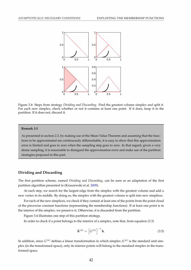
ASYMPTOTICALLY NECESSARY CONDITIONS EXPLOITING THE MEMBERSHIP FUNCTIONS
0 0.5 10
0.5
1
0 0.5 10
0.5
1
0 0.5 10
0.5
1
0 0.5 10
0.2
0.4
0.6
0.8
Figure 3.4: Steps from strategy Dividing and Discarding. Find the greatest volume simplex and split it.For each new simplex, check whether or not it contains at least one point. If it does, keep it in thepartition. If it does not, discard it.
Remark 3.5
As presented in section 2.3, by making use of the Mean Value Theorem and assuming that the func-tions to be approximated are continuously differentiable, it is easy to show that this approximationerror is limited and goes to zero when the sampling step goes to zero. In that regard, given a verydense sampling, it is reasonable to disregard the approximation error and make use of the partitionstrategies proposed in this part.
Dividing and Discarding
The first partition scheme, named Dividing and Discarding, can be seen as an adaptation of the firstpartition algorithm presented in (Kruszewski et al. 2009).
At each step, we search for the largest edge from the simplex with the greatest volume and add anew vertex in its middle. By doing so, the simplex with the greatest volume is split into new simplices.
For each of the new simplices, we check if they contain at least one of the points from the point cloudof the piecewise constant functions (representing the membership functions). If at least one point is inthe interior of the simplex, we preserve it. Otherwise, it is discarded from the partition.
Figure 3.4 illustrates one step of this partition strategy.
In order to check if a point belongs to the interior of a simplex, note that, from equation (3.3)
h(m) =[
G(m)]−1
h. (3.5)
In addition, since G(m) defines a linear transformation in which simplex ∆(m) is the standard unit sim-plex (in the transformed space), only its interior points will belong to the standard simplex in the trans-formed space.
42

EXPLOITING THE MEMBERSHIP FUNCTIONS ASYMPTOTICALLY NECESSARY CONDITIONS
0 0.5 10
0.2
0.4
0.6
0.8
0 0.5 10
0.2
0.4
0.6
0.8
0 0.5 10
0.2
0.4
0.6
0.8
0 0.5 1−0.5
0
0.5
1
Figure 3.5: Steps from strategy Grouping the membership points. Find the largest grouping (the one withthe greatest dispersion) and divide it into two new groupings. For each one of them, find a simplex thatcovers all of its points.
Therefore, a point, h, belongs to the interior of a simplex ∆(m) if and only if the transfomed point ,h(m), satisfy
h(m)i ≥ 0, ∀ir
∑i=1
h(m)i = 1.
Grouping the membership points
The second partition strategy, named Grouping the membership points, aims to solve the problem from adifferent angle. Instead of generating an increasingly finer mesh of simplices by their subdivision, wework with groupings of points in the image space.
At each iteration, choose a grouping (preferably the one with the greatest dispersion of its points)and divide it into two new groupings. For each of these groupings, find a simplex that covers all of itspoints.
Figure 3.5 illustrates one step of this partition strategy.
The regrouping step (the step in which a grouping is split into two new groupings) can be realizedby making use of any clustering algorithm, like the k-means (MacQueen 1967). In this work, we madeuse of the MATLAB function kmeans, that in addition to providing a way to divide the group of points,also gives a measure of the size of the new groups.
Different ways of finding a simplex covering a set of points are commonly presented in the tensorproduct model transformation literature (Baranyi 2004). These transformations, similarly to equation(3.3), can be seen as different ways of finding simplices with desired properties that cover a set of points.The CNO and RNO-INO transformations, for instance, find, respectively, the smallest volume simplexand a simplex whose every face is touched.
43

ASYMPTOTICALLY NECESSARY CONDITIONS EXPLOITING THE MEMBERSHIP FUNCTIONS
Remark 3.6
Note that the transformations proposed in the tensor product model transformation literature areusually presented as a transposed version of equation (3.5). Therefore, the G(m) matrix, contain-ing the vertices of the simplex that covers the points can be found transposing the inverse of thetransformation matrix.
Remark 3.7
The default behaviour of the k-means implementation in MATLAB is to use random starting posi-tions for the cluster’s centroids. Therefore, different realizations of the same problem may lead todifferent partitions. However, once the number of steps from the partition increases, the differencebetween the realizations should decrease.
Partition Strategies - Part II
The partition strategies proposed above disregard the approximation error, and consider that the mem-bership function can be perfectly represented as a point cloud in the image space. However, by makinguse of the content presented in section 2.3, we may consider an uncertain representation for the piece-wise constant functions, using the error polytopes and balls as an added uncertainty that guaranteesthat this representation covers the original membership functions, and extend the strategies proposedto take the approximation error into consideration.
Note that, even then, we still have sufficient and asymptotically necessary conditions. However, inthis new format, it is necessary for the number of simplices and the number of samples to go to infinity(so that the simplices volume and the approximation error go to zero).
Figure 3.6 illustrates the approximation of the membership functions by piecewise constant func-tions, and different possible representations for the approximation error (two different error polytopeschemes and an error ball).
Remark 3.8
Note that, since we are dealing with membership functions, the sum of the errors must always beequal to zero in order for us to only consider points that belong to the same hyperplane as themembership functions (the hyperplane of sum equal to one). Therefore we must impose that thesum of the coordinates of the polytope vertices is equal to zero (which is equivalent to taking the
intersection of the error polytope ∆h(x) with the hyperplaner
∑i=1
∆hi = 0).
Another approach, which is a little more conservative, is the following: consider a system withr rules. Given the values of r − 1 membership functions, the value of the other function is alwaysexactly known (one less the sum of the other membership functions). Therefore we can take themaximum and minimum values of only r − 1 approximation errors and complete the remainingdimension with the value that makes the sum of the coordinates equal to zero. In that regard, wereduce the number of vertices of the uncertainty polytope from 2r to 2r−1.
In the case presented in Figure 3.6 (c), we made use of only the bounds on the first and secondmembership function, and the values of the third are calculated as those that make the sum equal tozero, simplifying an 8 vertices polytope (or 6 vertices after the intersection with the zero sum plane,as presented in Figure 3.6 (b)) to 4 vertices.
44

EXPLOITING THE MEMBERSHIP FUNCTIONS ASYMPTOTICALLY NECESSARY CONDITIONS
−4 −2 0 2 40
0.2
0.4
0.6
0.8
(a)0 0.5 1
0
0.2
0.4
0.6
0.8
1
(b)
0 0.5 1
0
0.2
0.4
0.6
0.8
1
(c)0 0.5 1
0
0.2
0.4
0.6
0.8
1
(d)
Figure 3.6: Approximation of the membership functions by piecewise constant functions. (a) presentsthe approximation by piecewise constant functions. (b) presents the corresponding point cloud in theimage space using the error polytope obtained by the intersection of the error polytope with the zerosum plane and the standard simplex edges. (c) presents the error polytope described in Remark 3.8. (d)presents the error ball obtained using the Mean Value Theorem generalization for vector functions.
Dividing and discarding
In the first strategy proposed, we can make use of the error ball representation. In that regard, wesubstitute the tests of whether a point belongs to a simplex by tests of whether the simplex touches anyuncertainty ball.
This test can be carried out in the following way: find the interior point of the simplex that is closestto the ball center (which is the point in the image space that was considered in the approach present inthe previous subsection) and check if its distance to the center is less than or equal to the uncertaintyradius. If it is, then the simplex contains points that belong to the uncertainty ball and cannot be dis-carded. Otherwise, test it with the other samples and uncertainty balls. If the test is negative for all ofthe samples, the simplex is discarded.
In order to find the simplex’s closest interior point to the sample, note that a simplex is a convex
45

ASYMPTOTICALLY NECESSARY CONDITIONS EXPLOITING THE MEMBERSHIP FUNCTIONS
polygon and that every point in its interior can be written as
v =r
∑i=1
αivi,
αi ≥ 0,r
∑i=1
αi = 1
Given an external point p, the interior point of a simplex closest to this point can be found by solvingthe optimization problem
minαi
[(
r
∑i=1
αivi)− p
]T [(
r
∑i=1
αivi)− p
]
s.t. αi ≥ 0,r
∑i=1
αi = 1
Note that the objective function can be rewritten as
[α1 α2 . . . αr −1
]
vT1 v1 vT
1 v2 . . . vT1 vr vT
1 p∗ vT
2 v2 . . . vT2 vr vT
2 p...
.... . .
......
∗ ∗ . . . vTr vr vT
r p∗ ∗ . . . ∗ pTp
α1
α2
. . .αr
−1
Which allows us to rewrite the optimization problem as a quadratic optimization problem subjectto linear equality and inequality constraints
minαi ,ρ
f0 =[α1 α2 . . . αr ρ
]
vT1 v1 vT
1 v2 . . . vT1 vr vT
1 p∗ vT
2 v2 . . . vT2 vr vT
2 p...
.... . .
......
∗ ∗ . . . vTr vr vT
r p∗ ∗ . . . ∗ pTp
α1
α2
. . .αr
ρ
s.t.
fi ≤ 0, g0 = 0, g1 = 0
fi = −αi, g0 = (r
∑i=1
αi)− 1, g1 = ρ + 1
Or, in vector form
minx
f0 = xT Ax
s.t.
f = Hx ≤ 0
g = Gx− b = 0
46

EXPLOITING THE MEMBERSHIP FUNCTIONS ASYMPTOTICALLY NECESSARY CONDITIONS
with
A =
vT1 v1 vT
1 v2 . . . vT1 vr vT
1 p∗ vT
2 v2 . . . vT2 vr vT
2 p...
.... . .
......
∗ ∗ . . . vTr vr vT
r p∗ ∗ . . . ∗ pTp
,
H =
−1 0 . . . 0 00 −1 . . . 0 0...
. . ....
...0 0 . . . −1 0
,
G =
[1 1 . . . 1 00 0 . . . 0 1
], b =
[1−1
].
The objective function’s gradient is given by
∂ f0
∂x= 2Ax
and its Hessian by
∂2 f0
∂x2 = 2A
We can then make use of any method available to solving quadratic optimization problems (whichare not usually that computationally expensive to solve), like the quadprog command from MATLABor even a primal-dual interior point method (Boyd and Vandenberghe 2004, cap. 11.7) (which, in thisproblem, was implemented specifically for this problem).
Grouping the membership points
In the second strategy proposed, it suffices to do a simple modification: the clustering algorithm in theregrouping step still considers only the point cloud in the image space. However, the step of finding asimplex that cover the grouping’s points uses the vertices of the uncertainty polytopes of each samplefrom the grouping. As a result of that, we find a simplex that covers the vertices of the polytopes and,thus, also covers the points in the interior of the polytope (since a simplex is convex).
Discussing the case with several premise variables
Since in this work we consider TS models with a tensor product structure in its membership functions(i.e. models whose membership functions satisfy equation (2.2)), two different approaches are possiblefor the partition strategies of the image space:
1. Separately dividing the simplices of the image spaces of µi(vi) and compounding the equivalentsimplices in the image space of h(v). As can be inferred from the results presented in section 2.5,this composition is given by the tensor product of the vertices of the simplices for all possiblecombinations.
The problem with this approach is that the number of simplices grows too fast and in neither ofthe two partition strategies proposed we have a clear way of choosing what image space is goingto be split next.
The advantage of this approach is that we can use a reduced number of samples.
47

SWITCHED REPRESENTATION EXPLOITING THE MEMBERSHIP FUNCTIONS
2. Directly dividing the simplices in the image space of h(v).
The problem of this approach is that, in this case, we will need a considerably higher number ofsamples (for the same approximation error as in the other approach), since the samples will begiven by the tensor product of the samples of every function (in order for us to be able to find theerror polytope, or error ball, according to the contents presented in section 2.3).
The advantage of this approach is that we get more control over the growth of the number ofsimplices and the partition strategies presented can be directly applied (as long as one knowshow to calculate the approximation error).
3.2 Switched representation
A different point of view
Despite the partition strategies presented having been conceived in order to generate a set of constraintsin order to decrease the conservativeness of constraints commonly found in the literature (and reachingequivalency in the limit case), they can also be seen from another interesting point of view: a way offinding exact switched nonlinear representations for a nonlinear system.
In order to illustrate, consider the TS system defined by equation (2.4):
x =r
∑i=1
hi(v) (Aix + Biu) .
In each ∆(m) simplex, we will have a description given by:
x =r
∑i=1
h(m)i
[A(m)
i x + B(m)i u
]
h(m) =[
G(m)]−1
h
A(m)j =
r
∑i=1
gij Ai
B(m)j =
r
∑i=1
gijBi
in which h is the vector of the original membership functions, h(m) is the vector of transformed mem-bership functions, and G(m) defines a linear transformation in which simplex ∆(m) is the standard unitsimplex.
In addition, we have a switching signal, σ, given by
σ = m, if h ∈ ∆(m).
In cases where there exists a conflict (h belongs to more than one simplex), the switching signal is freeto be chosen as any of the conflicting simplices. In this work case, in order to resolve the conflicts, wechoose the switching signal according to the active simplex whose centroid is closer, in terms of the2-norm, to the current value of vector h.
Switching control according to the partitions
The idea of using a switched control law according to partitions on the image space of the membershipfunctions is not a novelty of this work. This type of control law was proposed in (Ko, Lee, and Park
48

EXPLOITING THE MEMBERSHIP FUNCTIONS SWITCHED REPRESENTATION
2012), however the authors do not present any method in order to partition the image space of themembership functions.
In this work, we propose the use of a control law switched according to the partitions. However,since the idea of the partition strategies is having simplicial meshes whose simplices volume (in the im-age space) is ever smaller, the vertex systems are ever closer to each other (which by itself asymptoticallyimplies in the partitions having a linear behaviour) and we choose to use a linear control law for each ofthe partitions.
This control law can be written as
u = K(m)x, if σ = m.
A different proposal of this work is the use of the tensor product model transformation (presentedin section 2.4) to recover a continuous controller (simpler to implement, since ideally we would like tohave a large number of partitions).
To that end, however, we must impose, on the synthesis conditions, that the controller of region (m)
also stabilizes the neighboring regions. With those extra conditions, we can prove that the solutions ofany switching between the controllers of neighboring regions stabilizes the system (because we will beproving the stability of the Filipov solutions). Therefore, by making use of (Liberzon 2003, corollary 2.3,page 25) or even the convexity property of the LMIs, we can show that any convex combination of thecontrollers will stabilize the system.
Remark 3.9
In this work, two regions are called neighbors if their simplices touch or intercept. Numerically,this can be verified by checking if at least one of the vertices of one of the simplices is contained inthe other one.
In particular, we may take several samples from the controller gain (walking through the imagespace of the membership functions) and the controller given by the linear interpolation of these gainswill stabilize the system (given that we draw at least one sample from each partition). These samples canthen be used in the tensor product model transformation and we can recover the TS representation ofthe controller. It is interesting to note that, instead of generating a different set of samples from the mem-bership functions’ image space, the samples used to generate the partitions can be reused (guaranteeingthat we draw at least one sample from each partition).
However, note that when using a large number of partitions (which is the idea when we are try-ing to achieve the necessity of the conditions), the difference between neighboring regions becomesever smaller and the chance of one partition’s controller also stabilizing its neighboring regions is high.Therefore, a possible synthesis methodology is to find the controller without adding the extra constraintsto the optimization problems, and checking afterwards if they are valid for the controller values found.If they are, the procedure described above can be done without any problems. Otherwise, we try tosolve the optimization problem a second time, but this time adding the extra conditions. In this way, theoptimization problem (which is the longest step of the methodology) can be reduced.
Remark 3.10
By making use of this methodology to reconstruct a continuous controller, we find a fuzzy controllaw for the system. In doing so, we can think that this method allow us to search, at the same time,for the controller gains and its membership functions (unlike PDC control laws usually employedin the literature that employ the same membership functions as the system).
49

EXAMPLES EXPLOITING THE MEMBERSHIP FUNCTIONS
3.3 Examples
In this section, two possible use cases for the conditions in this chapter are presented. We consider, first,the problem of stabilizing a TS system and, in the following, the problem of finding a controller thatminimizes an upper bound of the system’sH∞ norm.
In both cases we’ll make use of a quadratic Lyapunov function, and the conditions used are largelyknown in the literature (or have some minor modifications)1. In that regard we do not present theseconditions derivation (as that is not the focus of this section).
Stabilization
Consider a TS system defined by equation (2.4):
x =r
∑i=1
hi(v)Aix + Biu.
By making use of a linear state feedback control law, u = Kx, we may look for a stabilizing controllerby means of the conditions
r
∑i=1
hiQi < 0,
P > 0,
Qi = AiP + PATi + BiX + XT BT
i .
And the controller gains can be recovered by K = XP−1.
By making use of a PDC state feedback control law, u =r
∑j=1
hjKjx, we may look for a stabilizing
controller by means of the conditions
r
∑i=1
r
∑j=1
hihjQij < 0,
P > 0,
Qij = AiP + PATi + BiXj + XT
j BTi .
And the controller gains can be recovered by Kj = XjP−1.Both of the above presented conditions can be solved by making use of the techniques presented
in this chapter. Taking advantage of the partitions generated by these techniques, we may define aswitched control law (as presented in the previous section). Such a control law can be written as
u = K(m)x, if σ = m.
In that regard, we may look for a stabilizing controller by means of the conditions
r
∑j=1
h(m)j
r
∑i=1
g(m)ij Q(m)
i < 0, ∀m
P > 0,
Q(m)i = AiP + PAT
i + BiX(m) + (X(m))T BTi .
1To the interested reader, the stabilization conditions are presented in (Tanaka and Wang 2001, Sec-tion 3.3) and (Tuan et al. 2001, Theorem 3.2). Some slightly different conditions for the H∞ control arepresented in (Tuan et al. 2001, Theorem 5.1)
50

EXPLOITING THE MEMBERSHIP FUNCTIONS EXAMPLES
And the controller gains will be given by K(m) = X(m)P−1.In addition, as explained in the previous section, we may look for a switched controller that can be
represented in a continuous fashion (as discussed in the previous section) by imposing that the switchedgains are also stabilizing for the neighbouring regions. Therefore, the conditions presented can be mod-ified to
r
∑j=1
h(m)j
r
∑i=1
g(m)ij Q(n)
i < 0, ∀m, n = m or n is a neighbour of m
P > 0,
Q(n)i = AiP + PAT
i + BiX(n) + (X(n))T BTi .
In which the controller gains are given by K(m) = X(m)P−1 and a continuous control law can be recoverdby making use of the Tensor Product Model Transformation.
Remark 3.11
Note that, the way the above conditions were defined, the quadratic Lyapunov function found is ofthe form
V(x) = xT P−1x.
Example 3.1. Consider the TS model with a free b parameter presented in (Campos, Tôrres, and Palhares2012):
x =3
∑i=1
hi(x1) [Aix + Biu] ,
with
A1 =
[1.59 −7.290.01 0
], B1 =
[10
],
A2 =
[0.02 −4.640.35 0.21
], B2 =
[80
],
A3 =
[−2 −4.330 0.05
], B3 =
[−b + 6−1
],
and
h1(x1) =sin(x1) + 1
3,
h2(x1) =sin(x1 + 2π/3) + 1
3,
h3(x1) =sin(x1 − 2π/3) + 1
3.
We would like to find the largest value of b for which we are able to find a quadratically stabilizingcontrol law, and to that end, we will make use of the conditions presented above as well as the partitionstrategies presented in this chapter (taking the approximation error into account) and other similar ap-proaches available in the literature. Particularly, we will compare the results from this chapter with (Salaand Ariño 2007, Proposition 2), (Sala and Ariño 2007, Theorem 5), (Kruszewski et al. 2009, Algorithm1), all of these conditions as well as this chapter conditions augmented with the shape relaxation from(Sala and Ariño 2008, Proposition 3.1), and the conditions from (Lam and Narimani 2010, Theorem 2).
51

EXAMPLES EXPLOITING THE MEMBERSHIP FUNCTIONS
0 0.2 0.4 0.6 0.8 10
0.1
0.2
0.3
0.4
0.5
0.6
0.7
0.8
h1
h 2
Figure 3.7: Partition generated by the Divinding and Discarding strategy after 12 steps.
In order to take the approximation error into consideration, note that the membership functions
vector h =[
sin(x1)+13
sin(x1+2π/3)+13
sin(x1−2π/3)+13
]Tderivative regarding the premise variable x1 is
given by
∂
∂x1h =
13 cos(x1)
13 cos(x1 + 2π/3)13 cos(x1 − 2π/3)
.
Whose elements all have the same maximum, equal to 1/3, and the same minimum, equal to −1/3. Inaddition, its vector 2-norm is equal to
√6/6.
Note that the membership functions are periodic and share the same period, 2π. Thus, it suffices totake samples from the premise variable in the interval [−π, π] in order to cover all of the membershipfunctions’ image space (this same observation is valid for the conditions from Lam and Narimani 2010,Theorem 2).
By taking 1001 samples, we have a sampling step equal to π/500, which leads to an uncertainty
radius of π√
66000 and a possible uncertainty polytope equal to
π3000
π3000 − π
1500π
3000 − π3000 0
− π3000
π3000 0
− π3000 − π
3000π
1500
, in which every
row is a polytope vertex.Figures 3.7 and 3.8 illustrate the partition strategies after 12 iterations.In order to make use of the shape relaxation from (Sala and Ariño 2008, Proposition 3.1), note that
the membership functions are such that
hTSh + wTh + v ≤ 0,
with S = 6I, w =[−4 −4 −4
]T, and v = 1. It is interesting to note that when applied to single
fuzzy summation conditions, this relaxation transforms it into double fuzzy summation conditions, andthus allows the use of sum relaxations that are not available for the single summation case. It is alsointeresting to note that this shape inequality is actually an equality in this example (meaning that all ofthe membership functions values lie over the curve given by hTSh + wTh + v = 0).
52

EXPLOITING THE MEMBERSHIP FUNCTIONS EXAMPLES
-0.2 0 0.2 0.4 0.6 0.8-0.1
0
0.1
0.2
0.3
0.4
0.5
0.6
0.7
-0.2 0 0.2 0.4 0.6 0.8-0.1
0
0.1
0.2
0.3
0.4
0.5
0.6
0.7
0.8
Figure 3.8: Partition generated by the Grouping the membership points strategy after 12 steps on Example3.1. The left partition was generated using the CNO transformation, whereas the one on the right wasgenerated by the RNO-INO transformation.
In addition, the Γ matrix representing the γij elements used in the inequalities hihj− hi hj ≥ γij, withhi the staircase approximation of hi used in the conditions in (Lam and Narimani 2010, Theorem 2), canbe described by
Γ =−2π
np
1.39
1.7718
1.7718
1.7718
1.39
1.7718
1.7718
1.7718
1.39
,
with np the number of points used in the staircase approximation.
Tables 3.1, 3.2, 3.3 present the minimum number of rows of LMIs for each of the methods to find astabilizing PDC, linear and switched controller for a given value of b. Figures 3.9 to 3.17 present thesesame comparisons, but showing the largest feasible value of b for a given number of rows of LMIs. Notethat, due to the random initialization of the k-means, the values presented for the Grouping the membershippoints partition strategy may change. Finally, Table 3.4 presents the complexity analysis of each of themethods used for this example (by means of comparison we also present the complexity analysis for theusual conditions for a linear control law and a PDC control law).
Note that conditions (Sala and Ariño 2007, Proposition 2), (Sala and Ariño 2007, Theorem 5) and(Kruszewski et al. 2009, Algorithm 1) are shape-independent, and when used without the relaxation from(Sala and Ariño 2008, Proposition 3.1) are intrinsically more conservative than the other conditions (sincethey use less information). We can find an upper bound for shape-independent conditions by using thenecessary and asymptotically sufficient conditions from (Kruszewski et al. 2009). In this example theupper bound found b was 6.661.
These same necessary and asymptotically sufficient conditions could be used in conjunction with(Sala and Ariño 2008, Proposition 3.1) to find an upper bound for the shape-dependent case. However,we were not able to find a value with the number of partitions we tried in this example. Interestinglythough, we found that using Lemma 2.3 together with (Sala and Ariño 2008, Proposition 3.1) (whichis the same as using Sala and Ariño 2007, Theorem 5 with 2 summations and Sala and Ariño 2008,Proposition 3.1) found the largest feasible value of b, which was the same for the PDC, the linear and
53

EXAMPLES EXPLOITING THE MEMBERSHIP FUNCTIONS
Table 3.1: Comparison of different methods of sum relaxation for a PDC control law in example 3.1(minimum number of rows of LMIs required to find a stabilizing control law)
Method/b 4 5 5.5 6 6.3 6.6 6.7 6.72 6.75Sala and Ariño 2007, Proposition 2 158 464 994 3194 12212 - - - -
Sala and Ariño 2007, Theorem 5 34 34 34 34 34 60 - - -Kruszewski et al. 2009, Algorithm 1 74 386 722 1538 - - - - -Kruszewski et al. 2009, Algorithm 1 26 50 50 50 74 122 - - -with Lemma 2.3Sala and Ariño 2007, Proposition 2 24 24 34 46 94 760 3910 - -with Sala and Ariño 2008, Proposition 3.1
Sala and Ariño 2007, Theorem 5 32 32 32 32 32 32 32 32 32with Sala and Ariño 2008, Proposition 3.1Kruszewski et al. 2009, Algorithm 1 28 28 28 40 52 52 1720 1720 1720with Sala and Ariño 2008, Proposition 3.1
Dividing and Discarding 98 170 170 170 170 170 - - -Dividing and Discarding 38 74 74 74 146 254 - - -with Lemma 2.3Dividing and Discarding 28 28 28 40 52 88 628 760 760with Sala and Ariño 2008, Proposition 3.1
Grouping the membership points-CNO 26 26 50 50 50 170 194 350 -Grouping the membership points-CNO 38 38 74 74 74 254 290 380 -with Lemma 2.3Grouping the membership points-CNO 28 28 28 40 52 64 76 100 184with Sala and Ariño 2008, Proposition 3.1
Grouping the membership points-RNO-INO 62 98 98 110 194 362 - - -Grouping the membership points-RNO-INO 74 92 146 164 290 542 - - -with Lemma 2.3Grouping the membership points-RNO-INO 28 52 64 76 112 184 376 376 556with Sala and Ariño 2008, Proposition 3.1
Lam and Narimani 2010, Theorem 2 54 74 94 134 194 494 1114 1474 2934
the switched control law, equal to 6.7803 (and that’s the reason why the tables do not show any methodusing both Lemma 2.3 and (Sala and Ariño 2008, Proposition 3.1)).
From these tables and figures, we can see that, for this particular example, the conditions proposedperformed well against the other conditions and can be used as an alternative to them.
Note that the Grouping the membership points partition strategy performed better than the Dividingand Discarding strategy, but, as can be seen from the Figures presented, it does not guarantee that it willbe less conservative with every partition iteration (unlike the other sum relaxation strategies presented).This stems from the fact that a simplex found to cover a new group that has just been split can add pointsthat were not being considered in the LMIs before. This problem is however mitigated as the simplicesvolume approaches zero.
It is also interesting to note that, for this example, after a reasonable number of iterations of theproposed partition strategies, the use of Lemma 2.3 instead of Lemma 2.1 did not reduce the conser-vativeness and only increased the computational cost (as can be more explicitly seen by comparing theresults for the CNO transformation with and without Lemma 2.3 on Table 3.1).
54
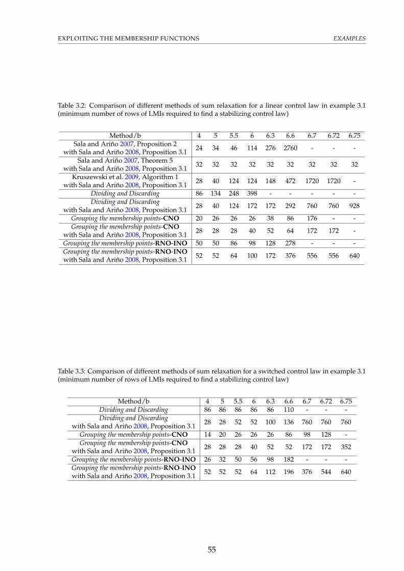
EXPLOITING THE MEMBERSHIP FUNCTIONS EXAMPLES
Table 3.2: Comparison of different methods of sum relaxation for a linear control law in example 3.1(minimum number of rows of LMIs required to find a stabilizing control law)
Method/b 4 5 5.5 6 6.3 6.6 6.7 6.72 6.75Sala and Ariño 2007, Proposition 2 24 34 46 114 276 2760 - - -with Sala and Ariño 2008, Proposition 3.1
Sala and Ariño 2007, Theorem 5 32 32 32 32 32 32 32 32 32with Sala and Ariño 2008, Proposition 3.1Kruszewski et al. 2009, Algorithm 1 28 40 124 124 148 472 1720 1720 -with Sala and Ariño 2008, Proposition 3.1
Dividing and Discarding 86 134 248 398 - - - - -Dividing and Discarding 28 40 124 172 172 292 760 760 928with Sala and Ariño 2008, Proposition 3.1
Grouping the membership points-CNO 20 26 26 26 38 86 176 - -Grouping the membership points-CNO 28 28 28 40 52 64 172 172 -with Sala and Ariño 2008, Proposition 3.1
Grouping the membership points-RNO-INO 50 50 86 98 128 278 - - -Grouping the membership points-RNO-INO 52 52 64 100 172 376 556 556 640with Sala and Ariño 2008, Proposition 3.1
Table 3.3: Comparison of different methods of sum relaxation for a switched control law in example 3.1(minimum number of rows of LMIs required to find a stabilizing control law)
Method/b 4 5 5.5 6 6.3 6.6 6.7 6.72 6.75Dividing and Discarding 86 86 86 86 86 110 - - -Dividing and Discarding 28 28 52 52 100 136 760 760 760with Sala and Ariño 2008, Proposition 3.1
Grouping the membership points-CNO 14 20 26 26 26 86 98 128 -Grouping the membership points-CNO 28 28 28 40 52 52 172 172 352with Sala and Ariño 2008, Proposition 3.1
Grouping the membership points-RNO-INO 26 32 50 56 98 182 - - -Grouping the membership points-RNO-INO 52 52 52 64 112 196 376 544 640with Sala and Ariño 2008, Proposition 3.1
55

EXAMPLES EXPLOITING THE MEMBERSHIP FUNCTIONS
0 2000 4000 6000 8000 10000 12000 14000 16000−4
−2
0
2
4
6
8
Sala, Ariño 2007 Proposition 2
number of rows of LMIs
b
30 40 50 60 70 802
3
4
5
6
7
Sala, Ariño 2007 Theorem 5
number of rows of LMIs
b
Figure 3.9: Maximum feasible b for a given number of rows of LMIs using the conditions in (Sala andAriño 2007). Since these are shape-independent conditions, the maximum feasible value was found usingthe necessary and asymptotically sufficient conditions from (Kruszewski et al. 2009) and is displayed asthe dashed line.
56

EXPLOITING THE MEMBERSHIP FUNCTIONS EXAMPLES
0 1000 2000 3000 4000 5000 6000−4
−2
0
2
4
6
8
Kruszeswki et al 2009 Algorithm 1 (using Lemma 2.1)
number of rows of LMIs
b
0 20 40 60 80 100 120 1402
3
4
5
6
7
Kruszeswki et al 2009 Algorithm 1 (using Lemma 2.3)
number of rows of LMIs
b
Figure 3.10: Maximum feasible b for a given number of rows of LMIs using the conditions in(Kruszewski et al. 2009, Algorithm 1). Since these are shape-independent conditions, the maximum fea-sible value was found using the necessary and asymptotically sufficient conditions from (Kruszewskiet al. 2009) and is displayed as the dashed line.
57

EXAMPLES EXPLOITING THE MEMBERSHIP FUNCTIONS
0 1000 2000 3000 4000 5000 60003
4
5
6
7
Sala, Ariño 2007 − Proposition 2 + Sala, Arino 2008 − Proposition 3.1
number of rows of LMIs
b
0 500 1000 1500 2000 2500 3000 35003
4
5
6
7
Kruszeswki et al 2009 − Algorithm 1 (using Lemma 2.1) + Sala, Arino 2008 − Proposition 3.1
number of rows of LMIs
b
Figure 3.11: Maximum feasible b for a given number of rows of LMIs using the conditions in (Sala andAriño 2007) and (Kruszewski et al. 2009, Algorithm 1) together with the shape relaxation from (Sala andAriño 2008). The blue line represents a PDC control law, whereas the red one represents a linear controllaw. The maximum feasible value of b found with any of the methods in Example 3.1 is displayed as adashed line.
58

EXPLOITING THE MEMBERSHIP FUNCTIONS EXAMPLES
0 200 400 600 800 1000 1200 1400 1600 1800−4
−2
0
2
4
6
8
Divinding and Discarding PDC control law
number of rows of LMIs
b
0 100 200 300 400 500 600
−2
0
2
4
6
Divinding and Discarding linear/switched control law
number of rows of LMIs
b
Figure 3.12: Maximum feasible b for a given number of rows of LMIs using the Dividing and Discardingpartition strategy. The blue line represents the conditions for a PDC control law using Lemma 2.1, thegreen one represents the conditions for a PDC control law using Lemma 2.3, the red one represents alinear control law, and the magenta line represents a switched control law. The maximum feasible valueof b found with any of the methods in Example 3.1 is displayed as a dashed line.
59

EXAMPLES EXPLOITING THE MEMBERSHIP FUNCTIONS
0 200 400 600 800 1000 12003
4
5
6
7
Divinding and Discarding + Sala, Arino 2008 − Proposition 3.1 PDC control law
number of rows of LMIs
b
0 200 400 600 800 1000 12003
4
5
6
7
Divinding and Discarding + Sala, Arino 2008 − Proposition 3.1 linear/switched control law
number of rows of LMIs
b
Figure 3.13: Maximum feasible b for a given number of rows of LMIs using the Dividing and Discardingpartition strategy together with proposition 3.1 from (Sala and Ariño 2008). The blue line represents aPDC control law, the red one represents a linear control law, and the magenta line represents a switchedcontrol law. The maximum feasible value of b found with any of the methods in Example 3.1 is displayedas a dashed line.
60

EXPLOITING THE MEMBERSHIP FUNCTIONS EXAMPLES
0 500 1000 1500 2000−4
−2
0
2
4
6
8
Grouping the membership points − CNO PDC control law
number of rows of LMIs
b
0 200 400 600 800 1000 1200 1400 1600 1800−2
0
2
4
6
Grouping the membership points − RNO−INO PDC control law
number of rows of LMIs
b
Figure 3.14: Maximum feasible b for a given number of rows of LMIs using the Grouping the membershippoints partition strategy. The blue line represents the conditions for a PDC control law using Lemma2.1 and the green one represents the conditions for a PDC control law using Lemma 2.3. The maximumfeasible value of b found with any of the methods in Example 3.1 is displayed as a dashed line.
61

EXAMPLES EXPLOITING THE MEMBERSHIP FUNCTIONS
0 100 200 300 400 500 600−2
0
2
4
6
Grouping the membership points − CNO linear/switched control law
number of rows of LMIs
b
0 100 200 300 400 500 600−2
0
2
4
6
Grouping the membership points − RNO−INO linear/switched control law
number of rows of LMIs
b
Figure 3.15: Maximum feasible b for a given number of rows of LMIs using the Grouping the membershippoints partition strategy. The red line represents a linear control law, and the magenta line represents aswitched control law. The maximum feasible value of b found with any of the methods in Example 3.1is displayed as a dashed line.
62

EXPLOITING THE MEMBERSHIP FUNCTIONS EXAMPLES
0 200 400 600 800 1000 1200 14003
4
5
6
7
Grouping the membership points − CNO + Sala, Arino 2008 − Proposition 3.1 PDC control law
number of rows of LMIs
b
0 200 400 600 800 1000 1200 14003
4
5
6
7
Grouping the membership points − RNO−INO + Sala, Arino 2008 − Proposition 3.1 PDC control law
number of rows of LMIs
b
Figure 3.16: Maximum feasible b for a given number of rows of LMIs using the Grouping the membershippoints partition strategy together with proposition 3.1 from (Sala and Ariño 2008). The blue line repre-sents the conditions for a PDC control law using Lemma 2.1. The maximum feasible value of b foundwith any of the methods in Example 3.1 is displayed as a dashed line.
63

EXAMPLES EXPLOITING THE MEMBERSHIP FUNCTIONS
0 200 400 600 800 1000 1200 14003
4
5
6
7
Grouping the membership points − CNO + Sala, Arino 2008 − Proposition 3.1 linear/switched control law
number of rows of LMIs
b
0 200 400 600 800 1000 1200 14003
4
5
6
7
Grouping the membership points − RNO−INO + Sala, Arino 2008 − Proposition 3.1 linear/switched control law
number of rows of LMIs
b
Figure 3.17: Maximum feasible b for a given number of rows of LMIs using the Grouping the membershippoints partition strategy together with proposition 3.1 from (Sala and Ariño 2008). The red line representsa linear control law, and the magenta line represents a switched control law. The maximum feasiblevalue of b found with any of the methods in Example 3.1 is displayed as a dashed line.
64

EX
PL
OIT
ING
TH
EM
EM
BE
RSH
IPFU
NC
TIO
NS
EXA
MPLES
Table 3.4: Complexity analysis for the different methods of sum relaxation used in example 3.1.
Method Number of rows of LMIs Number of scalar decision variablesLinear control law 8 5
PDC control law using Lemma 2.1 14 9PDC - Sala and Ariño 2007, Proposition 2 with qsummations
2 +(2 + q)!
q!9
PDC - Sala and Ariño 2007, Theorem 5with degree q
16 +floor(q/2)
∑i=0
2(
2 + q− 2iq− 2i
), if q is even,
8 +floor(q/2)
∑i=0
2(
2 + q− 2iq− 2i
), if q is odd
9 +floor(q/2)
∑i=0
3i(2× 3i + 1)
PDC - Kruszewski et al. 2009, Algorithm 1 withns simplices 2 + 12ns 9
PDC - Kruszewski et al. 2009, Algorithm 1 withLemma 2.3 and ns simplices 2 + 18ns 9 + 15ns
Partition strategies proposed in this chapterwith ns simplices - PDC control 2 + 12ns 9
Partition strategies proposed in this chapterwith ns simplices - linear control 2 + 6ns 5
Partition strategies proposed in this chapterwith ns simplices - switched control 2 + 6ns 3 + 2ns
PDC - Lam and Narimani 2010, Theorem 2 withnp points 14 + 2np 27
Using Sala and Ariño 2008, Proposition 3.1 forPDC control (any of the methods) +2 +3
Using Sala and Ariño 2008, Proposition 3.1 forlinear control (any of the methods) same as PDC with (Sala and Ariño 2008) 4 less than PDC
Using Sala and Ariño 2008, Proposition 3.1 forswitched control (Partition strategies proposedin this chapter)
same as PDC with (Sala and Ariño 2008) +3
65

EXAMPLES EXPLOITING THE MEMBERSHIP FUNCTIONS
−6 −4 −2 0 2 4 6
−6
−4
−2
0
2
4
6
x1
x 2
Figure 3.18: Linear stabilizing controller’s phase plane for b = 6.75. The arrows represent the directionof the vector field in each point in space, the red level curves are the level curves of the Lyapunovfunction, and the blue lines are the system’s trajectory from two different initial conditions.
As discussed earlier, none of the shape-independent conditions are able to find a stabilizing controllerfor b > 6.661 whereas some of the shape-dependent conditions were able to find stabilizing controllers upto 6.7803.
In order to illustrate the system’s behaviour in closed loop, we obtained controllers using the Group-ing the membership points strategy for b = 6.75.
In the linear control law case, we made use of the RNO-INO transformation to find the simplices,and the controller gains found were
K =[−0.9260 0.2970
],
and the Lyapunov parameter matrix
P =
[27.2336 −1.1192−1.1192 1.8838
].
The system’s phase plane in closed loop is presented in Figure 3.18.
In the PDC control law case, we made use of the CNO transformation to find the simplices, and thecontrollers gains found were
K1 =[−1.2018 2.1324
],
K2 =[0.3414 −0.9099
],
K3 =[−0.5113 3.1824
],
66

EXPLOITING THE MEMBERSHIP FUNCTIONS EXAMPLES
−6 −4 −2 0 2 4 6
−6
−4
−2
0
2
4
6
x1
x 2
Figure 3.19: PDC stabilizing controller’s phase plane for b = 6.75. The arrows represent the direction ofthe vector field in each point in space, the red level curves are the level curves of the Lyapunov function,and the blue lines are the system’s trajectory from two different initial conditions.
and the Lyapunov parameter matrix
P =
[27.0756 −1.0860−1.0860 1.8352
].
The system’s phase plane in closed loop is presented in Figure 3.19.In the switched control law case, we made use of the CNO transformation to find the simplices. The
Lyapunov parameter matrix found was
P =
[28.3290 −1.1073−1.1073 1.8532
].
The system’s phase plane in closed loop is presented in Figure 3.20.We are not presenting the controller gains found for this case since 100 partitions of the image space
were used (correspoding to 100 different gain matrices). In addition, in order to fully describe the controllaw found, we would also need to present the simplices that describe each image space partition.
Finally, we also made use of modification to allow for a continuous controller to be found from thepiecewise controller. The conditions were found to be feasible for b = 6.75 for the same simplices usedin the switched control law synthesis.
An initial idea could be to make use of the original 1001 samples from the membership functions’image space to sample the controller gains (thus guaranteeing that at least one sample from each switch-ing region is sampled) and consider that the intersample values are given by linear interpolation so thatwe can make use of the Tensor Product Model Transformation to recover a continuous more compactrepresentation of the controller.
Note, however, that since we are using a lot more samples than switching regions we would besampling the same value many times inside of each region, thus leading to a staircase-like membership
67

EXAMPLES EXPLOITING THE MEMBERSHIP FUNCTIONS
−6 −4 −2 0 2 4 6
−6
−4
−2
0
2
4
6
x1
x 2
Figure 3.20: Stabilizing switched controller’s phase plan for b = 6.75. The arrows represent the directionof the vector field in each point in space, the red level curves are the level curves of the Lyapunovfunction, and the blue lines are the system’s trajectory from two different initial conditions.
function for the gains (implying that the membership values would change too fast from one switchingregion to the other).
In order to avoid this and “smooth” the controller’s membership functions a little, we go throughthe 1001 samples and check their current switching region. By doing this we are capable of definingintervals in the premise variable corresponding to each switching region2. We then pick only one samplefrom each region. For the extremal regions, we pick the extremes, whereas for all the other regions wepick the middle point. In addition, we make use of the piecewise sinusoidal functions proposed in 2.4to generate continuously differentiable membership functions.
The membership functions obtained from both approaches are presented in Figure 3.21.The fuzzy controller gains found were
K1 =[1.1617 11.2484
],
K2 =[−1.4358 11.0590
],
K3 =[−0.4847 −5.8339
],
and the Lyapunov parameter matrix found was
P =
[29.2791 −1.1450−1.1450 1.9159
],
and the system’s phase plane is presented in Figure 3.22.
2note that for a case with more than one premise variable, this would mean dealing with each ofthe image spaces of the tensor product separately - i.e. we would only be able to deal with the first casediscussed previously in this chapter.
68

EXPLOITING THE MEMBERSHIP FUNCTIONS EXAMPLES
−3 −2 −1 0 1 2 30
0.2
0.4
0.6
0.8
1
x1
u cno
Fuzzy controller found − cno
−3 −2 −1 0 1 2 30
0.2
0.4
0.6
0.8
1
x1
u cno
Fuzzy controller found − cno
Figure 3.21: Fuzzy controller’s membership functions. The plot on the top presents the membershipfunctions using all 1001 samples and linear interpolation. The plot on the bottom presents a “smoothed”approach using less samples and a piecewise sinusoidal interpolation.
Guaranteed costH∞ controller
Consider a system described by:
x =r
∑i=1
hi [Aix + Biu + Bwi w]
z =r
∑i=1
hi [Cix + Diu + Dwi w]
itsH∞ norm is the smallest γ such that
‖z(t)‖2 ≤ γ‖w‖2,
for a system with zero initial conditions.
By making use of a linear state feedback control law, u = Kx, we may search for a controller with
69

EXAMPLES EXPLOITING THE MEMBERSHIP FUNCTIONS
−6 −4 −2 0 2 4 6
−6
−4
−2
0
2
4
6
x1
x 2
Figure 3.22: Stabilizing fuzzy (reconstructed from a switched controller) controller’s phase plan forb = 6.75. The arrows represent the direction of the vector field in each point in space, the red levelcurves are the level curves of the Lyapunov function, and the blue lines are the system’s trajectory fromtwo different initial conditions.
minimum guaranteed cost by minimizing δ, subject to
r
∑i=1
hiQi < 0,
P > 0,
Qi =
AiP + PATi + BiX + XT BT
i Bwi PCTi + XT DT
i∗ −I DT
wi
∗ ∗ −δI
and the H∞ norm is guaranteed to be less than γ =√
δ and the controller gains will be given byK = XP−1.
This problem can be solved using the techniques proposed in this chapter. In addition to this, thepartitions generated by these techniques can be taken advantage of and used to define a control lawthat switches according to each region of the membership functions’ image space (as presented in theprevious section). This control law will have the form
u = K(m)x, if σ = m.
70

EXPLOITING THE MEMBERSHIP FUNCTIONS EXAMPLES
In that regard, we may look for a guaranteed cost controller by minimizing δ, subject to
r
∑j=1
h(m)j
r
∑i=1
g(m)ij Q(m)
i < 0, ∀m
P > 0,
Q(m)i =
AiP + PATi + BiX(m) + (X(m))T BT
i Bwi PCTi + (X(m))T DT
i∗ −I DT
wi
∗ ∗ −δI
and the H∞ norm is guaranteed to be less than γ =√
δ and the controller gains will be given byK(m) = X(m)P−1.
In addition, as explained previously, by changing the LMI conditions such that the switched gainsare also valid in the neighbouring regions, we will be able to reconstruct a continuous controller fromthe conditions. In that regard we modify the LMI to
r
∑j=1
h(m)j
r
∑i=1
g(m)ij Q(n)
i < 0, ∀m, n = m or n is a neighbour of m
P > 0,
Q(n)i =
AiP + PATi + BiX(n) + (X(n))T BT
i Bwi PCTi + (X(n))T DT
i∗ −I DT
wi
∗ ∗ −δI
so that the H∞ norm is guaranteed to be less than γ =√
δ, the controller gains will be given by K(m) =
X(m)P−1, and a continuous controller may be reconstructed by means of the Tensor Product ModelTransformation (in a similar way as done in the previous example).
Example 3.2. Consider the 3 rule system described by matrices:
A1 =
[1.59 −7.290.01 0
], B1 =
[10
], Bw1 =
[10
], C1 =
[1 1
], D1 = 0, Dw1 = 0
A2 =
[0.02 −4.640.35 0.21
], B2 =
[80
], Bw2 =
[11
], C2 =
[1 1
], D2 = 0, Dw2 = 0
A3 =
[−2 −4.330 0.05
], B3 =
[0−1
], Bw3 =
[10
], C3 =
[1 1
], D3 = 0, Dw3 = 0
with the membership functions
h1(θ) =cos(10x1) + 1
4, h2(θ) =
sin(10x1) + 14
, h3(θ) = 0.5− cos(10x1) + sin(10x1)
4
By taking 1001 samples from x1 ∈ [−π/10, π/10] (since the membership functions are periodic,this interval covers all of their image space), we find an approximation error polytope (in the image
space) that will be smaller than
π4000
π4000 − π
2000π
4000 − π4000 0
− π4000
π4000 0
− π4000 − π
4000π
2000
, with everyone row representing a vertex. In
addition, we get an approximation error radius equal to π2000 .
We made use of the Dividing and Discarding partition strategy and the Grouping the membership pointspartition strategy with RNO-INO transformation to find both a linear control law and a switched control
71

EXAMPLES EXPLOITING THE MEMBERSHIP FUNCTIONS
0 20 40 60 80 100 120 140 160 1800
5
10
15
20
25
# simplices
γ
40 60 80 100 120 140 1601.5
1.6
1.7
1.8
1.9
2
# simplices
γ
Figure 3.23: Guaranteed H∞ norm for a given number of simplices. The top plot presents the resultsobtained for the number of simplices tested, whereas the bottom plot presents a zoom in of the upperplot. The blue line represents the guaranteed cost found by the linear control law using the Dividing andDiscarding partition strategy. The red line represents the linear control law using the Grouping the mem-bership points partition strategy with RNO-INO transformation. The dashed magenta line represents theguaranteed cost found by the switched control law using the Dividing and Discarding partition strategy.The black dashed line represents the linear control law using the Grouping the membership points partitionstrategy with RNO-INO transformation.
law. Figure 3.23 presents a comparison of the results obtained from these methods by checking theguaranteedH∞ norm they were able to find according to the number of simplices used.
In addition to this, we also made use of the Grouping the membership points partition strategy withRNO-INO transformation to find a continuous controller, reconstructed from a switched one by meansof the Tensor Product Model Transformation.
We made use of 4001 samples of the membership functions from x1 ∈ [−π/10, π/10], resulting in
an error polytope of
π16000
π16000 − π
8000π
16000 − π16000 0
− π16000
π16000 0
− π16000 − π
16000π
8000
.
We made use of 600 groupings of the samples and the controller found had a guaranteed cost of1.5374. Just as in the previous example, we are able to reconstruct a fuzzy controller from the switchedcontroller found by making use of the Tensor Product Model Transformation (and the same observa-tions are valid here as to how to obtain a smoother set of membership functions). In that regard the
72

EXPLOITING THE MEMBERSHIP FUNCTIONS EXAMPLES
−0.3 −0.2 −0.1 0 0.1 0.2 0.30
0.2
0.4
0.6
0.8
1
x1
u cno
Fuzzy controller found − cno
−0.3 −0.2 −0.1 0 0.1 0.2 0.30
0.2
0.4
0.6
0.8
1
x1
u cno
Fuzzy controller found − cno
Figure 3.24: Membership functions found in Example 3.2. A single period of the function is presented.The plot on the top presents the membership functions using all 4001 samples and linear interpolation.The plot on the bottom presents a “smoothed” approach using less samples and a piecewise sinusoidalinterpolation.
membership functions are presented in Figure 3.24. The controller gains found were
K1 =[1.1011 1.0872
],
K2 =[−2.3099 2.9830
],
K3 =[−2.9565 −0.0449
].
In order to check the controller’s performance in closed loop we simulated it with zero initial con-dition and a disturbance signal w(t) = cos( π
10 t). The system’s output z(t), as well as the disturbancesignal are presented in Figure 3.25.
73

EXAMPLES EXPLOITING THE MEMBERSHIP FUNCTIONS
0 10 20 30 40 50−1
−0.5
0
0.5
1
t
w
0 10 20 30 40 50−0.5
0
0.5
1
t
z
Figure 3.25: System’s disturbance rejection in Example 3.2. The top plot is the disturbance signal w(t) =cos( π
10 t), whereas the bottom plot is the system’s output z.
74

4 Rule Reduction
Quite often, a model with a large number of rules might be undesirable. Be it because their analysis/synthesisconditions require a too large number of LMIs that make them prohibitly costly, be it because we are searching fora more convenient representation, and thus require a model with a reduced number of rules.
In this chapter, we propose the use of the tensor product model transformation technique for rule reduction. Weaim to show that, even without the sampling step, the HOSVD and the convex hull manipulation steps couldbe used to reduce the number of rules of a given TS fuzzy system. In addition, we also present how a polytopicuncertainty could be added to the reduced system such that this uncertain reduced system represents the originalone. Afterwards, we present LMI conditions that allow the transformation of this polytopic uncertainty into otherkinds of uncertainty that are more common in the TS literature.
The presentation and the results in this chapter were based on (Campos, Tôrres, and Palhares 2015).
4.1 Rule reduction by means of tensor approximation
As stated in Section 2.4 (in the equivalence between equations (2.10) and (2.11)), a tensor product TSrepresentation of a matrix function L(v) : R` → Rκ1×κ2
L(v) =r1
∑i1=1
r2
∑i2=1· · ·
r`
∑i`=1
`
∏n=1
µ(n)in (vn)Li1i2 ...i` ,
with Li1i2 ...i` ∈ Rκ1×κ2 , can be written with tensor notation as
L(v) = L `×n=1
µTn (vn), (4.1)
in which L ∈ Rr1×r2×···×r`×κ1×κ2 is a tensor whose element li1i2 ...i`k1k2 corresponds to the element in rowk1 and column k2 of matrix Li1i2 ...i` , and µn(vn) is a vector formed by stacking the membership functionsrelated to premise variable vn.
By applying the HOSVD over tensor L, we arrive at an approximation
L ≈ S `×n=1
Ui.
Note that the HOSVD step may be used simply to find a minimal TS representation, by discarding nononzero higher order singular values. In this case, the equation above is actually an equality.
75
RULE REDUCTION BY MEANS OF TENSOR APPROXIMATION RULE REDUCTION
In cases where singular values are discarded, we can write a tensor describing the approximationerror
L = L−(S `×
n=1Ui
),
whose Frobenius norm will be limited by (De Lathauwer, De Moor, and Vandewalle 2000a, equation 24)
∥∥L∥∥ ≤
k1
∑i1=1
σ(1)2
i1+
k2
∑i2=1
σ(2)2
i2+ · · ·+
k`
∑i`=1
σ(`)2
i`,
in which σ(m)2
im denotes the square of the discarded m-mode singular values, and km the number of m-modesingular values discarded.
This reduction step can be seen as searching for a tensor with rank restrictions that approximatesL. Note, however, that if we discard columns in more than one direction (i.e. if we impose a rankconstraint in more than one direction), the solution given by the truncation of the HOSVD will notusually be optimal. This solution can be refined, for instance, by using the Higher Order OrthogonalIteration (HOOI) (De Lathauwer, De Moor, and Vandewalle 2000b) which is an alternating least squaresmethod that converges to a locally optimal solution.
Note that, the weight matrices found by the HOSVD (or HOOI) do not posses membership func-tions’ characteristics (SN and NN) and induce transformations over the original membership functionsthat would make them loose these characteristics. In that regard, just like in the usual tensor productmodel transformation technique, we make use of the convex hull manipulation step in order to im-pose desired characteristics over the weight matrices. Since this step does not really change the tensorapproximation, we have
L ≈ L `×n=1
Ui = S`×
n=1Ui.
A naïve method to find a norm bounded uncertainty that could be added to the reduced model sothat the uncertain model covers the original one, would be to use the upper bound of the Frobenius normof the error between the original tensor and the approximated one. That approach would, however,completely ignore the structure of the rule reduction error.
Instead of doing that, note that we can rewrite equation (4.1) as
L(v)
=
((L `×
n=1Ui
)+ L
)`×
n=1µT
n (vn),
=
(L `×
n=1Ui
)`×
n=1µT
n (vn) + L`×
n=1µT
n (vn),
= L `×n=1
µTn (vn)Ui + L
`×n=1
µTn (vn),
= L `×n=1
µTn (vn) + L
`×n=1
µTn (vn),
with µTn (vn) = µT
n (vn)Ui.This last equation, in turn, can be rewritten using the summations as
L(v) =r1
∑i1=1
r2
∑i2=1· · ·
r`
∑i`=1
`
∏n=1
µ(n)in (vn)Li1i2 ...iν + ∆L,
with
∆L =r1
∑i1=1
r2
∑i2=1· · ·
r`
∑i`=1
`
∏n=1
µ(n)in (vn)Li1i2 ...iν . (4.2)
Given the discussion above, we may state the following result.
76

RULE REDUCTION RULE REDUCTION BY MEANS OF TENSOR APPROXIMATION
Theorem 4.1
The matrix function
L(v) =r1
∑i1=1
r2
∑i2=1· · ·
r`
∑i`=1
`
∏n=1
µ(n)in (vn)Li1i2 ...i`
can be represented by the uncertain matrix function
L(v) + ∆L
found by the procedure described in this section, with
L(v) =r1
∑i1=1
r2
∑i2=1· · ·
r`
∑i`=1
`
∏n=1
µ(n)in (vn)Li1i2 ...iν ,
∆L =r1
∑i1=1
r2
∑i2=1· · ·
r`
∑i`=1
`
∏n=1
α(n)in Li1i2 ...iν ,
and α(n)in unknown functions with the properties
rn
∑in=1
α(n)in = 1, α
(n)in ≥ 0.
Proof. Note that ∆L in equation (4.2) is a polytopic description of the approximation error of the proce-dure described in this chapter, and thus the original matrix function is recovered in the uncertain matrixfunction by taking α
(n)in = µ
(n)in (vn).
As presented in this section, we see that, in cases where we have a tensor product TS representation,the HOSVD and convex hull manipulation steps can be used to find an approximate model with areduced number of rules. As a byproduct, we are also able to find a polytopic uncertainty, representedby equation (4.2), that, when added to the approximate model, covers the original one.
Note that, even though the rule reduction steps were presented for Tensor Product TS models, theycould also be used for generic TS models by means of the change of representation
r
∑i=1
hi(v)Li = L×1 hT(v),
instead of equation (4.1).
Remark 4.1
Comparing the strategy proposed in this section with the usual tensor product model transforma-tion, we can think that when we find the Ui matrices, we are finding membership functions for themembership functions.
77

UNCERTAINTY TRANSFORMATION RULE REDUCTION
Remark 4.2
Note that the strategy proposed in this section is different from the usual strategies found in theliterature (Baranyi 1999; Taniguchi et al. 2001), since we are dealing with approximating the tensorL instead of directly dealing with aproximating function L(v).
This rule reduction strategy is best used in cases where all the membership functions attain thevalue 1 at some point, as is the case of the tensor product TS representations found by the samplingstep. In these cases, we can think that most of the information regarding the membership functionsare present in the tensor L and this model reduction scheme will yield good results. When thatis not the case, the sampling step could always be used in order to generate tensor product TSrepresentations with this property, reducing the conservativeness of the rule reduction.
4.2 Uncertainty transformation
Even though we were able to find an uncertain model with a reduced number of rules, the polytopicuncertainty is not very common in the TS literature since it will usually yield an even larger numberof LMIs than the original model. In that regard, in the following we present LMI conditions that allowus to transform this polytopic uncertainty into a norm bounded uncertainty or into a structured linearfractional form. The conditions presented here were inspired by those in (Balas, Packard, and Seiler2009).
Before we present the conditions, note that equation (4.2), can be rewritten, by a simple change ofindices, as
∆L =r
∑i=1
hi(v)Li,
with r = ∏`i=1 ri and hi(v) = ∏`
n=1 µ(n)in (vn).
Norm bounded uncertainty
We seek a norm bounded representation for the uncertainty such that
∆L ⊂ D∆E
‖∆‖2 ≤ 1.
We need, therefore, conditions that satisfy
r
∑i=1
hi(v)Li ⊂ D∆E,
||∆||2 ≤ 1.
In order for these conditions to be true, one has that
∆ = D−1
(r
∑i=1
hi(v)Li
)E−1,
78

RULE REDUCTION UNCERTAINTY TRANSFORMATION
for some ∆ respecting the norm condition and assuming that matrices D and E are square and invertible.This condition can be rewritten as
∆∆T ≤ I
I − ∆∆T ≥ 0
I − D−1
(r
∑i=1
hi(v)Li
)E−1E−T
(r
∑i=1
hi(v)LTi
)D−T ≥ 0
r
∑i=1
hi(v)
[I D−1 Li
∗ ETE
]≥ 0, (4.3)
where the last step comes from Schur’s complement.The problem is then reduced to finding matrices D and E that satisfy (4.3). We may then state the
following result.
Theorem 4.2
Given a polytopic model
r
∑i=1
hi(v)Li,
r
∑i=1
hi(v) = 1, hi(v) ≥ 0,
the norm bounded uncertain model
D∆E,
||∆||2 ≤ 1,
is such that
r
∑i=1
hi(v)Li ⊂ D∆E,
if the LMIs
Y = YT > 0,
Z = ZT > I,r
∑i=1
hi(v)
[I ZLi
∗ Y
]≥ 0,
are feasible with D = Z−1, ETE = Y.
From the theorem, we see that a way to search for a “small” uncertainty representation is throughthe optimization problem
min tr(Y)
s.t. Y = YT > 0
Z = ZT > Ir
∑i=1
hi(v)
[I ZLi
∗ Y
]≥ 0
79

UNCERTAINTY TRANSFORMATION RULE REDUCTION
and matrices D and E are recovered by
D = Z−1, ETE = Y.
Structured linear fractional form
We seek a structured linear fractional form representation for the uncertainty such that
r
∑i=1
hi(v)Li ⊂ D∆E,
∆ = F [I − JF]−1
I − J JT > 0 and J known
||F||2 ≤ 1.
In order for these conditions to be true, one has that
∆ = D−1
(r
∑i=1
hi(v)Li
)E−1,
for some ∆ and assuming that matrices D and E are square and invertible. However, ∆ = F [I − JF]−1,which implies that
F = D−1
(r
∑i=1
hi(v)Li
)E−1 [I − JF] ,
F = Λ−1D−1
(r
∑j=1
hi(v)Li
)E−1,
with
Λ = I + D−1
(r
∑j=1
hi(v)Li
)E−1 J.
Since FT F ≤ I, we may write
E−T
(r
∑j=1
hi(v)Li
)T
D−TΛ−TΛ−1D−1
(r
∑j=1
hi(v)Li
)E−1 ≤ I.
By making use of Schur’s complement, I E−T
(∑r
j=1 hi(v)Li
)T
∗ DΛΛT DT
≥ 0,
I E−T
(∑r
j=1 hi(v)Li
)T
∗ ΛΛT
≥ 0, (4.4)
with
Λ = D +
(r
∑j=1
hi(v)Li
)E−1 J.
By taking J = ERD−T ,
ΛΛT = DDT +
(r
∑j=1
hi(v)Li
)R + RT
(r
∑j=1
hi(v)Li
)T
+
(r
∑j=1
hi(v)Li
)RD−T D−1RT
(r
∑j=1
hi(v)Li
)T
.
80

RULE REDUCTION UNCERTAINTY TRANSFORMATION
We then use the fact that
ΛΛT ≥ DDT +
(r
∑j=1
hi(v)Li
)R + RT
(r
∑j=1
hi(v)Li
)T
,
to write the following sufficient condition to (4.4)
I E−T(
∑rj=1 hi(v)Li
)T
∗ DDT +(
∑rj=1 hi(v)Li
)R + RT
(∑r
j=1 hi(v)Li
)T
≥ 0. (4.5)
Another condition imposed by this uncertainty representation model is that J JT ≤ I, which can berewritten as
[I ER∗ DDT
]≥ 0,
which, by making use of Schur’s Complement, is equivalent to
[E−1E−T R∗ DDT
]≥ 0. (4.6)
By noting that
E−1E−T ≥ E−1 + E−T − I,
we can write the following sufficient condition to (4.6)
[E−1 + E−T − I R
∗ DDT
]≥ 0. (4.7)
It then suffices to find matrices E, D and R satisfying equations (4.5) and (4.7). We may then statethe following result.
81

UNCERTAINTY TRANSFORMATION RULE REDUCTION
Theorem 4.3
Given a polytopic model
r
∑i=1
hi(v)Li,
r
∑i=1
hi(v) = 1, hi(v) ≥ 0,
the structured linear fractional uncertain model
D∆E,
∆ = F [I − JF]−1
||F||2 ≤ 1,
is such that
r
∑i=1
hi(v)Li ⊂ D∆E,
if the LMIs
Y = YT > 0,r
∑j=1
hi(v)
[I XT LT
i∗ Y + LiR + RT LT
i
]≥ 0,
[X + XT − I R
∗ Y
]≥ 0,
are feasible with DDT = Y, E = X−1, and J = ERD−T .
From the theorem, we see that a way to search for a “small” uncertainty representation is throughthe optimization problem
min tr(Y)
s.t. Y = YT > 0r
∑j=1
hi(v)
[I XT LT
i∗ Y + LiR + RT LT
i
]≥ 0
[X + XT − I R
∗ Y
]≥ 0
and matrices E, D and J are recovered by
E = X−1,
DDT = Y,
J = ERD−T .
82

RULE REDUCTION NUMERICAL EXAMPLE
4.3 Numerical Example
In this section we apply the uncertainty modelling presented above to find a controller for a TS fuzzymodel with a reduced number of rules that will still work for the original TS model.
We consider the TORA benchmark system (Baranyi et al. 2006; Bupp, Bernstein, and Coppola 1998;Petres, Baranyi, and Hashimoto 2010; Petres et al. 2007), described by equations
x = A(x)x + B(x)u,
with x the system states, u the input signal, and
A(x) =
0 1 0 0−1
1−ε2 cos2 x30 0 εx4 sin x3
1−ε2 cos2 x3
0 0 0 1ε cos x3
1−ε2 cos2 x30 0 −ε2x4 cos x3 sin x3
1−ε2 cos2 x3
,
B(x) =
0−ε cos x3
1−ε2 cos2 x3
01
1−ε2 cos2 x3
.
We find an approximate model by means of the TP model transformation sampling step. We con-sider that x3 ∈ [−π/4, π/4], x4 ∈ [−0.5, 0.5] and we use a sampling grid with 25 samples in x3 and 25samples in x4 and triangular shaped membership functions. These considerations lead us to a tensorS ∈ R25×25×4×5 when approximating the matrix function S(x) = [A(x)B(x)].
When applying the HOSVD to this tensor, we find σ(1)1 = 51.2576, σ
(1)2 = 0.7258, σ
(1)3 = 0.6903, σ
(1)4 =
0.0111 and σ(1)5 = 0.0074 as singular values for the x3 direction, and σ
(2)1 = 51.263 and σ
(2)2 = 0.69043 as
singular values for the x4 direction.
We decide to keep only the first singular value in the x3 and x4 directions. Since we are discardingnonzero singular values, this rule reduction will generate an uncertain model. Ideally, that would leadus to an uncertain system with a single rule. However, when applying the convex hull manipulationstep to the weight matrices, we were forced to add an extra column to the x3 weight matrix in order toattain the SN property. After imposing the CNO property the weight matrices, we arrive at an uncertainTS model with 2 rules.
The reduced order model is represented by
A1 =
0 1 0 0−1.0416 0 0 0
0 0 0 10.20898 0 0 0
, B1 =
0−0.20898
01.0416
,
A2 =
0 1 0 0−1.0202 0 0 0
0 0 0 10.14551 0 0 0
, B2 =
0−0.14551
01.0202
and membership functions presented in Figure 4.1.
In addition, by making use of the LMI conditions presented in the previous section, we are ableto find a norm bounded uncertainty that, when used in conjunction with the reduced TS model, iscapable of covering the TS model obtained in the sampling step. This uncertainty can be represented by
83

NUMERICAL EXAMPLE RULE REDUCTION
−1 −0.5 0 0.5 10
0.5
1
x3
w(x
3)
Figure 4.1: Membership functions found for the TORA system with a reduced number of rules.
∆ [A|B] = D∆E, with
D =
0.69314 0 0 00 0.9999 0 00 0 0.69295 00 0 0 0.9999
,
E =
0.003407 0 0 0 −0.00110 0.003162 0 0 00 0 0.003162 0 00 0 0 0.073518 00 0 0 0 0.0097257
.
By following similar steps to ones deriving the LMI conditions in (Tanaka and Wang 2001, chapter5), we know that a robustly stabilizing controller
u =2
∑i=1
wi(x3)Kix
can be found by solving the LMI feasibility problem
P > 0,2
∑i=1
2
∑j=1
wi(x3)wj(x3)
[AiP + PAT
i + BiSj + STj BT
i + DDT PETa + ST
j ETb
∗ −I
]< 0,
with Ea the first 4 columns of E and Eb the last column, and the controller gains recovered by Ki = SiP−1.In the case of this example, we have found the gains
K1 =[1.5565 −0.63924 −1.6553 −2.1105
],
K2 =[1.6325 −0.61135 −1.6619 −2.1293
]
for the system. Finally, the system’s closed loop behaviour with initial conditions [0.1, 0.1, 0.1, 0.1]T andthe control signal are presented in Figure 4.2.
84

RULE REDUCTION NUMERICAL EXAMPLE
0 5 10 15 20 25 30 35 40−0.2
0
0.2
x 1
0 5 10 15 20 25 30 35 40−0.2
0
0.2
x 3
0 5 10 15 20 25 30 35 40−0.5
0
0.5
Time
u
Figure 4.2: Evolution of the states and input signal through time for the closed loop TORA system.
85


Part II
Premise variables are state variables
87


5 New stability analysis conditionsusing piecewise fuzzy Lyapunovfunctions
As it is known in the literature (Sala 2009), LMI conditions for TS systems have many sources of conservativeness.In this chapter, we try to deal with two of these sources: the fact that, in general, the conditions are independent ofthe membership functions shape, and the choice of the family of candidate Lyapunov functions to be used.
The presentation and the results in this chapter were based on (Campos et al. 2013).
5.1 Introduction
Recent results in the literature have shown how to relax fuzzy summation conditions by incorporatingthe ordering relations of the membership functions by means of local transformations (Bernal, Guerra,and Kruszewski 2009). Taking these results as motivation, we propose the use of local transformationsaccording to the shape of the membership functions such that the corresponding LMIs need to be validfor a smaller class of systems, thus reducing the conservativeness of the conditions. In addition, it isimportant to note that the search for these transformations can be done in a way that does not increasethe number of rules of the corresponding local fuzzy model (e.g. by making use of the transformationsfrom the tensor product model transformation literature presented in section 2.4).
Regarding the choice of the family of candidate Lyapunov functions, despite the use of a commonquadratic Lyapunov function usually leading to simpler conditions, they are inherently conservativesince they are sufficient for a larger class of systems (Johansson, Rantzer, and Arzen 1999). With that inmind, different families of candidate Lyapunov families have been proposed for TS systems (e.g. fuzzyLyapunov functions and piecewise quadratic Lyapunov functions).
Fuzzy Lyapunov functions (Bernal and Guerra 2010; Faria, Silva, and Oliveira 2012; Guedes et al.2013; Guerra et al. 2012; Ko and Park 2012; Ko, Lee, and Park 2012; Lee, Park, and Joo 2012; Mozelli,Palhares, and Avellar 2009; Mozelli et al. 2009; Rhee and Won 2006; Tanaka, Hori, and Wang 2003;Tognetti, Oliveira, and Peres 2011; Zhang and Xie 2011) are those composed by the fuzzy mixture ofquadratic Lyapunov functions, using the same membership functions as the system. Some of theseworks (Faria, Silva, and Oliveira 2012; Guedes et al. 2013; Ko and Park 2012; Ko, Lee, and Park 2012; Lee,
89

LOCAL TRANSFORMATION MATRICES NEW STABILITY ANALYSIS CONDITIONS
Park, and Joo 2012; Mozelli et al. 2009; Tanaka, Hori, and Wang 2003; Tognetti, Oliveira, and Peres 2011;Zhang and Xie 2011) make use of bounds over the time derivative of the membership functions, others(Mozelli, Palhares, and Avellar 2009; Rhee and Won 2006) impose a special structure over the parametermatrices in order to obtain conditions that are independent of these bounds, still others (Bernal andGuerra 2010; Guerra et al. 2012) make use of bounds over the partial derivatives of the membershipfunctions and generate a set of conditions that guarantee the time derivative bound will be respected ina local region.
Piecewise quadratic Lyapunov functions (Bernal, Guerra, and Kruszewski 2009; Chen et al. 2009;Feng et al. 2005; Johansson, Rantzer, and Arzen 1999; Zhang, Li, and Liao 2005) divide the system intoregions and make use of a different quadratic Lyapunov functions for each region. Some additionalconsiderations over each of these functions need to be made in order for their combination to generatea proper candidate Lyapunov function.
In this chapter, two different piecewise fuzzy Lyapunov functions are proposed, depending onwhether or not bounds on the time derivatives of the membership functions are known, together withthe use of local transformations of the membership functions according to their image space distribution(instead of using their ordering relations as in Bernal, Guerra, and Kruszewski 2009).
The main contribution of this chapter is the fact that this nontrivial combination of strategies, inthe sense that new theorems had to be demonstrated in order to prove these methodologies, has shownitself to be very interesting in the stability analysis of TS fuzzy models. Specifically, by applying theproposed methodologies to a standard exampled found in many recent works in the literature (Faria,Silva, and Oliveira 2012; Guedes et al. 2013; Ko and Park 2012; Ko, Lee, and Park 2012; Lee, Park, andJoo 2012; Mozelli, Palhares, and Avellar 2009; Rhee and Won 2006; Tognetti, Oliveira, and Peres 2011;Zhang and Xie 2011), significant improvement was noticed, as presented in section 5.4.
Throughout this chapter, we consider TS models whose premise variables are state variables. Specif-ically, we consider models that can be represented like the one in equation (2.5):
x =r
∑i=1
hi(x)Aix,
in which
x =
[x1
], Ai =
[Ai ai
0 0
],
and relationships (2.1), (2.2) and (2.3) are valid.
5.2 Local Transformation Matrices
The main motivation of the transformation matrices presented in (Campos et al. 2013) is finding a trans-formation matrix that reduces the conservativeness of the conditions, by means of lemma 2.5, but with-out increasing the number of conditions (differently from what happens when we make use of the trans-formation matrices proposed in Bernal, Guerra, and Kruszewski 2009, that always increase the numberof conditions).
The main point behind this reduction is the fact that, most of the LMI conditions presented in theliterature prove some property (like stability) for all the systems that can be represented by the locallinear models of the TS model. In that way, this property is not proven only for the desired system,but for a whole family of system, and reducing the “size” of this family leads to a reduction in theconservativeness of the conditions.
90
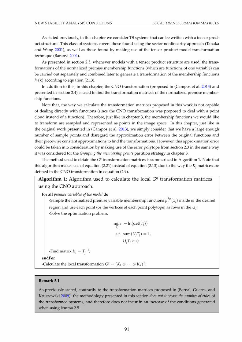
NEW STABILITY ANALYSIS CONDITIONS LOCAL TRANSFORMATION MATRICES
As stated previously, in this chapter we consider TS systems that can be written with a tensor prod-uct structure. This class of systems covers those found using the sector nonlinearity approach (Tanakaand Wang 2001), as well as those found by making use of the tensor product model transformationtechnique (Baranyi 2004).
As presented in section 2.5, whenever models with a tensor product structure are used, the trans-formations of the normalized premise membership functions (which are functions of one variable) canbe carried out separately and combined later to generate a transformation of the membership functionshi(x) according to equation (2.13).
In addition to this, in this chapter, the CNO transformation (proposed in (Campos et al. 2013) andpresented in section 2.4) is used to find the transformation matrices of the normalized premise member-ship functions.
Note that, the way we calculate the transformation matrices proposed in this work is not capableof dealing directly with functions (since the CNO transformation was proposed to deal with a pointcloud instead of a function). Therefore, just like in chapter 3, the membership functions we would liketo transform are sampled and represented as points in the image space. In this chapter, just like inthe original work presented in (Campos et al. 2013), we simply consider that we have a large enoughnumber of sample points and disregard the approximation error between the original functions andtheir piecewise constant approximations to find the transformations. However, this approximation errorcould be taken into consideration by making use of the error polytope from section 2.3 in the same wayit was considered for the Grouping the membership points partition strategy in chapter 3.
The method used to obtain the Gq transformation matrices is summarized in Algorithm 1. Note thatthis algorithm makes use of equation (2.21) instead of equation (2.13) due to the way the Kj matrices aredefined in the CNO transformation in equation (2.9).
Algorithm 1: Algorithm used to calculate the local Gq transformation matricesusing the CNO approach.
for all premise variables of the model do-Sample the normalized premise variable membership functions µ
αijj (xj) inside of the desired
region and use each point (or the vertices of each point polytope) as rows in the Uj;-Solve the optimization problem:
minTj− ln(det(Tj))
s.t. sum(UjTj) = 1,
UjTj 0.
-Find matrix Kj = T−1j ;
endFor-Calculate the local transformation Gq = (K1 ⊗ · · · ⊗ Kn)T ;
Remark 5.1
As previously stated, contrarily to the transformation matrices proposed in (Bernal, Guerra, andKruszewski 2009). the methodology presented in this section does not increase the number of rules ofthe transformed systems, and therefore does not incur in an increase of the conditions generatedwhen using lemma 2.5.
91

RELAXED STABILITY CONDITIONS NEW STABILITY ANALYSIS CONDITIONS
Remark 5.2
It is worth noting that, when we are dealing with tensor product models whose premise variablespossess only two fuzzy sets, like those obtained via sector nonlinearity (Tanaka and Wang 2001)if we only have at most one nonlinearity for each state, the convex hull of the sample points (orthe uncertainty vertices) is always a simplex with 2 vertices. In this case, finding the Kj matricesreduces to finding the extrema of these points, and the optimization problem in algorithm 1, albeitcostly, can be seen as an alternative to doing this search.
Remark 5.3
Despite the discussion and the algorithm presented for the local transformation matrices have beendirected towards models with a tensor product structure, they can also be applied to find a trans-formation when that is not the case. In that case, we search directly for the Gq matrices, instead ofthe Kj matrices, and samples of the hi(x) functions, instead of the µ
αijj (xj) functions. Note however
that, in order to find an approximation of these functions, we usually need a much larger numberof samples, leasing to a possibly costlier optimization problem.
5.3 Relaxed Stability Conditions
In order to make the most out of the relaxations introduced by the transformations discussed in theprevious section, it is interesting to apply them over local regions (as suggested by the name of theprevious section) instead of the whole state space. In this case, an interesting methodology (similar tothe one presented in (Bernal, Guerra, and Kruszewski 2009)) is to use piecewise Lyapunov functions.In that regard, we propose the use of two different piecewise fuzzy Lyapunov functions (leading totwo different sets of LMI stability conditions) together with the local transformation matrices from theprevious section. Note as well that the results presented in this section could be used regardless of thetransformations, but are more relaxed when the transformations are considered.
In order to apply the new stability conditions, the state space is partitioned into polyhedral regionsΩq, q = 1, 2, . . . , nq, such that the following assumptions are valid.
Assumption 5.1
In each Ωq region, the relation
Eqx 0, ∀ x ∈ Ωq, (5.1)
is valid, and Eq=[
Eq eq], with eq = 0 for regions that include the origin of the state space. In
addition, given two neighboring regions Ωq and Ωp, we have that
Fqx = Fpx, ∀ x ∈ Ωq ∩Ωp, (5.2)
in which Fq=[
Fq fq], with fq = 0 for regions that include the origin.
It is important to note that, given the vertices of each polyhedral region, matrices Eq, Fq and Fp fromAssumption 5.1 can be found using the procedures described in (Johansson, Rantzer, and Arzen 1999).
92

NEW STABILITY ANALYSIS CONDITIONS RELAXED STABILITY CONDITIONS
In a different way, the Eq are easily found by stacking the inequalities that describe the region, and theFq matrices can be found by solving a set of homogeneous linear equations for each state variable.
Assumption 5.2
In each Ωq region there are Gq ∈ Rr×rq matrices describing local transformations of the hi(x) mem-bership functions such that
h = Gqhq,
in which h is the vector formed by stacking the hi(x), i ∈ 1, . . . , r membership functions, and his the vector formed by stacking the hq
j (x), j ∈ 1, . . . , rq membership functions. In addition, thetransformed membership functions are such that (2.1), (2.2) and (2.3) are still valid.
Note that, if this is not the case, we can take Gq to be the r× r identity matrix.Besides the transformation matrices discussed in the previous section, an alternative, from (Bernal,
Guerra, and Kruszewski 2009), to find transformed membership functions that satisfy Assumption 5.2is found by splitting the state space such that the possible ordering relations among the membershipfunctions can be taken into consideration. As a consequence of this procedure, it is possible to find Gq
matrices with the additional property that Gq 0.
Membership derivative independent conditions
For each Ωq region, it is possible to write a fuzzy candidate Lyapunov function (Rhee and Won 2006) ofthe form:
Vq(x) = 2∫
Γ[0,x]〈
r
∑i=1
hi(s)Pqi s, ds〉, (5.3)
in which Γ[0, x] is an arbitrary trajectory from the origin to x, with s ∈ Rn+1 being the trajectory variableand s ∈ Rn equal to the first n components of s.
The Pqi ∈ R(n+1)×(n+1) matrices parametrize the candidate Lyapunov function, and in order for
Vq(x) to be similar to potential energy functions, such that the integral in (5.3) is path independent, it issufficient that the Pq
i matrices be symmetric and have the following structure (Rhee and Won 2006):
Pqi =
[Pq
i pq1
∗ pq2
],
Pqi = Dq
0 + Dqi ,
Dq0 =
0 d12q · · · d1nq
d12q 0 · · · d2nq...
.... . .
...d1nq d2nq · · · 0
,
Dqi =
dαi111q 0 · · · 0
0 dαi222q · · · 0
......
. . ....
0 0 · · · dαinnnq
. (5.4)
The structure in (5.4) indicates that, in each region Ωq, the elements of Pqi outside of the diagonal, and
the elements pq1 and pq
2 have to be the same for all of the rules. Nevertheless, the diagonal elements of
93

RELAXED STABILITY CONDITIONS NEW STABILITY ANALYSIS CONDITIONS
Pqi , d
αijjjq, may change according to the rules, but need to be the same for two rules sharing the same fuzzy
set regarding variable xj; i.e. given two rules i and k, if αij = αkj, then dαijjjq = d
αkjjjq .
For regions Ωq that contain the origin, pq1 = 0 and pq
2 = 0, and equation (5.3) can be rewritten as
Vq(x) = 2∫
Γ[0,x]〈
r
∑i=1
hi(s)Pqi s, ds〉, (5.5)
with the Pqi matrices following the structure presented in equation (5.4). Having made these assump-
tions, the following theorem can be stated.
Theorem 5.1: Membership functions’ time derivative independent stability conditions
Given matrices Eq=[
Eq eq]
and Fq=[
Fq fq]
satisfying conditions (5.1) and (5.2), together with
matrices Gq ∈ Rr×rq describing membership functions transformations such that Assumption 5.2 is valid,
system (2.5) is asymptotically stable if there are matrices M =
[M m1
mT2 m3
]and N =
[N n1
nT2 n3
], symmetric
matrices Uqi 0 and Wq
i 0, and symmetric matrices Ti, such that the following conditions are met:
Pqi − (Eq
)TUqi Eq
> 0, (5.6)r
∑i=1
gqijLiq < 0, j ∈ 1, . . . , rq, (5.7)
with Pqi = (Fq
)TTiFq having the structure in (5.4), and
Liq =
[MT Ai + AT
i M + (Eq)TWq
i Eq Pqi −MT
+ ATi N
∗ −N − NT
], (5.8)
for regions that do not contain the origin of the state space. In a similar way,
Pqi − (Eq)TUq
i Eq > 0, (5.9)r
∑i=1
gqijLiq < 0, j ∈ 1, . . . , rq, (5.10)
with Pqi = (Fq)TTiFq having the structure in (5.4), and
Liq =
[MT Ai + AT
i M + (Eq)TWqi Eq Pq
i −MT + ATi N
∗ −N − NT
], (5.11)
for regions that contain the origin of the state space.
Proof. Consider that the state space is divided into Ωq polyhedral regions described by (5.1). If wewould like to use a piecewise combination of (5.3) and (5.5) as a candidate Lyapunov function, we mustguarantee the continuity of this combination when we switch from one region to the other. Therefore,we would like that
Vq(x) = Vp(x),
2∫
Γ[0,x]〈
r
∑i=1
hi(s)Pqi s, ds〉 = 2
∫
Γ[0,x]〈
r
∑i=1
hi(s)Ppi s, ds〉, (5.12)
be true for two neighboring regions Ωq and Ωp, whenever x is on the border of these two regions.
94

NEW STABILITY ANALYSIS CONDITIONS RELAXED STABILITY CONDITIONS
Since the structure imposed by equation (5.4) over the Pqi and Pq
i matrices guarantees that the lineintegral is path independent (Rhee and Won 2006), choosing the path s = τx, with τ ∈ [0, 1], condition(5.12) can be rewritten as
∫ 1
0τxT
r
∑i=1
hi(τx)Pqi xdτ =
∫ 1
0τxT
r
∑i=1
hi(τx)Ppi xdτ,
∫ 1
0τ
r
∑i=1
hi(τx)xT Pqi xdτ =
∫ 1
0τ
r
∑i=1
hi(τx)xT Ppi xdτ. (5.13)
A sufficient condition for (5.13) is that
r
∑i=1
hi(τx)xT Pqi x =
r
∑i=1
hi(τx)xT Ppi x,
which, in turn, can be assured byxT Pq
i x = xT Ppi x, (5.14)
whenever x is on the intersection of regions Ωq and Ωp.Assuming that there are Fq matrices such that, whenever x lies on the switching surface of the two
regions, condition (5.2) is valid, matrices Pqi can be written as
Pqi = (Fq
)TTiFq
to satisfy condition (5.14). By doing this,
xT(Fq)TTiF
qx = xT(Fp)TTiF
px.
On the other hand, the condition that the candidate Lyapunov function must be positive definiteimplies that, over region Ωq,
xT Pqi x > 0, for regions not including the origin, (5.15)
xT Pqi x > 0, for regions including the origin. (5.16)
The inequalities above need be satisfied only when x ∈ Ωq; i.e. only when expression (5.1) is true. Inorder to deal with this problem, the following quadratic constraints are considered
xT(Eq)TUq
i Eqx ≥ 0, (5.17)
xT(Eq)TUqi Eqx ≥ 0, (5.18)
which, from (5.1) and picking copositive Uqi matrices, are satisfied for every x ∈ Ωq. Note that it is
possible that these inequalities are also valid for some x 6∈ Ωq; i.e. the inequalities above are onlysufficient for (5.15) and (5.16).
In order to simplify the problem, we use non-negative matrices (matrices whose elements are non-negative), which is a subset of the copositive matrices (Bundfuss 2009).
Therefore, a sufficient condition to ensure that the candidate Lyapunov function is positive definiteover each region Ωq is that (5.15)) and (5.16) be valid whenever (5.17) and (5.18), respectively, are valid.And by applying the S-procedure we get conditions (5.6) and (5.9).
In regions that do not include the origin, the time derivative of the Lyapunov function can be writtenas
V(x) =
[xx
]T r
∑i=1
hi(x)
[0 Pq
i∗ 0
] [xx
], (5.19)
95

RELAXED STABILITY CONDITIONS NEW STABILITY ANALYSIS CONDITIONS
whereas in regions that include the origin, it can be written as
V(x) =
[xx
]T r
∑i=1
hi(x)
[0 Pq
i∗ 0
] [xx
]. (5.20)
Consider arbitrary real matrices M =
[M m1
mT2 m3
]and N =
[N n1
nT2 n3
]. The following null-term (Mozelli,
Palhares, and Avellar 2009)
[xx
]T r
∑i=1
hi(x)
[MT Ai + AT
i M −MT+ AT
i N
∗ −N − NT
] [xx
]= 0, (5.21)
can be added to the time derivative in regions that do not include the origin. And the null-term
[xx
]T r
∑i=1
hi(x)
[MT Ai + AT
i M −MT + ATi N
∗ −N − NT
] [xx
]= 0, (5.22)
in regions that include the origin.By making use of quadratic constraints, similar to the one presented above, to represent regions that
contain each region Ωq, from (5.1), and using Wqi matrices whose elements are non-negative, we can
write[
xx
]T r
∑i=1
hi(x)
[(Eq
)TWqi Eq 0
∗ 0
] [xx
]≥ 0,
[xx
]T r
∑i=1
hi(x)
[(Eq)TWq
i Eq 0∗ 0
] [xx
]≥ 0.
Therefore, adding each term to the respective time derivative in (5.19) and (5.20), we assure that the timederivative of the Lyapunov function is negative definite over regions Ωq, and at the same time, allowfor a relaxation of this constraint outside of these regions (where this conditions is not really necessary).The final expression can be written as
r
∑i=1
hi(x)Liq < 0, for regions not including the origin,
r
∑i=1
hi(x)Liq < 0, for regions including the origin,
in which Liq and Liq are given by (5.8) and (5.11), respectively.If there are Gq ∈ Rr×rq matrices defining valid transformations of the membership functions accord-
ing to Assumption 5.2, we can make use of lemma 2.5 in the conditions above to write
rq
∑j=1
hqj
(r
∑i=1
gqijLiq
)< 0, (5.23)
for regions not including the origin,
rq
∑j=1
hqj
(r
∑i=1
gqijLiq
)< 0, (5.24)
for regions including the origin.And it is clear that conditions (5.7) and (5.10) are sufficient for (5.23) and (5.24).
96
NEW STABILITY ANALYSIS CONDITIONS RELAXED STABILITY CONDITIONS
Remark 5.4
Since the Fq matrices change according to each Ωq polyhedral region considered, a generic wayof imposing structure (5.4) to matrices Pq
i is by means of linear equality constraints (since, in thiscase, the decision variables are the Ti matrices instead of the Pq
i matrices). However, it is possible toremove the equality constraints from the optimization problem by means of a reduction of the set ofdecision variables, which also reduces the computational time associated with the optimization. Inthe case here presented, these constraints (if well posed) determine a well behaved transformationbasis, such that numerical problems should not occur from eliminating the constraints a.
athis can be done, for instance, using YALMIP (Löfberg 2004) and asking the interpreter toreduce the decision variables based on the equality constraints.
Membership derivative dependent conditions
For each region, it is also possible to write a fuzzy candidate Lyapunov function (Tanaka, Hori, andWang 2003):
Vq(x) =r
∑i=1
hi(x)xT Pqi x, (5.25)
in which Pqi ∈ R(n+1)×(n+1) are matrices parametrizing the Lyapunov function. In a similar way to what
was previously presented, these matrices can be written as
Pqi =
[Pq
i pq1i
∗ pq2i
].
However, unlike the previous case, there are no restrictions over the structure of the Pqi matrices regard-
ing the rules of the TS model. Instead, we assume that the membership functions’ time derivatives arebounded such that1
|hi(x)| ≤ φi, i = 1, 2, . . . , r. (5.26)
For regions containing the origin, pq1i= 0 and pq
2i= 0, and the corresponding candidate Lyapunov
function can be rewritten as
Vq(x) =r
∑i=1
hi(x)xT Pqi x. (5.27)
Given these assumptions, the following theorem can be stated.
1In order to simplify the demonstration, we make use of the same bounds for every region in thestate space. Note however that we are not forced to do so, and different bounds could be used for eachregion.
97

RELAXED STABILITY CONDITIONS NEW STABILITY ANALYSIS CONDITIONS
Theorem 5.2: Membership functions’ time derivative dependent stability conditions
Given matrices Eq=[
Eq eq]
and Fq=[
Fq fq]
satisfying conditions (5.1) and (5.2), together with
matrices Gq ∈ Rr×rq describing membership functions transformations such that Assumption 5.2 is valid,and considering that the time derivative of the membership functions is bounded according to (5.26), system
(2.5) is asymptotically stable if there are matrices M =
[M m1
mT2 m3
]and N =
[N n1
nT2 n3
], symmetric
matrices Uqi 0 and Wq
i 0, and symmetric matrices Ti and Qq (or Qq), such that the following conditionsare met:
Pqi − (Eq
)TUqi Eq
> 0, (5.28)
Pqi + Qq
> 0, (5.29)r
∑i=1
gqijLiq < 0, j ∈ 1, . . . , rq, (5.30)
with Pqi = (Fq
)TTiFq, and
Liq =[
Pqφ + MT Ai + AT
i M + (Eq)TWq
i Eq Pqi −MT
+ ATi N
∗ −N − NT
], (5.31)
Pqφ =
r
∑i=1
φi(Pqi + Qq
),
for regions not containing the origin of the state space. In a similar way,
Pqi − (Eq)TUq
i Eq > 0, (5.32)
Pqi + Qq > 0, (5.33)r
∑i=1
gqijLiq < 0, j ∈ 1, . . . , rq, (5.34)
with Pqi = (Fq)TTiFq, and
Liq =[
Pqφ + MT Ai + AT
i M + (Eq)TWqi Eq Pq
i −MT + ATi N
∗ −N − NT
], (5.35)
Pqφ =
r
∑i=1
φi(Pqi + Qq),
for regions containing the origin of the state space.
Proof. Consider that the state space is divided into Ωq polyhedral regions described by (5.1). If we wouldlike to use a piecewise combination of (5.25) and (5.27) as a candidate Lyapunov function, we mustguarantee the continuity of this combination when switching from one region to another. Therefore,
98

NEW STABILITY ANALYSIS CONDITIONS RELAXED STABILITY CONDITIONS
∀x ∈ Ωq ∩Ωp,
Vq(x) = Vp(x),r
∑i=1
hi(x)xT Pqi x =
r
∑i=1
hi(x)xT Ppi x.
A sufficient condition for that is that
xT Pqi x = xT Pp
i x, ∀x ∈ Ωq ∩Ωp.
On the other hand, from (5.2), this can be guaranteed by rewriting the Pqi matrices as
Pqi = (Fq
)TTiFq,
as was shown in the proof of Theorem 5.1.Conditions (5.28) and (5.32) are sufficient to guarantee that the piecewise combination of these Lya-
punov functions will be positive definite over regions Ωq. This can be proved by following the samedevelopment done in the proof of Theorem 5.1.
In regions not including the origin, the time derivative of the Lyapunov function can be written as
V(x) =
[xx
]T r
∑i=1
hi(x)
[∑r
k=1 hk(x)Pqk Pq
i∗ 0
] [xx
], (5.36)
whereas, for regions including the origin, it can be written as
V(x) =
[xx
]T r
∑i=1
hi(x)
[∑r
k=1 hk(x)Pqk Pq
i∗ 0
] [xx
]. (5.37)
Taking into account the bounds in (5.26) over the membership functions time derivatives, and consid-ering that conditions (5.29) and (5.33) are satisfied, we can make use of the idea presented in (Mozelliet al. 2009) to write
r
∑k=1
hk(x)Pqk =
r
∑k=1
hk(x)(Pqk + Qq
) ≤ Pqφ =
r
∑k=1
φk(Pqk + Qq
),
r
∑k=1
hk(x)Pqk =
r
∑k=1
hk(x)(Pqk + Qq) ≤ Pq
φ =r
∑k=1
φk(Pqk + Qq),
which, from (5.36) and (5.37), leads to
V(x) ≤[
xx
]T r
∑i=1
hi(x)
[Pq
φ Pqi
∗ 0
] [xx
],
for regions not including the origin, and
V(x) ≤[
xx
]T r
∑i=1
hi(x)
[Pq
φ Pqi
∗ 0
] [xx
],
for regions including the origin.By following the same steps of using the null-terms (5.21) and (5.22), and the same relaxations re-
garding the Wqi variables that were used in the proof of Theorem 5.1, sufficient conditions for the time
derivative of the Lyapunov function to negative definite can be written as
r
∑i=1
hi(x)Liq < 0, for regions not including the origin, (5.38)
r
∑i=1
hi(x)Liq < 0, for regions including the origin, (5.39)
99

RELAXED STABILITY CONDITIONS NEW STABILITY ANALYSIS CONDITIONS
in which Liq and Liq are given by (5.31) and (5.35), respectively.As in Theorem 5.1, considering that there exist valid Gq transformation matrices according to as-
sumption 5.2, conditions (5.30) and (5.34) are sufficient for (5.38) and (5.39) to be true.
Remark 5.5
It is important to note that, when dealing with piecewise Lyapunov functions, the stability willonly be proven for the largest Lyapunov sublevel set that is contained in the union of all of the statespace regions considered. However, if the regions are written and used as in (Johansson, Rantzer,and Arzen 1999) (which is the case in this chapter) and all of the regions considered contain theorigin, the conditions will be valid for all of the state space. However, in the case of Theorem5.2, we will only get global stability if the bound used for the time derivative of the membershipfunctions is global. In the other cases, the stability region proven will be the largest sublevel setof the Lyapunov function that is contained in the region where the bound is valid. In case wewould like to use local conditions, an interesting approach is to employ instead bounds the partialderivatives of the membership functions, as in (Bernal and Guerra 2010).
Remark 5.6
Note that Theorems 5.1 and 5.2 are more general than (Bernal, Guerra, and Kruszewski 2009, Theo-rem 2), if the bound used for the time derivative of the membership functions considered in Theo-rem 5.2 is valid in all of the regions considered. In both cases, if the Pq
i matrices are chosen to changeonly with q, conditions in Theorems 5.1 are 5.2 relaxed versions of (Bernal, Guerra, and Kruszewski2009, Theorem 2).
Proof. In order to prove the remark above, we will show only the proof for the regions that contain theorigin of the state space. The proof for the other regions follows by analogy.
Note that conditions from (Bernal, Guerra, and Kruszewski 2009, Theorem 2) can be written as
Pq − (Eq)T UqEq > 0, ∀q, (5.40)r
∑i=1
hi
(AT
i Pq + Pq Ai + (Eq)T Wqi Eq
)< 0, ∀q. (5.41)
By taking Pqi = Pq and Uq
i = Uq in (5.9) and (5.32), we recover (5.40).By making use of Finsler’s lemma (Mozelli, Palhares, and Mendes 2010), the constraint (5.41) can be
written as
r
∑i=1
r
∑j=1
hihj
[AT
i Mj + MTj Ai + (Eq)T Wq
i Eq Pq −MTj + AT
i Nj
∗ −Nj − NTj
]< 0, ∀q.
However, note that, if the above constraint is satisfied, there are matrices M and N such thatr
∑i=1
hiLiq < 0, ∀q,
Liq =
[AT
i M + MT Ai + (Eq)T Wqi Eq Pq −MT + AT
i N∗ −N − NT
].
Applying the local transformation matrices, we can write
r
∑i=1
gqijLiq < 0, ∀q, j ∈ 1, . . . , rq. (5.42)
100
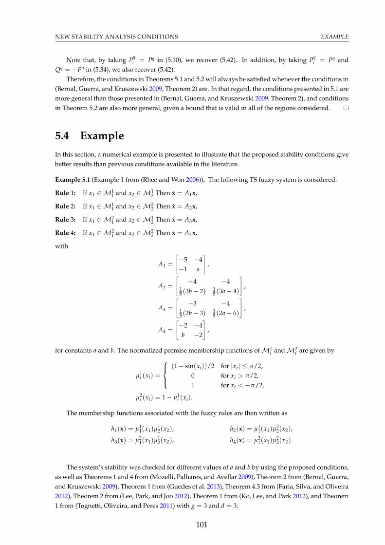
NEW STABILITY ANALYSIS CONDITIONS EXAMPLE
Note that, by taking Pqi = Pq in (5.10), we recover (5.42). In addition, by taking Pq
i = Pq andQq = −Pq in (5.34), we also recover (5.42).
Therefore, the conditions in Theorems 5.1 and 5.2 will always be satisfied whenever the conditions in(Bernal, Guerra, and Kruszewski 2009, Theorem 2) are. In that regard, the conditions presented in 5.1 aremore general than those presented in (Bernal, Guerra, and Kruszewski 2009, Theorem 2), and conditionsin Theorem 5.2 are also more general, given a bound that is valid in all of the regions considered.
5.4 Example
In this section, a numerical example is presented to illustrate that the proposed stability conditions givebetter results than previous conditions available in the literature.
Example 5.1 (Example 1 from (Rhee and Won 2006)). The following TS fuzzy system is considered:
Rule 1: If x1 ∈ M11 and x2 ∈ M1
2 Then x = A1x,
Rule 2: If x1 ∈ M11 and x2 ∈ M2
2 Then x = A2x,
Rule 3: If x1 ∈ M21 and x2 ∈ M1
2 Then x = A3x,
Rule 4: If x1 ∈ M21 and x2 ∈ M2
2 Then x = A4x,
with
A1 =
[−5 −4−1 a
],
A2 =
[−4 −4
15 (3b− 2) 1
5 (3a− 4)
],
A3 =
[−3 −4
15 (2b− 3) 1
5 (2a− 6)
],
A4 =
[−2 −4b −2
],
for constants a and b. The normalized premise membership functions ofM1i andM2
i are given by
µ1i (xi) =
(1− sin(xi))/2 for |xi| ≤ π/2,0 for xi > π/2,1 for xi < −π/2,
µ2i (xi) = 1− µ1
i (xi).
The membership functions associated with the fuzzy rules are then written as
h1(x) = µ11(x1)µ
12(x2), h2(x) = µ1
1(x1)µ22(x2),
h3(x) = µ21(x1)µ
12(x2), h4(x) = µ2
1(x1)µ22(x2).
The system’s stability was checked for different values of a and b by using the proposed conditions,as well as Theorems 1 and 4 from (Mozelli, Palhares, and Avellar 2009), Theorem 2 from (Bernal, Guerra,and Kruszewski 2009), Theorem 1 from (Guedes et al. 2013), Theorem 4.3 from (Faria, Silva, and Oliveira2012), Theorem 2 from (Lee, Park, and Joo 2012), Theorem 1 from (Ko, Lee, and Park 2012), and Theorem1 from (Tognetti, Oliveira, and Peres 2011) with g = 3 and d = 3.
101

EXAMPLE NEW STABILITY ANALYSIS CONDITIONS
In order to apply Theorem 5.1 and 5.2, as well as Theorem 2 from (Bernal, Guerra, and Kruszewski2009), the system was divided into 4 regions according to the ordering relations of the membershipfunctions (this was done to allow the use, for comparison purposes, of the local transformation matricesproposed in Bernal, Guerra, and Kruszewski 2009). The following regions were chosen
Region 1: x1 < 0, x2 < 0h1 > h2 > h4 and h1 > h3 > h4
Region 2: x1 < 0, x2 > 0h2 > h4 > h3 and h2 > h1 > h3
Region 3: x1 > 0, x2 < 0h3 > h1 > h2 and h3 > h4 > h2
Region 4: x1 > 0, x2 > 0h4 > h2 > h1 and h4 > h3 > h1
The following Eq and Fq matrices satisfying conditions (5.1) and (5.2) were used:
E1 =
−0.1 00 00 −0.10 0
, F1 =
0 0−0.1 0
0 00 00 −0.10 0
,
E2 =
−0.1 00 00 00 0.1
, F2 =
0 0−0.1 0
0 00 00 00 0.1
,
E3 =
0 00.1 00 −0.10 0
, F3 =
0 00 0
0.1 00 00 −0.10 0
,
E4 =
0 00.1 00 00 0.1
, F4 =
0 00 0
0.1 00 00 00 0.1
.
In order to allow the use of Theorem 5.2, Theorem 1 from (Mozelli, Palhares, and Avellar 2009),Theorem 1 from (Guedes et al. 2013), Theorem 4.3 from (Faria, Silva, and Oliveira 2012), Theorem 2from (Lee, Park, and Joo 2012), Theorem 1 from (Ko, Lee, and Park 2012), and Theorem 1 from (Tognetti,Oliveira, and Peres 2011), the following bound on the time derivative of the membership functions was
102

NEW STABILITY ANALYSIS CONDITIONS EXAMPLE
used:
φi = 0.85, ∀i.
Note that, most likely, this is not a global bound for the membership functions time derivative in thisexample (and given large values of a and b, most likely, is valid only for a very small region around theorigin). Therefore, as stated in Section 5.3, conditions based on this bound will only assert the system’slocal stability. Nevertheless, this is a very common value for this bound found on the literature (Faria,Silva, and Oliveira 2012; Guedes et al. 2013; Ko and Park 2012; Ko, Lee, and Park 2012; Lee, Park, andJoo 2012; Mozelli, Palhares, and Avellar 2009; Rhee and Won 2006; Tognetti, Oliveira, and Peres 2011;Zhang and Xie 2011) and will be used for comparison purposes.
In order to compare the relaxation brought about by the transformation matrices, both the methodproposed in (Bernal, Guerra, and Kruszewski 2009) as well as the method discussed in Section 5.2 wereused.
Using the constructing method detailed in (Bernal, Guerra, and Kruszewski 2009), the transforma-tion matrices are
G1 =
0.5 0.5 0.5 0.5 10 1 0 0 10 0 0 1 10 0 0 0 1
,
G2 =
0 0 0 1 10.5 0.5 0.5 0.5 10 0 0 0 10 1 0 0 1
,
G3 =
0 1 0 0 10 0 0 0 1
0.5 0.5 0.5 0.5 10 0 0 1 1
,
G4 =
0 0 0 0 10 1 0 0 10 0 0 1 1
0.5 0.5 0.5 0.5 1
.
103

EXAMPLE NEW STABILITY ANALYSIS CONDITIONS
Using the method presented in Section 5.2, the transformation matrices are:
G1 =
1 0.5 0.5 0.250 0.5 0 0.250 0 0.5 0.250 0 0 0.25
,
G2 =
0.5 0 0.25 00.5 1 0.25 0.50 0 0.25 00 0 0.25 0.5
,
G3 =
0.5 0.25 0 00 0.25 0 0
0.5 0.25 1 0.50 0.25 0 0.5
,
G4 =
0.25 0 0 00.25 0.5 0 00.25 0 0.5 00.25 0.5 0.5 1
.
The results are presented in Tables 5.1 and 5.2, where a line search method was used to find thelargest value of b, given a fixed a, in which the conditions were still feasible. Table 5.1 shows the resultsobtained using different derivative independent conditions (Theorem 5.1, Theorem 4 from Mozelli, Pal-hares, and Avellar 2009, and Theorem 2 from (Bernal, Guerra, and Kruszewski 2009)), whereas Table 5.2shows the results obtained using different derivative dependent conditions (Theorem 5.2, Theorem 1from Mozelli, Palhares, and Avellar 2009, Theorem 1 from (Guedes et al. 2013), Theorem 4.3 from Faria,Silva, and Oliveira 2012, Theorem 2 from Lee, Park, and Joo 2012, Theorem 1 from Ko, Lee, and Park2012, and Theorem 1 from Tognetti, Oliveira, and Peres 2011).
From these tables, we can see that Theorem 5.1 has a better performance than the other derivativeindependent conditions, as well as better performance than many derivative dependent conditions fora = −2 (with the exception of Theorem 5.2). In addition, note that, when Theorem 5.1 is used inconjunction with the CNO transformation it behaves better than Theorem 1 from (Mozelli, Palhares, andAvellar 2009) (which is a derivative dependent condition). From Table 5.2, we also see that Theorem 5.2had a better perfomance than the other derivative dependent conditions.
Note that, in general, the derivative dependent conditions presented a superior performance thanthe independent conditions for this example. However, in this case, the larger the values of a and b,the smaller the corresponding region on the state space for which these conditions assure the stability.Whereas, in this example, the derivative independent conditions always assure the global stability of thesystem when they are feasible (and for that reason they are valid for a smaller set of a and b parametersthan the derivative dependent conditions).
Another interesting observation that can be made regarding the tables is that, in this example, theuse of the CNO transformation against the use of the transformation presented in (Bernal, Guerra, andKruszewski 2009) yielded better results.
Figures 5.1 to 5.5 illustrate the conditions and transformations proposed for a ∈ [−18, 0] and b ∈[0, 1000].
Figure 5.1 compares Theorem 5.1, using the transformation matrices from (Bernal, Guerra, andKruszewski 2009), with other conditions from the literature.
104

NEW STABILITY ANALYSIS CONDITIONS EXAMPLE
Table 5.1: Maximum feasible values of b, in the example, for the derivative independent conditions.Compares Theorem 5.1 used in conjunction with the transformation proposed in (Bernal, Guerra, andKruszewski 2009) and the CNO transformation, (Bernal, Guerra, and Kruszewski 2009, Theorem 2) usedin conjunction with the transformation proposed in (Bernal, Guerra, and Kruszewski 2009) and the CNOtransformation, and (Mozelli, Palhares, and Avellar 2009, Theorem 4).
Method a-16 -12 -8 -4 -2
Mozelli, Palhares, and Avellar 2009, Th.4 441 339 233 120 65Bernal, Guerra, and Kruszewski 2009, Th.2 317 222 139 74 48+ Bernal, Guerra, and Kruszewski 2009
Bernal, Guerra, and Kruszewski 2009, Th.2 + CNO 421 292 186 103 70Th.5.1 + Bernal, Guerra, and Kruszewski 2009 780 638 390 288 201
Th.5.1 + CNO 1012 782 558 352 253
Table 5.2: Maximum feasible values of b, in the example, for the derivative dependent conditions.Compares Theorem 5.2 used in conjunction with the transformation proposed in (Bernal, Guerra, andKruszewski 2009) and the CNO transformation, (Mozelli, Palhares, and Avellar 2009, Theorem 1),(Guedes et al. 2013, Theorem 1), (Faria, Silva, and Oliveira 2012, Theorem 4.3), (Lee, Park, and Joo 2012,Theorem 2), (Ko, Lee, and Park 2012, Theorem 1), and (Tognetti, Oliveira, and Peres 2011, Theorem 1)with g = 3 and d = 3.
Method a-16 -12 -8 -4 -2
Mozelli, Palhares, and Avellar 2009, Th.1 964 603 323 123 51Guedes et al. 2013, Th.1 1284 805 431 161 66
Faria, Silva, and Oliveira 2012, Th.4.3 1360 850 452 167 66Lee, Park, and Joo 2012, Th.2 1914 1072 547 202 88Ko, Lee, and Park 2012, Th.1 2836 1704 853 286 104
Tognetti, Oliveira, and Peres 2011, Th.1(3,3) 4727 2789 1383 469 188Th.5.2 + Bernal, Guerra, and Kruszewski 2009 37244 39911 4979 463 219
Th.5.2 + CNO 983122 992028 726248 4529 846
Figure 5.2 compares Theorem 5.2, using the transformation matrices from (Bernal, Guerra, andKruszewski 2009), with other conditions from the literature.
Figures 5.3, 5.4 and 5.5 compare the results obtained with the transformation discussed in Section5.2 with those obtained with the transformation proposed in (Bernal, Guerra, and Kruszewski 2009).They deal, respectively, with Theorem 2 from (Bernal, Guerra, and Kruszewski 2009), Theorem 5.1, andTheorem 5.2. There are no guarantees that the transformation matrices discussed in Section 5.2 willhave a better behaviour than the transformation matrices from (Bernal, Guerra, and Kruszewski 2009).However, as can be seen from the figures presented, that was the case in this example.
105
EXAMPLE NEW STABILITY ANALYSIS CONDITIONS
−15 −10 −5 00
200
400
600
800
1000
a
b
Figure 5.1: Feasibility space for different conditions using the local transformation matrices in (Bernal,Guerra, and Kruszewski 2009). Theorem 2 from (Bernal, Guerra, and Kruszewski 2009) is feasible inthe × and + region. Theorem 4 from (Mozelli, Palhares, and Avellar 2009) is feasible in the ×, and ·region. Theorem 1 from (Mozelli, Palhares, and Avellar 2009) is feasible in the ×, , © and 4 region.Theorem 5.1 is feasible in the ×, ,©, ∗, + and · region.
106

NEW STABILITY ANALYSIS CONDITIONS EXAMPLE
−15 −10 −5 00
200
400
600
800
1000
a
b
Figure 5.2: Feasibility space for different conditions using the local transformation matrices in (Bernal,Guerra, and Kruszewski 2009). Theorem 2 from (Bernal, Guerra, and Kruszewski 2009) is feasible inthe × and + region. Theorem 4 from (Mozelli, Palhares, and Avellar 2009) is feasible in the ×, and ·.Theorem 1 from (Mozelli, Palhares, and Avellar 2009) is feasible in the ×, and© region. Theorem 5.2is feasible for all the points shown in the figure.
−15 −10 −5 00
200
400
600
800
1000
a
b
Figure 5.3: Feasibility space for different transformation matrices using Theorem 2 from (Bernal, Guerra,and Kruszewski 2009). With the transformation proposed in (Bernal, Guerra, and Kruszewski 2009),conditions are feasible in the × region. With the transformation discussed in Section 5.2, conditions arevalid for all the points shown in the figure.
107

EXAMPLE NEW STABILITY ANALYSIS CONDITIONS
−15 −10 −5 00
200
400
600
800
1000
a
b
Figure 5.4: Feasibility space for different transformation matrices using Theorem 5.1. With the transfor-mation proposed in (Bernal, Guerra, and Kruszewski 2009), conditions are feasible in the× region. Withthe transformation discussed in Section 5.2, conditions are valid for all the points shown in the figure.
−15 −10 −5 00
200
400
600
800
1000
a
b
Figure 5.5: Feasibility space for different transformation matrices using Theorem 5.2. With the transfor-mation proposed in (Bernal, Guerra, and Kruszewski 2009), conditions are feasible in the× region. Withthe transformation discussed in Section 5.2, conditions are valid for all the points shown in the figure.
108

6 A Novel Way to Deal withNonquadratic Lyapunov Functions inContinuous Time TS Systems:Stability and Stabilization Conditions
A novel way to deal with the time-derivative of nonquadratic Lyapunov functions in local conditions is proposed.This new proposition allow us to avoid the use of direct bounds over the time-derivative of the membership func-tions, and therefore avoid the need of a separate set of conditions to guarantee those bounds. New stability andstabilization conditions are presented as well as examples to illustrate their uses.
The work presented in this chapter was done in collaboration with Raymundo Márquez under the supervision ofProf. Thierry Marie Guerra.
6.1 Introduction
Since TS systems are nonlinear systems, an important source of conservatism in the LMIs comes fromthe family of candidate Lyapunov functions used in the conditions (Sala 2009). Among these families offunctions, quadratic Lyapunov functions yield the simplest LMI conditions and can be readily appliedin most of the cases due to their simplicity. However, they usually yield the most conservative results(since other families of functions are usually constructed in a way that they cover quadratic functions).
Nonquadratic, or fuzzy Lyapunov functions (Tanaka, Hori, and Wang 2003) use a quadratic functionfor each of the system’s rules with the same membership functions, yielding a convex sum of quadraticfunctions. When deriving stability conditions for continuous-time systems using these functions, thetime derivative of the membership functions usually appears.
Many conditions in the literature (Campos et al. 2013; Faria, Silva, and Oliveira 2012; Guedes et al.2013; Ko and Park 2012; Ko, Lee, and Park 2012; Mozelli, Palhares, and Avellar 2009; Mozelli et al. 2009;Tognetti, Oliveira, and Peres 2011; Zhang and Xie 2011) make use of previously known upper boundson these time derivatives in order to present LMI analysis and synthesis conditions. In the analysis case,these upper bounds can usually be found beforehand and this does not usually represent a restriction.In the synthesis case, however, if any of the premise variables are state variables, this assumption is
109

CONSIDERATIONS AND SPECIAL NOTATION NONQUADRATIC LYAPUNOV FUNCTIONS
violated and stability is only assured for the largest sublevel-set of the Lyapunov function inside theregion given by the upper bound used.
Trying to get rid of a priori bounds on the time-derivatives, recent works in the literature (Bernal andGuerra 2010; Guerra et al. 2012; Lee, Joo, and Tak 2014; Lee and Kim 2014; Lee, Park, and Joo 2012; Pan etal. 2012) give up on asserting global stability and instead pursue a local certification. Some (Bernal andGuerra 2010; Guerra et al. 2012) use the state space region the model is confined in, as well as boundson the membership functions partial derivatives regarding the states and bounds on the control effortto enforce previously specified bounds on the time derivatives. Others (Lee and Kim 2014; Lee, Park,and Joo 2012; Pan et al. 2012), present conditions that need not directly bound the control efforts, whilesome others (Lee, Joo, and Tak 2014) also remove the need to specify the time derivative bounds (in theanalysis case).
By making use of a polytopic representation of a local region in state space and some novel ma-nipulations, this chapter avoids the use of bounds on the membership functions time derivative byexplicitly including the state vector into the stability conditions. In the stabilization case, we make useof a non-PDC control law and some sufficient conditions to adapt the results from the stability case. Thestabilization conditions are, in a way, conservative but are still guaranteed to give better results thanthose with a quadratic Lyapunov function.
6.2 Considerations and special notation
Throughout this chapter, we consider continuous-time TS systems described by
x =r
∑i=1
hi(x)Aix, (6.1)
for the stability conditions, or
x =r
∑i=1
hi(x) (Aix + Biu) , (6.2)
for the stabilization conditions. In these equations, x ∈ Rn is the state vector, u ∈ Rm is the input vector,Ai ∈ Rn×n and Bi ∈ Rn×m are the system matrices, hi(x) are the membership functions (that we assumemay only depend on the system’s states), and r is the number of rules.
Since we are dealing with TS models, the membership functions respect condition (2.3).Throughout this chapter, we also consider a TS model for the Jacobian of the membership functions’
vector h =[
h1 h2 . . . hr
]T∈ Rr (which can be found either by sector nonlinearity (Tanaka and
Wang 2001), or by the Tensor Product Model Transformation (Baranyi 2004)). We consider this model tobe described by
∂h∂x
=ng
∑j=1
gj(x)Jj, (6.3)
with Jj ∈ Rr×n the matrices that represent the Jacobian, ng the number of rules that describe its TSmodel, and gj(x) its membership functions with properties
gj ≥ 0,ng
∑j=1
gj = 1.
For the stability case, we restrict our analysis to a polytopic region around the origin given by
x =nα
∑k=1
αkxk,nα
∑k=1
αk = 1, αk ≥ 0, (6.4)
110

NONQUADRATIC LYAPUNOV FUNCTIONS CONSIDERATIONS AND SPECIAL NOTATION
with xk the vertices of the polytopic region and nα the number of vertices describing the region.In the stabilization case, we work instead with a transformed state space (represented in this chapter
by the variable s). In the same manner as in the stability case, we restrict our conditions to a polytopicregion around the origin given by
s =nα
∑k=1
αksk,nα
∑k=1
αk = 1, αk ≥ 0. (6.5)
with sk the vertices of the polytopic region and nα the number of vertices describing the region.For the remainder of the chapter, the following short representations will be used for a single fuzzy
sum and its inverse
Ph =r
∑i=1
hi(x)Pi,
P−1h =
(r
∑i=1
hi(x)Pi
)−1
.
Similarly, the following short representations will be used for a multiple fuzzy sum and its inverse
Phq =r
∑i1=1· · ·
r
∑iq=1
(q
∏`=1
hi`(x)
)Pi1 ...iq ,
P−1hq =
r
∑i1=1· · ·
r
∑iq=1
(q
∏`=1
hi`(x)
)Pi1 ...iq
−1
.
In addition to h, we also consider that g and α can also be used as subscripts in this same manner todenote fuzzy summations. Therefore, if at some point we have a matrix Lhqgα, it will represent
Lhqgα =r
∑i1=1· · ·
r
∑iq=1
ng
∑j=1
nα
∑k=1
(q
∏`=1
hi`
)gjαkLi1 ...iq jk.
The following Lemmas will prove useful in later developments
Lemma 6.1: Finsler’s Lemma (Mozelli, Palhares, and Mendes 2010)
The following statements are equivalent:
1. xTQx < 0, ∀x | Bx = 0,
2. B⊥TQB⊥ < 0, BB⊥ = 0 (i.e. B⊥ is a base for the null space of B),
3. ∃N | xT (Q + NT B + BT N)
x < 0,
4. ∃µ > 0 | xT (Q− µBT B)
x < 0.
Lemma 6.2: Derivative of the matrix inverse
The derivate of the inverse of a matrix function is related to the derivative of the matrix function by meansof the following equality
˙(Q−1(t)) = −Q−1(t)Q(t)Q−1(t).
Proof. By taking the derivative of both sides of the equality
Q−1(t)Q(t) = I,
111

CONSIDERATIONS AND SPECIAL NOTATION NONQUADRATIC LYAPUNOV FUNCTIONS
we get that
˙(Q−1(t))Q(t) + Q−1(t)Q(t) = 0,˙(Q−1(t)) = −Q−1(t)Q(t)Q−1(t).
Since in this chapter we work with multiple fuzzy summations, we make use of Lemma 2.4 tocomputationally implement them.
In order to illustrate the assumptions and notations presented in this section, we present an examplesystem.
Example 6.1. Consider a system with four rules, with
A1 =
[−3 20 −0.9
], A2 =
[−0.8 3
0 −0.9
]
A3 =
[−1.9 2−0.5 0.1
], A4 =
[0.1 3−0.5 −2
]
in a polytopic region given by vertices
x1 =
[22
], x2 =
[−22
], x3 =
[2−2
], x4 =
[−2−2
]
and membership functions
h1(x) =
(4− x2
1) (
4− x22)
16, h2(x) =
(4− x2
1)
x22
16,
h3(x) =x2
1(4− x2
2)
16, h4(x) =
x21x2
216
,
The Jacobian of the membership functions’ is given by
∂h∂x
=18
−x1(4− x22) −x2(4− x2
1)
−x1x22 x2(4− x2
1)
x1(4− x22) −x2x2
1x1x2
2 x2x21
,
112

NONQUADRATIC LYAPUNOV FUNCTIONS STABILITY CONDITIONS
and we can write a 16 rule TS model for it with
J1 =
0 01 00 1−1 −1
, J2 =
0 21 −20 −1−1 1
, J3 =
2 0−1 0−2 11 −1
, J4 =
2 2−1 −2−2 −11 1
,
J5 =
0 −21 20 1−1 −1
, J6 =
0 01 00 −1−1 1
, J7 =
2 −2−1 2−2 11 −1
, J8 =
2 0−1 0−2 −11 1
,
J9 =
−2 01 02 1−1 −1
, J10 =
−2 21 −22 −1−1 1
, J11 =
0 0−1 00 11 −1
, J12 =
0 2−1 −20 −11 1
,
J13 =
−2 −21 22 1−1 −1
, J14 =
−2 01 02 −1−1 1
, J15 =
0 −2−1 20 11 −1
, J16 =
0 0−1 00 −11 1
.
and
g1(x) = ω11ω21ω31ω41, g2(x) = ω11ω21ω31ω42,
g3(x) = ω11ω21ω32ω41, g4(x) = ω11ω21ω32ω42,
g5(x) = ω11ω22ω31ω41, g6(x) = ω11ω22ω31ω42,
g7(x) = ω11ω22ω32ω41, g8(x) = ω11ω22ω32ω42,
g9(x) = ω12ω21ω31ω41, g10(x) = ω12ω21ω31ω42,
g11(x) = ω12ω21ω32ω41, g12(x) = ω12ω21ω32ω42,
g13(x) = ω12ω22ω31ω41, g14(x) = ω12ω22ω31ω42,
g15(x) = ω12ω22ω32ω41, g16(x) = ω12ω22ω32ω42,
with
ω11(x) =2− x1
4, ω12(x) =
2 + x1
4,
ω21(x) =2− x2
4, ω22(x) =
2 + x2
4,
ω31(x) =8− x1x2
216
, ω32(x) =8 + x1x2
216
,
ω41(x) =8− x2x2
116
, ω42(x) =8 + x2x2
116
.
6.3 Stability Conditions
The main idea of the stability conditions proposed in this section is to avoid using bounds over themembership functions time derivative by explicitly including the state vector into the stability condi-tions. By using a polytopic representation of a local region in state space, we are then able to get LMIconditions.
113
STABILITY CONDITIONS NONQUADRATIC LYAPUNOV FUNCTIONS
Consider a Lyapunov function of the form
V(x) = xT Phx,
its time derivative is given by
V(x) = xT Phx + xT Phx + xT Phx.
However, note that the last term can be written as
xT Phx =r
∑k
hkxT Pkx,
=xT[
P1x . . . Prx]
h1...
hr
,
=xT[
P1x . . . Prx]
h,
and, by considering a polytopic region in the state space given by (6.4), we get that
xT Phx = xT[
P1xα . . . Prxα
]h,
= xTQαh,
=12
(xTQαh + hTQT
α x)
,
in which we used xα to indicate that we replace the state vector by its polytopic representation.
From this point forward, we only need the relations
x = Ahx,
h = Jgx,r
∑i=1
hi = 0,
in order to get suitable LMI conditions for the stability problem.
In the following, we present a generalization of this idea to the case in which the Lyapunov functionmay be described by multiple fuzzy summations. In addition, we apply the conditions to the system inExample 6.1 to illustrate its use.
114
NONQUADRATIC LYAPUNOV FUNCTIONS STABILITY CONDITIONS
Theorem 6.1: Nonquadratic stability conditions
Given a system described by (6.1) in a polytopic region given by (6.4) whose membership functions’ Jacobianmatrix can be described by (6.3), and a desired number q of fuzzy summations in the Lyapunov function
V(x) = xT Phq x. (6.6)
If there exists Phq and Nhq−1α such that
Phq > 0,
Λhqα + NThq−1α
Ahg + AThgNhq−1α < 0,
with
Λhqα =
0 Phq 12 Qhq−1α
∗ 0 0∗ ∗ 0
,
Ahg =
Ah −I 00 Jg −I0 0 1T
,
and
Qhq−1α =[
P(1)hq−1 xα . . . P(r)
hq−1 xα
], (6.7)
P(k)hq−1 =
r
∑i1=1
. . .r
∑iq−1=1
(q−1
∏`=1
hi`(x)
)(Pki1 ...iq−1 + Pi1k...iq−1 + · · ·+ Pi1 ...kiq−1 + Pi1 ...iq−1k
), (6.8)
then the system is locally asymptotically stable with the Lyapunov function (6.6) and an estimate of itsdomain of attraction is given by the largest sublevel set of the Lyapunov function that is inside the polytopicregion described by (6.4).
Proof. Consider that we have a fuzzy Lyapunov function of the form (6.6).
In order to assure that it is positive definite, it suffices that
Phq > 0.
Its time derivative is given by
V(x) = xT Phq x + xT Phq x + xT Phq x.
115

STABILITY CONDITIONS NONQUADRATIC LYAPUNOV FUNCTIONS
However, note that we can write
Phq =r
∑i1=1· · ·
r
∑iq=1
hi1
q
∏`=1` 6=1
hi`(x) + · · ·+ hiq
q
∏`=1` 6=q
hi`(x)
Pi1 ...iq ,
=r
∑i1=1· · ·
r
∑iq=1
q
∑κ=1
hiκ
q
∏`=1` 6=κ
hi`(x)
Pi1 ...iq ,
=r
∑k
hk
r
∑i1=1· · ·
r
∑iq−1=1
(q−1
∏`=1
hi`(x)
)
(Pki1 ...iq−1 + Pi1k...iq−1 + · · ·+ Pi1 ...kiq−1 + Pi1 ...iq−1k
).
By using P(k)hq−1 defined in (6.8) we get that
xT Phq x =r
∑k
hkxT P(k)hq−1 x,
=xT[
P(1)hq−1 x . . . P(r)
hq−1 x]
h1...
hr
,
=xT[
P(1)hq−1 x . . . P(r)
hq−1 x]
h.
Inside the region described by (6.4), we can write
xT Phq x =xT[
P(1)hq−1 xα . . . P(r)
hq−1 xα
]h,
=xTQhq−1αh,
=12
xTQhq−1αh +12
hTQThq−1α
x,
with Qhq−1α given by (6.7).Therefore, the time derivative of the Lyapunov function can be written as
V(x) = xT Phq x + xT Phq x +12
xTQhq−1αh +12
hTQThq−1α
x,
=[xT xThT
]
0 Phq 12 Qhq−1α
∗ 0 0∗ ∗ 0
xxh
,
= ζTΛhqαζ.
So to check if V(x) < 0, we need only to check that ζTΛhqαζ < 0 under the equality constraints
Ah −I 00 Jg −I0 0 1T
xxh
= 0,
Ahgζ = 0,
in which 1T represents a row vector of ones.
116

NONQUADRATIC LYAPUNOV FUNCTIONS STABILITY CONDITIONS
x1
x 2
−1 −0.5 0 0.5 1
−1
−0.5
0
0.5
1
Figure 6.1: Largest domain of attraction found in Example 6.2 using Theorem 6.1 with q = 1.
So applying Finsler’s Lemma (3 implies 1), and choosing the slack matrices in a way that we do notincrease the number of fuzzy summations, we get that sufficient conditions for V(x) < 0 are given by
Λhqα + NThq−1α
Ahg + AThgNhq−1α < 0.
Remark 6.1
By making use of Lemma 2.4 to implement Theorem 6.1, we have(r + q− 1)!r!(q− 1)!
(n + (2n + r)ngnα)
rows of LMIs andrq(n2 + n)
2+ nαrq−1(n + r + 1)(2n + r) scalar decision variables, with n the num-
ber of states, r the number of rules of the TS model of the system, nα the number of vertices usedto described the local region, q the number of fuzzy summations in the Lyapunov function, and ng
the number of vertices used to describe the Jacobian of the membership functions vector.
Example 6.2. Consider the system in Example 6.1. If we apply the conditions from Theorem 6.1 withq = 1, they are not feasible for the region presented in Example 6.1. However, by doing a bisectionsearch, we find that the conditions are feasible in the region ‖x‖∞ ≤ 1.178. Figure 6.1 presents thelargest Lyapunov sublevel set that fits inside of the polytopic region which is the largest domain ofattraction we are able to estimate using q = 1 in Theorem 6.1.
Using Theorem 6.1 with q = 2, the conditions work inside of the desired region, i.e. ‖x‖∞ ≤ 2.Figure 6.2 presents the largest Lyapunov sublevel set that fits inside of the polytopic region which is thelargest domain of attraction we are able to estimate using q = 2 in Theorem 6.1. Figure 6.3 comparesthis domain of attraction with the ones found using (Lee, Joo, and Tak 2014, Theorem 1) and (Lee andKim 2014, Theorem 1).
117
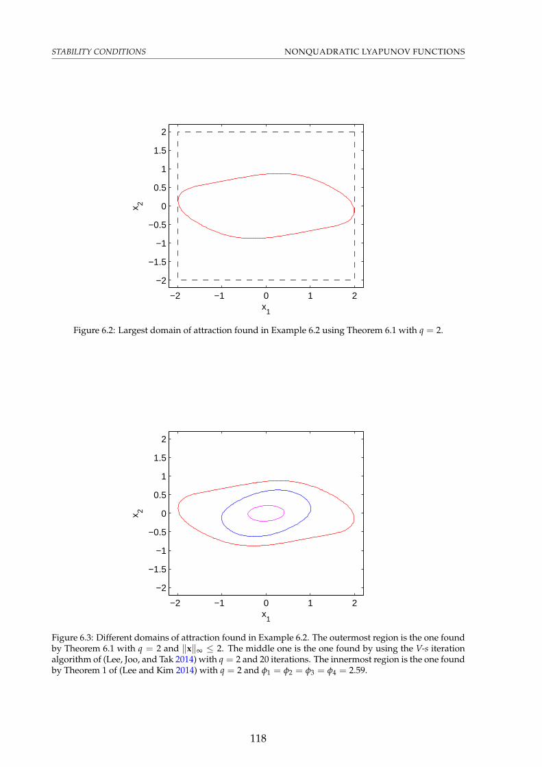
STABILITY CONDITIONS NONQUADRATIC LYAPUNOV FUNCTIONS
x1
x 2
−2 −1 0 1 2
−2
−1.5
−1
−0.5
0
0.5
1
1.5
2
Figure 6.2: Largest domain of attraction found in Example 6.2 using Theorem 6.1 with q = 2.
x1
x 2
−2 −1 0 1 2
−2
−1.5
−1
−0.5
0
0.5
1
1.5
2
Figure 6.3: Different domains of attraction found in Example 6.2. The outermost region is the one foundby Theorem 6.1 with q = 2 and ‖x‖∞ ≤ 2. The middle one is the one found by using the V-s iterationalgorithm of (Lee, Joo, and Tak 2014) with q = 2 and 20 iterations. The innermost region is the one foundby Theorem 1 of (Lee and Kim 2014) with q = 2 and φ1 = φ2 = φ3 = φ4 = 2.59.
118

NONQUADRATIC LYAPUNOV FUNCTIONS STABILIZATION CONDITIONS
6.4 Stabilization Conditions
The main idea of the stabilization conditions proposed in this section is to adapt the idea of the stabilityconditions to the closed loop scenario. If we were to directly substitute the closed loop system in theconditions from the previous section, it is not possible to get a set of LMI conditions. Therefore wepresent a set of conservative sufficient conditions to solve the problem, but that are guaranteed to givebetter results than a quadratic Lyapunov function coupled with a PDC control law would.
Theorem 6.2: Nonquadratic stabilization conditions
Given a system described by (6.2) whose membership functions’ Jacobian matrix can be described by (6.3), adesired number q of fuzzy summations in the Lyapunov function and control gains, a scalar value µ, and apolytopic design region given by (6.5), if there exists matrices Phq , Khq , Fhq and Xhq−1 , and a scalar β solvingthe optimization problem
max β,
β > 0,
Phq > βI,[
AhPhq + Phq ATh + Bh (Khq + Fhq) +
(KT
hq + FThq)
BTh ∗
Jg(
Phq ATh + KT
hq BTh)+ µQhq−1α −µ
(4I − QT
hq−1αJTg − JgQhq−1α
)]< 0,
withQhq−1α =
[(P(1)
hq−1 + Xhq−1
)sα . . .
(P(r)
hq−1 + Xhq−1
)sα
], (6.9)
and P(k)hq−1 in (6.8), then the system is locally asymptotically stable in closed loop with control law
u =
(Khq + Fhq
(I − 1
2JTg QT
hq−1α
))P−1
hq x,
and Lyapunov functionV(x) = xT P−1
hq x (6.10)
inside of the region Phq s, where s is given by (6.5). In addition, an estimate of its domain of attraction isgiven by the largest sublevel set of the Lyapunov function that is inside this region.
Proof. Consider we have a Lyapunov function as in (6.10), its time derivative would be given by
V(x) = xT P−1hq x + xT P−1
hq x + xT ˙(P−1
hq
)x.
By remembering the fact the time derivative of the inverse of a matrix can be written as
˙(P−1
hq
)= −P−1
hq Phq P−1hq ,
we get thatV(x) = xT P−1
hq x + xT P−1hq x− xT P−1
hq Phq P−1hq x.
Similarly to the stability conditions, note that we can write
xT P−1hq Phq P−1
hq x =r
∑k
hkxT P−1hq P(k)
hq−1 P−1hq x,
=xT P−1hq
[P(1)
hq−1 P−1hq x . . . P(r)
hq−1 P−1hq x
]h,
119

STABILIZATION CONDITIONS NONQUADRATIC LYAPUNOV FUNCTIONS
with P(k)hq−1 given by (6.8).
Sincer
∑k
hkxT P−1hq Xhq−1 P−1
hq x = 0,
we can add the extra matrix Xhq−1 into this equality to get
xT P−1hq Phq P−1
hq x = xT P−1hq
[(P(1)
hq−1 + Xhq−1
)P−1
hq x . . .(
P(r)hq−1 + Xhq−1
)P−1
hq x]
h.
By defining s = P−1hq x and choosing a design region given by (6.5), we get that
xT P−1hq PhP−1
hq x =xT P−1hq
[(P(1)
hq−1 + Xhq−1
)sα . . .
(P(r)
hq−1 + Xhq−1
)sα
]h,
=xT P−1hq Qhq−1αh,
=12
(xT P−1
hq Qhq−1αh + hTQThq−1α
P−1hq x
),
with Qhq−1α given by equation (6.9).By using these last developments in the Lyapunov function’s time derivative equation leads to
V(x) = xT P−1hq x + xT P−1
hq x− 12
(xT P−1
hq Qhq−1αh + hTQThq−1α
P−1hq x
).
By using the relations that
x =Ahx + Bhu,
u =
(Khq + Fhq
(I − 1
2JTg QT
hq−1α
))P−1
hq x,
h =Jgx,
we get that
x =
(Ah + Bh
(Khq + Fhq
(I − 1
2JTg QT
hq−1α
))P−1
hq
)x,
h =Jg
(Ah + Bh
(Khq + Fhq
(I − 1
2JTg QT
hq−1α
))P−1
hq
)x,
such that sufficient conditions for the time derivative of the Lyapunov function to be negative definiteare given by
P−1hq Ah + (∗) + P−1
hq
(Bh
(Khq + Fhq
(I − 1
2JTg QT
hq−1α
))+ (∗)
)P−1
hq
− 12
P−1hq Qhq−1α Jg
(Ah + Bh
(Khq + Fhq
(I − 1
2JTg QT
hq−1α
))P−1
hq
)− (∗) < 0,
in which (∗) represents the transpose of the term just before it.By multiplying it left and right by Phq , we get
AhPhq + (∗) + Bh
(Khq + Fhq
(I − 1
2JTg QT
hq−1α
))+ (∗)
− 12
Qhq−1α Jg
(AhPhq + Bh
(Khq + Fhq
(I − 1
2JTg QT
hq−1α
)))− (∗) < 0,
(I − 1
2Qhq−1α Jg
)(AhPhq + BhKhq) + (∗)
+
(I − 1
2Qhq−1α Jg
)(BhFhq + FT
hq BTh
)(I − 1
2JTg QT
hq−1α
)< 0.
120

NONQUADRATIC LYAPUNOV FUNCTIONS STABILIZATION CONDITIONS
From the matrix inversion lemma, we get that
(I − 1
2JTg QT
hq−1α
)−1= I + JT
g
(2I − QT
hq−1αJTg
)−1QT
hq−1α
and by multiplying the last inequality we had on the left by(
I − 12 Qhq−1α Jg
)−1and on the right by
(I − 1
2 JTg QT
hq−1α
)−1, we get
(AhPhq + BhKhq + BhFhq) + (∗) + (AhPhq + BhKhq) JTg
(2I − QT
hq−1αJTg
)−1QT
hq−1α+ (∗) < 0,
which can be recast in the form L⊥T∆L⊥ < 0, with
∆ =
[AhPhq + Bh (Khq + Fhq) + (∗) ∗
Jg(
Phq ATh + KT
hq BTh)
0
],
L⊥ =
I(
2I − QThq−1α
JTg
)−1QT
αhq−1
< 0.
By noting that L⊥ is a base to the null space of
L =[
QThq−1α
−(
2I − QThq−1α
JTg
)],
and by making use of Finsler’s Lemma statements (2) and (3), another equivalent condition would be
∆ + MT L + LT M < 0. (6.11)
By choosing a specific M with the structure,
M =[0 µI
],
we get that a sufficient condition for the time derivative of the Lyapunov function to be negative definiteis given by
[AhPhq + Phq AT
h + Bh (Khq + Fhq) +(KT
hq + FThq)
BTh ∗
Jg(
Phq ATh + KT
hq BTh)+ µQhq−1α −µ
(4I − QT
hq−1αJTg − JgQhq−1α
)]< 0.
Note, however, that, when we defined the design variable s and chose a design region, our condi-tions became only valid inside of the region x = Phq s, with s given by (6.5). In that regard, we will searchfor the “largest” Phq matrices such that our conditions are valid in the largest region possible. In order todo that, instead of solving a feasiblilty problem, we will solve a maximization problem over β and addthe conditions
β > 0,
Phq > βI.
In doing so, not only do we search for the “largest” Phq matrices, but also assure that the Lyapunovfunction is positive definite.
121

STABILIZATION CONDITIONS NONQUADRATIC LYAPUNOV FUNCTIONS
Remark 6.2
We have(r + q− 1)!
(r− 1)!(q− 1)!
(nr+
(n + r)nαng(r + q)q(q + 1)
)+ 1 rows of LMIs in Theorem 6.2 when we em-
ploy Lemma 2.4 to implement it, as well as 1 + rq−1n(
r(n + 1)2
+ n + 2rm)
scalar decision vari-
ables . In these relations, n is the number of states, m the number of controlled inputs, r the numberof rules of the TS model of the system, nα the number of vertices used to describe the design region,q the number of fuzzy summations in the Lyapunov function and control gains, and ng the numberof vertices used to describe the Jacobian of the membership functions vector.
Remark 6.3
Note that if we take Phq = P, and Xhq−1 = −P(k)hq−1 (note that P(k)
hq−1 does not depend on k whenPhq = P), we will have Qhq−1α = 0 in Theorem 6.2. In this case, if we take a large enough value of µ,we will recover the quadratic stabilization conditions.
In order to avoid having to find the largest Lyapunov sublevel set by inspection, we make use ofa set of LMI conditions that find an estimate of the largest sublevel set that is guaranteed to be insideof the region under which the conditions presented are valid. These conditions are presented in thefollowing lemma.
Lemma 6.3
Given a Lyapunov function of the form sT Phq s = xT P−1hq x, and a polytopic region described by |aT
i s| ≤bi, i ∈ 1, 2, . . . , nineq, the solution of the LMI optimization problem
max γ,[−b2
i√
γaTi
∗ −Phq
]< 0, ∀i ∈ 1, 2, . . . , nineq,
gives a maximum guaranteed sublevel set of the Lyapunov function (sT Phq s ≤ γ) that fits inside of thepolytopic region.
Proof. Consider that the region in s can be written, in an inequality representation, as |aTi s| ≤ bi, and
we want to find the maximum γ such that sT Phq s ≤ γ is guaranteed to be inside the limiting region.Since Phq > 0, there exists a matrix R(x) such that Phq = R(x)T R(x), therefore, an equivalent repre-
sentation of the Lyapunov sublevel set is s = R−1(x)y, ‖y‖2 ≤√
γ.By using the Cauchy-Schwarz inequality on the limiting region we get that
|aTi s| ≤ ‖aT
i R−1(x)‖2‖y‖2,
≤ √γ‖aTi R−1(x)‖2.
Then, a sufficient condition for the Lyapunov sublevel set to fit inside the desired region is that
√γ‖aT
i R−1(x)‖2 ≤ bi,
γaTi R−1(x)R−T(x)ai ≤ b2
i ,
γaTi P−1
hq ai ≤ b2i ,
122

NONQUADRATIC LYAPUNOV FUNCTIONS STABILIZATION CONDITIONS
and, using Schur’s complement,[−b2
i√
γaTi
∗ −Phq
]< 0.
Remark 6.4
By making use of Lemma 2.4 to implement Lemma 6.3 we have(r + q− 1)!r!(q− 1)!
nineq(n + 1) rows of
LMIs and one scalar decision variable, with n the number of states, r the number of rules of theLyapunov function, nineq the number of inequalities used to described the region, and q the numberof fuzzy summations in the Lyapunov function.
Remark 6.5
It is important to observe that, these exact same conditions could also be applied to the stabilitycase to find an estimate of the largest Lyapunov sublevel set that fits inside of the region. Eventhough the results obtained may be a little more conservative than the ones obtained by meansof inspection, the estimate found is guaranteed to be contained within the polytopic region andusually yield good results (with optimal results if we have a quadratic Lyapunov function). Inaddition, it is a lot simpler to employ Lemma 6.3 than to try and find the largest Lyapunov sublevelset by inspection for systems with more than 3 states (since we can’t draw the state space in thiscase).
Remark 6.6
Note that conditions from Lemma 6.3 could easily be incorporated directly into either Theorems6.1 or 6.2. However, by doing them separately, we reduce the computational cost (as solving theseoptimization problems probably does not scale linearly with the number of conditions).
Example 6.3. Consider the two rule system given by
A1 =
[4 −4−1 −2
], B1 =
[110
],
A2 =
[−2 −420 −2
], B2 =
[1−8
].
with membership functions
h1(x) =1 + sin(x1)
2, h2(x) = 1− h1(x).
The Jacobian of the membership functions’ is then given by
∂h∂x
=
[cos(x1)
2 0
− cos(x1)2 0
]
123

STABILIZATION CONDITIONS NONQUADRATIC LYAPUNOV FUNCTIONS
x1
x 2
−0.1 −0.05 0 0.05 0.1 0.15−0.2
−0.15
−0.1
−0.05
0
0.05
0.1
0.15
0.2
Figure 6.4: Largest domain of attraction found for the closed loop in Example 6.3 using Theorem 6.2with q = 2, µ = 1.4 and Lemma 6.3, as well as the system’s trajectory from different initial conditions.
which can be globally described by the vertex matrices
J1 =
[0.5 0−0.5 0
], J2 =
[−0.5 00.5 0
],
with membership functions
g1(x) =1 + cos x1
2, g2(x) =
1− cos x1
2.
We consider a region in s given by ‖s‖1 ≤ 1, which can be described by the vertices
s1 =
[10
], s2 =
[−10
], s3 =
[01
], s4 =
[0−1
]
and also as |aTi s| ≤ bi with
a1 =[−1 1
]T, b1 = 1,
a2 =[1 1
]T, b2 = 1.
Using Theorem 6.2 with the design region in s above, q = 2 and µ = 1.4, we are able to find a controllaw that locally stabilizes the system. Figure 6.4 presents the estimation of the domain of attraction ofthe Lyapunov function found by using Lemma 6.3 as well as the system’s trajectory in closed loop fordifferent initial conditions. Figure 6.5 presents the domains of attraction found by using Theorem 6.2with q = 2, q = 4 and q = 6. It is worth noting that the conditions in (Pan et al. 2012, Theorem 2) and(Lee and Kim 2014, Theorem 2) (with q ≤ 6) were found to be unfeasible for this example.
124

NONQUADRATIC LYAPUNOV FUNCTIONS STABILIZATION CONDITIONS
x1
x 2
−0.2 −0.1 0 0.1 0.2
−0.2
−0.1
0
0.1
0.2
0.3
Figure 6.5: Different domains of attraction found in Example 6.3 with Theorem 6.2. The outermostregion is the one found with q = 6. The middle one is the one found with q = 4. The innermost regionis the one found with q = 2.
125


7 LMI synthesis conditions usingpiecewise-like Lyapunov functions
Even though we showed that, by making use of local transformation matrices, piecewise Lyapunov functions canyield very nice stability analysis conditions (as shown in chapter 5), they are usually too cumbersome to be used insynthesis conditions (we usually end up with Bilinear Matrix Inequalities (BMIs) (Feng et al. 2005), or we needto augment the system with virtual stable dynamics that allow us to invert the parameter matrices (Qiu, Feng,and Gao 2013)).
The work presented in this chapter was done under the supervision of Prof. João Pedro Hespanha.
7.1 Problem definition
Given a nonlinear system that can be described, in an hyperrectangle Ω of the state space including theorigin, by a qLPV model
x = A(x)x + B(x)u, (7.1)
with x ∈ Rn, u ∈ Rm, A(x) a continuous and bounded function fromRn toRn×n, and B(x) a continuousand bounded function from Rn to Rn×m, we would like to find a set of sufficient LMI conditions for thesynthesis of a control law that renders the origin locally asymptotically stable.
Remark 7.1
Note that every input affine nonlinear system
x = f(x) + B(x)u,
with the origin as an equilibrium point, f(x) a continuous and bounded function, and B(x) a contin-uous and bounded function, can be cast as a qLPV model as in (7.1). However, this representationis generally not unique.
127

SOLUTION PROPOSED LMI SYNTHESIS CONDITIONS
7.2 Solution proposed
Given
Ω = [x1, x1]× [x2, x2]× · · · × [xn, xn],
define a partition of each interval [xi, xi] as
[xi, xi] =ri⋃
k=1
ω(i)k ,
ω(i)k =
[xi + (k− 1)δi, xi + kδi), if k < ri,[xi + (ri − 1)δi, xi] , if k = ri,
with ri the number of desired subintervals and δi =(xi − xi)
ri, so that
Ω =⋃
Ωi1i2 ...in ,
Ωi1i2 ...in = ω(1)i1×ω
(2)i2× · · · ×ω
(n)in . (7.2)
This amounts to dividing Ω into r =n
∏i=1
ri hyperrectangles.
Remark 7.2
By defining a specific ordering of the indices (i1, i2, . . . , in) (or a one-to-one relation between themand the set of positive integers less than or equal to r) a single index can be used to represent eachregion. Therefore, whenever it will not create confusion, a single index will be used to represent theregion.
Inside each Ωi region, the system in (7.1) may be exactly represented by a TS fuzzy model
x =qi
∑j=1
hij(x)[Aijx + Biju
],
= Ahix + Bhi
u,
with qi the number of linear models composing the TS model, hij(x) the system’s membership functionswith
qi
∑j=1
hij(x) = 1, hij(x) ≥ 0,qi
∑j=1
hij(x) = 0,
and Ahiand Bhi
short notations for the fuzzy summations over the matrices composing the model.By making use of the Ωi regions’ indicator functions, the TS models can be combined to represent
the system in the Ω region as
x =r
∑i=1
θi(x)[Ahi
x + Bhiu]= Aθhi
x + Bθhiu, (7.3)
with
θi(x) =
1, if x ∈ Ωi,0, otherwise.
128

LMI SYNTHESIS CONDITIONS SOLUTION PROPOSED
Remark 7.3
Note that the representation in (7.3) is simply a TS representation of the piecewise TS model found.Therefore a straightforward way of deriving less conservative LMI conditions for the system wouldbe to make use of a piecewise Lyapunov function. However, when deriving synthesis conditions,the special structure imposed over the parameter matrices hinders their use in continuous timesystems (they imply in either getting BMI conditions (Bernal, Guerra, and Kruszewski 2009), oraugmenting the system with artificial dynamics (Qiu, Feng, and Gao 2013)). In that regard, thischapter proposes the use of a piecewise-like Lyapunov function (which is a fuzzy Lyapunov func-tion whose premise variables are different from the system’s, but have some special properties)to deal with these piecewise systems. In order to deal with the time derivative of the Lyapunovfunction’s membership functions, it adapts the ideas from (Lee and Kim 2014; Lee, Park, and Joo2012) to derive sufficient conditions that guarantee that a bound over the time derivatives will berespected in closed loop.
Remark 7.4
A piecewise TS model could also be obtained from finding a single TS model for the system andapplying the local transformation proposed in chapter 5 inside each of the Ωi regions, or applyingthe transformation proposed in (Bernal, Guerra, and Kruszewski 2009) in the regions induced bythe ordering relations of the membership functions.
Due to the nature of the partitions proposed in this chapter, the Lyapunov function’s membershipfunctions can be defined with a tensor product structure, i.e. each partition’s membership functionis given by the product of single variable membership functions relating to each of the intervals thatcompose the partition. This particular structure eases the proposition of the membership functions sinceit is simply a combination of the membership functions devised for each of the state variables separatelyand endows the region’s function with some interesting properties. Namely, if its written as
gi(x) =n
∏k=1
α(k)ik
(xk),
and
rk
∑j=1
α(k)j (xk) = 1,
α(k)j (xk) ≥ 0,
α(k)j (xk) 6= 0 only if xk ∈ ω
(k)j or neighbours(ω(k)
j ), (7.4)
then
r
∑i=1
gi(x) = 1,
gi(x) ≥ 0,
gi(x) 6= 0 only if x ∈ Ωi or neighbours(Ωi),
in which two partitions are said to be neighbours if they share at least one common vertex.
129

LMI CONDITIONS - GENERIC MEMBERSHIP FUNCTIONS LMI SYNTHESIS CONDITIONS
Considering membership functions with these properties, we can define a piecewise-like Lyapunovfunction as
V(x) = xT
(r
∑i=1
gi(x)Pi
)−1
x = xT P−1g x (7.5)
and a continuous piecewise-like control law as
u =
(r
∑i=1
gi(x)Ki
)(r
∑i=1
gi(x)Pi
)−1
x = KgP−1g x,
with P−1g a short notation for
(r
∑i=1
gi(x)Pi
)−1
and Kg a short notation for
(r
∑i=1
gi(x)Ki
).
Remark 7.5
Defining this fuzzy Lyapunov function and control law leads to conditions one would expect to getfrom using a piecewise quadratic Lyapunov function. The main difference, however is that, insteadof enforcing a special structure upon the Pi matrices guaranteeing the function’s continuity (that,as stated before, leads to either BMI conditions or augmenting the system with virtual dynamics),one needs to deal with the membership functions’ time derivative and the fact that they are also“active” on the neighbouring regions.
7.3 LMI conditions - generic membership functions
The Lyapunov function’s time derivative is given by
V(x) = xT P−1g x + xT P−1
g x + xT ˙P−1g x,
= xT P−1g x + xT P−1
g x− xT P−1g PgP−1
g x,
= xT(
ATθhi
P−1g + P−1
g Aθhi+ P−1
g
(KT
g BTθhi
+ BθhiKg − Pg
)P−1
g
)x.
Sufficient conditions to ensure the system’s stability are then given by
P−1g > 0,
ATθhi
P−1g + P−1
g Aθhi+ P−1
g
(KT
g BTθhi
+ BθhiKg − Pg
)P−1
g < 0.
By performing a similarity transformation with Pg (i.e by multiplying it on the right by this valueand on the left by its transpose),
Pg > 0,
Pg ATθhi
+ AθhiPg + KT
g BTθhi
+ BθhiKg − Pg < 0.
which actually represent
r
∑i=1
gi(x)Pi > 0,
r
∑i=1
r
∑j=1
qj
∑k=1
gi(x)θj(x)hjk(x)
[Pi AT
jk + AjkPi + KTi BT
jk + BjkKi −(
r
∑`=1
g`(x)P`
)]< 0. (7.6)
130

LMI SYNTHESIS CONDITIONS LMI CONDITIONS - GENERIC MEMBERSHIP FUNCTIONS
By noting that
gi(x)θj(x) 6= 0, only if i = j or i is a neighbor of j,
gi(x)θj(x) 6= 0, only if i = j or i is a neighbor of j,
the following sufficient conditions are sufficient to ensure the system’s stability
Pi > 0, ∀i ∈ 1, . . . , r
Pi ATjk + AjkPi + KT
i BTjk + BjkKi −
∑
`∈L(j)g`(x)P`
< 0, ∀
j ∈ 1, . . . , r,i ∈ L(j),k ∈ 1, . . . , qj
in which L(j) denotes the set composed by j and its neighbors.Because of the membership functions gi properties, their time derivatives have the interesting prop-
erty that
∑`∈L(j)
g`(x)P` = ∑`∈L(j)
g`(x)(
P` + Xj)
.
Considering this property, one way to deal with the g` terms is to consider that |g`| ≤ φ` and thatP` + Xj > 0, ∀` ∈ L(j), in that way
− ∑`∈L(j)
g`(x)P` ≤ ∑`∈L(j)
φ`
(P` + Xj
)= Pφj
and the summation term can be replaced by Pφj to get LMI conditions.In order to enforce the bound |g`| ≤ φ` in closed loop, the ideas from (Lee and Kim 2014; Lee,
Park, and Joo 2012) are adapted to a piecewise scenario. The main idea in those papers was to makethe square of the membership functions’ time derivative less than φ2
k times the Lyapunov function andassuring that the 1-sublevel set of the Lyapunov function is inside the desired region. By doing that, theLMI conditions assures the system’s stability only inside of the 1-sublevel set of the Lyapunov function(which also serves as the best estimate of the domain of attraction their conditions can find). In thatregard, the authors search for the “largest” 1-sublevel set trying to find the largest domain of attractionpossible with their conditions.
However, those ideas cannot be directly applied in this context because of the several differentregions. In that regard, this work uses an auxiliary function in every region and forces it to be lessthan 1 for every value inside of the region (in that regard, one could think of the approach here as anouter approximation of the regions instead of the inner approximation used in (Lee and Kim 2014; Lee,Park, and Joo 2012)). The main drawback, however, is that we do not get an explicit approximation ofthe domain of attraction.
In that regard, we want that
g2`
φ2`
≤ xT P−1g Qgθ P−1
g x ≤ 1, x ∈ Ωj, ` ∈ L(j). (7.7)
The first inequality can be written as
xT(
P−1g KT
g BTθhi
+ ATθhi
)∇gT
` φ−2` ∇g`
(Aθhi
+ BθhiKgP−1
g
)x ≤ xT P−1
g Qgθ P−1g x,
r
∑i=1
r
∑j=1
qj
∑k=1
gi(x)θj(x)hjk(x)
[−Qij
(Pi AT
jk + KTi BT
jk
)∇gT
`
∗ −φ2`
]< 0,
131

LMI CONDITIONS - GENERIC MEMBERSHIP FUNCTIONS LMI SYNTHESIS CONDITIONS
for which a sufficient condition is that
[−Qij
(Pi AT
jk + KTi BT
jk
)∇gT
`
∗ −φ2`
]< 0, ∀
j ∈ 1, . . . , r,i, ` ∈ L(j),k ∈ 1, . . . , qj
The second inequality can be written as
xT P−1g Qgθ P−1
g x ≤ 1,[−1 xT
∗ −PgQ−1gθ Pg
]< 0,
and by using the fact that, for Qgθ > 0, −PgQ−1gθ Pg < −2Pg + Qgθ , sufficient conditions for it are
[−1 xT
∗ −2Pg + Qgθ
]< 0, ∀x ∈ Ωj,
r
∑i=1
r
∑j=1
gi(x)θj(x)
[−1 xT
∗ −2Pi + Qij
]< 0, ∀x ∈ Ωj,
Since Ωj is a hyper-rectangle (and thus a polytope), a necessary and sufficient condition is that thecondition above is fulfilled at the vertices of Ωj. By remembering the remark about the membershipfunctions only being different than zero in neighbouring regions, we then get that sufficient conditionsto find a stabilizing controller are
Pi > 0, ∀i ∈ 1, . . . , rP` + Xj > 0, ∀j ∈ 1, . . . , r, ` ∈ L(j)
Pφj = ∑`∈L(j)
φ`
(P` + Xj
)
Pi ATjk + AjkPi + KT
i BTjk + BjkKi + Pφj < 0, ∀
j ∈ 1, . . . , r,i ∈ L(j),k ∈ 1, . . . , qj
[−Qij
(Pi AT
jk + KTi BT
jk
)∇gT
`
∗ −φ2`
]< 0, ∀
j ∈ 1, . . . , r,i, ` ∈ L(j),k ∈ 1, . . . , qj
[−1 xT
v
∗ −2Pi + Qij
]< 0, ∀
j ∈ 1, . . . , rxv ∈ V(j)i ∈ L(j)
with φ` given, L(j) the set composed by j and its neighbors, and V(j) the set of vertices composing Ωj.
132

LMI SYNTHESIS CONDITIONS CHOICE OF THE MEMBERSHIP FUNCTIONS
Remark 7.6
It is important to notice two things about the above conditions. First is that, since they are localconditions, they only ensure local stability inside of the largest Lyapunov sublevel-set that fits in-side of Ω. Second is that, whenever we would like to apply these conditions, we need to choosethe values of φ` that are going to upper bound the time derivative of our membership functions.A smaller value usually lead to less restrictive LMI conditions regarding the time derivative of theLyapunov function (because they lead to a smaller Pφj term), however they also lead to harder re-strictions upon the control gains (since we would have tighter bounds on the membership functionstime derivative). A higher value of φ` would lead to the opposite situation. Notice also that as φ`
tends to infinity, our conditions tend to the quadratic stability conditions (since we would be forcedto choose all of the Pi with the same value and Xj = −Pi and we would not impose any conditionover the time derivative of the membership functions).
Remark 7.7
Note that the LMI conditions proposed in this work do not make explicit use of the system’s mem-bership function (so they give them, locally, the same treatment as polytopic uncertainties). A wayto further relax the conditions could be employ the system’s membership functions in the controllaw and in the Q matrices (at the cost of an increased number of LMIs and decision variables.
Remark 7.8
The advantages of the proposed solution in this work over others available on the literature isthat, unlike piecewise Lyapunov function, we have LMI synthesis conditions, and, unlike the reg-ular fuzzy Lyapunov function approach (using the system’s membership function in the Lyapunovfunction), the system’s membership function need not be continuously differentiable.
7.4 Choice of the membership functions
Notice that the choice of the membership functions used for the Lyapunov function and the control lawdirectly affects the LMI stabilization conditions proposed above. Notice as well that, in order to trulyhave LMI conditions, we need to find a polytopic representation for them, similar to what we did to usex in the conditions.
Because of the tensor product structure, we get that
gi(x) =n
∏k=1
α(k)ik
(xk)
∇gi(x) =
[d
dx1α(1)i1
(x1)n
∏k=2
α(k)ik
(xk) . . . ddxn
α(n)in (xn)
n−1
∏k=1
α(k)ik
(xk)
]. (7.8)
Therefore, we would like to choose a set of α(k)ik
(xk) whose derivatived
dxkα(k)ik
(xk) is small (so that
we get less conservative LMI conditions).
133

CHOICE OF THE MEMBERSHIP FUNCTIONS LMI SYNTHESIS CONDITIONS
In that regard, we can write an optimization problem to search for an optimal “worst case” set ofmembership functions. That is, we can write an optimization program to search for a set of α
(k)j (xk)
membership functions respecting (7.4) and minimizing the maximum norm of their derivative. In otherwords,
min t,
s.t.rk
∑j=1
α(k)j (xk) = 1,
α(k)j (xk) ≥ 0,
α(k)j (xk) 6= 0 only if xk ∈ ω
(k)j or neighbours(ω(k)
j ),∣∣∣∣
ddxk
α(k)j (xk)
∣∣∣∣ < t, ∀xk ∈ [xk, xk], ∀j. (7.9)
By approximating the membership functions as piecewise linear functions, the search for the mem-bership functions can be replaced with the search for points along [xk, xk], and the inequality involvingthe norm of the derivative (which now will only be valid almost everywhere), can be replaced by thenorm of the difference between a point and its neighbour. With this approximation, the optimizationproblem presented above becomes a linear optimization problem and can be efficiently solved for a largenumber of points in [xk, xk].
An important step when doing this approximation is ensuring that the points on the borders of twoωj regions is always chosen by the optimization problem, in order to guarantee that the neighbouringconstraint will be respected. Notice also that, due to the neighbouring constraint, we only need to seekthe values of the membership functions when they are active (i.e. when they are in their own regions, orin a neighbouring region).
Figure 7.1 presents the result obtained for xk ∈ [−5, 5] with 2, 3, 4, 5, 6, and 7 regions. Note that, ifwe have less than 4 regions in xk, it is better to assume a single region in that variable (since, just like inthe LMI conditions presented, it does not make a difference). For that reason, in this work, we supposethat either rk = 1 or rk > 3.
Note also that, from 4 regions upwards, the shape of the membership functions is fixed. The mem-bership functions that are not active in the limit regions (i.e. the ones that are zero in -5 and 5 in thefigure) all have a trapezoidal shape, whereas the others have a different shape (a little strange, proba-bly due to a “border effect”). However, the derivative in these regions are all less than the worst case,and we can impose a trapezoidal structure to these regions as well without changing the “worst case”derivative.
Figure 7.2 presents the alternative optimal membership functions obtained for xk ∈ [−5, 5] with 4,5, 6, and 7 regions. Note that these membership functions are simpler to implement and grant our LMIsynthesis conditions with some interesting properties (that will be presented in the following section).
The optimization problem used to find these membership functions does not depend on the rangeused for xk, but rather it depends only on the number of regions used. In that case, we can say, consider-ing that j ∈ 1, 2, . . . , rk and rk > 3, that an almost everywhere differentiable solution to the optimization
134

LMI SYNTHESIS CONDITIONS CHOICE OF THE MEMBERSHIP FUNCTIONS
problem in (7.9) is given by
α(k)j (xk) =
0.5, if
xk ∈ ω(k)j ,
xk ∈ ω(k)1 , j = 2,
xk ∈ ω(k)rk , j = rk − 1,
xk − xk(j−1)
xk(j−1) − xk(j−2), if xk ∈ ω
(k)j−1, j > 2,
−xk + xk(j+2)
xk(j+2) − xk(j+1), if xk ∈ ω
(k)j+1, j < rk − 1,
0, otherwise.
(7.10)
with xkj = xk + (j− 1)δk, δk =(xk − xk)
rk, and its derivative, for xk 6= xkm with m ∈ 1, 2, . . . , rk, is given
by
dα(k)j
dxk(xk) =
1δk
, if xk ∈ ω(k)j−1, j > 2,
−1δk
, if xk ∈ ω(k)j+1, j < rk − 1,
0, otherwise.
For the simple case, in which rk = 1, we have
α(k)1 (xk) = 1,
dα(k)1
dxk(xk) = 0. (7.11)
Remembering from (7.8) that
∂gi∂xk
(x) =d
dxkα(k)ik
(xk)n
∏j=1,j 6=k
α(j)ij(xj)
and noting that, since the maximum of α(j)ij(xj) is 1 if rj = 1, or 0.5 if rj > 3,
n
∏j=1,j 6=k
α(j)ij(xj) ∈ [0, (0.5)κk ]
with κk being the number of regions, aside from k, that have more than 3 regions. We have that
∂gi∂xk
(x) ∈
co
0,(0.5)κk
δk
, if xk ∈ ω
(k)ik−1, ik > 2,
co −(0.5)κk
δk, 0
, if xk ∈ ω
(k)ik+1, ik < rk − 1,
0, otherwise,
(7.12)
which, as desired in the beginning of this section, allow us to write a polytopic representation for ∇gi.Note that this expression for the gradient will not be valid for xk = xkm with m ∈ 1, 2, . . . , rk for every k,which is a zero Lebesgue measure set, and thus our expression in only valid almost everywhere.
It is important to note that, even though α(k)j (xk) is not continuously differentiable, it is bounded and
Lipschitz continuous (with Lipschitz constant 1/δk). This ensures that the gi(x) membership functionsare also Lipschitz continuous and that the Lyapunov in (7.5) is locally Lipschitz continuous.
135

CHOICE OF THE MEMBERSHIP FUNCTIONS LMI SYNTHESIS CONDITIONS
−5 0 50.5
0.5
0.5
xk
(a)
α j(k)
−5 0 50
0.5
1
xk
(b)
α j(k)
−5 0 50
0.2
0.4
0.6
0.8
xk
(c)
α j(k)
−5 0 50
0.2
0.4
0.6
0.8
xk
(d)
α j(k)
−5 0 50
0.2
0.4
0.6
0.8
xk
(e)
α j(k)
−5 0 50
0.2
0.4
0.6
0.8
xk
(f)
α j(k)
Figure 7.1: Optimal membership functions for xk ∈ [−5, 5] with 2, 3, 4, 5, 6, and 7 regions in (a), (b), (c),(d), (e), and (f) respectively.
136

LMI SYNTHESIS CONDITIONS LMI CONDITIONS - OPTIMAL MEMBERSHIP FUNCTIONS
−5 0 50
0.2
0.4
0.6
0.8
xk
(a)
α j(k)
−5 0 50
0.2
0.4
0.6
0.8
xk
(b)
α j(k)
−5 0 50
0.2
0.4
0.6
0.8
xk
(c)
α j(k)
−5 0 50
0.2
0.4
0.6
0.8
xk
(d)
α j(k)
Figure 7.2: Alternative optimal membership functions for xk ∈ [−5, 5] with 4, 5, 6, and 7 regions in (a),(b), (c), and (d) respectively.
7.5 LMI conditions - optimal membership functions
In this section, we present how to take further advantage from the structure on the optimal membershipfunctions found in the previous section to further relax the LMI conditions proposed in section 7.3.
First, note that, due to the trapezoidal shape of the membership functions, we have that
gi(x)θi(x) = 0,
so that the summationr
∑j=1
r
∑`=1
θj((x))g`(x)P` in (7.6) can now be replaced byr
∑j=1
∑`∈S(j)
θj((x))g`(x)P`,
with S(j) the set of neighbours of j. That means that now we use the set S(j), instead of L(j), in thedefinition of Pφj and in P` + Xj > 0.
Second, note that, from (7.8) we can write (7.12) as
∂gi∂xk
(x) = λik(x)(0.5)κkd
dxkα(k)ik
(xk)
with λik(x) ∈ [0, 1]. But this implies that
g2` =
n
∑k=1
(xk
∂g`∂xk
)2=
n
∑k=1
(xkλ`k(0.5)κk
ddxk
α(k)`k
)2=
n
∑k=1
x2kλ2
`k(0.5)2κk
(d
dxkα(k)`k
)2
≤n
∑k=1
x2k(0.5)2κk
(d
dxkα(k)`k
)2=
r
∑j=1
θj(x)xTν`jνT`jx.
137

LMI CONDITIONS - OPTIMAL MEMBERSHIP FUNCTIONS LMI SYNTHESIS CONDITIONS
with ν`j a vector whose k-th element, ν`jk, given by
ν`jk =
(0.5)κk
δk, if `k > 2, `k = jk − 1,
−(0.5)κk
δk, if `k < rk − 1, `k = jk + 1,
0, otherwise,
(7.13)
and this means that we can replace ∇gT` by ν`j in the LMIs in order to get sufficient conditions for (7.7)
at the points where g` is differentiable.Note that, with the optimal membership functions, our LMI conditions only assure that ∇Vx < 0
almost everywhere in the state space. But, since x is continuous (because of our assumptions and thefact that we are using a continuous control law) and V(x) is locally Lipschitz continuous, by applying(Hespanha, Liberzon, and Teel 2008, Lemma 1) we get that V(t) is absolutely continuous and V(x(t)) <0 almost everywhere on t (which implies that the system is locally asymptotically stable).
Having discussed all of this, we can enunciate the following theorem.
Theorem 7.1: LMI synthesis conditions for piecewise-like Lyapunov functions
Given a system described by (7.3) in a region given by Ω in (7.2), and scalars φi > 0, if there exists matricesPi, Ki, and Qij solving the LMI feasibility problem
Pi > 0, ∀i ∈ 1, . . . , rP` + Xj > 0, ∀j ∈ 1, . . . , r, ` ∈ S(j)
Pφj = ∑`∈S(j)
φ`
(P` + Xj
)
Pi ATjk + AjkPi + KT
i BTjk + BjkKi + Pφj < 0, ∀
j ∈ 1, . . . , r,i ∈ L(j),k ∈ 1, . . . , qj
[−Qij
(Pi AT
jk + KTi BT
jk
)ν`j
∗ −φ2`
]< 0, ∀
j ∈ 1, . . . , r,i ∈ L(j), ` ∈ S(j),k ∈ 1, . . . , qj
[−1 xT
v
∗ −2Pi + Qij
]< 0, ∀
j ∈ 1, . . . , rxv ∈ V(j)i ∈ L(j)
with ν`j given by (7.13), then the system is locally asymptotically stable with control law
u =
(r
∑i=1
gi(x)Ki
)(r
∑i=1
gi(x)Pi
)−1
x
and Lyapunov function
V(x) = xT
(r
∑i=1
gi(x)Pi
)−1
x = xT P−1g x
with gi(x) =n
∏k=1
α(k)ik
(xk) and α(k)ik
(xk) given by either (7.10) or (7.11).
138

LMI SYNTHESIS CONDITIONS EXAMPLE
−0.5 0 0.5
−2
−1.5
−1
−0.5
0
0.5
1
1.5
2
Figure 7.3: Phase plane of the system in example 7.1 with the control law found. The curves presentedin the figure are Lyapunov level curves.
7.6 Example
In this section, a numerical example is presented to illustrate the proposed stabilization conditions.
Example 7.1 (Same example system used in Example 6.3). Consider the nonlinear system given byequation (7.1) with
A(x) =
[1 + 3 sin(x1) −4
19−21 sin(x1)2 −2
], B(x) =
[1
2+18 sin(x1)2
],
and x1 ∈ [−1.2, 1.2], x2 ∈ [−2, 2].Using the conditions from Theorem 7.1 with 401 partitions in x1 and considering [−2, 2] as the only
region in x2 (since there are only nonlinear terms in x1, we have decided to only partition the state spacein this variable) and choosing φi = φ = 6000, we are able to find a control law that locally stabilizesthe system. Figure 7.3 presents the phase plane of the closed loop system with some of the Lyapunovlevel curves. Figure 7.4 presents an estimate of the closed loop domain of attraction (given by the largestLyapunov sublevel set that fits inside of the given region) as well as several different trajectories for thesystem whose initial conditions are all on the border of the domain of attraction estimated.
139

EXAMPLE LMI SYNTHESIS CONDITIONS
−0.5 0 0.5
−2
−1.5
−1
−0.5
0
0.5
1
1.5
2
Figure 7.4: Estimated domain of attraction for the closed loop system in example 7.1. The red curves arethe system’s trajectories in closed loop, whereas the red balls are their initial conditions.
140

Part III
Conclusions
141


8 Discussion and Future Directions
8.1 Discussion
Exploiting the membership functions
In chapter 3 we presented two different partition strategies for the membership functions’ image spacein order to generate sufficient and asymptotically necessary conditions by means of Theorems 3.1 and3.2.
Two examples were presented in order to illustrate the proposed methods. The first example dealtwith the stabilization and comparing the proposed methods with others from the literature, whereas thesecond one focused in guaranteedH∞ control and comparing the proposed methods among themselves.
It is interesting to note that the proposed partition strategies performed well when compared tothe other strategies (despite having been outperformed by the combination of (Sala and Ariño 2007,Theorem 5) and (Sala and Ariño 2008, Proposition 3.1)) and that, overall, the second partition strategyperformed better than the first one. However, that increase in performance comes in exchange for thelost of determinism of the partition strategy and conditions that are not “monotically less conservative”(i.e. conditions that are guaranteed to be always less conservative as the number of partitions increase).
Some possible enhancements for the partition strategy are:
• Defining a formal stop criterion to be used when the partitions are being used to generate suffi-cient and asymptotically necessary conditions (i.e. how to we check if the conditions have reachednecessity). So far the criterion used is the number of iterations in the method;
• The use of heuristics, similar to (Kruszewski et al. 2009, Algorithm 2), in order to direct the divi-sion of the simplices (or groupings) so that more divisions are made in regions that affect/violatemore the LMI conditions and the performance/iteration (or performance/number of simplices)ratio is increased;
• Defining a systematic and deterministic manner to initialize the center of the clusters used in thesecond strategy, making it deterministic without compromising performance;
• The conditions from the Grouping the membership points partition strategy could be made “monot-ically less conservative” if we were able to impose that the new simplices had to be containedinside of the previous ones;
• The conditions from the Dividing and Discarding partition strategy could converge faster if a dif-ferent partition strategy were chosen for the simplicial partition step. An interesting alternativecould be given by (Gonçalves et al. 2006).
143

DISCUSSION DISCUSSION AND FUTURE DIRECTIONS
We briefly touched the topic that, even though the conditions presented are sufficient and asymptot-ically necessary for the parametric LMIs, they might not be for the original quadratic conditions if any ofthe premise variables are functions of the state variables (due to the fact that in this case the parametricLMIs are only sufficient for the quadratic form).
In addition, we also showed that these partitions correspond to an exact switched representationof the TS model, and this representation inspired the use of the partitions to look for control laws thatswitch according to the membership functions. We also showed how these control law conditions couldbe modified so that a continuous fuzzy controller could be reconstructed by means of the Tensor ProductModel Transformation.
Rule reduction
Chapter 4 presented an alternative rule reduction technique for TS models based on tensor approxima-tion by using the HOSVD, as well as how to model the uncertainty generated by this rule reduction.
The proposed approach differs from the usual approaches in the literature since it deals with approx-imating a tensor composed by the “vertex systems” instead of dealing with approximating the nonlinearfunction directly. This approach advantages and disadvantages were discussed throughout the chapter.
The model uncertainty generated by the rule reduction proposed is given in a polytopic form. How-ever, since the polytopic uncertainty representation is not very common in the TS fuzzy control litera-ture, we presented LMI conditions that allow converting this uncertainty into either a norm boundedrepresentation or a structured linear fractional form.
New stability analysis conditions
Chapter 5 proposed the use of local transformation matrices that, unlike the matrices generated by themembership functions ordering relations (Bernal, Guerra, and Kruszewski 2009), does not increase thenumber of LMI conditions.
New conditions were proposed to check the stability of continuous time TS systems. They made useof two piecewise fuzzy Lyapunov functions and the local transformation matrices.
The first of these conditions, based on the Lyapunov function proposed in (Rhee and Won 2006), leadto a set of conditions that do not depend on the knowledge of upper bounds on the time derivatives ofthe membership functions. However, as in (Rhee and Won 2006), they demand a particular structure onthe matrices parametrizing the Lyapunov functions.
The second, based on the Lyapunov function proposed in (Tanaka, Hori, and Wang 2003), lead toa set of conditions that impose a less complex structure over the parameter matrices, but that demandthe knowledge of upper bounds on the membership functions time derivatives and that, in some cases,only check for local stability.
Both conditions made use of the null-term approach (Mozelli, Palhares, and Mendes 2010) in orderto relax the results. Theorem 5.1 can be seen as a generalization of (Bernal, Guerra, and Kruszewski2009, Theorem 2). If global bounds on the time derivatives of the membership functions are known, thenTheorem 5.2 can also be seen as a generalization of (Bernal, Guerra, and Kruszewski 2009, Theorem 2).
An example was presented to illustrate the relaxation introduced by the proposed conditions andthe proposed local transformation matrices. As can be seen in the example, the proposed conditionswhere valid for a larger region than other conditions available in the literature. Its interesting to notethat, for this particular example, the proposed local transformation matrices outperformed those usingthe matrices defined by the ordering relations from the membership functions in (Bernal, Guerra, andKruszewski 2009).
144

DISCUSSION AND FUTURE DIRECTIONS DISCUSSION
A problem regarding the proposed candidate Lyapunov functions is that, in a direct way, the con-troller synthesis conditions will be BMIs. However, it might be possible to get LMI conditions by usinga derivation similar to the one in (Qiu, Feng, and Gao 2013).
A parallel between chapters 3 and 5 can be traced, and in a similar way as the one discussed in chap-ter 3, we may say that the use of the local transformation matrices is equivalent to finding a switchedrepresentation, in the state space, for the original TS system.
Nonquadratic Lyapunov functions
Chapter 6 proposed new conditions for the local stability and local stabilization of continuous time TSfuzzy systems by using a nonquadratic Lyapunov function. These conditions avoid the use of upperbounds on the time derivative of the membership functions by making use of a novel manipulationthat instead employs the membership functions Jacobian matrix and a polytopic description of the localregion.
From the example presented in Section 6.3, we can see that the proposed stability conditions arean interesting alternative to other conditions available in the literature, with its main advantage beingthe fact that there is no need to choose a value for the upper bound of the membership functions’ timederivative.
It is important to note that, even though the examples presented performed better than the onesfrom (Lee and Kim 2014) for the stability conditions, that was not always the case. It is also noteworthythat, whenever the stabilization conditions from (Lee and Kim 2014) were feasible, they yielded thelargest domain of attraction out of all conditions we tested against (which in turn led us to present anexample in which it does not work, in order to motivate the use of the proposed conditions).
By choosing a particular structure for M in (6.11), we were able to find a set of conditions for the sta-bilization problem which are guaranteed to find better results than those found by a quadratic Lyapunovfunction (given a suitable choice of µ).
LMI synthesis conditions
Chapter 7 proposed a set of new LMI synthesis conditions for continuous-time TS fuzzy systems bymaking use of piecewise-like Lyapunov functions. It adapted the bounding conditions on the member-ship functions time derivative from (Lee and Kim 2014) to work in this switched scenario and thereforemade use of a chosen bound on the time derivative of the Lyapunov function’s memberhsip functionsin closed loop.
In order to diminish the effects of this time-derivative, we presented an optimal choice of the mem-bership functions for these Lyapunov functions that guarantees the best worst-case derivative of themembership functions (and some other interesting properties that allows us to further relax the LMIs).
Finally, the same stabilization example from chapter 6 was used, and, in this case, the stabilizationconditions proposed in chapter 7 were able to find a larger domain of attraction than those from chapter6.
It is important to note that, for every example we tested in which the conditions from (Lee and Kim2014) were also feasible, they were always able to find a larger domain of attraction (by correctly choos-ing the bounds on the membership functions’ time derivative). Which motivates us to keep saerchingfor different ways to relax the results from this chapter.
145

FUTURE DIRECTIONS DISCUSSION AND FUTURE DIRECTIONS
8.2 Future Directions
Many different possible future directions are possible for the research presented in this thesis startingfrom the results presented so far.
A first, more theoretical, direction aims to try and understand under what conditions the feasi-bility of a parametric LMI is necessary for the feasibility of the quadratic form (a possible numericaldirection could be to rewrite the quadratic form using a polytopic representation and trying to employPolya’s Theorem for homogenous polynomials to try and get asymptotically necessary conditions forthe quadratic form).
Still on the topic of Polya’s Theorem for homogenous polynomials, we would like to study if itcould be used to generate a set of sufficient and asymptotically necessary conditions for solving generalcopositive programming problems like it has been used to solve fuzzy summation conditions.
Another interesting research direction would be continuing the research on the conditions of chapter7. More specifically, we would like to determine a more systematic way of choosing the values of theupper bounds used for gi.
A different research direction, which would have direct impact over LMI synthesis conditions,would be to study under what conditions does the stability of the system
x =r
∑i=1
hi(x)ATi x
is related to the stability of the system
x =r
∑i=1
hi(x)Aix.
Another research direction would be on the use of sufficient and asymptotically necessary condi-tions to define a SDP feasibility solver based on approximating LMIs by scalar linear inequalities con-straints. We are specially interested in using something similar to (Kruszewski et al. 2009, Algorithm 2)as that would allow for the scalar linear inequalities approximation to be refined only where it mattered.
146

Bibliography
Ariño, C. V. (2007). “Relaxed LMI conditions for control of nonlinear Takagi-Sugenomodels”. PhD thesis. Universidad Politécnica de Valencia - Departamento de Inge-niería de Sistemas y Automática.
Ariño, C. and A. Sala (2007). “Relaxed LMI conditions for closed-loop fuzzy systemswith tensor-product structure”. In: Engineering Applications of Artificial Intelligence20.8, pp. 1036 –1046. ISSN: 0952-1976. DOI: 10.1016/j.engappai.2007.02.011.
Balas, G. J., A. K. Packard, and P. J. Seiler (2009). “Uncertain Model Set Calculation fromFrequency Domain Data”. In: Model-Based Control. Ed. by P. M. Hof, C. Scherer, andP. S. Heuberger. Springer US, pp. 89–105. ISBN: 978-1-4419-0895-7. DOI: 10.1007/978-1-4419-0895-7_6.
Baranyi, P. (1999). “Reduction of fuzzy rule base via singular value decomposition”. In:IEEE Transactions on Fuzzy Systems 7.2, pp. 120–132. ISSN: 10636706. DOI: 10.1109/91.755394.
Baranyi, P. (2004). “TP model transformation as a way to LMI-based controller design”.In: IEEE Transactions on Industrial Electronics 51.2, pp. 387–400. ISSN: 0278-0046.
Baranyi, P., D. Tikk, Y. Yam, and R. J. Patton (2003). “From differential equations toPDC controller design via numerical transformation”. In: Computers in Industry51.3, pp. 281 –297. DOI: http://dx.doi.org/10.1016/S0166-3615(03)00058-7.
Baranyi, P., Z. Petres, P. Varlaki, and P. Michelberger (2006). “Observer and controllaw design to the TORA system via TPDC framework.” In: WSEAS Transactions onSystems 5.1, pp. 156–163.
Baranyi, P., Z. Petres, P. Korondi, Y. Yam, and H. Hashimoto (2007). “Complexity re-laxation of the tensor product model transformation for higher dimensional prob-lems”. In: Asian Journal of Control 9.2, pp. 195–200.
Bernal, M. and T. M. Guerra (2010). “Generalized Nonquadratic Stability of Continuous-Time Takagi-Sugeno Models”. In: IEEE Transactions on Fuzzy Systems 18.4, pp. 815–822.
147
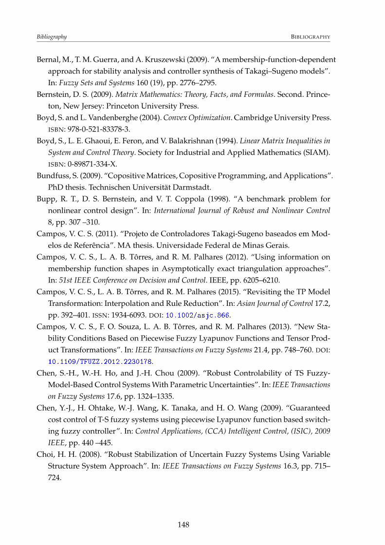
Bibliography BIBLIOGRAPHY
Bernal, M., T. M. Guerra, and A. Kruszewski (2009). “A membership-function-dependentapproach for stability analysis and controller synthesis of Takagi–Sugeno models”.In: Fuzzy Sets and Systems 160 (19), pp. 2776–2795.
Bernstein, D. S. (2009). Matrix Mathematics: Theory, Facts, and Formulas. Second. Prince-ton, New Jersey: Princeton University Press.
Boyd, S. and L. Vandenberghe (2004). Convex Optimization. Cambridge University Press.ISBN: 978-0-521-83378-3.
Boyd, S., L. E. Ghaoui, E. Feron, and V. Balakrishnan (1994). Linear Matrix Inequalities inSystem and Control Theory. Society for Industrial and Applied Mathematics (SIAM).ISBN: 0-89871-334-X.
Bundfuss, S. (2009). “Copositive Matrices, Copositive Programming, and Applications”.PhD thesis. Technischen Universität Darmstadt.
Bupp, R. T., D. S. Bernstein, and V. T. Coppola (1998). “A benchmark problem fornonlinear control design”. In: International Journal of Robust and Nonlinear Control8, pp. 307 –310.
Campos, V. C. S. (2011). “Projeto de Controladores Takagi-Sugeno baseados em Mod-elos de Referência”. MA thesis. Universidade Federal de Minas Gerais.
Campos, V. C. S., L. A. B. Tôrres, and R. M. Palhares (2012). “Using information onmembership function shapes in Asymptotically exact triangulation approaches”.In: 51st IEEE Conference on Decision and Control. IEEE, pp. 6205–6210.
Campos, V. C. S., L. A. B. Tôrres, and R. M. Palhares (2015). “Revisiting the TP ModelTransformation: Interpolation and Rule Reduction”. In: Asian Journal of Control 17.2,pp. 392–401. ISSN: 1934-6093. DOI: 10.1002/asjc.866.
Campos, V. C. S., F. O. Souza, L. A. B. Tôrres, and R. M. Palhares (2013). “New Sta-bility Conditions Based on Piecewise Fuzzy Lyapunov Functions and Tensor Prod-uct Transformations”. In: IEEE Transactions on Fuzzy Systems 21.4, pp. 748–760. DOI:10.1109/TFUZZ.2012.2230178.
Chen, S.-H., W.-H. Ho, and J.-H. Chou (2009). “Robust Controlability of TS Fuzzy-Model-Based Control Systems With Parametric Uncertainties”. In: IEEE Transactionson Fuzzy Systems 17.6, pp. 1324–1335.
Chen, Y.-J., H. Ohtake, W.-J. Wang, K. Tanaka, and H. O. Wang (2009). “Guaranteedcost control of T-S fuzzy systems using piecewise Lyapunov function based switch-ing fuzzy controller”. In: Control Applications, (CCA) Intelligent Control, (ISIC), 2009IEEE, pp. 440 –445.
Choi, H. H. (2008). “Robust Stabilization of Uncertain Fuzzy Systems Using VariableStructure System Approach”. In: IEEE Transactions on Fuzzy Systems 16.3, pp. 715–724.
148

BIBLIOGRAPHY Bibliography
Choi, H. H. (2010). “Robust Stabilization of Uncertain Fuzzy-Time-Delay Systems Us-ing Sliding-Mode-Control Approach”. In: IEEE Transactions on Fuzzy Systems 18.5,pp. 979–984.
de Boor, C. (2001). A Pratical Guide to Splines: Revised Edition. New York: Springer.De Lathauwer, L., B. De Moor, and J. Vandewalle (2000a). “A Multilinear Singular
Value Decomposition”. In: SIAM Journal on Matrix Analysis and Applications 21.4,p. 1253. ISSN: 08954798. DOI: 10.1137/S0895479896305696.
De Lathauwer, L., B. De Moor, and J. Vandewalle (2000b). “On the Best Rank-1 andRank-(R1 ,R2 ,. . .,RN) Approximation of Higher-Order Tensors”. In: SIAM Journalon Matrix Analysis and Applications 21.4, pp. 1324–1342. DOI: 10.1137/S0895479898346995.
Faria, F. A., G. N. Silva, and V. A. Oliveira (2012). “Reducing the conservatism ofLMI-based stabilisation conditions for TS fuzzy systems using fuzzy Lyapunovfunctions”. In: International Journal of Systems Science 0.0, pp. 1–14. DOI: 10.1080/00207721.2012.670307.
Feng, G. (2011). Analysis and Synthesis of Fuzzy Control Systems. CRC Press. ISBN: 9781420092653.Feng, G., C.-L. Chen, D. Sun, and Y. Zhu (2005). “H∞ controller synthesis of fuzzy
dynamic systems based on piecewise Lyapunov functions and bilinear matrix in-equalities”. In: IEEE Transactions on Fuzzy Systems 13.1, pp. 94 –103.
Gonçalves, E. N., R. M. Palhares, R. H. C. Takahashi, and R. C. Mesquita (2006). “Al-gorithm 860: SimpleS - an Extension of Freudenthal’s Simplex Subdivision”. In:ACM Trans. Math. Softw. 32.4, pp. 609–621. ISSN: 0098-3500. DOI: 10.1145/1186785.1186792.
Guedes, J. A., M. C. M. Teixeira, R. Cardim, and E. Assunção (2013). “Stability of Non-linear System Using Takagi-Sugeno Fuzzy Models and Hyper-Rectangle of LMIs”.In: Journal of Control, Automation and Electrical Systems 24.1-2, pp. 46–53. ISSN: 2195-3880. DOI: 10.1007/s40313-013-0015-4.
Guerra, T. M., M. Bernal, K. Guelton, and S. Labiod (2012). “Non-quadratic local sta-bilization for continuous-time Takagi-Sugeno models”. In: Fuzzy Sets and Systems201.0, pp. 40 –54.
Hespanha, J. P., D. Liberzon, and A. R. Teel (2008). “Lyapunov conditions for input-to-state stability of impulsive systems”. In: Automatica 44.11, pp. 2735 –2744. DOI:10.1016/j.automatica.2008.03.021.
Ho, W.-H., J.-T. Tsai, and J.-H. Chou (2007). “Robust-Stable and quadratic-optimal con-trol for TS-fuzzy-model-based control systems with elemental parametric uncer-tainties”. In: IET Control Theory and Appl. 3.1, pp. 731–742.
Johansson, M., A. Rantzer, and K.-E. Arzen (1999). “Piecewise quadratic stability offuzzy systems”. In: IEEE Transactions on Fuzzy Systems 7.6, pp. 713–722.
149

Bibliography BIBLIOGRAPHY
Ko, J. W. and P. G. Park (2012). “Further enhancement of stability and stabilisabilitymargin for Takagi-Sugeno fuzzy systems”. In: IET Control Theory Applications 6.2,pp. 313–318.
Ko, J. W., W. I. Lee, and P. Park (2012). “Stabilization for Takagi-Sugeno fuzzy systemsbased on partitioning the range of fuzzy weights”. In: Automatica 48.5, pp. 970 –973.
Kruszewski, A., A. Sala, T. Guerra, and C. Ariño (2009). “A Triangulation Approach toAsymptotically Exact Conditions for Fuzzy Summations”. In: Fuzzy Systems, IEEETransactions on 17.5, pp. 985 –994.
Lam, H.-K. and F. H.-F. Leung (2011). Stability Analysis of Fuzzy-Model-Based ControlSystems. Springer. ISBN: 9783642178443.
Lam, H. and M. Narimani (2010). “Quadratic-Stability Analysis of Fuzzy-Model-BasedControl Systems Using Staircase Membership Functions”. In: IEEE Transactions onFuzzy Systems 18.1, pp. 125–137. DOI: 10.1109/TFUZZ.2009.2037744.
Lee, D. H., Y. H. Joo, and M. H. Tak (2014). “Local stability analysis of continuous-timeTakagi-Sugeno fuzzy systems: A fuzzy Lyapunov function approach”. In: Informa-tion Sciences 257.0, pp. 163 –175. DOI: 10.1016/j.ins.2013.08.036.
Lee, D. H. and D. W. Kim (2014). “Relaxed LMI Conditions for Local Stability andLocal Stabilization of Continuous-Time Takagi-Sugeno Fuzzy Systems”. In: IEEETransactions on Cybernetics 44.3, pp. 394–405. DOI: 10.1109/TCYB.2013.2256781.
Lee, D. H., J. B. Park, and Y. H. Joo (2012). “A fuzzy Lyapunov function approachto estimating the domain of attraction for continuous-time Takagi-Sugeno fuzzysystems”. In: Information Sciences 185.1, pp. 230 –248.
Liberzon, D. (2003). Switching in systems and control. Birkhäuser.Lin, C., Y. He, Q.-G. Wang, and T. H. Lee (2007). LMI Approach to Analysis and Control of
Takagi-Sugeno Fuzzy Systems with Time Delay. Springer. ISBN: 3540495525.Lo, J.-C. and M.-Z. Liu (2010). “Exact solutions to fuzzy PD-LMIs via SOS”. In: Proc.
2010 IEEE International Conference on Fuzzy Systems (FUZZ-IEEE 2010), pp. 1 –6.Löfberg, J. (2004). “YALMIP : A Toolbox for Modeling and Optimization in MATLAB”.
In: Proceedings of the CACSD Conference. Taipei, Taiwan.MacQueen, J. (1967). “Some methods for classification and analysis of multivariate ob-
servations”. In: Proc. Fifth Berkeley Symposium on Mathematical Statistics and Probabil-ity, pp. 281 –297.
Mansouri, B., N. Manamanni, K. Guelton, A. Kruszewski, and T. Guerra (2009). “Out-put feedback LMI tracking control conditions with H∞ criterion for uncertain anddisturbed T-S models”. In: Information Sciences 179.4, pp. 446–457. ISSN: 00200255.
Mean Value Theorem (2012). URL: http : // en .wikipedia. org / wiki/ Mean _ value_theorem.
150
BIBLIOGRAPHY Bibliography
Montagner, V., R. Oliveira, and P. Peres (2009). “Convergent LMI Relaxations for QuadraticStabilizability andH∞ Control of Takagi-Sugeno Fuzzy Systems”. In: Fuzzy Systems,IEEE Transactions on 17.4, pp. 863 –873.
Mozelli, L. A., R. M. Palhares, and G. S. C. Avellar (2009). “A systematic approachto improve multiple Lyapunov function stability and stabilization conditions forfuzzy systems”. In: Information Sciences 179.8, pp. 1149–1162.
Mozelli, L. A., R. M. Palhares, and E. M. A. M. Mendes (2010). “Equivalent techniques,extra comparisons and less conservative control design for Takagi-Sugeno (TS)fuzzy systems”. In: IET Control Theory and Applications 4.12, pp. 2813–2822.
Mozelli, L. A., R. M. Palhares, F. O. Souza, and E. M. A. M. Mendes (2009). “Reducingconservativeness in recent stability conditions of TS fuzzy systems”. In: Automatica45.6, pp. 1580–1583.
Nagy, S., Z. Petres, P. Baranyi, and H. Hashimoto (2009). “Computational relaxed TPmodel transformation: restricting the computation to subspaces of the dynamicmodel”. In: Asian Journal of Control 11.5, pp. 461–475.
Pan, J.-T., T.-M. Guerra, S. min Fei, and A. Jaadari (2012). “Nonquadratic Stabilizationof Continuous T-S Fuzzy Models: LMI Solution for a Local Approach”. In: IEEETransactions on Fuzzy Systems 20.3, pp. 594–602. DOI: 10.1109/TFUZZ.2011.2179660.
Petres, Z., P. Baranyi, and H. Hashimoto (2010). “Approximation and complexity trade-off by TP model transformation in controller design: A case study of the TORAsystem”. In: Asian Journal of Control 12.5, pp. 575–585. ISSN: 1934-6093. DOI: 10.1002/asjc.222.
Petres, Z., P. Baranyi, F. Kolonic, and A. Poljugan (2005). “Approximation Trade-off byTP Model Transformation”. In: 6th International Symposium of Hungarian Researcherson Computational Intelligence.
Petres, Z., P. Baranyi, P. Korondi, and H. Hashimoto (2007). “Trajectory Tracking by TPModel Transformation: Case Study of a Benchmark Problem”. In: IEEE Transactionson Industrial Electronics 54.3, pp. 1654–1663. ISSN: 0278-0046. DOI: 10.1109/TIE.2007.894697.
Qhull (2011). URL: http://www.qhull.org/.Qiu, J., G. Feng, and H. Gao (2013). “Static-Output-FeedbackH∞ Control of Continuous-
Time T-S Fuzzy Affine Systems Via Piecewise Lyapunov Functions”. In: IEEE Trans-actions on Fuzzy Systems 21.2, pp. 245–261. DOI: 10.1109/TFUZZ.2012.2210555.
Rhee, B. and S. Won (2006). “A new fuzzy Lyapunov function approach for a Takagi-Sugeno fuzzy control system design”. In: Fuzzy Sets and Systems 157.9, pp. 1211–1228.
Sala, A. (2007). “Is bridging the gap between fuzzy and nonlinear control possible (par-tially)?” In: Proc. European Control Conference. Kos, Greece.
151

Bibliography BIBLIOGRAPHY
Sala, A. (2009). “On the conservativeness of fuzzy and fuzzy-polynomial control ofnonlinear systems”. In: Annual Reviews in Control 33.1, pp. 48 –58.
Sala, A. and C. Ariño (2007). “Asymptotically necessary and sufficient conditions forstability and performance in fuzzy control: Applications os Polya’s theorem”. In:Fuzzy Sets and Systems 158 (24), pp. 2671 –2686.
Sala, A. and C. Ariño (2008). “Relaxed Stability and Performance LMI Conditions forTakagi–Sugeno Fuzzy Systems With Polynomial Constraints on Membership Func-tion Shapes”. In: Fuzzy Systems, IEEE Transactions on 16.5, pp. 1328 –1336.
Sofianos, N. A. and O. I. Kosmidou (2009). “Robust Fuzzy Control of Nonlinear Discrete-Time Systems with Polytopic Uncertainties”. In: 2009 IEEE Mediterranean Conferenceon Control and Automation. IEEE, pp. 25–30.
Stein, P. (1966). “A Note on the Volume of a Simplex”. In: The American MathematicalMonthly 73.3, pp. 299–301.
Takagi, T. and M. Sugeno (1985). “Fuzzy identification of systems and its application tomodeling and control”. In: IEEE Transactions on Systems, Man, and Cybernetics SMC-15.1, pp. 116–132.
Tanaka, K., T. Hori, and H. Wang (2003). “A multiple Lyapunov function approach tostabilization of fuzzy control systems”. In: IEEE Transactions on Fuzzy Systems 11.4,pp. 582 –589.
Tanaka, K. and H. Wang (2001). Fuzzy control systems design and analysis: a linear matrixinequality approach. Wiley-Interscience. ISBN: 0471323241.
Taniguchi, T., K. Tanaka, H. Ohtake, and H. Wang (2001). “Model construction, rulereduction, and robust compensation for generalized form of Takagi-Sugeno fuzzysystems”. In: IEEE Transactions on Fuzzy Systems 9.4, pp. 525–538. DOI: 10.1109/91.940966.
Teixeira, M. C. M. and E. Assunção (2007). “Enciclopédia de Automática - Controle eAutomação”. In: ed. by L. A. Aguirre. Vol. 1. Editora Blucher. Chap. 9 - Extensõespara sistemas não-lineares, pp. 218–231.
Tognetti, E. S., R. C. L. F. Oliveira, and P. L. D. Peres (2011). “Selective H2 and H∞ Sta-bilization of Takagi-Sugeno Fuzzy Systems”. In: IEEE Transactions on Fuzzy Systems19.5, pp. 890–900.
Tognetti, E. S., R. C. Oliveira, and P. L. Peres (2012). “Reduced-order dynamic outputfeedback control of continuous-time T-S fuzzy systems”. In: Fuzzy Sets and Systems207.0, pp. 27 –44. DOI: http://dx.doi.org/10.1016/j.fss.2012.04.013.
Tuan, H., P. Apkarian, T. Narikiyo, and Y. Yamamoto (2001). “Parameterized linearmatrix inequality techniques in fuzzy control system design”. In: IEEE Transactionson Fuzzy Systems 9.2, pp. 324–332. ISSN: 1063-6706. DOI: 10.1109/91.919253.
Varkonyi, P., D. Tikk, P. Korondi, and P. Baranyi (2005). “A new algorithm for RNO-INO type tensor product model representation”. In: 2005 IEEE International Confer-
152

BIBLIOGRAPHY Bibliography
ence on Intelligent Engineering Systems, INES ’05. IEEE, pp. 263–266. ISBN: 0-7803-9474-7. DOI: 10.1109/INES.2005.1555170.
Wang, H. and G.-H. Yang (2013). “Controller design for affine fuzzy systems via char-acterization of dilated linear matrix inequalities”. In: Fuzzy Sets and Systems 217.0,pp. 96 –109. ISSN: 0165-0114. DOI: 10.1016/j.fss.2012.10.006.
Xiaodong, L. and Z. Qingling (2003). “New approaches to H∞ controller designs basedon fuzzy observers for T-S fuzzy systems via LMI”. In: Automatica 39.9, pp. 1571–1582. ISSN: 0005-1098. DOI: 10.1016/S0005-1098(03)00172-9.
Zhang, B., S. Zhou, and T. Li (2007). “A new approach to robust and non-fragile H∞
control for uncertain fuzzy systems”. In: Information Sciences 177, pp. 5118–5133.Zhang, H., C. Li, and X. Liao (2005). “Stability analysis and H∞; controller design of
fuzzy large-scale systems based on piecewise Lyapunov functions”. In: IEEE Trans-actions on Systems, Man, and Cybernetics, Part B: Cybernetics 36.3, pp. 685 –698.
Zhang, H. and X. Xie (2011). “Relaxed Stability Conditions for Continuous-Time T-SFuzzy-Control Systems Via Augmented Multi-Indexed Matrix Approach”. In: IEEETransactions on Fuzzy Systems 19.3, pp. 478 –492.
Zhou, S., G. Feng, J. Lam, and S. Xu (2005). “Robust H∞ control for discrete-time fuzzysystems via basis-dependent Lyapunov functions”. In: Information Sciences 174.3–4,pp. 197–217. ISSN: 0020-0255. DOI: 10.1016/j.ins.200407.015.
153