Target Tracking with Binary Proximity Sensors: Fundamental Limits, Minimal

Descriptions, and Algorithms

N. Shrivastava, R. Mudumbai, U. Madhow, and S. SuriUniv. of California Santa Barbara

SENSYS 2006

Presented by Jeffrey Hsiao

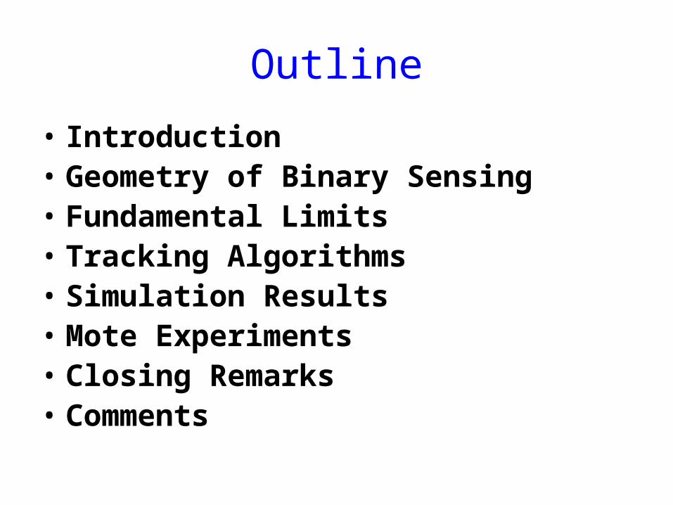
Outline

• Introduction• Geometry of Binary Sensing• Fundamental Limits• Tracking Algorithms• Simulation Results• Mote Experiments• Closing Remarks• Comments

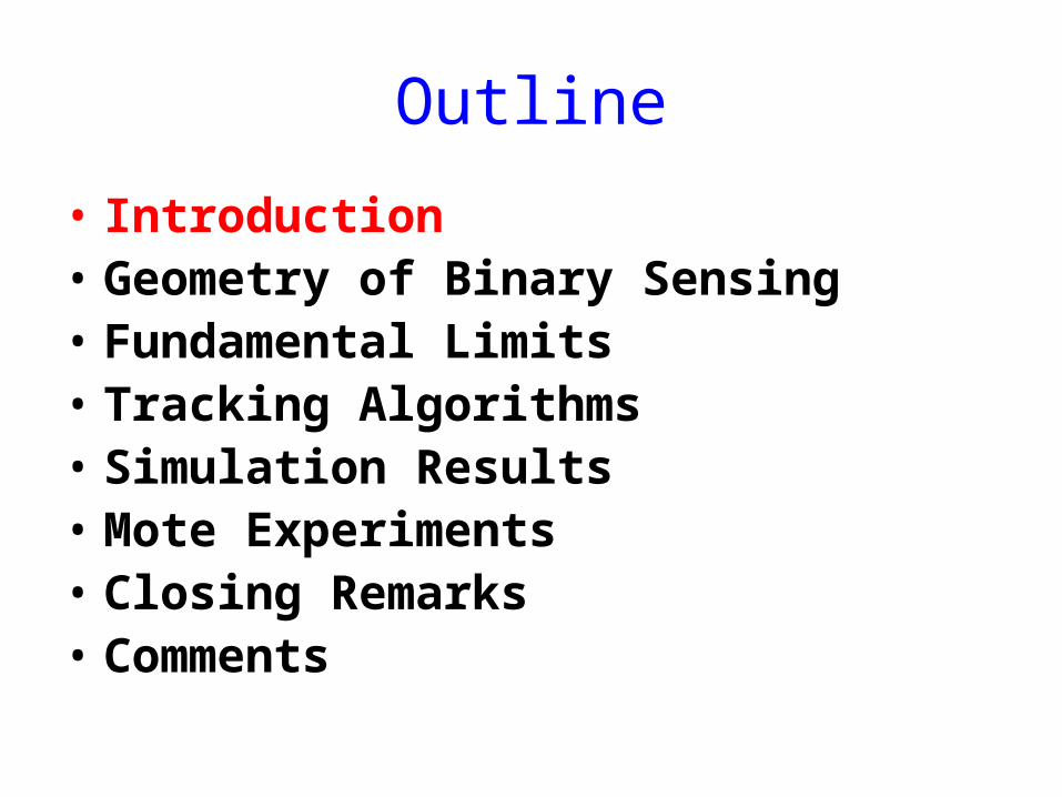
Outline

• Introduction• Geometry of Binary Sensing• Fundamental Limits• Tracking Algorithms• Simulation Results• Mote Experiments• Closing Remarks• Comments

Introduction

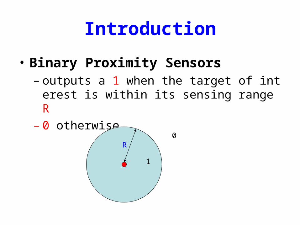
• Binary Proximity Sensors– outputs a 1 when the target of interest is withi

n its sensing range R– 0 otherwise

1

0R

Fundamental Limit Of Spatial Resolution

• Spatial Resolution– worst-case deviation between the estimated

and the actual paths

• Ideal achievable resolution is of the order of 1/R– R is the sensing range of individual sensors is the sensor density per unit area

Minimal Representations For The Target’s Trajectory

• Analogy between binary sensing and the sampling theory and quantization– “high-frequency” variations in the target’s

trajectory are invisible to the sensor field– estimate the shape or velocity for a “low-pass”

version of the trajectory.– consider piecewise linear approximations to

the trajectory that can be described economically

Occam’s Razor Approach

• Explanation of any phenomenon should make as few assumptions as possible

• Entities should not be multiplied beyond necessity

• All things being equal, the simplest solution tends to be the best one

Outline

• Introduction• Geometry of Binary Sensing• Fundamental Limits• Tracking Algorithms• Simulation Results• Mote Experiments• Closing Remarks• Comments

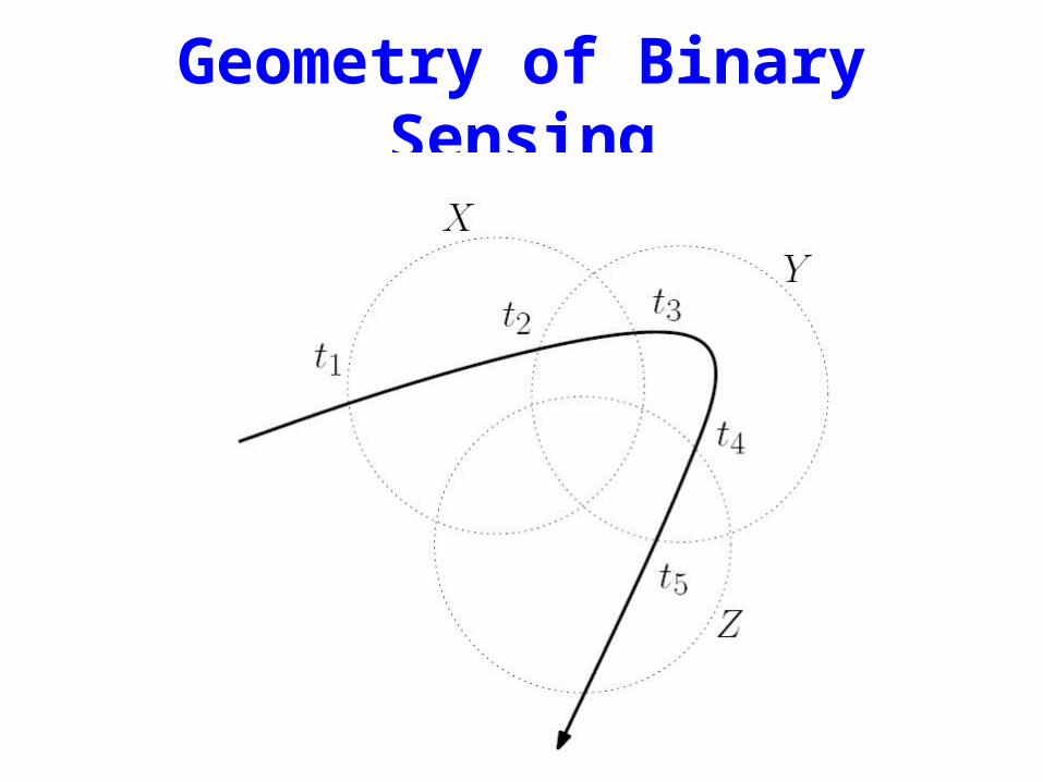
Geometry of Binary Sensing

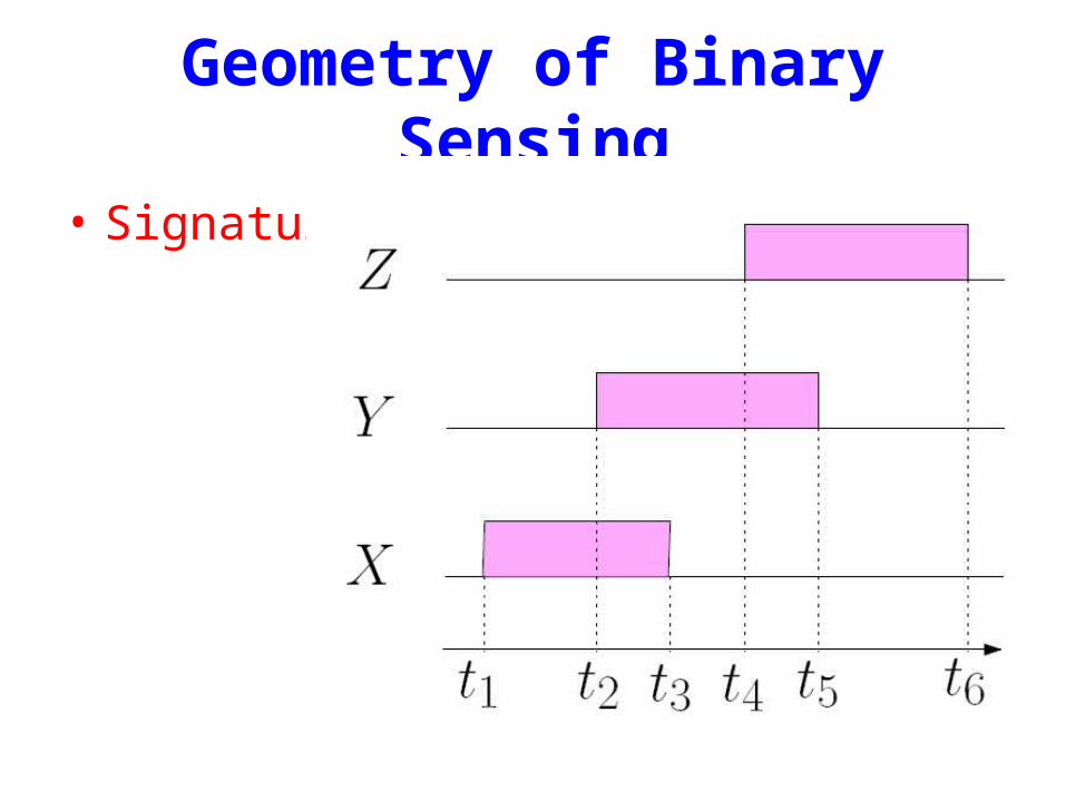
Geometry of Binary Sensing

• Signature

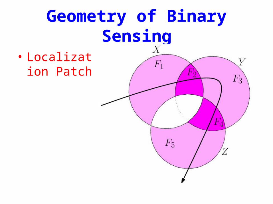
Geometry of Binary Sensing

• Localization Patch

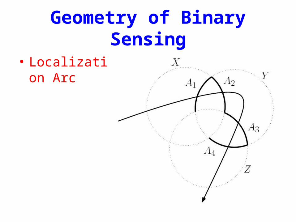
Geometry of Binary Sensing

• Localization Arc

Outline

• Introduction• Geometry of Binary Sensing• Fundamental Limits• Tracking Algorithms• Simulation Results• Mote Experiments• Closing Remarks• Comments

Fundamental Limits

• An Upper Bound on Spatial Resolution

• Achievability of Spatial Resolution Bound

• Remarks on Spatial Resolution Theorems

• Sampling and Velocity Estimation

An Upper Bound on Spatial Resolution

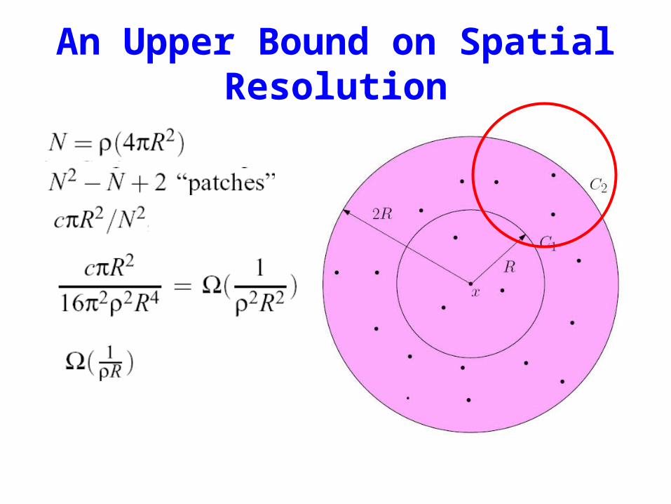
• THEOREM 1

• If a network of binary proximity sensors has average sensor density and each sensor has sensing radius R

• Then the worst-case error in localizing the target is at least W(1/ R)

An Upper Bound on Spatial Resolution

Achievability of Spatial Resolution Bound

• THEOREM 2– Consider a network of binary proximity sensor

s, distributed according to the Poisson distribution of density , where each sensor has sensing radius R.

– Then the localization error at any point in the plane is of order 1/R .

Remarks on Spatial Resolution Theorems

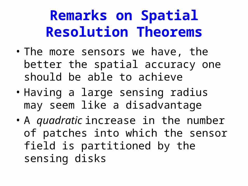
• The more sensors we have, the better the spatial accuracy one should be able to achieve

• Having a large sensing radius may seem like a disadvantage

• A quadratic increase in the number of patches into which the sensor field is partitioned by the sensing disks

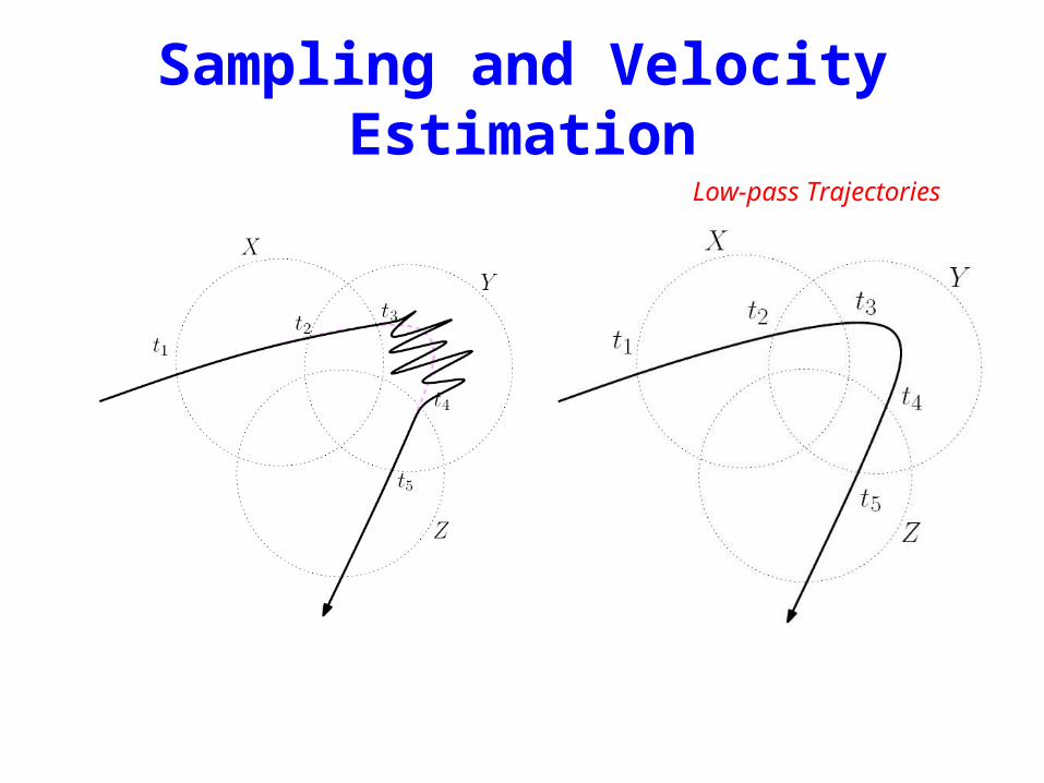
Sampling and Velocity Estimation

Low-pass Trajectories

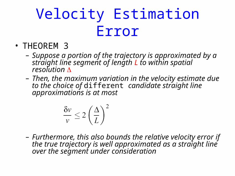
Velocity Estimation Error

• THEOREM 3– Suppose a portion of the trajectory is approximated by

a straight line segment of length L to within spatial resolution

– Then, the maximum variation in the velocity estimate due to the choice of different candidate straight line approximations is at most

– Furthermore, this also bounds the relative velocity error if the true trajectory is well approximated as a straight line over the segment under consideration

Outline

• Introduction• Geometry of Binary Sensing• Fundamental Limits• Tracking Algorithms• Simulation Results• Mote Experiments• Closing Remarks• Comments

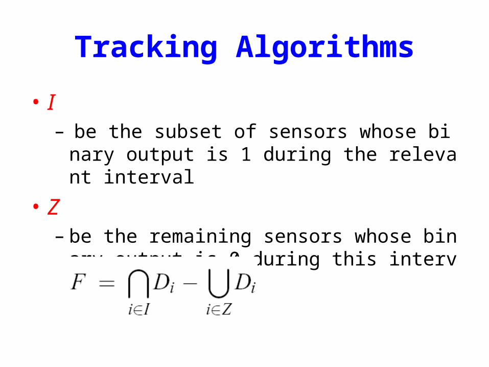
Tracking Algorithms

• I– be the subset of sensors whose binary output

is 1 during the relevant interval

• Z – be the remaining sensors whose binary output

is 0 during this interval

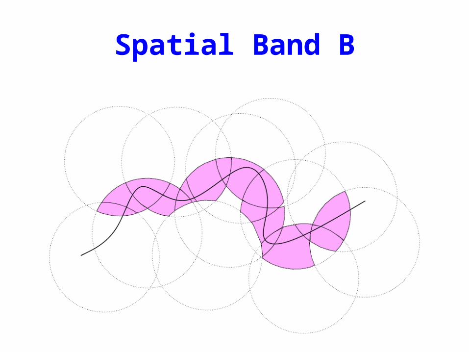
Spatial Band B

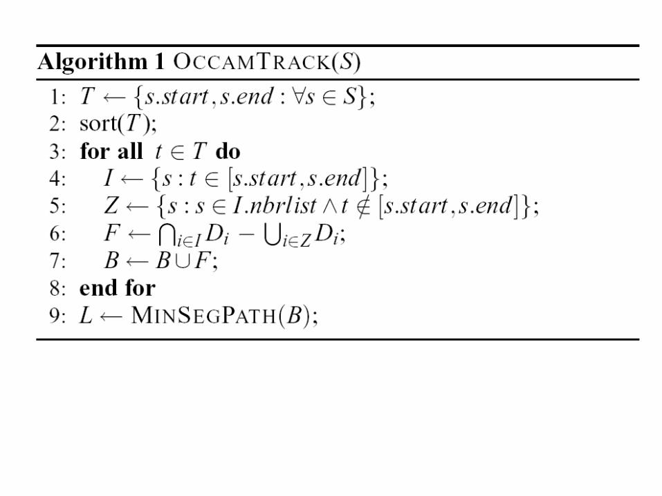
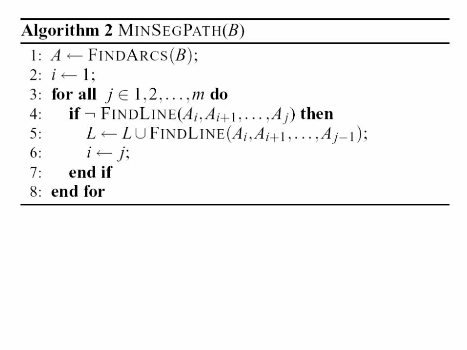
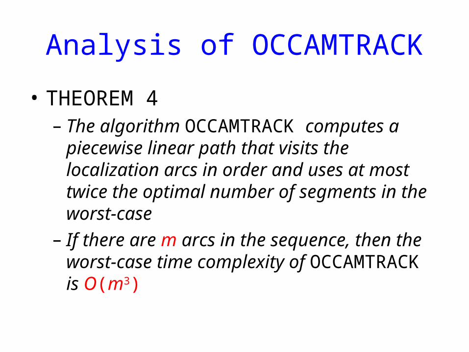
Analysis of OCCAMTRACK

• THEOREM 4– The algorithm OCCAMTRACK computes a

piecewise linear path that visits the localization arcs in order and uses at most twice the optimal number of segments in the worst-case

– If there are m arcs in the sequence, then the worst-case time complexity of OCCAMTRACK is O(m3)

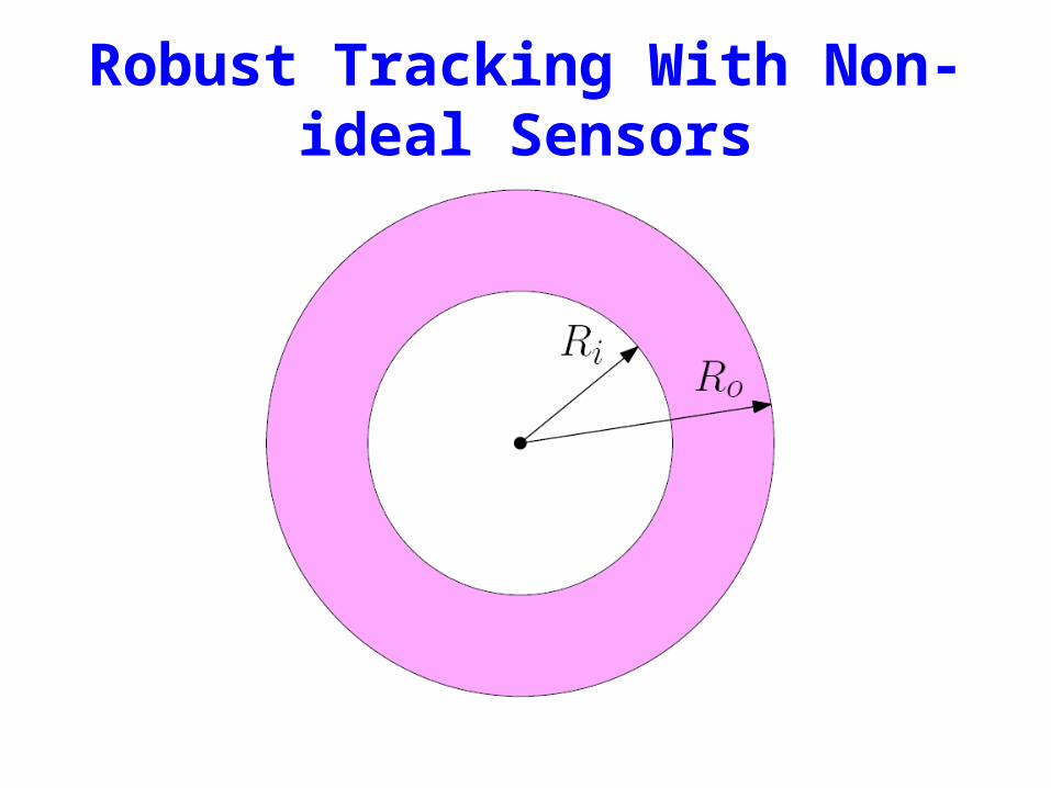
Robust Tracking With Non-ideal Sensors

Particle Filtering Algorithm

• At any time n, we have K particles (or candidate trajectories)– with the current location for the kth particle denoted b

y xk[n]

• At the next time instant n+1, suppose that the localization patch is F– Choose m candidates for xk [n+1] uniformly at random

from F

• We now have mK candidate trajectories• Pick the K particles with the best cost functions

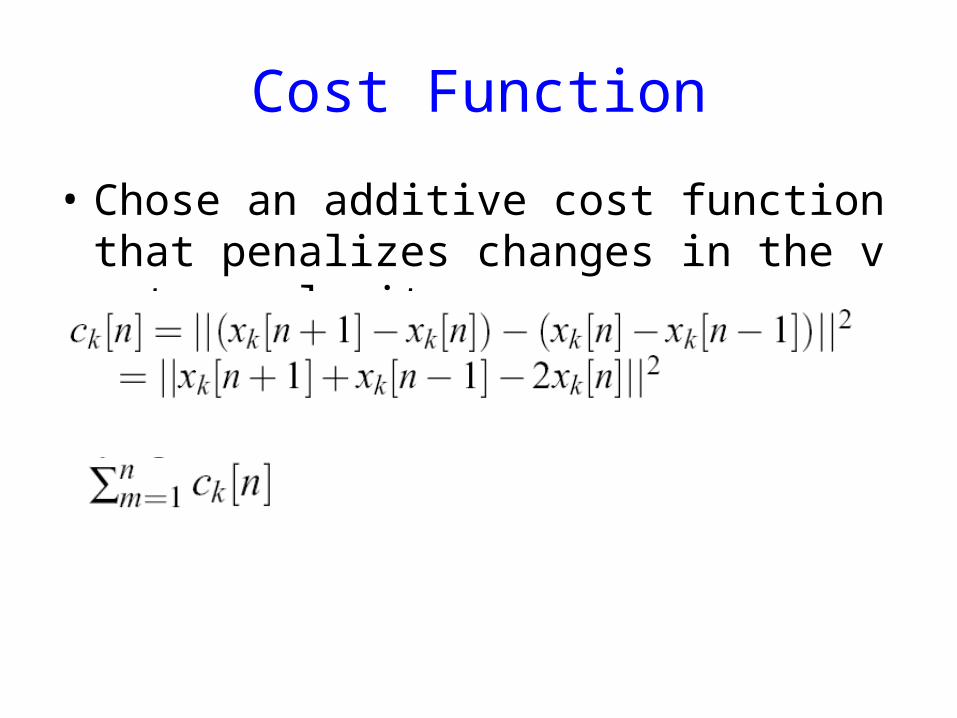
Cost Function

• Chose an additive cost function that penalizes changes in the vector velocity

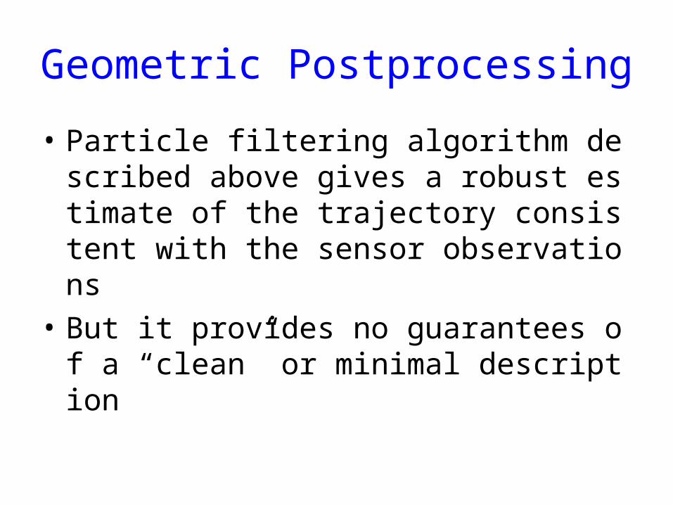
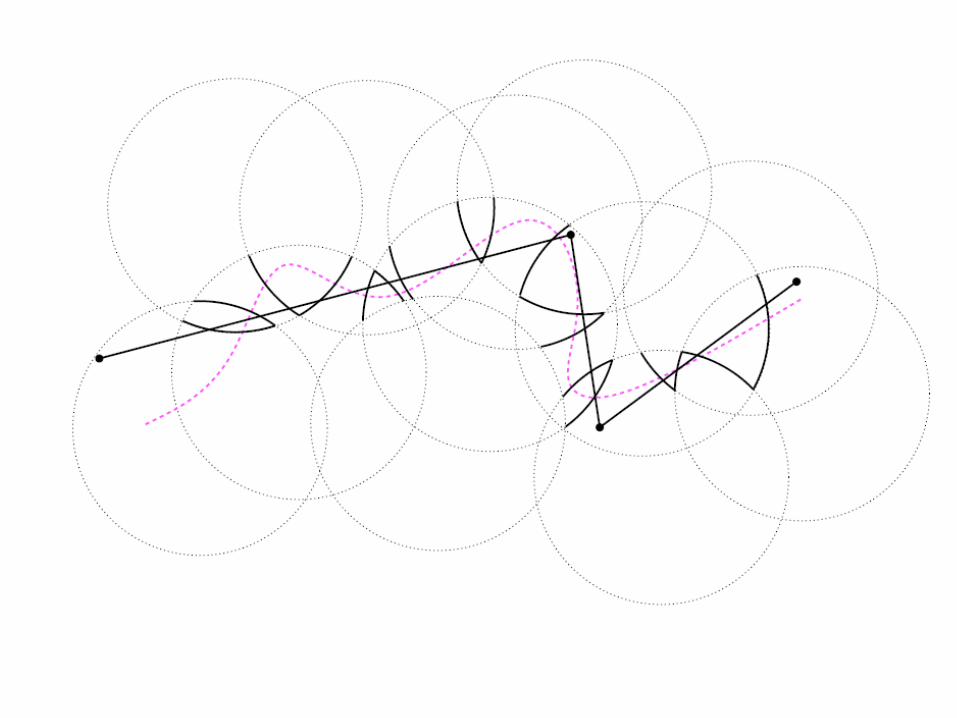
Geometric Postprocessing

• Particle filtering algorithm described above gives a robust estimate of the trajectory consistent with the sensor observations

• But it provides no guarantees of a “clean” or minimal description

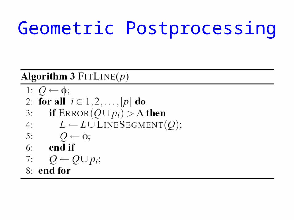
Geometric Postprocessing

Outline

• Introduction• Geometry of Binary Sensing• Fundamental Limits• Tracking Algorithms• Simulation Results• Mote Experiments• Closing Remarks• Comments

Simulation Results

• The code for OCCAMTRACK was Written in C and C++

• The code for PARTICLE-FILTER was written in Matlab

• The experiments were performed on an AMD Athlon 1.8 Ghz PC with 350 MB RAM

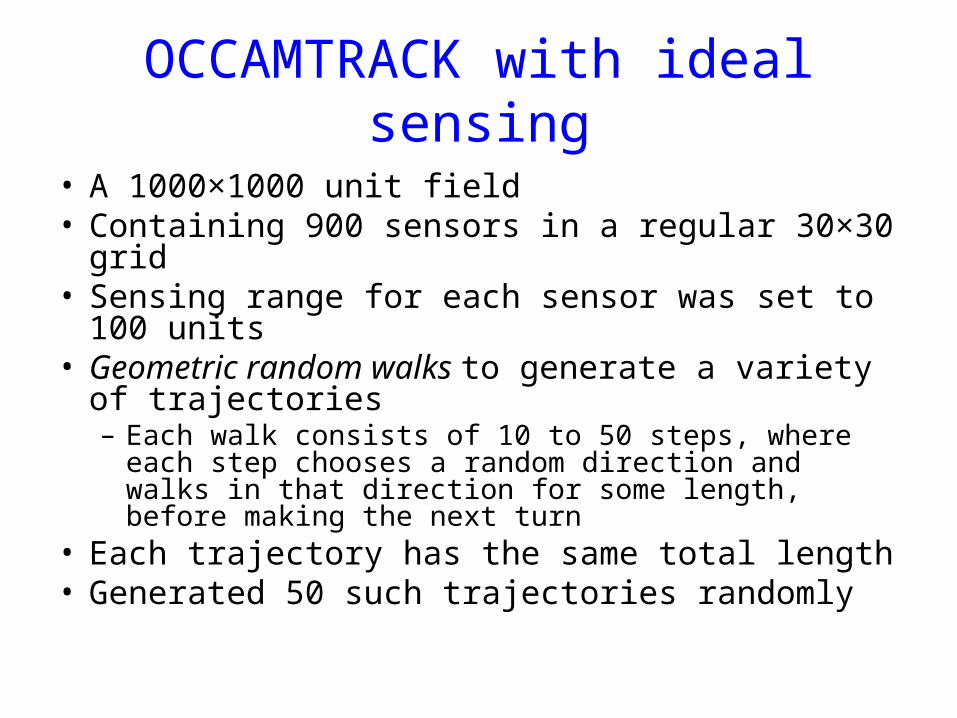
OCCAMTRACK with ideal sensing

• A 1000×1000 unit field• Containing 900 sensors in a regular 30×30 grid• Sensing range for each sensor was set to 100

units• Geometric random walks to generate a variety of

trajectories– Each walk consists of 10 to 50 steps, where each

step chooses a random direction and walks in that direction for some length, before making the next turn

• Each trajectory has the same total length• Generated 50 such trajectories randomly

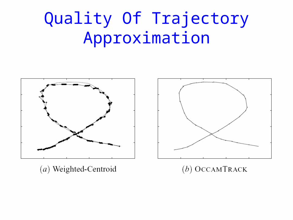
Quality Of Trajectory Approximation

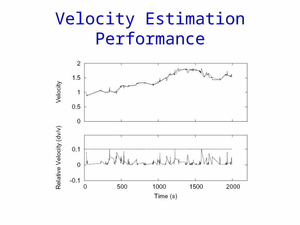
Velocity Estimation Performance

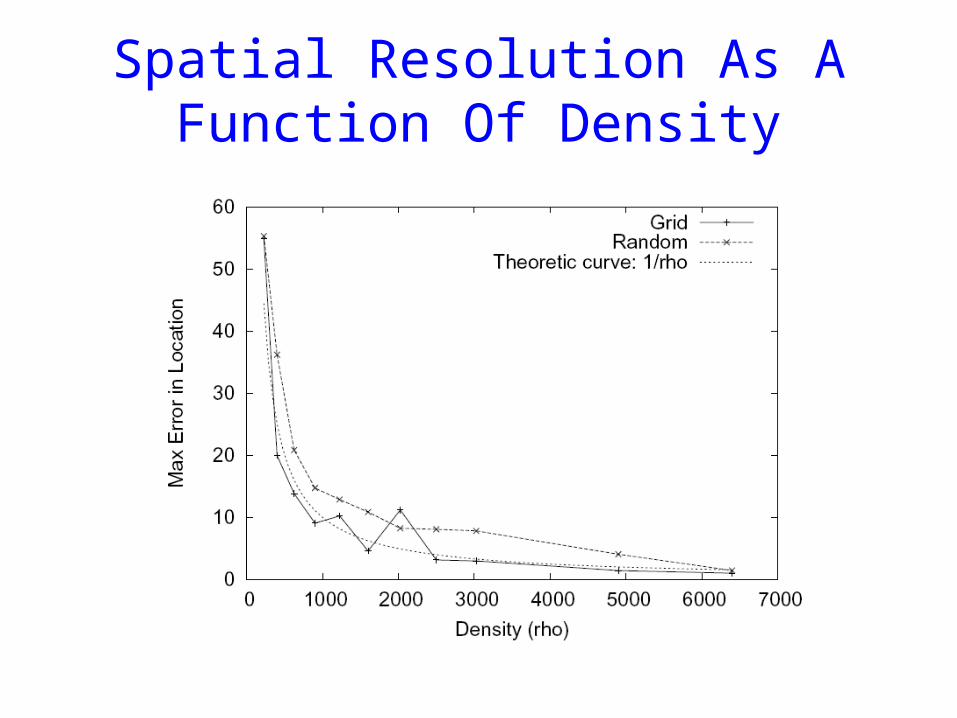
Spatial Resolution As A Function Of Density

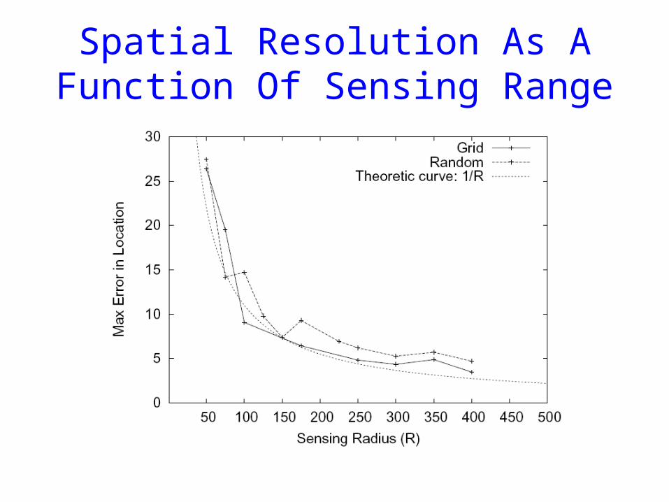
Spatial Resolution As A Function Of Sensing Range

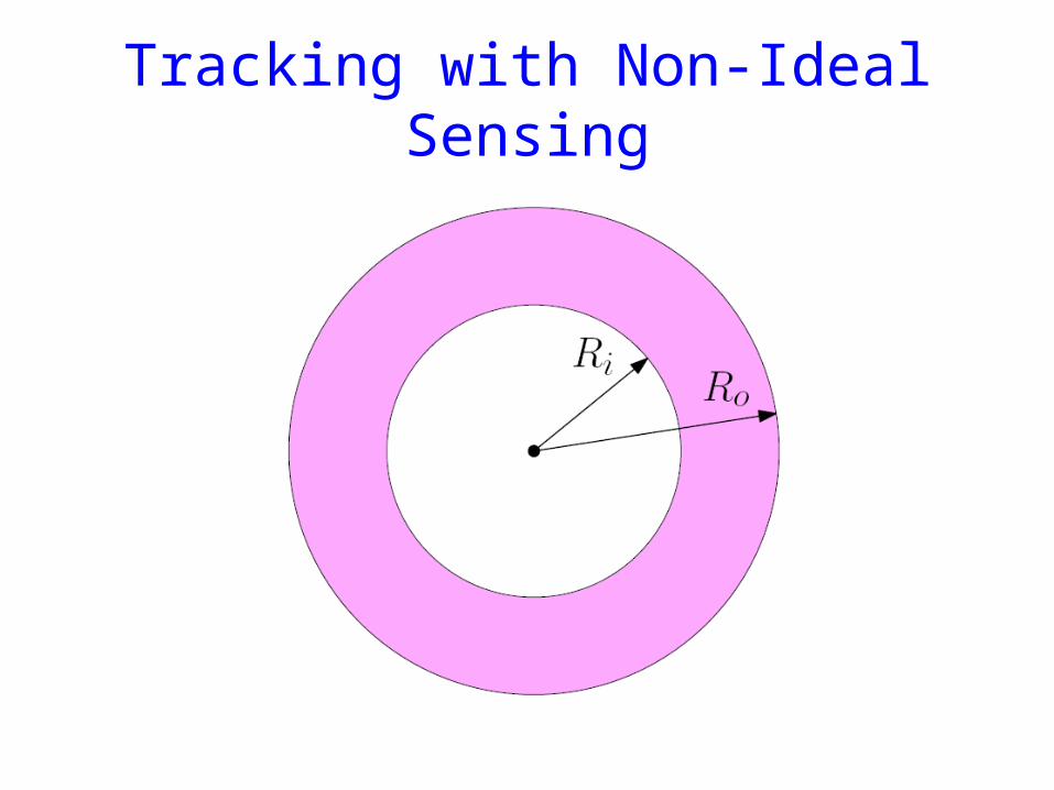
Tracking with Non-Ideal Sensing

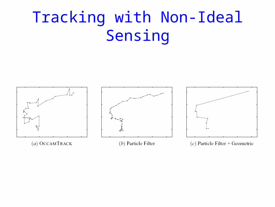
Tracking with Non-Ideal Sensing

Outline

• Introduction• Geometry of Binary Sensing• Fundamental Limits• Tracking Algorithms• Simulation Results• Mote Experiments• Closing Remarks• Comments

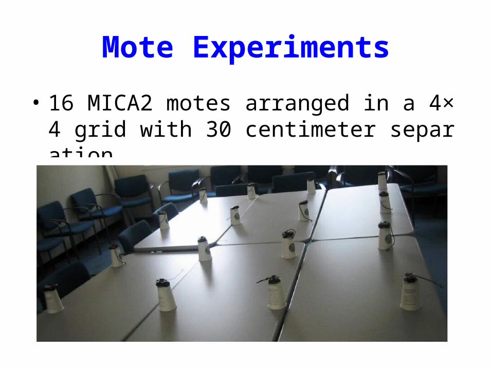
Mote Experiments

• 16 MICA2 motes arranged in a 4×4 grid with 30 centimeter separation

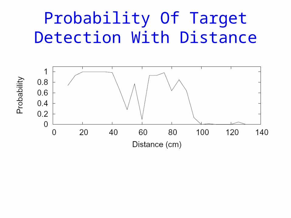
Probability Of Target Detection With Distance

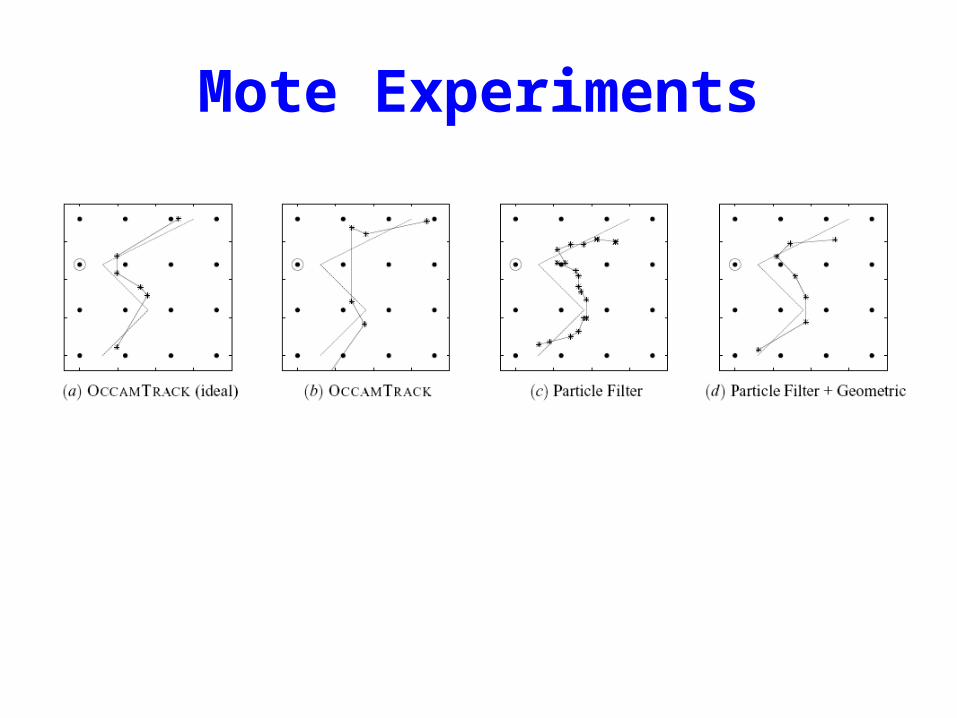
Mote Experiments

Outline

• Introduction• Geometry of Binary Sensing• Fundamental Limits• Tracking Algorithms• Simulation Results• Mote Experiments• Closing Remarks• Comments

Closing Remarks

• Have identified the fundamental limits of tracking performance possible with binary proximity sensors

• Have provided algorithms that approach these limits

Closing Remarks

• Results show that the binary proximity model, despite its minimalism, does indeed provide enough information to achieve respectable tracking accuracy– assuming that the product of the sensing radi

us and sensor density is large enough

Future Works

• An in-depth understanding, and accompanying algorithms, for multiple targets is therefore an important topic for future investigation

• To incorporate additional information (e.g., velocity, distance) if available

• To embed Occam’s razor criteria in the particle filtering algorithm

Outline

• Introduction• Geometry of Binary Sensing• Fundamental Limits• Tracking Algorithms• Simulation Results• Mote Experiments• Closing Remarks• Comments

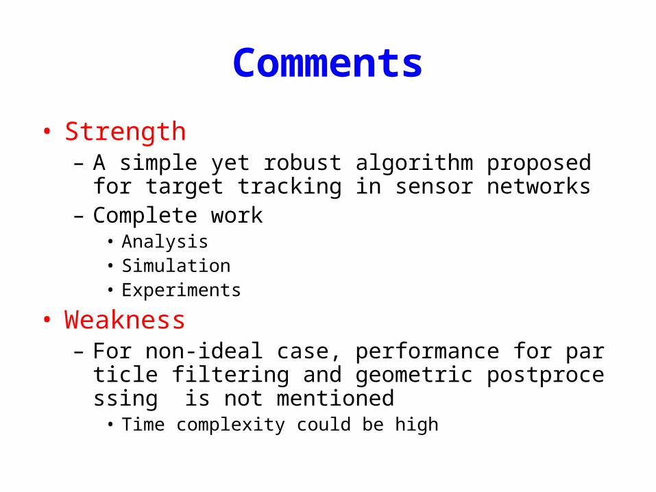
Comments

• Strength – A simple yet robust algorithm proposed for target trac

king in sensor networks– Complete work

• Analysis• Simulation• Experiments

• Weakness– For non-ideal case, performance for particle filtering a

nd geometric postprocessing is not mentioned• Time complexity could be high

Thank You Very Much For Your Attention!

Any More Questions?