TASI Lectures on Collider Physics

Matthew D. Schwartz

Department of PhysicsHarvard University

Abstract

These lectures provide an introduction to the physics of particle colliders. Topicscovered include a quantitative examination of the design and operational param-eters of Large Hadron Collider, kinematics and observables at colliders, such asrapidity and transverse mass, and properties of distributions, such as Jacobianpeaks. In addition, the lectures provide a practical introduction to the decaymodes and signatures of important composite and elementary and particles in theStandard Model, from pions to the Higgs boson. The aim of these lectures isprovide a bridge between theoretical and experimental particle physics. Wheneverpossible, results are derived using intuitive arguments and estimates rather thanprecision calculations.

arX

iv:1

709.

0453

3v1

[he

p-ph

] 1

3 Se

p 20

17

Contents

1 Introduction 3

2 The Large Hadron Collider 3

3 Kinematics 7

4 Observables 10

5 Distributions 12

6 Jets 17

7 Meet the Standard Model 197.1 W boson . . . . . . . . . . . . . . . . . . . . . . . . . . . . . . . . . . . . . . . . . 197.2 Z boson . . . . . . . . . . . . . . . . . . . . . . . . . . . . . . . . . . . . . . . . . 207.3 Top quark . . . . . . . . . . . . . . . . . . . . . . . . . . . . . . . . . . . . . . . . 217.4 Bottom quark . . . . . . . . . . . . . . . . . . . . . . . . . . . . . . . . . . . . . . 237.5 Charm quark . . . . . . . . . . . . . . . . . . . . . . . . . . . . . . . . . . . . . . 247.6 Strange quark . . . . . . . . . . . . . . . . . . . . . . . . . . . . . . . . . . . . . . 257.7 Up and down quarks . . . . . . . . . . . . . . . . . . . . . . . . . . . . . . . . . . 267.8 Electrons and muons . . . . . . . . . . . . . . . . . . . . . . . . . . . . . . . . . . 267.9 Tauons . . . . . . . . . . . . . . . . . . . . . . . . . . . . . . . . . . . . . . . . . 287.10 Higgs boson . . . . . . . . . . . . . . . . . . . . . . . . . . . . . . . . . . . . . . . 29

2

1 Introduction

These lectures provide an introduction to the physics of colliders, particularly focused on theLarge Hadron Collider. They are based on summer school lectures given at the TheoreticalAdvanced Study Institute (TASI) in Boulder, Colorado and at the Galileo Galilei Institute inFlorence, Italy. The target audience is graduate students who have already had some exposure toquantum field theory and particle physics. While the subject of these lectures, collider physics,has much overlap with the perturbative and non-perturbative physics of quantum chromody-namics, those more technical topics are not included (see [1–3] for more information).

Typically, collider physics is not covered in most quantum field theory sequences. Colliderphysics is a practical subject: how does one extract information from the data at a collider?What are the kinds of things that can be observed, and what do we learn from their observation?To answer these questions, I begin in Section 2 with an introduction to colliders, particularlythe Large Hadron Collider (LHC). A basic familiarity with the units and design specifications ofthe LHC is essential for even the most basic understanding of contemporary collider physics. Ithen proceed to discuss kinematics in Section 3 and some of the most important observables atcolliders, like invariant mass distributions and transverse mass in Sections 4 and 5. Section 6 isa very brief introduction to jets; even though jet physics is one of my favorite collider physicstopics, there are already many good reviews of the subject.

The final part of these lectures in Section 7 is about the particles in the Standard Model(SM). I wrote this section because I have found that while most graduate students in highenergy physics can name the particles in the SM, hardly any of them would recognize one ofthese particles if they saw it. To really understand particle physics, is important to get to knowthe actual particles. For this reason, Section 7 comprises a large fraction of these notes: I goone-by-one through the SM particles discussing their properties and signatures.

2 The Large Hadron Collider

Our first task is to answer one of the most essential questions about the LHC: why is it designedthe way it is? To get a handle on this question, we can ask what are roughly the requirementswe would need to be able to discover a Higgs boson? We will approach this question usingdimensional analysis and some basic particle physics.

The base unit for scattering cross sections at colliders is the barn (b): 1b = 10−28 m2. Thename of this unit of area comes from a joke by Enrico Fermi, that neutrons in nuclear reactorshit Uranium targets as easily as hitting the broad side of a barn. This joke provides a startingpoint for dimensional analysis: the cross section for n-U235 scattering is ∼ 1 b. What is thecross section for proton-proton scattering at the LHC? Well, if the volume of a nucleus scales likethe atomic number Z, then the radius scales like r ∼ Z1/3 and so the area like Z2/3. Hence oneexpects proton-proton scattering to have an inclusive cross section of 235−2/3 b = 0.03 b = 30 mb.

3

To convert between length and energy, the formula is

1

GeV2~2c2 = 3.894× 10−32m2 (1)

This is a little hard to remember. I prefer

200 MeV =1

fm(2)

where fm = femtometer = 10−15 m. This says that the strong interaction scale of QCD, ΛQCD ∼200 MeV is the same as the “radius” of the proton, rp ∼ 1 fm. What does the radius of theproton mean? It means that the proton scattering cross section should be σ ∼ πr2

p = 3 fm2 =3 × 10−30m2 = 0.03 b. So this is consistent with the estimate from scaling the n-U235 crosssection.

So proton-proton scattering happens at the tens-of-millibarns level. There is some energydependence to this total cross section, but it is fairly weak (logarithmic). Actually, the totalscattering cross section is not even precisely defined theoretically. One can define the inelasticcross section from the probability for the protons to break apart. However, the elastic crosssection, where pp→ pp, has an infrared divergence in the forward scattering region: for protonsthat glance off each other infinitesimally, you can’t tell if the protons have scattered at all. Inaddition, it’s possible to have some hard interaction among the partons in the protons but stillhave exactly two protons in the final state (this is called diffractive scattering). A trick to geta handle on the cross section is to use the optical theorem. This theorem relates the inclusiveinelastic-plus-diffractive scattering total cross section to the imaginary part of the amplitude forforward scattering. Unfortunately, one can neither measure an exactly forward scattering crosssection (because the beam is in the way) or measure an imaginary part. What is done in practiceis to place a detector at very small angle θ to the beam line (at the LHC one of these detectors iscalled totem) to measure pp→ pp scattering. Then the limit θ → 0 is taken and the interferencebetween the QED and QCD components of the amplitude is used to find the imaginary part.I’m not convinced that this procedure is on entirely sound theoretical footing, but it seems togive reasonable answers.

In any case, a number σ ∼ 30 mb for the total pp cross section is enough to get us started.Next, we can ask how this compares to the cross section for some process of interest. For example,what is the rate for W boson production? Well, the typical scale for weak interactions is Fermi’sconstant

σ(pp→ W ) ∼ GF ∼g2

m2W

∼ 1

(100 GeV)2= 10−6 mb = 1 nb (3)

Thus we expect roughly 1 in a million proton collisions will produce a W boson. What aboutthe Higgs boson? Well, as you hopefully know, the dominant mechanism for Higgs productionis from gluon fusion through a top loop. Thus we expect the Higgs cross section to be down byroughly a loop factor of 1

16π2 ∼ 10−3 from weak interaction cross sections that proceed at tree

4

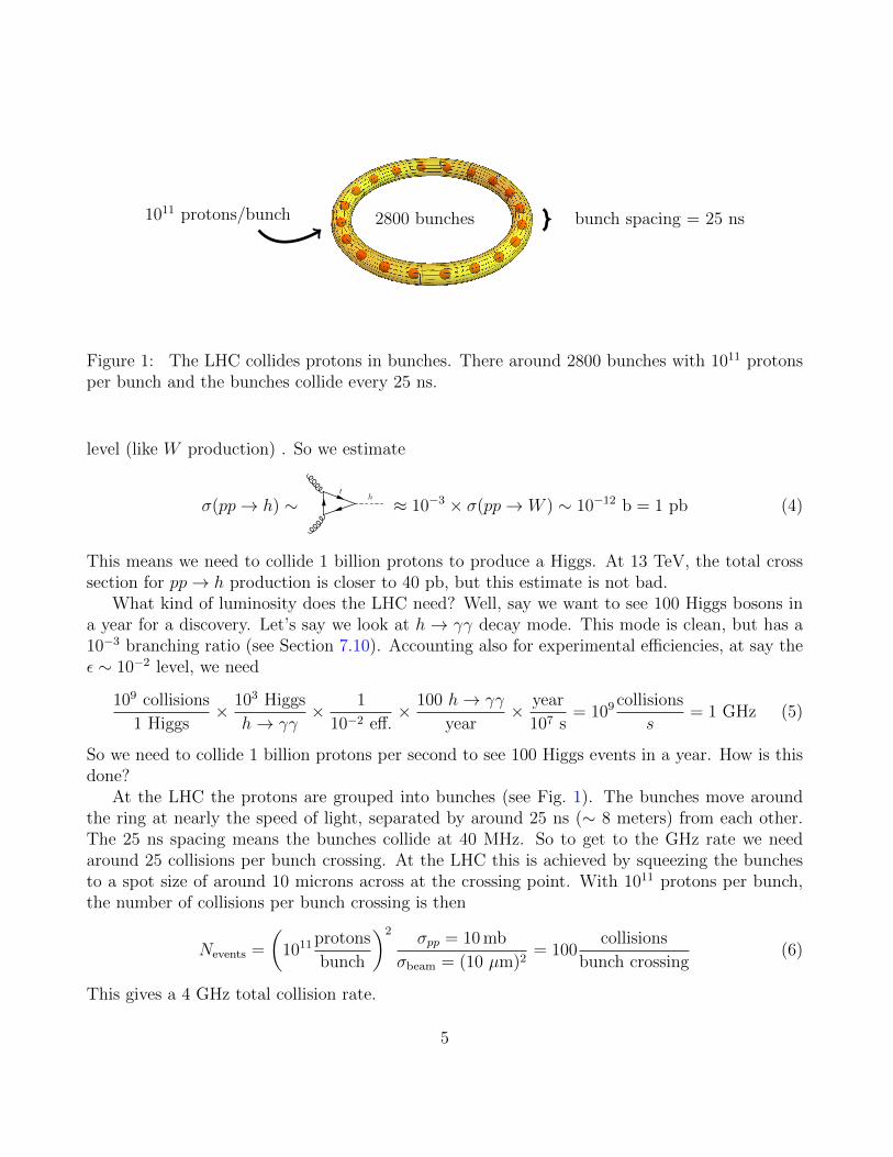
1011 protons/bunch 2800 bunches bunch spacing = 25 ns

Figure 1: The LHC collides protons in bunches. There around 2800 bunches with 1011 protonsper bunch and the bunches collide every 25 ns.

level (like W production) . So we estimate

σ(pp→ h) ∼t

h ≈ 10−3 × σ(pp→ W ) ∼ 10−12 b = 1 pb (4)

This means we need to collide 1 billion protons to produce a Higgs. At 13 TeV, the total crosssection for pp→ h production is closer to 40 pb, but this estimate is not bad.

What kind of luminosity does the LHC need? Well, say we want to see 100 Higgs bosons ina year for a discovery. Let’s say we look at h → γγ decay mode. This mode is clean, but has a10−3 branching ratio (see Section 7.10). Accounting also for experimental efficiencies, at say theε ∼ 10−2 level, we need

109 collisions

1 Higgs× 103 Higgs

h→ γγ× 1

10−2 eff.× 100 h→ γγ

year× year

107 s= 109 collisions

s= 1 GHz (5)

So we need to collide 1 billion protons per second to see 100 Higgs events in a year. How is thisdone?

At the LHC the protons are grouped into bunches (see Fig. 1). The bunches move aroundthe ring at nearly the speed of light, separated by around 25 ns (∼ 8 meters) from each other.The 25 ns spacing means the bunches collide at 40 MHz. So to get to the GHz rate we needaround 25 collisions per bunch crossing. At the LHC this is achieved by squeezing the bunchesto a spot size of around 10 microns across at the crossing point. With 1011 protons per bunch,the number of collisions per bunch crossing is then

Nevents =

(1011 protons

bunch

)2σpp = 10 mb

σbeam = (10 µm)2= 100

collisions

bunch crossing(6)

This gives a 4 GHz total collision rate.

5

Trigger Rate1 isolated electron, pT > 25 GeV

40 Hz2 isolated electrons, both pT > 15 GeV

1 photon, pT > 60 GeV40 Hz

2 photons, pT > 20 GeV1 muon, pT > 20 GeV

40 Hz2 muons, pT > 10 GeV

1 jet, pT > 400 GeV25 Hz3 jets, pT > 165 GeV

4 jets, pT > 110 GeV1 jet, pT > 165 GeV and /ET > 70 GeV 20 Hz

1 tauon, pT > 35 GeV and /ET > 45 GeV 5 Hz2 muons + displaced vertex b-tag 10 Hz

prescales (e.g.1% of 1 jet, pT > 200 GeV) 5 Hz

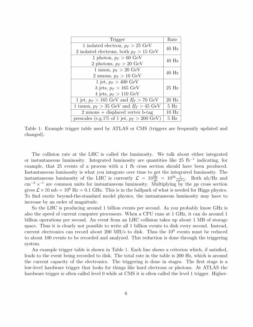
Table 1: Example trigger table used by ATLAS or CMS (triggers are frequently updated andchanged).

The collision rate at the LHC is called the luminosity. We talk about either integratedor instantaneous luminosity. Integrated luminosity are quantities like 25 fb−1 indicating, forexample, that 25 events of a process with a 1 fb cross section should have been produced.Instantaneous luminosity is what you integrate over time to get the integrated luminosity. Theinstantaneous luminosity of the LHC is currently L = 10Hz

nb= 1034 1

cm2·s . Both nb/Hz andcm−2 s−1 are common units for instantaneous luminosity. Multiplying by the pp cross sectiongives L×10 mb = 108 Hz = 0.1 GHz. This is in the ballpark of what is needed for Higgs physics.To find exotic beyond-the-standard model physics, the instantaneous luminosity may have toincrease by an order of magnitude.

So the LHC is producing around 1 billion events per second. As you probably know GHz isalso the speed of current computer processors. When a CPU runs at 1 GHz, it can do around 1billion operations per second. An event from an LHC collision takes up about 1 MB of storagespace. Thus it is clearly not possible to write all 1 billion events to disk every second. Instead,current electronics can record about 200 MB/s to disk. Thus the 109 events must be reducedto about 100 events to be recorded and analyzed. This reduction is done through the triggeringsystem.

An example trigger table is shown in Table 1. Each line shows a criterion which, if satisfied,leads to the event being recorded to disk. The total rate in the table is 200 Hz, which is aroundthe current capacity of the electronics. The triggering is done in stages. The first stage is alow-level hardware trigger that looks for things like hard electrons or photons. At ATLAS thehardware trigger is often called level 0 while at CMS it is often called the level 1 trigger. Higher-

6

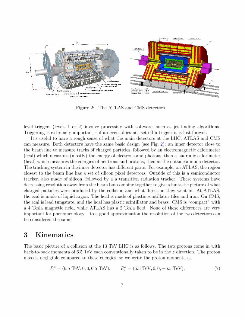
Figure 2: The ATLAS and CMS detectors.

level triggers (levels 1 or 2) involve processing with software, such as jet finding algorithms.Triggering is extremely important – if an event does not set off a trigger it is lost forever.

It’s useful to have a rough sense of what the main detectors at the LHC, ATLAS and CMScan measure. Both detectors have the same basic design (see Fig. 2): an inner detector close tothe beam line to measure tracks of charged particles, followed by an electromagnetic calorimeter(ecal) which measures (mostly) the energy of electrons and photons, then a hadronic calorimeter(hcal) which measures the energies of neutrons and protons, then at the outside a muon detector.The tracking system in the inner detector has different parts. For example, on ATLAS, the regionclosest to the beam line has a set of silicon pixel detectors. Outside of this is a semiconductortracker, also made of silicon, followed by a a transition radiation tracker. These systems havedecreasing resolution away from the beam but combine together to give a fantastic picture of whatcharged particles were produced by the collision and what direction they went in. At ATLAS,the ecal is made of liquid argon. The hcal is made of plastic scintillator tiles and iron. On CMS,the ecal is lead tungstate, and the hcal has plastic scintillator and brass. CMS is “compact” witha 4 Tesla magnetic field, while ATLAS has a 2 Tesla field. None of these differences are veryimportant for phenomenology – to a good approximation the resolution of the two detectors canbe considered the same.

3 Kinematics

The basic picture of a collision at the 13 TeV LHC is as follows. The two protons come in withback-to-back momenta of 6.5 TeV each conventionally taken to be in the z direction. The protonmass is negligible compared to these energies, so we write the proton momenta as

P µ1 = (6.5 TeV, 0, 0, 6.5 TeV), P µ

2 = (6.5 TeV, 0, 0,−6.5 TeV), (7)

7

η = 0

θ = 90◦

η = 1

θ = 40◦η = −1

θ = 130◦

η = 2, θ = 15◦

η = 3, θ = 6◦

η = 4, θ = 2◦φ

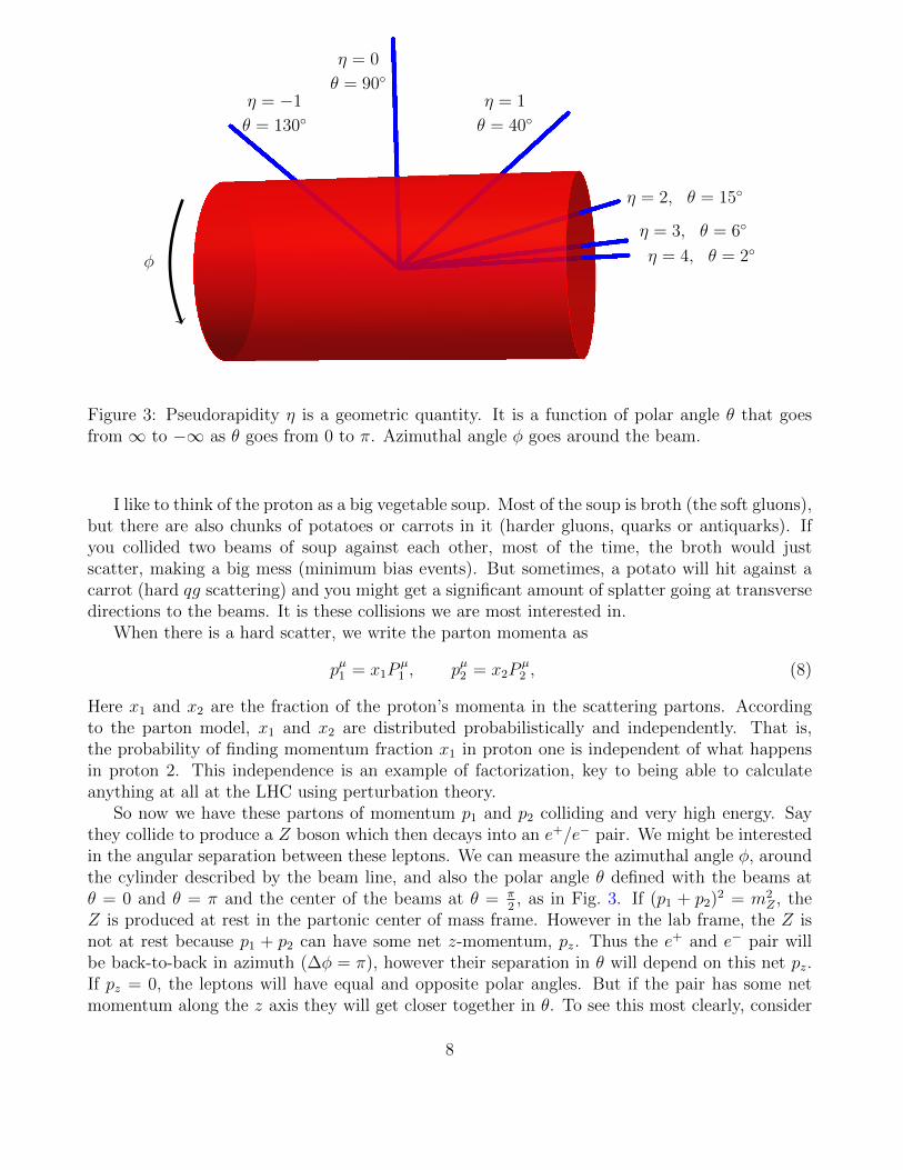
Figure 3: Pseudorapidity η is a geometric quantity. It is a function of polar angle θ that goesfrom ∞ to −∞ as θ goes from 0 to π. Azimuthal angle φ goes around the beam.

I like to think of the proton as a big vegetable soup. Most of the soup is broth (the soft gluons),but there are also chunks of potatoes or carrots in it (harder gluons, quarks or antiquarks). Ifyou collided two beams of soup against each other, most of the time, the broth would justscatter, making a big mess (minimum bias events). But sometimes, a potato will hit against acarrot (hard qg scattering) and you might get a significant amount of splatter going at transversedirections to the beams. It is these collisions we are most interested in.

When there is a hard scatter, we write the parton momenta as

pµ1 = x1Pµ1 , pµ2 = x2P

µ2 , (8)

Here x1 and x2 are the fraction of the proton’s momenta in the scattering partons. Accordingto the parton model, x1 and x2 are distributed probabilistically and independently. That is,the probability of finding momentum fraction x1 in proton one is independent of what happensin proton 2. This independence is an example of factorization, key to being able to calculateanything at all at the LHC using perturbation theory.

So now we have these partons of momentum p1 and p2 colliding and very high energy. Saythey collide to produce a Z boson which then decays into an e+/e− pair. We might be interestedin the angular separation between these leptons. We can measure the azimuthal angle φ, aroundthe cylinder described by the beam line, and also the polar angle θ defined with the beams atθ = 0 and θ = π and the center of the beams at θ = π

2, as in Fig. 3. If (p1 + p2)2 = m2

Z , theZ is produced at rest in the partonic center of mass frame. However in the lab frame, the Z isnot at rest because p1 + p2 can have some net z-momentum, pz. Thus the e+ and e− pair willbe back-to-back in azimuth (∆φ = π), however their separation in θ will depend on this net pz.If pz = 0, the leptons will have equal and opposite polar angles. But if the pair has some netmomentum along the z axis they will get closer together in θ. To see this most clearly, consider

8

very large pz where both leptons are close to θ = 0. In fact, values and differences of θ anglestend to tell us more about the parton momenta in the proton than about the angular distributionfrom Z decays.

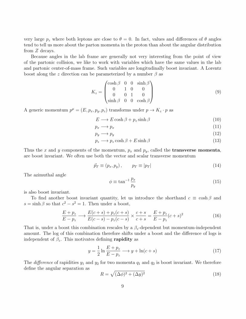
Because angles in the lab frame are generally not very interesting from the point of viewof the partonic collision, we like to work with variables which have the same values in the laband partonic center-of-mass frame. Such variables are longitudinally boost invariant. A Lorentzboost along the z direction can be parameterized by a number β as

Kz =

cosh β 0 0 sinh β

0 1 0 00 0 1 0

sinh β 0 0 cosh β

(9)

A generic momentum pµ = (E, px, py, pz) transforms under p→ Kz · p as

E −→ E cosh β + pz sinh β (10)

px −→ px (11)

py −→ py (12)

pz −→ pz cosh β + E sinh β (13)

Thus the x and y components of the momentum, px and py, called the transverse momenta,are boost invariant. We often use both the vector and scalar transverse momentum

~pT ≡ (px, py) , pT ≡ |pT | (14)

The azimuthal angle

φ ≡ tan−1 pxpy

(15)

is also boost invariant.To find another boost invariant quantity, let us introduce the shorthand c ≡ cosh β and

s = sinh β so that c2 − s2 = 1. Then under a boost,

E + pzE − pz

−→ E(c+ s) + pz(c+ s)

E(c− s)− pz(c− s)× c+ s

c+ s=E + pzE − pz

(c+ s)2 (16)

That is, under a boost this combination rescales by a βz-dependent but momentum-independentamount. The log of this combination therefore shifts under a boost and the difference of logs isindependent of βz. This motivates defining rapidity as

y =1

2lnE + pzE − pz

−→ y + ln(c+ s) (17)

The difference of rapidities y1 and y2 for two momenta q1 and q2 is boost invariant. We thereforedefine the angular separation as

R =√

(∆φ)2 + (∆y)2 (18)

9

This angular separation is boost invariant. Plotting distributions as functions of rapidity ratherthan polar angle makes it easier to disentangle the physics of the protons that produced theboost from the physics of the hard collision that we are studying.

To get intuition for rapidity, consider massless particles. These have E = |~p|. Then, drawinga little momentum triangle:

pT|~p|

pz

θ

(19)

we see that cos θ = pz|~p| = pz

E. So,

y =1

2lnE + pzE − pz

=1

2ln

1 + cos θ

1− cos θ=

1

2ln

2 cos2 θ2

2 sin2 θ2

= ln cotθ

2, m = 0 only (20)

Thus there is a simple mapping between rapidity and angle for massless particles. This motivatesdefining pseudorapidity η as

η ≡ ln cotθ

2(21)

Taylor expanding this relation around θ ≈ π2, we see

η ≈ π

2− θ (22)

For exampleθ − π

20 0.1 −1 10◦ from beam

η 0 −0.1001 1.22 ±2.5(23)

Some values for θ and η are shown in Fig. 3. Note that particles at η ∼ ±5 are practicallydown the beam line. The ATLAS and CMS detectors measure particles up to pseudorapiditiesof around ±5.

In summary, rapidity is a kinematic quantity defined as y ≡ 12

ln E+pzE−pz . Rapidity itself is not

boost invariant, but differences in rapidity are boost invariant. Other boost invariant quantitiesare ~pT ≡ (px, py) and φ = tan−1 px

py. Pseudorapidity η ≡ ln cot θ

2is a geometric quantity. It is

equal to rapidity only for massless particles. For massive particles, differences in pseudorapiditiesare not boost invariant.

4 Observables

All collider observables are functions of the momentum and energy of the particles produced.Ideally, we would like to measure the 4-momentum of every particle in the event, but this is not

10

quite possible in practice. To a first approximation, what can be measured is the energy of all theparticles stable on detector timescales, through deposits to the various calorimeters, and theirdirections (η, φ). Since most particles of interest are essentially massless, energy and angle areenough to reconstruct the momentum. Most particles deposit all their energy within the centralcalorimetry system. The two exceptions are neutrinos, which leave the detector rarely havinginteracted at all, and muons. Muons are like little cannonballs that get all the way throughthe detector before depositing all their energy. Nevertheless, the momentum of muons can bemeasured by using the curvature of their trajectories through the muon calorimeter. To do sorequires strong magnetic fields to shift the muons’ trajectories, and lots of space to see the smallcurvature of the energetic tracks. The muon system is much of the reason why ATLAS and CMSare so big. Curvature of tracks is also used in the inner detector, to distinguish charged particleslike electrons, positrons and pions, and to help measure their 3-momentum.

A standard observable constructed from the particles’ momenta is missing transverse mo-mentum:

/~pT ≡ −∑j

~pT (24)

Missing transverse momentum is a 2-vector. A related quantity is missing transverse energy

/ET ≡ | /~pT | (25)

Missing transverse energy (MET) is a scalar.For example, if an event has a W− boson in it which decays to e−ν, then we will only see

the electron, not the neutrino. The electron’s 4-momentum can essentially be measured. Themomentum of the neutrino should have opposite px and py components to the electron, but itspz component does not have to be opposite to that of the electron, due to the longitudinal boostof the partonic system. Thus /~pT gives the transverse components of the neutrino. Knowing thatthe W boson was on-shell gives an additional constraint that allows the neutrino momentumto be fully reconstructed (up to a 2-fold ambiguity from the 2 roots of the quadratic equationm2W = p2

e + p2ν). If there is more than one neutrino in the event, we cannot reconstruct all the

neutrinos’ momenta. For example, in p→ Z → νν events, there may be no transverse momentumat all, so the neutrinos could have gone anywhere (of course, there is nothing at all to see hereso this event would not even trigger).

Another quantity commonly discussed is HT . There is not a unique definition of HT , butit usually refers to the scalar sum of the missing transverse momentum in certain objects. Forexample, we might see

HT =

∣∣∣∣∣∑jets j

~p jT

∣∣∣∣∣ , or HT =∑jets j

∣∣~p jT

∣∣ , or HT =∑

leptons j

∣∣~p jT

∣∣ , (26)

Whenever you see HT used, makes sure you know what quantity it refers to.

11

We also are often interested in the invariant mass of some objects

mobjects =

∣∣∣∣∣ ∑objects j

pµj

∣∣∣∣∣2

(27)

For example, in pp→ γγ events, we might look at the invariant mass of the two photons. Plottingthe number of events observed as a function of invariant mass should show a resonant peak atthe mass of the Higgs boson, mγγ ∼ mh.

The invariant mass of two particles is m2 =√

(E1 + E2)2 − (~p1 + ~p2)2. Sometimes we don’tknow all three components of the momentum, so the best we can do is consider the transversemass

mT ≡√

(E1T + E2

T )2 − (p1T + p2

T )2 (28)

where ET =√m2 + p2

T is the transverse energy. If both p1 and p2 are purely transverse(η = 0), then mT = m. If p1 and p2 are purely longitudinal then mT = 0. For other situations,0 < mT < m. It is helpful sometimes to expand

mT =√

(E1T )2 + (E1

T )2 + 2(E1T )(E2

T ) (29)

The usefulness of transverse mass is discussed more in the next section.

5 Distributions

Consider the production of e+e− pairs through an intermediate Z boson. This process is calledthe Drell-Yan Process and is one of the simplest and most important processes that occur athadron colliders. One thing we might look at in Drell-Yan is the invariant mass of the leptonpair: m2 = (q1 + q2)2 where q1 and q2 are the lepton momenta. If we measure this observable, itshould have a peak at the Z-boson mass. One nice feature of Drell-Yan is that if we only measurethe lepton momenta, the cross section has been proven to factorize. That is, we can write it as

dσ

dm2=

∫dx1dx2fq(x1, µ)fq(x2, µ)

dσ(qq → e+e−, µ)

dm2(30)

Here x1 and x2 are the momentum fractions of the quark and anti-quark partons in the protonsand fq(xi, µ) are the parton distribution functions which depend on a factorization scale µ. Thisfactorization formula as written is really only valid at leading order. At next-to-leading order,one must sum over other production channels and the final state can have more particles in it,for example, a gluon radiating off of the initial state quarks.

We use s to denote the partonic center-of-mass energy. In general, we put hats on quantitieswhen they are partonic. This s can be easily related to the machine center-of-mass energyS = (13 TeV)2 by using

s = (p1 + p2)2 = p21 + p2

2 + 2p1 · p2 = 2x1x2P1 · P2 = x1x2S (31)

12

where p1 and p2 are the (massless) parton momenta. Because of this relation, the cross sectiondepends only on the combination x1x2 and not on x1 and x2 separately. Thus it is helpful towrite Eq. (30) as

dσ

dm2= Lqq(m2)

dσ

dm2(32)

where the quark-antiquark luminosity function is defined by

Lqq(s) ≡∫dx1dx2f(x1, µ)f(x2, µ)δ(x1x2S − s) (33)

The nice thing about Drell-Yan is that by measuring the lepton invariant mass one is directlymeasuring the partonic s (at leading order).

This factorization of the cross section into a luminosity function times a partonic cross sectionis very useful. By looking at the values of Lqq(s) at various energies, we can get a sense of therelative importance of different partonic channels. Note that the cross section is the product ofLqq(s) and a partonic cross section only if there is only s-channel production, as for Drell-Yan atleading order. If there is also a t-channel contribution, the cross section will depend on x1 andx2 in some combination other than x1x2 and luminosity functions are not so useful.

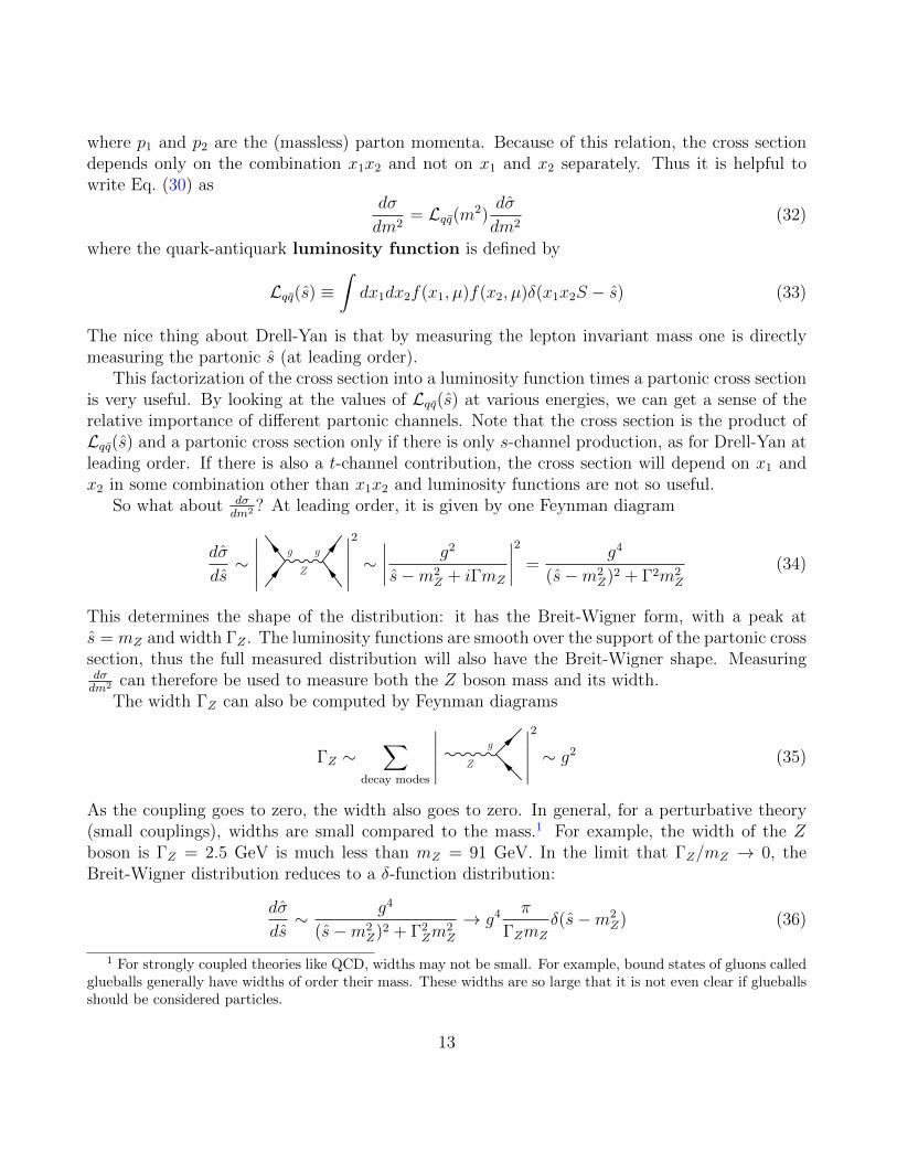
So what about dσdm2 ? At leading order, it is given by one Feynman diagram

dσ

ds∼

∣∣∣∣∣ Z

g g

∣∣∣∣∣2

∼∣∣∣∣ g2

s−m2Z + iΓmZ

∣∣∣∣2 =g4

(s−m2Z)2 + Γ2m2

Z

(34)

This determines the shape of the distribution: it has the Breit-Wigner form, with a peak ats = mZ and width ΓZ . The luminosity functions are smooth over the support of the partonic crosssection, thus the full measured distribution will also have the Breit-Wigner shape. Measuringdσdm2 can therefore be used to measure both the Z boson mass and its width.

The width ΓZ can also be computed by Feynman diagrams

ΓZ ∼∑

decay modes

∣∣∣∣∣ Z

g

∣∣∣∣∣2

∼ g2 (35)

As the coupling goes to zero, the width also goes to zero. In general, for a perturbative theory(small couplings), widths are small compared to the mass.1 For example, the width of the Zboson is ΓZ = 2.5 GeV is much less than mZ = 91 GeV. In the limit that ΓZ/mZ → 0, theBreit-Wigner distribution reduces to a δ-function distribution:

dσ

ds∼ g4

(s−m2Z)2 + Γ2

Zm2Z

→ g4 π

ΓZmZ

δ(s−m2Z) (36)

1 For strongly coupled theories like QCD, widths may not be small. For example, bound states of gluons calledglueballs generally have widths of order their mass. These widths are so large that it is not even clear if glueballsshould be considered particles.

13

Note that although the cross section scales like g4, since ΓZ ∼ g2, on resonance the cross sectiononly scales like g2. This is a resonant enhancement: the cross section is much larger on resonancethan off resonance, by a factor of 1

g2.

Because of the δ-function in Eq. (36), the cross section nicely factorizes into production anddecay:

σ(qq → Z → e+e−) = σ(qq → Z)× BR(Z → e+e−) (37)

where the branching ratio is defined as

BR(Z → e+e−) =Γ(Z → e+e−)

ΓZ(38)

Here ΓZ = 2.5 GeV is the total decay width of the Z boson while Γ(Z → e+e−) ≈ 0.03 ΓZis the partial width for the Z to decay to e+e− pairs. The factorization into production anddecay follows from this narrow-width approximation. The narrow width approximation saysthat quantum-mechanical interference between corrections from production and decay can beneglected so that production and decay are separate well-defined probabilities.

At least one of the branching ratios is usually of order 1. So while the original process scaledgenerically like g4, the actual rate is determined by σ(qq → Z → e+e−) which scales only like g2.As noted above, the missing factors of g2 are canceled by the resonance enhancement.

Next, consider the hadroproduction of a W boson which decays to e−ν. We would love to beable to measure the W mass from looking at the e−ν invariant mass, like we do for the Z boson.However, this is impossible as the neutrino is unobservable. Instead, we can look at the electronalone. It is helpful to define θ? as the polar angle of the electron in the W center-of-mass frame.Then a basic QFT calculation gives

1

σ0

dσ(qq → W → e−ν)

d cos θ?=

3

8(1 + cos2 θ?) (39)

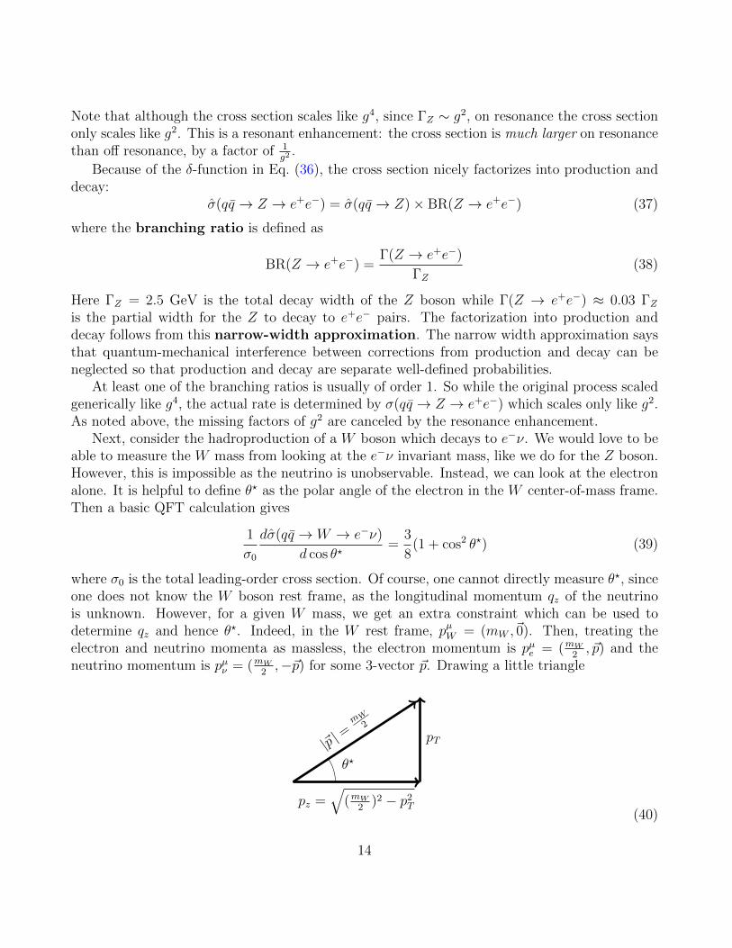
where σ0 is the total leading-order cross section. Of course, one cannot directly measure θ?, sinceone does not know the W boson rest frame, as the longitudinal momentum qz of the neutrinois unknown. However, for a given W mass, we get an extra constraint which can be used todetermine qz and hence θ?. Indeed, in the W rest frame, pµW = (mW ,~0). Then, treating theelectron and neutrino momenta as massless, the electron momentum is pµe = (mW

2, ~p) and the

neutrino momentum is pµν = (mW2,−~p) for some 3-vector ~p. Drawing a little triangle

pT|~p |=mW

2

pz =√

(mW2

)2 − p2T

θ?

(40)

14

[GeV]lT

p

30 32 34 36 38 40 42 44 46 48 50

Eve

nts

/ 0.

5 G

eV

20

40

60

80

100

120

140

160

310×

Dataν+ e→+W

Background

ATLAS-1 = 7 TeV, 4.6 fbs

/dof = 36/392χ

[GeV]lT

p30 32 34 36 38 40 42 44 46 48 50D

ata

/ Pre

d.

0.980.99

11.011.02

[GeV]T m

60 70 80 90 100 110 120

Eve

nts

/ G

eV

20

40

60

80

100

120

140

160

310×

Dataν+ e→+W

Background

ATLAS-1 = 7 TeV, 4.6 fbs

/dof = 54/592χ

[GeV]T m60 70 80 90 100 110 120D

ata

/ Pre

d.

0.980.99

11.011.02

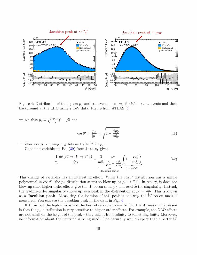
Jacobian peak at ∼ mW2 Jacobian peak at ∼ mW

Figure 4: Distribution of the lepton pT and transverse mass mT for W+ → e+ν events and theirbackground at the LHC using 7 TeV data. Figure from ATLAS [4].

we see that pz =√

(mW2

)2 − p2T and

cos θ? =pz|~p |

=

√1− 4p2

T

m2W

(41)

In other words, knowing mW lets us trade θ? for pT .Changing variables in Eq. (39) from θ? to pT gives

1

σ0

dσ(qq → W → e−ν)

dpT=

3

m2W

pT√1− 4p2T

m2W︸ ︷︷ ︸

Jacobian factor

(1− 2p2

T

m2W

)︸ ︷︷ ︸

1+cos2 θ?

(42)

This change of variables has an interesting effect. While the cos θ? distribution was a simplepolynomial in cos θ?, the pT distribution seems to blow up as pT → mW

2. In reality, it does not

blow up since higher order effects give the W boson some pT and resolve the singularity. Instead,the leading-order singularity shows up as a peak in the distribution at pT = mW

2. This is known

as a Jacobian peak. Measuring the location of this peak is one way the W boson mass ismeasured. You can see the Jacobian peak in the data in Fig. 4

It turns out the lepton pT is not the best observable to use to find the W mass. One reasonis that the pT distribution is very sensitive to higher order effects. For example, the NLO effectsare not small on the height of the peak – they take it from infinity to something finite. Moreover,no information about the neutrino is being used. One naturally would expect that a better W

15

mass measurement should result from incorporating the pT of the neutrino, which is known fromthe missing pT in the event, than by throwing it out. In W → eν decays, the W boson mass is

m2W = ( Ee︸︷︷︸

known

+ Eν︸︷︷︸unknown

)2 − ( ~pTe︸︷︷︸known

+ ~pTν︸︷︷︸known

)2 − ( pze︸︷︷︸known

+ pzν︸︷︷︸unknown

)2 (43)

There are two unknowns here. We can use the neutrino’s mass-shell condition to remove oneunknown, but there is still one unknown quantity. That is to say, we cannot reconstruct the Wmass exactly. However, note that if we look at the transverse mass from Eq. (28):

m2T = (EeT + EνT )2 − (~pTe + ~pTν)

2 (44)

where the transverse energy for a particle is defined as

E2T = m2 + p2

T (45)

we see that everything is known. Moreover, the transverse mass, in contrast to the lepton pT ,depends on neutrino transverse momentum so it incorporates more information.

To get a sense of what the transverse mass is, consider the situation when the electron andneutrino are completely transverse, so pze = pzν = 0. Then EeT = Ee and EνT = Eν andmT = m. Thus for transverse production, the transverse mass reduces to the invariant mass.

In general, the W boson will be produced with some longitudinal momentum. The lab frameis related to the W rest frame by a longitudinal boost. This boost doesn’t change mT or m, asboth are boost invariant. In the W rest frame, pµe = (E, ~pT , pz) and pµν = (E,−~pT ,−pz). Som2 = (2E)2 = 4p2

T + 4p2z and

m2T = (EeT + EνT )2 − (~pTe + ~pTν)

2 = 2EeTEνT − 2~pTe · ~pTν = 4p2T (46)

hence m2 = m2T + 4p2

z. Thus mT ≤ m. We conclude that (at leading order) the transverse masscan never be larger than the W boson mass.

Including the Jacobian factor, the distribution in m = (qe + qν)2 and mT is

1

σ0

dσ(qq → W → e−ν)

dm2dm2T

∝ ΓWmW

(m2 −m2W )2 − Γ2

Wm2W︸ ︷︷ ︸

Breit-Wigner

1

m√m2 −m2

T︸ ︷︷ ︸Jacobian

(47)

From this formula we see that the kinematic endpoint at mT = mW has turned into a Jacobianpeak. As with the lepton pT due to higher order effects (additional radiation), it is possible tohave mT > mW . The mT distribution from ATLAS data is shown in Fig. 4. Both pT and mT

are useful for measuring the W boson mass.The power of transverse mass comes partly from its natural leading-order kinematic endpoint

at mT = mW . This endpoint is a leading-order kinematic feature and does not depend on the

16

neutrino being massless. If the neutrino were massive (think neutralino in supersymmetry) thenthe transverse mass would be

mT (~pe, ~pν ,me,mν) = m2e +m2

ν + 2(ETeETν − ~pTe · ~pTν) (48)

This is a useful quantity as long as there is only one unmeasured particle, since then ~pTν can bereconstructed. But consider the case when there are two neutrinos, like in W+W− production. Orconsider the historically important supersymmetric scenario in which two sleptons l are produced,which subsequently decay to electrons and a neutral fermion χ: pp → ll → e−χe+χ. Think ofthis like W pair production with the slepton representing the W and the neutralino representinga massive neutrino. In this case, not only do we not know the neutralino mass, but because ofthe two neutralinos, we don’t know the transverse momentum of each, only their sum. In such asituation, a useful quantity is MT2:

mT2(mχ) ≡ min~pTχ1+~pTχ2= /~pT

[mT (~pe1, ~pχ1,me,mχ),mT (~pe2, ~pχ2,me,mχ)

](49)

For a putative value of mχ one can measure the distribution of mT2. If mχ is chosen correctly,there will be an endpoint of the distribution at mT2 = ml (like how mT has an endpoint at mW

for the correct neutrino mass). If the neutralino mass is not correct, then there will genericallystill be an endpoint of the distribution, but it may not be at the correct slepton mass. However,we can compute

mmaxT2 (mχ) = max

eventsmT2 (50)

This mmaxT2 has a remarkable feature that it has kink when mχ is chosen correctly. Thus one can

in principle use mT2 to determine both the neutralino mass, through the location of the kink inmmaxT2 , and the slepton mass, through the endpoint. See [5] for more information.

6 Jets

The physics of jets is a huge subject and there are many great reviews (e.g. [6, 7]). I will justgive here the briefest of overviews.

A jet is a collection of particles that go towards the same direction in the detector. Intuitively,the come from bremsstrahlung (showering) and fragmentation of a primordial hard quark orgluon. In practice, jets must be defined from experimental observables, namely the 4-momentaof the observed particles in the event. There is no unique jet definition. One desirable propertyof a jet definition is that it allows for a calculation done at the parton level (quarks and gluons)to agree with a measurement done at the particle level (pions and protons). Another desirablefeature is that a jet algorithm should be local in the detector – not pulling in particles fromfar away. This property is important from an experimental point of view to reduce systematicuncertainty of jet measurements.

The simplest way to define a jet is to draw a cone of size R =√

(∆η)2 + (∆φ)2 around someparticle and include everything in that cone as the jet. Such a procedure depends strongly on

17

which particle is chosen as the center of the cone. For example, one might take the hardest particlein the event as the center. However, such a choice is not infrared safe: if a particle happened tosplit into two collinear particles with half its energy in each, then the hardest particle quicklybecomes not the hardest. There are infrared safe cone algorithms, the most notable is perhapsSIScone, but they are not commonly used.

Most popular jet algorithms are based on the idea of iterative clustering:

1. Calculate the pairwise distance dij between every pair of objects.

2. Merge the two closest particles.

3. Repeat until no two particles are closer than some given R.

Such an algorithm will result in n jets of size R.The “objects” on which the jet algorithm operates can be quarks and gluons (for theory

calculations), they can be all measured particles (pions, protons, electrons, etc.). Or they canbe energy deposits in the calorimeters or topoclusters (aggregate energy deposits in the ATLASdetector) or particle-flow candidates, as reconstructed by CMS.

The distance measure can be chosen in different ways. Some options are

• JADE algorithm: dij =mijQ2 , where mij is the invariant mass of the two objects.

• Cambridge/Aachen algorithm dij = Rij =√

(ηi − ηj)2 + (φi − φj)2.

• kT : dij = min(p2T i, p

2Tj)

R2ij

R2

• anti-kT : dij = min( 1p2Ti, 1p2Tj

)R2ij

R2

These last 3 measures are all of the form

dij = min(pαTi, pαTj)

(Rij)2

R2(51)

with α = 2 for kT , α = 0 for Cambridge/Aachen, and α = −2 for anti-kT . For hadron collisions,one must also define a distance measure to the beam. For anti-kT , the beam distance is

diB =1

p2T

(52)

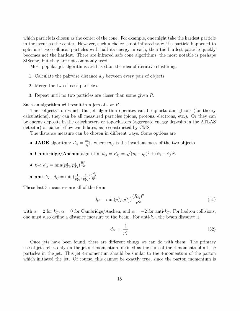
Once jets have been found, there are different things we can do with them. The primaryuse of jets relies only on the jet’s 4-momentum, defined as the sum of the 4-momenta of all theparticles in the jet. This jet 4-momentum should be similar to the 4-momentum of the partonwhich initiated the jet. Of course, this cannot be exactly true, since the parton momentum is

18

a theoretical construction – quantum effects necessarily make the quark-radiating-gluons semi-classical picture imprecise. The jet 4-momentum is nevertheless very useful: angular and pTdistributions of jets provide signatures of SM and BSM physics.

Before the LHC, essentially all that jets were used for was approximating the momentumof a primordial parton. However, in recent years there has been an explosion of interest in jetsubstructure. This revolution in jet physics is due partly to the improved resolution of thedetectors in ATLAS and CMS compared to those of previous machines. With increased angularresolution one can approach a complete classification of all the particles in the jet, rather thanjust the aggregate energy in a region (as at the TeVatron).

The other reason jet substructure has ballooned in recent years is because it is needed formany searches. For example, the high energy of the LHC means that particles such as top quarksare often produced not at rest, but with energies much larger than their mass. When such ahighly boosted top quark decays into 3 jets (see Sec. 7.3), those jets will all be going in nearly thesame direction. Thus a tt event at the LHC may look a lot like a dijet event [8]. To distinguishthe two event classes, a very powerful method is to start by finding fat jets, of size R ∼ 1.0 andthen look for subjets of size R ∼ 0.4 inside those jets [9]. There are many ways by which thiscan be done, and new methods are continually being developed.

7 Meet the Standard Model

In this section, we will go through the particles in the Standard Model, discussing how they decayand various things you should know about them from a collider perspective. A good resource fora lot of this information is the PDG website http://pdglive.lbl.gov/.

7.1 W boson

The W boson has mass and width

mW = 80.385± 0.015 GeV, ΓW = 2.085± 0.042 GeV (53)

The W boson mass is currently best measured through methods like fitting the MT distribution(see Section 5).

The W decays through weak interactions with amplitudes proportional to the appropriateCKM elements. These elements are

VCKM =

Vud ∼ 1 Vus ∼ 0.2 Vub ∼ 0.003Vcd ∼ 0.2 Vcs ∼ 1 Vcb ∼ 0.04Vtd ∼ 0.008 Vts ∼ 0.04 Vtb ∼ 1

(54)

Decays of W to top quarks are forbidden since the top quark is heavier than the W . Thus, thereare only two hadronic decay modes of the W with order 1 rates. There are also the 3 leptonic

19

decay modes.

W+ → ud︸ ︷︷ ︸×3 colors

, W+ → cs︸ ︷︷ ︸×3 colors

, W+ → e+ν, W+ → µ+ν, W+ → τ+ν, (55)

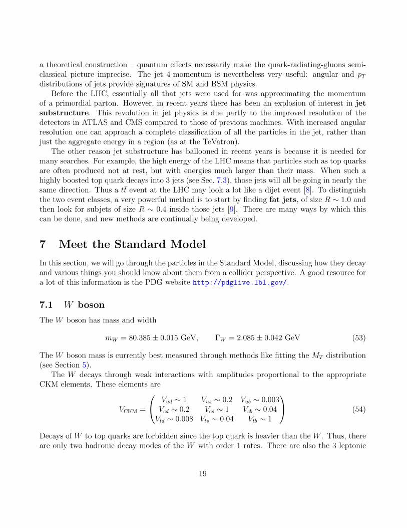
Because of the 3 colors of the hadronic decays, there are 3×2+3 = 9 “modes”, of which 6/9 = 2/3are hadronic (jets) and 1/9 goes to each lepton flavor. This rough estimate is consistent with theactual decay modes of the W :

W boson

branching ratios

e±ν

10%

µ±ν

10%

τ±ν

10%

jets

70%

7.2 Z boson

The Z boson has mass and width

mZ = 91.1876± 0.0021 GeV, ΓZ = 2.4952± 0.0023 GeV (56)

Its couplings are flavor-diagonal and do not depend on the CKM elements. The Z boson couplesto fermions proportional to T3 −Q sin2 θ, where sin2 θ ∼ 0.23, T3 is the SU(2) quantum numberand Q is the electric charge. For the left and right handed fermions, the Z boson couplings are

LH particle T3 Q T3 −Q sin2 θνe, νµ, ντ

12

0 0.5e−, µ−, τ− −1

2-1 -0.28

u, c, t 12

23

0.35d, s, b −1

2−1

3-0.42

RH particle T3 Q T3 −Q sin2 θνe, νµ, ντ 0 0 0e−, µ−, τ− 0 -1 0.23u, c, t 0 2

3-0.15

d, s, b 0 −13

0.08

(57)

The Z decay rate to a particular mode is proportional to (T3 −Q sin2 θw)2. Thus the branchingratio is given by (T3 − Q sin2 θw)2 for that mode divided by the sum over (T3 − Q sin2 θw)2 over

20

all the modes (excluding top to which the Z cannot decay). This sum is ΓZ ∝ 3.30. Then thebranching ratio to electrons for example is

BR(Γ→ e+e−) =(−0.28)2 + (0.22)2

3.30= 3.5% (58)

to up quarks is

BR(Γ→ uu) = 3× (0.35)2 + (−0.15)2

3.30= 13% (59)

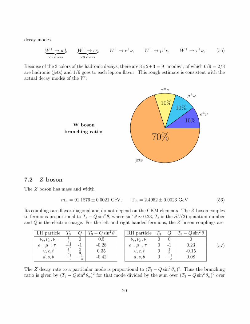
and so on. The resulting decay modes are summarized in this chart:

Z boson

branching ratios

e+e−3.3%

µ+µ−

3.3%

τ+τ−

3.3%

jets

55%

νν

20% bb

15%

Note that the Z boson only decays around 7% of the time to the “golden” modes, e+e− orµ−µ−. Most of the time it decay to jets.

7.3 Top quark

The pole mass and width of the top quark are

mpolet = 173.1± 0.6 GeV, Γt = 1.41± 0.19 GeV (60)

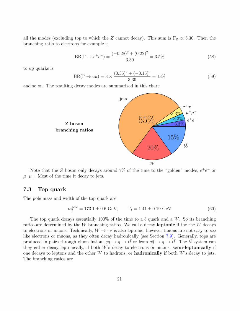
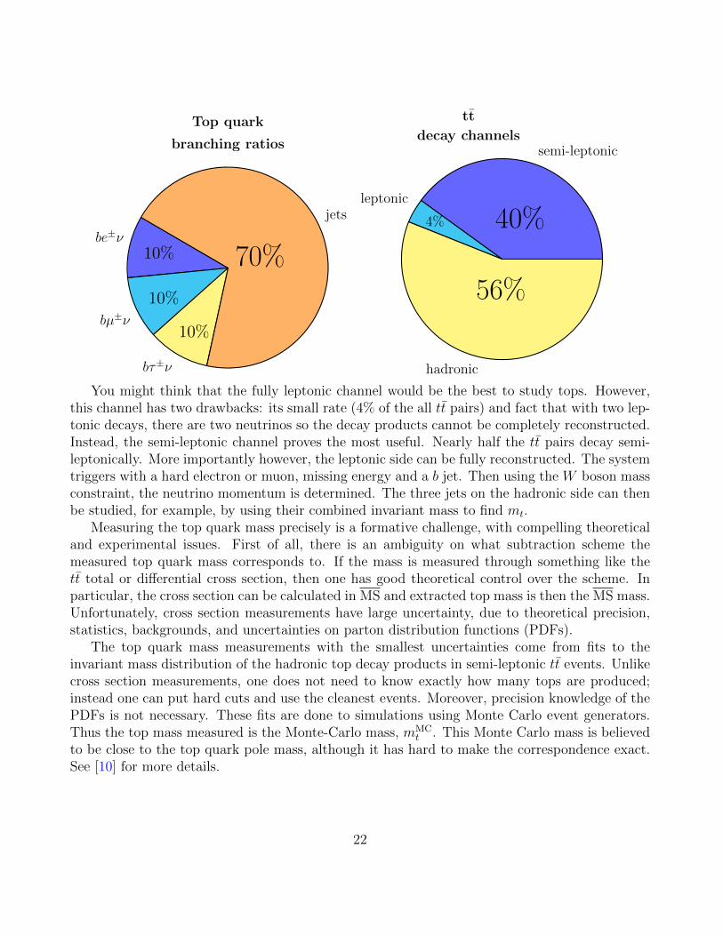
The top quark decays essentially 100% of the time to a b quark and a W . So its branchingratios are determined by the W branching ratios. We call a decay leptonic if the the W decaysto electrons or muons. Technically, W → τν is also leptonic, however tauons are not easy to seelike electrons or muons, as they often decay hadronically (see Section 7.9). Generally, tops areproduced in pairs through gluon fusion, gg → g → tt or from qq → g → tt. The tt system canthey either decay leptonically, if both W ’s decay to electrons or muons, semi-leptonically ifone decays to leptons and the other W to hadrons, or hadronically if both W ’s decay to jets.The branching ratios are

21

Top quark

branching ratios

be±ν10%

bµ±ν

10%

bτ±ν

10%

jets

70%

tt

decay channelssemi-leptonic

40%leptonic

4%

hadronic

56%

You might think that the fully leptonic channel would be the best to study tops. However,this channel has two drawbacks: its small rate (4% of the all tt pairs) and fact that with two lep-tonic decays, there are two neutrinos so the decay products cannot be completely reconstructed.Instead, the semi-leptonic channel proves the most useful. Nearly half the tt pairs decay semi-leptonically. More importantly however, the leptonic side can be fully reconstructed. The systemtriggers with a hard electron or muon, missing energy and a b jet. Then using the W boson massconstraint, the neutrino momentum is determined. The three jets on the hadronic side can thenbe studied, for example, by using their combined invariant mass to find mt.

Measuring the top quark mass precisely is a formative challenge, with compelling theoreticaland experimental issues. First of all, there is an ambiguity on what subtraction scheme themeasured top quark mass corresponds to. If the mass is measured through something like thett total or differential cross section, then one has good theoretical control over the scheme. Inparticular, the cross section can be calculated in MS and extracted top mass is then the MS mass.Unfortunately, cross section measurements have large uncertainty, due to theoretical precision,statistics, backgrounds, and uncertainties on parton distribution functions (PDFs).

The top quark mass measurements with the smallest uncertainties come from fits to theinvariant mass distribution of the hadronic top decay products in semi-leptonic tt events. Unlikecross section measurements, one does not need to know exactly how many tops are produced;instead one can put hard cuts and use the cleanest events. Moreover, precision knowledge of thePDFs is not necessary. These fits are done to simulations using Monte Carlo event generators.Thus the top mass measured is the Monte-Carlo mass, mMC

t . This Monte Carlo mass is believedto be close to the top quark pole mass, although it has hard to make the correspondence exact.See [10] for more details.

22

7.4 Bottom quark

The bottom (or beauty) quark has an MS mass of

mb(µ = mb) = 4.18± 0.03 GeV (61)

Unlike the top quark, the bottom quark hadronizes before it decays. The hadrons are B-mesonsand B-baryons. The most common B-hadrons are

B− = bu, B0 = bd, Bs = bs (62)

These B-hadrons decay through the weak decay of the bottom quark itself. The dominant decaymode of the bottom quark is b→ cW .

Let’s try to estimate the b lifetime using dimensional analysis. One way to do the estimate isto compare the b decay to another weakly decaying particle, the muon, whose lifetime is around2µs (this is a number worth knowing, but also not hard to estimate by dimensional analysis).Weak decays are proportional to | g

m2W|2 ∼ G2

F . To get a rate, with mass dimension 1, we must

compensate by something with mass dimension 5. If the decay products’ masses are negligible,the only scale left is the decaying particles mass. So the rate scales like m5

µ or m5b . The muon

can decay to e−νν only. However, the b can decay to ce−ν as well as cµ−ν, cud and csc. Adding3 colors for the hadronic channels, there can be about 9 times as many decay modes from the bas the µ. We then have

Γµ ∼ G2Fm

5µ, Γb ∼ 9|Vcb|2G2

Fm5b = 9|Vcb|2

m5b

m5µ

× Γµ = 10−6 × Γµ (63)

The factor of 1 million means that the typical B-hadron lifetimes are in picoseconds (10−12s).Thus, the decay length (how far a B hadron goes before decaying) is

cτ ∼ 500× 10−6 m ∼ 0.5 mm (64)

If the b is produced relativistically, this decay length is longer due to time dilation. For example,an 50 GeV b from a top decay would have a Lorentz factor γ ∼ 10 and its decay length might beγcτ ∼ 5 mm. Tagging of b quark products at the LHC is predicated on being able to see these∼mm decay lengths.

A typical decay chain of a B meson is

B0 → (D+ → (K+ → π+π0)π+π−)µ−ν (65)

This final state has 4 charged particles. Having 4, 5 or 6 charged decay products is typical ofa B decay. Is it also possible for B mesons to decay to leptons (µ or e). This happens around10% of the time. There is also a 10% chance that a D meson to which the B decays will decayleptonically. Thus there is a 20% chance of getting a lepton from a B decay.

Typical B-tagging algorithms combine these observables:

23

1. Look for a relatively high multiplicity of tracks.

2. Look for a displaced (secondary) vertex. That is, look for tracks which converge on a pointseparated by a distance d ∼ 0.5 mm from the primary vertex.

3. If the secondary vertex cannot be resolved, one can instead use the impact parameters ofthe various tracks which do not converge on the primary vertex. The impact parameter isthe shortest distance between the line represented by a track and the primary vertex.

4. Construct the invariant mass of the particles converging on the secondary vertex. Look forthis to be close to mb.

5. Combine the relevant observables with simple cuts or more typically using a neural networkor boosted decision tree.

For some rough efficiency numbers, current b tagging algorithms can keep 70% of the b’s whilerejecting light quark jet (u, d, s-initiated) backgrounds by a factor of 50. Generally, gluon jetsand charm quark jets are harder to distinguish from b jets than light quark jets.

Bottom quark mesons have a very heavy b quark surrounded by a light quark. This systemcan be studied in good analogy with the hydrogen atom – the heavy proton is surrounded by alight electron. For example, relations between ground state B mesons and angular excitations,such as the B? (spin 1) can be derived up to corrections in ΛQCD/mb. There is a very powerfuleffective field theory for studying B hadrons called Heavy Quark Effective Theory (HQET).

Bottom quarks also form bb bound states called bottomonium. The lightest is the Υ(1S)with a mass of mΥ(1S) = 9460. The Υ(1S) is too light to decay to B mesons. There are otherUpsilon particles, analogous to the excited states for the hydrogen atom. The Υ(4S) has massmΥ(4S) = 10.5 GeV. It almost exclusively decays to BB. Thus the B-factories (Belle and BaBar)would run at the center-of-mass energy to resonantly produce the Υ(4S). This procedure madean endless supply of B mesons for precision study.

7.5 Charm quark

The charm quark has an MS mass of

mc(µ = mc) = 1.29± 0.1 GeV (66)

Charm mesons are called “D” mesons (these are not mesons with a down quark in them!). Forexample,

D+ = cd, D0 = cu, Ds = cs (67)

A similar estimate to Eq. (63), using |Vcs| ∼ 1 gives

Γc ∼ 5m5c

m5µ

× Γµ = 10−6 × Γµ (68)

24

So we also get picosecond lifetimes for charm mesons. It turns out order-one numbers are impor-tant here and the typical decay length for a D meson is around 300 µm. Thus charmed mesonstravel about 60% as far as bottom mesons before they decay.

Charm-jet tagging is generally harder than bottom-jet tagging for various reasons:

• The decay length of charm is shorter than bottom, so it is harder to resolve the displacedvertex and the impact parameters of the displaced tracks are smaller.

• Charm hadron decays have lower multiplicity than bottom hadron decays – fewer chargedparticles means less information to work with in charm tagging.

• B mesons almost always decay to D mesons, so there is usually a charm in a bottom decay.Thus distinguishing charm from bottom presents extra challenges.

On the other hand, even if we could tag charm, it would not be terribly useful for Higgsor top physics at the LHC. In contrast to b-jets, which are important for finding top quarksand the dominant H → bb decay mode, charm jets are not dominant in any Standard Modelprocess. Eventually, it would be nice to measure the H → cc branching ratio, but this will bevery challenging at the LHC and is probably impossible without an inverse attobarn of dataat minimum. Charm quarks are mostly of interest for precision flavor physics that can provideindirect evidence of new particles.

One charm meson of particular interest is the J/Ψ particle. This particle has two namesbecause it was discovered independently by two groups within a few months of each other. TheJ/Ψ is the lightest charmonium state, that is, it is a cc bound state. It has a mass of 3 GeVand an extremely narrow width of 93 keV. It decays about 5% of the time to e+e− and 5% toµ+µ−. Because of its narrow width and purely leptonic decays it plays a special role as a standardcandle at colliders, useful for energy calibration for example.

7.6 Strange quark

The strange quark has an MS mass of

ms(µ = ms) = 95± 5 MeV (69)

Strange mesons are Kaons:

K− = su, K0 = sd, K0 = ds, K+ = su (70)

The neutral kaons, K0 and K0 have the same quantum numbers and can mix. They can decayto 2 pions or 3 pions. The 2 pion state is CP even and the 3 pion state is CP odd. Since CP isconserved in QCD, it is natural to use CP eigenstates

K1 =K0 + K0

√2

→ π+π− (CP even) K2 =K0 − K0

√2

→ π+π−π0 (CP odd) (71)

25

Because CP is violated by the weak interactions, K2 can sometimes decay to π+π− determinedby a parameter ε′ ∼ 10−6. In addition, CP violation implies that K1 and K2 are not exact masseigenstates. The mass eigenstates are

KL = K2 − εK1, KS = K1 + εK2 (72)

These are the physical particles, called “K-long” and “K-short”. At the LHC, we are not reallysensitive to the CP violation. So essentially there are two neutral kaons, KL with a lifetime ofτ ∼ 10−8s, similar to the K± lifetimes, and a decay length of γcτL & 3 m (depending on boost)and KS with a lifetime of 10−10s and a decay length of γcτS & 3 cm.

7.7 Up and down quarks

Up and down quarks are effectively massless at the LHC. Their bound states are pions

π+ = ud, π0 =1√2

(uu− dd), π− = du (73)

The charged pions have lifetimes of τ ∼ 10−8s and decay lengths of γcτπ & 8 m. There are alsobaryonic bound states of up and down quarks, such as the proton and neutron.

Charged pions decay to muons and neutrinos. However, they are considered stable on thetime and length scales of the experiment. Charged pions leave charged tracks and deposit someof their energy in the ecal and most of their energy in the hcal. Neutral pions decay to photonsπ0 → γγ. This decay occurs through a quark triangle diagram and is a strong, not a weak decay.The lifetime of π0 is therefore much shorter than that of the π±, around 10−17 s. Thus the π0

particles are not considered stable; they decay before they reach the detector and show up astwo photons in the ecal.

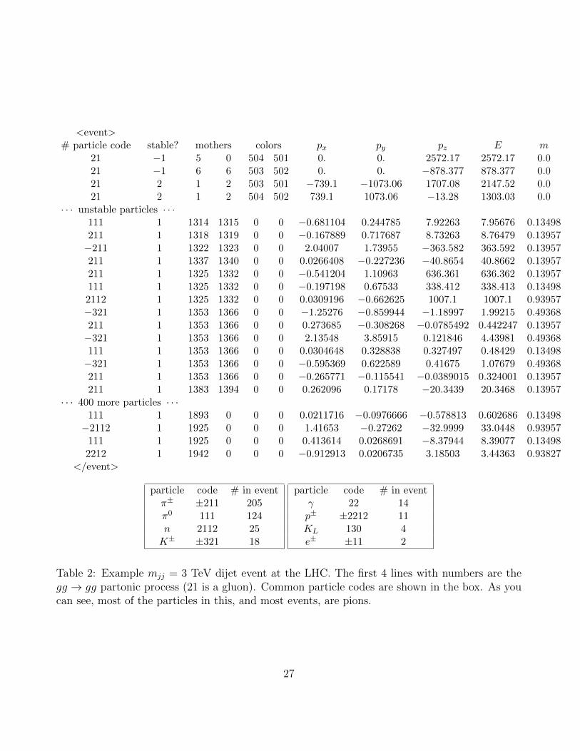
An example list of particles produce in an LHC event is shown in Table 2. This is the outputfrom pythia for a dijet process, gg → gg at the parton level, with s = 3 TeV. This particularevent has 403 particles, of which 329, or 80%, are pions. The π0’s decay promptly to photons, butthey have not been decayed in this table for pedagogical reasons. For example, you can see thatthere are about twice as many charged pions as neutral ones. This follows simply from isospin,or more simply from there being two charged pions but only one neutral one. Thus about 2/3 ofparticles produced at the LHC leave charged tracks.

7.8 Electrons and muons

I don’t have too much to say about electrons and muons. Electrons are light so they radiate alot. They leave tracks and deposit all their energy in the electromagnetic calorimeter.

Muons have mass mµ = 105 MeV. The muon lifetime is τ = 2 × 10−6 s which gives a decaylength γcτ & 300 m. Thus muons are stable as far as the experiment is concerned. Becausemuons leave the detector before depositing all their energy, their momenta must be measured

26

<event># particle code stable? mothers colors px py pz E m

21 −1 5 0 504 501 0. 0. 2572.17 2572.17 0.021 −1 6 6 503 502 0. 0. −878.377 878.377 0.021 2 1 2 503 501 −739.1 −1073.06 1707.08 2147.52 0.021 2 1 2 504 502 739.1 1073.06 −13.28 1303.03 0.0

· · · unstable particles · · ·111 1 1314 1315 0 0 −0.681104 0.244785 7.92263 7.95676 0.13498211 1 1318 1319 0 0 −0.167889 0.717687 8.73263 8.76479 0.13957−211 1 1322 1323 0 0 2.04007 1.73955 −363.582 363.592 0.13957211 1 1337 1340 0 0 0.0266408 −0.227236 −40.8654 40.8662 0.13957211 1 1325 1332 0 0 −0.541204 1.10963 636.361 636.362 0.13957111 1 1325 1332 0 0 −0.197198 0.67533 338.412 338.413 0.134982112 1 1325 1332 0 0 0.0309196 −0.662625 1007.1 1007.1 0.93957−321 1 1353 1366 0 0 −1.25276 −0.859944 −1.18997 1.99215 0.49368211 1 1353 1366 0 0 0.273685 −0.308268 −0.0785492 0.442247 0.13957−321 1 1353 1366 0 0 2.13548 3.85915 0.121846 4.43981 0.49368111 1 1353 1366 0 0 0.0304648 0.328838 0.327497 0.48429 0.13498−321 1 1353 1366 0 0 −0.595369 0.622589 0.41675 1.07679 0.49368211 1 1353 1366 0 0 −0.265771 −0.115541 −0.0389015 0.324001 0.13957211 1 1383 1394 0 0 0.262096 0.17178 −20.3439 20.3468 0.13957

· · · 400 more particles · · ·111 1 1893 0 0 0 0.0211716 −0.0976666 −0.578813 0.602686 0.13498−2112 1 1925 0 0 0 1.41653 −0.27262 −32.9999 33.0448 0.93957111 1 1925 0 0 0 0.413614 0.0268691 −8.37944 8.39077 0.134982212 1 1942 0 0 0 −0.912913 0.0206735 3.18503 3.44363 0.93827

</event>

particle code # in eventπ± ±211 205π0 111 124n 2112 25K± ±321 18

particle code # in eventγ 22 14p± ±2212 11KL 130 4e± ±11 2

Table 2: Example mjj = 3 TeV dijet event at the LHC. The first 4 lines with numbers are thegg → gg partonic process (21 is a gluon). Common particle codes are shown in the box. As youcan see, most of the particles in this, and most events, are pions.

27

from the curvature of their trajectories in a magnetic field. That’s why the muon detectors andmagnetic fields at ATLAS and CMS are so big – hard muons have very straight tracks, so we needthese strong fields and large detectors to see enough curvature to measure the muons’ momenta.

7.9 Tauons

The τ lepton has a mass mτ = 1.77 GeV. It decays through the weak force. Rescaling the factorsfrom the muon decay rate, as in Eq. (63), gives basically the same thing as for charm, Eq. (68),

Γτ ∼ 5m5τ

m5µ

× Γµ = 10−7 × Γµ (74)

As for charm, the factor of 5 comes from one hadronic channel with 3 colors and 2 leptonicchannels. So the τ decays around ∼ 20% of the time to electrons, ∼ 20% to muons and ∼ 60%to hadrons. This rate implies ττ ∼ 10−13s, so τ decays are prompt.

In leptonic τ decays, the final state is µνν or eνν. Since the τ decays promptly (before it leavesa track), these final states are essentially indistinguishable from promptly-produced electrons ormuons. Sometimes leptonic decays are still the best indication of a tauon – for example, inh → ττ , the leptonic modes are cleaner than the hadronic ones and h → e+e− and h → µ+µ−

have negligible rates. But a general τ -tagger, which hopes to distinguish tauons from electronsand muons as well, must utilize the hadronic channels.

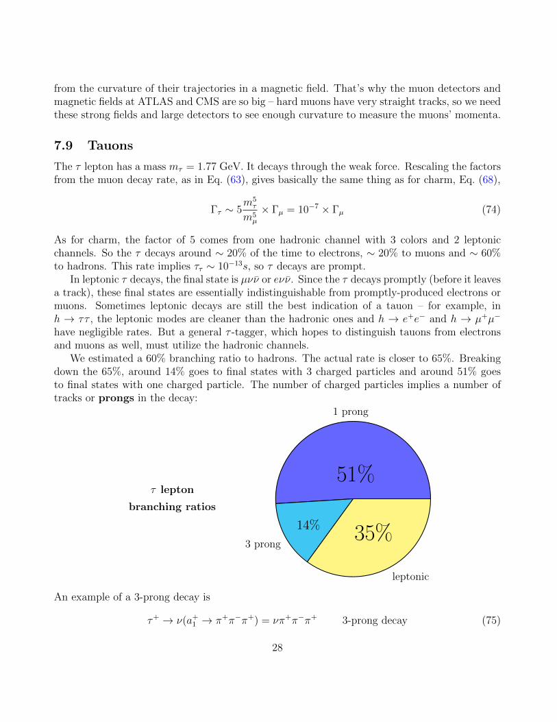
We estimated a 60% branching ratio to hadrons. The actual rate is closer to 65%. Breakingdown the 65%, around 14% goes to final states with 3 charged particles and around 51% goesto final states with one charged particle. The number of charged particles implies a number oftracks or prongs in the decay:

τ lepton

branching ratios

1 prong

51%

3 prong

14%

leptonic

35%

An example of a 3-prong decay is

τ+ → ν(a+1 → π+π−π+) = νπ+π−π+ 3-prong decay (75)

28

Examples of the 1-prong decays are

τ+ → π+ν, τ+ → ν(ρ+ → π+(π0 → γγ)) = νπ+γγ 1-prong decays (76)

The hadronic decays of tauons produce tiny little jets, with only a handful of particles inthem. The procedure for finding tauons, τ -tagging, involves looking for

• Low multiplicity “jets” – 1 or 3 prongs

• Narrow jets

• Isolated jets (not many hadrons nearby)

This last point is important – because tauons are leptons, they are not generally produced in thecontext of lots of other QCD radiation, for example, from within a gluon jet. Thus one generallydoes not expect much hadronic radiation in the vicinity of the τ .

7.10 Higgs boson

Finally we come to the Higgs boson. The Higgs boson has a mass

mh = 125.09± 0.3 GeV (77)

Note that the uncertainty on the Higgs boson mass is at the sub-percent level already.The Higgs can be produced in various ways. The cross sections for the various production

channels at 13 TeV are

• Gluon fusion σ(gg → h) ∼ 44 pb.

• Vector boson fusion σ(pp→ qqh) ∼ 4 pb.

• Associated production: σ(pp→ Wh) ∼ 1.5 pb.

• Associated production: σ(pp→ Zh) ∼ 0.88 pb.

• Associated production: σ(pp→ tth) ∼ 0.5 pb.

• Associated production: σ(pp→ bbh) ∼ 0.5 pb.

At 8 TeV, the cross sections are about half of these numbers. For example, in run 1, the LHCaccumulated 25 fb−1 of data which amounts to 20 pb×25 fb−1 = 500, 000 Higgs bosons produced.

Most of these production channels and rates are straightforward to compute. Since there is nogluon-gluon-Higgs interaction in the Standard Model, gluon fusion proceeds through a top looptriangle diagram, as in Eq. (4). This diagram can be computed exactly, but it is often computed

29

to leading order in 1mt

(sometimes called the mt → ∞ limit). In this limit, the production rateis equivalent to what one would get from the operator

th

−→ αs12π

h

vGaµνG

aµν (78)

Note that there is no dependence on the top mass at leading order in 1mt

– the net factor of1mt

from the top propagators (or dimensional analysis) multiplies the top Yukawa on the Higgsvertex leaving only the Higgs vev v = mt

λt. The mt →∞ limit is a very good approximation.

The vector boson fusion channel is worth some discussion. In this channel, the Higgs bosonis produced through the t-channel exchange of two W bosons which fuse to form the Higgs.

W−

W+ h(79)

Because the process is t-channel, the cross section is dominated by the kinematic region wheret is small, which is where the outgoing quarks remain close to the beam. Thus a signature ofvector boson fusion is two forward jets. Because vector boson fusion involves the scattering ofvector bosons, it is also useful for looking for anomalous triple gauge boson couplings.

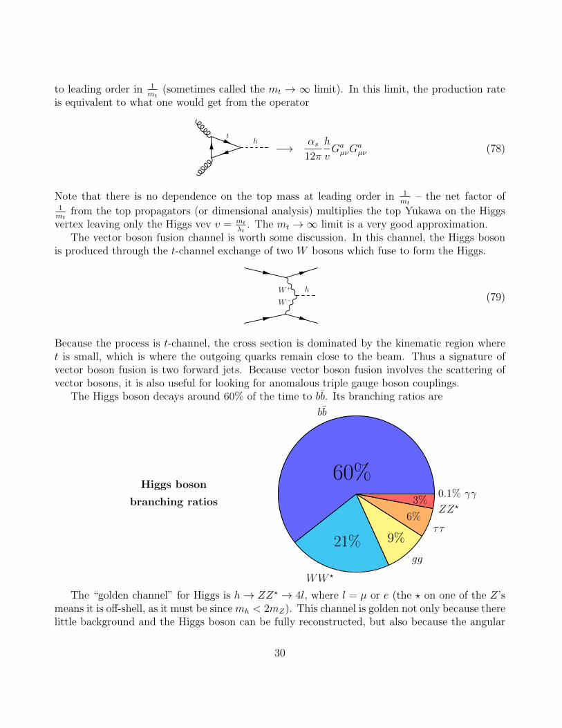
The Higgs boson decays around 60% of the time to bb. Its branching ratios are

Higgs boson

branching ratios

bb

60%

WW ?

21%gg

9%ττ

6%ZZ?

3%0.1% γγ

The “golden channel” for Higgs is h→ ZZ? → 4l, where l = µ or e (the ? on one of the Z’smeans it is off-shell, as it must be since mh < 2mZ). This channel is golden not only because therelittle background and the Higgs boson can be fully reconstructed, but also because the angular

30

(GeV)ℓ4m80 100 120 140 160 180

Eve

nts

/ 3 G

eV

0

2

4

6

8

10

12

14

16Data

Z+X*, ZZγZ=125 GeVHm

CMS-1 = 8 TeV, L = 5.3 fbs -1 = 7 TeV, L = 5.1 fbs

(GeV)ℓ4m120 140 160

Eve

nts

/ 3 G

eV

0

1

2

3

4

5

6 > 0.5DK

(GeV)γγm110 120 130 140 150S

/(S+B

) Wei

ghte

d E

vent

s / 1

.5 G

eV0

500

1000

1500

DataS+B FitB Fit Component

σ1±σ2±

-1 = 8 TeV, L = 5.3 fbs-1 = 7 TeV, L = 5.1 fbsCMS

(GeV)γγm120 130

Eve

nts

/ 1.5

GeV

1000

1500Unweighted

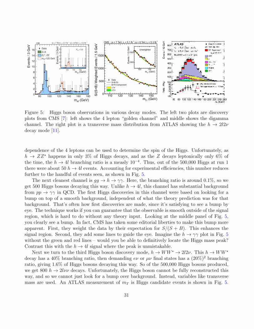
Figure 5: Higgs boson observations in various decay modes. The left two plots are discoveryplots from CMS [7]: left shows the 4 lepton “golden channel” and middle shows the digammachannel. The right plot is a transverse mass distribution from ATLAS showing the h → 2l2νdecay mode [11].

dependence of the 4 leptons can be used to determine the spin of the Higgs. Unfortunately, ash → ZZ? happens in only 3% of Higgs decays, and as the Z decays leptonically only 6% ofthe time, the h → 4l branching ratio is a measly 10−4. Thus, out of the 500,000 Higgs at run 1there were about 50 h→ 4l events. Accounting for experimental efficiencies, this number reducesfurther to the handful of events seen, as shown in Fig. 5.

The next cleanest channel is gg → h→ γγ. Here, the branching ratio is around 0.1%, so weget 500 Higgs bosons decaying this way. Unlike h→ 4l, this channel has substantial backgroundfrom pp → γγ in QCD. The first Higgs discoveries in this channel were based on looking for abump on top of a smooth background, independent of what the theory prediction was for thatbackground. That’s often how first discoveries are made, since it’s satisfying to see a bump byeye. The technique works if you can guarantee that the observable is smooth outside of the signalregion, which is hard to do without any theory input. Looking at the middle panel of Fig. 5,you clearly see a bump. In fact, CMS has taken some editorial liberties to make this bump moreapparent. First, they weight the data by their expectation for S/(S + B). This enhances thesignal region. Second, they add some lines to guide the eye. Imagine the h → γγ plot in Fig. 5without the green and red lines – would you be able to definitively locate the Higgs mass peak?Contrast this with the h→ 4l signal where the peak is unmistakable.

Next we turn to the third Higgs boson discovery mode, h→ WW ? → 2l2ν. This h→ WW ?

decay has a 40% branching ratio, then demanding eν or µν final states has a (20%)2 branchingratio, giving 1.6% of Higgs bosons decaying this way. So of the 500,000 Higgs bosons produced,we get 800 h→ 2lνν decays. Unfortunately, the Higgs boson cannot be fully reconstructed thisway, and so we cannot just look for a bump over background. Instead, variables like transversemass are used. An ATLAS measurement of mT is Higgs candidate events is shown in Fig. 5.

31

Importantly, it is only possible to see a Higgs in this channel if the backgrounds are known,including accurate theoretical predictions for their cross sections.

In summary, the are three Higgs‘ ‘discovery” channels. First, the golden channel h→ ZZ? →4l which had around 50 events in run 1. In this golden channel, S/B is large and one can fullyreconstruct the Higgs, allowing its spin to be measured. Next, h→ γγ had ∼ 500 events, smallS/B, but the Higgs could be fully reconstructed producing a visible bump in mγγ with enoughstatistics. This bump could be seen over a smooth fit to the sideband region, independent oftheory predictions. Then, h → WW ? → 2l2ν had 5000 events, but one could not see the Higgsas a bump. Instead there is a broad excess, so the Higgs can only be seen if the backgrounds areknown.

All the above channels have the Higgs decaying to vector bosons. The fermionic decay modesof the Higgs are harder to see. It is nearly impossible to see h→ bb if the Higgs boson is producedfrom gluon fusion. The problem is that there is a QCD pp→ bb background whose cross sectionis many orders of magnitude larger. The best place to see h→ bb is in the associated productionchannels, pp → Zh, pp → Wh and pp → tth, or in vector boson fusion, where the forward jetshelp reduce backgrounds. h→ ττ can also, in principle, be seen in these channels. In particular,with vector boson fusion, since h → ττ is an electroweak decay, one expects a relative absenceof QCD radiation in the central region compared to QCD backgrounds, 2 forward jets, and twolow-multiplicity central jets from the tauons.

Acknowledgements

I would like to thank the organizers of TASI, Rouven Essig, Ian Low and Tom DeGrand forinviting me to lecture, and to the students for all their excellent questions and discussions. Iwould also like to thank the Galileo Galilei Institute for inviting me as well, where a versionof these lectures were also given. My work is conducted with support in part from the U.S.Department of Energy under contract de-sc0013607.

References

[1] R. K. Ellis, W. J. Stirling, and B. R. Webber, “QCD and collider physics,” Camb. Monogr.Part. Phys. Nucl. Phys. Cosmol. 8 (1996) 1–435.

[2] M. D. Schwartz, Quantum Field Theory and the Standard Model. Cambridge UniversityPress, 2014.

[3] P. Z. Skands, “QCD for Collider Physics,” in Proceedings, High-energy Physics.Proceedings, 18th European School (ESHEP 2010): Raseborg, Finland, June 20 - July 3,2010. 2011. arXiv:1104.2863 [hep-ph].

32

[4] ATLAS Collaboration, M. Aaboud et al., “Measurement of the W -boson mass in ppcollisions at

√s = 7 TeV with the ATLAS detector,” arXiv:1701.07240 [hep-ex].

[5] C. G. Lester and D. J. Summers, “Measuring masses of semiinvisibly decaying particlespair produced at hadron colliders,” Phys. Lett. B463 (1999) 99–103,arXiv:hep-ph/9906349 [hep-ph].

[6] G. P. Salam, “Towards Jetography,” Eur. Phys. J. C67 (2010) 637–686, arXiv:0906.1833[hep-ph].

[7] A. Altheimer et al., “Jet Substructure at the Tevatron and LHC: New results, new tools,new benchmarks,” J. Phys. G39 (2012) 063001, arXiv:1201.0008 [hep-ph].

[8] D. E. Kaplan, K. Rehermann, M. D. Schwartz, and B. Tweedie, “Top Tagging: A Methodfor Identifying Boosted Hadronically Decaying Top Quarks,” Phys. Rev. Lett. 101 (2008)142001, arXiv:0806.0848 [hep-ph].

[9] J. M. Butterworth, A. R. Davison, M. Rubin, and G. P. Salam, “Jet substructure as a newHiggs search channel at the LHC,” Phys. Rev. Lett. 100 (2008) 242001, arXiv:0802.2470[hep-ph].

[10] S. Moch et al., “High precision fundamental constants at the TeV scale,”arXiv:1405.4781 [hep-ph].

[11] ATLAS Collaboration, G. Aad et al., “Observation of a new particle in the search for theStandard Model Higgs boson with the ATLAS detector at the LHC,” Phys. Lett. B716(2012) 1–29, arXiv:1207.7214 [hep-ex].

33