Task Allocation and Scheduling of Concurrent Applications ...€¦ · 1 Abstract Task Allocation and Scheduling of Concurrent Applications to Multiprocessor Systems by Kaushik Ravindran

Task Allocation and Scheduling of ConcurrentApplications to Multiprocessor Systems

Kaushik Ravindran

Electrical Engineering and Computer SciencesUniversity of California at Berkeley

Technical Report No. UCB/EECS-2007-149

http://www.eecs.berkeley.edu/Pubs/TechRpts/2007/EECS-2007-149.html

December 13, 2007

Copyright © 2007, by the author(s).All rights reserved.

Permission to make digital or hard copies of all or part of this work forpersonal or classroom use is granted without fee provided that copies arenot made or distributed for profit or commercial advantage and that copiesbear this notice and the full citation on the first page. To copy otherwise, torepublish, to post on servers or to redistribute to lists, requires prior specificpermission.

Task Allocation and Scheduling ofConcurrent Applications to Multiprocessor Systems

by

Kaushik Ravindran

B.S. (Georgia Institute of Technology) 2001

A dissertation submitted in partial satisfaction of therequirements for the degree of

Doctor of Philosophy

in

Engineering - Electrical Engineering and Computer Sciences

in the

GRADUATE DIVISIONof the

UNIVERSITY OF CALIFORNIA, BERKELEY

Committee in charge:Professor Kurt Keutzer, Chair

Professor John WawrzynekProfessor Alper Atamturk

Fall 2007

Task Allocation and Scheduling of

Concurrent Applications to Multiprocessor Systems

Copyright 2007

by

Kaushik Ravindran

1

Abstract

Task Allocation and Scheduling of

Concurrent Applications to Multiprocessor Systems

by

Kaushik Ravindran

Doctor of Philosophy in Engineering - Electrical Engineering and Computer Sciences

University of California, Berkeley

Professor Kurt Keutzer, Chair

Programmable multiprocessors are increasingly popular platforms for high performance em-

bedded applications. An important step in deploying applications on multiprocessors is to allo-

cate and schedule concurrent tasks to the processing and communication resources of the platform.

When the application workload and execution profiles can be reliably estimated at compile time,

it is viable to determine an application mapping statically. Many applications from the signal pro-

cessing and network processing domains are statically scheduled on multiprocessor systems. Static

scheduling is also relevant to design space exploration for micro-architectures and systems.

Owing to the computational complexity of optimal static scheduling, a number of heuristic

methods have been proposed for different scheduling conditions and architecture models. Un-

fortunately, these methods lack the flexibility necessary to enforce implementation and resource

constraints that complicate practical multiprocessor scheduling problems. While it is important to

find good solutions quickly, an effective scheduling method must also reliably capture the problem

specification and flexibly accommodate diverse constraints and objectives.

This dissertation is an attempt to develop insight into efficient and flexible methods for allocat-

ing and scheduling concurrent applications to multiprocessor architectures. We conduct our study

in four parts. First, we analyze the nature of the scheduling problems that arise in a realistic ex-

ploration framework. Second, we evaluate competitive heuristic, randomized, and exact methods

for these scheduling problems. Third, we propose methods based on mathematical and constraint

programming for a representative scheduling problem. Though expressiveness and flexibility are

advantages of these methods, generic constraint formulations suffer prohibitive run times even on

2

modestly sized problems. To alleviate this difficulty, we advance several strategies to accelerate

constraint programming, such as problem decompositions, search guidance through heuristic meth-

ods, and tight lower bound computations. The inherent flexibility, coupled with improved run times

from a decomposition strategy, posit constraint programming as a powerful tool for multiproces-

sor scheduling problems. Finally, we present a toolbox of practical scheduling methods, which

provide different trade-offs with respect to computational efficiency, quality of results, and flexi-

bility. Our toolbox is composed of heuristic methods, constraint programming formulations, and

simulated annealing techniques. These methods are part of an exploration framework for deploying

network processing applications on two embedded platforms: Intel IXP network processors and

Xilinx FPGA based soft multiprocessors.

Professor Kurt KeutzerDissertation Committee Chair

i

“Better to remain silent and be thought a fool than to speak out and remove all doubt.”

– Abraham Lincoln

ii

Contents

List of Figures v

List of Tables vii

1 The Trend to Single Chip Multiprocessor Systems 11.1 Deploying Concurrent Applications on Multiprocessors . . . . . . . . . . . . . . . 3

1.1.1 The Implementation Gap . . . . . . . . . . . . . . . . . . . . . . . . . . . 31.1.2 A Methodology to Bridge the Implementation Gap . . . . . . . . . . . . . 4

1.2 The Mapping Problem for Multiprocessor Systems . . . . . . . . . . . . . . . . . 51.2.1 Static Models, Static Scheduling . . . . . . . . . . . . . . . . . . . . . . . 71.2.2 Complexity of Static Scheduling . . . . . . . . . . . . . . . . . . . . . . . 81.2.3 Common Methods for Static Scheduling . . . . . . . . . . . . . . . . . . . 10

1.3 The Quest for Efficient and Flexible Scheduling Methods . . . . . . . . . . . . . . 121.4 Contributions of this Dissertation . . . . . . . . . . . . . . . . . . . . . . . . . . . 14

2 A Framework for Mapping and Design Space Exploration 162.1 A Framework for Mapping and Exploration . . . . . . . . . . . . . . . . . . . . . 16

2.1.1 Domain Specific Language for Application Representation . . . . . . . . . 172.1.2 The Mapping Step . . . . . . . . . . . . . . . . . . . . . . . . . . . . . . 172.1.3 Performance Analysis and Feedback . . . . . . . . . . . . . . . . . . . . . 19

2.2 The Network Processing Domain: Applications and Platforms . . . . . . . . . . . 202.2.1 Network Processing Applications . . . . . . . . . . . . . . . . . . . . . . 212.2.2 Intel IXP Network Processors . . . . . . . . . . . . . . . . . . . . . . . . 222.2.3 Xilinx FPGA based Soft Multiprocessors . . . . . . . . . . . . . . . . . . 24

2.3 Exploration Framework for Network Processing Applications . . . . . . . . . . . . 262.3.1 Domain Specific Language for Application Representation . . . . . . . . . 272.3.2 The Mapping Step . . . . . . . . . . . . . . . . . . . . . . . . . . . . . . 282.3.3 Performance Analysis and Feedback . . . . . . . . . . . . . . . . . . . . . 30

2.4 Motivation for an Efficient and Flexible Mapping Approach . . . . . . . . . . . . . 30

3 Models and Methods for the Scheduling Problem 313.1 Models for Static Scheduling . . . . . . . . . . . . . . . . . . . . . . . . . . . . . 32

3.1.1 The Application Task Graph Model . . . . . . . . . . . . . . . . . . . . . 323.1.2 The Multiprocessor Architecture Model . . . . . . . . . . . . . . . . . . . 34

iii

3.1.3 Performance Model for the Task Graph . . . . . . . . . . . . . . . . . . . 353.1.4 Optimization Objective . . . . . . . . . . . . . . . . . . . . . . . . . . . . 363.1.5 Implementation and Resource Constraints . . . . . . . . . . . . . . . . . . 37

3.2 Methods for Static Scheduling . . . . . . . . . . . . . . . . . . . . . . . . . . . . 393.2.1 Heuristic Methods . . . . . . . . . . . . . . . . . . . . . . . . . . . . . . 413.2.2 List Scheduling using Dynamic Levels . . . . . . . . . . . . . . . . . . . 423.2.3 Evolutionary Algorithms . . . . . . . . . . . . . . . . . . . . . . . . . . . 433.2.4 Simulated Annealing . . . . . . . . . . . . . . . . . . . . . . . . . . . . . 443.2.5 Enumerative Branch-and-Bound . . . . . . . . . . . . . . . . . . . . . . . 453.2.6 Mathematical and Constraint Programming . . . . . . . . . . . . . . . . . 45

3.3 Scheduling Tools and Frameworks . . . . . . . . . . . . . . . . . . . . . . . . . . 463.4 The Right Method for the Job . . . . . . . . . . . . . . . . . . . . . . . . . . . . . 48

4 Constraint Programming Methods for Static Scheduling 504.1 A Representative Static Scheduling Problem . . . . . . . . . . . . . . . . . . . . . 50

4.1.1 Multiprocessor Architecture Model . . . . . . . . . . . . . . . . . . . . . 514.1.2 Application Task Graph . . . . . . . . . . . . . . . . . . . . . . . . . . . 524.1.3 Execution Time and Communication Delay Models . . . . . . . . . . . . . 524.1.4 Valid Allocation, Valid Schedule . . . . . . . . . . . . . . . . . . . . . . . 534.1.5 Optimization Objective . . . . . . . . . . . . . . . . . . . . . . . . . . . . 544.1.6 Example . . . . . . . . . . . . . . . . . . . . . . . . . . . . . . . . . . . 544.1.7 Implementation and Resource Constraints . . . . . . . . . . . . . . . . . . 554.1.8 Complexity of the Scheduling Problem . . . . . . . . . . . . . . . . . . . 57

4.2 A Mixed Integer Linear Programming Formulation . . . . . . . . . . . . . . . . . 584.2.1 Variables . . . . . . . . . . . . . . . . . . . . . . . . . . . . . . . . . . . 594.2.2 Constraints . . . . . . . . . . . . . . . . . . . . . . . . . . . . . . . . . . 60

4.3 Mapping Results for Network Processing Applications . . . . . . . . . . . . . . . 614.3.1 IPv4 Packet Forwarding on FPGA based Soft Multiprocessors . . . . . . . 624.3.2 Differentiated Services on the IXP1200 Network Processor . . . . . . . . . 69

4.4 A Case for an Efficient and Flexible Mapping Approach . . . . . . . . . . . . . . 71

5 Techniques to Accelerate Constraint Programming Methods 735.1 The Concept of Problem Decomposition . . . . . . . . . . . . . . . . . . . . . . . 74

5.1.1 Related Decomposition Approaches for Scheduling Problems . . . . . . . 755.1.2 Overview of the Decomposition Approach . . . . . . . . . . . . . . . . . 75

5.2 A Decomposition Approach for Static Scheduling . . . . . . . . . . . . . . . . . . 765.2.1 Master Problem Formulation . . . . . . . . . . . . . . . . . . . . . . . . . 785.2.2 Sub Problem Decomposition Constraints . . . . . . . . . . . . . . . . . . 805.2.3 Algorithmic Extensions to Improve Performance . . . . . . . . . . . . . . 83

5.3 Evaluation of the Decomposition Approach . . . . . . . . . . . . . . . . . . . . . 855.3.1 Benchmark Set . . . . . . . . . . . . . . . . . . . . . . . . . . . . . . . . 855.3.2 Comparisons to Heuristics and Single-Pass MILP Formulations . . . . . . 855.3.3 Extensibility of Constraint Programming . . . . . . . . . . . . . . . . . . 89

5.4 An Efficient and Flexible Mapping Approach . . . . . . . . . . . . . . . . . . . . 92

iv

6 A Toolbox of Scheduling Methods 946.1 The Value of Good Heuristics . . . . . . . . . . . . . . . . . . . . . . . . . . . . . 94

6.1.1 Dynamic Level Scheduling Revisited . . . . . . . . . . . . . . . . . . . . 956.1.2 Guidance for Search in Branch-and-Bound Methods . . . . . . . . . . . . 976.1.3 Evaluation of Heuristic Search Guidance . . . . . . . . . . . . . . . . . . 99

6.2 Simulated Annealing for Large Task Graphs . . . . . . . . . . . . . . . . . . . . . 1026.2.1 A Generic Simulated Annealing Algorithm . . . . . . . . . . . . . . . . . 1026.2.2 Annealing Strategy for the Representative Scheduling Problem . . . . . . . 103

6.3 Evaluation of Scheduling Methods . . . . . . . . . . . . . . . . . . . . . . . . . . 1056.4 The Right Method for the Job . . . . . . . . . . . . . . . . . . . . . . . . . . . . . 109

7 Conclusions and Further Work 1127.1 Constraint Programming Methods for Scheduling . . . . . . . . . . . . . . . . . . 1137.2 A Toolbox of Practical Scheduling Methods . . . . . . . . . . . . . . . . . . . . . 1157.3 Exploration Framework for Network Processing Applications . . . . . . . . . . . . 118

Bibliography 120

v

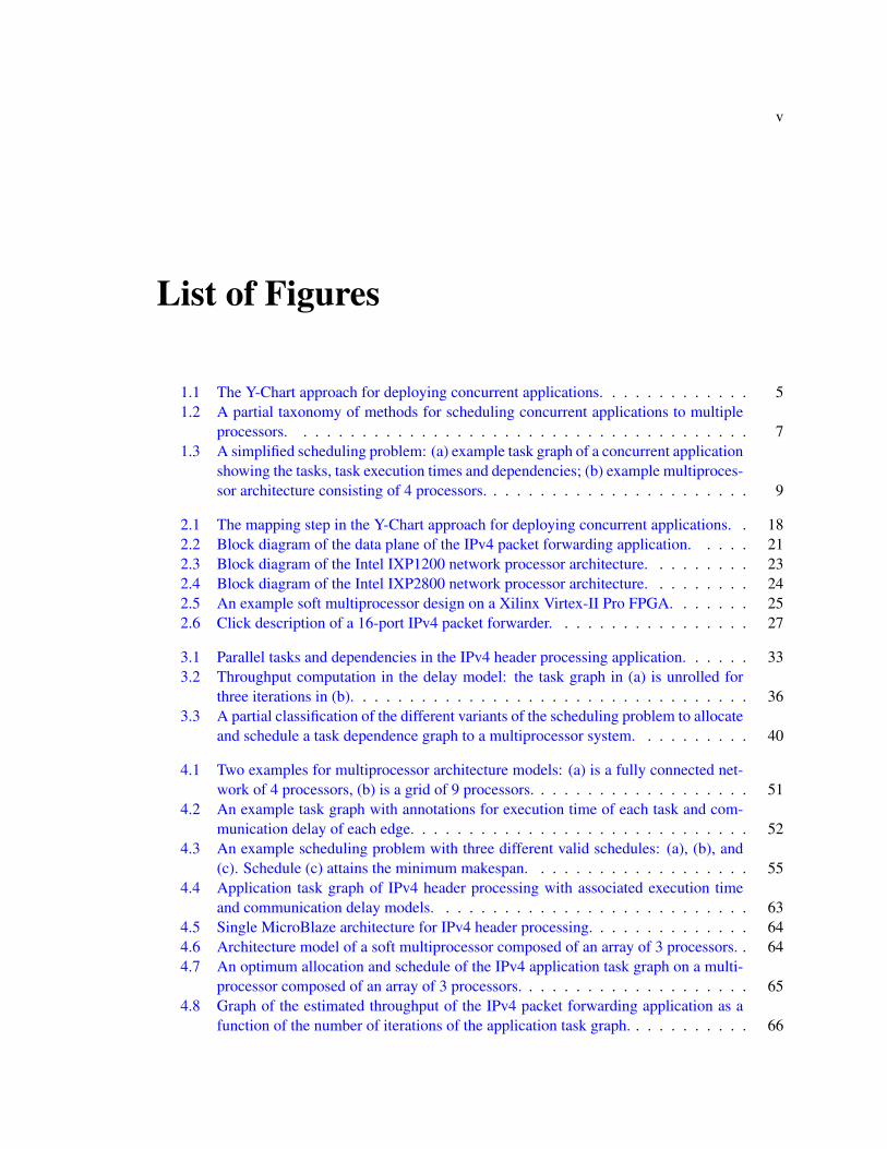
List of Figures

1.1 The Y-Chart approach for deploying concurrent applications. . . . . . . . . . . . . 51.2 A partial taxonomy of methods for scheduling concurrent applications to multiple

processors. . . . . . . . . . . . . . . . . . . . . . . . . . . . . . . . . . . . . . . 71.3 A simplified scheduling problem: (a) example task graph of a concurrent application

showing the tasks, task execution times and dependencies; (b) example multiproces-sor architecture consisting of 4 processors. . . . . . . . . . . . . . . . . . . . . . . 9

2.1 The mapping step in the Y-Chart approach for deploying concurrent applications. . 182.2 Block diagram of the data plane of the IPv4 packet forwarding application. . . . . 212.3 Block diagram of the Intel IXP1200 network processor architecture. . . . . . . . . 232.4 Block diagram of the Intel IXP2800 network processor architecture. . . . . . . . . 242.5 An example soft multiprocessor design on a Xilinx Virtex-II Pro FPGA. . . . . . . 252.6 Click description of a 16-port IPv4 packet forwarder. . . . . . . . . . . . . . . . . 27

3.1 Parallel tasks and dependencies in the IPv4 header processing application. . . . . . 333.2 Throughput computation in the delay model: the task graph in (a) is unrolled for

three iterations in (b). . . . . . . . . . . . . . . . . . . . . . . . . . . . . . . . . . 363.3 A partial classification of the different variants of the scheduling problem to allocate

and schedule a task dependence graph to a multiprocessor system. . . . . . . . . . 40

4.1 Two examples for multiprocessor architecture models: (a) is a fully connected net-work of 4 processors, (b) is a grid of 9 processors. . . . . . . . . . . . . . . . . . . 51

4.2 An example task graph with annotations for execution time of each task and com-munication delay of each edge. . . . . . . . . . . . . . . . . . . . . . . . . . . . . 52

4.3 An example scheduling problem with three different valid schedules: (a), (b), and(c). Schedule (c) attains the minimum makespan. . . . . . . . . . . . . . . . . . . 55

4.4 Application task graph of IPv4 header processing with associated execution timeand communication delay models. . . . . . . . . . . . . . . . . . . . . . . . . . . 63

4.5 Single MicroBlaze architecture for IPv4 header processing. . . . . . . . . . . . . . 644.6 Architecture model of a soft multiprocessor composed of an array of 3 processors. . 644.7 An optimum allocation and schedule of the IPv4 application task graph on a multi-

processor composed of an array of 3 processors. . . . . . . . . . . . . . . . . . . . 654.8 Graph of the estimated throughput of the IPv4 packet forwarding application as a

function of the number of iterations of the application task graph. . . . . . . . . . . 66

vi

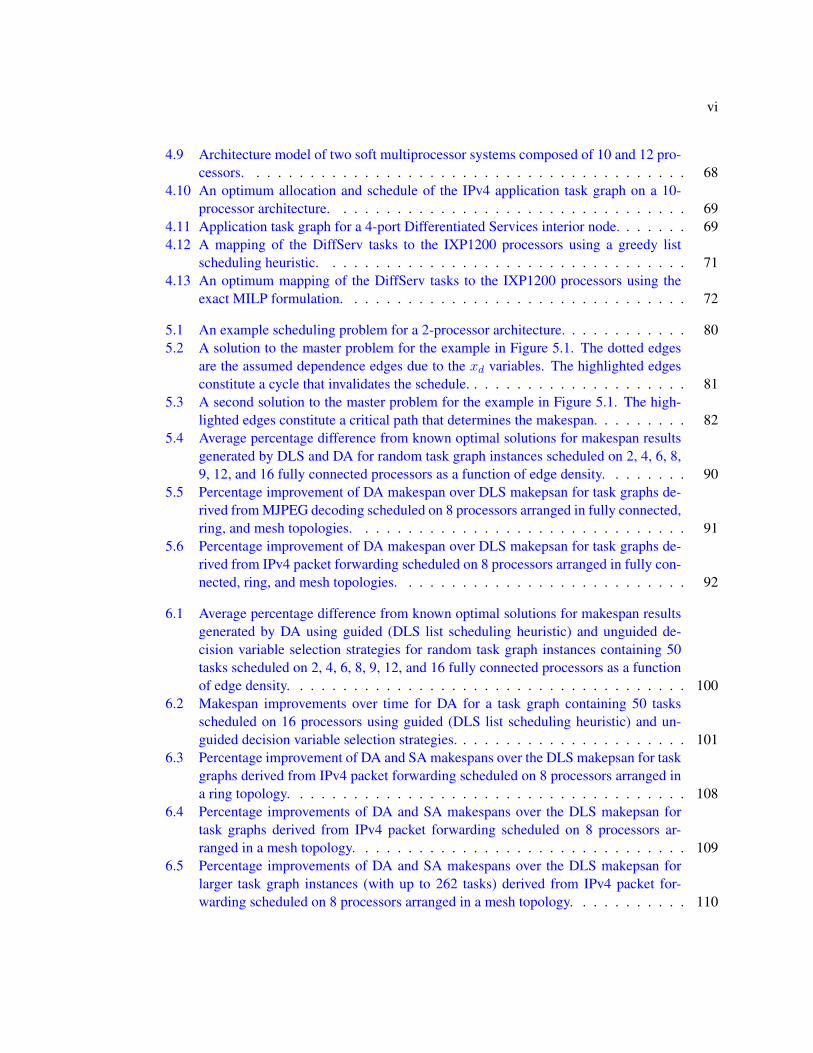
4.9 Architecture model of two soft multiprocessor systems composed of 10 and 12 pro-cessors. . . . . . . . . . . . . . . . . . . . . . . . . . . . . . . . . . . . . . . . . 68

4.10 An optimum allocation and schedule of the IPv4 application task graph on a 10-processor architecture. . . . . . . . . . . . . . . . . . . . . . . . . . . . . . . . . 69

4.11 Application task graph for a 4-port Differentiated Services interior node. . . . . . . 694.12 A mapping of the DiffServ tasks to the IXP1200 processors using a greedy list

scheduling heuristic. . . . . . . . . . . . . . . . . . . . . . . . . . . . . . . . . . 714.13 An optimum mapping of the DiffServ tasks to the IXP1200 processors using the

exact MILP formulation. . . . . . . . . . . . . . . . . . . . . . . . . . . . . . . . 72

5.1 An example scheduling problem for a 2-processor architecture. . . . . . . . . . . . 805.2 A solution to the master problem for the example in Figure 5.1. The dotted edges

are the assumed dependence edges due to the xd variables. The highlighted edgesconstitute a cycle that invalidates the schedule. . . . . . . . . . . . . . . . . . . . . 81

5.3 A second solution to the master problem for the example in Figure 5.1. The high-lighted edges constitute a critical path that determines the makespan. . . . . . . . . 82

5.4 Average percentage difference from known optimal solutions for makespan resultsgenerated by DLS and DA for random task graph instances scheduled on 2, 4, 6, 8,9, 12, and 16 fully connected processors as a function of edge density. . . . . . . . 90

5.5 Percentage improvement of DA makespan over DLS makepsan for task graphs de-rived from MJPEG decoding scheduled on 8 processors arranged in fully connected,ring, and mesh topologies. . . . . . . . . . . . . . . . . . . . . . . . . . . . . . . 91

5.6 Percentage improvement of DA makespan over DLS makepsan for task graphs de-rived from IPv4 packet forwarding scheduled on 8 processors arranged in fully con-nected, ring, and mesh topologies. . . . . . . . . . . . . . . . . . . . . . . . . . . 92

6.1 Average percentage difference from known optimal solutions for makespan resultsgenerated by DA using guided (DLS list scheduling heuristic) and unguided de-cision variable selection strategies for random task graph instances containing 50tasks scheduled on 2, 4, 6, 8, 9, 12, and 16 fully connected processors as a functionof edge density. . . . . . . . . . . . . . . . . . . . . . . . . . . . . . . . . . . . . 100

6.2 Makespan improvements over time for DA for a task graph containing 50 tasksscheduled on 16 processors using guided (DLS list scheduling heuristic) and un-guided decision variable selection strategies. . . . . . . . . . . . . . . . . . . . . . 101

6.3 Percentage improvement of DA and SA makespans over the DLS makepsan for taskgraphs derived from IPv4 packet forwarding scheduled on 8 processors arranged ina ring topology. . . . . . . . . . . . . . . . . . . . . . . . . . . . . . . . . . . . . 108

6.4 Percentage improvements of DA and SA makespans over the DLS makepsan fortask graphs derived from IPv4 packet forwarding scheduled on 8 processors ar-ranged in a mesh topology. . . . . . . . . . . . . . . . . . . . . . . . . . . . . . . 109

6.5 Percentage improvements of DA and SA makespans over the DLS makepsan forlarger task graph instances (with up to 262 tasks) derived from IPv4 packet for-warding scheduled on 8 processors arranged in a mesh topology. . . . . . . . . . . 110

vii

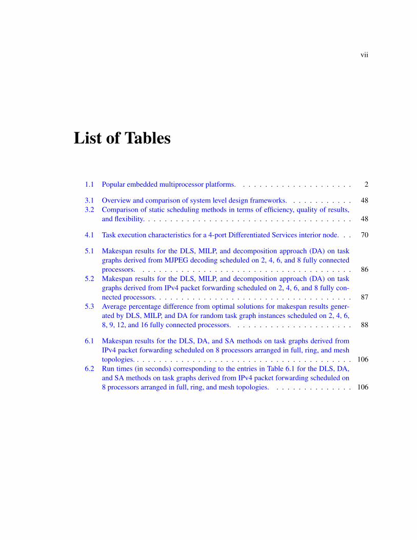
List of Tables

1.1 Popular embedded multiprocessor platforms. . . . . . . . . . . . . . . . . . . . . 2

3.1 Overview and comparison of system level design frameworks. . . . . . . . . . . . 483.2 Comparison of static scheduling methods in terms of efficiency, quality of results,

and flexibility. . . . . . . . . . . . . . . . . . . . . . . . . . . . . . . . . . . . . . 48

4.1 Task execution characteristics for a 4-port Differentiated Services interior node. . . 70

5.1 Makespan results for the DLS, MILP, and decomposition approach (DA) on taskgraphs derived from MJPEG decoding scheduled on 2, 4, 6, and 8 fully connectedprocessors. . . . . . . . . . . . . . . . . . . . . . . . . . . . . . . . . . . . . . . 86

5.2 Makespan results for the DLS, MILP, and decomposition approach (DA) on taskgraphs derived from IPv4 packet forwarding scheduled on 2, 4, 6, and 8 fully con-nected processors. . . . . . . . . . . . . . . . . . . . . . . . . . . . . . . . . . . . 87

5.3 Average percentage difference from optimal solutions for makespan results gener-ated by DLS, MILP, and DA for random task graph instances scheduled on 2, 4, 6,8, 9, 12, and 16 fully connected processors. . . . . . . . . . . . . . . . . . . . . . 88

6.1 Makespan results for the DLS, DA, and SA methods on task graphs derived fromIPv4 packet forwarding scheduled on 8 processors arranged in full, ring, and meshtopologies. . . . . . . . . . . . . . . . . . . . . . . . . . . . . . . . . . . . . . . . 106

6.2 Run times (in seconds) corresponding to the entries in Table 6.1 for the DLS, DA,and SA methods on task graphs derived from IPv4 packet forwarding scheduled on8 processors arranged in full, ring, and mesh topologies. . . . . . . . . . . . . . . 106

viii

Acknowledgments

I thank Professor Kurt Keutzer for guiding me through my graduate career. It is an honor to

have worked with him and I will forever treasure his acquaintance. There is so much to learn from

him, but if I should steal one attribute of his, it would be his “efficiency of thought” - his ability

to quickly distill a concept without getting entangled in the details, ask discerning questions, and

cogently articulate his reasoning and evaluation. And if I should remember one aphorism from his

book, it would be: “you get to choose the game, choose the rules, but then you must play to win”.

I thank Professors John Wawrzynek and Alper Atamturk for serving on my dissertation com-

mittee. Professor Wawrzynek’s course on reconfigurable computing helped impart initial directions

to this research. I also thank him for providing valuable feedback during the preparation of this

document. Professor Atamturk conducted an engaging and instructive course on computational op-

timization, and I am happy to have been part of it. This course provided the foundations for our

study on constraint methods for scheduling.

I thank Professor Andreas Kuehlmann and Dr. Chandu Visweswariah for granting me the

privilege to work with them. Professor Kuehlmann instructed me in his logic synthesis course and

mentored my first research project in Berkeley. I am grateful for his tutelage and aspire to inculcate

his discipline and rigor. Dr. Visweswariah supervised my internship at IBM and bestowed a truly

unforgettable experience. I hope his clarity of thought and word has rubbed off on me. It is an honor

to have been part of his project and co-author of his paper on statistical timing.

I thank my closest collaborators in the MESCAL research group: Yujia Jin, William Plishker,

and Nadathur Satish. Our research efforts complemented each other well: William studied program-

ming models for network processors and built a prototype exploration framework, Yujia studied

design space exploration approaches for programmable multiprocessors, and Satish and I studied

different models and optimization methods to solve the mapping problems that arose in these frame-

works. I hope I get a chance to work with them in the future.

I thank the members of the MESCAL group who made this research possible: Hugo Andrade,

Bryan Catanzaro, Dave Chinnery, Jike Chong, Matthias Gries, Chidamber Kulkarni, Andrew Mihal,

Matt Moskewicz, Christian Sauer, Niraj Shah, Martin Trautmann, and Scott Weber. They freely

exchanged ideas, collaborated on papers and presentations, and made the workplace enjoyable. I

am grateful to Bryan Catanzaro, Jike Chong, and Nadathur Satish for taking time to read and critique

this dissertation. A special thanks to Abhijit Davare, a member of a “rival” group, who nevertheless

shared his insights on related research problems and engaged in many useful discussions.

ix

I thank the members of the EECS Department administration for providing us a comfortable

workplace: Mary Byrnes, Ruth Gjerde, Jontae Gray, Patrick Hernan, Cindy Keenon, Brad Krepes,

Ellen Lenzi, Loretta Lutcher, Dan MacLeod, Marvin Motley, Jennifer Stone, and Carol Zalon. I

specially thank Ruth Gjerde of EE Graduate Student Affairs for patiently monitoring our progress

through the degree program.

I thank my colleagues of the EECS Department, who kindly collaborated with me on home-

works, projects, and exam preparations: Donald Chai, Douglas Densmore, Ashwin Ganesan, Yan-

mei Li, Cong Liu, Slobodan Matic, Trevor Meyerowitz, Manikandan Narayanan, Alessandro Pinto,

Farhana Sheikh, Gerald Wang, and Haiyang Zheng. The days of our combined study efforts for the

CAD preliminary exam do not seem like long ago.

I thank my roommates and friends who make my years in Berkeley memorable: Krishnendu

Chatterjee, a “roommate from heaven”; Satrajit Chatterjee, a thoroughbred; Arindam Chakrabarti,

our moral and legal adviser; Mohan Dunga, the resident devices expert; Arkadeb Ghosal, a born

leader; Abhishek Ghose, the dude; Pankaj Kalra, a man of clarity and wisdom; Animesh Kumar,

a humble savant; Anshuman Sharma, a hard-hitting tennis partner; Rahul Tandra, our academy’s

superstar batsman. I cherish our hallway discussions, gastronomic outings, poker nights, tennis and

cricket sessions, sport and movie viewings, and Federer fan-club activities. Now I know why it has

been so hard to leave . . .

1

Chapter 1

The Trend to Single Chip

Multiprocessor Systems

Intel and AMD announced their first single chip dual core processor offerings for desktop

computers in early 2005. As of 2007, four core processors from Intel, AMD, IBM, and Sun are

available for servers, and similar parts for the desktop space are expected to appear soon. Keeping

with Moore’s law, the semiconductor roadmap forecasts a doubling in the number of processors per

die with every process generation [Asanovic et al., 2006].

The shift from conventional single processor systems to multiprocessors is an important water-

shed in the history of computing. The reason for this shift is that popular approaches to maximize

single processor performance are at their limits. Prohibitive power consumption and design com-

plexity are prominent factors that obstruct performance scaling [Borkar, 1999]. However, Moore’s

law continues to enable a doubling in the number of transistors on a single die every 18-24 months.

Consequently, the semiconductor industry has pursued the alternative of adding multiple processors

on a chip to utilize the additional transistors delivered by Moore’s law and improve performance.

The single chip multiprocessor is a recent trend in mainstream computing. However, appli-

cation specific multiprocessors have existed for several years in various embedded application do-

mains to exploit the inherent concurrency in the applications. The continuous increase in perfor-

mance requirements of embedded applications has fueled the need for high-performance platforms.

At the same time, the need to adapt products to rapid market changes has made software programma-

bility an important criterion for the success of these devices. Hence, the general trend has been

toward multiprocessor platforms specialized for an application domain to address the combined

2

needs of programmability and performance [Keutzer et al., 2000] [Rowen, 2003] [Sangiovanni-

Vincentelli, 2007].

Application specific programmable platforms are dominant in a variety of markets including

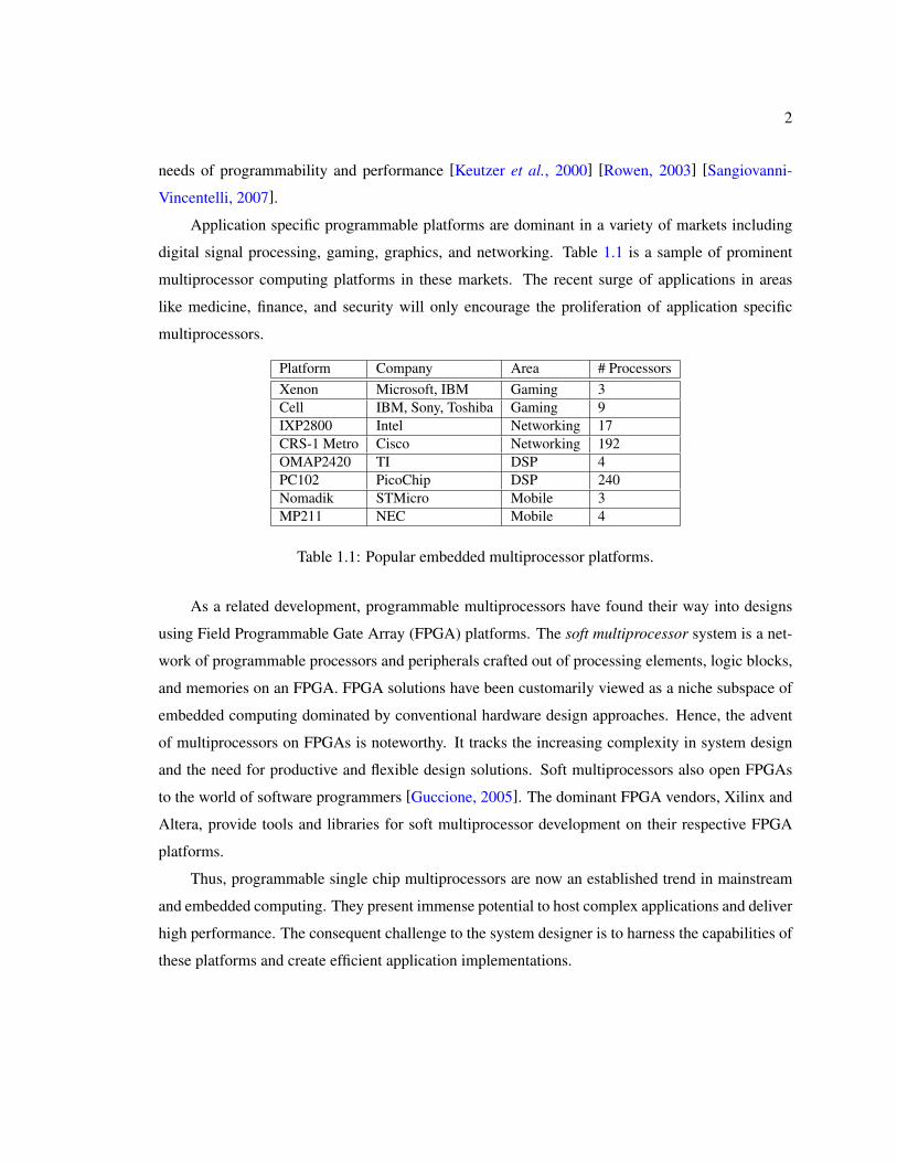
digital signal processing, gaming, graphics, and networking. Table 1.1 is a sample of prominent

multiprocessor computing platforms in these markets. The recent surge of applications in areas

like medicine, finance, and security will only encourage the proliferation of application specific

multiprocessors.

Platform Company Area # ProcessorsXenon Microsoft, IBM Gaming 3Cell IBM, Sony, Toshiba Gaming 9IXP2800 Intel Networking 17CRS-1 Metro Cisco Networking 192OMAP2420 TI DSP 4PC102 PicoChip DSP 240Nomadik STMicro Mobile 3MP211 NEC Mobile 4

Table 1.1: Popular embedded multiprocessor platforms.

As a related development, programmable multiprocessors have found their way into designs

using Field Programmable Gate Array (FPGA) platforms. The soft multiprocessor system is a net-

work of programmable processors and peripherals crafted out of processing elements, logic blocks,

and memories on an FPGA. FPGA solutions have been customarily viewed as a niche subspace of

embedded computing dominated by conventional hardware design approaches. Hence, the advent

of multiprocessors on FPGAs is noteworthy. It tracks the increasing complexity in system design

and the need for productive and flexible design solutions. Soft multiprocessors also open FPGAs

to the world of software programmers [Guccione, 2005]. The dominant FPGA vendors, Xilinx and

Altera, provide tools and libraries for soft multiprocessor development on their respective FPGA

platforms.

Thus, programmable single chip multiprocessors are now an established trend in mainstream

and embedded computing. They present immense potential to host complex applications and deliver

high performance. The consequent challenge to the system designer is to harness the capabilities of

these platforms and create efficient application implementations.

3

1.1 Deploying Concurrent Applications on Multiprocessors

Modern applications, particularly in the embedded domain, exhibit a lot of concurrency at dif-

ferent levels of granularity. A common classification identifies three categories or levels of concur-

rency differentiated by their granularity: task level, data level, and datatype level concurrency [Gries

and Keutzer, 2005] [Mihal, 2006]. Most applications express concurrency at all three levels. Task

level concurrency (also called process or thread level concurrency) is the coarsest grained category

and is exhibited when the computation contains multiple flows of control. For example, a program

using libraries like Pthreads exploits task level concurrency [Butenhof, 1997]. Shared memory and

message passing are two common modes for task level communication. Data level concurrency

occurs within a task and is exhibited when the computation operates on individual pieces of data in

parallel. Instruction-level parallelism is a common form of data level concurrency. Datatype level

concurrency is the finest-grained category and is exhibited when there is concurrent computation

within a piece of data. Arithmetical and logical operations that perform concurrent computation on

individual bits, such as addition, checksum, and parity computations, exploit datatype level concur-

rency.

Like embedded applications, programmable multiprocessors are capable of concurrency at

these three levels. Task level concurrency is supported by multiple programmable processors which

execute in parallel and communicate over an on-chip network. Data level concurrency is supported

by the individual processors if they allow multiple instructions to be issued and executed in parallel.

Datatype level concurrency is supported if the processing elements have instruction sets and func-

tional units that operate on datatypes of different bit widths (for example, integer, fixed-point, and

custom datatypes).

1.1.1 The Implementation Gap

The key to successful application deployment lies in effectively mapping the concurrency in

the application to the architectural resources provided by the platform. However, a concurrent

application and programmable multiprocessor typically exhibit different types of concurrency at the

three levels. There is no clear match between the concurrency in the application and the capabilities

of the architecture. This mismatch in the styles of concurrency of the application and architecture

is called the implementation gap [Gries and Keutzer, 2005].

The success of an approach for deploying concurrent applications on multiprocessors is deter-

mined by two main properties:

4

• The ability to produce high-performance implementations on the target platform.

• The ability to develop implementations productively.

The implementation gap adversely affects these abilities of a design approach. For instance, con-

sider the challenges in mapping task level concurrency in an application to the processing elements

in the architecture. At the onset, there is the difficulty of obtaining a representation of the applica-

tion that coherently expresses the computation tasks and dependencies. Second, there is no estab-

lished template to represent the task level parallelism accorded by the multiprocessor. To meet per-

formance requirements, these devices use complex architectural features: multiple heterogeneous

processors, distributed memories, special purpose hardware, and myriad on-chip communication

mechanisms. The onus is hence on the designer to produce high-performance implementations by

balancing computation between the different processors, distributing data to memory, and coordinat-

ing communication between concurrent tasks. The dual challenges of reasoning about application

concurrency and negotiating architectural intricacies often compels designers to spend many design

iterations before arriving at reasonable implementations.

1.1.2 A Methodology to Bridge the Implementation Gap

There are two prominent implications of the implementation gap. First, correct models of

the application concurrency and architectural capabilities are required for an effective deployment.

Second, a systematic approach is required to map the application model to the architecture and

fully harness its performance. Based on this insight, we believe there are three key imperatives to a

disciplined approach for bridging the implementation gap:

• Conceive a model for the application that naturally represents its concurrency.

• Conceive a model for the architecture that captures performance salient features.

• Develop an systematic mapping step that allows the designer to easily explore the design

space of possible solutions.

The application model provides a natural way of representing the task, data, and datatype level

concurrency in an application. The architecture model is an abstraction that exposes a subset of

architectural features that are necessary for a designer to effectively implement applications. The

last component that completes the framework is a systematic mapping step that binds the appli-

cation functionality to architectural resources. For a single processor system, the mapping step is

5

performed by the compiler. The compiler translates the user program into instructions and binds

them to function units and memories in the architecture. However, the mapping step is more com-

plicated when the target is a multiprocessor. The main focus of this dissertation is on the challenges

associated with the mapping step for multiprocessor systems.

1.2 The Mapping Problem for Multiprocessor Systems

A disciplined approach for bridging the implementation gap, as described in the previous sec-

tion, advocates a deliberate separation of concerns related to the application representation, archi-

tecture model, and mapping step. This is inspired by the popular Y-chart approach for system

design and design space exploration (DSE) [Kienhuis et al., 2002] [Balarin et al., 1997] [Keutzer

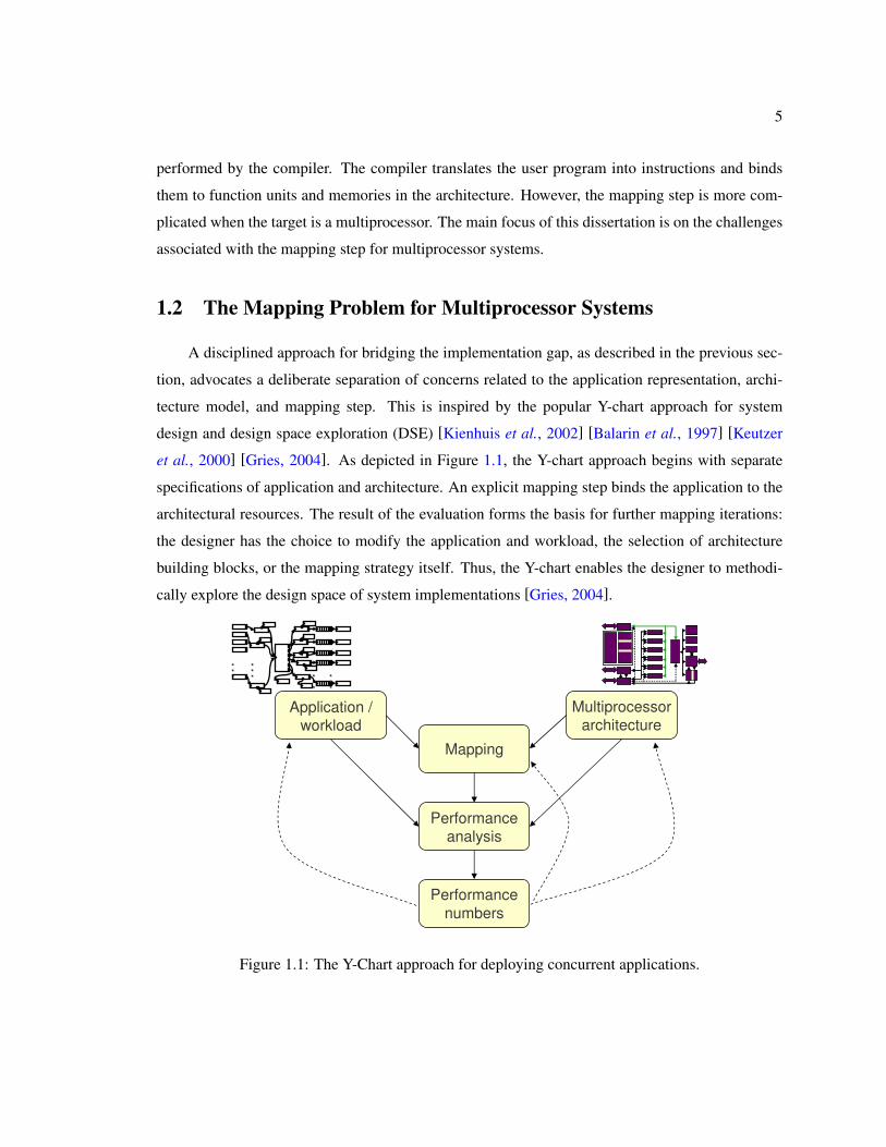
et al., 2000] [Gries, 2004]. As depicted in Figure 1.1, the Y-chart approach begins with separate

specifications of application and architecture. An explicit mapping step binds the application to the

architectural resources. The result of the evaluation forms the basis for further mapping iterations:

the designer has the choice to modify the application and workload, the selection of architecture

building blocks, or the mapping strategy itself. Thus, the Y-chart enables the designer to methodi-

cally explore the design space of system implementations [Gries, 2004].

Multiprocessor

architectureApplication /

workload

Mapping

Performance

analysis

Performance

numbers

…

… …

…

Figure 1.1: The Y-Chart approach for deploying concurrent applications.

6

The goal of the mapping step in the Y-chart framework (Figure 1.1) is to maximize application

performance (or some other design objective) by an effective distribution of computation and com-

munication on to the resources of the target architecture. The mapping is performed for every level

of concurrency in an application. The focus of this dissertation is particularly on techniques for

mapping task level concurrency in an application to the processing and communication resources in

the architecture. Once tasks are assigned to processors, it is the role of the compiler to exploit data

and datatype level concurrency inside a task to derive efficient implementations. The recent book

“Building ASIPs: The Mescal Methodology” by Gries and Keutzer details approaches to map data

and datatype level concurrency to application specific instruction set processors (ASIPs) [Gries and

Keutzer, 2005, Chapters 3-4].

Some components in mapping task level concurrency are: (a) allocation of tasks (or processes)

to processors, (b) allocation of states to memories, (c) allocation of task interactions to communi-

cation resources, (d) scheduling of tasks in time, and (e) scheduling of communications and syn-

chronizations between tasks. The feasibility of an allocation and schedule is regulated by various

constraints imposed by the application and architecture. A few prominent constraints from the appli-

cation model are task dependencies, deadlines, memory requirements, and communication and syn-

chronization overheads due to data exchange. Architectural constraints include processor speeds,

memory sizes, network topology, and data transfer rates. The mapping is typically directed by a

combination of objectives that characterize the quality of a solution. Objective functions related

to application performance are throughput, total execution time, and communication cost. Other

common mapping objectives are related to system power, reliability, and scalability.

Thus, to map the task level concurrency in an application to a multiprocessor entails solving a

complex multi-objective combinatorial optimization problem subject to several implementation and

resource constraints. Clearly, an exhaustive evaluation of all possible mappings quickly becomes

intractable. A manual designer-driven approach, based on commonly accepted “good practice”

decisions, may be satisfactory today; but the relative quality of solutions will only deteriorate in the

future as the complexity of applications and architectures continues to increase. Therefore, it is less

and less likely that a good design is a simple and intuitive solution to a design challenge [Gries,

2004]. This motivates the need for an automated and disciplined approach to guide a designer in

evaluating large design spaces and creating successful system implementations.

7

1.2.1 Static Models, Static Scheduling

The problem of mapping task level concurrency to a multiprocessor architecture is still quite

general. A large body of work, dating back to the 1960s, has focused on methods for solving dif-

ferent components of this problem [Hall and Hochbaum, 1997]. These methods are referred to

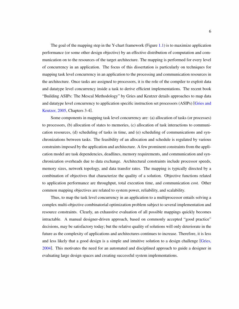
generally as scheduling methods. A partial taxonomy of well known scheduling methods is pre-

sented in Figure 1.2. A similar classification is found in the works of Casavant and Kuhl [Casavant

and Kuhl, 1988] and Kwok and Ahmad [Kwok and Ahmad, 1999b].

static dynamic

job scheduling

(independent tasks)

allocation and scheduling

(interacting tasks)

exact

enumerative integer-linear /

constraint

programming

randomized

evolutionary simulated

annealing

heuristic

list

scheduling

load

balancing /

clustering

scheduling methods

Figure 1.2: A partial taxonomy of methods for scheduling concurrent applications to multipleprocessors.

At the highest level, the taxonomy distinguishes between two categories of methods: (a) job

scheduling, and (b) allocation and scheduling. Job scheduling methods are relevant in the context

of regulating operations in factories and assembly lines. The goal is to distribute independent jobs

across multiple processing elements to optimize system performance [Coffman, 1976] [Lawler et

al., 1993]. In contrast, allocation and scheduling methods concern the execution of multiple in-

teracting tasks. The goal is to distribute interacting tasks to processing elements, and order and

schedule tasks and task interactions in time. The focus of this work is on allocation and schedul-

ing methods for interacting tasks. These methods are more pertinent to the problem of mapping

application task level concurrency to multiprocessors.

At the next level, allocation and scheduling methods can be differentiated based on the nature

8

of the execution and resource models associated with the scheduling problem. In static scheduling,

the scheduling method makes decisions before the start of application execution based on represen-

tative and reliable models of the concurrent application and target architecture. The scheduling is

performed at “compile time” and the result is used to deploy the application. In contrast, a dynamic

scheduling method makes decisions at “run time” as the application executes. It does not assume

knowledge about future task activations and dependencies when scheduling a set of active tasks and

hence recomputes schedules on-the-fly.

In this dissertation, we study methods to statically schedule concurrent tasks to multiple pro-

cessors. Static models and methods are applicable when deterministic average or worst case be-

havior is a reasonable assumption for the system under evaluation. When the application workload

and concurrent tasks are known at compile time, it is viable to determine an application mapping

statically. Lee and Messerschmitt argue that the run time overhead of dynamic scheduling may be

prohibitive in some real time or cost sensitive applications [Lee and Messerschmitt, 1987b]. Fur-

thermore, some applications that enforce hard timing deadlines may not tolerate schedule alterations

at run time. In these cases, compile time validation of an allocation and schedule is more crucial

than execution performance. Several applications in the signal processing and network processing

domain are amenable to static scheduling [Sih and Lee, 1993] [Shah et al., 2004]. The static models

are derived from analytical evaluations of application behavior, or through extensive simulations

and profilings of application run time characteristics on the target platform.

Static methods are also relevant to rapid design space exploration (DSE) for micro-architectures

and systems, as embodied in the Y-chart approach (Figure 1.1). In many situations, building an exe-

cutable model of the system might be too costly or even impossible at the time of exploration. Static

models and methods ease early design decisions by quickly restricting the space of interesting sys-

tem configurations [Gries, 2004].

1.2.2 Complexity of Static Scheduling

While static scheduling methods are integral to concurrent application deployment and design

space exploration frameworks, the scheduling problem itself is not easy to solve. In terms of the-

oretical complexity, the scheduling problem is NP-COMPLETE for most practical variants, barring

a few simplified cases [Garey and Johnson, 1979] [Graham et al., 1979] [Lawler et al., 1993]. For

instance, consider the following optimization problem of scheduling a set of dependent tasks on

a fully connected multiprocessor. The concurrent application is represented by a directed acyclic

9

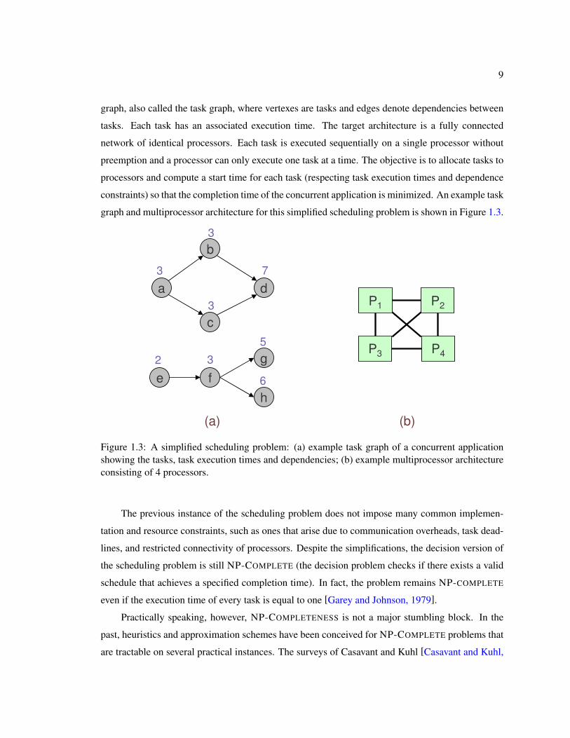
graph, also called the task graph, where vertexes are tasks and edges denote dependencies between

tasks. Each task has an associated execution time. The target architecture is a fully connected

network of identical processors. Each task is executed sequentially on a single processor without

preemption and a processor can only execute one task at a time. The objective is to allocate tasks to

processors and compute a start time for each task (respecting task execution times and dependence

constraints) so that the completion time of the concurrent application is minimized. An example task

graph and multiprocessor architecture for this simplified scheduling problem is shown in Figure 1.3.

P1 P2

P3 P4

a

b

c

d

g

h

fe

3

3

3

7

2 3

5

6

(a) (b)

Figure 1.3: A simplified scheduling problem: (a) example task graph of a concurrent applicationshowing the tasks, task execution times and dependencies; (b) example multiprocessor architectureconsisting of 4 processors.

The previous instance of the scheduling problem does not impose many common implemen-

tation and resource constraints, such as ones that arise due to communication overheads, task dead-

lines, and restricted connectivity of processors. Despite the simplifications, the decision version of

the scheduling problem is still NP-COMPLETE (the decision problem checks if there exists a valid

schedule that achieves a specified completion time). In fact, the problem remains NP-COMPLETE

even if the execution time of every task is equal to one [Garey and Johnson, 1979].

Practically speaking, however, NP-COMPLETENESS is not a major stumbling block. In the

past, heuristics and approximation schemes have been conceived for NP-COMPLETE problems that

are tractable on several practical instances. The surveys of Casavant and Kuhl [Casavant and Kuhl,

10

1988] and Kwok and Ahmad [Kwok and Ahmad, 1999b] point to specialized algorithms from pre-

vious research literature that are computationally efficient for several static scheduling problems.

But besides computational efficiency of the scheduling method, another desired characteristic

is flexibility: a practical mapping and exploration framework should consist of a scheduling method

that is capable of accommodating various types of constraints. The basic problem is to allocate

tasks to processors and compute start times for tasks, as in the example in Figure 1.3. In a prac-

tical setting, however, this problem is complicated by a variety of constraints from the application

and architecture that determine the feasibility of a schedule. For example, the application may

impose constraints related to synchronization, deadlines, task affinities, communication overheads,

and memory needs over the basic scheduling problem. Similarly, the architecture may impose con-

straints on task allocations, processor speeds, and network topologies. Moreover, in design space

exploration, the result of a certain mapping introduces new restrictions on the application and ar-

chitecture models. The human designer may also offer insight into the problem in the form of

additional constraints or secondary objectives to guide exploration. The scheduling method should

be flexible to incorporate new problem constraints and objectives for it to be viable in a practical

mapping framework.

1.2.3 Common Methods for Static Scheduling

Following back to the taxonomy of scheduling methods in Figure 1.2, many different methods

have been studied for static scheduling. The diversity of methods attests to the theoretical complex-

ity of the problem as well as the need to cope with different models, constraints, and objectives. We

identify three primary metrics to compare and evaluate different scheduling methods:

• Efficiency (related to speed, memory utilization, and other computational characteristics of a

method).

• Quality of results (related to how well a method, independent of computational efficiency, can

certify optimality of the solution or guarantee lower and upper bounds for it).

• Flexibility (related to ease of problem specification and extensibility of a method to incorpo-

rate diverse constraints).

It is clear that these metrics are conflicting and this motivates the study of different methods that

trade off one metric over another. Scheduling methods fall under three broad classes: heuristic,

randomized, and exact methods.

11

Heuristic methods

Heuristic methods are typically the most computationally efficient. Heuristics based on list

scheduling and load balancing have been popularly studied for several variants of the scheduling

problem [Coffman, 1976] [Hu, 1961] [Sih and Lee, 1993] [Gerasoulis and Yang, 1992] [Hoang

and Rabaey, 1993]. Common heuristics are greedy or “short-sighted” and provide no guarantee

of optimality; rather, they are intended to deliver acceptable results in a short amount of time. In

most cases, experimental studies are used to demonstrate their computational efficiency and quality

of results. However, a limitation of most heuristic methods is that they are not easily extensible

to account for varied implementation and resource constraints that arise in practical scheduling

problems. They are customized for a specific problem, trading off flexibility for efficiency, and

will have to be reworked each time new assumptions or constraints are imposed. In practice, it

is invariably the scheduling problem instance that is reworked to fit the models assumed by the

heuristic.

Randomized methods

In contrast to greedy heuristics, randomized methods use search techniques that retain a global

view of the solution space and are more flexible in handling different types of constraints and ob-

jectives. Evolutionary algorithms are randomized methods that have been applied to solve combi-

natorial optimization problems like scheduling [Dhodhi et al., 2002] [Grajcar, 1999]. The search

technique is based on concepts from biological evolution: the idea is to iteratively track the “fittest”

solutions based on a cost function, while allowing random “mutations” to evolve new solutions.

Simulated annealing is another randomized method that has been used for many complex optimiza-

tion problems [Kirkpatrick et al., 1983] [Devadas and Newton, 1989] [Orsila et al., 2006]. The

algorithm probabilistically transitions between different states in the solution space; the probabil-

ities and annealing schedule are geared to guide the algorithm into states which represent good

solutions. The randomness averts the search from becoming stuck at local minima, which are the

bane of greedy heuristics. However, the potential of randomized methods to locate good solutions

comes at an expense of longer running time. Further, the quality of results becomes less predictable

if the cost functions or transition probabilities are not finely tuned to ensure stabilization of the

stochastic behavior.

12

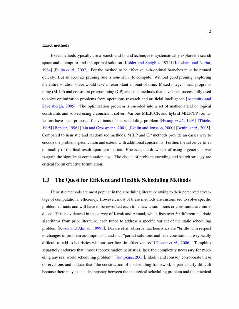
Exact methods

Exact methods typically use a branch-and-bound technique to systematically explore the search

space and attempt to find the optimal solution [Kohler and Steiglitz, 1974] [Kasahara and Narita,

1984] [Fujita et al., 2002]. For the method to be effective, sub-optimal branches must be pruned

quickly. But an accurate pruning rule is non-trivial to compute. Without good pruning, exploring

the entire solution space would take an exorbitant amount of time. Mixed integer linear program-

ming (MILP) and constraint programming (CP) are exact methods that have been successfully used

to solve optimization problems from operations research and artificial intelligence [Atamturk and

Savelsbergh, 2005]. The optimization problem is encoded into a set of mathematical or logical

constraints and solved using a constraint solver. Various MILP, CP, and hybrid MILP/CP formu-

lations have been proposed for variants of the scheduling problem [Hwang et al., 1991] [Thiele,

1995] [Bender, 1996] [Jain and Grossmann, 2001] [Ekelin and Jonsson, 2000] [Benini et al., 2005].

Compared to heuristic and randomized methods, MILP and CP methods provide an easier way to

encode the problem specification and extend with additional constraints. Further, the solver certifies

optimality of the final result upon termination. However, the drawback of using a generic solver

is again the significant computation cost. The choice of problem encoding and search strategy are

critical for an effective formulation.

1.3 The Quest for Efficient and Flexible Scheduling Methods

Heuristic methods are most popular in the scheduling literature owing to their perceived advan-

tage of computational efficiency. However, most of these methods are customized to solve specific

problem variants and will have to be reworked each time new assumptions or constraints are intro-

duced. This is evidenced in the survey of Kwok and Ahmad, which lists over 30 different heuristic

algorithms from prior literature, each tuned to address a specific variant of the static scheduling

problem [Kwok and Ahmad, 1999b]. Davare et al. observe that heuristics are “brittle with respect

to changes in problem assumptions”, and that “partial solutions and side constraints are typically

difficult to add to heuristics without sacrifices in effectiveness” [Davare et al., 2006]. Tompkins

separately endorses that “most (approximation heuristics) lack the complexity necessary for mod-

eling any real world scheduling problem” [Tompkins, 2003]. Ekelin and Jonsson corroborate these

observations and adduce that “the construction of a scheduling framework is particularly difficult

because there may exist a discrepancy between the theoretical scheduling problem and the practical

13

aspects of the system being designed” [Ekelin and Jonsson, 2000].

We contend that a mapping and exploration framework for deploying concurrent applications

on multiprocessor platforms should consist of scheduling methods that not only have tractable run

time complexity, but also offer expressibility and flexibility in modeling diverse constraints. In

particular, the following characteristics are desired for practical scheduling methods:

• They must be computationally efficient on realistic problems.

• They must find optimal or near-optimal solutions.

• They must reliably capture the intended problem specification and flexibly accommodate di-

verse constraints and objectives.

This dissertation is an attempt to develop insight into efficient and flexible methods that are vi-

able for scheduling problems that arise in a practical concurrent application deployment and design

space exploration framework. We conduct this study in four parts. First, we analyze the nature of

the scheduling problems that arise in a realistic mapping and exploration framework. The frame-

work under study maps network processing applications to Intel IXP network processors and Xilinx

FPGA based soft multiprocessors [Intel Corp., 2001b] [Xilinx Inc., 2004]. This is the content of

Chapter 2.

Second, based on this study, we classify important features and constraints that are typically

part of the application and architecture models associated with the mapping problem. We then

survey competitive heuristic, randomized, and exact methods for practical scheduling problems.

We also examine existing exploration frameworks and their approaches to the mapping problem.

This is the content of Chapter 3.

Third, we focus in detail on methods based on mixed integer linear programming (MILP) and

constraint programming (CP). We formalize a representative scheduling problem that arises in our

framework for deploying network processing applications. We then derive an MILP formulation

for this problem and evaluate its viability on practical scheduling instances. This is the content of

Chapter 4.

The ease of problem specification and flexibility are inherent advantages of these methods.

Further, to improve the computational efficiency of constraint methods, we advance techniques for

accelerating the search performed by the solver:

• Alternate MILP and CP formulations with tighter constraints and bounds.

14

• A “master-sub” problem decomposition to accelerate search, in the manner of the Benders

decomposition problem solving strategy [Benders, 1962] [Geoffrion, 1972].

• Search guidance through heuristic methods.

• Tight lower bound derivations to prune inferior solutions early in the search.

We believe these techniques are applicable to most variants of the scheduling problem. The inherent

flexibility combined with improved search strategies posit mathematical and constraint program-

ming methods as powerful tools for practical mapping problems. This is the content of Chapter 5.

Finally, we present a comprehensive view of a toolbox of methods that are applicable for

realistic mapping problems. We do not expect that a single method will be successful for all op-

timization problems that may arise in a practical mapping and exploration framework. The nature

of the constraints and optimization objectives would determine the appropriate scheduling method.

Our toolbox is a collection of multiple heuristic methods, specialized constraint programming for-

mulations, and simulated annealing techniques. These methods provide different trade-offs with

respect to computational efficiency, quality of results, and flexibility. We present our insights on

how to choose the right method for a problem and how to tune it for effective performance. This is

the content of Chapter 6.

1.4 Contributions of this Dissertation

We identify three main contributions of this dissertation. First, we demonstrate the viability

of mathematical and constraint programming methods for scheduling problems that arise in a prac-

tical mapping and exploration framework. Constraint methods can flexibly accommodate diverse

constraints and guarantee optimality of the final solution. However, the computational efficiency

of these methods rapidly deteriorates as the problem instances increase in size. To alleviate this

difficulty, we propose a decomposition based problem solving strategy to accelerate the search in a

constraint solver for a representative scheduling problem. In the manner of Benders decomposition,

the scheduling problem is divided into “master” and “sub” problems, which are then iteratively

solved in a coordinated manner [Benders, 1962] [Hooker and Ottosson, 1999]. Prior constraint

formulations for a representative problem are not effective on instances with over 30 application

tasks. In contrast, a constraint formulation coupled with our decomposition strategy computes near-

optimal solutions efficiently on instances with over 150 tasks. Thus, decomposition based constraint

15

programming is a flexible solution method that has significant potential for many variants of the

scheduling problem.

Second, we advance a toolbox of scheduling methods for a representative problem, in which

each method is effective for a certain class of problem models or optimization objectives. Our

toolbox comprises of multiple heuristic methods, mathematical and constraint programming formu-

lations, and simulated annealing techniques. The premise for a toolbox of methods for a mapping

and exploration framework is to provide a selection of methods that differently trade-off computa-

tional efficiency, quality of results, and flexibility. This grants a facility to the system designer to

choose an appropriate method based on the problem requirements.

Third, we integrate our toolbox of scheduling methods in an Y-chart based automated map-

ping and exploration framework for deploying network processing applications on two embedded

platforms: Intel IXP network processors and Xilinx FPGA based soft multiprocessors [Intel Corp.,

2001b] [Xilinx Inc., 2004]. This exploration framework is a product of the MESCAL research group

in the Department of Electrical Engineering and Computer Sciences at the University of California

at Berkeley [Gries and Keutzer, 2005] [Plishker et al., 2004] [Jin et al., 2005]. The framework and

associated toolbox of scheduling methods are effective in productively achieving high-performance

implementations of common networking applications, such as IPv4 packet forwarding, Network

Address Translation, and Differentiated Services, on the two target platforms.

16

Chapter 2

A Framework for Mapping and Design

Space Exploration

The mapping step binds application functionality to architectural resources. It is integral to a

framework for concurrent application deployment and design space exploration. In this chapter, we

describe the rudiments of such a framework. Specifically, we present an exploration framework to

deploy network processing applications on two multiprocessor platforms: Intel IXP network pro-

cessors and Xilinx FPGA based soft multiprocessors. The study highlights the common problems

that arise in mapping the task level concurrency in an application to the processing elements and

communication resources in the target platform.

2.1 A Framework for Mapping and Exploration

An ideal framework for deploying concurrent applications on multiprocessor architectures

would enable a natural representation of application concurrency, efficient utilization of the ar-

chitectural resources, and fast solutions to the mapping problem. In Chapter 1, we presented the

concept of the Y-chart (Figure 1.1) for such a framework. The Y-chart approach begins with sep-

arate specifications of the concurrent application and multiprocessor architecture. The application

is bound to the architecture in a distinct mapping step. The result of the evaluation drives further

mapping iterations through modifications to the application or architecture. These iterative revi-

sions form the basis for systematic design space exploration. In the following sections, we examine

the properties of the application representation, architecture model, and mapping step in an ideal

concurrent application deployment and design space exploration framework.

17

2.1.1 Domain Specific Language for Application Representation

While C and C++ may be the most prevalent languages for developing embedded applications,

they do not naturally capture concurrency. An alternative is to adopt domain specific languages

(DSLs) to describe concurrent applications [Keutzer et al., 2000] [Lee, 2002] [Paulin et al., 2004]

[Sangiovanni-Vincentelli, 2007]. DSLs serve as an abstraction for representing the concurrency

indigenous to an application domain and enable a productive approach to design entry. They provide

component libraries and computation and communication models to express task, data, and datatype

level concurrency. DSL descriptions are also a good starting point for application level optimizations

and transformations. Further, they facilitate portability to multiple target platforms. For example,

Simulink is a DSL for capturing dynamic dataflow applications in digital signal processing [The

MathWorks Inc., 2005]. Simulink has associated simulation, visualization, and testing tools to

ease application development. Simulink applications are executed on conventional workstations

or ported to embedded multiprocessors in the automotive and communication domains. Click is

another actor oriented DSL for describing packet processing applications in the networking domain

[Kohler et al., 2000]. The individual actors in Click are C/C++ classes; the DSL simply provides a

layer of abstraction that enables an expression of the concurrency natural to the domain.

2.1.2 The Mapping Step

The mapping step starts with abstract models for the concurrent application and multiprocessor

architecture. The primary goal of the mapping step is to derive high-performance implementations

of the concurrent application on the target architecture. A secondary goal is to produce these im-

plementations quickly and facilitate many design iterations in the exploration framework. The main

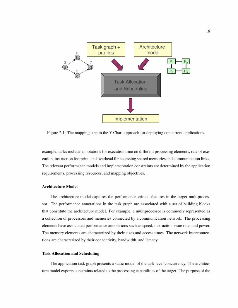
components of the mapping step in the Y-chart approach are summarized in Figure 2.1.

Application Task Graph

Domain specific languages enable productive design entry and portability for concurrent appli-

cations. The aim of the mapping step, however, is to derive an efficient implementation on a specific

architecture. The DSL description must hence be transformed into a model that is mappable to the

intended target. This model is called the task graph. The task graph exposes the concurrent tasks,

dependencies, and other application constraints requisite for an useful mapping. The task graph is

specific to a pairing of an application and architecture. It is composed of computational elements

and has associated performance and resource usage models for a particular target platform. For

18

P1 P2

P3 P4

Task Allocation

and Scheduling

Implementation

Architecture

modelTask graph +

profiles

a

b

c

d3 7

3

8

Figure 2.1: The mapping step in the Y-Chart approach for deploying concurrent applications.

example, tasks include annotations for execution time on different processing elements, rate of exe-

cution, instruction footprint, and overhead for accessing shared memories and communication links.

The relevant performance models and implementation constraints are determined by the application

requirements, processing resources, and mapping objectives.

Architecture Model

The architecture model captures the performance critical features in the target multiproces-

sor. The performance annotations in the task graph are associated with a set of building blocks

that constitute the architecture model. For example, a multiprocessor is commonly represented as

a collection of processors and memories connected by a communication network. The processing

elements have associated performance annotations such as speed, instruction issue rate, and power.

The memory elements are characterized by their sizes and access times. The network interconnec-

tions are characterized by their connectivity, bandwidth, and latency.

Task Allocation and Scheduling

The application task graph presents a static model of the task level concurrency. The architec-

ture model exports constraints related to the processing capabilities of the target. The purpose of the

19

mapping step is compute an allocation and schedule of the application task graph on the architecture

resources that respects the problem constraints and optimizes some combination of objectives. This

is typically a complex multi-objective combinatorial optimization problem. We focus in depth on

methods to solve these problems in the remaining chapters.

Implementation

The scheduling result specifies how the concurrent application must be mapped to the target

platform based on abstract task graph and architecture models. The last component in the mapping

step aims to derive an implementation from the scheduling result. The application task graph is

composed of elements from a library that is specific to the target multiprocessor platform. For

example, the tasks correspond to blocks of sequential code in a common programming language.

The allocation and schedule computed in the mapping step are realized by combining these blocks

of code and compiling them for individual processors to create executable specifications. The code

generation process also converts task interactions to memory and communication access routines in

the target platform.

2.1.3 Performance Analysis and Feedback

The mapping step generates an implementation of the concurrent application that is intended

for execution. The implementation may be executed on an instruction level or cycle accurate sim-

ulator, or directly on the hardware device. The last step in the Y-chart approach is a performance

analysis of the implementation. The performance analysis in turn initiates revisions to the applica-

tion and architecture models, or the mapping strategy itself. For instance, the designer can iteratively

revise the architecture model and validate questions, such as:

• How many processors are necessary for the application and workload?

• Is more interprocessor communication bandwidth necessary?

• What is a suitable processor topology?

• What are useful co-processors to improve performance?

Similarly, the designer can alter the application and address design questions, such as:

• Is there a different application description that increases task level concurrency?

20

• Is a decomposition with smaller granularity tasks suitable for the application?

• Should certain tasks be clustered to improve performance?

• What is a suitable computation to communication ratio for the application?

2.2 The Network Processing Domain: Applications and Platforms

The previous sections outlined the components of a general framework for concurrent applica-

tion deployment and design space exploration. We now present a realization of such a framework

for deploying network processing applications on two multiprocessor target platforms: (a) Intel IXP

network processors [Intel Corp., 2001b], and (b) Xilinx FPGA based soft multiprocessors [Xilinx

Inc., 2004].

Network processing has been a popular domain for embedded systems research and innovation.

There are varieties of applications that span different parts of the network and different layers of the

protocol stack. The demand for high performance coupled with the need to adhere to rapidly chang-

ing specifications has necessitated adoption of programmable multiprocessor systems. The past

eight years have witnessed over 30 different design offerings for programmable network processing

architectures [Shah, 2004].

Typical network processing applications exhibit a high degree of task, data, and datatype level

concurrency. Multiple independent streams of packets are in flux in a router, and multiple inde-

pendent tasks operate on a single packet: this proffers several opportunities to exploit task level

concurrency. Tasks frequently perform independent computations on several different fields within

a single packet header, which is a form of data level concurrency. Packet processing tasks also use

custom mathematical operations (such as checksum or hash function calculations) on custom data

types (such as irregular packet header fields), and this is a form of bit level concurrency [Mihal,

2006]. The challenge then is to derive efficient implementations of concurrent network process-

ing applications on multiprocessor platforms, which motivates incorporation of a Y-chart based

mapping and exploration framework. Thus, the diversity of architectures, applications, and pro-

gramming approaches makes networking an interesting niche to explore key problems related to

concurrent application deployment.

21

2.2.1 Network Processing Applications

There are several popular application benchmarks to evaluate the performance of network pro-

cessing devices. In the following subsections, we describe two common benchmarks: IPv4 packet

forwarding and Differentiated Services (DiffServ). We later use these applications to demonstrate

the viability of our framework and scheduling methods in Section 4.3 .

IPv4 Packet Forwarding

The IPv4 packet forwarding application runs at the core of network routers and forwards pack-

ets to their final destinations [Baker, 1995]. The forwarding decision consists of finding the next

hop address and egress port to which a packet should be sent. The decision depends only on the

contents of the IP header. The data plane of the application involves three operations: (a) receive

packet and check its validity by examining the checksum, header length, and IP version, (b) find

the next hop and egress port by performing a longest prefix match lookup in the route table using

the destination address, and (c) update header checksum and time-to-live fields (TTL), recombine

header with payload, and forward the packet on the appropriate port.

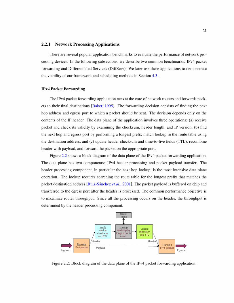
Figure 2.2 shows a block diagram of the data plane of the IPv4 packet forwarding application.

The data plane has two components: IPv4 header processing and packet payload transfer. The

header processing component, in particular the next hop lookup, is the most intensive data plane

operation. The lookup requires searching the route table for the longest prefix that matches the

packet destination address [Ruiz-Sanchez et al., 2001]. The packet payload is buffered on chip and

transferred to the egress port after the header is processed. The common performance objective is

to maximize router throughput. Since all the processing occurs on the header, the throughput is

determined by the header processing component.

Lookup

next-hop by

longest prefix

match

Receive

IPv4 packet

Verify

version,

checksum

and TTL

Update

checksum

and TTL

Transmit

IPv4 packet

Header

PayloadIngress Egress

Route

Table

Header

Figure 2.2: Block diagram of the data plane of the IPv4 packet forwarding application.

22

Differentiated Services

Differentiated Services (DiffServ) extends the basic IPv4 packet forwarding application and

specifies a coarse grained mechanism to manage network traffic and guarantee quality of service

(QoS) [Blake et al., 1998]. For example, DiffServ can be used to ensure low-latency guaranteed

service to critical network traffic such as voice or video, while providing simple best effort traffic

guarantees to less critical services such as web traffic or file transfers. Interior nodes of the network

apply different per-hop behaviors to various traffic classes. The common behavior classes are: (a)

best effort: no guarantees of packet loss or latency; (b) assured forwarding: 4 classes of traffic with

varying degrees of loss and latency; (c) expedited forwarding: low packet loss and latency. Routers

are augmented with special schedulers for each packet class and bandwidth metering mechanisms

to police the traffic. The performance objective is again to maximize router throughput.

2.2.2 Intel IXP Network Processors

We now briefly review the target multiprocessor platforms that are part of our exploration

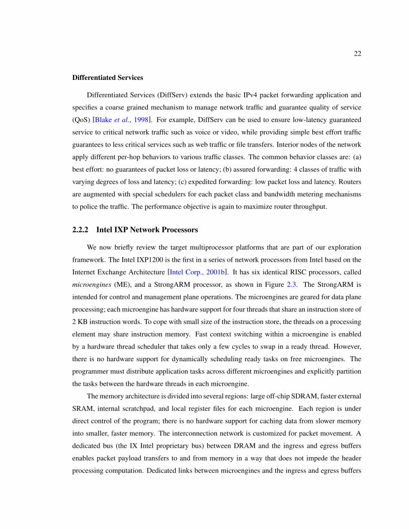
framework. The Intel IXP1200 is the first in a series of network processors from Intel based on the

Internet Exchange Architecture [Intel Corp., 2001b]. It has six identical RISC processors, called

microengines (ME), and a StrongARM processor, as shown in Figure 2.3. The StrongARM is

intended for control and management plane operations. The microengines are geared for data plane

processing; each microengine has hardware support for four threads that share an instruction store of

2 KB instruction words. To cope with small size of the instruction store, the threads on a processing

element may share instruction memory. Fast context switching within a microengine is enabled

by a hardware thread scheduler that takes only a few cycles to swap in a ready thread. However,

there is no hardware support for dynamically scheduling ready tasks on free microengines. The

programmer must distribute application tasks across different microengines and explicitly partition

the tasks between the hardware threads in each microengine.

The memory architecture is divided into several regions: large off-chip SDRAM, faster external

SRAM, internal scratchpad, and local register files for each microengine. Each region is under

direct control of the program; there is no hardware support for caching data from slower memory

into smaller, faster memory. The interconnection network is customized for packet movement. A

dedicated bus (the IX Intel proprietary bus) between DRAM and the ingress and egress buffers

enables packet payload transfers to and from memory in a way that does not impede the header

processing computation. Dedicated links between microengines and the ingress and egress buffers

23

SDRAM Bus

64-bit

32-bit

SDRAMController

PCIInterface

32-bitSRAM

Controller

µ-engine 1

StrongARM

(166 MHz)

16 KB

I-Cache

µ-engine 2

µ-engine 3

µ-engine 4

µ-engine 5

µ-engine 6

64-bit

HashEngine

IX Bus

ScratchPadSRAM

TF

IFO

CSR

FBIEngine

I/F

RF

IFO

1 KB MiniD-Cache

8 KBD-Cache

SRAM Bus

Command Bus

Figure 2.3: Block diagram of the Intel IXP1200 network processor architecture.

allow packet headers to be moved directly to the register files for immediate access.

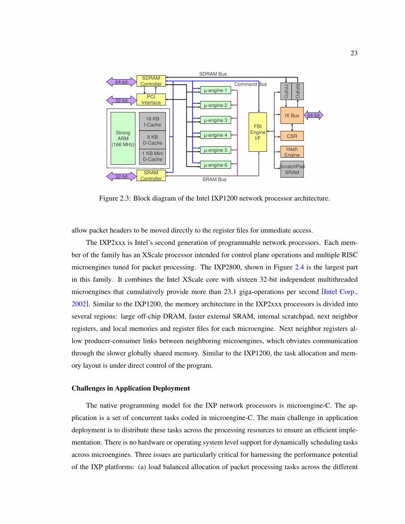
The IXP2xxx is Intel’s second generation of programmable network processors. Each mem-

ber of the family has an XScale processor intended for control plane operations and multiple RISC

microengines tuned for packet processing. The IXP2800, shown in Figure 2.4 is the largest part

in this family. It combines the Intel XScale core with sixteen 32-bit independent multithreaded

microengines that cumulatively provide more than 23.1 giga-operations per second [Intel Corp.,

2002]. Similar to the IXP1200, the memory architecture in the IXP2xxx processors is divided into

several regions: large off-chip DRAM, faster external SRAM, internal scratchpad, next neighbor

registers, and local memories and register files for each microengine. Next neighbor registers al-

low producer-consumer links between neighboring microengines, which obviates communication

through the slower globally shared memory. Similar to the IXP1200, the task allocation and mem-

ory layout is under direct control of the program.

Challenges in Application Deployment

The native programming model for the IXP network processors is microengine-C. The ap-

plication is a set of concurrent tasks coded in microengine-C. The main challenge in application

deployment is to distribute these tasks across the processing resources to ensure an efficient imple-

mentation. There is no hardware or operating system level support for dynamically scheduling tasks

across microengines. Three issues are particularly critical for harnessing the performance potential

of the IXP platforms: (a) load balanced allocation of packet processing tasks across the different

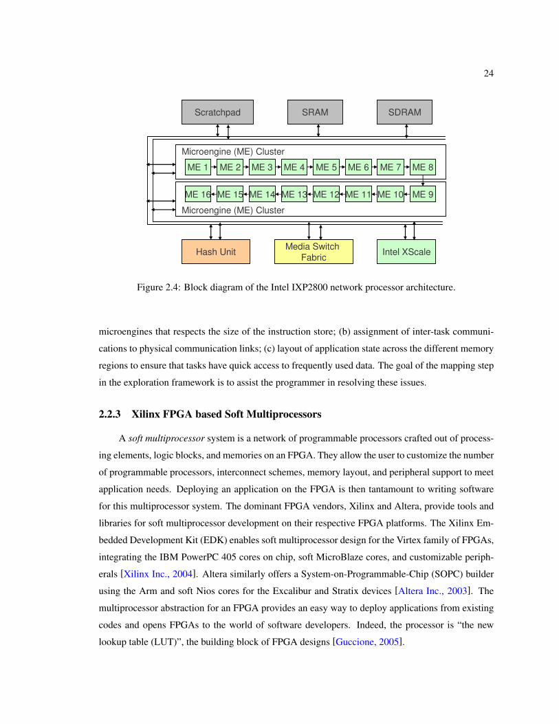
24

Microengine (ME) Cluster

Microengine (ME) Cluster

Scratchpad SRAM SDRAM

Hash UnitMedia Switch

FabricIntel XScale

ME 1 ME 2 ME 3 ME 4 ME 5 ME 6 ME 7 ME 8

ME 16 ME 15 ME 14 ME 13 ME 12 ME 11 ME 10 ME 9

Figure 2.4: Block diagram of the Intel IXP2800 network processor architecture.

microengines that respects the size of the instruction store; (b) assignment of inter-task communi-

cations to physical communication links; (c) layout of application state across the different memory

regions to ensure that tasks have quick access to frequently used data. The goal of the mapping step

in the exploration framework is to assist the programmer in resolving these issues.

2.2.3 Xilinx FPGA based Soft Multiprocessors

A soft multiprocessor system is a network of programmable processors crafted out of process-

ing elements, logic blocks, and memories on an FPGA. They allow the user to customize the number

of programmable processors, interconnect schemes, memory layout, and peripheral support to meet

application needs. Deploying an application on the FPGA is then tantamount to writing software

for this multiprocessor system. The dominant FPGA vendors, Xilinx and Altera, provide tools and

libraries for soft multiprocessor development on their respective FPGA platforms. The Xilinx Em-

bedded Development Kit (EDK) enables soft multiprocessor design for the Virtex family of FPGAs,

integrating the IBM PowerPC 405 cores on chip, soft MicroBlaze cores, and customizable periph-

erals [Xilinx Inc., 2004]. Altera similarly offers a System-on-Programmable-Chip (SOPC) builder

using the Arm and soft Nios cores for the Excalibur and Stratix devices [Altera Inc., 2003]. The

multiprocessor abstraction for an FPGA provides an easy way to deploy applications from existing

codes and opens FPGAs to the world of software developers. Indeed, the processor is “the new

lookup table (LUT)”, the building block of FPGA designs [Guccione, 2005].

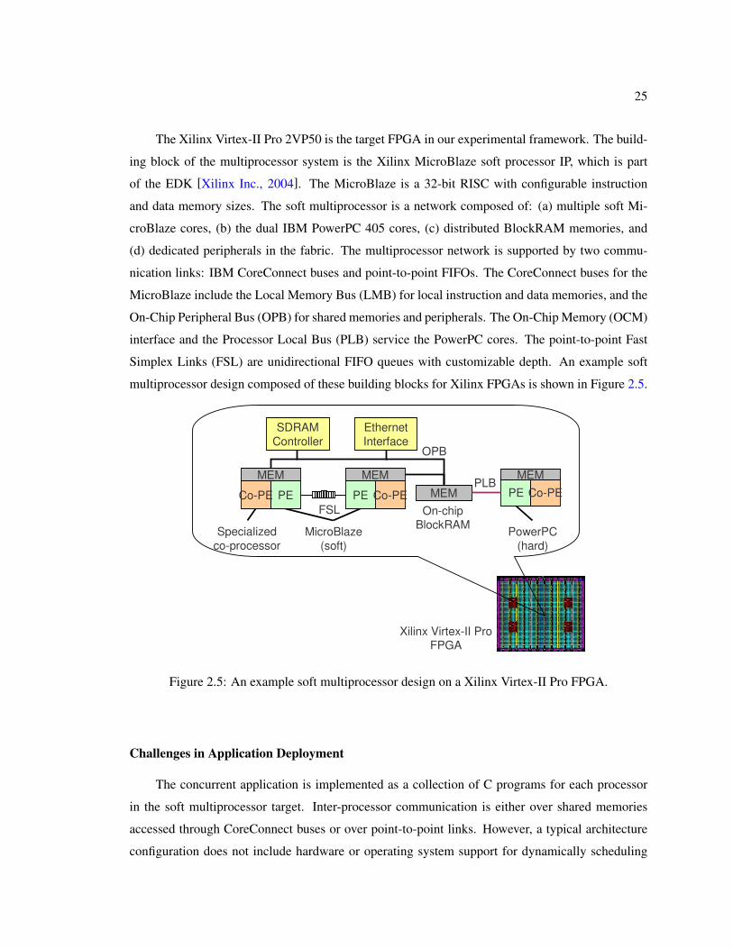
25

The Xilinx Virtex-II Pro 2VP50 is the target FPGA in our experimental framework. The build-

ing block of the multiprocessor system is the Xilinx MicroBlaze soft processor IP, which is part

of the EDK [Xilinx Inc., 2004]. The MicroBlaze is a 32-bit RISC with configurable instruction

and data memory sizes. The soft multiprocessor is a network composed of: (a) multiple soft Mi-

croBlaze cores, (b) the dual IBM PowerPC 405 cores, (c) distributed BlockRAM memories, and

(d) dedicated peripherals in the fabric. The multiprocessor network is supported by two commu-

nication links: IBM CoreConnect buses and point-to-point FIFOs. The CoreConnect buses for the

MicroBlaze include the Local Memory Bus (LMB) for local instruction and data memories, and the

On-Chip Peripheral Bus (OPB) for shared memories and peripherals. The On-Chip Memory (OCM)

interface and the Processor Local Bus (PLB) service the PowerPC cores. The point-to-point Fast

Simplex Links (FSL) are unidirectional FIFO queues with customizable depth. An example soft

multiprocessor design composed of these building blocks for Xilinx FPGAs is shown in Figure 2.5.

PowerPC

(hard)

MicroBlaze

(soft)

FSL

OPB

PLB

Specialized

co-processor

On-chip BlockRAM

PECo-PE PE Co-PE

MEM MEM

MEM PE Co-PE

MEM

Ethernet

Interface

SDRAM

Controller

Xilinx Virtex-II Pro FPGA

Figure 2.5: An example soft multiprocessor design on a Xilinx Virtex-II Pro FPGA.

Challenges in Application Deployment

The concurrent application is implemented as a collection of C programs for each processor

in the soft multiprocessor target. Inter-processor communication is either over shared memories

accessed through CoreConnect buses or over point-to-point links. However, a typical architecture

configuration does not include hardware or operating system support for dynamically scheduling

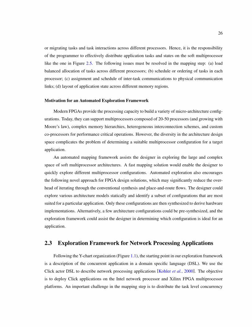
26

or migrating tasks and task interactions across different processors. Hence, it is the responsibility

of the programmer to effectively distribute application tasks and states on the soft multiprocessor

like the one in Figure 2.5. The following issues must be resolved in the mapping step: (a) load

balanced allocation of tasks across different processors; (b) schedule or ordering of tasks in each

processor; (c) assignment and schedule of inter-task communications to physical communication

links; (d) layout of application state across different memory regions.

Motivation for an Automated Exploration Framework

Modern FPGAs provide the processing capacity to build a variety of micro-architecture config-

urations. Today, they can support multiprocessors composed of 20-50 processors (and growing with

Moore’s law), complex memory hierarchies, heterogeneous interconnection schemes, and custom

co-processors for performance critical operations. However, the diversity in the architecture design

space complicates the problem of determining a suitable multiprocessor configuration for a target

application.

An automated mapping framework assists the designer in exploring the large and complex

space of soft multiprocessor architectures. A fast mapping solution would enable the designer to

quickly explore different multiprocessor configurations. Automated exploration also encourages

the following novel approach for FPGA design solutions, which may significantly reduce the over-

head of iterating through the conventional synthesis and place-and-route flows. The designer could

explore various architecture models statically and identify a subset of configurations that are most

suited for a particular application. Only these configurations are then synthesized to derive hardware

implementations. Alternatively, a few architecture configurations could be pre-synthesized, and the

exploration framework could assist the designer in determining which configuration is ideal for an

application.

2.3 Exploration Framework for Network Processing Applications

Following the Y-chart organization (Figure 1.1), the starting point in our exploration framework

is a description of the concurrent application in a domain specific language (DSL). We use the

Click actor DSL to describe network processing applications [Kohler et al., 2000]. The objective

is to deploy Click applications on the Intel network processor and Xilinx FPGA multiprocessor

platforms. An important challenge in the mapping step is to distribute the task level concurrency

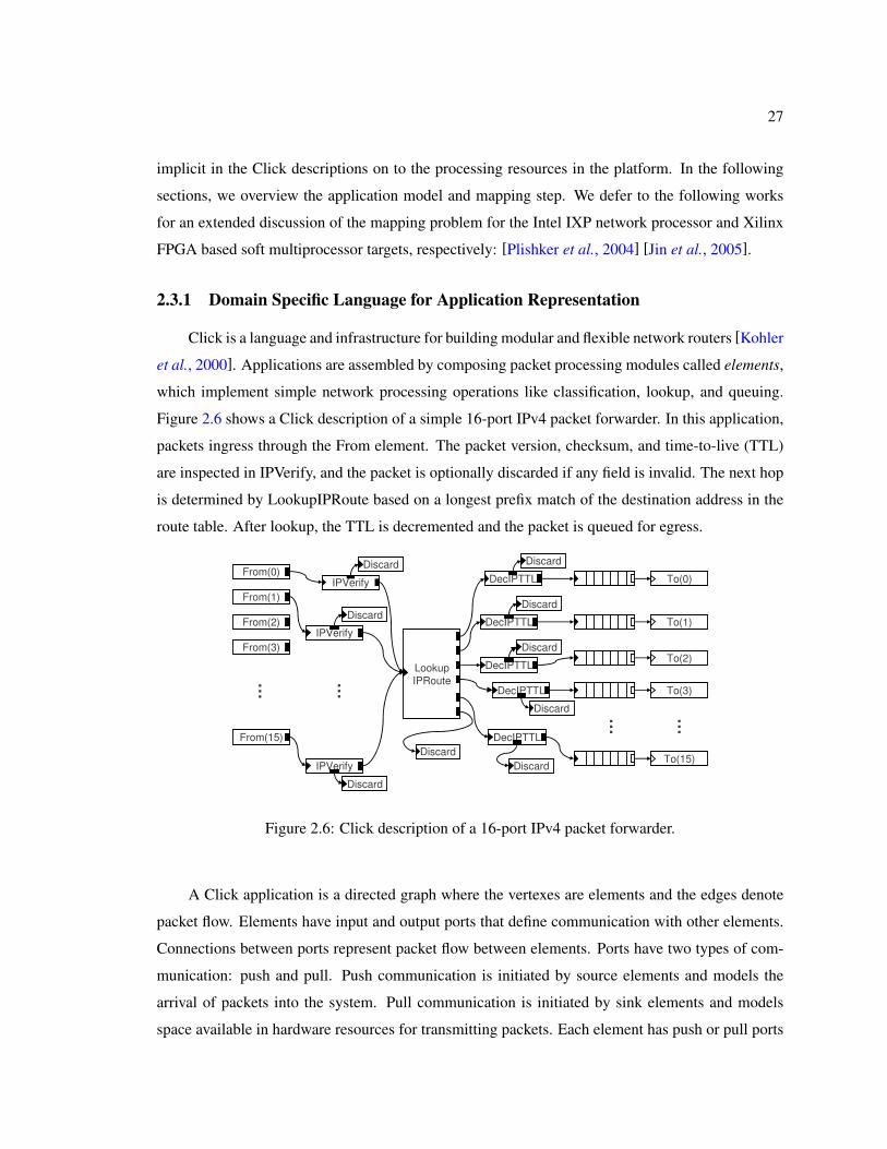
27

implicit in the Click descriptions on to the processing resources in the platform. In the following

sections, we overview the application model and mapping step. We defer to the following works

for an extended discussion of the mapping problem for the Intel IXP network processor and Xilinx

FPGA based soft multiprocessor targets, respectively: [Plishker et al., 2004] [Jin et al., 2005].

2.3.1 Domain Specific Language for Application Representation

Click is a language and infrastructure for building modular and flexible network routers [Kohler

et al., 2000]. Applications are assembled by composing packet processing modules called elements,

which implement simple network processing operations like classification, lookup, and queuing.

Figure 2.6 shows a Click description of a simple 16-port IPv4 packet forwarder. In this application,

packets ingress through the From element. The packet version, checksum, and time-to-live (TTL)

are inspected in IPVerify, and the packet is optionally discarded if any field is invalid. The next hop

is determined by LookupIPRoute based on a longest prefix match of the destination address in the

route table. After lookup, the TTL is decremented and the packet is queued for egress.

From(0)Discard

To(0)

From(1)

From(2)

From(3)

Discard

To(1)

To(2)

To(3)

Discard

…

From(15)

Lookup

IPRoute

To(15)

… …

IPVerify DecIPTTL

DiscardDiscard

IPVerifyDecIPTTL

Discard

DiscardIPVerify

DecIPTTL

…

Discard

DecIPTTL

Discard

DecIPTTL

Figure 2.6: Click description of a 16-port IPv4 packet forwarder.

A Click application is a directed graph where the vertexes are elements and the edges denote

packet flow. Elements have input and output ports that define communication with other elements.

Connections between ports represent packet flow between elements. Ports have two types of com-

munication: push and pull. Push communication is initiated by source elements and models the

arrival of packets into the system. Pull communication is initiated by sink elements and models

space available in hardware resources for transmitting packets. Each element has push or pull ports

28

that may be composed with other elements to form exclusive push or pull chains. The individual

chains can execute concurrently, while elements along a particular chain must execute in sequence

for every incoming packet.

Click was originally conceived for single processor systems running Linux. It consists of a li-

brary of C++ classes to define element behaviors, and communications are implemented with virtual

function calls [Kohler et al., 2002]. However, Click descriptions naturally extend to multiprocessor

systems. The push and pull chains form independent computational paths in the graph and expose

the task level concurrency in the application. Shah et al. concur that “significant concurrency may

be gleamed from Click designs in which the application designer has made no special effort to ex-

press it” [Shah et al., 2003]. Thus, the motivations for using Click to describe network processing

applications are: (a) Click provides an productive way to describe and optimize general packet pro-

cessing applications, and (b) it exposes the task level concurrency in an application, which enables

deployment on multiprocessor targets.

2.3.2 The Mapping Step

The Click DSL enables productive design entry of concurrent network processing applications.

The network processor and FPGA platforms provide multiprocessing resources and are capable of

high performance. However, the DSL description does not imply any obvious distribution of the

task level concurrency on to the architectural resources. This behooves an explicit mapping step

composed of the components shown in Figure 2.1. In the following subsections, we informally

discuss these components in the context of our exploration framework. Chapter 4 contains a formal

presentation of the task graph, architecture model, and representative scheduling problem.

Task Graph Models from Click Applications

The Click application description exposes concurrent tasks and dependencies. The simplest

task graph is hence identical to the Click application graph. The static performance model associated

with the task graph is derived by profiling the individual tasks on the target processors, either in

simulation, or by execution on the target hardware. Common performance annotations for the tasks

are execution time and instruction and data footprint size. The dependence edges between tasks are

annotated with the amount of data transferred over the edge.

29

Multiprocessor Architecture Model for the Target Platform

The architecture model is a network of processors and memories interconnected in a specific

topology. For instance, the IXP1200 (Figure 2.3) is a fully connected network of 6 microengines,

and all the processors and links are homogeneous. The soft multiprocessor architectures like the

one in Figure 2.5 are more restricted topologies. The processing elements in the architecture model

are annotated with their type, execution rates, and instruction and data memory sizes. The commu-

nication links are annotated with their latency and bandwidth.

Task Allocation and Scheduling

The basic mapping problem relevant to our framework is to allocate application tasks to pro-

cessors and compute a start time for each task (respecting task execution times and dependence

constraints) so that the completion time of the concurrent program is minimized. A common op-

timization objective in mapping network processing applications is to maximize throughput. Al-

ternate objectives are to minimize end-to-end latency or to minimize average communication cost.

Two additional considerations for the mapping problem are the scheduling of inter-task communi-

cations on physical communication resources and assignment of task states to distributed memories

in the architecture.

The mapping problem is beset with various implementation and resource constraints imposed

by the application and architecture. Implementation constraints from the application include task

deadlines, task release times, relative timing constraints, mutual exclusions, preferred allocations of

tasks, task clusterings, and task anti-clusterings. Resource constraints from the architecture include

multiprocessor topology, data memory limits, instruction store limits, and access restrictions for

shared resources. Section 4.1 formalizes the scheduling problems that arise in our framework.

Implementation

The last component of the mapping step is to synthesize an implementation on the target plat-

form based on the derived allocation and schedule. A single block of code is generated for each

processor by combining the tasks allocated on it. The code generation step additionally translates

communications between tasks to respective access routines for the interprocessor network. For the

IXP target, interacting tasks may communicate over shared registers, scratchpad, or external mem-

ory. For the soft multiprocessor target, if interacting tasks are assigned to the same processor, the

communication is always over memory local to that processor. However, if the interacting tasks are

30

assigned to different processors, the communication is either over shared memory or point-to-point

links. The code blocks for each processor are subsequently compiled to create executables for the

target platform.

The scheduling component computes a fully static schedule that prescribes the start times of

tasks. In practice however, self-timed schedules are more suitable on the two hardware targets.

Self-timed schedules are derived from fully static schedules by discarding start time specifications

and adding synchronization primitives to regulate task initiations and terminations [Poplavko et al.,

2003]. Hence, the implementation retains the allocation and ordering stipulated by the schedule,

but allows flexibility in the execution of individual tasks.

2.3.3 Performance Analysis and Feedback

The Intel IXP network processors have an associated simulation environment on which the

performance of the implementations are analyzed. Implementations for the soft multiprocessor

target are directly synthesized on to the Virtex-II Pro FPGA using the Xilinx EDK and ISE synthesis

tools [Xilinx Inc., 2004]. The performance analysis feeds back to drive revisions to the application

model, architecture model, and mapping strategy.

2.4 Motivation for an Efficient and Flexible Mapping Approach

The Y-chart based mapping and exploration framework presented in this chapter is in place

for deploying network processing applications on the two target multiprocessor platforms: Intel

IXP network processors and Xilinx FPGA based soft multiprocessors. The framework is viable

for deploying common applications, such as IPv4 packet forwarding, Network Address Translation,

and Differentiated Services, on the two target platforms [Shah et al., 2004] [Plishker et al., 2004]

[Jin et al., 2005] [Ravindran et al., 2005].

The mapping step is an integral component of this exploration framework. The challenge of

distributing the task level concurrency on to the target architecture is critical for successful applica-

tion deployment. The mapping step entails solving complex combinatorial optimization problems

subject to diverse constraints and objectives, which necessitates computationally efficient and flex-

ible methods for deriving useful allocations and schedules. Such methods in turn facilitate many

design iterations in the Y-chart approach and expedite design space exploration.

31

Chapter 3

Models and Methods for the Scheduling

Problem

The focus of this dissertation is on static allocation and scheduling methods to map the task

level concurrency in an application to the processing and communication resources in a multipro-

cessor architecture. The inputs to a generic static scheduling method are: (a) a task dependence

graph of a concurrent application, (b) an architecture model of the multiprocessor platform, and (c)

static performance models for the task graph on the target architecture. The goals of the scheduling

algorithm are to: (a) allocate tasks to processors and task interactions to communication resources,

(b) order task executions and communications in time, (c) enforce that dependence and other im-

plementation and resource constraints are satisfied, and (d) obtain a schedule that optimizes some

performance metric, such as schedule length or throughput.

A plethora of methods based on heuristic, randomized, and exact techniques have been studied

for specializations of the static scheduling problem. These methods are based on diverse assump-

tions and differ in the application and architecture models and mapping objectives. In this chapter,

we first review prominent components of the concurrent application and multiprocessor architecture

models that common static methods take into account to obtain an effective mapping. Then, we sur-

vey various scheduling methods to solve practical scheduling problems. We also outline mapping

and exploration frameworks from current research and highlight their choice of scheduling methods.

32

3.1 Models for Static Scheduling

We presented a taxonomy of scheduling methods in Chapter 1 Section 1.2.1 (Figure 1.2). The

taxonomy broadly differentiates between static and dynamic methods based on the nature of the

application and architecture models associated with the scheduling problem. In static scheduling,

which is usually done at compile time, the scheduling methods assume complete knowledge of

the characteristics of the concurrent application (such as computation tasks, dependencies, execu-

tion times, and deadlines) before actual execution. In contrast, dynamic methods make scheduling

decisions at run time and do not assume knowledge about future task activations and dependen-

cies. Dynamic methods attempt to maximize application performance on-the-fly, while keeping the

scheduling overhead to a minimum.

The conceptual distinction between static and dynamic methods does not imply that only one of

the two is applicable for concurrent application deployment. Often, a practical scheduling problem

consists of multiple interrelated decisions. Static methods may be useful for some decisions, while

others may require dynamic methods. This is analogous to the problem of memory management

on single processor systems: the compiler statically manages data movement between memory and

registers, while the hardware dynamically manages data movement between memory and caches at

run time. In the context of scheduling dependent tasks to multiprocessors, three broad decisions

are: (a) allocation: assigning tasks to processors, (b) ordering: arranging the execution of the tasks

in a single processor, and (c) timing: computing the start time of each task. A fully static method

would settle the three decisions statically at compile time. An intermediate method would perform

allocation statically, and postpone ordering and timing to run time. A fully dynamic method would

allocate, order, and initiate tasks at run time.

The following sections focus on models and methods in which important scheduling decisions

are resolved statically. We start by reviewing an application and architecture model that has been

commonly used to study multiprocessor scheduling problems.

3.1.1 The Application Task Graph Model

A popular and generic representation of the task level concurrency in a concurrent application

is the task graph model [Graham et al., 1979] [Bokhari, 1981] [Gajski and Peir, 1985] [Kwok and

Ahmad, 1999b]. The task graph is a directed acyclic graph (DAG) G = (V,E), where vertexes

V are tasks and directed edges E denote dependence relations and data transfers between tasks.

Figure 3.1 shows the task graph for the IPv4 header processing application, previously discussed in

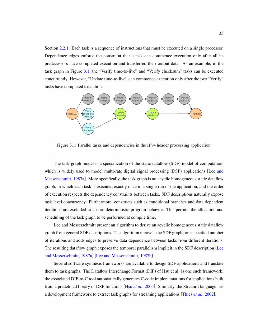
33

Section 2.2.1. Each task is a sequence of instructions that must be executed on a single processor.

Dependence edges enforce the constraint that a task can commence execution only after all its

predecessors have completed execution and transferred their output data. As an example, in the

task graph in Figure 3.1, the “Verify time-to-live” and “Verify checksum” tasks can be executed

concurrently. However, “Update time-to-live” can commence execution only after the two “Verify”

tasks have completed execution.

Receive

Route

lookup 1

Route

lookup 2

Verify

time-to-live,version

Verify

checksum

Route

lookup 3

TransmitUpdate

time-to-live

Update

checksum

Route

lookup 4

Route

lookup 5

Route

lookup 6

Route

lookup 7

Figure 3.1: Parallel tasks and dependencies in the IPv4 header processing application.

The task graph model is a specialization of the static dataflow (SDF) model of computation,

which is widely used to model multi-rate digital signal processing (DSP) applications [Lee and

Messerschmitt, 1987a]. More specifically, the task graph is an acyclic homogeneous static dataflow

graph, in which each task is executed exactly once in a single run of the application, and the order

of execution respects the dependency constraints between tasks. SDF descriptions naturally expose

task level concurrency. Furthermore, constructs such as conditional branches and data dependent

iterations are excluded to ensure deterministic program behavior. This permits the allocation and

scheduling of the task graph to be performed at compile time.

Lee and Messerschmitt present an algorithm to derive an acyclic homogeneous static dataflow

graph from general SDF descriptions. The algorithm unravels the SDF graph for a specified number

of iterations and adds edges to preserve data dependence between tasks from different iterations.

The resulting dataflow graph exposes the temporal parallelism implicit in the SDF description [Lee

and Messerschmitt, 1987a] [Lee and Messerschmitt, 1987b].

Several software synthesis frameworks are available to design SDF applications and translate

them to task graphs. The Dataflow Interchange Format (DIF) of Hsu et al. is one such framework;

the associated DIF-to-C tool automatically generates C-code implementations for applications built

from a predefined library of DSP functions [Hsu et al., 2005]. Similarly, the StreamIt language has

a development framework to extract task graphs for streaming applications [Thies et al., 2002].

34

In the context of our exploration framework for network processing applications from Chap-

ter 2, the starting point for application description is the Click domain specific language (Sec-

tion 2.3.1). The Click description is translated into multiple acyclic homogeneous dataflow graphs,

which are decoupled at queue boundaries. The tasks are packet processing operations and packet

descriptors are transferred along the edges. The task level concurrency in Click is implicit in the

form of push and pull chains. Individual push and pull chains can execute concurrently, while ele-

ments along a particular chain must execute in sequence for every incoming packet [Plishker et al.,

2004] [Plishker, 2006] [Jin et al., 2005].

3.1.2 The Multiprocessor Architecture Model

A common model for the multiprocessor architecture is a network of processors P = p1, . . . , pm.

The interconnection network is abstracted as a set of direct point-to-point links between processors.

It is specified by the set C ⊆ P ×P of the pairs of processors that are connected to each other. The

pair (p1, p2) ∈ C indicates that there is a directed link from processor p1 to processor p2. It is natu-

ral to assume that a processor is always connected to itself, i.e. (pi, pi) ∈ C,∀pi ∈ P . Optionally,

C could be treated as a multi-set if there are multiple links between two processors. The processors

in P and the links in C may be heterogeneous.

The (P,C) model is accurate for distributed memory multiprocessors in which the processors

do not share any memory and the communication solely relies on message passing over buffered

links. Each processor is assumed to contain dedicated communication hardware so that compu-

tation can be overlapped with communication. The processors could be arranged in any arbitrary

network topology specified by C; common examples are fully connected, mesh, ring, or hypercube

topologies.

In the context of our exploration framework, the (P,C) model is well suited for multipro-

cessor designs on Xilinx FPGAs (Section 2.2.3) crafted out of processors and point-to-point FIFO

links. The micro-architecture, however, could use alternate communication links such as buses or

crossbars to connect processors. In these cases, the (P,C) model abstracts only the interconnection

between processors. A bus connecting multiple processors, such as in the IXP1200 network proces-

sor (Section 2.2.2), is modeled as a completely connected network in the (P,C) model [Kwok and

Ahmad, 1999b] [Sih and Lee, 1993].

35

3.1.3 Performance Model for the Task Graph

The task graph and architecture models expose the concurrency in the application and target

platform. To generate useful mappings, it is important to additionally extend the task graph with

performance annotations for the target architecture. A common performance model is related to the

temporal behavior of the system. A weight w(v, p) is associated with each vertex or task v ∈ V to

denote its execution time on a processor p ∈ P . The vertex weight is a function w : V × P → <+.

Similarly, weight c((v1, v2), (p1, p2)) along an edge (v1, v2) ∈ E denotes the latency or delay

due to data transfer when tasks v1, v2 ∈ V execute on processors p1, p2 ∈ P , respectively, and

(p1, p2) ∈ C. The edge weight is a function c : E × C → <+, i.e. it is a function of the amount of

data transferred along an edge and the nature of physical link to which the edge is assigned.

The (G, w, c) task graph and performance model has been used in many multiprocessor schedul-

ing problems [Hu, 1961] [Coffman, 1976] [Papadimitriou and Ullman, 1987] [Veltman et al., 1990]

[El-Rewini et al., 1995] [Teich and Thiele, 1996] [Dick et al., 2003]. In this model, the execution

times and communication delays are approximated by real-valued constants, and time (in units of

seconds or cycles) is the principle metric of performance both for computation and communication

operations. The (G, w, c) model is popularly referred to in the scheduling literature as the delay

model [Papadimitriou and Ullman, 1987] [Boeres and Rebello, 2003].

The performance model is usually obtained from run time profilings of the task graph on the

target architecture for average or worst case execution scenarios. Alternate approaches estimate

performance using analytical models based on the distribution of numerical operations, memory

accesses, and communication accesses [Kwok and Ahmad, 1999b]. Various techniques have been

proposed to compute worst case execution times (WCET) of programs. Some advanced approaches

incorporate considerations for infeasible execution paths in the program to improve the accuracy of

the estimation [Gajski and Wu, 1990] [Suhendra et al., 2006]. These techniques perform a detailed

path analysis of the program execution, similar to static timing analysis in hardware design.

One limitation of the (G, w, c) model is that it does not directly capture the effects of contention

and arbitration for shared resources, which are the main sources of uncertainty that differentiate the

estimates of analytical models from the performance of hardware implementations. Nevertheless, it

exposes the application tasks, dependencies, and execution and communication costs on the target

architecture, which are important considerations to derive effective system mappings. The (G, w, c)

model is a widely studied static analytical model of performance. Similar analytical models have

been generated to measure power, reliability, cost, and other system properties.

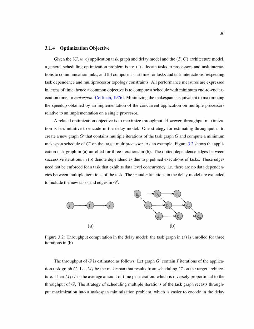
36

3.1.4 Optimization Objective

Given the (G, w, c) application task graph and delay model and the (P,C) architecture model,

a general scheduling optimization problem is to: (a) allocate tasks to processors and task interac-

tions to communication links, and (b) compute a start time for tasks and task interactions, respecting

task dependence and multiprocessor topology constraints. All performance measures are expressed

in terms of time, hence a common objective is to compute a schedule with minimum end-to-end ex-

ecution time, or makespan [Coffman, 1976]. Minimizing the makespan is equivalent to maximizing

the speedup obtained by an implementation of the concurrent application on multiple processors

relative to an implementation on a single processor.

A related optimization objective is to maximize throughput. However, throughput maximiza-

tion is less intuitive to encode in the delay model. One strategy for estimating throughput is to

create a new graph G′ that contains multiple iterations of the task graph G and compute a minimum

makespan schedule of G′ on the target multiprocessor. As an example, Figure 3.2 shows the appli-

cation task graph in (a) unrolled for three iterations in (b). The dotted dependence edges between

successive iterations in (b) denote dependencies due to pipelined executions of tasks. These edges

need not be enforced for a task that exhibits data level concurrency, i.e. there are no data dependen-

cies between multiple iterations of the task. The w and c functions in the delay model are extended

to include the new tasks and edges in G′.

a cb

a1c1b1

a2c2b2

a3c3b3

(a) (b)

Figure 3.2: Throughput computation in the delay model: the task graph in (a) is unrolled for threeiterations in (b).

The throughput of G is estimated as follows. Let graph G′ contain I iterations of the applica-

tion task graph G. Let MI be the makespan that results from scheduling G′ on the target architec-

ture. Then MI/I is the average amount of time per iteration, which is inversely proportional to the

throughput of G. The strategy of scheduling multiple iterations of the task graph recasts through-

put maximization into a makespan minimization problem, which is easier to encode in the delay

37

model. However, the result is only a lower bound on the maximum throughput. A better estimate of

throughput may be obtained by scheduling a greater number of task graph iterations.

A third objective for the (G, w, c) model is to compute a schedule that minimizes the total

amount of time incurred in performing communications between tasks, given a target makespan or

throughput. This objective is relevant for minimizing the usage of shared communication resources.

Another objective is to compute a schedule that achieves an optimum load balance. A load bal-

anced schedule distributes the workload as evenly as possible across all processors to obtain a good

utilization of system resources.

It is sometimes necessary to optimize multiple objectives in tandem, for example, to compute

a schedule with minimum makespan that also minimizes total communication time. One way to

encode multiple objectives is to combine them in a weighted function. A theoretical definition

of multi-objective optimization is based on Pareto optimality: a solution is Pareto optimal if no

single objective can be improved without causing another objective to become inferior. Most often,

there are a large number of Pareto optimal solutions with disparate characteristics, especially if a

few objectives are contradictory. Hence, the optimization problem must be suitably constrained to

generate useful solutions that do not unduly penalize individual objectives.

3.1.5 Implementation and Resource Constraints

Beside the constraints that arise from the task graph, architecture, and performance models,

practical scheduling problems are further complicated by implementation and resource constraints

that govern the validity of schedules. These may be a consequence of application requirements,

architecture restrictions, or designer insights into the nature of useful schedules. In this section, we

identify some constraints applicable to scheduling problems derived from the (G, w, c) and (P,C)

models. We refer to the following works for related discussions on the origin and nature of typical

constraints for multiprocessor scheduling: [Ekelin and Jonsson, 2000] [Redell, 1998].

Implementation Constraints from the Application

Implementation constraints regulate the timing and execution behavior of tasks in the (G, w, c)

delay model. These constraints may be classified based on whether they pertain to individual tasks

(intra-task constraints), or to interactions between tasks (inter-task constraints). The following are

common implementation constraints pertaining to the execution and timing behavior of individual

tasks (intra-task constraints) in the application model:

38

• Task execution time: Task weights in the performance model specify the amount of time a

task must execute on a processor.

• Instruction and data memory sizes: The memory requirements for the individual tasks must

be satisfied by the processor to which the task is allocated.

• Deadline: A task must complete execution before a certain time in the global schedule. This

enforces responsiveness required by the system.

• Release time: A task must start execution only after a certain time in the global schedule.

• Jitter: A jitter constraint specifies an upper bound on the difference between the release time

and actual start time, or deadline and actual end time of a task.

• Preferred allocation: The constraint requires a task be assigned to a specific processor or to

one from a subset of processors. This may arise when a task requires access to instruction

extensions or I/O interfaces available only on selected processors.

• Preemption: The constraint indicates if a task can be preempted during execution and option-

ally imposes a delay penalty on the context switch.

The following are common implementation constraints pertaining to the execution and timing be-

havior of task interactions (inter-task constraints) in the application model:

• Relative timing: The start times of two tasks must be separated by a certain amount of time.

In this manner, task executions can be synchronized.

• Dependence: Tasks must execute in a certain order, as enforced by the dependence edges in

the task graph.

• Edge communication delay: Edge weights in the performance model specify a fixed commu-

nication delay to transfer data between two tasks on a specific communication link.

• Clustering: A set of tasks must be allocated to the same processor. This may arise when the

tasks share a large amount of data and it is prohibitive to communicate between processors.

• Anti-clustering: A set of tasks cannot all be allocated to the same processor. This may arise

when the amount of memory needed by the tasks is larger than the capacity of the processor.

• Mutual exclusion: The execution of a set of tasks must be mutually exclusive in time. Alter-

natively, a set of tasks must necessarily be assigned to distinct processors.

39

Resource Constraints from the Architecture

Resource constraints concern the performance and capacities of the processing and communi-

cation resources. The (P,C) architecture model specifies the number and type of processors and

the network topology. The following are common resource constraints pertaining to the processing

resources in the architecture model:

• Processor speed: Execution time of a task depends on which processor it is allocated. This is

captured by the task weights in the performance model.

• Memory size: The aggregate memory footprint of all tasks assigned to a processor must not

exceed the size of the local memory in the processor.

• Context switch: Context switch delays penalize task preemptions in a processor. Alterna-

tively, non-preemptive scheduling enforces that at most one task is active in a processor.

• Execution and communication gap: This is a lower bound on the interval between two suc-

cessive task executions or communications.

The following are common resource constraints pertaining to the communication resources in the

architecture model:

• Network topology: Processor interconnections specified in the architecture model constrain

the placement of interacting tasks.

• Link delay: Communication delay along a dependence edge depends on which physical link

it is assigned. This is captured by the edge delays in the performance model.

• Communication overhead: Interacting tasks on different processors incur a processing over-

head above their execution times to initiate and terminate data transfers.

• Communication routing: Message routes between processors are specified a priori and data

transfers between interacting tasks are scheduled along these routes.

3.2 Methods for Static Scheduling

The (G, w, c) and (P,C) models are simplified representations of the concurrent application

and multiprocessor architecture for static scheduling. Nevertheless, these simple models encompass

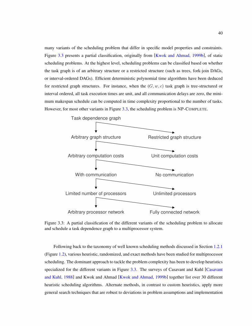
40

many variants of the scheduling problem that differ in specific model properties and constraints.

Figure 3.3 presents a partial classification, originally from [Kwok and Ahmad, 1999b], of static

scheduling problems. At the highest level, scheduling problems can be classified based on whether

the task graph is of an arbitrary structure or a restricted structure (such as trees, fork-join DAGs,

or interval-ordered DAGs). Efficient deterministic polynomial time algorithms have been deduced

for restricted graph structures. For instance, when the (G, w, c) task graph is tree-structured or

interval ordered, all task execution times are unit, and all communication delays are zero, the mini-

mum makespan schedule can be computed in time complexity proportional to the number of tasks.

However, for most other variants in Figure 3.3, the scheduling problem is NP-COMPLETE.

Task dependence graph

Arbitrary graph structure

Arbitrary computation costs

With communication

Limited number of processors

Arbitrary processor network

Restricted graph structure

Unit computation costs

No communication

Unlimited processors

Fully connected network

Figure 3.3: A partial classification of the different variants of the scheduling problem to allocateand schedule a task dependence graph to a multiprocessor system.

Following back to the taxonomy of well known scheduling methods discussed in Section 1.2.1

(Figure 1.2), various heuristic, randomized, and exact methods have been studied for multiprocessor

scheduling. The dominant approach to tackle the problem complexity has been to develop heuristics

specialized for the different variants in Figure 3.3. The surveys of Casavant and Kuhl [Casavant

and Kuhl, 1988] and Kwok and Ahmad [Kwok and Ahmad, 1999b] together list over 30 different

heuristic scheduling algorithms. Alternate methods, in contrast to custom heuristics, apply more

general search techniques that are robust to deviations in problem assumptions and implementation

41

constraints. Methods based on simulated annealing, evolutionary algorithms, and mathematical and

constraint programming have been advanced on account of their flexibility and ease of use.

The next few sections describe scheduling methods from the different categories of the taxon-

omy in Figure 1.2. The following works complement this survey of methods for scheduling task

dependence graphs to multiprocessor systems: [Kwok and Ahmad, 1999b] [Casavant and Kuhl,

1988] [Redell, 1998] [Davidovic and Crainic, 2006] [McCreary et al., 1994].

3.2.1 Heuristic Methods

Heuristic methods for scheduling fall under two prominent categories based on their strategy to

compute valid schedules: (a) clustering and critical path heuristics, and (b) list scheduling heuristics.

Clustering and Critical Path Heuristics

The general concept behind clustering methods is to iteratively merge tasks into large grained

clusters. The clustering process terminates when the number of clusters is about the same as the

number of processors, at which point the clusters are mapped to processors. At the first step, each

task is an individual cluster. A common clustering strategy is to merge tasks to form a single cluster

based on the critical path: the algorithm repeatedly clusters a subset of vertexes (also called the

dominant sequence) along the critical path and removes them from the graph [Kim and Browne,

1988] [Gerasoulis and Yang, 1992]. Hoang and Rabaey demonstrate the efficacy of a clustering

scheme to schedule DSP algorithms to multiprocessors to maximize throughput [Hoang and Rabaey,

1993]. Gajski and Wu also advocate clustering methods for Hypertool, their code generation tool to

map parallel programs to the iPSC/2 hypercube computer [Gajski and Wu, 1990].

List Scheduling Heuristics

Almost all list scheduling algorithms have the following structure. First, the algorithm com-

putes a total ordering or list of tasks based on some priority metric. Tasks are then considered

according to the list order and scheduled on available processors. The algorithm repeatedly exe-

cutes the following two steps until a valid schedule is obtained:

• Select the next task to schedule, which is typically the task with highest priority and whose

predecessors have completed execution.

• Allocate the selected task to a processor that allows the earliest start time for that task.

42

The algorithm progresses by allocating a task at each iteration and terminates when all tasks are

scheduled. Graham, as early as 1966, formalized list scheduling for multiprocessors and proposed

approximation bounds on schedule lengths for some restricted problems [Graham et al., 1979] [Pa-

padimitriou and Yannakakis, 1988]. List scheduling algorithms differ in the rule used to pick the

next task from the list when a processor is free [Chekuri, 1998]. A common choice of priority is the

static level, the largest sum of execution times along any path from a task to any sink vertex in the

graph [Hu, 1961]. Ties are broken based on the task processing times or the number of immediate

successors [Kasahara and Narita, 1984]. Specific implementation and resource constraints are also

factored into the priority metric computation.

Other Heuristic Methods

There are heuristic methods that do not fall into the clustering and list scheduling categories.

Graph decomposition methods break a graph into a hierarchy of subgraphs, which are typically

easier to analyze. For instance, if the subgraphs are fully ordered chains of tasks, trees, or fork-join

structures, then optimum algorithms can be applied to compute the schedule in polynomial time

[McCreary et al., 1994]. A second heuristic is based on the concept of force directed scheduling

[Paller and Wolinski, 1995]. In this method, the scheduling constraints and performance models are

incorporated in a force system, and the algorithm uses heuristic rules to iteratively converge to a

local optimum.

3.2.2 List Scheduling using Dynamic Levels

In Figure 3.3, the most general scheduling problem variant is to find a schedule with minimum

makespan when mapping an arbitrary task dependence graph with arbitrary execution and commu-

nication models to an arbitrary processor network. The successful heuristics for this problem have

typically been evolved from list scheduling. Dynamic Level Scheduling (DLS) is such a compile

time list scheduling heuristic [Sih and Lee, 1993]. Independent benchmarking efforts for static

scheduling algorithms, due to Kwok and Ahmad, Davidovic and Crainic, and Koch, endorse the ef-

fectiveness of the DLS algorithm for scheduling task graphs on to a bounded number of processors

[Kwok and Ahmad, 1999a] [Davidovic and Crainic, 2006] [Koch, 1995]. The algorithm schedules

problem instances with over 200 tasks within seconds, and the results are often close to the mini-

mum makespan. We later use DLS as a competitive baseline reference to evaluate other scheduling

methods in the context of our mapping framework.

43

List scheduling assigns a priority to each task and schedules them in descending order of

priority. Conventionally, the scheduling list is statically constructed before task allocation begins,

and the ordering is not modified during algorithm execution. The premise for the DLS heuristic is

that a static list does not accurately capture task priority in the delay model [Sih and Lee, 1993]

[Kwok and Ahmad, 1999a] [Gerasoulis and Yang, 1992]. The remedy is to update the priorities of

all unscheduled tasks at each list scheduling step. The DLS algorithm introduces a priority metric

called dynamic level, which is the difference between the static level of a task and its earliest start

time on a processor. The metric is qualified as “dynamic” since it is recomputed at each scheduling

step for all ready tasks on all processors. At each step, the algorithm schedules the task-processor

pair with the highest dynamic level.

Several works have proposed extensions to DLS to enforce additional constraints related to

task release times and deadlines, processor heterogeneity, and irregular multiprocessor topologies

[Bambha and Bhattacharyya, 2002] [Kwok and Ahmad, 1999a]. The strategy for incorporating

these extensions is to update the dynamic level computation to capture the relevant constraints.

However, it is non-trivial to conceive how the dynamic level function should be modified for a

specific extension. Furthermore, the feasibility of the final schedule computed by DLS is not guar-

anteed when there are arbitrary implementation constraints. This is fundamentally because DLS is

a greedy method, which makes scheduling decisions with only a local view of the solution space.

Although it may be possible to look-ahead one or more scheduling steps, there may always exist

a condition that renders a scheduling decision detrimental to the objective. This phenomenon is

referred to as the horizon effect and is a handicap to greedy search methods [Sih and Lee, 1993].

This drawback motivates the study of more general search methods that retain a global view of the

solution space.

3.2.3 Evolutionary Algorithms

Evolutionary algorithms use global search techniques to explore different regions of the search

space simultaneously. They keep track of a set of potential solutions of diverse characteristics, called

a population. The search is based on concepts from biological evolution: the idea is to iteratively

track the “fittest” solutions based on a cost function, while allowing random “mutations” to evolve

new solutions. The problem constraints are encoded in the permissible mutations. The work of

Dhodhi et al. presents a detailed analysis of evolutionary algorithms for scheduling [Dhodhi et al.,

2002]. As Kwok and Ahmad point out, the motivation for using an evolutionary method is that the

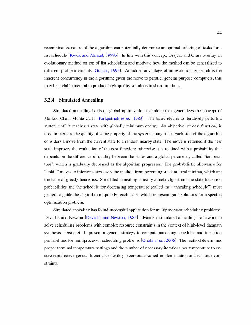
44

recombinative nature of the algorithm can potentially determine an optimal ordering of tasks for a

list schedule [Kwok and Ahmad, 1999b]. In line with this concept, Grajcar and Grass overlay an

evolutionary method on top of list scheduling and motivate how the method can be generalized to

different problem variants [Grajcar, 1999]. An added advantage of an evolutionary search is the

inherent concurrency in the algorithm; given the move to parallel general purpose computers, this

may be a viable method to produce high-quality solutions in short run times.

3.2.4 Simulated Annealing

Simulated annealing is also a global optimization technique that generalizes the concept of

Markov Chain Monte Carlo [Kirkpatrick et al., 1983]. The basic idea is to iteratively perturb a

system until it reaches a state with globally minimum energy. An objective, or cost function, is

used to measure the quality of some property of the system at any state. Each step of the algorithm

considers a move from the current state to a random nearby state. The move is retained if the new

state improves the evaluation of the cost function; otherwise it is retained with a probability that

depends on the difference of quality between the states and a global parameter, called “tempera-

ture”, which is gradually decreased as the algorithm progresses. The probabilistic allowance for

“uphill” moves to inferior states saves the method from becoming stuck at local minima, which are

the bane of greedy heuristics. Simulated annealing is really a meta-algorithm: the state transition

probabilities and the schedule for decreasing temperature (called the “annealing schedule”) must

geared to guide the algorithm to quickly reach states which represent good solutions for a specific

optimization problem.

Simulated annealing has found successful application for multiprocessor scheduling problems.

Devadas and Newton [Devadas and Newton, 1989] advance a simulated annealing framework to

solve scheduling problems with complex resource constraints in the context of high-level datapath

synthesis. Orsila et al. present a general strategy to compute annealing schedules and transition

probabilities for multiprocessor scheduling problems [Orsila et al., 2006]. The method determines

proper terminal temperature settings and the number of necessary iterations per temperature to en-

sure rapid convergence. It can also flexibly incorporate varied implementation and resource con-

straints.

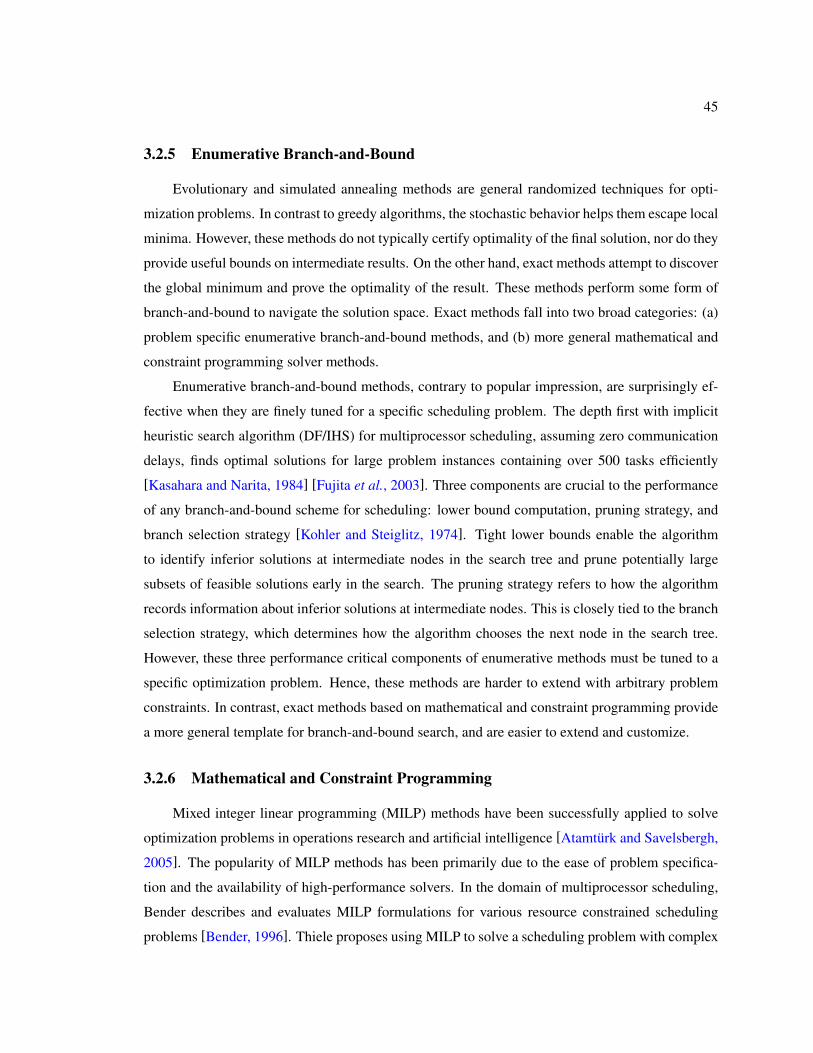
45

3.2.5 Enumerative Branch-and-Bound

Evolutionary and simulated annealing methods are general randomized techniques for opti-

mization problems. In contrast to greedy algorithms, the stochastic behavior helps them escape local

minima. However, these methods do not typically certify optimality of the final solution, nor do they

provide useful bounds on intermediate results. On the other hand, exact methods attempt to discover

the global minimum and prove the optimality of the result. These methods perform some form of

branch-and-bound to navigate the solution space. Exact methods fall into two broad categories: (a)

problem specific enumerative branch-and-bound methods, and (b) more general mathematical and

constraint programming solver methods.

Enumerative branch-and-bound methods, contrary to popular impression, are surprisingly ef-

fective when they are finely tuned for a specific scheduling problem. The depth first with implicit

heuristic search algorithm (DF/IHS) for multiprocessor scheduling, assuming zero communication

delays, finds optimal solutions for large problem instances containing over 500 tasks efficiently

[Kasahara and Narita, 1984] [Fujita et al., 2003]. Three components are crucial to the performance

of any branch-and-bound scheme for scheduling: lower bound computation, pruning strategy, and

branch selection strategy [Kohler and Steiglitz, 1974]. Tight lower bounds enable the algorithm

to identify inferior solutions at intermediate nodes in the search tree and prune potentially large

subsets of feasible solutions early in the search. The pruning strategy refers to how the algorithm

records information about inferior solutions at intermediate nodes. This is closely tied to the branch

selection strategy, which determines how the algorithm chooses the next node in the search tree.

However, these three performance critical components of enumerative methods must be tuned to a

specific optimization problem. Hence, these methods are harder to extend with arbitrary problem

constraints. In contrast, exact methods based on mathematical and constraint programming provide

a more general template for branch-and-bound search, and are easier to extend and customize.

3.2.6 Mathematical and Constraint Programming

Mixed integer linear programming (MILP) methods have been successfully applied to solve

optimization problems in operations research and artificial intelligence [Atamturk and Savelsbergh,

2005]. The popularity of MILP methods has been primarily due to the ease of problem specifica-

tion and the availability of high-performance solvers. In the domain of multiprocessor scheduling,

Bender describes and evaluates MILP formulations for various resource constrained scheduling

problems [Bender, 1996]. Thiele proposes using MILP to solve a scheduling problem with complex

46

resource constraints on memory size, communication bandwidth, and access conflicts to memories

and buses [Thiele, 1995]. Hwang et al. present a formal model and solution approach using MILP to

solve scheduling problems in high-level synthesis [Hwang et al., 1991]. These are all “single-pass”

formulations (the problem constraints are presented at the start of execution) intended to be solved

using a commercial MILP solver like ILOG CPLEX [ILOG Inc., b].

Constraint programming (CP) is another solver method for discrete optimization problems.

CP has its origin in two declarative paradigms: constraint solving and logic programming [Redell,

1998]. In CP, the problem variables take discrete values from finite domains, and the constraints

are propositional or first order logic predicates. The CP formulations are solved using a com-

mercial solver, such as the ILOG Constraint Programming Optimizer [ILOG Inc., a]. Various CP

formulations have been studied for the multiprocessor scheduling problem. Wurtz presents diverse

formulations for the Oz constraint programming language [Wurtz, 1997]. Ekelin and Jonsson pro-

pose a framework based on CP specifically for embedded system scheduling problems and employ

the SICtus Prolog constraint solver [Ekelin and Jonsson, 2000]. They justify CP for the following

two reasons: (a) it is easy to express the scheduling problem in terms much closer to the actual sys-

tem requirements, and (b) the framework supports different strategies for single and multi-objective

optimization for practical scheduling problems.

3.3 Scheduling Tools and Frameworks

The scheduling methods from the previous sections are typically part of a system level mapping

and design space exploration (DSE) framework for an application domain or class of architectures.

A broad survey of DSE frameworks is presented in [Gries, 2004, Chapter 6]. Many frameworks

in this survey do not provide automated mapping capabilities and advocate fully manual designer

driven efforts for the mapping step. In this section, we review a few frameworks that especially

support automated mapping to assist the designer in exploring the design space and highlight their

choice of methods for solving relevant optimization problems.

The Artemis framework explores mappings of Kahn process network descriptions of concur-

rent applications on to abstract performance models of reconfigurable architectures [Pimentel et al.,

2001]. The framework adds facilities to iteratively explore reconfigurable architectures and refine

performance models. A related tool in this framework is SPADE, a trace-driven system level sim-

ulator. The methods to guide application mappings employ evolutionary algorithms to minimize

complex multi-objective cost functions composed of performance and power metrics.

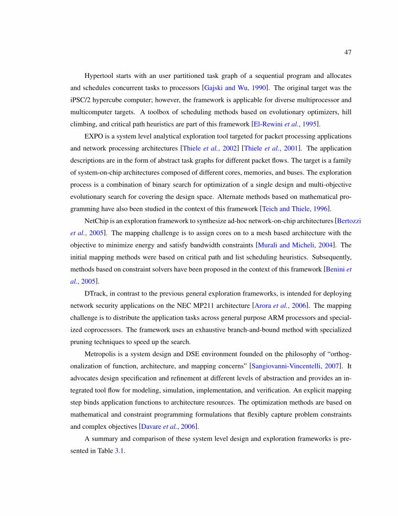
47

Hypertool starts with an user partitioned task graph of a sequential program and allocates

and schedules concurrent tasks to processors [Gajski and Wu, 1990]. The original target was the

iPSC/2 hypercube computer; however, the framework is applicable for diverse multiprocessor and

multicomputer targets. A toolbox of scheduling methods based on evolutionary optimizers, hill

climbing, and critical path heuristics are part of this framework [El-Rewini et al., 1995].

EXPO is a system level analytical exploration tool targeted for packet processing applications

and network processing architectures [Thiele et al., 2002] [Thiele et al., 2001]. The application

descriptions are in the form of abstract task graphs for different packet flows. The target is a family

of system-on-chip architectures composed of different cores, memories, and buses. The exploration

process is a combination of binary search for optimization of a single design and multi-objective

evolutionary search for covering the design space. Alternate methods based on mathematical pro-

gramming have also been studied in the context of this framework [Teich and Thiele, 1996].

NetChip is an exploration framework to synthesize ad-hoc network-on-chip architectures [Bertozzi

et al., 2005]. The mapping challenge is to assign cores on to a mesh based architecture with the

objective to minimize energy and satisfy bandwidth constraints [Murali and Micheli, 2004]. The

initial mapping methods were based on critical path and list scheduling heuristics. Subsequently,

methods based on constraint solvers have been proposed in the context of this framework [Benini et

al., 2005].

DTrack, in contrast to the previous general exploration frameworks, is intended for deploying

network security applications on the NEC MP211 architecture [Arora et al., 2006]. The mapping

challenge is to distribute the application tasks across general purpose ARM processors and special-

ized coprocessors. The framework uses an exhaustive branch-and-bound method with specialized

pruning techniques to speed up the search.

Metropolis is a system design and DSE environment founded on the philosophy of “orthog-

onalization of function, architecture, and mapping concerns” [Sangiovanni-Vincentelli, 2007]. It

advocates design specification and refinement at different levels of abstraction and provides an in-

tegrated tool flow for modeling, simulation, implementation, and verification. An explicit mapping

step binds application functions to architecture resources. The optimization methods are based on

mathematical and constraint programming formulations that flexibly capture problem constraints

and complex objectives [Davare et al., 2006].

A summary and comparison of these system level design and exploration frameworks is pre-

sented in Table 3.1.

48

Name Application Architecture MappingModel Model Method

Artemis Process networks Abstract models Evolutionary optimizerHypertool Task graph Abstract models Evolutionary optimizer,

Hill climbingEXPO Task graph Network processors Evolutionary optimizer,

MILP solverNetChip Task graph Network-on-chip models Heuristics,

CP solverDTrack Task graph NEC security processors Branch-and-boundMetropolis Task graph Embedded automotive processors, MILP solver,

MXP media processors CP solver

Table 3.1: Overview and comparison of system level design frameworks.

3.4 The Right Method for the Job

In this chapter, we reviewed different methods to schedule concurrent applications to multi-

processor architectures in ways that optimize relevant performance metrics. Table 3.2 summarizes

the strengths of prominent scheduling methods. The evaluation is based on three primary metrics:

(a) efficiency (related to speed, memory utilization, and other computational characteristics of a

method), (b) quality of results (related to how well a method, independent of computational effi-

ciency, can certify optimality of the solution or guarantee bounds), and (c) flexibility (related to

ease of problem specification and extensibility of a method to incorporate diverse constraints).

Method Efficiency Quality of Results FlexibilityHeuristics +Evolutionary +Simulated annealing +Enumerative +MILP/CP + +

Table 3.2: Comparison of static scheduling methods in terms of efficiency, quality of results, andflexibility.

In terms of computational efficiency, heuristic methods, such as list scheduling and clustering,

are superior to the rest. They are greedy or “short-sighted” by design and do not provide any guar-

antee of optimality. Rather, they are intended run in polynomial time to deliver acceptable results.

However, the difficulty in generalizing heuristic solutions to accommodate a range of constraints

and objectives deters their usefulness in general exploration frameworks.

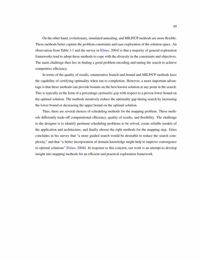
49

On the other hand, evolutionary, simulated annealing, and MILP/CP methods are more flexible.

These methods better capture the problem constraints and ease exploration of the solution space. An

observation from Table 3.1 and the survey in [Gries, 2004] is that a majority of general exploration

frameworks tend to adopt these methods to cope with the diversity in the constraints and objectives.

The main challenge then lies in finding a good problem encoding and tuning the search to achieve

competitive efficiency.

In terms of the quality of results, enumerative branch-and-bound and MILP/CP methods have

the capability of certifying optimality when run to completion. However, a more important advan-

tage is that these methods can provide bounds on the best known solution at any point in the search.

This is typically in the form of a percentage optimality gap with respect to a proven lower bound on

the optimal solution. The methods iteratively reduce the optimality gap during search by increasing

the lower bound or decreasing the upper bound on the optimal solution.

Thus, there are several choices of scheduling methods for the mapping problem. These meth-

ods differently trade-off computational efficiency, quality of results, and flexibility. The challenge

to the designer is to identify pertinent scheduling problems to be solved, create reliable models of

the application and architecture, and finally choose the right methods for the mapping step. Gries

concludes in his survey that “a more guided search would be desirable to reduce the search com-

plexity,” and that “a better incorporation of domain knowledge might help to improve convergence

to optimal solutions” [Gries, 2004]. In response to this concern, our work is an attempt to develop

insight into mapping methods for an efficient and practical exploration framework.

50

Chapter 4

Constraint Programming Methods for

Static Scheduling

In Chapter 2, we presented a framework to deploy network processing applications and an-

alyzed the problems related to mapping application task level concurrency to the target multipro-

cessor. Based on these insights, in this chapter we formalize a representative compile time static

task allocation and scheduling problem that arises in our framework. The problem captures the

salient performance critical components of the mapping step. At the same time, it is not tightly cou-

pled to application and architectural intricacies. The problem forms a basis for comparing different

scheduling methods and assessing their efficiency and flexibility.

We derive a mixed integer linear program programming (MILP) formulation for this problem

and use it to map network processing applications to different multiprocessor platforms. These de-

sign studies serve as examples for practical allocation and scheduling problems that arise in a map-

ping and exploration framework. They also underscore the need for computationally efficient and

flexible scheduling methods that can reliably capture diverse problem specifications and resource

constraints. Experimental results provide a preliminary evaluation of mathematical and constraint

programming methods for static scheduling problems.

4.1 A Representative Static Scheduling Problem

The problem we consider is the non-preemptive compile time scheduling of a task graph of a

concurrent application on to a multiprocessor architecture. The task dependencies, task execution

times, and interprocessor communication overheads between tasks are assumed to be known at

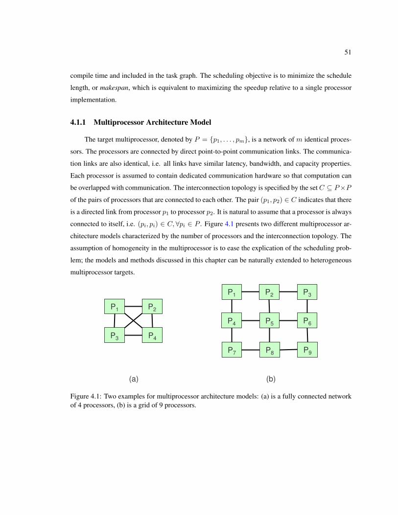
51

compile time and included in the task graph. The scheduling objective is to minimize the schedule

length, or makespan, which is equivalent to maximizing the speedup relative to a single processor

implementation.

4.1.1 Multiprocessor Architecture Model

The target multiprocessor, denoted by P = p1, . . . , pm, is a network of m identical proces-

sors. The processors are connected by direct point-to-point communication links. The communica-

tion links are also identical, i.e. all links have similar latency, bandwidth, and capacity properties.

Each processor is assumed to contain dedicated communication hardware so that computation can

be overlapped with communication. The interconnection topology is specified by the set C ⊆ P×P

of the pairs of processors that are connected to each other. The pair (p1, p2) ∈ C indicates that there

is a directed link from processor p1 to processor p2. It is natural to assume that a processor is always

connected to itself, i.e. (pi, pi) ∈ C,∀pi ∈ P . Figure 4.1 presents two different multiprocessor ar-

chitecture models characterized by the number of processors and the interconnection topology. The

assumption of homogeneity in the multiprocessor is to ease the explication of the scheduling prob-

lem; the models and methods discussed in this chapter can be naturally extended to heterogeneous

multiprocessor targets.

P1 P2

P3 P4

(a)

P1 P2

P4 P5

P3

P6

P7 P8 P9

(b)

Figure 4.1: Two examples for multiprocessor architecture models: (a) is a fully connected networkof 4 processors, (b) is a grid of 9 processors.

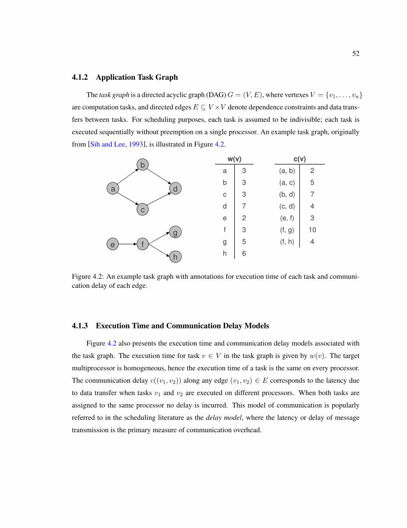
52

4.1.2 Application Task Graph

The task graph is a directed acyclic graph (DAG) G = (V,E), where vertexes V = v1, . . . , vnare computation tasks, and directed edges E ⊆ V ×V denote dependence constraints and data trans-

fers between tasks. For scheduling purposes, each task is assumed to be indivisible; each task is

executed sequentially without preemption on a single processor. An example task graph, originally

from [Sih and Lee, 1993], is illustrated in Figure 4.2.

a

b

c

d

g

h

fe

w(v)

6h

5g

3f

2e

7d

3c

3b

3a

c(v)

4(f, h)

10(f, g)

3(e, f)

4(c, d)

7(b, d)

5(a, c)

2(a, b)

Figure 4.2: An example task graph with annotations for execution time of each task and communi-cation delay of each edge.

4.1.3 Execution Time and Communication Delay Models

Figure 4.2 also presents the execution time and communication delay models associated with

the task graph. The execution time for task v ∈ V in the task graph is given by w(v). The target

multiprocessor is homogeneous, hence the execution time of a task is the same on every processor.

The communication delay c((v1, v2)) along any edge (v1, v2) ∈ E corresponds to the latency due

to data transfer when tasks v1 and v2 are executed on different processors. When both tasks are

assigned to the same processor no delay is incurred. This model of communication is popularly

referred to in the scheduling literature as the delay model, where the latency or delay of message

transmission is the primary measure of communication overhead.

53

4.1.4 Valid Allocation, Valid Schedule

Given a task graph G = (V,E) and an architecture model (P,C), a valid allocation A is a

function A : V → P that assigns every task in V to a single processor in P and enforces the

following condition pertaining to the placement of interacting tasks in an arbitrary topology:

∀(v1, v2) ∈ E (allocation constraints),(A(v1), A(v2)

)∈ C .

In other words, if there is a dependence edge between tasks v1 and v2, then the tasks can only

be allocated to processors that are connected in the multiprocessor topology specified by C. The

underlying assumption is that the communication network does not provide a facility to route data

between any arbitrary pair of processors; hence, interacting tasks must be allocated on connected

processors.

For a valid allocation A, a valid schedule S is a function S : V → <+ that assigns a non-

negative start time to every task and satisfies the following three conditions:

∀(v1, v2) ∈ E (dependence constraints),

(a) S(v2) ≥ S(v1) + w(v1)

(b) A(v1) 6= A(v2) ⇒ S(v2) ≥ S(v1) + w(v1) + c((v1, v2))

∀v1, v2 ∈ V, v1 6= v2 (ordering constraints),

(c) A(v1) = A(v2) ⇒ S(v1) ≥ S(v2) + w(v2) ∨ S(v2) ≥ S(v1) + w(v1) .

Constraints (a) and (b) pertain to dependencies between tasks. Constraint (a) specifies that if

there is a dependence edge from task v1 to task v2 in the task graph, then task v2 can start only

after task v1 has completed execution. Constraint (b) additionally enforces that if tasks v1 and v2

are allocated to different processors, then v2 can start only after task v1 has completed execution

and the communication delay along edge (v1, v2) is incurred. Constraint (c) orders tasks that are

allocated to the same processor. It specifies that if tasks v1 and v2 are on the same processor, then

either task v1 starts after task v2 has completed, or task v2 starts after task v1 has completed. This

ensures that at most one task is actively executed at any time on a single processor; the task, once

started, executes till completion and cannot be preempted by another task.

Note that constraint (c) is redundant for tasks v1 and v2 that are related by dependencies, i.e.

there is a sequence of dependence edges connecting tasks v1 and v2 in G. In this case, constraint

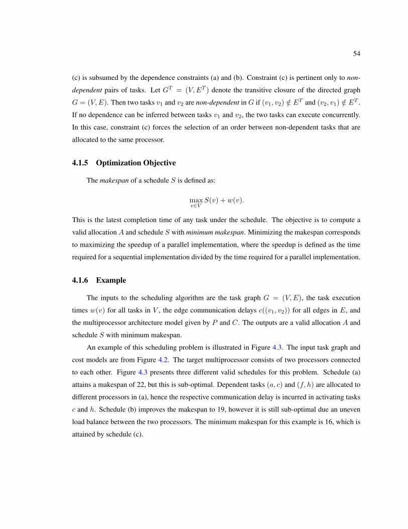
54

(c) is subsumed by the dependence constraints (a) and (b). Constraint (c) is pertinent only to non-

dependent pairs of tasks. Let GT = (V,ET ) denote the transitive closure of the directed graph

G = (V,E). Then two tasks v1 and v2 are non-dependent in G if (v1, v2) /∈ ET and (v2, v1) /∈ ET .

If no dependence can be inferred between tasks v1 and v2, the two tasks can execute concurrently.

In this case, constraint (c) forces the selection of an order between non-dependent tasks that are

allocated to the same processor.

4.1.5 Optimization Objective

The makespan of a schedule S is defined as:

maxv∈V

S(v) + w(v).

This is the latest completion time of any task under the schedule. The objective is to compute a

valid allocation A and schedule S with minimum makespan. Minimizing the makespan corresponds

to maximizing the speedup of a parallel implementation, where the speedup is defined as the time

required for a sequential implementation divided by the time required for a parallel implementation.

4.1.6 Example

The inputs to the scheduling algorithm are the task graph G = (V,E), the task execution

times w(v) for all tasks in V , the edge communication delays c((v1, v2)) for all edges in E, and

the multiprocessor architecture model given by P and C. The outputs are a valid allocation A and

schedule S with minimum makespan.

An example of this scheduling problem is illustrated in Figure 4.3. The input task graph and

cost models are from Figure 4.2. The target multiprocessor consists of two processors connected

to each other. Figure 4.3 presents three different valid schedules for this problem. Schedule (a)

attains a makespan of 22, but this is sub-optimal. Dependent tasks (a, c) and (f, h) are allocated to

different processors in (a), hence the respective communication delay is incurred in activating tasks

c and h. Schedule (b) improves the makespan to 19, however it is still sub-optimal due an uneven

load balance between the two processors. The minimum makespan for this example is 16, which is

attained by schedule (c).

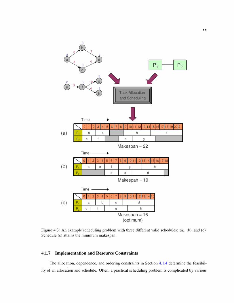
55

P1 P2

Task Allocation

and Scheduling

Makespan = 16(optimum)

15

hgfeP2

dcbaP1

14131211109876543210

Time

Makespan = 22

2120191817

d

161514136 7

c

8 12

g

1110

h

9

b

5

feP2

aP1

43210

Time

(a)

(c)

1817161514

h

1312

d

g

114

e

321

a

0 106 9

c

87

b

f

5

P2

P1

Makespan = 19

Time

(b)

3

3

3

32

7

5

63

2

5

7

4

10

4

a

b

c

d

g

h

fe

Figure 4.3: An example scheduling problem with three different valid schedules: (a), (b), and (c).Schedule (c) attains the minimum makespan.

4.1.7 Implementation and Resource Constraints

The allocation, dependence, and ordering constraints in Section 4.1.4 determine the feasibil-

ity of an allocation and schedule. Often, a practical scheduling problem is complicated by various

56

implementation and resource constraints that further limit the space of valid schedules. It is im-

portant for a scheduling method to accommodate these additional constraints without compromis-

ing the computational efficiency or quality of results. The following implementation and resource

constraints, originally introduced in Section 3.1.5, are applicable to the scheduling problem from

Section 4.1.4.

• Deadlines for task completion: A task v must complete execution before a certain time td in

the global schedule, i.e.,

S(v) ≤ td.

• Release times for tasks: A task v must start execution only after a certain time tr in the global

schedule, i.e.,

S(v) ≥ tr.

• Preferred allocations for tasks: A task v must be assigned to a specific processor p or to one

from a subset of processors PS in the target architecture, i.e.,

A(v) ∈ PS ⊆ P.

• Relative timing constraints between tasks: The start times of two tasks v1 and v2 must be

separated by a certain amount of time ts, i.e.,

S(v1)− S(v2) ≥,≤,= ts.

• Mutual exclusions for a set of tasks: The execution of a set of tasks VS must be mutually

exclusive in time. Alternatively, a set of tasks must necessarily be assigned to distinct proces-

sors. Notationally,

∀v1, v2 ∈ VS , v1 6= v2, (a) S(v1) ≥ S(v2) + w(v2) ∨ S(v2) ≥ S(v1) + w(v1)

(b) A(v1) 6= A(v2).

• Clustering of tasks: A set of tasks VS = v1, v2, . . . , vk must all be allocated to the same

processor, i.e.,

∀v ∈ VS − v1, A(v) = A(v1).

57

• Anti-clustering of tasks: A set of tasks VS = v1, v2, . . . , vk cannot all be allocated to the

same processor, i.e.,

∃vi, vj ∈ VS , vi 6= vj , A(vi) 6= A(vj).

To continue the scheduling example from Figure 4.3, a possible implementation constraint

could be that tasks a and h must be allocated to the same processor, i.e. A(a) = A(h). Then,

schedule (c) in Figure 4.3, which was originally the optimum result, is no longer valid. Schedule (a)

and (b) are both valid, and schedule (b) attains the minimum makespan of 19 for this example with

the additional task clustering constraint.

4.1.8 Complexity of the Scheduling Problem

Graham et al. originally introduced the α|β|γ scheme to classify multiprocessor scheduling

problems depending on the machine environment, task types, and objective function [Graham et

al., 1979]. According to this scheme, the scheduling problem presented in Section 4.1.4 targeting

a fully connected network of homogeneous processors belongs to the class P |prec|Cmax. The first

term, P , in this notation denotes that tasks have identical processing times on all the processors in

the system. The second term denotes precedence constraints between tasks. The last term denotes

that the objective is to minimize the maximum processing time or makespan. The P |prec|Cmax

class of problems is known to be strongly NP-COMPLETE.

In fact, the scheduling problem remains NP-COMPLETE for two simpler variants [Coffman,

1976]:

• All tasks have unit execution time and the communication cost between any pair of tasks is 0.

• All tasks have an execution time of 1 or 2 and the target architecture has 2 processors.

Previous literature reports the following special cases of the scheduling problem for which optimal

polynomial time algorithms have been deduced:

• The task graph is tree-structured or interval-ordered [Fishburn, 1985], all task execution times

are unit, and all communication costs are 0.

• All task execution times are unit, all communication costs are 0, and the target architecture

has 2 processors.

58

• The task graph is tree-structured, all task execution times are unit, all communication costs

are unit, and the target architecture has 2 processors.

• The task graph is interval-ordered, all task execution times are unit, and all communication

costs are unit [Kwok and Ahmad, 1999b] [El-Rewini et al., 1995].

However, the assumptions regarding the task graph structure and performance models imposed in

these cases are very restrictive. Task graphs for common concurrent applications are seldom tree-

structured or interval-ordered, and there is significant variation in the execution times of tasks and

the communication costs of edges. Given these observations about the theoretical complexity of

scheduling, it is difficult to expect polynomial time algorithms (unless P = NP ) for most problem

variants, and especially in the presence of problem specific implementation and resource constraints.

4.2 A Mixed Integer Linear Programming Formulation

In this section, we evaluate mixed integer linear programming (MILP) methods for the repre-

sentative scheduling problem. Typical MILP formulations are “single-pass” formulations (the prob-

lem constraints are presented at the start of execution) intended for a commercial general purpose

MILP solver like ILOG CPLEX [ILOG Inc., b]. Authors of previous literature concur that MILP

based methods using general purpose solvers are not viable for large-scale scheduling problems

[Davidovic et al., 2004] [Tompkins, 2003]. Nevertheless, the motivation for using MILP methods

is that medium-sized instances can be solved to optimality. In the cases where optimality is not

certified, the MILP solver still provides useful information about upper and lower bounds for the

optimal solution. Additionally, the ease of problem specification and the ability to easily extend the

formulation with diverse implementation and resource constraints make MILP methods attractive

in an exploration framework.

The various MILP formulations for the scheduling problem can be classified broadly by their

representation of time [Davare et al., 2006]. At the highest level, the variables corresponding to the

task schedule times are either discrete or continuous. Discrete time formulations introduce a variable

for every instance of time. This is the preferred way of representing time in propositional logic or

pseudo-Boolean formulations. However, the drawback of representing time discretely is that the

number of schedule variables is proportional to the value of the makespan. If the application has

n tasks, and M is an upper bound on the makespan, then the number of schedule variables in a

discrete time formulation is of the order O(nM).

59

In contrast, continuous time formulations represent time with real-valued variables. There are

three common continuous time encodings: (a) sequences: the scheduling variables encode the start

and end times of tasks and hence capture the order in which tasks are scheduled [Bender, 1996]

[Coll et al., 2006]; (b) slots: tasks are explicitly ordered into slots on each processor, but the start

and end times are not determined a priori [Davidovic et al., 2004]; (c) overlaps: variables capture

overlap in the execution of tasks and the scheduling constraints enforce that tasks allocated to the

same processor do not overlap [Tompkins, 2003].

The formulation presented here is derived from a more general formulation using overlap vari-

ables, due to Tompkins [Tompkins, 2003]. From experiments, we observed that this MILP formu-

lation is superior to others over a large set of examples. The results of Davare et al. corroborate this

claim [Davare et al., 2006]. In the following sections, we first present the MILP formulation using

overlap variables for the scheduling problem from Section 4.1.4. We then show its application to

solve mapping problems that arise in our exploration framework from Chapter 2.

4.2.1 Variables

The problem input parameters are the task graph G = (V,E), the task execution times w(v),

the edge communication delays c((v1, v2)), and the multiprocessor architecture model given by P

and C. The MILP formulation for the scheduling problem from Section 4.1.4 contains three sets of

variables:

∀v ∈ V,

xs(v) ∈ <+ (start time of task v)

∀v ∈ V,∀p ∈ P,

xa(v, p) =

1 : if task v assigned to processor p

0 : else

∀v1, v2 ∈ V, v1 6= v2, (v1, v2) /∈ ET , (v2, v1) /∈ ET ,

xo(v1, v2) =

1 : if task v2 completes after task v1 starts

0 : else

The schedule variables xs are non-negative real-valued numbers that indicate the start time of

60

each task. The allocation variables xa are binary variables that indicate task assignment to proces-

sors. The overlap variables xo are binary variables that capture an overlap in the execution periods

of two non-dependent tasks. If xo(v1, v2) = 1 and xo(v2, v1) = 1, then the execution periods of

tasks v1 and v2 overlap, which in turn implies that they cannot both be assigned to the same proces-

sor. The contrapositive of this case is used to enforce an ordering between non-dependent tasks v1

and v2 when they are assigned to the same processor.

4.2.2 Constraints

The objective and constraints in the MILP formulation are detailed below:

min maxv∈V

S(v) + w(v) , subject to:

∀v ∈ V,

(A1)∑p∈P

xa(v, p) = 1

∀(v1, v2) ∈ E,∀(p1, p2) ∈ (P × P )− C

(A2) xa(v1, p1) + xa(v2, p2) ≤ 1

∀(v1, v2) ∈ E,

(S1) xs(v2)− xs(v1) ≥ w(v1)

∀(v1, v2) ∈ E, ∀p ∈ P,

(S2) xs(v2)− xs(v1) ≥ w(v1) + c((v1, v2))(xa(v1, p)− xa(v2, p)

)

∀v1, v2 ∈ V, (v1, v2) /∈ ET , (v2, v1) /∈ ET ,

(O1) xs(v2) + w(v2)− xs(v1) ≤ Mxo(v1, v2)

∀v1, v2 ∈ V, (v1, v2) /∈ ET , (v2, v1) /∈ ET ,∀p ∈ P,

(O2) xo(v1, v2) + xo(v2, v1) + xa(v1, p) + xa(v2, p) ≤ 3

The objective is to minimize the makespan of the schedule. The allocation, dependence, and

ordering constraints from Section 4.1.4 that determine the feasibility of a schedule are encoded as

constraint sets A, S, and O, respectively, in the MILP formulation. Constraints A1 and A2 ensure a

61

valid allocation of the tasks to an arbitrary multiprocessor topology. Constraints S1 and S2 enforce

dependencies between tasks in the schedule and additionally account for the communication delay

when two dependent tasks are allocated to different processors.

Constraints O1 and O2 serve as ordering constraints for non-dependent tasks. Constraint O1

sets the value of the overlap variable xo(v1, v2) to 1 if task v2 completes after task v1 starts. In

this constraint, M is a large constant, which can be no less than the maximum completion time or

makespan. Any known upper bound on the makespan, such as the sum of all task execution times

or the result of a heuristic list schedule, is an acceptable value for M . Constraint O2 finally ensures

the execution periods of two non-dependent tasks v1 and v2 do not overlap when they are assigned

to the same processor. The sum term xo(v1, v2)+xo(v2, v1) is equal to 2 if and only if the execution

periods of tasks v1 and v2 overlap. Similarly, the sum term xa(v1, p) +xa(v2, p) is equal to 2 if and

only if v1 and v2 are both assigned to the same processor p. The inequality in constraint O2 hence

prevents the case when the execution periods of v1 and v2 overlap and the tasks are assigned to the

same processor. Alternatively, when v1 and v2 are assigned to the same processor p, only one of

xo(v1, v2) or xo(v2, v1) is 1, and that indicates the chosen ordering between the tasks.

The MILP formulation presented in this section does not incorporate the implementation and

resource constraints from Section 4.1.7. However, the formulation can be extended with the obvious

encodings for these constraints in terms of the primary variables. Thus, MILP eases the challenge

of specifying a complex optimization problem and minimizes the effort of establishing a fully-

functional mapping step in an exploration framework.

4.3 Mapping Results for Network Processing Applications

In Chapter 2, we presented an exploration framework to deploy network processing applica-

tions and discussed the application and architecture models that were inputs to the mapping step. In

this section, we apply our MILP formulation to solve scheduling problems that arise in this map-

ping step. The following two design examples are discussed in detail: (a) IPv4 packet forwarding

on FPGA based soft multiprocessors, and (b) Differentiated Services (DiffServ) quality of service

on the IXP1200 network processor. The main goals of this study are to: (a) illustrate the nature of

the allocation and scheduling problems that arise in an exploration framework, and (b) demonstrate

the viability of the MILP formulation for solving these problems.

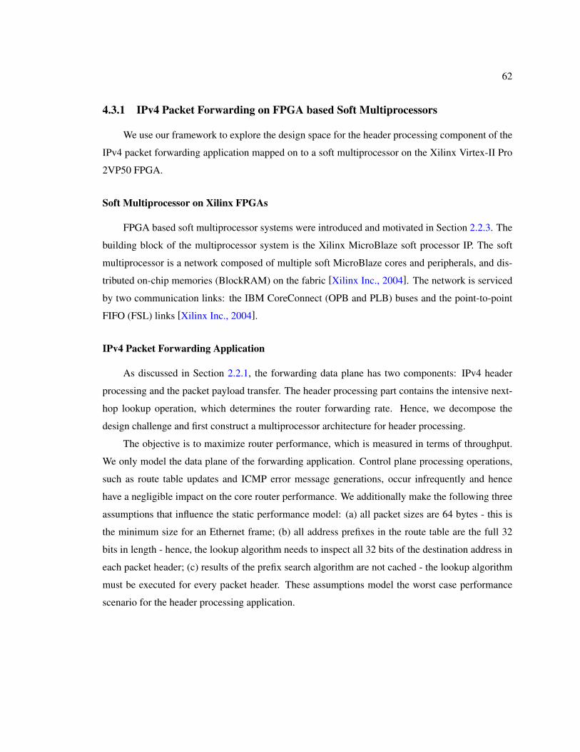
62

4.3.1 IPv4 Packet Forwarding on FPGA based Soft Multiprocessors

We use our framework to explore the design space for the header processing component of the

IPv4 packet forwarding application mapped on to a soft multiprocessor on the Xilinx Virtex-II Pro

2VP50 FPGA.

Soft Multiprocessor on Xilinx FPGAs

FPGA based soft multiprocessor systems were introduced and motivated in Section 2.2.3. The

building block of the multiprocessor system is the Xilinx MicroBlaze soft processor IP. The soft

multiprocessor is a network composed of multiple soft MicroBlaze cores and peripherals, and dis-

tributed on-chip memories (BlockRAM) on the fabric [Xilinx Inc., 2004]. The network is serviced

by two communication links: the IBM CoreConnect (OPB and PLB) buses and the point-to-point

FIFO (FSL) links [Xilinx Inc., 2004].

IPv4 Packet Forwarding Application

As discussed in Section 2.2.1, the forwarding data plane has two components: IPv4 header

processing and the packet payload transfer. The header processing part contains the intensive next-

hop lookup operation, which determines the router forwarding rate. Hence, we decompose the

design challenge and first construct a multiprocessor architecture for header processing.

The objective is to maximize router performance, which is measured in terms of throughput.

We only model the data plane of the forwarding application. Control plane processing operations,

such as route table updates and ICMP error message generations, occur infrequently and hence

have a negligible impact on the core router performance. We additionally make the following three

assumptions that influence the static performance model: (a) all packet sizes are 64 bytes - this is

the minimum size for an Ethernet frame; (b) all address prefixes in the route table are the full 32

bits in length - hence, the lookup algorithm needs to inspect all 32 bits of the destination address in

each packet header; (c) results of the prefix search algorithm are not cached - the lookup algorithm

must be executed for every packet header. These assumptions model the worst case performance

scenario for the header processing application.

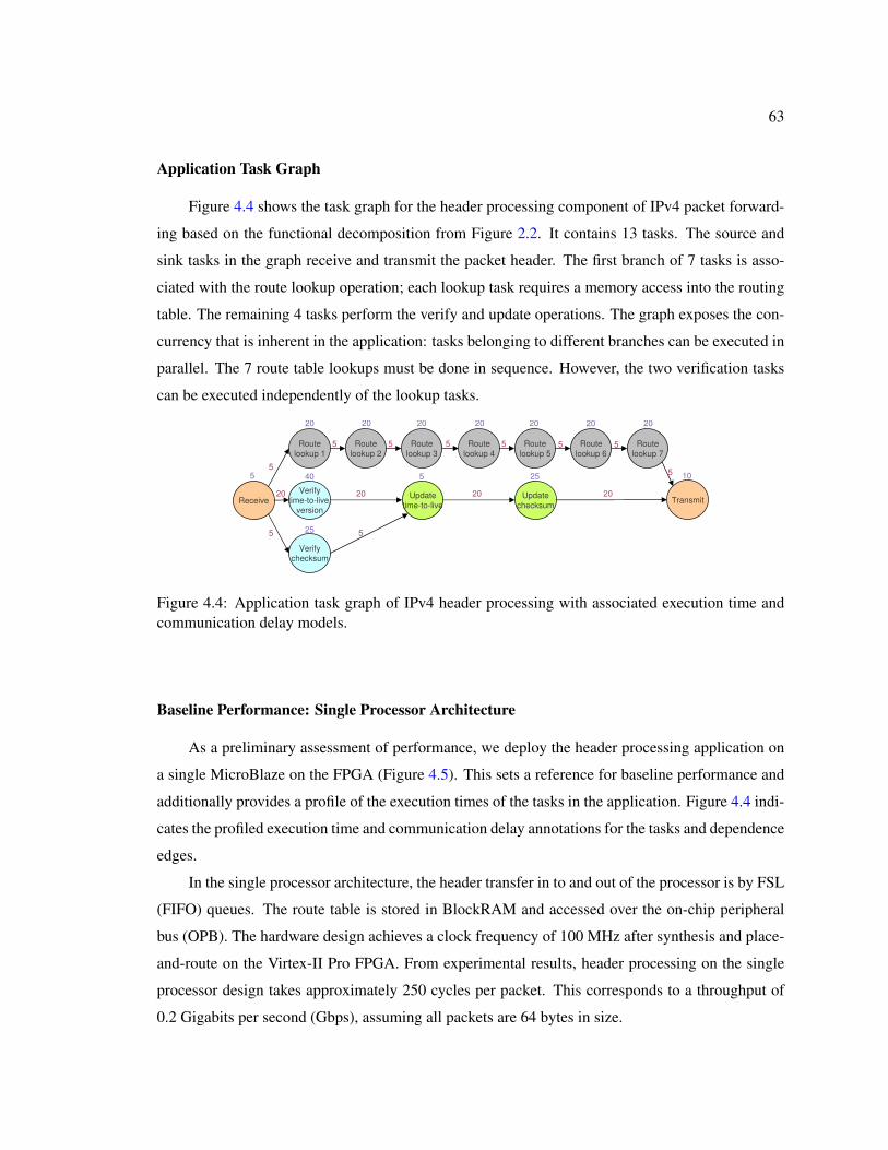
63

Application Task Graph

Figure 4.4 shows the task graph for the header processing component of IPv4 packet forward-

ing based on the functional decomposition from Figure 2.2. It contains 13 tasks. The source and

sink tasks in the graph receive and transmit the packet header. The first branch of 7 tasks is asso-

ciated with the route lookup operation; each lookup task requires a memory access into the routing

table. The remaining 4 tasks perform the verify and update operations. The graph exposes the con-

currency that is inherent in the application: tasks belonging to different branches can be executed in

parallel. The 7 route table lookups must be done in sequence. However, the two verification tasks

can be executed independently of the lookup tasks.

Receive

Route

lookup 1

Route

lookup 2

Verify


Verify

checksum

Route

lookup 3

TransmitUpdate

time-to-live

Update

checksum

Route

lookup 4

Route

lookup 5

Route

lookup 6

Route

lookup 7

5

20 20 20 20 20 20 20

40

25

5 25 105

5 5 5 5 5 5

5

20 20 20 20

5 5

Figure 4.4: Application task graph of IPv4 header processing with associated execution time andcommunication delay models.

Baseline Performance: Single Processor Architecture

As a preliminary assessment of performance, we deploy the header processing application on

a single MicroBlaze on the FPGA (Figure 4.5). This sets a reference for baseline performance and

additionally provides a profile of the execution times of the tasks in the application. Figure 4.4 indi-

cates the profiled execution time and communication delay annotations for the tasks and dependence

edges.

In the single processor architecture, the header transfer in to and out of the processor is by FSL

(FIFO) queues. The route table is stored in BlockRAM and accessed over the on-chip peripheral

bus (OPB). The hardware design achieves a clock frequency of 100 MHz after synthesis and place-

and-route on the Virtex-II Pro FPGA. From experimental results, header processing on the single

processor design takes approximately 250 cycles per packet. This corresponds to a throughput of

0.2 Gigabits per second (Gbps), assuming all packets are 64 bytes in size.

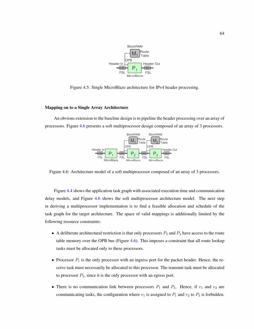
64

Header In

M1

FSL FSL

MicroBlaze

BlockRAM

Route

Table

OPB

Header Out

P1

Figure 4.5: Single MicroBlaze architecture for IPv4 header processing.

Mapping on to a Single Array Architecture

An obvious extension to the baseline design is to pipeline the header processing over an array of

processors. Figure 4.6 presents a soft multiprocessor design composed of an array of 3 processors.

Header In

P1

M1 M2

FSL FSL FSL FSLMicroBlaze MicroBlaze MicroBlaze

BlockRAM BlockRAM

Route

Table

Route

Table

OPB

Header Out

P2 P3

OPB

Figure 4.6: Architecture model of a soft multiprocessor composed of an array of 3 processors.

Figure 4.4 shows the application task graph with associated execution time and communication

delay models, and Figure 4.6 shows the soft multiprocessor architecture model. The next step

in deriving a multiprocessor implementation is to find a feasible allocation and schedule of the

task graph for the target architecture. The space of valid mappings is additionally limited by the

following resource constraints:

• A deliberate architectural restriction is that only processors P2 and P3 have access to the route

table memory over the OPB bus (Figure 4.6). This imposes a constraint that all route lookup

tasks must be allocated only to these processors.

• Processor P1 is the only processor with an ingress port for the packet header. Hence, the re-

ceive task must necessarily be allocated to this processor. The transmit task must be allocated

to processor P3, since it is the only processor with an egress port.

• There is no communication link between processors P1 and P3. Hence, if v1 and v2 are

communicating tasks, the configuration where v1 is assigned to P1 and v2 to P3 is forbidden.

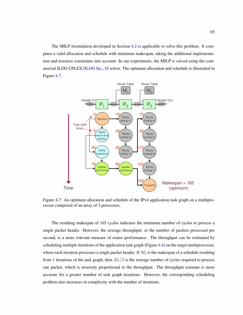
65

The MILP formulation developed in Section 4.2 is applicable to solve this problem. It com-

putes a valid allocation and schedule with minimum makespan, taking the additional implementa-

tion and resource constraints into account. In our experiments, the MILP is solved using the com-

mercial ILOG CPLEX [ILOG Inc., b] solver. The optimum allocation and schedule is illustrated in

Figure 4.7.

Header In

P1

M1 M2

Route TableRoute Table

Header Out

P2 P3

Receive

Verify


Verify

checksum

Update

time-to-live

Route

lookup 1

Route

lookup 2

Route

lookup 3

Update

checksum

Transmit

Route

lookup 4

Route

lookup 5

Route

lookup 6

Route

lookup 7

0 10 75

5 30 95

45 50 115

70 95 135

155Makespan = 165

(optimum)

Task start

times

Time

Figure 4.7: An optimum allocation and schedule of the IPv4 application task graph on a multipro-cessor composed of an array of 3 processors.

The resulting makespan of 165 cycles indicates the minimum number of cycles to process a

single packet header. However, the average throughput, or the number of packets processed per

second, is a more relevant measure of router performance. The throughput can be estimated by

scheduling multiple iterations of the application task graph (Figure 4.4) on the target multiprocessor,

where each iteration processes a single packet header. If MI is the makespan of a schedule resulting

from I iterations of the task graph, then MI/I is the average number of cycles required to process

one packet, which is inversely proportional to the throughput. The throughput estimate is more

accurate for a greater number of task graph iterations. However, the corresponding scheduling

problem also increases in complexity with the number of iterations.

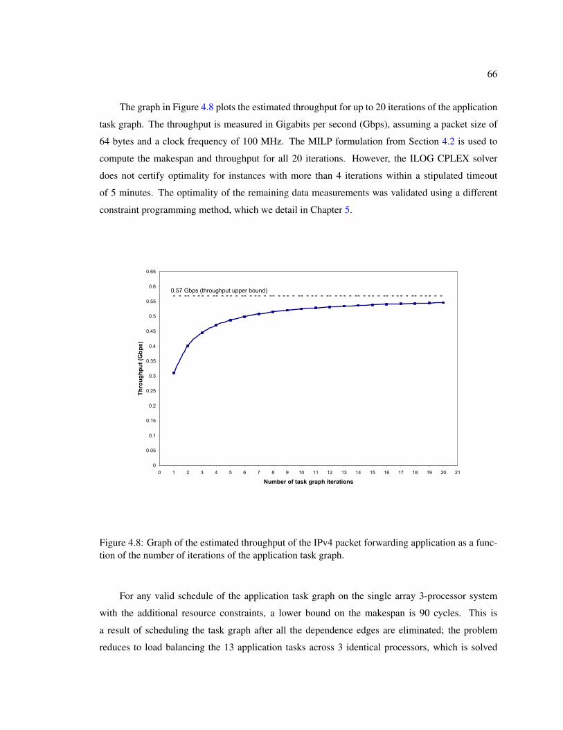
66

The graph in Figure 4.8 plots the estimated throughput for up to 20 iterations of the application

task graph. The throughput is measured in Gigabits per second (Gbps), assuming a packet size of

64 bytes and a clock frequency of 100 MHz. The MILP formulation from Section 4.2 is used to

compute the makespan and throughput for all 20 iterations. However, the ILOG CPLEX solver

does not certify optimality for instances with more than 4 iterations within a stipulated timeout

of 5 minutes. The optimality of the remaining data measurements was validated using a different

constraint programming method, which we detail in Chapter 5.

0

0.05

0.1

0.15

0.2

0.25

0.3

0.35

0.4

0.45

0.5

0.55

0.6

0.65

0 1 2 3 4 5 6 7 8 9 10 11 12 13 14 15 16 17 18 19 20 21

Number of task graph iterations

Throughput (Gbps)

0.57 Gbps (throughput upper bound)

Figure 4.8: Graph of the estimated throughput of the IPv4 packet forwarding application as a func-tion of the number of iterations of the application task graph.

For any valid schedule of the application task graph on the single array 3-processor system

with the additional resource constraints, a lower bound on the makespan is 90 cycles. This is

a result of scheduling the task graph after all the dependence edges are eliminated; the problem

reduces to load balancing the 13 application tasks across 3 identical processors, which is solved

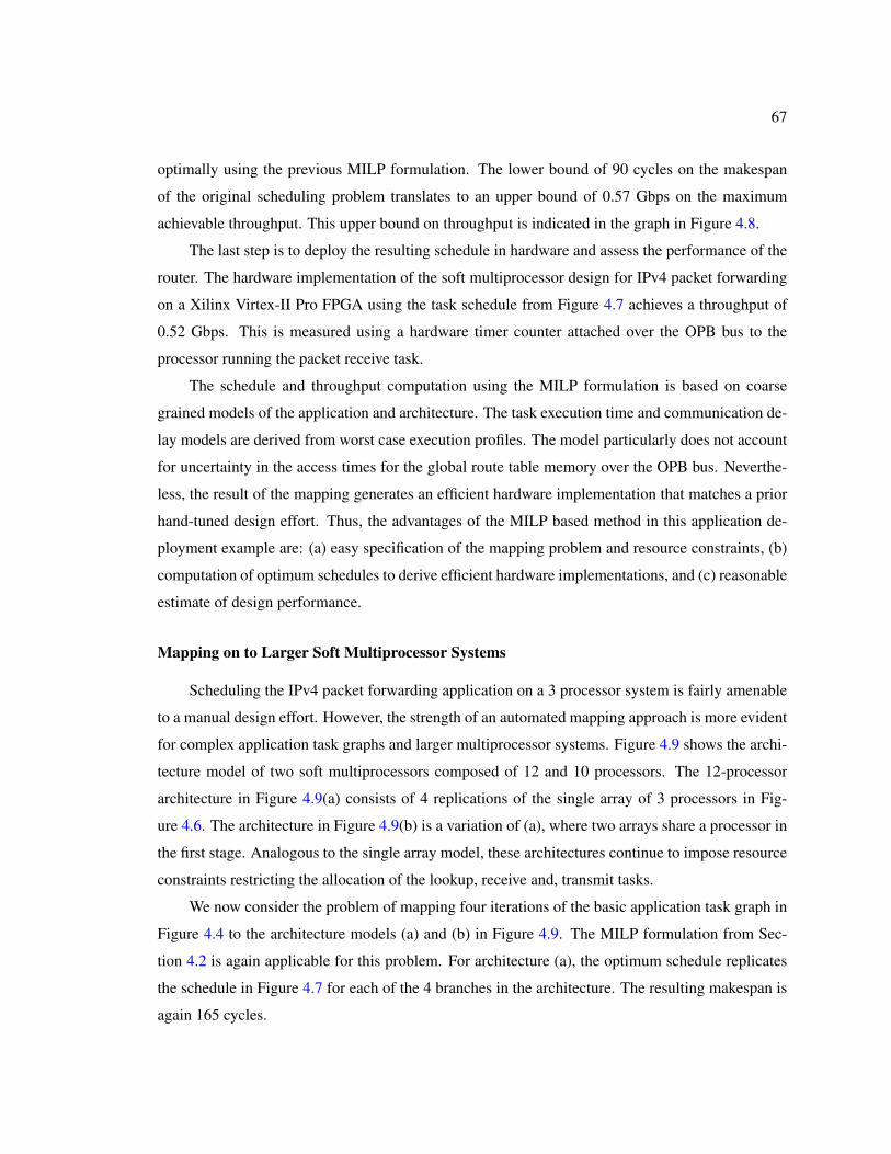
67

optimally using the previous MILP formulation. The lower bound of 90 cycles on the makespan

of the original scheduling problem translates to an upper bound of 0.57 Gbps on the maximum

achievable throughput. This upper bound on throughput is indicated in the graph in Figure 4.8.

The last step is to deploy the resulting schedule in hardware and assess the performance of the

router. The hardware implementation of the soft multiprocessor design for IPv4 packet forwarding

on a Xilinx Virtex-II Pro FPGA using the task schedule from Figure 4.7 achieves a throughput of

0.52 Gbps. This is measured using a hardware timer counter attached over the OPB bus to the

processor running the packet receive task.

The schedule and throughput computation using the MILP formulation is based on coarse

grained models of the application and architecture. The task execution time and communication de-

lay models are derived from worst case execution profiles. The model particularly does not account

for uncertainty in the access times for the global route table memory over the OPB bus. Neverthe-

less, the result of the mapping generates an efficient hardware implementation that matches a prior

hand-tuned design effort. Thus, the advantages of the MILP based method in this application de-

ployment example are: (a) easy specification of the mapping problem and resource constraints, (b)

computation of optimum schedules to derive efficient hardware implementations, and (c) reasonable

estimate of design performance.

Mapping on to Larger Soft Multiprocessor Systems

Scheduling the IPv4 packet forwarding application on a 3 processor system is fairly amenable

to a manual design effort. However, the strength of an automated mapping approach is more evident

for complex application task graphs and larger multiprocessor systems. Figure 4.9 shows the archi-

tecture model of two soft multiprocessors composed of 12 and 10 processors. The 12-processor

architecture in Figure 4.9(a) consists of 4 replications of the single array of 3 processors in Fig-

ure 4.6. The architecture in Figure 4.9(b) is a variation of (a), where two arrays share a processor in

the first stage. Analogous to the single array model, these architectures continue to impose resource

constraints restricting the allocation of the lookup, receive and, transmit tasks.

We now consider the problem of mapping four iterations of the basic application task graph in

Figure 4.4 to the architecture models (a) and (b) in Figure 4.9. The MILP formulation from Sec-

tion 4.2 is again applicable for this problem. For architecture (a), the optimum schedule replicates

the schedule in Figure 4.7 for each of the 4 branches in the architecture. The resulting makespan is

again 165 cycles.

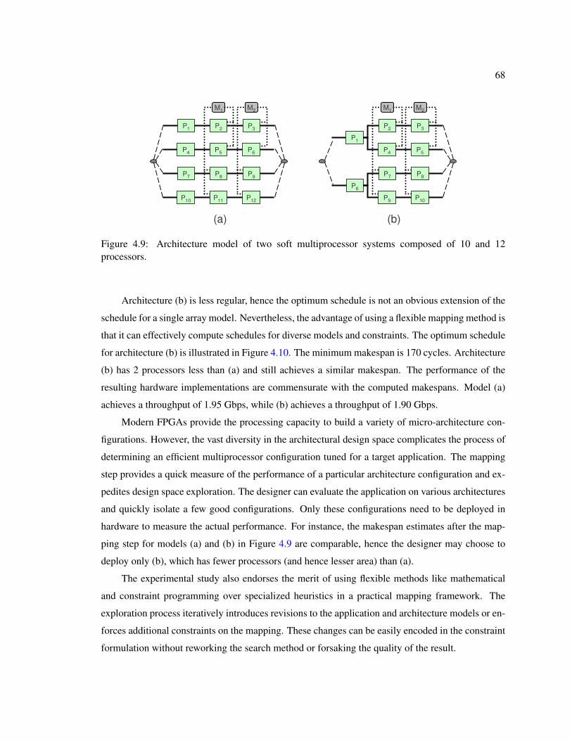
68

P1

M1 M2

P4

P7

P10

P8

P2 P3

P5 P6

P9

P11 P12

M1 M2

P1

P6

P7

P2 P3

P4 P5

P8

P9 P10

(a) (b)

Figure 4.9: Architecture model of two soft multiprocessor systems composed of 10 and 12processors.

Architecture (b) is less regular, hence the optimum schedule is not an obvious extension of the

schedule for a single array model. Nevertheless, the advantage of using a flexible mapping method is

that it can effectively compute schedules for diverse models and constraints. The optimum schedule

for architecture (b) is illustrated in Figure 4.10. The minimum makespan is 170 cycles. Architecture

(b) has 2 processors less than (a) and still achieves a similar makespan. The performance of the

resulting hardware implementations are commensurate with the computed makespans. Model (a)

achieves a throughput of 1.95 Gbps, while (b) achieves a throughput of 1.90 Gbps.

Modern FPGAs provide the processing capacity to build a variety of micro-architecture con-

figurations. However, the vast diversity in the architectural design space complicates the process of

determining an efficient multiprocessor configuration tuned for a target application. The mapping

step provides a quick measure of the performance of a particular architecture configuration and ex-

pedites design space exploration. The designer can evaluate the application on various architectures

and quickly isolate a few good configurations. Only these configurations need to be deployed in

hardware to measure the actual performance. For instance, the makespan estimates after the map-

ping step for models (a) and (b) in Figure 4.9 are comparable, hence the designer may choose to

deploy only (b), which has fewer processors (and hence lesser area) than (a).

The experimental study also endorses the merit of using flexible methods like mathematical

and constraint programming over specialized heuristics in a practical mapping framework. The

exploration process iteratively introduces revisions to the application and architecture models or en-

forces additional constraints on the mapping. These changes can be easily encoded in the constraint

formulation without reworking the search method or forsaking the quality of the result.

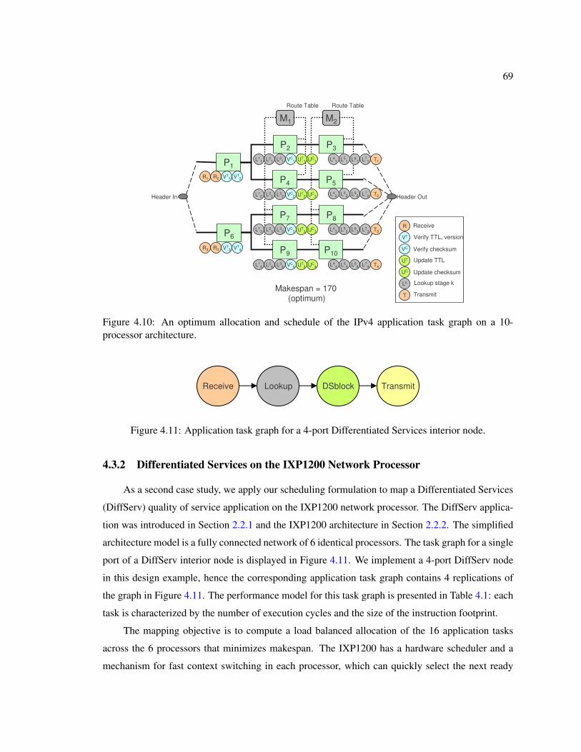
69

T2

M1 M2

P1

P6

P7

P2 P3

P4 P5

P8

P9 P10

Header In Header Out

Route TableRoute Table

R1 R2 VT1 VT

2

R3 R4

T1

T3

T4

VT3 VT

4

VC2

VC1

VC3

VC4

UT1

UT2

UT3

UT4

UC1

UC2

UC3

UC4

L11 L2

1 L31 L4

1 L51 L6

1 L71

L12 L2

2 L32 L4

2 L52 L6

2 L72

L13 L2

3 L33 L4

3 L53 L6

3 L73

L14 L2

4 L34 L4

4 L54 L6

4 L74

Makespan = 170(optimum)

R

VT

VC

UT

UC

Lk

T

Receive

Verify TTL, version

Verify checksum

Update TTL

Update checksum

Lookup stage k

Transmit

Figure 4.10: An optimum allocation and schedule of the IPv4 application task graph on a 10-processor architecture.

Receive Lookup DSblock Transmit

Figure 4.11: Application task graph for a 4-port Differentiated Services interior node.

4.3.2 Differentiated Services on the IXP1200 Network Processor

As a second case study, we apply our scheduling formulation to map a Differentiated Services

(DiffServ) quality of service application on the IXP1200 network processor. The DiffServ applica-

tion was introduced in Section 2.2.1 and the IXP1200 architecture in Section 2.2.2. The simplified

architecture model is a fully connected network of 6 identical processors. The task graph for a single

port of a DiffServ interior node is displayed in Figure 4.11. We implement a 4-port DiffServ node

in this design example, hence the corresponding application task graph contains 4 replications of

the graph in Figure 4.11. The performance model for this task graph is presented in Table 4.1: each

task is characterized by the number of execution cycles and the size of the instruction footprint.

The mapping objective is to compute a load balanced allocation of the 16 application tasks

across the 6 processors that minimizes makespan. The IXP1200 has a hardware scheduler and a

mechanism for fast context switching in each processor, which can quickly select the next ready

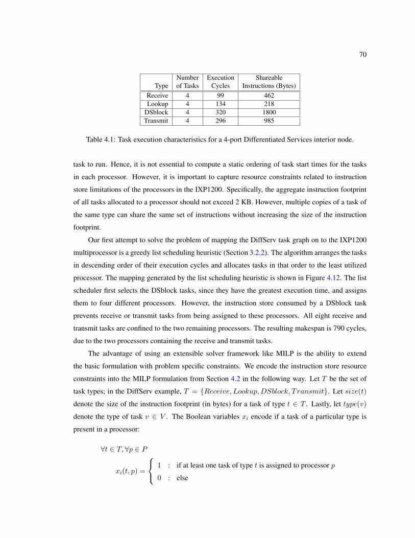
70

Number Execution ShareableType of Tasks Cycles Instructions (Bytes)

Receive 4 99 462Lookup 4 134 218

DSblock 4 320 1800Transmit 4 296 985

Table 4.1: Task execution characteristics for a 4-port Differentiated Services interior node.

task to run. Hence, it is not essential to compute a static ordering of task start times for the tasks

in each processor. However, it is important to capture resource constraints related to instruction

store limitations of the processors in the IXP1200. Specifically, the aggregate instruction footprint

of all tasks allocated to a processor should not exceed 2 KB. However, multiple copies of a task of

the same type can share the same set of instructions without increasing the size of the instruction

footprint.

Our first attempt to solve the problem of mapping the DiffServ task graph on to the IXP1200

multiprocessor is a greedy list scheduling heuristic (Section 3.2.2). The algorithm arranges the tasks

in descending order of their execution cycles and allocates tasks in that order to the least utilized

processor. The mapping generated by the list scheduling heuristic is shown in Figure 4.12. The list

scheduler first selects the DSblock tasks, since they have the greatest execution time, and assigns

them to four different processors. However, the instruction store consumed by a DSblock task

prevents receive or transmit tasks from being assigned to these processors. All eight receive and

transmit tasks are confined to the two remaining processors. The resulting makespan is 790 cycles,

due to the two processors containing the receive and transmit tasks.

The advantage of using an extensible solver framework like MILP is the ability to extend

the basic formulation with problem specific constraints. We encode the instruction store resource

constraints into the MILP formulation from Section 4.2 in the following way. Let T be the set of

task types; in the DiffServ example, T = Receive, Lookup,DSblock, Transmit. Let size(t)

denote the size of the instruction footprint (in bytes) for a task of type t ∈ T . Lastly, let type(v)

denote the type of task v ∈ V . The Boolean variables xi encode if a task of a particular type is

present in a processor:

∀t ∈ T,∀p ∈ P

xi(t, p) =

1 : if at least one task of type t is assigned to processor p

0 : else

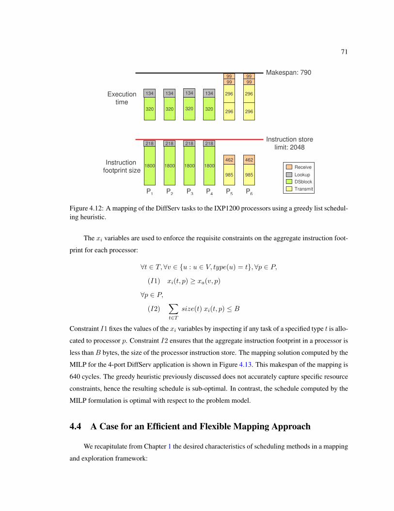
71

18001800

218218

296 296

320 320320 320296

134

99

296

134

99

134

99

134

99

18001800

985

462

985

462

218218

Makespan: 790

P1 P2 P3 P4 P5 P6

Instruction store limit: 2048

Executiontime

Instruction footprint size

Receive

Lookup

DSblock

Transmit

Figure 4.12: A mapping of the DiffServ tasks to the IXP1200 processors using a greedy list schedul-ing heuristic.

The xi variables are used to enforce the requisite constraints on the aggregate instruction foot-

print for each processor:

∀t ∈ T,∀v ∈ u : u ∈ V, type(u) = t,∀p ∈ P,

(I1) xi(t, p) ≥ xa(v, p)

∀p ∈ P,

(I2)∑t∈T

size(t) xi(t, p) ≤ B

Constraint I1 fixes the values of the xi variables by inspecting if any task of a specified type t is allo-

cated to processor p. Constraint I2 ensures that the aggregate instruction footprint in a processor is

less than B bytes, the size of the processor instruction store. The mapping solution computed by the

MILP for the 4-port DiffServ application is shown in Figure 4.13. This makespan of the mapping is

640 cycles. The greedy heuristic previously discussed does not accurately capture specific resource

constraints, hence the resulting schedule is sub-optimal. In contrast, the schedule computed by the

MILP formulation is optimal with respect to the problem model.

4.4 A Case for an Efficient and Flexible Mapping Approach

We recapitulate from Chapter 1 the desired characteristics of scheduling methods in a mapping

and exploration framework:

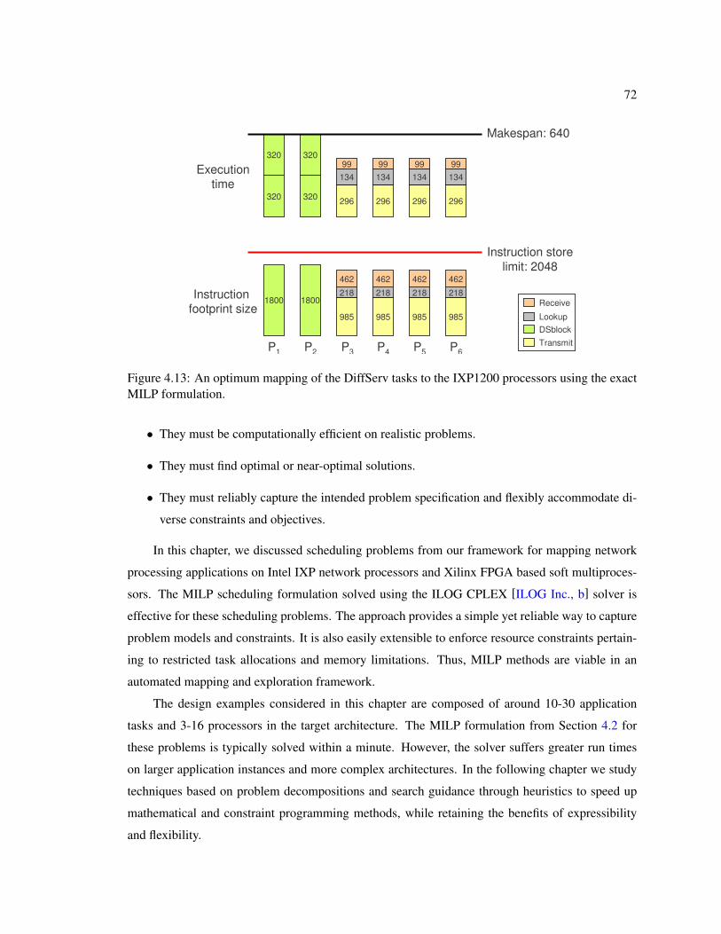
72

320

320

320

320

296

134

99

296

134

99

296

134

99

296

134

99

18001800

985

218

462

985

218

462

985

218

462

985

218

462

Makespan: 640

P1 P2 P3 P4 P5 P6

Instruction store limit: 2048

Executiontime

Instruction footprint size

Receive

Lookup

DSblock

Transmit

Figure 4.13: An optimum mapping of the DiffServ tasks to the IXP1200 processors using the exactMILP formulation.

• They must be computationally efficient on realistic problems.

• They must find optimal or near-optimal solutions.

• They must reliably capture the intended problem specification and flexibly accommodate di-

verse constraints and objectives.

In this chapter, we discussed scheduling problems from our framework for mapping network

processing applications on Intel IXP network processors and Xilinx FPGA based soft multiproces-

sors. The MILP scheduling formulation solved using the ILOG CPLEX [ILOG Inc., b] solver is

effective for these scheduling problems. The approach provides a simple yet reliable way to capture

problem models and constraints. It is also easily extensible to enforce resource constraints pertain-

ing to restricted task allocations and memory limitations. Thus, MILP methods are viable in an

automated mapping and exploration framework.

The design examples considered in this chapter are composed of around 10-30 application

tasks and 3-16 processors in the target architecture. The MILP formulation from Section 4.2 for

these problems is typically solved within a minute. However, the solver suffers greater run times

on larger application instances and more complex architectures. In the following chapter we study

techniques based on problem decompositions and search guidance through heuristics to speed up

mathematical and constraint programming methods, while retaining the benefits of expressibility

and flexibility.

73

Chapter 5

Techniques to Accelerate Constraint

Programming Methods

In the previous chapter, we discussed a representative task allocation and scheduling prob-

lem (Section 4.1) relevant to our exploration framework. The problem was amenable to mixed

integer linear programming (MILP) based solution methods for many practical instances. Other

general constraint programming (CP) formulations have also been studied for related scheduling

problems [Ekelin and Jonsson, 2000] [Jain and Grossmann, 2001] [Benini et al., 2005]. MILP and

CP methods support easy problem specification and flexibly accommodate diverse implementation

and resource constraints. However, typical “single-pass” MILP and CP formulations (in which the

problem constraints are presented at the start of execution) are feasible only on modestly sized in-

stances. The MILP formulations from Chapter 4 suffer prohibitive run times on instances with more

than 30 application tasks.

In this chapter, we present a decomposition strategy to accelerate MILP and CP methods for

the representative scheduling problem. In the manner of Benders decomposition, our technique

solves relaxed versions of the problem and iteratively learns constraints to prune the solution space

[Benders, 1962] [Hooker and Ottosson, 1999]. The decomposition strategy, along with algorithmic

extensions for solver search guidance, enhances constraint optimization to robustly handle instances

with over 150 tasks. The inherent extensibility, coupled with improved run times from a decomposi-

tion strategy, establish constraint optimization as a powerful tool for practical scheduling problems.

74

5.1 The Concept of Problem Decomposition

Our decomposition strategy to accelerate constraint optimization is applicable to many variants

of the scheduling problem with diverse implementation and resource constraints. The basic idea is

to divide the scheduling problem into a constraint-based “master” problem and a fast graph-theoretic

“sub” problem and solve them iteratively. The master solves a simplified optimization problem and

generates trial solutions. The sub-problem analyzes these solutions and in turn learns constraints to

incrementally prune inferior parts of the solution space. The master problem preserves the generality

of constraint optimization, while the sub-problem is specialized to quickly analyze partial solutions,

derive tight lower bounds, learn constraints to prune inferior parts of the solution space, and direct

search in the master problem.

The use of a decomposition strategy to accelerate constraint optimization is not new. This

strategy is inspired by the more general Benders decomposition technique of “learning from one’s

mistakes” [Benders, 1962] [Geoffrion, 1972]. Benders decomposition has been successfully applied

to various mathematical programming formulations. It iteratively assigns some variables trial values

and finds the best solution consistent with these values. In the process, it learns something about

the quality of other solutions. This information is useful in reducing the number of solutions that

must be enumerated to find the optimal solution [Hooker and Ottosson, 1999]. A pivotal factor

that determines its effectiveness is the derivation of Benders cuts to exclude superfluous solutions.

For linear and convex programming problems where the dual multipliers of the sub-problem are

defined, Benders cuts can be computed by solving the dual of the sub-problem that remains after

the trial values are fixed.

However, Benders decomposition need not be restricted to mathematical programming prob-

lems. Hooker and Ottoson formally show that the concept of decomposition can be generalized

to a broader class of combinatorial optimization problems [Hooker and Ottosson, 1999]. They ex-

plain how decomposition is applicable to logic based problems such as propositional satisfiability

(SAT) and 0-1 linear programming (0-1 LP). In these cases, the sub-problem decouples into several

smaller independent SAT and 0-1 LP problems after the trial variables are fixed. The advantage of

decomposition is evident when the number of sub-problem components increases. Hooker and Yan

further extend the concept of decomposition for the satisfiability problem to verify the equivalence

of logic circuits [Hooker and Yan, 1995]. Their results endorse the effectiveness of decomposition

methods for special classes of circuits over popular binary decision diagram (BDD) methods for

equivalence checking.

75

5.1.1 Related Decomposition Approaches for Scheduling Problems

Decomposition methods for scheduling problems is an area of recent interest in optimization

literature. In the context of static scheduling, Jain and Grossman apply a decomposition method

to schedule a set of independent tasks with release and finish times on a multiprocessor [Jain and

Grossmann, 2001]. The master problem is formulated as an MILP and its result is an allocation

of tasks to processors. The sub-problem computes a feasible schedule of the tasks that adheres to

the release and finish time constraints. Since there are no precedence constraints between tasks, the

tasks assigned to a single processor can be scheduled independently of the other processors. A CP

formulation is used to compute a schedule for each processor based on the allocation generated by

the master problem. Any processor for which a feasible schedule does not exist provides an integer

cut to exclude the corresponding allocation. The hybrid MILP and CP method was shown to achieve

run time improvements over “single-pass” MILP and CP models.

Benini et al. consider a task allocation and scheduling problem, very similar to the one from

Section 4.1, also in the context of mapping concurrent applications to multiprocessor systems-on-

chips [Benini et al., 2005]. The authors again apply an hybrid MILP/CP decomposition and show

that decomposition is superior to solving either model separately. The solution scheme decomposes

the problem into two parts: allocation of tasks to processors, and scheduling of tasks in time. The

allocation is solved using an MILP model and the scheduling is solved using a CP model. The

interaction between these models is regulated by Benders cuts that prohibit certain task allocations

for which no feasible schedules exist.

5.1.2 Overview of the Decomposition Approach

The prior work due to Benini et al. reports experimental results for scheduling problems con-

taining fewer than 20 tasks. We contend that the use of CP solvers for the sub-problem is compu-

tationally less efficient. CP models are generic and do not sufficiently exploit the underlying graph

structure of the scheduling problem. It is essential to choose a problem decomposition, based on in-

sight into the problem structure, that enables fast sub-problem computations and eases incorporation

of Benders cuts.

We propose a problem decomposition for the scheduling problem from Section 4.1 using a

fast graph-theoretic sub-problem algorithm that operates directly on the task graph. We formulate

the constraints for the master problem in conjunctive normal form (CNF) and use a satisfiability

(SAT) solver to solve the problem. Our choice of a CNF based encoding is motivated in part by

76

the ease of incorporating learned constraints from the sub-problem as Boolean clauses. The sub-

problem derives valid schedules using longest path delay computations on the directed acyclic task

graph based on the trial assignments generated by the master problem. Inferior schedules generate

Benders cuts, which are then encoded in CNF for the master problem. The main strengths of our

decomposition strategy compared to the prior hybrid MILP/CP methods are: (a) fast master and sub-

problem iterations, and (b) compact sub-problem constraints to record inferior parts of the solution

space. We advance three extensions to further improve the performance of our approach: (a) sub-

problem invocation from intermediate nodes in the satisfiability search in the master problem, (b)

tight lower bounds to prune inferior solutions, and (c) variable selection to guide search.

We evaluate the performance of our decomposition approach against two competitive meth-

ods: the “single-pass” overlap-based MILP formulation (Section 4.2) and the greedy dynamic level

scheduling heuristic (Section 3.2.2) [Tompkins, 2003] [Sih and Lee, 1993]. The overlap-based

MILP formulation is superior to other MILP and CP formulations for the scheduling problem over a

large set of examples [Davare et al., 2006]. We show that our decomposition approach can robustly

handle large problem instances with over 150 tasks, outdoing the overlap-based MILP formula-

tion. We also discuss how practical implementation and resource constraints can be easily enforced,

and show that the resulting schedules are superior to those computed by the popular dynamic level

scheduling heuristic.

5.2 A Decomposition Approach for Static Scheduling

We refer to Section 4.1 for a detailed specification of the representative static scheduling prob-

lem. Briefly, the inputs to the scheduling algorithm are the task graph G = (V,E), the task ex-

ecution times w(v) for all tasks in V , the edge communication delays c((v1, v2)) for all edges in

E, the set of processors P , and the interconnection topology C specified by the set of the pairs of

processors that are connected to each other. The outputs are a valid allocation A and schedule S

with minimum makespan.

The goal of the decomposition strategy is to improve the performance of constraint formula-

tions for this static scheduling problem. Our solution scheme is a problem decomposition with two

components which are solved iteratively: a constraint based “master” problem, and a graph-theoretic

“sub” problem. Instead of solving a complex optimization problem in one pass, the decomposition

approach iteratively solves simpler versions of the same problem and learns constraints at each

iteration to prune the solution space.

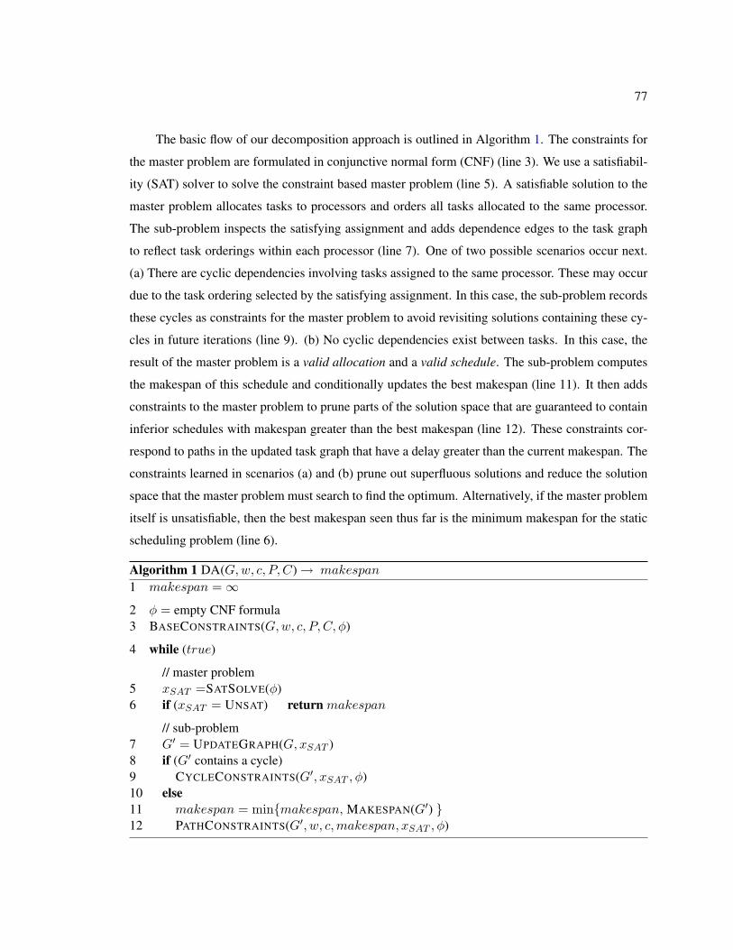
77

The basic flow of our decomposition approach is outlined in Algorithm 1. The constraints for

the master problem are formulated in conjunctive normal form (CNF) (line 3). We use a satisfiabil-

ity (SAT) solver to solve the constraint based master problem (line 5). A satisfiable solution to the

master problem allocates tasks to processors and orders all tasks allocated to the same processor.

The sub-problem inspects the satisfying assignment and adds dependence edges to the task graph

to reflect task orderings within each processor (line 7). One of two possible scenarios occur next.

(a) There are cyclic dependencies involving tasks assigned to the same processor. These may occur

due to the task ordering selected by the satisfying assignment. In this case, the sub-problem records

these cycles as constraints for the master problem to avoid revisiting solutions containing these cy-

cles in future iterations (line 9). (b) No cyclic dependencies exist between tasks. In this case, the

result of the master problem is a valid allocation and a valid schedule. The sub-problem computes

the makespan of this schedule and conditionally updates the best makespan (line 11). It then adds

constraints to the master problem to prune parts of the solution space that are guaranteed to contain

inferior schedules with makespan greater than the best makespan (line 12). These constraints cor-

respond to paths in the updated task graph that have a delay greater than the current makespan. The

constraints learned in scenarios (a) and (b) prune out superfluous solutions and reduce the solution

space that the master problem must search to find the optimum. Alternatively, if the master problem

itself is unsatisfiable, then the best makespan seen thus far is the minimum makespan for the static

scheduling problem (line 6).

Algorithm 1 DA(G, w, c, P, C) → makespan

1 makespan = ∞

2 φ = empty CNF formula3 BASECONSTRAINTS(G, w, c, P, C, φ)

4 while (true)

// master problem5 xSAT =SATSOLVE(φ)6 if (xSAT = UNSAT) return makespan

// sub-problem7 G′ = UPDATEGRAPH(G, xSAT )8 if (G′ contains a cycle)9 CYCLECONSTRAINTS(G′, xSAT , φ)10 else11 makespan = minmakespan, MAKESPAN(G′) 12 PATHCONSTRAINTS(G′, w, c, makespan, xSAT , φ)

78

The master problem generates an allocation of tasks to processors and a total ordering of tasks

in each processor respecting the original dependence constraints. The sub-problem essentially up-

dates the task graph based on this ordering, detects if a cycle exists, and computes the longest path

in the updated graph when it does not contain a cycle. This decomposition is motivated primarily by

the simplicity of the sub-problem computation. In Algorithm 1, G′ = (V,E′) denotes the updated

graph, where V is the original set of tasks and E′ ⊇ E is the set of edges. Cycle detection and

longest path computation both linear time operations in the size of the updated graph with complex-

ity O(|V | + |E′|). Hence, the sub-problem computation is very fast, which in turn speeds up the

“master-sub” iteration. The satisfiability computation in the master problem also invariably takes

about the same time as the sub-problem computation for most practical instances. Thus, our choice

of decomposition enables fast master and sub-problem iterations for the scheduling problem.

5.2.1 Master Problem Formulation

We refer to Section 4.1.4 for the specification of a valid allocation and schedule. The master

problem allocates tasks to processors and orders task executions. It does not explicitly compute a

schedule. There are three sets of Boolean variables in the CNF formulation of the master problem:

∀v ∈ V,∀p ∈ P,

xa(v, p) =

1 : if task v assigned to processor p

0 : else

∀(v1, v2) ∈ E,

xc(v1, v2) =

1 : if tasks v1 and v2 are assigned

to different processors

0 : else

∀v1, v2 ∈ V, (v1, v2) /∈ ET , (v2, v1) /∈ ET ,

xd(v1, v2) =

1 : if task v1 precedes task v2

0 : else

Allocation variables xa indicate task assignment to processors. Communication variables xc

indicate if the communication delay is incurred between two dependent tasks (this occurs when the

tasks are assigned to different processors). Ordering variables xd indicate an assumed precedence

between two non-dependent tasks when assigned to the same processor. Let GT = (V,ET ) denote

79

the transitive closure of the directed graph G = (V,E). Then two tasks v1 and v2 are non-dependent

if (v1, v2) /∈ ET and (v2, v1) /∈ ET . No dependence can be inferred between v1 and v2 in G, hence

the master problem selects an ordering between v1 and v2 when they are assigned to the same

processor.

There are three types of base constraints for the master problem:

∀v ∈ V,

(A1)( ∨

p∈P

xa(v, p))

∀v ∈ V, ∀p1, p2 ∈ P, p1 6= p2,

(A2) xa(v, p1) ∧ xa(v, p2) ⇒ 0

∀(v1, v2) ∈ E, ∀(p1, p2) ∈ (P × P )− C,

(A3)(xa(v1, p1) ∧ xa(v2, p2)

)∨

(xa(v1, p2) ∧ xa(v2, p1)

)⇒ 0

∀(v1, v2) ∈ E, ∀p1, p2 ∈ P, p1 6= p2,

(C1) xa(v1, p1) ∧ xa(v2, p2) ⇒ xc(v1, v2)

∀v1, v2 ∈ V, (v1, v2) /∈ ET , (v2, v1) /∈ ET , ∀p ∈ P,

(D1) xa(v1, p) ∧ xa(v2, p) ⇒ xd(v1, v2) ∨ xd(v2, v1)

(D2) xd(v1, v2) ∧ xd(v2, v1) ⇒ 0

Constraints A1, A2, and A3 are allocation constraints which assign each task to exactly one

processor, while respecting processor interconnections in the multiprocessor topology. Constraint

A1 specifies that a task must be assigned to at least one processor. Constraint A2 specifies that

a conflict occurs if a task is assigned to any two processors. Constraint A3 specifies that if there

is a dependence between tasks v1 and v2, then a conflict occurs if the two tasks are assigned to

processors that are not connected in the multiprocessor topology. Constraint C1 determines when

a communication delay is incurred between two dependent tasks. The value of the communication

variable xc(v1, v2) depends entirely on the values of the allocation variables for v1 and v2. Nev-

ertheless, using xc as a primary variable enables the sub-problem to record compact constraints.

Constraints D1 and D2 enforce the selection of a valid order between two non-dependent tasks

assigned to the same processor. These constraints create a total order among all tasks in a processor.

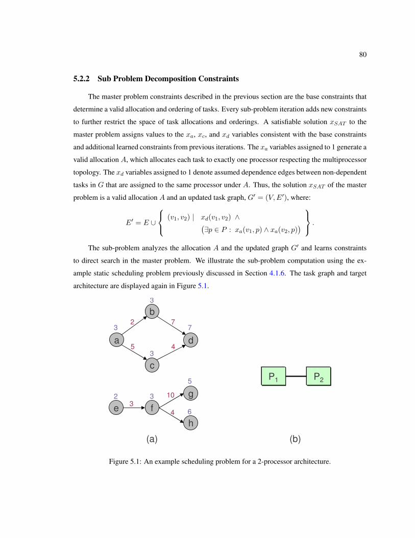
80

5.2.2 Sub Problem Decomposition Constraints

The master problem constraints described in the previous section are the base constraints that

determine a valid allocation and ordering of tasks. Every sub-problem iteration adds new constraints

to further restrict the space of task allocations and orderings. A satisfiable solution xSAT to the

master problem assigns values to the xa, xc, and xd variables consistent with the base constraints

and additional learned constraints from previous iterations. The xa variables assigned to 1 generate a

valid allocation A, which allocates each task to exactly one processor respecting the multiprocessor

topology. The xd variables assigned to 1 denote assumed dependence edges between non-dependent

tasks in G that are assigned to the same processor under A. Thus, the solution xSAT of the master

problem is a valid allocation A and an updated task graph, G′ = (V,E′), where:

E′ = E ∪

(v1, v2) | xd(v1, v2) ∧(∃p ∈ P : xa(v1, p) ∧ xa(v2, p)

) .

The sub-problem analyzes the allocation A and the updated graph G′ and learns constraints

to direct search in the master problem. We illustrate the sub-problem computation using the ex-

ample static scheduling problem previously discussed in Section 4.1.6. The task graph and target

architecture are displayed again in Figure 5.1.

a

b

c

d

g

h

fe

3

3

3

32

7

5

63

2

5

7

4

10

4

P1 P2

(a) (b)

Figure 5.1: An example scheduling problem for a 2-processor architecture.

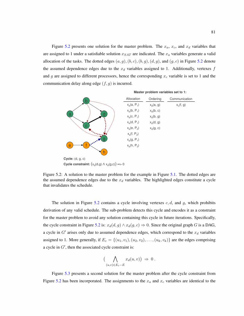
81

Figure 5.2 presents one solution for the master problem. The xa, xc, and xd variables that

are assigned to 1 under a satisfiable solution xSAT are indicated. The xa variables generate a valid

allocation of the tasks. The dotted edges (a, g), (b, c), (b, g), (d, g), and (g, c) in Figure 5.2 denote

the assumed dependence edges due to the xd variables assigned to 1. Additionally, vertexes f

and g are assigned to different processors, hence the corresponding xc variable is set to 1 and the

communication delay along edge (f, g) is incurred.

a

b

c

d

g

h

fe

xa(g, P1)

xa(h, P2)

xa(f, P2)

xa(e, P2)

xa(d, P1)

xa(c, P1)

xa(b, P1)

xa(a, P1)

Allocation

xc(f, g)

Communication

xd(g, c)

xd(d, g)

xd(b, g)

xd(b, c)

xd(a, g)

Ordering

Master problem variables set to 1:

Cycle: (d, g, c)

Cycle constraint: (xd(d,g) Λ xd(g,c)) > 0

Figure 5.2: A solution to the master problem for the example in Figure 5.1. The dotted edges arethe assumed dependence edges due to the xd variables. The highlighted edges constitute a cyclethat invalidates the schedule.

The solution in Figure 5.2 contains a cycle involving vertexes c, d, and g, which prohibits

derivation of any valid schedule. The sub-problem detects this cycle and encodes it as a constraint

for the master problem to avoid any solution containing this cycle in future iterations. Specifically,

the cycle constraint in Figure 5.2 is: xd(d, g) ∧ xd(g, c) ⇒ 0. Since the original graph G is a DAG,

a cycle in G′ arises only due to assumed dependence edges, which correspond to the xd variables

assigned to 1. More generally, if Ec = (u1, v1), (u2, v2), . . . , (uk, vk) are the edges comprising

a cycle in G′, then the associated cycle constraint is:

( ∧(u,v)∈Ec−E

xd(u, v))⇒ 0 .

Figure 5.3 presents a second solution for the master problem after the cycle constraint from

Figure 5.2 has been incorporated. The assignments to the xa and xc variables are identical to the

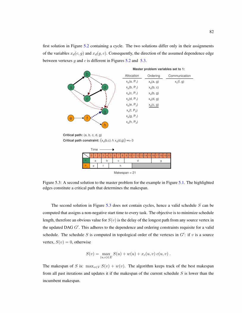
82

first solution in Figure 5.2 containing a cycle. The two solutions differ only in their assignments

of the variables xd(c, g) and xd(g, c). Consequently, the direction of the assumed dependence edge

between vertexes g and c is different in Figures 5.2 and 5.3.

a

b

c

d

g

h

fe

Makespan = 21

g

16 17 1813 14 15 2019121110

d

987

h

c

6

b

5

feP2

aP1

43210

Time

xa(g, P1)

xa(h, P2)

xa(f, P2)

xa(e, P2)

xa(d, P1)

xa(c, P1)

xa(b, P1)

xa(a, P1)

Allocation

xc(f, g)

Communication

xd(c, g)

xd(d, g)

xd(b, g)

xd(b, c)

xd(a, g)

Ordering

Master problem variables set to 1:

Critical path: (a, b, c, d, g)

Critical path constraint: (xd(b,c) Λ xd(d,g)) > 0

Figure 5.3: A second solution to the master problem for the example in Figure 5.1. The highlightededges constitute a critical path that determines the makespan.

The second solution in Figure 5.3 does not contain cycles, hence a valid schedule S can be

computed that assigns a non-negative start time to every task. The objective is to minimize schedule

length, therefore an obvious value for S(v) is the delay of the longest path from any source vertex in

the updated DAG G′. This adheres to the dependence and ordering constraints requisite for a valid

schedule. The schedule S is computed in topological order of the vertexes in G′: if v is a source

vertex, S(v) = 0, otherwise

S(v) = max(u,v)∈E

S(u) + w(u) + xc(u, v) c(u, v) .

The makespan of S is: maxv∈V S(v) + w(v). The algorithm keeps track of the best makespan

from all past iterations and updates it if the makespan of the current schedule S is lower than the

incumbent makespan.

83

Coming back to the example, the valid schedule S for the second solution is shown in Fig-

ure 5.3. The resulting makespan is 21 due to the critical path (a, b, c, d, g). Furthermore, any

solution to the master problem containing this critical path cannot yield a makespan lower than 21.

The sub-problem records this information as a constraint to eliminate all solutions containing the

critical path. Specifically, the constraint that encodes this critical path is: xd(b, c) ∧ xd(d, g) ⇒ 0.

Note that the algorithm is not restricted to learning only the critical path as a constraint. Any

path in G′ with delay greater than or equal to the best makespan provides a valid path constraint. In

Figure 5.3, if we assume that the incumbent makespan is 20, then the path (e, f, g) also bounds the

makespan and is a valid constraint (the path has delay 20 since edge (f, g) incurs a communication

delay). This can be encoded as: xc(f, g) ⇒ 0. The delay of any path is due only to the assumed

dependence edges (xd assignments) and the original graph edges on which a communication delay

is incurred (xc assignments). More generally, if Ep = (u1, v1), (u2, v2), . . . , (uk, vk) are the

edges comprising a path in G′ with delay greater than or equal to the best makespan at an iteration,

then the associated path constraint is:( ∧(u,v)∈Ep−E

xd(u, v))∧

( ∧(u,v)∈Ep∩E,A(u) 6=A(v)

xc(u, v))⇒ 0.

In this manner, each invocation of the sub-problem always adds at least one cycle constraint or

path constraint to restrict the space of valid allocations and orderings in the master problem. The

sub-problem also conditionally updates the best known makespan each time a path constraint is

detected. As long as at least one sub-problem constraint is generated, Algorithm 1 would terminate

with the optimum solution after a finite number of iterations. Termination occurs when the master

problem is unsatisfiable and the best known makespan at that point is the minimum makespan for

the static scheduling problem.

5.2.3 Algorithmic Extensions to Improve Performance

The use of a decomposition strategy opens opportunities to closely monitor and guide the

search in the constraint solver. We describe three algorithmic extensions to boost the performance

of the search method.

Sub-Problem Invocation from Intermediate Nodes in the Search

In Algorithm 1, the sub-problem is invoked only after the master fully solves the satisfiability

problem and generates an assignment for all primary variables. However, valid cycle and path

84

constraints can be derived from partial solutions at intermediate nodes in the search tree of the SAT

solver. If a partial solution contains a cycle, then subsequent assignments to the primary variables in

the SAT formulation evolving from this partial solution will not clear that cycle. Hence, the search

can be reset after the corresponding cycle constraint is learned and a new iteration of the master

problem can be commenced. When there are no cycles in a partial solution, the graph G′ = (V,E′)

can be generated based on the assignments in the partial solution. The delay of any path in G′ is

a lower bound on the makespan that can be achieved from the current partial solution. Therefore,

if a partial solution contains a path with delay greater than or equal to the incumbent makespan,

ensuing variable assignments will only result in inferior schedules. Hence, further search continuing

from this intermediate node can be averted. The corresponding path constraint prohibits the master

problem search from visiting any solution containing this path. Thus, sub-problem invocation from

intermediate nodes in the SAT search tree for the master problem provides a technique to identify

inferior solutions early and prune potentially large subsets of the solution space.

Tight Lower Bounds to Prune Inferior Solutions

Tight lower bounds on the makespan of partial solutions reinforce the pruning condition at

intermediate nodes in the SAT search. Lower bounds can be computed based on structural properties

of the task graphs and the partial solution. Two obvious lower bounds on the makespan are: (a) the

delay of the longest path in the task graph, and (b) the ratio of the total execution time of unassigned

tasks to the number of processors. A more complex lower bound, due to Gerasoulis and Yang,

propagates the minimum schedule length of primitive fork and join graph structures in the presence

of communication delays [Gerasoulis and Yang, 1992]. Fernandez and Bussell propose an alternate

lower bound, a good implementation of which is given by Fujita et al. in their FBB algorithm

[Fernandez and Bussel, 1973] [Fujita et al., 2002].

Variable Selection to Guide Search

An useful side-effect of inspecting partial solutions is that the sub-problem can recommend

decision variables to regulate branching in the master problem. For example, if two tasks assigned to

the same processor violate ordering constraints, the sub-problem can determine the next xd variable

that must be set to resolve this conflict. Additionally, the sub-problem can apply a priority metric,

such as dynamic level, and select a task-processor allocation for the master problem. Choosing an

appropriate variable directs search to inspect those schedules first that are deemed to be superior

85

by the selection heuristic, which in turn strengthens the conditions for pruning subsequent partial

solutions. Thus, the technique of inspecting partial solutions enables the sub-problem to closely

guide search and prune the solution space quickly. The concept of using a heuristic method for

local optimization and search guidance is further elaborated in Section 6.1.

5.3 Evaluation of the Decomposition Approach

In this section, we present results of our experiments to evaluate the decomposition strategy

against the Dynamic Level Scheduling (DLS) heuristic (Section 3.2.2) [Sih and Lee, 1993] and the

“single-pass” MILP formulation using overlap variables [Tompkins, 2003] for the scheduling prob-

lem from Section 4.1. We created a prototype implementation of the decomposition approach on

top of the MiniSAT SAT solver [Een and Sorensson, 2003]. The MILP instances were solved using

the ILOG CPLEX v10.1 solver [ILOG Inc., b]. The experiments were conducted on a PentiumIV

2.4 GHz processor with 1GB RAM running Linux.

5.3.1 Benchmark Set

Two benchmark sets are used in our experiments. The first benchmark consists of task graph

instances derived from two practical applications from the multimedia and networking domains, viz.

MJPEG decoding and IPv4 packet forwarding. The task execution times and communication delays

are profiled for the Xilinx MicroBlaze soft processor and the point-to-point fast simplex links (FSL)

available with the Xilinx Embedded Development Kit (EDK) [Xilinx Inc., 2004]. The base task

graph can be replicated to exploit the coarse grained parallelism available in these applications. For

MJPEG decoding, each replicated copy processes a different frame. For IPv4 packet forwarding,

the number of replications corresponds to the number of network input ports. We generate 10

problem instances for each application for different replications of the base task graph. The second

benchmark is a set of random task graph instances proposed by Davidovic et al. [Davidovic and

Crainic, 2006]. These problems are designed to be unbiased with respect to the solution technique

and are reportedly harder than other existing benchmarks for scheduling task graphs.

5.3.2 Comparisons to Heuristics and Single-Pass MILP Formulations

Tables 5.1 and 5.2 report the results of the different scheduling approaches for MJPEG decod-

ing and packet forwarding applications. The target architecture models consist of 2, 4, 6 or 8 fully

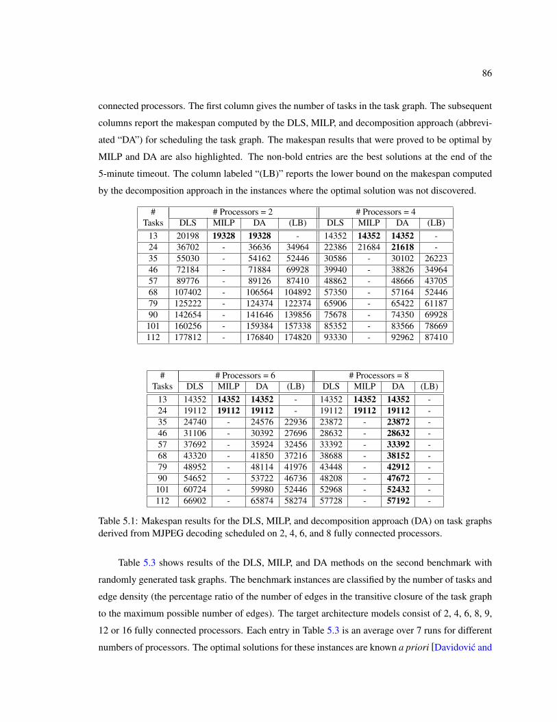
86

connected processors. The first column gives the number of tasks in the task graph. The subsequent

columns report the makespan computed by the DLS, MILP, and decomposition approach (abbrevi-

ated “DA”) for scheduling the task graph. The makespan results that were proved to be optimal by

MILP and DA are also highlighted. The non-bold entries are the best solutions at the end of the

5-minute timeout. The column labeled “(LB)” reports the lower bound on the makespan computed

by the decomposition approach in the instances where the optimal solution was not discovered.

# # Processors = 2 # Processors = 4Tasks DLS MILP DA (LB) DLS MILP DA (LB)

13 20198 19328 19328 - 14352 14352 14352 -24 36702 - 36636 34964 22386 21684 21618 -35 55030 - 54162 52446 30586 - 30102 2622346 72184 - 71884 69928 39940 - 38826 3496457 89776 - 89126 87410 48862 - 48666 4370568 107402 - 106564 104892 57350 - 57164 5244679 125222 - 124374 122374 65906 - 65422 6118790 142654 - 141646 139856 75678 - 74350 69928

101 160256 - 159384 157338 85352 - 83566 78669112 177812 - 176840 174820 93330 - 92962 87410


13 14352 14352 14352 - 14352 14352 14352 -24 19112 19112 19112 - 19112 19112 19112 -35 24740 - 24576 22936 23872 - 23872 -46 31106 - 30392 27696 28632 - 28632 -57 37692 - 35924 32456 33392 - 33392 -68 43320 - 41850 37216 38688 - 38152 -79 48952 - 48114 41976 43448 - 42912 -90 54652 - 53722 46736 48208 - 47672 -

101 60724 - 59980 52446 52968 - 52432 -112 66902 - 65874 58274 57728 - 57192 -

Table 5.1: Makespan results for the DLS, MILP, and decomposition approach (DA) on task graphsderived from MJPEG decoding scheduled on 2, 4, 6, and 8 fully connected processors.

Table 5.3 shows results of the DLS, MILP, and DA methods on the second benchmark with

randomly generated task graphs. The benchmark instances are classified by the number of tasks and

edge density (the percentage ratio of the number of edges in the transitive closure of the task graph

to the maximum possible number of edges). The target architecture models consist of 2, 4, 6, 8, 9,

12 or 16 fully connected processors. Each entry in Table 5.3 is an average over 7 runs for different

numbers of processors. The optimal solutions for these instances are known a priori [Davidovic and

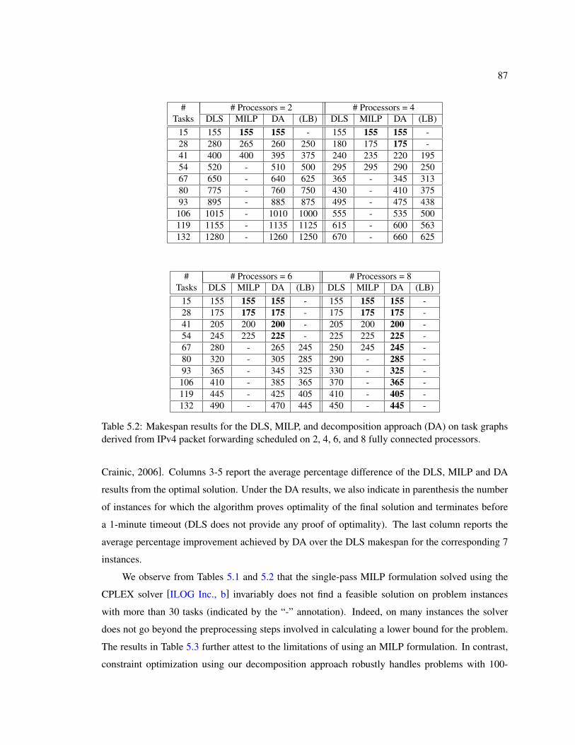
87


15 155 155 155 - 155 155 155 -28 280 265 260 250 180 175 175 -41 400 400 395 375 240 235 220 19554 520 - 510 500 295 295 290 25067 650 - 640 625 365 - 345 31380 775 - 760 750 430 - 410 37593 895 - 885 875 495 - 475 438

106 1015 - 1010 1000 555 - 535 500119 1155 - 1135 1125 615 - 600 563132 1280 - 1260 1250 670 - 660 625


15 155 155 155 - 155 155 155 -28 175 175 175 - 175 175 175 -41 205 200 200 - 205 200 200 -54 245 225 225 - 225 225 225 -67 280 - 265 245 250 245 245 -80 320 - 305 285 290 - 285 -93 365 - 345 325 330 - 325 -

106 410 - 385 365 370 - 365 -119 445 - 425 405 410 - 405 -132 490 - 470 445 450 - 445 -

Table 5.2: Makespan results for the DLS, MILP, and decomposition approach (DA) on task graphsderived from IPv4 packet forwarding scheduled on 2, 4, 6, and 8 fully connected processors.

Crainic, 2006]. Columns 3-5 report the average percentage difference of the DLS, MILP and DA

results from the optimal solution. Under the DA results, we also indicate in parenthesis the number

of instances for which the algorithm proves optimality of the final solution and terminates before

a 1-minute timeout (DLS does not provide any proof of optimality). The last column reports the

average percentage improvement achieved by DA over the DLS makespan for the corresponding 7

instances.

We observe from Tables 5.1 and 5.2 that the single-pass MILP formulation solved using the

CPLEX solver [ILOG Inc., b] invariably does not find a feasible solution on problem instances

with more than 30 tasks (indicated by the “-” annotation). Indeed, on many instances the solver

does not go beyond the preprocessing steps involved in calculating a lower bound for the problem.

The results in Table 5.3 further attest to the limitations of using an MILP formulation. In contrast,

constraint optimization using our decomposition approach robustly handles problems with 100-

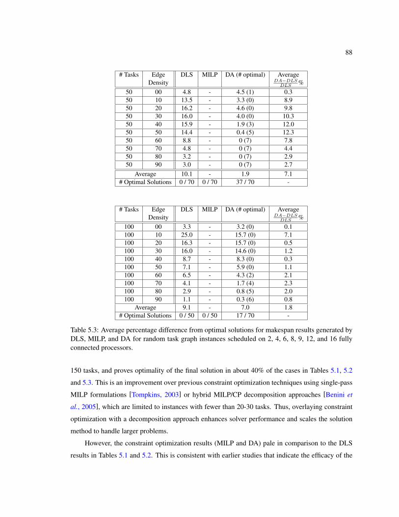
88

# Tasks Edge DLS MILP DA (# optimal) AverageDensity DA−DLS

DLS %50 00 4.8 - 4.5 (1) 0.350 10 13.5 - 3.3 (0) 8.950 20 16.2 - 4.6 (0) 9.850 30 16.0 - 4.0 (0) 10.350 40 15.9 - 1.9 (3) 12.050 50 14.4 - 0.4 (5) 12.350 60 8.8 - 0 (7) 7.850 70 4.8 - 0 (7) 4.450 80 3.2 - 0 (7) 2.950 90 3.0 - 0 (7) 2.7

Average 10.1 - 1.9 7.1# Optimal Solutions 0 / 70 0 / 70 37 / 70 -

# Tasks Edge DLS MILP DA (# optimal) AverageDensity DA−DLS

DLS %100 00 3.3 - 3.2 (0) 0.1100 10 25.0 - 15.7 (0) 7.1100 20 16.3 - 15.7 (0) 0.5100 30 16.0 - 14.6 (0) 1.2100 40 8.7 - 8.3 (0) 0.3100 50 7.1 - 5.9 (0) 1.1100 60 6.5 - 4.3 (2) 2.1100 70 4.1 - 1.7 (4) 2.3100 80 2.9 - 0.8 (5) 2.0100 90 1.1 - 0.3 (6) 0.8

Average 9.1 - 7.0 1.8# Optimal Solutions 0 / 50 0 / 50 17 / 70 -

Table 5.3: Average percentage difference from optimal solutions for makespan results generated byDLS, MILP, and DA for random task graph instances scheduled on 2, 4, 6, 8, 9, 12, and 16 fullyconnected processors.

150 tasks, and proves optimality of the final solution in about 40% of the cases in Tables 5.1, 5.2

and 5.3. This is an improvement over previous constraint optimization techniques using single-pass

MILP formulations [Tompkins, 2003] or hybrid MILP/CP decomposition approaches [Benini et

al., 2005], which are limited to instances with fewer than 20-30 tasks. Thus, overlaying constraint

optimization with a decomposition approach enhances solver performance and scales the solution

method to handle larger problems.

However, the constraint optimization results (MILP and DA) pale in comparison to the DLS

results in Tables 5.1 and 5.2. This is consistent with earlier studies that indicate the efficacy of the

89

DLS heuristic for the representative scheduling problem without specialized topology or resource

constraints[Kwok and Ahmad, 1999b] [Davidovic and Crainic, 2006]. We observe from many

experiments that the DLS solution is usually within 5-10% of the optimum on realistic task graphs

and problem instances with over 200 tasks are solved in seconds. Our DA method quickly finds the

DLS solution on all instances, since the sub-problem internally uses dynamic levels to recommend

task-processor allocations for the master problem. It is successful in improving the DLS makespan

or proving its optimality on instances with 100-150 tasks. But on larger problems, DA seldom

improves the DLS makespan. Nevertheless, the utility of MILP and DA, and constraint optimization

methods in general, becomes evident when there is a need for methods that can flexibly allow

additional implementation and resource constraints on valid schedules. We discuss this advantage

in Section 5.3.3 below.

Figure 5.4 graphically illustrates the results from Table 5.3 for the random task graph instances.

It plots the average percentage difference of the DLS and DA makespans from known optimal

solutions versus the edge density of the graph. An interesting trend in Figure 5.4 is that the quality

of the DLS and DA results improve as the edge density increases. A lower edge density indicates

fewer dependence constraints along edges, which allows greater flexibility in the ordering of tasks

within a processor (this translates to more xd ordering variables for non-dependent task pairs in

the constraint formulation of Algorithm 1). The flexibility in ordering tasks in turn increases the

complexity of the scheduling problem.

5.3.3 Extensibility of Constraint Programming

Heuristic methods like DLS are not easily extensible to include specialized implementation

and resource constraints in the problem. For example, practical multiprocessor architectures consist

of processors that may be connected in arbitrary topologies. The results in the previous section

assume fully connected topologies. Other common topologies are array, ring, or mesh topologies.

Figure 4.9 presents instances of irregular array based topologies that are viable architecture targets

for the IPv4 packet forwarding application on soft multiprocessors.

Bambha and Bhattacharyya propose an extension to the DLS list scheduling heuristic for ir-

regular multiprocessor topologies [Bambha and Bhattacharyya, 2002]. However, we observe from

our experiments that extending DLS with topology constraints compromises the original quality of

its results. Figures 5.5 and 5.6 illustrate the percentage improvement achieved by DA over the DLS

makespan for task graphs derived from MJPEG decoding and IPv4 packet forwarding scheduled on

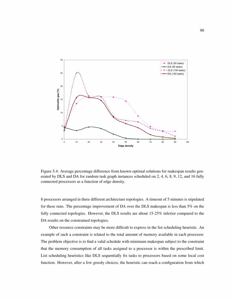
90

0

5

10

15

20

25

30

0 10 20 30 40 50 60 70 80 90 100

Edge density

Optimality gap (%)

DLS (50 tasks)

DA (50 tasks)

DLS (100 tasks)

DA (100 tasks)

Figure 5.4: Average percentage difference from known optimal solutions for makespan results gen-erated by DLS and DA for random task graph instances scheduled on 2, 4, 6, 8, 9, 12, and 16 fullyconnected processors as a function of edge density.

8 processors arranged in three different architecture topologies. A timeout of 5 minutes is stipulated

for these runs. The percentage improvement of DA over the DLS makespan is less than 5% on the

fully connected topologies. However, the DLS results are about 15-25% inferior compared to the

DA results on the constrained topologies.

Other resource constraints may be more difficult to express in the list scheduling heuristic. An

example of such a constraint is related to the total amount of memory available in each processor.

The problem objective is to find a valid schedule with minimum makespan subject to the constraint

that the memory consumption of all tasks assigned to a processor is within the prescribed limit.

List scheduling heuristics like DLS sequentially fix tasks to processors based on some local cost

function. However, after a few greedy choices, the heuristic can reach a configuration from which

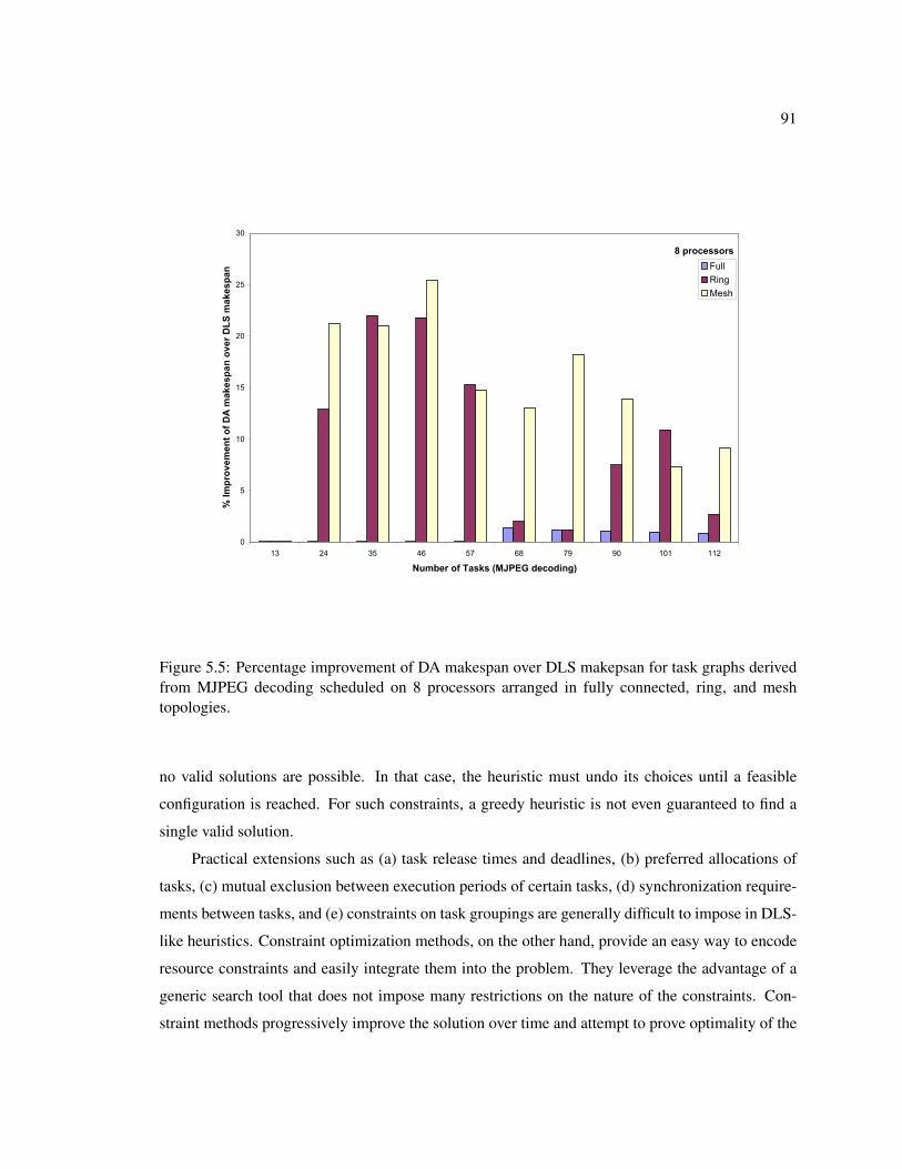
91

0

5

10

15

20

25

30

13 24 35 46 57 68 79 90 101 112

Number of Tasks (MJPEG decoding)

% Improvement of DA makespan over DLS makespan Full

Ring

Mesh

8 processors

Figure 5.5: Percentage improvement of DA makespan over DLS makepsan for task graphs derivedfrom MJPEG decoding scheduled on 8 processors arranged in fully connected, ring, and meshtopologies.

no valid solutions are possible. In that case, the heuristic must undo its choices until a feasible

configuration is reached. For such constraints, a greedy heuristic is not even guaranteed to find a

single valid solution.

Practical extensions such as (a) task release times and deadlines, (b) preferred allocations of

tasks, (c) mutual exclusion between execution periods of certain tasks, (d) synchronization require-

ments between tasks, and (e) constraints on task groupings are generally difficult to impose in DLS-

like heuristics. Constraint optimization methods, on the other hand, provide an easy way to encode

resource constraints and easily integrate them into the problem. They leverage the advantage of a

generic search tool that does not impose many restrictions on the nature of the constraints. Con-

straint methods progressively improve the solution over time and attempt to prove optimality of the

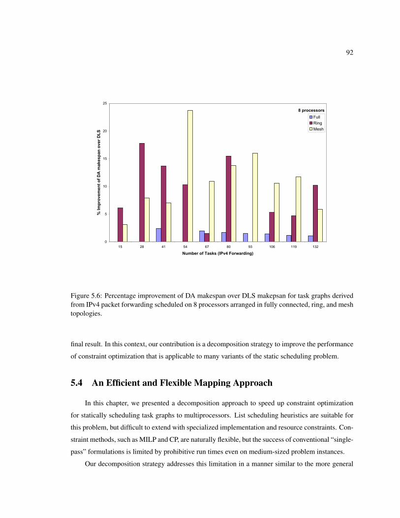
92

0

5

10

15

20

25

15 28 41 54 67 80 93 106 119 132

Number of Tasks (IPv4 Forwarding)

% Improvement of DA makespan over DLS

Full

Ring

Mesh

8 processors

Figure 5.6: Percentage improvement of DA makespan over DLS makepsan for task graphs derivedfrom IPv4 packet forwarding scheduled on 8 processors arranged in fully connected, ring, and meshtopologies.

final result. In this context, our contribution is a decomposition strategy to improve the performance

of constraint optimization that is applicable to many variants of the static scheduling problem.

5.4 An Efficient and Flexible Mapping Approach

In this chapter, we presented a decomposition approach to speed up constraint optimization

for statically scheduling task graphs to multiprocessors. List scheduling heuristics are suitable for

this problem, but difficult to extend with specialized implementation and resource constraints. Con-

straint methods, such as MILP and CP, are naturally flexible, but the success of conventional “single-

pass” formulations is limited by prohibitive run times even on medium-sized problem instances.

Our decomposition strategy addresses this limitation in a manner similar to the more general

93

Benders decomposition technique. The main elements of our strategy are: (a) fast graph theoretic

sub-problem algorithm that operates directly on the task graph, (b) effective encoding of problem

constraints to drive systematic exploration, (c) compact sub-problem constraints to record inferior

parts of the solution space, (d) tight lower bounds to prune inferior solutions, and (e) variable selec-

tion to guide search. While a single-pass MILP formulation for the scheduling problem is ineffective

on instances with over 30 tasks, our decomposition approach computes near-optimal solutions effi-

ciently on instances with over 150 tasks. Thus, the decomposition strategy retains the flexibility of

constraint programming methods and improves solver performance. We advance this as a general

solution technique that has significant potential for many variants of the scheduling problem with

complex implementation and resource constraints.

94

Chapter 6

A Toolbox of Scheduling Methods

The taxonomy from Chapter 1, Section 1.2.1 distinguishes three broad classes of scheduling

methods: heuristic, randomized, and exact. Though heuristics may be most computationally effi-

cient, their lack of flexibility motivates the study of exact mathematical and constraint programming

methods (Chapter 4). The integration of a decomposition strategy improves solver efficiency, while

retaining the flexibility of constraint programming (Chapter 5). However, mathematical and con-

straint programming methods lose their efficacy on large problem instances. The increasing magni-

tude of the solution space adversely affects the computational efficiency and quality of results.

More generally, it is unlikely that any single method can cope with the diversity of scheduling

problem variants encountered in an exploration framework. Rather, it may be prudent to advance

a toolbox of scheduling methods, in which each method is effective for a certain class of problem

models or optimization objectives. These methods provide different trade-offs with respect to com-

putational efficiency, quality of results, and flexibility. In this chapter, we propose such a toolbox

of methods for the representative scheduling problem from Chapter 4. Our toolbox is composed

of multiple heuristic methods, specialized constraint programming formulations, and simulated an-

nealing techniques. We assess the characteristics of individual methods and present our insights on

their relative merits and relevance to different types of scheduling problems.

6.1 The Value of Good Heuristics

In view of the intractability of most scheduling problem variants, the common approach has

been to design heuristics that can find good solutions quickly. Heuristics are finely tuned for specific

problem models and optimization objectives. Section 3.2.1 is a summary of popular heuristics for

95

static scheduling. However, heuristics are typically customized for a specific problem, sacrificing

flexibility for computational efficiency, and will have to be reworked each time new assumptions or

constraints are imposed. The results from Section 5.3.3 validate the advantages of using a flexible

constraint programming method over restricted heuristics for practical scheduling problems that

arise in an exploration framework.

Nevertheless, heuristic methods are still of great value in a toolbox of scheduling methods. As a

standalone scheduling method, a heuristic can be used to quickly evaluate upper bounds for specific

optimization problems. A second, and arguably more important advantage, is that a good heuristic

can guide search in more general scheduling methods, such as constraint programming or simulated

annealing. Redell’s distinction between global and local scheduling optimization problems clarifies

this concept [Redell, 1998]. The formulations in Chapters 4 and 5 pertain to the global problem,

which aims to compute a valid schedule for all system tasks. In contrast, an example of a local

optimization is to simply find the best allocation and start time for a single task, given a partial

schedule comprising a few other tasks. Heuristics are typically ill-suited for global optimization

due in part to their “short-sighted” view of the solution space. However, they may still be relevant

to local optimization. We elaborate on this capability in the context of the representative scheduling

problem from Section 4.1.

6.1.1 Dynamic Level Scheduling Revisited

The list scheduling technique is a workhorse for most heuristic methods. The basic idea is to

assign priorities to tasks and order them in a list by descending priorities; tasks with higher priori-

ties are examined for scheduling before tasks with lower priorities. The Dynamic Level Scheduling

(DLS) algorithm (Section 3.2.2), which was used as a reference to evaluate our constraint program-

ming methods in Chapter 5, is an effective list scheduling heuristic [Sih and Lee, 1993]. In the

following sections, we outline the DLS heuristic and then discuss its utility for local optimization

within general branch-and-bound based search methods like constraint programming.

Algorithm 2 illustrates the application of the DLS heuristic for the representative scheduling

problem specified in Section 4.1. The inputs to the scheduling algorithm are the task graph G =

(V,E), the task execution times w(v) for all tasks in V , the edge communication delays c((v1, v2))

for all edges in E. The multiprocessor architecture model is assumed to consist of P identical fully

connected processors. The additional resource constraints in Section 4.1.7 are not enforced.

Following the notations in Section 4.1.4, let A(v) and S(v) denote a valid allocation and non-

96

negative start time, respectively, for any task v ∈ V . A(v) and S(v) are initially undefined (denoted

ε) for all tasks (line 1). The list scheduling algorithm executes in |V | scheduling steps. At each step,

exactly one task and processor are chosen to be scheduled based on a priority metric (line 3). The

algorithm is qualified as “dynamic” since task priorities are updated at each list scheduling step. The

A and S variables for the chosen task are updated to reflect this selection (line 4). The algorithm

terminates after all tasks are allocated and returns the makespan (line 5).

Algorithm 2 DLS(G, w, c, P ) → makespan

// task allocation and start time variables1 A(v) = ε, S(v) = ε, ∀v ∈ V

2 for (i = 1 . . . |V |)

// choose next task processor pair to schedule3 (v, p) = DLSDECIDE(A,S,G, w, c, P )

// update schedule based on selection4 S(v) = maxDA(v, p, A, S), TF (p, A, S), A(v) = p

5 return maxv∈V S(v) + w(v)

A and S specify an intermediate schedule, which is iteratively updated as the algorithm exe-

cutes. Given an intermediate schedule, the earliest possible start time for some unscheduled task v

on a processor p (line 4) is determined by the following parameters:

DA(v, p, A, S) =

∞ : if A(v) 6= ε

∞ : else if ∃(v1, v) ∈ E, A(v1) = ε

max(v1,v)∈E S(v1) + w(v1) : else

+c((v1, v))

TF (p, A, S) = maxv∈V,A(v)=p

S(v) + w(v).

DA(v, p, A, S) is the earliest time that all data required by task v is available at processor p, after

all predecessors of v are scheduled according to A and S. TF (p, A, S) is the earliest time that

processor p is free after the last task assigned to it finishes execution.

The crux of the DLS algorithm is the selection of the next task and processor, based on a

priority metric, to schedule at each step (line 3). Algorithm 3 summarizes the computation of

the dynamic level metric used by DLS. The inputs to the algorithm are the problem models and

intermediate schedule. The dynamic level, denoted DL(v, p), is computed for every task v ∈ V

and processor p ∈ P (line 2). In this expression, the static level SL(v) for task v ∈ V is the

97

largest sum of execution times (specified by w) along any path from v to any sink vertex in G. The

maximization term represents the earliest time that task v can start execution on processor p. The

dynamic level considers two factors when evaluating a selection: (a) when comparing prospective

tasks, one with a high static level is desirable, since it indicates a high priority for execution, and

(b) when comparing candidate processors, a later start time is undesirable [Sih and Lee, 1993]. The

algorithm returns the task processor pair with highest dynamic level (line 3).

Algorithm 3 DLSDECIDE(A,S,G, w, c, P ) → (v ∈ V, p ∈ P )1 foreach (v ∈ V, p ∈ P )

// compute dynamic level for each task processor pair2 DL(v, p) = SL(v)−maxDA(v, p, A, S), TF (p, A, S)

// return task processor pair with highest dynamic level3 return arg maxv∈V,p∈P DL(v, p)

Independent benchmarking efforts for static scheduling algorithms, due to Kwok and Ahmad,

Davidovic and Crainic, and Koch, endorse the effectiveness of DLS for the scheduling problem

in Section 4.1 [Kwok and Ahmad, 1999a] [Davidovic and Crainic, 2006] [Koch, 1995]. Many

practical instances with over 200 tasks are scheduled by DLS under a second. The effectiveness

of the algorithm lies in the accuracy of the dynamic level metric computed in Algorithm 3, which

drives local scheduling decisions.

6.1.2 Guidance for Search in Branch-and-Bound Methods

The DLS algorithm approaches the global scheduling problem (Algorithm 2) by solving a

sequence of local optimization problems (Algorithm 3), in which each step fixes the allocation and

start time of a single task. However, a sequence of local decisions may result in a sub-optimal

global schedule. In order to maintain computational efficiency, the algorithm does not attempt to

revert inferior decisions.

In contrast, general branch-and-bound based search methods provide a facility to backtrack

search decisions and more systematically explore a complex solution space. The effectiveness of

branch-and-bound methods relies on two factors: (a) the ability to narrow the search space quickly

and accurately, and (b) the ability to guide search to find good solutions quickly. An heuristic based

local decision strategy is an useful mechanism to guide the search into more relevant regions of the

solution space. Following this concept, the DLS heuristic can be leveraged to improve the search in

our decomposition based constraint programming method (DA) from Chapter 5.

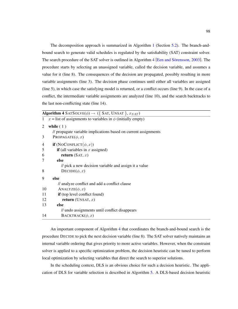
98

The decomposition approach is summarized in Algorithm 1 (Section 5.2). The branch-and-

bound search to generate valid schedules is regulated by the satisfiability (SAT) constraint solver.

The search procedure of the SAT solver is outlined in Algorithm 4 [Een and Sorensson, 2003]. The

procedure starts by selecting an unassigned variable, called the decision variable, and assumes a

value for it (line 8). The consequences of the decision are propagated, possibly resulting in more

variable assignments (line 3). The decision phase continues until either all variables are assigned

(line 5), in which case the satisfying model is returned, or a conflict occurs (line 9). In the case of a

conflict, the intermediate variable assignments are analyzed (line 10), and the search backtracks to

the last non-conflicting state (line 14).

Algorithm 4 SATSOLVE(φ) → ( SAT, UNSAT , xSAT )1 x = list of assignments to variables in φ (initially empty)

2 while ( 1 )// propagate variable implications based on current assignments

3 PROPAGATE(φ, x)

4 if (NOCONFLICT(φ, x))5 if (all variables in x assigned)6 return (SAT, x)7 else

// pick a new decision variable and assign it a value8 DECIDE(φ, x)

9 else// analyze conflict and add a conflict clause

10 ANALYZE(φ, x)11 if (top level conflict found)12 return (UNSAT, x)13 else

// undo assignments until conflict disappears14 BACKTRACK(φ, x)

An important component of Algorithm 4 that coordinates the branch-and-bound search is the

procedure DECIDE to pick the next decision variable (line 8). The SAT solver natively maintains an

internal variable ordering that gives priority to more active variables. However, when the constraint

solver is applied to a specific optimization problem, the decision heuristic can be tuned to perform

local optimization by selecting variables that direct the search to superior solutions.

In the scheduling context, DLS is an obvious choice for such a decision heuristic. The appli-

cation of DLS for variable selection is described in Algorithm 5. A DLS-based decision heuristic

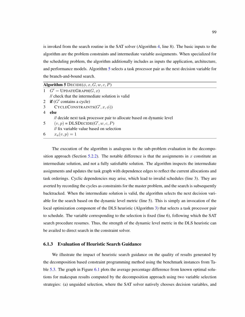
99

is invoked from the search routine in the SAT solver (Algorithm 4, line 8). The basic inputs to the

algorithm are the problem constraints and intermediate variable assignments. When specialized for

the scheduling problem, the algorithm additionally includes as inputs the application, architecture,

and performance models. Algorithm 5 selects a task processor pair as the next decision variable for

the branch-and-bound search.

Algorithm 5 DECIDE(φ, x,G, w, c, P )1 G′ = UPDATEGRAPH(G, x)

// check that the intermediate solution is valid2 if (G′ contains a cycle)3 CYCLECONSTRAINTS(G′, x, φ))4 else

// decide next task processor pair to allocate based on dynamic level5 (v, p) = DLSDECIDE(G′, w, c, P )

// fix variable value based on selection6 xa(v, p) = 1

The execution of the algorithm is analogous to the sub-problem evaluation in the decompo-

sition approach (Section 5.2.2). The notable difference is that the assignments in x constitute an

intermediate solution, and not a fully satisfiable solution. The algorithm inspects the intermediate

assignments and updates the task graph with dependence edges to reflect the current allocations and

task orderings. Cyclic dependencies may arise, which lead to invalid schedules (line 3). They are

averted by recording the cycles as constraints for the master problem, and the search is subsequently

backtracked. When the intermediate solution is valid, the algorithm selects the next decision vari-

able for the search based on the dynamic level metric (line 5). This is simply an invocation of the

local optimization component of the DLS heuristic (Algorithm 3) that selects a task processor pair

to schedule. The variable corresponding to the selection is fixed (line 6), following which the SAT

search procedure resumes. Thus, the strength of the dynamic level metric in the DLS heuristic can

be availed to direct search in the constraint solver.

6.1.3 Evaluation of Heuristic Search Guidance

We illustrate the impact of heuristic search guidance on the quality of results generated by

the decomposition based constraint programming method using the benchmark instances from Ta-

ble 5.3. The graph in Figure 6.1 plots the average percentage difference from known optimal solu-

tions for makespan results computed by the decomposition approach using two variable selection

strategies: (a) unguided selection, where the SAT solver natively chooses decision variables, and

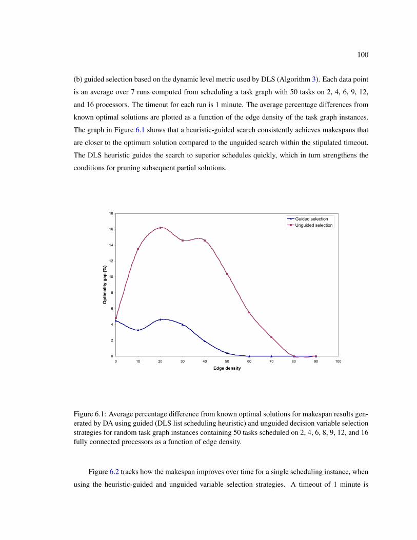
100

(b) guided selection based on the dynamic level metric used by DLS (Algorithm 3). Each data point

is an average over 7 runs computed from scheduling a task graph with 50 tasks on 2, 4, 6, 9, 12,

and 16 processors. The timeout for each run is 1 minute. The average percentage differences from

known optimal solutions are plotted as a function of the edge density of the task graph instances.

The graph in Figure 6.1 shows that a heuristic-guided search consistently achieves makespans that

are closer to the optimum solution compared to the unguided search within the stipulated timeout.

The DLS heuristic guides the search to superior schedules quickly, which in turn strengthens the

conditions for pruning subsequent partial solutions.

0

2

4

6

8

10

12

14

16

18

0 10 20 30 40 50 60 70 80 90 100

Edge density

Optimality gap (%)

Guided selection

Unguided selection

Figure 6.1: Average percentage difference from known optimal solutions for makespan results gen-erated by DA using guided (DLS list scheduling heuristic) and unguided decision variable selectionstrategies for random task graph instances containing 50 tasks scheduled on 2, 4, 6, 8, 9, 12, and 16fully connected processors as a function of edge density.

Figure 6.2 tracks how the makespan improves over time for a single scheduling instance, when

using the heuristic-guided and unguided variable selection strategies. A timeout of 1 minute is

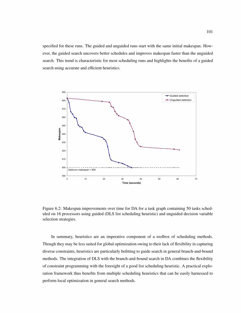
101

specified for these runs. The guided and unguided runs start with the same initial makespan. How-

ever, the guided search uncovers better schedules and improves makespan faster than the unguided

search. This trend is characteristic for most scheduling runs and highlights the benefits of a guided

search using accurate and efficient heuristics.

590

600

610

620

630

640

650

660

670

680

690

0 10 20 30 40 50 60 70

Time (seconds)

Makespan

Guided selection

Unguided selection

Optimum makespan = 600

Figure 6.2: Makespan improvements over time for DA for a task graph containing 50 tasks sched-uled on 16 processors using guided (DLS list scheduling heuristic) and unguided decision variableselection strategies.

In summary, heuristics are an imperative component of a toolbox of scheduling methods.

Though they may be less suited for global optimization owing to their lack of flexibility in capturing

diverse constraints, heuristics are particularly befitting to guide search in general branch-and-bound

methods. The integration of DLS with the branch-and-bound search in DA combines the flexibility

of constraint programming with the foresight of a good list scheduling heuristic. A practical explo-

ration framework thus benefits from multiple scheduling heuristics that can be easily harnessed to

perform local optimization in general search methods.

102

6.2 Simulated Annealing for Large Task Graphs

In Chapters 4 and 5, we justified the viability of mathematical and constraint programming

methods for solving the representative scheduling problem from Section 4.1. The experimental

evaluations from Section 5.3 indicate that these methods are effective on instances with over 150

tasks and diverse implementation and resource constraints. Furthermore, the optimality of the final

result is certified in about 40% of the experimental instances. In the remaining cases, the methods

establish tight lower bounds and compute near-optimum results with optimality gaps less than 20%.

However, exact constraint methods begin to lose their efficacy on larger problem instances.

The increasing magnitude of the solution space adversely affects the computational efficiency and

quality of results. A possible compensation to surmount the large solution space is to forgo the

guarantee of optimality and incorporate randomness in the search. Complex combinatorial global

optimization problems have been surprisingly amenable to randomized search.

Simulated annealing (SA) is one such randomized search technique that serves to complement

constraint programming in our toolbox of practical scheduling methods. SA is a generic probabilis-

tic non-greedy algorithm that adapts the Markov Chain Monte Carlo method for global optimization

problems [Kirkpatrick et al., 1983]. The basic idea is to iteratively perturb a system, starting from

an arbitrary initial state, until it reaches a state with globally minimum energy. Each step of the

algorithm considers a move from the current state to a random nearby state. The probability of

making a transition depends on the two states and a global time-varying control parameter, called

“temperature”. In the following sections, we outline the concept of simulated annealing and then

discuss its application to the representative scheduling problem.

6.2.1 A Generic Simulated Annealing Algorithm

Algorithm 6 illustrates a generic simulated annealing method. The inputs are an initial state s0

from the space of valid solutions, an initial temperature t0, and a final temperature t∞. The function

Cost measures the quality of some property of a state as a real number. The output of the algorithm

is the state sbest that minimizes the Cost function among all states encountered during search.

The algorithm operates in the following manner. Parameters si and ti denote the state and

temperature at iteration i of the algorithm. The function Temp computes the temperature at iteration

i (line 3). The temperature is typically the highest at the first iteration and is gradually reduced as

the simulation proceeds, according to an “annealing schedule”. The function Move proposes a

new state s′ for transition (line 4). The algorithm computes the difference ∆ in the Cost function

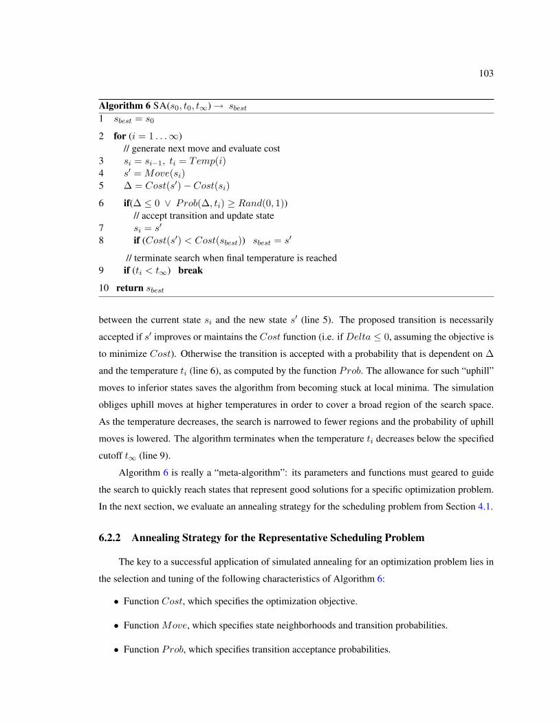
103

Algorithm 6 SA(s0, t0, t∞) → sbest

1 sbest = s0

2 for (i = 1 . . .∞)// generate next move and evaluate cost

3 si = si−1, ti = Temp(i)4 s′ = Move(si)5 ∆ = Cost(s′)− Cost(si)

6 if(∆ ≤ 0 ∨ Prob(∆, ti) ≥ Rand(0, 1))// accept transition and update state

7 si = s′

8 if (Cost(s′) < Cost(sbest)) sbest = s′

// terminate search when final temperature is reached9 if (ti < t∞) break

10 return sbest

between the current state si and the new state s′ (line 5). The proposed transition is necessarily

accepted if s′ improves or maintains the Cost function (i.e. if Delta ≤ 0, assuming the objective is

to minimize Cost). Otherwise the transition is accepted with a probability that is dependent on ∆

and the temperature ti (line 6), as computed by the function Prob. The allowance for such “uphill”

moves to inferior states saves the algorithm from becoming stuck at local minima. The simulation

obliges uphill moves at higher temperatures in order to cover a broad region of the search space.

As the temperature decreases, the search is narrowed to fewer regions and the probability of uphill

moves is lowered. The algorithm terminates when the temperature ti decreases below the specified

cutoff t∞ (line 9).

Algorithm 6 is really a “meta-algorithm”: its parameters and functions must geared to guide

the search to quickly reach states that represent good solutions for a specific optimization problem.

In the next section, we evaluate an annealing strategy for the scheduling problem from Section 4.1.

6.2.2 Annealing Strategy for the Representative Scheduling Problem

The key to a successful application of simulated annealing for an optimization problem lies in

the selection and tuning of the following characteristics of Algorithm 6:

• Function Cost, which specifies the optimization objective.

• Function Move, which specifies state neighborhoods and transition probabilities.

• Function Prob, which specifies transition acceptance probabilities.

104

• Function Temp, which specifies the annealing schedule for updating temperature.

• Parameter t0, the initial temperature.

• Parameter t∞, the final temperature.

The works of Orsila et al. and Koch propose annealing strategies for related scheduling prob-

lems [Orsila et al., 2006] [Koch, 1995]. We follow the techniques from these works in customizing

the parameters and functions of Algorithm 6 for the representative scheduling problem.

The inputs to the scheduling problem are the task graph G = (V,E), the task execution times

w(v) for all tasks in V , the edge communication delays c((v1, v2)) for all edges in E, and the

multiprocessor architecture model given by P and C. The objective is to compute a valid allocation

A and schedule S with minimum makespan. Let Ω denote the state space for the annealing search.

Then, for the representative scheduling problem, Ω is the set of all valid allocations and schedules,

as specified in Section 4.1.4. An obvious Cost function is the makespan of a valid schedule, i.e.

Cost(s) = Makespan(s), ∀s ∈ Ω.

The annealing search occurs on a connected, undirected graph on Ω, sometimes called a

“neighborhood structure”. The Move function implicitly defines the neighborhood structure in

Ω: it randomly selects a state s′ in the neighborhood of the current state s for the next transition. In

the context of the scheduling problem, any state s ∈ Ω is characterized by a valid allocation As and

schedule Ss. Let Vp = v ∈ V | As(v) = p be the set of tasks currently assigned to processor

p ∈ P under allocation As. Then, the schedule Ss equivalently imposes a total order on the tasks

in Vp. Starting with the current state s, the Move function randomly selects a task v ∈ V and

processor p ∈ P , and fixes the allocation of v to p for the new state s′, i.e. As′(v) = p. Move then

randomly selects a position in the total order of Vp for task v. The global schedule Ss′ is recomputed

after the relocation.

The transition acceptance probability function Prob determines whether a transition occurs to

the state proposed by the Move function. A common definition of the acceptance probability for

annealing algorithms is:

Prob(∆, ti) =

1 : if ∆ ≤ 0

exp(− ∆

ti

): else

The definition implies that the probability of accepting a transition decreases as the temperature

decreases, or as difference in cost relative to the current state increases.

105

The temperature update function Temp defines the annealing schedule. Following the strategy

of Koch, we define Temp in the following manner [Koch, 1995]:

Temp(i) =

ti−1

1 + δti−1

σi−R,i

: if (i mod R) = 0

ti−1 : else

The Temp function is regulated by two parameters: R and δ. The temperature is updated once

every R iterations. The parameter δ (0 < δ < 1) is a multiplicative factor that controls how

much the temperature is decreased. The decrease in temperature is greater for a larger value of

δ. The parameters R and δ determine how aggressively the annealing schedule converges to a low

temperature “steady-state”, where the probability of accepting uphill transitions to inferior states is

minimal. The annealing schedule is additionally influenced by a third factor, σi−R,i, in the Temp

function. This represents the standard deviation of the Cost evaluations at all states visited since

the last temperature update. More formally,

σi−R,i = stddevCost(sk) | i−R ≤ k < i

.

Intuitively, a lower value for σi−R,i implies that the system accepted fewer transitions in the last R

iterations. A low σi−R,i in turn induces a greater decrease in the temperature to speed up system

convergence.

Given this definition of the Temp function and the annealing schedule, a reasonable choice

for the initial temperature is t0 = 1. The final temperature t∞ must be greater than 0 to ensure

Algorithm 6 terminates. A lower value for t∞ encourages a greater number of search iterations.

6.3 Evaluation of Scheduling Methods

In this section, we evaluate the simulated annealing (SA) method described in Algorithm 6

against the dynamic list scheduling (DLS) heuristic (Section 3.2.2) and the decomposition based

constraint programming (DA) method (Section 5.3). Table 6.1 compares the different methods for

scheduling task graphs derived from multiple data parallel iterations of the IPv4 packet forwarding

application (Section 4.3). The target architecture models consist of 8 processors arranged in fully-

connected, ring, and mesh topologies. The first column in Table 6.1 gives the number of tasks in

the task graph. The subsequent columns report the makespan computed by the DLS, DA, and SA

methods for scheduling the task graph. A timeout of 5 minutes is stipulated for the DA method. The

makespan results proved to be optimal by DA are highlighted. The column labeled “(LB)” reports

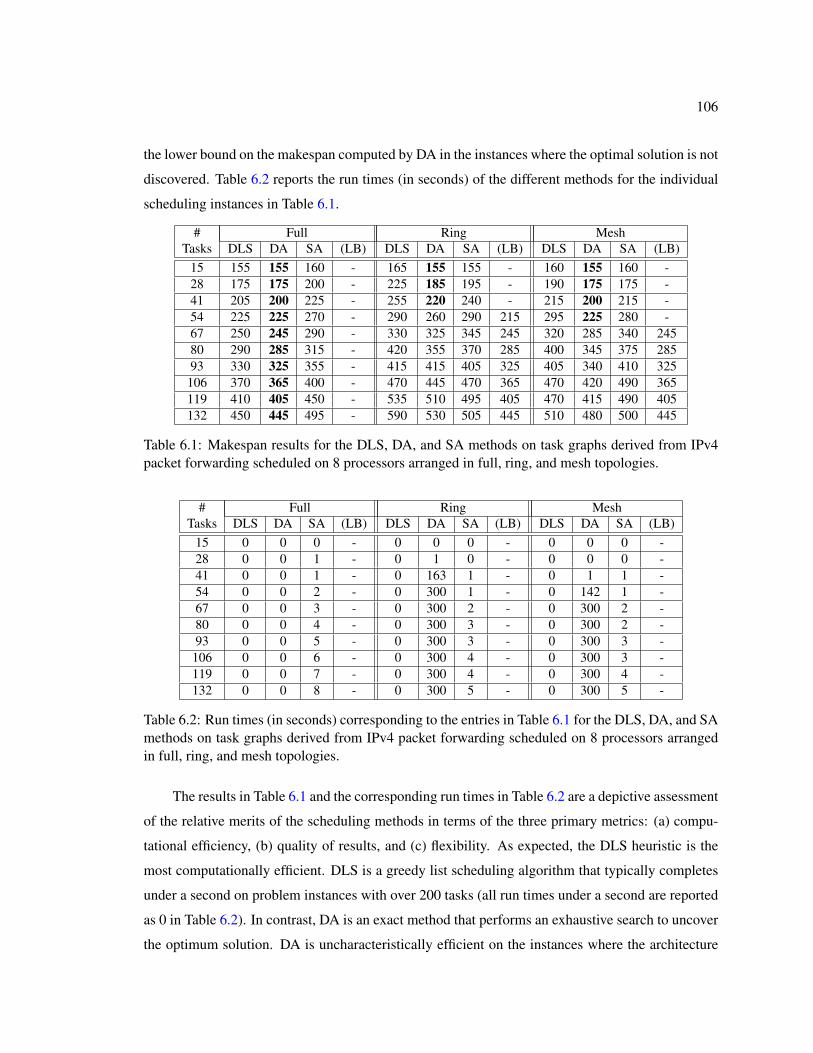
106

the lower bound on the makespan computed by DA in the instances where the optimal solution is not

discovered. Table 6.2 reports the run times (in seconds) of the different methods for the individual

scheduling instances in Table 6.1.

# Full Ring MeshTasks DLS DA SA (LB) DLS DA SA (LB) DLS DA SA (LB)

15 155 155 160 - 165 155 155 - 160 155 160 -28 175 175 200 - 225 185 195 - 190 175 175 -41 205 200 225 - 255 220 240 - 215 200 215 -54 225 225 270 - 290 260 290 215 295 225 280 -67 250 245 290 - 330 325 345 245 320 285 340 24580 290 285 315 - 420 355 370 285 400 345 375 28593 330 325 355 - 415 415 405 325 405 340 410 325

106 370 365 400 - 470 445 470 365 470 420 490 365119 410 405 450 - 535 510 495 405 470 415 490 405132 450 445 495 - 590 530 505 445 510 480 500 445

Table 6.1: Makespan results for the DLS, DA, and SA methods on task graphs derived from IPv4packet forwarding scheduled on 8 processors arranged in full, ring, and mesh topologies.

# Full Ring MeshTasks DLS DA SA (LB) DLS DA SA (LB) DLS DA SA (LB)

15 0 0 0 - 0 0 0 - 0 0 0 -28 0 0 1 - 0 1 0 - 0 0 0 -41 0 0 1 - 0 163 1 - 0 1 1 -54 0 0 2 - 0 300 1 - 0 142 1 -67 0 0 3 - 0 300 2 - 0 300 2 -80 0 0 4 - 0 300 3 - 0 300 2 -93 0 0 5 - 0 300 3 - 0 300 3 -

106 0 0 6 - 0 300 4 - 0 300 3 -119 0 0 7 - 0 300 4 - 0 300 4 -132 0 0 8 - 0 300 5 - 0 300 5 -

Table 6.2: Run times (in seconds) corresponding to the entries in Table 6.1 for the DLS, DA, and SAmethods on task graphs derived from IPv4 packet forwarding scheduled on 8 processors arrangedin full, ring, and mesh topologies.

The results in Table 6.1 and the corresponding run times in Table 6.2 are a depictive assessment

of the relative merits of the scheduling methods in terms of the three primary metrics: (a) compu-

tational efficiency, (b) quality of results, and (c) flexibility. As expected, the DLS heuristic is the

most computationally efficient. DLS is a greedy list scheduling algorithm that typically completes

under a second on problem instances with over 200 tasks (all run times under a second are reported

as 0 in Table 6.2). In contrast, DA is an exact method that performs an exhaustive search to uncover

the optimum solution. DA is uncharacteristically efficient on the instances where the architecture

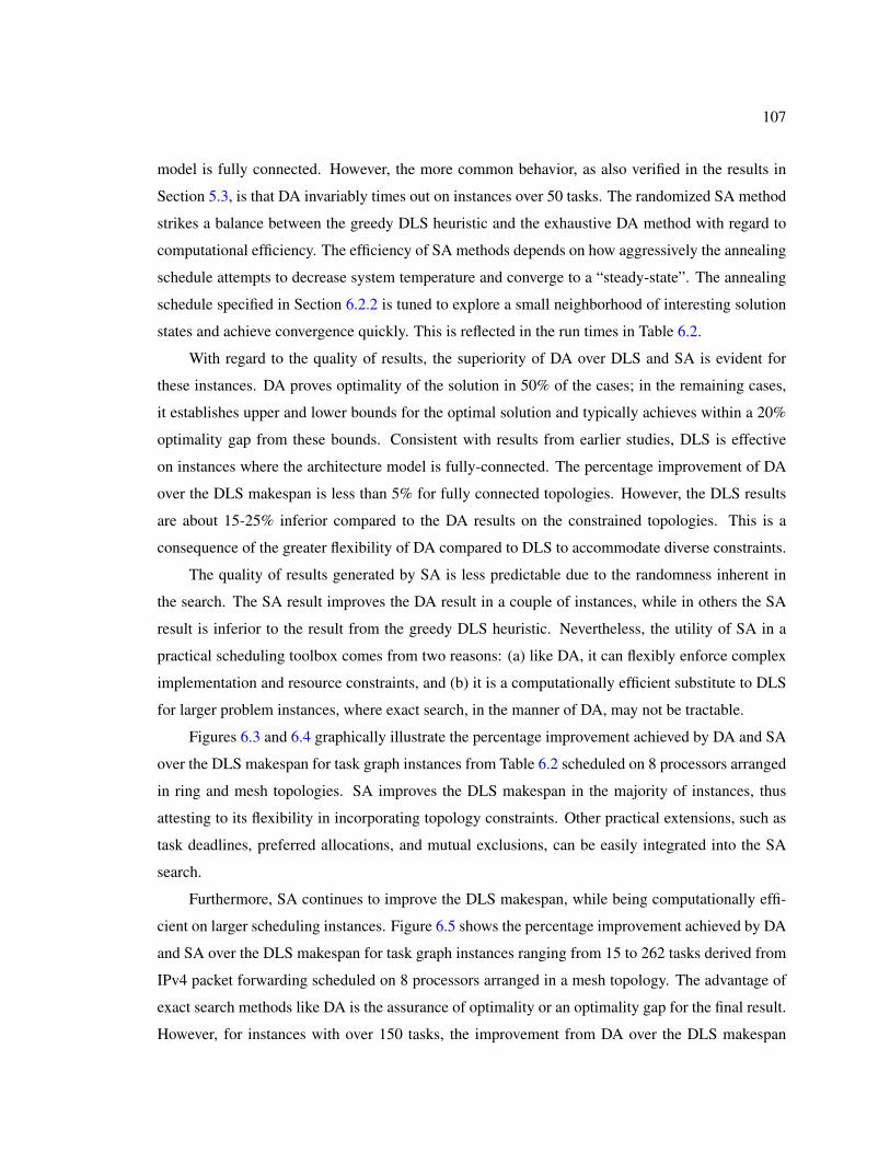
107

model is fully connected. However, the more common behavior, as also verified in the results in

Section 5.3, is that DA invariably times out on instances over 50 tasks. The randomized SA method

strikes a balance between the greedy DLS heuristic and the exhaustive DA method with regard to

computational efficiency. The efficiency of SA methods depends on how aggressively the annealing

schedule attempts to decrease system temperature and converge to a “steady-state”. The annealing

schedule specified in Section 6.2.2 is tuned to explore a small neighborhood of interesting solution

states and achieve convergence quickly. This is reflected in the run times in Table 6.2.

With regard to the quality of results, the superiority of DA over DLS and SA is evident for

these instances. DA proves optimality of the solution in 50% of the cases; in the remaining cases,

it establishes upper and lower bounds for the optimal solution and typically achieves within a 20%

optimality gap from these bounds. Consistent with results from earlier studies, DLS is effective

on instances where the architecture model is fully-connected. The percentage improvement of DA

over the DLS makespan is less than 5% for fully connected topologies. However, the DLS results

are about 15-25% inferior compared to the DA results on the constrained topologies. This is a

consequence of the greater flexibility of DA compared to DLS to accommodate diverse constraints.

The quality of results generated by SA is less predictable due to the randomness inherent in

the search. The SA result improves the DA result in a couple of instances, while in others the SA

result is inferior to the result from the greedy DLS heuristic. Nevertheless, the utility of SA in a

practical scheduling toolbox comes from two reasons: (a) like DA, it can flexibly enforce complex

implementation and resource constraints, and (b) it is a computationally efficient substitute to DLS

for larger problem instances, where exact search, in the manner of DA, may not be tractable.

Figures 6.3 and 6.4 graphically illustrate the percentage improvement achieved by DA and SA

over the DLS makespan for task graph instances from Table 6.2 scheduled on 8 processors arranged

in ring and mesh topologies. SA improves the DLS makespan in the majority of instances, thus

attesting to its flexibility in incorporating topology constraints. Other practical extensions, such as

task deadlines, preferred allocations, and mutual exclusions, can be easily integrated into the SA

search.

Furthermore, SA continues to improve the DLS makespan, while being computationally effi-

cient on larger scheduling instances. Figure 6.5 shows the percentage improvement achieved by DA

and SA over the DLS makespan for task graph instances ranging from 15 to 262 tasks derived from

IPv4 packet forwarding scheduled on 8 processors arranged in a mesh topology. The advantage of

exact search methods like DA is the assurance of optimality or an optimality gap for the final result.

However, for instances with over 150 tasks, the improvement from DA over the DLS makespan

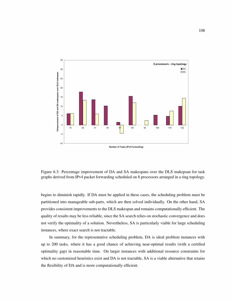
108

-10

-5

0

5

10

15

20

25

30

35

15 28 41 54 67 80 93 106 119 132


%Improvement of DA and SA makespans over DLS makespan

DA

SA

8 processors - ring topology

Figure 6.3: Percentage improvement of DA and SA makespans over the DLS makepsan for taskgraphs derived from IPv4 packet forwarding scheduled on 8 processors arranged in a ring topology.

begins to diminish rapidly. If DA must be applied in these cases, the scheduling problem must be

partitioned into manageable sub-parts, which are then solved individually. On the other hand, SA

provides consistent improvements to the DLS makespan and remains computationally efficient. The

quality of results may be less reliable, since the SA search relies on stochastic convergence and does

not verify the optimality of a solution. Nevertheless, SA is particularly viable for large scheduling

instances, where exact search is not tractable.

In summary, for the representative scheduling problem, DA is ideal problem instances with

up to 200 tasks, where it has a good chance of achieving near-optimal results (with a certified

optimality gap) in reasonable time. On larger instances with additional resource constraints for

which no customized heuristics exist and DA is not tractable, SA is a viable alternative that retains

the flexibility of DA and is more computationally efficient.

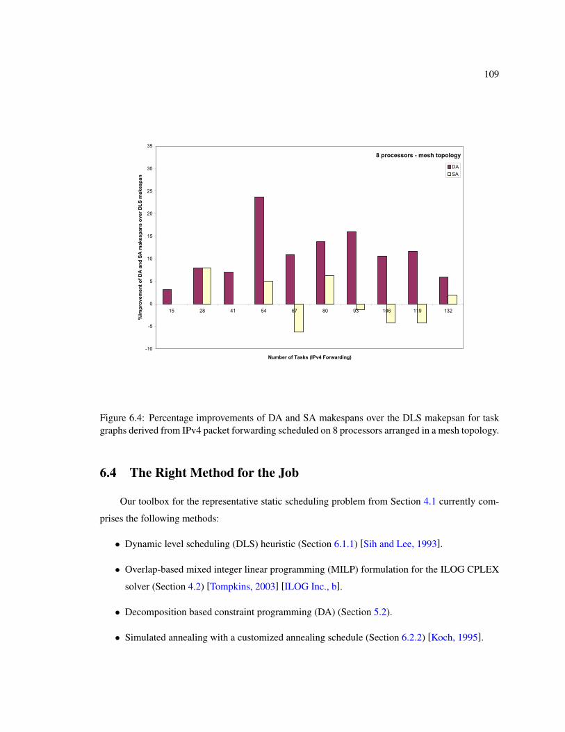
109

-10

-5

0

5

10

15

20

25

30

35

15 28 41 54 67 80 93 106 119 132



DA

SA

8 processors - mesh topology

Figure 6.4: Percentage improvements of DA and SA makespans over the DLS makepsan for taskgraphs derived from IPv4 packet forwarding scheduled on 8 processors arranged in a mesh topology.

6.4 The Right Method for the Job

Our toolbox for the representative static scheduling problem from Section 4.1 currently com-

prises the following methods:

• Dynamic level scheduling (DLS) heuristic (Section 6.1.1) [Sih and Lee, 1993].

• Overlap-based mixed integer linear programming (MILP) formulation for the ILOG CPLEX

solver (Section 4.2) [Tompkins, 2003] [ILOG Inc., b].

• Decomposition based constraint programming (DA) (Section 5.2).

• Simulated annealing with a customized annealing schedule (Section 6.2.2) [Koch, 1995].

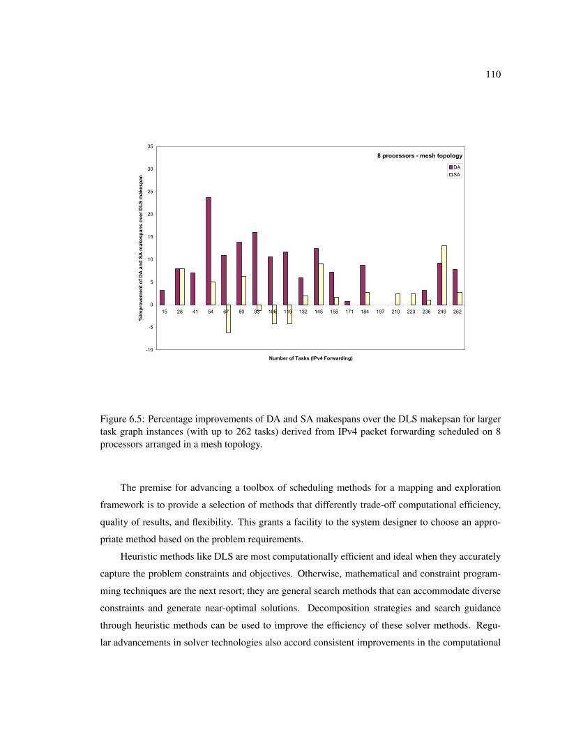
110

-10

-5

0

5

10

15

20

25

30

35

15 28 41 54 67 80 93 106 119 132 145 158 171 184 197 210 223 236 249 262



DA

SA

8 processors - mesh topology

Figure 6.5: Percentage improvements of DA and SA makespans over the DLS makepsan for largertask graph instances (with up to 262 tasks) derived from IPv4 packet forwarding scheduled on 8processors arranged in a mesh topology.

The premise for advancing a toolbox of scheduling methods for a mapping and exploration

framework is to provide a selection of methods that differently trade-off computational efficiency,

quality of results, and flexibility. This grants a facility to the system designer to choose an appro-

priate method based on the problem requirements.

Heuristic methods like DLS are most computationally efficient and ideal when they accurately

capture the problem constraints and objectives. Otherwise, mathematical and constraint program-

ming techniques are the next resort; they are general search methods that can accommodate diverse

constraints and generate near-optimal solutions. Decomposition strategies and search guidance

through heuristic methods can be used to improve the efficiency of these solver methods. Regu-

lar advancements in solver technologies also accord consistent improvements in the computational

111

efficiency and quality of results. However, exact solver methods suffer prohibitive run times on

large problem instances. Alternatively, simulated annealing methods retain the flexibility of exact

methods; though the quality of results may be less predictable, annealing methods are more compu-

tationally efficient on larger instances. Thus, this collection of methods provide different strengths

to address varied problem requirements and objectives, and are hence integral to a practical schedul-

ing toolbox in a framework for concurrent application deployment and design space exploration.

112

Chapter 7

Conclusions and Further Work

The premise for this dissertation is the advent of programmable single chip multiprocessors in

mainstream and embedded computing, and the associated challenge of productively deploying con-

current applications to harness the performance potential of these parallel platforms. The challenge

motivates the need for a disciplined application deployment and design space exploration approach

to assist the designer in building efficient system implementations. A key step in this exploration ap-

proach is mapping the task level concurrency in an application to the processing and communication

resources in a multiprocessor architecture.

Our work focuses on methods for static compile time task allocation and scheduling to map

application task level concurrency to a multiprocessor architecture. When the application workload

and execution profiles can be reliably estimated at compile time, an application mapping can be

determined statically. Static models and methods ease early design decisions and are integral to

rapid design space exploration of micro-architectures and systems.

Static scheduling entails solving a complex combinatorial optimization problem subject to a

variety of implementation and resource constraints. Owing to the computational complexity of

optimal scheduling, a number of heuristic algorithms have been studied for different scheduling

conditions and application and architecture models. However, heuristic methods are brittle with re-

spect to changes in the problem models; they lack the flexibility necessary to accommodate diverse

implementation and resource constraints that complicate practical multiprocessor scheduling prob-

lems. Heuristics are customized for specific scheduling problem variants, sacrificing flexibility for

computational efficiency, and will have to be reworked each time new assumptions and constraints

are introduced.

In this dissertation, we argue that a practical mapping and design space exploration framework

113

for deploying concurrent applications on multiprocessor platforms should consist of scheduling

methods that not only have tractable run time complexity, but also offer expressibility and flexi-

bility to capture diverse problem models and optimization objectives. In particular, we advocate

scheduling methods that emphasize the following characteristics: (a) high computational efficiency,

(b) ability to compute optimal or near-optimal results, and (c) high flexibility and expressibility. In

this study, we identify and evaluate efficient, near-optimal, and flexible methods for static schedul-

ing, and demonstrate their application to scheduling problems that arise in a practical mapping and

exploration framework. This chapter reviews the contributions of our study and suggests directions

for further work.

7.1 Constraint Programming Methods for Scheduling

A key contribution of this work is the demonstration of the viability of mathematical and con-

straint programming methods for practical scheduling problems. These methods are motivated by

the ease of problem specification and flexibility to accommodate diverse models and constraints.

Constraint methods guarantee optimality of the final solution, or alternatively establish upper and

lower bounds for the optimum solution and iteratively minimize the optimality gap during search.

A latent advantage of constraint methods is the easy access to advancements in solver technolo-

gies. As an example, Atamturk and Savelsbergh observe that a solution to an integer program

obtains a 2500-fold speedup when the ILOG CPLEX [ILOG Inc., b] commercial constraint solver

is upgraded from version 5.0 (1997) to version 8.0 (2007) on the same host system [Atamturk and

Savelsbergh, 2005]. Regular advances in solver technologies accord consistent improvements to the

computational efficiency and quality of results.

However, the main obstacle to the success of constraint methods for practical scheduling prob-

lems is the prohibitive computation cost even on modestly sized problem instances. Prior formula-

tions for a representative scheduling problem (Section 4.1) are not effective on instances with over

30 application tasks [Tompkins, 2003] [Davidovic et al., 2004] [Benini et al., 2005]. To counter this

difficulty, in this work we propose a decomposition based problem solving strategy to accelerate

the search in a constraint solver for a representative scheduling problem. In the manner of Benders

decomposition, the scheduling problem is divided into “master” and “sub” problems, which are then

iteratively solved in a coordinated manner [Benders, 1962] [Hooker and Ottosson, 1999].

The concept of decomposition for combinatorial optimization problems is itself not new. The

novelty of our work is in the choice of a decomposition that enables fast sub-problem computations

114

and eases incorporation of Benders cuts for many variants of the static scheduling problem. The

main strengths of our strategy are: (a) fast graph-theoretic sub-problem algorithm that operates

directly on the application task graph, (b) effective encoding of constraints in the master problem

to drive systematic exploration, (c) compact sub-problem constraints to record inferior parts of the

solution space, (d) tight lower bounds to prune inferior solutions early in the search, and (e) variable

selection to guide search.

A constraint formulation for the representative scheduling problem, coupled with our decom-

position strategy, computes near-optimal solutions efficiently on instances with over 150 tasks. The

inherent flexibility of constraint programming, coupled with improved search performance due to a

decomposition strategy, posit mathematical and constraint programming methods as powerful tools

for practical mapping problems. The following are some directions for further work to improve the

viability of constraint methods for static scheduling.

Solver Customizations

Modern mathematical and constraint programming solvers provide several means to customize

parameter settings of the search algorithm, such as preprocessing optimizations, dynamic cut gen-

erations, and specialized branching heuristics. One direction of work is to evaluate different solver

customizations for the scheduling problem. A complementary effort is to explore alternate problem

decompositions and encodings to enhance the performance of solver methods.

Symmetry Representation in the Problem Encoding

With regard to problem encoding, a consideration pertinent to scheduling problems is the rep-

resentation of symmetry in the solution space. Symmetries are natural in scheduling problems; it is

common that multiple tasks or processors have identical characteristics, which leads to many sym-

metric allocations and schedules. However, symmetry impairs the efficiency of branch-and-bound

search methods, since variable assignments along different branches represent the same solution.

Rather than detect symmetric branches on-the-fly, it may be more effective to conceive a problem

encoding to express and resolve these symmetries. This can potentially prune significant portions

of the solution space and improve computational efficiency.

115

New Solver Technologies

Propositional satisfiability and constraint programming are two solver technologies that have

found considerable industrial application over the last decade to express complex discrete combina-

torial problems [Bordeaux et al., 2006]. In the last three years, this community of researchers have

diverted considerable attention to Satisfiability Modulo Theories (SMT), i.e. satisfiability of for-

mulas with respect to background theories for which specialized decision procedures exist, such as

the theory of difference logics, arrays, bit vectors, and linear arithmetic [Ranise and Tinelli, 2006].

Novel general-purpose solver techniques have been concordantly developed to solve SMT prob-

lems. The representative scheduling problem from Section 4.1 can be formulated in the theory of

Quantifier-Free Integer Difference Logics (QF-IDL). The regulation of common interface formats

eases problem specification and enables access to multiple solver technologies for such theories.

For instance, Slice and Yices are two dominant solvers for the QF-IDL theory [Wang et al., 2006]

[Dutertre and de Moura, 2006]. Such theory solvers provide computationally efficient and flexible

means to express and solve diverse scheduling problems. To leverage these advances, it is essential

to develop insight into what solver methods and constraint encodings are appropriate for different

scheduling problems.

7.2 A Toolbox of Practical Scheduling Methods

In this work, we advance a toolbox of scheduling methods and evaluate their characteristics for

a representative scheduling problem. The motivation for a toolbox is that it there is no single method

which can successfully cope with the diversity of problem variants encountered in an exploration

framework. Our toolbox comprises of multiple heuristic methods, mathematical and constraint

programming formulations, and simulated annealing techniques. These methods provide different

trade-offs with respect to computational efficiency, quality of results, and flexibility. In the context

of a mapping and exploration framework, such a toolbox provides a facility to the system designer

to choose an appropriate method based on the problem requirements.

The justification for studying flexible methods is that heuristics are customized for a specific

problem and are not easily extensible to enforce diverse constraints. Nevertheless, heuristic methods

are still valuable in our toolbox. As a standalone scheduling method, heuristics can be used to

quickly evaluate upper bounds for specific optimization problems. A greater advantage is that good

heuristics can perform local optimization and guide search in more general scheduling methods,

116

such as constraint programming or simulated annealing.

Mathematical and constraint programming are general search methods that can accommodate

diverse constraints and consistently generate near-optimal solutions. Decomposition strategies and

search guidance through heuristic methods improve the efficiency of constraint methods. However,

these methods lose their efficacy on larger problem instances. For example, on instances of the

representative scheduling problem with over 200 tasks, the improvement due to an exact search

method over a naive heuristic solution diminishes rapidly. On these larger instances, there are

too many variables in the constraint system, hence branch-and-bound search takes long to visit

interesting leaf configurations.

Simulated annealing methods retain the flexibility of constraint methods. The main difficulty

with annealing methods is that the quality of results is unpredictable. How the annealing schedule is

tuned to guide search is quite ad hoc. Nevertheless, simulated annealing is a more flexible substitute

to heuristic methods that is also computationally efficient on larger problem instances, where exact

search, in the manner of constraint programming, may not be tractable. Thus, this collection of

methods provide different strengths to address varied problem requirements and objectives, and are

hence integral to a practical scheduling toolbox in a concurrent application deployment and design

space exploration framework. The following are some directions for further work in developing a

more comprehensive toolbox of scheduling methods for mapping and exploration.

Partitioning Heuristics for Complex Scheduling Problems

Static scheduling is a complex discrete combinatorial optimization problem and most practical

variants are NP-COMPLETE. The methods presented in this work are typically viable on instances

of the representative scheduling problem with hundreds of tasks. However, general search methods

do not easily scale to solve larger instances with thousands of tasks. One resolution is to develop

techniques to partition complex scheduling problems into manageable sub-parts that can be handled

by the scheduling methods in our toolbox. The challenge then is to develop heuristics to quickly find

partitions that can be solved efficiently, such that subsequent combination of individual solutions

produces a competitive result for the original problem.

Evolutionary Methods for Scheduling

One limitation of our study is that we did not assess the viability of evolutionary algorithms for

our toolbox of practical scheduling methods. Evolutionary algorithms have been previously applied

117

to scheduling problems and are known to be more flexible than customized heuristics [Dhodhi et

al., 2002] [Grajcar, 1999]. More recently, a search method called Ant colony optimization (ACO),

founded on the concept of evolution, has gained attention as a viable and novel method for discrete

combinatorial optimization. First introduced by Dorigo et al., ACO is a randomized meta-algorithm

inspired by the distributed behavior of ant colonies in finding paths to food sources [Dorigo et

al., 1996]. ACO has been successfully applied to a variety of NP-HARD optimization problems

like the Traveling Salesman Problem (TSP). In the scheduling context, Wang et al. propose an

ACO based method for resource constrained scheduling problems [Wang et al., 2007]. Their results

indicate that ACO is a computationally efficient alternative to list scheduling heuristics that produces

good solutions under diverse constraints. Thus, ACO has great potential in a toolbox for practical

scheduling methods.

An Expert Scheduling System

The availability of a toolbox of methods forwards the idea of developing an “expert schedul-

ing system” to coordinate its use in an exploration framework. The expert system selects a subset

of methods that may be appropriate for a specific scheduling problem after inspecting the problem

models and constraints. For example, prominent characteristics of the task graph model include

the number of tasks, edge density, communication to computation ratio, and common subgraph

structures. Prominent characteristics of the architecture model include the number of processors,

topology, and communication delay. The expert system weighs these parameter to choose a method

for a scheduling problem. Furthermore, the expert system can serve to tune the behavior of indi-

vidual methods, such as the temperature update schedule in simulated annealing, or the decision

heuristic in a constraint solver. Finally, such an expert system provides a means to effectively en-

gage the participation of the real “expert”, the human designer, and obtain his or her insight to guide

design process.

Parallel Implementations of Scheduling Methods

The goal of our study is to enable automated mapping and exploration frameworks for con-

current applications and parallel architectures primarily in the embedded domain. However, the

advent of “many-cores” in mainstream computing implies that the general-purpose platforms used

to perform mapping and exploration are also increasingly parallel multiprocessor targets [Asanovic

et al., 2006]. In order to exploit the parallelism accorded by the host platforms, the scheduling

118

methods must scale with processing resources. Research related to parallel branch-and-bound and

related constraint solver methods is still in a nascent stage and an important direction for further

work. Interestingly, randomized methods such as simulated annealing and evolutionary algorithms

are easy to parallelize, since the search is conducted along several relatively independent iterations

[Kwok and Ahmad, 1999b]. Hence, these methods may become particularly viable as the explo-

ration framework is relocated to many-core computers.

7.3 Exploration Framework for Network Processing Applications

Our toolbox of scheduling methods is part of an automated mapping and exploration frame-

work for deploying network processing applications on two embedded platforms: Intel IXP network

processors and Xilinx FPGA based soft multiprocessors [Intel Corp., 2001a] [Xilinx Inc., 2004].

The starting point in the exploration framework is a description of the application in the Click do-

main specific language [Kohler et al., 2000]. An important challenge in the mapping step is to

distribute the task level concurrency implicit in Click descriptions on to the processing resources in

the platform.

With regard to the Intel IXP network processors, the issues critical to harnessing performance

that must be addressed by the mapping step are: (a) load balanced allocation of packet processing

tasks across different microengines that respects the size of the instruction store; (b) the assignment

of inter-task communications to physical communication links. With regard to the FPGA based

soft multiprocessors, the important decisions in the mapping step are: (a) load balanced allocation

of tasks across different processors; (b) a schedule or ordering of the tasks in each processor; (c)

assignment and schedule of inter-task communications to physical communication links.

The representative scheduling problem that is used to evaluate different scheduling methods

captures the salient components of the mapping step for these multiprocessor platforms. The frame-

work and associated toolbox of scheduling methods are effective in productively achieving high-

performance implementations of common networking applications, such as IPv4 packet forwarding,

Network Address Translation, and Differentiated Services, on the two target platforms.

Statistical Performance Models

Our exploration framework is founded on static models and methods, which assume exact

knowledge of the performance model at compile time. However, real task execution times can vary

119

significantly across different runs due to: (a) loops, conditionals, and data dependent iterations,

which lead to different execution traces, and (b) variations in memory access times and communi-

cation overheads. Static methods typically assume worst case behavior for performance analysis.

However, a large class of soft real-time applications do not require worst case performance guar-

antees, but only require statistical guarantees on steady-state behavior. For example, a real-time

streaming application may require that 95% of all packets are processed within a specified latency.

For such applications, scheduling for worst case behavior may not best utilize system resources.

This motivates a move to statistical models that expose the variability inherent in the application be-

havior. The challenge then is to develop scheduling and optimization methods to accompany these

statistical models for effectively mapping soft real-time applications.

Considerations for Dynamic Scheduling

Static models and methods are intended for compile time analysis and design space explo-

ration. However, static models are often restrictive and do not accurately capture input dependent

execution characteristics. Hence, a single statically computed schedule may not be suitable for all

execution scenarios. In these cases, it is imperative for the system to dynamically adapt to different

workloads at run time. The challenge then is to device run time methods that maximize applica-

tion performance, while keeping the scheduling overhead to a minimum. Typical dynamic methods

are based on deterministic rules for migrating tasks among processors. The work of Sgall surveys

on-line scheduling algorithms and studies list scheduling heuristics using competitive analysis tech-

niques [Sgall, 1997]. An alternative on-line approach, analogous to randomized static methods

like simulated annealing, is to use statistical relaxations in a dynamic environment to generate good

schedules in the long run [Chang and Oldham, 1995]. The conceptual distinction between static and

dynamic methods does not imply that only one of the two is applicable for concurrent application

deployment. Dynamic scheduling can be effectively assisted by off-line compile time static meth-

ods. One approach is to statically pre-compute multiple schedules using exact solver methods for

dominant execution scenarios; a low-overhead dynamic scheduler then selects from these precom-

puted schedules at run time depending on the workload. Another approach is to periodically halt

the application and run a static scheduling method that inspects the recent workloads and execution

profiles and computes a global schedule for the system. In this context, our study of efficient and

flexible methods for static scheduling is also relevant for dynamically scheduled systems.

120

Bibliography

[Altera Inc., 2003] Altera Inc. System-on-Programmable-Chip (SOPC) Builder. Altera Corpora-

tion, user guide version 1 edition, June 2003.

[Arora et al., 2006] Divya Arora, Anand Raghunathan, Srivaths Ravi, Murugan Sankaradass, Niraj

Jha, and Srimat Chakradhar. Software Architecture Exploration for High-Performance Security

Processing on a Multiprocessor Mobile SoC. In 43rd ACM/IEEE Design Automation Conference,

pages 496–501, July 2006.

[Asanovic et al., 2006] Krste Asanovic, Ras Bodik, Bryan Christopher Catanzaro, Joseph James

Gebis, Parry Husbands, Kurt Keutzer, David Patterson, William Lester Plishker, John Shalf,

Samuel Webb Williams, and Katherine Yelick. The Landscape of Parallel Computing Research:

A View from Berkeley. Technical Report UCB/EECS-2006-183, University of California at

Berkeley, Dec 2006.

[Atamturk and Savelsbergh, 2005] Alper Atamturk and Martin W.P. Savelsbergh. Integer Program-

ming Software Systems. Annals of Operations Research, 140:67–124, 2005.

[Baker, 1995] F. Baker. Requirements for IP Version 4 Routers. Network Working Group, Request

for Comments RFC-1812 edition, June 1995.

[Balarin et al., 1997] Felice Balarin, Massimiliano Chiodo, Paolo Giusto, Harry Hsieh, Attila Ju-

recska, Luciano Lavango, Claudio Passerone, Alberto Sangiovanni-Vincentelli, Ellen Sentovich,

Kei Suzuki, and Bassam Tabbara. Hardware-Software Co-Design of Embedded Systems: The

POLIS Approach. Kluwer Academic Publishing, 1997.

[Bambha and Bhattacharyya, 2002] Neal K. Bambha and Shuvra S. Bhattacharyya. System Syn-

thesis for Optically Connected Multiprocessors on Chip. In Proc. of the International Workshop

for System on Chip, 2002.

121

[Bender, 1996] Armin Bender. MILP Based Task Mapping for Heterogeneous Multiprocessor Sys-

tems. In Proc. of EDAC, pages 283–288, 1996.

[Benders, 1962] Jacques F. Benders. Partitioning Procedures for Solving Mixed-Variables Pro-

gramming Problems. Numerische Mathematik, 4(1):238–252, Dec 1962.

[Benini et al., 2005] Luca Benini, Davide Bertozzi, Alberto Guerri, and Michela Milano. Alloca-

tion and Scheduling for MPSoCs via Decomposition and No-Good Generation. In Principles

and Practice of Constraint Programming, 11th International Conference, pages 107–121, 2005.

[Bertozzi et al., 2005] Davide Bertozzi, Antoine Jalabert, Srinivasan Murali, Rutuparna

Tamhankar, Stergios Stergiou, Luca Benini, and Giovanni De Micheli. NoC Synthesis Flow for

Customized Domain Specific Multiprocessor Systems-on-Chip. IEEE Transactions on Parallel

and Distributed Systems, 16(2):113–129, Feb 2005.

[Blake et al., 1998] S. Blake, D. Black, M. Carlson, E. Davies, Z. Wang, and W. Weiss. An Ar-

chitecture for Differentiated Services. Internet Engineering Task Force (IETF), request for com-

ments (rfc) - 2475 edition, December 1998.

[Boeres and Rebello, 2003] Cristina Boeres and Vinod E. F. Rebello. Towards optimal static task

allocation and scheduling for realistic machine models: Theory and practice. International Jour-

nal of High Performance Computing Applications, 17(2):173–189, 2003.

[Bokhari, 1981] Shahid Hussain Bokhari. On the Mapping Problem. IEEE Transactions on Com-

puting, C-30(5):207–214, 1981.

[Bordeaux et al., 2006] Lucas Bordeaux, Youssef Hamadi, and Lintao Zhang. Propositional Satisfi-

ability and Constraint Programming: a Comparative Survey. ACM Computing Surveys, 38(4):1–

62, Dec 2006.

[Borkar, 1999] Shekhar Borkar. Design Challenges of Technology Scaling. IEEE Micro, 19(4):23–

29, July-August 1999.

[Butenhof, 1997] David R. Butenhof. Programming with POSIX Threads. Addison Wesley Profes-

sional Computing Series. Addison Wesley Professional, 1st edition, May 1997.

[Casavant and Kuhl, 1988] Thomas L. Casavant and Jon G. Kuhl. A Taxonomy of Scheduling in

General-Purpose Distributed Computing Systems. IEEE Transactions on Software Engineering,

14(2):141–154, 1988.

122

[Chang and Oldham, 1995] Hua Wu David Chang and William J. B. Oldham. Dynamic Task Al-

location Models for Large Distributed Computing Systems. IEEE Transactions on Parallel and

Distributed Systems, 6(12):1301–1315, Dec 1995.

[Chekuri, 1998] Chandra Chekuri. Approximation Algorithms for Scheduling Problems. PhD the-

sis, Computer Science Department, Stanford University, Aug 1998. CS-TR-98-1611.

[Coffman, 1976] Edward G. Coffman. Computer and Job-Shop Scheduling Theory. John Wiley

and Sons, Inc., New York, February 1976.

[Coll et al., 2006] Pablo E. Coll, Celso C. Ribeiro, and Cid C. de Souza. Multiprocessor Scheduling

under Precedence Constraints: Polyhedral Results. Discrete Appl. Math., 154(5):770–801, 2006.

[Davare et al., 2006] Abhijit Davare, Jike Chong, Qi Zhu, Douglas Michael Densmore, and Alberto

Sangiovanni-Vincentelli. Classification, Customization, and Characterization: Using MILP for

Task Allocation and Scheduling. Technical Report UCB/EECS-2006-166, EECS Department,

University of California, Berkeley, Dec 2006.

[Davidovic and Crainic, 2006] Tatjana Davidovic and Teodor Gabriel Crainic. Benchmark-

Problem Instances for Static Scheduling of Task Graphs with Communication Delays

on Homogeneous Multiprocessor Systems. Computers & OR, 33:2155–2177, 2006.

http://www.mi.sanu.ac.yu/∼tanjad/tanjad pub.htm.

[Davidovic et al., 2004] Tatjana Davidovic, Leo Liberti, Nelson Maculan, and Nenad Mladenovic.

Mathematical Programming-Based Approach to Scheduling of Communicating Tasks. Technical

Report G-2004-99, Cahiers du GERAD, December 2004.

[Devadas and Newton, 1989] Srinivas Devadas and Arthur Richard Newton. Algorithms for Hard-

ware Allocation in Data Path Synthesis. IEEE Transactions on Computer-Aided Design,

8(7):768–781, July 1989.

[Dhodhi et al., 2002] Muhammad K. Dhodhi, Imtiaz Ahmad, Anwar Yatama, and Ishfaq Ahmad.

An Integrated Technique for Task Matching and Scheduling onto Distributed Heterogeneous

Computing Systems. J. Parallel Distrib. Comput., 62(9):1338–1361, 2002.

[Dick et al., 2003] Robert P. Dick, David L. Rhodes, Keith S. Vallerio, and Wayne Wolf. TGFF:

Task Graphs for Free (TGFF v3.0), Aug 2003. http://ziyang.ece.northwestern.edu/tgff/.

123

[Dorigo et al., 1996] Marco Dorigo, Vittorio Maniezzo, and Alberto Colorni. Ant System: Opti-

mization by a Colony of Cooperating Agents. IEEE Transactions on Systems, Man and Cyber-

netics, Part B,, 26(1):29–41, Feb 1996.

[Dutertre and de Moura, 2006] Bruno Dutertre and Leonardo de Moura. A Fast Linear-Arithmetic

Solver for DPLL(T). In Proceedings of the 18th Computer-Aided Verification conference, volume

4144 of LNCS, pages 81–94. Springer-Verlag, 2006.

[Een and Sorensson, 2003] Niklas Een and Niklas Sorensson. An Extensible SAT-solver [ver 1.2].

In E. Giunchiglia and A. Tacchella, editors, Lecture Notes in Computer Science, volume 2919 of

SAT, pages 502–518. Springer, 2003.

[Ekelin and Jonsson, 2000] Cecilia Ekelin and Jan Jonsson. Solving Embedded System Scheduling

Problems using Constraint Programming. In IEEE Real-Time Systems Symposium, Orlando,

Florisa, USA, Nov 2000.

[El-Rewini et al., 1995] Hesham El-Rewini, Hesham H. Ali, and Ted Lewis. Task Scheduling in

Multiprocessing Systems. Computer, 28(12):27–37, 1995.

[Fernandez and Bussel, 1973] E.B. Fernandez and B. Bussel. Bounds on the Number of Proce-

sors and Time for Multiprocessor Optimal Schedules. IEEE Transactions on Computers, C-

22(8):745–751, Aug 1973.

[Fishburn, 1985] Peter C. Fishburn. Interval Orders and Interval Graphs. John Wiley and Sons,

Inc, March 1985.

[Fujita et al., 2002] Satoshi Fujita, Masayuki Masukawa, and Shigeaki Tagashira. A Fast Branch-

and-Bound Scheme with an Improved Lower Bound for Solving the Multiprocessor Scheduling

Problem. In Proc. of The International Conference on Parallel and Distributed Systems (IC-

PADS), pages 611–616, 2002.

[Fujita et al., 2003] Satoshi Fujita, Masayuki Masukawa, and Shigeaki Tagashira. A Fast Branch-

and-Bound Scheme for the Multiprocessor Scheduling Problem with Communication Time. In

ICPP Workshops, pages 104–110, 2003.

[Gajski and Peir, 1985] Daniel D. Gajski and Jib-Kwon Peir. Essential Issues in Multiprocessor

Systems. IEEE Computer, 18:9–27, June 1985.

124

[Gajski and Wu, 1990] Daniel D. Gajski and M.-Y Wu. Hypertool: A Programming Aid for Mes-

sage Passing Systems. IEEE Transactions on Parallel and Distributed Systems, 1(2):330–343,

1990.

[Garey and Johnson, 1979] Michael R. Garey and David S. Johnson. Computer and Intractibility:

A Guide to the Theory of NP-Completeness. W.H. Freeman and Company, 1979.

[Geoffrion, 1972] Arthur M. Geoffrion. Generalized Benders Decomposition. Journal of Opti-

mization Theory and Applications, 10(4):237–260, Oct 1972.

[Gerasoulis and Yang, 1992] Apostolos Gerasoulis and Tao Yang. A Comparison of Cluster-

ing Heuristics for Scheduling DAGs onto Multiprocessors. J. Parallel Distrib. Computing,

16(4):276–291, Dec 1992.

[Graham et al., 1979] Ronald L. Graham, Eugene L. Lawler, Jan K. Lenstra, and Alexander

H.G. Rinnooy Kan. Optimization and Approximation in Deterministic Sequencing and Schedul-

ing: A Survey. In Annals of Discrete Mathematics, volume 5, pages 287–326. North-Holland,

1979.

[Grajcar, 1999] Martin Grajcar. Genetic List Scheduling Algorithm for Scheduling and Allocation

on a Loosely Coupled Heterogeneous Multiprocessor System. In Proc. of the Design Automation

Conference (DAC), pages 280–285, New York, NY, USA, 1999. ACM Press.

[Gries and Keutzer, 2005] Matthias Gries and Kurt Keutzer. Building ASIPs: The Mescal Method-

ology. Springer, 2005.

[Gries, 2004] Matthias Gries. Methods for Evaluating and Covering the Design Space during Early

Design Development. Integration, the VLSI Journal, 38(2):131–183, 2004.

[Guccione, 2005] Steven Guccione. Microprocessors: The New LUT. Engineering of Reconfig-

urable Systems and Architectures, June 2005. http://www.cmpware.com/Resources.php.

[Hall and Hochbaum, 1997] Leslie A. Hall and Dorit S. Hochbaum. Approximation Algorithms

for NP-Hard Problems, chapter Approximation Algorithms for Scheduling. PWS Publishing

Company, Boston, MA, 1997.

[Hoang and Rabaey, 1993] Phu D. Hoang and Jan M. Rabaey. Scheduling of DSP Programs

onto Multiprocessors for Maximum Throughput. IEEE Transactions on Signal Processing,

41(6):2225–2235, June 1993.

125

[Hooker and Ottosson, 1999] John N. Hooker and Gregor Ottosson. Logic-Based Benders Decom-

position, Dec 1999. http://www.citeseer.ist.psu.edu/hooker95logicbased.html.

[Hooker and Yan, 1995] John N. Hooker and Hong Yan. Logic Circuit Verification by Benders De-

composition. In Vijay A. Saraswat and Pascal Van Hentenryck, editors, Principles and Practice

of Constraint Programming, The Newport Papers, pages 267–288. MIT Press, Cambridge, MA,

1995.

[Hsu et al., 2005] Chia-Jui Hsu, Ming-Yung Ko, and Shuvra S. Bhattacharyya. Software Synthesis

from the Dataflow Interchange Format. In Internations Worksop on Software and Compilers for

Embedded Processors, Dallas, Texas, September 2005.

[Hu, 1961] Te C. Hu. Parallel Sequencing and Assembly Line Problems. Oper. Res., 19(6):841–

848, Nov 1961.

[Hwang et al., 1991] C.-T. Hwang, J.-H. Lee, and Y.-C. Hsu. A Formal Approach to the Scheduling

Problem in High Level Synthesis. IEEE Transactions on Computer-Aided Design of Integrated

Circuits and Systems, 10(4):464–475, April 1991.

[ILOG Inc., a] ILOG Inc. ILOG Constraint Programming (CP) Optimizer.

http://www.ilog.com/products/cpoptimizer.

[ILOG Inc., b] ILOG Inc. ILOG CPLEX Mathematical Programming (MP) Optimizer v10.1.

http://www.ilog.com/products/cplex/.

[Intel Corp., 2001a] Intel Corp. Intel Internet Exchange Architecture Software Development Kit,

2001. http://www.intel.com/design/network/products/npfamily/sdk.htm.

[Intel Corp., 2001b] Intel Corp. Intel IXP1200 Network Processor Product Datasheet, Dec 2001.

[Intel Corp., 2002] Intel Corp. Intel IXP2800 Network Processor Product Brief, 2002.

[Jain and Grossmann, 2001] Vipul Jain and Ignacio E. Grossmann. Algorithms for Hybrid MILP/-

CLP Models for a Class of Optimization Problems. INFORMS Journal on Computing, 13:258–

276, 2001.

[Jin et al., 2005] Yujia Jin, Nadathur Satish, Kaushik Ravindran, and Kurt Keutzer. An Automated

Exploration Framework for FPGA-based Soft Multiprocessor Systems. In Proceedings of the 3rd

126

IEEE/ACM/IFIP International Conference on Hardware/Software Codesign and System Synthe-

sis (CODES’05), pages 273–278. ACM Press, 2005.

[Kasahara and Narita, 1984] Hironori Kasahara and Seinosuke Narita. Practical Multiprocessor

Scheduling Algorithms for Efficient Parallel Processing. IEEE Transactions on Computers, C-

33(11), Nov 1984.

[Keutzer et al., 2000] Kurt Keutzer, Sharad Malik, Arthur Richard Newton, Jan Rabaey, and Al-

berto Sangiovanni-Vincentelli. System Level Design: Orthogonalization of Concerns and

Platform-Based Design. IEEE Transactions on Computer-Aided Design of Integrated Circuits

and Systems, 19(12), Dec 2000.

[Kienhuis et al., 2002] Bart Kienhuis, Ed Deprettere, Pieter van der Wolf, and Kees Vissers. A

Methodology to Design Programmable Embedded Systems: The Y-Chart Approach. In Embed-

ded Processor Design Challenges: Systems, Architectures, Modeling and Simulation (SAMOS),

pages 18–37. Springer-Verlag LNCS 2268, 2002.

[Kim and Browne, 1988] S. J. Kim and J. C. Browne. A General Approach to Mapping of Parallel

Computation upon Multiprocessor Architectures. In Proceedings of the Internation Conference

on Parallel Processing, pages 1–8, August 1988.

[Kirkpatrick et al., 1983] Scott Kirkpatrick, C. D. Gelatt Jr., and Mario P. Vecchi. Optimization by

Simulated Annealing. Science, 220(4598):498–516, May 1983.

[Koch, 1995] Peter Koch. Strategies for Realistic and Efficient Static Scheduling of Data Indepen-

dent Algorithms onto Multiple Digital Signal Processors. Technical report, The DSP Research

Group, Institure for Electronic Systems, Aalbborg University, Aalborg, Denmark, December

1995.

[Kohler and Steiglitz, 1974] Walter H. Kohler and Kenneth Steiglitz. Characterization and The-

oretical Comparison of Branch-and-Bound Algorithms for Permutation Problems. J. ACM,

21(1):140–156, 1974.

[Kohler et al., 2000] Eddie Kohler, Robert Morris, Benjie Chen, John Jannotti, and M. Frans

Kaashoek. The Click Modular Router. ACM Transactions on Computer Systems, 18(3):263–

297, 2000.

127

[Kohler et al., 2002] Eddie Kohler, Robert Morris, and Benjie Chen. Programming Language Op-

timizations for Modular Router Configurations. In International Conference on Architectural

Support for Programming Languages and Operating Systems, pages 251–263, Oct 2002.

[Kwok and Ahmad, 1999a] Yu-Kwong Kwok and Ishfaq Ahmad. Benchmarking and Compari-

son of the Task Graph Scheduling Algorithms. Journal of Parallel and Distributed Computing,

59(3):381–422, 1999.

[Kwok and Ahmad, 1999b] Yu-Kwong Kwok and Ishfaq Ahmad. Static Scheduling Algorithms

for Allocating Directed Task Graphs to Multiprocessors. ACM Comput. Surv., 31(4):406–471,

1999.

[Lawler et al., 1993] E.L. Lawler, J.K. Lenstra, A.H.G. Rinnooy Kan, and D.B. Shmoys. Sequenc-

ing and Scheduling: Algorithms and Complexity. In A.H.G. Rinnooy Kan S.C. Graves and

eds. P.H. Zipkin, editors, Logistics of Production and Inventory, pages 445–522. North-Holland,

1993.

[Lee and Messerschmitt, 1987a] Edward A. Lee and David G. Messerschmitt. Synchronous Data

Flow. Proceedings of the IEEE, 75(9):1235–1245, September 1987.

[Lee and Messerschmitt, 1987b] Edward Ashford Lee and David G. Messerschmitt. Static

Scheduling of Synchronous Data Flow Programs for Digital Signal Processing. IEEE Trans-

actions on Computers, 36(1):24–35, 1987.

[Lee, 2002] Edward Lee. Embedded Software. In Marvin Zelkowitz, editor, Advances in Comput-

ers, volume 56, pages 56–99. Academic Press, 2002.

[McCreary et al., 1994] C. L. McCreary, A. A. Khan, J. J. Thompson, and M. E. McArdle. A

Comparison of Heuristics for Scheduling DAGs on Multiprocessors. In Proceedings of the In-

ternational Parallel Processing Symposium, pages 446–451, 1994.

[Mihal, 2006] Andrew Mihal. Deploying Concurrent Applications on Heterogeneous Multiproces-

sors. PhD thesis, University of California, Berkeley, 2006.

[Murali and Micheli, 2004] Srinivasan Murali and Giovanni De Micheli. SUNMAP: A Tool for

Automatic Topology Selection and Generation for NoCs. In Design Automation Conference,

pages 914–919, Jun 2004.

128

[Orsila et al., 2006] Heikki Orsila, Tero Kangas, Erno Salminen, and Timo D. Hamalainen. Param-

eterizing Simulated Annealing for Distributing Task Graphs on Multiprocessor SoCs. In Proc.

of the International Symposium on System-On-Chip, pages 1–4, November 2006.

[Paller and Wolinski, 1995] Gabor Paller and Christophe Wolinski. Springplay: A New Class of

Compile-Time Scheduling Algorithm for Heterogenous Target Architectures. Technical report,

IRISA/IRIA, EP-ATR group, 1995.

[Papadimitriou and Ullman, 1987] Christos H. Papadimitriou and Jeffrey D. Ullman. A

Communication-Time Tradeoff. SIAM Journal of Computing, 16(4):639–646, 1987.

[Papadimitriou and Yannakakis, 1988] Christos Papadimitriou and Mihalis Yannakakis. Towards

an Architecture-Independent Analysis of Parallel Algorithms. In STOC ’88: Proceedings of

the twentieth annual ACM symposium on Theory of computing, pages 510–513, New York, NY,

USA, 1988. ACM Press.

[Paulin et al., 2004] Pierre Paulin, Chuck Pilkington, Michel Langevin, Essaid Bensoudane, and

Gabriela Nicolescu. Parallel Programming Models for a Multi-Processor SoC Platform Applied

to High-Speed Traffic Management. In IEEE/ACM/IFIP International Conference on Hard-

ware/Software Codesign and System Synthesis, pages 48–53, 2004.

[Pimentel et al., 2001] Andy D. Pimentel, Louis O. Hertzberger, Pail Lieverse, Pieter van der Wolf,

and Ed F. Deprettere. Exploring Embedded Systems Architectures with Artemis. Computer,

34(11):57–63, 2001.

[Plishker et al., 2004] Willian Plishker, Kaushik Ravindran, Niraj Shah, and Kurt Keutzer. Auto-

mated Task Allocation for Network Processors. In Network System Design Conference, pages

235–245, Oct 2004.

[Plishker, 2006] William Plishker. Automated Mapping of Domain Specific Languages to Applica-

tion Specific Multiprocessors. PhD thesis, University of California, Berkeley, 2006.

[Poplavko et al., 2003] P. Poplavko, T. Basten, M. Bekooij, J. van Meerbergen, and B. Mesman.

Task-level Timing Models for Guaranteed Performance in Multiprocessor Networks-on-Chip. In

Proceedings of the 2003 International Conference on Compilers, Architecture and Synthesis for

Embedded Systems (CASES), pages 63–72, New York, NY, USA, 2003. ACM Press.

129

[Ranise and Tinelli, 2006] Silvio Ranise and Cesare Tinelli. The SMT-LIB Standard: Version 1.2.

Benchmarks for satisfiability modulo theories, Aug 2006.

[Ravindran et al., 2005] Kaushik Ravindran, Nadathur Satish, Yujia Jin, and Kurt Keutzer. An

FPGA-based Soft Multiprocessor for IPv4 Packet Forwarding. In 15th International Conferenece

on Field Programmable Logic and Applications (FPL-05), pages 487–492, Aug 2005.

[Redell, 1998] Ola Redell. Global Scheduling in Distributed Real-Time Computer Systems: An

Automatic Control Perspective. Technical Report ISSN 1400-1179, Department of Machine

Learning, Royal Institute of Technology, S-100 44 Stockholm, Sweden, March 1998.

[Rowen, 2003] Chris Rowen. Fundamental Change in MPSoCs: A fifteen year outlook. In MP-

SOC’03 Workshop Proceedings. International Seminar on Application-Specific Multi-Processor

SoC, 2003.

[Ruiz-Sanchez et al., 2001] Miguel Angel Ruiz-Sanchez, Ernst W. Biersack, and Walid Dabbous.

Survey and Taxonomy of IP Address Lookup Algorithms. Network, IEEE, Vol.15, Iss.2, pages

8–23, March-April 2001.

[Sangiovanni-Vincentelli, 2007] Alberto L. Sangiovanni-Vincentelli. Quo Vadis SLD: Reasoning

about Trends and Challenges of System-Level Design. Proceedings of the IEEE, 95(3):467–506,

March 2007.

[Sgall, 1997] J. Sgall. Online Scheduling - A Survey. Lecture Notes in Computer Science. Springer-

Verlag, Berlin, 1997.

[Shah et al., 2003] Niraj Shah, William Plishker, and Kurt Keutzer. NP-Click: A Programming

Model for the Intel IXP1200. In Workshop on Network Processors at the International Sympo-

sium on High Performance Computer Architecture, Feb 2003.

[Shah et al., 2004] Niraj Shah, William Plishker, Kaushik Ravindran, and Kurt Keutzer. NP-Click:

A Productive Software Development Approach for Network Processors. IEEE Micro, 24(5):45–

54, Sep 2004.

[Shah, 2004] Niraj Shah. Programming Models for Application-Specific Instruction Processors.

PhD thesis, University of California, Berkeley, 2004.

130

[Sih and Lee, 1993] Gilbert. C. Sih and Edward. A. Lee. A Compile-Time Scheduling Heuristic

for Interconnection-Constrained Heterogeneous Processor Architectures. IEEE Transactions on

Parallel and Distributed Systems, 4(2):175–187, 1993.

[Suhendra et al., 2006] Vivy Suhendra, Tulika Mitra, Abhik Roychoudhury, and Ting Chen. Ef-

ficient Detection and Exploitation of Infeasible Paths for Software Timing Analysis. In 43rd

Design Automation Conference, pages 358–363, July 2006.

[Teich and Thiele, 1996] Jurgen Teich and Lothar Thiele. A Flow-Based Approach to Solving

Resource-Constrained Scheduling Problems. Technical Report 17, Computer Engineering and

Communication Networks Lab (TIK), Swiss Federal Institute of Technology (ETH), Zurich,

Switzerland, April 1996.

[The MathWorks Inc., 2005] The MathWorks Inc. Simulink User’s Guide, 2005.

http://www.mathworks.com.

[Thiele et al., 2001] Lothar Thiele, Samarjit Chakraborty, Matthias Gries, Alexander Maxiaguine,

and Jonas Greutert. Embedded Software in Network Processors - Models and Algorithms. In

International Workshop on Embedded Software (EMSOFT), pages 416–434. Springer-Verlag

LNCS 2211, Oct 2001.

[Thiele et al., 2002] Lothar Thiele, Samarjit Chakraborty, Matthias Gries, and S. Kunzli. A Frame-

work for Evaluating Design Tradeoffs in Packet Processing Architectures. In Proc. of the 39th

Design Automation Conference (DAC), pages 880–885, New Orleans, LA, USA, June 2002.

[Thiele, 1995] Lothar Thiele. Resource Constrained Scheduling of Uniform Algorithms. VLSI

Signal Processing, 10(3):295–310, Aug 1995.

[Thies et al., 2002] Willian Thies, Michal Karczmarek, and Saman Amarasinghe. StreamIt: A

Language for Streaming Applications. In International Conference on Compiler Construction,

pages 179–196, Apr 2002.

[Tompkins, 2003] Mark F. Tompkins. Optimization Techniques for Task Allocation and Scheduling

in Distributed Multi-Agent Operations. Master’s thesis, Massachusetts Institute of Technology,

Cambridge, MA, June 2003.

[Veltman et al., 1990] B. Veltman, B. J. Lagevreg, and J. K. Lenstra. Multiprocessor Scheduling

with Communication Delays. Parallel Computing, 16(2-3):173–182, 1990.

131

[Wang et al., 2006] Chao Wang, Aarti Gupta, and Malay Ganai. Predicate Learning and Selective

Theory Deduction for a Difference Logic Solver. In Proc. of the Design Automation Conference

(DAC), pages 235–240, San Francisco, CA, USA, July 2006.

[Wang et al., 2007] Gang Wang, Wenrui Gong, Brian DeRenzi, and Ryan Kastner. Ant Colony

Optimizations for Resource and Timing Constrained Operation Scheduling. IEEE Transactions

on Computer-Aided Design of Integrated Circuits and Systems,, 26(6):1010–1029, June 2007.

[Wurtz, 1997] Jorg Wurtz. Constraint-Based Scheduling in Oz. In U. Zimmermann, U. Derigs,

W. Gaul, R. Mohrig, and K.-P. Schuster, editors, Operations Research Proceedings 1996, pages

218–223. Springer-Verlag, Berlin, Heidelberg, New York, 1997. Selected Papers of the Sympo-

sium on Operations Research (SOR 96), Braunschweig, Germany, September 3–6, 1996.

[Xilinx Inc., 2004] Xilinx Inc. Embedded Systems Tools Guide. Xilinx Inc., Xilinx Embedded

Development Kit, EDK version 6.3i edition, June 2004.

Documents

Task Allocation and Scheduling of Concurrent Applications ...€¦ · 1 Abstract Task Allocation and Scheduling of Concurrent Applications to Multiprocessor Systems by Kaushik Ravindran