Embed Size (px)
Citation preview

Tasmania Mineral Province
Geoscientific database, 3D Geological Modeling, Mines and Mineral Prospectivity
Project T3: Release Notes
Barry Murphy^, Kim Denwer^, Richard Keele^, Penny Stapleton+, Russell Korsch*, David Seymour# and Geoff Green#
^ pmd*CRC, University of Melbourne, Parkville, Melbourne, Vic 3010 + Geoinformatics Exploration Australia, 57 Havelock St, West Perth, WA 6005 * pmd*CRC, Geoscience Australia, P.O. Box 378,Canberra, ACT 2601 # Mineral Resources Tasmania, Rosny Park, Hobart, Tasmania 7018

Project T3_Final Report 2
Summary With a view to stimulating Tasmania’s mineral exploration potential, all relevant data sets have been assembled onto a common visualisation platform. Through integration and processing of geophysical and geological data sets and the construction of serial cross sections, a 3D geological model is presented which displays the distribution of major geological entities to a depth of ca 10 km. Ore shells of all major mines in the region are embedded within the 3D model. The multiscale nature of the data provides a unique context and perspective of these mines in their regional setting. Particular emphasis is placed on the structural controls on mineralisation and developing predictive concepts for targeting new mineral exploration opportunities. The geological evolution of Tasmania involves a number of crustal elements. Assembly of these into their current geometries and their boundaries, as represented in the current 3D model, remains a source of some debate and a pointer for research input. The main building blocks are:
• Proterozoic elements (Rocky Cape, Tyennan), variably metamorphosed and deformed in the ca. 760Ma Penguin orogeny, and each with rift-related successions (e.g. Togari Group and equivalents) and associated with a ca. 600Ma dyke swarm. Correlation of the late Proterozoic elements across eastern and central Tasmania suggests an original continuity. Research input is needed to constrain the relative uplift histories of individual blocks, including constraining metamorphic grade distributions and isotopic dating.
• Early Cambrian “oceanic-affinity” successions (e.g. Cleveland-Waratah, Adamsfield) which are interpreted as allochthonous units, being emplaced at ca. 500Ma in an Oman-style obduction event. Whether these represent true oceanic ophiolites and mélanges or originate in back-arc settings needs further research to resolve.
• Cambrian Dundas and Sheffield elements, including the Mt Read Volcanics and plutonic rocks, Tyndall and Owen Groups, which formed in an extensional setting above the oceanic-affinity remnants and the Proterozoic basement.
• Ordovician to Silurian overlap or sag-phase successions of fluvial to shallow marine origin in eastern Tasmania (Denison, Gordon, Eldon Groups). These contrast with a deep marine succession, the Mathinna Group, in north-east Tasmania which is interpreted as an allochthonous terrane that docked in the early Devonian.
• Devonian orogeny and subsequent emplacement of granite batholiths continuing through to the early Carboniferous. The extent of Devonian displacements and degree of re-activation of the Cambrian structural framework are flagged as areas of further research.
• Mesozoic sediments (Tasmania Basin), Jurassic dolerites and various Tertiary basins drape the Palaeozoic and Proterozoic framework. These “cover” units have not been modeled in 3D but are displayed in serial cross section views.
The mineral potential is examined in the context of the regional structural architecture. Locations of exiting deposits within this framework are evaluated and areas of high exploration potential are identified for a diverse range of target styles and commodities of potential interest.
Project T3_Final Report 3
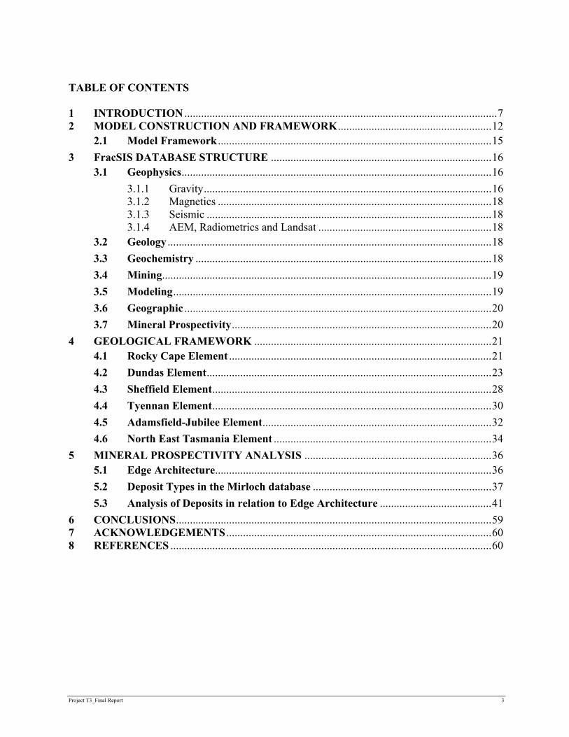
TABLE OF CONTENTS 1 INTRODUCTION ................................................................................................................7 2 MODEL CONSTRUCTION AND FRAMEWORK.......................................................12
2.1 Model Framework ..................................................................................................15 3 FracSIS DATABASE STRUCTURE ...............................................................................16
3.1 Geophysics...............................................................................................................16 3.1.1 Gravity.......................................................................................................16 3.1.2 Magnetics ..................................................................................................18 3.1.3 Seismic ......................................................................................................18 3.1.4 AEM, Radiometrics and Landsat ..............................................................18
3.2 Geology ....................................................................................................................18 3.3 Geochemistry ..........................................................................................................18 3.4 Mining......................................................................................................................19 3.5 Modeling..................................................................................................................19 3.6 Geographic ..............................................................................................................20 3.7 Mineral Prospectivity.............................................................................................20
4 GEOLOGICAL FRAMEWORK .....................................................................................21 4.1 Rocky Cape Element ..............................................................................................21 4.2 Dundas Element......................................................................................................23 4.3 Sheffield Element....................................................................................................28 4.4 Tyennan Element....................................................................................................30 4.5 Adamsfield-Jubilee Element..................................................................................32 4.6 North East Tasmania Element ..............................................................................34
5 MINERAL PROSPECTIVITY ANALYSIS ...................................................................36 5.1 Edge Architecture...................................................................................................36 5.2 Deposit Types in the Mirloch database ................................................................37 5.3 Analysis of Deposits in relation to Edge Architecture ........................................41
6 CONCLUSIONS.................................................................................................................59 7 ACKNOWLEDGEMENTS ...............................................................................................60 8 REFERENCES ...................................................................................................................60

Project T3_Final Report 4
List of Figures Fig. 1: Geology of Tasmania and standard legend Fig.2: Time Space plot of Geological Elements in Tasmania Fig. 3: Geographic domains, geological cross section lines and seismic lines Fig. 4: Fault Framework, surface traces of major faults Fig. 5: Ore shell of major deposits from western Tasmania, DEM, viewed from north. Fig. 6: Perspectives of Rocky Cape Element showing Arthur Lineament and Tenth Legion
Thrust, a) viewed from south, b) viewed from north Fig. 7: Perspective of the Mt Read Belt, Dundas Element, viewed from the northeast Fig. 8: Perspective of Tyennan Margin Fault, Cambrian granites and magnetic worm
sheets, western Tasmania, viewed from the southwest Fig. 9: Major structural elements in Pasminco’s Mt Read Belt Model, perspective view
from south, showing alternative geometry of east dipping crustal penetrating shear zone truncating west dipping Tyennan Margin Fault.
Fig. 10: Sheffield Element, viewed to north Fig. 11: Tyennan Element and adjacent regions, viewed from southeast Fig. 12: Adamsfield/Jubilee Element, viewed from northeast Fig. 13: NE Tasmania Element, viewed from southeast Fig. 14: Relative Depth-weighted image of combined gravity and magnetic vector data. Fig. 15: Length-weighted image of combined gravity, magnetic and fault vector data Fig. 16: Example of Fault Length Buffers and Mirloch Occurrences. Fig. 17: Fault Length Buffer Map, Type 1 VHMS deposits ranked by size, and polygon Fig. 18: Type 1 VHMS deposits, Fault Length Buffer Proximity Analysis Fig. 19: VHMS Type 1 Deposits, Gravity Worm Vector, buffer proximity analysis a) length
and b) relative depth weighted Fig. 20: VHMS Deposits, Magnetic Worm Vector, buffer proximity analysis, a) length, b)
Type 1.1 deposits and relative depth, c) Type 1.2 deposits and relative depth Fig. 21: Type 1 VHMS Deposits, Total Edge Length Image, inset shows detail of Central
Mt Read Belt. Fig. 22: Type 1 VHMS Deposits, Total Worm Relative Depth, inset Central Mt Read Belt Fig. 23: Type 2 Intrusion-related Deposits, Fault Length Buffer Proximity Analysis Fig. 24: Type 2 Intrusion-related Deposits, Devonian granite spine, western Tasmania. a)
total edge length, b) total worm relative depth_intersection weighted Fig. 25: Type 3 Fe-replacement deposits, Timbs Group ODZ, Magnetic W amplitudes Fig. 26: Type 3 Fe-replacement Deposits, Vector Buffer plots for a) faults, and b) magnetic
worms by relative depth Fig. 27: Type 3 Fe-replacement Deposits, Total Edge Length Image, Timbs Group ODZ Fig. 28: Type 4 Orogenic Gold Deposits, Vector Buffer Plots for a) gravity relative depth,
and magentic relative_depth Fig. 29: Type 4 Orogenic Gold Deposits, Total Edge Length Image

Project T3_Final Report 5
Fig. 30: Type 4 Orogenic Gold Deposits, Total Worm Rel. Depth_Intersection Weighted Fig. 31: Type 6 Irish-type SHMS deposits, Gordon Group ODZ, western Tasmania Fig. 32: Type 6 Irish-type SHMS deposits, Buffer Vector plots, a) fault length, b) gravity
worm length. Fig. 33: Type 8 Neoproterozoic Gold Deposits, Buffer Vector Plots, a) fault length, b)
magnetic worm length Fig. 34: Type 8 Neoproterozoic Gold, Total Edge Length Image, western Tasmania Fig. 35: Type 8 Hyrdothermal Magnesite Deposits, Buffer Proximity plots, a) fault length,
b) magnetic worm relative-depth Fig. 36: Type 9 Hydrothermal Magnesite, Total Edge Length Image, western Tasmania Fig. 37: Type 10 PGE Deposits, Buffer Proximity plots, a) fault length, b) magnetic worm
relative depth Fig. 38: Type 10 PGE Deposits, Total Worm relative depth image, western Tasmania Fig. 39: 3D visualisation of a synthetic model (bottom layer), calculated gravity response
(middle layer) and resulting 3D multiscale edge map (Archibald et al. 1999). Fig. 40: Wavelet transformation: a) gravity profiles over buried source become flatter with
increasing depth, b) wavelet transforms and maxima of those transforms, c) plot of wavelet maxima for increasing height, d) 3D visualisation of multiscale edges due to an inclined cylinder (Archibald et al. 1999).
Fig. 41: Gravity profiles and successive upward continuations (Holden et al. 2000) Gravity profile on bottom, with 4 scales of upward migration above, edges marked as spikes, horizontal derivative as curved lines.
Fig. 42: Fine to Coarse scale worms from Western Victoria aeromagnetic data, a) total magnetic intensity image, b) fine scale and c) coarse scale worms(Archibald et al. 1999).
Fig. 43: Wavelet maxima over various model fault geometries (Archibald et al. 1999; CSIRO Exploration and Mining)
Fig. 44: Example of a) magnetic worm profiles and b) interpreted geological cross section, Mt Read Belt
Fig. 45: Tasmania, magnetic worms colour coded by level of upward continuation (Z). Fig. 46: Tasmania, migrated magnetic worms colour coded by level of upward continuation
(Zwt) projected to shallow crustal level Fig. 47: Point-to-Vector processing for depth–weighted image processing Fig. 48: Point-to-Vector processing for length–weighted image processing Fig. 49: Intersection-weighted images for relative depth and length functions. Fig. 50: Western Tasmania, magnetic worms, threshold for Z<10km, colour coded by W. List of Tables Table 1: Data Inputs Table 2: Mirloch Deposit Types

Project T3_Final Report 6
List of Appendices Appendix 1: Processing and Interpretation of Potential Field Worms Appendix 2: Windowed Buffer Analysis of Major Deposit Types

Project T3_Final Report 7
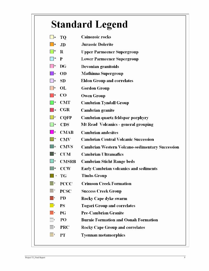
1 INTRODUCTION While the mineral wealth of Tasmania is renowned, and it remains a significant producer of a variety of metals, the industry is currently faced with a maturing of in-ground resources and historically low expenditure on exploration activities. Funded by the Tasmanian Government, the concept for this project grew from a “crisis meeting” on mineral exploration, convened by the Tasmanian Minerals Council (TMC) in May 2002. The primary objective is to facilitate explorers in making informed decisions regarding mineral prospectivity in Tasmania that could promote a discovery cycle. Tasmania boasts a large repository of high quality data available to the explorationist, as witnessed by the Mineral Resource Tasmania (MRT) TIGER database and by the combined MRT-Geoscience Australia (GA) TASGO and TASMAP projects (e.g. Rawlinson et al., 1998; Drummond et al., 1998). However, the current 2D data sets alone do not enable explorers to justify deep drilling, as the risk and cost of failure is high. Consequently, the challenge is to reduce the risk by making major shifts in understanding the geology of Tasmania (Fig. 1) and the context of its mineralisation. We seek to achieve this by developing a 3D geological model of the whole of Tasmania to ca.10km depth, constructed from serial geological cross sections, and within which the ore shells of major mineral deposits are embedded. The project compiles all significant geoscientific data sets onto a single platform, FracSIS, for use by explorers, miners and researchers. Table 1 lists the input data. We use these data sets to derive project generation opportunities for a range of commodities and deposit types. In a global mineral-province context, this is a unique undertaking in terms of the aerial extent, scale and scope of analysis. This was achieved through a collaborative effort over 10 months on the part of the Predictive Mineral Discovery Cooperative Research Centre (pmd*CRC, Project T3; B. Murphy, K. Denwer, R. Keele), Geoscience Australia (GA; R.J. Korsch, R. Jones and M. G. Nicoll), Mineral Resources Tasmania (MRT; D. Seymour, G. Green, S. Forsyth and others) and Geoinformatics Exploration Australia Pty Ltd (GEA; P. Stapleton and D. Holden). Additional inputs on the Mt Read Volcanics were supplied by researchers from CODES at the University of Tasmania (W. Herrmann and C. Gifkins). Importantly, the project gained the support and active participation of the local mining and exploration sector who donated data for input to the database. An earlier 3D geological model of the Mt Read Volcanics in western Tasmania, constructed by Pasminco Exploration and Fractal Graphics, is incorporated in the data base. This presents an alternative view of the Mt Read Volcanics that is largely superceded by the whole of Tasmania “T3” model.

Project T3_Final Report 8
Fig. 1: Tasmanian geology, using standard legend.
Project T3_Final Report 9

Project T3_Final Report 10
Table 1: Data Inputs
Data Inputs Source Format
Geology 1:25K, 1:100K, 1:250K MRT 2D GIS MirLoch – Mineral Occurrences MRT Digital Gravity and Worms MRT & Geoinformatics Digital Aeromagnetics and Worms MRT & Geoinformatics Digital Airborne EM MRT Digital Radiometrics MRT Digital Landsat TM GA Digital IP/EM Grid Lines Pasminco MapInfo Exploration Geochemistry: Streams, Soils Industry MapInfo Land Use and Tenure MRT Digital DEM MRT Digital Geophysical Interpretations/Inversions MRT PDF Seismic Sections GA & Industry Digital Seg-Y Time-Space plots MRT-GA PDF Ore Deposit Models MRT PDF Mt Read 3D model Pasminco FracView VHMS Alteration Map CODES Digital Volcanic Facies Map CODES Digital Geochronology GA/MRT Digital Whole Rock & Isotope Geochemistry GA/MRT Digital AMIRA geological cross sections AMIRA Digital Mine scale models and ore shells Industry Digital & Hardcopy New cross sections pmd*CRC Digital & Hardcopy Upgraded granite model MRT Digital TASGO Crustal Model GA Digital
Constraints on the geometries of major geological boundaries are provided by onshore and offshore seismic profiles, together with geophysical images, multiscale upward continued potential field gradient maps (“worms”) and geological mapping at 1:250 000, 1:100 000 and 1:25 000 scales. Following the subdivisions defined in the MRT-GA Time-Space plot (Fig. 2), we describe six major tectonic elements and derive a structural architecture or template for the modeled rock volumes according to a standard geological legend. The rock volumes generally relate to sub-Permian lithological groups and subgroups, rather than individual formations, and to major intrusive bodies. With data contributed by the local mining sector, ore shells and infrastructure (where available) of virtually all major mines have been constructed and are embedded in the 3D model. Mineral prospectivity is addressed through analysis of these frameworks in an empirical way to determine regions of high exploration potential for a range of deposit types.
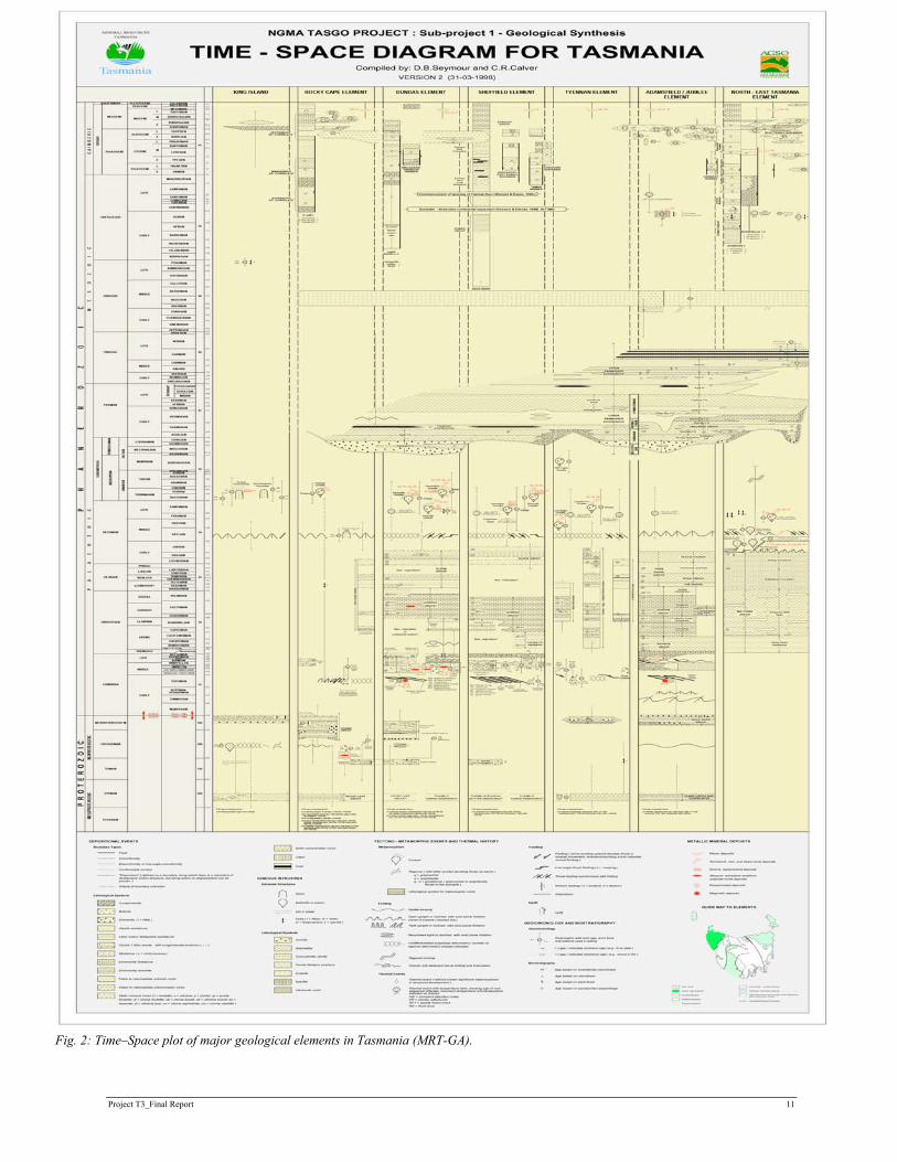
Project T3_Final Report 11
Fig. 2: Time–Space plot of major geological elements in Tasmania (MRT-GA).

Project T3_Final Report 12
The 3D model is a simplification of an inherently complex terrain (Cooke and Kitto 1994). Some important geometric and timing issues are the shape and uplift histories along the Proterozoic margins, the allochthonous nature of the oceanic-affinity rocks and the degree of Cambrian versus Devonian regional-scale tectonic transport. The 3D model outlined here is but one solution that will hopefully stimulate research into key uncertainties. Levels of confidence in the interpretations will vary laterally and with depth, with a key determinant being the structural architecture. This is guided by seismic profiles and potential field data, and is ultimately determined by geological interpretations as to the style and timing of assembly of the tectonic elements that make up the terrain. A significant aspect to the analysis is the use of potential field worms for determining the relative shape, depth extent and continuity of edges (e.g. faults, intrusive boundaries). The term “Worm” derives from an automated edge detection process that defines 3D arrays of maximum gradient points over a range of scales of upward continuation. This type of processing was developed through collaborative research between CSIRO and Fractal Graphics as a means of reducing ambiguity in the interpretation of potential field data (“FracwormsTM”, see Appendix 1). The process relies on the existence of a density (or susceptibility) gradient. Where such gradients are absent, e.g. edges without a density contrast, the interpreter seeks to take account of significant vacancies and truncations in the worm distributions (see Appendix 1). Only a limited degree of validation using 2D inversion profiles of potential field data was undertaken, as the scope of the project has not allowed a quantitative application of these methods. 2 MODEL CONSTRUCTION AND FRAMEWORK A standard legend of 29 geological units (Fig. 1) was applied on a state-wide basis. The stratigraphic units have been modeled mainly at a Group level, with greater detail and complexity developed for the more mineral-rich Palaeozoic section (Mt Read Volcanics). The state was divided into seven geographic domains for the purpose of geological cross section construction; these subdivisions have some geological basis, though the boundaries of domains are not necessarily delimited by geological structures. This resulted in 133 individual serial cross sections across the entire state, mostly at a nominal 10 km spacing and E-W orientation, covering ca. 9,000 line km to an average depth of 7 km (Fig. 3). These sections have been joined across the domains, resulting in the 51 cross sections embedded in the FracSIS database. The geographic domains are: • Central Mount Read Volcanic Belt (5 km spaced E-W sections and 2 N-S sections at
1:50,000 scale, 15 sections for 400 line km). • Southern Mount Read Volcanic Belt (10 km spaced E-W sections at 1:50,000 scale, 8
sections for 400 line km). • Northern Mount Read Volcanic Belt/Central North (10 km spaced E-W sections and some
N-S sections at 1:50,000 scale, 13 sections for 650 line km). • NW Tasmania/Rocky Cape (10 km spaced E-W sections at 1:50,000 scale, 17 sections for
1200 line km).

Project T3_Final Report 13
• Tyennan Nucleus (10 km spaced E-W sections at both 1:50,000 and 1:100,000 scale, 21 sections for 1050 line km).
• NE Tasmania/Mathinna (10 km spaced E-W sections at 1:100,000 scale, 15 sections, 1250 line km).
• Tasmania Basin (10 km spaced E-W sections at 1:100,000 scale, 44 sections for 4000 line km).
Most cross sections were drawn by K. Denwer and R. Keele (pmd*CRC) in collaboration with MRT personnel - D. Seymour (Mount Read Volcanic Belt, Rocky Cape and Tyennan Nucleus) and S. Forsyth (Tasmania Basin). Sections were completed on a domain by domain basis. Adjacent sections were drawn by alternating authors to reduce the potential of individual bias. Numerous discussions were held with other MRT geologists who had significant input to the sections including: T. Brown, G. Green, C. Calver, J. Everard and M. McClenaghan. Each section was drawn onto a template which portrayed: • Topographic surface line, colour coded to 1:25K and 1:250K geology • Stacked gravity and magnetic worm profiles, coloured by amplitude (W) • Existing model outlines (including granite boundaries, TASGO and Pasminco’s Mt Read
model). On each cross section, lines and polygons were named, labeled and colour coded to assist in the model construction, i.e. blue = faults, pink = lithological boundaries, red = intrusive boundaries, green = unconformable boundaries, black = form lines. Polygons were labeled with the standard geology legend. Once completed, each cross section was scanned and dispatched electronically for digitizing and model construction using the Vulcan software package. A series of intermediate sections were constructed in the software using the drawn sections and surface geology as a constraint. These were subsequently wireframed and block modeled, with each block attributed to the standard geological code. A number of iterations were required between the geologists and the model builder (P. Stapleton) to resolve issues that arose as the 3D picture unfolded.

Project T3_Final Report 14
Fig. 3: Geographic domains, geological cross section lines and seismic lines

Project T3_Final Report 15
2.1 Model Framework A fault framework for the model was derived (Fig. 4) using the statewide coverage of mapped faults and the potential field worms. Most major boundaries have been wireframed in 3D and these are tied to surface traces. Note, however, there are some instances where mismatch remains. We find that steep boundaries are more prevalent in the near surface, whereas at depth listric geometries are interpreted on a regional scale, with 6-10km depth being the approximate depth range where relatively flat structures seem to prevail. A major control on the gross geometry, especially at deeper levels, is the interpretation of extensive mafic-ultramafic sheets in the subsurface whose bounding surfaces are shear zones. They are most pronounced in, but not limited to, western Tasmania. These high magnetic intensity features in the near surface are represented at depth by broad scale anomalies which previous workers have interpreted in a similar fashion to us (e.g. Leaman 1996), that is, allochthonous sheets of early Cambrian oceanic (fore-arc or back-arc) mélange. These “oceanic-affinity” rocks are sandwiched by variably metamorphosed Proterozoic cratonic elements of the Rocky Cape region in the northwest and the Tyennan “basement” in the centre of Tasmania. These latter regions share a similar Neoproterozoic passive margin history of rift-facies sediments and volcanics, prior to emplacement of the oceanic allochthon, such that there is an implied connection of the Proterozoic elements below the allochthon base. Another determinant of the gross geometry is the existence of Devonian granite batholiths that are extensive in the subsurface. We have represented the top surface of the granites as an isosurface which derives from detailed 2D inversion models and from the TASGO seismic interpretation. The likelihood is that the granites are relatively thin (km scale) sheet-like bodies, but we have not placed lower boundaries to these bodies in our model. Given the relatively late stage (mainly post-tectonic) emplacement of the granites, we have interpolated structural boundaries that may have existed prior to granite emplacement. Note that some detailed topography of the granite surface has been generalised, e.g. the Pine Hill granite in the area of the Renison Bell tin mine. High levels of uncertainty in the modeling of basement rocks exist in areas of deep Mesozoic and Tertiary cover, particularly those with strong susceptibilities, e.g. Jurassic dolerites in the Tasmania Basin. We have relied on limited drilling data and potential field worms to determine distributions of Palaeozoic and Proterozoic rocks in such covered areas. Note that the post-Palaeozoic rock units have not been wireframed, but their distributions are shown in the serial cross sections.

Project T3_Final Report 16
3 FracSIS DATABASE STRUCTURE The seven primary directories are: Geophysics, Geology, Geochemistry, Mining, Modeling, Geographic and Mineral Prospectivity
3.1 Geophysics Sub-directories: Gravity, Aeromagnetics, Seismic, AEM, Radiometrics and Landsat.
3.1.1 Gravity • Worms: The gravity data was gridded at 500 m cell size and upward continued to
40 km. The two types of point data are Horizontal Derivative (Max) and Effective First Vertical Derivative (EFVD). Each file lists the processing used and the level of upward continuation or height (Z) in metres, e.g.: o tas grav max z01755.330 is from the Max technique at 1755.33m. o tas grav efvd z2811 is from the EFVD technique at 2811m.
Two interpretations of the worms are presented. The first (by D. Holden) shows a line set of 1) interpreted edges (Z) at 2 km depth and 2) polygon regions traced out on the basis of amplitude signatures (W). The second (by B. Murphy) uses an automated processing (Geoscope, see Appendix 1) of 1) the total Z point levels projected to a near surface representation and weighted by the maximum height of migration (Zwt), and 2) interpretation of W amplitude values, for a subset of the data (Z<10 km height), that are thresholded and represented as polygon regions. • Images: A selection of Bouguer gravity images • Grids: Source grids for the image files • Granite model: Isosurfaced upper surface of the Devonian granites from GA’s
TASGO model • Inversion Models: These derive from inversion of gravity and magnetic profiles
from studies for the MRT by Leaman and Webster (2002).

Project T3_Final Report 17
Figure 4: Fault Framework, surface traces of major faults
Project T3_Final Report 18
3.1.2 Magnetics Sub-directories are: • West Tasmania data: subset by grid cell sizes into 100 m and 200 m datasets,
with each directory containing worms, grids and images. These show upward continuations to 7 km and 5 km respectively.
• Regional Tasmania 400m: the state-wide data was gridded at 400 m and upward continued (wormed) to 40 km. Because of phase changes in magnetic properties with depth, the higher levels of upward continuation must be viewed with caution. Other subdirectories contain images, grids and an interpretation of the worm data. The latter interpretation follows the same process (see Appendix 1) as for the gravity worms.
3.1.3 Seismic This contains all onshore and offshore seismic data and interpretations undertaken by GA. Additional seismic profiles for on-shore regions in northern and central Tasmania were made available by Great South Land Minerals N. L. to aid the interpretation of the serial cross sections, but the seismic data itself is not included in the FracSIS database. 3.1.4 AEM, Radiometrics and Landsat Each subdirectory has relevant images of these data.
3.2 Geology Sub-directories are: • Tas 250K geology, comprising:
o 250K geology relimited recoded regrouped: 1:250 000 geology coded by the standard geological legend (Table 2)
o 250K Struc point data: all the structural point data for the state. o 250K Geology original: the original 1:250 000 geology.
• Tas 25K geology: 1:25 000 scale geology, coded by the standard geological legend (Table 2)
• Cross Sections: this houses all the sections created to produce the 3D model. For each section line, separate files are used for each lithology and each fault.
• CODES Volcanic Facies: This relates to the Mt Read Volcanic Belt in western Tasmania and derives from Gifkins and Kimber (2003)
• Cross Sections_PhD_Owen: this contains cross sections though the Owen Conglomerates in western Tasmania by C. Noll (Monash University)
3.3 Geochemistry This comprises six subfolders:
Project T3_Final Report 19
• Geochron Data: point files of samples using various dating techniques. • Pasminco_Soils: Compilation of soil samples for various grids with up to 5 elements,
mostly relevant to the Mt Read Volcanic Belt. • MRT Stream Sediments: Distribution of stream sediment samples with up to 11
elements. • Whole Rock GA: Whole rock analyses for suite of elements. • CODES Alteration Facies: This relates to the Mt Read Volcanic Belt in western
Tasmania and derives from Herrmann and Kimber (2003) • Local Grids_Tas: This shows the locations of exploration grid lines and some point
files, mostly relevant to the Mt Read Volcanic Belt.
3.4 Mining This contains drill collars, drill traces, infrastructure (where available) and ore shell data from all the major mines: Hellyer, Rosebery, Henty, Beaconsfield, Que River, Savage River, Mt Lyell, Renison and Hercules (e.g. Fig. 5). It also contains the MRT open file DORIS drilling database and the Mirloch mineral occurrence database. The Mirloch data were recoded for the purpose of the prospectivity analysis (see below). 3.5 Modeling Three subdirectories reside here: • Pasminco_Mt Read Modeling: the Pasminco Mt Read model for western Tasmania
created in 1999. Subdirectories of major lithology models, fault structure models and the interpreted cross sections.
• TASGO Modeling_GA: the model created by GA in 1998, with subdirectories of: o MOHO Models (created by N. Rawlinson, ANU), and o GOCAD_General: comprising Seismic Line Interpretation and GOCAD_models
of isosurfaced geological units and major boundaries. • Tasmania_T3_Model: created by this project, with three subdirectories:
o Tasmania Structure: with surface traces and wireframes of faults o Tasmania_geology_by_block: individual models of the seven domains o Tasmanian geology by rocktype: models of individual rock type distributions
according to the standard legend.

Project T3_Final Report 20
Fig. 5: Ore shell of major deposits (in red) from western Tasmania, DEM underlay, viewed from north. Yellow lines are
the main fault traces
3.6 Geographic This contains subdirectories of: Tenements (as at October 2003), Coastline, Topography (with Digital Elevation Model), National Parks, Transport, Streams and Lakes. 3.7 Mineral Prospectivity This comprises images of the interpreted potential field worm and fault architectures used in the analysis of mineral exploration potential (see Section 5). Subdirectories are: Gravity Vector Analysis, Magnetic Vector Analysis, Combined Vector Analysis and Mirloch Deposit Types. The Gravity and Magnetic vector analysis images show representations of the interpreted “Edge Architecture” in terms of edge length, relative depth and intersections of edges thereof (Appendix 1). The Combined Vector Images are subset according to: 1) length into total worm (gravity + magnetics) and total worm and fault images, 2) relative depth into total worm_reldepth_Zwt_Max images, and 3) images of weighted intersections by length and relative depth respectively.
Project T3_Final Report 21
4 GEOLOGICAL FRAMEWORK This section provides a geological context for the modeling and describes the six tectonic elements that make up pre-Mesozoic Tasmania, as detailed in the Time-Space chart (Fig. 2): Rocky Cape, Dundas, Sheffield, Tyennan, Adamsfield-Jubilee and Northeast Tasmania. Aspects of each element are outlined below, in terms of rock associations, tectonic setting and structure, intrusions and mineralization, with specific reference to their representation in the 3D Model.
4.1 Rocky Cape Element The eastern boundary coincides with the most westerly occurrence of Cambrian ultramafics (CUM) in western Tasmania (Fig. 6). This boundary is called the Tenth Legion Thrust (Brown and Findlay, 1992; 10LT), which is an east-directed Cambrian (to Devonian) aged fault that can be traced from south of Macquarie Harbour to Ulverstone in the north. On the Sorell Peninsula, associated structures are the Liberty Creek Thrust (LCT) and Albina Creek Thrust (ACT). Rock Associations This consists of thick, unfossiliferous, siliciclastic shelf sequences of Meso- to Neoproterozoic age (PRC and sub-divisions PRP, PRL, PRB) and rift-related turbiditic successions of the Burnie and Oonah Formations (PO). The Neoproterozoic Togari Group, also related to a rift event, lie above the Black River unconformity, whose surface expression can be traced across the entire element. The Scopus Formation (CMT), a Late Cambrian Tyndall Group correlate, occupies the core of the Smithton Syncline and is the youngest of the pre-Parmeener Supergroup strata in this element. The Scopus Formation contains clasts of Cambrian ultramafic rocks, implying that the Early Cambrian allochthon (see below) shed detritus further west than its present outcrop extent. The upper part of the Scopus Formation may be younger than the top of the Tyndall Group. Tectonic Setting and Structure The Rocky Cape Group was deposited along the margins of an extension of the East Antarctic Shield. Tilting and possibly gentle folding of the rocks may have been due to marginal effects of the ca 750 Ma Wickham Orogeny on King Island, or they may have been due to block rotations in an early phase of pre-Togari Group extensional tectonism. In the Balfour district, at least 5 km of stratigraphy had been removed prior to deposition of the Neoproterozoic Togari Group. The tilt of the craton may have been towards the north, as the upper units - Detention Sub-Group (PRD), Irby Siltstone (PRI) and Jacob Quartzite (PRJ) – crop out in the north of the element. The Roger River Fault (RRF) was an important half-graben structure that controlled the distribution of tholeiitic lavas during the second (Togari) extension. It predominantly dips west, implying rotation during the Delamerian Orogeny.
Project T3_Final Report 22
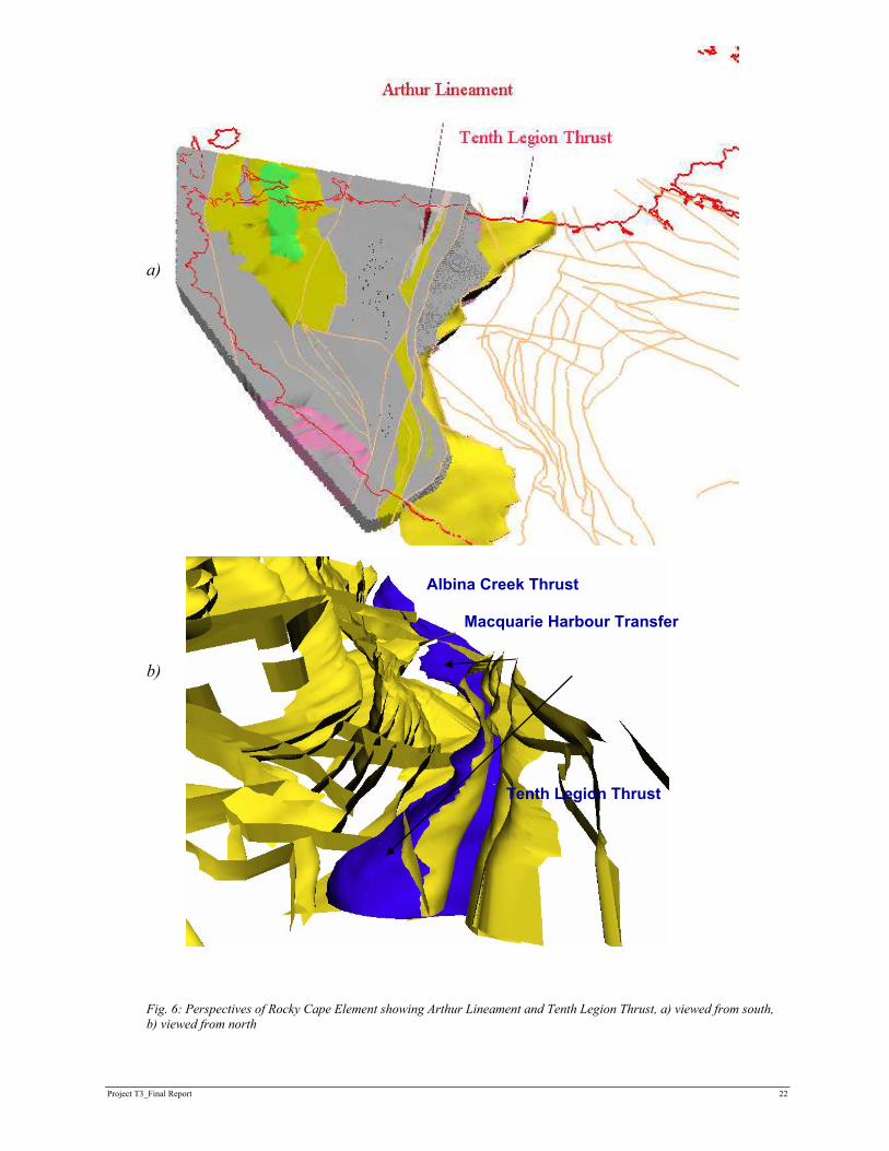
a) b) Fig. 6: Perspectives of Rocky Cape Element showing Arthur Lineament and Tenth Legion Thrust, a) viewed from south, b) viewed from north
Macquarie Harbour Transfer
Albina Creek Thrust
Tenth Legion Thrust
Project T3_Final Report 23
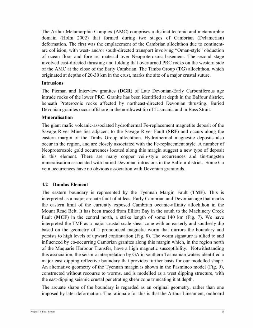
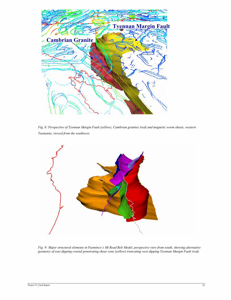
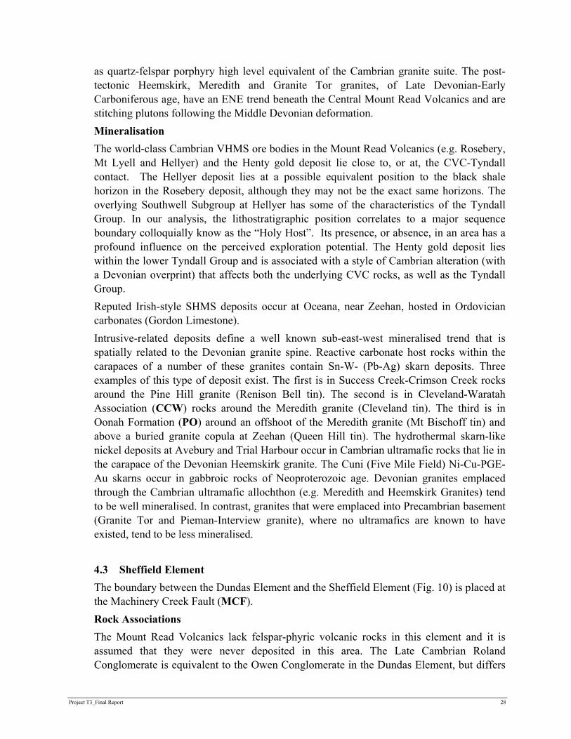
The Arthur Metamorphic Complex (AMC) comprises a distinct tectonic and metamorphic domain (Holm 2002) that formed during two stages of Cambrian (Delamerian) deformation. The first was the emplacement of the Cambrian allochthon due to continent-arc collision, with west- and/or south-directed transport involving “Oman-style” obduction of ocean floor and fore-arc material over Neoproterozoic basement. The second stage involved east-directed thrusting and folding that overturned PRC rocks on the western side of the AMC at the close of the Early Cambrian. The Timbs Group (TG) allochthon, which originated at depths of 20-30 km in the crust, marks the site of a major crustal suture. Intrusions The Pieman and Interview granites (DGR) of Late Devonian-Early Carboniferous age intrude rocks of the lower PRC. Granite has been identified at depth in the Balfour district, beneath Proterozoic rocks affected by northeast-directed Devonian thrusting. Buried Devonian granites occur offshore in the northwest tip of Tasmania and in Bass Strait. Mineralisation The giant mafic volcanic-associated hydrothermal Fe-replacement magnetite deposit of the Savage River Mine lies adjacent to the Savage River Fault (SRF) and occurs along the eastern margin of the Timbs Group allochthon. Hydrothermal magnesite deposits also occur in the region, and are closely associated with the Fe-replacement style. A number of Neoproterozoic gold occurrences located along this margin suggest a new type of deposit in this element. There are many copper vein-style occurrences and tin-tungsten mineralisation associated with buried Devonian intrusions in the Balfour district. Some Cu vein occurrences have no obvious association with Devonian granitoids. 4.2 Dundas Element The eastern boundary is represented by the Tyennan Margin Fault (TMF). This is interpreted as a major arcuate fault of at least Early Cambrian and Devonian age that marks the eastern limit of the currently exposed Cambrian oceanic-affinity allochthon in the Mount Read Belt. It has been traced from Elliott Bay in the south to the Machinery Creek Fault (MCF) in the central north, a strike length of some 140 km (Fig. 7). We have interpreted the TMF as a major crustal scale shear zone with an easterly and southerly dip based on the geometry of a pronounced magnetic worm that mirrors the boundary and persists to high levels of upward continuation (Fig. 8). The worm signature is allied to and influenced by co-occurring Cambrian granites along this margin which, in the region north of the Maquarie Harbour Transfer, have a high magnetic susceptibility. Notwithstanding this association, the seismic interpretation by GA in southern Tasmanian waters identified a major east-dipping reflective boundary that provides further basis for our modelled shape. An alternative geometry of the Tyennan margin is shown in the Pasminco model (Fig. 9), constructed without recourse to worms, and is modelled as a west dipping structure, with the east-dipping seismic crustal penetrating shear zone truncating it at depth. The arcuate shape of the boundary is regarded as an original geometry, rather than one imposed by later deformation. The rationale for this is that the Arthur Lineament, outboard
Project T3_Final Report 24
of the Tyennan Margin, maintains a northerly strike, and that facies variations in the Mt Read Volcanics and the Owen Group are mirrored by the changing nature of the Tyennan Margin. We suggest this boundary has had a complex history - perhaps originating as a west-dipping Neoproterozoic rift margin, was again active in the Early Cambrian during emplacement of the ultramafic sheet which became smeared out in the crustal penetrating shear zone, and that it was overridden (and overturned) during this event. The timing and uplift history along this boundary is constrained in part by the mid-Cambrian Sticht Range beds that unconformably overlie the Tyennan metamorphics. Soon afterwards, this became the site of crustal melting to produce the mid Cambrian granites, which stitch rocks on either side of the TMF in northern Tasmania and, with continued uplift, the Tyennan Metamorphics supplied detritus to the Cambro-Ordovician Owen Group. The boundary zone was reactivated in the Devonian, deforming the Cambrian granites. While we have attached a complex evolution to this boundary, this evidently demands further research to test and constrain its geometry and history. Rock Associations This element consists of Middle Cambrian volcano-sedimentary successions that lie unconformably on the following two major associations: (1) the rifted successions of the Burnie and Oonah Formations (PO), Success Creek Group (PCSC), Crimson Creek Formation (PCCC), or Togari Group correlates, and (2) the Early Cambrian oceanic allochthon. Unconformities exist at the base of the Tyndall Group, Owen Group and later Ordovician rocks (e.g. the Haulage Unconformity at Mt Lyell separating Late Cambrian siliciclastic successions (CO) from the Pioneer Beds (OD). Semi-continuous sag-phase sedimentation continued through to Early Devonian time under marine conditions. It was not possible to maintain a clear and unequivocal distinction between Tyndall Group and Eastern quartz-phyric (EQP) successions during the Modeling process. As a consequence, the rocks normally regarded as EQP have been placed in a generalised Mount Read Volcanics grouping (CDS), with the possibility that they may be either Tyndall Group correlates or time equivalents of the Central Volcanic Complex (CVC). At Rosebery, this position is marked by the changeover from felspar-phyric to quartz-phyric lavas and volcaniclastics, and is the contact between the Central Volcanic Complex (CMV) and the Cambrian western volcano-sedimentary succession (CMVS). Elsewhere, this changeover tends to occur at the contact between the CVC and the Tyndall Group. This difference may be due to the fact that the White Spur Formation, which is considered to be part of the western sedimentary succession, may in fact be a Tyndall Group correlate (the strict definition of the western succession is as a lateral equivalent to the CVC). Although the Sticht Range beds (CMSRB) are a separate entity in the model we believe that there are good reasons why these rocks should be considered as a Tyndall Group correlate, as well. The Mount Read Volcanics south of Macquarie Harbour are unassigned (CDS) on the basis that the CVC has not been shown unequivocally to exist here.
Project T3_Final Report 25
Fig. 7: Perspective of the Mt Read Belt, Dundas Element, viewed from the northeast.
Project T3_Final Report 26
Fig. 8: Perspective of Tyennan Margin Fault (yellow), Cambrian granites (red) and magnetic worm sheets, western
Tasmania, viewed from the southwest.
. Fig. 9: Major structural elements in Pasminco’s Mt Read Belt Model, perspective view from south, showing alternative geometry of east dipping crustal penetrating shear zone (yellow) truncating west dipping Tyennan Margin Fault (red).
Cambrian Granite
Tyennan Margin Fault

Project T3_Final Report 27
Tectonic Setting and Structure The Mount Read Volcanics (MRV) formed in an extensional setting at a time when the obducted sheet of Early Cambrian ultramafics, and their associated Cleveland Waratah Association rocks (CCW), collapsed briefly during the middle-Middle Cambrian. The presence of tholeiites in the Tyndall Group (CMT) implies an extended crust with high heat flow towards the close of this event. The base of the allochthonous sheet is interpreted as riding on multiple shear zone surfaces (UF1-4) to the west of the Marionoak Fault (MF). The basement to the MRV consists of Neoproterozoic rift successions of the Success Creek Group, Crimson Creek Formation and Togari Group equivalents. The presence of faulted Oonah Formation in the Mount Read Volcanics presents two Modeling scenarios: either the MRV was laid down on a heterogeneous basement that included the Burnie-Oonah Formation rift successions, or the Oonah Formation occurrences in the MRV represent “klippe” basement transported from the west by the Tenth Legion Thrust. In the latter case, the Oonah Formation need not be present as basement and the Crimson Creek Formation might lie directly on Tyennan basement (PT). We have adopted the former interpretation in the 3D model. The North and South Henty Faults (NHF and SHF) originated as back-thrusts to the east-dipping Rosebery and Marionoak thrusts (RF and MF), resulting in a Devonian-aged “pop-up” structure. Another difference between the Pasminco and T3 models is the relationship of the Rosebery and Henty Faults at depth. The Great Lyell Fault (GLF) controls the western margin of the Owen Conglomerate (CO) basin. However, the continuation of this fault to the south of Mt Lyell on the eastern flanks of Mt Jukes is here interpreted as the Tyennan Margin Fault (TMF) and not the Great Lyell Fault, contrary to previous interpretations. The Macquarie Harbour Transfer (MHT) is an enigmatic structure that follows the highly magnetic CCW rocks along the West Coast, and separates the central from the southern Mount Read Volcanics. There is an apparent sinistral rotation and translation of ca 50 km across this stucture (Fig. 6b), affecting the distribution of the ultramafic sheet, yet this translation does not penetrate the Tyennan Margin, and nor do we recognise major changes in metamorphic grade in the Tyennan rocks or changes in structural level in the Lower Palaeozoic succession either side of the transfer. The implication is that the transfer geometry is inherited from the Early Cambrian and that the later depositional history is compartmentalised by the MHT. This may have a bearing on the mineral potential of the Mt Read Belt south of Macquarie Harbour. A Tertiary basin containing upward of 1 km of Tertiary sediments (TQ) occurs south of Macquarie Harbour and was controlled by reactivation of this crustal scale structure. Intrusions Cambrian Granite (CGR) is related to the emplacement of the Central Volcanic Complex (CMV) and takes the form of an intrusive “spine” of buried granite beneath the volcanic belt (Fig. 8). The Henty Fault (HF) is the western bounding structure to the Cambrian granites, although the lack of magnetic expression of the granite here adds a degree of uncertainty to the position of this contact. The Bond Range porphyry has been interpreted
Project T3_Final Report 28
as quartz-felspar porphyry high level equivalent of the Cambrian granite suite. The post-tectonic Heemskirk, Meredith and Granite Tor granites, of Late Devonian-Early Carboniferous age, have an ENE trend beneath the Central Mount Read Volcanics and are stitching plutons following the Middle Devonian deformation. Mineralisation The world-class Cambrian VHMS ore bodies in the Mount Read Volcanics (e.g. Rosebery, Mt Lyell and Hellyer) and the Henty gold deposit lie close to, or at, the CVC-Tyndall contact. The Hellyer deposit lies at a possible equivalent position to the black shale horizon in the Rosebery deposit, although they may not be the exact same horizons. The overlying Southwell Subgroup at Hellyer has some of the characteristics of the Tyndall Group. In our analysis, the lithostratigraphic position correlates to a major sequence boundary colloquially know as the “Holy Host”. Its presence, or absence, in an area has a profound influence on the perceived exploration potential. The Henty gold deposit lies within the lower Tyndall Group and is associated with a style of Cambrian alteration (with a Devonian overprint) that affects both the underlying CVC rocks, as well as the Tyndall Group. Reputed Irish-style SHMS deposits occur at Oceana, near Zeehan, hosted in Ordovician carbonates (Gordon Limestone). Intrusive-related deposits define a well known sub-east-west mineralised trend that is spatially related to the Devonian granite spine. Reactive carbonate host rocks within the carapaces of a number of these granites contain Sn-W- (Pb-Ag) skarn deposits. Three examples of this type of deposit exist. The first is in Success Creek-Crimson Creek rocks around the Pine Hill granite (Renison Bell tin). The second is in Cleveland-Waratah Association (CCW) rocks around the Meredith granite (Cleveland tin). The third is in Oonah Formation (PO) around an offshoot of the Meredith granite (Mt Bischoff tin) and above a buried granite copula at Zeehan (Queen Hill tin). The hydrothermal skarn-like nickel deposits at Avebury and Trial Harbour occur in Cambrian ultramafic rocks that lie in the carapace of the Devonian Heemskirk granite. The Cuni (Five Mile Field) Ni-Cu-PGE-Au skarns occur in gabbroic rocks of Neoproterozoic age. Devonian granites emplaced through the Cambrian ultramafic allochthon (e.g. Meredith and Heemskirk Granites) tend to be well mineralised. In contrast, granites that were emplaced into Precambrian basement (Granite Tor and Pieman-Interview granite), where no ultramafics are known to have existed, tend to be less mineralised. 4.3 Sheffield Element The boundary between the Dundas Element and the Sheffield Element (Fig. 10) is placed at the Machinery Creek Fault (MCF). Rock Associations The Mount Read Volcanics lack felspar-phyric volcanic rocks in this element and it is assumed that they were never deposited in this area. The Late Cambrian Roland Conglomerate is equivalent to the Owen Conglomerate in the Dundas Element, but differs

Project T3_Final Report 29
from it in respect to certain stratigraphic units that cannot be traced across the element boundary. The Ordovician Moina Sandstone, which is equivalent to the Pioneer beds, contains more conglomeratic beds and is thicker than its counterpart in the adjoining Dundas Element.
Fig. 10: Sheffield Element, viewed to north

Project T3_Final Report 30
Tectonic Setting and Structure The Forth Metamorphic Complex is interpreted as a “pop-up” allochthonous piece of high-grade metamorphosed Tyennan basement (PTH) identical to that occurring on the southern edge of the element. Whether this originated as an extensional core complex remains a subject of further research. The Cambrian ultramafic allochthon rests directly on basement throughout the element. The reason for the lack of Togari Group rocks is not known. The shape of the Cambrian volcano-sedimentary succession is interpreted as a primary depositional feature; hence the wrap around of the Tyennan margin reflects, in part, the trend of the Late Cambrian depocentres such as the Fossey Mountain Trough. The Eastern Tyennan Margin Fault (ETMF) is the continuation of the Tyennan Margin Fault in the Dundas Element. It is displaced northwards from the Tyennan Margin Fault by the Machinery Creek Fault (MCF). It dips north and northeast and is one of a number of Middle Devonian structures that facilitated the amalgamation of the eastern and western Tasmanian terrains. Intrusions The 492 Ma Beulah intrusion is andesitic in composition and therefore younger than the Cambrian granite suite in the Dundas Element. The Housetop Granite is the oldest of the Devonian-Carboniferous granitoids in the western Tasmanian terrain, although it is some 10 Ma younger than the youngest of the tin-bearing granite of the North East Tasmania Element (Black et al. 1997). It has a flat base, reflecting either synkinematic intrusion, that is, Devonian reactivation of the Early Cambrian allochthon boundary, or a post-tectonic intrusion shape, that is, passive emplacement along pre-existing structures. Mineralisation Magnetite skarns occur around the Housetop Granite and gold and base metal skarns occur over the Dolcoath Granite, near Round Mountain at Cethana. There are no major mineral deposits in the Sheffield Element. 4.4 Tyennan Element The Tyennan Element (Fig. 11) occupies central Tasmania and is bounded by Cambrian successions on its northern, western and southern sides. The Northeast Tasmania Element and the Adamsfield-Jubilee Element border its eastern side. Rock Associations Quartzites and phyllites of Precambrian age dominate the rocks in the Tyennan Element. In the southwest corner, a veneer of Neoproterozoic Togari Group, which may be up to 2 km thick in the keels of the synclines, covers these low-grade Mesoproterozoic successions. Synclinal troughs of the Denison and Gordon Groups (OD) are preserved as marginal “furrows” around the edge of the nucleus.

Project T3_Final Report 31
The Tasmania Basin and thick Jurassic Dolerite sheets cover the eastern and northeastern parts of the element. The geometry of the Tasmania Basin across the Tyennan Element is uncertain. Seismic data indicate the Togari Group (PS) is present beneath the basin and that the lowest Permian is controlled by a half-graben fault. Tectonic Setting and Structure The Tyennan Element consists of interleaved units of varying metamorphic grade and composition that were folded, thrust and uplifted over a long period of time. High-grade metamorphic rocks (garnet amphibolite schists (PTH) occur along the northern and western flanks of the nucleus. The south-dipping Fury Fault (FF) defines the boundary between high- and low-grade rocks in the northern part of the Tyennan Element. On the western side, a series of west-dipping faults emplaced higher-grade rocks over lower-grade rocks at the close of the Cambrian orogeny. The phyllite-garnet schist contacts east of Queenstown were folded during the Devonian. The Olga Fault (OF) is a northwest-directed Devonian thrust that mimics the Tyennan Margin Fault and disappears under the Jurassic Dolerites (JD) of the Tasmania Basin. On its southern flank it steepens up to become a side ramp running the length of the Arthur Ranges. From there it swings southward and passes into the Southern Ocean at Prion Bay. The Payne Bay Fault (PBF) is another Delamerian structure that elevated higher-grade rocks along the southern-western flanks of the element: the northwest-trending De Witt Range Fault (DWRF) is a younger fault than the PBF and their crosscutting relationship can be seen on cross section 5 210 000mN. Intrusions The presence of Cambrian granite at South West Cape indicates that the Mount Read Volcanics continue off shore for some distance. Magnetic data collected by BHP in the 1970’s is currently being assessed and is likely to confirm the continuation of Cleveland-Waratah Association rocks off the south west coast. Devonian granites underlie the Tyennan Element at shallow depths varying from 1 to 5 km, between Bathurst Harbour and Coxs Bight. Jurassic Dolerite intrudes at two crustal levels: (1) at the base of the Permian, just above the basal unconformity, and (2) within the Triassic, at or below the Coal Measures. A large feeder occurs on the Western Tiers at 510 000E. Mineralisation Tin was mined in small quantities in the vicinity of Coxs Bight for a number of years. There are no major deposits in this element. There may be potential for Fe-replacement deposits associated with amphibolites.

Project T3_Final Report 32
Fig. 11: Tyennan Element and adjacent regions, viewed from southeast.
4.5 Adamsfield-Jubilee Element The west-directed Cambrian Lake Gordon Fault (LGF) defines the western boundary of the Adamsfield-Jubilee Element (Fig. 12) and marks the western edge of the Cleveland-Waratah Association rocks (CCW) rocks of Cambrian age. The LGF disappears under the ocean between South Cape and South East Cape. The Lake Crescent Fault (LCF) acted as a transfer fault during emplacement of the Cambrian allochthon and essentially defines the northern boundary to this element. The Miller Bluff Fault represents a continuation of the East Tyennan Margin Fault (ETMF) and defines easternmost expression of allochthonous magnetic Cambrian rocks underneath the Tasmania Basin.

Project T3_Final Report 33
Rock Associations Mesoproterozoic basement and Togari Group equivalents are present beneath the Early Cambrian Ragged Basin Complex of the Adamsfield-Jubilee Element. The Cambrian allochthon is overlain unconformably by the Middle Cambrian Trial Ridge Beds. The Late Cambrian to Early Devonian succession is thicker here than in any of the other five elements of western Tasmania. Likewise, the Tasmania Basin has its best development in this element. Sheared basalts of calcalkaline affinity that have an identical REE profile to the Anthony Road Andesite of the MRV (CDS) have been located in a deep hole drilled in the Hobart suburb of Glenorchy. Tectonic Setting and Structure The ENE-trending Lake Crescent Fault (LCF; Fig. 12) is interpreted as defining the northern edge of the buried Cambrian successions and related the emplacement of the allochthon. The LCF coincides with a marked change in outcrop patterns of Triassic rocks in the Tasmania Basin. This may be due to reactivation of the LCF as a basin margin fault that controlled sedimentation during that time. The dominant surface structures in this element are Jurassic to Tertiary-age faults: the northwest-trending faults in the upper Derwent Valley are good examples of these. The northeast-trending Derwent-Maatsuyker Fault (DMF) is interpreted as a deep-seated Cambrian-aged structure (with gravity and magnetic expression) that passes through Cygnet and Hobart. Intrusions Cretaceous alkali syenitic bodies intruded rocks of the Tasmania Basin at Cygnet. These rocks are considered to have originated in a mantle hot spot that produced partial melts in the lower crust-upper mantle region during this time. The hot spot may have persisted into the Tertiary, when basalts were extruded in a number of localities south of Hobart. Mineralisation The Cambrian ultramafics in the Adamsfield-Jubilee Element contain low levels of PGE metals (osmium and iridium) that have been mined in the past from alluvial deposits. Gold mineralisation is associated with the Cretaceous syenite at Cygnet. There are no major ore deposits in the Adamsfield-Jubilee Element.

Project T3_Final Report 34
Fig. 12: Adamsfield/Jubilee Element, viewed from northeast
4.6 North East Tasmania Element The boundary between the North-East Tasmania Element and the Western Tasmania Terranes (principally, the Sheffield, Tyennan and Adamsfield-Jubilee Elements) occurs across a 30 km wide zone (Fig. 13). On the north coast, the Port Sorell Fault (PSL) marks the western edge of the North-East Tasmania Element, whilst the Verwood Fault (TVF) marks the eastern edge of western Tasmania (with the Badger Head Block lying between them). The Highway Fault (HF) lies entirely within this element and defines the western edge of the Mathinna Group (OD). The Port Sorell Fault merges with the Verwood Fault at Cressy, and further south the latter merges with the Highway Fault, which extends into the Southern Ocean via Storm Bay. Rock Associations Cambrian ultramafic rocks (with different geochemical affinities to the ultramafics in the other five elements) underlie much of the northern half of the North-East Tasmania Element. The Lower Ordovician to Lower Devonian (OD) Mathinna Group turbiditic sequence has variously been correlated with the Melbourne Zone and Tabberabberan Zone in Victoria. The transitional nature of the element boundary is reflected in the nature of the siliciclastics at Beaconsfield (Cabbage Tree Conglomerates) whose textures are closer to the Owen and Roland Conglomerates of the Sheffield Element than the finer-grained sandstones of the Stony Head Sandstone in this element. Tectonic Setting and Structure Collision took place between an accretionary fore-arc prism (Mathinna Group) and a stabilised continental crust - comprising the other five elements of Tasmania - in Middle Devonian times. The early Cato Creek Thrust (CCT) and the Mt Victoria Thrust are west-dipping structures of Late Ordovician-Early Silurian to Early Devonian age, pre-dating the collision. The CCT merges southwards with the Great Oyster Bay Fault (GOBF). The east-dipping D3 Devonian thrusts are the structures that accommodated the Mid-Devonian

Project T3_Final Report 35
collision and can be found throughout all six elements of Tasmania. The Mathinna Group rocks were metamorphosed in the anchizone. The GOF marks one of the eastern shoulders of the Tasmania rift-sag Basin, exposing Devonian granite at Freycinet and Maria Island. The Castle Carey Fault (CAF) is a west-dipping normal fault that marks the edge of the alkali-felspar granite at Rossarden. It extends for at least 75 km along the eastern side of the Tertiary-aged Tamar Rift where it terminates at its southern end along an east-west fault at 5 320 000mN. Intrusions This element is characterised by two fractionated granite pluton suites (Scottsdale and Blue Tier Batholith) spanning a 25 Ma period between the Early and Late Devonian. The element is dominated by a granite substratum, of which the Mathinna Group is a 1-2.5 km thick roof pendant. Granite compositions range from granodiorite, adamellite-granite to alkali-felspar granite in both batholiths. The “Great Granite Wall”, prominent in the Bouguer Gravity map of Tasmania, can be traced from Anderson Bay in the north to the Tasman Peninsula. It is the western boundary of the adamellite granite suite. Mineralisation Deposit types include Orogenic Lode Gold (Beaconsfield, Lefroy and Mathinna) and Intrusion-related/hosted Au (Enterprise) and Sn-W lodes (Storeys Creek, Aberfoyle). Zoned W, Mo, Sn, Cu, Ag, Pb, Zn deposits occur around the Mount Pearson Pluton within the Blue Tier Batholith. Beaconsfield is the only mine currently operating in the North-East Tasmania Element.
Fig. 13: NE Tasmania Element, viewed from southeast

Project T3_Final Report 36
5 MINERAL PROSPECTIVITY ANALYSIS The scope of this analysis is designed to impact on the project generation phase of the exploration process by providing area selection predictions from a regional scale base. This should help the explorer make informed decisions regarding what to look for and where. The background for this analysis comes from the view that there are “a priori” regions which are more prone to contain ore bodies than others, that is, regions with the right combinations of metal sources, host rock and structure. The emphasis here is to use the regional scale nature of the data in order to derive a basis for area selections. Narrowing the focus to using more local scale inputs, such as alteration geochemistry, limits the ability to make predictions in areas under cover –where the greatest potential intuitatively lies. Hence, we rely here on the regional geology and geophysics. Naturally, aspects of alteration geochemistry and other criteria derived from outcropping areas will greatly assist during evaluation of new prospect areas. The structural control on mineral distribution is a recurrent theme in many deposit types, through localisation and focusing of metal-bearing fluids. We address this through a regional scale “Edge Architecture” derived from the potential field worms and related geological structures. The existing deposits are used as a “training set” in this analysis whereby their positions within the structural architecture is evaluated and, if correlations are recognized, we map out these factors in a regional sense to determine areas where similar conditions might exist. This could assist in finding more deposits of the types that currently exist, but the ore deposit geologist should be cognisant of finding the unexpected. As such, the approach is an empirical or “detective” analysis which uses a combination of simple mathematics and the experience of the interpreters. A caveat to this approach is that the analysis is essentially a “static” one, meaning we have not used the structural architecture to constrain the age, kinematic history or dip directions. The age of mineralisation in relation to the controlling structures is a key factor, as is demonstrated in the Mt Read Belt (Berry 1997). The following sections outline 1) the derivation of the “Edge Architecture”, 2) a classification of the Mirloch data in terms of Deposit Types, and 3) analysis of the spatial relationship of the major deposits types to the 21/2D architecture.
5.1 Edge Architecture An “Edge” is used here in a general sense and relates to the mapped faults at 1:250 000 and 1:25 000 scales and to the potential field worms. The objective is to construct a near surface 21/2D representation of the geological structure that is weighted by the 3D nature of the data sets. The process for generating vector line distributions from the worm data is outlined in Appendix 1. The magnetic and gravity worm data are treated separately in the processing, but yield data that can be used in a combined way. Two derived variables from these lines are used to characterise the edges in terms of strike length and relative depth. A suite of images of length, relative depth and weighed intersections of these variables are provided for gravity and magnetics separately. The
Project T3_Final Report 37
comparable nature of the data allows a combined imaging of gravity + magnetic vectors (for relative depth; Fig. 14) and gravity + magnetic + faults (for length; Fig. 15).
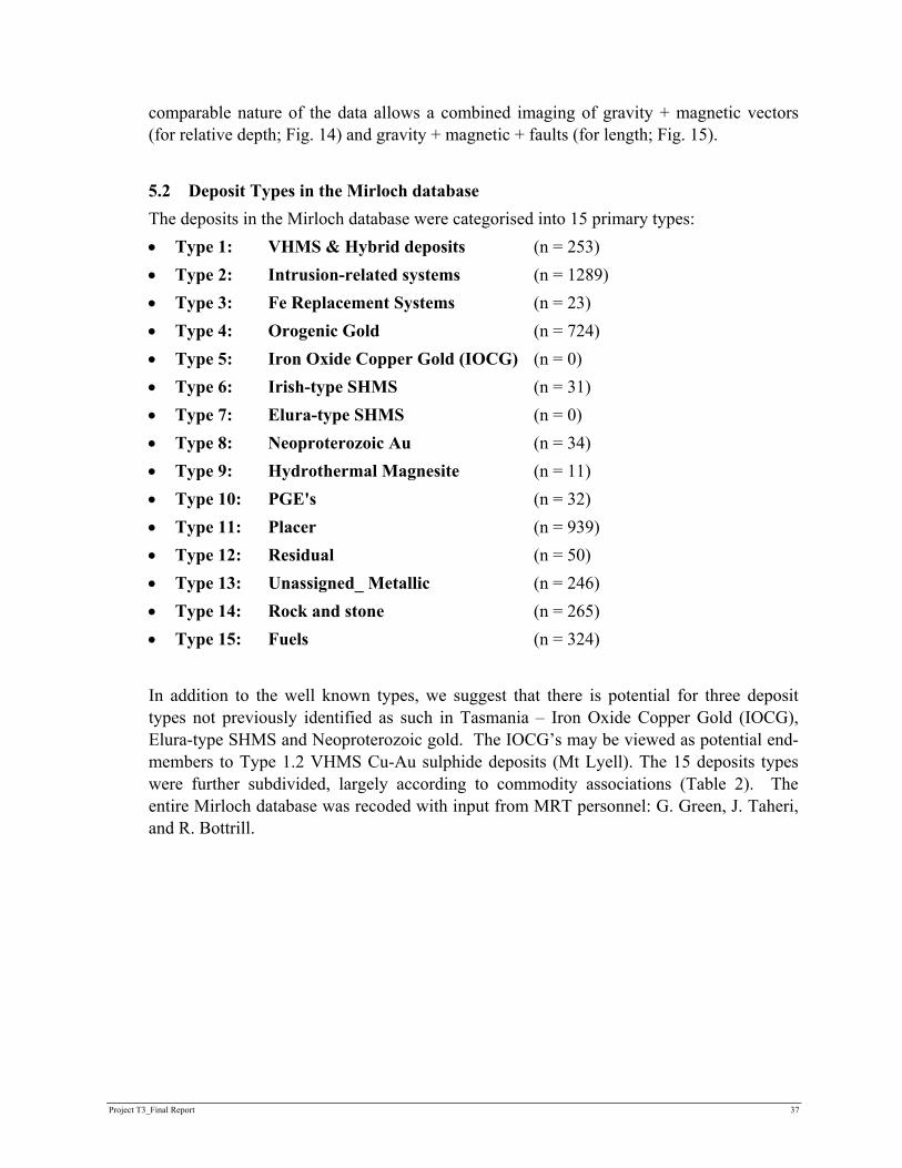
5.2 Deposit Types in the Mirloch database The deposits in the Mirloch database were categorised into 15 primary types: • Type 1: VHMS & Hybrid deposits (n = 253) • Type 2: Intrusion-related systems (n = 1289) • Type 3: Fe Replacement Systems (n = 23) • Type 4: Orogenic Gold (n = 724) • Type 5: Iron Oxide Copper Gold (IOCG) (n = 0) • Type 6: Irish-type SHMS (n = 31) • Type 7: Elura-type SHMS (n = 0) • Type 8: Neoproterozoic Au (n = 34) • Type 9: Hydrothermal Magnesite (n = 11) • Type 10: PGE's (n = 32) • Type 11: Placer (n = 939) • Type 12: Residual (n = 50) • Type 13: Unassigned_ Metallic (n = 246) • Type 14: Rock and stone (n = 265) • Type 15: Fuels (n = 324) In addition to the well known types, we suggest that there is potential for three deposit types not previously identified as such in Tasmania – Iron Oxide Copper Gold (IOCG), Elura-type SHMS and Neoproterozoic gold. The IOCG’s may be viewed as potential end-members to Type 1.2 VHMS Cu-Au sulphide deposits (Mt Lyell). The 15 deposits types were further subdivided, largely according to commodity associations (Table 2). The entire Mirloch database was recoded with input from MRT personnel: G. Green, J. Taheri, and R. Bottrill.

Project T3_Final Report 38
Fig. 14: Relative Depth-weighted image of combined gravity and magnetic vector data. Scale= level of upward continuation
in meters

Project T3_Final Report 39
Fig. 15: Length-weighted image of combined gravity, magnetic and fault vector data.
Project T3_Final Report 40
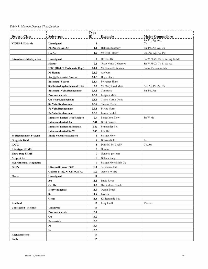
Table 3: Mirloch Deposit Classification
Deposit Class Sub-types Type ID Example Major Commodities
VHMS & Hybrids Unassigned 1 Zn, Pb, Ag, Au,, Cu
Pb-Zn-Cu-Au-Ag 1.1 Hellyer, Rosebery Zn, Pb, Ag, Au, Cu
Cu-Au 1.2 Mt Lyell, Henty Cu, Au, Ag, Zn, Pb
Intrusion-related systems Unassigned 2 Oliver's Hill Sn W Pb Zn Cu Bi Au Ag Fe Mn
Skarns 2.1 Great North Colebrook Sn W Pb Zn Cu Bi Au Ag
HTC (High T Carbonate Repl) 2.1.1 Mt Bischoff, Renison Sn-W +\- basemetals
Ni Skarns 2.1.2 Avebury
Au +\- Basemetal Skarns 2.1.3 Hugo Skarn
Basemetal Skarns 2.1.4 Sylvester Skarn
Sed hosted hydrothermal veins 2.2 Mt Mary Gold Mine Au, Ag, Pb, Zn, Cu
Basemetal Vein/Replacement 2.3.1 Comstock Zn, Pb, Ag
Precious metals 2.3.2 Penguin Mine
Cu Vein/Replacement 2.3.3 Crown Curtin Davis
Sn Vein/Replacement 2.3.4 Storeys Creek
Fe Vein/Replacement 2.3.5 Blythe North
Ba Vein/Replacement 2.3.6 Lower Beulah
Intrusion-hosted Vein/Replace 2.4 Longs Iron Blow Sn W Mo
Intrusion-hosted Au 2.41 Great Panama
Intrusion-hosted Basemetals 2.42 Scamander Bell
Intrusion-hosted Sn/W 2.43 Rex Hill
Fe Replacement Systems Mafic-volcanic associated 3 Savage River
Orogenic Gold 4 Beaconsfield Au
IOCG 5 Darwin? Mt Lyell? Cu, Au
Irish-type SHMS 6 Oceana
Elura-type SHMS 7 None (at present)
Neoprot Au 8 Golden Ridge
Hydrothermal Magnesite 9 Savage River/Main Ck
PGE's Ultramafic assoc PGE 10.1 Serpentine Hill
Gabbro assoc. Ni-Cu-PGE Au 10.2 Genet’s Winze
Placer Unassigned 11
Au 11.1 Inglis River
Cr, Os 11.2 Osmiridium Beach
Heavy minerals 11.3 Ocean Beach
Sn 11.4 Fosters
Gems 11.5 Killiecrankie Bay
Residual 12 King Lyell Various
Unassigned_ Metallic Unknown 13
Precious metals 13.1
Cu 13.2
Basemetals 13.3
Ni 13.4
Fe 13.5
Rock and stone 14
Fuels 15
Project T3_Final Report 41
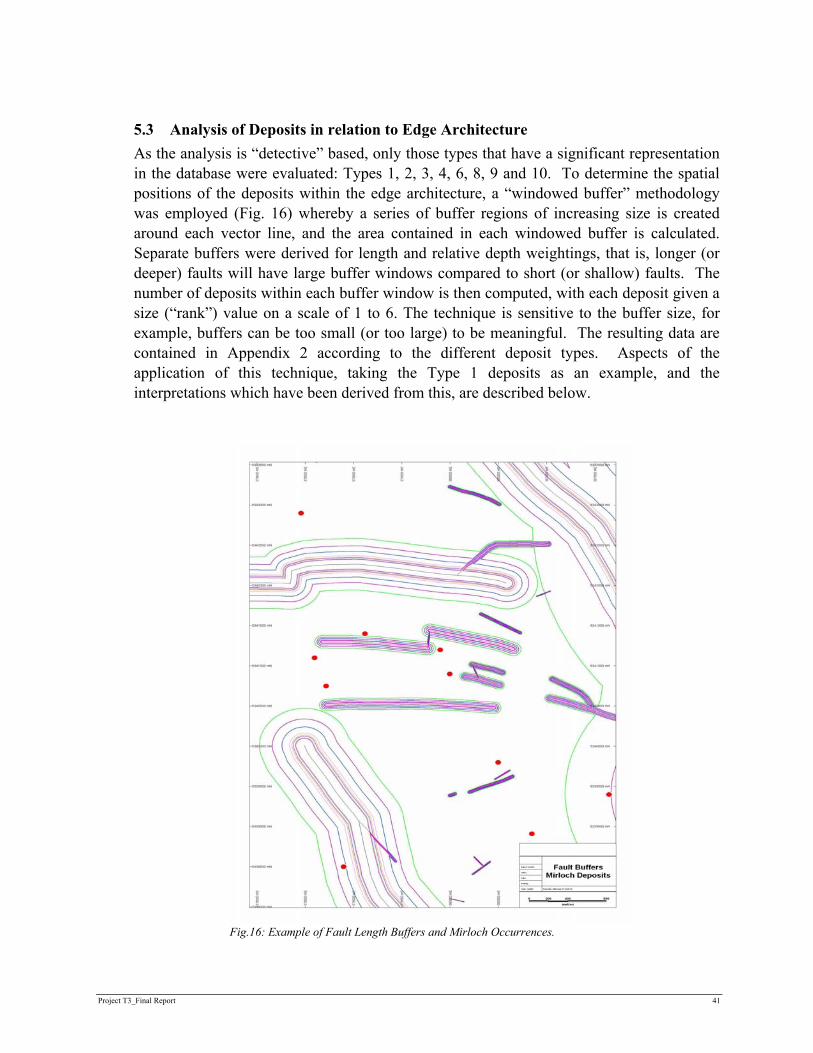
5.3 Analysis of Deposits in relation to Edge Architecture As the analysis is “detective” based, only those types that have a significant representation in the database were evaluated: Types 1, 2, 3, 4, 6, 8, 9 and 10. To determine the spatial positions of the deposits within the edge architecture, a “windowed buffer” methodology was employed (Fig. 16) whereby a series of buffer regions of increasing size is created around each vector line, and the area contained in each windowed buffer is calculated. Separate buffers were derived for length and relative depth weightings, that is, longer (or deeper) faults will have large buffer windows compared to short (or shallow) faults. The number of deposits within each buffer window is then computed, with each deposit given a size (“rank”) value on a scale of 1 to 6. The technique is sensitive to the buffer size, for example, buffers can be too small (or too large) to be meaningful. The resulting data are contained in Appendix 2 according to the different deposit types. Aspects of the application of this technique, taking the Type 1 deposits as an example, and the interpretations which have been derived from this, are described below.
Fig.16: Example of Fault Length Buffers and Mirloch Occurrences.
Project T3_Final Report 42
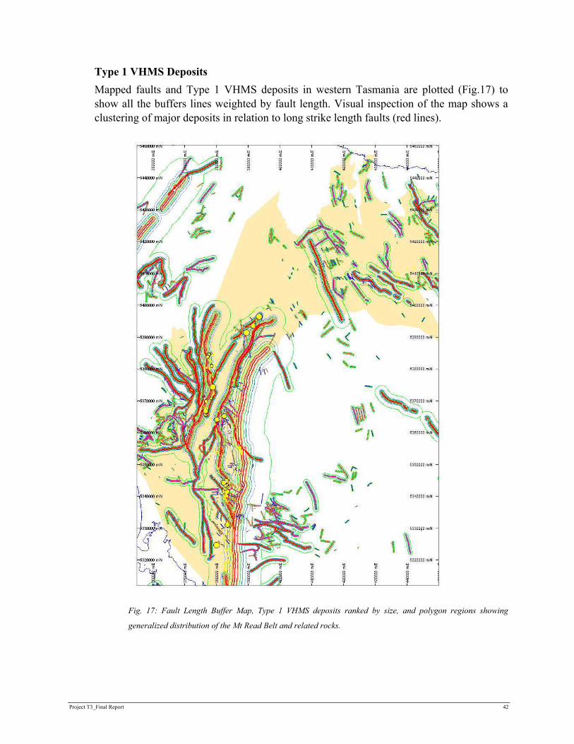
Type 1 VHMS Deposits Mapped faults and Type 1 VHMS deposits in western Tasmania are plotted (Fig.17) to show all the buffers lines weighted by fault length. Visual inspection of the map shows a clustering of major deposits in relation to long strike length faults (red lines).
Fig. 17: Fault Length Buffer Map, Type 1 VHMS deposits ranked by size, and polygon regions showing
generalized distribution of the Mt Read Belt and related rocks.
Project T3_Final Report 43
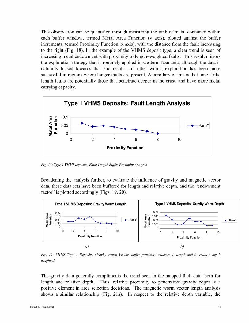
This observation can be quantified through measuring the rank of metal contained within each buffer window, termed Metal Area Function (y axis), plotted against the buffer increments, termed Proximity Function (x axis), with the distance from the fault increasing to the right (Fig. 18). In the example of the VHMS deposit type, a clear trend is seen of increasing metal endowment with proximity to length–weighted faults. This result mirrors the exploration strategy that is routinely applied in western Tasmania, although the data is naturally biased towards that end result – in other words, exploration has been more successful in regions where longer faults are present. A corollary of this is that long strike length faults are potentially those that penetrate deeper in the crust, and have more metal carrying capacity.
Fig. 18: Type 1 VHMS deposits, Fault Length Buffer Proximity Analysis
Broadening the analysis further, to evaluate the influence of gravity and magnetic vector data, these data sets have been buffered for length and relative depth, and the “endowment factor” is plotted accordingly (Figs. 19, 20). a) b)
Fig. 19: VHMS Type 1 Deposits, Gravity Worm Vector, buffer proximity analysis a) length and b) relative depth
weighted.
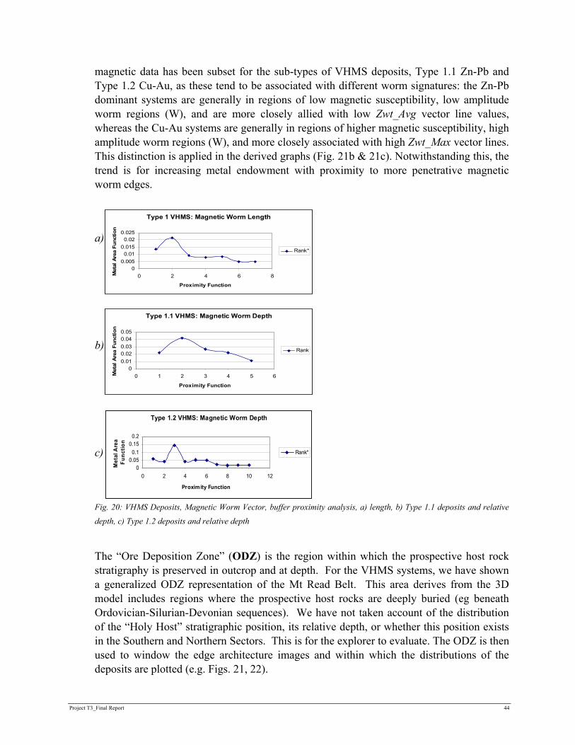
The gravity data generally compliments the trend seen in the mapped fault data, both for length and relative depth. Thus, relative proximity to penetrative gravity edges is a positive element in area selection decisions. The magnetic worm vector length analysis shows a similar relationship (Fig. 21a). In respect to the relative depth variable, the
Type 1 VHMS Deposits: Fault Length Analysis
0
0.05
0.1
0 2 4 6 8 10
Proximity Function
Mat
al A
rea
Func
tion
Rank*
Type 1 VHMS Deposits: Gravity Worm Length
00.005
0.010.015
0.02
0 2 4 6 8 10
Proximity Function
Met
al A
rea
Func
tion
Rank*
Type 1 VHMS Deposits: Gravity Worm Depth
00.0050.01
0.0150.02
0 2 4 6 8 10
Proximity Function
Met
al A
rea
Func
tion
Rank*
Project T3_Final Report 44
magnetic data has been subset for the sub-types of VHMS deposits, Type 1.1 Zn-Pb and Type 1.2 Cu-Au, as these tend to be associated with different worm signatures: the Zn-Pb dominant systems are generally in regions of low magnetic susceptibility, low amplitude worm regions (W), and are more closely allied with low Zwt_Avg vector line values, whereas the Cu-Au systems are generally in regions of higher magnetic susceptibility, high amplitude worm regions (W), and more closely associated with high Zwt_Max vector lines. This distinction is applied in the derived graphs (Fig. 21b & 21c). Notwithstanding this, the trend is for increasing metal endowment with proximity to more penetrative magnetic worm edges. a)
b) c) Fig. 20: VHMS Deposits, Magnetic Worm Vector, buffer proximity analysis, a) length, b) Type 1.1 deposits and relative
depth, c) Type 1.2 deposits and relative depth
The “Ore Deposition Zone” (ODZ) is the region within which the prospective host rock stratigraphy is preserved in outcrop and at depth. For the VHMS systems, we have shown a generalized ODZ representation of the Mt Read Belt. This area derives from the 3D model includes regions where the prospective host rocks are deeply buried (eg beneath Ordovician-Silurian-Devonian sequences). We have not taken account of the distribution of the “Holy Host” stratigraphic position, its relative depth, or whether this position exists in the Southern and Northern Sectors. This is for the explorer to evaluate. The ODZ is then used to window the edge architecture images and within which the distributions of the deposits are plotted (e.g. Figs. 21, 22).
Type 1 VHMS: Magnetic Worm Length
00.0050.01
0.0150.02
0.025
0 2 4 6 8
Proximity Function
Met
al A
rea
Func
tion
Rank*
Type 1.1 VHMS: Magnetic Worm Depth
00.010.020.030.040.05
0 1 2 3 4 5 6
Proximity Function
Met
al A
rea
Func
tion
Rank
Type 1.2 VHMS: Magnetic Worm Depth
00.050.1
0.150.2
0 2 4 6 8 10 12
Proximity Function
Met
al A
rea
Func
tion
Rank*

Project T3_Final Report 45
Fig. 21: Type 1 VHMS Deposits, Total Edge Length Image, inset shows detail of Central Mt Read Belt.

Project T3_Final Report 46
Fig. 22: Type 1 VHMS Deposits, Total Worm Relative Depth, inset Central Mt Read Belt

Project T3_Final Report 47
This representation highlights the correlation of edges with the existing deposits. While the length image is biased by the inclusion of mapped faults, the relative depth image is not. An intriguing aspect is the segmentation of the Mt Read Belt by northwest-trending structures and their association with major mineral systems, e.g. Henty Gold and Hercules on one such feature, Hellyer on another, while Rosbery and Mt Lyell lie at major NW deflections or jogs. The Northern Mt Read Belt seems to hold the best potential for repetition of similar structural positions, although NW-trending structures are common in the MRV south of Macquarie Harbour. Type 2 Intrusion-related Deposits This deposit type consists of a spectrum of sub-types (Table 2) that are almost entirely related to proximity to Devonian granites and the different host rocks that control metal speciation. These are widely distributed geographically, with concentrations in the west, north and northeast Tasmania. Examples are Mt Bischoff and Renison Bell. Summary buffer plots are shown in Appendix 2. Like the VHMS deposits, proximity to faults (Fig. 23) is correlated, though with less emphasis (cf. Fig. 18). This may indicate that fault length (and by inference depth) is not as critical a factor, that is, provided the fault intersects the granite. This may be reflected in the relatively flat distributions seen in the gravity and magnetic vector buffer proximity plots (Appendix 2). Fig. 23: Type 2 Intrusion-related Deposits, Fault Length Buffer Proximity Analysis
Images of these distributions are shown for the region of the Devonian Granite spine in western Tasmania, portraying the total edge length (Fig. 24a) and total edge relative depth_intersection weighted.(Fig. 24b) regions. Areas of granite outcrop are shaded in these images and the ODZ is windowed for areas within ca 2km to the top of the granite model depth (with blank areas where the granite is >2km deep). Renison Bell’s position along the NW trending Federal Basset Fault zone is a continuation of the NW corridor along associated with VHMS deposits (Hercules and Henty), suggesting this structure was metal-prone since the Cambrian. The relative depth image shows clusters of intersection-weighted areas, some of which are ore associated (e.g. Renison Bell). The analysis highlights similar areas with strong exploration potential.
Type 2 Intrusion-related: Fault Length Analysis
00.05
0.10.15
0 2 4 6 8 10
Proximity Function
Met
al A
rea
Func
tion
Rank

Project T3_Final Report 48
Fig. 24: Type 2 Intrusion-related Deposits, Devonian granite spine, western Tasmania. a) total edge length, b) total worm
relative depth_intersection weighted.

Project T3_Final Report 49
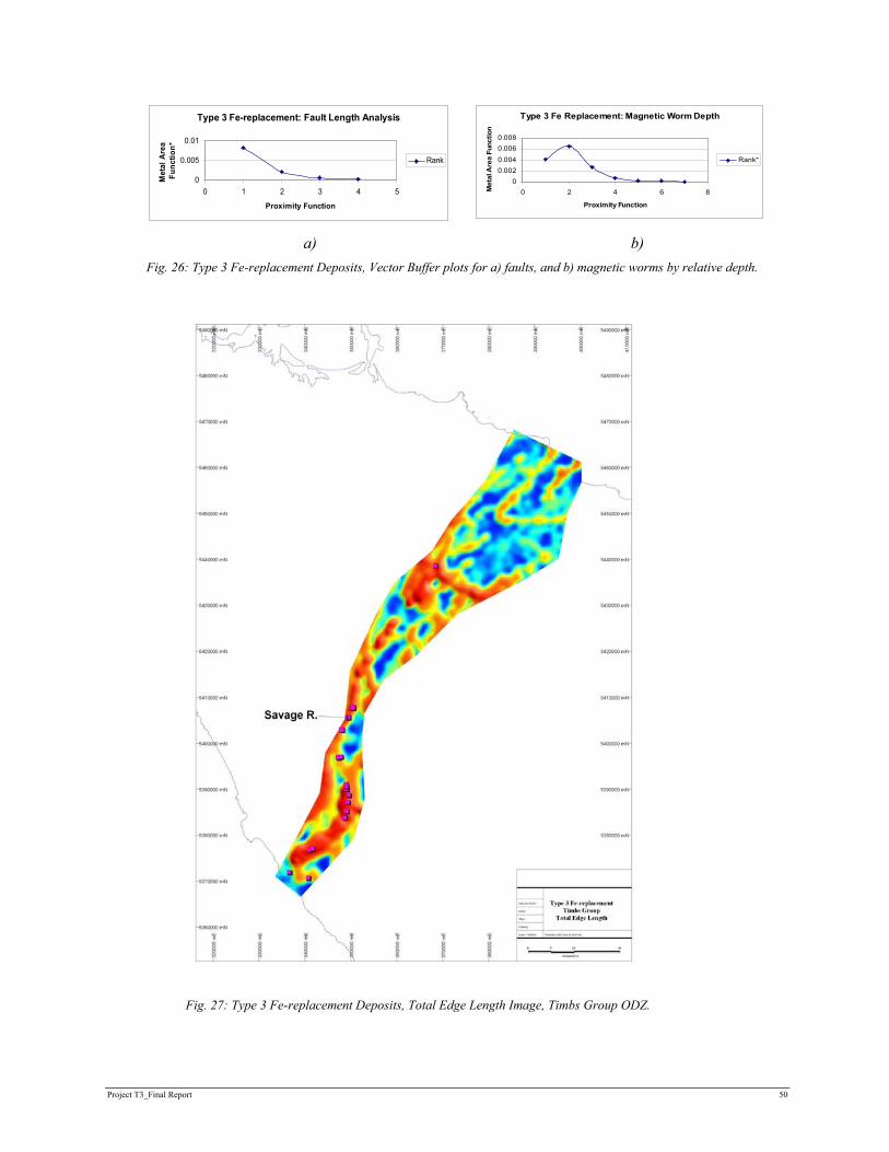
Type 3 Fe-replacement Deposits The type example, Savage River, has a strong aeromagnetic response, as illustrated using the worm amplitude W values (Fig. 25). Related deposits are clustered in the high amplitude regions. Some areas in the north are highlighted as potential targets. The host rock in this region is the Timbs Group. The location of Savage River is strongly related to fault length (Fig. 26a), reflecting the location of these deposits proximal to the Arthur Lineament. Magnetite associated with these systems provides a key area selection tool, as highlighted in the magnetic worm depth plot (Fig. 26b). A map representation of these aspects is shown in Fig. 27 for the total edge length factor.
Fig. 25: Type 3 Fe-replacement deposits, Timbs Group ODZ, Magnetic W amplitudes (red = high, grey = low).
Project T3_Final Report 50
a) b) Fig. 26: Type 3 Fe-replacement Deposits, Vector Buffer plots for a) faults, and b) magnetic worms by relative depth.
Fig. 27: Type 3 Fe-replacement Deposits, Total Edge Length Image, Timbs Group ODZ.
Type 3 Fe-replacement: Fault Length Analysis
0
0.005
0.01
0 1 2 3 4 5
Proximity Function
Met
al A
rea
Func
tion*
Rank
Type 3 Fe Replacement: Magnetic Worm Depth
00.0020.0040.0060.008
0 2 4 6 8
Proximity Function
Met
al A
rea
Func
tion
Rank*
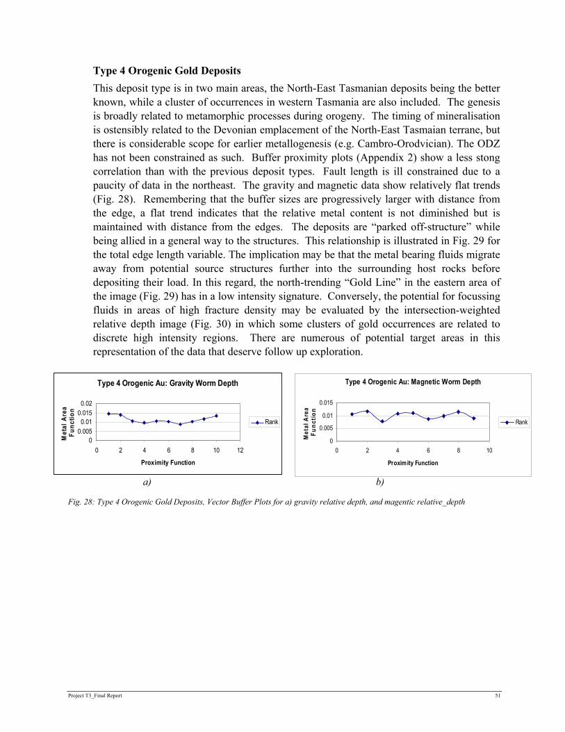
Project T3_Final Report 51
Type 4 Orogenic Gold Deposits This deposit type is in two main areas, the North-East Tasmanian deposits being the better known, while a cluster of occurrences in western Tasmania are also included. The genesis is broadly related to metamorphic processes during orogeny. The timing of mineralisation is ostensibly related to the Devonian emplacement of the North-East Tasmaian terrane, but there is considerable scope for earlier metallogenesis (e.g. Cambro-Orodvician). The ODZ has not been constrained as such. Buffer proximity plots (Appendix 2) show a less stong correlation than with the previous deposit types. Fault length is ill constrained due to a paucity of data in the northeast. The gravity and magnetic data show relatively flat trends (Fig. 28). Remembering that the buffer sizes are progressively larger with distance from the edge, a flat trend indicates that the relative metal content is not diminished but is maintained with distance from the edges. The deposits are “parked off-structure” while being allied in a general way to the structures. This relationship is illustrated in Fig. 29 for the total edge length variable. The implication may be that the metal bearing fluids migrate away from potential source structures further into the surrounding host rocks before depositing their load. In this regard, the north-trending “Gold Line” in the eastern area of the image (Fig. 29) has in a low intensity signature. Conversely, the potential for focussing fluids in areas of high fracture density may be evaluated by the intersection-weighted relative depth image (Fig. 30) in which some clusters of gold occurrences are related to discrete high intensity regions. There are numerous of potential target areas in this representation of the data that deserve follow up exploration.
a) b)
Fig. 28: Type 4 Orogenic Gold Deposits, Vector Buffer Plots for a) gravity relative depth, and magentic relative_depth
Type 4 Orogenic Au: Gravity Worm Depth
00.0050.01
0.0150.02
0 2 4 6 8 10 12
Proximity Function
Met
al A
rea
Func
tion
Rank
Type 4 Orogenic Au: Magnetic Worm Depth
0
0.005
0.01
0.015
0 2 4 6 8 10
Proximity Function
Met
al A
rea
Func
tion
Rank

Project T3_Final Report 52
Fig. 29: Type 4 Orogenic Gold Deposits, Total Edge Length Image
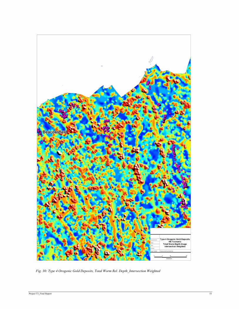
Project T3_Final Report 53
Fig. 30: Type 4 Orogenic Gold Deposits, Total Worm Rel. Depth_Intersection Weighted
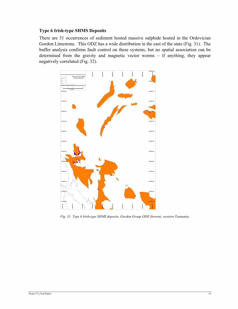
Project T3_Final Report 54
Type 6 Irish-type SHMS Deposits There are 31 occurrences of sediment hosted massive sulphide hosted in the Ordovician Gordon Limestone. This ODZ has a wide distribution in the east of the state (Fig. 31). The buffer analysis confirms fault control on these systems, but no spatial association can be determined from the gravity and magnetic vector worms – if anything, they appear negatively correlated (Fig. 32).
Fig. 31: Type 6 Irish-type SHMS deposits, Gordon Group ODZ (brown), western Tasmania.
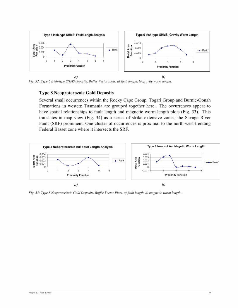
Project T3_Final Report 55
a) b) Fig. 32: Type 6 Irish-type SHMS deposits, Buffer Vector plots, a) fault length, b) gravity worm length.
Type 8 Neoproterozoic Gold Deposits Several small occurrences within the Rocky Cape Group, Togari Group and Burnie-Oonah Formations in western Tasmania are grouped together here. The occurrences appear to have spatial relationships to fault length and magnetic worm length plots (Fig. 33). This translates in map view (Fig. 34) as a series of strike extensive zones, the Savage River Fault (SRF) prominent. One cluster of occurrences is proximal to the north-west-trending Federal Basset zone where it intersects the SRF.
a) b)
Fig. 33: Type 8 Neoproterizoic Gold Deposits, Buffer Vector Plots, a) fault length, b) magnetic worm length.
Type 6 Irish-type SHMS: Fault Length Analysis
00.002
0.0040.006
0 1 2 3 4 5 6 7
Proximity Function
Met
al A
rea
Func
tion*
Rank
Type 6 Irish-type SHMS: Gravity Worm Length
0
0.0005
0.001
0.0015
0 2 4 6 8
Proximity Function
Met
al A
rea
Func
tion
Rank*
Type 8 Neoproterozoic Au: Fault Length Analysis
00.0010.0020.0030.004
0 1 2 3 4 5 6
Proximity Function
Mea
tl A
rea
Func
tion
Rank
Type 8 Neoprot Au: Magetic Worm Length
-0.0010
0.0010.0020.0030.004
0 2 4 6 8
Proximity Function
Met
al A
rea
Func
tion
Rank*

Project T3_Final Report 56
Fig. 34: Type 8 Neoproterozoic Gold, Total Edge Length Image, western Tasmania.
Type 9 Hydrothermal Magnesite Deposits These occurrences in northwestern Tasmanian are mostly hosted in the Rocky Cape Group and Burnie-Oonah Formations. These are closely related to the Type 3 Fe-replacement deposits, and follow similar spatial distributions. The buffer analysis (Fig. 35) suggests control by long strike length faults and penetrative magnetic worms. This is represented in map view (Fig. 36) with clusters of occurrences associated with high fracture length regions.

Project T3_Final Report 57
a) b) Fig. 35: Type 8 Hyrdothermal Magnesite Deposits, Buffer Proximity plots, a) fault length, b) magnetic worm relative-depth.
Fig. 36: Type 9 Hydrothermal Magnesite, Total Edge Length Image, western Tasmania
Type 10 PGE Deposits The mafic and ultramafic hosted Or-Ir deposits are located within the Early Cambrian allochthon. Major low angle shear zones control the distribution of the allochthon, and the associated deposits show a strong fault control and are spatially associated with penetrative edges in the magnetic data (Fig. 37). The spatial distributions are shown in Fig. 38). Note that this analysis has not separated the Or-Ir deposits (associated with allochthonous ultramafics) from the Cuni Ni-Cu-Au-Pt-Pd deposits (hosted by Togari Rift equivalents) and, being in different parts of the stratigraphy, could be treated separately.
Type 9 Hydrothermal Magnesite: Fault Length
00.0010.0020.0030.004
0 1 2 3 4 5 6
Proximity Function
Met
al A
rea
Func
tion
Rank*
Type 9 Hydrothermal Magnesite: Magetic Worm Depth
-0.0020
0.0020.004
0.006
0 2 4 6 8
Proximity Function
Met
al A
rea
Func
tion
Rank*
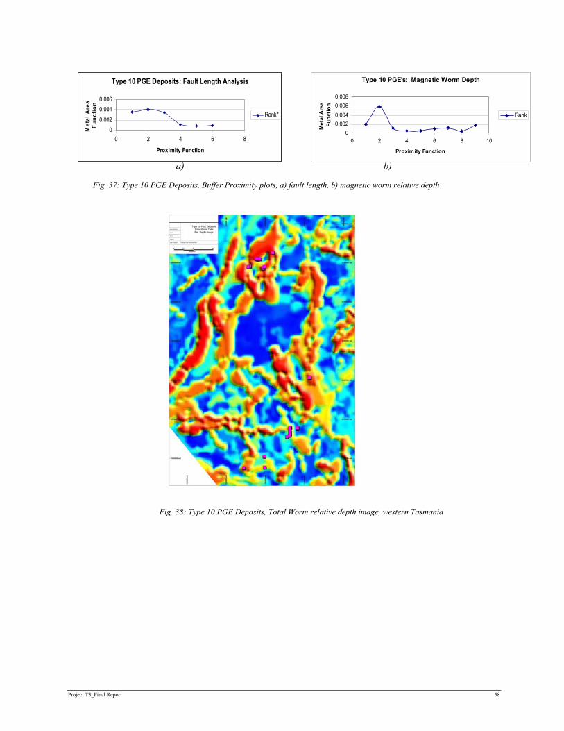
Project T3_Final Report 58
a) b)
Fig. 37: Type 10 PGE Deposits, Buffer Proximity plots, a) fault length, b) magnetic worm relative depth
Fig. 38: Type 10 PGE Deposits, Total Worm relative depth image, western Tasmania
Type 10 PGE Deposits: Fault Length Analysis
00.002
0.0040.006
0 2 4 6 8
Proximity Function
Met
al A
rea
Func
tion
Rank*
Type 10 PGE's: Magnetic Worm Depth
00.0020.004
0.0060.008
0 2 4 6 8 10
Proximity Function
Met
al A
rea
Func
tion
Rank

Project T3_Final Report 59
6 CONCLUSIONS The assembly of extensive data sets in and around the Tasmanian mineral provinces into a common visualisation platform (FracSIS) has allowed significant advances to be made in understanding the 3D geometry of the state. The project is designed as a stimulus to mineral exploration, through an assessment and representation of its complex 3D architecture together with its mineral deposits. The data allows for visualisation and analysis of regional geology, geophysics, geochemistry, mineral deposits and mineral prospectivity. As for any project with a large scope, some fundamental geological problems are addressed in terms of geometry that in turn raises significant questions for the research and exploration communities to address. Uncertainties largely derive from the non-uniqueness of interpretations in 2D and 3D at a variety of scales. Using serial geological cross sections, a 3D model was constructed of the top 10 km of the crust. Viewed dynamically, the model is a pointer for further research to validate and change, as more information and better interpretations are developed. For example, the emplacement direction and translation distance involved in the early Cambrian oceanic allochthon, if viewed as an exotic crustal component, has not been evaluated. Rather, the “exotic” nature of the succession may be called to question if derived from a back-arc setting(s). Also, the inferred nature and dip of the Tyennan Margin Fault is a critical geometry in the model that needs further constraint, given its potentially complex and long lived history. Other issues are of direct exploration significance, with the analysis showing potential target areas for follow up evaluation for a range of commodities, in particular Pb, Zn, Cu, Au and Fe. The role of NW trending structures and fault intersections along them in controlling the locations of Cambrian VHMS and Devonian skarn mineral systems in western Tasmania is notable, while Devonian orogenic gold targets in north-east Tasmania offer some potential. Project generation opportunities for VHMS deposits are identified in some non-standard areas (e.g. under Tertiary cover north of Hellyer, in the northern Mt Read Belt of the Sheffield element, and to the south of Macquarie Harbour). On a regional scale structural template, new generation target regions for a range of commodities are identified that should appeal to those explorers who choose to venture into this often rugged, remote and rewarding terrain.
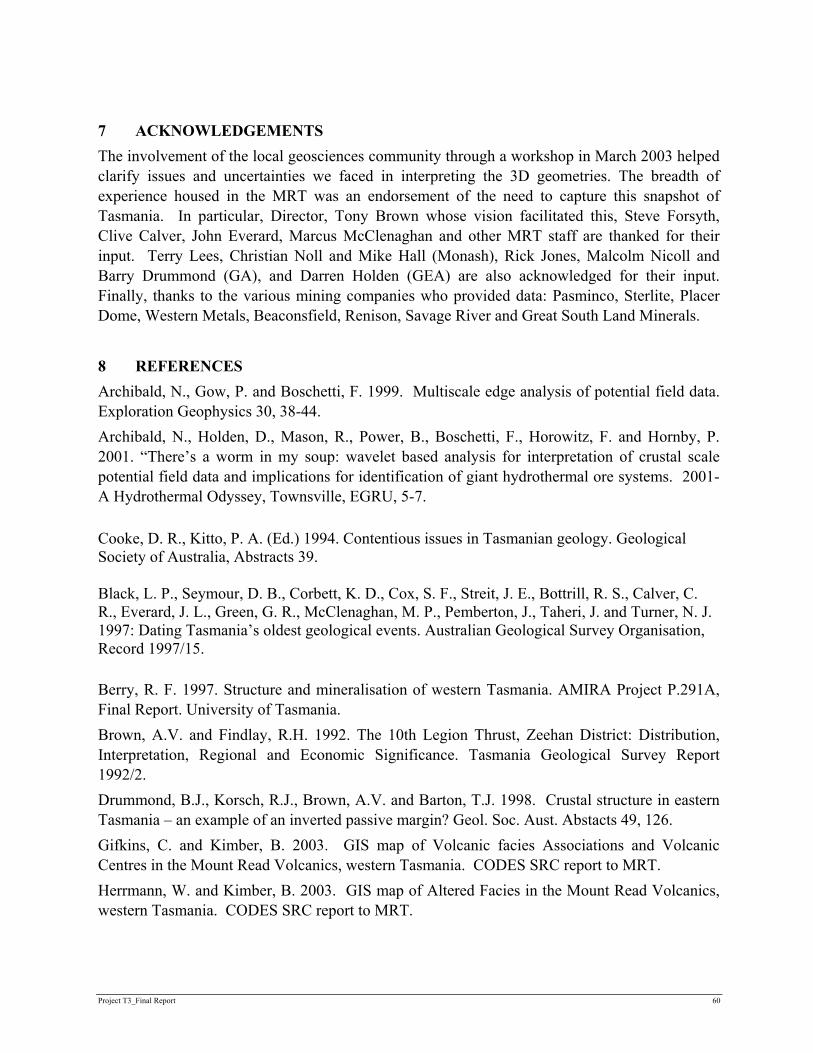
Project T3_Final Report 60
7 ACKNOWLEDGEMENTS The involvement of the local geosciences community through a workshop in March 2003 helped clarify issues and uncertainties we faced in interpreting the 3D geometries. The breadth of experience housed in the MRT was an endorsement of the need to capture this snapshot of Tasmania. In particular, Director, Tony Brown whose vision facilitated this, Steve Forsyth, Clive Calver, John Everard, Marcus McClenaghan and other MRT staff are thanked for their input. Terry Lees, Christian Noll and Mike Hall (Monash), Rick Jones, Malcolm Nicoll and Barry Drummond (GA), and Darren Holden (GEA) are also acknowledged for their input. Finally, thanks to the various mining companies who provided data: Pasminco, Sterlite, Placer Dome, Western Metals, Beaconsfield, Renison, Savage River and Great South Land Minerals. 8 REFERENCES Archibald, N., Gow, P. and Boschetti, F. 1999. Multiscale edge analysis of potential field data. Exploration Geophysics 30, 38-44. Archibald, N., Holden, D., Mason, R., Power, B., Boschetti, F., Horowitz, F. and Hornby, P. 2001. “There’s a worm in my soup: wavelet based analysis for interpretation of crustal scale potential field data and implications for identification of giant hydrothermal ore systems. 2001- A Hydrothermal Odyssey, Townsville, EGRU, 5-7. Cooke, D. R., Kitto, P. A. (Ed.) 1994. Contentious issues in Tasmanian geology. Geological Society of Australia, Abstracts 39. Black, L. P., Seymour, D. B., Corbett, K. D., Cox, S. F., Streit, J. E., Bottrill, R. S., Calver, C. R., Everard, J. L., Green, G. R., McClenaghan, M. P., Pemberton, J., Taheri, J. and Turner, N. J. 1997: Dating Tasmania’s oldest geological events. Australian Geological Survey Organisation, Record 1997/15. Berry, R. F. 1997. Structure and mineralisation of western Tasmania. AMIRA Project P.291A, Final Report. University of Tasmania. Brown, A.V. and Findlay, R.H. 1992. The 10th Legion Thrust, Zeehan District: Distribution, Interpretation, Regional and Economic Significance. Tasmania Geological Survey Report 1992/2. Drummond, B.J., Korsch, R.J., Brown, A.V. and Barton, T.J. 1998. Crustal structure in eastern Tasmania – an example of an inverted passive margin? Geol. Soc. Aust. Abstacts 49, 126. Gifkins, C. and Kimber, B. 2003. GIS map of Volcanic facies Associations and Volcanic Centres in the Mount Read Volcanics, western Tasmania. CODES SRC report to MRT. Herrmann, W. and Kimber, B. 2003. GIS map of Altered Facies in the Mount Read Volcanics, western Tasmania. CODES SRC report to MRT.
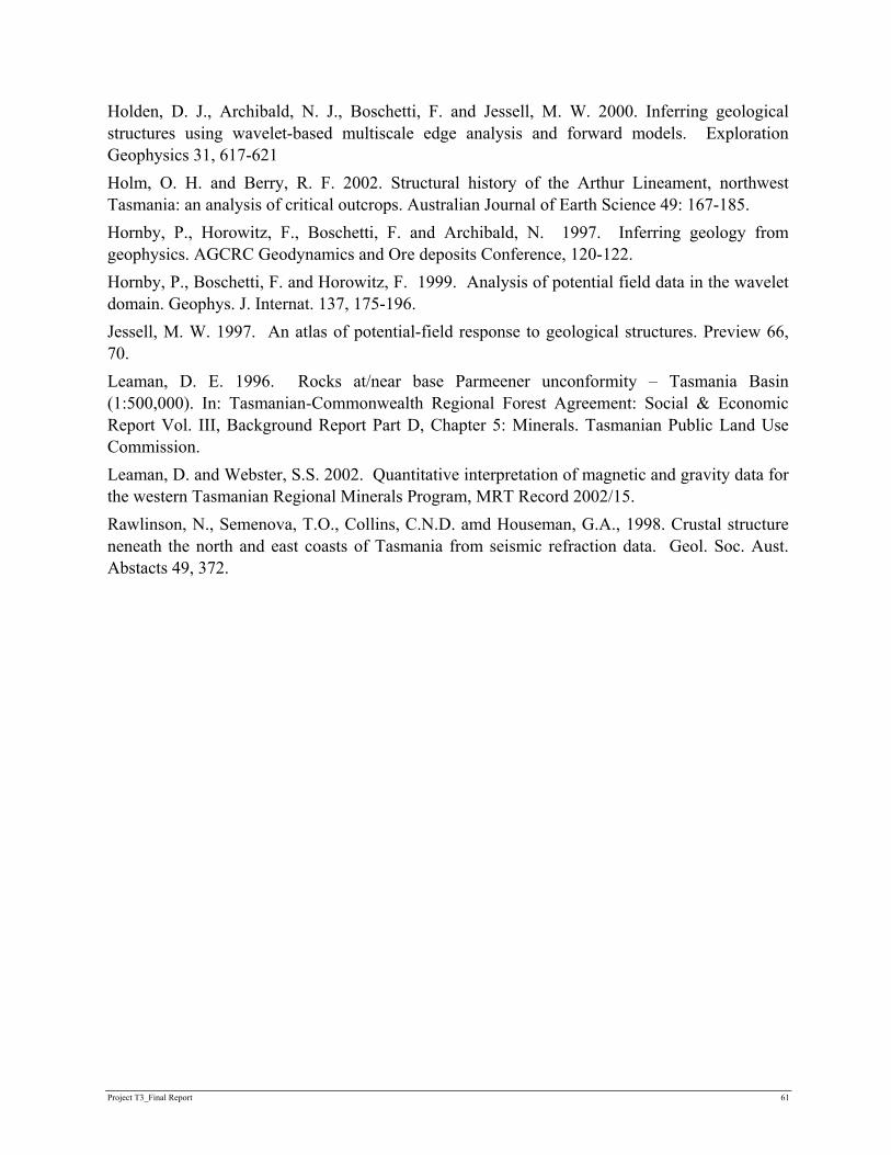
Project T3_Final Report 61
Holden, D. J., Archibald, N. J., Boschetti, F. and Jessell, M. W. 2000. Inferring geological structures using wavelet-based multiscale edge analysis and forward models. Exploration Geophysics 31, 617-621 Holm, O. H. and Berry, R. F. 2002. Structural history of the Arthur Lineament, northwest Tasmania: an analysis of critical outcrops. Australian Journal of Earth Science 49: 167-185. Hornby, P., Horowitz, F., Boschetti, F. and Archibald, N. 1997. Inferring geology from geophysics. AGCRC Geodynamics and Ore deposits Conference, 120-122. Hornby, P., Boschetti, F. and Horowitz, F. 1999. Analysis of potential field data in the wavelet domain. Geophys. J. Internat. 137, 175-196. Jessell, M. W. 1997. An atlas of potential-field response to geological structures. Preview 66, 70. Leaman, D. E. 1996. Rocks at/near base Parmeener unconformity – Tasmania Basin (1:500,000). In: Tasmanian-Commonwealth Regional Forest Agreement: Social & Economic Report Vol. III, Background Report Part D, Chapter 5: Minerals. Tasmanian Public Land Use Commission. Leaman, D. and Webster, S.S. 2002. Quantitative interpretation of magnetic and gravity data for the western Tasmanian Regional Minerals Program, MRT Record 2002/15. Rawlinson, N., Semenova, T.O., Collins, C.N.D. amd Houseman, G.A., 1998. Crustal structure neneath the north and east coasts of Tasmania from seismic refraction data. Geol. Soc. Aust. Abstacts 49, 372.
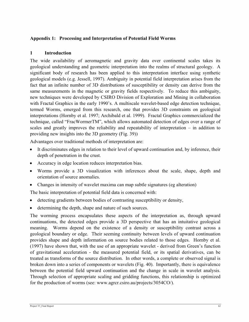
Project T3_Final Report 62
Appendix 1: Processing and Interpretation of Potential Field Worms 1 Introduction The wide availability of aeromagnetic and gravity data over continental scales takes its geological understanding and geometric interpretation into the realms of structural geology. A significant body of research has been applied to this interpretation interface using synthetic geological models (e.g. Jessell, 1997). Ambiguity in potential field interpretation arises from the fact that an infinite number of 3D distributions of susceptibility or density can derive from the same measurements in the magnetic or gravity fields respectively. To reduce this ambiguity, new techniques were developed by CSIRO Division of Exploration and Mining in collaboration with Fractal Graphics in the early 1990’s. A multiscale wavelet-based edge detection technique, termed Worms, emerged from this research, one that provides 3D constraints on geological interpretations (Hornby et al. 1997; Archibald et al. 1999). Fractal Graphics commercialized the technique, called “FracWormerTM”, which allows automated detection of edges over a range of scales and greatly improves the reliability and repeatability of interpretation – in addition to providing new insights into the 3D geometry (Fig. 39)) Advantages over traditional methods of interpretation are: • It discriminates edges in relation to their level of upward continuation and, by inference, their
depth of penetration in the crust. • Accuracy in edge location reduces interpretation bias. • Worms provide a 3D visualization with inferences about the scale, shape, depth and
orientation of source anomalies. • Changes in intensity of wavelet maxima can map subtle signatures (eg alteration) The basic interpretation of potential field data is concerned with: • detecting gradients between bodies of contrasting susceptibility or density, • determining the depth, shape and nature of such sources. The worming process encapsulates these aspects of the interpretation as, through upward continuations, the detected edges provide a 3D perspective that has an intuitative geological meaning. Worms depend on the existence of a density or susceptibility contrast across a geological boundary or edge. Their seeming continuity between levels of upward continuation provides shape and depth information on source bodies related to those edges. Hornby et al. (1997) have shown that, with the use of an appropriate wavelet - derived from Green’s function of gravitational acceleration - the measured potential field, or its spatial derivatives, can be treated as transforms of the source distribution. In other words, a complete or observed signal is broken down into a series of components or wavelets (Fig. 40). Importantly, there is equivalence between the potential field upward continuation and the change in scale in wavelet analysis. Through selection of appropriate scaling and gridding functions, this relationship is optimized for the production of worms (see: www.agrcr.csiro.au/projects/3054CO/).

Project T3_Final Report 63
Fig. 39: 3D visualisation of a synthetic model (bottom layer), calculated gravity response (middle layer) and resulting 3D multiscale edge map (Archibald et al. 1999).
d)
Fig 40: Wavelet transformation: a) gravity profiles over buried source become flatter with increasing depth, b) wavelet transforms and maxima of those transforms, c) plot of wavelet maxima for increasing height, d) 3D visualisation of multiscale edges due to an inclined cylinder (Archibald et al. 1999)
2 Upward Continuations, Edge Detection, and Worm points Worm data consists of an ascii point file located in 3D space (X,Y,Z) with each point characterised by an intensity value (W) that is related to the magnitude or strength of the signal. Processing involves the follows steps: A regular grid is constructed from the input data. For irregular shaped survey areas, the grid is padded out to a required dimension, that is, introduce dummy data from which dummy worms
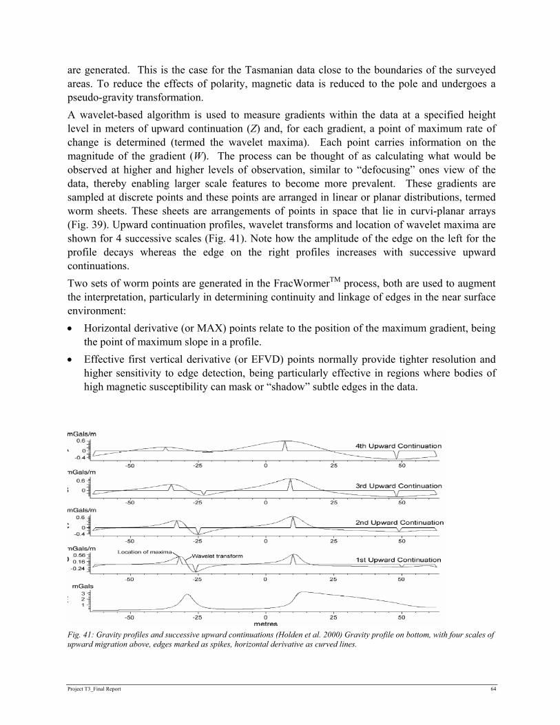
Project T3_Final Report 64
are generated. This is the case for the Tasmanian data close to the boundaries of the surveyed areas. To reduce the effects of polarity, magnetic data is reduced to the pole and undergoes a pseudo-gravity transformation. A wavelet-based algorithm is used to measure gradients within the data at a specified height level in meters of upward continuation (Z) and, for each gradient, a point of maximum rate of change is determined (termed the wavelet maxima). Each point carries information on the magnitude of the gradient (W). The process can be thought of as calculating what would be observed at higher and higher levels of observation, similar to “defocusing” ones view of the data, thereby enabling larger scale features to become more prevalent. These gradients are sampled at discrete points and these points are arranged in linear or planar distributions, termed worm sheets. These sheets are arrangements of points in space that lie in curvi-planar arrays (Fig. 39). Upward continuation profiles, wavelet transforms and location of wavelet maxima are shown for 4 successive scales (Fig. 41). Note how the amplitude of the edge on the left for the profile decays whereas the edge on the right profiles increases with successive upward continuations. Two sets of worm points are generated in the FracWormerTM process, both are used to augment the interpretation, particularly in determining continuity and linkage of edges in the near surface environment: • Horizontal derivative (or MAX) points relate to the position of the maximum gradient, being
the point of maximum slope in a profile. • Effective first vertical derivative (or EFVD) points normally provide tighter resolution and
higher sensitivity to edge detection, being particularly effective in regions where bodies of high magnetic susceptibility can mask or “shadow” subtle edges in the data.
Fig. 41: Gravity profiles and successive upward continuations (Holden et al. 2000) Gravity profile on bottom, with four scales of upward migration above, edges marked as spikes, horizontal derivative as curved lines.

Project T3_Final Report 65
Worm Distributions There are two values of interest: W – the wavelet intensity, and Z – the level of upward continuation.
W distributions: a measure of the amplitude of an edge at a particular level of upward continuation. It can be thought of as the strength of contrast in the source materials. Aspects of this include: • Variations in intensity values over different levels of upward continuation provide
constraints on the source geometry. Typically, the intensity increases to a maximum at a certain level of upward continuation, after which it decays (Fig. 40d). The level at which the W peak occurs on a worm sheet relates to the depth to the centre of gravity of the object.
• Up to this W peak, the form of a worm sheet typically mirrors the shape of the edge that creates the worm, that is, the dip direction and its magnitude.
• Colour mapping the W value at selected Z levels yields meaningful geological distributions. In particular, discrete changes may be good pointers for regions of hydrothermal alteration.
Z distributions: the worm sheets describe a hierarchy of edges that migrate to different levels of upward continuation. This spectrum ranges from “fine scale” worms at low levels to “coarse scale” worms at high levels of upward continuation. Fine scale worms detect high frequency/short wavelength responses and typically reflect near surface features, while coarse scale worms detect low frequency/long wavelength edges and reflect structures occurring at deep crustal levels or gross changes in the potential field (Fig. 42). Aspects of the data include: • Fine scale worms map subtle variations at shallow levels, e.g. sedimentary packages (Fig.
42b). Coarse scale worms for the same area discriminate intrusive margins at depth (Fig. 42c).
• Coarse scale worms typically cascade into fine scale worms. In this way the surface positions of “major” worm sheets is determined.
• Spatial distributions of Z values can be colour mapped to show the relative significance of edges at different heights. This allows depth slicing and ranking of edges according to their maximum level of upward migration.
• Relative dip directions and dip angles of edges can be determined through observing the positions of worm points as they migrate to successive levels. For example, synthetic models of different fault geometries produce different worm patterns that mirror-image the dip of a fault (Fig. 43; Archibald et al. 1999) - provided determinations are made at or below the W intensity peak.
• Ambiguity arises for some broad wavelength features and their coarse scale worms. While these usually relate to deep sourced geological features, there are exceptions and independent geological confirmation should be sought. For example, a flat shallow dense layer (e.g. Jurassic dolerite sheet) which tapers gradually may produce a similar worm response as a deep dense layer which ends abruptly. Similar ambiguity arises with strongly magnetic

Project T3_Final Report 66
sources (e.g. ultramafics) which influence the magnetic field for considerable distances from the source – such that small high susceptibility bodies can cause broad wavelength responses.
• As a rule of thumb, the maximum level of upward continuation of a worm sheet is proportional (by a factor of about 2) to the depth of penetration of the edge below surface, e.g. worms at Z = 1000m upward continuation relate to edges at about 500m depth.
• Truncations, offsets and vacancies of worms are an important feature, particularly in relation to regional scale structural analysis of the data.
Fig. 42: Fine to Coarse scale worms from Western Victoria aeromagnetic data, a) total magnetic intensity image, b) fine scale and c) coarse scale worms(Archibald et al. 1999).
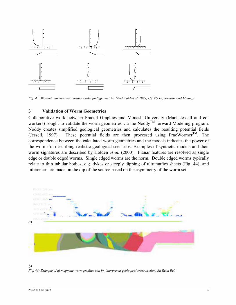
Project T3_Final Report 67
Fig. 43: Wavelet maxima over various model fault geometries (Archibald et al. 1999; CSIRO Exploration and Mining)
3 Validation of Worm Geometries Collaborative work between Fractal Graphics and Monash University (Mark Jessell and co-workers) sought to validate the worm geometries via the NoddyTM forward Modeling program. Noddy creates simplified geological geometries and calculates the resulting potential fields (Jessell, 1997). These potential fields are then processed using FracWormerTM. The correspondence between the calculated worm geometries and the models indicates the power of the worms in describing realistic geological scenarios. Examples of synthetic models and their worm signatures are described by Holden et al. (2000). Planar features are resolved as single edge or double edged worms. Single edged worms are the norm. Double edged worms typically relate to thin tabular bodies, e.g. dykes or steeply dipping of ultramafics sheets (Fig. 44), and inferences are made on the dip of the source based on the asymmetry of the worm set.
a)
b) Fig. 44: Example of a) magnetic worm profiles and b) interpreted geological cross section, Mt Read Belt
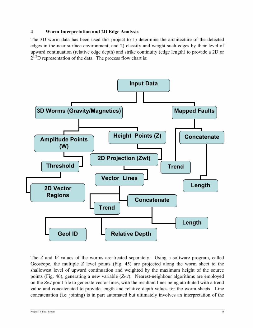
Project T3_Final Report 68
4 Worm Interpretation and 2D Edge Analysis The 3D worm data has been used this project to 1) determine the architecture of the detected edges in the near surface environment, and 2) classify and weight such edges by their level of upward continuation (relative edge depth) and strike continuity (edge length) to provide a 2D or 21/2D representation of the data. The process flow chart is: The Z and W values of the worms are treated separately. Using a software program, called Geoscope, the multiple Z level points (Fig. 45) are projected along the worm sheet to the shallowest level of upward continuation and weighted by the maximum height of the source points (Fig. 46), generating a new variable (Zwt). Nearest-neighbour algorithms are employed on the Zwt point file to generate vector lines, with the resultant lines being attributed with a trend value and concatenated to provide length and relative depth values for the worm sheets. Line concatenation (i.e. joining) is in part automated but ultimately involves an interpretation of the
Input Data
3D Worms (Gravity/Magnetics) Mapped Faults
Amplitude Points (W)
Height Points (Z)
2D Projection (Zwt)
Vector Lines
2D Vector Regions
Threshold
Concatenate
Length
Relative Depth
Trend
Concatenate
Length
Geol ID
Trend
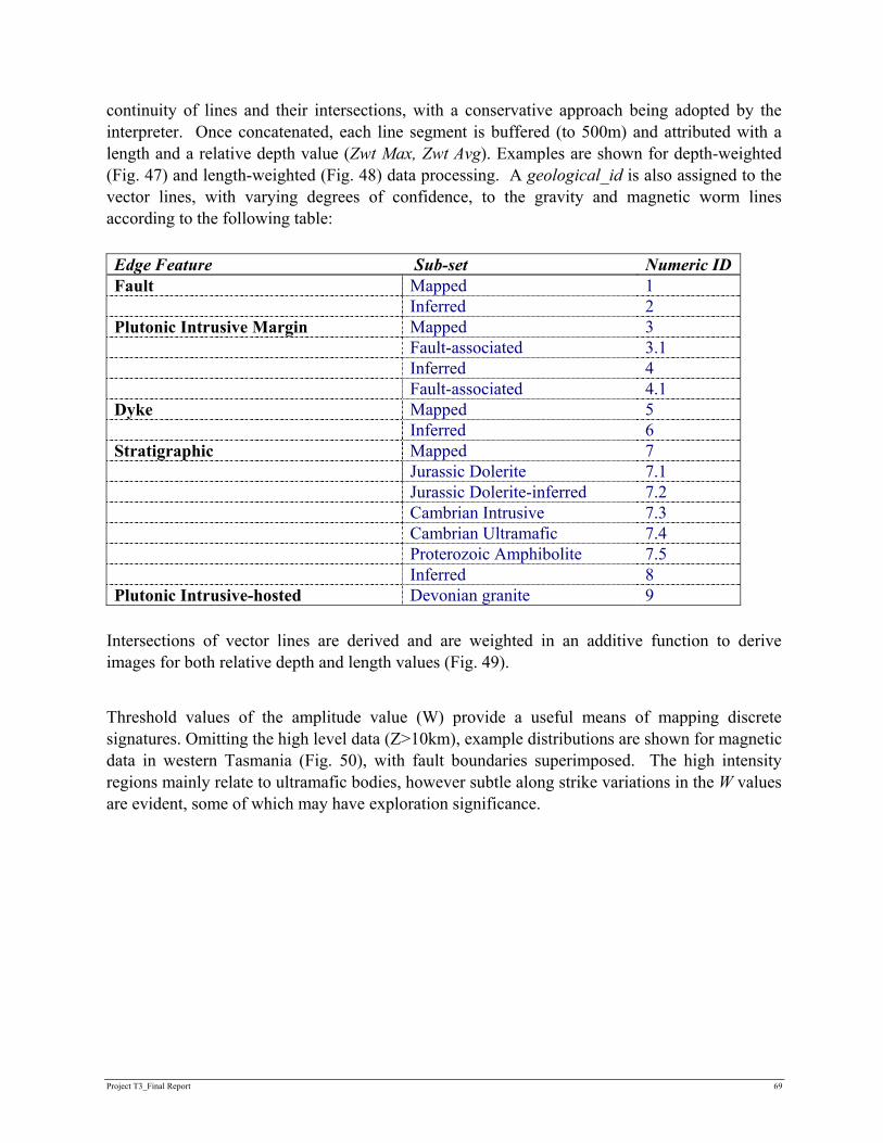
Project T3_Final Report 69
continuity of lines and their intersections, with a conservative approach being adopted by the interpreter. Once concatenated, each line segment is buffered (to 500m) and attributed with a length and a relative depth value (Zwt Max, Zwt Avg). Examples are shown for depth-weighted (Fig. 47) and length-weighted (Fig. 48) data processing. A geological_id is also assigned to the vector lines, with varying degrees of confidence, to the gravity and magnetic worm lines according to the following table: Edge Feature Sub-set Numeric ID Fault Mapped 1 Inferred 2 Plutonic Intrusive Margin Mapped 3 Fault-associated 3.1 Inferred 4 Fault-associated 4.1 Dyke Mapped 5 Inferred 6 Stratigraphic Mapped 7 Jurassic Dolerite 7.1 Jurassic Dolerite-inferred 7.2 Cambrian Intrusive 7.3 Cambrian Ultramafic 7.4 Proterozoic Amphibolite 7.5 Inferred 8 Plutonic Intrusive-hosted Devonian granite 9
Intersections of vector lines are derived and are weighted in an additive function to derive images for both relative depth and length values (Fig. 49). Threshold values of the amplitude value (W) provide a useful means of mapping discrete signatures. Omitting the high level data (Z>10km), example distributions are shown for magnetic data in western Tasmania (Fig. 50), with fault boundaries superimposed. The high intensity regions mainly relate to ultramafic bodies, however subtle along strike variations in the W values are evident, some of which may have exploration significance.
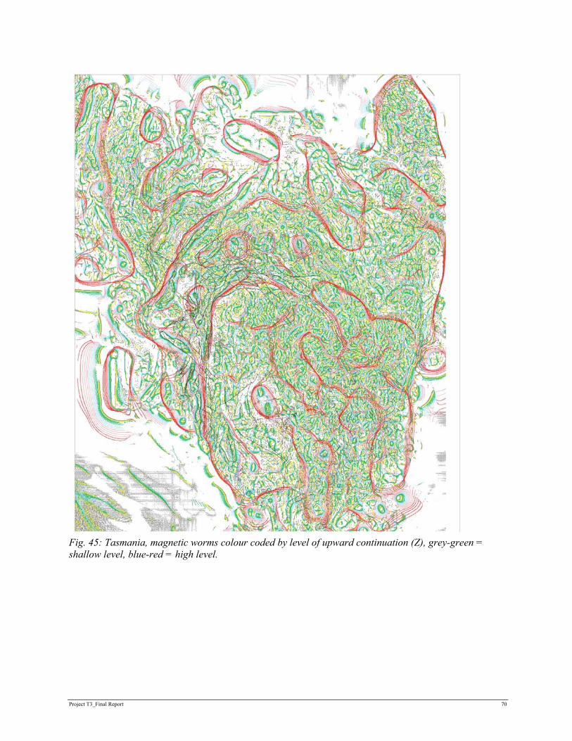
Project T3_Final Report 70
Fig. 45: Tasmania, magnetic worms colour coded by level of upward continuation (Z), grey-green = shallow level, blue-red = high level.
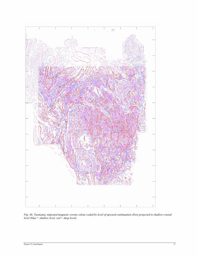
Project T3_Final Report 71
Fig. 46: Tasmania, migrated magnetic worms colour coded by level of upward continuation (Zwt) projected to shallow crustal level (blue = shallow level, red = deep level).

Project T3_Final Report 72
Fig. 47: Point-to-Vector processing for depth–weighted image processing
Fig. 48: Point-to-Vector processing for length–weighted image processing
a) Zwt_points
b) Vector Lines Depth Weighted
c) Depth Image
c) Length Image
a) Zwt_points b) Vector Lines Length Weighted
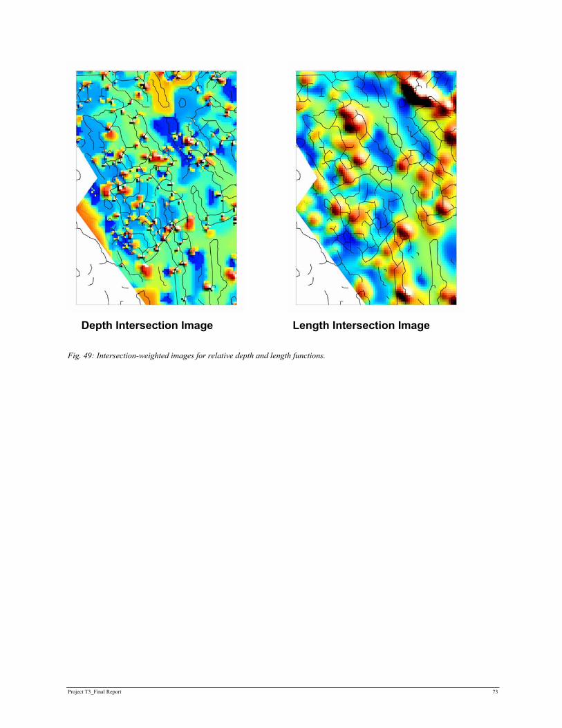
Project T3_Final Report 73
Fig. 49: Intersection-weighted images for relative depth and length functions.
Depth Intersection Image Length Intersection Image
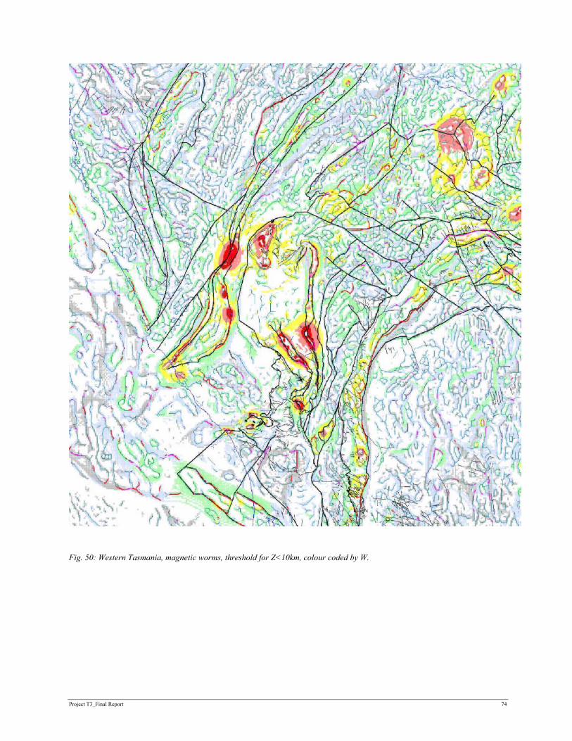
Project T3_Final Report 74
Fig. 50: Western Tasmania, magnetic worms, threshold for Z<10km, colour coded by W.

Project T3_Final Report 75
Appendix 2: Windowed Buffer Analysis of Major Deposit Types • Type 1: VHMS & Hybrid deposits • Type 2: Intrusion-related system • Type 3: Fe Replacement Systems • Type 4: Orogenic Gold • Type 6: Irish-type SHMS • Type 8: Neoproterozoic Au • Type 9: Hydrothermal Magnesite • Type 10: PGE's

Type 1 VHMS Deposits: Fault Length Analysis
0
0.05
0.1
0 2 4 6 8 10
Proximity Function
Mat
al A
rea
Func
tion
Rank*
Type 1 VHMS: Magnetic Worm Length
00.0050.01
0.0150.02
0.025
0 2 4 6 8
Proximity Function
Met
al A
rea
Func
tion
Rank*
Type 1 VHMS Deposits: Gravity Worm Length
00.005
0.010.015
0.02
0 2 4 6 8 10
Proximity Function
Met
al A
rea
Func
tion
Rank*
Type 1 VHMS Deposits: Gravity Worm Depth
00.0050.01
0.0150.02
0 2 4 6 8 10
Proximity Function
Met
al A
rea
Func
tion
Rank*
Type 1.1 VHMS: Magnetic Worm Depth
00.010.020.030.040.05
0 1 2 3 4 5 6
Proximity Function
Met
al A
rea
Func
tion
Rank
Type 1.2 VHMS: Magnetic Worm Depth
00.050.1
0.150.2
0 2 4 6 8 10 12
Proximity Function
Met
al A
rea
Func
tion
Rank*
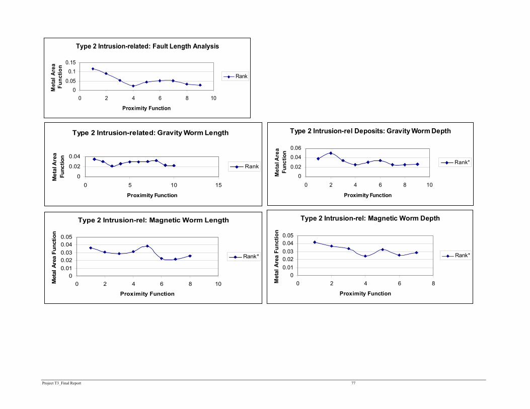
Project T3_Final Report 77
Type 2 Intrusion-related: Fault Length Analysis
00.05
0.10.15
0 2 4 6 8 10
Proximity Function
Met
al A
rea
Func
tion
Rank
Type 2 Intrusion-related: Gravity Worm Length
0
0.02
0.04
0 5 10 15
Proximity Function
Met
al A
rea
Func
tion
Rank
Type 2 Intrusion-rel Deposits: Gravity Worm Depth
0
0.02
0.04
0.06
0 2 4 6 8 10
Proximity Function
Met
al A
rea
Func
tion
Rank*
Type 2 Intrusion-rel: Magnetic Worm Length
00.010.020.030.040.05
0 2 4 6 8 10
Proximity Function
Met
al A
rea
Func
tion
Rank*
Type 2 Intrusion-rel: Magnetic Worm Depth
00.010.020.030.040.05
0 2 4 6 8
Proximity Function
Met
al A
rea
Func
tion
Rank*
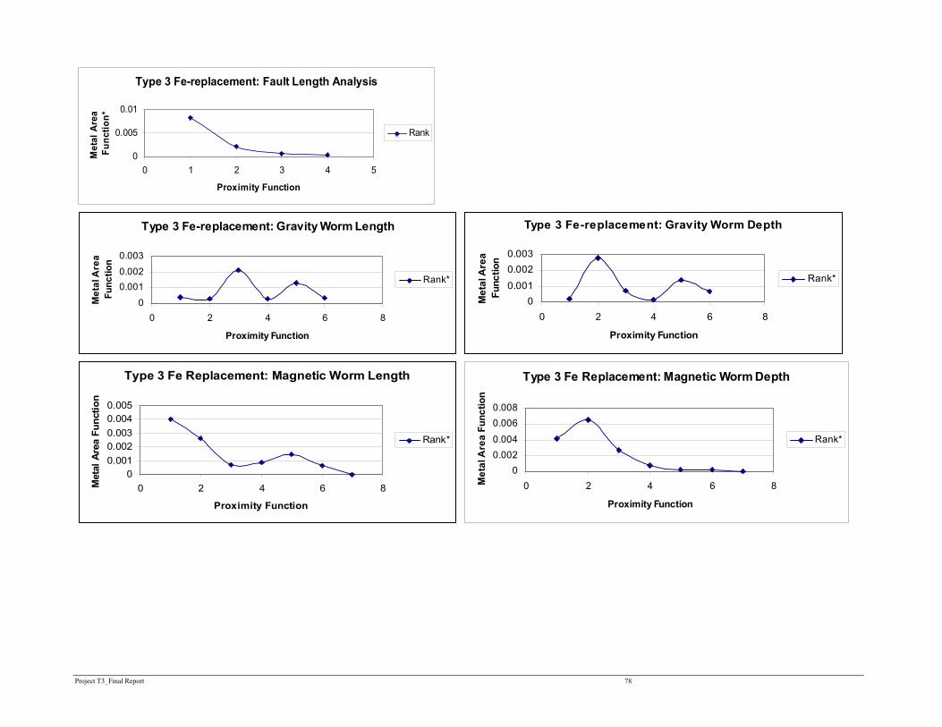
Project T3_Final Report 78
Type 3 Fe-replacement: Fault Length Analysis
0
0.005
0.01
0 1 2 3 4 5
Proximity Function
Met
al A
rea
Func
tion*
Rank
Type 3 Fe-replacement: Gravity Worm Length
00.0010.0020.003
0 2 4 6 8
Proximity Function
Met
al A
rea
Func
tion
Rank*
Type 3 Fe-replacement: Gravity Worm Depth
00.001
0.0020.003
0 2 4 6 8
Proximity Function
Met
al A
rea
Func
tion
Rank*
Type 3 Fe Replacement: Magnetic Worm Length
00.0010.0020.0030.0040.005
0 2 4 6 8
Proximity Function
Met
al A
rea
Func
tion
Rank*
Type 3 Fe Replacement: Magnetic Worm Depth
00.0020.0040.0060.008
0 2 4 6 8
Proximity Function
Met
al A
rea
Func
tion
Rank*

Project T3_Final Report 79
Type 4 Orogenic Gold: Fault Length Analysis
00.01
0.020.03
0 2 4 6 8 10
Proximity Function
Met
al A
rea
Func
tion*
Rank
Type 4 Orogenic Au: Gravity Worm Length
00.005
0.010.015
0.02
0 2 4 6 8 10
Proximity Function
Met
al A
rea
Func
tion
Rank*
Type 4 Orogenic Au: Gravity Worm Depth
00.0050.01
0.0150.02
0 2 4 6 8 10 12
Proximity Function
Met
al A
rea
Func
tion
Rank
Type 4 Orogenic Au: Magnetic Worm Length
0
0.01
0.02
0.03
0 2 4 6 8 10
Proximity Function
Met
al A
rea
Func
tion
Rank*
Type 4 Orogenic Au: Magnetic Worm Depth
0
0.005
0.01
0.015
0 2 4 6 8 10
Proximity Function
Met
al A
rea
Func
tion
Rank
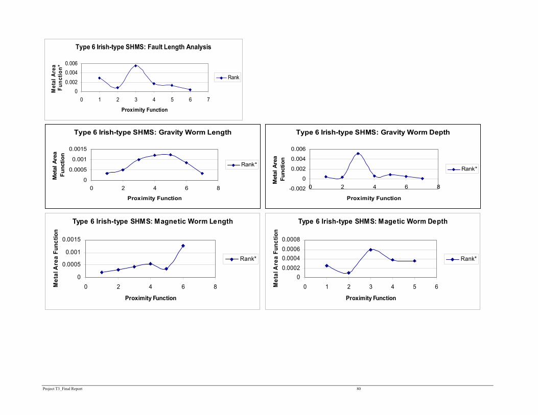
Project T3_Final Report 80
Type 6 Irish-type SHMS: Fault Length Analysis
00.002
0.0040.006
0 1 2 3 4 5 6 7
Proximity Function
Met
al A
rea
Func
tion*
Rank
Type 6 Irish-type SHMS: Gravity Worm Length
0
0.0005
0.001
0.0015
0 2 4 6 8
Proximity Function
Met
al A
rea
Func
tion
Rank*
Type 6 Irish-type SHMS: Gravity Worm Depth
-0.002
0
0.002
0.004
0.006
0 2 4 6 8
Proximity Function
Met
al A
rea
Func
tion
Rank*
Type 6 Irish-type SHMS: Magnetic Worm Length
0
0.0005
0.001
0.0015
0 2 4 6 8
Proximity Function
Met
al A
rea
Func
tion
Rank*
Type 6 Irish-type SHMS: Magetic Worm Depth
00.00020.00040.00060.0008
0 1 2 3 4 5 6
Proximity Function
Met
al A
rea
Func
tion
Rank*

Project T3_Final Report 81
Type 8 Neoproterozoic Au: Fault Length Analysis
00.0010.0020.0030.004
0 1 2 3 4 5 6
Proximity Function
Mea
tl Ar
ea
Func
tion
Rank
Type 8 Neoprot Au: Gravity Worm Length
0
0.0005
0.001
0 1 2 3 4 5 6
Proximity Function
Met
al A
rea
Func
tion
Rank*
Type 8 Neoprot Au: Gravity Worm Depth
00.00020.00040.00060.0008
0 2 4 6 8
Proximity Function
Met
al A
rea
Func
tion
Rank*
Type 8 Neoprot Au: Magetic Worm Length
-0.0010
0.0010.0020.0030.004
0 2 4 6 8
Proximity Function
Met
al A
rea
Func
tion
Rank*
Tyep 8 Neoprot Au: Magnetic Worm Depth
00.0010.0020.0030.004
0 2 4 6 8
Proximity FunctionM
etal
Are
a Fu
nctio
n
Rank*
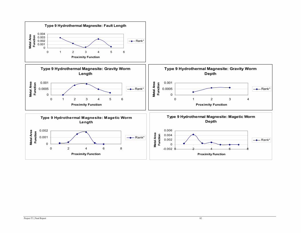
Project T3_Final Report 82
Type 9 Hydrothermal Magnesite: Fault Length
00.0010.0020.0030.004
0 1 2 3 4 5 6
Proximity Function
Met
al A
rea
Func
tion
Rank*
Type 9 Hydrothermal Magnesite: Gravity Worm
Length
0
0.0005
0.001
0 1 2 3 4 5 6
Proximity Function
Met
al A
rea
Func
tion
Rank*
Type 9 Hydrothermal Magnesite: Gravity Worm Depth
0
0.0005
0.001
0 1 2 3 4
Proximity Function
Met
al A
rea
Func
tion
Rank*
Type 9 Hydrothermal Magnesite: Magetic Worm Length
0
0.001
0.002
0 2 4 6 8
Proximity Function
Met
al A
rea
Func
tion
Rank*
Type 9 Hydrothermal Magnesite: Magetic Worm Depth
-0.0020
0.0020.004
0.006
0 2 4 6 8
Proximity FunctionM
etal
Are
a Fu
nctio
n
Rank*

Project T3_Final Report 83
Type 10 PGE Deposits: Fault Length Analysis
00.002
0.0040.006
0 2 4 6 8
Proximity Function
Met
al A
rea
Func
tion
Rank*
Type 10 PGE's: Gravity Worm Length
00.00050.001
0.00150.002
0 2 4 6 8
Proximity Function
Met
al A
rea
Func
tion
Rank*
Type 10 PGE's: Gravity Worm Depth
0
0.002
0.004
0.006
0 2 4 6 8 10
Proximity Function
Met
al A
rea
Func
tion
Rank*
Type 10 PGE's: Magnetic Worm Length
0
0.001
0.002
0.003
0 2 4 6 8
Proximity Function
Met
al A
rea
Func
tion
Rank*
Type 10 PGE's: Magnetic Worm Depth
00.0020.004
0.0060.008
0 2 4 6 8 10
Proximity FunctionM
etal
Are
a Fu
nctio
n
Rank