Tax management strategies with multiple risky assets

ARTICLE IN PRESS

Journal of Financial Economics 80 (2006) 243–291

0304-405X/$

doi:10.1016/j

$We wou

J. Spencer M

University of

Mexico, the 2

and the 200

concerning th

Sergey Kolo

Computing C�CorrespoE-mail ad

www.elsevier.com/locate/jfec

Tax management strategies with multiplerisky assets$

Michael F. Gallmeyera,�, Ron Kanielb, Stathis Tompaidisc

aMays Business School, Texas A&M University, College Station, TX 77843, USAbFuqua School of Business, Duke University, Durham, NC 27708, USA

cMcCombs School of Business, University of Texas at Austin, Austin, TX 78712, USA

Received 13 March 2002; received in revised form 27 July 2004; accepted 2 August 2004

Available online 2 November 2005

Abstract

We study the consumption-portfolio problem in a setting with capital gain taxes and

multiple risky stocks to understand how short selling influences portfolio choice with a

shorting-the-box restriction. Our analysis uncovers a novel trading flexibility strategy whereby,

to minimize future tax-induced trading costs, the investor optimally shorts one of the stocks

(or equivalently, buys put options) even when no stock has an embedded gain. Alternatively,

an imperfect form of shorting the box can reduce aggregate equity exposure ex post. Given

these two short selling strategies, it is common for an unconstrained investor to short some

- see front matter r 2005 Published by Elsevier B.V.

.jfineco.2004.08.010

ld like to thank Lorenzo Garlappi, Bruce Grundy, Campbell Harvey, Burton Hollifield,

artin, an anonymous referee, and seminar participants at the University of Florida, the

South Carolina, the University of Texas at Austin, the Instituto Tecnologico Autonomo de

002 Bachelier World Congress meeting, the 2002 SIRIF Strategic Asset Allocation meeting,

2 European Finance Association meeting for comments; Eric Bradley for conversations

e U.S. tax code; Patrick Jaillet for assisting us with obtaining computing resources; and

s for programming assistance. We would also would like to thank the Texas Advanced

enter for providing computing resources. The usual disclaimer applies.

nding author. Fax: +1412 268 6837.

dress: [email protected] (M.F. Gallmeyer).

www.elsevier.com/locate/jfec

ARTICLE IN PRESS

M.F. Gallmeyer et al. / Journal of Financial Economics 80 (2006) 243–291244

equity while a constrained investor holds a positive investment in all stocks. With no shorting,

the benefit of trading separately in multiple stocks is not economically significant.

r 2005 Published by Elsevier B.V.

JEL classification: G11; H20

Keywords: Portfolio choice; Capital gain taxation; Short selling

1. Introduction

When investors are faced with asset allocation and consumption decisions, capitalgain taxation plays an important role in the investor’s optimal strategy. In hisseminal work valuing the tax loss selling option from capital gain taxation,Constantinides (1983) shows that an investor’s portfolio choice problem is integrallylinked to realized capital gain taxation. With the only friction being taxation, theinvestor optimally defers all gains and immediately realizes all losses withoutinfluencing his optimal consumption strategy. This separation result is achieved bythe investor rebalancing his portfolio without triggering a tax liability by engaging ina shorting-the-box strategy: if an investor is overexposed to a stock with a largeembedded capital gain, he shorts that security instead of selling it so that his netposition in the stock is optimal. By shorting, the investor has rebalanced anddeferred realizing any taxable capital gains since none of the original position wassold. Before the 1997 Tax Reform Act, shorting the box was not viewed as a taxtriggering transaction. Besides the collateral costs of shorting, the investor couldeffectively shield all gains from capital gain taxation over his lifetime given the U.S.tax code provision of resetting the tax basis of all securities to market prices at thetime of death.

However, given that the shorting-the-box strategy for identical securitiesis no longer permitted under U.S. tax laws and that short selling is costly, investorsdo realize gains. For recent empirical evidence, see the references in Poterba(2001) as well as Auerbach and Siegel (2000). The work of Dammon et al. (2001b)uses this evidence as one motivation for studying capital gain tax portfolio-consumption problems where the separation result fails. They study a short-sale-constrained investor’s consumption-portfolio problem with a single stock.Since the investor cannot trade without tax liabilities, the optimal policy isinfluenced by the current portfolio composition. They find results similar toportfolio problems with transaction costs—the optimal mix between the stockand a riskless money market account can deviate from the optimal policy withno capital gain tax due to the tax-induced costs of trading. A limitation of theirwork is their assumption of one risky stock. As a result, they are unable toanalyze how the composition of a portfolio with multiple risky stocks is affectedby realized capital gain taxation. With the introduction of taxes, risk-based motivesfor portfolio rebalancing now interact with motives for reducing realized capitalgains.

ARTICLE IN PRESS

M.F. Gallmeyer et al. / Journal of Financial Economics 80 (2006) 243–291 245

In this paper, we study the role of realized capital gain taxation on an investor’sconsumption-portfolio problem with two risky stocks and a riskless money marketaccount where costly shorting is allowed under a no shorting-the-box constraint. Ourtwo-stock setting allows us to qualitatively analyze the tradeoff between diversifica-tion and minimizing tax liabilities, where we consider both diversification betweenthe riskless money market account and stocks and diversification within the equityportion of the portfolio. The choice of two stocks is for tractability. However, themain features of our results should extend to portfolio choice with additional stocks.The setting we have in mind is one where an investor considers moving frominvesting in a single index fund and a money market account to a portfolio of twoindex funds and a money market account. Current investment vehicles make thistransition particularly easy with the introduction of several exchange-traded funds(ETFs) in recent years like the SPDR and the DIAMONDS contract.1

As a baseline in our analysis, we start by studying optimal portfolio choice with ashort sale constraint. Our results show that for stocks that are not highly correlatedðr ¼ 0:4Þ, the asset allocation in one stock is largely unaffected by the embeddedcapital gain in the other stock. As in the single-stock case, the basis reset provision atthe investor’s death leads to holding more equity as the investor ages. However, ifembedded gains are large enough, the investor holds an undiversified equityportfolio. When the stock return correlation rises to a level commonly observedbetween U.S. large-capitalization ETFs (r ¼ 0:8 and above), the optimal portfoliopolicy is different since tax considerations now outweigh diversification costs. Theportfolio allocation for one stock is not just driven by its own basis and position, butby the basis and position of the other stock. If initially overinvested in equity, theinvestor sells the stock with the lowest tax cost. If short sale constrained, the investormight entirely liquidate his position in one stock. This behavior leads to the investorholding a less diversified equity position than before.

Allowing the investor to short sell while still imposing a shorting-the-boxconstraint dramatically changes behavior. When the cost of shorting is not too largeand the return correlation between the two stocks is high enough, the investoremploys two tax management trading strategies that utilize short selling. The firststrategy, new in our analysis, is an ex ante way of minimizing future tax-inducedtrading costs by shorting one of the stocks even when the stock portfolio contains noembedded capital gains. This trade, termed the trading flexibility strategy, is usedwhen the benefit of holding a well-diversified stock portfolio is outweighed by theexpected future rebalancing costs of such a position. From our parameterizations,the trading flexibility strategy is employed when the return correlation between thetwo stocks is greater than or equal to r ¼ 0:65. The second strategy, present whenthe correlation between the two stocks is as low as r ¼ 0:4, is an imperfect form of

shorting the box used to reduce ex post the investor’s total equity exposure byshorting the stock with the largest tax basis. Given that the two stocks are not

1Interestingly, many ETFs pass on lower taxable unrealized capital gains to investors than mutual

funds. This is due to active creations and destructions of ETFs (Poterba and Shoven, 2002). Also, ETFs

are marginable and most can be shorted without being subject to the uptick rule.

ARTICLE IN PRESS


perfectly correlated, such a trade entails fundamental risk and is permitted undercurrent U.S. tax laws. From these two incentives to short, the optimal equityportfolio is significantly different from both the no-tax well-diversified allocationand the allocation when short selling is disallowed. In particular, a short-sellinginvestor is better able to manage his total equity exposure over his lifetime ascompared to a short-sale-constrained investor.

The ability to short sell introduces another interesting feature to the tradingstrategy relative to the case of no short sales. Given that the net tax benefit of sellingshares is not monotonic in the trading strategy when shorting is allowed, we showthat it is common for an unconstrained investor to short equity while an otherwiseidentical constrained investor holds strictly positive positions in all stocks. Thisfeature is especially common when the portfolio contains no embedded capital gains,but occurs even when the portfolio’s stock positions contain capital gains.

Whether the portfolio strategies identified in our analysis should be used asnormative advice to investors depends on two important factors. The first factor isthe magnitude of the welfare improvement that can be obtained by following suchstrategies. Somewhat surprisingly, we find that when short sales are prohibited, thewelfare benefit of using the optimal strategy is negligible relative to the case in whichthe investor invests in a single index fund and a money market account. On the otherhand, with short selling the benefit can be significant. The second factor is theinvestor’s type. We show that use of the trading flexibility and the imperfectshorting-the-box strategies can be beneficial to wealthy investors, but not to the samedegree for small investors who pay higher shorting costs.

As an alternative to shorting, we also consider how derivative securities can beused by an investor to manage tax trading costs when rebalancing. Constantinidesand Scholes (1980) discuss a similar trading strategy without exploring its feasibility.The introduction of derivatives in the opportunity set restores a small investor’sflexibility to defer capital gains while keeping the equity exposure of the optimalportfolio closer to the no-tax benchmark. In particular, we consider a strategy inwhich the investor, in addition to trading a single risky stock, is able to trade a putoption written on a highly correlated stock. This strategy is available to both smalland large investors and is an implicit use of the trading flexibility strategy. We showthat the welfare benefit of using puts is similar in magnitude to that of using low-costshort selling.

Two recent papers developed at the same time as this work, Dammon et al.(2001a) and Garlappi et al. (2001), have also numerically analyzed some aspects ofthe capital gain tax investment problem with multiple stocks. The focus of each ofthese papers is quite different in that neither studies the role of shorting in portfoliochoice or the welfare benefits of investing in two stocks relative to one. Thenumerical analysis in Dammon et al. (2001a) focuses on demonstrating that thediversification benefit of reducing the exposure to a highly volatile concentratedposition can significantly outweigh the tax cost of selling. The paper of Garlappiet al. (2001) mostly analyzes features of the ‘‘no trade region’’ in the presence ofcapital gain taxes when an investor maximizes the expected utility of terminal wealthover ten periods with tax forgiveness at the terminal date.

ARTICLE IN PRESS


Our work is also related to several earlier papers characterizing portfolio choicewith capital gain taxes or transaction costs. Building from Constantinides (1983), thepricing implications of optimal after-tax portfolios with shorting-the-box trades isstudied in Constantinides (1984). Our analysis considers the case in which shorting-the-box trades are prohibited. Dybvig and Koo (1996) is one of the earliestnumerical studies of after-tax portfolio choice in a single stock and bond setting withno short sales. Due to computational difficulties, they only study the portfolioproblem for a limited number of time periods, in contrast to the lifetime portfolioproblem considered here. Using the single stock and bond framework of Dammonet al. (2001b), Huang (2001) and Dammon et al. (2004) study the asset locationdecision when taxable and tax-deferred accounts are available to investors. Byretaining the single-stock assumption, these studies face a less complex numericalcharacterization than the multiple-stock case. Other early works on after-taxportfolio choice but in a single-period setting are Elton and Gruber (1978) andBalcer and Judd (1987). For exact solutions to capital gain tax portfolio problemsunder restrictive conditions, see Cadenillas and Pliska (1999) and Jouini et al. (2000).Using results from the literature on portfolio problems with transaction costs,2

Leland (2001) numerically characterizes a portfolio allocation problem for a stockand a bond with capital gain taxes when the objective is to minimize the deviationfrom exogenous portfolio weights subject to capital gain taxes and transaction costs.Finally, the numerical study of our capital gain tax problem is related to numericalcharacterizations of portfolio problems with transaction costs (Balduzzi and Lynch,1999, 2000).

The remainder of the paper is organized as follows. Section 2 formulates theconsumption-portfolio problem. Sections 3 and 4 present our numerical analysiswhere we characterize the trading strategies and provide comparative statics as wellas a welfare analysis. An alternative trading strategy using derivative securities isdiscussed in Section 5. Section 6 concludes. Appendix A gives a formal mathematicaldefinition of the problem studied in Sections 3 and 4. Appendix B modifies theportfolio problem to incorporate investment in a put option as discussed in Section5. Appendix C discusses the numerical procedure.

2. The consumption-portfolio problem with taxes

We consider a discrete-time economy with trading dates t ¼ 0; . . . ;T in which aninvestor chooses an optimal consumption and investment policy in the presence ofrealized capital gain taxation. Our framework is an extension of the single risky assetmodel of Dammon et al. (2001b) modified to incorporate multiple risky assets andshort sales with margin requirements and shorting collateral costs. Thesemodifications greatly expand the opportunity set of the investor as compared to asetting with no short sales as will be described in Sections 3 and 4, where we provide

2See, for example, Constantinides (1986), Davis and Norman (1990), Davis et al. (1993), Shreve and

Soner (1994), and Akian et al. (1996).

ARTICLE IN PRESS


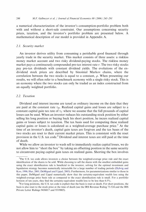
a numerical characterization of the investor’s consumption-portfolio problem bothwith and without a short-sale constraint. Our assumptions concerning securityprices, taxation, and the investor’s portfolio problem are presented below. Amathematical description of our model is provided in Appendix A.

2.1. Security market

An investor derives utility from consuming a perishable good financed throughyearly trade in the security market. This market consists of three assets: a risklessmoney market account and two risky dividend-paying stocks. The riskless moneymarket pays a continuously compounded pre-tax interest rate r. The two risky stockspay pre-tax dividends with constant dividend yields. The evolutions of the ex-dividend stock prices are described by binomial Markov chains, where thecorrelation between the two stocks is equal to a constant, r. When presenting ourresults, we will often refer to a benchmark economy with a single risky stock. This isan economy where the two stocks can only be traded as an index constructed froman equally weighted portfolio.

2.2. Taxation

Dividend and interest income are taxed as ordinary income on the date that theyare paid at the constant rate tD. Realized capital gains and losses are subject to aconstant capital gain tax rate of tC where we assume that the full proceeds of capitallosses can be used. When an investor reduces his outstanding stock position by eitherselling his long position or buying back his short position, he incurs realized capitalgains or losses subject to taxation. The tax basis used for computing these realizedcapital gains or losses is calculated as a weighted-average purchase price.3 At thetime of an investor’s death, capital gain taxes are forgiven and the tax bases of thetwo stocks are reset to their current market prices. This is consistent with the resetprovision in the U.S. tax code.4 Dividend and interest taxes are still paid at the timeof death.

While we allow an investor to wash sell to immediately realize capital losses, we donot allow him to ‘‘short the box’’ by taking an offsetting position in the same securityto circumvent paying capital gain taxes on realized gains. Shorting the box involves

3The U.S. tax code allows investors a choice between the weighted-average price rule and the exact

identification of the shares to be sold. While choosing to sell the shares with the smallest embedded gains

using the exact identification rule is beneficial to the investor, solving for the optimal investment and

liquidation strategy becomes numerically intractable for a large number of trading periods (Dybvig and

Koo, 1996; Hur, 2001; DeMiguel and Uppal, 2003). Furthermore, for parameterizations similar to those in

this paper, DeMiguel and Uppal numerically show that the certainty-equivalent wealth loss using the

weighted-average price basis rule as compared to the exact identification rule is small. For a portfolio

horizon of ten years, they find the certainty-equivalent wealth loss to be less than 0.5%.4For long positions, the U.S. tax code is explicit that the basis is reset at death. For short positions, the

basis is also reset to the stock price at the time of death (see the IRS Revenue Ruling 73-524 and the IRS

Private Letter Rulings 9436017 and 9319005).

ARTICLE IN PRESS


realizing a gain without tax consequences. Suppose an investor is currently longequity with a large embedded gain. Instead of selling this position, the investor couldtake an offsetting short position in the same security. He has now effectively sold hislong position with no tax consequences. The 1997 Taxpayer Relief Act reclassifiedsuch a trade as a sale of the original position and thus subject to capital gaintreatment.5

To accommodate short sales with a shorting-the-box restriction, the evolution ofthe tax basis for each stock includes a variety of cases. At each trading date, the taxbasis for each stock position either evolves as a share-weighted average of the currentstock price and the previous basis when increasing the absolute size of a stock’sposition, resets to the current stock price, or remains unchanged. The basis resets tothe current stock price under two different scenarios: when an investor incurs acapital loss on his position, or when the investor’s position changes sign from timet� 1 to time t. If a position in the investor’s portfolio incurs a capital loss, it isoptimally liquidated to realize the loss given that wash sales are allowed. We assumethat the full amount of this loss can be used immediately.6 A transaction where theinvestor’s position changes sign from time t� 1 to t is treated as a closing of the t� 1position, since shorting the box is prohibited. Any gains or losses on this position aretaxed at the capital gain rate. A stock’s tax basis remains unchanged either when theinvestor does not trade in the stock or when the investor reduces but does not fullyliquidate the absolute size of his stock holdings.

2.3. Investor problem

In order to finance consumption, an investor dynamically trades in the two riskystocks and a riskless money market account. Short sales of equity are allowed subjectto collateral and margin requirements. The collateral and margin constraints lead to aconstraint on the minimum amount invested in the money market account. Investorsmust also pay lending fees when shorting stocks. These fees are incorporated byreducing the rate of return received on the short-sale collateral as compared to moneyinvested in the money market account. While small investors typically receive nointerest on short-sale proceeds, large investors face much smaller fees. The size ofthese fees is discussed later when specific parameter values are presented.

Given an initial equity endowment, a consumption and security trading policy isan admissible trading strategy if it satisfies the collateral and margin requirements, issubject to lending fees, is self-financing, and leads to nonnegative wealth over the

5Strictly speaking, the 1997 Taxpayer Relief Act did not completely rule out shorting the box for

deferring gains, but it seriously limited its effectiveness. Under the Act, shorting the box is still allowed to

defer gains for one year but you must close your short position within 30 days after the end of the year,

and then you must stay long in the stock unhedged for 60 days before closing your long position. To

simplify our analysis, we assume that shorting the box is prohibited.6Under the current U.S. tax code, realized losses can only offset up to $3; 000 of ordinary income, but

can be carried forward indefinitely. Relaxing our full loss usage assumption would add one state variable

to the formulation, significantly increasing the complexity of the problem. For an analysis of the role of

capital losses with no after-tax arbitrage, see Gallmeyer and Srivastava (2003).

ARTICLE IN PRESS


lifetime of the investor. The investor is assumed to live at most T periods and faces apositive probability of death each period. The probability that an investor lives up toperiod toT is given by a survival function, calibrated to the 1990 U.S. Life Table,compiled by the National Center for Health Statistics where we assume period t ¼ 0corresponds to age 20 and period T ¼ 80 corresponds to age 100. At period T ¼ 80,the investor exits the economy with certainty.

The investor’s objective is to maximize his discounted expected utility of reallifetime consumption and a time of death bequest motive by choosing an admissibleconsumption-trading strategy given an initial endowment. For tractability and easeof comparison with no tax portfolio problems, the utility function for consumptionand wealth is of the constant relative risk aversion form with a coefficient of relativerisk aversion of g. Using the principle of dynamic programming, the Bellmanequation for the investor’s optimization problem, derived in Appendix A, can besolved numerically by backward induction starting at time T. Details of thecomputational complexity of this problem are outlined in Appendix C.

2.4. Scenarios considered with parameter values

To understand how an expanded opportunity set due to shorting can influence theallocation decision and welfare of an investor, we focus on several cases where aninvestor has different investment opportunities and faces different tax trading costs.While a variety of different investor scenarios could be studied in the context ofportfolio choice with multiple risky assets, we focus on an index investor whoconsiders moving from investing in a single index fund and a money market accountto a portfolio of two funds that compose the index and the money market account.Our benchmark is the case when the investor trades a money market and a singlerisky index fund with realized capital gain taxation. (When the investor is not subjectto capital gain taxation, a mutual fund theorem results irrespective of the number ofrisky assets; he only trades in an appropriately weighted index fund of the two stocksand the money market.) We compare this benchmark to an investor who has accessto two identical risky stocks that are subject to capital gain taxes. We considerinvestors who are restricted from shorting equity, as well as investors who can shortsubject to margin constraints and collateral costs.

Given that the main emphasis of our work is to understand the quantitativefeatures of portfolio choice with taxes and short sales, especially the use of theflexibility and the imperfect shorting-the-box strategies, our index fund setting ischosen given the large number of exchange-traded funds (ETFs) that are nowavailable for investing in broad-based market indices. Currently, roughly 40 differentETFs trade on the American Stock Exchange that are pegged to marketwide indices.All of these ETFs are marginable and can be shorted, while only a handful of themare subject to the ‘‘uptick rule.’’ (Rule 10a-1 of the Securities Exchange Act of 1934,more commonly known as the ‘‘uptick’’ rule, precludes short selling when securityprices are falling.) Additionally, the market for shorting ETFs is very active. Forexample, the NASDAQ 100 tracking stock, QQQ, had an average open interest of27% of shares outstanding and an average days to cover of 2.60 over the year 2002.

ARTICLE IN PRESS


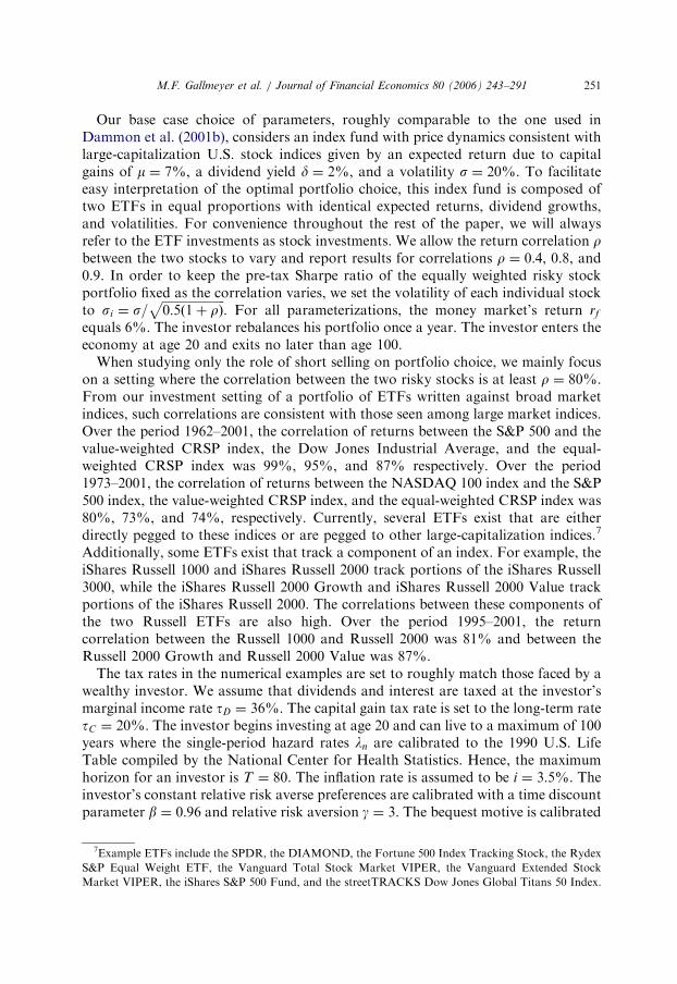
Our base case choice of parameters, roughly comparable to the one used inDammon et al. (2001b), considers an index fund with price dynamics consistent withlarge-capitalization U.S. stock indices given by an expected return due to capitalgains of m ¼ 7%, a dividend yield d ¼ 2%, and a volatility s ¼ 20%. To facilitateeasy interpretation of the optimal portfolio choice, this index fund is composed oftwo ETFs in equal proportions with identical expected returns, dividend growths,and volatilities. For convenience throughout the rest of the paper, we will alwaysrefer to the ETF investments as stock investments. We allow the return correlation rbetween the two stocks to vary and report results for correlations r ¼ 0:4, 0.8, and0.9. In order to keep the pre-tax Sharpe ratio of the equally weighted risky stockportfolio fixed as the correlation varies, we set the volatility of each individual stockto si ¼ s=

ffiffiffiffiffiffiffiffiffiffiffiffiffiffiffiffiffiffiffiffiffi0:5ð1þ rÞ

p. For all parameterizations, the money market’s return rf

equals 6%. The investor rebalances his portfolio once a year. The investor enters theeconomy at age 20 and exits no later than age 100.

When studying only the role of short selling on portfolio choice, we mainly focuson a setting where the correlation between the two risky stocks is at least r ¼ 80%.From our investment setting of a portfolio of ETFs written against broad marketindices, such correlations are consistent with those seen among large market indices.Over the period 1962–2001, the correlation of returns between the S&P 500 and thevalue-weighted CRSP index, the Dow Jones Industrial Average, and the equal-weighted CRSP index was 99%, 95%, and 87% respectively. Over the period1973–2001, the correlation of returns between the NASDAQ 100 index and the S&P500 index, the value-weighted CRSP index, and the equal-weighted CRSP index was80%, 73%, and 74%, respectively. Currently, several ETFs exist that are eitherdirectly pegged to these indices or are pegged to other large-capitalization indices.7

Additionally, some ETFs exist that track a component of an index. For example, theiShares Russell 1000 and iShares Russell 2000 track portions of the iShares Russell3000, while the iShares Russell 2000 Growth and iShares Russell 2000 Value trackportions of the iShares Russell 2000. The correlations between these components ofthe two Russell ETFs are also high. Over the period 1995–2001, the returncorrelation between the Russell 1000 and Russell 2000 was 81% and between theRussell 2000 Growth and Russell 2000 Value was 87%.

The tax rates in the numerical examples are set to roughly match those faced by awealthy investor. We assume that dividends and interest are taxed at the investor’smarginal income rate tD ¼ 36%. The capital gain tax rate is set to the long-term ratetC ¼ 20%. The investor begins investing at age 20 and can live to a maximum of 100years where the single-period hazard rates ln are calibrated to the 1990 U.S. LifeTable compiled by the National Center for Health Statistics. Hence, the maximumhorizon for an investor is T ¼ 80. The inflation rate is assumed to be i ¼ 3:5%. Theinvestor’s constant relative risk averse preferences are calibrated with a time discountparameter b ¼ 0:96 and relative risk aversion g ¼ 3. The bequest motive is calibrated

7Example ETFs include the SPDR, the DIAMOND, the Fortune 500 Index Tracking Stock, the Rydex

S&P Equal Weight ETF, the Vanguard Total Stock Market VIPER, the Vanguard Extended Stock

Market VIPER, the iShares S&P 500 Fund, and the streetTRACKS Dow Jones Global Titans 50 Index.

ARTICLE IN PRESS


such that the investor plans to provide a perpetual real income stream to his heirs.This parameterization is consistent with the one used in Dammon et al. (2001b).

To short stock, U.S. investors must trade in a margin account and are required todeposit and maintain a minimum amount of cash or securities with their broker. TheFederal Reserve Board’s Regulation T sets the initial margin requirement for stockpositions undertaken through brokers. The initial margin requirement is currently50% for a long equity position and 150% for a short equity position. For a longposition, the investor cannot borrow more than 50% of the market value of thestock. For a short position, 102% of the short sale proceeds must typically be held incash as noted by Geczy et al. (2002) and Duffie et al. (2002). The remaining 48%needed to cover the margin requirement can be held in other securities such as U.S.Treasury Bills.8 Small retail investors do not typically receive any interest on the cashcollateral although large investors do. From data in Geczy et al., the rate of interestreceived on collateral, or the general collateral rate, is on average eight basis pointsbelow the federal funds effective rate, while for medium-size loans the generalcollateral rate is on average 15 basis points below the federal funds rate.

For our analysis, we consider conservative estimates for these lending rates wherewe assume that a large investor receives interest on his collateral at a rate of 30 basispoints below the riskless money market rate. We frequently refer to the lending ratein terms of a shorting cost defined as the difference between the riskless moneymarket rate and the general collateral rate. For tractability, we make no distinctionbetween initial and maintenance margin collateral and assume that whenrebalancing, the investor’s portfolio must conform with Regulation T initial marginrequirements.

3. Structure of optimal portfolios

We begin our numerical analysis by studying the structure of optimal portfolios.Specifically, our goal is to numerically characterize how and when investor behaviorchanges by expanding the investment opportunity set to include costly short sellingwhere the flexibility and imperfect shorting-the-box strategies can be employed.

3.1. Single stock benchmark

To facilitate comparison with the two-stock setting, we first briefly analyzeportfolio choice when the investor’s only risky asset is a single index fund. Fig. 1outlines the characteristics of this case both with and without realized capital gaintaxation. Using the parameterization outlined above when the index volatility iss ¼ 20%, the optimal equity allocation for an investor who faces no capital gaintaxation but pays interest and dividend taxes is summarized by the solid line with

8For margin requirement institutional details, see Fortune, 2000 as well as the Federal Reserve Board’s

Regulation T available at http://www.gpoaccess.gov/cfr/index.html by searching the Code of Federal

Regulations for 12CFR220.1.

http://www.gpoaccess.gov/cfr/index.html

ARTICLE IN PRESS

0.16

0.18

0.2

0.22

0.24

0.26

0.28

0.3

20 30 40 50 60 70 80 90

Equ

ity/W

ealth

Age

One stock, optimal asset allocation with and without capital gains taxes

No capital gains taxInitial basis 100%

Initial basis 75%Initial basis 50%

One asset, Volatility 20%, Age 20

0.1 0.2 0.3 0.4

0.5 0.6 0.7

0.8 0.9

Initial Asset Allocation

0.2 0.4

0.6 0.8

1 Basis

0.1 0.2 0.3 0.4 0.5 0.6

Opt

imal

Ass

et A

lloca

tion

One asset, Volatility 20%, Age 80

0.1 0.2

0.3 0.4

0.5 0.6

0.7 0.8

0.9

Initial Asset Allocation

0 0.2

0.4 0.6

0.8 1 Basis

0.1 0.2 0.3 0.4 0.5 0.6

Opt

imal

Ass

et A

lloca

tion

0

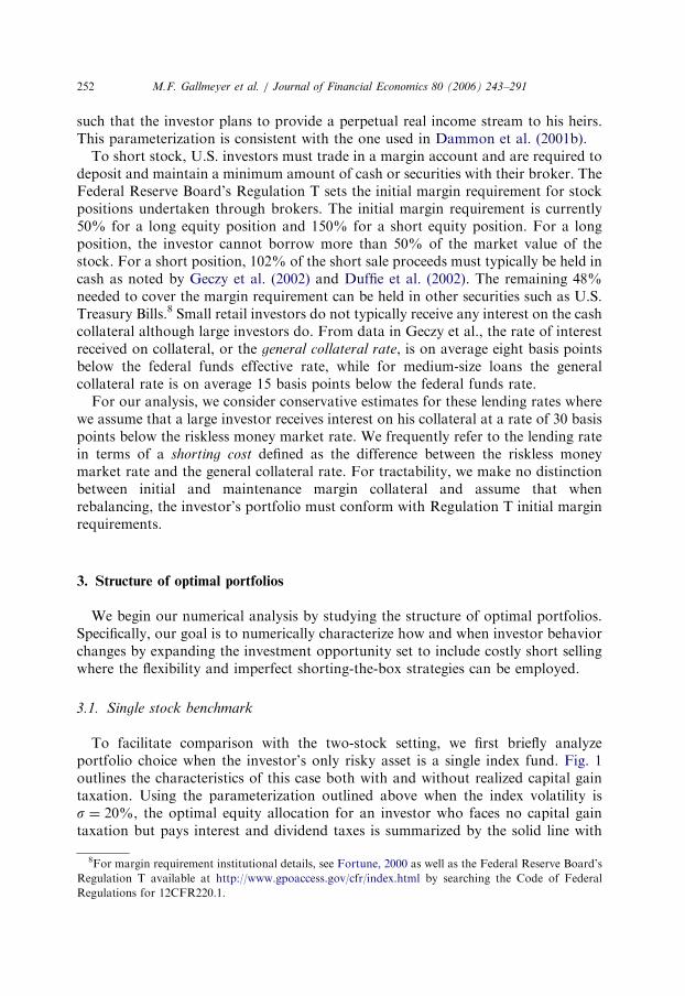
Fig. 1. Benchmark portfolio choice with a single index fund. The top panel of the figure summarizes the

equity to wealth ratio as a function of age. The line labeled ‘‘No capital gain tax’’ presents the optimal

equity allocation when the investor faces no capital gain tax (tD ¼ 36%, tC ¼ 0%, s ¼ 20%). The other

three lines present the optimal equity allocation when the investor enters age t with 30% of his wealth

invested in equity and faces realized capital gain taxation (tC ¼ 20%). The three lines plot different basis-

price ratios (50%, 75%, and 100%) entering the trading period. The bottom panels of the figure

summarize portfolio choice when the investor faces capital gain taxation on one risky stock. The left

(right) panel presents the equity-to-wealth ratio as a function of the stock allocation and the basis-price

ratio entering the trading period at age 20 (80). Parameters used for the bottom panels: tD ¼ 36%,

tC ¼ 20%, s ¼ 20%.


cross marks in the top panel of Fig. 1. Under this benchmark, the equity-to-wealthratio is constant at 20% since the opportunity set with no capital gain tax is constantthrough time.

The bottom panels of Fig. 1 document optimal portfolio choice with realizedcapital gain taxation at ages 20 and 80. This is the setting studied by Dammon et al.(2001b). In this case, the investor’s optimal equity exposure is a function of thebeginning-period allocation and the basis-price ratio. When the marginal tax costs oftrading are high due to a large embedded capital gain (a low basis-price ratio), theinvestor optimally holds more equity. This behavior occurs at a smaller embeddedgain as the investor ages, since it is driven by the basis reset provision at death. The

ARTICLE IN PRESS


top panel of Fig. 1 demonstrates this age effect of embedded capital gains on equitychoice conditional on three different basis-price ratios and a stock allocationentering age t of 30%. When the embedded gain in the stock portfolio is high (a 50%basis-price ratio), an age 20 investor reduces his equity exposure to 26.5% of wealthwhile an age 80 investor fully retains his 30% equity position. As the embedded gainin the stock position falls, the investor optimally liquidates more stock but less whenolder. This is captured in the basis-price ratio cases of 75% and 100% plotted inFig. 1. Relative to the setting with no capital gain tax, the investor can besignificantly overexposed to equity when older with a large embedded gain.

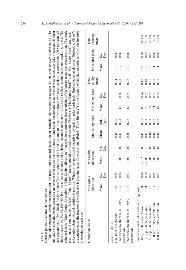
While examining optimal portfolio choice at a particular time and state is useful inunderstanding the conditional asset trading behavior of an investor, it provides onlylimited information about portfolio composition over the investor’s lifetime. To gaininsights about the unconditional optimal portfolio choice, we perform Monte Carlosimulations starting with no embedded stock gains at age 20 to track the evolution ofthe investor’s optimal portfolio at ages 40, 60, and 80 conditional on the investor’ssurvival. These results are reported in the lines labeled ‘‘One Stock Benchmark’’ inPanels A through C of Table 1. The columns labeled ‘‘Max Equity Allocation’’ and‘‘Max Equity Basis’’ present the mean and standard deviation of equity exposureand the basis-price ratio, respectively. The equity exposure is expressed as a fractionof total financial wealth. The column ‘‘Embedded Gains’’ measures the fraction offinancial wealth that is an unrealized capital gain. All simulations are over 50,000paths. The standard error for each mean estimate can be computed by dividing theMonte Carlo standard deviation by

ffiffiffiffiffiffiffiffiffiffiffiffiffiffi50; 000p

¼ 223:6. Given the largest standarddeviation in the table is 0:28, the largest standard error for the mean estimate of anyquantity in the table is 0.00125.

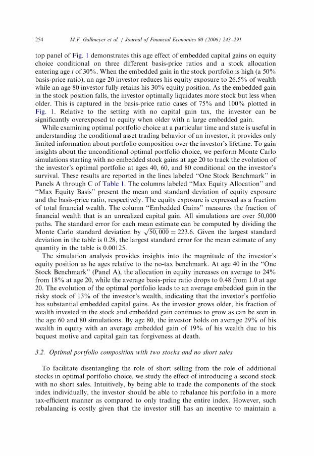
The simulation analysis provides insights into the magnitude of the investor’sequity position as he ages relative to the no-tax benchmark. At age 40 in the ‘‘OneStock Benchmark’’ (Panel A), the allocation in equity increases on average to 24%from 18% at age 20, while the average basis-price ratio drops to 0.48 from 1.0 at age20. The evolution of the optimal portfolio leads to an average embedded gain in therisky stock of 13% of the investor’s wealth, indicating that the investor’s portfoliohas substantial embedded capital gains. As the investor grows older, his fraction ofwealth invested in the stock and embedded gain continues to grow as can be seen inthe age 60 and 80 simulations. By age 80, the investor holds on average 29% of hiswealth in equity with an average embedded gain of 19% of his wealth due to hisbequest motive and capital gain tax forgiveness at death.

3.2. Optimal portfolio composition with two stocks and no short sales

To facilitate disentangling the role of short selling from the role of additionalstocks in optimal portfolio choice, we study the effect of introducing a second stockwith no short sales. Intuitively, by being able to trade the components of the stockindex individually, the investor should be able to rebalance his portfolio in a moretax-efficient manner as compared to only trading the entire index. However, suchrebalancing is costly given that the investor still has an incentive to maintain a

ARTICLE IN PRESS


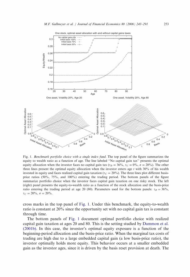
well-diversified portfolio for risk exposure purposes. To understand how these twoincentives quantitatively determine portfolio composition, we consider two differentscenarios. Under the first scenario, the investor is grossly overinvested in equitycompared to the single-stock benchmark. Specifically, we consider an investor at aget who holds 70% of his wealth in equity with 40% in stock 1 and 30% in stock 2.This allows us to study the tradeoff between holding the optimal mix of equity andmoney market holdings and minimizing tax-induced trading costs. To capture thecosts of holding an undiversified equity position, our second scenario assumes thatthe investor’s investment in equity at age t is 20% of wealth, which is roughly equalto the optimal total equity exposure with no capital gain tax. However, the investorholds only one of the stocks at the start of age t, which makes him grosslyundiversified but not overexposed to equity versus the money market account.

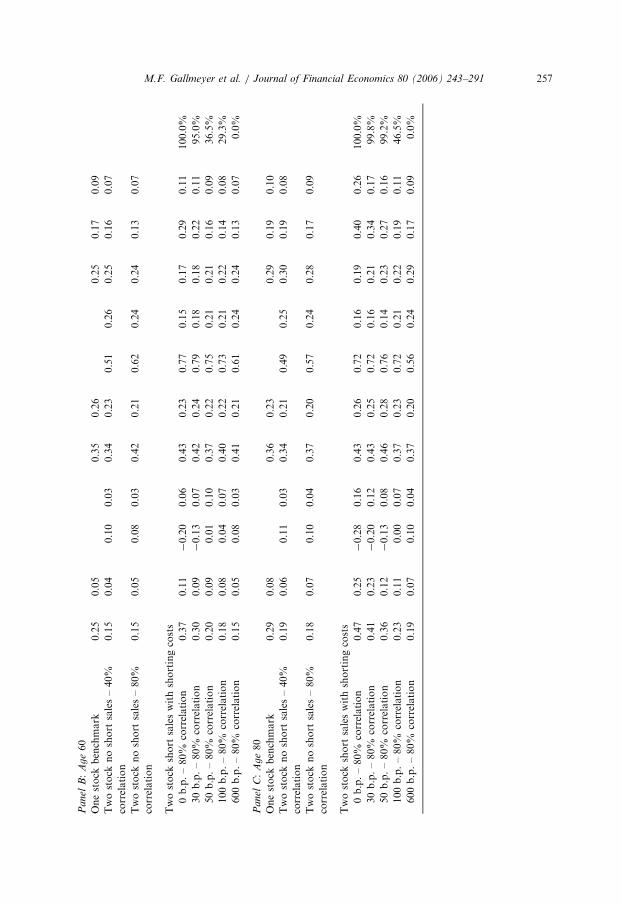
Starting when the investor is overexposed to equity relative to the money marketaccount, the optimal strategies for a stock return correlation of 80% are presented inFig. 2. The left (right) panel describes the optimal equity allocation at age 20 (80) asa function of the equity basis-price ratios. From the figure, the optimal tradingstrategy is sensitive to tax trading costs. The optimal portfolio choice in one stock isnot independent of the investor’s position in the other. For example, the optimalallocation for stock 2 is weakly increasing in the basis-price ratio of stock 1 for bothyoung and old investors. Given that the two stocks are highly correlated, the investorsells the stock with the smallest embedded gain to reduce the total equity exposure.The smallest optimal position in stock 2 occurs when its basis is in the tax-loss sellingregion and the embedded gain of stock 1 is high. Here, the investor completelyliquidates his position in the stock in order to reduce his total equity exposure ascheaply as possible. When the basis-price ratios are close to each other, the optimalallocation can change dramatically for small perturbations in the initial bases. Forexample, at age 20, stock 2’s optimal allocation is 8.1% of wealth for a basis-pricedistribution of b1 ¼ 0:6 and b2 ¼ 0:8, while it changes to 17.3% of wealth when theinitial basis-price ratios are reversed to b1 ¼ 0:8 and b2 ¼ 0:6. In unreported results,when the correlation between the two stocks is reduced to 40%, the optimal strategymirrors the strategy of the investor who only has access to a single stock. Theinvestor optimally sells more of the stock when its embedded gains are smaller. Inthis case, the existence of a second stock does not appear to significantly influence theinvestor’s action in the other stock. Summarizing these results, as the correlationbetween the two stocks increases, the investor sells the stock with the smallest cost totrade to reduce his total equity exposure.

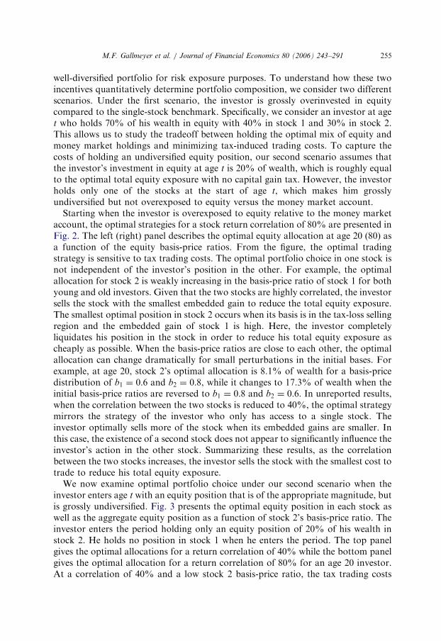
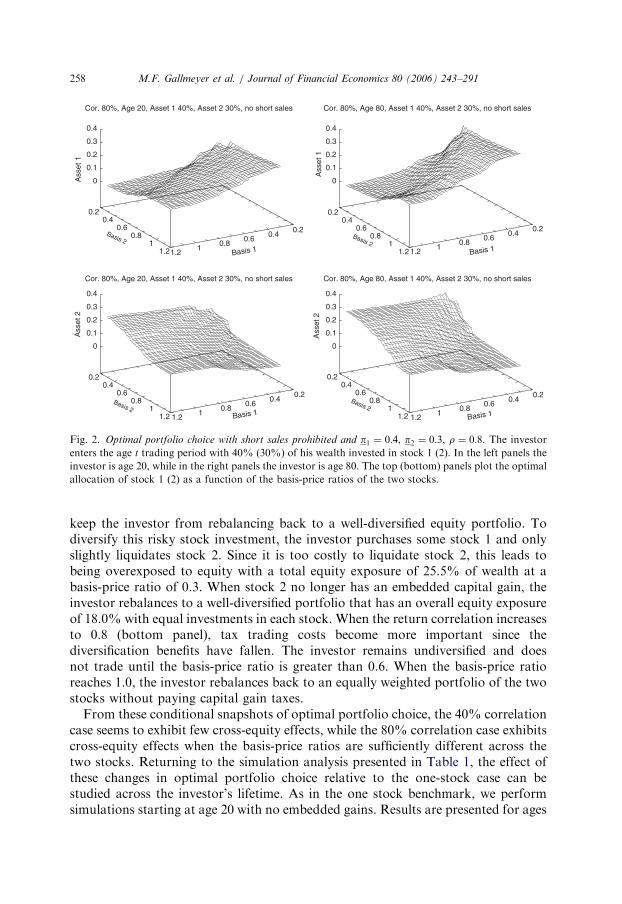
We now examine optimal portfolio choice under our second scenario when theinvestor enters age t with an equity position that is of the appropriate magnitude, butis grossly undiversified. Fig. 3 presents the optimal equity position in each stock aswell as the aggregate equity position as a function of stock 2’s basis-price ratio. Theinvestor enters the period holding only an equity position of 20% of his wealth instock 2. He holds no position in stock 1 when he enters the period. The top panelgives the optimal allocations for a return correlation of 40% while the bottom panelgives the optimal allocation for a return correlation of 80% for an age 20 investor.At a correlation of 40% and a low stock 2 basis-price ratio, the tax trading costs

ARTICLE IN PRESS

Table

1

Optimalportfoliochoicecharacteristics

This

table

presents

simulationresultsforthemeanandstandard

deviationofportfoliocharacteristics

atages

40,60,and80over

50,000paths.

The

simulationsconsider

severalscenarios:aninvestorwhotrades

oneriskystock

(‘‘O

neStock

Benchmark’’),aninvestorwhotrades

tworiskystocksandisshort

saleconstrained

(‘‘TwoStock

NoShortSales’’)atcorrelationsof0.4

and0.8,andaninvestorwhotrades

tworiskystocksatacorrelationof0.8

andcansell

short

atacost

(0,30,50,100,600b.p.).In

allcases,interest

anddividendincomeistaxed

att D¼

0:36andrealizedcapitalgainsare

taxed

att C¼

0:2.The

columnlabeled

‘‘MaxEquityAllocation’’(‘‘M

inEquityAllocation’’)recordsthesimulationcharacteristics

ofthelargest(smallest)stock

position.Thestock

positionsandtotalequity(labeled

‘‘TotalEquity’’)are

computedasfractionofwealth.Thebases(‘‘M

axEquityBasis’’and‘‘Min

EquityBasis’’)are

basis-

price

ratioswhen

thestock

positionispositive.When

astock

positionisnegative,thebasisisaprice-basisratio.Embedded

gains(labeled

‘‘Embedded

Gains’’)

are

calculatedasthefractionofwealththatisacapitalgain.Tim

eshorting(labeled

‘‘Tim

eShorting’’)isthefractionofsimulationpathsin

whichtheinvestor

isshortingateach

age.

Sim

ulationresults

Maxequity

Min

equity

Total

Tim

e

allocation

allocation

Maxequitybasis

Min

equitybasis

equity

mean

Embedded

gains

shorting

mean

Mean

Std.

Dev.

Mean

Std.

Dev.

Mean

Std.

Dev.

Mean

Std.

Dev.

Mean

Std.

Dev.

Pan

elA:

Ag

e40

Onestock

benchmark

0.24

0.05

0.48

0.26

0.24

0.13

0.08

Twostock

noshort

sales–40%

correlation

0.14

0.04

0.09

0.02

0.41

0.23

0.63

0.26

0.23

0.12

0.06

Twostock

noshort

sales–80%

correlation

0.13

0.03

0.09

0.02

0.48

0.22

0.64

0.24

0.22

0.10

0.06

Twostock

short

saleswithshortingcosts

0b.p.–80%

correlation

0.31

0.06

�0.15

0.03

0.45

0.25

0.83

0.14

0.17

0.22

0.10

100.0%

30b.p.–80%

correlation

0.21

0.10

�0.03

0.10

0.45

0.23

0.76

0.22

0.18

0.15

0.09

55.3%

50b.p.–80%

correlation

0.16

0.07

0.05

0.06

0.46

0.23

0.74

0.22

0.21

0.12

0.07

20.0%

100b.p.–80%

correlation

0.14

0.05

0.07

0.04

0.48

0.22

0.71

0.23

0.22

0.11

0.06

7.7%

600b.p.–80%

correlation

0.13

0.03

0.09

0.02

0.48

0.22

0.64

0.24

0.22

0.11

0.06

0.0%


ARTICLE IN PRESS

Pan

elB:

Ag

e60

Onestock

benchmark

0.25

0.05

0.35

0.26

0.25

0.17

0.09

Twostock

noshort

sales–40%

correlation

0.15

0.04

0.10

0.03

0.34

0.23

0.51

0.26

0.25

0.16

0.07

Twostock

noshort

sales–80%

correlation

0.15

0.05

0.08

0.03

0.42

0.21

0.62

0.24

0.24

0.13

0.07

Twostock

short


0b.p.–80%

correlation

0.37

0.11

�0.20

0.06

0.43

0.23

0.77

0.15

0.17

0.29

0.11

100.0%

30b.p.–80%

correlation

0.30

0.09

�0.13

0.07

0.42

0.24

0.79

0.18

0.18

0.22

0.11

95.0%

50b.p.–80%

correlation

0.20

0.09

0.01

0.10

0.37

0.22

0.75

0.21

0.21

0.16

0.09

36.5%

100b.p.–80%

correlation

0.18

0.08

0.04

0.07

0.40

0.22

0.73

0.21

0.22

0.14

0.08

29.3%

600b.p.–80%

correlation

0.15

0.05

0.08

0.03

0.41

0.21

0.61

0.24

0.24

0.13

0.07

0.0%

Pan

elC:

Ag

e80

Onestock

benchmark

0.29

0.08

0.36

0.23

0.29

0.19

0.10

Twostock

noshort

sales–40%

correlation

0.19

0.06

0.11

0.03

0.34

0.21

0.49

0.25

0.30

0.19

0.08

Twostock

noshort

sales–80%

correlation

0.18

0.07

0.10

0.04

0.37

0.20

0.57

0.24

0.28

0.17

0.09

Twostock

short


0b.p.–80%

correlation

0.47

0.25

�0.28

0.16

0.43

0.26

0.72

0.16

0.19

0.40

0.26

100.0%

30b.p.–80%

correlation

0.41

0.23

�0.20

0.12

0.43

0.25

0.72

0.16

0.21

0.34

0.17

99.8%

50b.p.–80%

correlation

0.36

0.12

�0.13

0.08

0.46

0.28

0.76

0.14

0.23

0.27

0.16

99.2%

100b.p.–80%

correlation

0.23

0.11

0.00

0.07

0.37

0.23

0.72

0.21

0.22

0.19

0.11

46.5%

600b.p.–80%

correlation

0.19

0.07

0.10

0.04

0.37

0.20

0.56

0.24

0.29

0.17

0.09

0.0%


ARTICLE IN PRESS

Cor. 80%, Age 20, Asset 1 40%, Asset 2 30%, no short sales

0.2 0.4

0.6 0.8

1 1.2 Basis 1 Basis 1

0.2 0.4

0.6 0.8

1 1.2

Basis 2

Basis 1

Basis 2

Basis 2

Basis 1

Basis 2

0

0.1

0.2

0.3

0.4

Ass

et 1

Ass

et 1


0.2 0.4

0.6 0.8

1 1.2

0.2 0.4

0.6 0.8

1 1.2

0

0.1

0.2

0.3

0.4


0.2 0.4

0.6 0.8

1 1.2

0.2 0.4

0.6 0.8

1 1.2

0

0.1

0.2

0.3

0.4


0.2 0.4

0.6 0.8

1 1.2

0.2 0.4

0.6 0.8

1 1.2

0

0.1

0.2

0.3

0.4

Ass

et 2

Ass

et 2

Fig. 2. Optimal portfolio choice with short sales prohibited and p1 ¼ 0:4, p2 ¼ 0:3, r ¼ 0:8. The investor

enters the age t trading period with 40% (30%) of his wealth invested in stock 1 (2). In the left panels the

investor is age 20, while in the right panels the investor is age 80. The top (bottom) panels plot the optimal

allocation of stock 1 (2) as a function of the basis-price ratios of the two stocks.


keep the investor from rebalancing back to a well-diversified equity portfolio. Todiversify this risky stock investment, the investor purchases some stock 1 and onlyslightly liquidates stock 2. Since it is too costly to liquidate stock 2, this leads tobeing overexposed to equity with a total equity exposure of 25.5% of wealth at abasis-price ratio of 0.3. When stock 2 no longer has an embedded capital gain, theinvestor rebalances to a well-diversified portfolio that has an overall equity exposureof 18.0% with equal investments in each stock. When the return correlation increasesto 0.8 (bottom panel), tax trading costs become more important since thediversification benefits have fallen. The investor remains undiversified and doesnot trade until the basis-price ratio is greater than 0.6. When the basis-price ratioreaches 1.0, the investor rebalances back to an equally weighted portfolio of the twostocks without paying capital gain taxes.

From these conditional snapshots of optimal portfolio choice, the 40% correlationcase seems to exhibit few cross-equity effects, while the 80% correlation case exhibitscross-equity effects when the basis-price ratios are sufficiently different across thetwo stocks. Returning to the simulation analysis presented in Table 1, the effect ofthese changes in optimal portfolio choice relative to the one-stock case can bestudied across the investor’s lifetime. As in the one stock benchmark, we performsimulations starting at age 20 with no embedded gains. Results are presented for ages

ARTICLE IN PRESS

0

0.05

0.1

0.15

0.2

0.25

0.3

0.2 0.3 0.4 0.5 0.6 0.7 0.8 0.9 1 1.1 1.2

Equ

ity/W

ealth

Basis 2

Correlation 40%, Age 20, Asset 1 0%, Asset 2 20%, no short sales

Asset 1Asset 2

Total Equity

0

0.05

0.1

0.15

0.2

0.25

0.3

0.2 0.3 0.4 0.5 0.6 0.7 0.8 0.9 1 1.1 1.2

Equ

ity/W

ealth

Basis 2

Correlation 80%, Age 20, Asset 1 0%, Asset 2 20%, no short sales

Asset 1Asset 2

Total Equity

Fig. 3. Optimal portfolio choice with short sales prohibited and p1 ¼ 0:0, p2 ¼ 0:2 at age 20. The investor

enters the trading period with 0% (20%) of his wealth invested in stock 1 (2). The top (bottom) panel is for

the case when the correlation between the two stocks is r ¼ 0:4 (r ¼ 0:8).


ARTICLE IN PRESS


40, 60, and 80 for both the 40% and 80% correlation cases in the lines labeled ‘‘TwoStock No Short Sales.’’ The column labeled ‘‘Max Equity Allocation’’ records thesimulation characteristics of the largest stock position, while ‘‘Min EquityAllocation’’ records the smallest stock position’s characteristics. Given that thetwo stocks are ex ante identical, we arrive at the same statistics for each stock if theallocation characteristics are recorded on a stock-by-stock basis.

From the simulations, trading in two stocks is quite similar to trading in the index,as the overall mean equity allocations for both correlations are only slightly lowerthan the index case. However, the equity portfolio can deviate from the no-taxbenchmark of equal investments in each stock. For example, at age 40, an investorwho trades two stocks with an 80% correlation on average holds 22% of his wealthin equity as compared to holding 24% of his wealth in equity if he just invests in theindex. He does, however, hold unequal positions in the two stocks on average. Hisaverage maximum equity allocation in one of the stocks is 13% of wealth, whilehis average minimum equity allocation in one of the stocks is 9% of wealth. Hisembedded gains in the portfolio are slightly lower than the index case: 10% of wealthas compared to 13% of wealth for the index investor. As in the single-stock case, theinvestor tends to hold more equity as he ages. For example, from the age 80simulations, the investor holds 40% more equity on average than his untaxedcounterpart when the correlation between the two stocks is 80%. This overexposureto equity is only slightly lower than when trading in the index and taxed on realizedcapital gains.

3.3. Optimal portfolio composition with two stocks and short sales

By allowing short selling, the investor’s after-tax opportunity set is expanded.Short selling allows two additional trading strategies: a trading flexibility strategy inwhich an investor currently not overexposed to total equity ex ante shorts one stockto optimally manage realized capital gains when portfolio rebalancing in the future;and an imperfect shorting-the-box strategy in which an investor overexposed toequity with embedded gains ex post trades to reduce the exposure by shorting thecheaper-to-trade stock. These strategies are more effective for stocks that are highlycorrelated where the costs of not being well diversified are low. At a correlationbetween the two stocks of 40% as studied in the case with no short sales, ournumerical analysis verifies that it is rarely optimal to short except at later ages whenoverexposed to one stock with a large embedded gain. Most of the time, anunconstrained investor acts like his constrained counterpart. Given that our settingis one where the investor’s portfolio holdings are in exchange traded funds wherehighly correlated substitutes for particular securities are common, our discussion isfocused on a setting where the correlation between the two stocks is r ¼ 80% andhigher.

3.3.1. Optimal strategies

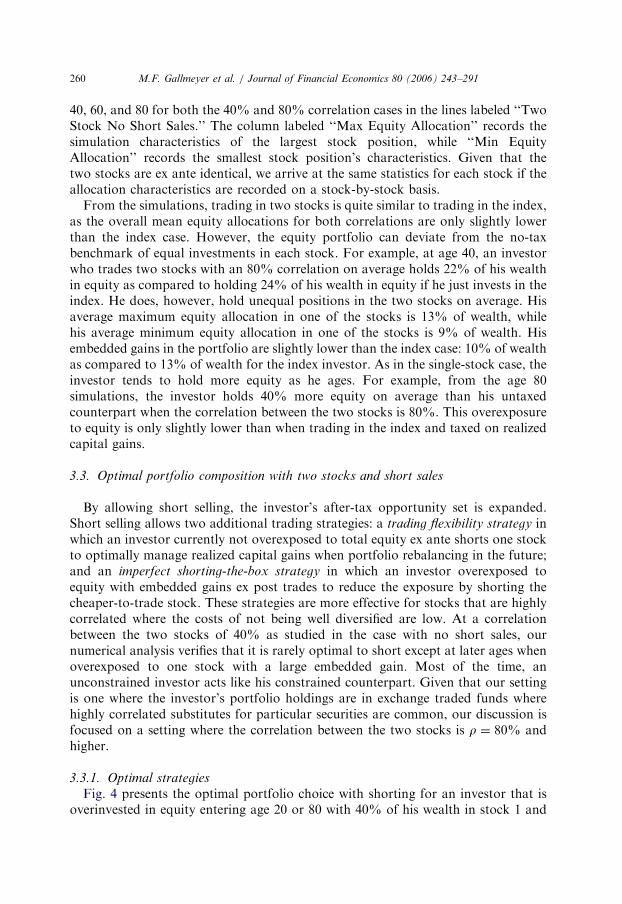
Fig. 4 presents the optimal portfolio choice with shorting for an investor that isoverinvested in equity entering age 20 or 80 with 40% of his wealth in stock 1 and

ARTICLE IN PRESS


30% of his wealth in stock 2. The investor faces a shorting cost where the generalcollateral rate is 30 basis points below the riskless interest rate. Compared to the casewith no short sales documented in Fig. 2, the optimal trading strategies are strikinglydifferent. With shorting available, the investor no longer holds positive positions inboth stocks.

As compared to the no-tax benchmark, surprisingly, the investor may choose tooptimally short stock even when he has no embedded gains in either stock. Forexample, at age 80 when the basis-price ratio is one for both stocks, the investorinvests 32% of his wealth in stock 1 and shorts 14% of his wealth in stock 2 for a netequity exposure of 18%. This trading flexibility strategy preserves the investor’sflexibility for future asset reallocation by minimizing realized capital gains whenrebalancing. This strategy leads to additional trading flexibility by providing capitallosses in the portfolio when they are most needed. For example, consider twodifferent ways of holding a net equity position of 18% of wealth as the investor doesat age 80 in Fig. 4 with no embedded gains. To simplify the discussion, assume thatthe two stocks are perfectly correlated. In the first strategy, the investor holds 9% ofhis wealth in each stock. In the second strategy, the investor holds 32% of his wealth

Cor. 80%, Age 20, Asset 1 40%, Asset 2 30%, short sales, repo rate 30 b.p.

0.2 0.4

0.6 0.8

1 1.2 Basis 1

0.2 0.4

0.6 0.8

1 1.2

Basis 2

-0.3-0.2-0.1

0 0.1 0.2 0.3 0.4 0.5

Cor. 80%, Age 20, Asset 1 40%, Asset 2 30%, short sales,repo rate 30 b.p.

0.2 0.4

0.6 0.8

1 1.2

0.2 0.4

0.6 0.8

1 1.2

-0.3-0.2-0.1

0 0.1 0.2 0.3 0.4 0.5

Cor. 80%, Age 80, Asset 1 40%, Asset 2 30%, short sales, repo rate 30 b.p.

0.2 0.4

0.6 0.8

1 1.2 Basis 1

0.2 0.4

0.6 0.8

1 1.2

Basis 2

Basis 1

Basis 2Basis 1

Basis 2

-0.3-0.2-0.1

0 0.1 0.2 0.3 0.4 0.5

Ass

et 1

Ass

et 1

Cor. 80%, Age 80, Asset 1 40%, Asset 2 30%, short sales,repo rate 30 b.p.

0.2 0.4

0.6 0.8

1 1.2

0.2 0.4

0.6 0.8

1 1.2

-0.3-0.2-0.1

0 0.1 0.2 0.3 0.4 0.5

Ass

et 2

Ass

et 2

Fig. 4. Optimal portfolio choice with short sales allowed, p1 ¼ 0:4, p2 ¼ 0:3, r ¼ 0:8, and shorting costs of

30 basis points. The investor enters the age t trading period with 40% (30%) of his wealth invested in stock

1 (2). In the left panels the investor is age 20, while in the right panels the investor is age 80. The top

(bottom) panels plot the optimal allocation of stock 1 (2) as a function of the basis-price ratios of the two

stocks. The investor can sell short subject to a shorting cost of 30 basis points.

ARTICLE IN PRESS


in stock 1 and �14% of his wealth in stock 2 as he does at age 80 in the no-embedded-gains region. With no capital gain taxes, these positions would beidentical. However, with capital gain taxes, the second strategy leads to more tradingflexibility.

If the stock market increases over the next year, the investor’s proportion ofwealth in equity increases. Without taxes, the investor optimally sells some equity torebalance back to his optimal total equity-wealth ratio. Under strategy 1, theinvestor has an embedded gain in both stock positions. To rebalance he pays capitalgain taxes on the amount he sells. Strategy 2, however, gives the investor a way torebalance while paying lower capital gain taxes than in strategy 1. By liquidating hislosses in the short position in stock 2, the investor can offset the realized capital gainfrom rebalancing his stock 1 position. (This assumes that the capital loss from stock2 is large enough to offset the realized gain in rebalancing stock 1, as occurs for thecase considered.) Hence, strategy 2 creates a capital loss when it is most useful—when the investor’s aggregate equity position has increased in value and he needs tosell to rebalance. If the stock market falls, the investor sells his long stock positionsto create a tax loss under either strategy. However, under strategy 2 the shortposition in stock 2 now has an embedded gain. In the worst case scenario, he can alsoliquidate this position. His realized capital loss for the entire position under strategy2 is identical to his realized capital loss under strategy 1. As a result, the investor isno worse off when the stock market falls under strategy 2 as compared to owning9% of his wealth in each stock (strategy 1). Combining the two possible marketoutcomes, the investor is better off under strategy 2.

Returning to Fig. 4, when the investor’s portfolio contains embedded gains, hisstrategy is to short the stock that is cheapest to trade. This imperfect shorting-the-box

strategy leads to an overall exposure to equity that is smaller than that of ashort-sale-constrained investor. For example, at age 20 with an initial position of40% in stock 1 and 30% in stock 2 and a basis-price ratio of 0.3 for both stocks, theinvestor liquidates some of his stock 1 position which falls to 38.9% of wealth whileshorting 15.7% of his wealth in stock 2. By doing so, the investor’s net equityposition is reduced to 23.2% as compared to 30.0% when short sales are notallowed. This imperfect shorting-the-box strategy is optimal even though theinvestor faces fundamental price risk given that the two stocks are not perfectlycorrelated.

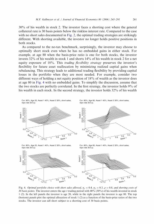
3.3.2. Trading flexibility strategy

To explore the sensitivity of the trading flexibility strategy to different shortingcosts and correlations, Fig. 5 examines the optimal stock allocation as a function ofage for three different general collateral rates: 0 basis points (top panels), 30 basispoints (middle panels), and 50 basis points (bottom panels) below the money marketrate. In the three left plots, the investor’s portfolio entering age t contains noembedded gains in either stock. The three right plots capture the scenario when theinvestor’s total equity exposure entering age t is close to the no-tax optimal, but eachstock contains embedded gains. Specifically, the investor’s equity position enteringage t is 10% of his wealth in each stock with a 0:5 basis-price ratio for each stock.

ARTICLE IN PRESS

-0.8

-0.6

-0.4

-0.2

0

0.2

0.4

0.6

0.8

1

20 30 40 50 60 70 80 90

Equ

ity/W

ealth

Age

Repo rate 0 b.p.

-0.8

-0.6

-0.4

-0.2

0

0.2

0.4

0.6

0.8

1

20 30 40 50 60 70 80 90

Equ

ity/W

ealth

Age

Repo rate 30 b.p.

-0.8

-0.6

-0.4

-0.2

0

0.2

0.4

0.6

0.8

1

20 30 40 50 60 70 80 90

Equ

ity/W

ealth

Age

Repo rate 50 b.p.

Asset 1, cor. 80%Asset 2, cor. 80%Asset 1, cor. 90%Asset 2, cor. 90%

-0.8

-0.6

-0.4

-0.2

0

0.2

0.4

0.6

0.8

1

20 30 40 50 60 70 80 90

Equ

ity/W

ealth

Age

Repo rate 0 b.p.

-0.8

-0.6

-0.4

-0.2

0

0.2

0.4

0.6

0.8

1

20 30 40 50 60 70 80 90

Equ

ity/W

ealth

Age

Repo rate 30 b.p.

-0.8

-0.6

-0.4

-0.2

0

0.2

0.4

0.6

0.8

1

20 30 40 50 60 70 80 90

Equ

ity/W

ealth

Age

Repo rate 50 b.p.






Fig. 5. Trading flexibility strategy use versus age. The plots examine the optimal allocation in the risky

assets versus age as a fraction of wealth when the investor is engaged in the trading flexibility strategy and

the correlation between the two stocks is r ¼ 0:8 or r ¼ 0:9. For the top, middle, and bottom panels, the

investor can sell short subject to shorting costs of 0, 30, and 50 basis points. In the left panels, the investor

enters the trading period with no embedded gains in either security. In the right panels, the investor enters

the trading period with 10% of his wealth in each stock and a basis-price ratio of 0.5 for each stock.


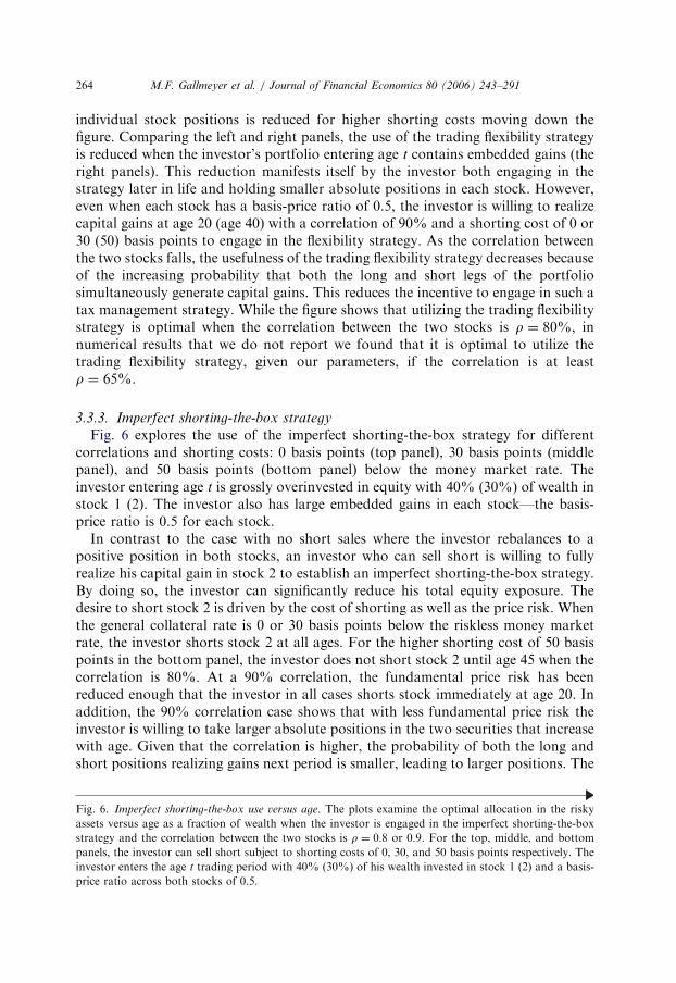
Here the investor might desire to engage in the flexibility strategy to reduce futuretax trading costs even though he will pay some capital gain taxes today to rebalance.

From Fig. 5, the use of the trading flexibility strategy is decreasing in the shortingcost and increasing in age and correlation. At a correlation of 90%, the flexibilitystrategy is used from age 20 for all shorting costs; however, the magnitude of the

ARTICLE IN PRESS


individual stock positions is reduced for higher shorting costs moving down thefigure. Comparing the left and right panels, the use of the trading flexibility strategyis reduced when the investor’s portfolio entering age t contains embedded gains (theright panels). This reduction manifests itself by the investor both engaging in thestrategy later in life and holding smaller absolute positions in each stock. However,even when each stock has a basis-price ratio of 0.5, the investor is willing to realizecapital gains at age 20 (age 40) with a correlation of 90% and a shorting cost of 0 or30 (50) basis points to engage in the flexibility strategy. As the correlation betweenthe two stocks falls, the usefulness of the trading flexibility strategy decreases becauseof the increasing probability that both the long and short legs of the portfoliosimultaneously generate capital gains. This reduces the incentive to engage in such atax management strategy. While the figure shows that utilizing the trading flexibilitystrategy is optimal when the correlation between the two stocks is r ¼ 80%, innumerical results that we do not report we found that it is optimal to utilize thetrading flexibility strategy, given our parameters, if the correlation is at leastr ¼ 65%.

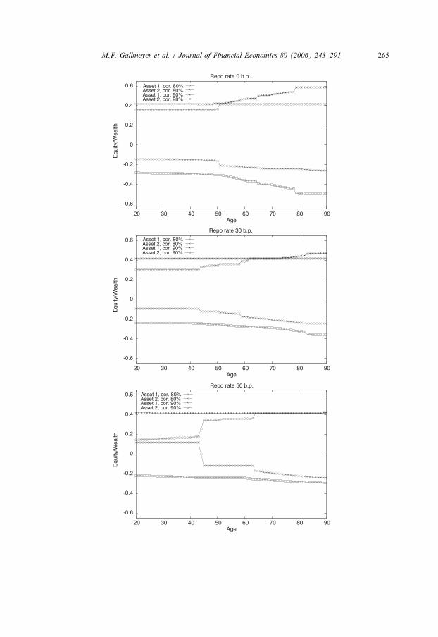
3.3.3. Imperfect shorting-the-box strategy

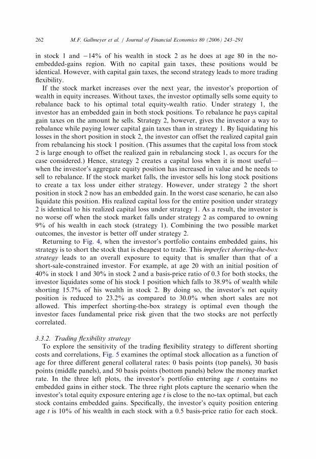
Fig. 6 explores the use of the imperfect shorting-the-box strategy for differentcorrelations and shorting costs: 0 basis points (top panel), 30 basis points (middlepanel), and 50 basis points (bottom panel) below the money market rate. Theinvestor entering age t is grossly overinvested in equity with 40% (30%) of wealth instock 1 (2). The investor also has large embedded gains in each stock—the basis-price ratio is 0.5 for each stock.

In contrast to the case with no short sales where the investor rebalances to apositive position in both stocks, an investor who can sell short is willing to fullyrealize his capital gain in stock 2 to establish an imperfect shorting-the-box strategy.By doing so, the investor can significantly reduce his total equity exposure. Thedesire to short stock 2 is driven by the cost of shorting as well as the price risk. Whenthe general collateral rate is 0 or 30 basis points below the riskless money marketrate, the investor shorts stock 2 at all ages. For the higher shorting cost of 50 basispoints in the bottom panel, the investor does not short stock 2 until age 45 when thecorrelation is 80%. At a 90% correlation, the fundamental price risk has beenreduced enough that the investor in all cases shorts stock immediately at age 20. Inaddition, the 90% correlation case shows that with less fundamental price risk theinvestor is willing to take larger absolute positions in the two securities that increasewith age. Given that the correlation is higher, the probability of both the long andshort positions realizing gains next period is smaller, leading to larger positions. The

Fig. 6. Imperfect shorting-the-box use versus age. The plots examine the optimal allocation in the risky

assets versus age as a fraction of wealth when the investor is engaged in the imperfect shorting-the-box

strategy and the correlation between the two stocks is r ¼ 0:8 or 0.9. For the top, middle, and bottom

panels, the investor can sell short subject to shorting costs of 0, 30, and 50 basis points respectively. The

investor enters the age t trading period with 40% (30%) of his wealth invested in stock 1 (2) and a basis-

price ratio across both stocks of 0.5.

ARTICLE IN PRESS

-0.6

-0.4

-0.2

0

0.2

0.4

0.6

20 30 40 50 60 70 80 90

Equ

ity/W

ealth

Age

Repo rate 0 b.p.

-0.6

-0.4

-0.2

0

0.2

0.4

0.6

20 30 40 50 60 70 80 90

Equ

ity/W

ealth

Age

Repo rate 30 b.p.

-0.6

-0.4

-0.2

0

0.2

0.4

0.6

20 30 40 50 60 70 80 90

Equ

ity/W

ealth

Age

Repo rate 50 b.p.





ARTICLE IN PRESS


imperfect shorting-the-box strategy is also employed when the return correlationbetween the two stocks is considerably lower than 80%. In numerical simulations,we find that it is optimal to utilize the imperfect shorting-the-box strategy, given ourparameters, if the correlation is at least r ¼ 40% at later ages when the investor isoverexposed to one stock with a large embedded gain.

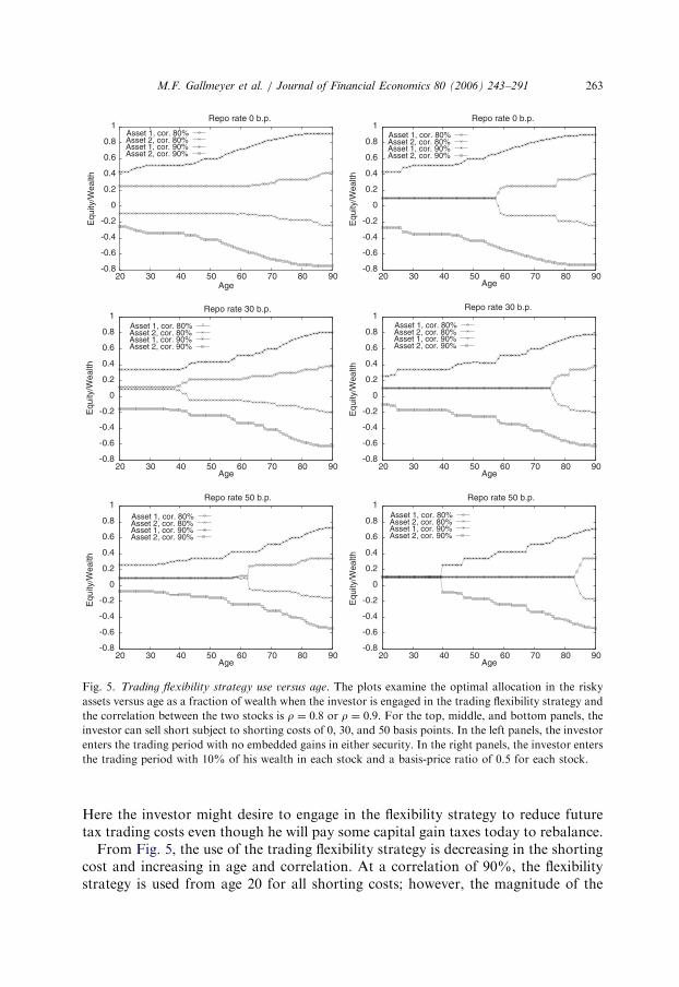
3.3.4. Implications for stock allocation relative to no short sales

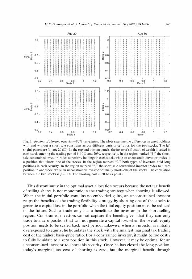
The use of the trading flexibility strategy highlights an interesting feature of shortselling.9 With no embedded gains, a short-sale-constrained investor holds a positiveposition in each stock, but if the constraint is relaxed, he optimally shorts one of thestocks at a low enough shorting cost. Figs. 7 and 8 explore this feature across allbasis distributions by considering a risky stock portfolio where the investor enteringage 20 or 80 owns equal weights in each security. Each panel explores thecharacteristics of optimal portfolio choice across the basis-price ratios of the twostocks. In the region marked ‘‘1,’’ a constrained investor trades to positive holdingsin both stocks, while a shorting investor trades to a negative position in one stock. Ifboth investor types hold positive positions in each stock, the region is marked ‘‘2.’’Finally, the region marked ‘‘3’’ corresponds to the short-sale-constrained investorholding a zero position in one stock and the unconstrained investor shorting one ofthe stocks. The left (right) panels characterize trading behavior at age 20 (80). Thetotal portion of wealth in equity entering the trading period increases moving downthe panels. We present results when the equity exposure in each stock is 10% (theresults are identical for an equity exposure in each stock less than or equal to 10%)and 20% of wealth initially. The correlation between the two stocks is 80% for Fig. 7and 90% for Fig. 8; the general collateral rate when short selling is 30 basis pointsbelow the money market rate.

From both figures, it is very common for an unconstrained investor to short, whilea constrained investor holds positive weights in each stock (region ‘‘1’’). Suchbehavior is most prominent at age 80. For this age, the only time the short-sale-constrained investor holds a zero position in one of the stocks is in the two regionsmarked ‘‘3’’ in the lower right panel of the 90% correlation figure. Given that in thispanel the investor holds 40% of his wealth in equity entering the trading period, anunconstrained investor always shorts one of the stocks to engage in the tradingflexibility or the imperfect shorting-the-box strategy. The constrained investorentirely liquidates one of his equity positions only when it has small embedded gainsrelative to the other stock. At age 20, this behavior is more dependent on the returncorrelation between the two stocks. In the top left panel of Fig. 7 where the investorsare not overexposed to equity, both types of investors hold strictly positive positionsin both stocks. This behavior is driven by the flexibility strategy not being optimalfor the unconstrained investor at age 20 and a return correlation of 80%. However,when the return correlation increases to 90% (top left panel of Fig. 8), theunconstrained investor at age 20 again shorts while the constrained investor holdspositive weights in each stock.

9We thank the referee for drawing this feature to our attention.

ARTICLE IN PRESS

0.2

0.4

0.6

0.8

1

1.2

0.2 0.4 0.6 0.8 1 1.2

Bas

is 2

Basis 1

2 2 2 2 2 2 2 2 2 2 2 2 2 2 2 2 2 2 22 2 2 2 2 2 2 2 2 2 2 2 2 2 2 2 2 2 22 2 2 2 2 2 2 2 2 2 2 2 2 2 2 2 2 2 22 2 2 2 2 2 2 2 2 2 2 2 2 2 2 2 2 2 22 2 2 2 2 2 2 2 2 2 2 2 2 2 2 2 2 2 22 2 2 2 2 2 2 2 2 2 2 2 2 2 2 2 2 2 22 2 2 2 2 2 2 2 2 2 2 2 2 2 2 2 2 2 22 2 2 2 2 2 2 2 2 2 2 2 2 2 2 2 2 2 22 2 2 2 2 2 2 2 2 2 2 2 2 2 2 2 2 2 22 2 2 2 2 2 2 2 2 2 2 2 2 2 2 2 2 2 22 2 2 2 2 2 2 2 2 2 2 2 2 2 2 2 2 2 22 2 2 2 2 2 2 2 2 2 2 2 2 2 2 2 2 2 22 2 2 2 2 2 2 2 2 2 2 2 2 2 2 2 2 2 22 2 2 2 2 2 2 2 2 2 2 2 2 2 2 2 2 2 22 2 2 2 2 2 2 2 2 2 2 2 2 2 2 2 2 2 22 2 2 2 2 2 2 2 2 2 2 2 2 2 2 2 2 2 22 2 2 2 2 2 2 2 2 2 2 2 2 2 2 2 2 2 22 2 2 2 2 2 2 2 2 2 2 2 2 2 2 2 2 2 22 2 2 2 2 2 2 2 2 2 2 2 2 2 2 2 2 2 2

Age 20

10%

0.2

0.4

0.6

0.8

1

1.2

0.2 0.4 0.6 0.8 1 1.2

Bas

is 2

Basis 1

2 2 2 2 2 2 2 2 2 2 1 3 3 3 3 3 3 3 32 2 2 2 2 2 2 2 2 2 1 3 3 3 3 3 3 3 32 2 2 2 2 2 2 2 2 2 1 3 3 3 3 3 3 3 32 2 2 2 2 2 2 2 2 2 1 1 3 3 3 3 3 3 32 2 2 2 2 2 2 2 2 2 1 1 3 3 3 3 3 3 32 2 2 2 2 2 2 2 2 2 1 1 3 3 3 3 3 3 32 2 2 2 2 2 2 2 2 1 1 1 1 3 3 3 3 3 32 2 2 2 2 2 2 2 2 2 1 1 1 1 1 1 1 1 12 2 2 2 2 2 2 2 2 2 1 1 1 1 1 1 1 1 12 2 2 2 2 2 1 2 2 2 1 1 1 1 1 1 1 1 11 1 1 1 1 1 1 1 1 1 2 1 1 1 1 1 1 1 13 3 3 1 1 1 1 1 1 1 1 2 1 1 1 1 1 1 13 3 3 3 3 3 1 1 1 1 1 1 2 1 1 1 1 1 13 3 3 3 3 3 3 1 1 1 1 1 1 2 2 2 2 2 23 3 3 3 3 3 3 1 1 1 1 1 1 2 2 2 2 2 23 3 3 3 3 3 3 1 1 1 1 1 1 2 2 2 2 2 23 3 3 3 3 3 3 1 1 1 1 1 1 2 2 2 2 2 23 3 3 3 3 3 3 1 1 1 1 1 1 2 2 2 2 2 23 3 3 3 3 3 3 1 1 1 1 1 1 2 2 2 2 2 2

20%

0.2

0.4

0.6

0.8

1

1.2

0.2 0.4 0.6 0.8 1 1.2

Bas

is 2

Basis 1

1 1 1 1 1 1 1 1 1 1 1 1 1 1 1 1 1 1 11 1 1 1 1 1 1 1 1 1 1 1 1 1 1 1 1 1 11 1 1 1 1 1 1 1 1 1 1 1 1 1 1 1 1 1 11 1 1 1 1 1 1 1 1 1 1 1 1 1 1 1 1 1 11 1 1 1 1 1 1 1 1 1 1 1 1 1 1 1 1 1 11 1 1 1 1 1 1 1 1 1 1 1 1 1 1 1 1 1 11 1 1 1 1 1 1 1 1 1 1 1 1 1 1 1 1 1 11 1 1 1 1 1 1 1 1 1 1 1 1 1 1 1 1 1 11 1 1 1 1 1 1 1 1 1 1 1 1 1 1 1 1 1 11 1 1 1 1 1 1 1 1 1 1 1 1 1 1 1 1 1 11 1 1 1 1 1 1 1 1 1 1 1 1 1 1 1 1 1 11 1 1 1 1 1 1 1 1 1 1 1 1 1 1 1 1 1 11 1 1 1 1 1 1 1 1 1 1 1 1 1 1 1 1 1 11 1 1 1 1 1 1 1 1 1 1 1 1 1 1 1 1 1 11 1 1 1 1 1 1 1 1 1 1 1 1 1 1 1 1 1 11 1 1 1 1 1 1 1 1 1 1 1 1 1 1 1 1 1 11 1 1 1 1 1 1 1 1 1 1 1 1 1 1 1 1 1 11 1 1 1 1 1 1 1 1 1 1 1 1 1 1 1 1 1 11 1 1 1 1 1 1 1 1 1 1 1 1 1 1 1 1 1 1

Age 80

0.2

0.4

0.6

0.8

1

1.2

0.2 0.4 0.6 0.8 1 1.2

Bas

is 2

Basis 1

1 1 1 1 1 1 1 1 1 1 1 1 1 1 1 1 1 1 11 1 1 1 1 1 1 1 1 1 1 1 1 1 1 1 1 1 11 1 1 1 1 1 1 1 1 1 1 1 1 1 1 1 1 1 11 1 1 1 1 1 1 1 1 1 1 1 1 1 1 1 1 1 11 1 1 1 1 1 1 1 1 1 1 1 1 1 1 1 1 1 11 1 1 1 1 1 1 1 1 1 1 1 1 1 1 1 1 1 11 1 1 1 1 1 1 1 1 1 1 1 1 1 1 1 1 1 11 1 1 1 1 1 1 1 1 1 1 1 1 1 1 1 1 1 11 1 1 1 1 1 1 1 1 1 1 1 1 1 1 1 1 1 11 1 1 1 1 1 1 1 1 1 1 1 1 1 1 1 1 1 11 1 1 1 1 1 1 1 1 1 1 1 1 1 1 1 1 1 11 1 1 1 1 1 1 1 1 1 1 1 1 1 1 1 1 1 11 1 1 1 1 1 1 1 1 1 1 1 1 1 1 1 1 1 11 1 1 1 1 1 1 1 1 1 1 1 1 1 1 1 1 1 11 1 1 1 1 1 1 1 1 1 1 1 1 1 1 1 1 1 11 1 1 1 1 1 1 1 1 1 1 1 1 1 1 1 1 1 11 1 1 1 1 1 1 1 1 1 1 1 1 1 1 1 1 1 11 1 1 1 1 1 1 1 1 1 1 1 1 1 1 1 1 1 11 1 1 1 1 1 1 1 1 1 1 1 1 1 1 1 1 1 1

Fig. 7. Regions of shorting behavior—80% correlation. The plots examine the differences in asset holdings

with and without a short-sale constraint across different basis-price ratios for the two stocks. The left

(right) panels are for age 20 (80). In the top and bottom panels, the investor’s fraction of wealth invested in

each stock entering the trading period is 10% and 20%, respectively. In the region marked ‘‘1,’’ the short-

sale-constrained investor trades to positive holdings in each stock, while an unconstraint investor trades to

a position that shorts one of the stocks. In the region marked ‘‘2,’’ both types of investors hold long

positions in each security. In the region marked ‘‘3,’’ the short-sale-constrained investor trades to a zero

position in one stock, while an unconstrained investor optimally shorts one of the stocks. The correlation

between the two stocks is r ¼ 0:8. The shorting cost is 30 basis points.


This discontinuity in the optimal asset allocation occurs because the net tax benefitof selling shares is not monotonic in the trading strategy when shorting is allowed.When the initial portfolio contains no embedded gains, an unconstrained investorreaps the benefits of the trading flexibility strategy by shorting one of the stocks togenerate a capital loss in the portfolio when the total equity position must be reducedin the future. Such a trade only has a benefit to the investor in the short sellingregion. Constrained investors cannot capture the benefit given that they can onlytrade to a zero position that will not generate a capital loss when the overall equityposition needs to be scaled back next period. Likewise, when an investor is initiallyoverexposed to equity, he liquidates the stock with the smallest marginal tax tradingcost or the highest basis-price ratio. For a constrained investor, it might be too costlyto fully liquidate to a zero position in this stock. However, it may be optimal for anunconstrained investor to short this security. Once he has closed the long position,today’s marginal tax cost of shorting is zero, but the marginal benefit through

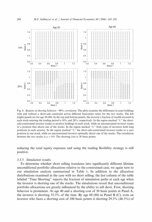
ARTICLE IN PRESS

0.2

0.4

0.6

0.8

1

1.2

0.2 0.4 0.6 0.8 1 1.2

Bas

is 2

Basis 1

2 1 1 1 1 1 1 1 1 1 1 1 1 1 1 1 1 1 11 1 1 1 1 1 1 1 1 1 1 1 1 1 1 1 1 1 11 1 1 1 1 1 1 1 1 1 1 1 1 1 1 1 1 1 11 1 1 1 1 1 1 1 1 1 1 1 1 1 1 1 1 1 11 1 1 1 1 1 1 1 1 1 1 1 1 1 1 1 1 1 11 1 1 1 1 1 1 1 1 1 1 1 1 1 1 1 1 1 11 1 1 1 1 1 1 1 1 1 1 1 1 1 1 1 1 1 11 1 1 1 1 1 1 1 1 1 1 1 1 1 1 1 1 1 11 1 1 1 1 1 1 1 1 1 1 1 1 1 1 1 1 1 11 1 1 1 1 1 1 1 1 1 1 1 1 1 1 1 1 1 11 1 1 1 1 1 1 1 1 1 1 1 1 1 1 1 1 1 11 1 1 1 1 1 1 1 1 1 1 1 1 1 1 1 1 1 11 1 1 1 1 1 1 1 1 1 1 1 1 1 1 1 1 1 11 1 1 1 1 1 1 1 1 1 1 1 1 1 1 1 1 1 11 1 1 1 1 1 1 1 1 1 1 1 1 1 1 1 1 1 11 1 1 1 1 1 1 1 1 1 1 1 1 1 1 1 1 1 11 1 1 1 1 1 1 1 1 1 1 1 1 1 1 1 1 1 11 1 1 1 1 1 1 1 1 1 1 1 1 1 1 1 1 1 11 1 1 1 1 1 1 1 1 1 1 1 1 1 1 1 1 1 1

Age 20

10%

0.2

0.4

0.6

0.8

1

1.2

0.2 0.4 0.6 0.8 1 1.2

Bas

is 2

Basis 1

1 1 1 1 1 1 1 1 1 3 3 3 3 3 3 3 3 3 31 1 1 1 1 1 1 1 1 3 3 3 3 3 3 3 3 3 31 1 1 1 1 1 1 1 1 3 3 3 3 3 3 3 3 3 31 1 1 1 1 1 1 1 1 3 3 3 3 3 3 3 3 3 31 1 1 1 1 1 1 1 1 3 3 3 3 3 3 3 3 3 31 1 1 1 1 1 1 1 1 1 3 3 3 3 3 3 3 3 31 1 1 1 1 1 1 1 1 1 3 3 3 3 3 3 3 3 31 1 1 1 1 1 1 1 1 1 3 3 3 3 3 3 3 3 31 1 1 1 1 1 1 1 1 1 1 3 3 3 3 3 3 3 33 3 3 3 3 1 1 1 1 1 1 1 1 3 3 3 3 3 33 3 3 3 3 3 3 3 1 1 1 1 1 1 3 3 3 3 33 3 3 3 3 3 3 3 3 1 1 1 1 1 1 1 1 1 13 3 3 3 3 3 3 3 3 1 1 1 1 1 1 1 1 1 13 3 3 3 3 3 3 3 3 3 1 1 1 1 1 1 1 1 13 3 3 3 3 3 3 3 3 3 3 1 1 1 1 1 1 1 13 3 3 3 3 3 3 3 3 3 3 1 1 1 1 1 1 1 13 3 3 3 3 3 3 3 3 3 3 1 1 1 1 1 1 1 13 3 3 3 3 3 3 3 3 3 3 1 1 1 1 1 1 1 13 3 3 3 3 3 3 3 3 3 3 1 1 1 1 1 1 1 1

20%

0.2

0.4

0.6

0.8

1

1.2

0.2 0.4 0.6 0.8 1 1.2

Bas

is 2

Basis 1

1 1 1 1 1 1 1 1 1 1 1 1 1 1 1 1 1 1 11 1 1 1 1 1 1 1 1 1 1 1 1 1 1 1 1 1 11 1 1 1 1 1 1 1 1 1 1 1 1 1 1 1 1 1 11 1 1 1 1 1 1 1 1 1 1 1 1 1 1 1 1 1 11 1 1 1 1 1 1 1 1 1 1 1 1 1 1 1 1 1 11 1 1 1 1 1 1 1 1 1 1 1 1 1 1 1 1 1 11 1 1 1 1 1 1 1 1 1 1 1 1 1 1 1 1 1 11 1 1 1 1 1 1 1 1 1 1 1 1 1 1 1 1 1 11 1 1 1 1 1 1 1 1 1 1 1 1 1 1 1 1 1 11 1 1 1 1 1 1 1 1 1 1 1 1 1 1 1 1 1 11 1 1 1 1 1 1 1 1 1 1 1 1 1 1 1 1 1 11 1 1 1 1 1 1 1 1 1 1 1 1 1 1 1 1 1 11 1 1 1 1 1 1 1 1 1 1 1 1 1 1 1 1 1 11 1 1 1 1 1 1 1 1 1 1 1 1 1 1 1 1 1 11 1 1 1 1 1 1 1 1 1 1 1 1 1 1 1 1 1 11 1 1 1 1 1 1 1 1 1 1 1 1 1 1 1 1 1 11 1 1 1 1 1 1 1 1 1 1 1 1 1 1 1 1 1 11 1 1 1 1 1 1 1 1 1 1 1 1 1 1 1 1 1 11 1 1 1 1 1 1 1 1 1 1 1 1 1 1 1 1 1 1

Age 80

0.2

0.4

0.6

0.8

1

1.2

0.2 0.4 0.6 0.8 1 1.2

Bas

is 2

Basis 1

1 1 1 1 1 1 1 1 1 1 1 1 1 1 3 3 3 3 31 1 1 1 1 1 1 1 1 1 1 1 1 1 3 3 3 3 31 1 1 1 1 1 1 1 1 1 1 1 1 1 3 3 3 3 31 1 1 1 1 1 1 1 1 1 1 1 1 1 3 3 3 3 31 1 1 1 1 1 1 1 1 1 1 1 1 1 3 3 3 3 31 1 1 1 1 1 1 1 1 1 1 1 1 1 3 3 3 3 31 1 1 1 1 1 1 1 1 1 1 1 1 1 3 3 3 3 31 1 1 1 1 1 1 1 1 1 1 1 1 1 3 3 3 3 31 1 1 1 1 1 1 1 1 1 1 1 1 1 3 3 3 3 31 1 1 1 1 1 1 1 1 1 1 1 1 1 3 3 3 3 31 1 1 1 1 1 1 1 1 1 1 1 1 1 3 1 1 1 11 1 1 1 1 1 1 1 1 1 1 1 1 1 1 1 1 1 11 1 1 1 1 1 1 1 1 1 1 1 1 1 1 1 1 1 11 1 1 1 1 1 1 1 1 1 1 1 1 1 1 1 1 1 13 3 3 3 3 3 3 3 3 3 3 1 1 1 1 1 1 1 13 3 3 3 3 3 3 3 3 3 1 1 1 1 1 1 1 1 13 3 3 3 3 3 3 3 3 3 1 1 1 1 1 1 1 1 13 3 3 3 3 3 3 3 3 3 1 1 1 1 1 1 1 1 13 3 3 3 3 3 3 3 3 3 1 1 1 1 1 1 1 1 1

Fig. 8. Regions of shorting behavior—90% correlation. The plots examine the differences in asset holdings

with and without a short-sale constraint across different basis-price ratios for the two stocks. The left

(right) panels are for age 20 (80). In the top and bottom panels, the investor’s fraction of wealth invested in

each stock entering the trading period is 10% and 20%, respectively. In the region marked ‘‘1,’’ the short-

sale-constrained investor trades to positive holdings in each stock, while an unconstrained investor trades

to a position that shorts one of the stocks. In the region marked ‘‘2,’’ both types of investors hold long

positions in each security. In the region marked ‘‘3,’’ the short-sale-constrained investor trades to a zero

position in one stock, while an unconstrained investor optimally shorts one of the stocks. The correlation

between the two stocks is r ¼ 0:9. The shorting cost is 30 basis points.


reducing the total equity exposure and using the trading flexibility strategy is stillpositive.

3.3.5. Simulation results

To determine whether short selling translates into significantly different lifetimeunconditional portfolio allocations relative to the constrained case, we again turn toour simulation analysis summarized in Table 1. In addition to the allocationdistributions examined in the case with no short selling, the last column of the tablelabeled ‘‘Time Shorting’’ reports the fraction of simulation paths at each age whenthe investor is shorting one of the stocks. The simulations reveal that unconditionalportfolio allocations are greatly influenced by the ability to sell short. First, shortingbehavior is prominent. At age 40 and a shorting cost of 30 basis points in Panel A,the investor is shorting 55.3% of the time. By age 60 (80) in Panel B (C), even aninvestor who faces a shorting cost of 100 basis points is shorting 29.3% (46.5%) of

ARTICLE IN PRESS


the time. This shorting behavior leads to the investor better managing his net equityexposure relative to the money market account. For example, at age 80 in thecolumn labeled ‘‘Total Equity Mean’’ in Panel C, an unconstrained investor payingshorting costs of 30 basis points on average holds 21% of his wealth in equity — a25% reduction as compared to a constrained investor. Additionally, this allocation isonly slightly larger than the optimal total equity allocation of 20% with no capitalgain tax. Shorting also leads to higher embedded gains in the portfolio. At age 80, anunconstrained investor paying shorting costs of 30 basis points has embedded gainsof 34% of his financial wealth on average, as compared to 17% for a constrainedinvestor. These embedded gains are concentrated in one stock as can be seen fromthe reported average bases of the two stocks. Essentially, the investor’s portfoliogenerates increased embedded gains in one stock, but the investor is able to maintainan equity exposure closer to the no-tax benchmark by shorting the other stock. Thisleads to the composition of the short seller’s equity portfolio becoming lessdiversified with age since the sizes of the long and short equity positions grow, as canbe seen at ages 60 and 80.

This increased embedded gain relative to the case with no short sales highlights theability of the trading flexibility strategy to defer gains. If instead we assume thatcapital gains are not forgiven at death as in the Canadian tax code, the investor nolonger uses the trading flexibility strategy due to the large embedded gain it generatesthat will not be forgiven. Even under the Canadian tax code, however, the investorwill still short one stock if he is currently overinvested in the other stock with a largeembedded gain.10

4. Economic significance and comparative statics of optimal portfolios

Our analysis of the structure of optimal portfolios in Section 3 highlights thatwhen short-sale constrained, an investor’s portfolio experiences limited cross-holding effects due to taxation even when the correlation is high. In contrast,allowing costly short selling leads to optimal portfolios that are greatly influenced bytax trading costs. By employing the trading flexibility and imperfect shorting-the-boxstrategies, it is common for the investor to be short one stock and long the otherwhen an otherwise identical short-sale-constrained investor holds positive positionsin both stocks. However, we have yet to address how economically beneficial it is totrade the components of the stock index relative to the index itself. Table 2 reportsthe age 20 lifetime utility benefits of investing in multiple risky stocks as well as theno-embedded-gains stock allocations at ages 20, 40, and 60. Panel A considers thebase case model parameters used in the previous section, while Panel B considers avariety of different parameterizations.

The wealth benefit ratios measure the fraction of wealth an age 20 index investorwould pay to be indifferent between his current index fund investment and a two-stock equity portfolio with or without costly shorting. In contrast to existing

10These results are available from the authors.

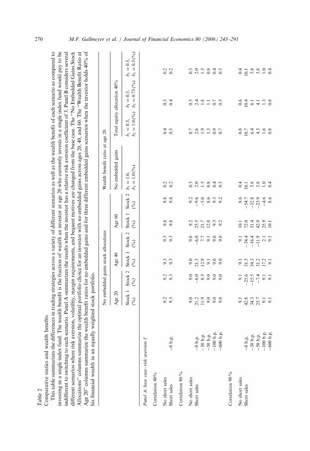
ARTICLE IN PRESS

Table

2

Comparativestatics

andwealthbenefits

Thistablesummarizesthedifferencesin

tradingstrategiesacross

avarietyofdifferentscenariosaswellasthewealthbenefitofeach

scenarioascomparedto

investingin

asingleindex

fund.Thewealthbenefitisthefractionofwealthaninvestoratage20whocurrentlyinvestsin

asingleindex

fundwould

payto

be

indifferentto

switchingto

each

scenario.PanelAsummarizestheresultswhen

theinvestorhasarelativerisk

aversioncoefficientof3.PanelBconsidersseveral

differentscenarioswhererisk

aversion,volatility,margin

requirem

ents,andbequestmotives

are

changed

from

thebase

case.The‘‘NoEmbedded

GainsStock

Allocations’’columnssummarize

theoptimalportfoliochoiceforaninvestorwithnoem

bedded

gainsacross

ages

20,40,and60.The‘‘WealthBenefitRatioat

Age20’’columnssummarize

thewealthbenefitratiosfornoem

bedded

gainsandforthreedifferentem

bedded

gainsscenarioswhen

theinvestorholds40%

of

hisfinancialwealthin

anequallyweightedstock

portfolio.

Noem

bedded

gainsstock

allocations

Wealthbenefitratioatage20

Age20

Age40

Age60

Noem

bedded

gains

Totalequityallocation40%

Stock

1Stock

2Stock

1Stock

2Stock

1Stock

2b1¼

1:0,

b1¼

0:5,

b1¼

0:5,

b1¼

0:5,

(%)

(%)

(%)

(%)

(%)

(%)

b2¼

1:0ð%Þ

b2¼

1:0ð%Þ

b2¼

0:75ð%Þ

b2¼

0:5ð%Þ

Pa

nel

A:

base

case

–ri

skave

rsio

n3

Correlation40%

Noshort

sales

9.2

9.2

9.3

9.3

9.8

9.8

0.2

0.4

0.3

0.2

Short

sales

�0b.p.

9.3

9.3

9.3

9.3

9.8

9.8

0.2

0.5

0.4

0.2

Correlation80%

Noshort

sales

9.0

9.0

9.0

9.0

9.2

9.2

0.3

0.7

0.5

0.3

Short

sales

�0b.p.

21.2

�6.0

21.5

�6.0

25.5

�9.6

2.0

2.6

2.4

2.0

�30b.p.

11.9

8.5

12.9

7.7

21.7

�5.0

1.5

1.9

1.8

1.5

�50b.p.

9.0

9.0

9.1

9.1

12.0

8.6

0.8

1.3

1.1

0.8

�100b.p.

9.0

9.0

9.0

9.0

9.3

9.3

0.4

0.9

0.7

0.4

�600b.p.

9.0

9.0

9.0

9.0

9.2

9.2

0.3

0.7

0.5

0.3

Correlation90%

Noshort

sales

9.1

9.1

9.1

9.1

10.1

8.6

0.4

0.8

0.6

0.4

Short

sales

�0b.p.

42.8

�25.6

51.3

�34.4

72.0

�54.7

10.1

10.7

10.4

10.1

�30b.p.

34.3

�15.5

34.3

�16.4

51.4

�32.8

5.8

6.4

6.1

5.8

�50b.p.

25.7

�7.4

31.2

�11.9

42.9

�23.9

3.8

4.3

4.1

3.8

�100b.p.

9.1

9.1

17.2

2.1

25.9

�4.6

1.0

1.6

1.3

1.0

�600b.p.

9.1

9.1

9.1

9.1

10.1

8.6

0.4

0.8

0.6

0.4


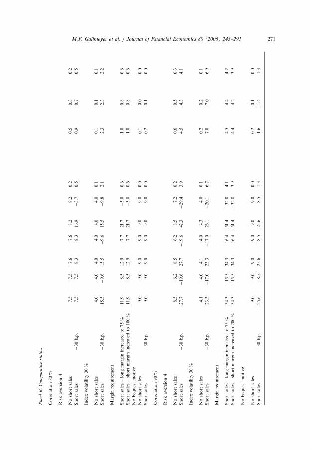
ARTICLE IN PRESS

Pa

nel

B:

Com

para

tive

stati

cs

Correlation80%

Riskaversion4

Noshort

sales

7.5

7.5

7.6

7.6

8.2

8.2

0.2

0.5

0.3

0.2

Short

sales

�30b.p.

7.5

7.5

8.3

8.3

16.9

�3.7

0.5

0.9

0.7

0.5

Index

volatility

30%

Noshort

sales

4.0

4.0

4.0

4.0

4.0

4.0

0.1

0.1

0.1

0.1

Short

sales

�30b.p.

15.5

�9.6

15.5

�9.6

15.5

�9.8

2.1

2.3

2.3

2.2

Margin

requirem

ent

Short

sales–longmargin

increasedto

75%

11.9

8.5

12.9

7.7

21.7

�5.0

0.6

1.0

0.8

0.6

Short

sales–short

margin

increasedto

100%

11.9

8.5

12.9

7.7

21.7

�5.0

0.6

1.0

0.8

0.6

Nobequestmotive

Noshort

sales

9.0

9.0

9.0

9.0

9.0

9.0

0.0

0.1

0.0

0.0

Short

sales

�30b.p.

9.0

9.0

9.0

9.0

9.0

9.0

0.0

0.2

0.1

0.0

Correlation90%

Riskaversion4

Noshort

sales

8.5

6.2

8.5

6.2

8.5

7.2

0.2

0.6

0.5

0.3

Short

sales

�30b.p.

27.7

�19.6

27.7

�19.6

42.3

�29.4

3.9

4.5

4.3

4.1

Index

volatility

30%

Noshort

sales

4.1

4.0

4.1

4.0

4.3

4.0

0.1

0.2

0.2

0.1

Short

sales

�30b.p.

23.3

�17.0

23.3

�17.0

26.1

�20.1

6.7

7.0

7.0

6.9

Margin

requirem

ent

Short

sales–longmargin

increasedto

75%

34.3

�15.5

34.3

�16.4

51.4

�32.8

4.1

4.5

4.4

4.2

Short

sales–short

margin

increasedto

200%

34.3

�15.5

34.3

�16.4

51.4

�32.8

3.9

4.4

4.2

3.9

Nobequestmotive

Noshort

sales

9.0

9.0

9.0

9.0

9.0

9.0

0.0

0.2

0.1

0.0

Short

sales

�30b.p.

25.6

�8.5

25.6

�8.5

25.6

�8.5

1.3

1.6

1.4

1.3


ARTICLE IN PRESS


literature (Constantinides, 1983; Dammon et al., 2001b; Garlappi et al., 2001), we donot measure the wealth benefits relative to an accrual-based capital gain taxationsystem where all gains and losses are marked to market annually. Instead, our wealthbenefit ratio is meant to capture the marginal contribution to investor welfare ofswitching from a single index fund to a portfolio of risky stocks—measuring thewealth benefit relative to an accrual-based tax would lead to significantly higherwealth benefits. We present results when the initial portfolio has no embedded gainsas well as when the investor is initially overexposed to equity with embedded gains.Specifically, we examine the wealth benefit for an investor who holds 40% of hisfinancial wealth in an equally weighted equity portfolio under three differentembedded gain scenarios.

When short sales are prohibited, the wealth benefits from Panels A and B show astriking feature—the benefits of trading the components of the index are very small.From Panel A, the wealth benefit ratio of trading each stock separately with a shortsale constraint is 0.2%, 0.3%, and 0.4% for stock return correlations of 40%, 80%,and 90%, respectively, with no embedded gains. Additionally, the wealth benefits aresmall across the comparative static exercises of Panel B. Given the small differencesin the simulation results in Table 1 between the one- and two-stock cases with noshort sales, the small wealth benefits are not necessarily surprising.

When short sales are allowed, the wealth benefits increase relative to the case withno short sales at age 20, but are sensitive to the correlation between the two stocks.At 90% correlation, wealth benefit ratios are 10.1%, 5.8%, and 3.8% with noembedded gains and shorting costs of 0, 30, and 50 basis points, respectively. Whenmore price risk is introduced when engaging in a short position by dropping thestock correlation to 80%, the wealth benefit drops to 2.0%, 1.5%, and 0.8% forrespective shorting costs of 0, 30, and 50 basis points. Although these are smallerthan the 90% correlation setting, they are significantly larger than the wealth benefitratios with no short sales. When the shorting costs increase to a rate faced by a smallinvestor (600 basis points), the welfare benefits of shorting disappear, leading to thesame welfare benefits as the constrained case. In summary, the bulk of the economicbenefits of splitting the index into its components are through short selling whenshorting costs are not too high—short-sale-constrained portfolios only lead to smallwealth benefit increases. The optimal consumption strategies (not reported) underthe different stock trading scenarios mirror the welfare results in that allowing shortselling with low shorting costs leads to higher consumption rates. In addition, whenembedded gains are large, the investor reduces his consumption slightly due to aneffectively lower wealth today given future tax liabilities.

To understand the sensitivity of the results to different model parameters, Panel Bof Table 2 considers several variations on the base case set of parameters when thereturn correlation between the two stocks is 80% or 90%. The cases of no short salesand short sales with a shorting cost of 30 basis points are again considered. Theoptimal stock allocations with no embedded gains are presented for ages 20, 40, and60 along with the wealth benefit ratios for age 20.

First, the relative risk aversion is increased to 4 from the base case of 3. Notsurprisingly, the total equity positions are decreasing in risk aversion. Given smaller

ARTICLE IN PRESS


equity positions in the portfolio for higher risk aversions, the wealth benefit ratiosare slightly lower than the base case. Second, increasing the index volatility to 30%leads to lower pre-tax Sharpe ratios and hence lower equity investments. However, incontrast to when the risk aversion is increased, the wealth benefit ratios actuallyincrease when the index volatility is 30%. This occurs because the value of the taxloss selling option in the portfolio increases in volatility as in Constantinides (1983).

We also consider tightening either the long margin requirement to 75% from 50%or the short margin requirement to 200% from 150%. From Panel B of Table 2, theoptimal equity positions with no embedded gains are not influenced up to age 60 bytightening the margin constraints. However, the trading strategy is influenced at laterages. To gain insight on how frequently the margin constraints bind, we use oursimulation analysis for the 80% return correlation case where we tabulate thefrequency of binding margin constraints in our base case parameters with shortingcosts of 30 basis points. From the simulation starting at age 20 with no embeddedgains, the margin constraints never bind before age 70. Along a path starting at age20, the unconditional probability that the constraint eventually binds is 4.3%. If thelong margin requirement increases to 75% from 50%, this probability increases to8.0%. If instead the short margin requirement increases to 200% from 150%, theunconditional probability that the margin constraint eventually binds is 15.2%. Thistranslates into lower wealth benefit ratios as can be seen in the table.

Finally, we examine the role of the bequest motive on optimal behavior and on thewealth benefits. The last entry in Panel B of Table 2 considers the case when theinvestor has no bequest motive. At a stock return correlation of 80%, the stockallocations with no embedded gains are identical whether or not short sales areallowed. With no bequest motive, wealth benefits are also significantly reduced. Atthe 80% correlation, no wealth benefit is larger than 0.2%. However, this is stilllarger than the case with no short sales due to the investor optimally employing theimperfect shorting-the-box strategy in some scenarios when overexposed to onestock with a large embedded gain. When the return correlation increases to 90%, theinvestor again engages in the trading flexibility strategy when short selling is allowed.By doing so, the investor can defer realizing capital gains leading to wealth benefitsno smaller than 1.3% at age 20.

5. Tax management through derivative trading

While we have established that large investors who pay low shorting costs arebetter off trading components of an index than the index itself, our results alsoindicate that small investors with large shorting costs are effectively precluded fromfollowing the tax management strategies we have described. In this section wepresent a different strategy that most investors would be able to implement, restoringthe ability of investors to balance gains in one stock with losses in another tominimize realized capital gains when portfolio rebalancing.

This strategy is related to the one discussed in Constantinides and Scholes (1980),where an investor uses derivatives to defer capital gain taxes. We investigate the case

ARTICLE IN PRESS


where the investor trades in one stock while holding a one-year, at-the-money putoption on another highly correlated stock. We focus on trading a put option on astock with high correlation but not actually held by the investor since buying putoptions against positions owned by an investor can be viewed as a sale for taxpurposes. Holding a put is similar to the tax management strategies we described forthe wealthy investor who can sell short at a low cost since a put can be decomposedinto a short position in the stock and an investment in the money market account.The put generates gains (losses) when the stock tends to generate losses (gains). Sincethe put option is reset every trading period, this setting is especially tractable sincethe only state variables needed to characterize the investor’s portfolio choice at aparticular age are the stock’s basis and position entering the trading period. Theunderlying stocks have the same characteristics as in the cases we have considered sofar. The parameters used are the same as described in Section 2.4. We also assumethat the investor is precluded from short positions in any security.

Pricing the put option by no arbitrage is complicated by the taxes in our economy.When the participants in the option market are differentially taxed on the option’scash flows, it is not immediately clear who is the marginal pricer of the option giventhat different valuations can arise for different tax rates. These issues are discussed indetail in Schaefer (1982), Dybvig and Ross (1986), Dammon and Green (1987), andRoss (1987). For our portfolio choice problem with a put option, we assume that theprice of the option is set by an investor who faces realized capital gain taxation andcan costlessly short. The option price is determined by using standard replicationarguments on the option’s after-tax payoff. The after-tax valuation actually leads toa higher price than if the pre-tax cash flows are used to value the option. This isbecause the put option generates a positive after-tax cash flow when the stock priceincreases due to the capital loss write-off from the put option. By using this higherput price, our calculated wealth benefits of trading the put are understated ascompared to a put option valued using pre-tax cash flows. The modifications of ourearlier model to incorporate investing in a put option and computing its price areprovided in Appendix B.

Table 3 describes the optimal strategy as well as the welfare benefits for differentcorrelations for a 20-year-old investor. Panel A presents the optimal trading strategywhen the only risky security is the stock index combining the two individual stocks inan equally weighted portfolio. Panel B documents optimal portfolio choice acrossdifferent correlations between the two stocks when the risky investment opportunityset consists of stock 1 and the put written against stock 2. For each correlationbetween the two stocks, the top line gives the optimal portfolio when the portfolioinitially contains no embedded gains. The other four lines describe optimal portfoliochoice when the investor initially holds 20% or 40% of his wealth in stock 1 withbasis-price ratio of either 0.8 or 0.4.

By trading in the put, the investor is able to engage in both the trading flexibilityand imperfect shorting-the-box strategies from the previous section. From the table,the investor uses the put to construct a trading flexibility strategy when he initiallyholds no embedded gains in his portfolio. When the stock return correlation is 90%with no embedded gains in the portfolio, the investor places 0.6% of his wealth in the

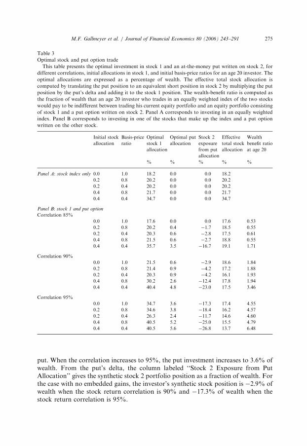
ARTICLE IN PRESS

Table 3

Optimal stock and put option trade

This table presents the optimal investment in stock 1 and an at-the-money put written on stock 2, for

different correlations, initial allocations in stock 1, and initial basis-price ratios for an age 20 investor. The

optimal allocations are expressed as a percentage of wealth. The effective total stock allocation is

computed by translating the put position to an equivalent short position in stock 2 by multiplying the put

position by the put’s delta and adding it to the stock 1 position. The wealth-benefit ratio is computed as

the fraction of wealth that an age 20 investor who trades in an equally weighted index of the two stocks

would pay to be indifferent between trading his current equity portfolio and an equity portfolio consisting

of stock 1 and a put option written on stock 2. Panel A corresponds to investing in an equally weighted

index. Panel B corresponds to investing in one of the stocks that make up the index and a put option

written on the other stock.

Initial stock Basis-price Optimal Optimal put Stock 2 Effective Wealth

allocation ratio stock 1 allocation exposure total stock benefit ratio

allocation from put allocation at age 20

allocation

% % % % %

Panel A: stock index only 0.0 1.0 18.2 0.0 0.0 18.2

0.2 0.8 20.2 0.0 0.0 20.2

0.2 0.4 20.2 0.0 0.0 20.2

0.4 0.8 21.7 0.0 0.0 21.7

0.4 0.4 34.7 0.0 0.0 34.7

Panel B: stock 1 and put option

Correlation 85%

0.0 1.0 17.6 0.0 0.0 17.6 0.53

0.2 0.8 20.2 0.4 �1.7 18.5 0.55

0.2 0.4 20.3 0.6 �2.8 17.5 0.61

0.4 0.8 21.5 0.6 �2.7 18.8 0.55

0.4 0.4 35.7 3.5 �16.7 19.1 1.71

Correlation 90%

0.0 1.0 21.5 0.6 �2.9 18.6 1.84

0.2 0.8 21.4 0.9 �4.2 17.2 1.88

0.2 0.4 20.3 0.9 �4.2 16.1 1.93

0.4 0.8 30.2 2.6 �12.4 17.8 1.94

0.4 0.4 40.4 4.8 �23.0 17.5 3.46

Correlation 95%

0.0 1.0 34.7 3.6 �17.3 17.4 4.55

0.2 0.8 34.6 3.8 �18.4 16.2 4.57

0.2 0.4 26.3 2.4 �11.7 14.6 4.60

0.4 0.8 40.5 5.2 �25.0 15.5 4.79

0.4 0.4 40.5 5.6 �26.8 13.7 6.48


put. When the correlation increases to 95%, the put investment increases to 3.6% ofwealth. From the put’s delta, the column labeled ‘‘Stock 2 Exposure from PutAllocation’’ gives the synthetic stock 2 portfolio position as a fraction of wealth. Forthe case with no embedded gains, the investor’s synthetic stock position is �2:9% ofwealth when the stock return correlation is 90% and �17:3% of wealth when thestock return correlation is 95%.

ARTICLE IN PRESS


The investor also uses the put to construct an imperfect form of the shorting-the-box strategy. For example, when the return correlation between the two stocks is90%, the investor places 4.8% of his wealth in the put (a synthetic position of �23%of his wealth in stock 2) and does not trade his stock 1 position when he initiallyholds 40% of his wealth in equity with a basis-price ratio of 0:4. By so doing, theinvestor’s effective total equity exposure falls to 17.5% of wealth.11 If instead theinvestor holds only the index (Panel A), his equity exposure only falls to 34.7% ofwealth.

We note that the welfare benefits at age 20 of investing in a put are sensitive to thereturn correlation as well as to the pricing of the put.12 However, the put’s welfarebenefits are comparable to the welfare benefits of an investor who can sell shortsubject to low shorting costs even using the conservative valuation of the put. Forexample, with no embedded gains, the wealth benefit of investing in the put is 0.53%,1.84%, and 4.55% across return correlations of 85%, 90%, and 95%, respectively. Ifinstead we assume the put is priced by no arbitrage by a tax-exempt investor leadingto a lower initial price, the respective wealth benefits (not reported in the table)across the three previous correlations are significantly higher: 4.6%, 7.6%, and12.4% of wealth. This analysis indicates that investing in puts is a viable alternativefor the tax management of capital gains for investors who face large shorting costs.

6. Conclusion

In selecting an optimal consumption-investment strategy, investors need tobalance two considerations: present and future tax selling costs and diversificationboth within the equity portfolio and between bonds and equity. In contrast toConstantinides (1983) where shorting the box is allowed, the consumption-portfolioproblem in our paper is not independent of tax trading concerns.

We have shown that with shorting prohibited, the investor’s optimal strategy issimilar to the case of one risky stock with the notable exception that tax trading costscan lead to the investor holding an undiversified equity position. With no embeddedgains, however, the welfare benefit of being able to trade the two stocks separately asopposed to holding an index fund that combines the two is small.

Allowing short sales leads to dramatically different behavior. The investor can useshort selling both as an ex ante and as an ex post tax-efficient mechanism to reduceoverall equity exposure and tax-related trading costs. The combination of lowertrading costs and the ability to scale back overexposure to equity dominates the lossin diversification within the equity portion of the portfolio. Specifically, we describe a

11To compute the effective total stock allocation, we translate the position in the put to an equivalent

short position in the stock 2 by multiplying the put position by the put’s delta, i.e., its sensitivity to the

underlying stock price, and adding it to the stock 1 position.12The welfare benefits of investing in a put option are captured by the wealth benefit ratio calculated in

the same fashion as in the two-stock case, namely, the fraction of wealth an age 20 index investor would

pay to be indifferent between his current index fund investment or a risky portfolio consisting of stock 1

and a put option written on stock 2.

ARTICLE IN PRESS


novel ex ante strategy that an investor can use, the trading flexibility strategy, wherehe shorts one of the stocks even when no stock has an embedded capital gain. Expost, he can use an imperfect form of shorting the box. Interestingly, this shortingbehavior commonly occurs when an otherwise identical but short-sale-constrainedinvestor would hold strictly positive investments in all stocks. This behavior arisesbecause the investor’s net tax benefit of selling shares is not monotonic in the tradingstrategy when shorting is allowed.

Not surprisingly, the tax benefit from shorting depends on the shorting cost that theinvestor faces. For a large investor, the benefit of shorting outweighs the cost. Forsmall investors who get a low rebate rate on their short sale proceeds, the benefit isreduced. For a high enough shorting cost, a small investor will no longer use thetrading flexibility strategy. We have proposed buying puts as an alternative mechanismfor utilizing the trading flexibility strategy. The welfare benefit associated with usingputs is similar to the one obtained with equity short sales at a low shorting cost,making put-based strategies a viable tax management tool even for smaller investors.

While we have restricted the analysis to two risky stocks and a money marketaccount for tractability, we expect similar results to hold when the investor is allowedto hold more than two stocks. To manage tax trading costs, the investor could usethe trading flexibility and imperfect shorting-the-box strategies on highly correlatedsets of stocks within the portfolio.

Appendix A. Investor consumption-portfolio problem with two stocks

The mathematical description of the framework described in Section 2 is nowpresented. Our two risky stock model is an extension of the single-stock setting ofDammon et al. (2001b) that accommodates costly short selling with marginconstraints. We consider a discrete-time economy with trading dates t ¼ 0; . . . ;T inwhich an investor endowed with initial wealth in the assets chooses an optimalconsumption and investment policy in the presence of realized capital gain taxation.We assume that the investor lives for at most T periods and faces a positiveprobability of death each period. The probability that an investor lives up to periodt, 0otoT , is given by the survival function HðtÞ ¼ expð�

Ptn¼0 lnÞ where ln is the

single-period hazard rate for period n where we assume ln40; 8n, and lT ¼ 1. Thisimplies 0pHðtÞo1; 8 0ptoT . At T, the investor exits the economy, implyingHðTÞ ¼ 0. We assume that the investor makes annual decisions starting at age 20corresponding to t ¼ 0 with certain exit from the economy at age 100 implyingT ¼ 80. The hazard rates ln are calibrated to the 1990 U.S. Life Table compiled bythe National Center for Health Statistics to compute the survival function HðtÞ fromages 20 (t ¼ 0) to 99 (t ¼ 79).

A.1. Security market

The market consists of three assets: a riskless money market account and two riskydividend-paying stocks. The riskless money market account with time t price S0ðtÞ

ARTICLE IN PRESS


pays a continuously compounded pre-tax interest rate r. The price dynamics over thetime interval Dt are

S0ðtþ DtÞ

S0ðtÞ¼ expðrDtÞ. (A.1)

The two risky stocks with time t ex-dividend prices SiðtÞ; i 2 f1; 2g; pay pre-taxdividends of diSiðtÞ at time tþ Dt where di is each stock’s dividend yield. The pre-taxex-dividend stock prices follow binomial processes with price dynamics over the timeinterval Dt given by

Siðtþ DtÞ

SiðtÞ¼ exp mi �

1

2s2i

� �Dt þ si

ffiffiffiffiffiDt

p~zi

� �; i 2 f1; 2g, (A.2)

where ~zi is a binomial random variable taking the two values �1 and 1 with ajoint probability distribution specified as pð~z1 ¼ 1; ~z2 ¼ 1Þ ¼ pð~z1 ¼ �1; ~z2 ¼ �1Þ ¼14ð1þ rÞ and pð~z1 ¼ 1; ~z2 ¼ �1Þ ¼ pð~z1 ¼ �1; ~z2 ¼ 1Þ ¼ 1

4ð1� rÞ where r is the

correlation between the two stock prices. For each stock, the quantity mi is theinstantaneous capital gain expected growth rate and si is the instantaneous volatility.We also assume that Dt ¼ 1 matching the trading interval of the investor in the economywith time units measured in years. A trading strategy from time t to tþ 1 in the moneymarket account and two stocks is given by ðaðtÞ; y1ðtÞ; y2ðtÞÞ where aðtÞ denotes theshares of the money market held and yiðtÞ denotes the shares of stock i held.

A.2. Capital gain taxation

Realized capital gains and losses are subject to a constant capital gain tax rate oftC where we assume that the full proceeds of capital losses can be used. Given thatour investor trades at an annual frequency, no distinction is made between long- andshort-term capital gains.

The tax basis for computing capital gains or losses is calculated as a weighted-average purchase price for tractability. Let Biðtþ 1Þ denote the nominal tax basis ofstock i after trading at time tþ 1. If long stock at date tþ 1, yiðtþ 1Þ40, the stockbasis evolves as

Biðtþ 1Þ ¼

Siðtþ 1Þ if yiðtÞp0 or BiðtÞSiðtþ1Þ

41;

BiðtÞyiðtÞ þ ðyiðtþ 1Þ � yiðtÞÞþSiðtþ 1Þ

yiðtÞ þ ðyiðtþ 1Þ � yiðtÞÞþ otherwise;

8>><>>:

(A.3)

where xþ ¼nmaxðx; 0Þ. If short stock at date tþ 1, yiðtþ 1Þo0, the stock basis

evolves as

Biðtþ 1Þ ¼

Siðtþ 1Þ if yiðtÞX0 or BiðtÞSiðtþ1Þ

o1;

BiðtÞjyiðtÞj þ ðjyiðtþ 1Þj � jyiðtÞjÞþSiðtþ 1Þ

jyiðtÞj þ ðjyiðtþ 1Þj � jyiðtÞjÞþ

otherwise:

8>><>>:

(A.4)

ARTICLE IN PRESS


If yiðtþ 1Þ ¼ 0, the basis resets to the current stock price, Biðtþ 1Þ ¼ Siðtþ 1Þ. Insummary, stock i’s basis resets to the current stock price when the position changessign from the previous period or when the investor is tax-loss selling. For stock i

trades that increase the magnitude of the current position, the basis evolves as ashare-weighted average of the previous basis and the current share price given by the‘‘otherwise’’ case in (A.3) and (A.4). Note that this case also covers the scenariowhen the investor reduces the magnitude of his stock i position without changing itssign, implying an unchanged basis.

Any realized capital gains or losses are subject to capital gain taxation. Severaldifferent types of trades trigger realized capital gains or losses. First, tax-loss selling(denoted TL) induces realized capital losses. The tax-loss selling contribution to timet capital gain taxation is denoted as FTL

CGðtÞ and given by

FTLCGðtÞ ¼ tC

X2i¼1

ðSiðtÞ � Biðt� 1ÞÞyiðt� 1Þ

�ð1fyiðt�1Þ40; Biðt�1Þ4SiðtÞg þ 1fyiðt�1Þo0; Biðt�1ÞoSiðtÞgÞ, ðA:5Þ

where the first (second) indicator function denotes tax-loss selling when holding along (short) position. Second, since the investor is precluded from shorting the box,closing out a time t� 1 position and investing at time t in the position of oppositesign for that stock triggers a taxable event. Such a trade is denoted CP for ‘‘closeposition.’’ The time t realized capital gain taxes, FCP

CGðtÞ, from such a trade are

FCPCGðtÞ ¼ tC

X2i¼1

ðSiðtÞ � Biðt� 1ÞÞyiðt� 1Þ

�ð1fyiðtÞp0; yiðt�1Þ40; Biðt�1ÞpSiðtÞg þ 1fyiðtÞX0; yiðt�1Þo0; Biðt�1ÞXSiðtÞgÞ. ðA:6Þ

The first (second) indicator function in (A.6) captures moving from a long (short)position to a short (long) position in stock i when the t� 1 position contains acapital gain. The capital loss case of closing out a t� 1 position is captured by (A.5).Finally, when the investor reduces the size of his t� 1 position at time t denotedRP, capital gain taxes are assessed. Their contribution to time t capital gain taxes,FRP

CGðtÞ, is

FRPCGðtÞ ¼ tC

X2i¼1

ðSiðtÞ � Biðt� 1ÞÞ

�ð1fyiðtÞ40; yiðt�1ÞX0; Biðt�1ÞpSiðtÞgðyiðt� 1Þ � yiðtÞÞþ

� 1fyiðtÞo0; yiðt�1Þp0; Biðt�1ÞXSiðtÞgðyiðtÞ � yiðt� 1ÞÞþÞ, ðA:7Þ

where the first (second) indicator function captures reducing a long (short) positionin stock i. In summary, the total capital gain taxes paid at time t, FCGðtÞ, consistingof realized capital gains/losses from tax-loss selling (TL), closing positions (CP), andreducing positions (RP), are

FCGðtÞ ¼ FTLCGðtÞ þ FCP

CGðtÞ þ FRPCGðtÞ. (A.8)

ARTICLE IN PRESS


If death occurs at some time t0, all capital gain taxes are forgiven implyingFCGðt

0Þ ¼ 0.

A.3. Admissible trading strategies

We now define the set of admissible trading strategies when the investor can shortstock in a margin account. To model the margin requirements, we assume that thereis no difference between initial and maintenance margins. Explicitly incorporatingmaintenance margins into our optimization problem would lead to the problembeing numerically intractable. The quantity 1þ k�X1 denotes the proportionalmargin requirement on short stock positions satisfied by cash or other securities and1� kþ 2 ½0; 1� denotes the fraction of the value of a long position that is marginable.From Regulation T on initial margin requirements, this implies k� ¼ kþ ¼ 0:5.Denoting aCðtÞ as the amount of money in cash collateral at time t, short sellingbounds this amount from below by

aCðtÞX1:02X2i¼1

yiðtÞ�SiðtÞ, (A.9)

where x�9maxð�x; 0Þ and we have assumed that the required cash collateral is102% of the value of the short position. The margin requirements impose arestriction that the investor can only borrow using as collateral cash or stock inexcess of the required margin. This implies a lower bound on the dollar amountinvested in the money market account,

aðtÞS0ðtÞX� aC � ð1þ k�ÞX2i¼1

yiðtÞ�SiðtÞ

þð1� kþÞX2i¼1

yiðtÞþSiðtÞ

!. ðA:10Þ

The term aC � ð1þ k�ÞP2

i¼1 yiðtÞ�SiðtÞ is the additional margin needed in other

securities after taking into account the cash collateral when short selling. The termð1� kþÞ

P2i¼1 yiðtÞ

þSiðtÞ is the marginable value of all long stock positions.Given the money market account’s return always dominates the return received on

cash collateral, Eq. (A.9) always holds with equality, so cash collateral is completelydetermined by the size of the investor’s short position. The bound on the moneymarket account given by (A.10) can also be simplified by appealing to the time t self-financing condition. Let W ðtÞ denote the time t wealth before portfolio rebalancingand before any capital gain taxes are paid, but after dividend and interest taxes arepaid. Given that no resources are lost when rebalancing the portfolio at time t,

W ðtÞ ¼ aC þ aðtÞS0ðtÞ þX2i¼1

yiðtÞSiðtÞ þ CðtÞ þ FCGðtÞ, (A.11)

where CðtÞ40 is the time t consumption. Solving the above expression for moneymarket holdings and using

P2i¼1 yiðtÞSiðtÞ ¼

P2i¼1 yiðtÞ

þSiðtÞ �P2

i¼1 yiðtÞ�SiðtÞ,

ARTICLE IN PRESS


Eq. (A.10) simplifies to

W ðtÞ � CðtÞ � FCGðtÞXk�X2i¼1

yiðtÞ�SiðtÞ þ kþ

X2i¼1

yiðtÞþSiðtÞ. (A.12)

Dividend and interest income are taxed as ordinary income at the constant rate tD.Each period, the investor pays taxes on his dividend and interest income. The totaltaxes paid on this income at time t is

FDðtÞ ¼ tDaðt� 1ÞS0ðt� 1Þ ðexpðrÞ � 1Þ

þ tDð1:02ÞX2i¼1

yiðt� 1Þ�Siðt� 1ÞðexpðrcÞ � 1Þ

þ tD

X2i¼1

yiðt� 1ÞSiðt� 1Þdi. ðA:13Þ

The first term in (A.13) is the income tax due to money market interest. The secondterm captures the taxes on any interest on cash collateral while the last term accountsfor the dividend taxes. If the investor dies at time t, interest and dividend taxes arestill paid.

Again letting W ðtþ 1Þ denote the time tþ 1 wealth before portfolio rebalancingand any capital gain taxes are paid, but after dividend and interest taxes are paid,W ðtþ 1Þ is given by

W ðtþ 1Þ ¼ aðtÞS0ðtÞðð1� tDÞ expðrÞ þ tDÞ

þ ð1:02ÞX2i¼1

yiðtÞ�SiðtÞðð1� tDÞ expðrcÞ þ tDÞ

þX2i¼1

yiðtÞðSiðtþ 1Þ þ SiðtÞdið1� tDÞÞ, ðA:14Þ

where (A.13) has been substituted. Substituting (A.11) into (A.14) gives the dynamicafter-tax wealth evolution of the investor,

W ðtþ 1Þ ¼ W ðtÞ �X2i¼1

yiðtÞSiðtÞ � CðtÞ � FCGðtÞ

� ð1:02ÞX2i¼1

yiðtÞ�SiðtÞ

!ðð1� tDÞ expðrÞ þ tDÞ

þ ð1:02ÞX2i¼1

yiðtÞ�SiðtÞðð1� tDÞ expðrcÞ þ tDÞ

þX2i¼1

yiðtÞðSiðtþ 1Þ þ SiðtÞdið1� tDÞÞ.

ðA:15Þ

ARTICLE IN PRESS


An admissible trading strategy is a consumption and security trading policyðC; a; y1; y2Þ such that for all t, CðtÞX0, W ðtÞX0, and Eqs. (A.9)–(A.15) are satisfied.The set of admissible trading strategies is denoted A.

A.4. Investor’s objective

The investor’s objective is to maximize his discounted expected utility of reallifetime consumption and final-period wealth at the time of death by choosing anadmissible trading strategy given an initial endowment. If death occurs on date t, theinvestor’s assets totalling W ðtÞ are liquidated and used to purchase a perpetuity thatpays to his heirs a constant real after-tax cash flow of R�W ðtÞ each period startingon date tþ 1. The quantity R� is the one-period after-tax real riskless interest ratecomputed using simple compounding. In terms of the instantaneous nominal risklessmoney market rate r and the instantaneous inflation rate i, R� is defined by

R� ¼ ðð1� tDÞ expðrÞ þ tDÞ expð�iÞ � 1.

Under the assumption that the investor and his heirs have identical preferences of theconstant relative risk aversion (CRRA) form with a coefficient of relative riskaversion of g and a common time preference parameter b, the investor’s optimizationproblem is given by

maxðC;a;y1;y2Þ2A

EXT

t¼0

bt HðtÞ

1� gðexpð�itÞCðtÞÞ1�g

("

þHðt� 1Þ �HðtÞ

1� g

X1s¼tþ1

bs�tðexpð�itÞR�W ðtÞÞ1�g

)#ðA:16Þ

subject to (A.9)–(A.15) where b is the time-preference parameter. The objectivefunction captures the expected utility of future real consumption as well as thebequest motive to the investor’s heirs. In Section 4, we consider one scenario wherethe investor has no bequest motive. In this setting, the last term is eliminated fromthe above objective function.

SinceP1

s¼tþ1 bs�t¼

b1�b, the investor’s objective function simplifies, leading to the

optimization problem

maxðC;a;y1;y2Þ2A

EXT

t¼0

bt HðtÞ

1� gðexpð�itÞCðtÞÞ1�g

�"

þHðt� 1Þ �HðtÞ

1� gb

1� bðexpð�itÞR�W ðtÞÞ1�g

�#ðA:17Þ

subject to (A.9) through (A.15).

A.5. A convenient change of variables

As in a no-tax portfolio choice problem with CRRA preferences, the optimizationproblem (A.17) is homogeneous in wealth, and thus independent of the investor’s

ARTICLE IN PRESS


initial wealth. To show that wealth is not needed as a state variable when solving(A.17), we express the optimization problem’s controls as being proportional to timet wealth W ðtÞ before trade has occurred but after dividend and interest taxes havebeen paid. We define

piðtÞ ¼n SiðtÞyiðt� 1Þ

W ðtÞ; piðtÞ ¼

n SiðtÞyiðtÞ

W ðtÞ, (A.18)

where piðtÞ and piðtÞ are the proportions of stock i owned entering and leaving periodt, with respect to time t wealth W ðtÞ. Since we allow for short sales in ourformulation, it is possible that financial wealth W ðtÞ no longer remains positiveimplying that it is not possible to define portfolio weights. However, the investor willnever choose a trading strategy that leads to a non-positive wealth at any time givenour utility function choice, the bequest motive, and the positive probability of deathover each period.

Using (A.18), it is useful to express the basis BiðtÞ as a basis-price ratiobiðtþ 1Þ ¼

nBiðtÞ=Siðtþ 1Þ. Using (A.3), if long stock at date t, piðtÞ40, the basis-price

ratio evolves as

biðtþ 1Þ ¼

SiðtÞ

Siðtþ 1Þif piðtÞp0 or biðtÞ41;

biðtÞpiðtÞ þ ðpiðtÞ � piðtÞÞþ

Siðtþ1ÞSiðtÞðpiðtÞ þ ðpiðtÞ � piðtÞÞ

þÞ

otherwise:

8>>>><>>>>:

(A.19)

If short stock at date t, piðtÞo0, the stock basis-price ratio evolves as

biðtþ 1Þ ¼

SiðtÞ

Siðtþ 1Þif piðtÞX0 or biðtÞo1;

biðtÞjpiðtÞj þ ðjpiðtÞj � jpiðtÞjÞþ

Siðtþ1ÞSiðtÞðjpiðtÞj þ ðjpiðtÞj � jpiðtÞjÞ

þÞ

otherwise:

8>>>><>>>>:

(A.20)

If piðtÞ ¼ 0, the basis-price ratio biðtþ 1Þ resets to the ratio of the time t and tþ 1stock price, biðtþ 1Þ ¼ SiðtÞ=Siðtþ 1Þ. The basis-price ratio at time tþ 1 can beexpressed as a function of the capital gain of stock i over one period Siðtþ 1Þ=SiðtÞ,the previous period’s basis-price ratio biðtÞ, and the equity proportions piðtÞ and piðtÞ.

Using the equity proportions and the basis-price ratios, the total capital gain taxespaid at time t, FCGðtÞ ¼ FTL

CGðtÞ þ FCPCGðtÞ þ FRP

CGðtÞ, can be written proportional toW ðtÞ, FCGðtÞ ¼W ðtÞfCGðtÞ where fCGðtÞ is independent of W ðtÞ, since eachcomponent of the total capital gain taxes paid can be written proportional to W ðtÞ:

FTLCGðtÞ ¼ tCW ðtÞ

X2i¼1

ð1� biðtÞÞpiðtÞ

�ð1fpiðtÞ40; biðtÞ41g þ 1fpiðtÞo0; biðtÞo1gÞ, ðA:21Þ

ARTICLE IN PRESS


FCPCGðtÞ ¼ tCW ðtÞ

X2i¼1

ð1� biðtÞÞpiðtÞ

�ð1fpiðtÞp0; piðtÞ40; biðtÞp1g þ 1fpiðtÞX0; piðtÞo0; biðtÞX1gÞ, ðA:22Þ

FRPCGðtÞ ¼ tCW ðtÞ

X2i¼1

ð1� biðtÞÞð1fyiðtÞ40; piðtÞX0; biðtÞp1gðpiðtÞ � piðtÞÞþ

� 1fpiðtÞo0; piðtÞp0; biðtÞX1gðpiðtÞ � piðtÞÞþÞ. ðA:23Þ

Given that no resources are lost when portfolio rebalancing and paying taxes,Eq. (A.11) implies that the money market investment aðtÞS0ðtÞ can be writtenproportional to W ðtÞ:

aðtÞS0ðtÞ ¼W ðtÞ 1� ð1:02ÞX2i¼1

piðtÞ��X2i¼1

piðtÞ � cðtÞ � fCGðtÞ

!, (A.24)

where cðtÞ9CðtÞ=W ðtÞ. Using (A.24), the margin requirement constraint given by(A.10) can be written independent of wealth:

1� cðtÞ � fCGðtÞXk�X2i¼1

piðtÞ�þ kþ

X2i¼1

piðtÞþ. (A.25)

The wealth evolution (A.15) can also be written proportional to W ðtÞ implying

W ðtþ 1Þ

W ðtÞ¼

1

1�P2

i¼1 piðtþ 1Þðð1� tDÞ expðrÞ þ tDÞ

"

� 1�X2i¼1

piðtÞ � cðtÞ � fCGðtÞ � ð1:02Þ

X2i¼1

piðtÞ�

!

þ ð1:02ÞX2i¼1

piðtÞ�ðð1� tDÞ expðrcÞ þ tDÞ þ

X2i¼1

piðtÞdið1� tDÞ

#.

ðA:26Þ

Additionally, the stock proportion evolution is given by

piðtþ 1Þ ¼Siðtþ 1Þ=SiðtÞpiðtÞ

W ðtþ 1Þ=W ðtÞ, (A.27)

a quantity that is independent of time t wealth. This evolution is needed in thedynamic programming formulation of the investor’s problem where pi is a statevariable and pi is a control variable.

ARTICLE IN PRESS


Using the principle of dynamic programming and substituting out W ðtÞ,the Bellman equation for the investor’s optimization problem (A.17) is givenby

V ðt; p1ðtÞ;p2ðtÞ; b1ðtÞ; b2ðtÞÞ

¼ maxcðtÞ;p1ðtÞ;p2ðtÞ

e�lt cðtÞ1�g

1� gþð1� e�lt ÞbðR�Þ1�g

ð1� bÞð1� gÞþ e�ltbEt

e�iW ðtþ 1Þ

W ðtÞ

� �ð1�gÞ"

�V ðtþ 1; p1ðtþ 1Þ;p2ðtþ 1Þ; b1ðtþ 1Þ; b2ðtþ 1ÞÞ

#, ðA:28Þ

for t ¼ 0; 1; . . . ;T � 1 subject to the wealth evolution (A.26), the margin requirementconstraint (A.25), and the stock proportion dynamics (A.27).

Appendix B. Investor consumption-portfolio problem with one stock and a put option

The modifications to the portfolio problem to incorporate investment in a putoption as described in Section 5 are now presented. The setup is the same asdescribed in Appendix A with the following notable exceptions.

B.1. Security market

The market consists of four assets every trading period: a riskless money marketaccount, two risky dividend-paying stocks, and a European put option that expiresin one trading period (one year in our analysis). The price dynamics of the risklessmoney market account and the two risky stocks are given by (A.1) and (A.2),respectively.

The investor trades in the riskless money market, stock 1, and the put option.He does not trade in stock 2; rather, the stock 2’s only role is to be the putoption’s underlying asset. The put option’s strike price is the current price of stock 2,S2ðtÞ. The put option’s price pðtÞ is presented below after discussing capital gaintaxation.

B.2. Capital gain taxation

As in the two-stock portfolio problem, realized capital gains and losses are subjectto a constant capital gain tax rate of tC where we assume that the full proceeds ofcapital losses can be used.

The calculation of the tax basis for the investment in stock 1 is simplified in thatwe assume the investor cannot short any security. The tax basis for stock 1 forcomputing capital gains or losses is calculated as a weighted-average purchase pricefor tractability. Let B1ðtþ 1Þ denote the nominal tax basis of stock 1 after trading at

ARTICLE IN PRESS


time tþ 1. The stock basis evolves as

B1ðtþ 1Þ ¼

S1ðtþ 1Þ if y1ðtÞ ¼ 0 orB1ðtÞ

S1ðtþ 1Þ41;

B1ðtÞy1ðtÞ þ ðy1ðtþ 1Þ � y1ðtÞÞþS1ðtþ 1Þ

y1ðtÞ þ ðy1ðtþ 1Þ � y1ðtÞÞþ

otherwise;

8>>><>>>:

(B.1)

where xþ ¼nmaxðx; 0Þ. If y1ðtþ 1Þ ¼ 0, the basis resets to the current stock price,

B1ðtþ 1Þ ¼ S1ðtþ 1Þ.The put option is treated as a cash-settled contract, so capital gain taxes are

assessed on the realized gain or loss on the put investment. By assuming that the putoption expires after one trading period, computing the capital gain on the putposition is simplified since the tax basis is always the purchase price of the put. Ifypðt� 1Þ is the number of units of the put owned from time t� 1 to t, the dollarcapital gain or loss from the put position at time t is ypðt� 1ÞðmaxfS2ðt� 1Þ �S2ðtÞ; 0g � pðt� 1ÞÞ since the strike price of the put is S2ðt� 1Þ.

Any realized capital gains or losses are subject to capital gain taxation. The capitalgain taxes FCGðtÞ at time t are

FCGðtÞ ¼ tCððS1ðtÞ � B1ðt� 1ÞÞy1ðt� 1Þ1fB1ðt�1Þ4S1ðtÞg

þ ðS1ðtÞ � B1ðt� 1ÞÞ1fB1ðt�1ÞpS1ðtÞgðy1ðt� 1Þ � y1ðtÞÞþ

þ ypðt� 1ÞðmaxfS2ðt� 1Þ � S2ðtÞ; 0g � pðt� 1ÞÞÞ, ðB:2Þ

where the first line calculates capital losses from tax-loss selling stock 1, the secondline calculates taxes from selling stock with a capital gain, and the last line calculatescapital gains or losses from the put option holdings. If death occurs at some time t0,all capital gain taxes are forgiven implying FCGðt

0Þ ¼ 0.

B.3. Valuation of the put option

The put option is priced by no arbitrage, but this is complicated by the taxes in oureconomy. When the participants in the option market are differentially taxed on theoption’s cash flows, it is not immediately clear who is the marginal pricer of theoption given different valuations can arise for different tax rates. These pricing withdifferential taxation issues are discussed in detail in Schaefer (1982), Dybvig andRoss (1986), Dammon and Green (1987), and Ross (1987). For our portfolio choiceexercise with a put option, we assume that the price of the option is set by an investorwho faces realized capital gain taxation and can costlessly short.

This price is determined by using standard replication arguments on the after-taxpayoffs of the option. Let a and y be the respective portfolio positions in the risklessmoney market and stock 2 used to replicate the put option’s after-tax payoff. Ifstock 2 increases (denoted S2ðtþ 1; UÞ) or decreases (denoted S2ðtþ 1; DÞ) nextperiod, the replicating portfolio’s after-tax payoff must match the put’s after-tax

ARTICLE IN PRESS


payoff, implying

tc pðtÞ

¼ ðð1� tcÞS2ðtþ 1; UÞ þ tcS2ðtÞ þ ð1� tDÞS2ðtÞd2Þy

þ S0ðtÞðð1� tDÞ expðrÞ þ tDÞa, ðB:3Þ

ð1� tcÞðS2ðtÞ � S2ðtþ 1; DÞÞ þ tc pðtÞ

¼ ðð1� tcÞS2ðtþ 1; DÞ þ tcS2ðtÞ þ ð1� tDÞS2ðtÞd2Þy

þ S0ðtÞðð1� tDÞ expðrÞ þ tDÞa. ðB:4Þ

By no arbitrage, the price of the put pðtÞmust equal the initial value of the replicatingportfolio,

pðtÞ ¼ S2ðtÞyþ S0ðtÞa. (B.5)

Given the parameters used for the price system, the put is only in the money if stock2 decreases over the next period. Solving (B.3)–(B.5) yields the put price pðtÞ as wellas the replicating strategy.

This valuation of the option actually leads to a higher price than if the pre-capitalgain tax cash flows are used to value the option by setting tc ¼ 0. In contrast to avaluation with no capital gain tax, the put option has a positive after-tax payoff oftc pðtÞ if the option expires out of the money. This payoff is the capital loss write-offfrom the put option. By using this higher put price, our calculated wealth benefits oftrading the put are understated as compared to a put option valued using pre-taxcash flows.

B.4. Admissible trading strategies

We now define the set of admissible trading strategies when the investor can investin stock 1, the put option, and the riskless money market account. Again, we assumethat the investor is prohibited from shorting any security. Dividend and interestincome are taxed as ordinary income at the constant rate tD. Each period, theinvestor pays taxes on his dividend and interest income. The total taxes paid on thisincome at time t is

FDðtÞ ¼ tDaðt� 1ÞS0ðt� 1ÞðexpðrÞ � 1Þ þ tDy1ðt� 1ÞS1ðt� 1Þd1. (B.6)

If the investor dies at time t, interest and dividend taxes are still paid.Letting W ðtþ 1Þ denote the time tþ 1 wealth before portfolio rebalancing and

any capital gain taxes are paid, but after dividend and interest taxes are paid, W ðtþ

1Þ is given by

W ðtþ 1Þ ¼ aðtÞS0ðtÞðð1� tDÞ expðrÞ þ tDÞ

þ y1ðtÞðS1ðtþ 1Þ þ S1ðtÞd1ð1� tDÞÞ

þ ypðtÞmaxfS2ðtÞ � S2ðtþ 1Þ; 0g, ðB:7Þ

ARTICLE IN PRESS


where (B.6) has been substituted. Given that no resources are lost when rebalancingthe portfolio at time t, W ðtÞ is given by

W ðtÞ ¼ aðtÞS0ðtÞ þ y1ðtÞS1ðtÞ þ ypðtÞpðtÞ þ CðtÞ þ FCGðtÞ, (B.8)

where CðtÞ40 is the time t consumption.Substituting (B.8) into (B.7) gives the dynamic after-tax wealth evolution of the

investor,

W ðtþ 1Þ

¼ ðW ðtÞ � y1ðtÞS1ðtÞ � ypðtÞpðtÞ � CðtÞ � FCGðtÞÞðð1� tDÞ expðrÞ þ tDÞ

þ y1ðtÞðS1ðtþ 1Þ þ S1ðtÞd1ð1� tDÞÞ þ ypðtÞmaxfS2ðtÞ � S2ðtþ 1Þ; 0g.

ðB:9Þ

An admissible trading strategy is a consumption and a security trading policyðC; a; y1; ypÞ such that for all t, CðtÞX0, W ðtÞX0, aðtÞX0, y1ðtÞX0, ypðtÞX0, and(B.9) is satisfied. The set of admissible trading strategies is denoted A.

B.5. Investor’s objective

The investor’s optimization problem is given by (A.17) where the investment instock 2 is replaced by the investment in the put option. As in Appendix A, theoptimization problem can be written independent of wealth leading to a dynamicprogramming problem with one less state variable given that the capital gain taxbasis of the put option is no longer needed since the contract expires every period.

Appendix C. Numerical setup and optimization

The value function (A.28) is solved numerically by backward recursion starting attime T. The optimization problem is 80 years long with annual time steps, four statevariables, and three choice variables. The state variables are the beginning-of-periodwealth allocation in each risky asset and the beginning-of-period tax basis for eachrisky asset. In the notation introduced earlier, the state variables correspond to(p1ðtÞ; p2ðtÞ; b1ðtÞ; b2ðtÞ).

On each point on the grid of state variables we solve an optimization problem forthree choice variables: the optimal consumption level and the wealth allocation ineach risky asset (cðtÞ;p1ðtÞ;p2ðtÞ). We limit the search over a set of values for whichthe margin constraint is satisfied, and we search this set using a grid, in a recursivemanner (coarse grid to fine grid). Specifically, for each period and each point in thestate variable grid, an initial coarse grid in consumption levels and wealth allocationin equity levels is searched for the choice variable values that maximize the valuefunction. Subsequently the search grid is refined around the choice variable pointswith the highest level of the value function. The procedure is repeated until the size ofthe dimensions of the grid are smaller than some required level of accuracy. Theaccuracy used in the optimizations reported in the paper was 10 basis points in the

ARTICLE IN PRESS


optimal wealth allocations in equity and 1 basis point in the consumption level. Thestate variables for each period are discretized with a discretization step of 5% bothfor the tax basis and the wealth allocation in each asset. Due to the discrete nature ofthe state variable grid, and the arbitrary positions taken when exploring the set ofallowed values in the choice variables, we interpolate the value function on the statevariable grid. The interpolation algorithm we use relies on first scaling the valuefunction by the appropriate wealth-related factor, and on linear interpolation of theresulting deflated value function.

C.1. Numerical accuracy

Our numerical scheme potentially suffers from inaccuracies due to the discretiza-tion of the state variable grid, and the subsequent interpolation algorithm. Toestimate the level of accuracy we use grids with different step sizes for the statevariable and checked the calculated results for consistency. We vary the grid stepsizes in both the basis and initial asset allocation directions between 2.5% and 10%.The results are uniformly consistent with those reported in the paper, with thebiggest differences across different grid sizes in wealth benefits being 0.2%, and inoptimal asset allocations 2%.

C.2. Parallelization

When solving a dynamic programming problem with many state variables, oneruns into the well-known curse of dimensionality. For the problem we consider, itwould take more than two weeks on a single 2GHz computer to compute theoptimal allocations for one set of parameters. To partially overcome the curse, wehave parallelized many of the computations. Specifically, each optimization problemthat is solved on the grid for each time slice is independent of all other maximizationproblems on the same time slice. To parallelize the computation, we have divided thegrid for each time slice into subgrids which are allocated to a specific computer in acluster. Once all computers have solved the optimization problem for their subgrid,they communicate the value function to all other computers in the cluster and theoptimization problems for all the nodes in the grid of the previous time slice isundertaken. This parallelization procedure is very general and can be successfullyapplied to other dynamic programming problems.

We used two different Cray machines, available at the Texas Advanced Center forComputing (TACC). The first machine had 88 nodes operating at 300Mhz each, butwe were never allocated more than 32 nodes at a time. The second machine had 270nodes operating at 300 MHz each, and we were allocated either 64 or 128 nodes. Inaddition, at TACC, we had access to an IBM Power4 system with 224 processorsoperating at 1.3GHz each (we were allowed to use up to 64 processors at a time),and an IBM Pentium III Linux cluster with 64 processors operating at 1GHz each(we were allowed to use up to 32 processors at a time). Other computing resourcesused included two computer clusters at the McCombs Business School withindividual machine speeds from 300 to 400MHz. By parallelizing the dynamic

ARTICLE IN PRESS


programming problem, we were able to obtain computational speeds thatcorresponded approximately to an 83GHz stand-alone machine.

References

Akian, M., Menaldi, J.L., Sulem, A., 1996. On an investment-consumption model with transaction costs.

SIAM Journal of Control and Optimization 34 (1), 329–364.

Auerbach, A., Siegel, J., May 2000. Capital gains realizations of the rich and sophisticated. American

Economic Review 90, 276–282.

Balcer, Y., Judd, K., 1987. Effects of capital gains taxation on life-cycle investment and portfolio

management. Journal of Finance 42, 743–761.

Balduzzi, P., Lynch, A., 1999. Transaction costs and predictability: some utility cost calculations. Journal

of Financial Economics 52, 47–78.

Balduzzi, P., Lynch, A., 2000. Predictability and transaction costs: the impact on rebalancing rules and

behavior. Journal of Finance 55, 2285–2310.

Cadenillas, A., Pliska, S.R., February 1999. Optimal trading of a security when there are taxes and

transaction costs. Finance and Stochastics 3 (2), 137–165.

Constantinides, G., 1983. Capital market equilibrium with personal tax. Econometrica 51, 611–636.

Constantinides, G., 1984. Optimal stock trading with personal taxes: implications for prices and the

abnormal January returns. Journal of Financial Economics 13, 65–89.

Constantinides, G., 1986. Capital market equilibrium with transaction costs. Journal of Political Economy

94, 842–862.

Constantinides, G., Scholes, M.S., 1980. Optimal liquidation of assets in the presence of personal taxes:

implications for asset pricing. Journal of Finance 35, 439–449.

Dammon, R., Green, R., 1987. Tax arbitrage and the existence of equilibrium prices for financial assets.

Journal of Finance 42, 1143–1166.

Dammon, R., Spatt, C., Zhang, H., November 2001a. Diversification and Capital Gains Taxes with

Multiple Risky Assets. Carnegie Mellon University.

Dammon, R., Spatt, C., Zhang, H., 2001b. Optimal consumption and investment with capital gains tax.

Review of Financial Studies 14 (3), 583–616.

Dammon, R., Spatt, C., Zhang, H., 2004. Optimal asset location and allocation with taxable and tax-

deferred investing. Journal of Finance 59 (3), 999–1037.

Davis, M., Norman, A., 1990. Portfolio selection with transaction costs. Mathematics of Operations

Research 15, 676–713.

Davis, M., Panas, V., Zariphopoulou, T., 1993. European option pricing with transaction costs. SIAM

Journal of Control and Optimization 31, 470–493.

DeMiguel, A.-V., Uppal, R., 2003. Portfolio Investment with the Exact Tax Basis via Nonlinear

Programming. London Business School.

Duffie, D., Garleanu, N., Pedersen, L., 2002. Securities lending, shorting, and pricing. Journal of Financial

Economics 66, 307–339.

Dybvig, P., Koo, H.K., 1996. Investment with taxes. Washington University.

Dybvig, P., Ross, S., 1986. Tax clienteles and asset pricing. Journal of Finance 41, 751–762.

Elton, E.J., Gruber, M.J., 1978. Taxes and portfolio composition. Journal of Financial Economics 6,

399–410.

Fortune, P., September/October 2000. Margin requirements, margin loans, and margin rates: practice and

principles. New England Economic Review 23, 19–44.

Gallmeyer, M., Srivastava, S., 2003. Arbitrage and the Tax Code. Carnegie Mellon University.

Garlappi, L., Naik, L.V., Slive, J., 2001. Portfolio Selection with Multiple Assets and Capital Gains Taxes.

University of British Columbia, New York.

Geczy, C.C., Musto, D.K., Reed, A.V., 2002. Stocks are special too: an analysis of the equity lending

market. Journal of Financial Economics 66 (2–3), 241–269.

ARTICLE IN PRESS


Huang, J., 2001. Taxable or tax-deferred account? Portfolio Decisions with Multiple Investment Goals.

MIT Sloan School of Management.

Hur, S.-K., 2001. Optimal Portfolio Selection with Personal Tax. University of Chicago, New York.

Jouini, E., Koehl, P.-F., Touzi, N., May 2000. Optimal investment with taxes: an existence result. Journal

of Mathematical Economics 33 (4), 373–388.

Leland, H., 2001. Optimal Portfolio Management with Transaction Costs and Capital Gains Taxes.

University of California-Berkeley.

Poterba, J.M., 2001. Taxation and portfolio structure: issues and implications. NBER Working Paper

8223.

Poterba, J.M., Shoven, J.B., 2002. Exchange traded funds: a new investment option for taxable investors.

NBER Working Paper 8781.

Ross, S., 1987. Arbitrage and martingales with taxation. Journal of Political Economy 95, 371–393.

Schaefer, S.M., 1982. Taxes and security market equilibrium. In: Sharpe, W., Cootner, C. (Eds.), Financial

Economics: Essays in Honor of Paul H. Cootner. Prentice-Hall, Englewood Cliffs, NJ, pp. 159–178.

Shreve, S., Soner, H.M., 1994. Optimal investment and consumption with transaction costs. Annals of

Applied Probability 4 (3), 609–692.

Documents

Tax management strategies with multiple risky assets