HAL Id: hal-01474437https://hal-amu.archives-ouvertes.fr/hal-01474437

Submitted on 2 Apr 2020

HAL is a multi-disciplinary open accessarchive for the deposit and dissemination of sci-entific research documents, whether they are pub-lished or not. The documents may come fromteaching and research institutions in France orabroad, or from public or private research centers.

L’archive ouverte pluridisciplinaire HAL, estdestinée au dépôt et à la diffusion de documentsscientifiques de niveau recherche, publiés ou non,émanant des établissements d’enseignement et derecherche français ou étrangers, des laboratoirespublics ou privés.

Tax me if you can! Optimal Nonlinear Income TaxBetween Competing Governments

Etienne Lehmann, Laurent Simula, Alain Trannoy

To cite this version:Etienne Lehmann, Laurent Simula, Alain Trannoy. Tax me if you can! Optimal Nonlinear Income TaxBetween Competing Governments. Quarterly Journal of Economics, Oxford University Press (OUP),2014, 129 (4), pp.1995–2030. �10.1093/qje/qju027�. �hal-01474437�

TAX ME IF YOU CAN!

OPTIMAL NONLINEAR INCOME TAX BETWEEN

COMPETING GOVERNMENTS∗

Etienne LEHMANN Laurent SIMULA Alain TRANNOY

We investigate how potential tax-driven migrations modify the Mirrlees income tax sched-ule when two countries play Nash. The social objective is the maximin and preferences arequasilinear in consumption. Individuals differ both in skills and migration costs, which are con-tinuously distributed. We derive the optimal marginal income tax rates at the equilibrium, ex-tending the Diamond-Saez formula. We show that the level and the slope of the semi-elasticityof migration (on which we lack empirical evidence) are crucial to derive the shape of optimalmarginal income tax. JEL Codes: D82, H21, H87, F22.

I. INTRODUCTION

The globalization process has not only made the mobility of capital easier. The transmissionof ideas, meanings and values across national borders associated with the decrease in trans-portation costs has also reduced the barriers to international labor mobility. In this context,individuals are more likely to vote with their feet in response to high income taxes. This is inparticular the case for highly skilled workers, as recently emphasized by Liebig et al. (2007),Kleven et al. (2013) and Kleven et al. (2014). Consequently, the possibility of tax-driven migra-tions appears as an important policy issue and must be taken into account as a salient constraintwhen thinking about the design of taxes and benefits affecting households.

The goal of this article is to cast light on this issue from the viewpoint of optimal tax theory.We investigate in what respects potential migrations affect the nonlinear income tax schedulesthat competing governments find optimal to implement in a Nash equilibrium. For this pur-pose, we consider the archetypal case of two countries between which individuals are free tomove. We extend the model of Mirrlees (1971) to this setting and highlight the impact of po-tential migrations. By assumption, taxes can only be conditioned on income and are leviedaccording to the residence principle.

∗We thanks the Editor, the anonymous Referees, Spencer Bastani, Craig Brett, Soren Blomquist, Tomer Blumkin,Pierre Boyer, Giacomo Corneo, Peter Egger, Nathalie Ethchart-Vincent, John Hassler, Andreas Haufler, LaurenceJacquet, Eckhart Janeba, Hubert Kempf, Marko Koethenbuerger, Raphael Lalive, Jean-Marie Lozachmeur, Jean-BaptisteMichau, Fabien Moizeau, Olle Folke, Sebastian Koehne, Per Krusell, Ali Sina Onder, Torsten Persson, Thomas Piketty,Jukka Pirttila, Regis Renault, Emmanuel Saez, Hakan Selin, Yotam Shem-Tov, Emmanuelle Taugourdeau, Farid Toubal,Bruno Van der Linden, John D. Wilson, Owen Zidar and numerous seminar participants for helpful comments and dis-cussions. A part of this research was realized while Etienne Lehmann was visiting UC Berkeley. Financial support fromCEG/UC Berkeley, Fulbright and IUF is gratefully acknowledged.

1

The migration margin differs from the “usual” extensive margin because it intrinsically isassociated with competition. In contrast, many papers have investigated the extensive marginwhere agents decide whether or not to work, either in isolation as in Laroque (2005) or in com-bination with an intensive choice as in Saez (2002), Jacquet et al. (2013) or Kleven et al. (2009).The possibility that individuals can move between countries shares some similarities with themobility between economic sectors, which is at the core of the recent analysis by Scheuer andRothschild (2013). However, in the latter article, agents interact with only one policymaker.Moreover, the agents necessarily remain productive in their home economy, so that there isno specific conflict from the policymaker’s viewpoint between the desire to maintain nationalincome per capita and redistribution.

To represent migration responses to taxation in a realistic way, we introduce a distributionof migration costs at each skill level. Hence, every individual is characterized by three char-acteristics: her birthplace, her skill and the cost she would incur in case of migration, the lasttwo being private information. As emphasized by Borjas (1999), “the migration costs probablyvary among persons [but] the sign of the correlation between costs and (skills) is ambiguous”.This is why we do not make any assumption on the correlation between skills and migrationcosts. Individuals make decisions along two margins. The choice of taxable income operateson the intensive margin, whereas the location choice operates on the extensive margin. In ac-cordance with Hicks’s idea, an individual decides to move abroad if her indirect utility in herhome country is lower than her utility abroad net of her migration costs. To make the anal-ysis more transparent, we assume away income effects on labor supply as in Diamond (1998)and consider the most redistributive social objective (maximin). Absent mobility, the optimalmarginal tax rates under the maximin are the largest implementable ones.1 We therefore expectthat the effect of migration will be maximum under this criterion.

Because of the combination of asymmetric information and potential migration, each gov-ernment has to solve a self-selection problem with random participation a la Rochet and Stole(2002). Intuitively, each government faces a trade-off between three conflicting objectives: (i)redistributing incomes to achieve a fairer allocation of resources; (ii) limiting the variations ofthe tax liability with income to reduce marginal tax rates, thereby prevent distortions alongthe intensive margin; (iii) minimizing the distortions along the extensive margin to avoid a toolarge leakage of taxpayers. An additional term appears in the optimal marginal tax rate formulato take the third objective into account. This term depends on the semi-elasticity of migration,defined as the percentage change in the mass of taxpayers of a given skill level when their con-sumption is increased by one unit. Our main message is that the shape of the tax function dependson the slope of the semi-elasticity, which cannot be deduced from the slope of the elasticity. Our theo-retical analysis calls for a change of focus in the empirical analysis: in an open economy, if onewants to say something about the shape of tax function, one needs to estimate the profile ofthe semi-elasticity of migration with respect to earning capacities. We now articulate this mainmessage with the main findings of the paper.

We first characterize the best-response of each policymaker and obtain a simple formulafor the optimal marginal tax rates. The usual optimal tax formula obtained by Piketty (1997),Diamond (1998) and Saez (2001) for a closed economy is augmented by a “migration effect”.

1See Boadway and Jacquet (2008) for a study of the optimal tax scheme under the maximin in the absence of individ-ual mobility.

2

When the marginal tax rates are slightly increased on some income interval, everyone withlarger income faces a lump-sum increase in taxes. This reduces the number of taxpayers inthe given country. The magnitude of this new effect is proportional to the semi-elasticity ofmigration.

Second, we provide a full characterization of the overall shape of the tax function. Whenthe semi-elasticity of migration is constant along the skill distribution, the tax function is in-creasing. This situation is for example obtained in a symmetric equilibrium when skills andmigration costs are independently distributed, as assumed by Morelli et al. (2012) and Blumkinet al. (2012). A similar profile is obtained when the semi-elasticity of migration is decreasingin skills, because for example of a constant elasticity of migration. When the semi-elasticityis increasing, the tax function may be either increasing, with positive marginal tax rates, orhump-shaped, with negative marginal tax rates in the upper part of the income distribution. Asufficient condition for the hump-shaped pattern is that the semi-elasticity becomes arbitrarilylarge in the upper part of the skill distribution. If this is the case, progressivity of the optimaltax schedule does not only collapse because of tax competition; the tax liability itself becomesstrictly decreasing. There are then “middle-skilled” individuals who pay higher taxes than top-income earners. A situation that can be seen as a “curse of the middle-skilled” (Simula andTrannoy, 2010).

Third, we numerically illustrate that the slope is as important as the level of the semi-elasticity, even when one focuses on the upper part of the income distribution. To make thispoint, we consider three economies, with an income distribution based on that of the US, whichonly differ by the profile of the migration responses. More specifically, the average elasticityof migration within the top percentile is the same in all of them. We take this number fromthe study by Kleven et al. (2014). However, we consider different plausible scenarios for theslope of the semi-elasticity. We obtain dramatically different optimal tax schedules. Obtain-ing an estimate of the profile of the semi-elasticity is therefore essential to make public policyrecommendations.

The article is organized as follows. Section II reviews the literature which is related to thispaper. Section III sets up the model. Section IV derives the optimal tax formula in the Nashequilibrium. Section V shows how to sign the optimal marginal tax rates and provides somefurther analytical characterization of the whole tax function. Section VI numerically investi-gates the sensitivity of the tax function to the slope of the semi-elasticity of migration. SectionVII concludes.

II. RELATED LITERATURE

We can distinguish two phases in the literature devoted to optimal income taxation in an openeconomy. In Mirrlees (1971) seminal paper, migrations are supposed to be impossible. How-ever, Mirrlees emphasizes that this is an assumption one would rather not make because thethreat of migration has probably a major influence on the degree of progressivity of actual taxsystems. Mirrlees (1982) and Wilson (1980, 1982a) are the first to relax this assumption. Mirrlees(1982) assumes that incomes are exogenously given and derives a tax formula a la Ramsey, theoptimal average tax being inversely proportional to the elasticity of migration. Leite-Monteiro(1997) considers the same framework, with differentiated lump-sum taxes and two countries,

3

and shows that tax competition may result in more redistribution in one of the countries. Wilson(1980, 1982a) considers the case of a linear tax. Osmundsen (1999) is the first to apply contracttheory with type-dependent outside options to the issue of optimal income taxation in an openeconomy. He studies how highly skilled individuals distribute their working time between twocountries. However, there is no individual trade-off between consumption and effort along theintensive margin.

A second generation of articles investigates optimal nonlinear income tax models in an openeconomy with the main ingredients that matter, i.e. asymmetric information, intensive choice ofeffort, migration costs and location choice. Among them, Hamilton and Pestieau (2005), Piaser(2007) and Lipatov and Weichenrieder (2012) consider tax competition on nonlinear incometax schedules in the two-type model of Stiglitz (1982). However, in a two-type setting, thepossibility of countervailing incentives is ruled out by assumption. This is one of the reasonswhy Morelli et al. (2012) and Bierbrauer et al. (2013) consider more than two types. Breweret al. (2010), Simula and Trannoy (2010, 2011) and Blumkin et al. (2012) consider tax competitionover nonlinear income tax schedules in a model with a continuous skill distribution. Thanksto the continuous population, it is possible to have insights into the marginal tax rates overthe whole income range. Brewer et al. (2010) find that top marginal tax rates should be strictlypositive under a Pareto unbounded skill distribution and derive a simple formula to computethem. In contrast, Blumkin et al. (2012) find that top marginal tax rates should be zero. Ourarticle makes clear that this discrepancy arises because Brewer et al. (2010) assume that theelasticity of migration is constant in the upper part of the income distribution. This implies thatthe semi-elasticity is decreasing. Blumkin et al. (2012) conversely assume that the skills andmigration costs are independently distributed. This implies that the semi-elasticity of migrationis constant and, thus, that the asymptotic elasticity of migration is infinite. So, the asymptoticmarginal tax rate is zero. This is also the case in the framework considered by Bierbrauer et al.(2013). Two utilitarian governments compete when labor is perfectly mobile whatever the skilllevel. They show that there does not exist equilibria in which individuals with the highestskill pay positive taxes to either country. In our model, there will be some perfectly mobileagents at each skill level. This feature makes our symmetric Nash equilibrium different fromthe autarkic solution. However, there will also be agents with strictly positive migration costs.Finally, Simula and Trannoy (2010, 2011) assume that there is a single level of migration costper skill level. There is thus a skill level below which the semi-elasticity of migration is zeroand above which it is infinite. This is the reason why Simula and Trannoy (2010) find thatmarginal tax rates may be negative in the upper part of the income distribution. The presentarticle proposes a general framework that encompasses all previous studies.

III. MODEL

We consider an economy consisting of two countries, indexed by i = A, B. The same constant-return to scales technology is available in both countries. Each worker is characterized by threecharacteristics: her native country i ∈ {A, B}, her productivity (or skill) w ∈ [w0, w1], andthe migration cost m ∈ R+ she supports if she decides to live abroad. Note that w1 may beeither finite or infinite and w0 is non-negative. In addition, the empirical evidence that somepeople are immobile is captured by the possibility of infinitely large migration costs. This in

4

particular implies that there will always be a mass of natives of skills w0 in each country.2 Themigration cost corresponds to a loss in utility, due to various material and psychic costs ofmoving: application fees, transportation of persons and household’s goods, forgone earnings,costs of speaking a different language and adapting to another culture, costs of leaving one’sfamily and friends, etc.3 We do not make any restriction on the correlation between skills andmigration costs. We simply consider that there is a distribution of migration costs for eachpossible skill level.

We denote by hi(w) the continuous skill density in country i = A, B, by Hi(w) ≡∫ w

w0hi (x) dx

the corresponding cumulative distribution function (CDF) and by Ni the size of the popula-tion. For each skill w, gi (m |w ) denotes the conditional density of the migration cost andGi (m |w ) ≡

∫ m0 gi (x |w ) dx the conditional CDF. The initial joint density of (m, w) is thus

gi (m|w) hi(w) whilst Gi (m |w ) hi (w) is the mass of individuals of skill w with migration costslower than m.

Following Mirrlees (1971), the government does not observe individual types (w, m). More-over, it is constrained to treat native and immigrant workers in the same way.4 Therefore, it canonly condition transfers on earnings y through an income tax function Ti(·). It is unable to basethe tax on an individual’s skill level w, migration cost m, or native country.

III.1. Individual Choices

Every worker derives utility from consumption c, and disutility from effort and migration, ifany. Effort captures the quantity as well as the intensity of labor supply. The choice of effortcorresponds to an intensive margin and the migration choice to an extensive margin. Let v(y; w)

be the disutility of a worker of skill w to obtain pre-tax earnings y ≥ 0 with v′y > 0 > v′w andv′′yy > 0 > v′′yw. Let 1 be equal to 1 if she decides to migrate, and to zero otherwise. Individualpreferences are described by the quasi-linear utility function:

(1) c− v(y; w)− 1 ·m.

Note that the Spence-Mirrlees single-crossing condition holds because v′′yw < 0. The quasi-linearity in consumption implies that there is no income effect on taxable income and appearsas a reasonable approximation. For example, Gruber and Saez (2002) estimate both income andsubstitution effects in the case of reported incomes, and find small and insignificant incomeeffects. The cost of migration is introduced in the model as a monetary loss.

Intensive Margin

We focus on income tax competition under the residence principle. Everyone living in countryi is liable to an income tax Ti(·), which is solely based on earnings y ≥ 0, and thus in partic-

2We could instead assume that m ∈ [0, m] but this would only complicate the analysis. In particular, we might haveto deal with the possibilities of “exclusion” of consumer types (namely, a government trying to make its poor emigrate),as typical in the nonlinear price competition literature. In our optimal tax setting, this possibility of exclusion wouldraise difficult ethical issues, that we prefer to avoid.

3Alternatively, the cost of migration can be regarded as the costs incurred by cross-border commuters, who stillreside in their home country but work across the border.

4In several countries, highly skilled foreigners are eligible to specific tax cuts for a limited time duration. This is forexample the case in Sweden and in Denmark. These exemptions are temporary.

5

ular independent of the native country. Because of the separability of the migration costs, twoindividuals living in the same country and having the same skill level choose the same grossincome/consumption bundle, irrespective of their native country. Hence, a worker of skill w,who has chosen to work in country i, solves:

(2) Ui (w) ≡ maxy

y− Ti (y)− v (y; w) .

We call Ui(w) the gross utility of a worker of skill w in country i. It is the net utility level for anative and the utility level absent migration cost for an immigrant. We call Yi(w) the solutionto program (2) and Ci(w) = Yi(w)− T (Yi(w)) the consumption level of a worker of skill w incountry i.5 The first-order condition can be written as:

(3) 1− T′i (Yi(w)) = v′y (Yi(w); w) .

Differentiating (3), we obtain the elasticity of gross earnings with respect to the retention rate1− T′i ,

(4) εi (w) ≡1− T′i (Yi(w))

Yi(w)

∂Yi(w)

∂(1− T′i (Yi(w))

) =v′y (Yi(w); w)

Yi(w) v′′yy (Yi(w); w),

and the elasticity of gross earnings with respect to productivity w:

(5) αi (w) ≡ wYi(w)

∂Yi(w)

∂w= −

w v′′yw (Yi(w); w)

Yi(w) v′′yy (Yi(w); w).

Migration Decisions

A native of country A of type (w, m) gets utility UA(w) if she stays in A and utility UB(w)−mif she relocates to B. She therefore emigrates if and only if: m < UB(w)−UA(w). Hence, amongindividuals of skill w born in country A, the mass of emigrants is given by GA (UB(w)−UA(w) |w ) hA(w) NA

and the mass of agents staying in their native country by (1− GA (UB(w)−UA(w) |w )) hA(w) NA.Natives of country B behave in a symmetric way.

Combining the migration decisions made by agents born in the two countries, we see thatthe mass of residents of skill w in country A, denoted ϕA (UA(w)−UB(w); w), depends on thedifference in the gross utility levels ∆ = UA(w)−UB(w), with:

(6) ϕi (∆; w) ≡{

hi(w) Ni + G−i(∆|w) h−i(w) N−i when ∆ ≥ 0,(1− Gi(−∆|w)) hi(w) Ni when ∆ ≤ 0.

We impose the technical restriction that gA(0|w)hA(w)NA = gB(0|w)hB(w)NB to ensure thatϕi(·; w) is differentiable. This restriction is automatically verified when A and B are symmetricor when there is a fixed cost of migration, implying gi(0|w) = 0. We have:

∂ϕi(·; w)

∂∆=

{g−i(∆|w) h−i(w) N−i when ∆ ≥ 0,gi(−∆|w) hi(w) Ni when ∆ ≤ 0.

5If (2) admits more than one solution, we make the tie-breaking assumption that individuals choose the one preferredby the government.

6

Hence, ϕi(·; w) is increasing in the difference ∆ in the gross utility levels. By symmetry, themass of residents of skill w in country B is given by ϕB (UB(w)−UA(w); w).

All the responses along the extensive margin can be summarized in terms of elasticity con-cepts. We define the semi-elasticity of migration in country i as:

(7) ηi (∆i(w); w) ≡ ∂ϕ(∆i(w); w)

∂∆1

ϕ(∆i(w); w)with ∆i(w) = Ui(w)−U−i(w).

Because of quasi-linearity in consumption, this semi-elasticity corresponds to the percentagechange in the density of taxpayers with skill w when their consumption Ci (w) is increased atthe margin. The elasticity of migration is defined as:

(8) νi (∆i(w); w) ≡ Ci (w)× η (∆i(w), w) .

In words, (8) means that if the consumption of the agents of skill w is increased by 1% in countryi, the mass of taxpayers with this skill level in country i will change by νi (∆i(w); w)%. Definingthe elasticity by multiplying by Ci(w) instead of ∆i(w) will pay dividends in terms of ease ofexposition later.

III.2. Governments

In country i = A, B, a benevolent policymaker designs the tax system to maximize the welfareof the worst-off individuals. We chose a maximin criterion for several reasons. The maximintax policy is the most redistributive one, as it corresponds to an infinite aversion to incomeinequality. A first motivation is therefore to explore the domain of potential redistribution inthe presence of tax competition. A second motivation is that in an open economy, there is noobvious way of specifying the set of agents whose welfare is to count (Blackorby et al., 2005).The policymaker may care for the well-being of the natives, irrespective of their country ofresidence. Alternatively, it may only account for the well-being of the native taxpayers, orfor that of all taxpayers irrespective of native country. As an economist, there is no reasonto favor one of these criteria (Mirrlees, 1982). In our framework and in a second-best setting,all these criteria are equivalent. This provides an additional reason for considering maximingovernments. The budget constraint faced by country i’s government is:

(9)∫ w1

w0

Ti (Y (w)) ϕi(Ui(w)−U−i(w); w) dw ≥ E

where E ≥ 0 is an exogenous amount of public expenditures to finance.6

6The dual problem is to maximize tax revenues, subject to a minimum utility requirement for the worst-off individu-als, Ui(w0) ≥ Ui(w0). In a closed economy, the dual problem gives rise to the same marginal tax rates as the Leviathan(maximization of tax revenues without a minimum utility requirement). Indeed, a variation in the minimum utilityrequirement Ui(w0) corresponds to a lump-sum transfer and does not alter the profile of marginal tax rates. This isno longer the case in an open economy because a variation in Ui(w0) alters each Ui(w), and thus each ∆i(w), therebymodifying the density of taxpayers.

7

IV. OPTIMAL TAX FORMULA

Following Mirrlees (1971), the standard optimal income tax formula provides the optimal mar-ginal tax rates that should be implemented in a closed economy (e.g., Atkinson and Stiglitz(1980); Diamond (1998); Saez (2001)). From another perspective, these rates can also be seenas those that should be implemented by a supranational organization (“world welfare pointof view” (Wilson, 1982b)) or in the presence of tax cooperation. In this section, we derive theoptimal marginal tax rates when policymakers compete on a common pool of taxpayers. Weinvestigate in which way this formula differs from the standard one.

IV.1. Best Responses

We start with the characterization of each policymaker’s best response. Because a taxpayer in-teracts with only one policymaker at the same time, it is easy to show that the standard taxationprinciple holds. Hence, it is equivalent to choose a non-linear income tax, taking individualchoices into account, or to directly select an allocation satisfying the usual incentive-compatibleconstraints Ci(w)− v(Yi(w); w) ≥ Ci(x)− v(Yi(x); w) for every (w, x) ∈ [w0, w1]

2. Due to thesingle-crossing condition, these constraints are equivalent to:

U′i (w) = −v′w (Yi (w) ; w) ,(10)

Yi(·) non-decreasing.(11)

The best-response allocation of government i to government −i is therefore solution to:

maxUi(w),Yi(w)

Ui(w0) s.t. U′i (w) = −v′w (Yi (w) ; w) and(12) ∫ w1

w0

(Yi (w)− v (Yi (w) ; w)−Ui (w)) ϕi (Ui (w)−U−i (w) ; w) dw ≥ E,

in which U−i (.) is given.7 To save on notations, we from now on drop the i-subscripts anddenote the skill density of taxpayers and the semi-elasticity in the Nash equilibrium by f ∗(w) =

ϕi(Ui(w)−U−i(w); w) and η∗(w) = ηi(Ui(w)−U−i(w); w) respectively.

IV.2. Nash Equilibria

In Appendix A, we derive the first-order conditions for (12) and rearrange them to obtain acharacterization of the optimal marginal tax rates in a Nash equilibrium.8 We below providean intuitive derivation based on the analysis of the effects of a small tax reform perturbationaround the equilibrium.

7The government solves a similar problem as in a closed economy in which agents would also respond to taxationalong their participation margin, except that in our setting the reservation utility is exogenous to the government.

8If the solution to the relaxed program that ignores the monotonicity constraint is characterized by incomes that arenon-decreasing in skills, then this solution is also the solution to the full program that also includes the monotonicityconstraint. In a closed economy and with preferences that are concave in effort, bunching arises when there is a masspoint in the skill distribution (Hellwig, 2010). In our model, mass points are ruled out by assumption. Moreover, in oursimulations, bunching was never optimal.

8

PROPOSITION 1. In a Nash equilibrium, the optimal marginal tax rates are:

(13)T′(Y(w))

1− T′(Y(w))=

α(w)

ε(w)

X(w)

w f ∗(w),

with

(14) X(w) =∫ w1

w[1− η∗(x) T (Y(x))] f ∗(x) dx.

Our optimal tax formula (13) differs from the one derived by Piketty (1997), Diamond (1998)and Saez (2001) for a closed economy in two ways: on the one hand, the mass of taxpayers f ∗(·)naturally replaces the initial density of skills and, on the other hand, η∗(·) T(Y(·)) appears inthe expectation term X(w). The starred terms capture the competitive nature of Nash equilib-rium.9

Proposition 1 – and all other results – hold in the absence of symmetry. The symmetric casewhere the two countries are identical (NA = NB, hA(·) = hB(·) = h(·) and gA(·|w) = gB(·|w) =

g(·|w)) is however particularly interesting. Indeed, both countries then implement the samepolicy, which implies UA(w) = UB(w). Then, in the equilibrium, no one actually moves but thetax policies differ from the closed-economy ones because of the threat of migration. The skilldensity of taxpayers f ∗(·) is therefore equal to the exogenous skill density h(·) whilst (7) im-plies that the semi-elasticity of migration reduces to the structural parameter g(0|·). Obviously,if g(0|w) ≡ 0 for all skill levels, the optimal fiscal policy coincides with the optimal tax policyin a closed economy. For instance, this is the case when migration costs include a fixed-costcomponent. However, in practice, countries are asymmetric and the semi-elasticity is positiveas long as the difference in utility in the two countries is larger than the lower bound of the sup-port of the distribution of migration costs. The main difference is that for asymmetric countriesthe mass of taxpayers f ∗(·) and the semi-elasticity of migration η∗(·) are both endogenous.

IV.3. Interpretation

We now give an intuitive proof which in particular clarifies the economic interpretation ofX(w). To this aim, we investigate the effects of a small tax reform in a unilaterally-deviatingcountry: the marginal tax rate T′(Y(w)) is uniformly increased by a small amount ∆ on a smallinterval [Y(w)− δ, Y(w)] as shown in Figure I. Hence, tax liabilities above Y(w) are uniformlyincreased by ∆ δ. This gives rise to the following effects.

First, an agent with earnings in [Yi(w) − δ, Yi(w)] responds to the rise in the marginal taxrate by a substitution effect. From (4), the latter reduces her taxable income by:

dY(w) =Y(w)

1− T′ (Y(w))ε(w) ∆.

9An alternative benchmark would be to look at the country-specific tax schedules that a unique tax authority wouldimplement, taking into account the possibilities of international migration. In such an institutional environment, thewell-being of the population would obviously be larger. However, we believe that this benchmark is - for the moment -very idealistic and we therefore prefer to contrast our results to autarky.

9

y

T(y)

Y(w)Y(w) -

T’(y)=

T(y) =

Substitution effectTax liability effect:

•Mechanical effect

•Migration response

Initial tax schedule

Perturbated tax schedule

FIGURE I: SMALL TAX REFORM PERTURBATION

This decreases the taxes she pays by an amount:

dT (Y(w)) = T′ (Y(w)) dY(w) =T′ (Y(w))

1− T′ (Y(w))Y(w) ε(w) ∆.

Taxpayers with income in [Yi(w)− δ, Yi(w)] have a skill level within the interval [w− δw, w] ofthe skill distribution. From (5), the widths δ and δw of the two intervals are related through:

δw =w

Y(w)

1α(w)

δ.

The mass of taxpayers whose earnings are in the interval [Yi(w)− δ, Yi(w)] being δw f ∗(w), thetotal substitution effect is equal to:

(15) dT (Y(w)) δw f ∗(w) =T′ (Y(w))

1− T′ (Y(w))

ε(w)

α(w)w f ∗(w) ∆ δ.

Second, every individual with skill x above w faces a lump-sum increase ∆δ in her tax liabil-ity. In the absence of migration responses, this mechanically increases collected taxes from thosex-individuals by f ∗(x)∆ δ. This is referred to as the “mechanical” effect in the literature. How-ever, an additional effect takes place in the present open-economy setting. The reason is thatthe unilateral rise in tax liability reduces the gross utility in the deviating country, compared toits competitor. Consequently, the number of emigrants increases or the number of immigrantsdecreases. From (7), the number of taxpayers with skill x decreases by η∗(x) f ∗(x) ∆ δ, andthus collected taxes are reduced by:

(16) η∗(x) T (Y(x)) f ∗(x) δ ∆

We define the tax liability effect X(w) δ ∆ as the sum of the mechanical and migration effects forall skill levels x above w, where X(w) – defined in (14) – is the intensity of the tax liability effectsfor all skill levels above w.

The unilateral deviation we consider cannot induce any first-order effect on the tax revenuesof the deviating country; otherwise the policy in the deviating country would not be a best

10

response. This implies that the substitution effect (15) must be offset by the tax liability effectX(w) δ ∆. We thus obtain Proposition 1’s formula.

An alternative way of writing formula (13) illuminates the relationship between the marginaland the average optimal tax rates, and captures the long-held intuition that migration is a re-sponse to average tax rates. Using the definition of the elasticity of migration, we obtain:

(17)T′ (Y (w))

1− T′ (Y (w))=

α (w)

ε (w)

1− F∗ (w)

w f ∗ (w)

[1−E∗f

(T (Y (x))

Y (x)− T (Y (x))ν0 (x) |x ≥ w

)].

We see that the new “migration factor” makes the link between the marginal tax rate at a givenw and the mean of the average tax rates above this w. More precisely, it corresponds to theweighted mean of the average tax rates T(Y(x))

Y(x)−T(Y(x)) weighted by the elasticity of migrationν0(x), for everyone with productivity x above w. The reason is that migration choices are basi-cally driven by average tax rates, instead of the marginal tax rates.

V. THE PROFILE OF THE OPTIMAL MARGINAL TAX RATES

It is trivial to show that the optimal marginal tax rate is equal to zero at the top if skills arebounded from above. It directly follows from (17) computed at the upper bound. We alsofind that the optimal marginal tax rate at the bottom is non negative.10 Our contribution is tocharacterize the overall shape of the tax function, and thus of the entire profile of the optimalmarginal tax rates.

The second-best solution is potentially complicated because it takes both the intensive laborsupply decisions and the location choices into account. To derive qualitative properties, wefollow the method developed by Jacquet et al. (2013) and start by considering the same problemas in the second best, except that skills w are common knowledge (migration costs m remainprivate information). We call this benchmark the Tiebout best, as a tribute to Tiebout’s seminalintroduction of migration issues in the field of public finance.

V.1. The “Tiebout Best” as a Useful Benchmark

In the Tiebout best, each government faces the same program as in the second best but withoutthe incentive-compatibility constraint (10):

maxUi(w),Yi(w)

Ui(w0)

s.t.∫ w1

w0

(Yi (w)− v (Yi (w) ; w)−Ui (w)) ϕ (Ui (w)−U−i (w) ; w) dw ≥ E,(18)

The first-order condition with respect to gross earnings v′ (Y(w); w) = 1 highlights the fact thatthere is no need to implement distortionary taxes given that skills w are observable. There-fore, a set of skill-specific lump-sum transfers Ti(w) decentralizes the Tiebout best. We nowconsider the optimality condition with respect to U(w). Because preferences are quasilinearin consumption, increasing utility U(w) by one unit for a given Y(w) amounts to giving oneextra unit of consumption, i.e. to decreasing Ti(w) by one unit. In the policymaker’s program,

10Indeed, in (13), the effect of a lump-sum increase in the tax liability of the least skilled agents is given by X(w0).

11

the only effect of such a change is to tighten the budget constraint. In the Tiebout best, thef ∗(w) workers’ taxes are reduced by one unit. However, the number of taxpayers with skillw increases by η∗(w) f ∗(w) according to (7), each of these paying Ti(w). In the Tiebout best,the negative migration effect of an increase in tax liability fully offsets the positive mechanicaleffect, implying:

(19) Ti(w) =1

η∗(w).

The tax liability Ti(w) required from the residents with skill w > w0 is equal to the inverseof their semi-elasticity of migration η∗i (w). The least productive individuals receive a trans-fer determined by the government’s budget constraint. Therefore, the optimal tax function isdiscontinuous at w = w0, as illustrated in Figures 2 – 5. We can alternatively express the best re-sponse of country i’s policymaker using the elasticity of migration instead of the semi-elasticity.We recover the formula derived by Mirrlees (1982):

(20)Ti(w)

Yi(w)− Ti(w)=

1ν(∆i; w)

.

Combining best responses, we easily obtain the following characterization for the Nash equi-librium in the Tiebout best. We state it as a proposition because it provides a benchmark to signsecond-best optimal marginal tax rates.

PROPOSITION 2. In a Nash equilibrium equilibrium, the Tiebout-best tax liabilities are given by(19) for every w > w0, with an upwards jump discontinuity at w0.

V.2. Signing Optimal Marginal Tax Rates

The Tiebout-best tax schedule provides insights into the second-best solution, where both skillsand migration costs are private information. Using (19), Equation (14) can be rewritten as:

X(w) =∫ w1

w

[T(x)− T (Y(x))

]η∗(x) f ∗(x) dx.(21)

We see that the tax level effect X(w) is a weighted sum of the difference between the Tiebout-best tax liabilities and second-best tax liabilities for all skill levels x above w. The weights aregiven by the product of the semi-elasticity of migration and the skill density, i.e. by the massof pivotal individuals of skill w, who are indifferent between migrating or not. In the Tieboutbest, the mechanical and migration effects of a change in tax liabilities cancel out. Therefore,the Tiebout-best tax schedule defines a target for the policymaker in the second best, wheredistortions along the intensive margin have also to be minimized. The second-best solutionthus proceeds from the reconciliation of three underlying forces: i) maximizing the welfare ofthe worst-off; ii) being as close as possible to the Tiebout-best tax liability to limit the distortionsstemming from the migration responses; iii) being as flat at possible to mitigate the distortionscoming from the intensive margin. These three goals cannot be pursued independently becauseof the incentive constraints (10). The following proposition is established in Appendix B, butwe below provide graphs that cast light on the main intuitions. We consider the case of purelyredistributive tax policies (E = 0).

12

PROPOSITION 3. Let E = 0. In a Nash equilibrium:

i) if η∗′(·) = 0, then T′(Y(w)) > 0 and T(Y(w)) < 1/η∗ for all w ∈ (w0, w1);

ii) if η∗′(·) < 0, then T′(Y(w)) > 0 for all w ∈ (w0, w1);

iii) if η∗′(·) > 0, then either

(a) T′(Y(w)) ≥ 0 for all w ∈ (w0, w1);

(b) or there exists a threshold w ∈ [w0, w1) such that T′(Y(w)) ≥ 0 for all w ∈ (w0, w)

and T′(Y(w)) < 0 for all w ∈ (w, w1).

iv) if η∗′(·) > 0 and limw→∞

η∗(w) = +∞, then there exists a threshold w ∈ (w0, w1) such that

T′(Y(w)) ≥ 0 for all w ∈ (w0, w) and T′(Y(w)) < 0 for all w ∈ (w, w1).

This proposition casts light on the part played by the slope of the semi-elasticity of migra-tion. It considers the three natural benchmarks that come to mind when thinking about it. First,the costs of migration may be independent of w as in Blumkin et al. (2012) and Morelli et al.(2012), implying a constant semi-elasticity in a symmetric equilibrium. This makes sense, inparticular, if most relocation costs are material (moving costs, flight tickets, etc.).11 Second, onemight want to consider a constant elasticity of migration, as in Brewer et al. (2010) and Pikettyand Saez (2012). In this case, the semi-elasticity must be decreasing: if everyone receives oneextra unit of consumption in country i, then the relative increase in the number of taxpayersbecomes smaller for more skilled individuals. Third, the costs of migration may be decreasingin w. This seems to be supported by the empirical evidence that highly skilled are more likely toemigrate than low skilled (Docquier and Marfouk, 2006). This suggests that the semi-elasticityof migration may be increasing in skills. A special case is investigated in Simula and Trannoy(2010,2011) , with a semi-elasticity equal to zero up to a threshold and infinite above.

The case of a constant semi-elasticity of migration is illustrated in Figure II. The dashed linerepresents the “Tiebout target” given by Equation (19). It consists of a constant tax level, equalto at 1/η∗ > 0 for all w > w0 and redistributes the obtained collected taxes to workers of skillw0. It is therefore negative at w0 and then jumps upwards to a positive value 1/η∗ > 0 forevery w > w0. The solid line corresponds to the Nash-equilibrium tax schedule in the secondbest. A flat tax schedule, with T(Y(w)) ≡ 1/η∗(w), would maximize tax revenues and avoiddistortions along the intensive margin. It would however not benefit to workers of skill w0.Actually, the laissez-faire policy with T(Y) ≡ 0, which is feasible because E = 0, would provideworkers of skill w0 with a higher utility level. Consequently, the best compromise is achieved bya tax schedule that is continuously increasing over the whole skill distribution, from a negativevalue – so that workers of skill w0 receive a net transfer – to positive values that converge to theTiebout target 1/η∗ from below. In particular, implementing a negative marginal tax rate at agiven w would just make the tax liabilities of the less skilled individuals further away from theTiebout target, thereby reducing the transfer to the w0-individuals.

The case of a decreasing semi-elasticity of migration is illustrated in Figure III. The Tiebouttarget is thus increasing above w0. This reinforces the rationale for having an increasing taxschedule over the whole skill distribution in the second best.

11Morelli et al. (2012) compare a unified nonlinear optimal taxation with the equilibrium taxation that would bechosen by two competing tax authorities if the same economy were divided into two States. In their conclusion, theydiscuss the possible implications of modifying this independence assumption and consider that allowing for a negativecorrelation might be more reasonable.

13

T(Y(w))

w0

Optimal schedule

Tiebout target: T(Y(w))=1/

FIGURE II: CONSTANT SEMI-ELASTICITY OF MIGRATION

T(Y(w))

w0

Tiebout target: T(Y(w))=1/ (w)

Optimal schedule

FIGURE III: DECREASING SEMI-ELASTICITY OF MIGRATION

The case of an increasing semi-elasticity of migration is illustrated in Figure IV. The Tiebouttarget is now decreasing for w > w0. To provide the workers of skill w0 with a net transfer,the tax schedule must be negative at w0. It then increases to get closer to the Tiebout target.This is why marginal tax rates must be positive in the lower part of the skill distribution. Asshown in Figure 4, two cases are possible for larger w. In case a), the tax schedule is alwaysslowly increasing, to get closer to the Tiebout target, as skill increases. The optimal marginaltax rates are therefore always positive. In case b), the Tiebout target is so decreasing that oncethe optimal tax schedule becomes close enough to the Tiebout target, it becomes decreasing inskills so as to remain close enough to the target.When the semi-elasticity of migration tends to infinity, the target converges to 0 as skill goesup. Consequently, the optimal tax schedule cannot remain below the target and only case b)can occur, as illustrated in Figure 5.

14

T(Y(w))

w0

Tiebout target: T(Y(w))=1/ (w)

Optimal schedule: case a)

Optimal schedule: case b)

FIGURE IV: INCREASING SEMI-ELASTICITY OF MIGRATION

T(Y(w))

w0

Optimal schedule

Tiebout target: T(Y(w))=1/ (w)

FIGURE V: INCREASING SEMI-ELASTICITY OF MIGRATION, CONVERGING TO INFINITY

V.3. Asymptotic Properties

First, the studies by Brewer et al. (2010) and Piketty and Saez (2012) can be recovered as specialcases of our analysis. The latter look at the asymptotic marginal tax rate given potential migra-tion. They assume that the elasticity of migration is constant, equal to ν. From Equation (8),a constant elasticity of migration is a special case of a decreasing semi-elasticity, because C(w)

must be non-decreasing in the second best. They also assume that the elasticities ε(w), α(w)

converge asymptotically to ε and α respectively. They finally assume that the distribution ofskills is Pareto in its upper part, so that (w f ∗(w))/(α(w)(1− F∗(w))) asymptotically convergesto k. Making skill w tends to infinity in the optimal tax formula (17), we retrieve their formulafor the optimal asymptotic marginal tax rate:12

(22) T′(Y(∞)) =1

1 + kε + ν.

12By L’Hopital’s rule, limw 7→w1

T(Y(w))

Y(w)− T(Y(w))= lim

w 7→w1

T′(Y(w))

1− T′(Y(w)).

15

We see that the asymptotic marginal tax rate is then strictly positive. For example, if k = 1.5,ε = 0.25 and ν = 0.25, we obtain T′(Y(∞)) = 61.5% instead of 72.7% in the absence of migrationresponses. Note that when migration costs and skills are independently distributed and theskill distribution is unbounded, as assumed by Blumkin et al. (2012), the elasticity of migrationtends to infinity according to (8). In this case, the asymptotic optimal marginal tax rate is equalto zero. The result of a zero asymptotic marginal tax obtained by Blumkin et al. (2012) is thus alimiting case of Piketty and Saez (2012).

Second, one may wonder whether the optimal tax schedule must converge asymptoticallyto the Tiebout target, as suggested in Figure II for the case of a constant elasticity of migration.13

We can however provide counter-examples where this is not the case. For instance, when theskill distribution is unbounded and approximated by a Pareto distribution, and when the elas-ticity of migration converges asymptotically to a constant value ν0, the optimal tax scheduleconverges to an asymptote that increases at a slope given by the optimal asymptotic marginaltax rate provided by Piketty’s and Saez’s (2012) formula. Conversely, the Tiebout target isgiven by (20). The Tiebout target therefore converges to an asymptote that increases at a pace1/(1 + ν0), which is larger than the asymptotic optimal marginal tax rate. The two schedulesmust therefore diverge when the skill level tend to infinity.

V.4. Discussion

Proposition 3 shows that the slope of the semi-elasticity of migration is crucial to derive theshape of optimal income tax. According to (8), even under the plausible case where the elasticityof migration is increasing over the skill distribution, the semi-elasticity may be either decreasingor increasing, depending on whether the elasticity of migration is increasing at a lower or higherpace than consumption. In the former case, the optimal tax schedule is increasing and theoptimal marginal tax rates are positive everywhere. In the latter case, the optimal tax schedulemay be hump-shaped and optimal marginal tax rates may be negative in the upper part of theskill distribution. Therefore, the qualitative features of the optimal tax schedule may be verydifferent, even with a similar elasticity of migration in the upper part of the skill distribution.This point will be emphasized by the numerical simulations of the next section.

One may wonder why this is the slope of the semi-elasticity of migration and not that ofthe elasticity that matters in Proposition 3. This is because the distortions along the intensivemargin depend on whether marginal tax rates are positive or negative, i.e. on whether theoptimal tax liability is increasing or decreasing. Consequently, the second-best optimal taxschedule inherits the qualitative properties of the Tiebout-best solution, in which tax liabilitiesare equal to the inverse of the semi-elasticity of migration. We see that in order to clarify howmigrations affect the optimal tax schedule, it is not sufficient to use an empirical strategy thatonly estimates the level of the migration response, as estimated by Liebig et al. (2007), Klevenet al. (2013) or Kleven et al. (2014)). Our theoretical analysis thus calls for a change of focusin the empirical analysis: in an open economy, one needs to also estimate the profile of thesemi-elasticity of migration with respect to earning capacities.

13In this case, when the skill distribution is unbounded, Blumkin et al. (2012) show that the tax liability converges tothe Tiebout target (that they call the “Laffer tax”) when the skill increases to infinity.

16

VI. NUMERICAL ILLUSTRATION

This section numerically implements the equilibrium optimal tax formula, so as to emphasizethe part played by the slope of the semi-elasticity of migration. In particular, we illustrate thefact that the marginal tax rates faced by rich individuals may be highly sensitive to the overallshape of this semi-elasticity.

For simplicity, we consider that the world consists of two symmetric countries. The distri-bution of the skill levels is based on the CPS data (2007) extended by a Pareto tail, so that thetop 1% of the population gets 18% of total income, as in the US. The disutility of effort is givenby v(y; w) = (y/w)1+1/ε. This specification implies a constant elasticity of gross earnings withrespect to the retention rate ε, as in Diamond (1998) and Saez (2001). We choose ε = 0.25, whichis a reasonable value based on the survey by Saez et al. (2012).

Even though the potential impact of income taxation on migration choices has been exten-sively discussed in the theoretical literature, there are still few empirical studies estimating themigration responses to taxation. A first set of studies consider the determinants of migrationacross US states (see Barro and Sala-i Martin (1992); Barro and Sala-I-Martin (1991), Ganongand Shoag (2013) and Suarez Serrato and Zidar (2013)). They find that per capita income hasa positive effect on net migration rates into a state. This conclusion is entirely compatible withan explanation based on tax differences between US states, but may also be due to other dif-ferences (e.g., in productivities, housing rents, amenities or public goods). Strong structuralassumptions are therefore required to disentangle the pure tax component. A second set ofstudies focuses exclusively on migration responses to taxation. Liebig et al. (2007) use differ-ences across Swiss cantons and compute migration elasticities for different subpopulations, inparticular for different groups in terms of education. Young and Varner (2011) use a millionairetax specific to New Jersey. Because the salience of this millionaire tax is limited, their estimatesof the causal effect of taxation on migration are not statistically significant, except for extremelyspecific subpopulations. Still, their results suggest that the elasticity of migration is increasingin the upper part of the income distribution. Only two studies are devoted to the estimationof migration elasticities between countries. Kleven et al. (2013) examine tax-induced mobilityof football players in Europe and find substantial mobility elasticities. More specifically, themobility of domestic players with respect to domestic tax rate is rather small around 0.15, butthe mobility of foreign players is much larger, around 1. Kleven et al. (2014) confirm that theselarge estimates apply to the broader market of highly skilled foreign workers and not only tofootball players. They find an elasticity above 1 in Denmark. In a given country, the numberof foreigners at the top is however relatively small. Hence, these findings would translate intoa global elasticity at the top of about 0.25 (see Piketty and Saez (2012)). Our model pertains tointernational migrations and based on our survey of the empirical literature, we believe thatthe best we can do is to use an average elasticity of 0.25 for the top 1%. Moreover, there is noempirical evidence regarding the slope of the semi-elasticity of migration.

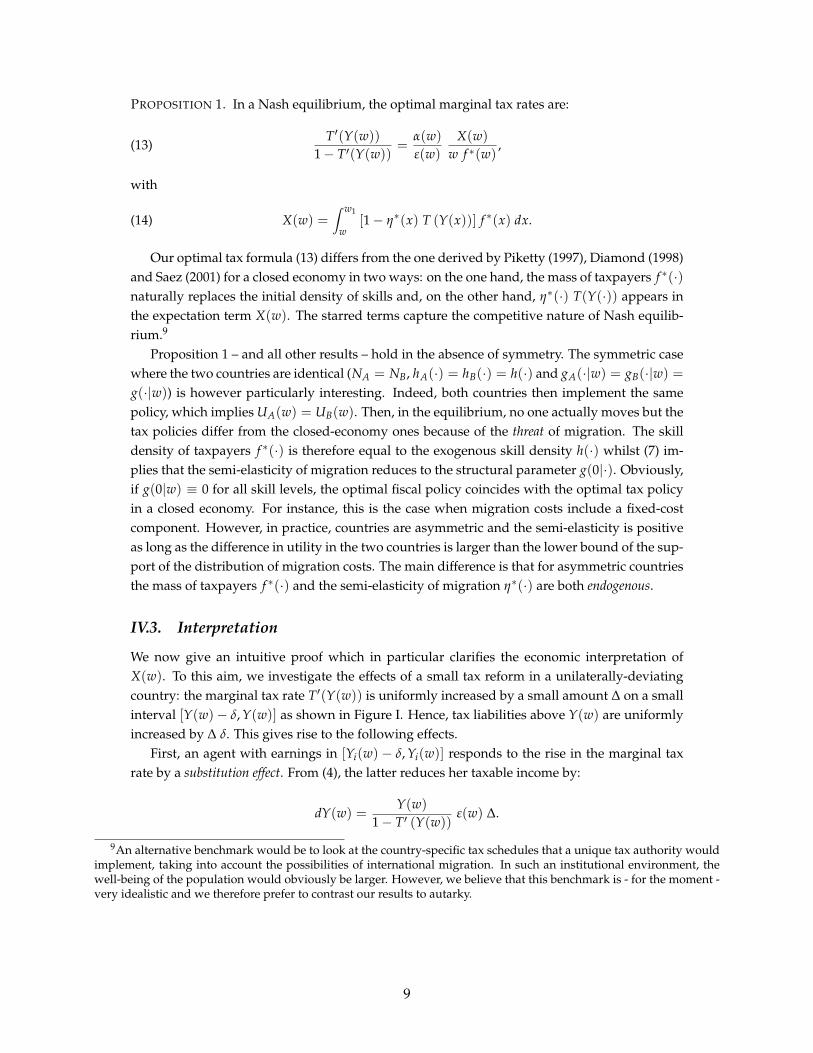
We therefore investigate three possible scenarios, as shown in Figure VI. In each of them,the average elasticity in the actual economy top 1% of the population is equal to 0.25. In thefirst scenario, the semi-elasticity is constant up to the top centile and then decreasing in such away that the elasticity of migration is constant within the top centile. In the second scenario,the semi-elasticity is constant throughout the whole skill distribution. In the third scenario, thesemi-elasticity is zero up to the top centile and then increasing. Note that, in the three scenar-

17

ios, the elasticity of migration is non-decreasing along the skill distribution and remains finite,whilst the semi-elasticity of migration is constant across the bottom 99% of the skill distribu-tion. The average elasticity in the population is higher in the first scenario (0.028) than in thesecond (0.013) and third (0.003) ones.

0 20 40 60 80 100

F w

0.05

0.10

0.15

0.20

0.25

0.30

w

(a)

0 2 4 6 8

YHwL0

2.´ 10-7

4.´ 10-7

6.´ 10-7

8.´ 10-7

1.´ 10-6

1.2´ 10-6

1.4´ 10-6

ΗHwL

(b)

FIGURE VI: ELASTICITY (A) AND SEMI-ELASTICITY (B) OF MIGRATION. CASE 1 (PLAIN), CASE 2(DOTTED) AND CASE 3 (DASHED). Y IN MILLIONS OF USD.

The optimal tax liabilities and optimal marginal tax rates in the equilibrium are shown onthe the left and right panels of Figure VII respectively. The x-axis represents annual gross earn-ings in millions of US dollars. In addition to the three scenarios presented above, we added thetax schedule that would be chosen in a closed economy or in the presence of tax coordination(black curves). Even though the average elasticity of migration is the same for the top 1% ofincome earners in the three scenarios, we observe significant differences due to variations inthe shape of the semi-elasticity of migration. Moreover, the threat of migration implies a non-negligible decrease in the total taxes paid by top income earners whilst differences in the slopeof the semi-elasticity may translate into large differences in marginal tax rates for high-incomeearners. These numerical results put the stress on the need for empirical studies on the slope ofthe semi-elasticity of migration, in addition to its level.

In the first case, the tax function is close to being linear for high-income earners and remainsclose to the closed-economy benchmark. In the second case, the tax function is more concavefor large incomes, but remains increasing. In the third case, the tax function becomes decreasingaround Y = $2.9 millions. In particular, the richest people are not those paying the largest taxes.It is very striking that the largest difference in tax liabilities is observed in the third case whichyet exhibits the lowest average elasticity of migration over the total population. This illustratesthe fact that the profile of the semi-elasticity of migration within the top centile has a muchstronger impact on the optimal tax schedule than the average elasticity of migration within thebottom 99% of the population.

18

0 1 2 3 4 5Y $MM0

1

2

3

4

T Y $MM

(a)

1 2 3 4 5Y0

20

40

60

80

100

T ' Y

(b)

FIGURE VII: OPTIMAL TAX LIABILITIES (A) AND OPTIMAL MARGINAL TAX RATES (B). AUTARKY

(BOLD), CASE 1 (PLAIN), CASE 2 (DOTTED) AND CASE 3 (DASHED). Y IN MILLIONS OF USD.

VII. CONCLUDING COMMENTS

This paper characterizes the nonlinear income tax schedules that competing Rawlsian govern-ments should implement when individuals with private information on skills and migrationcosts decide where to live and how much to work. First, we obtain an optimality rule in whicha migration term comes in addition to the standard formula obtained by Diamond (1998) fora closed economy. Second, we show that the optimal tax schedule for top income earners notonly depends on the intensity of the migration response of this population, which has been esti-mated by Liebig et al. (2007), Kleven et al. (2013) and Kleven et al. (2014), but also on the way inwhich the semi-elasticity of migration varies along the skill distribution. If the latter is constantor decreasing, optimal marginal tax rates are positive. Conversely, marginal tax rates may benegative if the semi-elasticity of migration is increasing along the skill distribution. To illus-trate the sensitivity of marginal tax rates to the slope, we numerically compare three economiesthat are identical in all aspects, including the average elasticity of migration among the top per-centile of the distribution, except that they differ in term of the slope of the semi-elasticity ofmigration along the skill distribution. We obtain significantly different tax schedules.

Therefore, it is not sufficient to estimate the elasticity of migration. The level as well as theslope of the semi-elasticity of migration are crucial to derive the shape of optimal marginal in-come tax, even for high income earners. The empirical specification (2) of Kleven et al. (2014)does not allow one to recover the slope of the semi-elasticity. Another specification with addi-tional terms should be estimated.

Different conclusions can be drawn from our results. From a first perspective, the uncer-tainty about the profile of the semi-elasticity of migration may justify very low, and maybeeven negative, marginal tax rates for the top 1% of the income earners. This may partly explainwhy OECD countries were reducing their top marginal tax rates before the financial crisis of2007. From a second perspective, the potential consequences of mobility might be so substan-tial in terms of redistribution that governments might want to hinder migration. For example,departure taxes have recently been implemented in Australia, Bangladesh, Canada, Nether-

19

lands and South Africa. Finally, from a third viewpoint, the problem is not globalization per sebut the lack of cooperation between national tax authorities.

A first possibility is an agreement among national policymakers resulting in the implemen-tation of supranational taxes, for example at the EU level. A second possibility relies on theexchange of information between Nation states. Thanks to this exchange, the policymaker ofa given country would be able to levy taxes on its citizens living abroad, as implemented bythe United States. Indeed, in a citizenship-based income tax system, moving abroad wouldnot change the tax schedule an individual faces, so that the distortions due to tax competitionwould vanish. There has been some advances in the direction of a better exchange of infor-mation between tax authorities. For example, the OECD Global Forum Working Group onEffective Exchange of Information was created in 2002 and contains two models of agreementsagainst harmful tax practices. However, these agreements remain for the moment non-bindingand are extremely incomplete.

Among the various potential extensions, a particularly promising one concerns the possi-bility for governments to offer nonlinear preferential tax treatments to foreign workers, as forexample in Denmark (Kleven et al., 2014). In particular, it would be interesting to compare ourresults with the social outcome arising when discrimination based on citizenship is allowed.

CRED - UNIVERSITE PARIS II PANTHEON ASSAS & CRESTUCFS & DEPARTMENT OF ECONOMICS, UPPSALA UNIVERSITY

AIX-MARSEILLE UNIVERSITE (AIX-MARSEILLE SCHOOL OF ECONOMICS), CNRS & EHESS

A PROOF OF PROPOSITION 1

We use the dual problem to characterize best response allocations:

maxUi(w),Yi(w)

∫ w1

w0

(Yi (w)− v (Yi (w) ; w)−Ui (w)) ϕi (Ui (w)−U−i (w) ; w) dw

s.t. U′i (w) = −v′w (Yi (w) ; w) and Ui(w0) ≥ Ui(w0),(23)

in which Ui(w0) is given. We adopt a first-order approach by assuming that the monotonicityconstraint is slack. We further assume that Y(·) is differentiable. Denoting q(·) the co-statevariable, the Hamiltonian associated to Problem (23) is:

H(Ui, Yi, q; w) ≡ [Yi − v(Yi; w)−Ui] ϕi(Ui −U−i; w)− q(w) v′w (Yi; w) .

Using Pontryagin’s principle, the first-order conditions for a maximum are:

1− v′y (Yi(w); w) =q (w)

ϕi (∆i(w); w)v′′yw (Yi(w); w) ,(24)

q′(w) = {1− [Yi(w)− v(Yi(w); w)−Ui(w)] ηi(∆i(w); w)} ϕi (∆i(w); w) ,(25)

q(w1) = 0 when w1 < ∞ and q(w1)→ 0 when w1 → ∞,(26)

q (w0) ≤ 0.(27)

20

Integrating Equation (25) between w and w1 and using the transversality condition (26), weobtain:

(28) q(w) = −∫ w1

w[1− η∗(x) T(Y(x))] f ∗(x) dx.

Defining X(w) = −q(w) leads to (14). Equation (24) can be rewritten as:

(29) 1− v′y (Y(w); w) = −X (w)

f ∗(w)v′′yw (Y(w); w)

Dividing (5) by (4) and making use of (3), we get

v′′yw(Y(w); w) = −α(w)

ε(w)

1− T′(Y(w))

w.

Plugging (3) and the latter equation into (29) leads to (13).

B PROOF OF PROPOSITION 3

From (13), T′(Y(w)) has the same sign as the tax level effect X(w). The transversality condition(27) is equivalent to X(w0) ≥ 0, while (26) is equivalent to lim

w 7→w1X(w) = 0. From (14), the

derivative of X(w) is

(30) X′(w) =

[T(Y(w))− 1

η∗(w)

]η∗(w) f ∗(w)

We now turn to the proofs of the different parts of Proposition 3.

i) η∗(w) is constant and equal to η∗

We successively show that any configuration but T′(Y(w)) > 0 for all w ∈ (w0, w1) con-tradicts at least one of the transversality conditions (26) or (27). We start by establishing thefollowing Lemmas, which will also be useful for the case where η∗(w) is decreasing.

LEMMA 1. Assume that for any w ∈ [w0, w1], η∗′(w) ≤ 0 and assume there exists a skill levelw ∈ (w0, w1) such that T′(Y(w)) ≤ 0 and T(Y(w)) > 1/η∗(w). Then X(w0) < 0, so thetransversality condition (27) is violated.

Proof As T(Y(w)) = Y(w) − C(w) and η(w) are continuous functions of w, there exists bycontinuity an open interval around w where T(Y(w)) > 1/η∗(w). Let w∗ ∈ [w0, w) be thelowest bound of this interval. Then either w∗ = w0 or T(Y(w∗)) = 1/η∗(w∗). Moreover, forall w ∈ (w∗, w], one has that T(Y(w)) > 1/η∗(w), thereby X′(w) > 0 according to (30). Hence,one has that X(w) < X(w) ≤ 0, thereby T′ (Y(w)) < 0 for all w ∈ [w∗, w). Consequently,T(Y(w∗)) > T(Y(w)) > 1/η∗(w) ≥ 1/η∗(w∗). So, one must have w∗ = w0. Finally, we getX(w∗) = X(w0) < 0, which contradicts the transversality condition (27). QED

21

LEMMA 2. Assume that for any w ∈ [w0, w1], η∗′(w) ≤ 0 and assume there exists a skill levelw ∈ (w0, w1) such that T′(Y(w)) ≤ 0 and T(Y(w)) < 1/η∗(w). Then X(w1) < 0, so thetransversality condition (26) is violated.

Proof As T(Y(w)) = Y(w) − C(w) and η(w) are continuous functions of w, there exists bycontinuity an open interval around w where T(Y(w)) < 1/η∗(w). Let w∗ ∈ (w, w1] be thehighest bound of this interval. Then either w∗ = w1 or T(Y(w∗)) = 1/η∗(w∗). Moreover, forall w ∈ [w, w∗), one has that T(Y(w)) < 1/η∗(w), thereby X′(w) < 0, according to (30). Hence,one has that X(w) < X(w) ≤ 0, thereby T′ (Y(w)) < 0 for all w ∈ (w, w∗]. Consequently,T(Y(w∗)) < T(Y(w)) < 1/η∗(w) ≤ 1/η∗(w∗). So, one must have w∗ = w1. Finally, we getX(w∗) = X(w1) < 0, which contradicts the transversality condition (26). QED

From Lemmas 1 and 2, it is not possible to have T′(Y(w)) ≤ 0 and T(Y(w)) 6= 1/η(w),otherwise one of the transversality conditions is violated. Assume there exists a skill levelw ∈ (w0, w1) such that T′(Y(w)) < 0 and T(Y(w)) = 1/η0(w). By continuity, there exists ε > 0such that T′(Y(w− ε)) < 0 and T(Y(w− ε)) > 1/η∗, in which case, Lemma 1 applies.

Last, assume there exists a skill level w ∈ (w0, w1) such that T′(Y(w)) = 0 and T(Y(w)) =

1/η∗(w). According to the Cauchy-Lipschitz theorem (equivalently, the Picard–Lindelof the-orem), the differential system of equations in U(w) and X(w) defined by (10) and (30) (andincluding (13) to express Y (w) as a function of X(w)) with initial conditions that correspond toT′(Y(w)) = X(w) = 0 and T(Y(w)) = 1/η∗(w) admits a unique solution where X(w) ≡ 0 andT(·) = 1/η∗ for all w. From (9), such a solution provides excess budget resources when E isassumed nil and provides less utility level than the laissez faire policy where T(·) = 0.

Consequently, any case where T′(Y(w)) ≤ 0 for w ∈ (w0, w1) leads to the violation of atleast one of the transversality conditions.

We finally show that T(Y(w)) < 1/η∗(w) for all w ∈ (w0, w1). Assume by contradiction thatthere exists a skill level w ∈ (w0, w1) such that T(Y(w)) ≥ 1/η∗(w). Because T′(Y(w)) > 0 andη∗′(w) = 0 for all w ∈ (w0, w1), we have T(Y(w)) > 1/η∗(w) for all w ∈ (w, w1]. Equation (30)thus implies X′(w) > 0 for all w ∈ (w, w1]. Moreover, as we know from above that T′(Y(w)) >

0 for all w ∈ (w0, w1), we have in particular X(w) > 0. Combined with X′(w) > 0 for allw ∈ (w, w1], this implies that X(w) does not tend to zero as w tends to w1, which contradictsthe transversality condition (26).

ii) η∗(w) is decreasing

If there exists a skill level w ∈ (w0, w1) such that T′(Y(w)) ≤ 0 and T(Y(w)) > 1/η∗(w),Lemma 1 applies. If there exists a skill level w ∈ (w0, w1) such that T′(Y(w)) ≤ 0 andT(Y(w)) < 1/η∗(w), Lemma 2 applies. Finally, if there exists a skill level w ∈ (w0, w1) suchthat T′(Y(w)) ≤ 0 and T(Y(w)) = 1/η∗(w), then the function w 7→ T(Y(w)) − 1/η∗(w) isnon-positive and admits a negative derivative at w, as η∗′(·) < 0. Hence, there exists w > wsuch that T(Y(w)) < 1/η∗(w), thereby X′(w) < 0 for all w ∈ (w, w]. Consequently, X′(w) < 0(equivalently T(Y(w)) < 1/η∗(w)) and X(w) < X(w) = 0 (equivalently T′(Y(w)) < 0), inwhich case Lemma 2 applies at w. Consequently, any case where T′(Y(w)) ≤ 0 for w ∈ (w0, w1)

leads to the violation of at least one of the transversality conditions, which ends the proof ofPart ii) of Proposition 3.

22

iii) η∗(w) is increasing

We first show two useful lemmas.

LEMMA 3. Assume that for any w ∈ [w0, w1], η∗′(w) > 0 and assume there exists a skill levelw ∈ (w0, w1) such that T′(Y(w)) ≥ 0 and T(Y(w)) ≥ 1/η∗(w). Then, X(w1) > 0, so thetransversality condition (26) is violated.

Proof We first show that we can assume that T(Y(w)) > 1/η∗(w) without any loss of gen-erality. Assume that T(Y(w)) = 1/η∗(w) and T′(Y(w)) ≥ 0. As η∗′(·) > 0, the functionw 7→ T(Y(w))− 1/η∗(w) is non-negative and admits a positive derivative at w. Hence, thereexists w > w such that T(Y(w)) > 1/η∗(w), thereby X′(w) > 0 for all w ∈ (w, w]. Conse-quently, X′(w) > 0 (equivalently T(Y(w)) > 1/η∗(w)) and X(w) > X(w) = 0 (equivalentlyT′(Y(w)) > 0).

Consider now that T′(Y(w)) ≥ 0 and T(Y(w)) > 1/η∗(w). As T(Y(w)) = Y(w)−C(w) andη(w) are continuous functions of w, there exists by continuity an open interval around w whereT(Y(w)) > 1/η∗(w). Let w∗ ∈ (w, w1] be the highest bound of this interval. Then, either w∗ =w1 or T(Y(w∗)) = 1/η∗(w∗). Moreover, for all w ∈ [w, w∗), we have T(Y(w)) > 1/η∗(w), andthereby X′(w) > 0 according to (30). Hence, we have X(w) > X(w) ≥ 0, thereby T′ (Y(w)) > 0for all w ∈ (w, w∗]. Consequently, T(Y(w∗)) > T(Y(w)) > 1/η∗(w) > 1/η∗(w∗). So, w∗ = w1.Finally, we get X(w∗) = X(w1) > 0, which contradicts the transversality condition (26). QED

LEMMA 4. Assume that for any w ∈ [w0, w1], η∗′(w) > 0 and assume there exists a skill levelw ∈ (w0, w1) such that T′(Y(w)) ≥ 0 and T(Y(w)) < 1/η∗(w). Then, X(w) > 0 for all w < w.

Proof As T(Y(w)) = Y(w) − C(w) and η(w) are continuous functions of w, there exists bycontinuity an open interval around w where T(Y(w)) < 1/η∗(w). Let w∗ ∈ [w0, w) be thelowest bound of this interval. Then, either w∗ = w0 or T(Y(w∗)) = 1/η∗(w∗). Moreover,for all w ∈ (w∗, w], we have T(Y(w)) < 1/η∗(w), and thereby X′(w) < 0 according to (30).Hence, we have X(w) > X(w) ≥ 0, thereby T′ (Y(w)) > 0 for all w ∈ (w∗, w]. Consequently,T(Y(w∗)) < T(Y(w)) < 1/η∗(w) < 1/η∗(w∗). So, w∗ = w0 and X(w) > 0 for all w ∈ [w0, w).QED

According to the transversality condition (27), either X(w0) > 0 or X(w0) = 0. However, inthe latter case where X(w0) = 0, we must have T′(Y(w)) < 0 for all w ∈ (w0, w1). Otherwise,either there exists w ∈ (w0, w1) such that T′(Y(w)) ≥ 0 and T(Y(w)) ≥ 1/η∗(w), in which caseLemma 3 implies that the transversality condition (26) is violated, or there exists w ∈ (w0, w1)

such that T′(Y(w)) ≥ 0 and T(Y(w)) < 1/η∗(w), in which case Lemma 4 implies that X(w0) >

0. Consequently, if X (w0) = 0, we must have T′ (Y (w)) < 0 for all w ∈ (w0, w1). Using (9)and the assumption that E = 0, this implies that T(Y(w0)) > 0 > T(Y(w1)). Hence, this policyprovides the workers of skill w0 with less utility than the laissez-faire policy T(·) = 0, whichcontradicts X (w0) = 0. We therefore have established that X (w0) > 0.

By continuity of function X(·), either X(w) > 0 for all w ∈ [w0, w1) (equivalently T′(Y(w)) ≥0 for all w < w1) which corresponds to case (a) of Part iii) of Proposition 3, or there existsw ∈ (w0, w1) such that X(w) > 0 for all w < w and X(w) = 0. We now show that in the

23

latter case, we must have T′(Y(w)) < 0, or equivalently X(w) < 0, for all w ∈ (w, w1). Oth-erwise, either there exist w ∈ (w, w1) such that T′(Y(w)) ≥ 0 and T(Y(w)) ≥ 1/η∗(w), inwhich case Lemma 3 implies that the transversality condition (26) is violated, or there mustexist w ∈ (w, w1) such that T′(Y(w)) ≥ 0 and T(Y(w)) < 1/η∗(w), in which case Lemma 4implies that X(w) > 0), which contradicts X(w) = 0. Therefore, if there exists w ∈ (w0, w1)

such X(w) = 0, then we must have X(w) > 0, thereby T′(Y(w)) > 0, for all w < w andX(w) < 0, thereby T′(Y(w)) < 0, for all w ∈ (w, w1), which corresponds to case (b) of Part iii)of Proposition 3.

iv) η∗(w) is increasing and tends to infinity

From case iii), we know that the marginal tax rates are either positive or there exists a thresholdabove which they are negative. Assume by contradiction that the marginal tax rates are posi-tive. Then, the tax function is increasing. In addition, it must be positive for some individuals soas to clear the budget constraint. As the semi-elasticity of migration increases to infinity, thereexists a skill level w at which T′(Y(w)) ≥ 0 and T(Y(w)) > 1/η∗(w). Then, the transversalitycondition (26) is violated according to Lemma 3, which leads to the desired contradiction.

REFERENCES

Anthony B. Atkinson and Joseph E. Stiglitz. Lectures on Public Economics. McGraw-Hill Inc.,1980.

Robert J. Barro and Xavier Sala-I-Martin. Convergence across states and regions. BrookingsPapers on Economic Activity, 1991(1):107–182, 1991.

Robert J. Barro and Xavier Sala-i Martin. Convergence. Journal of Political Economy, 100(2):223–51, April 1992.

Felix Bierbrauer, Craig Brett, and John A. Weymark. Strategic nonlinear income tax competitionwith perfect labor mobility. Games and Economic Behavior, 82:292–311, 2013.

Charles Blackorby, Walter Bossert, and David Donaldson. Population Issues In Social Choice The-ory, Welfare Economics and Ethics. Cambridge University Press, 2005.

Tomer Blumkin, Efraim Sadka, and Yotam Shem-Tov. International tax competition: Zero taxrate at the top re-established. Technical Report 3820, CESifo WP, May 2012.

Robin Boadway and Laurence Jacquet. Optimal marginal and average income taxation undermaximin. Journal of Economic Theory, 143:425–441, 2008.

George J. Borjas. The economic analysis of immigration. In O. Ashenfelter and D. Card, editors,Handbook of Labor Economics, chapter 28, pages 1697–1760. North-Holland, 1999.

Mike Brewer, Emmanuel Saez, and Andrew Shephard. Means-testing and tax rates on earnings.In J. Mirrlees, S. Adam, T. Besley, R. Blundell, S. Bond, R. Chote, M. Gammie, P. Johnson,G. Myles, and J. Poterba, editors, Dimensions of Tax Design: the Mirrlees Review, chapter 3,pages 90–173. Oxford University Press, 2010.

24

Peter A. Diamond. Optimal income taxation: An example with u-shaped pattern of optimalmarginal tax rates. American Economic Review, 88(1):83–95, 1998.

Frederic Docquier and Abdeslam Marfouk. International migration by educational attainment(1990-2000) - release 1.1. In Calglar Ozden and Maurice Schiff, editors, International Migration,Remittances and Development, chapter 5. Palgrave Macmillan, New-York, 2006.

Peter Ganong and Daniel Shoag. Why has regional income convergence in the u.s. declined?Technical report, HKS WP RWP12-028, 2013.

Jonathan H. Gruber and Emmanuel Saez. The elasticity of taxable income: Evidence and impli-cations. Journal of Public Economics, 84:1–32, 2002.

Jonathan C. Hamilton and Pierre Pestieau. Optimal income taxation and the ability distribution:Implications for migration equilibria. International Tax and Public Finance, 12:29–45, 2005.

Martin F. Hellwig. Incentive Problems With Unidimensional Hidden Characteristics: A UnifiedApproach. Econometrica, 78(4):1201–1237, 07 2010.

Laurence Jacquet, Etienne Lehmann, and Bruno Van der Linden. Optimal redistributive taxa-tion with both extensive and intensive responses. Journal of Economic Theory, 148(5):1770 –1805, 2013.

Henrik Kleven, Claus T. Kreiner, and Emmanuel Saez. The optimal income taxation of couples.Econometrica, 77(2):537–560, 2009.

Henrik J. Kleven, Camille Landais, and Emmanuel Saez. Taxation and international migrationof superstars: Evidence from the european football market. American Economic Review, 103:1892–1924, 2013.

Henrik J. Kleven, Camille Landais, Emmanuel Saez, and Esben A. Schultz. Migration and wageeffects of taxing top earners: Evidence from the foreigners’ tax scheme in denmark. QuarterlyJournal of Economics, 129:333–378, 2014.

Guy Laroque. Income maintenance and labor force participation. Econometrica, 73:341–376,2005.

Manuel Leite-Monteiro. Redistributive policy with labour mobility accross countries. Journal ofPublic Economics, 65:229–244, 1997.

Thomas Liebig, Patrick A. Puhani, and Alfonso Sousa-Poza. Taxation and internal migration-evidence from the swiss census using community-level variation in income tax rates. Journalof Regional Science, 47(4):807–836, 2007.

Vilen Lipatov and Alfons Weichenrieder. Optimal income taxation with tax competition. Work-ing Papers 1207, Oxford University Centre for Business Taxation, 2012.

James A. Mirrlees. An exploration in the theory of optimum income taxation. Review of EconomicStudies, 38:175–208, 1971.

25

James A. Mirrlees. Migration and optimal income taxes. Journal of Public Economics, 18:319–341,1982.

Massimo Morelli, Huanxing Yang, and Lixin Ye. Competitive nonlinear taxation and constitu-tional choice. American Economic Journal: Microeconomics, 4(1):142–75, 2012.

Petter Osmundsen. Taxing internationally mobile individuals– a case of countervailing incen-tives. International Tax and Public Finance, 6:149–164, 1999.

Gwenael Piaser. Labor mobility and income tax competition. In Greg. N. Gregoriou and Reads.Colin, editors, International Taxation Handbook, chapter 4, pages 73–94. Elsevier, 2007.

Thomas Piketty. La redistribution fiscale face au chomage. Revue Francaise d’Economie, 12:157–201, 1997.

Thomas Piketty and Emmanuel Saez. Optimal labor income taxation. Technical Report WP No.18521, NBER, Forthcoming in Handbook of Public Economics, vol. 5., December 2012.

Jean-Charles Rochet and Lars A. Stole. Nonlinear pricing with random participation. The Reviewof Economic Studies, 69(1):pp. 277–311, 2002.

Emmanuel Saez. Using elasticities to derive optimal income tax rates. Review of Economic Stud-ies, 68:205–229, 2001.

Emmanuel Saez. Optimal income transfer programs: Intensive versus extensive labor supplyresponses. Quarterly Journal of Economics, 117:1039–1073, 2002.

Emmanuel Saez, Joel Slemrod, and Seth H. Giertz. The elasticity of taxable income with respectto marginal tax rates: A critical review. Journal of Economic Literature, 50(1):3–50, March 2012.

Florian Scheuer and Casey Rothschild. Redistributive taxation in the roy model. QuarterlyJournal of Economics, 128:623–668, 2013.

Laurent Simula and Alain Trannoy. Optimal income tax under the threat of migration by top-income earners. Journal of Public Economics, 94:163–173, July 2010.

Laurent Simula and Alain Trannoy. Shall we keep the highly skilled at home? the optimalincome tax perspective. Social Choice and Welfare, pages 1–32, 2011.

Joseph E. Stiglitz. Self-selection and pareto efficient taxation. Journal of Public Economics, 17(2):213–240, March 1982.

Juan C. Suarez Serrato and Owen Zidar. Who Benefits from State Corporate Tax Cuts? A LocalLabor Markets Approach with Heterogeneous Firms. Technical report, UC Berkeley andStanford U., 2013.

John D. Wilson. The effect of potential emigration on the optimal linear income tax. Journal ofPublic Economics, 14:339–353, 1980.

John D. Wilson. Optimal linear income taxation in the presence of emigration. Journal of PublicEconomics, 18:363–379, 1982a.

26

John D. Wilson. Optimal income taxation and migration: A world welfare point of view. Journalof Public Economics, 18(3):381 – 397, 1982b.

Cristobal Young and Charles Varner. Millionaire migration and state taxation of top incomes:Evidence from a natural experiment. National Tax Journal, 64:255–284, 2011.

27