Tax Reforms and Intertemporal Shifting of Wage Income

American Economic Journal: Economic Policy 2016, 8(3): 233–257 http://dx.doi.org/10.1257/pol.20140233

233

Tax Reforms and Intertemporal Shifting of Wage Income: Evidence from Danish Monthly Payroll Records†

By Claus Thustrup Kreiner, Søren Leth-Petersen, and Peer Ebbesen Skov*

This paper uses monthly payroll records for all Danish employees to identify widespread intertemporal shifting of labor income in response to a tax reform that significantly reduced the marginal tax rates for one-fourth of all employees. When ignoring shifting, the estimate of the overall elasticity of taxable income equals 0.1, and the elasticity is increasing with earnings. When removing the shift-ing component, the elasticity is close to zero at all earnings levels. The evidence also indicates that tax salience, liquidity constraints and firm willingness to cooperate in shifting are important factors in explaining shifting behavior. (JEL H24, H31, J22, J31)

This paper provides clear empirical evidence of large, widespread intertempo-ral shifting responses in wage income. Intertemporal shifting of wage income

takes place when income earned in one tax year is paid out in another tax year, so as to reduce the tax payment of the individual. The incentive to do so is present whenever marginal tax rates vary over time, for example, because of changes in indi-vidual circumstances (retirement, marriage, promotion, etc.), because of sunset pro-visions that automatically change marginal tax rates at some specified future date, or because of reforms that change the tax system from one year to the next year.1 Knowledge of intertemporal shifting behavior is therefore relevant for evaluating the revenue implications of tax reforms and the efficiency loss and distributional impact of the tax system.

1 A recent example of a sunset provision is the American Economic Growth and Tax Relief Reconciliation Act of 2001 that lowered the top marginal tax rate from 39.6 percent to 35 percent but introduced a clause stating that the tax cut would expire by 2011. After a two-year extension of the tax cut in 2010, the American Taxpayer Relief Act of 2012 returned the top marginal tax rate to its 2001 level of 39.6 percent. The Congressional Budget Office (2013) projects that 2013 tax revenue decreases because of shifting of income from calendar year 2013 into late 2012 in anticipation of the higher 2013 tax rate.

* Kreiner: Department of Economics, University of Copenhagen, Øster Farimagsgade 5, DK-1353 Copenhagen K, Denmark (e-mail: [email protected]); Leth-Petersen: Department of Economics, University of Copenhagen, Øster Farimagsgade 5, DK-1353 Copenhagen K, Denmark (e-mail: [email protected]); Skov: Auckland University of Technology and Rockwool Foundation Research Unit, Sølvgade 10, 2. tv. DK-1307 Copenhagen K, Denmark (e-mail: [email protected]). We are grateful to Morten Appelsø, Raj Chetty, Christian Gillitzer, Hilary Hoynes, Henrik Kleven, Wojciech Kopczuk, Søren Pedersen, Ray Rees, Emmanuel Saez, Joel Slemrod, Shlomo Yitzhaki, four anonymous referees, and numerous seminar participants for comments and discussion. We also thank the Danish tax administration (SKAT) for providing data and the Economic Policy Research Network (EPRN) and the Rockwool Foundation Research Unit for providing financial support. Søren Leth-Petersen acknowledges finan-cial support from the the Danish Council for Independent Research, grant number 0602-01719B.

† Go to http://dx.doi.org/10.1257/pol.20140233 to visit the article page for additional materials and author disclosure statement(s) or to comment in the online discussion forum.

http://dx.doi.org/10.1257/pol.20140233

mailto:[email protected]




234 AmEricAn Economic JournAL: Economic PoLicy AugusT 2016

Our empirical analysis is based on new Danish administrative records with monthly information about wages and salaries of all employees, allowing us to identify intertemporal income shifting in a way not possible with data measured at the annual frequency. The identifying variation is provided by a large tax reform in Denmark, which reduced the highest marginal tax rate on earnings from 63 per-cent to 56 percent, thereby significantly changing incentives for the one-fourth of full-time employees with the highest incomes. The reform was passed in parliament at the end of May 2009 and changed the tax scheme from 2010 onward, thereby cre-ating an incentive for high-wage earners to postpone wage payments from the end of 2009 to the beginning of 2010. This type of income shifting requires the cooper-ation of the employer, who reports the earnings to the tax authorities, but is possible without coming into conflict with the tax law. The shifting behavior studied here is therefore a classic example of tax avoidance. This is in contrast to, for example, the United States, where such activity is not legal and would therefore be classified as tax evasion.

Our analysis starts with graphical evidence revealing income shifting taking place around the implementation of the tax reform. We observe a clear negative spike in reported earnings of high-income individuals in the last months of 2009 and a positive spike in the beginning of 2010, and at the individual level we detect taxpayers with a significant drop in reported earnings at the end of 2009 followed by a jump in the beginning of 2010. We detect no systematic effects in other months or for a group of middle-income individuals with only negligible changes in incen-tives, confirming that the observed pattern is driven by income shifting. We obtain the same picture after controlling for a large number of covariates and also when looking across industry sectors, showing that shifting behavior is a widespread phenomenon.

Considering all the individuals with an incentive to shift income, we find that the average level of reported wage income is nearly 10 percent higher in January 2010 and correspondingly lower in November and December 2009, revealing large shift-ing effects even at the macro level. The share of income shifted is steadily increasing with income. On average, individuals in percentiles 95–99 shifted 15 percent of the average monthly wage income around New Year 2010, and for the top 1 percent of wage earners it was close to 30 percent.

Knowledge of intertemporal shifting behavior is relevant for the burgeoning lit-erature, recently surveyed by Saez, Slemrod, and Giertz (2012), that exploits tax reforms to identify the elasticity of taxable income (ETI) used to quantify the wel-fare loss from taxation. It is well-known that short-run income shifting responses around the implementation of tax reforms may cause the estimate of the ( short-run) ETI to differ from the ( long-run) elasticity relevant for evaluating the distortionary effects of taxation (e.g., Slemrod 1998).

When we run a simple difference-in-differences estimation on annual earnings before and after the reform, we find an overall ETI of around 0.1. The estimated ETI is increasing as a function of income from 0 for individuals with the lowest income levels within the treatment group to 0.25 for the taxpayers in the top 1 per-cent of the income distribution. We show in different ways, for example, by exclud-ing December and January observations, that these ETI estimates are almost entirely

VoL. 8 no. 3 235kreiner et al.: intertemporal shifting of wage income

due to income shifting responses. After removing the shifting component, short-run elasticities are close to zero at all earnings levels.

The large income shifting response at the aggregate level is concentrated on a few taxpayers. Among the employees with an incentive to shift income, we find less than 5 percent exploit the opportunity to shift income, but that these individ-uals shift large amounts. This observed pattern in reported earnings is difficult to reconcile with intertemporal changes in the timing of work, indicating the observed movements in income are due to tax avoidance rather than real responses (Slemrod 1995). Moreover, the conclusion concerning bias in ETI estimates from temporary variation in income is independent of whether the temporary variation is due to tax avoidance or due to real responses.

The low share of employees engaging in shifting activity may seem surprising but is consistent with other types of evidence showing taxpayers engage less in tax avoidance than what is predicted by a standard economic model (Andreoni, Erard, and Feinstein 1998). There may be different reasons why an employee does not engage in intertemporal income shifting. First, we find that shifting is negligible among government employees, is more common in small private firms than in large firms, and is much more common among the top-five earners within a firm. This may suggest that some employers are less willing to participate in tax avoidance due to the risk of bad publicity, which limits income shifting to small/medium sized private firms and top management. Second, we find that shifting is less pronounced for individuals with a low level of liquid assets relative to income, consistent with the explanation that liquidity constraints prevent some tax taxpayers from shifting income forward.

Third, by conducting a telephone survey of a randomly selected group of indi-viduals and combining their responses with the register data, we show taxpayer information and attention are important, in line with recent studies of other types of behavioral responses to taxation (Chetty, Loony, and Kroft 2009; Chetty, Friedman, and Saez 2013). Among the survey respondents with an incentive to shift income only one out of five is aware of the tax incentive and know it is legal to shift the wage payments. The results further indicate that income shifting is concentrated among those who are informed in the treatment group but, on the other hand, less than 10 percent of the informed individuals actually engage in shifting. To conclude, the results do not point to a single explanation but rather to several reasons that com-plement each other in explaining why some employees engage in shifting activities while others do not.

Previous studies of intertemporal income shifting have looked at annual income data or aggregate data. Goolsbee (2000) looks at intertemporal income shifting of the five highest-paid employees in US public companies in response to the mar-ginal tax rate increase implemented by President Clinton in 1993. He applies a standard difference-in-differences setup on annual income but allows tax-reform variation across treatment and control groups to affect income already in the year before the reform in order to detect income shifting. The results indicate that most of the variation in taxable income of these very highly paid individuals seems to be driven by retiming in the realization of stock options, implying that most of the ETI is driven by intertemporal income shifting rather than by permanent income


responses. He finds little responsiveness of salary and bonuses to the tax hike. This is in contrast to Sammartino and Weiner (1997), who find evidence in aggregate data of time-adjustments in bonuses due to the 1993 US tax reform. A reason for this discrepancy may be that it is easier and more valuable for top executives to change the timing of the realization of stock options rather than bonuses, while other high-income individuals, who do not have stock options, instead focus their effort on shifting bonuses and regular wage and salary payments. Our results pro-vide some support for this conjecture as our income measure only includes wage income, implying the shifting behavior documented in our study is not related to the realization of stock options.

Heim (2009) uses a similar approach as Goolsbee but without detecting signif-icant intertemporal effects in income responses to the US tax reforms in 2001 and 2003, while Giertz (2010) finds evidence of intertemporal shifting effects in response to the US tax reforms in the 1990s. Compared to these studies, based on annual income, the monthly frequency of our data offers a unique possibility to obtain a more precise empirical identification of intertemporal income shifting responses.

The remainder of the paper is organized as follows. Section I describes the Danish 2010 tax reform, the data sources, and our approach to identify income shift-ing behavior. Section II describes the empirical results on income shifting, while Section III analyzes how much of the elasticity of taxable income may be attributed to temporary income shifting behavior. Finally, Section IV concludes.

I. Description of Policy, Data, and Identification Approach

The analysis is based on the Danish 2010 tax reform that significantly reduced the taxation of labor income with the declared goal of stimulating labor supply. The tax cut on labor income was financed by decreasing the value of deductions (including interest payments), reducing business subsidies, and increasing energy and envi-ronmental taxes, thereby keeping government revenue constant (before behavioral responses). The reform was proposed on March 1, 2009 , passed in the Danish par-liament on May 28 the same year, and signed into law taking effect from January 1, 2010 . As is usually the case with tax reforms, the distance between the proposal/decision and the actual implementation gave taxpayers an opportunity to save taxes by shifting income across the two tax years.

The reform mainly reduced marginal tax rates on labor income for high-wage earners. Table 1 displays the different taxes applying to labor income in Denmark before and after the reform. It consists of so-called labor market contribution, a regional tax, a church tax and a bottom tax, which apply to all income above a small standard deduction and give in total a marginal tax rate on labor income of 43.5 per-cent in 2009 (column 1). In addition to these taxes, high-wage earners with income above a cutoff of 377,000 Danish kroner (DKK) in 2009 have to pay a middle tax and a top tax implying that they face a marginal tax rate of 62.8 percent (column 2).2

2 With an exchange rate of 6 DKK per US dollar, the middle/top tax cutoff of DKK 377,000 corresponds to around US$63,000.


The tax reform abolished the middle tax bracket altogether and reduced the bottom tax rate a little, implying that the marginal tax rate for high-wage earners ( τ H ) dropped to 56.0 percent in 2010 (column 4), equivalent to an increase in the net-of-tax rate, 1 − τ H , of 18 percent. For comparison, individuals with income just below the middle/top tax cutoff faced a marginal tax rate of 42.2 percent after the reform (column 3), corresponding to an increase in the net-of-tax rate, 1 − τ L , of only 2 percent.

The incentive to shift income was also influenced by a change in the middle/top tax income cutoff, which was increased from DKK 377,000 to DKK 424,000 as shown in Table 1. Figure 1 shows how the incentive to shift one month’s salary from 2009 to 2010 varies with the (average) monthly level of gross taxable earnings and salaries in 2009. The left panel shows the gain measured in DKK and the right panel shows the gain measured in proportion to the monthly net-of-tax earnings. For individuals with monthly incomes below DKK 32,000, the gain from shifting is very small (less than DKK 1,000). It then increases with earnings due to the change in the middle/top tax cutoff, and for people with monthly earnings above DKK 35,000, the incentive is constant at 7 percent of the amount shifted (the slope in panel A), giv-ing a sizable economic gain corresponding to 18 percent of the monthly net-of-tax earnings (see panel B). Note that the changes displayed in panel B correspond to the changes in the net-of-tax rate of 2 percent and 18 percent for individuals below and above, respectively, the top/middle tax cut-off, with the exception of individuals in a small income range where the incentive is affected by the change in the middle/top tax income cutoff.

It was possible to shift payments of income earned in the second half of 2009 into 2010 without coming into conflict with the Danish tax law. According to the tax law, companies have to remit taxes on labor income at the time when income is paid out to the employees, and wages and salaries have to be paid out no later than six

Table 1—Marginal Tax Rates on Labor Income

Year 2009 Year 2010

Labor income (LI) in 1,000 DKK: < 377 > 377 < 424 > 424Tax Tax base Rate (%) Rate (%) Rate (%) Rate (%)

Labor market contributions (LMC) LI 8 8 8 8Regional tax (RT) LI × (1 − LMC) 32.8 32.8 32.8 32.8Bottom tax bracket (BT) LI × (1 − LMC) 5.04 5.04 3.67 3.67Middle tax bracket (MT) LI × (1 − LMC) 0 6 0 0Top tax bracket (TT) LI × (1 − LMC) 0 15 0 15Church tax (CT) LI × (1 − LMC) 0.7 0.7 0.7 0.7

Marginal tax rate on labor income 43.5 62.8 42.2 56.0

notes: The marginal tax rate equals LMC + (1 − LMC) × (RT + BT + MT + TT + CT). These computations of the marginal tax rates apply to the majority of taxpayers. The regional tax varies a little across municipalities. The top/middle tax cutoff depends also on the size of net capital income (excluding stock income) but only if it is positive, and the large majority of taxpayers have negative net capital income. We also disregard the possibility of transferring unutilized allowances between spouses when computing the middle tax, implying that some married persons with income in a certain range pay the top tax but not the middle tax.

source: Website of the Danish Ministry of Taxation (www.skm.dk)

www.skm.dk


months after the income is earned.3 This gave workers an opportunity to save taxes legally if their employers would collaborate by postponing the payout of wages and salaries from 2009 to 2010. After the reform was passed, several articles appeared in the popular press describing the possibility of shifting earnings and discussing whether or not it was legal, and in mid-October an official spokesperson from the Danish tax agency stated publicly that it was legal to postpone wage payments into 2010.4

The empirical analysis is based on a new administrative register, known in Denmark as the eincome register, containing third-party information about monthly wages and salaries for all employees. All firms in Denmark have to report wages and salaries for each employee to the tax agency (SKAT) and tax evasion on wage income is very small (Kleven et al. 2011). The new register has been in place since January 2008 when the frequency of the reporting requirement was changed from yearly to monthly. The register contains the personal registration number of the employee and a firm identifier, which enable us to link the data to various background information of the individual and of the firm from other administrative registers at Statistics

3 This is stated in §46 part 1 and 2 in the Danish law on income taxation called Kildeskatteloven. See www.retsinformation.dk/Forms/R0710.aspx?id=134306.

4 The tax official was cited by the Danish newspaper Jyllandsposten on October 13, 2009 (see www.epn.dk/privat/article1849439.ece).

0

5

10

15

20

25

Per

cent

0

1.000

2.000

3.000

4.000

5.000

6.000

7.000

2530

3540

4550

5560

6570

7580

8590

95100

2530

3540

4550

5560

6570

7580

8590

95100

DK

K

Monthly gross earnings in 2009 (1,000 DKK)

Monthly gross earnings in 2009 (1,000 DKK)

Panel A. Tax savings in DKK Panel B. Tax saving in percent of monthlynet-of-tax earnings

Figure 1. Incentive to Shift One Month’s Salary from 2009 to 2010

notes: The graphs show the increase in disposable income of a taxpayer who shifts wages and salaries earned in one month of 2009 to 2010 as a function of the monthly gross earnings in 2009 of the taxpayer. Panel A shows the amount saved in taxes, while panel B shows the amount in percent of the monthly net-of-tax earnings. It is assumed that the taxpayer has the same monthly earnings level in all months. The computations are based on a 2 percent growth rate in nominal wages from 2009 to 2010.

source: Author’s own calculations

www.retsinformation.dk/Forms/R0710.aspx

www.retsinformation.dk/Forms/R0710.aspx

www.epn.dk/privat/article1849439.ece

www.epn.dk/privat/article1849439.ece


Denmark. We also link the register data to a small survey sample containing infor-mation about taxpayer awareness of the opportunity to shift income.

Our dataset covers the period from January 2008 to December 2011 and con-tains monthly information on all individuals who have been employed at some point during this period. Some of these individuals are children and other people with irregular earnings and temporary employment contracts. In the analysis, we focus on individuals who are employed throughout 2008, corresponding to having a wage record for every month, and who have positive income in all years.5 For these indi-viduals, Figure 2 displays the distribution of the average monthly income in 2008. The median income level is approximately DKK 30,000, and around one-fourth of the full time employees have monthly earnings above DKK 35,000, where incen-tives to shift income are nonnegligible.

In order to identify intertemporal shifting behavior, we divide the sample into taxpayers with a strong incentive to shift income (treatment group) and taxpayers with only a negligible incentive (control group). This is done by allocating people to a tax bracket based on income in 2008, i.e., before the tax reform could have impacted their income. We define the treatment group ( T-group) as the employees in the private sector with monthly gross earnings above DKK 35,000 in 2008, which is percentile 75 in Figure 2, and define the control group ( C-group) as those having monthly income in the range DKK 30, 000–35,000. This leaves us with 328,679 individuals out of which 219,179 belong to the treatment group.

For each individual, we compute the percentage change in the monthly wage relative to the wage level in 2008,

(1) w y, m, i = z y, m, i − z 2008, m, i ____________ z ̅ 2008, i ,

where y denotes the year, m denotes the month, i denotes the individual, and z ̅ 2008, i denotes the average monthly gross earnings of individual i in 2008. We compute percentage changes instead of using a log-transformation because earnings may be zero or close to zero in some months, for example due to income shifting.

Shifting behavior is characterized by an unusually low income growth rate in the months leading up to the implementation of the reform and an unusually high income growth afterwards. These effects may be detected—assuming a common wage growth rate in absence of the reform—by comparing the growth rates in the months around implementation of the reform to other months and by comparing income growth patterns of the T-group relative to the C-group,

(2) w y, m = 1 _ n T

∑ i∈T

w y, m, i − 1 _ n c

∑ i∈c

w y, m, i ,

5 We do not analyse intertemporal income shifting of the self-employed, which has recently been studied by le Marie and Schjerning (2013). Our sample includes individuals who are both wage earners and self-employed at the same time. Removing self-employed completely from the sample has only negligible effects on the results.


where T denotes the treatment group, c denotes the control group, and n denotes the number of individuals in each of the groups.

Using formula (2), it is possible to obtain an estimate of the average income share shifted from 2009 to 2010, but the identification strategy does not fully exploit that intertemporal shifting behavior generates both a decrease in the observed income before the reform and an increase in income after the reform at the individual level. By exploiting this characteristic of shifting behavior, we may obtain a stronger iden-tification of taxpayers engaging in shifting activity. Specifically, we construct the following shifting indicator dummy variable for each individual and each month

(3) D y, m, i = { 1 if w y, m, i > 50 % and w y, m−1, i < −50 % 0

otherwise .

The indicator equals one if income in a month is high compared to its (counterfac-tual) level in the same month of 2008 and income in the preceding month is low compared to its level in the same month of 2008. The shifting indicator is equal to one in January 2010 for an individual who defers his payment of regular earnings from December 2009 to January 2010 and an individual that normally receives a bonus in December but postpones the December 2009 bonus to January 2010 in order to save taxes. The shifting indicator may also equal one due to large random

50th pctl.

75th pctl.

90th pctl.

95th pctl.

00

2

Per

cent

4

6

8

20,000 40,000

Average monthly wage DKK

60,000 80,000

Figure 2. Wage Distribution of Full-Time Employees

notes: The figure shows the distribution of average monthly 2008 wage income of all full-time employees. The top tax bracket starts around the income level of the seventy-fifth percentile. The distribution is truncated at percentile 1 and percentile 99.

source: The monthly payroll (eIncome) register from the Danish tax authority (SKAT)


income movements at the individual level, but the average value of the shifting indicator at all other months may be used to evaluate the importance of this effect because, by construction, December 2009 to January 2010 is the only consecutive bimonthly period where tax-motivated shifting of income can take place. Note, finally, that this identification strategy is not very sensitive to differences in income trends across treatment and control groups, as is the case for the measure based on (2) and for studies of intertemporal shifting based on annual observations (Goolsbee 2000, Heim 2009, Giertz 2010).

II. Results

This section presents the empirical evidence of shifting behavior. First, we esti-mate the average share of income shifted and the share of individuals engaging in shifting activity. Then, we explore how shifting activity varies across different indi-vidual characteristics. Finally, we present survey evidence on the role of information and awareness.

A. main results

Panel A of Figure 3 shows the average monthly wage income from January 2008 to January 2011 of the T-group and the C-group, respectively. It reveals systematic seasonal variation in wages over time for both groups with high average wage income in April and December and low average wage income in the winter and in the fall. More importantly, the graph uncovers important differences around New Year 2010 across the two groups. The income in December 2009 for the T-group is below the annual average of the group for 2009, and income increases from December 2009 to January 2010. This is in contrast to both the year before and the year after where the December income of the T-group is above the annual average, and where income decreases from December to January. The December 2009–January 2010 income pattern of the T-group is also in stark contrast to the pattern of the C-group where the December wage income level is clearly above the annual average and where the monthly income decreases from December to January. Moreover, this opposite pat-tern of the control group is observed across all three years. Overall, these observed income patterns are consistent with the T-group shifting income from 2009 to 2010 as a result of the 2010 tax reform.

Panel B of Figure 3 shows the growth rate of wages of the T-group relative to the C-group for each month estimated using formula (2). By definition, the estimates are zero in the baseline months of 2008. In 2009, it fluctuates around zero before it drops in November and December of 2009, the last two months before the imple-mentation of the tax reform. It then increases sharply just after implementation of the reform, and finally drops to a lower level in the remaining months of 2010. The wage income of the T-group is 3 percent and 5 percent below its counterfactual levels in the two months leading up to the reform, and 9 percent above in January 2010. These differences are highly significant with a 95 percent confidence interval of (−5.0 percent, −4.2 percent) for December 2009 and (8.7 percent, 9.6 percent) for January 2010.


Figure 3 indicates that income shifting takes place, but it is also evident that the data exhibit some noise. There are, for example, positive spikes in April, August, and October of 2010, but note that these spikes are not systematically preceded by negative spikes in the previous months, which is a characteristic of intertemporal shifting. These variations can arise for many reasons, for example, because of dif-ferences in the level and timing of bonus payments across the treatment and control groups.

In Figure 4, we repeat the analysis, but this time using the shifting indicator defined in (3). Panel A plots the average value of the shifting indicator for the T-group and C-group across the observation period. There is a clear spike in January 2010 for the T-group, and movements are otherwise relatively small for both the T-group and the C-group. Panel B plots the difference between the two groups. It clearly shows how income shifting takes place around New Year 2010 when compared to any other month, including January 2011. The size of the spike in panel B is 2.7 percent with a 95 percent confidence interval of (2.6 percent, 2.8 percent). Thus, according to this estimate about 3 percent of the taxpayers in the top tax bracket engage in shifting behavior.6 If, in addition, we impose the criteria that November 2009 income is

6 The 50 percent–50 percent cut-off criteria defining shifting behavior is somewhat arbitrarily chosen, and we have therefore also experimented with a 25 percent–25 percent criteria and a 75 percent–75 percent criteria. This

15

20

25

30

35

40

45

50

55

60

65

1,00

0 D

KK

Month

Panel A. Average monthly wages

−10

−5

0

5

10

Per

cent

Month

Panel B. Change in wages of T-group relative to C-group

Jan

2008

Mar

200

8

May

200

8

Jul 2

008

Sep 2

008

Nov 2

008

Jan

2009

Mar

200

9

May

200

9

Jul 2

009

Sep 2

009

Nov 2

009

Jan

2010

Jan

2011

Mar

201

0

May

201

0

Jul 2

010

Sep 2

010

Nov 2

010

Jan

2008

Mar

200

8

May

200

8

Jul 2

008

Sep 2

008

Nov 2

008

Jan

2009

Mar

200

9

May

200

9

Jul 2

009

Sep 2

009

Nov 2

009

Jan

2010

Jan

2011

Mar

201

0

May

201

0

Jul 2

010

Sep 2

010

Nov 2

010

T-group

C-group

Figure 3. Monthly Wages and Income Shifted

notes: Panel A shows the monthly wage income of the T-group and the C-group. The T-group consists of all private sector employees with average monthly wage income above DKK 35,000 in 2008 and positive wage income in 2009 and 2010. The C-group consists of all private sector employees with average monthly wage income in the range DKK 30,000–35,000 in 2008 and positive wage income in 2009 and 2010. This gives 219,598 employees in the T-group and 109,672 employees in the C-group. Panel B shows the difference between the wages in a given month and the same month in 2008 (as a percentage of the average monthly wage in 2008) for the T-group and measured relative to the C-group (in percentage points).source: The monthly payroll (eIncome) register from the Danish tax authority (SKAT)


unusual low (50 percent) compared to November 2008, then the result indicates that around 1.5 percent of the taxpayers in the T-group shift income from both November and December. Finally, if we extend the period of the analysis to October 2009, then it indicates that only around 0.4 percent of the taxpayers shift income from the three months leading up to the reform.

B. results by Different groups

The finding that shifting activity is concentrated among a small group of employ-ees is consistent with other types of evidence showing that taxpayers engage less in tax avoidance than what is predicted by a standard economic model (Andreoni,

gives similar results, although the number of shifters varies a little across the different criteria. With a 25 percent– 25 percent criteria, the share of shifters becomes 3.0 percent, while it becomes 1.9 percent with a 75 percent–75 per-cent criteria. Another concern is whether the results are affected by changes in bonus patterns and in exit rates from the labor market due to the financial crisis during this period. In a sensitivity analysis, we have restricted the sample to employees without any exit to unemployment during 2009 and 2010. This did not have any significant effect on the results. Some employees may not have received a bonus, that they would otherwise have received, because of the crisis. This may imply that we underestimate the degree of income shifting in a normal business cycle situation.

0

1

2

3

4

Feb 2

009

Mar

200

9

Apr 2

009

May

200

9

Jun

2009

Jul 2

009

Aug 2

009

Sep 2

009

Oct 20

09

Nov 2

009

Dec 2

009

Jan

2010

Feb 2

010

Mar

201

0

Apr 2

010

May

201

0

Jun

2010

Jul 2

010

Aug 2

010

Sep 2

010

Oct 20

10

Nov 2

010

Dec 2

010

Jan

2011

Feb 2

009

Mar

200

9

Apr 2

009

May

200

9

Jun

2009

Jul 2

009

Aug 2

009

Sep 2

009

Oct 20

09

Nov 2

009

Dec 2

009

Jan

2010

Feb 2

010

Mar

201

0

Apr 2

010

May

201

0

Jun

2010

Jul 2

010

Aug 2

010

Sep 2

010

Oct 20

10

Nov 2

010

Dec 2

010

Jan

2011

Per

cent

Month

Panel A. Shifting indicator by treatment status

-1

0

1

2

3

4

Per

cent

Month

Panel B. Shifting indicator of T-group relative to C-group

T-group

C-group

Figure 4. Share of Employees Shifting Income

notes: The shifting indicator is constructed separately for all months and equals 1 if the income of the employee in that month is at least 50 percent above the average monthly income level in 2008 and income in the preceding month is at least 50 percent below the 2008 average income level, see formula (3). Panel A shows, for each month, the share of employees with a shifting indicator equal to one across treatment status. Panel B shows the difference in the share of employees with a shifting indicator equal to one between the T-group and the C-group, where the size of this difference in January 2010 is taken as an approximation of the share of income shifters. The construction of the T-group and the C-group is described in the note to Figure 3.



Erard, and Feinstein 1998). In this subsection, we analyze whether the shifting activity is concentrated on certain types of individuals, and how it is related to char-acteristics of employees and employers that might be expected to be important.

We start by looking at the degree of shifting across income groups. A conclusion from studies estimating the elasticity of taxable income is that income responses to taxation are larger at higher income levels (Saez, Slemrod, and Giertz 2012). In line with this conclusion, Figure 5 shows that shifting activity is increasing in income. The figure shows the share of individuals shifting in each of the income intervals [p80, p90), [p90, p95), [p95, p99), and [p99, p100], where “p” denotes the percentile in the overall income distribution illustrated in Figure 2. Figure 5 shows that shifting takes place across the entire distribution, but that the extent of shifting is increasing in the level of income. The share of shifters is 1–2 percent in the group with the lowest income, 3 percent in the second group, 5 percent in the third group, and close to 8 percent for the top-1 percent highest paid employees.

In Figure A1 in the online Appendix, we analyze the share of income shifted for each of the four groups by repeating Figure 3 for each subgroup. It shows that the share of income shifted is steadily increasing in the income level with around 5 percent of the average monthly wage income being shifted around New Year 2010 for the first group, 10 percent in the second group, 15 percent in the third group, and close to 30 percent among the top earners. These estimates are striking as they only concern wage and salary income. People at the highest end of the income dis-tribution may also receive payments in the form of stock options or other forms of compensation, cf. Goolsbee (2000), that we do not observe in our data.

-1

0

1

2

3

4

5

6

7

8

Feb 2

009

Mar

200

9

Apr 2

009

May

200

9

Jun

2009

Jul 2

009

Aug 2

009

Sep 2

009

Oct 20

09

Nov 2

009

Dec 2

009

Jan

2010

Feb 2

010

Mar

201

0

Apr 2

010

May

201

0

Jun

2010

Jul 2

010

Aug 2

010

Sep 2

010

Oct 20

10

Nov 2

010

Dec 2

010

Jan

2011

Per

cent

Month

[p99,+]

[p95,p99)

[p90,p95)

[p80,p90)

Figure 5. Share of Employees Shifting Income by Income Percentiles

notes: The figure shows the share of income shifters within different income segments of the treatment group. The black solid curve represents employees with average monthly earnings within the eightieth and ninetieth percentile of the wage distribution and so on. Each graph is constructed by computing the differences in the share of income shifters, according to the shifting indicator in formula (3), between the relevant income segment of the T-group and the C-group for each month.



Table 2 displays shifting prevalence by industry. The table is constructed by decomposing all firms into ten industry groups and repeating the analysis in Figure 4 for each group. The row labeled “all industries” shows that 2.7 percent of all tax-payers in the treatment group are shifters, corresponding to the spike at January 2010 in panel B of Figure 4. For each industry group, we obtain a graph similar to Figure 4 with a clear spike at January 2010, and the size of the spike is reported in Table 2. The results reveal that people shifting income are surprisingly equally spread out across the various industry groups, suggesting that shifting conditions, for example, the willingness of employers to cooperate about shifting, are similar across industries.7

In Figure 6, we analyze shifting behavior in the public sector. A natural presump-tion is that public sector employers are less willing to cooperate in organizing tax avoidance. In line with this hypothesis, the evidence reveals no sign of any shifting activity taking place in the public sector. The curve is lying slightly above the x-axis and is almost flat without any clear spike at January 2010.

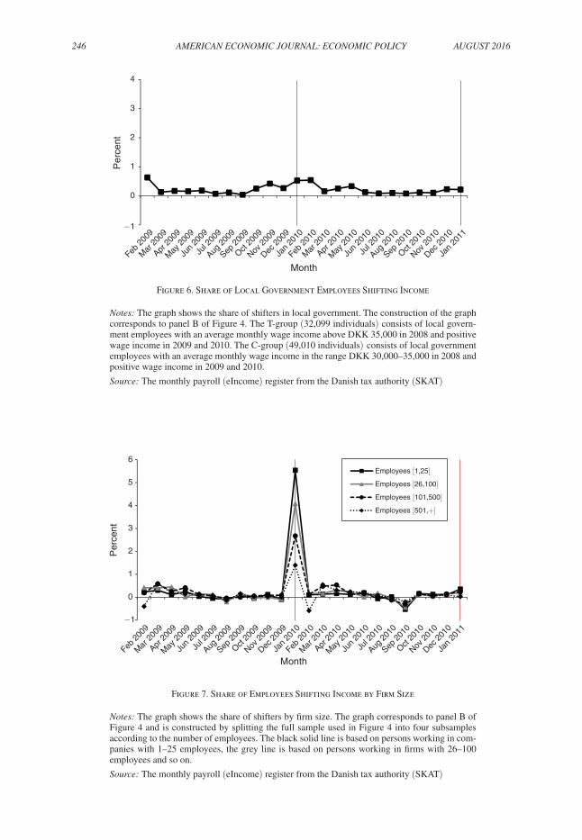
It may be easier to organize shifting in a small firm than in a large firm, for exam-ple, because a large firm may be more in the public eye and care more about its public reputation, or because the workers are closer to the decision-making process in a small firm. In Figure 7, we split the sample by firm size. The graph displays the extent of shifting for individuals working in firms with less than 25 employees, with 25–99 employees, with 100–499 employees, and with 500 or more employees.

7 The industry groups in Table 2 are relatively broad with many different kinds of firms within each group, so it is natural to expect some variation within each group. For example, accountants—a small subgroup within other business services—is a group likely to be well informed and capable of organizing income shifting. For this group, the fraction of shifters reaches 6 percent, twice the industry average of 3 percent.

Table 2—Share of Employees Shifting Income by Industry Sector

Industry sector Percent 95% conf.

1. Agriculture, forestry, and fishing 3.4 (0.9, 6.0)2. Manufacturing, mining, quarrying, and utility services 2.6 (2.4, 2.7)3. Construction 2.5 (2.1, 2.8)4. Trade and transport, etc. 3.2 (3.1, 3.4)5. Information and communication 2.4 (2.1, 2.7)6. Financial and insurance 1.5 (1.2, 1.7)7. Real estate 4.3 (3.1, 5.4)8. Other business services and activity not stated 3.1 (2.8, 3.5)9. Public administration, education, and health 2.1 (1.3, 2.9)10. Arts, entertainment, and other services 2.6 (1.5, 3.7)All sectors 2.7 (2.6, 2.8)

notes: The table reports the share of income shifters across industry types with 95 percent con-fidence intervals in brackets. For each industry, the estimate measures the difference in the share of employees fulfilling the shifting criteria in formula (3) between the T-group and the C-group. The shifting indicator equals 1 if the income of the employee in January 2010 is at least 50 per-cent above the average monthly income level in 2008 and income in December 2009 is at least 50 percent below the 2008 average monthly income level. The construction of the T-group and the C-group is described in the note to Figure 3.



−1

0

1

2

3

4

Feb 2

009

Mar

200

9

Apr 2

009

May

200

9

Jun

2009

Jul 2

009

Aug 2

009

Sep 2

009

Oct 20

09

Nov 2

009

Dec 2

009

Jan

2010

Feb 2

010

Mar

201

0

Apr 2

010

May

201

0

Jun

2010

Jul 2

010

Aug 2

010

Sep 2

010

Oct 20

10

Nov 2

010

Dec 2

010

Jan

2011

Per

cent

Month

−1

0

1

2

3

4

5

6

Feb 2

009

Mar

200

9

Apr 2

009

May

200

9

Jun

2009

Jul 2

009

Aug 2

009

Sep 2

009

Oct 20

09

Nov 2

009

Dec 2

009

Jan

2010

Feb 2

010

Mar

201

0

Apr 2

010

May

201

0

Jun

2010

Jul 2

010

Aug 2

010

Sep 2

010

Oct 20

10

Nov 2

010

Dec 2

010

Jan

2011

Per

cent

Month

Employees [1,25]

Employees [26,100]

Employees [101,500]

Employees [501,+]

Figure 6. Share of Local Government Employees Shifting Income

notes: The graph shows the share of shifters in local government. The construction of the graph corresponds to panel B of Figure 4. The T-group (32,099 individuals) consists of local govern-ment employees with an average monthly wage income above DKK 35,000 in 2008 and positive wage income in 2009 and 2010. The C-group (49,010 individuals) consists of local government employees with an average monthly wage income in the range DKK 30,000–35,000 in 2008 and positive wage income in 2009 and 2010.


Figure 7. Share of Employees Shifting Income by Firm Size

notes: The graph shows the share of shifters by firm size. The graph corresponds to panel B of Figure 4 and is constructed by splitting the full sample used in Figure 4 into four subsamples according to the number of employees. The black solid line is based on persons working in com-panies with 1–25 employees, the grey line is based on persons working in firms with 26–100 employees and so on.



Shifting appears to be much more widespread among small firms where 5–6 percent are shifters according to the analysis. The share of shifters declines steadily as firm size increases, and for the largest firms, shifting only takes place for about 1 percent of the employees.

In Figure 8, we repeat the firm size stratification but confine our sample to include only the top-five paid employees from each firm. That changes the picture. We still observe about 6 percent shifters among the small firms, but the share of shifters is now at the same level for larger firms. Thus, income shifting is a more prevalent phenomenon among the top management within each firm. This aligns with the findings of Goolsbee (2000) showing that income shifting is prevalent among the highest paid top executives in large US public companies. More importantly, our results show that shifting by top management in large companies only accounts for a limited part of the overall income shifting. If we remove the top-5 paid employees in large companies (defined as more than 100 employees, the top decile measured by number of employees) from the sample, then the share of shifters changes from 2.7 percent to 2.6 percent. Thus, shifting is not confined to the small elite of top managers in large firms.

The decision to engage in income shifting likely also depends on the financial capacity of the employee. Shifting a full month of income from December 2009 to January 2010 requires financial resources enough to maintain living expenses in that month, or access to credit at a level of cost that does not exceed the gains from shifting. As a proxy for financial capacity of an employee, we compute the amount of financial assets, i.e., money in bank accounts and the value of shares and bonds, at the end of 2008, and measure it relative to annual disposable income in 2008.

−2

−1

0

1

2

3

4

5

6

7

8

Feb 2

009

Mar

200

9

Apr 2

009

May

200

9

Jun

2009

Jul 2

009

Aug 2

009

Sep 2

009

Oct 20

09

Nov 2

009

Dec 2

009

Jan

2010

Mar

201

0

Apr 2

010

May

201

0

Jun

2010

Jul 2

010

Aug 2

010

Sep 2

010

Oct 20

10

Nov 2

010

Dec 2

010

Jan

2011

Per

cent

Month

Employees [1,25]

Employees [26,100]

Employees [101,500]

Employees [501,+]

Feb 2

010

Figure 8. Share of Top Five Wage Earners Shifting Income by Firm Size

notes: The graph shows the share of shifters among top five wage earners by firm size. The graph corresponds to Figure 7 with the exception that only top five wage earners within each firm are included in the analysis.



This is similar to the approach commonly applied in the consumption literature (e.g., Johnson, Parker, and Souledes 2006; Leth-Petersen 2010). Figure 9 repeats the analysis in Figure 4 separately for individuals with a level of liquidity below one month of disposable income, between one and two months of disposable income, and above two months of disposable income. The spike at January 2010 is increas-ing from 2.3 percent shifters in the group with low financial capacity to 3.0 percent in the group with high financial capacity, indicating that liquidity constraints have a role to play when employees decide whether or not to engage in shifting behavior.

So far we have provided evidence based on bivariate correlations of the shifting indicator with industry type workplace, firm size, top five paid employees within the firm, and financial capacity of the employees. In Table 3, we collect all these factors in a linear probability model by estimating

(4) D i = β 0 + d i T β 1 + x i β 2 + d i T ( x i − x ̅ i ) β 3 + ε i ,

where D i is the shifting indicator in equation (3) measured in January 2010, d i T is a dummy variable that equals one if the employee belongs to the T-group, x i is a vector of explanatory factors, x ̅ i is the sample mean of the explanatory vari-ables, and ε i is an error term. In this specification, β 1 measures the overall share of individuals who are shifting income after controlling for observable differences between the treatment group and the control group, and β 3 captures variation in the

−0.5

0.0

0.5

1.0

1.5

2.0

2.5

3.0

3.5

Feb 2

009

Mar

200

9

Apr 2

009

May

200

9

Jun

2009

Jul 2

009

Aug 2

009

Sep 2

009

Oct 20

09

Nov 2

009

Dec 2

009

Jan

2010

Feb 2

010

Mar

201

0

Apr 2

010

May

201

0

Jun

2010

Jul 2

010

Aug 2

010

Sep 2

010

Oct 20

10

Nov 2

010

Dec 2

010

Jan

2011

Per

cent

Month

Liquid assets equal to 2+ months net-of-tax wage payments

Liquid assets equal to 1–2 months net-of-tax wage payments

Liquid assets equal to 0–1months net-of-tax wage payments

Figure 9. Share of Employees Shifting Income by Liquidity Level

notes: The graph shows the share of individuals shifting income in the treatment group across employees with different levels of liquidity. The liquidity measure is constructed as the value in 2008 of stocks, bonds, and deposit accounts, and employees are divided into three groups depending on their level of liquidity relative to their average monthly net-of-tax wage level in 2008. Each graph is constructed by computing the differences in the share of income shifters, according to the shifting indicator in formula (3), between the relevant liquidity segment of the T-group and the C-group for each month.

source: The monthly payroll (eIncome) register from the Danish tax authority (SKAT) and information on liquidity from administrative registers at Statistics Denmark

Vol. 8 No. 3 249kreiner et al.: intertemporal shifting of wage income

share of shifters across observables around the mean effect (Wooldridge 2002). We include among the explanatory variables, x , the factors studied in the partial analy-ses described above as well as demographic and geographic control variables. The first conclusion from Table 3 is that the β 1 -estimate of the average number of shifters

Table 3—Income Shifter Characteristics

Coeff. Conf. 95%

T-group 2.5 (2.3, 2.6)

Sector 1: Agriculture, forestry, and fishing—omittedSector 2: Manufacturing, mining, quarrying, and utility services −0.2 (−1.6, 1.0)Sector 3: Construction −0.4 (−1.8, 0.8)Sector 4: Trade and transport, etc. −0.4 (−1.7, 0.8)Sector 5: Information and communication −0.1 (1.5, 1.1)Sector 6: Financial and insurance −0.7 (−2.1, 0.5)Sector 7: Real estate 0.0 (−1.5, 1.4)Sector 8: Other business services and activity not stated 0.4 (−1.0, 1.6)Sector 9: Public administration, education, and health −0.2 (−1.7, 1.0)Sector 10: Arts, entertainment, and other services −0.6 (−2.1, 0.7)500 < Company employees—omitted100 < Company employees ≤ 500 −0.0 (−0.2, 0.1)25 < Company employees ≤ 100 0.4 (0.2, 0.5)Company employees ≤ 25 0.6 (0.3, 0.9)Company top 5 wage earner 0.2 (−0.1, 0.5)Liquid assets less than one months net-of-tax wage payments—omittedLiquid assets equal to 1–2 months net-of-tax wage payments 0.1 (−0.1, 0.2)Liquid assets equal to 2+ months net-of-tax wage payments 0.3 (0.2, 0.4)Tgrp × (sector 1 − m(sector 1))—omitted Tgrp × (sector 2 − m(sector 2)) 1.3 (−1.3, 3.7)Tgrp × (sector 3 − m(sector 3)) 0.6 (−2.1, 3.0)Tgrp × (sector 4 − m(sector 4)) 1.3 (−1.3, 3.7)Tgrp × (sector 5 − m(sector 5)) 1.0 (−1.6, 3.5)Tgrp × (sector 6 − m(sector 6)) 0.6 (−2.0, 3.1)Tgrp × (sector 7 − m(sector 7)) 1.3 (−1.5, 3.8)Tgrp × (sector 8 − m(sector 8)) 1.5 (−1.1, 4.1)Tgrp × (sector 9 − m(sector 9)) 1.0 (−1.7, 3.4)Tgrp × (sector 10 − m(sector 10)) 0.6 (−2.3, 3.2)Tgrp × (Employees501 − m(Employees501))—omitted Tgrp × (101Employees500 − m(101Employees500)) 0.9 (0.7, 1.1)Tgrp × (26Employees100 − m(26Employees100)) 1.3 (1.0, 1.6)Tgrp × (Employees25 − m(Employees25)) 1.2 (0.7, 1.7)Tgrp × (top5 − m(top5)) 3.5 (3.1, 4.0)Tgrp × (liquidity of 1month − m(liquidity of 1month))—omittedTgrp × (liquidity of 1–2month − m(liquidity of 1–2month)) 0.7 (0.4, 1.0)Tgrp × (liquidity of 2+month − m(liquidity of 2+month)) 1.1 (0.9, 1.3)Additional controls XConstant 1.3 (0.1, 2.7)

Observations 324.126

Notes: The table reports the estimates from the LPM specification in (4) and the 95 percent confidence intervals of these estimates. The confidence intervals are based on bootstrapped standard errors with 1,000 replications. The dependent variable is the shifting indicator in (3), which equals 1 if the income of the employee in January 2010 is at least 50 percent above the average monthly income level in 2008 and income in December 2009 is at least 50 per-cent below the 2008 average monthly income level. The additional control variables include gender, age dummy variables, marital status and geographic location of residence, and m(·) denotes the mean of a variable. The con-struction of the T-group and the C-group is described in the note to Figure 3.

Source: Monthly payroll (eIncome) register from the Danish tax authority (SKAT) and socioeconomic information from administrative registers at Statistics Denmark


is almost unchanged compared to the baseline analysis in Figure 4: 2.5 percent of the employees shift income compared to 2.7 percent in the baseline analysis. The second conclusion is that all the results from the partial analysis also hold in the multivariate analysis. None of the β 3 coefficients for industry types are significant, showing shifting is widespread in the economy rather than concentrated on a few sectors. The other estimates show that the share of shifters is higher in smaller firms, is higher among the five best paid employees within firms, and is higher among employees with nonbinding liquidity constraints.

C. survey results

A reason why only a few individuals in the T-group exploit the opportunity to shift income and save taxes could be that taxpayers are unaware of the possibility and of the potential benefits associated with shifting. As described in Section I, there were articles in the popular press describing the possibility of shifting income, and in mid-October a tax official from the Danish tax agency stated publicly that it was legal to postpone wage payments into 2010.

In order to get a better understanding about the level of information and aware-ness, we included two questions in a telephone survey of a random sample of indi-viduals from the adult population in January 2011. The survey response rate was 67 percent. The survey data was then merged at the individual level to the eincome register giving us a sample of 878 taxpayers with 588 individuals belonging to the T-group and 290 individuals belonging to the C-group.

The first question was (own translation): “The last tax reform changed the taxation of income from January 1, 2010. Imagine that you had earned a little extra income at the end of 2009. From a tax point of view, when would it be most beneficially for you to have the extra income paid out: (i) Just before January 1, 2010, or (ii) Just after January 1, 2010 or (iii) Equally beneficial.” For almost all taxpayers, it would be beneficial to receive the income after New Year because of the tax reform, although the incentive is modest for individuals in the control group as described above.

The second question was: “Do you perceive it to be legal or illegal for an employee to arrange with their employer to postpone the payout of some of the income earned in 2009 to 2010? (i) Legal or (ii) Illegal.”

Table 4 shows the distribution of answers across the treatment and control groups. Only about one-third of the taxpayers state it is most beneficial to obtain extra wage income after January 1, 2010, and most people state it is equally beneficial to get it before or after January 1. The share of individuals answering “after January 1” is nearly twice as big in the treatment group as in the control group. Nevertheless, only two out of five respondents in the treatment group were able to point out that it would be most beneficial to receive the extra payment after January 1. Around 40 percent of the respondents stated they perceived it to be legal to postpone the payout of earned income from 2009 to 2010, and without any significant differences in the responses across the treatment group and the control group. Finally, if we define individuals to be aware of the shifting opportunity if they answer both “after January 1” and “legal,” then only 17 percent of the individuals in the treatment group are informed.


In Figure A2 in the online Appendix, we analyze shifting behavior in the survey sample. First, we repeat the analysis in Figure 4 by plotting the evolution of the average value of the shifting indicator for the T-group and the C-group, respectively (panel A). With only 588 and 290 individuals in the two groups, the series become rather noisy, but January 2010 still has the largest spike and the difference between the T-group and the C-group is around 2.5 percent, which corresponds to our esti-mates for the full population. We would expect the shifting effect to be driven by the informed part of the T-group and the evidence also indicates that this is the case. When we redo the graphical analysis for the T-group including only informed indi-viduals, we see a clear spike at January 2010 with a 5.5 percentage point difference between the informed T-group and the C-group (panel B).

To conclude, the survey evidence suggests that awareness of the legal possibility and the financial gain has been an important factor in explaining why some employ-ees are shifting income while others are not. This aligns with the point emphasized by Chetty, Loony, and Kroft (2009) that tax incentives need to be salient to actually affect consumer behavior. On the other hand, the extent of shifting among those who seem to be aware of the opportunity is not large, indicating that salience alone cannot explain why some taxpayers engage in shifting activity while many others do not.

III. Implications for Elasticity of Taxable Income

The elasticity of taxable income (ETI) is a key parameter in determining optimal tax policies. The excess burden of the tax system and the limits to redistribution (the Laffer rate) are governed by the income responses to taxation summarized by the ETI. For the design of optimal policies, the main interest is in the (long-run) ETI that may be used to compute the permanent tax distortions of a given tax structure.

Table 4— Share of Survey Answers on Shifting Awareness

Percent

All T-group C-group

Q1 = “Before 1st of January” 9 9 10Q1 = “After 1st of January” 35 41 23Q1 = “Equally beneficial” 56 51 67Q2 = “Legal” 40 39 43Q2 = “Illegal” 60 61 57Q1 = “After 1st of January” & Q2 = “Legal” 15 17 11Number of respondents 878 588 290

notes: The table reports answers to two questions on income shifting from survey respondents across treatment sta-tus. The table is based on answers in a telephone survey of a random sample of the adult population and conducted for a group of researchers by the survey company Capacent Epinion in January 2011. The T-group consists of pri-vate sector employees with average monthly wage income above DKK 35,000 in 2008 and positive wage income in 2009 and 2010. The C-group consists of private sector employees with average monthly wage income in the range DKK 30,000–35,000 in 2008 and positive wage income in 2009 and 2010.

source: The monthly payroll (eIncome) register from the Danish tax authority (SKAT) and telephone survey infor-mation obtained by Capacent Epinion


The transitory income movements due to income shifting may have implica-tions for the estimation of the ETI that exploits reform-driven variation in tax rates for identification (Saez, Slemrod, and Giertz 2012). If taxpayers temporarily shift income from a period with a high tax rate to a period with a low tax rate then this effect may enter into the empirical estimate, implying the estimated short run ETI is an upward biased estimate of the long run elasticity.

In this section, we exploit the monthly frequency of our data to identify in a new way the extent to which the short-run ETI may be attributed to income shifting responses. We start by deriving a traditional difference-in-differences estimate of the ETI by estimating

(5) w y, m, i = β 0 + β 1 d y, i 2010 + β 2 d i T + β 3 1 − τ y, i _

1 − τ 2009, i + ε y, m, i ,

where w y, m, i is defined in (1), d y, i 2010 is a dummy variable that equals one in year 2010, d i T is a treatment dummy, τ y, i is the tax rate applying to individual i in year y , and ε y, m, i is an error term. This regression is estimated on values of w y, m, i from January 2009 to December 2010 and with standard errors clustered at the individual level. In this specification, β 3 corresponds to the ETI. To see this, note equations (1) and (5) imply

(6) ETI = E [

z ̅ 2010, i − z ̅ 2009, i _ z ̅ 2008, i | i ∈ T] − E [ z ̅ 2010, i − z ̅ 2009, i _ z ̅ 2008, i | i ∈ c]

__________________________________ ( 1 − τ 2010 T _

1 − τ 2009 T − 1) − ( 1 − τ 2010 c _

1 − τ 2009 c − 1)

= β 3 ,

where the numerator is the percentage change in average monthly income of the T-group from the year before the implementation of the reform to the year after implementation, and measured relative to the C-group, while the denominator is the percentage change in the net-of-tax rate of the T-group due to the reform (18 percent) minus the corresponding change of the C-group (2 percent) described in Section I.8

The top-left corner of Table 5 reports the ETI estimate obtained from running regression (5). The ETI equals 0.1 and is very precisely estimated. The size of the elasticity is in line with recent empirical evidence for Denmark by Kleven and Schultz (2014) using yearly income data, spanning a period of 25 years with iden-tifying variation provided by a series of tax reforms. In the rows 2–6 of column 1, we present the ETI estimate for different points in the income distribution, follow-ing the income grouping applied in Figure 5. It shows that the ETI is increasing in income, as is also found in other studies (Saez, Slemrod, and Giertz 2012), and is equal to around 0.25 for the top 1 percent of the earners.

8 We measure the income differences relative to 2008 rather than 2009 income levels because the latter is influenced by the shifting behavior and in order to keep consistency with the remaining part of the analysis. The sensitivity analysis in Table A2 in the online Appendix shows that the ETI results are similar if we instead use 2009 as the baseline year for the analysis.


In order to analyze how much of the ETI estimate that may be attributed to shift-ing, we first recalculate the ETI using a subset of the data where we leave out indi-viduals from the T-group and the C-group who are classified as shifters according to the shifting indicator in (3). This procedure removes only around 9,000 out of 330,000 individuals from the sample but implies that the overall ETI estimate drops from 0.10 to 0.05. This result is reported in column 2 of Table 5. Looking at the effect through the income distribution in column 5, we see that the impact on the ETI estimate is largest at the top of the income distribution.

Another way to analyze the effect of shifting is to decompose the overall ETI esti-mate into the variation coming from December 2009–January 2010, where income shifting is most prevalent, and the variation in the data coming from the remaining 22 months. Column 3 of Table 1 displays the result from running the regression (5) on the subsample of w -values from December 2009 and January 2010. It shows that the ETI estimate explodes to about 0.9, i.e., nine times as high as the basic estimate, and the effect is even more dramatic when going to the top of the income distribu-tion where the elasticity estimate is above three.

If we assume that shifting only takes place in December and January, then we can remove shifting from the ETI estimate by basing the estimation on the remain-ing 22 months. This gives an estimate equal to 0.03 (column 4). However, the evi-dence in Section II, for example, Figure 3, shows that some individuals also shift their November 2009 income into 2010, and in column 5 we therefore also exclude November 2009 from the estimation. In that case, the point estimate of the ETI without shifting becomes 0.01, and it is statistically insignificant. These results sug-gest that intertemporal income shifting, taking place very locally around the point of the implementation of the tax reform, is responsible for almost all the variation that is used for estimating the short-run ETI. Results align when we move through the income distribution. Many of the elasticity estimates in columns 4 and 5 are

Table 5—Importance of Shifting for Estimates of the Elasticity of Taxable Income

All months All months Only D09 & J10 Excl. D09 & J10 Excl. N09, D09, & J10Income group All individuals Nonshifters All individuals All individuals All individuals (1) (2) (3) (4) (5)

Full sample 0.10 (0.08, 0.11) 0.05 (0.03, 0.06) 0.86 (0.82, 0.89) 0.03 (0.01, 0.04) 0.01 (−0.00, 0.03)income ≤ P80 0.01 (−0.01, 0.04) 0.00 (−0.02, 0.03) 0.16 (0.11, 0.22) 0.00 (−0.03, 0.03) −0.01 (−0.03, 0.02) P80 ≤ income < P90 0.06 (0.05, 0.08) 0.04 (0.02, 0.05) 0.48 (0.44, 0.53) 0.02 (0.01, 0.04) 0.02 (−0.00, 0.03)P90 ≤ income < P95 0.12 (0.10, 0.14) 0.07 (0.05, 0.08) 0.89 (0.84, 0.94) 0.05 (0.03, 0.07) 0.03 (0.01, 0.05)P95 ≤ income < P99 0.16 (0.14, 0.18) 0.06 (0.04, 0.08) 1.47 (1.40, 1.54) 0.04 (0.02, 0.06) 0.01 (−0.01, 0.03)P99 ≤ income 0.26 (0.21, 0.31) 0.10 (0.05, 0.15) 3.17 (2.88, 3.47) −0.00 (−0.06, 0.05) −0.06 (−0.11, −0.01)

notes: The table reports ETI estimates using specification (5) and 95 percent confidence intervals in brackets. The construction of the T-group (219,179) and the C-group (109,500) is described in the note to Figure 3. The column label “nonshifters” refers to estimations where employees shifting income around New Year 2010, according to the shifting criteria described in the note to Figure 4 and formula (3), are excluded from the sample. This excludes 9,088 taxpayers from the total sample of 329,270 taxpayers. The ETI estimates under the column label “Only D09 & J10” are based on estimation of (5) on the subsample of wage observations from December 2009 and January 2010. The ETI estimates under the column label “Excl. D09 & J10” are based on estimation of (5) on a subsample where wage observations in December 2009 and January 2010 are excluded from the estimation. The ETI estimates under the column label “Excl. N09, D09, and J10” are computed by excluding wage observations in November 2009, December 2009, and January 2010 from the estimation.



insignificant, and the point estimates indicate that income shifting explains at least half of the standard ETI estimate, and in some cases all of it. In particular, the high ETI estimates in the top of the income distribution can be explained entirely by intertemporal income shifting.

The standard difference-in-differences approach relies on a strong assumption of a common trend of the T-group and the C-group. This assumption may be prob-lematic, for example, because young wage earners have a more steep income profile and are more dominant in the control group. In Table A1 in the online Appendix, we repeat the ETI estimates in Table 5 but from a regression where we allow income growth to be explained by cohort dummies, gender, marital status, region dummies, industry type dummies, and firm size dummies (these controls and interactions with d y, i 2010 are added to the right-hand side of the specification (5)). All the ETI estimates change only a little and the conclusions are therefore the same; this is also the case if we include only a subset of the control variables. Unobserved heterogeneity may still imply that top income individuals have experienced a different income devel-opment than the control group, but the fact that top income shares have been almost constant for two decades in Denmark, unlike many other countries, indicates that this is not the case (Kleven and Schultz 2014).

A number of sensitivity analyses reported in Table A2 in the online Appendix show that the results are robust to changing the size of the control group, to chang-ing the baseline year, and to the exclusion of all taxpayers in a band around the top tax threshold. The exclusion of taxpayers within an income range around the top tax threshold (the Doughnut sample) is a way to reduce the importance of mean reversion, which can lead to a downward bias in the ETI estimates. The estimates are largely unaffected suggesting that mean-reversion is not a major concern for our overall ETI estimate.

It is common in the literature to look at three-year income differences, using annual income in the year before the reform and annual income observed two years after the reform. The idea is that the use of a longer period may be better at over-coming adjustment costs in short-run decision-making and thereby provide a better estimate of the long run ETI. This procedure also reduces the bias from income shifting because now it is only the year before the reform that is affected by shifting. The last row of Table A2 reports the results if we use data from 2011 (the last year in our data) instead of 2010 for our analysis, i.e., a two-year window. In this case, the baseline ETI estimate drops from 0.10 to 0.08. As expected, the shifting component also becomes smaller, implying that the ETI estimates after controlling for shifting are now slightly higher and significant (although still rather small), but shifting may still account for more than half of the ETI estimates.

IV. Conclusion

Our results contribute in several ways to the empirical literature on the behavioral effects of taxation. First, using high-frequency payroll data, we show that intertem-poral income shifting is a significant issue for regular wage income and not only for more exotic types of compensation. Second, shifting may well account for all the income variation used to estimate the short-run ETI and may explain why estimates


are increasing with income. Third, shifting is widespread—it takes place at practi-cally all levels of income and the extent of shifting is similar across industry sectors. Fourth, shifting is concentrated on very few individuals who shift large amounts. Fifth, the fact that only a few of the taxpayers with an incentive to shift income exploit the opportunity is probably related to unawareness of the potential benefits and legality of income shifting, and taxpayers being liquidity constrained as well as limited willingness of employers to cooperate with the employees in organizing this type of tax avoidance.

It is possible to engage in intertemporal income shifting by deferring payment of regular earnings or by postponing bonus payments. Our empirical approach cap-tures both types of avoidance strategies but cannot distinguish between them. In an extension of this paper, we look more closely at year-end tax planning of top managers and their choice of avoidance strategies (Kreiner, Leth-Petersen, and Skov 2014). The results show that income shifting is much more common among top managers who normally receive a year-end bonus, and that they shift the bonus payment from December 2009 to January 2010 but do not defer payment of regular wage income.

Our finding of an ETI estimate close to zero after removing the shifting compo-nent does not necessarily imply that the long-run elasticity relevant for tax policy analyses is negligible. As shown in Chetty (2012), small frictions may imply that the long-run elasticity is of a considerable size, although the estimated short-run ETI is small or even zero. Consistent with this view, studies have found larger ETI estimates when considering a longer time horizon (e.g., Giertz 2010). Other types of evidence also point to a nontrivial long-run elasticity, for example, the compelling non-parametric evidence of longer run effects in Kleven and Schultz (2014) and the structural analysis of labor mobility in Kreiner, Munch, and Whitta-Jacobsen (2015).

Our results indicate that information and salience is important for income shift-ing, but our analysis cannot establish a causal relationship, as is done by Chetty, Loony, and Kroft (2009). Nevertheless, it is striking that we obtain reasonably large effects in a setting where only one out of five seems to be informed about the possi-bility of income shifting. It is also remarkable that so few taxpayers engage in shift-ing among those who seem to be informed. Our evidence points to the importance of liquidity constraints and firm cooperation but we cannot rule out other explanations, for example, tax moral and social norms.

Significant intertemporal shifting effects in wage income may have policy impli-cations. For example, standard optimal tax theories call for age-dependency in tax rates (Banks and Diamond 2011), while the possibility of shifting, ceteris paribus, calls for constant marginal tax rates over the life cycle, which removes incentives to shift income payments across time. Evaluation of tax reforms normally focuses on the long-run effects. However, often a tax reform is replaced by a new reform a few years later, implying that income shifting effects are nontrivial in the long run. For example, the Danish 2010 tax reform studied in this paper was the sixth tax reform within a period of 25 years and 7 reforms were implemented in the United States in the 25 year period from 1980 to 2005. The individual benefits from shifting are very unequally distributed with large benefits in the top of the income distribution,


and without any corresponding gain in economic efficiency.9 Thus, from a standard equality-efficiency trade-off perspective, social welfare would increase if income shifting is reduced.

In Denmark, it is possible to engage in intertemporal income shifting without breaking the tax law. This is not the case in all countries. For example, shifting of wage and salary income across years for the purpose of legal tax avoidance is not permitted in the United States, and intertemporal income shifting effects may there-fore be less pronounced. On the other hand, the difference may not be large in prac-tice as it is difficult for tax authorities to prove intertemporal income shifting has taken place when, say, a bonus payment is received in January instead of December.

REFERENCES

Andreoni, James, Brian Erard, and Jonathan Feinstein. 1998. “Tax Compliance.” Journal of Eco-nomic Literature 36 (2): 818–60.

Banks, James, and Peter Diamond. 2011. “The Base for Direct Taxation.” In Dimensions of Tax Design: The mirrlees review, edited by James Mirrlees, Stuart Adam, Timothy Besley, Richard Blundell, Stephen Bond, Robert Chote, Malcolm Gammie et al., 548–648. Oxford: Oxford University Press.

Chetty, Raj. 2012. “Bounds on Elasticities with Optimization Frictions: A Synthesis of Micro and Macro Evidence on Labor Supply.” Econometrica 80 (3): 969–1018.

Chetty, Raj, John N. Friedman, and Emmanuel Saez. 2013. “Using Differences in Knowledge Across Neighborhoods to Uncover the Impacts of the EITC on Earnings.” American Economic review 103 (7): 2683–2721.

Chetty, Raj, Adam Looney, and Kory Kroft. 2009. “Salience and Taxation: Theory and Evidence.” American Economic review 99 (4): 1145–77.

Congressional Budget Office. 2013. The Budget and Economic outlook: Fiscal years 2013 to 2023. Congress of the United States. Washington, DC, February.

Giertz, Seth H. 2010. “The Elasticity of Taxable Income during the 1990s: New Estimates and Sensi-tivity Analyses.” southern Economic Journal 77 (2): 406–33.

Goolsbee, Austan. 2000. “What Happens When You Tax the Rich? Evidence from Executive Compen-sation.” Journal of Political Economy 108 (2): 352–78.

Johnson, David S., Jonathan A. Parker, and Nicholas S. Souleles. 2006. “Household Expenditure and the Income Tax Rebates of 2001.” American Economic review 96 (5): 1589–1610.

Heim, Bradley T. 2009. “The Effect of Recent Tax Changes on Taxable Income: Evidence from a New Panel of Tax Returns.” Journal of Policy Analysis and management 28 (1): 147–63.

Kleven, Henrik Jacobsen, Martin B. Knudsen, Claus Thustrup Kreiner, Søren Pedersen, and Emman-uel Saez. 2011. “Unwilling or Unable to Cheat? Evidence from a Tax Audit Experiment in Den-mark.” Econometrica 79 (3): 651–92.

Kleven, Henrik Jacobsen, and Esben Anton Schultz. 2014. “Estimating Taxable Income Responses using Danish Tax Reforms.” American Economic Journal: Economic Policy 6 (4): 271–301.

Kreiner, Claus Thustrup, Søren Leth-Petersen, and Peer Ebbesen Skov. 2014. “Year-End Tax Planning of Top Management: Evidence from High-Frequency Payroll Data.” American Economic review 104 (5): 154–58.

Kreiner, Claus Thustrup, Jakob Roland Munch, and Hans Jørgen Whitta-Jacobsen. 2015. “Taxation and the long run allocation of labor: Theory and Danish evidence.” Journal of Public Economics 127: 74–86.

Kreiner, Claus Thustrup, Søren Leth-Petersen, and Peer Ebbesen Skov. 2016. “Tax Reforms and Inter-temporal Shifting of Wage Income: Evidence from Danish Monthly Payroll Records: Dataset.” American Economic Journal: Economic Policy. http://dx.doi.org/10.1257/pol.20140233.

le Maire, Daniel, and Bertel Schjerning. 2013. “Tax bunching, income shifting and self-employment.” Journal of Public Economics 107: 1–18.

9 The effect on economic efficiency is negative in a standard neoclassical setting. The change in economic effi-ciency from a (small) tax reform is approximately equal to the behavioral effects on government revenue, which is negative because shifting behavior reduces tax revenue.


http://pubs.aeaweb.org/action/showLinks?crossref=10.4284%2Fsej.2010.77.2.406

http://pubs.aeaweb.org/action/showLinks?crossref=10.3982%2FECTA9113

http://pubs.aeaweb.org/action/showLinks?system=10.1257%2Faer.96.5.1589



http://pubs.aeaweb.org/action/showLinks?crossref=10.1002%2Fpam.20406

http://pubs.aeaweb.org/action/showLinks?crossref=10.1086%2F262122

http://pubs.aeaweb.org/action/showLinks?system=10.1257%2Fpol.6.4.271

http://pubs.aeaweb.org/action/showLinks?crossref=10.3982%2FECTA9043

http://pubs.aeaweb.org/action/showLinks?crossref=10.1016%2Fj.jpubeco.2014.03.012


http://pubs.aeaweb.org/action/showLinks?crossref=10.1016%2Fj.jpubeco.2013.08.002


Leth-Petersen, Søren. 2010. “Intertemporal Consumption and Credit Constraints: Does Consumption Respond to an Exogenous Shock to Credit?” American Economic review 100 (3): 1080–1103.

Saez, Emmanuel, Joel Slemrod, and Seth H. Giertz. 2012. “The Elasticity of Taxable Income with Respect to Marginal Tax Rates: A Critical Review.” Journal of Economic Literature 50 (1): 3–50.

Sammartino, Frank, and David Weiner. 1997. “Recent Evidence on Taxpayers’ Response to the Rate Increases in the 1990’s.” national Tax Journal 50 (3): 683–705.

Slemrod, Joel. 1995. “Income Creation or Income Shifting? Behavioral Responses to the Tax Reform Act of 1986.” American Economic review 85 (2): 175–80.

Slemrod, Joel. 1998. “Methodological Issues in Measuring and Interpreting Taxable Income Elastici-ties.” national Tax Journal 51 (4): 773–88.

Wooldridge, Jeffrey M. 2002. Econometric Analysis of cross section and Panel Data. Cambridge: MIT Press.

http://pubs.aeaweb.org/action/showLinks?system=10.1257%2Fjel.50.1.3


Documents

Tax Reforms and Intertemporal Shifting of Wage Income