BESC 320 – Water and Bioenvironmental Science(Climate change models and case study of Texas water – 7 Mar 2018)

At the global level, a major factor in determining the extent of warming (and corresponding shifts in water balance) is GH gas emissions. IPCC defines four scenarios (A1B used most often):

E.g., recall the figure from last time, using 21 of the major climate models, under A1B:

E.g.—The types of information derived from the emmisions scenarios:

A1B is considered a little “optimistic”, but is most broadly used, and will suffice to start thinking about our regional (Texas) impacts of warming, assuming strong global reduced reliance on fossil fuels. (A2 seems most plausible to your 320 prof)

NOAA Climate Summary (October 2012)

“The average temperature across land and ocean surfaces during October was 14.63°C (58.23°F). This is 0.63°C (1.13°F)

above the 20th century average…This is the 332nd consecutive month with an above-average temperature.”

What this means... If you are under 27 years old, you have never lived through a

month that was colder than the modern average.

Although major global predictions are for increased temperature, increased precipitation, and greater variability of precipitation, there is also geographic variability expected in these trends.

The outlook is not good for Texas:

The yellow-blue boundary is the “zero change isocline”.

Takehome message for your grandchildren in Texas: +2 °C temperature change -5 % or worse precipitation change increased climate volatility

The goal today is to understand at least an approach to predicting and dealing with regional changes. We will focus on “water budgets” for Texas.

Texas climate change and Texas water

(data from a public presentation by George Ward)

Exercise: You are a water policy and planning official in Texas. How do you design a water plan? To begin, consider the information you will need to make an informed decision (list, draft flowchart).

To foment ideas—here is a review of nature’s part of the hydrologic cycle:

I’ll work toward George’s model. First, more regional information:

Precipitation isoclines:

Facts about Texas surface water rainfall is produced near entirely from deep convection rainfall declines precipitously from EW runoff is small as a proportion of rainfall runoff declines even more precipitously from EW river flows are flashy (tjd: more so going EW)

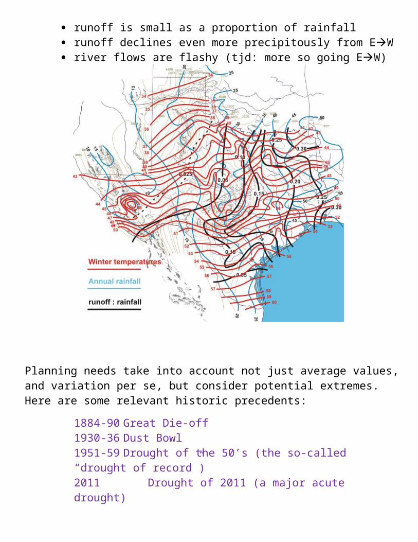
Planning needs take into account not just average values, and variation per se, but consider potential extremes. Here are some relevant historic precedents:

1884-90 Great Die-off1930-36 Dust Bowl1951-59 Drought of the 50’s (the so-called “drought of record”)2011 Drought of 2011 (a major acute drought)

Here is George’s water budget flowchart:

What is missing? temporal change, including climate change

Summary:

Now what’s missing—changing demand through time (40 year foresight)

Ward model with projected changes in water usage:

And now adding regional climate change projection

Conclusions