fitdistrplus: An R Package for Fitting Distributions

Marie Laure Delignette-MullerUniversite de LyonChristophe Dutang

Universite de Strasbourg

October 2014∗

Abstract

The package fitdistrplus provides functions for fitting univariate distributions to different types of data (con-tinuous censored or non-censored data and discrete data) and allowing different estimation methods (maximumlikelihood, moment matching, quantile matching and maximum goodness-of-fit estimation). Outputs of fitdist

and fitdistcens functions are S3 objects, for which kind generic methods are provided, including summary, plotand quantile. This package also provides various functions to compare the fit of several distributions to a samedata set and can handle bootstrap of parameter estimates. Detailed examples are given in food risk assessment,ecotoxicology and insurance contexts.

Keywords: probability distribution fitting, bootstrap, censored data, maximum likelihood, moment matching,quantile matching, maximum goodness-of-fit, distributions, R

1 Introduction

Fitting distributions to data is a very common task in statistics and consists in choosing a probability distributionmodelling the random variable, as well as finding parameter estimates for that distribution. This requires judgmentand expertise and generally needs an iterative process of distribution choice, parameter estimation, and quality offit assessment. In the R (R Development Core Team, 2013) package MASS (Venables and Ripley, 2010), maximumlikelihood estimation is available via the fitdistr function; other steps of the fitting process can be done usingother R functions (Ricci, 2005). In this paper, we present the R package fitdistrplus (Delignette-Muller et al., 2014)implementing several methods for fitting univariate parametric distribution. A first objective in developing this packagewas to provide R users a set of functions dedicated to help this overall process.

The fitdistr function estimates distribution parameters by maximizing the likelihood function using the optim

function. No distinction between parameters with different roles (e.g., main parameter and nuisance parameter) ismade, as this paper focuses on parameter estimation from a general point-of-view. In some cases, other estimationmethods could be prefered, such as maximum goodness-of-fit estimation (also called minimum distance estimation),as proposed in the R package actuar with three different goodness-of-fit distances (Dutang et al., 2008). Whiledevelopping the fitdistrplus package, a second objective was to consider various estimation methods in addition tomaximum likelihood estimation (MLE). Functions were developped to enable moment matching estimation (MME),quantile matching estimation (QME), and maximum goodness-of-fit estimation (MGE) using eight different distances.Moreover, the fitdistrplus package offers the possibility to specify a user-supplied function for optimization, useful incases where classical optimization techniques, not included in optim, are more adequate.

In applied statistics, it is frequent to have to fit distributions to censored data (Klein and Moeschberger, 2003;Helsel, 2005; Busschaert et al., 2010; Leha et al., 2011; Commeau et al., 2012). The MASS fitdistr function doesnot enable maximum likelihood estimation with this type of data. Some packages can be used to work with censoreddata, especially survival data (Therneau, 2011; Hirano et al., 1994; Jordan, 2005), but those packages generally focuson specific models, enabling the fit of a restricted set of distributions. A third objective is thus to provide R users afunction to estimate univariate distribution parameters from right-, left- and interval-censored data.

Few packages on CRAN provide estimation procedures for any user-supplied parametric distribution and supportdifferent types of data. The distrMod package (Kohl and Ruckdeschel, 2010) provides an object-oriented (S4)implementation of probability models and includes distribution fitting procedures for a given minimization criterion.This criterion is a user-supplied function which is sufficiently flexible to handle censored data, yet not in a trivial way,see Example M4 of the distrMod vignette. The fitting functions MLEstimator and MDEstimator return an S4 class forwhich a coercion method to class mle is provided so that the respective functionalities (e.g., confint and logLik) frompackage stats4 are available, too. In fitdistrplus, we chose to use the standard S3 class system for its understandingby most R users. When designing the fitdistrplus package, we did not forget to implement generic functions also

∗Paper accepted in the Journal of Statistical Software

1

available for S3 classes. Finally, various other packages provide functions to estimate the mode, the moments or theL-moments of a distribution, see the reference manuals of modeest, lmomco and Lmoments packages.

This manuscript reviews the various features of version 1.0-2 of fitdistrplus. The package is available fromthe Comprehensive R Archive Network at http://cran.r-project.org/package=fitdistrplus. The developmentversion of the package is located at R-forge as one package of the project “Risk Assessment with R” (http://r-forge.r-project.org/projects/riskassessment/). The paper is organized as follows: Section 2 presents tools for fittingcontinuous distributions to classic non-censored data. Section 3 deals with other estimation methods and other typesof data, before Section 4 concludes.

2 Fitting distributions to continuous non-censored data

2.1 Choice of candidate distributions

For illustrating the use of various functions of the fitdistrplus package with continuous non-censored data, we willfirst use a data set named groundbeef which is included in our package. This data set contains pointwise values ofserving sizes in grams, collected in a French survey, for ground beef patties consumed by children under 5 years old.It was used in a quantitative risk assessment published by Delignette-Muller et al. (2008).

R> library("fitdistrplus")

R> data("groundbeef")

R> str(groundbeef)

'data.frame': 254 obs. of 1 variable:

$ serving: num 30 10 20 24 20 24 40 20 50 30 ...

Before fitting one or more distributions to a data set, it is generally necessary to choose good candidates amonga predefined set of distributions. This choice may be guided by the knowledge of stochastic processes governing themodelled variable, or, in the absence of knowledge regarding the underlying process, by the observation of its empiricaldistribution. To help the user in this choice, we developed functions to plot and characterize the empirical distribution.

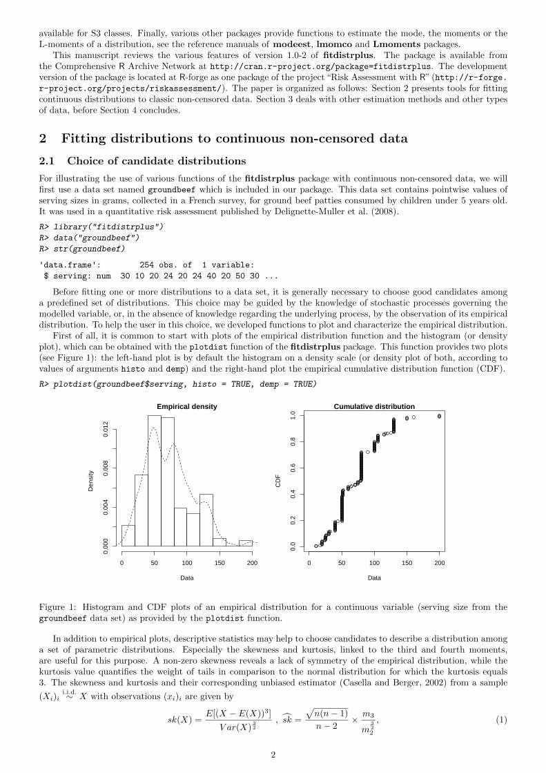
First of all, it is common to start with plots of the empirical distribution function and the histogram (or densityplot), which can be obtained with the plotdist function of the fitdistrplus package. This function provides two plots(see Figure 1): the left-hand plot is by default the histogram on a density scale (or density plot of both, according tovalues of arguments histo and demp) and the right-hand plot the empirical cumulative distribution function (CDF).

R> plotdist(groundbeef$serving, histo = TRUE, demp = TRUE)

Empirical density

Data

Den

sity

0 50 100 150 200

0.00

00.

004

0.00

80.

012

0 50 100 150 200

0.0

0.2

0.4

0.6

0.8

1.0

Cumulative distribution

Data

CD

F

Figure 1: Histogram and CDF plots of an empirical distribution for a continuous variable (serving size from thegroundbeef data set) as provided by the plotdist function.

In addition to empirical plots, descriptive statistics may help to choose candidates to describe a distribution amonga set of parametric distributions. Especially the skewness and kurtosis, linked to the third and fourth moments,are useful for this purpose. A non-zero skewness reveals a lack of symmetry of the empirical distribution, while thekurtosis value quantifies the weight of tails in comparison to the normal distribution for which the kurtosis equals3. The skewness and kurtosis and their corresponding unbiased estimator (Casella and Berger, 2002) from a sample

(Xi)ii.i.d.∼ X with observations (xi)i are given by

sk(X) =E[(X − E(X))3]

V ar(X)32

, sk =

√n(n− 1)

n− 2× m3

m322

, (1)

2

kr(X) =E[(X − E(X))4]

V ar(X)2, kr =

n− 1

(n− 2)(n− 3)((n+ 1)× m4

m22

− 3(n− 1)) + 3, (2)

where m2, m3, m4 denote empirical moments defined by mk = 1n

∑ni=1(xi−x)k, with xi the n observations of variable

x and x their mean value.The descdist function provides classical descriptive statistics (minimum, maximum, median, mean, standard devi-

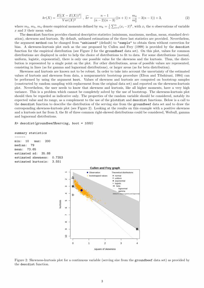
ation), skewness and kurtosis. By default, unbiased estimations of the three last statistics are provided. Nevertheless,the argument method can be changed from "unbiased" (default) to "sample" to obtain them without correction forbias. A skewness-kurtosis plot such as the one proposed by Cullen and Frey (1999) is provided by the descdist

function for the empirical distribution (see Figure 2 for the groundbeef data set). On this plot, values for commondistributions are displayed in order to help the choice of distributions to fit to data. For some distributions (normal,uniform, logistic, exponential), there is only one possible value for the skewness and the kurtosis. Thus, the distri-bution is represented by a single point on the plot. For other distributions, areas of possible values are represented,consisting in lines (as for gamma and lognormal distributions), or larger areas (as for beta distribution).

Skewness and kurtosis are known not to be robust. In order to take into account the uncertainty of the estimatedvalues of kurtosis and skewness from data, a nonparametric bootstrap procedure (Efron and Tibshirani, 1994) canbe performed by using the argument boot. Values of skewness and kurtosis are computed on bootstrap samples(constructed by random sampling with replacement from the original data set) and reported on the skewness-kurtosisplot. Nevertheless, the user needs to know that skewness and kurtosis, like all higher moments, have a very highvariance. This is a problem which cannot be completely solved by the use of bootstrap. The skewness-kurtosis plotshould then be regarded as indicative only. The properties of the random variable should be considered, notably itsexpected value and its range, as a complement to the use of the plotdist and descdist functions. Below is a call tothe descdist function to describe the distribution of the serving size from the groundbeef data set and to draw thecorresponding skewness-kurtosis plot (see Figure 2). Looking at the results on this example with a positive skewnessand a kurtosis not far from 3, the fit of three common right-skewed distributions could be considered, Weibull, gammaand lognormal distributions.

R> descdist(groundbeef$serving, boot = 1000)

summary statistics

------

min: 10 max: 200

median: 79

mean: 73.65

estimated sd: 35.88

estimated skewness: 0.7353

estimated kurtosis: 3.551

0 1 2 3 4

Cullen and Frey graph

square of skewness

kurt

osis

109

87

65

43

21 Observation

bootstrapped values

Theoretical distributions

normaluniformexponentiallogistic

betalognormalgamma

(Weibull is close to gamma and lognormal)

Figure 2: Skewness-kurtosis plot for a continuous variable (serving size from the groundbeef data set) as provided bythe descdist function.

3

2.2 Fit of distributions by maximum likelihood estimation

Once selected, one or more parametric distributions f(.|θ) (with parameter θ ∈ Rd) may be fitted to the data set, oneat a time, using the fitdist function. Under the i.i.d. sample assumption, distribution parameters θ are by defaultestimated by maximizing the likelihood function defined as:

L(θ) =

n∏i=1

f(xi|θ) (3)

with xi the n observations of variable X and f(.|θ) the density function of the parametric distribution. The otherproposed estimation methods are described in Section 3.1.

The fitdist function returns an S3 object of class "fitdist" for which print, summary and plot functionsare provided. The fit of a distribution using fitdist assumes that the corresponding d, p, q functions (stand-ing respectively for the density, the distribution and the quantile functions) are defined. Classical distributions arealready defined in that way in the stats package, e.g., dnorm, pnorm and qnorm for the normal distribution (see?Distributions). Others may be found in various packages (see the CRAN task view: Probability Distributionsat http://cran.r-project.org/web/views/Distributions.html). Distributions not found in any package mustbe implemented by the user as d, p, q functions. In the call to fitdist, a distribution has to be specified via theargument dist either by the character string corresponding to its common root name used in the names of d, p, qfunctions (e.g., "norm" for the normal distribution) or by the density function itself, from which the root name isextracted (e.g., dnorm for the normal distribution). Numerical results returned by the fitdist function are (1) theparameter estimates, (2) the estimated standard errors (computed from the estimate of the Hessian matrix at themaximum likelihood solution), (3) the loglikelihood, (4) Akaike and Bayesian information criteria (the so-called AICand BIC), and (5) the correlation matrix between parameter estimates. Below is a call to the fitdist function to fita Weibull distribution to the serving size from the groundbeef data set.

R> fw <- fitdist(groundbeef$serving, "weibull")

R> summary(fw)

Fitting of the distribution ' weibull ' by maximum likelihood

Parameters :

estimate Std. Error

shape 2.186 0.1046

scale 83.348 2.5269

Loglikelihood: -1255 AIC: 2514 BIC: 2522

Correlation matrix:

shape scale

shape 1.0000 0.3218

scale 0.3218 1.0000

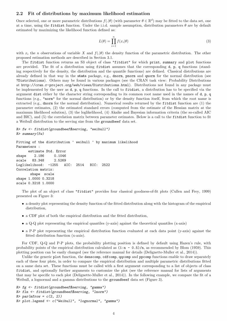
The plot of an object of class "fitdist" provides four classical goodness-of-fit plots (Cullen and Frey, 1999)presented on Figure 3:

• a density plot representing the density function of the fitted distribution along with the histogram of the empiricaldistribution,

• a CDF plot of both the empirical distribution and the fitted distribution,

• a Q-Q plot representing the empirical quantiles (y-axis) against the theoretical quantiles (x-axis)

• a P-P plot representing the empirical distribution function evaluated at each data point (y-axis) against thefitted distribution function (x-axis).

For CDF, Q-Q and P-P plots, the probability plotting position is defined by default using Hazen’s rule, withprobability points of the empirical distribution calculated as (1:n - 0.5)/n, as recommended by Blom (1959). Thisplotting position can be easily changed (see the reference manual for details (Delignette-Muller et al., 2014)).

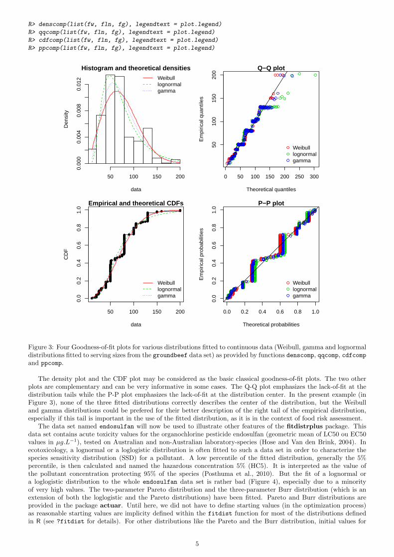
Unlike the generic plot function, the denscomp, cdfcomp, qqcomp and ppcomp functions enable to draw separatelyeach of these four plots, in order to compare the empirical distribution and multiple parametric distributions fittedon a same data set. These functions must be called with a first argument corresponding to a list of objects of classfitdist, and optionally further arguments to customize the plot (see the reference manual for lists of argumentsthat may be specific to each plot (Delignette-Muller et al., 2014)). In the following example, we compare the fit of aWeibull, a lognormal and a gamma distributions to the groundbeef data set (Figure 3).

R> fg <- fitdist(groundbeef$serving, "gamma")

R> fln <- fitdist(groundbeef$serving, "lnorm")

R> par(mfrow = c(2, 2))

R> plot.legend <- c("Weibull", "lognormal", "gamma")

4

R> denscomp(list(fw, fln, fg), legendtext = plot.legend)

R> qqcomp(list(fw, fln, fg), legendtext = plot.legend)

R> cdfcomp(list(fw, fln, fg), legendtext = plot.legend)

R> ppcomp(list(fw, fln, fg), legendtext = plot.legend)

Histogram and theoretical densities

data

Den

sity

50 100 150 200

0.00

00.

004

0.00

80.

012 Weibull

lognormalgamma

0 50 100 150 200 250 300

5010

015

020

0

Q−Q plot

Theoretical quantiles

Em

piric

al q

uant

iles

Weibulllognormalgamma

50 100 150 200

0.0

0.2

0.4

0.6

0.8

1.0

Empirical and theoretical CDFs

data

CD

F

Weibulllognormalgamma

0.0 0.2 0.4 0.6 0.8 1.0

0.0

0.2

0.4

0.6

0.8

1.0

P−P plot

Theoretical probabilities

Em

piric

al p

roba

bilit

ies

Weibulllognormalgamma

Figure 3: Four Goodness-of-fit plots for various distributions fitted to continuous data (Weibull, gamma and lognormaldistributions fitted to serving sizes from the groundbeef data set) as provided by functions denscomp, qqcomp, cdfcompand ppcomp.

The density plot and the CDF plot may be considered as the basic classical goodness-of-fit plots. The two otherplots are complementary and can be very informative in some cases. The Q-Q plot emphasizes the lack-of-fit at thedistribution tails while the P-P plot emphasizes the lack-of-fit at the distribution center. In the present example (inFigure 3), none of the three fitted distributions correctly describes the center of the distribution, but the Weibulland gamma distributions could be prefered for their better description of the right tail of the empirical distribution,especially if this tail is important in the use of the fitted distribution, as it is in the context of food risk assessment.

The data set named endosulfan will now be used to illustrate other features of the fitdistrplus package. Thisdata set contains acute toxicity values for the organochlorine pesticide endosulfan (geometric mean of LC50 ou EC50values in µg.L−1), tested on Australian and non-Australian laboratory-species (Hose and Van den Brink, 2004). Inecotoxicology, a lognormal or a loglogistic distribution is often fitted to such a data set in order to characterize thespecies sensitivity distribution (SSD) for a pollutant. A low percentile of the fitted distribution, generally the 5%percentile, is then calculated and named the hazardous concentration 5% (HC5). It is interpreted as the value ofthe pollutant concentration protecting 95% of the species (Posthuma et al., 2010). But the fit of a lognormal ora loglogistic distribution to the whole endosulfan data set is rather bad (Figure 4), especially due to a minorityof very high values. The two-parameter Pareto distribution and the three-parameter Burr distribution (which is anextension of both the loglogistic and the Pareto distributions) have been fitted. Pareto and Burr distributions areprovided in the package actuar. Until here, we did not have to define starting values (in the optimization process)as reasonable starting values are implicity defined within the fitdist function for most of the distributions definedin R (see ?fitdist for details). For other distributions like the Pareto and the Burr distribution, initial values for

5

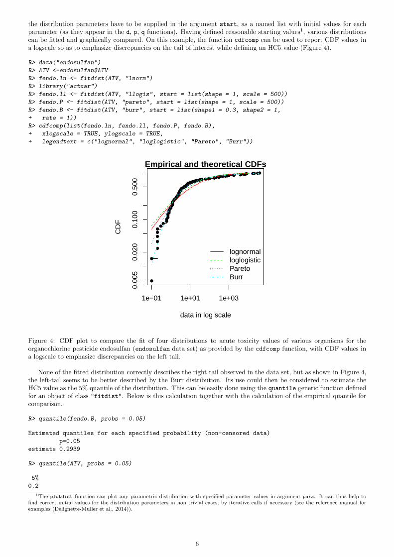
the distribution parameters have to be supplied in the argument start, as a named list with initial values for eachparameter (as they appear in the d, p, q functions). Having defined reasonable starting values1, various distributionscan be fitted and graphically compared. On this example, the function cdfcomp can be used to report CDF values ina logscale so as to emphasize discrepancies on the tail of interest while defining an HC5 value (Figure 4).

R> data("endosulfan")

R> ATV <-endosulfan$ATV

R> fendo.ln <- fitdist(ATV, "lnorm")

R> library("actuar")

R> fendo.ll <- fitdist(ATV, "llogis", start = list(shape = 1, scale = 500))

R> fendo.P <- fitdist(ATV, "pareto", start = list(shape = 1, scale = 500))

R> fendo.B <- fitdist(ATV, "burr", start = list(shape1 = 0.3, shape2 = 1,

+ rate = 1))

R> cdfcomp(list(fendo.ln, fendo.ll, fendo.P, fendo.B),

+ xlogscale = TRUE, ylogscale = TRUE,

+ legendtext = c("lognormal", "loglogistic", "Pareto", "Burr"))

1e−01 1e+01 1e+03

0.00

50.

020

0.10

00.

500

Empirical and theoretical CDFs

data in log scale

CD

F

lognormalloglogisticParetoBurr

Figure 4: CDF plot to compare the fit of four distributions to acute toxicity values of various organisms for theorganochlorine pesticide endosulfan (endosulfan data set) as provided by the cdfcomp function, with CDF values ina logscale to emphasize discrepancies on the left tail.

None of the fitted distribution correctly describes the right tail observed in the data set, but as shown in Figure 4,the left-tail seems to be better described by the Burr distribution. Its use could then be considered to estimate theHC5 value as the 5% quantile of the distribution. This can be easily done using the quantile generic function definedfor an object of class "fitdist". Below is this calculation together with the calculation of the empirical quantile forcomparison.

R> quantile(fendo.B, probs = 0.05)

Estimated quantiles for each specified probability (non-censored data)

p=0.05

estimate 0.2939

R> quantile(ATV, probs = 0.05)

5%

0.2

1The plotdist function can plot any parametric distribution with specified parameter values in argument para. It can thus help tofind correct initial values for the distribution parameters in non trivial cases, by iterative calls if necessary (see the reference manual forexamples (Delignette-Muller et al., 2014)).

6

In addition to the ecotoxicology context, the quantile generic function is also attractive in the actuarial–financialcontext. In fact, the value-at-risk V ARα is defined as the 1−α-quantile of the loss distribution and can be computedwith quantile on a "fitdist" object.

The computation of different goodness-of-fit statistics is proposed in the fitdistrplus package in order to fur-ther compare fitted distributions. The purpose of goodness-of-fit statistics aims to measure the distance betweenthe fitted parametric distribution and the empirical distribution: e.g., the distance between the fitted cumulativedistribution function F and the empirical distribution function Fn. When fitting continuous distributions, threegoodness-of-fit statistics are classicaly considered: Cramer-von Mises, Kolmogorov-Smirnov and Anderson-Darlingstatistics (D’Agostino and Stephens, 1986). Naming xi the n observations of a continuous variable X arranged inan ascending order, Table 1 gives the definition and the empirical estimate of the three considered goodness-of-fitstatistics. They can be computed using the function gofstat as defined by Stephens (D’Agostino and Stephens,1986).

R> gofstat(list(fendo.ln, fendo.ll, fendo.P, fendo.B),

+ fitnames = c("lnorm", "llogis", "Pareto", "Burr"))

Goodness-of-fit statistics

lnorm llogis Pareto Burr

Kolmogorov-Smirnov statistic 0.1672 0.1196 0.08488 0.06155

Cramer-von Mises statistic 0.6374 0.3827 0.13926 0.06803

Anderson-Darling statistic 3.4721 2.8316 0.89206 0.52393

Goodness-of-fit criteria

lnorm llogis Pareto Burr

Akaike's Information Criterion 1069 1069 1048 1046

Bayesian Information Criterion 1074 1075 1053 1054

Statistic General formula Computational formulaKolmogorov-Smirnov sup |Fn(x)− F (x)| max(D+, D−) with(KS) D+ = max

i=1,...,n

(in − Fi

)D− = max

i=1,...,n

(Fi − i−1

n

)Cramer-von Mises n

∫∞−∞(Fn(x)− F (x))2dx 1

12n +n∑i=1

(Fi − 2i−1

2n

)2(CvM)

Anderson-Darling n∫∞−∞

(Fn(x)−F (x))2

F (x)(1−F (x)) dx −n− 1n

n∑i=1

(2i− 1) log(Fi(1− Fn+1−i))

(AD)

where Fi4= F (xi)

Table 1: Goodness-of-fit statistics as defined by Stephens (D’Agostino and Stephens, 1986).

As giving more weight to distribution tails, the Anderson-Darling statistic is of special interest when it matters toequally emphasize the tails as well as the main body of a distribution. This is often the case in risk assessment (Cullenand Frey, 1999; Vose, 2010). For this reason, this statistics is often used to select the best distribution among thosefitted. Nevertheless, this statistics should be used cautiously when comparing fits of various distributions. Keeping inmind that the weighting of each CDF quadratic difference depends on the parametric distribution in its definition (seeTable 1), Anderson-Darling statistics computed for several distributions fitted on a same data set are theoreticallydifficult to compare. Moreover, such a statistic, as Cramer-von Mises and Kolmogorov-Smirnov ones, does not takeinto account the complexity of the model (i.e., parameter number). It is not a problem when compared distributionsare characterized by the same number of parameters, but it could systematically promote the selection of the morecomplex distributions in the other case. Looking at classical penalized criteria based on the loglikehood (AIC, BIC)seems thus also interesting, especially to discourage overfitting.

In the previous example, all the goodness-of-fit statistics based on the CDF distance are in favor of the Burrdistribution, the only one characterized by three parameters, while AIC and BIC values respectively give the preferenceto the Burr distribution or the Pareto distribution. The choice between these two distributions seems thus less obviousand could be discussed. Even if specifically recommended for discrete distributions, the Chi-squared statistic may alsobe used for continuous distributions (see Section 3.3 and the reference manual for examples (Delignette-Muller et al.,2014)).

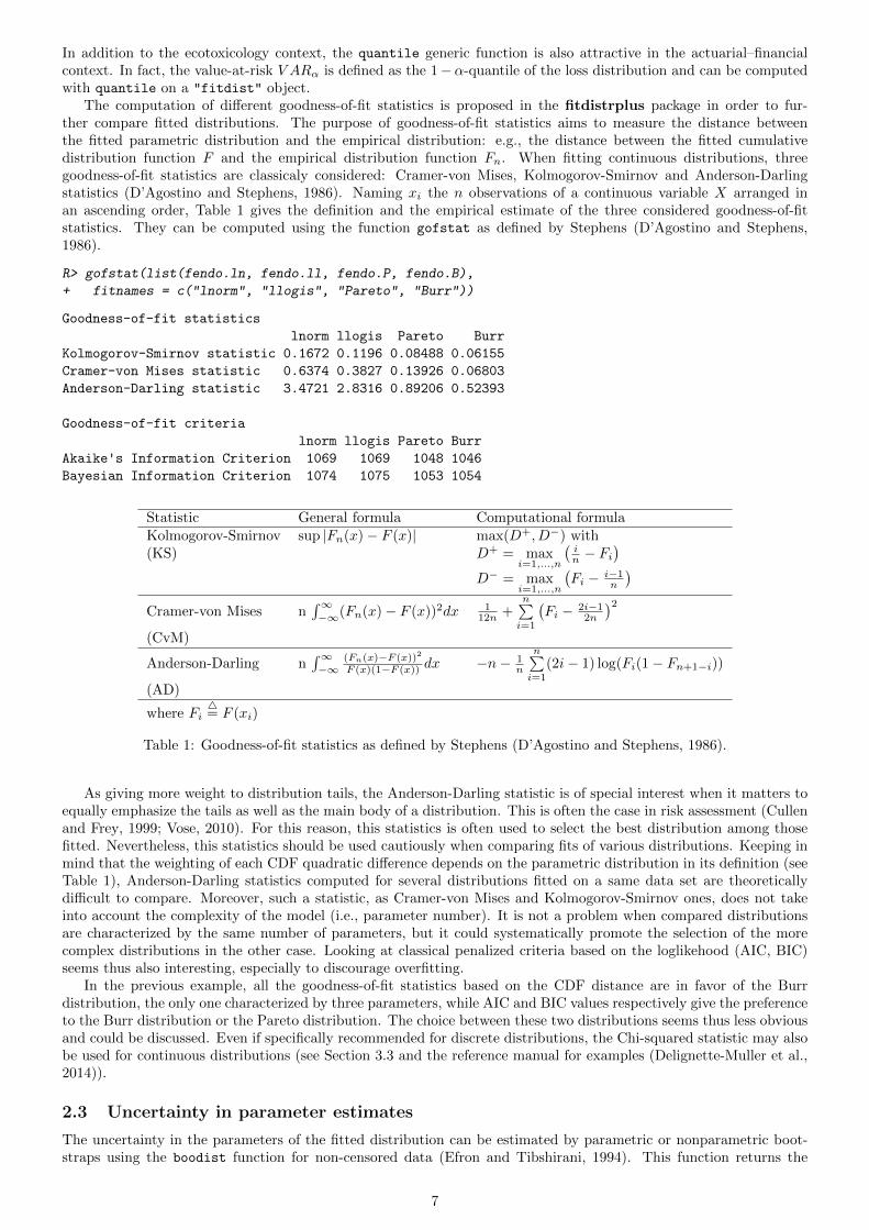
2.3 Uncertainty in parameter estimates

The uncertainty in the parameters of the fitted distribution can be estimated by parametric or nonparametric boot-straps using the boodist function for non-censored data (Efron and Tibshirani, 1994). This function returns the

7

bootstrapped values of parameters in an S3 class object which can be plotted to visualize the bootstrap region. Themedians and the 95 percent confidence intervals of parameters (2.5 and 97.5 percentiles) are printed in the summary.When inferior to the whole number of iterations (due to lack of convergence of the optimization algorithm for somebootstrapped data sets), the number of iterations for which the estimation converges is also printed in the summary.

The plot of an object of class "bootdist" consists in a scatterplot or a matrix of scatterplots of the bootstrappedvalues of parameters providing a representation of the joint uncertainty distribution of the fitted parameters. Belowis an example of the use of the bootdist function with the previous fit of the Burr distribution to the endosulfan

data set (Figure 5).

R> bendo.B <- bootdist(fendo.B, niter = 1001)

R> summary(bendo.B)

Parametric bootstrap medians and 95% percentile CI

Median 2.5% 97.5%

shape1 0.1998 0.09727 0.3642

shape2 1.5864 1.03456 2.9978

rate 1.4929 0.68682 2.8314

The estimation method converged only for 1000 among 1001 iterations

R> plot(bendo.B)

shape1

0 20 40 60 80 100

0.0

0.2

0.4

0.6

020

4060

80

shape2

0.0 0.2 0.4 0.6 1 2 3 4 5

12

34

5

rate

Bootstrapped values of parameters

Figure 5: Bootstrappped values of parameters for a fit of the Burr distribution characterized by three parameters(example on the endosulfan data set) as provided by the plot of an object of class "bootdist".

Bootstrap samples of parameter estimates are useful especially to calculate confidence intervals on each parameterof the fitted distribution from the marginal distribution of the bootstraped values. It is also interesting to look at thejoint distribution of the bootstraped values in a scatterplot (or a matrix of scatterplots if the number of parametersexceeds two) in order to understand the potential structural correlation between parameters (see Figure 5).

The use of the whole bootstrap sample is also of interest in the risk assessment field. Its use enables the characteri-zation of uncertainty in distribution parameters. It can be directly used within a second-order Monte Carlo simulationframework, especially within the package mc2d (Pouillot et al., 2011). One could refer to Pouillot and Delignette-Muller (2010) for an introduction to the use of mc2d and fitdistrplus packages in the context of quantitative riskassessment.

The bootstrap method can also be used to calculate confidence intervals on quantiles of the fitted distribution.For this purpose, a generic quantile function is provided for class bootdist. By default, 95% percentiles bootstrapconfidence intervals of quantiles are provided. Going back to the previous example from ecotoxicolgy, this functioncan be used to estimate the uncertainty associated to the HC5 estimation, for example from the previously fitted Burrdistribution to the endosulfan data set.

R> quantile(bendo.B, probs = 0.05)

8

(original) estimated quantiles for each specified probability (non-censored data)

p=0.05

estimate 0.2939

Median of bootstrap estimates

p=0.05

estimate 0.3024

two-sided 95 % CI of each quantile

p=0.05

2.5 % 0.1758

97.5 % 0.5035

The estimation method converged only for 1000 among 1001 bootstrap iterations.

3 Advanced topics

3.1 Alternative methods for parameter estimation

This subsection focuses on alternative estimation methods. One of the alternative for continuous distributions isthe maximum goodness-of-fit estimation method also called minimum distance estimation method (D’Agostino andStephens, 1986; Dutang et al., 2008). In this package this method is proposed with eight different distances: the threeclassical distances defined in Table 1, or one of the variants of the Anderson-Darling distance proposed by Luceno(2006) and defined in Table 2. The right-tail AD gives more weight to the right-tail, the left-tail AD gives moreweight only to the left tail. Either of the tails, or both of them, can receive even larger weights by using second orderAnderson-Darling Statistics.

Statistic General formula Computational formula

Right-tail AD∫∞−∞

(Fn(x)−F (x))2

1−F (x) dx n2 − 2

n∑i=1

Fi − 1n

n∑i=1

(2i− 1)ln(Fn+1−i)

(ADR)

Left-tail AD∫∞−∞

(Fn(x)−F (x))2

(F (x)) dx − 3n2 + 2

n∑i=1

Fi − 1n

n∑i=1

(2i− 1)ln(Fi)

(ADL)

Right-tail AD ad2r =∫∞−∞

(Fn(x)−F (x))2

(1−F (x))2 dx ad2r = 2n∑i=1

ln(F i) + 1n

n∑i=1

2i−1Fn+1−i

2nd order (AD2R)

Left-tail AD ad2l =∫∞−∞

(Fn(x)−F (x))2

(F (x))2 dx ad2l = 2n∑i=1

ln(Fi) + 1n

n∑i=1

2i−1Fi

2nd order (AD2L)AD 2nd order ad2r + ad2l ad2r + ad2l(AD2)

where Fi4= F (xi); F i

4= 1− F (xi)

Table 2: Modified Anderson-Darling statistics as defined by Luceno (2006).

To fit a distribution by maximum goodness-of-fit estimation, one needs to fix the argument method to "mge" inthe call to fitdist and to specify the argument gof coding for the chosen goodness-of-fit distance. This function isintended to be used only with continuous non-censored data.

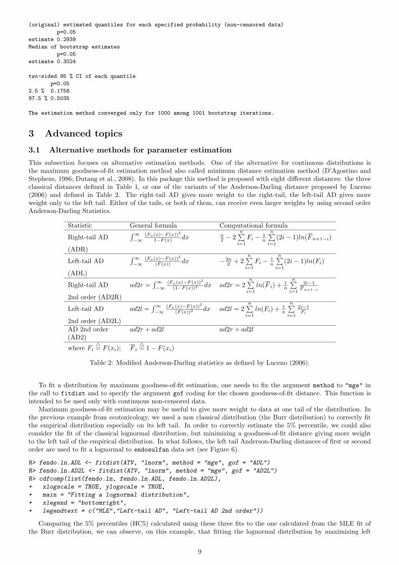
Maximum goodness-of-fit estimation may be useful to give more weight to data at one tail of the distribution. Inthe previous example from ecotoxicology, we used a non classical distribution (the Burr distribution) to correctly fitthe empirical distribution especially on its left tail. In order to correctly estimate the 5% percentile, we could alsoconsider the fit of the classical lognormal distribution, but minimizing a goodness-of-fit distance giving more weightto the left tail of the empirical distribution. In what follows, the left tail Anderson-Darling distances of first or secondorder are used to fit a lognormal to endosulfan data set (see Figure 6).

R> fendo.ln.ADL <- fitdist(ATV, "lnorm", method = "mge", gof = "ADL")

R> fendo.ln.AD2L <- fitdist(ATV, "lnorm", method = "mge", gof = "AD2L")

R> cdfcomp(list(fendo.ln, fendo.ln.ADL, fendo.ln.AD2L),

+ xlogscale = TRUE, ylogscale = TRUE,

+ main = "Fitting a lognormal distribution",

+ xlegend = "bottomright",

+ legendtext = c("MLE","Left-tail AD", "Left-tail AD 2nd order"))

Comparing the 5% percentiles (HC5) calculated using these three fits to the one calculated from the MLE fit ofthe Burr distribution, we can observe, on this example, that fitting the lognormal distribution by maximizing left

9

1e−01 1e+01 1e+03

0.00

50.

020

0.10

00.

500

Fitting a lognormal distribution

data in log scale

CD

FMLELeft−tail ADLeft−tail AD 2nd order

Figure 6: Comparison of a lognormal distribution fitted by MLE and by MGE using two different goodness-of-fitdistances : left-tail Anderson-Darling and left-tail Anderson Darling of second order (example with the endosulfan

data set) as provided by the cdfcomp function, with CDF values in a logscale to emphasize discrepancies on the lefttail.

tail Anderson-Darling distances of first or second order enables to approach the value obtained by fitting the Burrdistribution by MLE.

R> (HC5.estimates <- c(

+ empirical = as.numeric(quantile(ATV, probs = 0.05)),

+ Burr = as.numeric(quantile(fendo.B, probs = 0.05)$quantiles),

+ lognormal_MLE = as.numeric(quantile(fendo.ln, probs = 0.05)$quantiles),

+ lognormal_AD2 = as.numeric(quantile(fendo.ln.ADL,

+ probs = 0.05)$quantiles),

+ lognormal_AD2L = as.numeric(quantile(fendo.ln.AD2L,

+ probs = 0.05)$quantiles)))

empirical Burr lognormal_MLE lognormal_AD2 lognormal_AD2L

0.20000 0.29393 0.07259 0.19591 0.25877

The moment matching estimation (MME) is another method commonly used to fit parametric distributions (Vose,2010). MME consists in finding the value of the parameter θ that equalizes the first theoretical raw moments of theparametric distribution to the corresponding empirical raw moments as in Equation (4):

E(Xk|θ) =1

n

n∑i=1

xki , (4)

for k = 1, . . . , d, with d the number of parameters to estimate and xi the n observations of variable X. For momentsof order greater than or equal to 2, it may also be relevant to match centered moments. Therefore, we match themoments given in Equation (5):

E(X|θ) = x , E((X − E(X))k|θ

)= mk, for k = 2, . . . , d, (5)

where mk denotes the empirical centered moments. This method can be performed by setting the argument method to"mme" in the call to fitdist. The estimate is computed by a closed-form formula for the following distributions: nor-mal, lognormal, exponential, Poisson, gamma, logistic, negative binomial, geometric, beta and uniform distributions.In this case, for distributions characterized by one parameter (geometric, Poisson and exponential), this parameteris simply estimated by matching theoretical and observed means, and for distributions characterized by two param-eters, these parameters are estimated by matching theoretical and observed means and variances (Vose, 2010). Forother distributions, the equation of moments is solved numerically using the optim function by minimizing the sumof squared differences between observed and theoretical moments (see the fitdistrplus reference manual for technicaldetails (Delignette-Muller et al., 2014)).

10

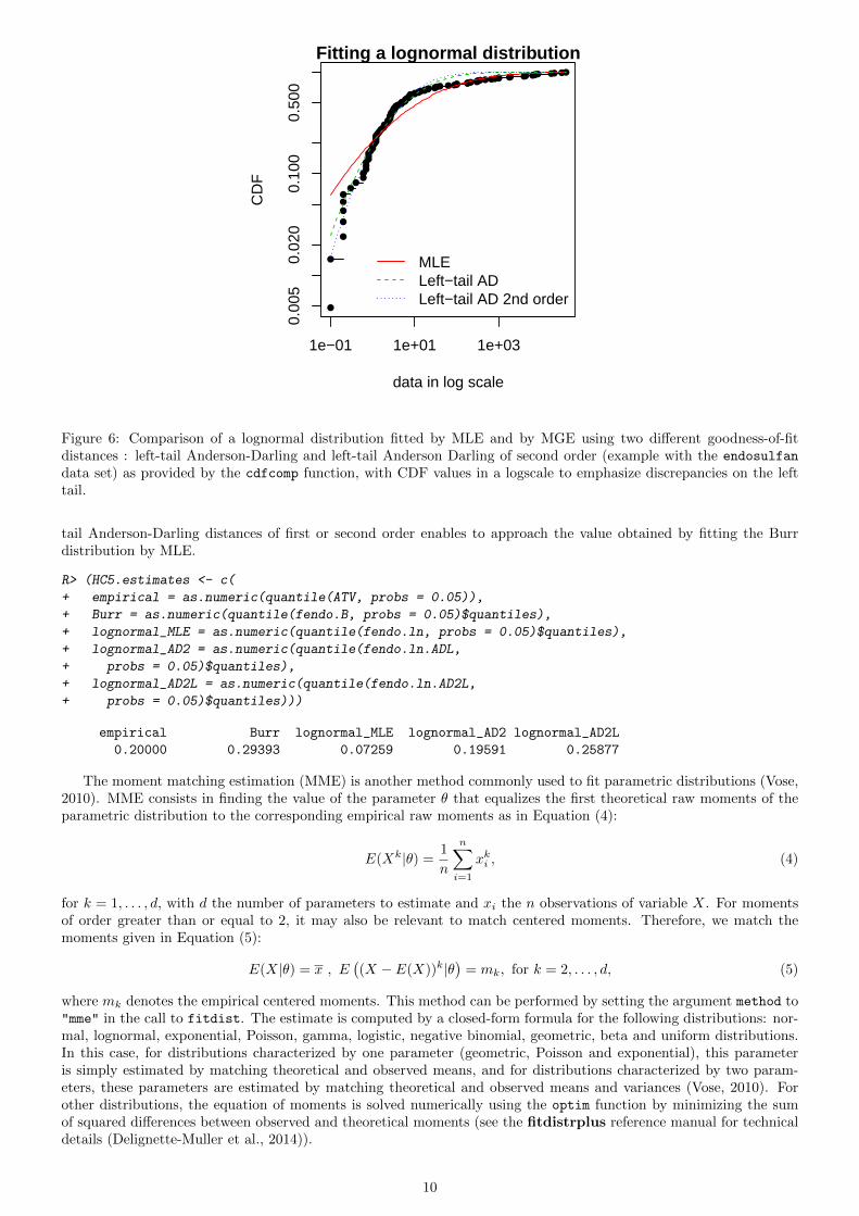
A classical data set from the Danish insurance industry published in McNeil (1997) will be used to illustratethis method. In fitdistrplus, the data set is stored in danishuni for the univariate version and contains the lossamounts collected at Copenhagen Reinsurance between 1980 and 1990. In actuarial science, it is standard to considerpositive heavy-tailed distributions and have a special focus on the right-tail of the distributions. In this numericalexperiment, we choose classic actuarial distributions for loss modelling: the lognormal distribution and the Paretotype II distribution (Klugman et al., 2009).

The lognormal distribution is fitted to danishuni data set by matching moments implemented as a closed-formformula. On the left-hand graph of Figure 7, the fitted distribution functions obtained using the moment matchingestimation (MME) and maximum likelihood estimation (MLE) methods are compared. The MME method provides amore cautious estimation of the insurance risk as the MME-fitted distribution function (resp. MLE-fitted) underesti-mates (overestimates) the empirical distribution function for large values of claim amounts.

R> data("danishuni")

R> str(danishuni)

'data.frame': 2167 obs. of 2 variables:

$ Date: Date, format: "1980-01-03" "1980-01-04" ...

$ Loss: num 1.68 2.09 1.73 1.78 4.61 ...

R> fdanish.ln.MLE <- fitdist(danishuni$Loss, "lnorm")

R> fdanish.ln.MME <- fitdist(danishuni$Loss, "lnorm", method = "mme",

+ order = 1:2)

R> cdfcomp(list(fdanish.ln.MLE, fdanish.ln.MME),

+ legend = c("lognormal MLE", "lognormal MME"),

+ main = "Fitting a lognormal distribution",

+ xlogscale = TRUE, datapch = 20)

1 2 5 20 50 200

0.0

0.2

0.4

0.6

0.8

1.0

Fitting a lognormal distribution

data in log scale

CD

F

lognormal MLElognormal MME

1 2 5 20 50 200

0.0

0.2

0.4

0.6

0.8

1.0

Fitting a Pareto distribution

data in log scale

CD

F

Pareto MLEPareto MME

Figure 7: Comparison between MME and MLE when fitting a lognormal or a Pareto distribution to loss data fromthe danishuni data set.

In a second time, a Pareto distribution, which gives more weight to the right-tail of the distribution, is fitted. Asthe lognormal distribution, the Pareto has two parameters, which allows a fair comparison.

We use the implementation of the actuar package providing raw and centered moments for that distribution (inaddition to d, p, q and r functions (Goulet, 2012). Fitting a heavy-tailed distribution for which the first and thesecond moments do not exist for certain values of the shape parameter requires some cautiousness. This is carriedout by providing, for the optimization process, a lower and an upper bound for each parameter. The code below callsthe L-BFGS-B optimization method in optim, since this quasi-Newton allows box constraints2. We choose matchmoments defined in Equation (4), and so a function for computing the empirical raw moment (called memp in ourexample) is passed to fitdist. For two-parameter distributions (i.e., d = 2), Equations (4) and (5) are equivalent.

R> library("actuar")

R> fdanish.P.MLE <- fitdist(danishuni$Loss, "pareto",

+ start = list(shape = 10, scale = 10), lower = 2+1e-6, upper = Inf)

2That is what the B stands for.

11

R> memp <- function(x, order) sum(x^order)/length(x)

R> fdanish.P.MME <- fitdist(danishuni$Loss, "pareto", method = "mme",

+ order = 1:2, memp = "memp", start = list(shape = 10, scale = 10),

+ lower = c(2+1e-6, 2+1e-6), upper = c(Inf, Inf))

R> cdfcomp(list(fdanish.P.MLE, fdanish.P.MME),

+ legend = c("Pareto MLE", "Pareto MME"),

+ main = "Fitting a Pareto distribution",

+ xlogscale = TRUE, datapch = ".")

R> gofstat(list(fdanish.ln.MLE, fdanish.P.MLE,

+ fdanish.ln.MME, fdanish.P.MME),

+ fitnames = c("lnorm.mle", "Pareto.mle", "lnorm.mme", "Pareto.mme"))

Goodness-of-fit statistics

lnorm.mle Pareto.mle lnorm.mme Pareto.mme

Kolmogorov-Smirnov statistic 0.1375 0.3124 0.4368 0.37

Cramer-von Mises statistic 14.7911 37.7227 88.9503 55.43

Anderson-Darling statistic 87.1933 208.3388 416.2567 281.58

Goodness-of-fit criteria

lnorm.mle Pareto.mle lnorm.mme Pareto.mme

Akaike's Information Criterion 8120 9250 9792 9409

Bayesian Information Criterion 8131 9261 9803 9420

As shown on Figure 7, MME and MLE fits are far less distant (when looking at the right-tail) for the Paretodistribution than for the lognormal distribution on this data set. Furthermore, for these two distributions, the MMEmethod better fits the right-tail of the distribution from a visual point of view. This seems logical since empiricalmoments are influenced by large observed values. In the previous traces, we gave the values of goodness-of-fit statistics.Whatever the statistic considered, the MLE-fitted lognormal always provides the best fit to the observed data.

Maximum likelihood and moment matching estimations are certainly the most commonly used method for fittingdistributions (Cullen and Frey, 1999). Keeping in mind that these two methods may produce very different results,the user should be aware of its great sensitivity to outliers when choosing the moment matching estimation. This maybe seen as an advantage in our example if the objective is to better describe the right tail of the distribution, but itmay be seen as a drawback if the objective is different.

Fitting of a parametric distribution may also be done by matching theoretical quantiles of the parametric dis-tributions (for specified probabilities) against the empirical quantiles (Tse (2009)). The equality of theoretical andempirical qunatiles is expressed by Equation (6) below, which is very similar to Equations (4) and (5):

F−1(pk|θ) = Qn,pk (6)

for k = 1, . . . , d, with d the number of parameters to estimate (dimension of θ if there is no fixed parameters) andQn,pk the empirical quantiles calculated from data for specified probabilities pk.

Quantile matching estimation (QME) is performed by setting the argument method to "qme" in the call to fitdist

and adding an argument probs defining the probabilities for which the quantile matching is performed. The lengthof this vector must be equal to the number of parameters to estimate (as the vector of moment orders for MME).Empirical quantiles are computed using the quantile function of the stats package using type=7 by default (see?quantile and Hyndman and Fan (1996)). But the type of quantile can be easily changed by using the qty argumentin the call to the qme function. The quantile matching is carried out numerically, by minimizing the sum of squareddifferences between observed and theoretical quantiles.

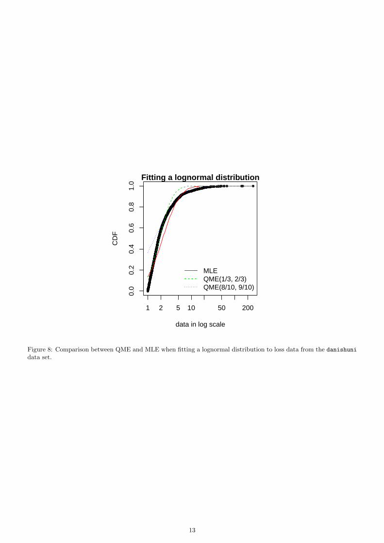
R> fdanish.ln.QME1 <- fitdist(danishuni$Loss, "lnorm", method = "qme",

+ probs = c(1/3, 2/3))

R> fdanish.ln.QME2 <- fitdist(danishuni$Loss, "lnorm", method = "qme",

+ probs = c(8/10, 9/10))

R> cdfcomp(list(fdanish.ln.MLE, fdanish.ln.QME1, fdanish.ln.QME2),

+ legend = c("MLE", "QME(1/3, 2/3)", "QME(8/10, 9/10)"),

+ main = "Fitting a lognormal distribution",

+ xlogscale = TRUE, datapch = 20)

Above is an example of fitting of a lognormal distribution to danishuni data set by matching probabilities (p1 =1/3, p2 = 2/3) and (p1 = 8/10, p2 = 9/10). As expected, the second QME fit gives more weight to the right-tail ofthe distribution. Compared to the maximum likelihood estimation, the second QME fit best suits the right-tail of thedistribution, whereas the first QME fit best models the body of the distribution. The quantile matching estimation isof particular interest when we need to focus around particular quantiles, e.g., p = 99.5% in the Solvency II insurancecontext or p = 5% for the HC5 estimation in the ecotoxicology context.

12

1 2 5 10 50 200

0.0

0.2

0.4

0.6

0.8

1.0

Fitting a lognormal distribution

data in log scale

CD

F

MLEQME(1/3, 2/3)QME(8/10, 9/10)

Figure 8: Comparison between QME and MLE when fitting a lognormal distribution to loss data from the danishuni

data set.

13

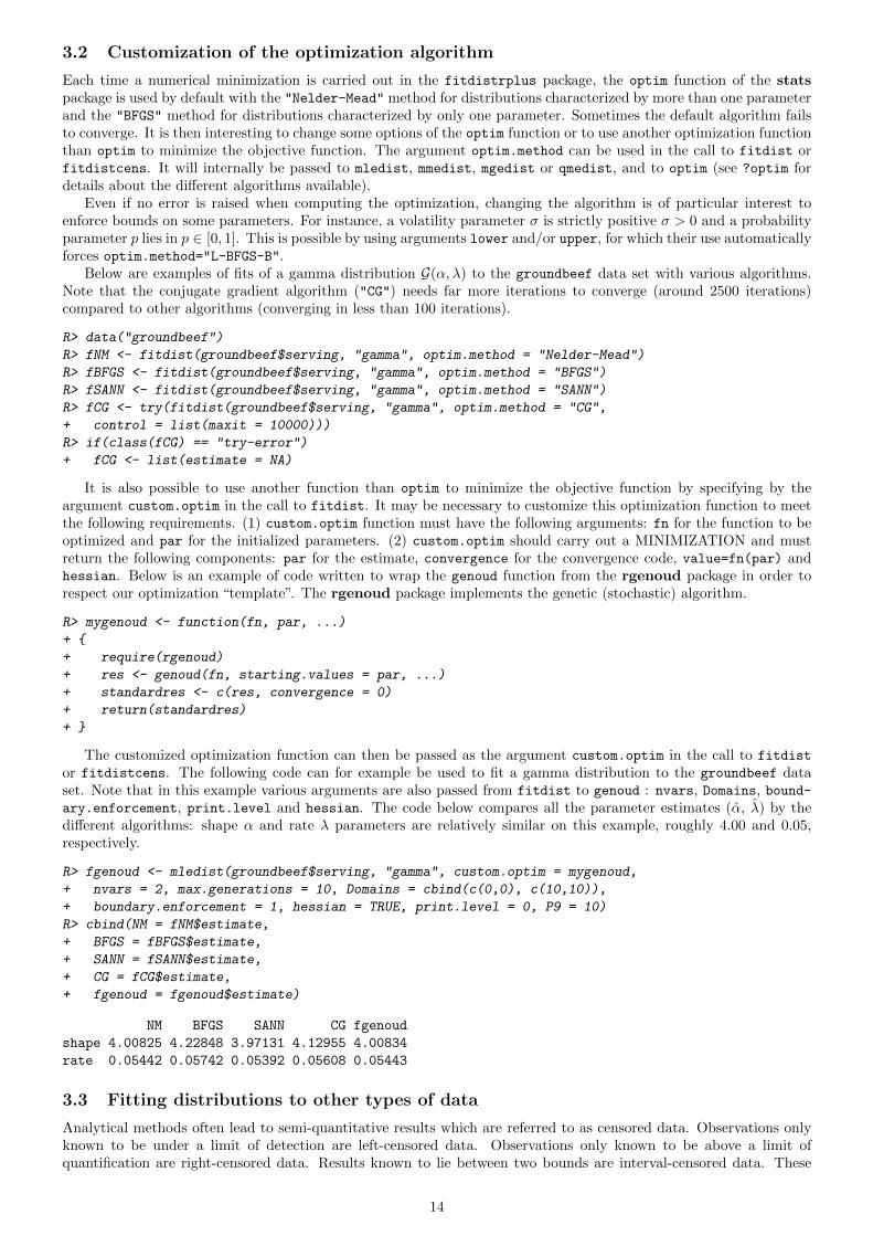
3.2 Customization of the optimization algorithm

Each time a numerical minimization is carried out in the fitdistrplus package, the optim function of the statspackage is used by default with the "Nelder-Mead" method for distributions characterized by more than one parameterand the "BFGS" method for distributions characterized by only one parameter. Sometimes the default algorithm failsto converge. It is then interesting to change some options of the optim function or to use another optimization functionthan optim to minimize the objective function. The argument optim.method can be used in the call to fitdist orfitdistcens. It will internally be passed to mledist, mmedist, mgedist or qmedist, and to optim (see ?optim fordetails about the different algorithms available).

Even if no error is raised when computing the optimization, changing the algorithm is of particular interest toenforce bounds on some parameters. For instance, a volatility parameter σ is strictly positive σ > 0 and a probabilityparameter p lies in p ∈ [0, 1]. This is possible by using arguments lower and/or upper, for which their use automaticallyforces optim.method="L-BFGS-B".

Below are examples of fits of a gamma distribution G(α, λ) to the groundbeef data set with various algorithms.Note that the conjugate gradient algorithm ("CG") needs far more iterations to converge (around 2500 iterations)compared to other algorithms (converging in less than 100 iterations).

R> data("groundbeef")

R> fNM <- fitdist(groundbeef$serving, "gamma", optim.method = "Nelder-Mead")

R> fBFGS <- fitdist(groundbeef$serving, "gamma", optim.method = "BFGS")

R> fSANN <- fitdist(groundbeef$serving, "gamma", optim.method = "SANN")

R> fCG <- try(fitdist(groundbeef$serving, "gamma", optim.method = "CG",

+ control = list(maxit = 10000)))

R> if(class(fCG) == "try-error")

+ fCG <- list(estimate = NA)

It is also possible to use another function than optim to minimize the objective function by specifying by theargument custom.optim in the call to fitdist. It may be necessary to customize this optimization function to meetthe following requirements. (1) custom.optim function must have the following arguments: fn for the function to beoptimized and par for the initialized parameters. (2) custom.optim should carry out a MINIMIZATION and mustreturn the following components: par for the estimate, convergence for the convergence code, value=fn(par) andhessian. Below is an example of code written to wrap the genoud function from the rgenoud package in order torespect our optimization “template”. The rgenoud package implements the genetic (stochastic) algorithm.

R> mygenoud <- function(fn, par, ...)

+ {

+ require(rgenoud)

+ res <- genoud(fn, starting.values = par, ...)

+ standardres <- c(res, convergence = 0)

+ return(standardres)

+ }

The customized optimization function can then be passed as the argument custom.optim in the call to fitdist

or fitdistcens. The following code can for example be used to fit a gamma distribution to the groundbeef dataset. Note that in this example various arguments are also passed from fitdist to genoud : nvars, Domains, bound-ary.enforcement, print.level and hessian. The code below compares all the parameter estimates (α, λ) by thedifferent algorithms: shape α and rate λ parameters are relatively similar on this example, roughly 4.00 and 0.05,respectively.

R> fgenoud <- mledist(groundbeef$serving, "gamma", custom.optim = mygenoud,

+ nvars = 2, max.generations = 10, Domains = cbind(c(0,0), c(10,10)),

+ boundary.enforcement = 1, hessian = TRUE, print.level = 0, P9 = 10)

R> cbind(NM = fNM$estimate,

+ BFGS = fBFGS$estimate,

+ SANN = fSANN$estimate,

+ CG = fCG$estimate,

+ fgenoud = fgenoud$estimate)

NM BFGS SANN CG fgenoud

shape 4.00825 4.22848 3.97131 4.12955 4.00834

rate 0.05442 0.05742 0.05392 0.05608 0.05443

3.3 Fitting distributions to other types of data

Analytical methods often lead to semi-quantitative results which are referred to as censored data. Observations onlyknown to be under a limit of detection are left-censored data. Observations only known to be above a limit ofquantification are right-censored data. Results known to lie between two bounds are interval-censored data. These

14

two bounds may correspond to a limit of detection and a limit of quantification, or more generally to uncertaintybounds around the observation. Right-censored data are also commonly encountered with survival data (Klein andMoeschberger, 2003). A data set may thus contain right-, left-, or interval-censored data, or may be a mixture of thesecategories, possibly with different upper and lower bounds. Censored data are sometimes excluded from the dataanalysis or replaced by a fixed value, which in both cases may lead to biased results. A more recommended approachto correctly model such data is based upon maximum likelihood (Klein and Moeschberger, 2003; Helsel, 2005).

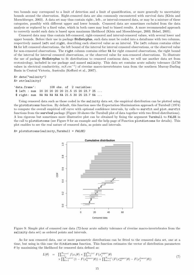
Censored data may thus contain left-censored, right-censored and interval-censored values, with several lower andupper bounds. Before their use in package fitdistrplus, such data must be coded into a dataframe with two columns,respectively named left and right, describing each observed value as an interval. The left column contains eitherNA for left censored observations, the left bound of the interval for interval censored observations, or the observed valuefor non-censored observations. The right column contains either NA for right censored observations, the right boundof the interval for interval censored observations, or the observed value for non-censored observations. To illustratethe use of package fitdistrplus to fit distributions to censored continous data, we will use another data set fromecotoxicology, included in our package and named salinity. This data set contains acute salinity tolerance (LC50values in electrical conductivity, mS.cm−1) of riverine macro-invertebrates taxa from the southern Murray-DarlingBasin in Central Victoria, Australia (Kefford et al., 2007).

R> data("salinity")

R> str(salinity)

'data.frame': 108 obs. of 2 variables:

$ left : num 20 20 20 20 20 21.5 15 20 23.7 25 ...

$ right: num NA NA NA NA NA 21.5 30 25 23.7 NA ...

Using censored data such as those coded in the salinity data set, the empirical distribution can be plotted usingthe plotdistcens function. By default, this function uses the Expectation-Maximization approach of Turnbull (1974)to compute the overall empirical cdf curve with optional confidence intervals, by calls to survfit and plot.survfit

functions from the survival package (Figure 10 shows the Turnbull plot of data together with two fitted distributions).A less rigorous but sometimes more illustrative plot can be obtained by fixing the argument Turnbull to FALSE inthe call to plotdistcens (see Figure 9 for an example and the help page of Function plotdistcens for details). Thisplot enables to see the real nature of censored data, as points and intervals.

R> plotdistcens(salinity,Turnbull = FALSE)

0 20 40 60

0.0

0.2

0.4

0.6

0.8

1.0

Cumulative distribution

Censored data

CD

F

Figure 9: Simple plot of censored raw data (72-hour acute salinity tolerance of riverine macro-invertebrates from thesalinity data set) as ordered points and intervals.

As for non censored data, one or more parametric distributions can be fitted to the censored data set, one at atime, but using in this case the fitdistcens function. This function estimates the vector of distribution parametersθ by maximizing the likelihood for censored data defined as:

L(θ) =∏NnonC

i=1 f(xi|θ)×∏NleftC

j=1 F (xupperj |θ)×∏NrightC

k=1 (1− F (xlowerk |θ))×∏NintC

m=1 (F (xupperm |θ)− F (xlowerj |θ))(7)

15

with xi the NnonC non-censored observations, xupperj upper values defining the NleftC left-censored observations,

xlowerk lower values defining the NrightC right-censored observations, [xlowerm ;xupperm ] the intervals defining the NintCinterval-censored observations, and F the cumulative distribution function of the parametric distribution (Klein andMoeschberger, 2003; Helsel, 2005).

As fitdist, fitdistcens returns the results of the fit of any parametric distribution to a data set as an S3 classobject that can be easily printed, summarized or plotted. For the salinity data set, a lognormal distribution or aloglogistic can be fitted as commonly done in ecotoxicology for such data. As with fitdist, for some distributions (seeDelignette-Muller et al. (2014) for details), it is necessary to specify initial values for the distribution parameters inthe argument start. The plotdistcens function can help to find correct initial values for the distribution parametersin non trivial cases, by a manual iterative use if necessary.

R> fsal.ln <- fitdistcens(salinity, "lnorm")

R> fsal.ll <- fitdistcens(salinity, "llogis",

+ start = list(shape = 5, scale = 40))

R> summary(fsal.ln)

Fitting of the distribution ' lnorm ' By maximum likelihood on censored data

Parameters

estimate Std. Error

meanlog 3.3854 0.06487

sdlog 0.4961 0.05455

Fixed parameters:

data frame with 0 columns and 0 rows

Loglikelihood: -139.1 AIC: 282.1 BIC: 287.5

Correlation matrix:

meanlog sdlog

meanlog 1.0000 0.2938

sdlog 0.2938 1.0000

R> summary(fsal.ll)

Fitting of the distribution ' llogis ' By maximum likelihood on censored data

Parameters

estimate Std. Error

shape 3.421 0.4158

scale 29.930 1.9447

Fixed parameters:

data frame with 0 columns and 0 rows

Loglikelihood: -140.1 AIC: 284.1 BIC: 289.5

Correlation matrix:

shape scale

shape 1.0000 -0.2022

scale -0.2022 1.0000

Computations of goodness-of-fit statistics have not yet been developed for fits using censored data but the quality offit can be judged using Akaike and Schwarz’s Bayesian information criteria (AIC and BIC) and the goodness-of-fit CDFplot, respectively provided when summarizing or plotting an object of class "fitdistcens". Function cdfcompcens

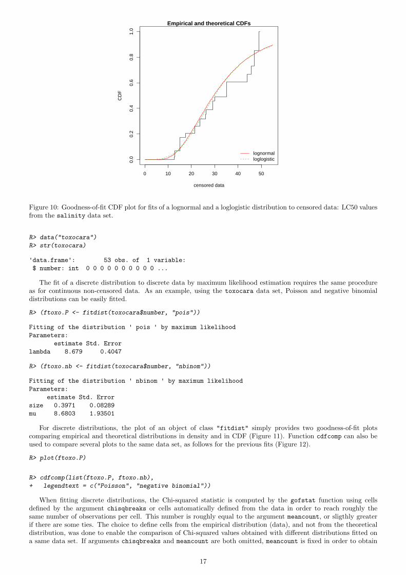
can also be used to compare the fit of various distributions to the same censored data set. Its call is similar to theone of cdfcomp. Below is an example of comparison of the two fitted distributions to the salinity data set (seeFigure 10).

R> cdfcompcens(list(fsal.ln, fsal.ll),

+ legendtext = c("lognormal", "loglogistic "))

Function bootdistcens is the equivalent of bootdist for censored data, except that it only proposes nonparametricbootstrap. Indeed, it is not obvious to simulate censoring within a parametric bootstrap resampling procedure.The generic function quantile can also be applied to an object of class "fitdistcens" or "bootdistcens", as forcontinuous non-censored data.

In addition to the fit of distributions to censored or non censored continuous data, our package can also accomodatediscrete variables, such as count numbers, using the functions developped for continuous non-censored data. Thesefunctions will provide somewhat different graphs and statistics, taking into account the discrete nature of the modeledvariable. The discrete nature of the variable is automatically recognized when a classical distribution is fitted to data(binomial, negative binomial, geometric, hypergeometric and Poisson distributions) but must be indicated by fixingargument discrete to TRUE in the call to functions in other cases. The toxocara data set included in the packagecorresponds to the observation of such a discrete variable. Numbers of Toxocara cati parasites present in digestivetract are reported from a random sampling of feral cats living on Kerguelen island (Fromont et al., 2001). We will useit to illustrate the case of discrete data.

16

0 10 20 30 40 50

0.0

0.2

0.4

0.6

0.8

1.0

Empirical and theoretical CDFs

censored data

CD

F

lognormalloglogistic

Figure 10: Goodness-of-fit CDF plot for fits of a lognormal and a loglogistic distribution to censored data: LC50 valuesfrom the salinity data set.

R> data("toxocara")

R> str(toxocara)

'data.frame': 53 obs. of 1 variable:

$ number: int 0 0 0 0 0 0 0 0 0 0 ...

The fit of a discrete distribution to discrete data by maximum likelihood estimation requires the same procedureas for continuous non-censored data. As an example, using the toxocara data set, Poisson and negative binomialdistributions can be easily fitted.

R> (ftoxo.P <- fitdist(toxocara$number, "pois"))

Fitting of the distribution ' pois ' by maximum likelihood

Parameters:

estimate Std. Error

lambda 8.679 0.4047

R> (ftoxo.nb <- fitdist(toxocara$number, "nbinom"))

Fitting of the distribution ' nbinom ' by maximum likelihood

Parameters:

estimate Std. Error

size 0.3971 0.08289

mu 8.6803 1.93501

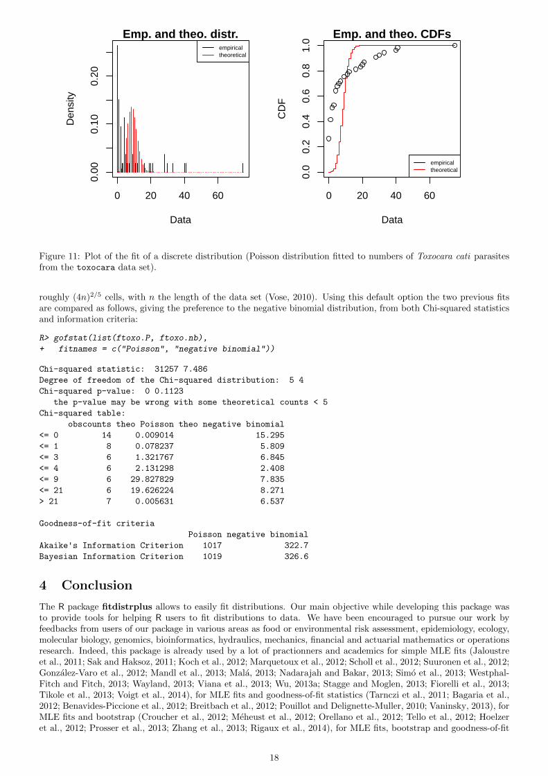
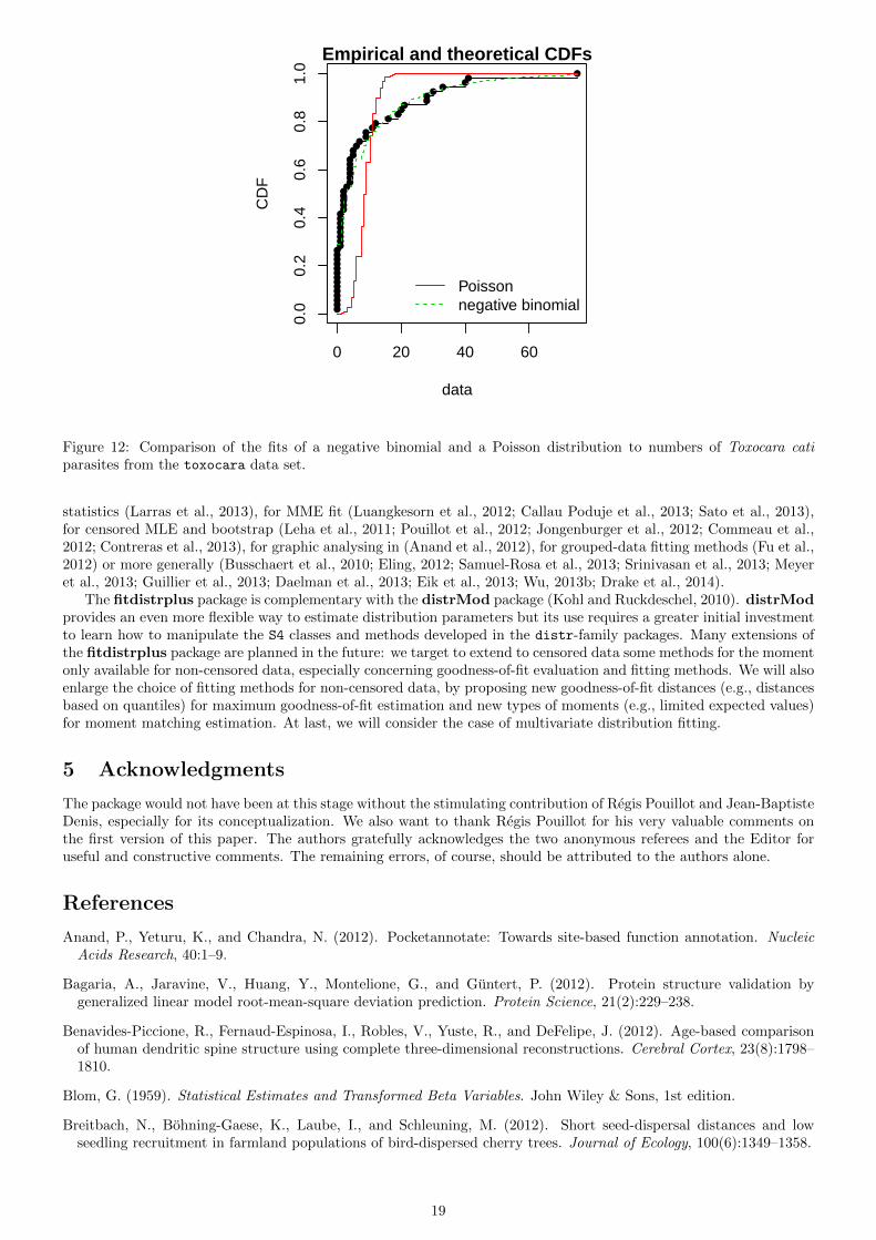
For discrete distributions, the plot of an object of class "fitdist" simply provides two goodness-of-fit plotscomparing empirical and theoretical distributions in density and in CDF (Figure 11). Function cdfcomp can also beused to compare several plots to the same data set, as follows for the previous fits (Figure 12).

R> plot(ftoxo.P)

R> cdfcomp(list(ftoxo.P, ftoxo.nb),

+ legendtext = c("Poisson", "negative binomial"))

When fitting discrete distributions, the Chi-squared statistic is computed by the gofstat function using cellsdefined by the argument chisqbreaks or cells automatically defined from the data in order to reach roughly thesame number of observations per cell. This number is roughly equal to the argument meancount, or sligthly greaterif there are some ties. The choice to define cells from the empirical distribution (data), and not from the theoreticaldistribution, was done to enable the comparison of Chi-squared values obtained with different distributions fitted ona same data set. If arguments chisqbreaks and meancount are both omitted, meancount is fixed in order to obtain

17

0 20 40 60

0.00

0.10

0.20

Emp. and theo. distr.

Data

Den

sity

empiricaltheoretical

0 20 40 60

0.0

0.2

0.4

0.6

0.8

1.0

Emp. and theo. CDFs

Data

CD

F

empiricaltheoretical

Figure 11: Plot of the fit of a discrete distribution (Poisson distribution fitted to numbers of Toxocara cati parasitesfrom the toxocara data set).

roughly (4n)2/5 cells, with n the length of the data set (Vose, 2010). Using this default option the two previous fitsare compared as follows, giving the preference to the negative binomial distribution, from both Chi-squared statisticsand information criteria:

R> gofstat(list(ftoxo.P, ftoxo.nb),

+ fitnames = c("Poisson", "negative binomial"))

Chi-squared statistic: 31257 7.486

Degree of freedom of the Chi-squared distribution: 5 4

Chi-squared p-value: 0 0.1123

the p-value may be wrong with some theoretical counts < 5

Chi-squared table:

obscounts theo Poisson theo negative binomial

<= 0 14 0.009014 15.295

<= 1 8 0.078237 5.809

<= 3 6 1.321767 6.845

<= 4 6 2.131298 2.408

<= 9 6 29.827829 7.835

<= 21 6 19.626224 8.271

> 21 7 0.005631 6.537

Goodness-of-fit criteria

Poisson negative binomial

Akaike's Information Criterion 1017 322.7

Bayesian Information Criterion 1019 326.6

4 Conclusion

The R package fitdistrplus allows to easily fit distributions. Our main objective while developing this package wasto provide tools for helping R users to fit distributions to data. We have been encouraged to pursue our work byfeedbacks from users of our package in various areas as food or environmental risk assessment, epidemiology, ecology,molecular biology, genomics, bioinformatics, hydraulics, mechanics, financial and actuarial mathematics or operationsresearch. Indeed, this package is already used by a lot of practionners and academics for simple MLE fits (Jaloustreet al., 2011; Sak and Haksoz, 2011; Koch et al., 2012; Marquetoux et al., 2012; Scholl et al., 2012; Suuronen et al., 2012;Gonzalez-Varo et al., 2012; Mandl et al., 2013; Mala, 2013; Nadarajah and Bakar, 2013; Simo et al., 2013; Westphal-Fitch and Fitch, 2013; Wayland, 2013; Viana et al., 2013; Wu, 2013a; Stagge and Moglen, 2013; Fiorelli et al., 2013;Tikole et al., 2013; Voigt et al., 2014), for MLE fits and goodness-of-fit statistics (Tarnczi et al., 2011; Bagaria et al.,2012; Benavides-Piccione et al., 2012; Breitbach et al., 2012; Pouillot and Delignette-Muller, 2010; Vaninsky, 2013), forMLE fits and bootstrap (Croucher et al., 2012; Meheust et al., 2012; Orellano et al., 2012; Tello et al., 2012; Hoelzeret al., 2012; Prosser et al., 2013; Zhang et al., 2013; Rigaux et al., 2014), for MLE fits, bootstrap and goodness-of-fit

18

0 20 40 60

0.0

0.2

0.4

0.6

0.8

1.0

Empirical and theoretical CDFs

data

CD

F

Poissonnegative binomial

Figure 12: Comparison of the fits of a negative binomial and a Poisson distribution to numbers of Toxocara catiparasites from the toxocara data set.

statistics (Larras et al., 2013), for MME fit (Luangkesorn et al., 2012; Callau Poduje et al., 2013; Sato et al., 2013),for censored MLE and bootstrap (Leha et al., 2011; Pouillot et al., 2012; Jongenburger et al., 2012; Commeau et al.,2012; Contreras et al., 2013), for graphic analysing in (Anand et al., 2012), for grouped-data fitting methods (Fu et al.,2012) or more generally (Busschaert et al., 2010; Eling, 2012; Samuel-Rosa et al., 2013; Srinivasan et al., 2013; Meyeret al., 2013; Guillier et al., 2013; Daelman et al., 2013; Eik et al., 2013; Wu, 2013b; Drake et al., 2014).

The fitdistrplus package is complementary with the distrMod package (Kohl and Ruckdeschel, 2010). distrModprovides an even more flexible way to estimate distribution parameters but its use requires a greater initial investmentto learn how to manipulate the S4 classes and methods developed in the distr-family packages. Many extensions ofthe fitdistrplus package are planned in the future: we target to extend to censored data some methods for the momentonly available for non-censored data, especially concerning goodness-of-fit evaluation and fitting methods. We will alsoenlarge the choice of fitting methods for non-censored data, by proposing new goodness-of-fit distances (e.g., distancesbased on quantiles) for maximum goodness-of-fit estimation and new types of moments (e.g., limited expected values)for moment matching estimation. At last, we will consider the case of multivariate distribution fitting.

5 Acknowledgments

The package would not have been at this stage without the stimulating contribution of Regis Pouillot and Jean-BaptisteDenis, especially for its conceptualization. We also want to thank Regis Pouillot for his very valuable comments onthe first version of this paper. The authors gratefully acknowledges the two anonymous referees and the Editor foruseful and constructive comments. The remaining errors, of course, should be attributed to the authors alone.

References

Anand, P., Yeturu, K., and Chandra, N. (2012). Pocketannotate: Towards site-based function annotation. NucleicAcids Research, 40:1–9.

Bagaria, A., Jaravine, V., Huang, Y., Montelione, G., and Guntert, P. (2012). Protein structure validation bygeneralized linear model root-mean-square deviation prediction. Protein Science, 21(2):229–238.

Benavides-Piccione, R., Fernaud-Espinosa, I., Robles, V., Yuste, R., and DeFelipe, J. (2012). Age-based comparisonof human dendritic spine structure using complete three-dimensional reconstructions. Cerebral Cortex, 23(8):1798–1810.

Blom, G. (1959). Statistical Estimates and Transformed Beta Variables. John Wiley & Sons, 1st edition.

Breitbach, N., Bohning-Gaese, K., Laube, I., and Schleuning, M. (2012). Short seed-dispersal distances and lowseedling recruitment in farmland populations of bird-dispersed cherry trees. Journal of Ecology, 100(6):1349–1358.

19

Busschaert, P., Geeraerd, A., Uyttendaele, M., and VanImpe, J. (2010). Estimating distributions out of qualitativeand (semi)quantitative microbiological contamination data for use in risk assessment. International Journal of FoodMicrobiology, 138:260–269.

Callau Poduje, A. C., Belli, A., and Haberlandt, U. (2013). Dam risk assessment based on univariate versus bivariatestatistical approaches - a case study for argentina. Hydrological Sciences Journal.

Casella, G. and Berger, R. (2002). Statistical Inference. Duxbury Thomson Learning, 2nd edition.

Commeau, N., Parent, E., Delignette-Muller, M.-L., and Cornu, M. (2012). Fitting a lognormal distribution toenumeration and absence/presence data. International Journal of Food Microbiology, 155:146–152.

Contreras, V. D. L. H., Huerta, H. V., and Arnold, B. (2013). A test for equality of variance with censored samples.Journal of Statistical Computation and Simulation.

Croucher, N. J., Harris, S. R., Barquist, L., Parkhill, J., and Bentley, S. D. (2012). A high-resolution view of genome-wide pneumococcal transformation. PLoS Pathogens, 8(6):e1002745.

Cullen, A. and Frey, H. (1999). Probabilistic Techniques in Exposure Assessment. Plenum Publishing Co., 1st edition.

Daelman, J., Membre, J.-M., Jacxsens, L., Vermeulen, A., Devlieghere, F., and Uyttendaele, M. (2013). A quantitativemicrobiological exposure assessment model for Bacillus cereus in repfeds. International Journal of Food Microbiology,166(3):433–449.

D’Agostino, R. and Stephens, M. (1986). Goodness-of-Fit Techniques. Dekker, 1st edition.

Delignette-Muller, M., Pouillot, R., Denis, J., and Dutang, C. (2014). fitdistrplus: Help to Fit of a ParametricDistribution to Non-Censored or Censored Data. R package version 1.0-2.

Delignette-Muller, M. L., Cornu, M., and AFSSA-STEC-Study-Group (2008). Quantitative Risk Assessment forEscherichia coli O157:H7 in Frozen Ground Beef Patties Consumed by Young Children in French Households.International Journal of Food Microbiology, 128(1, SI):158–164.

Drake, T., Chalabi, Z., and Coker, R. (2014). Buy Now, saved Later? The Critical Impact of Time-to-PandemicUncertainty on Pandemic Cost-Effectiveness Analyses. Health Policy and Planning.

Dutang, C., Goulet, V., and Pigeon, M. (2008). actuar: an R Package for Actuarial Science. Journal of StatisticalSoftware, 25(7):1–37.

Efron, B. and Tibshirani, R. (1994). An Introduction to the Bootstrap. Chapman & Hall, 1st edition.

Eik, M., Luhmus, K., Tigasson, M., Listak, M., Puttonen, J., and Herrmann, H. (2013). DC-Conductivity TestingCombined with Photometry for Measuring Fibre Orientations in SFRC. Journal of Materials Science, 48(10):3745–3759.

Eling, M. (2012). Fitting Insurance Claims to Skewed Distributions: Are the Skew-normal and the Skew-student GoodModels? Insurance: Mathematics and Economics, 51(2):239–248.

Fiorelli, L., Ezcurra, M., Hechenleitner, E., naraz, E. A., Jeremias, R., Taborda, A., Trotteyn, M., von Baczko,M. B., and Desojo, J. (2013). The Oldest Known Communal Latrines Provide Evidence of Gregarism in TriassicMegaherbivores. Scientific Reports, 3(3348):1–7.

Fromont, E., Morvilliers, L., Artois, M., and Pontier, D. (2001). Parasite Richness and Abundance in Insular andMainland Feral Cats: Insularity or Density? Parasitology, 123(Part 2):143–151.

Fu, C., Steiner, H., and Costafreda, S. (2012). Predictive neural biomarkers of clinical response in depression: Ameta-analysis of functional and structural neuroimaging studies of pharmacological and psychological therapies.Neurobiology of Disease, 52:75–83.

Gonzalez-Varo, J., Lopez-Bao, J., and Guitian, J. (2012). Functional diversity among seed dispersal kernels generatedby carnivorous mammals. Journal of Animal Ecology, 82:562–571.

Goulet, V. (2012). actuar: An R Package for Actuarial Science. R package version 1.1-5.

Guillier, L., Danan, C., Bergis, H., Delignette-Muller, M.-L., Granier, S., Rudelle, S., Beaufort, A., and Brisabois,A. (2013). Use of Quantitative Microbial Risk Assessment when Investigating Foodborne Illness Outbreaks: theExample of a Monophasic Salmonella Typhimurium 4,5,12:i:- Outbreak Implicating Beef Burgers. InternationalJournal of Food Microbiology, 166(3):471 – 478.

Helsel, D. (2005). Nondetects and Data Analysis: Statistics for Censored Environmental Data. John Wiley & Sons,1st edition.

20

Hirano, S., Clayton, M., and Upper, C. (1994). Estimation of and Temporal Changes in Means and Variances ofPopulations of Pseudomonas syringae on Snap Bean Leaflets. Phytopathology, 84(9):934–940.

Hoelzer, K., Pouillot, R., Gallagher, D., Silverman, M., Kause, J., and Dennis, S. (2012). Estimation of Listeria Mono-cytogenes Transfer Coefficients and Efficacy of Bacterial Removal Through Cleaning and Sanitation. InternationalJournal of Food Microbiology, 157(2):267–277.

Hose, G. and Van den Brink, P. (2004). Confirming the Species-Sensitivity Distribution Concept for Endosulfan UsingLaboratory, Mesocosm, and Field Data. Archives of Environmental Contamination and Toxicology, 47(4):511–520.

Hyndman, R. and Fan, Y. (1996). Sample Quantiles in Statistical Packages. The American Statistician, 50:361–365.

Jaloustre, S., Cornu, M., Morelli, E., Noel, V., and Delignette-Muller, M. (2011). Bayesian Modeling of Clostridiumperfringens Growth in Beef-in-Sauce Products. Food microbiology, 28(2):311–320.

Jongenburger, I., Reij, M., Boer, E., Zwietering, M., and Gorris, L. (2012). Modelling homogeneous and heterogeneousmicrobial contaminations in a powdered food product. International Journal of Food Microbiology, 157(1):35–44.

Jordan, D. (2005). Simulating the sensitivity of pooled-sample herd tests for fecal salmonella in cattle. PreventiveVeterinary Medicine, 70(1-2):59–73.

Kefford, B., Fields, E., Clay, C., and Nugegoda, D. (2007). Salinity Tolerance of Riverine Macroinvertebrates fromthe Southern Murray-Darling Basin. Marine and Freshwater Research, 58:1019–1031.

Klein, J. and Moeschberger, M. (2003). Survival Analysis: Techniques for Censored and Truncated Data. Springer-Verlag, 2nd edition.

Klugman, S., Panjer, H., and Willmot, G. (2009). Loss Models: from Data to Decisions. John Wiley & Sons, 3rdedition.

Koch, F., Yemshanov, D., Magarey, R., and Smith, W. (2012). Dispersal of invasive forest insects via recreationalfirewood: a quantitative analysis. Journal of Economic Entomology, 105(2):438–450.

Kohl, M. and Ruckdeschel, P. (2010). R Package distrMod: S4 Classes and Methods for Probability Models. Journalof Statistical Software, 35(10):1–27.

Larras, F., Montuelle, B., and Bouchez, A. (2013). Assessment of Toxicity Thresholds in Aquatic Environments: DoesBenthic Growth of Diatoms Affect their Exposure and Sensitivity to Herbicides? Science of The Total Environment,463-464:469–477.

Leha, A., Beissbarth, T., and Jung, K. (2011). Sequential Interim Analyses of Survival Data in DNA MicroarrayExperiments. BMC Bioinformatics, 12(127):1–14.

Luangkesorn, K., Norman, B., Zhuang, Y., Falbo, M., and Sysko, J. (2012). Practice Summaries: Designing DiseasePrevention and Screening Centers in Abu Dhabi. Interfaces, 42(4):406–409.

Luceno, A. (2006). Fitting the Generalized Pareto Distribution to Data Using Maximum Goodness-of-fit Estimators.Computational Statistics and Data Analysis, 51(2):904–917.

Mala, I. (2013). The use of finite mixtures of lognormal and gamma distributions. Research Journal of Economics,Business and ICT, 8(2):55–61.

Mandl, J., Monteiro, J., Vrisekoop, N., and Germain, R. (2013). T Cell-Positive Selection Uses Self-Ligand BindingStrength to Optimize Repertoire Recognition of Foreign Antigens. Immunity, 38(2):263–274.

Marquetoux, N., Paul, M., Wongnarkpet, S., Poolkhet, C., Thanapongtham, W., Roger, F., Ducrot, C., and Chalvet-Monfray, K. (2012). Estimating Spatial and Temporal Variations of the Reproduction Number for Highly PathogenicAvian Influenza H5N1 Epidemic in Thailand. Preventive Veterinary Medicine, 106(2):143–151.

McNeil, A. (1997). Estimating the tails of loss severity distributions using extreme value theory. ASTIN Bulletin,27(1):117–137.

Meheust, D., Cann, P. L., Reponen, T., Wakefield, J., and Vesper, S. (2012). Possible Application of the EnvironmentalRelative Moldiness Index in France: a Pilot Study in Brittany. International Journal of Hygiene and EnvironmentalHealth, 216(3):333–340.

Meyer, W. K., Zhang, S., Hayakawa, S., Imai, H., and Przeworski, M. (2013). The convergent evolution of blue irispigmentation in primates took distinct molecular paths. American Journal of Physical Anthropology, 151(3):398–407.

Nadarajah, S. and Bakar, S. (2013). CompLognormal: An R Package for Composite Lognormal Distributions. Rjournal, 5(2):98–104.

21

Orellano, P., Reynoso, J., Grassi, A., Palmieri, A., Uez, O., and Carlino, O. (2012). Estimation of the Serial Intervalfor Pandemic Influenza (pH1N1) in the Most Southern Province of Argentina. Iranian Journal of Public Health,41(12):26–29.

Posthuma, L., Suter, G., and Traas, T. (2010). Species Sensitivity Distributions in Ecotoxicology. Environmental andEcological Risk Assessment Series. Taylor & Francis.

Pouillot, R. and Delignette-Muller, M. (2010). Evaluating Variability and Uncertainty Separately in Microbial Quan-titative Risk Assessment using two R Packages. International Journal of Food Microbiology, 142(3):330–340.

Pouillot, R., Delignette-Muller, M., and Denis, J. (2011). mc2d: Tools for Two-Dimensional Monte-Carlo Simulations.R package version 0.1-12.

Pouillot, R., Hoelzer, K., Chen, Y., and Dennis, S. (2012). Estimating Probability Distributions of Bacterial Con-centrations in Food Based on Data Generated Using the Most Probable Number (MPN) Method for Use in RiskAssessment. Food Control, 29(2):350–357.

Prosser, D., Hungerford, L., Erwin, R., Ottinger, M., Takekawa, J., and Ellis, E. (2013). Mapping avian influenzatransmission risk at the interface of domestic poultry and wild birds. Frontiers in Public Health, 1(28):1–11.

R Development Core Team (2013). R: A Language and Environment for Statistical Computing. Vienna, Austria.

Ricci, V. (2005). Fitting distributions with R. Contributed Documentation available on CRAN.

Rigaux, C., Andre, S., Albert, I., and Carlin, F. (2014). Quantitative assessment of the risk of microbial spoilage infoods. prediction of non-stability at 55 ◦c caused by Geobacillus stearothermophilus in canned green beans. Interna-tional Journal of Food Microbiology, 171:119 – 128.

Sak, H. and Haksoz, C. (2011). A copula-based simulation model for supply portfolio risk. Journal of OperationalRisk, 6(3):15–38.

Samuel-Rosa, A., Dalmolin, R. S. D., and Miguel, P. (2013). Building predictive models of soil particle-size distribution.Revista Brasileira de Ciencia do Solo, 37:422–430.

Sato, M. I. Z., Galvani, A. T., Padula, J. A., Nardocci, A. C., de Souza Lauretto, M., Razzolini, M. T. P., and Hachich,E. M. (2013). Assessing the Infection Risk of Giardia and Cryptosporidium in Public Drinking Water Delivered bySurface Water Systems in Sao Paulo State, Brazil. Science of The Total Environment, 442:389–396.

Scholl, C., Nice, C., Fordyce, J., Gompert, Z., and Forister, M. (2012). Larval performance in the context of ecologicaldiversification and speciation in lycaeides butterflies. International Journal of Ecology, 2012(ID 242154):1–13.

Simo, J., Casana, F., and Sabate, J. (2013). Modelling “calcots” (Alium cepa L.) Growth by Gompertz Function.Statistics and Operations Research Transactions, 37(1):95–106.

Srinivasan, S., Sorrell, T., Brooks, J., Edwards, D., and McDougle, R. D. (2013). Workforce Assessment Method foran Urban Police Department: Using Analytics to Estimate Patrol Staffing. Policing: An International Journal ofPolice Strategies & Management, 36(4):702–718.

Stagge, J. H. and Moglen, G. E. (2013). A nonparametric stochastic method for generating daily climate-adjustedstreamflows. Water Resources Research, 49(10):6179–6193.

Suuronen, J., Kallonen, A., Eik, M., Puttonen, J., Serimaa, R., and Herrmann, H. (2012). Analysis of short fibresorientation in steel fibre-reinforced concrete (sfrc) by x-ray tomography. Journal of Materials Science, 48(3):1358–1367.

Tarnczi, T., Fenyves, V., and Bcs, Z. (2011). The business uncertainty and variability management with real optionsmodels combined two dimensional simulation. International Journal of Management Cases, 13(3):159–167.

Tello, A., Austin, B., and Telfer, T. (2012). Selective pressure of antibiotic pollution on bacteria of importance topublic health. Environmental Health Perspectives, 120(8):1100–1106.

Therneau, T. (2011). survival: Survival Analysis, Including Penalized Likelihood. R package version 2.36-9.

Tikole, S., Jaravine, V., Orekhov, V. Y., and Guentert, P. (2013). Effects of NMR spectral resolution on proteinstructure calculation. PloS one, 8(7):e68567.

Tse, Y. (2009). Nonlife Actuarial Models: Theory, Methods and Evaluation. International Series on Actuarial Science.Cambridge University Press, 1st edition.

Turnbull, B. (1974). Nonparametric Estimation of a Survivorship Function with Doubly Censored Data. Journal ofthe American Statistical Association, 69(345):169–173.

22

Vaninsky, A. (2013). Stochastic DEA with a Perfect Object and Its Application to Analysis of Environmental Efficiency.American Journal of Applied Mathematics and Statistics, 1(4):57–63.

Venables, W. N. and Ripley, B. D. (2010). Modern Applied Statistics with S. Springer-Verlag, 4th edition.

Viana, D. S., Santamara, L., Michot, T. C., and Figuerola, J. (2013). Allometric scaling of long-distance seed dispersalby migratory birds. The American Naturalist, 181(5):649–662.

Voigt, C. C., Lehnert, L. S., Popa-Lisseanu, A. G., Ciechanowski, M., Estok, P., Gloza-Rausch, F., Goerfoel, T.,Goettsche, M., Harrje, C., Hoetzel, M., Teige, T., Wohlgemuth, R., and Kramer-Schadt, S. (2014). The Trans-Boundary Importance of Artificial Bat hibernacula in Managed European Forests. Biodiversity and Conservation,23:617–631.

Vose, D. (2010). Quantitative Risk Analysis. A Guide to Monte Carlo Simulation Modelling. John Wiley & Sons, 1stedition.

Wayland, M. (2013). Morphological Variation in Echinorhynchus truttae Schrank, 1788 and the Echinorhynchusbothniensis Zdzitowiecki & Valtonen, 1987 species complex from freshwater fishes of northern Europe. BiodiversityData Journal, 1:e975.

Westphal-Fitch, G. and Fitch, W. T. (2013). Spatial analysis of “crazy quilts”, a class of potentially random aestheticartefacts. PloS one, 8(9):e74055.

Wu, X. Z. (2013a). Probabilistic slope stability analysis by a copula-based sampling method. Computational Geo-sciences, 17(5):739–755.

Wu, X. Z. (2013b). Trivariate analysis of soil ranking-correlated characteristics and its application to probabilisticstability assessments in geotechnical engineering problems. Soils and Foundations, 53(4):540 – 556.

Zhang, Y., Habib, E., Kuligowski, R. J., and Kim, D. (2013). Joint distribution of multiplicative errors in radar andsatellite {QPEs} and its use in estimating the conditional exceedance probability. Advances in Water Resources,59:133 – 145.

23