1

Teacher’s Guide to

Fundamental Applied Maths (Third Edition)

Oliver Murphy

©2021

2

5th Year Chapter Ordinary Level Higher Level No. of weeks Changes from the old course

1. Units and Vectors Ex 1.A: All Ex 1.B: All Ex 1.C: All Ex 1.D: Q1–6 Ex 1.E: Q1–3 Ex 1.F: Q1 only Ex 1.G: All

Cover all material in this

chapter.

2 • Dimensional analysis • Dot product • Time-displacement graphs • Vectors in polar form

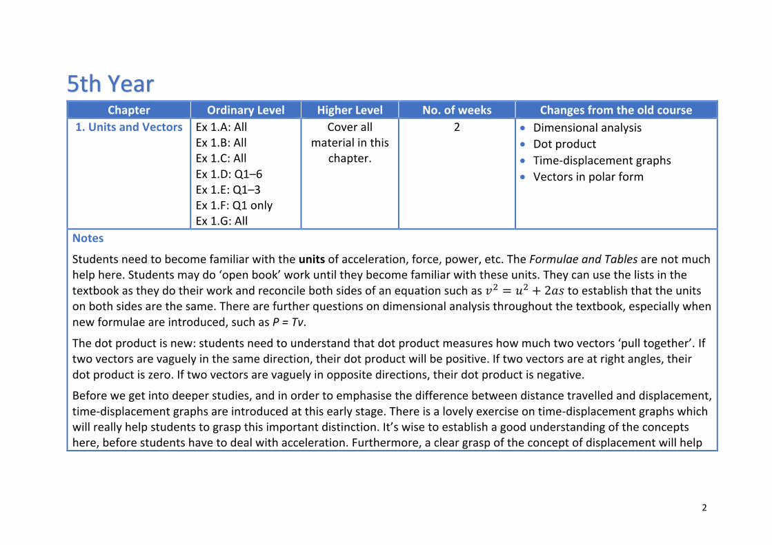
Notes

Students need to become familiar with the units of acceleration, force, power, etc. The Formulae and Tables are not much help here. Students may do ‘open book’ work until they become familiar with these units. They can use the lists in the textbook as they do their work and reconcile both sides of an equation such as 𝑣! = 𝑢! + 2𝑎𝑠to establish that the units on both sides are the same. There are further questions on dimensional analysis throughout the textbook, especially when new formulae are introduced, such as P = Tv.

The dot product is new: students need to understand that dot product measures how much two vectors ‘pull together’. If two vectors are vaguely in the same direction, their dot product will be positive. If two vectors are at right angles, their dot product is zero. If two vectors are vaguely in opposite directions, their dot product is negative.

Before we get into deeper studies, and in order to emphasise the difference between distance travelled and displacement, time-displacement graphs are introduced at this early stage. There is a lovely exercise on time-displacement graphs which will really help students to grasp this important distinction. It’s wise to establish a good understanding of the concepts here, before students have to deal with acceleration. Furthermore, a clear grasp of the concept of displacement will help

3

students later, when they have to decide if the acceleration of a body is g or -g in differential equations or when they have to decide if the velocities and accelerations are positive or negative.

Vectors may be given in polar form, where the vector is defined by its magnitude, m, followed by the argument A (the angle between the vector and the positive sense of the x-axis): ⟨𝑚 < 𝐴⟩. Students will have to be able to convert vectors from polar form to i–j form (and vice versa). For example, ⟨10 < 80°⟩ = 10 cos 80° 𝚤 + 10 sin 80° 𝚥 = 1.74𝚤 + 9.85𝚥. This is all covered in the textbook.

4

Chapter Ordinary Level Higher Level No. of weeks Changes from the old course 2. Uniform

Acceleration Up to the end of Ex 2.B

Perhaps leave the material after Ex. 2.G until

6th Year (unless the class is very strong).

5 • In the exam, students may be asked to prove the formulae

𝑣 = 𝑢 + 𝑎𝑡 𝑠 = 𝑢𝑡 + "

!𝑎𝑡!

𝑣! = 𝑢! + 2𝑎𝑠 using calculus. This will be covered in Chapter 10.

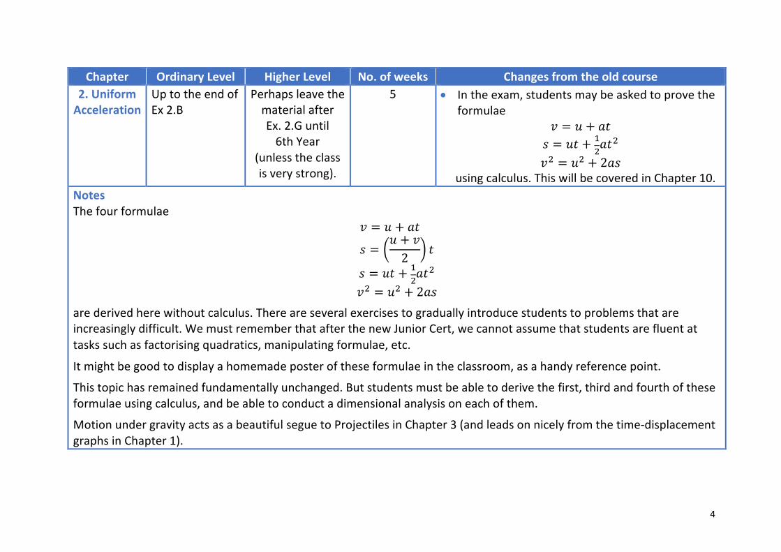
Notes The four formulae

𝑣 = 𝑢 + 𝑎𝑡

𝑠 = @𝑢 + 𝑣2

A 𝑡

𝑠 = 𝑢𝑡 + "!𝑎𝑡

! 𝑣! = 𝑢! + 2𝑎𝑠

are derived here without calculus. There are several exercises to gradually introduce students to problems that are increasingly difficult. We must remember that after the new Junior Cert, we cannot assume that students are fluent at tasks such as factorising quadratics, manipulating formulae, etc.

It might be good to display a homemade poster of these formulae in the classroom, as a handy reference point.

This topic has remained fundamentally unchanged. But students must be able to derive the first, third and fourth of these formulae using calculus, and be able to conduct a dimensional analysis on each of them.

Motion under gravity acts as a beautiful segue to Projectiles in Chapter 3 (and leads on nicely from the time-displacement graphs in Chapter 1).

5

Chapter Ordinary Level Higher Level No. of weeks Changes from the old course 3. Projectiles Up to the end of

Ex 3.C Cover all material

in this chapter. 3 • Projectiles on the inclined plane are no

longer on the course. Notes

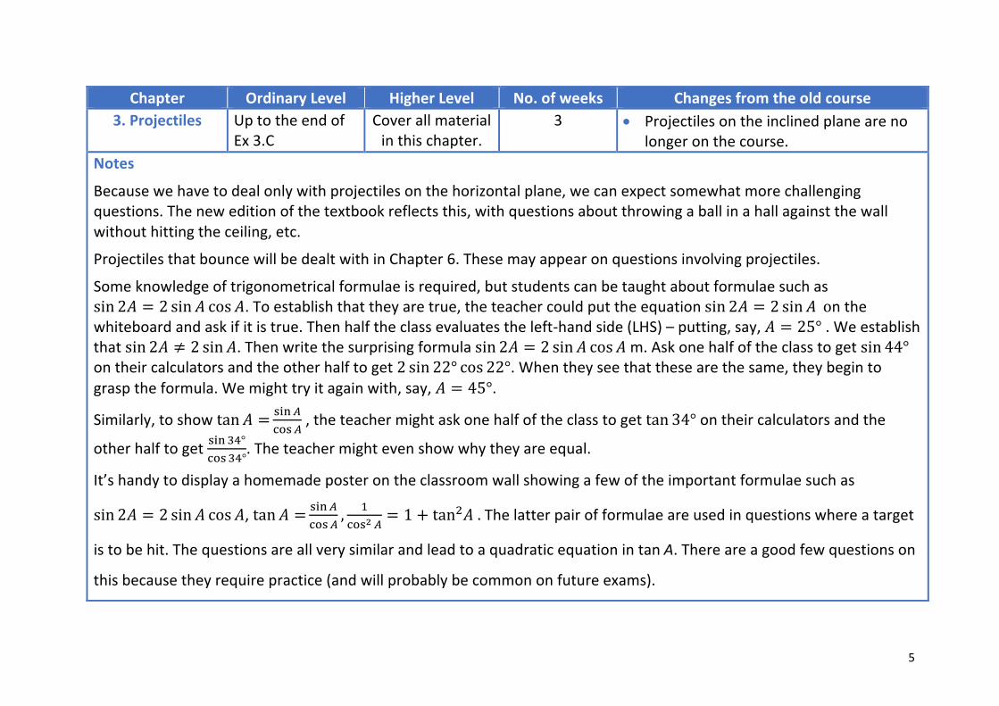
Because we have to deal only with projectiles on the horizontal plane, we can expect somewhat more challenging questions. The new edition of the textbook reflects this, with questions about throwing a ball in a hall against the wall without hitting the ceiling, etc.

Projectiles that bounce will be dealt with in Chapter 6. These may appear on questions involving projectiles.

Some knowledge of trigonometrical formulae is required, but students can be taught about formulae such as sin 2𝐴 = 2 sin 𝐴 cos 𝐴. To establish that they are true, the teacher could put the equation sin 2𝐴 = 2 sin 𝐴 on the whiteboard and ask if it is true. Then half the class evaluates the left-hand side (LHS) – putting, say, 𝐴 = 25° . We establish thatsin 2𝐴 ≠ 2 sin 𝐴. Then write the surprising formula sin 2𝐴 = 2 sin 𝐴 cos 𝐴m. Ask one half of the class to get sin 44° on their calculators and the other half to get 2 sin 22° cos 22°. When they see that these are the same, they begin to grasp the formula. We might try it again with, say, 𝐴 = 45°.

Similarly, to show tan 𝐴 = #$%&'(#&

, the teacher might ask one half of the class to get tan 34° on their calculators and the

other half to get #$%)*°'(#)*°

. The teacher might even show why they are equal.

It’s handy to display a homemade poster on the classroom wall showing a few of the important formulae such as

sin 2𝐴 = 2 sin 𝐴 cos 𝐴, tan 𝐴 = #$%&'(#&

, "'(#! &

= 1 + tan!𝐴. The latter pair of formulae are used in questions where a target

is to be hit. The questions are all very similar and lead to a quadratic equation in tan A. There are a good few questions on

this because they require practice (and will probably be common on future exams).

6

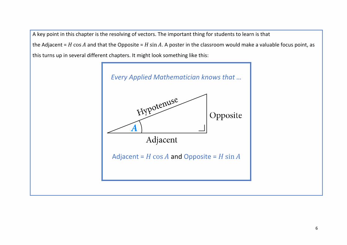
A key point in this chapter is the resolving of vectors. The important thing for students to learn is that

the Adjacent = 𝐻 cos 𝐴 and that the Opposite = 𝐻 sin 𝐴. A poster in the classroom would make a valuable focus point, as

this turns up in several different chapters. It might look something like this:

Every Applied Mathematician knows that …

Adjacent = 𝐻 cos𝐴 and Opposite = 𝐻 sin𝐴

23

Summary of Important Points

Fig. 1.102

Summary of Important Points

2. Dimensional analysis is used to check that thedimensions in an equation are the same on bothsides.

3. The magnitude of a __›i + b

__›j = √

_______ a2 + b 2

4. (a_›i + b

_›j ) . (c

_›i + d

_›j ) = ac + bd

5. _›x .

_›y = 0 if and only if _›x A�

_›y

6. If θ is the angle between_›p and

_›q then cos θ = _›p .�

_›q _______›| p | �

___›| q |

Do● Do draw large diagrams on graph paper.● Do use a ruler to draw vectors.● Do put arrowheads on all vectors.● Do label every vector.● Do show all calculations.

Don’t● Don’t draw small unclear diagrams.● Don’t forget to answer precisely what you were

asked.● Don’t mix up minutes and decimals when dealing in

parts of degrees.● Don’t omit to put in units in all answers.

AnswersExercise 1.A

1. Both m/s2. Both m3. Both m/s4. Both N or kg m/ s2

5. Both m6. Both m7. Both s 2

8. Both J or kg m 2/s 2

9. Both J or kg m 2/s 2

10. Both J or kg m 2/s 2

11. Both W or kg m 2/ s3

12. Both s13. Both J or kg m 2/s 2

14. Both m 2/ s2

16. (iii) is incorrectExercise 1.B

6. (ii) Yes9. 13 N to the right

10. 5 cm; E 53°N

11. Approximately 7 cm due east

12. 13 cm13. 18.345°14. 16.7° S of E

15.

Fig. 1.105

Exercise 1.C1. (i) √

___29; E 21.8° N

(ii) √__8 ; NE

(iii) 5; E 36.87° S

"

7

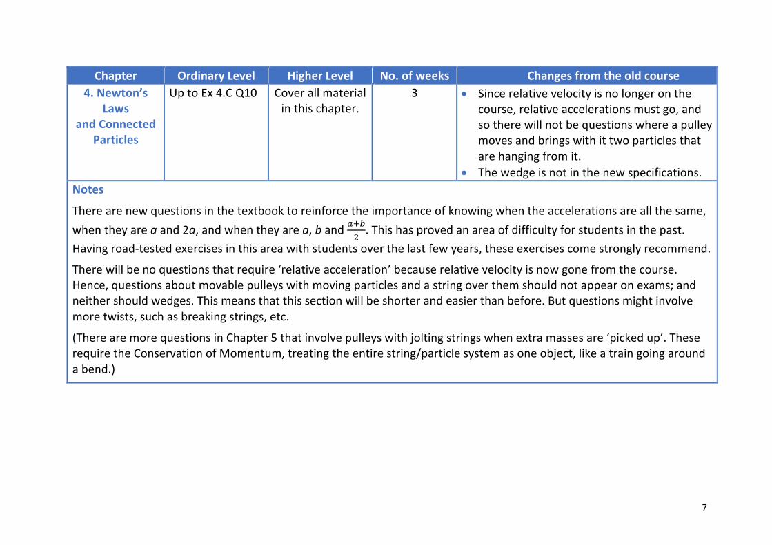
Chapter Ordinary Level Higher Level No. of weeks Changes from the old course 4. Newton’s

Laws and Connected

Particles

Up to Ex 4.C Q10 Cover all material in this chapter.

3 • Since relative velocity is no longer on the course, relative accelerations must go, and so there will not be questions where a pulley moves and brings with it two particles that are hanging from it.

• The wedge is not in the new specifications. Notes

There are new questions in the textbook to reinforce the importance of knowing when the accelerations are all the same, when they are a and 2a, and when they are a, b and ,-.

!. This has proved an area of difficulty for students in the past.

Having road-tested exercises in this area with students over the last few years, these exercises come strongly recommend.

There will be no questions that require ‘relative acceleration’ because relative velocity is now gone from the course. Hence, questions about movable pulleys with moving particles and a string over them should not appear on exams; and neither should wedges. This means that this section will be shorter and easier than before. But questions might involve more twists, such as breaking strings, etc.

(There are more questions in Chapter 5 that involve pulleys with jolting strings when extra masses are ‘picked up’. These require the Conservation of Momentum, treating the entire string/particle system as one object, like a train going around a bend.)

8

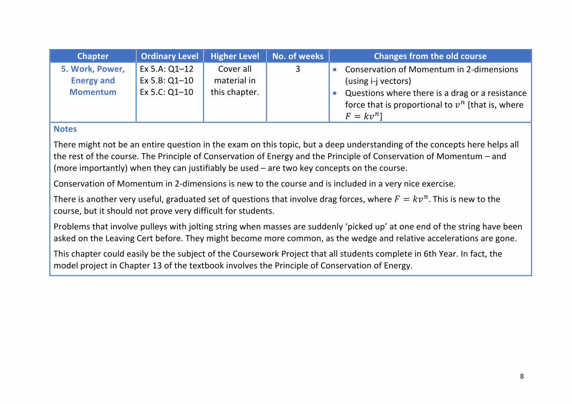
Chapter Ordinary Level Higher Level No. of weeks Changes from the old course 5. Work, Power,

Energy and Momentum

Ex 5.A: Q1–12 Ex 5.B: Q1–10 Ex 5.C: Q1–10

Cover all material in

this chapter.

3 • Conservation of Momentum in 2-dimensions (using i-j vectors)

• Questions where there is a drag or a resistance force that is proportional to 𝑣/ [that is, where 𝐹 = 𝑘𝑣/]

Notes

There might not be an entire question in the exam on this topic, but a deep understanding of the concepts here helps all the rest of the course. The Principle of Conservation of Energy and the Principle of Conservation of Momentum – and (more importantly) when they can justifiably be used – are two key concepts on the course.

Conservation of Momentum in 2-dimensions is new to the course and is included in a very nice exercise.

There is another very useful, graduated set of questions that involve drag forces, where 𝐹 = 𝑘𝑣/. This is new to the course, but it should not prove very difficult for students.

Problems that involve pulleys with jolting string when masses are suddenly ‘picked up’ at one end of the string have been asked on the Leaving Cert before. They might become more common, as the wedge and relative accelerations are gone.

This chapter could easily be the subject of the Coursework Project that all students complete in 6th Year. In fact, the model project in Chapter 13 of the textbook involves the Principle of Conservation of Energy.

9

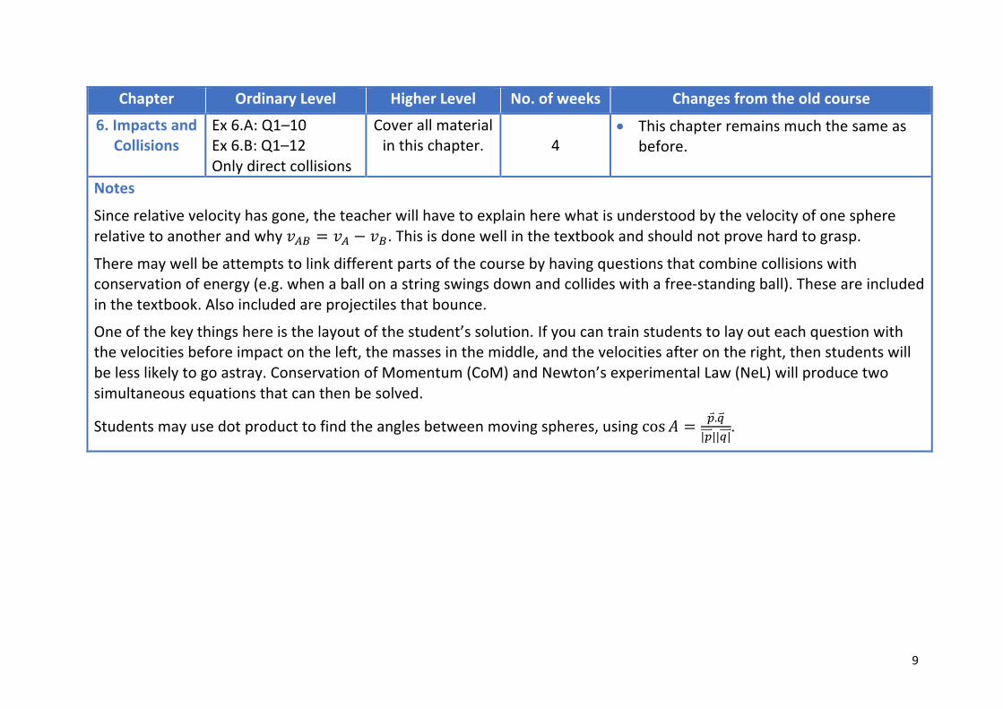
Chapter Ordinary Level Higher Level No. of weeks Changes from the old course

6. Impacts and Collisions

Ex 6.A: Q1–10 Ex 6.B: Q1–12 Only direct collisions

Cover all material in this chapter.

4

• This chapter remains much the same as before.

Notes

Since relative velocity has gone, the teacher will have to explain here what is understood by the velocity of one sphere relative to another and why 𝑣&0 = 𝑣& − 𝑣0. This is done well in the textbook and should not prove hard to grasp.

There may well be attempts to link different parts of the course by having questions that combine collisions with conservation of energy (e.g. when a ball on a string swings down and collides with a free-standing ball). These are included in the textbook. Also included are projectiles that bounce.

One of the key things here is the layout of the student’s solution. If you can train students to lay out each question with the velocities before impact on the left, the masses in the middle, and the velocities after on the right, then students will be less likely to go astray. Conservation of Momentum (CoM) and Newton’s experimental Law (NeL) will produce two simultaneous equations that can then be solved.

Students may use dot product to find the angles between moving spheres, using cos 𝐴 = 1⃑.45⃑|1555⃑ ||4|555⃑

.

10

Chapter Ordinary Level Higher Level No. of weeks Changes from the old course 7. Motion in

a Circle Ex 7.A: Q1–10 Ex 7.B: Q1–10 Ex 7.C: Q1–9

Cover all material in this chapter.

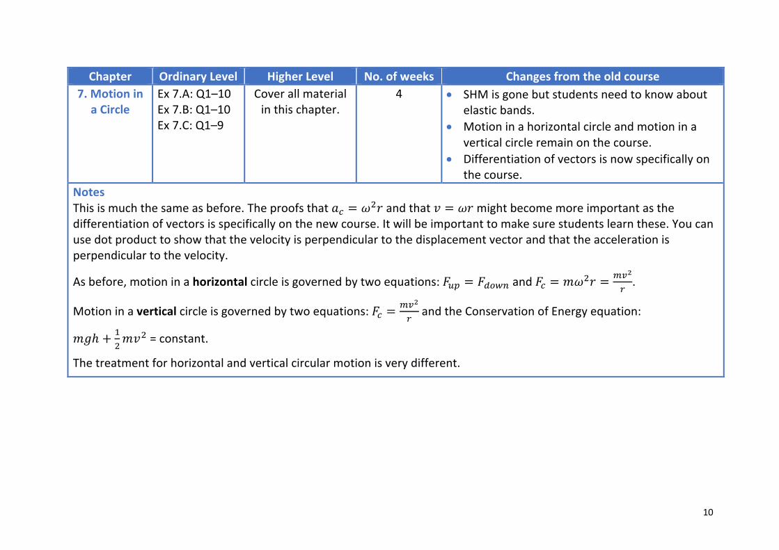
4 • SHM is gone but students need to know about elastic bands.

• Motion in a horizontal circle and motion in a vertical circle remain on the course.

• Differentiation of vectors is now specifically on the course.

Notes This is much the same as before. The proofs that 𝑎7 = 𝜔!𝑟 and that 𝑣 = 𝜔𝑟 might become more important as the differentiation of vectors is specifically on the new course. It will be important to make sure students learn these. You can use dot product to show that the velocity is perpendicular to the displacement vector and that the acceleration is perpendicular to the velocity.

As before, motion in a horizontal circle is governed by two equations: 𝐹81 = 𝐹9:;/ and 𝐹7 = 𝑚𝜔!𝑟 = <=!

>.

Motion in a vertical circle is governed by two equations: 𝐹7 =<=!

> and the Conservation of Energy equation:

𝑚𝑔ℎ + "!𝑚𝑣! = constant.

The treatment for horizontal and vertical circular motion is very different.

11

6th YearChapter Ordinary Level Higher Level No. of weeks Changes from the old course

8. Difference Equations

Ex 8.A: All Ex 8.B: All Ex 8.C: Q1–6 Ex 8.E: Q1–12

Cover all material in this

chapter.

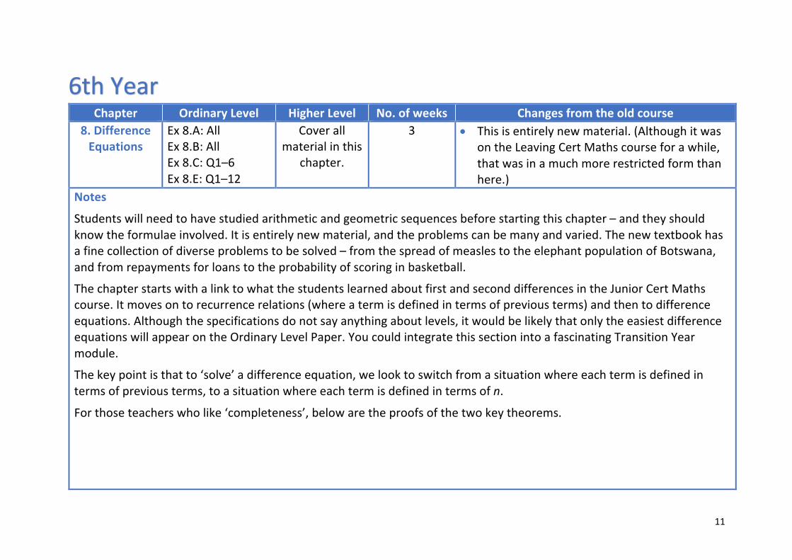
3 • This is entirely new material. (Although it was on the Leaving Cert Maths course for a while, that was in a much more restricted form than here.)

Notes

Students will need to have studied arithmetic and geometric sequences before starting this chapter – and they should know the formulae involved. It is entirely new material, and the problems can be many and varied. The new textbook has a fine collection of diverse problems to be solved – from the spread of measles to the elephant population of Botswana, and from repayments for loans to the probability of scoring in basketball.

The chapter starts with a link to what the students learned about first and second differences in the Junior Cert Maths course. It moves on to recurrence relations (where a term is defined in terms of previous terms) and then to difference equations. Although the specifications do not say anything about levels, it would be likely that only the easiest difference equations will appear on the Ordinary Level Paper. You could integrate this section into a fascinating Transition Year module.

The key point is that to ‘solve’ a difference equation, we look to switch from a situation where each term is defined in terms of previous terms, to a situation where each term is defined in terms of n.

For those teachers who like ‘completeness’, below are the proofs of the two key theorems.

12

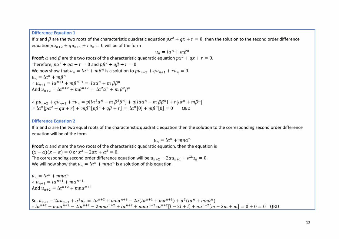
Difference Equation 1 If 𝛼 and 𝛽 are the two roots of the characteristic quadratic equation 𝑝𝑥! + 𝑞𝑥 + 𝑟 = 0, then the solution to the second order difference equation 𝑝𝑢"#! + 𝑞𝑢"#$ + 𝑟𝑢" = 0 will be of the form

𝑢" = 𝑙𝛼" +𝑚𝛽" Proof: 𝛼 and 𝛽 are the two roots of the characteristic quadratic equation 𝑝𝑥! + 𝑞𝑥 + 𝑟 = 0. Therefore, 𝑝𝛼! + 𝑞𝛼 + 𝑟 = 0 and 𝑝𝛽! + 𝑞𝛽 + 𝑟 = 0 We now show that 𝑢" = 𝑙𝛼" +𝑚𝛽" is a solution to 𝑝𝑢"#! + 𝑞𝑢"#$ + 𝑟𝑢" = 0. 𝑢" = 𝑙𝛼" +𝑚𝛽" ∴ 𝑢"#$ = 𝑙𝛼"#$ +𝑚𝛽"#$ = 𝑙𝛼𝛼" +𝑚𝛽𝛽" And𝑢"#! = 𝑙𝛼"#! +𝑚𝛽"#! = 𝑙𝛼!𝛼" +𝑚𝛽!𝛽" ∴ 𝑝𝑢"#! + 𝑞𝑢"#$ + 𝑟𝑢" = 𝑝[𝑙𝛼!𝛼" +𝑚𝛽!𝛽"] + 𝑞[𝑙𝛼𝛼" +𝑚𝛽𝛽"] + 𝑟[𝑙𝛼" +𝑚𝛽"] = 𝑙𝛼"[𝑝𝛼! + 𝑞𝛼 + 𝑟] +𝑚𝛽"[𝑝𝛽! + 𝑞𝛽 + 𝑟] = 𝑙𝛼"[0] + 𝑚𝛽"[0] = 0 QED Difference Equation 2 If 𝛼 and 𝛼 are the two equal roots of the characteristic quadratic equationthen the solution to the corresponding second order difference equation will be of the form

𝑢" = 𝑙𝛼" +𝑚𝑛𝛼" Proof: 𝛼 and 𝛼 are the two roots of the characteristic quadratic equation, then the equation is (𝑥 − 𝛼)(𝑥 − 𝛼) = 0 or 𝑥! − 2𝛼𝑥 + 𝛼! = 0. The corresponding second order difference equation will be 𝑢"#! − 2𝑎𝑢"#$ + 𝛼!𝑢" = 0. We will now show that 𝑢" = 𝑙𝛼" +𝑚𝑛𝛼" is a solution of this equation. 𝑢" = 𝑙𝛼" +𝑚𝑛𝛼" ∴ 𝑢"#$ = 𝑙𝛼"#$ +𝑚𝛼"#$ And𝑢"#! = 𝑙𝛼"#! +𝑚𝑛𝛼"#! So, 𝑢"#! − 2𝑎𝑢"#$ + 𝛼!𝑢" = 𝑙𝛼"#! +𝑚𝑛𝛼"#! − 2𝛼(𝑙𝛼"#$ +𝑚𝛼"#$) + 𝛼!(𝑙𝛼" +𝑚𝑛𝛼") =𝑙𝛼"#! +𝑚𝑛𝛼"#! − 2𝑙𝛼"#! − 2𝑚𝑛𝛼"#! + 𝑙𝛼"#! +𝑚𝑛𝛼"#!=𝛼"#![𝑙 − 2𝑙 + 𝑙] + 𝑛𝛼"#![𝑚 − 2𝑚 +𝑚] = 0 + 0 = 0QED

13

Chapter Ordinary Level Higher Level No. of weeks Changes from the old course 9. Differentiation and Integration

None Cover all material in this

chapter.

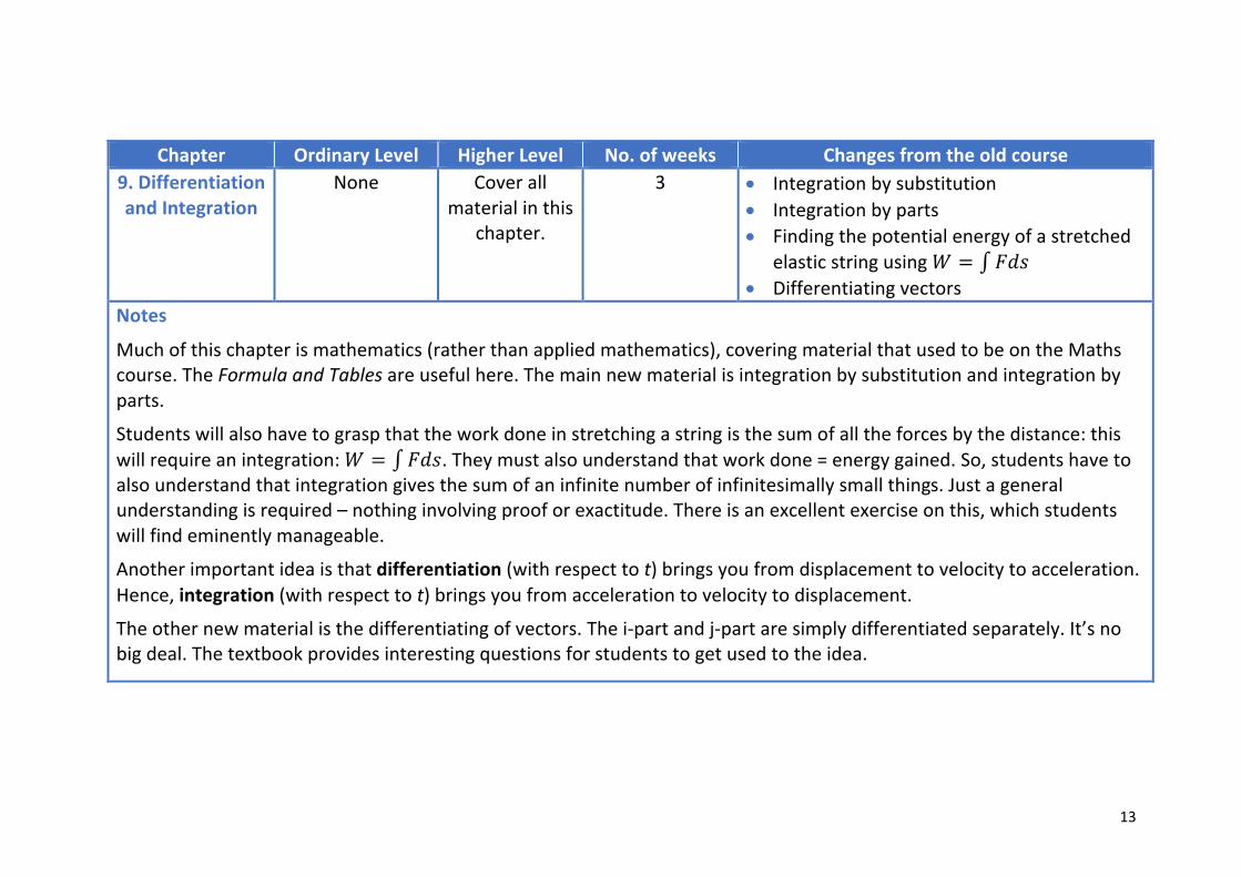
3 • Integration by substitution • Integration by parts • Finding the potential energy of a stretched

elastic string using 𝑊 = ∫𝐹𝑑𝑠 • Differentiating vectors

Notes

Much of this chapter is mathematics (rather than applied mathematics), covering material that used to be on the Maths course. The Formula and Tables are useful here. The main new material is integration by substitution and integration by parts.

Students will also have to grasp that the work done in stretching a string is the sum of all the forces by the distance: this will require an integration: 𝑊 = ∫𝐹𝑑𝑠. They must also understand that work done = energy gained. So, students have to also understand that integration gives the sum of an infinite number of infinitesimally small things. Just a general understanding is required – nothing involving proof or exactitude. There is an excellent exercise on this, which students will find eminently manageable.

Another important idea is that differentiation (with respect to t) brings you from displacement to velocity to acceleration. Hence, integration (with respect to t) brings you from acceleration to velocity to displacement.

The other new material is the differentiating of vectors. The i-part and j-part are simply differentiated separately. It’s no big deal. The textbook provides interesting questions for students to get used to the idea.

14

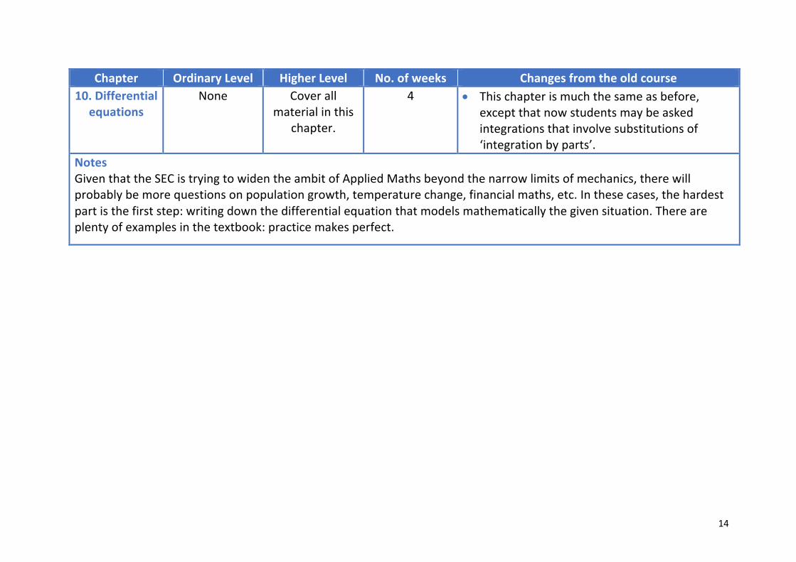
Chapter Ordinary Level Higher Level No. of weeks Changes from the old course 10. Differential

equations None Cover all

material in this chapter.

4 • This chapter is much the same as before, except that now students may be asked integrations that involve substitutions of ‘integration by parts’.

Notes Given that the SEC is trying to widen the ambit of Applied Maths beyond the narrow limits of mechanics, there will probably be more questions on population growth, temperature change, financial maths, etc. In these cases, the hardest part is the first step: writing down the differential equation that models mathematically the given situation. There are plenty of examples in the textbook: practice makes perfect.

15

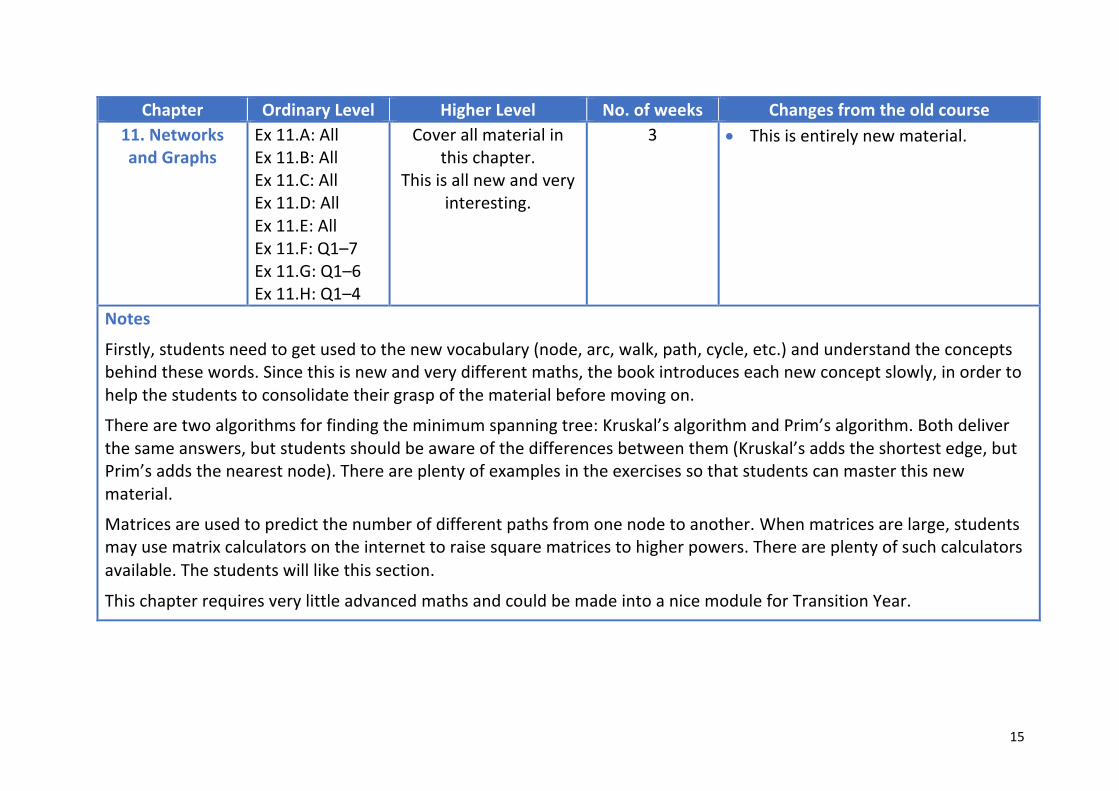
Chapter Ordinary Level Higher Level No. of weeks Changes from the old course 11. Networks and Graphs

Ex 11.A: All Ex 11.B: All Ex 11.C: All Ex 11.D: All Ex 11.E: All Ex 11.F: Q1–7 Ex 11.G: Q1–6 Ex 11.H: Q1–4

Cover all material in this chapter.

This is all new and very interesting.

3 • This is entirely new material.

Notes

Firstly, students need to get used to the new vocabulary (node, arc, walk, path, cycle, etc.) and understand the concepts behind these words. Since this is new and very different maths, the book introduces each new concept slowly, in order to help the students to consolidate their grasp of the material before moving on.

There are two algorithms for finding the minimum spanning tree: Kruskal’s algorithm and Prim’s algorithm. Both deliver the same answers, but students should be aware of the differences between them (Kruskal’s adds the shortest edge, but Prim’s adds the nearest node). There are plenty of examples in the exercises so that students can master this new material.

Matrices are used to predict the number of different paths from one node to another. When matrices are large, students may use matrix calculators on the internet to raise square matrices to higher powers. There are plenty of such calculators available. The students will like this section.

This chapter requires very little advanced maths and could be made into a nice module for Transition Year.

16

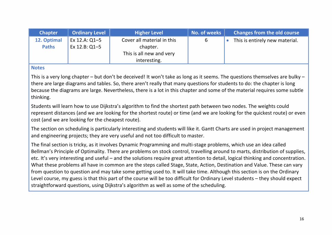
Chapter Ordinary Level Higher Level No. of weeks Changes from the old course 12. Optimal

Paths Ex 12.A: Q1–5 Ex 12.B: Q1–5

Cover all material in this chapter.

This is all new and very interesting.

6 • This is entirely new material.

Notes

This is a very long chapter – but don’t be deceived! It won’t take as long as it seems. The questions themselves are bulky – there are large diagrams and tables. So, there aren’t really that many questions for students to do: the chapter is long because the diagrams are large. Nevertheless, there is a lot in this chapter and some of the material requires some subtle thinking.

Students will learn how to use Dijkstra’s algorithm to find the shortest path between two nodes. The weights could represent distances (and we are looking for the shortest route) or time (and we are looking for the quickest route) or even cost (and we are looking for the cheapest route).

The section on scheduling is particularly interesting and students will like it. Gantt Charts are used in project management and engineering projects; they are very useful and not too difficult to master.

The final section is tricky, as it involves Dynamic Programming and multi-stage problems, which use an idea called Bellman’s Principle of Optimality. There are problems on stock control, travelling around to marts, distribution of supplies, etc. It’s very interesting and useful – and the solutions require great attention to detail, logical thinking and concentration. What these problems all have in common are the steps called Stage, State, Action, Destination and Value. These can vary from question to question and may take some getting used to. It will take time. Although this section is on the Ordinary Level course, my guess is that this part of the course will be too difficult for Ordinary Level students – they should expect straightforward questions, using Dijkstra’s algorithm as well as some of the scheduling.

17

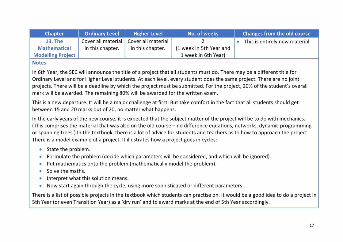
Chapter Ordinary Level Higher Level No. of weeks Changes from the old course 13. The

Mathematical Modelling Project

Cover all material in this chapter.

Cover all material in this chapter.

2 (1 week in 5th Year and

1 week in 6th Year)

• This is entirely new material

Notes

In 6th Year, the SEC will announce the title of a project that all students must do. There may be a different title for Ordinary Level and for Higher Level students. At each level, every student does the same project. There are no joint projects. There will be a deadline by which the project must be submitted. For the project, 20% of the student’s overall mark will be awarded. The remaining 80% will be awarded for the written exam.

This is a new departure. It will be a major challenge at first. But take comfort in the fact that all students should get between 15 and 20 marks out of 20, no matter what happens.

In the early years of the new course, it is expected that the subject matter of the project will be to do with mechanics. (This comprises the material that was also on the old course – no difference equations, networks, dynamic programming or spanning trees.) In the textbook, there is a lot of advice for students and teachers as to how to approach the project. There is a model example of a project. It illustrates how a project goes in cycles:

• State the problem. • Formulate the problem (decide which parameters will be considered, and which will be ignored). • Put mathematics onto the problem (mathematically model the problem). • Solve the maths. • Interpret what this solution means. • Now start again through the cycle, using more sophisticated or different parameters.

There is a list of possible projects in the textbook which students can practise on. It would be a good idea to do a project in 5th Year (or even Transition Year) as a ‘dry run’ and to award marks at the end of 5th Year accordingly.

18

It would be a mistake to give over too much class time to the project. Just make sure students are making progress. Nudge them in the right direction and help them when they get stuck. Otherwise, let them off with it! You might be surprised.

Like with all coursework, when the deadline approaches, panic can set in. The procrastinating student, who has said all along that progress was being made, suddenly wants to leave other classes to finish the project. The teacher gets anxious because there is no sign of some of the projects. It could also be difficult to be certain that each student did all the work in their project by themselves. The students’ command of written English might not be perfect – and the presentation might be poor. Some challenges will arise. Again, the teacher’s role is to encourage, to point students in the right direction, and to trust them. If they are late, they have to live with the consequences. This is real life.

Revision: The rest of the year can be spent revising. Because the past papers are no longer relevant, for the most part, the textbook has a revision exercise in all chapters (except in the first and last chapters). This comprises eight questions in Leaving Cert style, as they might appear on the exam. These exercises will be particularly useful at revision time.