Teachers in the South African Education systemresep.sun.ac.za/wp-content/uploads/2015/04/Paula-Armstrong-Thesis.pdf · Teachers in the South African education system: An economic

Teachers in the South African education system: An

economic perspective

Paula Louise Armstrong

Dissertation presented for the degree

Doctor of Philosophy (Economics)

in the Faculty of Economic and Management Science at

Stellenbosch University

Supervisor: Prof Servaas van der Berg

March 2015

ii

DECLARATION

By submitting this dissertation electronically, I declare that the entirety of the work contained

therein is my own, original work, that I am the sole author thereof (save to the extent explicitly

otherwise stated), that reproduction and publication thereof by Stellenbosch University will not

infringe any third party rights and that I have not previously in its entirety or in part submitted

it for obtaining any qualification.

March 2015

iii

ABSTRACT

Chapter 1 investigates teacher wages in the South African labour market, in order to ascertain

whether teaching is a financially attractive profession, and whether high ability individuals are

likely to be attracted to the teaching force. Making use of labour force survey data for the years

2000 to 2007 and for 2010, wage returns to educational attainment and experience are measured

for teachers, non-teachers and non-teaching professionals. The returns to higher levels of

education for teachers are significantly lower than for non-teachers and non-teaching

professionals. Similarly, the age-wage profile for teachers is significantly flatter than it is for

non-teachers, indicating that there is little wage incentive to remain in teaching beyond roughly

12 years. The profession is therefore unlikely to attract high ability individuals who are able to

collect attractive remuneration elsewhere in the labour market.

Chapter 2 deals with explicit teacher incentives in education. It provides a technical analysis

of Holstrom and Milgrom’s (1991) multitasking model and Kandel and Lazear’s (1992) model

of peer pressure as an incentivising force, highlighting aspects of these models that are

necessary to ensure that incentive systems operate successfully. The chapter provides an

overview of incentive systems internationally, discussing elements of various systems that may

be useful in a South African setting. The prospects for the introduction of incentives in South

Africa are discussed, with the conclusion that the systems in place at the moment are not

conducive to introducing teacher incentives. There are however models in Chile and Brazil, for

example, that may work effectively in a South African setting, given their explicit handling of

inequality within the education system. Chapter 3 makes use of hierarchical linear modelling

to investigate which teacher characteristics impact significantly on student performance. Using

data from the SACMEQ III study of 2007, an interesting and potentially important finding is

that younger teachers are better able to improve the mean mathematics performance of their

students. Furthermore, younger teachers themselves perform better on subject tests than do

their older counterparts. Changes in teacher education in the late 1990s and early 2000s may

explain the differences in the performance of younger teachers relative to their older

counterparts. However, further investigation is required to fully understand these differences.

iv

OPSOMMING

In Hoofstuk 1 word die lone van onderwysers in die Suid-Afrikaanse arbeidsmark ondersoek

om vas te stel of onderwys ŉ finansieel aantreklike beroep is en hoe waarskynlik dit is dat

mense met sterk vermoëns na die onderwys gelok sal word. Met gebruik van

arbeidsmagopnamedata van 2000 tot 2007 en van 2010 word die loonopbrengs op jare

onderwys en ervaring vir onderwysers, nie-onderwysers en beroepslui buite die onderwys

gemeet. Die opbrengste vir hoër vlakke van opvoeding is beduidend laer vir onderwysers as

vir nie-onderwysers en nie-onderwys beroepslui. Netso is die ouderdom-loonprofiel van

onderwysers beduidend platter as vir nie-onderwysers, wat dui op weinig looninsentief om

langer as ongeveer 12 jaar in die onderwysveld te bly. Dit is dus onwaarskynlik dat hierdie

beroep baie bekwame mense sal lok wat elders in die arbeidsmark goed sou kon verdien.

In Hoofstuk 2 word na eksplisiete insentiewe in die onderwys gekyk. Die hoofstuk verskaf ŉ

tegniese analise van die multi-taak-model van Holstrom en Milgrom (1991) en van Kandel en

Lazear (1992) se model van portuur-druk as aansporingskrag, met klem op die aspekte van

hierdie modelle wat in Suid-Afrikaanse omstandighede van nut mag wees. Vooruitsigte vir die

instelling van insentiewe in Suid-Afrika word bespreek, met die slotsom dat die stelsels wat

tans in plek is nie bevorderlik vir die instelling van onderwysersinsentiewe is nie. Daar is egter

modelle in byvoorbeeld Chili en Brasilië wat effektief in Suid-Afrikaanse omstandighede sou

kon funksioneer, gegewe hulle eksplisiete klem op ongelykheid binne die onderwys.

In Hoofstuk 3 word hiërargiese liniêre programmering gebruik om te ondersoek watter

eienskappe van onderwysers ŉ belangrike invloed op studenteprestasie uitoefen. Met gebruik

van data van die SACMEQ III studie van 2007 is ŉ interessante bevinding dat jonger

onderwysers beter in staat is om die gemiddelde wiskunde prestasie van hulle student te

verbeter. Verder vertoon sulke jonger onderwysers self ook beter in die vaktoetse in Wiskunde

en taal as hulle ouer kollegas. Veranderings in onderwysopleiding in die laat negentigerjare en

vroeë jare van hierdie eeu kan dalk die verskille in die vertonings van jonger onderwysers

relatief tot hulle ouer eweknieë verklaar. Verdere ondersoek is egter nodig om hierdie verskille

beter te verstaan.

v

ACKNOWLEDGEMENTS

I thank Servaas van der Berg for his insights, patience and friendship during the writing of this

thesis. I am grateful to members of the ReSEP group for valuable criticism, comments and

contributions. I have learnt immeasurable amounts working as part of this team.

I also thank my parents, Patrick and Mary Armstrong for their unconditional support and

understanding. I am exceptionally grateful to friends who encourared me and provided

perspective and humour when mine were in short supply.

vi

TABLE OF CONTENTS

Introduction ............................................................................................................................... 1

The role of education and of teachers in South African economic development .................. 1

Education and South African economic development ........................................................... 2

Teachers and their role in improving educational outcomes.................................................. 4

Chapter 1: Teacher wages in South Africa: how attractive is the teaching profession? .. 10

1. The importance of teachers in achieving quality education: A case for effective wage

incentives .................................................................................................................................. 11

2. International evidence: Teacher pay and student performance ........................................ 13

3. Wage analysis ................................................................................................................... 16

3.1 Wage Differentials ...................................................................................................... 19

3.2 Local polynomial smoothed lines ............................................................................... 23

3.3 Mincerian wage functions .......................................................................................... 25

3.4 Lemieux decomposition .............................................................................................. 31

3.5 Conclusion .................................................................................................................. 37

4. Academic performance of future teachers ........................................................................ 38

4.1 Data ............................................................................................................................. 38

4.2 Performance across faculties ...................................................................................... 38

5. Conclusion ........................................................................................................................ 42

Chapter 2: Teacher incentives in South Africa: A theoretical investigation of the

possibilities ............................................................................................................................... 44

1. Introduction: Teacher quality in South Africa and the possibility of incentives .............. 44

2. Economic theory and incentives ....................................................................................... 51

2.1 Finding performance measures to use with incentives ............................................... 52

2.2 Different effects of incentives on different people ..................................................... 54

2.3 Effects of uncertainty and control in providing incentives ......................................... 55

2.4 Effects of groups in providing incentives ................................................................... 56

2.5 Weighing the costs and benefits of incentives ............................................................ 57

3. Theoretical models of teacher incentives ......................................................................... 58

3.1 Incentives based on input and output ......................................................................... 58

3.1.1 Output-based pay .................................................................................................. 58

3.1.2 Input-based pay..................................................................................................... 59

3.1.3 What works better? ............................................................................................... 59

3.2 Sorting versus incentive effects and the likelihood of success ................................... 60

vii

3.3 Moral hazard and the risk of distortion ....................................................................... 61

3.3.1 Multitasking and the risk of distortion .................................................................. 62

3.3.2 The efficiency of incentive pay in education ........................................................ 64

3.3.3 Contamination and hidden actions ....................................................................... 66

3.4 Peer pressure and partnerships .................................................................................... 68

3.4.1 Free-rider effects and peer pressure ...................................................................... 68

3.4.2 Creating peer pressure .......................................................................................... 70

3.4.3 Mutual monitoring ................................................................................................ 72

3.5 Return to distortion ..................................................................................................... 74

4. Characteristics of successful incentive programmes ........................................................ 74

4.1 Sorting versus incentives ............................................................................................ 75

4.2 Potential for distortion ................................................................................................ 75

4.3 Possibility for peer pressure ....................................................................................... 75

5. International examples of incentive programmes ............................................................. 76

5.1 Andhra Pradesh, India (2005 – 2007) ......................................................................... 76

5.2 Israel (2001) ................................................................................................................ 78

5.3 Kenya (1997) .............................................................................................................. 79

5.4 Pernambuco, Brazil (since 2008) ................................................................................ 81

5.5 Chile (since 1991) ....................................................................................................... 83

5.6 Incentive systems: What does the evidence say?........................................................ 85

5.7 North Carolina, USA .................................................................................................. 87

5.8 Finland ........................................................................................................................ 88

5.9 Potential costs of incentive systems and alternative solutions ................................... 89

6. South Africa: where do we stand? .................................................................................... 90

6.1 Lessons from international experience ....................................................................... 90

6.2 Incentives inherent in the South African teaching profession .................................... 92

6.3 Prospects for peer pressure as an incentivising force: Professionalising teaching ..... 94

6.4 Mutual monitoring: The Integrated Quality Management System ............................. 97

6.5 Inequality prevails ...................................................................................................... 98

Chaper 3: The impact of teacher characteristics on student performance: An analysis

using hierarchical linear modelling ....................................................................................... 99

1. Introduction ...................................................................................................................... 99

2. Research question and data ............................................................................................. 107

2.1 Defining the research question ................................................................................. 107

2.2 Data: SACMEQ III ................................................................................................... 107

viii

2.3 Variables included in the model ............................................................................... 108

3. Hierarchical linear modelling: The necessity of the method .......................................... 110

3.1 Hierarchical linear modelling: The analytical method ............................................. 114

3.2 Means-as-outcome regression................................................................................... 115

4. Modelling the impact of teacher characteristics on student performance ...................... 116

5. Results ............................................................................................................................ 120

6. Discussion and conclusion.............................................................................................. 127

6.1 Differences in teacher training .................................................................................. 135

6.2 Other sources of differentials by teacher age............................................................ 137

Conclusion: How attractive is the teaching profession and which teachers are considered

most effective? ....................................................................................................................... 138

Appendix A ............................................................................................................................ 145

Appendix B ............................................................................................................................ 155

Appendix C ............................................................................................................................ 159

List of References .................................................................................................................. 164

ix

LIST OF TABLES

TABLE 1: Number of teachers and non-teachers .................................................................... 18

TABLE 2: Wage differentials between teachers, non-teachers and non-teaching professionals

(2000–2007 and 2010) ............................................................................................................. 20

TABLE 3: Regression estimates for augmented Mincerian wage function on log hourly

wages (2000–2007 and 2010) .................................................................................................. 25

TABLE 4: Reasons for wanting to leave the teaching profession ........................................... 49

TABLE 5: Description and descriptive statistics for variables included in the model .......... 109

TABLE 6: Student-level model ............................................................................................. 121

TABLE 7: Full hierarchical linear model .............................................................................. 124

TABLE 8: HLM coefficients on teacher age variables for 4 SACMEQ countries ............... 128

TABLE 9: Regression of teacher test performance on teacher age ....................................... 133

TABLE 10: HLM coefficients on teacher age variables using SACMEQ II (2000) ............. 134

TABLE A1: Non-teaching professionals in the LFS (2000–2007) and QLFS (2010) .......... 146

TABLE A2: Variables included in augmented Mincerian wage function ............................. 146

TABLE A3: Means (and standard deviations) of variables used .......................................... 148

TABLE A4: Regression estimates for augmented Mincerian wage function on log hourly

wages (2000–2007)1............................................................................................................... 149

TABLE B1: OLS estimates obtained after clustering standard errors (SACMEQ III, 2007) 155

TABLE B2: Full Hierarchical Linear Model (SACMEQ II, 2000) ....................................... 157

TABLE D1: Teaching specialisation for initial teacher education qualifications ................. 160

x

LIST OF FIGURES FIGURE 1: Boxplots of log real hourly wage (2000–2007) .................................................... 21

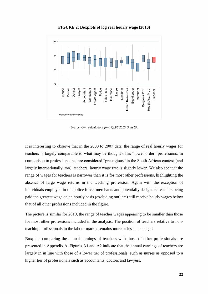
FIGURE 2: Boxplots of log real hourly wage (2010) .............................................................. 22

FIGURE 3: Local polynomial smoothed lines for age-wage profile (2000–2007) ................. 23

FIGURE 4: Local polynomial smoothed lines for age-wage profile (2010) ........................... 24

FIGURE 5: Returns to potential experience (2000) ................................................................ 27

FIGURE 6: Returns to potential experience (2007) ................................................................ 27

FIGURE 7: Returns to potential Experience (2010) ................................................................ 28

FIGURE 8: Wage differential between teachers and non-teachers (2000–2007) .................... 29

FIGURE 9: Wage differential between teachers and non-teachers with at least 10 years of

education (2000–2007) ............................................................................................................ 30

FIGURE 10: Teachers and non-teachers, 2000 ....................................................................... 34



FIGURE 13: Teachers and non-teaching professionals, 2000 ................................................. 36



FIGURE 16: Percentage of students who took higher grade mathematics, 2005-2007 .......... 39

FIGURE 17: Performance in mathematics, 2005-2009 ........................................................... 40

FIGURE 18: Performance in language, 2005-2009 ................................................................. 41

FIGURE 19: Age distribution of teachers, 2009 – 2012 ......................................................... 46

FIGURE 20: Angle between vectors (f1, f2) and (g1, g2)....................................................... 64

FIGURE 21: Distribution of grade 12 mathematics marks for first years enrolments, 2005 –

2009.......................................................................................................................................... 93

FIGURE 22: Distribution of grade 12 language marks for first years enrolments, 2005 –

2009.......................................................................................................................................... 94

FIGURE 23: Teacher mathematics score by age group ......................................................... 129

FIGURE 24: Teacher language score by age group .............................................................. 129

FIGURE 25: Teacher mathematics score by age (Botswana) ............................................... 130

FIGURE 26: Teacher mathematics score by age (Kenya) ..................................................... 130

FIGURE 27: Teacher mathematics score by age (Zimbabwe) .............................................. 131

FIGURE 28: Teacher language score by age (Botswana) ..................................................... 131

FIGURE 29: Teacher language score by age (Kenya)........................................................... 132

xi

FIGURE 30: Teacher language score by age (Zimbabwe) .................................................... 132

1

Introduction

The role of education and of teachers in South African economic development

Education and economic development are inextricably linked. Amartrya Sen (1997) explains

development as the ability to choose the way in which one lives one’s life and as having the

capability to function at a certain level (Sen, 1997: 199). The process of development is

therefore the process of enhancing the level of freedom that people have to live the life of their

choice (Sen, 1999: 297). Different capabilities are interdependent according to this framework.

For example, the level of educational attainment and the health status of people depend to a

large extent on their level of income, yet the income individuals generate is governed to a large

extent by their level of education and the state of their health (Sen, 1999: 19). In this way,

freedom is both the means by which development is achieved as well as the ultimate objective.

A more conventional notion of economic development incorporates an element of economic

growth, which includes the increase in per capita income over time (Ray, 1998: 7). On its own

this is an incomplete notion of economic development. Economic development involves

understanding how economic growth facilitates characteristics of development – health, life

expectancy, sanitation and literacy – and how growth in per capita income results in long-term

social change (Meier, 1995: 7). The traditional notion of economic development therefore

needs to be broadened to encompass Sen’s idea of development as freedom.

The role of education in economic development is vital. To some extent, access to education is

seen as one of the outcomes of economic development. Access to basic education has been

achieved in most countries in the world and the challenge facing governments internationally

is enhancing the quality of education received by their citizens. Education is also a necessary

driver of economic development, however. Indeed, the economic growth literature documents

the role of “human capital” in economic growth, explaining that human capital is comprised of

skills and knowledge, and that the generation and accumulation of human capital requires direct

investment (Schultz, 1961: 1). Innovation and productivity are enhanced with higher levels of

human capital. This applies at an individual level, too. The human capital model hypothesises

that investment in education (and consequently higher levels of educational attainment)

enhances individual productivity and in turn labour market earnings.

2

Education and South African economic development

Given its centrality in achieving a dignified standard of living as well as economic growth,

education is one of the biggest components of government spending. In 2012, education

comprised 20.6 percent of government expenditure in South Africa (World Bank, 2014).

Furthermore, by far the largest expenditure item in education is teacher salaries. Personnel

spending (comprised predominantly of teacher salaries) accounted for roughly 78 percent of

education spending in South Africa in 2010 (Oxford Policy Management & University of

Stellenbosch, 2012). From an economic perspective then, education is relevant and important,

and the role of teachers is central to education.

South Africa’s educational performance is worrying. Spaull (2013a: 53) provides a brief

overview of South Africa’s performance in an international perspective with a discussion of

the results of three international studies conducted at different grades in the education system

across different years. In 2006 South Africa was one of 45 countries participating in the

Progress in Reading Literacy Study (at grade 4 and 5 level). Some other middle-income

countries also participated in the study, namely Macedonia, Trinidad and Tobago, Indonesia

and Morocco. More than three-quarters of the South African sample performed below the low

international benchmark. This means that 78% of the South African sample may well never

learn how to read, given their failure to achieve this basic level of competence at the grade 5

level (Trong, 2010: 2). In 2011, an easier version of the assessment, prePIRLS, was offered.

PrePIRLS was designed specifically for underachieving developing countries and South

Africa, Botswana and Colombia opted to participate in prePIRLS rather than PIRLS in 2011

(Spaull, 2013a: 53). The performance in prePIRLS was comparable to that of South Africa’s

neighbouring country Botswana. However, the average South African child was roughly three

years behind the average Colombian child in grade 4.

South Africa also participated in international testing conducted by the Southern and Eastern

African Consortium for Monitoring Educational Quality (SACMEQ) in 2007. This was the

third round of such testing and is referred to as SACMEQ III.1 South Africa performed below

the average of a number of African countries, even with lower pupil-teacher ratios, better

qualified teachers and more resources (Van der Berg, Burger, Burger, De Vos, Du Randt,

Gustafsson, Moses, Shepherd et al., 2011: 4).

1 The data used in this analysis is from SACMEQ III. A thorough description of the study is presented in section

2 of this paper.

3

South Africa participated in the Trends in International Maths and Science Survey in 1995,

1995, 2002 and 2011 (Spaull, 2013a: 54). Despite marked improvement in performance

between 2002 and 2011,2 an international comparison of results reveals that South African

grade 9 students were performing 2 to 3 grade levels below grade 8 students in countries at

similar levels of income (Spaull, 2013b: 4). The improvement observed must therefore be

considered in the context of excessively low performance in previous studies. In 2011, 76% of

South African grade 9 students did not understand whole numbers, basic graphs, decimals or

operations.

It is clear then that South Africa’s education performance is less than desirable. Education

performance differs dramatically across the socioeconomic spectrum, with a bimodal

distribution characterising South African performance. Shepherd (2013: 3) explains that

substantial and significant differences exist between historically black schools and schools

serving other parts of the population. Van der Berg (2006: 6) reports that differences in the

performance of rich and poor schools in South Africa far exceeded that of any other country in

the SACMEQ II study (conducted in 2000).

South African’s legacy of inequality in education therefore continues, with historical divisions

still playing a major role, despite massive resource shifts towards schools with lower

socioeconomic status. One area in which the equalisation of resources remains a challenge,

however, is that of attracting skilled teachers to poor and often remote schools. The mid-1990s

saw the Department of Education employing policies aimed at enhancing quality across the

education system, an element of which included the equalisation of teacher provisions across

schools (Crouch & Perry, 2003: 477). More teachers were employed in understaffed schools,

and a policy of rationalisation and redeployment was conducted. Excess teachers were

identified and were offered either posts at understaffed schools or voluntary severance

packages. It became clear by 1998 that the areas in which there had been an undersupply of

teachers had indeed experienced increased teacher numbers, but there was not an adequate

reduction of teachers in areas where there was an oversupply. In order to remedy this situation,

the DoE expedited the rationalisation process by decreasing enrolment in education training

facilities and reducing the number of these facilities by roughly half. Teacher training colleges

were later incorporated into universities and universities of technology (discussed in chapter 3)

2 An improvement of approximately one and half grades was observed for the South African sample between 2002

and 2011 (Reddy et al., 2012). However, in 2011 only grade 9s in South Africa (compared to a mixture of grade

8s and grade 9s in 2002) wrote the grade 8 level test.

4

(Crouch & Perry, 2003: 479). The supply of teachers was affected significantly by these

measures.

How best to remedy the state of education in South Africa? What can be done to improve the

educational quality? The difficulties and nuances in education are numerous and it may be

argued that a focus on any particular aspect of education is too narrow to realistically impact

on the status quo. Even if one specific resource is isolated – in this case teachers – multiple

factors determine effectiveness and quality. Furthermore, most of these factors are outside the

scope of economics.

Teachers and their role in improving educational outcomes

This thesis investigates teachers in the South African education system, seeking inter alia to

understand the attractiveness of teaching from a labour market perspective by comparing the

wage structure facing teachers with that facing non-teachers, including non-teaching

professionals. It then investigates the theoretical underpinning of incentives in teaching and the

prospects for success of such incentives in South Africa. Finally, an analysis of the relationship

between teacher characteristics and student performance is conducted.

Teachers are one of many inputs in the education process, so why focus on this particular

resource in isolation from the myriad of factors impacting on student performance? Vegas and

Umanksy (2005: 14) explain that at lower levels of material resources, the teacher becomes

increasingly important in ensuring that learning takes place, and Hanushek contends that “by

many accounts, the quality of teachers is the key element to improving student performance”

(Hanushek, 2009: 171). The state of South African education renders it crucial to understand

the mechanics determining who enters the teaching profession, what is done to encourage and

manage teacher effort and how effective teachers are identified.

Economics provides tools which are particularly pertinent to the analysis of teachers’ role in

education. Economists are, for instance, well placed to analyse the structure of teacher

remuneration and to compare it to that facing other professions. Economic models of the

theoretical aspects of incentives faced by teachers are also useful for understanding the benefits

and potential challenges associated with explicitly incentivising student performance. Finally,

the education production function framework widely used in the economics of education

literature provides a useful tool with which to consider the teacher characteristics most strongly

associated with effective student performance. These are the topics that this thesis will deal

with.

5

To what extent do we ensure that those entering the teaching force provide high quality

teaching? There is considerable debate about the question whether it is possible to improve the

performance of teachers already in the profession or whether the only genuine hope of ensuring

high quality teaching is to ensure that high quality candidates enter the profession. Although

by no means the only motivating factor for individuals entering teaching, the primary incentive

for doing so is whether or not the profession is well paid (Hernani-Limarino, 2005: 65). We

can think of the wage structure facing teachers as the financial consideration in terms of the

labour market decision to join the teaching profession.

A profession that inherently attracts low quality teachers is catastrophic for education

performance. To what extent does this characterise teaching in South Africa? To answer this

question, this research investigates the attractiveness of the teaching profession from a wage

perspective.

The question of whether teaching is an attractive profession from such a wage perspective

depends on how the wages of teachers compare with those of non-teachers in the labour market.

Gustafsson & Patel (2009: 11) show that despite sizeable increases in average teacher pay in

the 1990s (which arose as a result of the equalisation of apartheid pay scales, an ageing teaching

force and ‘management drift’ whereby teachers move into management positions paying higher

salaries), the ratio of teacher pay to GDP has been declining since the late 1990s. This seems

to contradict what the relative wage data is saying and may mean that the remuneration

received by teachers is becoming increasingly less attractive relative to the rest of the economy.

A comparison of the unconditional wage gap between teachers and non-teacher professionals

in South Africa, that of developed countries the US and UK (Gould, Abraham & Bailey, 2005)

and that observed in middle income countries in Latin America (Hernani-Limarino, 2005;

Mizala & Romaguera, 2005) reveal that while the wage gap in South Africa is roughly in line

with what is observed in developed countries, the wage gap is substantially larger in South

Africa than it is in other middle income countries in Latin America, suggesting that the position

of teachers in the South African labour market is somewhat less attractive than it is for their

colleagues in Latin American countries (Gustafsson & Patel, 2009: 15). Therefore it appears

that despite pay increases experienced during the 1990s, teacher wages have remained below

those of non-teaching professionals.

Chapter 1 updates and continues the analysis of teacher wages in South Arica. The most recent

wage data available, the Labour Force Surveys from 2000 to 2007 and the Quarterly Labour

6

Force surveys from 2010, are used to compare the wage structure of teachers with that of non-

teachers and non-teaching professionals in the South African labour market. By making use of

Mincerian wage functions as well as Lemieux decompositions, the returns to productive

characteristics of teachers (education attainment and experience) are compared to those of non-

teachers and non-teaching professionals. In order to investigate what impact this has on the

quality of individuals entering the teaching profession, the distribution of grade 12 marks for

students enrolled at different faculties at the University of Stellenbosch are investigated.

Whether teachers are well-paid is important to the extent that it ensures high quality teaching

and therefore improved student performance. Although this research does not extend beyond

an analysis of teacher pay, a further step in evaluating whether teachers are well-paid is

therefore to consider how their pay affects student performance. The data requirements for this

type of evaluation are extensive, but this is the question that should ultimately be answered.

Does attractive remuneration persuade individuals best able to improve student performance to

join the teaching profession, and does this ultimately improve education outcomes? Evidence

from two studies – that of Menezes-Filho and Pazello (2007) using Brazilian data and a study

using OECD data conducted by Dolton and Marcenaro-Gutierrez (2011) – suggests that

improvements in teacher wages (Menezes-Filho & Pazello, 2007) or an attractive position in

the wage distribution for teachers relative to other professionals (Dolton & Marcenaro-

Gutierrez, 2011) is positively correlated with student performance. This may leave us

optimistic about the prospect of improving education by attracting top-performers to the

teaching profession. The details of these studies are discussed in chapter 1. In the case of South

Africa, the data requirements to conduct such a study exceed data availability.

Wages may be thought of as the implicit incentives associated with the teaching profession. It

is also important to understand whether there is scope for the introduction of explicit, pay-for-

performance type incentives in teaching. Teacher incentives have been implemented

internationally with the objective of ultimately improving student performance. Numerous

examples of pay-for-performance type incentive systems exist which differ in their design,

effectiveness and the duration of their effects. The results of such systems have been mixed.

Chapter 2 focuses on explicit incentives in teaching. It provides a theoretical analysis of

Milgrom and Holstrom’s (1991) multitasking and risk of distortion model as well as Kandel

and Lazear’s (1992) model of peer pressure as an incentivising force. The chapter highlights

key characteristics likely to render incentives successful in encouraging productive behaviour,

provides evidence of where these systems have been successfully and unsuccessfully

7

implemented internationally and discusses the likelihood of successful implementation of

teacher incentive programmes in South Africa. This literature on the use of teacher incentives

seems to suggest that they tend to improve student performance. However, very little evidence

of the long term effects of particular incentive schemes exist. Furthermore, in an education

system fraught with the level of inequality experienced in South Africa, it is vitally important

to ensure that incentive systems do not exacerbate the problem by rewarding those teachers

teaching in wealthier schools in which student performance is stronger. The result of such a

trend may be that teachers better able to achieve higher levels of student performance are drawn

to schools with these conditions, resulting in a distribution of teacher quality that favours

schools already better placed to achieve high levels of educational outcomes.

Chapter 2 then considers the international literature on teacher incentives in education with a

view to understanding whether or not the South African education system is likely to succeed

in implementing incentive schemes for teachers, and whether or not these schemes are likely

to result in improved student performance.

The first two chapters therefore examine the inherent attractiveness of the teaching profession

as determined by its wage structure and the prospects for explicit incentives in South Africa’s

teaching profession. A final step is to consider what characteristics identify high quality

teachers, in terms of their ability to have an effect on student learning. The challenge is to

understand what best serves the objective of improving educational outcomes in South Africa.

Having considered the attractiveness of the teaching profession in South Africa, it is also

important to understand what type of individuals are likely to have the biggest impact on

student performance.

Investigation into the relationship between teacher characteristics and student performance has

yielded mixed results. Numerous studies across a wide range of countries have investigated the

impact of various teacher-level variables on student performance. Studies have investigated the

relationship between student performance and teacher demographic characteristics (Slater,

Davies and Burgess, 2009), different types of teacher content knowledge (Hill, Loewenberg

Ball & Schilling, 2008), teacher training and experience (Chingos & Peterson, 2011; Angrist

& Lavy, 2001), teaching methods (Anderson, 2000), teacher test performance (Ehrenberg &

Brewer, 1995; Hanushek, 1992; Rowan, Chiang & Miller, 1997), amongst others.

In the context of South Africa, Crouch & Mabogoane (1998) find a relationship between

secondary school student performance and the number of years of post-secondary training

8

amongst teachers. Using student performance data at a grade 6 level, Gustafsson (2007)

explains that the effect of teacher training on student performance largely reflects the effect of

apartheid’s racially delineated teacher training institutions. For example, just 12% of white

teachers report having received fewer than 4 years of training in comparison to some 44% of

black teachers. Information on teacher training is largely understood to be a proxy for

individual teacher’s ability, so in cases where this data is available, the link between teacher

test score and student performance is significantly stronger (Gustafsson & Patel, 2009: 6). This

link is measured by Lee, Zuze & Ross (2005) using data from the SACMEQ II study for those

countries that also participated in the testing of teachers, and the results show a strong

relationship between teacher test scores and student performance. As is explained later, South

African teachers were only tested in the third SACMEQ study and was thus not included in the

SACMEQ II study. This thesis makes use of SACMEQ III data. Of importance in terms of the

policy process is not whether or not teacher ability impacts on student performance, but rather

whether there are any patterns in, for example, the link between teacher ability and teacher

training (Gustaffson & Patel, 2009: 6). Gustafsson (2007: 12) finds a significant link between

teacher behaviour variables (specifically, teacher punctuality) and student performance, as well

as for different teaching methodologies. Importantly, the impact of teaching methodology

appears to act independently of teacher training.

Chapter 3 adds to this literature by using hierarchical linear modelling to investigate which

teacher characteristics (demographic and education background) contribute significantly to

student performance. The relationship between teacher characteristics and student performance

has been difficult to measure. However, significant relationships between both education and

demographic characteristics have been found in developed and developing countries. As

mentioned above, SACMEQ III is the first dataset in which teacher test results have been

recorded in South Africa, allowing for different types of investigation around teacher test

performance and teacher content knowledge than was possible in earlier studies. An interesting

and important result found in chapter 3 is that there are important differences in the extent to

which teachers of different ages are able to affect student performance, as well as differences

in their performance on teacher tests. This relationship is not observed in other Sub-Saharan

African countries participating in the SACMEQ III study (2007), nor is it observed in South

African data from the earlier SACMEQ II (2000) study. Chapter 3 considers the possible

explanations of this result, and also what this may mean in terms of teacher training and quality.

9

This thesis therefore provides an economic perspective on teachers in the South African

education system. The wage structure and incentives faced by teachers may well influence first

of all who enters the teaching profession and secondly who remains in teaching and the level

of effort at which teachers are willing to perform. An investigation into the relationship

between teacher characteristics and student performance may aid in identifying individuals

most likely to enhance education outcomes amongst students. An understanding of teachers

from an economic perspective may well provide a point of entry to investigating the processes

that ultimately result in improved education outcomes.

10

Chapter 1

Teacher wages in South Africa: how attractive is the

teaching profession?

“Attracting qualified individuals into the teaching profession, retaining those qualified

teachers, providing them with the necessary skills and knowledge, and motivating them to work

hard and to do the best job they can is arguably the key education challenge” (Vegas &

Umansky, 2005).

The above statement was written in the context of Latin American schools and opens the first

chapter of their book Improving Teaching and Learning through Effective Incentives. It is clear

that the question of effective teachers and their role in educational performance is considered

pertinent internationally, and this matter becomes increasingly important as the level of

resources in communities decrease. A substantial amount of literature exists on policies

designed to improve teacher quality. Such policies are broadly grouped into three categories:

i) policies that aim to improve the preparation and professional development of teachers; ii)

policies designed to affect who enters the teaching profession and the time these individuals

remain in the teaching profession; and iii) policies designed to affect the work that teachers

carry out in the classroom (Vegas & Umansky, 2005). Although this chapter looks at some of

the literature on policies aimed at improving teacher quality, its focus is on the second category,

and comprises a labour market overview of the wage structures in the teaching profession and

how this compares to those in non-teaching professions where similar levels of education and

labour market experience are required. The question this chapter seeks to answer is: “How

attractive is the teaching profession from a labour market perspective?”

11

1. The importance of teachers in achieving quality education: A case for effective

wage incentives

It is widely believed by both teachers and non-teachers in South Africa that teachers are under-

paid. Indeed, it is widely thought that well-performing teachers are under-paid, and so at the

upper end of the teacher skills distribution, this sentiment may well be founded. However,

when mean student performance and mean teacher pay in South Africa is taken into account,

it can be argued that teachers may in fact be over-paid, given the apparent lack of productivity

associated with their work. One of the fundamental problems underlying this apparent lack of

productivity is the fact that South Africa’s teacher pay system barely differentiates between

well and poorly performing teachers. This largely results from the fact that data on teacher

quality are rare, if they exist at all (Taylor, Van der Berg, Spaull, Gustafsson & Armstrong,

2011: 4)

Internationally teachers are generally found to be under-paid relative to those employed in non-

teaching professions, given their level of educational attainment and experience in the teaching

force. It is often argued that this is the case because of the poor productivity of the profession

relative to other professions. In the South African context, one is hard-pressed to argue that

teachers should be paid more. Between 2007 and 2009, teachers experienced a 15 percent

increase in real terms in average pay, despite the financial crisis. In fact, even before this

substantial increase, teacher pay in South Africa was exceptionally high relative to per capita

GDP. The question therefore becomes: How should teacher pay be adjusted in order to attain

higher performance within South African schools? What is required is a pay system designed

to incentivise good teaching as well as linking salary increments to experience in a way that

discourages good teachers from leaving the profession. Indeed, top-performing teachers are

often attracted out of the teaching profession and into private sector jobs with far more

attractive wages (Taylor et al., 2011:6).

The importance of teachers in the South African education system should not be

underestimated. In terms of the distribution of public resources, the proportion spent on

teachers is immense. Gustafsson and Patel (2009:3) point out that approximately 3.0 percent

of economically active South Africans are teachers (although this is limited to teachers who

are publicly employed; this proportion increases to 4.5 percent if all individuals classifying

themselves as teachers are counted), and the teacher wage bill is roughly 3.5 percent of GDP.

In 2009 some 17.9 percent of government spending was spent on education, and 81.5 percent

12

of that education spending was spent on teacher salaries (Gustafsson & Patel, 2009: 5) – a clear

indication that an immense proportion of public spending on education is personnel spending.

It is therefore important to investigate and understand the performance of teachers as their

wages constitute a considerable expenditure item in the government’s budget.

Low teacher effort and low levels of teacher skills present a sizeable challenge in the South

African education system. Many argue that low teacher effort is a greater challenge to

educational performance than a low level of teacher skills, suggesting that policy response in

terms of teachers should be focused more on designing attractive incentives rather than on in-

service training “solutions”. Indeed, high levels of absence from classrooms, poor lesson

preparation and very low levels of interest in the progress of learners are key signs that teacher

effort is critically low in South Africa. It is often reported that such low levels of effort result

from weak incentive systems. Furthermore, the structure of the teacher workforce, in particular

the exceptionally strong influence that teacher unions have in the structuring of this workforce,

make it close to impossible to even discuss changes to the status quo (Taylor et al., 2011:5).

In terms of teacher incentives, three key areas of empirical enquiry present themselves, namely

the time that teachers actually spend teaching, whether or not teacher pay is considered

adequate (as well as the structure of teacher salary scales), and the number of new teachers that

are taken in annually (Taylor et al., 2011:6). All three are important in understanding the appeal

of the teaching profession and the level of effort teachers are likely to provide. However, this

chapter focuses solely on the adequacy of teacher pay. It takes a look at the earnings of teachers

in comparison to those of their non-teaching counterparts in the South African labour force,

investigating whether the profession is considered attractive from a labour market perspective.

This chapter addresses the question of the adequacy of teacher pay and the attractiveness of the

profession as follows: Section 2 discusses some interesting international evidence from two

studies that link teacher pay to student performance, suggesting perhaps that improving the

financial attractiveness of the teaching profession may improve educational performance.

Section 3 presents an analysis of teacher wages in which the remuneration structures of teachers

and non-teachers are compared. Section 4 provides a brief analysis of the academic

performance of students enrolled for education degrees in comparison to those enrolled in other

areas of study as a possible explanation for the differences observed in the remuneration of the

two groups. Section 5 concludes the paper with a summary of the results.

13

2. International evidence: Teacher pay and student performance

“In the 2003 PISA assessment ... Brazilian students had the lowest average outcome out of 40

countries, with a mean score of 350 in mathematics, relative to the OECD mean of 496.

Moreover, Brazil is one of the most unequal countries in the world and education is often seen

as the main culprit” (Menezes-Filho & Pazello, 2007: 660). This statement may well be

applicable to the South African context - an enormously unequal country with a faltering

education system which perpetuates the level of inequality and poverty experienced by a

significant proportion of the population3. In 1998, Brazil introduced FUNDEF (Fundo para

Manutenção e Desenvolvimento do Ensino Fundamental e Valorização do Magistério), an

initiative designed to redistribute resources from richer regions to the poorer regions and to

improve the wages of teachers in the Brazilian public sector (Menezes-Filho & Pazello, 2007:

660). A substantial amount of research exists around the issue of teacher pay and whether

teachers are paid enough. Numerous studies of teacher pay have been conducted (Mizala &

Romaguera, 2004; Ballou & Podgursky, 1997; Barnett, 2003; Hanushek, 2007). However, an

important question seldom asked4 is whether increased teacher wages impacted positively on


Menezes-Filho & Pazello (2007: 671) are able to show that increasing the wage of public

school teachers in Brazil did impact positively on student performance. Taking advantage of

the wage increase received by teachers in 1998, the authors instrument teacher wages with the

municipality in which a school is located, year and schooling system (municipal or state) as

well as their interactions. The positive impact of teacher wages on student performance seems

largest for Portuguese, followed in turn by mathematics and science. The mechanism by which

this works is unclear and the authors do not explore the possible channels of influence. It is an

important relationship to understand, however, and one worth exploring in a country like South

Africa, given its similarity to Brazil. Important to note is that the Brazilian study says nothing

about whether new teachers were attracted to the profession as a result of higher wages. This

is something to consider when investigating the impact of wages on student performance, i.e.

the source of improvement. It is vital to understand whether it is possible to improve the

3 An important differences between South Africa and Brazil is that Brazilian teacher wages are determined sub-

nationally while the wages of South African teachers are determined at the national level. 4 Hanushek, Rivkin and Kain (2005: 422) point out the difficulty in acquiring non-biased estimates of the impact

of teacher wages on student performance given the influence of unobservable characteristics of students, teacher

and schools.

14

proficiency of teachers already in the system or whether it is necessary to employ more able

teachers to enhance teacher quality. The policy implications of these alternatives are quite

different.

Dolton and Marcenaro-Gutierrez (2011) use cross-country data to test the relationship between

teacher pay and student proficiency. Comparing teacher pay within countries is problematic.

Cross-sectional variation in teacher remuneration is unlikely to render a measurable impact on

student performance because each district has its own teacher supply curve (Dolton &

Marcenaro-Gutierrez, 2011: 16). Furthermore, within a country teachers are likely to be paid

according to the same or similar pay scales and are likely to be drawn from similar parts of the

ability distribution. The result is that not enough variation in teacher wages and teacher quality

exists to identify the relationship between teacher remuneration and student performance

(Dolton & Marcenaro-Gutierrez, 2011: 16). The authors explain that only by using the variation

in teachers’ relative position in wage distribution across countries can researchers say

something about teacher pay.

Dolton and Marcenaro-Gutierrez hypothesize that the relationship between teacher pay and

educational outcomes (measured by student outcomes on standardised tests) works by

attracting highly able people to the teaching profession by higher wages and by improving the

standing of teachers in the national income distribution by attaching a certain status or prestige

to the profession (Dolton & Marcenaro-Gutierrez, 2011: 8-9). As more individuals are attracted

towards the profession by remuneration prospects, entry into teaching will become increasingly

competitive and individuals of higher ability will want to enter teaching (Dolton & Marcenaro-

Gutierrez, 2011: 8). The higher status of teaching will also render it a sought after profession,

attracting a higher number of applicants and allowing training institutions to be more selective

regarding who is admitted for teacher training, which in turn results in attracting individuals of

higher ability to the profession. This process “facilitates the recruitment of more able

individuals” to teaching (Dolton & Marcenaro-Gutierrez, 2011:9).

Dolton and Marcenaro-Gutierrez use data on teachers and education systems from the OECD’s

Education at a Glance publications. Data from 39 countries between 1996 and 2009 for 39

countries are used, as well as student performance data from the Programme for International

Student Assessment (PISA) surveys and the Trends in International Mathematics and Science

15

Study (TIMSS)5. The authors investigate whether improving teachers’ relative standing in the

income distribution within their country improves student performance (Dolton & Marcenaro-

Gutierrez, 2011: 21)6. A strong, positive and statistically significant relationship exists between

teacher wages and student test performance (Dolton & Marcenaro-Gutierrez, 2011: 41). They

find that a 10% increase in teacher wages translate into improvements in student performance

of 5% to 10%, and that a 5% improvement in relative position of the earnings distribution has

a similar effect on student performance.

Mehrotra & Buckland (2001: 4570) report that in most countries, teacher salary scales take

account of teacher qualifications in the sense that a large proportion of unqualified or lower

qualified teachers find themselves at the lower end of the teacher salary distribution. In African

countries experiencing low and negative economic growth in the 1980s, the academic

qualifications of teachers decreased – the result perhaps of students moving into teaching from

higher education as this required lower levels of financial investment (Mehrotra & Buckland,

2001: 4570).

Although evidence of a positive relationship between teacher remuneration and student

performance does exist, the conclusion that the two are positively correlated is tentative at best.

An important element to consider in investigating teacher remuneration is the profile of

earnings over an individual’s lifetime. If high quality teachers enter the profession, then what

incentives exist for them to remain in teaching? Highly productive, dedicated and hard-working

individuals are attractive in multiple occupations and so individuals must consider the

opportunity cost of teaching when they decide whether to enter the teaching profession. Having

entered teaching, the incentive to remain in the profession is a function of how earnings are

expected to change over the teacher’s lifetime. An attractive incentive then to enter the teaching

profession would be an age-wage profile that offers wage growth comparable to or higher than

that offered in other professions.

Evidence exists therefore that improving teacher remuneration or teachers’ relative position in

the income distribution may improve student performance.

5 The authors make use of PISA data from 2000, 2003 and 2006 and TIMSS data from 1995, 1999 and 2005. 6 The authors admit that they were unable to construct a consistent home background measure across countries

(Dolton & Marcenaro-Gutierrez, 2011: 20) – a noteworthy omission in any analysis of student outcomes given

the importance of family background in student performance.

16

3. Wage analysis7

Hernani-Limarino (2005:65) points out that arguably the most important determinant of the

recruitment, performance and retention of effective teachers is whether or not they are well-

paid. He points out, however, that although wages are the central point of the employment

contract, there are important aspects of employment aside from wages that determine the

attractiveness of a job. It is argued that the recruitment, performance and retention of teachers

are directly related to the opportunity cost of being a teacher and that in most cases, the

opportunity cost of being a teacher is restricted to the wage that an individual entering the

teaching profession might have received in a profession other than teaching. However, this idea

of the opportunity cost of teaching ignores some very important factors that may impact on

how individuals perform their role as teachers, the incentives that teachers face to perform well

and, importantly, the probability that well-performing teachers (and high-ability individuals)

will remain in the teaching profession.

Some of the characteristics of employment that affect its attractiveness include the hours

individuals are expected to work in a particular job, the stability of the job, and the flexibility

of schedules and non-monetary benefits (such as in-kind payments and holidays) that may not

be easily captured by survey data collection (Hernani-Limarino, 2005: 66). However, as we

broaden the definition of the opportunity cost of being a teacher, we also increase the

information requirement regarding the non-wage aspects of the labour contract, and although

this information is useful and contributes to our understanding of the attractiveness of the

teaching profession, it complicates the analysis somewhat. The difficulties involved with the

assignment of values to non-monetary benefits and other employment characteristics may lead

to inaccuracies in the calculation of teaching’s opportunity cost.

For that reason, the analysis conducted in this section focuses primarily on the wage aspect of

teaching in comparison to other professions.

This section makes use of data from the March and September rounds of the Labour Force

Surveys (LFS) from 2000 to 2007, as well as the Quarterly Labour Force Survey (QLFS) of

2010. Earnings data were not collected for the 2008 and 2009 versions of the QLFS, hence the

7The fact that earnings data in the Labour Force Survey (to be used in this paper) is self-reported introduces

potential for bias. In order to measure the potential bias in the self-reported earnings data, a brief analysis of the

possibility of underreporting of wages by teachers using Persal payroll data is presented in Appendix A. It is

impossible to ascertain whether under-reporting differs across different groups of workers, however.

17

two year gap between the surveys which are used in this analysis. Furthermore, earnings data

were only collected in one quarter of the QLFS, so the sample for 2010 is significantly smaller

than what is available for the 2000 to 2007 LFSs. The analysis is conducted only for employed

workers in the South African labour market. Workers reporting real monthly earnings in excess

of R200 000, workers employed in the informal and agricultural sectors, domestic workers and

the self-employed are excluded from the analysis.

The absence of wage data in 2008 and 2009 is problematic for an analysis of teacher wages. It

is impossible to ascertain whether any wage movements particular to the teaching profession

occurred in those years and as the results show, it appears that significant changes in the age-

wage profile for teachers took place between 2007 and 2010.

Real hourly wages are used throughout the analysis. Hourly wages are calculated by dividing

the reported monthly wage by the number of hours workers reported working in a week

multiplied by four. The number of hours worked by teachers is a point of contention, and the

major issues that arise in relation to teachers’ working hours are largely to do with the fact that

a considerable portion of teachers’ work takes place outside of official school hours. For

example, marking and preparation often require that teachers work a considerable number of

hours after official working hours. Important to bear in mind then is that unclear first of all

whether the number of hours reported by teachers are their official working hours or the number

of hours they actually worked, and second of all whether the calculated hourly wage for

teachers accurately captures their remuneration on an hourly basis.

The analysis is conducted using real wages. Real values were calculated using a CPI deflator

with 2000 as the base year. It is important to note that earnings captured in 2010 are implausibly

high, even when deflated to 2000 prices.8 This is apparent in the constant term observed in

table 4 below.

Table 1 below presents the number of teachers and non-teachers9 in the data, by year.

8 Inconsistencies are observed amongst respondent in the 2010 QLFS (Q3) who reported the actual amount of

their earnings as well as the income category into which their earnings fell. For example, respondents reporting

that they earned R5 000 per month also reported that their earnings interval was R8 001 to R11 000. 19.92% of

earners reported both the actual amount they earned as well as the income category into which their income fell.

Stats SA has never clarified why this is the case. 9 Table 1 presents the number of all non-teacher workers, including non-teaching professionals. For 2000 to 2007,

the totals presented in table 1 are pooled across the March and September release of the LFS. For 2010, wage data

was only made available in one quarter of the QLFS. There, the totals presented for 2010 are from one quarter of

2010 only.

18

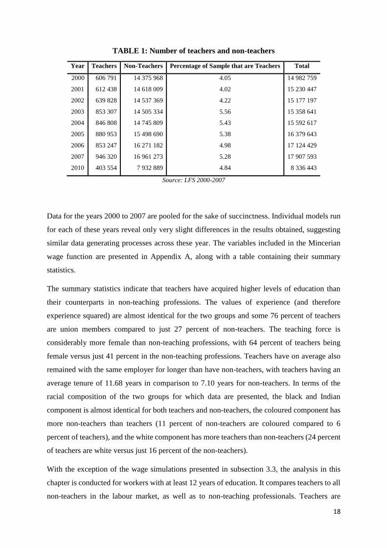
TABLE 1: Number of teachers and non-teachers

Year Teachers Non-Teachers Percentage of Sample that are Teachers Total

2000 606 791 14 375 968 4.05 14 982 759

2001 612 438 14 618 009 4.02 15 230 447

2002 639 828 14 537 369 4.22 15 177 197

2003 853 307 14 505 334 5.56 15 358 641

2004 846 808 14 745 809 5.43 15 592 617

2005 880 953 15 498 690 5.38 16 379 643

2006 853 247 16 271 182 4.98 17 124 429

2007 946 320 16 961 273 5.28 17 907 593

2010 403 554 7 932 889 4.84 8 336 443

Source: LFS 2000-2007

Data for the years 2000 to 2007 are pooled for the sake of succinctness. Individual models run

for each of these years reveal only very slight differences in the results obtained, suggesting

similar data generating processes across these year. The variables included in the Mincerian

wage function are presented in Appendix A, along with a table containing their summary

statistics.

The summary statistics indicate that teachers have acquired higher levels of education than

their counterparts in non-teaching professions. The values of experience (and therefore

experience squared) are almost identical for the two groups and some 76 percent of teachers

are union members compared to just 27 percent of non-teachers. The teaching force is

considerably more female than non-teaching professions, with 64 percent of teachers being

female versus just 41 percent in the non-teaching professions. Teachers have on average also

remained with the same employer for longer than have non-teachers, with teachers having an

average tenure of 11.68 years in comparison to 7.10 years for non-teachers. In terms of the

racial composition of the two groups for which data are presented, the black and Indian

component is almost identical for both teachers and non-teachers, the coloured component has

more non-teachers than teachers (11 percent of non-teachers are coloured compared to 6

percent of teachers), and the white component has more teachers than non-teachers (24 percent

of teachers are white versus just 16 percent of the non-teachers).

With the exception of the wage simulations presented in subsection 3.3, the analysis in this

chapter is conducted for workers with at least 12 years of education. It compares teachers to all

non-teachers in the labour market, as well as to non-teaching professionals. Teachers are

19

defined as teaching professionals and associate teaching professionals in primary and

secondary schools. Specifically, the group includes primary education teaching professionals

and associate professionals and secondary education teaching professionals and associate

professionals.

A list of non-teaching professionals, as defined in the LFS and QLFS, is presented in table A3

in Appendix A.

3.1 Wage Differentials

In order to determine whether or not teachers are well-paid, one possibility is to investigate the

wages that teachers receive relative to the wages that they might have received in non-teaching

professions. The gross (unadjusted) wage differential is a very basic measure of this

relationship and reflects differences in wages that result from differences in both the

remuneration structures for teachers and non-teachers, as well as differences in the productive

endowments of members of both groups (Hernani-Limarino, 2005:68-71). The gross wage

differential is calculated as

𝐺𝑇𝑁 = (�̅�𝑇

�̅�𝑁) − 1 (1)

where �̅�𝑇 is the mean hourly wage of teacher and �̅�𝑁 is the mean hourly wage of non-teachers.

Equation 1 is approximately equal to the mean log wage differential:

𝐺𝑇𝑁 ≈ ln(𝐺𝑇𝑁 + 1) = ln(�̅�𝑇) − ln (�̅�𝑁) (2)

In order for the gross wage differential to provide any substantial meaning, the group to whom

teachers are compared should share similar productive characteristics.

Under the assumption of competitive labour markets, wages are understood to reflect the

marginal product of labour. Wages are therefore a function of the worker’s productive

characteristics and the returns that those characteristics fetch in the labour market. If we let

�̅�𝑇𝑂 and �̅�𝑁𝑂 reflect the mean wages received by teachers and non-teachers, respectively, and

if they both face the same return structure for their productive characteristics, then the mean

productivity wage differential is given by

𝑄𝑇𝑁 = (�̅�𝑇𝑂

�̅�𝑁𝑂) − 1 (3)

Therefore, the part of the wage differential that can be attributed to differences in the structure

of returns faced by teachers and non-teachers – the conditional mean wage differential – will

20

be calculated by the difference between the gross mean wage differential and the productivity

wage differential:

𝐷𝑇𝑁 = [(�̅�𝑇

�̅�𝑁) − (

�̅�𝑇𝑂

�̅�𝑁𝑂)] / (

�̅�𝑇𝑂

�̅�𝑁𝑂) (4)

It is therefore possible to decompose the gross wage differential into

ln(𝐺𝑇𝑁 + 1) = ln(𝑄𝑇𝑁 + 1) + ln(𝐷𝑇𝑁 + 1) (5)

In other words, it is possible to decompose the gross wage differential into a part that is

explained by differences in productive characteristics and a part that is explained by differences

in the way that productive characteristics are remunerated for teachers and non-teachers.

Table 2 presents wage differentials for teachers and non-teachers and for teachers and non-

teaching professionals, respectively.

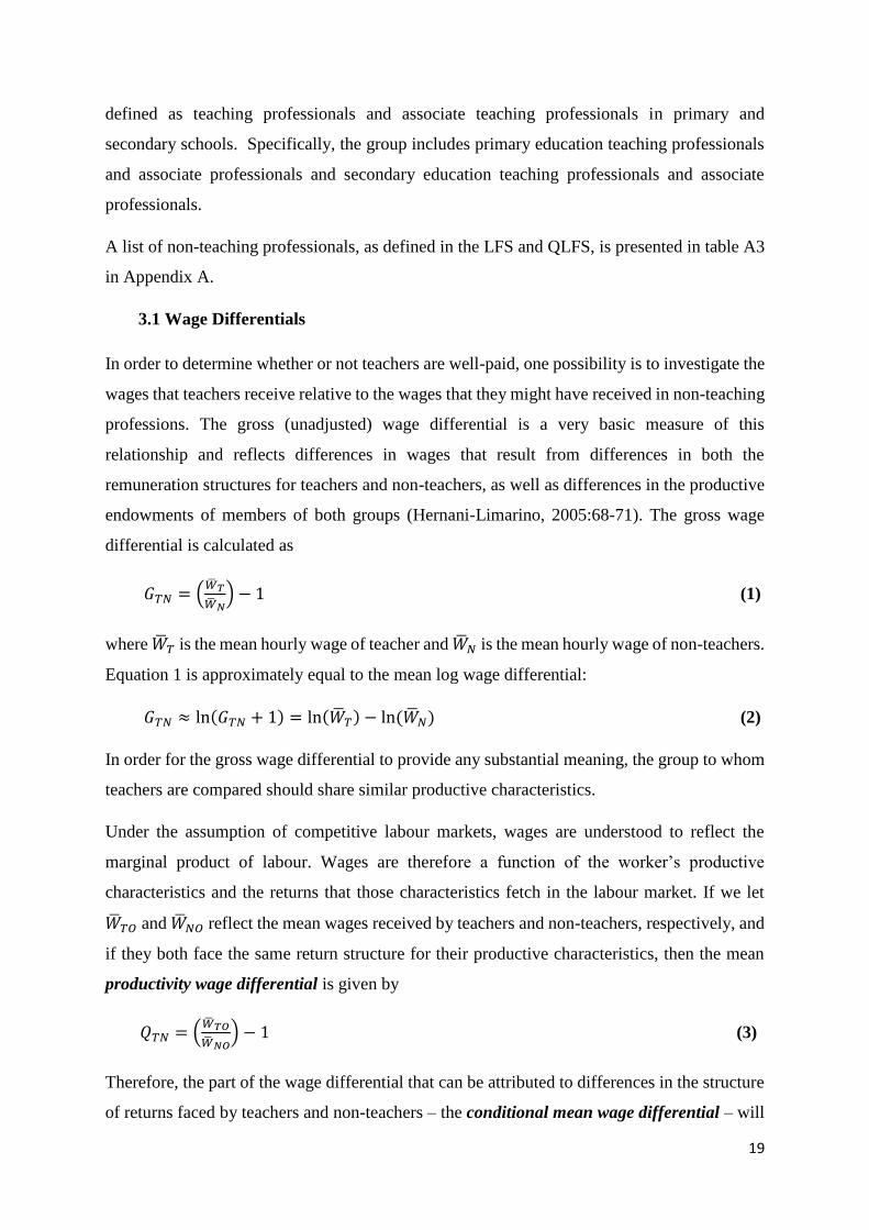
TABLE 2: Wage differentials between teachers, non-teachers and non-teaching

professionals (2000–2007 and 2010)

Gross gap

(1)

Productivity gap

(2)

Conditional gap

(3)

2000-2007 2010 2000-2007 2010 2000-2007 2010

Teachers and non-teachers 1.41 0.97 0.59 0.54 0.52 0.28

Teachers and non-teaching professionals -0.30 -0.13 -0.02 0.08 -0.28 -0.19

Source: Own calculations from LFS (March and September) 2000 –2007 and QLFS (2020), Stats SA

From table 2 we see that wage differentials favour teachers when compared to all non-teachers

in the South African labour market. However, when teachers are compared to non-teaching

professionals, teachers perform worse for most measures of wage differentials. As explained

earlier, the conditional gap represents the portion of the overall wage differential that is

attributable to differences in the remuneration structures faced by teachers and non-teachers.

The negative conditional gap in favour of non-teaching professionals suggests that these

professionals face a more attractive remuneration structure in the sense that the remuneration

they receive for their productive characteristics are higher than those received by teachers.

Comparing teachers to all other non-teachers, we observe a positive wage gap that favours

teachers, which is associated with the higher levels of human capital endowment amongst

teachers relative to this larger sample (of non-teachers, rather than non-teaching professionals).

21

The negative productivity gap relative to non-teaching professionals for the 2000 to 2007

sample is associated with the observation that non-teaching professionals are in fact better

endowed in terms of human capital than their teaching counterparts. This appears to reverse in

favour of teachers in 2010.

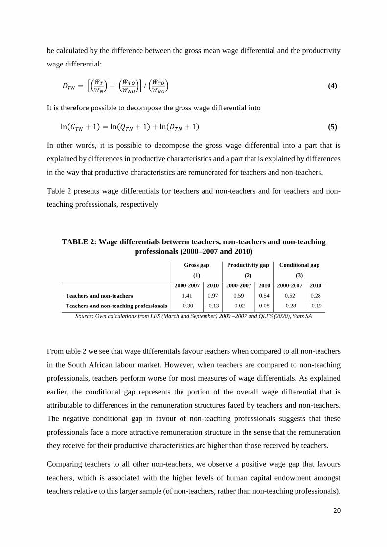
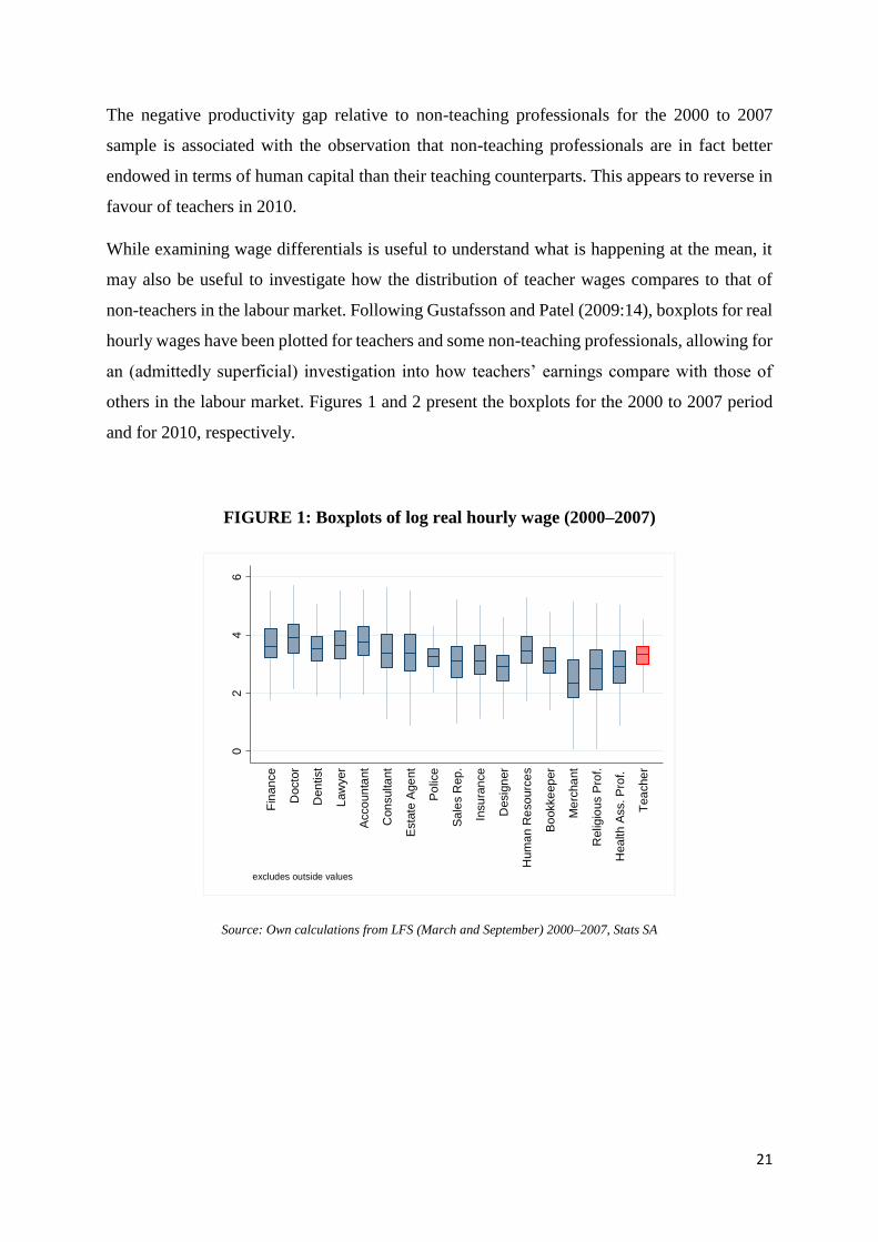
While examining wage differentials is useful to understand what is happening at the mean, it

may also be useful to investigate how the distribution of teacher wages compares to that of

non-teachers in the labour market. Following Gustafsson and Patel (2009:14), boxplots for real

hourly wages have been plotted for teachers and some non-teaching professionals, allowing for

an (admittedly superficial) investigation into how teachers’ earnings compare with those of

others in the labour market. Figures 1 and 2 present the boxplots for the 2000 to 2007 period

and for 2010, respectively.

FIGURE 1: Boxplots of log real hourly wage (2000–2007)

Source: Own calculations from LFS (March and September) 2000–2007, Stats SA

02

46

log

re

al h

ou

rly w

ag

e

Fin

an

ce

Docto

r

Den

tist

Law

yer

Acco

un

tant

Con

sulta

nt

Esta

te A

ge

nt

Po

lice

Sa

les R

ep

.

Insu

ran

ce

Desig

ner

Hum

an R

eso

urc

es

Bo

okke

ep

er

Me

rcha

nt

Relig

ious P

rof.

Hea

lth A

ss. P

rof.

Tea

che

r

excludes outside values

22

FIGURE 2: Boxplots of log real hourly wage (2010)

Source: Own calculations from QLFS 2010, Stats SA

It is interesting to observe that in the 2000 to 2007 data, the range of real hourly wages for

teachers is largely comparable to what may be thought of as “lower order” professions. In

comparison to professions that are considered “prestigious” in the South African context (and

largely internationally, too), teachers’ hourly wage rate is slightly lower. We also see that the

range of wages for teachers is narrower than it is for most other professions, highlighting the

absence of large wage returns in the teaching profession. Again with the exception of

individuals employed in the police force, merchants and potentially designers, teachers being

paid the greatest wage on an hourly basis (excluding outliers) still receive hourly wages below

that of all other professions included in the figure.

The picture is similar for 2010, the range of teacher wages appearing to be smaller than those

for most other professions included in the analysis. The position of teachers relative to non-

teaching professionals in the labour market remains more or less unchanged.

Boxplots comparing the annual earnings of teachers with those of other professionals are

presented in Appendix A. Figures A1 and A2 indicate that the annual earnings of teachers are

largely in in line with those of a lower tier of professionals, such as nurses as opposed to a

higher tier of professionals such as accountants, doctors and lawyers.

24

68

log

re

al h

ou

rly w

ag

e

Fin

an

ce

Docto

r

Den

tist

Law

yer

Acco

un

tant

Con

sulta

nt

Esta

te A

ge

nt

Po

lice

Sa

les R

ep

.

Insu

ran

ce

Nurs

e

Desig

ner

Hum

an R

eso

urc

es

Bo

okke

ep

er

Me

rcha

nt

Relig

ious P

rof.

Hea

lth A

ss. P

rof.

Tea

che

r


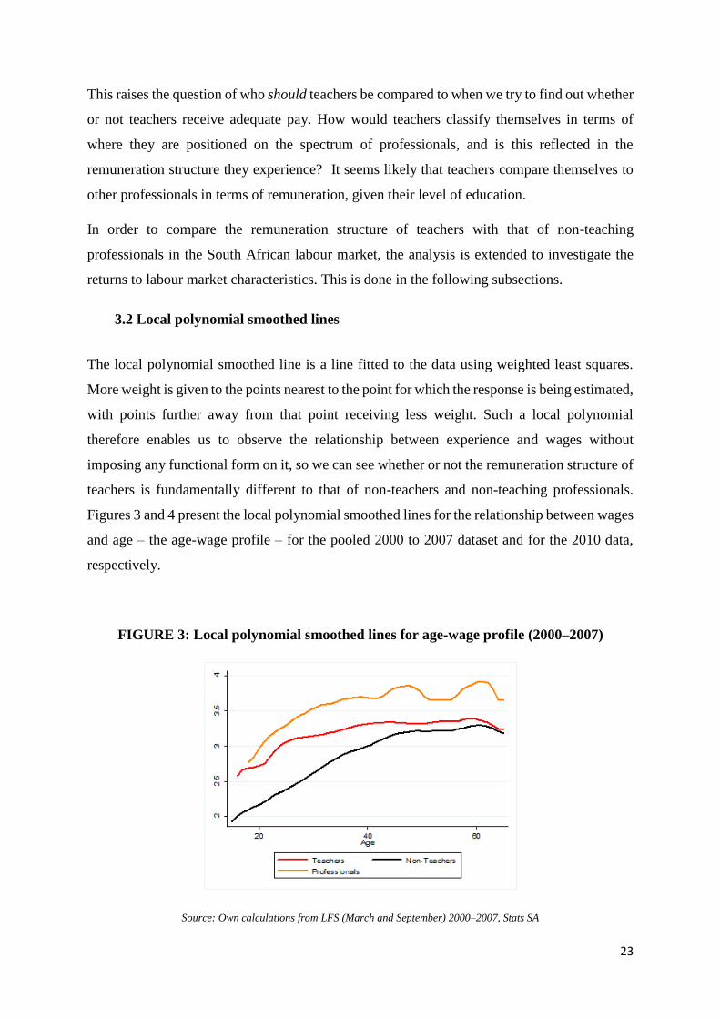
23

This raises the question of who should teachers be compared to when we try to find out whether

or not teachers receive adequate pay. How would teachers classify themselves in terms of

where they are positioned on the spectrum of professionals, and is this reflected in the

remuneration structure they experience? It seems likely that teachers compare themselves to

other professionals in terms of remuneration, given their level of education.

In order to compare the remuneration structure of teachers with that of non-teaching

professionals in the South African labour market, the analysis is extended to investigate the

returns to labour market characteristics. This is done in the following subsections.

3.2 Local polynomial smoothed lines

The local polynomial smoothed line is a line fitted to the data using weighted least squares.

More weight is given to the points nearest to the point for which the response is being estimated,

with points further away from that point receiving less weight. Such a local polynomial

therefore enables us to observe the relationship between experience and wages without

imposing any functional form on it, so we can see whether or not the remuneration structure of

teachers is fundamentally different to that of non-teachers and non-teaching professionals.

Figures 3 and 4 present the local polynomial smoothed lines for the relationship between wages

and age – the age-wage profile – for the pooled 2000 to 2007 dataset and for the 2010 data,

respectively.

FIGURE 3: Local polynomial smoothed lines for age-wage profile (2000–2007)

Source: Own calculations from LFS (March and September) 2000–2007, Stats SA

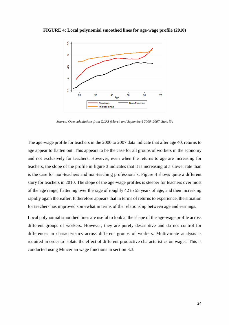
24

FIGURE 4: Local polynomial smoothed lines for age-wage profile (2010)

Source: Own calculations from QLFS (March and September) 2000–2007, Stats SA

The age-wage profile for teachers in the 2000 to 2007 data indicate that after age 40, returns to

age appear to flatten out. This appears to be the case for all groups of workers in the economy

and not exclusively for teachers. However, even when the returns to age are increasing for

teachers, the slope of the profile in figure 3 indicates that it is increasing at a slower rate than

is the case for non-teachers and non-teaching professionals. Figure 4 shows quite a different

story for teachers in 2010. The slope of the age-wage profiles is steeper for teachers over most

of the age range, flattening over the rage of roughly 42 to 55 years of age, and then increasing

rapidly again thereafter. It therefore appears that in terms of returns to experience, the situation

for teachers has improved somewhat in terms of the relationship between age and earnings.

Local polynomial smoothed lines are useful to look at the shape of the age-wage profile across

different groups of workers. However, they are purely descriptive and do not control for

differences in characteristics across different groups of workers. Multivariate analysis is

required in order to isolate the effect of different productive characteristics on wages. This is

conducted using Mincerian wage functions in section 3.3.

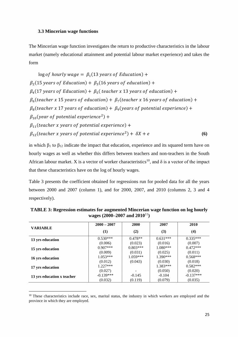
25

3.3 Mincerian wage functions

The Mincerian wage function investigates the return to productive characteristics in the labour

market (namely educational attainment and potential labour market experience) and takes the

form

log 𝑜𝑓 ℎ𝑜𝑢𝑟𝑙𝑦 𝑤𝑎𝑔𝑒 = 𝛽1(13 𝑦𝑒𝑎𝑟𝑠 𝑜𝑓 𝐸𝑑𝑢𝑐𝑎𝑡𝑖𝑜𝑛) +

𝛽2(15 𝑦𝑒𝑎𝑟𝑠 𝑜𝑓 𝐸𝑑𝑢𝑐𝑎𝑡𝑖𝑜𝑛) + 𝛽3(16 𝑦𝑒𝑎𝑟𝑠 𝑜𝑓 𝑒𝑑𝑢𝑐𝑎𝑡𝑖𝑜𝑛) +

𝛽4(17 𝑦𝑒𝑎𝑟𝑠 𝑜𝑓 𝐸𝑑𝑢𝑐𝑎𝑡𝑖𝑜𝑛) + 𝛽5( 𝑡𝑒𝑎𝑐ℎ𝑒𝑟 𝑥 13 𝑦𝑒𝑎𝑟𝑠 𝑜𝑓 𝑒𝑑𝑢𝑐𝑎𝑡𝑖𝑜𝑛) +

𝛽6(𝑡𝑒𝑎𝑐ℎ𝑒𝑟 𝑥 15 𝑦𝑒𝑎𝑟𝑠 𝑜𝑓 𝑒𝑑𝑢𝑐𝑎𝑡𝑖𝑜𝑛) + 𝛽7(𝑡𝑒𝑎𝑐ℎ𝑒𝑟 𝑥 16 𝑦𝑒𝑎𝑟𝑠 𝑜𝑓 𝑒𝑑𝑢𝑐𝑎𝑡𝑖𝑜𝑛) +

𝛽8(𝑡𝑒𝑎𝑐ℎ𝑒𝑟 𝑥 17 𝑦𝑒𝑎𝑟𝑠 𝑜𝑓 𝑒𝑑𝑢𝑐𝑎𝑡𝑖𝑜𝑛) + 𝛽9(𝑦𝑒𝑎𝑟𝑠 𝑜𝑓 𝑝𝑜𝑡𝑒𝑛𝑡𝑖𝑎𝑙 𝑒𝑥𝑝𝑒𝑟𝑖𝑒𝑛𝑐𝑒) +

𝛽10(𝑦𝑒𝑎𝑟 𝑜𝑓 𝑝𝑜𝑡𝑒𝑛𝑡𝑖𝑎𝑙 𝑒𝑥𝑝𝑒𝑟𝑖𝑒𝑛𝑐𝑒2) +

𝛽11(𝑡𝑒𝑎𝑐ℎ𝑒𝑟 𝑥 𝑦𝑒𝑎𝑟𝑠 𝑜𝑓 𝑝𝑜𝑡𝑒𝑛𝑡𝑖𝑎𝑙 𝑒𝑥𝑝𝑒𝑟𝑖𝑒𝑛𝑐𝑒) +

𝛽12(𝑡𝑒𝑎𝑐ℎ𝑒𝑟 𝑥 𝑦𝑒𝑎𝑟𝑠 𝑜𝑓 𝑝𝑜𝑡𝑒𝑛𝑡𝑖𝑎𝑙 𝑒𝑥𝑝𝑒𝑟𝑖𝑒𝑛𝑐𝑒2) + 𝛿𝑋 + 𝑒 (6)

in which β1 to β12 indicate the impact that education, experience and its squared term have on

hourly wages as well as whether this differs between teachers and non-teachers in the South

African labour market. X is a vector of worker characteristics10, and δ is a vector of the impact

that these characteristics have on the log of hourly wages.

Table 3 presents the coefficient obtained for regressions run for pooled data for all the years

between 2000 and 2007 (column 1), and for 2000, 2007, and 2010 (columns 2, 3 and 4

respectively).

TABLE 3: Regression estimates for augmented Mincerian wage function on log hourly

wages (2000–2007 and 201011)

VARIABLE 2000 – 2007

(1)

2000

(2)

2007

(3)

2010

(4)

13 yrs education 0.530***

(0.006)

0.478**

(0.023)

0.631***

(0.016)

0.335***

(0.007)


(0.009)

0.803***

(0.031)

1.080***

(0.025)

0.472***

(0.011)


(0.012)

1.059***

(0.043)

1.390***

(0.030)

0.568***

(0.018)


(0.027) -

1.383***

(0.050)

0.582***

(0.020)

13 yrs education x teacher -0.139***

(0.032)

-0.145

(0.119)

-0.104

(0.079)

-0.137***

(0.035)

10 These characteristics include race, sex, marital status, the industry in which workers are employed and the

province in which they are employed.

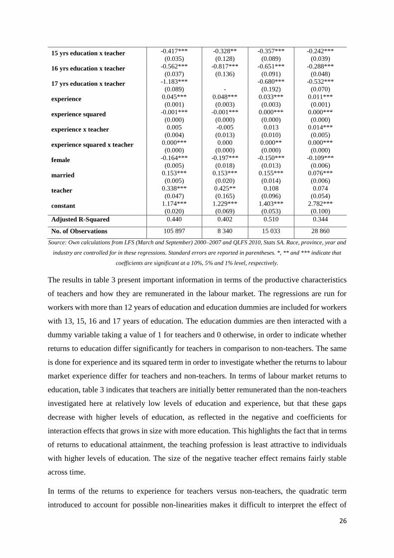
26


(0.035)

-0.328**

(0.128)

-0.357***

(0.089)

-0.242***

(0.039)


(0.037)

-0.817***

(0.136)

-0.651***

(0.091)

-0.288***

(0.048)


(0.089) -

-0.680***

(0.192)

-0.532***

(0.070)

experience 0.045***

(0.001)

0.048***

(0.003)

0.033***

(0.003)

0.011***

(0.001)

experience squared -0.001***

(0.000)

-0.001***

(0.000)

0.000***

(0.000)

0.000***

(0.000)

experience x teacher 0.005

(0.004)

-0.005

(0.013)

0.013

(0.010)

0.014***

(0.005)

experience squared x teacher 0.000***

(0.000)

0.000

(0.000)

0.000**

(0.000)

0.000***

(0.000)

female -0.164***

(0.005)

-0.197***

(0.018)

-0.150***

(0.013)

-0.109***

(0.006)

married 0.153***

(0.005)

0.153***

(0.020)

0.155***

(0.014)

0.076***

(0.006)

teacher 0.338***

(0.047)

0.425**

(0.165)

0.108

(0.096)

0.074

(0.054)

constant 1.174***

(0.020)

1.229***

(0.069)

1.403***

(0.053)

2.782***

(0.100)

Adjusted R-Squared 0.440 0.402 0.510 0.344

No. of Observations 105 897 8 340 15 033 28 860

Source: Own calculations from LFS (March and September) 2000–2007 and QLFS 2010, Stats SA. Race, province, year and

industry are controlled for in these regressions. Standard errors are reported in parentheses. *, ** and *** indicate that

coefficients are significant at a 10%, 5% and 1% level, respectively.

The results in table 3 present important information in terms of the productive characteristics

of teachers and how they are remunerated in the labour market. The regressions are run for

workers with more than 12 years of education and education dummies are included for workers

with 13, 15, 16 and 17 years of education. The education dummies are then interacted with a

dummy variable taking a value of 1 for teachers and 0 otherwise, in order to indicate whether

returns to education differ significantly for teachers in comparison to non-teachers. The same

is done for experience and its squared term in order to investigate whether the returns to labour

market experience differ for teachers and non-teachers. In terms of labour market returns to

education, table 3 indicates that teachers are initially better remunerated than the non-teachers

investigated here at relatively low levels of education and experience, but that these gaps

decrease with higher levels of education, as reflected in the negative and coefficients for

interaction effects that grows in size with more education. This highlights the fact that in terms

of returns to educational attainment, the teaching profession is least attractive to individuals

with higher levels of education. The size of the negative teacher effect remains fairly stable

across time.

In terms of the returns to experience for teachers versus non-teachers, the quadratic term

introduced to account for possible non-linearities makes it difficult to interpret the effect of

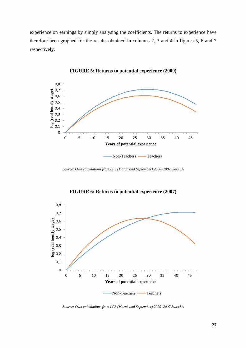
27

experience on earnings by simply analysing the coefficients. The returns to experience have

therefore been graphed for the results obtained in columns 2, 3 and 4 in figures 5, 6 and 7

respectively.

FIGURE 5: Returns to potential experience (2000)

Source: Own calculations from LFS (March and September) 2000–2007 Stats SA

FIGURE 6: Returns to potential experience (2007)


0

0,1

0,2

0,3

0,4

0,5

0,6

0,7

0,8

0 5 10 15 20 25 30 35 40 45

log

(re

al

ho

url

y w

ag

e)

Years of potential experience

Non-Teachers Teachers

0

0,1

0,2

0,3

0,4

0,5

0,6

0,7

0,8

0 5 10 15 20 25 30 35 40 45

log

(re

al

ho

url

y w

ag

e)


Non-Teachers Teachers

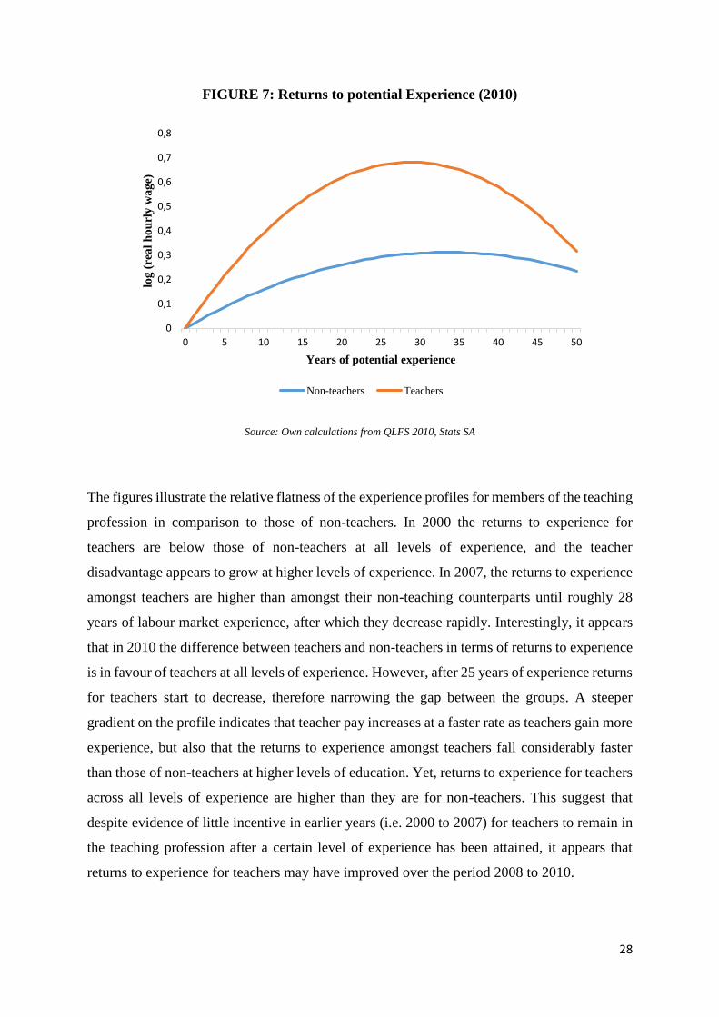
28

FIGURE 7: Returns to potential Experience (2010)

Source: Own calculations from QLFS 2010, Stats SA

The figures illustrate the relative flatness of the experience profiles for members of the teaching

profession in comparison to those of non-teachers. In 2000 the returns to experience for

teachers are below those of non-teachers at all levels of experience, and the teacher

disadvantage appears to grow at higher levels of experience. In 2007, the returns to experience

amongst teachers are higher than amongst their non-teaching counterparts until roughly 28

years of labour market experience, after which they decrease rapidly. Interestingly, it appears

that in 2010 the difference between teachers and non-teachers in terms of returns to experience

is in favour of teachers at all levels of experience. However, after 25 years of experience returns

for teachers start to decrease, therefore narrowing the gap between the groups. A steeper

gradient on the profile indicates that teacher pay increases at a faster rate as teachers gain more

experience, but also that the returns to experience amongst teachers fall considerably faster

than those of non-teachers at higher levels of education. Yet, returns to experience for teachers

across all levels of experience are higher than they are for non-teachers. This suggest that

despite evidence of little incentive in earlier years (i.e. 2000 to 2007) for teachers to remain in

the teaching profession after a certain level of experience has been attained, it appears that

returns to experience for teachers may have improved over the period 2008 to 2010.

0

0,1

0,2

0,3

0,4

0,5

0,6

0,7

0,8

0 5 10 15 20 25 30 35 40 45 50

log

(re

al

ho

url

y w

ag

e)


Non-teachers Teachers

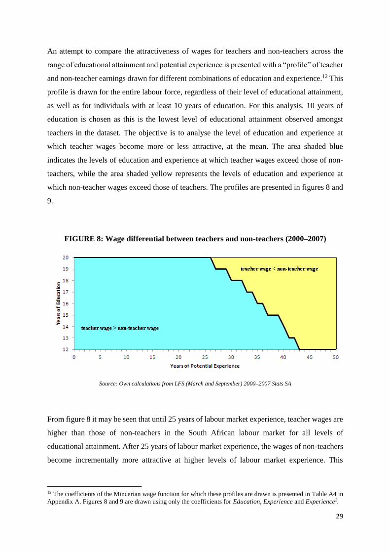
29

An attempt to compare the attractiveness of wages for teachers and non-teachers across the

range of educational attainment and potential experience is presented with a “profile” of teacher

and non-teacher earnings drawn for different combinations of education and experience.12 This

profile is drawn for the entire labour force, regardless of their level of educational attainment,

as well as for individuals with at least 10 years of education. For this analysis, 10 years of

education is chosen as this is the lowest level of educational attainment observed amongst

teachers in the dataset. The objective is to analyse the level of education and experience at

which teacher wages become more or less attractive, at the mean. The area shaded blue

indicates the levels of education and experience at which teacher wages exceed those of non-

teachers, while the area shaded yellow represents the levels of education and experience at

which non-teacher wages exceed those of teachers. The profiles are presented in figures 8 and

9.

FIGURE 8: Wage differential between teachers and non-teachers (2000–2007)


From figure 8 it may be seen that until 25 years of labour market experience, teacher wages are

higher than those of non-teachers in the South African labour market for all levels of

educational attainment. After 25 years of labour market experience, the wages of non-teachers

become incrementally more attractive at higher levels of labour market experience. This

12 The coefficients of the Mincerian wage function for which these profiles are drawn is presented in Table A4 in

Appendix A. Figures 8 and 9 are drawn using only the coefficients for Education, Experience and Experience2.

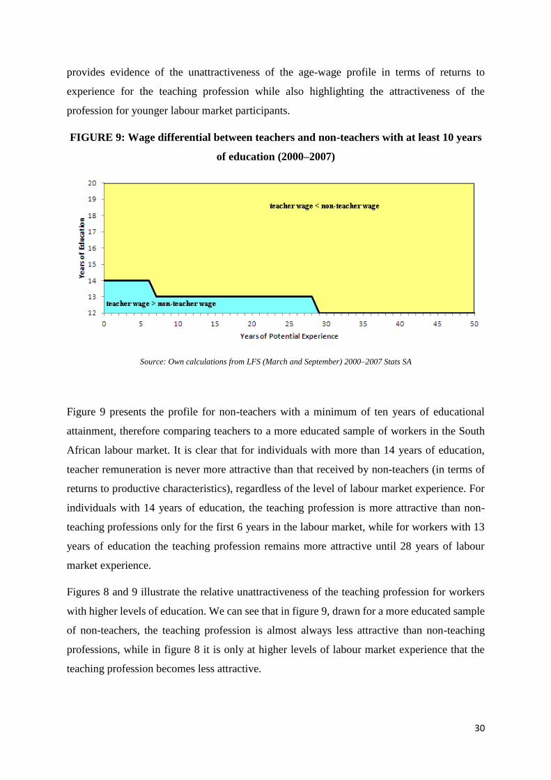
30

provides evidence of the unattractiveness of the age-wage profile in terms of returns to

experience for the teaching profession while also highlighting the attractiveness of the

profession for younger labour market participants.

FIGURE 9: Wage differential between teachers and non-teachers with at least 10 years

of education (2000–2007)


Figure 9 presents the profile for non-teachers with a minimum of ten years of educational

attainment, therefore comparing teachers to a more educated sample of workers in the South

African labour market. It is clear that for individuals with more than 14 years of education,

teacher remuneration is never more attractive than that received by non-teachers (in terms of

returns to productive characteristics), regardless of the level of labour market experience. For

individuals with 14 years of education, the teaching profession is more attractive than non-

teaching professions only for the first 6 years in the labour market, while for workers with 13

years of education the teaching profession remains more attractive until 28 years of labour

market experience.

Figures 8 and 9 illustrate the relative unattractiveness of the teaching profession for workers

with higher levels of education. We can see that in figure 9, drawn for a more educated sample

of non-teachers, the teaching profession is almost always less attractive than non-teaching

professions, while in figure 8 it is only at higher levels of labour market experience that the

teaching profession becomes less attractive.

31

The analysis so far has highlighted the fact that teachers’ productive characteristics are not

rewarded as attractively as those of non-teachers in the labour market. What if teachers’

productive characteristics were remunerated in the same way as those of non-teachers? Would

the distribution of teacher wages be higher or lower than that of their non-teaching

counterparts? This is investigated using a Lemieux decomposition.

3.4 Lemieux decomposition

This decomposition technique is used to create a counterfactual wage distribution for teachers

and non-teachers in the South African labour force. The Lemieux decomposition used in this

paper may be understood to be a generalization of the decomposition technique first introduced

by Oaxaca and Blinder in 1973 (Lemieux, 2002). The Oaxaca-Blinder decomposition

decomposes the difference in the mean wage between two groups into the component explained

by differences in productive characteristics and into an “unexplained” component (i.e. a

component resulting from differences in how productive characteristics are remunerated

between the two groups in question, or “discrimination”).

Decomposing the wage gap at the mean involves estimating the Ordinary Least Squares (OLS)

wage regression

yit = btxit + uit (7)

where yit is the log hourly wage of individual i belonging to group t (in this case to the group

teachers), xit is a vector of covariates, bt is a vector of parameters and uit is an error term

constructed to have a mean of 0 and to be uncorrelated with the covariates in the vector xit

(Lemieux, 2002). The sample average outcome y for teachers is therefore

�̅�𝑡 = 𝑥�̅�𝑏𝑡 (8)

where �̅�𝑡 = ∑ 𝜔𝑖𝑡 𝑦𝑖𝑡 1

and 𝑥�̅� = ∑ 𝜔𝑖𝑡1 𝑥𝑖𝑡 .

The outcome for individuals belonging to the second group in the sample (in this case non-

teachers) is estimated by

yin = btxin + uin (9)

32

where yin is the log hourly wage of individual i belonging to group n (i.e. non-teachers), xis is a

vector of covariates, bs is vector of parameters and uis is an error term constructed to have a

mean of 0 and to be uncorrelated with the covariates in the vector xis. The sample average

outcome y for teachers is therefore

�̅�𝑛 = �̅�𝑛𝑏𝑛 (10)

where �̅�𝑛 = ∑ 𝜔𝑖𝑛 𝑦𝑖𝑛 1

and 𝑥�̅� = ∑ 𝜔𝑖𝑛1 𝑥𝑖𝑛 .

Calculating the difference between the mean outcomes of teachers and non-teachers therefore

yields

�̅�𝑡 − �̅�𝑛 = �̅�𝑡 (𝑏𝑡 − 𝑏𝑛) + 𝑏𝑛(�̅�𝑡 − �̅�𝑛) (11)

where �̅�𝑡 (𝑏𝑡 − 𝑏𝑛) is the difference in wages arising from differences in the remuneration

structures faced by teachers and non-teachers (i.e. the “unexplained” component) and

𝑏𝑛(�̅�𝑡 − �̅�𝑛) is the difference in wages arising from differences in productive characteristics

between teachers and non-teachers (Lemieux, 2002). 𝑏𝑛�̅�𝑡 may therefore be seen as the

counterfactual mean value of y that would result if the remuneration structure of teachers was

replaced with that of non-teachers. In other words, 𝑏𝑛�̅�𝑡 would be the wage prevalent for

teachers if the “price” of human capital amongst teachers was equal to that experienced by non-

teachers in the labour market.

The counterfactual wage for teachers is therefore

�̅�𝑡𝑎 = �̅�𝑡𝑏𝑛 (12)

which may be used to rewrite equation 12 as

�̅�𝑡 – �̅�𝑛 = (�̅�𝑡𝑏𝑡 − �̅�𝑡𝑎) + (�̅�𝑡

𝑎 − �̅�𝑛𝑏𝑛 ) = (�̅�𝑡 − �̅�𝑡𝑎) + (�̅�𝑡

𝑎 + �̅�𝑡).

Individual counterfactual wages are therefore denoted 𝑦𝑖𝑡 𝑎 and are calculated as

𝑦𝑖𝑡𝑎 = 𝑥𝑖𝑡 𝑏𝑛 + 𝑢𝑖𝑡 = 𝑦𝑖𝑡 + 𝑥𝑖𝑡(𝑏𝑠 − 𝑏𝑡).

�̅�𝑡𝑎 may also be calculated by computing a sample mean of 𝑦𝑖𝑡

𝑎 :

�̅�𝑡𝑎 = ∑ 𝜔𝑖𝑡 𝑦𝑖𝑡.

𝑎1 (13)

33

In order to estimate what the entire distribution of teacher wages would look like (as opposed

to just the mean wage), the probit for the probability of being a teacher is estimated on the

pooled sample of teachers and non-teachers. The probit model produces the probability of

being a member of the teaching force conditional on individual worker characteristics, or

individual xs.

𝑃𝑖𝑡 = 𝑃𝑟𝑜𝑏(𝑡𝑒𝑎𝑐ℎ𝑒𝑟 = 1 | 𝑥𝑖𝑡).

The reweighting function is then calculated using the estimated probability of being a teacher

as

𝛹𝑖 = [1−𝑃𝑖𝑡

𝑃𝑖𝑡]

[𝑃𝑡

(1−𝑃𝑡)]

where Pt is the unconditional probability of an observed worker being a member of the teaching

force, or the weighted share of the pooled sample who are teachers (Lemieux, 2002). The

reweighted distribution or the counterfactual distribution is therefore

𝑦𝑡𝑎 = 𝛹(𝑥𝑡𝑏𝑛) = 𝛹′𝑦𝑛 (14)

where 𝛹′ = 1

𝛹 (Lemieux, 2002).

The decomposition has been used by various authors to investigate wage distributions across a

number of countries. DiNardo, Fortin & Lemieux (1996) used a precursor to the method to

investigate the impact of labour market and institutional factors on the distribution of wages in

the US. These authors explain that the technique provides a “visually clear representation of

where in the density of wages these various factors exert the greatest impact” (DiNardo et al,

1996: 1001). Using the technique, DiNardo et al (1996: 1009) are able to assess what wages

would have looked like had particular factors taken on different values. “What would the

density of wages have been in 1988 if workers’ attributes . . . remained at their 1979 level”

(DiNardo et al, 1996: 1009). Shimizutani & Yokoyama (2009) analyse changes in the

distribution of years of tenure in Japan’s long-term employment since the 1990s following a

decade-long recession. The method is used because it allows for the decomposition of the

changes into the part explained by changes in distribution of worker and firm attributes and the

part explained by the effect of these attributes on workers’ tenure (Shimizutani & Yokoyama,

2009: 318). Shimizutani & Yokoyama (2009: 318) examine what the distribution of worker

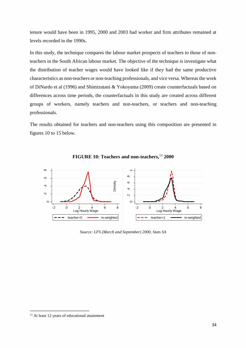
34

tenure would have been in 1995, 2000 and 2003 had worker and firm attributes remained at

levels recorded in the 1990s.

In this study, the technique compares the labour market prospects of teachers to those of non-

teachers in the South African labour market. The objective of the technique is investigate what

the distribution of teacher wages would have looked like if they had the same productive

characteristics as non-teachers or non-teaching professionals, and vice versa. Whereas the work

of DiNardo et al (1996) and Shimizutani & Yokoyama (2009) create counterfactuals based on

differences across time periods, the counterfactuals in this study are created across different

groups of workers, namely teachers and non-teachers, or teachers and non-teaching

professionals.

The results obtained for teachers and non-teachers using this composition are presented in

figures 10 to 15 below.

FIGURE 10: Teachers and non-teachers,13 2000

Source: LFS (March and September) 2000, Stats SA

13 At least 12 years of educational attainment

0.2

.4.6

.8

Density

-2 0 2 4 6 8Log Hourly Wage

teacher=0 re-weighted

0.2

.4.6

.81

Density



-.2

-.1

0.1

.2.3

Diffe

rence in D

ensitie

s


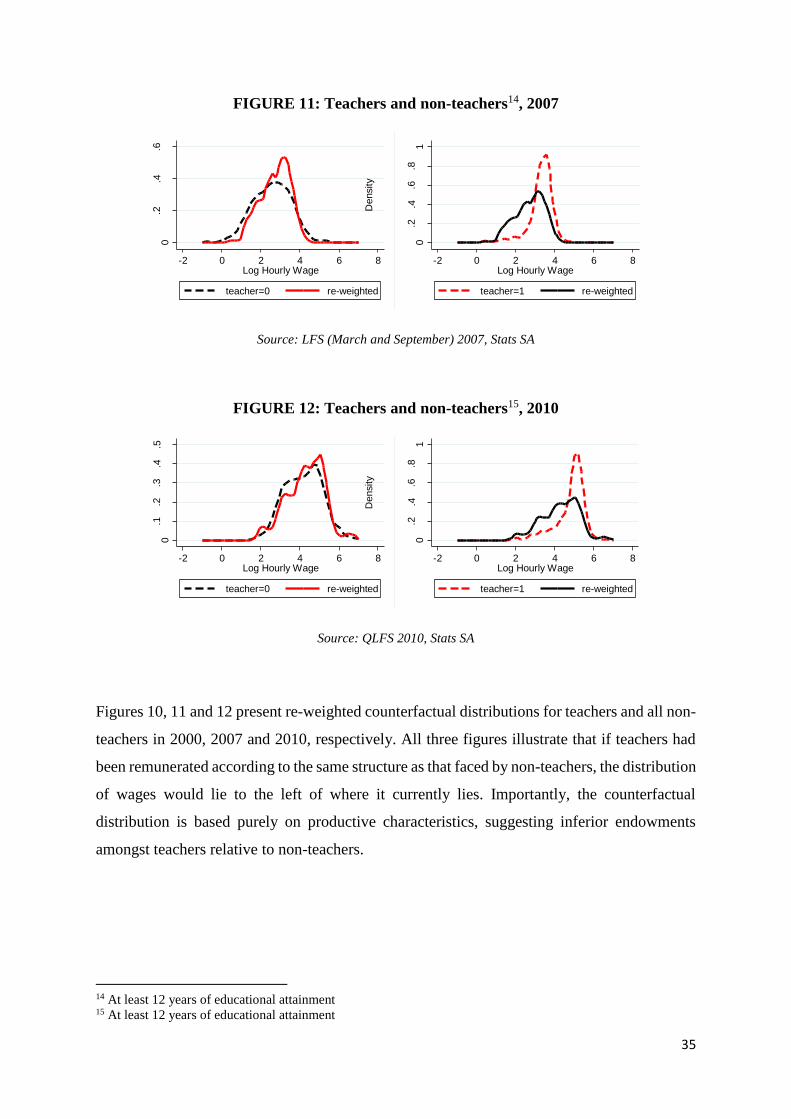
35

FIGURE 11: Teachers and non-teachers14, 2007


FIGURE 12: Teachers and non-teachers15, 2010

Source: QLFS 2010, Stats SA

Figures 10, 11 and 12 present re-weighted counterfactual distributions for teachers and all non-

teachers in 2000, 2007 and 2010, respectively. All three figures illustrate that if teachers had

been remunerated according to the same structure as that faced by non-teachers, the distribution

of wages would lie to the left of where it currently lies. Importantly, the counterfactual

distribution is based purely on productive characteristics, suggesting inferior endowments

amongst teachers relative to non-teachers.

14 At least 12 years of educational attainment 15 At least 12 years of educational attainment

0.2

.4.6

Density



0.2

.4.6

.81

Density



-.4

-.2

0.2

.4.6

Diffe

rence in D

ensitie

s


0.1

.2.3

.4.5

Density



0.2

.4.6

.81

Density



-.2

0.2

.4.6

Diffe

rence in D

ensitie

s


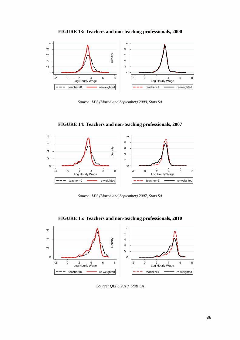
36

FIGURE 13: Teachers and non-teaching professionals, 2000





Source: QLFS 2010, Stats SA

0.2

.4.6

.81

Density



0.2

.4.6

.81

Density



-.02

0

.02

.04

.06

.08

Diffe

rence in D

ensitie

s


0.2

.4.6

.8

Density



0.2

.4.6

.81

Density



-.1

-.05

0

.05

.1.1

5

Diffe

rence in D

ensitie

s


0.2

.4.6

Density



0.2

.4.6

.81

Density



-.2

-.1

0.1

.2.3

Diffe

rence in D

ensitie

s


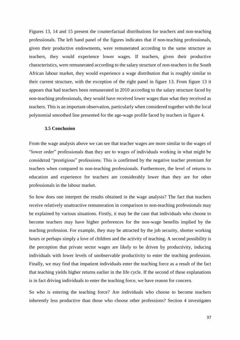
37

Figures 13, 14 and 15 present the counterfactual distributions for teachers and non-teaching

professionals. The left hand panel of the figures indicates that if non-teaching professionals,

given their productive endowments, were remunerated according to the same structure as

teachers, they would experience lower wages. If teachers, given their productive

characteristics, were remunerated according to the salary structure of non-teachers in the South

African labour market, they would experience a wage distribution that is roughly similar to

their current structure, with the exception of the right panel in figure 13. From figure 13 it

appears that had teachers been remunerated in 2010 according to the salary structure faced by

non-teaching professionals, they would have received lower wages than what they received as

teachers. This is an important observation, particularly when considered together with the local

polynomial smoothed line presented for the age-wage profile faced by teachers in figure 4.

3.5 Conclusion

From the wage analysis above we can see that teacher wages are more similar to the wages of

“lower order” professionals than they are to wages of individuals working in what might be

considered “prestigious” professions. This is confirmed by the negative teacher premium for

teachers when compared to non-teaching professionals. Furthermore, the level of returns to

education and experience for teachers are considerably lower than they are for other

professionals in the labour market.

So how does one interpret the results obtained in the wage analysis? The fact that teachers

receive relatively unattractive remuneration in comparison to non-teaching professionals may

be explained by various situations. Firstly, it may be the case that individuals who choose to

become teachers may have higher preferences for the non-wage benefits implied by the

teaching profession. For example, they may be attracted by the job security, shorter working

hours or perhaps simply a love of children and the activity of teaching. A second possibility is

the perception that private sector wages are likely to be driven by productivity, inducing

individuals with lower levels of unobservable productivity to enter the teaching profession.

Finally, we may find that impatient individuals enter the teaching force as a result of the fact

that teaching yields higher returns earlier in the life cycle. If the second of these explanations

is in fact driving individuals to enter the teaching force, we have reason for concern.

So who is entering the teaching force? Are individuals who choose to become teachers

inherently less productive than those who choose other professions? Section 4 investigates

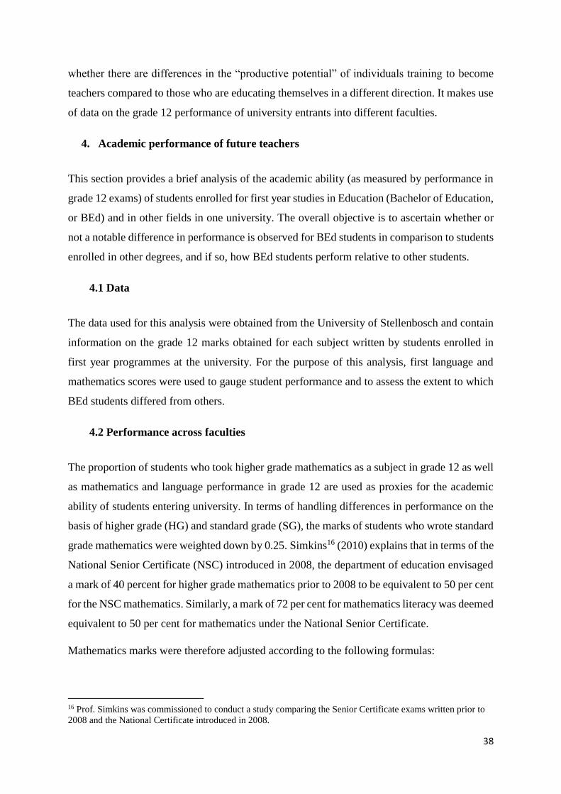
38

whether there are differences in the “productive potential” of individuals training to become

teachers compared to those who are educating themselves in a different direction. It makes use

of data on the grade 12 performance of university entrants into different faculties.

4. Academic performance of future teachers

This section provides a brief analysis of the academic ability (as measured by performance in

grade 12 exams) of students enrolled for first year studies in Education (Bachelor of Education,

or BEd) and in other fields in one university. The overall objective is to ascertain whether or

not a notable difference in performance is observed for BEd students in comparison to students

enrolled in other degrees, and if so, how BEd students perform relative to other students.

4.1 Data

The data used for this analysis were obtained from the University of Stellenbosch and contain

information on the grade 12 marks obtained for each subject written by students enrolled in

first year programmes at the university. For the purpose of this analysis, first language and

mathematics scores were used to gauge student performance and to assess the extent to which

BEd students differed from others.

4.2 Performance across faculties

The proportion of students who took higher grade mathematics as a subject in grade 12 as well

as mathematics and language performance in grade 12 are used as proxies for the academic

ability of students entering university. In terms of handling differences in performance on the

basis of higher grade (HG) and standard grade (SG), the marks of students who wrote standard

grade mathematics were weighted down by 0.25. Simkins16 (2010) explains that in terms of the

National Senior Certificate (NSC) introduced in 2008, the department of education envisaged

a mark of 40 percent for higher grade mathematics prior to 2008 to be equivalent to 50 per cent

for the NSC mathematics. Similarly, a mark of 72 per cent for mathematics literacy was deemed

equivalent to 50 per cent for mathematics under the National Senior Certificate.

Mathematics marks were therefore adjusted according to the following formulas:

16 Prof. Simkins was commissioned to conduct a study comparing the Senior Certificate exams written prior to

2008 and the National Certificate introduced in 2008.

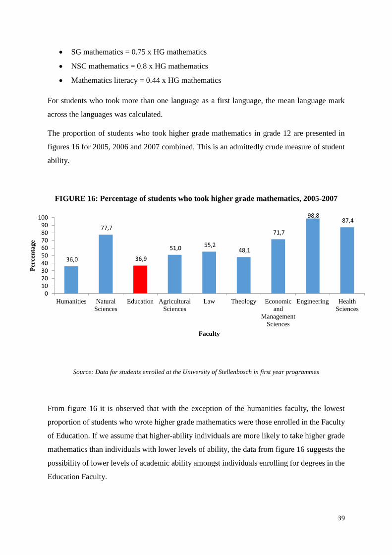
39

SG mathematics = 0.75 x HG mathematics

NSC mathematics = 0.8 x HG mathematics

Mathematics literacy = 0.44 x HG mathematics

For students who took more than one language as a first language, the mean language mark

across the languages was calculated.

The proportion of students who took higher grade mathematics in grade 12 are presented in

figures 16 for 2005, 2006 and 2007 combined. This is an admittedly crude measure of student

ability.

FIGURE 16: Percentage of students who took higher grade mathematics, 2005-2007

Source: Data for students enrolled at the University of Stellenbosch in first year programmes

From figure 16 it is observed that with the exception of the humanities faculty, the lowest

proportion of students who wrote higher grade mathematics were those enrolled in the Faculty

of Education. If we assume that higher-ability individuals are more likely to take higher grade

mathematics than individuals with lower levels of ability, the data from figure 16 suggests the

possibility of lower levels of academic ability amongst individuals enrolling for degrees in the

Education Faculty.

36,0

77,7

36,9

51,0 55,2 48,1

71,7

98,8 87,4

0102030405060708090

100

Humanities Natural

Sciences

Education Agricultural

Sciences

Law Theology Economic

and

Management

Sciences

Engineering Health

Sciences

Per

cen

tag

e

Faculty

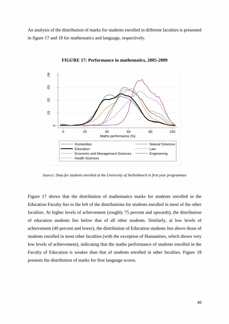
40

An analysis of the distribution of marks for students enrolled in different faculties is presented

in figure 17 and 18 for mathematics and language, respectively.

FIGURE 17: Performance in mathematics, 2005-2009


Figure 17 shows that the distribution of mathematics marks for students enrolled in the

Education Faculty lies to the left of the distributions for students enrolled in most of the other

faculties. At higher levels of achievement (roughly 75 percent and upwards), the distribution

of education students lies below that of all other students. Similarly, at low levels of

achievement (40 percent and lower), the distribution of Education students lies above those of

students enrolled in most other faculties (with the exception of Humanities, which shows very

low levels of achievement), indicating that the maths performance of students enrolled in the

Faculty of Education is weaker than that of students enrolled in other faculties. Figure 18

presents the distribution of marks for first language scores.

0

.01

.02

.03

.04

0 20 40 60 80 100

Maths performance (%)

Humanities Natural Sciences

Education Law

Economic and Management Sciences Engineering

Health Sciences

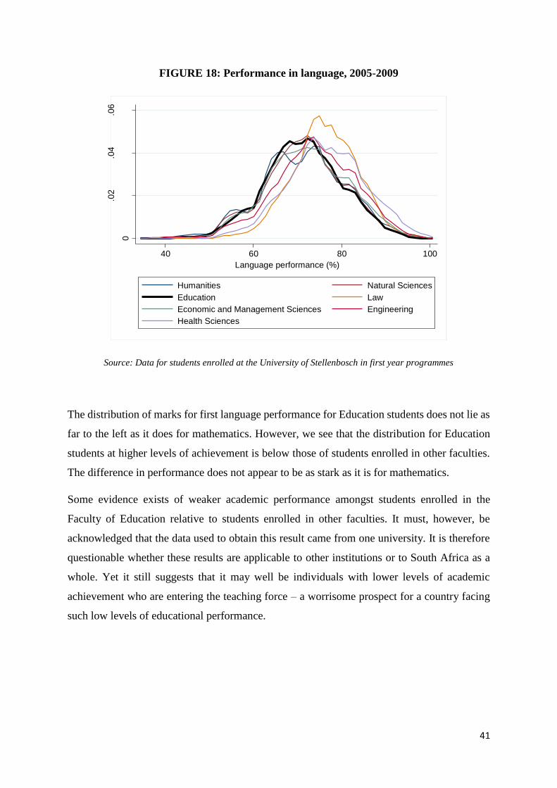
41

FIGURE 18: Performance in language, 2005-2009


The distribution of marks for first language performance for Education students does not lie as

far to the left as it does for mathematics. However, we see that the distribution for Education

students at higher levels of achievement is below those of students enrolled in other faculties.

The difference in performance does not appear to be as stark as it is for mathematics.

Some evidence exists of weaker academic performance amongst students enrolled in the

Faculty of Education relative to students enrolled in other faculties. It must, however, be

acknowledged that the data used to obtain this result came from one university. It is therefore

questionable whether these results are applicable to other institutions or to South Africa as a

whole. Yet it still suggests that it may well be individuals with lower levels of academic

achievement who are entering the teaching force – a worrisome prospect for a country facing

such low levels of educational performance.

0

.02

.04

.06

40 60 80 100

Language performance (%)

Humanities Natural Sciences

Education Law

Economic and Management Sciences Engineering

Health Sciences

42

5. Conclusion

This paper investigated the remuneration structure for teachers in the South African labour

force and how this compares to that of non-teachers. In comparison to non-teaching

professionals with higher levels of educational attainment, the remuneration structure of

teachers is unattractive, but relative to all non-teachers in the South African labour market, the

remuneration structure for teachers is more appealing. The wage profiles drawn in section 3

revealed that teacher wages are attractive to individuals with lower levels of educational

attainment, with the profession becoming less attractive as individuals enhance their level of

educational attainment and as labour market experience increases. A worrying aspect of teacher

remuneration in South Africa is the flatness of the age-wage profiles faced by teachers.

However, it appears as if this may be changing slowly, becoming comparable to what is

observed for individuals employed in other professions, therefore potentially eroding some of

the relative unattractiveness of the wage structure faced by teachers. In addition, Irving (2012:

394) explains that in South Africa’s apartheid era, teaching was considered an opportunity for

upward social mobility in a labour market context in which certain race groups were not

allowed to enter other professions. In 1986, teacher salaries were equalized along racial and

gender lines and teaching therefore became a very attractive choice of profession for black

South Africans, particularly for black women, given the rapid rise in salaries (Irving, 2012:

394). However, since 1994 professional opportunities for black South Africans have expanded

dramatically and skilled black South Africans qualified for positions from which they had been

previously excluded. This is likely to have dramatically increased the opportunity cost of

teaching relative to other professions (Irving, 2012: 394).

The brief analysis of the academic quality of students enrolled for first year studies at the

University of Stellenbosch revealed that students enrolled in the Faculty of Education perform

somewhat worse than their counterparts in other faculties in mathematics, and to a lesser degree

in language, too. If we assume that wages are driven by productivity, then this may explain the

relative unattractiveness of teachers’ wage structure in comparison to that received by non-

teaching professionals. Either way, the prospect is worrisome for the South African education

system. Further research to ascertain what motivates individuals to become teachers would

prove extremely useful in understanding who is drawn to the teaching profession, and

potentially also how high-ability individuals can be attracted to the profession. The current

43

remuneration structure relative to that of non-teaching professions seems unlikely on its own

to ensure that top-ability individuals would follow a career in teaching.

44

Chapter 2 Teacher incentives in South Africa: A theoretical

investigation of the possibilities

1. Introduction: Teacher quality in South Africa and the possibility of incentives

For the country’s level of development and the proportion of the budget that is spent on

education, South Africa performs substantially below what is expected of it in terms of

educational performance (National Education Evaluation and Development Unit, 2012: 13).

Performance amongst learners in this country is markedly worse that amongst learners in

countries which are poorer than South Africa. In the third round of international tests conducted

by the Southern African Consortium for the Measurement of Educational Quality (SACMEQ)

in 2007, South Africa performed worse than most of the participating countries in both

mathematics and language (Spaull, 2011a: 43), managing only to outperform Lesotho,

Mozambique, Uganda, Malawi and Zambia. In reading, South Africa was tenth of the fifteen

countries measured. In mathematics, South Africa ranked eighth out of the fifteen countries

(Spaull, 2011a: 24). Educational quality in South Africa therefore leaves much to be desired.

Poor teacher quality and low levels of teacher effort are often cited as major drivers of South

Africa’s education crisis. The question then is why South African teachers are performing as

poorly as they do. NEEDU’s National Report of 2012 suggests that teachers are unable to

ensure high quality education for students either because they won’t or because they can’t

(NEEDU, 2013: 20). Where teachers and schools won’t provide quality education, poor

performance is the result of a lack of discipline amongst staff member and any remedial action

should focus on changing behaviour. Where teachers can’t provide quality education

intervention should focus on improving and enhancing the knowledge base of teachers to equip

them with the skills necessary for quality teaching and learning to take place in classrooms

(NEEDU, 2013: 20).

45

This chapter focuses on the potential to change teacher behaviour in a way that enhances


Many argue that the lack of effort amongst teachers is the greatest hindrance to the development

of student skills in South Africa, suggesting that the appropriate policy response should be

directed towards designing attractive incentives for teachers. High levels of absenteeism from

school and from classrooms, poor lesson preparation and lack of interest in the progress of

learners are key signs that teacher effort is critically low in South Africa, and it is often reported

that such low levels of effort result from weak incentive systems.

This problem is not particular to South Africa. Low levels of teacher effort are observed

internationally. Teacher motivation is often explained as being driven by factors other than

financial incentives, for example a love of children, passion for their subject or a drive to

interact with students. However, Bennell (2004: 16) points out that in economic conditions in

which teachers and their families struggle to make ends meet, remuneration is likely to be a

significant factor in motivating teachers and indeed in attracting individuals to the profession.

Research in low income countries in Sub-Saharan Africa and South Asia indicate low levels of

teacher motivation. The cause of low levels of motivation vary by country, but factors such as

low morale, lack of job satisfaction, low levels of incentives, and inadequate behavioural

sanctions feature across education systems (Bennell, 2004: 22). Furthermore, the expectations

associated with teachers’ work are unrealistic given the environment in which teachers are

expected to teach and live, the monetary rewards associated with teaching and the workloads

with which they contend (Bennell, 2004: 20). Importantly, the conditions in which teachers in

low income countries are expected to teach have special demands for which teachers may not

be sufficiently trained. A prominent example is widespread multi-grade teaching in Sub-

Saharan countries – an exceptionally demanding skill. Most teachers are simply not prepared

for the demands associated with such practices (Bennell, 2004: 21).

International research findings indicate that an important source of service delivery failure in

education is the teacher. The principal-agent problem in education is complicated because of

the nature of service provision in education (Bruns, Filmer & Patrinos, 2010: 10-11). The

interaction between teachers and learners is discretionary (in that it is the teacher’s own

judgement that will determine what is taught and how it is taught), variable (in that teachers

are required to tailor their teaching style to a diverse group of students) and requires repetition.

It is exceptionally difficult to define beforehand what type of behaviour and actions teachers

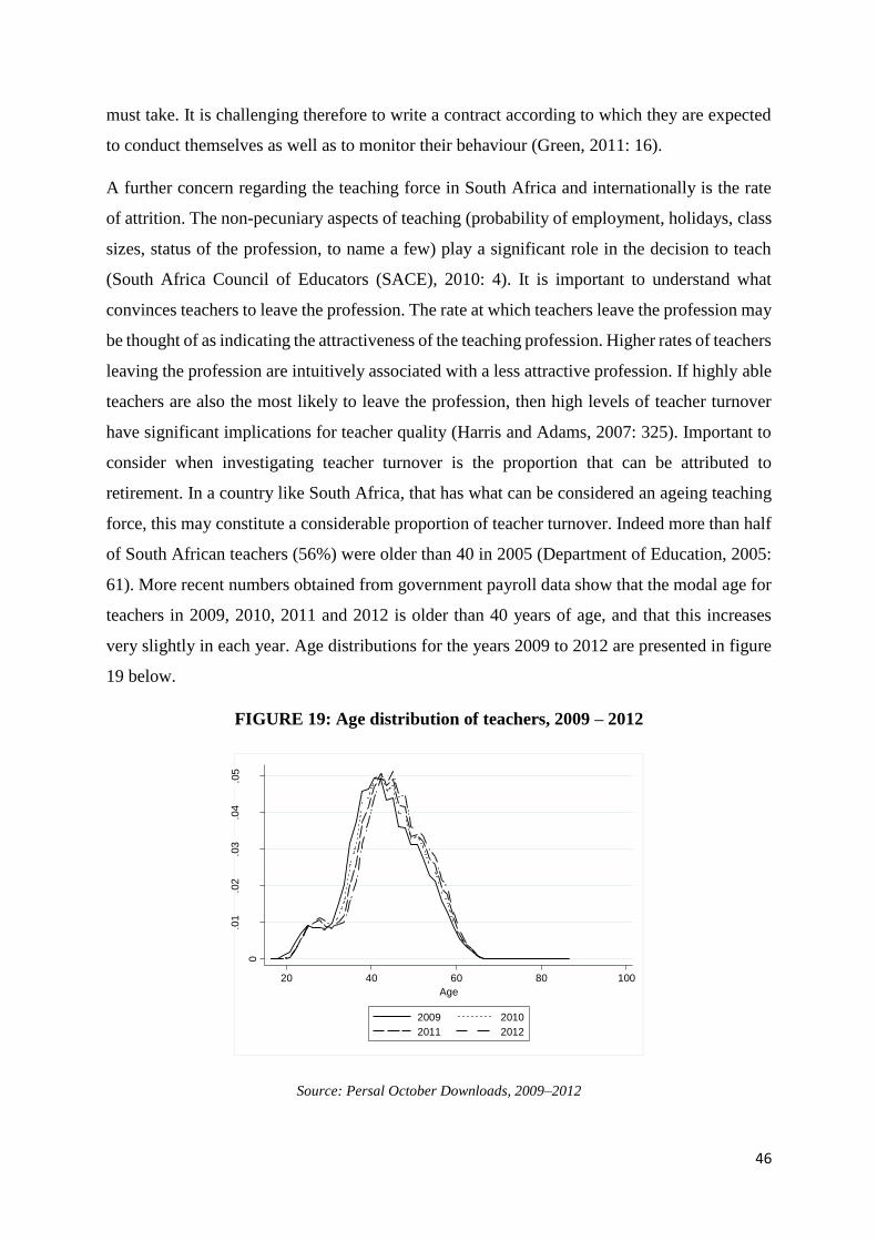
46

must take. It is challenging therefore to write a contract according to which they are expected

to conduct themselves as well as to monitor their behaviour (Green, 2011: 16).

A further concern regarding the teaching force in South Africa and internationally is the rate

of attrition. The non-pecuniary aspects of teaching (probability of employment, holidays, class

sizes, status of the profession, to name a few) play a significant role in the decision to teach

(South Africa Council of Educators (SACE), 2010: 4). It is important to understand what

convinces teachers to leave the profession. The rate at which teachers leave the profession may

be thought of as indicating the attractiveness of the teaching profession. Higher rates of teachers

leaving the profession are intuitively associated with a less attractive profession. If highly able

teachers are also the most likely to leave the profession, then high levels of teacher turnover

have significant implications for teacher quality (Harris and Adams, 2007: 325). Important to

consider when investigating teacher turnover is the proportion that can be attributed to

retirement. In a country like South Africa, that has what can be considered an ageing teaching

force, this may constitute a considerable proportion of teacher turnover. Indeed more than half

of South African teachers (56%) were older than 40 in 2005 (Department of Education, 2005:

61). More recent numbers obtained from government payroll data show that the modal age for

teachers in 2009, 2010, 2011 and 2012 is older than 40 years of age, and that this increases

very slightly in each year. Age distributions for the years 2009 to 2012 are presented in figure

19 below.

FIGURE 19: Age distribution of teachers, 2009 – 2012

Source: Persal October Downloads, 2009–2012

0

.01

.02

.03

.04

.05

20 40 60 80 100

Age

2009 2010

2011 2012

47

Harris and Adams (2007: 336) point out the importance of understanding the role of retirement

in teacher turnover. In the USA teachers tend to retire earlier than workers in non-teaching

professions, so if teacher turnover is to be used as a measure of the appeal and “health” of the

teaching profession, caution must be exercised.

Teacher turnover may also differ according to teacher specialisation. Murnane, Singer and

Willet (1989: 32-33) find evidence in North Carolina that the median “lifetime” of secondary

school teachers differs according to subject speciality, with chemistry and physics teachers as

well as biology teachers having significantly shorter lifetimes within the schooling system than

do their colleagues in English, social science and mathematics17. The authors explain that a

possible explanation for this is the higher mean starting salaries for occupations in the field of

physics, chemistry and biology (Murnane et al., 1989: 333). The authors have no persuasive

explanation for the peculiar result that mathematics teachers have the longest median lifetime

but suggest that this may be due a “mismatch” between the skills required amongst

mathematics professionals in the business and industry and the skills acquired by mathematics

teachers (Murnane et al., 1989: 334). They refer to computer skills as an example. Despite the

fact that the results obtained are from a US context, there does appear to be evidence that the

opportunity cost of teaching is higher for teachers of subjects that may be considered “scarce

skills” in the sense that they are likely able to command higher remuneration in non-teaching

professions.

Falch and Strøm (2005) attempt to quantify the impact of non-pecuniary factors on teacher

attrition in Norway18. This study is possible in the Norwegian context given the fact that teacher

wage setting is completely centralized and schools may not offer wages different to what has

been stipulated by teacher unions (Falch & Strøm, 2005: 612). This eliminates identification

problems that may arise as a result of compensating wage differentials which means it is

possible to interpret teacher behaviour as a response to non-pecuniary factors. They find that

high proportions of minority students (i.e. non-Norwegian students) and special needs students

are associated with a higher quit rate amongst teachers (Falch & Strøm, 2005: 628) and school

17 The observed lifetimes for chemistry and physics, biology, English, social studies and mathematics teachers

are 5.9, 6.3, 6.5, 7.6 and 10.1 years respectively (Murnane et al., 1989: 333). 18 Norway is admittedly a weak compactor country for South Africa. However, very few studies attempt to

quantify the impact of non-pecuniary aspects in the form of school characteristics (i.e. student composition,

school size) of teaching.

48

size is also positively and significantly associated with teachers quitting (Falch & Strøm, 2005:

627). These results pertain to movements between schools within the same district, movements

between districts as well as departures from the education sector.

From an economic perspective, it may be difficult to measure the effect of non-pecuniary

characteristics of teaching on teacher turnover in South Africa, as economics assumes that

wages will adjust to reflect the non-pecuniary aspects of teaching. The Norwegian example is

useful (and possible to measure) due to the fact that deviations from the national salary structure

do not occur. This is not the case in the South African context. In South Africa, schools may

offer teachers wages that differ from what has been stipulated centrally. Many schools employ

and remunerate additional teachers or supplement the wages of teachers with privately raised

funds. This differs somewhat from the Norwegian case.

Hall, Altman, Nkomo, Peltzer and Zuma (2005) conducted a study into the reasons for teacher

attrition in South Africa. The study was conducted in order to “determine the impact of job

satisfaction, morale, workload and HIV/AIDS on South African teachers who are thinking

about leaving the profession” (Hall et al., 2005: 5). The study was conducted on a nationally

representative sample of 24 200 teachers from 1 766 schools across South Africa. Table 4

below presents the reasons given for wanting to leave the teaching profession by those who

indicated they considered doing so and the proportion of this group who stated the respective

reasons.

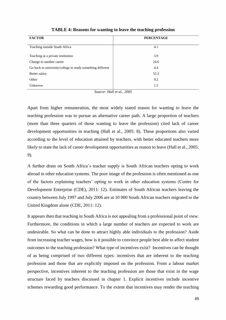
49

TABLE 4: Reasons for wanting to leave the teaching profession

FACTOR PERCENTAGE

Teaching outside South Africa 4.1

Teaching at a private institution 3.9

Change to another career 24.6

Go back to university/college to study something different 4.4

Better salary 52.3

Other 9.2

Unknown 1.5

Source: Hall et al., 2005

Apart from higher remuneration, the most widely stated reason for wanting to leave the

teaching profession was to pursue an alternative career path. A large proportion of teachers

(more than three quarters of those wanting to leave the profession) cited lack of career

development opportunities in teaching (Hall et al., 2005: 8). These proportions also varied

according to the level of education attained by teachers, with better educated teachers more

likely to state the lack of career development opportunities as reason to leave (Hall et al., 2005:

9).

A further drain on South Africa’s teacher supply is South African teachers opting to work

abroad in other education systems. The poor image of the profession is often mentioned as one

of the factors explaining teachers’ opting to work in other education systems (Centre for

Development Enterprise (CDE), 2011: 12). Estimates of South African teachers leaving the

country between July 1997 and July 2006 are at 10 000 South African teachers migrated to the

United Kingdom alone (CDE, 2011: 12).

It appears then that teaching in South Africa is not appealing from a professional point of view.

Furthermore, the conditions in which a large number of teachers are expected to work are

undesirable. So what can be done to attract highly able individuals to the profession? Aside

from increasing teacher wages, how is it possible to convince people best able to affect student

outcomes to the teaching profession? What type of incentives exist? Incentives can be thought

of as being comprised of two different types: incentives that are inherent to the teaching

profession and those that are explicitly imposed on the profession. From a labour market

perspective, incentives inherent to the teaching profession are those that exist in the wage

structure faced by teachers discussed in chapter 1. Explicit incentives include incentive

schemes rewarding good performance. To the extent that incentives may render the teaching

50

profession more financially attractive as well as present opportunities for professional

development, they may discourage teachers who would otherwise leave the profession to stay.

Many advocate the implementation of incentives for teachers as a possible channel through

which to enhance student ability and skills development. An important motivation for

implementing incentives for teachers is that they explicitly state the results that are valued by

the education authority and therefore of teachers, thereby enhancing their accountability. The

agreement between authorities and schools is enhanced because expectations with regard to

service provision are explicitly specified. Bruns et al. (2010: 19-20) discuss pay-for-

performance as a possible avenue to provide incentives to teachers and ensure accountability.

Pay-for-performance largely leaves the teacher salary scale untouched while creating

incentives at the margin. Unlike salaries, this kind of incentive pay rewards teachers for what

they actually do or achieve during a specified period, rather than for what their qualifications

and training suggest they are capable of doing. The correlation between the observable

characteristics of teachers and the level of achievement attained by their students is weak

(Bruns et al., 2010: 20).

Examples exist of incentive schemes which have succeeded in improving student performance.

Ballou (2001) investigates the implementation of incentive schemes in private and public

schools in the USA. Ballou finds that private schools employ incentive schemes for teachers

more often than do public schools. Ballou (2001: 57) explains that different “market sanctions”

are at play in the private school sector surrounding performance. Private schools’ survival

depends on their ability to “retain the kinds of teachers that sustain the school’s reputation”

(Ballou, 2001: 57). Schools place themselves at a significant disadvantage if they are unable to

retain a staff of teachers considered by parents to be “cream of the crop”. Attracting highly able

teachers through implementing incentive systems therefore renders a school attractive to

prospective clients and ensures that enrolment is high. This aspect of incentives systems in

private schools suggests that incentives may be experienced as beneficial for all teachers within

a particular private school, resulting in private school teachers being more inclined to support

the implementation of incentive schemes (Ballou, 2001: 57). In other words, in private school

settings the prestige of the school is to some extent dependent on the perceived quality of the

teachers. It seems then that when teacher quality is important, administrators make use of

incentives. Ballou (2001: 60) concludes that it is not the nature of teaching that renders teacher

incentives ineffective, but rather the conditions and incentives of the public school sector.

51

Figlio and Kenny (2007: 903) also find a positive influence of teacher incentives on student

learning. They offer two possible interpretations for this result. The first is understanding that

teacher incentives could result in higher levels of effort amongst teachers, which translates into

improvement in student performance. The second is that schools that implement teacher

incentives are most effective in unobservable ways, suggesting spurious results for teacher

incentives (Figlio & Kenny, 2007: 903).

Podgursky and Springer (2010) conducted a review on teacher performance pay in the US

education system from kindergarten to senior secondary school and find an overall positive

relationship between the use of teacher incentives and student performance, but they explain

that there is less clarity surrounding the exact form that incentives schemes take.

This paper examines the theoretical characteristics of incentive systems, detailing the potential

for distortion as well as the conditions under which peer pressure is effective as an

accountability- and performance-enhancing force. Section 2 provides a brief overview of

incentives in economic theory and specifically in education. Section 3 presents theoretical

models of incentive systems and investigates the characteristics of such systems while section

4 draws up a brief framework from the theoretical models presented in section 3 according to

which international incentive systems are evaluated in section 5. Section 6 analyses the

potential for the introduction of incentive systems in South Africa and explores incentives

inherent to the South African teaching profession.

2. Economic theory and incentives

This section serves as an introduction to thinking about incentives in an economic context with

specific reference to education. The objective is to sketch the broad framework in which the

theoretical models of section 4 are situated.

Research on the use of incentives in organizations generally makes use of an economic

framework which analyses the difference in the objectives of different individuals who make

up an economic organization. Specifically, the objective of the organization as a whole (which

is characterized by the objective of the owner or “principal” of the organization) is contrasted

with the objectives of workers within the organization, i.e. the objectives of the “agent”.

Differences in these objectives imply that workers will not necessarily behave in a way that

maximizes the objective of the organization as a whole or with the principal’s objectives for

the organization, therefore rendering it less productive and worsening the situation for workers

52

in the long run by diminishing either productivity or employment. Incentives may therefore be

used to encourage workers to work towards the objectives of the organization as a whole.

A classic example of such incentives is what is referred to as a “piece rate” – a rate paid to

workers based on their level of productivity or the number of “pieces” they produce as opposed

to a salary based on the number of hours workers work. Increased profits will result from

workers producing more per hour, so incentivizing this production directly may have a greater

positive impact on productivity than would be the case if workers were paid by the hour (Hout

and Elliott, 2011: 21).

The efficiency of incentives is, however, very much dependent on the social relations that

evolve around “piece work”. Complexities beyond simply paying for productivity instead of

paying hourly arise when dealing with incentives, and these require some understanding of

how incentives work in different contexts and for different people. Five complexities requiring

attention are:

1. Finding performance measures

2. Different incentive effects on different people

3. Uncertainty and control

4. Effects of working in groups

5. Weighing the costs and benefits of incentives.

These complexities are each considered below.

2.1 Finding performance measures to use with incentives

In most jobs, output cannot be counted in any meaningful way, making it difficult to measure

the contribution of each worker. Often the qualitative aspects of the job performed are more

important than the aspects that can be quantified. The difficulties inherent in quantifying

incentives are a major constraint to providing them, and the gap between the measures available

for the measurement of incentives and the actual value of the output has important implications

for the operation of incentives. “Objective” measures of performance obviously focus on the

quantifiable aspect of the job at the expense of qualitative aspects, given the difficulty in

measuring these. It is not surprising then that when incentives are attached to the quantifiable

performance measures, workers focus on these aspects of the job and neglect those that do not

affect the performance measure. This is problematic when performance measures are not

closely aligned with the true value of the work being done. The performance measures are said

53

to be “distorted” when they result in behaviour that is detrimental to the true value of the

organization or simply fail to enhance the value to the firm (Hout & Elliott, 2011: 22-23).

Defining the underlying goals that performance measures should reflect can be highly

problematic. In the case of education, schools are required to ensure that students meet some

minimal standard of academic performance, but are also held responsible for developing

cognitive skills, ensuring physical and emotional development, preparing students to enter the

workplace and society and for students’ health and safety. Whilst these goals are not

inconsistent they compete for limited resources, forcing schools to make difficult trade-offs.

Ideally each goal would have one performance measure, but this is simply not practical to

implement and so further trade-offs in the selection of performance criteria are needed (Dixit,

2002: 712). Once performance measures have been selected, further decisions need to be made

regarding how each performance measure will be weighted in the overall incentive scheme.

Agreeing on a performance measure to be implemented is therefore a considerable challenge.

A theoretical analysis (Baker, 2002 – discussed below) shows that more important than

correlation between the performance measure and the value of the organization is whether

behaviour that improves the performance measure also enhances genuine value; in the case of

education, this would be genuine learning amongst students. This distinction is important

because a performance measure may be correlated with a wide range of outcomes-absent

incentives (i.e. high levels of the performance measure is correlated with high overall

performance). However, once incentives are attached to the performance measure, behaviour

that increases the performance measure at the margin may not enhance overall performance at

all. This is known as “gaming” the system (Koretz, 2008: 24).

In the field of education, the strength of incentives currently in place is not straightforward.

Studies of cheating by teachers show that even when incentives are small, some teachers react

quite strongly in a distorting way while others genuinely increase their level of effort (Hout &

Elliot, 2011: 26). As mentioned before and as will be discussed below, the behavioural impact

of a given incentive or set of incentives will cause different people to behave in different ways

and will depend largely on the context in which individuals work.

Incentives systems therefore inevitably have some level of distortion in them and so the

objective of evaluating incentive systems is not to ascertain whether incentives exist, but rather

whether the costs involved in minimizing the distortion are outweighed by the benefits of

implementing the incentive system.

54

A possible alternative to using student test scores to evaluate teachers is requiring school

principals to rank teachers according to their perceived performance. Some may again question

the fairness of this measure given its subjectivity. However, Jacob and Walsh (2011: 447) find

evidence that principals’ rating of teachers correlates strongly with teacher characteristics that

are strong predictors of student performance. For example, they find positive associations

between ratings and experience for the initial years of teaching, but no association for 10 years

of teaching experience and higher. They find a negative association between teacher absence

and ratings and positive correlations between characteristics of teachers’ educational

background19 and ratings (Jacob & Walsh, 2011: 435)20. The authors admit that their analysis

does not provide a direct link between ratings and student performance, but given the

relationship between teacher ratings and correlates of teacher productivity, there is reason to

be optimistic about the ability of principals to recognise teacher quality.

2.2 Different effects of incentives on different people

Economic theory postulates that different people are likely to respond differently to incentive

structures. Amongst people for whom the target is easily attainable, incentives are likely to

result in greater levels of effort relative to those for whom the target is difficult to achieve

(Lazear, 2003: 186). This means that people who are able to reach the target are likely to be

attracted to and remain at the organization while those who are likely to be unsuccessful will

become discouraged and leave. This may enhance productivity since low-productivity workers

will leave the organization and be replaced by more productive workers. An application of this

to the area of teaching by Lazear (2003) applies a model in which teachers have different

abilities to raise student test scores and produces the result that some teachers increase their

effort while others leave the teaching profession. The fact that the teachers that left the

profession are the teachers who are less able to raise test scores would be an enhancement in

the overall effectiveness of teaching over time.

A variation of this model is one in which teachers respond to incentives by either increasing

effort or by increasing effort in test preparation (assuming test scores are the performance

measures upon which the incentives are based). The performance for teachers engaging in both

19 Whether teachers majored in education, maths, English or social sciences (Jacob and Walsh, 2011: 440). 20 Jacob and Walsh (2011: 447) point out that the association between principals’ ratings of teachers and attributes

linked to higher student proficiency is stronger at the upper and lower end of the “ability distribution”. Principals

seem less able to identify teacher quality in the middle section of the ability distribution.

55

forms of behaviour will increase student test scores, but actual learning will only take place

amongst students taught by teachers in the first group. This type of distortion is discussed in

detail in section 3.3.

2.3 Effects of uncertainty and control in providing incentives

In almost all jobs, a worker’s actual performance and the performance measure may be affected

by factors outside of the worker’s control. In the case of pay-for-performance incentives, it is

likely that payoffs received by workers as part of the incentive scheme will depend both on the

workers’ effort and factors beyond their control. As a result, in situations where their pay is

going to be affected by factors beyond their control, they will require compensation for this

uncertainty in the form of higher levels of pay (Hout & Elliott, 2011: 27).

Theoretical analysis shows that optimal incentive schemes will allocate less weight to measures

that are more dependent on factors beyond the worker’s control (Baker, 2002: 3) since these

incentive schemes require greater average pay levels in order to compensate workers for the

greater level of uncertainty in their pay relative to what they might have received in another

job (without incentives). Ultimately then, although productivity is enhanced by the use of

incentives, the higher level of average pay that workers require is costly (Baker, 2002: 4-5).

There are numerous factors beyond the control of schools and teachers that impact on student

learning. In particular, characteristics of students’ home environments result in substantial

variation in the performances of students and a student’s performance over time – one of the

primary reason for the strong opposition to incentives based on student performance amongst

teachers.

56

2.4 Effects of groups in providing incentives

Trade-offs in performance available performance measures are inevitable in environments

where the value of work done depends on cooperation amongst workers. Performance measures

that consider only individual worker production will neglect the contribution made by

individual workers to the productivity of the entire team, while measures of the productivity of

the team will provide a vague and possibly inaccurate indication of an individual worker’s

performance because they are determined by the contributions of the entire team. Whether

team-level or individual-level measures of performance should be incentivized is dependent on

the relative importance of cooperation and on the uncertainty inherent in such performance

measures (Hout & Elliot, 2011: 30).

Education is a prime example of a field requiring cooperation amongst workers. Research in

fields other than economics points out the importance of understanding how schools function

as organizations i.e. understanding the extent of cooperation required amongst teachers. For

example, sociological research looks at understanding incentives in a setting where

consequences are not explicitly defined, investigating how incentives are communicated in an

informal way between workers (Meyer & Rowan in Hout & Elliott, 2011: 30. The combination

of economic and other research indicates the importance of considering the impact of incentives

beyond those directly relevant to the individuals within an organization. Furthermore, the

degree to which work in done jointly and the degree to which the direct effect of incentives

will be transmitted to other members of the organization must be considered (Hout & Elliott,

2011: 31).

An organizational structure as complicated as a school requires one to consider the different

roles and interactions between individuals working at the school. There may well be value in

incentivizing individuals relatively high up in the hierarchy who have the capability to transmit

the incentives in ways that result in cooperative behaviour (or at least encourage such

behaviour). It is important to note that the extent to which the diffusion of incentives is

imperfect requires that the behaviour which one is trying to adjust, as well as the ability of

members in different roles within the organization to adjust the behaviour, should be

considered carefully.

57

2.5 Weighing the costs and benefits of incentives

Ballou (2001: 51) examines teacher incentives in different settings (i.e. in the context of public

and private schools) and provides a useful summary of some of the complications involved in

implementing incentive schemes. He explains that the majority of literature on teacher

incentives reports that they do not translate into long term improvements in student

performance for a number of reasons. The first of these is that it is difficult to observe teachers’

output, largely because educational output is the product of cooperative behaviour and so the

isolated contribution of any individual teacher is difficult to measure. Secondly, the

relationship between teaching and learning is quite obscure and it is often difficult for those

tasked with administering incentives to explain why one teacher qualifies for the incentive and

others do not. It is therefore difficult to stipulate criteria for awarding incentives and teachers

often become frustrated and disillusioned with the process. Thirdly, education output is

difficult to measure. Awarding incentives based on observable measures of output may result

in distortive “gaming” behaviour. Finally, incentives may create a culture of competition

amongst teachers, resulting in non-cooperative and opportunistic behaviour – a situation that

is likely to affect education outcomes negatively (Ballou, 2001: 51). It seems therefore that the

ineffectiveness of teacher incentives is largely due to the nature of the process of education (i.e.

how teaching is translated into learning) and the nature of the teaching profession. If the process

of education was in fact what rendered incentives ineffective, then incentive systems would be

used (or avoided) to the same extent in both private and public schools. However, if these

systems are employed to differing extents across the public and private schooling systems, then

it important to understand how differences between the two sectors affect the effectiveness of

incentives (Ballou, 2001: 52).

The fact that distortion occurs with performance incentives does not mean that they should not

be used at all. Distortion will mean that it is more difficult to measure the benefits associated

with incentives and that some parts of the organization may function less efficiently than they

might have in the absence of incentives. It may, however, still be true that the benefits resulting

from the implementation of incentives are greater than the costs. Improvement in cognitive

skills is associated with improvements in income distribution, individual earnings and

economic growth (Hanushek & Woessman, 2008) and an incentive system that produces true

learning gains may well produce a sizeable net benefit. However, unless one accounts for the

58

level of distortion in such test-based incentives the size of the benefit is likely to be grossly

exaggerated.

Incentives can therefore prove useful in the context of education, despite the problems inherent

in their implementation. Section 3 provides a theoretical analysis of incentives in the teaching

profession.

3. Theoretical models of teacher incentives

Section 2 placed incentives in the context of economic theory and discussed some of the

complexities involved in making use of incentives. This section looks at particular models of

incentives in the context of teaching.

3.1 Incentives based on input and output

The payment of incentives on the basis of inputs or outputs is a central question in the literature

on teacher incentives. The risk inherent in rewarding workers on the basis of what they produce

means that output-based incentives are not always fair. As discussed above, this characteristic

of output-based pay is particularly relevant in education. In some cases therefore, it may be

necessary and preferable to reward workers on the basis of input. Lazear (2003) explains input-

and output-based pay.

3.1.1 Output-based pay

The most important objective in an education system is the education of the population so as

to ensure productivity, allowing individuals to generate skills and thereby an earning to sustain

themselves and in turn generate economic growth. It may therefore be said that generating and

developing earning capacity is the central objective of education (Lazear, 2003: 183).

Earnings, however, are only observed some time after individuals have left the schooling

system, rendering it impossible to determine teacher pay on this basis. As a result, student

achievement test scores are usually used as proxies.

When test scores are used as the basis for teacher pay, it is difficult to distinguish the increases

in test scores resulting from teacher efforts and those resulting from the activities of others.

Furthermore, improved test scores may result from distortive behaviour on the part of teachers

as opposed to genuinely enhanced effort levels.

59

3.1.2 Input-based pay

The advantage of paying workers based on input is that it removes the risk inherent in output-

based pay, therefore discouraging teachers from focussing exclusively on the performance

metric according to which they are paid.

Input-based pay may be seen as a solution to the problem of “teaching to the test”, or distortion

in the context of the incentives literature (Baker, 2000; Holmstrom & Milgrom, 1991). In the

extreme case, a perfect measure of the disutility of working21 would be used as the measure

according to which workers were paid. In this case, there would be no incentive to focus on

one area of the curriculum at the expense of others. Teachers would receive full compensation

for their efforts and would likely be willing to do what is in the best interest of their students,

regardless of the level of effort required. Using disutility as the basis for compensation would

ensure that teachers remained indifferent to which areas of the curriculum they emphasise and

hopefully induce them to make sure that all areas are covered. This results from the fact that

providing payment on the basis of disutility ensures that they receive enough to compensate

them for teaching the “disagreeable” subjects.

Input-based pay works well insofar as hours worked are a proxy for the disutility of teaching.

However, when teachers care about what activities they engage in while teaching, input-based

pay will no longer be effective at eliciting sufficient effort from teachers. The non-teaching

labour market deals with this problem to some extent by compensating different occupations

differently. Lazear (2003: 195) explains that “[institutions are prevented from] hiring

professors of accounting at the same wage that can attract professors of organisational

behaviour” due to the fact that “[the wage] difference is compensation for perhaps less pleasant

or more difficult work”.

3.1.3 What works better?

The literature on teacher incentives favours output-based pay for two reasons. The first

advantage (the “informational” part) is that output-based incentives clearly signal to teachers

what is valued and required. The second advantage (the “alignment” part) ensures that the

21 It is assumed that different aspects of teaching or teaching different parts of the curriculum have different

disutilities.

60

objectives of teachers closely parallel those of society as a whole. It may well be the case that

teachers work hard, but that there is disagreement about which areas of the curriculum are

important. By tying teacher compensation to an agreed-upon metric, it is possible to ensure that

the education provided by teachers results in the accumulation of agreed-upon skills amongst

learners (Lazear, 2003: 209). Finally, there may be some divergence between the preferences

of teachers and the best interests of their students. Lazear (2003: 182-183) gives the example

of teachers deciding against giving assignments because of burden of grading, even though

they are fully aware that their students would benefit from completing the assignments.

Therefore compensation based on students’ performance on the assignment may induce

teachers to behave in a way that is beneficial to their students.

If incentivising teacher performance is thought to be effective in enhancing the quality of

education, then it is important to understand the mechanism through which the improvement

is likely to occur. Section 3.2 explains two possible avenues of influence through which teacher

incentives are likely to impact on student performance – an “incentive effect” and a “sorting

effect”.

3.2 Sorting versus incentive effects and the likelihood of success

The “selection” aspect of compensation is arguably the most important aspect in the context of

education. The individuals attracted by various compensation schemes determine the quality

of individuals within a profession. It is widely accepted that teacher quality is critical to quality

education and so the question of who is likely to enter the profession is crucial.

When teachers are faced with an incentive based on student performance, they must improve

student performance in order to be rewarded. Sorting refers to using incentives in order to

attract individuals who are better able to improve test scores to the teaching profession,

resulting in a teaching force that is better able to improve student performance. Payment based

on output therefore attracts individuals who are best able to enhance student performance and

may discourage weak teachers from continuing in the profession given the relatively lower

levels of pay they will receive as a result of their inability to improve student performance.

Sorting therefore results in better teachers replacing less able teachers. This differs from the

effect of incentives, as in the case of incentives the individual is not replaced but adjusts his or

her behaviour (Lazear, 2003: 187).

61

Teachers able to raise student performance therefore do better on a performance-based

schedule while those unable to do so will do better on a fixed wage schedule. Pay based on

student performance therefore favours teachers who are able to increase student performance

relative to those who are unable to do so.

Is teacher quality and teacher productivity therefore driven primarily by teachers’ innate ability

or does the level of effort put into teaching influence the level of teacher productivity? Neal

(2011) discusses the importance of distinguishing whether teacher quality is dependent on

teacher effort, teacher ability or a combination of both. He maintains that it is only if teacher

quality is a function (at least in part) of teacher effort that incentives are likely to influence

student performance. Ignoring teacher effort as a contributing factor in educational quality

counters much of the empirical literature on the subject of teacher productivity; if poor teachers

are teachers who are unable to master the skill of teaching well, then incentive provision is

unlikely to improve student performance in any significant way. However, if poor teachers are

unmotivated and “lazy” teachers, then the introduction of well-designed incentives may well

contribute to improved student performance. The extent to which teacher productivity is driven

by effort determines to some degree the likelihood of success in the implementation of

incentives (Neal, 2011: 8).

It is undeniable that teachers vary substantially in their levels of productivity, in South Africa

and internationally. The fact that differences in productivity exist says nothing about whether

teachers provide efficient effort given their level of talent. Teachers may well operate according

to different “effort norms”. It is therefore necessary to ascertain whether or not productivity is

likely to change if effort is incentivized, and this means ascertaining whether or not

productivity depends on teacher effort.

3.3 Moral hazard and the risk of distortion

“I come to the following pessimistic laws. . .: The more any quantitative social indicator is used

for social decision-making, the more subject it will be to corruption pressures and the more apt

it will be to distort and corrupt the social processes it is intended to monitor” (Campbell, 1976).

This section discusses the risk involved in incentivising teacher performance. It discusses the

risk of encouraging sub-optimal behaviour and how this comes about with the introduction of

incentive schemes.

62

3.3.1 Multitasking and the risk of distortion

A criticism often levelled at performance-based incentives is that if incentives are used in order

to encourage teachers to provide higher quality education to their students, teachers may

improve test scores (according to which payments are made) without actually enhancing

learning – behaviour known as distortion. Distortion may also occur when the sorting effect is

at play. If we believe that education is valuable to individuals because of its impact on future

earnings and we are using student test performance as a measure of learning, it may well happen

that teachers who are able to increase student test scores without influencing their learning are

drawn into the profession (Lazear, 2003: 187).

Neal (2011: 10) uses a special case of the multi-tasking model of Holstrom and Milgrom

(1991), a model often used to explain the behaviour of teachers in various merit pay schemes.

Assume that in an education system teachers allocate their effort between two tasks. The

amount of time the teacher allocates to task 1 and task 2, respectively, is denoted by t1 and t2.

The human capital production function is given by

ℎ = 𝑓1𝑡1 + 𝑓2𝑡2 + 𝑒 (1)

where human capital acquired by the student as a result of teacher effort is (h – e) (Neal, 2011:

10). h denotes additional student skill and it is measured in dollars. f1 and f2 are constants and

e is a random error term that captures factors affecting a student’s rate of learning beyond the

teacher’s control. h, t1 and t2 are not observable by the authority, but the authority is able to

observe a statistical measure of teacher performance p,

𝑝 = 𝑔1𝑡1 + 𝑔2𝑡2 + 𝑣 (2)

where g1 and g2 are constants and v is a random error influencing measured performance (Neal,

2011: 10-11). v and e are shocks and are independently drawn with mean zero. They are also

assumed to be independent of t1 and t2. The teacher’s utility function is

𝑈 = 𝑋 − 𝐶(𝑡1, 𝑡2) (3)

where the teacher’s expected income is given by X and the cost associated with any pair (t1, t2)

is given by C(t1, t2). An optimal compensation contract is designed by the education authority,

given by

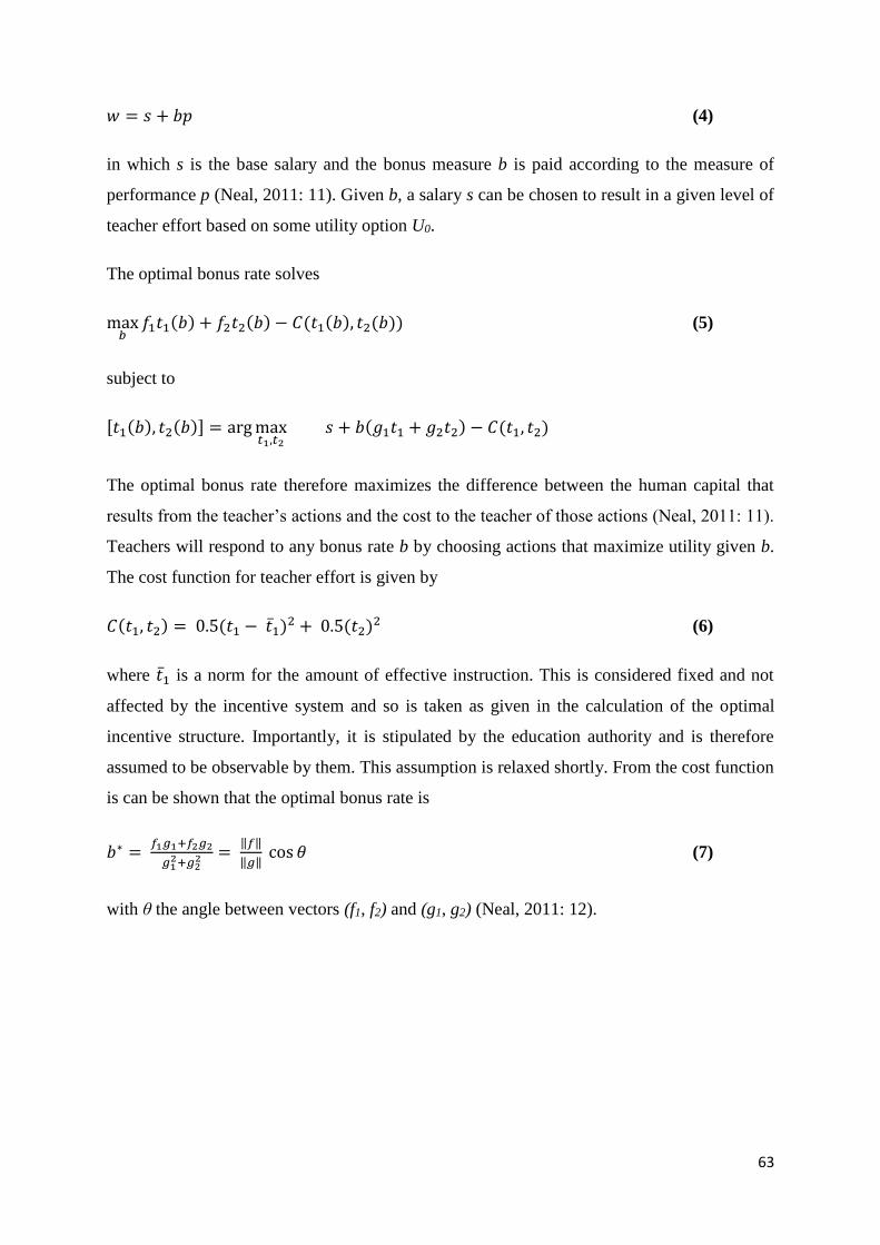
63

𝑤 = 𝑠 + 𝑏𝑝 (4)

in which s is the base salary and the bonus measure b is paid according to the measure of

performance p (Neal, 2011: 11). Given b, a salary s can be chosen to result in a given level of

teacher effort based on some utility option U0.

The optimal bonus rate solves

max𝑏

𝑓1𝑡1(𝑏) + 𝑓2𝑡2(𝑏) − 𝐶(𝑡1(𝑏), 𝑡2(𝑏)) (5)

subject to

[𝑡1(𝑏), 𝑡2(𝑏)] = arg max𝑡1,𝑡2

𝑠 + 𝑏(𝑔1𝑡1 + 𝑔2𝑡2) − 𝐶(𝑡1, 𝑡2)

The optimal bonus rate therefore maximizes the difference between the human capital that

results from the teacher’s actions and the cost to the teacher of those actions (Neal, 2011: 11).

Teachers will respond to any bonus rate b by choosing actions that maximize utility given b.

The cost function for teacher effort is given by

𝐶(𝑡1, 𝑡2) = 0.5(𝑡1 − 𝑡1̅)2 + 0.5(𝑡2)2 (6)

where 𝑡1̅ is a norm for the amount of effective instruction. This is considered fixed and not

affected by the incentive system and so is taken as given in the calculation of the optimal

incentive structure. Importantly, it is stipulated by the education authority and is therefore

assumed to be observable by them. This assumption is relaxed shortly. From the cost function

is can be shown that the optimal bonus rate is

𝑏∗ = 𝑓1𝑔1+𝑓2𝑔2

𝑔12+𝑔2

2 = ‖𝑓‖

‖𝑔‖ cos 𝜃 (7)

with θ the angle between vectors (f1, f2) and (g1, g2) (Neal, 2011: 12).

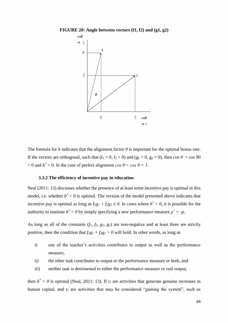
64

FIGURE 20: Angle between vectors (f1, f2) and (g1, g2)

The formula for b indicates that the alignment factor θ is important for the optimal bonus rate.

If the vectors are orthogonal, such that (f1 = 0, f2 > 0) and (g1 > 0, g2 = 0), then cos θ = cos 90

= 0 and b* = 0. In the case of perfect alignment cos θ = cos 0 = 1.

3.3.2 The efficiency of incentive pay in education

Neal (2011: 13) discusses whether the presence of at least some incentive pay is optimal in this

model, i.e. whether b* > 0 is optimal. The version of the model presented above indicates that

incentive pay is optimal as long as f1g1 + f2g2 ≠ 0. In cases where b* < 0, it is possible for the

authority to institute b* > 0 by simply specifying a new performance measure p’ = -p.

As long as all of the constants (f1, f2, g1, g2) are non-negative and at least three are strictly

positive, then the condition that f1g1 + f2g2 > 0 will hold. In other words, as long as

i) one of the teacher’s activities contributes to output as well as the performance

measure,

ii) the other task contributes to output or the performance measure or both, and

iii) neither task is detrimental to either the performance measure or real output,

then b* > 0 is optimal (Neal, 2011: 13). If t1 are activities that generate genuine increases in

human capital, and t2 are activities that may be considered “gaming the system”, such as

65

teaching to the test or changing the answers of students before the assessment is graded, then

it is widely assumed that the impact productive behaviour on genuine human capital

accumulation amongst students is positive (f1 > 0), that this behaviour improves the

performance measure (g1 > 0), that gaming behaviour improves the performance measure (g2

> 0), and as long as gaming activities do not diminish human capital amongst students, then

their impact will not diminish human capital amongst students (f2 ≥ 0). Optimal policy should

always then include b*> 0. The separability of the cost function is an important assumption for

this framework. b* is only optimal to the extent that teachers can consciously and willingly

decide on the combination of t1 and t2, implying that they are able to distinguish between which

of their actions genuinely enhance the skills of students and which of them simply enhance

their performance measure. Without this assumption, the optimal policy of b*> 0 is not a robust

feature of the multi-tasking model (Neal, 2011: 13).

Given that education requires the time of both students and teachers, and given the restricted

nature of students’ attention and energy, it may be worth considering cost functions that take

the form

𝐶(𝑡1, 𝑡2) = 0.5(𝑡1 + 𝑡2 − 𝑡)̅2 (8)

In this cost function, t1 and t2 are perfectly interchangeable and 𝑡̅ is a total effort norm that

impacts on teacher costs. It is assumed that teachers choose t1 = 𝑡̅ and that t2 = 0 when no

incentives exist. Given this setting, if the education system chooses b > 0, then teachers will

choose t1 = 0 as long as g2 > g1 and as long as there are many combinations of 𝑡̅, f1, f2 and g2

that would result in b = 0. So when f1 > f2 and f1𝑡̅ are baseline outputs, an incentive scheme

that results in teachers substituting a small amount of t2 for t1 will lower human capital gains

to students without affecting teacher remuneration costs (Neal, 2011: 13-14).

However, if 𝑡̅ is low enough, the result may still be an increased total surplus. Since t1 can

never be negative, the diminished output associated with the loss of t1 = 𝑡̅ may be compensated

for by the benefits associated with increasing t2 far beyond 𝑡̅. Therefore, whether or not an

optimal bonus rate (b*) exists depends on what type of instruction happens in the classroom

(effective teaching or “gaming” behaviour) and on the norm 𝑡̅ within the education system

(Neal, 2011: 14).

66

The nature of teacher activities denoted by t2 that result from the introduction of incentive

schemes is important to consider, as well as the relative values of f2 and g2 given the assumption

that g2 > g1. Equally important, however, is considering whether increased t2 activities result

in increased teacher effort or whether it is simply substitution away from effective teacher

behaviour t1. If teacher effort is directed away from effective teaching practices towards

gaming behaviour, the effect this will have on learning depends on the level of productive effort

initially. In education systems where very little effort was directed towards effective teaching

practices, an increase in gaming practices will increase the overall performance of the system

because of the overall increase in teacher effort. In education systems in which the level of

effort devoted to t1 is high, incentives systems which result in less effective teaching practices

and more gaming practices will result in a decline in the overall output of the system (Neal,

2011: 14). For example, it may be argued that in a system where teacher effort is extremely

low, a change from no teaching to “teaching to the test” still represents an increase in the

amount of teaching and learning compared to what was happening before, albeit only in areas

which are likely to be tested and therefore impact on the performance measure. Therefore the

overall output of the education system has increased. However, in the case where effective

teaching and learning are taking place and students’ skill bases are being expanded in all areas

and not just those related to material likely to be tested, a movement towards “teaching to the

test” and away from genuine skills-enhancing teaching will diminish the output of the

education system. Furthermore, although it is possible to say that enhancing t2 in systems

characterised by extremely low levels of 𝑡̅ may still enhance overall output of the education

system, the long-term implications of encouraging such behaviour are significant and the

development of a hard-working teaching force which contributes in a meaningful way to

students’ skills development becomes less likely.

The question is therefore whether incentive systems lead to improvements in student

performance that result from increases in student skills, or whether the improvement in

performance is the result of gaming behaviour which improves the measure of student

performance without enhancing students’ skills to the same extent that quality skills-enhancing

teaching would.

3.3.3 Contamination and hidden actions

Coaching is not an optimal allocation of teacher effort, but some positive skills enhancement

may result from certain forms of coaching. Indeed if coaching reflects a reduction in leisure

67

time on the part of teachers rather than a reduction in effective teaching time, then teacher

performance under an incentive scheme may well be enhanced relative to what it would have

been under an accountability programme alone. However, teachers respond in ways other than

coaching that constitute what Koretz (2008) refers to as cheating and which are unequivocally

wasteful from the perspective of public welfare.

Jacob and Levitt (2003) give evidence of behaviour of Chicago teachers that clearly constitutes

cheating: the teachers altered the answers of the students on high-stakes22 assessments. This

type of cheating is usually quite easy to detect because the performance of students being taught

by cheating teachers is significantly out of line with their performance in other areas. In

addition, the performance of these students reflected significant increases from the previous

year, but only small increases (if any at all) in the year following the cheating.

Figlio and Winicki (2005) present evidence from Virginia that on the day that an assessment

took place, the sugar content of the meals given to students was increased. It appears that school

officials were responding to literature on the positive correlation between academic

performance and glucose intake. This is a prime example of agents’ behaviour which enhances

their performance measure but does not actually have a real impact on skills enhancement.

The multi-tasking model underlines the possibility that inefficient teaching behaviour may

result from the implementation of incentive schemes. However, it also draws attention to the

fact that in situations where the level of teacher effort is very low, even teaching practices that

enhance only the performance measure may result in an overall increase in teacher effort,

leading to an overall increase in welfare within the education system. In terms of the long term

objectives of education (the improvement of students’ skills), it is clear that teaching behaviour

that enhances the performance measure without actually altering the level of human capital

generated amongst learners is undesirable. This emphasizes a problem with using measures of

student performance as the basis upon which incentives are paid. The fact that it is susceptible

to “gaming” highlights the difficulties faced by the education authority with regards to

monitoring teacher responses to incentive programmes. A possible remedy to the issue of

monitoring is the use of partnerships and peer pressure amongst teachers to elicit appropriate

teaching behaviour in the presence of an incentive programme. Subsection 3.4 analyses the

22 “High-stakes” refers to the fact that either incentives are awarded or sanctions are imposed on the basis of the

outcome of the assessments.

68

channels through which peer pressure and partnerships are likely to influence behaviour under

incentive schemes.

3.4 Peer pressure and partnerships

The creation of partnerships and profit-sharing arrangements stems from the need for internal

motivation which arises mainly because of the prohibitive cost of monitoring employees, as

well as the problem of the the accuracy of observable performance measures. By rewarding

and punishing workers as a team, sufficient incentive may be provided for workers to supply

an adequate level of effort. The idea is that team members are in a better position to control

and discipline one another while simultaneously having a real incentive to do so, given that the

overall payoff and therefore their individual payoff is contingent on producing a level of output

that is only attainable with a certain amount of effort from each individual worker (Kandel &

Lazear, 1992: 802).

This subsection explores the conditions under which peer pressure operates.

3.4.1 Free-rider effects and peer pressure

Suppose that a group of identical workers produces output f(e), so that output is a function of

the individual effort of each worker ei. Therefore e is an N-dimensional vector of the levels of

workers’ effort with N workers. f(e) is assumed to be non-separable in ei ensuring a reason for

partnerships. This would be tantamount to saying that pupil education depends on the effort of

all of their teachers and that overall effort is non-separable (Kandel & Lazear, 1992: 803).

The cost of effort is denoted C(ei) with C` > 0 and C`` > 0. The worker seeks to maximize

max𝑒𝑖

𝑓(𝒆)

𝑁− 𝐶(𝑒𝑖) (9)

with first-order conditions

𝑓𝑖(𝒆)

𝑁− 𝐶′(𝑒𝑖) = 0. (10)

Efficient production requires the maximization of total surplus

max𝑒1,𝑒2,….𝑒𝑁

𝑓(𝒆) − ∑ 𝐶(𝑒𝑖)𝑁𝑖=1 (11)


69

𝑓𝑖(𝒆) − 𝐶′(𝑒𝑖) = 0 ∀ 𝑖. (12)

Given that C`` > 0, e*, the solution to (12), is therefore larger than e`, the solution to (10), for

all N > 1. The level of effort chosen in a partnership is below the efficient level (Kandel &

Lazear, 1992: 804).

When effort is observable, the best solution would be to pay workers a + be where b = fi(e*).

However, the root of the problem is the observability of effort. Payment on the basis of effort

is therefore ruled out and we investigate the effect of peer pressure on effort.

The “peer pressure” function is written as

𝑝𝑒𝑒𝑟 𝑝𝑟𝑒𝑠𝑠𝑢𝑟𝑒 = 𝑃(𝑒𝑖; 𝑒𝑗 , . . . , 𝑒𝑁 , 𝑎𝑖, . . . , 𝑎𝑁) (13)

The pressure felt by worker i is dependent on his or her own efforts (ei), the effort of peers (ej,

. . . ,eN) and other actions taken by peers (ai, aj, . . . , aN). The actions of workers23 have no

effect on output, but they do involve some cost to the workers. Cost is therefore redefined as

C(ei, ai). The general maximization problem for worker i then becomes

max𝑒𝑖,𝑎𝑖

𝑓(𝒆)

𝑁− 𝐶(𝑒𝑖, 𝑎𝑖) − 𝑃(𝑒𝑖; 𝑒𝑗 , … , 𝑒𝑁 , 𝑎𝑖, … , 𝑎𝑁) (14)

Peer pressure differs from the cost of effort in the sense that it is social and dependent on the

effort and actions of others, so it is to some extent external to the worker. That is, 𝑃(∙) is subject

to manipulation by the group in which the worker works. C(e) is not. We may therefore think

about C(e) as the exogenous part of the utility of effort (in the sense that it is determined

independently of the effect that peer pressure may have on utility) and 𝑃(∙) as the part that is

endogenous and cultural (Kandel & Lazear, 1992: 804). Introducing the peer pressure function

is an attempt to explain differences in preferences and work ethics amongst workers. Making

explicit assumptions about 𝑃(∙) allows us to make statements about the tastes that drive

particular behaviour.

The Cournot-Nash assumption that the actions of all other workers are taken as given is used.

Each worker receives 𝑓(𝒆)

𝑁 in a pure partnership of size N. The actions of other workers (the

a’s) are assumed to have no effect on P and are therefore set to zero. The worker’s problem

becomes

23 These are discussed in more detail later.

70

max𝑒𝑖,𝑎𝑖

𝑓(𝒆)

𝑁− 𝐶(𝑒𝑖, 𝑎𝑖) − 𝑃(𝑒𝑖, … ) (15)


𝜕𝑓/𝜕𝑒𝑖

𝑁− 𝐶1 −

𝜕𝑃

𝜕𝑒𝑖= 0 (16)

given that ai is set to zero.

Peer pressure implies that 𝜕𝑃/𝜕𝑒𝑖 < 0 (the disutility associated with peer pressure diminishes

as workers exert more effort), which means that the level of effort that solves (16) is greater

than the level of effort that solves (10). That is, effort is higher with peer pressure than without

peer pressure. The 𝑃(∙) function implies that workers get utility from effort. This has only been

assumed, however. Workers working in an environment in which peer pressure exists may be

worse off because of it. Peer pressure may increase effort, but it does not necessarily mean

higher utility because pressure itself is a cost that is borne by all firm members. Despite the

higher output that results from peer pressure, workers may not enjoy working in a high-

pressured environment (Kandel & Lazear, 1992: 805).

3.4.2 Creating peer pressure

Considering the actions of organizations in the peer pressure function allows us to analyse how

peer pressure is created and how partnerships result in higher effort levels.

The effectiveness of peer pressure as a motivator is conditional on two things: first of all, the

effort of member i must affect the well-being of other team members in order for them to have

the incentive to exert pressure on him. Secondly, team members must be able to affect the

choices of member i. Profit-sharing in some form (or sharing of the incentive in the case of

teachers) is required in order for the first component to hold. If workers are paid straight

salaries, their level of effort does not impact on the salaries received by any of their peers,

removing the incentive for workers to exert pressure on their peers since they are not concerned

with the level of effort they choose. Profit-sharing is therefore necessary for peer pressure to

provide motivation for workers to influence their peers’ behaviour. However, it is not

sufficient. Even if workers have reason to influence the behaviour of their peers, they need to

be able to exert pressure for peer pressure to actually provide incentives. Both components are

assumed to be created and manipulated to some extent by the education authority (Kandel &

Lazear, 1992: 806).

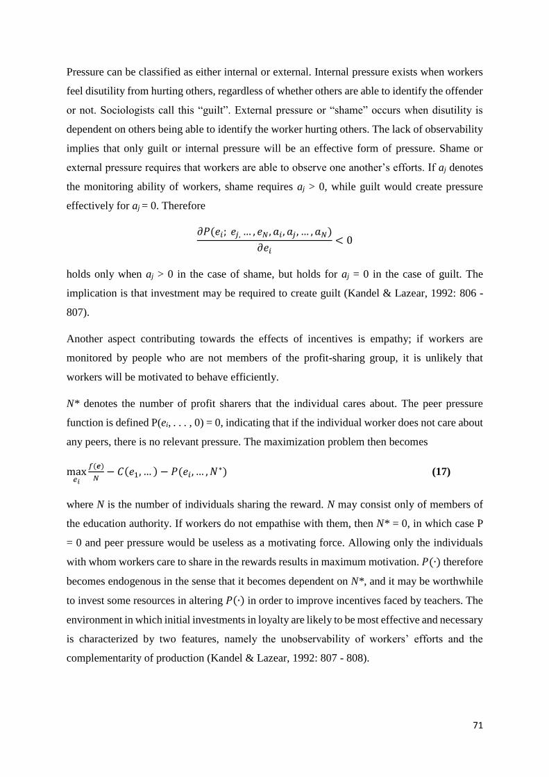
71

Pressure can be classified as either internal or external. Internal pressure exists when workers

feel disutility from hurting others, regardless of whether others are able to identify the offender

or not. Sociologists call this “guilt”. External pressure or “shame” occurs when disutility is

dependent on others being able to identify the worker hurting others. The lack of observability

implies that only guilt or internal pressure will be an effective form of pressure. Shame or

external pressure requires that workers are able to observe one another’s efforts. If aj denotes

the monitoring ability of workers, shame requires aj > 0, while guilt would create pressure

effectively for aj = 0. Therefore

𝜕𝑃(𝑒𝑖; 𝑒𝑗, … , 𝑒𝑁 , 𝑎𝑖, 𝑎𝑗 , … , 𝑎𝑁)

𝜕𝑒𝑖< 0

holds only when aj > 0 in the case of shame, but holds for aj = 0 in the case of guilt. The

implication is that investment may be required to create guilt (Kandel & Lazear, 1992: 806 -

807).

Another aspect contributing towards the effects of incentives is empathy; if workers are

monitored by people who are not members of the profit-sharing group, it is unlikely that

workers will be motivated to behave efficiently.

N* denotes the number of profit sharers that the individual cares about. The peer pressure

function is defined P(ei, . . . , 0) = 0, indicating that if the individual worker does not care about

any peers, there is no relevant pressure. The maximization problem then becomes

max𝑒𝑖

𝑓(𝒆)

𝑁− 𝐶(𝑒1, … ) − 𝑃(𝑒𝑖, … , 𝑁∗) (17)

where N is the number of individuals sharing the reward. N may consist only of members of

the education authority. If workers do not empathise with them, then N* = 0, in which case P

= 0 and peer pressure would be useless as a motivating force. Allowing only the individuals

with whom workers care to share in the rewards results in maximum motivation. 𝑃(∙) therefore

becomes endogenous in the sense that it becomes dependent on N*, and it may be worthwhile

to invest some resources in altering 𝑃(∙) in order to improve incentives faced by teachers. The

environment in which initial investments in loyalty are likely to be most effective and necessary

is characterized by two features, namely the unobservability of workers’ efforts and the

complementarity of production (Kandel & Lazear, 1992: 807 - 808).

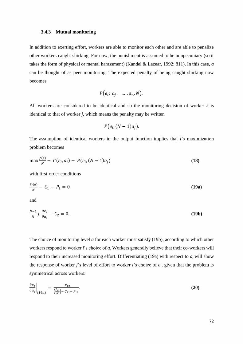
72

3.4.3 Mutual monitoring

In addition to exerting effort, workers are able to monitor each other and are able to penalize

other workers caught shirking. For now, the punishment is assumed to be nonpecuniary (so it

takes the form of physical or mental harassment) (Kandel & Lazear, 1992: 811). In this case, a

can be thought of as peer monitoring. The expected penalty of being caught shirking now

becomes

𝑃(𝑒𝑖; 𝑎𝑗 , … , 𝑎𝑛, 𝑁).

All workers are considered to be identical and so the monitoring decision of worker k is

identical to that of worker j, which means the penalty may be written

𝑃(𝑒𝑖, (𝑁 − 1)𝑎𝑗).

The assumption of identical workers in the output function implies that i’s maximization

problem becomes

max𝑓(𝒆)

𝑁− 𝐶(𝑒𝑖, 𝑎𝑖) − 𝑃(𝑒𝑖, (𝑁 − 1)𝑎𝑗) (18)


𝑓𝑖(𝒆)

𝑁− 𝐶1 − 𝑃1 = 0 (19a)

and

𝑁−1

𝑁𝑓𝑖

𝜕𝑒𝑗

𝜕𝑎𝑖− 𝐶2 = 0. (19b)

The choice of monitoring level a for each worker must satisfy (19b), according to which other

workers respond to worker i’s choice of a. Workers generally believe that their co-workers will

respond to their increased monitoring effort. Differentiating (19a) with respect to aj will show

the response of worker j’s level of effort to worker i’s choice of ai, given that the problem is

symmetrical across workers:

𝜕𝑒𝑗

𝜕𝑎𝑗|

(19𝑎)

= −𝑃12

(𝑓𝑖𝑖𝑁

)− 𝐶11− 𝑃11

. (20)

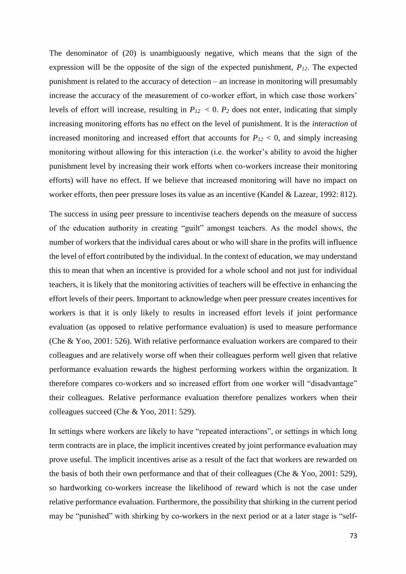
73

The denominator of (20) is unambiguously negative, which means that the sign of the

expression will be the opposite of the sign of the expected punishment, P12. The expected

punishment is related to the accuracy of detection – an increase in monitoring will presumably

increase the accuracy of the measurement of co-worker effort, in which case those workers’

levels of effort will increase, resulting in P12 < 0. P2 does not enter, indicating that simply

increasing monitoring efforts has no effect on the level of punishment. It is the interaction of

increased monitoring and increased effort that accounts for P12 < 0, and simply increasing

monitoring without allowing for this interaction (i.e. the worker’s ability to avoid the higher

punishment level by increasing their work efforts when co-workers increase their monitoring

efforts) will have no effect. If we believe that increased monitoring will have no impact on

worker efforts, then peer pressure loses its value as an incentive (Kandel & Lazear, 1992: 812).

The success in using peer pressure to incentivise teachers depends on the measure of success

of the education authority in creating “guilt” amongst teachers. As the model shows, the

number of workers that the individual cares about or who will share in the profits will influence

the level of effort contributed by the individual. In the context of education, we may understand

this to mean that when an incentive is provided for a whole school and not just for individual

teachers, it is likely that the monitoring activities of teachers will be effective in enhancing the

effort levels of their peers. Important to acknowledge when peer pressure creates incentives for

workers is that it is only likely to results in increased effort levels if joint performance

evaluation (as opposed to relative performance evaluation) is used to measure performance

(Che & Yoo, 2001: 526). With relative performance evaluation workers are compared to their

colleagues and are relatively worse off when their colleagues perform well given that relative

performance evaluation rewards the highest performing workers within the organization. It

therefore compares co-workers and so increased effort from one worker will “disadvantage”

their colleagues. Relative performance evaluation therefore penalizes workers when their

colleagues succeed (Che & Yoo, 2011: 529).

In settings where workers are likely to have “repeated interactions”, or settings in which long

term contracts are in place, the implicit incentives created by joint performance evaluation may

prove useful. The implicit incentives arise as a result of the fact that workers are rewarded on

the basis of both their own performance and that of their colleagues (Che & Yoo, 2001: 529),

so hardworking co-workers increase the likelihood of reward which is not the case under

relative performance evaluation. Furthermore, the possibility that shirking in the current period

may be “punished” with shirking by co-workers in the next period or at a later stage is “self-

74

enforcing” in the sense that workers “punishing “ shirking co-workers in subsequent periods is

not stipulated in any incentive contract and therefore does not need to be enforced by the

education authority. Che and Yoo (2001: 231) explain that this is an endogenous characteristic

of the relationship in a setting of joint performance evaluation and is likely to ensure that

workers actually work (as opposed to shirk).

3.5 Return to distortion

The model discussed above indicates that introducing monitoring amongst teachers will in

theory enhance their level of effort. However, it is not clear whether the expected increased

earnings will result in an increase in human capital-enhancing teaching behaviour or behaviour

that may be considered distortion. Therefore peer pressure does not necessarily result in

improved long-term outcomes for students – the ultimate objective of implementing teacher

incentives. Although peer pressure as an incentivising instrument may enhance the level of

effort in a setting in which observability is limited, it does not remedy the problem of distortion

in teaching behaviour.

Which features of the theoretical models discussed above should therefore be considered most

important to successfully incentivise teachers to enhance their students’ performance? Section

4 puts together a brief framework of the characteristics that enable incentive systems for

teachers to result in improved performance for their students. Section 5 then presents

international examples of teacher incentive programmes and analyses them according to the

characteristics mentioned in section 4.

4. Characteristics of successful incentive programmes

Three aspects of incentive programmes need to be investigated when evaluating the likelihood

of success: whether or not incentive programmes are likely to improve student outcomes

through sorting or through enhanced effort; the risk of distortion that arises with the

introduction of incentive programmes; and, in the case of low observability of worker effort

(which is certainly the case in the teaching profession), whether an internal source of

performance monitoring and accountability can be utilised to provide incentives (i.e. peer

pressure). Each of these is discussed briefly below.

75

4.1 Sorting versus incentives

Whether or not incentive programmes are likely to result in improved performance depends on

whether the programme results in higher levels of effort amongst teachers (assuming that

increased teacher effort will result in improved student performance) or whether individuals

better able to enhance student performance will be drawn to the teaching profession. Whether

incentive programmes are likely to result in sorting or enhanced effort is an important question

to consider because it is possible that the introduction of incentive programmes may have

negative implications for poorly performing schools. Clotfelter, Ladd, Vigdor and Diaz (2004)

examine this question in detail, using data from North Carolina. This aspect is discussed in

more detail in section 5.

4.2 Potential for distortion

Another aspect to consider is the likelihood of distortion. The extent to which the introduction

of incentives results in genuine improvements in learning as opposed to improvements in

performance measures as well as the long term effects that incentives will have on student

learning are important considerations. Neal (2011: 14) points out that even distortive behaviour

may be a net gain in the case of extremely low productivity, in other words that teaching to the

test may be better than no teaching at all. The risk for gaming behaviour as well as potentially

short-term benefits should be investigated.

4.3 Possibility for peer pressure

The likely success of using peer pressure to incentivise teachers is dependent on teachers being

able to monitor one another as well as being able to impose a penalty on workers who are found

to be shirking. The combination of monitoring and penalising is important for this method of

incentivising to be effective. Importantly, it requires that incentives be provided for the school

and not for individual teachers.

How do incentive systems measure up internationally when evaluated according to the features

highlighted in this section? Do they result in sorting or in enhanced teacher effort, and does

this in turn result in improved student performance? Where improvement occurs, is this

genuine human capital development or is it the result of gaming behaviour by teachers? Do the

incentive systems in place enable the use of peer pressure as an incentivising mechanism?

76

Section 5 discusses incentive systems used in India, Israel, Kenya, Brazil, Chile, the USA and

Finland, and analyses whether they are likely to fulfil the criteria outlined above.

5. International examples of incentive programmes

As mentioned above, this section discusses incentive systems implemented internationally. The

last three incentive systems discussed in this section – those of the USA, Chile and Finland –

are not analysed in terms of the framework laid out in section 4, but serve as examples of the

risks associated with implementing incentive programmes (USA); the success with which

pragmatic incentive programmes can be implemented in the context of a developing country

(Chile); and the potential benefit that comes from incentivising the teaching profession through

factors such as selectivity, prestige and relatively attractive compensation (Finland).

5.1 Andhra Pradesh, India (2005 – 2007)

A random control trial (RCT) conducted in India is an example of performance pay on an

individual level based on student learning outcomes. In this study, individual teacher bonuses

were awarded in 100 schools, bonuses were awarded to groups of teachers in 100 schools, an

extra contract teacher was provided in 100 schools and a school grant was awarded to 100

schools. A further 100 schools were also included as a comparison group. The study was

conducted over 2 years, and performance bonuses were promised to teachers at the beginning

of the following school year (Muralidharan & Sundararaman, 2011). Bonuses were awarded to

any teacher or school managing to increase student test scores by at least 5 percentage points,

with higher increases being awarded with larger bonuses. Individual and group-level bonuses

were paid at the beginning of the next school year, and block grants and extra contract teachers

were provided unconditionally at the beginning of the school year.

At the end of the two year programme significant differences existed between individual- and

group-level bonuses, as well as between schools receiving teacher bonuses and those receiving

either block grants or extra contracted teachers. Individual incentives increased student

performance on tests by 0.27 standard deviations (roughly 9 percentage points) in comparison

with an increase of 0.16 (roughly 5 percentage points) for group incentives. Input strategies

(block grants and extra contracted teachers) also improved student performance, but by a

substantially smaller amount – 0.08 standard deviations.

77

During the study teachers were monitored by observers through unannounced classroom visits

as well as interviews (Muralidharan & Sundararaman, 2011: 67). Teachers were monitored

during 20 to 30 minute classroom observations in which enumerators coded whether or not

certain actions took place in the classroom from a position at the back of the class, without

interfering with proceedings. Teachers were then interviewed about their teaching methods and

practices. The interviews took place at the end of the school year after testing had taken place

but before results were available. Teachers were asked open-ended questions about how their

teaching practices differed over the school year (Muralidharan & Sundararaman, 2011: 67 –

68). Although differences in classroom observations were not significant between treatment

and control schools, teachers teaching in schools which received the incentives were

significantly more likely to have given extra classes after school hours, to have focussed

additional attention on weaker students, to have assigned more class work and more homework

and to have given more tests as practice for exams. It is true that self-reported behaviour is less

credible than classroom observations. However, the authors found a positive and significant

relationship between teachers’ self-reported behaviour and the performance of their students,

suggesting that the teachers’ reports were credible (Muralidharan & Sundararaman, 2011: 68).

They conclude that although there was no difference in the proportion of teachers captured as

“actively teaching” by classroom observers, it is likely that teachers increased the intensity of

their teaching efforts (Muralidharan & Sundararaman, 2011: 69).

This study therefore provides evidence that teacher effort was enhanced by the introduction of

incentives. The brief framework constructed in section 4 lists three criteria according to which

incentive systems can be evaluated; whether incentive systems are likely to improve student

performance through sorting in the teaching profession or enhanced teacher effort or both,

whether incentive systems are likely to introduced distortion into teacher behaviour and

whether peer pressure is a likely channel through which incentives can be implemented.

Evaluating the incentive system introduced in Andra Pradesh according to this framework

reveals that the incentives were effective in enhancing student performance through enhanced

teacher effort. From the reported results it is difficult to see whether the performance gains

were long-lasting and reflecting genuine skills development, or short term and reflecting an

improvement in the performance measure. Although the gains were observed at the end of both

years in the programme, students were not tested after the incentive programme had ended, and

therefore it is not clear whether the effects of the programme outlasted its duration. The fact

that teachers reported higher levels of practice tests and more extra tuition suggests that

78

“coaching” may have been responsible for enhanced student performance. However, an

increased focus on weaker students indicates higher levels of effort directed towards improving

student human capital. Regarding the ability of group incentives to render peer pressure a viable

channel through which incentives can be implemented, it is not clear whether teachers in Andra

Pradesh used any kind of pressure or punishment to achieve increased effort levels. What we

can see is that individual level incentives improved student performance by a greater margin

than group level incentives, indicating that individual level incentives were more effective,

although the group level incentives did also result in improvements in test scores.

5.2 Israel (2001)

Lavy (2009) presents evidence from a tournament-type bonus programme introduced in Israel

in 2000. In 18 schools, teachers were ranked within schools based on their value-added

contributions to the predicted matriculation marks of their students after controlling for

socioeconomic characteristics, grade level, their level of study and school-level fixed effects.

A control group of 18 schools was also included (Lavy, 2009: 1980). Teachers were ranked

according to the deviation of the mean residual of the pass rate achieved by the students in their

class, as well as the mean residual of the score that students achieved in various subjects (Lavy,

2009: 1983). Students who did not take the examination were assigned a score of zero but not

excluded from the sample. The four top-ranked teachers in each subject (English and Maths

were the core subjects, with awards being offered in other optional subjects) received an award

that amounted to a substantial proportion of their salary (25% for teachers ranked first, 19.2%

for teachers ranked second, 11.7% for teachers ranked third and 5.8% for teachers ranked

fourth) (Lavy, 2009: 1983). Significant positive effects on student achievement were observed,

with increases observed in test-taking amongst high school seniors, average scores and average

pass rates in both mathematics and English. Although test-taking was optional, students who

appeared on enrolment lists but did not take the test were given a score of zero but not excluded

from the sample, therefore diminishing the incentive to discourage weak students from taking

the exam (Lavy, 2009: 1983). Furthermore, given that the incentive programme was only

revealed to teachers in the middle of the year (December 2000, with exams being written in

June 2001), it is unlikely that teachers were able to influence the composition of their classes

in order to ensure a stronger group of students (Lavy, 2009: 1982 – 1983). Teachers in schools

for which the incentives were offered reported interesting modifications in their behaviour

compared to teachers in control schools. Teachers in treatment schools were significantly more

79

likely to track students by ability in the classroom (Lavy, 2009: 2004), to offer extra classes

after school (Lavy, 2009: 2004) and to adjust their methods of instruction to the individual

needs of the students (Lavy 2009: 2004). As a result, an increased proportion of students took

the mathematics exam in schools in which the incentive was offered relative to to those in the

control group.

Interestingly, it was observed that teacher effectiveness (as measured by their success in

obtaining the bonus on offer) was not correlated to their observable characteristics (such as

education level, gender, age, years of experience or certification level) but was correlated to

the calibre of university that the teacher had attended (Lavy, 2009: 2004-2005). A significantly

higher level of effectiveness was observed amongst teachers who graduated from top-ranked

Israeli universities in comparison to those who attended teacher colleges or less prestigious

universities.

This incentive programme is interesting to analyse in terms of the framework described in

section 4. The results indicate that student performance did improve. Lavy (2009: 2004) reports

that ability tracking, extra classes and focus on the specific needs of students was observed

amongst teachers in both control and treatment schools, but that this behaviour was more

prevalent amongst teachers who were offered the incentive. This suggests that the incentive

programme encouraged increases in genuine effort and not merely “gaming behaviour”. It is

therefore unlikely that improvements in student performance resulted from gaming behaviour

(Lavy, 2009: 2004). The observation that teachers who qualified at more prestigious

universities performed better is an interesting and potentially important one. If individuals with

the ability to perform well academically were the ones who attended prestigious universities,

this may well indicate that there may be a potential to draw high ability individuals into the

teaching profession through substantial monetary rewards attached to performance, as they are

most likely to benefit from such a programme. This provides some support to the hypothesis

that teacher incentives may enhance student performance through a process of sorting.

5.3 Kenya (1997)

Glewwe, Ilias and Kremer (2010) present evidence from an incentive programme run in 50

rural schools (with a control group of 50 schools) in Kenya. In-kind prizes (such as bicycles),

which were valued at a significant proportion of a typical fourth to eighth grade teacher salaries,

were awarded for improvements in average student performance over two years (Glewwe et

80

al., 2010: 14). The prizes were awarded as group incentives, and performance was measured

as improvements in baseline test scores obtained in Kenya’s district-wide government exams.

Prizes were awarded for “top-performing” schools and for “most improved” schools, schools

being eligible for awards from only one of these categories. Three prizes each were awarded

for first, second, third and fourth place, resulting in 24 out of 50 schools receiving prizes during

the two years in which the programme was run. Teachers therefore felt that the reward was

obtainable (Glewwe et al., 2010: 14).

A higher proportion of students in schools for which rewards were available compared to

control schools achieved gains in test scores. By the second year, an average gain of 1.4

standard deviations was observed in treatment schools, with the largest effects being observed

in geography, religion and history (roughly 0.34 standard deviations in the first year, and 0.20

standard deviations in the second year of the programme), followed by mathematics and

science (with improvements of 0.20 and 0.15 standard deviations respectively) (Glewwe, Illias

& Kremer, 2010: 29). However, these improvements did not persist. Differences in test

performance had disappeared a year after the programme had ended. Glewwe, Ilias and Kremer

(2010: 33) speculate that the introduction of rewards resulted in a short-run focus on improving

test performance. They suspect, for example, that teachers may have focused more on short-

term approaches such as increased coaching in test-taking techniques rather than an increased

focus on pedagogical adjustments that may have resulted in longer-term learning gains. No

evidence of behavioural changes was observed, with teacher absenteeism failing to decline

over the period for which the rewards were offered (Glewwe, 2010: 20). There was also no

evidence that more homework was assigned relative to the baseline year (Glewwe et al., 2010:

21). However, during the second year of the programme, schools that were eligible for rewards

were more likely (by 7.4 percentage points) to conduct extra exam preparation classes (Glewwe

et al., 2010: 22). Interestingly, when researchers changed the format of the exam from the

format in which the government exams were presented, there was no difference in the

performance of schools who were eligible for performance bonuses and control schools,

suggesting that the benefits of increased exam preparation classes was limited to performance

in the government exam, i.e. the target that teachers were aiming at (Glewwe et al., 2010: 30).

It did not extend to more general learning. The authors report that there was no evidence of

outright cheating amongst schools who received the incentive (Glewwe et al., 2010: 26).

However, the fact that there was no significant difference between the performance of students

in schools who received the incentive and those who did not when students wrote a different

81

exam (one for which incentives were not provided) provides strong evidence that the improved

student performance amongst students in the incentivised schools was probably not the result

of genuine human capital development. Furthermore, the fact that improved performance did

not continue after the termination of the incentive programme is a clear indication of the short-

term focus of teacher effort (Glewwe et al., 2010: 29). There is therefore strong evidence of

distortion in this incentive programme. The incentive programme did achieve improvements

in student performance on the performance measure, but not on any other measure. The

increased efforts of the teachers seem to have been directed towards gaming behaviour.

5.4 Pernambuco, Brazil (since 2008)

The Brazilian government’s establishment in 2007 of the Index of Basic Education

Development (IDEB) is central to Brazil’s incentive structure that awards schools for

improvements in student performance as well as other characteristics. IDEB captures school

performance on Prova Brasil test results (a national assessment conducted every two years for

all fifth, ninth and twelfth grade students in maths and language) as well as administrative data

on enrolment, repetition and grade promotion (Fernandes in Bruns, Evans & Luque, 2012: 9).

Importantly, IDEB results are reported widely in the Brazilian media and targets for each

school within the 26 state and 5564 municipal school systems have been established by the

federal government.

The state of Pernambuco implemented an incentive system in 2008 which rewarded school

staff for the attainment of school improvement targets (Bruns, Filmer & Patrinos, 2010: 169).

All teachers in schools achieving at least 50 percent of the target set by the federal government

received bonuses proportional to their schools level of achievement. The size of the bonus is

substantial by international standards since state education departments budget an additional

month’s payroll for the programme each year, and so if less than 100 percent of schools achieve

the bonus, the mean bonus for those who do receive it will be greater than an additional month’s

salary. Schools achieving less than 50 percent of their target receive no bonus. School

principals have no say in the distribution of the bonus, and the teachers in the school receive

equal percentage bonuses on their monthly salaries (Parandekàr, Amorim & Welsh, 2008: 2).

The initial targets are established according to the quartile of the performance distribution into

which schools fall, with performance targets being more or less ambitious according to the

quartile. The differentiation of targets allows for an analysis of how achieving targets in one

82

year impacts on the likelihood of achievement in subsequent years, as well as of how the

achievement of targets and receiving a bonus is likely to impact on teacher behaviour

(Parandekàr et al., 2008: 2).

The programme was widely accepted by schools in Pernambuco, where 64 percent of school

principals indicated that the programme was appropriate and 66 percent indicated that they

experienced the policy as having a positive impact on their schools, regardless of whether or

not they received the bonus. Furthermore, schools for whom targets were more ambitious

achieved greater student progress than those with less ambitious targets. Indeed, learning levels

across the state increased substantially, with language score improving for the eighth and

eleventh grade by 0.44 and 0.57 standard deviations over the period of a year, respectively. As

the programme was applicable across the entire state, these gains are raw score gains and not

gains relative to any comparison group. Schools that narrowly missed achieving the bonus in

2008 improved more in 2009 than did schools who barely achieved it. It therefore appears that

not receiving the bonus improved school motivation and performance. Finally, schools in

which teachers spent a larger proportion of time on instruction had a much greater likelihood

of achieving the bonus (Bruns et al., 2010: 172).

Overall, teachers in schools achieving bonuses spent considerably less time on activities other

than teaching and were also observed (in unannounced visits to the school) to make greater use

of classroom resources (Bruns et al., 2010: 166). However, because of a lack of a “control

group”, the causality of “better” teacher behaviour cannot be inferred from the analysis

conducted on the schools in Pernambuco. It is not clear whether the change in teacher behaviour

reflects greater incentive to perform well or whether students in schools achieving the bonus

are better students and easier to teach and manage. However, the fact that bonus achievers came

from all parts of the performance distribution, including a substantial number of low-

performing and low-income schools, suggests that the performance bonus may well induce

improved teacher behaviour (Bruns et al., 2010: 174).

When the incentive scheme in place in Pernambuco is evaluated in terms of the framework

introduced in section 4, it does not appear that sorting takes place. It is impossible to analyse

whether individuals with higher ability entered the teaching profession. However,

improvements were observed across the distribution of schools. This is probably the result of

individualised targets for each school – a feature that should seriously be considered in the case

of South Africa. When the possibility of distortion is considered, it seems fair to say that

83

increased teacher effort may be directed towards ensuring improvements on the performance

measure according to which teachers are evaluated. However, the fact that the performance

measures are not limited to student test performance eliminates the possibility of distortive

behaviour to some extent. It is possible that principals were dishonest in the reporting of

enrolment and repetition rates, but the fact that these elements are included in the IDEB

performance measure mitigates the risk of distortion to the extent that performance is not

measured exclusively according to the Prova Brasil test results. The potential to make use of

peer pressure as an incentivising force is heightened by the fact that incentives are awarded to

a school and not to individual teachers. However, whether or not teachers are realistically able

to monitor each other’s behaviour and enforce punishment in the case of shirking is unclear

from the results reported above. Group incentives do, however, heighten the probability that

this will occur.

5.5 Chile (since 1991)

The System for Measuring the Quality of Education (SIMCE) was introduced in 1990

(Gustafsson, 2006: 3). The objective of SIMCE is the identification of schools in special need

of intervention. The test is conducted yearly and involves the testing of an entire grade

(approximately 300 000 learners) in either grade 4, 8 or 10 (alternated cyclically), ensuring that

each grade is tested every three years (Gustafsson, 2006: 3). Importantly, the tests are marked

at a single national centre and reports on the performance of individual schools are made

available to the public (Delannoy, 2000: 17). Schools are compared within their region and

within their socioeconomic category. It is argued that this encourages school principals to over-

state the school’s poverty level, therefore enabling the school to compete against poorly

performing schools. Furthermore, poorly performing learners may be discouraged from

attending school on the day that the testing takes place (Delannoy, 2000: 17). Teacher

incentives in the Chilean education system have been introduced in phases. The first phase was

introduced in 1991 with the Teacher Statute. It introduced a system designed to reward

continued service as a teacher. Part of the monetary incentives introduced in Chile in 1991

were directed towards teachers in difficult-to-teach urban schools and remote rural areas

(Gustafsson, 2006: 4). A 2003 regulation of the 1991 Teacher Statute details a 12 point index

of school remoteness or difficulty, attaching various values to each indicator in order to

ascertain the size of the incentive necessary to compensate for the remoteness and difficulty of

the school. Provincial authorities then distribute earmarked funds as incentives through teacher

84

salaries to those teaching in the most remote rural and otherwise difficult schools (Gusstafsson,

2006: 5).

The National Performance Evaluation System (SNED) was introduced in 1996, according to

which all teachers in a well-performing school are rewarded. SNED is conducted biannually

and is heavily reliant on learner performance data provided by SIMCE. Schools are compared

within regions (of which there are 13) and within socioeconomic groups (of which there are 5),

resulting in 65 groups in which SNED comparisons are made. The top 20 percent

(approximately) of schools in each group are considered to be outstanding performers and

receive additional funding for 2 years, 90 percent of which is paid to teachers as a monetary

incentive, and 10 percent of which is allocated to schools and which may be spent according

to the schools’ own development plan. The money rewarded to teachers in outstanding schools

amounts to approximately a month’s salary, effectively providing a thirteenth pay cheque for

them (McMeekin, 2000: 12).

SNED is based on a number of indicators and not solely on the learner performance data gained

from SIMCE. These include value added (improvement in SIMCE scores since the last

evaluation), school governance features and learner retention and graduation rates (Gustafsson,

2006: 5). Roughly half of all schools have received SNED incentives at some stage which

means that the perceived likelihood of receiving an award is quite high. Rau & Contreras (2009:

24) provide evidence that student performance only improved in the portion of the schooling

system which had received the reward. Student performance in large parts of the Chilean

schooling system is unaffected by the teacher incentives system in place. Further research is

necessary in order to understand how best to design incentive systems in a way that affects a

larger proportion of students (Rau &Contreras, 2009: 25).

The Teacher Evaluation System was put in place in 2000. Evaluation occurs every four years,

and involves four items: documentation from the teacher related to learner assessment, a series

of the teacher’s lesson plans, reflective notes produced by the teacher and a 40 minute video

recording of a lesson. University-based evaluators then assess the material and classify teachers

as excellent, competent, basic or unsatisfactory (Gustafsson, 2006: 5). A number of non-

monetary incentives exist for good performance in the Teacher Evaluation System, one being

the eligibility of good performers to participate in the Ministry’s overseas experiential learning

programme.

85

The Pedagogical Excellence Award (AEP) was also introduced during this phase. This award

is a monetary incentive and it is relatively independent of the Teacher Evaluation System.

Teachers are divided into four segments according to their years of teaching experience, with

teachers in the first segment having between 2 and 12 years of teaching experience, teachers in

the second segment having between 12 and 21 years of experience, and so on. A quota of AEP

is established for each region, and the competition involves teachers submitting a portfolio of

their methodology and writing a test covering both subject content knowledge and

methodology. Winners receive a monetary award roughly equal to a month’s salary for all the

years in which they had been in their segment (Gustafsson, 2006: 6) Only a small group of

teachers actually receive the award – 1500 received it in 2004 and 722 in 2005. It is clear,

therefore, that the AEP has a very small reach. Teachers do not seem to consider it worthwhile

to enter the competition. In addition to its role as an incentive programme, the AEP serves as

a selection system for the Network for Teachers’ Mentors, which is a remunerated programme.

AEP recipients may therefore be seen to have a double monetary incentive, namely the

financial award received for good performance as well as the opportunity to earn additional

money as part of the Network for Teachers’ Mentors (Gustafsson, 2006; Mizala & Romaguera,

2004).

Since 2005, teachers who achieve an “excellent” or “competent” rating on the Teacher

Evaluation System can take a test administered on one day of the year at a national level (the

same day as the AEP evaluations), according to which the Variable Allocation for Individual

Performance (AVDI) is awarded for good performance. The AVDI amounts to between

approximately 15 and 25 percent of the Minimum Basic National Pay. Teachers who are not

yet eligible to be evaluated for AVDI may still apply for AEP (Gustafsson, 2006: 6).

Finally, a very interesting and controversial incentive in place in Chile is the Demerit List

system. According to this system, a teacher receiving unsatisfactory ratings in the Teacher

Evaluation System for three consecutive years, despite having received rigorous professional

support and the assistance of an assigned tutor, will be dismissed and will receive a dismissal

package. Importantly, teacher unions have agreed to this (Gustafsson, 2006: 6).

5.6 Incentive systems: What does the evidence say?

The incentive systems discussed above all provide evidence that introducing teacher incentives

results in improvements in the measured performance of students. In the case of Andra Pradesh

86

important adjustments in teacher effort were observed, although it is not possible to see whether

the improved performance lasted beyond the duration of the incentive programme. An

important result of the programmes is an increased focus on weaker students. In the case of

Israel, teacher efforts were also found to increase. Interestingly, correlation between the

positive effect of the incentive programme and student performance was observed most

strongly for teachers from elite universities, suggesting the potential for more able individuals

to benefit most from such incentive systems. Although improvements in the performance

measure were observed after the introduction of teacher incentives in Kenya, the improvement

could not be generalized to tests that were not included as part of the performance measure

according to which teachers were rewarded. Furthermore, the improvement in test performance

disappeared once the incentive system had been removed. Both of these observations suggest

that gaming behaviour in the form of “teaching to the test” took place, rather than genuine skills

development. The cases of Pernambuco and Chile illustrate the value of creating individualised

incentives for schools. The fact that schools achieved improvements across the socioeconomic

status distribution indicates the potential for system-wide improvement when the

socioeconomic context of schools is taken into account. The Chilean example illustrates the

possibility of introducing an element of fairness to incentive programmes by comparing

schools within their socioeconomic status and within their region. In addition to ensuring fair

competition, this also ensures that a large number of schools receive the award, therefore

increasing the probability of receiving it. The fact that the AEP and the AVDI do not include

measures of student performance may be perceived by teachers to increase the fairness of

performance pay since their achievement is not affected by student performance which is

widely known to be affected by numerous factors outside the teacher’s control. However, while

this eliminates the possibility of teachers behaving in a distortive way in order to qualify for

rewards, it also means that teachers are rewarded on the basis of inputs rather than outputs. It

is therefore possible that despite the fact that teachers perform well on these measures, they

may not be able to enhance student performance. The AEP and AVDI are nevertheless useful

programmes to enhance teacher pedagogical and content knowledge.

The two incentive programmes (from North Carolina in the USA and Finland) discussed below

present examples of the potential risks and benefits associated with different incentive systems.

The final example discussed – that of Finland – is presented as an example of an education

system in which the absence of incentive pay does not compromise the performance of that

education system.

87

5.7 North Carolina, USA

Clotfelter, Ladd, Vigdor and Diaz (2004) present evidence from North Carolina in the United

States of America. The purpose of analysing the accountability system introduced in North

Carolina is to highlight some of the risks associated with the introduction of incentive systems.

North Carolina introduced an accountability system entitled ABC (A for accountability, B for

basic skills and C for local control) in the 1996 – 1997 academic year (Clotfelter et al., 2004:

254). The accountability programme involves evaluating the gains in Maths and Reading scores

from year to year, as well as the proportion of students performing at or above the grade

appropriate level (Clotfelter et al., 2004: 255). Making use of the gain scores mitigates the

disadvantages experienced by schools catering for students from low socioeconomic status

communities, because it does not consider the level of test scores. Rewards are distributed at

the level of the school, and a school’s performance is evaluated relative to its expected gain for

each year. This is calculated by adjusting the state average for the initial level of proficiency

of the school’s students as well as for mean reversion (Clotfelter et al., 2004: 255). A school is

classified as having met its expected growth if the mean score of the students attending the

school is at least as large as the calculated expected gain. Schools in which the mean student

score is 10 percentage points higher than the calculated expected growth are classified as

“exemplary”, and schools not reaching their expected gain are classified as either “no

recognition” or “low-performing” schools. “Low-performing” schools differ from “no

recognition” schools because in the former, less than 50 percent of students performed at the

appropriate grade level, whereas in “no recognition” schools at least 50% of the students

performed at the appropriate grade level (Clotfelter et al., 2004: 255). Growth standards are

therefore school-specific and low-performing schools are those that reached neither their

school-specific growth standard, nor the 50 percent of grade appropriate performance standard.

Financial bonuses of $1500 are awarded to teachers in “exemplary” schools (Clotfelter et al.,

2004: 255). Schools results are made public on the ABC’s website.

As mentioned earlier, this study provides interesting evidence of the potential negative

implications of introducing incentive programmes. Clotfelter et al. (2004: 256) report that

schools labelled as “low-performing” experienced a higher teacher turnover in the years

following the introduction of the accountability system and subsequent classification.

Interestingly, in weak performing schools in which less than 50 percent of students performed

at the appropriate grade level but in which student test performance had met the expected test

88

performance (and who were therefore not labelled as “low-performing”), teacher turnover did

not change (Clotfelter et al., 2004: 258).

This example illustrates that labelling low-performing schools as such imposes additional

“costs” on them in the form of higher teacher turnover. Higher teacher turnover makes it

difficult to create continuity and momentum in reform efforts. This represents a challenge

associated with rewarding some schools and not others: it may incentivise teachers to migrate

away from weak performing schools towards better performing schools in which performance-

related rewards are more likely. The extent to which this is a real risk depends on the ease with

which teachers are able to move in and out of schools, and the extent to which teaching posts

are available in schools classified as exemplary.

5.8 Finland

The Finnish education system is characterised by a very high level of equality, with schools

performing in the lowest decile achieving average marks higher than the OECD median. It is

therefore clear that educational quality is high throughout the Finish education system (August,

Kihn & Miller, 2010: 18).

Selection into the teaching profession in Finland is highly competitive, and once candidates

have been selected to enter the profession, they are required to obtain a master’s degree in a

five-year programme. Students must fall within the top 20 percent of their secondary school

academic cohort. Students qualifying to apply to teach are examined in a first round of

screening, after which only the top performers are invited to write an exam based on education

literature. This is a further round of selection, after which top performers in the second exam

are interviewed and screened on “softer” skills in order to ascertain whether they are likely to

excel in the teaching profession. This third round of screening includes a “micro-teaching

exam”, in which students are evaluated in a classroom-like setting so that examiners are able

to observe whether students work well with children (August, Kihn & Miller, 2010: 19).

Compensation for Finnish teachers is surprisingly modest, with teachers earning approximately

81 percent of per capita GDP (August, Kihn & Miller, 2010: 19). Performance pay and bonuses

are not given to teachers. Graduate level training for teachers is paid for by the Finnish

government, and students receive a living stipend. Interestingly, the complete absence of union

politics within the Finnish teaching profession differentiates it quite substantially from the

profession in other countries (Simola, 2005: 460).

89

Prestige is widely believed to account for the popularity of the teaching profession amongst

top-performing students. Indeed, traditionally favoured professions such as lawyers,

psychologists, physicians, engineers and journalists all trail teaching in terms of the number of

applications at Finnish universities (Simola, 2005: 459). It is said that “people know that if

you’ve been trained as a teacher you must be something really special” (Pasi Sahlberg in

August, Kihn & Miller, 2010: 19). As a result of this signal of high quality emanating from the

teaching profession, teachers have a substantial amount of autonomy in their work and are well-

trusted by the public and the political and economic elite (Simola, 2005: 460). Teachers have

a significant amount of authority in school policy and school management, textbook selection,

course content, student assessment and budget allocations within schools and importantly, are

left to teach the prescribed curriculum in the way that they see fit (August, Kihn & Miller,

2010: 19-20).

5.9 Potential costs of incentive systems and alternative solutions

The last two examples of international incentive systems (or in the case of Finland, a

description of the factors that contribute towards the attractiveness of the teaching profession)

have pointed out the possible risk associated with the introduction of incentive programmes to

the teaching profession. In North Carolina the higher teacher turnover that resulted from the

labelling of schools as low-performing schools with the introduction of the accountability

programme had a negative effect that may not have been anticipated by the education authority.

High teacher turnover makes it difficult to achieve any continuity and gather any momentum

in school reform, therefore hindering the opportunity of these low-performing schools to

improve their performance. This is a useful demonstration of the possibility that negative

externalities may be associated with the introduction of incentives. In the case of North

Carolina, “punishing” poor-performing schools may worsen their situation.

The Finnish example illustrates the possibility of ensuring high quality teaching without

offering pay-for-performance incentives. The prestige of the teaching profession in Finland

ensures that it remains a highly selective profession, admitting only high performing

individuals into teacher training courses. Possibly as a result of this selectivity, teachers enjoy

a high degree of trust and respect and have a large degree of autonomy in how the curriculum

is taught. The superior performance of the Finnish education system is a testament to the high

quality of teachers in Finland. The degree of selectivity and prestige observed in the Finnish

teaching profession may be what is required for the achievement of the performance standards

90

observed in that education system, and it is debatable whether their modus operandi is

replicable in the context of a developing country context.

Section 6 discusses incentives systems from around the world, from both developed and

developing countries. The first five examples of specific incentive systems provide evidence

of their impact on student performance and teacher behaviour, while the last two provide

examples of the potential costs associated with implementing incentive systems as well as an

example of incentives inherent in the teaching profession (as opposed to those introduced

through the implementation of an incentive scheme). These inherent incentives provide an

example of sorting into the teaching profession. Are incentives likely to be effective in

improving educational quality? What lessons can South Africa learn from these examples?

What can we learn from international experience?

6. South Africa: where do we stand?

This section explores the lessons that South Africa might learn from international experience

and analyses of the incentives inherent in the teaching profession in this country. It looks at the

prospects for professionalising the teaching profession as a means of enhancing accountability

within the profession and it examines the performance monitoring system currently in place in

the South African education system, the Integrated Quality Management System (IQMS).

6.1 Lessons from international experience

The first four incentive systems analysed in section 4 (those of Andra Pradesh, Israel, Kenya

and Pernambuco) illustrate the possibility for improvements in student performance through

the implementation of incentive systems. In all cases, measured student performance improved

with the introduction of the incentive system and the authors of the various studies (with the

exception of the Kenyan case) indicated that the improvements appeared to result from genuine

increases in teacher effort. The only study in which results were reported when the incentive

system was no longer running (the Kenyan example) showed, however, that improvements in

performance did not persist beyond the time period of the incentive system. Whether or not

improvements in test scores were the result of gaming behaviour or genuine increases in teacher

effort is therefore debatable. It still appears as if there is something to be said for incentives for

teachers based on student performance.

91

An interesting aspect of incentive systems in place in Brazil and Chile, and one that is pertinent

to the South African context, is dividing the education system into subsections in the setting of

incentives. In the case of Chile, schools compete within their regional socioeconomic

categories. In the case of Pernambuco in Brazil, school targets are set according to where they

perform on the performance distribution. Given the extent of inequality in South Africa,

comparing schools across socioeconomic quintiles would be grossly unfair. The educational

and socioeconomic backgrounds of both students and teachers render comparison within

socioeconomic groups a much fairer format for incentives used in South Africa. An appealing

feature of the IDEB targets in place in Pernambuco is that they account to some extent for

school-specific characteristics by setting targets at the level of the school. Consideration for

the different circumstances across schools is crucial in the context of South Africa and should

be part of any incentive programme if at all possible.

The unexpected outcomes of labelling poor performing schools as such are illustrated in the

example of North Carolina’s ABC accountability framework. Attracting teachers to teach in

undesirable locations is already a problem in South Africa. Labelling schools as under-

performing will probably exacerbate the problem, particularly if rewards are promised to

teachers in schools that are publically recognised as performing well.

The Finnish example of illustrates the possibility of ensuring a high quality teaching force

without explicitly introducing an incentive system. One of the key elements in the success of

the Finnish education system is the prestige associated with the teaching profession. Section 4

details the competitiveness of teacher training courses in Finland, the high quality teachers that

result from these courses and as a result, the high degree of trust and autonomy enjoyed by

teachers. Perhaps the most startling feature of the teaching profession in Finland is the modesty

of teacher wages relative to per capita GDP. This highlights the importance of the prestige

associated with the teaching profession in ensuring a high-quality teaching force and brings to

the light the “inherent” incentives in the Finnish teaching profession. .

The following section analyses the consequences of the lack of incentives for teachers in the

South African teaching profession. Ironically, whereas the prestige of the teaching profession

in Finland results in the profession’s attractiveness despite the relatively low levels of

remuneration, the relatively low levels of remuneration and prestige associated with the

teaching profession render it a relatively less prestigious profession in the South African

context.

92

6.2 Incentives inherent in the South African teaching profession

Although this chapter deals predominantly with explicit incentive programmes implemented

to enhance student performance, it is important to recognise the incentives implicit in the salary

structure of the teaching profession. Earlier sections discussed the possibility of attracting high-

ability individuals to the profession through the implementation of incentives as part of an

explanation for the “sorting” effect of incentives. Equally, if not more, important for the

possibility of attracting high-ability individuals to the profession is their earning potential over

the entire span of their career. An exploration of teacher incentives should therefore include a

discussion of the incentives inherent in the profession, independent of those introduced with

the express purpose of enhancing teacher effort.

An additional year of service in the teaching profession in South Africa is associated with

approximately 1% increase in remuneration (Education Labour Relations Council (ELRC),

2011: 14). This appears to be the case “across the board” with every additional year of service.

This is a point of contention amongst stakeholders. Each salary notch is 1% higher than the

previous one. An REQV level 14 qualified teacher is employed at notch 85. It is possible for

that individual to progress at a rate quicker than 1%, but if an REQV level 14 qualified educator

remains a classroom based educator (post level 1). He or she will only have progressed to notch

125 after 40 years of service (ELRC, 2011: 14). Despite improvements in notch level

progression24, the slow rate at which teachers progress up the salary scale is problematic and

will probably continue to cause dissatisfaction amongst educators.

The implication of this slow progression up the salary scale plays out in the type of individuals

attracted to the teaching profession. Lortie (1975) explains the phenomenon of staging in

remuneration for different professions. Staging refers to individuals within a profession

receiving different levels of remuneration at different stages of their career. He explains that

fields in which an individual’s income increases substantially from one stage to the next usually

reflect a significant change in status between different stages of the career. In contrast, in fields

in which remuneration does not change significantly from one stage or phase to the next,

differences in the status of individuals at different stages in their careers are less prominent and

24 Collective Agreement number 4 of 2009 allowed for notch progression based on years of service which saw an

improvement in the salary progression of teachers who had been teaching for longer. For example, in 2007

teachers who had been teaching for 40 years with an REQV level 14 qualification earned just 29% more than

entry-level teachers. The agreement saw these teachers earning 62% more than entry-level teachers in 2010.

Similarly, educators with 11 to 15 years of teaching experience who were earning just 8% more than entry-level

teachers in 2007 earned 26% more than this group in 2010 (ELRC, 2011).

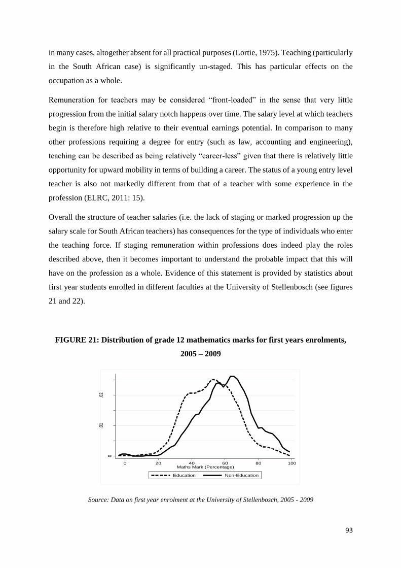
93

in many cases, altogether absent for all practical purposes (Lortie, 1975). Teaching (particularly

in the South African case) is significantly un-staged. This has particular effects on the

occupation as a whole.

Remuneration for teachers may be considered “front-loaded” in the sense that very little

progression from the initial salary notch happens over time. The salary level at which teachers

begin is therefore high relative to their eventual earnings potential. In comparison to many

other professions requiring a degree for entry (such as law, accounting and engineering),

teaching can be described as being relatively “career-less” given that there is relatively little

opportunity for upward mobility in terms of building a career. The status of a young entry level

teacher is also not markedly different from that of a teacher with some experience in the

profession (ELRC, 2011: 15).

Overall the structure of teacher salaries (i.e. the lack of staging or marked progression up the

salary scale for South African teachers) has consequences for the type of individuals who enter

the teaching force. If staging remuneration within professions does indeed play the roles

described above, then it becomes important to understand the probable impact that this will

have on the profession as a whole. Evidence of this statement is provided by statistics about

first year students enrolled in different faculties at the University of Stellenbosch (see figures

21 and 22).

FIGURE 21: Distribution of grade 12 mathematics marks for first years enrolments,

2005 – 2009

Source: Data on first year enrolment at the University of Stellenbosch, 2005 - 2009

0

.005

.01

.015

.02

.025

0 20 40 60 80 100Maths Mark (Percentage)

Education Non-Education

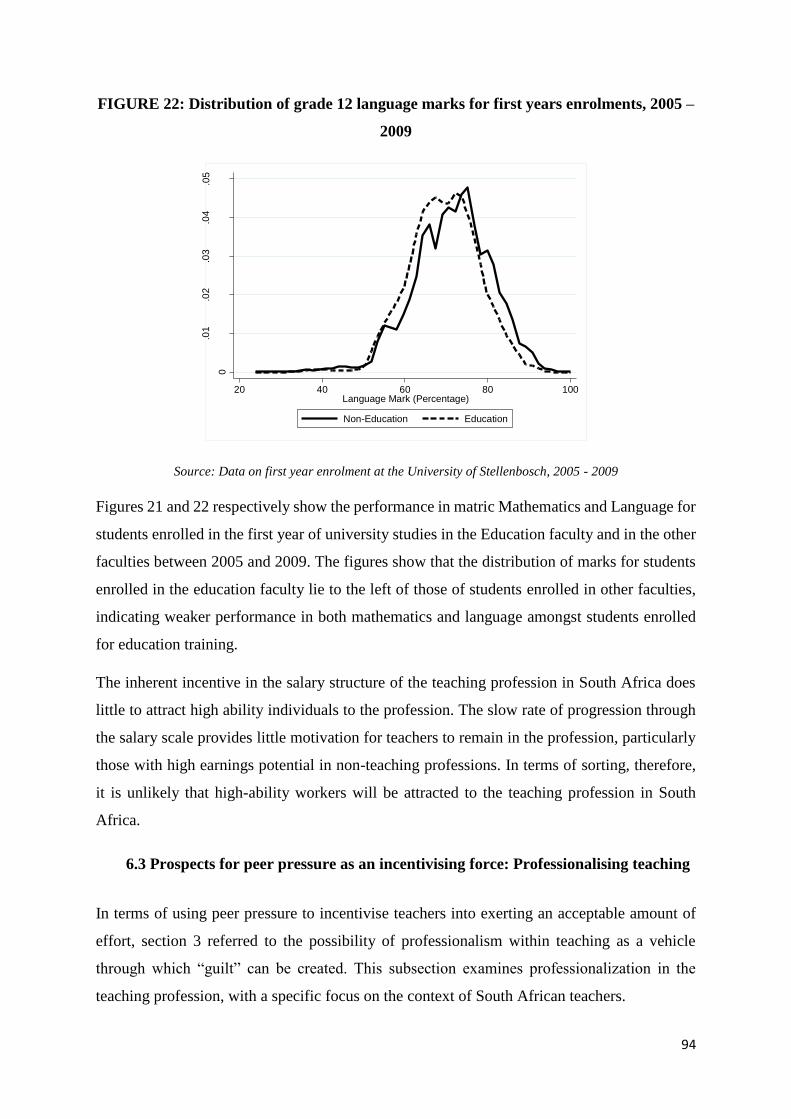
94

FIGURE 22: Distribution of grade 12 language marks for first years enrolments, 2005 –

2009

Source: Data on first year enrolment at the University of Stellenbosch, 2005 - 2009

Figures 21 and 22 respectively show the performance in matric Mathematics and Language for

students enrolled in the first year of university studies in the Education faculty and in the other

faculties between 2005 and 2009. The figures show that the distribution of marks for students

enrolled in the education faculty lie to the left of those of students enrolled in other faculties,

indicating weaker performance in both mathematics and language amongst students enrolled

for education training.

The inherent incentive in the salary structure of the teaching profession in South Africa does

little to attract high ability individuals to the profession. The slow rate of progression through

the salary scale provides little motivation for teachers to remain in the profession, particularly

those with high earnings potential in non-teaching professions. In terms of sorting, therefore,

it is unlikely that high-ability workers will be attracted to the teaching profession in South

Africa.

6.3 Prospects for peer pressure as an incentivising force: Professionalising teaching

In terms of using peer pressure to incentivise teachers into exerting an acceptable amount of

effort, section 3 referred to the possibility of professionalism within teaching as a vehicle

through which “guilt” can be created. This subsection examines professionalization in the

teaching profession, with a specific focus on the context of South African teachers.

0

.01

.02

.03

.04

.05

20 40 60 80 100Language Mark (Percentage)

Non-Education Education

95

Bennell (2004: 3) explains that in many low-income countries, teachers have a “semi-

professional” status relative to occupations such as lawyers, engineers and doctors. This is

largely the result of lower levels of education, relative to such professions, as well as a result

of the size of the teaching force. “[T]he sheer size of the teaching force militates against

professional exclusivity” (Bennell, 2004: 3). In many Sub-Saharan African and South Asian

countries, teaching is considered “employment of last resort” and as a result, a fair number of

teachers do not consider staying in the profession long term.

The ELRC’s Revised Salary Structure Proposal of 2011 indicates that teachers feel that their

social and economic status have been eroded (ELRC, 2011: 28). There is a strong need amongst

teachers to be recognised as professionals. There is a strong belief that the knowledge and skills

requirements for teachers are equal to what is required in other professions, and that this is

likely to be the case increasingly given that teaching now officially requires a degree for entry

into the profession (ELRC, 2011: 28).

Pratte and Rury (1991: 64) describe professionalism as “an ideal to which individuals and

occupational groups aspire, in order to distinguish themselves from other workers”. The

characteristics of a profession from which professionals derive their prestige are a) mastery of

a distinctive body of knowledge, b) the control of membership of the profession and c) a

commitment to the well-being of their client.

Professionals are expected to have expert knowledge in their field and the profession is largely

based around identification with a distinctive body of knowledge. Organisations employing

professionals function largely as communities of associates as opposed to being based on

supervisory authority. The expertise of the professionals is the basis of their professional

autonomy and authoritative power (Pratte & Rury, 1991: 66).

In terms of controlled access to the profession, the creation, diffusion and implementation of

the professional standards of practice are assumed collectively by members of the profession.

The licensing and to some extent the education of members is controlled by members of the

profession and entrance into the profession (typically graduate level university study) is

rationed to those achieving a minimum level of competency in their education up to that point.

Having completed the academic programme, candidates are required to pass demanding tests

of their theoretical knowledge as well as complete a kind of internship during which they are

continuously evaluated. The function of controlling the membership of the profession therefore

96

serves the function both of controlling induction into the profession and ensuring that the

acquisition of knowledge is standardised across the profession (Pratte & Rury, 1991: 66).

Finally, professional practitioners commit to the pursuit of the welfare of their clients, usually

through the acceptance of codes of ethics established by professional peers. Client

dissatisfaction with the service of professionals is therefore dealt with through the initiation of

a legal process rather than by reporting to the supervisor of the professional (Ambroise &

Harley, 1988).

Lortie (1975) explains that the educational preparation of teachers is relatively general by

comparison to that required by individuals entering into what are typically regarded as

professions in the labour market. Teacher education does not require the same degree of

intellectual rigour required in professions such as law, medicine or engineering. Education

lacks the scientific roots or scholarly development that characterise those professions (Lortie,

1975); furthermore, teacher education and training takes place largely in the format of lectures

and discussions, whereas traditional professions often require candidates to master the skills

necessary for their professions in special settings such as laboratories. Teaching therefore does

not require mastery of distinctive body of knowledge to the same extent that other widely

recognised professions do.

Controlling access to the teaching profession in South Africa is not characteristic of “an ideal

to which individuals and occupational groups aspire, in order to distinguish themselves from

other workers” (Pratte & Rury, 1991: 72). Charles Simkins (2010: 11) reports that some 45%

of new teacher registrations with the South African Council of Educators (SACE) in 2009/10

were provisional registrations given to teachers with less than the required qualifications.

Therefore, a very large portion of individuals entering the occupation and being allowed to

practise as teachers did not have the legally required qualifications (Simkins, 2010: 11). This

stands in stark contrast to the pursuit of prestige and exclusivity inherent in controlling access

to a profession.

South African teachers are exposed to approximately 150 to 160 practice teaching days (in the

case of a 3 year teaching qualification), 200 to 220 practice teaching days (in the case of a 4

year teaching qualification) or 50 to 55 days (in the case of a 1 year postgraduate teaching

qualification) over the duration of their teacher education (University of Stellenbosch, 2012).

This is justification for Lortie’s (1975) observation that “one of the striking features of teaching

is the abruptness with which full responsibility is assumed.” By comparison to professions

97

requiring extensive residency or clerical work once formal education has been completed, the

“internship” required by teachers is significantly less rigorous.

It seems then that teaching in South Africa (as in many other countries) is ill-fitted to

professionalization. The nature of the knowledge required to enter the occupation and the

absence of the rigorous entry procedures that exist for other professions make it difficult to

justify a call for the professionalization of teaching in its current state. The teaching profession

would have to be “recast” as one requiring rigorous preparation and one which holds a fair

amount of prestige. Countries in which teaching is considered a prestigious profession have,

however, achieved phenomenal educational success.

In the absence of strong professionalism, peer pressure may incentivise teachers if ways can be

found in which teachers can monitor one another’s behaviour and exert pressure on teachers

who do not exert the required amount of effort, and if this pressure is likely to result in a change

in behaviour.

Section 6.4 explores the monitoring system currently in place amongst South African teachers

and considers the probability that such monitoring would result in increased effort amongst

teachers.

6.4 Mutual monitoring: The Integrated Quality Management System

In the absence of professionalization, peer pressure is created through mutual monitoring of

workers. The use of peer pressure to enhance effort levels requires that monitoring by peers

actually results in enhanced effort. The possibility of imposing punishment on team members

who do not pull their weight should therefore exist.

Currently, the system whereby teacher performance is measured and recorded in South Africa

is the Integrated Quality Management System (IQMS). The IQMS handles teacher evaluation

through self-evaluation by teachers and through a development support group (DSG) (ELRC,

2003). The self-evaluation and the evaluation conducted by the development support group use

the same instrument so that teachers are familiar with the criteria according to which they are

to be judged. The DSG is comprised of the teacher’s immediate senior (i.e. head of department,

or deputy principal in the case of a head of department) and one peer in their field of

specialisation. They may choose which of their peers they would like to be part of the DSG.

Teachers are graded according to 12 performance standards and both the self-evaluation and

the evaluation conducted by the development support group are considered in the overall

98

evaluation. The evaluation happens once every year and its primary objective is to help teachers

develop growth plans (ELRC, 2003). Teachers are therefore involved directly in monitoring

the performance of their peers. The procedure is intended to have a nurturing and

developmental role, however, and is most definitely not designed to enable teachers to apply

any kind of pressure or disciplinary actions against their peers. Furthermore, the fact that

teachers are allowed to choose the peer who will form part of the DSG provides the opportunity

for teachers to influence the type of assessment they may receive from the group members.

Although it is stipulated that educators must appoint peers from their field of specialisation,

there are no other requirements or restrictions on who teachers may choose to be part of the

group. It is therefore possible that teachers will choose peers most likely to provide them with

a good assessment. In this way, distortion may occur as a teacher is able to influence the

outcome of the performance measure, albeit indirectly.

Peer pressure as a mechanism for incentivising teachers is unlikely to prove effective in the

present system. Because it is a once-yearly exercise and because teachers choose their

assessors, it is highly unlikely that teachers will be able to exert any kind of pressure on their

co-workers, or that increased monitoring will result in higher effort levels.

6.5 Inequality prevails

A common problem with teacher incentives and one which is particularly relevant in the South

African context is that evaluation depends on student performance on standardised tests. A

strong argument against using such measures for evaluation is that student performance is

significantly affected by many factors outside the classroom and the school and therefore

outside the teacher’s control. It is seems grossly unfair to rank and reward teachers according

to a measure that is to a large extent outside their control. Also important in South Africa is the

issue of inequality and fairness. South Africa’s history of inequality, particularly in the

education sector, resulted in substantial differences in the quality of the training received by

teachers from different race groups (Van der Berg, 2006: 3). Furthermore, the endurance of the

apartheid legacy in educational quality means that awarding incentives based on student

performance is simply not fair. Teachers cannot be judged on the performance of their students

alone.

99

Chapter 3 The impact of teacher characteristics on student

performance: An analysis using hierarchical linear

modelling

1. Introduction

The impact of teacher characteristics (both qualifications and demographic characteristics) is

important for education policy. Ensuring that teachers best suited and most able to enhance

student performance are employed is a key responsibility for policymakers. Wayne and Youngs

(2003: 89) explain that a large body of literature about teacher characteristics and education

outcomes exists. The focus on the studies vary between questions about teacher quantity and

turnover and issues surrounding teacher quality. In many countries (South Africa included)

certain qualifications need to be obtained before teachers are permitted to enter the teaching

force. Much of the literature surrounding teacher characteristics and student performance is

comprised of analyses of the impact of these and other qualifications. Attempts have been made

to identify trends in the quality of teachers, and the question whether characteristics of teachers

in different parts of the schooling system exist is often investigated (Wayne & Youngs, 2003:

90).

The relationship between teacher characteristics and student performance is surprisingly

elusive, however. Researchers have found it difficult to find aspects of teacher training that

correlate with student performance in a statistically significant way (Chingos & Peterson, 2011:

449). Conflicting or indeterminate results occur often. Summers and Wolfe (1977) investigated

the impact of teacher scores on “Philadelphia’s National Teacher Evaluations” on performance

amongst primary schools students in that state, finding a negative relationship between teacher

performance and student scores on standardised tests. Anderson (2000) investigates the

determinants of student performance in mathematics and language in Mexico and finds a

positive and statistically significant impact in both mathematics and language for teachers

making use of a more interactive approach to teaching as opposed to a traditional approach in

100

which lessons are dominated by teachers talking and instructing (Anderson, 2000: 144). She

also finds evidence of a positive relationship between hours spent teaching and performance in

both subjects25 (Anderson, 2000: 145). Teacher effort variables therefore impact positively and

statistically significantly on student performance. An interesting and important result is the

positive and significant impact on both language and mathematics observed for teacher training

during the year in which the study was conducted (Anderson, 2000: 146). Angrist and Lavy

(2001) find positive estimates of the impact of in-service teacher training on both mathematics

and language in secular primary schools in Jerusalem. They report that their results are robust

to a number of estimation techniques, namely regression, difference-in-difference techniques

as well as matching techniques. The fact that the effect is only observed in secular schools may

be due to the fact that the training programme was introduced later and on a smaller scale in

religious schools (Angrist & Lavy, 2001: 365).

Ferguson (1998) used data from the “Texas Examination of Current Administrators and

Teachers” to evaluate the impact of student performance at all levels of the schooling system.

Contrary to the results obtained by Summers and Wolfe, Ferguson found a positive correlation

between student performance and teacher test scores.26 The relationship between teacher

performance on tests in the subject they teach and student performance in that subject has also

been tested extensively. Positive associations between teacher test score and student

performance are observed in some studies across a range of subjects (Ehrenberg & Brewer,

1995; Hanushek, 1992; Rowan, Chiang & Miller, 1997), while others find a negative impact

of teacher test scores on student outcomes (Murnane & Phillips, 1981). It seems then that the

evidence regarding the impact of teacher content knowledge on student outcomes is mixed.

Results obtained for formal teacher qualifications were also mixed, with the majority of studies

conducted returning indeterminate results. Amongst those that did return results, both negative

and positive impacts were observed (Wayne & Youngs, 2003: 101-103). The existing research

therefore leaves us with few answers to questions about the relationship between teacher

qualifications and student performance. Indeed, are teacher qualifications important at all?

25 Anderson notes that this variable is self-reported (Anderson, 2000: 145) and may well be over-reported.

However, if this is the case, it likely that the coefficient on this variables is a lower bound of the effect of time

on task of student performance. 26 Important to note is that Ferguson’s study aggregated data to the district level. Hanushek, Rivkin and Taylor

(1996: 616) explain that aggregating data to a “higher” level (i.e. school, district or state level) increases the

likelihood of obtaining positive results.

101

Evidence from Pakistan suggests that teacher qualifications are indeed important for student

performance. Arif and Saqib (2003) control for the individual and family characteristics of

students, the characteristics of the schools they attend, geographic characteristics as well as a

range of teacher characteristics and find that whether a teacher has a bachelor’s degree or higher

is positively and statistically significantly associated with student performance in language,

mathematics and general knowledge as well as a measure capturing performance in all three

(Arif & Saqib, 2003: 19-20). An earlier study conducted in Pakistan (Behrman, Kahn, Ross &

Sabot, 1997) construct teacher quality indices for language and mathematics. These indices are

linear functions of teacher performance on literacy or numeracy tests, educational attainment,

and teaching experience and its squared term (Behrman et al., 1997: 131). Controlling for

student demographic characteristics and family background, school characteristics, student-

teacher ratios and student ability, they find a positive and statistically significant relationship

between the teacher quality index and student performance in both numeracy and literacy

(although the effect seems to be larger in literacy – an interesting result, since an effect, if

observed at all, is usually stronger in the case of mathematics) (Behrman et al., 1997: 133).

Another study that finds a relationship between observable teacher characteristics and student

performance was conducted by Slater, Davies and Burgess (2009) using UK data for 7 000

students (14 year olds) writing GCSE Keystage 4 examinations.27 Slater et al. (2009)

investigate whether the observable characteristics of teachers are correlated with measures of

teacher effectiveness. Teacher effectiveness is measured as the effect that teachers have on

student performance on the examinations. The observable characteristics available are teacher

gender, age, educational attainment and teaching experience. None of these characteristics are

statistically significant in explaining teacher effectiveness (Slater et al., 2009: 12). Interesting

to note, however, is that Slater et al. (2009: 13) find a correlation (albeit weak) between the

ability of students and teacher effectiveness, suggesting non-random allocation of students

within a school. Allocating students to teachers in such a way that places less able students

with more effective teachers may well enhance the positive impact of teacher effectiveness.

27 Keystage 4 examinations are compulsory examinations dictating entrance to post-secondary education. These

are written at age 16. Keystage 3 examinations are written at the beginning of Keystage 4 programme during the

year that students turn 14 (Slater, Davies & Burgess, 2009: 4). Keystage 3 examinations are often used as a

“pre-test” measure in education research, or an as indication of prior attainment.

102

Raudenbush, Eamsukkawat, Di-Ibor, Kamali and Taoklam (1993) investigate whether in-

service training affects student performance significantly. They measure in-service training by

including a variable capturing the amount of exposure (in terms of days) of in-service training

as well as a variable controlling for the number of times that teachers received internal

supervision (Raudenbush et al., 1993: 286). They also include a measure of whether a teacher

has a bachelor’s degree. They come up with a very interesting result: although in-service

training does not appear to have any significant effect on student performance, internal

supervision (by the school principal or another teacher at the school)28 has a large and

significant effect. They explain the effect of intensive internal supervision as being as large as

a teacher obtaining a bachelor’s degree (Raudenbush et al., 1993: 294). It appears then that

although formal in-service training does not appear to improve teacher quality, a type of

mentoring and “coaching” approach does. Results from a study conducted using Cambodian

data (Marshall, Chinna, Nessay, Hok, Savoeun, Tinon & Vaesna, 2009: 406) show positive and

significant effects (as well as inequality reducing effects) on the performance of grade 6

students on language tests. High levels of mathematical content knowledge amongst teachers

also showed a positive and significant effect on grade 6 mathematics performance and high

levels of mathematics pedagogical content knowledge had a significant impact on grade 3

mathematics performance (Marshall et al., 2009: 406). The authors did not control for formal

teacher qualifications or teaching experience separate to content knowledge. Luschei and

Carnoy (2010: 175) find no significant impact for teachers’ postgraduate education on student

performance in mathematics or language in a study conducted using Uruguayan data.

Interestingly, however, high levels of teaching experience (10 years and above) are positively

and significantly associated with both mathematics and language performance (Luschei &

Carnoy, 2010: 175-176).

Another study that finds a statistically significant relationship between teaching experience and

student performance is that of Clotfleter, Ladd and Vigdor (2007). These authors use North

Carolina data to investigate the relationship between teacher characteristics and student

performance. Since the early 1990s, the state of North Carolina has administered standardised

mathematics and reading tests to all students between grades 3 and 8 (Clotfelter et al., 2007:

675). Furthermore, it is possible to match students to their teachers for each year. The authors

are able to identify the teachers of at least 75% of grade 3, 4 and 5 students in the state’s

28 This is in contrast to external supervision by a district official (Raudenbush et al., 1993: 294) which shows no

significant impact on student performance.

103

education system between 1993/1994 and 2003/2004, rendering it possible for them to conduct

analysis on the impact of teacher characteristics on both the levels of mathematics and English

performance and the gains in performance from year to year (and therefore controlling for

various student and school-level effects, the gains that may be tentatively associated with the

teacher) (Clotfelter et al., 2007: 675). The authors find a positive and statistically significant

impact for teacher experience on student performance in both mathematics and English

(Clotfelter et al., 2007: 676).29 The size of the coefficients indicate that the majority (or more

than half) of the returns to teaching experience occur within the first two years of teaching. An

issue often raised when investigating returns to teaching experience is the possibility that

positive returns to experience are overstated if it is likely that underperforming or weaker

teachers will leave the profession after their initial year (Rockoff, 2004: 248). The authors test

for this possibility by adding a variable controlling for whether a teacher remained in the

profession in North Carolina for at least three years. They interact it with the categorical

variables controlling teachers with 1 to 2 years of teaching experience. If weaker teachers leave

the profession after their early years as teachers, a positive coefficient on the variable

controlling for those who remain in the profession is expected. However, the opposite is

observed. In the case of mathematics, a negative and statistically significant coefficient is

observed in both the levels and gains model, suggesting that those who leave teaching are not

less able than their counterparts who remain in the profession. Furthermore, the interaction

term is not statistically significant in either subject, suggesting that it is not differential attrition

that drives the increasing returns to teaching experience observed in the data (Clotfelter et al.,

2007: 676).

“By many accounts, the quality of teachers is the key element to improving student

performance” (Hanushek, 2009: 171). The impact of being taught by a good teacher is

quantified by Hanushek (2011: 42) where he estimates that students who perform a standard

deviation above average (as measured by performance on high school tests) earn between 10

and 15 percent more per annum than average – an estimate he deems conservative as it is

measured in the early years of their career (before they have reached their full earning potential)

and it does not account for the possibility that higher performance at high school level probably

29 Teacher experience is captured by categorical variables denoting 1 to 2 years of experience, 3 to 5 years of

experience, 6 to 12 years of experience, 13 to 20 years of experience, 21 to 27 years of experience and more than

27 years of experience. They therefore control for non-linear returns to teaching experience (Clotfelter et al., 2007:

676). The returns observed are higher for mathematics than they are for English – a finding largely in line with

what is found in the literature about teaching experience and student performance.

104

results in higher educational attainment (Hanushek, 2011: 42). The home background and

motivation of the student obviously contribute significantly to the level of success that students

are able to achieve, but rigorous research has isolated the impact of effective teaching on

student performance. Hanushek (2011: 42) reports that studies have consistently shown that

high-performing teachers (performing 1 standard deviation above the mean, or at the 84th

percentile of the distribution) result in student grades that are at least 0.2 standard deviations

higher at the end of a school year. Although these gains diminish over time, it is estimated

(although somewhat less conclusively) that the long term benefit of being taught by an effective

teacher is 70 percent of the immediate gain, and so consecutive years of high quality teachers

result in student outcomes markedly higher than they would have been had students been taught

by teachers at the 50th percentile of the distribution (Hanushek, 2011: 42). It is clear then

teacher quality and teacher effectiveness have a considerable effect on the lifetime earnings of

students.

Evidence of the impact of teacher quality in later life also exists. Chetty, Friedman and Rockoff

(2011) find evidence of fairly sizeable impacts of teacher quality on adult earnings of their

students. Teacher quality (measured by value added) improves the probability of college

attendance, the quality of college attended by students (measured by the earnings of former

students of colleges) as well as future earnings of students (Chetty et al., 2011: 2).

How then should we measure teacher quality? To what extent are we “missing the point?” An

important aspect of teacher quality and teacher effectiveness to consider is the extent to which

the education received by teachers is well-suited to enabling them to teach. A significant

literature (some of which is discussed above) exists around whether teaching is an attractive

profession to highly able individuals endowed with skills that fetch a high price in the labour

market. It is important to understand whether or not those skills are likely to translate into

positive outcomes for students or whether there is “something else” required of teachers that

does not necessarily guarantee that highly able individuals will be effective teachers. One way

to approach this question is to investigate the specific knowledge requirements of teachers.

The National Council of Teachers of Mathematics in US (NCTM) refers to teacher’s

knowledge of their students as students as being central to their ability to influence their

performance (NCTM, 2000: 17). This broadly refers to teachers being able to identify

“preconceptions and background knowledge that students typically bring to each subject”

(National Board for Professional Teaching Standards (NBPTS), 2012: vi). This is essentially

105

what is referred to as Pedagogical Content Knowledge (PCK) (Hill, Loewenberg Ball &

Schilling, 2008: 373). Although its importance in improving student outcomes is widely

acknowledged, very little exists in the way of empirical evidence and understanding of this

relationship. Hill et al. (2008: 373) believe that this results from two factors. Firstly, there is an

absence of studies that are able to prove that teachers possess such knowledge, and secondly,

measures to assess programmes which aim to develop this knowledge and its impact on student

achievement have not yet been developed. In the absence of such measures, it may be difficult

to measure the aspect of teacher quality that truly affects student performance.

Research that does investigate the type and depth of subject (and other) knowledge required to

teach presents some very important results. The mathematical knowledge required of

mathematics teachers is extensive (Ball, Thames & Phelps, 2008: 399). The tasks involved in

teaching mathematics require “significant mathematical knowledge, skill, habits of mind and

insight” (Ball et al., 2008: 399). What is referred to as common content knowledge is the

mathematical knowledge that teachers require to perform their job. Teachers also require

specialised content knowledge – mathematical knowledge and skills particular to teaching. This

type of mathematical knowledge is not particularly useful (or even desirable) outside the

context of teaching and requires a certain “unpacking” of mathematical knowledge. Examples

of this kind of mathematical content knowledge would be the analysis of student errors or

evaluating whether a nonstandard approach to calculation would work in general (Ball et al.,

2008: 400). A third domain, knowledge of content and students, involves understanding and

therefore anticipating how students will interpret and understand the work and where they will

experience difficulty (Ball et al., 2008: 401). The fourth domain, knowledge of mathematics

and teaching, refers to an understanding of how mathematics should be taught. For example,

the sequencing of topics and examples would fall under this category of mathematical

knowledge (Ball et al., 2008: 401). The authors point out that the mathematical knowledge

required of teachers (and indeed teachers across different fields and subjects) includes and

extends beyond that of other professions requiring mathematical knowledge. This is important

to acknowledge this when evaluating the importance of the profession in society.

A rare study in which the impact of different kinds of mathematics knowledge amongst

teachers (based to a large extent on the findings of Ball et al. discussed above) was tested

amongst students attending schools in rural Guatemala (Marshall & Sorto, 2012) presented

encouraging results. Using hierarchical linear modelling, they test the impact of different kinds

of teacher knowledge in different areas of mathematics performance. Interestingly, they find

106

coefficients of very similar size to those observed in US studies. Marshall and Sorto (2012:

188) find significant results for what they call “mathematics knowledge for teaching” (as

opposed to common content knowledge and specialised content knowledge). Interestingly and

importantly, the coefficients for mathematics knowledge for teaching are largest and most

significant for areas of the mathematics test that have the highest degree of cognitive demand

required of students (Marshall & Sorto, 2012: 191). This makes intuitive sense – the more

difficult the content, the more specialised a teacher needs to be to ensure that student learning

takes place.

In a South African context, Fleisch (2004: 264) finds inconclusive results regarding the

relationship between higher levels of teacher resources and student performance. However,

Fleisch explains the importance of understanding the absence of the relationship. Indeed, if

education policy aims to improve the state of education through changes around teacher policy,

then caution must be exercised when considering this policy (Fleisch, 2004: 264). Qualitative

research on what happens in schools is required in order to understand how teachers can be

best utilised to improve education outcomes. Other South African research by Crouch &

Mabogoane (2001: 64-65) finds a strong correlation between teacher qualifications and student

performance on matric (grade 12) examinations. As a result, these authors suggest the

possibility of upgrading teacher qualifications as a means to improve student outcomes (Crouch

& Mabogoane, 2001: 75).

This chapter aims to investigate which characteristics of South African teachers, both

demographic and in terms of qualifications and teaching experience, impact on student

performance. The chapter is organised as follows: section 2 defines the research question,

introduces the dataset that will be used in the analysis, SACMEQ III, and provides the

descriptive statistics of the variables that will be included in the model. Section 3 discusses the

necessity for hierarchical linear modelling, while section 4 presents the model that will be

specified in attempting to answer the research question. Section 5 presents the results obtained

from the model, and section 6 concludes with a discussion of the possible driving factors behind

these results.

107

2. Research question and data

2.1 Defining the research question

As indicated, this research aims to answer the question of whether teacher characteristics (both

demographic and human capital) impact student performance. As explained, South Africa’s

educational performance is weak. The question we attempt to answer in this chapter is whether

this weak performance can be explained by observable teacher characteristics. In order to

measure the impact of these characteristics, the fact that students share “teacher characteristics”

with the students in the same class means that the assumptions that would render ordinary least

squares (OLS) regression coefficients accurate (i.e. that students are drawn from a random

sample) are violated. The multi-level nature of the data requires that this element be controlled

for and modelled in the investigation. This is discussed at length in section 3. In summary, the

confidence intervals that would result from OLS would be deceptively narrow as a result of

inaccurately small standard errors (Arnold, 1992: 62). Students being taught by the same

teacher not only share “teacher characteristics”, but are also more likely to be more similar to

one another than to students taught by different teachers. This further violates the assumption

of students being drawn at random (Arnold, 1992: 62).

The following subsection explains the data used to conduct the analysis – the third study

conducted, in 2007, by the Southern and Eastern African Consortium for Monitoring

Educational Quality (SACMEQ III).

2.2 Data: SACMEQ III

The paper makes use of data collected by the third study conducted by SACMEQ in 2007.

SACMEQ was launched in 1995 with the objective of conducting research and providing

training that enables policy makers to monitor and improve their education systems (Moloi and

Strauss, 2005: 12). SACEMQ undertook 3 major surveys (referred to as SACMEQ I, II and III)

in 1995, 1998 and 2007 respectively. 15 countries participated in SACMEQ III, namely

Botswana, Kenya, Lesotho, Malawi, Mauritius, Mozambique, Namibia, Seychelles, South

Africa, Tanzania (Mainland and Zanzibar), Uganda, Zambia and Zimbabwe (Spaull, 2011b:

4).

SACMEQ III involved administering 3 tests to grade 6 students - a reading test, a mathematics

test and a health test (aimed largely at measuring the level of knowledge about HIV/AIDS). In

108

South Africa, 9 038 grade 6 students in 392 schools were tested, along with 498 mathematics

teachers, 498 reading teachers and 492 health teachers (totalling 1 488). All the teachers

completed a health test, and reading and mathematics teachers completed a test in the subject

that they taught (Spaull, 2011b: 5).

The data obtained from SACMEQ III comprise the most extensive nationally representative

sample available for the South African education system.30 Importantly, the testing was only

conducted in English and Afrikaans. It is therefore highly likely (if not certain) that a significant

proportion of the students writing the tests were disadvantaged in terms of understanding the

mathematics questions, given that neither English nor Afrikaans was their first language. The

extent to which English is spoken outside of school is controlled for at the student level but the

dataset did not contain the corresponding variable for Afrikaans. It is worth noting, however,

that the aforementioned language disadvantage applies to the majority of students tested in

South Africa (Moloi and Strauss, 2005: 67).

Importantly, in any analysis of performance in education making use of cross-sectional data

that does not contain a pre-test score, unobservable characteristics of students (such as

motivation or intelligence) which influence their performance on mathematics tests are

therefore not controlled for. It is also important to bear in mind that the impact of teachers on

students’ education is cumulative. The results observed in grade 6 therefore reflect the impact

of teachers throughout students’ educational “career” and cannot be attributed only to the

teachers by whom students are taught in that year. Having said that, we do not have a pre-test

score and we are therefore not able to control for students’ ability or level of performance

before their exposure to their current teacher.

2.3 Variables included in the model

Table 5 below provides a brief explanation of the variables included in the investigation as well

as the means and standard deviations. The dependent variable, 𝑍𝑀𝐴𝑇𝑖𝑗, is the z-scored

(standardised) mathematics score of student i in classroom j. Z-scoring the dependent variable

centres the variable around a mean value of 0 and gives the variable a standard deviation of 1.

30 Mullens, Murnane and Willett (1996: 140) explain the need for longitudinal data in assessing the impact of

teachers on student learning. In the majority of studies investigating this topic in the developing world,

longitudinal data are not available and so researchers have no choice but to use cross-sectional data. Cross-

sectional data can only tell us about the level of student achievement and not about the progress that takes place

(i.e. the actual learning). However, data on changes in achievement are necessary to truly evaluate the

effectiveness of teachers (Mullens et al., 1996: 140).

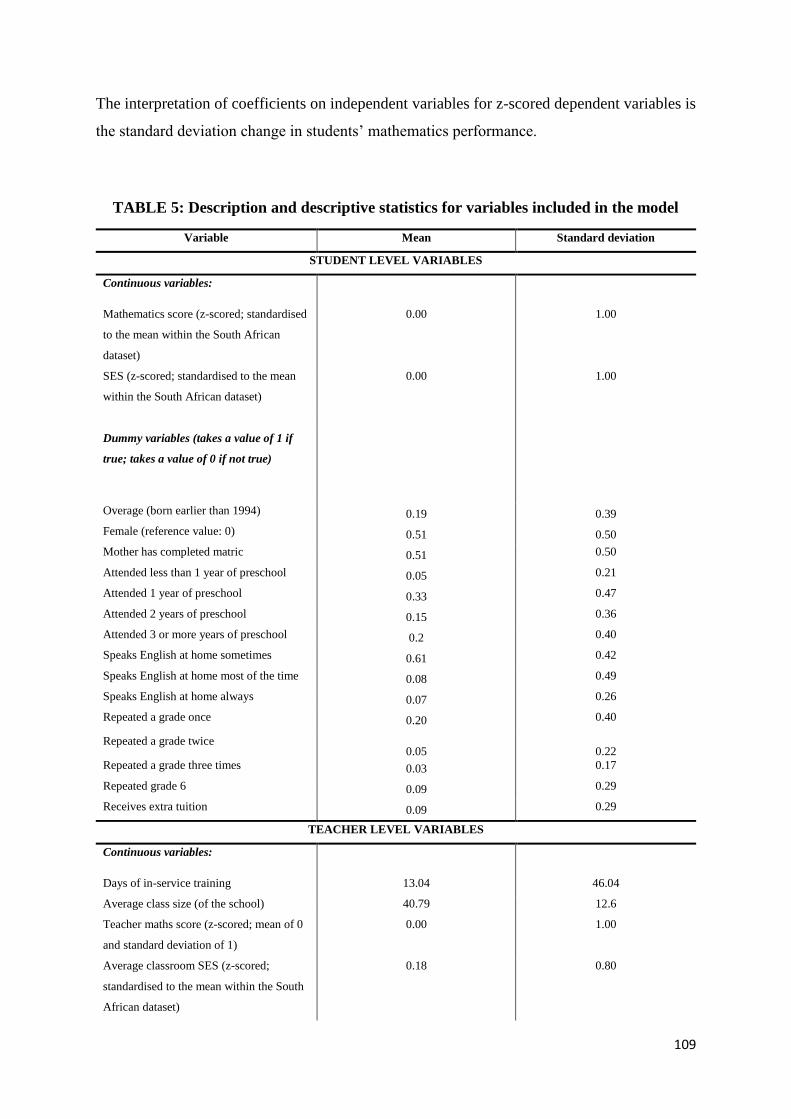
109

The interpretation of coefficients on independent variables for z-scored dependent variables is

the standard deviation change in students’ mathematics performance.

TABLE 5: Description and descriptive statistics for variables included in the model

Variable Mean Standard deviation

STUDENT LEVEL VARIABLES

Continuous variables:

Mathematics score (z-scored; standardised

to the mean within the South African

dataset)

0.00 1.00

SES (z-scored; standardised to the mean

within the South African dataset)

0.00

1.00

Dummy variables (takes a value of 1 if

true; takes a value of 0 if not true)

Overage (born earlier than 1994) 0.19 0.39

Female (reference value: 0) 0.51 0.50

Mother has completed matric 0.51 0.50

Attended less than 1 year of preschool 0.05 0.21

Attended 1 year of preschool 0.33 0.47

Attended 2 years of preschool 0.15 0.36

Attended 3 or more years of preschool 0.2 0.40

Speaks English at home sometimes 0.61 0.42

Speaks English at home most of the time 0.08 0.49

Speaks English at home always 0.07 0.26

Repeated a grade once 0.20 0.40

Repeated a grade twice

0.05

0.22

Repeated a grade three times 0.03 0.17

Repeated grade 6 0.09 0.29

Receives extra tuition 0.09 0.29

TEACHER LEVEL VARIABLES

Continuous variables:

Days of in-service training 13.04 46.04

Average class size (of the school) 40.79 12.6

Teacher maths score (z-scored; mean of 0

and standard deviation of 1)

0.00 1.00

Average classroom SES (z-scored;

standardised to the mean within the South

African dataset)

0.18 0.80

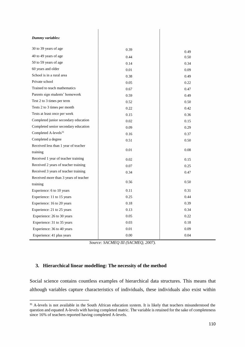
110

Dummy variables:

30 to 39 years of age 0.39

0.49

40 to 49 years of age 0.44 0.50

50 to 59 years of age 0.14 0.34

60 years and older 0.01 0.09

School is in a rural area 0.38 0.49

Private school 0.05 0.22

Trained to teach mathematics 0.67 0.47

Parents sign students’ homework 0.59 0.49

Test 2 to 3 times per term 0.52 0.50

Tests 2 to 3 times per month 0.22 0.42

Tests at least once per week 0.15 0.36

Completed junior secondary education 0.02 0.15

Completed senior secondary education 0.09 0.29

Completed A-levels31 0.16 0.37

Completed a degree 0.51 0.50

Received less than 1 year of teacher

training 0.01 0.08

Received 1 year of teacher training 0.02 0.15

Received 2 years of teacher training 0.07 0.25

Received 3 years of teacher training 0.34 0.47

Received more than 3 years of teacher

training

0.56

0.50

Experience: 6 to 10 years 0.11 0.31







Experience: 41 plus years 0.00 0.04

Source: SACMEQ III (SACMEQ, 2007).

3. Hierarchical linear modelling: The necessity of the method

Social science contains countless examples of hierarchical data structures. This means that

although variables capture characteristics of individuals, these individuals also exist within

31 A-levels is not available in the South African education system. It is likely that teachers misunderstood the

question and equated A-levels with having completed matric. The variable is retained for the sake of completeness

since 16% of teachers reported having completed A-levels.

111

larger groups and a set of variables describe the groups (Raudenbush & Bryk, 2002: xix). A

classic example of hierarchical data structure is education data. Students are grouped according

to the schools they attend, so individual or learner-level variables describe individual students,

and school-level variables describe schools. Although school-level variables may be

independent of the students (for example, the type of buildings or the geographical location of

the school), school-level variables may also represent aggregated learner-level data (for

example, the racial or gender composition of the school or the average socioeconomic status

of the students attending the school). The school probably consists of smaller groups such as

classrooms, which have their own characteristics captured by classroom-level variables.

Schools may also form the smaller groups contained in school districts (Raudenbush & Bryk,

2002: xix).

In this chapter we are interested in understanding how teacher characteristics influence student

performance. As described above, students are grouped within classrooms which in turn are

grouped within schools. In education the context in which students are educated is immensely

influential in determining their performance. In other words, characteristics of the school

classroom significantly influence the level of learning that takes place for individual students

and therefore their performance on standardised tests (Luke, 2004: 1). Relationships and

occurrences at the higher level of analysis affect what happens at the lower level of analysis.

In South Africa the context in which learning takes place differs dramatically across the school

system and so the variables describing characteristics at the classroom and school level reflect

large differences between schools within the country. We are interested in how these

differences at the higher level impact on lower level performance (Luke, 2004: 4-5). For

example, how do differences in school management characteristics translate into differences in

the performance of students on standardised mathematics and language tests? How does

teacher training impact on student performance in mathematics and language tests?

The strongest motivation for making use of hierarchical linear modelling has to do with

inaccuracies in the measurement of standard errors. If multi-level data are analysed solely at

the level of the individual, two problems arise. The first of these is that the individual error

term contains all the contextual information that has not been modelled (Duncan, Jones &

Moon, 1998: 98). One of the basic assumptions of multiple regression is that there is no

correlation between the error terms of individual observations – an assumption which is

violated if individuals (students) share the same context (classroom or school) and the

characteristics of this context are not modelled (Luke, 2004: 7). Students who attend the same

112

school or who are taught in the same classroom will probably be more similar to one another

than if they were selected at random. Secondly, if the context in which individuals find

themselves is not explicitly acknowledged and modelled, regression coefficients is assumed to

be equally relevant for all contexts (Duncan et al., 1998: 98). This would indicate that variables

affect one another in the same way in all schools in the South African education system, for

example – a notion that we know to be false.

How then does estimation in HLM differ from that in OLS? Furthermore, do the estimates and

standard errors obtained using OLS and HLM differ substantially enough to warrant the use of

HLM over OLS? It may be argued that making use of fixed effects in OLS circumvents the

need for HLM. Chaplin (2008: 7) explains that fixed effects models in OLS are models in

which the covariance between the error term and some of the explanatory variables is not

constrained to be 0. Fixed effects may then control for the effects of characteristics not captured

by explanatory variables (i.e. unobserved effects). Using fixed effects in OLS modelling would

therefore allow the researcher to claim that the relationship of interest was not biased by

unobservable characteristics in the data. For example, in order to observe the relationship

between SES and student performance at an individual level and to be sure that the result

obtained was not biased by unobservable characteristics at the level of the school, a fixed

effects model would include individual school dummies to control for the impact of

unobservable characteristics at the level of the school. Fixed effects do not, however, control

for the strong possibility that students within a particular school are more similar to one another

than students who have been randomly selected.

HLM is therefore often suggested as a safeguard against school effects biasing results obtained

for individual level effects. However, this is only the case if multilevel models are actually

modelled in the way in which they are presented: as multi-stage models (Chaplin, 2008: 8).

Estimating HLM in this way would require first running the individual level model for each

school individually, followed by an estimation of second stage equations to investigate the

impact of school-level factors on the relationship between individual-level characteristics. This

two-stage estimation strategy would allow researchers to claim legitimately that their

estimation of the relationship between individual level characteristics is not biased by school

level factors (Chaplin, 2008: 8). However, HLM is not estimated in two stages. Coefficients

are estimated using both within- and between-school variation and so any omitted variables at

the level of the school will bias estimates of the relationship between variables at the level of

the individual. HLM assumes zero covariance between explanatory variables and error terms,

113

while OLS estimation using fixed effects allows for non-zero covariance. HLM estimates may

therefore be biased (Chaplin, 2008: 8).

One possible way in which to avoid this bias is by centring second level variables (Raudenbush

and Bryk, 2002: 23). Centring variables allows the researcher to investigate how the dependent

variable responds when the value of explanatory variables change. By centring variables, the

researcher is able to see what a standard deviation change in the explanatory variable does to

the dependent variable. Centring involves subtracting the group mean (the average value within

the group) from the individual values of the variable in order to capture the variation while

getting rid of the “group effect”. Goldberger (1991: 42) points out that group centring is one

way in which fixed effects modelling is conducted in OLS. Chaplin (2008: 9) explains that the

HLM estimates arrived at when group-mean centring is used are unbiased. Therefore, despite

the fact that HLM controls for the possibility that students selected from the same school are

more similar to one another than would be the case had they been selected at random, the fact

that HLM models are not estimated in two stages means that variables must first be centred in

order to ensure that the estimates obtained using HLM are unbiased.

A question often asked when considering whether to use HLM is whether similar results may

not be achieved in OLS by making use of interaction effects. Newman, Newman and Salzman

(2010: 5) point out that interaction terms are usually used to investigate the effect within a

certain group of a given variable already included in the model over and above the main effect

of that variable on the outcome of interest. That is, interaction effects are used to ascertain

whether the effect of a particular variable on the outcome variable in one group differs

significantly from its overall effect in the entire sample. They explain this as the “differential

effect” across groups. HLM investigates the differential effects across groups. The second level

of an HLM model therefore provides insights into differences between groups (slope

differentials, for example). Interaction terms provide information on the differences over and

above the main effect of the explanatory variable in question. Including interaction terms in an

OLS model is therefore not the same as explicitly modelling multiple levels of data – the overall

objective of HLM.

In summary then, estimates obtained using HLM are only unbiased if variables are.

Furthermore, fixed effects estimation in OLS, while remedying the problem of biased estimates

resulting from unobservable characteristics at the level of the school, do not control for the

likelihood that students attending the same school are more similar than students selected at

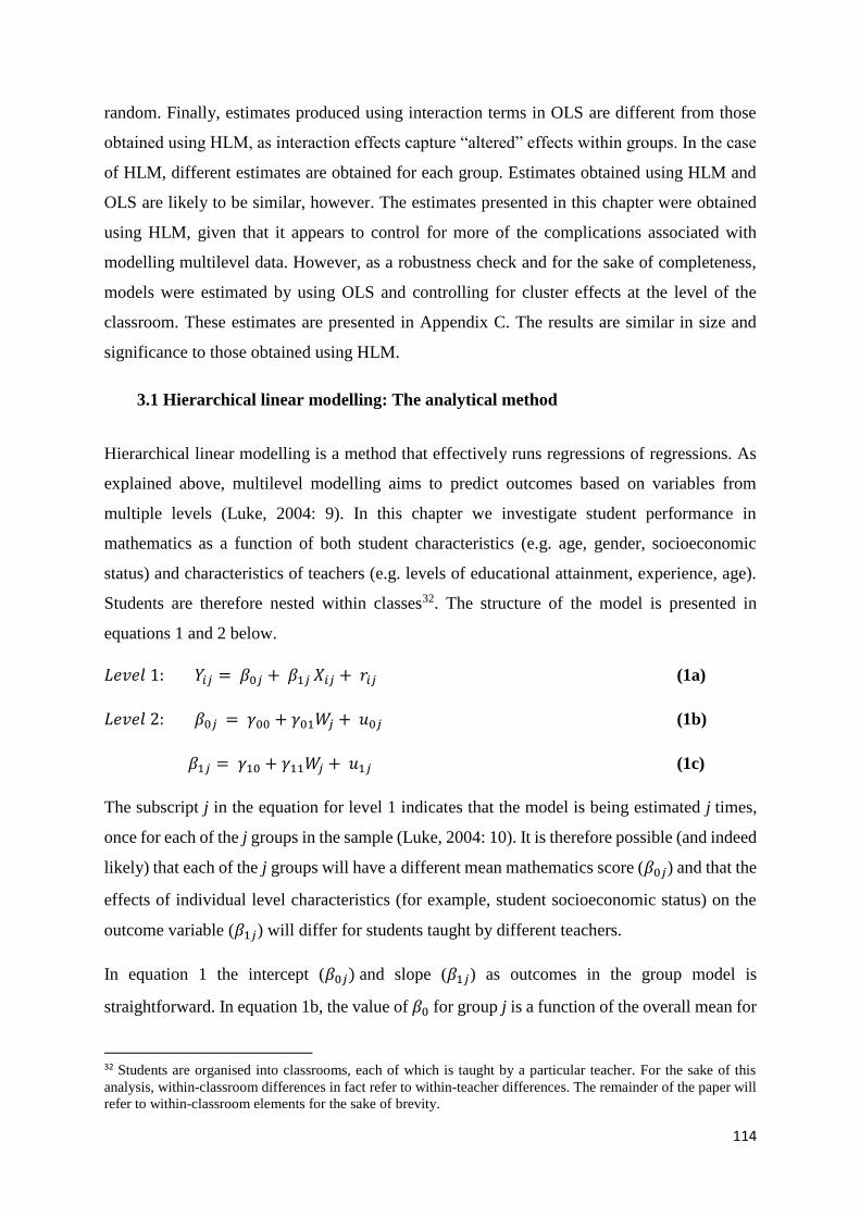
114

random. Finally, estimates produced using interaction terms in OLS are different from those

obtained using HLM, as interaction effects capture “altered” effects within groups. In the case

of HLM, different estimates are obtained for each group. Estimates obtained using HLM and

OLS are likely to be similar, however. The estimates presented in this chapter were obtained

using HLM, given that it appears to control for more of the complications associated with

modelling multilevel data. However, as a robustness check and for the sake of completeness,

models were estimated by using OLS and controlling for cluster effects at the level of the

classroom. These estimates are presented in Appendix C. The results are similar in size and

significance to those obtained using HLM.

3.1 Hierarchical linear modelling: The analytical method

Hierarchical linear modelling is a method that effectively runs regressions of regressions. As

explained above, multilevel modelling aims to predict outcomes based on variables from

multiple levels (Luke, 2004: 9). In this chapter we investigate student performance in

mathematics as a function of both student characteristics (e.g. age, gender, socioeconomic

status) and characteristics of teachers (e.g. levels of educational attainment, experience, age).

Students are therefore nested within classes32. The structure of the model is presented in

equations 1 and 2 below.

𝐿𝑒𝑣𝑒𝑙 1: 𝑌𝑖𝑗 = 𝛽0𝑗 + 𝛽1𝑗 𝑋𝑖𝑗 + 𝑟𝑖𝑗 (1a)

𝐿𝑒𝑣𝑒𝑙 2: 𝛽0𝑗 = 𝛾00 + 𝛾01𝑊𝑗 + 𝑢0𝑗 (1b)

𝛽1𝑗 = 𝛾10 + 𝛾11𝑊𝑗 + 𝑢1𝑗 (1c)

The subscript j in the equation for level 1 indicates that the model is being estimated j times,

once for each of the j groups in the sample (Luke, 2004: 10). It is therefore possible (and indeed

likely) that each of the j groups will have a different mean mathematics score (𝛽0𝑗) and that the

effects of individual level characteristics (for example, student socioeconomic status) on the

outcome variable (𝛽1𝑗) will differ for students taught by different teachers.

In equation 1 the intercept (𝛽0𝑗) and slope (𝛽1𝑗) as outcomes in the group model is

straightforward. In equation 1b, the value of 𝛽0 for group j is a function of the overall mean for

32 Students are organised into classrooms, each of which is taught by a particular teacher. For the sake of this

analysis, within-classroom differences in fact refer to within-teacher differences. The remainder of the paper will

refer to within-classroom elements for the sake of brevity.

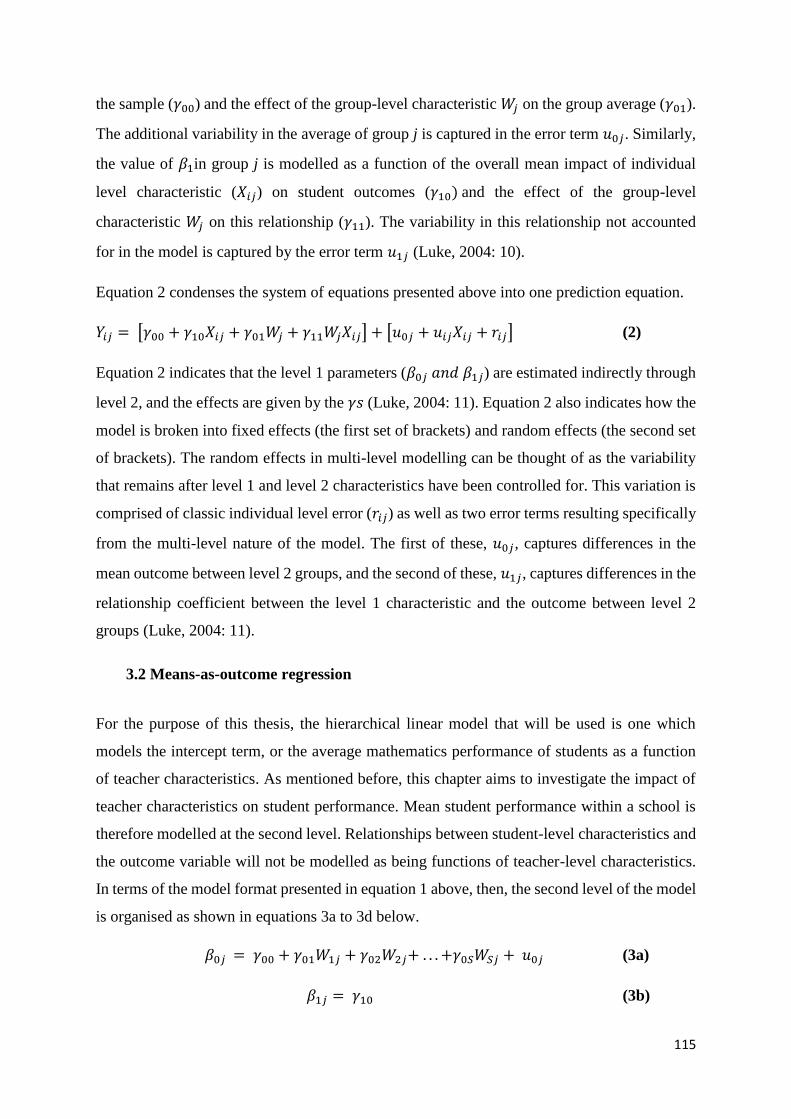
115

the sample (𝛾00) and the effect of the group-level characteristic 𝑊𝑗 on the group average (𝛾01).

The additional variability in the average of group j is captured in the error term 𝑢0𝑗. Similarly,

the value of 𝛽1in group j is modelled as a function of the overall mean impact of individual

level characteristic (𝑋𝑖𝑗) on student outcomes (𝛾10) and the effect of the group-level

characteristic 𝑊𝑗 on this relationship (𝛾11). The variability in this relationship not accounted

for in the model is captured by the error term 𝑢1𝑗 (Luke, 2004: 10).

Equation 2 condenses the system of equations presented above into one prediction equation.

𝑌𝑖𝑗 = [𝛾00 + 𝛾10𝑋𝑖𝑗 + 𝛾01𝑊𝑗 + 𝛾11𝑊𝑗𝑋𝑖𝑗] + [𝑢0𝑗 + 𝑢𝑖𝑗𝑋𝑖𝑗 + 𝑟𝑖𝑗] (2)

Equation 2 indicates that the level 1 parameters (𝛽0𝑗 𝑎𝑛𝑑 𝛽1𝑗) are estimated indirectly through

level 2, and the effects are given by the 𝛾𝑠 (Luke, 2004: 11). Equation 2 also indicates how the

model is broken into fixed effects (the first set of brackets) and random effects (the second set

of brackets). The random effects in multi-level modelling can be thought of as the variability

that remains after level 1 and level 2 characteristics have been controlled for. This variation is

comprised of classic individual level error (𝑟𝑖𝑗) as well as two error terms resulting specifically

from the multi-level nature of the model. The first of these, 𝑢0𝑗, captures differences in the

mean outcome between level 2 groups, and the second of these, 𝑢1𝑗, captures differences in the

relationship coefficient between the level 1 characteristic and the outcome between level 2

groups (Luke, 2004: 11).

3.2 Means-as-outcome regression

For the purpose of this thesis, the hierarchical linear model that will be used is one which

models the intercept term, or the average mathematics performance of students as a function

of teacher characteristics. As mentioned before, this chapter aims to investigate the impact of

teacher characteristics on student performance. Mean student performance within a school is

therefore modelled at the second level. Relationships between student-level characteristics and

the outcome variable will not be modelled as being functions of teacher-level characteristics.

In terms of the model format presented in equation 1 above, then, the second level of the model

is organised as shown in equations 3a to 3d below.

𝛽0𝑗 = 𝛾00 + 𝛾01𝑊1𝑗 + 𝛾02𝑊2𝑗+ . . . +𝛾0𝑆𝑊𝑆𝑗 + 𝑢0𝑗 (3a)

𝛽1𝑗 = 𝛾10 (3b)

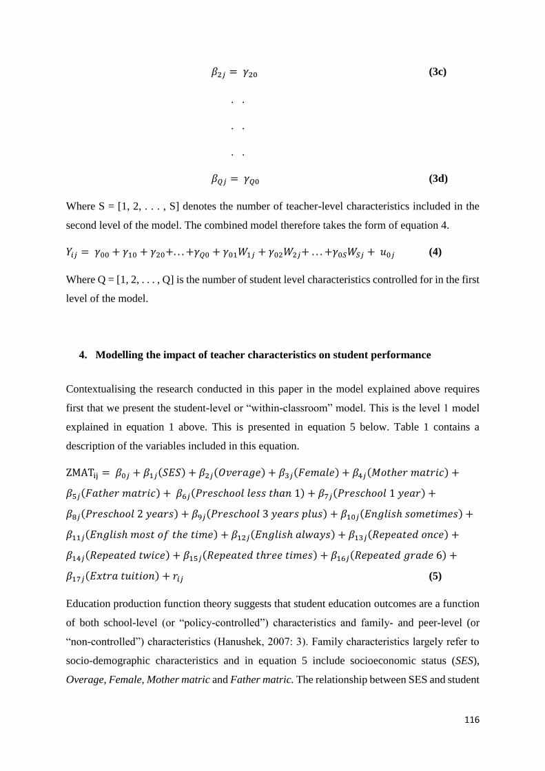
116

𝛽2𝑗 = 𝛾20 (3c)

. .

. .

. .

𝛽𝑄𝑗 = 𝛾𝑄0 (3d)

Where S = [1, 2, . . . , S] denotes the number of teacher-level characteristics included in the

second level of the model. The combined model therefore takes the form of equation 4.

𝑌𝑖𝑗 = 𝛾00 + 𝛾10 + 𝛾20+. . . +𝛾𝑄0 + 𝛾01𝑊1𝑗 + 𝛾02𝑊2𝑗+ . . . +𝛾0𝑆𝑊𝑆𝑗 + 𝑢0𝑗 (4)

Where Q = [1, 2, . . . , Q] is the number of student level characteristics controlled for in the first

level of the model.

4. Modelling the impact of teacher characteristics on student performance

Contextualising the research conducted in this paper in the model explained above requires

first that we present the student-level or “within-classroom” model. This is the level 1 model

explained in equation 1 above. This is presented in equation 5 below. Table 1 contains a

description of the variables included in this equation.

ZMATij = 𝛽0𝑗 + 𝛽1𝑗(𝑆𝐸𝑆) + 𝛽2𝑗(𝑂𝑣𝑒𝑟𝑎𝑔𝑒) + 𝛽3𝑗(𝐹𝑒𝑚𝑎𝑙𝑒) + 𝛽4𝑗(𝑀𝑜𝑡ℎ𝑒𝑟 𝑚𝑎𝑡𝑟𝑖𝑐) +

𝛽5𝑗(𝐹𝑎𝑡ℎ𝑒𝑟 𝑚𝑎𝑡𝑟𝑖𝑐) + 𝛽6𝑗(𝑃𝑟𝑒𝑠𝑐ℎ𝑜𝑜𝑙 𝑙𝑒𝑠𝑠 𝑡ℎ𝑎𝑛 1) + 𝛽7𝑗(𝑃𝑟𝑒𝑠𝑐ℎ𝑜𝑜𝑙 1 𝑦𝑒𝑎𝑟) +

𝛽8𝑗(𝑃𝑟𝑒𝑠𝑐ℎ𝑜𝑜𝑙 2 𝑦𝑒𝑎𝑟𝑠) + 𝛽9𝑗(𝑃𝑟𝑒𝑠𝑐ℎ𝑜𝑜𝑙 3 𝑦𝑒𝑎𝑟𝑠 𝑝𝑙𝑢𝑠) + 𝛽10𝑗(𝐸𝑛𝑔𝑙𝑖𝑠ℎ 𝑠𝑜𝑚𝑒𝑡𝑖𝑚𝑒𝑠) +

𝛽11𝑗(𝐸𝑛𝑔𝑙𝑖𝑠ℎ 𝑚𝑜𝑠𝑡 𝑜𝑓 𝑡ℎ𝑒 𝑡𝑖𝑚𝑒) + 𝛽12𝑗(𝐸𝑛𝑔𝑙𝑖𝑠ℎ 𝑎𝑙𝑤𝑎𝑦𝑠) + 𝛽13𝑗(𝑅𝑒𝑝𝑒𝑎𝑡𝑒𝑑 𝑜𝑛𝑐𝑒) +

𝛽14𝑗(𝑅𝑒𝑝𝑒𝑎𝑡𝑒𝑑 𝑡𝑤𝑖𝑐𝑒) + 𝛽15𝑗(𝑅𝑒𝑝𝑒𝑎𝑡𝑒𝑑 𝑡ℎ𝑟𝑒𝑒 𝑡𝑖𝑚𝑒𝑠) + 𝛽16𝑗(𝑅𝑒𝑝𝑒𝑎𝑡𝑒𝑑 𝑔𝑟𝑎𝑑𝑒 6) +

𝛽17𝑗(𝐸𝑥𝑡𝑟𝑎 𝑡𝑢𝑖𝑡𝑖𝑜𝑛) + 𝑟𝑖𝑗 (5)

Education production function theory suggests that student education outcomes are a function

of both school-level (or “policy-controlled”) characteristics and family- and peer-level (or

“non-controlled”) characteristics (Hanushek, 2007: 3). Family characteristics largely refer to

socio-demographic characteristics and in equation 5 include socioeconomic status (SES),

Overage, Female, Mother matric and Father matric. The relationship between SES and student

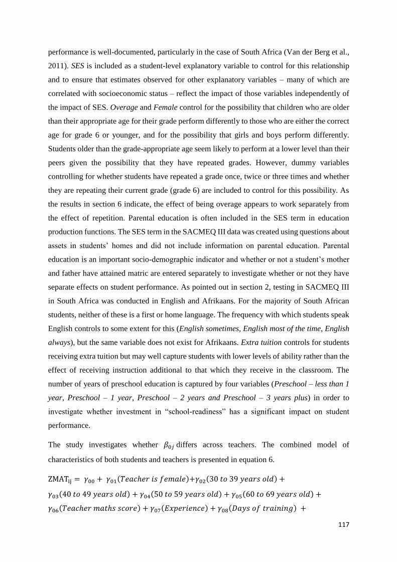
117

performance is well-documented, particularly in the case of South Africa (Van der Berg et al.,

2011). SES is included as a student-level explanatory variable to control for this relationship

and to ensure that estimates observed for other explanatory variables – many of which are

correlated with socioeconomic status – reflect the impact of those variables independently of

the impact of SES. Overage and Female control for the possibility that children who are older

than their appropriate age for their grade perform differently to those who are either the correct

age for grade 6 or younger, and for the possibility that girls and boys perform differently.

Students older than the grade-appropriate age seem likely to perform at a lower level than their

peers given the possibility that they have repeated grades. However, dummy variables

controlling for whether students have repeated a grade once, twice or three times and whether

they are repeating their current grade (grade 6) are included to control for this possibility. As

the results in section 6 indicate, the effect of being overage appears to work separately from

the effect of repetition. Parental education is often included in the SES term in education

production functions. The SES term in the SACMEQ III data was created using questions about

assets in students’ homes and did not include information on parental education. Parental

education is an important socio-demographic indicator and whether or not a student’s mother

and father have attained matric are entered separately to investigate whether or not they have

separate effects on student performance. As pointed out in section 2, testing in SACMEQ III

in South Africa was conducted in English and Afrikaans. For the majority of South African

students, neither of these is a first or home language. The frequency with which students speak

English controls to some extent for this (English sometimes, English most of the time, English

always), but the same variable does not exist for Afrikaans. Extra tuition controls for students

receiving extra tuition but may well capture students with lower levels of ability rather than the

effect of receiving instruction additional to that which they receive in the classroom. The

number of years of preschool education is captured by four variables (Preschool – less than 1

year, Preschool – 1 year, Preschool – 2 years and Preschool – 3 years plus) in order to

investigate whether investment in “school-readiness” has a significant impact on student

performance.

The study investigates whether 𝛽0𝑗 differs across teachers. The combined model of

characteristics of both students and teachers is presented in equation 6.

ZMATij = 𝛾00 + 𝛾01(𝑇𝑒𝑎𝑐ℎ𝑒𝑟 𝑖𝑠 𝑓𝑒𝑚𝑎𝑙𝑒)+𝛾02(30 𝑡𝑜 39 𝑦𝑒𝑎𝑟𝑠 𝑜𝑙𝑑) +

𝛾03(40 𝑡𝑜 49 𝑦𝑒𝑎𝑟𝑠 𝑜𝑙𝑑) + 𝛾04(50 𝑡𝑜 59 𝑦𝑒𝑎𝑟𝑠 𝑜𝑙𝑑) + 𝛾05(60 𝑡𝑜 69 𝑦𝑒𝑎𝑟𝑠 𝑜𝑙𝑑) +

𝛾06(𝑇𝑒𝑎𝑐ℎ𝑒𝑟 𝑚𝑎𝑡ℎ𝑠 𝑠𝑐𝑜𝑟𝑒) + 𝛾07(𝐸𝑥𝑝𝑒𝑟𝑖𝑒𝑛𝑐𝑒) + 𝛾08(𝐷𝑎𝑦𝑠 𝑜𝑓 𝑡𝑟𝑎𝑖𝑛𝑖𝑛𝑔) +

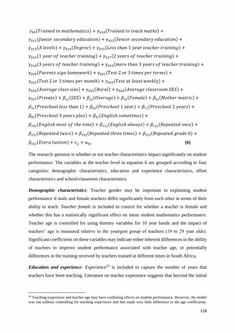
118

𝛾09(𝑇𝑟𝑎𝑖𝑛𝑒𝑑 𝑖𝑛 𝑚𝑎𝑡ℎ𝑒𝑚𝑎𝑡𝑖𝑐𝑠) + 𝛾010(𝑇𝑟𝑎𝑖𝑛𝑒𝑑 𝑡𝑜 𝑡𝑒𝑎𝑐ℎ 𝑚𝑎𝑡ℎ𝑠) +

𝛾011(𝐽𝑢𝑛𝑖𝑜𝑟 𝑠𝑒𝑐𝑜𝑛𝑑𝑎𝑟𝑦 𝑒𝑑𝑢𝑐𝑎𝑡𝑖𝑜𝑛) + 𝛾012(𝑆𝑒𝑛𝑖𝑜𝑟 𝑠𝑒𝑐𝑜𝑛𝑑𝑎𝑟𝑦 𝑒𝑑𝑢𝑐𝑎𝑡𝑖𝑜𝑛) +

𝛾013(𝐴 𝑙𝑒𝑣𝑒𝑙𝑠) + 𝛾014(𝐷𝑒𝑔𝑟𝑒𝑒) + 𝛾015(𝐿𝑒𝑠𝑠 𝑡ℎ𝑎𝑛 1 𝑦𝑒𝑎𝑟 𝑡𝑒𝑎𝑐ℎ𝑒𝑟 𝑡𝑟𝑎𝑖𝑛𝑖𝑛𝑔) +

𝛾016(1 𝑦𝑒𝑎𝑟 𝑜𝑓 𝑡𝑒𝑎𝑐ℎ𝑒𝑟 𝑡𝑟𝑎𝑖𝑛𝑖𝑛𝑔) + 𝛾017(2 𝑦𝑒𝑎𝑟𝑠 𝑜𝑓 𝑡𝑒𝑎𝑐ℎ𝑒𝑟 𝑡𝑟𝑎𝑖𝑛𝑖𝑛𝑔) +

𝛾018(3 𝑦𝑒𝑎𝑟𝑠 𝑜𝑓 𝑡𝑒𝑎𝑐ℎ𝑒𝑟 𝑡𝑟𝑎𝑖𝑛𝑖𝑛𝑔) + 𝛾019(𝑚𝑜𝑟𝑒 𝑡ℎ𝑎𝑛 3 𝑦𝑒𝑎𝑟𝑠 𝑜𝑓 𝑡𝑒𝑎𝑐ℎ𝑒𝑟 𝑡𝑟𝑎𝑖𝑛𝑖𝑛𝑔) +

𝛾020(𝑃𝑎𝑟𝑒𝑛𝑡𝑠 𝑠𝑖𝑔𝑛 ℎ𝑜𝑚𝑒𝑤𝑜𝑟𝑘) + 𝛾021(𝑇𝑒𝑠𝑡 2 𝑜𝑟 3 𝑡𝑖𝑚𝑒𝑠 𝑝𝑒𝑟 𝑡𝑒𝑟𝑚𝑠) +

𝛾022(𝑇𝑒𝑠𝑡 2 𝑜𝑟 3 𝑡𝑖𝑚𝑒𝑠 𝑝𝑒𝑟 𝑚𝑜𝑛𝑡ℎ) + 𝛾023(𝑇𝑒𝑠𝑡 𝑎𝑡 𝑙𝑒𝑎𝑠𝑡 𝑤𝑒𝑒𝑘𝑙𝑦) +

𝛾024(𝐴𝑣𝑒𝑟𝑎𝑔𝑒 𝑐𝑙𝑎𝑠𝑠 𝑠𝑖𝑧𝑒) + 𝛾025(𝑅𝑢𝑟𝑎𝑙) + 𝛾026(𝐴𝑣𝑒𝑟𝑎𝑔𝑒 𝑐𝑙𝑎𝑠𝑠𝑟𝑜𝑜𝑚 𝑆𝐸𝑆) +

𝛾027(𝑃𝑟𝑖𝑣𝑎𝑡𝑒) + 𝛽1𝑗(𝑆𝐸𝑆) + 𝛽2𝑗(𝑂𝑣𝑒𝑟𝑎𝑔𝑒) + 𝛽3𝑗(𝐹𝑒𝑚𝑎𝑙𝑒) + 𝛽4𝑗(𝑀𝑜𝑡ℎ𝑒𝑟 𝑚𝑎𝑡𝑟𝑖𝑐) +

𝛽5𝑗(𝑃𝑟𝑒𝑠𝑐ℎ𝑜𝑜𝑙 𝑙𝑒𝑠𝑠 𝑡ℎ𝑎𝑛 1) + 𝛽6𝑗(𝑃𝑟𝑒𝑠𝑐ℎ𝑜𝑜𝑙 1 𝑦𝑒𝑎𝑟) + 𝛽7𝑗(𝑃𝑟𝑒𝑠𝑐ℎ𝑜𝑜𝑙 2 𝑦𝑒𝑎𝑟𝑠) +

𝛽8𝑗(𝑃𝑟𝑒𝑠𝑐ℎ𝑜𝑜𝑙 3 𝑦𝑒𝑎𝑟𝑠 𝑝𝑙𝑢𝑠) + 𝛽9𝑗(𝐸𝑛𝑔𝑙𝑖𝑠ℎ 𝑠𝑜𝑚𝑒𝑡𝑖𝑚𝑒𝑠) +

𝛽10𝑗(𝐸𝑛𝑔𝑙𝑖𝑠ℎ 𝑚𝑜𝑠𝑡 𝑜𝑓 𝑡ℎ𝑒 𝑡𝑖𝑚𝑒) + 𝛽11𝑗(𝐸𝑛𝑔𝑙𝑖𝑠ℎ 𝑎𝑙𝑤𝑎𝑦𝑠) + 𝛽12𝑗(𝑅𝑒𝑝𝑒𝑎𝑡𝑒𝑑 𝑜𝑛𝑐𝑒) +

𝛽13𝑗(𝑅𝑒𝑝𝑒𝑎𝑡𝑒𝑑 𝑡𝑤𝑖𝑐𝑒) + 𝛽14𝑗(𝑅𝑒𝑝𝑒𝑎𝑡𝑒𝑑 𝑡ℎ𝑟𝑒𝑒 𝑡𝑖𝑚𝑒𝑠) + 𝛽15𝑗(𝑅𝑒𝑝𝑒𝑎𝑡𝑒𝑑 𝑔𝑟𝑎𝑑𝑒 6) +

𝛽16𝑗(𝐸𝑥𝑡𝑟𝑎 𝑡𝑢𝑖𝑡𝑖𝑜𝑛) + 𝑟𝑖𝑗 + 𝑢0𝑗 (6)

The research question is whether or not teacher characteristics impact significantly on student

performance. The variables at the teacher level in equation 6 are grouped according to four

categories: demographic characteristics, education and experience characteristics, effort

characteristics and school/classroom characteristics.

Demographic characteristics: Teacher gender may be important in explaining student

performance if male and female teachers differ significantly from each other in terms of their

ability to teach. Teacher female is included to control for whether a teacher is female and

whether this has a statistically significant effect on mean student mathematics performance.

Teacher age is controlled for using dummy variables for 10 year bands and the impact of

teachers’ age is measured relative to the youngest group of teachers (19 to 29 year olds).

Significant coefficients on these variables may indicate either inherent differences in the ability

of teachers to improve student performance associated with teacher age, or potentially

differences in the training received by teachers trained at different times in South Africa.

Education and experience: Experience33 is included to capture the number of years that

teachers have been teaching. Literature on teacher experience suggests that beyond the initial

33 Teaching experience and teacher age may have conflating effects on student performance. However, the model

was run without controlling for teaching experience and this made very little difference to the age coefficients.

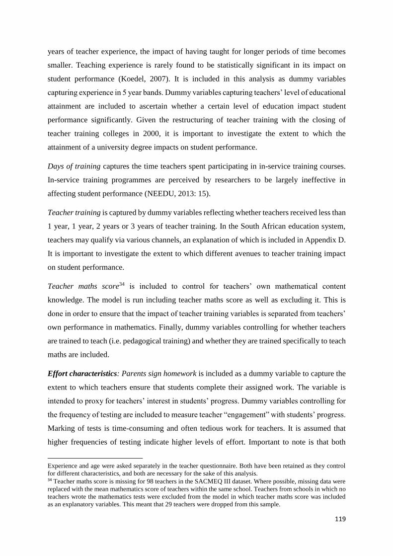
119

years of teacher experience, the impact of having taught for longer periods of time becomes

smaller. Teaching experience is rarely found to be statistically significant in its impact on

student performance (Koedel, 2007). It is included in this analysis as dummy variables

capturing experience in 5 year bands. Dummy variables capturing teachers’ level of educational

attainment are included to ascertain whether a certain level of education impact student

performance significantly. Given the restructuring of teacher training with the closing of

teacher training colleges in 2000, it is important to investigate the extent to which the

attainment of a university degree impacts on student performance.

Days of training captures the time teachers spent participating in in-service training courses.

In-service training programmes are perceived by researchers to be largely ineffective in

affecting student performance (NEEDU, 2013: 15).

Teacher training is captured by dummy variables reflecting whether teachers received less than

1 year, 1 year, 2 years or 3 years of teacher training. In the South African education system,

teachers may qualify via various channels, an explanation of which is included in Appendix D.

It is important to investigate the extent to which different avenues to teacher training impact

on student performance.

Teacher maths score34 is included to control for teachers’ own mathematical content

knowledge. The model is run including teacher maths score as well as excluding it. This is

done in order to ensure that the impact of teacher training variables is separated from teachers’

own performance in mathematics. Finally, dummy variables controlling for whether teachers

are trained to teach (i.e. pedagogical training) and whether they are trained specifically to teach

maths are included.

Effort characteristics: Parents sign homework is included as a dummy variable to capture the

extent to which teachers ensure that students complete their assigned work. The variable is

intended to proxy for teachers’ interest in students’ progress. Dummy variables controlling for

the frequency of testing are included to measure teacher “engagement” with students’ progress.

Marking of tests is time-consuming and often tedious work for teachers. It is assumed that

higher frequencies of testing indicate higher levels of effort. Important to note is that both

Experience and age were asked separately in the teacher questionnaire. Both have been retained as they control

for different characteristics, and both are necessary for the sake of this analysis. 34 Teacher maths score is missing for 98 teachers in the SACMEQ III dataset. Where possible, missing data were

replaced with the mean mathematics score of teachers within the same school. Teachers from schools in which no

teachers wrote the mathematics tests were excluded from the model in which teacher maths score was included

as an explanatory variables. This meant that 29 teachers were dropped from this sample.

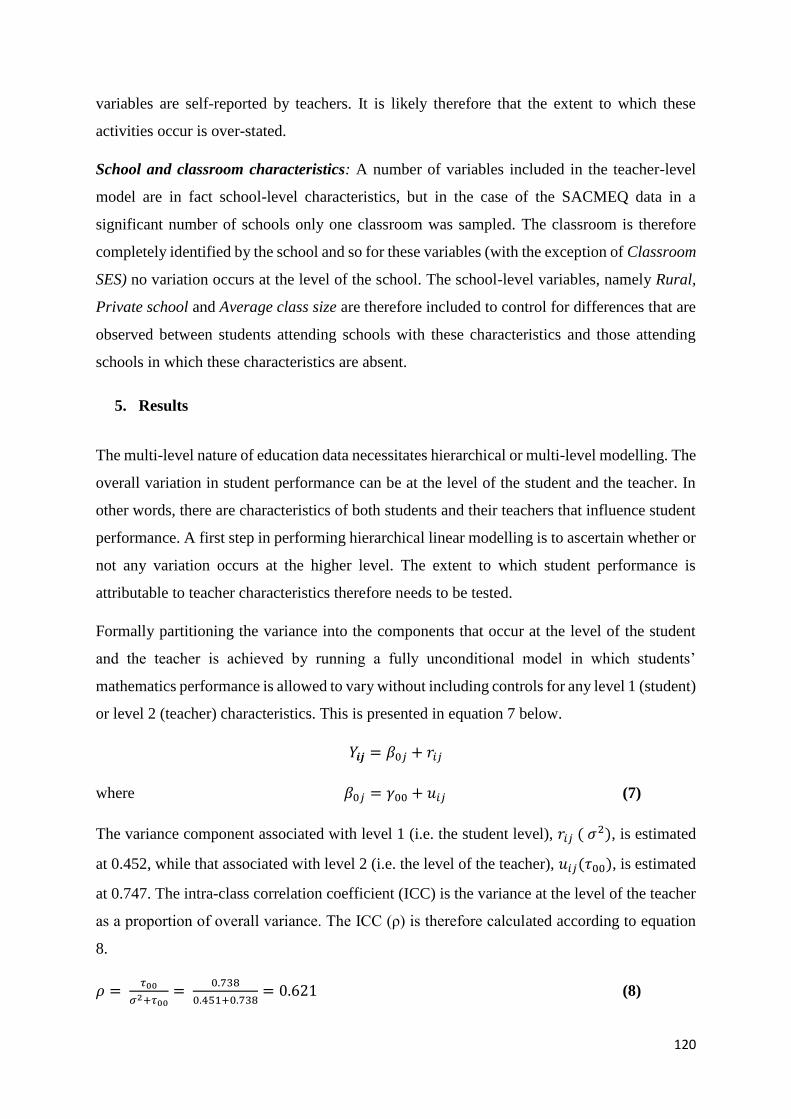
120

variables are self-reported by teachers. It is likely therefore that the extent to which these

activities occur is over-stated.

School and classroom characteristics: A number of variables included in the teacher-level

model are in fact school-level characteristics, but in the case of the SACMEQ data in a

significant number of schools only one classroom was sampled. The classroom is therefore

completely identified by the school and so for these variables (with the exception of Classroom

SES) no variation occurs at the level of the school. The school-level variables, namely Rural,

Private school and Average class size are therefore included to control for differences that are

observed between students attending schools with these characteristics and those attending

schools in which these characteristics are absent.

5. Results

The multi-level nature of education data necessitates hierarchical or multi-level modelling. The

overall variation in student performance can be at the level of the student and the teacher. In

other words, there are characteristics of both students and their teachers that influence student

performance. A first step in performing hierarchical linear modelling is to ascertain whether or

not any variation occurs at the higher level. The extent to which student performance is

attributable to teacher characteristics therefore needs to be tested.

Formally partitioning the variance into the components that occur at the level of the student

and the teacher is achieved by running a fully unconditional model in which students’

mathematics performance is allowed to vary without including controls for any level 1 (student)

or level 2 (teacher) characteristics. This is presented in equation 7 below.

𝑌𝒊𝒋 = 𝛽0𝑗 + 𝑟𝑖𝑗

where 𝛽0𝑗 = 𝛾00 + 𝑢𝑖𝑗 (7)

The variance component associated with level 1 (i.e. the student level), 𝑟𝑖𝑗 ( 𝜎2), is estimated

at 0.452, while that associated with level 2 (i.e. the level of the teacher), 𝑢𝑖𝑗(𝜏00), is estimated

at 0.747. The intra-class correlation coefficient (ICC) is the variance at the level of the teacher

as a proportion of overall variance. The ICC (ρ) is therefore calculated according to equation

8.

𝜌 = 𝜏00

𝜎2+𝜏00=

0.738

0.451+0.738= 0.621 (8)

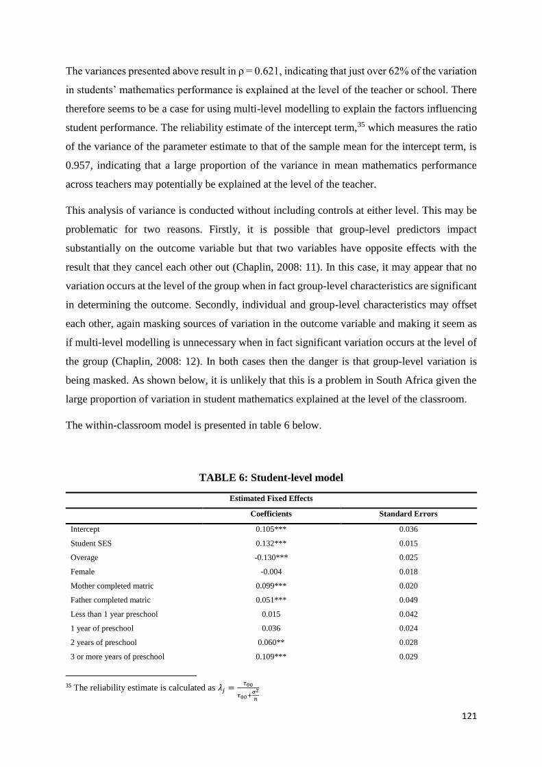
121

The variances presented above result in ρ = 0.621, indicating that just over 62% of the variation

in students’ mathematics performance is explained at the level of the teacher or school. There

therefore seems to be a case for using multi-level modelling to explain the factors influencing

student performance. The reliability estimate of the intercept term,35 which measures the ratio

of the variance of the parameter estimate to that of the sample mean for the intercept term, is

0.957, indicating that a large proportion of the variance in mean mathematics performance

across teachers may potentially be explained at the level of the teacher.

This analysis of variance is conducted without including controls at either level. This may be

problematic for two reasons. Firstly, it is possible that group-level predictors impact

substantially on the outcome variable but that two variables have opposite effects with the

result that they cancel each other out (Chaplin, 2008: 11). In this case, it may appear that no

variation occurs at the level of the group when in fact group-level characteristics are significant

in determining the outcome. Secondly, individual and group-level characteristics may offset

each other, again masking sources of variation in the outcome variable and making it seem as

if multi-level modelling is unnecessary when in fact significant variation occurs at the level of

the group (Chaplin, 2008: 12). In both cases then the danger is that group-level variation is

being masked. As shown below, it is unlikely that this is a problem in South Africa given the

large proportion of variation in student mathematics explained at the level of the classroom.

The within-classroom model is presented in table 6 below.

TABLE 6: Student-level model

Estimated Fixed Effects

Coefficients Standard Errors

Intercept 0.105*** 0.036

Student SES 0.132*** 0.015

Overage -0.130*** 0.025

Female -0.004 0.018

Mother completed matric 0.099*** 0.020

Father completed matric 0.051*** 0.049

Less than 1 year preschool 0.015 0.042

1 year of preschool 0.036 0.024

2 years of preschool 0.060** 0.028

3 or more years of preschool 0.109*** 0.029

35 The reliability estimate is calculated as 𝜆𝑗 =

𝜏00

𝜏00+𝜎2

𝑛

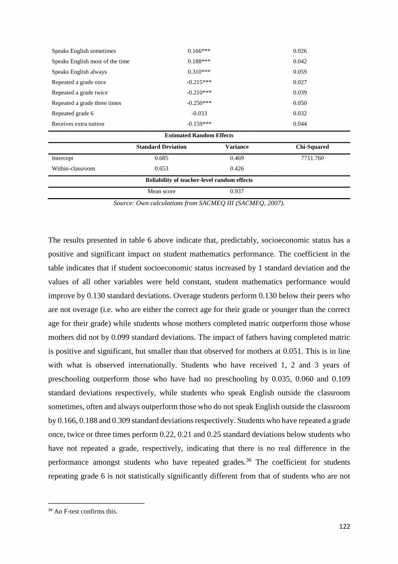
122

Speaks English sometimes 0.166*** 0.026

Speaks English most of the time 0.188*** 0.042

Speaks English always 0.310*** 0.059

Repeated a grade once -0.215*** 0.027

Repeated a grade twice -0.210*** 0.039

Repeated a grade three times -0.250*** 0.050

Repeated grade 6 -0.033 0.032

Receives extra tuition -0.159*** 0.044

Estimated Random Effects

Standard Deviation Variance Chi-Squared

Intercept 0.685 0.469 7711.760

Within-classroom 0.653 0.426

Reliability of teacher-level random effects

Mean score 0.937

Source: Own calculations from SACMEQ III (SACMEQ, 2007).

The results presented in table 6 above indicate that, predictably, socioeconomic status has a

positive and significant impact on student mathematics performance. The coefficient in the

table indicates that if student socioeconomic status increased by 1 standard deviation and the

values of all other variables were held constant, student mathematics performance would

improve by 0.130 standard deviations. Overage students perform 0.130 below their peers who

are not overage (i.e. who are either the correct age for their grade or younger than the correct

age for their grade) while students whose mothers completed matric outperform those whose

mothers did not by 0.099 standard deviations. The impact of fathers having completed matric

is positive and significant, but smaller than that observed for mothers at 0.051. This is in line

with what is observed internationally. Students who have received 1, 2 and 3 years of

preschooling outperform those who have had no preschooling by 0.035, 0.060 and 0.109

standard deviations respectively, while students who speak English outside the classroom

sometimes, often and always outperform those who do not speak English outside the classroom

by 0.166, 0.188 and 0.309 standard deviations respectively. Students who have repeated a grade

once, twice or three times perform 0.22, 0.21 and 0.25 standard deviations below students who

have not repeated a grade, respectively, indicating that there is no real difference in the

performance amongst students who have repeated grades.36 The coefficient for students

repeating grade 6 is not statistically significantly different from that of students who are not

36 An F-test confirms this.

123

repeating grade 6, suggesting that students repeating grade 6 do not perform differently from

students repeating other grades37. Students receiving extra tuition are outperformed by their

peers not receiving extra tuition by 0.159 standard deviations. This may well reflect a lower

ability in the students receiving extra tuition rather than the extra tuition having a negative

impact on their performance.

Controlling for the student level characteristics decreases the within-classroom variance by

roughly 37% from 0.747 to 0.469. The fact that level 1 characteristics explain so little of the

variance of the mean highlight the fact that a substantial portion of the variation in student

performance is explained at a higher level or not at all. Most educational performance data for

South Africa contain neither pre-test scores nor racial classification – both of which are highly

correlated with educational performance. This is obvious in the case of pre-test scores. In the

case of race, performance in the South African education system is still significantly correlated

with performance of the system under apartheid, with the part of the schooling system

historically serving South Africa’s white population far outperforming the part of the schooling

system historically serving South Africa’s black population. The historically white part of the

schooling system is now substantially more representative of South Africa’s population than

in previous years, while the historically black portion remains almost entirely black. Most white

children find themselves in the historically white part of the schooling system and for this

reason race is a significant determinant of schooling performance.

In addition, the variables included in the within-classroom model control for the home

background and variables pertaining to previous education performance. Unobservable

characteristics such as intelligence or ambition play a significant role in school performance.

However, it is impossible to measure and control for them.

In order to investigate the extent to which teacher-level characteristics impact on student

performance, level 2 variables are added to the model. Table 7 below presents the results from

the full multilevel model. Model 1 contains the results for the full teacher model including

teacher maths score, while model 2 excludes teacher maths score.

37 An F-test confirms this.

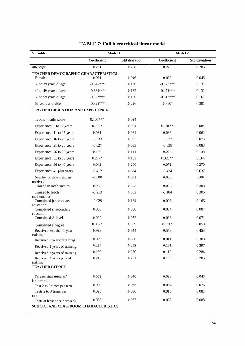
124

TABLE 7: Full hierarchical linear model

Variable Model 1 Model 2

Coefficient Std deviation Coefficient Std deviation

Intercept 0.231 0.208 0.278 0.286

TEACHER DEMOGRAPHIC CHARACTERISTICS

Female 0.071 0.046 0.063 0.045

30 to 39 years of age -0.345*** 0.130 -0.378*** 0.131

40 to 49 years of age -0.389*** 0.132 -0.474*** 0.132

50 to 59 years of age -0.522*** 0.160 -0.618*** 0.161

60 years and older -0.325*** 0.296 -0.360* 0.301

TEACHER EDUCATION AND EXPERIENCE

Teacher maths score 0.105*** 0.024

Experience: 6 to 10 years 0.150* 0.084 0.181** 0.084

Experience: 11 to 15 years 0.031 0.064 0.086 0.062

Experience: 16 to 20 years -0.033 0.077 -0.022 0.075

Experience: 21 to 25 years -0.027 0.083 -0.038 0.083


Experience: 31 to 35 years 0.267* 0.162 0.323** 0.164


Experience: 41 plus years -0.412 0.624 -0.434 0.637

Number of days training

received

-0.000 0.001 0.000 0.00

Trained in mathematics 0.093 0.303 0.086 0.308

Trained to teach

mathematics

-0.213 0.302 -0.184 0.306

Completed jr secondary

education

-0.029 0.164 0.006 0.166

Completed sr secondary

education

0.058 0.086 0.064 0.087

Completed A-levels 0.002 0.072 0.033 0.071

Completed a degree 0.097* 0.059 0.111* 0.058

Received less than 1 year

training

0.923 0.644 0.579 0.453

Received 1 year of training 0.029 0.306 0.011 0.308

Received 2 years of training 0.254 0.293 0.191 0.297

Received 3 years of training 0.169 0.280 0.112 0.284

Received 3 years plus of

training

0.215 0.281 0.180 0.285

TEACHER EFFORT

Parents sign students’

homework

0.032 0.048 0.023 0.048

Test 2 to 3 times per term 0.020 0.075 0.034 0.076

Tests 2 to 3 times per

month

0.025 0.080 0.015 0.081

Tests at least once per week 0.088 0.087 0.082 0.088

SCHOOL AND CLASSROOM CHARACTERISTICS

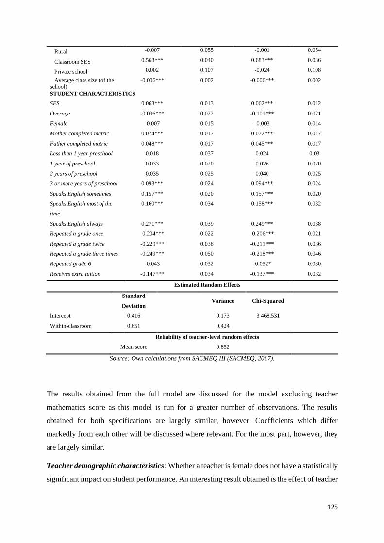
125

Rural -0.007 0.055 -0.001 0.054

Classroom SES 0.568*** 0.040 0.683*** 0.036

Private school 0.002 0.107 -0.024 0.108

Average class size (of the

school)

-0.006*** 0.002 -0.006*** 0.002

STUDENT CHARACTERISTICS

SES 0.063*** 0.013 0.062*** 0.012

Overage -0.096*** 0.022 -0.101*** 0.021

Female -0.007 0.015 -0.003 0.014

Mother completed matric 0.074*** 0.017 0.072*** 0.017

Father completed matric 0.048*** 0.017 0.045*** 0.017

Less than 1 year preschool 0.018 0.037 0.024 0.03

1 year of preschool 0.033 0.020 0.026 0.020

2 years of preschool 0.035 0.025 0.040 0.025

3 or more years of preschool 0.093*** 0.024 0.094*** 0.024

Speaks English sometimes 0.157*** 0.020 0.157*** 0.020

Speaks English most of the

time

0.160*** 0.034 0.158*** 0.032

Speaks English always 0.271*** 0.039 0.249*** 0.038

Repeated a grade once -0.204*** 0.022 -0.206*** 0.021

Repeated a grade twice -0.229*** 0.038 -0.211*** 0.036

Repeated a grade three times -0.249*** 0.050 -0.218*** 0.046

Repeated grade 6 -0.043 0.032 -0.052* 0.030

Receives extra tuition -0.147*** 0.034 -0.137*** 0.032

Estimated Random Effects

Standard

Deviation

Variance Chi-Squared

Intercept 0.416 0.173 3 468.531

Within-classroom 0.651 0.424


Mean score 0.852


The results obtained from the full model are discussed for the model excluding teacher

mathematics score as this model is run for a greater number of observations. The results

obtained for both specifications are largely similar, however. Coefficients which differ

markedly from each other will be discussed where relevant. For the most part, however, they

are largely similar.

Teacher demographic characteristics: Whether a teacher is female does not have a statistically

significant impact on student performance. An interesting result obtained is the effect of teacher

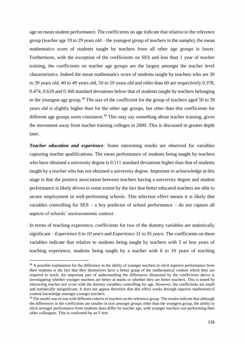
126

age on mean student performance. The coefficients on age indicate that relative to the reference

group (teacher age 19 to 29 years old – the youngest group of teachers in the sample), the mean

mathematics score of students taught by teachers from all other age groups is lower.

Furthermore, with the exception of the coefficients on SES and less than 1 year of teacher

training, the coefficients on teacher age groups are the largest amongst the teacher level

characteristics. Indeed the mean mathematics score of students taught by teachers who are 30

to 39 years old, 40 to 49 years old, 50 to 59 years old and older than 60 are respectively 0.378,

0.474, 0.618 and 0.360 standard deviations below that of students taught by teachers belonging

to the youngest age group.38 The size of the coefficient for the group of teachers aged 50 to 59

years old is slightly higher than for the other age groups, but other than this coefficients for

different age groups seem consistent.39 This may say something about teacher training, given

the movement away from teacher training colleges in 2000. This is discussed in greater depth

later.

Teacher education and experience: Some interesting results are observed for variables

capturing teacher qualifications. The mean performance of students being taught by teachers

who have obtained a university degree is 0.111 standard deviations higher than that of students

taught by a teacher who has not obtained a university degree. Important to acknowledge at this

stage is that the positive association between teachers having a university degree and student

performance is likely driven to some extent by the fact that better educated teachers are able to

secure employment in well-performing schools. This selection effect means it is likely that

variables controlling for SES – a key predictor of school performance – do not capture all

aspects of schools’ socioeconomic context.

In terms of teaching experience, coefficients for two of the dummy variables are statistically

significant – Experience 6 to 10 years and Experience 31 to 35 years. The coefficients on these

variables indicate that relative to students being taught by teachers with 5 or less years of

teaching experience, students being taught by a teacher with 6 to 10 years of teaching

38 A possible explanation for the difference in the ability of younger teachers to elicit superior performance from

their students is the fact that they themselves have a better grasp of the mathematical content which they are

required to teach. An important part of understanding the differences illustrated by the coefficients above is

investigating whether younger teachers are better at maths or whether they are better teachers. This is tested by

interacting teacher test score with the dummy variables controlling for age. However, the coefficients are small

and statistically insignificant. It does not appear therefore that this effect works through superior mathematical

content knowledge amongst younger teachers. 39 The model was re-run with different cohorts of teachers as the reference group. The results indicate that although

the differences in the coefficients are smaller in size amongst groups older than the youngest group, the ability to

elicit stronger performance from students does differ by teacher age, with younger teachers out-performing their

older colleagues. This is confirmed by an F-test.

127

experience perform on average 0.181 standard deviations better, and students being taught by

teachers with between 31 and 35 years of teaching experience perform 0.323 standard

deviations above other students. Interestingly, in model 1 (which controls for teachers’

performance on their mathematics tests), teachers’ mathematics test performance results are

statistically significantly positively related to mean student mathematics performance. As

teachers’ maths scores are z-scored, the coefficient of 0.105 indicates that an improvement of

1 standard deviation in teacher maths performance results in an improvement of 0.105 standard

deviations in mean mathematics performance amongst students.

Teacher effort: None of the teacher effort variables included in the model appears to impact

on mean mathematics performance in a significant way. This may be due to the fact that these

variables are self-reported by teachers. The frequency of testing as well as whether parents are

required to sign homework may well be over-reported.

School and classroom characteristics: The large and statistically significant coefficient

observed for classroom SES is to be expected. The coefficient of 0.627 indicates that a 1

standard deviation increase in classroom SES is associated with a 0.627 standard deviation

increase in mean mathematics performance. The statistically significant negative coefficient

for Average class size (of the school) is intuitive, suggesting that larger classes are associated

with weaker performance. The size of the coefficient is very small, however. Increasing class

size by one student decreases mean student performance by 0.006 of a standard deviation.

Despite the fact that it is statistically significant, it is not economically significant. It is too

small to indicate any real relationship between the variables.

6. Discussion and conclusion

The results presented above are important in the context of South Africa’s education system.

Teachers are an important resource in education and it is necessary to understand how best to

utilise the resource.

The results for the hierarchical linear model reveal that younger teachers are better able to

increase the mean performance of students. In order to test whether this is a trend observed

amongst teachers across different countries or whether this is a trend particular to South Africa,

the identical HLM model was run for 3 other countries in the SACMEQ III dataset – two of

South Africa’s neighbouring countries, Botswana and Zimbabwe, and a high-performing East

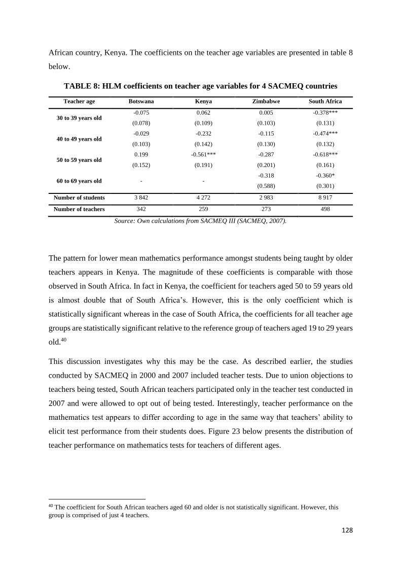
128

African country, Kenya. The coefficients on the teacher age variables are presented in table 8

below.

TABLE 8: HLM coefficients on teacher age variables for 4 SACMEQ countries

Teacher age Botswana Kenya Zimbabwe South Africa

30 to 39 years old -0.075

(0.078)

0.062

(0.109)

0.005

(0.103)

-0.378***

(0.131)

40 to 49 years old -0.029

(0.103)

-0.232

(0.142)

-0.115

(0.130)

-0.474***

(0.132)

50 to 59 years old 0.199

(0.152)

-0.561***

(0.191)

-0.287

(0.201)

-0.618***

(0.161)

60 to 69 years old - - -0.318

(0.588)

-0.360*

(0.301)

Number of students 3 842 4 272 2 983 8 917

Number of teachers 342 259 273 498


The pattern for lower mean mathematics performance amongst students being taught by older

teachers appears in Kenya. The magnitude of these coefficients is comparable with those

observed in South Africa. In fact in Kenya, the coefficient for teachers aged 50 to 59 years old

is almost double that of South Africa’s. However, this is the only coefficient which is

statistically significant whereas in the case of South Africa, the coefficients for all teacher age

groups are statistically significant relative to the reference group of teachers aged 19 to 29 years

old.40

This discussion investigates why this may be the case. As described earlier, the studies

conducted by SACMEQ in 2000 and 2007 included teacher tests. Due to union objections to

teachers being tested, South African teachers participated only in the teacher test conducted in

2007 and were allowed to opt out of being tested. Interestingly, teacher performance on the

mathematics test appears to differ according to age in the same way that teachers’ ability to

elicit test performance from their students does. Figure 23 below presents the distribution of

teacher performance on mathematics tests for teachers of different ages.

40 The coefficient for South African teachers aged 60 and older is not statistically significant. However, this

group is comprised of just 4 teachers.

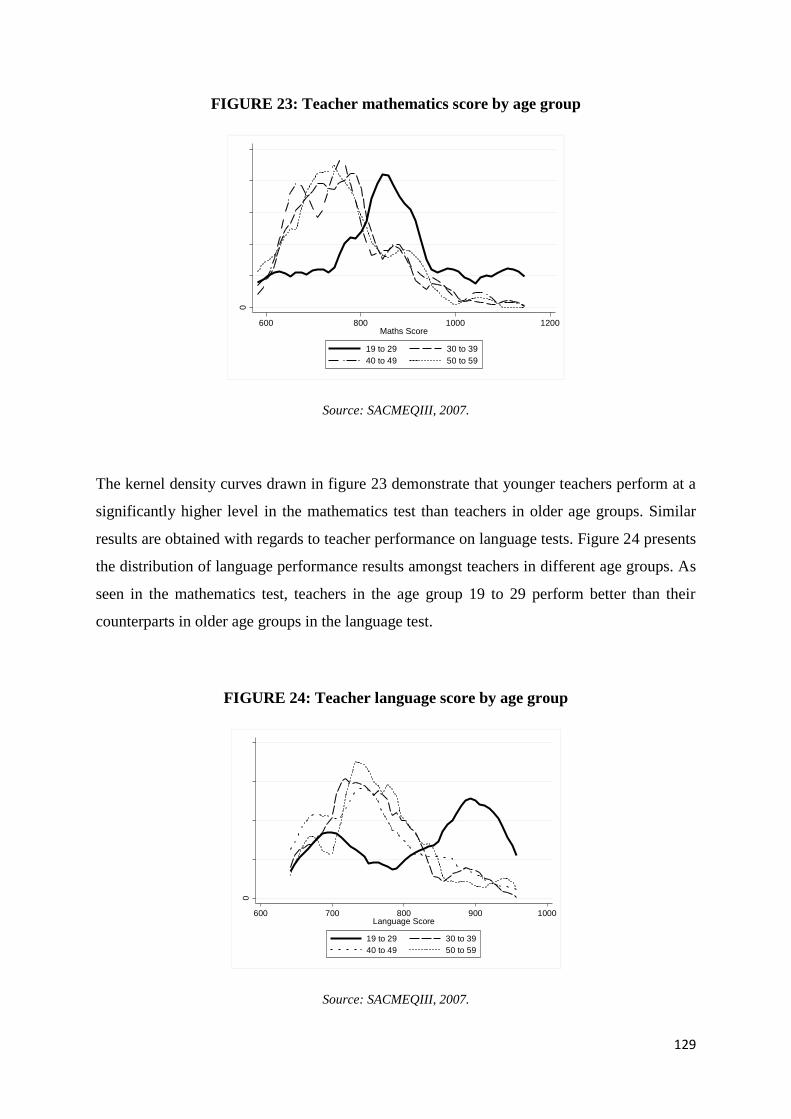
129

FIGURE 23: Teacher mathematics score by age group

Source: SACMEQIII, 2007.

The kernel density curves drawn in figure 23 demonstrate that younger teachers perform at a

significantly higher level in the mathematics test than teachers in older age groups. Similar

results are obtained with regards to teacher performance on language tests. Figure 24 presents

the distribution of language performance results amongst teachers in different age groups. As

seen in the mathematics test, teachers in the age group 19 to 29 perform better than their

counterparts in older age groups in the language test.

FIGURE 24: Teacher language score by age group

Source: SACMEQIII, 2007.

0

.00

1.0

02

.00

3.0

04

.00

5

600 800 1000 1200Maths Score

19 to 29 30 to 39

40 to 49 50 to 59

0

.00

2.0

04

.00

6.0

08

600 700 800 900 1000Language Score

19 to 29 30 to 39

40 to 49 50 to 59

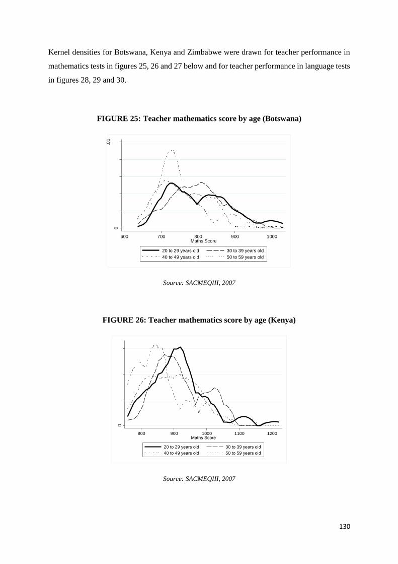
130

Kernel densities for Botswana, Kenya and Zimbabwe were drawn for teacher performance in

mathematics tests in figures 25, 26 and 27 below and for teacher performance in language tests

in figures 28, 29 and 30.

FIGURE 25: Teacher mathematics score by age (Botswana)

Source: SACMEQIII, 2007

FIGURE 26: Teacher mathematics score by age (Kenya)


0

.002

.004

.006

.008

.01

600 700 800 900 1000Maths Score

20 to 29 years old 30 to 39 years old


0

.002

.004

.006

800 900 1000 1100 1200Maths Score



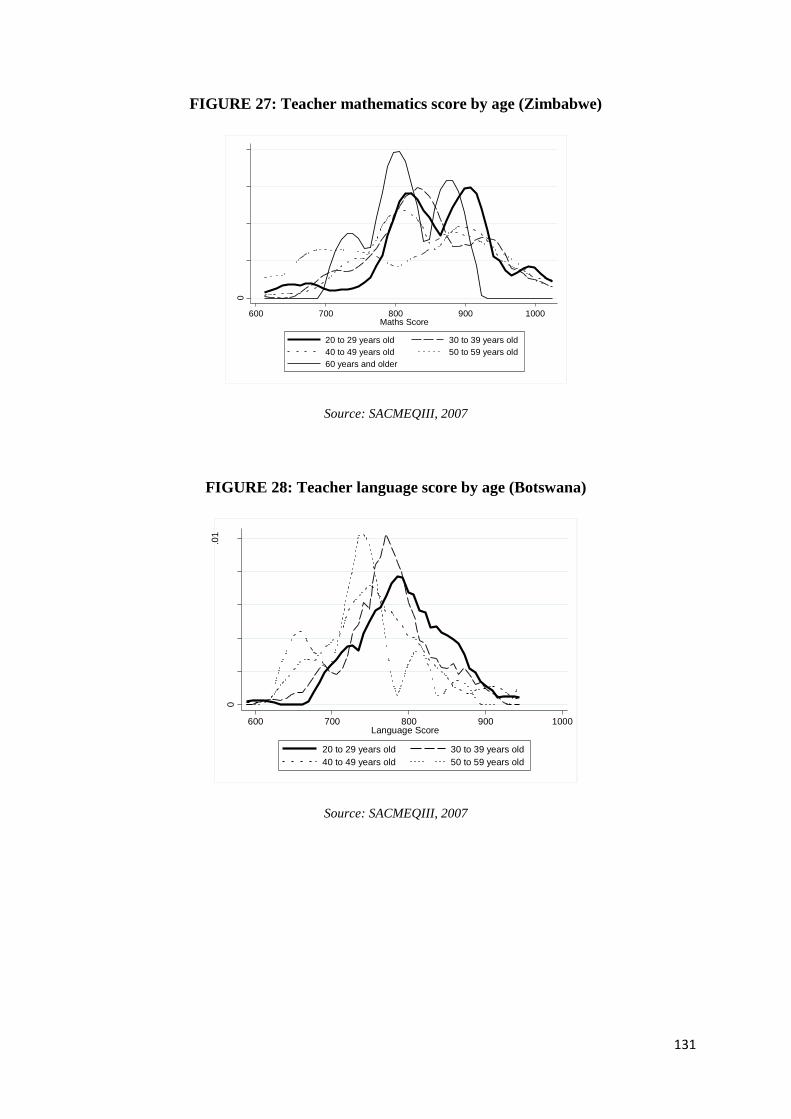
131

FIGURE 27: Teacher mathematics score by age (Zimbabwe)


FIGURE 28: Teacher language score by age (Botswana)


0

.002

.004

.006

.008

600 700 800 900 1000Maths Score



60 years and older

0

.002

.004

.006

.008

.01

600 700 800 900 1000Language Score



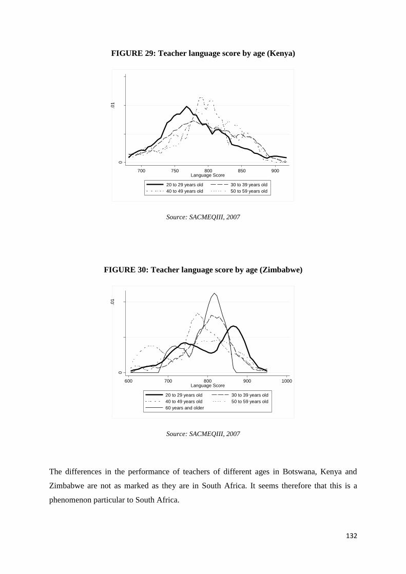
132

FIGURE 29: Teacher language score by age (Kenya)


FIGURE 30: Teacher language score by age (Zimbabwe)


The differences in the performance of teachers of different ages in Botswana, Kenya and

Zimbabwe are not as marked as they are in South Africa. It seems therefore that this is a

phenomenon particular to South Africa.

0

.005

.01

.015

700 750 800 850 900Language Score



0

.005

.01

600 700 800 900 1000Language Score



60 years and older

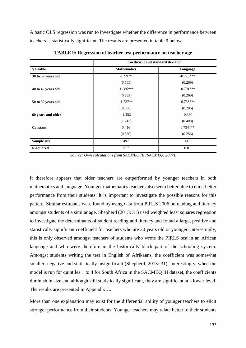
133

A basic OLS regression was run to investigate whether the difference in performance between

teachers is statistically significant. The results are presented in table 9 below.

TABLE 9: Regression of teacher test performance on teacher age

Coefficient and standard deviation

Variable Mathematics Language

30 to 39 years old -0.997*

(0.555)

-0.715***

(0.269)

40 to 49 years old -1.586***

(0.552)

-0.701***

(0.269)

50 to 59 years old -1.237**

(0.596)

-0.738***

(0.286)

60 years and older -1.452

(1.243)

-0.330

(0.408)

Constant 0.416

(0.530)

0.734***

(0.256)

Sample size 497 415

R-squared 0.03 0.01


It therefore appears that older teachers are outperformed by younger teachers in both

mathematics and language. Younger mathematics teachers also seem better able to elicit better

performance from their students. It is important to investigate the possible reasons for this

pattern. Similar estimates were found by using data from PIRLS 2006 on reading and literacy

amongst students of a similar age. Shepherd (2013: 31) used weighted least squares regression

to investigate the determinants of student reading and literacy and found a large, positive and

statistically significant coefficient for teachers who are 30 years old or younger. Interestingly,

this is only observed amongst teachers of students who wrote the PIRLS test in an African

language and who were therefore in the historically black part of the schooling system.

Amongst students writing the test in English of Afrikaans, the coefficient was somewhat

smaller, negative and statistically insignificant (Shepherd, 2013: 31). Interestingly, when the

model is run for quintiles 1 to 4 for South Africa in the SACMEQ III dataset, the coefficients

diminish in size and although still statistically significant, they are significant at a lower level.

The results are presented in Appendix C.

More than one explanation may exist for the differential ability of younger teachers to elicit

stronger performance from their students. Younger teachers may relate better to their students

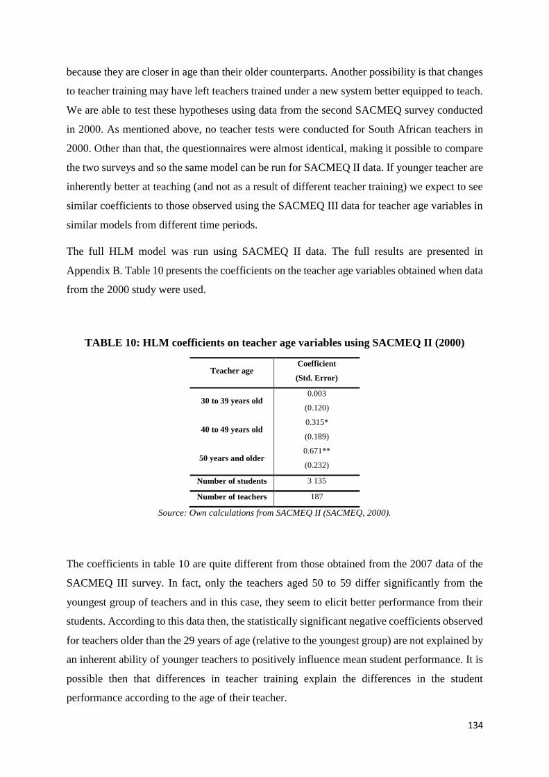
134

because they are closer in age than their older counterparts. Another possibility is that changes

to teacher training may have left teachers trained under a new system better equipped to teach.

We are able to test these hypotheses using data from the second SACMEQ survey conducted

in 2000. As mentioned above, no teacher tests were conducted for South African teachers in

2000. Other than that, the questionnaires were almost identical, making it possible to compare

the two surveys and so the same model can be run for SACMEQ II data. If younger teacher are

inherently better at teaching (and not as a result of different teacher training) we expect to see

similar coefficients to those observed using the SACMEQ III data for teacher age variables in

similar models from different time periods.

The full HLM model was run using SACMEQ II data. The full results are presented in

Appendix B. Table 10 presents the coefficients on the teacher age variables obtained when data

from the 2000 study were used.

TABLE 10: HLM coefficients on teacher age variables using SACMEQ II (2000)

Teacher age Coefficient

(Std. Error)

30 to 39 years old 0.003

(0.120)

40 to 49 years old 0.315*

(0.189)

50 years and older 0.671**

(0.232)

Number of students 3 135

Number of teachers 187

Source: Own calculations from SACMEQ II (SACMEQ, 2000).

The coefficients in table 10 are quite different from those obtained from the 2007 data of the

SACMEQ III survey. In fact, only the teachers aged 50 to 59 differ significantly from the

youngest group of teachers and in this case, they seem to elicit better performance from their

students. According to this data then, the statistically significant negative coefficients observed

for teachers older than the 29 years of age (relative to the youngest group) are not explained by

an inherent ability of younger teachers to positively influence mean student performance. It is

possible then that differences in teacher training explain the differences in the student

performance according to the age of their teacher.

135

As explained in the next subsection, teacher training is one of the few characteristics that may

render younger teachers better able to impact positively on their students’ performance.

Changes in teacher training in the South African education system occurred in the late 1990s

and early 2000s – the time in which the youngest cohort of teachers were trained. The following

section discusses these changes.

6.1 Differences in teacher training41

An obvious avenue to pursue in understanding the differences that are observed in the

performance of teachers of different ages is to investigate the extent to which the training

received by teachers differed across years. A potential source of differences in teacher training

is the shift from teacher training colleges as the institutions responsible for training teachers to

the incorporation of teacher training within universities. Chisholm (2009: 9) explains that

teacher training colleges expanded predominantly in the 1960s. The apartheid state located the

majority of teacher training colleges in the “homeland” areas with the objective of staffing the

colleges with the graduates. Chisholm (2009: 14) explains that enrolment in the teacher

colleges was high due to the fact that opportunities in the formal economy were restricted for

non-white South Africans, and entering a teacher training college was one of the very few ways

in which people living in the homelands could enter higher education.

Teacher training colleges were expensive to run and were heavily subsidised by the state

(Chisholm, 2009: 16). Because of a movement towards decreasing unit costs and enhancing

productivity within the higher education sector, teacher colleges were offered the option of

remaining open as independent institutions if they were able to enrol 2 000 full-time students

in 1999, or becoming integrated as part of universities or universities of technology. Teacher

training colleges were formally incorporated into universities and universities of technology

from January 2001 (Chisholm, 2009: 16). Irving (2012: 389) explains that changes to teacher

training in South Africa have been abrupt and dramatic. The closure of teacher colleges and

the relocation of teacher training to universities was a considerable change and required

adjustment.

Teachers trained after the incorporation of teacher training colleges into universities or

universities of technology would therefore have been 25 years old in 2007 when SACMEQ III

41 A brief explanation of the minimum requirements for the education of teachers is contained in Appendix C.

136

was conducted42 and allowing for some violations of the assumptions explained in footnote 1

below, the age group of 19 to 29 years old (the reference group in the analysis conducted above)

captures teachers who are likely to have completed their teacher training at universities or

universities of technology.43

If we assume that teacher training does in fact influence teacher performance, then it appears

that teachers trained at universities and universities of technology are better able to teach than

are teachers trained at teacher training colleges. If this is the correct interpretation of the results

obtained in table 4, it has important implications for the teacher training landscape in South

Africa. South African teacher unions have since 2002 called for the reopening of teacher

training colleges (Chisholm, 2009: 17). The South African Democratic Teachers Union

(SADTU), the biggest union as it represents two thirds of teachers (Wills: 2014: 4), is of the

opinion that teacher shortages (particularly in the areas of mother tongue and foundation phase

education) result in excessively large class sizes which interfere significantly with the ability

of their members to provide quality education. Indeed, at SADTU’s 2006 National Conference,

there was a recommendation for setting a maximum acceptable class size of 30 students – a

number which requires substantial increases in teacher supply in order to be achieved

(Chisholm, 2009: 17). This resulted in SADTU’s 2007/08 call for the reopening of teacher

training colleges.

A second argument in favour of reopening teacher training colleges has to do with the quality

of teacher training provided by universities and universities of technology. Patterson and

Arends (2008: 85) are of the opinion that primary and secondary school teaching are not given

the attention they require in the higher education system. They consider university fees for

studying to teach primary education high enough to exclude candidates from the teaching

profession. Finally, university education is considered by teachers already teaching in schools

to be excessively theoretical and abstract relative to what is required to teach primary school

(Patterson and Arends, 2008: 86). Teachers and lecturers trained in teacher training colleges

feel that universities and universities of technology lack the “hands on” practical guidance that

was provided by colleges. They are of the opinion that principals and experienced teachers do

42 With the data available there is no way of knowing at what age teachers were trained. The age of 25 is based

on the assumptions that teachers started higher education directly after finishing secondary school, and that

teachers left secondary school at the grade appropriate age of 18, therefore turning 19 in their first year of tertiary

education. In many instances these assumptions are most definitely violated. It is likely for example that

individuals took longer than the prescribed amount of time to complete tertiary education, and that individuals

started teacher training after having completed other courses of study. 43 73% of the teachers in this age group are younger than 25 years old.

137

not have the same opportunities for involvement in training future teachers as had been

available in teacher training colleges (Chisholm, 2009: 17).

For various reasons, therefore, there is a strong belief that re-opening teacher training colleges

may improve the quality (and quantity) of teachers in general, and primary teachers in

particular. The evidence above suggests that this may not be the case.

6.2 Other sources of differentials by teacher age

Other explanations for differences in the performance of older and younger teachers have less

to do with the structures within which teacher training takes place and more with the nature of

teaching itself. Anecdotal evidence from teachers suggests that younger teachers are better able

to engage and build rapport with their students because they are closer in age to students and

because successful teaching requires high levels of energy. Younger teachers are also likely to

be more familiar with the current curriculum and may therefore be more familiar with the

content they are required to teach to students (Education Forum, 2006). An unflattering view

of the performance gap between older and younger teachers is the tendency or willingness of

younger teachers to “cheat” or teach to the test in order to appear to be performing well,

compared to older teachers who would probably be more intent on ensuring that students

receive a broader, more complete education rather than to focus on what is prescribed by the

curriculum (Education Forum, 2006). Literature on differences in performance of teachers by

age is scarce in the area of primary education. Very little empirical evidence exists of such

disparities, which renders the results obtained in this paper quite important.

The most important finding from this chapter then has been that younger teachers are better

able to elicit performance from students in mathematics at a grade 6 level. Similar results are

found by Shepherd (2013) using different data, also at a grade 6 level but for performance in

reading literacy. More must be done to fully understand this finding and to further investigate

the reasons for differences in the ability of teachers of different ages to affect student

performance. Differences in the training received by teachers in universities and universities

of technology and that received by teachers trained at teacher training colleges need to be

understood. How exactly do these differences translate into student learning? Are there

unobservable characteristics according to which teachers differ that are correlated with age? If

so, what should be done to ensure that student have access to teachers with these

characteristics?

138

Conclusion How attractive is the teaching profession and which

teachers are considered most effective?

This thesis provides an economic perspective on teachers in the South African education

system. The challenges facing education in South Africa are vast and complicated and require

research from different perspectives and disciplines to arrive at appropriate policy responses.

Indeed, even the challenges surrounding one aspect of the education system (teachers) require

a broad spectrum of expertise. Economics is, however, well placed to analyse particular aspects

of the teachers and the teaching profession and may contribute to understanding how the

profession is viewed by prospective teachers. Furthermore, it enables us to quantify the effect

of particular teacher characteristics on student performance. This is an admittedly “clinical”

and one-dimensional approach to understanding a complex process, a process which in many

ways is unique to the individual teacher. However, using econometric techniques to investigate

this relationship can reveal important patterns that warrant further investigation and may

therefore be thought of as an initial step in understanding the intricacies of the process of

teaching.

Attracting high quality teachers to the profession is one of the key challenges facing the South

African education system. As reviewed in chapter 1 and to some extent in chapter 3 (although

this literature focuses specifically on the teacher characteristics that most significantly affect

student performance), considerable evidence exists on the importance of teacher behaviour in

achieving desirable education outcomes. High quality teaching is paramount to achieving

acceptable levels of student performance and may well mitigate some of the issues brought

about by lack of access to other education resources.

Internationally then it is important to convince highly able individuals to become teachers. A

key consideration in career choice is remuneration. Individuals’ willingness to pursue a career

is to some extent correlated with the wage return to their level of educational attainment, as

well as the extent to which their remuneration is likely to grow as they accumulate more

experience in their role. An age wage profile that rewards additional years in the profession is

139

likely to convince all teachers to remain in the profession longer but, more importantly, is likely

to convince highly able teachers to remain in the profession. If the age-wage profile associated

with teaching is unattractive (relative to those associated with other professions), the

individuals most able to leave teaching and enter other professions (i.e. highly able teachers)

are most likely to leave the profession.

Chapter 1 investigated the attractiveness of the teaching profession from a wage perspective.

The results suggest that the returns to higher levels of education for teachers are significantly

lower for teachers than they are for all non-teachers with at least 12 years of educational

attainment in the South African labour market. Importantly, the gap between the labour market

returns to education for teachers and non-teachers increases at higher levels of education,

suggesting that from a wage perspective, the teaching profession for highly educated

individuals is not an attractive option. The age-wage profiles drawn for teachers appears to

increase remarkably between 2007 and 2010, in that both the non-parametric local polynomial

smoothed lines and the profile drawn from the Mincerian wage function indicate that the age-

wage profile for teachers has improved somewhat since 2007.

Simulating the combinations of education and potential experience for which the wage returns

to teaching are higher than they are for non-teaching occupations reveals that teaching is an

attractive option only for individuals without degrees and lower experience. From a wage

perspective teaching does not appeal to individuals with degrees or postgraduate qualifications.

This finding aligns with the finding that the distribution of matric mathematics and language

marks for those enrolled in the education faculty at the University of Stellenbosch are

significantly weaker than those of students enrolled in other faculties. Furthermore, a lower

proportion of education students took higher grade mathematics as a matric subject. It therefore

appears that from the perspective of ability (in so far we assume that this is captured by matric

performance), prospective teachers fall within the weaker part of the distribution of cognitive

outcomes.

As discussed earlier, attracting highly able individuals to the teaching profession is key to

achieving high quality education. An ideal scenario would be to ensure that all those entering

the teaching profession come from the upper end of the ability distribution. However, the

evidence from the University of Stellenbosch (albeit not representative of South Africa as a

whole) suggests that this is unlikely to be the case. It is necessary therefore to ensure that

individuals who have already joined the profession perform to the best of their ability. Teacher

140

incentives have proved effective internationally in improving student performance.

Furthermore, in addition to improving the performance of individuals already in the teaching

profession, the introduction of incentives may induce those best able to elicit strong student

performance (i.e. high quality teachers) to enter the profession since they stand to benefit from

their implementation.

Chapter 1 therefore “updates” what we currently know about the relative position of teachers

in the wage distribution. The absence of wage data for 2008 and 2009 is unfortunate as it

appears that important changes in favour of teachers took place between 2007 and 2010. This

is an important finding and one that should be communicated to prospective teachers. In terms

of attracting highly able candidates to the profession, this type of analysis may prove extremely

useful both from the perspective of understanding how labour market participants view

teaching from a remuneration perspective and also for the purpose of assessing whether the

widely-held opinion of teaching as an underpaid profession is valid.

Chapter 2 investigated teacher incentives in education. The potential for distortive behaviour

on the part of teachers was highlighted by Holstrom and Milgrom’s multitasking model. The

danger of individuals behaving in a way that improves performance measures without actually

improving outcomes is not particular to teachers and education. It is prevalent across incentive

systems and in the case of education could lead to a scenario in which student performance on

standardised tests improves without any genuine learning taking place. Importantly and

relevant in the context of South Africa is the hypothesis that if student performance is

exceptionally weak, even distortive “teaching to the test” may represent an improvement in

education outcomes since students will learn more than they would in the absence of such

incentives. In other words, some learning is taking place in a situation where previously very

little was taking place.

Evidence of the use of incentives for teachers is presented from numerous countries. In the

majority of cases, incentives improve student performance. However, the context of education

in South Africa needs to be considered when investigating the possibility of implementing

incentives. The level of inequality characterising the South African education system (and

indeed many education system internationally, in both developed and developing countries)

makes it difficult to implement any kind of incentive scheme in which teachers are ranked

according to their performance (or the performance of their students) without inadvertently

favouring teachers in schools with higher socioeconomic status. Incentive systems from two

141

countries, Chile and Brazil, are useful examples of circumventing some of the issues associated

with high levels of inequality. In those countries schools are divided, ranked and rewarded

according to region and socioeconomic group (in the case of Chile) and according to their level

of performance (in the case of Pernambuco, Brazil), which deals to some extent with the

unfairness inherent in comparing schools drawing children from highly different parts of the

SES distribution

Comparing teachers and schools with relevant peers does not, however, take care of the fact

that teacher incentives are awarded on the basis of student performance on standardised tests.

Numerous factors – a large number of which are outside the teacher’s control - affect student

performance. An attractive aspect of teacher incentives in place in Chile and one that to some

extent remedies the problem of awarding incentives on the basis of only one noisy measure of

teacher performance is the multidimensional measure according to which teachers are

rewarded. The fact that teachers are given multiple opportunities for evaluation as well as the

fact that they are evaluated according to different criteria means that student performance is

not the only measure dictating the awarding of incentives.

In terms of incentives amongst South African teachers, the current monitoring of teacher

performance (IQMS), very little exists in terms of formal systems put in place to elicit high

levels of effort from teachers.

Incentivising teacher performance is useful and effective if it does in fact result in increased

effort and improved performance of teachers and ultimately their students. However, incentives

may not prove as useful and desirable if they are not able to affect teacher behaviour. Hanushek

(2011) puts forward an argument for “deselecting teachers”, arguing that low quality teachers

cannot be turned into high quality teachers. Therefore, if the objective is a high quality teaching

force, then high quality teachers must be drawn into the teaching force. “The idea is that

policies be put in place to identify the most-ineffective teachers and to move them out of the

classroom” (Hanushek, 2011: 174). According to Hanushek, unless the bottom 5 to 10 percent

of teachers are permanently removed from the teaching force, there is little hope of attaining

the illusive high quality teaching force (Hanushek, 2011: 174). Hanushek (2011: 175) points

out that deselection of teachers (i.e. forcing weakly performing teachers out of the profession)

may well result in higher ability individuals entering the teaching profession since more risk-

averse (and lower ability) people would be more likely to avoid the teaching profession while

those more convinced of their ability to deliver good results may be more willing to be

142

evaluated and judged on their performance. Another impact of forcing weak teachers out of

teaching may be higher levels of efficiency in professional development, for example. In the

absence of evaluation of teacher performance, the quality and usefulness of professional

development programs are of secondary importance. However, in the case where teacher

effectiveness will be evaluated and in cases where this evaluation is high-stakes, teachers

certainly have more incentive to participate in high quality professional development

programmes in order to genuinely improve their performance (Hanushek, 2011: 175). This is

an example of where the “sorting” effect of incentives may come into play by discouraging

those unable to perform at the required level from joining the teaching profession. Whether this

is feasible in South Africa is questionable, however. The dominance of trade unions in South

African teacher labour relations makes it extremely difficult to remove underperforming

teachers from schools. Unless there is a willingness amongst union leadership to improve the

quality of teacher in South Africa and as is the case in Chile, to some extent take responsibility

for and become involved in the process of improving teacher quality, it is unlikely that negative

incentives (i.e. incentives that “punish” poor performance as opposed to rewarding good

performance) will be effective in the South African education system.

Having investigated the prospects for ensuring high ability individuals enter the profession as

well as the prospects of improving the performance of people already in the profession, chapter

3 investigated which teacher characteristics are associated with improved student performance.

Analysis using hierarchical linear modelling to control for characteristics at the level of both

the individual student and the teacher by whom they are taught reveals that younger teachers

are significantly more efficient at eliciting stronger student performance. Interestingly, this

result is not observed in other Sub-Saharan African countries. In order to test whether this result

is observed for all South African teachers (as opposed to just the youngest cohort of teachers

observed in the 2007 SACMEQ III study), identical models were run using an almost identical

dataset from seven years earlier (SACMEQ II study, conducted in 2000). Interestingly, the

result appears only in South Africa in SACMEQ III. Younger teachers in this study also

perform better on the teachers’ mathematics test than did their older counterparts, another result

that is observed only amongst South African mathematics teachers.44 Shepherd (2013) finds

similar results using grade 6 reading literacy data. The source of this differentiation is important

to determine. This is an extremely important result and one that needs to be investigated further

44 South African teachers did not take the teacher mathematics test in the SACMEQ II study. It is therefore not

possible to see whether the pattern of younger teacher outperformed teacher in older cohorts was present in 2000.

143

in order to understand what drives this relationship. The fact that the positive effect of younger

teachers can be quantified in the South African context and not in the other countries for which

the model was run is very interesting and requires more focussed future work.

A possible explanation for the differences in teachers’ ability to affect student performance is

the shift in the institutions in which teachers were trained from teacher training colleges to

universities and universities of technology. This explanation would account for the fact that the

relationship between teacher age and student performance is not observed in earlier studies

(SACMEQ II) and why it is not seen in other Sub-Saharan African countries. The availability

of data from the SACMEQ IV study (scheduled for implementation between 2012 and 2014)

will allow for the investigation of whether this cohort of teachers, now older, still outperforms

their older counterparts and whether still younger cohorts appear to be better teachers than their

older colleagues. If a change in teacher training is the correct explanation for the observed

differences, it is important to understand it better as it is widely believed that the shifting of

teacher training to universities and universities of technology was ill-suited to the needs of the

education system. Further investigation into the nature of the training received by teachers and

the impact that this has on student performance is required.

This thesis used analytical tools from economics to investigate questions around teacher

quality. The wage structure faced by teachers is relatively unattractive when compared to that

of non-teaching professionals, but is still somewhat appealing when compared to that faced by

non-teachers who would not be classified as professionals and those with lower levels of

educational attainment. Furthermore, the age-wage profile for teachers is considerably less

attractive than observed for all non-teachers in the labour market. It is hypothesised that this

may serve to discourage highly able individuals from joining the teaching force – a hypothesis

which seems to be supported by data from the University of Stellenbosch. In terms of incentives

to improve teacher effort and ultimately student performance, very few (if any) explicit

incentives are in place in South Africa. Although the infrastructure for such monitoring is in

place in the form of the IQMS and to some extent the ANAs, these are both low stakes and are

unlikely to elicit higher levels of teacher effort. Finally, students seem on average to perform

better when being taught by younger teachers. A possible explanation for this observation is

the change in the institutions responsible for training teachers that were concluded in 2000,

with the closure of teacher training colleges and the incorporation of some of these into

universities and universities of technology. However, this requires more investigation.

144

Chapter 1 looked at the wage prospects facing individuals when they decide whether or not to

enter the teaching profession. In some way, this can be thought of one of the factors determining

whether highly able individuals (who are assumed to be high quality teachers) will join the

teaching profession and so may be thought of as the first step in ensuring a high quality teaching

force. Chapter 2 then investigated the possibilities for using incentives to enhance teacher

quality amongst those already in the system. The first two chapters therefore look at the issues

of securing high quality teachers and enhancing the quality of teaching amongst those already

in the profession. Chapter 3 then focused more on a question that is investigated using

education production function type analysis, investigating the characteristics of teachers

associated with high levels of student performance. Younger teachers appear to be better able

to elicit strong performance from students. Furthermore, they appear to perform better on

teacher tests than their older counterparts. A possible explanation for this is the changes that

took place in teacher training during the late 1990s and early 2000s which saw the closing of

teacher training colleges and the relocation of teacher training to universities and universities

of technology.

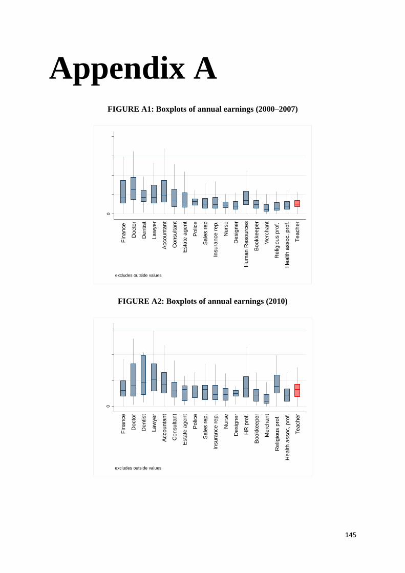
145

Appendix A

FIGURE A1: Boxplots of annual earnings (2000–2007)

FIGURE A2: Boxplots of annual earnings (2010)

0

10

00

00

20

00

00

30

00

00

40

00

00

an

nu

al

Fin

ance

Do

cto

r

De

ntist

La

wye

r

Accou

nta

nt

Co

nsu

ltan

t

Esta

te a

ge

nt

Polic

e

Sale

s r

ep

Insura

nce

re

p.

Nu

rse

De

sig

ne

r

Hu

man

Reso

urc

es

Boo

kkee

pe

r

Merc

han

t

Re

ligio

us p

rof.

He

alth

assoc. p

rof.

Te

ach

er


0

10

00

00

20

00

00

30

00

00

an

nu

al

Fin

ance

Do

cto

r

De

ntist

La

wye

r

Accou

nta

nt

Co

nsu

ltan

t

Esta

te a

ge

nt

Polic

e

Sale

s r

ep

.

Insura

nce

re

p.

Nu

rse

De

sig

ne

r

HR

pro

f.

Boo

kkee

pe

r

Merc

han

t

Re

ligio

us p

rof.

He

alth

assoc, p

rof.

Te

ach

er


146

TABLE A1: Non-teaching professionals in the LFS (2000–2007) and QLFS (2010)

NON-TEACHING PROFESSIONALS

Business professionals

Legal professionals

Archivists, librarians and related information professionals

Social science and related professionals

Writers and creative or performing artists

Religious professionals

College, university and higher education teaching professionals

Health professionals (except nursing)

Life science professionals

Physical sciences technologists

Computing professionals

Architects, engineers and related professionals

Mathematicians, statisticians and related professionals

Physicists, chemists and related professionals

TABLE A2: Variables included in augmented Mincerian wage function

VARIABLE DESCRIPTION

13 years of education A dummy variable taking the value of 1 if the worker has 13 years of education and 0 otherwise.




Educ A continuous variable reflecting the number of years of education an individual has completed.

Educ2 A quadratic term (number of years of education squared) included to control for the possibility of

non-linearities in the returns to education.

Exp A continuous variable reflecting the number of years the worker has been employed in the labour

market (calculated as [age – 6 – years of educational attainment])

Exp2 A quadratic term (number of years of experience squared) included to control for the possibility of

non-linearities in the returns to experience.

Union45 A dummy variable taking the value of 1 if the workers is a union member and 0 otherwise.

Female A dummy variable taking the value of 1 if a worker is female and 0 otherwise.

Tenure A continuous variable controlling for the number of years a worker has worked for their current

employer.

Teacher A dummy variable taking the value of 1 if the worker is a teacher and 0 otherwise.

Black A dummy variable taking the value of 1 if the worker is black and 0 otherwise.

Coloured A dummy variable taking the value of 1 if the worker is coloured and 0 otherwise.

Indian A dummy variable taking the value of 1 if the worker is Indian and 0 otherwise.

White A dummy variable taking the value of 1if the worker is white and 0 otherwise.

45 Not available in the QLFS 2010

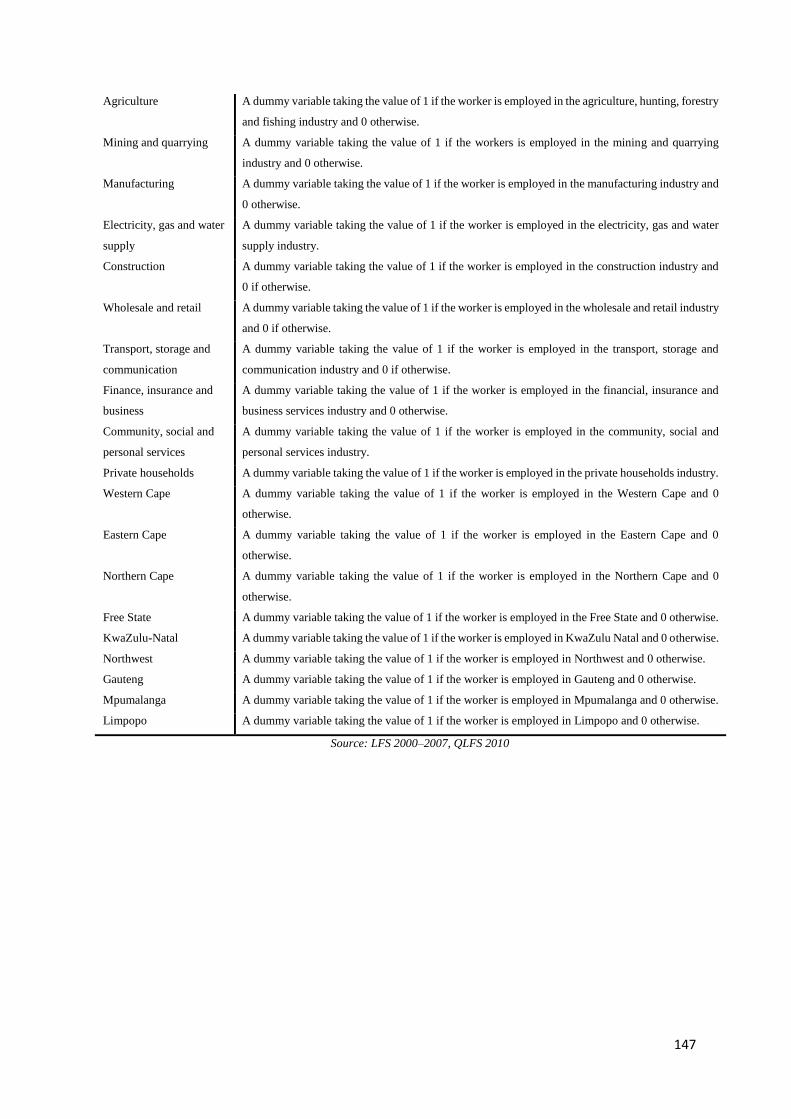
147

Agriculture A dummy variable taking the value of 1 if the worker is employed in the agriculture, hunting, forestry

and fishing industry and 0 otherwise.

Mining and quarrying A dummy variable taking the value of 1 if the workers is employed in the mining and quarrying

industry and 0 otherwise.

Manufacturing A dummy variable taking the value of 1 if the worker is employed in the manufacturing industry and

0 otherwise.

Electricity, gas and water

supply

A dummy variable taking the value of 1 if the worker is employed in the electricity, gas and water

supply industry.

Construction A dummy variable taking the value of 1 if the worker is employed in the construction industry and

0 if otherwise.

Wholesale and retail A dummy variable taking the value of 1 if the worker is employed in the wholesale and retail industry

and 0 if otherwise.

Transport, storage and

communication

A dummy variable taking the value of 1 if the worker is employed in the transport, storage and

communication industry and 0 if otherwise.

Finance, insurance and

business

A dummy variable taking the value of 1 if the worker is employed in the financial, insurance and

business services industry and 0 otherwise.

Community, social and

personal services

A dummy variable taking the value of 1 if the worker is employed in the community, social and

personal services industry.

Private households A dummy variable taking the value of 1 if the worker is employed in the private households industry.

Western Cape A dummy variable taking the value of 1 if the worker is employed in the Western Cape and 0

otherwise.

Eastern Cape A dummy variable taking the value of 1 if the worker is employed in the Eastern Cape and 0

otherwise.

Northern Cape A dummy variable taking the value of 1 if the worker is employed in the Northern Cape and 0

otherwise.

Free State A dummy variable taking the value of 1 if the worker is employed in the Free State and 0 otherwise.

KwaZulu-Natal A dummy variable taking the value of 1 if the worker is employed in KwaZulu Natal and 0 otherwise.

Northwest A dummy variable taking the value of 1 if the worker is employed in Northwest and 0 otherwise.

Gauteng A dummy variable taking the value of 1 if the worker is employed in Gauteng and 0 otherwise.

Mpumalanga A dummy variable taking the value of 1 if the worker is employed in Mpumalanga and 0 otherwise.

Limpopo A dummy variable taking the value of 1 if the worker is employed in Limpopo and 0 otherwise.

Source: LFS 2000–2007, QLFS 2010

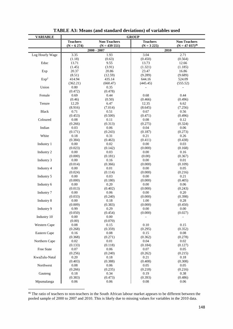
148

TABLE A3: Means (and standard deviations) of variables used

VARIABLE GROUP

Teachers

(N = 6 274)

Non-Teachers

(N = 439 551)

Teachers

(N = 3 225)

Non-Teachers

(N = 47 037)46

2000 - 2007 2010

Log Hourly Wage 3.35

(1.18)

1.93

(0.63)

3.04

(0.450)

2.71

(0.564)

Educ 13.71

(1.45)

9.55

(3.91)

13.73

(1.321)

12.66

(1.185)

Exp 20.37

(8.51)

20.86

(12.59)

23.47

(9.289)

16.86

(9.689)

Exp2 414.94

(362.21)

435.14

(660.47)

644.16

(445.45)

524.09

(555.52)

Union 0.80

(0.472)

0.35

(0.478)

- -

Female 0.69

(0.46)

0.44

(0.50)

0.68

(0.466)

0.44

(0.496)

Tenure 12.29

(8.916)

6.47

(7.014)

12.35

(8.645)

6.62

(7.256)

Black 0.71

(0.453)

0.51

(0.500)

0.67

(0.471)

0.56

(0.496)

Coloured 0.08

(0.266)

0.11

(0.313)

0.08

(0.275)

0.12

(0.324)

Indian 0.03

(0.171)

0.06

(0.243)

0.04

(0.187)

0.06

(0.273)

White 0.18

(0.384)

0.31

(0.463)

0.21

(0.411)

0.26

(0.438)

Industry 1 0.00

(0.023)

0.02

(0.142)

0.00

(0.000)

0.03

(0.168)

Industry 2 0.00

(0.000)

0.03

(0.181)

0.00

(0.00)

0.16

(0.367)

Industry 3 0.00

(0.014)

0.16

(0.366)

0.00

(0.000)

0.01

(0.109)

Industry 4 0.00

(0.024)

0.01

(0.114)

0.00

(0.000)

0.05

(0.216)

Industry 5 0.00

(0.000)

0.03

(0.180)

0.00

(0.000)

0.21

(0.405)

Industry 6 0.00

(0.013)

0.20

(0.402)

0.00

(0.000)

0.06

(0.243)

Industry 7 0.00

(0.033)

0.06

(0.240)

0.00

(0.000)

0.20

(0.398)

Industry 8 0.00

(0.009)

0.18

(0.383)

1.00

(0.000)

0.28

(0.450)

Industry 9 0.99

(0.050)

0.29

(0.454)

0.00

(0.000)

0.00

(0.027)

Industry 10 0.00

(0.00)

0.00

(0.070)

- -

Western Cape 0.08

(0.268)

0.15

(0.359)

0.10

(0.295)

0.15

(0.352)

Eastern Cape 0.16

(0.368)

0.08

(0.271)

0.15

(0.362)

0.08

(0.278)

Northern Cape 0.02

(0.133)

0.01

(0.118)

0.04

(0.184)

0.02

(0.127)

Free State 0.07

(0.256)

0.06

(0.240)

0.07

(0.262)

0.05

(0.215)

KwaZulu-Natal 0.20

(0.403)

0.18

(0.388)

0.21

(0.408)

0.18

(0.308)

Northwest 0.08

(0.266)

0.06

(0.235)

0.05

(0.218)

0.05

(0.216)

Gauteng 0.18

(0.383)

0.34

(0.473)

0.19

(0.393)

0.38

(0.486)

Mpumalanga 0.06 0.06 0.08 0.06

46 The ratio of teachers to non-teachers in the South African labour market appears to be different between the

pooled sample of 2000 to 2007 and 2010. This is likely due to missing values for variables in the 2010 data.

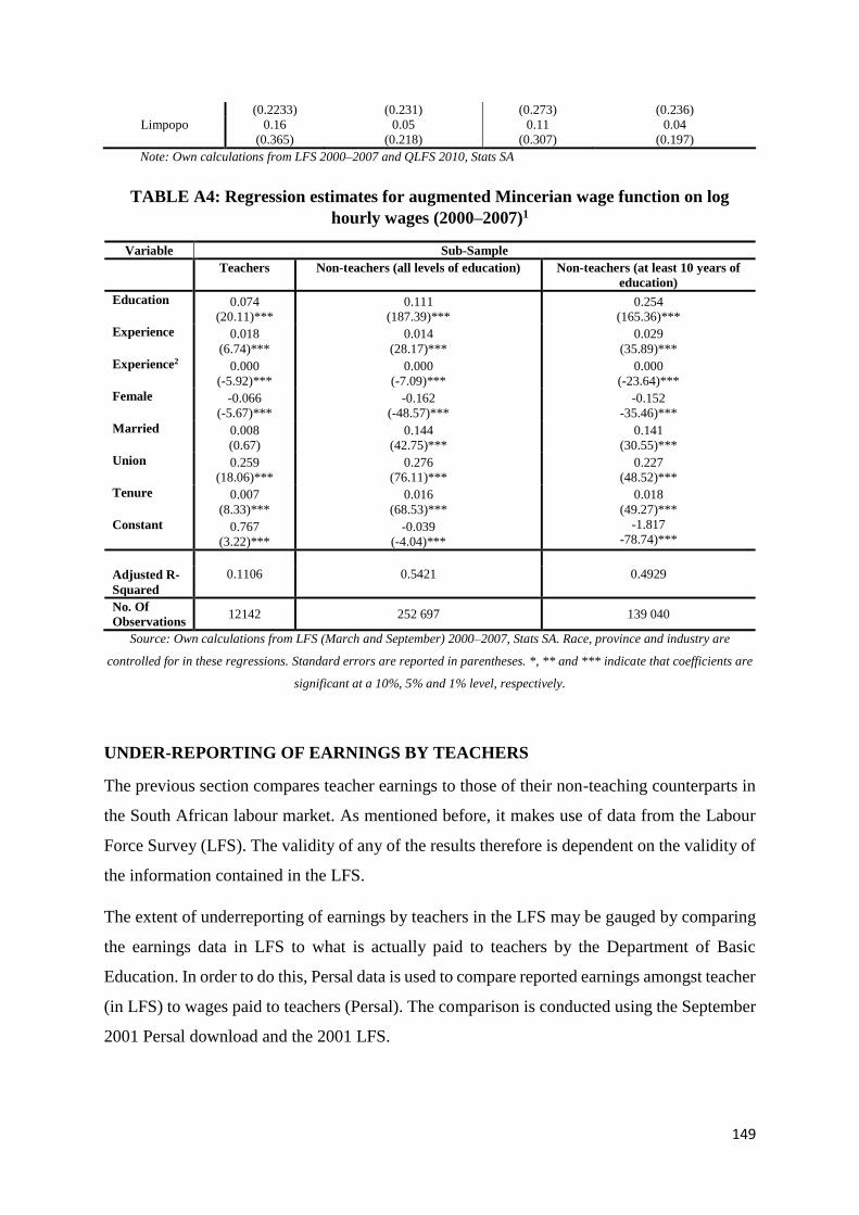
149

(0.2233) (0.231) (0.273) (0.236)

Limpopo 0.16

(0.365)

0.05

(0.218)

0.11

(0.307)

0.04

(0.197)

Note: Own calculations from LFS 2000–2007 and QLFS 2010, Stats SA

TABLE A4: Regression estimates for augmented Mincerian wage function on log

hourly wages (2000–2007)1

Variable Sub-Sample

Teachers Non-teachers (all levels of education) Non-teachers (at least 10 years of

education)

Education 0.074

(20.11)***

0.111

(187.39)***

0.254

(165.36)***

Experience 0.018

(6.74)***

0.014

(28.17)***

0.029

(35.89)***

Experience2 0.000

(-5.92)***

0.000

(-7.09)***

0.000

(-23.64)***

Female -0.066

(-5.67)***

-0.162

(-48.57)***

-0.152

-35.46)***

Married 0.008

(0.67)

0.144

(42.75)***

0.141

(30.55)***

Union 0.259

(18.06)***

0.276

(76.11)***

0.227

(48.52)***

Tenure 0.007

(8.33)***

0.016

(68.53)***

0.018

(49.27)***

Constant 0.767

(3.22)***

-0.039

(-4.04)***

-1.817

-78.74)***

0.1106 0.5421 0.4929 Adjusted R-

Squared

No. Of

Observations 12142 252 697 139 040

Source: Own calculations from LFS (March and September) 2000–2007, Stats SA. Race, province and industry are

controlled for in these regressions. Standard errors are reported in parentheses. *, ** and *** indicate that coefficients are

significant at a 10%, 5% and 1% level, respectively.

UNDER-REPORTING OF EARNINGS BY TEACHERS

The previous section compares teacher earnings to those of their non-teaching counterparts in

the South African labour market. As mentioned before, it makes use of data from the Labour

Force Survey (LFS). The validity of any of the results therefore is dependent on the validity of

the information contained in the LFS.

The extent of underreporting of earnings by teachers in the LFS may be gauged by comparing

the earnings data in LFS to what is actually paid to teachers by the Department of Basic

Education. In order to do this, Persal data is used to compare reported earnings amongst teacher

(in LFS) to wages paid to teachers (Persal). The comparison is conducted using the September

2001 Persal download and the 2001 LFS.

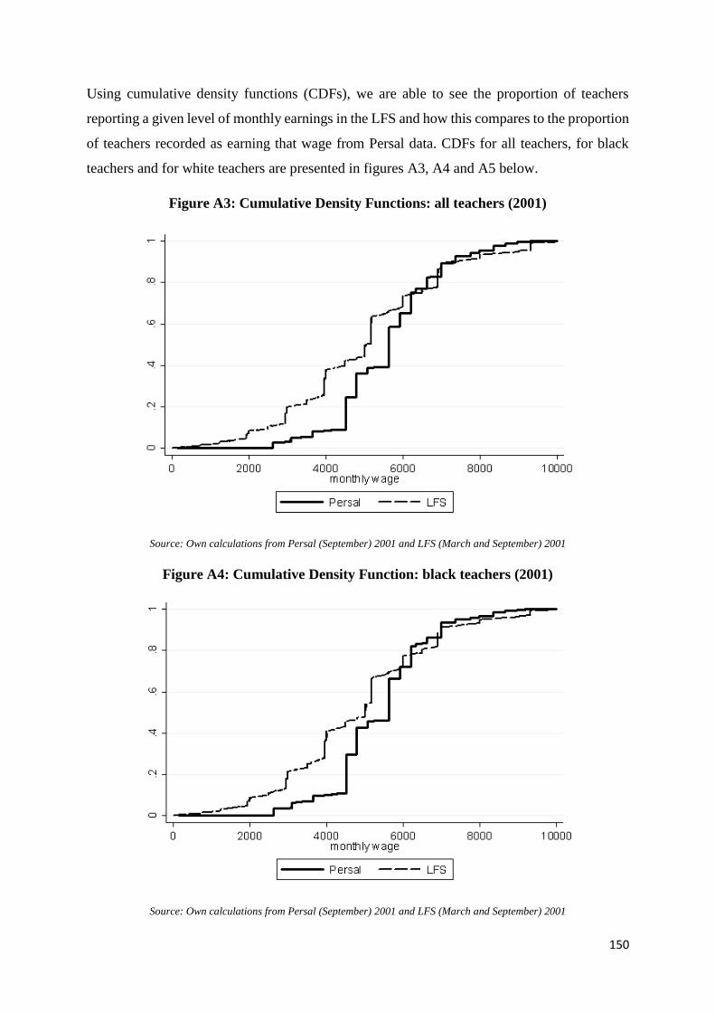
150

Using cumulative density functions (CDFs), we are able to see the proportion of teachers

reporting a given level of monthly earnings in the LFS and how this compares to the proportion

of teachers recorded as earning that wage from Persal data. CDFs for all teachers, for black

teachers and for white teachers are presented in figures A3, A4 and A5 below.

Figure A3: Cumulative Density Functions: all teachers (2001)

Source: Own calculations from Persal (September) 2001 and LFS (March and September) 2001

Figure A4: Cumulative Density Function: black teachers (2001)


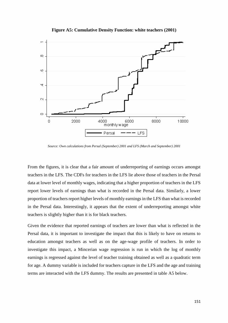
151

Figure A5: Cumulative Density Function: white teachers (2001)


From the figures, it is clear that a fair amount of underreporting of earnings occurs amongst

teachers in the LFS. The CDFs for teachers in the LFS lie above those of teachers in the Persal

data at lower level of monthly wages, indicating that a higher proportion of teachers in the LFS

report lower levels of earnings than what is recorded in the Persal data. Similarly, a lower

proportion of teachers report higher levels of monthly earnings in the LFS than what is recorded

in the Persal data. Interestingly, it appears that the extent of underreporting amongst white

teachers is slightly higher than it is for black teachers.

Given the evidence that reported earnings of teachers are lower than what is reflected in the

Persal data, it is important to investigate the impact that this is likely to have on returns to

education amongst teachers as well as on the age-wage profile of teachers. In order to

investigate this impact, a Mincerian wage regression is run in which the log of monthly

earnings is regressed against the level of teacher training obtained as well as a quadratic term

for age. A dummy variable is included for teachers capture in the LFS and the age and training

terms are interacted with the LFS dummy. The results are presented in table A5 below.

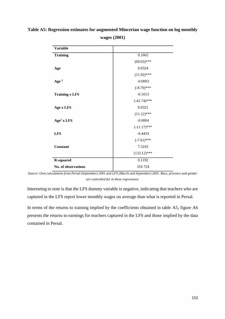
152

Table A5: Regression estimates for augmented Mincerian wage function on log monthly

wages (2001)

Variable

Training 0.1602

(69.03)***

Age 0.0324

(11.92)***

Age 2 -0.0003

(-8.70)***

Training x LFS -0.1013

(-41.74)***

Age x LFS 0.0321

(11.12)***

Age2 x LFS -0.0004

(-11.17)***

LFS -0.4433

(-7.61)***

Constant 7.3243

(133.12)***

R-squared 0.1192

No. of observations 316 724

Source: Own calculations from Persal (September) 2001 and LFS (March and September) 2001. Race, province and gender

are controlled for in these regressions.

Interesting to note is that the LFS dummy variable is negative, indicating that teachers who are

captured in the LFS report lower monthly wages on average than what is reported in Persal.

In terms of the returns to training implied by the coefficients obtained in table A5, figure A6

presents the returns to earnings for teachers captured in the LFS and those implied by the data

contained in Persal.

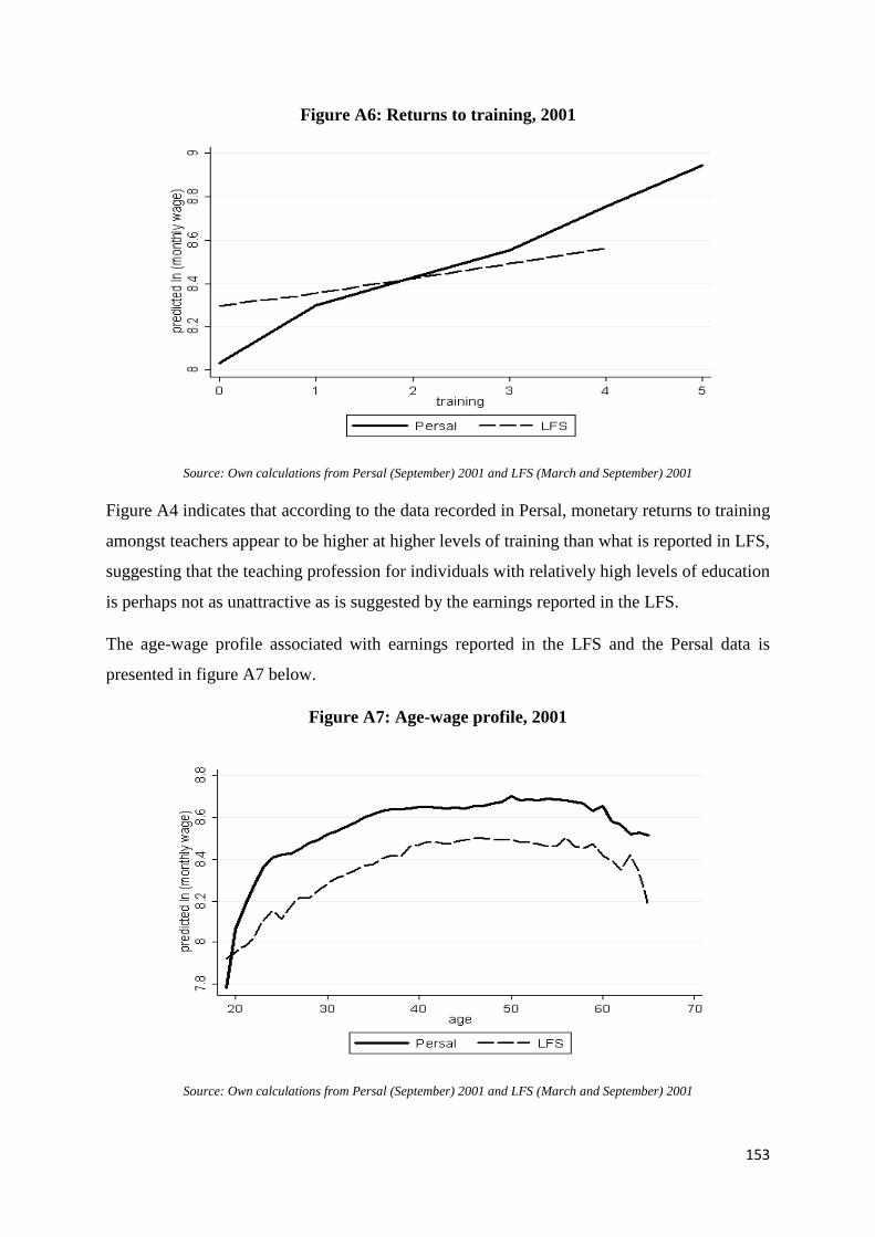
153

Figure A6: Returns to training, 2001


Figure A4 indicates that according to the data recorded in Persal, monetary returns to training

amongst teachers appear to be higher at higher levels of training than what is reported in LFS,

suggesting that the teaching profession for individuals with relatively high levels of education

is perhaps not as unattractive as is suggested by the earnings reported in the LFS.

The age-wage profile associated with earnings reported in the LFS and the Persal data is

presented in figure A7 below.

Figure A7: Age-wage profile, 2001


154

From figure A5, we see that although the profile is lower at all age for teachers captured in the

LFS, is appears that the age-wage profile takes a similar shape for both the LFS and the Persal

data, with the exception of the oldest teachers in the data. For these teachers, monthly earnings

in the LFS appear to drop by a significantly greater amount after the age of roughly 61 or 62

than they do in the Persal data.

This brief analysis has therefore pointed out that there is evidence of underreporting of earnings

amongst teachers in the LFS relative to what is recorded in the Persal dataset. It is important to

bear in mind that the unattractiveness of the teaching profession implied in the previous section

of this paper may thus be overstated.

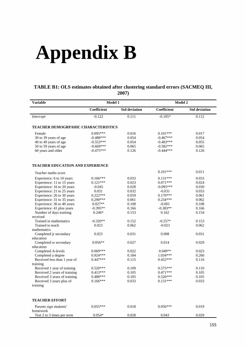
155

Appendix B

TABLE B1: OLS estimates obtained after clustering standard errors (SACMEQ III,

2007)

Variable Model 1 Model 2

Coefficient Std deviation Coefficient Std deviation

Intercept -0.122 0.111 -0.185* 0.112

TEACHER DEMOGRPAHIC CHARACTERISTICS

Female 0.095*** 0.016 0.101*** 0.017

30 to 39 years of age -0.488*** 0.054 -0.467*** 0.054

40 to 49 years of age -0.553*** 0.054 -0.483*** 0.055

50 to 59 years of age -0.669*** 0.065 -0.582*** 0.065

60 years and older -0.475*** 0.126 -0.444*** 0.126


Teacher maths score 0.101*** 0.011

Experience: 6 to 10 years 0.166*** 0.033 0.131*** 0.033


Experience: 16 to 20 years -0.045 0.028 -0.095*** 0.030

Experience: 21 to 25 years 0.031 0.032 -0.031 0.033



Experience: 36 to 40 years 0.027** 0.108 -0.001 0.108

Experience: 41 plus years -0.395** 0.166 -0.383** 0.166


received

0.246* 0.153 0.162 0.154

Trained in mathematics -0.320** 0.152 -0.257* 0.153

Trained to teach

mathematics

0.023 0.062 -0.023 0.062


education

0.023 0.031 0.008 0.031


education

0.056** 0.027 0.014 0.029

Completed A-levels 0.069*** 0.022 0.049** 0.023

Completed a degree 0.924*** 0.184 1.034*** 0.266

Received less than 1 year of

training

0.447*** 0.115 0.452*** 0.116

Received 1 year of training 0.520*** 0.109 0.575*** 0.110

Received 2 years of training 0.413*** 0.105 0.471*** 0.105

Received 3 years of training 0.488*** 0.105 0.526*** 0.105


training

0.166*** 0.033 0.131*** 0.033

TEACHER EFFORT


homework

0.055*** 0.018 0.056*** 0.019

Test 2 to 3 times per term 0.054* 0.028 0.043 0.029

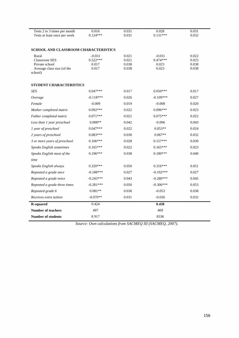
156

Tests 2 to 3 times per month 0.016 0.031 0.028 0.031

Tests at least once per week 0.124*** 0.031 0.131*** 0.032


Rural -0.031 0.021 -0.031 0.022

Classroom SES 0.522*** 0.021 0.474*** 0.023

Private school 0.017 0.038 0.023 0.038


school)

0.017 0.038 0.023 0.038


SES 0.047*** 0.017 0.050*** 0.017

Overage -0.118*** 0.026 -0.109*** 0.027

Female -0.009 0.019 -0.008 0.020

Mother completed matric 0.092*** 0.022 0.096*** 0.023

Father completed matric 0.071*** 0.021 0.075*** 0.022

Less than 1 year preschool 0.008** 0.042 -0.006 0.043

1 year of preschool 0.047*** 0.022 0.053** 0.024

2 years of preschool 0.083*** 0.030 0.067** 0.032

3 or more years of preschool 0.166*** 0.028 0.157*** 0.030

Speaks English sometimes 0.165*** 0.022 0.165*** 0.023

Speaks English most of the

time

0.196*** 0.038 0.180*** 0.040

Speaks English always 0.320*** 0.050 0.316*** 0.051

Repeated a grade once -0.188*** 0.027 -0.192*** 0.027

Repeated a grade twice -0.243*** 0.043 -0.280*** 0.045

Repeated a grade three times -0.281*** 0.050 -0.306*** 0.053

Repeated grade 6 0.081** 0.036 -0.053 0.038

Receives extra tuition -0.070** 0.031 -0.026 0.032

R-squared 0.424 0.438

Number of teachers 497 469

Number of students 8 917 8336


157

TABLE B2: Full Hierarchical Linear Model (SACMEQ II, 2000)

Variable Coefficient Std deviation

Intercept 0.048 0.176

TEACHER DEMOGRAPHIC CHARACTERISTICS

Female 0.083 0.077

30 to 39 years of age 0.003 0.120

40 to 49 years of age 0.315* 0.189

50 years and older 0.671** 0.232

60 years and older -


Teacher maths score -

Experience: 6 to 10 years -0.17 0.118

Experience: 11 to 15

years

-0.245* 0.139


years

-0.431* 0.229


years

-0.454** 0.194


years

-0.803*** 0.259


years

-0.952** 0.413

Experience: 36 plus -0.603** 0.292


received

-0.001** 0.001

Trained in mathematics -

Trained to teach

mathematics

-


education

-0.082 0.275


education

0.243 0.157

Completed A-levels 0.473*** 0.115

Completed a degree 0.403*** 0.126

Received less than 1 year

of training

-

Received 1 year of

training

-

Received 2 years of

training

-0.588*** 0.179

Received 3 years of

training

-0.351* 0.196


training

-0.412*** 0.096

TEACHER EFFORT


homework

0.014 0.095

Test 2 to 3 times per term -

Tests 2 to 3 times per

month

0.135 0.184

Tests at least once per

week

0.111 0.099

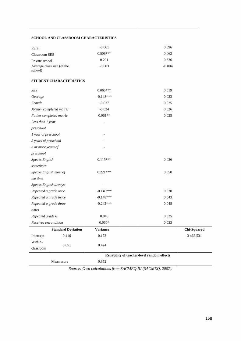
158


Rural -0.061 0.096

Classroom SES 0.506*** 0.062

Private school 0.291 0.336


school)

-0.003 -0.004


SES 0.065*** 0.019

Overage -0.148*** 0.023

Female -0.027 0.025

Mother completed matric -0.024 0.026

Father completed matric 0.061** 0.025

Less than 1 year

preschool

-

1 year of preschool -

2 years of preschool -

3 or more years of

preschool

-

Speaks English

sometimes

0.115*** 0.036

Speaks English most of

the time

0.221*** 0.050

Speaks English always -

Repeated a grade once -0.140*** 0.030

Repeated a grade twice -0.148*** 0.043

Repeated a grade three

times

-0.242*** 0.048

Repeated grade 6 0.046 0.035

Receives extra tuition 0.060* 0.033

Standard Deviation Variance Chi-Squared

Intercept 0.416 0.173 3 468.531

Within-

classroom 0.651 0.424


Mean score 0.852


159

Appendix C Minimum requirements for teacher education

qualifications

The Government Gazette No. 34467 of 2011 on Minimum Requirements for Teacher Education

Qualifications lists the professional and academic qualifications selected for teacher education

(DHET, 2011):

i. Qualifications for initial teacher education (ITE):

Bachelor of Education degree

Advanced Diploma in Teaching

ii. Qualifications for the continuing professional and academic development of

teachers:

Advanced Certificate in Teaching

Advanced Diploma in Education

Postgraduate Diploma in Education

Bachelor of Education Honours degree

Master of Education degree

Doctoral degree

iii. Qualification for grade R teaching:

Diploma in grade R teaching

Students enrolled in ITE programmes are students who may be considered part of the potential

stock of future teachers. It is possible and probable that students enrolled in continuing

professional and academic development may already belong to the teaching force, or that they

have continued from initial teacher education.

The gazette explains that “[t]he primary purpose of all Initial Teacher Education qualifications

is to certify that the holder has specialized as a beginner teacher in a specific phase and/or

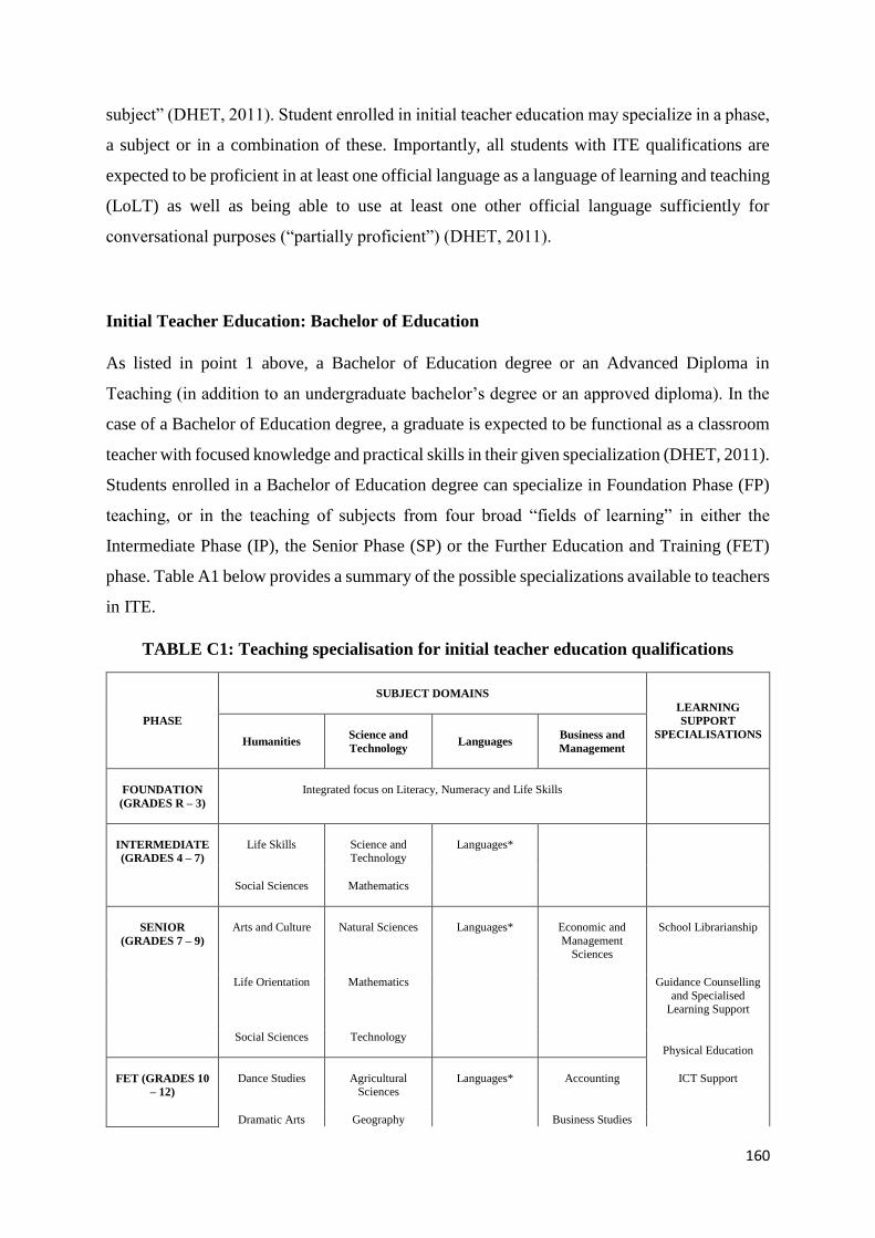
160

subject” (DHET, 2011). Student enrolled in initial teacher education may specialize in a phase,

a subject or in a combination of these. Importantly, all students with ITE qualifications are

expected to be proficient in at least one official language as a language of learning and teaching

(LoLT) as well as being able to use at least one other official language sufficiently for

conversational purposes (“partially proficient”) (DHET, 2011).

Initial Teacher Education: Bachelor of Education

As listed in point 1 above, a Bachelor of Education degree or an Advanced Diploma in

Teaching (in addition to an undergraduate bachelor’s degree or an approved diploma). In the

case of a Bachelor of Education degree, a graduate is expected to be functional as a classroom

teacher with focused knowledge and practical skills in their given specialization (DHET, 2011).

Students enrolled in a Bachelor of Education degree can specialize in Foundation Phase (FP)

teaching, or in the teaching of subjects from four broad “fields of learning” in either the

Intermediate Phase (IP), the Senior Phase (SP) or the Further Education and Training (FET)

phase. Table A1 below provides a summary of the possible specializations available to teachers

in ITE.

TABLE C1: Teaching specialisation for initial teacher education qualifications

PHASE

SUBJECT DOMAINS

LEARNING

SUPPORT

SPECIALISATIONS Humanities

Science and

Technology

Languages Business and

Management

FOUNDATION

(GRADES R – 3)

Integrated focus on Literacy, Numeracy and Life Skills

INTERMEDIATE

(GRADES 4 – 7)

Life Skills

Science and Technology

Languages*

Social Sciences

Mathematics

SENIOR

(GRADES 7 – 9)

Arts and Culture

Natural Sciences

Languages*

Economic and

Management Sciences

School Librarianship

Life Orientation Mathematics Guidance Counselling

and Specialised Learning Support

Social Sciences

Technology Physical Education

FET (GRADES 10

– 12)

Dance Studies

Agricultural Sciences

Languages*

Accounting

ICT Support

Dramatic Arts Geography Business Studies

161

History

Life Sciences Economics

Life Orientation Mathematics Hospitality Studies

Music Mathematical

Literacy

Tourism

Religion Studies Physical Sciences

Visual Arts Computer Applications

Technology

Agricultural

Management

Practices

Civil Technology

Electrical Technology

Engineering

Graphics and Design

Information Technology

Mechanical Technology

Design

Consumer Studies

Source: Department of Higher Education and Training (2011). Minimum Requirements for Teacher Education Qualifications.

Teachers are qualified to teach the phase and/or subjects in which they specialised while

studying for a Bachelor of Education degree. Of importance in the FP specialisation is that

teachers must specialise in First Language teaching in at least one of the official languages, as

well as in First Additional Language teaching. Certain stipulations exist regarding which

languages teachers must choose. These can be found on page 23 of the Minimum Requirements

for Teacher Education Qualifications. Students specialising in the IP must specialise in the

teaching of at least four subjects indicated in the IP domain in table 1. Because the first year of

senior phase is often taught with the intermediate phase, teachers who has specialised in the

intermediate phase must be able to teacher grade 7. IP specialists employed to teach subjects

at a grade 7 level may enrol for an Advanced Certificate (discussed later) in the SP subject in

order to develop competence in the grade 7 subjects which they are to teach (DHET, 2011). In

order to teach in secondary schools, teachers must have completed a combined SP and FET

programme. Teachers must have completed a minimum of three specialisations: i) two SP

subjects and one FET subject; ii) one SP subject and two FET subjects; or iii) one SP subject,

one FET subject and one support role. At least one SP subject and as least one FET subject are

therefore required for teachers specialising in this combination.

162

Initial Teacher Education: Advanced Diploma in Teaching

The Advanced Diploma in Teaching “offers entry-level initial professional preparation for

graduates and diplomats who wish to develop focused knowledge and skills as classroom

teachers in a chosen phase(s) and/or subject(s)” (DHET, 2011). The Minimum Requirements

for Teacher Education Qualifications stipulates that a Bachelor’s degree is the preferred

minimum entry requirement for the Advanced Diploma in teaching and that it should include

sufficient academic content knowledge of the school subjects in the phase that the student

would like to teacher (DHET, 2011). A number of diplomas are also listed as being acceptable

for entry into the Advanced Diploma in Teaching. These are presented in Appendix E on page

56 of the Minimum Requirements for Teacher Education Qualifications.

The requirements for the Advanced Diploma in Teaching for different phases are largely

similar to those stipulated for the Bachelor of Education degree. However, in the case of SP

and FET teaching, only two subject specialisations (only one SP subject and one FET subject)

are required, whereas a minimum of three is required in the case of the Bachelor of Education.

Furthermore, it is possible to specialise only in FET teaching in the case of an Advanced

Diploma in Teaching. In this case, the subject in which the students specialises must have been

a major subject in the Bachelor’s degree or diploma in the qualification through which the

student entered the Advanced Diploma in Teaching.

ITE in the form of a Bachelor of Education and Advanced Diploma in Teaching prepares

students who have not yet entered the teaching force to do so. Graduates from these

programmes may therefore be thought of as “potential teachers” as there is no guarantee that

they will enter the teaching profession once they have completed these programmes. The higher

education system also provides for teachers who already belong to the teaching force, but who

are involved in Continuing Professional Development (CPD). For the sake of this report, the

focus will fall on teachers enrolled in the Advanced Certificate in Teaching. It is true that an

extensive list of CPD programmes exists, but it is only the Advanced Certificate in Teaching

that can qualify teachers to teach in areas that they were previously not qualified to teach rather

than enhancing the research or academic qualifications of teachers. The Advanced Certificate

in Teaching is therefore the only means of quantifying the potential stock of teachers.

Continuing Professional Development: Advanced Certificate in Teaching

163

The Advanced Certificate in Teaching is designed to prepare teachers to teach new subjects or

phases, or to enhance their knowledge and competence in an existing subject or phase. The

certificate was established to address the needs of three sets of teachers:

1. Teachers seeking retraining: These are teachers who would like to specialise in

teaching a subject for which they have not previously obtained a professional

teaching qualification.

2. Recognition of prior learning (RPL) upgrading: Teachers with prior professional

teaching qualifications teaching FP or IP but who did not specialise in the phase.

The Advanced Certificate in Teaching allows them to complete a formal

qualification in either FP or IP, given that they have obtained the appropriate

knowledge by teaching FP or IP.

3. Teachers who completed a three-year diploma in education at a former college of

education, or a National Professional Diploma in Education and who want to

strengthen their specialisation in their particular subject or phase.

The Minimum Requirements for Teacher Education Qualifications stipulates that “the

Advanced Certificate may only be utilised for the retraining or upgrading of teachers who hold

prior professional teaching qualifications in a subject and/or phase. It is not available for new

roles in education” (DHET, 2011).

164

List of References

Anderson, J.B. 2000. Factors affecting learning of Mexican primary school children. Estudios

Economicos. 15(1):117-152.

Angrist, J.D. & Lavy, V. 2001. Does teacher training affect pupil learning? Evidence from

matched comparisons in Jerusalem public schools. Journal of Labor Economics.

19(2):343-369.

Arif, G.M. & Saqib, N. 2003. Production of cognitive and life skills in public, private, and

NGO schools in Pakistan. Pakistan Development Review. 42(1):1-28.

Arnold, C.L. 1992. Methods, plainly speaking: An introduction to hierarchical linear models.

Measurement and Evaluation in Counselling and Development. 25:58-90.

August, B., Kihn, P. & Miller, M. 2010. Closing the talent gap: Attracting and retaining top

third graduates to careers in teaching. McKinsey Quarterly. September 2010.

Available:

http://www.mckinsey.com/clientservice/Social_Sector/our_practices/Education/Know

ledge_Highlights/~/media/Reports/SSO/Closing_the_talent_gap.ashx. [3 March

2011].

Baker, G. 2002. Distortion and risk in optimal incentive contracts. The Journal of Human

Resources. 37(4):4–24.

Ball, D., Thames, M.H. & Phelps, G. 2008. Content knowledge for teaching: What makes it

special? Journal of Teacher Education. 59:389-408.

Ballou, D. & Podgursky, M. 1997. Teacher pay and teacher quality. Kalamazoo: Upjohn

Institute for Employment Research.

Ballou, D. 2001. Pay for performance in public and private schools. Economics of Education

Review. 20:51-61.

Barnett, W.S. 2003. Low wages = low quality. Solving the real preschool teacher crisis.

Preschool Policy Facts. 3:1-2.

Behrman, J.R., Kahn, S., Ross, D. & Sabot, R. 1997. School quality and cognitive

achievement production: A case study for rural Pakistan. Economics of Education

Review. 16(2):127-142.

Bennell, P. 2004. Teacher motivations and incentives in Sub-Saharan Africa and Asia.

Knowledge and Skills for Development. Brighton: Department for International

Development.

165

Bot, M. 1996. A brief overview of education. EduSource: Data News, no. 12. Johannesburg:

EduSource.

Bruns, B., Filmer, D. & Patrinos, H. 2010. Making schools work: New evidence on

accountability reforms. Washington DC: The World Bank.

Bruns, B., Evans, D. & Luque, J. 2012. Achieving world-class education in Brazil.

Washington DC: The World Bank.

Campbell, D.T. 1976. Assessing the impact of planned social change. Occasional paper for

for the Public Affairs Centre. Dartmouth College, New Hampshire.

Centre for Development Enterprise (CDE). 2011. Value in the classroom: The quantity and

quality of South African teachers. Johannesburg: CDE.

Chaplin, D. 2008. Hierarchical linear modelling: Strengths and weaknesses. Paper prepared

for the conference of the Association of Public Policy Analysis and Management,

November 2008. Washington, DC.

Che, Y. & Yoo, S. 2001. Optimal incentives for teams. American Economic Review.

91(3):525-541.

Chetty, R., Friedman, J.N. & Rockoff, J.E. 2011. Measuring the impact of teachers: Teacher

value-added and student outcomes in adulthood. (National Bureau of Economic

Research (NBER) working paper no. 17699). Cambridge MA: NBER.

Chingos, M.M. & Peterson, P.E. 2011. It’s easier to pick a good teacher than to train one:

Familiar and new results on the correlates of teacher effectiveness. Economics of

Education Review. 30:449-465.

Chisholm, L. 1999. The democratization of schools and politics of teachers’ work in South

Africa. Compare: A Journal of Comparative and International Education. 29(2):111-

126.

Chisholm, L. 2009. An overview of research, policy and practice in teacher supply and

demand 1994-2008. Cape Town: HSRC Press.

Clotfelter, C., Ladd, H., Vigdor, J. & Diaz, R. 2004. Do schools accountability systems make

it more difficult for low-performing schools to attract and retain high-quality

teachers? Journal of Policy Analysis and Management. 23(2):251-271.

Clotfelter, C., Ladd, H. & Vigdor, J. 2005. Who teaches whom? Race and the distribution of

novice teachers. Economics of Education Review. 24:377-392.

166

Clotfelter, C.T., Ladd, H.F. & Vigdor, J.L. 2007. Teacher credential and student

achievement: Longitudinal analysis with student fixed effects. Education of Education

Review. 26:673-682.

Crouch, L. 2001. Turbulence or orderly change? Teacher supply and demand in the age of

AIDS. Occasional paper. Department of Education: Pretoria. April 2001.

Crouch, L. & Mabogoane, T. 2001. Not magic bullets, just tracer bullets: The role of learning

resources, social advantage and education management in improving the performance

of South African schools. Social Dynamics: A journal of African studies. 27(1):60-78.

Crouch, L. & Perry, H. 2003. “Educators” in A. Kraak & H. Perold (Eds). Human resources

development review: Education, employment and skills in South Africa. Cape Town:

HSRC. 476-499.

Delannoy, F. 2000. Education reform in Chile: 1980–1998. A lesson in pragmatism. The

World Bank Country Studies: Education Reform and Management Series. 1(1).

Department of Basic Eduction (DBE). 2013. Annual Report: 2012/2013. Pretoria: DBE.

Department of Education (DoE). 2005. Teacher for the future: meting teacher shortages to

achieve education for all. Pretoria: DoE.

Department of High Education and Training. 2011. Minimum requirements for teacher

education qualifications. Pretoria: Department of High Education and Training.

DiNardo, J., Fortin, N.M. & Lemieux, T. 1996. Labour market institutions and the

distribution of wages, 1973 – 1992: A semiparametric approach. Econometrica.

64(5):1001-1044.

Dixit, A. 2002. Incentives and accountability in the public sector: An interpretive review. The

Journal of Human Resources. 37(1):696-727.

Dolton, P. & Marcenaro-Gutierrex, O.D. 2011. If you pay peanuts do you get monkeys? A

cross-country analysis of teacher pay and pupil performance. Economic Policy.

26(5):5-55.

Duflo, E., Hanna, R. & Ryan, S. 2012. Incentives work: Getting teachers to come to school.

American Economic Review. 102(4):1241-1278.

Duncan, C., Jones, K. & Moon, G. 1998. Context, composition and heterogeneity: Using

multilevel models in health research. Social Science and Medicine. 46:97-117.

Education Forum. 2006. Teacher age and performance. Available:

http://educationforum.ipbhost.com/index.php?showtopic=8063. [30 May 2014].

167

Education Labour Relations Council (ELRC). 2003. Integrated quality management system

(IQMS) for school-based educators. Pretoria: ELRC.

Education Labour Relations Council (ELRC). 2011. Revised salary structure proposals.

Pretoria: ELRC.

Ehrenberg, R.G. & Brewer, D.J. 1995. Did teachers’ verbal ability and race matter in the

1960s? Coleman revisited. Economics of Education Review. 14:1-21.

Falch, T. & Strøm, B. 2005. Teacher turnover and non-pecuniary factors. Economics of

Education Review. 24:611-631.

Ferguson, R. F. 1998. Can schools narrow the Black-White test score gap? In C. Jencks & M.

Phillips (Eds). The Black-White test score gap. Washington, DC: Brookings

Institution. 318-374.

Figlio, D.N. & Kenny, L.W. 2007. Individual teacher incentives and student performance.

Journal of Public Policy. 91:901-914.

Figlio, D. & Winicki, J. 2005. The effect of school accountability plans on school nutrition.

The Journal of Public Economics. 89(2):381-394.

Fleisch, B. 2004. Does higher education expenditure generate higher learner achievement? A

study of historically disadvantaged schools in Gauteng. South African Journal of

Education. 24(4):264-269.

Glewwe, P., Ilias, N. & Kremer, M. 2010. Teacher incentives. American Economic Journal:

Applied Economics. 2(3):205–227.

Goldberger, A. S. 1991. A course in econometrics. Cambridge: Harvard University Press.

Gould, J.C., Abraham, J. & Bailey, B. 2005. Survey and analysis of teacher salary trends.

Washington: American Federation of Teachers.

Green, J. 2011. Education, professionalism and the quest for accountability: Hitting the

target but missing the point. New York: Routledge.

Gustafsson, M. 2006. Learning from Chile’s teacher incentives experience. Stellenbosch:

University of Stellenbosch. (Unpublished paper).

Gustafsson, M. 2007. Using the hierarchical linear model to understand school production in

South Africa. Working paper number 01/07. Stellenbosch: Department of Economics,

University of Stellenbosch.

Gustafsson, M. & Patel, F. 2009. Managing the teacher pay system: What the local and

international data are telling us. Cape Town: Development Policy Research Unit,

University of Cape Town.

168

Hall, E., Altman, M., Nkomo, N., Peltzer, K. & Zuma, K. 2005. Potential attrition in

education: The impact of job satisfaction, morale, workload and HIV/AIDS. Cape

Town: HSRC.

Hanushek, E.A. 1992. The trade-off between child quantity and quality. Journal of Political

Economy. 100:85-117.

Hanushek, E.A. 2007. The single salary structure and other issues of teacher pay. Peabody

Journal of Education. 82(4).

Hanushek, E. 2009. “Teacher deselection” in D. Goldhaber and J. Hannaway (Eds). 2009.

Creating a new teaching profession. Washington DC: The Urban Institute Press.

Hanushek, E. 2011. Valuing teachers. Education Next. 11(3):40-45.

Hanushek, E. & Woessman, L. 2008. The role of cognitive skills in economic development.

The Journal of Economic Literature. 46(3):607-668.

Harris, D.N. & Adams, S.J. 2007. Understanding the level and causes of teacher turnover: A

comparison with other professions. Economics of Education Review. 26:325-337.

Hernani-Limarino, W. 2005. “Are teachers well-paid in Latin America and the Caribbean?

Relative wage and structure of returns of teachers” in E. Vegas (Ed.). 2005. Incentives

to improve teaching: Lessons from Latin America. Washington DC: The World Bank.

Hill, H.C., Loewenberg Ball, D. & Schilling, S.G. 2008. Unpacking pedagogical content

knowledge: Conceptualising and measuring teachers’ topic-specific knowledge of

students. Journal for Research in Mathematics Education. 39(4):372-400.

Holstrom, B. & Milgrom, P. 1991. Multitask principal-agent analyses: Incentive contracts,

asset ownership and job design. The Journal of Law, Economics and Organization.

7:24-52.

Hosking, S.G. 2000. Government-induced teacher failure in South Africa – causes and

analysis. Development Southern Africa. 17(5):641-665.

Hout, M. & Elliot, S. (Eds). 2011. Incentives and test-based accountability in education.

Washington DC: The National Academies Press.

Hoxby, C. & Leigh, A. 2004. Pulled away or pushed out? Explaining the decline in teacher

aptitude in the United States. American Economic Review. 94(2):236-246.

Irving, M. 2012. Teacher labour markets in South Africa and Botswana: A comparative

analysis. Prospects. 42:389-402.

Jacob, B.A. & Levitt, S. 2003. Rotten apples: An investigation of the prevalence and

predictors of teacher cheating. Quarterly Journal of Economics. 118(3):843-877.

169

Jacob, B.A. & Walsh, E. 2011. What’s in a rating? Economics of Education Review. 30:434-

448.

Kandel, P. & Lazear, E. 1992. Peer pressure and partnership. The Journal of Political

Economy. 100(4):801-817.

Koedel, C. 2007. Teacher quality and educational production in secondary school. Working

paper for the National Centre on Performance Incentives. Nashville, Tennessee.

Koretz, D. 2008. A measured approach: Value added models are a promising improvement,

but no one can evaluate teacher performance. American Educator. Fall 2008:18-39.

Kremer, M., Glewwe, P., Chen, D. & Moulin, S. 2001. Interim report on a teacher incentive

program in Kenya. Cambridge MA: Harvard University. (Unpublished paper).

Lavy, V. 2002. Evaluating the effect of teachers’ group performance incentives on pupil

achievement. The Journal of Political Economy. 110(6):1286-1317.

Lavy, V. 2009. Performance pay and teachers’ effort, productivity and grading ethics.

American Economic Review. 99(5):1979-2011.

Lazear, P. 2003. Teacher incentives. Swedish Economic Policy Review. 23(10):179-214.

Lee, V.E., Zuze, T.L. & Ross, K.N. 2005. School effectiveness in 14 Sub-Saharan African

countries: Links with 6th graders’ learning achievement. Studies in Educational

Evaluation. 31:207-246.

Lemieux, T. 2002. Decomposing changes in wage distributions: A unified approach.

Canadian Journal of Economics. 35(4):646-688.

Lortie, D. 1975. Schoolteacher: A Sociological Study. Chicago: University of Chicago Press.

Luke, D.A. 2004. Multilevel modeling. Thousand Oaks, CA: Sage Publications.

Luschei, T.F., & Carnoy, M. 2010. Educational production and the distribution of teachers in

Uruguay. International Journal of Educational Development. 30(2):169-181.

Marshall, J.H., Chinna, U., Nessay, P., Hok, U.N., Savoeun, V., Tinon, S., & Veasna, M.

2009. Student achievement and education policy in a period of rapid expansion:

Assessment data evidence from Cambodia. International Review of Education.

55(4):393-413.

Marshall, J.H. & Sorto, A. 2012. The effects of teacher mathematics knowledge and

pedagogy on student achievement in rural Guatemala. International Review of

Education. 58:173-197.

170

McMeekin, R. 2000. Implementing school-based merit awards: Chile’s experience. Technical

notes. Country studies: Education reform and management publication series. 3(1).

Washington DC: World Bank.

Mehrotra, S. & Buckland,P. 2001. Managing school teacher costs for access and quality in

developing countries: A comparative analysis. Economic and Political Weekly.

36(49):4567-4579.

Meier, G.M. 1995. Leading issues in economic development. 6th edition. Oxford: Oxford

University Press.

Menesez-Filho, N. & Pazello, E. 2007. Do teachers’ wages matter for proficiency? Evidence

from a funding reform in Brazil. Economics of Education Review. 26:660-672.

Milgrom, B. & Holstrom, P. 1991. Multi-task principal agent analyses: Incentive contracts,

asset ownership and job design. Journal of Law, Economics and Organisation. 7:24-

52.

Mizala, A. & Romaguera, P. 2004. Teachers’ salary structure and incentives in Chile.

Department of Economics working paper number 193. Santiago: Universidad de

Chile.

Moloi, M. & Strauss, J. 2005. The SACMEQ II project in South Africa: A study of the

conditions of schooling and the quality of education – South Africa working report.

Available: http://www.sacmeq.org/education‐south‐africa.htm. [5 May 2014]

Mullens, J.E., Murnane, R.J., & Willett, J.B. 1996. The contribution of training and subject

matter knowledge to teaching effectiveness: A multilevel analysis of longitudinal

evidence from Belize. Comparative Education Review. 40(2):139-157.

Muralidharan, K. & Sundararaman, V. 2011. Teacher performance pay: Experimental

evidence from India. Journal of Political Economy. 119(1):38-77.

Murnane, R.J. & Phillips, B.R. 1981. What do effective teachers of inner-city children have

in common? Social Science Research. 10(1):83-100.

Murnane, R.J., Singer, J.D. & Willett, J.B. 1989. The influences of salaries and “opportunity

costs” on teachers’ career choices: Evidence from North Carolina. Harvard

Educational Review. 59(3):325-346.

National Board for Professional Teaching Standards (NBPTS). 2012. NBPTS early childhood

generalist standards: Third edition. Arlington: NBPTS.

National Education Evaluation and Development Unit (NEEDU), 2013. National Report

2012: The state of literacy teaching and learning in the foundation phase. Pretoria:

National Education Evaluations and Development Unit.

171

National Council of Teachers of Mathematics (NCTM). 2000. Principles and standards for

school mathematics. Reston: NCTM.

Neal, D. 2011. The Design of performance pay in education. NBER working paper number

16710. Cambridge MA: National Bureau of Economic Research.

Newman, D., Newman, I. & Salzman, J. 2010. Comparing OLS and HLM models and the

questions they answer: Potential concerns for type VI error. Multiple Linear

Regression Viewpoints. 36(1):1-8.

Oxford Policy Management & University of Stellenbosch. 2012. Public Expenditure Analysis

for the Department of Basic Education.

Parandekàr, S., Amorim, E. & Welsh, A. 2008. Prova Brasil: Building a framework to

promote measurable progress in learning outcomes. En Breve. 121:1-4.

Patterson, A. & Arends, F. 2008. Teacher graduate production in South Africa. Cape Town:

HSRC Press.

National Treasury. 2012. Persal unit record download (dataset). Pretoria.

Podgursky, M.J. & Springer, M.G. 2010. Teacher performance pay: A review. Working paper

for the National Centre on Performance Incentives. Nashville, Tennessee.

Pratte, R. & Rury, J. 1991. Teacher, professionalism and craft. Teachers College Records.

93:59-72.

Rau, T. and Contreras, D. 2009. Tournaments, gift exchanges and the effect of monetary

incentives for teacher: the case of Chile. Department of Economics Working Paper

305. Universidad de Chile, Santiago.

Raudenbush, S.W. & Bryk, A.S. 2002. Hierarchical linear models: Applications and data

analysis methods. London: Sage Publications.

Raudenbush, S.W., Eamsukkawat, S., Di-Ibor, I., Kamali, M., & Taoklam, W. 1993. On-the-

job improvements in teacher competence: Policy options and their effects on teaching

and learning in Thailand. Educational Evaluation and Policy Analysis. 15(3):279-

297.Ray, D. 1998. Development Economics. Princeton: Princeton University Press.

Reddy, V., Prinsloo, C., Visser, M., Arends, F., Winnaar, L., Rogers, S. et al. 2012.

Highlights from TIMSS 2011: The South African perspective. Pretoria: Human

Sciences Research Council.

Rivkin, S., Hanushek, E., & Kain, J. 2005. Teachers, schools and academic achievement.

Econometrica. 73(2):417-458.

Rockoff, J.E. 2004. The impact of individual teachers on student performance: Evidence

using panel data. American Economic Review. 94(2):247-252.

172

Rowan, B., Chiang, F.-S., & Miller, R. J. 1997. Using research on employees’ performance to

study the effects of teachers on students’ achievement. Sociology of Education.

70:256-284.

Schultz, T.W. 1961. Investment in human capital. American Economic Review. 51(1):1-17.

Seekings, J. 2004. Trade unions, social policy and class compromise in post-apartheid South

Africa. Review of African Political Economy. 100(4):299-312.

Sen, A.K. 1997. On economic freedom. Oxford: Clarendon Press.

Sen, A.K. 1999. Development as freedom. Oxford: Oxford University Press.Sclafani, S. 2008.

Rethinking human capital in education: Singapore as a model for teacher

development. (Paper prepared for The Aspen Institute Education and Society

Program). Available:

http://www.aspeninstitute.org/sites/default/files/content/docs/education%20and%25.

[11 March 2011].

Shepherd, D. 2013. A question of efficiency: Decomposing South African reading test scores

using PIRLS 2006. Working paper number 20/13. Stellenbosch: Department of

Economics, University of Stellenbosch.

Shimizutani, S. & Yokoyama, I. 2009. Has Japan’s long-term employment practice survived?

Developments since the 1990s. ILR Review. 62(3):313-326.

Simkins, C. 2010. The maths and science performance of South Africa’s public schools.

Working paper for the Centre for Development Enterprise, Number 1, September

2010. Available: www.cde.org.za/attachment_view.php?aa_id=333. [July 2011].

Simola, H. 2005. The Finnish miracle of PISA: Historical and sociological remarks on

teaching and teacher education. Comparative Education. 41(4):455-470.

Slater, H., Davies, N. & Burgess, S. 2009. Do teachers matter? Measuring the variation in

teacher effectiveness in England. (Centre for Market and Public Organisation

(CMPO) Working Paper Series; number 09/212). Bristol: CMPO.

South African Council of Educators (SACE), 2010. A review of teacher demand and supply:

Identifying research gaps and the role of SACE. Pretoria: SACE.

Spaull, N. 2011a. A preliminary analysis of SACMEQ III South Africa. Working paper

number 1/11. Stellenbosch: Department of Economics, University of Stellenbosch.

Spaull, N. 2011b. Primary school performance in Botswana, Mozambique, Namibia and

South Africa: A comparative analysis of SACMEQ III. SACMEQ III Working paper

No. 8. Available: http://www.sacmeq.org/reports.htm#working_papers. [7 April

2013].

173

Spaull, N. 2013a. “Accountability in South African Education” in J. Hofmeyer, & A. Nyoka

(Eds.). Transformation audit 2013: Confronting exclusion. Cape Town: Institute for

Justice and Reconciliation:47-66.

Spaull, N. 2013b. South Africa’s education crisis. Johannesburg: Centre for Development

Enterprise.

Statistics South Africa, 2000–2007. Labour force surveys. [Raw data]. Available: on request

from Statistics South Africa.

Statistics South Africa, 2010. Quarterly labour force surveys. [Raw data]. Available: on

request from Statistics South Africa.

Summers, A.A., & Wolfe, B.L. 1977. Do schools make a difference? American Economic

Review. 67:639-652.

Taylor, S., Van der Berg, S., Gustafsson, M., Spaull, N. and Armstrong, P. 2011. Improving

Education Quality in South Africa. A report of the National Planning Commission.

Stellenbosch. Available: http://resep.sun.ac.za/wp-content/uploads/2012/10/2011-

Report-for-NPC.pdf. [2 May 2013].

The Southern and Eastern Africa Consortium for Monitoring Educational Quality

(SACMEQ). 2000. The SACMEQ II project. Paris: SACMEQ. Available:

http://www.sacmeq.org/sacmeq-projects/sacmeq-ii. [30 November 2008].

The Southern and Eastern Africa Consortium for Monitoring Educational Quality

(SACMEQ). 2007. The SACMEQ II project. Paris: SACMEQ. Available:

http://www.sacmeq.org/sacmeq-projects/sacmeq-iii. [23 July 2013].

Trong, L. 2012. The relative risk-percentage equity index: Measuring equity in reading

achievement across PIRLS 2006 countries. Hamburg: International Association for

the Evaluation of Education.

Van der Berg, S. 2006. How effective are poor schools? Poverty and educational outcomes in

South Africa. Working paper 6/06. Stellenbosch: Department of Economics,


Van der Berg, S. & Burger, R. 2010. Teacher pay in South Africa. Working paper 26/10.

Stellenbosch: Department of Economics, University of Stellenbosch.

Van der Berg, S., Burger, C., Burger, R., De Vos, M., Du Randt, G., Gustafsson, M., Moses,

E., Shepherd et al. 2011. Low quality education as a poverty trap. Stellenbosch:


Vegas, E. & Umansky, I. 2005. “Improving teaching and learning through effective

incentives: Lessons from education reforms in Latin America” in E. Vegas (Ed.).

2005. Incentives to improve teaching: Lessons from Latin America. Washington DC:

The World Bank.

http://resep.sun.ac.za/wp-content/uploads/2012/10/2011-Report-for-NPC.pdf

http://resep.sun.ac.za/wp-content/uploads/2012/10/2011-Report-for-NPC.pdf

174

Wayne, J. & Youngs, P. 2003. Teacher characteristics and student gains: A review. Review of

Educational Research. 73(1):89-122.

Wills, G. 2014. The effects of teacher strike activity on student learning in South African

primary schools. (University of Stellenbosch Economic working papers; number

01/14). Stellenbosch: University of Stellenbosch.

World Bank. 2005. World Development Report 2005: A better investment climate for

everyone. Washington DC: The World Bank.

World Bank, 2014. World Development Indicators. Washington DC: The World Bank.

Available:http://data.worldbank.org/indicator/SE.XPD.TOTL.GB.ZS/countries/1W?di

splay=default. [29 September 2014]

Documents

Teachers in the South African Education systemresep.sun.ac.za/wp-content/uploads/2015/04/Paula-Armstrong-Thesis.pdf · Teachers in the South African education system: An economic