Embed Size (px)
Citation preview
TEACHING GUIDE FOR SENIOR HIGH SCHOOL
Basic Calculus CORE SUBJECT
This Teaching Guide was collaboratively developed and reviewed by educators from public and private schools, colleges, and universities. We encourage teachers and other education
stakeholders to email their feedback, comments, and recommendations to the Commission on Higher Education, K to 12 Transition Program Management Unit - Senior High School
Support Team at [email protected]. We value your feedback and recommendations.
Commission on Higher Education in collaboration with the Philippine Normal University
This Teaching Guide by the Commission on Higher Education is licensed under a Creative Commons Attribution-NonCommercial-ShareAlike 4.0 International License. This means you are free to:
Share — copy and redistribute the material in any medium or format
Adapt — remix, transform, and build upon the material.
The licensor, CHED, cannot revoke these freedoms as long as you follow the license terms. However, under the following terms:
Attribution — You must give appropriate credit, provide a link to the license, and indicate if changes were made. You may do so in any reasonable manner, but not in any way that suggests the licensor endorses you or your use.
NonCommercial — You may not use the material for commercial purposes.
ShareAlike — If you remix, transform, or build upon the material, you must distribute your contributions under the same license as the original.
Printed in the Philippines by EC-TEC Commercial, No. 32 St. Louis Compound 7, Baesa, Quezon City, [email protected]
Published by the Commission on Higher Education, 2016 Chairperson: Patricia B. Licuanan, Ph.D.
Commission on Higher Education K to 12 Transition Program Management Unit Office Address: 4th Floor, Commission on Higher Education, C.P. Garcia Ave., Diliman, Quezon City Telefax: (02) 441-1143 / E-mail Address: [email protected]
DEVELOPMENT TEAM
Team Leader: Jose Maria P. Balmaceda, Ph.D.
Writers:Carlene Perpetua P. Arceo, Ph.D. Richard S. Lemence, Ph.D. Oreste M. Ortega, Jr., M.Sc. Louie John D. Vallejo, Ph.D.
Technical Editors: Jose Ernie C. Lope, Ph.D. Marian P. Roque, Ph.D.
Copy Reader: Roderick B. Lirios
Cover Artists: Paolo Kurtis N. Tan, Renan U. Ortiz
CONSULTANTS
THIS PROJECT WAS DEVELOPED WITH THE PHILIPPINE NORMAL UNIVERSITY.University President: Ester B. Ogena, Ph.D. VP for Academics: Ma. Antoinette C. Montealegre, Ph.D. VP for University Relations & Advancement: Rosemarievic V. Diaz, Ph.D.
Ma. Cynthia Rose B. Bautista, Ph.D., CHEDBienvenido F. Nebres, S.J., Ph.D., Ateneo de Manila University Carmela C. Oracion, Ph.D., Ateneo de Manila University Minella C. Alarcon, Ph.D., CHEDGareth Price, Sheffield Hallam University Stuart Bevins, Ph.D., Sheffield Hallam University
SENIOR HIGH SCHOOL SUPPORT TEAM CHED K TO 12 TRANSITION PROGRAM MANAGEMENT UNIT
Program Director: Karol Mark R. Yee
Lead for Senior High School Support: Gerson M. Abesamis
Lead for Policy Advocacy and Communications: Averill M. Pizarro
Course Development Officers: Danie Son D. Gonzalvo, John Carlo P. Fernando
Teacher Training Officers: Ma. Theresa C. Carlos, Mylene E. Dones
Monitoring and Evaluation Officer: Robert Adrian N. Daulat
Administrative Officers: Ma. Leana Paula B. Bato, Kevin Ross D. Nera, Allison A. Danao, Ayhen Loisse B. Dalena
IntroductionAs the Commission supports DepEd’s implementation of Senior High School (SHS), it upholds the vision and mission of the K to 12 program, stated in Section 2 of Republic Act 10533, or the Enhanced Basic Education Act of 2013, that “every graduate of basic education be an empowered individual, through a program rooted on...the competence to engage in work and be productive, the ability to coexist in fruitful harmony with local and global communities, the capability to engage in creative and critical thinking, and the capacity and willingness to transform others and oneself.”
To accomplish this, the Commission partnered with the Philippine Normal University (PNU), the National Center for Teacher Education, to develop Teaching Guides for Courses of SHS. Together with PNU, this Teaching Guide was studied and reviewed by education and pedagogy experts, and was enhanced with appropriate methodologies and strategies.
Furthermore, the Commission believes that teachers are the most important partners in attaining this goal. Incorporated in this Teaching Guide is a framework that will guide them in creating lessons and assessment tools, support them in facilitating activities and questions, and assist them towards deeper content areas and competencies. Thus, the introduction of the SHS for SHS Framework.
The SHS for SHS Framework The SHS for SHS Framework, which stands for “Saysay-Husay-Sarili for Senior High School,” is at the core of this book. The lessons, which combine high-quality content with flexible elements to accommodate diversity of teachers and environments, promote these three fundamental concepts:
SAYSAY: MEANING Why is this important?
Through this Teaching Guide, teachers will be able to facilitate an understanding of the value of the lessons, for each learner to fully engage in the content on both the cognitive and affective levels.
HUSAY: MASTERY How will I deeply understand this?
Given that developing mastery goes beyond memorization, teachers should also aim for deep understanding of the subject matter where they lead learners to analyze and synthesize knowledge.
SARILI: OWNERSHIP What can I do with this?
When teachers empower learners to take ownership of their learning, they develop independence and self-direction, learning about both the subject matter and themselves.
The Parts of the Teaching Guide This Teaching Guide is mapped and aligned to the DepEd SHS Curriculum, designed to be highly usable for teachers. It contains classroom activities and pedagogical notes, and integrated with innovative pedagogies. All of these elements are presented in the following parts:
1. INTRODUCTION • Highlight key concepts and identify the
essential questions
• Show the big picture
• Connect and/or review prerequisite knowledge
• Clearly communicate learning competencies and objectives
• Motivate through applications and connections to real-life
2. INSTRUCTION/DELIVERY • Give a demonstration/lecture/simulation/
hands-on activity
• Show step-by-step solutions to sample problems
• Use multimedia and other creative tools
• Give applications of the theory
• Connect to a real-life problem if applicable
3. PRACTICE • Discuss worked-out examples
• Provide easy-medium-hard questions
• Give time for hands-on unguided classroom work and discovery
• Use formative assessment to give feedback
4. ENRICHMENT • Provide additional examples and
applications
• Introduce extensions or generalisations of concepts
• Engage in reflection questions
• Encourage analysis through higher order thinking prompts
5. EVALUATION • Supply a diverse question bank for written
work and exercises
• Provide alternative formats for student work: written homework, journal, portfolio, group/individual projects, student-directed research project
Pedagogical Notes The teacher should strive to keep a good balance between conceptual understanding and facility in skills and techniques. Teachers are advised to be conscious of the content and performance standards and of the suggested time frame for each lesson, but flexibility in the management of the lessons is possible. Interruptions in the class schedule, or students’ poor reception or difficulty with a particular lesson, may require a teacher to extend a particular presentation or discussion.
Computations in some topics may be facilitated by the use of calculators. This is encour- aged; however, it is important that the student understands the concepts and processes involved in the calculation. Exams for the Basic Calculus course may be designed so that calculators are not necessary.
Because senior high school is a transition period for students, the latter must also be prepared for college-level academic rigor. Some topics in calculus require much more rigor and precision than topics encountered in previous mathematics courses, and treatment of the material may be different from teaching more elementary courses. The teacher is urged to be patient and careful in presenting and developing the topics. To avoid too much technical discussion, some ideas can be introduced intuitively and informally, without sacrificing rigor and correctness.
The teacher is encouraged to study the guide very well, work through the examples, and solve exercises, well in advance of the lesson. The development of calculus is one of humankind’s greatest achievements. With patience, motivation and discipline, teaching and learning calculus effectively can be realized by anyone. The teaching guide aims to be a valuable resource in this objective.
On DepEd Functional Skills and CHED’s College Readiness Standards As Higher Education Institutions (HEIs) welcome the graduates of the Senior High School program, it is of paramount importance to align Functional Skills set by DepEd with the College Readiness Standards stated by CHED.
The DepEd articulated a set of 21st century skills that should be embedded in the SHS curriculum across various subjects and tracks. These skills are desired outcomes that K to 12 graduates should possess in order to proceed to either higher education, employment, entrepreneurship, or middle-level skills development.
On the other hand, the Commission declared the College Readiness Standards that consist of the combination of knowledge, skills, and reflective thinking necessary to participate and succeed - without remediation - in entry-level undergraduate courses in college.
The alignment of both standards, shown below, is also presented in this Teaching Guide - prepares Senior High School graduates to the revised college curriculum which will initially be implemented by AY 2018-2019.
College Readiness Standards Foundational Skills DepEd Functional Skills
Produce all forms of texts (written, oral, visual, digital) based on: 1. Solid grounding on Philippine experience and culture; 2. An understanding of the self, community, and nation; 3. Application of critical and creative thinking and doing processes; 4. Competency in formulating ideas/arguments logically, scientifically,
and creatively; and 5. Clear appreciation of one’s responsibility as a citizen of a multicultural
Philippines and a diverse world;
Visual and information literacies Media literacy Critical thinking and problem solving skills Creativity Initiative and self-direction
Systematically apply knowledge, understanding, theory, and skills for the development of the self, local, and global communities using prior learning, inquiry, and experimentation
Global awareness Scientific and economic literacy Curiosity Critical thinking and problem solving skills Risk taking Flexibility and adaptability Initiative and self-direction
Work comfortably with relevant technologies and develop adaptations and innovations for significant use in local and global communities;
Global awareness Media literacy Technological literacy Creativity Flexibility and adaptability Productivity and accountability
Communicate with local and global communities with proficiency, orally, in writing, and through new technologies of communication;
Global awareness Multicultural literacy Collaboration and interpersonal skills Social and cross-cultural skills Leadership and responsibility
Interact meaningfully in a social setting and contribute to the fulfilment of individual and shared goals, respecting the fundamental humanity of all persons and the diversity of groups and communities
Media literacy Multicultural literacy Global awareness Collaboration and interpersonal skills Social and cross-cultural skills Leadership and responsibility Ethical, moral, and spiritual values
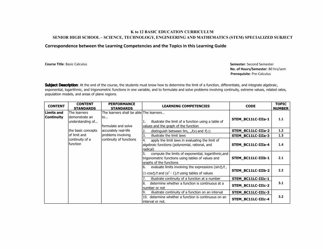
K to 12 BASIC EDUCATION CURRICULUM SENIOR HIGH SCHOOL – SCIENCE, TECHNOLOGY, ENGINEERING AND MATHEMATICS (STEM) SPECIALIZED SUBJECT
Correspondence*between*the*Learning*Competencies*and*the*Topics*in*this*Learning*Guide
Course*Title:"Basic"Calculus Semester:"Second"SemesterNo.*of*Hours/Semester:"80"hrs/semPrerequisite:"Pre8Calculus
CONTENT CONTENT STANDARDS
PERFORMANCE STANDARDS
LEARNING COMPETENCIES CODE TOPIC NUMBER
The learners…
1. illustrate the limit of a function using a table of values and the graph of the function
STEM_BC11LC-IIIa-1 1.1
2. distinguish between limx→cf(x)!and f(c) STEM_BC11LC-IIIa-2 1.23. illustrate the limit laws STEM_BC11LC-IIIa-3 1.34. apply the limit laws in evaluating the limit of algebraic functions (polynomial, rational, andradical)
STEM_BC11LC-IIIa-4 1.4
5. compute the limits of exponential, logarithmic,and trigonometric functions using tables of values and graphs of the functions
STEM_BC11LC-IIIb-1 2.1
6. evaluate limits involving the expressions (sint)/t ,
(1-cost)/t and (et - 1)/t using tables of valuesSTEM_BC11LC-IIIb-2 2.2
7. illustrate continuity of a function at a number STEM_BC11LC-IIIc-18. determine whether a function is continuous at a number or not
STEM_BC11LC-IIIc-2
9. illustrate continuity of a function on an interval STEM_BC11LC-IIIc-310. determine whether a function is continuous on an interval or not.
STEM_BC11LC-IIIc-4
Subject Description: At the end of the course, the students must know how to determine the limit of a function, differentiate, and integrate algebraic, exponential, logarithmic, and trigonometric functions in one variable, and to formulate and solve problems involving continuity, extreme values, related rates, population models, and areas of plane regions.
3.1
3.2
Limits andContinuity
The learners demonstrate an understanding of...
the basic concepts of limit and continuity of a function
The learners shall be able to...
formulate and solve accurately real-life problems involving continuity of functions
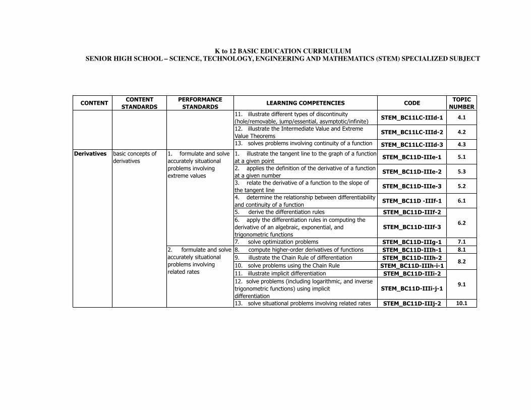
K to 12 BASIC EDUCATION CURRICULUM!SENIOR HIGH SCHOOL – SCIENCE, TECHNOLOGY, ENGINEERING AND MATHEMATICS (STEM) SPECIALIZED SUBJECT
CONTENT CONTENT STANDARDS
PERFORMANCE STANDARDS
LEARNING COMPETENCIES CODE TOPIC NUMBER
11. illustrate different types of discontinuity(hole/removable, jump/essential, asymptotic/infinite)
STEM_BC11LC-IIId-1 4.1
12. illustrate the Intermediate Value and Extreme Value Theorems
STEM_BC11LC-IIId-2 4.2
13. solves problems involving continuity of a function STEM_BC11LC-IIId-3 4.31. illustrate the tangent line to the graph of a function at a given point
STEM_BC11D-IIIe-1 5.1
2. applies the definition of the derivative of a function at a given number
STEM_BC11D-IIIe-2 5.3
3. relate the derivative of a function to the slope of the tangent line
STEM_BC11D-IIIe-3 5.2
4. determine the relationship between differentiability and continuity of a function
STEM_BC11D -IIIf-1 6.1
5. derive the differentiation rules STEM_BC11D-IIIf-26. apply the differentiation rules in computing the derivative of an algebraic, exponential, andtrigonometric functions
STEM_BC11D-IIIf-3
7. solve optimization problems STEM_BC11D-IIIg-1 7.18. compute higher-order derivatives of functions STEM_BC11D-IIIh-1 8.19. illustrate the Chain Rule of differentiation STEM_BC11D-IIIh-210. solve problems using the Chain Rule STEM_BC11D-IIIh-i-111. illustrate implicit differentiation STEM_BC11D-IIIi-212. solve problems (including logarithmic, and inverse trigonometric functions) using implicitdifferentiation
STEM_BC11D-IIIi-j-1
13. solve situational problems involving related rates STEM_BC11D-IIIj-2 10.1
6.2
8.2
9.1
Derivatives basic concepts of derivatives
1. formulate and solve accurately situational problems involving extreme values
2. formulate and solve accurately situational problems involving related rates
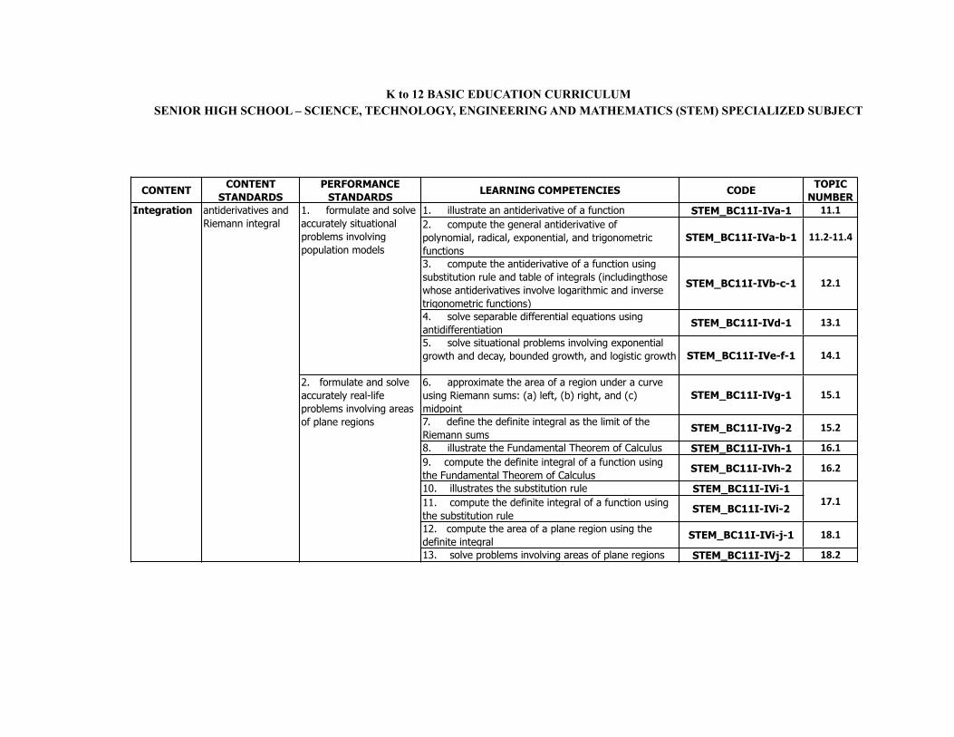
K to 12 BASIC EDUCATION CURRICULUMSENIOR HIGH SCHOOL – SCIENCE, TECHNOLOGY, ENGINEERING AND MATHEMATICS (STEM) SPECIALIZED SUBJECT
CONTENT CONTENT STANDARDS
PERFORMANCE STANDARDS
LEARNING COMPETENCIES CODE TOPIC NUMBER
1. illustrate an antiderivative of a function STEM_BC11I-IVa-1 11.12. compute the general antiderivative of polynomial, radical, exponential, and trigonometric functions
STEM_BC11I-IVa-b-1 11.2J11.4
3. compute the antiderivative of a function using substitution rule and table of integrals (includingthose whose antiderivatives involve logarithmic and inverse trigonometric functions)
STEM_BC11I-IVb-c-1 12.1
4. solve separable differential equations using antidifferentiation
STEM_BC11I-IVd-1 13.1
5. solve situational problems involving exponential growth and decay, bounded growth, and logistic growth STEM_BC11I-IVe-f-1 14.1
6. approximate the area of a region under a curve using Riemann sums: (a) left, (b) right, and (c) midpoint
STEM_BC11I-IVg-1 15.1
7. define the definite integral as the limit of the Riemann sums
STEM_BC11I-IVg-2 15.2
8. illustrate the Fundamental Theorem of Calculus STEM_BC11I-IVh-1 16.19. compute the definite integral of a function using the Fundamental Theorem of Calculus
STEM_BC11I-IVh-2 16.2
10. illustrates the substitution rule STEM_BC11I-IVi-111. compute the definite integral of a function using the substitution rule
STEM_BC11I-IVi-2
12. compute the area of a plane region using the definite integral
STEM_BC11I-IVi-j-1 18.1
13. solve problems involving areas of plane regions STEM_BC11I-IVj-2 18.2
Integration antiderivatives andRiemann integral
1. formulate and solve accurately situational problems involving population models
2. formulate and solve accurately real-life problems involving areas of plane regions
17.1
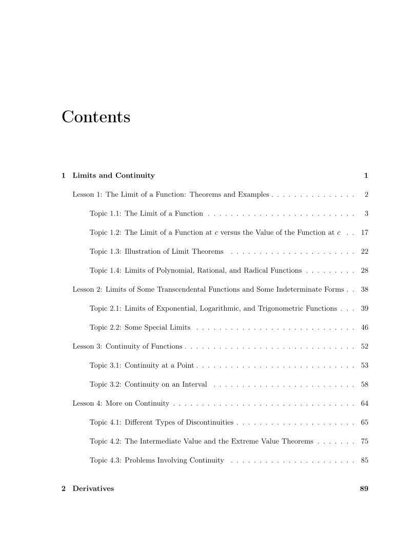
Contents
1 Limits and Continuity 1
Lesson 1: The Limit of a Function: Theorems and Examples . . . . . . . . . . . . . . . 2
Topic 1.1: The Limit of a Function . . . . . . . . . . . . . . . . . . . . . . . . . . 3
Topic 1.2: The Limit of a Function at c versus the Value of the Function at c . . 17
Topic 1.3: Illustration of Limit Theorems . . . . . . . . . . . . . . . . . . . . . . 22
Topic 1.4: Limits of Polynomial, Rational, and Radical Functions . . . . . . . . . 28
Lesson 2: Limits of Some Transcendental Functions and Some Indeterminate Forms . . 38
Topic 2.1: Limits of Exponential, Logarithmic, and Trigonometric Functions . . . 39
Topic 2.2: Some Special Limits . . . . . . . . . . . . . . . . . . . . . . . . . . . . 46
Lesson 3: Continuity of Functions . . . . . . . . . . . . . . . . . . . . . . . . . . . . . . 52
Topic 3.1: Continuity at a Point . . . . . . . . . . . . . . . . . . . . . . . . . . . . 53
Topic 3.2: Continuity on an Interval . . . . . . . . . . . . . . . . . . . . . . . . . 58
Lesson 4: More on Continuity . . . . . . . . . . . . . . . . . . . . . . . . . . . . . . . . 64
Topic 4.1: Different Types of Discontinuities . . . . . . . . . . . . . . . . . . . . . 65
Topic 4.2: The Intermediate Value and the Extreme Value Theorems . . . . . . . 75
Topic 4.3: Problems Involving Continuity . . . . . . . . . . . . . . . . . . . . . . 85
2 Derivatives 89
Lesson 5: The Derivative as the Slope of the Tangent Line . . . . . . . . . . . . . . . 90
Topic 5.1: The Tangent Line to the Graph of a Function at a Point . . . . . . . . 91
Topic 5.2: The Equation of the Tangent Line . . . . . . . . . . . . . . . . . . . . 100
Topic 5.3: The Definition of the Derivative . . . . . . . . . . . . . . . . . . . . . . 107
Lesson 6: Rules of Differentiation . . . . . . . . . . . . . . . . . . . . . . . . . . . . . . 119
Topic 6.1: Differentiability Implies Continuity . . . . . . . . . . . . . . . . . . . . 120
Topic 6.2: The Differentiation Rules and Examples Involving Algebraic, Expo-nential, and Trigonometric Functions . . . . . . . . . . . . . . . . . . . . . 126
Lesson 7: Optimization . . . . . . . . . . . . . . . . . . . . . . . . . . . . . . . . . . . 141
Topic 7.1: Optimization using Calculus . . . . . . . . . . . . . . . . . . . . . . . . 142
Lesson 8: Higher-Order Derivatives and the Chain Rule . . . . . . . . . . . . . . . . . 156
Topic 8.1: Higher-Order Derivatives of Functions . . . . . . . . . . . . . . . . . . 157
Topic 8.2: The Chain Rule . . . . . . . . . . . . . . . . . . . . . . . . . . . . . . . 162
Lesson 9: Implicit Differentiation . . . . . . . . . . . . . . . . . . . . . . . . . . . . . . 168
Topic 9.1: What is Implicit Differentiation? . . . . . . . . . . . . . . . . . . . . . 169
Lesson 10: Related Rates . . . . . . . . . . . . . . . . . . . . . . . . . . . . . . . . . . 180
Topic 10.1: Solutions to Problems Involving Related Rates . . . . . . . . . . . . . 181
3 Integration 191
Lesson 11: Integration . . . . . . . . . . . . . . . . . . . . . . . . . . . . . . . . . . . . 192
Topic 11.1: Illustration of an Antiderivative of a Function . . . . . . . . . . . . . 193
Topic 11.2: Antiderivatives of Algebraic Functions . . . . . . . . . . . . . . . . . 196
Topic 11.3: Antiderivatives of Functions Yielding Exponential Functions andLogarithmic Functions . . . . . . . . . . . . . . . . . . . . . . . . . . . . . 199
Topic 11.4: Antiderivatives of Trigonometric Functions . . . . . . . . . . . . . . . 202
Lesson 12: Techniques of Antidifferentiation . . . . . . . . . . . . . . . . . . . . . . . . 204
Topic 12.1: Antidifferentiation by Substitution and by Table of Integrals . . . . . 205
Lesson 13: Application of Antidifferentiation to Differential Equations . . . . . . . . . 217
Topic 13.1: Separable Differential Equations . . . . . . . . . . . . . . . . . . . . . 218
Lesson 14: Application of Differential Equations in Life Sciences . . . . . . . . . . . . . 224
Topic 14.1: Situational Problems Involving Growth and Decay Problems . . . . . 225
Lesson 15: Riemann Sums and the Definite Integral . . . . . . . . . . . . . . . . . . . . 237
Topic 15.1: Approximation of Area using Riemann Sums . . . . . . . . . . . . . . 238
Topic 15.2: The Formal Definition of the Definite Integral . . . . . . . . . . . . . 253
Lesson 16: The Fundamental Theorem of Calculus . . . . . . . . . . . . . . . . . . . . 268
Topic 16.1: Illustration of the Fundamental Theorem of Calculus . . . . . . . . . 269
Topic 16.2: Computation of Definite Integrals using the Fundamental Theoremof Calculus . . . . . . . . . . . . . . . . . . . . . . . . . . . . . . . . . . . 273
Lesson 17: Integration Technique: The Substitution Rule for Definite Integrals . . . . 280
Topic 17.1: Illustration of the Substitution Rule for Definite Integrals . . . . . . . 281
Lesson 18: Application of Definite Integrals in the Computation of Plane Areas . . . . 292
Topic 18.1: Areas of Plane Regions Using Definite Integrals . . . . . . . . . . . . 293
Topic 18.2: Application of Definite Integrals: Word Problems . . . . . . . . . . . 304
Biographical Notes 309
Chapter 1
Limits and Continuity
LESSON 1: The Limit of a Function: Theorems and Examples
TIME FRAME: 4 hours
LEARNING OUTCOMES: At the end of the lesson, the learner shall be able to:
1. Illustrate the limit of a function using a table of values and the graph of the function;2. Distinguish between lim
x!cf(x) and f(c);
3. Illustrate the limit theorems; and4. Apply the limit theorems in evaluating the limit of algebraic functions (polynomial, ratio-
nal, and radical).
LESSON OUTLINE:
1. Evaluation of limits using a table of values2. Illustrating the limit of a function using the graph of the function3. Distinguishing between lim
x!cf(x) and f(c) using a table of values
4. Distinguishing between lim
x!cf(x) and f(c) using the graph of y = f(x)
5. Enumeration of the eight basic limit theorems6. Application of the eight basic limit theorems on simple examples7. Limits of polynomial functions8. Limits of rational functions9. Limits of radical functions
10. Intuitive notions of infinite limits
2
TOPIC 1.1: The Limit of a Function
DEVELOPMENT OF THE LESSON
(A) ACTIVITY
In order to find out what the students’ idea of a limit is, ask them to bring cutouts ofnews items, articles, or drawings which for them illustrate the idea of a limit. These maybe posted on a wall so that they may see each other’s homework, and then have each oneexplain briefly why they think their particular cutout represents a limit.
(B) INTRODUCTION
Limits are the backbone of calculus, and calculus is called the Mathematics of Change.The study of limits is necessary in studying change in great detail. The evaluation of aparticular limit is what underlies the formulation of the derivative and the integral of afunction.
For starters, imagine that you are going to watch a basketball game. When you chooseseats, you would want to be as close to the action as possible. You would want to be asclose to the players as possible and have the best view of the game, as if you were in thebasketball court yourself. Take note that you cannot actually be in the court and join theplayers, but you will be close enough to describe clearly what is happening in the game.
This is how it is with limits of functions. We will consider functions of a single variable andstudy the behavior of the function as its variable approaches a particular value (a constant).The variable can only take values very, very close to the constant, but it cannot equal theconstant itself. However, the limit will be able to describe clearly what is happening to thefunction near that constant.
(C) LESSON PROPER
Consider a function f of a single variable x. Consider a constant c which the variable x
will approach (c may or may not be in the domain of f). The limit, to be denoted by L, isthe unique real value that f(x) will approach as x approaches c. In symbols, we write thisprocess as
lim
x!cf(x) = L.
This is read, ‘ ‘The limit of f(x) as x approaches c is L.”
3
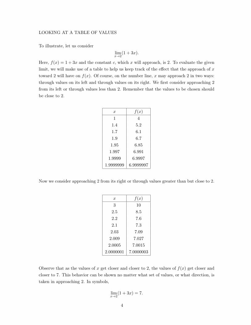
LOOKING AT A TABLE OF VALUES
To illustrate, let us considerlim
x!2
(1 + 3x).
Here, f(x) = 1+ 3x and the constant c, which x will approach, is 2. To evaluate the givenlimit, we will make use of a table to help us keep track of the effect that the approach of xtoward 2 will have on f(x). Of course, on the number line, x may approach 2 in two ways:through values on its left and through values on its right. We first consider approaching 2
from its left or through values less than 2. Remember that the values to be chosen shouldbe close to 2.
x f(x)
1 4
1.4 5.2
1.7 6.1
1.9 6.7
1.95 6.85
1.997 6.991
1.9999 6.9997
1.9999999 6.9999997
Now we consider approaching 2 from its right or through values greater than but close to 2.
x f(x)
3 10
2.5 8.5
2.2 7.6
2.1 7.3
2.03 7.09
2.009 7.027
2.0005 7.0015
2.0000001 7.0000003
Observe that as the values of x get closer and closer to 2, the values of f(x) get closer andcloser to 7. This behavior can be shown no matter what set of values, or what direction, istaken in approaching 2. In symbols,
lim
x!2
(1 + 3x) = 7.
4
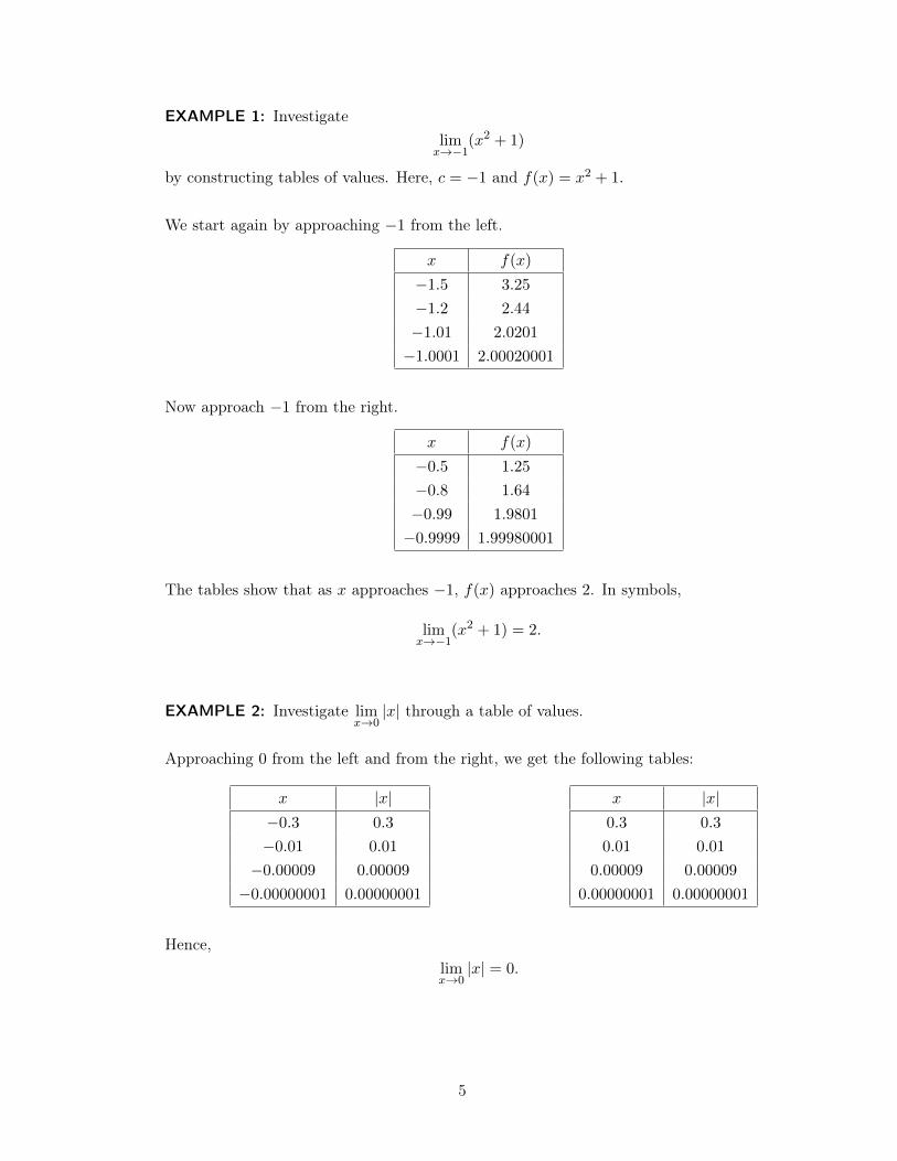
EXAMPLE 1: Investigatelim
x!�1
(x2 + 1)
by constructing tables of values. Here, c = �1 and f(x) = x2 + 1.
We start again by approaching �1 from the left.
x f(x)
�1.5 3.25
�1.2 2.44
�1.01 2.0201
�1.0001 2.00020001
Now approach �1 from the right.
x f(x)
�0.5 1.25
�0.8 1.64
�0.99 1.9801
�0.9999 1.99980001
The tables show that as x approaches �1, f(x) approaches 2. In symbols,
lim
x!�1
(x2 + 1) = 2.
EXAMPLE 2: Investigate lim
x!0
|x| through a table of values.
Approaching 0 from the left and from the right, we get the following tables:
x |x|�0.3 0.3
�0.01 0.01
�0.00009 0.00009
�0.00000001 0.00000001
x |x|0.3 0.3
0.01 0.01
0.00009 0.00009
0.00000001 0.00000001
Hence,lim
x!0
|x| = 0.
5
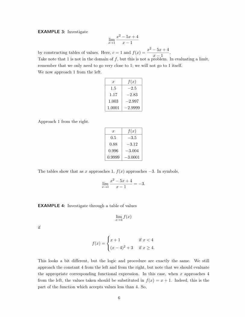
EXAMPLE 3: Investigate
lim
x!1
x2 � 5x+ 4
x� 1
by constructing tables of values. Here, c = 1 and f(x) =x2 � 5x+ 4
x� 1
.
Take note that 1 is not in the domain of f , but this is not a problem. In evaluating a limit,remember that we only need to go very close to 1; we will not go to 1 itself.We now approach 1 from the left.
x f(x)
1.5 �2.5
1.17 �2.83
1.003 �2.997
1.0001 �2.9999
Approach 1 from the right.
x f(x)
0.5 �3.5
0.88 �3.12
0.996 �3.004
0.9999 �3.0001
The tables show that as x approaches 1, f(x) approaches �3. In symbols,
lim
x!1
x2 � 5x+ 4
x� 1
= �3.
EXAMPLE 4: Investigate through a table of values
lim
x!4
f(x)
if
f(x) =
8<
:x+ 1 if x < 4
(x� 4)
2
+ 3 if x � 4.
This looks a bit different, but the logic and procedure are exactly the same. We stillapproach the constant 4 from the left and from the right, but note that we should evaluatethe appropriate corresponding functional expression. In this case, when x approaches 4
from the left, the values taken should be substituted in f(x) = x + 1. Indeed, this is thepart of the function which accepts values less than 4. So,
6
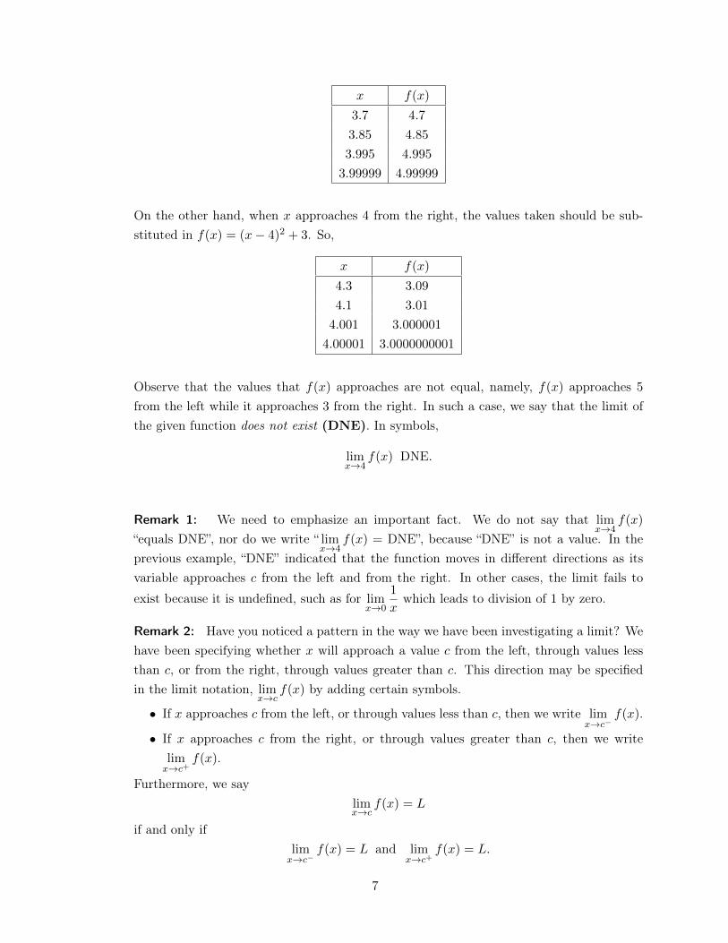
x f(x)
3.7 4.7
3.85 4.85
3.995 4.995
3.99999 4.99999
On the other hand, when x approaches 4 from the right, the values taken should be sub-stituted in f(x) = (x� 4)
2
+ 3. So,
x f(x)
4.3 3.09
4.1 3.01
4.001 3.000001
4.00001 3.0000000001
Observe that the values that f(x) approaches are not equal, namely, f(x) approaches 5
from the left while it approaches 3 from the right. In such a case, we say that the limit ofthe given function does not exist (DNE). In symbols,
lim
x!4
f(x) DNE.
Remark 1: We need to emphasize an important fact. We do not say that lim
x!4
f(x)
“equals DNE”, nor do we write “ limx!4
f(x) = DNE”, because “DNE” is not a value. In theprevious example, “DNE” indicated that the function moves in different directions as itsvariable approaches c from the left and from the right. In other cases, the limit fails toexist because it is undefined, such as for lim
x!0
1
xwhich leads to division of 1 by zero.
Remark 2: Have you noticed a pattern in the way we have been investigating a limit? Wehave been specifying whether x will approach a value c from the left, through values lessthan c, or from the right, through values greater than c. This direction may be specifiedin the limit notation, lim
x!cf(x) by adding certain symbols.
• If x approaches c from the left, or through values less than c, then we write lim
x!c�f(x).
• If x approaches c from the right, or through values greater than c, then we writelim
x!c+f(x).
Furthermore, we saylim
x!cf(x) = L
if and only iflim
x!c�f(x) = L and lim
x!c+f(x) = L.
7
In other words, for a limit L to exist, the limits from the left and from the right must bothexist and be equal to L. Therefore,
lim
x!cf(x) DNE whenever lim
x!c�f(x) 6= lim
x!c+f(x).
These limits, lim
x!c�f(x) and lim
x!c+f(x), are also referred to as one-sided limits, since you
only consider values on one side of c.Thus, we may say:
• in our very first illustration that lim
x!2
(1 + 3x) = 7 because lim
x!2
�(1 + 3x) = 7 and
lim
x!2
+(1 + 3x) = 7.
• in Example 1, lim
x!�1
(x2 + 1) = 2 since lim
x!�1
�(x2 + 1) = 2 and lim
x!�1
+(x2 + 1) = 2.
• in Example 2, lim
x!0
|x| = 0 because lim
x!0
�|x| = 0 and lim
x!0
+|x| = 0.
• in Example 3, lim
x!1
x2 � 5x+ 4
x� 1
= �3 because lim
x!1
�
x2 � 5x+ 4
x� 1
= �3 and
lim
x!1
+
x2 � 5x+ 4
x� 1
= �3.
• in Example 4, lim
x!4
f(x) DNE because lim
x!4
�f(x) 6= lim
x!4
+f(x).
LOOKING AT THE GRAPH OF y = f(x)
If one knows the graph of f(x), it will be easier to determine its limits as x approachesgiven values of c.
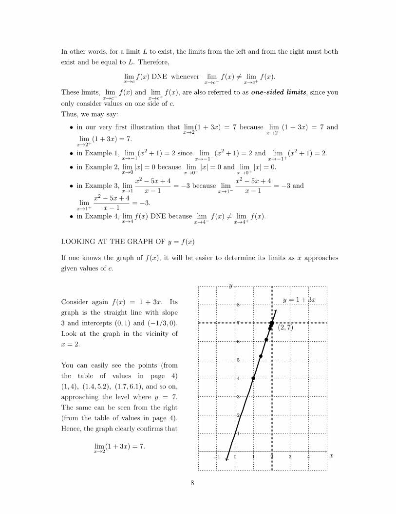
Consider again f(x) = 1 + 3x. Itsgraph is the straight line with slope3 and intercepts (0, 1) and (�1/3, 0).Look at the graph in the vicinity ofx = 2.
You can easily see the points (fromthe table of values in page 4)(1, 4), (1.4, 5.2), (1.7, 6.1), and so on,approaching the level where y = 7.The same can be seen from the right(from the table of values in page 4).Hence, the graph clearly confirms that
lim
x!2
(1 + 3x) = 7.x
y
y = 1 + 3x
(2, 7)
�1 0 1 2 3 4
1
2
3
4
5
6
7
8
8
Let us look at the examples again, one by one.
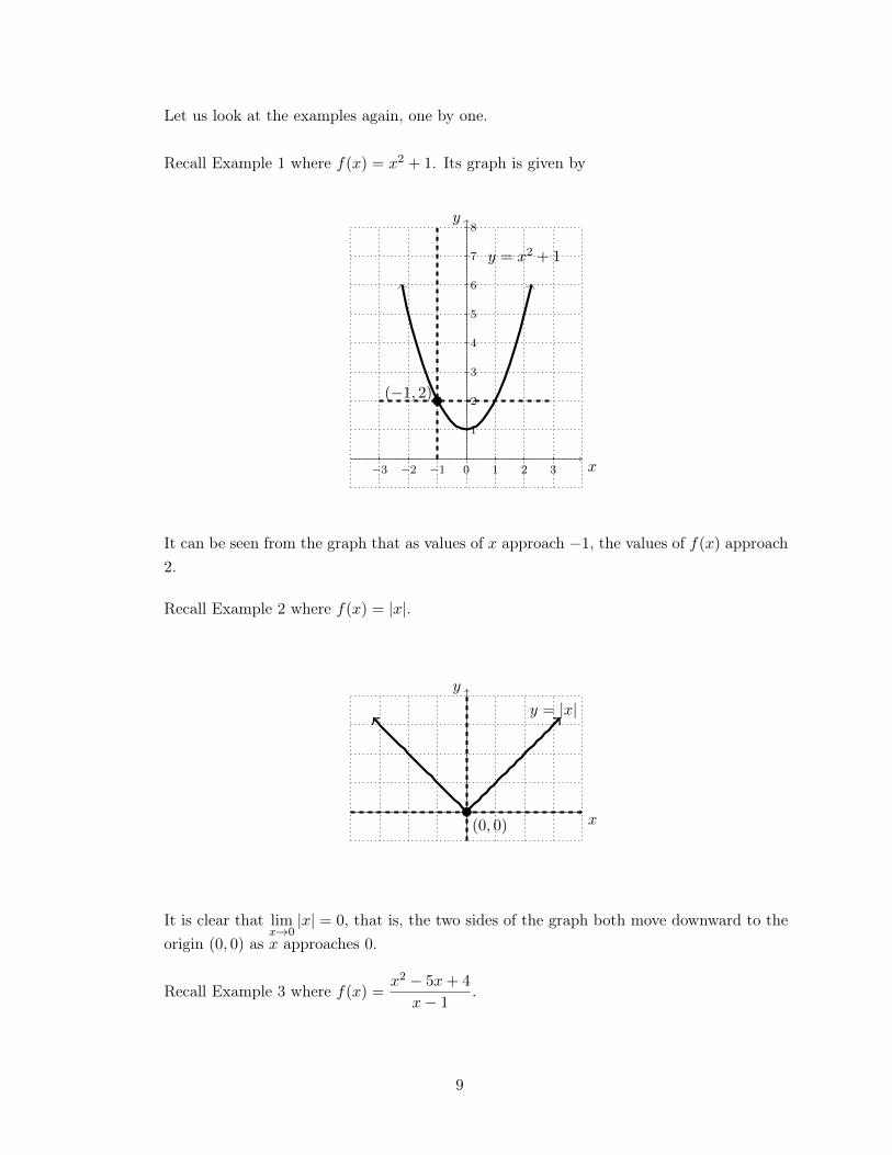
Recall Example 1 where f(x) = x2 + 1. Its graph is given by
�3 �2 �1 0 1 2 3
1
2
3
4
5
6
7
8
x
y
y = x2 + 1
(�1, 2)
It can be seen from the graph that as values of x approach �1, the values of f(x) approach2.
Recall Example 2 where f(x) = |x|.
x
y
y = |x|
(0, 0)
It is clear that lim
x!0
|x| = 0, that is, the two sides of the graph both move downward to theorigin (0, 0) as x approaches 0.
Recall Example 3 where f(x) =x2 � 5x+ 4
x� 1
.
9
1 2 3 4
�4
�3
�2
�1
0
x
y
y =
x2 � 5x+ 4
x� 1
(1,�3)
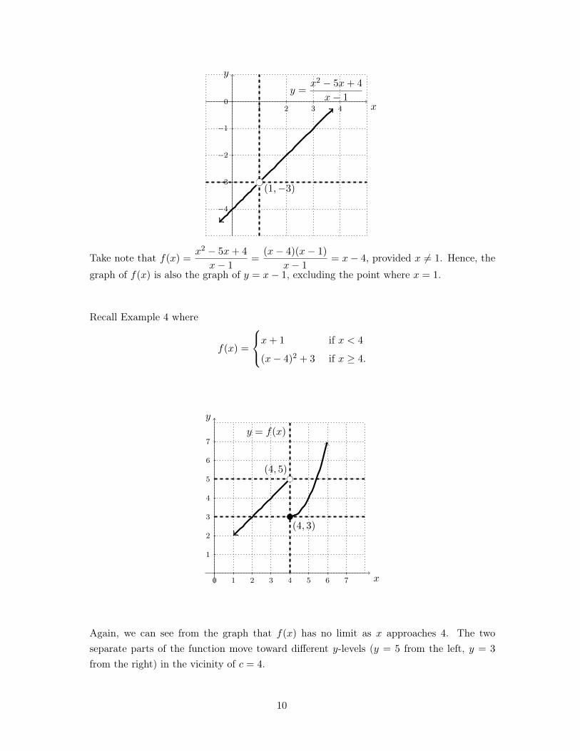
Take note that f(x) =x2 � 5x+ 4
x� 1
=
(x� 4)(x� 1)
x� 1
= x� 4, provided x 6= 1. Hence, thegraph of f(x) is also the graph of y = x� 1, excluding the point where x = 1.
Recall Example 4 where
f(x) =
8<
:x+ 1 if x < 4
(x� 4)
2
+ 3 if x � 4.
0 1 2 3 4 5 6 7
1
2
3
4
5
6
7
x
y
y = f(x)
(4, 5)
(4, 3)
Again, we can see from the graph that f(x) has no limit as x approaches 4. The twoseparate parts of the function move toward different y-levels (y = 5 from the left, y = 3
from the right) in the vicinity of c = 4.
10
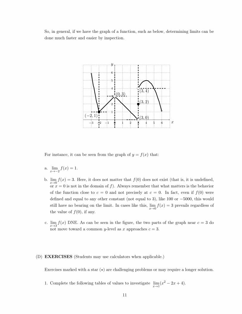
So, in general, if we have the graph of a function, such as below, determining limits can bedone much faster and easier by inspection.
�3 �2 �1 0 1 2 3 4 5 6
1
2
3
4
5
6
x
y
(�2, 1)
(0, 3)
(3, 0)
(3, 2)
(3, 4)
For instance, it can be seen from the graph of y = f(x) that:
a. lim
x!�2
f(x) = 1.
b. lim
x!0
f(x) = 3. Here, it does not matter that f(0) does not exist (that is, it is undefined,or x = 0 is not in the domain of f). Always remember that what matters is the behaviorof the function close to c = 0 and not precisely at c = 0. In fact, even if f(0) weredefined and equal to any other constant (not equal to 3), like 100 or �5000, this wouldstill have no bearing on the limit. In cases like this, lim
x!0
f(x) = 3 prevails regardless ofthe value of f(0), if any.
c. lim
x!3
f(x) DNE. As can be seen in the figure, the two parts of the graph near c = 3 donot move toward a common y-level as x approaches c = 3.
(D) EXERCISES (Students may use calculators when applicable.)
Exercises marked with a star (?) are challenging problems or may require a longer solution.
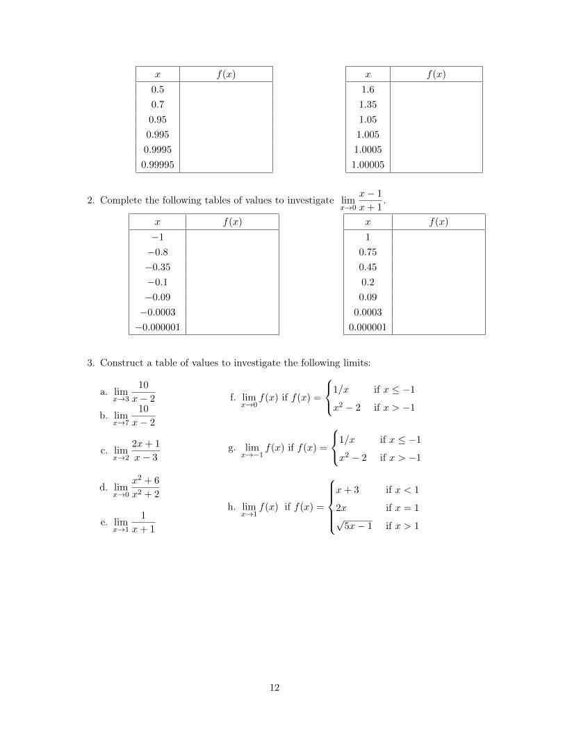
1. Complete the following tables of values to investigate lim
x!1
(x2 � 2x+ 4).
11
x f(x)
0.5
0.7
0.95
0.995
0.9995
0.99995
x f(x)
1.6
1.35
1.05
1.005
1.0005
1.00005
2. Complete the following tables of values to investigate lim
x!0
x� 1
x+ 1
.
x f(x)
�1
�0.8
�0.35
�0.1
�0.09
�0.0003
�0.000001
x f(x)
1
0.75
0.45
0.2
0.09
0.0003
0.000001
3. Construct a table of values to investigate the following limits:
a. lim
x!3
10
x� 2
b. lim
x!7
10
x� 2
c. lim
x!2
2x+ 1
x� 3
d. lim
x!0
x2 + 6
x2 + 2
e. lim
x!1
1
x+ 1
f. lim
x!0
f(x) if f(x) =
8<
:1/x if x �1
x2 � 2 if x > �1
g. lim
x!�1
f(x) if f(x) =
8<
:1/x if x �1
x2 � 2 if x > �1
h. lim
x!1
f(x) if f(x) =
8>>><
>>>:
x+ 3 if x < 1
2x if x = 1
p5x� 1 if x > 1
12

4. Consider the function f(x) whose graph is shown below.
x
y
1 2 3 4 5 6
�1�2�3�4�5
1
2
3
4
5
6
�1
�2
Determine the following:
a. lim
x!�3
f(x)
b. lim
x!�1
f(x)
c. lim
x!1
f(x)
d. lim
x!3
f(x)
e. lim
x!5
f(x)
5. Consider the function f(x) whose graph is shown below.
x
y
0 1 2 3 4 5 6
1
2
3
4
5
6
What can be said about the limit off(x)
a. at c = 1, 2, 3, and 4?
b. at integer values of c?
c. at c = 0.4, 2. 3, 4.7, and 5.5?
d. at non-integer values of c?
13
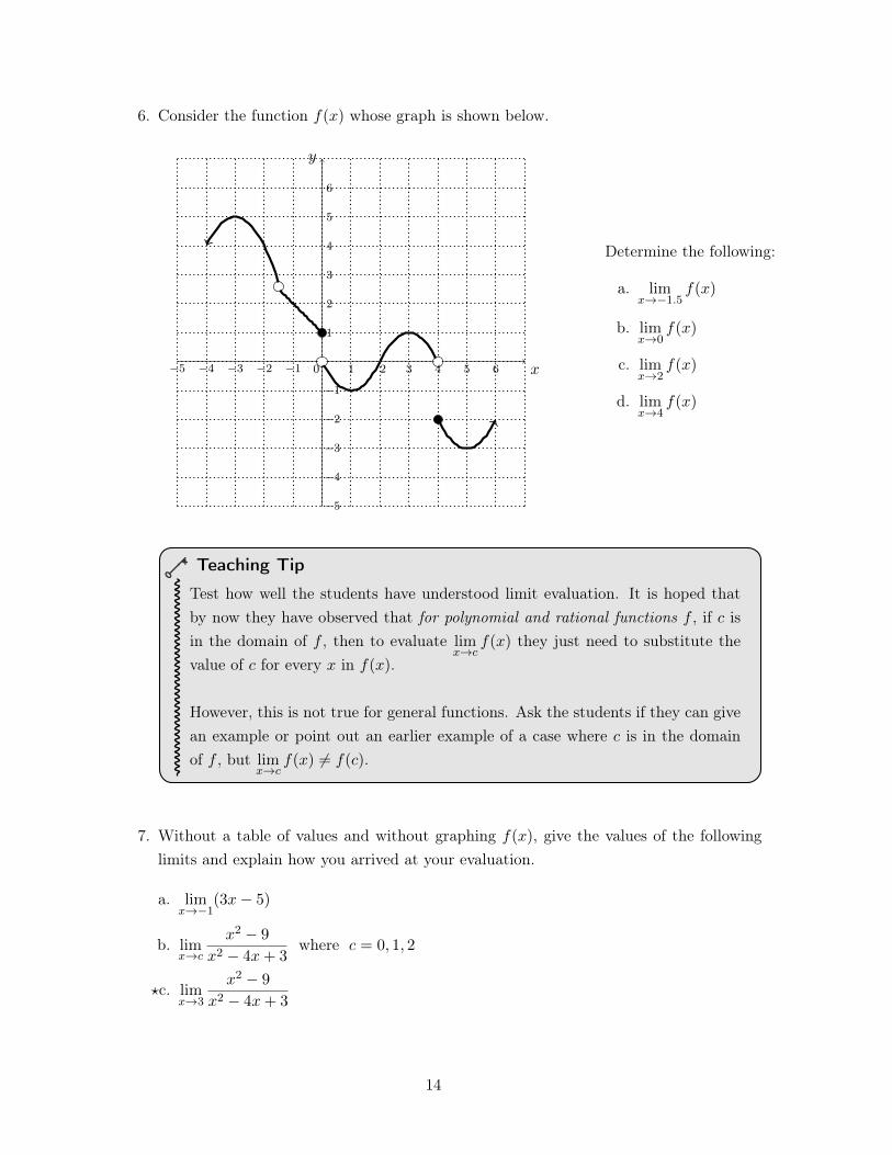
6. Consider the function f(x) whose graph is shown below.
x
y
0
�1�2�3�4�5
1 2 3 4 5 6
1
2
3
4
5
6
�1
�2
�3
�4
�5
Determine the following:
a. lim
x!�1.5f(x)
b. lim
x!0
f(x)
c. lim
x!2
f(x)
d. lim
x!4
f(x)
Teaching Tip
Test how well the students have understood limit evaluation. It is hoped thatby now they have observed that for polynomial and rational functions f , if c isin the domain of f , then to evaluate lim
x!cf(x) they just need to substitute the
value of c for every x in f(x).
However, this is not true for general functions. Ask the students if they can givean example or point out an earlier example of a case where c is in the domainof f , but lim
x!cf(x) 6= f(c).
7. Without a table of values and without graphing f(x), give the values of the followinglimits and explain how you arrived at your evaluation.
a. lim
x!�1
(3x� 5)
b. lim
x!c
x2 � 9
x2 � 4x+ 3
where c = 0, 1, 2
?c. lim
x!3
x2 � 9
x2 � 4x+ 3
14
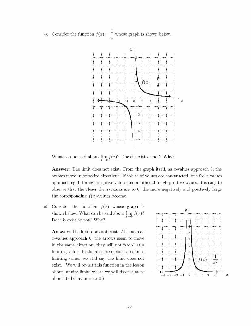
?8. Consider the function f(x) =1
xwhose graph is shown below.
�4 �3 �2 �1 0 1 2 3 4
�5
�4
�3
�2
�1
1
2
3
4
5
x
y
f(x) =1
x
What can be said about lim
x!0
f(x)? Does it exist or not? Why?
Answer: The limit does not exist. From the graph itself, as x-values approach 0, thearrows move in opposite directions. If tables of values are constructed, one for x-valuesapproaching 0 through negative values and another through positive values, it is easy toobserve that the closer the x-values are to 0, the more negatively and positively largethe corresponding f(x)-values become.
?9. Consider the function f(x) whose graph isshown below. What can be said about lim
x!0
f(x)?Does it exist or not? Why?
Answer: The limit does not exist. Although asx-values approach 0, the arrows seem to movein the same direction, they will not “stop” at alimiting value. In the absence of such a definitelimiting value, we still say the limit does notexist. (We will revisit this function in the lessonabout infinite limits where we will discuss moreabout its behavior near 0.)
�4 �3 �2 �1 0 1 2 3 4
1
2
3
4
5
6
7
8
x
y
f(x) =1
x2
15
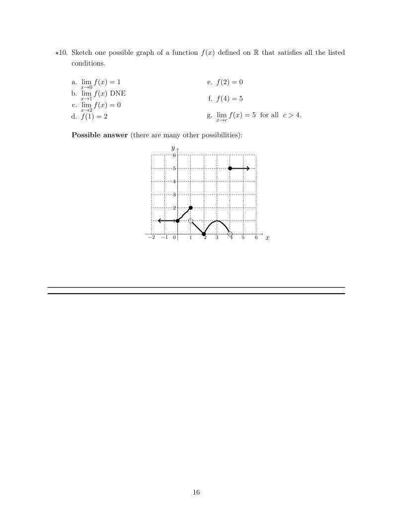
?10. Sketch one possible graph of a function f(x) defined on R that satisfies all the listedconditions.
a. lim
x!0
f(x) = 1
b. lim
x!1
f(x) DNEc. lim
x!2
f(x) = 0
d. f(1) = 2
e. f(2) = 0
f. f(4) = 5
g. lim
x!cf(x) = 5 for all c > 4.
Possible answer (there are many other possibilities):
x
y
1
�1
2
�2
3 4 5 60
1
2
3
4
5
6
16
TOPIC 1.2: The Limit of a Function at c versus the Value of theFunction at c
DEVELOPMENT OF THE LESSON
(A) INTRODUCTION
Critical to the study of limits is the understanding that the value of
lim
x!cf(x)
may be distinct from the value of the function at x = c, that is, f(c). As seen in previousexamples, the limit may be evaluated at values not included in the domain of f . Thus,it must be clear to a student of calculus that the exclusion of a value from the domain ofa function does not prohibit the evaluation of the limit of that function at that excludedvalue, provided of course that f is defined at the points near c. In fact, these cases areactually the more interesting ones to investigate and evaluate.
Furthermore, the awareness of this distinction will help the student understand the conceptof continuity, which will be tackled in Lessons 3 and 4.
(B) LESSON PROPER
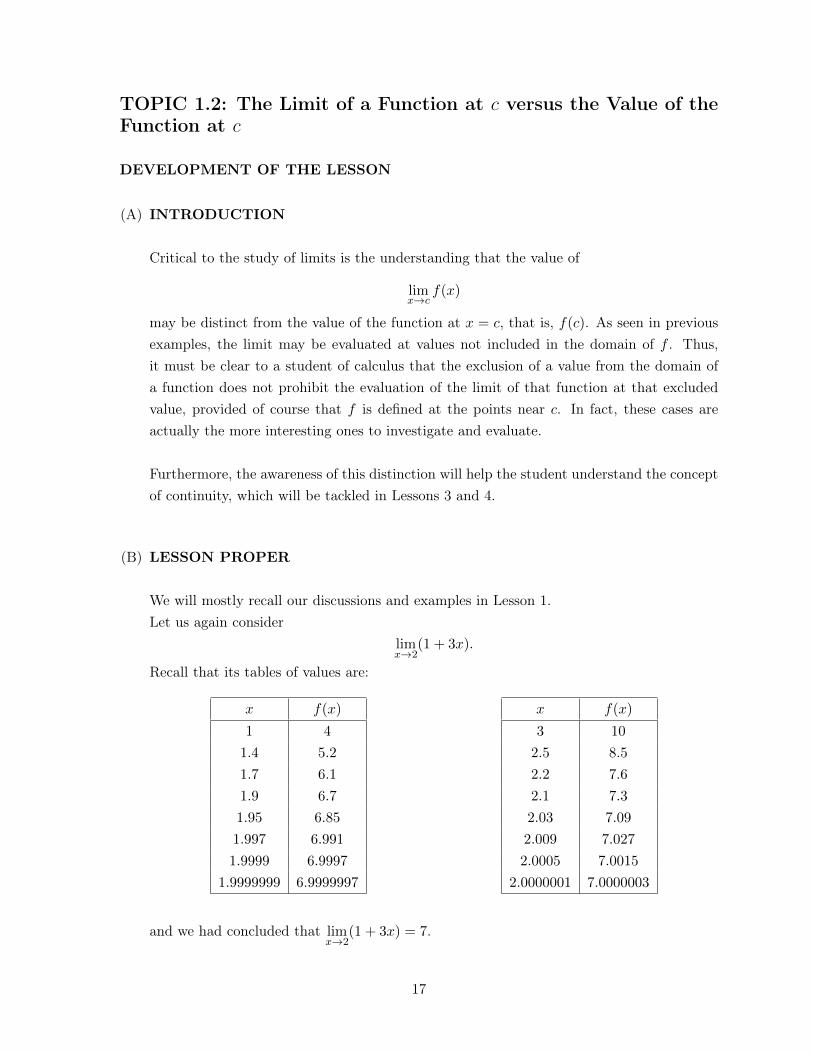
We will mostly recall our discussions and examples in Lesson 1.Let us again consider
lim
x!2
(1 + 3x).
Recall that its tables of values are:
x f(x)
1 4
1.4 5.2
1.7 6.1
1.9 6.7
1.95 6.85
1.997 6.991
1.9999 6.9997
1.9999999 6.9999997
x f(x)
3 10
2.5 8.5
2.2 7.6
2.1 7.3
2.03 7.09
2.009 7.027
2.0005 7.0015
2.0000001 7.0000003
and we had concluded that lim
x!2
(1 + 3x) = 7.
17
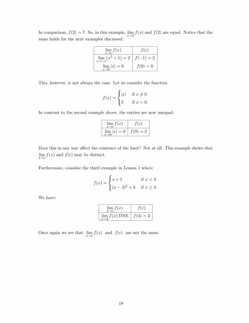
In comparison, f(2) = 7. So, in this example, limx!2
f(x) and f(2) are equal. Notice that thesame holds for the next examples discussed:
lim
x!cf(x) f(c)
lim
x!�1
(x2 + 1) = 2 f(�1) = 2
lim
x!0
|x| = 0 f(0) = 0
This, however, is not always the case. Let us consider the function
f(x) =
8<
:|x| if x 6= 0
2 if x = 0.
In contrast to the second example above, the entries are now unequal:
lim
x!cf(x) f(c)
lim
x!0
|x| = 0 f(0) = 2
Does this in any way affect the existence of the limit? Not at all. This example shows thatlim
x!cf(x) and f(c) may be distinct.
Furthermore, consider the third example in Lesson 1 where
f(x) =
8<
:x+ 1 if x < 4
(x� 4)
2
+ 3 if x � 4.
We have:
lim
x!cf(x) f(c)
lim
x!4
f(x) DNE f(4) = 2
Once again we see that lim
x!cf(x) and f(c) are not the same.
18
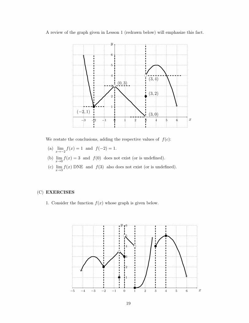
A review of the graph given in Lesson 1 (redrawn below) will emphasize this fact.
�3 �2 �1 0 1 2 3 4 5 6
1
2
3
4
5
6
x
y
(�2, 1)
(0, 3)
(3, 0)
(3, 2)
(3, 4)
We restate the conclusions, adding the respective values of f(c):
(a) lim
x!�2
f(x) = 1 and f(�2) = 1.
(b) lim
x!0
f(x) = 3 and f(0) does not exist (or is undefined).
(c) lim
x!3
f(x) DNE and f(3) also does not exist (or is undefined).
(C) EXERCISES
1. Consider the function f(x) whose graph is given below.
�5 �4 �3 �2 �1 0 1 2 3 4 5 6
1
2
3
4
5
6
x
y
19
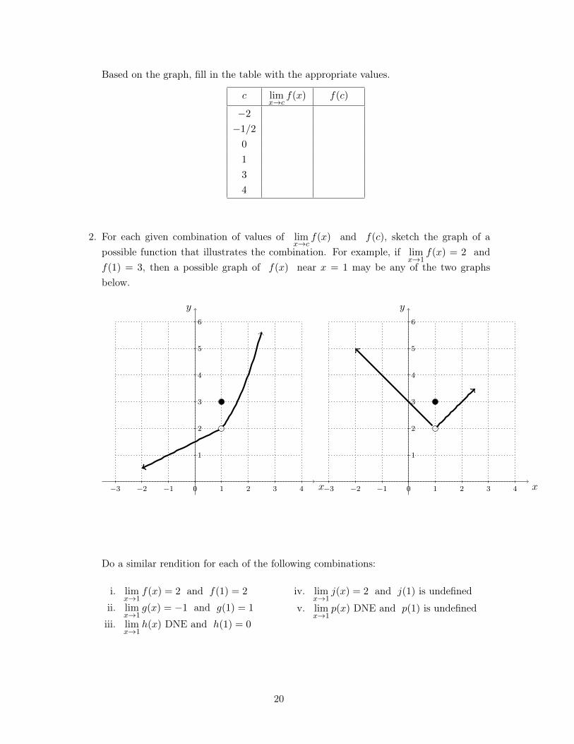
Based on the graph, fill in the table with the appropriate values.
c lim
x!cf(x) f(c)
�2
�1/2
0
1
3
4
2. For each given combination of values of lim
x!cf(x) and f(c), sketch the graph of a
possible function that illustrates the combination. For example, if lim
x!1
f(x) = 2 andf(1) = 3, then a possible graph of f(x) near x = 1 may be any of the two graphsbelow.
�3 �2 �1 0 1 2 3 4
1
2
3
4
5
6
x
y
�3 �2 �1 0 1 2 3 4
1
2
3
4
5
6
x
y
Do a similar rendition for each of the following combinations:
i. lim
x!1
f(x) = 2 and f(1) = 2
ii. lim
x!1
g(x) = �1 and g(1) = 1
iii. lim
x!1
h(x) DNE and h(1) = 0
iv. lim
x!1
j(x) = 2 and j(1) is undefined
v. lim
x!1
p(x) DNE and p(1) is undefined
20
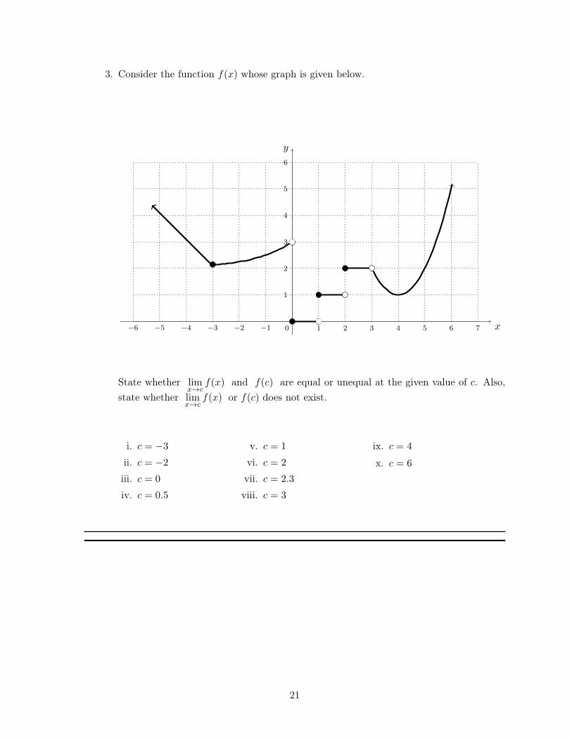
3. Consider the function f(x) whose graph is given below.
x
y
0 1 2 3 4 5 6 7
�1�2�3�4�5�6
1
2
3
4
5
6
State whether lim
x!cf(x) and f(c) are equal or unequal at the given value of c. Also,
state whether lim
x!cf(x) or f(c) does not exist.
i. c = �3
ii. c = �2
iii. c = 0
iv. c = 0.5
v. c = 1
vi. c = 2
vii. c = 2.3
viii. c = 3
ix. c = 4
x. c = 6
21
TOPIC 1.3: Illustration of Limit Theorems
DEVELOPMENT OF THE LESSON
(A) INTRODUCTION
Lesson 1 showed us how limits can be determined through either a table of values or thegraph of a function. One might ask: Must one always construct a table or graph thefunction to determine a limit? Filling in a table of values sometimes requires very tediouscalculations. Likewise, a graph may be difficult to sketch. However, these should not bereasons for a student to fail to determine a limit.
In this lesson, we will learn how to compute the limit of a function using Limit Theorems.
Teaching Tip
It would be good to recall the parts of Lesson 1 where the students were asked togive the value of a limit, without aid of a table or a graph. Those exercises wereintended to lead to the Limit Theorems. These theorems are a formalization ofwhat they had intuitively concluded then.
(B) LESSON PROPER
We are now ready to list down the basic theorems on limits. We will state eight theorems.These will enable us to directly evaluate limits, without need for a table or a graph.
In the following statements, c is a constant, and f and g are functions which may or maynot have c in their domains.
1. The limit of a constant is itself. If k is any constant, then,
lim
x!ck = k.
For example,
i. lim
x!c2 = 2
ii. lim
x!c�3.14 = �3.14
iii. lim
x!c789 = 789
22
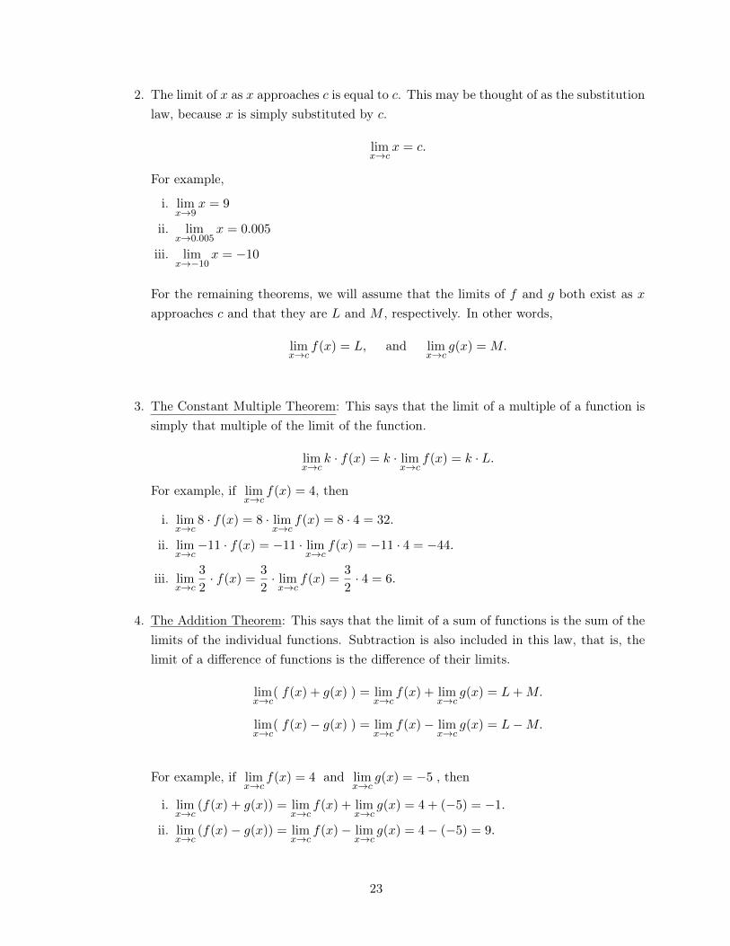
2. The limit of x as x approaches c is equal to c. This may be thought of as the substitutionlaw, because x is simply substituted by c.
lim
x!cx = c.
For example,
i. lim
x!9
x = 9
ii. lim
x!0.005x = 0.005
iii. lim
x!�10
x = �10
For the remaining theorems, we will assume that the limits of f and g both exist as x
approaches c and that they are L and M , respectively. In other words,
lim
x!cf(x) = L, and lim
x!cg(x) = M.
3. The Constant Multiple Theorem: This says that the limit of a multiple of a function issimply that multiple of the limit of the function.
lim
x!ck · f(x) = k · lim
x!cf(x) = k · L.
For example, if lim
x!cf(x) = 4, then
i. lim
x!c8 · f(x) = 8 · lim
x!cf(x) = 8 · 4 = 32.
ii. lim
x!c�11 · f(x) = �11 · lim
x!cf(x) = �11 · 4 = �44.
iii. lim
x!c
3
2
· f(x) = 3
2
· limx!c
f(x) =3
2
· 4 = 6.
4. The Addition Theorem: This says that the limit of a sum of functions is the sum of thelimits of the individual functions. Subtraction is also included in this law, that is, thelimit of a difference of functions is the difference of their limits.
lim
x!c( f(x) + g(x) ) = lim
x!cf(x) + lim
x!cg(x) = L+M.
lim
x!c( f(x)� g(x) ) = lim
x!cf(x)� lim
x!cg(x) = L�M.
For example, if lim
x!cf(x) = 4 and lim
x!cg(x) = �5 , then
i. lim
x!c(f(x) + g(x)) = lim
x!cf(x) + lim
x!cg(x) = 4 + (�5) = �1.
ii. lim
x!c(f(x)� g(x)) = lim
x!cf(x)� lim
x!cg(x) = 4� (�5) = 9.
23
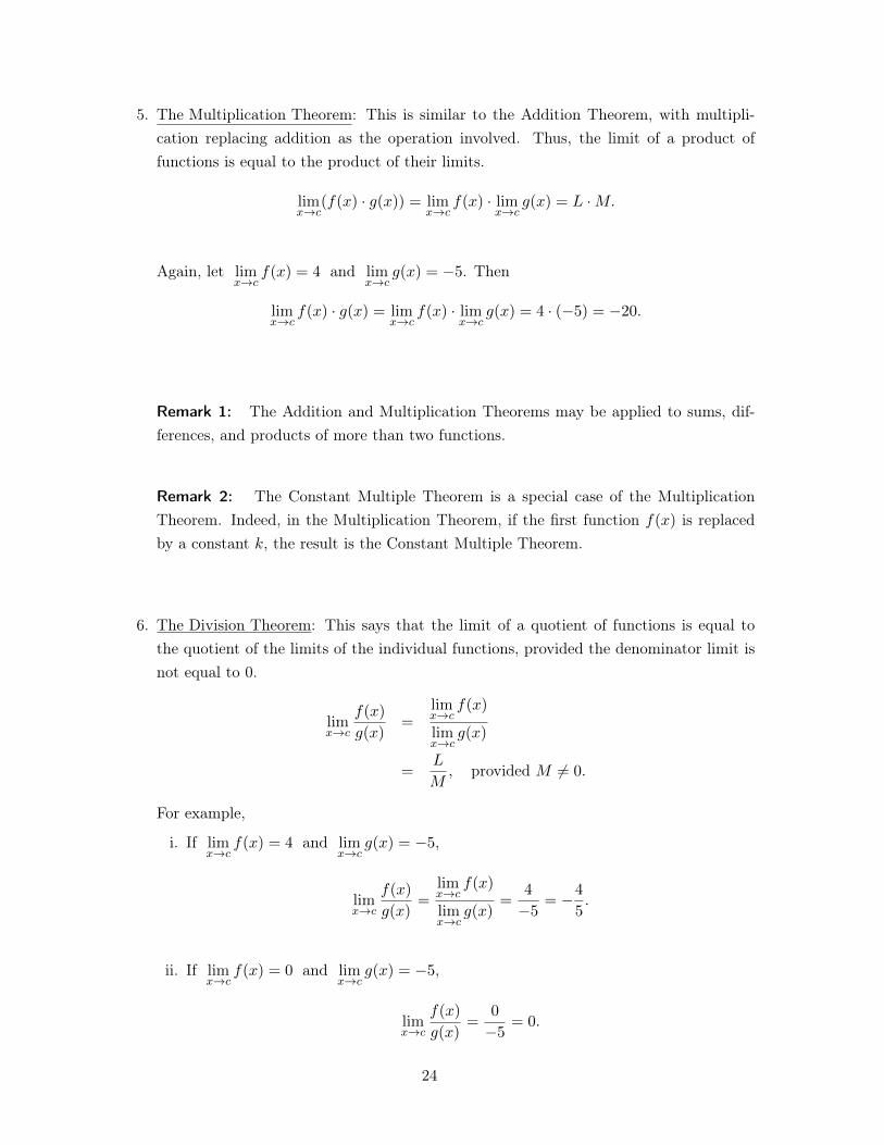
5. The Multiplication Theorem: This is similar to the Addition Theorem, with multipli-cation replacing addition as the operation involved. Thus, the limit of a product offunctions is equal to the product of their limits.
lim
x!c(f(x) · g(x)) = lim
x!cf(x) · lim
x!cg(x) = L ·M.
Again, let lim
x!cf(x) = 4 and lim
x!cg(x) = �5. Then
lim
x!cf(x) · g(x) = lim
x!cf(x) · lim
x!cg(x) = 4 · (�5) = �20.
Remark 1: The Addition and Multiplication Theorems may be applied to sums, dif-ferences, and products of more than two functions.
Remark 2: The Constant Multiple Theorem is a special case of the MultiplicationTheorem. Indeed, in the Multiplication Theorem, if the first function f(x) is replacedby a constant k, the result is the Constant Multiple Theorem.
6. The Division Theorem: This says that the limit of a quotient of functions is equal tothe quotient of the limits of the individual functions, provided the denominator limit isnot equal to 0.
lim
x!c
f(x)
g(x)=
lim
x!cf(x)
lim
x!cg(x)
=
L
M, provided M 6= 0.
For example,
i. If lim
x!cf(x) = 4 and lim
x!cg(x) = �5,
lim
x!c
f(x)
g(x)=
lim
x!cf(x)
lim
x!cg(x)
=
4
�5
= �4
5
.
ii. If lim
x!cf(x) = 0 and lim
x!cg(x) = �5,
lim
x!c
f(x)
g(x)=
0
�5
= 0.
24
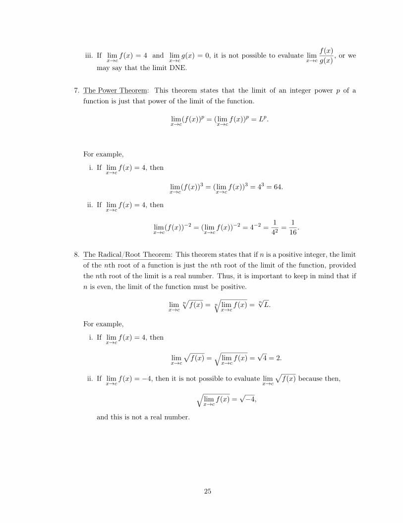
iii. If lim
x!cf(x) = 4 and lim
x!cg(x) = 0, it is not possible to evaluate lim
x!c
f(x)
g(x), or we
may say that the limit DNE.
7. The Power Theorem: This theorem states that the limit of an integer power p of afunction is just that power of the limit of the function.
lim
x!c(f(x))p = (lim
x!cf(x))p = Lp.
For example,
i. If lim
x!cf(x) = 4, then
lim
x!c(f(x))3 = (lim
x!cf(x))3 = 4
3
= 64.
ii. If lim
x!cf(x) = 4, then
lim
x!c(f(x))�2
= (lim
x!cf(x))�2
= 4
�2
=
1
4
2
=
1
16
.
8. The Radical/Root Theorem: This theorem states that if n is a positive integer, the limitof the nth root of a function is just the nth root of the limit of the function, providedthe nth root of the limit is a real number. Thus, it is important to keep in mind that ifn is even, the limit of the function must be positive.
lim
x!c
n
pf(x) = n
qlim
x!cf(x) =
n
pL.
For example,
i. If lim
x!cf(x) = 4, then
lim
x!c
pf(x) =
qlim
x!cf(x) =
p4 = 2.
ii. If lim
x!cf(x) = �4, then it is not possible to evaluate lim
x!c
pf(x) because then,
qlim
x!cf(x) =
p�4,
and this is not a real number.
25
(C) EXERCISES
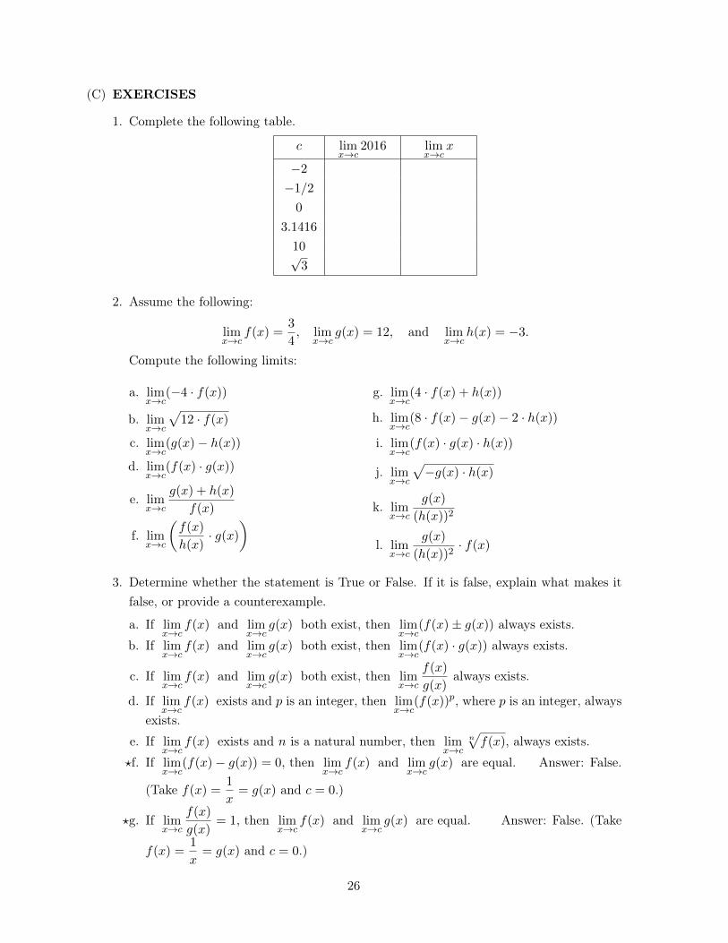
1. Complete the following table.
c lim
x!c2016 lim
x!cx
�2
�1/2
0
3.1416
10p3
2. Assume the following:
lim
x!cf(x) =
3
4
, lim
x!cg(x) = 12, and lim
x!ch(x) = �3.
Compute the following limits:
a. lim
x!c(�4 · f(x))
b. lim
x!c
p12 · f(x)
c. lim
x!c(g(x)� h(x))
d. lim
x!c(f(x) · g(x))
e. lim
x!c
g(x) + h(x)
f(x)
f. lim
x!c
✓f(x)
h(x)· g(x)
◆
g. lim
x!c(4 · f(x) + h(x))
h. lim
x!c(8 · f(x)� g(x)� 2 · h(x))
i. lim
x!c(f(x) · g(x) · h(x))
j. lim
x!c
p�g(x) · h(x)
k. lim
x!c
g(x)
(h(x))2
l. lim
x!c
g(x)
(h(x))2· f(x)
3. Determine whether the statement is True or False. If it is false, explain what makes itfalse, or provide a counterexample.
a. If lim
x!cf(x) and lim
x!cg(x) both exist, then lim
x!c(f(x)± g(x)) always exists.
b. If lim
x!cf(x) and lim
x!cg(x) both exist, then lim
x!c(f(x) · g(x)) always exists.
c. If lim
x!cf(x) and lim
x!cg(x) both exist, then lim
x!c
f(x)
g(x)always exists.
d. If lim
x!cf(x) exists and p is an integer, then lim
x!c(f(x))p, where p is an integer, always
exists.e. If lim
x!cf(x) exists and n is a natural number, then lim
x!c
n
pf(x), always exists.
?f. If lim
x!c(f(x)� g(x)) = 0, then lim
x!cf(x) and lim
x!cg(x) are equal. Answer: False.
(Take f(x) =1
x= g(x) and c = 0.)
?g. If lim
x!c
f(x)
g(x)= 1, then lim
x!cf(x) and lim
x!cg(x) are equal. Answer: False. (Take
f(x) =1
x= g(x) and c = 0.)
26
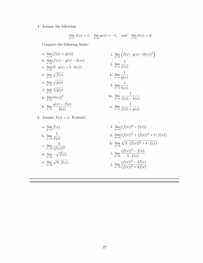
4. Assume the following:
lim
x!cf(x) = 1, lim
x!cg(x) = �1, and lim
x!ch(x) = 2.
Compute the following limits:
a. lim
x!c(f(x) + g(x))
b. lim
x!c(f(x)� g(x)� h(x))
c. lim
x!c(3 · g(x) + 5 · h(x))
d. lim
x!c
pf(x)
e. lim
x!c
pg(x)
f. lim
x!c
3pg(x)
g. lim
x!c(h(x))5
h. lim
x!c
g(x)� f(x)
h(x)
i. lim
x!c
⇣f(x) · g(x) · (h(x))2
⌘
j. lim
x!c
1
f(x)
k. lim
x!c
1
g(x)
l. lim
x!c
1
h(x)
m. lim
x!c
1
f(x)� h(x)
n. lim
x!c
1
f(x) + g(x)
5. Assume f(x) = x. Evaluate
a. lim
x!4
f(x).
b. lim
x!4
1
f(x).
c. lim
x!4
1
(f(x))2.
d. lim
x!4
�p
f(x).
e. lim
x!4
p9 · f(x).
f. lim
x!4
((f(x))2 � f(x)).
g. lim
x!4
((f(x))3 + (f(x))2 + 2 · f(x)).
h. lim
x!4
n
p3 · (f(x))2 + 4 · f(x).
i. lim
x!4
(f(x))2 � f(x)
5 · f(x) .
j. lim
x!4
(f(x))2 � 4f(x)
(f(x))2 + 4f(x).
27
TOPIC 1.4: Limits of Polynomial, Rational, and Radical Func-tions
DEVELOPMENT OF THE LESSON
(A) INTROUCTIONIn the previous lesson, we presented and illustrated the limit theorems. We start by recallingthese limit theorems.
Theorem 1. Let c, k, L and M be real numbers, and let f(x) and g(x) be functions definedon some open interval containing c, except possibly at c.
1. If lim
x!cf(x) exists, then it is unique. That is, if lim
x!cf(x) = L and lim
x!cf(x) = M , then
L = M .
2. lim
x!cc = c.
3. lim
x!cx = c
4. Suppose lim
x!cf(x) = L and lim
x!cg(x) = M .
i. (Constant Multiple) lim
x!c[k · g(x)] = k ·M .
ii. (Addition) lim
x!c[f(x)± g(x)] = L±M .
iii. (Multiplication) lim
x!c[f(x)g(x)] = LM .
iv. (Division) lim
x!c
f(x)
g(x)=
L
M, provided M 6= 0.
v. (Power) lim
x!c[f(x)]p = Lp for p, a positive integer.
vi. (Root/Radical) lim
x!c
n
pf(x) =
n
pL for positive integers n, and provided that L > 0
when n is even.
Teaching Tip
It would be helpful for the students if these limit theorems remain written on theboard or on manila paper throughout the discussion of this lesson.
In this lesson, we will show how these limit theorems are used in evaluating algebraic func-tions. Particularly, we will illustrate how to use them to evaluate the limits of polynomial,rational and radical functions.
(B) LESSON PROPER
LIMITS OF ALGEBRAIC FUNCTIONS
We start with evaluating the limits of polynomial functions.
28
EXAMPLE 1: Determine lim
x!1
(2x+ 1).
Solution. From the theorems above,
lim
x!1
(2x+ 1) = lim
x!1
2x+ lim
x!1
1 (Addition)
=
✓2 lim
x!1
x
◆+ 1 (Constant Multiple)
= 2(1) + 1
✓lim
x!cx = c
◆
= 2 + 1
= 3.
.
EXAMPLE 2: Determine lim
x!�1
(2x3 � 4x2 + 1).
Solution. From the theorems above,
lim
x!�1
(2x3 � 4x2 + 1) = lim
x!�1
2x3 � lim
x!�1
4x2 + lim
x!�1
1 (Addition)
= 2 lim
x!�1
x3 � 4 lim
x!�1
x2 + 1 (Constant Multiple)
= 2(�1)
3 � 4(�1)
2
+ 1 (Power)= �2� 4 + 1
= �5.
.
EXAMPLE 3: Evaluate lim
x!0
(3x4 � 2x� 1).
Solution. From the theorems above,
lim
x!0
(3x4 � 2x� 1) = lim
x!0
3x4 � lim
x!0
2x� lim
x!0
1 (Addition)
= 3 lim
x!0
x4 � 2 lim
x!0
x2 � 1 (Constant Multiple)
= 3(0)
4 � 2(0)� 1 (Power)= 0� 0� 1
= �1.
.
We will now apply the limit theorems in evaluating rational functions. In evaluating thelimits of such functions, recall from Theorem 1 the Division Rule, and all the rules statedin Theorem 1 which have been useful in evaluating limits of polynomial functions, such asthe Addition and Product Rules.
29
EXAMPLE 4: Evaluate lim
x!1
1
x.
Solution. First, note that lim
x!1
x = 1. Since the limit of the denominator is nonzero, we canapply the Division Rule. Thus,
lim
x!1
1
x=
lim
x!1
1
lim
x!1
x(Division)
=
1
1
= 1.
.
EXAMPLE 5: Evaluate lim
x!2
x
x+ 1
.
Solution. We start by checking the limit of the polynomial function in the denominator.
lim
x!2
(x+ 1) = lim
x!2
x+ lim
x!2
1 = 2 + 1 = 3.
Since the limit of the denominator is not zero, it follows that
lim
x!2
x
x+ 1
=
lim
x!2
x
lim
x!2
(x+ 1)
=
2
3
(Division)
.
EXAMPLE 6: Evaluate lim
x!1
(x� 3)(x2 � 2)
x2 + 1
. First, note that
lim
x!1
(x2 + 1) = lim
x!1
x2 + lim
x!1
1 = 1 + 1 = 2 6= 0.
Thus, using the theorem,
lim
x!1
(x� 3)(x2 � 2)
x2 + 1
=
lim
x!1
(x� 3)(x2 � 2)
lim
x!1
(x2 + 1)
(Division)
=
lim
x!1
(x� 3) · limx!1
(x2 � 2)
2
(Multipication)
=
✓lim
x!1
x� lim
x!1
3
◆✓lim
x!1
x2 � lim
x!1
2
◆
2
(Addition)
=
(1� 3)(1
2 � 2)
2
= 1.
30
Theorem 2. Let f be a polynomial of the form
f(x) = anxn+ an�1
xn�1
+ an�2
xn�2
+ ...+ a1
x+ a0
.
If c is a real number, thenlim
x!cf(x) = f(c).
Proof. Let c be any real number. Remember that a polynomial is defined at any realnumber. So,
f(c) = ancn+ an�1
cn�1
+ an�2
cn�2
+ ...+ a1
c+ a0
.
Now apply the limit theorems in evaluating lim
x!cf(x):
lim
x!cf(x) = lim
x!c(anx
n+ an�1
xn�1
+ an�2
xn�2
+ ...+ a1
x+ a0
)
= lim
x!canx
n+ lim
x!can�1
xn�1
+ lim
x!can�2
xn�2
+ ...+ lim
x!ca1
x+ lim
x!ca0
= an lim
x!cxn + an�1
lim
x!cxn�1
+ an�2
lim
x!cxn�2
+ ...+ a1
lim
x!cx+ a
0
= ancn+ an�1
cn�1
+ an�2
cn�2
+ ...+ a1
c+ a0
= f(c).
Therefore, limx!c
f(x) = f(c).
EXAMPLE 7: Evaluate lim
x!�1
(2x3 � 4x2 + 1).
Solution. Note first that our function
f(x) = 2x3 � 4x2 + 1,
is a polynomial. Computing for the value of f at x = �1, we get
f(�1) = 2(�1)
3 � 4(�1)
2
+ 1 = 2(�1)� 4(1) + 1 = �5.
Therefore, from Theorem 2,
lim
x!�1
(2x3 � 4x2 + 1) = f(�1) = �5.
.
Note that we get the same answer when we use limit theorems.
Theorem 3. Let h be a rational function of the form h(x) =
f(x)
g(x)where f and g are
polynomial functions. If c is a real number and g(c) 6= 0, then
lim
x!ch(x) = lim
x!c
f(x)
g(x)=
f(c)
g(c).
31
Proof. From Theorem 2, lim
x!cg(x) = g(c), which is nonzero by assumption. Moreover,
lim
x!cf(x) = f(c). Therefore, by the Division Rule of Theorem 1,
lim
x!c
f(x)
g(x)=
lim
x!cf(x)
lim
x!cg(x)
=
f(c)
g(c).
EXAMPLE 8: Evaluate lim
x!1
1� 5x
1 + 3x2 + 4x4.
Solution. Since the denominator is not zero when evaluated at x = 1, we may applyTheorem 3:
lim
x!1
1� 5x
1 + 3x2 + 4x4=
1� 5(1)
1 + 3(1)
2
+ 4(1)
4
=
�4
8
= �1
2
.
.
We will now evaluate limits of radical functions using limit theorems.
EXAMPLE 9: Evaluate lim
x!1
px.
Solution. Note that lim
x!1
x = 1 > 0. Therefore, by the Radical/Root Rule,
lim
x!1
px =
qlim
x!1
x =
p1 = 1.
.
EXAMPLE 10: Evaluate lim
x!0
px+ 4.
Solution. Note that lim
x!0
(x+ 4) = 4 > 0. Hence, by the Radical/Root Rule,
lim
x!0
px+ 4 =
qlim
x!0
(x+ 4) =
p4 = 2.
.
EXAMPLE 11: Evaluate lim
x!�2
3p
x2 + 3x� 6.
Solution. Since the index of the radical sign is odd, we do not have to worry that the limitof the radicand is negative. Therefore, the Radical/Root Rule implies that
lim
x!�2
3px2 + 3x� 6 =
3
rlim
x!�2
(x2 + 3x� 6) =
3p4� 6� 6 =
3p�8 = �2.
.
32
EXAMPLE 12: Evaluate lim
x!2
p2x+ 5
1� 3x.
Solution. First, note that lim
x!2
(1 � 3x) = �5 6= 0. Moreover, lim
x!2
(2x + 5) = 9 > 0. Thus,using the Division and Radical Rules of Theorem 1, we obtain
lim
x!2
p2x+ 5
1� 3x=
lim
x!2
p2x+ 5
lim
x!2
1� 3x=
qlim
x!2
(2x+ 5)
�5
=
p9
�5
= �3
5
.
.
INTUITIVE NOTIONS OF INFINITE LIMITSWe investigate the limit at a point c of a rational function of the form
f(x)
g(x)where f and g
are polynomial functions with f(c) 6= 0 and g(c) = 0. Note that Theorem 3 does not coverthis because it assumes that the denominator is nonzero at c.
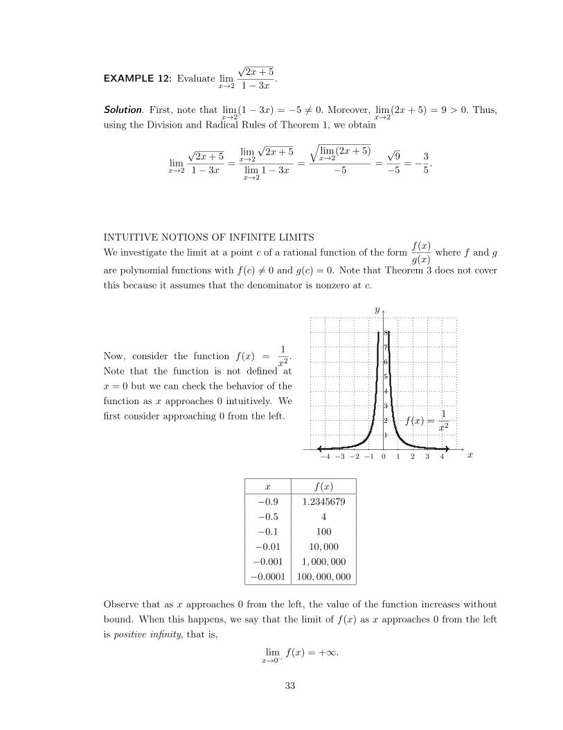
Now, consider the function f(x) =
1
x2.
Note that the function is not defined atx = 0 but we can check the behavior of thefunction as x approaches 0 intuitively. Wefirst consider approaching 0 from the left.
�4 �3 �2 �1 0 1 2 3 4
1
2
3
4
5
6
7
8
x
y
f(x) =1
x2
x f(x)
�0.9 1.2345679
�0.5 4
�0.1 100
�0.01 10, 000
�0.001 1, 000, 000
�0.0001 100, 000, 000
Observe that as x approaches 0 from the left, the value of the function increases withoutbound. When this happens, we say that the limit of f(x) as x approaches 0 from the leftis positive infinity, that is,
lim
x!0
�f(x) = +1.
33
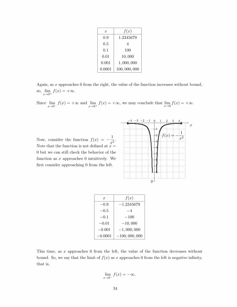
x f(x)
0.9 1.2345679
0.5 4
0.1 100
0.01 10, 000
0.001 1, 000, 000
0.0001 100, 000, 000
Again, as x approaches 0 from the right, the value of the function increases without bound,so, lim
x!0
+f(x) = +1.
Since lim
x!0
�f(x) = +1 and lim
x!0
+f(x) = +1, we may conclude that lim
x!0
f(x) = +1.
Now, consider the function f(x) = � 1
x2.
Note that the function is not defined at x =
0 but we can still check the behavior of thefunction as x approaches 0 intuitively. Wefirst consider approaching 0 from the left.
�4 �3 �2 �1
0 1 2 3 4
�1
�2
�3
�4
�5
�6
�7
�8
x
y
f(x) = � 1
x2
x f(x)
�0.9 �1.2345679
�0.5 �4
�0.1 �100
�0.01 �10, 000
�0.001 �1, 000, 000
�0.0001 �100, 000, 000
This time, as x approaches 0 from the left, the value of the function decreases withoutbound. So, we say that the limit of f(x) as x approaches 0 from the left is negative infinity,that is,
lim
x!0
�f(x) = �1.
34
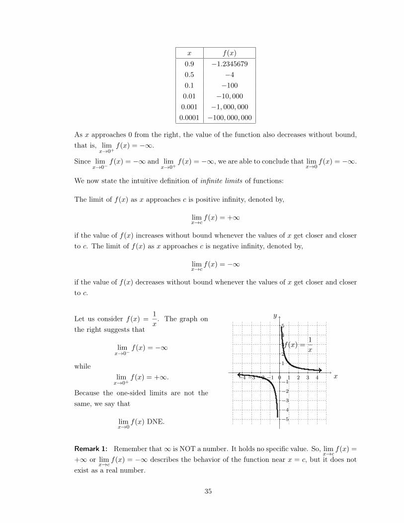
x f(x)
0.9 �1.2345679
0.5 �4
0.1 �100
0.01 �10, 000
0.001 �1, 000, 000
0.0001 �100, 000, 000
As x approaches 0 from the right, the value of the function also decreases without bound,that is, lim
x!0
+f(x) = �1.
Since lim
x!0
�f(x) = �1 and lim
x!0
+f(x) = �1, we are able to conclude that lim
x!0
f(x) = �1.
We now state the intuitive definition of infinite limits of functions:
The limit of f(x) as x approaches c is positive infinity, denoted by,
lim
x!cf(x) = +1
if the value of f(x) increases without bound whenever the values of x get closer and closerto c. The limit of f(x) as x approaches c is negative infinity, denoted by,
lim
x!cf(x) = �1
if the value of f(x) decreases without bound whenever the values of x get closer and closerto c.
Let us consider f(x) =
1
x. The graph on
the right suggests that
lim
x!0
�f(x) = �1
whilelim
x!0
+f(x) = +1.
Because the one-sided limits are not thesame, we say that
lim
x!0
f(x) DNE.
�4 �3 �2 �1 0 1 2 3 4
�5
�4
�3
�2
�1
1
2
3
4
5
x
y
f(x) =1
x
Remark 1: Remember that 1 is NOT a number. It holds no specific value. So, limx!c
f(x) =
+1 or lim
x!cf(x) = �1 describes the behavior of the function near x = c, but it does not
exist as a real number.
35
Remark 2: Whenever lim
x!c+f(x) = ±1 or lim
x!c�f(x) = ±1, we normally see the dashed
vertical line x = c. This is to indicate that the graph of y = f(x) is asymptotic to x = c,meaning, the graphs of y = f(x) and x = c are very close to each other near c. In this case,we call x = c a vertical asymptote of the graph of y = f(x).
Teaching Tip
Computing infinite limits is not a learning objective of this course, however, we willbe needing this notion for the discussion on infinite essential discontinuity, whichwill be presented in Topic 4.1. It is enough that the student determines that thelimit at the point c is +1 or �1 from the behavior of the graph, or the trend ofthe y-coordinates in a table of values.
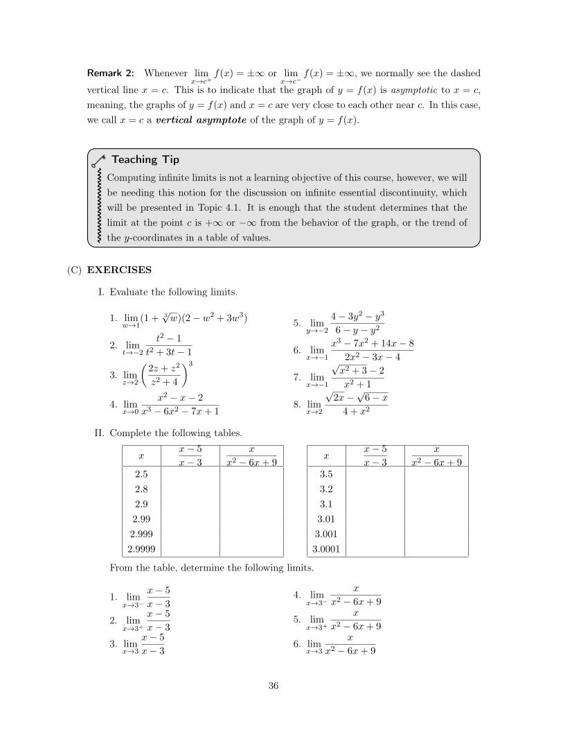
(C) EXERCISES
I. Evaluate the following limits.
1. lim
w!1
(1 +
3pw)(2� w2
+ 3w3
)
2. lim
t!�2
t2 � 1
t2 + 3t� 1
3. lim
z!2
✓2z + z2
z2 + 4
◆3
4. lim
x!0
x2 � x� 2
x3 � 6x2 � 7x+ 1
5. lim
y!�2
4� 3y2 � y3
6� y � y2
6. lim
x!�1
x3 � 7x2 + 14x� 8
2x2 � 3x� 4
7. lim
x!�1
px2 + 3� 2
x2 + 1
8. lim
x!2
p2x�
p6� x
4 + x2
II. Complete the following tables.
xx� 5
x� 3
x
x2 � 6x+ 9
2.5
2.8
2.9
2.99
2.999
2.9999
xx� 5
x� 3
x
x2 � 6x+ 9
3.5
3.2
3.1
3.01
3.001
3.0001
From the table, determine the following limits.
1. lim
x!3
�
x� 5
x� 3
2. lim
x!3
+
x� 5
x� 3
3. lim
x!3
x� 5
x� 3
4. lim
x!3
�
x
x2 � 6x+ 9
5. lim
x!3
+
x
x2 � 6x+ 9
6. lim
x!3
x
x2 � 6x+ 9
36
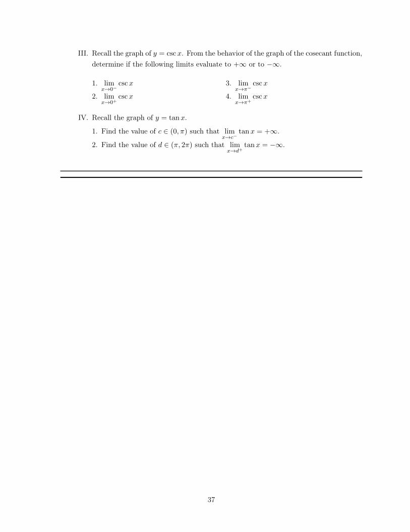
III. Recall the graph of y = cscx. From the behavior of the graph of the cosecant function,determine if the following limits evaluate to +1 or to �1.
1. lim
x!0
�cscx
2. lim
x!0
+cscx
3. lim
x!⇡�cscx
4. lim
x!⇡+cscx
IV. Recall the graph of y = tanx.
1. Find the value of c 2 (0,⇡) such that lim
x!c�tanx = +1.
2. Find the value of d 2 (⇡, 2⇡) such that lim
x!d+tanx = �1.
37
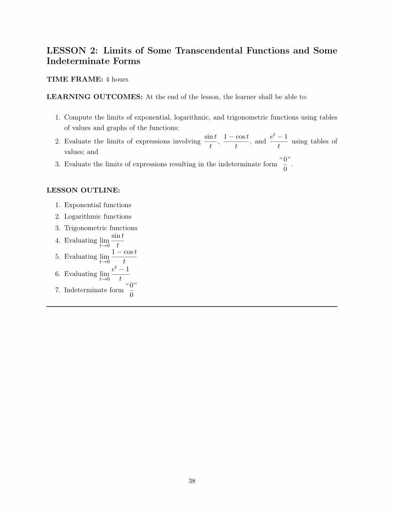
LESSON 2: Limits of Some Transcendental Functions and SomeIndeterminate Forms
TIME FRAME: 4 hours
LEARNING OUTCOMES: At the end of the lesson, the learner shall be able to:
1. Compute the limits of exponential, logarithmic, and trigonometric functions using tablesof values and graphs of the functions;
2. Evaluate the limits of expressions involvingsin t
t,1� cos t
t, and
et � 1
tusing tables of
values; and
3. Evaluate the limits of expressions resulting in the indeterminate form “ 00
”.
LESSON OUTLINE:
1. Exponential functions2. Logarithmic functions3. Trigonometric functions
4. Evaluating lim
t!0
sin t
t
5. Evaluating lim
t!0
1� cos t
t
6. Evaluating lim
t!0
et � 1
t
7. Indeterminate form “ 00
”
38
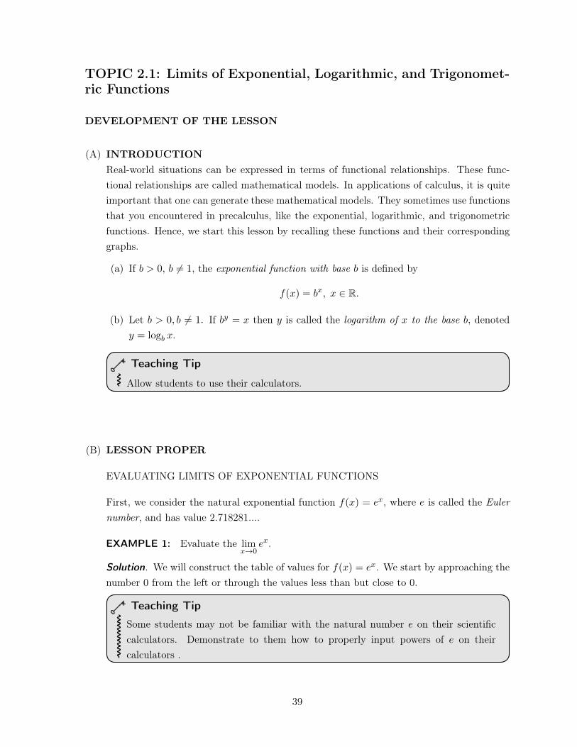
TOPIC 2.1: Limits of Exponential, Logarithmic, and Trigonomet-ric Functions
DEVELOPMENT OF THE LESSON
(A) INTRODUCTIONReal-world situations can be expressed in terms of functional relationships. These func-tional relationships are called mathematical models. In applications of calculus, it is quiteimportant that one can generate these mathematical models. They sometimes use functionsthat you encountered in precalculus, like the exponential, logarithmic, and trigonometricfunctions. Hence, we start this lesson by recalling these functions and their correspondinggraphs.
(a) If b > 0, b 6= 1, the exponential function with base b is defined by
f(x) = bx, x 2 R.
(b) Let b > 0, b 6= 1. If by = x then y is called the logarithm of x to the base b, denotedy = logb x.
Teaching Tip
Allow students to use their calculators.
(B) LESSON PROPER
EVALUATING LIMITS OF EXPONENTIAL FUNCTIONS
First, we consider the natural exponential function f(x) = ex, where e is called the Eulernumber, and has value 2.718281....
EXAMPLE 1: Evaluate the lim
x!0
ex.
Solution. We will construct the table of values for f(x) = ex. We start by approaching thenumber 0 from the left or through the values less than but close to 0.
Teaching Tip
Some students may not be familiar with the natural number e on their scientificcalculators. Demonstrate to them how to properly input powers of e on theircalculators .
39
x f(x)
�1 0.36787944117
�0.5 0.60653065971
�0.1 0.90483741803
�0.01 0.99004983374
�0.001 0.99900049983
�0.0001 0.999900049983
�0.00001 0.99999000005
Intuitively, from the table above, lim
x!0
�ex = 1. Now we consider approaching 0 from its
right or through values greater than but close to 0.
x f(x)
1 2.71828182846
0.5 1.6487212707
0.1 1.10517091808
0.01 1.01005016708
0.001 1.00100050017
0.0001 1.000100005
0.00001 1.00001000005
From the table, as the values of x get closer and closer to 0, the values of f(x) get closerand closer to 1. So, lim
x!0
+ex = 1. Combining the two one-sided limits allows us to conclude
thatlim
x!0
ex = 1.
.
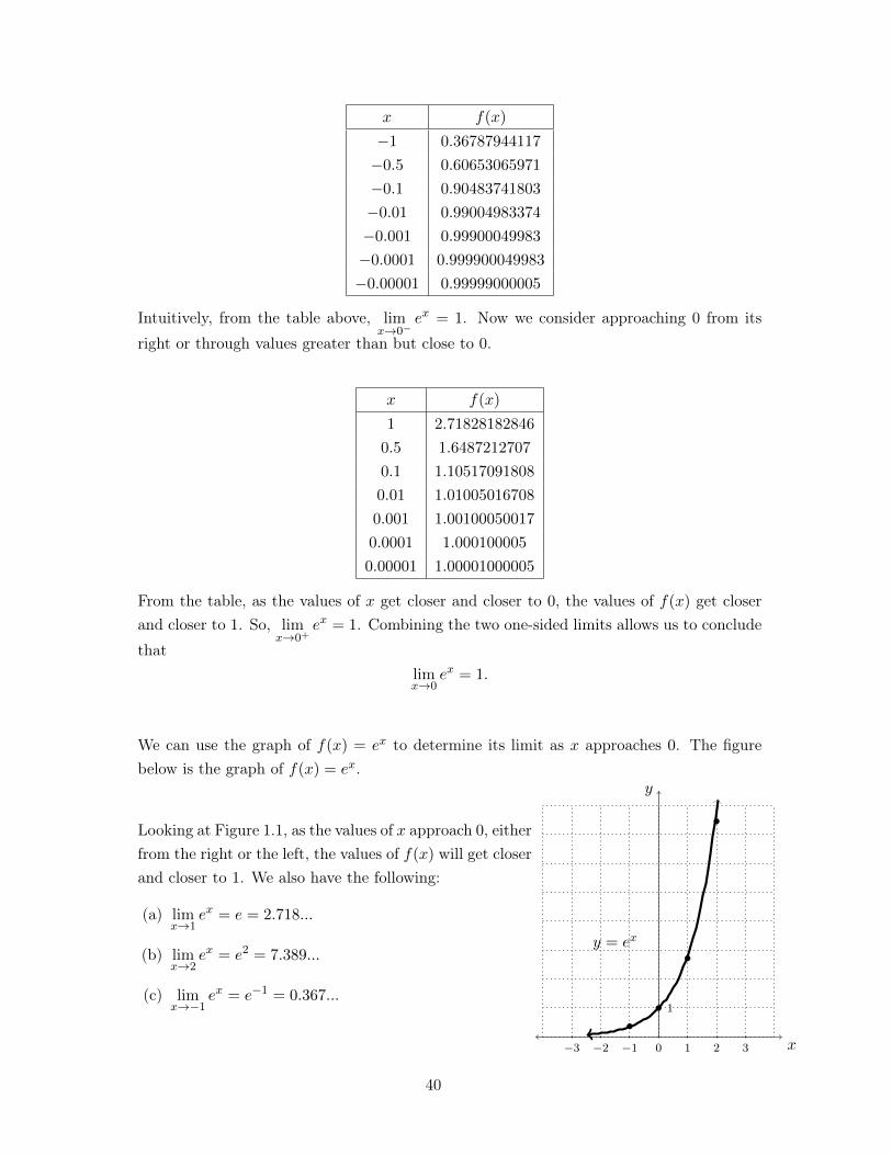
We can use the graph of f(x) = ex to determine its limit as x approaches 0. The figurebelow is the graph of f(x) = ex.
Looking at Figure 1.1, as the values of x approach 0, eitherfrom the right or the left, the values of f(x) will get closerand closer to 1. We also have the following:
(a) lim
x!1
ex = e = 2.718...
(b) lim
x!2
ex = e2 = 7.389...
(c) lim
x!�1
ex = e�1
= 0.367...
�3 �2 �1 0 1 2 3
x
y
1
y = ex
40
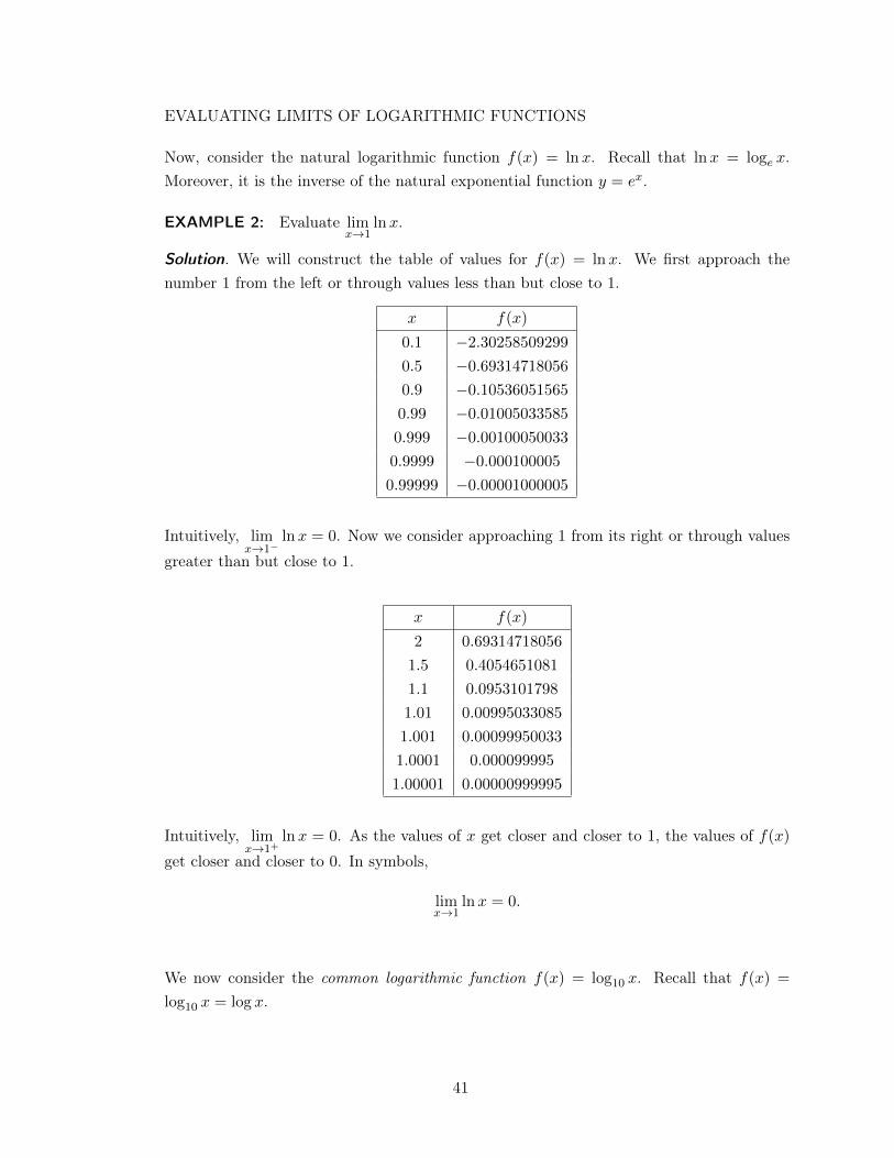
EVALUATING LIMITS OF LOGARITHMIC FUNCTIONS
Now, consider the natural logarithmic function f(x) = lnx. Recall that lnx = loge x.Moreover, it is the inverse of the natural exponential function y = ex.
EXAMPLE 2: Evaluate lim
x!1
lnx.
Solution. We will construct the table of values for f(x) = lnx. We first approach thenumber 1 from the left or through values less than but close to 1.
x f(x)
0.1 �2.30258509299
0.5 �0.69314718056
0.9 �0.10536051565
0.99 �0.01005033585
0.999 �0.00100050033
0.9999 �0.000100005
0.99999 �0.00001000005
Intuitively, lim
x!1
�lnx = 0. Now we consider approaching 1 from its right or through values
greater than but close to 1.
x f(x)
2 0.69314718056
1.5 0.4054651081
1.1 0.0953101798
1.01 0.00995033085
1.001 0.00099950033
1.0001 0.000099995
1.00001 0.00000999995
Intuitively, lim
x!1
+lnx = 0. As the values of x get closer and closer to 1, the values of f(x)
get closer and closer to 0. In symbols,
lim
x!1
lnx = 0.
.
We now consider the common logarithmic function f(x) = log
10
x. Recall that f(x) =
log
10
x = log x.
41
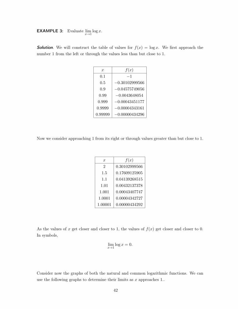
EXAMPLE 3: Evaluate lim
x!1
log x.
Solution. We will construct the table of values for f(x) = log x. We first approach thenumber 1 from the left or through the values less than but close to 1.
x f(x)
0.1 �1
0.5 �0.30102999566
0.9 �0.04575749056
0.99 �0.0043648054
0.999 �0.00043451177
0.9999 �0.00004343161
0.99999 �0.00000434296
Now we consider approaching 1 from its right or through values greater than but close to 1.
x f(x)
2 0.30102999566
1.5 0.17609125905
1.1 0.04139268515
1.01 0.00432137378
1.001 0.00043407747
1.0001 0.00004342727
1.00001 0.00000434292
As the values of x get closer and closer to 1, the values of f(x) get closer and closer to 0.In symbols,
lim
x!1
log x = 0.
.
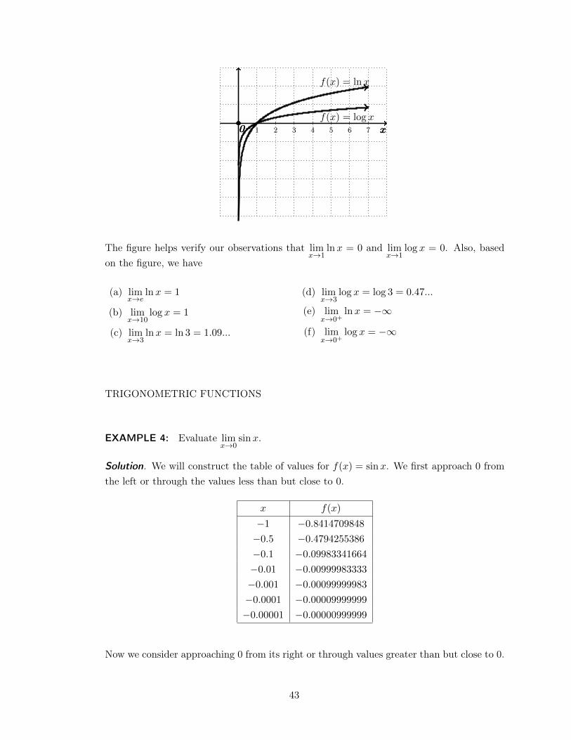
Consider now the graphs of both the natural and common logarithmic functions. We canuse the following graphs to determine their limits as x approaches 1..
42
x
1 2 3 4 5 6 7
f(x) = lnx
0
x
f(x) = log x0
The figure helps verify our observations that lim
x!1
lnx = 0 and lim
x!1
log x = 0. Also, basedon the figure, we have
(a) lim
x!elnx = 1
(b) lim
x!10
log x = 1
(c) lim
x!3
lnx = ln 3 = 1.09...
(d) lim
x!3
log x = log 3 = 0.47...
(e) lim
x!0
+lnx = �1
(f) lim
x!0
+log x = �1
TRIGONOMETRIC FUNCTIONS
EXAMPLE 4: Evaluate lim
x!0
sinx.
Solution. We will construct the table of values for f(x) = sinx. We first approach 0 fromthe left or through the values less than but close to 0.
x f(x)
�1 �0.8414709848
�0.5 �0.4794255386
�0.1 �0.09983341664
�0.01 �0.00999983333
�0.001 �0.00099999983
�0.0001 �0.00009999999
�0.00001 �0.00000999999
Now we consider approaching 0 from its right or through values greater than but close to 0.
43
x f(x)
1 0.8414709848
0.5 0.4794255386
0.1 0.09983341664
0.01 0.00999983333
0.001 0.00099999983
0.0001 0.00009999999
0.00001 0.00000999999
As the values of x get closer and closer to 1, the values of f(x) get closer and closer to 0.In symbols,
lim
x!0
sinx = 0.
.
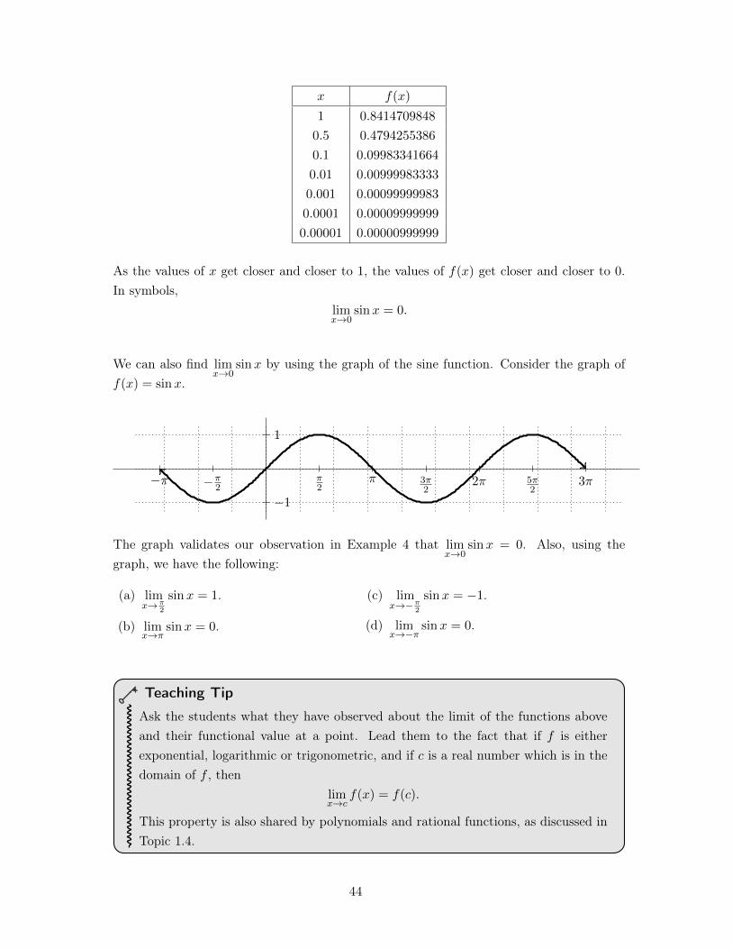
We can also find lim
x!0
sinx by using the graph of the sine function. Consider the graph off(x) = sinx.
1
�1
⇡2
⇡�⇡2
�⇡ 3⇡2
2⇡ 5⇡2
3⇡
The graph validates our observation in Example 4 that lim
x!0
sinx = 0. Also, using thegraph, we have the following:
(a) lim
x!⇡
2
sinx = 1.
(b) lim
x!⇡sinx = 0.
(c) lim
x!�⇡
2
sinx = �1.
(d) lim
x!�⇡sinx = 0.
Teaching Tip
Ask the students what they have observed about the limit of the functions aboveand their functional value at a point. Lead them to the fact that if f is eitherexponential, logarithmic or trigonometric, and if c is a real number which is in thedomain of f , then
lim
x!cf(x) = f(c).
This property is also shared by polynomials and rational functions, as discussed inTopic 1.4.
44
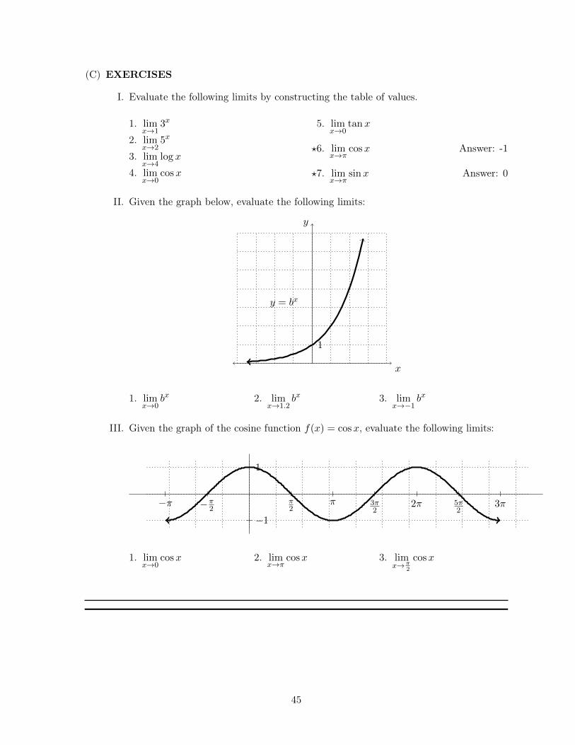
(C) EXERCISES
I. Evaluate the following limits by constructing the table of values.
1. lim
x!1
3
x
2. lim
x!2
5
x
3. lim
x!4
log x
4. lim
x!0
cosx
5. lim
x!0
tanx
?6. lim
x!⇡cosx Answer: -1
?7. lim
x!⇡sinx Answer: 0
II. Given the graph below, evaluate the following limits:
x
y
1
y = bx
1. lim
x!0
bx 2. lim
x!1.2bx 3. lim
x!�1
bx
III. Given the graph of the cosine function f(x) = cosx, evaluate the following limits:
⇡2
⇡�⇡2
�⇡ 3⇡2
2⇡ 5⇡2
3⇡
1
�1
1. lim
x!0
cosx 2. lim
x!⇡cosx 3. lim
x!⇡
2
cosx
45
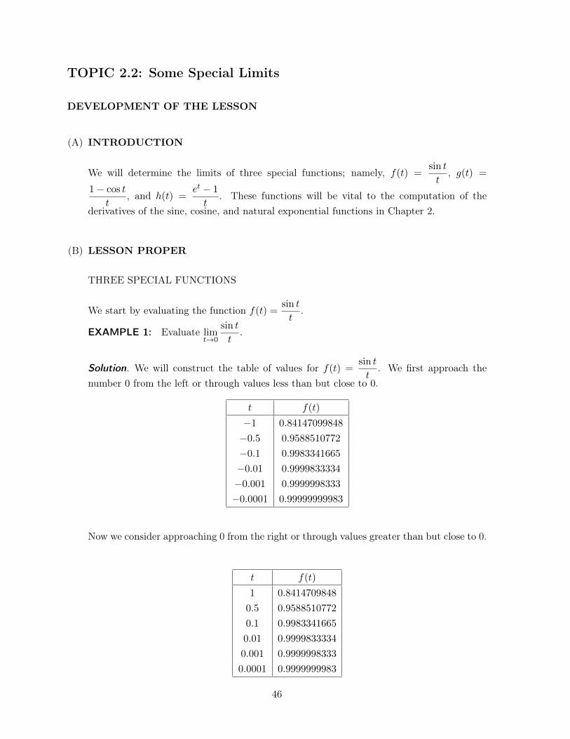
TOPIC 2.2: Some Special Limits
DEVELOPMENT OF THE LESSON
(A) INTRODUCTION
We will determine the limits of three special functions; namely, f(t) =
sin t
t, g(t) =
1� cos t
t, and h(t) =
et � 1
t. These functions will be vital to the computation of the
derivatives of the sine, cosine, and natural exponential functions in Chapter 2.
(B) LESSON PROPER
THREE SPECIAL FUNCTIONS
We start by evaluating the function f(t) =sin t
t.
EXAMPLE 1: Evaluate lim
t!0
sin t
t.
Solution. We will construct the table of values for f(t) =
sin t
t. We first approach the
number 0 from the left or through values less than but close to 0.
t f(t)
�1 0.84147099848
�0.5 0.9588510772
�0.1 0.9983341665
�0.01 0.9999833334
�0.001 0.9999998333
�0.0001 0.99999999983
Now we consider approaching 0 from the right or through values greater than but close to 0.
t f(t)
1 0.8414709848
0.5 0.9588510772
0.1 0.9983341665
0.01 0.9999833334
0.001 0.9999998333
0.0001 0.9999999983
46
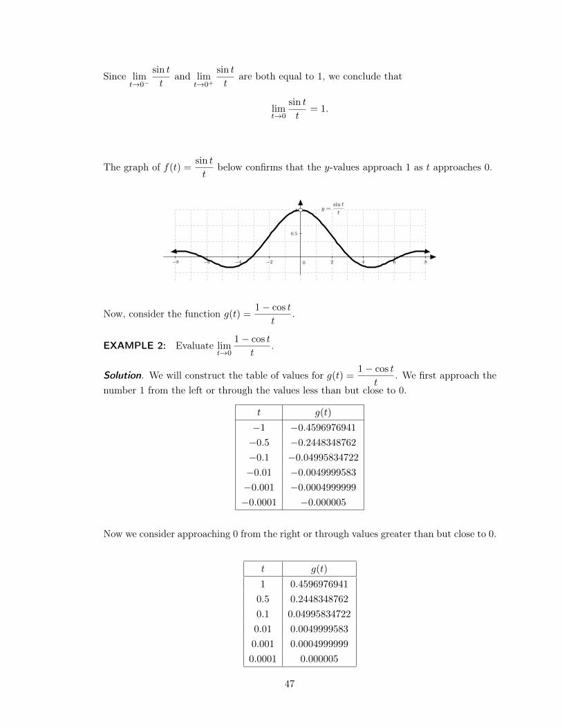
Since lim
t!0
�
sin t
tand lim
t!0
+
sin t
tare both equal to 1, we conclude that
lim
t!0
sin t
t= 1.
.
The graph of f(t) =sin t
tbelow confirms that the y-values approach 1 as t approaches 0.
�8 �6 �4 �2 2 4 6 8
0.5
1
0
y =
sin t
t
Now, consider the function g(t) =1� cos t
t.
EXAMPLE 2: Evaluate lim
t!0
1� cos t
t.
Solution. We will construct the table of values for g(t) =1� cos t
t. We first approach the
number 1 from the left or through the values less than but close to 0.
t g(t)
�1 �0.4596976941
�0.5 �0.2448348762
�0.1 �0.04995834722
�0.01 �0.0049999583
�0.001 �0.0004999999
�0.0001 �0.000005
Now we consider approaching 0 from the right or through values greater than but close to 0.
t g(t)
1 0.4596976941
0.5 0.2448348762
0.1 0.04995834722
0.01 0.0049999583
0.001 0.0004999999
0.0001 0.000005
47
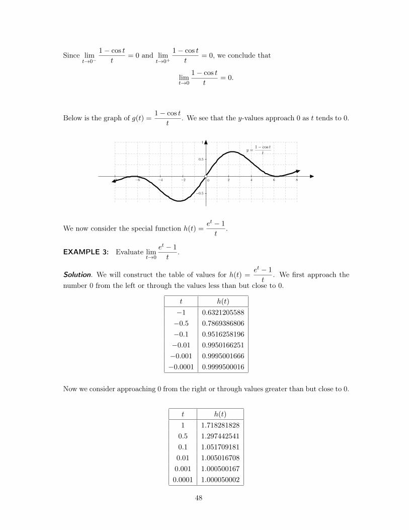
Since lim
t!0
�
1� cos t
t= 0 and lim
t!0
+
1� cos t
t= 0, we conclude that
lim
t!0
1� cos t
t= 0.
.
Below is the graph of g(t) =1� cos t
t. We see that the y-values approach 0 as t tends to 0.
�8 �6 �4 �2 2 4 6 8
�0.5
0.5
1
0
y =
1� cos t
t
We now consider the special function h(t) =et � 1
t.
EXAMPLE 3: Evaluate lim
t!0
et � 1
t.
Solution. We will construct the table of values for h(t) =
et � 1
t. We first approach the
number 0 from the left or through the values less than but close to 0.
t h(t)
�1 0.6321205588
�0.5 0.7869386806
�0.1 0.9516258196
�0.01 0.9950166251
�0.001 0.9995001666
�0.0001 0.9999500016
Now we consider approaching 0 from the right or through values greater than but close to 0.
t h(t)
1 1.718281828
0.5 1.297442541
0.1 1.051709181
0.01 1.005016708
0.001 1.000500167
0.0001 1.000050002
48
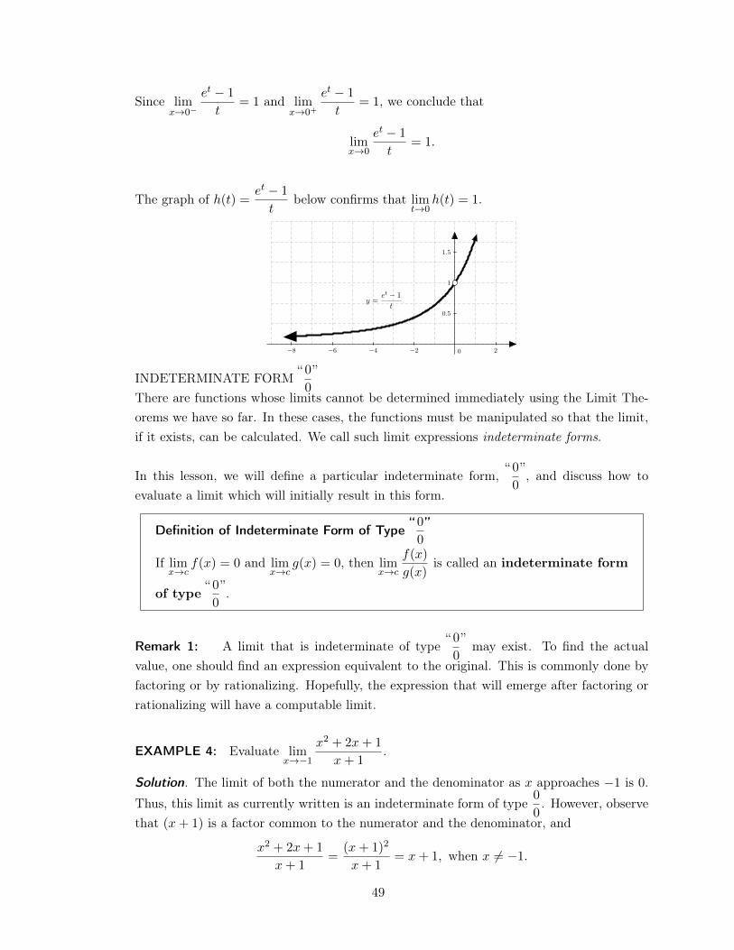
Since lim
x!0
�
et � 1
t= 1 and lim
x!0
+
et � 1
t= 1, we conclude that
lim
x!0
et � 1
t= 1.
.
The graph of h(t) =et � 1
tbelow confirms that lim
t!0
h(t) = 1.
�8 �6 �4 �2 2
0.5
1
1.5
0
y =
et � 1
t
INDETERMINATE FORM “ 00
”
There are functions whose limits cannot be determined immediately using the Limit The-orems we have so far. In these cases, the functions must be manipulated so that the limit,if it exists, can be calculated. We call such limit expressions indeterminate forms.
In this lesson, we will define a particular indeterminate form, “ 00
”, and discuss how toevaluate a limit which will initially result in this form.
Definition of Indeterminate Form of Type “ 00
”
If lim
x!cf(x) = 0 and lim
x!cg(x) = 0, then lim
x!c
f(x)
g(x)is called an indeterminate form
of type “ 00
”.
Remark 1: A limit that is indeterminate of type “ 00
” may exist. To find the actualvalue, one should find an expression equivalent to the original. This is commonly done byfactoring or by rationalizing. Hopefully, the expression that will emerge after factoring orrationalizing will have a computable limit.
EXAMPLE 4: Evaluate lim
x!�1
x2 + 2x+ 1
x+ 1
.
Solution. The limit of both the numerator and the denominator as x approaches �1 is 0.Thus, this limit as currently written is an indeterminate form of type
0
0
. However, observethat (x+ 1) is a factor common to the numerator and the denominator, and
x2 + 2x+ 1
x+ 1
=
(x+ 1)
2
x+ 1
= x+ 1, when x 6= �1.
49
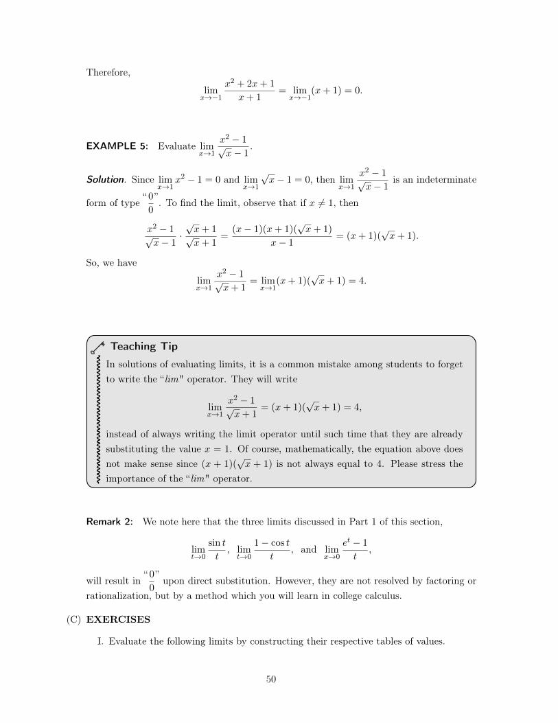
Therefore,
lim
x!�1
x2 + 2x+ 1
x+ 1
= lim
x!�1
(x+ 1) = 0.
.
EXAMPLE 5: Evaluate lim
x!1
x2 � 1px� 1
.
Solution. Since lim
x!1
x2 � 1 = 0 and lim
x!1
px� 1 = 0, then lim
x!1
x2 � 1px� 1
is an indeterminate
form of type “ 00
”. To find the limit, observe that if x 6= 1, then
x2 � 1px� 1
·px+ 1px+ 1
=
(x� 1)(x+ 1)(
px+ 1)
x� 1
= (x+ 1)(
px+ 1).
So, we have
lim
x!1
x2 � 1px+ 1
= lim
x!1
(x+ 1)(
px+ 1) = 4.
.
Teaching Tip
In solutions of evaluating limits, it is a common mistake among students to forgetto write the “ lim" operator. They will write
lim
x!1
x2 � 1px+ 1
= (x+ 1)(
px+ 1) = 4,
instead of always writing the limit operator until such time that they are alreadysubstituting the value x = 1. Of course, mathematically, the equation above doesnot make sense since (x + 1)(
px + 1) is not always equal to 4. Please stress the
importance of the “ lim" operator.
Remark 2: We note here that the three limits discussed in Part 1 of this section,
lim
t!0
sin t
t, lim
t!0
1� cos t
t, and lim
x!0
et � 1
t,
will result in “ 00
” upon direct substitution. However, they are not resolved by factoring orrationalization, but by a method which you will learn in college calculus.
(C) EXERCISES
I. Evaluate the following limits by constructing their respective tables of values.
50
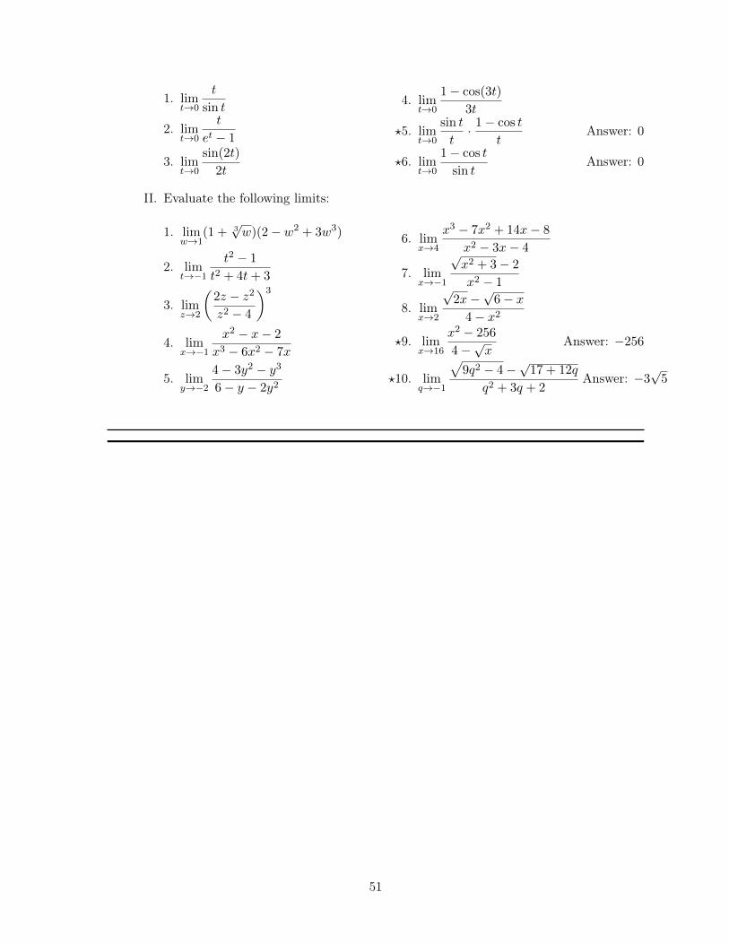
1. lim
t!0
t
sin t
2. lim
t!0
t
et � 1
3. lim
t!0
sin(2t)
2t
4. lim
t!0
1� cos(3t)
3t
?5. lim
t!0
sin t
t· 1� cos t
tAnswer: 0
?6. lim
t!0
1� cos t
sin tAnswer: 0
II. Evaluate the following limits:
1. lim
w!1
(1 +
3pw)(2� w2
+ 3w3
)
2. lim
t!�1
t2 � 1
t2 + 4t+ 3
3. lim
z!2
✓2z � z2
z2 � 4
◆3
4. lim
x!�1
x2 � x� 2
x3 � 6x2 � 7x
5. lim
y!�2
4� 3y2 � y3
6� y � 2y2
6. lim
x!4
x3 � 7x2 + 14x� 8
x2 � 3x� 4
7. lim
x!�1
px2 + 3� 2
x2 � 1
8. lim
x!2
p2x�
p6� x
4� x2
?9. lim
x!16
x2 � 256
4�px
Answer: �256
?10. lim
q!�1
p9q2 � 4�
p17 + 12q
q2 + 3q + 2
Answer: �3
p5
51
LESSON 3: Continuity of Functions
TIME FRAME: 3-4 hours
LEARNING OUTCOMES: At the end of the lesson, the learner shall be able to:
1. Illustrate continuity of a function at a point;2. Determine whether a function is continuous at a point or not;3. Illustrate continuity of a function on an interval; and4. Determine whether a function is continuous on an interval or not.
LESSON OUTLINE:
1. Continuity at a point2. Determining whether a function is continuous or not at a point3. Continuity on an interval4. Determining whether a function is continuous or not on an interval
52
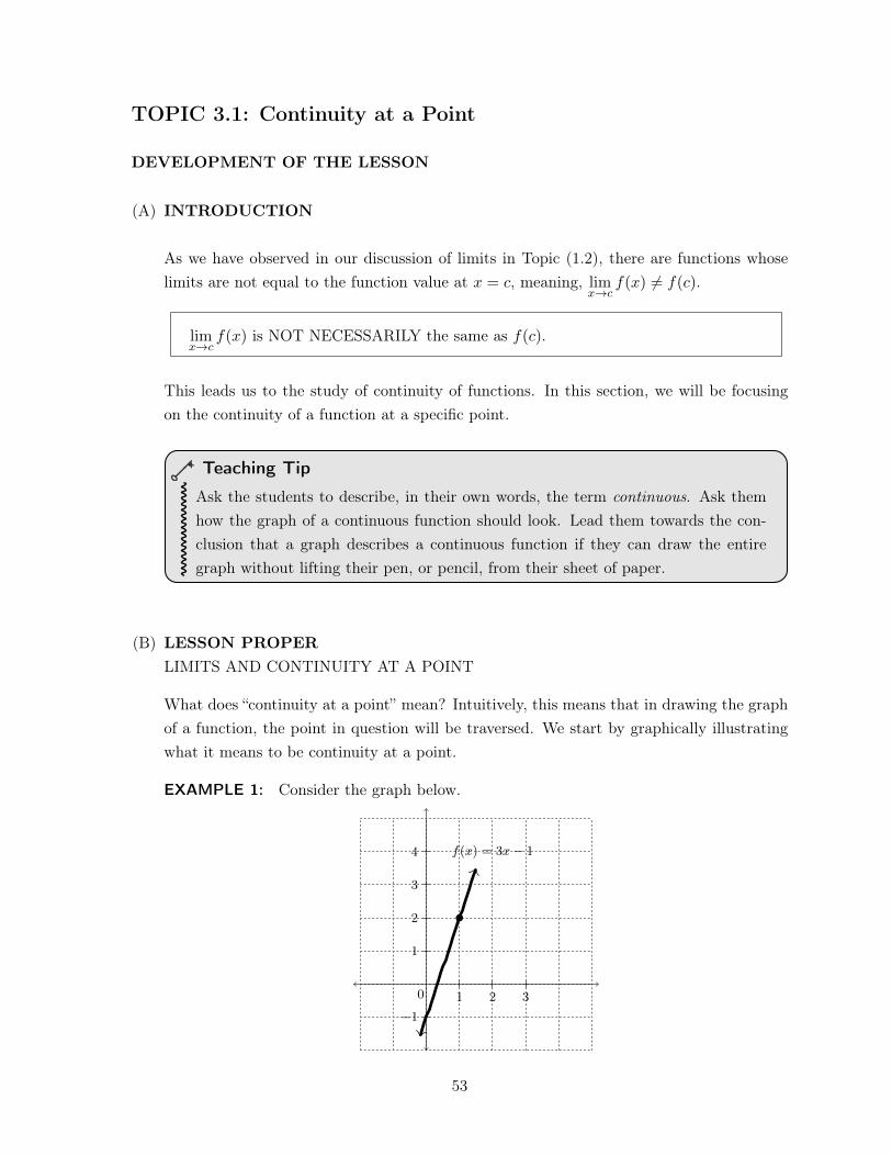
TOPIC 3.1: Continuity at a Point
DEVELOPMENT OF THE LESSON
(A) INTRODUCTION
As we have observed in our discussion of limits in Topic (1.2), there are functions whoselimits are not equal to the function value at x = c, meaning, lim
x!cf(x) 6= f(c).
lim
x!cf(x) is NOT NECESSARILY the same as f(c).
This leads us to the study of continuity of functions. In this section, we will be focusingon the continuity of a function at a specific point.
Teaching Tip
Ask the students to describe, in their own words, the term continuous. Ask themhow the graph of a continuous function should look. Lead them towards the con-clusion that a graph describes a continuous function if they can draw the entiregraph without lifting their pen, or pencil, from their sheet of paper.
(B) LESSON PROPERLIMITS AND CONTINUITY AT A POINT
What does “continuity at a point” mean? Intuitively, this means that in drawing the graphof a function, the point in question will be traversed. We start by graphically illustratingwhat it means to be continuity at a point.
EXAMPLE 1: Consider the graph below.
1 2 3
�1
1
2
3
4
0
f(x) = 3x� 1
53
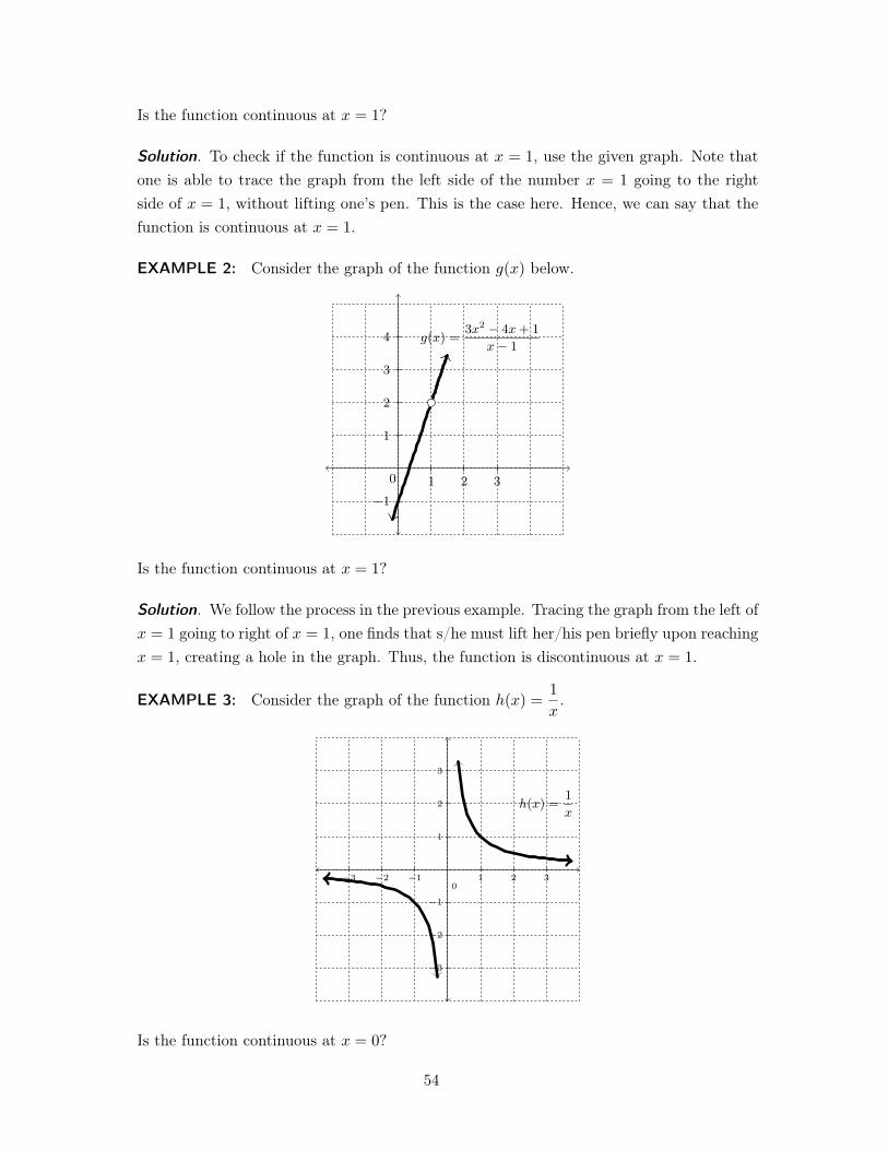
Is the function continuous at x = 1?
Solution. To check if the function is continuous at x = 1, use the given graph. Note thatone is able to trace the graph from the left side of the number x = 1 going to the rightside of x = 1, without lifting one’s pen. This is the case here. Hence, we can say that thefunction is continuous at x = 1. .
EXAMPLE 2: Consider the graph of the function g(x) below.
1 2 3
�1
1
2
3
4
0
g(x) =3x2 � 4x+ 1
x� 1
Is the function continuous at x = 1?
Solution. We follow the process in the previous example. Tracing the graph from the left ofx = 1 going to right of x = 1, one finds that s/he must lift her/his pen briefly upon reachingx = 1, creating a hole in the graph. Thus, the function is discontinuous at x = 1. .
EXAMPLE 3: Consider the graph of the function h(x) =1
x.
�3 �2 �1 1 2 3
�3
�2
�1
1
2
3
0
h(x) =1x
Is the function continuous at x = 0?
54
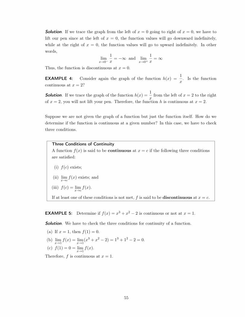
Solution. If we trace the graph from the left of x = 0 going to right of x = 0, we have tolift our pen since at the left of x = 0, the function values will go downward indefinitely,while at the right of x = 0, the function values will go to upward indefinitely. In otherwords,
lim
x!0
�
1
x= �1 and lim
x!0
+
1
x= 1
Thus, the function is discontinuous at x = 0. .
EXAMPLE 4: Consider again the graph of the function h(x) =
1
x. Is the function
continuous at x = 2?
Solution. If we trace the graph of the function h(x) =1
xfrom the left of x = 2 to the right
of x = 2, you will not lift your pen. Therefore, the function h is continuous at x = 2. .
Suppose we are not given the graph of a function but just the function itself. How do wedetermine if the function is continuous at a given number? In this case, we have to checkthree conditions.
Three Conditions of ContinuityA function f(x) is said to be continuous at x = c if the following three conditionsare satisfied:
(i) f(c) exists;
(ii) lim
x!cf(x) exists; and
(iii) f(c) = lim
x!cf(x).
If at least one of these conditions is not met, f is said to be discontinuous at x = c.
EXAMPLE 5: Determine if f(x) = x3 + x2 � 2 is continuous or not at x = 1.
Solution. We have to check the three conditions for continuity of a function.
(a) If x = 1, then f(1) = 0.
(b) lim
x!1
f(x) = lim
x!1
(x3 + x2 � 2) = 1
3
+ 1
2 � 2 = 0.
(c) f(1) = 0 = lim
x!1
f(x).
Therefore, f is continuous at x = 1. .
55
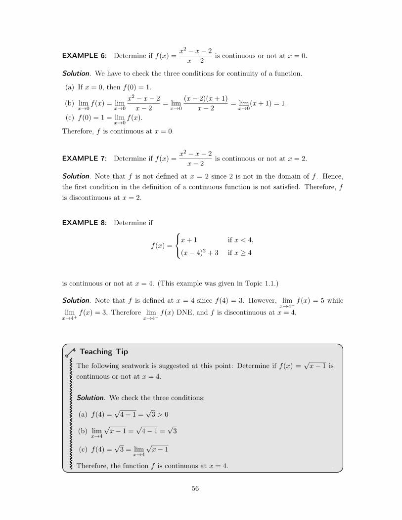
EXAMPLE 6: Determine if f(x) =x2 � x� 2
x� 2
is continuous or not at x = 0.
Solution. We have to check the three conditions for continuity of a function.
(a) If x = 0, then f(0) = 1.
(b) lim
x!0
f(x) = lim
x!0
x2 � x� 2
x� 2
= lim
x!0
(x� 2)(x+ 1)
x� 2
= lim
x!0
(x+ 1) = 1.
(c) f(0) = 1 = lim
x!0
f(x).
Therefore, f is continuous at x = 0. .
EXAMPLE 7: Determine if f(x) =x2 � x� 2
x� 2
is continuous or not at x = 2.
Solution. Note that f is not defined at x = 2 since 2 is not in the domain of f . Hence,the first condition in the definition of a continuous function is not satisfied. Therefore, fis discontinuous at x = 2. .
EXAMPLE 8: Determine if
f(x) =
8<
:x+ 1 if x < 4,
(x� 4)
2
+ 3 if x � 4
is continuous or not at x = 4. (This example was given in Topic 1.1.)
Solution. Note that f is defined at x = 4 since f(4) = 3. However, lim
x!4
�f(x) = 5 while
lim
x!4
+f(x) = 3. Therefore lim
x!4
�f(x) DNE, and f is discontinuous at x = 4. .
Teaching Tip
The following seatwork is suggested at this point: Determine if f(x) =px� 1 is
continuous or not at x = 4.
Solution. We check the three conditions:
(a) f(4) =p4� 1 =
p3 > 0
(b) lim
x!4
px� 1 =
p4� 1 =
p3
(c) f(4) =p3 = lim
x!4
px� 1
Therefore, the function f is continuous at x = 4. .
56
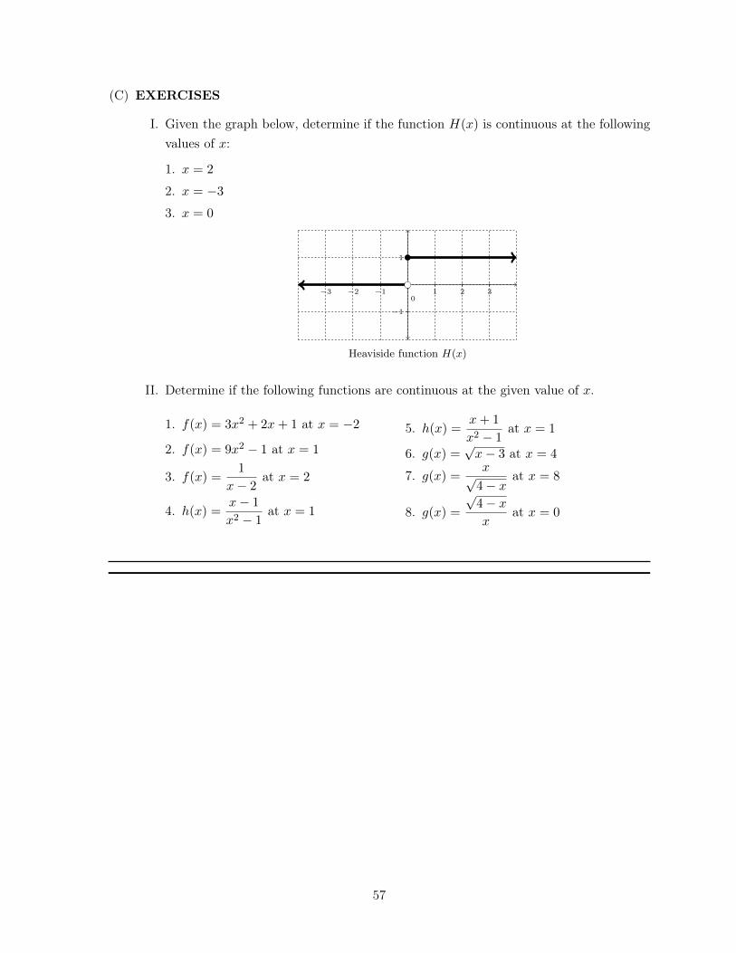
(C) EXERCISES
I. Given the graph below, determine if the function H(x) is continuous at the followingvalues of x:
1. x = 2
2. x = �3
3. x = 0
�3 �2 �1 1 2 3
�1
1
0
Heaviside function H(x)
II. Determine if the following functions are continuous at the given value of x.
1. f(x) = 3x2 + 2x+ 1 at x = �2
2. f(x) = 9x2 � 1 at x = 1
3. f(x) =1
x� 2
at x = 2
4. h(x) =x� 1
x2 � 1
at x = 1
5. h(x) =x+ 1
x2 � 1
at x = 1
6. g(x) =px� 3 at x = 4
7. g(x) =xp4� x
at x = 8
8. g(x) =
p4� x
xat x = 0
57
TOPIC 3.2: Continuity on an Interval
DEVELOPMENT OF THE LESSON
(A) INTRODUCTION
A function can be continuous on an interval. This simply means that it is continuous atevery point on the interval. Equivalently, if we are able to draw the entire graph of thefunction on an interval without lifting our tracing pen, or without being interrupted by ahole in the middle of the graph, then we can conclude that the the function is continuouson that interval.
We begin our discussion with two concepts which are important in determining whether afunction is continuous at the endpoints of closed intervals.
One-Sided Continuity
(a) A function f is said to be continuous from the left at x = c if
f(c) = lim
x!c�f(x).
(b) A function f is said to be continuous from the right at x = c if
f(c) = lim
x!c+f(x).
Here are known facts on continuities of functions on intervals:
Continuity of Polynomial, Absolute Value, Rational and Square Root Functions
(a) Polynomial functions are continuous everywhere.
(b) The absolute value function f(x) = |x| is continuous everywhere.
(c) Rational functions are continuous on their respective domains.
(d) The square root function f(x) =px is continuous on [0,1).
58
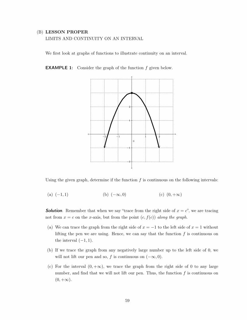
(B) LESSON PROPERLIMITS AND CONTINUITY ON AN INTERVAL
We first look at graphs of functions to illustrate continuity on an interval.
EXAMPLE 1: Consider the graph of the function f given below.
�2 �1 1 2
�2
�1
1
2
0
Using the given graph, determine if the function f is continuous on the following intervals:
(a) (�1, 1) (b) (�1, 0) (c) (0,+1)
Solution. Remember that when we say “trace from the right side of x = c”, we are tracingnot from x = c on the x-axis, but from the point (c, f(c)) along the graph.
(a) We can trace the graph from the right side of x = �1 to the left side of x = 1 withoutlifting the pen we are using. Hence, we can say that the function f is continuous onthe interval (�1, 1).
(b) If we trace the graph from any negatively large number up to the left side of 0, wewill not lift our pen and so, f is continuous on (�1, 0).
(c) For the interval (0,+1), we trace the graph from the right side of 0 to any largenumber, and find that we will not lift our pen. Thus, the function f is continuous on(0,+1).
.
59
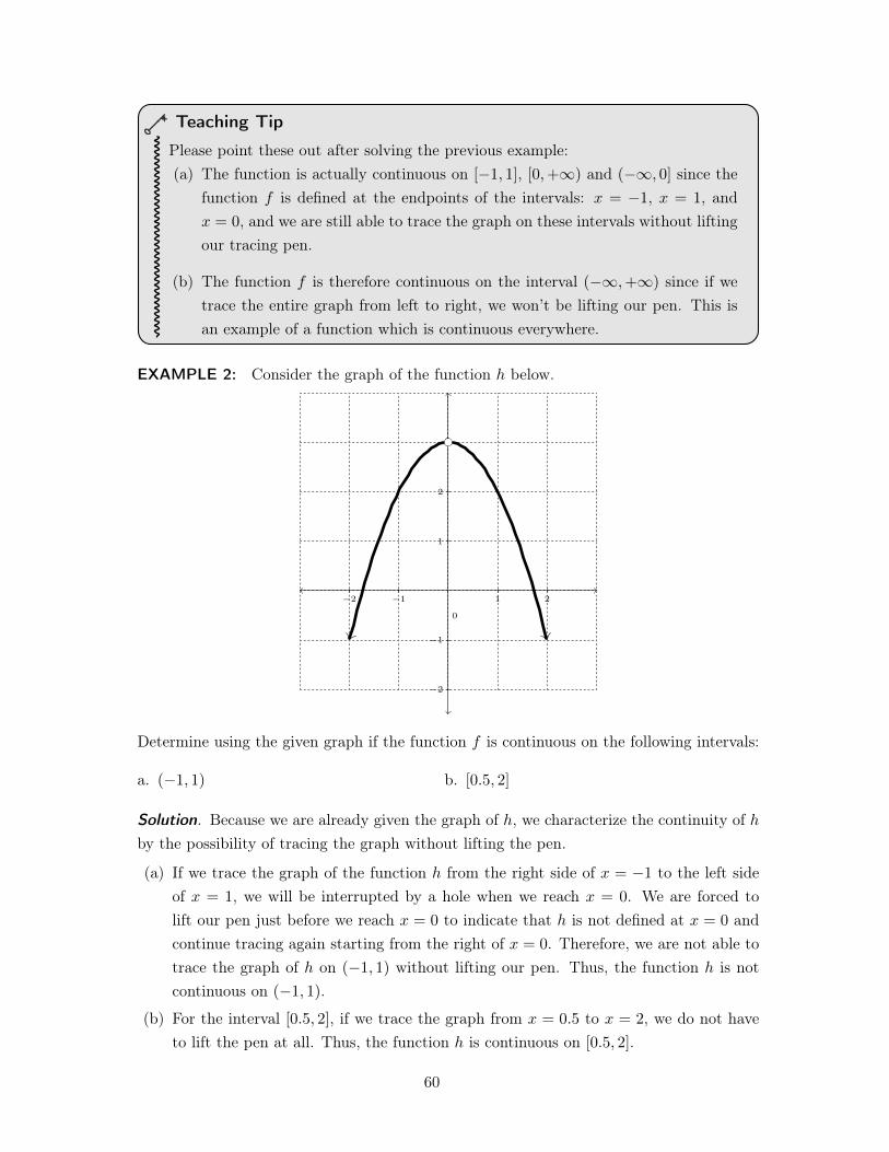
Teaching Tip
Please point these out after solving the previous example:(a) The function is actually continuous on [�1, 1], [0,+1) and (�1, 0] since the
function f is defined at the endpoints of the intervals: x = �1, x = 1, andx = 0, and we are still able to trace the graph on these intervals without liftingour tracing pen.
(b) The function f is therefore continuous on the interval (�1,+1) since if wetrace the entire graph from left to right, we won’t be lifting our pen. This isan example of a function which is continuous everywhere.
EXAMPLE 2: Consider the graph of the function h below.
�2 �1 1 2
�2
�1
1
2
0
Determine using the given graph if the function f is continuous on the following intervals:
a. (�1, 1) b. [0.5, 2]
Solution. Because we are already given the graph of h, we characterize the continuity of hby the possibility of tracing the graph without lifting the pen.
(a) If we trace the graph of the function h from the right side of x = �1 to the left sideof x = 1, we will be interrupted by a hole when we reach x = 0. We are forced tolift our pen just before we reach x = 0 to indicate that h is not defined at x = 0 andcontinue tracing again starting from the right of x = 0. Therefore, we are not able totrace the graph of h on (�1, 1) without lifting our pen. Thus, the function h is notcontinuous on (�1, 1).
(b) For the interval [0.5, 2], if we trace the graph from x = 0.5 to x = 2, we do not haveto lift the pen at all. Thus, the function h is continuous on [0.5, 2].
60
.
Now, if a function is given without its corresponding graph, we must find other means todetermine if the function is continuous or not on an interval. Here are definitions that willhelp us:
A function f is said to be continuous...
(a) everywhere if f is continuous at every real number. In this case, we also say f
is continuous on R.
(b) on (a, b) if f is continuous at every point x in (a, b).
(c) on [a, b) if f is continuous on (a, b) and from the right at a.
(d) on (a, b] if f is continuous on (a, b) and from the left at b.
(e) on [a, b] if f is continuous on (a, b] and on [a, b).
(f) on (a,1) if f is continuous at all x > a.
(g) on [a,1) if f is continuous on (a,1) and from the right at a.
(h) on (�1, b) if f is continuous at all x < b.
(i) on (�1, b] if f is continuous on (�1, b) and from the left at b.
EXAMPLE 3: Determine the largest interval over which the function f(x) =px+ 2 is
continuous.
Solution. Observe that the function f(x) =px+ 2 has function values only if x+ 2 � 0,
that is, if x 2 [�2,+1). For all c 2 (�2,+1),
f(c) =pc+ 2 = lim
x!c
px+ 2.
Moreover, f is continuous from the right at �2 because
f(�2) = 0 = lim
x!�2
+
px+ 2.
Therefore, for all x 2 [�2,+1), the function f(x) =px+ 2 is continuous. .
61
EXAMPLE 4: Determine the largest interval over which h(x) =x
x2 � 1
is continuous.
Solution. Observe that the given rational function h(x) =x
x2 � 1
is not defined at x = 1
and x = �1. Hence, the domain of h is the set R \ {�1, 1}. As mentioned at the startof this topic, a rational function is continuous on its domain. Hence, h is continuous overR \ {�1, 1}. .
EXAMPLE 5: Consider the function g(x) =
8>>>><
>>>>:
x if x 0,
3 if 0 < x 1,
3� x2 if 1 < x 4,
x� 3 if x > 4.Is g continuous on (0, 1]? on (4,1)?
Solution. Since g is a piecewise function, we just look at the ‘piece’ of the function corre-sponding to the interval specified.
(a) On the interval (0, 1], g(x) takes the constant value 3. Also, for all c 2 (0, 1],
lim
x!cg(x) = 3 = g(c).
Thus, g is continuous on (0, 1].
(b) For all x > 4, the corresponding ‘piece’ of g is g(x) = x � 3, a polynomial function.Recall that a polynomial function is continuous everywhere in R. Hence, f(x) = x�3
is surely continuous for all x 2 (4,+1).
.
(C) EXERCISES
1. Is the function g(x) =
8>>>><
>>>>:
x if x 0,
3 if 0 < x 1,
3� x2 if 1 < x 4,
x� 3 if x > 4,
continuous on [1, 4]? on (�1, 0)?
?2. Do as indicated.
a. Find all values of m such that g(x) =
(x+ 1 if x m,
x2 if x > m,is continuous everywhere.
62
b. Find all values of a and b that make
h(x) =
8>><
>>:
x+ 2a if x < �2,
3ax+ b if � 2 x 1,
3x� 2b if x > 1,
continuous everywhere.
63
LESSON 4: More on Continuity
TIME FRAME: 4 hours
LEARNING OUTCOMES: At the end of the lesson, the learner shall be able to:
1. Illustrate different types of discontinuity (hole/removable, jump/essential, asymptotic/infinite);2. Illustrate the Intermediate Value and Extreme Value Theorems; and3. Solve problems involving the continuity of a function.
LESSON OUTLINE:
1. Review of continuity at a point2. Illustration of a hole/removable discontinuity at a point3. Illustration of a jump essential discontinuity at a point4. Illustration of an infinite essential discontinuity at a point5. Illustration of a consequence of continuity given by the Intermediate Value Theorem6. Illustration of a consequence of continuity given by the Extreme Value Theorem7. Situations which involve principles of continuity8. Solutions to problems involving properties/consequences of continuity
64
TOPIC 4.1: Different Types of Discontinuities
DEVELOPMENT OF THE LESSON
(A) INTRODUCTION
In Topic (1.2), it was emphasized that the value of lim
x!cf(x) may be distinct from the
value of the function itself at x = c. Recall that a limit may be evaluated at values whichare not in the domain of f(x).
In Topics (3.1) - (3.2), we learned that when lim
x!cf(x) and f(c) are equal, f(x) is said
to be continuous at c. Otherwise, it is said to be discontinuous at c. We will revisit theinstances when lim
x!cf(x) and f(c) have unequal or different values. These instances of
inequality and, therefore, discontinuity are very interesting to study. This section focuseson these instances.
(B) LESSON PROPER
Consider the functions g(x), h(x) and j(x) where
g(x) =
8><
>:
3x2 � 4x+ 1
x� 1
if x 6= 1,
1 if x = 1.
h(x) =
8<
:x+ 1 if x < 4,
(x� 4)
2
+ 3 if x � 4.
and
j(x) =1
x, x 6= 0.
We examine these for continuity at the respective values 1, 4, and 0.
(a) lim
x!1
g(x) = 2 but g(1) = 1.
(b) lim
x!4
h(x) DNE but h(4) = 3.
(c) lim
x!0
j(x) DNE and f(0) DNE.
65
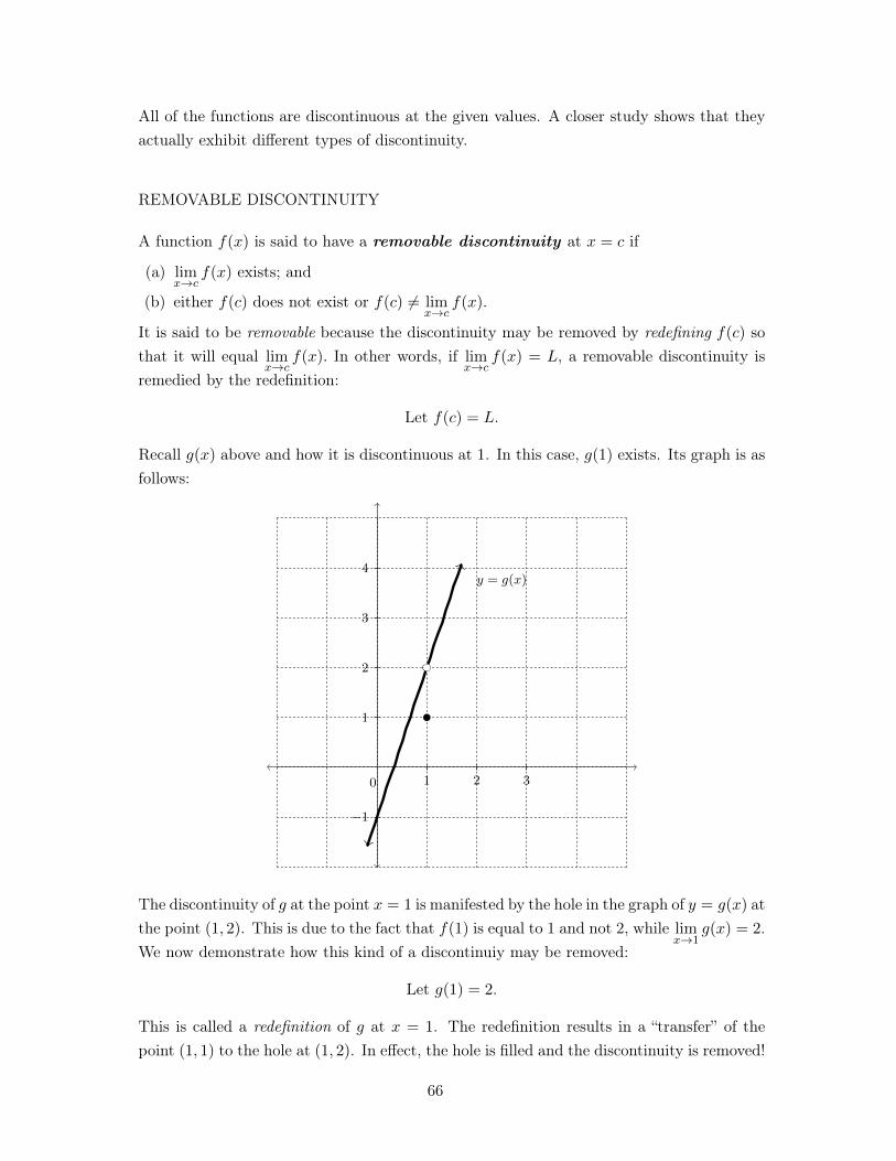
All of the functions are discontinuous at the given values. A closer study shows that theyactually exhibit different types of discontinuity.
REMOVABLE DISCONTINUITY
A function f(x) is said to have a removable discontinuity at x = c if
(a) lim
x!cf(x) exists; and
(b) either f(c) does not exist or f(c) 6= lim
x!cf(x).
It is said to be removable because the discontinuity may be removed by redefining f(c) sothat it will equal lim
x!cf(x). In other words, if lim
x!cf(x) = L, a removable discontinuity is
remedied by the redefinition:
Let f(c) = L.
Recall g(x) above and how it is discontinuous at 1. In this case, g(1) exists. Its graph is asfollows:
1 2 3
�1
1
2
3
4
0
y = g(x)
The discontinuity of g at the point x = 1 is manifested by the hole in the graph of y = g(x) atthe point (1, 2). This is due to the fact that f(1) is equal to 1 and not 2, while lim
x!1
g(x) = 2.We now demonstrate how this kind of a discontinuiy may be removed:
Let g(1) = 2.
This is called a redefinition of g at x = 1. The redefinition results in a “transfer” of thepoint (1, 1) to the hole at (1, 2). In effect, the hole is filled and the discontinuity is removed!
66
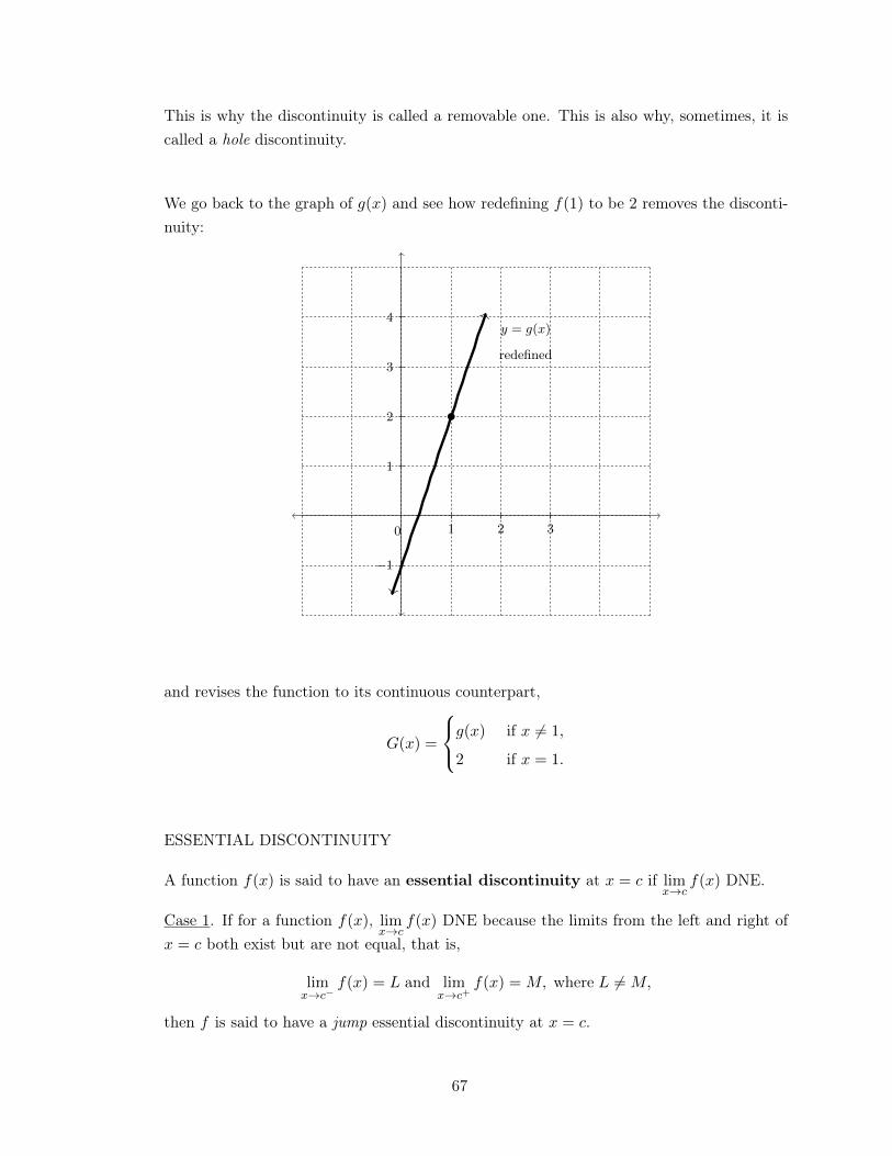
This is why the discontinuity is called a removable one. This is also why, sometimes, it iscalled a hole discontinuity.
We go back to the graph of g(x) and see how redefining f(1) to be 2 removes the disconti-nuity:
1 2 3
�1
1
2
3
4
0
y = g(x)
redefined
and revises the function to its continuous counterpart,
G(x) =
8<
:g(x) if x 6= 1,
2 if x = 1.
ESSENTIAL DISCONTINUITY
A function f(x) is said to have an essential discontinuity at x = c if lim
x!cf(x) DNE.
Case 1. If for a function f(x), limx!c
f(x) DNE because the limits from the left and right ofx = c both exist but are not equal, that is,
lim
x!c�f(x) = L and lim
x!c+f(x) = M, where L 6= M,
then f is said to have a jump essential discontinuity at x = c.
67
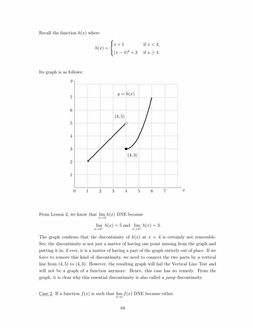
Recall the function h(x) where
h(x) =
8<
:x+ 1 if x < 4,
(x� 4)
2
+ 3 if x � 4.
Its graph is as follows:
x
y
(4, 5)
(4, 3)
y = h(x)
0 1 2 3 4 5 6 7
1
2
3
4
5
6
7
From Lesson 2, we know that lim
x!4
h(x) DNE because
lim
x!4
�h(x) = 5 and lim
x!4
+h(x) = 3.
The graph confirms that the discontinuity of h(x) at x = 4 is certainly not removable.See, the discontinuity is not just a matter of having one point missing from the graph andputting it in; if ever, it is a matter of having a part of the graph entirely out of place. If weforce to remove this kind of discontinuity, we need to connect the two parts by a verticalline from (4, 5) to (4, 3). However, the resulting graph will fail the Vertical Line Test andwill not be a graph of a function anymore. Hence, this case has no remedy. From thegraph, it is clear why this essential discontinuity is also called a jump discontinuity.
Case 2. If a function f(x) is such that lim
x!cf(x) DNE because either
68
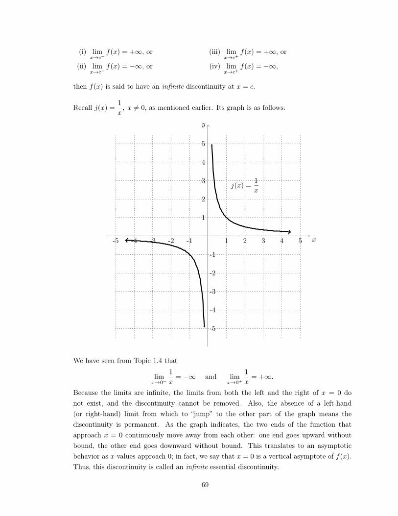
(i) lim
x!c�f(x) = +1, or
(ii) lim
x!c�f(x) = �1, or
(iii) lim
x!c+f(x) = +1, or
(iv) lim
x!c+f(x) = �1,
then f(x) is said to have an infinite discontinuity at x = c.
Recall j(x) =1
x, x 6= 0, as mentioned earlier. Its graph is as follows:
x
y
j(x) =1
x
1 2 3 4 5
1
2
3
4
5
-1-2-3-4-5
-1
-2
-3
-4
-5
We have seen from Topic 1.4 that
lim
x!0
�
1
x= �1 and lim
x!0
+
1
x= +1.
Because the limits are infinite, the limits from both the left and the right of x = 0 donot exist, and the discontinuity cannot be removed. Also, the absence of a left-hand(or right-hand) limit from which to “jump” to the other part of the graph means thediscontinuity is permanent. As the graph indicates, the two ends of the function thatapproach x = 0 continuously move away from each other: one end goes upward withoutbound, the other end goes downward without bound. This translates to an asymptoticbehavior as x-values approach 0; in fact, we say that x = 0 is a vertical asymptote of f(x).Thus, this discontinuity is called an infinite essential discontinuity.
69
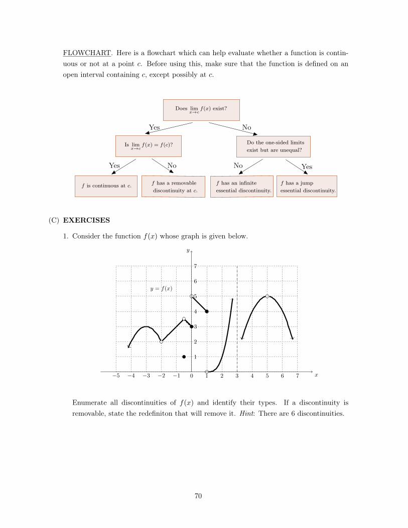
FLOWCHART. Here is a flowchart which can help evaluate whether a function is contin-uous or not at a point c. Before using this, make sure that the function is defined on anopen interval containing c, except possibly at c.
Does lim
x!c
f(x) exist?
Is lim
x!c
f(x) = f(c)? Do the one-sided limits
exist but are unequal?
f is continuous at c. f has a removable
discontinuity at c.
f has an infinite
essential discontinuity.
f has a jump
essential discontinuity.
Yes
Yes No
No
No Yes
(C) EXERCISES
1. Consider the function f(x) whose graph is given below.
x
y
y = f(x)
0
�1�2�3�4�5
1 2 3 4 5 6 7
1
2
3
4
5
6
7
Enumerate all discontinuities of f(x) and identify their types. If a discontinuity isremovable, state the redefiniton that will remove it. Hint: There are 6 discontinuities.
70
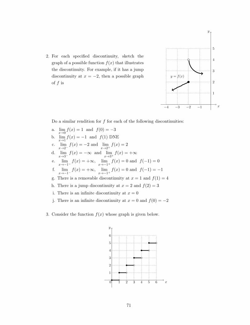
2. For each specified discontinuity, sketch thegraph of a possible function f(x) that illustratesthe discontinuity. For example, if it has a jumpdiscontinuity at x = �2, then a possible graphof f is
x
y
y = f(x)
1
2
3
4
5
�1�2�3�4
Do a similar rendition for f for each of the following discontinuities:
a. lim
x!0
f(x) = 1 and f(0) = �3
b. lim
x!1
f(x) = �1 and f(1) DNE
c. lim
x!2
�f(x) = �2 and lim
x!2
+f(x) = 2
d. lim
x!3
�f(x) = �1 and lim
x!3
+f(x) = +1
e. lim
x!�1
�f(x) = +1, lim
x!�1
+f(x) = 0 and f(�1) = 0
f. lim
x!�1
�f(x) = +1, lim
x!�1
+f(x) = 0 and f(�1) = �1
g. There is a removable discontinuity at x = 1 and f(1) = 4
h. There is a jump discontinuity at x = 2 and f(2) = 3
i. There is an infinite discontinuity at x = 0
j. There is an infinite discontinuity at x = 0 and f(0) = �2
3. Consider the function f(x) whose graph is given below.
x
y
0 1 2 3 4 5 6
1
2
3
4
5
6
71
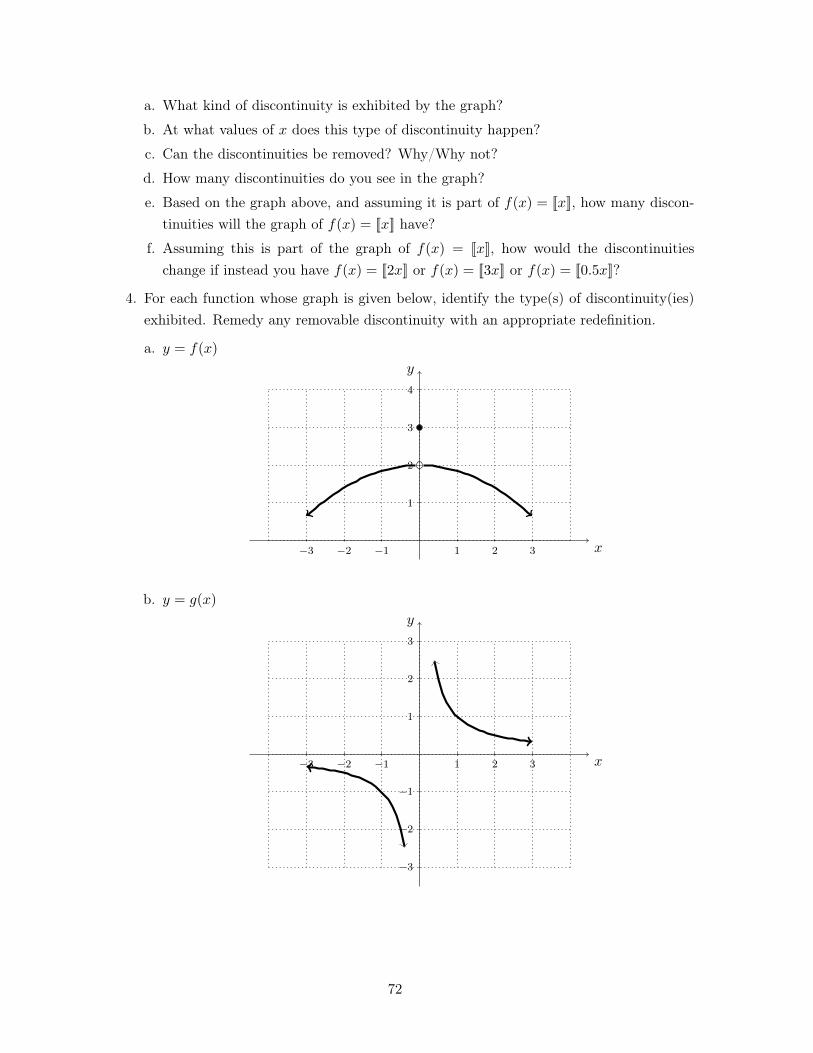
a. What kind of discontinuity is exhibited by the graph?
b. At what values of x does this type of discontinuity happen?
c. Can the discontinuities be removed? Why/Why not?
d. How many discontinuities do you see in the graph?
e. Based on the graph above, and assuming it is part of f(x) = [[x]], how many discon-tinuities will the graph of f(x) = [[x]] have?
f. Assuming this is part of the graph of f(x) = [[x]], how would the discontinuitieschange if instead you have f(x) = [[2x]] or f(x) = [[3x]] or f(x) = [[0.5x]]?
4. For each function whose graph is given below, identify the type(s) of discontinuity(ies)exhibited. Remedy any removable discontinuity with an appropriate redefinition.
a. y = f(x)
�3 �2 �1 1 2 3
1
2
3
4
x
y
b. y = g(x)
�3 �2 �1 1 2 3
�3
�2
�1
1
2
3
x
y
72
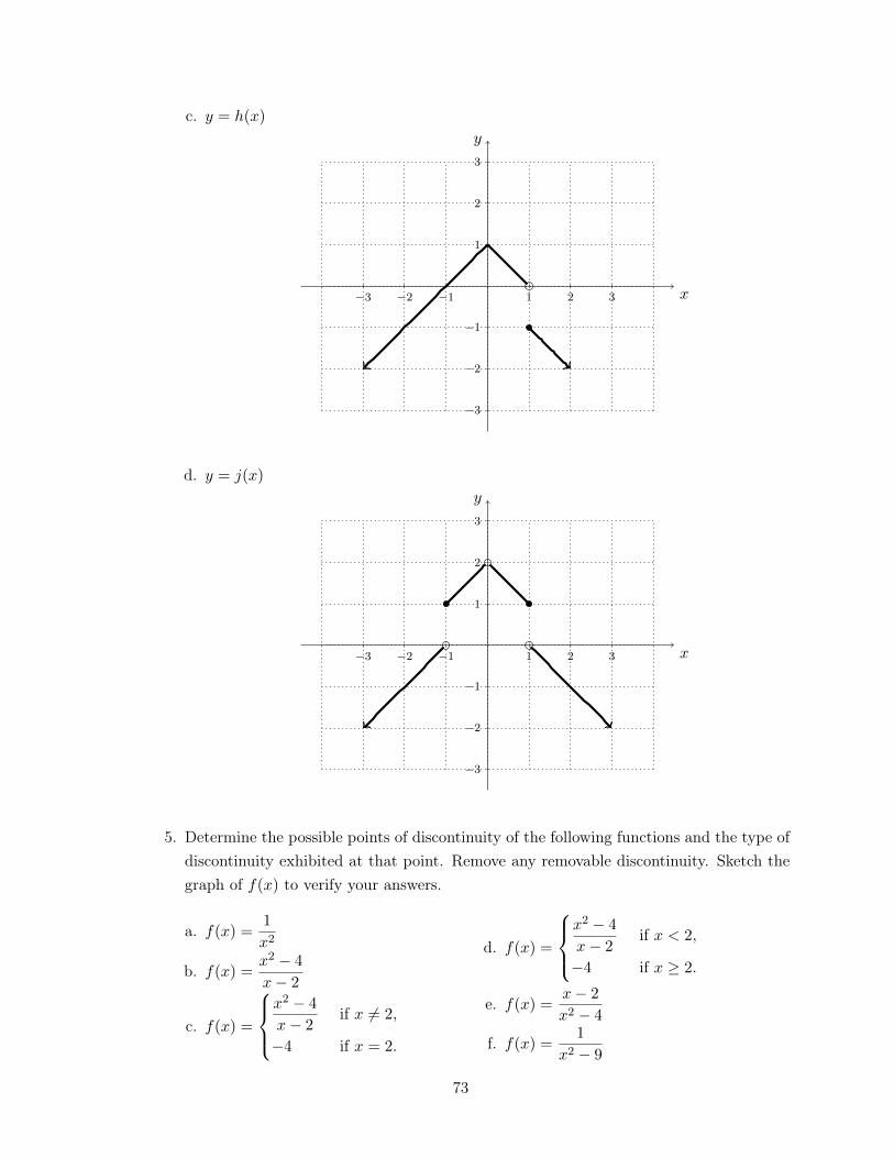
c. y = h(x)
�3 �2 �1 1 2 3
�3
�2
�1
1
2
3
x
y
d. y = j(x)
�3 �2 �1 1 2 3
�3
�2
�1
1
2
3
x
y
5. Determine the possible points of discontinuity of the following functions and the type ofdiscontinuity exhibited at that point. Remove any removable discontinuity. Sketch thegraph of f(x) to verify your answers.
a. f(x) =1
x2
b. f(x) =x2 � 4
x� 2
c. f(x) =
8><
>:
x2 � 4
x� 2
if x 6= 2,
�4 if x = 2.
d. f(x) =
8><
>:
x2 � 4
x� 2
if x < 2,
�4 if x � 2.
e. f(x) =x� 2
x2 � 4
f. f(x) =1
x2 � 9
73
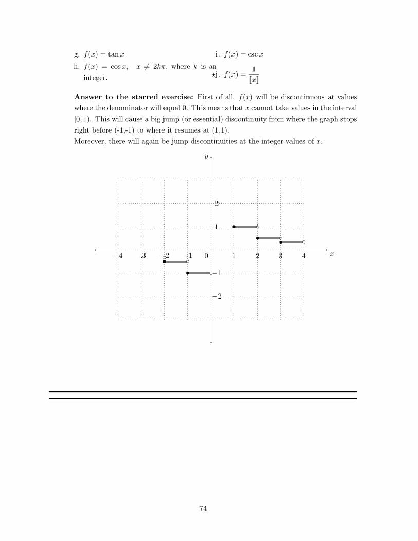
g. f(x) = tanx
h. f(x) = cosx, x 6= 2k⇡, where k is aninteger.
i. f(x) = cscx
?j. f(x) =1
[[x]]
Answer to the starred exercise: First of all, f(x) will be discontinuous at valueswhere the denominator will equal 0. This means that x cannot take values in the interval[0, 1). This will cause a big jump (or essential) discontinuity from where the graph stopsright before (-1,-1) to where it resumes at (1,1).Moreover, there will again be jump discontinuities at the integer values of x.
x
y
0 1 2 3 4
1
2
�1�2�3�4
�1
�2
74
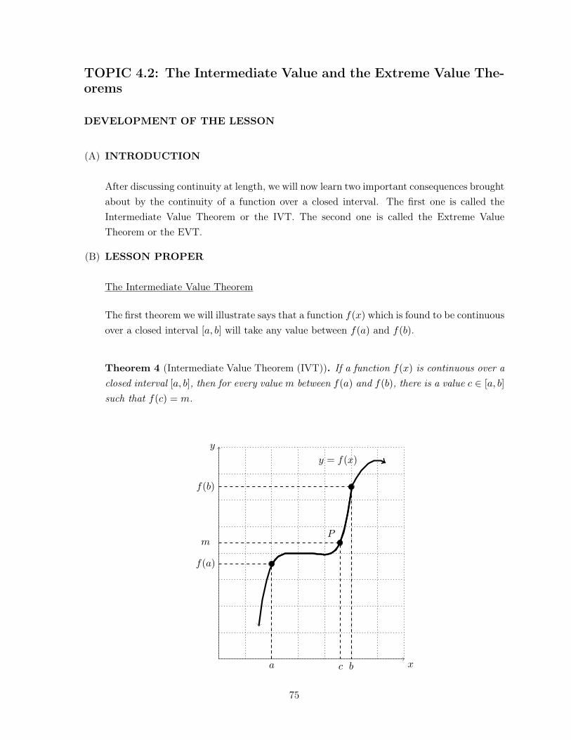
TOPIC 4.2: The Intermediate Value and the Extreme Value The-orems
DEVELOPMENT OF THE LESSON
(A) INTRODUCTION
After discussing continuity at length, we will now learn two important consequences broughtabout by the continuity of a function over a closed interval. The first one is called theIntermediate Value Theorem or the IVT. The second one is called the Extreme ValueTheorem or the EVT.
(B) LESSON PROPER
The Intermediate Value Theorem
The first theorem we will illustrate says that a function f(x) which is found to be continuousover a closed interval [a, b] will take any value between f(a) and f(b).
Theorem 4 (Intermediate Value Theorem (IVT)). If a function f(x) is continuous over aclosed interval [a, b], then for every value m between f(a) and f(b), there is a value c 2 [a, b]
such that f(c) = m.
x
y
P
y = f(x)
a bc
f(a)
f(b)
m
75
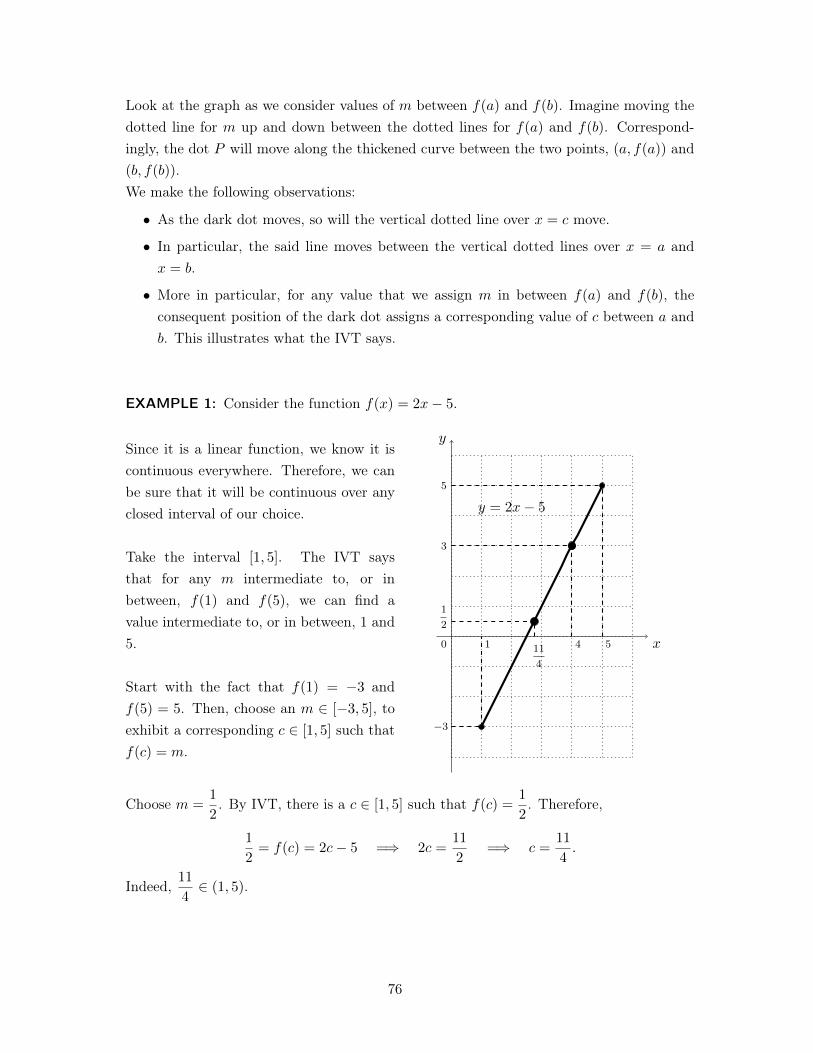
Look at the graph as we consider values of m between f(a) and f(b). Imagine moving thedotted line for m up and down between the dotted lines for f(a) and f(b). Correspond-ingly, the dot P will move along the thickened curve between the two points, (a, f(a)) and(b, f(b)).We make the following observations:
• As the dark dot moves, so will the vertical dotted line over x = c move.
• In particular, the said line moves between the vertical dotted lines over x = a andx = b.
• More in particular, for any value that we assign m in between f(a) and f(b), theconsequent position of the dark dot assigns a corresponding value of c between a andb. This illustrates what the IVT says.
EXAMPLE 1: Consider the function f(x) = 2x� 5.
Since it is a linear function, we know it iscontinuous everywhere. Therefore, we canbe sure that it will be continuous over anyclosed interval of our choice.
Take the interval [1, 5]. The IVT saysthat for any m intermediate to, or inbetween, f(1) and f(5), we can find avalue intermediate to, or in between, 1 and5.
Start with the fact that f(1) = �3 andf(5) = 5. Then, choose an m 2 [�3, 5], toexhibit a corresponding c 2 [1, 5] such thatf(c) = m.
x
y
1 54
11
4
�3
5
0
3
1
2
y = 2x� 5
Choose m =
1
2
. By IVT, there is a c 2 [1, 5] such that f(c) =1
2
. Therefore,
1
2
= f(c) = 2c� 5 =) 2c =11
2
=) c =11
4
.
Indeed,11
4
2 (1, 5).
76
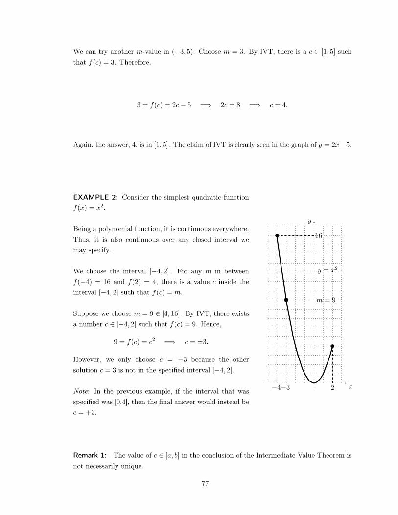
We can try another m-value in (�3, 5). Choose m = 3. By IVT, there is a c 2 [1, 5] suchthat f(c) = 3. Therefore,
3 = f(c) = 2c� 5 =) 2c = 8 =) c = 4.
Again, the answer, 4, is in [1, 5]. The claim of IVT is clearly seen in the graph of y = 2x�5.
EXAMPLE 2: Consider the simplest quadratic functionf(x) = x2.
Being a polynomial function, it is continuous everywhere.Thus, it is also continuous over any closed interval wemay specify.
We choose the interval [�4, 2]. For any m in betweenf(�4) = 16 and f(2) = 4, there is a value c inside theinterval [�4, 2] such that f(c) = m.
Suppose we choose m = 9 2 [4, 16]. By IVT, there existsa number c 2 [�4, 2] such that f(c) = 9. Hence,
9 = f(c) = c2 =) c = ±3.
However, we only choose c = �3 because the othersolution c = 3 is not in the specified interval [�4, 2].
Note: In the previous example, if the interval that wasspecified was [0,4], then the final answer would instead bec = +3.
x
y
y = x2
m = 9
�4�3
2
16
Remark 1: The value of c 2 [a, b] in the conclusion of the Intermediate Value Theorem isnot necessarily unique.
77
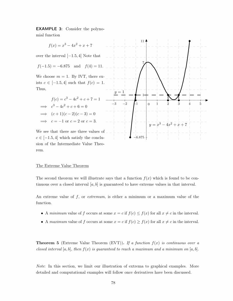
EXAMPLE 3: Consider the polyno-mial function
f(x) = x3 � 4x2 + x+ 7
over the interval [�1.5, 4] Note that
f(�1.5) = �6.875 and f(4) = 11.
We choose m = 1. By IVT, there ex-ists c 2 [�1.5, 4] such that f(c) = 1.
Thus,
f(c) = c3 � 4c2 + c+ 7 = 1
=) c3 � 4c2 + c+ 6 = 0
=) (c+ 1)(c� 2)(c� 3) = 0
=) c = �1 or c = 2 or c = 3.
We see that there are three values ofc 2 [�1.5, 4] which satisfy the conclu-sion of the Intermediate Value Theo-rem.
�3 �2 �1 1 2 3 4 5
�6.875
1
7
11
0
y = 1
y = x3 � 4x2 + x+ 7
The Extreme Value Theorem
The second theorem we will illustrate says that a function f(x) which is found to be con-tinuous over a closed interval [a, b] is guaranteed to have extreme values in that interval.
An extreme value of f , or extremum, is either a minimum or a maximum value of thefunction.
• A minimum value of f occurs at some x = c if f(c) f(x) for all x 6= c in the interval.
• A maximum value of f occurs at some x = c if f(c) � f(x) for all x 6= c in the interval.
Theorem 5 (Extreme Value Theorem (EVT)). If a function f(x) is continuous over aclosed interval [a, b], then f(x) is guaranteed to reach a maximum and a minimum on [a, b].
Note: In this section, we limit our illustration of extrema to graphical examples. Moredetailed and computational examples will follow once derivatives have been discussed.
78
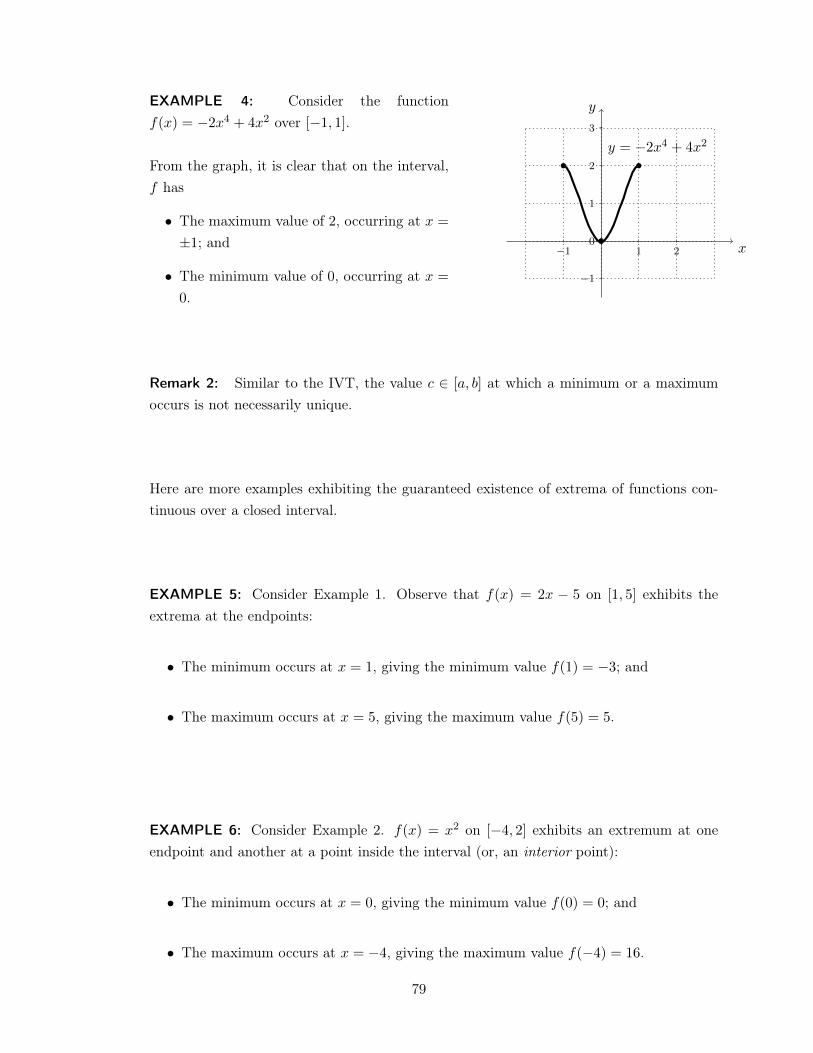
EXAMPLE 4: Consider the functionf(x) = �2x4 + 4x2 over [�1, 1].
From the graph, it is clear that on the interval,f has
• The maximum value of 2, occurring at x =
±1; and
• The minimum value of 0, occurring at x =
0.
�1 1 2
�1
0
1
2
3
x
y
y = �2x4 + 4x2
Remark 2: Similar to the IVT, the value c 2 [a, b] at which a minimum or a maximumoccurs is not necessarily unique.
Here are more examples exhibiting the guaranteed existence of extrema of functions con-tinuous over a closed interval.
EXAMPLE 5: Consider Example 1. Observe that f(x) = 2x � 5 on [1, 5] exhibits theextrema at the endpoints:
• The minimum occurs at x = 1, giving the minimum value f(1) = �3; and
• The maximum occurs at x = 5, giving the maximum value f(5) = 5.
EXAMPLE 6: Consider Example 2. f(x) = x2 on [�4, 2] exhibits an extremum at oneendpoint and another at a point inside the interval (or, an interior point):
• The minimum occurs at x = 0, giving the minimum value f(0) = 0; and
• The maximum occurs at x = �4, giving the maximum value f(�4) = 16.
79
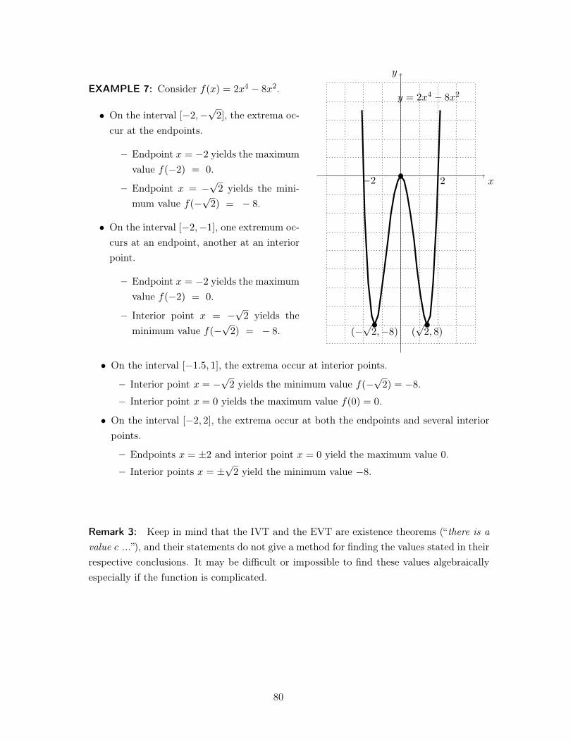
EXAMPLE 7: Consider f(x) = 2x4 � 8x2.
• On the interval [�2,�p2], the extrema oc-
cur at the endpoints.
– Endpoint x = �2 yields the maximumvalue f(�2) = 0.
– Endpoint x = �p2 yields the mini-
mum value f(�p2) = � 8.
• On the interval [�2,�1], one extremum oc-curs at an endpoint, another at an interiorpoint.
– Endpoint x = �2 yields the maximumvalue f(�2) = 0.
– Interior point x = �p2 yields the
minimum value f(�p2) = � 8.
x
y
y = 2x4 � 8x2
�2
2
(�p2,�8) (
p2, 8)
• On the interval [�1.5, 1], the extrema occur at interior points.
– Interior point x = �p2 yields the minimum value f(�
p2) = �8.
– Interior point x = 0 yields the maximum value f(0) = 0.
• On the interval [�2, 2], the extrema occur at both the endpoints and several interiorpoints.
– Endpoints x = ±2 and interior point x = 0 yield the maximum value 0.
– Interior points x = ±p2 yield the minimum value �8.
Remark 3: Keep in mind that the IVT and the EVT are existence theorems (“there is avalue c ...”), and their statements do not give a method for finding the values stated in theirrespective conclusions. It may be difficult or impossible to find these values algebraicallyespecially if the function is complicated.
80
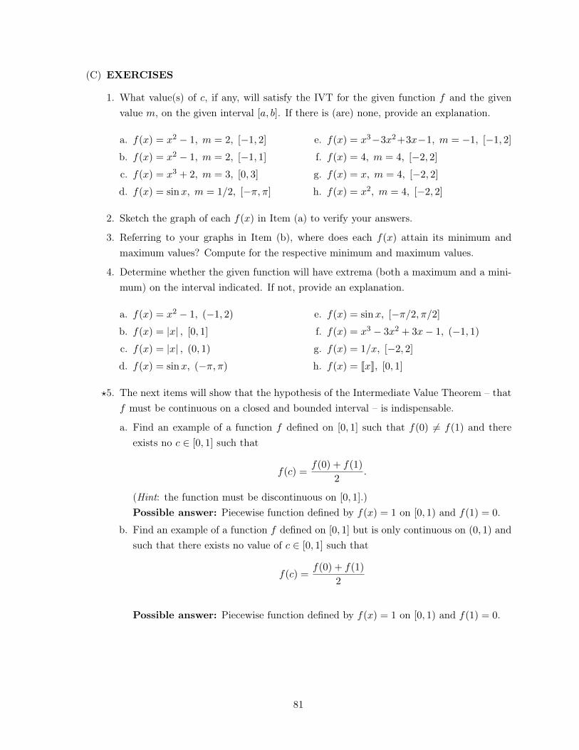
(C) EXERCISES
1. What value(s) of c, if any, will satisfy the IVT for the given function f and the givenvalue m, on the given interval [a, b]. If there is (are) none, provide an explanation.
a. f(x) = x2 � 1, m = 2, [�1, 2]
b. f(x) = x2 � 1, m = 2, [�1, 1]
c. f(x) = x3 + 2, m = 3, [0, 3]
d. f(x) = sinx, m = 1/2, [�⇡,⇡]
e. f(x) = x3�3x2+3x�1, m = �1, [�1, 2]
f. f(x) = 4, m = 4, [�2, 2]
g. f(x) = x, m = 4, [�2, 2]
h. f(x) = x2, m = 4, [�2, 2]
2. Sketch the graph of each f(x) in Item (a) to verify your answers.
3. Referring to your graphs in Item (b), where does each f(x) attain its minimum andmaximum values? Compute for the respective minimum and maximum values.
4. Determine whether the given function will have extrema (both a maximum and a mini-mum) on the interval indicated. If not, provide an explanation.
a. f(x) = x2 � 1, (�1, 2)
b. f(x) = |x| , [0, 1]c. f(x) = |x| , (0, 1)d. f(x) = sinx, (�⇡,⇡)
e. f(x) = sinx, [�⇡/2,⇡/2]
f. f(x) = x3 � 3x2 + 3x� 1, (�1, 1)
g. f(x) = 1/x, [�2, 2]
h. f(x) = [[x]], [0, 1]
?5. The next items will show that the hypothesis of the Intermediate Value Theorem – thatf must be continuous on a closed and bounded interval – is indispensable.
a. Find an example of a function f defined on [0, 1] such that f(0) 6= f(1) and thereexists no c 2 [0, 1] such that
f(c) =f(0) + f(1)
2
.
(Hint: the function must be discontinuous on [0, 1].)Possible answer: Piecewise function defined by f(x) = 1 on [0, 1) and f(1) = 0.
b. Find an example of a function f defined on [0, 1] but is only continuous on (0, 1) andsuch that there exists no value of c 2 [0, 1] such that
f(c) =f(0) + f(1)
2
Possible answer: Piecewise function defined by f(x) = 1 on [0, 1) and f(1) = 0.
81
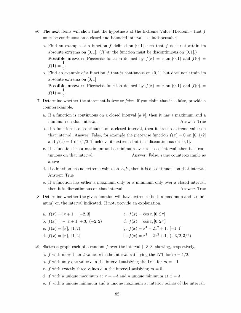
?6. The next items will show that the hypothesis of the Extreme Value Theorem – that f
must be continuous on a closed and bounded interval – is indispensable.
a. Find an example of a function f defined on [0, 1] such that f does not attain itsabsolute extrema on [0, 1]. (Hint: the function must be discontinuous on [0, 1].)Possible answer: Piecewise function defined by f(x) = x on (0, 1) and f(0) =
f(1) =1
2
.
b. Find an example of a function f that is continuous on (0, 1) but does not attain itsabsolute extrema on [0, 1]
Possible answer: Piecewise function defined by f(x) = x on (0, 1) and f(0) =
f(1) =1
2
.
7. Determine whether the statement is true or false. If you claim that it is false, provide acounterexample.
a. If a function is continuous on a closed interval [a, b], then it has a maximum and aminimum on that interval. Answer: True
b. If a function is discontinuous on a closed interval, then it has no extreme value onthat interval. Answer: False, for example the piecewise function f(x) = 0 on [0, 1/2]
and f(x) = 1 on (1/2, 1] achieve its extrema but it is discontinuous on [0, 1].
c. If a function has a maximum and a minimum over a closed interval, then it is con-tinuous on that interval. Answer: False, same counterexample asabove
d. If a function has no extreme values on [a, b], then it is discontinuous on that interval.Answer: True
e. If a function has either a maximum only or a minimum only over a closed interval,then it is discontinuous on that interval. Answer: True
8. Determine whether the given function will have extrema (both a maximum and a mini-mum) on the interval indicated. If not, provide an explanation.
a. f(x) = |x+ 1| , [�2, 3]
b. f(x) = � |x+ 1|+ 3, (�2, 2)
c. f(x) = [[x]], [1, 2)
d. f(x) = [[x]], [1, 2]
e. f(x) = cosx, [0, 2⇡]
f. f(x) = cosx, [0, 2⇡)
g. f(x) = x4 � 2x2 + 1, [�1, 1]
h. f(x) = x4 � 2x2 + 1, (�3/2, 3/2)
?9. Sketch a graph each of a random f over the interval [�3, 3] showing, respectively,
a. f with more than 2 values c in the interval satisfying the IVT for m = 1/2.
b. f with only one value c in the interval satisfying the IVT for m = �1.
c. f with exactly three values c in the interval satisfying m = 0.
d. f with a unique maximum at x = �3 and a unique minimum at x = 3.
e. f with a unique minimum and a unique maximum at interior points of the interval.
82
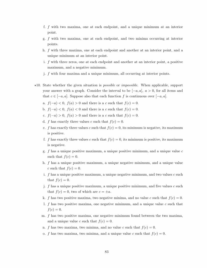
f. f with two maxima, one at each endpoint, and a unique minimum at an interiorpoint.
g. f with two maxima, one at each endpoint, and two minima occurring at interiorpoints.
h. f with three maxima, one at each endpoint and another at an interior point, and aunique minimum at an interior point.
i. f with three zeros, one at each endpoint and another at an interior point, a positivemaximum, and a negative minimum.
j. f with four maxima and a unique minimum, all occurring at interior points.
?10. State whether the given situation is possible or impossible. When applicable, supportyour answer with a graph. Consider the interval to be [�a, a], a > 0, for all items andthat c 2 [�a, a]. Suppose also that each function f is continuous over [�a, a].
a. f(�a) < 0, f(a) > 0 and there is a c such that f(c) = 0.
b. f(�a) < 0, f(a) < 0 and there is a c such that f(c) = 0.
c. f(�a) > 0, f(a) > 0 and there is a c such that f(c) = 0.
d. f has exactly three values c such that f(c) = 0.
e. f has exactly three values c such that f(c) = 0, its minimum is negative, its maximumis positive.
f. f has exactly three values c such that f(c) = 0, its minimum is positive, its maximumis negative.
g. f has a unique positive maximum, a unique positive minimum, and a unique value c
such that f(c) = 0.
h. f has a unique positive maximum, a unique negative minimum, and a unique valuec such that f(c) = 0.
i. f has a unique positive maximum, a unique negative minimum, and two values c suchthat f(c) = 0.
j. f has a unique positive maximum, a unique positive minimum, and five values c suchthat f(c) = 0, two of which are c = ±a.
k. f has two positive maxima, two negative minima, and no value c such that f(c) = 0.
l. f has two positive maxima, one negative minimum, and a unique value c such thatf(c) = 0.
m. f has two positive maxima, one negative minimum found between the two maxima,and a unique value c such that f(c) = 0.
n. f has two maxima, two minima, and no value c such that f(c) = 0.
o. f has two maxima, two minima, and a unique value c such that f(c) = 0.
83
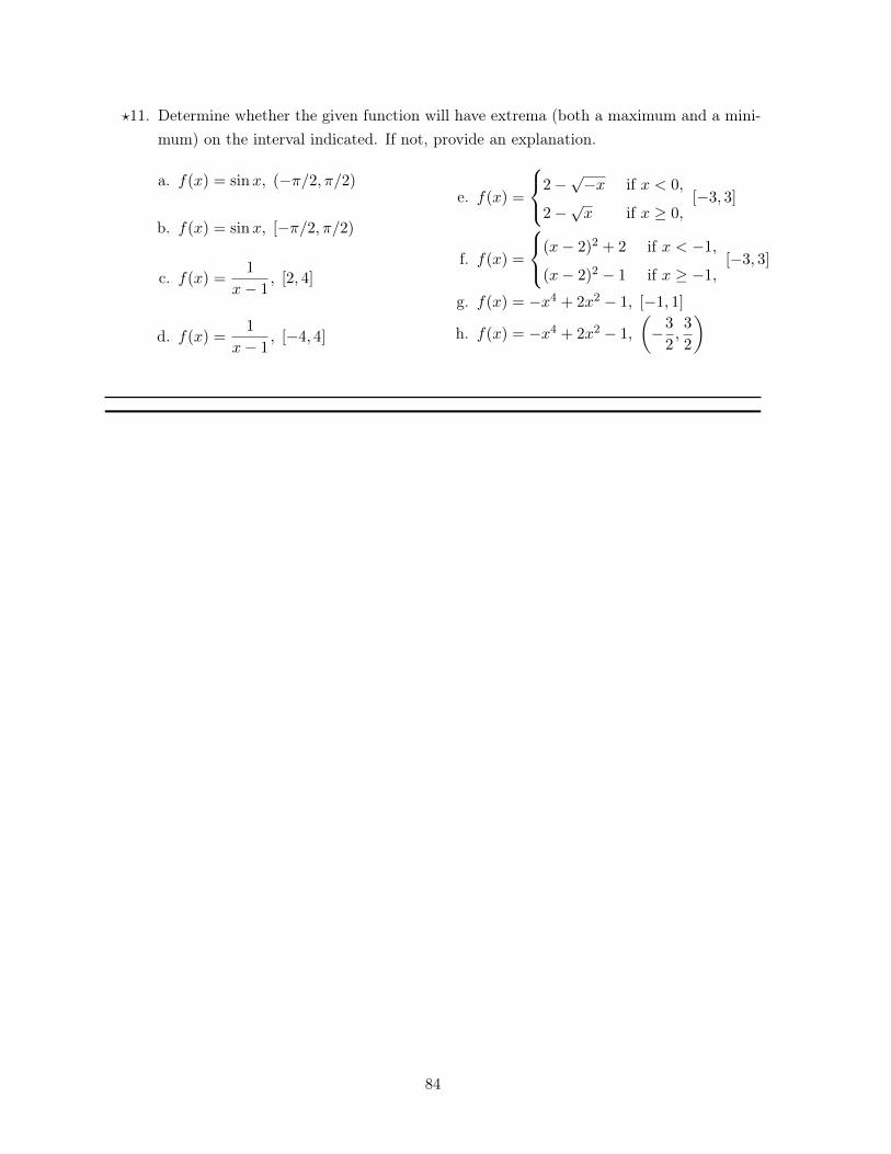
?11. Determine whether the given function will have extrema (both a maximum and a mini-mum) on the interval indicated. If not, provide an explanation.
a. f(x) = sinx, (�⇡/2,⇡/2)
b. f(x) = sinx, [�⇡/2,⇡/2)
c. f(x) =1
x� 1
, [2, 4]
d. f(x) =1
x� 1
, [�4, 4]
e. f(x) =
8<
:2�
p�x if x < 0,
2�px if x � 0,
[�3, 3]
f. f(x) =
8<
:(x� 2)
2
+ 2 if x < �1,
(x� 2)
2 � 1 if x � �1,[�3, 3]
g. f(x) = �x4 + 2x2 � 1, [�1, 1]
h. f(x) = �x4 + 2x2 � 1,
✓�3
2
,3
2
◆
84
TOPIC 4.3: Problems Involving Continuity
This is an OPTIONAL topic. It is intended for the enrichment of the students, toenhance their understanding of continuity and the properties it makes possible, suchas stated in the Intermediate Value Theorem.
DEVELOPMENT OF THE LESSON
(A) INTRODUCTION
Continuity is a very powerful property for a function to possess. Before we even moveon to its possibilities with respect to differentiation and integration, let us take a look atsome types of problems which may be solved if one has knowledge of the continuity of thefunction(s) involved.
(B) LESSON PROPER
For every problem that will be presented, we will provide a solution that makes use ofcontinuity and takes advantage of its consequences, such as the Intermediate Value Theorem(IVT).
APPROXIMATING ROOTS (Method of Bisection)
Finding the roots of polynomials is easy if they are special products and thus easy to fac-tor. Sometimes, with a little added effort, roots can be found through synthetic division.However, for most polynomials, roots, can at best, just be approximated.
Since polynomials are continuous everywhere, the IVT is applicable and very useful in ap-proximating roots which are otherwise difficult to find. In what follows, we will alwayschoose a closed interval [a, b] such that f(a) and f(b) differ in sign, meaning, f(a) > 0 andf(b) < 0, or f(a) < 0 and f(b) > 0.
In invoking the IVT, we take m = 0. This is clearly an intermediate value of f(a) and f(b)
since f(a) and f(b) differ in sign. The conclusion of the IVT now guarantees the existenceof c 2 [a, b] such that f(c) = 0. This is tantamount to looking for the roots of polynomialf(x).
EXAMPLE 1: Consider f(x) = x3 � x+ 1. Its roots cannot be found using factoring andsynthetic division. We apply the IVT.
85
• Choose any initial pair of numbers, say �3 and 3.
• Evaluate f at these values.
f(�3) = �23 < 0 and f(3) = 25 > 0.
Since f(�3) and f(3) differ in sign, a root must lie between �3 and 3.
• To approach the root, we trim the interval.
– Try [0, 3]. However, f(0) = 1 > 0 like f(3) so no conclusion can be made abouta root existing in [0, 3].
– Try [�3, 0]. In this case, f(0) and f(�3) differ in sign so we improve the searchspace for the root from [�3, 3] to [�3, 0].
• We trim further.
– f(�1) = 1 > 0 so the root is in [�3,�1].
– f(�2) = �5 < 0 so the root is in [�2,�1].
– f(�3
2
) = �7
8
< 0 so the root is in [�3
2
,�1].
– f(�5
4
) =
19
64
> 0 so the root is in [�3
2
,�5
4
].
• Further trimming and application of the IVT will yield the approximate root x =
�53
40
= �1.325. This gives f(x) ⇡ �0.0012.
The just-concluded procedure gave one root, a negative one. There are two more possiblereal roots.
FINDING INTERVALS FOR ROOTS
When finding an exact root of a polynomial, or even an approximate root, proves tootedious, some problem-solvers are content with finding a small interval containing thatroot
EXAMPLE 2: Consider again f(x) = x3 � x + 1. If we just need an interval of length 1,we can already stop at [�2,�1]. If we need an interval of length 1/2, we can already stopat [�3
2
,�1]. If we want an interval of length 1/4, we stop at [�3
2
,�5
4
].
EXAMPLE 3: Consider f(x) = x3 � x2 + 4. Find three distinct intervals of length 1, orless, containing a root of f(x).
When approximating, we may choose as sharp an estimate as we want. The same goes foran interval. While some problem-solvers will make do with an interval of length 1, somemay want a finer interval, say, of length 1/4. We should not forget that this type of searchis possible because we are dealing with polynomials, and the continuity of polynomialseverywhere allows us repeated use of the IVT.
86
SOME CONSEQUENCES OF THE IVT
Some interesting applications arise out of the logic used in the IVT.
EXAMPLE 4: We already know from our first lessons on polynomials that the degree of apolynomial is an indicator of the number of roots it has. Furthermore, did you know thata polynomial of odd degree has at least one real root?
Recall that a polynomial takes the form,
f(x) = a0
xn + a1
xn�1
+ ...+ an�1
x+ an
where a0
, a1
, ..., an are real numbers and n is an odd integer.
Take for example a0
= 1. So,
f(x) = xn + a1
xn�1
+ ...+ an�1
x+ an.
Imagine x taking bigger and bigger values, like ten thousand or a million. For such values,the first term will far outweigh the total of all the other terms. See, if x is positive, for big n
the value of f(x) will be positive. If x is negative, for big n the value of f(x) will be negative.
We now invoke the IVT. Remember, n is odd.
• Let a be a large-enough negative number. Then, f(a) < 0.
• Let b be a large-enough positive number. Then, f(b) > 0.
By the IVT, there is a number c 2 (a, b) such that f(c) = 0. In other words, f(x) doeshave a real root!
Teaching Tip
Ask the class why the claim may not hold for polynomials of even degree.
Answer: It is possible that the graphs of polynomials of even degree only stayabove the x-axis, or only below the x-axis. For example, the graph of f(x) = x2+1
stays only above the x-axis and therefore does not intersect x-axis, that is, f(x)has no roots.
87
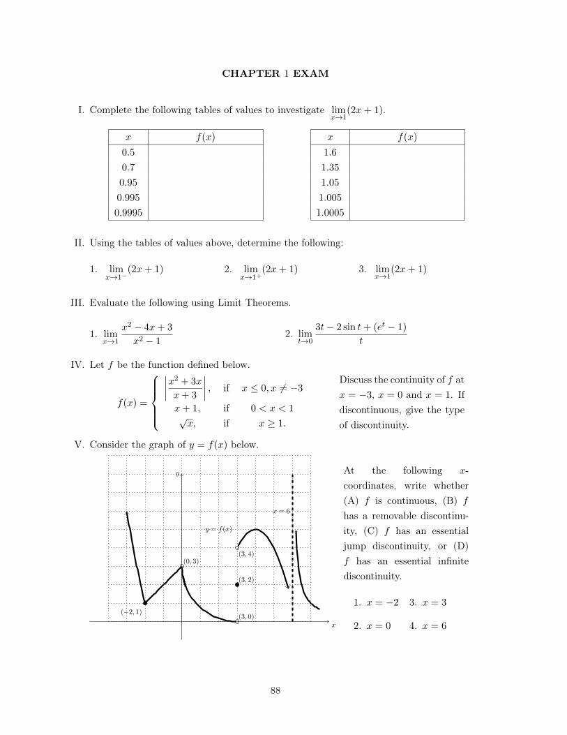
CHAPTER 1 EXAM
I. Complete the following tables of values to investigate lim
x!1
(2x+ 1).
x f(x)
0.5
0.7
0.95
0.995
0.9995
x f(x)
1.6
1.35
1.05
1.005
1.0005
II. Using the tables of values above, determine the following:
1. lim
x!1
�(2x+ 1) 2. lim
x!1
+(2x+ 1) 3. lim
x!1
(2x+ 1)
III. Evaluate the following using Limit Theorems.
1. lim
x!1
x2 � 4x+ 3
x2 � 1
2. lim
t!0
3t� 2 sin t+ (et � 1)
t
IV. Let f be the function defined below.
f(x) =
8>>><
>>>:
����x2 + 3x
x+ 3
���� , if x 0, x 6= �3
x+ 1, if 0 < x < 1
px, if x � 1.
Discuss the continuity of f atx = �3, x = 0 and x = 1. Ifdiscontinuous, give the typeof discontinuity.
V. Consider the graph of y = f(x) below.
x
y
y = f(x)
(�2, 1)
(0, 3)
(3, 0)
(3, 2)
(3, 4)
x = 6
At the following x-coordinates, write whether(A) f is continuous, (B) f
has a removable discontinu-ity, (C) f has an essentialjump discontinuity, or (D)f has an essential infinitediscontinuity.
1. x = �2
2. x = 0
3. x = 3
4. x = 6
88

Chapter 2
Derivatives
LESSON 5: The Derivative as the Slope of the Tangent Line
TIME FRAME: 4 hours
LEARNING OUTCOMES: At the end of the lesson, the learner shall be able to:
1. Illustrate the tangent line to the graph of a function at a given point;2. Apply the definition of the derivative of a function at a given number; and3. Relate the derivative of a function to the slope of the tangent line.
LESSON OUTLINE:
1. Tangent and secant lines to a circle2. Tangent line to the graph of an arbitrary function3. Cases where the tangent line does not exist4. The slope of the tangent line of an arbitrary function5. The equation of the tangent line6. The definition and evaluation of the derivative
90
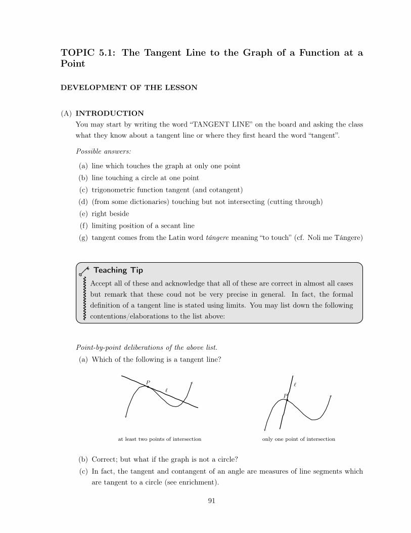
TOPIC 5.1: The Tangent Line to the Graph of a Function at aPoint
DEVELOPMENT OF THE LESSON
(A) INTRODUCTIONYou may start by writing the word “TANGENT LINE” on the board and asking the classwhat they know about a tangent line or where they first heard the word “tangent”.
Possible answers:
(a) line which touches the graph at only one point(b) line touching a circle at one point(c) trigonometric function tangent (and cotangent)(d) (from some dictionaries) touching but not intersecting (cutting through)(e) right beside(f) limiting position of a secant line(g) tangent comes from the Latin word tángere meaning “to touch” (cf. Noli me Tángere)
Teaching Tip
Accept all of these and acknowledge that all of these are correct in almost all casesbut remark that these coud not be very precise in general. In fact, the formaldefinition of a tangent line is stated using limits. You may list down the followingcontentions/elaborations to the list above:
Point-by-point deliberations of the above list.(a) Which of the following is a tangent line?
P
`
at least two points of intersection
P
`
only one point of intersection
(b) Correct; but what if the graph is not a circle?(c) In fact, the tangent and contangent of an angle are measures of line segments which
are tangent to a circle (see enrichment).
91
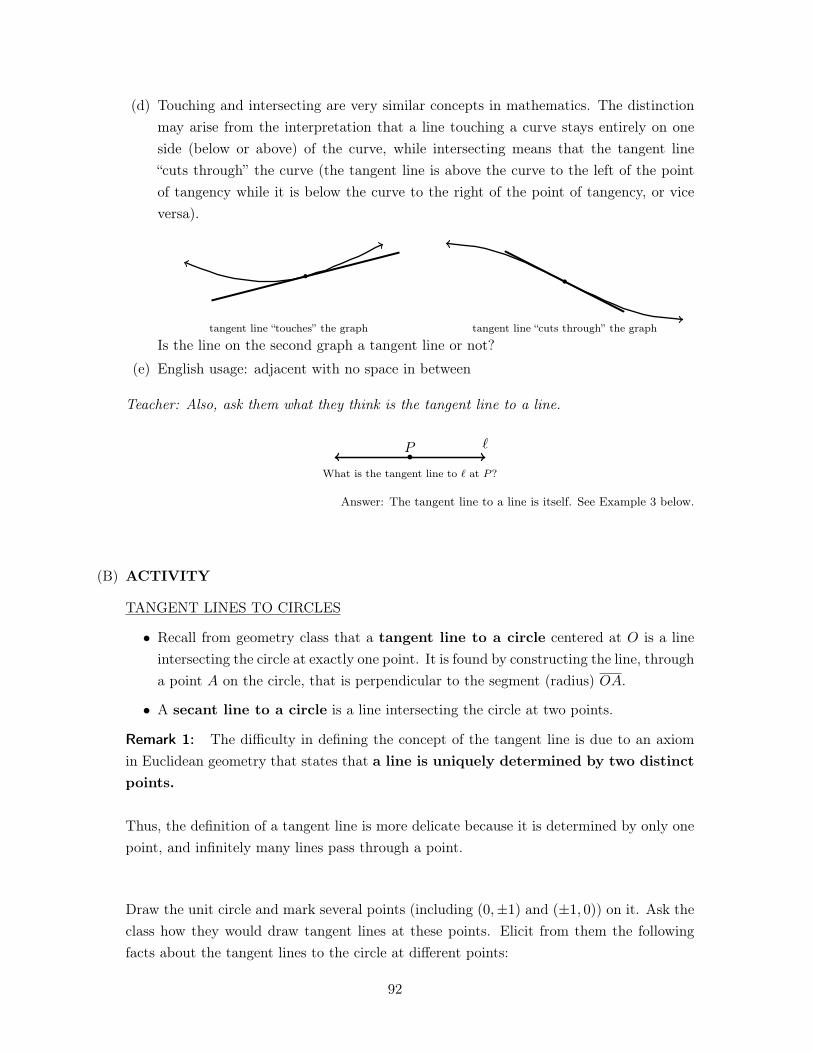
(d) Touching and intersecting are very similar concepts in mathematics. The distinctionmay arise from the interpretation that a line touching a curve stays entirely on oneside (below or above) of the curve, while intersecting means that the tangent line“cuts through” the curve (the tangent line is above the curve to the left of the pointof tangency while it is below the curve to the right of the point of tangency, or viceversa).
tangent line “touches” the graph tangent line “cuts through” the graph
Is the line on the second graph a tangent line or not?(e) English usage: adjacent with no space in between
Teacher: Also, ask them what they think is the tangent line to a line.
P `
What is the tangent line to ` at P?
Answer: The tangent line to a line is itself. See Example 3 below.
(B) ACTIVITY
TANGENT LINES TO CIRCLES
• Recall from geometry class that a tangent line to a circle centered at O is a lineintersecting the circle at exactly one point. It is found by constructing the line, througha point A on the circle, that is perpendicular to the segment (radius) OA.
• A secant line to a circle is a line intersecting the circle at two points.
Remark 1: The difficulty in defining the concept of the tangent line is due to an axiomin Euclidean geometry that states that a line is uniquely determined by two distinctpoints.
Thus, the definition of a tangent line is more delicate because it is determined by only onepoint, and infinitely many lines pass through a point.
Draw the unit circle and mark several points (including (0,±1) and (±1, 0)) on it. Ask theclass how they would draw tangent lines at these points. Elicit from them the followingfacts about the tangent lines to the circle at different points:
92
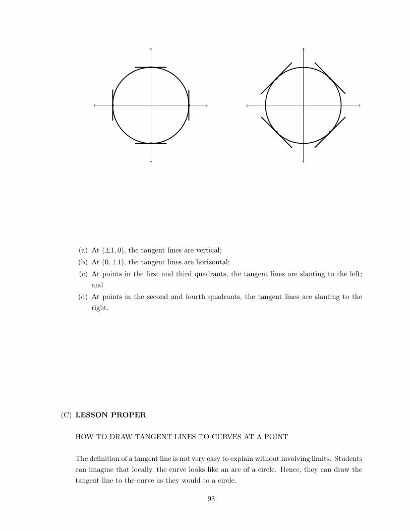
(a) At (±1, 0), the tangent lines are vertical;(b) At (0,±1), the tangent lines are horizontal;(c) At points in the first and third quadrants, the tangent lines are slanting to the left;
and(d) At points in the second and fourth quadrants, the tangent lines are slanting to the
right.
(C) LESSON PROPER
HOW TO DRAW TANGENT LINES TO CURVES AT A POINT
The definition of a tangent line is not very easy to explain without involving limits. Studentscan imagine that locally, the curve looks like an arc of a circle. Hence, they can draw thetangent line to the curve as they would to a circle.
93
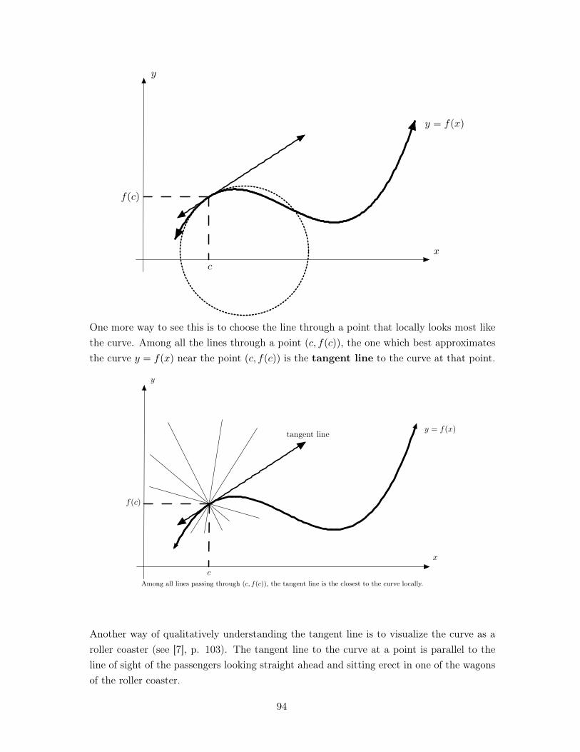
x
y
y = f(x)
c
f(c)
One more way to see this is to choose the line through a point that locally looks most likethe curve. Among all the lines through a point (c, f(c)), the one which best approximatesthe curve y = f(x) near the point (c, f(c)) is the tangent line to the curve at that point.
x
y
y = f(x)tangent line
c
f(c)
Among all lines passing through (c, f(c)), the tangent line is the closest to the curve locally.
Another way of qualitatively understanding the tangent line is to visualize the curve as aroller coaster (see [7], p. 103). The tangent line to the curve at a point is parallel to theline of sight of the passengers looking straight ahead and sitting erect in one of the wagonsof the roller coaster.
94
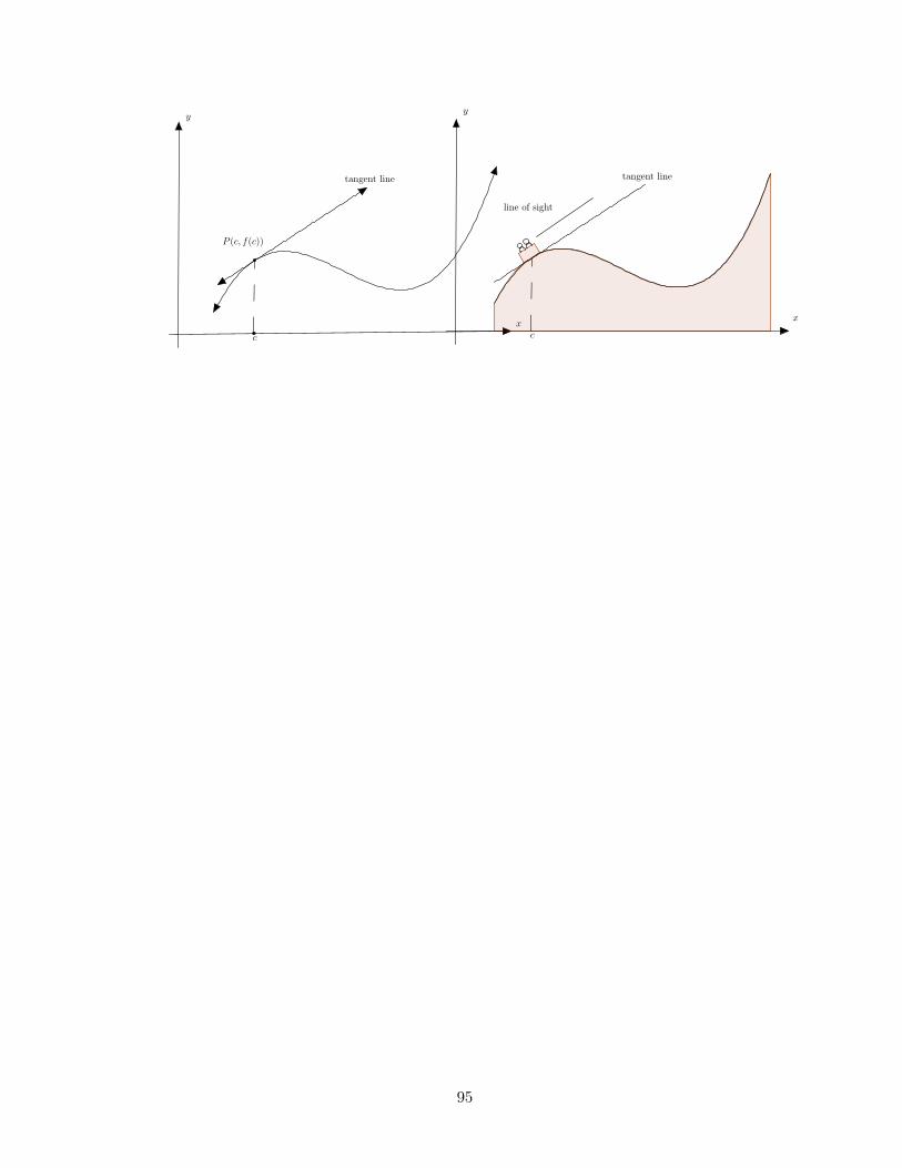
P (c, f(c))
x
y
tangent line
c
x
y
line of sight
tangent line
c
95
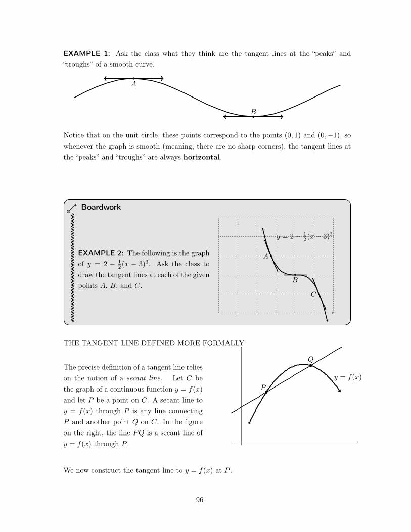
EXAMPLE 1: Ask the class what they think are the tangent lines at the “peaks” and“troughs” of a smooth curve.
A
B
Notice that on the unit circle, these points correspond to the points (0, 1) and (0,�1), sowhenever the graph is smooth (meaning, there are no sharp corners), the tangent lines atthe “peaks” and “troughs” are always horizontal.
Boardwork
EXAMPLE 2: The following is the graphof y = 2 � 1
2
(x � 3)
3. Ask the class todraw the tangent lines at each of the givenpoints A, B, and C.
y = 2� 1
2
(x� 3)
3
A
B
C
THE TANGENT LINE DEFINED MORE FORMALLY
The precise definition of a tangent line relieson the notion of a secant line. Let C bethe graph of a continuous function y = f(x)
and let P be a point on C. A secant line toy = f(x) through P is any line connectingP and another point Q on C. In the figureon the right, the line PQ is a secant line ofy = f(x) through P .
y = f(x)
P
Q
We now construct the tangent line to y = f(x) at P .
96
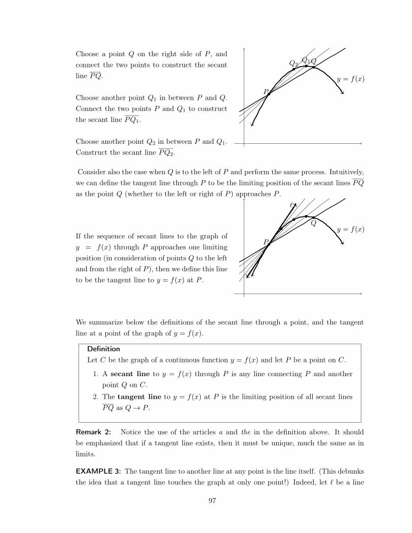
Choose a point Q on the right side of P , andconnect the two points to construct the secantline PQ.
Choose another point Q1
in between P and Q.Connect the two points P and Q
1
to constructthe secant line PQ
1
.
Choose another point Q2
in between P and Q1
.Construct the secant line PQ
2
.
y = f(x)
P
QQ1Q
2
Consider also the case when Q is to the left of P and perform the same process. Intuitively,we can define the tangent line through P to be the limiting position of the secant lines PQ
as the point Q (whether to the left or right of P ) approaches P .
If the sequence of secant lines to the graph ofy = f(x) through P approaches one limitingposition (in consideration of points Q to the leftand from the right of P ), then we define this lineto be the tangent line to y = f(x) at P .
y = f(x)
P
Q
`
We summarize below the definitions of the secant line through a point, and the tangentline at a point of the graph of y = f(x).
DefinitionLet C be the graph of a continuous function y = f(x) and let P be a point on C.
1. A secant line to y = f(x) through P is any line connecting P and anotherpoint Q on C.
2. The tangent line to y = f(x) at P is the limiting position of all secant linesPQ as Q ! P .
Remark 2: Notice the use of the articles a and the in the definition above. It shouldbe emphasized that if a tangent line exists, then it must be unique, much the same as inlimits.
EXAMPLE 3: The tangent line to another line at any point is the line itself. (This debunksthe idea that a tangent line touches the graph at only one point!) Indeed, let ` be a line
97
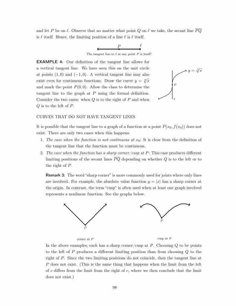
and let P be on `. Observe that no matter what point Q on ` we take, the secant line PQ
is ` itself. Hence, the limiting position of a line ` is ` itself.
P `
The tangent line to ` at any point P is itself!
EXAMPLE 4: Our definition of the tangent line allows fora vertical tangent line. We have seen this on the unit circleat points (1, 0) and (�1, 0). A vertical tangent line may alsoexist even for continuous functions. Draw the curve y =
3px
and mark the point P (0, 0). Allow the class to determine thetangent line to the graph at P using the formal definition.Consider the two cases: when Q is to the right of P and whenQ is to the left of P .
P
`
y =
3px
CURVES THAT DO NOT HAVE TANGENT LINES
It is possible that the tangent line to a graph of a function at a point P (x0
, f(x0
)) does notexist. There are only two cases when this happens:
1. The case when the function is not continuous at x0
: It is clear from the definition ofthe tangent line that the function must be continuous.
2. The case when the function has a sharp corner/cusp at P : This case produces differentlimiting positions of the secant lines PQ depending on whether Q is to the left or tothe right of P .
Remark 3: The word “sharp corner” is more commonly used for joints where only linesare involved. For example, the absolute value function y = |x| has a sharp corner atthe origin. In contrast, the term “cusp” is often used when at least one graph involvedrepresents a nonlinear function. See the graphs below.
P
corner at P
P
cusp at P
In the above examples, each has a sharp corner/cusp at P . Choosing Q to be pointsto the left of P produces a different limiting position than from choosing Q to theright of P . Since the two limiting positions do not coincide, then the tangent line atP does not exist. (This is the same thing that happens when the limit from the leftof c differs from the limit from the right of c, where we then conclude that the limitdoes not exist.)
98
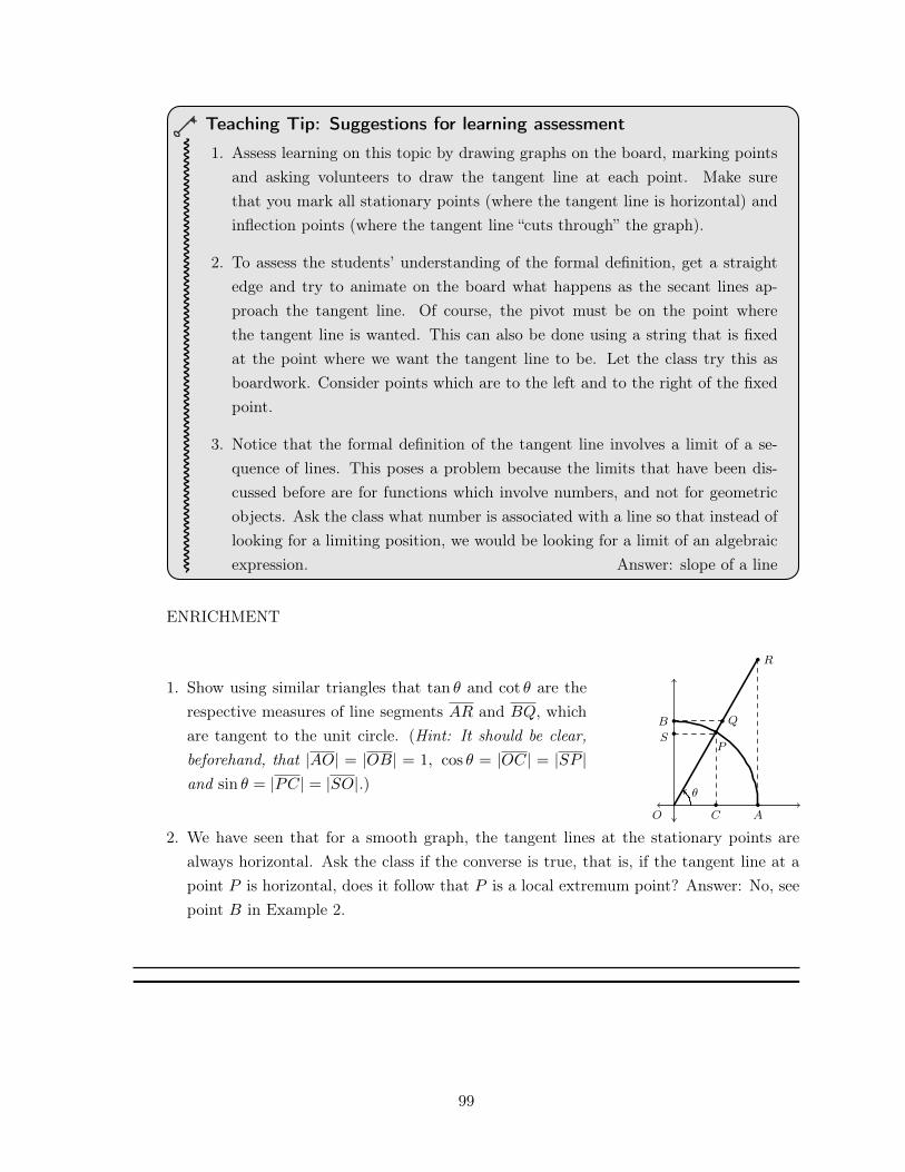
Teaching Tip: Suggestions for learning assessment
1. Assess learning on this topic by drawing graphs on the board, marking pointsand asking volunteers to draw the tangent line at each point. Make surethat you mark all stationary points (where the tangent line is horizontal) andinflection points (where the tangent line “cuts through” the graph).
2. To assess the students’ understanding of the formal definition, get a straightedge and try to animate on the board what happens as the secant lines ap-proach the tangent line. Of course, the pivot must be on the point wherethe tangent line is wanted. This can also be done using a string that is fixedat the point where we want the tangent line to be. Let the class try this asboardwork. Consider points which are to the left and to the right of the fixedpoint.
3. Notice that the formal definition of the tangent line involves a limit of a se-quence of lines. This poses a problem because the limits that have been dis-cussed before are for functions which involve numbers, and not for geometricobjects. Ask the class what number is associated with a line so that instead oflooking for a limiting position, we would be looking for a limit of an algebraicexpression. Answer: slope of a line
ENRICHMENT
1. Show using similar triangles that tan ✓ and cot ✓ are therespective measures of line segments AR and BQ, whichare tangent to the unit circle. (Hint: It should be clear,beforehand, that |AO| = |OB| = 1, cos ✓ = |OC| = |SP |and sin ✓ = |PC| = |SO|.)
O
P
R
A
B Q
S
C
✓
2. We have seen that for a smooth graph, the tangent lines at the stationary points arealways horizontal. Ask the class if the converse is true, that is, if the tangent line at apoint P is horizontal, does it follow that P is a local extremum point? Answer: No, seepoint B in Example 2.
99
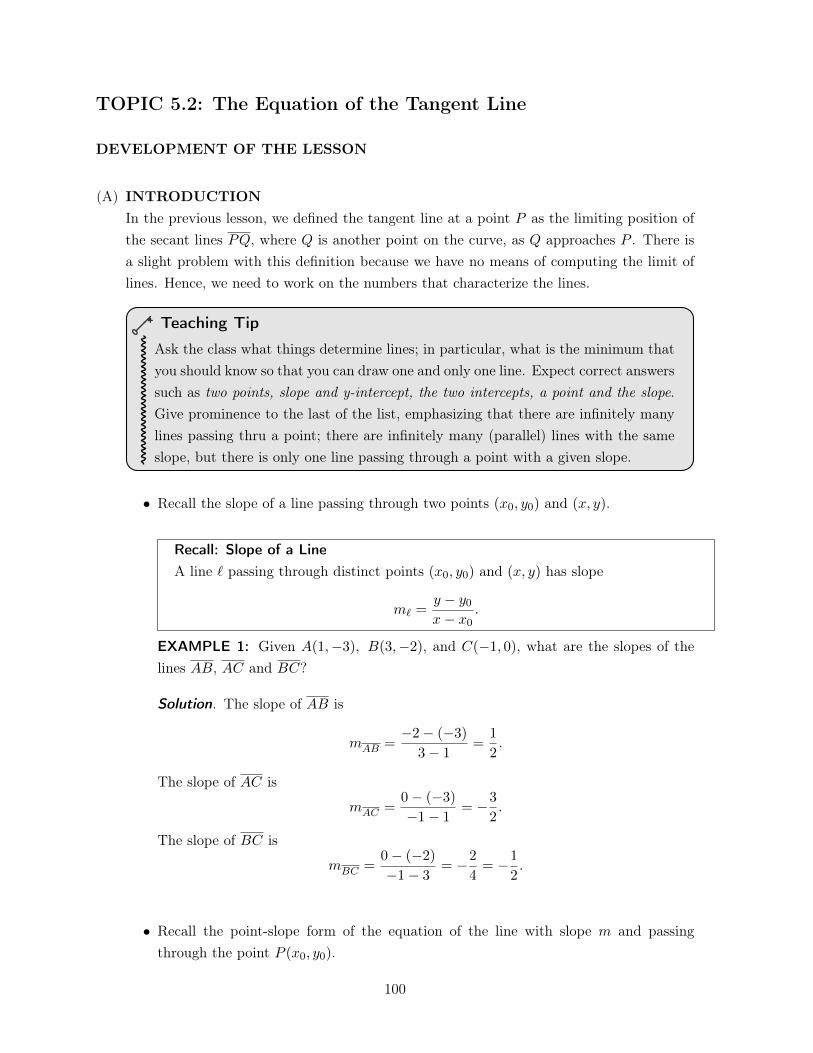
TOPIC 5.2: The Equation of the Tangent Line
DEVELOPMENT OF THE LESSON
(A) INTRODUCTIONIn the previous lesson, we defined the tangent line at a point P as the limiting position ofthe secant lines PQ, where Q is another point on the curve, as Q approaches P . There isa slight problem with this definition because we have no means of computing the limit oflines. Hence, we need to work on the numbers that characterize the lines.
Teaching Tip
Ask the class what things determine lines; in particular, what is the minimum thatyou should know so that you can draw one and only one line. Expect correct answerssuch as two points, slope and y-intercept, the two intercepts, a point and the slope.Give prominence to the last of the list, emphasizing that there are infinitely manylines passing thru a point; there are infinitely many (parallel) lines with the sameslope, but there is only one line passing through a point with a given slope.
• Recall the slope of a line passing through two points (x0
, y0
) and (x, y).
Recall: Slope of a LineA line ` passing through distinct points (x
0
, y0
) and (x, y) has slope
m` =y � y
0
x� x0
.
EXAMPLE 1: Given A(1,�3), B(3,�2), and C(�1, 0), what are the slopes of thelines AB, AC and BC?
Solution. The slope of AB is
mAB =
�2� (�3)
3� 1
=
1
2
.
The slope of AC is
mAC =
0� (�3)
�1� 1
= �3
2
.
The slope of BC is
mBC =
0� (�2)
�1� 3
= �2
4
= �1
2
.
.
• Recall the point-slope form of the equation of the line with slope m and passingthrough the point P (x
0
, y0
).
100
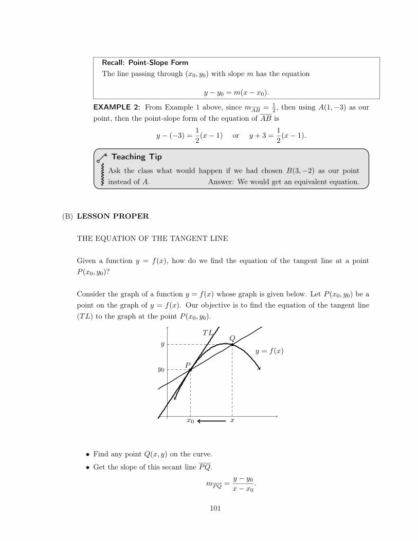
Recall: Point-Slope FormThe line passing through (x
0
, y0
) with slope m has the equation
y � y0
= m(x� x0
).
EXAMPLE 2: From Example 1 above, since mAB =
1
2
, then using A(1,�3) as ourpoint, then the point-slope form of the equation of AB is
y � (�3) =
1
2
(x� 1) or y + 3 =
1
2
(x� 1).
Teaching Tip
Ask the class what would happen if we had chosen B(3,�2) as our pointinstead of A. Answer: We would get an equivalent equation.
(B) LESSON PROPER
THE EQUATION OF THE TANGENT LINE
Given a function y = f(x), how do we find the equation of the tangent line at a pointP (x
0
, y0
)?
Consider the graph of a function y = f(x) whose graph is given below. Let P (x0
, y0
) be apoint on the graph of y = f(x). Our objective is to find the equation of the tangent line(TL) to the graph at the point P (x
0
, y0
).
y = f(x)
Py0
Q
x
y
TL
x0
• Find any point Q(x, y) on the curve.
• Get the slope of this secant line PQ.
mPQ =
y � y0
x� x0
.
101
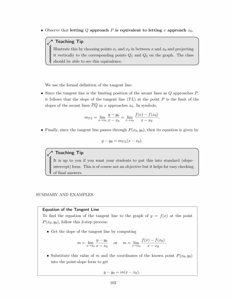
• Observe that letting Q approach P is equivalent to letting x approach x0
.
Teaching Tip
Illustrate this by choosing points x1
and x2
in between x and x0
and projectingit vertically to the corresponding points Q
1
and Q2
on the graph. The classshould be able to see this equivalence.
We use the formal definition of the tangent line:
• Since the tangent line is the limiting position of the secant lines as Q approaches P ,it follows that the slope of the tangent line (TL) at the point P is the limit of theslopes of the secant lines PQ as x approaches x
0
. In symbols,
mTL = lim
x!x0
y � y0
x� x0
= lim
x!x0
f(x)� f(x0
)
x� x0
.
• Finally, since the tangent line passes through P (x0
, y0
), then its equation is given by
y � y0
= mTL(x� x0
).
Teaching Tip
It is up to you if you want your students to put this into standard (slope-intercept) form. This is of course not an objective but it helps for easy checkingof final answers.
SUMMARY AND EXAMPLES
Equation of the Tangent LineTo find the equation of the tangent line to the graph of y = f(x) at the pointP (x
0
, y0
), follow this 2-step process:
• Get the slope of the tangent line by computing
m = lim
x!x0
y � y0
x� x0
or m = lim
x!x0
f(x)� f(x0
)
x� x0
.
• Substitute this value of m and the coordinates of the known point P (x0
, y0
)
into the point-slope form to get
y � y0
= m(x� x0
).
102
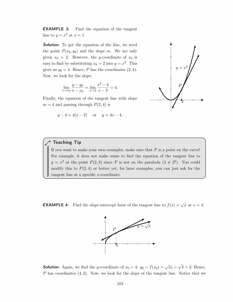
EXAMPLE 3: Find the equation of the tangentline to y = x2 at x = 1.
Solution. To get the equation of the line, we needthe point P (x
0
, y0
) and the slope m. We are onlygiven x
0
= 2. However, the y-coordinate of x0
iseasy to find by substituting x
0
= 2 into y = x2. Thisgives us y
0
= 4. Hence, P has the coordinates (2, 4).Now, we look for the slope:
lim
x!x0
y � y0
x� x0
= lim
x!2
x2 � 4
x� 2
= 4.
Finally, the equation of the tangent line with slopem = 4 and passing through P (2, 4) is
y � 4 = 4(x� 2) or y = 4x� 4.
.
2
P
y = x2
Teaching Tip
If you want to make your own examples, make sure that P is a point on the curve!For example, it does not make sense to find the equation of the tangent line toy = x2 at the point P (2, 3) since P is not on the parabola (3 6= 2
2). You couldmodify this to P (2, 4) or better yet, for later examples, you can just ask for thetangent line at a specific x-coordinate.
EXAMPLE 4: Find the slope-intercept form of the tangent line to f(x) =px at x = 4.
4
Py =
px
Solution. Again, we find the y-coordinate of x0
= 4: y0
= f(x0
) =
px0
=
p4 = 2. Hence,
P has coordinates (4, 2). Now, we look for the slope of the tangent line. Notice that we
103
have to rationalize the numerator to evaluate the limit.
m = lim
x!x0
f(x)� f(x0
)
x� x0
= lim
x!4
px� 2
x� 4
·px+ 2px+ 2
= lim
x!4
x� 4
(x� 4)(
px+ 2)
= lim
x!4
1px+ 2
=
1
4
.
Finally, with point P (4, 2) and slope m =
1
4
, the equation of the tangent line is
y � 2 =
1
4
(x� 4) or y =
x
4
+ 1.
.
The next example shows that our process of finding the tangent line works even for hori-zontal lines.
EXAMPLE 5: Show that the tangent line to y = 3x2 � 12x + 1 at the point (2,�11) ishorizontal.
Solution. Recall that a horizontal line has zero slope. Now, computing for the slope, weget:
m = lim
x!x0
y � y0
x� x0
= lim
x!2
(3x2 � 12x+ 1)� (�11)
x� 2
= lim
x!2
3(x2 � 4x+ 4)
x� 2
= lim
x!2
(3(x� 2)) = 0.
Since the slope of the tangent line is 0, it must be horizontal. Its equation is
y � (�11) = 0(x� 2) or y = �11.
.
EXAMPLE 6: Verify that the tangent line to the line y = 2x + 3 at (1, 5) is the lineitself.
Solution. We first compute for the slope of the tangent line. Note that x0
= 1 and y0
= 5.
m = lim
x!x0
y � y0
x� x0
= lim
x!1
(2x+ 3)� 5
x� 1
= lim
x!1
2x� 2
x� 1
= 2.
Therefore, substituting this into the point-slope form with P (1, 5) and m = 2, we get
y � 5 = 2(x� 1) i.e., y = 2x+ 3.
This is the same equation as that of the given line. .
104
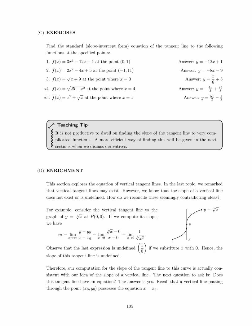
(C) EXERCISES
Find the standard (slope-intercept form) equation of the tangent line to the followingfunctions at the specified points:
1. f(x) = 3x2 � 12x+ 1 at the point (0, 1) Answer: y = �12x+ 1
2. f(x) = 2x2 � 4x+ 5 at the point (�1, 11) Answer: y = �8x� 9
3. f(x) =px+ 9 at the point where x = 0 Answer: y =
x
6
+ 3
?4. f(x) =p25� x2 at the point where x = 4 Answer: y = �4x
3
+
25
3
?5. f(x) = x2 +px at the point where x = 1 Answer: y =
5x2
� 1
2
Teaching Tip
It is not productive to dwell on finding the slope of the tangent line to very com-plicated functions. A more efficient way of finding this will be given in the nextsections when we discuss derivatives.
(D) ENRICHMENT
This section explores the equation of vertical tangent lines. In the last topic, we remarkedthat vertical tangent lines may exist. However, we know that the slope of a vertical linedoes not exist or is undefined. How do we reconcile these seemingly contradicting ideas?
For example, consider the vertical tangent line to thegraph of y =
3px at P (0, 0). If we compute its slope,
we have
m = lim
x!x0
y � y0
x� x0
= lim
x!0
3px� 0
x� 0
= lim
x!0
1
3px2
.
P
`
y =
3px
Observe that the last expression is undefined✓1
0
◆if we substitute x with 0. Hence, the
slope of this tangent line is undefined.
Therefore, our computation for the slope of the tangent line to this curve is actually con-sistent with our idea of the slope of a vertical line. The next question to ask is: Doesthis tangent line have an equation? The answer is yes. Recall that a vertical line passingthrough the point (x
0
, y0
) possesses the equation x = x0
.
105
Equation of Vertical Tangent LinesLet f be a function that is continuous at x
0
. Assuming that the tangent line to thegraph of y = f(x) at the point P (x
0
, y0
) is vertical, then its equation is
x = x0
.
106
TOPIC 5.3: The Definition of the Derivative
DEVELOPMENT OF THE LESSON
(A) INTRODUCTION
The expression
lim
x!x0
f(x)� f(x0
)
x� x0
computes more than just the slope of the tangent line. The fraction in the limit alsogives us the relative change of the function on the time or space interval [x
0
, x]. Thus,we may interpret this limit as the instantaneous rate of change of f with respect to x.(See Enrichment) It is therefore fitting to make an abstraction out of this. Afterwards, wecan regard this as a tool that can be used in finding the slope of the tangent line, or infinding the instantaneous rate of change. In what follows, we define this expression as thederivative of f(x) at x
0
.
(B) LESSON PROPER
We present the formal definition of the derivative.
Definition of the DerivativeLet f be a function defined on an open interval I ✓ R, and let x
0
2 I. The derivativeof f at x
0
is defined to be
f 0(x
0
) = lim
x!x0
f(x)� f(x0
)
x� x0
if this limit exists. That is, the derivative of f at x0
is the slope of the tangent lineat (x
0
, f(x0
)), if it exists.
Notations: If y = f(x), the derivative of f is commonly denoted by
f 0(x), Dx[f(x)],
d
dx[f(x)],
d
dx[y],
dy
dx.
Remark 1: Note that the limit definition of the derivative is inherently indeterminate!Hence, the usual techniques for evaluating limits which are indeterminate of type
0
0
areapplied, e.g., factoring, rationalization, or using one of the following establishedlimits:
(i) lim
x!0
sinx
x= 1
(ii) lim
x!0
1� cosx
x= 0 (iii) lim
x!0
ex � 1
x= 1.
107
EXAMPLE 1: Compute f 0(1) for each of the following functions:
1. f(x) = 3x� 1
2. f(x) = 2x2 + 4
3. f(x) =2x
x+ 1
4. f(x) =px+ 8
Solution. Here, x0
is fixed to be equal to 1. Using the definition above,
f 0(1) = lim
x!1
f(x)� f(1)
x� 1
.
Remember that what we are computing, f 0(1), is just the slope of the tangent line to
y = f(x) at x = 1.
1. Note that f(1) = 2, so by factoring
f 0(1) = lim
x!1
(3x� 1)� 2
x� 1
= lim
x!1
3(x� 1)
x� 1
= lim
x!1
3
= 3.
2. Here, f(1) = 6 so again, by factoring,
f 0(1) = lim
x!1
(2x2 + 4)� 6
x� 1
= lim
x!1
2(x+ 1)(x� 1)
x� 1
= lim
x!1
2(x+ 1)
= 4.
3. We see that f(1) = 1. So, from the definition,
f 0(1) = lim
x!1
2xx+1
� 1
x� 1
.
We multiply both the numerator and the denominator by x+1 to simplify the complexfraction:
f 0(1) = lim
x!1
2xx+1
� 1
x� 1
· x+ 1
x+ 1
= lim
x!1
2x� (x+ 1)
(x� 1)(x+ 1)
= lim
x!1
x� 1
(x� 1)(x+ 1)
= lim
x!1
1
x+ 1
=
1
2
.
108
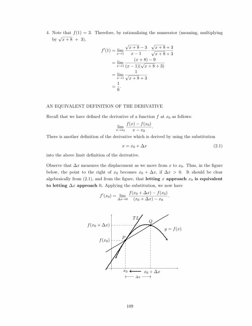
4. Note that f(1) = 3. Therefore, by rationalizing the numerator (meaning, multiplyingby
px+ 8 + 3),
f 0(1) = lim
x!1
px+ 8� 3
x� 1
·px+ 8 + 3px+ 8 + 3
= lim
x!1
(x+ 8)� 9
(x� 1)(
px+ 8 + 3)
= lim
x!1
1px+ 8 + 3
=
1
6
.
.
AN EQUIVALENT DEFINITION OF THE DERIVATIVE
Recall that we have defined the derivative of a function f at x0
as follows:
lim
x!x0
f(x)� f(x0
)
x� x0
.
There is another definition of the derivative which is derived by using the substitution
x = x0
+�x (2.1)
into the above limit definition of the derivative.
Observe that �x measures the displacement as we move from x to x0
. Thus, in the figurebelow, the point to the right of x
0
becomes x0
+ �x, if �x > 0. It should be clearalgebraically from (2.1), and from the figure, that letting x approach x
0
is equivalentto letting �x approach 0. Applying the substitution, we now have
f 0(x
0
) = lim
�x!0
f(x0
+�x)� f(x0
)
(x0
+�x)� x0
.
y = f(x)
Pf(x
0
)
Q
x0
+�x
f(x0
+�x)
TL
x0
�x
109
We present this fact formally below:
Alternative Definition of the DerivativeLet f be a function defined on an open interval I ✓ R, and let x 2 I. The derivativeof f at x is defined to be
f 0(x) = lim
�x!0
f(x+�x)� f(x)
�x(2.2)
if this limit exists.
Teaching Tip
Confusion may arise when students think of �x as �⇥ x or � as an operator thataffects x. Here, �x should be treated like any other variable. This is why manytextbooks use h instead of �x. In this case, equation (2.2) becomes
f 0(x) = lim
h!0
f(x+ h)� f(x)
h.
Usually, this is the definition used to obtain the general expression of the derivativeof a function at any point x 2 I.
Remark 2: Please remind the students that f(x0
+ h) is basically a composition of twofunctions. Therefore, it is determined by replacing all instances of x in the definition of fby x
0
+ h. For example, if
f(x) = x2 + 3x and g(x) = cos(3x)� ex,
then
f(x0
+ h) = (x0
+ h)2 + 3(x0
+ h) and g(x0
+ h) = cos(3(x0
+ h))� ex0+h.
EXAMPLE 2: Let f(x) = sinx, g(x) = cosx, and s(x) = ex. Find f 0(2⇡), g0(⇡), and
s0(3).
Solution. We use the alternative definition of the derivative.
(a) Here, we substitute x0
= 2⇡.
f 0(2⇡) = lim
h!0
f(2⇡ + h)� f(2⇡)
h
= lim
h!0
sin(2⇡ + h)� 0
h.
110
Using the sum identity of the sine function: sin(↵+ �) = sin↵ cos� + cos↵ sin�, andnoting that sin(2⇡) = 0 and cos(2⇡) = 1, we get
f 0(2⇡) = lim
h!0
sin(2⇡) cosh+ cos(2⇡) sinh
h
= lim
h!0
sinh
h
= 1. (Why?)
(b)
g0(⇡) = lim
h!0
g(⇡ + h)� g(⇡)
h
= lim
h!0
cos(⇡ + h)� (�1)
h.
Using the sum identity of the cosine function: cos(↵ + �) = cos↵ cos� � sin↵ sin�,
and noting that cos⇡ = �1 and sin⇡ = 0, we get
g0(⇡) = lim
h!0
cos⇡ cosh� sin⇡ sinh+ 1
h
= lim
h!0
� cosh+ 1
h
= 0. (Why?)
(c)
s0(3) = lim
h!0
s(3 + h)� s(3)
h
= lim
h!0
e3+h � e3
h.
Using the exponent laws, e3+h= e3eh. Moreover, since e3 is just a constant, we can
factor it out of the limit operator. So,
s0(3) = lim
h!0
e3eh � e3
h
= e3 limh!0
eh � 1
h
= e3. (Why?)
.
111
Seatwork: Let f(x) = 2x2 + 3x� 1. Use the definition of the derivative to find f 0(�1).
Solution. Note that f(�1) = �2. Thus,
f 0(�1) = lim
x!�1
f(x)� f(�1)
x� (�1)
= lim
x!�1
2x2 + 3x� 1 + 2
x+ 1
= lim
x!�1
(2x+ 1)(x+ 1)
x+ 1
= lim
x!�1
(2x+ 1) = �1.
.
INSTANTANEOUS VELOCITY OF A PARTICLE IN RECTILINEAR MOTION
The derivative of a function is also interpreted as the instantaneous rate of change. Wediscuss here a particular quantity which is important in physics – the instantaneous ve-locity of a moving particle. The general setting of the difference between the average andinstantaneous rates of change will be presented in the Enrichment section.
Suppose that an object or a particle starts from a fixed point A and moves along a straightline towards a point B. Suppose also that its position along line AB at time t is s. Thenthe motion of the particle is completely described by the position function
s = s(t), t � 0
and since the particle moves along a line, it is said to be in rectilinear motion .
EXAMPLE 3: Suppose that a particle moves along a line with position function s(t) =
2t2 + 3t+ 1 where s is in meters and t is in seconds.
a. What is its initial position?
b. Where is it located after t = 2 seconds?
c. At what time is the particle at position s = 6?
Solution. .
a. The initial position corresponds to the particle’s location when t = 0. Thus,
s(0) = 2(0)
2
+ 3(0) + 1.
This means that the particle can be found 1 meter to the right of the origin.
b. After 2 seconds, it can now be found at position s(2) = 2(2)
2
+ 3(2) + 1 = 15 meters.
112
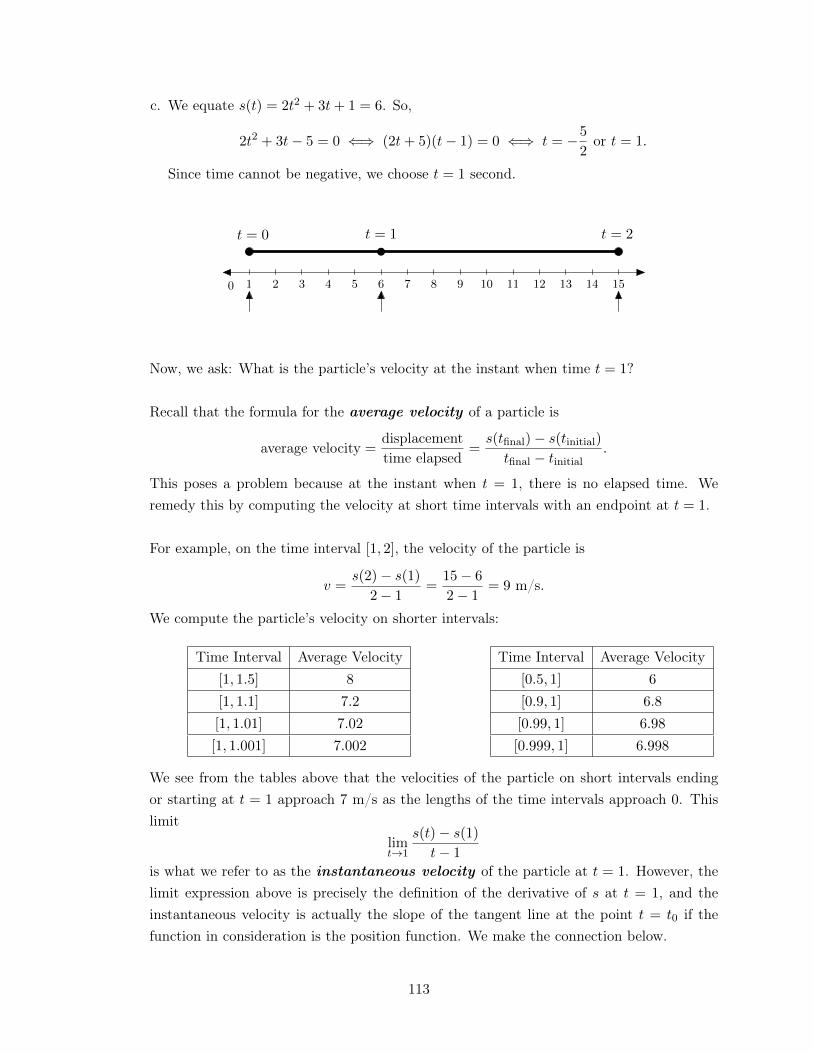
c. We equate s(t) = 2t2 + 3t+ 1 = 6. So,
2t2 + 3t� 5 = 0 () (2t+ 5)(t� 1) = 0 () t = �5
2
or t = 1.
Since time cannot be negative, we choose t = 1 second.
.
1 2 3 4 5 6 7 8 9 10 11 12 13 14 150
t = 0
t = 1 t = 2
Now, we ask: What is the particle’s velocity at the instant when time t = 1?
Recall that the formula for the average velocity of a particle is
average velocity =
displacementtime elapsed
=
s(tfinal
)� s(tinitial
)
tfinal
� tinitial
.
This poses a problem because at the instant when t = 1, there is no elapsed time. Weremedy this by computing the velocity at short time intervals with an endpoint at t = 1.
For example, on the time interval [1, 2], the velocity of the particle is
v =
s(2)� s(1)
2� 1
=
15� 6
2� 1
= 9 m/s.
We compute the particle’s velocity on shorter intervals:
Time Interval Average Velocity[1, 1.5] 8
[1, 1.1] 7.2
[1, 1.01] 7.02
[1, 1.001] 7.002
Time Interval Average Velocity[0.5, 1] 6
[0.9, 1] 6.8
[0.99, 1] 6.98
[0.999, 1] 6.998
We see from the tables above that the velocities of the particle on short intervals endingor starting at t = 1 approach 7 m/s as the lengths of the time intervals approach 0. Thislimit
lim
t!1
s(t)� s(1)
t� 1
is what we refer to as the instantaneous velocity of the particle at t = 1. However, thelimit expression above is precisely the definition of the derivative of s at t = 1, and theinstantaneous velocity is actually the slope of the tangent line at the point t = t
0
if thefunction in consideration is the position function. We make the connection below.
113
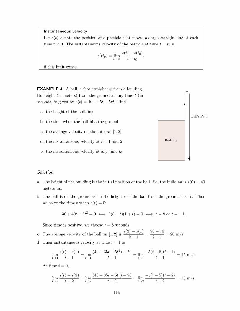
Instantaneous velocityLet s(t) denote the position of a particle that moves along a straight line at eachtime t � 0. The instantaneous velocity of the particle at time t = t
0
is
s0(t0
) = lim
t!t0
s(t)� s(t0
)
t� t0
,
if this limit exists.
EXAMPLE 4: A ball is shot straight up from a building.Its height (in meters) from the ground at any time t (inseconds) is given by s(t) = 40 + 35t� 5t2. Find
a. the height of the building.
b. the time when the ball hits the ground.
c. the average velocity on the interval [1, 2].
d. the instantaneous velocity at t = 1 and 2.
e. the instantaneous velocity at any time t0
.
Building
Ball’s Path
Solution. .
a. The height of the building is the initial position of the ball. So, the building is s(0) = 40
meters tall.
b. The ball is on the ground when the height s of the ball from the ground is zero. Thuswe solve the time t when s(t) = 0:
30 + 40t� 5t2 = 0 () 5(8� t)(1 + t) = 0 () t = 8 or t = �1.
Since time is positive, we choose t = 8 seconds.
c. The average velocity of the ball on [1, 2] iss(2)� s(1)
2� 1
=
90� 70
2� 1
= 20 m/s.
d. Then instantaneous velocity at time t = 1 is
lim
t!1
s(t)� s(1)
t� 1
= lim
t!1
(40 + 35t� 5t2)� 70
t� 1
= lim
t!1
�5(t� 6)(t� 1)
t� 1
= 25 m/s.
At time t = 2,
lim
t!2
s(t)� s(2)
t� 2
= lim
t!2
(40 + 35t� 5t2)� 90
t� 2
= lim
t!2
�5(t� 5)(t� 2)
t� 2
= 15 m/s.
114
e. The instantaneous velocity function at any time t0
is
lim
t!t0
s(t)� s(t0
)
t� t0
= lim
t!1
(40 + 35t� 5t2)� (40 + 35t0
� 5t20
)
t� t0
= lim
t!1
5(t� t0
)(7� (t+ t0
))
t� t0
= (35� 10t0
) m/s.
.
Remark 3: Note that in (e) of the previous example, if we set t0
= 4, then the instan-taneous velocity is �5 m/s. The negative sign gives the direction of the velocity (since itis a vector quantity), and means that the ball is moving towards the negative direction ofthe line, in this case, moving downwards. If the sign of the velocity is positive, then theparticle is moving towards the positive direction (that is, in the direction from the origintowards the positive numbers) of the s-axis.
(C) EXERCISES
1. For each of the following functions, find the indicated derivative using the definition.
a. f(x) = x2 � 4x+ 1; f 0(2) Answer: 0
b. f(x) = x3 + 2; f 0(�2) Answer: 12
c. f(x) = 2x4 + 3x3 � 2x+ 7; f 0(0) Answer: �2
d. f(x) =p2x+ 7; f 0
(1) Answer: 1/3
e. f(x) = 1 +
px2 + 3x+ 6; f 0
(2) Answer: 7/8
f. f(x) =x
x+ 4
; f 0(�3) Answer: 4
g. f(x) =x2 + 3
4� x2; f 0
(�1) Answer: �14/9
h. f(x) =
px+ 3
x� 4
; f 0(1) Answer: �11/36
i. f(x) =3�
p5x� 9
2x� 1
; f 0(2) Answer: �23/18
j. f(x) = 2 sin(⇡x); f 0(�3) Answer: �2⇡
k. f(x) = x2 cosx; f 0(0) Answer: 0
l. f(x) = ex+1
; f 0(�1) Answer: 1
?m. f(x) = 3px� 1; f 0
(9) Answer: 1/12
?n. f(x) = 3p7x+ 6; f 0
(3) Answer: 7/27
?o. f(x) = tan(3x); f 0(⇡/4) Answer: 6
?p. f(x) = 2 cosx� 3 sin(2x); f 0(⇡/6) Answer: �4
?q. f(x) = 1� 3 sin
2 x; f 0(⇡/3) Answer: �3
p3/2
115
?r. f(x) = xex; f 0(1) Answer: 2e
?s. f(x) =x
1 + sin(⇡x); f 0
(1/2) Answer: 1/2
?t. f(x) =x+ cos(3⇡x)
x2; f 0
(1) Answer: 1
2. A billiard ball is hit and travels in a straight line. If s centimeters is the distance ofthe ball from its initial position at t seconds, then s = 100t2 + 100t. If the ball hitsthe cushion at 39 cm from its initial position, at what velocity does it hit the cushionat that particular instant? (Hint : Determine first the time when s = 39 and find theinstantaneous velocity at this time.)
3. A particle is moving along a straight line and its position at any time t � 0 (in seconds)is given by s(t) = t3 � 6t2 + 9t meters.
a. Find the average velocity of the particle on the time interval [0, 2]?b. Find the velocity of the particle at the instant when t = 2?
4. A stone is thrown vertically upward from the top of a building. If the equation of themotion of the stone is s = �5t2 + 30t + 200, where s is the directed distance from theground in meters and t is in seconds,
a. what is the height of the building?b. what is the average velocity on the time interval [1, 3]?c. what is the instantaneous velocity at time t = 1?d. at what time will the stone hit the ground?e. what is the instantaneous velocity of the stone upon impact?
(D) ENRICHMENT
In this section, we discuss average and instantaneous rate of change.
AVERAGE RATE OF CHANGE
There are several instances where the rate of change of a certain quantity is of interest.(a) A statistician may be interested in how the population of a certain city changes with
time.(b) A civil engineer may want to know how the length of metal bars changes with tem-
perature.(c) A company manager can study how the production cost of a certain product increases
as the number of manufactured products also increases.(d) A chemist may be interested in how the volume of a certain compound changes with
increased pressure.
116
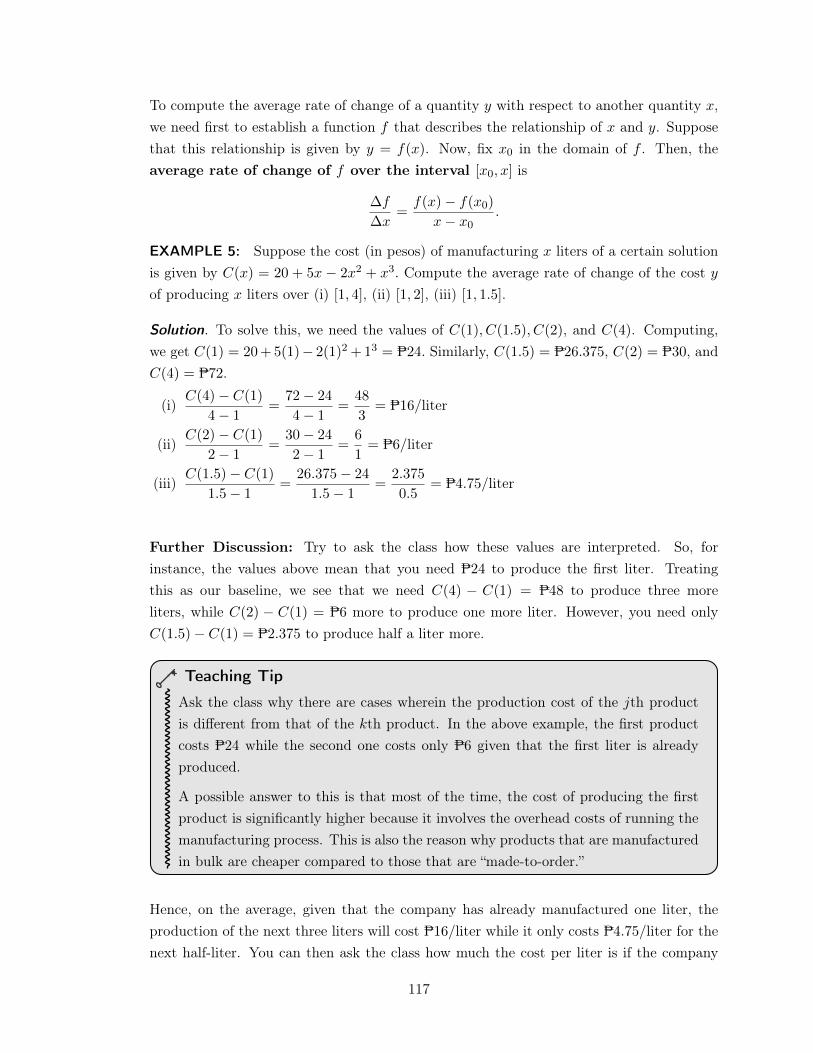
To compute the average rate of change of a quantity y with respect to another quantity x,we need first to establish a function f that describes the relationship of x and y. Supposethat this relationship is given by y = f(x). Now, fix x
0
in the domain of f . Then, theaverage rate of change of f over the interval [x
0
, x] is
�f
�x=
f(x)� f(x0
)
x� x0
.
EXAMPLE 5: Suppose the cost (in pesos) of manufacturing x liters of a certain solutionis given by C(x) = 20 + 5x � 2x2 + x3. Compute the average rate of change of the cost y
of producing x liters over (i) [1, 4], (ii) [1, 2], (iii) [1, 1.5].
Solution. To solve this, we need the values of C(1), C(1.5), C(2), and C(4). Computing,we get C(1) = 20+5(1)� 2(1)
2
+1
3
= P24. Similarly, C(1.5) = P26.375, C(2) = P30, andC(4) = P72.
(i)C(4)� C(1)
4� 1
=
72� 24
4� 1
=
48
3
= P16/liter
(ii)C(2)� C(1)
2� 1
=
30� 24
2� 1
=
6
1
= P6/liter
(iii)C(1.5)� C(1)
1.5� 1
=
26.375� 24
1.5� 1
=
2.375
0.5= P4.75/liter
.
Further Discussion: Try to ask the class how these values are interpreted. So, forinstance, the values above mean that you need P24 to produce the first liter. Treatingthis as our baseline, we see that we need C(4) � C(1) = P48 to produce three moreliters, while C(2) � C(1) = P6 more to produce one more liter. However, you need onlyC(1.5)� C(1) = P2.375 to produce half a liter more.
Teaching Tip
Ask the class why there are cases wherein the production cost of the jth productis different from that of the kth product. In the above example, the first productcosts P24 while the second one costs only P6 given that the first liter is alreadyproduced.
A possible answer to this is that most of the time, the cost of producing the firstproduct is significantly higher because it involves the overhead costs of running themanufacturing process. This is also the reason why products that are manufacturedin bulk are cheaper compared to those that are “made-to-order.”
Hence, on the average, given that the company has already manufactured one liter, theproduction of the next three liters will cost P16/liter while it only costs P4.75/liter for thenext half-liter. You can then ask the class how much the cost per liter is if the company
117
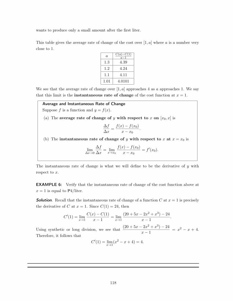
wants to produce only a small amount after the first liter.
This table gives the average rate of change of the cost over [1, a] where a is a number veryclose to 1.
a C(a)�C(1)
a�1
1.3 4.391.2 4.241.1 4.111.01 4.0101
We see that the average rate of change over [1, a] approaches 4 as a approaches 1. We saythat this limit is the instantaneous rate of change of the cost function at x = 1.
Average and Instantaneous Rate of ChangeSuppose f is a function and y = f(x).
(a) The average rate of change of y with respect to x on [x0
, x] is
�f
�x=
f(x)� f(x0
)
x� x0
.
(b) The instantaneous rate of change of y with respect to x at x = x0
is
lim
�x!0
�f
�x= lim
x!x0
f(x)� f(x0
)
x� x0
= f 0(x
0
).
The instantaneous rate of change is what we will define to be the derivative of y withrespect to x.
EXAMPLE 6: Verify that the instantaneous rate of change of the cost function above atx = 1 is equal to P4/liter.
Solution. Recall that the instantaneous rate of change of a function C at x = 1 is preciselythe derivative of C at x = 1. Since C(1) = 24, then
C 0(1) = lim
x!1
C(x)� C(1)
x� 1
= lim
x!1
(20 + 5x� 2x2 + x3)� 24
x� 1
.
Using synthetic or long division, we see that(20 + 5x� 2x2 + x3)� 24
x� 1
= x2 � x + 4.Therefore, it follows that
C 0(1) = lim
x!1
(x2 � x+ 4) = 4.
.
118
LESSON 6: Rules of Differentiation
TIME FRAME: 3 hours
LEARNING OUTCOMES: At the end of the lesson, the learner shall be able to:
1. Determine the relationship between differentiability and continuity;2. Derive the differentiation rules; and3. Apply the differentiation rules in computing the derivatives of algebraic, exponential, and
trigonometric functions.
LESSON OUTLINE:
1. Definitions on continuity and differentiability2. Relationship between differentiability and continuity3. Sample exercises on the relationship between differentiability and continuity4. Derivation of the different differentiation rules5. Examples on the different differentiation rules6. Applications
119
TOPIC 6.1: Differentiability Implies Continuity
DEVELOPMENT OF THE LESSON
(A) INTRODUCTION
The difference between continuity and differentiability is a critical issue. Most, but not all,of the functions we encounter in calculus will be differentiable over their entire domain.Before we can confidently apply the rules regarding derivatives, we need to be able torecognize the exceptions to the rule.
Recall the following definitions:
Definition 1 (Continuity at a Number). A function f is continuous at a number c ifall of the following conditions are satisfied:
(i) f(c) is defined;
(ii) lim
x!cf(x) exists; and
(iii) lim
x!cf(x) = f(c).
If at least one of the these conditions is not satisfied, the function is said to be discontin-
uous at c.
Definition 2 (Continuity on R). A function f is said to be continuous everywhere if fis continuous at every real number.
Definition 3. A function f is differentiable at the number c if
f 0(c) = lim
h!0
f(c+ h)� f(c)
h
exists.
(B) LESSON PROPERWe now present several examples of determining whether a function is continuous or dif-ferentiable at a number.
120
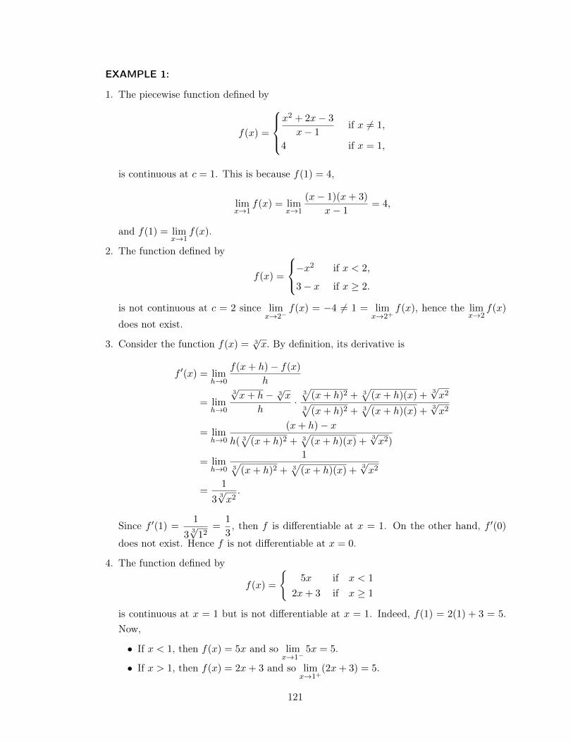
EXAMPLE 1:
1. The piecewise function defined by
f(x) =
8><
>:
x2 + 2x� 3
x� 1
if x 6= 1,
4 if x = 1,
is continuous at c = 1. This is because f(1) = 4,
lim
x!1
f(x) = lim
x!1
(x� 1)(x+ 3)
x� 1
= 4,
and f(1) = lim
x!1
f(x).
2. The function defined by
f(x) =
8<
:�x2 if x < 2,
3� x if x � 2.
is not continuous at c = 2 since lim
x!2
�f(x) = �4 6= 1 = lim
x!2
+f(x), hence the lim
x!2
f(x)
does not exist.
3. Consider the function f(x) = 3px. By definition, its derivative is
f 0(x) = lim
h!0
f(x+ h)� f(x)
h
= lim
h!0
3px+ h� 3
px
h·
3p(x+ h)2 + 3
p(x+ h)(x) +
3px2
3p(x+ h)2 + 3
p(x+ h)(x) +
3px2
= lim
h!0
(x+ h)� x
h( 3p(x+ h)2 + 3
p(x+ h)(x) +
3px2)
= lim
h!0
1
3p
(x+ h)2 + 3p(x+ h)(x) +
3px2
=
1
3
3px2
.
Since f 0(1) =
1
3
3p1
2
=
1
3
, then f is differentiable at x = 1. On the other hand, f 0(0)
does not exist. Hence f is not differentiable at x = 0.
4. The function defined by
f(x) =
(5x if x < 1
2x+ 3 if x � 1
is continuous at x = 1 but is not differentiable at x = 1. Indeed, f(1) = 2(1) + 3 = 5.Now,
• If x < 1, then f(x) = 5x and so lim
x!1
�5x = 5.
• If x > 1, then f(x) = 2x+ 3 and so lim
x!1
+(2x+ 3) = 5.
121
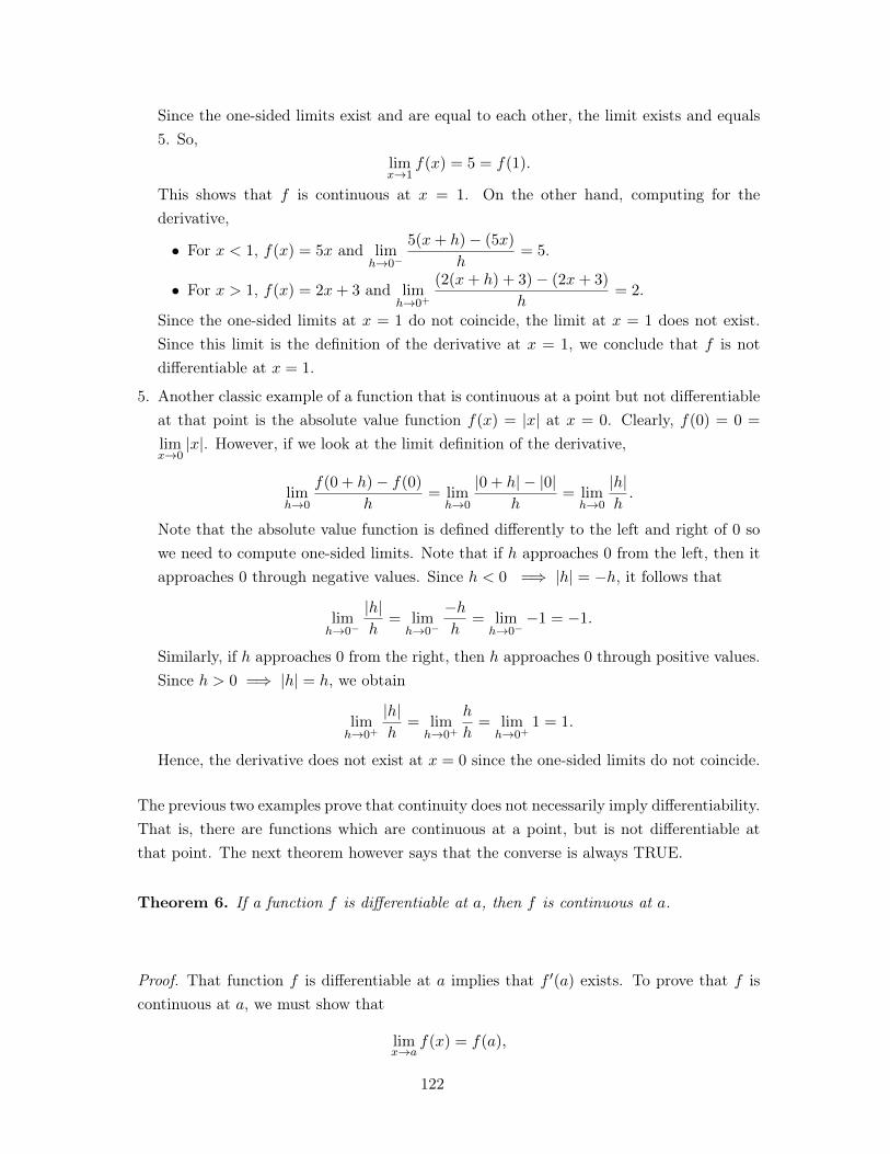
Since the one-sided limits exist and are equal to each other, the limit exists and equals5. So,
lim
x!1
f(x) = 5 = f(1).
This shows that f is continuous at x = 1. On the other hand, computing for thederivative,
• For x < 1, f(x) = 5x and lim
h!0
�
5(x+ h)� (5x)
h= 5.
• For x > 1, f(x) = 2x+ 3 and lim
h!0
+
(2(x+ h) + 3)� (2x+ 3)
h= 2.
Since the one-sided limits at x = 1 do not coincide, the limit at x = 1 does not exist.Since this limit is the definition of the derivative at x = 1, we conclude that f is notdifferentiable at x = 1.
5. Another classic example of a function that is continuous at a point but not differentiableat that point is the absolute value function f(x) = |x| at x = 0. Clearly, f(0) = 0 =
lim
x!0
|x|. However, if we look at the limit definition of the derivative,
lim
h!0
f(0 + h)� f(0)
h= lim
h!0
|0 + h|� |0|h
= lim
h!0
|h|h.
Note that the absolute value function is defined differently to the left and right of 0 sowe need to compute one-sided limits. Note that if h approaches 0 from the left, then itapproaches 0 through negative values. Since h < 0 =) |h| = �h, it follows that
lim
h!0
�
|h|h
= lim
h!0
�
�h
h= lim
h!0
��1 = �1.
Similarly, if h approaches 0 from the right, then h approaches 0 through positive values.Since h > 0 =) |h| = h, we obtain
lim
h!0
+
|h|h
= lim
h!0
+
h
h= lim
h!0
+1 = 1.
Hence, the derivative does not exist at x = 0 since the one-sided limits do not coincide.
The previous two examples prove that continuity does not necessarily imply differentiability.That is, there are functions which are continuous at a point, but is not differentiable atthat point. The next theorem however says that the converse is always TRUE.
Theorem 6. If a function f is differentiable at a, then f is continuous at a.
Proof. That function f is differentiable at a implies that f 0(a) exists. To prove that f is
continuous at a, we must show that
lim
x!af(x) = f(a),
122
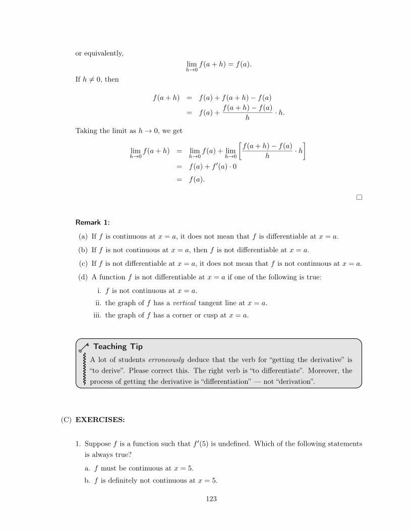
or equivalently,lim
h!0
f(a+ h) = f(a).
If h 6= 0, then
f(a+ h) = f(a) + f(a+ h)� f(a)
= f(a) +f(a+ h)� f(a)
h· h.
Taking the limit as h ! 0, we get
lim
h!0
f(a+ h) = lim
h!0
f(a) + lim
h!0
f(a+ h)� f(a)
h· h�
= f(a) + f 0(a) · 0
= f(a).
Remark 1:
(a) If f is continuous at x = a, it does not mean that f is differentiable at x = a.
(b) If f is not continuous at x = a, then f is not differentiable at x = a.
(c) If f is not differentiable at x = a, it does not mean that f is not continuous at x = a.
(d) A function f is not differentiable at x = a if one of the following is true:
i. f is not continuous at x = a.
ii. the graph of f has a vertical tangent line at x = a.
iii. the graph of f has a corner or cusp at x = a.
Teaching Tip
A lot of students erroneously deduce that the verb for “getting the derivative” is“to derive”. Please correct this. The right verb is “to differentiate”. Moreover, theprocess of getting the derivative is “differentiation” — not “derivation”.
(C) EXERCISES:
1. Suppose f is a function such that f 0(5) is undefined. Which of the following statements
is always true?
a. f must be continuous at x = 5.
b. f is definitely not continuous at x = 5.
123
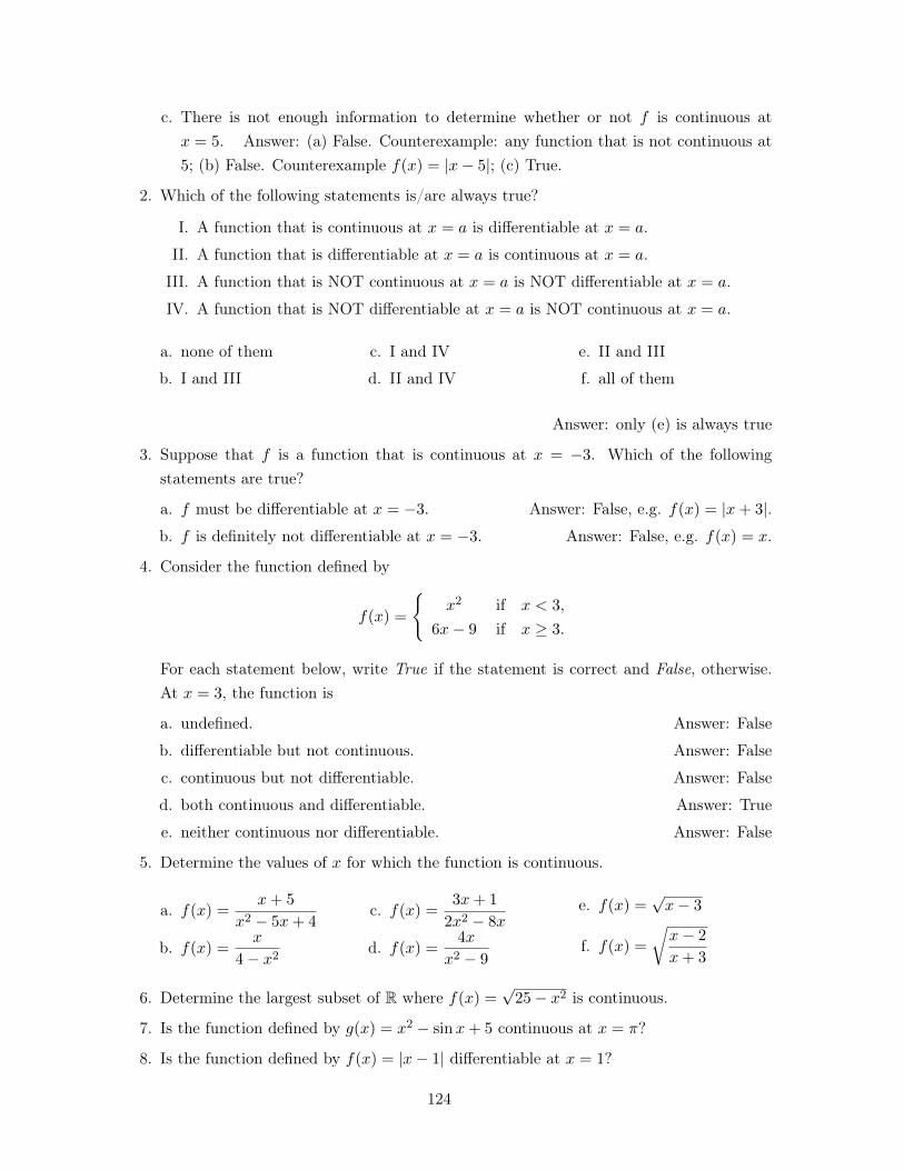
c. There is not enough information to determine whether or not f is continuous atx = 5. Answer: (a) False. Counterexample: any function that is not continuous at5; (b) False. Counterexample f(x) = |x� 5|; (c) True.
2. Which of the following statements is/are always true?
I. A function that is continuous at x = a is differentiable at x = a.
II. A function that is differentiable at x = a is continuous at x = a.
III. A function that is NOT continuous at x = a is NOT differentiable at x = a.
IV. A function that is NOT differentiable at x = a is NOT continuous at x = a.
a. none of them
b. I and III
c. I and IV
d. II and IV
e. II and III
f. all of them
Answer: only (e) is always true
3. Suppose that f is a function that is continuous at x = �3. Which of the followingstatements are true?
a. f must be differentiable at x = �3. Answer: False, e.g. f(x) = |x+ 3|.b. f is definitely not differentiable at x = �3. Answer: False, e.g. f(x) = x.
4. Consider the function defined by
f(x) =
(x2 if x < 3,
6x� 9 if x � 3.
For each statement below, write True if the statement is correct and False, otherwise.At x = 3, the function is
a. undefined. Answer: False
b. differentiable but not continuous. Answer: False
c. continuous but not differentiable. Answer: False
d. both continuous and differentiable. Answer: True
e. neither continuous nor differentiable. Answer: False
5. Determine the values of x for which the function is continuous.
a. f(x) =x+ 5
x2 � 5x+ 4
b. f(x) =x
4� x2
c. f(x) =3x+ 1
2x2 � 8x
d. f(x) =4x
x2 � 9
e. f(x) =px� 3
f. f(x) =
rx� 2
x+ 3
6. Determine the largest subset of R where f(x) =p25� x2 is continuous.
7. Is the function defined by g(x) = x2 � sinx+ 5 continuous at x = ⇡?
8. Is the function defined by f(x) = |x� 1| differentiable at x = 1?
124
9. Is the function defined by
f(x) =
(x3 � 3 if x 2,
x2 + 1 if x > 2.
continuous at x = 2? differentiable at x = 2?
10. Consider the function defined by f(x) =px. Is f differentiable at x = 1? at x = 0? at
x = �1?
125
TOPIC 6.2: The Differentiation Rules and Examples InvolvingAlgebraic, Exponential, and Trigonometric Functions
DEVELOPMENT OF THE LESSON
(A) INTRODUCTION
How do we find derivatives?
The procedure for finding the exact derivative directly from a formula of the functionwithout having to use graphical methods is called differential calculus. In practice, we usesome rules that tell us how to find the derivative of almost any function. In this lesson, wewill introduce these rules.
You may start by asking the students to compute the derivatives of the following functionsusing the limit definition (formal definition):
(a) f(x) = 3x2 + 4 (b) g(x) =�4x2 + 3
x� 1
Give them a few minutes to solve.
After a few minutes, (using their answers) tell the students that computing the derivativeof a given function from the definition is usually time consuming. Thus, this lesson willhelp them compute the derivative of a given function more easily.
(B) LESSON PROPER
We first recall the definition of the derivative of a function.
The derivative of the function f the function f 0 whose value at a number x in the domainof f is given by
f 0(x) = lim
h!0
f(x+ h)� f(x)
h(2.3)
if the limit exists.
For example, let us compute the derivative of the first function of the seatwork above:f(x) = 3x2 + 4. Let us first compute the numerator of the quotient in (2.3):
f(x+ h)� f(x) = (3(x+ h)2 + 4)� (3x2 + 4)
= (3x2 + 6xh+ 3h2 + 4)� (3x2 + 4)
= 6xh+ 3h2
= h(6x+ 3h).
126
Therefore,
f 0(x) = lim
h!0
f(x+ h)� f(x)
h
= lim
h!0
3(x+ h)2 + 4� (3x2 + 4)
h
= lim
h!0
h(6x+ 3h)
h= lim
h!0
(6x+ 3h)
= 6x.
We see that computing the derivative using the definition of even a simple polynomial is alengthy process. What follows next are rules that will enable us to find derivatives easily.We call them DIFFERENTIATION RULES.
Teaching Tip
You may prove some of the rules and let the class derive the other rules.
DIFFERENTIATING CONSTANT FUNCTIONS
The graph of a constant function is a horizontal line and a horizontal line has zero slope.The derivative measures the slope of the tangent, and so the derivative is zero.
RULE 1: The Constant Rule
If f(x) = c where c is a constant, then f 0(x) = 0. The derivative of a constant is equal to
zero.
Proof:
f 0(x) = lim
h!0
f(x+ h)� f(x)
h= lim
h!0
c� c
h= lim
h!0
0 = 0.
EXAMPLE 1:
(a) If f(x) = 10, then f 0(x) = 0.
(b) If h(x) = �p3, then h0(x) = 0.
(c) If g(x) = 5⇡, then g0(x) = 0.
DIFFERENTIATING POWER FUNCTIONS
A function of the form f(x) = xk, where k is a real number, is called a power function.Below are some examples of power functions.
127
(a) f(x) = x
(b) g(x) = x2
(c) h(x) =px
(d) p(x) = 4px
(e) `(x) = x�5
(f) s(x) = 1/x8
The definition of the derivative discussed in the previous lesson can be used to find thederivatives of many power functions. For example, it can be shown that
If f(x) = x2, then f 0(x) = 2x.
If f(x) = x3, then f 0(x) = 3x2.
If f(x) = x4, then f 0(x) = 4x3.
If f(x) = x5, then f 0(x) = 5x4.
If f(x) = x6, then f 0(x) = 6x5.
Notice the pattern in these derivatives. In each case, the new power of f becomes thecoefficient in f 0 and the power of f 0 is one less than the original power of f . In general, wehave the following rule:
RULE 2: The Power Rule
If f(x) = xn where n 2 N, then f 0(x) = nxn�1.
Teaching Tip
At the least, prove the case when n = 1 and n = 2.Proof. (The cases n = 1 and n = 2) Using the limit definition,
f(x) = x =) f 0(x) = lim
h!0
f(x+ h)� f(x)
h= lim
h!0
(x+ h)� x
h= lim
h!0
1 = 1 = 1x1�1.
On the other hand, if f(x) = x2, then
f 0(x) = lim
h!0
f(x+ h)� f(x)
h
= lim
h!0
(x+ h)2 � x2
h
= lim
h!0
h(2x+ h)
h= 2x = 2x2�1.
If you wish to demonstrate the general case, the proof is stated below.
For the function f(x) = xn, in computing f(x + h) = (x + h)n, we need to invoke theBinomial Theorem:
(x+ h)n = xn + nxn�1h+
n(n� 1)
2!
xn�2h2 + · · · +
n!
r!(n� r)!xn�rhr + · · ·+ nxhn�1
+ hn.
128
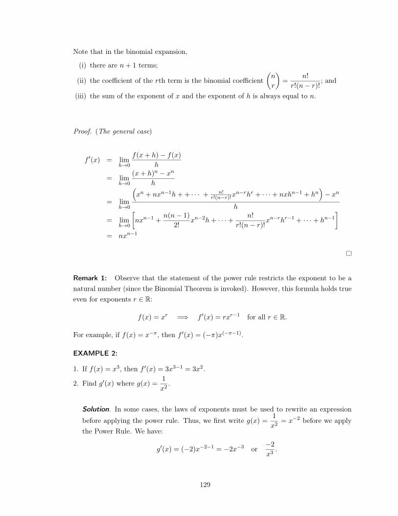
Note that in the binomial expansion,
(i) there are n+ 1 terms;
(ii) the coefficient of the rth term is the binomial coefficient✓n
r
◆=
n!
r!(n� r)!; and
(iii) the sum of the exponent of x and the exponent of h is always equal to n.
Proof. (The general case)
f 0(x) = lim
h!0
f(x+ h)� f(x)
h
= lim
h!0
(x+ h)n � xn
h
= lim
h!0
⇣xn + nxn�1h++ · · · +
n!r!(n�r)!x
n�rhr + · · ·+ nxhn�1
+ hn⌘� xn
h
= lim
h!0
nxn�1
+
n(n� 1)
2!
xn�2h+ · · ·+ n!
r!(n� r)!xn�rhr�1
+ · · ·+ hn�1
�
= nxn�1
Remark 1: Observe that the statement of the power rule restricts the exponent to be anatural number (since the Binomial Theorem is invoked). However, this formula holds trueeven for exponents r 2 R:
f(x) = xr =) f 0(x) = rxr�1 for all r 2 R.
For example, if f(x) = x�⇡, then f 0(x) = (�⇡)x(�⇡�1).
EXAMPLE 2:
1. If f(x) = x3, then f 0(x) = 3x3�1
= 3x2.
2. Find g0(x) where g(x) =1
x2.
Solution. In some cases, the laws of exponents must be used to rewrite an expressionbefore applying the power rule. Thus, we first write g(x) =
1
x2= x�2 before we apply
the Power Rule. We have:
g0(x) = (�2)x�2�1
= �2x�3 or�2
x3.
.
129
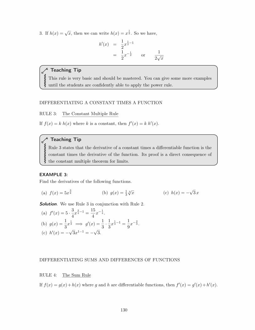
3. If h(x) =px, then we can write h(x) = x
12 . So we have,
h0(x) =
1
2
x12�1
=
1
2
x�12 or
1
2
px
Teaching Tip
This rule is very basic and should be mastered. You can give some more examplesuntil the students are confidently able to apply the power rule.
DIFFERENTIATING A CONSTANT TIMES A FUNCTION
RULE 3: The Constant Multiple Rule
If f(x) = k h(x) where k is a constant, then f 0(x) = k h0(x).
Teaching Tip
Rule 3 states that the derivative of a constant times a differentiable function is theconstant times the derivative of the function. Its proof is a direct consequence ofthe constant multiple theorem for limits.
EXAMPLE 3:Find the derivatives of the following functions.
(a) f(x) = 5x34 (b) g(x) = 1
3
3px (c) h(x) = �
p3x
Solution. We use Rule 3 in conjunction with Rule 2.
(a) f 0(x) = 5 · 3
4
x34�1
=
15
4
x�14 .
(b) g(x) =1
3
x13
=) g0(x) =1
3
· 13
x13�1
=
1
9
x�23 .
(c) h0(x) = �p3x1�1
= �p3.
.
DIFFERENTIATING SUMS AND DIFFERENCES OF FUNCTIONS
RULE 4: The Sum Rule
If f(x) = g(x)+h(x) where g and h are differentiable functions, then f 0(x) = g0(x)+h0(x).
130
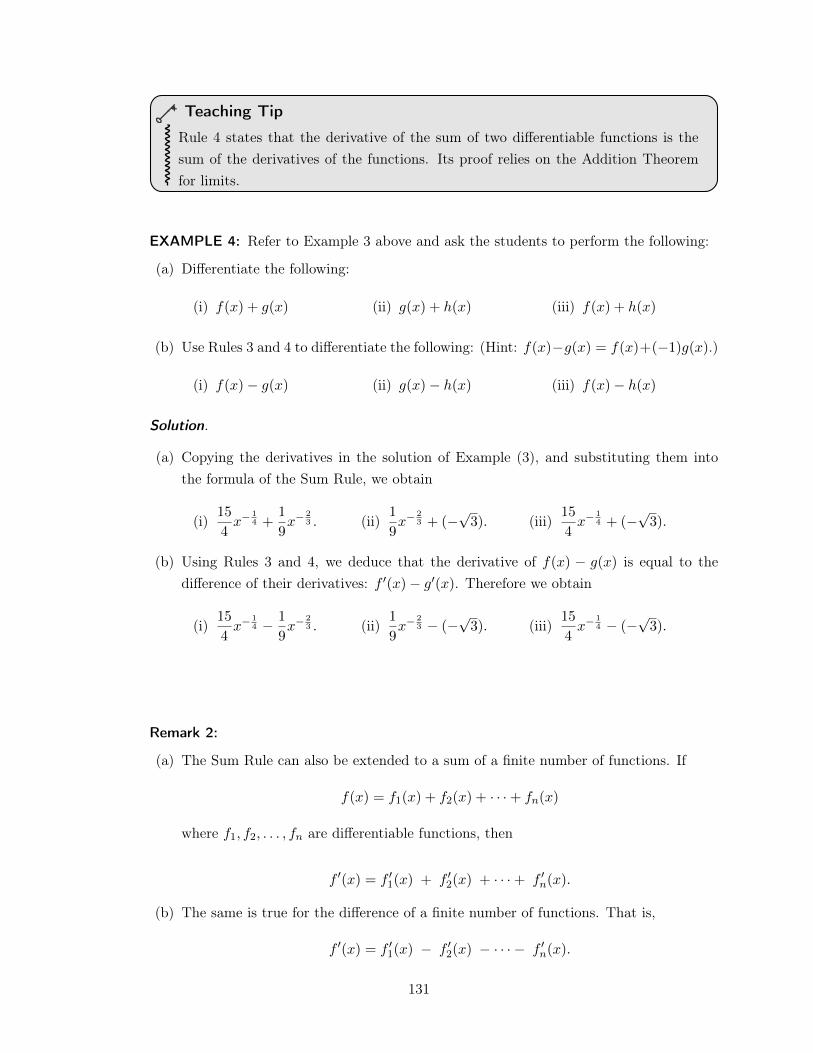
Teaching Tip
Rule 4 states that the derivative of the sum of two differentiable functions is thesum of the derivatives of the functions. Its proof relies on the Addition Theoremfor limits.
EXAMPLE 4: Refer to Example 3 above and ask the students to perform the following:
(a) Differentiate the following:
(i) f(x) + g(x) (ii) g(x) + h(x) (iii) f(x) + h(x)
(b) Use Rules 3 and 4 to differentiate the following: (Hint: f(x)�g(x) = f(x)+(�1)g(x).)
(i) f(x)� g(x) (ii) g(x)� h(x) (iii) f(x)� h(x)
Solution. .
(a) Copying the derivatives in the solution of Example (3), and substituting them intothe formula of the Sum Rule, we obtain
(i)15
4
x�14+
1
9
x�23 . (ii)
1
9
x�23+ (�
p3). (iii)
15
4
x�14+ (�
p3).
(b) Using Rules 3 and 4, we deduce that the derivative of f(x) � g(x) is equal to thedifference of their derivatives: f 0
(x)� g0(x). Therefore we obtain
(i)15
4
x�14 � 1
9
x�23 . (ii)
1
9
x�23 � (�
p3). (iii)
15
4
x�14 � (�
p3).
.
Remark 2:
(a) The Sum Rule can also be extended to a sum of a finite number of functions. If
f(x) = f1
(x) + f2
(x) + · · ·+ fn(x)
where f1
, f2
, . . . , fn are differentiable functions, then
f 0(x) = f 0
1
(x) + f 02
(x) + · · ·+ f 0n(x).
(b) The same is true for the difference of a finite number of functions. That is,
f 0(x) = f 0
1
(x) � f 02
(x) � · · ·� f 0n(x).
131
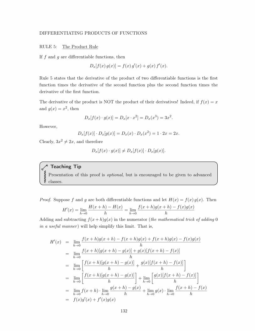
DIFFERENTIATING PRODUCTS OF FUNCTIONS
RULE 5: The Product Rule
If f and g are differentiable functions, then
Dx[f(x) g(x)] = f(x) g0(x) + g(x) f 0(x).
Rule 5 states that the derivative of the product of two differentiable functions is the firstfunction times the derivative of the second function plus the second function times thederivative of the first function.
The derivative of the product is NOT the product of their derivatives! Indeed, if f(x) = x
and g(x) = x2, then
Dx[f(x) · g(x)] = Dx[x · x2] = Dx(x3
) = 3x2.
However,Dx[f(x)] ·Dx[g(x)] = Dx(x) ·Dx(x
2
) = 1 · 2x = 2x.
Clearly, 3x2 6= 2x, and therefore
Dx[f(x) · g(x)] 6= Dx[f(x)] ·Dx[g(x)].
Teaching Tip
Presentation of this proof is optional, but is encouraged to be given to advancedclasses.
Proof. Suppose f and g are both differentiable functions and let H(x) = f(x) g(x). Then
H 0(x) = lim
h!0
H(x+ h)�H(x)
h= lim
h!0
f(x+ h)g(x+ h)� f(x)g(x)
h
Adding and subtracting f(x+h)g(x) in the numerator (the mathematical trick of adding 0
in a useful manner) will help simplify this limit. That is,
H 0(x) = lim
h!0
f(x+ h)g(x+ h)� f(x+ h)g(x) + f(x+ h)g(x)� f(x)g(x)
h
= lim
h!0
f(x+ h)[g(x+ h)� g(x)] + g(x)[f(x+ h)� f(x)]
h
= lim
h!0
f(x+ h)[g(x+ h)� g(x)]
h+
g(x)[f(x+ h)� f(x)]
h
�
= lim
h!0
f(x+ h)[g(x+ h)� g(x)]
h
�+ lim
h!0
g(x)[f(x+ h)� f(x)]
h
�
= lim
h!0
f(x+ h) · limh!0
g(x+ h)� g(x)
h+ lim
h!0
g(x) · limh!0
f(x+ h)� f(x)
h= f(x)g0(x) + f 0
(x)g(x)
132
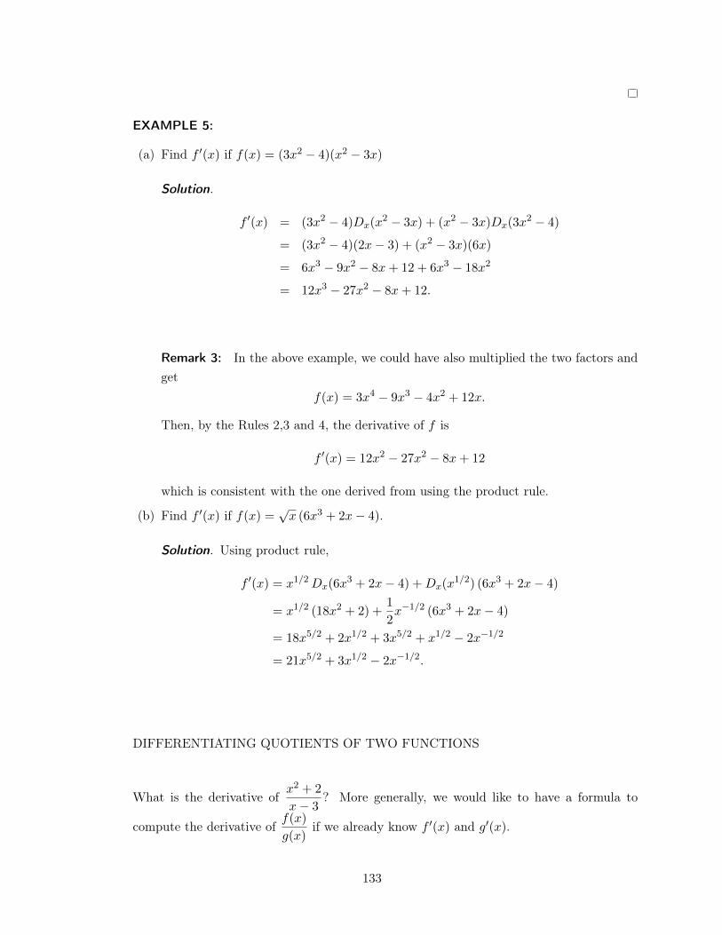
EXAMPLE 5:
(a) Find f 0(x) if f(x) = (3x2 � 4)(x2 � 3x)
Solution.
f 0(x) = (3x2 � 4)Dx(x
2 � 3x) + (x2 � 3x)Dx(3x2 � 4)
= (3x2 � 4)(2x� 3) + (x2 � 3x)(6x)
= 6x3 � 9x2 � 8x+ 12 + 6x3 � 18x2
= 12x3 � 27x2 � 8x+ 12.
.
Remark 3: In the above example, we could have also multiplied the two factors andget
f(x) = 3x4 � 9x3 � 4x2 + 12x.
Then, by the Rules 2,3 and 4, the derivative of f is
f 0(x) = 12x2 � 27x2 � 8x+ 12
which is consistent with the one derived from using the product rule.
(b) Find f 0(x) if f(x) =
px (6x3 + 2x� 4).
Solution. Using product rule,
f 0(x) = x1/2Dx(6x
3
+ 2x� 4) +Dx(x1/2
) (6x3 + 2x� 4)
= x1/2 (18x2 + 2) +
1
2
x�1/2(6x3 + 2x� 4)
= 18x5/2 + 2x1/2 + 3x5/2 + x1/2 � 2x�1/2
= 21x5/2 + 3x1/2 � 2x�1/2.
.
DIFFERENTIATING QUOTIENTS OF TWO FUNCTIONS
What is the derivative ofx2 + 2
x� 3
? More generally, we would like to have a formula to
compute the derivative off(x)
g(x)if we already know f 0
(x) and g0(x).
133
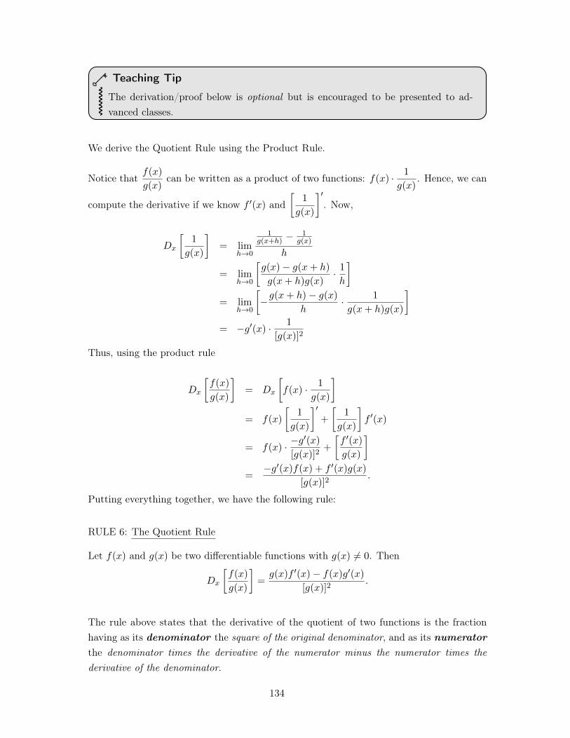
Teaching Tip
The derivation/proof below is optional but is encouraged to be presented to ad-vanced classes.
We derive the Quotient Rule using the Product Rule.
Notice thatf(x)
g(x)can be written as a product of two functions: f(x) · 1
g(x). Hence, we can
compute the derivative if we know f 0(x) and
1
g(x)
�0. Now,
Dx
1
g(x)
�= lim
h!0
1
g(x+h) �1
g(x)
h
= lim
h!0
g(x)� g(x+ h)
g(x+ h)g(x)· 1h
�
= lim
h!0
�g(x+ h)� g(x)
h· 1
g(x+ h)g(x)
�
= �g0(x) · 1
[g(x)]2
Thus, using the product rule
Dx
f(x)
g(x)
�= Dx
f(x) · 1
g(x)
�
= f(x)
1
g(x)
�0+
1
g(x)
�f 0(x)
= f(x) · �g0(x)
[g(x)]2+
f 0(x)
g(x)
�
=
�g0(x)f(x) + f 0(x)g(x)
[g(x)]2.
Putting everything together, we have the following rule:
RULE 6: The Quotient Rule
Let f(x) and g(x) be two differentiable functions with g(x) 6= 0. Then
Dx
f(x)
g(x)
�=
g(x)f 0(x)� f(x)g0(x)
[g(x)]2.
The rule above states that the derivative of the quotient of two functions is the fractionhaving as its denominator the square of the original denominator, and as its numerator
the denominator times the derivative of the numerator minus the numerator times thederivative of the denominator.
134
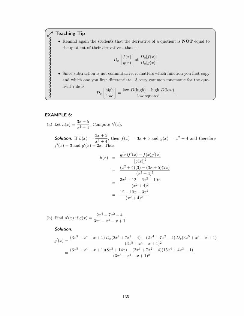
Teaching Tip
• Remind again the students that the derivative of a quotient is NOT equal tothe quotient of their derivatives, that is,
Dx
f(x)
g(x)
�6= Dx[f(x)]
Dx[g(x)].
• Since subtraction is not commutative, it matters which function you first copyand which one you first differentiate. A very common mnemonic for the quo-tient rule is
Dx
highlow
�=
low D(high) � high D(low)low squared
.
EXAMPLE 6:
(a) Let h(x) =3x+ 5
x2 + 4
. Compute h0(x).
Solution. If h(x) =
3x+ 5
x2 + 4
, then f(x) = 3x + 5 and g(x) = x2 + 4 and thereforef 0(x) = 3 and g0(x) = 2x. Thus,
h(x) =
g(x)f 0(x)� f(x)g0(x)
[g(x)]2
=
(x2 + 4)(3)� (3x+ 5)(2x)
(x2 + 4)
2
=
3x2 + 12� 6x2 � 10x
(x2 + 4)
2
=
12� 10x� 3x2
(x2 + 4)
2
.
.
(b) Find g0(x) if g(x) =2x4 + 7x2 � 4
3x5 + x4 � x+ 1
.
Solution.
g0(x) =(3x5 + x4 � x+ 1)Dx(2x4 + 7x2 � 4)� (2x4 + 7x2 � 4)Dx(3x5 + x4 � x+ 1)
(3x5 + x4 � x+ 1)
2
=
(3x5 + x4 � x+ 1)(8x3 + 14x)� (2x4 + 7x2 � 4)(15x4 + 4x3 � 1)
(3x5 + x4 � x+ 1)
2
.
.
135
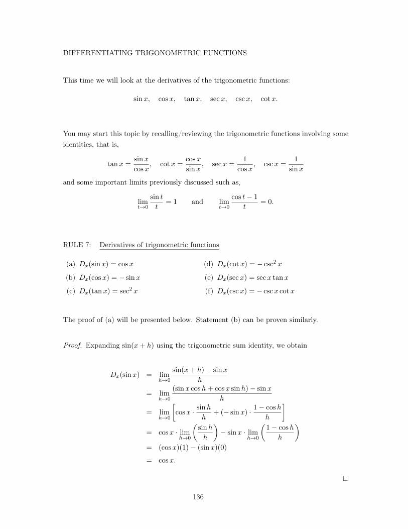
DIFFERENTIATING TRIGONOMETRIC FUNCTIONS
This time we will look at the derivatives of the trigonometric functions:
sinx, cosx, tanx, secx, cscx, cotx.
You may start this topic by recalling/reviewing the trigonometric functions involving someidentities, that is,
tanx =
sinx
cosx, cotx =
cosx
sinx, secx =
1
cosx, cscx =
1
sinx
and some important limits previously discussed such as,
lim
t!0
sin t
t= 1 and lim
t!0
cos t� 1
t= 0.
RULE 7: Derivatives of trigonometric functions
(a) Dx(sinx) = cosx
(b) Dx(cosx) = � sinx
(c) Dx(tanx) = sec
2 x
(d) Dx(cotx) = � csc
2 x
(e) Dx(secx) = secx tanx
(f) Dx(cscx) = � cscx cotx
The proof of (a) will be presented below. Statement (b) can be proven similarly.
Proof. Expanding sin(x+ h) using the trigonometric sum identity, we obtain
Dx(sinx) = lim
h!0
sin(x+ h)� sinx
h
= lim
h!0
(sinx cosh+ cosx sinh)� sinx
h
= lim
h!0
cosx · sinh
h+ (� sinx) · 1� cosh
h
�
= cosx · limh!0
✓sinh
h
◆� sinx · lim
h!0
✓1� cosh
h
◆
= (cosx)(1)� (sinx)(0)
= cosx.
136
Statements (c) - (f) can be proved using Statements (a) and (b) and the Quotient Rule.We only present the proof of (c) below.
Proof. Using Quotient Rule and Statements (a) and (b) above, we have
Dx(tanx) = Dx
sinx
cosx
�=
cosxDx(sinx)� sinxDx(cosx)
(cosx)2
=
cosx(cosx)� (sinx)(� sinx)
cos
2 x
=
cos
2 x+ sin
2 x
cos
2 x.
Using the identity cos
2 x+ sin
2 x = 1, we get Dx(tanx) =1
cos
2 x= sec
2 x.
EXAMPLE 7: Differentiate the following functions:
(a) f(x) = secx+ 3 cscx (b) g(x) = x2 sinx� 3x cosx+ 5 sinx
Solution. Applying the formulas above, we get
(a) If f(x) = secx+ 3 cscx, then
f 0(x) = secx tanx+ 3(� cscx cotx) = secx tanx� 3 cscx cotx.
(b) If g(x) = x2 sinx� 3x cosx+ 5 sinx, then
g0(x) = [(x2)(cosx) + (sinx)(2x)]� 3[(x)(� sinx) + (cosx(1)] + 5(cos)x)]
= x2 cosx+ 2x sinx+ 3x sinx� 3 cosx+ 5 cosx
= x2 cosx+ 5x sinx+ 2 cosx.
.
Remark 4:
(a) Whenever Rule 7 is applied to problems where the trigonometric functions are viewedas functions of angles, the unit measure must be in radians.
(b) Every trigonometric function is differentiable on its domain. In particular, the sineand cosine functions are everywhere differentiable.
DIFFERENTIATING AN EXPONENTIAL FUNCTION
RULE 8: Derivative of an exponential function
If f(x) = ex, then f 0(x) = ex.
137
Proof. (Optional) Using the definition of the derivative,
f 0(x) = lim
h!0
f(x+ h)� f(x)
h= lim
h!0
ex+h � ex
h.
Using a law of exponent, ex+h= ex · eh. Therefore, since lim
h!0
eh � 1
h= 1,
f 0(x) = lim
h!0
ex(eh � 1)
h= ex · lim
h!0
eh � 1
h= ex.
EXAMPLE 8:
(a) Find f 0(x) if f(x) = 3ex.
Solution. Applying Rules 3 and 7, we have
f 0(x) = 3Dx[e
x] = 3ex.
.
(b) Find g0(x) if g(x) = �4x2ex + 5xex � 10ex.
Solution. Applying Rule 5 to the first two terms and Rule 3 to the third term, wehave
g0(x) = [(�4x2)(ex) + (ex)(�8x)] + [(5x)(ex) + (ex)(5)� 10 · ex]
= �4x2ex � 3xex � 5ex.
.
(c) Find h0(x) if h(x) = ex sinx� 3ex cosx.
Solution. We apply the Product Rule to each term.
h0(x) = [(ex)(cosx) + (sinx)(ex)]� 3 · [(ex)(� sinx) + (cosx)(ex)]
= ex cosx+ ex sinx+ 3ex sinx� 3ex cosx
= ex(4 sinx� 2 cosx).
.
138
(d) Finddy
dxwhere y =
17
exxe + 2x� 3
px
.
Solution. Using Quotient Rule (also Product Rule when differentiating xeex), weobtain
dy
dx=
(exxe + 2x� 3
px)(0)� (17)([(ex)(exe�1
) + (xe)(ex)] + 2� 3
2
px)
(exxe + 2x� 3
px)2
=
�17ex+1xe�1 � 17exxe � 34 +
51
2
px
(exxe + 2x� 3
px)2
.
.
Remark 5: Since the domain of the exponential function is the set of real numbers, andd
dx[ex] = ex, it follows that the exponential function is differentiable everywhere.
(C) EXERCISES
1. Let f(x) = mx+b, the line with slope m and y-intercept b. Use the rules of differentiationto show that f 0
(x) = m. This again proves that the derivative of a line is just the slopeof the line.
2. Find the derivatives of the following functions. Locate the derivative in the table belowand encircle the answer. Keep working until you have five encircled answers in a linehorizontally, vertically or diagonally. (BINGO!)
a. y = x2 � x+ 1
b. f(x) =1
2x+ 1
c. y = (3x� 1)(2x+ 5)
d. g(x) = x3 � 3x2 + 2
e. y =
2x+ 5
3x� 2
f. y = (2x2 + 2)(x2 + 3)
g. f(x) =x2 + 1
x2 � 1
h. y = x3 � 4x2 � 3x
i. f(x) = 5x3 � 3x5
j. y = (2x+ 3)
2
k. f(x) = (x+
1
x)
2
l. y = x2(x3 � 1)
m. f(x) =2x
3x2 + 1
n. y =
x
x2 + 1
o. f(x) = (x� 2)(x+ 3)
139
2x� 2x�3
2x+
1
x22x� 1
19
3x� 2
�(2x3 + 2)
�4x
(x2 � 1)
2
12x� 7 4x (x+ 1)
�2
3(x2 + 3x)2
5x4 � 2x 6x3 8x+ 12
2� 6x2
(3x2 + 1)
2
8x3 + 16x
15(x2 � x4) 3x2 � 6x 3x2 � 8x� 3
2x
(1� x2)2�19
(3x� 2)
2
12x+ 13 2x+ 1
�2
(2x+ 1)
2
1� x2
(x2 + 1)
2
2
✓x+
1
x
◆
3. Use the Rules of Differentiation to differentiate the following functions:
a. f(x) = 2x3 + 6x
b. g(x) = 7x4 � 3x2
c. y(x) = 4x3 � 18x2 + 6x
d. h(x) = (3x+ 4)
2
e. h(x) = 9x2/3 +2
4px
4. Find the derivative of each of the following functions:
a. f(u) = (4u+ 5)(7u3 � 2u)
b. h(t) =4
t23
c. f(z) = �6z3 � 1
2z
d. g(s) =3s� s3
s2 + 1
e. f(a) =17
2a3+
1
8a2� 11a
f. f(r) = (r2 + 2r � 3)(3r + 4)
g. g(b) =3b� 4
b+ 5
· (2b+ 5)
h. h(v) =3v2 � 4v + 1
(3v2 � 2v + 1)(7v3 � v2 + 3v � 5)
5. Finddy
dxand simplify the result, if possible.
a. y =
px� 1p
xb. y = x2 + ⇡2
+ x⇡
c. y = x2 secx
d. y =
sinx� 1
cosx
e. y =
1
ex + 2
f. y = ex + xe + ee
g. y = x2 sinx cosx
h. y =
8
x� tanx cotx
6. Find the derivative of f(x) = x2 � 3x. Use the result to find the slope of the tangentline to the curve f(x) = x2 � 3x at the point where x = 2.
7. If y =
1
x, find y0 and use this result to find the points on the curve y =
1
xwhere the
tangent line has the slope �4.
8. Find all points on the graph of y = (x+ 3)
2 at which the tangent line is parallel to theline with equation y � 4x+ 2 = 0.
140
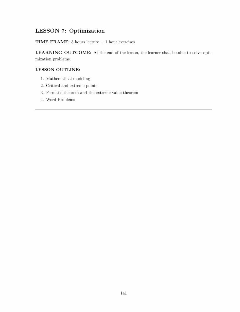
LESSON 7: Optimization
TIME FRAME: 3 hours lecture + 1 hour exercises
LEARNING OUTCOME: At the end of the lesson, the learner shall be able to solve opti-mization problems.
LESSON OUTLINE:
1. Mathematical modeling2. Critical and extreme points3. Fermat’s theorem and the extreme value theorem4. Word Problems
141

TOPIC 7.1: Optimization using Calculus
DEVELOPMENT OF THE LESSON
(A) INTRODUCTION
This topic presents one of the most important applications of calculus – optimization.
We first review mathematical modelling. Next, we define the notions of a critical point andan extremum of a function f . Then, we proceed with the discussion of the two importanttheorems – Fermat’s and the Extreme Value Theorem. Finally, we discuss the step-by-stepsolutions of word problems involving optimization.
(B) ACTIVITY
• Discuss with the class the importance of optimization in every decision process. Askthem how they maximize or minimize something when they go to school, shopping,church, etc: For example, they look at the greatest advantage and the least disadvan-tage when they choose:
– Routes they take (minimize time travel, traffic congestion)
– What to wear (maximize appearance/personality)
– What food to eat at the canteen (minimize costs, maximize hunger satisfaction),etc.
• You could also expound on the adage “Everything in moderation.” Ask which quanti-ties they know become bad if they are increased or decreased too much. For example:
– Sleep/rest (fatigue/weakness vs. conditions linked to depression/anxiety, obesityand heart problems, etc.: The rule of thumb is 8 hours.)
– Study hours (delinquent/failure in course vs. lacking time to do other aspects oflife e.g., family time/social life: The rule of thumb is 1� 3 hours every night afterclass)
– Food intake (being underweight vs. overweight with optimal values specified byRDA (recommended dietary allowance)), etc.
• Now, wrap up the discussion by reinforcing the idea that logical decisions in real lifeare made by optimizing some quantities (objectives) that depend on things you cancontrol (variables). Of course, in real life, there are several objectives and variablesinvolved. In this section, we will only be concerned with problems with one objectivethat depends on controlling only one variable.
142
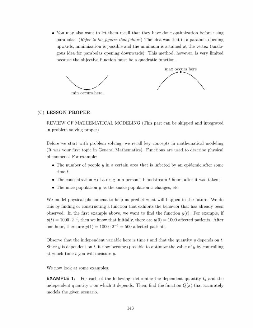
• You may also want to let them recall that they have done optimization before usingparabolas. (Refer to the figures that follow.) The idea was that in a parabola openingupwards, minimization is possible and the minimum is attained at the vertex (analo-gous idea for parabolas opening downwards). This method, however, is very limitedbecause the objective function must be a quadratic function.
min occurs here
max occurs here
(C) LESSON PROPER
REVIEW OF MATHEMATICAL MODELING (This part can be skipped and integratedin problem solving proper)
Before we start with problem solving, we recall key concepts in mathematical modeling(It was your first topic in General Mathematics). Functions are used to describe physicalphenomena. For example:
• The number of people y in a certain area that is infected by an epidemic after sometime t;
• The concentration c of a drug in a person’s bloodstream t hours after it was taken;
• The mice population y as the snake population x changes, etc.
We model physical phenomena to help us predict what will happen in the future. We dothis by finding or constructing a function that exhibits the behavior that has already beenobserved. In the first example above, we want to find the function y(t). For example, ify(t) = 1000 ·2�t, then we know that initially, there are y(0) = 1000 affected patients. Afterone hour, there are y(1) = 1000 · 2�1
= 500 affected patients.
Observe that the independent variable here is time t and that the quantity y depends on t.Since y is dependent on t, it now becomes possible to optimize the value of y by controllingat which time t you will measure y.
We now look at some examples.
EXAMPLE 1: For each of the following, determine the dependent quantity Q and theindependent quantity x on which it depends. Then, find the function Q(x) that accuratelymodels the given scenario.
143
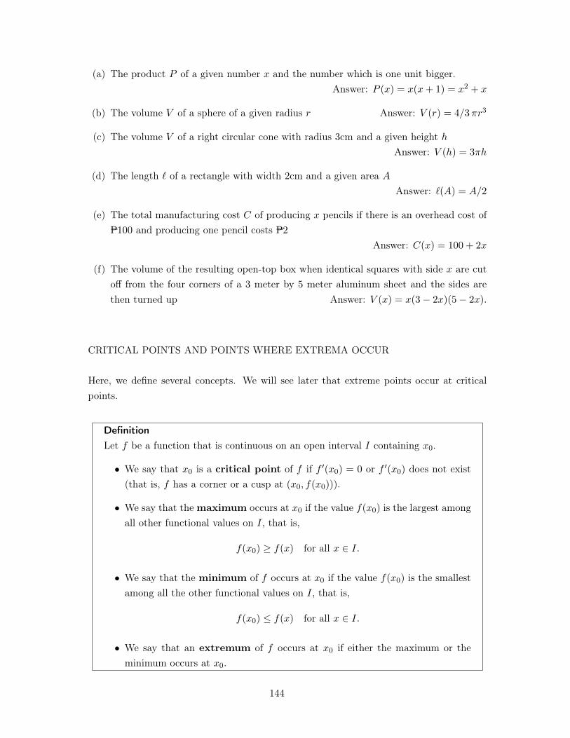
(a) The product P of a given number x and the number which is one unit bigger.. Answer: P (x) = x(x+ 1) = x2 + x
(b) The volume V of a sphere of a given radius r . Answer: V (r) = 4/3⇡r3
(c) The volume V of a right circular cone with radius 3cm and a given height h
. Answer: V (h) = 3⇡h
(d) The length ` of a rectangle with width 2cm and a given area A
. Answer: `(A) = A/2
(e) The total manufacturing cost C of producing x pencils if there is an overhead cost ofP100 and producing one pencil costs P2. Answer: C(x) = 100 + 2x
(f) The volume of the resulting open-top box when identical squares with side x are cutoff from the four corners of a 3 meter by 5 meter aluminum sheet and the sides arethen turned up . Answer: V (x) = x(3� 2x)(5� 2x).
CRITICAL POINTS AND POINTS WHERE EXTREMA OCCUR
Here, we define several concepts. We will see later that extreme points occur at criticalpoints.
DefinitionLet f be a function that is continuous on an open interval I containing x
0
.
• We say that x0
is a critical point of f if f 0(x
0
) = 0 or f 0(x
0
) does not exist(that is, f has a corner or a cusp at (x
0
, f(x0
))).
• We say that the maximum occurs at x0
if the value f(x0
) is the largest amongall other functional values on I, that is,
f(x0
) � f(x) for all x 2 I.
• We say that the minimum of f occurs at x0
if the value f(x0
) is the smallestamong all the other functional values on I, that is,
f(x0
) f(x) for all x 2 I.
• We say that an extremum of f occurs at x0
if either the maximum or theminimum occurs at x
0
.
144
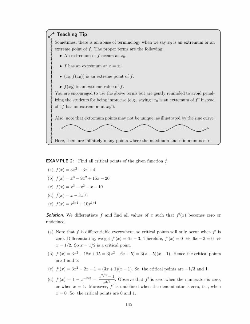
Teaching Tip
Sometimes, there is an abuse of terminology when we say x0
is an extremum or anextreme point of f . The proper terms are the following:
• An extremum of f occurs at x0
.
• f has an extremum at x = x0
• (x0
, f(x0
)) is an extreme point of f .
• f(x0
) is an extreme value of f .You are encouraged to use the above terms but are gently reminded to avoid penal-izing the students for being imprecise (e.g., saying “x
0
is an extremum of f ” insteadof “f has an extremum at x
0
”).
Also, note that extremum points may not be unique, as illustrated by the sine curve:
Here, there are infinitely many points where the maximum and minimum occur.
EXAMPLE 2: Find all critical points of the given function f .
(a) f(x) = 3x2 � 3x+ 4
(b) f(x) = x3 � 9x2 + 15x� 20
(c) f(x) = x3 � x2 � x� 10
(d) f(x) = x� 3x1/3
(e) f(x) = x5/4 + 10x1/4
Solution. We differentiate f and find all values of x such that f 0(x) becomes zero or
undefined.
(a) Note that f is differentiable everywhere, so critical points will only occur when f 0 iszero. Differentiating, we get f 0
(x) = 6x� 3. Therefore, f 0(x) = 0 , 6x� 3 = 0 ,
x = 1/2. So x = 1/2 is a critical point.
(b) f 0(x) = 3x2 � 18x+ 15 = 3(x2 � 6x+ 5) = 3(x� 5)(x� 1). Hence the critical points
are 1 and 5.
(c) f 0(x) = 3x2 � 2x� 1 = (3x+ 1)(x� 1). So, the critical points are �1/3 and 1.
(d) f 0(x) = 1 � x�2/3
=
x2/3 � 1
x2/3. Observe that f 0 is zero when the numerator is zero,
or when x = 1. Moreover, f 0 is undefined when the denominator is zero, i.e., whenx = 0. So, the critical points are 0 and 1.
145
(e) f 0(x) =
5
4
x1/4 +10
4
x�3/4=
5(x+ 2)
4x3/4. Note that the domain of f is [0,1); therefore
�2 cannot be a critical point. The only critical point is 0.
.
FERMAT’S THEOREM AND THE EXTREME VALUE THEOREM
We now discuss the theory behind optimization using calculus. The first gives a relationshipbetween the critical points and extremum points. The second is a guarantee that a problemhas extreme points. We will illustrate the theorems by graphs.
Theorem 7 (Fermat’s Theorem). Let f be continuous on an open interval I containingx0
. If f has an extremum at x0
, then x0
must be a critical point of f .
To illustrate this, recall that the derivative of f at x0
is the slope of the tangent line of fat x
0
.
Teaching Tip
Draw several graphs of smooth curves and let the class deduce that the extremepoints are where there is a horizontal tangent line (the slope of the tangent line is 0).Then, cross-reference this to the definition of a critical point when f is differentiable(f 0
(x0
) = 0).
Also, there are points where f may not be differentiable. So, we also have to checkthose points where f 0 does not exist. This is still part of the definition of a criticalpoint.
Theorem 8 (Extreme Value Theorem). Let f be a function which is continuous on a closedand bounded interval [a, b]. Then the extreme values (maximum and minimum) of f alwaysexist, and they occur either at the endpoints or at the critical points of f .
146
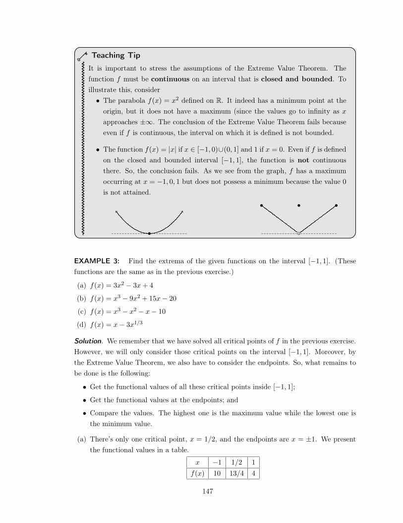
Teaching Tip
It is important to stress the assumptions of the Extreme Value Theorem. Thefunction f must be continuous on an interval that is closed and bounded. Toillustrate this, consider
• The parabola f(x) = x2 defined on R. It indeed has a minimum point at theorigin, but it does not have a maximum (since the values go to infinity as x
approaches ±1. The conclusion of the Extreme Value Theorem fails becauseeven if f is continuous, the interval on which it is defined is not bounded.
• The function f(x) = |x| if x 2 [�1, 0)[(0, 1] and 1 if x = 0. Even if f is definedon the closed and bounded interval [�1, 1], the function is not continuousthere. So, the conclusion fails. As we see from the graph, f has a maximumoccurring at x = �1, 0, 1 but does not possess a minimum because the value 0
is not attained.
EXAMPLE 3: Find the extrema of the given functions on the interval [�1, 1]. (Thesefunctions are the same as in the previous exercise.)
(a) f(x) = 3x2 � 3x+ 4
(b) f(x) = x3 � 9x2 + 15x� 20
(c) f(x) = x3 � x2 � x� 10
(d) f(x) = x� 3x1/3
Solution. We remember that we have solved all critical points of f in the previous exercise.However, we will only consider those critical points on the interval [�1, 1]. Moreover, bythe Extreme Value Theorem, we also have to consider the endpoints. So, what remains tobe done is the following:
• Get the functional values of all these critical points inside [�1, 1];
• Get the functional values at the endpoints; and
• Compare the values. The highest one is the maximum value while the lowest one isthe minimum value.
(a) There’s only one critical point, x = 1/2, and the endpoints are x = ±1. We presentthe functional values in a table.
x �1 1/2 1
f(x) 10 13/4 4
147
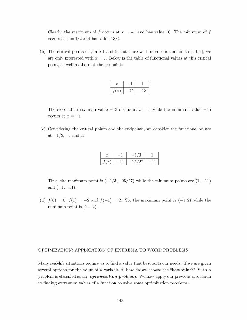
Clearly, the maximum of f occurs at x = �1 and has value 10. The minimum of foccurs at x = 1/2 and has value 13/4.
(b) The critical points of f are 1 and 5, but since we limited our domain to [�1, 1], weare only interested with x = 1. Below is the table of functional values at this criticalpoint, as well as those at the endpoints.
x �1 1
f(x) �45 �13
Therefore, the maximum value �13 occurs at x = 1 while the minimum value �45
occurs at x = �1.
(c) Considering the critical points and the endpoints, we consider the functional valuesat �1/3,�1 and 1:
x �1 �1/3 1
f(x) �11 �25/27 �11
Thus, the maximum point is (�1/3,�25/27) while the minimum points are (1,�11)
and (�1,�11).
(d) f(0) = 0, f(1) = �2 and f(�1) = 2. So, the maximum point is (�1, 2) while theminimum point is (1,�2).
.
OPTIMIZATION: APPLICATION OF EXTREMA TO WORD PROBLEMS
Many real-life situations require us to find a value that best suits our needs. If we are givenseveral options for the value of a variable x, how do we choose the “best value?” Such aproblem is classified as an optimization problem . We now apply our previous discussionto finding extremum values of a function to solve some optimization problems.
148
Suggested Steps in Solving Optimization Problems
1. If possible, draw a diagram of the problem.
2. Assign variables to all unknown quantities involved.
3. Specify the objective function. This function must be continuous.
i. Identify the quantity, say q, to be maximized or minimized.
ii. Formulate an equation involving q and other quantities. Express q in termsof a single variable, say x. If necessary, use the information given and rela-tionships between quantities to eliminate some variables.
iii. The objective function is
maximize q = f(x)
or minimize q = f(x).
4. Determine the domain or constraints of q from the physical restrictions of theproblem. The domain must be a closed and bounded interval.
5. Use appropriate theorems involving extrema to solve the problem. Make sureto give the exact answer (with appropriate units) to the question.
EXAMPLE 4: Find the number in the interval [�2, 2] so that the difference of the numberfrom its square is maximized.
Solution. Let x be the desired number. We want to maximize
f(x) = x2 � x
where x 2 [�2, 2]. Note that f is continuous on [�2, 2] and thus, we can apply the ExtremeValue Theorem.
We first find the critical numbers of f in the interval (�2, 2). We have
f 0(x) = 2x� 1,
which means that we only have one critical number in (�2, 2): x =
1
2
.
Then we compare the function value at the critical number and the endpoints. We see that
f(�2) = 6, f(2) = 2, f
✓1
2
◆= �1
4
.
From this, we conclude that f attains a maximum on [�2, 2] at the left endpoint x = �2.Hence, the number we are looking for is �2. .
149
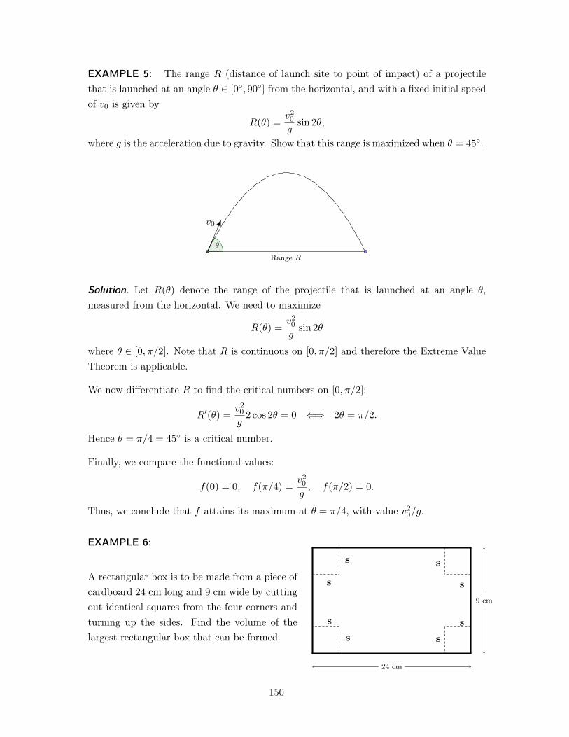
EXAMPLE 5: The range R (distance of launch site to point of impact) of a projectilethat is launched at an angle ✓ 2 [0
�, 90�] from the horizontal, and with a fixed initial speedof v
0
is given by
R(✓) =v20
gsin 2✓,
where g is the acceleration due to gravity. Show that this range is maximized when ✓ = 45
�.
v0
✓
Range R
Solution. Let R(✓) denote the range of the projectile that is launched at an angle ✓,measured from the horizontal. We need to maximize
R(✓) =v20
gsin 2✓
where ✓ 2 [0,⇡/2]. Note that R is continuous on [0,⇡/2] and therefore the Extreme ValueTheorem is applicable.
We now differentiate R to find the critical numbers on [0,⇡/2]:
R0(✓) =
v20
g2 cos 2✓ = 0 () 2✓ = ⇡/2.
Hence ✓ = ⇡/4 = 45
� is a critical number.
Finally, we compare the functional values:
f(0) = 0, f(⇡/4) =v20
g, f(⇡/2) = 0.
Thus, we conclude that f attains its maximum at ✓ = ⇡/4, with value v20
/g. .
EXAMPLE 6:
A rectangular box is to be made from a piece ofcardboard 24 cm long and 9 cm wide by cuttingout identical squares from the four corners andturning up the sides. Find the volume of thelargest rectangular box that can be formed.
s
s
sss
s
s
s
24 cm
9 cm
150
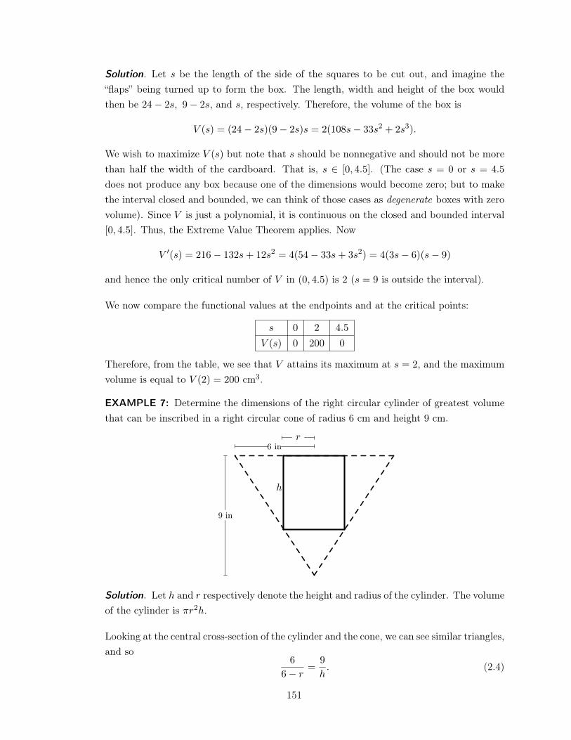
Solution. Let s be the length of the side of the squares to be cut out, and imagine the“flaps” being turned up to form the box. The length, width and height of the box wouldthen be 24� 2s, 9� 2s, and s, respectively. Therefore, the volume of the box is
V (s) = (24� 2s)(9� 2s)s = 2(108s� 33s2 + 2s3).
We wish to maximize V (s) but note that s should be nonnegative and should not be morethan half the width of the cardboard. That is, s 2 [0, 4.5]. (The case s = 0 or s = 4.5
does not produce any box because one of the dimensions would become zero; but to makethe interval closed and bounded, we can think of those cases as degenerate boxes with zerovolume). Since V is just a polynomial, it is continuous on the closed and bounded interval[0, 4.5]. Thus, the Extreme Value Theorem applies. Now
V 0(s) = 216� 132s+ 12s2 = 4(54� 33s+ 3s2) = 4(3s� 6)(s� 9)
and hence the only critical number of V in (0, 4.5) is 2 (s = 9 is outside the interval).
We now compare the functional values at the endpoints and at the critical points:
s 0 2 4.5
V (s) 0 200 0
Therefore, from the table, we see that V attains its maximum at s = 2, and the maximumvolume is equal to V (2) = 200 cm3. .
EXAMPLE 7: Determine the dimensions of the right circular cylinder of greatest volumethat can be inscribed in a right circular cone of radius 6 cm and height 9 cm.
h
6 in
9 in
r
Solution. Let h and r respectively denote the height and radius of the cylinder. The volumeof the cylinder is ⇡r2h.
Looking at the central cross-section of the cylinder and the cone, we can see similar triangles,and so
6
6� r=
9
h. (2.4)
151
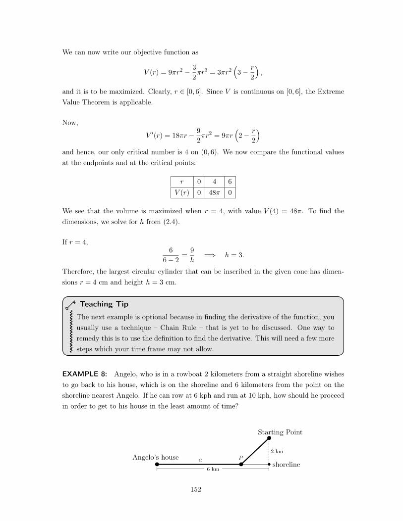
We can now write our objective function as
V (r) = 9⇡r2 � 3
2
⇡r3 = 3⇡r2⇣3� r
2
⌘,
and it is to be maximized. Clearly, r 2 [0, 6]. Since V is continuous on [0, 6], the ExtremeValue Theorem is applicable.
Now,
V 0(r) = 18⇡r � 9
2
⇡r2 = 9⇡r⇣2� r
2
⌘
and hence, our only critical number is 4 on (0, 6). We now compare the functional valuesat the endpoints and at the critical points:
r 0 4 6
V (r) 0 48⇡ 0
We see that the volume is maximized when r = 4, with value V (4) = 48⇡. To find thedimensions, we solve for h from (2.4).
If r = 4,6
6� 2
=
9
h=) h = 3.
Therefore, the largest circular cylinder that can be inscribed in the given cone has dimen-sions r = 4 cm and height h = 3 cm. .
Teaching Tip
The next example is optional because in finding the derivative of the function, youusually use a technique – Chain Rule – that is yet to be discussed. One way toremedy this is to use the definition to find the derivative. This will need a few moresteps which your time frame may not allow.
EXAMPLE 8: Angelo, who is in a rowboat 2 kilometers from a straight shoreline wishesto go back to his house, which is on the shoreline and 6 kilometers from the point on theshoreline nearest Angelo. If he can row at 6 kph and run at 10 kph, how should he proceedin order to get to his house in the least amount of time?
shorelineAngelo’s house
Starting Point
P
6 km
2 km
c
152
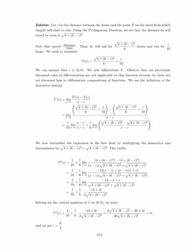
Solution. Let c be the distance between the house and the point P on the shore from whichAngelo will start to run. Using the Pythagorean Theorem, we see that the distance he willtravel by boat is
p4 + (6� c)2.
Note that speed=distancetime . Thus, he will sail for
p4 + (6� c)2
6
hours and run forc
10
hours. We wish to minimize
T (c) =
p4 + (6� c)2
6
+
c
10
.
We can assume that c 2 [0, 6]. We now differentiate T . Observe that our previouslydiscussed rules of differentiation are not applicable to this function because we have notyet discussed how to differentiate compositions of functions. We use the definition of thederivative instead.
T 0(c) = lim
x!c
T (x)� T (c)
x� c
= lim
x!c
p4 + (6� x)2
6
+
x
10
!� p
4 + (6� c)2
6
+
c
10
!
x� c
=
1
10
lim
x!c
x� c
x� c+
1
6
lim
x!c
p4 + (6� x)2 �
p4 + (6� c)2
x� c
!.
We now rationalize the expression in the first limit by multiplying the numerator anddenominator by
p4 + (6� x)2 +
p4 + (6� c)2. This yields:
T 0(c) =
1
10
+
1
6
lim
x!c
(4 + (6� x)2)� (4 + (6� c)2)
(x� c)(p4 + (6� x)2 +
p4 + (6� c)2
=
1
10
+
1
6
lim
x!c
�12(x� c) + (x� c)(x+ c)
(x� c)(p4 + (6� x)2 +
p4 + (6� c)2)
=
1
10
+
1
6
lim
x!c
�12 + x+ cp4 + (6� x)2 +
p4 + (6� c)2
=
1
10
+
1
6
· �12 + 2c
2
p4 + (6� c)2
.
Solving for the critical numbers of f on (0, 6), we solve
T 0(c) =
1
10
+
1
6
· �12 + 2c
2
p4 + (6� c)2
=
3
p4 + (6� c)2 � 30 + 5c
30
p4 + (6� c)2
= 0,
and we get c =9
2
.
153
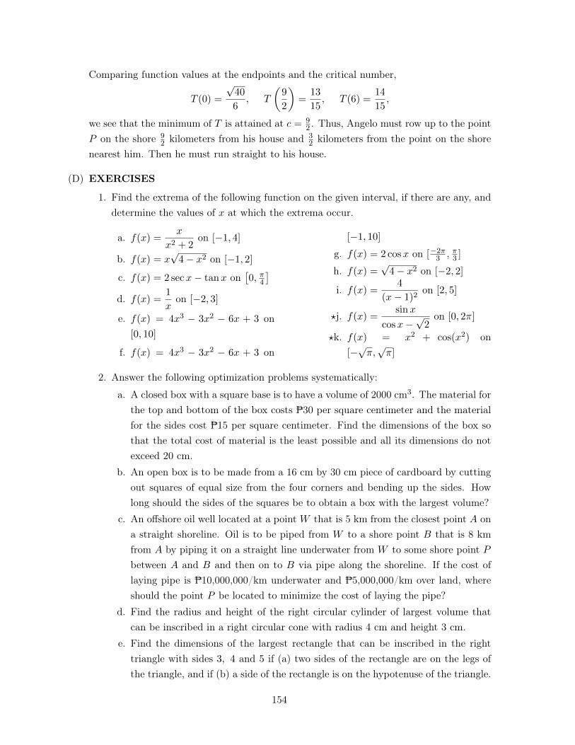
Comparing function values at the endpoints and the critical number,
T (0) =
p40
6
, T
✓9
2
◆=
13
15
, T (6) =14
15
,
we see that the minimum of T is attained at c = 9
2
. Thus, Angelo must row up to the pointP on the shore 9
2
kilometers from his house and 3
2
kilometers from the point on the shorenearest him. Then he must run straight to his house. .
(D) EXERCISES
1. Find the extrema of the following function on the given interval, if there are any, anddetermine the values of x at which the extrema occur.
a. f(x) =x
x2 + 2
on [�1, 4]
b. f(x) = xp4� x2 on [�1, 2]
c. f(x) = 2 secx� tanx on⇥0, ⇡
4
⇤
d. f(x) =1
xon [�2, 3]
e. f(x) = 4x3 � 3x2 � 6x + 3 on[0, 10]
f. f(x) = 4x3 � 3x2 � 6x + 3 on
[�1, 10]
g. f(x) = 2 cosx on [
�2⇡3
, ⇡3
]
h. f(x) =p4� x2 on [�2, 2]
i. f(x) =4
(x� 1)
2
on [2, 5]
?j. f(x) =sinx
cosx�p2
on [0, 2⇡]
?k. f(x) = x2 + cos(x2) on[�
p⇡,
p⇡]
2. Answer the following optimization problems systematically:
a. A closed box with a square base is to have a volume of 2000 cm3. The material forthe top and bottom of the box costs P30 per square centimeter and the materialfor the sides cost P15 per square centimeter. Find the dimensions of the box sothat the total cost of material is the least possible and all its dimensions do notexceed 20 cm.
b. An open box is to be made from a 16 cm by 30 cm piece of cardboard by cuttingout squares of equal size from the four corners and bending up the sides. Howlong should the sides of the squares be to obtain a box with the largest volume?
c. An offshore oil well located at a point W that is 5 km from the closest point A ona straight shoreline. Oil is to be piped from W to a shore point B that is 8 kmfrom A by piping it on a straight line underwater from W to some shore point P
between A and B and then on to B via pipe along the shoreline. If the cost oflaying pipe is P10,000,000/km underwater and P5,000,000/km over land, whereshould the point P be located to minimize the cost of laying the pipe?
d. Find the radius and height of the right circular cylinder of largest volume thatcan be inscribed in a right circular cone with radius 4 cm and height 3 cm.
e. Find the dimensions of the largest rectangle that can be inscribed in the righttriangle with sides 3, 4 and 5 if (a) two sides of the rectangle are on the legs ofthe triangle, and if (b) a side of the rectangle is on the hypotenuse of the triangle.
154
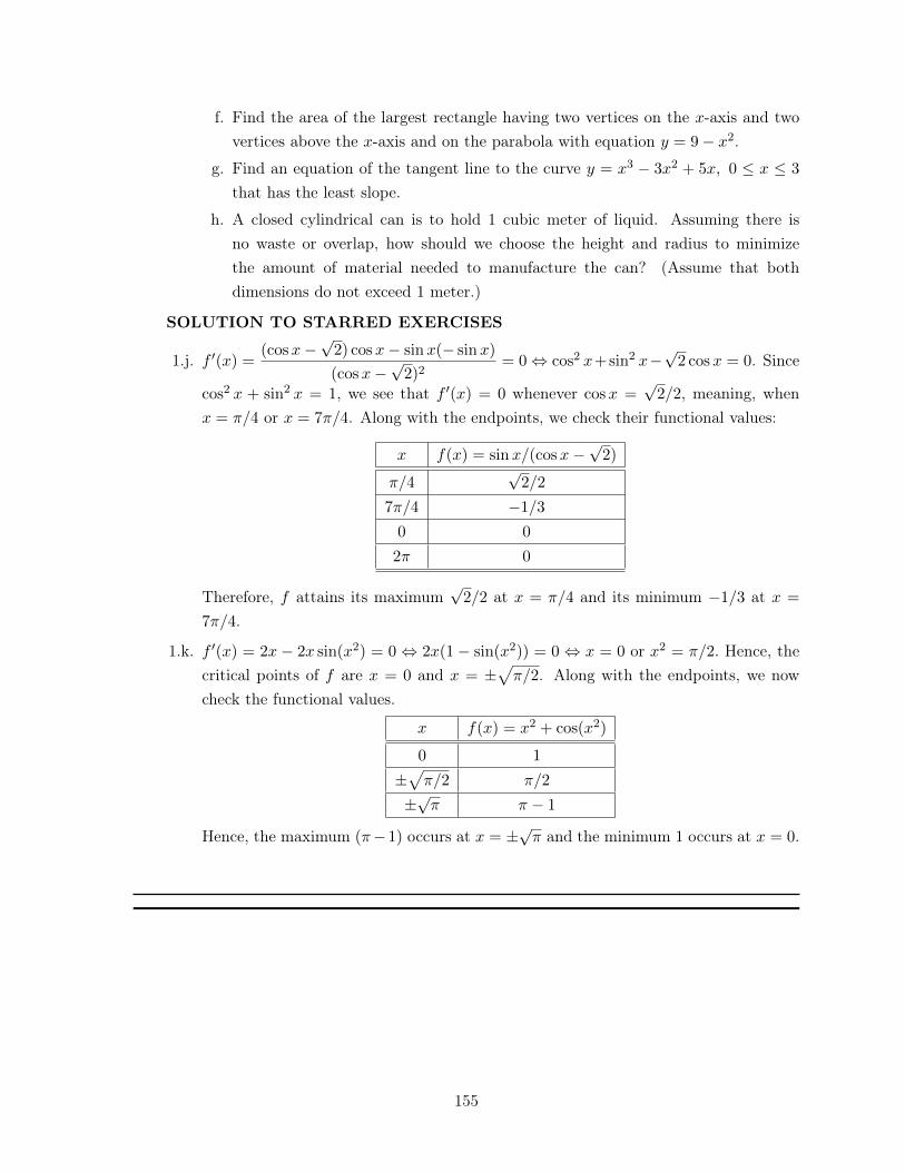
f. Find the area of the largest rectangle having two vertices on the x-axis and twovertices above the x-axis and on the parabola with equation y = 9� x2.
g. Find an equation of the tangent line to the curve y = x3 � 3x2 + 5x, 0 x 3
that has the least slope.
h. A closed cylindrical can is to hold 1 cubic meter of liquid. Assuming there isno waste or overlap, how should we choose the height and radius to minimizethe amount of material needed to manufacture the can? (Assume that bothdimensions do not exceed 1 meter.)
SOLUTION TO STARRED EXERCISES
1.j. f 0(x) =
(cosx�p2) cosx� sinx(� sinx)
(cosx�p2)
2
= 0 , cos
2 x+sin
2 x�p2 cosx = 0. Since
cos
2 x + sin
2 x = 1, we see that f 0(x) = 0 whenever cosx =
p2/2, meaning, when
x = ⇡/4 or x = 7⇡/4. Along with the endpoints, we check their functional values:
x f(x) = sinx/(cosx�p2)
⇡/4p2/2
7⇡/4 �1/3
0 0
2⇡ 0
Therefore, f attains its maximump2/2 at x = ⇡/4 and its minimum �1/3 at x =
7⇡/4.
1.k. f 0(x) = 2x � 2x sin(x2) = 0 , 2x(1� sin(x2)) = 0 , x = 0 or x2 = ⇡/2. Hence, the
critical points of f are x = 0 and x = ±p⇡/2. Along with the endpoints, we now
check the functional values.
x f(x) = x2 + cos(x2)
0 1
±p
⇡/2 ⇡/2
±p⇡ ⇡ � 1
Hence, the maximum (⇡�1) occurs at x = ±p⇡ and the minimum 1 occurs at x = 0.
155
LESSON 8: Higher-Order Derivatives and the Chain Rule
TIME FRAME: 4 hours
LEARNING OUTCOMES: At the end of the lesson, the learner shall be able to:
1. Compute higher-order derivatives of functions;2. Illustrate the Chain Rule of differentiation; and3. Solve problems using the Chain Rule.
LESSON OUTLINE:
1. Definition of higher order derivatives2. Examples on computing higher order derivatives3. The Chain Rule4. Examples and problems
156
TOPIC 8.1: Higher-Order Derivatives of Functions
DEVELOPMENT OF THE LESSON
(A) INTRODUCTION
Consider the polynomial function f(x) = x4 + 3x3 � 4x+ 2. Its derivative,
f 0(x) = 4x3 + 9x2 � 4,
is again differentiable. Therefore, we may still differentiate f 0 to get
(f 0)
0(x) = f 00
(x) = 12x2 + 18x.
This is again another differentiable function. We call f 00 and its subsequent derivativesthe higher-order derivatives of f . Like f 0, which we interpret as the slope of the tangentline, the function f 00 will have an interpretation on the graph of f (This will be a lesson incollege). It also has an important interpretation in physics if f denotes the displacementof a particle. For now, this lesson will reinforce our skills in differentiating functions.
(B) LESSON PROPER
Consider the function y = f(x). The derivative y0, f 0(x), Dxy or
dy
dxis called the first
derivative of f with respect to x. The derivative of the first derivative is called the secondderivative of f with respect to x and is denoted by any of the following symbols:
y00 , f 00(x) , D2
x y ,d2y
dx2
The third derivative of f with respect to x is the derivative of the second derivative andis denoted by any of the following symbols:
y000 , f 000(x) , D3
x y ,d3y
dx3
In general, the nthderivative of f with respect to x is the derivative of the (n � 1)
st
derivative and is denoted by any of the following symbols:
y(n) , f (n)(x) , Dn
x y ,dny
dxn
Formally, we have the following definition.
Definition 4. The nthderivative of the function f is defined recursively by
f 0(x) = lim
�x!0
f(x+�x)� f(x)
�xfor n = 1, and
157
f (n)(x) = lim
�x!0
f (n�1)
(x+�x)� f (n�1)
(x)
�xfor n > 1,
provided that these limits exist. Thus, the nth derivative of f is just the derivative of the(n� 1)
st derivative of f .
Remark 1:
(a) The function f can be written as f (0)
(x).
(b) In the notation f (n)(x), n is called the order of the derivative.
EXAMPLE 1:
1. Find the fourth derivative of the function f(x) = x5 � 3x4 + 2x3 � x2 + 4x� 10.
Solution. We differentiate the function repeatedly and obtain
f 0(x) = 5x4 � 12x3 + 6x2 � 2x+ 4
f 00(x) = 20x3 � 36x2 + 12x� 2
f 000(x) = 60x2 � 72x+ 12
f (4)
(x) = 120x� 72.
.
2. Find the first and second derivatives of the function defined by
y = (3x2 � 4)(x2 � 3x).
Solution. Using the Product Rule, we compute the first derivative:
y0 = (3x2 � 4)Dx(x2 � 3x) + (x2 � 3x)Dx(3x
2 � 4)
= (3x2 � 4)(2x� 3) + (x2 � 3x)(6x)
= 6x3 � 9x2 � 8x+ 12 + 6x3 � 18x2
= 12x3 � 27x2 � 8x+ 12.
Similarly, we obtain the second derivative:
y00 = Dx(12x3 � 27x2 � 8x+ 12)
= 36x2 � 54x� 8.
.
158
3. Let y =
3x+ 5
x2 + 4
. Findd2y
dx2.
Solution. Using the Quotient Rule twice, we have
dy
dx=
(x2 + 4)Dx(3x+ 5)� (3x+ 5)Dx(x2 + 4)
(x2 + 4)
2
=
(x2 + 4)(3)� (3x+ 5)(2x)
(x2 + 4)
2
=
3x2 + 12� 6x2 � 10x
(x2 + 4)
2
=
12� 10x� 3x2
(x2 + 4)
2
,
and
d2y
dx2=
d
dx
✓12� 10x� 3x2
(x2 + 4)
2
◆
=
d
dx
✓12� 10x� 3x2
x4 + 8x2 + 16
◆
=
(x4 + 8x2 + 16)
d
dx(12� 10x� 3x2)� (12� 10x� 3x2)
d
dx(x4 + 8x2 + 16)
(x4 + 8x2 + 16)
2
=
(x4 + 8x2 + 16)(�10� 6x)� (12� 10x� 3x2)(4x3 + 16x)
(x4 + 8x2 + 16)
2
=
6x5 + 30x4 � 48x3 + 80x2 � 288x� 160
(x4 + 8x2 + 16)
2
.
.
4. Find the third derivative of the function defined by g(x) = �4x2ex + 5xex � 10ex.
Solution. We differentiate repeatedly (applying the Product Rule) and obtain
g(1)(x) = [(�4x2)(ex) + (ex)(�8x)] + [(5x)(ex) + (ex)(5)� 10 · ex]
= �4x2ex � 3xex � 5ex
= ex(�4x2 � 3x� 5).
g(2)(x) = (ex)(�8x� 3) + (�4x2 � 3x� 5)(ex)
= ex(�4x2 � 11x� 8).
g(3)(x) = (ex)(�8x� 11) + (�4x2 � 11x� 8)(ex)
= ex(�4x2 � 19x� 19).
159
.
5. If f(x) = ex sinx� 3ex cosx, find f (5)
(x).
Solution. We differentiate repeatedly (applying the Product Rule) and obtain
f (1)
(x) = [(ex)(cosx) + (sinx)(ex)]� 3 · [(ex)(� sinx) + (cosx)(ex)]
= ex cosx+ ex sinx+ 3ex sinx� 3ex cosx
= ex(4 sinx� 2 cosx).
f (2)
(x) = ex[4(cosx)� 2(� sinx)] + (4 sinx� 2 cosx)(ex)
= ex(2 cosx+ 6 sinx).
f (3)
(x) = ex[2(� sinx) + 6(cosx)] + (2 cosx+ 6 sinx)(ex)
= ex(8 cosx+ 4 sinx).
f (4)
(x) = ex[8(� sinx) + 4(cosx)] + (8 cosx+ 4 sinx)(ex)
= ex(12 cosx� 4 sinx).
f (5)
(x) = ex[12(� sinx)� 4(cosx)] + (12 cosx� 4 sinx)(ex)
= ex(8 cosx� 16 sinx).
.
(C) EXERCISES
1. Find y0, y00, y000, and y0000 for the following expressions:
a. y = x4
b. y = x�7
c. y = x227
d. y = x�13
e. y = x3.2
f. y = x�3.5
2. Find the first and second derivatives of the following:
a. y = xpx
b. f(u) =1
u3
c. f(t) = 3pt
d. g(x) =1
x2px
e. k(t) =t
t2pt
f. h(s) =s3ps
3ps
160
3. If f(x) = 6x5 � 5x4 + 3x3 � 7x2 + 9x� 14, then find f (n)(x) for all n 2 N.
4. Find f 0⇣⇡6
⌘, f 00
⇣⇡6
⌘, and f 000
⇣⇡6
⌘, given f(x) = � sinx.
5. If g(x) = sinx, then find g(n)(x) for all n 2 N.
6. Find f (5)
(x) if f(x) = 3p3x+ 2.
?7. Find D55
x (cosx) and D56
x (cosx).
Answer: D55
x (cosx) = sinx and D56
x (cosx) = cosx
?8. Find f (n)(x) for all n 2 N where f(x) = e�x. (Hint: Write f(x) as a quotient.)
Answer: f (n)(x) = �e�x if n is odd while f (n)
(x) = e�x when n is even.
?9. Let p(x) be a polynomial of degree n with leading coefficient 1. What is p(k)(x) if (a)k = n; and if (b) k > n.
Answer: (a) n!; (b) 0
161
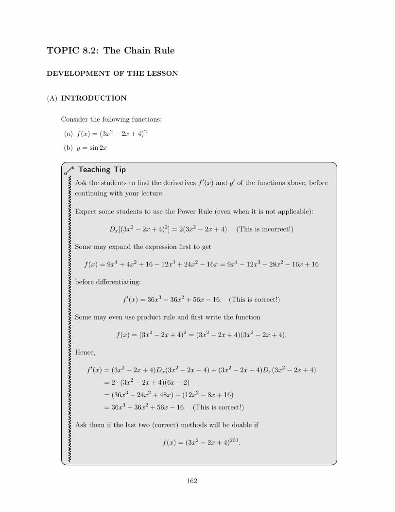
TOPIC 8.2: The Chain Rule
DEVELOPMENT OF THE LESSON
(A) INTRODUCTION
Consider the following functions:
(a) f(x) = (3x2 � 2x+ 4)
2
(b) y = sin 2x
Teaching Tip
Ask the students to find the derivatives f 0(x) and y0 of the functions above, before
continuing with your lecture.
Expect some students to use the Power Rule (even when it is not applicable):
Dx[(3x2 � 2x+ 4)
2
] = 2(3x2 � 2x+ 4). (This is incorrect!)
Some may expand the expression first to get
f(x) = 9x4 + 4x2 + 16� 12x3 + 24x2 � 16x = 9x4 � 12x3 + 28x2 � 16x+ 16
before differentiating:
f 0(x) = 36x3 � 36x2 + 56x� 16. (This is correct!)
Some may even use product rule and first write the function
f(x) = (3x2 � 2x+ 4)
2
= (3x2 � 2x+ 4)(3x2 � 2x+ 4).
Hence,
f 0(x) = (3x2 � 2x+ 4)Dx(3x
2 � 2x+ 4) + (3x2 � 2x+ 4)Dx(3x2 � 2x+ 4)
= 2 · (3x2 � 2x+ 4)(6x� 2)
= (36x3 � 24x2 + 48x)� (12x2 � 8x+ 16)
= 36x3 � 36x2 + 56x� 16. (This is correct!)
Ask them if the last two (correct) methods will be doable if
f(x) = (3x2 � 2x+ 4)
200.
162
On the other hand, for the function y = sin 2x, some of them may have used a trigonometricidentity to first rewrite y into
y = sin 2x = 2 sinx cosx.
In this case
y0 = 2[(sinx)(� sinx) + (cosx)(cosx)]
= 2(cos
2 x� sin
2 x)
= 2 cos(2x).
In this lesson students will learn a rule that will allow them to differentiate a given functionwithout having to perform any preliminary multiplication, or apply any special formula.
(B) LESSON PROPER
The Chain Rule below provides for a formula for the derivative of a composition of functions.
Theorem 9 (Chain Rule). Let f be a function differentiable at c and let g be a functiondifferentiable at f(c). Then the composition g � f is differentiable at c and
Dx(g � f)(c) = g0(f(c)) · f 0(c).
Remark 1: Another way to state the Chain Rule is the following: If y is a differentiablefunction of u defined by y = f(u) and u is a differentiable function of x defined by u = g(x),then y is a differentiable function of x, and the derivative of y with respect to x is given by
dy
dx=
dy
du· dudx
.
In words, the derivative of a composition of functions is the derivative of the outer functionevaluated at the inner function, times the derivative of the inner function.
EXAMPLE 1:
(a) Recall our first illustration f(x) = (3x2 � 2x+ 4)
2. Find f 0(x) using the Chain Rule.
Solution. We can rewrite y = f(x) = (3x2 � 2x + 4)
2 as y = f(u) = u2 whereu = 3x2 � 2x+ 4, a differentiable function of x. Using the Chain Rule, we have
f 0(x) = y0 =
dy
du· dudx
= (2u)(6x� 2)
= 2(3x2 � 2x+ 4)(6x� 2)
= 36x3 � 36x2 + 56x� 16.
.
163
(b) For the second illustration, we have y = sin(2x). Find y0 using the Chain Rule.
Solution. We can rewrite y = sin(2x) as y = f(u) where f(u) = sinu and u = 2x.Hence,
y0 =
dy
du· dudx
= cosu · 2
= 2 cos(2x).
.
(c) Finddz
dyif z =
4
(a2 � y2)2, where a is a real number.
Solution. Notice that we can write z =
4
(a2 � y2)2as z = 4(a2 � y2)�2. Applying
the Chain Rule, we have
dz
dy= 4 ·�2(a2 � y2)�2�1 · d
dy(a2 � y2)
= �8(a2 � y2)�3 ·�2y
= 16y(a2 � y2)�3
=
16y
(a2 � y2)3.
.
Now, suppose we want to find the derivative of a power function of x. That is, we areinterested in Dx[f(x)n]. To derive a formula for this, we let y = un where u is a differentiablefunction of x given by u = f(x). Then by the Chain Rule,
dy
dx=
dy
du· dudx
= nun�1 · f 0(x)
= n[f(x)]n�1 · f 0(x)
Thus, Dx[f(x)]n = n[f(x)]n�1 · f 0(x). This is called the GENERALIZED POWER RULE.
EXAMPLE 2:
(a) What is the derivative of y = (3x2 + 4x� 5)
5
?
164
Solution.
Dx[(3x2
+ 4x� 5)
5
] = 5 · (3x2 + 4x� 5)
5�1 ·Dx(3x2
+ 4x� 5)
= 5(3x2 + 4x� 5)
4
(6x+ 4).
.
(b) Finddy
dxwhere y =
p3x3 + 4x+ 1.
Solution.
dy
dx=
1
2
(3x3 + 4x+ 1)
12�1Dx(3x
3
+ 4x+ 1)
=
1
2
(3x34x+ 1)
� 12(9x2 + 4)
=
9x2 + 4
2
p3x34x+ 1
.
.
(c) Finddy
dxwhere y = (sin 3x)2.
Solution.
dy
dx= 2 · (sin 3x)2�1 · d
dx(sin 3x)
= 2(sin 3x) · cos 3x · d
dx(3x)
= 2(sin 3x)(cos 3x) · 3
= 6 sin 3x cos 3x.
.
(d) Differentiate (3x2 � 5)
3.
Solution.
d(3x2 � 5)
3
dx= 3(3x2 � 5)
3�1 ·Dx(3x2 � 5)
= 3(3x2 � 5)
2 · 6x
= 18x(3x2 � 5)
2.
.
165
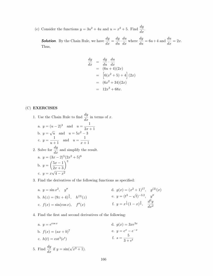
(e) Consider the functions y = 3u2 + 4u and u = x2 + 5. Finddy
dx.
Solution. By the Chain Rule, we havedy
dx=
dy
du· dudx
wheredy
du= 6u+4 and
du
dx= 2x.
Thus,
dy
dx=
dy
du· dudx
= (6u+ 4)(2x)
=
h6(x2 + 5) + 4
i(2x)
= (6x2 + 34)(2x)
= 12x3 + 68x.
.
(C) EXERCISES
1. Use the Chain Rule to finddy
dxin terms of x.
a. y = (u� 2)
3 and u =
1
2x+ 1
b. y =
pu and u = 5x2 � 3
c. y =
1
u+ 1
and u =
1
x+ 1
2. Solve fordy
dxand simplify the result.
a. y = (3x� 2)
5
(2x2 + 5)
6
b. y =
✓5x� 1
2x+ 3
◆3
c. y = xp4� x2
3. Find the derivatives of the following functions as specified:
a. y = sinx2, y00
b. h(z) = (9z + 4)
32 , h(3)(z)
c. f(x) = sin(cosx), f 00(x)
d. g(x) = (x2 + 1)
17, g(2)(x)
e. y = (t3 �pt)�3.2, y00
f. y = x13(1� x)
23 ,
d2y
dx2
4. Find the first and second derivatives of the following:
a. y = ecosx
b. f(x) = (ax+ b)7
c. h(t) = cot
3
(et)
d. g(x) = 3xe3x
e. y = ex � e�x
f. s =5
3 + et
5. Finddy
dxif y = sin(
px3 + 1).
166
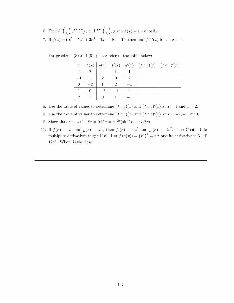
6. Find h0⇣⇡3
⌘, h00
�⇡3
�, and h000
⇣⇡3
⌘, given h(x) = sinx cos 3x.
7. If f(x) = 6x5 � 5x4 + 3x3 � 7x2 + 9x� 14, then find f (n)(x) for all x 2 N.
For problems (8) and (9), please refer to the table below:
x f(x) g(x) f 0(x) g0(x) (f � g)(x) (f � g)0(x)
�2 2 �1 1 1
�1 1 2 0 2
0 �2 1 2 �1
1 0 �2 �1 2
2 1 0 1 �1
8. Use the table of values to determine (f � g)(x) and (f � g)0(x) at x = 1 and x = 2.
9. Use the table of values to determine (f � g)(x) and (f � g)0(x) at x = �2,�1 and 0.
10. Show that z00 + 4z0 + 8z = 0 if z = e�2x(sin 2x+ cos 2x).
11. If f(x) = x4 and g(x) = x3, then f 0(x) = 4x3 and g0(x) = 3x2. The Chain Rule
multiplies derivatives to get 12x5. But f (g(x)) =�x3�4
= x12 and its derivative is NOT12x5. Where is the flaw?
167
LESSON 9: Implicit Differentiation
TIME FRAME: 2 hours
LEARNING OUTCOMES: At the end of the lesson, the learner shall be able to:
1. Illustrate implicit differentiation;2. Apply the derivatives of the natural logarithmic and inverse tangent functions; and3. Use implicit differentiation to solve problems.
LESSON OUTLINE:
1. What is implicit differentiation?2. The derivative of the natural logarithmic and inverse tangent functions3. Solving problems using implicit differentiation4. Enrichment: Derivatives of other transcendental functions
168
TOPIC 9.1: What is Implicit Differentiation?
DEVELOPMENT OF THE LESSON
(A) INTRODUCTION
The majority of differentiation problems in basic calculus involves functions y written ex-plicitly as functions of the independent variable x. This means that we can write thefunction in the form y = f(x). For such a function, we can find the derivative directly. Forexample, if
y = 4x5 + cos(2x� 7),
then the derivative of y with respect to x is
dy
dx= 20x4 � 2 sin(2x� 7).
However, some functions y are written implicitly as functions of x. This means that theexpression is not given directly in the form y = f(x). A familiar example of this is theequation
x2 + y2 = 5,
which represents a circle of radiusp5 with its center at the origin (0, 0). We can think of
the circle as the union of the graphs of two functions, namely the function represented bythe upper semi-circle and the function represented by the lower semi-circle. Suppose thatwe wish to find the slope of the line tangent to the circle at the point (�2, 1).
The solution is to find the the derivative at the point (�2, 1). Since the equation of thecircle is not complicated, one way to do this is to write y explicitly in terms of x. Thus,from x2 + y2 = 5, we obtain y = ±
p5� x2. The positive square root represents the upper
semi-circle while the negative square root represents the bottom semi-circle. Since thepoint (�2, 1) is on the upper semi-circle, the slope of the tangent line is now obtained bydifferentiating the function
y =
p5� x2 = (5� x2)1/2
and evaluating the derivative at x = �2. Thus, using the Chain Rule,
dy
dx=
1
2
(5� x2)�1/2(�2x) =
�xp5� x2
.
Therefore, the slope of the tangent line at the point (�2, 1) is the value of the abovederivative evaluated at x = �2, namely
dy
dx=
2p5� (�2)
2
=
2p1
= 2.
169
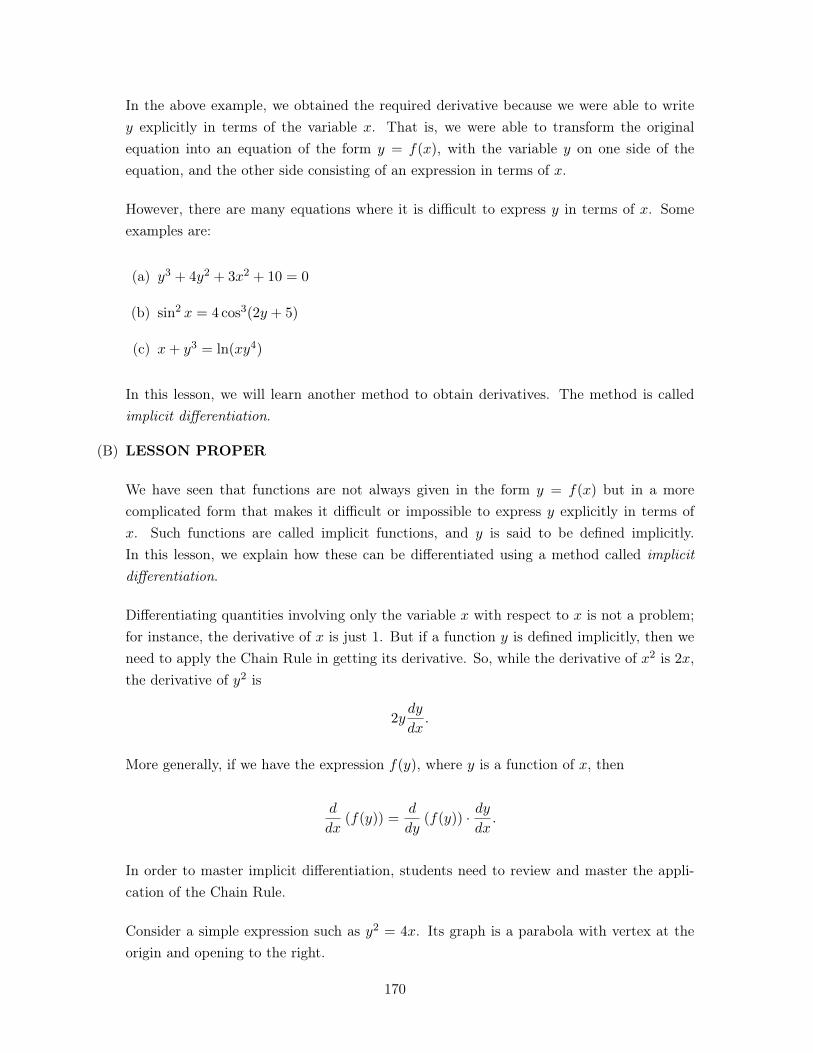
In the above example, we obtained the required derivative because we were able to writey explicitly in terms of the variable x. That is, we were able to transform the originalequation into an equation of the form y = f(x), with the variable y on one side of theequation, and the other side consisting of an expression in terms of x.
However, there are many equations where it is difficult to express y in terms of x. Someexamples are:
(a) y3 + 4y2 + 3x2 + 10 = 0
(b) sin
2 x = 4 cos
3
(2y + 5)
(c) x+ y3 = ln(xy4)
In this lesson, we will learn another method to obtain derivatives. The method is calledimplicit differentiation.
(B) LESSON PROPER
We have seen that functions are not always given in the form y = f(x) but in a morecomplicated form that makes it difficult or impossible to express y explicitly in terms ofx. Such functions are called implicit functions, and y is said to be defined implicitly.In this lesson, we explain how these can be differentiated using a method called implicitdifferentiation.
Differentiating quantities involving only the variable x with respect to x is not a problem;for instance, the derivative of x is just 1. But if a function y is defined implicitly, then weneed to apply the Chain Rule in getting its derivative. So, while the derivative of x2 is 2x,the derivative of y2 is
2ydy
dx.
More generally, if we have the expression f(y), where y is a function of x, then
d
dx(f(y)) =
d
dy(f(y)) · dy
dx.
In order to master implicit differentiation, students need to review and master the appli-cation of the Chain Rule.
Consider a simple expression such as y2 = 4x. Its graph is a parabola with vertex at theorigin and opening to the right.
170
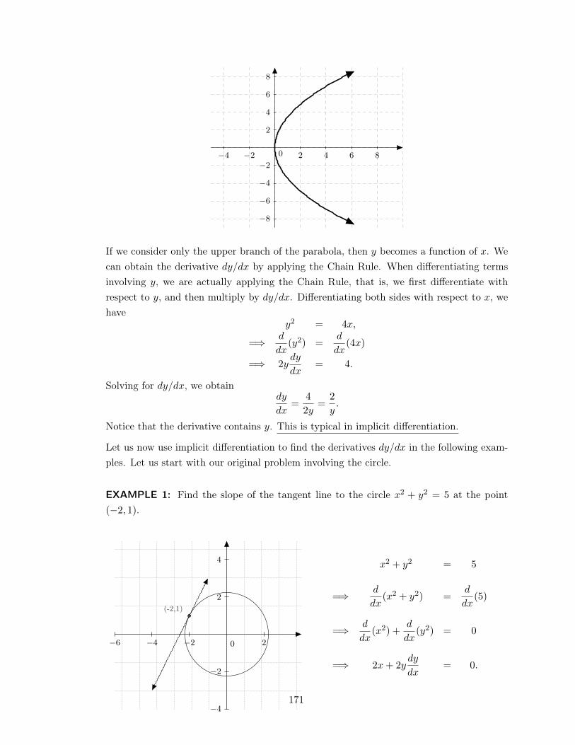
�4 �2 2 4 6 8
�8
�6
�4
�2
2
4
6
8
0
If we consider only the upper branch of the parabola, then y becomes a function of x. Wecan obtain the derivative dy/dx by applying the Chain Rule. When differentiating termsinvolving y, we are actually applying the Chain Rule, that is, we first differentiate withrespect to y, and then multiply by dy/dx. Differentiating both sides with respect to x, wehave
y2 = 4x,
=) d
dx(y2) =
d
dx(4x)
=) 2ydy
dx= 4.
Solving for dy/dx, we obtaindy
dx=
4
2y=
2
y.
Notice that the derivative contains y. This is typical in implicit differentiation.
Let us now use implicit differentiation to find the derivatives dy/dx in the following exam-ples. Let us start with our original problem involving the circle.
EXAMPLE 1: Find the slope of the tangent line to the circle x2 + y2 = 5 at the point(�2, 1).
�6 �4 �2 2
�4
�2
2
4
0
(-2,1)
x2 + y2 = 5
=) d
dx(x2 + y2) =
d
dx(5)
=) d
dx(x2) +
d
dx(y2) = 0
=) 2x+ 2ydy
dx= 0.
171
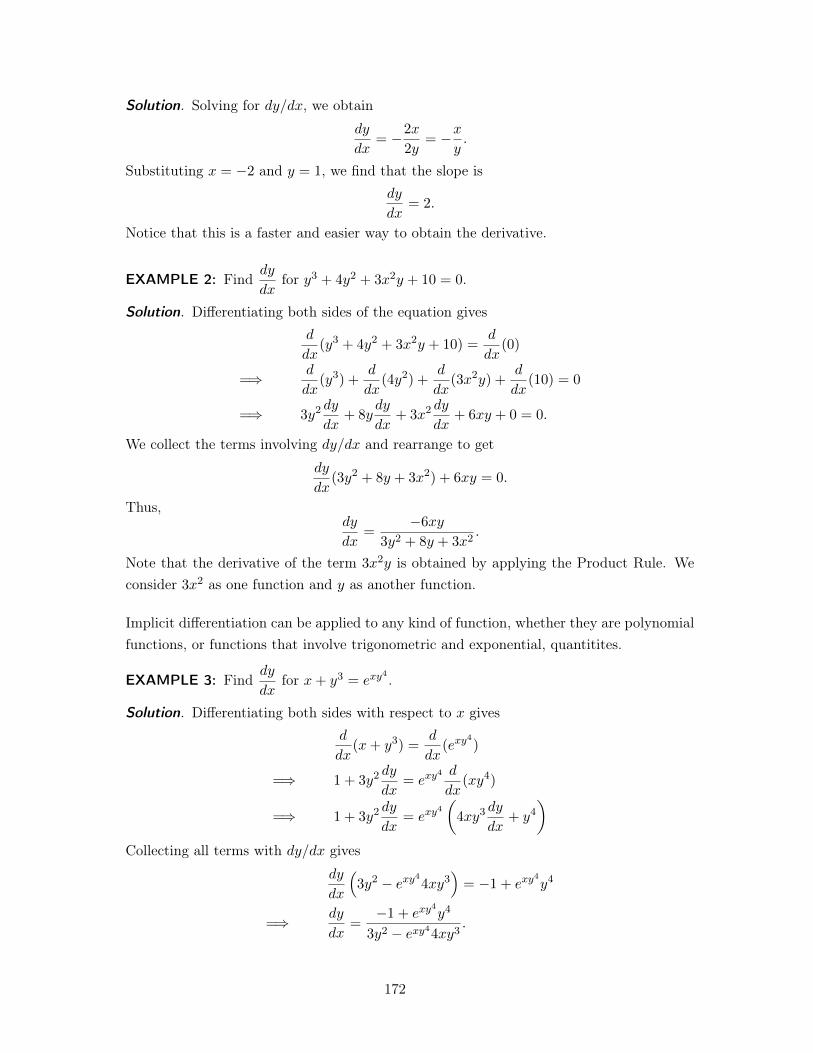
Solution. Solving for dy/dx, we obtaindy
dx= �2x
2y= �x
y.
Substituting x = �2 and y = 1, we find that the slope isdy
dx= 2.
Notice that this is a faster and easier way to obtain the derivative. .
EXAMPLE 2: Finddy
dxfor y3 + 4y2 + 3x2y + 10 = 0.
Solution. Differentiating both sides of the equation givesd
dx(y3 + 4y2 + 3x2y + 10) =
d
dx(0)
=) d
dx(y3) +
d
dx(4y2) +
d
dx(3x2y) +
d
dx(10) = 0
=) 3y2dy
dx+ 8y
dy
dx+ 3x2
dy
dx+ 6xy + 0 = 0.
We collect the terms involving dy/dx and rearrange to getdy
dx(3y2 + 8y + 3x2) + 6xy = 0.
Thus,dy
dx=
�6xy
3y2 + 8y + 3x2.
Note that the derivative of the term 3x2y is obtained by applying the Product Rule. Weconsider 3x2 as one function and y as another function. .
Implicit differentiation can be applied to any kind of function, whether they are polynomialfunctions, or functions that involve trigonometric and exponential, quantitites.
EXAMPLE 3: Finddy
dxfor x+ y3 = exy
4 .
Solution. Differentiating both sides with respect to x givesd
dx(x+ y3) =
d
dx(exy
4)
=) 1 + 3y2dy
dx= exy
4 d
dx(xy4)
=) 1 + 3y2dy
dx= exy
4
✓4xy3
dy
dx+ y4
◆
Collecting all terms with dy/dx givesdy
dx
⇣3y2 � exy
44xy3
⌘= �1 + exy
4y4
=) dy
dx=
�1 + exy4y4
3y2 � exy44xy3.
.
172
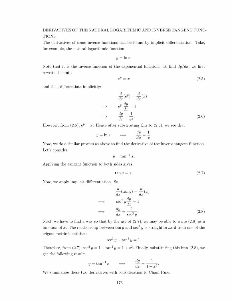
DERIVATIVES OF THE NATURAL LOGARITHMIC AND INVERSE TANGENT FUNC-TIONSThe derivatives of some inverse functions can be found by implicit differentiation. Take,for example, the natural logarithmic function
y = lnx.
Note that it is the inverse function of the exponential function. To find dy/dx, we firstrewrite this into
ey = x (2.5)
and then differentiate implicitly:d
dx(ey) =
d
dx(x)
=) eydy
dx= 1
=) dy
dx=
1
ey. (2.6)
However, from (2.5), ey = x. Hence after substituting this to (2.6), we see that
y = lnx =) dy
dx=
1
x.
Now, we do a similar process as above to find the derivative of the inverse tangent function.Let’s consider
y = tan
�1 x.
Applying the tangent function to both sides gives
tan y = x. (2.7)
Now, we apply implicit differentiation. So,d
dx(tan y) =
d
dx(x)
=) sec
2 ydy
dx= 1
=) dy
dx=
1
sec
2 y. (2.8)
Next, we have to find a way so that by the use of (2.7), we may be able to write (2.8) as afunction of x. The relationship between tan y and sec
2 y is straightforward from one of thetrigonometric identitites:
sec
2 y � tan
2 y = 1.
Therefore, from (2.7), sec2 y = 1+ tan
2 y = 1+ x2. Finally, substituting this into (2.8), weget the following result:
y = tan
�1 x =) dy
dx=
1
1 + x2.
We summarize these two derivatives with consideration to Chain Rule.
173
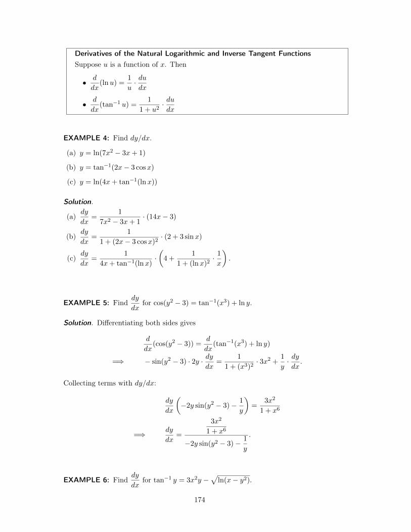
Derivatives of the Natural Logarithmic and Inverse Tangent FunctionsSuppose u is a function of x. Then
• d
dx(lnu) =
1
u· dudx
• d
dx(tan
�1 u) =1
1 + u2· dudx
EXAMPLE 4: Find dy/dx.
(a) y = ln(7x2 � 3x+ 1)
(b) y = tan
�1
(2x� 3 cosx)
(c) y = ln(4x+ tan
�1
(lnx))
Solution. .
(a)dy
dx=
1
7x2 � 3x+ 1
· (14x� 3)
(b)dy
dx=
1
1 + (2x� 3 cosx)2· (2 + 3 sinx)
(c)dy
dx=
1
4x+ tan
�1
(lnx)·✓4 +
1
1 + (lnx)2· 1x
◆.
.
EXAMPLE 5: Finddy
dxfor cos(y2 � 3) = tan
�1
(x3) + ln y.
Solution. Differentiating both sides gives
d
dx(cos(y2 � 3)) =
d
dx(tan
�1
(x3) + ln y)
=) � sin(y2 � 3) · 2y · dydx
=
1
1 + (x3)2· 3x2 + 1
y· dydx
.
Collecting terms with dy/dx:
dy
dx
✓�2y sin(y2 � 3)� 1
y
◆=
3x2
1 + x6
=) dy
dx=
3x2
1 + x6
�2y sin(y2 � 3)� 1
y
.
.
EXAMPLE 6: Finddy
dxfor tan
�1 y = 3x2y �pln(x� y2).
174
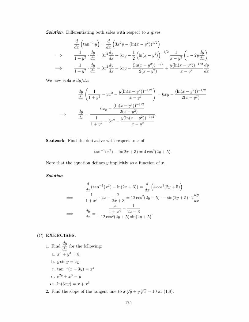
Solution. Differentiating both sides with respect to x gives
d
dx
⇣tan
�1 y⌘=
d
dx
⇣3x2y � (ln(x� y2))1/2
⌘
=) 1
1 + y2· dydx
= 3x2dy
dx+ 6xy � 1
2
⇣ln(x� y2)
⌘�1/21
x� y2
✓1� 2y
dy
dx
◆
=) 1
1 + y2· dydx
= 3x2dy
dx+ 6xy � (ln(x� y2))�1/2
2(x� y2)+
y(ln(x� y2))�1/2
x� y2dy
dx.
We now isolate dy/dx:
dy
dx
1
1 + y2� 3x2 � y(ln(x� y2))�1/2
x� y2
!= 6xy � (ln(x� y2))�1/2
2(x� y2)
=) dy
dx=
6xy � (ln(x� y2))�1/2
2(x� y2)
1
1 + y2� 3x2 � y(ln(x� y2))�1/2
x� y2
.
.
Seatwork: Find the derivative with respect to x of
tan
�1
(x2)� ln(2x+ 3) = 4 cos
3
(2y + 5).
Note that the equation defines y implicitly as a function of x.
Solution.
d
dx(tan
�1
(x2)� ln(2x+ 3)) =
d
dx
⇣4 cos
3
(2y + 5)
⌘
=) 1
1 + x4· 2x� 2
2x+ 3
= 12 cos
2
(2y + 5) ·� sin(2y + 5) · 2dydx
=) dy
dx=
x
1 + x4� 1
2x+ 3
�12 cos
2
(2y + 5) sin(2y + 5)
.
.
(C) EXERCISES.
1. Finddy
dxfor the following:
a. x3 + y3 = 8
b. y sin y = xy
c. tan
�1
(x+ 3y) = x4
d. e2y + x3 = y
?e. ln(3xy) = x+ x5
2. Find the slope of the tangent line to x 3py + y 3
px = 10 at (1,8).
175
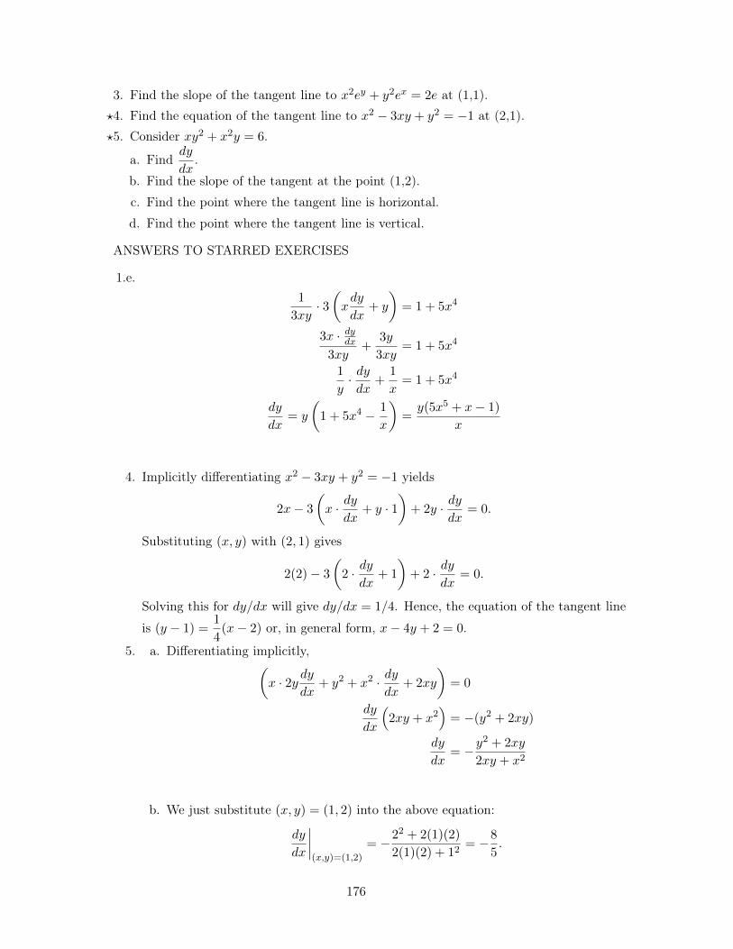
3. Find the slope of the tangent line to x2ey + y2ex = 2e at (1,1).?4. Find the equation of the tangent line to x2 � 3xy + y2 = �1 at (2,1).?5. Consider xy2 + x2y = 6.
a. Finddy
dx.
b. Find the slope of the tangent at the point (1,2).c. Find the point where the tangent line is horizontal.d. Find the point where the tangent line is vertical.
ANSWERS TO STARRED EXERCISES
1.e.1
3xy· 3
✓xdy
dx+ y
◆= 1 + 5x4
3x · dydx
3xy+
3y
3xy= 1 + 5x4
1
y· dydx
+
1
x= 1 + 5x4
dy
dx= y
✓1 + 5x4 � 1
x
◆=
y(5x5 + x� 1)
x
4. Implicitly differentiating x2 � 3xy + y2 = �1 yields
2x� 3
✓x · dy
dx+ y · 1
◆+ 2y · dy
dx= 0.
Substituting (x, y) with (2, 1) gives
2(2)� 3
✓2 · dy
dx+ 1
◆+ 2 · dy
dx= 0.
Solving this for dy/dx will give dy/dx = 1/4. Hence, the equation of the tangent line
is (y � 1) =
1
4
(x� 2) or, in general form, x� 4y + 2 = 0.
5. a. Differentiating implicitly,✓x · 2y dy
dx+ y2 + x2 · dy
dx+ 2xy
◆= 0
dy
dx
⇣2xy + x2
⌘= �(y2 + 2xy)
dy
dx= �y2 + 2xy
2xy + x2
b. We just substitute (x, y) = (1, 2) into the above equation:
dy
dx
����(x,y)=(1,2)
= �2
2
+ 2(1)(2)
2(1)(2) + 1
2
= �8
5
.
176
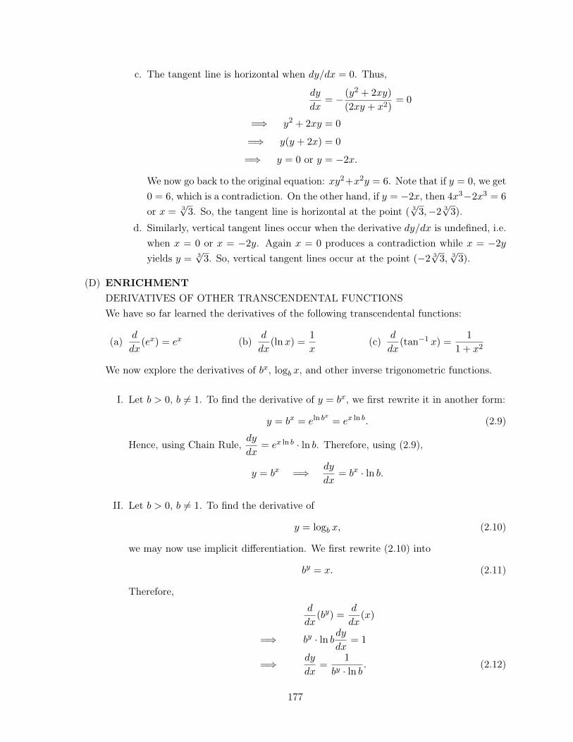
c. The tangent line is horizontal when dy/dx = 0. Thus,
dy
dx= � (y2 + 2xy)
(2xy + x2)= 0
=) y2 + 2xy = 0
=) y(y + 2x) = 0
=) y = 0 or y = �2x.
We now go back to the original equation: xy2+x2y = 6. Note that if y = 0, we get0 = 6, which is a contradiction. On the other hand, if y = �2x, then 4x3�2x3 = 6
or x =
3p3. So, the tangent line is horizontal at the point (
3p3,�2
3p3).
d. Similarly, vertical tangent lines occur when the derivative dy/dx is undefined, i.e.when x = 0 or x = �2y. Again x = 0 produces a contradiction while x = �2y
yields y =
3p3. So, vertical tangent lines occur at the point (�2
3p3, 3
p3).
(D) ENRICHMENTDERIVATIVES OF OTHER TRANSCENDENTAL FUNCTIONSWe have so far learned the derivatives of the following transcendental functions:
(a)d
dx(ex) = ex (b)
d
dx(lnx) =
1
x(c)
d
dx(tan
�1 x) =1
1 + x2
We now explore the derivatives of bx, logb x, and other inverse trigonometric functions.
I. Let b > 0, b 6= 1. To find the derivative of y = bx, we first rewrite it in another form:
y = bx = eln bx= ex ln b. (2.9)
Hence, using Chain Rule,dy
dx= ex ln b · ln b. Therefore, using (2.9),
y = bx =) dy
dx= bx · ln b.
II. Let b > 0, b 6= 1. To find the derivative of
y = logb x, (2.10)
we may now use implicit differentiation. We first rewrite (2.10) into
by = x. (2.11)
Therefore,d
dx(by) =
d
dx(x)
=) by · ln bdydx
= 1
=) dy
dx=
1
by · ln b . (2.12)
177
Finally substituting (2.11) into (2.12) gives
y = logb x =) dy
dx=
1
x ln b.
III. We only show how to find the derivative of sin�1 x, and leave the analogous proofsof the other derivatives to the teacher. Let x 2 [�1, 1], and consider y = sin
�1 x.Applying the sine function to both sides of the equation gives
sin y = x. (2.13)
Implicitly differentiating (2.13), we obtaind
dx(sin y) =
d
dx(x)
=) cos ydy
dx= 1
=) dy
dx=
1
cos y. (2.14)
We now find a way to express cos y in terms of x using equation (2.13). However, weknow from trigonometry that
cos
2 y + sin
2 y = 1
=) cos y = ±q1� sin
2 y.
Recall that in Precalculus, the range of y = sin
�1 x has been restricted to⇥�⇡
2
, ⇡2
⇤
(the fourth and first quadrants). Therefore, cos y > 0 and so we only choose cos y =
+
p1� sin
2 y. Finally, substituting this into (2.14) gives
y = sin
�1 x =) dy
dx=
1p1� x2
.
We summarize these three derivatives of the other inverse trigonometric functions:
Summary of Derivatives of Transcendental FunctionsLet u be a differentiable function of x.
(a)d
dx(eu) = eu
du
dx
(b)d
dx(bu) = bu · ln b du
dx
(c)d
dx(lnu) =
1
u
du
dx
(d)d
dx(logb u) =
1
u ln b
du
dx
(e)d
dx(sin
�1
(x)) =1p
1� x2du
dx
(f)d
dx(cos
�1
(x)) = � 1p1� x2
du
dx
(g)d
dx(tan
�1
(x)) =1
1 + x2du
dx
(h)d
dx(cot
�1
(x)) = � 1
1 + x2du
dx
(i)d
dx(sec
�1
(x)) =1
xpx2 � 1
du
dx
(j)d
dx(csc
�1
(x)) = � 1
xpx2 � 1
du
dx
178
Teaching Tip
A curious student will realize that the derivative of a cofunction of a trigonometricfunction is the negative of the derivative of the original trigonometric function. Thisis because of the identities
• cos
�1 x =
⇡
2
� sin
�1
(x)
• cot
�1 x =
⇡
2
� tan
�1
(x)
• csc
�1 x =
⇡
2
� sec
�1
(x).
EXAMPLE 7: Finddy
dxfor the following.
(a) y = log
2
x
(b) y = 5
x
(c) 3
y= sec
�1 x� cos
�1
(y2 + 1)
Solution. (a)dy
dx=
1
x ln 2
(b)dy
dx= 5
x · ln 5
(c) We use implicit differentiation here.
3
yln 3
dy
dx=
1
xpx2 � 1
� � 1p
1� (y2 + 1)
2
· 2y dydx
!
3
yln 3� 1p
1� (y2 + 1)
2
· 2y!
dy
dx=
1
xpx2 � 1
dy
dx=
1
xpx2 � 1
3
yln 3� 1p
1� (y2 + 1)
2
· 2y.
.
179
LESSON 10: Related Rates
TIME FRAME: 2 hours lecture
LEARNING OUTCOME: At the end of the lesson, the learner shall be able to solve situa-tional problems involving related rates.
LESSON OUTLINE:
1. Process of solving related rates problems2. Word problems
180
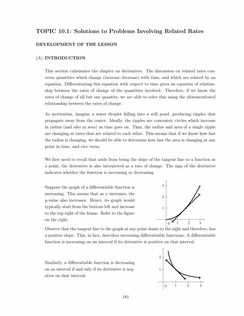
TOPIC 10.1: Solutions to Problems Involving Related Rates
DEVELOPMENT OF THE LESSON
(A) INTRODUCTION
This section culminates the chapter on derivatives. The discussion on related rates con-cerns quantities which change (increase/decrease) with time, and which are related by anequation. Differentiating this equation with respect to time gives an equation of relation-ship between the rates of change of the quantities involved. Therefore, if we know therates of change of all but one quantity, we are able to solve this using the aforementionedrelationship between the rates of change.
As motivation, imagine a water droplet falling into a still pond, producing ripples thatpropagate away from the center. Ideally, the ripples are concentric circles which increasein radius (and also in area) as time goes on. Thus, the radius and area of a single rippleare changing at rates that are related to each other. This means that if we know how fastthe radius is changing, we should be able to determine how fast the area is changing at anypoint in time, and vice versa.
We first need to recall that aside from being the slope of the tangent line to a function ata point, the derivative is also interpreted as a rate of change. The sign of the derivativeindicates whether the function is increasing or decreasing.
Suppose the graph of a differentiable function isincreasing. This means that as x increases, they-value also increases. Hence, its graph wouldtypically start from the bottom left and increaseto the top right of the frame. Refer to the figureon the right.
1 2 3
1
2
3
0
Observe that the tangent line to the graph at any point slants to the right and therefore, hasa positive slope. This, in fact, describes increasing differentiable functions: A differentiablefunction is increasing on an interval if its derivative is positive on that interval.
Similarly, a differentiable function is decreasingon an interval if and only if its derivative is neg-ative on that interval.
1 2 3
1
2
0
181
RemarkLet x be a differentiable function which represents a quantity that changes withtime t, then
• dx
dtis the rate of change of x with respect to t;
• dx
dtis positive if and only if x increases with time; and
• dx
dtis negative if and only if x decreases with time.
The unit of measurement ofdx
dtis
unit of measurement of xunit of measurement of t
.
(B) LESSON PROPERA related rates problem concerns the relationship among the rates of change of severalvariables with respect to time, given that each variable is also dependent on the others. Inparticular, if y is dependent on x, then the rate of change of y with respect to t is dependent
on the rate of change of x with respect to t, that is,dy
dtis dependent on
dx
dt.
To be systematic in our solutions, we present the following steps:
Suggestions in solving problems involving related rates:
1. If possible, provide an illustration for the problem that is valid for any time t.
2. Identify those quantities that change with respect to time, and represent them withvariables. (Avoid assigning variables to quantities which are constant, that is, which donot change with respect to time. Label them right away with the values provided in theproblem.)
3. Write down any numerical facts known about the variables. Interpret each rate ofchange as the derivative of a variable with respect to time. Remember that if a quantitydecreases over time, then its rate of change is negative.
4. Identify which rate of change is being asked, and under what particular conditions thisrate is being computed.
5. Write an equation showing the relationship of all the variables by an equation that isvalid for any time t.
6. Differentiate the equation in (5) implicitly with respect to t.
7. Substitute into the equation, obtained in (6), all values that are valid at the particulartime of interest. Sometimes, some quantities still need to be solved by substituting theparticular conditions written in (4) to the equation in (6). Then, solve for what is beingasked in the problem.
182
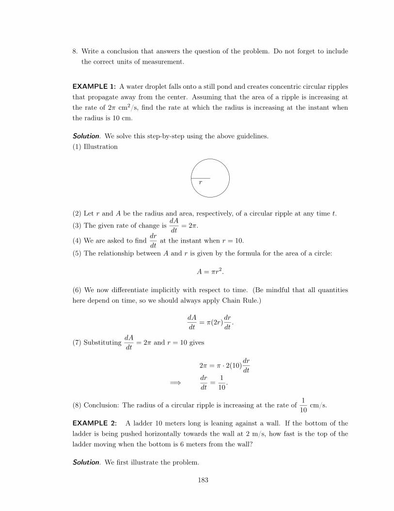
8. Write a conclusion that answers the question of the problem. Do not forget to includethe correct units of measurement.
EXAMPLE 1: A water droplet falls onto a still pond and creates concentric circular ripplesthat propagate away from the center. Assuming that the area of a ripple is increasing atthe rate of 2⇡ cm2/s, find the rate at which the radius is increasing at the instant whenthe radius is 10 cm.
Solution. We solve this step-by-step using the above guidelines.(1) Illustration
r
(2) Let r and A be the radius and area, respectively, of a circular ripple at any time t.
(3) The given rate of change isdA
dt= 2⇡.
(4) We are asked to finddr
dtat the instant when r = 10.
(5) The relationship between A and r is given by the formula for the area of a circle:
A = ⇡r2.
(6) We now differentiate implicitly with respect to time. (Be mindful that all quantitieshere depend on time, so we should always apply Chain Rule.)
dA
dt= ⇡(2r)
dr
dt.
(7) SubstitutingdA
dt= 2⇡ and r = 10 gives
2⇡ = ⇡ · 2(10)drdt
=) dr
dt=
1
10
.
(8) Conclusion: The radius of a circular ripple is increasing at the rate of1
10
cm/s. .
EXAMPLE 2: A ladder 10 meters long is leaning against a wall. If the bottom of theladder is being pushed horizontally towards the wall at 2 m/s, how fast is the top of theladder moving when the bottom is 6 meters from the wall?
Solution. We first illustrate the problem.
183
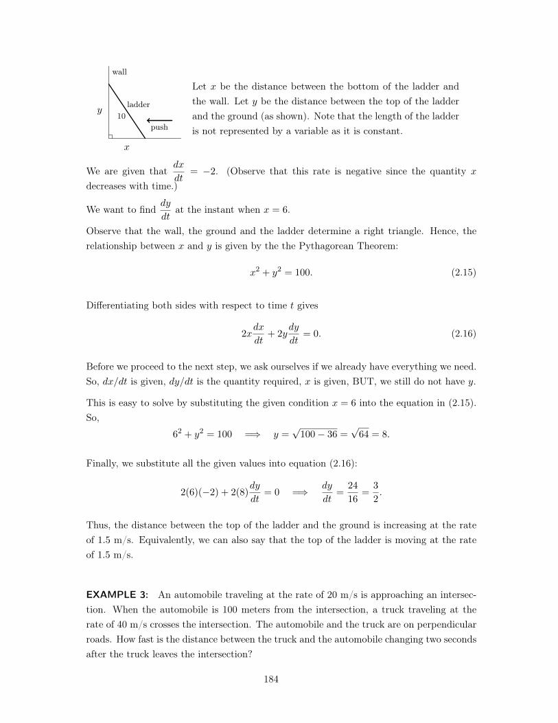
ladder10
wall
x
y
push
Let x be the distance between the bottom of the ladder andthe wall. Let y be the distance between the top of the ladderand the ground (as shown). Note that the length of the ladderis not represented by a variable as it is constant.
We are given thatdx
dt= �2. (Observe that this rate is negative since the quantity x
decreases with time.)
We want to finddy
dtat the instant when x = 6.
Observe that the wall, the ground and the ladder determine a right triangle. Hence, therelationship between x and y is given by the the Pythagorean Theorem:
x2 + y2 = 100. (2.15)
Differentiating both sides with respect to time t gives
2xdx
dt+ 2y
dy
dt= 0. (2.16)
Before we proceed to the next step, we ask ourselves if we already have everything we need.So, dx/dt is given, dy/dt is the quantity required, x is given, BUT, we still do not have y.
This is easy to solve by substituting the given condition x = 6 into the equation in (2.15).So,
6
2
+ y2 = 100 =) y =
p100� 36 =
p64 = 8.
Finally, we substitute all the given values into equation (2.16):
2(6)(�2) + 2(8)
dy
dt= 0 =) dy
dt=
24
16
=
3
2
.
Thus, the distance between the top of the ladder and the ground is increasing at the rateof 1.5 m/s. Equivalently, we can also say that the top of the ladder is moving at the rateof 1.5 m/s. .
EXAMPLE 3: An automobile traveling at the rate of 20 m/s is approaching an intersec-tion. When the automobile is 100 meters from the intersection, a truck traveling at therate of 40 m/s crosses the intersection. The automobile and the truck are on perpendicularroads. How fast is the distance between the truck and the automobile changing two secondsafter the truck leaves the intersection?
184
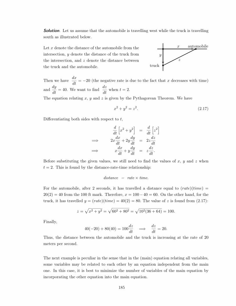
Solution. Let us assume that the automobile is travelling west while the truck is travellingsouth as illustrated below.
Let x denote the distance of the automobile from theintersection, y denote the distance of the truck fromthe intersection, and z denote the distance betweenthe truck and the automobile.
y
truck
x automobile
z
Then we havedx
dt= �20 (the negative rate is due to the fact that x decreases with time)
anddy
dt= 40. We want to find
dz
dtwhen t = 2.
The equation relating x, y and z is given by the Pythagorean Theorem. We have
x2 + y2 = z2. (2.17)
Differentiating both sides with respect to t,
d
dt
hx2 + y2
i=
d
dt
hz2i
=) 2xdx
dt+ 2y
dy
dt= 2z
dz
dt
=) xdx
dt+ y
dy
dt= z
dz
dt.
Before substituting the given values, we still need to find the values of x, y and z whent = 2. This is found by the distance-rate-time relationship:
distance = rate ⇥ time.
For the automobile, after 2 seconds, it has travelled a distance equal to (rate)(time) =
20(2) = 40 from the 100 ft mark. Therefore, x = 100�40 = 60. On the other hand, for thetruck, it has travelled y = (rate)(time) = 40(2) = 80. The value of z is found from (2.17):
z =
px2 + y2 =
p60
2
+ 80
2
=
p10
2
(36 + 64) = 100.
Finally,
40(�20) + 80(40) = 100
dz
dt=) dz
dt= 20.
Thus, the distance between the automobile and the truck is increasing at the rate of 20
meters per second. .
The next example is peculiar in the sense that in the (main) equation relating all variables,some variables may be related to each other by an equation independent from the mainone. In this case, it is best to minimize the number of variables of the main equation byincorporating the other equation into the main equation.
185
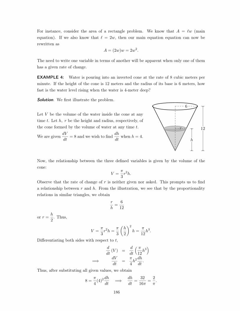
For instance, consider the area of a rectangle problem. We know that A = `w (mainequation). If we also know that ` = 2w, then our main equation equation can now berewritten as
A = (2w)w = 2w2.
The need to write one variable in terms of another will be apparent when only one of themhas a given rate of change.
EXAMPLE 4: Water is pouring into an inverted cone at the rate of 8 cubic meters perminute. If the height of the cone is 12 meters and the radius of its base is 6 meters, howfast is the water level rising when the water is 4-meter deep?
Solution. We first illustrate the problem.
Let V be the volume of the water inside the cone at anytime t. Let h, r be the height and radius, respectively, ofthe cone formed by the volume of water at any time t.
We are givendV
dt= 8 and we wish to find
dh
dtwhen h = 4.
6
r
h
12
Now, the relationship between the three defined variables is given by the volume of thecone:
V =
⇡
3
r2h.
Observe that the rate of change of r is neither given nor asked. This prompts us to finda relationship between r and h. From the illustration, we see that by the proportionalityrelations in similar triangles, we obtain
r
h=
6
12
or r =
h
2
. Thus,
V =
⇡
3
r2h =
⇡
3
✓h
2
◆2
h =
⇡
12
h3.
Differentiating both sides with respect to t,
d
dt(V ) =
d
dt
⇣ ⇡
12
h3⌘
=) dV
dt=
⇡
4
h2dh
dt.
Thus, after substituting all given values, we obtain
8 =
⇡
4
(4)
2
dh
dt=) dh
dt=
32
16⇡=
2
⇡.
186
Finally, we conclude that the water level inside the cone is rising at the rate of2
⇡me-
ters/minute. .
(C) EXERCISES
1. Starting from the same point, Reden starts walking eastward at 60 cm/s while Neilstarts running towards the south at 80 cm/s. How fast is the distance between Redenand Neil increasing after 2 seconds?
2. A woman standing on a cliff is watching a motor boat through a telescope as the boatapproaches the shoreline directly below her. If the telescope is 25 meters above the waterlevel and if the boat is approaching the cliff at 20 m/s, at what rate is the acute anglemade by the telescope with the vertical changing when the boat is 250 meters from theshore?
3. A balloon, in the shape of a right circular cylinder, is being inflated in such a way thatthe radius and height are both increasing at the rate of 3 cm/s and 8 cm/s, respectively.What is the rate of change of its total surface area when its radius and height are 60 cmand 140 cm, respectively?
4. If two resistors with resistance R1
and R2
are connected in parallel, the total resistanceR in ohms is given by
1
R=
1
R1
+
1
R2
. If R1
and R2
are increasing at 0.4 ohms/s and
0.25 ohms/s, respectively, how fast is R changing when R1
= 600 ohms and R2
= 400
ohms?
5. A baseball diamond has the shape of a square with sides 90 ft long. A player 60 ft fromsecond base is running towards third base at a speed of 28 ft/min. At what rate is theplayer’s distance from the home plate changing?
6. Shan, who is 2 meters tall, is approaching a post that holds a lamp 6 meters above theground. If he is walking at a speed of 1.5 m/s, how fast is the end of his shadow moving(with respect to the lamp post) when he is 6 meters away from the base of the lamppost?
?7. Water is being poured at the rate of 2⇡ m3/min. into an inverted conical tank that is12-meter deep with a radius of 6 meters at the top. If the water level is rising at therate of 1
6
m/min and there is a leak at the bottom of the tank, how fast is the waterleaking when the water is 6-meter deep?
(D) ENRICHMENT
1. A ladder 20-meter long is leaning against an embankment inclined 60
� with the horizon-tal. If the bottom of the ladder is being moved horizontally towards the embankmentat 1 m/s, how fast is the top of the ladder moving when the bottom is 4 meters fromthe embankment?
187
2. A boat is pulled in by means of a winch on the dock 4 meters above the deck of theboat. The winch pulls in rope at the rate of 1 m/s. Determine the speed of the boatwhen there is 3 meters of rope out.
3. A ladder, inclined at 60� with the horizontal is leaning against a vertical wall. The footof the ladder is 3 m away from the foot of the wall. A boy climbs the ladder such that hisdistance z m with respect to the foot of the ladder is given by z = 6t, where t is the timein seconds. Find the rate at which his vertical distance from the ground changes withrespect to t. Find the rate at which his distance from the foot of the wall is changingwith respect to t when he is 3 m away from the foot of the ladder.
?4. A particle is moving along the curve y =
px. As the particle passes through the point
(4,2), its x-coordinate changes at a rate of 3 cm/s. How fast is the distance of theparticle from the origin changing at this instant?
ANSWERS TO STARRED EXERCISES
(C) 7. Let V , h and r be the volume, height and radius respectively, of the water collectedin the cone at any point t. Then V = V
in
� Vout
. Moreover, it is given that
dVin
dt= +2⇡, and
dh
dt= +
1
6
.
Now, the formula for the volume of a cone is V =
1
3
⇡r2h. We wish to express V interms of a single variable only. Since we have dh/dt in the given, it is better to expressr in terms of h.
Using similar triangles and the fact that the height and radius of the conical containerare 12 and 6 respectively, we have
r
h=
6
12
which means r =
h
2
.
Substituting this expression r, we get V =
1
3
⇡h
✓h
2
◆2
=
⇡h3
12
. Differentiating with
respect to t (don’t forget to apply Chain Rule) gives
dV
dt=
⇡
12
(3h2)dh
dt=
⇡h2
4
dh
dt.
Hence, at the instant when h = 6,
dV
dt=
⇡(6)2
4
· 16
=
3⇡
2
.
Finally,dV
dt=
dVin
dt� dV
out
dt. This implies that
dVout
dt=
dVin
dt� dV
dt= 2⇡ � 3⇡
2
=
⇡
2
m3
min.
188
(D) 4. Let h, x and y denote the distance from the origin, x-coordinate and y-coordinaterespectively, of a point P on the curve y =
px at any time t. We are given that
dx
dt= +3 and we want to find
dh
dtat the instant when x = 4 and y = 2.
Using the distance formula,h = x2 + y2.
Since the curve has equation y =
px, the formula above simplifies to
h = x2 + x.
Differentiating with respect to t gives
dh
dt= (2x+ 1)
dx
dt.
Substituting x = 4 anddx
dt= 3 gives
dh
dt= 9(3) = 27 cm/s.
189
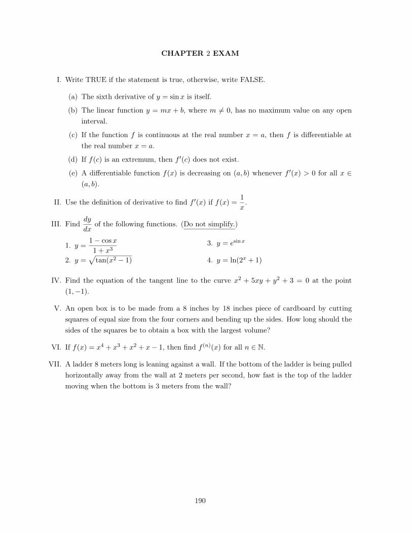
CHAPTER 2 EXAM
I. Write TRUE if the statement is true, otherwise, write FALSE.
(a) The sixth derivative of y = sinx is itself.
(b) The linear function y = mx + b, where m 6= 0, has no maximum value on any openinterval.
(c) If the function f is continuous at the real number x = a, then f is differentiable atthe real number x = a.
(d) If f(c) is an extremum, then f 0(c) does not exist.
(e) A differentiable function f(x) is decreasing on (a, b) whenever f 0(x) > 0 for all x 2
(a, b).
II. Use the definition of derivative to find f 0(x) if f(x) =
1
x.
III. Finddy
dxof the following functions. (Do not simplify.)
1. y =
1� cosx
1 + x3
2. y =
ptan(x2 � 1)
3. y = esinx
4. y = ln(2
x+ 1)
IV. Find the equation of the tangent line to the curve x2 + 5xy + y2 + 3 = 0 at the point(1,�1).
V. An open box is to be made from a 8 inches by 18 inches piece of cardboard by cuttingsquares of equal size from the four corners and bending up the sides. How long should thesides of the squares be to obtain a box with the largest volume?
VI. If f(x) = x4 + x3 + x2 + x� 1, then find f (n)(x) for all n 2 N.
VII. A ladder 8 meters long is leaning against a wall. If the bottom of the ladder is being pulledhorizontally away from the wall at 2 meters per second, how fast is the top of the laddermoving when the bottom is 3 meters from the wall?
190
Chapter 3
Integration
LESSON 11: Integration
TIME FRAME: 5 hours
LEARNING OUTCOMES: At the end of the lesson, the learner shall be able to:
1. Illustrate the antiderivative of a function;2. Compute the general antiderivative of polynomial functions;3. Compute the general antiderivative of root functions;4. Compute the general antiderivative of exponential functions; and,5. Compute the general antiderivative of trigonometric functions.
LESSON OUTLINE:
1. Antiderivatives of functions2. Antiderivatives of polynomial and root functions3. Antiderivatives of integrals yielding exponential and logarithmic functions4. Antiderivatives of trigonometric functions
192
TOPIC 11.1: Illustration of an Antiderivative of a Function
DEVELOPMENT OF THE LESSON
(A) ACTIVITY
Matching Type. Match the functions in Column A with their corresponding derivatives inColumn B.
Column A
1. F (x) = x3 + 2x2 + x
2. F (x) = x3 + x2 + x
3. F (x) = x4 + 3x3 + 1
4. F (x) = x4 + x3 + 2
5. F (x) = x2 + 2x+ 1
6. F (x) = x2 � 2x+ 1
7. F (x) = 3x3 + 3x+ 1
8. F (x) = 3x3 � 3x+ 1
Column B
a. f(x) = 4x3 + 3x2
b. f(x) = 9x2 + 3
c. f(x) = 3x2 + 2x+ 1
d. f(x) = 9x2 � 3
e. f(x) = 2x+ 2
f. f(x) = 2x� 2
g. f(x) = 3x2 + 4x+ 1
h. f(x) = 4x3 + 9x2
(B) INTRODUCTION
In the previous discussions, we learned how to find the derivatives of different functions.Now, we will introduce the inverse of differentiation. We shall call this process antidiffer-entiation. A natural question then arises:
Given a function f , can we find a function F whose derivative is f?
Definition 5. A function F is an antiderivative of the function f on an interval I ifF 0
(x) = f(x) for every value of x in I.
Teaching Tip
The teacher must go back to the activity and explain to the students that the func-tions in Column A are indeed antiderivatives of the their corresponding derivativesin Column B.
193
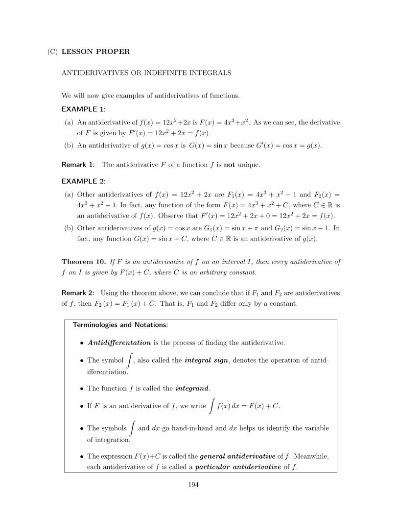
(C) LESSON PROPER
ANTIDERIVATIVES OR INDEFINITE INTEGRALS
We will now give examples of antiderivatives of functions.
EXAMPLE 1:
(a) An antiderivative of f(x) = 12x2+2x is F (x) = 4x3+x2. As we can see, the derivativeof F is given by F 0
(x) = 12x2 + 2x = f(x).
(b) An antiderivative of g(x) = cosx is G(x) = sinx because G0(x) = cosx = g(x).
Remark 1: The antiderivative F of a function f is not unique.
EXAMPLE 2:
(a) Other antiderivatives of f(x) = 12x2 + 2x are F1
(x) = 4x3 + x2 � 1 and F2
(x) =
4x3 + x2 + 1. In fact, any function of the form F (x) = 4x3 + x2 + C, where C 2 R isan antiderivative of f(x). Observe that F 0
(x) = 12x2 + 2x+ 0 = 12x2 + 2x = f(x).
(b) Other antiderivatives of g(x) = cosx are G1
(x) = sinx+ ⇡ and G2
(x) = sinx� 1. Infact, any function G(x) = sinx+ C, where C 2 R is an antiderivative of g(x).
Theorem 10. If F is an antiderivative of f on an interval I, then every antiderivative off on I is given by F (x) + C, where C is an arbitrary constant.
Remark 2: Using the theorem above, we can conclude that if F1
and F2
are antiderivativesof f , then F
2
(x) = F1
(x) + C. That is, F1
and F2
differ only by a constant.
Terminologies and Notations:
• Antidifferentation is the process of finding the antiderivative.
• The symbolZ
, also called the integral sign , denotes the operation of antid-ifferentiation.
• The function f is called the integrand .
• If F is an antiderivative of f , we writeZ
f(x) dx = F (x) + C.
• The symbolsZ
and dx go hand-in-hand and dx helps us identify the variableof integration.
• The expression F (x)+C is called the general antiderivative of f . Meanwhile,each antiderivative of f is called a particular antiderivative of f .
194
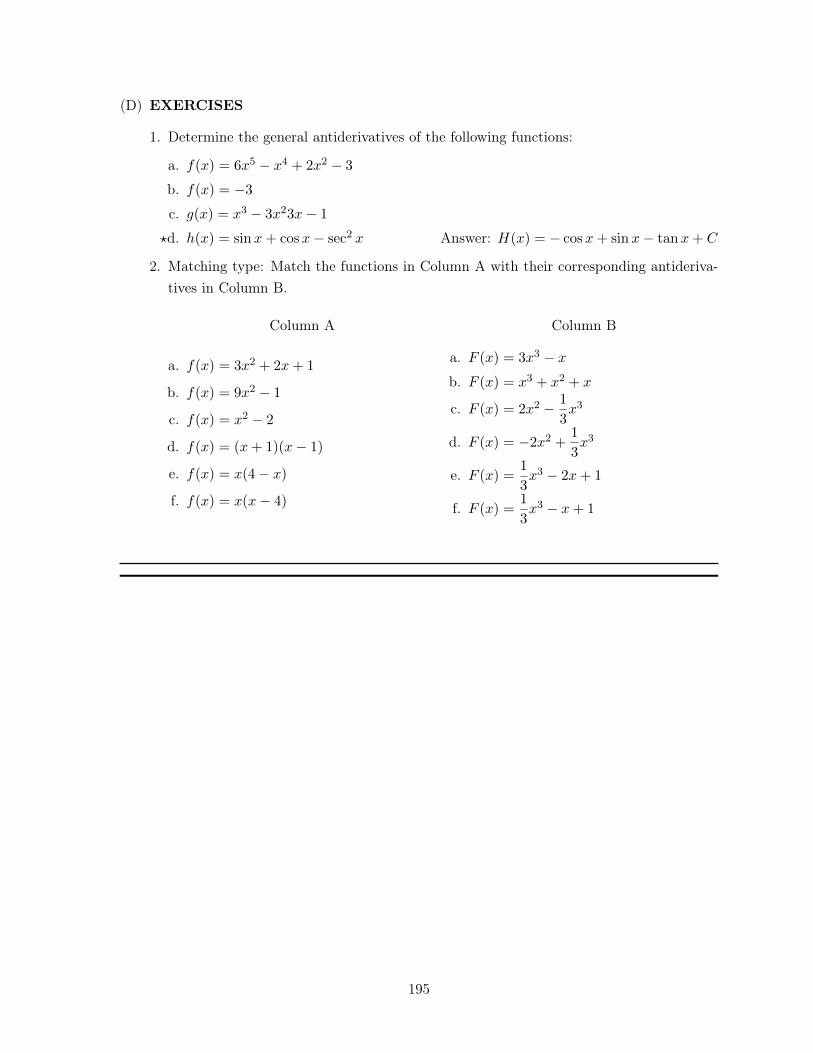
(D) EXERCISES
1. Determine the general antiderivatives of the following functions:
a. f(x) = 6x5 � x4 + 2x2 � 3
b. f(x) = �3
c. g(x) = x3 � 3x23x� 1
?d. h(x) = sinx+ cosx� sec
2 x Answer: H(x) = � cosx+ sinx� tanx+ C
2. Matching type: Match the functions in Column A with their corresponding antideriva-tives in Column B.
Column A
a. f(x) = 3x2 + 2x+ 1
b. f(x) = 9x2 � 1
c. f(x) = x2 � 2
d. f(x) = (x+ 1)(x� 1)
e. f(x) = x(4� x)
f. f(x) = x(x� 4)
Column B
a. F (x) = 3x3 � x
b. F (x) = x3 + x2 + x
c. F (x) = 2x2 � 1
3
x3
d. F (x) = �2x2 +1
3
x3
e. F (x) =1
3
x3 � 2x+ 1
f. F (x) =1
3
x3 � x+ 1
195
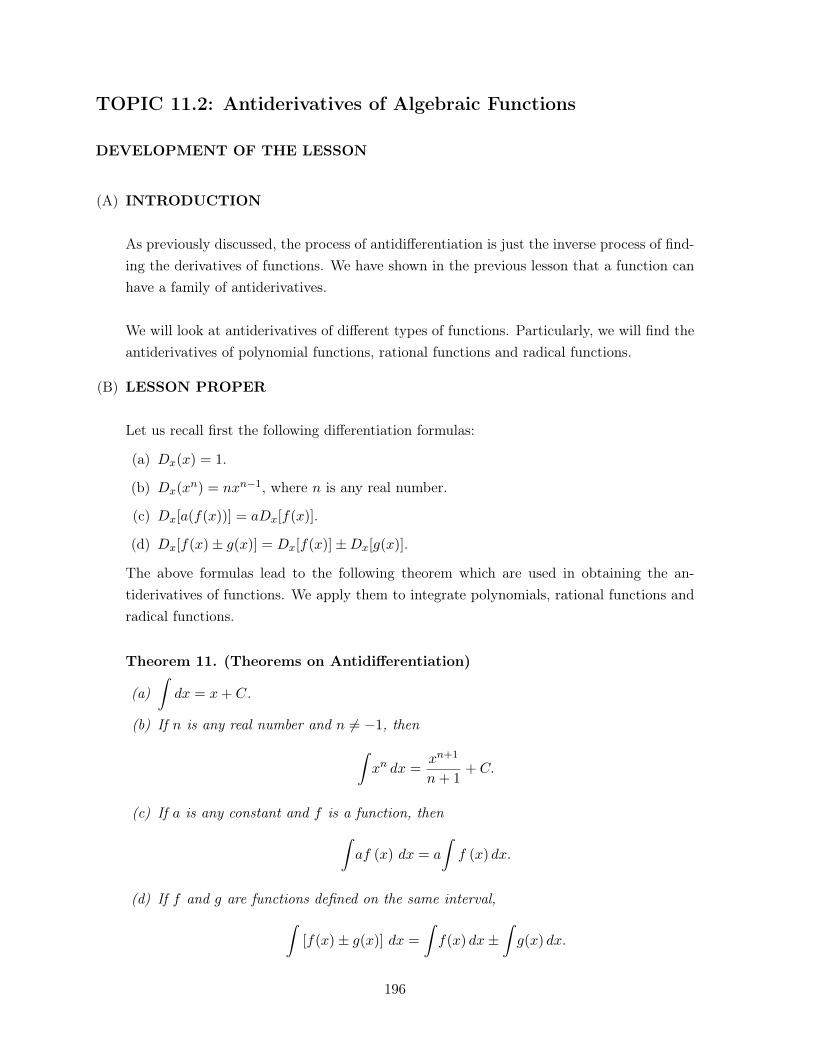
TOPIC 11.2: Antiderivatives of Algebraic Functions
DEVELOPMENT OF THE LESSON
(A) INTRODUCTION
As previously discussed, the process of antidifferentiation is just the inverse process of find-ing the derivatives of functions. We have shown in the previous lesson that a function canhave a family of antiderivatives.
We will look at antiderivatives of different types of functions. Particularly, we will find theantiderivatives of polynomial functions, rational functions and radical functions.
(B) LESSON PROPER
Let us recall first the following differentiation formulas:
(a) Dx(x) = 1.
(b) Dx(xn) = nxn�1, where n is any real number.
(c) Dx[a(f(x))] = aDx[f(x)].
(d) Dx[f(x)± g(x)] = Dx[f(x)]±Dx[g(x)].
The above formulas lead to the following theorem which are used in obtaining the an-tiderivatives of functions. We apply them to integrate polynomials, rational functions andradical functions.
Theorem 11. (Theorems on Antidifferentiation)
(a)Z
dx = x+ C.
(b) If n is any real number and n 6= �1, thenZxn dx =
xn+1
n+ 1
+ C.
(c) If a is any constant and f is a function, thenZ
af (x) dx = a
Zf (x) dx.
(d) If f and g are functions defined on the same interval,Z
[f(x)± g(x)] dx =
Zf(x) dx±
Zg(x) dx.
196
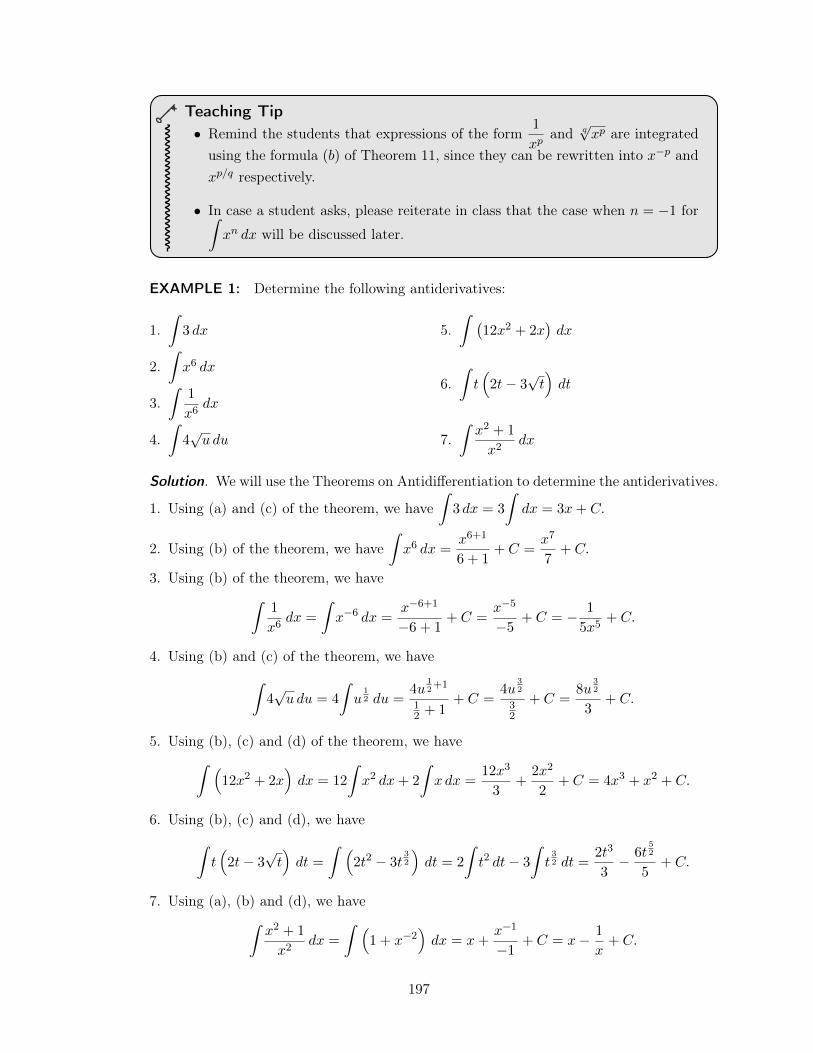
Teaching Tip
• Remind the students that expressions of the form1
xpand q
pxp are integrated
using the formula (b) of Theorem 11, since they can be rewritten into x�p andxp/q respectively.
• In case a student asks, please reiterate in class that the case when n = �1 forZxn dx will be discussed later.
EXAMPLE 1: Determine the following antiderivatives:
1.Z3 dx
2.Zx6 dx
3.Z
1
x6dx
4.Z4
pu du
5.Z �
12x2 + 2x�dx
6.Zt⇣2t� 3
pt⌘dt
7.Z
x2 + 1
x2dx
Solution. We will use the Theorems on Antidifferentiation to determine the antiderivatives.
1. Using (a) and (c) of the theorem, we haveZ3 dx = 3
Zdx = 3x+ C.
2. Using (b) of the theorem, we haveZx6 dx =
x6+1
6 + 1
+ C =
x7
7
+ C.
3. Using (b) of the theorem, we haveZ
1
x6dx =
Zx�6 dx =
x�6+1
�6 + 1
+ C =
x�5
�5
+ C = � 1
5x5+ C.
4. Using (b) and (c) of the theorem, we haveZ4
pu du = 4
Zu
12 du =
4u12+1
1
2
+ 1
+ C =
4u32
3
2
+ C =
8u32
3
+ C.
5. Using (b), (c) and (d) of the theorem, we haveZ ⇣
12x2 + 2x⌘dx = 12
Zx2 dx+ 2
Zx dx =
12x3
3
+
2x2
2
+ C = 4x3 + x2 + C.
6. Using (b), (c) and (d), we haveZt⇣2t� 3
pt⌘dt =
Z ⇣2t2 � 3t
32
⌘dt = 2
Zt2 dt� 3
Zt32 dt =
2t3
3
� 6t52
5
+ C.
7. Using (a), (b) and (d), we haveZ
x2 + 1
x2dx =
Z ⇣1 + x�2
⌘dx = x+
x�1
�1
+ C = x� 1
x+ C.
197
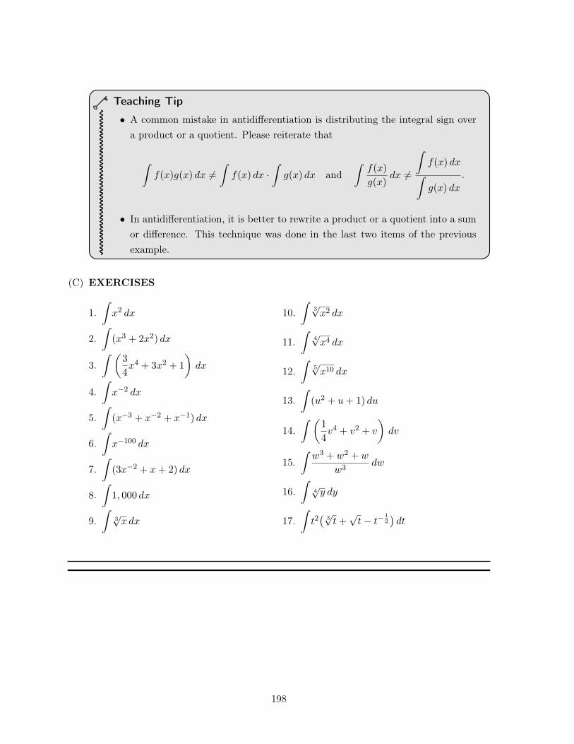
.
Teaching Tip
• A common mistake in antidifferentiation is distributing the integral sign overa product or a quotient. Please reiterate that
Zf(x)g(x) dx 6=
Zf(x) dx ·
Zg(x) dx and
Zf(x)
g(x)dx 6=
Zf(x) dx
Zg(x) dx
.
• In antidifferentiation, it is better to rewrite a product or a quotient into a sumor difference. This technique was done in the last two items of the previousexample.
(C) EXERCISES
1.Z
x2 dx
2.Z
(x3 + 2x2) dx
3.Z ✓
3
4
x4 + 3x2 + 1
◆dx
4.Z
x�2 dx
5.Z
(x�3
+ x�2
+ x�1
) dx
6.Z
x�100 dx
7.Z
(3x�2
+ x+ 2) dx
8.Z
1, 000 dx
9.Z
3px dx
10.Z
3px2 dx
11.Z
4px4 dx
12.Z
5px10 dx
13.Z(u2 + u+ 1) du
14.Z ✓
1
4
v4 + v2 + v
◆dv
15.Z
w3
+ w2
+ w
w3
dw
16.Z
4py dy
17.Zt2�
3pt+
pt� t�
12�dt
198
TOPIC 11.3: Antiderivatives of Functions Yielding ExponentialFunctions and Logarithmic Functions
DEVELOPMENT OF THE LESSON
(A) INTRODUCTION
We will introduce the antiderivatives of two important functions namely, the exponentialfunction
f(x) = ex
and the function yielding the logarithmic function
f(x) = lnx.
We will present first the basic formulas, then their examples once we have already dis-cussed integration by substitution. The technique of integration by substitution will helpus integrate complicated functions yielding exponential and logarithmic functions.
(B) LESSON PROPER
In this lesson, we will present the basic formulas for integrating functions that yield expo-nential and logarithmic functions. Let us first recall the following differentiation formulas:
(a) Dx(ex) = ex.
(b) Dx(ax) = ax ln a.
(c) Dx(lnx) =1
x.
Because antidifferentiation is the inverse operation of differentiation, the following theoremshould be immediate.
Theorem 12. (Theorems on integrals yielding the exponential and logarithmicfunctions)
(a)Z
ex dx = ex + C.
(b)Z
ax dx =
ax
ln a+ C. Here, a > 0 with a 6= 1.
(c)Z
x�1 dx =
Z1
xdx = ln |x|+ C.
199
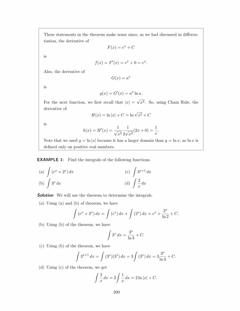
These statements in the theorem make sense since, as we had discussed in differen-tiation, the derivative of
F (x) = ex + C
isf(x) = F 0
(x) = ex + 0 = ex.
Also, the derivative ofG(x) = ax
isg(x) = G0
(x) = ax ln a.
For the next function, we first recall that |x| =px2. So, using Chain Rule, the
derivative ofH(x) = ln |x|+ C = ln
px2 + C
ish(x) = H 0
(x) =1px2
1
2
px2
(2x+ 0) =
1
x.
Note that we used y = ln |x| because it has a larger domain than y = lnx, as lnx isdefined only on positive real numbers.
EXAMPLE 1: Find the integrals of the following functions.
(a)Z
(ex + 2
x) dx
(b)Z
3
x dx
(c)Z
3
x+1 dx
(d)Z
2
xdx
Solution. We will use the theorem to determine the integrals.
(a) Using (a) and (b) of theorem, we haveZ
(ex + 2
x) dx =
Z(ex) dx+
Z(2
x) dx = ex +
2
x
ln 2
+ C.
(b) Using (b) of the theorem, we haveZ
3
x dx =
3
x
ln 3
+ C.
(c) Using (b) of the theorem, we haveZ
3
x+1 dx =
Z(3
x)(3
1
) dx = 3
Z(3
x) dx = 3
3
x
ln 3
+ C.
(d) Using (c) of the theorem, we getZ
2
xdx = 2
Z1
xdx = 2 ln |x|+ C.
200
.
We will take more integrals yielding the exponential and logarithmic functions oncewe discuss integration by substitution. For instance, we will try to see how we canevaluate the following:
(a)Z
e3x dx (b)Z
2
4x dx (c)Z
1
2x� 1
dx.
(C) EXERCISESSolve the following integrals:
(1)Z
2ex dx
(2)Z
(2ex + 4
x) dx
(3)Z
2(5
x) dx
(4)Z
5
x+2 dx
(5)Z
2
xdx
(6)Z
3x�1 dx
201
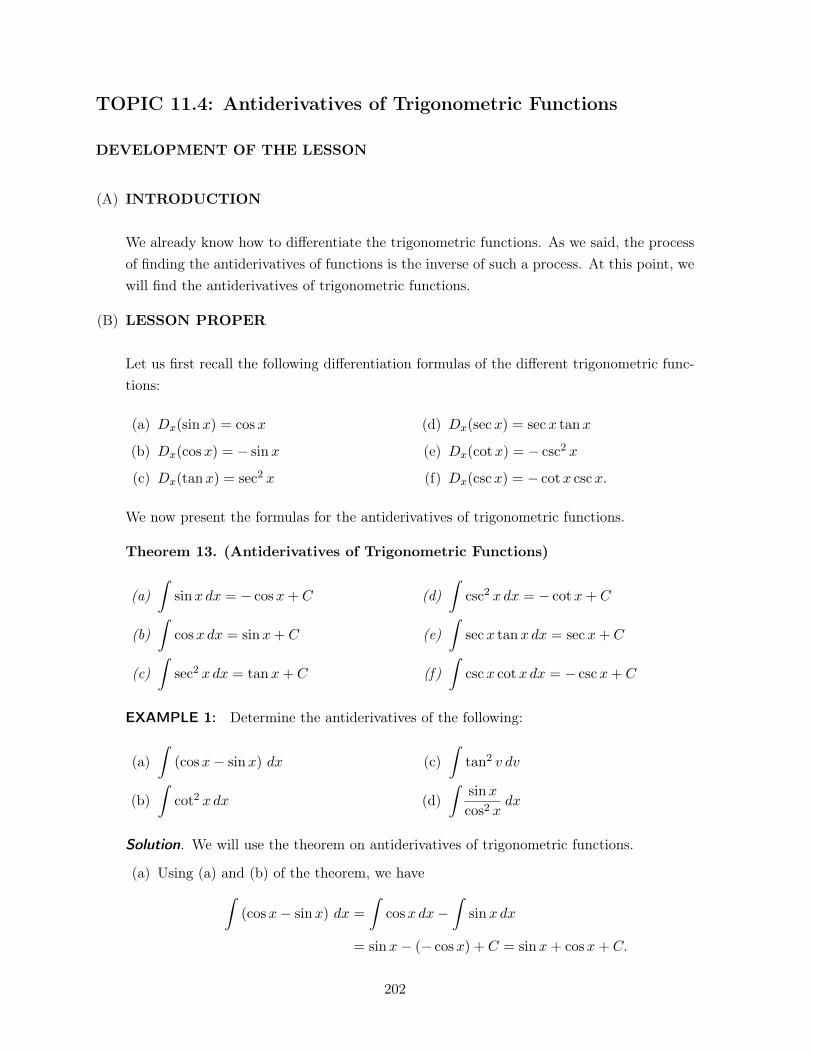
TOPIC 11.4: Antiderivatives of Trigonometric Functions
DEVELOPMENT OF THE LESSON
(A) INTRODUCTION
We already know how to differentiate the trigonometric functions. As we said, the processof finding the antiderivatives of functions is the inverse of such a process. At this point, wewill find the antiderivatives of trigonometric functions.
(B) LESSON PROPER
Let us first recall the following differentiation formulas of the different trigonometric func-tions:
(a) Dx(sinx) = cosx
(b) Dx(cosx) = � sinx
(c) Dx(tanx) = sec
2 x
(d) Dx(secx) = secx tanx
(e) Dx(cotx) = � csc
2 x
(f) Dx(cscx) = � cotx cscx.
We now present the formulas for the antiderivatives of trigonometric functions.
Theorem 13. (Antiderivatives of Trigonometric Functions)
(a)Z
sinx dx = � cosx+ C
(b)Z
cosx dx = sinx+ C
(c)Z
sec
2 x dx = tanx+ C
(d)Z
csc
2 x dx = � cotx+ C
(e)Z
secx tanx dx = secx+ C
(f)Z
cscx cotx dx = � cscx+ C
EXAMPLE 1: Determine the antiderivatives of the following:
(a)Z
(cosx� sinx) dx
(b)Z
cot
2 x dx
(c)Z
tan
2 v dv
(d)Z
sinx
cos
2 xdx
Solution. We will use the theorem on antiderivatives of trigonometric functions.
(a) Using (a) and (b) of the theorem, we haveZ
(cosx� sinx) dx =
Zcosx dx�
Zsinx dx
= sinx� (� cosx) + C = sinx+ cosx+ C.
202
(b) Since we know that cot
2 x = csc
2�1, thenZ
cot
2 x dx =
Z ⇣csc
2 x� 1
⌘dx =
Zcsc
2 x�Z
dx = � cot
2�x+ C.
(c) Since tan
2 v = sec
2 v � 1, we haveZ
tan
2 v dv =
Z ⇣sec
2 v � 1
⌘dv =
Zsec
2 v dv �Zdv = tan v � v + C.
(d)Z
sinx
cos
2 xdx =
Zsinx
cosx
1
cosxdx =
Ztanx secx dx = secx+ C.
.
Note that we have just presentedZ
sinx dx andZ
cosx dx. One can then ask thefollowing:
(a)Z
tanx dx =?
(b)Z
cotx dx =?
(c)Z
secx dx =?
(d)Z
cscx dx =?
We will derive these integrals once we discuss the technique of integration by sub-stitution.
(C) EXERCISESEvaluate the following integrals:
1.Z
tan
2 x dx
2.Z
cot
2 x dx
3.Z
cosx
sin
2 xdx
4.Z
cosx
sin
2 xdx
5.Z
sinx
cos
2 x+ x
�dx
6.Z(sinu+ u) du
7.Z(1� cos v) dv
?8.Z
1
sec y tan ydy
. Answer: � cos y + C
?9.Z
1
sin
2 x cos2 xdx
. Answer: � cotx+ tanx+ C
203
LESSON 12: Techniques of Antidifferentiation
TIME FRAME: 7 hours
LEARNING OUTCOMES: At the end of the lesson, the learner shall be able to:
1. Compute the antiderivative of a function using the substitution rule; and2. Compute the antiderivative of a function using a table of integrals (including those whose
antiderivatives involve logarithmic and inverse trigonometric functions).
LESSON OUTLINE:
1. Antidifferentiation by substitution2. Table of Integrals
204
TOPIC 12.1: Antidifferentiation by Substitution and by Table ofIntegrals
DEVELOPMENT OF THE LESSON
(A) INTRODUCTION
Antidifferentiation is more challenging than differentiation. To find the derivative of agiven function, there are well-established rules that are always applicable to differentiablefunctions. For antidifferentiation, the antiderivatives given in the previous lesson may notsuffice to integrate a given function.
A prerequisite is knowledge of the basic antidifferentiation formulas. Some formulas areeasily derived, but most of them need to be memorized.
No hard and fast rules can be given as to which method applies in a given situation.In college, several techniques such as integration by parts, partial fractions, trigonometricsubtitution will be introduced. This lesson focuses on the most basic technique - antidiffer-entiation by substitution - which is the inverse of the Chain Rule in differentiation.
There are occasions when it is possible to perform a difficult piece of integration by firstmaking a substitution . This has the effect of changing the variable and the integrand.The ability to carry out integration by substitution is a skill that develops with practiceand experience, but sometimes a sensible substitution may not lead to an integral that canbe evaluated. We must then be prepared to try out alternative substitutions.
Suppose we are given an integral of the formZ
f(g(x))·g0(x) dx. We can transform this into
another form by changing the independent variable x to u using the substitution u = g(x).
In this case,du
dx= g0(x) dx. Therefore,
Zf(g(x))g0(x) dx =
Zf(u) du.
This change of variable is one of the most important tools available to us. This technique iscalled integration by substitution. It is often important to guess what will be the usefulsubstitution.
Usually, we make a substitution for a function whose derivative also occurs in the integrand.
205
(B) LESSON PROPER
EXAMPLE 1: EvaluateZ
(x+ 4)
5 dx.
Solution. Notice that the integrand is in the fifth power of the expression (x+4). To tacklethis problem, we make a substitution. We let u = x + 4. The point of doing this is tochange the integrand into a much simpler u5. However, we must take care to substituteappropriately for the term dx too.
Now, since u = x+ 4 it follows thatdu
dx= 1 and so du = dx. So, substituting (x+ 4) and
dx, we have Z(x+ 4)
5 dx =
Zu5 du.
The resulting integral can be evaluated immediately to giveu6
6
+C. Recalling that u = x+4,we have
Z(x+ 4)
5 dx =
Zu5 du
=
u6
6
+ C
=
(x+ 4)
6
6
+ C.
.
An alternative way of finding the antiderivative above is to expand the expression in theintegrand and antidifferentiate the resulting polynomial (of degree 5) term by term. Wewill NOT do this. Obviously, the solution above is simpler than the mentioned alternative.
EXAMPLE 2: EvaluateZ
(x5 + 2)
9
5x4 dx.
Solution. If we let u = x5 + 2, then du = 5x4 dx, which is precisely the other factor in theintegrand. Thus, in terms of the variable u, this is essentially just a power rule integration.
That is,
Z(x5 + 2)
9
5x4 dx =
Zu9 du, where u = x5 + 2
=
u10
10
+ C
=
(x5 + 2)
10
10
+ C.
.
206
Again, the alternative way is to expand out the expression in the integrand, and integratethe resulting polynomial (of degree 49) term by term. Again, we would rather NOT dothis.
EXAMPLE 3: EvaluateZ
z2p1 + z3
dz.
Solution. In this example, we let u = 1+ z3 so thatdu
dz= 3z2. If u = 1+ z3, then we need
to express z2 dz in the integrand in terms of du or a constant multiple of du.
Fromdu
dz= 3z2 it follows that du = 3z2 dz and z2 dz =
1
3
du. Thus,
Zz2p1 + z3
dz =
Z1p
1 + z3· z2 dz
=
Z1pu· 13
du
=
1
3
Zu�
12 du
=
1
3
u
12
1
2
+ C1
!
=
2
3
u12+
C1
3
=
2
3
(1 + z3)12+ C where C =
C1
3
.
.
Teaching Tip
To avoid unnecessary arithmetic on the constant of integration, we will henceforthwrite C as a separate summand, and add it only after integrating.
EXAMPLE 4: EvaluateZ
xpx2 � 1
dx.
Solution. Notice that if u = x2� 1, then du = 2x dx. This implies that x dx =
1
2
du, so wehave
Zxp
x2 � 1
dx =
Z1
u12
· 12
du
=
1
2
Zu�
12 du
=
1
2
u
12
1
2
!+ C
= (x2 � 1)
12+ C.
207
.
EXAMPLE 5: EvaluateZ
x3px3 + 5
dx.
Solution. Let u = x3 + 5. Then x3 = u� 5 and du = 3x2 dx. Thus,Z
x3px3 + 5
dx =
Zu� 5
u12
dx
=
Z ✓u
u12
� 5
u12
◆dx
=
Z(u
12 � 5u�
12) dx
=
u32
3
2
� 5u12
1
2
+ C
=
2
3
u32 � 10u
12+ C
=
2
3
(x3 + 5)
32 � 10(x3 + 5)
12+ C.
.
EXAMPLE 6: EvaluateZ
dx
x 3plnx
.
Solution. We substitute u = lnx so that du =
1
xdx, which occurs in the integrand. Thus,
Zdx
x 3plnx
=
Z1
3pudu
=
Zu�
13 du
=
u23
2
3
+ C
=
3
2
(lnx)23+ C
.
We recall the theorem we stated in the previous lesson.
Theorem 14. (Theorems on integrals yielding the exponential and logarithmicfunctions)
1.Z
ex dx = ex + C.
2.Z
ax dx =
ax
ln a+ C. Here, a > 0 with a 6= 1.
3.Zx�1 dx =
Z1
xdx = ln |x|+ C.
208
As we said before, we will have more integrals yielding the exponential and logarithmicfunctions once we have discussed integration by substitution.
EXAMPLE 7: Evaluate the following integrals.
(a)Z
e3x dx
(b)Z
2
4x dx
(c)Z
1
2x� 1
dx
Solution. .
(a) We let u = 3x. Then du = 3dx. Hence, dx =
du
3
. So,
Ze3x dx =
Zeu
du
3
=
1
3
Zeu du =
1
3
eu + C =
1
3
e3x + C.
(b) Here, we let u = 4x and so du = 4dx. Thus, dx =
du
4
. Hence, we have
Z2
4x dx =
Z2
u du
4
=
1
4
Z2
u du =
1
4
2
u
ln 2
+ C =
1
4 ln 2
2
4x+ C.
(c) Suppose we let u = 2x� 1. Then du = 2dx. Hence, dx =
du
2
. We have
Z1
2x� 1
dx =
Z1
u
du
2
=
1
2
Z1
udu =
1
2
ln |u|+ C =
1
2
ln |2x� 1|+ C.
.
EXAMPLE 8: EvaluateZ
cos(4x+ 3) dx.
Solution. Observe that if we make the substitution u = 4x+ 3, the integrand will containa much simpler form, cosu, which we can easily integrate. So, if u = 4x+3, then du = 4 dx
and dx =
1
4
du. So,
Zcos(4x+ 3) dx =
Zcosu · 1
4
du
=
1
4
Zcosu du
=
1
4
sinu+ C
=
1
4
sin(4x+ 3) + C.
.
209
EXAMPLE 9: Evaluate the integralZ
sinx cosx dx.
Solution. Note that if we let u = sinx, its derivative is du = cosx dx which is the otherfactor in the integrand and our integral becomes
Zsinx cosx dx =
Zu du
=
u2
2
+ C1
=
sin
2 x
2
+ C1
.
.
Alternative solution to the problem: If we let u = cosx, then du = � sinx dx which is alsothe other factor in the integrand. Even if the integral
Zsinx cosx dx = �cos
2 x
2
+ C2
looks different from the above answer, we can easily show that the two answers are indeedequal with by using the trigonometric identity sin
2 x+cos
2 x = 1. In this case, C2
= C1
+
1
2
.
EXAMPLE 10: Evaluate the integralZ
esinxcosx dx.
Solution. We let u = sinx so that the other factor in the integrand cosx dx = du. Thus,the integral becomes
Zesinx
cosx dx =
Zeu du
= eu + C
= esinx+ C.
.
Recall that we had earlier presented the integralsZ
sinx dx andZ
cosx dx. Now thatwe already know integration by substitution, we can now present the integrals of othertrigonometric functions: tanx, cotx, secx, and cscx.
First, let us use substitution technique to findZ
tanx dx. Note that tanx =
sinx
cosx. Hence,
Ztanx dx =
Zsinx
cosxdx.
210
Now, if we let u = cosx, then du = � sinx dx. Hence, we haveZ
tanx dx =
Zsinx
cosxdx
=
Z1
u(�du)
= �Z
1
udu
= � ln |u|+ C
= � ln | cosx|+ C.
Equivalently, � ln | cosx|+ C = ln | cosx|�1
= ln | secx|+ C.
Similarly, we can use substitution technique to showZ
cotx dx = ln | sinx|+ C. Here, we
use cotx =
cosx
sinxand choose u = sinx.
Let us now findZ
secx dx. The usual trick is to multiply the numerator and the denomi-nator by secx+ tanx.
Zsecx dx =
Z(secx)
secx+ tanx
secx+ tanxdx =
Z1
secx+ tanx(secx tanx+ sec
2 x) dx.
Now, if we let u = secx+ tanx, then du = secx tanx+ sec
2 x. Thus, we haveZ
secx dx =
Z1
secx+ tanx(secx tanx+ sec
2 x) dx.
=
Z1
udu
= ln |u|+ C
= ln | secx+ tanx|+ C.
Similarly, we can showZ
cscx dx = ln | cscx� cotx|+ C.Hence, we have the following formulas:
1.Z
tanx dx = � ln | cosx|+ C = ln | secu|+ C.
2.Z
cotx dx = ln | sinx|+ C.
3.Z
secx dx = ln | secx+ tanx|+ C.
4.Z
cscx dx = ln | cscx� cotx|+ C.
Teaching Tip
It would help the students if the formulas above are written either on a sheet ofmanila paper or on the board while the following examples are discussed.
211
EXAMPLE 11: EvaluateZx4 sec(x5) dx.
Solution. We let u = x5. Then du = 5x4dx. Thus, x4dx =
du
5
. We have
Zx4 sec(x5) dx =
Zsecu
du
5
=
1
5
Zsecu du
=
1
5
ln | secu+ tanu|+ C
=
1
5
ln | secx5 + tanx5|+ C.
.
EXAMPLE 12: EvaluateZ
4 + cos
x4
sin
x4
dx.
Solution. Let u =
x4
. Then du =
1
4
dx and so 4 du = dx. Thus, we haveZ
4 + cos
x4
sin
x4
dx =
Z4 + cosu
sinu4du
= 4
Z ⇥4
sinu+
cosu
sinu
⇤du
= 4
Z 4 cscu+ cotu
�du
= 4
Zcotu du+ 16
Zcscu du
= 4 ln | sinu|+ 16 ln | cscu� cotu|+ C
= 4 ln
���� sinx
4
����+ 16 ln
���� cscx
4
� cot
x
4
����+ C.
.
INTEGRALS OF INVERSE CIRCULAR FUNCTIONS
We now present the formulas for integrals yielding the inverse circular functions.
1.Z
dup1� u2
= sin
�1 u+ C
2.Z
du
1 + u2= tan
�1 u+ C
3.Z
du
upu2 � 1
= sec
�1 u+ C
If the constant 1 in these integrals is replaced by some other positive number, one can usethe following generalizations:
212
Let a > 0. Then
Zdxp
a2 � x2= sin
�1
⇣xa
⌘+ C (3.1)
Zdx
a2 + x2=
1
atan
�1
⇣xa
⌘+ C (3.2)
Zdx
xpx2 � a2
=
1
asec
�1
⇣xa
⌘+ C (3.3)
Teaching Tip
Again, it would help the students if the formulas above are written either on a sheetof manila paper or on the board while the following examples are discussed.
EXAMPLE 13: EvaluateZ
1p9� x2
dx.
Solution. From Formula (3.1) with a = 3, we write this intoZ
1p9� x2
dx =
Z1p
3
2 � x2dx = sin
�1
⇣x3
⌘+ C.
.
EXAMPLE 14:Z
dx
9x2 + 36
Solution. Let u = 3x, du = 3 dx. Then from Formula (3.2),
Zdx
9x2 + 36
=
1
3
Zdu
u2 + 36
=
1
3
· 16
tan
�1
⇣u6
⌘+ C
=
1
18
tan
�1
✓3x
6
◆+ C
=
1
18
tan
�1
⇣x2
⌘+ C.
.
213
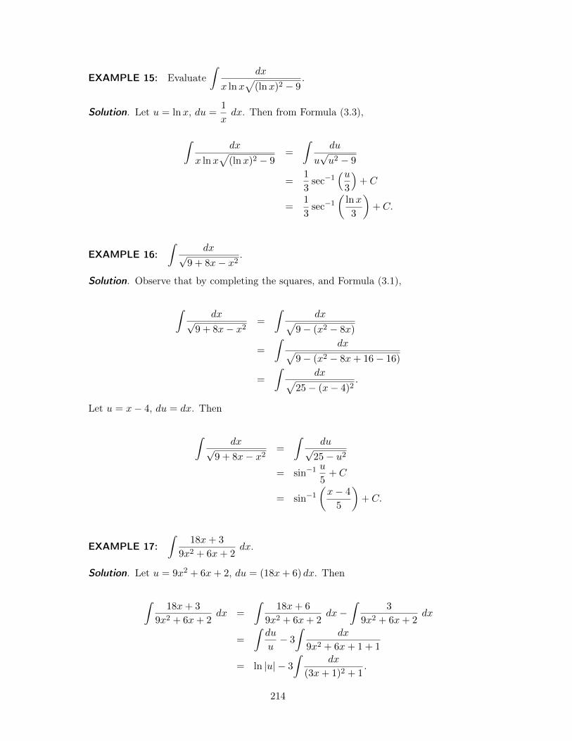
EXAMPLE 15: EvaluateZ
dx
x lnxp(lnx)2 � 9
.
Solution. Let u = lnx, du =
1
xdx. Then from Formula (3.3),
Zdx
x lnxp
(lnx)2 � 9
=
Zdu
upu2 � 9
=
1
3
sec
�1
⇣u3
⌘+ C
=
1
3
sec
�1
✓lnx
3
◆+ C.
.
EXAMPLE 16:Z
dxp9 + 8x� x2
.
Solution. Observe that by completing the squares, and Formula (3.1),
Zdxp
9 + 8x� x2=
Zdxp
9� (x2 � 8x)
=
Zdxp
9� (x2 � 8x+ 16� 16)
=
Zdxp
25� (x� 4)
2
.
Let u = x� 4, du = dx. Then
Zdxp
9 + 8x� x2=
Zdup
25� u2
= sin
�1
u
5
+ C
= sin
�1
✓x� 4
5
◆+ C.
.
EXAMPLE 17:Z
18x+ 3
9x2 + 6x+ 2
dx.
Solution. Let u = 9x2 + 6x+ 2, du = (18x+ 6) dx. Then
Z18x+ 3
9x2 + 6x+ 2
dx =
Z18x+ 6
9x2 + 6x+ 2
dx�Z
3
9x2 + 6x+ 2
dx
=
Zdu
u� 3
Zdx
9x2 + 6x+ 1 + 1
= ln |u|� 3
Zdx
(3x+ 1)
2
+ 1
.
214
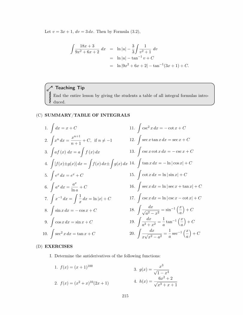
Let v = 3x+ 1, dv = 3 dx. Then by Formula (3.2),
Z18x+ 3
9x2 + 6x+ 2
dx = ln |u|� 3
3
Z1
v2 + 1
dv
= ln |u|� tan
�1 v + C
= ln |9x2 + 6x+ 2|� tan
�1
(3x+ 1) + C.
.
Teaching Tip
End the entire lesson by giving the students a table of all integral formulas intro-duced.
(C) SUMMARY/TABLE OF INTEGRALS
1.Z
dx = x+ C
2.Zxn dx =
xn+1
n+ 1
+ C, if n 6= �1
3.Zaf (x) dx = a
Zf (x) dx
4.Z[f(x)±g(x)] dx =
Zf(x) dx±
Zg(x) dx
5.Z
ex dx = ex + C
6.Z
ax dx =
ax
ln a+ C
7.Z
x�1 dx =
Z1
xdx = ln |x|+ C
8.Z
sinx dx = � cosx+ C
9.Z
cosx dx = sinx+ C
10.Z
sec
2 x dx = tanx+ C
11.Z
csc
2 x dx = � cotx+ C
12.Z
secx tanx dx = secx+ C
13.Z
cscx cotx dx = � cscx+ C
14.Z
tanx dx = � ln | cosx|+ C
15.Z
cotx dx = ln | sinx|+ C
16.Z
secx dx = ln | secx+ tanx|+ C
17.Z
cscx dx = ln | cscx� cotx|+ C
18.Z
dxpa2 � x2
= sin
�1
⇣xa
⌘+ C
19.Z
dx
a2 + x2=
1
atan
�1
⇣xa
⌘+ C
20.Z
dx
xpx2 � a2
=
1
asec
�1
⇣xa
⌘+ C
(D) EXERCISES
I. Determine the antiderivatives of the following functions:
1. f(x) = (x+ 1)
100
2. f(x) = (x2 + x)10(2x+ 1)
3. g(x) =x3p1� x4
4. h(x) =6x2 + 2px3 + x+ 1
215
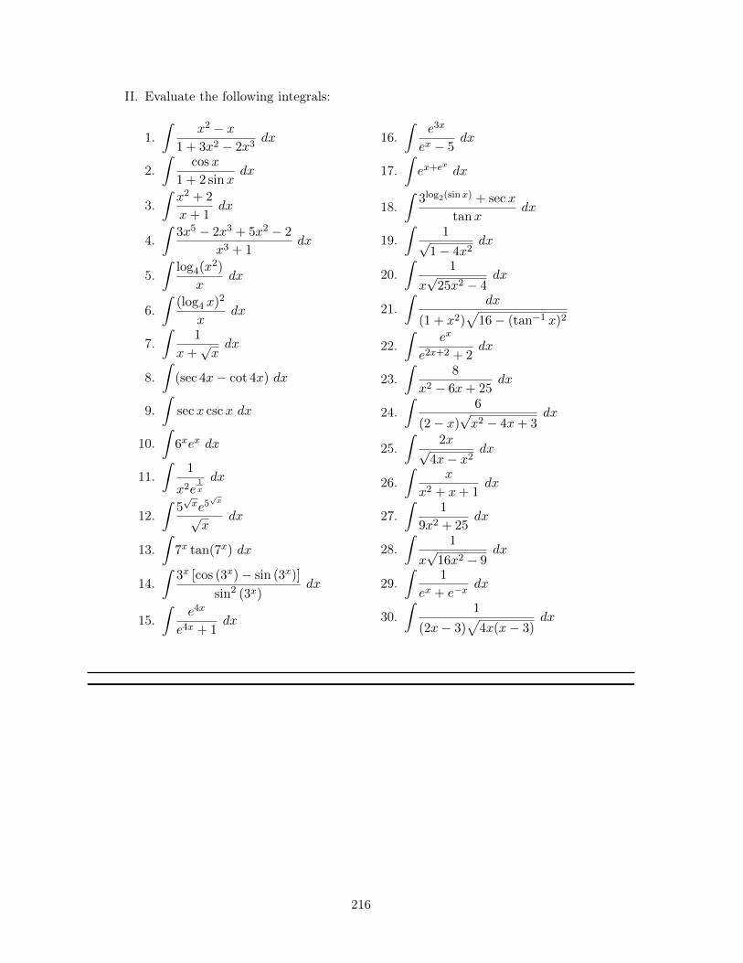
II. Evaluate the following integrals:
1.Z
x2 � x
1 + 3x2 � 2x3dx
2.Z
cosx
1 + 2 sinxdx
3.Z
x2 + 2
x+ 1
dx
4.Z
3x5 � 2x3 + 5x2 � 2
x3 + 1
dx
5.Z
log
4
(x2)
xdx
6.Z
(log
4
x)2
xdx
7.Z
1
x+
px
dx
8.Z(sec 4x� cot 4x) dx
9.Z
secx cscx dx
10.Z6
xex dx
11.Z
1
x2e1x
dx
12.Z
5
pxe5
px
px
dx
13.Z7
xtan(7
x) dx
14.Z
3
x[cos (3
x)� sin (3
x)]
sin
2
(3
x)
dx
15.Z
e4x
e4x + 1
dx
16.Z
e3x
ex � 5
dx
17.Z
ex+ex dx
18.Z
3
log2(sinx)+ secx
tanxdx
19.Z
1p1� 4x2
dx
20.Z
1
xp25x2 � 4
dx
21.Z
dx
(1 + x2)p16� (tan
�1 x)2
22.Z
ex
e2x+2
+ 2
dx
23.Z
8
x2 � 6x+ 25
dx
24.Z
6
(2� x)px2 � 4x+ 3
dx
25.Z
2xp4x� x2
dx
26.Z
x
x2 + x+ 1
dx
27.Z
1
9x2 + 25
dx
28.Z
1
xp16x2 � 9
dx
29.Z
1
ex + e�xdx
30.Z
1
(2x� 3)
p4x(x� 3)
dx
216
LESSON 13: Application of Antidifferentiation to DifferentialEquations
TIME FRAME: 3 hours
LEARNING OUTCOME: At the end of the lesson, the learner shall be able to solve sepa-rable differential equations using antidifferentiation.
LESSON OUTLINE:
1. Separable differential equations
217
TOPIC 13.1: Separable Differential Equations
DEVELOPMENT OF THE LESSON
(A) INTRODUCTION
Imagine you are behind a microscope in a biology laboratory and you are trying to countthe growing number of bacteria in a petri dish. You observe that at any point in time,one-fourth of the population is reproduced. You may eventually give up on counting be-cause the bacteria are multiplying very fast, but you can use your calculus skills to find thepopulation of bacteria at any given time.
Let y denote the population at any time t. According to your observation, the change in thepopulation at any time is
1
4
y. Since the derivative quantifies change, the above observationcan be expressed mathematically as
dy
dt=
1
4
y.
This is an example of a differential equation, and our objective is to recover the populationy from the above equation using integration.
(B) LESSON PROPER
A differential equation (DE) is an equation that involves x, y and the derivatives of y.The following are examples of differential equations:
(a)dy
dx= 2x+ 5 (b)
dy
dx= �x
y(c) y00 + y = 0
The order of a differential equation pertains to the highest order of the derivative thatappears in the differential equation.
The first two examples above are first-order DEs because they involve only the first deriva-tive, while the last example is a second-order DE because y00 appears in the equation.
A solution to a differential equation is a function y = f(x) or a relation f(x, y) = 0 thatsatisfies the equation.
218
Teaching Tip
In the answers below, we will always try to express y in terms of x. However,recalling our discussion on implicit differentiation, it may be difficult or impossibleto express y explicitly in terms of x. Therefore, a solution to a differential equationmay as well be only a relation.
For example, y = x2 + 5x+ 1 is a solution tody
dx= 2x+ 5 since
d
dx(y) =
d
dx(x2 + 5x+ 1) = 2x+ 5.
The relation x2 + y2 = 1 is a solution tody
dx= �x
ybecause if we differentiate the relation
implicitly, we get
2x+ 2ydy
dx= 0 =) dy
dx= �x
y.
Finally, y = sinx solves the differential equation y00+y = 0 since y0 = cosx and y00 = � sinx,and therefore
y00 + y = (� sinx) + sinx = 0.
Solving a differential equation means finding all possible solutions to the DE.
A differential equation is said to be separable if it can be expressed as
f(x) dx = g(y) dy,
where f and g are functions of x and y, respectively. Observe that we have separated thevariables in the sense that the left-hand side only involves x while the right-hand side ispurely in terms of y.
If it is possible to separate the variables, then we can find the solution of the differentialequation by simply integrating:
Zf(x) dx =
Zg(y) dy
and applying appropriate techniques of integration. Note that the left-hand side yields afunction of x, say F (x)+C
1
, while the right-hand side yields a function of y, say G(y)+C2
.We thus obtain
F (x) = G(y) + C (Here, C = C2
� C1
)
which we can then express into a solution of the form y = H(x) + C, if possible.
We will now look at some examples of how to solve separable differential equations.
219
EXAMPLE 1: Solve the differential equationdy
dt=
1
4
y.
Solution. Observe that y = 0 is a solution to the differential equation. Suppose that y 6= 0.We divide both sides of the equation by y to separate the variables:
dy
y=
1
4
dt.
Integrating the left-hand side with respect to y and integrating the right-hand side withrespect to t yield Z
dy
y=
Z1
4
dt =) ln |y| = 1
4
t+ C.
Taking the exponential of both sides, we obtain
|y| = e14 t+C
= eC e14 t.
Therefore, y = ±Ae14 t, where A = eC is any positive constant. Therefore, along with
the solution y = 0 that we have found at the start, the solution to the given differentialequation is y = Ae
14 t where A is any real number. .
EXAMPLE 2: Solve the differential equation 2y dx� 3x dy = 0.
Solution. If y = 0, thendy
dx= 0 which means that the function y = 0 is a solution to the
differential equation 2y � 3xdy
dx= 0. Assume that y 6= 0. Separating the variables, we get
2y dx = 3x dy
2
xdx =
3
ydy.
Integrating both sides, we obtainZ
2
xdx =
Z3
ydy
2 ln |x| = 3 ln |y|+ C
ln |x|2 � C = ln |y|3
|y|3 = e�C eln |x|2= e�C |x|2.
Therefore, the solutions are y = ± 3pAx2/3 where A = e�C is any positive constant. Along
with the trivial solution y = 0, the set of solutions to the differential equation is y = Bx2/3
where B is any real number. Note: The absolute value bars are dropped since x2 is alreadynonnegative. .
220
EXAMPLE 3: Solve the equation xy3 dx+ ex2dy = 0.
Solution. First, we separate the variables. We have
�xy3 dx = ex2dy
�xe�x2dx =
1
y3dy.
Integrating both sides of the equation with respect to their variables, we have
�Z
xe�x2dx =
Zy�3 dy.
Meanwhile, if u = �x2, then du = �2x dx so that �du
2
= x dx. Hence,
�Z
xe�x2dx =
1
2
Zeu du =
1
2
eu + C =
1
2
e�x2+ C.
Therefore,
�Z
xe�x2dx =
Zy�3 dy
1
2
e�x2= �y�2
2
+ C.
.
If we solve for y in terms of x, we get y = ±�A� e�x2��1/2, where A = 2C is any constant.
EXAMPLE 4: Solve the equation 3(y + 2) dx� xy dy = 0.
Solution. Separating the variables of the differential equation gives us
3 (y + 2) dx = xy dy3
xdx =
y
y + 2
dy
3
xdx =
(y + 2)� 2
y + 2
dy
3
xdx =
✓1� 2
y + 2
◆dy.
Now that we have separated the variables, we now integrate the equation term by term:Z
3
xdx =
Z ✓1� 2
y + 2
◆dy
3 ln |x| = y � 2 ln |y + 2|+ C.
.
221
Teaching Tip
The solution to the above example is impossible to express in the form y = H(x)+C.So, we are contented with expressing this as a relation.
Note that in the previous examples, a constant of integration is always present. If thereare initial conditions, or if we know that the solution passes through a point, we can solvethis constant and get a particular solution to the differential equation.
EXAMPLE 5: Find the particular solutions of the following given their correspondinginitial conditions:
(a)dy
dt=
1
4
y when y = 100 and t = 0
(b) 2y dx� 3x dy = 0 when x = 1 and y = 1
(c) xy3 dx+ ex2dy = 0 when x = 0 and y = 1
(d) 3(y + 2) dx� xy dy = 0 when x = 1 and y = �1
Solution. We will use the general solutions from the previous examples.
(a) The solution to Example 1 is y = Ae1/4t. Using the conditions y = 100 and t = 0, weget 100 = Ae0. Hence, A = 100 and therefore the particular solution is y = 100e
14 t.
(b) The solution to Example 2 is y = B x2/3. Substituting (x, y) = (1, 1) gives 1 =
B 1
2/3= B. Hence, the particular solution is y =
3px2.
(c) From the Example 3, the general solution is y = ± 1pA� e�x2
. Substituting (x, y) =
(1, 0) yields 1 = ± 1pA� 1
. Since the square root of a real number is never negative,pA� 1 = +1 and so A = 2. Finally, the particular solution is y = ± 1p
2� e�x2.
(d) From Example 4, the general solution is 3 ln |x| = y� 2 ln |y+2|+C. Substituting thegiven values (x, y) = (1,�1), we obtain 3 ln |1| = �1�2 ln |�1+2|+C. Simplifying thisgives C = 1. Hence, the particular solution is the relation 3 ln |x| = y� 2 ln |y+2|+1.
.(C) EXERCISES
1. Determine whether each of the following differential equations is separable or not, if itis separable, rewrite the equation in the form g(y) dy = f(x) dx.
a.dy
dx+ 4y = 8
b.dy
dx=
p1 + x2
c.dy
dx= 3y2 � y2 sinx
d. xdy
dx= (x� y)2
e.dy
dx+ 4y = x2
f.dy
dx= sin(x+ y)
222
g.dy
dx+ xy = 4x h. y
dy
dx= ex�3y2
2. Find the general solution of the following differential equations.
a.dy
dx=
x
y
b.dy
dx= y(1 + ex)
c.dy
dx= 9x2y
d.4
y3dy
dx=
1
x
e.dy
dx=
1
xy3
f.dy
dx=
2y
x
g.dy
dx= x3 � 3x2 + x
h.dy
dx= � x
2y
i.dy
dx=
cos
2 y
sin
2 x
j. cos ydy
dx= sinx
k. xydy
dx= y2 + 9
3. Solve the following initial-value problems.
a.dy
dx= x2y3 and y(3) = 1
b.dy
dx= (1 + y2) tanx and y(0) =
p3
c.dy
dx= 1 + y2 and y(⇡) = 0
d.dy
dx=
x
yand y(�3) = �2
e.dy
dx=
y + 1
x, x 6= 0 and y(�1) = 1
f.dy
dx=
x3
y2and y(2) = 3
g.dy
dx=
3x
yand y(6) = �4
h.dy
dx= cos(2x) and y(0) = 1
i.dy
dx= 4� y and y(0) = 2
4. Find all constant solutions, if possible, to each of the following differential equations.
a.dy
dx= xy � 4x
b.dy
dx� 6y = 3
c. ydy
dx= xy2 � 9x
d.dy
dx= sin y
5. Find all solutions to the differential equationdy
dx= � x
y � 3
and a particular solution
satisfying y(0) = 1.
6. Find the particular solution of the differential equationd2y
dx2= � 3
x4determine by the
initial conditions y =
1
2
anddy
dx= �1 when x = 1.
223
LESSON 14: Application of Differential Equations in Life Sciences
TIME FRAME: 8 hours
LEARNING OUTCOME: At the end of the lesson, the learner shall be able to solve situa-tional problems involving: exponential growth and decay, bounded growth, and logistic growth.
LESSON OUTLINE:
1. Understanding which parts of a problem play roles in a differential or integral expression2. Recognizing whether a situation is indicative of exponential, bounded, or logistic growth3. Setting up a differential or integral given situations involving exponential, bounded, and
logistic growth4. Solving these differential equations and integrals
224
TOPIC 14.1: Situational Problems Involving Growth and DecayProblems
DEVELOPMENT OF THE LESSON
(A) INTRODUCTIONWhen studying a real-world problem, the ability to recognize the type of mathematicalsituation it may adhere to is an advantage. It is an added advantage if the problemdescribes certain patterns with already known solution approaches. Such is the case forso-called exponential, bounded and logistic growth. The following discussion focuses onsituations falling under these categories, where growth (or decay) is expressed as a rate ofchange. Hence, the solution is obtained via integration.
Teaching Tip
This is a good opportunity for the students to practice the use of the calculator.Some computations will require rational powers of e and natural logarithms.
(B) LESSON PROPER
EXPONENTIAL GROWTH AND DECAY
The simplest growth model for a population depends only on the occurrence of birthsand deaths. Births and deaths, in turn, depend on the current size of a population. Inparticular, they are fractions or percentages of the population. Thus, if y = f(t) is thesize of a certain population at time t, and the birth and death rates are given by positiveconstants b and d, respectively, the rate of change in the population at time t is given by
dy
dt= by � dy .
Before we continue, we will henceforth replace b� d with the constant k.
dy
dt= ky .
To depict rates of change, it follows that k may be positive or negative. If it is positive,meaning b > d or there are more births than deaths, it denotes growth. If it is negative,meaning b < d or there are more deaths than births, it denotes decay.
How does integration come into play?
Did you recognize the differential equation above as a separable one? If so, then you knowthat solving it will yield y = f(t) or the size of the population at any time t. Indeed,
dy
dt= ky
225
and so,dy
y= k dt.
Integrating both sides of the equationZ
dy
y=
Zk dt,
we getln y = kt+ C
1
.
Thus,eln y
= ekt+C1 .
Therefore,y = ekt · eC1 ,
and so it follows thaty = C · ekt,
where C = eC1 .
The foregoing result explains why this pattern of growth is called exponential or unboundedgrowth.
Teaching Tip
Point out immediately the several “automatic” assumptions in the solution, namely,• Why is it possible to divide by y?
• Why is “ln y” in the third line and not “ln |y|”?
• Why does “ln y” in the third line not have any constant of integration?
Ask the students to figure out the reasons why these assumptions are allowed and“automatic.”
We improve the resulting equation by solving for C. To find a particular solution, the valueof C must be determined. This can be done if the value of y is given at a particular timet. For instance, if at t = 0, we know that y = y
0
, then
y0
= C · ek·0
= C · e0
= C
This makes y = y0
ekt.
226
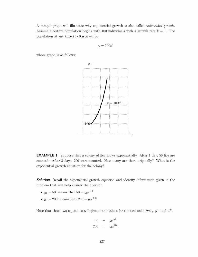
A sample graph will illustrate why exponential growth is also called unbounded growth.Assume a certain population begins with 100 individuals with a growth rate k = 1. Thepopulation at any time t > 0 is given by
y = 100et
whose graph is as follows:
t
y
y = 100et
100
EXAMPLE 1: Suppose that a colony of lice grows exponentially. After 1 day, 50 lice arecounted. After 3 days, 200 were counted. How many are there originally? What is theexponential growth equation for the colony?
Solution. Recall the exponential growth equation and identify information given in theproblem that will help answer the question.
• y1
= 50 means that 50 = y0
ek·1.
• y3
= 200 means that 200 = y0
ek·3.
Note that these two equations will give us the values for the two unknowns, y0
and ek.
50 = y0
ek
200 = y0
e3k.
227
From the first equation, y0
= 50e�k. Using this in the second equation,
200 = (50 e�k)e3k
200 = 50 e2k
4 = e2k
4 = (ek)2
or 2 = ek.
Substituting this in the first equation,
50 = y0
· 2
or y0
= 25.
We now have the answers to the two questions given. First, there were originally 25 lice inthe colony. Second, the exponential growth equation for the given word problem is
y = 25 · 2t.
.
Now, let us take a decay problem.
EXAMPLE 2: The rate of decay of radium is said to be proportional to the amount ofradium present. If the half-life of radium is 1690 years and there are 200 grams on handnow, how much radium will be present in 845 years?
Solution. The exponential decay equation again starts off as y = Cekt.
Since there are 200 grams present at the start, the equation immediately evolves to
y = 200ekt.
A half-life of 1690 years means that the initial amount of 200 grams of radium will reduceto half, or just 100 grams, in 100 years. Thus,
100 = 200ek·1690.
This gives
ek =
✓1
2
◆1/1690
,
and consequently,
y = 200
✓1
2
◆t/1690
.
228
To answer the problem,
y = 200
✓1
2
◆845/1690
= 200
✓1
2
◆1/2
= 200
✓1p2
◆
⇡ 200
✓1
0.707
◆
= 141.4.
Therefore, after 845 years, there will be approximately 141.4 grams of radium left. .
BOUNDED GROWTH
Thinking back, populations cannot really grow without bound. In many cases, the popu-lation is limited by some resource, such as food or space. This limiting quantity or upperbound is sometimes referred to as the carrying capacity, and researchers measure the differ-ence between this limiting quantity and the actual population. If the carrying capacity isgiven by a positive constant, K, the rate of change of y with respect to time t is proportionalto the difference (K � y). That is,
dy
dt= k(K � y) .
This type of growth is called bounded growth.
Now,dy
dt= k(K � y) implies that
dy
(K � y)= k dt.
Integrating both sides of the equation, we get
� ln |K � y| = kt+ C1
and so|K � y| = e�kt+C1 .
Finally, we have|K � y| = C · e�kt.
Two cases emerge from the absolute value expression on the left: K�y > 0 and K�y < 0.The former means that population is lower than the carrying capacity, while the latter has
229
the opposite meaning. It is more usual that the former happens, thus for the succeedingcomputation we consider the former, i.e., y < K.
y < K =) |K � y| = K � y
=) K � y = C · e�kt
=) y = K � C · e�kt.
For future problem-solving, it is useful to note that C is equal to K � y0
, where again y0
is the initial population, or the population at time t.
Teaching Tip
It would be good to ask the students to explore the consequence on the resultingequation if y > K, and the possible scenarios when this may occur.
EXAMPLE 3: A certain pawikan breeding site is said to be able to sustain 5000 pawikans.One thousand pawikans are brought there initially. After a year, this increased to 1100pawikans. How many pawikans will there be after 5 years? Assume that pawikans followthe limited growth model.
Solution. We recall the bounded growth equation and identify parts given in the wordproblem.
• K = 5000.
• y0
= 1000. This means that C = 5000� 1000 = 4000 and the equation becomes
y = 5000� 4000 · e�kt.
The population after 1 year, y1
= 1100, means we can substitute y with 1100 and t with 1to obtain e�k.
1100 = 5000� 4000 · e�k
4000 · e�k= 5000� 1100
= 3900
e�k=
3900
4000
= 0.975.
With the values we have enumerated and solved, the bounded equation is now of the form
y = 5000� 4000 · (0.975)t.
230
We can now find the required population, y5
.
y = 5000� 4000 · (0.975)5
⇡ 5000� 4000 · (0.881)
= 5000� 3524
= 1476.
Therefore, there will be approximately 1476 pawikans in the breeding site. .
The next example illustrates a sort of “decay.” Remember we said earlier that there areoccasions when y > K? This is one instance.
Teaching Tip
At this point, it would be good to relate this to the remarks at the start of boundedgrowth that sometimes y > K. Ideally, cooling would have been one of the scenariosmentioned when you asked for cases that y > K. (See next example.)
EXAMPLE 4: Suppose that newly-baked cupcakes are taken out of the oven which is setat 100 degrees. Room temperature is found to be 25 degrees, and in 15 minutes the cupcakesare found to have a temperature of 50 degrees. Determine the approximate temperature ofthe cupcakes after 30 minutes.
Solution. Newton’s Law of Cooling states that the rate of change of the temperature ofan object is equal to the difference between the object’s temperature and that of thesurrounding air. This gives the differential equation
dy
dt= �k(y � 25).
Since the situation anticipates that the temperature of an object, y, will decrease towardsthat of the surrounding air, ya. Thus, y is assumed to be greater than ya. Furthermore, todenote the decrease, the constant of proportionality is written as �k, with k > 0. t in thisproblem is measured in minutes.
By separation of variables, this becomes
y = 25 + Ce�kt.
• y0
= 100, we get C = 75 and the equation becomes
y = 25 + 75e�kt.
231
• The 50-degree temperature after 15 minutes gives
e�k=
✓1
3
◆1/15
,
and the equation changes further to
y = 25 + 75
✓1
3
◆t/15
.
We can now proceed to approximate the temperature after 30 minutes:
y = 25 + 75
✓1
3
◆30/15
= 25 + 75
✓1
3
◆2
= 25 + 75
✓1
9
◆
⇡ 25 + 8.33
= 33.33.
Hence, after 30 minutes, the cupcakes’ temperature will be approximately 33 degrees. .
LOGISTIC GROWTH
Further studies say that it is more appropriate for the rate of change of a population to beexpressed as proportional to both the size of the population, y, and the difference betweena limiting quantity, K, and the size of the population. Hence,
dy
dt= ky(K � y) .
This is called logistic growth.
In preparation for integration, we write the above equation as
dy
y(K � y)= k dt,
where the left side of the equation may be written as
1
K
✓1
y+
1
K � y
◆.
232
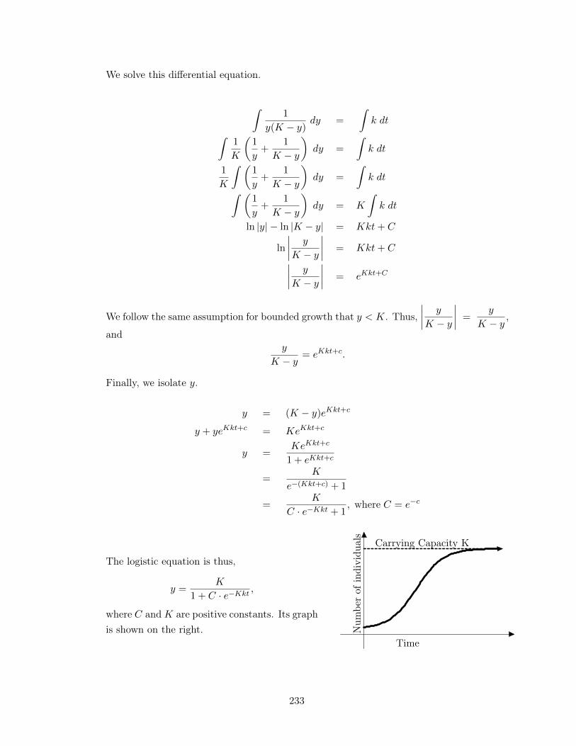
We solve this differential equation.
Z1
y(K � y)dy =
Zk dt
Z1
K
✓1
y+
1
K � y
◆dy =
Zk dt
1
K
Z ✓1
y+
1
K � y
◆dy =
Zk dt
Z ✓1
y+
1
K � y
◆dy = K
Zk dt
ln |y|� ln |K � y| = Kkt+ C
ln
����y
K � y
���� = Kkt+ C����
y
K � y
���� = eKkt+C
We follow the same assumption for bounded growth that y < K. Thus,����
y
K � y
���� =
y
K � y,
andy
K � y= eKkt+c.
Finally, we isolate y.
y = (K � y)eKkt+c
y + yeKkt+c= KeKkt+c
y =
KeKkt+c
1 + eKkt+c
=
K
e�(Kkt+c)+ 1
=
K
C · e�Kkt+ 1
, where C = e�c
The logistic equation is thus,
y =
K
1 + C · e�Kkt,
where C and K are positive constants. Its graphis shown on the right.
Carrying Capacity K
Time
Num
ber
ofin
divi
dual
s
233
Teaching Tip
In case the students ask, be ready to show them
• the solution to1
K
✓1
y+
1
K � y
◆=
1
y(K � y);
• the interim steps in the isolation of y; and
• why C is guaranteed to be positive.
The last bullet may be a recitation question.
EXAMPLE 5: Ten Philippine eagles were introduced to a national park 10 years ago.There are now 23 eagles in the park. The park can support a maximum of 100 eagles.Assuming a logistic growth model, when will the eagle population reach 50?
Solution. To solve the problem, we first recognize how the given information will fit intoand improve our equation.
• Since K = 100, we have y =
100
1 + C · e�100kt
• Since y0
= 23, we can solve for C.
10 =
100
1 + C · e0
10 =
100
1 + C10 + 10C = 100
10C = 90
or C = 9.
Hence, the equation becomes
y =
100
1 + 9 · e�100kt.
The current population of 23 eagles is equal to the population after 10 years, or y10
= 23.
234
This piece of information allows us to solve for the exponential term.
23 =
100
1 + 9e�100k·10
23 =
100
1 + 9e�1000k
1 + 9e�1000k=
100
23
9e�1000k=
100
23
� 1
9e�1000k=
77
23
e�1000k=
77
23 · 9or e�1000k ⇡ 0.37.
Instead of solving for k, it will suffice to find a substitute for e�Kk= e�100k. Clearly, if
e�1000k ⇡ 0.37, then e�100k ⇡ (0.37)1/10. So,
y =
100
1 + 9 · (0.37)t/10.
We are now ready to answer the question, “When will the eagle population reach 50?”Given the most recent version of our logistic equation, we just substitute y with 50 andsolve for t, the time required to have 50 eagles in the population.
50 =
100
1 + 9 · (0.37)t/10
50(1 + 9 · (0.37)t/10) = 100
50 + 450 · (0.37)t/10 = 100
(0.37)t/10 =
100� 50
450
(0.37)t/10 =
1
9
(0.37)t =
✓1
9
◆10
ln(0.37)t = ln
✓1
9
◆10
t · ln(0.37) = 10 · ln✓1
9
◆
t = 10 · ln(1/9)ln(0.37)
t ⇡ 10(2.2) = 22.
The eagle population in the said national park will reach 50 in approximately 22 years. .
235
(C) EXERCISES
(a) The population of Barangay Siksikan is increasing at a rate proportional to its currentpopulation. In the year 2000, the population was 10,000. In 2003, it became 15,000.What was its population in 2009? In approximately what year will its population be100,000?
(b) Certain bacteria cells are being observed in an experiment. The population triples in1 hour. If at the end of 3 hours, the population is 27,000, how many bacteria cellswere present at the start of the experiment? After how many hours, approximately,will the number of cells reach 1 million?
(c) The half-life of a radioactive substance refers to the amount of time it will take forthe quantity to decay to half as much as it was originally. Substance Q has a half-lifeof 20 years. If in 2015, 100g of Q was at hand, how much will be at hand in 2055?How much will be at hand in 2060?
(d) Your parents bought a car in 2012 at the price of P1.2 million. The value of your carwill depreciate over the years due to use. Thus, in 2015 your car is valued at P900,000.What will be your car?s worth in 2018? In what year, approximately, will your carjust be worth P200,000?
(e) Marimar comes from an island-town of 2000 people. She goes to the mainland witha friend and there they catch a highly contagious virus. A week after their returnto their island-town, 8 people are infected. How many will be affected after anotherweek? Their public health center decides that once 30
(f) As the biologist for a certain crocodile farm, you know that its carrying capacity is20,000 crocodiles. You initially release 5000 crocodiles into the farm. After 6 weeks,the crocodile population has increased to 7500. In how many weeks will the populationreach 10,000? In how many weeks will the population reach 20,000?
236
LESSON 15: Riemann Sums and the Definite Integral
TIME FRAME: 4 hours
LEARNING OUTCOMES: At the end of the lesson, the learner shall be able to:
1. Approximate the area of a region under a curve using Riemann sums: (a) left, (b) right,and (c) midpoint; and
2. Define the definite integral as the limit of the Riemann sums.
LESSON OUTLINE:
1. Method of exhaustion2. Riemann sums and Partition points3. Left, right, and midpoint Riemann sums4. Refinement5. Irregular partition6. Formal definition of a definite integral7. Geometric interpretation of a definite integral8. Computing definite integrals9. Properties of the definite integral
10. The definite integral as a net signed area11. Exercises and enrichment
237
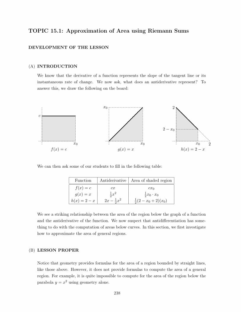
TOPIC 15.1: Approximation of Area using Riemann Sums
DEVELOPMENT OF THE LESSON
(A) INTRODUCTION
We know that the derivative of a function represents the slope of the tangent line or itsinstantaneous rate of change. We now ask, what does an antiderivative represent? Toanswer this, we draw the following on the board:
x0
x0
x0
f(x) = c g(x) = x h(x) = 2� x
c
x0
2� x0
2
2
We can then ask some of our students to fill in the following table:
Function Antiderivative Area of shaded region
f(x) = c cx cx0
g(x) = x 1
2
x2 1
2
x0
· x0
h(x) = 2� x 2x� 1
2
x2 1
2
(2� x0
+ 2)(x0
)
We see a striking relationship between the area of the region below the graph of a functionand the antiderivative of the function. We now suspect that antidifferentiation has some-thing to do with the computation of areas below curves. In this section, we first investigatehow to approximate the area of general regions.
(B) LESSON PROPER
Notice that geometry provides formulas for the area of a region bounded by straight lines,like those above. However, it does not provide formulas to compute the area of a generalregion. For example, it is quite impossible to compute for the area of the region below theparabola y = x2 using geometry alone.
238
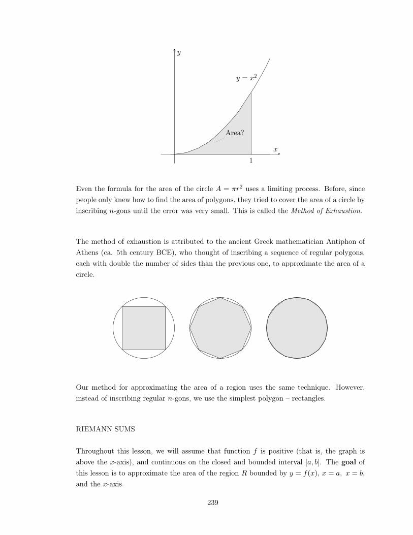
1
y = x2
Area?
x
y
Even the formula for the area of the circle A = ⇡r2 uses a limiting process. Before, sincepeople only knew how to find the area of polygons, they tried to cover the area of a circle byinscribing n-gons until the error was very small. This is called the Method of Exhaustion.
The method of exhaustion is attributed to the ancient Greek mathematician Antiphon ofAthens (ca. 5th century BCE), who thought of inscribing a sequence of regular polygons,each with double the number of sides than the previous one, to approximate the area of acircle.
Our method for approximating the area of a region uses the same technique. However,instead of inscribing regular n-gons, we use the simplest polygon – rectangles.
RIEMANN SUMS
Throughout this lesson, we will assume that function f is positive (that is, the graph isabove the x-axis), and continuous on the closed and bounded interval [a, b]. The goal ofthis lesson is to approximate the area of the region R bounded by y = f(x), x = a, x = b,
and the x-axis.
239
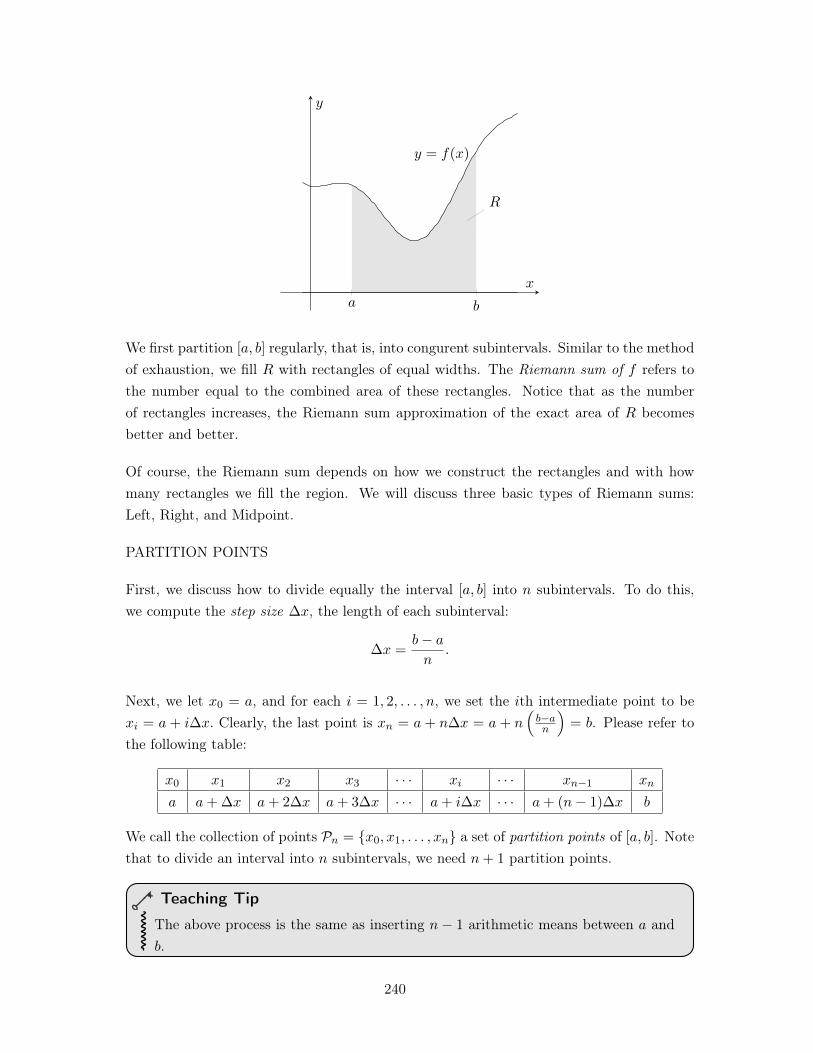
a b
y = f(x)
R
x
y
We first partition [a, b] regularly, that is, into congurent subintervals. Similar to the methodof exhaustion, we fill R with rectangles of equal widths. The Riemann sum of f refers tothe number equal to the combined area of these rectangles. Notice that as the numberof rectangles increases, the Riemann sum approximation of the exact area of R becomesbetter and better.
Of course, the Riemann sum depends on how we construct the rectangles and with howmany rectangles we fill the region. We will discuss three basic types of Riemann sums:Left, Right, and Midpoint.
PARTITION POINTS
First, we discuss how to divide equally the interval [a, b] into n subintervals. To do this,we compute the step size �x, the length of each subinterval:
�x =
b� a
n.
Next, we let x0
= a, and for each i = 1, 2, . . . , n, we set the ith intermediate point to bexi = a + i�x. Clearly, the last point is xn = a + n�x = a + n
⇣b�an
⌘= b. Please refer to
the following table:
x0
x1
x2
x3
· · · xi · · · xn�1
xn
a a+�x a+ 2�x a+ 3�x · · · a+ i�x · · · a+ (n� 1)�x b
We call the collection of points Pn = {x0
, x1
, . . . , xn} a set of partition points of [a, b]. Notethat to divide an interval into n subintervals, we need n+ 1 partition points.
Teaching Tip
The above process is the same as inserting n� 1 arithmetic means between a andb.
240
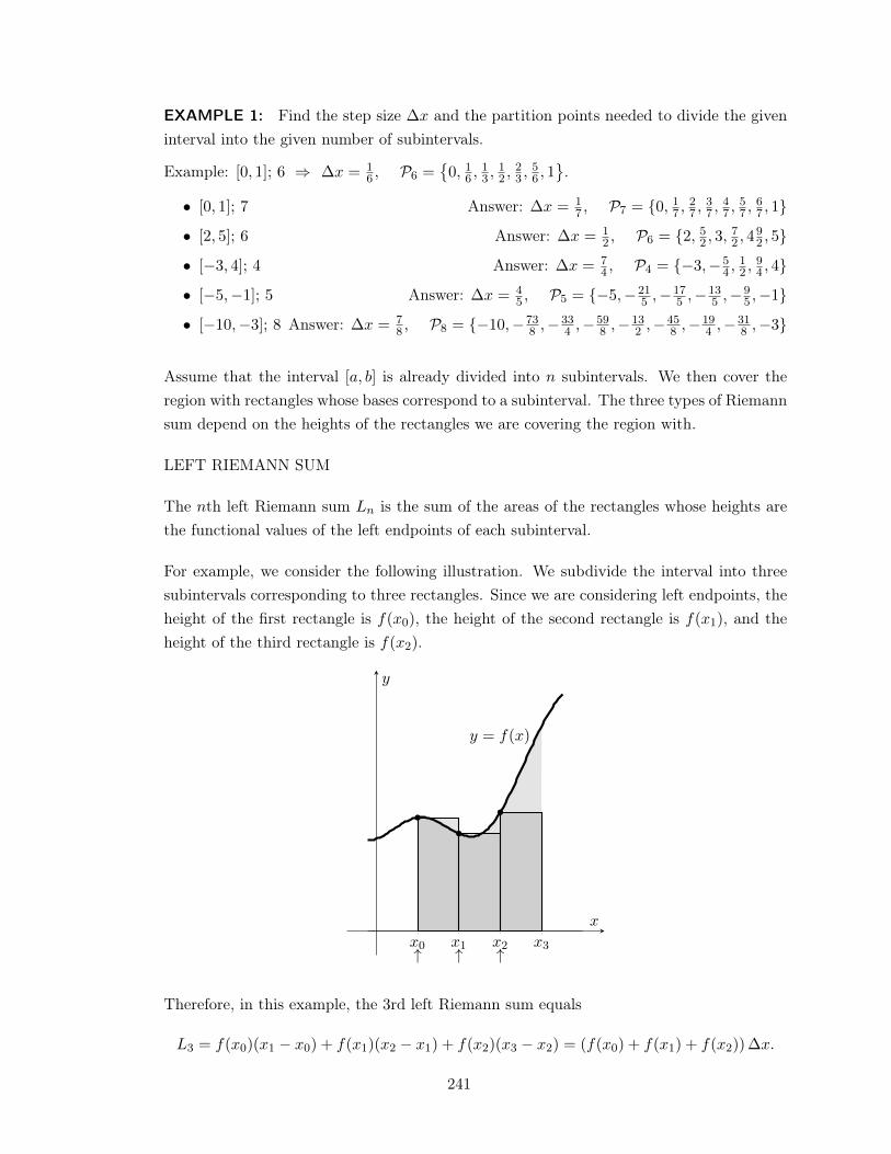
EXAMPLE 1: Find the step size �x and the partition points needed to divide the giveninterval into the given number of subintervals.
Example: [0, 1]; 6 ) �x =
1
6
, P6
=
�0, 1
6
, 13
, 12
, 23
, 56
, 1 .
• [0, 1]; 7 Answer: �x =
1
7
, P7
= {0, 17
, 27
, 37
, 47
, 57
, 67
, 1}
• [2, 5]; 6 Answer: �x =
1
2
, P6
= {2, 52
, 3, 72
, 49
2
, 5}
• [�3, 4]; 4 Answer: �x =
7
4
, P4
= {�3,�5
4
, 12
, 94
, 4}
• [�5,�1]; 5 Answer: �x =
4
5
, P5
= {�5,�21
5
,�17
5
,�13
5
,�9
5
,�1}
• [�10,�3]; 8 Answer: �x =
7
8
, P8
= {�10,�73
8
,�33
4
,�59
8
,�13
2
,�45
8
,�19
4
,�31
8
,�3}
Assume that the interval [a, b] is already divided into n subintervals. We then cover theregion with rectangles whose bases correspond to a subinterval. The three types of Riemannsum depend on the heights of the rectangles we are covering the region with.
LEFT RIEMANN SUM
The nth left Riemann sum Ln is the sum of the areas of the rectangles whose heights arethe functional values of the left endpoints of each subinterval.
For example, we consider the following illustration. We subdivide the interval into threesubintervals corresponding to three rectangles. Since we are considering left endpoints, theheight of the first rectangle is f(x
0
), the height of the second rectangle is f(x1
), and theheight of the third rectangle is f(x
2
).
" " "x0
x1
x2
x3
y = f(x)
x
y
Therefore, in this example, the 3rd left Riemann sum equals
L3
= f(x0
)(x1
� x0
) + f(x1
)(x2
� x1
) + f(x2
)(x3
� x2
) = (f(x0
) + f(x1
) + f(x2
))�x.
241
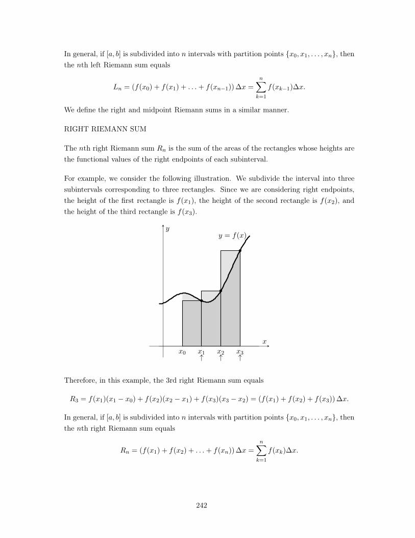
In general, if [a, b] is subdivided into n intervals with partition points {x0
, x1
, . . . , xn}, thenthe nth left Riemann sum equals
Ln = (f(x0
) + f(x1
) + . . .+ f(xn�1
))�x =
nX
k=1
f(xk�1
)�x.
We define the right and midpoint Riemann sums in a similar manner.
RIGHT RIEMANN SUM
The nth right Riemann sum Rn is the sum of the areas of the rectangles whose heights arethe functional values of the right endpoints of each subinterval.
For example, we consider the following illustration. We subdivide the interval into threesubintervals corresponding to three rectangles. Since we are considering right endpoints,the height of the first rectangle is f(x
1
), the height of the second rectangle is f(x2
), andthe height of the third rectangle is f(x
3
).
" " "x0
x1
x2
x3
y = f(x)
x
y
Therefore, in this example, the 3rd right Riemann sum equals
R3
= f(x1
)(x1
� x0
) + f(x2
)(x2
� x1
) + f(x3
)(x3
� x2
) = (f(x1
) + f(x2
) + f(x3
))�x.
In general, if [a, b] is subdivided into n intervals with partition points {x0
, x1
, . . . , xn}, thenthe nth right Riemann sum equals
Rn = (f(x1
) + f(x2
) + . . .+ f(xn))�x =
nX
k=1
f(xk)�x.
242
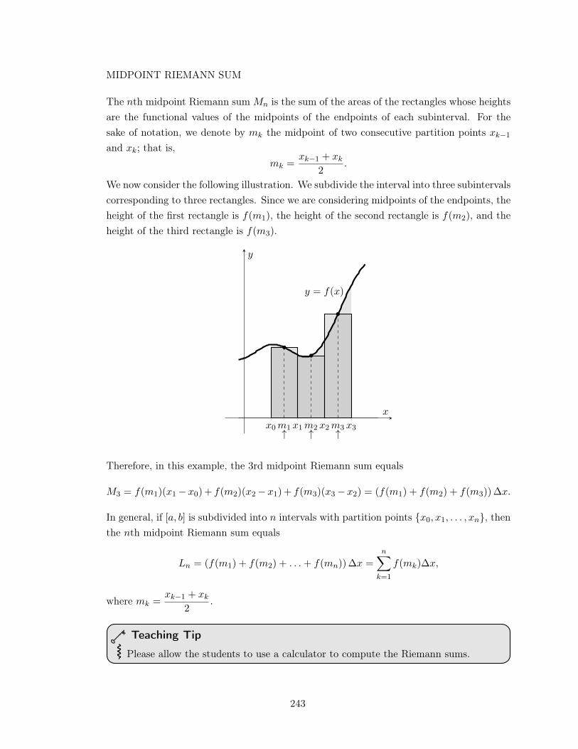
MIDPOINT RIEMANN SUM
The nth midpoint Riemann sum Mn is the sum of the areas of the rectangles whose heightsare the functional values of the midpoints of the endpoints of each subinterval. For thesake of notation, we denote by mk the midpoint of two consecutive partition points xk�1
and xk; that is,mk =
xk�1
+ xk2
.
We now consider the following illustration. We subdivide the interval into three subintervalscorresponding to three rectangles. Since we are considering midpoints of the endpoints, theheight of the first rectangle is f(m
1
), the height of the second rectangle is f(m2
), and theheight of the third rectangle is f(m
3
).
" " "x0
m1
x1
m2
x2
m3
x3
y = f(x)
x
y
Therefore, in this example, the 3rd midpoint Riemann sum equals
M3
= f(m1
)(x1
�x0
)+ f(m2
)(x2
�x1
)+ f(m3
)(x3
�x2
) = (f(m1
) + f(m2
) + f(m3
))�x.
In general, if [a, b] is subdivided into n intervals with partition points {x0
, x1
, . . . , xn}, thenthe nth midpoint Riemann sum equals
Ln = (f(m1
) + f(m2
) + . . .+ f(mn))�x =
nX
k=1
f(mk)�x,
where mk =
xk�1
+ xk2
.
Teaching Tip
Please allow the students to use a calculator to compute the Riemann sums.
243
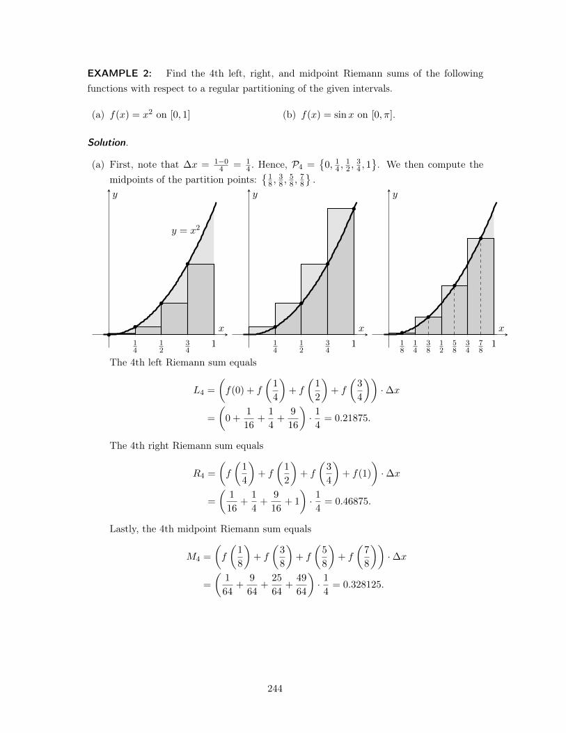
EXAMPLE 2: Find the 4th left, right, and midpoint Riemann sums of the followingfunctions with respect to a regular partitioning of the given intervals.
(a) f(x) = x2 on [0, 1] (b) f(x) = sinx on [0,⇡].
Solution. .
(a) First, note that �x =
1�0
4
=
1
4
. Hence, P4
=
�0, 1
4
, 12
, 34
, 1 . We then compute the
midpoints of the partition points:�1
8
, 38
, 58
, 78
.
1
4
1
2
3
4
1
y = x2
x
y
1
4
1
2
3
4
1
x
y
1
8
1
4
3
8
1
2
5
8
3
4
7
8
1
x
y
The 4th left Riemann sum equals
L4
=
✓f(0) + f
✓1
4
◆+ f
✓1
2
◆+ f
✓3
4
◆◆·�x
=
✓0 +
1
16
+
1
4
+
9
16
◆· 14
= 0.21875.
The 4th right Riemann sum equals
R4
=
✓f
✓1
4
◆+ f
✓1
2
◆+ f
✓3
4
◆+ f(1)
◆·�x
=
✓1
16
+
1
4
+
9
16
+ 1
◆· 14
= 0.46875.
Lastly, the 4th midpoint Riemann sum equals
M4
=
✓f
✓1
8
◆+ f
✓3
8
◆+ f
✓5
8
◆+ f
✓7
8
◆◆·�x
=
✓1
64
+
9
64
+
25
64
+
49
64
◆· 14
= 0.328125.
244
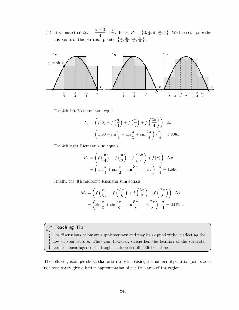
(b) First, note that �x =
⇡ � 0
4
=
⇡
4
. Hence, P4
=
�0, ⇡
4
, ⇡2
, 3⇡4
, 1 . We then compute the
midpoints of the partition points:�⇡8
, 3⇡8
, 5⇡8
, 7⇡8
.
⇡4
⇡2
3⇡4
⇡
y = sinx
x
y
⇡4
⇡2
3⇡4
⇡x
y
⇡8
1
4
3⇡8
1
2
5⇡8
3
4
7⇡8
1
x
y
The 4th left Riemann sum equals
L4
=
✓f(0) + f
⇣⇡4
⌘+ f
⇣⇡2
⌘+ f
✓3⇡
4
◆◆·�x
=
✓sin 0 + sin
⇡
4
+ sin
⇡
2
+ sin
3⇡
4
◆· ⇡4
= 1.896...
The 4th right Riemann sum equals
R4
=
✓f⇣⇡4
⌘+ f
⇣⇡2
⌘+ f
✓3⇡
4
◆+ f(⇡)
◆·�x
=
✓sin
⇡
4
+ sin
⇡
2
+ sin
3⇡
4
+ sin⇡
◆· ⇡4
= 1.896...
Finally, the 4th midpoint Riemann sum equals
M4
=
✓f⇣⇡8
⌘+ f
✓3⇡
8
◆+ f
✓5⇡
8
◆+ f
✓7⇡
8
◆◆·�x
=
✓sin
⇡
8
+ sin
3⇡
8
+ sin
5⇡
8
+ sin
7⇡
8
◆· ⇡4
= 2.052...
.
Teaching Tip
The discussions below are supplementary and may be skipped without affecting theflow of your lecture. They can, however, strengthen the learning of the students,and are encouraged to be taught if there is still sufficient time.
The following example shows that arbitrarily increasing the number of partition points doesnot necessarily give a better approximation of the true area of the region.
245
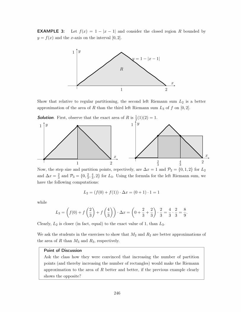
EXAMPLE 3: Let f(x) = 1 � |x � 1| and consider the closed region R bounded byy = f(x) and the x-axis on the interval [0, 2].
1 2
1y = 1� |x� 1|
x
y
R
Show that relative to regular partitioning, the second left Riemann sum L2
is a betterapproximation of the area of R than the third left Riemann sum L
3
of f on [0, 2].
Solution. First, observe that the exact area of R is 1
2
(1)(2) = 1.
1 2
1
x
y
2
3
4
3
2
1
x
y
Now, the step size and partition points, repectively, are �x = 1 and P2
= {0, 1, 2} for L2
and �x =
2
3
and P3
= {0, 23
, 43
, 2} for L3
. Using the formula for the left Riemann sum, wehave the following computations:
L2
= (f(0) + f(1)) ·�x = (0 + 1) · 1 = 1
while
L3
=
✓f(0) + f
✓2
3
◆+ f
✓4
3
◆◆·�x =
✓0 +
2
3
+
2
3
◆· 23
=
4
3
· 23
=
8
9
.
Clearly, L2
is closer (in fact, equal) to the exact value of 1, than L3
.
We ask the students in the exercises to show that M2
and R2
are better approximations ofthe area of R than M
3
and R3
, respectively. .
Point of DiscussionAsk the class how they were convinced that increasing the number of partitionpoints (and thereby increasing the number of rectangles) would make the Riemannapproximation to the area of R better and better, if the previous example clearlyshows the opposite?
246
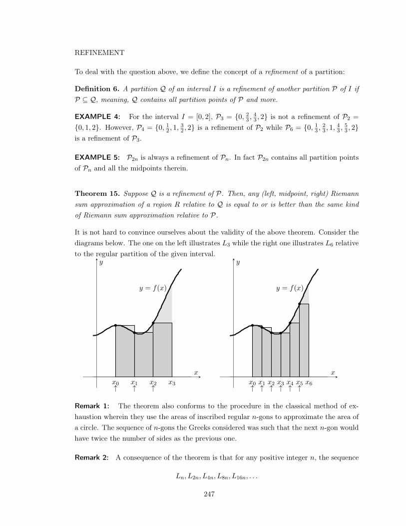
REFINEMENT
To deal with the question above, we define the concept of a refinement of a partition:
Definition 6. A partition Q of an interval I is a refinement of another partition P of I ifP ✓ Q, meaning, Q contains all partition points of P and more.
EXAMPLE 4: For the interval I = [0, 2], P3
= {0, 23
, 43
, 2} is not a refinement of P2
=
{0, 1, 2}. However, P4
= {0, 12
, 1, 32
, 2} is a refinement of P2
while P6
= {0, 13
, 23
, 1, 43
, 53
, 2}is a refinement of P
3
.
EXAMPLE 5: P2n is always a refinement of Pn. In fact P
2n contains all partition pointsof Pn and all the midpoints therein.
Theorem 15. Suppose Q is a refinement of P. Then, any (left, midpoint, right) Riemannsum approximation of a region R relative to Q is equal to or is better than the same kindof Riemann sum approximation relative to P.
It is not hard to convince ourselves about the validity of the above theorem. Consider thediagrams below. The one on the left illustrates L
3
while the right one illustrates L6
relativeto the regular partition of the given interval.
" " "x0
x1
x2
x3
y = f(x)
x
y
" " "" " "x0
x1
x2
x3
x4
x5
x6
y = f(x)
x
y
Remark 1: The theorem also conforms to the procedure in the classical method of ex-haustion wherein they use the areas of inscribed regular n-gons to approximate the area ofa circle. The sequence of n-gons the Greeks considered was such that the next n-gon wouldhave twice the number of sides as the previous one.
Remark 2: A consequence of the theorem is that for any positive integer n, the sequence
Ln, L2n, L4n, L8n, L16n, . . .
247
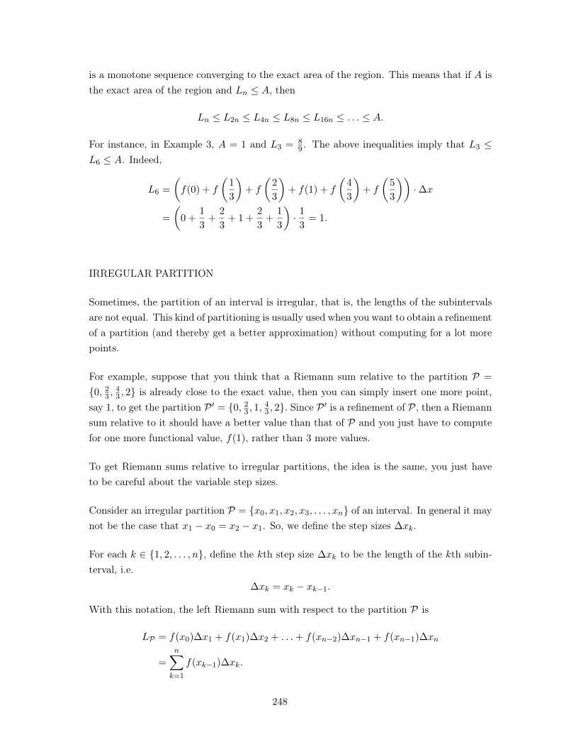
is a monotone sequence converging to the exact area of the region. This means that if A isthe exact area of the region and Ln A, then
Ln L2n L
4n L8n L
16n . . . A.
For instance, in Example 3, A = 1 and L3
=
8
9
. The above inequalities imply that L3
L6
A. Indeed,
L6
=
✓f(0) + f
✓1
3
◆+ f
✓2
3
◆+ f(1) + f
✓4
3
◆+ f
✓5
3
◆◆·�x
=
✓0 +
1
3
+
2
3
+ 1 +
2
3
+
1
3
◆· 13
= 1.
IRREGULAR PARTITION
Sometimes, the partition of an interval is irregular, that is, the lengths of the subintervalsare not equal. This kind of partitioning is usually used when you want to obtain a refinementof a partition (and thereby get a better approximation) without computing for a lot morepoints.
For example, suppose that you think that a Riemann sum relative to the partition P =
{0, 23
, 43
, 2} is already close to the exact value, then you can simply insert one more point,say 1, to get the partition P 0
= {0, 23
, 1, 43
, 2}. Since P 0 is a refinement of P, then a Riemannsum relative to it should have a better value than that of P and you just have to computefor one more functional value, f(1), rather than 3 more values.
To get Riemann sums relative to irregular partitions, the idea is the same, you just haveto be careful about the variable step sizes.
Consider an irregular partition P = {x0
, x1
, x2
, x3
, . . . , xn} of an interval. In general it maynot be the case that x
1
� x0
= x2
� x1
. So, we define the step sizes �xk.
For each k 2 {1, 2, . . . , n}, define the kth step size �xk to be the length of the kth subin-terval, i.e.
�xk = xk � xk�1
.
With this notation, the left Riemann sum with respect to the partition P is
LP = f(x0
)�x1
+ f(x1
)�x2
+ . . .+ f(xn�2
)�xn�1
+ f(xn�1
)�xn
=
nX
k=1
f(xk�1
)�xk.
248
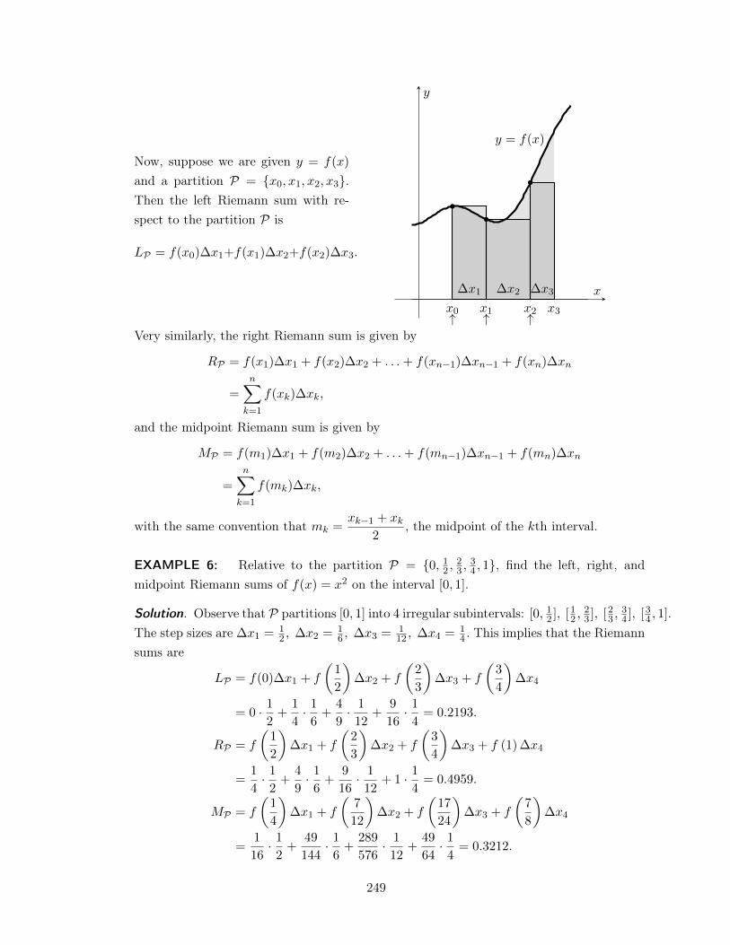
Now, suppose we are given y = f(x)
and a partition P = {x0
, x1
, x2
, x3
}.Then the left Riemann sum with re-spect to the partition P is
LP = f(x0
)�x1
+f(x1
)�x2
+f(x2
)�x3
.
" " "
�x1
�x2
�x3
x0
x1
x2
x3
y = f(x)
x
y
Very similarly, the right Riemann sum is given by
RP = f(x1
)�x1
+ f(x2
)�x2
+ . . .+ f(xn�1
)�xn�1
+ f(xn)�xn
=
nX
k=1
f(xk)�xk,
and the midpoint Riemann sum is given by
MP = f(m1
)�x1
+ f(m2
)�x2
+ . . .+ f(mn�1
)�xn�1
+ f(mn)�xn
=
nX
k=1
f(mk)�xk,
with the same convention that mk =
xk�1
+ xk2
, the midpoint of the kth interval.
EXAMPLE 6: Relative to the partition P = {0, 12
, 23
, 34
, 1}, find the left, right, andmidpoint Riemann sums of f(x) = x2 on the interval [0, 1].
Solution. Observe that P partitions [0, 1] into 4 irregular subintervals: [0, 12
], [12
, 23
], [23
, 34
], [34
, 1].The step sizes are �x
1
=
1
2
, �x2
=
1
6
, �x3
=
1
12
, �x4
=
1
4
. This implies that the Riemannsums are
LP = f(0)�x1
+ f
✓1
2
◆�x
2
+ f
✓2
3
◆�x
3
+ f
✓3
4
◆�x
4
= 0 · 12
+
1
4
· 16
+
4
9
· 1
12
+
9
16
· 14
= 0.2193.
RP = f
✓1
2
◆�x
1
+ f
✓2
3
◆�x
2
+ f
✓3
4
◆�x
3
+ f (1)�x4
=
1
4
· 12
+
4
9
· 16
+
9
16
· 1
12
+ 1 · 14
= 0.4959.
MP = f
✓1
4
◆�x
1
+ f
✓7
12
◆�x
2
+ f
✓17
24
◆�x
3
+ f
✓7
8
◆�x
4
=
1
16
· 12
+
49
144
· 16
+
289
576
· 1
12
+
49
64
· 14
= 0.3212.
249
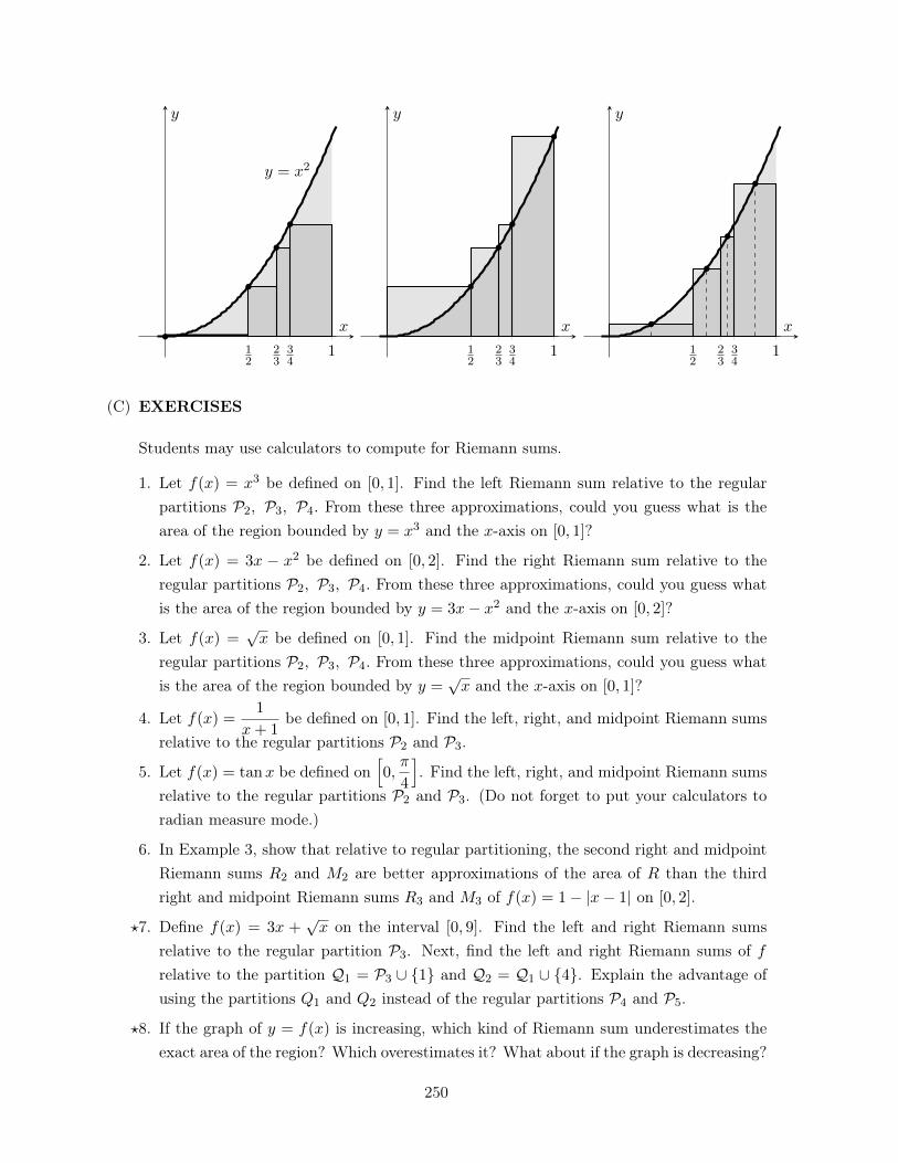
1
2
2
3
3
4
1
y = x2
x
y
1
2
2
3
3
4
1
x
y
1
2
2
3
3
4
1
x
y
.
(C) EXERCISES
Students may use calculators to compute for Riemann sums.
1. Let f(x) = x3 be defined on [0, 1]. Find the left Riemann sum relative to the regularpartitions P
2
, P3
, P4
. From these three approximations, could you guess what is thearea of the region bounded by y = x3 and the x-axis on [0, 1]?
2. Let f(x) = 3x � x2 be defined on [0, 2]. Find the right Riemann sum relative to theregular partitions P
2
, P3
, P4
. From these three approximations, could you guess whatis the area of the region bounded by y = 3x� x2 and the x-axis on [0, 2]?
3. Let f(x) =
px be defined on [0, 1]. Find the midpoint Riemann sum relative to the
regular partitions P2
, P3
, P4
. From these three approximations, could you guess whatis the area of the region bounded by y =
px and the x-axis on [0, 1]?
4. Let f(x) =1
x+ 1
be defined on [0, 1]. Find the left, right, and midpoint Riemann sumsrelative to the regular partitions P
2
and P3
.
5. Let f(x) = tanx be defined onh0,
⇡
4
i. Find the left, right, and midpoint Riemann sums
relative to the regular partitions P2
and P3
. (Do not forget to put your calculators toradian measure mode.)
6. In Example 3, show that relative to regular partitioning, the second right and midpointRiemann sums R
2
and M2
are better approximations of the area of R than the thirdright and midpoint Riemann sums R
3
and M3
of f(x) = 1� |x� 1| on [0, 2].
?7. Define f(x) = 3x +
px on the interval [0, 9]. Find the left and right Riemann sums
relative to the regular partition P3
. Next, find the left and right Riemann sums of frelative to the partition Q
1
= P3
[ {1} and Q2
= Q1
[ {4}. Explain the advantage ofusing the partitions Q
1
and Q2
instead of the regular partitions P4
and P5
.
?8. If the graph of y = f(x) is increasing, which kind of Riemann sum underestimates theexact area of the region? Which overestimates it? What about if the graph is decreasing?
250
?9. Relative to the same partition, which among the left, right, and midpoint Riemann sumsprovides the best approximation of the exact area of a region? (Without much loss ofgenerality, you can assume that the curve is monotone because if it is not monotoneon a subinterval, then a sufficient refinement of the partition on that subinterval wouldresult in monotone portions of the graph on each subinterval.)
Solution to starred exercises
7. We first collect the functional values that we will be needing.
x f(x) = 3x+
px
0 0
1 4
3 10.73
4 14
6 20.45
9 30
Now, P3
= {0, 3, 6, 9}. So,
• L3
= 3(f(0) + f(3) + f(5)) = 93.54
• R3
= 3(f(3) + f(6) + f(9)) = 183.54
Now, Q1
= {0, 1, 3, 6, 9}. So,
• LQ1 = 1 · f(0) + 2 · f(1) + 3 · f(3) + 3 · f(6) = 101.54
• RQ1 = 1 · f(1) + 2 · f(3) + 3 · f(6) + 3 · f(9) = 176.81
From the given, Q2
= {0, 1, 3, 4, 6, 9}. So,
• 1 · f(0) + 2 · f(1) + 1 · f(3) + 2 · f(4) + 3 · f(6) = 108.08
• 1 · f(1) + 2 · f(3) + 1 · f(4) + 2 · f(6) + 3 · f(9) = 170.36
It is attractive to consider Q1
and Q2
because we are sure that we get better approximations(as they are refinements of P
3
). Moreover, we already have values for f(3) and f(6) fromP3
. We just have to reuse them for the Riemann sums for Q1
and Q2
. In contrast, ifwe had used P
4
= {0, 9/4, 9/2, 27/4, 9}, we need to get the values of f(9/4), f(9/2) andf(27/4) and we are still not assured that the corresponding Riemann sums are better thanthose corresponding to P
3
.
8. If the graph is increasing the rectangles of the left Riemann sum are inscribed, hence itunderestimates the true area of the region. On the other hand, the rectangles of the rightRiemann sum are circumscribed by the region. Hence, they overestimate the area of theregion. The opposite situation happens for decreasing graphs.
251
9. For a monotone curve (i.e., either increasing or decreasing), the midpoint Riemann sumprovides the best approximation to the area of the region. If you bisect these rectanglesin the middle, you will see that one is inscribed and the other is circumscribed. Therefore,the underestimation of one is offset by the overestimation of the other.
252
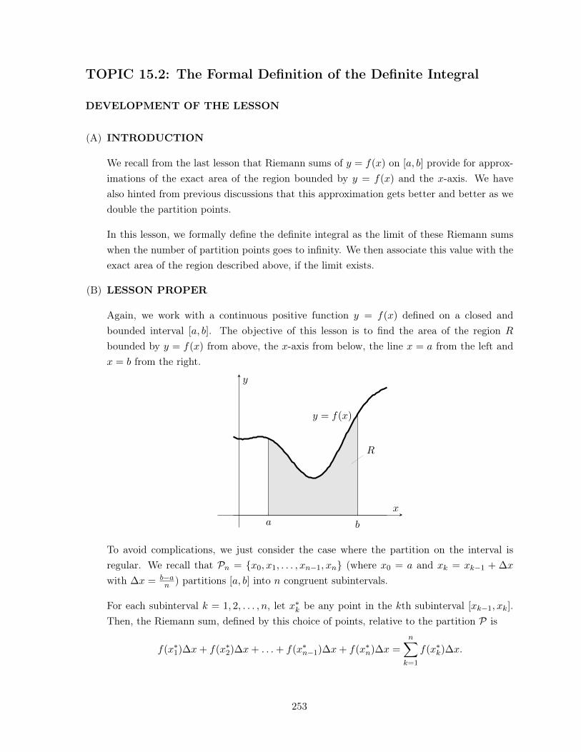
TOPIC 15.2: The Formal Definition of the Definite Integral
DEVELOPMENT OF THE LESSON
(A) INTRODUCTION
We recall from the last lesson that Riemann sums of y = f(x) on [a, b] provide for approx-imations of the exact area of the region bounded by y = f(x) and the x-axis. We havealso hinted from previous discussions that this approximation gets better and better as wedouble the partition points.
In this lesson, we formally define the definite integral as the limit of these Riemann sumswhen the number of partition points goes to infinity. We then associate this value with theexact area of the region described above, if the limit exists.
(B) LESSON PROPER
Again, we work with a continuous positive function y = f(x) defined on a closed andbounded interval [a, b]. The objective of this lesson is to find the area of the region R
bounded by y = f(x) from above, the x-axis from below, the line x = a from the left andx = b from the right.
a b
y = f(x)
R
x
y
To avoid complications, we just consider the case where the partition on the interval isregular. We recall that Pn = {x
0
, x1
, . . . , xn�1
, xn} (where x0
= a and xk = xk�1
+ �x
with �x =
b�an ) partitions [a, b] into n congruent subintervals.
For each subinterval k = 1, 2, . . . , n, let x⇤k be any point in the kth subinterval [xk�1
, xk].Then, the Riemann sum, defined by this choice of points, relative to the partition P is
f(x⇤1
)�x+ f(x⇤2
)�x+ . . .+ f(x⇤n�1
)�x+ f(x⇤n)�x =
nX
k=1
f(x⇤k)�x.
253
The class should realize that
• If this is a left Riemann sum, then x⇤k = xk�1
;
• If this is a right Riemann sum, then x⇤k = xk; and finally,
• If this is a midpoint Riemann sum, then x⇤k =
1
2
(xk�1
+ xk).
In any case, we know that the above Riemann sum is only an approximation of the exactarea of R. To make this estimate exact, we let n approach infinity. This limit of theRiemann sum is what we call the definite integral of f over [a, b]:
lim
n!1
nX
k=1
f(x⇤k)�x =
Z b
af(x) dx,
if this limit exists. The value of this integral does not depend on the kind (left, right, ormidpoint) of Riemann sum being used.
Teaching Tip
To make this lesson easy to remember, you may relate the anecdote on why theintegral sign
Rlooks like an elongated s: This is because the integral sign is nothing
but a limit l of a sum s andR
is the symbol that you get by joining the letters l
and s.
As the definite integral is the limit of a Riemann sum, many authors also refer toit as a Riemann integral.
Remember that �x actually depends on n: �x =
b� a
n. So, this term cannot be taken
out from the limit operator. After taking the limit, this �x becomes our differential dx.
The integral signR
and the differential dx act as delimiters, which indicate that everythingbetween them is the integrand - the upper boundary of the region whose area is whatthis integral is equal to. The numbers a and b are called the lower and upper limits ofintegration, respectively. Recall that the integral sign
Rwas earlier used to denote the
process of antidifferentiation. There is a reason why the same symbol (R
) is being used –we shall see later that antiderivatives are intimately related to finding areas below curves.
254
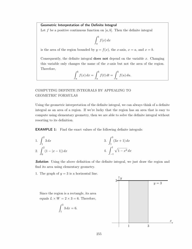
Geometric Interpretation of the Definite IntegralLet f be a positive continuous function on [a, b]. Then the definite integral
Z b
af(x) dx
is the area of the region bounded by y = f(x), the x-axis, x = a, and x = b.
Consequently, the definite integral does not depend on the variable x. Changingthis variable only changes the name of the x-axis but not the area of the region.Therefore, Z b
af(x) dx =
Z b
af(t) dt =
Z b
af(u) du.
COMPUTING DEFINITE INTEGRALS BY APPEALING TOGEOMETRIC FORMULAS
Using the geometric interpretation of the definite integral, we can always think of a definiteintegral as an area of a region. If we’re lucky that the region has an area that is easy tocompute using elementary geometry, then we are able to solve the definite integral withoutresorting to its definition.
EXAMPLE 1: Find the exact values of the following definite integrals:
1.Z
2
1
3 dx
2.Z
2
0
(1� |x� 1|) dx
3.Z
3
1
(3x+ 1) dx
4.Z
1
�1
p1� x2 dx
Solution. Using the above definition of the definite integral, we just draw the region andfind its area using elementary geometry.
1. The graph of y = 3 is a horizontal line.
Since the region is a rectangle, its areaequals L⇥W = 2⇥ 3 = 6. Therefore,
Z3
1
3 dx = 6.
1 3
3y = 3
x
y
255
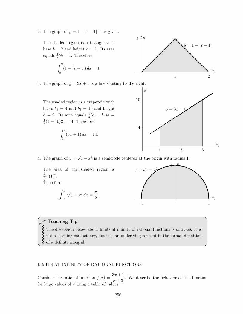
2. The graph of y = 1� |x� 1| is as given.
The shaded region is a triangle withbase b = 2 and height h = 1. Its areaequals 1
2
bh = 1. Therefore,Z
2
0
(1� |x� 1|) dx = 1.
1 2
1y = 1� |x� 1|
x
y
3. The graph of y = 3x+ 1 is a line slanting to the right.
The shaded region is a trapezoid withbases b
1
= 4 and b2
= 10 and heighth = 2. Its area equals 1
2
(b1
+ b2
)h =
1
2
(4 + 10)2 = 14. Therefore,Z
3
1
(3x+ 1) dx = 14.
1 2 3
4
10
y = 3x+ 1
x
y
4. The graph of y =
p1� x2 is a semicircle centered at the origin with radius 1.
The area of the shaded region is1
2
⇡(1)2.
Therefore,Z
1
�1
p1� x2 dx =
⇡
2
.
�1 1
1y =
p1� x2
x
y
.
Teaching Tip
The discussion below about limits at infinity of rational functions is optional. It isnot a learning competency, but it is an underlying concept in the formal definitionof a definite integral.
LIMITS AT INFINITY OF RATIONAL FUNCTIONS
Consider the rational function f(x) =3x+ 1
x+ 3
. We describe the behavior of this functionfor large values of x using a table of values:
256
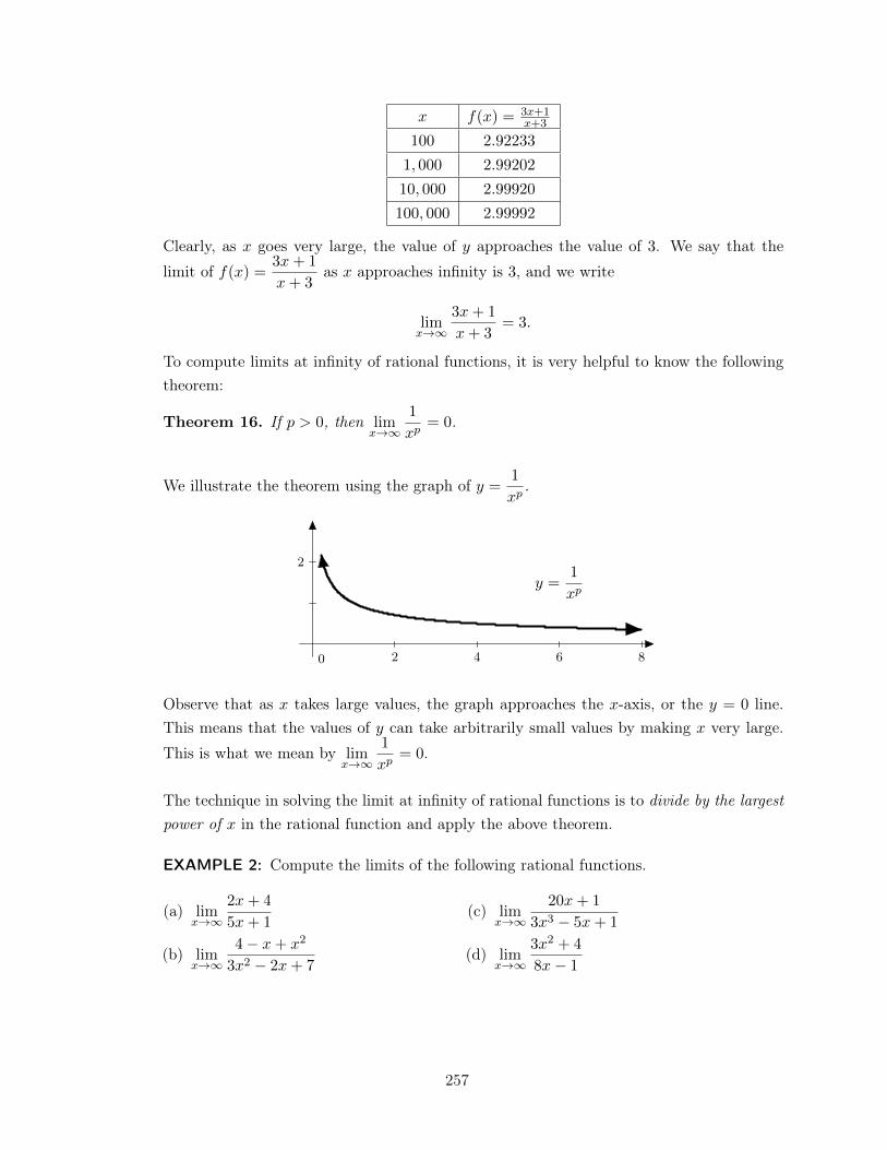
x f(x) = 3x+1
x+3
100 2.92233
1, 000 2.99202
10, 000 2.99920
100, 000 2.99992
Clearly, as x goes very large, the value of y approaches the value of 3. We say that thelimit of f(x) =
3x+ 1
x+ 3
as x approaches infinity is 3, and we write
lim
x!1
3x+ 1
x+ 3
= 3.
To compute limits at infinity of rational functions, it is very helpful to know the followingtheorem:
Theorem 16. If p > 0, then lim
x!1
1
xp= 0.
We illustrate the theorem using the graph of y =
1
xp.
2 4 6 8
2
0
y =
1
xp
Observe that as x takes large values, the graph approaches the x-axis, or the y = 0 line.This means that the values of y can take arbitrarily small values by making x very large.This is what we mean by lim
x!1
1
xp= 0.
The technique in solving the limit at infinity of rational functions is to divide by the largestpower of x in the rational function and apply the above theorem.
EXAMPLE 2: Compute the limits of the following rational functions.
(a) lim
x!1
2x+ 4
5x+ 1
(b) lim
x!1
4� x+ x2
3x2 � 2x+ 7
(c) lim
x!1
20x+ 1
3x3 � 5x+ 1
(d) lim
x!1
3x2 + 4
8x� 1
257
Solution. .
(a) The highest power of x here is x1. So,
lim
x!1
2x+ 4
5x+ 1
·
1
x1
x
=
2 +
4
x
5 +
1
x
.
Using limit theorems and Theorem 16,
lim
x!1
2x+ 4
5x+ 1
=
lim
x!12 + 4 lim
x!1
1
x
lim
x!15 + lim
x!1
1
x
=
2 + 0
5 + 0
=
2
5
.
(b) The highest power of x here is x2. So, by Theorem 16,
lim
x!1
4� x+ x2
3x2 � 2x+ 7
·
1
x21
x2
= lim
x!1
4
x2+
1
x+ 1
3� 2
x+
7
x2
=
0� 0 + 1
3� 0 + 0
=
1
3
.
(c) The highest power of x here is x3. Again, using Theorem 16,
lim
x!1
20x+ 1
3x3 � 5x+ 1
·
1
x31
x3
= lim
x!1
20
x2+
1
x3
3� 5
x2+
1
x3
=
0 + 0
3� 0 + 0
= 0.
(d) The highest power of x here is x2. So,
lim
x!1
3x2 + 4
8x� 1
·
1
x21
x2
= lim
x!1
3 +
4
x28
x� 1
x2
.
Notice that the numerator approaches 3 but the denominator approaches 0. Therefore,the limit does not exist.
.
Limits at Infinity of Rational FunctionsSuppose the degrees of the polynomials p(x) and q(x) are m and n, respectively.
There are only three cases that could happen in solving for lim
x!1
p(x)
q(x).
• If m = n, then lim
x!1
p(x)
q(x)exists. In fact, the limit is nonzero and equals the
ratio of the leading coefficient of p(x) to the leading coefficient of q(x).
• If m < n, then lim
x!1
p(x)
q(x)exists and is equal to 0.
• If m > n, then lim
x!1
p(x)
q(x)DNE.
258
COMPUTING AREAS USING THE FORMAL DEFINITION OFTHE DEFINITE INTEGRAL
The problem with the definition of the definite integral is that it contains a summation,which needs to be evaluated completely before we can apply the limit. For simple sum-mations like
Pnk=1
kp, where p is a positive integer, formulas exist which can be verifiedby the principle of mathematical induction. However, in general, formulas for complexsummations are scarce.
The next simple examples illustrate how a definite integral is computed by definition.
EXAMPLE 3: Show thatZ
3
1
3x + 1 dx = 14 using the definition of the definite integral
as a limit of a sum.
Solution. Let us first get the right (the choice of “right” here is arbitrary) Riemann sum off(x) = 3x + 1 relative to the regular partition Pn of [1, 3] into n subintervals. Note that�x =
3�1
n =
2
n . Since we are looking for the right Riemann sum, the partition points arexk = x
0
+ k�x = 1 + k 2
n = 1 +
2kn . Thus, by the formula of the right Riemann sum, we
have
Rn =
nX
k=1
f(xk)�xk =
nX
k=1
(3xk + 1)�xk.
Using the definitions of �x and xk above, we obtain
Rn =
nX
k=1
✓3
✓1 +
2k
n
◆+ 1
◆2
n=
nX
k=1
✓4 +
6k
n
◆2
n=
nX
k=1
✓8
n+
12k
n2
◆.
We apply properties of the summation: distributing the summation symbol over the sum,factoring out those which are independent of the index k, and finally, applying the formulas,
nX
k=1
1 = n andnX
k=1
k =
n(n+ 1)
2
.
This implies
Rn =
8
n
nX
k=1
1 +
12
n2
nX
k=1
k =
8
n· n+
12
n2
· n(n+ 1)
2
= 8 + 6
✓1 +
1
n
◆.
Finally, by definitionZ
3
1
3x+ 1 dx = lim
n!1Rn = lim
n!1
✓8 + 6
✓1 +
1
n
◆◆.
Using Theorem 16, lim
n!1
1
n= 0. Therefore, it follows that
Z3
1
3x+1 dx = 14, as desired. .
259
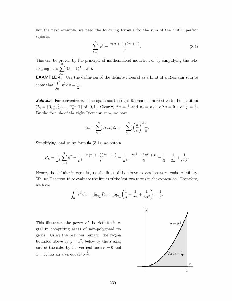
For the next example, we need the following formula for the sum of the first n perfectsquares:
nX
k=1
k2 =n(n+ 1)(2n+ 1)
6
. (3.4)
This can be proven by the principle of mathematical induction or by simplifying the tele-
scoping sumnX
k=1
((k + 1)
3 � k3).
EXAMPLE 4: Use the definition of the definite integral as a limit of a Riemann sum to
show thatZ
1
0
x2 dx =
1
3
.
Solution. For convenience, let us again use the right Riemann sum relative to the partitionPn = {0, 1
n ,2
n , . . . ,n�1
n , 1} of [0, 1]. Clearly, �x =
1
n and xk = x0
+ k�x = 0 + k · 1
n =
kn .
By the formula of the right Riemann sum, we have
Rn =
nX
k=1
f(xk)�xk =
nX
k=1
✓k
n
◆2
1
n.
Simplifying, and using formula (3.4), we obtain
Rn =
1
n3
nX
k=1
k2 =1
n3
· n(n+ 1)(2n+ 1)
6
=
1
n3
· 2n3
+ 3n2
+ n
6
=
1
3
+
1
2n+
1
6n2
.
Hence, the definite integral is just the limit of the above expression as n tends to infinity.We use Theorem 16 to evaluate the limits of the last two terms in the expression. Therefore,we have
Z1
0
x2 dx = lim
n!1Rn = lim
n!1
✓1
3
+
1
2n+
1
6n2
◆=
1
3
.
This illustrates the power of the definite inte-gral in computing areas of non-polygonal re-gions. Using the previous remark, the regionbounded above by y = x2, below by the x-axis,and at the sides by the vertical lines x = 0 andx = 1, has an area equal to
1
3
.
1
y = x2
x
y
Area= 1
3
.
.
260
Teaching Tip
As previously discussed, the computation of definite integrals is, in general, verycumbersome. We just have to wait a little more because a very powerful theorem(Fundamental Theorem of Calculus) in the next section will relate this with theantiderivative/indefinite integral. This connection will make the computation ofintegrals so much easier than finding the limit of the sum. This will also explainthe connection of the antiderivative with areas, as presented in the motivation of thelecture Riemann sums, and the reason why antiderivatives and the definite integralshare the same notation (
R).
PROPERTIES OF THE DEFINITE INTEGRAL
As a limit of a sum, the definite integral shares the common properties of the limit and ofthe summation.
Theorem 17 (Linearity of the Definite Integral). Let f and g be positive continuous func-tions on [a, b] and let c 2 R. Then
(a)Z b
acf(x) dx = c
Z b
af(x) dx
(b)Z b
a(f(x)± g(x)) dx =
Z b
af(x) dx±
Z b
ag(x) dx
Teaching Tip
Although the limit is distributive over products and quotients, the summation isnot. Therefore, the integral is also NOT distributive over products nor over quo-tients. This means
Z b
af(x)g(x) dx 6=
Z b
af(x) dx ·
Z b
ag(x) dx
and Z b
a
f(x)
g(x)dx 6=
R ba f(x) dxR ba g(x) dx.
EXAMPLE 5: Suppose we are given thatZ b
af(x) dx = 2 and
Z b
ag(x) dx = 7. Find the
exact value of the following:
(a)Z b
a3f(x) dx
(b)Z b
af(x)� g(x) dx
(c)Z b
a2f(x) + g(x) dx
(d)Z b
a3f(x)� 2g(x) dx
261
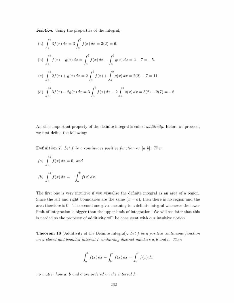
Solution. Using the properties of the integral,
(a)Z b
a3f(x) dx = 3
Z b
af(x) dx = 3(2) = 6.
(b)Z b
af(x)� g(x) dx =
Z b
af(x) dx�
Z b
ag(x) dx = 2� 7 = �5.
(c)Z b
a2f(x) + g(x) dx = 2
Z b
af(x) +
Z b
ag(x) dx = 2(2) + 7 = 11.
(d)Z b
a3f(x)� 2g(x) dx = 3
Z b
af(x) dx� 2
Z b
ag(x) dx = 3(2)� 2(7) = �8.
.
Another important property of the definite integral is called additivity. Before we proceed,we first define the following:
Definition 7. Let f be a continuous positive function on [a, b]. Then
(a)Z a
af(x) dx = 0, and
(b)Z a
bf(x) dx = �
Z b
af(x) dx.
The first one is very intuitive if you visualize the definite integral as an area of a region.Since the left and right boundaries are the same (x = a), then there is no region and thearea therefore is 0 . The second one gives meaning to a definite integral whenever the lowerlimit of integration is bigger than the upper limit of integration. We will see later that thisis needed so the property of additivity will be consistent with our intuitive notion.
Theorem 18 (Additivity of the Definite Integral). Let f be a positive continuous functionon a closed and bounded interval I containing distinct numbers a, b and c. Then
Z b
af(x) dx+
Z c
bf(x) dx =
Z c
af(x) dx
no matter how a, b and c are ordered on the interval I.
262
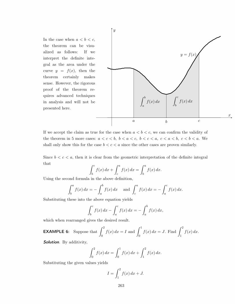
In the case when a < b < c,the theorem can be visu-alized as follows: If weinterpret the definite inte-gral as the area under thecurve y = f(x), then thetheorem certainly makessense. However, the rigorousproof of the theorem re-quires advanced techniquesin analysis and will not bepresented here.
Z b
af(x) dx
Z c
bf(x) dx
a b c
y = f(x)
x
y
If we accept the claim as true for the case when a < b < c, we can confirm the validity ofthe theorem in 5 more cases: a < c < b, b < a < c, b < c < a, c < a < b, c < b < a. Weshall only show this for the case b < c < a since the other cases are proven similarly.
Since b < c < a, then it is clear from the geometric interpretation of the definite integralthat Z c
bf(x) dx+
Z a
cf(x) dx =
Z a
bf(x) dx.
Using the second formula in the above definition,Z a
bf(x) dx = �
Z b
af(x) dx and
Z a
cf(x) dx = �
Z c
af(x) dx.
Substituting these into the above equation yieldsZ c
bf(x) dx�
Z c
af(x) dx = �
Z b
af(x) dx,
which when rearranged gives the desired result.
EXAMPLE 6: Suppose thatZ
2
0
f(x) dx = I andZ
1
0
f(x) dx = J . FindZ
2
1
f(x) dx.
Solution. By additivity,Z
2
0
f(x) dx =
Z1
0
f(x) dx+
Z2
1
f(x) dx.
Substituting the given values yields
I =
Z2
1
f(x) dx+ J.
263
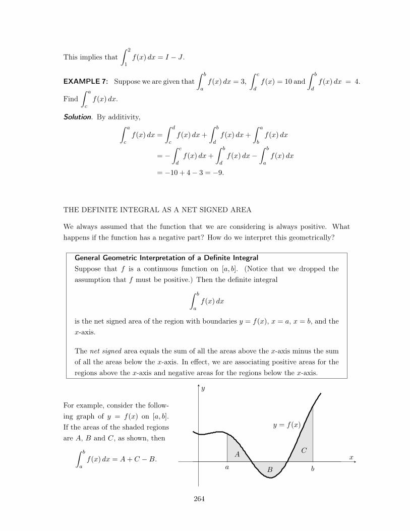
This implies thatZ
2
1
f(x) dx = I � J . .
EXAMPLE 7: Suppose we are given thatZ b
af(x) dx = 3,
Z c
df(x) = 10 and
Z b
df(x) dx = 4.
FindZ a
cf(x) dx.
Solution. By additivity,Z a
cf(x) dx =
Z d
cf(x) dx+
Z b
df(x) dx+
Z a
bf(x) dx
= �Z c
df(x) dx+
Z b
df(x) dx�
Z b
af(x) dx
= �10 + 4� 3 = �9.
.
THE DEFINITE INTEGRAL AS A NET SIGNED AREA
We always assumed that the function that we are considering is always positive. Whathappens if the function has a negative part? How do we interpret this geometrically?
General Geometric Interpretation of a Definite IntegralSuppose that f is a continuous function on [a, b]. (Notice that we dropped theassumption that f must be positive.) Then the definite integral
Z b
af(x) dx
is the net signed area of the region with boundaries y = f(x), x = a, x = b, and thex-axis.
The net signed area equals the sum of all the areas above the x-axis minus the sumof all the areas below the x-axis. In effect, we are associating positive areas for theregions above the x-axis and negative areas for the regions below the x-axis.
For example, consider the follow-ing graph of y = f(x) on [a, b].If the areas of the shaded regionsare A, B and C, as shown, then
Z b
af(x) dx = A+ C �B.
A
B
C
a b
y = f(x)
x
y
264
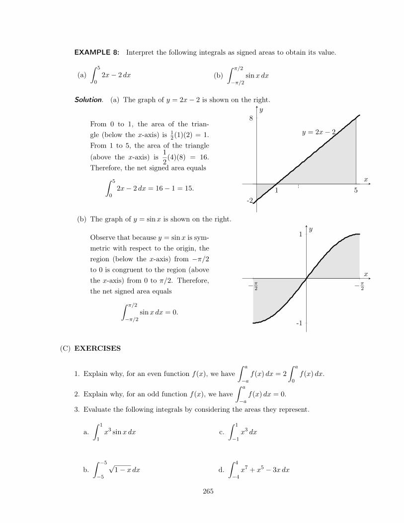
EXAMPLE 8: Interpret the following integrals as signed areas to obtain its value.
(a)Z
5
0
2x� 2 dx (b)Z ⇡/2
�⇡/2sinx dx
Solution. (a) The graph of y = 2x� 2 is shown on the right.
From 0 to 1, the area of the trian-gle (below the x-axis) is 1
2
(1)(2) = 1.
From 1 to 5, the area of the triangle(above the x-axis) is
1
2
(4)(8) = 16.
Therefore, the net signed area equalsZ
5
0
2x� 2 dx = 16� 1 = 15.1 5
-2
8
y = 2x� 2
x
y
(b) The graph of y = sinx is shown on the right.
Observe that because y = sinx is sym-metric with respect to the origin, theregion (below the x-axis) from �⇡/2
to 0 is congruent to the region (abovethe x-axis) from 0 to ⇡/2. Therefore,the net signed area equals
Z ⇡/2
�⇡/2sinx dx = 0.
�⇡2
�⇡2
-1
1
x
y
.
(C) EXERCISES
1. Explain why, for an even function f(x), we haveZ a
�af(x) dx = 2
Z a
0
f(x) dx.
2. Explain why, for an odd function f(x), we haveZ a
�af(x) dx = 0.
3. Evaluate the following integrals by considering the areas they represent.
a.Z
1
1
x3 sinx dx
b.Z �5
�5
p1� x dx
c.Z
1
�1
x3 dx
d.Z
4
�4
x7 + x5 � 3x dx
265
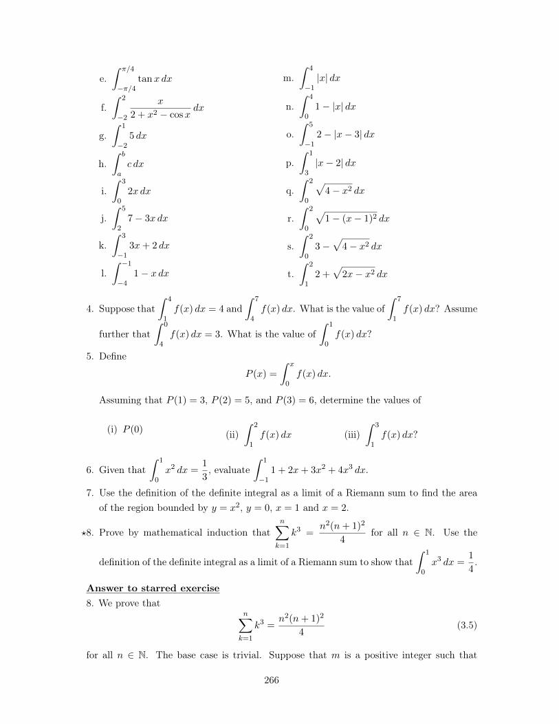
e.Z ⇡/4
�⇡/4tanx dx
f.Z
2
�2
x
2 + x2 � cosxdx
g.Z
1
�2
5 dx
h.Z b
ac dx
i.Z
3
0
2x dx
j.Z
5
2
7� 3x dx
k.Z
3
�1
3x+ 2 dx
l.Z �1
�4
1� x dx
m.Z
4
�1
|x| dx
n.Z
4
0
1� |x| dx
o.Z
5
�1
2� |x� 3| dx
p.Z
1
3
|x� 2| dx
q.Z
2
0
p4� x2 dx
r.Z
2
0
p1� (x� 1)
2 dx
s.Z
2
0
3�p4� x2 dx
t.Z
2
1
2 +
p2x� x2 dx
4. Suppose thatZ
4
1
f(x) dx = 4 andZ
7
4
f(x) dx. What is the value ofZ
7
1
f(x) dx? Assume
further thatZ
0
4
f(x) dx = 3. What is the value ofZ
1
0
f(x) dx?
5. Define
P (x) =
Z x
0
f(x) dx.
Assuming that P (1) = 3, P (2) = 5, and P (3) = 6, determine the values of
(i) P (0) (ii)Z
2
1
f(x) dx (iii)Z
3
1
f(x) dx?
6. Given thatZ
1
0
x2 dx =
1
3
, evaluateZ
1
�1
1 + 2x+ 3x2 + 4x3 dx.
7. Use the definition of the definite integral as a limit of a Riemann sum to find the areaof the region bounded by y = x2, y = 0, x = 1 and x = 2.
?8. Prove by mathematical induction thatnX
k=1
k3 =
n2
(n+ 1)
2
4
for all n 2 N. Use the
definition of the definite integral as a limit of a Riemann sum to show thatZ
1
0
x3 dx =
1
4
.
Answer to starred exercise8. We prove that
nX
k=1
k3 =n2
(n+ 1)
2
4
(3.5)
for all n 2 N. The base case is trivial. Suppose that m is a positive integer such that
266
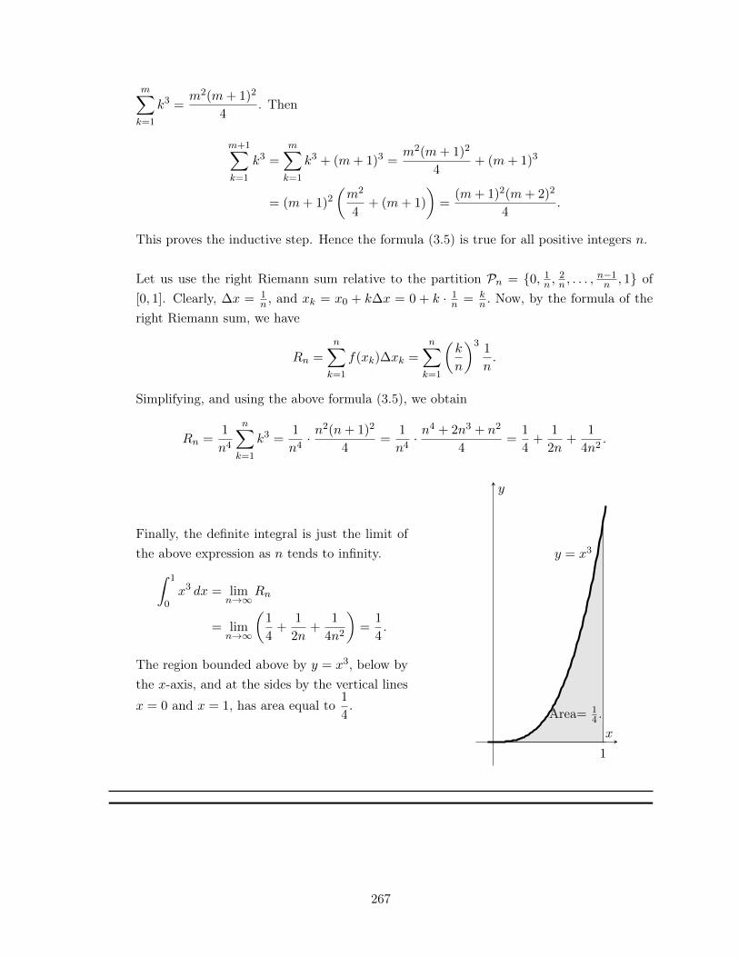
mX
k=1
k3 =m2
(m+ 1)
2
4
. Then
m+1X
k=1
k3 =mX
k=1
k3 + (m+ 1)
3
=
m2
(m+ 1)
2
4
+ (m+ 1)
3
= (m+ 1)
2
✓m2
4
+ (m+ 1)
◆=
(m+ 1)
2
(m+ 2)
2
4
.
This proves the inductive step. Hence the formula (3.5) is true for all positive integers n.
Let us use the right Riemann sum relative to the partition Pn = {0, 1
n ,2
n , . . . ,n�1
n , 1} of[0, 1]. Clearly, �x =
1
n , and xk = x0
+ k�x = 0 + k · 1
n =
kn . Now, by the formula of the
right Riemann sum, we have
Rn =
nX
k=1
f(xk)�xk =
nX
k=1
✓k
n
◆3
1
n.
Simplifying, and using the above formula (3.5), we obtain
Rn =
1
n4
nX
k=1
k3 =1
n4
· n2
(n+ 1)
2
4
=
1
n4
· n4
+ 2n3
+ n2
4
=
1
4
+
1
2n+
1
4n2
.
Finally, the definite integral is just the limit ofthe above expression as n tends to infinity.
Z1
0
x3 dx = lim
n!1Rn
= lim
n!1
✓1
4
+
1
2n+
1
4n2
◆=
1
4
.
The region bounded above by y = x3, below bythe x-axis, and at the sides by the vertical linesx = 0 and x = 1, has area equal to
1
4
.
1
y = x3
x
y
Area= 1
4
.
267
LESSON 16: The Fundamental Theorem of Calculus
TIME FRAME: 2 hours
LEARNING OUTCOMES: At the end of the lesson, the learner shall be able to:
1. Illustrate the Fundamental Theorem of Calculus; and2. Compute the definite integral of a function using the Fundamental Theorem of Calculus.
LESSON OUTLINE:
1. Statement of the theorem2. Examples3. Revisiting the Table of Integrals4. Integrands with absolute values
268
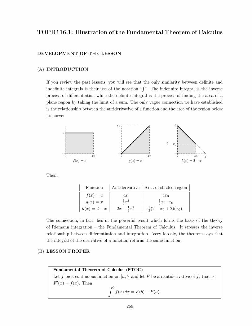
TOPIC 16.1: Illustration of the Fundamental Theorem of Calculus
DEVELOPMENT OF THE LESSON
(A) INTRODUCTION
If you review the past lessons, you will see that the only similarity between definite andindefinite integrals is their use of the notation “
R”. The indefinite integral is the inverse
process of differentiation while the definite integral is the process of finding the area of aplane region by taking the limit of a sum. The only vague connection we have establishedis the relationship between the antiderivative of a function and the area of the region belowits curve:
x0
x0
x0
f(x) = c g(x) = x h(x) = 2� x
c
x0
2� x0
2
2
Then,
Function Antiderivative Area of shaded region
f(x) = c cx cx0
g(x) = x 1
2
x2 1
2
x0
· x0
h(x) = 2� x 2x� 1
2
x2 1
2
(2� x0
+ 2)(x0
)
The connection, in fact, lies in the powerful result which forms the basis of the theoryof Riemann integration – the Fundamental Theorem of Calculus. It stresses the inverserelationship between differentiation and integration. Very loosely, the theorem says thatthe integral of the derivative of a function returns the same function.
(B) LESSON PROPER
Fundamental Theorem of Calculus (FTOC)Let f be a continuous function on [a, b] and let F be an antiderivative of f , that is,F 0
(x) = f(x). Then Z b
af(x) dx = F (b)� F (a).
269
EXAMPLE 1: Note that F (x) =x3
3
is an antiderivative of f(x) = x2 (since F 0(x) = f(x).)
Hence, by FTOC,Z
1
0
x2 dx =
x3
3
����1
0
= F (1)� F (0) =
1
3
� 0 =
1
3
,
as we have seen before.
Vertical Bar Notation
We adopt the following notation:
F (x)
����b
a
= F (b)� F (a).
For example,
(1 + x� x2)
����2
1
= (1 + 2� 2
2
)� (1 + 1� 1
2
) = (�1)� (1) = �2,
and
sinx
����⇡/2
⇡/4
= sin(⇡/2)� sin(⇡/4) = 1�p2
2
=
2�p2
2
.
Using the above notation, the FTOC now states: If F is an antiderivative of f , thenZ b
af(x) dx = F (x)
����b
a
.
The constant of integration that was necessary for indefinite integration will now just cancelout:
�F (x) + C
�����b
a
=
�F (b) + C
���F (a) + C
�= F (b)� F (a) = F (x)
����b
a
.
The next examples will validate that FTOC works by redoing the examples in the previoussection.
EXAMPLE 2: Without referring to the graphs of the integrands, find the exact values ofthe following definite integrals:
1.Z
2
1
3 dx
2.Z
2
0
(1� |x� 1|) dx
3.Z
3
1
(3x+ 1) dx
?4.Z
1
�1
p1� x2 dx
270
Solution. We integrate using the Fundamental Theorem of Calculus.
1.Z
2
1
3 dx = 3x
����2
1
= 3(2� 1) = 3.
2. The solution for this problem takes a few more steps because the absolute value functionis essentially a piecewise function. Recall that if E is any expression, then |E| = E ifE � 0, while |E| = �E if E < 0. With this in mind,
1� |x� 1| =
8<
:1� (x� 1) if x� 1 � 0
1� [�(x� 1)] if x� 1 < 0
=
8<
:2� x if x � 1
x if x < 1.
Therefore, by additivity,Z
2
0
(1� |x� 1|) dx =
Z2
1
2� x dx+
Z1
0
x dx
=
✓2x� x2
2
◆�����
2
1
+
✓x2
2
◆�����
1
0
=
✓4� 4
2
◆�✓2� 1
2
◆�+
1
2
� 0
�= 1.
3.Z
3
1
(3x+ 1) dx =
✓3x2
2
+ x
◆�����
3
1
=
✓27
2
+ 3
◆�✓3
2
+ 1
◆= 14.
4. (For very advanced learners) There is a technique of integration needed to integratep1� x2. This is called trigonometric substitution , and the student will learn this
in college. For now, we convince ourselves thatZ p
1� x2 dx =
1
2
⇣sin
�1 x+ xp1� x2
⌘+ C
by differentiating the right-hand side and observing that it yields the integrand of theleft-hand side. Hence, by FTOC,
Z1
�1
p1� x2 dx =
1
2
⇣sin
�1 x+ xp1� x2
⌘�����
1
�1
=
1
2
⇣⇡2
+ 0
⌘� 1
2
⇣�⇡
2
� 0
⌘=
⇡
2
.
.
Because, FTOC evaluates the definite integral using antiderivatives and not by “net signedarea,” we don’t have to look at the graph and look at those regions below the x-axis, i.e.,FTOC works even if the graph has a “negative part.”
271
EXAMPLE 3: Evaluate the following integrals using FTOC.
(a)Z
5
0
(2x� 2) dx (b)Z ⇡/2
�⇡/2sinx dx
Solution. .
(a)Z
5
0
(2x� 2) dx =
✓2
x2
2
� 2x
◆ �����
5
0
= (25� 10)� (0� 0) = 15.
(b)Z ⇡/2
�⇡/2sinx dx = (� cosx)
����⇡/2
�⇡/2
= (0� 0) = 0.
These answers are the same as when we appealed to the geometrical solution of the integralin the previous section. .
272
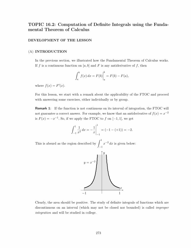
TOPIC 16.2: Computation of Definite Integrals using the Funda-mental Theorem of Calculus
DEVELOPMENT OF THE LESSON
(A) INTRODUCTION
In the previous section, we illustrated how the Fundamental Theorem of Calculus works.If f is a continuous function on [a, b] and F is any antiderivative of f , then
Z b
af(x) dx = F (b)
����b
a
= F (b)� F (a),
where f(x) = F 0(x).
For this lesson, we start with a remark about the applicability of the FTOC and proceedwith answering some exercises, either individually or by group.
Remark 1: If the function is not continuous on its interval of integration, the FTOC willnot guarantee a correct answer. For example, we know that an antiderivative of f(x) = x�2
is F (x) = �x�1. So, if we apply the FTOC to f on [�1, 1], we get
Z1
�1
1
x2dx = �1
x
�����
1
�1
= (�1� (+1)) = �2.
This is absurd as the region described byZ
1
�1
x�2 dx is given below:
�1 1
y = x�2
x
y
Clearly, the area should be positive. The study of definite integrals of functions which arediscontinuous on an interval (which may not be closed nor bounded) is called improperintegration and will be studied in college.
273
(B) LESSON PROPER
Table of Integrals
Observe that for FTOC to work, the student must be able to produce an antiderivative forthe integrand. This is why the student must be comfortable with the first few lessons inthis chapter. A very common and indispensable formula is the Power Rule:
Zxn dx =
xn+1
n+ 1
+ C, n 6= �1.
For other cases, we recall the table of integrals for reference.
1.Z
dx = x+ C
2.Z
xn dx =
xn+1
n+ 1
+ C, if n 6= �1
3.Z
af (x) dx = a
Zf (x) dx
4.Z
f(x)± g(x) dx =
Zf(x) dx±
Zg(x) dx
5.Z
ex dx = ex + C.
6.Z
ax dx =
ax
ln a+ C.
7.Z
x�1 dx =
Z1
xdx = ln |x|+ C.
8.Z
sinx dx = � cosx+ C
9.Z
cosx dx = sinx+ C
10.Z
sec
2 x dx = tanx+ C
11.Z
csc
2 x dx = � cotx+ C
12.Z
secx tanx dx = secx+ C
13.Z
cscx cotx dx = � cscx+ C
14.Z
tanx dx = � ln | cosx|+ C
15.Z
cotx dx = ln | sinx|+ C
16.Z
secx dx = ln | secx+ tanx|+ C
17.Z
cscx dx = ln | cscx� cotx|+ C
18.Z
dxpa2 � x2
= sin
�1
⇣xa
⌘+ C
19.Z
dx
a2 + x2=
1
atan
�1
⇣xa
⌘+ C
20.Z
dx
xpx2 � a2
=
1
asec
�1
⇣xa
⌘+ C
EXAMPLE 1: Using FTOC, evaluate the following definite integrals:
1.Z
4
1
px dx
2.Z
2
1
x3 � 2x2 + 4x� 2
xdx
3.Z ⇡/4
0
cosx+ tanx dx
4.Z
1/2
0
dxp1� x2
Solution. .
1.Z
4
1
px dx =
Z4
1
x1/2 dx =
x3/2
3/2
�����
4
1
=
2
3
(8� 1) =
14
3
.
274
2. We first divide the numerator by the denominator to express the fraction as a sum.Z
2
1
x3 � 2x2 + 4x� 2
xdx =
Z2
1
✓x2 � 2x+ 4� 2
x
◆dx
=
✓x3
3
� x2 + 4x� 2 ln |x|◆�����
2
1
=
✓8
3
� 4 + 8� 2 ln 2
◆�✓1
3
� 1 + 4� 0
◆
=
10
3
� 2 ln 2.
3.Z ⇡/4
0
cosx+ tanx dx = (sinx+ ln | secx|)����⇡/4
0
=
p2
2
+ ln(
p2)
4.Z
1/2
0
dxp1� x2
= sin
�1 x
����1/2
0
= sin
�1
(1/2)� sin
�1
(0) =
⇡
6
� 0 =
⇡
6
.
.
INTEGRANDS WITH ABSOLUTE VALUES
Solving definite integrals with absolute values in the integrands has been discussed in pass-ing in previous examples. We will now give a more in-depth discussion.
As has been said, for any continuous expression E, its absolute value can always be writtenin piecewise form:
|E| =
8<
:E if E � 0
�E if E < 0.
Therefore, the first step in solving this kind of integral is to eliminate the absolute value bars.This is done by dividing the interval of integration [a, b] into two subintervals accordingto the piecewise version of the function. Hence, one integrand is either purely positive (orzero) and the other is purely negative.
EXAMPLE 2: Evaluate the following definite integrals:
1.Z
2
�1
|x� 3| dx
2.Z
7
3
|x� 3| dx
3.Z
4
1
|x� 3| dx
4.Z
2
0
4x+ |2x� 1| dx
5.Z
2⇡/3
0
| cosx| dx
6.Z
3
�2
|x2 � 1| dx
Solution. For items 1-3, observe that by definition,
|x� 3| =
8<
:x� 3, if x� 3 � 0
�(x� 3), if x� 3 < 0,=
8<
:x� 3, if x � 3,
�x+ 3, if x < 3.
275
1. Since x � 3 is always negative on the interval of integration [�1, 2], we replace |x � 3|with �(x� 3). Hence,
Z2
�1
|x� 3| dx =
Z3
�1
�x+ 3 dx =
✓�x2
2
+ 3x
◆�����
2
�1
=
✓�4
2
+ 6
◆�✓�1
2
� 3
◆=
15
2
.
2. Since x� 3 is always nonnegative on [3, 7], we replace |x� 3| with x� 3. So,
Z7
3
|x� 3| dx =
Z7
3
x� 3 dx =
✓x2
2
� 3x
◆�����
7
3
=
✓49
2
� 21
◆�✓9
2
� 9
◆= 8.
3. Since x�3 is neither purely positive nor purely negative on [1, 4], we need to divide thisinterval into [1, 3] and [3, 4]. On the first, we replace |x � 3| with �x + 3, while on thesecond, we replace |x� 3| with x� 3.
Z4
1
|x� 3| dx =
Z3
1
�x+ 3 dx+
Z4
3
x� 3 dx
=
✓�x2
2
+ 3x
◆�����
3
1
+
✓x2
2
� 3x
◆�����
4
3
=
✓�9
2
+ 9
◆�✓�1
2
+ 3
◆�+
✓16
2
� 12
◆�✓9
2
� 9
◆�
=
9
2
� 5
2
�+
�8
2
+
9
2
�=
5
2
.
4. We split the interval of integration into [0, 12
] and [
1
2
, 2] since
|2x� 1| =
8<
:2x� 1 if 2x� 1 � 0
�(2x� 1) if 2x� 1 < 0.
Hence, 4x+ |2x� 1| =
8<
:4x+ (2x� 1) if x � 1
2
4x� (2x� 1) if x < 1
2
.
Therefore,
Z2
0
4x+ |2x� 1| dx =
Z 12
0
2x+ 1 dx+
Z2
12
6x� 1 dx
= (x2 + x)
����1/2
0
+ (3x2 � x)
����2
1/2
=
✓1
4
+
1
2
◆� (0 + 0)
�+
(12� 2)�
✓3
4
� 1
2
◆�=
21
2
.
276
5. The cosine function is nonnegative on [0,⇡/2] and negative on [⇡/2, 2⇡/3]. See graphbelow.
⇡2
2⇡3
⇡
y = cosx
x
y
Hence, | cosx| =
8<
:cosx, if cosx � 0,
� cosx, if cosx < 0
=
8<
:cosx, if x 2 [0,⇡/2],
� cosx, if x 2 [⇡/2, 2⇡/3].
Therefore,
Z2⇡/3
0
| cosx| dx =
Z ⇡/2
0
cosx dx+
Z2⇡/3
⇡/2� cosx dx
= sinx
����⇡/2
0
+ (� sinx)
����2⇡/3
⇡/2
= (1� 0) + [(�p3/2)� (�1)] = 2�
p3
2
.
6. The quadratic function y = x2 � 1 is below the x-axis only when x 2 (�1, 1). Thisconclusion can be deduced by solving the inequality x2 � 1 < 0 or by referring to thegraph below.
�2 �1 1 3
y = x2 � 1
x
y
This implies that we have to divide [�2, 3] into the three subintervals [�2,�1], [�1, 1],
and [1, 3]. On [�1, 1], we replace |x2 � 1| with �x2 + 1 while on the other subintervals,
277
we simply replace |x2 � 1| with x2 � 1. Hence,Z
3
�2
|x2 � 1| dx =
Z �1
�2
x2 � 1 dx+
Z1
�1
�x2 + 1 dx+
Z3
1
x2 � 1 dx
=
✓x3
3
� x
◆�����
�1
�2
+
✓�x3
3
+ x
◆�����
1
�1
+
✓x3
3
� x
◆�����
3
1
=
✓�1
3
+ 1
◆�✓�8
3
+ 2
◆�+
✓�1
3
+ 1
◆�✓1
3
� 1
◆�
+
✓27
3
� 3
◆�✓1
3
� 1
◆�
=
28
3
.
.
(C) EXERCISES
Evaluate the following definite integrals:
1.Z ⇡
2
0
sinx dx
2.Z
4
0
(1 + 3x� x2) dx
3.Z
64
1
1 +
3px
3px
dx
4.Z ⇡
4
0
1 + cos
2 x
cos
2 xdx
?5.Z ⇡
⇡
3
sin
⇣x2
⌘cos
⇣x2
⌘dx
?6.Z ⇡
2⇡3
tanx
secx� tanxdx
7.Z
0
�1
|3x+ 1 |dx
8.Z
3
0
(|3x� 6|� 1) dx
?9.Z
4
0
|x2 � 4x+ 3| dx
?10.Z ⇡
0
����sinx� 1
2
���� dx
11.Z
2
1
1
x2
✓1 +
1
x
◆2
dx
12.Z ⇡
�⇡f(x) dx if f(x) =
8<
:x if x 0
sinx if x > 0.
Solutions to starred exercises
5. Observe that by the identity
sin 2✓ = 2 sin ✓ cos ✓,
we can rewrite the integrand into sin(x/2) cos(x/2) = 1
2
sinx. Hence,Z ⇡
⇡
3
sin(x/2) cos(x/2) dx =
Z ⇡
⇡
3
1
2
sinx dx.
Since �1
2
cosx is an antiderivative for the integrand, FTOC says thatZ ⇡
⇡
3
1
2
sinx dx = �1
2
cosx
����⇡
⇡
3
= �1
2
✓�1� 1
2
◆=
3
4
.
278
6. We use trigonometric identities to rewrite the integrand.
tanx
secx� tanx· secx+ tanx
secx+ tanx=
secx tanx+ tan
2 x
sec
2 x� tan
2 x
= secx tanx+ tan
2 x = secx tanx+ sec
2 x� 1.
Note that secx+ tanx� x is an antiderivative of the integrand. Hence, by FTOC,Z ⇡
2⇡3
tanx
secx� tanxdx = (secx+ tanx� x)
����⇡
2⇡3
= (�1� 0� ⇡)� (�2�p3� (2⇡)/3) = 1 +
p3� ⇡/3.
9. Since x2 � 4x + 3 = (x � 1)(x � 3), a table of signs will show that this expression isnegative when x 2 (1, 3) and nonnegative otherwise. Therefore, we have to split theintegral over three intervals: [0, 1], [1, 3] and [3, 4]. Using the definition of the absolutevalue,
Z4
0
|x2 � 4x+ 3| dx =
Z1
0
|x2 � 4x+ 3| dx+
Z3
1
|x2 � 4x+ 3| dx+
Z4
3
|x2 � 4x+ 3| dx
=
Z1
0
(x2 � 4x+ 3) dx+
Z3
1
�(x2 � 4x+ 3) dx+
Z4
3
(x2 � 4x+ 3) dx
=
✓x3
3
� 2x2 + 3x
◆ ����4
0
�✓x3
3
� 2x2 + 3x
◆ ����3
1
+
✓x3
3
� 2x2 + 3x
◆ ����4
3
=
✓4
3
� 0
◆�✓0� 4
3
◆+
✓4
3
� 0
◆= 4.
10. On [0,⇡], sinx� 1
2
� 0 , x 2⇡
6
,5⇡
6
�.Therefore,
Z ⇡
0
���� sinx� 1
2
���� dx =
Z ⇡
6
0
���� sinx� 1
2
���� dx+
Z 5⇡6
⇡
6
���� sinx� 1
2
���� dx+
Z ⇡
5⇡6
���� sinx� 1
2
���� dx
=
Z ⇡
6
0
�✓sinx� 1
2
◆dx+
Z 5⇡6
⇡
6
✓sinx� 1
2
◆dx+
Z ⇡
5⇡6
�✓sinx� 1
2
◆dx
=
⇣cosx+
x
2
⌘ ����
⇡
6
0
+
⇣� cosx� x
2
⌘ ����
5⇡6
⇡
6
+
⇣cosx+
x
2
⌘ ����⇡
5⇡6
=
p3
2
+
⇡
12
!� 1
!+
p3
2
� 5⇡
12
!� �p3
2
� ⇡
12
!!
+
⇣�1 +
⇡
2
⌘� �p3
2
+
5⇡
12
!!
= 2
p3� 2� ⇡
6
.
279
LESSON 17: Integration Technique: The Substitution Rule forDefinite Integrals
TIME FRAME: 3 hours
LEARNING OUTCOMES: At the end of the lesson, the learner shall be able to:
1. Illustrate the substitution rule; and2. Compute the definite integral of a function using the substitution rule
LESSON OUTLINE:
1. Review of the substitution rule in solving indefinite integrals2. Two ways of solving a definite integral through substitution3. The Substitution Rule 1
1for Definite Integrals (SRDI)
280
TOPIC 17.1: Illustration of the Substitution Rule for DefiniteIntegrals
DEVELOPMENT OF THE LESSON
(A) INTRODUCTION
As mentioned before, a variety of integrals, especially those whose integrands are not im-mediately integrable, become easily solvable after we apply the substitution rule. In thissection, we illustrate how the substitution rule is still applicable in definite integration.That is, if in a definite integral, the integrand is not integrable at first sight, one mustcheck whether a substitution is possible. Just like in the indefinite case, the goal is for thesubstitution to eventually yield an integrable version of the integrand.
We take note this early, however, that not all initially nonintegrable integrands can be madeintegrable by using substitution. Still, the substitution rule is a very handy and powerfultool for a great variety of integrals, both definite and indefinite.
(B) LESSON PROPER
How do we evaluate definite integralsR ba f(x) dx where the substitution technique may be
applied?Let us first recall how a substitution is done. Consider the indefinite integral
Z(x� 2)
54 dx.
One option in solving this is by expanding f(x) = (x� 2)
54, meaning, multiplying (x� 2)
by itself 54 times. Fortunately, in Section 3, we were taught the substitution rule, whichallows us to solve the given integral without having to perform tedious multiplication atall, that is, with y = x� 2, we get
Z(x� 2)
54 dx =
Zy54 dy
=
1
55
y55 + C
=
1
55
(x� 2)
55
+ C.
Now, let us consider the definite integralZ
3
1
(x� 2)
54 dx.
281
How do we evaluate this through substitution? There are two ways of approaching thesolution of a definite integral through substitution.
Method 1.
We first consider the definite integral as an indefinite integral and apply the substitutiontechnique. The answer (antiderivative of the function) is expressed in terms of the originalvariable and the FTOC is applied using the limits of integration x = a and x = b.
To illustrate, to integrateZ
3
1
(x� 2)
54 dx, we first apply the substitution technique to the
indefinite integral using the substitution y = x� 2 and express the antiderivative in termsof x :
Z(x� 2)
54 dx =
1
55
(x� 2)
55
+ C.
We apply the FTOC using the original limits of integration x = 1 and x = 3, so we have
Z3
1
(x� 2)
54 dx =
1
55
(x� 2)
55
+ C���3
1
=
1
55
(1)
55 � 1
55
(�1)
55
=
2
55
.
Note that for definite integrals, we can omit the constant of integration C in the antideriva-tive since this will cancel when we evaluate at the limits of integration.
Method 2.
In the second method, the substitution is applied directly to the definite integral and thelimits or bounds of integration are also changed according to the substitution applied. Howis this done? If the substitution y = g(x) is applied, then the limits of integration x = a
and x = b are changed to g(a) and g(b), respectively. The FTOC is then applied to thedefinite integral where the integrand is a function of y and using the new limits of integra-tion y = g(a) and y = g(b).
To illustrate this method, let us consider the same definite integralZ
3
1
(x� 2)
54 dx. Apply-
ing the substitution technique, we let y = (x� 2) so dy = dx. For the limits of integrationin the given definite integral, these are changed in accordance to the substitution y = x� 2
:
If x = 1, then y = 1� 2 = �1 and if x = 3 then y = 3� 2 = 1.
282
We then apply the FTOC to the definite integrable involving the new variable y yielding:Z
3
1
(x� 2)
54 dx =
Z1
�1
y54 dy
=
y55
55
+ C���1
�1
=
(1)
55
55
� (�1)
55
55
=
2
55
.
This alternative solution pays special attention to the bounds of integration in performinga substitution. The two methods, of course, give the same result.
Why must special attention be given to the bounds of integration when performing a substi-tution? The bounds a and b in the definite integral
R ba f(x) dx refer to values of x. In the
final step of definite integration, the resulting expression is evaluated at x = a and at x = b.If substitution is applied, there is a change in variable, hence, the limits of integration mustcorrespond correctly to the variable.
Let us summarize:
In applying the substitution technique of integration to the definite integralZ b
af(x) dx,
the integrand “f(x) dx” is replaced by an expression in terms of y where y is a function ofx, say y = g(x) which implies dy = g0(x)dx. The antiderivative, say F (y) is thus expressedas a function of y.
In the first method, the variable y is then expressed in terms of x , giving the antiderivativeF (g(x)) and this is evaluated with the original bounds x = a and x = b.
In the second method, we proceed with the substitution as above and the new bounds arecomputed through the same equation used to perform the substitution. Thus, if y = g(x),then the new bounds are
y = g(a) and y = g(b)
and the definite integral is now expressed as
Z b
af(g(x)) g0(x) dx =
Z g(b)
g(a)f(y) dy.
This is known as the Substitution Rule for Definite Integrals.
EXAMPLE 1: ComputeZ
2
0
(2x� 1)
3 dx.
283
Solution. Method 1. Let y = 2x � 1. It follows that dy = 2 dx. Hence, dx =
1
2
dy.Evaluating the definite integral, we have
Z(2x� 1)
3 dx =
Zy3 · 1
2
dy
=
Z1
2
y3 dy
=
1
2
Zy3 dy
=
1
2
· y4
4
+ C
=
1
8
y4 + C
=
1
8
(2x� 1)
4
+ C.
So, by FTOC,Z
(2x� 1)
3 dx =
1
8
(2x� 1)
4
����2
0
=
1
8
(3)
4 � 1
8
(�1)
4
= 10.
Method 2. Let y = 2x � 1, and so dy = 2 dx. Hence, dx =
1
2
dy. The bounds are thentransformed as follows:If x = 0, then
y = 2(0)� 1 = �1.
If x = 2, theny = 2(2)� 1 = 3.
The substitution yields the transformed definite integralZ
3
�1
y3 · 12
dy.
Evaluating the above definite integral,
Z3
�1
y3 · 12
dy =
Z3
�1
1
2
y3 dy
=
1
2
Z3
�1
y3 dy
=
1
2
· 14
y4����3
�1
=
1
8
[(3)
4 � (�1)
4
]
=
1
8
(80)
= 10.
.
284
EXAMPLE 2: ComputeZ �1
�2
p2� 7x dx.
Solution. Let y = 2� 7x. It follows that dy = �7 dx or dx = �1
7
dy. For the transformedbounds: If x = �2, then
y = 2� 7(�2) = 16.
If x = �1, theny = 2� 7(�1) = 9.
The substitution yields the transformed definite integralZ
9
16
py ·�1
7
dy =
Z9
16
y1/2 ·�1
7
dy
= �1
7
Z9
16
y1/2 dy
=
1
7
Z16
9
y1/2 dy.
Hence, we haveZ �1
�2
p2� 7x dx =
1
7
Z16
9
y1/2 dy
=
1
7
· 23
y3/2����16
9
=
2
21
[16
3/2 � 9
3/2]
=
2
21
(64� 27)
=
74
21
.
.
EXAMPLE 3: EvaluateZ
1
0
14
3p1 + 7x dx.
Solution. Let y = 1 + 7x. Then dy = 7 dx, and 14dx = 2 dy.If x = 0, then y = 1. If x = 1, then y = 8.Hence,Z
1
0
14
3p1 + 7x dx =
Z8
1
2y1/3 dy =
1
4/3y4/3
����8
1
=
3
4
(8
4/3 � 1
4/3) =
3
4
(16� 1) =
45
4
.
.
285
EXAMPLE 4: EvaluateZ
2
0
9x2
(x3 + 1)
3/2dx.
Solution. Let y = x3 + 1. Then dy = 3x2 dx, and 9x2dx = 3 dy.If x = 0, then y = 1. If x = 2, then y = 9.Hence,
Z2
0
9x2
(x3 + 1)
3/2dx =
Z9
1
3
y3/2dy
=
Z9
1
3y�3/2 dy
=
3
�1/2y�1/2
����9
1
= �6(9
�1/2 � 1)
= �6
✓1
3
� 1
◆
= 4.
.
EXAMPLE 5: Evaluate the integralZ
9
4
px
(30� x32)
2
dx.
Solution. Notice that if we let y = 30� x32 , then we have dy = �3
2
x12 dx so that �2
3
dy =
px dx, which is the numerator of the integrand. Converting the limits of integration, we
have x = 4 implying y = 22 and x = 9 implying y = 3. Thus,
Z9
4
px
(30� x32)
2
dx =
Z3
22
✓1
y2
◆✓�2
3
dy
◆
= �2
3
Z3
22
y�2 dy
= �2
3
✓y�1
�1
◆ ����3
22
=
✓2
3
◆✓1
3
◆��✓
2
3
◆✓1
22
◆�
=
✓2
3
◆1
3
� 1
22
�
=
19
99
.
.
EXAMPLE 6: Evaluate the integralZ ⇡
4
0
sin
3
2x cos 2x dx.
286
Solution. Let y = sin 2x. Differentiating both sides we have, dy = 2 cos 2x dx and
cos 2x dx =
dy
2
. Now, when x = 0 it implies that y = sin 0 = 0 and when x =
⇡
4
implies y = sin
⇡
2
= 1. Thus,
Z ⇡
4
0
sin
3
2x cos 2x dx =
Z ⇡
4
0
(sin 2x)3 cos 2x dx =
Z1
0
y3 · dy2
=
1
2
✓y4
4
◆ ����1
0
=
1
8
.
.
EXAMPLE 7: EvaluateZ
0
�1
x2 ex3+1 dx.
Solution. Recall that Dt(et) = et, and thereforeZ
etdt = et + c. In other words, thederivative and the antiderivative of the exponential are both the exponential itself.
Now, let y = x3 + 1. Then dy = 3x2 dx, so that x2dx =
1
3
dy.If x = �1, then y = 0. If x = 0, then y = 1. Hence,
Z0
�1
x2 ex3+1 dx =
Z1
0
1
3
ey dy =
1
3
ey����1
0
=
1
3
(e1 � e0) =1
3
(e� 1) =
e� 1
3
.
.
If we are dealing with an integral whose lower limit of integration is greater than the upperlimit, we can use the property that says
Z b
af(x) dx = �
Z a
bf(x) dx.
EXAMPLE 8: Evaluate the definite integralZ
0
2
2x(1 + x2)3 dx.
Solution. First, note thatZ
0
2
2x(1 + x2)3 dx = �Z
2
0
2x(1 + x2)3 dx
Let u = 1 + x2 so that du = 2x dx which is the other factor. Changing the x�limits, wehave when x = 0, then u = 1 + 0
2
= 1 and when x = 2, then u = 1 + 2
2
= 5. Thus,
�Z
2
0
2x(1 + x2)3 dx = �Z
5
1
u3 du = �✓u4
4
◆ ����5
1
= �5
4
4
�1
4
4
= �625� 1
4
= �624
4
= �156.
.
287
(C) EXERCISES
Evaluate the following definite integrals.
1.Z
2x
1 + x2dx Ans: ln |1 + x2|+ C
2.Z
�2xex2�4 dx Ans: �ex
2�4
+ C
3.Z
x2
4px3 + 2
dx Ans:
4
9
(x3 + 2)
34+ C
4.Z
cosx
1 + sinxdx Ans: ln |1 + sinx|+ C
5.Z
dxpx(1 +
px)2
Ans: � 2
1+
px+ C
6.Z
z4(1 + z5)3 dz Ans:
1
20
(1 + z5)4 + C
7.Z
(sinx+ cosx)2 dx Ans: x+ sin
2 x+ C
8.Z
x
ex2 dx Ans: � 1
ex2 + C
9.Z
cosxp1 + sinx
dx Ans: 2
p1 + sinx+ C
10.Z
t3pt4 + 16
dt Ans:
1
2
pt4 + 16 + C
11.Z
cos
4
2w sin
3
2w dw Ans: � 1
10
cos
5
(2w) + 1
14
cos
7
(2w) + C
12.Z
cos
3
x
3
dx Ans: 3 sin(
x3
)� sin
3
(
x3
) + C
13.Z
3x
(x2 + 1)
7
dx Ans: � 1
(x2+1)
6
14.Z
ex
(ex + 5)
3
dx Ans: � 1
2(ex+5)
2 + C
15.Z
1
x lnxdx Ans: ln | lnx|+ C
16.Z
20y
(y2 + 1)
20
dy Ans: � 10
19(y2+1)
19 + C
17.Z
xe�3x2dx Ans: �1
6
e�3x2+ C
18.Z
12x3
3x4 + 1
dx Ans: ln |3x4 + 1|+ C
19.Z ⇡
2
0
esinxcosx dx Ans: e� 1
20.Z
6
1
dxpx+ 3
Ans: 2
21.Z
2
�1
(x+ 1) dxpx2 + 2x+ 4
Ans:
p3
288
22.Z
5
0
x3px4 + 1 dx Ans:
626
23�1
6
23.Z
1
�1
x2ex3dx Ans:
e2�1
3e
24.Z
3
�1
3x dx
x2 + 2
Ans:
3
2
�ln
11
3
�
25.Z
2
0
(ex + 1)
2ex dx Ans:
(e+1)
3�8
3
26.Z
1
0
(ex + 1)
2 dx Ans:
e2+4e�3
2
27.Z 1
2
0
tp1� t2
dt Ans:
2�p3
2
28.Z ⇡
4
0
cos
2 ✓ tan2 ✓ d✓ Ans:
⇡8
� 1
4
29.Z
1
0
ex+ex dx Ans: ee � e
30.Z e2
1
(lnx)8 + 1
xdx Ans:
530
9
31.Z
3
0
ex � e�x
ex + e�xdx Ans: ln | e6+1
2e3|
32.Z
2
0
(�3x+ 4)e�3x2+8x dx Ans:
e4�1
2
33.Z
8
3
x� 1px+ 1
dx Ans:
26
3
34.Z
1
�1
(x+ 2)(x2 + 4x� 3)
3 dx Ans: �160
35.Z
15
0
xpx+ 1
dx Ans: 36
Solutions to Selected Exercises
1. Letting u = 1 + x2 implies that du = 2dx. Thus,
Z2x
1 + x2dx =
Z1
udu
= ln |u|+ C
= ln |1 + x2|+ C
289
3. Letting u = x3 + 2 implies that du = 3x3dx. Thus, x2dx =
du3
. Hence,Z
x2
4px3 + 2
dx =
Z1
4pu
✓du
3
◆
=
1
3
Zu�
14 du
=
1
3
u
34
3
4
!+ C
=
4
9
(x3 + 2)
34+ C
4. Put u = 1 + sinx. It will yield du = cosx dx, thusZ
cosx
1 + sinxdx =
Z1
udu
= ln |u|+ C
= ln |1 + sinx|+ C
5. Letting u = 1 +
px implies that du =
1
2
pxdx. Hence, dxp
x= 2du, we have
Zdxp
x(1 +px)2
=
Z1
u2(2du)
= 2
Zu�2 du
= 2
✓u�2+1
�2 + 1
◆+ C
= � 2
1 +
px+ C
7. Simplifying (sinx+ cosx)2 yields (sin
2 x+ 2 sinx cosx+ cos
2 x). Thus,Z(sinx+ cosx)2 dx =
Z(sin
2 x+ 2 sinx cosx+ cos
2 x) dx.
Now,
•Z
sin
2 x dx =
Z1� cos(2x)
2
dx =
Z1
2
dx�Z
cos(2x)
2
dx =
1
2
x� 1
4
sin(2x) + C
•Z
(2 sinx cosx) dx = 2
Zu du = u2 + C = sin
2 x+ C, where u = sinx
•Z
cos
2 x dx =
Z(1� sin
2 x) dx
=
Zdx�
Z1� cos(2x)
2
dx
= x�1
2
x� 1
4
sin(2x)
�+ C
= x� 1
2
x+
1
4
sin(2x) + C
290
Thus,Z(sinx+ cosx)2 dx =
Z(sin
2 x+ 2 sinx cosx+ cos
2 x) dx
=
Zsin
2 x dx+
Z2 sinx cosx dx+
Zcos
2 x dx
=
1
2
x� 1
4
sin(2x)
�+ sin
2 x+
x� 1
2
x+
1
4
sin(2x)
�+ C
= x+ sin
2 x+ C
11. Let u = cos 2w. Thus du = �2 sin 2w dw anddu
�2
= sin 2w dw. Now, using the
trigonometric identity sin
2
2w = 1� cos
2
2w,
Zcos
4
2w sin
3
2w dw =
Zcos
4
2w(1� cos
2
2w)(sin 2w) dw
=
Z(cos
4
2w � cos
6
2w) sin 2w dw
=
Z(u4 � u6)
✓du
�2
◆
= �1
2
✓u5
5
� u7
7
◆+ C
= � 1
10
cos
5
2w +
1
14
cos
7
2w + C
16. Letting u = y2 + 1 implies that du = 2y dy which yields 10 du = 20y dy. Thus,
Z20y
(y2 + 1)
20
dy =
Z10 du
u20
= 10
Zu�20 du
= 10
✓u�19
�19
◆+ C
= � 10
19(y2 + 1)
19
+ C
291
LESSON 18: Application of Definite Integrals in the Computationof Plane Areas
TIME FRAME: 6 sessions
LEARNING OUTCOMES: At the end of the lesson, the learner shall be able to:
1. Compute the area of a plane region using the definite integral; and2. Solve problems involving areas of plane regions.
LESSON OUTLINE:
1. Areas of Plane Regions2. Application of Definite Integrals
292
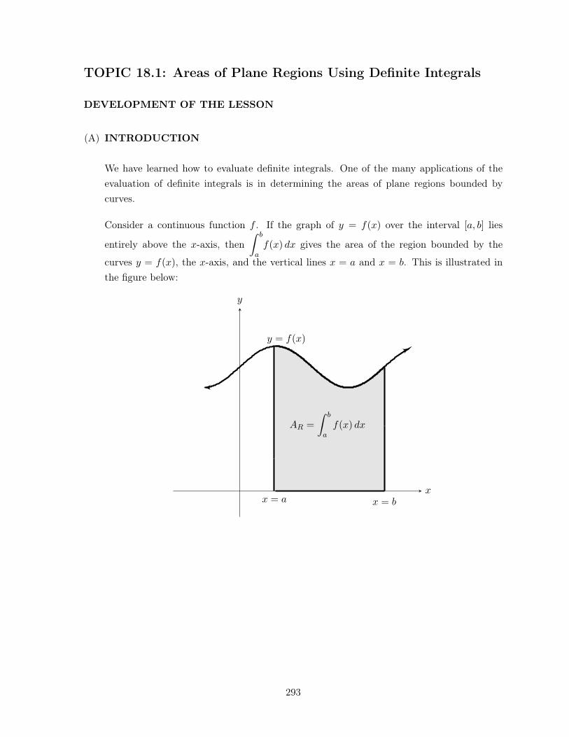
TOPIC 18.1: Areas of Plane Regions Using Definite Integrals
DEVELOPMENT OF THE LESSON
(A) INTRODUCTION
We have learned how to evaluate definite integrals. One of the many applications of theevaluation of definite integrals is in determining the areas of plane regions bounded bycurves.
Consider a continuous function f . If the graph of y = f(x) over the interval [a, b] lies
entirely above the x-axis, thenZ b
af(x) dx gives the area of the region bounded by the
curves y = f(x), the x-axis, and the vertical lines x = a and x = b. This is illustrated inthe figure below:
AR =
Z b
af(x) dx
y = f(x)
x = a x = bx
y
293
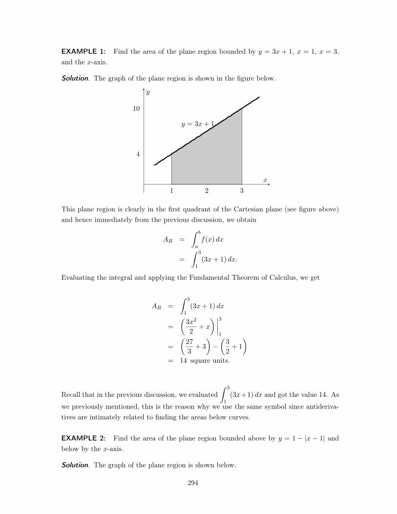
EXAMPLE 1: Find the area of the plane region bounded by y = 3x + 1, x = 1, x = 3,and the x-axis.
Solution. The graph of the plane region is shown in the figure below.
1 2 3
4
10
y = 3x+ 1
x
y
This plane region is clearly in the first quadrant of the Cartesian plane (see figure above)and hence immediately from the previous discussion, we obtain
AR =
Z b
af(x) dx
=
Z3
1
(3x+ 1) dx.
Evaluating the integral and applying the Fundamental Theorem of Calculus, we get
AR =
Z3
1
(3x+ 1) dx
=
✓3x2
2
+ x
◆ ����3
1
=
✓27
3
+ 3
◆�✓3
2
+ 1
◆
= 14 square units.
.
Recall that in the previous discussion, we evaluatedZ
3
1
(3x+1) dx and got the value 14. As
we previously mentioned, this is the reason why we use the same symbol since antideriva-tives are intimately related to finding the areas below curves.
EXAMPLE 2: Find the area of the plane region bounded above by y = 1 � |x � 1| andbelow by the x-axis.
Solution. The graph of the plane region is shown below.
294
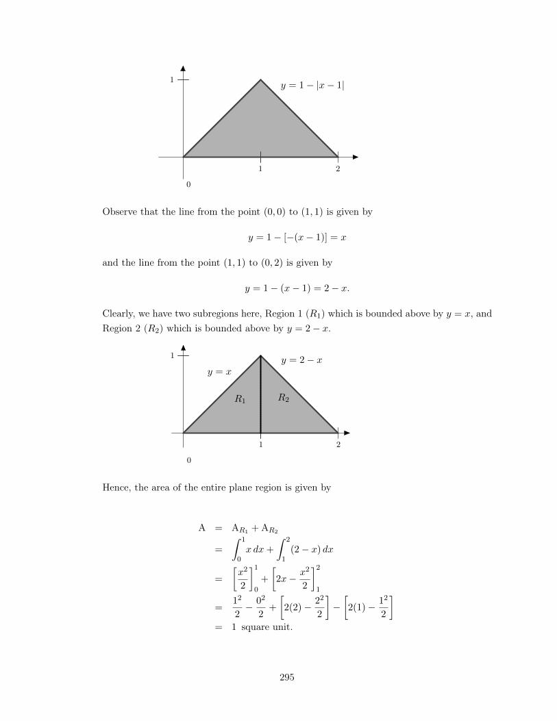
1 2
1
0
y = x
y = 1� |x� 1|
Observe that the line from the point (0, 0) to (1, 1) is given by
y = 1� [�(x� 1)] = x
and the line from the point (1, 1) to (0, 2) is given by
y = 1� (x� 1) = 2� x.
Clearly, we have two subregions here, Region 1 (R1
) which is bounded above by y = x, andRegion 2 (R
2
) which is bounded above by y = 2� x.
1 2
1
0
y = 2� xy = x
R1
R2
Hence, the area of the entire plane region is given by
A = AR1 + AR2
=
Z1
0
x dx+
Z2
1
(2� x) dx
=
x2
2
�1
0
+
2x� x2
2
�2
1
=
1
2
2
� 0
2
2
+
2(2)� 2
2
2
��2(1)� 1
2
2
�
= 1 square unit.
.
295
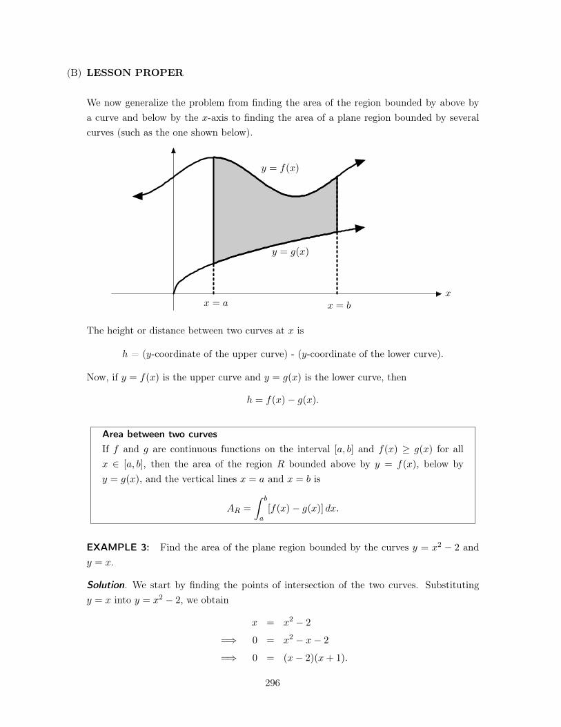
(B) LESSON PROPER
We now generalize the problem from finding the area of the region bounded by above bya curve and below by the x-axis to finding the area of a plane region bounded by severalcurves (such as the one shown below).
x
y = f(x)
y = g(x)
x = a x = b
The height or distance between two curves at x is
h = (y-coordinate of the upper curve) - (y-coordinate of the lower curve).
Now, if y = f(x) is the upper curve and y = g(x) is the lower curve, then
h = f(x)� g(x).
Area between two curvesIf f and g are continuous functions on the interval [a, b] and f(x) � g(x) for allx 2 [a, b], then the area of the region R bounded above by y = f(x), below byy = g(x), and the vertical lines x = a and x = b is
AR =
Z b
a[f(x)� g(x)] dx.
EXAMPLE 3: Find the area of the plane region bounded by the curves y = x2 � 2 andy = x.
Solution. We start by finding the points of intersection of the two curves. Substitutingy = x into y = x2 � 2, we obtain
x = x2 � 2
=) 0 = x2 � x� 2
=) 0 = (x� 2)(x+ 1).
296
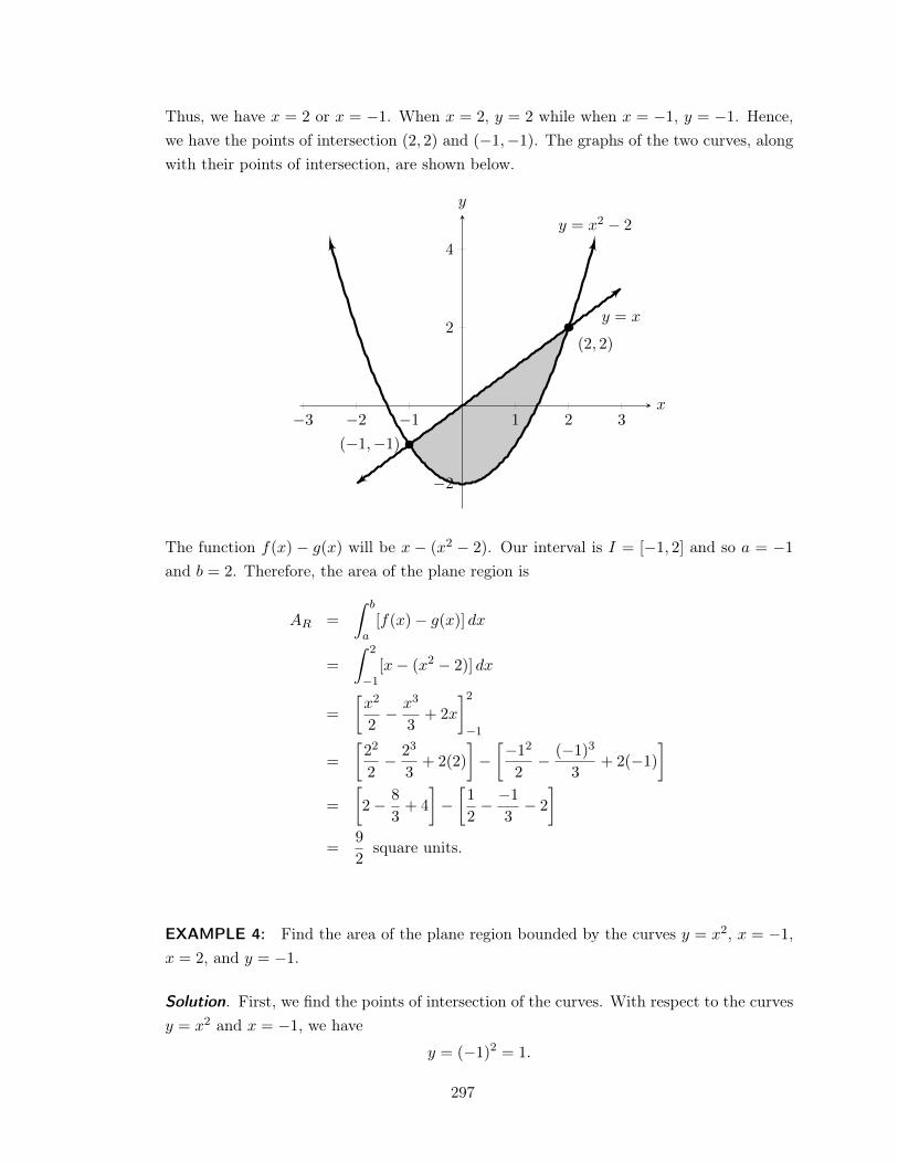
Thus, we have x = 2 or x = �1. When x = 2, y = 2 while when x = �1, y = �1. Hence,we have the points of intersection (2, 2) and (�1,�1). The graphs of the two curves, alongwith their points of intersection, are shown below.
�3 �2 �1 1 2 3
�2
2
4
y = x2 � 2
y = x
(2, 2)
(�1,�1)
x
y
The function f(x) � g(x) will be x � (x2 � 2). Our interval is I = [�1, 2] and so a = �1
and b = 2. Therefore, the area of the plane region is
AR =
Z b
a[f(x)� g(x)] dx
=
Z2
�1
[x� (x2 � 2)] dx
=
x2
2
� x3
3
+ 2x
�2
�1
=
2
2
2
� 2
3
3
+ 2(2)
���1
2
2
� (�1)
3
3
+ 2(�1)
�
=
2� 8
3
+ 4
��1
2
� �1
3
� 2
�
=
9
2
square units.
.
EXAMPLE 4: Find the area of the plane region bounded by the curves y = x2, x = �1,x = 2, and y = �1.
Solution. First, we find the points of intersection of the curves. With respect to the curvesy = x2 and x = �1, we have
y = (�1)
2
= 1.
297
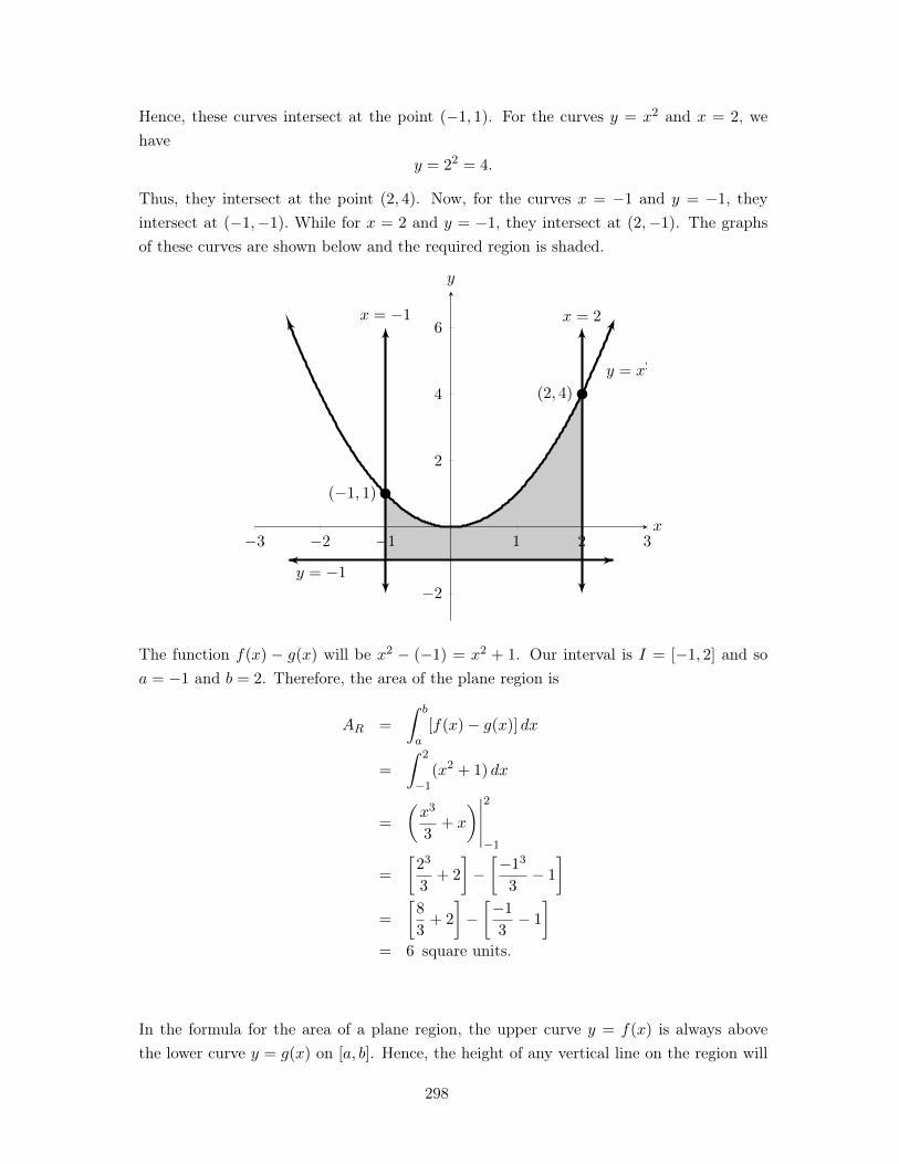
Hence, these curves intersect at the point (�1, 1). For the curves y = x2 and x = 2, wehave
y = 2
2
= 4.
Thus, they intersect at the point (2, 4). Now, for the curves x = �1 and y = �1, theyintersect at (�1,�1). While for x = 2 and y = �1, they intersect at (2,�1). The graphsof these curves are shown below and the required region is shaded.
�3 �2 �1 1 2 3
�2
2
4
6
y = x2
y = �1
x = 2
x = �1
(�1, 1)
(2, 4)
x
y
The function f(x) � g(x) will be x2 � (�1) = x2 + 1. Our interval is I = [�1, 2] and soa = �1 and b = 2. Therefore, the area of the plane region is
AR =
Z b
a[f(x)� g(x)] dx
=
Z2
�1
(x2 + 1) dx
=
✓x3
3
+ x
◆�����
2
�1
=
2
3
3
+ 2
���1
3
3
� 1
�
=
8
3
+ 2
���1
3
� 1
�
= 6 square units.
.
In the formula for the area of a plane region, the upper curve y = f(x) is always abovethe lower curve y = g(x) on [a, b]. Hence, the height of any vertical line on the region will
298
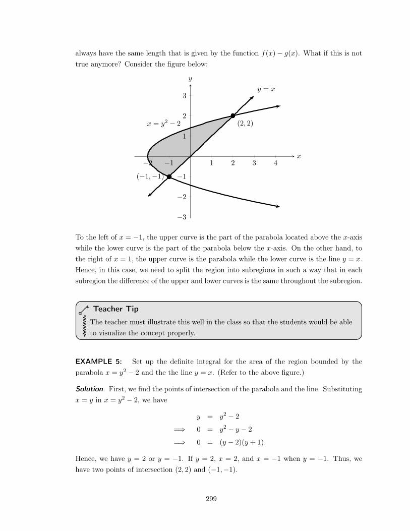
always have the same length that is given by the function f(x)� g(x). What if this is nottrue anymore? Consider the figure below:
�2 �1 1 2 3 4
�3
�2
�1
1
2
3
x = y2 � 2
y = x
(�1,�1)
(2, 2)
x
y
To the left of x = �1, the upper curve is the part of the parabola located above the x-axiswhile the lower curve is the part of the parabola below the x-axis. On the other hand, tothe right of x = 1, the upper curve is the parabola while the lower curve is the line y = x.Hence, in this case, we need to split the region into subregions in such a way that in eachsubregion the difference of the upper and lower curves is the same throughout the subregion.
Teacher Tip
The teacher must illustrate this well in the class so that the students would be ableto visualize the concept properly.
EXAMPLE 5: Set up the definite integral for the area of the region bounded by theparabola x = y2 � 2 and the the line y = x. (Refer to the above figure.)
Solution. First, we find the points of intersection of the parabola and the line. Substitutingx = y in x = y2 � 2, we have
y = y2 � 2
=) 0 = y2 � y � 2
=) 0 = (y � 2)(y + 1).
Hence, we have y = 2 or y = �1. If y = 2, x = 2, and x = �1 when y = �1. Thus, wehave two points of intersection (2, 2) and (�1,�1).
299
Note that the equation of the parabola x = y2�2 gives us two expressions for y: y =
px+ 2
(points on the parabola located above the x-axis) and y = �px+ 2 (points on the parabola
located below the x-axis).
We first set up the integral of subregion R1
(part of the region located on the left of x = �1).The upper curve here as we have observed earlier is y =
px+ 2 and the lower curve is
y = �px+ 2. Thus, the difference of the upper and lower curve is given by
upper curve � lower curve =
px+ 2� [�
px+ 2] = 2
px+ 2.
The interval I is [�2,�1]. Hence, the area of R1
is
AR1 =
Z �1
�2
2
px+ 2 dx.
For subregion R2
(part of the region located to the right of (�1,�1), the upper curve isy =
px+ 2 and the lower curve is y = x. So, we have
upper curve � lower curve =
px+ 2� x.
The interval I is [�1, 2]. Hence, the area of R2
is
AR2 =
Z �2
�1
[
px+ 2� 2] dx.
Finally, to get the area of the region R, we simply add the areas of subregions R1
and R2
,i.e.,
AR = AR1 +AR2
=
Z �1
�2
2
px+ 2 dx+
Z �2
�1
[
px+ 2� 2] dx.
.
300
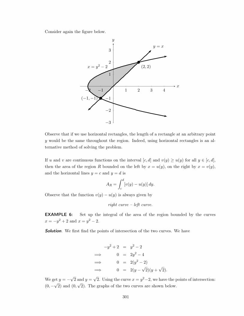
Consider again the figure below.
�2 �1 1 2 3 4
�3
�2
�1
1
2
3
x = y2 � 2
y = x
(�1,�1)
(2, 2)
x
y
Observe that if we use horizontal rectangles, the length of a rectangle at an arbitrary pointy would be the same throughout the region. Indeed, using horizontal rectangles is an al-ternative method of solving the problem.
If u and v are continuous functions on the interval [c, d] and v(y) � u(y) for all y 2 [c, d],then the area of the region R bounded on the left by x = u(y), on the right by x = v(y),and the horizontal lines y = c and y = d is
AR =
Z d
c[v(y)� u(y)] dy.
Observe that the function v(y)� u(y) is always given by
right curve – left curve.
EXAMPLE 6: Set up the integral of the area of the region bounded by the curvesx = �y2 + 2 and x = y2 � 2.
Solution. We first find the points of intersection of the two curves. We have
�y2 + 2 = y2 � 2
=) 0 = 2y2 � 4
=) 0 = 2(y2 � 2)
=) 0 = 2(y �p2)(y +
p2).
We get y = �p2 and y =
p2. Using the curve x = y2�2, we have the points of intersection:
(0,�p2) and (0,
p2). The graphs of the two curves are shown below.
301
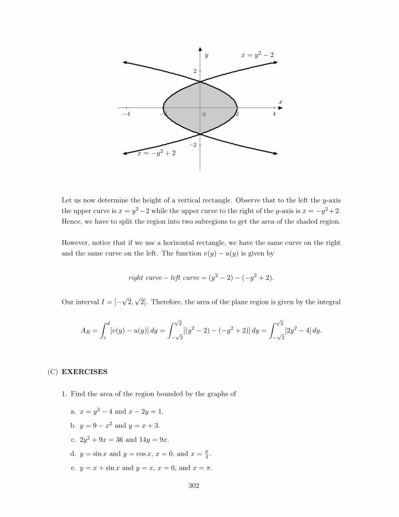
�4 �2 2 4
x
�2
2
y
0
x = y2 � 2
x = �y2 + 2
Let us now determine the height of a vertical rectangle. Observe that to the left the y-axisthe upper curve is x = y2�2 while the upper curve to the right of the y-axis is x = �y2+2.Hence, we have to split the region into two subregions to get the area of the shaded region.
However, notice that if we use a horizontal rectangle, we have the same curve on the rightand the same curve on the left. The function v(y)� u(y) is given by
right curve � left curve = (y2 � 2)� (�y2 + 2).
Our interval I = [�p2,p2]. Therefore, the area of the plane region is given by the integral
AR =
Z d
c[v(y)� u(y)] dy =
Z p2
�p2
[(y2 � 2)� (�y2 + 2)] dy =
Z p2
�p2
[2y2 � 4] dy.
.
(C) EXERCISES
1. Find the area of the region bounded by the graphs of
a. x = y2 � 4 and x� 2y = 1.
b. y = 9� x2 and y = x+ 3.
c. 2y2 + 9x = 36 and 14y = 9x.
d. y = sinx and y = cosx, x = 0, and x =
⇡4
.
e. y = x+ sinx and y = x, x = 0, and x = ⇡.
302
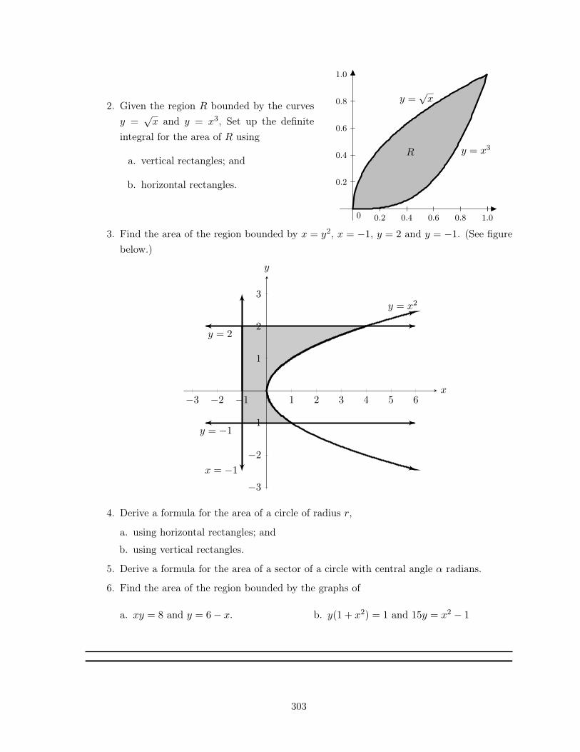
2. Given the region R bounded by the curvesy =
px and y = x3, Set up the definite
integral for the area of R using
a. vertical rectangles; and
b. horizontal rectangles.
0.2 0.4 0.6 0.8 1.0
0.2
0.4
0.6
0.8
1.0
0
y =
px
y = x3R
3. Find the area of the region bounded by x = y2, x = �1, y = 2 and y = �1. (See figurebelow.)
�3 �2 �1 1 2 3 4 5 6
�3
�2
�1
1
2
3
y = �1
y = 2
x = �1
y = x2
x
y
4. Derive a formula for the area of a circle of radius r,
a. using horizontal rectangles; and
b. using vertical rectangles.
5. Derive a formula for the area of a sector of a circle with central angle ↵ radians.
6. Find the area of the region bounded by the graphs of
a. xy = 8 and y = 6� x. b. y(1 + x2) = 1 and 15y = x2 � 1
303
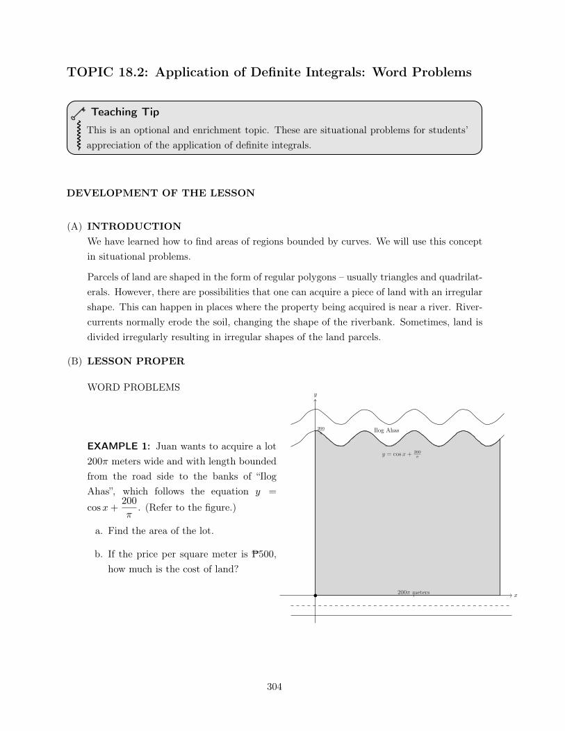
TOPIC 18.2: Application of Definite Integrals: Word Problems
Teaching Tip
This is an optional and enrichment topic. These are situational problems for students’appreciation of the application of definite integrals.
DEVELOPMENT OF THE LESSON
(A) INTRODUCTIONWe have learned how to find areas of regions bounded by curves. We will use this conceptin situational problems.
Parcels of land are shaped in the form of regular polygons – usually triangles and quadrilat-erals. However, there are possibilities that one can acquire a piece of land with an irregularshape. This can happen in places where the property being acquired is near a river. River-currents normally erode the soil, changing the shape of the riverbank. Sometimes, land isdivided irregularly resulting in irregular shapes of the land parcels.
(B) LESSON PROPER
WORD PROBLEMS
EXAMPLE 1: Juan wants to acquire a lot200⇡ meters wide and with length boundedfrom the road side to the banks of “IlogAhas”, which follows the equation y =
cosx+
200
⇡. (Refer to the figure.)
a. Find the area of the lot.
b. If the price per square meter is P500,how much is the cost of land?
x
y
Ilog Ahas
y = cosx+
200
⇡
200⇡ meters
200
⇡
304
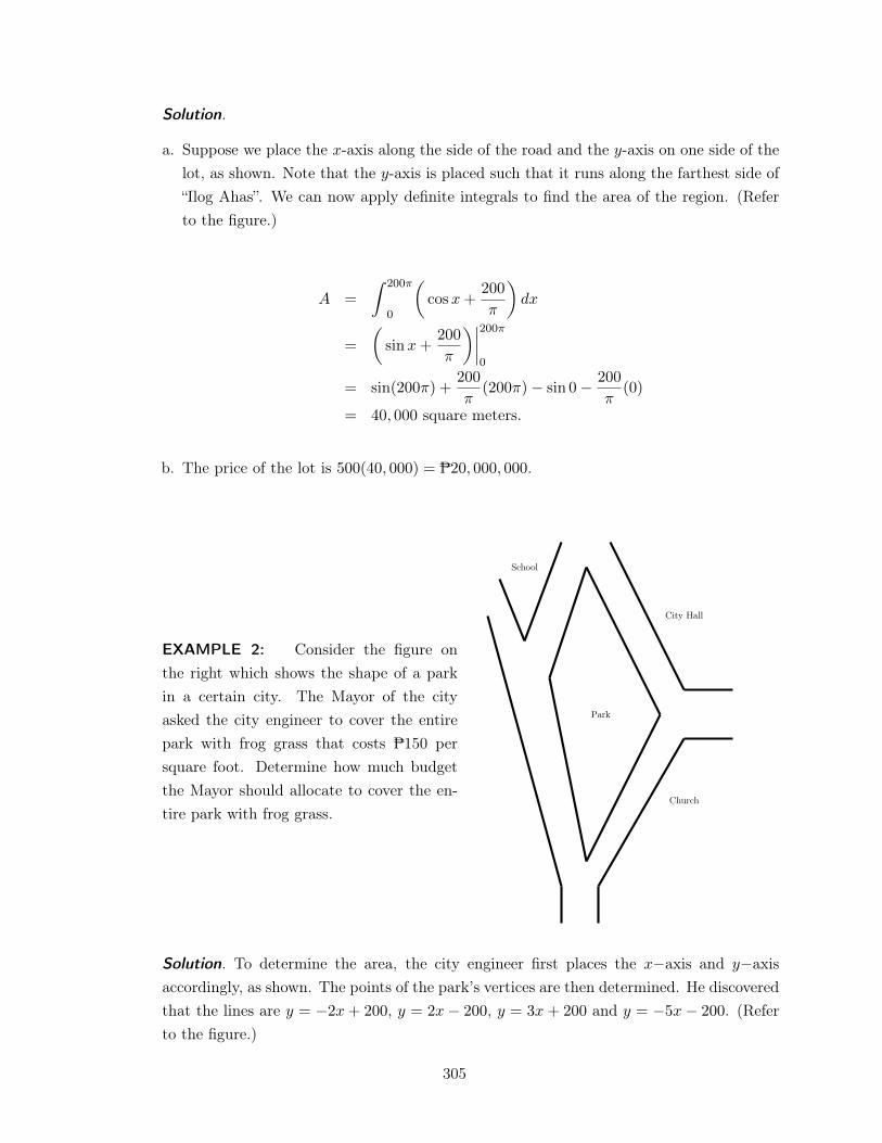
Solution. .
a. Suppose we place the x-axis along the side of the road and the y-axis on one side of thelot, as shown. Note that the y-axis is placed such that it runs along the farthest side of“Ilog Ahas”. We can now apply definite integrals to find the area of the region. (Referto the figure.)
A =
Z200⇡
0
✓cosx+
200
⇡
◆dx
=
✓sinx+
200
⇡
◆����200⇡
0
= sin(200⇡) +200
⇡(200⇡)� sin 0� 200
⇡(0)
= 40, 000 square meters.
b. The price of the lot is 500(40, 000) = P20, 000, 000.
.
EXAMPLE 2: Consider the figure onthe right which shows the shape of a parkin a certain city. The Mayor of the cityasked the city engineer to cover the entirepark with frog grass that costs P150 persquare foot. Determine how much budgetthe Mayor should allocate to cover the en-tire park with frog grass.
Church
Park
School
City Hall
Solution. To determine the area, the city engineer first places the x�axis and y�axisaccordingly, as shown. The points of the park’s vertices are then determined. He discoveredthat the lines are y = �2x+ 200, y = 2x� 200, y = 3x+ 200 and y = �5x� 200. (Referto the figure.)
305
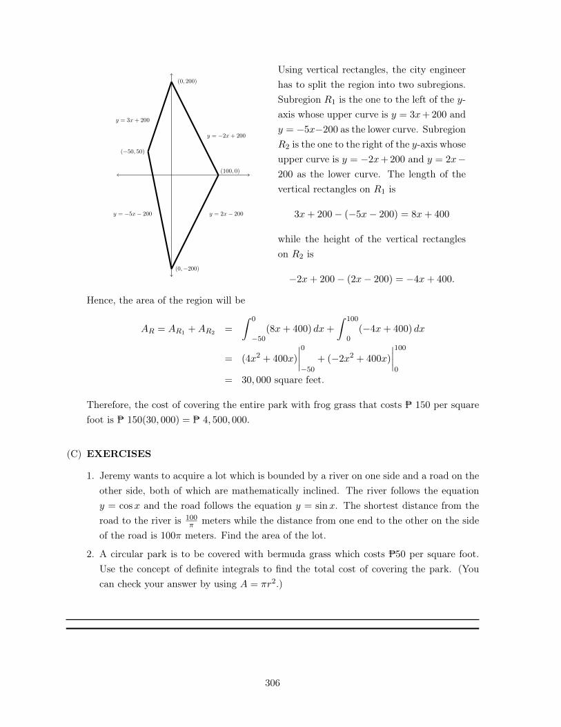
(0,�200)
(100, 0)
(0, 200)
(�50, 50)
y = �2x+ 200
y = 2x� 200y = �5x� 200
y = 3x+ 200
Using vertical rectangles, the city engineerhas to split the region into two subregions.Subregion R
1
is the one to the left of the y-axis whose upper curve is y = 3x+200 andy = �5x�200 as the lower curve. SubregionR
2
is the one to the right of the y-axis whoseupper curve is y = �2x+200 and y = 2x�200 as the lower curve. The length of thevertical rectangles on R
1
is
3x+ 200� (�5x� 200) = 8x+ 400
while the height of the vertical rectangleson R
2
is
�2x+ 200� (2x� 200) = �4x+ 400.
Hence, the area of the region will be
AR = AR1 +AR2 =
Z0
�50
(8x+ 400) dx+
Z100
0
(�4x+ 400) dx
= (4x2 + 400x)
����0
�50
+ (�2x2 + 400x)
����100
0
= 30, 000 square feet.
Therefore, the cost of covering the entire park with frog grass that costs P 150 per squarefoot is P 150(30, 000) = P 4, 500, 000.
.
(C) EXERCISES
1. Jeremy wants to acquire a lot which is bounded by a river on one side and a road on theother side, both of which are mathematically inclined. The river follows the equationy = cosx and the road follows the equation y = sinx. The shortest distance from theroad to the river is 100
⇡ meters while the distance from one end to the other on the sideof the road is 100⇡ meters. Find the area of the lot.
2. A circular park is to be covered with bermuda grass which costs P50 per square foot.Use the concept of definite integrals to find the total cost of covering the park. (Youcan check your answer by using A = ⇡r2.)
306
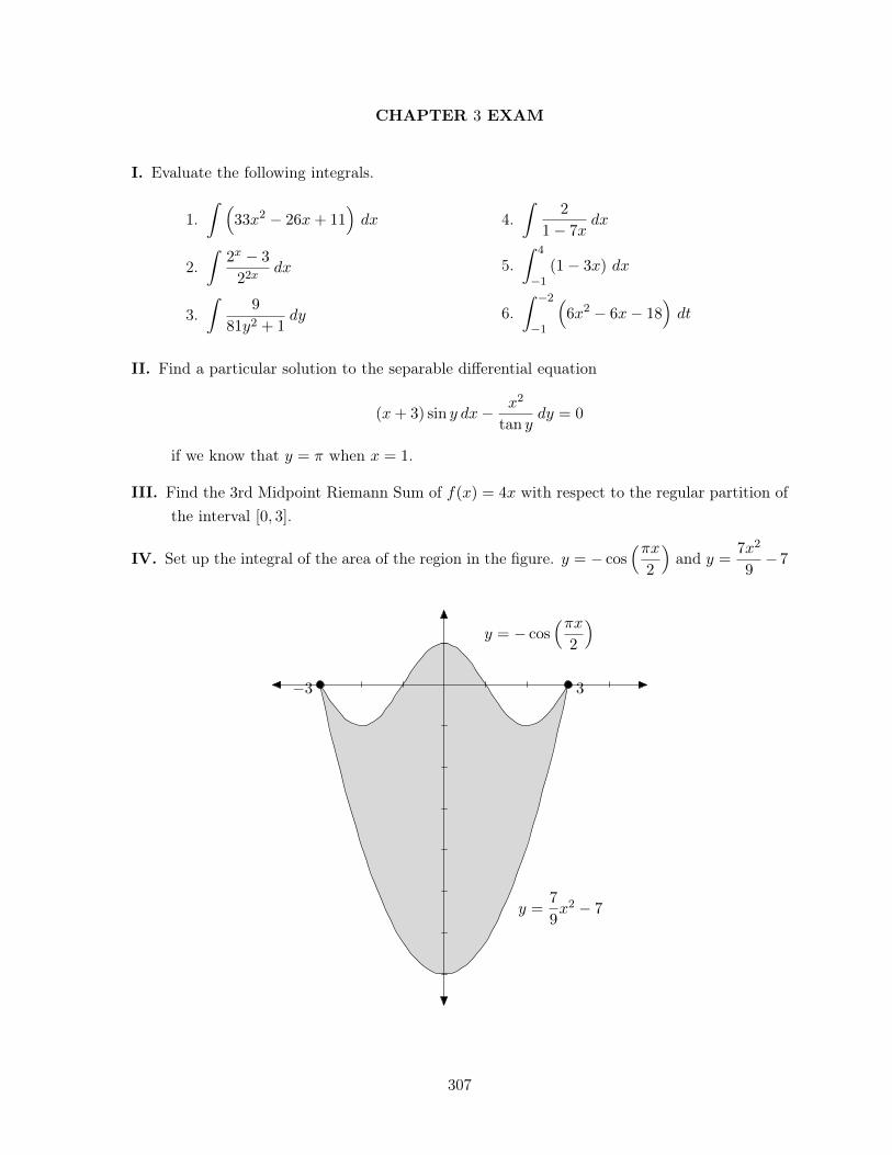
CHAPTER 3 EXAM
I. Evaluate the following integrals.
1.Z ⇣
33x2 � 26x+ 11
⌘dx
2.Z
2
x � 3
2
2xdx
3.Z
9
81y2 + 1
dy
4.Z
2
1� 7xdx
5.Z
4
�1
(1� 3x) dx
6.Z �2
�1
⇣6x2 � 6x� 18
⌘dt
II. Find a particular solution to the separable differential equation
(x+ 3) sin y dx� x2
tan ydy = 0
if we know that y = ⇡ when x = 1.
III. Find the 3rd Midpoint Riemann Sum of f(x) = 4x with respect to the regular partition ofthe interval [0, 3].
IV. Set up the integral of the area of the region in the figure. y = � cos
⇣⇡x2
⌘and y =
7x2
9
� 7
y = � cos
⇣⇡x2
⌘
y =
7
9
x2 � 7
�3 3
307
Bibliography
[1] H. Anton, I. Bivens, S. Davis, Calculus: Early Transcendentals, John Wiley andSons, 7th Edition, 2002.
[2] R. Barnett, M. Ziegler, K. Byleen Calculus for Business, Economics, Life Sciencesand Social Sciences, Pearson Education (Asia) Pre Ltd, 9th Edition, 2003.
[3] L. Leithold, College Algebra and Trigonometry, Addison Wesley Longman Inc.,1989, reprinted-Pearson Education Asia Pte. Ltd, 2002.
[4] L. Leithold, The Calculus 7, Harpercollins College Div., 7th edition, December1995.
[5] Math 53 Module Committee, Math 53 Elementary Analysis I Course Module, In-stitute of Mathematics, UP Diliman, 2012.
[6] J. Stewart, The Calculus: Early Transcendentals, Brooks/Cole, 6th Edition, 2008.
[7] S. Tan, Applied Calculus for the Managerial, Life and Social Sciences, Brooks/Cole,Cengage Learning, 9th Edition, 2014.
308
Biographical Notes
TEAM LEADER:
JOSE MARIA P. BALMACEDA
Dr. Jose Maria P. Balmaceda is a Professor of the Institute of Mathematics and Dean of theCollege of Science, University of the Philippines Diliman. He obtained the Ph.D. Mathematicsdegree from the University of Illinois at Urbana-Champaign and master’s and undergraduatedegrees in math from UP Diliman. He is a member of the National Academy of Science andTechnology (NAST Philippines), Chair of the CHED Technical Committee for Mathematics, andPresident of the Mathematical Society of the Philippines. He is a recipient of various awardssuch as the NAST Outstanding Young Scientist Award, Science Prize (for Mathematics) fromthe Third World Academy of Sciences, Achievement Award from the National Research Councilof the Philippines, and UP Diliman’s Gawad Chanselor Awards for Most Outstanding Teacherand Most Outstanding Researcher.
WRITERS:
RICHARD S. LEMENCE
Dr. Richard S. Lemence is an Associate Professor and Deputy Director for Facilities and Re-sources, Institute of Mathematics, University of the Philippines Diliman. He obtained thedoctorate degree in mathematics from Niigata University, Japan, specializing in differential ge-ometry. He was a former faculty member of the Department of Mathematics of the MindanaoState University-Iligan Institute of Technology, where he also completed his baccalaureate andmaster’s degrees in mathematics. Dr. Lemence was awarded by the National Academy of Sci-ence and Technology as Outstanding Young Scientist and designated by the University of thePhilippines as U.P. Scientist I. He is the current National Director of the Philippine Mathemat-ical Olympiad.
309
ORESTE M. ORTEGA JR.
Mr. Oreste M. Ortega Jr. is an Assistant Professor in the Mathematics Department of theLeyte Normal University, Tacloban City. He obtained his BS and MS in Mathematics degreesfrom the University of San Carlos in Cebu City. He is currently on dissertation writing for thePh.D. Mathematics degree from the Ateneo de Manila University. Mr. Ortega has extensiveexperience in teaching calculus and other mathematics subjects, and is an active member ofthe Mathematical Society of the Philippines and other professional organizations. His researchinterests include graph theory and combinatorics.
CARLENE P. C. PILAR-ARCEO
Dr. Carlene P.C. Pilar-Arceo obtained her doctorate degree in Mathematics from the Universityof the Philippines Diliman (UPD), where she also finished her master’s and baccalaureate de-grees. She is currently a Professor at the Institute of Mathematics, U.P. Diliman and ProgramDevelopment Associate of the UPD Office of the Vice Chancellor for Academic Affairs. She wasformer UPD College of Science Secretary and served as Assistant Secretary of the University.A sought-after resource person on the teaching and popularization of mathematics, Dr. Pilar-Arceo has also published scholarly articles on mathematical analysis and mathematical biologyand two high school mathematics textbooks. She has received U.P. Diliman’s Gawad ChanselorAward for Most Outstanding Teacher.
LOUIE JOHN D. VALLEJO
Dr. Louie John D. Vallejo is an Assistant Professor at the University of the Philippines Diliman.He holds a Ph.D. Mathematics degree from U.P. Diliman and master’s and baccalaureate degrees(summa cum laude) from the same university. His doctoral dissertation research is on approxi-mation theory and harmonic analysis. He has published his results in international journals andhas presented his work in international and national conferences. Dr. Vallejo is currently theDeputy Team Leader of the Philippine delegation to the International Mathematical Olympiadand has been a trainer in the Mathematical Olympiad Selection Camp for several years now.
310
TECHNICAL EDITORS:
MARIAN P. ROQUE
Dr. Marian P. Roque is a Professor and Director of the Institute of Mathematics, Universityof the Philippines Diliman, where she also obtained her undergraduate, master’s and doctor-ate degrees in mathematics. She occupies key positions in professional organizations such asmembership in the Executive Committee of the Centre International de Mathématiques Pures etAppliquées (CIMPA), based in France, and the National Board of Directors of the MathematicalSociety of the Philippines. She has received the Achievement Award from the National ResearchCouncil of the Philippines and UP Diliman’s Gawad Chanselor sa Natatanging Guro. She holdsa designation as UP Scientist I and is member of the UP Diliman General Education Committee.Dr. Roque co-authored the graduate textbook Introduction to Classical and Variational PartialDifferential Equations published by the UP Press.
JOSE ERNIE C. LOPE
Dr. Jose Ernie C. Lope is a Professor and former Chair of the then Department of Mathematics,University of the Philippines Diliman. He obtained master’s and doctorate degrees in mathe-matics from Sophia University, Japan. A Bachelor of Science Mathematics summa cum laudegraduate of UP Diliman, Dr. Lope has received awards for his research and teaching such as theUP Scientist I designation, Outstanding Young Scientist Awards from the NAST and the ThirdWorld Academy of Science and the Gawad Chanselor sa Natatanging Guro from UP Diliman.A former member of the Philippine Team to the International Mathematical Olympiad (IMO),he later became Team Leader of three Philippine delegations to the IMO that set Philippinerecords for medals and citations garnered by the team members.
LANGUAGE AND COPY EDITOR:
ERICK B. LIRIOS
Mr. Erick B. Lirios currently teaches journalism and photojournalism at the Manila TimesCollege, and works as a columnist for The Manila Bulletin. He edited academic books forMcGraw-Hill Education, the Department of Interior and Local Government and the AteneoSchool of Government. He worked as the Communications Executive for Singapore Telecommu-nications, as the Corporate Communications Executive for the Spastic Children’s Association ofSingapore, and the Editor-in-Chief of Telecable Magazine. Besides doing proofreading, he alsoworks as a photographer - the latest being with the World Health Organization.
311


Basic Calculus Teaching GuideCHED