UPennalizers RoboCup Standard Platform League

Team Report 2010

Jordan Brindza, Levi Cai, Ashleigh Thomas,

Ross Boczar, Alyin Caliskan, Alexandra Lee,

Anirudha Majumdar, Roman Shor, Barry

Scharfman, Dan Lee

General Robotics Automation Sensing Perception (GRASP)

Laboratory of Robotics Research and Education University

of Pennsylvania

1.0 Introduction

Robocup 2009 marked the beginning of a new era for the University of Pennsylvania

team, the “UPennalizers”. After successfully competing in the Sony Aibo 4-legged

league from 1999-2006, making it to at least the quarterfinal round in each of those years,

the team took a two year hiatus from Robocup. However, at the urging of engineering

undergraduates who wanted to participate, the team and code base were started anew to

prepare for the 2009 competition. With a code base already in place from 2009, the focus

for the year 2010 was to build new algorithms and improve on existing ones to help

develop a strong strategy.

In the Robocup 2010 competition in Singapore, the Upennalizers were quarterfinalists

and also finished 4th

in the dribbling challenge. We also released an open source

version of our code to make Robocup more accessible to new teams just starting out.

The release can be found at our website,

http://fling.seas.upenn.edu/~robocup/wiki/index.php?n=Main.HomePage .

1.1 Team Members

The UPennalizers are led by Professor Daniel Lee, Associate Professor in Electrical and

Systems Engineering at the University of Pennsylvania. The team consists of

undergraduate and graduate students in the departments of Mechanical Engineering and

Applied Mathematics, Electrical and Systems Engineering, and Computer and

Information Science.

2.0 Software Architecture

The software architecture for the robots is shown in Figure 1. The architecture used is an

expansion of the architecture used by the UPennalizers in the previous RoboCup

competition. This architecture retains MATLAB as a common development platform[2].

Since many of the students do not have strong programming backgrounds, this

development platform allows them to participate more fully on the team. This year we also

incorporated a number of Lua modules to handle so me of the low level computation in

order to increase our frame rate.

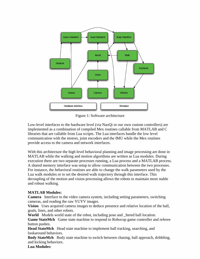
Figure 1: Software architecture

Low-level interfaces to the hardware level (via NaoQi or our own custom controllers) are

implemented as a combination of compiled Mex routines callable from MATLAB and C

libraries that are callable from Lua scripts. The Lua interfaces handle the low level

communication with the motors, joint encoders and the IMU while the Mex routines

provide access to the camera and network interfaces.

With this architecture the high level behavioral planning and image processing are done in

MATLAB while the walking and motion algorithms are written as Lua modules. During

execution there are two separate processes running, a Lua process and a MATLAB process.

A shared memory interface was setup to allow communication between the two processes.

For instance, the behavioral routines are able to change the walk parameters used by the

Lua walk modules or to set the desired walk trajectory through this interface. This

decoupling of the motion and vision processing allows the robots to maintain more stable

and robust walking.

MATLAB Modules:

Camera Interface to the video camera system, including setting parameters, switching

cameras, and reading the raw YUYV images.

Vision Uses acquired camera images to deduce presence and relative location of the ball,

goals, lines, and other robots.

World Models world state of the robot, including pose and _ltered ball location.

Game StateMch Game state machine to respond to Robocup game controller and referee

button pushes.

Head StateMch Head state machine to implement ball tracking, searching, and

lookaround behaviors.

Body StateMch Body state machine to switch between chasing, ball approach, dribbling,

and kicking behaviors.

Lua Modules:

Effector Module to set and vary motor joints and parameters, as well as body and face

LED's.

Sensor Module that is responsible for reading joint encoders, IMU, foot sensors, battery

status, and button presses on the robot.

Keyframe Keyframe motion generator used for scripted motions such as getup and kick

motions.

Walk Omnidirectional locomotion module.

In order to simplify development, all interprocess communications are performed by

passing Matlab structures between the various modules, as well as between robots.

3.0 Motion 3.1 Locomotion

The locomotion of the robots is controlled by a dynamic walk engine. All other motions,

such as kicks and the get up routine, are predetermined scripted motions. The main

development has been the new omni-directional bipedal walk engine that has a set of

tunable parameters that can be adjusted depending on surface conditions. The omni-

directionality of the walk allows for quick responses to changes in game conditions (such

as the ball changing direction due to a deflection).

Using inputs from our vision and localization modules, the walk engine generates

trajectories for the robot’s Center of Mass (COM). The robot uses the information about

the ball’s location and its relative orientation to determine rotational and translational

velocities. Inverse kinematics are then used to generate joint trajectories so that the

projection of the Zero Moment Point (ZMP) onto the ground lies within the convex

polygon of the support foot. This process is repeated to generate alternate support and

swing phases for the two legs.

Information from the Inertial Measurement Unit (IMU) and the foot sensors of the robot

is used to modulate the commanded joint angles and phase of the gait cycles to correct

against perturbations. Hence, minor disturbances caused by irregularities in the carpet

and bumping into obstacles do not cause the robot to lose stability.

Certain parameters of the walk engine can be manually optimized to improve

performance on different surfaces/robots. These include the body and step height, ZMP

time constant, joint stiffness during various phases of the gait, etc.

Figure 2 summarizes the functioning of the omni-directional walk engine.

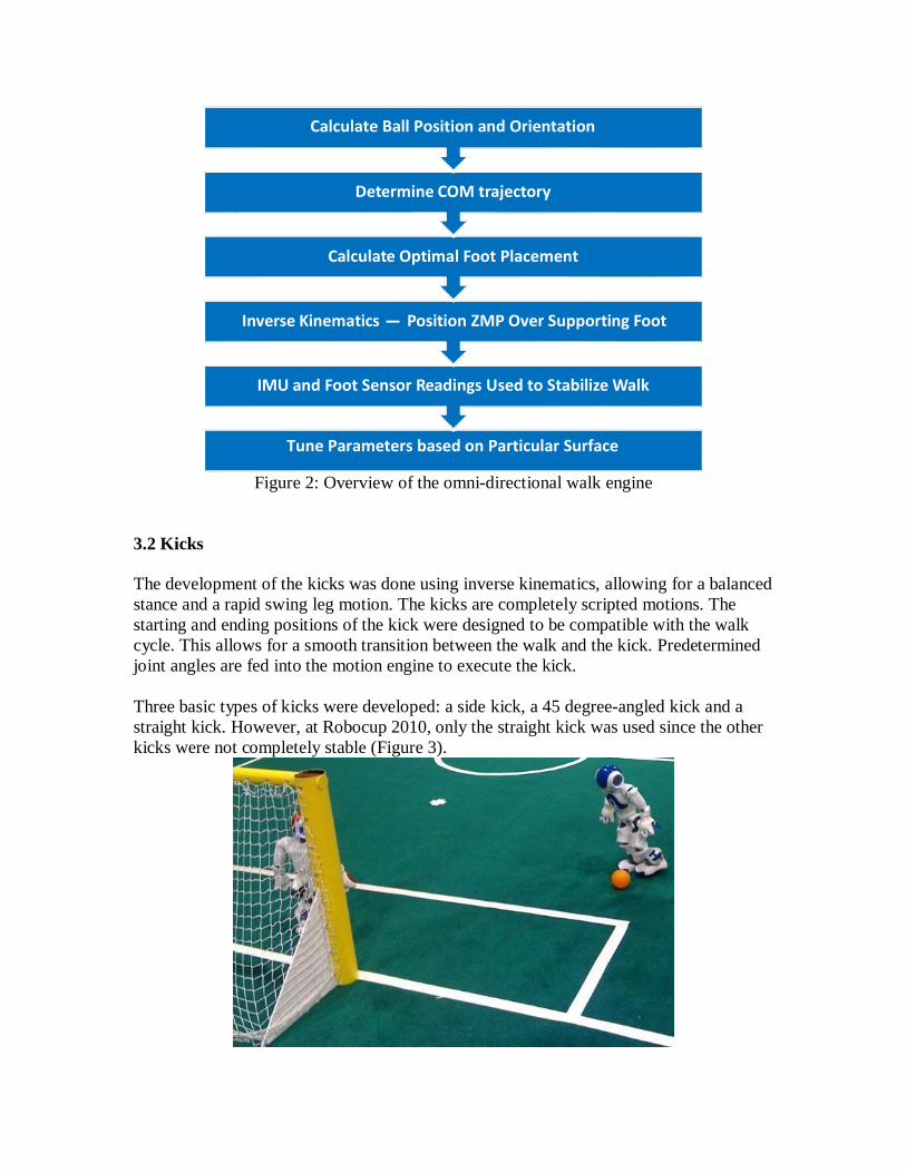
Calculate Ball Position and Orientation

Determine COM trajectory

Calculate Optimal Foot Placement

Inverse Kinematics - Position ZMP Over Supporting Foot

IMU and Foot Sensor Readings Used to Stabilize Walk

Tune Parameters based on Particular Surface

Figure 2: Overview of the omni-directional walk engine

3.2 Kicks The development of the kicks was done using inverse kinematics, allowing for a balanced

stance and a rapid swing leg motion. The kicks are completely scripted motions. The

starting and ending positions of the kick were designed to be compatible with the walk

cycle. This allows for a smooth transition between the walk and the kick. Predetermined

joint angles are fed into the motion engine to execute the kick.

Three basic types of kicks were developed: a side kick, a 45 degree-angled kick and a

straight kick. However, at Robocup 2010, only the straight kick was used since the other

kicks were not completely stable (Figure 3).

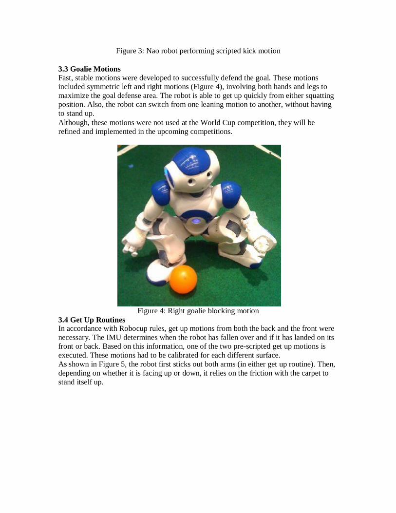
Figure 3: Nao robot performing scripted kick motion

3.3 Goalie Motions Fast, stable motions were developed to successfully defend the goal. These motions included symmetric left and right motions (Figure 4), involving both hands and legs to

maximize the goal defense area. The robot is able to get up quickly from either squatting

position. Also, the robot can switch from one leaning motion to another, without having

to stand up.

Although, these motions were not used at the World Cup competition, they will be

refined and implemented in the upcoming competitions.

3.4 Get Up Routines

Figure 4: Right goalie blocking motion

In accordance with Robocup rules, get up motions from both the back and the front were

necessary. The IMU determines when the robot has fallen over and if it has landed on its

front or back. Based on this information, one of the two pre-scripted get up motions is

executed. These motions had to be calibrated for each different surface.

As shown in Figure 5, the robot first sticks out both arms (in either get up routine). Then,

depending on whether it is facing up or down, it relies on the friction with the carpet to

stand itself up.

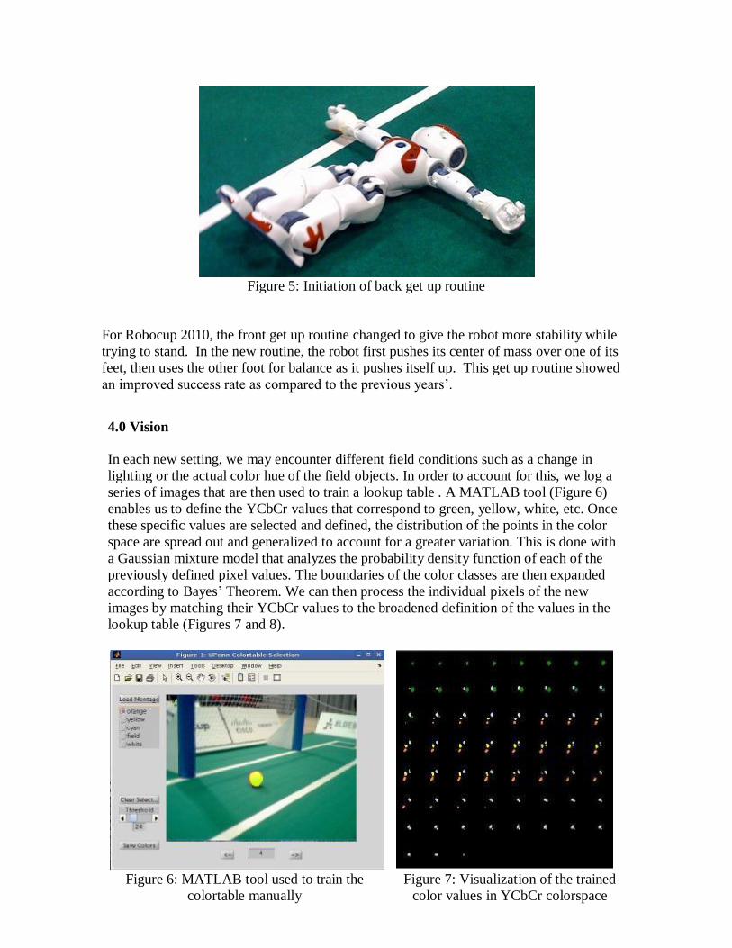
Figure 5: Initiation of back get up routine

For Robocup 2010, the front get up routine changed to give the robot more stability while

trying to stand. In the new routine, the robot first pushes its center of mass over one of its

feet, then uses the other foot for balance as it pushes itself up. This get up routine showed

an improved success rate as compared to the previous years’.

4.0 Vision In each new setting, we may encounter different field conditions such as a change in

lighting or the actual color hue of the field objects. In order to account for this, we log a

series of images that are then used to train a lookup table . A MATLAB tool (Figure 6)

enables us to define the YCbCr values that correspond to green, yellow, white, etc. Once

these specific values are selected and defined, the distribution of the points in the color

space are spread out and generalized to account for a greater variation. This is done with

a Gaussian mixture model that analyzes the probability density function of each of the

previously defined pixel values. The boundaries of the color classes are then expanded

according to Bayes’ Theorem. We can then process the individual pixels of the new

images by matching their YCbCr values to the broadened definition of the values in the

lookup table (Figures 7 and 8).

Figure 6: MATLAB tool used to train the

colortable manually

Figure 7: Visualization of the trained

color values in YCbCr colorspace

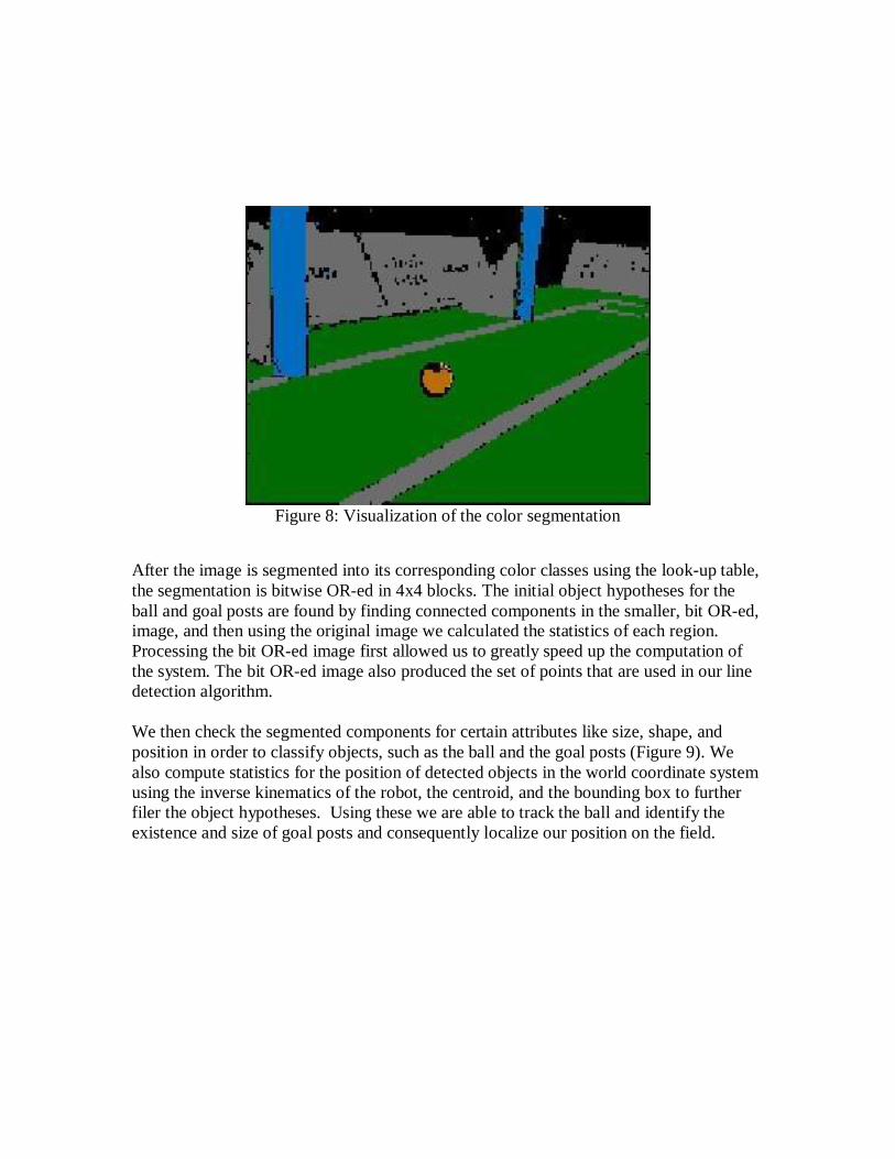
Figure 8: Visualization of the color segmentation

After the image is segmented into its corresponding color classes using the look-up table,

the segmentation is bitwise OR-ed in 4x4 blocks. The initial object hypotheses for the

ball and goal posts are found by finding connected components in the smaller, bit OR-ed, image, and then using the original image we calculated the statistics of each region.

Processing the bit OR-ed image first allowed us to greatly speed up the computation of

the system. The bit OR-ed image also produced the set of points that are used in our line

detection algorithm.

We then check the segmented components for certain attributes like size, shape, and

position in order to classify objects, such as the ball and the goal posts (Figure 9). We

also compute statistics for the position of detected objects in the world coordinate system

using the inverse kinematics of the robot, the centroid, and the bounding box to further

filer the object hypotheses. Using these we are able to track the ball and identify the

existence and size of goal posts and consequently localize our position on the field.

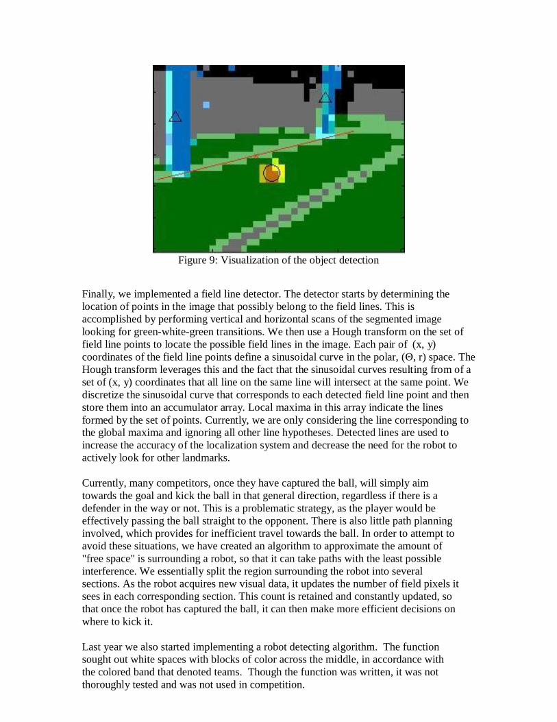
Figure 9: Visualization of the object detection

Finally, we implemented a field line detector. The detector starts by determining the

location of points in the image that possibly belong to the field lines. This is

accomplished by performing vertical and horizontal scans of the segmented image

looking for green-white-green transitions. We then use a Hough transform on the set of

field line points to locate the possible field lines in the image. Each pair of (x, y)

coordinates of the field line points define a sinusoidal curve in the polar, (Θ, r) space. The

Hough transform leverages this and the fact that the sinusoidal curves resulting from of a

set of (x, y) coordinates that all line on the same line will intersect at the same point. We

discretize the sinusoidal curve that corresponds to each detected field line point and then

store them into an accumulator array. Local maxima in this array indicate the lines

formed by the set of points. Currently, we are only considering the line corresponding to the global maxima and ignoring all other line hypotheses. Detected lines are used to

increase the accuracy of the localization system and decrease the need for the robot to

actively look for other landmarks.

Currently, many competitors, once they have captured the ball, will simply aim

towards the goal and kick the ball in that general direction, regardless if there is a

defender in the way or not. This is a problematic strategy, as the player would be

effectively passing the ball straight to the opponent. There is also little path planning

involved, which provides for inefficient travel towards the ball. In order to attempt to

avoid these situations, we have created an algorithm to approximate the amount of

"free space" is surrounding a robot, so that it can take paths with the least possible

interference. We essentially split the region surrounding the robot into several

sections. As the robot acquires new visual data, it updates the number of field pixels it

sees in each corresponding section. This count is retained and constantly updated, so

that once the robot has captured the ball, it can then make more efficient decisions on

where to kick it.

Last year we also started implementing a robot detecting algorithm. The function

sought out white spaces with blocks of color across the middle, in accordance with

the colored band that denoted teams. Though the function was written, it was not

thoroughly tested and was not used in competition.

5.0 Localization

The problem of knowing the location of the robots on the field is handled by a

probabilistic model incorporating information from visual landmarks such as goals and

lines, as well as odometry information from the effectors. Recently, probabilistic models

for pose estimation such as extended Kalman filters, grid-based Markov models, and

Monte Carlo particle filters have been successfully deployed. Unfortunately, complex

probabilistic models can be difficult to implement in real-time due to a lack of processing

power on board the robots. We address this issue with a new pose estimation algorithm

that incorporates a hybrid Rao-Blackwellized representation that reduces computational

time, while still providing for a high level of accuracy. Our algorithm models the pose

uncertainty as a distribution over a discrete set of heading angles and continuous

translational coordinates. The distribution over poses ( x, y,0 ), where ( x, y ) are the two-

dimensional translational coordinates of the robot on the field, and 0 is the heading angle,

is first generically decomposed into the product:

P( x, y,0 ) P(0 ) P( x, y | 0 ) P(0 i ) P( x, y | 0 i )

i

We model the distribution P(0 ) as a discrete set of weighted samples {0 i

}, and the

conditional likelihood P( x, y | 0 ) as simple two-dimensional Gaussians. This approach

has the advantage of combining discrete Markov updates for the heading angle with

Kalman filter updates for the translational degrees of freedom.

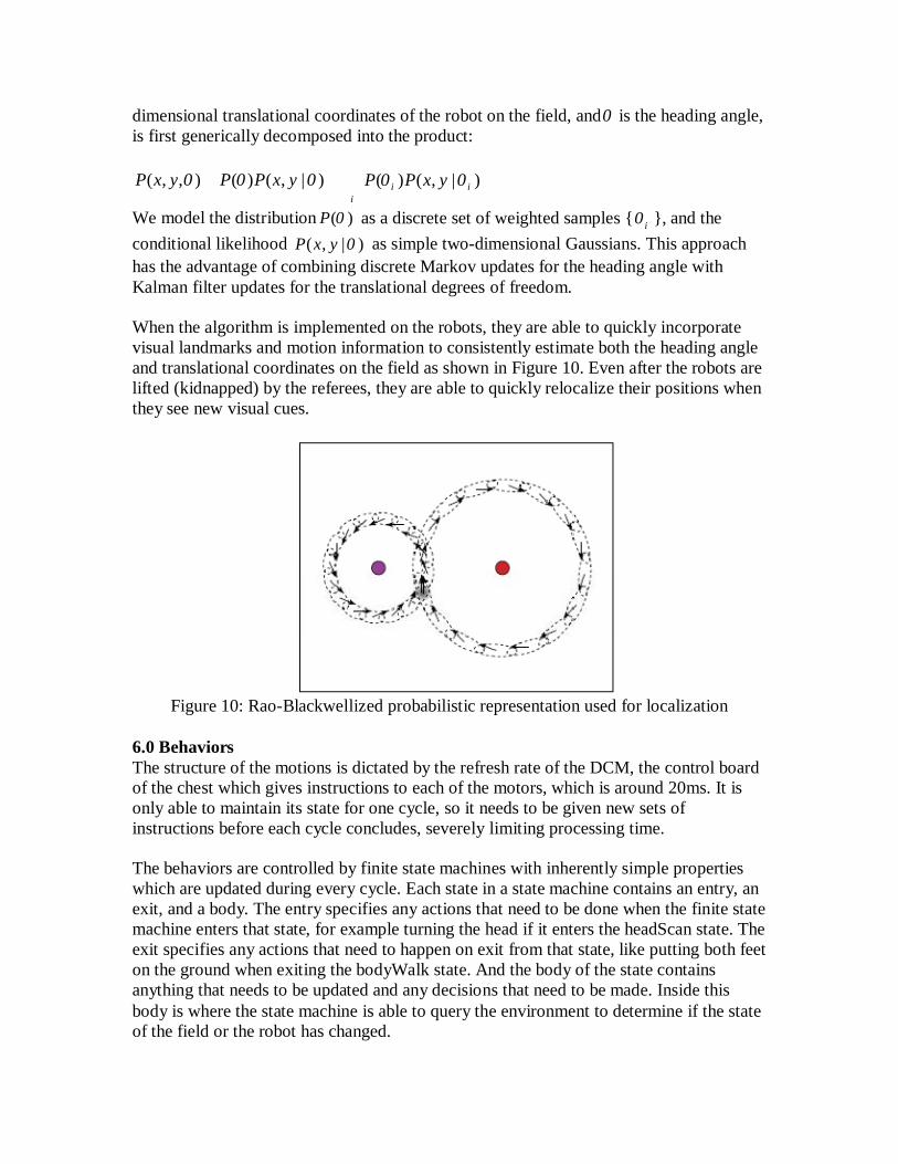
When the algorithm is implemented on the robots, they are able to quickly incorporate

visual landmarks and motion information to consistently estimate both the heading angle

and translational coordinates on the field as shown in Figure 10. Even after the robots are

lifted (kidnapped) by the referees, they are able to quickly relocalize their positions when

they see new visual cues.

Figure 10: Rao-Blackwellized probabilistic representation used for localization

6.0 Behaviors

The structure of the motions is dictated by the refresh rate of the DCM, the control board

of the chest which gives instructions to each of the motors, which is around 20ms. It is

only able to maintain its state for one cycle, so it needs to be given new sets of

instructions before each cycle concludes, severely limiting processing time.

The behaviors are controlled by finite state machines with inherently simple properties

which are updated during every cycle. Each state in a state machine contains an entry, an

exit, and a body. The entry specifies any actions that need to be done when the finite state

machine enters that state, for example turning the head if it enters the headScan state. The

exit specifies any actions that need to happen on exit from that state, like putting both feet

on the ground when exiting the bodyWalk state. And the body of the state contains

anything that needs to be updated and any decisions that need to be made. Inside this

body is where the state machine is able to query the environment to determine if the state

of the field or the robot has changed.

The head state machine (Figure 11) is simple: either the head is looking for the ball,

looking at the ball, or finding the goal posts. If the head is tracking the ball and loses it, it

throws a ballLost event and transitions to the headScan state, where the head begins to

scan the field for the ball.

Figure 11: Head state machine

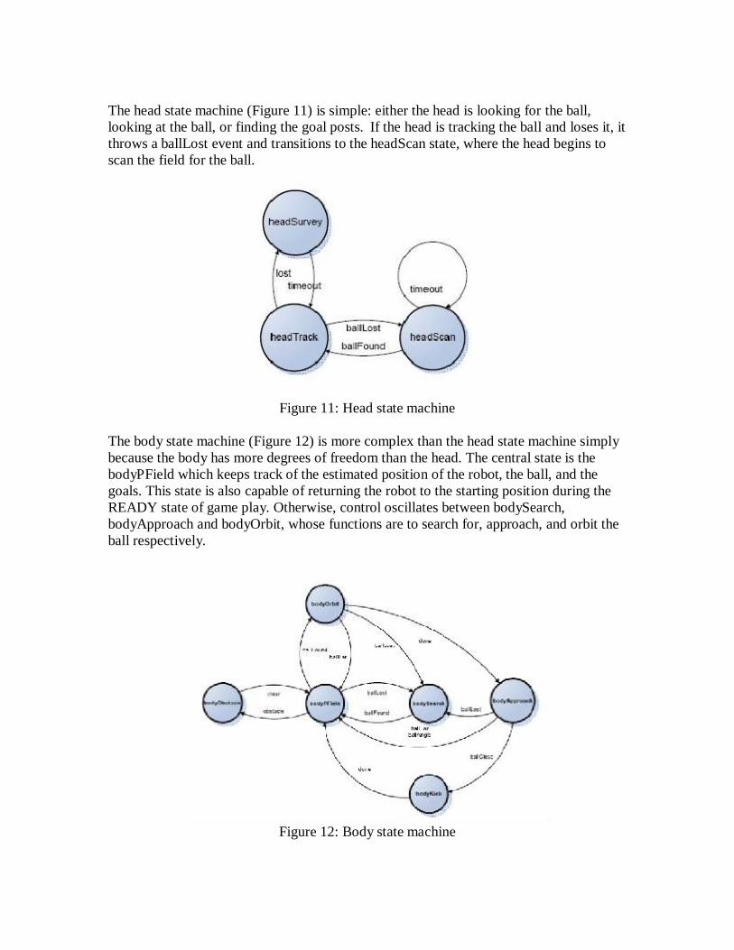
The body state machine (Figure 12) is more complex than the head state machine simply

because the body has more degrees of freedom than the head. The central state is the

bodyPField which keeps track of the estimated position of the robot, the ball, and the

goals. This state is also capable of returning the robot to the starting position during the

READY state of game play. Otherwise, control oscillates between bodySearch,

bodyApproach and bodyOrbit, whose functions are to search for, approach, and orbit the

ball respectively.

Figure 12: Body state machine

6.1 Changing Behaviors

The code is structured hierarchically, with the state machine definition residing the Body

StateMch and Head StateMch files. These files are where the actual states are defined

along with any possible transitions from each state. It is effectively a textual definition of

the state machines above. To change a transition, all that needs to be done is to change

the transition line in the state machine file. Each state resides in its own file, making the

changing of states simple.

6.2 Offense and Defense

The two player robots dynamically switch between offensive and defensive positions

throughout the game. At the start of the game, player one is assigned to offense and

player two is assigned to defense by default. The robots themselves send out heartbeat

packets to each other containing, among other things, their position and their relation to

the ball. The offensive state is characterized by the robot actively approaching the ball

and attempting to score a goal, and defense is characterized by the robot attempting to

place itself between the ball and the robot’s own goal. In the event of robot failure, the

remaining player robot will timeout and switch to offense if it has not received a

heartbeat message within specified period of time.

6.3 Goalie

The goalie maintains a simplified state machine and acts as a modified defensive player

that attempts to maintain its position inside the goalie box while placing itself between

the ball and the center of the goal. The body kick state is also augmented by the goalie

squat state. If the goalie notices the ball approaching, it squats to maximize the chances

of capturing the ball. Once captured, the ball is then kicked toward the far side of the

field.

Because the goalie often cannot process the precise location of ball travel following a

kick, it is often more useful to try to dive in the direction of an attempted shot, and thus

reduce the precision needed to block the ball. Once the goalie has determined that a ball

is within a relatively small distance from the goal, it will then actively begin to track

which direction the ball travels. If the ball increases in size, then it means it is

approaching the goalie, and if it begins to head to the left of its previous position, then

the goalie will attempt to fall in that direction. This algorithm still needs to be refined

and a better goalie diving motion must be developed before we can safely implement

this algorithm in actual matches.

7.0 Simulation

Because developing motions has the potential to cause damage to the mechanical parts of

the robot, the Webots simulation environment was utilized as a way to quickly test code

before attempting to load new scripts onto the physical robot. This was particularly

useful for developing kicks, as well as working on the get-up routines. Not every motion

developed on the simulator worked in the physical world, and vice versa, since many

properties, such as surface friction, were not perfectly modeled in the simulation

environment. However, using the simulator was still very useful as it could be used to

identify when incorrect joint angles were being sent to the robot. The simulation

environment was also useful to test behaviors and strategy, since, having only four Nao

robots, it was difficult to conduct practice matches.

8.0 Conclusion

This report detailed the work performed by the UPennalizers for the Robocup 2010

Standard Platform League competition. Since this was the team’s second year using the Nao platform, our main goal was to refine our motion and sensory code base and start

working on strategy. With this code now in place, our future work will be in refining

and expanding these elements for future Robocup competitions.