Embed Size (px)
Citation preview

The C-1 Flying Roc: A Next Generation Military Cargo Transport Aircraft
AE 4351 Design Team 6:
Marsal Bruna Gautham Kumar Brandon Liberi Michael Lopez Nana Obayashi
Junjie Zhai
April 24, 2015

I certify that I have abided by the honor code of the Georgia Institute of Technology and followed the collaboration guidelines as specified in the project description for this assignment.
_______________________________________ Marsal Bruna
_______________________________________ Gautham Kumar
_______________________________________ Brandon Liberi
_______________________________________ Michael Lopez
_______________________________________ Nana Obayashi
_______________________________________ Junjie Zhai

i Georgia Institute of Technology
Executive Summary
The next generation strategic airlift military transport proposed in this document is the C-1 Flying
Roc, designed in response to the Request for Proposal (RFP) by the armed forces for an aircraft system
capable of augmenting the overall performance of the current fleet. This modernization to the fleet will
provide major improvements over the current generation of aircraft such as the C-5 Galaxy and the C-17
Globemaster. As per the RFP, this vehicle is to have a 2030 entrance into service (EIS) date.
This aircraft proposal lays out a mission profile for a design payload of 205,000 lb with the capability
to conduct operations with payload weights up to 300,000 lb. The method used for the weight sizing
process is presented along with the considerations made in order to meet specific performance
requirements such as engine inoperative and hot day takeoff conditions. These considerations ensure that
the C-1 can fly in adverse conditions as well as recover and be safely controlled in the event of a failure.
The aircraft has been designed for tactical approaches and landings such that ground track and landing
times are minimized. These characteristics are desirable in order to maximize the efficiency of landing,
loading, and takeoff such that the vehicle can maximize air time and minimize ground time. This
performance has a large impact on the profitability of the aircraft. These efforts also result in a substantial
improvement on the low altitude performance of the current generation military transport fleet which the
armed forces utilize.
The increased performance and flight operations of the next generation strategic air lifter are balanced
with an effective cost and maintainability that is necessary for a modern armed force. The fly-away cost
of $402.1M of the system has been minimized with standard manufacturing and tooling techniques
proven on past aircraft. This is a 22% reduction over the fly-away cost per vehicle of the C-17. In
addition, the operation and support cost of the vehicle has been minimized as this has a large impact on
the lifetime cost of the vehicle. The annual operation and support cost per vehicle is $13.3M, a 29%
reduction over the annual cost of a C-17.

ii Georgia Institute of Technology
Table of Contents
Executive Summary ..................................................................................................................................................i
Table of Contents .................................................................................................................................................... ii
List of Figures .......................................................................................................................................................... v
List of Tables ........................................................................................................................................................ vii
1 Introduction ...................................................................................................................................................... 1
1.1 Aircraft Summary .................................................................................................................................... 1
2 Configuration Selection .................................................................................................................................... 3
2.1 Figures of Merit Analysis ........................................................................................................................ 3
2.2 Comparative Study .................................................................................................................................. 3
2.3 Chosen Preliminary Configuration .......................................................................................................... 5
3 Mission Specification and Decisions ................................................................................................................ 5
3.1 Mission Segments .................................................................................................................................... 5
3.1.1 Climb .............................................................................................................................................. 6
3.1.2 Cruise .............................................................................................................................................. 6
3.1.3 Takeoff ............................................................................................................................................ 7
3.1.4 Landing ........................................................................................................................................... 7
3.1.5 Range .............................................................................................................................................. 8
3.2 Mission Profile ......................................................................................................................................... 8
3.3 Payload Range Charts .............................................................................................................................. 9
3.4 Stakeholder Analysis ............................................................................................................................. 10
4 Advanced Technology .................................................................................................................................... 11
4.1 Geared Turbofan .................................................................................................................................... 11
4.2 Natural Laminar Flow Airfoil ................................................................................................................ 12
4.3 Composite Materials in Aircraft Design ................................................................................................ 13
4.4 Spiroid Winglet ...................................................................................................................................... 14
4.5 Weight Sizing Technology Factors ........................................................................................................ 15
5 Weight Sizing ................................................................................................................................................. 16
5.1 Weight Regression ................................................................................................................................. 16
5.2 Takeoff Weight Convergence ................................................................................................................ 17
5.3 Drag Polar Convergence ........................................................................................................................ 18
5.4 Sensitivity Studies ................................................................................................................................. 18
6 Constraint Sizing ............................................................................................................................................ 21
6.1 Constraint Sizing ................................................................................................................................... 21
6.2 Additional Constraints ........................................................................................................................... 22
6.3 Preliminary Sizing Results ..................................................................................................................... 23
7 Performance .................................................................................................................................................... 24
7.1 Takeoff ................................................................................................................................................... 24

iii Georgia Institute of Technology
7.2 Climb ..................................................................................................................................................... 25
7.3 V-n Diagram .......................................................................................................................................... 26
8 Fuselage Sizing ............................................................................................................................................... 27
8.1 Payload Considerations .......................................................................................................................... 27
8.2 Internal Cargo Fitting............................................................................................................................. 28
8.3 Final Fuselage Layout ............................................................................................................................ 30
9 Cockpit Layout ............................................................................................................................................... 32
10 Wing Sizing................................................................................................................................................ 34
10.1 Airfoil Selection and Analysis ............................................................................................................... 35
10.2 General Wing Planform Sizing .............................................................................................................. 37
10.3 High-Lift Device Sizing ......................................................................................................................... 38
10.4 Final Wing, Flap, and Lateral Control Layout ....................................................................................... 42
10.5 Wing Design Optimization .................................................................................................................... 44
11 Tail Sizing .................................................................................................................................................. 47
11.1 Horizontal and Vertical Stabilizer Sizing .............................................................................................. 47
11.2 Elevator and Rudder Sizing ................................................................................................................... 49
11.3 Final Tail Layout ................................................................................................................................... 50
12 Structure and Manufacturing ...................................................................................................................... 51
13 Subsystem Considerations ......................................................................................................................... 54
13.1 APU ....................................................................................................................................................... 54
13.2 Fuel Pumps ............................................................................................................................................ 55
13.3 Avionics ................................................................................................................................................. 55
13.4 Electrical System ................................................................................................................................... 55
13.5 Electrohydraulic Actuator ...................................................................................................................... 55
13.6 Ram Air Turbine .................................................................................................................................... 55
13.7 Defensive Subsystems ........................................................................................................................... 56
14 Weight and Balance Analysis .................................................................................................................... 56
14.1 Class I Component Weight Breakdown ................................................................................................. 56
14.2 Center of Gravity of Class I Weight Components ................................................................................. 58
14.3 Weight-C.G. Excursion Diagram and Feasibility of Design .................................................................. 61
15 Landing Gear Sizing .................................................................................................................................. 63
15.1 Geometric Criteria for Landing Gears ................................................................................................... 63
15.2 Final Landing Gear Configuration and Retracting Feasibility ............................................................... 65
16 Stability and Control .................................................................................................................................. 67
16.1 Neutral Point .......................................................................................................................................... 67
16.2 Static Margin ......................................................................................................................................... 68
16.3 Static Stability Derivatives .................................................................................................................... 69
16.4 Dynamic Stability .................................................................................................................................. 70
17 Final Layout ............................................................................................................................................... 72

iv Georgia Institute of Technology
18 Ground Operations ..................................................................................................................................... 77
19 Cost and Business Plan .............................................................................................................................. 81
19.1 Procurement & Development Cost ........................................................................................................ 81
19.1.1 Engineering Hours ........................................................................................................................ 82
19.1.2 Tooling Hours ............................................................................................................................... 82
19.1.3 Development Support Costs .......................................................................................................... 83
19.1.4 Flight Test Costs ........................................................................................................................... 83
19.1.5 Manufacturing Costs ..................................................................................................................... 83
19.1.6 Quality Assurance Cost ................................................................................................................. 83
19.1.7 Procurement & Development Cost Conclusion ............................................................................ 84
19.2 Operating & Support Costs .................................................................................................................... 84
19.3 Business Plan ......................................................................................................................................... 85
20 Conclusion ................................................................................................................................................. 87
21 References .................................................................................................................................................. 88

v Georgia Institute of Technology
List of Figures
Figure 1-1. Right isometric of painted aircraft. ........................................................................................................ 2
Figure 2-1. Configuration one model. ...................................................................................................................... 4
Figure 2-2: Configuration two model. ..................................................................................................................... 4
Figure 2-3: Configuration three model. ................................................................................................................... 4
Figure 3-1. Mission profile diagram. ....................................................................................................................... 9
Figure 3-2. Payload range chart. .............................................................................................................................. 9
Figure 3-3: Stakeholder analysis chart. .................................................................................................................. 11
Figure 4-1. Waterfall chart showcasing reductions in takeoff weight with the additions of technology. .............. 16
Figure 5-1. Weight regression plot. ....................................................................................................................... 17
Figure 5-2. Climb 1 rate of climb sensitivity study. ............................................................................................... 19
Figure 5-3. Cruise 2 altitude sensitivity study........................................................................................................ 20
Figure 5-4. Cruise 2 Mach number sensitivity study. ............................................................................................ 21
Figure 6-1. Constraint sizing plot. ......................................................................................................................... 22
Figure 6-2. Additional constraint sizing................................................................................................................. 23
Figure 7-1: V-n Diagram ....................................................................................................................................... 27
Figure 8-1. Omni-directional rollers. ..................................................................................................................... 29
Figure 8-2. Cross-section design of fuselage cargo space...................................................................................... 30
Figure 8-3. Geometric parameters of fuselage. ...................................................................................................... 31
Figure 9-1. ISO view of cockpit. ............................................................................................................................ 32
Figure 9-2. Dimensioned three-view of seating arrangements in the cockpit. ....................................................... 33
Figure 9-3. Side-view of nose part of fuselage. ..................................................................................................... 34
Figure 10-1. Geometry of HSNLF213 airfoil. ....................................................................................................... 36
Figure 10-2. Lift curve slope of HSNLF213 .......................................................................................................... 36
Figure 10-3. Lift coefficient plotted against drag coefficient for HSNLF213. ...................................................... 36
Figure 10-4: Dimensioned Drawing of Wing Planform ......................................................................................... 43
Figure 10-5: Flap and Lateral Control Layout ....................................................................................................... 43
Figure 10-6. Lift to drag of wings that met the CL required. .................................................................................. 45
Figure 10-7. Wing planform comparison. .............................................................................................................. 46
Figure 11-1. Dimensioned drawing of horizontal tail. ........................................................................................... 49
Figure 11-2. Dimensioned drawing of vertical tail. ............................................................................................... 49
Figure 11-3. Overall layout of empennage. ........................................................................................................... 51
Figure 12-1. Structure layout. ................................................................................................................................ 52
Figure 13-1. Side view of subsystem placement. ................................................................................................... 54
Figure 13-2. Top view of subsystem placement. ................................................................................................... 54
Figure 14-1. C.g. travel for aircraft without cargo. ................................................................................................ 61
Figure 14-2. C.g travel for aircraft one Wolverine Bridge. .................................................................................... 61
Figure 14-3. C.g travel for aircraft with 2 M-1 Abrams tanks. .............................................................................. 62
Figure 14-4. C.g travel for aircraft with 205,000 pound cargo. ............................................................................. 62
Figure 14-5. C.g travel for aircraft with 300,000 pound cargo. ............................................................................. 62
Figure 15-1. Longitudinal tip-over criteria and ground clearance. ........................................................................ 63
Figure 15-2. Lateral ground clearance. .................................................................................................................. 63
Figure 15-3. Lateral tip-over criteria. ..................................................................................................................... 64
Figure 15-4. Diagram for static load calculation.................................................................................................... 65
Figure 15-5. Three-view of nose and main landing gear. ...................................................................................... 66
Figure 15-6. Nose gear retracting process. ............................................................................................................. 66
Figure 15-7. Main gear retracting process. ............................................................................................................ 67
Figure 16-1. AVL input geometry. ........................................................................................................................ 68
Figure 16-2. Dynamic mode eigenvalues. .............................................................................................................. 71
Figure 17-1. Aircraft Front View ........................................................................................................................... 72
Figure 17-2. Aircraft Top View ............................................................................................................................. 72
Figure 17-3. Aircraft Side View ............................................................................................................................ 73
Figure 17-4. Aircraft Key Components ................................................................................................................. 73

vi Georgia Institute of Technology
Figure 17-5. Powerplant Layout ............................................................................................................................ 74
Figure 17-6. Series of drawings showing operation of nose and tail doors with their loading ramps deploying. .. 75
Figure 17-7. Three view of aircraft. ....................................................................................................................... 76
Figure 18-1: Master Pallet Loading Configuration ................................................................................................ 78
Figure 18-2: AH-64 Apache Loading Configuration ............................................................................................. 79
Figure 18-3: M1A1 Loading Configuration ........................................................................................................... 79
Figure 18-4: M2A3 Loading Configuration ........................................................................................................... 80
Figure 18-5: Wolverine Loading Configuration .................................................................................................... 81
Figure 19-1. Procurement and development cost. .................................................................................................. 84
Figure 19-2. Operating and support cost. ............................................................................................................... 85

vii Georgia Institute of Technology
List of Tables
Table 2-I. Aircraft configuration options. ................................................................................................................ 3
Table 2-II. Figures of merit analysis. ....................................................................................................................... 5
Table 3-I. Climb Performance ................................................................................................................................. 6
Table 3-II. Cruise Performance ................................................................................................................................ 6
Table 3-III. Takeoff Performance. ........................................................................................................................... 7
Table 3-IV. Landing Performance ........................................................................................................................... 7
Table 3-V: Stakeholder interests. ........................................................................................................................... 11
Table 4-I. Technology impact table. ...................................................................................................................... 15
Table 5-I. Weight regression aircraft. .................................................................................................................... 16
Table 6-I. Preliminary sizing results. ..................................................................................................................... 24
Table 7-I. Balanced field length and intermediate values for varying engine and takeoff conditions. .................. 25
Table 7-II. Climb gradient, rate of climb, and intermediate values for varying engine and takeoff conditions. .... 25
Table 8-I. Payload characteristics. ......................................................................................................................... 28
Table 8-II. Minimum cargo space dimension calculation. ..................................................................................... 28
Table 8-III. Dimension of cargo space. .................................................................................................................. 29
Table 8-IV. Components in the fuselage. ............................................................................................................... 31
Table 8-V. Geometric parameters of fuselage. ...................................................................................................... 31
Table 10-I. Critical Mach number values for each airfoil and intermediate values. .............................................. 35
Table 10-II. Summary of wing parameters. ........................................................................................................... 38
Table 10-III: Takeoff and Landing Flap down Required Incremental Lift Coefficient ......................................... 39
Table 10-IV: Incremental Lift Coefficient Values ................................................................................................. 40
Table 10-V: Convergence Results for Degree Deflection ...................................................................................... 40
Table 10-VI: Summary of Flap Sizing Results ...................................................................................................... 41
Table 10-VII: Front and rear spar location ............................................................................................................ 41
Table 10-VIII. Fuel Weight and Volume Parameters ............................................................................................ 42
Table 11-I. Horizontal tail sizing parameters and calculations. ............................................................................. 48
Table 11-II. Vertical tail sizing parameters and calculations. ................................................................................ 48
Table 11-III. Empennage control surface sizing. ................................................................................................... 50
Table 12-I. Geometric information of fuselage structure. ...................................................................................... 51
Table 12-II. Geometric data of structural layout for wing, vertical tail, and horizontal tail. ................................. 52
Table 12-III. Aircraft Material Selection ............................................................................................................... 53
Table 14-I. Empirical fraction weight estimates. ................................................................................................... 57
Table 14-II. System weight estimates from various sources. ................................................................................. 57
Table 14-III. Weight estimate and calculation comparisons. ................................................................................. 58
Table 14-IV. Payload weights and quantities. ....................................................................................................... 58
Table 14-V. Center of gravity calculations. ........................................................................................................... 59
Table 14-VI. Center of gravity locations for all payload configurations. .............................................................. 60
Table 15-I. Static load per strut calculation result. ................................................................................................ 65
1 Georgia Institute of Technology
1 Introduction
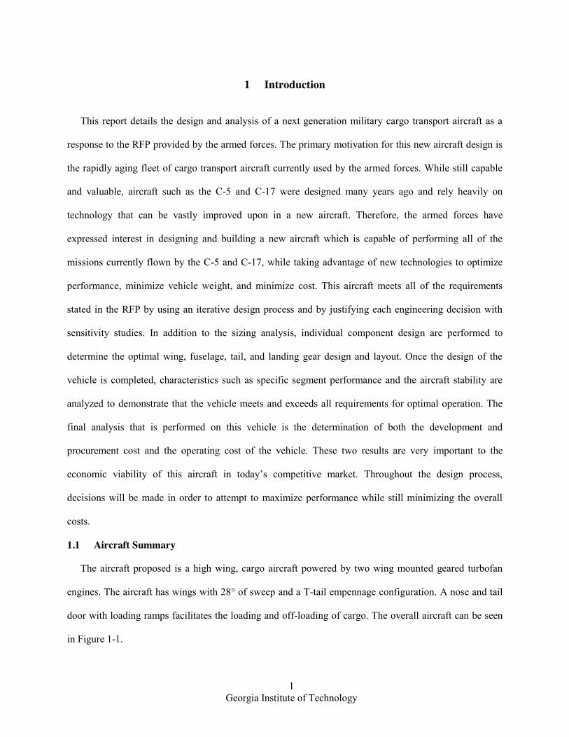
This report details the design and analysis of a next generation military cargo transport aircraft as a
response to the RFP provided by the armed forces. The primary motivation for this new aircraft design is
the rapidly aging fleet of cargo transport aircraft currently used by the armed forces. While still capable
and valuable, aircraft such as the C-5 and C-17 were designed many years ago and rely heavily on
technology that can be vastly improved upon in a new aircraft. Therefore, the armed forces have
expressed interest in designing and building a new aircraft which is capable of performing all of the
missions currently flown by the C-5 and C-17, while taking advantage of new technologies to optimize
performance, minimize vehicle weight, and minimize cost. This aircraft meets all of the requirements
stated in the RFP by using an iterative design process and by justifying each engineering decision with
sensitivity studies. In addition to the sizing analysis, individual component design are performed to
determine the optimal wing, fuselage, tail, and landing gear design and layout. Once the design of the
vehicle is completed, characteristics such as specific segment performance and the aircraft stability are
analyzed to demonstrate that the vehicle meets and exceeds all requirements for optimal operation. The
final analysis that is performed on this vehicle is the determination of both the development and
procurement cost and the operating cost of the vehicle. These two results are very important to the
economic viability of this aircraft in today’s competitive market. Throughout the design process,
decisions will be made in order to attempt to maximize performance while still minimizing the overall
costs.
1.1 Aircraft Summary
The aircraft proposed is a high wing, cargo aircraft powered by two wing mounted geared turbofan
engines. The aircraft has wings with 28° of sweep and a T-tail empennage configuration. A nose and tail
door with loading ramps facilitates the loading and off-loading of cargo. The overall aircraft can be seen
in Figure 1-1.

2 Georgia Institute of Technology
Figure 1-1. Right isometric of painted aircraft.
3 Georgia Institute of Technology
2 Configuration Selection
2.1 Figures of Merit Analysis
The first step in beginning the design process for this aircraft was to determine a desired configuration
of the major components. In order to determine optimal configuration for this aircraft, a figures of merit
analysis was used to weight each of the configurations based on performance and design characteristics.
These characteristics were chosen based on the requirements and guidelines as stated in the RFP. The
chosen figures of merit for this analysis included structural weight, cargo space, maintenance,
manufacturability, logistics and stability and controllability. Existing military aircraft such as the C-5 and
the C-17 were examined in order to determine realistic configuration options. In addition, futuristic and
experimental aircraft designs were examined. For each of the figures of merit, a weighting ranging from 1
to 5 was assigned based on the relative importance of that figure of merit on the overall design. In the
same way, a score was assigned for each configuration ranging from 1 to 5 based on how well it achieved
the figure of merit. The overall score of a configuration is the sum of the products between the weight of
the figure of merit and the score of that particular configuration.
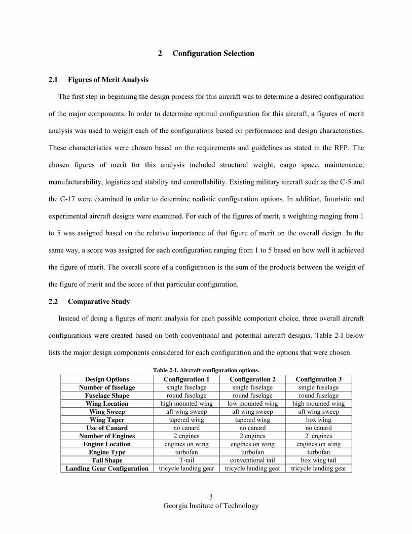
2.2 Comparative Study
Instead of doing a figures of merit analysis for each possible component choice, three overall aircraft
configurations were created based on both conventional and potential aircraft designs. Table 2-I below
lists the major design components considered for each configuration and the options that were chosen.
Table 2-I. Aircraft configuration options. Design Options Configuration 1 Configuration 2 Configuration 3
Number of fuselage single fuselage single fuselage single fuselage Fuselage Shape round fuselage round fuselage round fuselage Wing Location high mounted wing low mounted wing high mounted wing
Wing Sweep aft wing sweep aft wing sweep aft wing sweep Wing Taper tapered wing tapered wing box wing
Use of Canard no canard no canard no canard Number of Engines 2 engines 2 engines 2 engines
Engine Location engines on wing engines on wing engines on wing Engine Type turbofan turbofan turbofan Tail Shape T-tail conventional tail box wing tail
Landing Gear Configuration tricycle landing gear tricycle landing gear tricycle landing gear

4 Georgia Institute of Technology
A model for each of these configurations was created to provide a visual representation of what each
configuration might look like. These models are shown in Figure 2-1, Figure 2-2, and Figure 2-3 below.
Figure 2-1. Configuration one model.
Figure 2-2: Configuration two model.
Figure 2-3: Configuration three model.

5 Georgia Institute of Technology
Each of these configurations was scored using the figures of merit analysis. The result of this analysis
is shown below in Table 2-II.
Table 2-II. Figures of merit analysis. FOM Weighting Configuration 1 Configuration 2 Configuration 3
Structural Weight 4 4 5 3 Cargo Space 5 5 5 5
Maintenance (cost) 3 4 4 3 Manufacturability (cost) 3 3 3 1
Logistics 4 5 3 2 Stability and Control 2 5 4 4
Total 21 92 86 65
2.3 Chosen Preliminary Configuration
The result of the figure of merit analysis was the selection of configuration one as the design
configuration. This aircraft has a single, round fuselage, a high mounted, aft swept, tapered wing with no
canard, two turbofan engines mounted below the wings, a t-tail, and tricycle landing gear. This aircraft is
highly conventional and does not deviate greatly from current aircraft configurations. Therefore, the
improvements in the newly designed aircraft over any aircraft currently in service will come from the
technologies used as a part of the design.
3 Mission Specification and Decisions
3.1 Mission Segments
In order to analyze the vehicle to determine a takeoff weight, a mission for the vehicle must be
designed. The basic segments of the mission are start, taxi, takeoff, climb, cruise, descent, and landing. In
addition, there is a 200 nautical mile reserve that is assumed to be performed at the end of the cruise. To
optimize the performance of the vehicle throughout the mission, each of the segments has been divided
into smaller segments to determine the optimal mission parameters at each segment such as altitude, flight
speed, and rate of climb. The cruise segment has been divided into three smaller step cruise segments for
improved performance, cruise at higher altitudes becomes more efficient as the aircraft becomes lighter

6 Georgia Institute of Technology
due to burned fuel. The climb and descent segments were divided into smaller segments based on trade
study analysis. These trade studies will be demonstrated later in the report as a component of the weight
sizing process.
3.1.1 Climb
The climb segment of the mission profile for this aircraft contains an initial climb up to 10,000 feet
based on the maximum speed of 250 kts below 10,000 feet. The climb from 10,000 feet to the chosen
initial cruise altitude is divided into four climbs at varying rates of climb and forward velocities. This is
done to optimize the overall fuel efficiency of the vehicle to reduce the fuel weight required for the
mission. The climb performance parameters for each segment are shown in Table 3-I. The rate of climb
for the final climb segment is calculated such that the requirement that the total time to climb to cruise
altitude with a 205,000 lb payload be no more than 20 minutes is met.
Table 3-I. Climb Performance Mission Segment Initial Altitude (ft) Final Altitude (ft) Rate of Climb (ft/min) Mach Number
Climb 1 0 10,000 2,250 0.38 Climb 2a 10,000 15,625 2,000 0.50 Climb 2b 15,625 21,250 1,500 0.50 Climb 2c 26,875 26,875 1,400 0.60 Climb 2d 32,500 32,500 1,131 0.60
3.1.2 Cruise
The cruise segment of the mission for this aircraft is divided into three step cruise segments. This is
the maximum number of step cruise segments allowed as described by the RFP. The step cruise is optimal
because as the aircraft burns fuel and becomes lighter, the aircraft can improve fuel efficiency by flying at
a higher altitude. For each cruise segment, the altitude and speed are optimized to maximize the specific
range of the vehicle. The cruise performance parameters for each step cruise segment are shown below in
Table 3-II.
Table 3-II. Cruise Performance Mission Segment Altitude
(ft) Mach Number
Cruise 1 32,500 0.65 Cruise 2 39,000 0.70

7 Georgia Institute of Technology
Cruise 3 40,000 0.70
3.1.3 Takeoff
One of the required performance metrics for this aircraft is that the balanced field length be no greater
than 9,000 ft. This requirement must apply at all potential takeoff conditions including the hot day and
high altitude requirements. In order to meet these requirements, a constraint sizing analysis was
performed to determine the appropriate engine thrust. For the three required takeoff conditions, the
important constraint inputs that vary for each condition as well as the resulting thrust to weight ratio at sea
level takeoff are shown below in Table 3-III.
Table 3-III. Takeoff Performance. Takeoff Segment CL,clean CD ρ (slug/ft3) T/W
ISA at MSL 1.10 0.071 0.002378 0.150 ISA + 30°C 1.21 0.080 0.002153 0.178
ISA + 10°C at MSL + 10,000 ft 1.54 0.112 0.001692 0.249
The thrust to weight design point for the overall aircraft was chosen to be 0.25 due to the hot day and high
altitude takeoff requirement. As these two segments required the largest thrust to weight required.
3.1.4 Landing
Similarly to the takeoff, the landing requirement was also analyzed at three required conditions. The landing is of
great importance due to it setting a maximum limit for the wing loading at takeoff for the vehicle. For the three
required landing conditions, the important constraint inputs that vary for each condition as well as the resulting
maximum wing loading values at takeoff are shown below in Table 3-IV.
Table 3-IV. Landing Performance Landing Segment ρ
(slug/ft3) W/S (lb/ft2)
ISA at MSL 0.002378 173 ISA + 30°C 0.002153 156
ISA + 10°C at MSL + 10,000 ft 0.001692 123
Once again, the design point is driven by the hot day at high altitude requirement. This requirement resulted in a
wing loading at takeoff for the aircraft that can be no greater than 123 lb/ft2.

8 Georgia Institute of Technology
3.1.5 Range
The total range of the aircraft was determined as a sum of the horizontal distance travelled for each mission
segment. For the cruise segments, the design range of 6,300 nm was split equally into three 2,100 nm segments. The
reserve range of 200 nm is added at the end of the final cruise segment. For the climb and descent segments, the
horizontal distance travelled was calculated according to Equation 1.
(1)
The altitude change, rate of climb, and Mach number are selected using sensitivity studies to determine optimal
values based on the specific range and thrust to weight ratio. The speed of sound is calculated as an average value
over the range of altitudes travelled during the climb or descent segment. Using this approach, the overall range of
the vehicle for the designed mission payload of 205,000 lb. is calculated to be 6,805 nm. This range encompasses
common military transport routes between Europe and combat zones in the Middle East as well as flights from the
continental U.S. to either Europe or Asia.
3.2 Mission Profile
Once all the performance characteristics were determined for each segment of the mission, the
finalized mission profile was created. The final result of the mission profile optimization was a climb up
to 10,000 feet followed by a four part step climb up to the initial cruise altitude of 32,500 feet. This initial
cruise was the first of the three part step cruise. The second and third segments of the step cruise took
place at 39,000 and 40,000 feet respectively. Finally, the descent was broken into two segments above
10,000 feet and one segment below. The finalized mission profile can be seen below in Figure 3-1.

9 Georgia Institute of Technology
Figure 3-1. Mission profile diagram.
3.3 Payload Range Charts
After performing the weight and constraint sizing to determine the takeoff weight and empty weight of the
vehicle at the design point, it is also useful to know the range of the aircraft when carrying varying payload weights.
By determining the range at each of these payload weights, the overall payload range chart for the aircraft can be
created. For this aircraft, the payload range chart is shown below in Figure 3-2.
Figure 3-2. Payload range chart.
Design Point
Maximum Payload
Ferry Range
120,00 lb payload
Max Fuel Weight
0
50,000
100,000
150,000
200,000
250,000
300,000
350,000
0 2000 4000 6000 8000 10000 12000 14000 16000 18000
Payl
oad
Wei
ght (
lb)
Range (nm)

10 Georgia Institute of Technology
The points used to generate this payload range chart were a maximum payload of 300,000 lb., the design
point of 205,000 lb., the performance requirement of 120,000 lb., the max fuel weight of 368,585 lb. with a payload
of 50,950 lb., and the ferry range calculated at the max fuel weight of 368,585 lb. with no payload. For this aircraft,
the original design payload of 120,000 lb. was increased to a design payload of 205,000 lb. The reason for this
increase in payload was twofold. The initial design with a payload of 120,000 lb. was unable to accommodate the
maximum payload requirement of 300,000 lb. In addition, two of the required payload cargo, the M104 Wolverine
and the M1A Abrams tank exceed the weight of the initial design payload of 120,000 lb. Therefore, in order to
achieve a maximum payload of at least 300,000 lb. and be able to carry at least one Wolverine and one Abrams at
the design payload weight, the design payload weight was increased from 120,000 lb. to 205,000 lb. This payload
weight increase also results in an increased range of the vehicle. This increased range is optimal because it makes
nonstop flights from North America to Europe and Europe to the Middle East possible at higher, more useful
payload weights.
3.4 Stakeholder Analysis
An important aspect of aircraft design considered, was the stakeholder’s that are impacted by the final
design. It identifies the important shareholders within the process that will drive the design and usability
of the aircraft. Some of the important stakeholders for this project include the pilots, government,
manufacturers, suppliers, cargo master and light personnel. Using the stakeholder analysis chart, the
entities listed above can be placed on the chart dividing them between four different criteria. These
include “keep satisfied”, “manage closely”, “monitor” and “keep informed.” Each of these criteria have
varying degrees of power and interest within the project. Based off the interest of each relevant party,
their place on the chart was created. Their placement on the chart is based off each other’s relations. Table
3-V and Figure 3-3 below showcase both the interests of each stakeholder and their place on the
stakeholder analysis chart.

11 Georgia Institute of Technology
Table 3-V: Stakeholder interests. Stakeholder Interest
Pilots Aircraft capabilities, flight stability and control, use of advanced technologies, safety features and performance.
Government Initial cost of aircrafts, delivery on RFP requirements, safety and performance of aircraft, reduced maintenance cost.
Manufacturers/Suppliers
Complexity of parts, use of advanced materials & technologies, complexity of design.
Cargo Master Loading capabilities of aircraft, reduced turnover time, aircraft internal configuration.
Flight Personnel Use of aircraft technologies, ergonomics of internal cargo space.
Figure 3-3: Stakeholder analysis chart.
4 Advanced Technology
4.1 Geared Turbofan
For this aircraft, the engine will be augmented with a geared turbofan system. Currently there are a
handful of geared turbofans in production. The most well-known is the Pratt & Whitney PW1000G. The

12 Georgia Institute of Technology
engine is already in production; its current use is on the A320neo (Pratt and Whiteney). The A320neo is
expected to go into service in October 2015. There are multiple versions of the PW1000G for a handful of
aircraft.
The PW1000G is expected to have a fuel consumption decrease of 15% compared to current engines
in the same category. By mid-2020’s, P&W expects to produce engines that offer a 20-30% increase in
efficiency compared to current technologies. The performance increase is not only produced by the gear
box but by a handful of advancements in engine technologies.
The current geared turbofans do not produce enough thrust for comparable aircraft. The PW1428
produces a maximum thrust of 31,000lbf; the C-17 uses four PW F117 turbofans which each produce
40,440 lbf. Our aircraft is to enter service in 2030; by then it is reasonable to assume that geared turbofan
engines producing around 94,000 lbf would be possible. The expected fuel consumption decrease would
be around 20% compared to current technologies.
Currently, the baseline model chosen is the GE90-94B turbofan engine. It was chosen due to the thrust
requirement that the constraint sizing process revealed. The baseline engine has a weight of
approximately 17,000 lb. Its length is 287 inches and has a diameter of 134 inches. The engine is capable
of producing 93,000 lb of thrust at sea level which matches the requirements taken about earlier. With the
use of the geared turbofan, the weight can be further reduced and also improve the TSFC of the baseline
engine.
4.2 Natural Laminar Flow Airfoil
Through the use of composite materials, certain tolerances and levels of surface smoothness can be
achieved in order for natural laminar flow airfoils to be used successfully. Laminar flow over the surface
of the wing provides large performance improvements that can help the efficiency of the overall aircraft.
It can reduce drag produced overall by the wing versus a wing using a regular airfoil. Furthermore,
increased laminar flow over the wing also provides greater lift. Laminar flow airfoils are designed to have
favorable pressure gradients in order to allow the boundary layer to laminar. The usual definition of a
laminar flow airfoil is that the favorable pressure gradient ends somewhere between 30 and 75% of chord.
13 Georgia Institute of Technology
The idea of laminar flow airfoils is certainly not new to the aerospace field. The P-51 Mustang was the
first aircraft designed to use laminar flow airfoils. It could not benefit from the use of the airfoil due to the
surface unevenness of the wing. Currently, Aerion is proposing the use of laminar flow airfoils in
supersonic business jets in order to improve performance of its design.
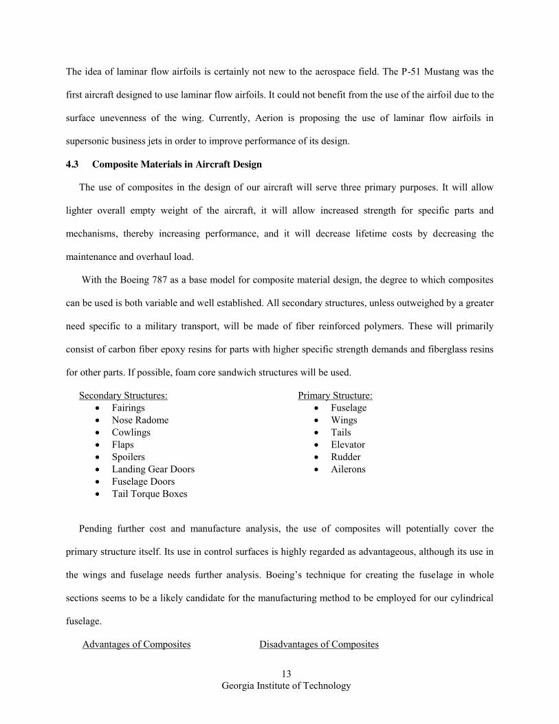
4.3 Composite Materials in Aircraft Design
The use of composites in the design of our aircraft will serve three primary purposes. It will allow
lighter overall empty weight of the aircraft, it will allow increased strength for specific parts and
mechanisms, thereby increasing performance, and it will decrease lifetime costs by decreasing the
maintenance and overhaul load.
With the Boeing 787 as a base model for composite material design, the degree to which composites
can be used is both variable and well established. All secondary structures, unless outweighed by a greater
need specific to a military transport, will be made of fiber reinforced polymers. These will primarily
consist of carbon fiber epoxy resins for parts with higher specific strength demands and fiberglass resins
for other parts. If possible, foam core sandwich structures will be used.
Secondary Structures: x Fairings x Nose Radome x Cowlings x Flaps x Spoilers x Landing Gear Doors x Fuselage Doors x Tail Torque Boxes
Primary Structure: x Fuselage x Wings x Tails x Elevator x Rudder x Ailerons
Pending further cost and manufacture analysis, the use of composites will potentially cover the
primary structure itself. Its use in control surfaces is highly regarded as advantageous, although its use in
the wings and fuselage needs further analysis. Boeing’s technique for creating the fuselage in whole
sections seems to be a likely candidate for the manufacturing method to be employed for our cylindrical
fuselage.
Advantages of Composites Disadvantages of Composites

14 Georgia Institute of Technology
x Tailor capability (directional properties) x Lower density (lower weight) x High strength and stiffness x Fatigue performance x Corrosion resistance x Wear resistance x Low heat transmission x Good electrical insulation x Low sound transmission
x Environmental degradation of resin dominated properties
x Notch sensitivity x Impact damage x Poor through thickness properties x Variability x Properties not established until manufactured x Limited availability of design data x Reinforcement incorrectly located x Lack of codes and standards
4.4 Spiroid Winglet
Up to 40% of total drag at cruise conditions and 80-90% of total drag in take-off configuration can be
attributed to lift-induced drag for the typical transport aircraft (Guerrero, Maestro, & Bottaro, 2012).
Since drag is balanced by the thrust of the aircraft engine in cruise conditions, reducing drag leads to fuel
savings, lower operating costs, or improved performance or range. Furthermore, the drag, wake, and
vortex characteristics for an aircraft during landing and take-off operations affects climb-rates and other
landing and take-off performance measures as well air traffic flow management at airports due to vortex
turbulence dissipation. Some research has shown that one way of reducing lift-induced drag is by using
wingtip devices, such as the blended winglet, wing grid, or spiroid wingtip, which is of particular interest.
An extensive wind tunnel study examined the effects of four winglet shapes on the vortex behind the
wing, static surface pressure over the wing, and wake of a swept wing at varying angles of attack
compared to a configuration without winglets, the bare wing (Nazarinia, Soltani, & Ghorbanian, 2006).
This study found that winglets change the flowfield over the wing significantly. The total pressure loss in
the wake of the model is significantly less when a winglet is included compared to the bare wing. Two
types of spiroid winglets were tested, a forward spiroid winglet and an aft spiroid winglet. It was found
that the forward spiroid winglet seems to be more suitable for the cruise flight phase (when angle of
attack is low), while the aft spiroid winglet is more suitable for the climb phase, with higher angle of
attack.
A spiroid wingtip was tested by adapting it to a clean wing, or bare wing, and performance of the wing
with the spiroid winglet relative to the clean wing was studied quantitatively and qualitatively. With any

15 Georgia Institute of Technology
winglet, there is a trade-off between the benefits realized from the reduction in lift-induced drag and the
additional parasitic drag through the increased wetted surface, causing with additional friction and
interference drag. The point where the marginal benefits and marginal cost of the winglet balance is
called the crossover point. Additionally, the study finds that the spiroid winglet is able to greatly reduce
the intensity of wingtip vortices, which dissipate quickly, compared to a clean wing. This can have
benefits in terms of air traffic flow management at airports. From the perspective of the aircraft operator,
the benefits of the spiroid winglet enumerated could mean increased range, improved take-off
performance, increased operating altitudes, improved roll rates, shorter time-to-climb rates, less take-off
noise, increased cruise speeds, reduced engine emissions, and improved safety during take-off and
landing due to vortex turbulence reduction.
4.5 Weight Sizing Technology Factors
The implementation of the technologies takes several forms in the weight sizing process. There is a
reduction to the empty weight of the aircraft in the form of a technology factor, η. This is calculated to be
0.851. The engine efficiency improvement translated into a reduction in the TSFC of the aircraft for each
mission segment, a result of increased rotational efficiency. A reduction in the skin friction coefficient is
realized with the inclusion of a natural laminar flow airfoil in the wing. This is a result of decreased
turbulent flow over the wing. The use of spiroid winglets decreases wingtip vortices, resulting in an
Oswald’s efficiency increase. The complete quantitative set of improvements made to the aircraft from
technology implementation can be seen in Table 4-I. A waterfall chart showing the takeoff weight
decrease of the aircraft after each technology implementation is shown in Figure 4-1.
Table 4-I. Technology impact table. Technology Description TRL Improvement Factor
Composites Advanced lighter materials 9 20% weight reduction
Geared Turbofan Optimizes rotational efficiency 8
15% weight reduction,
12% TSFC reduction Natural Laminar Flow
Airfoil Decreases turbulent
flow over wing 6 7% skin friction coefficient reduction
Spiroid Winglets Decreases wingtip 8 6% Oswald’s efficiency

16 Georgia Institute of Technology
vortices increase
Figure 4-1. Waterfall chart showcasing reductions in takeoff weight with the additions of technology.
5 Weight Sizing
5.1 Weight Regression
The first step in the weight sizing process is to calculate an empty weight for the vehicle based on a
linear regression formed from weight data of similar vehicles. The vehicles used for this regression were
composed of other military transport aircraft as well as large passenger jet aircraft. The chosen vehicles
for this regression are shown below in Table 5-I.
Table 5-I. Weight regression aircraft. Vehicle Vehicle 1 Boeing YC-14 9 Boeing 777-F 2 Boeing KC-135A 10 Xian Y-20 3 McDD C-17 11 Antonov An-124 4 McDD KC-10A 12 Ilyushin Il-76 5 Lockheed C-141B 13 Boeing 747-100B 6 Lockheed C-5A 14 Airbus 300B4 7 Tupolev Tu-16 15 Boeing 787 8 BAE Nimrod Mk2
For each of these vehicles, the empty weight of the vehicle is graphed against the take-off weight on a
logarithmic scale. The resulting linear regression creates a linear relationship between the empty and

17 Georgia Institute of Technology
takeoff weight. This relationship is used with a guessed takeoff weight to generate one estimate of the
empty weight of the vehicle. The linear regression is shown below in Table 5-I.
Figure 5-1. Weight regression plot.
5.2 Takeoff Weight Convergence
In addition to the historical weight regression, another method is used to produce an estimate for the
empty weight of the vehicle. This method uses a Microsoft Excel spreadsheet to compute mission fuel
fragments for each segment of the flight. The purpose of creating these mission fuel fragments is to
determine an overall fuel weight needed for the mission. This fuel weight can then be subtracted from the
takeoff weight along with the chosen payload weight, and the assumed crew weight to determine an
empty weight for the vehicle. This is shown in Equation 2.
(2)
The primary basis for calculating the fuel fraction for each mission segment is the Breguet range
equation. This relationship is shown below in Equation 3.
(3)

18 Georgia Institute of Technology
In this equation, the range for the mission segment is chosen, the speed is known based on the chosen
altitude and Mach number, the thrust specific fuel consumption is calculated using an engine deck for a
chosen baseline model, and the lift to drag ratio is calculated based on a drag polar convergence which is
described in the next section.
5.3 Drag Polar Convergence
One input to the Breguet range equation is the lift to drag ratio at the chosen segment of flight. To
compute this value, a drag polar analysis is necessary. Initially, a lift to drag ratio is assumed in order to
perform the weight sizing calculations. However, to achieve a finalized takeoff and empty weight value,
the lift to drag ratio must be converged using the drag polar analysis. To calculate this lift to drag ratio,
the coefficient of lift and the coefficient of drag at each segment of flight are calculated. The coefficient
of lift is calculated according to Equation 4.
(4)
The weight of the vehicle is taken from the weight sizing analysis at the appropriate segment of flight,
the density of the air is known from the chosen altitude, the airspeed is known from the chosen altitude
and Mach number, and the wing area is calculated from the guessed takeoff weight and the assumed wing
loading of the vehicle. The coefficient of drag is calculated according to Equation 5.
(5)
The aspect ratio and baseline Oswald’s efficiency factor of the vehicle are chosen based on
similar aircraft and the zero lift drag is calculated based on an assumed skin friction coefficient, the wing
area, and the wetted area as described in Roskam’s design books.
5.4 Sensitivity Studies
To determine the optimal parameters at each segment of the mission, sensitivity studies were
performed for each important performance characteristic. For each sensitivity study, the chosen parameter
is varied and the specific range of the vehicle over the mission segment is calculated. The optimal value

19 Georgia Institute of Technology
for each parameter is the one which maximizes the specific range over that segment. For example, to
determine the optimal climb rate for each portion of the initial climb, the climb rate for the first climb
segment is varied and the specific range is calculated. The resulting graph is shown below in Figure 5-2.
Figure 5-2. Climb 1 rate of climb sensitivity study.
In this particular example, the thrust to weight ratio is shown on the secondary vertical axis. This is
shown to demonstrate the strong effect that the climb rate has on the resulting thrust to weight ratio of the
aircraft. The calculation of this ratio is done in the constraint sizing process. For this example, the
increase in specific range was negligible for the various rates of climb so the initial climb segment rate of
climb was chosen to be 2,250 feet per minute to minimize the thrust to weight ratio. This process is
repeated for all other climb and descent segments.
Because the cruise was broken into three separate step cruise segments, the altitude of these step
cruises is of great importance. To determine the optimal altitude for each step cruise segment, the specific
range is graphed against the altitude. For the second step cruise segment, the resulting plot is shown
below in Figure 5-3.
0.24
0.245
0.25
0.255
0.26
0.265
0.27
0.275
0.28
0.285
0.027885
0.02789
0.027895
0.0279
0.027905
0.02791
0.027915
0.02792
0.027925
0.02793
0.027935
0.02794
750 1250 1750 2250 2750
Thur
st to
Wei
ght R
atio
Spec
ific
Rang
e (n
m/l
b)
Climb 1 Rate (ft/min)
Specific Range
T/W

20 Georgia Institute of Technology
Figure 5-3. Cruise 2 altitude sensitivity study.
For this cruise segment, the optimal specific range is obtained at an altitude of 39,000 feet. Therefore,
that altitude is chosen for this cruise segment. This process is repeated for all other mission flight
segments.
The final major parameter that is important to all segments of flight is the Mach number at that
segment. This Mach number is optimized at every segment of flight in order to produce the most efficient
vehicle possible. Similarly to the altitude sensitivity study, the specific range for each Mach number
studied is plotted against the corresponding Mach number. An example of this for the second step cruise
segment is shown below in Figure 5-4.
0.039
0.0392
0.0394
0.0396
0.0398
0.04
0.0402
32000 34000 36000 38000 40000 42000 44000 46000
Spec
ific
Rang
e (n
m/l
b)
Cruise 2 Altitude (ft)

21 Georgia Institute of Technology
Figure 5-4. Cruise 2 Mach number sensitivity study.
The optimal specific range for the second step cruise segment occurs at a cruise Mach number of 0.7.
Therefore, this Mach number is used for all calculations at this segment of flight. This process is repeated
for every segment of flight to determine optimal Mach numbers across the entire mission profile.
6 Constraint Sizing
6.1 Constraint Sizing
The final step in the preliminary sizing of the vehicle is the constraint sizing analysis. The purpose of
this analysis is to determine the sea level thrust to weight ratio required to fly each mission segment based
on a designated wing loading at takeoff. The basis for this analysis is the energy-based constraint
equation. This relationship is shown below in Equation 6.
[ ( )
( )
(
)]
(6)
0.0375
0.038
0.0385
0.039
0.0395
0.04
0.55 0.6 0.65 0.7 0.75 0.8 0.85
Spec
ific
Rang
e (n
m/l
b)
Cruise 2 Mach Number

22 Georgia Institute of Technology
This equation can be simplified for each segment of flight based on various assumptions such as
constant speed climb and constant altitude cruise. For each segment of the mission, this constraint
equation was applied to determine the necessary sea level thrust to weight ratio at takeoff to perform the
mission segment. The plot of all of the various mission segments is shown in Figure 6-1.
Figure 6-1. Constraint sizing plot.
The design point for this aircraft was chosen to be the point which met all of the thrust to weight
requirements while maximizing wing loading and minimizing the sea level thrust to weight ratio. For this
aircraft, that initial design point was placed at a thrust to weight ratio of 0.23 and a wing loading of 172
lb/ft2.
6.2 Additional Constraints
While the initially chosen design point is sufficient to perform all normal mission segments for this
aircraft, it is not sufficient to perform the additional takeoff, climb, and landing requirements at +30°C
above ISA as well as +10°C above ISA at 10,000 feet above MSL. Therefore, an additional constraint

23 Georgia Institute of Technology
analysis is performed at these conditions to determine a new, finalized design point. The result of this
additional analysis is shown below in Figure 6-2.
Figure 6-2. Additional constraint sizing.
For this aircraft, the finalized design point is placed at a sea level takeoff thrust to weight ratio of
0.25 and a wing loading at takeoff of 122 lb/ft2. This design point minimizes the trust to weight at sea
level takeoff and maximizes the wing loading at takeoff while meeting all mission segment requirements
for both normal and hot days.
6.3 Preliminary Sizing Results
Using the initial design point wing loading produced by the constraint sizing analysis, the weight
sizing and constraint sizing processes are then iterated to produce a finalized maximum takeoff weight,
empty weight, wing area, and sea level takeoff thrust required for the aircraft. These are the most
important results of the preliminary sizing process and will be used to drive the detailed design and
0.1
0.15
0.2
0.25
0.3
0.35
0.4
50 70 90 110 130 150 170 190
Thru
st to
Wei
ght a
t Sea
Lev
el T
akeo
ff (~
)
Wing Loading at Takeoff (lb/ft2)
Climb 2d
Landing
Takeoff + 30 °C
Climb 1 + 30 °C
Climb 2a + 30 °C
Climb 2b + 30 °C
Climb 2c + 30 °C
Climb 2d + 30 °C
Landing + 30 °C
Takeoff + 10 °C at 10000 ft
Landing + 10 °C at 10000 ft
Previous Design Point
New Design Point

24 Georgia Institute of Technology
specific component design. For this aircraft design, the results of the weight and constraint sizing analyses
are shown below in Table 6-I.
Table 6-I. Preliminary sizing results. Parameter Variable Units Value
Empty Weight WE lb 262,408 Fuel Weight WFuel lb 214,535
Payload Weight WPayload lb 205,000 Crew Weight WCrew lb 1,400
Maximum Takeoff Weight WTO lb 683,343 Wing Loading at Takeoff (W/S)TO lb/ft2 122
Wing Area Swing ft2 5,601 Thrust to Weight at Sea Level
Takeoff (T/W)SL ~ 0.25
Thrust Required Trequired lbf 170,836
7 Performance
7.1 Takeoff
A takeoff analysis was performed by calculating the balanced field length (BFL) at two engine
conditions. Since our aircraft only has two engines, these conditions are “all engines operative” or “one
engine inoperative.” The BFL was calculated by Equation 7 (Roskam & Lan, Airplane Aerodynamics and
Performance, 2003), where Δγ2 or change in climb gradient is calculated by Equation 8, WTO/S is 122 psf
from constraint sizing, ρ is the density at takeoff, g is gravitational acceleration, CL,2 is the lift coefficient
at V2 (or CL,2 ≈ 0.694CL,max,TO), hscreen is 35 ft as specified by the FAR 25 rules, T/WTO is the thrust loading
at takeoff, μ’ is defined as Equation 9, ΔSTO is the takeoff distance increment equal to 655 ft, and ζ is the
density ratio of the atmosphere. CL,max,TO is chosen as 2.37 from high-lift device sizing, γ2,min is 2.4% for a
two-engine aircraft, and γ2 values are listed in the climb analysis.
(
)( ⁄
)(
⁄ )
√
(7)
(8)
(9)

25 Georgia Institute of Technology
The resulting BFL and the intermediate values are shown in Table 7-I. It can be seen that the takeoff
can be performed in all listed conditions since their BFL is below the maximum takeoff length of 9,000 ft.
The maximum temperature offset in which the aircraft can takeoff with only one engine is 73°C while the
maximum altitude is 10,050 ft.
Table 7-I. Balanced field length and intermediate values for varying engine and takeoff conditions. Δγ2 (%) T/WTO ρ
(slugs/ft3) σ Engine
condition Temperature
offset (°C) Altitude
(ft) BFL (ft)
0.0966 0.238 0.00205 0.8617 all op 0 SL 7,130 0.0809 0.250 0.00169 0.7119 all op 10 10,000 8,443 0.0890 0.238 0.00185 0.7778 all op 30 SL 7,943 0.0145 0.238 0.00205 0.8617 1 inop 0 SL 8,304 0.0067 0.250 0.00169 0.7119 1 inop 10 10,000 8,985 0.0107 0.238 0.00215 0.9070 1 inop 30 SL 7,990 0.0107 0.238 0.00190 0.7990 1 inop 73 SL 8,990 0.0067 0.250 0.00169 0.7119 1 inop 10 10,050 8,999
7.2 Climb
A climb analysis was performed by calculating the climb gradient, γ2 at the aforementioned engine and
takeoff conditions by using Equation 10, where T or thrust varies for each engine/takeoff condition, WTO
is 669,676 lb from weight sizing, and L/D is 22.98 from drag polar calculations. The resulting climb
gradient, rate of climb, and some intermediate values are listed in Table 7-II.
All calculated climb gradients are greater than the minimum required climb gradient of 2.4%. It should
be noted that the rate of climb listed in the below table is the maximum capability only from the engines
and therefore, these values were not necessarily selected for our design mission.
(10)
Table 7-II. Climb gradient, rate of climb, and intermediate values for varying engine and takeoff conditions. Thrust (lbf) γ2 (%) Rate of climb
(fpm) Engine
condition Temperature
offset (°C) Altitude (ft)
109,922 12.06 3,015 all op 0 SL 99,393 10.49 2,622 all op 10 10,000
104,812 11.30 2,825 all op 30 SL 54,961 3.85 964 1 inop 0 SL 49,696 3.07 767 1 inop 10 10,000 52,406 3.47 868 1 inop 30 SL
26 Georgia Institute of Technology
7.3 V-n Diagram
The V-n diagram was created for the proposed aircraft in order to ensure that the mission does not
exceed the flight envelope of the design. The V-n diagram for this aircraft was created using the standard
techniques and processes. The maximum load factor was assumed to be 2.5 and the minimum was
assumed to be -1.5 based on flight expectations and load factors in similar, previously existing aircraft.
The design dive speed was set to 1.2 times the cruise speed. The maximum load factor, nmax , was found
using Equation 11 below.
(11)
The load factor was solved for repeatedly as the Ve was increased from zero to the design dive speed.
This linear relationship was then cutoff as it reached the maximum design load. The line was also
truncated to only have load factors with magnitudes above one. The same equation and method was used
to find the load factor that decreased until it reached the minimum load. To produce these results, the
CL,max of the wing was substituted with the CL,min. Lastly, gust lines were created to represent both the
maximum positive and negative gust up during both the cruise and dive segments of flight. These gust
lines were created using the Equation 12 shown below.
(12)
The gust speed, U, was taken from the FAA requirements for large aircraft. The finalized V-n diagram
is plotted on Figure 7-1 below.

27 Georgia Institute of Technology
Figure 7-1: V-n Diagram
8 Fuselage Sizing
8.1 Payload Considerations
Based on the RFP, it is required to carry at least one Wolverine Assault Bridge System and 44 463L
Master Pallets or optimal arrangements for other payloads. The 463L Master Pallets have no definite
height since it is a specific plate that is designed for holding cargos, and the height depends on the weight
of cargo on each plate. The pallet has a height of 0.1875 ft and a tare weight of 290 lb with maximum
capacity of 10,000 lb (Globid Inc., 2014). In the mission specification, the payload weight of each 463L
Master Pallet is chosen to be 6,000 lb and the corresponding volume of 6000 lb weight is estimated to be
6 ft. The following Table 8-I presents the maximum dimensions, weight and volume of each cargo
component (Kable, 2010) (Military Analysis Network, 2000) (Prado, 2008) (Bradley M2A3 AIFV, 2015).

28 Georgia Institute of Technology
Table 8-I. Payload characteristics.
Payload Dimension (ft) Weight (lb) Volume (ft3) Length Width Height 463 L Master Pallets 7.30 9.00 6.00 6000.00 394.20
Wolverine Bridge 43.96 13.12 15.00 153882.66 8651.33 AH-64 Apaches 49.08 17.17 15.25 23000.00 12851.23 M1A1 Abrams 32.25 12.00 9.47 126000.00 3664.89 M2A3 Bradley 21.50 10.76 11.09 72000.77 2565.56
8.2 Internal Cargo Fitting
Based on cargo arrangements of master pallets on previous transport aircrafts, the pallets are designed
with two master pallets in a row generally. The same arrangement of the master pallets is applied in the
process of determining the dimensions of the internal cargo space. Based on Figure 3.37 and 3.38 of
Roskam Airplane Design Part III, the spacing between the side of pallets and the internal frame of the
aircraft were 2 to 5 inches, and the spacing between pallets were not specified (Roskam J. , Airplane
Design Part III: Layout Desig of Cockpit, Fuselage, Wing and Empennage: Cutaways and Inboard
Profiles, 2002). As far as the loading operation on this aircraft is concerned, extra spacing on the sides
and between pallets are intentionally designed for loading personnel to pass through and check the
loading process and ensure the cargo are loaded and fixed correctly. The cargo space is designed to carry
one Wolverine assault bridge system due to the weight of one Wolverine is greater than half of the
maximum payload requirement. Besides the Wolverine bridge system, other cargo payloads are designed
to be arranged in a row in longitudinal direction. The following Table 8-II summarizes the minimum
cargo space dimensions with required payloads while the total payload weight does not exceeding the
maximum payload weight of 300,000 lb.
Table 8-II. Minimum cargo space dimension calculation.
Payload Quantity Minimum Cargo Space Dimension (ft) Total
Payload Weight (ft)
Length (Longitudinal)
Width (Lateral)
Height (Vertical)
463 L Master Pallets 44 160.60 18.00 6.00 264,000
Wolverine Bridge 1 43.96 13.12 15.00 153,883 AH-64 Apaches 3 147.24 17.17 15.25 69,000 M1A1 Abrams 2 64.50 12.00 9.47 252,000 M2A3 Bradley 4 86.00 10.76 11.09 288,003

29 Georgia Institute of Technology
As Table 8-II above shows, the length and width are determined by 44 master pallets such that the
length and width has to be at least 160.60 ft and 18.00 ft; and the height is determined by the Apache
which is at least 15.25 ft. With extra spacing of 1 ft on the sides of master pallets that allow personnel to
pass through, and some extra space are designed on purpose in order to handling some unexpected
situations and provides better spacing clearance and working space for all cargo payloads. The following
Table 8-III presents the decided minimum dimensions of cargo space.
Table 8-III. Dimension of cargo space. Parameter Units Minimum Required Value Designed Value
Floor Length (ft) 160.60 172.00 Floor Width (ft) 18.00 20.00
Height (ft) 15.25 18.00 Volume (ft3) 44084.70 61920.00
In order to minimize the loading and unloading operation time, the omni-directional rollers will be
used on the floor of the cargo space and the bottom fuselage is intentionally to be designed as close to the
ground as possible. The following Figure 8-1 shows the omni-directional rollers that will be applied on
the aircraft (Division, 2015).
Figure 8-1. Omni-directional rollers.
Based on the recommendations of cross-section design in Roskam Part III, the following Figure 8-2
presents the actual cross-section design of the cargo space, which meets the minimum cargo space
dimension requirements and creates enough volume for all cargo payload arrangements (Roskam J. ,

30 Georgia Institute of Technology
Airplane Design Part III: Layout Desig of Cockpit, Fuselage, Wing and Empennage: Cutaways and
Inboard Profiles, 2002, pp. 423-426).
Figure 8-2. Cross-section design of fuselage cargo space.
8.3 Final Fuselage Layout
According to the weight and sizing results, the empty weight of the aircraft is 262,408 lb. The ratio
of avionics weight to empty weight is estimated to be 0.06, and all the weight of radar and electronic
devices are included as Wavionics (Weston, 2014). Seven crew members were designed to operate the
aircraft, including the pilot, co-pilot, navigator, flight engineers and cargo loading masters. There will be
no passengers on this plane except the crew members. Dimensions of different mission requirements and
corresponding cargo arrangements are listed below in the Table 8-IV.

31 Georgia Institute of Technology
Table 8-IV. Components in the fuselage. Component Number Weight (lb) Volume (ft3)
Cockpit Crew 7 1,400 N/A Avionics N/A 15,744 N/A
Cargo Arrangement
463 L Master Pallets 44 264,000 17345 Wolverine Bridge 1 153,883 8,651 AH-64 Apaches 3 69,000 38,554 M1A1 Abrams 2 252,000 7,330 M2A3 Bradley 4 288,003 10,262
The critical geometric values are chosen for this aircraft based on Military Transports, Bombers and
Patrol Airplanes of Figure 4.1 and Table 4.1 in Roskam Part II (Roskam J. , Airplane Design Part II:
Preliminary Configuration Design and Integration of the Propulsion System, 2004, p. 110). The following
Table 8-V presents design values of key geometric parameters and Figure 8-3 presents the side view and
critical dimensions of geometric parameters of the fuselage.
Table 8-V. Geometric parameters of fuselage. Geometric Parameter Units Value
lf/df ~ 11.34 lfc/df ~ 2.50 θfc (deg) 23.00 df (ft) 21.38 lf (ft) 242.41 lfc (ft) 47.09
Structure Depth (ft) 0.50
Figure 8-3. Geometric parameters of fuselage.

32 Georgia Institute of Technology
9 Cockpit Layout
The cockpit is designed to carry seven crew members on board, including the pilot, co-pilot,
navigator, flight engineers and cargo loading masters. According to the Recommended Seat Arrangement
for Military Wheel Controlled Airplanes from Roskam Part III, the seating arrangements for all crew
members is shown in the following Figure 9-1. (Roskam J. , 2002, p. 19)
Figure 9-1. ISO view of cockpit.
The following three views in Figure 9-2 presents detailed dimensions of the seating arrangement in the
cockpit based on Figure 2.11 of Roskam Part III (Roskam J. , 2002, p. 19).

33 Georgia Institute of Technology
Figure 9-2. Dimensioned three-view of seating arrangements in the cockpit.
Based on the door and exit requirements for military airplanes and Table 3.4 Required Number of
Exits per FAR 25 in Roskam Part III, the crew number of seven determines that the aircraft should have
one exit on each side of the fuselage; and the exit door is designed according to the minimum dimensions
for exits from Table 3.5 Minimum Dimensions for Exits in Roskam Part II (Roskam J. , 2002, pp. 70-71).
The following Figure 9-3 of the side view of the nose part of the fuselage presents the dimensioned exits
and visibility clearance, which meets the visibility requirement from Figure 2.16 in Roskam Part II
(Roskam J. , 2002, p. 26).

34 Georgia Institute of Technology
Figure 9-3. Side-view of nose part of fuselage.
10 Wing Sizing
This section describes the procedures that were taken in order to size the wing and also the high-lift
devices, such as flaps, ailerons, and spoilers for the military transport. Past aircraft information were
considered to make reasonable guesses for other non-predefined values. The overall dimensions of the
wing were first obtained, and then the dimensions and locations for the high-lift devices were obtained
afterwards. The airfoil to be briefly analyzed in the first part of this section is the HSNLF213. The
following planform design characteristics were defined: wing area, aspect ratio, sweep angle, thickness to
chord ratio, airfoil type, taper ratio, incidence, twist, and dihedral angles, and lateral control surface size
and layout.

35 Georgia Institute of Technology
10.1 Airfoil Selection and Analysis
The HSNLF213 airfoil was selected among other NLF airfoils for its high critical Mach number, Mcr.
In order to calculate Mcr, the minimum pressure coefficient was first calculated from Equation 13. The
minimum pressure coefficient at an angle of attack of zero was obtained by XFOIL for each airfoil. The
Mcr was solved for from Equation 14 by setting M = 1 and γ = 1.4. The resulting number listed in Mcr’ is
the final critical Mach number value with the sweep angle of 28° taken into account. Table 10-I shows the
final critical Mach number for each airfoil and their intermediate values.
√ (13)
[ (
)
]
(14)
Table 10-I. Critical Mach number values for each airfoil and intermediate values. Airfoil cp,0,min Mcr Mcr’
hsnlf213 -0.6 0.6708 0.7597 nlf0115 -0.8 0.6137 0.6951 nlf215f -1.4 0.5015 0.5680 nlf414f -0.9 0.5899 0.6681 nlf416 -1.3 0.5161 0.5845 nlf1015 -1.3 0.5161 0.5845
The airfoil coordinates were acquired from the UIUC airfoil database. The airfoil geometry is shown
in Figure 10-1. Figure 10-2 shows the lift curve slope for this airfoil. It can be seen that the operational
angles of attack range approximately from -6° to about 8°. Since the airfoil is asymmetric and cambered,
there is some lift generated at an angle of attack of zero. Figure 10-3 shows the drag coefficient plotted
against the lift coefficient. It can be seen that there is a slight “drag bucket” around a lift coefficient value
of 0.3, meaning that the drag coefficient is minimum for a range of lift coefficients around 0.3.

36 Georgia Institute of Technology
Figure 10-1. Geometry of HSNLF213 airfoil.
Figure 10-2. Lift curve slope of HSNLF213
Figure 10-3. Lift coefficient plotted against drag coefficient for HSNLF213.
37 Georgia Institute of Technology
10.2 General Wing Planform Sizing
According to Roskam, the sweep angle and the thickness ratio are both critical parameters that have an
influence on the drag rise of the aircraft. Especially for supersonic aircrafts, the tradeoff between sweep
angle and thickness ratio is the deciding factor in the wing design. Moreover, these parameters have an
effect on the cruise CLcr. Using the weight sizing data and Equation 15 taken from Roskam Part II, this
value is calculated below.
x Total takeoff weight, WTO = 683,340 lb
x Fuel weight, WF = 214,450 lb
x Dynamic Pressure, q = 221 psf
x Wing area, S = 5,601 ft2
(15)
The sweep angle must be selected on the basis of a critical Mach number. It was initially assumed
during the weight sizing process, the thickness ratio is 0.13 and the chosen airfoil matches this
assumption. As such, these two values were used to find the sweep angle by examining similar aircrafts
within the military transport class of vehicles. It was decided that the sweep angle will be 28° which is
similar to other military transport.
The taper ratio is an important factor of wing design that directly influences many aerodynamic
properties. Roskam explains that it has important consequences to wing stall behavior and to wing weight.
As such, Table 6.9 in Roskam was used to find similar aircrafts to the proposed design to obtain a taper
ratio. It was decided that the taper ratio be 0.3142 for the proposed aircraft. This value was chosen as it is
similar to the taper ratio of similar transport aircrafts like the C-5.
From the taper ratio, the tip chord can be found by assuming a certain root chord. The tip and root
chords are used to calculate the area of the wing; the area of a trapezoid was assumed. The real root chord
can be found by converging the calculated area to the wing area used in the weight sizing process using

38 Georgia Institute of Technology
excel. From this analysis, the root chord was found to be 36.02 ft and the tip chord was found to be 11.32
ft.
The choice of deciding the dihedral angle involves a tradeoff between the lateral stability and the
Dutch roll stability. From examining Table 6.9 from Roskam Part II, a dihedral angle of -4° was chosen.
Since the aircraft is meant to be a high wing design, the dihedral angle was chosen to be negative to
reduce the overall stability of the aircraft. Although the engines are mounted under the wing, there is no
factor contributing to dihedral angle from the geometric ground clearance limitations due to being a high
wing design.
The choice of wing incidence angle has important consequences on the cruise drag and the take-off
distance. For this aircraft, the attitude of the fuselage is not relevant as it is a military transport aircraft.
The historical data provided in Table 6.9 was used once again to find both the wing incidence and the
twist angle. For the incidence angle, it was chosen to be 0°. Additionally, the twist angle was chosen to be
0° based on historical data. Table 10-II shows the summary of wing parameters.
Table 10-II. Summary of wing parameters. Parameter Variable Name Units Value Wing area S ft2 5,601
Aspect ratio AR ~ 10 Sweep angle Λc/4 degrees 28
Thickness to chord ratio t/c ~ 0.13 Taper ratio λ ~ 0.3142
Incidence angle iw degrees 0 Twist angle εt degrees 0
Dihedral angle Γw degrees -4
10.3 High-Lift Device Sizing
This portion of the report deals with the step by step method provided in Roskam to determine
whether the wing geometry selected can achieve the required clean CLmax used in the previous weight
sizing process. Additionally, the type and size of the high lift devices needed to achieve CLmax,TO and
CLmax,L are determined.
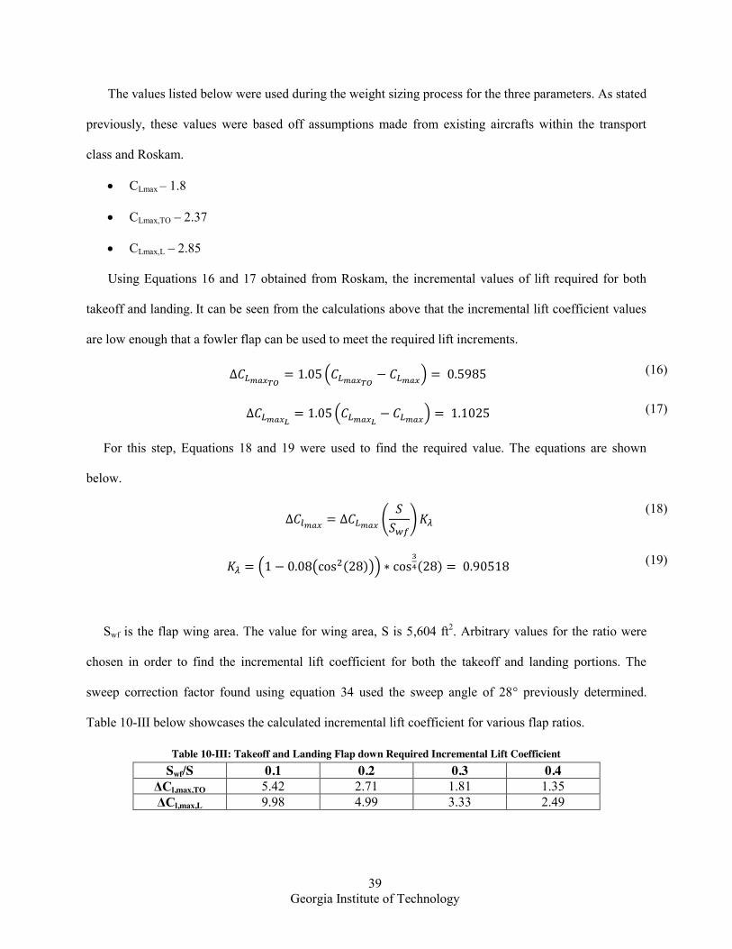
39 Georgia Institute of Technology
The values listed below were used during the weight sizing process for the three parameters. As stated
previously, these values were based off assumptions made from existing aircrafts within the transport
class and Roskam.
x CLmax – 1.8
x CLmax,TO – 2.37
x CLmax,L – 2.85
Using Equations 16 and 17 obtained from Roskam, the incremental values of lift required for both
takeoff and landing. It can be seen from the calculations above that the incremental lift coefficient values
are low enough that a fowler flap can be used to meet the required lift increments.
( ) (16)
( ) (17)
For this step, Equations 18 and 19 were used to find the required value. The equations are shown
below.
(
) (18)
( ( ( ))) ( ) (19)
Swf is the flap wing area. The value for wing area, S is 5,604 ft2. Arbitrary values for the ratio were
chosen in order to find the incremental lift coefficient for both the takeoff and landing portions. The
sweep correction factor found using equation 34 used the sweep angle of 28° previously determined.
Table 10-III below showcases the calculated incremental lift coefficient for various flap ratios.
Table 10-III: Takeoff and Landing Flap down Required Incremental Lift Coefficient Swf/S 0.1 0.2 0.3 0.4
ΔCl,max,TO 5.42 2.71 1.81 1.35 ΔCl,max,L 9.98 4.99 3.33 2.49

40 Georgia Institute of Technology
Using Equation 20 obtained from Roskam Part II, the incremental lift coefficient required due to flaps
can be calculated.
( )
(20)
Using the figures in Roskam, the K values were chosen from the graph, which corresponds to a flap
chord ratio of 0.4 which was chosen after the iteration process explained below. Using this values and the
equation above, the incremental lift coefficient was found for the various cases from table 5.
Table 10-IV: Incremental Lift Coefficient Values Swf/S 0.1 0.2 0.3 0.4
ΔCl,req (takeoff) 5.83 2.91 1.94 1.46 ΔCl,req (landing) 10.73 5.37 3.58 2.68
Next, the flap deflection was chosen based on if it could produce the required incremental sectional lift
coefficient. As stated in Roskam, the magnitude of depends on the flap chord ratio, type of flaps used
and the flap deflection angle. Initially, the assumption was made to used fowler flaps and calculate the
produced as both the flap deflection and the flap chord ratio varied. Equation 7.12 and figures 7.4 and 7.5
from Roskam were used in conjunction in order to find the various combinations of flap deflection and
flap chord ratio. Table 10-V below showcases the final results of the convergence between the
incremental sectional lift coefficients required versus calculated.
Table 10-V: Convergence Results for Degree Deflection Angle of deflection 10 15 20 25 30 35 ΔCl,calculated (takeoff) 0.80 1.17 1.53 1.85 2.17 2.44 ΔCl,calculated (landing) 0.80 1.19 1.59 2.00 2.39 2.78
As can be seen, the best correlation between the required and calculated incremental lift coefficient
accords where cf/c = 0.3 and Swf/S = 0.4. There values correspond to a flap deflection of 20° for the
takeoff and 35° for the landing.
Finally, the flap length can be calculated using the values found above. A convergence method was
employed using the Swf/S ratio and the known wing area. The length of the flap was assumed to be the

41 Georgia Institute of Technology
height of a trapezoid with the bases calculated using the flap chord ratio. Using this method, the flap
length was calculated. Table 10-VI tabulates all the results that have been calculated.
Table 10-VI: Summary of Flap Sizing Results Parameter Variable Name Units Value Flap length ~ ft 40 Flap type ~ ~ Fowler
Takeoff deflection δf,TO degrees 20 Landing deflection δf,L degrees 35
Flap to wing area ratio Swf/S ~ 0.4 Flap chord to wing chord ratio cf/c ~ 0.3
The location of the lateral control surface design is based purely on the compatibility with the high lift
devices. Since there is not an exact process for sizing the lateral control surface, Tables 8.12b in Roskam
Part II was used as a guide to size the aileron and outboard spoiler. Hence based on the compatibility with
the flap and also looking at the historical data of similar aircrafts, the aileron length was chosen to be 30
feet.
Spars support the loads experienced by the wing. As such, their placement plays an important role in
the sizing of the wing. As stated in Roskam, a clearance of 0.005c is required between the spar lines and
the outlines of the high lift devices and the aileron and spoiler. With the help of Roskam, the front spar
was placed at 0.25c and the rear chord was placed at 0.695c. The rear spar mainly helps in attaching the
high lifting and lateral stability devices. The remaining length, 0.3c is covered by the flaps, ailerons, and
spoilers. Table 10-VII below documents the spar locations.
Table 10-VII: Front and rear spar location Parameter Variable Name Units Value Front Spar F.S. ft 5.91 Rear Spar R.S. ft 16.56
It is assumed that the wing fuel is carried in the “wet wing” and that there is no additional fuel tanks
within the fuselage of the aircraft. As stated previously, the fuel is assumed to be stored in the wing
torque box and within 85% span as discussed in Roskam Part II. Due to the high vulnerability of the
aircraft structures, the fuel is not stored in the wingtips. Furthermore, no fuel is carried beyond the 85%

42 Georgia Institute of Technology
span point in order to prevent lightning strikes from starting in-flight fires. Total wing fuel volume is
calculated and compared with the total fuel requirement for the mission. The wing fuel volume is
calculated using Equation 21 from Roskam.
(
)( ) {
( ) } (
)
(21)
Given the value of t/c, cr and ct, an estimate of (t/c)r = 0.13 and the (t/c)t = 0.13.
( ) ( )
(22)
The fuel volume was calculated to be 7,619 ft3. From the weight sizing process, the fuel weight
required was calculated to be 183,600 lb. The fuel density was assumed to be 49 lb/ft3, which was taken
from Roskam Part II. Using this density and the fuel weight, the fuel volume required was calculated to
be 4,378 ft3. As can be seen, the wing provides enough fuel volume to store the required fuel. Table
10-VIII documents the results found.
Table 10-VIII. Fuel Weight and Volume Parameters Parameter Variable
Name Units Value Comments
Wing Fuel Volume VWF ft3 7,619 Calculated Total fuel weight WFuel lb 214,540 Calculated from Weight Sizing Total fuel volume
required VFuelRequired ft3 4,378 Calculated using density as 49
lb/ft3
10.4 Final Wing, Flap, and Lateral Control Layout
Figure 10-4 is a dimensioned drawing of the wing planform. All dimensions are in feet and a line is
drawn at the quarter chord point, where the sweep angle is measured.

43 Georgia Institute of Technology
Figure 10-4: Dimensioned Drawing of Wing Planform
Figure 10-5 shows the wing planform with the high-lift devices, such as flap, aileron, and spoiler. All
of these control devices are hinged at approximately 70% of the total chord. The location and size of the
spoiler was obtained by determining the average of historical spoiler data from the same tables.
Figure 10-5: Flap and Lateral Control Layout

44 Georgia Institute of Technology
10.5 Wing Design Optimization
In order to study potential increases in fuel efficiency a preliminary optimization on the wing planform
was conducted. A model for transonic flow developed in (Sankar, 1987) was incorporated into an
automated optimization process. The transonic flow model was used to provide values of CL and CD for
randomly generated planforms. The generated planforms had the same leading edge, wing area, span,
taper ratio, and root chord. The difference between them was the distribution of the chords along the span.
1,000 randomly generated wing planforms were ran through the transonic flow simulation. Of those
1,000, 234 planforms were able to meet the required CL cruise from the weight sizing process.
On Figure 10-6 the 234 wings were sorted by lift to drag ratio. For comparison, the conventionally
designed wing was also plotted. The optimized wing planform resulted in a 40% increase in lift to drag
and 9% decrease in drag at cruise conditions. The planform not only met the required CL but exceeded it
by over 20%. This indicates that a lower angle of attack could be used at cruise, resulting in even lower
cruise drag compared to the conventional wing.

45 Georgia Institute of Technology
Figure 10-6. Lift to drag of wings that met the CL required.
On Figure 10-7, the red line indicates the trailing edge of the optimized planform, the yellow dashed
line the conventional and the blue line the leading edge. The optimized planform has an increased chord
near the root and decreased near the tip. This was a common trend with all of the planforms with
increased lift to drag ratios. The same trend can be seen in the Boeing 787, the wing is thicker at the chord
and tapers off faster than conventional wings.

46 Georgia Institute of Technology
Figure 10-7. Wing planform comparison.
Even with the improvements in lift to drag and cruise drag the optimized planform was not
incorporated into our design. The major reasons for this were an increase in structural complexity, and
placement of control surfaces. Due to the sudden decrease in chord near the tip, the structure of the wing
would have to be reinforced when compared to a conventional design. This would likely lead to an
increase in the weight of the wing. The best placement of ailerons is near the wing tips in order to
increase the moment arm. The decreased chord would make the aileron placement near the wing tips
more difficult. In more advanced stages of design, it might be possible to incorporate this type of analysis
in order to create a more efficient wing.

47 Georgia Institute of Technology
11 Tail Sizing
11.1 Horizontal and Vertical Stabilizer Sizing
This aircraft is designed with a T-tail instead of a conventional tail to improve performance and
handling qualities. During the configuration selection process, a conventional tail design was ruled out for
several reasons. The primary reason is to keep the horizontal tail out of the wake of the wings and
fuselage. This allows for a greater dynamic pressure on the horizontal tail and elevators so that a smaller
surface is needed. The vertical tail also sees a benefit in the form of reduced 3D effects. The horizontal
tail functions as an endplate which improves the aerodynamic efficient of the tail, allowing a smaller size
with more effective handling qualities.
The sizing process for both the horizontal and vertical tails was followed according to the process
described in Reference (Roskam J. , Airplane Design Part II: Preliminary Configuration Design and
Integration of the Propulsion System, 2004). The tail volume, a sizing parameter which reflects an
aircraft’s ability to provide stability, was determined using historical values commensurate with the
aircraft size and performance for both the horizontal and vertical tails. The horizontal tail volume is 0.65,
while the vertical tail volume is 0.08. For comparison, the tail volumes of the C-5 Galaxy are 0.62 and
0.079 for the horizontal and vertical tails, respectively.
Using the wing area, wingspan, and wing geometric chord, the tail surface areas are calculated.
The aspect ratio, taper ratio, and all other relevant tail parameters are chosen using the Table 8.10a and
Table 8.10b from Roskam’s Part II book (Roskam J. , Airplane Design Part II: Preliminary Configuration
Design and Integration of the Propulsion System, 2004). The selected tail parameters, along with the
calculated geometric specifications, are shown in Table 11-I and Table 11-II.

48 Georgia Institute of Technology
Table 11-I. Horizontal tail sizing parameters and calculations. Horizontal Tail
Parameter Variable Name Units Value Horizontal Moment Arm xh ft 118.73 Horizontal Tail Volume Vh ~ 0.65
Surface Area Sh ft2 725.80 Aspect Ratio AR ~ 5.00
Sweep Angle (c/4) Lc/4 degrees 24.00 Sweep Angle (LE) LLE degrees 28.60
Taper Ratio l ~ 0.50 Thickness Ratio (t/c)h % 0.12
Airfoil ~ NACA 0012 Dihedral Gh degrees 0.00
Incidence Angle ih degrees 0.00 Tail Span bh ft 60.24
Root Chord cRh ft 16.06 Tip Chord cTh ft 8.03
Root Thickness tRh in 23.13 Tip Thickness tTh in 11.57
Wing Mean Geometric Chord ch ft 12.05 Min Pressure Coef. @ Zero AOA Cp0min ~ -0.40
Critical Mach Number (DM > 0.05) Mcr_HT ~ 0.91
Table 11-II. Vertical tail sizing parameters and calculations. Vertical Tail
Parameter Variable Name Units Value Vertical Moment Arm xh ft 110.00 Vertical Tail Volume Vh ~ 0.08
Surface Area Sh ft2 965.41 Aspect Ratio AR ~ 1.80
Sweep Angle (c/4) Lc/4 degrees 20.00 Sweep Angle (LE) LLE degrees 36.97
Taper Ratio l ~ 0.70 Thickness Ratio (t/c)h % 0.12
Airfoil ~ NACA 0015 Dihedral Gh degrees 0.00
Incidence Angle ih degrees 0.00 Tail Span bh ft 58.95
Root Chord cRh ft 19.27 Tip Chord cTh ft 13.49
Root Thickness tRh in 27.74 Tip Thickness tTh in 19.42
Wing Mean Geometric Chord ch ft 16.38 Min Pressure Coef. @ Zero AOA Cp0min ~ -0.40
Critical Mach Number (DM > 0.05) Mcr_HT ~ 0.91

49 Georgia Institute of Technology
Dimensioned drawings of the horizontal tail and vertical tail are shown in Figure 11-1 and Figure
11-2 below, along with added control surfaces. The detailed sizing of the control surfaces is continued in
the next subsection.
Figure 11-1. Dimensioned drawing of horizontal tail.
Figure 11-2. Dimensioned drawing of vertical tail.
11.2 Elevator and Rudder Sizing
The sizing of the empennage control surfaces is carried out to provide adequate longitudinal and
direction authority necessary to trim the aircraft correctly and to correct for an engine out condition. The
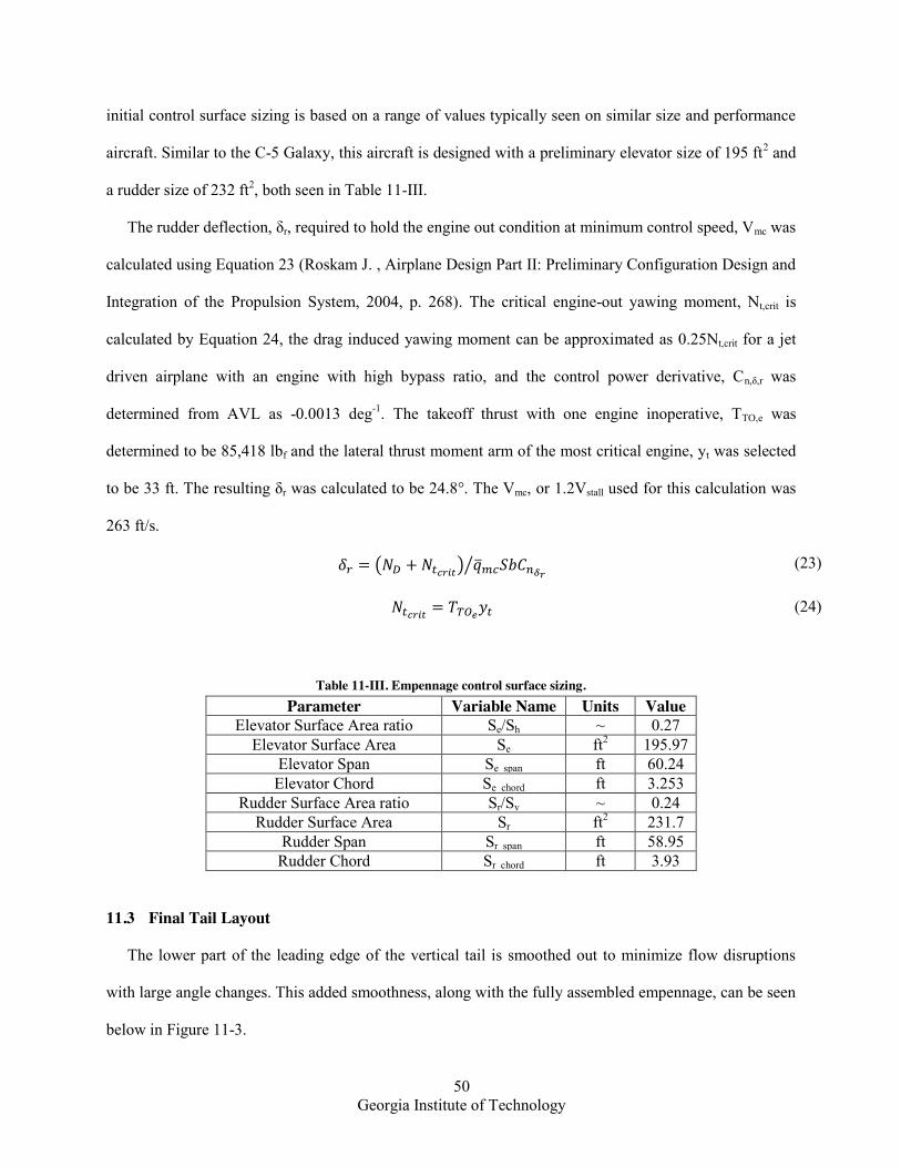
50 Georgia Institute of Technology
initial control surface sizing is based on a range of values typically seen on similar size and performance
aircraft. Similar to the C-5 Galaxy, this aircraft is designed with a preliminary elevator size of 195 ft2 and
a rudder size of 232 ft2, both seen in Table 11-III.
The rudder deflection, δr, required to hold the engine out condition at minimum control speed, Vmc was
calculated using Equation 23 (Roskam J. , Airplane Design Part II: Preliminary Configuration Design and
Integration of the Propulsion System, 2004, p. 268). The critical engine-out yawing moment, Nt,crit is
calculated by Equation 24, the drag induced yawing moment can be approximated as 0.25Nt,crit for a jet
driven airplane with an engine with high bypass ratio, and the control power derivative, Cn,δ,r was
determined from AVL as -0.0013 deg-1. The takeoff thrust with one engine inoperative, TTO,e was
determined to be 85,418 lbf and the lateral thrust moment arm of the most critical engine, yt was selected
to be 33 ft. The resulting δr was calculated to be 24.8°. The Vmc, or 1.2Vstall used for this calculation was
263 ft/s.
( ) ⁄ (23)
(24)
Table 11-III. Empennage control surface sizing. Parameter Variable Name Units Value
Elevator Surface Area ratio Se/Sh ~ 0.27 Elevator Surface Area Se ft2 195.97
Elevator Span Se_span ft 60.24 Elevator Chord Se_chord ft 3.253
Rudder Surface Area ratio Sr/Sv ~ 0.24 Rudder Surface Area Sr ft2 231.7
Rudder Span Sr_span ft 58.95 Rudder Chord Sr_chord ft 3.93
11.3 Final Tail Layout
The lower part of the leading edge of the vertical tail is smoothed out to minimize flow disruptions
with large angle changes. This added smoothness, along with the fully assembled empennage, can be seen
below in Figure 11-3.
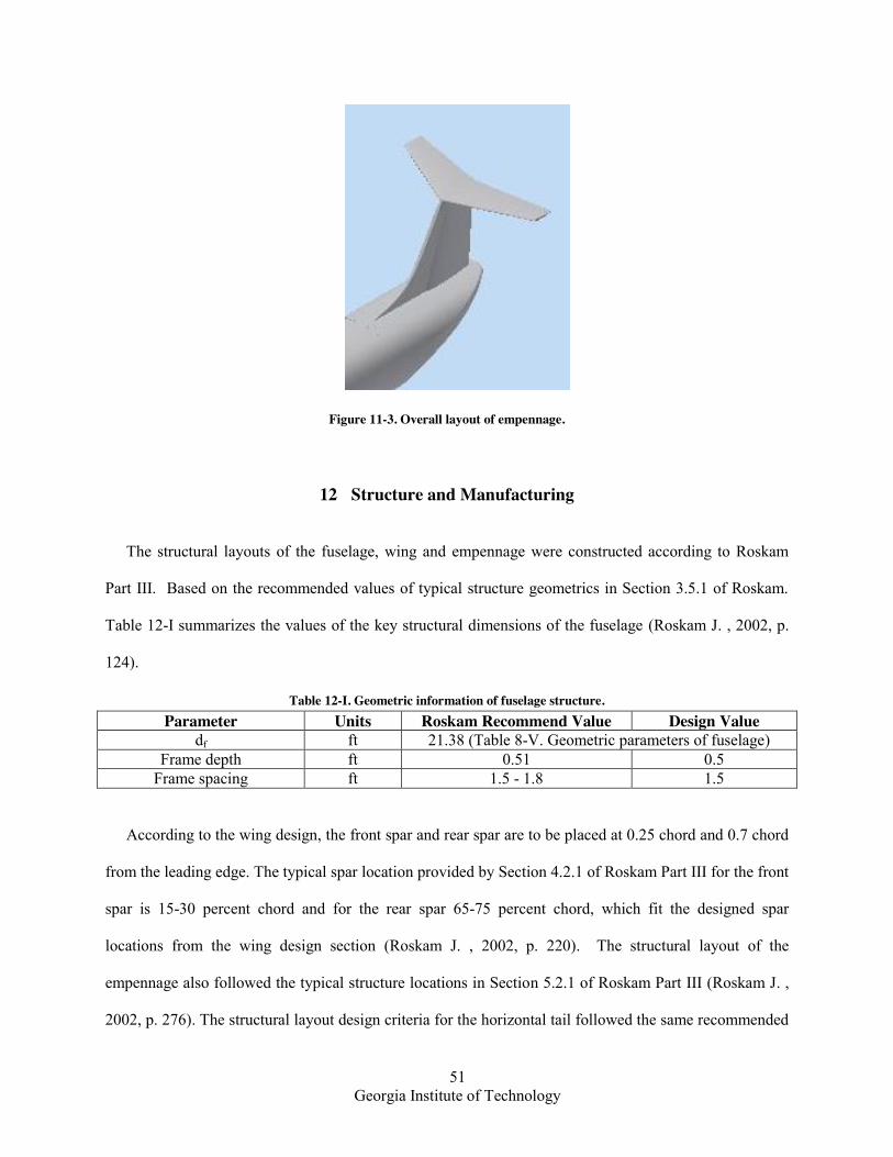
51 Georgia Institute of Technology
Figure 11-3. Overall layout of empennage.
12 Structure and Manufacturing
The structural layouts of the fuselage, wing and empennage were constructed according to Roskam
Part III. Based on the recommended values of typical structure geometrics in Section 3.5.1 of Roskam.
Table 12-I summarizes the values of the key structural dimensions of the fuselage (Roskam J. , 2002, p.
124).
Table 12-I. Geometric information of fuselage structure. Parameter Units Roskam Recommend Value Design Value
df ft 21.38 (Table 8-V. Geometric parameters of fuselage) Frame depth ft 0.51 0.5
Frame spacing ft 1.5 - 1.8 1.5
According to the wing design, the front spar and rear spar are to be placed at 0.25 chord and 0.7 chord
from the leading edge. The typical spar location provided by Section 4.2.1 of Roskam Part III for the front
spar is 15-30 percent chord and for the rear spar 65-75 percent chord, which fit the designed spar
locations from the wing design section (Roskam J. , 2002, p. 220). The structural layout of the
empennage also followed the typical structure locations in Section 5.2.1 of Roskam Part III (Roskam J. ,
2002, p. 276). The structural layout design criteria for the horizontal tail followed the same recommended

52 Georgia Institute of Technology
geometric value of the wing design. Table 12-II presents the structural layout geometric data of the wing
and empennage and Figure 12-1 presents the structural layout of the entire aircraft based on the geometric
data presented in Table 12-II.
Table 12-II. Geometric data of structural layout for wing, vertical tail, and horizontal tail. Component Parameter Roskam Recommend Value Design Value
Wing Front Spar 15-30 % chord 0.25 c Rear Spar 65-75 % chord 0.70 c
Rib Spacing 24 in. 24 in.
Vertical Tail Front Spar 15-25 % chord 0.25 c Rear Spar 70-75 % chord 0.75 c
Rib Spacing 24 in. 24 in.
Horizontal Tail Front Spar 15-30 % chord 0.25 Rear Spar 65-75 % chord 0.75
Rib Spacing 24 in. 24 in.
Figure 12-1. Structure layout.

53 Georgia Institute of Technology
Based on Section 7.2 and Table 7.1 of preliminary material selection in Roskam Part III, previous
discussion about composite structures, and considering the shapes and forms and typical airplane usage,
the following Table 12-III presents the selected material for essential structures of the aircraft for
manufacturing purpose (Roskam J. , Airplane Design Part III: Layout Desig of Cockpit, Fuselage, Wing
and Empennage: Cutaways and Inboard Profiles, 2002, pp. 386-387).
Table 12-III. Aircraft Material Selection Structure Component Material Selection Criteria
Fuselage Frame Steel High strength Skin Carbon Laminate Light weight
Wing
Spars Aluminum Strength, light weight Ribs
Control Surface Leading Edge
Carbon Laminate Light weight, laid up to any shape Trailing Edge Skin
Vertical Tail
Spars Aluminum Strength, light weight Ribs Control Surface Carbon Sandwich Light weight Leading Edge Aluminum Strength, light weight
Skin Carbon Laminate Light weight
Horizontal Tail
Spars Aluminum Strength, light weight Ribs Control Surface Carbon Sandwich Light weight Leading Edge Aluminum Strength, light weight
Skin Carbon Laminate Light weight
Landing Gear
Side Brace Polymer Matrix Composite
Light weight, increased durability & robustness (Materials,
2011) Retraction Cylinder Steel High strength
Shock Absorber Aluminum Strength, light weight Scissors Wing & Empennage attaching part
onto the fuselage Carbon Fiber Light weight, laid up to any shape

54 Georgia Institute of Technology
13 Subsystem Considerations
The major subsystems of Figure 13-1 and Figure 13-2 will be described in the following paragraphs.
Figure 13-1. Side view of subsystem placement.
Figure 13-2. Top view of subsystem placement.
13.1 APU
The auxiliary power unit provides enough power to run most of the subsystems of the aircraft and start
the main turbines. It facilitates quick ground operations by avoiding the need for an external power
55 Georgia Institute of Technology
source, this is crucial in a military operation. Most APU's are custom designed and made for each
aircraft's power needs and space requirements, an exact model number and specifications is therefore not
applicable. The two major manufacturers of APU's are Honeywell and Pratt & Whitney.
13.2 Fuel Pumps
Fuel pumps serve a dual role on our aircraft, they provide the engine with the fuel required and
adjust the weight and balance of the aircraft as fuel decreases. Since our aircraft has the fuel distributed in
the wing, two fuel pumps are required, for the right and left side of the aircraft. The fuel system would
have to be cross fed as banking can cause an imbalance in the lateral distribution of weight. Due to space
considerations most fuel pumps are custom made.
13.3 Avionics
Avionics is a catch all term that describes the communication, navigation and display management
subsystems. Avionics systems are composed of both off the shelf components and custom components.
The avionics have an estimated weight of 1.5% of the total empty weight of the aircraft.
13.4 Electrical System
The electrical system is fairly standard for our aircraft with the exception of the use of a fly by wire
control system. Fly by wire systems offer reduced weight and facilitate the incorporation of stability
augmentation devices (Walberg).
13.5 Electrohydraulic Actuator
Instead of the conventional hydraulic systems to provide power for the deflection of the control
surfaces, the aircraft will use electrohydraulic actuators. Electrohydraulic actuators resulted in a 1,000 lb
weight savings on the A380 (Kulshreshtha, 2007). The actuators also require less maintenance than
conventional systems (Kulshreshtha, 2007).
13.6 Ram Air Turbine
Ram air turbines (RAT) are small turbines that are placed into the airflow and only enough power to
allow control surface inputs and deflections. The RAT for this aircraft provides electrical power to the
electrohydraulic actuators in the case that both engines and the APU fail.

56 Georgia Institute of Technology
13.7 Defensive Subsystems
The defensive subsystems are composed of an infrared missile countermeasure, chaffs and flares. The
infrared missile countermeasure is the AN/AAQ-24 (15No), this provides focuses high power IR energy
on the seeker head. The focused energy disrupts the tracking capabilities of the missile are the RR-170
AL (House) which provide protection against RF guided missiles. The flares used are a combination of
the M212 and the M206 (Project Manager Close Combat Systems ), this combination provides protection
against IR guided missiles. They create radiation which can divert the incoming missile.
14 Weight and Balance Analysis
14.1 Class I Component Weight Breakdown
In order to determine the center of gravity of the proposed aircraft and its movement for all loading
scenarios, a Class I Weight and Balance analysis is presented here. The method is based upon one
detailed in Aircraft Design Part II (Roskam J. , Airplane Design Part II: Preliminary Configuration Design
and Integration of the Propulsion System, 2004). This method is important in verifying the component
weights and distributions for all systems and subsystem, regardless of weight or size. The locations of key
components such as wings and landing gear are determined through this process, as are minor subsystems
such as air conditioning, chaff dispensers, etc.
The first step in the process is the preliminary assignment of weights and locations for each
component. The major component weights are calculated using the empirical relations presented in Table
A10.1a and A10.1b in Aircraft Design Part V (Roskam D. J., 2003). These empirical relations are based
on a typical system group’s fraction of the gross weight. An example is that the fuselage is 15.4% of the
gross weight for the similarly sized C-5 Galaxy. The use of advanced composite materials in the fuselage
structure introduces a fuselage weight reduction of roughly 20% in the fuselage, as detailed previously in
technology factors. All subsystems utilizing an empirical fraction approach to weight estimation are
included in Table 14-I.
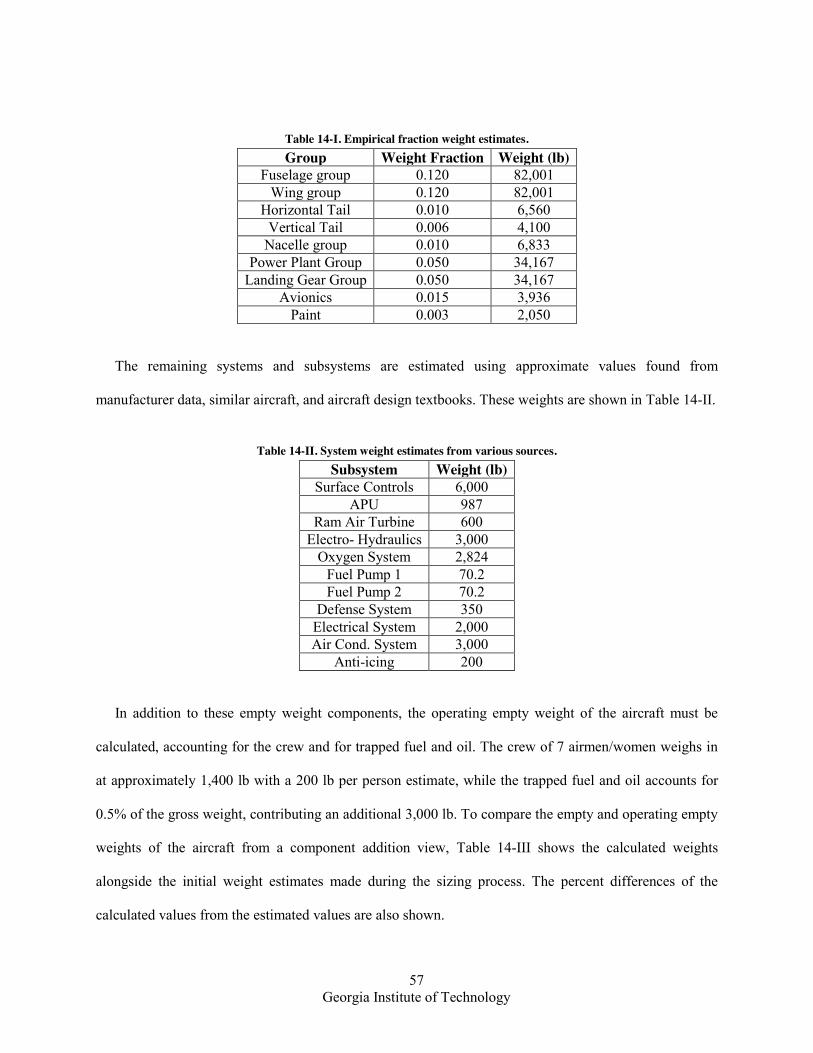
57 Georgia Institute of Technology
Table 14-I. Empirical fraction weight estimates. Group Weight Fraction Weight (lb)
Fuselage group 0.120 82,001 Wing group 0.120 82,001
Horizontal Tail 0.010 6,560 Vertical Tail 0.006 4,100
Nacelle group 0.010 6,833 Power Plant Group 0.050 34,167
Landing Gear Group 0.050 34,167 Avionics 0.015 3,936
Paint 0.003 2,050
The remaining systems and subsystems are estimated using approximate values found from
manufacturer data, similar aircraft, and aircraft design textbooks. These weights are shown in Table 14-II.
Table 14-II. System weight estimates from various sources.
Subsystem Weight (lb) Surface Controls 6,000
APU 987 Ram Air Turbine 600
Electro- Hydraulics 3,000 Oxygen System 2,824
Fuel Pump 1 70.2 Fuel Pump 2 70.2
Defense System 350 Electrical System 2,000 Air Cond. System 3,000
Anti-icing 200
In addition to these empty weight components, the operating empty weight of the aircraft must be
calculated, accounting for the crew and for trapped fuel and oil. The crew of 7 airmen/women weighs in
at approximately 1,400 lb with a 200 lb per person estimate, while the trapped fuel and oil accounts for
0.5% of the gross weight, contributing an additional 3,000 lb. To compare the empty and operating empty
weights of the aircraft from a component addition view, Table 14-III shows the calculated weights
alongside the initial weight estimates made during the sizing process. The percent differences of the
calculated values from the estimated values are also shown.

58 Georgia Institute of Technology
Table 14-III. Weight estimate and calculation comparisons. Empty Weight (lb) Operating Empty Weight (lb)
Weight Sizing Estimate 264,258 267,224 Component Weights 262,407 268,658 Percent Difference 0.705 0.536
The final weight bookkeeping necessary is to tabulate the payloads individual weights, quantities, and
total weights. Per the Request for Proposal, the cargo capable of being carried by the aircraft system must
be 44 465 L Master Pallets and one Wolverine Bridge System, separately. Addition cargo loads necessary
to meet the requirements include AH-64 Apache helicopters, M1A1 Abrams tanks, and M2 Bradley
vehicles, all of which are included in Table 14-IV. In addition, generic 205,000 pound and 300,000 pound
loads must be part of the cargo capabilities to fulfill the performance requirements.
Table 14-IV. Payload weights and quantities. Individual Weight (lb) Quantities Total Weight (lb)
463 L Master Pallets 2,000 44 88,000 AH-64 Apaches 23,000 3 69,000
Wolverine Bridge System 153,882 1 153,882 M1A1 Abrams 126,000 2 126,000
M2 Bradley 60,800 4 60,800 205k Load 205,000 1 205,000 300k Load 300,000 1 300,000
14.2 Center of Gravity of Class I Weight Components
The center of gravity estimations made for the aircraft are for all three degrees of freedom: x, y, and z.
The origin of the coordinate system has been established to be 20 feet below the nose of the aircraft, so all
x and z values are positive. With the exception of a few lightweight subsystem components offset from
the x-z plane, there is symmetry in the y direction. The balance method detailed in Reference (Roskam J. ,
Airplane Design Part II: Preliminary Configuration Design and Integration of the Propulsion System,
2004) proceeds with a center of gravity calculation by summing all moments in a particular direction,
caused by a system or component’s weight being offset from its axis. These moments and the total aircraft
weight are used to compute center of gravity (c.g.) locations for each payload and the different states

59 Georgia Institute of Technology
which the aircraft experiences while transporting that payload. These c.g. locations are computed using
Equations 25 to 27:
∑
∑
⁄ (25)
∑
∑
⁄ (26)
∑
∑
⁄ (27)
The tabulated calculations for each subsystem and component are detailed in Table 14-V.
Table 14-V. Center of gravity calculations.
Component Type Weight (lb)
X Location (ft)
Y Location (ft)
Z Location (ft)
W*X (lb-ft)
W*Y (lb-ft)
W*Z (lb-ft)
Fuselage group 82001 105.16 0.00 36.58 8623240 0 2999602 Wing group 82001 123.56 0.00 45.83 10132061 0 3758112
Horizontal Tail 6560 237.32 0.00 80.41 1556801 0 527490 Vertical Tail 4100 230.00 0.00 67.14 942993 0 275274
Nacelle group 6833 89.42 0.00 38.78 611045 0 265000 Power Plant group 34167 89.42 0.00 38.78 3055226 0 1325002
Landing Gear Group
34167 148.00 0.00 25.60 5056737 0 874679
Surface Controls 6000 135.00 0.00 50.00 810000 0 300000 APU 987 216.00 0.00 45.00 213192 0 44415
Avionics 3936 9.00 0.00 45.74 35425 0 180037 Ram Air Turbine 600 133.56 10.00 49.00 80136 6000 29400
Electro-Hydraulics 3000 165.00 0.00 50.00 495000 0 150000 Oxygen System 2824 9.00 2.00 45.74 25416 5648 129170
Fuel Pump 1 70.2 143.56 15.00 50.00 10078 1053 3510 Fuel Pump 2 70.2 143.56 -15.00 50.00 10078 -1053 3510
Defense System 350 230.00 3.00 50.00 80500 1050 17500 Electrical System 2000 220.00 0.00 45.00 440000 0 90000 Air Cond. System 3000 9.00 -3.00 45.74 27000 -9000 137220
Paint 2050 150.00 0.00 48.00 307504 0 98401 Anti-icing 200 105.00 0.00 45.00 21000 0 9000
Crew 1400 12.00 0.00 46.00 16800 0 64400 Trapped Fuel and
oil 3000 123.56 0.00 47.00 370680 0 141000
463 L Master Pallets
88000 130.00 0.00 36.00 11440000 0 3168000
AH-64 Apaches 69000 130.00 0.00 39.42 8970000 0 2719980 Wolverine Bridge
System 153883 125.00 0.00 39.29 19235375 0 6046063

60 Georgia Institute of Technology
M1A1 Abrams 252000 125.00 0.00 36.53 31500000 0 9205560 M2 Bradley 243200 109.32 0.00 37.34 26586624 0 9081088
Each payload configuration has a different fuel volume, a limit of the wet wing volume and the
maximum take-off weight. Each payload configuration therefore has several different weights during a
given mission and therefore several different centers of gravity. These include the fuel added to the
aircraft before payload, fuel and payload both added, solely payload without fuel, and finally operating
empty weight before and after operations. With the numerous payloads the aircraft system is capable of
handling, the extensive list of c.g. locations has been tabulated and is shown in Table 14-VI. Additionally,
the distance of each c.g. behind the leading edge of the wing at the root chord is included, as well as that
distance normalized by the root mean geometric chord of 23.7 ft.
Table 14-VI. Center of gravity locations for all payload configurations.
Xcg (ft) Ycg (ft) Zcg (ft) XLE (ft) XLE / C.G. Travel (in)
Empty Weight 123.1 0.01 42.45 38.11 1.60 ~ Operating Empty
Weight 122.5 0.01 42.52 37.54 1.58 0
No Cargo + Max Fuel 123.0 0.01 43.62 37.99 1.60 5.4 No Master Pallets +
Fuel 123.0 0.01 43.62 37.99 1.60 5.4
Master Pallets + Fuel 124.1 0.01 42.45 39.07 1.64 18.4 Master Pallets + No
Fuel 124.4 0.01 40.91 39.38 1.66 22.1
No Apache + Fuel 123.1 0.01 43.92 38.12 1.60 6.9 Apaches + Fuel 123.8 0.01 43.47 38.81 1.63 15.2
Apaches + No Fuel 124.1 0.01 41.88 39.06 1.64 18.3 No Wolverine + Fuel 123.0 0.01 43.75 38.05 1.60 6.1
Wolverine + Fuel 123.5 0.01 42.75 38.48 1.62 11.3 Wolverine + No Fuel 123.4 0.01 41.34 38.43 1.62 10.8 No M1A1 Abrams +
Fuel 122.9 0.01 43.47 37.93 1.60 4.7
M1A1 Abrams + Fuel 123.7 0.01 40.93 38.69 1.63 13.8 M1A1 Abrams + No
Fuel 123.7 0.01 39.62 38.73 1.63 14.3
No 205k + Fuel 123.0 0.01 43.62 37.99 1.60 5.4 205k + Fuel 124.3 0.01 41.35 39.33 1.66 21.6
205k + No Fuel 124.7 0.01 39.70 39.69 1.675 25.8 No 300k + Fuel 122.9 0.01 43.28 37.85 1.59 3.8
300k + Fuel 124.0 0.01 40.11 39.01 1.64 17.6 300k + No Fuel 124.1 0.01 39.08 39.10 1.65 18.7

61 Georgia Institute of Technology
14.3 Weight-C.G. Excursion Diagram and Feasibility of Design
The operation of the aircraft system for all payload configurations requires the knowledge and impact
of the c.g. locations and their travel during the course of a flight. This starts with the operating empty
weight, followed by the addition of the requisite fuel capacity for the mission. The cargo is then loaded
onto the aircraft via front and rear loading ramps.
Figure 14-1. C.g. travel for aircraft without cargo.
Figure 14-2. C.g. travel for aircraft one Wolverine Bridge.

62 Georgia Institute of Technology
Figure 14-3. C.g. travel for aircraft with 2 M-1 Abrams tanks.
Figure 14-4. C.g. travel for aircraft with 205,000 pound cargo.
Figure 14-5. C.g. travel for aircraft with 300,000 pound cargo.

63 Georgia Institute of Technology
15 Landing Gear Sizing
15.1 Geometric Criteria for Landing Gears
The landing gears were designed by following the process in Roskam Part II. The landing gear system
that is most applicable to our type of aircraft is retractable gears and tricycle configuration. Based on the
weight and balance data from Table 14-V, the main landing gear group is set at 148 ft from the nose of
the aircraft. Since the nose part of the fuselage is upward swinging design, the nose gear is designed at the
most forward location of the fuselage that does not swing. The longitudinal tip-over criteria and ground
clearance are shown in Figure 15-1, and the lateral ground clearance and tip-over criteria are shown in
Figure 15-2 and Figure 15-3. The location of the engines and most afterwards c.g. were determined by
previous weight and balance calculation from Table 14-V.
Figure 15-1. Longitudinal tip-over criteria and ground clearance.
Figure 15-2. Lateral ground clearance.

64 Georgia Institute of Technology
Figure 15-3. Lateral tip-over criteria.
The maximum static load per strut is calculated by Equations 28 and 29 from Roskam Part II (Roskam
J. , 2004, p. 222).
( ) ( )⁄ (28)
( ) ( )⁄ (29)
Figure 15-4 shows the distances of the nose gear and main gear group to the most afterward c.g.
location. These distances along with the maximum takeoff weight are used in static load per strut
calculations, Table 15-I presents the results.

65 Georgia Institute of Technology
Figure 15-4. Diagram for static load calculation.
Table 15-I. Static load per strut calculation result. Parameter Unit Value
lm ft 23.59 ln ft 101.10 Pm lb 138515.44 Pn lb 129281.07 ns ~ 4
WTO lb 683342.82 ns*Pm/WTO ~ 0.81
Based on the results from Table 15-I above and typical landing gear wheel specifications in Roskam
Part II, the main gear structures was determined to require four tires each. The tire dimension is
determined to be 49 in. x 20 in. (Roskam J. , 2004, p. 224).
15.2 Final Landing Gear Configuration and Retracting Feasibility
According to recommended landing gear wheel layouts in Figure 2.13 of Roskam Part IV, the static
load and the structural calculation above, the nose gear is to determined be a twin wheel design and the
main gear is determined to be the dual twin tandem design (Roskam J. , 2007, p. 19). The designs of nose
gear and main gear are based on Figure 2.2, Figure 2.53 and Figure 2.54 of Roskam Part IV with side
brace, retraction cylinder, shock absorber and scissors (Roskam J. , 2007, pp. 6, 78). The main gear of the
aircraft is designed to rotate the tire group horizontally along the structural axis first, and then retracts into
the main gear box and fuselage. The following Figure 15-5 to Figure 15-7 present the details of landing
gear designs and retracting process. The nose gear retracting process is designed with only a simple

66 Georgia Institute of Technology
rotation as shown in above Figure 15-6, and the retracting process for the main landing gear consists of
upward rotating, lateral rotating and folding steps.
Figure 15-5. Three-view of nose and main landing gear.
Figure 15-6. Nose gear retracting process.

67 Georgia Institute of Technology
Figure 15-7. Main gear retracting process.
16 Stability and Control
16.1 Neutral Point
One of the most important parameters to determine longitudinal stability is the location of the neutral
point on the aircraft. The neutral point is used in conjunction with the center of gravity to determine the
static margin of the vehicle. In order to calculate the neutral point of the aircraft, the designed wing and
tail geometry were inputted into the AVL analysis. The fuselage is not modelled in AVL as it does not
have a large impact on the stability of the vehicle. By placing the reference location at the center of
gravity for the design payload, the neutral point of the aircraft can be calculated in AVL. The aircraft
geometry used in the AVL model of this aircraft is shown below in Figure 16-1. For this aircraft, the
neutral point was determined to be 42.2 ft behind the leading edge of the root chord of the wing.

68 Georgia Institute of Technology
Figure 16-1. AVL input geometry.
16.2 Static Margin
With the neutral point of the aircraft calculated from AVL, the longitudinal static margin (S.M.)
of the aircraft can be calculated. This stability parameter is a measure of the aircraft’s ability to not
diverge from equilibrium when encountered by a perturbation such as a gust or wind shear. The static
margin is calculated as the difference between the neutral point and the c.g. locations normalized by the
mean geometric chord, which is 23.7 ft for the proposed aircraft, as shown as Equation 30.
( ) ⁄ (30)
For each mission loading type, the static margin is calculated and tabulated in Table 16-I.
Table 16-I. Static margins for all mission payload configurations. Mission S.M.
CALC: EW 0.172 CALC: OEW 0.197
No Cargo + Max Fuel 0.178 No Master Pallets +
Fuel 0.178 Master Pallets + Fuel 0.132 Master Pallets + No
Fuel 0.119 No Apache + Fuel 0.172 Apaches + Fuel 0.143
Apaches + No Fuel 0.132

69 Georgia Institute of Technology
No Wolverine + Fuel 0.175 Wolverine + Fuel 0.157
Wolverine + No Fuel 0.159 No M1A1 Abrams +
Fuel 0.180 M1A1 Abrams + Fuel 0.148 M1A1 Abrams + No
Fuel 0.146 No 205k + Fuel 0.178
205k + Fuel 0.121 205k + No Fuel 0.106 No 300k + Fuel 0.183
300k + Fuel 0.135 300k + No Fuel 0.131
16.3 Static Stability Derivatives
The other important output from the AVL stability analysis is the stability derivatives of the aircraft.
These stability derivatives are used to determine both the static and dynamic stability of the aircraft at the
chosen point in the flight. The static stability derivatives output from the AVL stability analysis are
shown below in Table 16-II.
Table 16-II. Static stability derivatives. Stability Derivative Value (/rad)
CL,α 4.868 Cm,α -0.590 Cl,β -0.099 Cn,β 0.137 Cl,p -0.488 Cm,q -32.02 Cn,r -0.086
The static stability derivatives outputted from the AVL stability analysis all show the correct response
to a disturbance from equilibrium. These static stability derivatives include important responses such as
the change in pitching moment with angle of attack, the effective dihedral, and the contributions of roll
moment, pitch moment, and yaw moment to roll rate, pitch rate, and yaw rate respectively are all of the

70 Georgia Institute of Technology
correct sign and reasonable magnitude. This indicates that the vehicle has been well designed and has
good static stability responses.
16.4 Dynamic Stability
The final step in the stability analysis that was performed was to determine the dynamic stability of the
vehicle. This is a very important characteristic of the stability of an aircraft because the aircraft must not
only come back to equilibrium, but also the oscillations of the vehicle must be damped out within an
appropriate amount of time. To determine the level of dynamic stability of the aircraft, the stability
derivatives obtained from the AVL analysis are used to find the five dynamic modes of the aircraft: short
period, phugoid, roll, Dutch roll, and spiral. Each of these modes must meet level 1 flying qualities on the
Cooper-Harper rating scale in order to be considered sufficient for flight. If the open loop response is not
sufficient to obtain level 1 flying qualities, a closed loop Stability Augmentation System (SAS) controller
must be employed to obtain the correct flying qualities.
To determine the open loop response of the aircraft, the non-dimensional stability derivatives are
used in conjunction with flight conditions and the aircraft geometry to calculate the dimensional stability
derivatives. These dimensional stability derivatives are then placed into the longitudinal and lateral [A]
matrices. By obtaining the eigenvalues of these [A] matrices, the flying qualities of each dynamic mode
can be analyzed. Both the longitudinal and lateral [A] matrices are shown below in Equations 31 and 32.
[
]
(31)
[
( )
]
(32)
The eigenvalues obtained from these longitudinal and lateral matrices are shown on a root locus plot in
the figure below.

71 Georgia Institute of Technology
Figure 16-2. Dynamic mode eigenvalues.
These eigenvalues are then analyzed to determine characteristics such as the damping ratio, natural
frequency, time constant, and time to double in order to evaluate the performance of the various dynamic
modes. The result of this analysis is shown below in Table 16-II.
Table 16-II. Dynamic mode analysis. Dynamic Mode Flying Quality Level ωn (rad/s) ζ (~) T2 (s) t1/2 (s)
Phugoid 2 0.119 0.031 - - Short Period 4 0.670 0.807 - -
Roll 1 - - - .950 Dutch Roll 3 - 0.078 - -
Spiral 1 - - 22.58 -
The results of this dynamic mode analysis show that in order to achieve level 1 flying qualities
for all dynamic modes, the vehicle will need a SAS for the phugoid, short period, and Dutch roll modes.
Short Period
Phugoid
Roll
Dutch Roll
Spiral
-0.8
-0.6
-0.4
-0.2
0
0.2
0.4
0.6
0.8
-1.2 -1 -0.8 -0.6 -0.4 -0.2 0 0.2
Ima
gin
ary
Axi
s
Real Axis

72 Georgia Institute of Technology
17 Final Layout
Figure 17-1. Aircraft Front View
Figure 17-2. Aircraft Top View

73 Georgia Institute of Technology
Figure 17-3. Aircraft Side View
Figure 17-4. Aircraft Key Components

74 Georgia Institute of Technology
Figure 17-5. Powerplant Layout

75 Georgia Institute of Technology
Figure 17-6. Series of drawings showing operation of nose and tail doors with their loading ramps deploying.

76 Georgia Institute of Technology
Figure 17-7. Three view of aircraft.

77 Georgia Institute of Technology
18 Ground Operations
As a military transport aircraft, it is imperative that the design is capable of loading and unloading
cargo is as short a time as possible. To that end, the aircraft itself has been designed around the use of the
cargo doors. Both the front and tail of the fuselage are capable of providing entry into the storage volume
of the craft. Using Omni-directional rollers and the combined surface area to hold 44 master pallets, the
ground operations should be extremely proficient. In fact, the aircraft itself can be loaded from both ends
if needed in order to minimize time on ground. The aircraft has been verified of providing enough
clearances for the anticipated cargo loads. Additionally, the aircraft landing gear system has been
designed to be lower to the ground to ensure that the movement of cargo into and out the system is as
easy as possible and reduce load times. Moreover, the aircraft has been designed in order to minimize
service and re-fueling time. The aircraft engines are expected to be derivatives of the GE-90 engines
which are designed in order to minimize service time. It should be known that as a military transport craft,
the tactical landing has been designed into the sizing of the aircraft. The aircraft is capable of landing
within 9000 ft with the calculated maximum weight. Furthermore, the aircraft is landing at speeds of 165
knots, which is relatively fast when compared the takeoff segment of the mission profile.
For the purpose to fast loading and unloading cargos, the aircraft is designed with an upward swing
nose door and a rear cargo door with ramps. Two cargo doors are designed to work at the same time on
the airfield. The nose door is designed to be deployed to loading position with longitudinal upwards
rotation, and then the folded ramps will be deployed after the nose door is in loading position. The rear
cargo door consists of three mechanical parts, the top board, fold-in door parts, and rotate-out door
supports. The fold-in door parts are designed to keep ground clearance such that the edges will not touch
the ground when the rotate-out door supports are in rotating process. The top board is designed to
provide more height clearance for cargos and rotates upwards in order to be deployed to loading position.
After all three parts of the rear cargo door being deployed in loading position, the folded rear ramps is

78 Georgia Institute of Technology
going to be deployed for cargo transporting. Figure 17-6 present the process of deploying cargo doors to
loading position.
The section below showcases the various loading operations for the varied cargo that the aircraft is
capable of loading within its cargo bay. The below figures showcase whether the load is capable of being
brought into the plane using both the front and rear cargo doors.
Figure 18-1: Master Pallet Loading Configuration
Figure 18-1 showcases that the master pallet can be loaded and de-loaded from the front and rear cargo
doors.

79 Georgia Institute of Technology
Figure 18-2: AH-64 Apache Loading Configuration
Figure 18-2 showcases that the aircraft is capable of holding three apache helicopters. For this loading
configuration, the cargo must be placed through the rear cargo door.
Figure 18-3: M1A1 Loading Configuration

80 Georgia Institute of Technology
Figure 18-3 showcases the M1A1 loading configuration. The aircraft is capable of holding four
vehicles and can be loaded the front and back cargo doors. Figure 18-4 showcases the M2A3 vehicle
loading configuration; the aircraft is capable of holding 2 vehicles and can be loaded from the front and
the rear.
Figure 18-4: M2A3 Loading Configuration
Figure 18-5 showcases the loading configuration of the Wolverine assault bridge. The aircraft is
capable of loading one bridge through the back cargo door.

81 Georgia Institute of Technology
Figure 18-5: Wolverine Loading Configuration
19 Cost and Business Plan
A preliminary analysis of the procurement and development cost along with the operating and support
cost was created. The procurement and development (P&D) cost was assessed by using the Rand DAPCA
IV model. The operations and support (O&S) cost focused on analyzing the major components of the
direct operating costs of the aircraft.
19.1 Procurement & Development Cost
The DAPCA IV model is a historical cost model that uses four air cost drivers. Those drivers are
1. Size – Empty weight and structural weight
2. Performance- maximum speed
3. Construction- airframe material
4. Program- Number of testable aircraft, number of aircraft built

82 Georgia Institute of Technology
These drivers are listed along with the variable that the model uses from the preliminary aircraft analysis
performed in section 5 of this report. From the drivers the model estimates both non-recurring and
recurring costs which are broken down into their major components. Each of these costs will be provided
along with a practical description. The RFP indicates an order of 120 aircraft; this is used to estimate
production costs.
19.1.1 Engineering Hours
The non-recurring engineering hours capture the one time research, design and test costs associated
only with engineering. This type of cost is required for the development of any new product and is
particularly high for the design of complex systems such as an aircraft. As this is a fixed cost, the cost per
unit decreases as the number of units is increased. For our aircraft the estimated non-recurring
engineering hours are 39.4 thousand hours, at current engineering hourly costs this is estimated to be
$4.26 B.
In the recurring engineering hours the cost associated with having a team of engineers supervise and
deal with manufacturing problems is assessed. This cost increases with the number of planes built but
decreases per plane due to economies of scale. The recurring engineering hours are 38 thousand hours, at
current engineering hourly costs this is estimated to be $4.60 B. This cost is heavily affected by the use of
composite materials
19.1.2 Tooling Hours
Non-recurring tooling hours capture the costs associated with creating test parts and initial test aircraft.
This is another type of required fixed cost for the development of any new product. The non-recurring
tooling hours for our aircraft is 27.5 thousand hours; at current tooling hourly costs this is estimated to be
$3.32 B. The higher hourly costs associated with tooling compared to engineering is a result of the higher
overhead associated. The recurring tooling cost is the labor cost associated with the tooling of the 120
aircraft produced. The recurring tooling cost is heavily affected by the use of composite materials, the
total cost is more than doubled by them. The estimated recurring hours is 19.1 thousand hours; at current
hourly costs this is estimated to be $1.55 B.
83 Georgia Institute of Technology
19.1.3 Development Support Costs
This broad title is a catch all for fixed costs associated with a more complex aircraft. As such, the
major driver of this cost is the maximum speed of the aircraft. This cost was calculated directly from the
model then using the inflation rate since the model was created adjusted to current prices. Traditionally
this cost is more difficult to model but is lower than the other two costs. The development and support
cost is $0.50 B.
19.1.4 Flight Test Costs
Flight testing is incredibly expensive due to the considerable risk associated with flying an unproven
vehicle for the first time. Extensive flight testing is required for any military vehicle due to the high risk
environment of operation. The flight test is a non-recurring cost and was estimated using the model, this
result was then adjusted for inflation. The total flight cost is estimated to be $0.573 B.
19.1.5 Manufacturing Costs
The manufacturing costs includes all costs associated with the physically creating the aircraft. It is
composed of both the labor and materials cost. The materials cost is the most affected by the composites
used. It carries a multiplier due to composite materials of 4.9. This multiplier is a very conservative
estimate as it has not been adjusted for the continual drops in price of composites in recent years. As such
our cost model can be generally considered to be quite conservative. The manufacturing labor hours are
estimated to be 146 thousand hours; at current wages, it is $18.2 B. The manufacturing material costs are
estimated to be 13.2 $B.
19.1.6 Quality Assurance Cost
Quality Assurance is required to maintain that each aircraft created meets the required safety
specifications. This includes materials and parts testing. It is a recurring cost that is also subject to
economies of scale. The quality assurance hours are estimated to be 14.8 thousand hours; at current
hourly costs, it is $1.7 B.

84 Georgia Institute of Technology
19.1.7 Procurement & Development Cost Conclusion
The total nonrecurring cost is estimated to be $9.02 B, the total recurring cost is estimated to be
$39.22 B totaling to $48.24 B for the total program cost. This is considerably less than the cost associated
with the current military cargo plane, C-17, which had a cost of $62 B for the same number of aircraft
produced. The unit cost per aircraft is $402 M.
Figure 19-1. Procurement and development cost.
19.2 Operating & Support Costs
The major components associated with the direct operating costs are fuel, maintenance, and crew
costs. The maintenance costs can be further broken down into material and labor costs. For this model the
yearly number of hours flown and maintenance hour per flight hour were estimated to be those of the C-
17.
The fuel cost was calculated by estimating the fuel consumption of our aircraft per flight hour. The
weight sizing process described in section 5 was used to find the fuel consumption and time of each
segment. This was then used to arrive at an average fuel consumption of 1,763 lb of fuel per typical flight
hour. Using current fuel prices and the estimated 780 flight hours per year a fuel cost of $6.35 M per
aircraft per year was found.
The maintenance cost was found by using the estimated maintenance hour per flight hour of 16, that of
the C-17. This amounts to a $0.5 M maintenance labor cost at current wages. The maintenance cost per
Engineering Tooling DS FT Manufacturing QA

85 Georgia Institute of Technology
flight hour was estimated using a model from Raymer. This model required the estimation of the engine
costs, as this is the driver of this cost. The estimated maintenance material cost per year is $5.4 M per
aircraft per year.
The estimated crew cost per year was found using for a three-man crew from Raymer. This model’s
inputs are the takeoff gross weight of the aircraft and the cruise speed. The total estimated crew cost per
aircraft per year is $1.0 M.
Figure 19-2. Operating and support cost.
The total estimated O&S cost is $13.27 M per aircraft per year. This is considerably less than that of
the C-17, $18.6 M per aircraft per year.
19.3 Business Plan
This aircraft was commissioned and designed as a response to the Air Force request for proposal.
Therefore, the primary consideration for all design decisions for this aircraft is the impact on the
performance of the vehicle as it corresponds to the primary and secondary objectives in the RFP. Once all
absolute requirements are met, the design choices focused on maximizing the performance while
minimizing the flyaway and operating cost of the vehicle. The result of this design was a modern
transport aircraft which exceeds both the performance and capabilities of all previous transport aircraft by
incorporating advanced, modern technologies such as composites, natural laminar flow airfoil, spiroid
Fuel Crew Mat. Material Mat. Labor

86 Georgia Institute of Technology
winglets, and geared turbofan engines. After delivery of the requested 120 aircraft to the Air Force, this
aircraft can be marketed to other foreign allies for similar style use in their militaries. This aircraft is
capable of performing heavy lifting missions over medium ranges in addition to lighter loads at long
ranges. This wide range of mission capabilities makes it an ideal aircraft because of its wide utility and
versatility. Over the next few decades, this aircraft will replace the large majority of the aging transport
aircraft fleet of both the United States and its allies.

87 Georgia Institute of Technology
20 Conclusion
The aircraft detailed in this report meets all of the requirements as described in the RFP while also
providing clear benefits when compared to the aircrafts used as baseline, with cost reduction, range
improvement, and payload capacity as the most distinguishing features. It can be seen from the sections
that the use of advanced technologies has provided clear benefits to the performance characteristics of the
proposed craft. The use of composite materials, NLF airfoils, geared turbofan, and spiroid winglet
lowered the operational weight of the aircraft while also improving the relevant aerodynamics properties.
The analysis of static and dynamic stability shows that through the use of a stability augmentation system,
the aircraft will meet all level 1 flying qualities. This will allow the pilots of this aircraft to maintain
complete control of the vehicle at all times without exerting large amounts of effort to maintain stable
equilibrium. The use of a wing planform optimization algorithm created one option for a wing planform
which maximizes the aerodynamic performance while being subject to specific constraints on the design
such as minimum coefficient of lift, the taper ratio, the span, and the area. Additionally, the fuselage has
been designed such that it is capable of loading and unloading all required cargo loads and other optional
loading configurations in a rapid and efficient manner to minimize overall ground track time. Throughout
each step of the process, the relevant stakeholders were carefully considered and if necessary, kept
informed of all key decisions. The design ideology adapted within this report lends itself to minimization
of cost. Through the use of advanced technologies as well as the improvement of current manufacturing
and maintenance techniques, the proposed aircraft has a 22% reduction in development and procurement
cost compared to the C-17 and an operations and support cost that is 29% less than the C-17. The
dramatic improvement in performance coupled with the large reduction in cost makes the vehicle much
more attractive from both a vehicle capabilities and financial standpoint to the armed forces who will
purchase this aircraft. The C-1 Flying Roc exceeds the performance and capabilities of current military
cargo transport designs while maximizing the efficiency of operation to reduce cost, making it an ideal
replacement for the current fleet employed by all the armed forces.

88 Georgia Institute of Technology
21 References
[1] J. E. Guerrero, D. Maestro and A. Bottaro, "Biomimetric spiroid winglets for lift and drag control," Comptes Rendus Mecanique, 2012.
[2] M. Nazarinia, M. R. Soltani and K. Ghorbanian, "Experimental Shape of Vortex Shapes behind a Wing Equipped with Different Winglets," Journal of Aerospace Science and Technology, 2006.
[3] J. Roskam and C.-T. E. Lan, Airplane Aerodynamics and Performance, Lawrence, Kansas: DARcorporation, 2003.
[4] Globid Inc., "463L Pallets," 2014. [Online]. Available: http://www.463lpallet.com/. [5] Kable, "AH-64A/D Apache Attack Helicopter," 2010. [Online]. Available: http://www.army-
technology.com/projects/apache/. [6] Military Analysis Network, "Wolverine (Heavy Assault Bridge)," 08 2 2000. [Online]. Available:
http://fas.org/man/dod-101/sys/land/wolverine.htm. [7] F. Prado, "Main Battle Tank - M1, M1A1 and M1A2 Abrams," 2008. [Online]. Available:
http://www.fprado.com/armorsite/abrams.htm. [8] "Bradley M2A3 AIFV," 2015. [Online]. Available:
http://www.armyrecognition.com/united_states_american_army_light_armoured_vehicle/bradley_m2a3_ifv_armoured_infantry_fighting_vehicle_technical_data_sheet_specifications_pictures.html.
[9] J. Roskam, Airplane Design Part III: Layout Desig of Cockpit, Fuselage, Wing and Empennage: Cutaways and Inboard Profiles, Lawrence, Kansas: Design, Analysis and Research Corporation (DARcorporation), 2002.
[10] A. A. Division, "Specialty Products-Cargo Handling Decks, Roller Mat Flooring," 2015. [Online]. Available: http://www.ancra.com/aircraft/decks.html.
[11] N. Weston, "Avionics Weight and Volume Estimation," 2014. [12] J. Roskam, Airplane Design Part II: Preliminary Configuration Design and Integration of the
Propulsion System, Lawrence, Kansas: DARcorportation, 2004. [13] L. Sankar, "Euler Solutions for Transonic Flow Past a Fighter Wing," J. Aircraft, vol. 24, no. 1,
pp. 10-16, 1987. [14] C. a. S. P. N. L. G. Materials, "New Landing Gear Materials," 2011. [Online]. Available:
http://www.shotpeener.com/library/pdf/2011123.pdf. [15] R. Walberg, Cutting Fuel Costs Wire by Wire, Thales Group . [16] A. Kulshreshtha, ELECTRIC ACTUATION for Flight & Engine Control: Evolution and
Challenges, Hispano-Suiza Safran Group, 2007. [17] Northrup Grumman , [Online]. Available:
http://www.northropgrumman.com/Capabilities/DIRCM/Pages/default.aspx?utm_source=PrintAd&utm_medium=Redirect&utm_campaign=LaserDIRCM_Redirect. [Accessed 22 April 2015].
[18] H. House, "International Electronic Countermeasures Handbook," Journal of Electronic Defense. [19] "Project Manager Close Combat Systems," [Online]. Available:
http://www.pica.army.mil/pmccs/supportmunitions/Flares/CounterMeasures.html. [Accessed April 2015].
[20] D. J. Roskam, Airplane Design Part V: Component Weight Estimation, Lawrence, Kansas: DAR Corporation, 2003.
[21] J. Roskam, Airplane Design Part IV: Layout of Landing Gear and Systems, Lawrence, Kansas: DARcorporation, 2007.

89 Georgia Institute of Technology


![Team6 updated adhd_computer_assisted_presentation[1]](https://img.pdfslide.net/doc/110x75/549d34ddac7959a62a8b48ba/team6-updated-adhdcomputerassistedpresentation1.jpg)