Embed Size (px)
Citation preview

Bachelor thesis in Financial Economics
Technical Analysis
Testing the performance of five commonly used technical indicators
Authors: Supervisor:
David Rundberg & Eric Strandqvist Charles Nadeau
Department of Economics Spring 2016
brought to you by COREView metadata, citation and similar papers at core.ac.uk
provided by Göteborgs universitets publikationer - e-publicering och e-arkiv

2
Abstract
This thesis examines five commonly used technical indicators and their performance on five
stocks listed at the Stockholm Stock Exchange during the time period January 2010 – March
2016. The research aims to see if the technical indicators can predict return in the upcoming
period and also compare the profitability of the indicators versus the buy and hold strategy.
Simple OLS regressions are used to analyze whether the different technical indicators are
statistically significant for return in the upcoming period. The predictive ability of the technical
indicators is overall quite poor as few of the indicators prove to be statistically significant. When
comparing return per week invested between the examined technical indicators versus the buy
and hold strategy, results find that the buy and hold strategy outperforms the Moving Average
and the Moving Average Cross-Over indicator while the Moving Average Convergence
Divergence and the Combined indicator provides higher average return per invested week for
the majority of the stocks. These slightly contradictory results make it hard to determine
whether weak form efficiency holds on Stockholm Stock Exchange and are much in line with
the mixed results from earlier research made on other stock markets.
JEL classification: G14
Key Words: technical analysis, weak form efficiency, random walk, moving average, moving
average cross-over, moving average convergence divergence
Acknowledgements
First and foremost we would like to thank Senior Lecturer Charles Nadeau for his supervision of this
thesis. The econometric expertise and support from the Gothenburg School of Business, Economics and
Law Stata support has been invaluable. Special thanks to Jens Malm for assistance throughout the thesis.

3
Contents
Introduction........................................................................................................................................5
Purpose and contribution................................................................................................................5
Background .....................................................................................................................................5
Research question...........................................................................................................................6
Delimitations ..................................................................................................................................6
Section description .........................................................................................................................6
Literature Review................................................................................................................................7
Market Efficiency ............................................................................................................................7
Technical Indicators ........................................................................................................................8
Theory .............................................................................................................................................. 10
Efficient market hypothesis ........................................................................................................... 10
Technical indicators ...................................................................................................................... 10
Moving Average ........................................................................................................................ 11
Moving Average Cross-Over ...................................................................................................... 11
Moving Average Convergence Divergence ................................................................................. 12
Econometric Theory ...................................................................................................................... 13
Optimal Least Squares-regression (OLS) .................................................................................... 13
Significance level ....................................................................................................................... 14
Dummy Variables ...................................................................................................................... 14
Assumptions ............................................................................................................................. 14
Time series data ........................................................................................................................ 15
Data and Methodology ..................................................................................................................... 16
Data description............................................................................................................................ 16
Methodology ................................................................................................................................ 16
Trading rules ............................................................................................................................. 17
Transaction costs ...................................................................................................................... 18
Risk ........................................................................................................................................... 19
Econometric model specification .................................................................................................. 19
Hypothesis ................................................................................................................................ 20
Assumption tests....................................................................................................................... 20
Results .............................................................................................................................................. 22
Individual results ........................................................................................................................... 23

4
Aggregated results ........................................................................................................................ 28
Conclusions....................................................................................................................................... 30
References ........................................................................................................................................ 32
Databases ..................................................................................................................................... 33
Appendix .......................................................................................................................................... 34

5
Introduction
Purpose and contribution This thesis examines five commonly used technical indicators and their performance on five
stocks listed at the Stockholm Stock Exchange. Unlike much of previous research, which has
been done on indices, this thesis concentrates on individual stocks.
Although the literature regarding technical analysis and the efficient market hypothesis is
extensive, few studies test the individual performance of technical indicators on individual
stocks listed on the Stockholm Stock Exchange. Five stocks have been selected, not only to
increase the number of observations, but also to see if any results are consistent among all
examined stocks. If so, results could give a hint on whether the Stockholm Stock Exchange is
weak form efficient. The thesis will contribute to the already existing literature, testing the
performance of individual technical indicators simultaneously resulting in conclusions, which
has to be interpreted with caution, regarding the weak form efficiency on the Stockholm Stock
Exchange. The empirical research conducted is based on the very latest data i.e. between the
first of January 2010 until the eleventh of March 2016, contributing to previous research in the
field of technical analysis and weak form market efficiency.
Background
Is it possible to consistently generate excess returns on the stock market? At least that is what
thousands of investors believes and tries every day. Some investors put great trust in
fundamental analysis, others in technical analysis and some use the strategies as a complement
to each other. Professionals have widely used technical analysis as a trading strategy for many
years (Menkhoff 2010). It can be referred to as how an investor, by analyzing historical
performance, charts and statistics for an asset, can predict future performance (Bodie et al.
2014).
Whether technical analysis can be used to predict future stock prices is something that has been
heavily debated in the academia throughout the years. Supporters of the famous efficient market
hypothesis believe that any form of technical analysis is fruitless, whereas many opponents to
the theory see it as a fundamental part of a profitable investment strategy. For that reason a
considerable amount of literature has been investigating the actual performance of technical
analysis over the years, finding ambiguous results.
6
Research question
The main purpose of this thesis is to investigate the actual profitability and predictive ability of
five commonly used technical indicators on five stocks listed on the Stockholm Stock
Exchange. According to the efficient market hypothesis one should not be able to generate
abnormal returns, nor predict future performance of an asset, by using technical analysis.
In order to see if any of the indicators are able to provide excess returns when investing
according to the indicators, returns are manually computed and compared to the buy-and-hold
strategy, which is used as a benchmark.
To test the predictive ability of each indicator five different null hypothesizes is investigated,
stating that none of the technical indicators are statistically significant for the return in the
upcoming time period:
𝐻0: 𝛽1 = 𝛽2 = 𝛽3 = 𝛽4 = 𝛽5 = 0
𝛽1 = 𝐶𝑜𝑒𝑓𝑓𝑖𝑐𝑖𝑒𝑛𝑡 𝑜𝑓 𝑀𝐴10 𝑖𝑛𝑑𝑖𝑐𝑎𝑡𝑜𝑟
𝛽2 = 𝐶𝑜𝑒𝑓𝑓𝑖𝑐𝑖𝑒𝑛𝑡 𝑜𝑓 𝑀𝐴50 𝑖𝑛𝑑𝑖𝑐𝑎𝑡𝑜𝑟
𝛽3 = 𝐶𝑜𝑒𝑓𝑓𝑖𝑐𝑖𝑒𝑛𝑡 𝑜𝑓 𝑀𝐴𝐶𝑂 𝑖𝑛𝑑𝑖𝑐𝑎𝑡𝑜𝑟
𝛽4 = 𝐶𝑜𝑒𝑓𝑓𝑖𝑐𝑖𝑒𝑛𝑡 𝑜𝑓 𝑀𝐴𝐶𝐷𝑖𝑛𝑑𝑖𝑐𝑎𝑡𝑜𝑟
𝛽5 = 𝐶𝑜𝑒𝑓𝑓𝑖𝑐𝑖𝑒𝑛𝑡 𝑜𝑓 𝑎 𝐶𝑜𝑚𝑏𝑖𝑛𝑒𝑑 𝑖𝑛𝑑𝑖𝑐𝑎𝑡𝑜𝑟
Delimitations The number of stocks investigated is limited to a manageable amount. If the sample included
all stocks listed on the Stockholm stock exchange, the total sample size would be too large for
a thesis of this magnitude. This makes any conclusions regarding the market efficiency on the
Stockholm Stock Exchange as a whole hard to argue for.
Section description The thesis consists of a theory section explaining the different theories underlying the empirical
research. Next up is a literature review of previous research on weak form efficiency and
technical indicators, followed by a section which presents the data and methodology used in the
thesis. The continuing section presents and analyses the results whereas the final section
concludes the thesis.

7
Literature Review
The literature regarding technical analysis and market efficiency is extensive. We have
reviewed literature from the beginning of the 1950s until very up to date material. For the
authors to achieve unbiasedness, literature with different findings for each theory and indicator
has been reviewed. Earlier research on indicators has been done on their performance and
profitability, both individually and combined with other indicators. As our thesis mainly
examines indicators individual performance, this is the research we have primarily reviewed.
Market Efficiency
Ever since Maurice Kendall (1953) found no predictable patterns in stock prices, in one of the
first empirical test of time series through the early adoption of computer technology in
economics, a substantial amount of research on whether markets are efficient or not have been
done. According to the efficient market hypothesis (Fama 1970), which have given rise to
various theories within modern financial economics theory, pricing on the market always
reflects all currently available information. The efficient market hypothesis is closely related to
something called “random walk,” which Malkiel (1973) wrote extensively about in his book
“A random walk down wall street.” He states that every following price fluctuation constitutes
with random deviations from previous prices. The actual logic behind the random walk is that
information flow is unrestricted, and that information is instantly reflected in stock prices while
the price of tomorrow is an effect of only tomorrow’s news and will be undependable of the
price fluctuations of today. Malkiel has several arguments that technical analysis is not working
and states that the market is very close to effective. Although Malkiel does not reject the fact
that price fluctuations have a memory, he believes that if they do exist they tend to be very
limited.
During the late 1980s, American academics started to question the “random walk” and stated
that the famous theory does not hold on the American stock market. One example is Brock,
Lakonishok and Lebaron (1992) who found strong support for the power of several commonly
used technical indicators to predict the Dow Jones Industrial Average Index. Jegadeesh and
Titman (1993) observes that it is possible to consistently gain abnormal returns compared to
the underlying market. The study examines the market efficiency by testing if it is possible to
make profitable trades based upon previous returns. They conclude that this strategy proves to
have significant abnormal returns over the period 1965-1989.

8
A rather recent review made by Park et al. (2007) finds evidence regarding the actual
profitability of technical analysis. They find that among 95 modern studies, 56 find positive
results, 20 negative results, and 19 mixed results when it comes to the profitability of technical
analysis. Park et al. (2007) are rather critical to some of the studies validity and addresses further
studies to be more detailed in their empirical research. An example of European market
efficiency is Maria Rosa Borges (2010) test for weak-form market efficiency conducted on the
France, German, UK, Greece, Portuguese and Spanish market indexes. She finds that France,
Germany, UK and Spain shows signs of a random walk behavior, while Greece and Portugal
obtain a high serial correlation.
Technical Indicators
Earlier studies on whether different indicators can be used to consistently outperform the market
is ambiguous. Ellis and Parbery (2005) tested different Moving Average trading strategies on
three indices. The research compared the performance of the 200-day Moving Average and the
buy-and-hold strategy. Results found that the buy-and-hold strategy outperformed the Moving
Average strategy on all three indices, especially when considering transaction costs. In more
recent years, Paskalis Glabadanidis (2015) and Han et al. (2013) found that an empirically tested
Moving Average-trading strategy provides excess returns, rather than if the underlying asset
were bought and held on to. Glabadanidis (2015) examines returns, both from composed
portfolios and individual stocks, while Han et al. (2013) focus solely on portfolios. The study
done by Glabadanidis (2015) mainly focuses on the 24-Moving Average indicator, but also tests
shorter lengths. Han et al. (2013) test several different averages, 10-day, 20-day, 50-day, 100-
day and 200-day, where it is found that usage of shorter lengths seems to result in greater
returns. Both Han et al. (2013) and Glabadanidis (2015) concludes that the examined strategy
provides greater returns, after adjusting for transaction costs, than the buy-and-hold strategy.
Brock (1992) conducted an experiment to investigate whether the Moving Average Cross-Over
indicator could be used to constantly gain abnormal returns. Brock tested both Variable Length
Moving Average and Fixed Length Moving Average on the most commonly used lengths,
(1/50), (1/150), (1/200, (2/200) and (5/150). Brock argued that earlier studies, which found
technical analysis useless, might have been premature as he provides results that all examined
indicators seem to outperform the underlying market. Camillo Lento (2008) later tested if the
Moving Average Cross-Over indicator could be used to forecast asset pricing, note the
difference from looking at the profitability of a technical indicator. Similar to Brock (1992),

9
Lento (2008) used both the Variable Length Moving Average and the Fixed Length Moving
Average rule. Lento (2008) concludes that none of the examined indicators are significant as
explanatory variables of pricing when using the Variable Length Moving Average rule.
However the Fixed Length Moving Average rule found, when using averages of (1/50), (5/150),
(1/200), that the examined indicators did explain part of future pricing, where R-squared ranged
between 44.7% and 47,8%. The (5/150) indicator provided the highest R-squared percent and
was therefore the indicator with the best forecasting ability.
The performance of the Moving Average Convergence Divergence indicator has been reviewed
several times on different markets. Tanaka-Yamawaki and Tokuoka (2007) examined the
effectiveness of the Moving Average Convergence Divergence applied on intraday and tick
data. The study focuses on eight stocks listed on the New York Stock Exchange. The authors
conclude that while the Moving Average Convergence Divergence is not a good predictor by
itself, using it with the combination of other indicator gives additional predictive ability. Chong
and Ng (2008) finds that the Moving Average Convergence and Divergence indicator can be
used to generate significantly greater returns than the buy-and-hold strategy on the London
Stock Exchange. Chong et al. (2014) then revisit the performance of the same indicator in five
OECD countries markets. This paper finds that Moving Average Convergence Divergence
indicator can be used to consistently gain excess returns in the Milan Comit General and the
S&P/TSX Composite Index, while the performance of the indicator seems poor on DAX 30,
Dow Jones Industrials, Nikkei 225. The fact that the indicator provides an advantage on the
Italian stock market could be caused by the market being less developed than other OECD
countries, therefore not being perfectly efficient (Chong et al. 2014). Similar to Chong et al.
(2014) Rosillo (2013) presents mixed results of the indicator. While Chong et al. (2014) found
the indicator to be profitable on specific markets, Rosillo found the indicator to generate
abnormal returns on the Spanish stock market during certain time periods.

10
Theory
Efficient market hypothesis
The rise of the efficient market hypothesis (EMH) can be traced back to the mid-1950s when
economists and statisticians started to analyze economic time series via the early adoption of
computers. Maurice Kendall (1953) was one of the first who found no predictable patterns in
stock prices when he examined the behavior of the stock market. Later Eugene Fama presented
the theory based on the perquisites that on average, stock prices will fully reflect all available
information (Fama 1965), often referred as the definition of the EMH.
Closely related with the EMH is the argument that stock prices should be totally random and
unpredictable, a so called “random walk”, which Malkiel (1973) wrote extensively about in his
book “A random walk down wall street”. It implies that when new information becomes
available and indicates that a stock is underpriced, investors instantly buy the stock. This results
in that the price of the stock reaches a fair level, where investors only can expect ordinary rates
of return. “Ordinary rates” are reasonable rates of returns that come with the risk exposure of
the stock. New information given to the investors is information that must be unpredictable,
which means that stock prices that fluctuate in response to the information must therefore also
move unpredictably (Bodie et al. 2014).
The efficient market hypothesis is often separated into three levels of efficiency: weak, semi-
strong and strong. The different levels are separated by the view of the term “all available
information”. This thesis primarily investigates the weak-form efficiency, which states that
stock prices reflect all information that can be gathered by examining historical data e.g.
historical prices and trading data. The weak-form level of EMH implies that any form of
technical analysis i.e. analyzing historical prices is non-essential. Information regarding stocks
are available for everyone, free and relatively easy to analyze. The weak form efficiency
concludes that if any kind of data ever produced adequate information about future
performance, investors would already have exploited the information. Therefore, adequate
information immediately loses its value the moment it becomes publicly known (Bodie et al.
2014).
Technical indicators
Traders who embrace a technical approach when investing often rely on different indicators.
The indicators are supposed to produce signals that tell the investor when to buy or sell an asset.
This subsection explains and derives the indicators that are examined in this thesis.

11
Moving Average
As prices fluctuate and often differs each minute, many investors use averages to smoothen out
otherwise volatile price action (Brock 1992). Instead of making investment decisions
exclusively based on the current price of an asset, the Moving Average indicator emphasizes
less volatile price action and focus on pricing over time. To obtain the Moving Average of an
asset, pricing is averaged out over an equally weighted set number of periods. The calculation
is illustrated below and provides the average price of n periods at time t (Han et al. 2013):
𝑀𝐴𝑡,𝑛 =𝑃𝑡−(𝑛−1)+𝑃𝑡−(𝑛−2)+...+𝑃𝑡−1+𝑃𝑡
𝑛 (1)
𝑛 = 𝑁𝑢𝑚𝑏𝑒𝑟 𝑜𝑓 𝑙𝑎𝑔𝑠
𝑃𝑡 = 𝑃𝑟𝑖𝑐𝑒 𝑎𝑡 𝑡𝑖𝑚𝑒 𝑡
𝑡 = 𝑇𝑖𝑚𝑒 𝑝𝑒𝑟𝑖𝑜𝑑
Among investors who use technical analysis, the Moving Average is the most commonly used
indicator (Brock et al. 1992, Han et al. 2013). Moving Average can be used to identify the
current trend of a specific asset or market and used in a trend-following strategy. The idea is
that an investor should invest and only hold the asset during an upward trend. When the trend
interrupts, the asset should be sold (Han et al. 2013). During optimal market conditions, this
allows the investor only to hold the asset during profitable periods.
Moving Average Cross-Over
Similar to the Moving Average this indicator is utilized in a trend following strategy. The
indicator is primarily used to identify when a change in trend occurs. The Moving Average
Cross-Over is derived from Moving Averages and consists of two different average lengths, a
long-period average and short-period average. When the short-period average price closes
above the long-period average, which would indicate that a positive trend emerges, this will
trigger a buy signal. A sell signal will be produced contrariwise (Lento 2008, Brock et al. 1992).
There are two different ways of how the indicator can be used. Firstly, every given period
produces a certain signal and the investor will act accordingly, Variable Length Moving
Average. Secondly, when a signal is triggered this will be acted upon and other signals given
for the next few days will be ignored, Fixed Length Moving Average (Lento 2008). The research
done in this thesis is based on the Variable Length Moving Average and the mathematical
calculation follows (Lento 2008):

12
(2)
𝑃𝑡−(𝑆−1) + 𝑃𝑡−(𝑆−2)+. . . +𝑃𝑡−1 + 𝑃𝑡
𝑆−
𝑃𝑡−(𝐿−1) + 𝑃𝑡−(𝐿−2)+. . . +𝑃𝑡−1 + 𝑃𝑡
𝐿=> 0 = 𝐵𝑢𝑦
𝑆 = 𝑆ℎ𝑜𝑟𝑡 𝑝𝑒𝑟𝑖𝑜𝑑 𝑙𝑎𝑔
𝐿 = 𝐿𝑜𝑛𝑔 𝑝𝑒𝑟𝑖𝑜𝑑 𝑙𝑎𝑔
𝑃𝑡 = 𝑃𝑟𝑖𝑐𝑒 𝑎𝑡 𝑡𝑖𝑚𝑒 𝑡
Moving Average Convergence Divergence
This indicator is similar to the Moving Average Cross-Over used to identify changes in trends
(Rosillo et al. 2013). The indicator is derived from the Exponential Moving Average, note the
difference from the Moving Average, and consists of two different average lengths. Unlike the
regular Moving Average this kind of average does not use equally weighted period, but instead
puts more weight in recent pricing information. The Exponential Moving Average is calculated
accordingly (Rosillo et al. 2013):
𝐸𝑀𝐴𝑛(𝑡) = 𝛼 ∗ 𝑝𝑡 + (1 − 𝛼) ∗ 𝐸𝑀𝐴𝑛(𝑡 − 1) (3)
𝑛 = 𝑁𝑢𝑚𝑏𝑒𝑟 𝑜𝑓 𝑙𝑎𝑔𝑠
𝑝(𝑡) = 𝐴𝑠𝑠𝑒𝑡 𝑝𝑟𝑖𝑐𝑒 𝑎𝑡 𝑡𝑖𝑚𝑒 𝑡
Where α is calculated as follows:
𝛼 =2
1+𝑛 (4)
𝑛 = 𝑛𝑢𝑚𝑏𝑒𝑟 𝑜𝑓 𝑝𝑒𝑟𝑖𝑜𝑑𝑠
𝛼 = 𝑀𝑢𝑙𝑡𝑖𝑝𝑙𝑖𝑒𝑟
The Moving Average Convergence Divergence is then calculated by subtracting the longer
Exponential Moving Average from the shorter Exponential Moving Average (Rosillo et al.
2013):
𝑀𝐴𝐶𝐷(𝑛) = 𝐸𝑀𝐴𝑘(𝑖) − 𝐸𝑀𝐴𝑑(𝑖) (5)
Where:
𝐸𝑀𝐴𝑘(𝑖) = 𝑆ℎ𝑜𝑟𝑡𝑒𝑟 𝐸𝑥𝑝𝑜𝑛𝑒𝑡𝑖𝑎𝑙 𝑀𝑜𝑣𝑖𝑛𝑔 𝐴𝑣𝑒𝑟𝑎𝑔𝑒 𝑎𝑡 𝑝𝑒𝑟𝑖𝑜𝑑 𝑖
𝐸𝑀𝐴𝑑(𝑖) = 𝐿𝑜𝑛𝑔𝑒𝑟 𝐸𝑥𝑝𝑜𝑛𝑒𝑡𝑖𝑎𝑙 𝑀𝑜𝑣𝑖𝑛𝑔 𝐴𝑣𝑒𝑟𝑎𝑔𝑒 𝑎𝑡 𝑝𝑒𝑟𝑖𝑜𝑑 𝑖
Usually, a signal line is included and calculated as either a Moving Average or Exponential
Moving Average of the Moving Average Convergence Divergence line (Rosillo et al. 2013):

13
𝑆𝑖𝑔𝑛(𝑛) = 𝑀𝐴𝑡(𝑀𝐴𝐶𝐷(𝑛)) (6)
Similar to previous indicators there are different ways of using the Moving Average Divergence
Convergence. Chong and Ng (2008) found it profitable to simply ignore the signal line and
interpret a buy signal as:
𝐵𝑢𝑦 = 𝑀𝐴𝐶𝐷(𝑡) > 0, 𝑀𝐴𝐶𝐷(𝑡 − 1) ≤ 0 (7)
In this thesis, a signal line will be included, which is also how the indicator was originally used
(Rosillo et al. 2013). A buy signal is produced when the Moving Average Convergence
Divergence is greater than the signal line (Appel 2003).
Econometric Theory
This subsection will briefly introduce the relevant econometric theory for the research
conducted in this thesis. All concepts and ideas is presented more thoroughly in “Introduction
to econometrics” (Wooldridge 2014)
Optimal Least Squares-regression (OLS)
Simple regression model
The OLS-regression can be used to create a model that describes a functional relationship
between a dependent variable and explanatory variables. The model is computed as follows:
𝑌 = 𝛽0 + 𝛽1𝑋1 + 𝑈 (8)
Where:
𝑌 = 𝐷𝑒𝑝𝑒𝑛𝑑𝑒𝑛𝑡 𝑣𝑎𝑟𝑖𝑎𝑏𝑙𝑒
𝛽0 = 𝐶𝑜𝑛𝑠𝑡𝑎𝑛𝑡
𝛽1 = 𝐶𝑜𝑒𝑓𝑓𝑖𝑐𝑖𝑒𝑛𝑡
𝑋1 = 𝑅𝑒𝑔𝑟𝑒𝑠𝑠𝑜𝑟
𝑈 = 𝐸𝑟𝑟𝑜𝑟 𝑡𝑒𝑟𝑚
Where Y is the dependent variable of the model. 𝛽1 equals the change in Y if 𝑋1is increased,
while keeping everything else constant, where 𝛽1 is called the causal effect if 𝑋1. 𝛽0 is the
model's constant and therefore the intercept. U, the so called error term, includes all explanatory
power of Y, which is not explained by 𝑋1.

14
Significance level
The significance level is a chosen percentage that determines if a variable is considered
statistically significant. A lower percentage level results in few significant results, but also
interprets variables with a higher accuracy. The most commonly used significance level is 5%.
Dummy Variables
Dummy variables is a certain type of regressor that only takes a value of either “0” or “1”. The
β-value of the X-variable equals the difference in output if the variable equals “1” rather than
“0”.
Assumptions
In order for the OLS-regression to be a good estimator the model needs to be unbiased and
consistent. Unbiasedness of the model indicates that it is a good estimator on average, while a
consistent model predicts values close to the “true values” in large samples. To achieve
unbiasedness of a regression where time-series data is used, assumptions 1-3 has to be fulfilled.
To declare a model the best linear unbiased estimator two additional assumptions, 4 and 5, has
to be made. Similar to previously described theory, the following assumptions and quotes are
discussed further by Wooldridge (2014).
Assumption 1: Linear in parameters
“The stochastic process (𝑋1 + 𝑋2, … , 𝑋𝑛: 𝑡 = 1,2, … , 𝑛) follows the linear model”
(Wooldridge 2014, p.279).
𝑌 = 𝛽0 + 𝛽1𝑋1 + 𝑈 (9)
Assumption 2: No perfect collinearity
“In the sample (and therefore in the underlying time series process), no independent variable is
constant nor a perfect linear combination of the others” (Wooldridge 2014, p.280).
Assumption 3: Zero conditional mean
“For each t, the expected value of the error 𝑈𝑡, given the explanatory variables for all time
periods is zero” (Wooldridge, 2014 p.280).
𝐸[𝑈𝑡|𝑋] = 0 , 𝑡 = 1,2, … , 𝑛 (10)

15
Assumption 4: Homoscedasticity
“Conditional on X, the variance of 𝑈𝑡, is the same for all t “(Wooldridge 2014, p.282).
𝑉𝑎𝑟[𝑈𝑡|𝑋] = 𝑉𝑎𝑟(𝑈𝑡) = 𝜎2 , 𝑡 = 1,2, … , 𝑛 (11)
Assumption 5: No serial correlation
“Conditional on X, the errors in two different time periods are uncorrelated” (Wooldridge,
2014, p.283).
𝐶𝑜𝑟𝑟[𝑈𝑡 , 𝑈𝑠|𝑋] = 0 , 𝑓𝑜𝑟 𝑎𝑙𝑙 𝑡 ≠ 𝑠 (12)
Time series data
Data which is collected during a certain time period and in chronological order is called “Time
series data”. When time series data is analyzed and used in an OLS-regression certain additional
assumptions has to be considered. If data is constantly increasing or decreasing the regression
might be affected by trending data. If data contains a trend, regardless if increasing or
decreasing, this has to be accounted for. If not, the regressor might be biased and inconsistent.
Depending on the number of observations being examined, the model might require strict
exogeneity, rather than the regular exogeneity assumption. If a large number of observations is
used, the strict assumption is not necessary, however contemporary exogeneity still has to hold.
If the amount of observations is large enough, hence dropping the strict exogeneity assumption,
highly persistent variables has to be considered instead. To determine whether the dependent
variable is highly persistent the first order autocorrelation is calculated. Autocorrelation
constitutes the correlation of a variable, amongst a given time series, and a lagged version of
itself over a certain time. The purpose is to measure the correlation between two different time
series, with the exception that one is in its original form and one variable is lagged. The time
series is considered highly persistent if the correlation of the first difference is above 0.9, where
1 is perfect correlation. If highly persistent variables are found the OLS estimators might be
inconsistent.
16
Data and Methodology
Data description
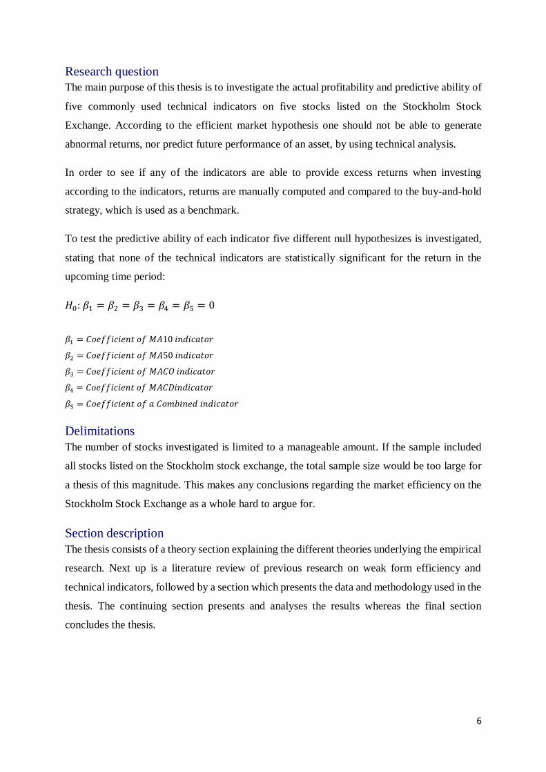
This subsection describes the data that is examined in this thesis. Weekly closing prices of the
five following stocks have been extracted from Bloomberg:
Sandvik AB - A Swedish high-technology engineering company.
AB Volvo - A Swedish manufacturing company.
Telia Company AB - A Swedish telephone company and mobile network operator.
Investor AB - A Swedish investment firm
Nordea Bank AB - A Nordic financial institution.
Time series data is collected in chronological order from the first of January 2010 until eleventh
of March 2016, which equals 324 observations for each stock. All historical prices have been
adjusted for dividends. If prices were not adjusted for dividends, this would affect the return of
the stock, thus resulting in an incomplete picture of the indicators performance.
Methodology
This subsection describes the methodology for how the research is conducted. Firstly the rule
of how a buy- or sell signal is produced will be explained. Afterwards the econometric model
will be specified along with the examined hypothesis. The last section describes how different
assumptions, which are mentioned in the theory section, will be dealt with.
As discussed in the theory section, whether an indicator is statistically significant will be
determined through OLS-regression. Also, a comparison in return between the buy-and-hold
strategy and trading according to the indicators will be made. When an indicator triggers a buy
signal, the stock will be bought at the start of the upcoming period and held until a sell signal
is produced.
While not invested in stocks, a risk-free asset is bought. The risk-free rate is assumed to be 2%
annually, which might seem high as interest rates in Sweden are currently relatively low.
However, even though Sweden still has historically low interest rates, Avanza Bank and Klarna
still offers a 1,2% risk-free rate, as the Swedish government guarantees deposits up to 100 000
euros (Riksgälden 2016). If the risk-free rate is averaged out over the years when the data is
gathered from, an annual rate of 2% is a fair interpretation.

17
The fictitious portfolio will always be fully invested, whether a stock or risk-free asset is held,
which allows for compounding returns. Total return is described with the following formula,
which is also how Han et al. (2013) conducted their study;
𝑅𝑡𝑜𝑡𝑎𝑙 = 𝑅𝑠,𝑡 + 𝑅𝑓,𝑡 (13)
𝑅𝑡𝑜𝑡𝑎𝑙 = 𝑇𝑜𝑡𝑎𝑙 𝑟𝑒𝑡𝑢𝑟𝑛 𝑑𝑢𝑟𝑖𝑛𝑔 𝑔𝑖𝑣𝑒𝑛 𝑡𝑖𝑚𝑒 𝑝𝑒𝑟𝑖𝑜𝑑
𝑅𝑠,𝑡 = 𝑅𝑒𝑡𝑢𝑟𝑛 𝑓𝑟𝑜𝑚 𝑑𝑎𝑦𝑠 𝑡 𝑤ℎ𝑒𝑟𝑒 𝑡ℎ𝑒 𝑠𝑡𝑜𝑐𝑘 𝑖𝑠 ℎ𝑒𝑙𝑑 𝑢𝑝𝑜𝑛 𝑎 𝑏𝑢𝑦 𝑠𝑖𝑔𝑛𝑎𝑙
𝑅𝑓,𝑡 = 𝑅𝑒𝑡𝑢𝑟𝑛 𝑓𝑟𝑜𝑚 𝑑𝑎𝑦𝑠 𝑡 𝑤ℎ𝑒𝑟𝑒 𝑟𝑖𝑠𝑘 𝑓𝑟𝑒𝑒 𝑎𝑠𝑠𝑒𝑡 𝑖𝑠 ℎ𝑒𝑙𝑑 𝑢𝑝𝑜𝑛 𝑎 𝑠𝑒𝑙𝑙 𝑠𝑖𝑔𝑛𝑎𝑙
Similar to previous research this thesis primarily focuses on a comparison in return between
𝑅𝑡𝑜𝑡𝑎𝑙 and the buy-and-hold strategy i.e. holding the asset during the whole time period. The
performance of the underlying asset versus the “market” is of less interest.
Trading rules
The indicators used in this thesis has found to gain excess returns on different markets in several
previous studies, thus making it interesting if the same strategy can be applied on the Stockholm
Stock Exchange. An illustration of different signals can be found in the appendix. No “short-
selling” will be done, if the indicator produces a sell signal, the underlying asset will be sold
and rebought upon next buy signal.
Trading rule 1 - Moving Averages
There are numerous ways of how Moving Averages can be used in trading. This thesis will use
it in its most simple form, which is also how Glabadanidis (2015) and Han et al. (2013) found
it profitable on the American stock market. If price close above the Moving Average this
triggers a buy-signal, likewise, if price close below the Moving Average line this will produce
a sell-signal (Glabadanidis 2015, Han et al. 2013). Two different periods, 10 day and 50 day
averages, will be used in this thesis. By using two different lengths this also tests the hypothesis
of Han et al. (2013), stating that using shorter averages increase returns.
𝐵𝑢𝑦 𝑠𝑖𝑔𝑛𝑎𝑙𝑡 = 𝑃𝑟𝑖𝑐𝑒𝑡 > 𝑀𝐴𝑛,𝑡 (14)
𝑆𝑒𝑙𝑙 𝑠𝑖𝑔𝑛𝑎𝑙𝑡 = 𝑃𝑟𝑖𝑐𝑒𝑡 < 𝑀𝐴𝑛,𝑡 (15)

18
Trading rule 2 - Moving Average Cross-Over
This indicator will use a 5-day and 150- average, the lengths which Lento (2008) found had the
best forecasting ability for future pricing. Brock (1992) also names (5/150) as one of the most
popular averages. A buy signal is produced when the 5-day average close above the 150-
average, a sell signal contrariwise.
𝐵𝑢𝑦 𝑠𝑖𝑔𝑛𝑎𝑙𝑡 = 𝑀𝐴(5)𝑡 > 𝑀𝐴(150)𝑡 (16)
𝑆𝑒𝑙𝑙 𝑠𝑖𝑔𝑛𝑎𝑙𝑡 = 𝑀𝐴(5)𝑡 < 𝑀𝐴(150)𝑡 (17)
Trading rule 3 - Moving Average Convergence Divergence
This indicator will consist of a 12-day and 26 day exponential moving average. These averages
are the most commonly used when computing Moving Average Convergence Divergence line
(Chong 2008, Rosillo et al. 2013). As discussed in the theory section a signal line will be used
and calculated from a 9-day average, which is how (Rosillo et al. 2013) conducted their
research. A buy signal is produced when the Moving Average Convergence Divergence line
close above the signal line:
𝐵𝑢𝑦𝑡 = 𝑀𝐴𝐶𝐷𝑡 > 𝑆𝑖𝑔𝑛𝑎𝑙𝑡 (18)
𝑆𝑒𝑙𝑙𝑡 = 𝑀𝐴𝐶𝐷𝑡 < 𝑆𝑖𝑔𝑛𝑎𝑙𝑡 (19)
Trading rule 4 - Combined indicator
This indicator will only trigger a buy signal when all of the previously described indicators
produce buy signals.
𝐵𝑢𝑦𝑡 = 𝑋1 + 𝑋2 + 𝑋3 + 𝑋4 = 4 (20)
𝑆𝑒𝑙𝑙𝑡 = 𝑋1 + 𝑋2 + 𝑋3 + 𝑋4 < 4 (21)
Trading rule 5 – Buy-and-hold
The stock is bought in the first week of January 2010 and sold in March 2016. Returns are
computed as the result of the entire period.
Transaction costs
To determine whether an investment strategy is profitable, transaction costs have to be
considered. A highly competitive stockbroker market has led to relative small transaction costs.

19
For example (pricing information taken from Avanza Bank), if each trade is made with an
amount of 1 000 000 SEK the transaction fee will be 99 SEK, which translates to around 0,01%.
A transaction fee is paid both when buying and selling the asset. When calculating and adjusting
returns for transaction costs, a fictitious portfolio of 1 000 000 SEK is assumed.
Risk
By holding an asset, of which the performance over a given time period is uncertain, the investor
is exposed to risk. The amount of risk carried by the asset affects pricing. If an investor is
exposed to a high amount of risk, the investor also expects an increase in return.
This thesis examines and compares the performance of different trading strategies used on the
same stock. Since the same asset will be traded regardless of which strategy implemented, the
risk can only be managed by holding the asset during a shorter period. When buying according
to the buy-and-hold strategy, the investor is exposed to risk during the whole period, since only
the risky asset i.e. the specific stock, is bought and held on to. If the same return can be
accomplished through buying and selling the asset, thus reducing the time where the asset is
held, it reduces the risk exposure. This makes it hard to compare risk-adjusted returns when
using the buy-and-hold strategy compared to others, as this strategy exposes the investor to a
higher amount of risk.
If average return per invested week of the stock is calculated, this accounts for risk exposure as
the time period is constant and same for each strategy. On average, this way of computing
returns, leads to the same amount of risk exposure of each strategy, thus enabling a fair
comparison of return.
Econometric model specification
An OLS-regression is used to analyze whether the different indicators are statistically
significant for return in the upcoming period. A simple regression model is used, where the
indicators is used as explanatory variables of return in the following period for each stock. The
simple model regression is used since the individual performance of each indicator is examined.
If the regression were to include all indicators as dummy variables in the same model this would
make them dependent of each other. The regression is computed as following:

20
𝑅𝑒𝑡𝑢𝑟𝑛𝑡+1 = 𝛽0 + 𝛽1,𝑡𝑋1,𝑡 + 𝑈𝑡 (22)
For each stock five regressions are done where 𝑋1 is the regressor of the examined indicator.
𝑋1 takes a value of “1”, when a buy signal is triggered, and “0” if a sell signal is produced.
Hypothesis
This thesis examines five different null hypothesis, which states that none of the indicators are
statistically significant for return in the upcoming period:
𝐻0: 𝛽1 = 𝛽2 = 𝛽3 = 𝛽4 = 𝛽5 = 0
𝛽1 = 𝐶𝑜𝑒𝑓𝑓𝑖𝑐𝑖𝑒𝑛𝑡 𝑜𝑓 𝑀𝐴10 𝑖𝑛𝑑𝑖𝑐𝑎𝑡𝑜𝑟
𝛽2 = 𝐶𝑜𝑒𝑓𝑓𝑖𝑐𝑖𝑒𝑛𝑡 𝑜𝑓 𝑀𝐴50 𝑖𝑛𝑑𝑖𝑐𝑎𝑡𝑜𝑟
𝛽3 = 𝐶𝑜𝑒𝑓𝑓𝑖𝑐𝑖𝑒𝑛𝑡 𝑜𝑓 𝑀𝐴𝐶𝑂 𝑖𝑛𝑑𝑖𝑐𝑎𝑡𝑜𝑟
𝛽4 = 𝐶𝑜𝑒𝑓𝑓𝑖𝑐𝑖𝑒𝑛𝑡 𝑜𝑓 𝑀𝐴𝐶𝐷𝑖𝑛𝑑𝑖𝑐𝑎𝑡𝑜𝑟
𝛽5 = 𝐶𝑜𝑒𝑓𝑓𝑖𝑐𝑖𝑒𝑛𝑡 𝑜𝑓 𝑎 𝐶𝑜𝑚𝑏𝑖𝑛𝑒𝑑 𝑖𝑛𝑑𝑖𝑐𝑎𝑡𝑜𝑟
Significance levels of either 10% or 5% will be assumed to determine the individual
significance of the indicators.
Assumption tests
This subsection discusses the assumptions that require to be tested for, and how it is done, to
achieve a constant and unbiased regressor. A significance level of 5% will be used to possibly
reject the null hypothesis stated by the used tests.
Breusch-Godfrey
The Breusch-Godfrey test is used to test for serial correlation in the error term. The given null
hypothesis states that there is no serial correlation. If rejected, robust standard errors is used in
the OLS-regression (Wooldridge 2014)
Breusch-Pagan/Cook-Weisberg
The Breusch-Pagan/Cook-Weisberg test is used to test for heteroscedasticity. The given null
hypothesis states that the error term is normally distributed. If rejected, robust standard errors
is used in the OLS-regression (Wooldridge 2014).

21
Endogeneity
To test whether the model suffers from endogeneity the Durbin-Wu-Hausman test is used. The
given null hypothesis states that the examined variable is uninformative about the error term. If
this null-hypothesis were rejected this could indicate that the variable was endogenous. The test
fails to reject the null-hypothesis in every regression conducted, so no endogeneity problems
are assumed (Wooldridge 2014).
Highly persistent variables
To check whether the dependent variable is highly persistent the first order autocorrelation is
tested. The correlation between the return variable and a lagged form of this variable is
calculated. If the correlation exceeds 0.9 the variable is considered highly persistent
(Wooldridge 2014).
Trend
Whether the data contain a trend can be observed by including a time variable in the regressor.
The data is first set in chronologic order. Afterwards, a new variable is defined as time period,
ranging between 1 and 324, and included in the regression. The variable is then observed as
either significant or not. If the latter were the case the data would not contain a trend, therefore
the time variable would not be included in the regression (Wooldridge 2014).

22
Results
This section is divided into individual- and aggregated results. In the first subsection results
obtained from each individual indicator is presented. Outputs generated by each OLS-
regression is displayed in tables, along with manually computed return data gained when
investing according to the different strategies. Results for each stock, gained from the buy-and-
hold strategy, will be used as a benchmark and compared to returns gained from investing
according to the indicators.
All returns have been adjusted for transaction costs. When adjusting returns a portfolio of
1 000 000 SEK is assumed. As mentioned in the methodology section, mainly the average
return per week invested of each strategy, has been compared. This is the only comparison in
terms of returns that can be fairly interpreted as the risk exposure of the examined investment
strategy is assumed on average, to be equal.
The tables will also include some of the different assumptions that are presented in the Theory
section. If any of the assumptions has failed, it has been handled as described in the
methodology section. None of the regressions has found any variable to be highly persistent,
suffer from endogeneity nor contain a trend in the dependent variable. Therefore, the additional
assumptions of whether the data contains a trend, endogeneity or highly persistent variables
have been excluded in the tables. The last subsection will discuss aggregated results along with
an answer to the examined hypothesis.

23
Individual results
Table 1: Results 10-Day Moving Average indicator
Sandvik Volvo Telia Investor Nordea
β-value -0,0080384 -0,0017043 -0,0062285 -0,0000637 -0,0017512
P-value 0,101 0,726 0,027** 0,985 0,645
Return (B&H) 13,3% 66,6% 15,9% 168,1% 58,0%
Avg.R/Week (B&H) 0,04% 0,21% 0,05% 0,52% 0,18%
Return -40,0% 26,5% -28,2% 102,2% 27,1%
Avg.R/week -0,24% 0,16% -0,16% 0,52% 0,15%
Weeks invested 164 165 179 196 180
# Trades 138 120 134 114 122
Heteroscedasticity No No No Yes No
Serial Correlation Yes No No No No
Notes: Results from 10-day Moving Average indicator where Return (B&H) denotes the total return, when holding the
stock during the time period and Return denotes total return if investing according to the indicator during the time period.
Avg.R/week (B&H) is the average return per week invested according to the Buy and Hold strategy, whereas Avg.R/week
is the average return per week invested according to the indicator. # Trades is the number of trades conducted if investing
according to the indicator. Results from OLS regression: 𝑅𝑒𝑡𝑢𝑟𝑛𝑡+1 = 𝛽0 + 𝛽1𝑀𝐴10 + 𝑈𝑡 where ** = 5 % significance
level, * = 10 % significance level
As shown in Table 1 the 10-Day Moving Average, at a 5% significance level, fails to predict
the return for the following period for all stocks except Telia. The Telia stock shows significant
results although with a negative β-value meaning one can, keeping everything else
constant, on average expect a negative return when investing upon given buy signal by the 10-
Day moving average. The Sandvik stock is very close to be statistically significant, at a 10%
significance level, also with a negative β-value. The result shows that the average return per
week for the Buy and Hold strategy outperforms investing according to the 10-day Moving
Average for all stock except Investor, where it equals average return per week. Trading
according to the 10-day Moving Average strategy will result in the highest total amount of
trades, resulting in relatively large transaction costs, compared to all other indicators used in
this thesis.

24
Table 2: Results 50-Day Moving Average indicator
Sandvik Volvo Telia Investor Nordea
β-value -0,0065303
0,0046966
-0,0038583
-0,0041746
-0,0037525
P-value 0,184
0,337
0,175
0,296
0,335
Return (B&H) 13,3% 66,6% 15,9% 168,1% 58,0%
Avg.R/week (B&H) 0,04% 0,21% 0,05% 0,52% 0,18%
Return -31,2% 87,6% -8,9% 68,0% 8,3%
Avg.R/week -0,19% 0,49% -0,05% 0,31% 0,05%
Weeks invested 164 180 172 220 177
# Trades 76 42 60 56 56
Heteroscedasticity Yes No No Yes Yes
Serial Correlation Yes No Yes No No
Notes: Results from 50-day Moving Average indicator where Return (B&H) denotes the total return, when holding the
stock during the time period and Return denotes total return if investing according to the indicator during the time period.
Avg.R/week (B&H) is the average return per week invested according to the Buy and Hold strategy, whereas Avg.R/week
is the average return per week invested according to the indicator. # Trades is the number of trades conducted if investing
according to the indicator. Results from OLS regression: 𝑅𝑒𝑡𝑢𝑟𝑛𝑡+1 = 𝛽0 + 𝛽1𝑀𝐴50 + 𝑈𝑡 where ** = 5 % significance
level, * = 10 % significance level
As shown in Table 2 the 50-Day Moving Average, at 5% significance level, fails to predict
return in the upcoming period for all stocks, similar to the 10-Day Moving Average. The
indicator is found to be statistically insignificant for all stocks during the examined time period,
which implies that the predictive power of return in the upcoming period is poor.
When investing according to the 50-day Moving Average one could on average expect excess
returns, compared to the buy-and-hold strategy when trading the Volvo stock. In all other cases
the buy-and-hold strategy outperforms the 50-day Moving Average indicator.

25
Table 3: Results Moving Average Cross-Over indicator
Sandvik Volvo Telia Investor Nordea
β-value -0,0027950
-0,0012964
-0,0048433
-0,0037710
-0,0040972
P-value 0,585
0,803
0,115
0,421
0,356
Return (B&H) 13,3% 66,6% 15,9% 168,1% 58,0%
Avg.R/week (B&H) 0,04% 0,21% 0,05% 0,52% 0,18%
Return 2,3% 44,7% -13,9% 92,6% 15,9%
Avg.R/week 0,01% 0,23% -0,07% 0,37% 0,08%
Weeks invested 178 193 200 251 207
# Trades 32 24 34 20 32
Heteroscedasticity Yes Yes Yes Yes Yes
Serial Correlation Yes No Yes No No
Notes: Results from Moving Average Cross-Over indicator where Return (B&H) denotes the total return, when holding
the stock during the time period and Return denotes total return if investing according to the indicator during the time
period. Avg.R/week (B&H) is the average return per week invested according to the Buy and Hold strategy, whereas
Avg.R/week is the average return per week invested according to the indicator. # Trades is the number of trades conducted
if investing according to the indicator. Results from OLS regression: 𝑅𝑒𝑡𝑢𝑟𝑛𝑡+1 = 𝛽0 + 𝛽1𝑀𝐴𝐶𝑂 + 𝑈𝑡 where ** = 5 %
significance level, * = 10 % significance level
As shown in Table 3 the Moving Average Cross-Over, at a 5% significance level, fails to predict
return in the upcoming period for all stocks. The indicator is found to be statistically
insignificant for all stocks during the examined time period, which implies that the predictive
power of return in the upcoming period is poor. However, the 50-Day Moving Average shows
that investing according to the Moving Average Cross-Over provides excess return, on average
when trading the Volvo stock, compared to the buy-and-hold strategy. This is in line with the
results from the 50-Day Moving Average indicator. In all other cases, the buy-and-hold strategy
outperforms the Moving Average Cross-Over indicator.

26
Table 4: Results Moving Average Convergence Divergence indicator
Sandvik Volvo Telia Investor Nordea
β-value 0,0006664
0,0022592 -0,0049441 0,0010251 -0,0018681
P-value 0,892 0,642 0,078* 0,753 0,621
Return (B&H) 13,3% 66,6% 15,9% 168,1% 58,0%
Avg.R/week (B&H) 0,04% 0,21% 0,05% 0,52% 0,18%
Return 17,8% 78,2% -20,3% 102,0% 30,0%
Avg.R/week 0,11% 0,48% -0,13% 0,62% 0,18%
Weeks invested 157 162 161 165 166
# Trades 94 96 108 100 102
Heteroscedasticity No No Yes Yes No
Serial Correlation Yes No No No No
Notes: Results from Moving Average Convergence Divergence indicator where Return (B&H) denotes the total return,
when holding the stock during the time period and Return denotes total return if investing according to the indicator during
the time period. Avg.R/week (B&H) is the average return per week invested according to the Buy and Hold strategy,
whereas Avg.R/week is the average return per week invested according to the indicator. # Trades is the number of trades
conducted if investing according to the indicator. Results from OLS regression: 𝑅𝑒𝑡𝑢𝑟𝑛𝑡+1 = 𝛽0 + 𝛽1𝑀𝐴𝐶𝐷 + 𝑈𝑡 where
** = 5 % significance level, * = 10 % significance level
As shown in Table 4 the Moving Average Convergence Divergence, at a 5% significance level,
fails to predict return in the upcoming period for all stocks. The indicator is found to be
statistically insignificant for all stocks during the examined time period, which implies that the
predictive power of return in the upcoming period is poor. The indicator is significant when
using on the Telia stock, at a 10% significant level, although a negative β-value which implies
that when investing in the Telia stock upon given buy signal one can on average, keeping
everything else constant, expect a negative return in the upcoming period.
Overall the return gained when investing according to the Moving Average Convergence
Divergence is higher per invested week for Sandvik, Volvo and Investor, with an equal average
return per week invested for Nordea. The Telia stock here once again proves to have a negative
return per invested week when using the trading strategy for the indicator.
27
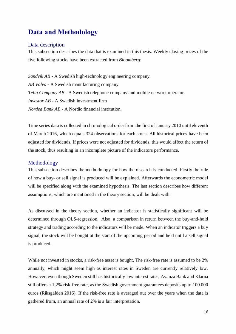
Table 5: Results Combined indicator
Sandvik Volvo Telia Investor Nordea
β-value -0,0012418 0,0010423 -0,0002862 0,0008383 0,0021895
P-value 0,815 0,853 0,917 0,781 0,548
Return (B&H) 13,3% 66,6% 15,9% 168,1% 58,0%
Avg.R/week (B&H) 0,04% 0,21% 0,05% 0,52% 0,18%
Return 8,4% 36,5% 14,70% 74,26% 3,49%
Avg.R/week 0,12% 0,46% 0,19% 0,65% 0,04%
Weeks invested 70 80 79 114 86
# Trades 64 66 66 88 66
Heteroscedasticity No No Yes Yes Yes
Serial Correlation Yes No Yes No No
Notes: Results from the Combined indicator where Return (B&H) denotes the total return, when holding the stock during
the time period and Return denotes total return if investing according to the indicator during the time period. Avg.R/week
(B&H) is the average return per week invested according to the Buy and Hold strategy, whereas Avg.R/week is the average
return per week invested according to the indicator. # Trades is the number of trades conducted if investing according to
the indicator. Results from OLS regression: 𝑅𝑒𝑡𝑢𝑟𝑛𝑡+1 = 𝛽0 + 𝛽1𝐶𝑜𝑚𝑏𝑖𝑛𝑒𝑑 + 𝑈𝑡 where ** = 5 % significance level, * =
10 % significance level
As shown in Table 5 the Combined indicator, at a 5% significance level, fails to predict return
of the upcoming period for all stocks. The indicator is found to be statistically insignificant for
all stocks during the examined time period, which implies that the predictive power of return in
the upcoming period is poor. The manually computed results find that trading according to the
Combined indicator provides excess returns per week invested for Sandvik, Volvo, Telia and
Investor compared to the buy-and-hold strategy. The buy-and-hold strategy outperforms usage
of the indicator when trading the Nordea stock.

28
Aggregated results
As shown in previous tables the predictive ability of the indicators are overall quite poor. The
indicators found to be statistically insignificant for the majority of the stocks examined. When
the indicator proved to be statistically significant, the β-value was negative. Even though these
findings could be useful if an investor were to short-sell a stock, one should never generate a
hypothesis after analyzing a set of data. The hypothesis should be formulated before conducting
the study, and since the methodology of this research ignores short-selling, this possibility will
not be analyzed.
On the few occasions where the null-hypothesis is rejected, which might imply that the indicator
can predict a return in the upcoming period, there does not seem to exist any pattern. Even
though the Telia stock is statistically significant twice, this is when using two different
indicators. When several OLS-regressions are conducted with the same explanatory variables,
and as in this research found to be statistically significant in only one of the regressions, this
could indicate that the rejection of the null-hypothesis might be a type-1 error. A type-1 error
occurs when one incorrectly rejects a true null hypothesis, which could lead to a false
conclusion being made. If using a 5% significance level, this also indicates that there is a 5%
risk that the null-hypothesis is falsely rejected. Therefore, when many similar OLS-regressions
are conducted without any pattern in the rejection of the null-hypothesis, as in this research, the
results have to be interpreted with caution.
As mentioned in the literature review, Lento (2008) found that the Moving Average Cross-Over
had poor predictive ability when interpreting signals according to the Variable Length Moving
Average rule. While Lento (2008) did not test the performance of all indicators that are
examined in this thesis, his conclusion is in line with results obtained from this research.
When analyzing returns from investing according to produced signals, unlike the predictive
ability, the performance differs a lot between the indicators. When investing according to the
Moving Average and Moving Average Cross Over indicators the buy-and-hold strategy
outperforms both in terms of total return and average return per week on all stocks with a few
exceptions. This contradicts the research done by Brock (1992), Glabadanidis (2015), and Han
et al (2013), who all found that the Moving Average and Moving Average Cross Over indicators
constantly provided excess returns. As there was no significant difference in return between the

29
two different Moving Average lengths, this also contradicts the findings of Han et al. (2013),
which states that using shorter average lengths increase return. These results are in line with the
conclusion made by Ellis and Parbery (2005) who, while using a different average length, found
that the Moving Average could not be used to outperform the buy-and-hold strategy.
The Moving Average Convergence Divergence seems to perform quite well when calculated
as average return per invested week. The indicator outperformed the buy-and-hold strategy on
three stocks and had equal return when trading the Nordea stock. Results that are in line with
the research made by Chong and Ng (2008), although they tested the indicator on the London
Stock Exchange. The indicator seems to perform better at the stocks used in this research,
compared to the asset examined in the research done by Rosillo et al. (2013) and Chong et al.
(2014). Of all five examined indicators, the Combined indicator found to be most profitable. It
outperformed the buy-and-hold strategy on four out of five stocks. Tanaka-Yamawaki and
Tokuoka (2007) found that the Moving Average Convergence Divergence indicator could be
combined with other indicators to provide additional predictive ability. Inspired by their
research, the results of this thesis suggests that the combination of Moving Average
Convergence Divergence along with other indicators could not increase predictive ability, but
instead generate abnormal returns.
When comparing returns between the stocks, the Volvo stock stands out. Trading the Volvo
stock according to four of the five examined indicators outperforms the buy-and-hold strategy.
Explanations to why the indicators seem to perform better when trading the Volvo stock is hard
to find. Therefore, the most feasible explanation would be that the result is a coincidence.
At first glance, the rather poor predictive ability of the examined indicators makes it hard to
argue for any kind of weak form inefficiency. However, since both the Moving Average
Convergence Divergence and the Combined indicator provides higher average return per
invested week in the majority of the stocks examined, this questions the statement that any form
of technical analysis is fruitless made by Malkiel (1973) and Bodie et al. (2014).

30
Conclusions
This thesis aims to test whether five commonly used indicators can be used to predict future
returns on five individual stocks listed on the Stockholm Stock Exchange. The research also
questions whether excess returns can be generated when investing according to the indicators.
As a benchmark, in terms of risk and return, the buy-and-hold strategy is used. The predictive
ability of each indicator is examined through an OLS-regression, while returns are manually
computed. Weekly pricing data is gathered and analyzed from 2010 until 2016.
The predictive ability of the technical indicators is quite poor as few of the indicators proves to
be statistically significant and when they are there does not seem to exist any pattern. These
findings support the efficient market hypothesis, as the Stockholm Stock Exchange is
considered a rather well-developed market and is therefore expected to be weak form efficient.
If an indicator were constantly statistically significant at a 5% significance level, this would
indicate that price action could be predicted with a 95% accuracy. If this were the case, traders
would probably exploit this inefficiency instantly according to the efficient market hypothesis.
When computing returns of investing according to the indicators, this seems to question the
efficient market hypothesis. The buy-and-hold strategy outperforms returns, adjusted for
transaction cost, when investing according to the different Moving Average lengths and the
Moving Average Cross-Over. However, the Moving Average Convergence Divergence and
Combined indicator seem to generate abnormal returns. The performance of these two
indicators appears to question the weak form efficiency, which states that previous pricing
information cannot be used to predict future performance of an asset. These contradictory
results, along with the small number of stocks that are examined in this thesis, makes it hard to
argue whether the weak form efficiency holds or not.
As the results of this thesis are ambiguous, further research is suggested on the area. When
testing the predictive ability of indicators, it is recommended that not every signal each day is
acted upon. Both this thesis and Lento (2008) has found that when using the indicators
according to the Variable Length Moving Average, the indicators have no predictive ability.
Instead, the Fixed Length Moving Average rule is recommended.

31
To our knowledge, the Combined indicator, has not been tested on any market before.
Therefore, additional testing of this indicator should be done, both on highly, and less so,
developed markets. The apparent success of the Moving Average Convergence Divergence
indicator should also be investigated further, both on stocks and indices. A recommendation to
increase the accuracy of future research is to divide the gathered data into two different periods.
If an indicator is found to be statistically significant or generates excess returns in both the first
and second time period the credibility of the research would increase.

32
References
Appel, Gerard (2003). Become your own technical analyst: how to identify significant market
turning points using the moving average convergence-divergence indicator or MACD. Journal
of Wealth Management. Summer 2003, vol. 6 Issue 1, page 27.
Bodie, Z., Kane, A., & Marcus, A. J. (2011). Investments. Ninth Edition (International).
McGraw-Hill.
Borges Maria Rosa (2010). Efficient market hypothesis in European stock markets, The
European Journal of Finance, 16:7, page 711-726
Brock, W. A., Lakonishok, J. & LeBaron, B. (1992). Simple technical trading rules and the
stochastic properties of stock returns. Journal of Finance 47, page 1731–1764.
Chong, T.T.-L.; Ng, W.-K.; Liew, V.K.-S. (2014). Revisiting the Performance of MACD and
RSI Oscillators. Journal Risk Financial Management. vol. 7, Issue 1, page 1-12.
Chong,T.T.-L; Ng, W.K. (2008). Technical analysis and the London stock exchange: Testing
the MACD and RSI rules using the FT30. Appl. Econ. Lett. 15, page 1111-1114
Ellis, C.; Parbery, S. (2005). Is smarter better? A comparison of adaptive, and
simple moving average trading strategies. Research in International Business and Finance,
2005, vol.19
Fama. Eugene (1965). The Behavior of Stock-Market Prices. The Journal of Business, vol. 38,
No. 1 (Jan., 1965), page 34-105
Fama. Eugene (1970). Efficient Capital Markets: A Review of Theory and Empirical Work.
Journal of Finance, 1970, vol. 25, issue 2, page 383-417
Glabadanidis (2015). Market timing with moving averages International Review of Finance,
vol.15, Issue 3, page 387-425
Han, Y., K. Yang, and G. Zhou (2013), A New Anomaly: The Cross-Sectional Profitability of
Technical Analysis, Journal of Financial and Quantitative Analysis, 48, page 1433–61.
Kendall. Maurice (1953). The analysis of economic time series, Part 1: Prices. Journal of the
Royal Statistical Society 96, page 11-25
Lento. Camilo (2008). Forecasting Security Returns With Simple Moving Averages,
International Business & Economics Research Journal, vol 7, Issue 11, page 11-22
Malkiel, Burton G. (1973). A Random Walk Down Wall Street (6th ed.). W.W. Norton &
Company
Menkhoff (2010). The use of technical analysis by fund managers: International evidence,
Journal of Banking & Finance 34, page 2573–2586

33
Narasimhan Jegadeesh and Sheridan Titman (1993). Returns to Buying Winners and Selling
Losers: Implications for Stock Market Efficiency. The Journal of Finance, vol. 48, page. 65-91
Park, Cheol-Ho, and Scott H. Irwin. (2007). What Do We Know about the Profitability of
Technical Analysis? Journal of Economic Surveys, page 786–826.
Tanaka-Yamawaki, M.; Tokuoka, S. (2007). Adaptive use of technical indicators for the
prediction of intra-day stock prices. Phys. A, 383, page 125-133
R. Rosillo , D. de la Fuente & J. A. L. Brugos (2013). Technical analysis and the Spanish stock
exchange: testing the RSI, MACD, momentum and stochastic rules using Spanish market
companies. Applied Economics, 45:12, page 1541-1550,
Wooldridge, J. (2014). Introductory Econometrics: EMEA adaptation. First Edition. Cengage
Learning.
Databases
Bloomberg. (2016). Bloomberg. (Online). Available at: Subscription Service (Accessed: 25
Mars 2016)
Riksgälden. (2016). Insättningsgaranti. (Online): Available at:
https://www.riksgalden.se/sv/Insattningsgarantin/Om_Insattningsgarantin/ (Accessed: 2 June
2016)

34
Appendix
Figure 1. Moving Average
Note: Figure 1 is extracted from Bloomberg and illustrates produced buy and sell signals according to the
Moving Average indicator the Volvo B stock
Figure 2. Moving Average Cross-Over
35
Note: Figure 2 is extracted from Bloomberg and illustrates produced buy and sell signals according to the
Moving Average Corss-Over for the Volvo B stock
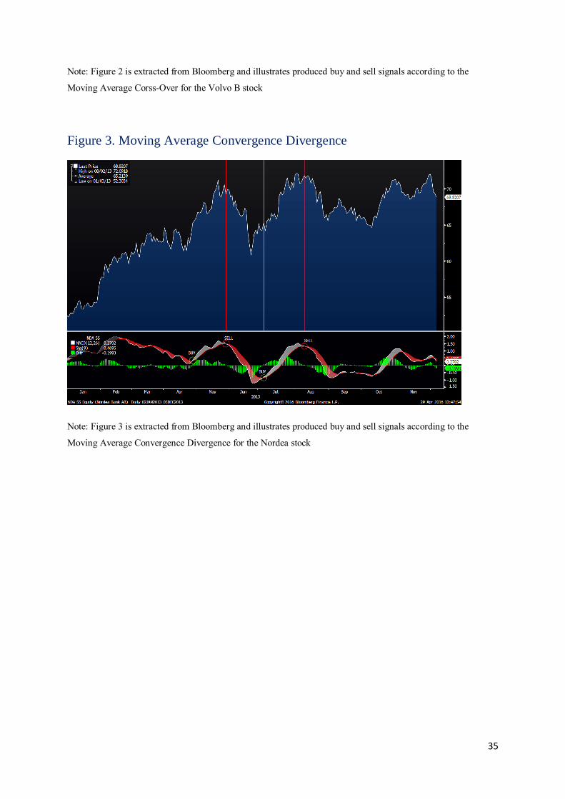
Figure 3. Moving Average Convergence Divergence
Note: Figure 3 is extracted from Bloomberg and illustrates produced buy and sell signals according to the
Moving Average Convergence Divergence for the Nordea stock


![Research Facility Core and Shell...[RESEARCH FACILITY CORE AND SHELL] April 1, 2013 Construction Management | Timothy Maffett ii Technical Analysis 3: Mobile Technology Integration-](https://img.pdfslide.net/doc/110x75/602ada2047710c41016d6094/research-facility-core-and-shell-research-facility-core-and-shell-april-1.jpg)