Embed Size (px)
Citation preview

Technical and economical optimization of surface mining processes – Development
of a data base and a program structure for the computer-based selection and dimensioning of equipment
in surface mining operations
Dissertation
zur Erlangung des Grades
eines Doktor-Ingenieurs
vorgelegt von
M.Sc. Raheb Bagherpour
Aus dem Iran
Genehmigt von der
Fakultät für Energie- und Wirtschaftswissenschaften
der Technischen Universität Clausthal
Tag der mündlichen Prüfung
17.09.2007

Vorsitzende: Prof.Dr. Heike. Y. Schenk-Mathes
Hauptberichterstatter: Prof. Dr.-Ing. habil. H. Tudeshki
Berichterstatter: Prof. Dr.-Ing. Oliver Langefeld

I
Contents
Contents .........................................................................................................................I
Figures List .................................................................................................................. IV
Tables List.................................................................................................................... VI
1 Introduction...................................................................................................1
2 Mining Industry Progresses ........................................................................3 2.1 The History of Mining......................................................................................3 2.2 Mining and Mineral Description ......................................................................4 2.3 Mining Technology Progresses.......................................................................5
3 Mineral Industry ............................................................................................9 3.1 Mineral Production and Consumption.............................................................9 3.2 Mineral Economics .......................................................................................15
4 Mining Stages and Methods ....................................................................19 4.1 Mining Stages...............................................................................................19 4.2 Exploitation ...................................................................................................19 4.3 Surface Mining..............................................................................................21
5 Mining Costs ...............................................................................................22 5.1 Mining Stages Costs.....................................................................................22 5.2 Mining Operation Cycles and Their Costs ....................................................24
6 Materials Handling......................................................................................27 6.1 Materials Handling Operation .......................................................................27 6.2 Principles of Loading and Excavation ...........................................................27 6.3 Selection of Loading Equipments .................................................................29 6.4 Principles of Haulage and Hoisting...............................................................33 6.5 Selection of Haulage and Hoisting Equipments............................................36 6.6 Selection of Materials Handlings Systems in Surface Mining .......................36
7 In-pit Crushing ............................................................................................40 7.1 In-pit Crushing System .................................................................................40 7.2 Mobile Crushers............................................................................................40 7.3 Advantages of Continuous Haulage Methods...............................................41 7.4 Location of Primary Crushers .......................................................................43
8 Cost Estimation in Open Pit Mines ...........................................................51 8.1 Cost Estimation for Operation Cycles ...........................................................51 8.2 Cost Estimation for Loading and Haulage Equipments.................................56

II
8.2.1 Cost Estimation for Bucket Wheel Excavators..............................................57 8.2.2 Cost Estimation for Power Shovel-Trucks Fleet ...........................................61 8.2.3 Cost Estimation for Hydraulic Shovel-Trucks Fleet.......................................66 8.2.4 Cost Estimation for Walking and Crawler Draglines .....................................71 8.2.5 Cost Estimation for Belt Conveyors ..............................................................76 8.2.6 Cost Estimation for Aerial Tramway..............................................................79 8.2.7 Cost Estimation for Scrapers ........................................................................82 8.2.8 Cost Estimation for Mobile Crushers ............................................................87
9 Estimation and Calculation of Size and Number of Loading and Haulage Equipments ...................................................................................................93 9.1 Estimation of Size and Number of Loading and Haulage Equipments..........93 9.2 Calculation of Size and Required Number of Loaders ..................................93 9.3 Calculation of Size and Required Number of Hydraulic Shovel ....................99 9.4 Calculation of Size and Required Number of Power Shovel.......................102 9.5 Calculation of Size and Required Number of Trucks ..................................108 9.6 Reserve Machines ......................................................................................114 9.7 Simultaneous Situation of Loading and Haulage Equipments ....................114
10 Estimation and Calculation of Production Costs for Loading and Haulage Equipments .................................................................................................115 10.1 Estimation of Production Costs for Loading and Haulage Equipments.......115 10.2 Calculation of Production Costs for Loading and Haulage Equipments......115 10.2.1 Capital Costs ..............................................................................................116 10.2.2 Operating Costs..........................................................................................117
10.2.2.1 Energy and Fuel Costs ...............................................................................117
10.2.2.2 Lubrication and Filter Costs ........................................................................119
10.2.2.3 Tire Costs ...................................................................................................119
10.2.2.4 Maintenance and Repair Parts Costs .........................................................119
10.2.2.5 Wear Parts Cost .........................................................................................121
10.2.2.6 Labor Costs ................................................................................................121
10.2.2.7 Total Production Costs ...............................................................................121
11 Conclusion ................................................................................................132
References .................................................................................................................134
Curriculum Vitae........................................................................................................140

III
Summary ....................................................................................................................141
Acknowledgement.....................................................................................................143

IV
Figures List
Figure1 Per capita consumption rate of minerals through the life in Germany (with an average assumption of life of 78 years)...............................................9
Figure 2 Estimated amount of ore production in metal mines........................................11 Figure 3 Trend of mineral and waste production in recent 10 years ..............................12 Figure 4 Estimated amount of materials handling in surface mines...............................13 Figure 5 World wide explorations (based on active sites) for Precious metals and
diamond [34]...........................................................................................15 Figure 6 World wide explorations (based on active sites) for base metals [34] .............16 Figure 7 World wide explorations (based on active sites) for other minerals [34] ..........16 Figure 8 Distribution of costs for relevant activities of production cycle in open pit
mines......................................................................................................25 Figure 9 Distribution of operating costs for relevant activities of production cycle with
considering of in-pit crushing in open pit mines......................................26 Figure 10 Distribution of total capital costs in open pit mines ........................................26 Figure 11 A mobile in- pit crusher [54] ...........................................................................40 Figure 12 A semi-mobile in- pit crusher [54] ..................................................................41 Figure 13 The Nett Present Value (NPV) of costs in both systems in different years
of life of the mine [60] .............................................................................43 Figure 14 Hauling cost in alternative 1 (Horizontal extension of the mine, ore mining
takes place on levels 5 to 13) [64] ..........................................................48 Figure 15 Hauling cost in alternative 2 (Horizontal and vertical extension of the
mine, ore mining takes place on levels 5 to 18)......................................49 Figure 16 Hauling cost in alternative 3 (Vertical extension of the mine, ore mining
takes place on levels 13 to 18) ...............................................................50 Figure 17 Material handling cost in world open pit mines ..............................................54 Figure 18 Materials handling cost in world surface mines .............................................55 Figure 19 Capital costs distribution for bucket wheel excavator ....................................57 Figure 20 Capital costs for bucket wheel excavator upon daily production ...................59 Figure 21 Operating cost for bucket wheel excavators upon daily mine production ......60 Figure 22 Operating costs distribution for bucket wheel excavator................................61 Figure 23 Capital cost distribution upon equipment type for power shovel-trucks
fleet ........................................................................................................62 Figure 24 Operating cost for power shovel –truck fleet upon daily mine production......64 Figure 25 Operating cost distribution upon equipment type for power shovel-trucks
fleet ........................................................................................................65 Figure 26 Total production costs for power shovel-truck shovel up on daily mine
production...............................................................................................66

V
Figure 27 Operating cost for hydraulic shovel –truck fleet upon daily mine production...............................................................................................68
Figure 28 Operating cost distribution upon equipment type for hydraulic shovel-truck fleet ........................................................................................................70
Figure 29 Production cost for hydraulic shovel–trucks fleet upon daily mine production...............................................................................................70
Figure 30 Distribution of capital costs for dragline .........................................................72 Figure 31 Operation cost for walking dragline upon daily mine production....................73 Figure 32 Operation cost for crawler dragline upon daily mine production ....................73 Figure 33 Production cost for walking dragline upon daily mine production ..................76 Figure 34 Operation cost for belt conveyor upon daily mine production ........................78 Figure 35 Production cost for belt conveyor upon daily mine production.......................79 Figure 36 Operating cost for aerial tramway upon daily mine production ......................81 Figure 37 Production cost for aerial tramway upon daily mine production.....................82 Figure 38 Distribution of capital costs for scraper upon type of equipment ...................83 Figure 39 Distribution of equipment operating cost for scraper upon type of
equipment...............................................................................................85 Figure 40 Operating cost for scraper upon daily mine production .................................86 Figure 41 Production cost for scraper upon daily mine production ................................86 Figure 42 Capital cost distributions for mobile crusher ..................................................88 Figure 43 Distribution of operating costs for mobile crusher..........................................90 Figure 44 Operating cost for mobile crusher upon daily mine production......................92 Figure 45 Relevant Algorithm ......................................................................................124 Figure 46 Data’s for loading equipments .....................................................................125 Figure 47 Truck data’s.................................................................................................126 Figure 48 Data’s for cost calculation of loader.............................................................127 Figure 49 Data’s for cost calculation of hydraulic shovel .............................................128 Figure 50 Data’s for cost calculation of power shovel..................................................129 Figure 51 Data’s for cost calculation of trucks .............................................................130 Figure 52 Data’s for calculation of output efficiency ....................................................131

VI
Tables List
Table 1 Human’s uses of mineral [4] ................................................................................3 Table 2 Chronological Development of Mining Technology [4]........................................8 Table 3 Waste/ore ratio for different mining ores [3] & [14] to [31].................................10 Table 4 Estimated amount of mine production (waste and ore) in world surface
mines......................................................................................................14 Table 5 Estimated amount of mine production (waste and ore) in world mines.............14 Table 6 Stages in the life of a mine ...............................................................................20 Table 7 Estimated costs for mining stages ....................................................................22 Table 8 Estimated overall costs for different mining methods [4]...................................23 Table 9 Consumed mining costs for surface mines in recent 5 year .............................24 Table 10 Classification of loading- Excavating Methods and Equipment [4] [75], [75].....28 Table 11 Comparison of features of Shovel, Dragline and Bucket wheel excavator
[4] [75], [75] .............................................................................................31 Table 12 Comparison of open pit loading equipment [4] [75], [75]..................................32 Table 13 Estimating parameters for surface excavators................................................33 Table 14 Classification of haulage and hoisting method and equipment [4] [75], [75] ....34 Table 15 Comparison of features of principal haulage units [4]; [75], [75] .....................35 Table 16 Comparison of materials handling cost for different system [51] ....................38 Table 17 Selecting guidelines for materials handling in surface mining [4] [75] , [51],
[51] [75] ...................................................................................................39 Table 18 Characteristics of model mine [64]..................................................................44 Table 19 Different alternatives in model mine [64].........................................................45 Table 20 Hauling cost in alternative 1 (Horizontal extension of the mine, ore mining
takes place on levels 5 to 13) [64] ..........................................................46 Table 21 Hauling cost in alternative 2 (Horizontal and vertical extension of the mine,
ore mining takes place on levels 5 to 18) [64] ........................................47 Table 22 Hauling cost in alternative 3 (Vertical extension of the mine, ore mining
takes place on levels 13 to 18) [64] ........................................................47 Table 23 Loading and haulage cost in world surface mines (million us. $)....................53 Table 24 Distribution of capital costs for bucket wheel excavator..................................57 Table 25 Distribution of capital costs for power shovel- trucks fleet ..............................61 Table 26 Distribution of operating labor costs for power shovel- truck fleet...................63 Table 27 Operating cost distribution for power shovel- truck fleet .................................65 Table 28 Operating cost distribution for power shovel- truck fleet upon equipment.......65 Table 29 Operating cost distribution for power shovel- truck fleet upon equipment
and cost type ..........................................................................................66

VII
Table 30 Distribution of capital costs for hydraulic shovel- truck fleet............................67 Table 31 Distribution of operating labor costs for hydraulic shovel –truck fleet .............68 Table 32 Operating cost distribution for hydraulic shovel- trucks fleet...........................69 Table 33 Operating cost distribution for hydraulic shovel- trucks fleet upon
equipment...............................................................................................69 Table 34 Operating cost distribution for hydraulic shovel- truck fleet upon equipment
and cost type ..........................................................................................69 Table 35 Distribution of capital costs for dragline ..........................................................71 Table 36 Distribution of operating labor costs for crawler dragline ................................74 Table 37 Distribution of direct operating labor costs for crawler dragline ......................74 Table 38 Distribution of operating labor costs for walking dragline................................74 Table 39 Distribution of direct operating labor costs for walking dragline ......................74 Table 40 Distribution of operating cost for crawler dragline upon type of equipment.....75 Table 41 Distribution of operating cost for waking dragline upon type of equipment .....75 Table 42 Distribution of operating cost upon type of equipment ....................................75 Table 43 Capital cost distribution for belt conveyor upon cost type ...............................77 Table 44 Cost distribution for belt conveyor upon type of equipment ............................77 Table 45 Capital cost distribution for aerial tramway upon cost type .............................80 Table 46 Capital cost distribution for scraper upon type of equipment ..........................83 Table 47 Distribution of operating labor cost for scraper ...............................................84 Table 48 Distribution of direct labor cost for scraper .....................................................84 Table 49 Distribution of equipment operating cost for scraper upon type of
equipment...............................................................................................84 Table 50 Distribution of equipment operating cost for scraper.......................................85 Table 51 Capital cost distributions for mobile crusher ...................................................88 Table 52 Distribution of operating costs for mobile crusher...........................................89 Table 53 Distribution of labor operating cost for mobile crusher....................................90 Table 54 Distribution of equipment operating cost for mobile crusher ...........................92 Table 55 Loader fill factor [80] .......................................................................................94 Table 56 Typical working hours and production data ....................................................95 Table 57 Loader cycle time............................................................................................96 Table 58 Time allowance because of operating bench height [80] ................................96 Table 59 Time allowance because of loaded materials type [80] ..................................97 Table 60 Time allowance because of ground conditions [80] ........................................98 Table 61 Time allowance because of dump conditions [80] ..........................................99 Table 62 Hydraulic shovel fill factor [80] ......................................................................100 Table 63 Hydraulic shovel cycle time [80]....................................................................100 Table 64 Time allowance because of operating bench height [79], [80] ......................101
VIII
Table 65 Time allowance because of loaded materials type [79], [80] ........................101 Table 66 Time allowance because of dump conditions [80] ........................................102 Table 67 Specific weight for different rocks based on bank and loose conditions [80] 104 Table 68 Shovel cycle times (t1 sec) [4], [79], [80].......................................................105 Table 69 Shovel availability upon operation conditions [4], [79], [80] ..........................106 Table 70 Availability in different surface mining methods [4], [79], [80] .......................106 Table 71 Shovel and loader operating efficiency [4], [79], [80] ....................................106 Table 72 Bench and swing angle correction [4], [79], [80] ...........................................107 Table 73 Optimal number of swings used to fill a truck [4], [79], [80]...........................109 Table 74 Bucket fill factor upon operating conditions [4], [79], [80].............................109 Table 75 Manoeuvre and dump times upon operating conditions ...............................110 Table 76 Rolling resistance up on ground conditions of road [80] ...............................111 Table 77 Factors for converting maximum speed to average speed (loaded trucks)
[79] .......................................................................................................112 Table 78 Factors for converting maximum speed to average speed (empty trucks)
[79] .......................................................................................................112 Table 79 Recommended average speeds in loading areas [79]..................................112 Table 80 Recommended maximum downgrade speeds [79].......................................113 Table 81 Operating life of mining equipment [36], [45], [79] ........................................117 Table 82 Energy usage for mining equipment [36], [45] ..............................................118 Table 83 Load factor for fuel usage calculation [36], [45] ............................................118 Table 84 Tire life for mining equipment upon operation conditions [36], [79]...............119 Table 85 Typical repair parts and maintenance factors [36] ........................................120 Table 86 Maintenance factor upon operating conditions [36] ......................................120 Table 87 Output Summary...........................................................................................122 Table 88 Production data’s ..........................................................................................122 Table 89 Capital Costs ................................................................................................123 Table 90 Operating Costs............................................................................................123 Table 91 Production Costs ..........................................................................................124

Introduction
1
1 Introduction
The mining industry is currently faced with constantly increasing capital and operating costs. Thus a need exists to reduce costs where possible. Loading and Haulage costs are natural items to consider, as it can represent up to 50 % of the total mine operating cost. With a brief look to production rate of minerals in worldwide surface mining (more than 67 milliard ton per year) and also spent costs for materials handling (about 100 milliard us. $ per year), it is two times more to have a close attention to this subject. Equipment selection for open-pit mining is definitely a major decision which will impact greatly the economic viability of an operation. On the other hand, equipment selecting is an important and effective item on surface mining production costs. Selection of loading and haulage equipment have a great share of cost price of mineral products (in a way that about % 90 of equipment capital costs and more than % 70 of operating costs in open pit mines is for loading and haulage of materials). In addition; the selection of a system is equally an important problem and could involve many criteria, including the operating conditions and the equipment technical specifications of an open pit stripping. The general equipment selection process involves assessment of the climatic, geological, geotechnical, environmental and ground, site-specific conditions. Furthermore, the equipment selection process implies choosing the types of equipment, the size of equipment and the number of units required to meet a selected production rate. Proper matching of equipment is also inherent to the process. The process involves computations, executed in a logical sequence prescribed by the experienced equipment selection engineer. This is corroborated by the fact that numerous attempts have already been made to develop expert systems applied to equipment selection. The problems thus have greater need for a vast knowledge-base and a chaining process rather than traditional programmable computations. In addition Cost estimation is an intrinsic component of the complete process. In fact, the essential objective is to select equipment which will minimise a specified measure of cost. Therefore the other considerable item is the useful benefit from experimental Tables and relations for considerations and feasibility at the time of prefeasibility studies and determination and selection of loading and haulage equipments. Then it is necessary and so much important to submit such Tables along with relations for different machinery and equipment. Since one of the general and current methods for any materials handling in open pit mines is benefiting from shovel and trucks, one of the reducing ways of costs, is optimization of suitable selection and application of the said equipment by the use of

Introduction
2
computer software. Since most of current software is applied for selection of optimized equipments by manufacturing companies with theoretical aspects of equipments for more marketing and sale and with lack of consideration of applicable and operational items, therefore, all presented numbers and values in Tables of mentioned companies have a great difference with obtained numbers and values in mining operations. Then, providing software for covering all mentioned weak points, consider all said problems, characteristics of deposits and ores, regional and environmental conditions is necessary. In addition, it is necessary to benefit from obtained values and digits out of practical and experimental results at the time of providing the said software. The rising operating costs and declining commodity prices at most properties have forced them to look at various alternatives to cut costs to stay competitive. Haulage costs have been an area that has risen significantly with the increase of diesel prices. One alternative to reduce haulage costs is to shorten the truck haul distance by bringing the truck dump point into the pit. Using an in-pit movable crusher or crushers, and conveying the ore and/or waste out of the pit can reduce the haul costs. The other method for reducing of transportation costs is to benefit from other alternatives instead of truck. Therefore, benefiting from continuous transportation systems (such as conveyors and so on…) along with in-pit crushing or a combination of both methods may have a great effect on reducing the costs. Regarding all above-mentioned items at first a brief description about mining industry and completion process of this industry, different stages and activities and relevant costs of each process in this report is presented, then an estimation of worldwide production rate of minerals and the share of surface mining is submitted. In next step and after a review of material handling systems in surface mines and providing a comparison of them, production costs have been analyzed for any equipment separately and provided different Tables and equations for estimation of operating and production costs of different machinery and equipment. Finally, a software algorithm has been submitted with ability for suitable selection of equipment and estimation of production costs in addition to an exact economic evaluations and analysis.

Mining Industry Progresses
3
2 Mining Industry Progresses
2.1 The History of Mining
After farming, mining is the second activity of primary human begins. Certainly that should be considered these two activities as the primary or mother of industries in human being civilization. In order to explaining the importance of mining in old and new culture, that is enough to mention that nature has provided limited resources for wealth for human being. Mining and farming (including hunting, fishing, and animal husbandry and foresting) are the access ways to the said resources [1]. Mining was a non-separable part of human life from prehistoric times. Here, mining has been used with its greatest meaning as extraction of all natural mineral (solid, liquid and gas) from the earth by the goal of benefiting and removing all human needs. In order to benefit and remove all need, those necessities of human being are required which may obtain only through extraction of minerals from the earth [2] & [3]. Table 1 is about these important needs.
Table 1 Human’s uses of mineral [4]
Need or Use Purpose Age
Tools and Utensils Food, shelter Prehistoric Weapons Hunting, defence, warfare Prehistoric Ornament and decoration Jewery, cosmetics, dye Ancient Currency Monetary exchange Early Structures and devices Shelter, transport Early Energy Heat, power Medieval Machinery Industry Modern Electronics Computers, communications Modern Nuclear fission Power, warfare Modern In fact, most part of cultural ages of human being could be recognized by minerals and their derivations. For example Stone Age (up to 4000 years before Christian), Bronze Age (1500 to 4000 years before Christian) , Iron age (1500 years before Christian up to 1780 ), Steel age (1780 up to 1945) and Atom age (From 1945). Not only we have different ages recognized and known with minerals but in most parts of human history (Travel of Marko polo to China, Marine travel of Wasco dogama to Africa & India, discovering of a new world by Coulomb and attack of gold researchers

Mining Industry Progresses
4
to California, South Africa, Australia and Canada) were also presented as the primary goal and emotion [5]. It is provable that minerals and mining have a close relation with priority of great historical civilizations. In fact, the major factor of interfere and development of Rome Imperator to England and Spain lands, Government of Spain, France and England on Northern & Southern America and African Colonization and some parts of Asia by different European forces was the access to all mineral reserves and resources. There is a different type of modern imperator in the world and in the format of an economic Union (OPEC or Organization of the Petroleum Exporting Countries) for controlling of production and petroleum oil prices and as a sign of the real power of minerals [4].
2.2 Mining and Mineral Description
According to a general classification, there are three groups of economic minerals upon their primary elements and applications [6] and [7]: Metallic ores: including of the ferrous metals (iron, manganese, molybdenum, and tungsten, the base metals (Copper, lead, zinc, and tin), the precious metals (gold, silver, the platinum group metals), and the radioactive minerals (uranium, thorium, and radium). Non-metallic minerals: insulating materials (mica, asbestos), refractory materials (silica, alumina, zircon. Graphite), industrial minerals (barite, gypsum, phosphate, potash, halite, trona, sand gravel, limestone, sulphur, and many others) Fossil fuels: solid fuels (coal, anthracite, lignite, oil shale), fluid fuels (petroleum oil, natural gas) It is important that although petroleum oil extraction is a branch of mining industry, but at present all relevant activities with oil & natural gas extraction would be performed in the formant of a separate industry and with its special technology [4]. Mining is generally described as excavation or creation of a hold from current level of earth to mineral deposit through a corridor. When all extraction operations are completely open or operated on the ground, it is named as surface mining. If excavation consists of openings for human entry below the earth’s it is called underground mining. Some special details of different localization methods and used equipment may cause some differences in different methods of mining. Generally physical, geologic, environmental, and economic conditions and some other limiting items such as legal circumstances have a basic role in determining of mining methods [2].

Mining Industry Progresses
5
Mining could not be considered as a separate and independent activity from other activities. This will be performed after some geological studies and considerations which may determine the place of mine and some economic analysis for confirming of financial aspects. After extraction of ores it is possible to process the extracted product with different methods under a general title of mineral processing. Perhaps the products of this process would be melted or refined in order to have more condensation and supplying of considered products of the buyer under exchanging functions. Marketing is the last step for changing valuable minerals into a useful product [4]. Some times creation of different holes in the ground may be performed for other purpose rather than extraction of minerals such as military and civil works with the goal of excavation of fixed spaces with suitable dimensions, positions and continuation. For example it is possible to name sewer tunnels, underground storage facilities, waste disposal areas, and military installations. Many of these excavations would be performed by means of standard mining technology. Since the goal in such activities is any thing rather than mineral extraction, therefore, there are other conditions and necessities such as time, form and life governing of these items. Generally all working fields of mineral industries have a close relation with other activities with necessary application in this industry. Locating and exploration of a mineral deposit will be placed in general scope of geology and earth sciences. Mining engineering includes different activities such as proving and confirming of reserve (along with geology unit), designing, planning, development and exploitation of mine. Although metallurgy has common extraction with mining engineering, but relevant fields of processing, refinery and melting must be basically considered in scope of work of metallurgy engineering.
2.3 Mining Technology Progresses
Mining as one of the oldest activities of human being (certainly as the first organized activities of human being), has a long-term and respectful history. To follow up completion process of mining technology in parallel with gradual completion of human being and development of civilization is useful for recognition of new activities of mining industries [6]. Mining started with Palaeolithic human beings about last 450000 years. Of course there is no more evidences for proving this idea, but incendiary tools (Flint stone) founded along with the carcass of primary humans of old age, may confirm this claim [8]. All people in Old Stone Age extracted the said stones from the earth and

Mining Industry Progresses
6
formed them through primary construction techniques. At first, the human being found raw mineral materials from the earth, but by the start of Stone Age, he managed to extract in different spaces with a height of 0.60 to 0.90 m and with a depth of more than 9 m [3]. The oldest recognized underground mine is a hematite one located on Bomvu Ridge and belonging to Stone Age. It is believed that it is 40000 years old. Old mining performed under the ground along with primary methods for ground control, ventilation, haulage, hoisting, lighting and rock breakage. There were different mines with a depth of 250 m in early Egypt times [2]. Prehistoric people were so much attracted by metallic ores. At first, they used metals with their free form and probably through washing of river sands in placer deposits. By the way and by the start of bronze and iron ages, human being innovated the melting and its change to minerals of free metals or their alloys forms. In the field of mineral extraction, the first highlighted work of miners was digging them and broken the heavy rock masses into a transportable form. Although they could extract easily soft soils or weak rocks, but their primary tools such as bone, wood or stone were unable to break hard rocks, unless with a track in it and by putting a wedge or breaking the rock. By innovation of fire setting technique, miners were enable to warm and expand the rock and freeze it by cooling it with water. Among all great innovations of human being and the first valuable consequences of mining, art and knowledge of rock breakage has a great importance. There was no other technical progress in the field of mining with such an effect while black powder was applied for the first time for blasting of rock in 17th century. By development of social and cultural systems, mining found more organization. Due to its hard and dangerous nature, most of guilty persons were sent for working in mines and only the engineers and managers were paid. Like all other industries, Mining technology faced with stagnation through dark Ages. The position of miners and situation of mining was changed by a political change in 1185 when bishop of Trent obtained the license of miners in his own scope of authorities and paid the miners similar social rights as other industries something such as any share in extracted minerals. This rule was an important step in mining industry with different consequences for many years up to now. By the ways, Industrial Revolution was the greatest change from the point of view of any need to minerals and benefiting from them in 18th century. It was simultaneous with series increasing of demands and considerable progresses in mining technology especially from scientific and mechanization aspects up to now. These changes had a foundation even up to long-term periods in future. The most important and special progress effective on industries and generally on total civilization has been presented in Table 2. These progresses reached to their peak point by the start of new age of

Mining Industry Progresses
7
mining at beginning of 20th century and with mechanization development and mass production and other pricing techniques and price /costs estimation and the newest one which is computer methods for benefiting from low grade deposits with high reserves [2], [10] and [11].

Mining Industry Progresses
8
Table 2 Chronological Development of Mining Technology [4]
Date Event
450,000 B.C.E First mining (at surface), by Palaeolithic humans for stone implements.
40,000 Surface mining progresses underground, in Swaziland, Africa.
30,000 Fired clay pots used in Czechoslovakia.
18,000 Possible use of gold and copper in native form.
5,000 Fire setting, used by Egyptians to break rock.
4,000 Early use of fabricated metals; start of Bronze Age.
3,400 First recorded mining, of turquoise by Egyptians in Sinai.
3,000 Probable first smelting, of copper with coal by Chinese; first use of iron implements by Egyptians.
2,000 Earliest known gold artifacts in New World, in Peru.
1,000 Steel used by Greeks.
100 C.E Thriving Roman mining industry.
122 Coal used by Romans in present–day United Kingdom.
1185 Edict by bishop of Trent gives rights to miners.
1524 First recorded mining in New World, by Spaniards in Cuba.
1550 First use of lift pump, at Joachimstal, Czechoslovakia.
1556 First mining technical work, De Re Metallica, published in Germany by Georgius Agricola.
1585 Discovery of iron ore in North America, in North Carolina.
1600s Mining commences in eastern United State (iron, coal, lead and gold).
1627 Explosives first used in European mines, in Hungary (possible prior use in China).
1646 First blast furnace installed in North America, in Massachusetts.
1716 First school of mines established, at Joachimstal, Czechoslovakia.
1780 Beginning of Industrial Revolution; pumps are first modern machines used in mines.
1800s Mining progresses in United State; gold rushes help open the west.
1815 Sir Humphrey Davy invents miner’s safety lamp in England.
1855 Bessemer steel process first used, in England.
1867 Dynamite invented by Nobel, applied to mining.
1903
Era of mechanization and mass production opens in U.S. mining with development of first low-grade copper porphyry, in Utah; although the first modern mine was an open pit, subsequent operations were underground as well.
1940 First continuous miner initiate the era of mining without explosives.
1945 Tungsten carbide bits developed by McKenna Metals Company (now Kennametal).
Mineral Industry
9
3 Mineral Industry
3.1 Mineral Production and Consumption
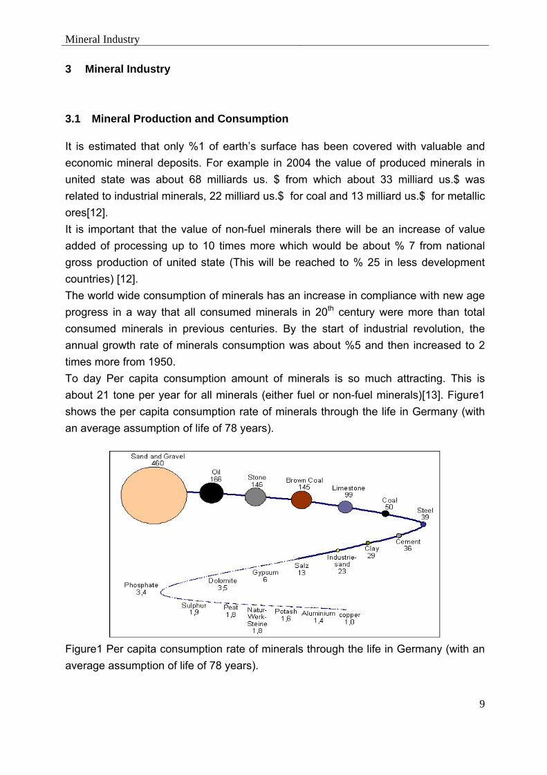
It is estimated that only %1 of earth’s surface has been covered with valuable and economic mineral deposits. For example in 2004 the value of produced minerals in united state was about 68 milliards us. $ from which about 33 milliard us.$ was related to industrial minerals, 22 milliard us.$ for coal and 13 milliard us.$ for metallic ores [12]. It is important that the value of non-fuel minerals there will be an increase of value added of processing up to 10 times more which would be about % 7 from national gross production of united state (This will be reached to % 25 in less development countries) [12]. The world wide consumption of minerals has an increase in compliance with new age progress in a way that all consumed minerals in 20th century were more than total consumed minerals in previous centuries. By the start of industrial revolution, the annual growth rate of minerals consumption was about %5 and then increased to 2 times more from 1950. To day Per capita consumption amount of minerals is so much attracting. This is about 21 tone per year for all minerals (either fuel or non-fuel minerals) [13]. Figure1 shows the per capita consumption rate of minerals through the life in Germany (with an average assumption of life of 78 years).
Figure1 Per capita consumption rate of minerals through the life in Germany (with an average assumption of life of 78 years).

Mineral Industry
10
The estimated amount of production of mineral including of important metallic ores , important non-metallic minerals and also sand and cement in recent 10 years have been mentioned in Table 4 and Table 5 and Figure 2 to Figure 4. The other amounts of non-mentioned minerals in Table 5 and 6 have not been considered due to the low amount of production. In addition, the estimated amounts for 2030 have been mentioned in these Tables. Needless to state that we have benefited from average stripping ratio in open pit mines for calculation of wastes rates of different metallic mines. The wastes amount rate for non-metallic minerals with regard to their lack of access to real amounts, we assumed it 1. All mentioned amounts have been inserted in Table 3.
Table 3 Waste/ore ratio for different mining ores [3] & [14] to [31]
Relevant ores Waste /ore Ratio
Copper ores 2,5
Iron ores 0,8
Lead 4,6
Zinc 5,1
Tin 3,4
Nickel 4,8
Manganese 3,1
Gold 3,3
Platinum and rare earth element 4,4
Uranium 3,4
Non-metallic ores 1
Lignite 3,5
As it is clear in above-mentioned Tables and diagrams, today the total amount of production of minerals (including of metals, non-metallic minerals and coal) is more than 16.6 milliard tone per year for which the share of surface mines are more than 11.5 milliard tones per year. The production rate of construction materials is about 23.5 milliard tone per year and the annual production rate of cement is 2.3 milliard tones. By calculation of wastes amount in surface mines (about 30 milliard tones), the total amount of material handling in surface mines would be more than 67.3 milliard tones in current year and it is estimated to have it as 138 milliard tones in 2030.

Mineral Industry
11
Metall Mines Production
0
2000
4000
6000
8000
10000
12000
14000
16000
18000
20000
1996 1997 1998 1999 2000 2001 2002 2003 2004 2005 2006 2030
Year
Prod
uctio
n ( m
illio
n to
n)
All Mines Open Pit Mines Undergrund Mines O&U Mines
Figure 2 Estimated amount of ore production in metal mines

Mineral Industry
12
Minerals Production
0
2000
4000
6000
8000
10000
12000
14000
16000
18000
1994 1996 1998 2000 2002 2004 2006 2008
year
prod
uctio
n(M
t)
all Mines open pit undergrund open pit&undergrund waste
Figure 3 Trend of mineral and waste production in recent 10 years

Mineral Industry
13
Materials Handling in Surface Mines
0
20000
40000
60000
80000
100000
120000
140000
160000
1996 1997 1998 1999 2000 2001 2002 2003 2004 2005 2006 2030
Year
Mat
eria
ls H
andl
in(m
illio
n to
ns)
total Materials Handling Mineral Waste Costruction Material
Figure 4 Estimated amount of materials handling in surface mines

Mineral Industry
14
Table 4 Estimated amount of mine production (waste and ore) in world surface mines
Ore production 1996 1997 1998 1999 2000 2001 2002 2003 2004 2005 2006 2030
Total mineral -open pit (mt) 7601 7243 8134 8654 9186 9138 9045 9569 10289 10902 11535 20468
Total waste (mt) 20331 19445 21535 22992 24251 24263 24130 25537 27242 28517 29967 54396
Open pit( waste +mineral) (mt) 27932 26687 29670 31646 33437 33401 33174 35105 37531 39419 41502 74864
Total construction material (mt) 17896 18608 20732 21530 21710 22039 22089 22778 24394 24843 25782 62942
Total material handling (mt) (open pit +cement +sand +rock)
45828 45296 50402 53176 55146 55440 55263 57883 61925 64263 67285 137805
Table 5 Estimated amount of mine production (waste and ore) in world mines
Ore production 1996 1997 1998 1999 2000 2001 2002 2003 2004 2005 2006 2030
All metal (mt) 5042 4810 5947 6826 7484 7215 7177 7443 7822 8347 9018 16811
Total non metals (mt) 537 547 536 543 539 532 532 554 574 592 601 1129
Coal mt) 5106 5132 5046 4941 4935 5233 5265 5648 6079 6218 6361 10979
Total mineral (metal +non metal+ coal) (mt) 10818 10613 11706 12500 13164 13205 13191 13874 14848 15700 16587 29369
Cement (mt) 1485 1515 1520 1600 1600 1750 1800 1950 2130 2220 2322 6834
Sand gravel construction (mt) 7815 8140 9149 9491 9576 9662 9662 9918 10602 10773 11172 26718
Crushed rock (mt) 8596 8954 10063 10440 10534 10628 10628 10910 11662 11850 12289 29390
Total waste (mt) 20331 19445 21535 22992 24251 24263 24130 25537 27242 28517 29967 54396

Mineral Industry
15
3.2 Mineral Economics
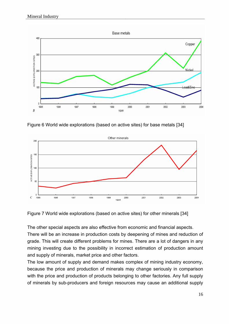
The exclusivity of mineral deposits may create more complexity for economic consideration of minerals and mining. It is impossible to replace the deposits or re-produced them in contrast with agricultural and forest products. It is possible to consider mineral deposits as some perishable assets and any producing activity on them would be limited to some areas created in them. These factors may create different limitations for mining companies from trading works and supplying of financial resources and also producing activities. Since the minerals would be obtained and reduced continuously, and if the mining companies want to remain in trading and working scene, it is necessary to discover new reserves or purchase them. For this purpose, all exploration activities are developing in the world. Figure 5 to Figure 7 show the increase of exploration activities within recent years according to different groups of minerals [32] to [35].
Figure 5 World wide explorations (based on active sites) for Precious metals and diamond [34]
Mineral Industry
16
Figure 6 World wide explorations (based on active sites) for base metals [34]
Figure 7 World wide explorations (based on active sites) for other minerals [34]
The other special aspects are also effective from economic and financial aspects. There will be an increase in production costs by deepening of mines and reduction of grade. This will create different problems for mines. There are a lot of dangers in any mining investing due to the possibility in incorrect estimation of production amount and supply of minerals, market price and other factors. The low amount of supply and demand makes complex of mining industry economy, because the price and production of minerals may change seriously in comparison with the price and production of products belonging to other factories. Any full supply of minerals by sub-producers and foreign resources may cause an additional supply

Mineral Industry
17
that may lead the market toward stagnation. Different types of minerals such as ferrous metals, base metals and precious metals would be returned to production cycle and in other words due to the use of their scraps, they have never been used (Lead is an exception with a % 50 consumption). Scrap warehouses may cause stagnation of market. Some special types of minerals are exempted from economic rules, because their prices would be fixed through governmental approvals or cartels. At present, there is a continuous fluctuation in the price of gold and silver in free markets of the world and all cartels are effective forcefully on the prices of industrial diamond, mercury, oil and tin. Any replacement of some special minerals (for example Aluminium instead of cupper, Plastic instead of metal), may be developed especially if the price of minerals remained in a high level. There is a suitable and estimated pattern for every country in its social and economic development. This pattern is reflecting different discovery, exploitation and ending of minerals reserves and growth or stagnation of mining industries in that country. These periods are as follows [37]: 1- Mine development period: Discovery, finding of new areas, most operating small mines, primary recognition of large deposits and development of large mines, quick increase of metal production. 2- Melting factories development period: Little amount of new discoveries, emptiness of small mines, production increase of large mines and high competence of smelting factories for production of metal 3- Industries development period: Reduction of costs, increasing the life level, quick centralization of wealth in domestic and foreign markets, finding the peak of trading power. 4- Emptiness period of raw materials inside the country: More increase of mining costs and produced minerals, great increase of necessary energy for finding of foreign markets, full domestic market with foreign imports either the raw materials (crude) and manufactured one. 5- Stagnation period of domestic and foreign markets: Increasing the dependence to foreign resources of raw materials may cause an increase of products costs. This period can be characterized bye decreasing the living level along with social problems and political disagreement. All shares, tariffs, governmental helps, cartels and other obtained thoughts would be applied for obtaining a competitive price in domestic and foreign markets. This period is the period of reducing of commercial power in which there will be a reduction in domestic resources. There are so many efforts for finding of cheap foreign resources of raw materials.

Mineral Industry
18
For example in current conditions, most of low-developed countries would be placed in period 1, Australia in period 2, New-independent countries of USSR period 3, USA in period 4 and England in period 5. Some of the economists believe that this cycle may have a slow and smooth process if there is no change and replacement. The last considerable subject in the field of minerals economy is the supply of financial resources of mining plans, similar to supplying methods of financial resources of other commercial and industrial activities. By the way and due to the high risk of financial resources in a mining investment, there is a higher interest rate and shorter capital return period and there would be a suitable marketing for produced minerals. The sale price would be determined generally through a performed estimation and according to the report of concerned engineer or geologist. At the time of calculation of present value of the property, all future incomes would be reduced with daily purchase rate. The mineral deposits would be valuable in case of high enrichment, greatness, easy access, high demand of market, suitable geographical position, low costs of extraction or to be militarily strategic [38] & [39].

Mining Stages and Methods
19
4 Mining Stages and Methods
4.1 Mining Stages
General stages of performed activities in modern mining would be present as different stages of a mine that are: prospecting, exploration, development, exploitation and reclamation. Prospecting and exploration are primary stages of mining that may perform under the title of a unique activity. All geologists and mining engineers have common responsibilities in these two stages (The responsibility of geologists is more in relation to prospecting and the responsibility of mining engineers is more for exploration), development and exploitation are also two related stages to each other. These two stages are considered as the basis stages of mining and as the major works of mining engineering. Table 6 is about brief stages of a mine life. This Table shows a time limit of different activities and costs in addition all stages and procedures for changing a mineral deposit into a mine have been mentioned in this Table.
4.2 Exploitation
In fourth stage of mining that means exploitation there is the real finding of ores in large amounts. Although it is necessary to perform different developing works through the exploitation stage, but the major focus of this stage is centralized production. Development before exploitation is only for ensuring about the start of production and its continuation through the life of the mine. Mining method is basically selected upon specifications of deposit, safety, technical and economic limitations. Different geologic conditions such as the depth and form of deposit, strength of ore and the surrounding rocks have a basic role in selection of mining method. Usual mining methods based upon their situation of ground level would be divided into two wide surface and underground groups. Surface mining methods include mechanical extraction such as open pit mining and open cast mining (strip mining) and aqueous methods. Underground mining has been divided into three great groups each with different methods (supported, unsupported, and caving) [40] & [41].

Mining Stages and Methods
20
Table 6 Stages in the life of a mine
Stage
Procedure
Time(Year)
Cost(Million $) unit cost($ /t)
Precursors to Mining
Prospecting
Search for ore a. Prospecting methods Direct: physical geologic Indirect: geophysical, geochemical b. Located favourable loci(maps, literature, old mines c. Air: aerial photography, airborne, geophysics, satellite d. Surface: ground geophysics, geology e. spot anomaly, analyze, evaluate
1 – 3
0.2 - 10 ( 0.05 – 1.1 )
Exploration
Defining extent and value of ore(examination/evaluation) a. sample (drilling ore excavation), assay, test b. estimate tonnage and grade c. valuate deposit ,present value, feasibility study
2 – 5
1 – 15 ( 0.22 – 1.65 )
Mining proper
Development
Opening up ore deposit for production a. Acquire mining rights(if not done in stage 2)b. file environmental impact statement, technology assessment, permit c. construct access roads, transport system d. locate surface plant, construct facilities e. excavate deposit (strip or sink shaft)
2 – 5
10 – 500 ( 0.275 – 11 )
Exploitation
Large–scale production of ore a. factors in choice of method: geologic, geographic, economic, environmental, societal safety b. types of mining methods: Surface, underground c. monitor costs and economic
10 – 30
5 – 75 ( 2.2 – 165 )

Mining Stages and Methods
21
4.3 Surface Mining
Surface mining is the famous extraction method around the world. For example about % 85 of all minerals, except for petroleum oil and natural gas, would be extracted with this method in America. Generally all metallic ores (% 98) and % 97 of non-metal minerals and % 60 of coals would be extracted in America with surface mining method and most with open pit or strip mining methods [31]. In open pit method which is a mechanical one, all deep and thick deposits would be mined on multi-bench conditions, while any extraction in near-surface deposits would bear only one work bench such as dimensional stones and extraction with strip mining methods. In open pit method, the wastes or overburden would be extracted before or through the extraction. In strip mining method, overburden at first would be removed and then the ore (normally coal) would be mined. The open pit and strip mining methods would be applied for near- surface deposits and deposits with low stripping ratio. This method needs a great amount of investing, but generally it has high productivity and low operating costs and good safety conditions [42] & [43]. Aqueous methods are exclusively based upon the water or other liquids (such as dilute sulphuric acid, weak cyanide solution, or ammonium carbonate) through the extraction processing functions. Placer mining method is used to exploit loosely consolidated deposits such as sand including of heavy metals. Gold, diamond Platinum and tin may be found with placer method. In hydraulic method a high-pressure stream of water currency with high-pressure is directed against the mineral deposit and undercutting it, than erosive action of the water is causing minerals removal. In extraction with floating deposits minerals would be extracted on mechanical or hydraulic of a dredge. Solution mining methods includes of borehole mining methods (such as method used for salt and sulphur extraction) and leaching, either through drill holes or in the dump or heaps on the surface. Placer and solution methods are the most economic mining methods. But they are only useful for limited categories of mineral deposits [21] & [40].

Mining Costs
22
5 Mining Costs
5.1 Mining Stages Costs
Total costs directly used for production of a mine through mentioned five stages of prospecting, exploration, development, exploitation, and reclamation would be named as direct costs of mining. If this quantity to be calculate accordance to a total amount, it would be total costs and if calculated according to the unit one would be named as unit costs ($/t). In addition to direct costs, any indirect costs of mining are overhead costs that may include %5 to %10 for administrative engineering affairs and other omitted or non-estimated services. The total indirect and direct costs of mining will be the costs of mining and on total costs or unit costs basis. If other costs (such as processing, smelting and so on) to be added to the final costs of mining, we will have the final costs of production. By the use of Table 7, it is possible to obtain estimated mining costs including of direct and indirect costs. The range of costs of mining costs is 3 to 180 us.$ /t. The total costs may be changed from 5.6 million to 77 millions us.$ per year for a mine with a general life of 20 years. For determining the final costs of mining, it is necessary to obtain total costs of every stages of mining on total or unit basis [44] & [45].
Table 7 Estimated costs for mining stages
Stage Unit costs ($/t) Total costs (mill. $) Cost share (%)
prospecting 0,50 - 1,10 0,20 to 10 1 to 4
exploration 0,22 - 1,65 1 to 500 1 to 6
development 0,28 - 11,00 10 - to 500 6 to 8
exploitation 2,20 - 165 100 to 1000 65 to 90
reclamation 0,22 - 4,40 1 to 20 2 to 6
total costs 0,50 - 1,10 112 to 1545 100
The estimated mining costs include the direct and indirect costs for different mining methods as mentioned in Table 8.

Mining Costs
23
Table 8 Estimated overall costs for different mining methods [4]
Average Relative cost Range of Absolute Mining cost Mining Method (percent) (us. $/t ) Surface mining Open pit mining 5 2-22 Quarrying 100 28-165 Open cast mining 10 4-22 Hydraulicking 5 2-11 Dredging <5 1-6 Borehole mining 5 2-11 Leaching 10 4-22 Underground mining Room-and- pillar mining 20 11-28 Stope-and-pillar mining 10 6-17 Shrinkage stoping 45 33-77 Sublevel stoping 20 13-39 Cut-and-fill stoping 55 33-77 Stull stoping 70 22-72 Square-set stoping 100 55-165 Longwall mining 15 11-22 Sublevel caving 15 11-33 Block caving 10 6-17 Since obtaining the real costs is a difficult task (The costs values would be considered as the private information of industries owners), therefore there will be a fluctuation in the labor costs and development of technology. It is not so much valuable to remember all digits and items of costs. (In order to update the old costs it is possible to apply current values of costs or indexes of consumer price which may be announced by the government. But the results are estimated in the best conditions). The used costs here have been updated with regard to price indexes. Regarding the production rate of minerals and average amounts mentioned in Table 5, the consumed costs for different stages of mining in surface mines would be as Table 9. Regarding to Table 9, the total yearly mining costs in surface mines is to day more than 138 milliards us.$ from which about 85.6 milliards us.$ is related to metal open pit mines, 7 milliards us.$ for non-metallic open pit mines and 45.8 milliards us.$ for surface coal mines.

Mining Costs
24
Table 9 Consumed mining costs for surface mines in recent 5 year
Mines Type 2000 2001 2002 2003 2004 2005 2006
Metal Mines (mill. us. $) 68427 65787 64439 67713 73022 79160 85629
Nun metal Mines (mill. us. $) 6274 6187 6187 6444 6679 6896 6990
Coal Mines (million us. $) 35532 37677 37910 40668 43766 44772 45802
All open pits mine (mill. us. $) 110233 109651 108535 114825 123467 130828 138421
5.2 Mining Operation Cycles and Their Costs
There are special cycles and operations for digging of rock and transportation of extracted materials which may be named as unit operation of mining. In case these activities have a direct role in extraction of ores, they would be named as production operations. The auxiliary activities may support from main activity of mining but it is not generally a part of production operations, unless it is necessary for safety of worker or the output. Here discussion is more focusing on producing functions that would be applied for development and exploitation stages. All extracted materials through mining have a wide range and include broken or weak strength rocks up to hard rocks (such as: Gabbros, Quartzite, and Taconite). These materials include wastes and ores (or dimensional stones or coal). These materials should be transported after extraction and then to be sent to processing factory, sale or loading dumps or waste dump hills. Therefore, it is necessary to perform two major activities in extraction of mine which are: rock breakage and materials handling. In contrast with weak materials, hard and dense rocks have been broken. Rocks in most of the mines would be broken through drilling and blasting it. Any materials handling would be performed in two steps of loading (or excavation and loading) and haulage. When it is necessary to have a considerable replacement vertically, it is required to have hoisting. All unit operations would be specified with the operating equipment. Toady mining is a complete mechanized operation. The scale of equipments is recognition and specifications of unit operations in surface and underground mining. All used equipment in both methods of mining is similar from both mechanism and operating type. In most of mining methods, as mentioned above, there are four basic activities in production cycles, which include drilling, blasting, loading, and haulage.

Mining Costs
25
Production cycles would be modified if necessary and in compliance with considered conditions. For example the main cycle in extraction of hard rocks (most of metallic and non-metallic minerals would be included in this group) have been used in most surface and underground mining. The only exception is the omission of drilling and blasting in remove of wastes or extraction of ores in those cases in which there are weak wastes or ore (Soil, weathered rocks, placer and so on.). The main cycle (with considering of above-mentioned exception) would be applicable in surface coal mines, in some cases the continuous mining would be replaced with drilling, blasting, and loading operations. Development and promotion of mechanical drilling systems for weak and average rocks and discovery of tunnel boring machines and shaft drilling systems have omitted drilling and blasting from production cycle. Finally, the main cycle has been changed in dimensional stones quarries without blasting and the blocks are often freed from rock mass through wire saws or other mechanical devices [44] to [49]. Any progress of mining industry is really a continuous activity that is in need to applying of both mentioned aspects of more applicable and continuous functions. Distribution of the costs for relevant activities of production cycle in open pit mines would be presented in Figures Figure 8 to Figure 10.
Figure 8 Distribution of costs for relevant activities of production cycle in open pit mines
Mining cost distribution
8%12%
10%
70%
DrillingBlastingLoadingHaulage

Mining Costs
26
Figure 9 Distribution of operating costs for relevant activities of production cycle with considering of in-pit crushing in open pit mines
As it is obvious from these diagrams, the major share of direct costs of mining operations is the costs of loading and haulage from which the most part of costs is %70 related to haulage equipment. In addition, more than % 90 of capital costs in open pit mines is related to loading and haulage equipments.
Mining Equipment Capital Costs
9%
19%
72%
Drilling Equipment Loading Equipment Haulage Equipment
Figure 10 Distribution of total capital costs in open pit mines
Cost distribution with considering of in-pit crushing
8%12% 10%
65%
5%
drilling blasting loading haulage mobile crusher

Materials Handling
27
6 Materials Handling
6.1 Materials Handling Operation
Materials handling means all unit operations of excavating and removing of bulk materials transportation through mining. There are two major activities of loading and haulage in cyclic operations along with hoisting when it is necessary to have vertical transportation of materials. Drilling and blasting steps would be omitted in continuous operations. Excavation and loading would be performed as a single function. In all load-haul-dump (LHD) machines materials handling is performed as a single activity. In new mechanized mines, all materials handling operations would be focused on equipment. Unit operation would be named in accordance with relevant equipment. There is a daily increase of criteria for materials handling equipments in surface mining. The highest rate is (325 T) for trucks, (170 cubic meters) for draglines and (140 cubic meter) for shovels. It is believed that the greatest hand-made moving structures in water and land are bucket wheel excavators used in coal mines. The different reasons for growth of giant equipment in surface mining are their high productivity and low operation costs. A part of this item is due to access possibility to various produces and competition in world trade with standardized production lines and supply of their products with different capacities and dimensions [42].
6.2 Principles of Loading and Excavation
Any extraction and elevation of minerals on broken in place conditions would be named as loading or excavating. If the materials are soil or include of very weak rocks, it is possible to dig them fixedly. Rock formations and compressive soils should be blasted before loading. Table 10 is about a classification of excavating and loading equipment. The basics of this classification include the mining method (surface or underground) and continuity of operation (cyclic or continuous). There are different examples of machines for this purpose. The variety of equipment is so much strange, but there is some special equipment with public application and with easy recognition. Shovel, dragline, loader and scrapper are general machines for surface mining and loaders, LHD machines and continuous miners are common for underground mining.

Materials Handling
28
Table 10 Classification of loading- Excavating Methods and Equipment [4] [75], [75]
Operation Category or
method Machine (application)
Surface Cyclic Continuous Underground Cyclic Continuous
Shovel Dragline Dozer Scraper Blasting Mechanical excavator Highwall mining Hydraulicking Dredging Loader Shaft mucker Self- loading Slusher Continuous miner Baring machine
Power shovel, front-end loader, hydraulic excavator, backhoe (mining ore, stripping overburden) Crawler, walking (stripping overburden) Rubber-tired, crawler(blade) Rubber-tired, crawler Explosives stripping 8overburden) Bucket wheel (BWE) (over burden), cutting – head (soil, coal) Auger, highwall miner (coal) Monitor or giant (placer) Bucket ladder, hydraulic (placer) Overhead, gathering arm, shovel, front-end Clamshell, orange peel, cactus grab Load-haul-dump(LHD) Rope-drawn scraper (metal ore) Milling type, drum, ripper, borer, auger, plow, shearer (coal or non-metallic) Tunnel-boring machine(TBM), roadheader, raise borer, shaft borer(soft rock)

Materials Handling
29
There is a wide application of surface mining equipments (drilling systems, dozers, shovels, trucks, loaders for compliance with operational conditions and safety work in them) in all underground mines with large spaces. Any group of equipments may have special executive specifications that help to separate them from others and considered as a special index in selection of equipments. Some of these equipments may have connected performance of loading and haulage as well. Some examples of loading equipments with major haulage are dozers, rubber- tire scrappers, cable scrappers and LHDs. Most of loaders and excavators are applied in three different working areas (digging, manoeuvre, transportation and dumping) with different executive limitations. The specified situation and limitation is about loading and removing of waste and over burden when boom types excavators (power shovel, dragline or bucket wheel excavator) to be used. When there is an exclusive application of scrappers, dozers or dredges, there will be some other conditions. The major specifications of shovels, draglines and bucket wheel excavators have been inserted in Table 11 Under the title of advantages and disadvantages. The general application of three mentioned machines for loading in surface coal mines needs an exact comparison of them for better selection. This is necessary to mention that there is a little scope of application of bucket wheel excavators in Northern America while there is a wide range of usage of it in Europe. Table 12 is about the application of hydraulic shovels and loaders in open pit mines and according to a similar comparison of power shovels. Today all power shovels are more preferable but betterment of operation of hydraulic shovels and loaders, especially in relation to lifetime of equipment, repairing and maintenance costs and conditions have increased the usage of this machine on a daily basis [41] & [50] to [53].
6.3 Selection of Loading Equipments
There are four groups of effective factors at the time of selecting surface mining loading equipments (Although our discussion is mainly focused on centralized surface mining equipment, but these factors would be applicable with the same correctness and safety in underground mining): 1- Performance factors: These factors are directly related to the productivity of machine and include the cycle speed or loading cycle, accessible energy (electricity), range of manoeuvre for digging, bucket capacity, travels speed and reliability ability for availability of machine for the work or ready times of operating).

Materials Handling
30
2- Designing factors: Designing factors may provide a searching possibility in quality and application of detailed plan including of complexity for facing of operators and repair & maintenance workers, applied technology level and different controls and accessible powers. 3- Support factors: Some times for evaluation of a machine we may benefit from supporting and supplying factors that are the sign of manner and rate of services and repair and maintenance of machines. The important considerations are easy servicing, required special skills, availability and to have access to spare parts and services and supplies of manufacturing factories. 4- Costs factors: Probably this factor is the most qualitative (final) factor. The costs would be defined for mines and construction equipment by the use of standard estimation methods. If different estimation theories such as lifetime, interest rate, inflation, fuel and repair and reasonable maintenance, to be considered, that will be obtained some meaningful and exact results. The general method for determining of costs is the estimation of costs total operating and capital costs all in accordance with ($/hr) and changing them into $/ton or $/m³.

Materials Handling
31
Table 11 Comparison of features of Shovel, Dragline and Bucket wheel excavator [4] [75], [75]
Machine Advantages Disadvantages
Shovel Dragline Bucket Wheel Excavator
1. Lower capital cost per m³ of
bucket capacity, although when boom length or machine weight is considered, the capital costs are roughly equivalent.
2. Digs poor blasts and tougher materials better.
3. Can handle partings well.
1. Flexible operation; easy to move.
2. Large digging depth capability. 3. Can handle a stack overburden
having poor stability. 4. Completely safe from spoil pile
slides or pit flooding during normal operation.
5. High percentage of coal recovery; less coal damage.
6. Will dig a deeper box cut. 7. Low maintenance cost 8. Can handle partings well. 9. Is not affected by an uneven or
rolling coal seam top surface. 10. Can move in any direction.
1. Continuous operation; no
swinging necessary. 2. Long discharge range. 3. Can be operated on a highwall
bench or on the coal seam. 4. Can easily handle spoil with
poor stacking characteristic and poor stability.
5. Can extend range of shovel or dragline when operated in tandem
6. Can facilitate land reclamation as it dumps surface material back on top of the spoil pile.
1. More coal damage can result in lower coal recovery.
2. Susceptible to spoil slides and pit flooding.
3. Cannot easily handle spoil having poor stability.
4. Cannot dig deep box cuts easily.
5. Reduced cover depth capability compared with a dragline of comparable cost.
6. Difficult to move.
1. Requires bench preparation. 2. Does not dig poor blasts well. 3. Higher capital cost per m³ of
bucket capacity, although when boom length or machine weight considered, capital costs are roughly equivalent.
1. Will not dig hard materials. 2. Some surface preparation
required. 3. Lower availability. 4. Large maintenance crew
required. 5. High capital cost compared with
output. 6. Can be susceptible to spoil
slides and flooding. 7. Can cause coal damage with
resulting lower cola recovery. 8. Poor mobility.

Materials Handling
32
Table 12 Comparison of open pit loading equipment [4] [75], [75]
Machine
Advantages
Disadvantages
Rope shovel Hydraulic shovel Front-end loader
1. Proven in hard, dense
rocks. 2. Low operating cost. 3. Less sensitive to poor
maintenance. 4. Operator fatigue not a
serious problem. 5. Low ground pressures. 6. Long lifetime. 1. Excellent breakout
threat. 2. Can mine selectively. 3. High fill factor. 4. Good cleanup capability. 5. Good load placement. 6. Short assembly time. 1. Excellent mobility. 2. Very versatile. 3. Lower capital cost. 4. Can operate on
moderate grades.
1. Lack of mobility. 2. High capital cost. 3. Poor cleanup capability. 4. Will not travel on steep
grades. 5. Affected by
obsolescence.
1. Relatively short lifetime. 2. Relatively high
maintenance. 3. High initial cost.
1. Unsuitable for hard, dense rocks.
2. High tire and operating costs.
3. Digging area must be kept clean.
4. High operator fatigue. 5. Short lifetime.
In order to estimate excavating and loading costs, when there are no real values or information, it is possible to benefit from mentioned information and values in Table 13. In next sections the numerical selection and estimation methods of costs will be discussed.

Materials Handling
33
Table 13 Estimating parameters for surface excavators
Equipment Capacity (m³)
Est. Weight (kg/ m³)
Est. Power (kW/ m³) Est. Life (hr)
Rubber-tired scraper 19 – 41 1840 14 12000 Front-end loader 2.7 – 28 7700 51 12000 Hydraulic excavator 3 – 51 17800 70 30000 Electric power shovel 4.6 – 61 29700 93 75000 Walking dragline 6.9 – 138 105000 73 100000 Bucket-wheel excavator 0.1 – 4 --- --- 30000 It is possible to find executive specifications of large mining excavators or loaders from different resources [41] & [50] to [53].
6.4 Principles of Haulage and Hoisting
All excavated or mined materials in the mine would be replaced or transported through haulage (horizontally) or hoisting (vertically). Some special machines mentioned in Table 14 would be classified similar to loading equipment. All relevant information of (1) general distance of haulage and (2) average operating and maximum applicable gradient, as two important performance parameters of machines applications have been also mentioned in this Table. The major work of all mentioned equipment in Table 14 is transportation, although some of them are loaders in themselves. The only real hoisting equipments are skip and cage. Of course as it is observable in applicable gradient column, all transportation items, may lift the materials along with transportation (Hydraulic conveyors and pneumatic pipes are completely different and without any limitation from distance and work gradient factors). Lifting of materials in all mining activity is a serious and necessary work, because most of mines either under ground or open pit will develop in the depth. The variety of equipment may seem highly from one side but on the other hand there are some other powerful machines as well. Trucks fleet along with shovel has the most application in multi bench surface mines such as open pit mines and in next step there are the conveyors and rubber-tired
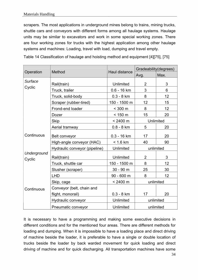
Materials Handling
34
scrapers. The most applications in underground mines belong to trains, mining trucks, shuttle cars and conveyors with different forms among all haulage systems. Haulage units may be similar to excavators and work in some special working zones. There are four working zones for trucks with the highest application among other haulage systems and machines: Loading, travel with load, dumping and travel empty.
Table 14 Classification of haulage and hoisting method and equipment [4] [75], [75]
Gradeability(degrees) Operation Method Haul distance
Avg. Max.
Rail(train) Unlimited 2 3 Truck, trailer 0.6 - 16 km 3 6 Truck, solid-body 0.3 - 8 km 8 12 Scraper (rubber-tired) 150 - 1500 m 12 15 Frond-end loader < 300 m 8 12 Dozer < 150 m 15 20 Skip < 2400 m Unlimited Aerial tramway 0.8 - 8 km 5 20
Belt conveyor 0.3 - 16 km 17 20 High-angle conveyor (HAC) < 1.6 km 40 90 Hydraulic conveyor (pipeline) Unlimited unlimited
Rail(train) Unlimited 2 3 Truck, shuttle car 150 - 1500 m 8 12 Slusher (scraper) 30 - 90 m 25 30 LHD 90 - 600 m 8 12 Skip, cage < 2400 m unlimited Conveyor (belt, chain and flight, monorail) 0.3 - 8 km 17 20 Hydraulic conveyor Unlimited unlimited
Surface Cyclic Continuous Underground Cyclic Continuous Pneumatic conveyor Unlimited unlimited It is necessary to have a programming and making some executive decisions in different conditions and for the mentioned four areas. There are different methods for loading and dumping. When it is impossible to have a loading place and direct driving of machine beside the loader, it is preferable to have a single or double location of trucks beside the loader by back warded movement for quick loading and direct driving of machine and for quick discharging. All transportation machines have some

Materials Handling
35
special working areas which would be analyzed exactly at the time of selecting the method and equipment. Table 15 is about brief major specifications (advantages and disadvantages) of haulage equipment. Most of the said equipments are used both on the surface and underground mines. However, the equipment used in underground mining is often more compact and has less capacity than equipment applied in surface mining [41] & [50] to [53].
Table 15 Comparison of features of principal haulage units [4]; [75], [75]
Machine Advantages Disadvantages
Dozer Truck Scraper (rubber-tired) Rail Belt conveyor
1. Flexible 2. Good gradeability 3. Negotiates rough terrain 1. Handles coarse ,blocky rock 2. moderate gradeability 3. flexible and manoeuvrable 1. Good gradeability 2. flexible and manoeuvrable
1. high Output, low cost 2. unlimited haul distance 3. Handles coarse ,blocky rock
1. high Output, continuous 2. very good gradeability 3. low operation cost
1. limited to short haul 2. discontinuous 3. low Output, slow
1. requires good haul roads 2. slowed by bad weather 3. high operating cost
1. may required push loading 2. limited to soil, small
fragments 3. high operating cost
1. track maintenance costly 2. poor gradeability 3. high investment cost
1. inflexible 2. limited to small or crushed
rock 3. high investment cost

Materials Handling
36
6.5 Selection of Haulage and Hoisting Equipments
All methods and factors in selection of suitable haulage equipment are similar to the relevant methods and factors of excavators with complete description as presented. Since the hoists and relevant equipment are used in vertical shafts (or with high gradient) of underground mines (and a little number of surface mines), therefore, they are some special systems with a partial and ordering designing and in compliance with special methods of selection and localization.
6.6 Selection of Materials Handlings Systems in Surface Mining
Any correct selection of machinery and equipment through the development stage is one of the most important decisions obtained in surface mining. Technical and economical feasibility and safety are major criteria in this section. Selection of equipments for materials handling and their two unit operations (loading and haulage) are generally the first and most important task. The equipment and machinery required for other operations may be followed reasonable from materials handling equipments. Since there is loading and haulage in any production cycle and for wastes removing and extraction of ores in open pit mining, in order to have a clear explanation about process and selection method of equipment, this method has been considered as a sample method among all other surface mining methods. In addition, this method is useful for loading and hauling of coal in strip mining method and different underground mining methods with transportation of materials either waste, coal and ores. In next chapter, different estimation methods of costs will be provided. The general principles and basics for selection of equipment and planning have been resented in previous sections and now the application of the said principles in operating conditions of surface mining to be explained. The considerable point in surface mining is the selection of equipment that is completely depending upon the waste removing method. This is because the materials handling is the basic items (major activity) of surface mining. At the time of selecting a wastes removing method, different factors of relevant equipment and the final purpose of materials handling (wastes, ores) with least possible costs should be considered. This may limit the scope of selecting the method and equipment. By the way, there are some other factors that should be considered and evaluated such as : Geologic structures (faults, folds, shear zones, water bearing areas and so on), alteration areas and materials (the presence of these areas may makes difficult to use any roads and make different problems for processing as well), production rate and life of the mine, the distance of horizontal haulage and vertical

Materials Handling
37
hoisting and any probability to apply special waste removing (stripping) equipment in future (after waste removing in extraction of ores or subsequent mining or reclamation and so on). The geometrical form of pit has great effects on the size and type of equipment along with more effects on their productivity. All major mechanical methods of surface mining may have its own special geometrical form. For example all metallic and non-metallic open pit mines would be planned with various short benches. Strip mines and coal mines include one or more work faces with high walls and in stone mines there is an extraction of one single high bench. Open pit mines would be developed at the time of deepening. Stripe mines have low depth and may progress in the way of parallel or vertical lines with wide stripes. The stone mines have a gradient wall that is possible to be deep. These geometrical differences may reveal that type of equipment may be helpful or may limit the work. As a general rule, the largest applicable equipments are the least and most suitable one from technical, economical and safety aspects in special conditions. It is possible to have some practical limitations (such as mobility) for some large hauling equipment which are useful especially from the point of view of production rate and costs and it seems there are no limitations in this regard for them. From the theoretical point of view in metallic, non- metallic, coal, and stones mines, it is possible to select a great number of equipment and system but in practice there is a little selection for it [41] & [50] to [53]. Followings are three major systems of rock -breakage and six materials handling systems with today general applications: 1- Rock breakage A) There is no need to breakage (soil materials) b) Ploughing and ripping with a dozer (hard soil, weak rocks) c) Drilling and blasting (medium to hard rock formations) 2- Materials handling A) Dragline (direct casting) B) Rope shovel or front-end loader and trucks C) Dozer and front-end loader D) Dozer and rubber-tired scraper E) Front-end loader or shovel in-pit crusher and belt conveyor F) Bucket wheel excavator and belt conveyor Since any selection of rock breakage systems are seriously under the effect of materials properties, there is no need to have any discussions in this regard. Table 17 is a good help for having a good selection of materials handlings systems for wastes removing or extraction (Preparing the work face or working bench are some other

Materials Handling
38
important conditions for a help in selection of equipment). Recently some different waste removing methods have been considered for open pit mining with shovels and trucks and with dozers and scrapers for stone mines. Hoisting-hauling equipments such as hydraulic conveyors and skips have practically limited application. It is difficult to obtain estimated costs for materials handling systems. The following values (Table 16) are useful for materials handling equipment (haulage) obtained from an iron open pit mine with 8.9 km of hauling distances [51].
Table 16 Comparison of materials handling cost for different system [51]
Equipment type Relative capital cost (%) Relative operating cost (%)
Truck 68 100
Train 92 86
Hydraulic conveyor 92 43
Belt conveyor 100 60
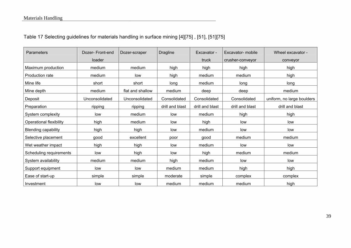
Materials Handling
39
Table 17 Selecting guidelines for materials handling in surface mining [4] [75] , [51], [51] [75]
Parameters
Dozer- Front-end
loader
Dozer-scraper
Dragline
Excavator -
truck
Excavator- mobile
crusher-conveyor
Wheel excavator -
conveyor
Maximum production medium medium high high high high
Production rate medium low high medium medium high
Mine life short short long medium long long
Mine depth medium flat and shallow medium deep deep medium
Deposit Unconsolidated Unconsolidated Consolidated Consolidated Consolidated uniform, no large boulders
Preparation ripping ripping drill and blast drill and blast drill and blast drill and blast
System complexity low medium low medium high high
Operational flexibility high medium low high low low
Blending capability high high low medium low low
Selective placement good excellent poor good medium medium
Wet weather impact high high low medium low low
Scheduling requirements low high low high medium medium
System availability medium medium high medium low low
Support equipment low low medium medium high high
Ease of start-up simple simple moderate simple complex complex
Investment low low medium medium medium high

In-pit Crushing
40
7 In-pit Crushing
7.1 In-pit Crushing System
There is a daily increase in using belt conveyor along with mobile crushers (in-pit crushing) from 1960. Due to positive experiences of conveyors in lignite mines of Germany caused to use from this tool in other surface mines. For this purpose, it is necessary to crush the extracted rocks. Mobile and semi-mobile crushers may crush the rock inside the mine pit. The first modern mobile crushers was used in quarry mine of Limestone in north of Hanover in 1956. Today mobile crushers would be applied widely in different mines with provided suppliers with different equipment [54] to [59].
7.2 Mobile Crushers
The mobile crusher system includes a feeding apron, a crusher and a belt conveyor. The shovel may fill the materials directly inside the apron and then transferred to dumping place by one set of conveyors. The crusher may move with loading system everywhere that is required (Figure 11).
Figure 11 A mobile in- pit crusher [54]

In-pit Crushing
41
Figure 12 A semi-mobile in- pit crusher [54]
The mobile crusher system has more advantages in layer deposits with low number of benches and semi- mobile crusher systems ( Figure 12 ) is more advantageous in multi benches mines.
7.3 Advantages of Continuous Haulage Methods
The larger and deeper open-pit mines are, the more profitable is the technology of continuous haulage mining systems. For hard material, mixed mining and haulage systems were developed in the 1960s, i.e. blasting the material, excavating it with shovels and then loading it into the hopper of a crusher which sizes the material down sufficiently to suit the connected belt-conveyor, forming the continuous haulage system.

In-pit Crushing
42
This technology has been developed from starting capacities achieved 25 years ago of 300 to 700 t/h, and is operating successfully, with major benefits for the user. The major advantages of In-Pit crushing continuous haulage systems against non-continuous truck transport are: ♦ powered by electric energy instead of fuel ♦ shorter haulage distance due to steeper ramps of the haulage route out of the
mine ♦ lower consumption of spare parts ♦ longer lifetime, up to 50 - 60 years of operation ♦ lower maintenance cost ♦ highly reduced road preparation ♦ less auxiliary equipment ♦ fewer movements during operation ♦ Major environmental advantages due to • electrically driven motors versus burned fuel • prevention of dust on the haulage route • in total less consumption of energy and consumables
One of the advantages of continuous haulage method is their low operation costs. For example, according to the performed considerations on haulage system renovation in Whaleback iron open pit mine, any benefit from semi- mobile crusher system along with belt conveyor and truck may cause a reduction in haulage costs up to % 52 in comparison with separate truck system (Figure 13) shows the Nett Present Value (NPV) of costs in both systems in different years of life of the mine). According to these studies, the number of required trucks in first method in comparison with second one was lower in first year with 6 trucks and in tenth year with 11 trucks and in 20th year with 28 trucks. The other advantage of continuous haulage system (conveyor with in-pit crushing) in comparison with truck is the high energy output of this system. While in the truck method only about 40 percentage of energy would be applied for transportation of materials and the remained would be spent for transportation of dead load (weight of truck), but in continuous haulage system about 80 percentage of energy applied for transportation of materials. Normally in the truck method balance of energy consumption is three times more than continuous system and this may reach to 8 times more in gradient roads. This is so much important today with regard to increasing prices of energy and also environmental problems [60] to [63].

In-pit Crushing
43
0
10000
20000
30000
40000
50000
60000
0 5 10 15 20 25
Year of Operation
Cos
ts N
PV( 1
000
us $
)
Trucks only Trucks and( semi mobile Crusher & Conveyor )
Figure 13 The Nett Present Value (NPV) of costs in both systems in different years of life of the mine [60]
7.4 Location of Primary Crushers
The important item in benefiting from continuous haulage system is determining the location of primary crusher (mobile or semi-mobile crusher) with a large effect on hauling costs. Theoretically, the optimum place of putting the primary crusher is the centre of deposits mass. More distance of primary crusher from this point may create more haulage costs. In addition, the horizontal distance of primary crusher from the centre of deposits mass has not a large effect on haulage costs, while the vertical distance may have a considerable effect on the costs. In other words, the localization of mobile crusher may be replaced on a horizontal sheet and equal with the centre of deposits mass without any considerable effect on haulage costs. But since the centre of deposits mass is inside the mine and there is no chance for putting the mobile crusher in possible levels, therefore, a point of mine with closest distance from the centre of deposits mass should be selected.

In-pit Crushing
44
By considering the effect of in-pit crushing on haulage costs in an open pit iron mine as a model, all obtained results are pointing to a reduction of costs. The specifications of model mine in this consideration are as mentioned.
Table 18 Characteristics of model mine [64]
Current depth 130 meter Height of the benches 10 meter Inclination of the road 10% Thickness of the overburden 40 meter Ore mining from level 5 to level 13 Annual output 4.2 Million tones Annual operating time 2000 hours Effective annual operating time 1667 hours Necessary out put per hour 2500 tones Ore density (solid ore) 3.26 tones per cubic meter Ore density (loose ore) 2.79 tones per cubic meter Availability of equipment 83% In this model, Rope-con (a combination of belt conveyor and aerial tramway) is used as a continuous haulage system with different considerations and assumption of three alternatives. Every alternative would be in different position (as mentioned in Table 19).
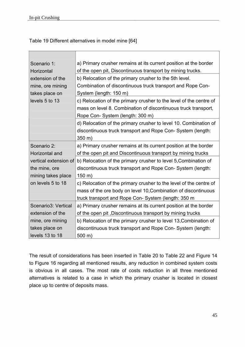
In-pit Crushing
45
Table 19 Different alternatives in model mine [64]
a) Primary crusher remains at its current position at the border of the open pit, Discontinuous transport by mining trucks. b) Relocation of the primary crusher to the 5th level. Combination of discontinuous truck transport and Rope Con- System (length: 150 m) c) Relocation of the primary crusher to the level of the centre of mass on level 8. Combination of discontinuous truck transport, Rope Con- System (length: 300 m)
Scenario 1: Horizontal extension of the mine, ore mining takes place on levels 5 to 13
d) Relocation of the primary crusher to level 10. Combination of discontinuous truck transport and Rope Con- System (length: 350 m) a) Primary crusher remains at its current position at the border of the open pit and Discontinuous transport by mining trucks b) Relocation of the primary crusher to level 5,Combination of discontinuous truck transport and Rope Con- System (length: 150 m)
Scenario 2: Horizontal and vertical extension of the mine, ore mining takes place on levels 5 to 18
c) Relocation of the primary crusher to the level of the centre of mass of the ore body on level 10,Combination of discontinuous truck transport and Rope Con- System (length: 350 m a) Primary crusher remains at its current position at the border of the open pit ,Discontinuous transport by mining trucks
Scenario3: Vertical extension of the mine, ore mining takes place on levels 13 to 18
b) Relocation of the primary crusher to level 13,Combination of discontinuous truck transport and Rope Con- System (length: 500 m)
The result of considerations has been inserted in Table 20 to Table 22 and Figure 14 to Figure 16 regarding all mentioned results, any reduction in combined system costs is obvious in all cases. The most rate of costs reduction in all three mentioned alternatives is related to a case in which the primary crusher is located in closest place up to centre of deposits mass.
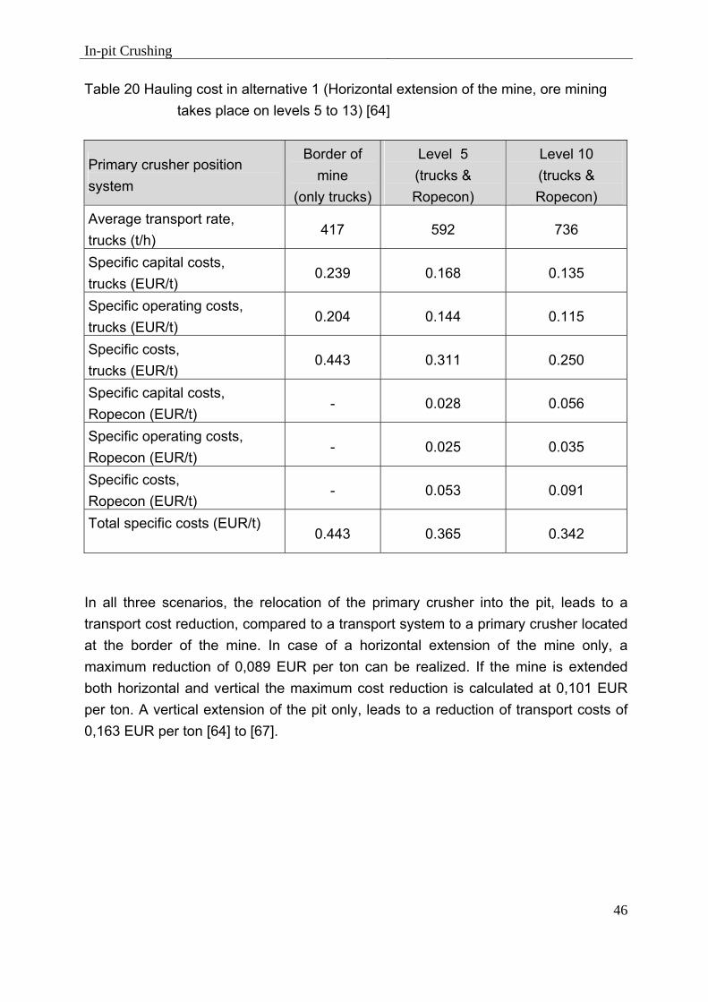
In-pit Crushing
46
Table 20 Hauling cost in alternative 1 (Horizontal extension of the mine, ore mining takes place on levels 5 to 13) [64]
Primary crusher position system
Border of mine
(only trucks)
Level 5 (trucks & Ropecon)
Level 10 (trucks & Ropecon)
Average transport rate, trucks (t/h)
417 592 736
Specific capital costs, trucks (EUR/t)
0.239 0.168 0.135
Specific operating costs, trucks (EUR/t)
0.204 0.144 0.115
Specific costs, trucks (EUR/t)
0.443 0.311 0.250
Specific capital costs, Ropecon (EUR/t)
- 0.028 0.056
Specific operating costs, Ropecon (EUR/t)
- 0.025 0.035
Specific costs, Ropecon (EUR/t)
- 0.053 0.091
Total specific costs (EUR/t)
0.443 0.365 0.342
In all three scenarios, the relocation of the primary crusher into the pit, leads to a transport cost reduction, compared to a transport system to a primary crusher located at the border of the mine. In case of a horizontal extension of the mine only, a maximum reduction of 0,089 EUR per ton can be realized. If the mine is extended both horizontal and vertical the maximum cost reduction is calculated at 0,101 EUR per ton. A vertical extension of the pit only, leads to a reduction of transport costs of 0,163 EUR per ton [64] to [67].

In-pit Crushing
47
Table 21 Hauling cost in alternative 2 (Horizontal and vertical extension of the mine, ore mining takes place on levels 5 to 18) [64]
Primary crusher position system
Border of mine (only trucks)
Level 5 (trucks & Ropecon)
Level 10 (trucks & Ropecon)
Average transport rate, trucks (t/h)
417 592 736
Specific capital costs, trucks (EUR/t)
0.239 0.168 0.135
Specific operating costs, trucks (EUR/t)
0.204 0.144 0.115
Specific costs, trucks (EUR/t) 0.443 0.311 0.250
Specific capital costs, Ropecon (EUR/t)
- 0.028 0.056
Specific operating costs, Ropecon (EUR/t)
- 0.025 0.035
Specific costs, Ropecon (EUR/t)
- 0.053 0.091
Total specific costs (EUR/t) 0.443 0.365 0.342
Table 22 Hauling cost in alternative 3 (Vertical extension of the mine, ore mining takes place on levels 13 to 18) [64]
Primary crusher position system Border of mine only
trucks Level 13
trucks & Ropecon Average transport rate, trucks (t/h) 342 709 Specific capital costs, trucks (EUR/t) 0.291 0.140 Specific operating costs, trucks (EUR/t) 0.248 0.120 Specific costs, trucks (EUR/t) 0.539 0.260 Specific capital costs, Ropecon (EUR/t) - 0.076 Specific operating costs, Ropecon (EUR/t) - 0.040 Specific costs, Ropecon (EUR/t) - 0.116 Total specific costs (EUR/t) 0.539 0.376

In-pit Crushing
48
0,310 0,321 0,326
0,399
-
0,10
0,20
0,30
0,40
0,50
0,60
0 10 20 30 40 50 60 70 80 90 100 110 120 130
Depth [m]sp
ecifi
c co
sts
[€/t]
primary crusher at the border of the mine
primary crusher on level 5
primary crusher on level 10
primary crusher on level 8
0,310 0,321 0,326
0,399
-
0,10
0,20
0,30
0,40
0,50
0,60
0 10 20 30 40 50 60 70 80 90 100 110 120 130
Depth [m]sp
ecifi
c co
sts
[€/t]
primary crusher at the border of the mine
primary crusher on level 5
primary crusher on level 10
primary crusher on level 8
a)b)
c)
d)
Miningdirection
a b c d
Figure 14 Hauling cost in alternative 1 (Horizontal extension of the mine, ore mining takes place on levels 5 to 13) [64]

In-pit Crushing
49
0,310 0,321 0,326
0,399
-
0,10
0,20
0,30
0,40
0,50
0,60
0 10 20 30 40 50 60 70 80 90 100 110 120 130Depth [m]
spec
ific
cost
s [€
/t]
primary crusher at the border of the mine
primary crusher on level 5
primary crusher on level 10
primary crusher on level 8
0,310 0,321 0,326
0,399
-
0,10
0,20
0,30
0,40
0,50
0,60
0 10 20 30 40 50 60 70 80 90 100 110 120 130Depth [m]
spec
ific
cost
s [€
/t]
primary crusher at the border of the mine
primary crusher on level 5
primary crusher on level 10
primary crusher on level 8
a)b)
c)
d)
Miningdirection
a b c d
Figure 15 Hauling cost in alternative 2 (Horizontal and vertical extension of the mine, ore mining takes place on levels 5 to 18)

In-pit Crushing
50
0,376
0,539
-
0,10
0,20
0,30
0,40
0,50
0,60
0,70
0 10 20 30 40 50 60 70 80 90 100 110 120 130 140 150 160 170 180Depth [m]
spec
ific
cost
s [€
/t]
primary crusher on level 13
primary crusher at the border of the mine
a)
b)Mining
direction
a
b
Figure 16 Hauling cost in alternative 3 (Vertical extension of the mine, ore mining takes place on levels 13 to 18)

Cost Estimation in Open Pit Mines
51
8 Cost Estimation in Open Pit Mines
8.1 Cost Estimation for Operation Cycles
Operation costs of open pit mines may be depending upon the size and number of drilling equipments, shovels and trucks that are also depending upon the daily tons of ore and wastes. In most open pit mines there are a little difference between the specific weight, blasting characteristics and drillabilities of ore and wastes with no more differences in the haulage distance of ore up to dump and wastes transportation distance up to dump hills of wastes. As a result, the costs of extraction one tone of ore are somehow equal to the costs of one tone wastes removing. Daily operations costs for different operations are estimated from equations 1 to 5.
Equation 1 Daily drilling cost ($) = 1.90 * t 0.7
Equation 2 Daily blasting cost ($) = 3.17 * t 0.7
Equation 3 Daily loading cost ($) = 2.67 * t 0.7
Equation 4 Daily haulage cost ($) = 18.07 * t0.7
Equation 5 Daily general services ($) = 6.65 * t0.7
The costs of general services in open pit mines include the pit maintenance costs, road grading, and waste dump grading, pumping and supervising of open pit [44] , [45] & [68] . In order to estimate all capital costs of loading and haulage equipments, it is necessary to use from equations 6 to 9 for obtaining the size and number of equipments and then the capital costs are calculated by the use of equations 10 and 11.
Equation 6 S = 0.13 * T0.4
Equation 7 Ns = 0.007 * T0.8 / S
Equation 8 t = 8 * S1.1
Equation 9 Nt = 0.2 * T0.8 / t

Cost Estimation in Open Pit Mines
52
Equation 10 Capital costs for loading equipments ($) = Ns * 499813* S 0.73
Equation 11 Capital costs for haulage equipments ($) = Nt * 19558 * t0.85
In all above mentioned equations T is the production rate of wastes and ore in small tone per day, S is the optimal nominal capacity of shovel bucket on cubic yard basis, Ns is the number of required shovels and t as the optimal size of truck in small tone basis and Nt is the number of required trucks. This is necessary to mention that all mentioned equations are with an assumption of an open pit mine with a daily production capacity of 43000 small tone, an oval shaped periphery pit with a depth of 120-150 m, width of 670 m, length of 1430 m, height of benches 12 m, overall pit slope (57 degree in competent rock and 43 degree in oxidized or altered rocks), gradient of roads inside the pit is averagely 9 percentage and the costs are completely according to 1988 amounts. By multiplying the obtained amounts out of above-mentioned equations in the rate of “costs indices in considered year to costs indices of 1988” it is possible to update the costs [44], [68] & [69]. The relevant loading and haulage costs in open pit mines by the use of above mentioned model and by considering the production rate in open pit mines have been presented through Table 23, Figure 17 and Figure 18.

Cost Estimation in Open Pit Mines
53
Table 23 Loading and haulage cost in world surface mines (million us. $)
Open pit type 1996 1997 1998 1999 2000 2001 2002 2003 2004 2005 2006 2030
Metal mines 16940 15480 19826 22922 25833 24805 24623 26240 28250 30706 33484 77995
Coal mines 17821 18221 18002 17727 18053 19213 19526 21307 23175 24001 24831 53732
Non- metallic mines 1346 1394 1374 1400 1417 1402 1416 1501 1572 1643 1684 3971
All open pit mines 36107 35095 39202 42049 45302 45420 45565 49048 52997 56350 59999 135698
Construction Materials mines 23133 24471 27392 28608 29413 29970 30340 31824 34447 35514 37273 114088
Open pits + quarries 59240 59566 66594 70657 74716 75390 75905 80872 87444 91864 97272 249786

Cost Estimation in Open Pit Mines
54
Materials Handling Costs in Open Pit Mines
0
20000
40000
60000
80000
100000
120000
140000
160000
1996 1997 1998 1999 2000 2001 2002 2003 2004 2005 2006 2030
Year
Load
ing
& H
aula
ge C
osts
(mill
ion
us. $
)
All Mines Metallic Mines Coal Mines Non Metallic Mines
Figure 17 Material handling cost in world open pit mines

Cost Estimation in Open Pit Mines
55
Materials Handling Costs in Surface Mines
0
50000
100000
150000
200000
250000
300000
1996 1997 1998 1999 2000 2001 2002 2003 2004 2005 2006 2030
Year
Load
ing
& H
aula
ge C
osts
(mill
ion
us. $
)
all mines open pit( metallic+non metallic+ coal mines) construction materials quarries
Figure 18 Materials handling cost in world surface mines

Cost Estimation in Open Pit Mines
56
8.2 Cost Estimation for Loading and Haulage Equipments
The presented method here is used for estimation of materials handling costs and other equipment of production cycle by both surface and underground mining. Estimation of costs here is made for selected equipment (power shovels, hydraulic shovels, trucks, front-end loaders, draglines, bucket wheel excavators, belt conveyors, aerial tramways and scrapper). This method of costs estimation is not an exact calculation method, but a close estimation to the real amounts of expected costs. It is tried to have a valid comparison between machines for a test through process of equipments selection. The real goal of determining of costs on $/T basis is for materials handling (digging , loading and haulage) then for this purpose it is necessary to calculate and determine all operational & capital costs in time unit. Some capital costs are fixed and include of depreciation, interest, tax, insurance and storage costs. The operational costs are various (although some times would be calculated which seems to be assumed as fixed costs), and the costs of tires (in case of any benefit from robber-tired equipment, repair part and maintenance, fuel or energy, lubrication and labor costs. When there is only dealing with special and unit operations of production cycle that should be considered only direct costs. The estimation method of applied costs would be based upon the benefit from values and numbers obtained from practical and experimental results instead of presented methods by manufacturers of materials handling equipments. It is necessary to note that some capital costs are fixed because they are separate from usage or lack of usage of equipment, while operational costs may be changed in compliance with type of presented services and type of equipment (such as time period, manner of usage, operating conditions and so on). The estimation of costs by the use of presented form has been made for each machine and then replaced the nominal items. The attachment is about considering more exact calculations made by the use of computer software. (Of course it is possible to have handy calculations by the use of presented equations).
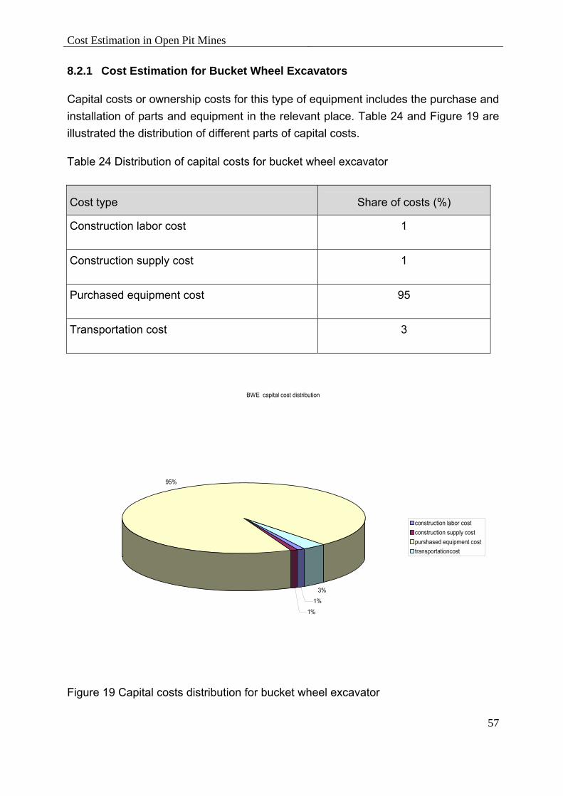
Cost Estimation in Open Pit Mines
57
8.2.1 Cost Estimation for Bucket Wheel Excavators
Capital costs or ownership costs for this type of equipment includes the purchase and installation of parts and equipment in the relevant place. Table 24 and Figure 19 are illustrated the distribution of different parts of capital costs.
Table 24 Distribution of capital costs for bucket wheel excavator
Cost type Share of costs (%)
Construction labor cost 1
Construction supply cost 1
Purchased equipment cost 95
Transportation cost 3
BWE capital cost distribution
1%
1%
95%
3%
construction labor cost construction supply cost purshased equipment cost transportationcost
Figure 19 Capital costs distribution for bucket wheel excavator

Cost Estimation in Open Pit Mines
58
This is necessary to mention that any calculation of capital costs of one unit includes excavating wheels, haulage vehicle (conveyor) and discharge part. Presented curves are valid for production rate from 2000 to 125000 tones per day, operating three shifts per day. Availability for machine is assumed % 50 (totally there is no high availability for these equipment and could be changed from 41 to 60 percent) and output efficiency is % 46. Total capital costs and also different parts of capital costs are possible to be calculated according to daily production and through equations 12 to 15.
Equation 12 Ys= 16.604*x0.684* A
Equation 13 Ye= 1627.238*x0.684* A
Equation 14 Yl = 16.604*x0.684 * A
Equation 15 Yc = 1660.446* x0.684 * A
Where, x is daily production of mine, A is the rate of costs indices of considered year to costs indexes of relevant year 1984 and Ys, Ye, Y1 and Yc are respectively the energy costs, purchase of parts and equipment , installation labor cost and total capital costs. If there is any difference between availability of machine with assumed amount, modified factor as mentioned in equation 16 is used.
Equation 16 Ft = [50/T] 0.683
Where, T is the availability of machine. Regarding all mentioned items, capital costs of bucket wheel excavators upon daily production would be in accordance with Figure 20.

Cost Estimation in Open Pit Mines
59
0
1000000
2000000
3000000
4000000
5000000
6000000
7000000
8000000
0 20000 40000 60000 80000 100000 120000 140000
mine production per day (t/day)
Cos
t($)
costruction labor cost($) construction supplycost ($) costruction material cost($) total capital cost($)
Figure 20 Capital costs for bucket wheel excavator upon daily production
The operational costs of bucket wheel excavators include three costs sections (labor operating costs, supply operating costs and equipment operating costs) for which it is possible to calculate upon daily production rate through equations 17 to 19.
Equation 17 Ys = 0,058*x0.859* A
Equation 18 Ye = 0,212*x0.681* A
Equation 19 Yl = 7,414*x0.556* A
Where, x is daily production of mine, A is the rate of costs indices of considered year to costs indices of relevant year 1984 and Ys, Ye, Y1 are respectively the daily costs of daily energy consumption, equipment operating costs (including of %100 of repair parts and material) and daily labor costs. Bucket wheel operation costs are distributed as Figure 21 and Figure 22.

Cost Estimation in Open Pit Mines
60
0
2000
4000
6000
8000
10000
12000
0 20000 40000 60000 80000 100000 120000 140000
mine production(t/day)
cost
($/d
ay)
labor cost ($/day) supply cost ($/day) equipment cost ($/day) total operation cost ($/day) Figure 21 Operating cost for bucket wheel excavators upon daily mine production If there is any difference between availability of machine with assumed amount (%50), modified factor as mentioned in equation 20 to be used.
Equation 20 Ft = [50/T] 0.554
Where, T is the availability of machine.
The other considerable point is that the output efficiency of machine (the real amount of production rate to theoretical capacity of system) is assumed as % 46 (which is variable from 44 to 85 percent). In case of any discrepancy between the outputs of machine with assumed amount, that may benefited from modified factors according to the equations 21 to 23 for modification of costs [22], [69] to [76].
Equation 21 Fl = [46/E] 0.555
Equation 22 Fs = [46/E] 0.858
Equation 23 Fe = [46/E] 0.680
Where, E is the output efficiency of system, F1, Fs and Fe are respectively the modified factors of labor, energy and equipment costs.

Cost Estimation in Open Pit Mines
61
BWE operating cost
75%
16%
9%
labor operating $/ tonsupply operating $/ ton equipment operating $/ ton
Figure 22 Operating costs distribution for bucket wheel excavator
8.2.2 Cost Estimation for Power Shovel-Trucks Fleet
Distribution of different parts of capital costs in power shovel- trucks fleets have been presented in Table 25 and Figure 23.
Table 25 Distribution of capital costs for power shovel- trucks fleet
Cost type Share of costs (%)
Loading equipment 34
Haulage equipment 66
This is important to mention that any calculation of capital costs is upon operating three shifts per day and Presented curves are valid for production rate from 2000 to 400000 tones per day. The curves reflect an average haul of 2000 meters one way on an 8 % grade from a pit 120 metre deep on wide, well maintained roads.

Cost Estimation in Open Pit Mines
62
capital cost distribution for " electric shovel- truck "
hauling equipmentlaoding equipment
Figure 23 Capital cost distribution upon equipment type for power shovel-trucks fleet Total capital costs and also different parts of capital costs are possible to be calculated according to daily production through equations 24 to 27.
Equation 24 Yc = 528.346*x0.782* A
Equation 25 Ys = 316.881*x0.782* A
Equation 26 Ye = 0.212*x0.782* A
Equation 27 Yl = 4573.211*x0.782* A
Where, x is daily production of mine, A is the rate of costs indices of considered year to costs indexes of relevant year 1984 and Ys, Ye, Y1 and Yc are respectively the energy costs, purchase of parts and equipment , installation labor cost and total capital costs. To determine costs for different haulage length or pit depth, multiply the costs obtained from mentioned equations bye the following factor (equation 28).
Equation 28 Fh = 0.0546*R0.047* L0.353
Where, R is depth of mine (meter), L is hauling distance (meter) and Fh is the modified factor of labor, energy and equipment costs.

Cost Estimation in Open Pit Mines
63
The operational costs of power shovel-trucks fleet include three costs sections (labor operating costs, supply operating costs and equipment operating costs) for which it is possible to calculate upon daily production rate through equations 29 to 31.these equation are valid for mines with daily production from 8000 to 300000 tones in three operating shifts [47], [68] to [72] & [76] to [81] .
Equation 29 Ys = 0188*x-0.220* A
Equation 30 Ye =1,850*x-0.133* A
Equation 31 Yl =2,694*x-0.210* A
Where, x is daily production of mine(waste and ore), A is the rate of costs indices of considered year to costs indexes of relevant year 1984 and Ys, Ye, Y1 are respectively the daily energy costs(include 100 % electric power), daily equipment operating costs(includes repair parts, tires, lubrication, and fuel consumption) and labor operating cost. Distribution of different parts of operation costs in power shovel- trucks fleets have been presented in Table 26 to Table 29 and Figure 24 to Figure 26.
Table 26 Distribution of operating labor costs for power shovel- truck fleet
Cost type Small ) per day50000-8000(
Large ) per day300000-50000(
Direct labor (%) 61
53
Maintenance labor (%) 39
47

Cost Estimation in Open Pit Mines
64
0
0,2
0,4
0,6
0,8
1
1,2
1,4
1,6
0 50000 100000 150000 200000 250000 300000 350000 400000 450000
Daily production (t)
oper
atin
g co
st( u
s. $
/t)
labor operating cost supply operating cost Equipment operating cost total operating cost
Figure 24 Operating cost for power shovel –truck fleet upon daily mine production To determine costs for different haulage length or pit depth, multiply the costs obtained from mentioned equations bye the following factors (equations 32 and 33).
Equation 32 Fl = 0.117*R0.030* L0.263
Equation 33 Fe = 0.55*R0.047* L0.353
Where, R is depth of mine (meter), L is hauling distance (meter) and Fl and Fe are respectively the modified factors for labor operating cost and equipment operating cost.

Cost Estimation in Open Pit Mines
65
operation cost distribution up on equipment
7
70
12
11
operation cost distribution electric shoveltruckdozerother
Figure 25 Operating cost distribution upon equipment type for power shovel-trucks fleet
Table 27 Operating cost distribution for power shovel- truck fleet
Relatively cost Small ) per day50000-8000(
Large ) per day300000-50000(
(%)Shovel operator 14 8 (%)Oiler 6 4
(%)Dozer operator 17 23 (%)Grader operator 5 7
Front-end loader operator (%) 3 1 (%)Truck driver 52 57
(%)General laborer 3 --
Table 28 Operating cost distribution for power shovel- truck fleet upon equipment
Equipment type Cost share (%)
Power shovel 7
Truck 70 Dozer 12
Rubber-tired support 11

Cost Estimation in Open Pit Mines
66
Table 29 Operating cost distribution for power shovel- truck fleet upon equipment and cost type
Equipment type Repair parts (%) Fuel and lube (%) Tires (%)
Power shovel 96 4 -
Truck 25 48 27
Dozer 50 50 -
Rubber-tired support 35 47 18
0
0,2
0,4
0,6
0,8
1
1,2
1,4
1,6
1,8
2
0 50000 100000 150000 200000 250000 300000 350000 400000 450000
daily production (t)
prod
uctio
n co
st (u
s. $
/t)
oparetaion$/ ton capital $/ ton total cost
Figure 26 Total production costs for power shovel-truck shovel up on daily mine production
8.2.3 Cost Estimation for Hydraulic Shovel-Trucks Fleet
Any calculation of capital costs is upon operating three shifts per day and Presented curves and equations are valid for production rate from 1000 to 10000 tones per day.

Cost Estimation in Open Pit Mines
67
Total capital costs are possible to be calculated according to daily production through equation 34.
Equation 34 Yc =88064.416*x0.407* A
Where, x is daily production of mine, A is the rate of costs indices of considered year to costs indexes of relevant year 1984 and Yc is total capital costs. Distribution of different parts of capital costs in hydraulic shovel-trucks fleets have been presented in Table 30.
Table 30 Distribution of capital costs for hydraulic shovel- truck fleet
Cost type Small ) 1000 – 3000 per day(
Large )3000 – 10000 per day(
Loading equipment (%) 51 30
Haulage equipment (%) 49 70
To determine capital costs for different haulage length or pit depth, multiply the costs obtained from mentioned equations bye the following factor (equation 35).
Equation 35 Fh = 0.080*R0.047* L0.353
Where, R is depth of mine (meter), L is hauling distance (meter) and Fh is the modified factor of labor, energy and equipment costs. The operational costs of hydraulic shovel-trucks fleet include two costs sections (labor operating costs and equipment operating costs) for which it is possible to be calculated upon daily production rate through equations 36 to 38.
Equation 36 Yl = 37.003*x-0.471*A
Equation 37 Ye = 24.620*x-0.424*A
Equation 38 Yc = Yl + Ye
Where, x is daily production of mine(waste and ore), A is the rate of costs indices of considered year to costs indexes of relevant year 1984 and Ye, Y1 are respectively the daily equipment operating costs(includes repair parts, tires, lubrication, and fuel

Cost Estimation in Open Pit Mines
68
consumption) and labor operating cost. Distribution of different parts of operation costs in hydraulic shovel- trucks fleets have been presented in Table 31 to Table 34 and Figure 27 to Figure 29.
Table 31 Distribution of operating labor costs for hydraulic shovel –truck fleet
Cost type Cost share (%)
Direct labor 70
Maintenance labor 30
0
0,2
0,4
0,6
0,8
1
1,2
1,4
0 20000 40000 60000 80000 100000 120000 140000 160000
Dily production (t)
cost
(us.
$ /t
)
labor operating cost equipment operating cost total operating cost
Figure 27 Operating cost for hydraulic shovel –truck fleet upon daily mine production
To determine operating costs for different haulage length or pit depth, multiply the costs obtained from mentioned equations bye the following factors (equations 39 and 40).
Equation 39 Fl = 0.155*R0.030* L0.263
Equation 40 Fl = 0.155*R0.030* L0.263

Cost Estimation in Open Pit Mines
69
Where, R is depth of mine (meter), L is hauling distance (meter) and Fl and Fe are respectively the modified factors for labor operating cost and equipment operating cost [22], [47], [68] to [72] & [76] to [81].
Table 32 Operating cost distribution for hydraulic shovel- trucks fleet
Relatively cost (%)Small
) 1000 – 3000 per day( Large
)3000 – 10000 per day(
Shovel operator 30 21
Truck driver 46 37
Dozer operator 24 17
Rubber-tired support operator
- 25
Table 33 Operating cost distribution for hydraulic shovel- trucks fleet upon equipment
Equipment type Cost share (%)
Hydraulic shovel 18
Truck 43
Dozer 23
Rubber-tired support 16
Table 34 Operating cost distribution for hydraulic shovel- truck fleet upon equipment and cost type
Equipment type Repair parts (%) Fuel and lube (%) Tires (%)
Hydraulic shovel 69.6 30.4 -
Front-end loader 32.5 44.2 23.3
Truck 28.1 51.6 20.3
Dozer 50.6 49.4 -
Rubber-tired support 28.5 62.7 8.8

Cost Estimation in Open Pit Mines
70
operating cost distribution for diesel shovel - truck up on equipment
18%
43%
23%
16%
Diesel shovel - LoadertruckdozerRubber- tired support
Figure 28 Operating cost distribution upon equipment type for hydraulic shovel-truck fleet
0
0,2
0,4
0,6
0,8
1
1,2
1,4
0 20000 40000 60000 80000 100000 120000 140000 160000
daily production (t)
prod
uctio
n co
st (u
s. $
)
operating costs capital costs total production costs
Figure 29 Production cost for hydraulic shovel–trucks fleet upon daily mine production
Cost Estimation in Open Pit Mines
71
8.2.4 Cost Estimation for Walking and Crawler Draglines
Total capital costs are possible to be calculated according to daily production through equations 41 and 42.
Equation 41 Ycw = 1504.727*x0.904* A
Equation 42 Ycc = 1069.3041*x0.803* A
Where, x is daily production of mine, A is the rate of costs indices of considered year to costs indexes of relevant year 1984, Ycc and Ycw are total capital costs respectively for crawler dragline and walking dragline. Any calculation of capital costs is upon (three operating shifts for walking dragline and one operating shift for crawler dragline) and presented curves and equations are valid for production rate (from 15000 to 150000 tones per day for walking dragline and 2000 to 1500 for crawler dragline). One dozer is provided for each dragline operation for cleanup and support. Distributions of different parts of capital costs for dragline have been presented in Table 35 and Figure 30. Table 35 Distribution of capital costs for dragline
Cost type Share of costs (%)
Construction labor cost 20
Construction supply cost 1
Purchased equipment cost 77
Transportation cost 2

Cost Estimation in Open Pit Mines
72
draglin capital costs distribution
20%1%
77%
2%
construction labor cost construction supply cost purshased equipment cost transportation
Figure 30 Distribution of capital costs for dragline
The operational costs for crawler dragline include two costs sections (labor operating costs and equipment operating costs) and walking dragline include three costs sections (labor operating cost, supply cost and equipment operating cost).for which it is possible to calculate upon daily production rate through equations 43 to 47.
Equation 43 Yec =2,218*x-0,312* A
Equation 44 Ylc = 43,884*x0.637* A
Equation 45 Ysw = 0,395*x0.003* A
Equation 46 Yew = 0,533*x-0.166* A
Equation 47 Ylw =12,249*x-0.458* A
Where, x is daily production of mine, A is the rate of costs indices of considered year to costs indexes of relevant year 1984 and Yec, Ylc are respectively equipment operating cost and labor operating cost for crawler dragline and Ysw, Yew and Ylw are respectively supply operating cost, equipment operating costs and labor operating cost for walking dragline [22], [68] to [81] .

Cost Estimation in Open Pit Mines
73
Distribution of different parts of operation costs have been presented for each two draglines in Table 36 to Table 42 and Figure 31 to Figure 33.
0
0,05
0,1
0,15
0,2
0,25
0,3
0,35
0,4
0,45
0,5
0 20000 40000 60000 80000 100000 120000 140000 160000
daily mine production(t/day)
oper
atin
g co
st($
/t)
labor operating cost($/t) supply operating cost($/t) Equipment operatin cost($/t) total operatin cost ($/t)
Figure 31 Operation cost for walking dragline upon daily mine production
0
0,1
0,2
0,3
0,4
0,5
0,6
0,7
0,8
0,9
0 2000 4000 6000 8000 10000 12000 14000 16000
daily mine production(t/day)
cost
($/t)
lobor operating cost Equipment operating cost total operating cost
Figure 32 Operation cost for crawler dragline upon daily mine production

Cost Estimation in Open Pit Mines
74
Table 36 Distribution of operating labor costs for crawler dragline Cost type (%) small
) 1000 – 10000 per day( large
)10000 – 15000 per day(
Direct labor cost 59 56
Maintenance labor 41 44
Table 37 Distribution of direct operating labor costs for crawler dragline
Relatively cost (%) small ) 2000 – 10000 per day(
large )10000 – 15000 per day(
Dragline operator 41 26
Oiler 24 22
Dozer operator 25 23
tired support -Rubberoperator
10 29
Table 38 Distribution of operating labor costs for walking dragline
Cost type Cost share (%)
Direct labor 62
Maintenance labor 38
Table 39 Distribution of direct operating labor costs for walking dragline
Relatively cost Share of costs (%)
Dragline operator 30
Oiler 26
Dozer operator 27
Rubber-tired support operator 17
Cost Estimation in Open Pit Mines
75
Table 40 Distribution of operating cost for crawler dragline upon type of equipment
Equipment type Share of costs (%)
Crawler dragline 70
Crawler tractor 25
Pick up tractor 5
Table 41 Distribution of operating cost for waking dragline upon type of equipment
Equipment type Share of costs (%)
Crawler dragline 66
Crawler tractor 31
Pick up tractor 3
Table 42 Distribution of operating cost upon type of equipment
Equipment type Repair parts (%) Fuel and lube (%) Tires (%)
Walking dragline 94 6 -
Crawler dragline 65 35 -
Dozer 49 51 -
Support equipments 8 90 2

Cost Estimation in Open Pit Mines
76
0
0,1
0,2
0,3
0,4
0,5
0,6
0,7
0 20000 40000 60000 80000 100000 120000 140000 160000
daily mine production(t/day)
prod
uctio
n co
st ($
/t)
operating cost capital cost total production cost
Figure 33 Production cost for walking dragline upon daily mine production
8.2.5 Cost Estimation for Belt Conveyors
Any calculation of capital costs is upon operating three shifts per day and Presented curves and equations are valid for production rate from 15000 to 150000 tones per day. The base curves and equations are based on a belt conveyor of 1000 meter in length with the slope of 10º and the conveyor availability is assumed 94 %. Total capital costs are possible to be calculated according to daily production through equation 48.
Equation 48 Yc =81292.281*x0.309* A
Where, x is daily production of mine, A is the rate of costs indices of considered year to costs indices of relevant year 1984 and Yc is total capital costs. Distribution of different parts of capital costs have been presented in Table 43 and Table 44.

Cost Estimation in Open Pit Mines
77
Table 43 Capital cost distribution for belt conveyor upon cost type
Cost type Share of costs (%)
Construction labor cost 31
Construction supply cost 5
Purchased equipment cost 64
Table 44 Cost distribution for belt conveyor upon type of equipment
Equipment type Share of costs (%)
Conveyor belt 36
Idler assembly units 44
Motors, drive trains, belt cleaner and other mechanical items 20
To determine costs for different conveyor length and slopes, multiply the costs obtained from mentioned equations bye the following factor (equation 49).
Equation 49 Fc = [0,917+0.00094*S]*L
Where, L is length of conveyor (in kilometre), S slope of conveyor in degree (between 0º and 15º) and Fc is the modified factor of capital costs. The operational costs include three costs sections (labor operating costs, supply operating costs and equipment operating costs) for which it is possible to calculate upon daily production rate through equations 50 to 52.
Equation 50 Ys = 0.068*x0.933* A
Equation 51 Ye = 2.226*x0.358* A
Equation 52 Yl = 7.429*x0.464* A
Where, x is daily production of mine (waste and ore), A is the rate of costs indices of considered year to costs indices of relevant year 1984 and Ys, Ye, Y1 are respectively the daily energy costs (include 100 % electric power), daily equipment operating costs

Cost Estimation in Open Pit Mines
78
(includes 95 % repair parts and 5 % lubrication for the idlers and mechanical parts) and labor operating cost. Distribution of different parts of operating costs has been presented in Figure 34 and Figure 35.
0
0,02
0,04
0,06
0,08
0,1
0,12
0,14
0 20000 40000 60000 80000 100000 120000 140000 160000
daily production(t/day)
Cos
t (us
.$/t)
labor operating cost supply operating cost Equipment operating cost total operating cost
Figure 34 Operation cost for belt conveyor upon daily mine production
To determine costs for different conveyor length and slopes, multiply the costs obtained from mentioned equations bye the following factors (equations 53 to 55).
Equation 53 Fl = 0.815+ 0.190*L
Equation 54 Fs = [0.208+0.0794*S]*L
Equation 55 Fe = L
Where, L is length of conveyor (in kilometres), S slope of conveyor in degree (between 0º and 15º), Fl, Fs and Fe are respectively the modified factors for labor, supply and equipment operating costs. Slope are assumed zero in above equations for decline conveyors [22], [68] to [83] .

Cost Estimation in Open Pit Mines
79
0
0,02
0,04
0,06
0,08
0,1
0,12
0,14
0,16
0,18
0,2
0 20000 40000 60000 80000 100000 120000 140000 160000
daily production(t/day)
cost
(us.
$ /t)
operating cost capital cost total production cost
Figure 35 Production cost for belt conveyor upon daily mine production
8.2.6 Cost Estimation for Aerial Tramway
Any calculation of capital costs is upon operating three shifts per day and Presented curves and equations are valid for production rate from 2040 to 13800 tones per day The base curves and equations are based on an aerial tramway of 3000 meter in length with the slope of 15º and bulk density of materials is 1442.5 kg/m³. Total capital costs would be calculated according to daily production through equation 56.
Equation 56 Yc = 208182.537*x0.385* A
Where, x is daily production of mine, A is the rate of costs indices of considered year to costs indices of relevant year 1984 and Yc is total capital costs. Distribution of different parts of capital costs has been presented in Table 45.
Cost Estimation in Open Pit Mines
80
Table 45 Capital cost distribution for aerial tramway upon cost type
Cost type Share of costs (%)
Construction labor cost 19
Construction supply cost 4.8
Purchased equipment cost 73.5
Transportation cost 2.7
To determine costs for different material density, tramway length and slopes, multiply the costs obtained from mentioned equations bye the following factor (equation 57).
Equation 57 Fc = 1.345+0.233*L - 0.00003*D
Where, L is slope length (in kilometre), D material density (based on kg/m³) and Fc is the modified factor of capital costs. The operating costs include three costs sections (labor operating costs, supply operating costs and equipment operating costs) for which it is possible to calculate upon daily production rate through equations 58 to 60.
Equation 58 Ys = 1,815*x0.451* A
Equation 59 Ye = 68,358*x0.782* A
Equation 60 Yl = 439,430*x0.121* A
Where, x is daily production of mine (waste and ore), A is the rate of costs indices of considered year to costs indices of relevant year 1984 and Ys, Ye, Y1 are respectively the daily energy costs (include 100 % electric power), daily equipment operating costs (includes 99.4 % repair parts and 0.6 % lubrication) and labor operating cost. Distribution of different parts of operation costs have been presented in Figure 36 and Figure 37.

Cost Estimation in Open Pit Mines
81
0
0,2
0,4
0,6
0,8
1
1,2
1,4
1,6
1,8
2
0 2000 4000 6000 8000 10000 12000 14000 16000
daily production(t/day)
oper
atin
g co
st (u
s.$/
t)
labor operating cost supply operating Equipment operating cost total operating cost
Figure 36 Operating cost for aerial tramway upon daily mine production
To determine costs for different material density, tramway length and slopes, multiply the costs obtained from mentioned equations bye the following factors (equations 61 to 63).
Equation 61 Fl = 0.113* L+0.660
Equation 62 Fs = 0.157* L+0.528
Equation 63 Fe = 1.278+ 0.226* L+ 0.00003*D
Where, L is slope length (in kilometres), D is material density (based on kg/m³), Fl, Fs and Fe are respectively the modified factors for labor, supply and equipment operating costs [22], [68] to [81].
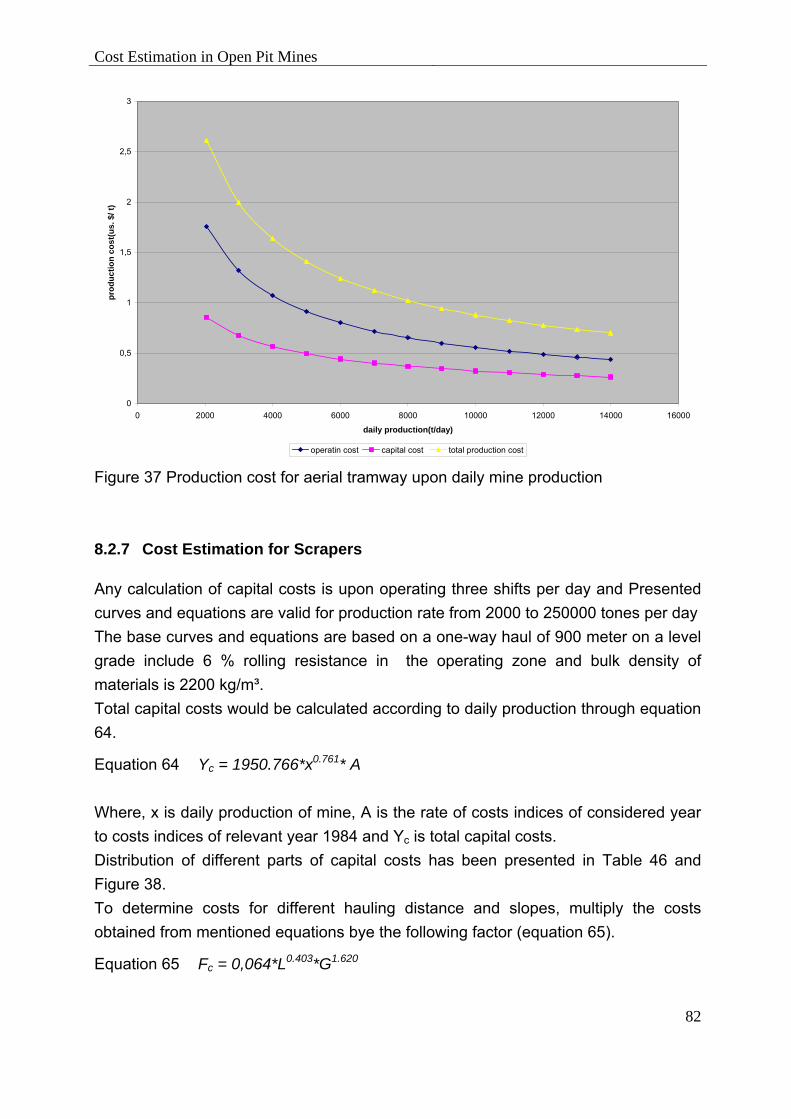
Cost Estimation in Open Pit Mines
82
0
0,5
1
1,5
2
2,5
3
0 2000 4000 6000 8000 10000 12000 14000 16000
daily production(t/day)
prod
uctio
n co
st(u
s. $
/ t)
operatin cost capital cost total production cost Figure 37 Production cost for aerial tramway upon daily mine production
8.2.7 Cost Estimation for Scrapers
Any calculation of capital costs is upon operating three shifts per day and Presented curves and equations are valid for production rate from 2000 to 250000 tones per day The base curves and equations are based on a one-way haul of 900 meter on a level grade include 6 % rolling resistance in the operating zone and bulk density of materials is 2200 kg/m³. Total capital costs would be calculated according to daily production through equation 64.
Equation 64 Yc = 1950.766*x0.761* A
Where, x is daily production of mine, A is the rate of costs indices of considered year to costs indices of relevant year 1984 and Yc is total capital costs. Distribution of different parts of capital costs has been presented in Table 46 and Figure 38. To determine costs for different hauling distance and slopes, multiply the costs obtained from mentioned equations bye the following factor (equation 65).
Equation 65 Fc = 0,064*L0.403*G1.620

Cost Estimation in Open Pit Mines
83
Where, L is slope length (in kilometres), G is grade factor (calculated from equation 66) and Fc is the modified factor of capital costs.
Equation 66 G = 1 ± (percent of grade/100)
capital cost distribution for scraper operation
66
26
8
ScrapperDozerRubber-tired support
Figure 38 Distribution of capital costs for scraper upon type of equipment
Table 46 Capital cost distribution for scraper upon type of equipment
Equipment type Share of costs (%)
Scrapers 66
Pit equipment (crawler dozer) 26
Road equipment ( graders, water trucks and pickup trucks
8
The operating costs include two costs sections (labor operating costs and equipment operating costs) for which it is possible to calculate upon daily production rate through equations 67 and 68.

Cost Estimation in Open Pit Mines
84
Equation 67 Ye =0,602*x0.0747* A
Equation 68 Yl =3.81*x-0.265* A
Where, x is daily production of mine (waste and ore), A is the rate of costs indices of considered year to costs indices of relevant year 1984, Yl and Ye are respectively the daily labor operating cost(Table 47 and Table 48) and equipment operating costs (Table 49 and Table 50). Distributions of different parts of operating costs have been presented in Table 47 to Table 50 and Figure 39 to Figure 41.
Table 47 Distribution of operating labor cost for scraper
Cost type Share of cost (%)
Direct labor costs 47
Maintenance labor costs 53
Table 48 Distribution of direct labor cost for scraper
Relatively cost Share of costs (%)
Scraper operator 58
Dozer operator 32
Support equipments operator 10
Table 49 Distribution of equipment operating cost for scraper upon type of equipment
Relatively cost Share of costs (%)
Scraper 71
Dozer 24
Support equipments 5
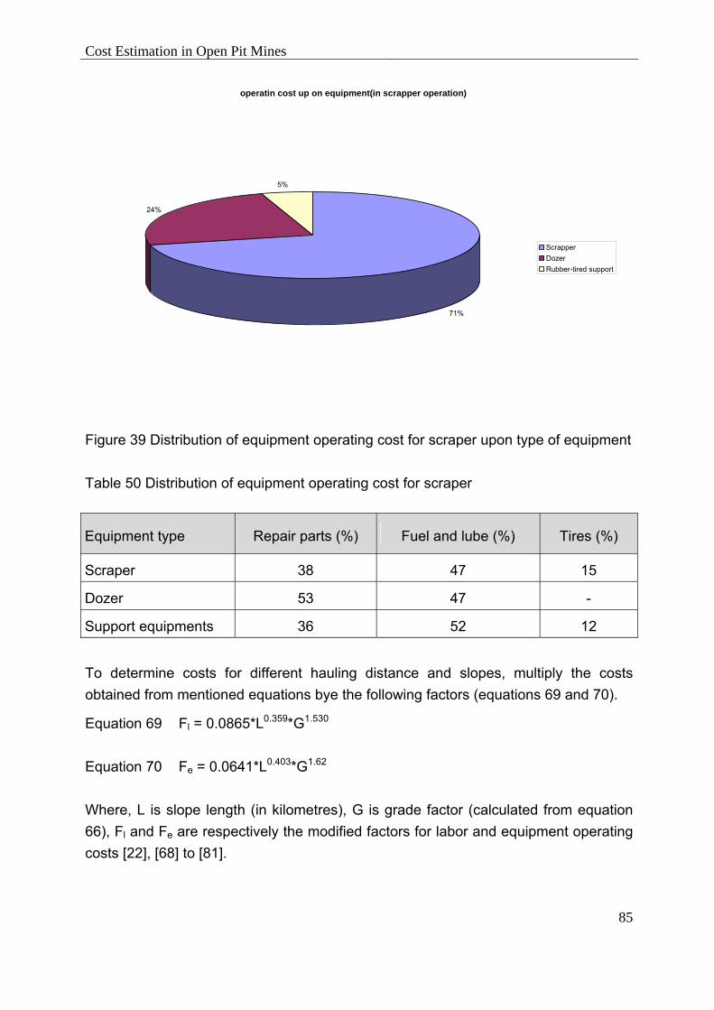
Cost Estimation in Open Pit Mines
85
operatin cost up on equipment(in scrapper operation)
71%
24%
5%
ScrapperDozerRubber-tired support
Figure 39 Distribution of equipment operating cost for scraper upon type of equipment
Table 50 Distribution of equipment operating cost for scraper
Equipment type Repair parts (%) Fuel and lube (%) Tires (%)
Scraper 38 47 15
Dozer 53 47 -
Support equipments 36 52 12
To determine costs for different hauling distance and slopes, multiply the costs obtained from mentioned equations bye the following factors (equations 69 and 70).
Equation 69 Fl = 0.0865*L0.359*G1.530
Equation 70 Fe = 0.0641*L0.403*G1.62
Where, L is slope length (in kilometres), G is grade factor (calculated from equation 66), Fl and Fe are respectively the modified factors for labor and equipment operating costs [22], [68] to [81].

Cost Estimation in Open Pit Mines
86
0
0,2
0,4
0,6
0,8
1
1,2
1,4
0 5000 10000 15000 20000 25000 30000
daily production(t/day)
oper
atin
g co
st(u
s.$/
t)
labor operating cost Equipment operating cost total operating cost
Figure 40 Operating cost for scraper upon daily mine production
0
0,5
1
1,5
2
2,5
0 50000 100000 150000 200000 250000 300000
Daily Production (t)
prod
uctio
n C
ost (
us.$
/t)
capital cost(us. $/ ton) oparetaion cost(us. $/ ton) production cost(us. $/ ton)
Figure 41 Production cost for scraper upon daily mine production

Cost Estimation in Open Pit Mines
87
8.2.8 Cost Estimation for Mobile Crushers
Calculated costs include the primary crusher, discharge conveyor and feed hopper. Any calculation of capital costs is upon operating three shifts per day and Presented curves and equations are valid for production rate from 17600 to 79000 tones per day. The base curves and equations are based on a direct dumping of the ore into the crusher and hauled with the crusher discharge conveyor, an open side setting of 17.78 cm and the ore has a hardness index of 14.3 kWh/t. Total capital costs are possible to be calculated according to daily production through equations 71 to 77.
Equation 71 Yc = 2532.149*x0.697* A
Equation 72 Yss = 5.064* x0.697* A
Equation 73 Yes = 2446.056*x^0.697* A
Equation 74 Yls = 81.029* x0.697* A
Equation 75 Ysl = 873.591* x0.697* A
Equation 76 Ysl = 873.591* x0.697* A
Equation 77 Yel = 1509.161* x0.697* A
Where, x is daily production of mine, A is the rate of costs indices of considered year to costs indices of relevant year 1984 and Yc is total capital costs. Yss, Yes and Yls are respectively installation supply cost, equipment purchases and installation labor costs in small capacities. Ysl, Yel and Yll Yls are respectively installation supply cost, equipment purchases and installation labor costs in large capacities. Distribution of different parts of capital costs has been presented in Table 51 and Figure 42. To adjust costs for different open-side setting and hardness index, multiply the costs obtained from mentioned equations bye the following factor (equation 78). Equation 78 Fc = 0.1545/ I-0.702 + 120* S0.734
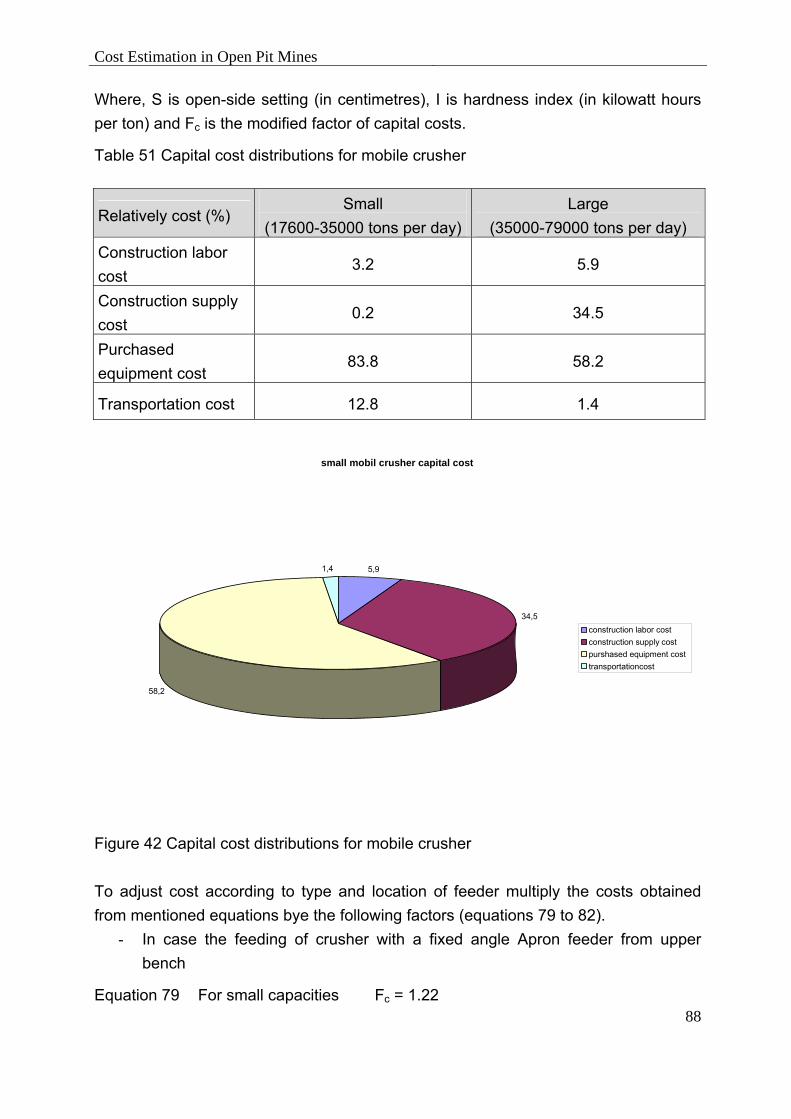
Cost Estimation in Open Pit Mines
88
Where, S is open-side setting (in centimetres), I is hardness index (in kilowatt hours per ton) and Fc is the modified factor of capital costs.
Table 51 Capital cost distributions for mobile crusher
Relatively cost (%)Small
)17600-35000 tons per day( Large
)35000-79000 tons per day( Construction labor cost
3.2 5.9
Construction supply cost
0.2 34.5
Purchased equipment cost
83.8 58.2
Transportation cost 12.8 1.4
small mobil crusher capital cost
5,9
34,5
58,2
1,4
construction labor cost construction supply cost purshased equipment cost transportationcost
Figure 42 Capital cost distributions for mobile crusher
To adjust cost according to type and location of feeder multiply the costs obtained from mentioned equations bye the following factors (equations 79 to 82).
- In case the feeding of crusher with a fixed angle Apron feeder from upper bench
Equation 79 For small capacities Fc = 1.22

Cost Estimation in Open Pit Mines
89
Equation 80 For small capacities Fc = 1.52
- In case the feeding of crusher with a fixed angle Apron feeder from same bench
Equation 81 Fc = 0.217 * x 0.188
- In case the feeding of crusher with a variable angle Apron feeder from same bench
Equation 82 Fc = 0.109* x0.266
The operating costs include three costs sections (labor operating costs, supply operating costs and equipment operating costs) for which it is possible to calculate upon daily production rate through equations 83 to 85.
Equation 83 Ys = 0.008 * x * A
Equation 84 Ye = 0.087 * x0.878 * A
Equation 85 Yl = 79.988 * x 0.248 * A
Where, x is daily production of mine (waste and ore), A is the rate of costs indices of considered year to costs indices of relevant year 1984 and Ys, Ye, Y1 are respectively the daily supply costs, equipment operating costs and labor operating costs. Distribution of different parts of operating costs has been presented in Table 52 to Table 54 and Figure 43 and Figure 44.
Table 52 Distribution of operating costs for mobile crusher
Cost type Share of cost (%)
Labor operating cost 46
Supply operating cost 14
Equipment operating cost 40

Cost Estimation in Open Pit Mines
90
operating cost distribution for mobil crusher
46%
14%
40%
labor operating cost supply operating costequopment operating cost
Figure 43 Distribution of operating costs for mobile crusher
To adjust costs for different open-side setting and hardness index, multiply the costs obtained from mentioned equations bye the following factors (equations 86 to 88).
Equation 86 Fl = 0,993*(14,300/I)-0,251 + (S/17.78)-0,174
Equation 87 Fs = 1,004*(14,300/I)-0.244 + (S/17.78)-0.230
Equation 88 Fe = 1,002*(14,300/I)-0.878 + (S/1.78)-0.646
Table 53 Distribution of labor operating cost for mobile crusher
Cost type Share of cost (%)
Direct labor cost 36
Maintenance labor cost 64

Cost Estimation in Open Pit Mines
91
To adjust operating cost according to type and location of feeder multiply the costs obtained from mentioned equations bye the following factors (equations 89 to 97).
- In case the feeding of crusher with a fixed angle Apron feeder from upper bench
Equation 89 Fs = 0.003 * x0.583
Equation 90 Fe = 0.0004 * x0.762
Equation 91 Fl = 1.22
- In case the feeding of crusher with a fixed angle Apron feeder from same bench
Equation 92 Fs = 0.078* x0.287
Equation 93 Fe = 0.0004* x0.762
Equation 94 Fl = 1.22
- In case the feeding of crusher with a variable angle Apron feeder from same bench
Equation 95 Fs = 2.06
Equation 96 Fe = 0.0004* x0.763
Equation 97 Fl = 1.35
Where, x is mine production, S is open-side setting (in centimetres), I is hardness index (in kilowatt hours per ton) and Fl, Fs and Fe are respectively the modified factors for labor, supply and equipment operating costs [68] to [81] & [83].

Cost Estimation in Open Pit Mines
92
Table 54 Distribution of equipment operating cost for mobile crusher
Cost type Share of cost (%)
Repair parts and maintenance 95.5
Lubrication 4.5
0
0,5
1
1,5
2
2,5
0 50000 100000 150000 200000 250000 300000
Daily Production (t)
prod
uctio
n C
ost (
us.$
/t)
capital cost(us. $/ ton) oparetaion cost(us. $/ ton) production cost(us. $/ ton)
Figure 44 Operating cost for mobile crusher upon daily mine production

Estimation and Calculation of Size and Number of
93
9 Estimation and Calculation of Size and Number of Loading and Haulage Equipments
The presented algorithm includes of any calculations for selecting of loading equipment (including of loader, power shovel and hydraulic shovel) and haulage equipment (truck) and also relevant costs of them. At the time of preparing this algorithm, we tried to benefit from practical and experimental values of machinery. Since in some cases there are no accesses to relevant details of systems, an estimation method is presented for selection of equipment and also calculation of relevant costs in addition to submission of exact calculations.
9.1 Estimation of Size and Number of Loading and Haulage Equipments
In order to estimate the size and number of loading and haulage equipments we may benefit from equations 98 to 101.
Equation 98 S = 0.13* T0.4
Equation 99 Ns = 0.007 * T0.8 / S
Equation 100 t = 8 * S1.1
Equation 101 Nt = 0.20 *T0.8 / t
Where, T is daily mine production based on small ton, S is optimum size of shovel, Ns is number of required shovel ,t is truck size and Nt is number of required trucks.
9.2 Calculation of Size and Required Number of Loaders
It is possible to calculate production rate of system (in tone per hour) by equation 102.
Equation 102 P = Nc * LD * Cb *Ff * E
Where, Nc is hourly loading cycle numbers, LD is loose material density, Cb is bucket capacity, Ff is bucket fill factor and E is output efficiency.

Estimation and Calculation of Size and Number of
94
It is possible to benefit from Table 55 for selection of filling factor of loader bucket with regard to type of loading materials.
Table 55 Loader fill factor [80]
Materials type
Fill factor [%]
Mixed soils, wet 100–120 Rock and compact soils ,mixed 100–130 Good blasted rock 90–110 Average rocks ,boulders 60–90 Broken Material 85–100 Sand, gravel, dry 85–95 Sand, gravel, wet 90–110 Heavy clay 70–90 Clayey sand , wet 80–100 In equation 105, we may benefit from Table 71 for determining of output efficiency with regard to management and also operating conditions. Also it is possible to calculate output efficiency (utilization and availability) through Table 56 and Figure 52.

Estimation and Calculation of Size and Number of
95
Table 56 Typical working hours and production data
Calendar days Total days 365 days
weekends 104 days
mine shutdown 0 days
public holidays 11 days
Less idle time scheduled ordinary time 250 days / year
repair/ unscheduled time -days
hours per shift 8 hours
shifts per day 3 per day
scheduled time per day scheduled time per day 24 hours / day
scheduled hours 6000 hours scheduled hours mechanical availability 75 percent
planned maintenance 750 hours /year
unplanned maintenance 750 hours /year
other hours /year
less maintenance subtotal maintenance(repair hours) 1500 hours /year
available hours 4500 hours /year available hours (equivalent to ) 562,5 shifts /year
weather(approx. 5 day / year) 120 hours /year
industrial 360 hours /year
no operator(assume Nil) - hours /year
conveyor moves - hours /year
not required - hours /year
no power - hours /year
await supporting equipment - hours /year
meal break ( 40 minute / shift9 375 hours /year
shift change (20 minute/ shift9 188 hours /year
preshift service (5 minute/ shift) 63 hours /year
less standby subtotal standby time 1106 hours /year
operating time 3394 hours /year operating hours Utilization 75%
fuel and service(5 minute/ shift) 63 hours /year
dead heading - hours /year
positioning - hours /year
less work delay minor delay 331hours /year

Estimation and Calculation of Size and Number of
96
delay hours 394hours /year work time 3000hours /year operating hours
work delay 88%
In addition, we can obtain the materials density by the use of Table 67. Following is the loader cycle time: - Filling of bucket - Manoeuvring with loaded bucket - Materials dumping - Manoeuvring with empty bucket With regard to the present experiences, it is possible to obtain loader cycle time according to the power of loader from Table 57.
Table 57 Loader cycle time
Loader power [kW] Cycle time[min] (t1)
To 48 0.40
48–112 0.45
112–186 0.50
over186 0.55
Assumptions: Loading materials are class 3 Additional loading height from 30- 70 percent Good ground conditions More trained operator Regarding all theories about Table 57, we should benefit from modifications of relevant amounts in accordance with Table 58 to Table61.
Table 58 Time allowance because of operating bench height [80]
Bench height [% bench height] Allowance time [min] (t2)
< 30 > 0,05
> 70 > 0,05

Estimation and Calculation of Size and Number of
97
Table 59 Time allowance because of loaded materials type [80]
Earth class
Designation Description Allowance time [min] (t3)
Class 1 Surface soil Highest layer of the soil, contains humus and organic soil(surface soil) ---
Class 2 Loose free running materials
Soil with relatively high water content, from liquid to soft consistency, water is delivered only heavily
---
Class 3
Easily excavate able soil types
Sand and gravel soil with small boulder, unconsolidated to weak to consolidated sand, gravel and sand gravel mixtures, organic soil types with small water content (peat)
----
Class 4
Moderate excavate able soil types
Compacted earth types with easier to middle plasticity, with small boulder (< 30% with a size of over 63 mm)
to 0.05
Class 5 difficulty excavate able soil types
soils with classes 3 and 4, however with large stone boulder (30% with a size of over 63 mm)
> 0.10
Class 6
Easy excavated rock and comparable soil types
Rocky soil, however fragile, fissured, softly or weathered as well as similarly into one another solidified soil types
No loader Operation
Class 7 Hard excavate able rocks
Rocky soil with a firm structure, a little fissured, fragile or weathers
No loader Operation
Finally it is possible to calculate actual cycle time by the use of equation 103.
Equation 103 Tt = t1 + t2+ t3 + t4 + t5
Where, Tt is cycle time and t1, t2, t3, t4, t5 are regarding the calculated cycle time. It is possible to calculate number of required cycles per hour by the use of equation 104.

Estimation and Calculation of Size and Number of
98
Equation 104 Nc = Te / Tt
Where, Nc is hourly required cycle numbers, Te is effective working time per hour and Tt is actual cycle time. For obtaining the bucket load in every cycle it is possible to benefit from equation 105.
Equation 105 CL = Ph / Nc
Where, CL is bucket load per cycle, Ph is required hourly production rate and Nc is hourly cycle numbers For obtaining the required hourly production rate we may use equation 106 with regard to output efficiency.
Equation 106 Ph = (Py / Hy) * E
Where, Ph is required hourly production rate, Hy is yearly working hours and E is output efficiency (according to Table 1). In order to have the size of bucket in each cycle we may use equation 107.
Equation 107 Cb = CL / Ff
Where, CL is bucket load per cycle and Ff is bucket fill factor.
Table 60 Time allowance because of ground conditions [80]
Ground conditions Allowance time [min]
(t4)
Very well, firm ground, evenly and drying, good traction, no tire penetration ---
Well, firm ground, unevenly, good traction, no tire penetration 0.05
Middle, soft ground, unevenly, rolling, middle traction, tire penetration to 10 cm
0.10
Badly, very soft ground, unevenly with stones, small traction, tire penetration over 10 cm 0.15
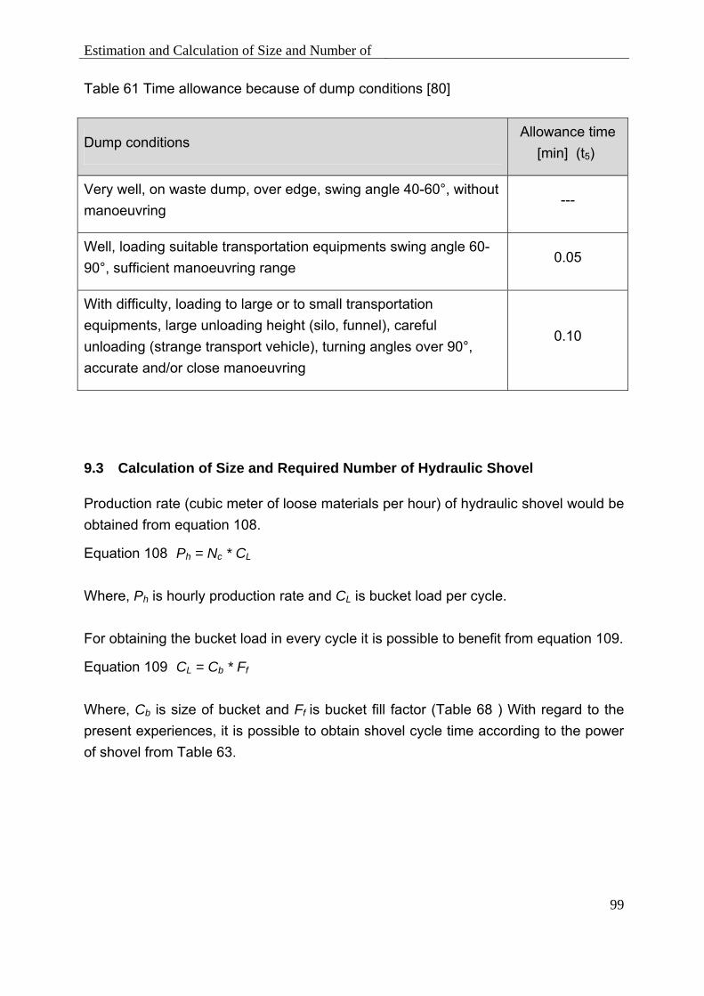
Estimation and Calculation of Size and Number of
99
Table 61 Time allowance because of dump conditions [80]
Dump conditions Allowance time
[min] (t5)
Very well, on waste dump, over edge, swing angle 40-60°, without manoeuvring
---
Well, loading suitable transportation equipments swing angle 60-90°, sufficient manoeuvring range
0.05
With difficulty, loading to large or to small transportation equipments, large unloading height (silo, funnel), careful unloading (strange transport vehicle), turning angles over 90°, accurate and/or close manoeuvring
0.10
9.3 Calculation of Size and Required Number of Hydraulic Shovel
Production rate (cubic meter of loose materials per hour) of hydraulic shovel would be obtained from equation 108.
Equation 108 Ph = Nc * CL
Where, Ph is hourly production rate and CL is bucket load per cycle. For obtaining the bucket load in every cycle it is possible to benefit from equation 109.
Equation 109 CL = Cb * Ff
Where, Cb is size of bucket and Ff is bucket fill factor (Table 68 ) With regard to the present experiences, it is possible to obtain shovel cycle time according to the power of shovel from Table 63.

Estimation and Calculation of Size and Number of
100
Table 62 Hydraulic shovel fill factor [80]
Material Fill factor [%]
Mixed soils, wet 110–130
Rock and compact soils ,mixed 90–120
Good blasted rock 75–90
Average rocks ,boulders 50–70
broken Material 80–95
Sand, gravel, dry 85–95
Sand, gravel, wet 90–110
Heavy clay 80–100
Clayey sand ,wet 100–120
Table 63 Hydraulic shovel cycle time [80]
Design power [kW] Base cycle time [min] (t1)
to 110 0,25 110–260 0,30 Backhoe over 260 0,35
Shovel - 0,35 Assumptions: Loading materials are class 3 Additional loading height to 2 meter Swing angle from 30 to 60 degrees More trained operator Regarding all assumptions about Table 63, that should be benefit from modifications of relevant amounts in accordance with Table 64 to Table 66. Finally it is possible to calculate actual cycle time by the use of equation 110.
Equation110 Tt = t1 + t2+ t3 + t4

Estimation and Calculation of Size and Number of
101
Where, Tt is actual cycle time, t1 is obtained time from Table 63 and t2, t3, t4 are addition time because of operating height, materially type and dumping conditions. Regarding the calculated cycle time, it is possible to calculate number of required cycles per hour by the use of equation 111.
Equation 111 Nc = Te / Tt
Where, Nc is hourly required cycle numbers (minute), Te is effective working time per hour (minute) and Tt is actual cycle time.
Table 64 Time allowance because of operating bench height [79], [80]
Operating height [m] Allowance time [min] (t2)
To 2,0 0,00 To 4,0 0,03 To 6,0 0,06 To 8,0 0,09 To 10,0 0,12
Table 65 Time allowance because of loaded materials type [79], [80]
Allowance time [min] (t3) Earth class Narrow spoon Middle spoon Large spoon Shovel bucket
3 0,00 0,00 0,0 0,00 4 0,00 0,02 0,03 0,03
5 0,02 0,04 0,06 0,06 6 0,04 0,06 0,10 0,10
7 --- --- --- ---
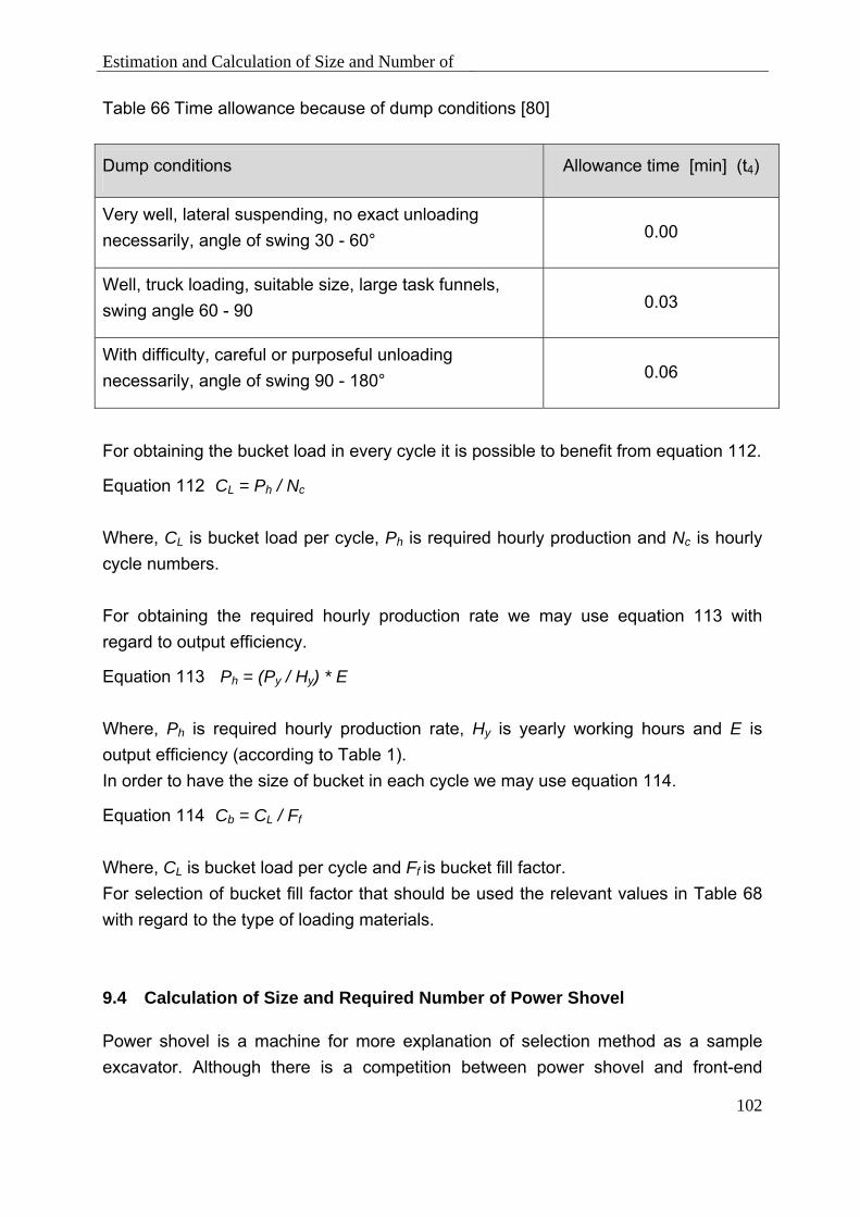
Estimation and Calculation of Size and Number of
102
Table 66 Time allowance because of dump conditions [80]
Dump conditions Allowance time [min] (t4)
Very well, lateral suspending, no exact unloading necessarily, angle of swing 30 - 60° 0.00
Well, truck loading, suitable size, large task funnels, swing angle 60 - 90 0.03
With difficulty, careful or purposeful unloading necessarily, angle of swing 90 - 180° 0.06
For obtaining the bucket load in every cycle it is possible to benefit from equation 112.
Equation 112 CL = Ph / Nc
Where, CL is bucket load per cycle, Ph is required hourly production and Nc is hourly cycle numbers. For obtaining the required hourly production rate we may use equation 113 with regard to output efficiency.
Equation 113 Ph = (Py / Hy) * E
Where, Ph is required hourly production rate, Hy is yearly working hours and E is output efficiency (according to Table 1). In order to have the size of bucket in each cycle we may use equation 114.
Equation 114 Cb = CL / Ff
Where, CL is bucket load per cycle and Ff is bucket fill factor. For selection of bucket fill factor that should be used the relevant values in Table 68 with regard to the type of loading materials.
9.4 Calculation of Size and Required Number of Power Shovel
Power shovel is a machine for more explanation of selection method as a sample excavator. Although there is a competition between power shovel and front-end

Estimation and Calculation of Size and Number of
103
loader, dragline, hydraulic shovel and other loading machines, but up to now it is considered as a working horse in surface mining industry. For this reason, all its executive data have been published with a high great of measuring which make it possible to have an exact selection. Followings are some important considerations at the time of selecting the process: - Nominal capacity or production: power shovels would be classified according to their nominal capacity in accordance with m3/hr. This is in compliance with the bucket size, type of materials, working time, difficulty of digging, type of haulage machine and working conditions. Generally all mentioned measures for the capacity of loaders are useful for bank (solid) materials. But in dealing with haulage systems, the applied capacity is the amounts of loose (broken) materials after excavation. It is possible to benefit from following estimated specific weights for soil or rocks on bank ore loose basis (Table 67 ).
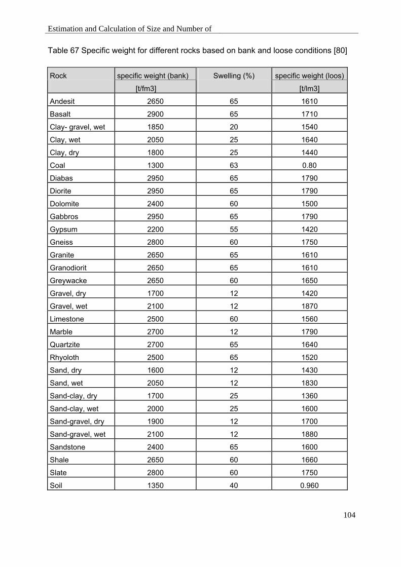
Estimation and Calculation of Size and Number of
104
Table 67 Specific weight for different rocks based on bank and loose conditions [80]
specific weight (bank) specific weight (loos)Rock [t/fm3]
Swelling (%) [t/lm3]
Andesit 2650 65 1610
Basalt 2900 65 1710
Clay- gravel, wet 1850 20 1540
Clay, wet 2050 25 1640
Clay, dry 1800 25 1440
Coal 1300 63 0.80
Diabas 2950 65 1790
Diorite 2950 65 1790
Dolomite 2400 60 1500
Gabbros 2950 65 1790
Gypsum 2200 55 1420
Gneiss 2800 60 1750
Granite 2650 65 1610
Granodiorit 2650 65 1610
Greywacke 2650 60 1650
Gravel, dry 1700 12 1420
Gravel, wet 2100 12 1870
Limestone 2500 60 1560
Marble 2700 12 1790
Quartzite 2700 65 1640
Rhyoloth 2500 65 1520
Sand, dry 1600 12 1430
Sand, wet 2050 12 1830
Sand-clay, dry 1700 25 1360
Sand-clay, wet 2000 25 1600
Sand-gravel, dry 1900 12 1700
Sand-gravel, wet 2100 12 1880
Sandstone 2400 65 1600
Shale 2650 60 1660
Slate 2800 60 1750
Soil 1350 40 0.960

Estimation and Calculation of Size and Number of
105
Table 68 is about nominal capacity of shovels with small shovels of 3 to 35 cubic meters, which may be applied, for loading in surface mining. - Operating factors: The obtained capacities from Table 68 should be in compliance with real conditions. These modifications should be applied only for three factors of working time, operating conditions and difficulty of digging which have been assumed ideal in the said Table.
Table 68 Shovel cycle times (t1 sec) [4], [79], [80]
Digging conditions
Bucket Capacity
(yd³)
Bucket capacity
)m³(
E
M
M-H
H
4 3 18 23 28 32
5 4 20 25 29 33
6 5 21 26 30 34
7 5,5 21 26 30 34
8 6 22 27 31 35
10 8 23 28 32 36
12 9 24 29 32 37
15 11,5 26 30 33 38
20 15 27 32 35 40
25 19 29 34 37 42
45 35 30 36 40 45
Average fill factor 1.00-0.95 0.90 – 0.85 0.85 – 0.80 0.80 – 0.75 E: Easy digging, loose, free-running material; e.g., sand, small gravel
M: Medium digging, partially consolidated materials; e.g., clayey gravel, packet earth, clay, anthracite, etc. M-H: Medium- hard digging; e.g., well blasted limestone’s, heavy wet clay, weaker ores, gravel with large boulders, etc. H: Hard digging – materials that require heavy blasting and tough plastic clays; e.g., granite, strong limestone, taconite, strong ores, etc. - Working time: Working time or real application time could be reduced basically according to % 100 of available time. All necessary decisions would be made according to the managerial and working conditions (according to Table 69 to Table 71) [4], [79], [80].

Estimation and Calculation of Size and Number of
106
Table 69 Shovel availability upon operation conditions [4], [79], [80]
Availability conditions Actual time
Favourable 7 hr / shift, 55 min / hr
Average 7 hr / shift, 50 min / hr
Poor 7 hr / shift, 40min / hr
Table 70 Availability in different surface mining methods [4], [79], [80]
Mining method Availability (%)
Strip mining 75
Open pit mining 85
Sand and gravel pits 90
Dimensional stone quarries 95
Table 71 Shovel and loader operating efficiency [4], [79], [80]
Management Conditions Operation Conditions
Excellent Good Fair Poor
Excellent 0,83 0,80 0,77 0,70
Good 0,76 0,73 0,70 0,64
Fair 0,72 0,69 0,66 0,60
Poor 0,63 0,61 0,59 0,54

Estimation and Calculation of Size and Number of
107
- Operating conditions: Operating conditions are reflecting different executive factors such as swing angel, digging depth or height of bench, bucket fill factor (the portion of bucket volume actually utilized during normal operation) and loading conditions. Since all mentioned values in Table 68 are assumed as ideal, it is necessary to use from correct coefficients in compliance with Table 72 for presenting of real amounts. Table 72 Bench and swing angle correction [4], [79], [80]
Angle of swing (degrees) 45 60 75 90 120 150 180
Swing factor (Fs) 0.83 0.91 0.95 1.00 1,1 1,19 1,3
Optimum digging depth (%) 40 60 80 100 - - -
Correction factor (Fh) 1,25 1,1 1,02 1.00 - - -
Finally for selecting a suitable size of power shovel, the following experimental equation (equation 115) for an estimated amount should be used.
Equation 115 Shovel bucket size (yd³) = T0.4 * 0.3
Where, T is daily production according to small tone. The size of shovel which is selected really should be equal or more than calculated amounts by equation 115. Production rate of hydraulic shovel (cubic meter of loose materials per hour) would be obtained from equation 116.
Equation 116 Ph = Nc * CL
Where, Ph is hourly production rate and CL is bucket load per cycle. For obtaining the bucket load in every cycle it is possible to benefit from equation 117.
Equation 117 CL = Cb * Ff
With regard to the present experiences, it is possible to obtain shovel cycle time according to the capacity of shovel from Table 68Table 68. It is possible to calculate actual cycle time by the use of equation 118.
Equation 118 Tt = t1 * Fs * Fh

Estimation and Calculation of Size and Number of
108
Where, Tt is actual cycle time, t1 is obtained time from Table 79, Fs and Fh are respectively modified factors because of swing angle and operating height. Regarding the calculated cycle time, it is possible to calculate number of required cycles per hour by the use of equation 119.
Equation 119 Nc = Te / Tt
Where, Nc is hourly required cycle numbers (minute), Te is effective working time per hour (minute) and Tt is actual cycle time. For obtaining the bucket load in every cycle it is possible to benefit from equation 120.
Equation 120 CL = Ph / Nc
Where, CL is bucket load per cycle, Ph is required hourly production and Nc is hourly cycle numbers. For obtaining the required hourly production rate we may use equation 121 with regard to output efficiency.
Equation 121 Ph = (Py / Hy) * E
Where, Ph is required hourly production rate, Hy is yearly working hours and E is output efficiency (according to Table 71). In order to have the size of bucket in each cycle we may use equation 122.
Equation 122 Cb = CL / Ff
Where, CL is bucket load per cycle and Ff is bucket fill factor. For selection of bucket fill factor we may use the relevant values in Table 68 with regard to the type of loading materials [4], [79], [80].
9.5 Calculation of Size and Required Number of Trucks
Here truck is being selected as the haulage equipment in open pit and strip mining. This is because of their applications more than conveyors, scrappers, dozers and other haulage equipments along with enough executive information like power shovel. For selecting the size of truck for use with a particular excavator following consideration must be noted: - Truck size: Truck capacity is generally calculated for prevention from additional load instead of volume in accordance with the weight. All mentioned volume amounts are in accordance with the volume of loose materials. There are different standard sizes

Estimation and Calculation of Size and Number of
109
between 20 to 350 tones among manufacturing factors. According to the present experiences all small sizes would be applied in underground mines and the average sizes would be applied in small open pit mines and large sizes are applied in large open pit mines. - Operating factors: These are similar to coefficients used for shovels, but with some differences in their description. - Working time: this time or availability is considered similar shovels meaning 50 min/hr and 7hr / shift, unless there is any other special condition. - Optimal number of loading swings (for filling the truck): This is depending upon the situation of truck beside the shovel and swing angle of it. The rate of optimal capacities of truck or number of loading the shovel for filling the truck has been presented in Table 73.
Table 73 Optimal number of swings used to fill a truck [4], [79], [80]
Haulage distance Loader
Hydraulic shovel
Power shovel
Short haulage distance (less than 500 meter) 3 5 4
Average haulage distance (less than 1000 meter) 4 7 5
long haulage distance (more than 1000 meter) 5 9 6
- Fill factor: The ability to fill the bucket of the excavator will affect the number of passes needed to fill a haulage truck and as mentioned in Table 74.
Table 74 Bucket fill factor upon operating conditions [4], [79], [80]
Bucket fill factor Loading conditions
1.2 Favourable
0.9 Average
0.6 Unfavourable
- Haulage cycle time: It is necessary to estimate special haulage times of a mine in haulage cycle and then the results should be added to each other. Equation 123 is for obtaining the haulage cycle time.
Equation 123 t = tte + tse + tl + ttl + twd + tsd + td

Estimation and Calculation of Size and Number of
110
Where, t is the total haulage cycle time and tte is the travel time of empty truck, twe is waiting time of truck beside a shovel, tse is manoeuvre time beside a shovel, tl is loading time, ttl is travel time of a loaded truck, twd is waiting time of truck in dump area (according to the experiences it is different from 0.5 to 0.8 minutes and This time would be considered 1.2 minutes at crusher), tsd is manoeuvre time of truck in dump area and td is dumping time (all mentioned times are according to seconds). It is possible to estimate waiting, manoeuvre and dump times. When it is possible to calculate loading and travel times of selected equipment, the waiting and dumping times would be generally estimated according to the operating conditions. Following times are for trucks (Table 75). But in order to have travel times, it is necessary to have relevant information about speed specifications, power of truck and the length and profile of hauling roads. Since all specifications of truck would be changed in compliance with different machines, here the selection process would be facilitated by the use of time-movement elements which have been determined up to now.
Table 75 Manoeuvre and dump times upon operating conditions
Operating conditions Manoeuvre time( min)
Dump time (min)
Favourable 0.15
1.00
Average 0.30
1.30
Unfavourable 0.50
1.80
Truck loading time would be obtained from equation 124.
Equation 124 tl = (Ns – 1) * tsl * + twe
Where, tl is truck loading time, tsl is shovel cycle time, Ns is number of loading swings and twe is waiting time of truck beside a shovel. Truck travel times (loaded and empty) would be obtained from equations 125 and 126.
Equation 125 Ttw (minute) = (Lh / Sl)* 60
Equation 126 Tte (minute) = (Lh / Se)* 60

Estimation and Calculation of Size and Number of
111
Where, Ttw is travel time for loaded truck, Tte is empty truck travel time, Lh is hauling distance, Sl and Se are respectively speed for loaded and empty truck. The speed of truck with load and on empty conditions could be obtained form curves that presented by manufacturing factories. For benefiting from these curves, it is necessary to calculate the total resistance of haul road which is a mathematical adds of rolling resistance (Table 76) and grade resistance of the haul road. Then it is possible to obtain the maximum rate of speed by the use of total resistance out of the mentioned curves [79], [80] .
Table 76 Rolling resistance up on ground conditions of road [80]
Ground conditions
Rolling resistance
(% of the total gross mass)
Hard, smooth, fastened road, no tire penetration, concrete, asphalt) 1–2
Firm, smooth road, which deforms under load something (to 2 cm), crushed stone or earth cover 5
Fastened road, with rather soft surface, (tire penetration up to 10 cm)
8
Loose sand or gravel 10
Soft, muddy, deeply rutted 10 – 20
Snow-packed 25 – 45
It is necessary to note that all obtained speeds could be modified with regard to Table 77 and Table 78 out of obtained amounts in relevant calculations (equations 125 and 126).
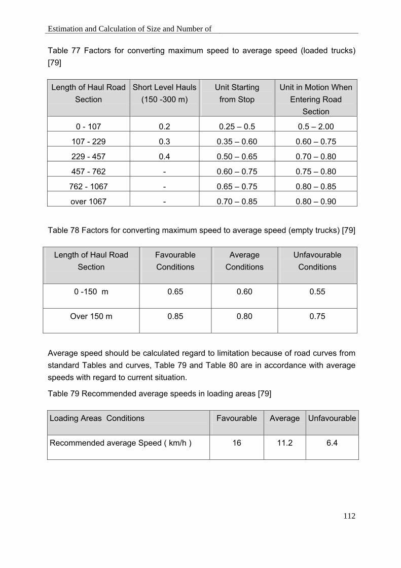
Estimation and Calculation of Size and Number of
112
Table 77 Factors for converting maximum speed to average speed (loaded trucks) [79] Length of Haul Road
Section
Short Level Hauls(150 -300 m)
Unit Starting from Stop
Unit in Motion When Entering Road
Section
0 - 107 0.2 0.5 – 0.25 2.00 – 0.5
107 - 229 0.3 0.60 – 0.35 0.75 – 0.60
229 - 457 0.4 0.65 – 0.50 0.80 – 0.70
457 - 762 - 0.75 – 0.60 0.80 – 0.75
762 - 1067 - 0.75 – 0.65 0.85 – 0.80
over 1067 - 0.85 – 0.70 0.90 – 0.80
Table 78 Factors for converting maximum speed to average speed (empty trucks) [79]
Length of Haul Road Section
Favourable Conditions
Average Conditions
Unfavourable Conditions
0 -150 m
0.65
0.60
0.55
Over 150 m
0.85
0.80
0.75
Average speed should be calculated regard to limitation because of road curves from standard Tables and curves, Table 79 and Table 80 are in accordance with average speeds with regard to current situation.
Table 79 Recommended average speeds in loading areas [79]
Loading Areas Conditions
Favourable
Average
Unfavourable
Recommended average Speed ( km/h )
16
11.2
6.4
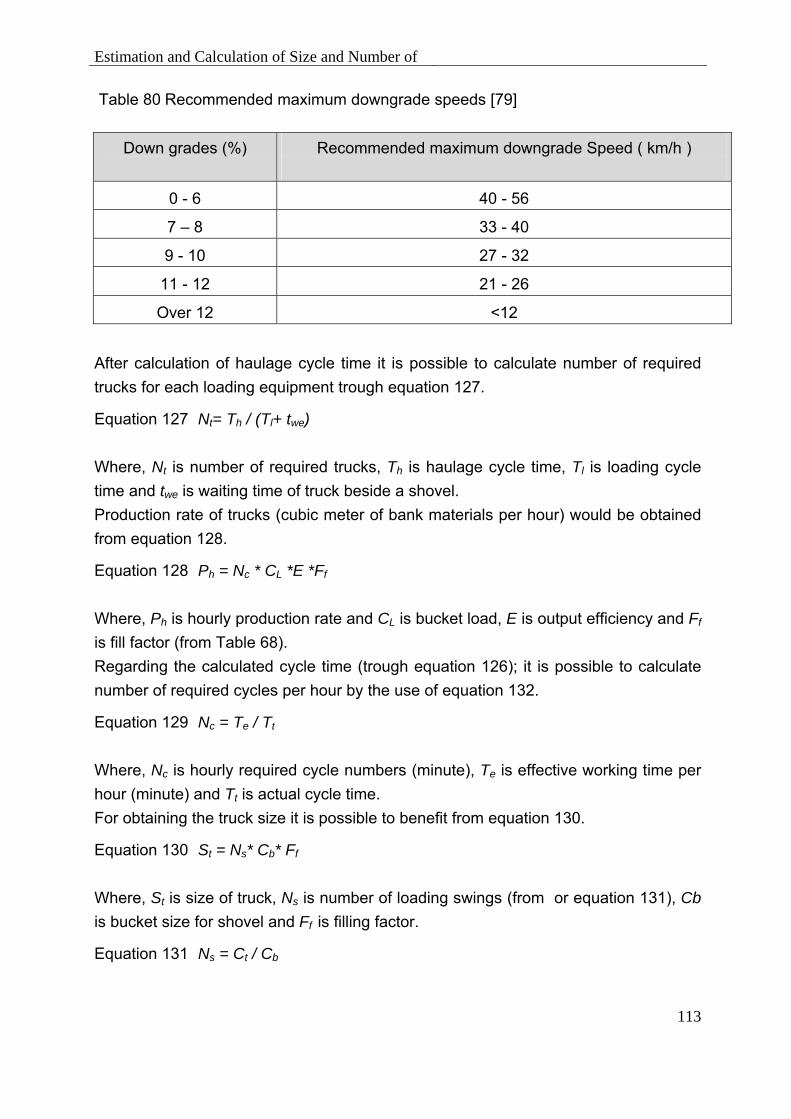
Estimation and Calculation of Size and Number of
113
Table 80 Recommended maximum downgrade speeds [79]
Down grades (%)
Recommended maximum downgrade Speed ( km/h )
0 - 6 40 - 56
7 – 8 33 - 40
9 - 10 27 - 32
11 - 12 21 - 26
Over 12 <12
After calculation of haulage cycle time it is possible to calculate number of required trucks for each loading equipment trough equation 127.
Equation 127 Nt= Th / (Tl+ twe)
Where, Nt is number of required trucks, Th is haulage cycle time, Tl is loading cycle time and twe is waiting time of truck beside a shovel. Production rate of trucks (cubic meter of bank materials per hour) would be obtained from equation 128.
Equation 128 Ph = Nc * CL *E *Ff
Where, Ph is hourly production rate and CL is bucket load, E is output efficiency and Ff
is fill factor (from Table 68). Regarding the calculated cycle time (trough equation 126); it is possible to calculate number of required cycles per hour by the use of equation 132.
Equation 129 Nc = Te / Tt
Where, Nc is hourly required cycle numbers (minute), Te is effective working time per hour (minute) and Tt is actual cycle time. For obtaining the truck size it is possible to benefit from equation 130.
Equation 130 St = Ns* Cb* Ff
Where, St is size of truck, Ns is number of loading swings (from or equation 131), Cb is bucket size for shovel and Ff is filling factor.
Equation 131 Ns = Ct / Cb

Estimation and Calculation of Size and Number of
114
Where, Cb is bucket size for shovel and Ct is volume of truck bucket. For obtaining the truck load in every cycle it is possible to benefit from equation 132.
Equation 132 TL = Ff * Ns * Cb * Swl
Where, TL is load of truck, Ns is number of loading swings, Cb is bucket size for shovel, Swl is loose material density and Ff is filling factor.
9.6 Reserve Machines
In order to repair and maintenance the trucks in haulage fleet and prevention from any shortage in production operations, generally we should purchase reserve machines. There is one reserve machine for 5 to 6 simultaneous active machines. In order to have a suitable adaptation between the shovel and truck, trucks should be selected with capacity of + - %5 calculated load. (When the size of truck is %5 smaller than the load, it is a sign of complete fullness of truck. Of course there is a possibility of additional load in this conditions) [79], [80].
9.7 Simultaneous Situation of Loading and Haulage Equipments
Before ending of selection the loading and haulage equipments, ensuring about simultaneous time of loading and haulage operations should be controlled. This is for ensuring about the following cases: 1) Shovel may not remain waiting for trucks 2) There will be no more minutes for waiting time of truck In case of non-satisfied operations simultaneous, selection of equipment should be modified or the cycle time of them should be changed (travel, waiting and dumping times). After determination of the mentioned times and obtaining knowledge about haulage cycle time, we can control the simultaneous conditions through the equation 133.
Equation 133 t<n (tl + ts)
Where, n is the number of trucks. In order to have an equal time conditions, we should have the haulage cycle of a truck (t) lower than required time for loading and waiting of loading and haulage fleet (n (t1 + ts)) [49], [79], [80].

Estimation and Calculation of Production Costs for
115
10 Estimation and Calculation of Production Costs for Loading and Haulage Equipments
10.1 Estimation of Production Costs for Loading and Haulage Equipments
In order to estimate operating and production costs of loading and haulage equipment, we may benefit from equations 134 and 135. The considerable point is that costs index of equations 1 and 2 is related to 1988. Therefore, the obtained results have been multiplied in rate of costs indices of considered year to costs indices of relevant year 1988 (This rate is 1.36 for current year).
Equation 134 Daily loading costs (us. $) = 2.67 * T0.7 *A
Equation 135 Daily haulage costs (us. $) = 18.07 * T 0.7 *A
By the use of equations 136 and 137 it will be possible to calculate capital costs of loading and transportation equipment.
Equation 136 Loading capital costs (us. $) = 2.67 * T 0.7 *B
Equation 137 Haulage capital costs (us. $) = 18.07 * T 0.7 *B
Where, T is daily mine production(based on small tone), S is bucket size of loading equipment, Ns is number of loading equipments, t is size of truck, Nt is number of trucks and A is the rate of costs indices of considered year to costs indices of relevant year 1988 . The other considerable point is that the index of costs has been assumed as 1400 in estimation of above-mentioned equations. Therefore, the obtained results have been multiplied in B as the costs index of considered year to 1400 (This is 0.803 for current year). Regarding the daily production rate and also useful lifetime of loading and haulage equipments, we may have output costs according to operating hour and production unit. [44], [45]
10.2 Calculation of Production Costs for Loading and Haulage Equipments
In order to calculate production costs of equipment, we should have these costs in two parts of capital costs (including purchase price of equipments, relevant costs of

Estimation and Calculation of Production Costs for
116
depreciation, interest, tax and insurance) and operating costs according to the type of systems including (fuel and energy costs, lubrication costs and filter and …, Tire costs, relevant costs of repair parts and maintenance, costs of spare parts and labor cost).
10.2.1 Capital Costs
Capital costs include purchase price of equipments, relevant costs of depreciation, interest, tax and insurance and calculated through equations 138 to 142.
Depreciation costs would be obtained from equation 138.
Equation 138 Depreciation costs (us. $/hr) = (purchase price–salvage value)/operating life of equipment (hr)
Relevant costs of interest would be calculated out of equation 139, relevant costs of tax from equation 140 and relevant costs of insurance out of equation 141.
Equation 139 Interest costs (us. $/hr) = (average annual investment * interest rate) / yearly operating hour
Equation 140 Tax costs (us. $/hr) = (average annual investment * tax rate) / yearly operating hour
Equation 141 Insurance costs (us. $/hr) = (average annual investment * insurance rate) / yearly operating hour
Equation 142 would calculate the average annual investment in equations 139 to 141.
Equation 142 Average annual investment = purchase price * (n+1)/2n
Where, n is the operating life of equipment according to the year. In order to obtain working hours of equipment through the operating life, we may benefit from amounts mentioned in Table 81 with regard to their different types.

Estimation and Calculation of Production Costs for
117
Table 81 Operating life of mining equipment [36], [45], [79]
Number of Hours Equipment type
Poor Conditions
Average Conditions
Good Conditions
Dozer 18000 25000 35000
Grader 20000 30000 50000
Large front-end loader 20000 30000 45000
Hydraulic excavator(small) 15000 22500 30000
Hydraulic excavator(large) 20000 30000 45000
Scraper 12000 16000 20000
Truck(50 to 100 t) 20000 30000 42000
Truck(large) 30000 45000 60000
Rope shovel 60000 80000 100000
Walking dragline 60000 100000 150000
10.2.2 Operating Costs
Operating costs of equipments upon their types include following items: - Energy and fuel costs - Lubrication and filter costs - Tire costs - Repair parts and maintenance costs - Spare part costs - Labor costs
10.2.2.1 Energy and Fuel Costs
Relevant costs of fuel and energy include the costs of electricity or fuel consumption and for its determination we should benefit from equation 143 for calculation of consumption rate and relevant price.

Estimation and Calculation of Production Costs for
118
Equation 143 Energy or fuel cost (us. $ /hr) = hourly usage * fuel price
Hourly usage of energy is according Table 82, or would be calculated out of equation 144.
Equation 144 Hourly fuel usage (litres) = rated power (kW) * 0.3 * load factor
Where load factor is according Table 83 upon operating conditions and equipments type.
Table 82 Energy usage for mining equipment [36], [45]
Equipment
Electricity (Energy ) Usage
Rope shovel (older, smaller shovels) 0,6 kW per m ³ /h
Rope shovel (newer, larger shovels) 0,35 kW per m ³ /h
Table 83 Load factor for fuel usage calculation [36], [45]
Equipment
Power (kW)
Load Factor , Low Range
Load Factor ,High Range
160 0.52 – 0.4 0.83 – 0.67
276 0.51 – 0.36 0.83 – 0.63 Tracked dozers 575 0.41 – 0.36 0.67 – 0.63
Wheel dozer 336 0.45 – 0.40 0.77 – 0.71
Grader 205 0.41 – 0.31 0.72 – 0.62
Hydraulic excavator 287 0.35 – 0.30 0.74 – 0.69
366 0.41 – 0.36 0.71 – 0.66
443 0.43 – 0.35 0.71 – 0.65 Scraper 708 0.46 – 0.41 0.77 – 0.72
485 0.26 – 0.18 0.49 – 0.38
649 0.27 – 0.18 0.50 – 0.38
962 0.28 – 0.18 0.50 – 0.35
1272 0.27 – 0.18 0.49 – 0.37
Rear dump trucks 1534 0.26 – 0.18 0.49 – 0.37
280 0.45 – 0.38 0.79 – 0.71
515 0.39 – 0.35 0.73 – 0.67 Front-end loaders 932 0.39 – 0.36 0.74 – 0.68

Estimation and Calculation of Production Costs for
119
10.2.2.2 Lubrication and Filter Costs
In order to calculate relevant costs of lubrication and filters which may be explained according to a percentage of fuel costs which is about 20 percent for low-movement equipments and 30 to 40 percent for full-movement equipment such as hydraulic shovel. Here is considered only 30 percent of fuel consumption in all calculations of this part of costs.
10.2.2.3 Tire Costs
When rubber-tired equipments have been used, the costs of tire would be calculated out of equation 145. The life of tire has been inserted in Table 84 with regard to operating conditions and also type of equipment.
Equation 145 Tire cost (us. $ /hr) = tire price / operating life
Table 84 Tire life for mining equipment upon operation conditions [36], [79]
Number of Hours Equipment Poor
Conditions Average
Conditions Good
Conditions
Large front-end loader 2000 3000 4000
Scraper 2500 3500 5500
Truck 2500 3200 4000
10.2.2.4 Maintenance and Repair Parts Costs
Relevant costs of repair parts and maintenance include of three parts of repair costs, major overhaul costs and maintenance labor costs and would be calculated through equations 146 to 148.
Equation 146 Repair cost (us. $ /hr) = purchased price *repair factor * maintenance factor
Where repair factor has been inserted in Table 85 and maintenance factor is according Table 86.

Estimation and Calculation of Production Costs for
120
Major overhaul is generally necessary in a time limit about 10000 working hours for equipment. Relevant costs of major overhaul are in accordance with a percentage of purchase costs and would be calculated by equation 147.
Equation 147 Major overhaul cost (us. $ /hr) = purchased price *relevant percentage / period for major overhaul
The percentage of major overhaul and also necessary period for major overhaul has been inserted in Table 85.
Table 85 Typical repair parts and maintenance factors [36]
Equipment
Typical Life (operating
hours)
Repair Factor
Major Overhaul
(% of capital)
Frequency of Major Overhaul( operating hours)
Maintenance Labor (person-
hours per operating hour
Dozer 22500 0,25*10-4 15 10000 0,4 – 0,7
Front-end- loader
30000 0,30*10-4 15 10000 0,5 – 0,8
Hydraulic excavator
27500
0,25*10-4 15 10000 1,1 – 1,5
Rope shovel (Hard rock)
80000
0,075*10-417,5 20000 1,2 – 1,5
Rope shovel(Coal)
100000
0,035*10-47,5 20000 1,00 - 1,25
Rear dump truck
45000 0,25*10-4 15 15000 0,5 – 0,8
Table 86 Maintenance factor upon operating conditions [36]
Maintenance and management conditions
Job conditions factor
Good 1,2
Average 1
Poor 0,8
The maintenance labor costs would be calculated by equation 148.
Equation 148 Maintenance cost (us. $ /hr) = maintenance labor factor * labor cost

Estimation and Calculation of Production Costs for
121
10.2.2.5 Wear Parts Cost
Wear items include bucket teeth, hoist ropes, drag ropes and dump rope for shovel. The Method of calculation of wear parts is to take the cost of all of the wear items and dived each of them by its estimated life.
10.2.2.6 Labor Costs
Labor costs are typically calculated on an annual basis and would be obtained with regard to insurance, tax and advantages.
10.2.2.7 Total Production Costs
The total production costs include the capital and operating costs. Input and out put data’s and calculation methods are illustrate in Figure 45 to Figure 52 and Table 87 to Table 91.

Estimation and Calculation of Production Costs for
122
Table 87 Output Summary
Trucks payloads: [t]
Maximum Trucks load: [t]
Loader bucket capacity: [m³]
Bucket loading mass: [t]
Number of swings:
Calculated trucks load: [t]
Trucks bucket capacity: [m³]
Density of loading materials(lose): [t/m³]
Volume of loading materials: [m³]
Loading cycle: [s]
Haulage cycle: [s] , [h]
Trucks type:
Loader type:
Table 88 Production data’s
Availability [%],min/h] Number of needing trucks: Normal - 1 Normal Normal +1 Hourly Production: [t] Hourly Volume (bulk): [m³] Hourly Volume (loos): [m³]

Estimation and Calculation of Production Costs for
123
Table 89 Capital Costs
Number of Equipments Normal -1 Normal Normal +1 Purchased price: € Calculated Depreciation: € Calculated Interest: € Calculated Taxes: € Calculated Insurance: € Total Capital Costs: €
Table 90 Operating Costs
Number of Equipment Normal -1 Normal Normal +1
Tire Costs: €
Fuel or Power Costs: €
Lubrication Costs: €
Maintenance and Repair parts : €
Major Overhaul Costs : €
Wear Parts : €
Maintenance Labor Costs : €
Labor Costs : €
Total Operation Costs : €

Estimation and Calculation of Production Costs for
124
Table 91 Production Costs
Production rate pro [t] pro [h] Number of Equipment Normal -1 Normal Normal +1 Normal-1 Normal Normal+1Capital Costs: € Operating Costs: € Production Costs: €
operation
calendar
Material & ground (TableS 59 &60 &67)
Mine inforamatin
Size and number of Trucks
Production costs
Size and number of laoding equipment
Input(Figures 49 to 55)
OutPut(Tables 88 to 92)
Figure 45 Relevant Algorithm

Estimation and Calculation of Production Costs for
125
Loading
Rope shovel LoaderDiesel shovel
Bucket size & number of loader estimation(Formula 98 & 99)
Nearest standard size seletion from equipment lits
Loader Cycle Time(Formula 103)
Basic cycle time
(table 57)
Adding time up on
matterial type (table 59)
Adding time up on loading
high(table 58)
Adding time up on grund
condition (table 60)
Adding time up on dump
condition (table 61)
Hourly necessary cycls(Formula 104)
hourly loading volume(Formula 106)
Bucket size (Formula 107)
Efficiency from
Table 71
Efficiency from
Calculation ( Table 55 & figure 55))
Bucket fill factor
(table 56)
Hourly production (Formula 102)
Bucket size & number of loader estimation(Formula 98& 99)
Nearest standard size seletion from equipment lits
Shovel Cycle Time(Formula 110)
Basic cycle time
(table 63)
Adding time up on
matterial type (table 65)
Adding time up on loading
high(table 64)
Adding time up on dump
condition (table 66)
Hourly necessay cycls(Formula 111)
hourly loading volume(Formula 113)
Bucket size (Formula 114)
Efficiency from
Table 71
Efficiency from
Calculation ( Table 55 & figure 55))
Bucket fill factor
(table 62)
Hourly production (Formula 108)
Cycly loading volume(Formula 105)
Cycly loading volume(Formula 109)
Bucket size & number of loader estimation
(Formula 98&99)
Nearest standard size seletion from equipment lits
Shovel Cycle Time(Formula 118)
Basic cycle time
(table 68)
Swing factor(Table 72 )
Bench hight factor
(Table 72 )
Hourly necessary cycls(Formula 121)
hourly loading volume(Formula 120)
Bucket size (Formula 122)
Efficiency from
Table 71
Efficiency from
Calculation ( Table 55 & figure 55))
Bucket fill factor
(table 62)
Hourly production (Formula 116)
Cycly loading volume(Formula 117)
Figure 46 Data’s for loading equipments

Estimation and Calculation of Production Costs for
126
Figure 47 Truck data’s
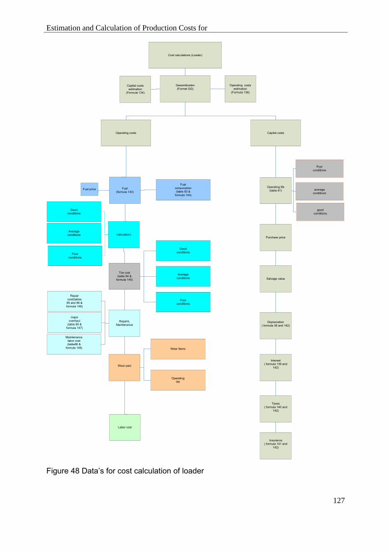
Estimation and Calculation of Production Costs for
127
Operating costs Capital costs
Fuel (formula 143)
lubrication)
Tire cost(table 84 &
formula 145)
Repairs, Maintenance
Wear pars
Labor cost
Fuel price Fuel
consumption (table 83 &
formula 144)
Good conditions
Average conditions
Poor conditions
Wear Items
Operating life
Good conditions
Average conditions
Poor conditions
Repair cost(tables
85 and 86 & formula 146)
major overhaul
(table 85 & formula 147)
Maintenance labor cost (table86 &
formula 148)
Insurance( formula 141 and
142)
Taxes( formula 140 and
142)
Interset( formula 139 and
142)
Salvage value
Purchase price
Operating life(table 81)
Depreciation ( formula 38 and 142)
Poor conditions
average conditions
good conditions
Cost calculations (Loader)
Gesamtkosten(Formel GG)
Operating costs estimation
(Formula 136)
Capital costs estimation
(Formula 134)
Figure 48 Data’s for cost calculation of loader

Estimation and Calculation of Production Costs for
128
Figure 49 Data’s for cost calculation of hydraulic shovel

Estimation and Calculation of Production Costs for
129
Operating costs Capital costs
Engergy cost (formula 143 )Energy price Energy
usage(table 82)
lubrication)
Repairs, Maintenance
Wear pars
Labor cost
Good conditions
Average conditions
Poor conditions
Repair cost(tables
85 and 86 & formula 146)
major overhaul
(table8 5 & formula 147)
Maintenance labor cost (table 86 & formula 148 Wear Items
Operating life
Insurance( formula141 and142)
Taxes( formula140 and142)
Interset( formula139 and142)
Salvage value
Purchase price
Operating life(table 81)
Depreciation ( formula 138 and
142)
Poor conditions
average conditions
good conditions
Cost calculations (Rope Shovel)
Gesamtkosten(Formel GG)
Operating costs estimation
(Formula 136)
Capital costs estimation
(Formula 134)
Figure 50 Data’s for cost calculation of power shovel

Estimation and Calculation of Production Costs for
130
Cost calculations (truck)
Gesamtkosten(Formel GG)
Capital costs
Operating costs estimation
(Formula 137)
Capital costs estimation
(Formula 135)
Insurance( formula 141 and
142)
Taxes( formula 140 and
142)
Interset( formula 139 and
142)
Salvage value
Purchase price
Operating life(table 81)
Depreciation ( formula 138 and
142)
Poor conditions
Operating costs
Fuel (formula 143)
lubrication)
Tire cost(table 4 & formula 12)
Repairs, Maintenance
Wear pars
Labor cost
Fuel price Fuel
consumption (table 83 &
formula 144)
Good conditions
Average conditions
Poor conditions
Wear Items
Operating life
Good conditions
Average conditions
Poor conditions
Repair cost(tables
85 and 86 & formula 146)
major overhaul
(table 85 & formula 147)
Maintenance labor cost (table 85 &
formula 148)
average conditions
good conditions
Figure 51 Data’s for cost calculation of trucks
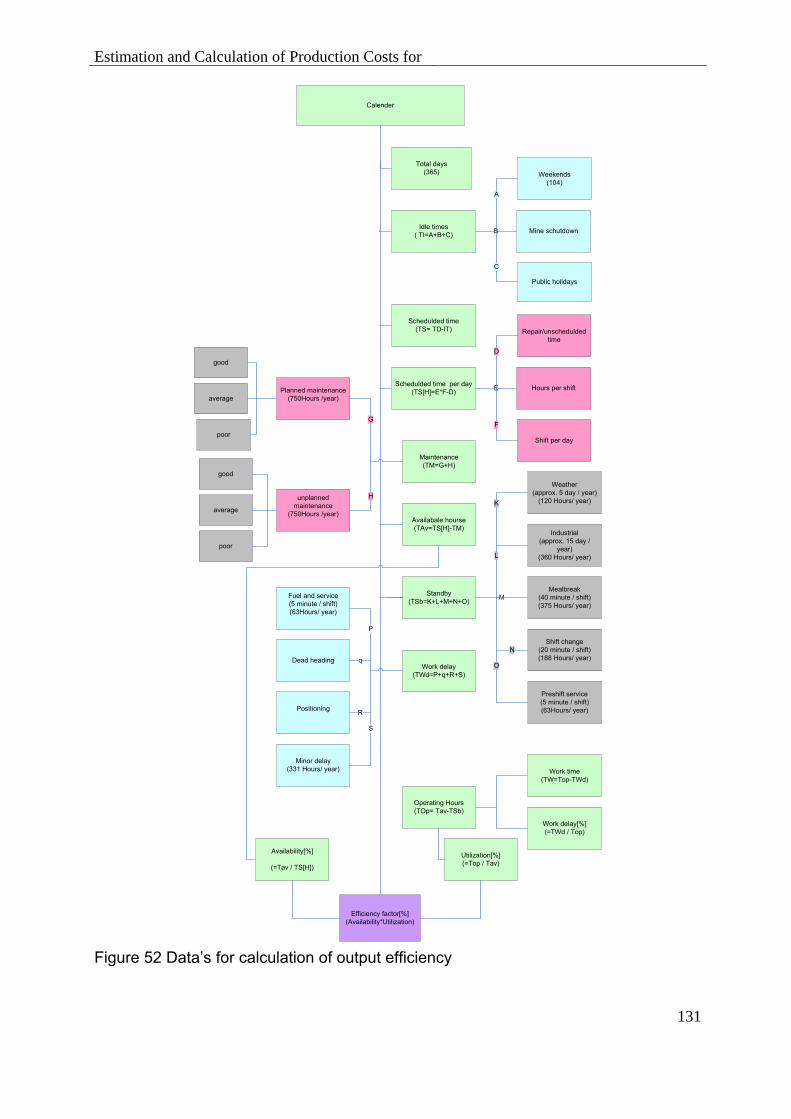
Estimation and Calculation of Production Costs for
131
Standby (TSb=K+L+M+N+O)
Idle times( TI=A+B+C)
Schedulded time(TS= TD-IT)
unplanned maintenance
(750Hours /year)
Planned maintenance(750Hours /year)
Total days(365)
Mine schutdown
Hours per shift
Weekends(104)
Public holidays
Schedulded time per day(TS[H]=E*F-D)
Shift per day
Repair/unschedulded time
Availabale hourse(TAv=TS[H]-TM)
Maintenance(TM=G+H)
Weather(approx. 5 day / year)
(120 Hours/ year)
Preshift service(5 minute / shift)(63Hours/ year)
Shift change(20 minute / shift)(188 Hours/ year)
Industrial(approx. 15 day /
year)(360 Hours/ year)
Mealbreak(40 minute / shift)(375 Hours/ year)
B
C
A
E
F
D
M
L
O
N
K
Operating Hours(TOp= Tav-TSb)
Work delay(TWd=P+q+R+S)
Minor delay(331 Hours/ year)
Positioning
Dead heading
Fuel and service(5 minute / shift)(63Hours/ year)
G
H
P
S
q
R
Work delay[%](=TWd / Top)
Work time(TW=Top-TWd)
Availability[%]
(=Tav / TS[H])
Utilization[%](=Top / Tav)
Calender
Efficiency factor[%](Availability*Utilization)
good
average
poor
good
average
poor
Figure 52 Data’s for calculation of output efficiency

132
11 Conclusion
- Today the total production rate of minerals (including metal ores, non-metallic ores and coal) is more than 16.6 milliards ton per year from which the share of surface mines are more than 11.5 milliards tones per year. The production rate of construction materials is about 23.5 milliards tones per year and the annual production rate of cement is more than 2.3 milliards tones. By calculation of wastes obtained in surface mines (about 30 milliard tones), the total amount of materials handling in open mines may reach to more than 67 milliards ton per year and it is estimated to have this rate up to 138 milliard tones in 2030. - Total mining costs in surface mines is 138 milliard us $ per year from which about 85.6 milliard us $ is related to metallic surface mines, 7 milliard us. $ for non-metallic surface mines and 45.8 milliard us. $ for surface coal mines. - The shares of loading and haulage costs in surface mines are about 100 milliards us. $ per year from which about 33.5 milliards us $ is related to metallic surface mines, 1.7 milliard us. $, for non-metallic surface mines, 24.8 milliards us. $ for surface coal mines and about 37 milliards us.$ for construction materials and cement mines. - One of the major present costs in a mine is related to hauling of materials, while in most cases in open pit mines the share of this part is reached about % 70 of total operating costs and % 90 for equipment capital costs. Therefore, considering these costs could be so much effective in total economy of the mine and consideration of this reality made the mine specialists to have daily increasing efforts for reducing the costs of this part. - Since the major common method for materials handling in open pit mines is benefiting from non-continuous methods (use of mining trucks), one of the methods for reducing of costs could be replacing of cheap transportation systems such as conveyors with mobile crushers (for layer mines with low number of benches) and semi-mobile crushers (for multi-benches mines) instead of truck. Of course, it is better to use from a combination of both methods in this field. - Regarding the high flexibility for using of trucks in open pit mines and since due to the diffusion and different distribution of grade in metallic mines makes no possibility only to use selected mining methods, it is impossible to have a complete replacement of truck with continuous haulage systems in such cases and there is no more chances only to use truck or a combined system. Therefore, in order to reduce the costs we should optimize planning of systems and select suitable equipment. For this purpose, it is necessary to benefit from computer software. But on the other hand, there are

133
different software about selection and calculation of mining equipment with various disadvantages. Following is a list of the mentioned software disadvantages: A- Since the current software have been submitted by equipments manufacturing companies and they have considered only theoretical aspects of machinery for more marketing and sale with a low consideration of applicable and operational problems, therefore, the presented digits and values in Tables of the said companies have an obvious difference with obtained values and amounts obtained from mining operations. B- Some of the current software may consider only technical aspects of using the equipment without any ability for any economic analysis. C- In most of these software’s there are separate calculation for loading and haulage equipments, therefore, it is not possible to consider any effects of loading and haulage systems on each other. D- There is low consideration of relevant conditions of deposits and mine and also regional and environmental conditions. - Regarding all above-mentioned items, it is necessary to provide software with coverage of all mentioned weak points and also considering all relevant problems of mineral deposit, ores, regional and environmental conditions. In addition, it is necessary to benefit from all practical and experimental results at the time of supplying the said software. - Considering the estimation of relevant costs of equipments in this report, it is obvious that in al cases any increase of capacity of equipments and also any increase in mines production rates may cause a considerable reduction of costs. Therefore, applying of greater equipments is so much preferable.

134
References
[1] Beal .J .V. mining’s place and contribution , SME mining engineering handbook, volume 1, 1973
[2] Cedric E. Gregory A concise history of mining, 1980
[3] B. Stoces Introduction to mining, 1954
[4] Haward L. Hartman Introductory mining engineering, 2002
[5] T. A. Rickard, M. Hil a history of American mining , New York ,1932
[6] Gregory, C. E rudiments of mining practice, Trans Tech Publ., 1983
[7] Koehler S. Stout mining methods and equipment, 1980
[8] Robert S. Lewis Elements of mining , 1964
[9] W.A.Vogely materials modelling, 1975
[10] Barbara Stack Handbook of mining and tunnelling machinery , 1982
[11] Peter M. Molloy The history of metal mining and metallurgy, 1986
[12] Bureau of Mines Mineral Commodity Summaries, Department of the Interior, 1986
[13] Bureau of Mines Status of the mineral industries mining, minerals, metals, mineral reclamation, United States Department of the Interior, 1979
[14] Cranstone, Donald Alfred a history of mining and mineral exploration and the outlook for the future Bundesanstalt für Geowissenschaften und Rohstoffe , 2003
[15] Deter Dähnert and Wolfgang Kwtzmer
the lusatian lignite area – an integrated system of modern and competitive open cast mines, world of mining - surface and underground 2006 No. 4, pp 208- 217
[16] P. Cerling and w. Wellmer
Raw material availability with a focus on fossil energy resources, , world of mining – surface and underground 2004 No. 4, pp 254- 262
[17] Bundesanstalt für Geowissenschaften und Rohstoff
Reserven, Ressourcen und Verfügbarkeit von Energierohstoffen,2002,Rohstoffwirtschaftliche Länderstudien, 2003
[18] l. Weber and g. Zsak World mining data, volume 18 , federal ministry for economy and labour of the republic of Austria, 2003

135
[19] l.E.Taylor, TJ Braoun World mineral production 2000-2004, British geological survey, 2006
[20] J L Collins and Fytas Surface mining of Canadian coal, R Singhal, coal international November 1994 pp. 212-218
[21] R Singhal, J L Collins and Fytas
Open pit trends, coal international august 1986 pp. 41-50
[22] Clement, G. K Capital and operating Cost Estimating System Manual for mining and beneficiation of metallic and non-metallic minerals except fossil fuels in the United States and Canada, 1980
[23] K. Häge German lignite industry perspectives in 2004, world of mining- surface & underground, 2004, No. 4, pp 242-253
[24] Charles E. Brown World energy resource, Springer 2002 Bundesrepublik Deutschland Rohstoffsituation, Bundesanstalt für Geowissenschaften und Rohstoff, 2002
[25] John E. Tilton
[26] S. D. Strauss
[27] W.A.Vogely
The future of nonfuel minerals, 1977 The mineral industry in transition, mining journal books, 1986 Economics of the mineral industries, American Institute of Mining, Metallurgical, and Petroleum Engineers, 1985
[28] Allen Reicks and Michael T. Myers
Bulk material handling by conveyor belts 5 , society of mining , metallurgy, and exploration, Inc.,2004
[29] M. Ruhrberg, S. Möllerherm and P.N. Martens
Untersuchung über die Auswirkungen der Umsetzung eines Ökologisch befriedigenden Bergwerkes auf Gewinnungskosten und Weltmarktpreis von Kupfer, 2004
[30] R. M. Wanless Finance for mine management ,1983
[31] U.S. Geological Survey http://minerals.usgs.gov/contacts/index.html
[32] D. R. Wilburn International mineral exploration activities from 1995 through 2004 , Usgs, 2005
[33] T. S. Lovering Minerals on world affairs, 1947
[34] J.F. Rudenberg output and availability factors of bucket wheel excavators under actual mining conditions, bulk handling in open pit mines & quarries, 1986, pp 13-24
[35] Tilton, John, E.
World mineral exploration : trends and economic issues, Resources for the Future, 1988

136
[36] Ian C. Runge.
Mining economics and strategy, society of mining , metallurgy, and exploration, Inc.,1998
[37] Federal Ministry for Economic Affairs,
World mining data, in coop. with the Association of Mining and Steel (Vienna) and the National Committees for the organisation of the World Mining ,Vienna
[38] C. R. Tinsley; M. E. Emerson
Finance for the minerals industry , AIME; SME., 1985
[39] J. W. Martin, T. J. Martin, T. P. Bennett
Surface Mining Equipment, 1982
[40] Paul T. Allsman and Paul F. Yopes
Current and future status of surface mining, SME mining engineering handbook, volume 2, 1973
[41] R.T. Moolick Stripping methods, including advanced stripping, SME mining engineering handbook, volume 2, 1973
[42] Hartman, Howard. L SME mining engineering handbook 2nd edition, volume 1, 1992
[43] E. Bozorgrahimi, R.A. Hall and G.H. Blackwell
Sizing equipment for open pit mining- a review of critical parameters, mining technology, December 2003, vol. 112, pp 171-179
[44] W. Hustrulid and M. Kuchta
Open pit mine planning & design, 1995
[45] A. L. Mular and R. Poulin a handbook for estimating mining and mineral processing equipment costs and capital expenditures and aiding mineral project evaluation, CIM special volume 47, Canadian institute of mining , metallurgy and petroleum, 1998
[46] S. D. Michaelson and R.E. Buckley
Production methods and economics, open pit copper mining, SME mining engineering handbook, volume 2, 1973
[47] E. P. Pfleider Surface haulage and storage, SME mining engineering handbook, volume 2, 1973
[48] M. Ruhrberg, S. Möllerherm and P.N. Martens
Untersuchung über die Auswirkungen der Umsetzung eines Ökologisch befriedigenden Bergwerkes auf Gewinnungskosten und Weltmarktpreis von Kupfer, 2004
[49] Eugene P. Pfleider and George. F. Weaton
Production methods and economics, ferrous ore mining, SME mining engineering handbook, volume 2, 1973

137
[50] j. R Willis Materials handling in open cut mines sate of the art and near future developments, large open pit mining conference, 1986 pp 45-50
[51] Pfleider E.P open pit and strip mining systems and equipment, sec. 17 SME mining handbook, 1973
[52] Atkinson, T , Surface Mining and Quarrying, Proc. 2nd Intl. Surface Mining and Quarrying Symposium, 1983
[53] J. W. Martin, T. J. Martin, T. P. Bennett
Surface Mining Equipment, 1982
[54] Ulrich Mentges Relocation of Semi-mobile crushing plants in Indonesia and china, world of mining – surface and underground 2003 No. 3, pp 237- 244
[55] S. Heuer outlines the advantages of belt conveyor transport over conventional truck transport, world cement November 1997 pp 34-39
[56] j. Coleman and R.d. Broglio
Semi mobile in-pit crushing for waste and coal at Mae Moh mine Thailand, large open pit mining conference, 1986, pp 31-43
[57] J. Plattner History and design of mobile in-pit crushers for open pit mines, large open pit mining conference, 1986 pp 17-22
[58] R. Franke Combined mining systems for open pit mines, bulk handling in open pit mines & quarries, 1986, pp 177-182
[59] H. Althof Cost reduction by in-pit crushing and conveying, bulk handling in open pit mines & quarries, 1986, pp 205- 208
[60] L. Tejchman and A.S. Hedge
feasibility of in-pit crushing and conveying of waste rock at MT Whaleback mine, large open pit mining conference, 1986 pp 23-30
[61] W. Guderley In-pit crushing and conveying, bulk handling in open pit mines & quarries,1986, pp 219-222
[62] C. Huss Cost consideration for in-pit crushing /conveying systems, bulk handling in open pit mines & quarries, 1986, pp 223-226
[63] W. Glanz and J. Weißflog Continuous conveying in open pit mines, bulk handling in open pit mines & quarries, 1986, pp 161-170
[64] H. Tudeshi, T. Hardebuscsh and R. Bagherpour
Cost reduction by optimization of the primary crusher position,20th WORLD MINING CONGRESS, geological survey of Iran, 2005

138
[65] H. Frühstück Rope con die Innovation in der Fördertechnik, Kolloquim Fördertechnik im Bergbau, Tu Clausthal, Taggunsband 2004
[66] R.d. Stoll, H .Tudeshki and R. Zühlsdorf
Einsatzmöglichkeiten der EDV im Tagebau, Braunkohle/surface mining, Jg. 45, Nr. 1, Januar 1996
[67] W. Platzek Untersuchungen zur Optimierung von primärbrechanlagen in Natursteinwerken über den Abbauzeitraum, Dissertation 1994 , RWTH Aachen
[68] Gentry D. W and O’Neil T. J
Mine investment analysis, SME, 1984
[69] J. R. Hoskins mineral industry cots, northwest mining association, 1982
[70] bureau of mines Bureau of mines cost estimating system handbook volume 1,surface and underground mining , bureau of mines information circular 1987
[71] western mine engineering
Mining cost service,, Inc. 1994
[72] western mine engineering
Mining cost service, Inc. 2006
[73] Bureau of mines cost estimating system handbook volume 2, mineral processing , bureau of mines information circular 1987
[74] J.F. Rudenberg output and availability factors of bucket wheel excavators under actual mining conditions, bulk handling in open pit mines & quarries, 1986, pp 13-24
[75] J.R. Hoskins and W.R. Green
Mineral industry costs, northwest mining associations, 1978
[76] Mular A.L Mining and processing equipment costs and preliminary capital costs estimations, Canadian institute of mining and metallurgy, 1982
[77] Michael Noakes and terry Lanz
Cost estimation handbook for the Australian mining industry, the Australasian institute of mining and metallurgy 1993
[78] B. Cavender Mineral production costs analysis and management, society of mining , metallurgy, and exploration, Inc., 1999
[79] R. L. Lowrie SME Mining reference handbook, society of mining , metallurgy, and exploration, Inc., 2002
[80] Wilfrid Eymer Grundlagen der Erdbewegung, Kirschbaum Verlag, 2006

139
[81] George W. Boulter Excavation and loading , shovels, backhoes, draglines, SME mining engineering handbook, volume 2, 1973
[82] Allen Reicks and Michael T. Myers
Bulk material handling by conveyor belts 5 , society of mining , metallurgy, and exploration, Inc.,2004
[83] conveyor equipment manufacture association
Belt conveyors for bulk materials, 2005
[84] Caterpillar Caterpillar performance handbook,1998
[85] Liebherr Technisches Handbuch Erdbewegung,1995

140
Curriculum Vitae
Raheb Bagherpour
Clausthal University of Technology, Department of Surface Mining and International
Mining, Institute of Mining
Erzstrasse 20 D-38678 Clausthal-Zellerfeld
E-Mail : [email protected]
Date of birth: 22 May 1972
Nationality: Iranian
1988 – 1992
Mathematics and Physics Diploma, Alavi High School, Tehran, Iran
1992 – 1996
B.Sc., Mining Engineering- Exploitation, Yazd University, Yazd, Iran
1996 – 2000
M.Sc., Mining Engineering- Exploitation, Amirkabir University of Technology (AUT), Tehran, Iran
2000 – 2003
Excavation Engineer, Sepasad Engineering CO, Tehran, Iran
2002 – 2003
Tunnel Engineer, Ghaem Engineering CO, Tehran, Iran
2003 – 2007
PhD student in Clausthal University of Technology, Department of Surface Mining and International Mining, Institute of Mining Supervisor: Prof. Dr.-Ing. habil. H. Tudeshki Thesis title: Technical and economical optimization of surface mining processes – Development of a data base and a program structure for the computer-based selection and dimensioning of equipment in surface mining operations
Publications: Comparison of steel fibre reinforced shotcrete and wire mesh shotcrete, First
International Conference on Concrete and Development, 2001
Cost reduction by optimization of the primary crusher position, 20th World Mining
Congress, 2005

141
Summary
Equipment selecting is an important and effective item on surface mining production costs. selection of loading and haulage equipment have a great share of cost price of mineral products( in a way that about 90 percent of equipment capital costs and more than 70 percent of operating costs in open pit mines is for loading and haulage of materials). Since one of the general and current methods for any materials handling in open pit mines is benefiting from shovel and trucks, one of the reducing ways of costs, is optimization of suitable selection and application of the said equipment by the use of computer software. Since most of current software is applied for selection of optimized equipments by manufacturing companies with theoretical aspects of equipments for more marketing and sale and with lack of consideration of applicable and operational items, therefore, all presented numbers and values in Tables of mentioned companies have a great difference with obtained numbers and values in mining operations. Then, providing software for covering all mentioned weak points, consider all said problems, characteristics of deposits and ores, regional and environmental conditions is necessary. In addition, it is necessary to benefit from obtained values and digits out of practical and experimental results at the time of providing the said software. The other method for reducing of transportation costs is to benefit from other alternatives instead of truck. Therefore, benefiting from continuous transportation systems (such as conveyors and so on…) along with in-pit crushing or a combination of both methods may have a great effect on reducing the costs. The other considerable item is the useful benefit from experimental Tables and relations for considerations and feasibility at the time of prefeasibility studies and determination and selection of loading and haulage equipments. Then it is necessary and so much important to submit such Tables along with relations for different machinery and equipment. Regarding all above-mentioned items at first a brief description about mining industry and completion process of this industry, different stages and activities and relevant costs of each process in this report is presented, then an estimation of worldwide production rate of minerals and the share of surface mining is submitted. In next step and after a review of materials handling systems in surface mines and providing a comparison of them, we have analyzed production costs of them separately and provide different Tables and relations for estimation of operation costs of different machinery and equipment. Finally a data base and a program structure for the

142
computer–based selection and dimensioning of equipment in surface mining operations are submitted.

143
Acknowledgement
With a deep of gratitude, I wish to express my sincere thanks to my supervisor Prof. Dr.-Ing. habil. H. Tudeshki for his immense help. His overly enthusiasm and integral view on research and his mission for providing the high quality work has made a deep impression on me. I owe him lots of gratitude for his help with great patience in correcting of this work.
I would like to thank my research advisor, Prof. Dr.-Ing. Oliver Langefeld for his productive advices and kind support during the period of my work.
My best regards I want to give to my colleague Dipl.-Ing. Thomas Hardebusch for his kindly collaborations.
Finally, I would like to extend my thanks to my family and all whose direct and indirect support helped me completing my thesis in time.