LBNL 40588

1

Technical Background for Default Values used for Forced Air Systemsin Proposed ASHRAE Standard 152P

Published in ASHRAE Transactions, Vol. 104, Pt. 1.

Iain S. Walker

AbstractASHRAE Standard 152P (Method of Test for Determining the Design and SeasonalEfficiencies of Residential Thermal Distribution Systems) includes default values for manyof the input parameters required to calculate delivery system efficiencies. These defaultvalues have several sources: measured field data in houses, laboratory testing, simple heattransfer analyses, etc. This paper will document and discuss these default values and theirsources for forced air systems.

1 IntroductionProposed ASHRAE Standard 152P is a method of test for estimating the efficiency ofHVAC energy distribution within residential buildings. In order to be of use to as wide anaudience as possible, it contains default values for many of the parameters used in thecalculation procedure. The default values were chosen to represent typical values so thatthey can be used in distribution system design. 152P includes forced air, hydronic, electricand refrigerant systems. This paper concentrates on forced system defaults, but thedefaults for design and seasonal temperatures apply to all system types.

2 Design and Seasonal Temperatures and EnthalpiesOne of the key parameters used in the standard is the outside temperature because itdetermines the temperature that distribution systems outside the conditioned space areexposed to. The following calculations provide a method for determining appropriateseasonal outdoor temperatures (and enthalpies for cooling calculations) from designoutdoor temperatures. This method uses hourly weather data, weighted by systemontime, to determine seasonal conditions. The length of the season is determined by thenumber of Heating Degree Days (HDD) or Cooling Degree days (CDD).

2.1. Design TemperaturesDesign temperatures for 152P are taken from the ASHRAE Fundamentals Handbook.The handbook gives heating season dry bulb and cooling dry and wet bulb designtemperatures. The design values are 2.5% of the heating and cooling seasons. TheHeating season is December, January and February (2160 hours) and the cooling season isJune through September (2928 hours).

2.2 Seasonal TemperaturesRather than have the user of 152P determine seasonal weather conditions, the followinganalysis provides a method of converting design conditions to seasonal conditions. This

LBNL 40588

2

analysis determines the seasonal conditions from standard weather data files anddetermines the average difference between seasonal and design temperatures. TMY(NCDC (1980)) data of hourly temperatures were used to calculate seasonal temperaturesfor heating and cooling seasons. These temperatures are weighted by indoor to outdoortemperature difference so as to simulate system ontime weighting because distributionsystem loss calculations require the temperature whilst the equipment is operating. It wasassumed that building load was proportional to indoor-outdoor temperature difference andthat system ontime was proportional to building load. Three example locations werechosen (Los Angeles, Atlanta and New York) that cover a range of weather conditions.The season length was determined by examining NOAA (1980) records for monthlyHeating Degree Days (HDD) and Cooling Degree Day (CDD) data. The criteria fordetermining the season were: from a base of 65°F (18°C), a heating month was assumed ifthere were more than 150 HDD (in °F). Table 1 shows the results of these calculations.

For heating the indoor temperature was assumed to be 70°F (20°C). Averaging the threelocations gives a seasonal temperature 9°°C (16°°F) higher than the design temperature.

For cooling a similar procedure to determine dry bulb did not work because most coolingload also depends on solar gains, and outdoor conditions rarely (if ever) produce a netload on the building for the assumed indoor conditions (26°C (78°F), 45%RH).Therefore, a cutoff outdoor temperature of 20°C (70°F) was used instead for averagingoutdoor conditions, i.e., all hours with an outdoor temperature above 20°C (70°F) wereaveraged. Averaging the results from all three cities gives seasonal dry bulb temperatureabout 9°°C (16°°F) lower than design temperature.

2.3 Humidity CalculationsRather than attempt to seasonally average the humidity conditions, the standard gives thefollowing specifications, and instructions and examples for calculating the enthalpy forduct locations. This is because each duct location has different air surrounding it, thusrequiring a different enthalpy calculation. The philosophy for these calculations is toassume that there are no sources or sinks for moisture and therefore the humidity ratiosare preserved in different duct locations and only the dry bulb temperature changes. It isalso assumed that outdoor relative humidity is the same for design and seasonalconditions.For example, attics will have the same air as outside (in terms of water vapor content) dueto their relatively high ventilation rates, but the dry bulb temperature will be different,however, ducts in basements or exterior walls will tend to have air from inside the buildingsurrounding them (again at a different dry bulb temperature). The source of the air (insideor outside) determines the humidity ratio. Together with the design dry bulb temperaturethis determines the design enthalpy conditions.For seasonal conditions there are two calculation methods, depending on the ductlocation:1. Ducts exposed to outside air: The outdoor seasonal relative humidity is assumed to be

the same as the outdoor design relative humidity. The outdoor seasonal humidity ratiois then determined from this design RH and the seasonal dry bulb temperatures. This

LBNL 40588

3

seasonal humidity ratio is used with seasonal duct location temperatures to calculatethe seasonal enthalpies at the duct locations.

2. Ducts exposed to indoor air: The indoor humidity ratio is calculated from the indoorwet and dry bulb temperatures. This indoor humidity ratio is used together with theseasonal dry bulb temperature at each duct location to calculate the enthalpy.

3 Design and Seasonal Conditions for Distribution System LocationsThe temperatures of each distribution system location are determined relative to theoutdoor design temperature to capture climatological differences between buildinglocations. Design conditions are defined to be 2.5% of the season, where the season is asdefined in ASHRAE fundamentals Handbook (see section 2.1). The distribution systemlocations in the standard can be found in Table 11.

3.1 AtticsCalculations are given for well vented and poorly vented attics. These base casetemperatures are then corrected for the presence of temperature mitigation factors: radiantbarriers, low emissivity exterior coatings and tiled roof systems. The attic temperaturesare based on measured attic data from three sources:• Source 1 - Parker et al. (1997)• Source 2 - Walker (1993)• Source 3 - Rose (1997)These data were chosen because they cover a sufficient time period that seasonalcalculations could be made.

3.1.1 Source 1 Attic MeasurementsParker et al. (1997) have analyzed 25 houses in Florida (for summer cooling conditions).10 Houses could be characterized as well vented attics, with design attic temperatures12°C (22°F) warmer than outside. Four houses were not well vented and had attics 20°C(36°F) warmer at design conditions. The results for the poorly vented attics are higherthan the source 2 and 3 results, due to different attic construction and solar gains.For seasonal conditions, the source 1 data showed that poorly vented attics were about10°F (6°C) hotter than outside and vented attics about 5.5°F (3°C) hotter. In addition,white painted roofs averaged slightly cooler than ambient conditions.

3.1.2 Source 2 Attic MeasurementsWalker (1993) measured attic temperatures in two attics from 1990 to 1992.Temperatures were measured in the attic air, joists, trusses, attic floor, and in fourlocations in each pitched roof surface. Attic 1 had no intentional venting and Attic 2 hadsoffit vents and mushroom cap vents to meet the 1:300 rule of thumb for ratio of vent areato attic floor area. In addition, Attic 2 was equipped with a power fan ventilator for thesecond winter of testing. More details can be found in Forest and Walker (1992), Forestand Walker (1993), and Walker and Forest (1995). Only small differences (1°C (2°F))were found between the two years results so they were averaged together here.

LBNL 40588

4

The seasonal temperatures were selected to have ambient temperatures > 20°C and areweighted by (20°C-ambient temperature) to simulate ontime weighting. The indoortemperatures were not used for weighting because these houses had no cooling systems.Table 2 summarizes the temperature differences between the attics and ambienttemperatures.

3.1.3 Source 3 Attic measurementsA building research laboratory with multiple attic test sections was used to monitor atticperformance with a variety of venting strategies, insulation, roof covering etc. The resultsof tests for four of the test sections are summarized in Table 2.

3.1.4 Summary of Attic air temperatures to be used in 152PThe attic temperatures to be used in 152P were determined by looking for consensusbetween the above studies. The differences between the results are due to different solargains, venting arrangements, climates, and attic construction.For heating, the source 2 and 3 results are close enough that choosing one or the other isnot significant. Also, the differences in venting do not produce significant differences intemperature. Therefore, there is no differentiation between vented and unvented attics forheating conditions.For cooling, the following points summarize the rationale used to select appropriatetemperatures:• Well vented attic, design conditions: The range of results was only 3°C (6°F), and the

source 1 and 2 results were in good agreement. Therefore the source 1 and 2 datawere chosen for this case.

• Poorly vented attic, design conditions: In this case, the source 1 and 3 results werethe same, with the source 2 results significantly lower, so the source 1 and 3 resultswere used.

• Well vented attic, seasonal conditions: The source 1 and 3 results were fairly close toeach other. Taking an average of these results gives attics that are 5°C (9°F) warmerthan ambient conditions. The source 2 result was significantly higher, presumably dueto differences in solar gain due to longer solar exposure times for northern climates.

• Poorly vented attic, seasonal conditions: Like the well vented attic case, the source 1and 3 results were fairly close to each other. Taking an average of these results givesattics that are 8°C (15°F) warmer than ambient conditions. Again, the source 2 resultwas significantly higher.

3.1.5 Summary of attic temperature mitigation methodsThere are several methods of reducing summer attic temperatures in attics. The methodsgiven credit in 152P are Radiant Barriers (RB), low absorbtivity exterior coatings and theuse of tile roofs. In all cases the credit can only be applied to cooling conditions and towell vented attics (vent area/plan area > 1/300). In addition, only RB’s that are trussmounted receive credit due to possible longevity problems with attic floor RB’s. Themagnitude of the credit was initially determined for radiant barriers. The magnitude of theother mitigation methods was then set equal to the RB credit for simplicity. The following

LBNL 40588

5

sections show how the RB credit was determined and how close the other methods are tothe effect of RB’s.

3.1.5.1 Radiant Barrier effect on attic air temperatures and duct top surfacetemperatures.The following is a summary of some existing research and publications discussing radiantbarrier effects. The publications used here are listed in the bibliography. There are a fewRB performance effects about which almost all researchers and practitioners agree:• For heating RB’s have a small effect and can be neglected.• For cooling, to have a significant effect, the attic must be well vented.• For duct surface temperatures to be reduced the RB must be between the ducts and

the roof.• RB’s at the underside of the roof are referred to as Truss Radiant Barriers (TRB).• It is assumed that foil backed roofing has the same effect as an independent RB. This

requires confirmation.Most research has concentrated on the reduction of heat flow through ceilings rather thanattic temperature reduction. The heat flux data can be analyzed to determine theequivalent attic air (or attic floor) temperature changes that would produce these changesin ceiling heat transfer. Therefore, this includes reduction in both radiation and convectionheat transfer. X, the fractional reduction in ceiling heat flow is used in Equation 1 to findthe reduced attic temperature for supplies, tamb,s. X is calculated for both peak (design)and average (seasonal) effects.

inatticnoRBs,amb Xtt)X1(t +−= (1)

where tatticnoRB is the design or seasonal temperature, and tin is the design indoortemperature. The bibliography lists many useful references for RB effects. Here we willuse the results of Levins and Karnitz (1987). The temperature implied from the changes inceiling heat transfer is the effective temperature at the top of the insulation in the ceiling.This temperature includes convection form the attic air and radiation from the otherinterior attic surfaces and is the correct surface temperature to use for supply duct losses.For supplies:• The average ceiling heat flow (used for seasonal calculations) was reduced by 30%,

therefore X=0.30, and the effective ambient temperature for the supply ducts is:

inatticnoRBs,amb t3.0t7.0t += (2)

• The difference between design and seasonal conditions was found by looking at thedifference between peak and average heat flow for an RB on the attic floor becausethis data was not available for the TRB case. The peak ceiling heat flow (used fordesign calculations) was reduced by 39% with the attic floor RB. The averagereduction in ceiling heat flow with attic floor RB was 35%. This implies a peakreduction about 5% greater than the average reduction. Assuming we can apply the

LBNL 40588

6

same 5% reduction to the other RB results, means that for design conditions X=0.35,and the effective ambient temperature for the supply ducts is :

inatticnoRBs,amb t35.0t65.0t += (3)

The return losses are a combination of leakage at the attic air temperature and conductionlosses at the combined air/radiation temperature used for supplies. The ambienttemperature for the return ducts (tamb,r) is assumed to be an average of the change in airtemperature and the change in surface temperature due to radiation reduction. If weassume equal contributions of leakage and conduction/radiation heat transfer, then we canaverage the air temperature with the air/radiation surface temperature given above for thesupplies. The attic air temperature for a vented attic with an RB was typically 3°C (5°F)lower than without the RB. For Returns:• For seasonal calculations:

2

3t3.0t7.1t inatticnoRB

r,amb−+

= (4)

• For design calculations:

2

3t35.0t65.1t inatticnoRB

r,amb−+

= (5)

3.1.5.2 Effect of low emissivity outer coatings:The measurements presented by Rose (1992) showed approximately 2.5°C (5°F)reduction in attic air temperature and 10°C (18°F) lower sheathing temperature for atticswith low absorbtivity exterior coatings. Parker et al. (1997) analyzed 25 houses inFlorida for summer cooling conditions. This data set contained seven houses with lowabsorbtivity (<0.4) exterior coatings that averaged 1.4°C (3°F) lower attic temperaturesthan outdoor air temperatures under design conditions. A single house was tested withand without white painted shingles, and the design attic temperatures were changed from10.5°C (19°F) warmer than outside to 1.8°C (3°F) cooler than outside. The following example calculations were used to determine if the attic temperaturereductions from RB’s above could also be applied to reduced absorbtivity exteriorcoatings by using Rose’s results.Given tin=26°C (78°F) and tout = 31°C (88°F), then Section 3.1.4 gives a seasonaltatticnoRB=34°C (93°F) and design tatticnoRB =43°C (109°F).Using Equation 2 for seasonal conditions, we get: tamb,s=32°C (90°F). This is a 2°C (4°F)reduction in seasonal temperature which seems reasonable compared to the results of Roseand Parker et al. Using Equation 3 for design conditions, we get: tamb,s=37°C (99°F).This is a reduction of 6°C (11°F) from tatticnoRB.Additional data from Parker (1997), for seasonal temperatures in attics with tiled roofs orwhite painted roofs showed temperature differences between the attic and outside of 2°C(5°F) and 0°C (0°F) respectively. The change from unaltered attics was 0.5°C (1°F) and3°C (5°F) respectively. This additional data appears to agree fairly well with the changespredicted in the example calculation given above.

LBNL 40588

7

For the attic air temperature used for the return duct calculations in Equations 11 and 12,the reduction of 3°C (6°F) of attic air temperature is close to the 2.5°C (5°F) reductionmeasured by Rose, and so this correction for return temperature for RB’s can also beapplied to low emissivity outer coatings.Given the uncertainty in the measurements, averaging procedure, geographical variationsetc., it is reasonable to use the same relationships (Equations 2 through 5) for both RB’sand reduced emissivity exterior coatings.

3.1.5.3 Tile Roof Attic MeasurementsProctor (1997) looked at four houses in desert conditions (Nevada), and found that theattics were not much warmer (4°C (8°F)) at design conditions and only 1°C (2.5°F)warmer than outside over a season. These results imply that tile roofs should be given thesame attic temperature credit as radiant barriers.

3.2 Garage TemperaturesGarage temperatures were calculated using two different methods. The first method isfrom an algorithm provided by Parker (1991). A simple empirical relationship was derivedto match the predictions of garage temperatures from a computer program. The garagetemperature is calculated from the indoor and outdoor temperatures and includes a 24hour diurnal cycle as well as correcting for the time of year for solar insolation effects. Theresults of method one are given in Table 3.The second method is also from Parker (1997) where measured outdoor and garagetemperatures for a single garage in Florida were used to determine mean garage tooutdoor temperature differences for design conditions.

Calculation procedure for method 1:garage median temperature [MED] = 0.813(Tout) + 0.360(Tin)garage minimum temperature [MIN] = 0.645(Tout) + 0.502(Tin)garage maximum temperature [MAX] = 0.950(Tout) + 0.083(Tin)The garage temperature is then given by:

( )t MED MED MIN

hour PCgarage = − −

−

cos2

24π

(6)

where hour is the time of day and PC is a phase correction, given by:

PC JulianDate= + −3 5 0 0192182 5. . .

The measured data showed that the garage temperature is about 0.5 °C (1°F) warmer thanoutside at cooling design conditions. For heating conditions, the garage is about 4°C(7°F) warmer at design conditions. These measured values show smaller differencesbetween the garage and outside than the values given in Table 3. However, thesemeasured results are for a different climate, so direct comparisons are difficult. Becausethe measured and predicted values are not too different this is not critical.For garages in 152P, the following values (based on the results of Method 1) are used:

LBNL 40588

8

Heating Design : tgarage=tdesign+9°C (16°F)Heating Seasonal : tgarage=tseasonal+7°C (13°F)Cooling Design : tgarage=tdesign + 3°C (5°F)Cooling Seasonal : tgarage=tseasonal + 5°C (9°F)

3.3 Basement TemperaturesBasement temperatures were calculated from simple steady-state energy balances based onthermal resistance (U) and surface area (A). The basement calculations are based on anexample basement where the house has a square plan 10m X 10m (33ft X 33ft). Thebasement walls are 1.25m (4 ft) above grade and 1.25m (4 ft) below grade. The ceilingarea (Ac) is equal to basement floor area (Af) of 100 m2 (1060 ft2). Above gradebasement area (Aa) = 50 m2 (530 ft2). Below grade basement area (Ab)= 150m2 (1600ft2). For infiltration flows an effective UA is UAinfiltration=24 for 0.35 ACH. This is thesame as assumed for the house in 152P and is the minimum requirement for ASHRAEStandard 62.The basement temperature is given by a UA weighted average of its surroundings:

( )t

t UcAc t UaAa UA t UbAb

UcAc UaAa UbAbbasementin design iltration ground=

+ + +

+ +inf (7)

For the following cases, the appropriate values of A and U are used in the above equation.The results have been simplified by converting to more rational fractions and removingsmall terms.

3.3.1 Uninsulated basementUc=3.3W/m2C (R2) for 1 cm plywood, Ua=Ub=3.6 W/m2C (R2) for 20 cm (8 inches) ofconcrete.

tt t t

basementin ground design=

+ +3 5 2

10(8)

3.3.2 Insulated basement ceilingUc=0.43 W/m2C (approximately RSI 2.5 (R15) insulation)

tt t

basementground design=

+3

4(9)

3.3.3 Insulated basement wallsThe basement surface area is separated into walls below grade and the floor. Below gradethere is 50 m2 (530 ft2) wall with U=0.31 (based on R15 insulation plus the effect of theground around the foundation) and 100 m2 (1060 ft2) of uninsulated floor with U=3.6W/m2C (R2) for 20 cm (8 inches) of concrete. The uninsulated ceiling has Uc=3.3W/m2C(R2) for 1 cm plywood.

LBNL 40588

9

tt t

basementin ground=

+

2(10)

3.4 Crawlspace temperaturesCrawlspace temperatures are calculated the same way as the basement temperatures, usingsimple steady-state energy balances. For crawlspaces, a floor plan of 10mX10m(33ftX33ft) is used with a 1m (3.3ft) high crawlspace. The walls of the crawlspace andthe floor are made of plywood (approximately RSI 0.3 (R-2)). The U value (0.57W/m2°C (0.1 Btu/hft2°F)) for the dirt floor is from ASHRAE Fundamentals Handbook(1985) p.23.15. This dirt floor U value is for the heat transfer through a concrete floor onthe ground, but is used here for convenience for the crawlspace floor. The crawlspaceventilation was assumed to be 1 ACH for an unvented crawlspace and 5 ACH for a ventedcrawlspace. The vented crawlspace ventilation rate is based on the work of Palmiter andBond (1994). Note that for the crawlspace the ground temperature for basements was notused because the top surface of the ground for a crawlspace is directly exposed to thehouse and ambient conditions.Uadirt=57 W/°C (30 Btu/h°F), Uafloor=330 W/°C (170 Btu/h°F), UAinfiltration=28 W/°C (15Btu/h°F), UAwalls=132 W/°C (67 Btu/h°F)Then:

5

t2t3

1322857330

)1322857(t)330(tt outinoutincrawlspace

+≈

++++++

= (11a)

At 5 ACH, UAinfiltration=140 W/°C (73 Btu/h°F)

tt t t t

crawlspacein out in out=

+ + ++ + +

≈+( ) (57 )330 140 132

330 57 140 132 2(11b)

With the crawlspace walls and the house floor insulated to RSI 2.5 (R-15):UAfloor=43 W/°C (22 Btu/h°F), UAwalls=17 W/°C (9 Btu/h°F)

tt t t t

crawlspacein out in out=

+ + ++ + +

≈+( ) (57 )43 28 17

43 57 28 17

3

4(12a)

At 5 ACH, UAinfiltration=140 W/°C (73 Btu/h°F)

tt t t t

crawlspacein out in out=

+ + ++ + +

≈+( ) (57 )43 140 17

43 57 140 17

5

6(12b)

For crawlspaces with uninsulated walls, but the house floor is insulated:

tt t t t

crawlspacein out in out=

+ + ++ + +

≈+( ) (57 )43 28 132

43 57 28 132

5

6(13a)

At 5 ACH:

tt t t t

crawlspacein out in out=

+ + ++ + +

≈+( ) (57 )43 140 132

43 57 140 132

8

9(13b)

3.5 Manufactured House Belly Pan TemperaturesTyson et al. (1996) measured five houses with belly pan ducts in Alabama. Exampleresults show that the belly pan temperature is close to indoor conditions. Therefore, for

LBNL 40588

10

duct calculations it is assumed that the belly pan temperature is the same as indoors.Other computer model studies (Cummings (1996)) have shown that regain is high(averaging 62%) for belly pan ducts. This reinforces the assumption of using indoortemperature for belly pan ducts because a high regain implies good thermalcommunication between inside and the belly pan compared to outside and the belly pan.There may be substantial variations from this simple assumption due to the range ofinsulation used in belly pans (approximately R-7 to R-33) and the relative airtightness ofthe exterior of the belly to the interface between the belly and the house. These effects arenot included in the standard for simplicity and because more research needs to be done tosupport a more complex calculation method.

4. Estimation of Ground TemperaturesAn estimate of ground temperature is required for basement and crawlspace temperaturecalculations. A simple approach is to assume that the ground temperature is the averageoutdoor air temperature for the year (The complex three dimensional change in losses withdepth is beyond the scope of 152P). The depth at which this is true depends on theclimate, so the variation of temperature with depth is ignored. The average yearlytemperature is not typically known or used by building designers, nor is it readily available.A first order approximation to the average yearly outdoor temperature would be toaverage the summer and winter design conditions. Table 4 shows the average twinter,2.5%

and tsummer,2.5% (the same design temperatures used in the rest of 152P) for 12 locations inthe U.S. The design temperatures are taken from ASHRAE Fundamentals (1993) Chapter24, Table 1. Average outdoor air temperature data is from NOAA (1980) and from TMY(NCDC 1980) data files. This table shows that averaging twinter,2.5% and tsummer,2.5% givesreasonable estimates for ground temperature. It gives average outdoor air temperaturesclose to the averages from the NOAA and TMY data.

5. Default Duct Surface Area Estimation MethodThe duct surface areas are those outside conditioned space and include plenum surfaces.The duct surface area estimation method was based on measured field data from 69systems. Extra details about these systems can be found in Andrews (1996), Jump,Walker and Modera (1996) and Modera (1993). All duct surface areas are based onoutside diameter, which includes the insulation thickness. Only the single story houses areused in this analysis. For these houses, all their ducts were exposed. The two storyhouses had hidden ducts of unknown surface area in walls, chases and floor spaces.Analysis of the two story houses indicated that they had about 30% less exposed ductsurface area for the same floor area. In 152P the fraction of exposed duct is a separateinput. Therefore this section concentrates on the total duct surface area which was onlyavailable for the single story houses. This reduced the data set to 45 of the 69 houses.The first parameter tested was the dependence of duct surface area on floor area. Asexpected, there was a strong correlation, with larger houses having larger duct systems.To remove the dependence on size of house, all the supply duct surface areas (As) arenormalized by dividing by the house floor area (Afloor). Other parameters that wereconsidered in determining duct surface area were:

LBNL 40588

11

1. Age of duct system (not always the same as house age).2. Duct material type - Sheet metal or Flex duct3. Equipment (furnace or A/C) location - Central or Outside wall (outside wall includes

garages).4. Register location - either central or perimeter (with respect to floor plan).5. Number of registers.6. Duct system topology. This is determined by the ratio (Y) of number of registers to

number of connections to the supply plenum. For 0<Y<1.5 the duct system is an“Octopus” (i.e. it has almost as many plenum connections as registers). For 1.5<Y<6the duct system is a “Tree”, in which a few plenum connections split into branches toeach register. For Y>6 the duct system is a “Trunk” in which there are only one ortwo plenum connections by large diameter ducts, which then have many smaller ductsalong their length. It was found that counting registers and connections in the abovemanner is an effective method for characterizing duct topology, even though ducttopology does not influence duct surface area.

A subset of 54 houses (it does not include Andrews houses), was used to determine whichof these parameters had a significant effect on the duct surface area. These 54 housesinclude both one and two story houses. The evaluation was done by performing linearregression between the parameter of interest and the duct surface area. For some of themethods that showed little linear correlation, an average value of the duct surface area tofloor area ratio was calculated. The standard deviation of the average compared to theaverage was then used to determine if a simple algebraic average value could be used as acorrelation. For system age, equipment location, register location and duct systemtopology, the regression and averaging results were poor. Note that only supply ductsurface areas were examined because the returns are very simple in the duct systemsanalyzed here. Table 5 summarizes the results.

5.1 Supply Duct CalculationsThe parameters for surface area from Table 5 are:• Floor area.• Number of registers.• Duct material type - Sheet metal OR Flex ductThe supplies were analyzed three different ways:1. The supply duct area depends on floor area, the number of registers, and the duct

material.2. The supply duct area depends on the number of registers and floor area.3. The supply duct area depends on floor area only.These four options were rated by the average absolute difference between the measuredduct surface area and the predicted duct surface area. This number gives the user anestimate of the average uncertainty for predicting duct surface area for an individualhouse. In all the analysis procedures, the duct surface area is normalized by the floor area,and it is the dependence of this ratio on the parameters discussed in points 1 to 4 abovethat will be discussed. All the coefficients, mean differences and absolute mean differences

LBNL 40588

12

are expressed in percentage points (the same units as the ratio of duct surface area to floorarea). In other words, the differences are not percentages of the measured value.

LBNL 40588

13

5.1.1 Option 1Equation 14 was used to determine As/Afloor as a function of number of registers (Nsupply)and duct type - flex or sheet metal. The systems were split into two groups:1. Flex duct2. Sheet metal.

A

AA B Ns

floorply[%] ( )sup= + (14)

where A and B were determined by least squares fitting to each group of measured data,and are given in Table 6. The average absolute error (AE) was calculated using:

AE

Measured edicted

Ni

N

=−

=∑ Pr

1 (15)

where N is the number of houses in each group, Measured is the measured area, andPredicted is found using Equation 14.

5.1.2 Option 2The differentiation between duct types was removed so that the only parameters werefloor area and number of registers. The measured data were least squares fitted to aEquation 14, resulting in the coefficients in Table 6.

5.1.3 Option 3This option just uses the mean measured values. Averaging all the systems (and removingzero size systems for returns), gives the values in Table 6.

5.1.4 Supply Duct SummaryThe results in Table 6 indicate that there is little reduction in prediction error by includingfactors other than floor area alone.

5.2 Return Duct Surface AreaThe returns for these houses are much simpler than the supplies. Therefore the number ofpossible dependent parameters is much smaller. For example, duct system topology isundefined for many return systems because they only have 1 or 2 return ducts. Inaddition, 20 out of 69 systems had no return ducts. In these houses the return wascomprised of an air handler unit that was connected directly to the equipment. Twooptions are examined below.In 152P, the default duct areas are total duct areas. The returns for two story houses donot include ducts inside the conditioned space, in walls or chases. To account for this,152P uses the results for single story houses only for the defaults. The user of thestandard must then determine the fraction of this total in the various duct locations,including inside conditioned space. Analysis of the two story systems indicates that about40% of returns for two story houses are not exposed.

LBNL 40588

14

5.2.1. Changing return duct surface area with the number of registers and numberof stories.Equation 16 was used to describe the variation with number of registers and stories:

A

AC Nr

floorreturn[%] ( )= (16)

A least squares fit to the measured surface areas gives C=5. The mean absolute error was2.1. Note that Nreturn is for the duct part of a system only. For furnaces connecteddirectly to a return plenum the registers in the plenum are NOT counted in Nreturn.Therefore, systems having ONLY a plenum (or air handler stand) have Nreturn=0, i.e. NOreturn surface area. Equation 16 has application limits due to the limited nature of thedata set used to develop the correlations. The largest number of returns for single storyhouses was five. Any single story house with more than 5 returns should use five returnsin Equation 15 to determine duct surface area. Using more than 5 results in unrealisticpredictions.

6. Building Plan and Default system fan flow6.1 Building PlanThe manufacturers fan flow rating specified in the building plans is reduced by 15%. Thisis based on the field measurements made by various committee members.

6.2 DefaultThe default fan flow is a function of the floor area of the building such that a largerbuilding will have a larger fan flow (corresponding to bigger equipment and higherbuilding loads). From the houses studied by Jump et al. (1996) the measured fan flowsaveraged 0.64 cfm/ft2 (11m3/hour m2) for air conditioning (AC) and heat pump (HP)systems. The large house to house variation means that no simple correlation with numberof stories, duct material, system topology etc. could be found. Therefore, simply using amean value is sufficient. Note that 0.64 cfm/ft2 (11m3/hour m2) is much lower than the 1cfm/ft2 (18m3/hour m2) used in many energy calculations. This reflects poor installationpractices that restrict the system flows and dirty heat exchangers or filters. This lowervalue is also supported by data from surveys sponsored by the California EnergyCommission (private communication, April 1997) which used equipment manufacturersspecifications. These specifications gave an average of 0.77 cfm/ft2 (14m3/hour m2). Thisis slightly higher than the measured results but was not measured directly and so does nottake into account reductions in flow below manufacturers specifications due to poor ductinstallation or system design.

7. Default Duct Leakage as a Fraction of Fan FlowThe bibliography lists references that discuss leakage flows as a fraction of fan flow. Inorder to keep 152P calculations simple, and because any correlations of leakage with otherhouse parameters are unclear, it is reasonable to choose a single leakage fraction for bothsupply and return. Most of the references listed in the bibliography indicate leakage rateof 10% to 20% of fan flow, therefore it is reasonable to choose the value of 17% found byJump et al. (1996).

LBNL 40588

15

8. Cyclic LossesThe impact of duct thermal mass on the energy delivered at the registers is included in thebuilding load factor used to calculate distribution efficiency. This impact depends on thematerials used for the ducts. Results from simulations of an attic-only central plenum ductsystem in Sacramento, CA for the month of January (Modera and Treidler (1995)) havebeen used to estimate the cyclic losses. Due to the limited range of duct system parametersexercised in the simulations, the results are not sufficient to allow for a complex cyclic lossfactor to be estimated. For simplicity, the correction is determined only as a function ofduct material. The correction to the delivery effectiveness is 2% for non-metallic (plasticflex duct or duct board) ducts and 5% for sheet metal.

9. Duct and equipment interactions9.1 Changes in equipment performance with reduced fan flows.Reductions in equipment efficiency associated with duct-induced reductions in flow acrossthe heat exchanger are accounted for by the flow factor in 152P. The flow factor is asimple reduction in equipment performance to encourage proper design procedures. An8% reduction in equipment efficiency was found by Rodriguez et al. (1995) for flowreduction of 15% (as used as the building plan default in 152P). This reduction of 8% inequipment performance was for orifice control systems. Rodriguez et al. found that therewas little equipment performance change for TXV systems or furnaces when fan flowswere reduced. Therefore, for cooling Fflow=1.0 if designed according to ACCA (1997)and Fflow=0.92 for orifice control without duct system layout or design calculations. Forheating or TXV controlled cooling Fflow=1.0. This correction factor does not include theeffects of other potential flow reducing devices, such as electronic air filters, because it isassumed that the HVAC system designer will account for this when sizing the system fan.

9.2 Variable Capacity Equipment9.2.1 Delivery Effectiveness, DEFor design calculations it is assumed that the equipment is properly sized (e.g., usingACCA manuals), and at design conditions the equipment should be operating in its highcapacity mode. Therefore, DE is calculated using the high capacity and matching systemfan flow for design conditions.For seasonal conditions, system operation is partly at high capacity and partly at lowcapacity. The fraction of time spent in high and low capacity modes to meet seasonalloads was based on manufacturers specifications and HPSF and SEER calculationmethods. The DE was calculated for seasonal temperature (and humidity) conditions forboth high (DEhi) and low (DElo) capacity modes. The seasonal DE is then a weightedaverage of the high and low capacity results. The weighting is given by the fraction oftime (T) in each mode:

total

lolo

total

hihi T

TDE

T

TDEDE += (17)

For example, for a typical air conditioner:

LBNL 40588

16

DE DE DEhi lo= +0 18 0 82. . (18)

Equation 18 indicates that DElo dominates for seasonal calculations. The followingexamples show that just using DElo, rather than the weighted average suggested byEquation 17, is acceptable.For poor ducts: DEhi=0.47, DElo=0.40. DE =0.41For typical ducts: DEhi=0.63, DElo=0.56. DE =0.57For good ducts: DEhi=0.82, DElo=0.79. DE =0.795

9.2.2 Distribution System Efficiency, ηηdist

In addition to the effect on DE shown above, an additional factor is required that accountsfor reduction of AFUE, SEER or HPSF equipment efficiency for seasonal calculations. Atdesign conditions the load factor is calculated for high capacity (and associated fan flow)only. For seasonal conditions, however, the load factor must be calculated for both highand low capacities and have the same weighting method as for DE in Equation 17. Anequipment factor, Fvc, is used to account for poorer duct systems making the equipmentoperate for a longer time in high capacity mode. The calculations below show how Fvc isestimated.

9.2.2.1 Derivation and example calculations for variable capacity equipmentefficiency derating factor Fvc

Equation 19 shows how the equipment efficiency, ηequip, is determined from the high andlow capacity efficiencies, ηhi and ηlo, and the fraction of time the equipment operates athigh capacity, Thi/Ttotal.

( )lohitotal

hiloequip T

Tη−η+η=η (19)

The duct losses change the ratio of Thi to Ttotal to be ducttotal

hi

T

T.

Fvc is defined as the ratio of equipment efficiency with a duct system, ηequip,duct, to thatwithout (i.e., the rated equipment efficiency):

( )

( )lohitotal

hilo

lohiducttotal

hilo

equip

duct,equipvc

T

T

T

T

Fη−η+η

η−η+η

=η

η= (20)

The ratio of Thi to Ttotal changes with distribution system efficiency. The distribution of thenumber of hours at a given building load are typically unknown. For simplicity, it isassumed that the number of hours at each load is the same. This assumption makes theproblem linear, as shown in Equation 21.

LBNL 40588

17

−−=

total

hi

ducttotal

hi

T

T1DE1

T

T(21)

Fvc can then be written in terms of Thi/Ttotal at which the equipment was rated:

−

ηη

+

−

ηη

−−+

=1

T

T1

1T

T1DE11

F

lo

hi

total

hi

lo

hi

total

hi

vc (22)

Calculation Fvc requires: the ratio of high to low capacity equipment efficiencies, the ratioof Thi to Ttotal at which the equipment efficiency is specified, and the DE calculated in152P. The effect of Fvc increases with larger differences between high and low efficiencyand poorer duct systems.

For furnaces Thi/Ttotal is typically 0.05 and ηhi /ηlo=0.90. Using these values, Equation 22can be simplified to:

F DEvc = +0 905 0 095. . (23)For a good duct system, with DE = 0.90 this results in Fvc = 0.990. For a poor ductsystem with DE = 0.60 then Fvc = 0.96. These results shows that the furnaces are not verysensitive to poor duct systems that increase the operating time at high capacity.

For AC systems the SEER rating procedure can be used to estimate the change inequipment efficiency to account for the added load of duct losses. From availablemanufacturer’s data, the ratio of high capacity (Ehi) to low capacity (Elo) is about 2. TheSEER rating method uses binned temperature data for climate zone 4 in rating equipment.The number of hours in each 5°F (2.5°C) bin from the 65°F (18°C) base to 105°F (41°C)is specified. Assuming Ehi meets the maximum load at 105°F (41°C) (a temperaturedifference of 40°F (22°C)), then Elo meets the load at a temperature difference of 20°F(11°C) or an outside temperature of 85°F (30°C). The number of hours at low capacity isthen found by adding up all the hours in the SEER distribution below 85°F (30°C). Fromthe SEER calculation procedure:

bin)8580(bin)8075(bin)7570(bin)7065(T

T

total

lo −+−+−+−=

822.0161.0216.0231.0214.0T

T

total

lo =+++=

Therefore 18.0T

T

total

hi ≅ .

The ratio of high to low capacity efficiencies (EER) can be found from manufacturersdata. Analyzing manufacturers output and consumption data to determine EER for high

LBNL 40588

18

and low capacity gives typical EERhi/EERlo≅0.8. Substituting these values into Equation22 we get a simplified version for use with AC equipment:

F DEvc = +0 83 0 17. . (24)

This approximation to Equation 22 is very good (within one percentage point for Fvc).

For heat pumps, the HPSF tests also use a bin temperature method. Because thiscalculation is for heating, the bins and the distribution are different from the ACcalculations above. Using the same approximate factor of two between high and lowcapacities (for cooling), and assuming that the heat pump will exactly meet the maximumload at maximum temperature difference. The maximum temperature difference forstandard (zone 4) conditions is 65°F-(-10°F) = 75°F (42°C). At half load (i.e. all lowcapacity operation) the temperature difference would be 75/2=37.5°F (21°C). Thedifference between 65°F (18°C) and half load conditions is 27.5°F (15°C). Adding up thefraction of time in each bin up to 27.5°F (the nearest bin is 25-30°F) from HPSF ratingcalculations:

bin)2530(bin)3035(bin)3540(bin)4045(

bin)4550(bin)5055(bin)5560(bin)6065(T

T

total

lo

−+−+−+−+

−+−+−+−=

861.0087.0126.0109.0100.0093.0103.0111.0132.0T

T

total

lo =+++++++=

Therefore 14.0T

T

total

hi ≅ .

Using the same EERhi and EERlo ratio as for AC, we can substitute this value of Thi/Ttotal

into Equation 24 to get a simplified version:

Fvc = +0 82 018DE. . (25)Given how close the AC and HP results are (Equations 24 and 25) the same relationshipcan be used for these pieces of equipment.

For heat pumps using strip heat in high capacity mode, the EERhi to EERlo ratio can beestimated by assuming that EERhi =1.0 (by definition for electric resistance heat), and byassuming EERlo = 2.5. Substituting these values into Equation 22 gives:

F DEvc = +0 44 056. . (26)

This shows how the use of strip heat has a significant impact on heat pump performance.Duct losses (reflected by reduced DE) force the system to operate with the strip heat on(with associated low EER) and results in much reduced heat pump performance.

9.3 Summary of duct and equipment interactions

LBNL 40588

19

Table 7 summarizes the duct and equipment interactions. In Table 7, hi cap and lo caprefer to the use of high or low equipment capacity and the corresponding fan flow rates in152P calculations. Note that fan flow effects must still be combined with these variablecapacity effects to get the total equipment factors for 152P.

10. Thermal RegainThe reduction in building load due to regain of duct losses by means of reduced duct zonetemperature differentials is based upon the relative thermal resistances of the buffer-space/conditioned-space interface and the total thermal resistance of the buffer-space. Thethermal regains are calculated from the following relationship:

FUA

UAregainc

total

= (27)

where UAc is the UA value for the interface between the conditioned space and the bufferspace, and UAtotal is the total UA value for the buffer space. These UA values includethermal conduction across the interface and air infiltration.

10.1 AtticsDuct losses will change the temperature of the surroundings in such a way that duct lossesmay be reduced due to the ambient air being closer to the duct temperature. This wasincluded in the thermal regain effect by including the UA of the duct system in the regaincalculations. This UA should include both conduction and leakage effects, but forsimplicity only conduction losses are included in these example calculations. In addition,this analysis will look at supply conduction only because this is the dominant source ofconduction losses. The magnitude of the change in attic temperatures due to duct lossescan be seen in the houses tested by Jump et al. (1996). The effect is most clearly seen inheating mode with a 3°C (5°F) increase in attic-outside temperature difference after theducts were retrofitted.As a first estimate of the thermal regain factor including reduced duct losses, the UA ofthe ducts is combined with the UA of the ceiling. The duct surface area is assumed to be27% of floor area (152P default for a single story) with either R4 or R6 insulation.The following example calculation shows how the attic regain factors were estimated.The attic has plywood sheathing approximately R2 (RSI 0.3) and a 1:1 pitch, 10m X 10m(33ft X 33ft) floor area, R30 (RSI 5) ceiling gives an equivalent U value of 0.2. The UAvalues are:UAceiling=100 x 0.2=20 W/k (10 Btu/h°F)UAduct=ceiling area x 0.27% x RSI 1=100 x 0.27 x 1 = 27 W/k (14 Btu/h°F)UAatticexterior=640 W/k (330 Btu/h°F)UAinfiltration = Cpair x Attic Volume x ACH/3600 = 1000 x 250 x ACH/3600At 1 ACH, UAinfiltration = 69 W/k (36 Btu/h°F). It is assumed that all the infiltration is tooutside.

LBNL 40588

20

06.0696402720

2720

UAUAUAUA

UAUAF

oninfiltratiioratticexterductceiling

ductceilingregain =

++++

=+++

+=

(28)This calculation was repeated for a range of ceiling and duct insulation and atticventilation rates and the results are summarized in Table 8. The results in Table 8 showthat a regain factor of 0.10 is typical (in the middle of the range) and so this will be used asFregain for the attic in 152P.

10.2 GaragesThe example calculation garage is 2.5m (8ft) high with a floor plan of 7m X 5m (23ft X16ft) (double garage) with one wall attached to the house (5m X 2.5m (16ft X 8ft) ,insulated to R15 (RSI 2.5)) and the other walls are plywood (R2 (RSI 0.3)). Assuming 1ACH ventilation rate gives Fregain=0.02. With R4 (RSI 0.6) walls, Fregain increases to 0.03.These calculations for garages are dominated by the large uninsulated surface are of thegarage, and the fact that the wall between the garage and the house is insulated.If the house to garage wall is not insulated and all the garage walls are R4 (RSI 0.3), thenFregain becomes 0.11. Given this wide range of Fregain (0.02 to 0.11) and the smallmagnitudes, a middle value of Fregain=0.05 is used in 152P.

10.3 CrawlspacesAs for the attic, the crawlspace walls are assumed to be plywood that is approximately R-2 (RSI 0.3). The floor of the house is also assumed to be of plywood of the samethickness. The crawlspace walls are 1m (3.3 ft) high. The U value (0.57 W/m2°C (0.1Btu/hft2°F)) for the dirt floor is the same as for crawlspace temperature calculations inSection 3.4. Table 9 summarizes the calculated crawlspace regain factors for a range ofinsulation locations and crawlspace infiltration rates. Adding duct losses to crawlspaceregain did not significantly change the regain factors (unlike for attics).

10.4 In/Under slab ductsFor this calculation it was assumed that the area above the slab to the house is the same asthe area below the ducts to the ground. With the same U value for the dirt under the slabas for the crawlspace, and using U=4.7 W/m2C (0.8 Btu/hft2°F) for 15 cm (six inches) ofconcrete above the ducts: Fregain =0.83With insulation under the slab and the ducts in the slab (i.e. on the house side of theinsulation): Fregain =0.90

10.5 BasementsThis example calculation uses the same U value for the floor as for crawlspaces. Based oncomments in ASHRAE Handbook of Fundamentals, the U value for the basement wallsbelow grade is doubled. Above grade, the basement walls are 20 cm (eight inches) ofconcrete with U=0.72 W/m2C (0.13 Btu/hft2°F) . The floor of the house is uninsulatedplywood and the basement walls are above and half are below grade. Table 10 gives Fregain

for a range of insulation locations and basement ventilation rates.

LBNL 40588

21

10.6 Exterior wallsIt is assumed that the ducts are located such that the thermal resistance to outside is thesame as the thermal resistance to inside and Fregain=0.5.

10.7 Belly Pans in manufactured houses:Computer modeling (Cummings (1996)) showed regain averaging 62% for five Floridahouses, plus two additional houses in North Carolina. This is a similar result to the aboveregain for crawlspaces with uninsulated floors. For simplicity in this standard it isassumed that the belly pan location is the same as a crawlspace.

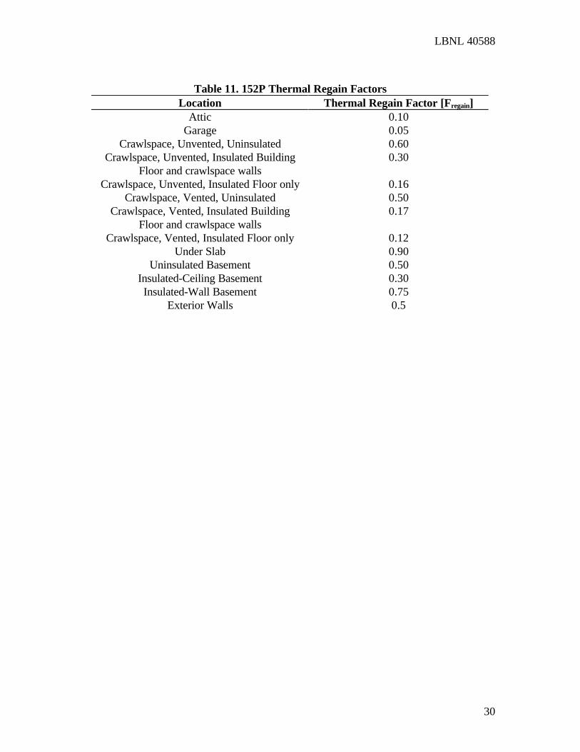
10.8 Summary of default thermal regain factorsDefault thermal regain factors are summarized in Table 11. This is the table used in 152P.

11 SummaryThis paper has shown how the default values for forced air systems in proposed ASHRAEstandard 152P were determined. These defaults were based on field measurements, simpleheat transfer analyses, modeling, and analysis of weather data. An approximate ranking ofthe importance of these parameters can be estimated from the sensitivity of the distributionsystem efficiency calculated using the standard to each parameter. The following list is inapproximately decreasing order of importance:

1. local climate2. system location3. duct leakage4. system fan flow5. duct surface area6. thermal regain7. interactions with equipment (includes variable capacity effects)8. cyclic losses

Acknowledgements

This work was supported by the Assistant Secretary for Conservation and RenewableEnergy of the U.S. Department of Energy, Office of Building Technologies, ExistingBuildings Research Program, under Contract No. DE-AC03-76SF00098.

The research reported here was funded in part by the California Institute for EnergyEfficiency (CIEE), a research unit of the University of California. Publication of researchresults does not imply CIEE endorsement of or agreement with these findings, nor that ofany CIEE sponsor.

The author would like to thank the following organizations for providing source data anddata analysis: the Alberta Home Heating Research Facility at the University of Alberta inCanada, Florida Solar Energy Center, and the Small Homes Council – Building ResearchCouncil at the University of Illinois.

LBNL 40588

22

References

ACCA. 1997. ACCA Manual D - Residential Duct Systems. Air Conditioning Contractorsof America. Washington, D.C.

Andrews, J. 1996. Field Comparison of Design and Diagnostic Pathways for DuctEfficiency Evaluation. Proc.1996 ACEEE Summer Study, Vol. 1. pp. 21–31.

ASHRAE. 1993. 1993 ASHRAE Handbook - Fundamentals, 1993. Atlanta. AmericanSociety of Heating, Refrigerating and Air-Conditioning Engineers, Inc.

ASHRAE. 1989. ASHRAE Standard 62-1989 Ventilation for Acceptable Indoor AirQuality. Atlanta. American Society of Heating, Refrigerating and Air-ConditioningEngineers, Inc.

ASHRAE. 1997. ASHRAE Standard 152P (Proposed) 1997 Method of Test ForDetermining the Design and Seasonal Efficiencies of Residential Thermal DistributionSystems. Atlanta. American Society of Heating, Refrigerating and Air-ConditioningEngineers, Inc.

Cummings, J., 1996. Computer model results for manufactured house belly pantemperatures. Private Communication. August 1996.

Forest, T.W., and Walker, I.S. 1991. Field Study on Attic Ventilation and Moisture.Proc. CANCAM '91, University of Manitoba, Winnipeg, Canada.

Forest, T.W., and Walker, I.S. 1992. Attic Ventilation Model. Proc.ASHRAE/DOE/BTECC/CIBSE Thermal Performance of the Exterior Envelopes ofBuildings V, pp. 399-408.

Forest, T.W., and Walker, I.S. 1993. Attic Ventilation and Moisture. Canada Mortgageand Housing Corporation report.

Jump, D., Walker, I. and Modera, M. 1996. Field measurements of Efficiency and DuctRetrofit Effectiveness in residential Forced Air Distribution Systems. Proc.1996 ACEEESummer Study. Vol. 1. pp. 147-157.

Levins, W.P. and Karnitz, M.A. 1987. Cooling Energy measurements of Single-FamilyHouses with Attics Containing Radiant Barriers in Combination With R-11 and R-30Ceiling Insulation. ORNL/CON-226. Oak Ridge National Laboratory report.

Modera, M. P. 1993. Characterizing the performance of Residential Air DistributionSystems. Energy and Buildings. Vol. 20. pp. 65-75.

NCDC. 1980. Climatography of U.S., #81, Monthly Normals of Temperature,

LBNL 40588

23

Precipitation and Heating and Cooling Degree days 1951-1980. National Climatic DataCenter, Federal Building, Asheville, NC.

NOAA (National Oceanic and Atmospheric Administration - U.S. Dept. of Commerce).1980. Local Climatological Data - annual summaries for 1980. Environmental data andinformation service. National Climatic Center. Asheville, N.C.

Palmiter, L. and Bond, T. 1994. Modeled and Measured Infiltration PhaseII, A Detailed caseStudy of three Homes. EPRI Report TR-102511. Electric Power Research Institute. PaloAlto, CA.

Parker, D.S., Sherwin, J.R., and Gu, L., 1997. Monitored Peak Attic Air Temperatures inFlorida Residences: Analysis in Support of ASHRAE Standard 152P. FSEC-CR-944-97.Florida Solar Energy Center, Cocoa, Fl.

Parker, D., 1991. Monitored Energy Use Characteristics of a Florida Residence. FSEC-RR-23-91. Florida Solar Energy Center, Cocoa, FL.

Proctor, J., 1997. Measured Attic Temperatures in Desert Conditions. Presentation atASHRAE 152P committee meeting. January 1997.

Rodriguez, A.G., O’Neal, D.L., Bain, J.A., and Davis, M.A. 1995. The Effect ofRefrigerant Charge, Duct Leakage, and Evaporator Air Flow on the High TemperaturePerformance of Air Conditioners and heat Pumps. Energy Systems Laboratory, Dept. ofMechanical Engineering, Texas Engineering Experiment Station, Texas A&M University.

Rose, W.B. 1992. Measured Values of Temperature and Sheathing Moisture Content inResidential Attic Assemblies. Proc. ASHRAE/DOE/BTECC/CIBSE Thermal Performanceof the Exterior Envelopes of Buildings V, Clearwater Beach, Florida, December 1992. pp.379-390.

Rose, W.B. 1997. Measured Attic Temperatures. Personal communication.

Tyson, J.,Gu, L., Anello, M., Swami, M.V., Chandra, S. and Moyer, M., 1996.Manufactured Housing Air Distribution Systems; Field Data and Analysis for theSoutheast. FSEC-CR-875-96. Florida Solar Energy Center. Cocoa, Fl.

Walker, I.S., and Forest, T.W. 1995. Field Measurements of Ventilation Rates in Attics.,Building and Environment, Vol. 30. No.3. pp. 333-347. Pergamon Press.

Walker, I.S., 1993. Attic Ventilation, Heat and Moisture Transfer. Ph.D. dissertation.University of Alberta. Edmonton. Alberta. Canada.

LBNL 40588

24

Attic radiant barrier and reduced emissivity coating bibliography

Abrantes, V. 1985. Thermal Exchanges Through Ventilated Attics. Proc.ASHRAE/DOE/BTECC/CIBSE Thermal Performance of the Exterior Envelopes ofBuildings III. Clearwater Beach. Florida. December 1985. pp. 296-308.

Carlson, J.D., Christian, J.E., and Smith, T.L. 1992. In Situ Thermal Performance of APP-Modified Bitumen Roof Membranes Coated with reflective Coatings. Proc.ASHRAE/DOE/BTECC/CIBSE Thermal Performance of the Exterior Envelopes ofBuildings V, Clearwater Beach. Florida. December 1992. pp. 420-428.

Chen, H., Larson, T., and Erickson, R.W. 1992. The Performance of an Attic RadiantBarrier for a Simulated Minnesota Winter. Proc. ASHRAE/DOE/BTECC/CIBSE ThermalPerformance of the Exterior Envelopes of Buildings V. Clearwater Beach. Florida.December 1992. pp. 114-122.

Griggs, E.I, and Shipp, P.H. 1988. The Impact of Surface Reflectance on the ThermalPerformance of roofs: An Experimental Study. ORNL/TM-10699. Oak Ridge NationalLaboratory. Oak Ridge, TN.

Levins, W.P. and Karnitz, M.A. 1986. Cooling Energy measurements of UnoccupiedSingle-Family Houses with Attics Containing Radiant Barriers. ORNL/CON-200. OakRidge National Laboratory. Oak Ridge, TN.

Levins, W.P. and Karnitz, M.A. 1987. Cooling Energy measurements of Single-FamilyHouses with Attics Containing Radiant Barriers in Combination With R-11 and R-30Ceiling Insulation. ORNL/CON-226. Oak Ridge National Laboratory. Oak Ridge, TN.

Levins, W.P. and Karnitz, M.A. 1988. Heating Energy measurements of Single-FamilyHouses with Attics Containing Radiant Barriers in Combination With R-11 and R-30Ceiling Insulation. ORNL/CON-239. Oak Ridge National Laboratory. Oak Ridge, TN.

Levins, W.P., Karnitz, M.A., and Hall, J.A. 1989. Moisture Measurements in Single-Family Houses with Attics Containing Radiant Barriers. ORNL/CON-255. Oak RidgeNational Laboratory. Oak Ridge, TN.

McDonald, J.M., Courville, G.E., Griggs, E.I., and Sharp, T.R. 1989. A Guide forEstimating Potential Energy Savings from Increased Solar Reflectance of a Low-SlopedRoof. Proc. ASHRAE/DOE/BTECC/CIBSE Thermal Performance of the ExteriorEnvelopes of Buildings IV. Orlando. Florida. December 1989. pp. 348-357.

Ober, D.G. 1989. Full-Scale Radiant Barrier Tests in Ocala, Florida: Summer 1988. Proc.ASHRAE/DOE/BTECC/CIBSE Thermal Performance of the Exterior Envelopes ofBuildings IV. Orlando. Florida. December 1989. pp. 286-293.

LBNL 40588

25

Parker, D.S., Sherwin, J.R., and Gu, L. 1997. Monitored Peak Attic Air Temperatures inFlorida Residences: Analysis in Support of ASHRAE Standard 152P. FSEC-CR-944-97,Florida Solar Energy Center, Cocoa, Fl.

Parker, D.S. 1997. Seasonal Attic temperatures. personal communication.

Rose, W.B., 1992. Measured Values of Temperature and Sheathing Moisture Content inResidential Attic Assemblies. Proc. ASHRAE/DOE/BTECC/CIBSE Thermal Performanceof the Exterior Envelopes of Buildings V. Clearwater Beach. Florida. December 1992. pp.379-390.

Wilkes, K.E. 1989. Thermal Modeling of Residential Attics with Radiant Barriers:Comparison with Laboratory and Field Data. Proc. ASHRAE/DOE/BTECC/CIBSEThermal Performance of the Exterior Envelopes of Buildings IV. Orlando. Florida.December 1989. pp. 294-311.

Wu, H. 1989. The Effect of Various Attic Venting Devices on the Performance of RadiantBarrier Systems in Hot Arid Climates. Proc. ASHRAE/DOE/BTECC/CIBSE ThermalPerformance of the Exterior Envelopes of Buildings IV. Orlando. Florida. December1989. pp. 261-270.

Duct Leakage bibliography

Cummings, J.B., Tooley, J., and Dunsmore, R. 1990. Impacts of Duct Leakage onInfiltration Rates, Space Conditioning Energy Use, and Peak Electrical Demand in FloridaHomes. Proc. 1990 ACEEE Summer Study. Pacific Grove. Ca.. August 1990. AmericanCouncil for an Energy Efficient Economy, 1001 Connecticut Ave. N.W., Suite 335,Washington, D.C. 20036.

Downey, T., and Proctor, J. 1994. Blower Door Guided Weatherization Test Project,Final Report. Proctor Engineering Group Report for Southern California EdisonCustomer Assistance Program.

Jump, D.A., Walker, I.S. and Modera, M.P. 1996. Field Measurements of Efficiency andDuct Retrofit Effectiveness in Residential Forced air Distribution Systems. Proc. 1996ACEEE Summer Study. Vol. 1. pp. 147-155.

Modera, M.P., and Wilcox, B. 1995. Treatment of Residential Duct Leakage in Title-24Energy Efficiency Standards. CEC contract report. California Energy Commission.

Modera, M.P. and Jump, D.A. 1995. Field Measurement of the Interactions Between HeatPumps and Attic Duct Systems in Residential Buildings. Proc. ASME International SolarEnergy Conference. March 1995.

LBNL 40588

26

Table 1. Estimating differences between design and seasonal temperatures using 2.5%design values

Location Winter Dry Bulb, °°C [°°F] Summer dry bulb, °°C [°°F]

Design(97.5%)

TMYseason avg.

Difference Design(2.5%)

TMYseason avg.

Difference

Los Angeles,CA.

4 [39] 12 [54] 8 [14] 32 [90] 21.7 [71] 10.3 [19]

Atlanta, GA. -6 [21] 4 [39] 10 [18] 33 [91] 24.4 [76] 8.6 [15]New York,NY

-9 [16] 0.5 [33] 9.5 [17] 32 [90] 23.4 [74] 8.6 [15]

AverageDifferences

9 [16] 9 [16]

Table 2. Summary of Attic to Ambient Temperature Differences, °°C [°°F]Source 1 Source 2 Source 3

Wellvented

Poorlyvented

Wellvented

Poorlyvented

Wellvented

Poorlyvented

Cooling Design 12 [22] 20 [36] 12 [22] 15 [27] 9 [16] 20 [36]Cooling Seasonal 3 [6] 6 [10] 12 [22] 17 [31] 7 [13] 9 [16]Heating Design - - 5 [9] 7 [13] 6 [11] 7 [13]

Heating Seasonal - - 0 [0] 1 [2] 2 [4] 2 [4]

Table 3. Difference between outside and garage Temperatures, °°C [°°F]Heating Cooling

Atlanta New York LosAngeles

Atlanta New York LosAngeles

Design 10 [18] 9 [16] 9 [16] 2 [4] 3 [5] 4 [7]Seasonal 7 [13] 7 [13] 6 [11] 5 [9] 4 [7] 5 [9]

LBNL 40588

27

Table 4. Using average design conditions to estimate ground temperatures, °°C [°°F]Location twinter,2.5% tsummer, 2.5%

2

tt %5.2,summer%5.2,winter + Average outdoor airtemperature

NOAA TMYFairbanks,Alaska

-44 [-47] 26 [15] -9 [16] -3 [27] -3.5 [26]

Phoenix,Arizona

1 [34] 42 [108] 21.5 [71] 21 [70] 22 [72]

Oakland,California

2 [36] 27 [81] 14.5 [58] 14 [57]

Athens, Georgia -6 [21] 33 [91] 13.5 [56] 16 [61]Boise, Idaho -12 [10] 34 [93] 11 [52] 11 [52] 11 [52]Chicago, Illinois -17 [1] 33 [91] 8 [46] 9 [48] 10 [50]New Orleans,Louisiana

1 [34] 33 [91] 17 [63] 20.5 [69] 20 [68]

St. Louis,Missouri

-14 [7] 34 [93] 10 [50] 13 [55] 13 [55]

NY,NY -9 [16] 31 [88] 11 [52] 12 [54] 12 [54]Bismark, N.Dakota

-28 [-18] 33 [91] 2.5 [37] 5 [41] 5 [41]

Dallas, Texas -6 [21] 38 [100] 16 [61] 19 [66]Seattle, WA. -3 [27] 28 [82] 12.5 [55] 10 [50] 10 [50]

Table 5. Duct surface area significant parametersParameter Surface area dependenceAge of duct system NOEquipment location NORegister location NODuct system topology NODuct material type YES - Flex duct systems have 50% more

normalized surface area than sheet metal.Number of registers YES - Normalized duct area increases with

increasing number of registersFloor Area YES - bigger houses have bigger systems

LBNL 40588

28

Table 6. Supply duct surface area coefficientsOption Duct

TypeA B Average Absolute

Error, AENumber of houses

in group1 Flex 19 1.3 9 181 Sheet

metal9 1.6 7 27

2 - 13 1.5 8.4 453 - 27 - 8.4 69

Table 7. Variable Capacity Equipment Effect in ASHRAE 152P152Pparameter

Furnaces AC HP HP in strip heatmode

DEdesign

hi cap hi cap hi cap Hi cap

DEseasonal

low cap low cap low cap Low cap

ηdist

designhi cap hi cap hi cap Hi cap

ηdist

seasonal

Fvc DE= +0 905 0 095. . Fvc = +0 82 0 18DE. . Fvc = +0 82 0 18DE. . Fvc DE= +0 44 056. .

Table 8. Attic thermal regain factorsFregain Infiltration (ACH) Ceiling

InsulationDuct Insulation

0.06 1 R-30 R60.05 5 R-30 R60.04 10 R-30 R60.08 1 R-30 R40.06 5 R-30 R40.05 10 R-30 R40.11 1 R-15 R40.08 5 R-15 R40.06 10 R-15 R40.16* 1 R-15 R40.11* 5 R-15 R40.07* 10 R-15 R4

* - for the smaller attic with 1:5 pitched roof

LBNL 40588

29

Table 9. Crawlspace regain factorsFregain Infiltration rate (ACH) Insulation0.63 0.1 None0.60 1 None0.5 5 None0.41 10 None0.36 0.1 R-15 house floor and crawlspace walls0.30 1 R-15 house floor and crawlspace walls0.17 5 R-15 house floor and crawlspace walls0.11 10 R-15 house floor and crawlspace walls0.18 0.1 R-15 house floor0.16 1 R-15 house floor0.12 5 R-15 house floor0.08 10 R-15 house floor

Table 10. Regain Factors for basementsFregain Ventilation Rate

[ACH]Insulation

0.55 0 Uninsulated0.51 0.35 Uninsulated0.78 0 R15 insulated basement walls0.74 0.35 R15 insulated basement walls0.32 0 R15 basement walls and house floor0.27 0.35 R15 basement walls and house floor

LBNL 40588

30

Table 11. 152P Thermal Regain FactorsLocation Thermal Regain Factor [Fregain]

Attic 0.10Garage 0.05

Crawlspace, Unvented, Uninsulated 0.60Crawlspace, Unvented, Insulated Building

Floor and crawlspace walls0.30

Crawlspace, Unvented, Insulated Floor only 0.16Crawlspace, Vented, Uninsulated 0.50

Crawlspace, Vented, Insulated BuildingFloor and crawlspace walls

0.17

Crawlspace, Vented, Insulated Floor only 0.12Under Slab 0.90

Uninsulated Basement 0.50Insulated-Ceiling Basement 0.30Insulated-Wall Basement 0.75

Exterior Walls 0.5