Technical Basis for Direct Scale-up of Small Scale Pulse

PNNL-24360 WTP-RPT-240, Rev. 0

Prepared for the U.S. Department of Energy under Contract DE-AC05-76RL01830

Technical Basis for Direct Scale-up of Small Scale Pulse Jet Mixing Results to Large Scale Vessels August 2015

BE Wells CW Enderlin MJ Minette

DISCLAIMER

This report was prepared as an account of work sponsored by an agency of the United States Government. Neither the United States Government nor any agency thereof, nor Battelle Memorial Institute, nor any of their employees, makes any warranty, express or implied, or assumes any legal liability or responsibility for the accuracy, completeness, or usefulness of any information, apparatus, product, or process disclosed for any uses other than those related to WTP for DOE, or represents that its use would not infringe privately owned rights. Reference herein to any specific commercial product, process, or service by trade name, trademark, manufacturer, or otherwise does not necessarily constitute or imply its endorsement, recommendation, or favoring by the United States Government or any agency thereof, or Battelle Memorial Institute. The views and opinions of authors expressed herein do not necessarily state or reflect those of the United States Government or any agency thereof.

PACIFIC NORTHWEST NATIONAL LABORATORY operated by

BATTELLE for the UNITED STATES DEPARTMENT OF ENERGY

under Contract DE-AC05-76RL01830

Printed in the United States of America

Available to DOE and DOE contractors from the Office of Scientific and Technical Information,

P.O. Box 62, Oak Ridge, TN 37831-0062; ph: (865) 576-8401 fax: (865) 576-5728

email: reports@adonis,osti.gov

Available to the public from the National Technical Information Service 5301 Shawnee Rd., Alexandria, VA 22312

ph: (800) 553-NTIS (6847) email: [email protected] <http://www.ntis.gov/about/form.aspx>

This document was printed on recycled paper.

(9/2003)


Technical Basis for Direct Scale-up of Small Scale Pulse Jet Mixing Results to Large Scale Vessels BE Wells CW Enderlin MJ Minette August 2015 Test Specification: N/A Work Authorization: WA# 048 Test Plan: TP-WTPSP-132, Rev 0.0 Test Exceptions: N/A Focus Area: Pretreatment Test Scoping Statement(s): NA QA Technology Level: Basic Research Project Number: 66560 Prepared for the U.S. Department of Energy under Contract DE-AC05-76RL01830 Pacific Northwest National Laboratory Richland, Washington 99352

iii

Summary

This report provides a technical basis for direct scale-up of Pulse Jet Mixer (PJM) performance from small scale testing with Newtonian and non-Newtonian simulants to the expected PJM performance in large scale vessels under similar conditions. As this report is based in part on data collected under a commercial grade quality assurance program, it is not intended to be used in Hanford Waste Treatment and Immobilization Plant (WTP) design activities. For this work, mixing performance is assessed relative to bottom motion and cloud height for Newtonian simulants, and cavern heights for non-Newtonian simulants. This application of scaling is for PJMs arranged in circular/distributed arrays in vessels with dished bottoms. The circular arrays contain no central PJM and the bulk flow patterns are dominated by a central up well within the PJM array and downward flow in the annular region surrounding the circular array. Data used for the scaling evaluation were generated from projects conducted in support of the development of the WTP. The analysis reported to address direct scale-up was performed in support of the development of a proposed 16 foot diameter Standard High Solids Vessel Design (SHSVD) for the high level waste (HLW) process stream.

Testing has been conducted in an 8 foot geometrically scaled vessel with similar scaled PJM configuration, operational parameters (duty cycle, pulse volume fraction), vessel fill level, and simulant to the 16 foot diameter proposed SHSVD. The difference in the mixing performance of the 8 foot vessel to the prototypic 16 foot vessel can therefore be expressed in terms of direct scale-up, where direct scale-up is used to define the mixing performance depending solely on geometric scale and PJM nozzle velocity.

For the direct scale-up approach, velocities that provide equivalent performance at both test scales with all other test conditions equivalent in the scales are identified. The scaling exponent can be obtained from the geometrically-scaled tests using the common approach,

S

L

S

L

DD

UU

(ES.1)

where

α = scale exponent U = jet velocity D = tank diameter L = large vessel size S = small vessel size.

Available data from multi-scale test programs having different PJM configurations than that of the proposed SHSVD were used to evaluate the impact on direct scale-up of operating conditions and simulant characteristics. Consistent scaling for both critical suspension velocity (bottom motion) and cloud height (suspension) is demonstrated by the data for direct scale-up for testing of simplified PJM mixing systems using monodisperse non-cohesive Newtonian simulants. Based on the reference case parameters and the clarity that if the mixing performance in the 8 foot vessel tests meets or exceeds adequate SHSVD performance with the largest scale exponent indicated by the test data there is increased confidence that adequate performance will be achieved in the SHSVD.

iv

The minimum recommended scale exponent for bottom motion is the maximum determined from the test data, α = 0.33, which is equivalent to power per unit volume scaling. Uncertainties for this direct scale exponent basis have been considered, and the recommended bottom motion scale exponent for the SHSVD prototypic configuration of 6 PJMs is α = 0.33 for the direct scale-up data. With a 12 m/s PJM nozzle velocity in the 16 foot SHSVD, this scale exponent corresponds to a PJM nozzle velocity of approximately 9.4 m/s in the 8 foot test vessel (actual measured test vessel size is 92.5” diameter).

Based on the direct scale-up of non-Newtonian Laponite simulant cavern height data, a scale exponent of α = 0 (equal peak average PJM nozzle velocity) is recommended to achieve equivalent nondimensional cavern heights in the 8 foot test vessel and 16 foot SHSVD with the operational and simulant parameters the same at the different scales. Difference in the jet Reynolds number between the 8 foot test vessel and 16 foot SHSVD at equal 12 m/s PJM nozzle velocity should not be significant to the jet behavior. Comparison of the power-per-volume in these vessels at equal PJM nozzle velocity suggests there is potential that gas release rates and solids segregation (i.e., stratification) in the yielded material may be over represented in the 8 foot vessel.

Quality Requirements

Pacific Northwest National Laboratory (PNNL) complies with the requirements found in the following standards and implements them in their Waste Treatment Plant Support Program (WTPSP) Quality Assurance Program (QAP):

ASME NQA-1-2000, Quality Assurance Requirements for Nuclear Facility Applications, Part I, Requirements for Quality Assurance Programs for Nuclear Facilities.

ASME NQA-1-2000, Part II, Subpart 2.7, Quality Assurance Requirements for Computer Software for Nuclear Facility Applications.

ASME NQA-1-2000, Part IV, Subpart 4.2, Guidance on Graded Application of Quality Assurance (QA) Requirements for Nuclear-Related Research and Development.

Records will be stored as hardcopy records in a two-hour fire-rated container.

This project recognizes that quality assurance applies in varying degrees to a broad spectrum of research and development (R&D) in the technology life cycle. The R&D elements in the technology life cycle are bulleted below. The WTPSP uses a graded approach for the application of the quality assurance controls such that the level of analysis, extent of documentation, and degree of rigor of process control are applied commensurate with their significance, importance to safety, life cycle state of work, or programmatic mission. The technology life cycle is characterized by flexible and informal quality assurance activities in Basic Research, which becomes more structured and formalized through the Applied R&D stages.

BASIC RESEARCH: Basic Research consists of research tasks that are conducted to acquire and disseminate new scientific knowledge. During Basic Research, maximum flexibility is desired in order to allow the researcher the necessary latitude to conduct the research.

APPLIED RESEARCH: Applied Research consists of research tasks that acquire data and documentation necessary to assure satisfactory reproducibility of results. The emphasis during this

v

stage of a research task is on achieving adequate documentation and controls necessary to be able to reproduce results.

DEVELOPMENT WORK: Development Work consists of research tasks moving toward technology commercialization. These tasks still require a degree of flexibility and there is still a degree of uncertainty that exists in many cases. The role of quality on Development Work is to make sure that adequate controls to support movement into commercialization exist.

RESEARCH AND DEVELOPMENT SUPPORT ACTIVITIES: Support Activities are those which are conventional and secondary in nature to the advancement of knowledge or development of technology, but allow the primary purpose of the work to be accomplished in a credible manner. An example of a Support Activity is controlling and maintaining documents and records. The level of quality for these activities is the same as for Developmental Work.

This report was conducted at the Basic Research Technology Level.

vii

Acknowledgments

The authors thank PP Schonewill for his independent technical review, SA Suffield and RC Daniel for their calculation reviews, and S Tackett and C Winters for the technical editing. In addition, the authors thank PP Schonewill for his evaluation of the 24590-QL-HC1-M00Z-00003-09-00176 Runsheet 7 test data, and JA Bamberger for her evaluation of additional test parameters for the Bamberger et al. (2005) tests.

ix

Acronyms and Abbreviations

CFD computational fluid dynamics

ECR effective cleaning radius

HLW high level waste

PJM pulse jet mixer (mixing)

PNNL Pacific Northwest National Laboratory

PPV power-per-volume

QA Quality Assurance

QAP Quality Assurance Program

R&D research and development

SHSVD Standard High Solids Vessel Design

WFD Waste Feed Delivery

WTP Hanford Waste Treatment and Immobilization Plant

WTPSP Waste Treatment Plant Support Program

x

Symbols

c’ effective cohesion intercept

C empirical constant

D diameter of tank

DC duty cycle equals drive time divided by the cycle time

d diameter of jet nozzle

g gravitational constant

Hc average peak cloud height

Hcavern cavern height

N number of installed jets or pulse tubes

Rej jet Reynolds number

Re yield Reynolds number

s ratio of solid to liquid density

U jet velocity

Ucs critical suspension velocity

UT unhindered terminal settling velocity

V nominal volume of tank

xi

Greek Symbols

scale exponent

ρ jet fluid density

τ yield stress in shear

β shear strength exponent

σ’ effective normal stress

Bingham consistency

’ effective friction angle

xiii

Contents

Summary ...................................................................................................................................................... iii

Acknowledgments ....................................................................................................................................... vii

Acronyms and Abbreviations ...................................................................................................................... ix

Symbols ........................................................................................................................................................ x

Greek Symbols ............................................................................................................................................. xi

1.0 Introduction ....................................................................................................................................... 1.1

1.1 Scope ...................................................................................................................................... 1.1

1.2 Quality .................................................................................................................................... 1.1

2.0 Direct Scale-up Technical Basis ........................................................................................................ 2.1

2.1 Newtonian Simulant Testing .................................................................................................. 2.2

2.1.1 Uncertainties ................................................................................................................. 2.16

2.2 Non-Newtonian Simulant Testing ........................................................................................ 2.29

3.0 Conclusions ....................................................................................................................................... 3.1

4.0 References ......................................................................................................................................... 4.1

xiv

Figures

1. Direct Scaling Example. Normalized Cloud Height as a Function of Nozzle Velocity for Direct Scale-up. ................................................................................................................................... 2.4

2. Normalized Cloud Height as a Function of Nozzle Velocity for Direct Scale-up .............................. 2.6




6. Comparison of Ucs and Hc/D Scale Exponents at Equivalent Test Conditions .................................. 2.9

7. Ucs a) and Hc/D b) Scale Exponents as a Function of Reference Solid Volume Fraction ............... 2.10

8. Ucs a) and Hc/D b) Scale Exponents as a Function of Solid Characteristics .................................... 2.12

9. Ucs a) and Hc/D b) Scale Exponents as a Function of Duty Cycle. .................................................. 2.13

10. Ucs a) and Hc/D b) Scale Exponents as a Function of Reference Pulse Volume Fraction ............... 2.14

11. Ratio of Unhindered Terminal Settling Velocity to Jet Velocity ...................................................... 2.20

12. Froude Number Based on Jet Velocity and Tank Diameter .............................................................. 2.20

13. Froude Number Based on Unhindered Terminal Settling Velocity and Tank Diameter ................... 2.21

14. Measured and Predicted Ucs for Runsheet 7 Soda-lime Glass Powder Tests ................................... 2.25

15. Measured and Predicted Effect of Reference Solid Volume Fraction on Ucs .................................. 2.26

16. Meyer et al. (2010) Adjusted New Physical Model Scale Exponent Analysis Applied to the Runsheet 7 Soda-lime Glass Powder Tests ....................................................................................... 2.27

17. Meyer et al. (2010) Adjusted New Physical Model Scale Exponent Analysis Applied to the Runsheet 7 Herting (2012) Simulant Test ......................................................................................... 2.29

18. Laponite Cavern Test Shear Strength for Test Condition Peak Average PJM Nozzle Velocity and Vessel Scale ................................................................................................................................ 2.31

19. Laponite Cavern Test Shear Strength for Test Condition Average PJM Nozzle Velocity and Vessel Scale ....................................................................................................................................... 2.32

20. Laponite Cavern Test Nondimensional Cavern Height as a Function of PJM Nozzle Velocity, 95 to 105 Pa ....................................................................................................................................... 2.33

21. Laponite Cavern Test Nondimensional Cavern Height as a Function of PJM Nozzle Velocity, 105 to 115 Pa ..................................................................................................................................... 2.34



24. Jet Reynolds Numbers Based on Peak Average PJM Nozzle Velocity for Laponite Cavern Tests .................................................................................................................................................. 2.35

25. PPV Based on Peak Average PJM Nozzle Velocity for Laponite Cavern Tests ............................... 2.37

26. PPV and Jet Reynolds Numbers with Equal Jet Velocity and Waste Properties, 8 foot and 16 foot Geometrically Scaled Vessels ............................................................................................... 2.37

xv

Tables

1. Direct Scale-up Summary, Data from Meyer et al. (2012) ................................................................. 2.5

2. Example Ranges of Newtonian Waste Slurry Conditions in SHSVD and Reference Case Solids Parameter Characterization .................................................................................................... 2.16

3. Example Reference Case and Scale-up Test Data Operating Conditions ......................................... 2.18

4. Comparison of Test and Prototypic Variables ................................................................................... 2.19

5. 24590-QL-HC1-M00Z-00003-09-00176 Runsheet 7 Soda-lime Glass Powder Test Parameters for Meyer et al. (2010) and Meyer et al. (2012) ............................................................. 2.24

6. 24590-QL-HC1-M00Z-00003-09-00176 Runsheet 7 Herting (2012) Simulant Test Parameters for Meyer et al. (2010) and Meyer et al. (2012) ............................................................. 2.28

1.1

1.0 Introduction

This report provides a technical basis for direct scale-up of Pulse Jet Mixer (PJM) performance from small scale testing to the expected PJM performance in large scale vessels under matched conditions (the mixing performance depends solely on geometric scale and PJM nozzle velocity). As this report is based in part on data collected under a commercial grade quality assurance program, it is not intended to be used in Hanford Waste Treatment and Immobilization Plant (WTP) design activities.

This supports WTP engineering studies and testing in an effort to reduce programmatic risk before full scale test vessel procurement. Establishing the likely performance of the proposed design at full scale based on small scale test performance will increase confidence that the proposed Standard High Solids Vessel Design (SHSVD) mixing system will work and will not require major redesign or reconfiguration, with subsequent unacceptable cost and schedule impact on the program.

The overall objective of the WTP engineering study (24590-WTP-ES-ENG-14-017 Rev 0, Technical Basis for Scaled Testing of Standard High Solids Vessel Design Mixing System) is to predict the performance of the pulse jet mixers in the SHSVD at full scale and show that, when coupled with spargers, it is likely to exceed adequate performance for Newtonian and non-Newtonian WTP process conditions. The analysis provides the technical basis for scaling results from the 8 foot test vessel to the expected performance at full scale based on results from other scaled tests.

1.1 Scope

The purpose of this report is to provide a technical basis for direct scale-up of PJM performance from small scale testing with Newtonian and non-Newtonian simulants to the expected PJM performance in large scale vessels under similar conditions. This application is for scaling PJMs arranged in circular/distributed arrays in vessels with dished bottoms. The circular arrays contain no central PJM and the bulk flow patterns are dominated by a central up well within the PJM array and downward flow in the annular region surrounding the circular array. Data used for the scaling evaluation were generated from projects conducted in support of the development of the WTP. The analysis reported to address direct scale-up was performed in support of the development of a proposed 16 foot diameter SHSVD for the high level waste (HLW) process stream.

The scope for this report is provided in TP-WTPSP-132 Test Plan in Section 5.1 Tasks i and j, with the contractual direction authority for this report being provided in Section 3.3.1 of the Haukur Hazen November 17, 2014 Subcontract change notice letter “Contract No. DE-AC2701RV14136 - Hanford Tank Waste Treatment and Immobilization Plant, Memorandum of Agreement (MOA) 24590-QL-HC-WA49-00001, - Directive Subcontract Change Notice No. 149 for WA 2014-48 FSVT Support – Increased Funding and Revised Statement of Work”, CCN 273280.

1.2 Quality

Pacific Northwest National Laboratory (PNNL) complies with the requirements found in the following standards and implements them in their Waste Treatment Plant Support Program (WTPSP) Quality Assurance Program (QAP):

1.2

ASME NQA-1-2000, Quality Assurance Requirements for Nuclear Facility Applications, Part I, Requirements for Quality Assurance Programs for Nuclear Facilities.

ASME NQA-1-2000, Part II, Subpart 2.7, Quality Assurance Requirements for Computer Software for Nuclear Facility Applications.

ASME NQA-1-2000, Part IV, Subpart 4.2, Guidance on Graded Application of Quality Assurance (QA) Requirements for Nuclear-Related Research and Development.

Records will be stored as hardcopy records in a two-hour fire-rated container.

This project recognizes that quality assurance applies in varying degrees to a broad spectrum of research and development (R&D) in the technology life cycle. The R&D elements in the technology life cycle are bulleted below. The WTPSP uses a graded approach for the application of the quality assurance controls such that the level of analysis, extent of documentation, and degree of rigor of process control are applied commensurate with their significance, importance to safety, life cycle state of work, or programmatic mission. The technology life cycle is characterized by flexible and informal quality assurance activities in Basic Research, which becomes more structured and formalized through the Applied R&D stages.

BASIC RESEARCH: Basic Research consists of research tasks that are conducted to acquire and disseminate new scientific knowledge. During Basic Research, maximum flexibility is desired in order to allow the researcher the necessary latitude to conduct the research.

APPLIED RESEARCH: Applied Research consists of research tasks that acquire data and documentation necessary to assure satisfactory reproducibility of results. The emphasis during this stage of a research task is on achieving adequate documentation and controls necessary to be able to reproduce results.

DEVELOPMENT WORK: Development Work consists of research tasks moving toward technology commercialization. These tasks still require a degree of flexibility and there is still a degree of uncertainty that exists in many cases. The role of quality on Development Work is to make sure that adequate controls to support movement into commercialization exist.

RESEARCH AND DEVELOPMENT SUPPORT ACTIVITIES: Support Activities are those which are conventional and secondary in nature to the advancement of knowledge or development of technology, but allow the primary purpose of the work to be accomplished in a credible manner. An example of a Support Activity is controlling and maintaining documents and records. The level of quality for these activities is the same as for Developmental Work.

This report was conducted at the Basic Research Technology Level.

2.1

2.0 Direct Scale-up Technical Basis

Testing has been conducted in the 8 foot geometrically scaled vessel with similar PJM configuration, operational parameters (duty cycle and pulse volume fraction), vessel fill level, and simulant to the proposed 16 foot SHSVD (Bontha et al. 2015, 24590-QL-HC1-M00Z-00003-09-00176). The difference in the mixing performance of the 8 foot vessel to the prototypic 16 foot vessel can therefore be expressed in terms of direct scale-up where direct scale-up is used to define the mixing performance depending solely on geometric scale and PJM nozzle velocity.

The PJM nozzle velocity for equivalent mixing performance at different test scales has been previously evaluated (e.g., Bamberger et al. 2005; Meyer et al. 2012). Kuhn et al. (2013) establishes technical bases for evaluating the mixing performance of the WTP which include the fluid mechanics affecting mixing for specified vessel configurations, operating parameters, and simulant properties. For the mixing performance criteria of bottom motion, Kuhn et al. (2013) provides a summary of scale exponents for the directly related criteria “critical suspension velocity,” Ucs, which range from 0.18 to 0.397 depending on the data set and model basis. The average critical suspension velocity scale exponent for direct scale-up is referenced as = 0.28 (see Section 2.1), and other exponents are determined from data sets which incorporate tank bottom geometries, simulants, and PJM configurations and operational parameters with statistical and physical model bases as well as inertial and shear stress theoretical approaches. Within the breadth of the test data, the different approaches yield different scale exponents for the same data.

Given the 8 foot testing has been conducted where essentially the only variation from the prototypic 16 foot SHSVD is the geometric scale, the approach described in this current work is based solely on direct scale-up data. As will be discussed, the analysis in Meyer et al. (2012) for direct scale-up of Ucs, which yields the average = 0.28 presented in Kuhn et al. (2013), shows variation on the scale exponent approximating the range listed in Kuhn et al. (2013) for the varying model approaches. To re-state, the scale exponent range obtained for Ucs with both the direct scale-up data and models that incorporate tank bottom geometries, simulants, and PJM configurations and operational parameters with statistical and physical model bases as well as inertial and shear stress theoretical approaches, have similar variability.

What is the “correct” scale exponent for Ucs, i.e., bottom motion? If a larger scale exponent is used (e.g., 0.40) and the mixing requirement(s) for that specific metric is/are met at smaller test scales, it is indicated that the prototypic vessel will meet the mixing requirement. However, if the mixing requirement(s) is/are not met at smaller test scales, the use of the larger scale exponent can be questioned. The converse is likewise true. If a lower scale exponent is used (e.g., 0) and the mixing requirement(s) is/are not met at smaller test scales, it is indicated that the prototypic vessel will not meet the mixing requirement for the specific metric. The variation in the direct scale exponent for Ucs from Meyer et al. (2012) is therefore investigated as part of the Newtonian (see Section 3) waste slurry condition.

In Section 2.1 the mixing performance metrics of bottom motion and particle suspension height for Newtonian simulant testing are discussed, and the mixing performance metric of cavern height for non-Newtonian simulant testing is discussed in Section 2.2. The cavern height scaling discussion is based on the testing and analysis of Bamberger et al. (2005).

2.2

Recommended scale exponents will be specified for both the Newtonian and non-Newtonian simulant testing such that if the 8 foot performance at the resultant velocity meets or exceeds adequate SHSVD performance with the lowest nozzle velocity indicated by the test data, there is increased confidence in the SHSVD. Conversely, if the 8 foot vessel performance is not adequate with PJM nozzle velocity equal to the prototypic SHSVD, it is likely that the 16 foot vessel will not have adequate performance.

2.1 Newtonian Simulant Testing

The PJM nozzle velocities required for equivalent bottom motion and cloud height in the 8 foot vessel for prototypic SHSVD operation are defined from the existing direct scale-up data. These data are taken from the extensive testing of simplified PJM mixing systems of Meyer et al. (2012) using monodisperse non-cohesive simulants.

What velocities provide equivalent performance at the test scales? For the direct scale-up approach, velocities are identified that provide equivalent performance at both test scales with all other test conditions equivalent in the scales. The scaling exponent can be obtained from the geometrically scaled tests using the common approach,

S

L

S

L

D

D

U

U

(1)

where

α = scale exponent U = jet velocity D = tank diameter L = large vessel size S = small vessel size.

This is a power law model, which can be expressed in the more convenient logarithmic form for data analysis. Taking the log of both sides of Equation (1) gives a linear relationship where α is the slope of data on a plot having ln(UL/US) on the ordinate and ln(DL./DS) on the abscissa (e.g., Meyer et al. 2012).

Test data from the Waste Feed Delivery (WFD) system has been used to demonstrate that different aspects of the mixing, e.g., effective cleaning radius (ECR) and suspension, can scale differently (Wells et al. 2013).1 For solid suspension, as related to transfer concentration in PJM mixed vessels, Meyer et al. (2012) considered the direct scale-up of the cloud height, Hc, at Ucs. Meyer et al. (2010), evaluating the cloud height normalized with tank diameter, likewise also considered Hc at Ucs. Meyer et al (2010) showed that the scaling of the cloud height at Ucs varied, and a sensitivity analysis indicated that the scaling is most strongly dependent on the solids loading. In each case, the direct scale-up of the cloud height is evaluated at the Ucs condition, whereas in the current work the direct scale-up of PJM nozzle velocity for equivalent normalized cloud height is investigated.

1 The WFD system is comprised of two rotating centrifugal mixer pumps with dual-opposing horizontal nozzles in 75 foot diameter flat bottom vessels; see Meacham et al. (2012).

2.3

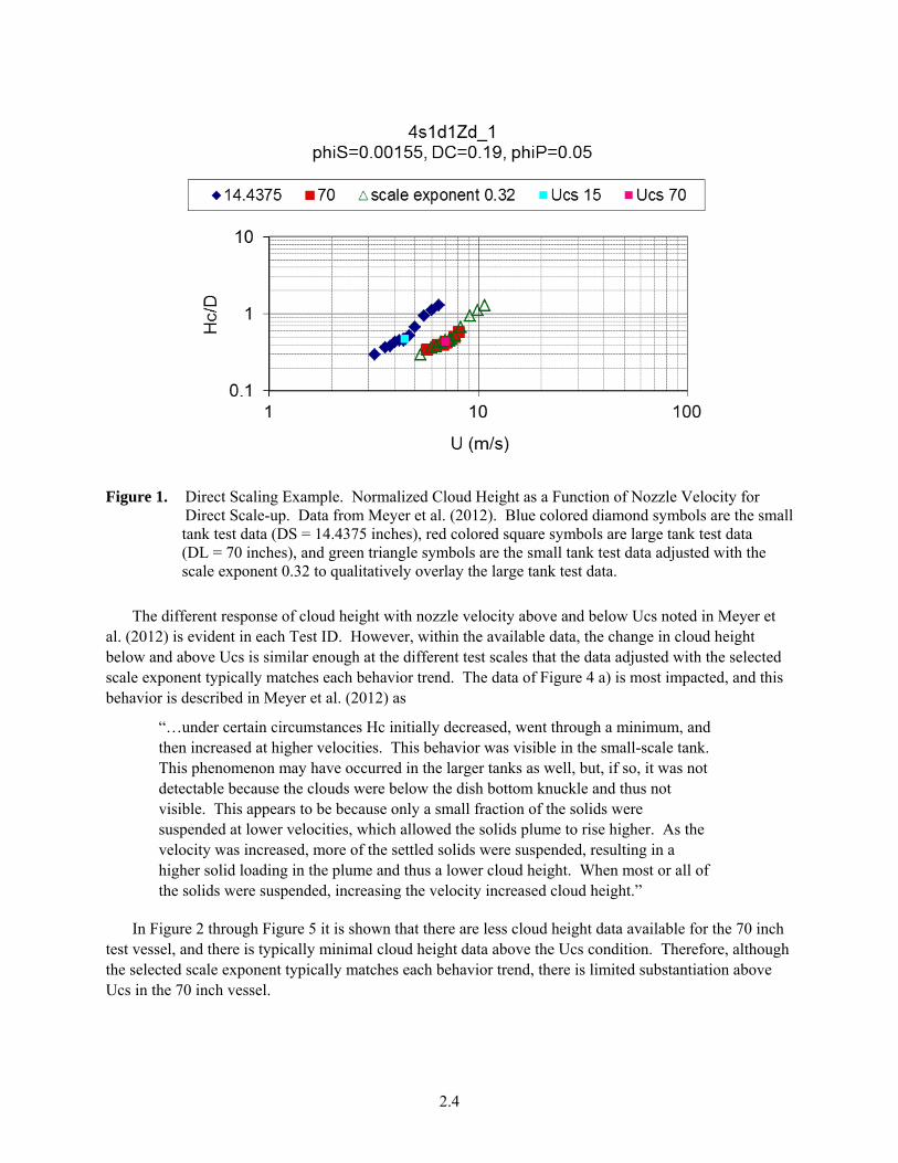
An example of how this question of velocities for equivalent scales can be addressed is provided with the cloud height data of Meyer et al. (2012) as shown in Figure 1 for normalized cloud height as a function of PJM nozzle velocity, including Ucs. In Figure 1, the blue colored symbols are the small tank test data (DS = 14.4375 inches) and the red symbols are large tank test data (DL = 70 inches). The light blue and pink solid square symbols denote the respective critical suspension velocity (Ucs) conditions. The indicated Test ID (4s1d1Zd_1: scaled test from prototypic 4 inch PJM nozzle, solid particles with median size of 166.4 m and density of 2.46 g/mL, reference solid volume fraction of 0.00155, duty cycle of 0.18, and reference pulse volume fraction of 0.05, see Table 1) and test conditions are detailed in Table 1.

In the red and blue test data, a different response of cloud height is indicated with nozzle velocity above and below Ucs as discussed in Meyer et al. (2012). For this example, the trend of cloud height in the green triangle symbols represent a scale-up of the small tank data using α = 0.32 which is shown in Figure 1 to give normalized cloud height with jet velocity very close to those of the large scale tank measurements over the range of velocities tested both above and below Ucs.1 Therefore, for this example, a scale exponent of 0.32 gives similar behavior at the different test scales. This indicates that test scale jet velocities need to be less than full-scale jet velocities by a factor of (DL/DS)0.32 to achieve equivalent performance for this example. For reference, a scale exponent of zero would indicate that the scaled jet velocities would be the same as full-scale jet velocities for equivalent performance.

The analysis in Meyer et al. (2012) for direct scale-up of Ucs is listed in Table 1. The PJM operational parameters and simulant are denoted. Also listed in Table 1 are the scale exponents determined for Hc/D, cloud height normalized by tank diameter determined as described for Figure 1. The scale exponent determinations for all the Test IDs are shown in Figure 2 for the 4 inch nozzle, 12 PJMs, s1d1 solids (median size of 166.4 m and density of 2.46 g/mL, Table 1), Figure 3 for the 4 inch nozzle, 12 PJMs, s1d2 solids (median size of 69.3 m and density of 2.48 g/mL, Table 1), Figure 4 for the 4 inch nozzle, 12 PJMs, s2d2 solids, and Figure 5 for the 6 inch nozzle, 8 PJMs tests. In each case, power law fit lines are included for the small (blue diamonds), large (red squares), and scaled (green triangles) data solely to provide additional reference for the comparison. The qualitatively identified scale exponent is listed in the legend entry, and the light blue and pink solid square symbols denote the respective Ucs conditions.

1 The comparison of the scaled 14.4375 inch tank data to the 70 inch tank data is made qualitatively. A simple approach for more quantitative comparison is provided in Wells et al. (2013), and more complex schemes can be employed. Given that the cloud height data is somewhat more variable than Ucs data (Meyer et al. 2010), visual observation of the goodness-of-fit- is used.

2.4

Figure 1. Direct Scaling Example. Normalized Cloud Height as a Function of Nozzle Velocity for Direct Scale-up. �Data from Meyer et al. (2012). Blue colored diamond symbols are the small tank test data (DS = 14.4375 inches), red colored square symbols are large tank test data (DL = 70 inches), and green triangle symbols are the small tank test data adjusted with the scale exponent 0.32 to qualitatively overlay the large tank test data.

The different response of cloud height with nozzle velocity above and below Ucs noted in Meyer et al. (2012) is evident in each Test ID. However, within the available data, the change in cloud height below and above Ucs is similar enough at the different test scales that the data adjusted with the selected scale exponent typically matches each behavior trend. The data of Figure 4 a) is most impacted, and this behavior is described in Meyer et al. (2012) as

“…under certain circumstances Hc initially decreased, went through a minimum, and then increased at higher velocities. This behavior was visible in the small-scale tank. This phenomenon may have occurred in the larger tanks as well, but, if so, it was not detectable because the clouds were below the dish bottom knuckle and thus not visible. This appears to be because only a small fraction of the solids were suspended at lower velocities, which allowed the solids plume to rise higher. As the velocity was increased, more of the settled solids were suspended, resulting in a higher solid loading in the plume and thus a lower cloud height. When most or all of the solids were suspended, increasing the velocity increased cloud height.”

In Figure 2 through Figure 5 it is shown that there are less cloud height data available for the 70 inch test vessel, and there is typically minimal cloud height data above the Ucs condition. Therefore, although the selected scale exponent typically matches each behavior trend, there is limited substantiation above Ucs in the 70 inch vessel.

2.5

Table 1. Direct Scale-up Summary, Data from Meyer et al. (2012)

Test ID

Full Scale Nozzle

Diameter, d (inches)1 Simulant

Particle Density (g/mL)

Particle Size (m)2

Reference Solid

Volume Fraction,

phiS3 Duty

Cycle, DC

Reference Pulse Volume

Fraction, phiP4 Ucs Scale Exponent5

Hc/D Scale Exponent6 d50 d95

4s1d1Zd_1 4 s1d1 2.46 166.4 195.1 0.00155 0.18 0.05 0.29 0.32

4s1d1Zc_1 4 s1d1 2.46 166.4 195.1 0.00155 0.33 0.05 0.33 0.33

4s1d2Zd_1 4 s1d2 2.48 69.3 82.1 0.00155 0.18 0.05 0.29 0.34

4s1d2Xd_1 4 s1d2 2.48 69.3 82.1 0.015 0.18 0.05 0.30 0.22

4s1d2Zc_1 4 s1d2 2.48 69.3 82.1 0.00155 0.34 0.05 0.31 0.32

4s1d2Yc_1 4 s1d2 2.48 69.3 82.1 0.005 0.34 0.05 0.21 0.22

4s1d2Rc_1 4 s1d2 2.48 69.3 82.1 0.01 0.34 0.05 0.19 0.16

4s1d2Xc_1 4 s1d2 2.48 69.3 82.1 0.015 0.34 0.05 0.24 0.19

4s2d2Zc_1 4 s2d2 4.18 75.6 93.1 0.00155 0.34 0.05 0.30 0.33

4s2d2Yc_1 4 s2d2 4.18 75.6 93.1 0.005 0.34 0.05 0.32 0.34

6s1d2Vc_1 6 s1d2 2.48 69.3 82.1 0.0143 0.33 0.05 0.22 0.16

6s1d2Zc_1 6 s1d2 2.48 69.3 82.1 0.00155 0.33 0.05 0.33 0.26

6s1d2Vc_2 6 s1d2 2.48 69.3 82.1 0.0143 0.33 0.1 0.24 0.16

6s1d2Zc_2 6 s1d2 2.48 69.3 82.1 0.00155 0.33 0.1 0.27 0.27

Average 0.28 0.26

1. Tests with 4 inch scaled PJM nozzles had 12 PJMs, and tests with 6 inch scaled PJM nozzles had 8 PJMs. 2. Volume based distribution. d50 denotes 50th percentile, d95 denotes 95th percentile. 3. Volume of solids divided by the reference volume, where reference volume is defined by the tank area times the tank diameter. 4. Volume of fluid ejected in a pulse times the number of PJMs divided by the reference volume, where reference volume is defined by the tank area times the tank diameter. 5. Meyer et al. (2012). 6. Current analysis.

2.6

a) b)

Figure 2. Normalized Cloud Height as a Function of Nozzle Velocity for Direct Scale-up�. Data from Meyer et al. (2012), 4 inch nozzle, 12 PJMs, s1d1 (median size of 166.4 m and density of 2.46 g/mL, Table 1).

2.7

a) b)

c) d)

e) f)


2.8

a) b)


a) b)

c) d)


As previously noted, test data from the WFD system demonstrated that different aspects of the mixing can scale differently. Wells et al. (2013) determined that the test results for all the evaluated WFD tests and simulants showed that stratified solid components (those components with varied vertical suspended concentration) scale with α = 0 to 0.1, and homogeneous solid components (vertically within cloud less than fill height) scale with α = 0.33 for the transfer concentration of solids. For the homogenous components, however, a difference is observed between single component simulants and

2.9

multi-component simulants, so it is apparent that this scaling is impacted by the presence of other solid components. For the data considered, nondimensional cloud height scales with α = 0.33. Scaling for nondimensional ECR varied from α ~ 0.1 to 0.33, but may have been impacted by jet rotation rate scaling. Thus, for the WFD system, different velocities may be required depending on the performance metric being evaluated.

Conversely, comparison of the Ucs and Hc/D scale exponents of Table 1 suggests that the PJM mixing behavior as characterized by bottom motion and cloud height scale similarly. For the range of test conditions, higher scale exponents for Ucs are generally associated with higher scale exponents for Hc/D, Figure 6. Given that the cloud height is employed in Meyer et al. (2012) to represent transfer inlet concentrations in the PJM mixed vessels, this result indicates that the single scale exponents may be generally sufficient.

The variability in the trend of scale exponents is investigated with respect to the test conditions. Meyer et al. (2010) performed sensitivity analyses and concluded that the Ucs scale exponent is most strongly dependent on the solids loading. With isolation of specific test conditions, the general trend of decreasing scale exponent with increasing reference solid volume fraction for Ucs is shown in Figure 7 a). Nearly equivalent behavior is shown for Hc/D, Figure 7 b). The test data set with s1d2 (median size of 69.3 m and density of 2.48 g/mL, Table 1), 4 inch nozzle, 0.33 duty cycle, and 0.05 reference pulse volume fraction has the most data (blue diamond symbols), and the trend of decreasing then increased scale exponent is shown for both Ucs and Hc/D. At equivalent test conditions except for simulant, the limited data set for s2d2 (solid density 4.18 g/mL as opposed to 2.48 g/mL for s1d2, Table 1) shows slightly increased scale exponent with increased solid volume fraction, as does the test data set with s1d2 (median size of 69.3 m and density of 2.48 g/mL, Table 1), 4 inch nozzle, 0.18 duty cycle, and 0.05 reference pulse volume fraction.

Figure 6. Comparison of Ucs and Hc/D Scale Exponents at Equivalent Test Conditions

2.10

a)

b)

Figure 7. Ucs a) and Hc/D b) Scale Exponents as a Function of Reference Solid Volume Fraction. s1d2 median size of 69.3 m and density of 2.48 g/mL, s2d2 median size of 75.6 m and density of 4.18 g/mL (Table 1).

2.11

The direct effect of solid characteristics (size and density) is shown in Figure 8 with very similar Ucs (a) and Hc/D (b) behavior. The available data are at the lower concentrations, and (as shown in Figure 7) there is minimal difference in scale exponent for the different solids (both size and density) at the reference solid volume fraction of 0.00155. However, there is an approximately 30% increase in scale exponent at an increased reference solid volume fraction of 0.005 with increased particle density.

At equivalent reference solid volume fractions, duty cycle is shown to have minimal impact with changing particle size, as shown in Figure 9 (trend of decreased scale exponent with increased reference solid volume fraction, Figure 7, is shown). A decrease in Ucs scale exponent is shown for increasing duty cycle at the higher reference solid volume fraction. In Figure 10 for similar reference solid volume fractions and scaled 6 inch nozzles (8 PJMs), the reference pulse volume fraction is indicated to have minimal effect but again the effect of reference solid volume fraction is shown. In each case, there is the expected (i.e., Figure 6) general agreement between the Ucs and Hc/D scaling.

2.12

a)

b)

Figure 8. Ucs a) and Hc/D b) Scale Exponents as a Function of Solid Characteristics. s1d1 median size of 166.4 m and density of 2.46 g/mL, s1d2 median size of 69.3 m and density of 2.48 g/mL, s2d2 median size of 75.6 m and density of 4.18 g/mL (Table 1).

2.13

a)

b)

Figure 9. Ucs a) and Hc/D b) Scale Exponents as a Function of Duty Cycle. s1d1 median size of 166.4 m and density of 2.46 g/mL, s1d2 median size of 69.3 m and density of 2.48 g/mL (Table 1).

2.14

a)

b)

Figure 10. Ucs a) and Hc/D b) Scale Exponents as a Function of Reference Pulse Volume Fraction. s1d2 median size of 69.3 m and density of 2.48 g/mL (Table 1).

The available test data from Meyer et al. (2012) demonstrate that the scale exponent or PJM nozzle velocity required at different scales for direct scale-up is dependent on both the simulant solid characteristics as well as the reference solid volume fraction. In this data set, the scale exponent is shown

2.15

to be relatively independent of the mixing metric (bottom motion and suspension) being evaluated as well as the PJM operational parameters.

Translation of these conclusions for the 8 foot vessel test results (Bontha et al. 2015, 24590-QL-HC1-M00Z-00003-09-00176) is made via comparison to example “normal” and “reference” case conditions for the SHSVD. As described, the functionalities in the scale exponents for Ucs and Hc/D are evident from the direct scale-up data with solid characteristics and concentration. The example normal and reference case conditions pertinent to these parameters are translated to compare directly with the solid conditions of Meyer et al. (2012) as listed in Table 2.

The reference case particles have larger size and decreased density range and magnitude than the normal operating range. In comparison to the Meyer et al. (2012) data set, recall that the test data is for monodisperse particulate. Therefore, the multi-part reference case has a much broader particle size and density distribution. The reference case is 33 to 40% reduced with respect to d50 in comparison to the smaller particle s1d2 and s2d2 simulants (s1d2 median size of 69.3 m and density of 2.48 g/mL, s2d2 median size of 75.6 m and density of 4.18 g/mL, Table 1), and the mass weighted average density of the reference case is bounded by the densities of the s1d1/s1d2 and s2d2 simulants (s1d1 median size of 166.4 m and density of 2.46 g/mL, s1d2 median size of 69.3 m and density of 2.48 g/mL, s2d2 median size of 75.6 m and density of 4.18 g/mL, Table 1).

For a more direct comparison of the mono- and polydisperse solids, the performance benchmarking of Meyer et al. (2012) using particle terminal settling velocity is evaluated. One of the Meyer et al. (2012) specified settling velocities representing polydisperse solids in relation to the monodispersed data set is the 95th percentile of the particle settling velocity distribution. The 95th percentile of the particle settling velocity distribution for the reference case is 0.072 m/s, which is much larger than the settling velocities of the Meyer et al. (2012) simulants (d95 particle sizes): 0.019 m/s for s1d1, 0.005 m/s for s1d2, and 0.012 for s2d2 (s1d1 median size of 166.4 m and density of 2.46 g/mL, s1d2 median size of 69.3 m and density of 2.48 g/mL, s2d2 median size of 75.6 m and density of 4.18 g/mL, Table 1).

In the limited data set, it was demonstrated (Figure 8) that the s2d2 particulate (median size of 75.6 m and density of 4.18 g/mL, Table 1) had a higher scale exponent than the s1d2 particulate (median size of 69.3 m and density of 2.48 g/mL, Table 1) at equivalent test conditions and reference solid volume fraction of 0.005. This reference solid volume fraction is almost 7 times less than the reference case at 10 wt%, so contradictory scale exponents are indicated. That is, the higher representative settling velocity particulate is shown to have higher scale exponents at increased solid concentrations, whereas increased solid concentration generally reduced the scale exponent as shown in Figure 7, Figure 9, and Figure 10. To ensure that the performance from a scaled system does not over-represent the performance in a prototypic system with the reference case simulant, high scale exponents are thus indicated.

2.16

Table 2. Example Ranges of Newtonian Waste Slurry Conditions in SHSVD and Reference Case Solids Parameter Characterization

Condition Example Normal Operating Range Value for Reference Case

Reference Case Solids Parameter Characterization

Particle size and density distribution

Diameter of 0.2 to 700 m Density of 2.2 to 11.4 g/ml (or 19 g/ml if Pu metal present)

Six-part model verification and validation simulant, Herting (2012)

Particle size range 0.25 to 2000 m

d50 ~ 45 m, d95 ~ 356 m Particle density range 2.5 to 9.6 g/mL, mass weighted average 2.96 g/mL, Herting (2012)

Liquid density

1-1.53 g/mL 1 g/mL

As listed Liquid viscosity

1 cP to 15 cP 1 cP

Undissolved solids concentration

Up to10 wt% pre-filtration 10 wt% At 10 wt%, reference solid volume fraction (see Table 1) is 0.033. At 4.7 wt%, reference solid volume fraction is approximately 0.015, maximum from Meyer et al. (2012) direct scale-up data, Table 1

Consistent scaling for both critical suspension velocity (bottom motion) and cloud height (suspension) is demonstrated by the data for direct scale-up from Meyer et al. (2012) for testing of simplified PJM mixing systems using monodisperse non-cohesive simulants. Based on consideration of the reference case parameters and the clarity that if the 8 foot test mixing performance meets or exceeds adequate SHSVD performance with the largest scale exponent indicated by the test data there is increased confidence that adequate performance will be achieved in the SHSVD, the minimum recommended scale exponent for bottom motion is the maximum determined from the test data, α = 0.33. Via Eq. (1) with 12 m/s PJM nozzle velocity in the SHSVD, this corresponds to a PJM nozzle velocity of approximately 9.4 m/s in an 8 foot vessel (actual measured test vessel size is 92.5” diameter). Uncertainties for this direct scale exponent basis are discussed below, and a scale exponent recommendation based on these uncertainties is provided. It is interesting to note that the 0.33 scale exponent is equivalent to power per unit volume scaling1 and is somewhat representative of the larger scale exponents from the general models which incorporate tank bottom geometries, simulants, and PJM configurations and operational parameters with statistical and physical model bases as well as inertial and shear stress theoretical approaches (Kuhn et al. 2013).

2.1.1 Uncertainties

As stated by Meyer et al. (2010), the variation in scale exponent from the direct scale-up analysis is not a result of uncertainty, as the UCS measurements were quite accurate and repeatable. Rather, the scale exponent is a function of other test variables as shown in Section 2.1. Although the cloud height measurements are more uncertain, the trends of scale exponent for Hc/D with test conditions are similar 1 Equating the power per volume, Eq. (10), at two different test scales with the same fluid density and number of PJMs and rearranging to the form of Eq. (1) yields a scale exponent of 1/3.

2.17

to the Ucs scale exponents. Therefore, the discussion of uncertainty to the recommended scale exponent is focused on aspects of the testing program and not the uncertainty of the measurements themselves.

The direct scale-up data from Meyer et al. (2012) results from testing of simplified PJM mixing systems using monodisperse non-cohesive simulants. Aspects of this testing different than the SHSVD and the actual waste include:

Range of operational parameters including PJM number and configuration, duty cycle, and pulse volume fraction

Solid particle characteristics including size, density, size and density distribution, shape, rheology, and concentration

Difference in test scales

PJM drive system.

Meyer et al. (2012) evaluated dimensionless variables identified in physical and generalized models to compare the test and prototypic parameters. A similar comparison is made here to the direct scale-up tests and reference case, excepting those variables specific to the Meyer et al. (2012) models, for the range of operational and simulant properties. The normal operating range solids, shown in Table 2, are included in this evaluation. Direct comparison of the test to SHSVD conditions are also made where applicable.

The dimensionless variables evaluated from Meyer et al. (2012) are the ratio of jet diameter (d) to tank diameter

D

d

(2)

Ratio of unhindered terminal settling velocity (UT) to jet velocity

U

UT

(3)

Froude number based on jet velocity and tank diameter

2U

gD1s

(4)

where s is the ratio of solid to liquid density and g is the gravitational constant. The Froude number based on unhindered terminal settling velocity and tank diameter is

2

TU

gD1s

(5)

The direct scale-up test data set is listed in Table 1, and Table 3 provides the basis for the operational parameters comparison. Test and reference case simulant characteristics are previously discussed. For

2.18

the normal operating range, Reid (2014) specifies the bulk maximum of the average solids density distribution (mass averaged density) expected for mixing of the tank farm as-received high level waste feed as 2.9 g/ml. With this density and the particle size range distribution from Jewett et al. (2002) as specified in Reid (2014), the reference solid volume fraction (see Table 1) at 10 wt% is 0.034, and the 95th percentile of the particle settling velocity distribution is 0.027 m/s.

Table 3. Example Reference Case and Scale-up Test Data (Table 1 and Meyer et al. 2012) Operating Conditions

Condition Value for Reference

Case Reference Case Operating Parameter Characterization

Direct Scale-up Test Data Operating Parameter

Characterization

Pulse volume fraction

0.2 Reference pulse volume fraction (see Table 1) is 0.184.

Reference pulse volume fraction 0.05 and 0.1

Drive time 15 s Duty Cycle, DC = 0.161 DC = 0.18 and 0.33

Cycle time 93 s

PJM nozzle velocity

12 m/s (prototypic drive using JPP model H80SX(2))

As listed

14.4375 D tests, 2 to 9.8 m/s 70 D tests, 3 to 13.7 m/s

Number of PJMs

6 12 and 8

PJM nozzle diameter

4 inches Scaled PJM nozzles from 4 and 6 inches

PJM nozzle orientation

Downward vertical Downward vertical

PJM Configuration

Single ring equally spaced at 70% tank radius

8-tube: inner ring radius/tank radius = 0.50, 4 PJMs, outer ring radius/tank radius = 0.67, 4 PJMs 12-tube: inner ring radius/tank radius = 0.34 (0.33 70 D), 4 PJMs, outer ring radius/tank radius = 0.62, 8 PJMs

Dish Type 2:1 Elliptical 2:1 Elliptical

Test and prototypic variables are summarized in Table 4. Also listed is the SHSVD difference relative to the test data as well as the implication of that difference on the scale exponent based on limited direct scale-up test data. For example, the ratio of unhindered terminal settling velocity to jet velocity for the reference case and normal operating range is shown in Figure 11 to be within the range of the test data, therefore no effect from this variable is expected on the recommended scale exponent.

Comparison of the test and prototypic conditions is made directly and via the specified variables. The ratio of unhindered terminal settling velocity to jet velocity is shown in Figure 11, the Froude number based on jet velocity and tank diameter, Figure 12, and Froude number based on unhindered terminal settling velocity and tank diameter, Figure 13. For each figure, the ordinate cumulative probability for the test data is simply based on test count following Meyer et al. (2012). The vertical orientation of the

2.19

normal range and reference case is arbitrary. Both the example normal range and reference case are shown to be within the test data range, with the normal range between approximately the 40th to 80th percentile of the test range and the reference case representing test conditions near the boundaries of the Meyer et al. (2012) testing range depending on the variable.

Table 4. Comparison of Test and Prototypic Variables

Variable

Meyer et al. (2012) Scaled

Tests

Example Reference

Case

Example Normal

Operating Range

SHSVD Difference Relative to Test Data: Implication to Scale Exponent

Based on Limited Direct Scale-up Test Data

D

d, Eq. (2)

0.009 and 0.013 0.021

Increased: Unknown

UT (m/s) s1d1, 0.019 s1d2, 0.005 s2d2, 0.012

0.072 0.027 Increased: Increased but depends on other variables (see Figure 7 and discussion)

Reference solid volume fraction

0.00155 to 0.015

0.033 0.034 Increased: Decreased but depends on other variables (see Figure 8 and discussion)

U

UT , Eq. (3) See Figure 11 Within range: No effect

2U

gD1s , Eq. (4) See Figure 12

Within range: No effect

2

TU

gD1s , Eq. (5) See Figure 13

Within range: No effect

Reference pulse volume fraction

0.05 and 0.1 0.184

Increased: Minimal effect

Duty cycle 0.18 and 0.33 0.161 Reduced: Minimal effect

Number of PJMs 8 and 12 6 Reduced: Unknown

PJM Configuration Double ring Single ring Different: Unknown

PJM nozzle orientation

Downward vertical

Downward vertical Same: No effect

PJM nozzle configuration

Straight nozzle Conical nozzle Different: Unknown

PJM body Straight pipe “pulse tubes”

Larger inner diameter prototypic tubes

Different: Unknown

PJM drive system Closed-loop intermittent jet operation

Pneumatically driven pulse tubes1

Different: No effect

Dish Type 2:1 Elliptical 2:1 Elliptical Same: No effect 1 Pneumatically driven pulse tubes can have the pressure varied between high pressure and suction using control valves for pressure isolation or by reversing air flow direction through an eductor system such as jet pump pairs (Meyer et al. 2012). The experimental data obtained for pneumatically driven pulse tubes utilized control valves as opposed to the prototypic jet pump pairs.

2.20

Figure 11. Ratio of Unhindered Terminal Settling Velocity to Jet Velocity

Figure 12. Froude Number Based on Jet Velocity and Tank Diameter

2.21

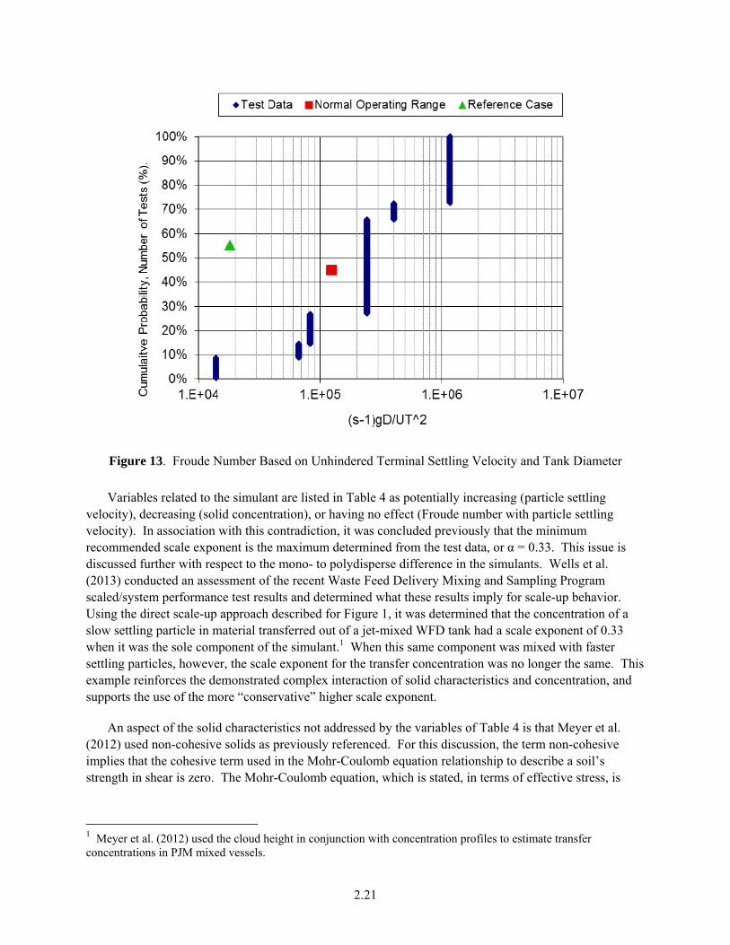
Figure 13. Froude Number Based on Unhindered Terminal Settling Velocity and Tank Diameter

Variables related to the simulant are listed in Table 4 as potentially increasing (particle settling velocity), decreasing (solid concentration), or having no effect (Froude number with particle settling velocity). In association with this contradiction, it was concluded previously that the minimum recommended scale exponent is the maximum determined from the test data, or α = 0.33. This issue is discussed further with respect to the mono- to polydisperse difference in the simulants. Wells et al. (2013) conducted an assessment of the recent Waste Feed Delivery Mixing and Sampling Program scaled/system performance test results and determined what these results imply for scale-up behavior. Using the direct scale-up approach described for Figure 1, it was determined that the concentration of a slow settling particle in material transferred out of a jet-mixed WFD tank had a scale exponent of 0.33 when it was the sole component of the simulant.1 When this same component was mixed with faster settling particles, however, the scale exponent for the transfer concentration was no longer the same. This example reinforces the demonstrated complex interaction of solid characteristics and concentration, and supports the use of the more “conservative” higher scale exponent.

An aspect of the solid characteristics not addressed by the variables of Table 4 is that Meyer et al. (2012) used non-cohesive solids as previously referenced. For this discussion, the term non-cohesive implies that the cohesive term used in the Mohr-Coulomb equation relationship to describe a soil’s strength in shear is zero. The Mohr-Coulomb equation, which is stated, in terms of effective stress, is

1 Meyer et al. (2012) used the cloud height in conjunction with concentration profiles to estimate transfer concentrations in PJM mixed vessels.

2.22

tanc (6)

where is the yield stress in shear (Pa), c’ is the effective cohesion intercept (Pa), ’ is the effective normal stress (Pa), and ’ is the effective friction angle (e.g., Campanella and Gupta 1969). Equation (6) is a simplification of the shearing resistance that depends on many factors including the solid concentration, solid composition, solid size and shape, stress history, temperature, strain, strain rate, etc. In general, however, c’ is the cohesive component of the shear strength and ’ is the frictional component.

Gauglitz et al. (2010) concluded that tank farm and scaled-test data for the WFD system suggest that, during tank mixing operations, a substantial fraction of the waste solids is not lifted above the bottom region of the tank but remains towards the bottom as a stratified layer. At sufficient solids concentration in this layer the slurry will be non-Newtonian with a small but still significant yield stress. It is thought that the non-Newtonian behavior and yield stress are caused primarily by cohesive particle interactions. This conclusion implies that the cohesive term of Eq. (6) can be non-zero for actual waste.

This conclusion also suggests that stratification of waste feed to the SHSVD for homogenous material with no yield stress may develop a yield stress in that stratified layer. Gauglitz et al. (2010) further stated that:

“Studies have shown that even a small yield stress reduces the jet momentum in the fluid at a distance from the jet and thus reduces the ability of the jet to mobilize solids. It is expected that any significant shear thinning behavior in a non-Newtonian fluid will have the same effect as a fluid having a yield stress, which is a specific type of shear thinning fluid. Accordingly, in the expected stratified condition of a jet-mixed tank, cohesive particle interactions will reduce the ability of the jet to lift particles into the upper region of the tank.”

The potential impact of this behavior on the recommended scale exponent is not encompassed in the direct scale-up data of Meyer et al. (2012). However, it is recommended in Section 2.2, from the direct scale-up of the nondimensional cavern height for non-Newtonian Laponite simulant cavern height data of Bamberger et al. (2005), that a scale exponent of = 0 (equal peak average PJM nozzle velocity) be used to achieve equivalent nondimensional cavern heights in the 8 foot test vessel and 16 foot SHSVD. Although the cavern height is a different performance metric than bottom motion, the phenomena of the mobilization of a non-Newtonian yield stress fluid due to the applied stress of the fluid jet is the same in each case, and thus a decrease in the scale exponent may be indicated. However, given the lack of specific test data, and as this approach would be non-conservative for the non-cohesive solids of the Newtonian simulants, no change to the scaling exponent is recommended.

The ratio of scaled tank diameters for the direct scale-up data is approximately 4.8, whereas the 8 foot test to prototypic scale for the SHSVD is approximately a factor of 2 (actual measured test vessel size is 92.5” diameter). This lower ratio suggests that the scale exponents should not be impacted by the 8 foot test to prototypic scale difference for the SHSVD. However the 8 foot and 16 foot prototypic SHSVD are much larger than the direct scale-up test scales with a factor of 12.8 between smallest test scale and prototypic scale. For the WFD system, Wells et al. (2013) concluded that the scale exponents determined from testing with a 2.8 difference in test scales (factor of approximately 20.8 between smallest test scale and prototypic) were meaningful for prototypic scale based on test data comparison to full-scale data and

2.23

computational fluid dynamics (CFD) predictions. Therefore, based on test scale difference to prototype, the recommendation of the scale exponent is not modified.

Meyer et al. (2010) address the issue of the simplified PJM drive of Meyer et al. (2012) relative to prototypic conditions. It was concluded that for the test conditions corresponding to the prototypic drive, a scale exponent of 0.40 for 8-tube tests and 0.36 for 12-tube tests might be expected. These larger scale exponents suggest the Meyer et al. (2012) scale-up data may not bound actual scale-up behavior for tests with prototypic PJM refill. Meyer et al. (2010) note that experimental verification is required to establish with certainty this difference in scaling.1 Regardless, the scale exponent is increased by reducing the number of PJMs from 12 to 8.2

Recent test data from 24590-QL-HC1-M00Z-00003-09-00176 are analyzed to determine if this trend of increased scale exponent with decreasing number of PJMs would follow to the prototypic configuration of 6 PJMs, noting the potential influence of the other altered parameters (e.g., double PJM rings to single ring).3 The Runsheet 7 tests of 24590-QL-HC1-M00Z-00003-09-00176 were conducted to collect critical suspension velocity data with different mixtures of Newtonian simulants, specifically the components of the reference case (see Table 2) simulant from Herting (2012). The first three tests of Runsheet 7 were conducted at increasing concentrations of the soda-lime glass powder component. This component has a median particle diameter by volume of 103 m (1st to 99th percentiles of 43 to 230 m) and density of 2.5 g/mL (Herting 2012), in comparison to the 69 m (1st to 99th percentiles of 54 to 90 m), 2.48 g/mL density of the Meyer et al. (2010) prototypic drive tests used to determine the referenced scale exponents and the s1d2 simulant (median size of 69.3 m and density of 2.48 g/mL, Table 1) of Meyer et al. (2012). The soda-lime glass powder component test results from 24590-QL-HC1-M00Z-00003-09-00176 are thus compared to direct scale-up tests of Table 1, and the scale exponent analysis of Meyer et al. (2010) is applied.

To compare the test results and evaluate the scale exponent, the Runsheet 7 soda-lime glass powder test parameters are presented on equivalent bases as Meyer et al. (2010) and Meyer et al. (2012) in Table 5. The “Adjusted New Physical Model” of Meyer et al. (2010), which accounts for the simplified PJM drive of Meyer et al. (2012) relative to prototypic conditions, predicts the “S” condition Ucs (see Table 5) of the Runsheet 7 soda-lime glass powder tests within -6% to 13%, Figure 14. At the 0.018 reference solid volume fraction, the predicted Ucs, 6.52 m/s, is within the UcsS and UcsW range of 6.93 to 6.40 m/s.

The reference solid volume fractions of the soda-lime glass powder are comparable to the 4s1d2Yc_1, 4s1d2Rc_1, and 4s1d2Xc_1 direct scale-up tests of Meyer et al. (2012), Table 1, as well as the Meyer et al. (2010) 8 and 12 tube test conditions evaluated for scale exponent which had reference solid volume

1 If the intermittent mixing of the rotating jet mixers is treated as analogous to the intermittent mixing of the PJMs and impact of drive system with respect to impact on particle settling between pulses, it can be noted that Wells et al. (2013) found that the scaling for ECR in the WFD system vessels was different depending on jet rotation rate scaling (other differences were also present in the analyzed tests). 2 The “Adjusted New Physical Model” of Meyer et al. (2010), which accounts for the simplified PJM drive of Meyer et al. (2012) relative to prototypic conditions, has three nondimensional parameters that are functions of the number of PJMs. The 33% decrease in PJM number from 12 to 8 results in a decrease of approximately 28% for the combined product of the three referenced nondimensional parameters. 3 The 24590-QL-HC1-M00Z-00003-09-00176 data that was used in this analysis was not collected using ASME NQA-1-2000 protocols. Therefore, this data was analyzed as “For Information Only.”

2.24

fractions of 0.014 and 0.009 respectively. Therefore, to compare the Adjusted New Physical Model test data basis and the 24590-QL-HC1-M00Z-00003-09-00176 soda-lime glass powder results, the functionality of Ucs with the reference solid volume fraction is considered. In Figure 15, to remove the difference in test scales and configuration, the ordinate is the Ucs at the specified reference solid volume fraction divided by the Ucs at the lowest reference solid volume fraction. The Meyer et al. (2012) and 24590-QL-HC1-M00Z-00003-09-00176 test data are shown in Figure 15 to respond relatively similarly to increasing reference solid volume fraction, but the Adjusted New Physical Model under-predicts the impact of solid concentration for the Runsheet 7 soda-lime glass powder test results at the highest solid concentration (reflecting the over-prediction of Ucs at the lower concentrations shown in Figure 14).

Table 5. 24590-QL-HC1-M00Z-00003-09-00176 Runsheet 7 Soda-lime Glass Powder Test Parameters for Meyer et al. (2010) and Meyer et al. (2012). For Information Only.

Tank Diameter (inches)

PJM Nozzle Diameter (inches)

Pulse Tube

Diameter (inches)

Average Duty

Cycle1

Average Reference

Pulse Volume Fraction2

Reference Solid

Volume Fraction3

Average Peak

Average UcsS4 (m/s)

Average Peak

Average UcsW5 (m/s)

92.5 1.94 15.7 0.16 0.19

0.005 4.36 3.74

0.01 4.95 4.43

0.018 6.93 6.40

1. PNNL analysis of test data. 2. Volume of fluid ejected in a pulse times the number of PJMs divided by the reference volume, where reference volume is defined by the tank area times the tank diameter. PNNL analysis of test data. 3. Volume of solids divided by the reference volume, where reference volume is defined by the tank area times the tank diameter. 4. “S” refers to a Ucs that was stated to be strong. PNNL analysis of test data. 5. “W” refers to a Ucs that was declared “incipient,” “marginal,” or is the next lowest velocity from a “S” Ucs. PNNL analysis of test data.

2.25

Figure 14. Measured and Predicted Ucs for Runsheet 7 Soda-lime Glass Powder Tests. For Information Only.

2.26

Figure 15. Measured and Predicted Effect of Reference Solid Volume Fraction on Ucs. For Information Only.

With the relatively favorable comparison of the measured and predicted Ucs results for the analyzed 24590-QL-HC1-M00Z-00003-09-00176 test and functionality with comparable Meyer et al. (2012) tests, the scale exponent analysis of Meyer et al. (2010) is applied to the Runsheet 7 soda-lime glass powder test conditions. All parameters in the Adjusted New Physical Model are held constant at the test conditions except for tank diameter which is varied over a similar range as in Meyer et al. (2010). Calculated scale exponents, from a power law fit of the model results with increasing tank diameter, for the proposed SHSVD prototypic configuration of 6 PJMs are shown in Figure 16 to have a maximum of α = 0.33 which corresponds to power per unit volume scaling. The increasing scale exponent trend from Meyer et al. (2010) with the number of PJMs reduced from 12 to 8 (scale exponents of 0.36 and 0.40 respectively) is thus not continued to the prototypic configuration of 6 PJMs, which may be due to the potential influence of the other altered parameters (e.g., double PJM rings to single ring). Note, as previously described, the Adjusted New Physical Model of Meyer et al. (2010) has three nondimensional parameters that are functions of the number of PJMs. The 25% reduction in PJM number from 8 to 6 results in a decrease of approximately 30% for the combined product of the three referenced nondimensional parameters.

2.27

a)

b)

y = 2.94x0.32

4

5

6

7

8

9

10

0 10 20 30 40

Ucs

(m/s

)

Vessel Diameter (ft)

Reference Solid VolumeFraction = 0.01

Test Data, UcsS

Test Data, UcsW

Meyer et al. (2010),Adjusted New PhyscialModel

SHSVD

c)

y = 3.33x0.33

6

7

8

9

10

11

0 10 20 30 40

Ucs

(m/s

)

Vessel Diameter (ft)

Reference SolidVolume Fraction =0.018

Test Data, UcsS

Test Data, UcsW

Meyer et al. (2010),Adjusted New PhyscialModel

SHSVD

Figure 16. Meyer et al. (2010) Adjusted New Physical Model Scale Exponent Analysis Applied to the Runsheet 7 Soda-lime Glass Powder Tests. For Information Only.

2.28

As expected from the functionality of the Adjusted New Physical Model, there is little effect of the reference solid volume fraction on the calculated scale exponent, Figure 16. The Runsheet 7 tests with soda-lime glass powder were not conducted at a reference solid volume fraction representing the SHSVD Newtonian waste slurry example reference solid volume fraction of 0.033, Table 2. However, tests were conducted with the multi-component example reference case simulant (see Table 2) at a reference solid volume fraction of 0.04 (24590-QL-HC1-M00Z-00003-09-00176). The Runsheet 7 reference case simulant test parameters are presented on equivalent bases as Meyer et al. (2010) and Meyer et al. (2012) in Table 6.

The Adjusted New Physical Model (Meyer et al. 2010) predicted Ucs for the reference case test is 8.6 m/s, which is within the UcsS and UcsW range of approximately 9 to 8.5 m/s obtained in the 8 foot test vessel. As done for the Runsheet 7 soda-lime glass powder test conditions, the scale exponent analysis of Meyer et al. (2010) is applied to the Runsheet 7 reference case. Again, all parameters in the Adjusted New Physical Model are held constant at the test conditions except for tank diameter which is varied over a similar range as in Meyer et al. (2010). The calculated scale exponent from a power law fit of the model results with increasing tank diameter is shown in Figure 17 as α = 0.26. This analysis indicates that these analyzed 24590-QL-HC1-M00Z-00003-09-00176 test conditions would have a Ucs of 10.4 m/s in a 16 foot diameter vessel. As argued previously, however, the maximum scale exponent for the proposed SHSVD prototypic configuration of 6 PJMs, α = 0.33, is recommended as the minimum scale exponent that should be applied for the proposed SHSVD assessment.

Table 6. 24590-QL-HC1-M00Z-00003-09-00176 Runsheet 7 Herting (2012) Simulant (Example Reference Case, Table 2) Test Parameters for Meyer et al. (2010) and Meyer et al. (2012). For Information Only.

Tank Diameter (inches)

PJM Nozzle Diameter (inches)

Pulse Tube

Diameter (inches)

Average Duty

Cycle1

Average Reference

Pulse Volume Fraction2

Reference Solid

Volume Fraction3

Average Peak

Average UcsS4 (m/s)

Average Peak

Average UcsW5 (m/s)

92.5 1.94 15.7 0.16 0.20 0.04 9.03 8.54

1. PNNL analysis of test data. 2. Volume of fluid ejected in a pulse times the number of PJMs divided by the reference volume, where reference volume is defined by the tank area times the tank diameter. PNNL analysis of test data. 3. Volume of solids divided by the reference volume, where reference volume is defined by the tank area times the tank diameter. 4. “S” refers to a Ucs that was stated to be strong. PNNL analysis of test data. 5. “W” refers to a Ucs that was declared “incipient,” “marginal,” or is the next lowest velocity from a “S” Ucs. PNNL analysis of test data.

2.29

Figure 17. Meyer et al. (2010) Adjusted New Physical Model Scale Exponent Analysis Applied to the Runsheet 7 Herting (2012) Simulant Test. For Information Only.

Based on the preceding discussion of uncertainties due to aspects of the testing program, the recommended scale exponent for bottom motion in the SHSVD prototypic configuration of 6 PJMs remains as in the preceding section, = 0.33, based on the direct scale-up data. Again, this scale exponent corresponds to a PJM nozzle velocity of approximately 9.4 m/s from Eq. (1) in an 8 foot vessel (12 m/s PJM nozzle velocity in the SHSVD, actual measured 8 foot test vessel size is 92.5” diameter). None of the other aspects of test program uncertainty provide a basis to argue that the scale exponent should be reduced. It can be noted that the Meyer et al. (2010) scale exponent of 0.40 for the 8-tube array is equivalent to the highest scale exponent of Kuhn et al. (2013) determined from the general models of the Meyer et al. (2012) data which incorporate tank bottom geometries, simulants, and PJM configurations and operational parameters with statistical and physical model bases as well as inertial and shear stress theoretical approaches. As previously presented for the direct scale-up data of Meyer et al. (2012), consistent scaling for both critical suspension velocity (bottom motion) and cloud height (suspension) is demonstrated; it is not clear if this conclusion is impacted by the PJM drive system differences (refer to Table 4).

2.2 Non-Newtonian Simulant Testing

Direct scale-up of the mixing performance metric of cavern height for non-Newtonian simulant testing are discussed in this section. PJM nozzle velocities required for equivalent cavern height in the 8 foot vessel for prototypic SHSVD operation are defined from the existing direct scale-up data of Bamberger et al. (2005). These data are taken from the three-scale PJM mixing systems tests using non-Newtonian yield stress slurries.

2.30

Bamberger et al. (2005) recommended that scaled testing of prototypic PJM systems in non-Newtonian slurries adhere to the following guidelines:

Use geometric scaling with a scale factor no greater than 4–5 since the testing was performed within this range.

Use the bounding WTP non-Newtonian rheology (e.g., 30 Pa yield strength, 30 cP consistency, Section 3).

Use the design peak average PJM velocity (e.g., 12 m/s, Section 3).

Use PJM drive times and cycle time reduced by the scale factor.

It was stated further that:

“If these guidelines are followed, the yield Reynolds and Strouhal numbers (the two most important nondimensional parameters affecting mixing in non-steady, non-Newtonian slurries) will be matched at small scale. In addition, the jet Reynolds number will be smaller in the small scale test, and the result will thus be conservative.”

This section discusses the Bamberger et al. (2005) recommendation of using the design peak average PJM nozzle velocity and the associated conclusion of conservatism associated with the jet Reynolds number in relation to the cavern height data (i.e., PJM Mixing Mode 1, Cavern Only, Bamberger et al. 2005) relative to direct scale-up. The yield Reynolds number, Reτ, is the ratio of dynamic stress to slurry yield stress in shear defined by

2URe

(7)

where is the jet fluid density. Bamberger et al. (2005) used shear vane measured values for and note that the yield Reynolds number can also be formed with the Bingham yield stress in the denominator. The jet Reynolds number is the ratio of dynamic stress to viscous stress and was defined by

Ud

Re j (8)

where is the Bingham consistency.

Based on the yield Reynolds number, Bamberger et al. (2005) demonstrated that there is a general trend that nondimensional cavern heights (measured cavern height divided by tank diameter) are larger with increasing vessel scale depending on the characterization of the PJM nozzle velocity as peak average or average.1 To re-state, it was concluded that nondimensional cavern heights are generally largest in the large test vessel and decreased for the smaller vessels at equivalent yield Reynolds numbers.

1 Peak average velocity is determined during the period of peak discharge to the end of pressurization, while the average velocity is taken over the entire discharge time.

2.31

As previously described, testing in the 8 foot geometrically scaled vessel was conducted with similar PJM configuration, operational parameters (duty cycle, pulse volume fraction), vessel fill level, and simulant to the 16 foot SHSVD. Specifically for the simulant characteristics, the rheology will be the same. The rheology of the Laponite simulant tests without breakthrough (“Mode 1” cavern only as defined in Bamberger et al. 2005), represented by the denominator of the yield Reynolds number as the shear strength in Bamberger et al. (2005), is shown in Figure 18 as a function of the peak average nozzle velocity. For all cases, the shear strength of the small scale tests (D = 0.438 m) is less than the medium (D = 0.858 m) and large (D = 3.88 m) tests. With constant density,1 this necessarily results in a higher yield Reynolds number for the small scale tests at equivalent velocity. For concurrent or near concurrent test velocities, the bulk of the large scale tests were at lower shear strength than the medium scale tests. Similar conditions are observed with the average PJM nozzle velocity in Figure 19, with perhaps the bulk of the large scale tests having higher shear strength than the medium scale tests for similar average PJM nozzle velocities.

Figure 18. Laponite Cavern Test Shear Strength for Test Condition Peak Average PJM Nozzle Velocity and Vessel Scale

1 Bamberger et al. (2005) specify that the Laponite used had a density of 1000 kg/m3over the range of shear strengths tested.

2.32

Figure 19. Laponite Cavern Test Shear Strength for Test Condition Average PJM Nozzle Velocity and Vessel Scale

The impact of the difference in shear strength at the test scales with respect to the implication of increased yield Reynolds number at the smaller scale – increased velocity for equivalent nondimensional cavern height – is demonstrated in Figure 20. Here, the nondimensional cavern height is plotted as a direct function of peak average PJM nozzle velocity at “constant” shear strength of 95 to 105 Pa for both the peak average and average PJM nozzle velocities.1 Likewise, the data for 10 Pa shear strength ranges of 105 to 115 Pa, 115 to 125 Pa, and 125 to 135 Pa are shown in Figure 21 through Figure 23 respectively. Within the scatter of the data, the general trend is that equivalent nondimensional cavern heights (“Mode 1” cavern only as defined in Bamberger et al. 2005) are achieved at equivalent velocity independent of test scale.2 To relate to the scale exponent of Eq. (1), this implies that = 0, whereas the yield Reynolds number approach implied a negative scale exponent. For the peak average nozzle velocity alone, a negative scale exponent may be indicated by the one data point for the 105 to 115 Pa data, Figure 21, and 125 to 135 Pa, Figure 23, while a positive scale exponent may be indicated by the 115 to

1 A 5% spread from 100 Pa is judged as meaningful with respect to “constant” shear strength for Laponite. 2 Bamberger et al. (2005) described the scaling of the drive time such that the geometric scale of the surface rise and the volume of fluid injected into the cavern were maintained across the test scales. Estimated, for information only, experimental values for the actual drive times indicate deviations up to approximately 13% low in the medium scale tank and 20% low in the small scale tank in comparison to the respective velocities used at large scale. Note that the experimental drive times are assumed to be sufficiently long for steady state flow conditions and cavern boundaries to be established. An estimated, for information only, correction to the cavern height can be made to account for the difference in volume displacement associated with the variation in the drive time from geometric scale. The estimated, for information only, correction to the measured cavern height is on the order of 0.3 cm or less, corresponding to less than 1% of the measured cavern heights at both the smaller test scales. In addition, the estimated, for information only, surface level change oscillated by approximately 5 cm and 1 cm in the medium and small scale tests respectively due to the operation of the PJMs.

2.33

125 Pa data, Figure 23, for the average PJM nozzle velocities. Given the sparseness and scatter of the data, no significance is placed on these velocity-based non-zero scale exponent indications. Similar results, = 0, are achieved at “constant” Bingham yield stress.

This result, equivalent nondimensional carven height at different geometric vessel scales for equal PJM nozzle velocity, is consistent with the results of non-Newtonian yield stress sediment erosion with Newtonian fluid jets summarized in Gauglitz et al. (2010). For different test scales, jet configurations, and simulants, the nondimensional ECR has been shown to have the functionality of

U

CD

ECR

(9)

where C is an empirically determined constant. The yield stress in shear exponent is on the order of ½, which is consistent with the nondimensional cavern height model functionality on yield Reynolds number (½) of Bamberger et al. (2005). In Gauglitz et al. (2010), actual Hanford waste in situ ECR data from WFD system operation were shown to have “remarkable agreement” with the scaled simulant testing results expressed via Eq. (9). For scaled testing of the WFD system, Wells et al. (2013) determined positive scale exponents for nondimensional ECR with variation that may have been impacted by jet rotation rate scaling.

a) b)

Figure 20. Laponite Cavern Test Nondimensional Cavern Height as a Function of PJM Nozzle Velocity, 95 to 105 Pa� a) Peak Average PJM Nozzle Velocity, b) Average PJM Nozzle Velocity

2.34

a)

0.3

0.4

0.5

0.6

0.7

0.8

0.9

1

1.1

1.2

2 4 6 8 10 12 14

Hca

vern

/D

Peak Average PJM Nozzle Velocity (m/s)

Shear Strength105 to 115 Pa

Medium

Large

b)


a) b)

0.3

0.4

0.5

0.6

0.7

0.8

0.9

1

1.1

1.2

2 4 6 8 10 12 14

Hca

vern

/D

Average PJM Nozzle Velocity (m/s)


Medium

Large

Figure 22. Laponite Cavern Test Nondimensional Cavern Height as a Function of PJM Nozzle Velocity, 115 to 125 Pa� a) Peak Average PJM Nozzle Velocity, b) Average PJM Nozzle Velocity.

a)

0.3

0.4

0.5

0.6

0.7

0.8

0.9

1

1.1

1.2

2 4 6 8 10 12 14

Hca

vern

/D

Peak Average PJM Nozzle Velocity (m/s)


Medium

Large

b)

0.3

0.4

0.5

0.6

0.7

0.8

0.9

1

1.1

1.2

2 4 6 8 10 12 14

Hca

vern

/D

Average PJM Nozzle Velocity (m/s)


Medium

Large


2.35

Bamberger et al. (2005) note that, at equivalent PJM nozzle velocity ( = 0) and simulant, the jet Reynolds number is reduced at smaller scale, and concluded that this testing approach is conservative because of generally reduced mixing phenomena. The jet Reynolds numbers for the Laponite cavern tests are shown in Figure 24 as a function of the peak average PJM nozzle velocity. Clearly, the small scale tests have reduced jet Reynolds numbers, followed by the medium scale tests, with the large scale tests having the largest jet Reynolds numbers.

Rajaratnam and Flint-Peterson (1989) show that for turbulent jet Reynolds numbers greater than approximately 3,000 there would be little impact of circular wall jet behavior on scaling for the laminar length and lateral spread rate, and for jet Reynolds numbers greater than approximately 10,000, these jet behaviors are essentially independent of scale. For the growth rate of the jet thickness in the vertical direction to be independent of scale, the results of Rajaratnam and Flint-Peterson (1989) indicate higher Rej are required. However, Beltaos (1975) (see also Poreh et al. 1967) indicates that the change of the skin friction coefficient (relating the jet velocity to the applied wall stress, e.g., Beltaos and Rajaratnam 1977) with the jet Reynolds number is limited above Rej ~ 3,000, and further reduced for Rej > 10,000. These jet Reynolds number ranges support that the reduced jet Reynolds numbers of the small scale tests (Figure 24) can impact the interpretation of these test results relative to the other test scales. However, the majority of the data shown above indicating = 0 is from the relation of the medium and large scale tests which have jet Reynolds numbers in excess of 6,000.

Figure 24. Jet Reynolds Numbers Based on Peak Average PJM Nozzle Velocity for Laponite Cavern Tests

Also of significance for the effect of the indicated equivalent jet velocity at reduced scale is the power-per-volume (PPV). Kuhn et al. (2013) stated that, if the power dissipation in an element of a

2.36

Bingham fluid is great enough, the fluid behaves as though it were a Newtonian fluid. PPV thus provides a means for matching the Newtonian nature of a yielded non-Newtonian fluid.

The PPV for the entire vessel of the Laponite cavern tests during the jet discharge can be calculated as

V

NUd8PPV

32

(10)

where N is the number of PJMs and V is the tank volume. The calculated PPV of the cavern height tests are shown in Figure 25 as a function of the peak average PJM nozzle velocity. The small scale tests had larger PPV than the large scale tests across the range of the test conditions. At a given peak average PJM nozzle velocity, the highest PPV was in the small tank, followed by the medium scale tank, with the lowest in the large scale tank. These results suggest that the fluid in the reduced scale vessels likely had a lower apparent viscosity. For a given PJM nozzle velocity, the larger scale apparent viscosity will be greater than that of the smaller until the limit of equality is obtained at sufficiently high PJM nozzle velocity. Therefore, for gas release (bubble rise in the yielded fluid) or solids segregation (settling of solids in the yielded fluid), the reduced scale tests would potentially over-represent conditions in the larger vessel at equivalent nondimensional cavern formation (i.e., equivalent PJM nozzle velocity).

Comparison of the calculated jet Reynolds number and PPV for the 8 foot test vessel and 16 foot SHSVD is made in Figure 26. Representative slurry density, 1,200 kg/m3, and viscosity, 30 cP, are used with a PJM nozzle velocity of 12 m/s for each scale. The jet Reynolds number calculation demonstrates that the difference in the jet Reynolds number should not be significant to the jet behavior (see discussion of Figure 24), but the PPV is greater by a factor of two in the 8 foot vessel, so gas release rates and solids segregation may be over-represented in the 8 foot vessel.

2.37

Figure 25. PPV Based on Peak Average PJM Nozzle Velocity for Laponite Cavern Tests

Figure 26. PPV and Jet Reynolds Numbers with Equal Jet Velocity and Waste Properties, 8 foot and 16 foot Geometrically Scaled Vessels

2.38

Based on the Laponite simulant cavern height data of Bamberger et al. (2005), a scale exponent of = 0 (equal peak average PJM nozzle velocity) is recommended to achieve equivalent nondimensional cavern heights (“Mode 1” cavern only as defined in Bamberger et al. 2005) in the 8 foot test vessel and 16 foot SHSVD with the operational and simulant parameters the same at the different scales. Based on comparison of the PPV in these vessels at equal PJM nozzle velocity, there is potential that gas release rates and solids segregation in the yielded material may be over-represented in the 8 foot vessel.

3.1

3.0 Conclusions

This report provides a technical basis for direct scale-up of PJM performance from small scale testing with Newtonian and non-Newtonian simulants to the expected PJM performance in larger vessels under similar conditions. As this report is based in part on data collected under a commercial grade quality assurance program, it is not intended to be used in WTP design activities. Testing has been conducted in the 8 foot geometrically scaled vessel with similar PJM configuration, operational parameters (duty cycle, pulse volume fraction), vessel fill level, and simulant to the proposed 16 foot diameter SHSVD. The difference in the mixing performance of the 8 foot vessel to the prototypic 16 foot vessel can therefore be expressed in terms of direct scale-up where direct scale-up is used to define the mixing performance depending solely on geometric scale and PJM nozzle velocity. For this work, mixing performance is assessed relative to bottom motion and cloud height for Newtonian simulants, and cavern heights for non-Newtonian simulants.

Consistent scaling for both critical suspension velocity (bottom motion) and cloud height (suspension) is demonstrated by the data for direct scale-up from Meyer et al. (2012) for testing of simplified PJM mixing systems using monodisperse non-cohesive Newtonian simulants. Based on the reference case parameters and the clarity that if the 8 foot test mixing performance meets or exceeds adequate SHSVD performance with the largest scale exponent indicated by the test data there is increased confidence that adequate performance will be achieved in the SHSVD.

The minimum recommended scale exponent for bottom motion is the maximum determined from the test data, α = 0.33, which is equivalent to power-per-volume (PPV) scaling. Consistent scaling for both bottom motion and cloud height suspension is demonstrated by the data. Uncertainties for this direct scale exponent basis have been considered, and the recommended bottom motion scale exponent for the SHSVD prototypic configuration of 6 PJMs is = 0.33 for the direct scale-up data. With a 12 m/s PJM nozzle velocity in the 16 foot SHSVD, this scale exponent corresponds to a PJM nozzle velocity of approximately 9.4 m/s in the 8 foot test vessel (actual measured test vessel size is 92.5” diameter).

Based on the direct scale-up of non-Newtonian Laponite simulant cavern height data of Bamberger et al. (2005), a scale exponent of = 0 (equal peak average PJM nozzle velocity) is recommended to achieve equivalent nondimensional cavern heights (“Mode 1” cavern only as defined in Bamberger et al. 2005) in the 8 foot test vessel and 16 foot SHSVD with the operational and simulant parameters the same at the different scales. Difference in the jet Reynolds number between the 8 foot test vessel and 16 foot SHSVD at equal 12 m/s PJM nozzle velocity should not be significant to the jet behavior. Comparison of the PPV in these vessels at equal PJM nozzle velocity suggests there is potential that gas release rates and solids segregation (i.e., stratification) in the yielded material may be over-represented in the 8 foot vessel.

4.1

4.0 References

24590-QL-HC4-M00Z-00003-09-00176. 2015. Pulse Jet Mixer (PJM) Test Platform Test Vessel V401 SHSVD Pilot-Scale Testing Test Sequence#: 8’ SHSVD-Tests-32 Rev 00. Energy Solutions, Richland, Washington.

Bamberger JA, PA Meyer, JR Bontha, CW Enderlin, DA Wilson, AP Poloski, JA Fort, ST Yokuda, HD Smith, F Nigl, MA Friedrich, DE Kurath, GL Smith, JM Bates, and MA Gerber. 2005. Technical Basis for Testing Scaled Pulse Jet Mixing Systems for Non-Newtonian Slurries. PNWD-3551, WTP-RPT-113, Battelle, Pacific Northwest Division, Richland, Washington.

Beltaos S. 1975. “Oblique Impingement of Circular Turbulent Jets.” Journal of Hydraulic Research. 14:(1976)1.

Beltaos S and N Rajaratnam. 1977. “Impingement of Axisymmetric Developing Jets.” Journal of Hydraulic Research 15:4.

Bontha JR, C Chapman, J Geeting, and JL Huckaby. 2015. Data Summary from 8-foot Vessel Testing of Potential Pulse Jet Mixer Configurations in the Standard High Solids Vessel Design. 24590-PTF-RPT-LST-15-001, Rev. 0. Bechtel National, Inc., Richland, Washington.

Campanella RG and RC Gupta. 1969. Effect of Structure on Shearing Resistance of a Sensitive Clay. British Columbia. University Dept. of Civil Engineering, Soil Mech. series, SM#6.

Gauglitz PA, BE Wells, JA Bamberger, JA Fort, J Chun, and JJ Jenks. 2010. The Role of Cohesive Particle Interactions on Solids Uniformity and Mobilization During Jet Mixing: Testing Recommendations. PNNL-19245, Pacific Northwest National Laboratory, Richland, Washington.

Herting DL. 2012. Simulant Qualification for Computational Fluid Dynamics Testing. 24590-WTP-RPT-RT-12-002, Rev. 0, Bechtel National, Inc., Richland, Washington.

Jewett JR, SD Estey, L Jensen, NW Kirch, DA Reynolds, and Y Onishi. 2002. Values of Particle Size, Particle Density, and Slurry Viscosity to Use in Waste Feed Delivery Transfer System Analysis. RPP-9805, Rev. 1, Numatec Hanford Corporation, Richland, Washington.

Kuhn WL, DR Rector, SD Rassat, CW Enderlin, MJ Minette, JA Bamberger, GB Josephson, BE Wells, and EJ Berglin. 2013. Scaling Theory for Pulsed Jet Mixed Vessels, Sparging, and Cyclic Feed Transport Systems for Slurries. PNNL-22816, Pacific Northwest National Laboratory, Richland, Washington.

Meacham JE, SJ Harrington, JS Rodriquez, VC Nguyen, JG Reynolds, BE Wells, GF Piepel, SK Cooley, CW Enderlin, DR Rector, J Chun, A Heredia-Langner, and RF Gimpel. 2012. One System Evaluation of Waste Transferred to the Waste Treatment Plant. RPP-RPT-51652, Rev. 0, PNNL-21410, Washington River Protection Solutions LLC, Richland, Washington.

Meyer PA, JA Bamberger, CW Enderlin, JA Fort, BE Wells, SK Sundaram, PA Scott, MJ Minette, GL Smith, CA Burns, MS Greenwood, GP Morgen, EBK Baer, SF Snyder, M White, GF Piepel,

4.2

BG Amidan, and A Heredia-Langner. 2012. Pulse Jet Mixing tests with Noncohesive Solids. PNNL-18098 Rev. 1, WTP-RPT-182, Rev. 1, Pacific Northwest National Laboratory, Richland, Washington.

Meyer PA, EBK Baer, JA Bamberger, JA Fort, and MJ Minette. 2010. Assessment of Differences in Phase 1 and Phase 2 Test Observations for Waste Treatment Plant Pulse Jet Mixer Tests with Non-Cohesive Solids. PNNL-19085, WTP-RPT-208, Pacific Northwest National Laboratory, Richland, Washington.

Poreh M, YG Tsuei, and JE Cermak. 1967. “Investigation of a Turbulent Radial Wall Jet.” Journal of Applied Mechanics 34:457-463.

Rajaratnam N and L Flint-Petersen. 1989. “Low Reynolds Number Circular Turbulent Jets.” Philippine Institute of Civil Engineers 87(2):299-305.

Reid D. 2014. Basis of Design. 24590-WTP-DB-ENG-01-001, Rev. 2, Bechtel National, Inc., Richland, Washington.

Wells BE, JA Fort, PA Gauglitz, DR Rector, and PP Schonewill. 2013. Preliminary Scaling Estimate for Select Small Scale Mixing Demonstration Tests. PNNL-22737, Pacific Northwest National Laboratory, Richland, Washington.


Distribution*

No. of No. of Copies Copies

Distr.1

8 INTERNAL DISTRIBUTION 8 Pacific Northwest National Laboratory JA Bamberger PDF CW Enderlin PDF MJ Minette PDF LM Peurrung PDF PP Schonewill PDF BE Wells K7-15 Information Release (pdf) PDF Project File (1) K3-52

3 EXTERNAL DISTRIBUTION 3 Bechtel National Inc. RA Brouns PDF MA Summers PDF WTP Docs PDF

*All distribution will be made electronically.

Documents

Technical Basis for Direct Scale-up of Small Scale Pulse