Technical Documentation Climate Impact Explorer

1

Technical Documentation Climate Impact Explorer

Last edited: June 7 2021

The Climate Impact Explorer (CIE) provides first-hand access to projections of physical climate

risks at the continental, national and subnational level. It shows maps and graphs illustrating the

projected changes in climate conditions, resulting impacts and damages on selected sectors for

several global warming levels, and also how they will play out over time according to various

policy-relevant emission scenarios (including those from the Network for Greening the Financial

System, or NGFS). All display materials and the underlying data can be downloaded through the

CIE interface.

Key functionalities.........................................................................................................................................2A guidance note for Users............................................................................................................................2Acknowledgements.......................................................................................................................................2Introduction: overview of the methodology used to derive the data visualised on the Climate Impact Explorer..............................................................................................................................................41. Methodology..............................................................................................................................................5

1.1 Core Concept..................................................................................................................................................51.2 Global Mean Temperature (GMT) Projections.........................................................................................61.3 Ascribing changes in climate impacts to GMT trajectories.....................................................................71.4 Impact projection uncertainty.....................................................................................................................11.5 Estimation of the full uncertainty range....................................................................................................21.6 Additional data processing steps................................................................................................................3

1.6.1 Masking of grid cells for specific variables..........................................................................................................................31.6.2 Temporal averages......................................................................................................................................................................41.6.3 National or subnational level averages................................................................................................................................41.6.4 Smoothing of time series..........................................................................................................................................................4

2. Models, scenarios and data sources......................................................................................................52.1 NGFS Scenarios..............................................................................................................................................52.2 ISIMIP data.....................................................................................................................................................52.3 CLIMADA.........................................................................................................................................................9

2.3.1. CLIMADA Model..........................................................................................................................................................................92.3.2. River Flood.................................................................................................................................................................................102.3.3. Tropical Cyclone.......................................................................................................................................................................11

3. Visualisation............................................................................................................................................12

2

3.1 Time series....................................................................................................................................................123.2 Country Maps...............................................................................................................................................13

4. References................................................................................................................................................15

Key functionalities ● Projections of climate impacts at the national and subnational level on annual and seasonal

scales:

○ Including uncertainty ranges encompassing both the global climate sensitivity to

emissions and the response of local impacts to global warming

○ Aggregation at the continental, national and subnational levels using weighted

averages by either area, GDP, or population

● Time evolution of future impacts for several policy-relevant scenarios from the NGFS, the

Climate Action Tracker and for the Representative Concentration Pathways

● Country maps for different warming levels containing information on the robustness of the

projections, based on the agreement between the various climate and impact models used

to derive them (model agreement)

● Climate and climate impact indicators covering several biophysical sectors and economic

damages from selected extreme events

● The possibility to download all displayed graphs and maps, as well as the data underlying

them

A guidance note for Users The Climate Impact Explorer provides a comprehensive, globally consistent dataset of physical

risk projections for different climate scenarios. The use of global datasets means regional

representations are not consistently evaluated and can show deviations from other datasets

used in risk assessments focused on the regional, national or subnational level. The findings

from the Climate Impact Explorer should thus be used to supplement rather than replace

national or regional risk assessments.

Acknowledgements The Climate Impact Explorer was developed by Climate Analytics with contributions from Thessa Beck, Quentin Lejeune, Inga Menke, Peter Pfleiderer, Eoin Quill, Carl-Friedrich Schleussner, Sylvia Schmidt, and Nicole van Maanen, and implemented by Flavio Gortana.

3

Its development was supported by ClimateWorks Foundation and Bloomberg Philanthropies in the context of a collaboration with the Network for Greening the Financial System, as well as the German Ministry for Education and Research.

We would like to thank the following contributors: David N. Bresch (Swiss Federal Institute of Technology - ETHZ), Katja Frieler (Potsdam Institute for Climate Impact Research - PIK), Chahan Kropf (Swiss Federal Institute of Technology - ETHZ), Christian Otto (Potsdam Institute for Climate Impact Research - PIK), Inga Sauer (Potsdam Institute for Climate Impact Research - PIK).

4

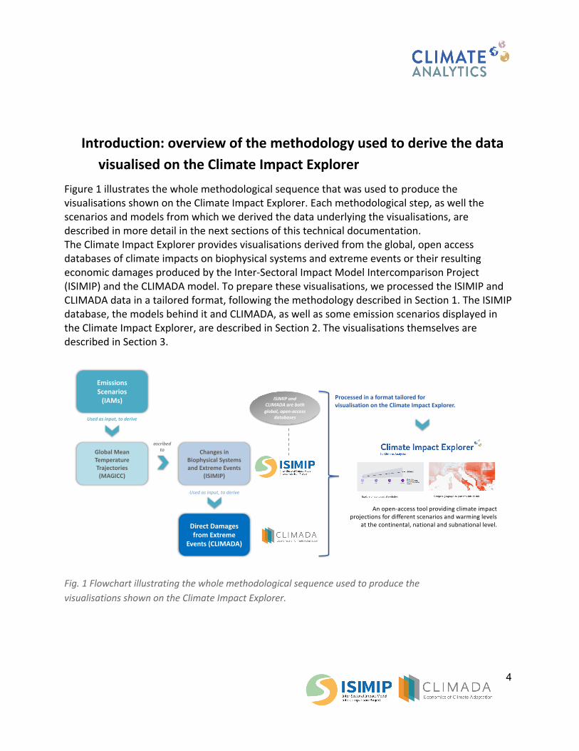
Introduction: overview of the methodology used to derive the data visualised on the Climate Impact Explorer

Figure 1 illustrates the whole methodological sequence that was used to produce the

visualisations shown on the Climate Impact Explorer. Each methodological step, as well the

scenarios and models from which we derived the data underlying the visualisations, are

described in more detail in the next sections of this technical documentation.

The Climate Impact Explorer provides visualisations derived from the global, open access

databases of climate impacts on biophysical systems and extreme events or their resulting

economic damages produced by the Inter-Sectoral Impact Model Intercomparison Project

(ISIMIP) and the CLIMADA model. To prepare these visualisations, we processed the ISIMIP and

CLIMADA data in a tailored format, following the methodology described in Section 1. The ISIMIP

database, the models behind it and CLIMADA, as well as some emission scenarios displayed in

the Climate Impact Explorer, are described in Section 2. The visualisations themselves are

described in Section 3.

Fig. 1 Flowchart illustrating the whole methodological sequence used to produce the visualisations shown on the Climate Impact Explorer.

Emissions Scenarios

(IAMs)

Changes in Biophysical Systems and Extreme Events

(ISIMIP)

Direct Damagesfrom Extreme

Events (CLIMADA)

Global Mean Temperature Trajectories(MAGICC)

An open-access tool providing climate impact projections for different scenarios and warming levels

at the continental, national and subnational level.

Used as input, to derive

ascribedto

Used as input, to derive

ISIMIP and CLIMADA are both global, open-access

databases

Processed in a format tailored forvisualisation on the Climate Impact Explorer.

5

1. Methodology

1.1 Core Concept

The Climate Impact Explorer is meant to provide information about projected changes in various

climate impact indicators for several levels of global warming, and how they may unfold over time

according to various scenarios of greenhouse gas emissions.

This information is provided at the country level, both in the format of time series with 5-year

time steps until 2100 and as maps visualizing projected changes for distinctive global warming

levels (1.5°C, 2°C, 2.5°C, and 3°C).

The information is derived from an ensemble of climate and climate impact models that

participated in international model intercomparison initiatives. The aim of the tool is to show

climate impact outcomes for different emissions scenarios, also providing the associated full

uncertainty ranges across global warming.

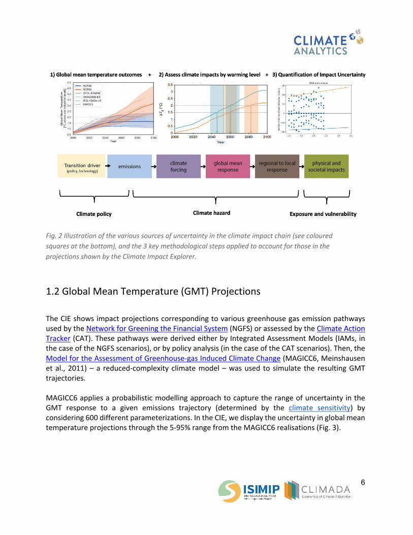
To achieve this, three key steps are applied (Fig. 2):

1. The MAGICC6 simple climate model is used to capture the full global mean temperature

(GMT) uncertainty for different emissions scenarios.

2. Impact projections are assessed for time slices centred around various global warming levels. They are averaged from the simulation results of several scenario experiments,

each conducted with a number of climate and climate impact models, thereby making use of the full information available in the Inter-Sectoral Impact Model Intercomparison

Project (ISIMIP) archive. This allows us to ascribe these projections to the GMT trajectories of different scenarios, including the NGFS scenarios.

3. Uncertainty ranges across the climate model / impact model ensemble from ISIMIP are

derived by quantifying the distribution of the results from the various model combinations

or by applying a quantile regression on those.

6

Fig. 2 Illustration of the various sources of uncertainty in the climate impact chain (see coloured squares at the bottom), and the 3 key methodological steps applied to account for those in the projections shown by the Climate Impact Explorer.

1.2 Global Mean Temperature (GMT) Projections

The CIE shows impact projections corresponding to various greenhouse gas emission pathways

used by the Network for Greening the Financial System (NGFS) or assessed by the Climate Action

Tracker (CAT). These pathways were derived either by Integrated Assessment Models (IAMs, in

the case of the NGFS scenarios), or by policy analysis (in the case of the CAT scenarios). Then, the

Model for the Assessment of Greenhouse-gas Induced Climate Change (MAGICC6, Meinshausen

et al., 2011) – a reduced-complexity climate model – was used to simulate the resulting GMT

trajectories.

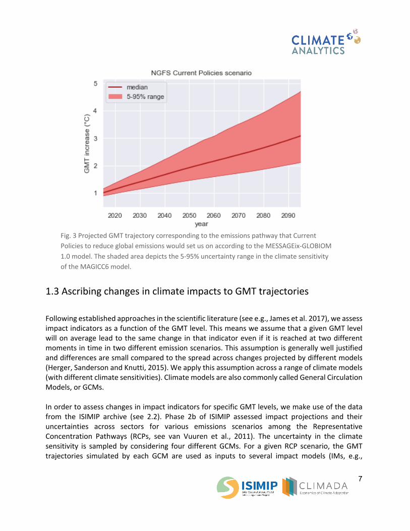
MAGICC6 applies a probabilistic modelling approach to capture the range of uncertainty in the

GMT response to a given emissions trajectory (determined by the climate sensitivity) by

considering 600 different parameterizations. In the CIE, we display the uncertainty in global mean

temperature projections through the 5-95% range from the MAGICC6 realisations (Fig. 3).

7

Fig. 3 Projected GMT trajectory corresponding to the emissions pathway that Current Policies to reduce global emissions would set us on according to the MESSAGEix-GLOBIOM 1.0 model. The shaded area depicts the 5-95% uncertainty range in the climate sensitivity of the MAGICC6 model.

1.3 Ascribing changes in climate impacts to GMT trajectories

Following established approaches in the scientific literature (see e.g., James et al. 2017), we assess

impact indicators as a function of the GMT level. This means we assume that a given GMT level

will on average lead to the same change in that indicator even if it is reached at two different

moments in time in two different emission scenarios. This assumption is generally well justified

and differences are small compared to the spread across changes projected by different models

(Herger, Sanderson and Knutti, 2015). We apply this assumption across a range of climate models

(with different climate sensitivities). Climate models are also commonly called General Circulation

Models, or GCMs.

In order to assess changes in impact indicators for specific GMT levels, we make use of the data

from the ISIMIP archive (see 2.2). Phase 2b of ISIMIP assessed impact projections and their

uncertainties across sectors for various emissions scenarios among the Representative

Concentration Pathways (RCPs, see van Vuuren et al., 2011). The uncertainty in the climate

sensitivity is sampled by considering four different GCMs. For a given RCP scenario, the GMT

trajectories simulated by each GCM are used as inputs to several impact models (IMs, e.g.,

8

hydrological models), in order to sample the uncertainty in the response of impact indicators (see

Fig. 4).

Fig. 4 Schematic representation of the increase in an impact indicator for a given scenario. Two GCMs (represented by the red and blue colours) are used to sample uncertainty in the climate sensitivity. Several IMs are then used to assess uncertainty in the impact response to a given GMT trajectory (visualised by the envelopes constituted by the dashed lines). A similar change in a given impact indicator can be expected for a given GMT level reached at a different moment in time by the two different GCMs. Looking at the median of the impact for the two GCMs gives more confidence on its actual value, while the dispersion across the results of each IM simulation for this GMT indicates the full uncertainty (in the climate and impact response).

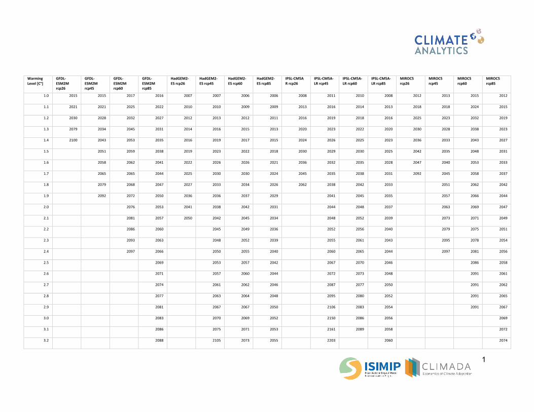
In our case, we have results for several RCP simulation runs (by default RCP2.6 and RCP6.0, as well

as RCP8.5 and RCP4.5 for some indicators). In each GCM simulation corresponding to each RCP

scenario (a scenario-GCM combination), we identify the year for which a certain GMT level is

reached (using a running mean over a 21-year period, see Table 1). We do so for all GMT levels

attained in the available scenario-GCM combinations, starting with 1°C and with a 0.1°C increment

(that is to say: 1°C, 1.1°C, etc.). Under the current rate of warming (~0.2°C per decade), this

increment corresponds to about 5 years of global warming.

1

Warming Level [C°]

GFDL-ESM2M rcp26

GFDL-ESM2M rcp45

GFDL-ESM2M rcp60

GFDL-ESM2M rcp85

HadGEM2-ES rcp26

HadGEM2-ES rcp45

HadGEM2-ES rcp60

HadGEM2-ES rcp85

IPSL-CM5A R rcp26

IPSL-CM5A-LR rcp45

IPSL-CM5A-LR rcp60

IPSL-CM5A-LR rcp85

MIROC5 rcp26

MIROC5 rcp45

MIROC5 rcp60

MIROC5 rcp85

1.0 2015 2015 2017 2016 2007 2007 2006 2006 2008 2011 2010 2008 2012 2013 2015 2012

1.1 2021 2021 2025 2022 2010 2010 2009 2009 2013 2016 2014 2013 2018 2018 2024 2015

1.2 2030 2028 2032 2027 2012 2013 2012 2011 2016 2019 2018 2016 2025 2023 2032 2019

1.3 2079 2034 2045 2031 2014 2016 2015 2013 2020 2023 2022 2020 2030 2028 2038 2023

1.4 2100 2043 2053 2035 2016 2019 2017 2015 2024 2026 2025 2023 2036 2033 2043 2027

1.5

2051 2059 2038 2019 2023 2022 2018 2030 2029 2030 2025 2042 2035 2048 2031

1.6

2058 2062 2041 2022 2026 2026 2021 2036 2032 2035 2028 2047 2040 2053 2033

1.7

2065 2065 2044 2025 2030 2030 2024 2045 2035 2038 2031 2092 2045 2058 2037

1.8

2079 2068 2047 2027 2033 2034 2026 2062 2038 2042 2033

2051 2062 2042

1.9

2092 2072 2050 2036 2036 2037 2029

2041 2045 2035

2057 2066 2044

2.0

2076 2053 2041 2038 2042 2031

2044 2048 2037

2063 2069 2047

2.1

2081 2057 2050 2042 2045 2034

2048 2052 2039

2073 2071 2049

2.2

2086 2060

2045 2049 2036

2052 2056 2040

2079 2075 2051

2.3

2093 2063

2048 2052 2039

2055 2061 2043

2095 2078 2054

2.4

2097 2066

2050 2055 2040

2060 2065 2044

2097 2081 2056

2.5

2069

2053 2057 2042

2067 2070 2046

2086 2058

2.6

2071

2057 2060 2044

2072 2073 2048

2091 2061

2.7

2074

2061 2062 2046

2087 2077 2050

2091 2062

2.8

2077

2063 2064 2048

2095 2080 2052

2091 2065

2.9

2081

2067 2067 2050

2106 2083 2054

2091 2067

3.0

2083

2070 2069 2052

2150 2086 2056

2069

3.1

2086

2075 2071 2053

2161 2089 2058

2072

3.2

2088

2105 2073 2055

2203

2060

2074

2

3.3

2092

2117 2076 2057

2240

2061

2076

3.4

2093

2156 2080 2058

2256

2063

2079

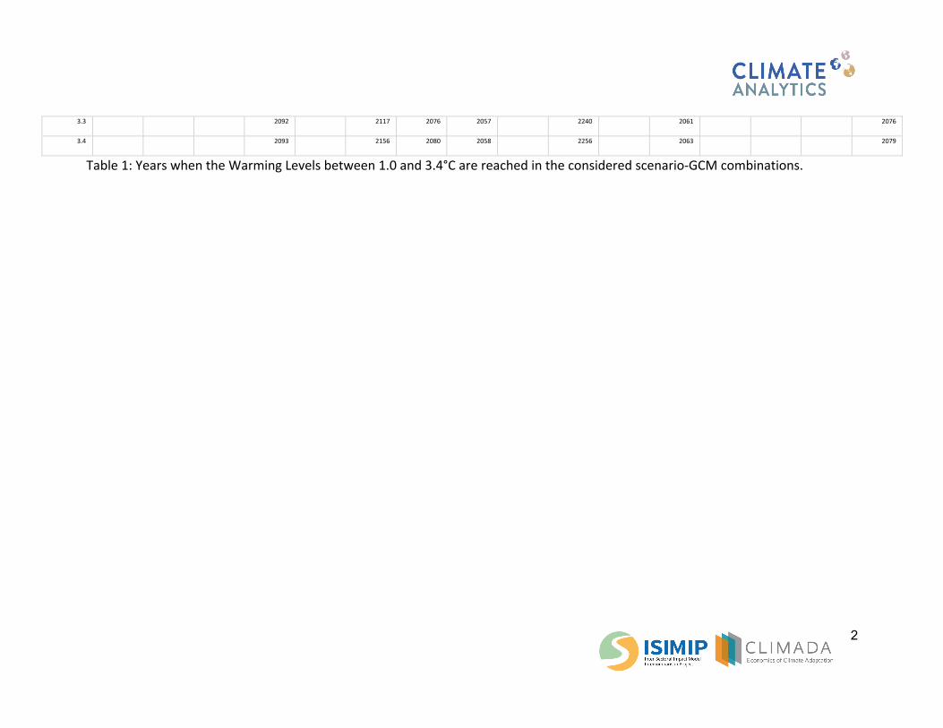
Table 1: Years when the Warming Levels between 1.0 and 3.4°C are reached in the considered scenario-GCM combinations.

1

Projected changes in the indicators shown on the Climate Impact Explorer are always expressed

as absolute or relative differences compared to the values in the 1986-2006 reference period (for

the indicators derived from ISIMIP data, see 2.2) or in the reference year 2020 (for the indicators

derived from CLIMADA data, see 2.3). These changes were simulated in scenario experiments

conducted either by GCMs or IMs (using GCMs outputs as input data). After identifying the year

for which a specific GMT level is reached in a scenario-GCM combination, for each indicator we

average the projected values over the 21-year period centred over that year in the corresponding

GCM or IM scenario experiment. We then average over all available scenarios for each GCM or

GCM-IM combination, before pooling the estimates obtained from all GCMs or GCM-IM

combinations, from which we compute their median values for each GMT level.

With these estimates of changes in impact indicators for each GMT level of interest, we can derive

impact projections for any scenario that reaches these levels. To that end, we identify the points

in time when these specific GMT levels are reached and ascribe to them the change in impact

indicator computed in the previous step.

It is important to note that our confidence in the results decreases for high warming levels (and

particularly beyond 2.5-3°C of global warming), since these levels have been attained in a smaller

number of the RCP experiments due to the differing climate sensitivity of the GCMs that

conducted them.

1.4 Impact projection uncertainty

The uncertainty in impact projections is estimated from the spread in the projections from all

GCMs (for climate indicators) or GCM-IM combinations (for sectoral impact indicators), over the

GMT levels that are attained by all GCMs in the RCP experiments available for the considered

indicator (see 1.3), starting with 1°C of global warming and with an increment of 0.1°C. We

calculate deviations of GCM-IM projections to their ensemble median and apply a quantile

regression to these deviations. As a result, we obtain the relationships between the 5th and 95th

percentiles of impact projections and the global warming levels (Fig. 5). A consistency check is

applied with regard to the regression estimates for the 5th or 95th percentiles. Specifically, issues

can arise when extrapolating linear quantile regressions to high warming levels for which limited

data are available. In case of unrealistic regression outcomes (i.e. crossing of the zero line), we

compute the corresponding percentile (5th or 95th) after having pooled impact projections for all

GMT levels reached by all GCMs in the available RCP experiments, and consider that its difference

to the ensemble median remains constant with global warming.

2

Fig 5. Deviations in area-weighted average annual near surface air temperature from the ensemble median of all GCMs, for each warming level (x-axis). The blue and orange lines

show the quantile regression lines for the 5th and 95th percentiles. Provided that they don’t cross the x-axis between 1° and 5°C, these two lines are used to quantify the

impact uncertainty at each warming level.

1.5 Estimation of the full uncertainty range

The full uncertainty range displayed is the combination of the uncertainty in the GMT response to

a given emission scenario (or climate sensitivity, see 1.2) and in the response of the indicator of

interest to a given GMT trajectory (assessed following the methodology described in 1.4). The 5-

95% uncertainty ranges characterizing each source of uncertainty are then combined to provide

the full uncertainty range. An example is provided in Fig. 6, with the 5-95% MAGICC6 uncertainty

for GMT projections highlighted in green and the 5-95% uncertainty for impact projections in

brown. The combined full uncertainty range is given by the blue markers.

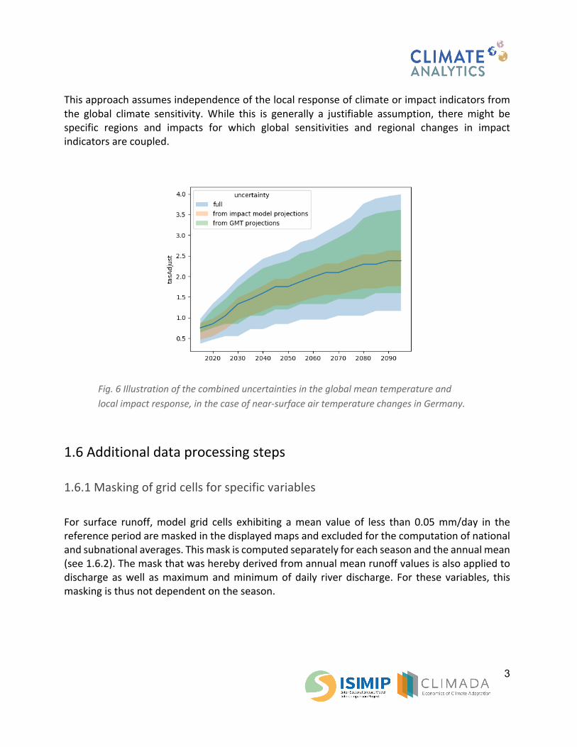
3

This approach assumes independence of the local response of climate or impact indicators from

the global climate sensitivity. While this is generally a justifiable assumption, there might be

specific regions and impacts for which global sensitivities and regional changes in impact

indicators are coupled.

Fig. 6 Illustration of the combined uncertainties in the global mean temperature and local impact response, in the case of near-surface air temperature changes in Germany.

1.6 Additional data processing steps

1.6.1 Masking of grid cells for specific variables

For surface runoff, model grid cells exhibiting a mean value of less than 0.05 mm/day in the

reference period are masked in the displayed maps and excluded for the computation of national

and subnational averages. This mask is computed separately for each season and the annual mean

(see 1.6.2). The mask that was hereby derived from annual mean runoff values is also applied to

discharge as well as maximum and minimum of daily river discharge. For these variables, this

masking is thus not dependent on the season.

4

1.6.2 Temporal averages For most impact indicators, changes in annual mean as well as seasonal mean values were

calculated. The considered seasons were: December-January-February, March-April-May, June-

July-August, and September-October-November.

1.6.3 National or subnational level averages Four different spatial aggregation methods have been used to derive the time series that can be

visualised in the CIE.

For many indicators, the user can choose between three spatial weighted averaging methods: by

area, population or GDP. To derive area-weighted averages, each grid cell is weighted by the

fraction of the land area of the selected territorial unit it covers. For population weighted

averages, each grid cell is weighted by the fraction of the population of the selected territorial unit

located in the grid cell. For grid cells that do not fully lie within a territorial unit, the population of

the grid cell is scaled to the fraction of the grid cell that is covered by this territory. GDP-weighting

is computed in a similar way as for population, but uses information on the repartition of the GDP

across a territorial unit. We use the gridded population and GDP data corresponding to year 2005

provided by ISIMIP, assuming that the repartition of population and GDP within a country will stay

constant in the future. The indicators land fraction or population annually exposed to a certain

category of extreme events (see 2.2) were originally derived by using one of these averaging

methods (area-weighted or population-weighted, respectively), therefore only one corresponding

option can be selected for these indicators.

The indicators quantifying economic damages derived from CLIMADA (see 2.3) were calculated

using a different spatial aggregation method: The locally estimated damages were summed over

the grid cells of interest. Therefore, only the option “sum” can be selected in the drop-down menu

for these indicators.

1.6.4 Smoothing of time series Although the projected changes in impact indicators for a specific GMT level are extracted from

21-year averages for each scenario-GCM or scenario-GCM-IM combination (the full procedure is

detailed in 1.3), they can still be subject to internal climate variability. Before showing them on

the Climate Impact Explorer, we therefore perform an additional smoothing of the calculated time

series by conducting a running average of the projected changes over three consecutive warming

levels (meaning, over a window of a 0.3°C size). This smoothing is applied on the median as well

as the upper and lower bounds of the projected changes.

5

2. Models, scenarios and data sources

2.1 NGFS Scenarios Within the Network for Greening the Financial System (NGFS) project a consortium of

international research institutes has developed a set of climate scenarios to serve as a common

reference framework for central banks and supervisors. The NGFS Climate Scenarios have been

developed to provide a common starting point for analysing climate risks to the economy and

financial system, not only for central banks and supervisors but also for the broader financial and

business sector. Please find more information about the NGFS scenarios here.

The CIE displays physical risks for three of the six NGFS scenarios:

1) Net-Zero 2050 is an ambitious scenario that limits global warming to 1.5°C through stringent climate policies and innovation, reaching net zero CO2 emissions around 2050. This narrative is represents a Paris Agreement compatible scenario.

2) Delayed 2°C assumes annual emissions do not decrease until 2030. Strong policies are then needed to limit warming to below 2°C.

3) Current Policies assumes that only currently implemented policies are preserved, leading to high physical risks at a warming up to 3°C.

2.2 ISIMIP data The Inter-Sectoral Impact Model Intercomparison Project (ISIMIP) is a community-driven initiative

with the aim of offering a consistent climate change impact modelling framework. By early 2021,

more than 100 models had contributed to the initiative. The participating impact models are listed

on the ISIMIP website where a factsheet is provided for each model. To participate, impact

modelling teams agree to run a minimal set of model experiments. These include scenario

experiments which simulate the evolution of sectoral impact variables until at least 2100 under

specific trajectories in terms of climate and socio-economic forcings, for which they are provided

with the corresponding input data. The resulting output data become open access after an

embargo period and can be downloaded from https://data.isimip.org. On the Climate Impact

Explorer, we show input (Table 2) and output data (Table 3 and 4) from phase 2b of ISIMIP

(ISIMIP2b), available at a spatial resolution of 0.5° (equivalent to ~50km at the equator, and

further reducing as one moves poleward). This spatial resolution has to be kept in mind when

interpreting the graphs and maps displayed on the Climate Impact Explorer, especially over small

areas such as small island states.

The ISIMIP2b climate input data were obtained with 4 GCMs from the fifth phase of the Coupled

Model Intercomparison Project (CMIP5). They have been bias-adjusted, meaning that biases

6

between the values simulated by each GCM and those from an observation-based reference

dataset over a common period have been corrected, and that this correction has been applied to

the whole period simulated by the GCMs (assuming that the identified biases stay constant over

time). The reference dataset used for the bias adjustment is EWEMBI (E2OBS, WFDEI and ERA-

Interim data merged and bias-corrected for ISIMIP; see Lange et al., 2019), which covers the 1979-

2005 period. The correction was done independently for each variable, grid cell and month. The

bias adjustment was performed on the regular 0.5° grid from EWEMBI, onto which the CMIP5

GCM data were interpolated (Frieler et al., 2017; Lange, 2018). It is important to note that the

bias-adjustment technique employed for ISIMIP preserves the indicators trends displayed in the

Climate Impact Explorer. More detailed information on the methodology can be found in the

ISIMIP2b bias-correction fact sheet under www.isimip.org/gettingstarted/isimip2b-bias-

correction/.

Unlike the climate indicators, the sectoral impact indicators displayed on the Climate Impact

Explorer did not undergo a bias-adjustment or validation procedure. While such a validation would

be highly desirable, it is generally challenging for sectoral climate impacts on the global level due

to a lack of data both on the biophysical quantities as well as on other human interventions (e.g.

dikes for flood protection, forest management, or groundwater extraction for irrigation).

Although country-level information is provided, it does not mean that the results of each impact

model have been evaluated and validated for each country. Importantly, the Climate Impact

Explorer delivers information on the sole effects of climate change according to the available

indicators derived from ISIMIP, while assuming constant socio-economic conditions (such as

population, GDP, water use, etc.). In reality, socio-economic development will strongly affect

future impacts.

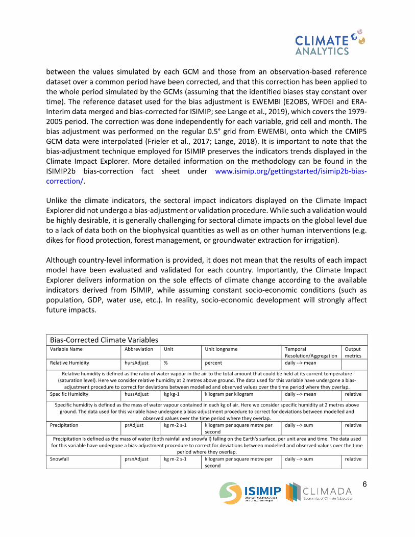
Bias-Corrected Climate Variables

Variable Name Abbreviation Unit Unit longname Temporal

Resolution/Aggregation

Output

metrics

Relative Humidity hursAdjust % percent daily --> mean

Relative humidity is defined as the ratio of water vapour in the air to the total amount that could be held at its current temperature

(saturation level). Here we consider relative humidity at 2 metres above ground. The data used for this variable have undergone a bias-

adjustment procedure to correct for deviations between modelled and observed values over the time period where they overlap.

Specific Humidity hussAdjust kg kg-1 kilogram per kilogram daily --> mean relative

Specific humidity is defined as the mass of water vapour contained in each kg of air. Here we consider specific humidity at 2 metres above

ground. The data used for this variable have undergone a bias-adjustment procedure to correct for deviations between modelled and

observed values over the time period where they overlap.

Precipitation prAdjust kg m-2 s-1 kilogram per square metre per

second

daily --> sum relative

Precipitation is defined as the mass of water (both rainfall and snowfall) falling on the Earth's surface, per unit area and time. The data used

for this variable have undergone a bias-adjustment procedure to correct for deviations between modelled and observed values over the time

period where they overlap.

Snowfall prsnAdjust kg m-2 s-1 kilogram per square metre per

second

daily --> sum relative

7

Snowfall is defined as the mass of water falling on the Earth's surface in the form of snow, per unit area and time. The data used for this

variable have undergone a bias-adjustment procedure to correct for deviations between modelled and observed values over the time period

where they overlap.

Atmospheric Pressure

(surface)

psAdjust Pa Pascal daily --> mean absolute

Atmospheric pressure quantifies the force exerted by the weight of the column of air situated above a given location, per unit area. Here we

consider atmospheric pressure at 2 metres above ground. The data used for this variable have undergone a bias-adjustment procedure to

correct for deviations between modelled and observed values over the time period where they overlap.

Atmospheric pressure

(adjusted to sea level)

pslAdjust Pa Pascal daily --> mean absolute

Atmospheric pressure quantifies the force that would be exerted by the weight of the column of air situated above a given location, per unit

area. Since atmospheric pressure decreases with altitude, here we inspect the atmospheric pressure at 2 metres above ground but adjusted

as if the location of interest was set at sea level. This allows comparison of locations situated at different altitudes. The data used for this

variable have undergone a bias-adjustment procedure to correct for deviations between modelled and observed values over the time period

where they overlap.

Downwelling Longwave

Radiation

rldsAdjust W m-2 Watt per square metre daily --> mean relative

Downwelling longwave radiation is defined as the downward energy flux in the form of infrared light that reaches the Earth's surface. The

data used for this variable have undergone a bias-adjustment procedure to correct for deviations between modelled and observed values

over the time period where they overlap.

Wind Speed sfcWindAdjust m s-1 metre per second daily --> mean relative

Wind speed quantifies the velocity of an air mass. Here we consider the wind speed 10 metres above ground. The data used for this variable

have undergone a bias-adjustment procedure to correct for deviations between modelled and observed values over the time period where

they overlap.

Air Temperature tasAdjust °C degrees Celsius daily --> mean absolute

Air temperature refers to the temperature of air masses near the Earth's surface (2 metres above the ground in this case). The data used for

this variable have undergone a bias-adjustment procedure to correct for deviations between modelled and observed values over the time

period where they overlap.

Daily Maximum Air

Temperature

tasmaxAdjust °C degrees Celsius daily --> mean absolute

Daily maximum air temperature is defined as the peak air temperature reached in a day, in this case at 2 metres above the ground. The data

used for this variable have undergone a bias-adjustment procedure to correct for deviations between modelled and observed values over the

time period where they overlap.

Daily Minimum Air

Temperature

tasminAdjust °C degrees Celsius daily --> mean absolute

Daily minimum air temperature is defined as the lowest air temperature reached in a day, in this case at 2 metres above the ground. The data

used for this variable have undergone a bias-adjustment procedure to correct for deviations between modelled and observed values over the

time period where they overlap.

Table 2: Bias-corrected climate variables used as input for ISIMIP

ISIMIP Primary Output Variables

Snow Depth snd m metre monthly -->

mean

relative

Snow depth is defined as the thickness of the snow layer covering the ground. [5 impact models]

Surface Runoff qs kg m-2 s-1 kilogram per square metre per

second

monthly -->

mean

relative

Surface runoff (also called overland flow) describes the flow of water occurring on the Earth's surface when excess water, e.g. rainwater, can no

longer be absorbed by the soil. [12 impact models]

River Discharge dis m3 s-1 cubic metres per second daily --> mean relative

Discharge (also called streamflow) is the volume of water flowing through a river or stream channel. [15 impact models]

Maximum of Daily River

Discharge

maxdis m3 s-1 cubic metres per second monthly --> max relative

Maximum of daily discharge is defined as the peak volume of water flowing through a river or stream channel in a day. [2 impact models]

8

Minimum of Daily River

Discharge

mindis m3 s-1 cubic meters per second monthly --> min relative

Minimum of daily discharge is defined as the lowest volume of water flowing through a river or stream channel in a day. [2 impact models]

Soil Moisture soilmoist kg m-2 kilogram per square metre monthly -->

mean

relative

Total soil moisture content quantifies water stored in soil, per unit area. Here we consider soil moisture contained within the root zone, i.e. until a

depth of approximately 1 metre. [15 impact models]

Maize Yields yield_maize t ha-1 (dry

matter)

tons of dry matter per hectare per growing

season

relative

Maize yields were calculated by assuming that the cultivated areas of both rainfed and irrigated maize will remain constant through the 21st century.

Their projected changes hence only reflect the future evolution of climate, and not that of agricultural management practices. [4 impact models]

Rice Yields yield_rice t ha-1 (dry

matter)


season

relative

Rice yields were calculated by assuming that cultivated areas of both rainfed and irrigated rice will remain constant through the 21st century. Their

projected changes hence only reflect the future evolution of climate, and not that of agricultural management practices. [4 impact models]

Soy Yields yield_soy t ha-1 (dry

matter)


season

relative

Soy yields were calculated by assuming that the cultivated areas of both rainfed and irrigated soy will remain constant through the 21st century.

Their projected changes hence only reflect the future evolution of climate, and not that of agricultural management practices. [4 impact models]

Wheat Yields yield_wheat t ha-1 (dry

matter)


season

relative

Wheat yields were calculated by assuming that the cultivated areas of both rainfed and irrigated wheat will remain constant through the 21st

century. Their projected changes hence only reflect the future evolution of climate, and not that of agricultural management practices. [4 impact

models]

Table 3: ISIMIP Primary Output Variables

ISIMIP Secondary Output Variables

Land fraction annually exposed to

River Floods

fldfrc % percent yearly

Land fraction annually exposed to river floods is defined as the land area fraction which is flooded during the annual maximum event. A flood

is considered to occur in a specific location if annual maximum discharge exceeds the local protection standard from the FLOPROS database.

River flood depth flddph m metre yearly relative

River flood depth is defined as the flood depth during the most severe flood of the year. A flood is considered to occur in a specific location

only if annual maximum discharge exceeds the local protection standard from the FLOPROS database.


Crop Failures

lec % percent yearly

Land fraction annually exposed to crop failures is defined as the fraction of a grid cell, of 0.5° resolution, in which one of the four considered

crops (maize, wheat, soybean, and rice) is grown, and where its annual yield falls short of the 2.5th percentile of the pre-industrial reference

distribution (i.e., an exceptionally low yield that would occur on average only 2-3 years per century in the absence of climate change). All crop-

specific land area fractions exposed are added together.

Population annually exposed to Crop

Failures

pec % percent yearly relative

Population annually exposed to crop failures is defined as the fraction of the labour force working in agriculture multiplied by the land area

exposed to crop failures, and divided by the grid cell area fraction used for agriculture. Land area exposed to crop failures is defined as the

fraction of a grid cell, of 0.5° resolution, in which one of the four considered crops (maize, wheat, soybean, and rice) is grown, and where its

annual yield falls short of the 2.5th percentile of the pre-industrial reference distribution (i.e., an exceptionally low yield that would occur on

average only 2-3 years per century in the absence of climate change). All crop-specific land area fractions exposed are added together.


Wildfires

lew % percent yearly

9

Land fraction annually exposed to wildfires describes the annual aggregate of land area burnt at least once a year by wildfires.

Population annually exposed to

Wildfires

pew % percent yearly relative

Population annually exposed to wildfires describes the annual aggregate of land area, within a grid cell of 0.5° resolution, burnt at least once a

year by wildfires, multiplied by the total population of that grid cell.


Heatwaves

leh % percent yearly

Land fraction annually exposed to heatwaves, in a grid cell of 0.5° resolution, equals the total area of that grid cell every year it is struck by a

heatwave, and zero otherwise. It thus reflects the frequency at which this grid cell is struck by heatwaves. In this context, a heatwave is

considered to occur when both a relative indicator based on air temperature and an absolute indicator based on the air temperature and

relative humidity exceed exceptionally high values.

Population annually exposed to

Heatwaves

peh % percent yearly relative

Population annually exposed to heatwaves, in a grid cell of 0.5° resolution, equals the total population of that grid cell every year it is struck by

a heatwave, and zero otherwise. It thus reflects the part of this population which experiences a heatwave on average every year. A heatwave

is here considered to occur when both a relative indicator based on air temperature and an absolute indicator based on air temperature and

relative humidity exceed exceptionally high values.

Labour Productivity due to Heat

Stress

ec1 % percent yearly absolute

Heat stress impact on labour productivity indicates the percentage decrease in labour productivity under hot and humid climate conditions

due to the reduced capacity of the human body to perform physical labour. The analysis is building on previous work by Gosling et al. (2018)

and further extended.

Table 4: ISIMIP Secondary Output Variables

2.3 CLIMADA

2.3.1. CLIMADA Model

CLIMADA, an open-source catastrophe risk modelling framework, is used to estimate the damages

from extreme events by modelling their likelihood of occurring and the hazard associated with

them. The expected damage to physical assets exposed to these events is calculated using

vulnerability functions which quantify the relationship between the amount of damage to an asset

and the intensity of the hazard. This mapping of hazard to damage is applied to all exposed assets

and allows an estimate of the total loss from physical damages to be calculated for each extreme

event.

CLIMADA is used to calculate direct losses from extreme events under current climate and climate

change conditions by considering the change in frequency and severity of extreme events

associated with various climate scenarios. The CIE displays changes in direct losses arising from

climate change relative to today’s baseline.

The exposure estimate for the damage calculation corresponds to the method previously applied

in Sauer et al. (2021). Gridded Gross Domestic Product (GDP) data for the year 2005 from the

ISIMIP project are used as a proxy for the distribution of assets. They have a spatial resolution of

5 arcmin and are reported in purchasing power parity (PPP) in 2005 USD. The data were obtained

using a downscaling methodology in combination with spatially-explicit population distributions

10

from the History Database of the Global Environment (HYDEv3.2), and national GDP estimates. To

provide a suitable asset indicator estimate gridded, the GDP data are translated into gridded

capital stock, using annual national data on capital stock (in PPP 2005 USD) and GDP from the

PennWorld Table (version 9.1, https://www.rug.nl/ggdc/productivity/pwt/). For each country the

annual ratio of national GDP and capital stock was calculated and smoothed with a 10-year

running mean to generate a conversion factor, which was then applied to translate exposed GDP

into asset values for the year 2005. The final exposure dataset is the global distribution of capital

stock on a 150 arcsec resolution (which equals a ~4.5km x ~4.5km at the equator) corresponding

to the year 2005.

2.3.2. River Flood We first derive spatially explicit global maps of flooded areas and flood depth (at a resolution of

150 arcsec) from the harmonized multi-model simulations of the global gridded global

hydrological models (GHMs) participating in ISIMIP2b for the scenarios RCP 2.6, RCP 6.0 and RCP

8.5. These GHMs were driven by the climate forcing data obtained with 4 GCMs.

We then assume constant socio-economic conditions from 2005 onwards regarding e.g.,

urbanisation patterns, river engineering and water withdrawal. For this ensemble of GCM/GHM

combinations, we follow the methodology applied previously in Willner et al. 2018, and first

harmonize the output of the different GHMs with respect to their fluvial network using the fluvial

routing model CaMa-Flood (version 3.6.2) yielding daily fluvial discharge at 15arcmin

(~25 km × 25 km) resolution. For the global annual flood maps, we select the annual maximum

daily discharge for each grid cell. For each simulation (GCM/GHM combination) of daily fluvial

discharge and each grid cell on 15arcmin resolution, we fit a generalized extreme value

distribution to the historical time series of the annual maximum discharge using L-moment

estimators of the distribution parameters allowing for a model bias correction, following the

approach by Hirabayashi et al. We map the return period of each event to the corresponding flood

depth in a MATSIRO model run driven by observed climate forcings, in bins of 1-year (1 to 100)

and 10-year (100 to 1000) return periods (linearly interpolated), providing flood depth at 15arcmin

resolution. Results from this observation-driven MATSIRO output have been shown to be

consistent with observation-based data. For this mapping, we also respect a threshold given as

current flood protection at the subnational scale. This has recently been compiled in a global

database (FLOPROS database) representing the currently best global-scale knowledge in the

maximum return period of flood that each country/region can prevent. In this work, we use the

“Merged layer” of this database, which combines empirical data about existing protection

infrastructure (“Design layer”), data on protection standards and requirements set by policy

measures (“Policy layer”), and model output from an observed relationship between gross

domestic product per capita and flood protection (“Model layer”). This threshold procedure

implies that, when the protection level is exceeded, the flood occurs as if there was no initial

protection; below the threshold no flooding takes place. For the final assessment, we re-aggregate

11

the high-resolution flood depth data from 0.3’ to a 2.5’ resolution (~5 km × 5 km) by retaining the

maximum flood depth as well as the flooded area fraction, defined as the fraction of all underlying

high-resolution grid cells where the flood depth was greater than zero.

The damage assessment is similar to the method previously applied in Sauer et al. (2021). To

derive a local damage from the annual flood map and exposure data we apply the continent-level

residential flood depth-damage functions developed by Huizinga et al. (2017). The quantification

of flood damages includes the following three steps:

1) determine exposed assets on the grid-level (150 arcmin) based on the flooded fraction

obtained from the river flood model

2) determine the grid level damage by multiplying the exposed assets by the flood fraction

and the flood-depth damage function

3) aggregate over all grid cells to the estimated damages on the country level

2.3.3. Tropical Cyclone The tropical cyclone modelling consists of two steps: first, generating a probabilistic track set

from historical tracks, and second, computing the wind fields at centroid points and performing

the climate change scaling. Both steps are conducted with the open-source probabilistic natural

catastrophe damage framework CLIMADA (Aznar-Siguan et al., 2019).

All historical tracks available in the IBTrACS dataset (downloaded on 18.01.2021,

https://www.ncdc.noaa.gov/ibtracs/index.php?name=ib-v4-access) for the years 1950 - 2020

are considered. For the wind field calculations, tracks are required to have both pressure and

wind speed information at all time steps. Some corrections are applied to racks with unreported

values: `environmental_pressure` is enforced to be larger than `central_pressure`, all wind

speeds are linearly rescaled to 1-minute sustained winds, temporal reporting gaps within a

variable (pressure, windspeed, or radius) are interpolated linearly if possible. Tracks which have

missing values after the application of the corrections are discarded. Afterwards, the reporting

of all variables is homogenized to one point per hour for all tracks by linear interpolation. Then,

a set of probabilistic tracks (9 per historical track, 56480 total) is generated with a random track

perturbation algorithm with parameters fine-tuned per basin (Aznar-Siguan et al., 2021). It is

also possible to use other track sets in CLIMADA which are generated with different methods.

The wind fields are computed from the tracks using the Holland (2008) model to obtain the

maximum wind speed value at each centroid point. The centroids (latitude/longitude

coordinates) are defined on the same grid as the exposures (150 arcsec resolution) on land. The

wind field computation is restricted to centroids between -71° and +61° latitude, and wind

speeds below 17.5m/s are set to 0. For future climate, the storms’ frequency and intensity are

scaled by basin with factors based on the factors reported in Table 2 of Knutson et al. (2010).

The values from Knutson et al. are assumed to describe changes in hazard intensity and

frequency between 2000 and 2100 according to the scenario RCP 4.5. Because of the

approximation of per category scaling from cumulative category scaling, the changes in some

12

basins, especially the East Pacific are overestimated but the effect of this error is small.

Furthermore, linear interpolation with respect to global temperatures, a simplified

approximation, is applied for scaling the considered scenarios RCP 2.6 and RCP 6.0 in the years

2020 to 2100 (Aznar-Siguan et al. 2021).

Socio-economic development is the driving factor for changes in direct losses, while the

magnitude of the uncertainty from hazard modelling is small in comparison to the uncertainty of

socio-economic development, e.g., assumption on GDP and population growth.

The damage modelling is analogous to the one reported in Aznar-Siguan et al. (2019). At each

exposure point, the damage is computed from the maximum sustained 1-min wind speed value

at the corresponding centroid point (same grid) using regionally calibrated vulnerability curves

(Eberenz et al. 2021). The damage per country is the aggregated sum over all centroids

contained in the country for both the average annual impact and the 1/100 years impact. The

reported standard deviation describes the spread of the aggregated data and corresponds to

aleatoric (intrinsic natural uncertainty) uncertainty arising from the probabilistic storm set.

The version used was CLIMADA 2.1.1 (Aznar-Siguan, 2021) and the code is publicly available on

github: https://github.com/CLIMADA-project/climada_python. Detailed information on the

application of the flood damage and the tropical cyclone modeling can be found at:

https://climada-python.readthedocs.io/en/stable/tutorial/climada_hazard_RiverFlood.html

https://climada-python.readthedocs.io/en/stable/tutorial/climada_hazard_TropCyclone.html

For more information on CLIMADA, please refer to Prof. Dr. David N. Bresch, Institute for

Environmental Decisions, ETH Zurich, Switzerland, www.wcr.ethz.ch or Dr. Chahan

Kropf, Institute for Environmental Decisions, ETH Zurich, Switzerland, www.wcr.ethz.ch

Note: While the variables land fraction annually exposed to river floods, river flood depth, river flood damages, and tropical cyclone damages are available on a higher resolution as the ISIMIP output (2.1), for technical reasons maps for bigger countries are displayed in a lower distribution (0.5° instead of 150arcsec). Those countries are Argentina, Antarctica, Australia, Brazil, Canada, China, Greenland, India, Indonesia, Kazakhstan, Russia, and the United States.

3. Visualisation

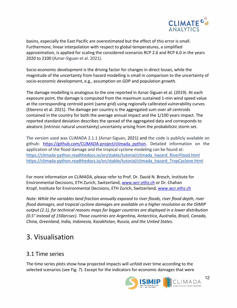
3.1 Time series The time series plots show how projected impacts will unfold over time according to the

selected scenarios (see Fig. 7). Except for the indicators for economic damages that were

13

derived from CLIMADA, which are summed over the territorial units of interest, the gridded data

are averaged over the selected continent, country or province by weighting the projected

changes in the selected indicator by either the area of each grid cell that lies within it, or by the

population or GDP that lives or is located within these grid cells (see 1.6). For some indicators,

seasonal averages can be displayed in addition to annually averaged impacts (see 1.6.2).

The units in which changes in the selected indicators are expressed are displayed next to the y-

axis. The thick coloured line represents the median changes over all models, while the shaded

area around it shows the 5-95% uncertainty range in impact projections for each year (see 1.5

for more details).

A compare function allows the display of two different scenarios in the same figure.

Please note: We do not show time series plots for country-indicator or region-indicator combinations for which either the median projected changes or the upper or lower bound of the full uncertainty range exceeds +1000% or -1000%. Such extreme ranges hint at challenges with the underlying dataset and are thus excluded from our presentation of results.

Fig. 7 Example of a time series plot: Comparison of two scenarios

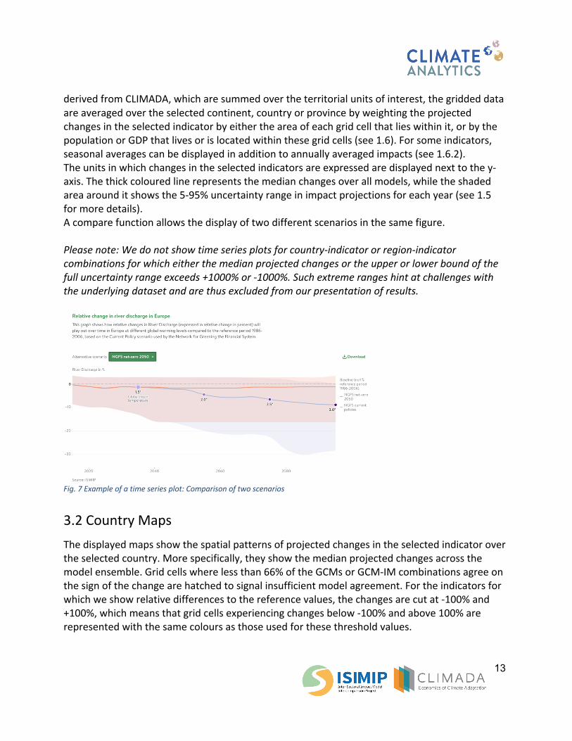
3.2 Country Maps The displayed maps show the spatial patterns of projected changes in the selected indicator over

the selected country. More specifically, they show the median projected changes across the

model ensemble. Grid cells where less than 66% of the GCMs or GCM-IM combinations agree on

the sign of the change are hatched to signal insufficient model agreement. For the indicators for

which we show relative differences to the reference values, the changes are cut at -100% and

+100%, which means that grid cells experiencing changes below -100% and above 100% are

represented with the same colours as those used for these threshold values.

14

The CIE allows users to compare country maps for different scenarios, years or warming levels

(see Fig. 8). Two different maps can be selected and then displayed side by side, with an

additional map on the right highlighting the differences between both selections.

Fig. 8. Example of a comparison of two Maps: projected impacts for two different scenarios

15

4. References Aznar-Siguan, G. and Bresch, D. N. (2019) CLIMADA v1: a global weather and climate risk assessment platform. Geoscientific Model Development 12, 3085–3097, https://doi.org/10.5194/gmd-12-3085-2019

Aznar-Siguan, G., Eberenz, S., Steinmann, C., Vogt, T., Roosli, T., Sauer, I., … Zhu, Q (2021) CLIMADA-project/climada_python_ v2.1.1 (Version v2.1.1.). Zenodo, http://doi.org/10.5281/zenodo.4699962 Dasgupta, S.; et al. (forthcoming) Impacts of climate change on combined labour productivity and supply. Eberenz, S. et al. (2021) Regional tropical cyclone impact functions for globally consistent risk assessments, Nat. Hazards Earth Syst. Sci., 21, 393–415, https://doi.org/10.5194/nhess-21-393-2021.

Frieler, K., Lange, S., Piontek, F., Reyer, C. P. O., Schewe, J., Warszawski, L., Zhao, F., Chini, L., Denvil, S., Emanuel, K., Geiger, T., Halladay, K., Hurtt, G., Mengel, M., Murakami, D., Ostberg, S., Popp, A., Riva, R., Stevanovic, M., … Yamagata, Y. (2017) Assessing the impacts of 1.5 °C global warming – simulation protocol of the Inter-Sectoral Impact Model Intercomparison Project (ISIMIP2b). Geosci. Model Dev., 10(12), 4321–4345. https://doi.org/10.5194/gmd-10-4321-2017

Gosling S. N., Zaherpour, J. and Ibarreta, D. (2018) PESETA III: Climate change impacts on labour productivity, EUR 29423 EN, Publications Office of the European Union, Luxembourg, 2018, ISBN 978-92-79- 96912-6, doi:10.2760/07911, JRC113740.

Herger, N., B. M. Sanderson, and Knutti, R. (2015) Improved pattern scaling approaches for the use in climate impact studies, Geophys. Res. Lett., 42, doi:10.1002/2015GL063569. Hirabayashi, Y. et al. (2013) Global flood risk under climate change. Nat. Clim. Change 3, 816–821 https://doi.org/10.1038/nclimate1911

Holland, G. (2008) A Revised Hurricane Pressure–Wind Model. Monthly Weather Review 136, no. 9: 3432–45. https://doi.org/10.1175/2008MWR2395.1 James, R., Washington, R., Schleussner, C.-F., Rogelj, J. and Conway, D. Characterizing half-a-degree difference: a review of methods for identifying regional climate responses to global warming targets. Wiley Interdiscip. Rev. Clim. Chang. e457 (2017). doi:10.1002/wcc.457 Klein Goldewijk, K., Beusen, A., van Drecht, G and de Vos, M (2011) The HYDE 3.1 spatially explicit database of human-induced global land-use change over the past 12,000 years. Glob. Ecol. Biogeogr. 20, 73–86 https://doi.org/10.1111/j.1466-8238.2010.00587.x Klein Goldewijk, K., Beusen, A., Doelman, J. and Stehfest, E. (2017) Anthropogenic land use estimates for the Holocene – HYDE 3.2. Earth Syst. Sci. Data 9, 927–953, https://doi.org/10.5194/essd-9-927-2017

16

Knutson, T., Sirutis, J., Zhao, M., Tuleya, R., Bender, M., Vecchi, G., Villarini, G, and Chavas, D. (2015) Global Projections of Intense Tropical Cyclone Activity for the Late Twenty-First Century from Dynamical Downscaling of CMIP5/RCP4.5 Scenarios. Journal of Climate. 28. 150729114230005. Doi/10.1175/JCLI-D-15-0129.1. Lange, S. (2018) Bias correction of surface downwelling longwave and shortwave radiation for the EWEMBI dataset, Earth Syst. Dynamics, 9, 627–645, https://doi.org/10.5194/esd-9-627-2018 Lange, S. (2019) EartH2Observe, WFDEI and ERA-Interim data Merged and Bias-corrected for ISIMIP (EWEMBI), https://doi.org/10.5880/pik.2019.004 Lange, S., Volkholz, J., Geiger, T., Zhao, F., Vega, I., Veldkamp, T., et al. (2020) Projecting exposure to extreme climate impact events across six event categories and three spatial scales. Earth's Future, 8, e2020EF001616. https://doi.org/10.1029/2020EF001616 Meinshausen, M., Raper, S. C. B., and Wigley, T. M. L. (2011) Emulating coupled atmosphere-ocean and carbon cycle models with a simpler model, MAGICC6 – Part 1: Model description and calibration. Atmos. Chem. Phys., 11(4), 1417–1456. https://doi.org/10.5194/acp-11-1417-2011 Murakami D. and Yamagata Y. (2019) Estimation of Gridded Population and GDP Scenarios with Spatially Explicit Statistical Downscaling. Sustainability.; 11(7):2106. https://doi.org/10.3390/su11072106 Sauer, I.J., Reese, R., Otto, C. et al. (2021) Climate signals in river flood damages emerge under sound regional disaggregation. Nat Commun 12, 2128. https://doi.org/10.1038/s41467-021-22153-9 Scussolini, P. et al. (2016) FLOPROS: an evolving global database of flood protection standards. Nat. Hazards Earth Syst. Sci.16, 1049–106, https://doi.org/10.5194/nhess-16-1049-2016

van Vuuren, D.P., Edmonds, J., Kainuma, M. et al. (2011) The representative concentration pathways: an overview. Climatic Change 109, 5. https://doi.org/10.1007/s10584-011-0148-z Willner, S. N., Levermann, A., Zhao, F. and Frieler, K. (2018) Adaptation required to preserve future high-end river flood risk at present levels. Sci. Adv. 4, eaao1914, DOI: 10.1126/sciadv.aao1914

Willner, S. N., Otto, C. and Levermann, A. (2018) Global economic response to river floods. Nat. Clim. Change 8, 594–598, https://doi.org/10.1038/s41558-018-0173-2

Yamazaki, D., Kanae, S., Kim, H. and Oki, T. (2011) A physically based description of floodplain inundation dynamics in a global river routing model. Water Resour. Res. 47. https://doi.org/10.1029/2010WR009726

Documents

Technical Documentation Climate Impact Explorer