TECHNICAL LIBRARY, - LIBRARY, - AD TECHNICAL MEMORANDUM NO. 110 METHODS FOR APPLYING A TRACKING SIGNAL TO MONITOR SINGLE EXPONENTIAL SMOOTHING FORECASTS MICHAEL R. CHERNICK AUGUST

TECHNICAL LIBRARY, -

AD

TECHNICAL MEMORANDUM NO. 110

METHODS FOR APPLYING A TRACKING SIGNAL TO

MONITOR SINGLE EXPONENTIAL SMOOTHING FORECASTS

MICHAEL R. CHERNICK

AUGUST 1972

Approved for public release; distribution unlimited.

U.S. ARMY MATERIEL SYSTEMS ANALYSIS AGENCY Aberdeen Proving Ground, Maryland

DISPOSITION

Destroy this report when no longer needed. Do not return it to the originator.

DISCLAIMER

The findings in this report are not to be construed as an official Department of the Army position.

WARNING

Information and data contained in this document are based on the input available at the time of preparation. The results may be subject to change and should not be construed as representing the AMC position unless so specified.


METHODS FOR APPLYING A TRACKING SIGNAL TO MONITOR SINGLE EXPONENTIAL SMOOTHING FORECASTS

Michael R. Chernick

August 1972

Approved for public release; distribution unlimited.

RDT&E Project No. IP765801 MM I 102

U.S. ARMY MATERIEL SYSTEMS ANALYSIS AGENCY

ABERDEEN PROVING GROUND, MARYLAND

U.S. ARMY MATERIEL SYSTEMS ANALYSIS AGENCY


MRChernick/sjj Aberdeen Proving Ground, Md August 1972


ABSTRACT

The tracking signal developed by Trigg which has gained wide

acceptance is useful for monitoring single exponential smoothing fore-

casts. If forecasts become biased, the tracking signal will increase

in absolute value indicating the possible need to change the smoothing

constant which is the one adjustable parameter in single exponential

smooth i ng.

Two methods of applying the tracking signal to monitor

exponential smoothing forecasts are discussed in this document. The

method which was applied to depot workload forecasts is described in

detail and the tables of confidence limits which are necessary to

apply this method are given.

FOREWORD

Single exponential smoothing is a technique used for determining

a forecast based on historical data. Given the historical data, the forecast is uniquely determined on the basis of one parameter known as the smoothing constant. In order to maintain as accurate a forecast as possible on the basis of this technique it is important to find the best value for the smoothing constant. Since the historical pattern can change with time or because there is not sufficient data to adequately develop the optimal smoothing constant, this constant should be revised periodically. The tracking signal is a statistic developed by D. W. Trigg (Reference I) which indicates when a change in the smoothing constant might be necessary.

Confidence limits for the tracking signal were determined by M. Batty (Reference 2). These limits are useful when 50 or more periods of historical data are available for the computation of the tracking signal. However, in many practical situations as few as 10 periods of historical data are available. In such situations the distribution of the tracking signal is significantly different.

The objective of this report is to illustrate how the tracking signal can be used to monitor exponential smoothing forecasts and to determine confidence limits when only 10 to 20 periods of data are available. One who applies the exponential smoothing procedure to his forecast can use these tables to decide whether to revise the smoothing constant. When the absolute value of the tracking signal exceeds the confidence limit the smoothing constant should be revised.

Trigg, D. W.; Monitoring a Forecasting System, Op I Res 015, 271-274, (1964).

2 Batty, M.; Monitoring an Exponential Smoothing Forecasting System, Op Res 020, No. 3, 319-325, (1969).

CONTENTS

Page

ABSTRACT 3

FOREWORD 4

1. THE NEED FOR A TRACKING SIGNAL IN EXPONENTIAL SMOOTHING FORECASTS 7

2. DEFINITION AND ELEMENTARY PROPERTIES OF THE TRACKING SIGNAL. . 7

3. TECHNIQUES FOR IMPROVING SMOOTHING FORECASTS BY USE OF THE TRACKING SIGNAL 8

3.1 Adaptive Smoothing 8 3.2 Monitoring Exponential Smoothing Forecasts Using

Confidence Limits for the Tracking Signal 9

LITERATURE CITED 13

APPENDIX - 90 PERCENT CONFIDENCE LIMITS 15

DISTRIBUTION LIST 17

Next page is blank.


I. THE NEED FOR A TRACKING SIGNAL IN EXPONENTIAL SMOOTHING FORECASTS

Single exponential smoothing is a forecasting technique that is useful when the historical data have no trend. In this case, the data are assumed to be relatively constant with random errors causing fluctuations. Based on the historical data an estimate of the assumed constant is determined and used for the next forecast period, t. When additional data become available the estimate is revised for the forecast period t + I.

The smoothing constant is the one parameter in single exponential smoothing which can be adjusted. A method for optimizing the smoothing constant and its application to a depot supply workload problem is given in Reference 3.

Because historical patterns change, the smoothing constant that works best during a given period may not continue to be the best in the future and thus, it may be necessary to revise it. Also, in some practical problems the limited amount of historical data available is not sufficient to adequately determine the optimal smoothing constant. In such situations, it would also be desirable to monitor the forecasts to determine when to revise the smoothing constant.

The tracking signal provides a method for monitoring the forecast. Two applications for adjusting the forecast by use of the tracking signal are presented in Section 3.

2. DEFINITION AND ELEMENTARY PROPERTIES OF THE TRACKING SIGNAL

Let A = the smoothing constant,

S. = data for period, t,

S. - = the forecast made for period, t, and

E = S - S Et 3t-l t

e. represents the error between the forecast and actual for

period, t. The smoothing forecast for period, t + I is obtained from the following formula:

Chernick, M. R.; Use of Exponential Smoothing to Forecast Depot Supply Workloads. SM&RSO Interim Note No. I, (1971), U.S. Army Materiel Systems Analysis Agency, Aberdeen Provinq Ground, Maryland.

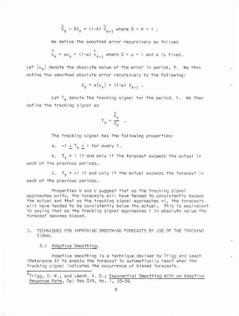
S+ = AS+ + (I-A) S where 0 < A < I .

We define the smoothed error recursively as follows

% % e. = ote. + (l-ot) e. . where 0 < a < I and a is fixed. T T t-l

Let |e,| denote the absolute value of the error in period, t. We then

define the smoothed absolute error recursively by the following:

6+ = o|e,| + (I-a) 5. . .

Let T, denote the tracking signal for the period, t. We then

define the tracking signal as

T .!! t «t

The tracking signal has the following properties:

a. -I <_ T. <_ I for every t.

b. T_= I if and only if the forecast exceeds the actual in

each of the previous periods.

c. T. = -1 if and only if the actual exceeds the forecast in

each of the previous periods.

Properties b and c suggest that as the tracking signal approaches unity, the forecasts will have tended to consistently exceed the actual and that as the tracking signal approaches -I, the forecasts will have tended to be consistently below the actual. This is equivalent to saying that as the tracking signal approaches I in absolute value the forecast becomes biased.

3. TECHNIQUES FOR IMPROVING SMOOTHING FORECASTS BY USE OF THE TRACKING SIGNAL

3.I Adaptive Smoothing.

Adaptive smoothing is a technique devised by Trigg and Leach (Reference 4) to enable the forecast to automatically react when the tracking signal indicates the occurrence of biased forecasts.

4 Trigg, D. W., and Leach, A. G.; Exponential Smoothing With an Adaptive Response Rate, Op I Res QI8, No. I, 53-59.

8

When the smoothing constant A Is small and a sudden change (either a rapid increase or decrease) occurs in the data, one obvious way to react would be to increase the smoothing constant. This would enable the forecast to home in on the new situation more quickly. Once the forecast has adjusted to the new situation, it may be desirable to lower the smoothing constant again. It may be that the pattern becomes stable in the new situation and if this is the case the high smoothing constant may then be causing too much reaction to the random noise.

To achieve these types of reaction Trigg and Leach thought of a very simple method; namely, to set the smoothing constant equal to the absolute value of the tracking signal. This method is called adaptive smoothing. This means that the smoothing constant will be continually changing from forecast to forecast according to the way the tracking signal is changing. As the absolute value of the tracking signal approaches unity, the smoothing constant increases toward one and thus the forecast reacts more quickly to the change. After the reaction takes place the errors should return to being unbiased and hence the tracking signal should decrease in absolute value. This would then produce the desired decrease in the smoothing constant.

A modification to this procedure would be to let the smoothing constant be equal to k times the absolute value of the tracking signal where 0 < k <_ I. This would produce the same effect and be less restrictive. Trigg's method would correspond to k = I.

The adaptive smoothing technique allows for an automated response to changes and thus would be desirable and easy to apply when forecasts are handled by computer for a large number of items. On the other hand in some situations it may be better for the individuals involved in preparing the forecast to be made more aware of the changes that are occurring. The tracking signal can also be used to alert the forecaster of changes and allow him to decide on the response. One such method is described in Section 3.2.

3.2 Monitoring Exponential Smoothing Forecasts Using Confidence Limits for the Tracking Signal.

If the single exponential smoothing forecast is behaving well, the error between the forecast and actual will have zero mean. If we assume that the errors are normally distributed with zero mean, we can attempt to determine the distribution of the tracking signal. This will yield confidence limits for the tracking signal which can then be used to detect when a change in the smoothing constant is necessary.

41b id.

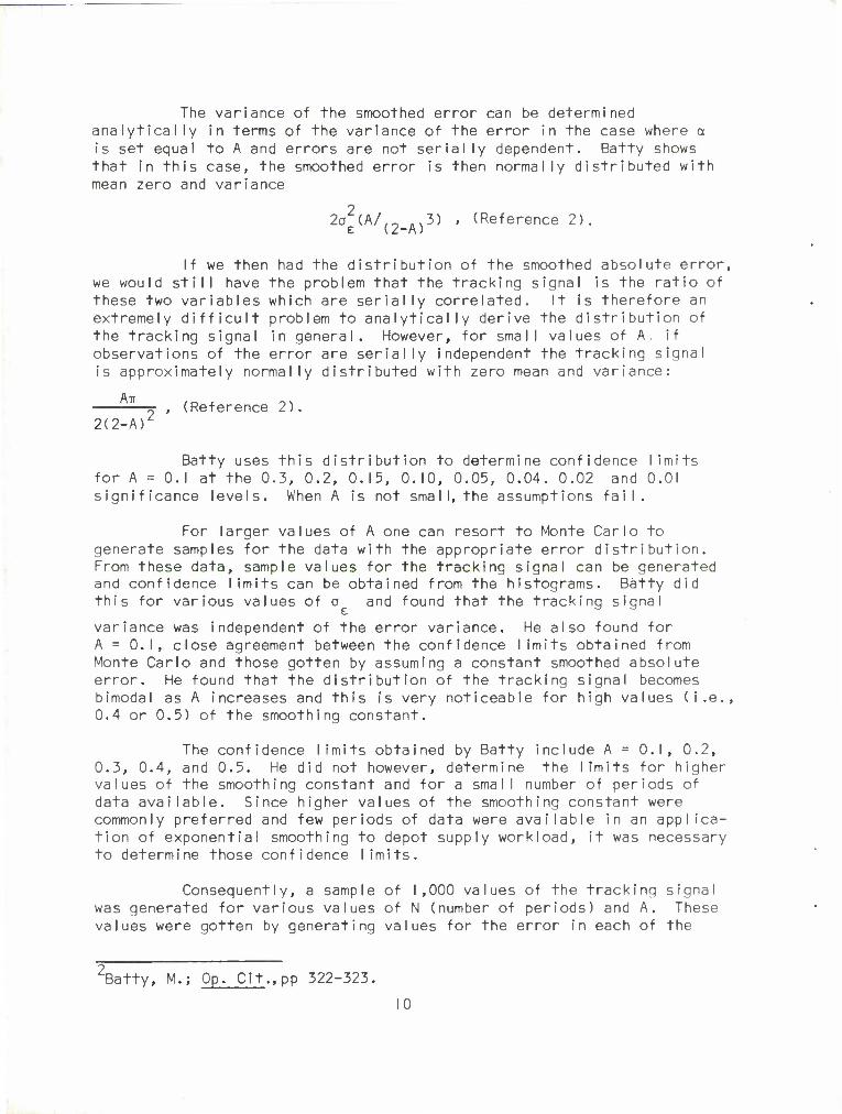
The variance of the smoothed error can be determined analytically in terms of the variance of the error in the case where a is set equal to A and errors are not serially dependent. Batty shows that in this case, the smoothed error is then normally distributed with mean zero and variance

2°e(A/(2 3) , (Reference 2).

If we then had the distribution of the smoothed absolute error, we would still have the problem that the tracking signal is the ratio of these two variables which are serially correlated. It is therefore an extremely difficult problem to analytically derive the distribution of the tracking signal in general. However, for small values of A if observations of the error are serially independent the tracking signal is approximately normally distributed with zero mean and variance:

ATT 2 '

2(2-A) (Reference 2)

Batty uses this distribution to determine confidence limits for A = 0.1 at the 0.3, 0.2, 0.15, 0.10, 0.05, 0.04. 0.02 and 0.01 significance levels. When A is not small, the assumptions fail.

For larger values of A one can resort to Monte Carlo to generate samples for the data with the appropriate error distribution. From these data, sample values for the tracking signal can be generated and confidence limits can be obtained from the histograms. Batty did this for various values of o and found that the tracking signal

variance was independent of the error variance. He also found for A = 0.1, close agreement between the confidence limits obtained from Monte Carlo and those gotten by assuming a constant smoothed absolute error. He found that the distribution of the tracking signal becomes bimodal as A increases and this is very noticeable for high values (i.e., 0.4 or 0.5) of the smoothing constant.

The confidence limits obtained by Batty include A = 0.1, 0.2, 0.3, 0.4, and 0.5. He did not however, determine the limits for higher values of the smoothing constant and for a small number of periods of data available. Since higher values of the smoothing constant were commonly preferred and few periods of data were available in an application of exponential smoothing to depot supply workload, it was necessary to determine those confidence limits.

Consequently, a sample of 1,000 values of the tracking signal was generated for various values of N (number of periods) and A. These values were gotten by generating values for the error in each of the

2Batty, M.; Op. Cit.,pp 322-323,

10

periods, computing the smoothed error and the smoothed absolute error, and getting the tracking signal as the quotient of these two quantities. The sample values for the error were gotten from a pseudo-random number generator for a normal distribution with mean zero and variance I. The distribution of the tracking signal is believed to be independent of the error variance o (Reference 2). To test this, a value of

e a = 101 was used and it gave the same tracking signal histogram. This

agrees with Batty's observation for large N.

From the 1,000 values of the tracking signal, the point below which 90 percent of the values of the absolute value of the tracking fell, was used as a 90 percent confidence limit for the absolute value of the tracking signal.

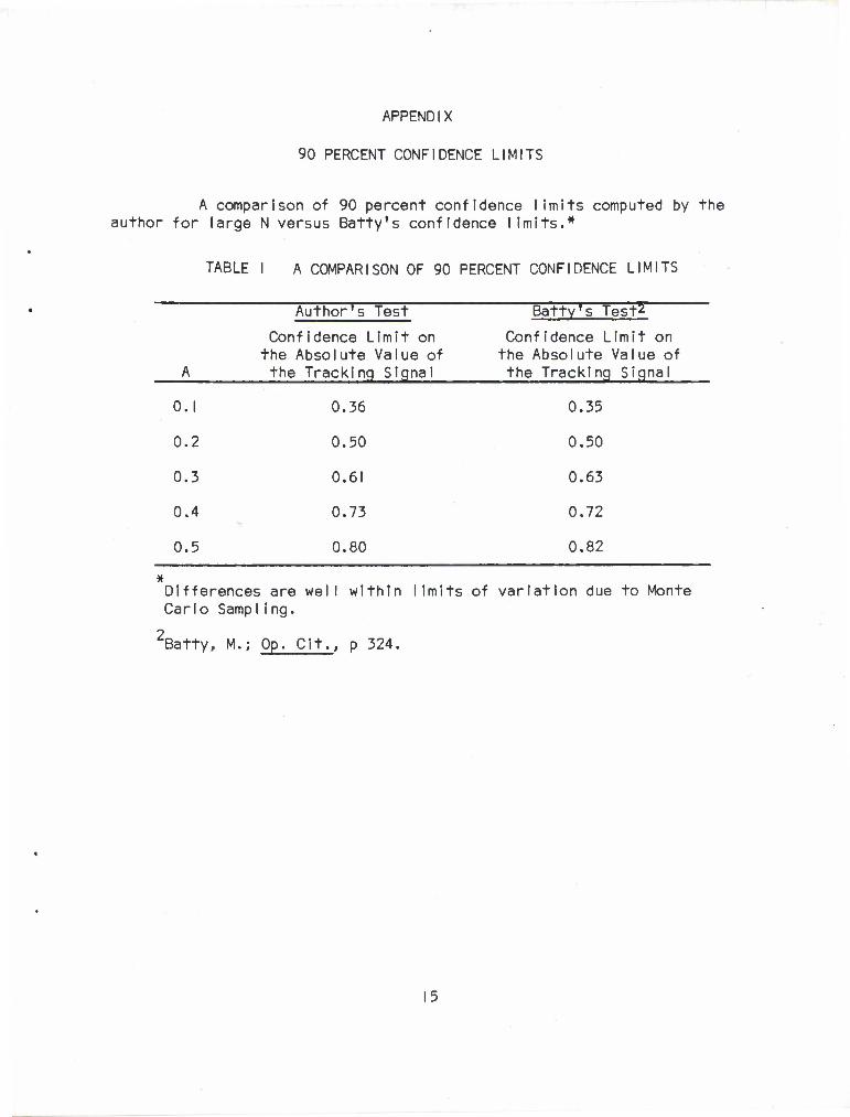
It was found that when the tracking signal was based on only a few periods of data its distribution appeared to be much different from when very many periods of data were used. It was discovered that for 50 to 100 periods the confidence limits were in close agreement with Batty's for A = 0.1, 0.2, 0.3, 0.4, and 0.5. However, when the number of periods was less than 20, confidence limits were significantly higher.

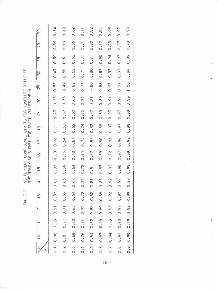
The Appendix gives the tables for the confidence limits for various values of N. A comparison for large N with Batty's confidence limits are also given in the Appendix.

The user can apply these tables to indicate when a bias exists in an exponential smoothing forecast. He must compute a tracking signal based on the errors he has experienced In the past. Given the value of the smoothing constant, for example, suppose a value of A = 0.4 is used, and given the number of periods of past data used to compute the forecast, say 13, he will find from Table 2, that the probability that the tracking signal will exceed 0.72 in absolute value is only 0.1. So, if the computed value is greater than 0.72, he may wish to infer that the forecast is biased. In that event, he may decide to revise the smoothing constant. One way to do this would be to recompute an optimal smoothing constant by using a technique such as the one mentioned in Reference 3.

2 Loc. Cit.

3Loc. Cit.

Next page is blank.

LITERATURE CITED

Trigg, D. W.; Monitoring a Forecasting System, Op I Res QI5, 271-274, (1964).

Batty, M.; Monitoring an Exponential Smoothing Forecasting System, Opl Res 020, No. 3, 319-325, (1969).

Chernick, M. R.; Use of Exponential Smoothing to Forecast Depot Supply Workloads, SM&RSO Interim Note No. I, (1971), U.S. Army Materiel Systems Analysis Agency, Aberdeen Proving Ground, Maryland.

Trigg, D. W., and Leach, A. G.; Exponential Smoothing With an Adaptive Response Rate, Opl Res QI8, No. I, 53-59.

13 Next page is blank.

APPENDIX

90 PERCENT CONFIDENCE LIMITS

A comparison of 90 percent confidence limits computed by the author for large N versus Batty's confidence limits.*

TABLE A COMPARISON OF 90 PERCENT CONFIDENCE LIMITS

Author's Test

Confidence Limit on the Absolute Value of the Tracking Signal

Batty's Test?

Confidence Limit on the Absolute Value of the Tracking Signal

0.1

0.2

0.3

0.4

0.5

0.36

0.50

0.61

0.73

0.80

0.35

0.50

0.63

0.72

0.82

Differences are well within limits of variation due to Monte Carlo Samp Iing.

2Batty, M.; Op. Cit., p 324.

15

O

LU

<L

ZD LL. -J O o co to CD LU < 3

_J C£ < O >

CO _l I- <

—I cc o

LU Ll_ O Z —I LU < Q 2 — a Ll_ — 2 CO O CJ CD

2 ^ LU CJ O < tr or LU I- CL

LU O X ox (-

CM

UJ

CD

o LA

O

in

O

in CM

O CM

ON

ao

co

K-I

CM

ND Ox <*

CM CD r»

CN CO

CO CO Ox Ox

ax ax

o o O o o o o o o

CO ax in CD r-

o CO CO Ox ax

Ox ax

O O o o o o o o CD

Ox in

CM CD r*» 00

o Ox

I*- ax

ax Ox

o o o o o o O o o

o in

C\l xO r-

o CO 00 ax Ox

Ox ax

o o o o o o o o o

in in

ax CM xO

o 00

oo 00

f~l ax a-

o o

O o o o o o o o —

in CO

o CO CO

Ox 00 Ox Ox

ax a*

O o O o o o o o o

CM in

CM CD

in CM CO

ax 00 Ox Ox

ax ax

o o o o o o o o o

r- en in

CM CD

CM CO

CO 00 a- ax

ax Ox

o O O o o o o o o

CO in CD

in r-

CM CO

o ax

CO ax

CO a- ax a.

o o O o o o o o o

o 00 in

O CO

CM CO

Ox CO

CM Ox Ox

ax ax

o o o o o o O o o

CO ax in CD

CNJ CO CO

CM Ox

00 Ox

ax Ox

O o o o o o o o o

in 00

to CO CD CO

00 00

CM ax a.

Ox ax

o O O o o o o o o

CO in

xo CN CM

CO CO CO

CM Ox Ox

ax a-

o o o o o o o o o

ax r* in CO

CM CM CO

ax CO Ox

r- ax

Ox Ox

o o o o o o o o o

ax r-- o r-

CM 00

CO 00 a>

00 ax

ax ax

o o o o o o o o o

CO a> CO

CO xO

CO "3- co CO Ox

r-- ax

ax ax

O o o o o o o o o

— CM en •* in CO r» CO OA

o o o o o o o o o

16

DISTRIBUTION LIST

No. of Copies Organization

Commander Defense Documentation Center ATTN: TIPCR Cameron Station Alexandria, Virginia 22314

No. of Copies

I

Commanding Genera U.S. Army Materie ATTN: AMCCP Washington, D.C.

Commanding Genera U.S. Army Materie ATTN: AMCDL Washington, D.C.

Commanding Genera U.S. Army Materie ATTN: AMCDT Washington, D.C.

Commanding Genera U.S. Army Materie ATTN: AMCDT-P Washington, D.C.

Comma n d i ng Ge ne ra U.S. Army Materie ATTN: AMCMA Washington, D.C.

Commanding Genera U.S. Army Materie ATTN: AMCMS Washington, D.C.

Comma n d i ng Ge ne ra U.S. Army Materie ATTN: AMCPA-SA Washington, D.C.

Command

20315

Command

20315

Comma nd

20315

Command

20315

Command

20315

Command

20315

Command

20315

Commanding Genera U.S. Army Materiel Command ATTN: AMCQA Washington, D.C. 20315

Organization

Commanding General U.S. Army Materiel Command ATTN: AMCRD-E Washington, D.C. 20315

Commanding General U.S. Army Materiel Command ATTN: AMCRD-G Washington, D.C. 20315

Commanding General U.S. Army Materiel Command ATTN: AMCRD-M Washington, D.C. 20315

Commanding General U.S. Army Materiel Command ATTN: AMCRD-P Washington, D.C. 20315

Commanding General U.S. Army Materiel Command ATTN: AMCRD-R Washington, D.C. 20315

Commanding General U.S. Army Materiel Command ATTN: AMCRD-T Washington, D.C. 20315

Commanding General U.S. Army Materiel Command ATTN: AMCRD-W Washington, D.C. 20315

Commanding General U.S. Army Materiel Command ATTN: AMCSA-PM-MBT Washington, D.C. 20315

Commanding General U.S. Army Materiel Command ATTN: AMCPM-SA Picatinny ArsenaI Dover, New Jersey 07801

17

DISTRIBUTION LIST

No. of No. of Copies Organization Copies

1 Director 1 MUCOM Operations Research

Group ATTN: Mr. Crumb Edgewood Arsenal, Maryland 21010

Organi zation

Commanding General U.S. Army Mobility Equipment Command

ATTN: AMSME-G 4300 Goodfellow Blvd St. Louis, Missouri 63120

Commanding Officer U.S. Army Harry Diamond

Laboratories ATTN: Sys Anal Ofc Washington, D.C. 20438

Commanding Officer Frankford Arsenal ATTN: Mr. George Schecter Philadelphia, Pennsylvania 19137

Chief, Analytical Sciences Office

USA Biological Defense Research Laboratory

ATTN: AMXBL-AS Dugway, Utah 84022

Commanding General U.S. Army Aviation Systems

Command ATTN: AMSAV-R-X P.O. Box 209, Main Office St. Louis, Missouri 63166

Commanding General U.S. Army Electronics Command ATTN: AMSEL-PL Fort Monmouth, New Jersey 07703

Commanding General U.S. Army Missile Command ATTN: AMSMI-DA Redstone Arsenal, Alabama 35809

I Commanding General U.S. Army Munitions Command ATTN: AMSMU-RE-R Dover, New Jersey 07801

I Commanding General U.S. Army Tank-Automotive

Command ATTN: AMSTA-CV Warren, Michigan 48090

I Commanding General U.S. Army Weapons Command ATTN: AMSWE-Y Rock Island, I I Iinois 61202

I Commanding Officer U.S. Army Logistics Management Center

ATTN: AMXMC-LR-LOS (Mr. Griswold)

Fort Lee, Virginia 23801

I Commanding Officer USA Major Item Data Agency ATTN: AMXMI-0 (Mr. W. Nye) Letterkenny Army Depot Chambersburg, Pennsylvania 17201

Aberdeen Proving Ground

CG, USATECOM ATTN: AMSTE-TS

18

i

OIU- c — — in > CO

£5 C 3

•1 l_ ro in in JC Ol o L

ID +- C l_ o — L. in u

— <D Q -C Q) 4- L. (D i- I cow

4- in a) o in ID

oi»»- 0 <0 $ ID

ui en TO 01 -G l_ — c — o -o

0) L C L. c > 0 L

— 0 o •— 4- Ol O Jt 4- C 4- C M- o — o Q.4-

(0 in L. 4" I- O X TJ 0) O m l-IUJ < 1- 4- ®

8 O

Dp c

i_ o

i en

g

O Q L- LU o —

2 O Ld CO z in

O Q Q CN 1- LU £ o O — to —

U_

oi — ti c to — CO

S3 1- o 2 00

L. O LU LA Q- Z Z 1C

s O <D —J •a .o cr s h-

to < Q or

ijco *o Ul —• -a-

— CO * < < — < £2 O O CO • h-

g£ §£ ^ U

h- o CD UL ~ E —) < >- 3 0

si U "D o L C C F Q_ 0) 10

— I Ol L _J

V 1- < Q < < z <

8:S o a; O to S

< CO in :•

(/) <C

tr -J — (D s o «C <0 O .* li_ — c — U

K < c ^ co z .c u c O LU in (J t L

£5 p 0)

fcft 4- CJ 10 < <

2 LU >~< to to z1 CL

— < <D >- a> TO i_ in D_ -C CJ o Q_ U +- o < is DC CM

O »r-

r? li. to o»

1 Lfl to

< ID < 4- O m

• >• UJ 3

D to i-

Ld gf < 2 ii- <

ID +- C l_

•D — — 0>«*- Q <0 y m Ol ID tf) JQ u

c — 0 o>— fe 9 L «• C L_ C > O

— 0 0) — •*- Dl -* +• c +- c

U — 0 Q-+- TO C a. TO l/l u I- o x -o « hflU<l-

A +-

r\i CD c

c in -H t u () in u~>

<D c > .* +- U tn TO TO

h- <.

<D a> _J t < S b

S *o t^ *-* ^~

or £ < c to • P J^ +-

2 u

E V 0)

>• a 0 o -a O l_ c c P a It) ID Ol t. _1

< Q < < z <

in S ID en

i; in trt < >^ —

— (0 g ID O .^ c — < c V

JC u C

ie« 5 L

U) h- JC +- a in < < >-< to to

-5 5 a:

9 >- d)

t- to | JC

58 U < #s o: CN

o * r- ^ u_ to o>

fe? ( CO to

< ID o < ••- Q O m • > I UJ D

to L p IX Ol

« ¥• in +• — L. »n m in JC i ID 4- C L- 0 Q Q — L_ Ul i

— o o J= CD +- i

ID L- E +- in c o to o in Ol1*- Q ID s m

IA Ol R) in JD L C) a

fftt a> u > o 1

- O 0) — »•- 0 J£ 4- C +- c

o — o a. +- ID C d ID to L 4- u o x l-Iiu

TJ 0} n l/)

< t- 4- 0)

8 9 « c

0

£ 8o

i s * g o * U)

t- Q X CN l_ LU X CM C o iu to o in o — to o

CL JZ 4- li- x: CTU- _J — 4- M ?« _J — 4- c — «f 10 51 © — to 0 — to

© > to F — I S5 h- — £ £5 z o t_ z o 0 LU GO o *- <-? UJ CO

tu Z LA «•- CL 5 Z ""* x p M3 (0 p »o 10

C 3 CL r- O) c li, r- 0 X Q_ •*- c it X Q- 4-

J£ OJ +- Uj _ c UJ — C o T3 C S L ?a ©

L. O UJ LU c O UJ UJ c c a a. —1 «0 o +- ID a> -J •« o L JD V ££ a. £> CC So CL V < oc X c < X -C — a UJ £ — CC LU c_> to *o* to

-~ o o> ^ ^f Id C in 4- — l_

< * < — 8£ V) i/i c in

-t i- m u> 5" o£ m K\ m t/> p- I ui £ CT o L to • ^~ E ui r Oio L

is — +- (0 -4- C l_ O Is — 4- (0 4- C l_ 0 (D U Q — L. t/1 L. 5 8 CD

— <D 8 x: <D in u

v • h- — © 6 ^ 0) 4- 1- t- 4- L- 10 L- E •*- i/) (D W E (0 L £ 4- in ©

>- E o X c o w O tn a >- D 0 X c o in o in a U 3 O L. a) CT*- Q (0 U (/) O -D O 1- CD CT1*- O (0 (j in C ID K Q- •u O (0 C c 1- 0. "O © 10 © C c V) CT (0 S -O L. — 4) ID c in CT (0 in x> L_ — CT (0 —J • » c — 0 J3 Dl C —1 t« c — O X> < L. 55 CT~ f • L < 2 < < CT— 4- ffi L

<1> C l_ C > O L, 1 z <c a> C L. C > O L. CJ to u — O <0 — «4- CT O w S O en u — o a — *-

J^ 4- C 4- ?£ — X 10 -* 4- C +- C *- — I Z^l (0 LTi X to < L. U — O Q-+- tn L O — O Q-4- >• H io c a. to ui L- 4- >* — H (0 c CL IO in L. 4-

is 8* L 0 XT3 (B t- S LU < 1-

0 L0 n S** L, 5 x -o a> HlUJ<h

0 »n 4- ©

— u — i— — u — t- <c — * — c < c ^ — c

c O c £ . m

jr O c i* in -C £ U ct a) |j cc a> a a* 1- x: P ^ 4- »- o •t- o < CM CT

C 5-5 < CM CT

to < o cc t/i tn U oi to — -C X — ^

— X (0 +- — < (0 4- a> < >- ID c o • 58 c 0

—1 ID CT 5 CT 5 L. * tl L. irt 8:^ a> in U) in CC CM

O *r- CM o »r* >• Li. to o JC +- >• u_ to CT» JC 4-

E? K — U Q. El t- — u a. to to (0 10 to to © © <: ro Q < +- I- T3 < (0

O U in L T3

Q CJ Ifl (- < t- < • >• X LU =J • >• X LiJ 3

F- cr u) CO 1_ I- a: CT to C o

D! LU O 3 Q 6£ LU O 3 < X U- < — •*• < X u_ < — ^

8 8 LU -

c: X

C 3

F , o a CT 0 o O CM f </> L. LiJ X CM C L UJ x o o — to o o — to —

Of Lu JZ li_ X: o P> — —1 — •1- CT — K c: to

— to 51 c to — to

Z

I §5 1 z o ff §5 K O

Z CO Ul L- O LU CD L O UJ in

Q. Z z m 0. z Z \D o 3 o vo «0 ZD o r- 1- C a r* C Q. Q-

O +- X D. ••- 0) 4- 4- _J © t- LU — c <D L. UJ C < TJ O • "O 0 LU © z L. Q- LU LU c L. a. LU -O c o O CD —t *a 0 CD <D —1 1- o 1/1 < So a.

X (0 c

^ CC < S§ CL X

— CC LU CT UJ

8 {2 *0 to *o to — *3" CT in -* ^~ CT

— to ^ < < — < 55 U1 If) C UI

Ki yi CT < — < g5 in in c in

Ki m O CJ to • F E

0)

tn r: CT O L c to • K | CD

in ^ CT O L < LU a: cc 5£ — 4-

Z O (0 +- c l_ y Q — *-

O J* §5 — -1-

Z U (0 4- c L. O O — L.

O in L

1— o g* H — <D 0 ^ as 4- l_ u °.» h- — <1) Q x: <D 4- L- u. E (0 L- E +• U) 0) a "^ E (0 L. E 4- tn © < >- 3 ^ P X c o IS o in 0 L >• 3 0 X c o in o in ©

8 s. (.J T3 O L.

1- Q. <D CT*- Q (0 u in

© 10 »-

c c o c 1- 0.

CD T3

CTH- Q (0 (j m © to

0) 10 C U) CT (0 ifl -d L. — <D (0 C in CT (0 in XJ L. — — X CD L. _J •- c — O XI CT L I >» c — O xi >- F < Q < < CT— -t- CO L 4- < Q < < CT— 4- 0) L.

C L_ C > O Z < 0) C L- C > O 1_ z < CD L 0- Q in ffi O to u — 0 03 — •*- CT O in S O CO U — O © — •*- CT 0 0- x — X a -^ 4- C -t- C -4- — I TO -^ 4- C 4- c <«~ < to M to - — h- (0 C Q. (0 V> L. 4- >• — (- (0 c CL io m l_ 4- CC —J o <

— (D ro o 8** L- O X *o a>

1- X UJ «c t- 0 (/) 4- O

— ro (0 u 8** L O XOO

1— X LU < K O tn 4- ©

Li- — c — — (J — t— c — — o — \— 1- < c ^ — C < c iC •- c

CO Z Q LU 5 . Sg «

0 t—

£ • in So E CD

© F ^^ in £ (D F- x: Efe 4- O ••- C_>

in < < CM CT in < < CM CT c 2 UJ >•< C >•<

to to o cc — £

to to X

o CC — x: — < (0 4- — < © 4-

0) >- <D c p 0) V CD C O —1 <0 CT Q -J (0 CT 5 u ir\ 0- ^ i_ in

< — © O +- O

CL U < — ui to £§ in in

£~ CC CM CT a> c > 5^ CC CM

O * r-

CT © C >

>* Li_ tO CXi JC 4- >^ u_ to o> •X 4-

El h- — to to

u a. (0 10 E? l

to to u a. © © L. T3 < © Q < +- L. T3 < (0 Q < 4-

Q O ui t- < O CJ in (— < • >- X LU D • >. X UJ 3

Q tO l_

= £ F CC CT LU O D s: u_ < — •* a <

tO L_ F % CT

^£5 — V

5

~ E >• 3 u -o

l/l ffi

— (0 (0 u c —

jl l/l < >-< l/l to a

L in o o •I- o

1

UJ oo

g£ — 4-

Q 0) *•? Pi 53 C3 to

co <

8* — o *: _

o < O IE

>- « -J 10 Q. £

< — 5 .S u. to o>

h- — to to §*? +• O in

LU 3

eg? X u. <

?S

¥ «

— 8 8 !c • tn o

•1- l_ t/) L.

C 0 W Q W re a) CTl-4- Q (D

<D 1/1 t/> CTI <D OS -O L. Q

0 —

C L. c > 0 ••- ja

— o • — *- en L j£ 4- c 4- C O u — 0 a+- •— *- ID c am VI L L O X -O V O 4-

4- W — 0) C 1-

o o £. UJ o — u- ?£

— to

°-5

i

=;*

V) 4- — l_ K"\ in

E in JZ en O L. Df CL 0

a> Db-i in l_ - - Q) Q r OJ 4- L. fl L Ef C O w o in

in o X

u m £ ro

0) on- Q IO

c LO en ro in .o L. — c — 0 -o

O)— 4- © L C L. C > O

••- • L U — O 0) — 4- Ol 0

J£ 4- C 4- C H- I U — O O- 4-

10 c o. to w - L. 4- tiasl 0 tn 4- a>

II O *r~ u_ in o*

I in in o «c +- Q O in X UJ U P or oi UJ o 3 Z u. < £ O -J O L CJ UJ CO a z z in

3 g (0 n C r^ <D 4- X Q- +- a- i_ LU c

•o o OJ L. a UJ UJ c a; a) _J w« o jo or g fe a. >- 3 0 X c O in Q in ro U "D o L- QJ en **- g ^ u in

O (0 c c F CL V a> io c in cn ID S ^i l_ — en L. •J c — O J3 < Q < < en — +- 03 L. 4-

z < a c L. C > 0 L in 35 O in y o j~*. CD O - s: 5 n X C 4- in in < L u - 0 af > — h- ja c a. ro in L. 4-

— <0 10 (J g X.

L O X T) » S UJ < t-

0 in 4- 0)

C — U — h-

£ •

L_ m 8:t 0) o 4- O < — ^^ g .P r?

U. l/l o> 1

in in < (0 o < +•

O O i/> • >^ X UJ 3 to t. F or a 6i UI O 3

3: u. <

< »tj — or »o to

—* ^j < — ftV to • P k# — 4-

£ >• 3 0 u -o O L. c c t- a. 0) (0 < Q < <

z < in 55 e> to — X - Si in to < >• —

— to SJ?

<: c ^ — JC O c

U •1* 4- u 5-5 < to to -5

o or

0 >- o> -1 ID

L. in tt 0) o

•n ?

<?E

c o m o in ro cn^- 6 io U in $ ro in O) ro in JZ> i_ —

O J3 Oi— +- <D L c t. c > o

•4- L

- O OJ -•*- ai o JrS 4- C 4- U — Q Q.4- n c an m l- 4-

K£I25,? 0 m 4- 0)

0 Q L- UJ

to —

g5

c » +- O L.

55 F ^ -1 y O

r c Q> 0 Dl L. <- y U) 1 Ifl >•

in n u

W <

tO tO

pi z o UJ CD

£2 T U

V 0)

!> f CL

J ... 1 < f < O c/>

Si

10 0)

0) o 0L O +- o < — *s X

or CN o -r- >- u. CO o

E? I to to

< ID Q *S +• SO ui • >* I UJ 3 tO L_

I U. < = *

O Q l_ UJ o —

S5

?R

§5 ~ E

O TJ

+• —

•D — — in U) m tfi X)

c pt 4- o u

r > o — 0 UJ — «•- J£ +- tr •t- O — b O.-*- ID C Cl <D in

•tfui:

tO tO o ct X 2 — < » >- 0)

u ir\ Q- i 0) o 0- o +- o < — 1* X

o: CN o • r- U. <S) &>

fc? l to t/i < ro Q < +- O O VI

«5 £• 6$ M

ETH

FO

RE

A

uqu

Kl Ul i o

in i •H L. t/i QJ n 0 01 0) «1 L o 13

I a 0

«•-

2 •

W W

O Q l- UJ

e> —

15

— s in >- —

s |

to o

_i —

if £5

£ vO

o o l_ UJ o —

U-

c?^ — to > « o J 1- u a. z

to o

_j —

£5

— a: tO

gfi

P *-

< < z < O to

rn in t_ O

c o ui Q wi m O)-*- O (O o in

$ ID in aim ifl J3 L —

c — O •£> cn — +- <D u C l_ C > 0 L - o qj — *- -* +- C +- CD O

C *- U — O Q.+- (c c a. to in u +- L n X T3 CD h SUJ<r-

o y> -•- 0)

(D 0 —i -o -C Q < *£ — a: - o to

< — < ft5 to - p 55 — +-

E >• 3 0 U X) o u c c t- Q_ a ro

< Q < < z < in 35 O to — S — I in >^ — — (0 to a Si

«c c *: —

in c in . fo m

tn £ cn o L A3 •*- C l_ O

— * Q -C 0) V) L.

••- U 10 i- E +- in Q) c o in o in (0 or*- 6 ID y in

W ID in g> ro m xi i_ —

o -o 571— -t- « u c u c > o L

— o a) — ««- gl 0 X 4- C +- U *- O CL-t- (0 c a. ro m u +• i. O X -O O l-SUJ<l-

0 in +- ©

•o — —

^ 5

as < to J/) o cc

<D >- <D

L in tfi (D O +• o < — *s X

CC CN O »r*

r? U. V)Oi 1

to to < (D Q < +-

Sow • >- X UJ D to u F a ui

UJ O 3 Z) 3E z u. <

$-5 to to

si

ll in C7> t-

jS i J Ul LU 1 ir m 1 o 3

Unclassi f ied Security Classification

DOCUMENT CONTROL DATA -R&D (Security cleasllicatlon of title, body ol abatract and Indexing annotation muat be entered when the overall report la elaaellled)

1. ORIGINATING ACTIVITY (Corporate author)

U.S. Army Materiel Systems Analysis Agency Aberdeen Proving Ground, Maryland

2«. REPORT SECURITY CLASSIFICATION

Unclassif ied 2b. GROUP

3. REPORT TITLE


4. DESCRIPTIVE NOTES (Type ol report mnd Incluelve datee)

5. AUTHOR(S) (Flret name, middle Initial, laet name)

Michael R. Chernick

S REPORT DATE

August 1972 7a. TOTAL NO. OF PAGES

18 76. NO. OF REFS

(a. CONTRACT OR GRANT NO.

b. PROJECTNO. RDT&E IP76580IMMI 102

ORIGINATOR'S REPORT NUkfBERUI

Technical Memorandum No. 140

•b. OTHER REPORT NOIS) (Any other numbere that may be aeel0ied thla report)

10. DISTRIBUTION STATEMENT

Approved for public release; distribution unlimited,

II SUPPLEMENTARY NOTES 12. SPONSORING MILITARY ACTIVITY

U.S. Army Materiel Command Washington, D.C. 20315

13. ABSTRACT

The tracking signal developed by Trigg which has gained wide acceptance is usefu for monitoring single exponential smoothing forecasts. If forecasts become biased, the tracking signal will increase in absolute value indicating the possible need to change the smoothing constant which is the one adjustable parameter in single exponential smoothing.

Two methods of applying the tracking signal to monitor exponential smoothing forecasts are discussed in this document. The method which was applied to depot workload forecasts is described in detail and the tables of confidence limits which are necessary to apply this method are given.

DD ,""..1473 o5So*i?TB zzmzi4J.v Unclassif ied Security Classification

Unclass i f ied Security Classification

LINK '

HOL E r. i I

K EY WORDS

RO LE »1

LINK B

ROLE W T

Trackinq signal Monitoring forecasts Exponential smoothing Adaptive smoothing Test for bias errors

Line I ass i f i oi Security Classification

Documents

TECHNICAL LIBRARY, - LIBRARY, - AD TECHNICAL MEMORANDUM NO. 110 METHODS FOR APPLYING A TRACKING SIGNAL TO MONITOR SINGLE EXPONENTIAL SMOOTHING FORECASTS MICHAEL R. CHERNICK AUGUST