TECHNICAL MEMORANDUM No. SEA SALT AND LIGHTNING …

773 San Marin Drive, Suite 2115, Novato, CA 94998 P: 415‐899‐0700 F: 415‐899‐0707 www.environcorp.com

June 25, 2012

TECHNICAL MEMORANDUM No. 12: SEA SALT AND LIGHTNING

To: Tom Moore, Western Regional Air Partnership (WRAP) From: Ralph Morris, Chris Emery and Jeremiah Johnson, ENVIRON Zac Adelman, University of North Carolina Subject: Sea Salt and Lightning Emissions

INTRODUCTION ENVIRON International Corporation (ENVIRON), Alpine Geophysics, LLC (Alpine) and the University of North Carolina (UNC) at Chapel Hill Institute for Environment are performing the West‐wide Jump‐start Air Quality Modeling Study (WestJumpAQMS) managed by the Western Governors’ Association (WGA) for the Western Regional Air Partnership (WRAP). WestJumpAQMS is setting up the CAMx photochemical grid model for the 2008 calendar year (plus spin up days for the end of December 2007) on a 36 km CONUS, 12 km WESTUS and several 4 km Inter‐Mountain West modeling domains. The WestJumpAQMS Team are currently compiling emissions to be used for the 2008 base case modeling, with the 2008 National Emissions Inventory (NEI) being a major data source. The Team is preparing 13 Technical Memorandums discussing the sources of the 2008 emissions by major source sector:

1. Point Sources including Electrical Generating Units (EGUs) and Non‐EGUs;

2. Area plus Non‐Road Mobile Sources;

3. On‐Road Mobile Sources that will be based on MOVES;

4. Oil and Gas Sources (in several installments);

5. Fires Emissions including wildfire, prescribed burns and agricultural burning;

6. Fugitive Dust Sources;

7. Off‐Shore Shipping Sources;

8. Ammonia Emissions;

9. Biogenic Emissions;

10. Eastern USA Emissions;

11. Mexico/Canada;

Page 2


12. Sea Salt and Lightning Emissions; and

13. Emissions Modeling Parameters including spatial surrogates, temporal adjustment parameters and chemical (VOC and PM) speciation profiles.

This Technical Memorandum #12 discusses the approach to be used for developing 2008 emissions for sea salt and lightning.

SEA SALT EMISSIONS

Marine aerosols are created by turbulence, bubble breaking and viscous shear from winds blowing over the ocean surface, and range in size from sub‐micron to larger than 100 microns (µm). As waves in the ocean break, they entrain air into the water, creating bubbles. Bubbles are transported through water column by turbulence and Langmuir circulations, and rise under their own buoyancy. As bubbles reach the ocean surface, surface tension on the interfacial film collapses and the film shatters. The collapse of the bubble cavity produces an upward‐moving jet of water, and velocity differences along the surface of the jet render it unstable and cause it to break up into droplets. Each bubble can make as many as 10 jet drops with typical radii of 1‐2 µm (possibly exceeding 10 µm), and several hundred film drops in the sub‐micron range. At wind speeds greater than ~9 m s‐1, spume droplets are produced as wind shears off the tops of waves. This mechanism produces large droplets with radii greater than 4 µm.

For the WestJumpAQMS we propose to use the sea salt emissions pre‐processor developed for the CAMx model that is described below.

SEA SALT EMISSIONS PROCESSOR

The sea salt emissions pre‐processor estimates time/space‐varying emissions of sea salt aerosol. The source code is distributed with Linux “make” scripts that invoke the Fortran90 compiler and compile/link the executable programs with system libraries. The user will need to edit the respective make scripts to ensure the correct compiler and associated flags are set according to their system specifications. The sea salt emissions pre‐processor is publicly available and one of the support programs available on the CAMx website1.

Sea salt production is usually calculated at a relative humidity of 80%, which is typical at 10 meters above the surface in the marine boundary layer. Because salt is hygroscopic, the size of a sea salt aerosol changes with the ambient relative humidity, growing when the humidity increases and shrinking in drier air. The radius at 80% relative humidity is roughly twice that of dry aerosol (Fitzgerald 1975); another way to state this is that the wet radius at 80% humidity is equivalent to the dry diameter. In parameterizing sea spray emissions, several assumptions are made. The most important is that the aerosol size can be described by a single quantity such as the dry mass or radius at a given relative humidity. All sea salt aerosols are assumed to have the same relative composition of dissolved substances, and properties like density and index of

1 http://www.camx.com/download/support‐software.aspx

Page 3


refraction are independent of particle size. Droplets are presumed to have an insoluble core of pure sodium chloride (NaCl).

A widely accepted formulation for sea spray droplet flux from the open ocean surface was proposed by Monahan et al. (1986). Monahan used discontinuous functions to predict marine aerosol production as a function of wind speed (at 10 meter height) and radius at 80% relative humidity for sizes of 0.8 μm, 10 μm, 75 μm, 100 μm, and over 100 μm. The Monahan parameterization is given by:

where F is the flux of particles (µm‐1m‐2s‐1), U10 is the 10 meter wind speed (m s‐1), and r is the droplet radius (microns) at 80% relative humidity. The exponential term B is given by:

The Monahan parameterization gives reasonable fluxes for the dry aerosol radius range of 0.2‐4 µm (Guelle et al. 2001; Gong et al. 2002; Gong 2003). However, Gong (2003) showed that the Monahan parameterization overestimates sea salt aerosol production at dry radii smaller than about 0.2 µm, and modified the Monahan flux equation as follows:

where

with Θ = 30, and

Either the Monahan or the Gong parameterization may be used in the sea salt aerosol emission program for aerosols with dry radii less than 4 µm.

The Monahan spume flux generation function also has been shown to generate too many sea spray droplets at dry radii greater than 4 µm (Guelle et al. 2001; Gong et al. 2002; Gong 2003). Following the work of Grini et al. (2002), and Liao et al. (2004), the Smith and Harrison (1998) parameterization is used for aerosols with dry radii greater than 4 µm:

where r01 = 3 µm, r02 = 30 µm, f1 = 1.5, f2 = 1, A1 = 0.2 U103.5, and A2 = 6.8×10

‐3 U103.

2exp19.105.1341.310 10057.01373.1 BrrU

r

F

65.0/log38.0 10 rB

2exp607.145.341.310 10057.01373.1 BA rrU

r

F

44.1017.017.4 rrA

433.0/log433.0 10 rB

2,1

20/lnexp

iiii rrfA

r

F

Page 4


The Smith‐Harrison parameterization gives a sea spray flux that is too small compared to observations for dry radii less than 4 µm, and so it is applied only above 4 microns. The fluxes from the Monahan/Gong and Smith‐Harrison parameterizations join reasonably well at ~4 microns dry radius for a range of wind speeds (Grini et al. 2002).

The emissions pre‐processor integrates the sea salt flux over a default distribution of size bins from Grini et al. (2002) and between minimum and maximum limits specified by the user in the job script. For example, if the desired range of sea salt dry diameters is 0 to 2.5 microns, the sea salt emissions program will integrate between those two extremes, breaking the integral up into smaller pieces defined by the default bins of Grini et al. in order to improve the accuracy of the integration. The emitted dry particle mass is calculated from the integrated flux assuming a spherical particle geometry and a dry aerosol density of 2250 kg m‐3 (Grini et al. 2002).

The emissions pre‐processor also considers the contribution from breaking waves in the coastal surf zone. The surf zone sea spray aerosol is calculated using either the parameterization of DeLeeuw et al. (2000) or the Gong (2003) open ocean approach by assuming 100% whitecap coverage. The Gong approach is strongly recommended as it leads to a more realistic emission flux that is less strongly influenced by wind speed. To calculate surf zone emissions, the user must specify the surf zone width and coastline length in each grid cell that contains a coastline. The coastline length can be set in two ways:

1. Let the program set the coastline length to the size of the grid cells (i.e., a linear coastline across the full width of each grid cell) [this is the default approach];

2. Set the coastline length manually for each grid cell (requires an additional program to prepare a separate input file) [to support this capability requires GIS processing to resolve actual coastline lengths].

The surf zone width is specified by the user for each coastline grid cell within a special text map file that defines the spatial distribution of ocean‐covered grid cells. Four surf zone widths are supported: 10, 20, 50, and 100 m. The structure of this ocean map file is described below.

The sea salt pre‐processor splits emissions into particulate sodium and chloride components for particulate modeling.

The sea salt program generates hourly gridded CAMx‐ready emission files containing sea salt aerosol for the day(s) specified in the job script.

The user must specify domain information (location, grid resolution, grid size). The meteorological input fields include the layer height grid, pressure, temperature, wind, and clouds.

The user must also supply a CAMx‐ready land use file and a separate text‐formatted ocean mask file. The text file should be developed independently by the user according to the CAMx landuse file. Since CAMx landuse classifications do not necessarily differentiate between water bodies as being ocean (salt water) or inland (fresh water), it is left to the user to make the distinction by developing the ocean mask file. This file defines which grid cells contain sea

Page 5


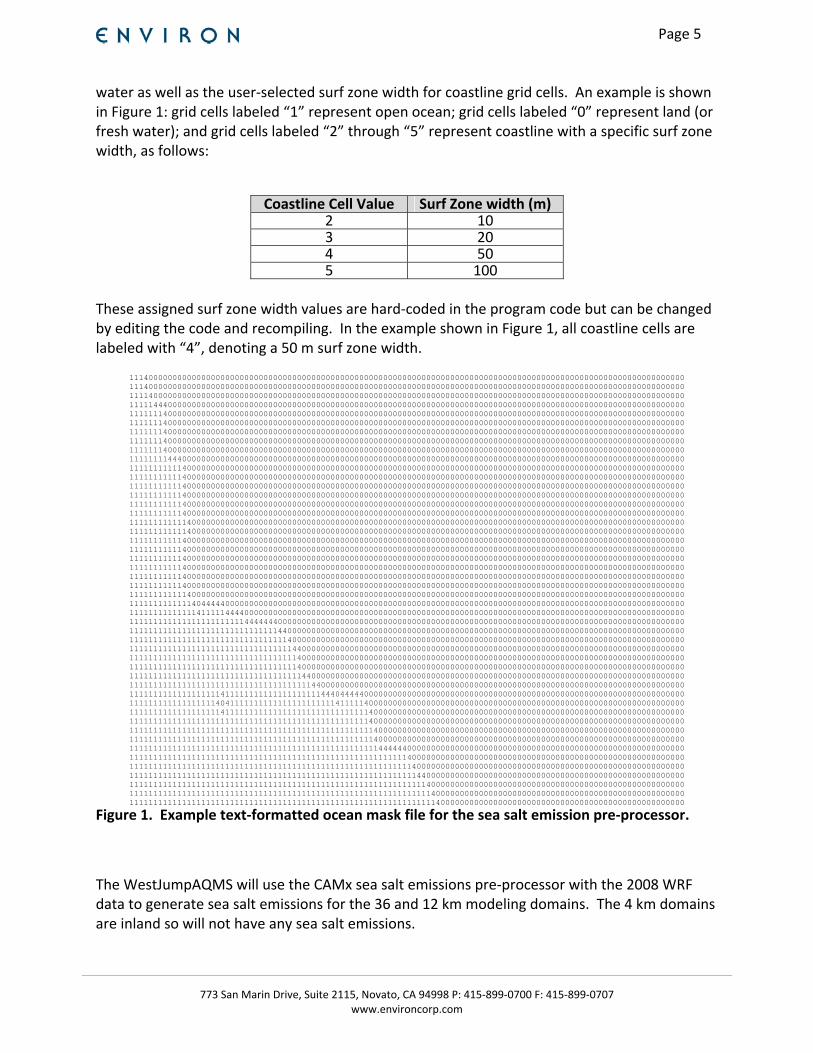
water as well as the user‐selected surf zone width for coastline grid cells. An example is shown in Figure 1: grid cells labeled “1” represent open ocean; grid cells labeled “0” represent land (or fresh water); and grid cells labeled “2” through “5” represent coastline with a specific surf zone width, as follows:

Coastline Cell Value Surf Zone width (m)

2 103 204 505 100

These assigned surf zone width values are hard‐coded in the program code but can be changed by editing the code and recompiling. In the example shown in Figure 1, all coastline cells are labeled with “4”, denoting a 50 m surf zone width.

11140000000000000000000000000000000000000000000000000000000000000000000000000000000000000000000000000000000000000000 11140000000000000000000000000000000000000000000000000000000000000000000000000000000000000000000000000000000000000000 11114000000000000000000000000000000000000000000000000000000000000000000000000000000000000000000000000000000000000000 11111444000000000000000000000000000000000000000000000000000000000000000000000000000000000000000000000000000000000000 11111114000000000000000000000000000000000000000000000000000000000000000000000000000000000000000000000000000000000000 11111114000000000000000000000000000000000000000000000000000000000000000000000000000000000000000000000000000000000000 11111114000000000000000000000000000000000000000000000000000000000000000000000000000000000000000000000000000000000000 11111114000000000000000000000000000000000000000000000000000000000000000000000000000000000000000000000000000000000000 11111114000000000000000000000000000000000000000000000000000000000000000000000000000000000000000000000000000000000000 11111111444000000000000000000000000000000000000000000000000000000000000000000000000000000000000000000000000000000000 11111111111400000000000000000000000000000000000000000000000000000000000000000000000000000000000000000000000000000000 11111111111400000000000000000000000000000000000000000000000000000000000000000000000000000000000000000000000000000000 11111111111400000000000000000000000000000000000000000000000000000000000000000000000000000000000000000000000000000000 11111111111400000000000000000000000000000000000000000000000000000000000000000000000000000000000000000000000000000000 11111111111400000000000000000000000000000000000000000000000000000000000000000000000000000000000000000000000000000000 11111111111400000000000000000000000000000000000000000000000000000000000000000000000000000000000000000000000000000000 11111111111140000000000000000000000000000000000000000000000000000000000000000000000000000000000000000000000000000000 11111111111140000000000000000000000000000000000000000000000000000000000000000000000000000000000000000000000000000000 11111111111400000000000000000000000000000000000000000000000000000000000000000000000000000000000000000000000000000000 11111111111400000000000000000000000000000000000000000000000000000000000000000000000000000000000000000000000000000000 11111111111400000000000000000000000000000000000000000000000000000000000000000000000000000000000000000000000000000000 11111111111400000000000000000000000000000000000000000000000000000000000000000000000000000000000000000000000000000000 11111111111400000000000000000000000000000000000000000000000000000000000000000000000000000000000000000000000000000000 11111111111400000000000000000000000000000000000000000000000000000000000000000000000000000000000000000000000000000000 11111111111140000000000000000000000000000000000000000000000000000000000000000000000000000000000000000000000000000000 11111111111114044444000000000000000000000000000000000000000000000000000000000000000000000000000000000000000000000000 11111111111111411111444400000000000000000000000000000000000000000000000000000000000000000000000000000000000000000000 11111111111111111111111144444440000000000000000000000000000000000000000000000000000000000000000000000000000000000000 11111111111111111111111111111114400000000000000000000000000000000000000000000000000000000000000000000000000000000000 11111111111111111111111111111111140000000000000000000000000000000000000000000000000000000000000000000000000000000000 11111111111111111111111111111111114400000000000000000000000000000000000000000000000000000000000000000000000000000000 11111111111111111111111111111111111400000000000000000000000000000000000000000000000000000000000000000000000000000000 11111111111111111111111111111111111400000000000000000000000000000000000000000000000000000000000000000000000000000000 11111111111111111111111111111111111144000000000000000000000000000000000000000000000000000000000000000000000000000000 11111111111111111111111111111111111111440000000000000000000000000000000000000000000000000000000000000000000000000000 11111111111111111114111111111111111111114440444440000000000000000000000000000000000000000000000000000000000000000000 11111111111111111140411111111111111111111114111114000000000000000000000000000000000000000000000000000000000000000000 11111111111111111114111111111111111111111111111111400000000000000000000000000000000000000000000000000000000000000000 11111111111111111111111111111111111111111111111111400000000000000000000000000000000000000000000000000000000000000000 11111111111111111111111111111111111111111111111111140000000000000000000000000000000000000000000000000000000000000000 11111111111111111111111111111111111111111111111111140000000000000000000000000000000000000000000000000000000000000000 11111111111111111111111111111111111111111111111111114444440000000000000000000000000000000000000000000000000000000000 11111111111111111111111111111111111111111111111111111111114000000000000000000000000000000000000000000000000000000000 11111111111111111111111111111111111111111111111111111111111400000000000000000000000000000000000000000000000000000000 11111111111111111111111111111111111111111111111111111111111144000000000000000000000000000000000000000000000000000000 11111111111111111111111111111111111111111111111111111111111111400000000000000000000000000000000000000000000000000000 11111111111111111111111111111111111111111111111111111111111111140000000000000000000000000000000000000000000000000000 11111111111111111111111111111111111111111111111111111111111111114000000000000000000000000000000000000000000000000000

Figure 1. Example text‐formatted ocean mask file for the sea salt emission pre‐processor.

The WestJumpAQMS will use the CAMx sea salt emissions pre‐processor with the 2008 WRF data to generate sea salt emissions for the 36 and 12 km modeling domains. The 4 km domains are inland so will not have any sea salt emissions.

Page 6


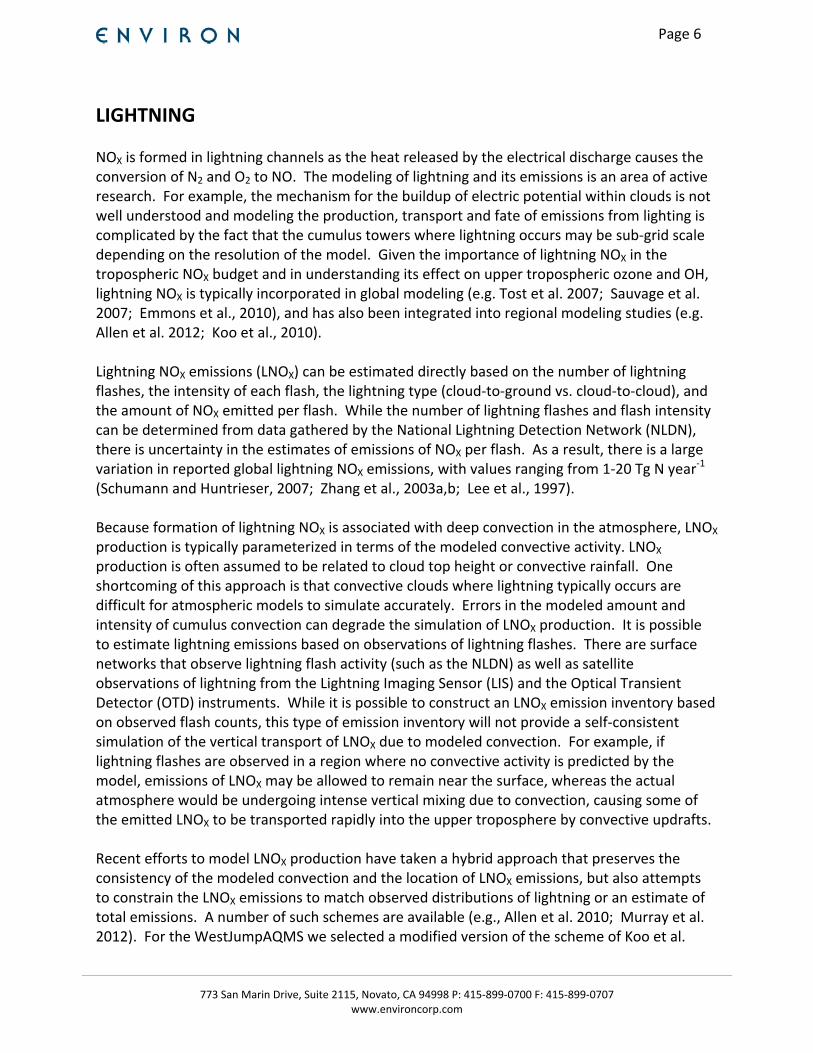
LIGHTNING NOX is formed in lightning channels as the heat released by the electrical discharge causes the conversion of N2 and O2 to NO. The modeling of lightning and its emissions is an area of active research. For example, the mechanism for the buildup of electric potential within clouds is not well understood and modeling the production, transport and fate of emissions from lighting is complicated by the fact that the cumulus towers where lightning occurs may be sub‐grid scale depending on the resolution of the model. Given the importance of lightning NOX in the tropospheric NOX budget and in understanding its effect on upper tropospheric ozone and OH, lightning NOX is typically incorporated in global modeling (e.g. Tost et al. 2007; Sauvage et al. 2007; Emmons et al., 2010), and has also been integrated into regional modeling studies (e.g. Allen et al. 2012; Koo et al., 2010). Lightning NOX emissions (LNOX) can be estimated directly based on the number of lightning flashes, the intensity of each flash, the lightning type (cloud‐to‐ground vs. cloud‐to‐cloud), and the amount of NOX emitted per flash. While the number of lightning flashes and flash intensity can be determined from data gathered by the National Lightning Detection Network (NLDN), there is uncertainty in the estimates of emissions of NOX per flash. As a result, there is a large variation in reported global lightning NOX emissions, with values ranging from 1‐20 Tg N year‐1 (Schumann and Huntrieser, 2007; Zhang et al., 2003a,b; Lee et al., 1997). Because formation of lightning NOX is associated with deep convection in the atmosphere, LNOX production is typically parameterized in terms of the modeled convective activity. LNOX production is often assumed to be related to cloud top height or convective rainfall. One shortcoming of this approach is that convective clouds where lightning typically occurs are difficult for atmospheric models to simulate accurately. Errors in the modeled amount and intensity of cumulus convection can degrade the simulation of LNOX production. It is possible to estimate lightning emissions based on observations of lightning flashes. There are surface networks that observe lightning flash activity (such as the NLDN) as well as satellite observations of lightning from the Lightning Imaging Sensor (LIS) and the Optical Transient Detector (OTD) instruments. While it is possible to construct an LNOX emission inventory based on observed flash counts, this type of emission inventory will not provide a self‐consistent simulation of the vertical transport of LNOX due to modeled convection. For example, if lightning flashes are observed in a region where no convective activity is predicted by the model, emissions of LNOX may be allowed to remain near the surface, whereas the actual atmosphere would be undergoing intense vertical mixing due to convection, causing some of the emitted LNOX to be transported rapidly into the upper troposphere by convective updrafts. Recent efforts to model LNOX production have taken a hybrid approach that preserves the consistency of the modeled convection and the location of LNOX emissions, but also attempts to constrain the LNOX emissions to match observed distributions of lightning or an estimate of total emissions. A number of such schemes are available (e.g., Allen et al. 2010; Murray et al. 2012). For the WestJumpAQMS we selected a modified version of the scheme of Koo et al.

Page 7


(2010) because this scheme is consistent with the approach outlined above and has already been implemented as a CAMx preprocessor. Koo et al. (2010) estimated annual total LNOX emissions for North America using NLDN flash data from Orville et al. (2002) and (Boccippio et al., 2001). The NO emissions factor that determines the amount of NO generated per flash of lightning is taken from the EULINOX study (Holler and Schumann, 2000) and is 9.3 kg N per flash. Using these data, Koo and co‐workers estimate the total LNOX emissions for North America to be 1.06 Tg N year‐1 . Lightning emissions are then allocated to grid cells where modeled convection occurs using convective precipitation as a proxy for lightning activity. The hourly and gridded 3‐D lightning NO emissions are calculated as follows:

, , , ,

where E(x,t) is the NO emission rate (mol hr‐1) at time t and grid location x; RNO is the NO emission factor; PC is the convective precipitation (m hr‐1) at time t and grid location x; D(x,t) is the convective cloud depth (m) at time t and grid location x; and p(x,t) is the pressure (Pa) at time t and grid location x. Constraining the total emissions within North America to 1.06 Tg N year‐1 requires that RNO be equal to 3.9x10

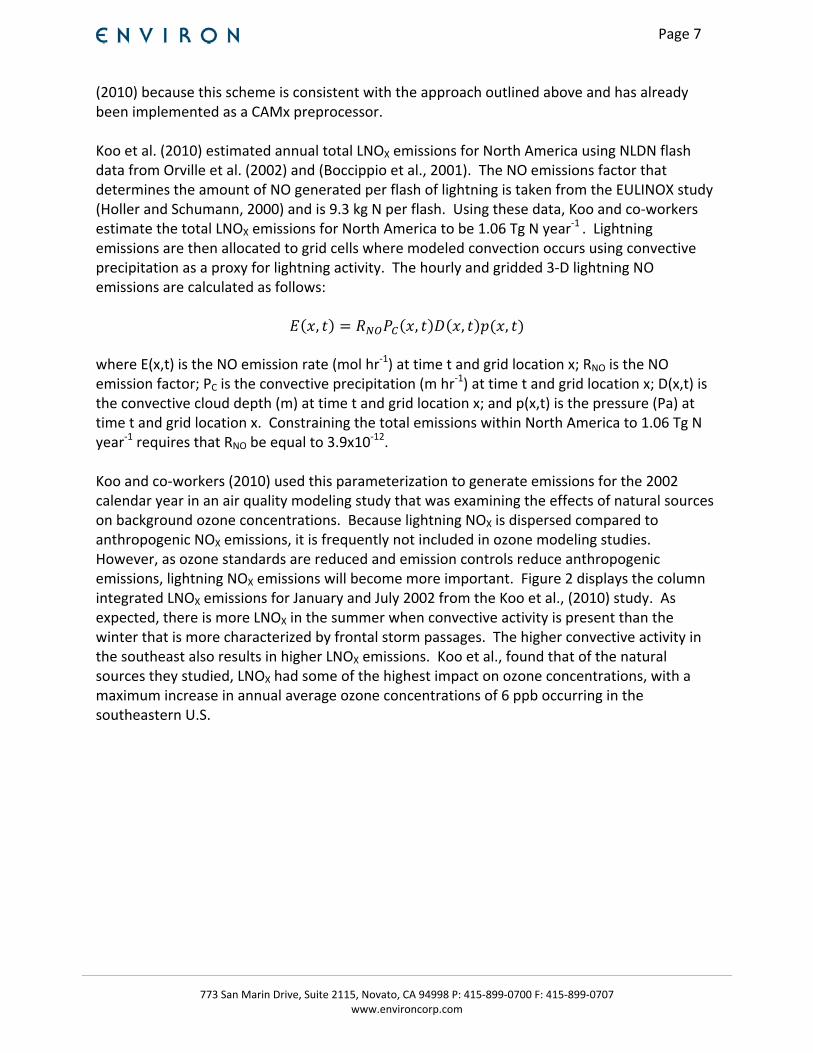
‐12. Koo and co‐workers (2010) used this parameterization to generate emissions for the 2002 calendar year in an air quality modeling study that was examining the effects of natural sources on background ozone concentrations. Because lightning NOX is dispersed compared to anthropogenic NOX emissions, it is frequently not included in ozone modeling studies. However, as ozone standards are reduced and emission controls reduce anthropogenic emissions, lightning NOX emissions will become more important. Figure 2 displays the column integrated LNOX emissions for January and July 2002 from the Koo et al., (2010) study. As expected, there is more LNOX in the summer when convective activity is present than the winter that is more characterized by frontal storm passages. The higher convective activity in the southeast also results in higher LNOX emissions. Koo et al., found that of the natural sources they studied, LNOX had some of the highest impact on ozone concentrations, with a maximum increase in annual average ozone concentrations of 6 ppb occurring in the southeastern U.S.

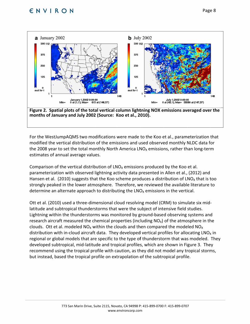
Figure 2.months o

For the Wmodifiedthe 2008estimate ComparisparameteHansen estrongly determin Ott et al.latitude aLightningresearch clouds. Odistributiregional developerecommebut inste

773 Sa

Spatial ploof January a

WestJumpAQd the vertical8 year to set s of annual a

son of the veerization witet al. (2010)peaked in thne an alterna

(2010) usedand subtropg within the aircraft meaOtt et al. moion with in‐cor global moed subtropicend using thead, based th

an Marin Drive,

ots of the totand July 200

QMS two mol distributionthe total moaverage valu

ertical distrith observed suggests thhe lower atmate approach

d a three‐dimical thunderthunderstorasured the codeled NOX wcloud aircrafodels that aral, mid‐latituhe tropical prhe tropical p

Suite 2115, Novwww.e

tal vertical c2 (Source: K

odifications wn of the emisonthly Northues.

bution of LNlightning ac

hat the Koo smosphere. Th to distribu

mensional clrstorms thatrms was monchemical prowithin the clft data. Theyre specific toude and troprofile with caprofile on ext

vato, CA 94998 Penvironcorp.com

column lightKoo et al., 20

were made ssions and uh America LN

NOX emissionctivity data pscheme prodTherefore, wuting the LNO

oud resolvin were the sunitored by goperties (incouds and thy developedo the type ofpical profilesaution, as thtrapolation o

P: 415‐899‐0700 m

tning NOX e010).

to the Koo eused observeNOX emission

ns producedpresented induces a distrwe reviewed OX emissions

ng model (CRubject of integround‐baseluding NOX) hen compared vertical prof thunderstos, which arehey did not mof the subtro

F: 415‐899‐070

emissions av

et al., paramed monthly Nns, rather th

by the Koo Allen et al.,ribution of Lthe availabls in the verti

RM) to simuensive field d observing of the atmoed the modeofiles for alloorm that was shown in Fimodel any tropical profil

Page

7

veraged over

meterization tNLDC data fohan long‐term

et al. , (2012) and NOX that is te literature ical.

ulate six mid‐studies. systems and

osphere in theled NOX ocating LNOX

s modeled. gure 3. Theropical storme.

e 8

r the

that or m

too to

‐

d he

X in They ey ms,

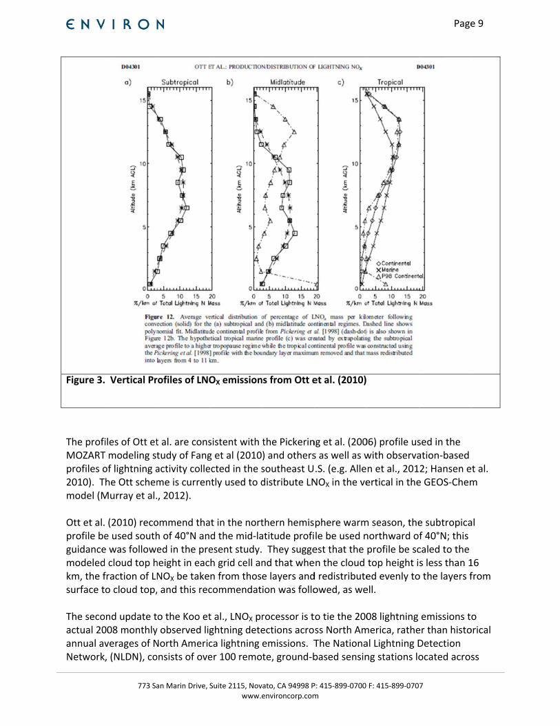
Figure 3.

The profiMOZARTprofiles o2010). Tmodel (M Ott et al.profile beguidancemodeledkm, the fsurface t The secoactual 20annual avNetwork

773 Sa

Vertical Pr

iles of Ott etT modeling stof lightning ahe Ott schemMurray et al.

(2010) recoe used southe was followed cloud top hfraction of LNo cloud top,

ond update t008 monthlyverages of N, (NLDN), co

an Marin Drive,

rofiles of LNO

t al. are constudy of Fangactivity colleme is curren, 2012).

ommend thah of 40°N aned in the preheight in eacNOX be take and this rec

o the Koo ety observed ligNorth Americonsists of ove


OX emission

sistent with g et al (2010ected in the sntly used to d

at in the nortd the mid‐laesent study.h grid cell ann from thoscommendat

t al., LNOX prghtning deteca lightning er 100 remo


ns from Ott e

the Pickerin) and otherssoutheast Udistribute LN

thern hemisatitude profi They suggend that whee layers andion was follo

rocessor is tections acroemissions. Tte, ground‐b

P: 415‐899‐0700 m

et al. (2010)

ng et al. (200s as well as w.S. (e.g. AlleNOX in the ve

phere warmle be used nest that the en the cloud d redistributeowed, as we

to tie the 200ss North AmThe Nationabased sensin

F: 415‐899‐070

06) profile uswith observan et al., 201ertical in the

m season, thenorthward oprofile be sctop height ied evenly toell.

08 lightning merica, ratheal Lightning Dng stations lo

Page

7

sed in the ation‐based 2; Hansen ee GEOS‐Chem

e subtropicaf 40°N; this caled to the s less than 1o the layers f

emissions toer than histoDetection ocated acros

e 9

t al. m

al

16 from

o orical

ss

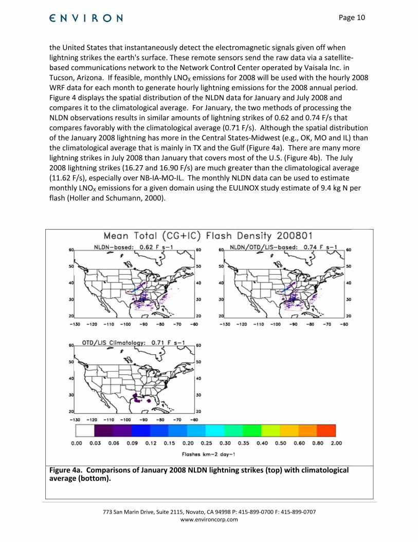
the Unitelightningbased coTucson, AWRF dataFigure 4 compareNLDN obcompareof the Janthe climalightning2008 ligh(11.62 F/monthly flash (Ho

Figure 4aaverage

773 Sa

ed States tha strikes the eommunicatioArizona. If fea for each mdisplays thees it to the clbservations res favorably wnuary 2008 atological av strikes in Juhtning strike/s), especiallLNOX emissi

oller and Sch

a. Comparis(bottom).

an Marin Drive,

at instantaneearth's surfaons network easible, monmonth to genspatial distrimatologicaresults in simwith the climlightning hasverage that isuly 2008 thans (16.27 andy over NB‐IAions for a givumann, 200

sons of Janu


eously detecace. These reto the Netwnthly LNOX enerate hourlyribution of thl average. Fmilar amountmatological as more in ths mainly in Tn January thd 16.90 F/s) aA‐MO‐IL. Thven domain 00).

ary 2008 NL


ct the electremote sensowork Controlemissions fory lightning ehe NLDN datFor January, ts of lightninaverage (0.7e Central StTX and the Ghat covers mare much gre monthly Nusing the EU

LDN lightnin

P: 415‐899‐0700 m

romagnetic sors send thel Center oper 2008 will bemissions forta for Januathe two metng strikes of 71 F/s). Althates‐MidweGulf (Figure 4ost of the Ureater than tNLDN data caULINOX stud

ng strikes (to

F: 415‐899‐070

signals given raw data vierated by Vabe used withr the 2008 ary and July 2thods of pro0.62 and 0.7ough the spest (e.g., OK, 4a). There a.S. (Figure 4the climatoloan be used tdy estimate o

op) with clim

Page

7

n off when a a satellite‐isala Inc. in h the hourly nnual period2008 and ocessing the 74 F/s that atial distribuMO and IL) re many mo4b). The Julyogical averagto estimate of 9.4 kg N p

matological

e 10

‐

2008 d.

ution than ore y ge

per

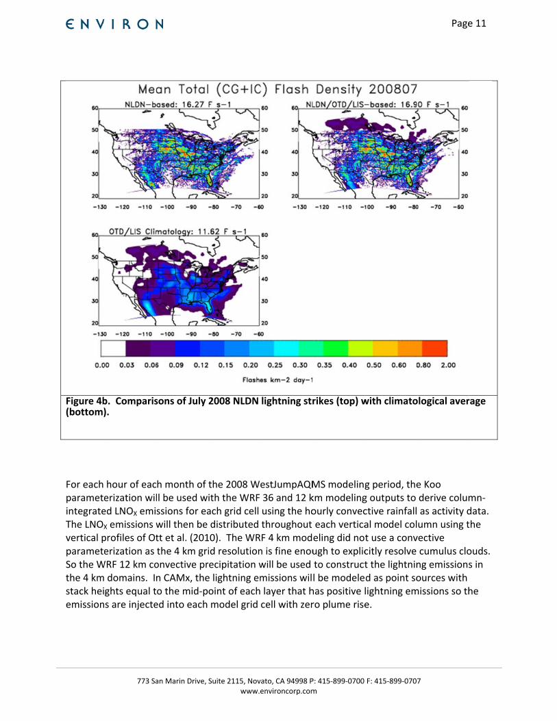
Figure 4b(bottom)

For each parameteintegrateThe LNOX

vertical pparameteSo the Wthe 4 kmstack heiemission

773 Sa

b. Comparis).

hour of eacerization wiled LNOX emi

X emissions wprofiles of Oterization as

WRF 12 km co domains. Ights equal ts are injecte

an Marin Drive,

sons of July

h month of ll be used wssions for eawill then be tt et al. (201the 4 km grionvective prn CAMx, theo the mid‐ped into each


2008 NLDN

the 2008 With the WRF ach grid celldistributed

10). The WRid resolutionrecipitation we lightning emoint of eachmodel grid


lightning str

estJumpAQM36 and 12 kusing the hothroughout F 4 km modn is fine enouwill be used missions wil layer that hcell with zer

P: 415‐899‐0700 m

rikes (top) w

MS modelingkm modelingourly conveceach verticaeling did nough to explicto constructl be modelehas positive lro plume rise

F: 415‐899‐070

with climato

g period, theg outputs to ctive rainfallal model colt use a convcitly resolve t the lightnind as point solightning eme.

Page

7

ological aver

e Koo derive colum as activity dumn using tvective cumulus clong emissionsources with missions so th

e 11

rage

mn‐data. the

ouds. s in

he

Page 12


QUALITY ASSURANCE

Quality assurance (QA) will be performed following the emissions quality assurance protocol developed during WRAP (Adelman, 20042). These procedures include systematic procedures for:

Modeling QA – accuracy assurance and problem identification.

System QA – software and data tracking.

Documentation – tracking QA issues, recording the QA process and report writing.

An emissions QA checklist is developed that delineates each step of the QA process and allows a systematic approach to the QA process to assure critical steps are not overlooked. The completed QA checklists and templates include:

Model configuration settings.

Inventory file log.

Ancillary input file log.

Model execution log.

A series of QA products are produced that are compared to other studies and the expected outcomes:

Spatial plots of emissions by source category.

Annual time series plots of emissions for subregions.

Diurnal time series plots. The emissions QA officer is required to generate, review and distribute the QA products to the modeling team and buy off on the results prior to execution of the air quality model.

2 http://www.epa.gov/ttnchie1/conference/ei13/qaqc/adelman_pres.pdf

Page 13


REFERENCES

Allen, D. J., K. E. Pickering, R. W. Pinder, B. H. Henderson, K. W. Appel, and A. Prados (2012). Impact of lightning‐NO on eastern United States photochemistry during the summer of 2006 as determined using the CMAQ model. Atmos. Chem. Phys., 10, 107–119.

Bey, I., et al. (2001), Global modeling of tropospheric chemistry with assimilated meteorology: Model description and evaluation, J. Geophys. Res., 106, 23,073– 23,096.

Boccippio, D.J., Cummins, K.L., Christian, H.J., Goodman, S.J., 2001. Combined satellite‐ and surface‐based estimation of the intracloud‐cloud‐to‐ground lightning ratio over the continental United States. Mon. Wea. Rev. 129, 108e122.

Boersma, K. F., E. J. Bucsela, E. J. Brinksma, and J. F. Gleason (2002). NO2 in OMI Algorithm Theoretical Basis Document, OMI Trace Gas Algorithms, ATB‐OMI‐04, Version 2.0, vol. 4, edited by K. Chance, NASA Distributed Active Archive Centers, Greenbelt, Md.

Boersma, K. F., H. J. Eskes, and E. J. Brinksma (2004). Error analysis for tropospheric NO2 retrieval from space, J. Geophys. Res., 109, D04311.

Boersma, K. F., D.J. Jacob, E.J. Bucsela, A.E. Perring, R. Dirksen, R.J. van der A, R.M. Yantosca, R.J. Park, M.O. Wenig, T.H. Bertram, R.C. Cohen (2008), Validation of OMI tropospheric NO2 observations during INTEX‐B and application to constrain NOx emissions over the eastern United States and Mexico, Atmos. Env., 42, 4480‐4497.

Boersma, K. F., H. J. Eskes, R. J. Dirksen, R. J. van der A, J. P. Veefkind, et al. (2011a). An improved tropospheric NO2 column retrieval algorithm for the Ozone Monitoring Instrument, Atmos. Meas. Tech., 4, 1905‐1928, doi:10.5194/amt‐4‐1905‐2011.

Boersma, R. Braak, and R. J. van der A (2011b). Dutch OMI NO2 (DOMINO) data product v2.0 HE5 data file user manual. http://www.temis.nl/docs/OMI_NO2_HE5_2.0_2011.pdf.

Bovensmann, H., Burrows, J. P., Buchwitz, M., Frerick, J., Noel, S., Rozanov, V. V., Chance, K. V., and Goede, A. P. H. (1999). SCIAMACHY: Mission Objectives and Measurement Modes, J. Atmos. Sci., 56, 127–150.

Bucsela, E. J., E. A. Celarier, M. O. Wenig, J. F. Gleason, J. P. Veefkind, K. F. Boersma, and E. J. Brinksma (2006). Algorithm for NO2 vertical column retrieval from the Ozone Monitoring Instrument, IEEE Trans. Geosci. Remote Sens., 44, 1245– 1258.

Bucsela, E. J., Perring, A. E., Cohen, R. C., Boersma, K. F., Celarier, E. A. Gleason, J. F., Wenig, M. O., Bertram, T. H., Wooldridge, P. J., Dirksen, R., and Veefkind, J. P. (2008)., Comparison of tropospheric NO2 from in‐situ aircraft measurements with near‐real time and standard product data from OMI, J. Geophys. Res., 113, D16S31.

Bucsela, E., Lamsal, L., Celarier, E., Krotkov, N., Swartz, W., Bhartia, P., and Gleason, J., (2011). New algorithm for satellite NO2 retrievals: Tropospheric results. Presentation at the AGU Fall Meeting.

DeLeeuw, G., Neele, F., Hill, M., Smith, M., and Vignati, E. 2000. “Production of sea spray aerosol in the surf zone.” J. Geophys. Res., 105, p. 29397.

Page 14


Emmons, L. K., S. Walters, P. G. Hess, J.‐F. Lamarque, G. G. Pfister, D. Fillmore, C. Granier, A. Guenther, D. Kinnison, T. Laepple, J. Orlando, X. Tie, G. Tyndall, C. Wiedinmyer, S. L. Baughcum, and S. Kloster, (2010), Description and evaluation of the Model for Ozone and Related Tracers, version 4 (MOZART‐4), Geosci. Model Dev., 3, 43–67.

Fang, Y., A. M. Fiore, L. W. Horowitz, H. Levy II, Y. Hu, and A. G. Russell, (2010), Sensitivity of the NOy budget over the United States to anthropogenic and lightning NOx in summer. J. Geophys. Res., 115, D18312.

Fitzgerald, J.W. 1975. “Approximation formulas for the equilibrium size of an aerosol particle as a function of its dry size and composition and the ambient relative humidity.” Journal of Applied Meteorology, 14, 1044–1049.

Gong, S.L., L.A. Barrie, and M. Lazare. 2002. “Canadian Aerosol Module (CAM): A size‐segregated simulation of atmospheric aerosol processes for climate and air quality models. 2. Global sea‐salt aerosol and its budgets.” J. Geophys. Res., 107(D24), 4779, doi:10.1029/2001JD002004.

Gong, S.L. 2003. “A parameterization for sea‐salt aerosol source function for sub‐ and super‐micron particle sizes.” Biogeochemical Cycles, 17, 1097‐1104.

Grini, A., G. Myhre, J.K. Sundet, I.S.A. Isaksen. 2002. “Modeling the Annual Cycle of Sea Salt in the Global 3D Model Oslo CTM2: Concentrations, Fluxes, and Radiative Impact.” J. Climate, 15, 1717–1730.

Guelle, W., M. Schulz, and Y. Balkanski. 2001. “Influence of the source formulation on modeling the atmospheric global distribution of sea salt aerosol.” J. Geophys. Res., 106, 27,509– 27,524.

Hansen, D. A., E. S. Edgerton, B. E. Hartsell, J. J. Jansen, N. Kandasamy, G. M. Hidy, and C. L. Blanchard (2003), The southeastern aerosol research and characterization study. Part 1: Overview, J. Air Waste Manage. Assoc., 53, 1460–1471.

Hansen, A., H. E. Fuelberg and K. E. Pickering, (2010), Vertical distributions of lightning sources and flashes over Kennedy Space Center, Florida. J. Geophys. Res., 115, D14203.

Herron‐Thorpe, F. L., Lamb, B. K., Mount, G. H., and Vaughan, J. K. (2010). Evaluation of a regional air quality forecast model for tropospheric NO2 columns using the OMI/Aura satellite tropospheric NO2 product. Atmos. Chem. Phys., 10, 8839–8854.

Holler, H., Schumann, U., 2000. EULINOX (European Lightning Nitrogen Oxides Project) final report. http://www.pa.op.dlr.de/eulinox/publications/finalrep/index.html.

Koo, B., Chien, C.‐J., Tonnesen, G., Morris, R., Johnson, J., Sakulyanontvittaya, T., Piyachaturawat, P., and Yarwood, G.: Natural emissions for regional modeling of background ozone and particulate matter and impacts on emissions control strategies, Atmos. Environ., 44, 2372–2382., doi:10.1016/j.atmosenv.2010.02.041, 2010.

Koshak, W. J., Peterson, H. S., McCaul, E. W., and Biazar, A., (2010). Estimates of the lightning‐NOx profile in the vicinity of the North Alabama Lightning Mapping Array, 21st International Lightning Detection Conference (ILDC)/Vaisala, 18–22 April 2010, Orlando, FL, United States, NASA Technical Report Document 20100021055.

Page 15


Lamsal, L. N., R. V. Martin, A. van Donkelaar, M. Steinbacher, E. A. Celarier, E. Bucsela, E. J. Dunlea, and J. P. Pinto (2008), Ground‐level nitrogen dioxide concentrations inferred from the satellite‐borne Ozone Monitoring Instrument, J. Geophys. Res., 113, D16308.

Lamsal, L. N., Martin, R. V., van Donkelaar, A., Celarier, E. A., Bucsela, E. J., Boersma, K. F., Dirksen, R., Luo, C., and Wang, Y. (2010). Indirect validation of tropospheric nitrogen dioxide retrieved from the OMI satellite instrument: Insight into the seasonal variation of nitrogen oxides at northern midlatitudes, J. Geophys. Res., 115, D0530.

Lee, D.S., Kohler, I., Grobler, E., Rohrer, F., Sausen, R., Gallardo‐Klenner, L., Olivier, J.G. J., Dentener, F.J., Bouwman, A.F., 1997. Estimations of global NOx emissions and their uncertainties. Atmos. Environ. 31 (12), 1735.

Leue, C., Wenig, M., Wagner, T., Klimm, O., Platt, U., and Jahne, B. (2001). Quantitative analysis of NOx emissions from Global Ozone Monitoring Experiment satellite image sequences, J. Geophys. Res., 106, 5493–5505.

Liao, H., J.H. Seinfeld, P.J. Adams, and L.J. Mickley. 2004. “Global radiative forcing of tropospheric ozone and aerosols in a unified general circulation model.” J. Geophys. Res., 109, D16207, doi:10.1029/2003JD004456.

Martin, R. V., D. J. Jacob, K. Chance, T. P. Kurosu, P. I. Perner, and M. J. Evans (2003), Global inventory of nitrogen oxide emission constrained by space‐based observations of NO2columns, J. Geophys. Res., 108(D17), 4537.

Monahan, E.C., D. Spiel, K. Davidson. 1986. “A model of marine aerosol generation via whitecaps and wave disruption.” In Oceanic Whitecaps and Their Role in Air‐Sea Exchange, E.C. Monahan and G. Mac NioCaill (Eds.), 167‐174.

Murray, Lee T., D. Jacob , J. A. Logan, R. Hudman, and W. Koshak (2012)., Optimized regional and interannual variability of lightning in a global chemical transport model constrained by LIS/OTD satellite data. Submitted to J. Geophys. Res.

OMI Team (2012), The OMI Data User’s Guide. http://disc.sci.gsfc.nasa.gov/Aura/additional/documentation/README.OMI_DUG.pdf.

Orville, R.E., Huffines, G.R., Burrows, W.R., Holle, R.L., Cummins, K.L., 2002. The North American Lightning Detection Network (NALDN)‐first results: 1998e2000. Mon. Wea. Rev. 130, 2098‐2109.

Ott, L. E., K. E. Pickering, G. L. Stenchikov, D. J. Allen, A. J. DeCaria, B. Ridley, R.‐F. Lin, S. Lang, and W.‐K. Tao (2010), Production of lightning NOx and its vertical distribution calculated from three‐dimensional cloud‐scale chemical transport model simulations, J. Geophys. Res., 115, doi:10.1029/2009JD011880.

Pickering, K. E., et al. (2006), Using results from cloud‐resolving models to improve lightning NOx parameterizations for global chemical transport and climate models, Eos Trans. AGU, 87(52), Fall Meet. Suppl., Abstract A52B‐05.

Price, C., and D. Rind (1992), A simple lightning parameterization for calculating lightning distributions, J. Geophys. Res. 97, 9919–9933.

Page 16


Price, C., and D. Rind (1993), What determines the cloud‐to‐ground lightning fraction in thunderstorms, Geophys. Res. Lett., 20(6), 463–466.

Price, C., and D. Rind (1994), Modeling global lightning distributions in a general‐circulation model, Mon. Weather Rev., 122(8), 1930–1939.

Sauvage, B., R. V. Martin, A. van Donkelaar, X. Liu, K. Chance, L. Jaeglé, P. I. Palmer, S. Wu, and T. M. Fu (2007), Remote sensed and in situ constraints on processes affecting tropical tropospheric ozone, Atmos. Chem. Phys., 7, 815–838.

Schumann, U., Huntrieser, H., 2007. The global lightning‐induced nitrogen oxides source. Atmos. Chem. Phys. Discuss. 7, 2623‐2818.

Smith, M.H. and Harrison, N.M. 1998. “The Sea Spray Generation Function.” J. Aerosol. Sci., 29, S189‐S190.

Tost, H., P. J. Joeckel, and J. Lelieveld (2007), Lightning and convection parameterisations ‐ uncertainties in global modeling, Atmos. Chem Phys., 7(17), 4553–4568.

Zhang, X., Helsdon, J.J.H., Farley, R.D., 2003a. Numerical modeling of lightning produced NOx using an explicit lightning scheme: 1. Two‐dimensional simulation as a ‘proof of concept’. J. Geophys. Res. 108 (D18) ACH 5‐1‐ACH 5‐20.

Zhang, X., Helsdon, J.J.H., Farley, R.D., 2003b. Numerical modeling of lightning produced NOx using an explicit lightning scheme: 2. Three‐dimensional simulation and expanded chemistry. J. Geophys. Res. 108 (D18) ACH 6‐1‐ACH 6‐17.

Documents

TECHNICAL MEMORANDUM No. SEA SALT AND LIGHTNING …