Embed Size (px)
Citation preview
I N S T I T U T E F O R D E F E N S E A N A L Y S E S
IDA Document D-4082
August 2010
Carl A. Curling Julia K. Burr
Lusine DanakianDeena S. DisraellyLucas A. LaViolet
Terri J. WalshRobert A. Zirkle
Log: H 10-000898
Technical Reference Manual: NATO Planning Guide for the
Estimation of Chemical, Biological, Radiological, and Nuclear (CBRN)
Casualties, Allied Medical Publication-8(C)
Approved for public release;distribution is unlimited.

About This PublicationThis work was conducted by the Institute for Defense Analyses (IDA)under contract DASW01-04-C-0003,Task CA-6-3079, “CBRN Casualty Estimation Update of the Medical CBRN Defense Planning and Response Project,” for the Joint Staff, Joint Requirements Office for CBRN Defense and the U.S. Army Office of the Surgeon General. The views, opinions, and findings should not be construed as representing the official position of either the Department of Defense or the sponsoring organization.
AcknowledgmentsThe authors wish to thank Ms. Mary Catherine Flythe, Dr. Jeffrey Grotte, Mr. David Hockaday, and Mr. Preston J. Lee for their contributions to the methodology documented in this Technical Reference Manual. The authors are also grateful to Dr. John Bombardt and Dr. James Heagy for their careful review of this document, to Ms. Elizabeth Johnson for editing this document, and to Ms. Barbara Varvaglione for producing this document.
Copyright Notice© 2010 Institute for Defense Analyses4850 Mark Center Drive, Alexandria, Virginia 22311-1882 • (703) 845-2000.
This material may be reproduced by or for the U.S. Government pursuantto the copyright license under the clause at DFARS 252.227-7013 (NOV 95).
The Institute for Defense Analyses is a non-profit corporation that operates three federally funded research and development centers to provide objective analyses of national security issues, particularly those requiring scientific and technical expertise, and conduct related research on other national challenges.
I N S T I T U T E F O R D E F E N S E A N A L Y S E S
IDA Document D-4082
Carl A. Curling Julia K. Burr
Lusine DanakianDeena S. DisraellyLucas A. LaViolet
Terri J. WalshRobert A. Zirkle
Technical Reference Manual: NATO Planning Guide for the
Estimation of Chemical, Biological, Radiological, and Nuclear (CBRN)
Casualties, Allied Medical Publication-8(C)

iii
Executive Summary
The Technical Reference Manual (TRM) serves as a supplement to the North Atlantic Treaty Organization (NATO) Allied Medical Publication-8(C) (AMedP-8(C)), NATO Planning Guide for the Estimation of CBRN [Chemical, Biological, Radiological, and Nuclear] Casualties (referred to in this document as AMedP-8(C)). The TRM documents the development process, analyses, rationale, underlying data, and additional information utilized to establish the environments, the human response, and the casualty estimation methodologies which comprise the AMedP-8(C) methodology. The IDA study team devised a “General Equation” to calculate the environments, by converting an exposure environment to a dose, dosage, or insult and allowing for the consideration of breathing rates, shielding, and personal protection, among other factors. The human response and casualty estimation methodologies employ profiles of injury severity over time to describe the human response to agents and effects and then result in an estimate of the casualty’s status.
AMEDP-8 (C) Background AMedP-8(C) presents a methodology for estimating casualties uniquely occurring as
a consequence of Chemical, Biological, Radiological and Nuclear (CBRN) attacks against Allied targets to support the planning processes described elsewhere in Allied publications. The AMedP-8(C) methodology provides the capability to estimate the numbers of casualties over time, as well as the incidence of injury by type and severity for a wide range of agents and effects. It can be used to estimate casualties resulting from exposure to chemical nerve agents sarin (GB) and VX; chemical blister agent HD (distilled mustard); the biological agents causing anthrax, botulism, pneumonic plague, smallpox, and Venezuelan equine encephalitis; radiological dispersal devices; radioactive fallout from nuclear explosions; and prompt nuclear effects. As the AMedP-8(C) NATO Planning Guide explains:
These estimates assist planners, logisticians, and staff officers by allowing for more effective quantification of contingency requirements for medical personnel; medical materiel stockpiles; patient transport or evacuation capabilities; and facilities needed for patient decontamination, triage, treatment, and supportive care. The AMedP-8(C) methodology is proposed solely for use in deliberative or crisis action planning and does not account for real-time or dynamic (i.e., evolving exposure) use. Moreover, this

iv
methodology is not intended for use in deployment health surveillance or for any post-event uses including diagnosis, medical treatment, or epidemiology.
Purpose The purpose of the Technical Reference Manual is to describe the information
presented in or used to develop the components of the AMedP-8(C) methodology. The TRM will:
• Describe the sources for, and justification of, the assumptions and recommended values employed by the methodology;
• Identify, where appropriate, the sources for definitions and key terms used by the methodology, or else describe where and how new definitions and terms were derived;
• Describe the underlying symptomatology resulting from the exposure to each agent or effect used in the methodology;
• Explain how the key underlying equations and parameters employed by the methodology—such as dose, dosage, and insult ranges; dose, dosage, or insult calculations; the radiation time-to-death equation and protracted dose factors for radiological agents; infectivity, incubation, and lethality probability functions and parameters for biological agents; the non-contagious biological agent tables; and the contagious biological agent equations—were derived; and
• Describe how the injury profiles for all chemical, radiological, and nuclear agents and effects were derived.
The goal of the TRM is to make the data underlying the AMedP-8(C) methodology and the process through which it was developed as clear as possible and to enable analysts and modelers to understand and replicate these results and procedures.
Organization This Technical Reference Manual is comprised of the following chapters, which
align closely with the chapters found in the AMedP-8(C) NATO Planning Guide.
Chapter 2 corresponds to AMedP-8(C) Chapter 1, “Introduction,” and discusses the basis for the definitions used in the NATO document as well as the assumptions and limitations with associated rationales for the document.
Chapter 3 corresponds to AMedP-8(C) Chapter 2, “Calculating Dose/Dosage/Insult,” and details the values and processes utilized to calculate the dose/dosage/insult from the CBRN environment.
Chapters 4 through 8 correspond to AMedP-8(C) Chapter 3, “Human Response Estimation,” and detail the derivations of the human response methodologies for

v
chemical nerve agents GB and VX; chemical blister agent HD; radiological agents; nuclear effects; and contagious and non-contagious biological agents, respectively.
Chapter 9 corresponds to AMedP-8(C) Chapter 4, “Casualty Estimation and Reporting,” and provides additional information on the casualty estimation procedures as well as casualty estimation conditions and equations specific to particular agents and insults.
Chapter 10 provides a brief review of the study’s conclusions and presents implementation considerations and potential ways ahead.

vii
Contents
1. Introduction .................................................................................................................1
A. Introduction .........................................................................................................1
B. Purpose ................................................................................................................2 C. Background .........................................................................................................3
D. Organization ........................................................................................................8
2. Applicable Definitions, Assumptions, Limitations, and Rationale of the AMedP-8(C) Methodology .....................................................................................................11 A. Introduction .......................................................................................................11
B. Definitions .........................................................................................................11 1. Definitions Derived from NATO References .............................................11 2. Definitions Specific to AMedP-8(C) Terminology .....................................13
C. Assumptions, Limitations, and Rationale..........................................................20
1. General Assumptions and Limitations ........................................................20 2. CRN Assumptions and Limitations .............................................................22 3. Chemical Assumptions and Limitations ......................................................24 4. Radiological Assumptions and Limitations ................................................28 5. Nuclear Assumptions and Limitations ........................................................30 6. Biological Assumptions and Limitations ....................................................32
3. Calculation of Dose/Dosage/Insult ............................................................................39 A. Introduction .......................................................................................................39
B. Approach ...........................................................................................................40 1. Background .................................................................................................40 2. Derivation of the General Equation .............................................................41
C. Agent-Specific Considerations ..........................................................................48
1. Exposure Factors .........................................................................................48 2. Shielding Factors .........................................................................................50 3. Respiratory Protection Factors ....................................................................53 4. Dose/Dosage/Insult .....................................................................................54
4. Chemical Human Response Review: Nerve Agents—Sarin and VX .......................61 A. Introduction .......................................................................................................61
B. Background .......................................................................................................61 1. Agent Physiological Effects ........................................................................61 2. Toxicity Values ...........................................................................................63
C. Dose/Dosage Ranges .........................................................................................64
D. Symptoms ..........................................................................................................72
viii
1. Severity Levels ............................................................................................72 2. Symptom Progression and Injury Profiles...................................................75
5. Chemical Human Response Review: Blister Agent—Distilled Mustard ..................99 A. Introduction .......................................................................................................99
B. Background .......................................................................................................99
1. Agent Physiological Effects ........................................................................99 2. Toxicity Values .........................................................................................102
C. Dosage Ranges ................................................................................................103 D. Symptoms ........................................................................................................110
1. Severity levels ...........................................................................................111 2. Symptom Progression and Injury Profiles.................................................113
6. Ionizing Radiation Human Response Review: Radiological Agents ......................121 A. Introduction .....................................................................................................121
B. Background .....................................................................................................122 1. Physiological Effects .................................................................................122 2. Toxicity Values .........................................................................................125
C. Dose Ranges ....................................................................................................125
D. Symptoms ........................................................................................................128 1. Injury Severity Levels ...............................................................................128 2. Injury Profiles ............................................................................................130 3. Radiological Injury Profiles ......................................................................140
7. Nuclear Human Response Review: Composite Nuclear Insults .............................143 A. Introduction .....................................................................................................143
B. Background .....................................................................................................143
1. Whole-Body Radiation ..............................................................................144 2. Blast ...........................................................................................................144 3. Thermal Energy .........................................................................................148 4. Combined Injury ........................................................................................150
C. Dose/Insult Ranges ..........................................................................................151 D. Symptoms ........................................................................................................155
1. Injury Severity Levels ...............................................................................156 2. Radiation, Blast, and Thermal Individual Insult Injury Profiles ...............159 3. Composite Nuclear Injury Profiles ............................................................172
8. Biological Agent Human Response Review: Non-Contagious and Contagious Diseases ...................................................................................................................177
A. Introduction .....................................................................................................177
B. Background .....................................................................................................177 C. Methodology Development .............................................................................177
1. Infectivity/Effectivity ................................................................................179 2. Incubation Period (Latent Period/Time to Onset) .....................................179 3. Lethality .....................................................................................................180 4. Duration of Illness .....................................................................................180 5. Injury Profile .............................................................................................180

ix
6. Medical Countermeasures—Vaccination/Antibiotic Prophylaxis ............181 7. Literature Review and Parameter Development .......................................181 8. Non-Contagious and Contagious Biological Agent Human Response .....182
D. Estimation of Non-Contagious Biological Agent Human Response ..............183 1. Convolution Approach ..............................................................................184 2. Anthrax ......................................................................................................188 3. Botulism ....................................................................................................203 4. Venezuelan Equine Encephalitis (VEE) ....................................................212
E. Contagious Biological Agent Human Response .............................................219
1. Derivation of the Susceptible-Exposed and infected-Infectious-Removed-Prophylaxis efficacious (SEIRP) Approach ..............................................220
2. SEIRP Approach .......................................................................................223 3. Plague ........................................................................................................228 4. Smallpox ....................................................................................................239
9. Casualty Estimation .................................................................................................257 A. Estimation of Casualties: General Considerations ..........................................257
1. Recommended Time to Reach a Medical Treatment Facility ...................257 2. Recommended Wounded in Action (WIA) Severity Level Threshold .....257 3. Time at Severity Level 4 (“Very Severe”) to Determine Fatalities ..........258
B. Estimation of Casualties: Special Considerations ...........................................259
1. Chemical Blister Agent (HD): Percutaneous Liquid Dose and Internal Sepsis .........................................................................................................259
2. Radiological Agents: Whole-Body Radiation Dose and the Protracted Dose Calculation.................................................................................................259
3. Radiological Agents and Radiation Insults: Whole-Body Radiation and the Time-to-Death Calculation ........................................................................263
4. Nuclear Blast Insults: Tertiary Blast Effects and Killed in Action (KIA) 268 5. Non-Contagious Biological Agents ...........................................................271 6. Contagious Biological Agents ...................................................................272
10. Conclusions .............................................................................................................275
x
Appendices
A. Abbreviations ............................................................................................................. A-1
Abbreviations ......................................................................................................... A-1 Symbols .................................................................................................................. A-6
B. Glossary of Medical Terms .........................................................................................B-1
C. References ...................................................................................................................C-1 D. Illustrations................................................................................................................. D-1
Figures .................................................................................................................... D-1 Tables ..................................................................................................................... D-4
1
1. Introduction
A. Introduction The North Atlantic Treaty Organization (NATO) has produced a series of Allied
Medical Publications (AMedP) on chemical, biological, radiological, and nuclear (CBRN) planning and casualty estimation. Allied Medical Publication-8 (AMedP-8) Nuclear1 was the published methodology for estimating Chemical, Biological, Radiological and Nuclear (CBRN) casualties. Several CBRN-related standardization agreements and documents followed. In 1999, AMedP-8(A) Chemical2 was published and it documented casualty estimates for chemical casualties and fatalities resulting from exposure to the nerve agents sarin (GB) and VX and the blister agent distilled mustard (HD). The publication of AMedP-8(B) Biological3
In 2010, a new version of the North Atlantic Treaty Organization (NATO) Allied Medical Publication-8 (i.e., AMedP-8(C), NATO Planning Guide for the Estimation of CBRN [Chemical, Biological, Radiological, and Nuclear] Casualties, referred to in this document as AMedP-8(C)), was distributed for ratification to the Allied Nations. This Technical Reference Manual (TRM) supplements the AMedP-8(C) by documenting the development process, rationales, underlying data, and additional information utilized to establish the calculation of the environments, and the human response and casualty estimation methodologies which comprise the AMedP-8(C) methodology. The IDA Study team devised a “General Equation” to calculate the environments by converting an exposure environment to a dose, dosage, or insult and allows for the consideration of breathing rates, shielding, and personal protection, among other factors. The human response and casualty estimation methodologies employ profiles of injury severity over time to describe the human response to agents and insults and then result in an estimate of the casualty’s status.
followed shortly thereafter, describing the processes for estimating biological casualties resulting from exposure to biological agents of military concern.
1 North Atlantic Treaty Organization (NATO), AMedP-8(A), Volume I: Medical Planning Guide of NBC
Battle Casualties (Nuclear), STANAG 2475 (AMedP-8(A) Nuclear) (2002). 2 NATO, AMedP-8(A), Volume III: Medical Planning Guide of NBC Battle Casualties (Chemical),
STANAG 2477 (AMedP-8(A) Chemical) (2005). 3 NATO, AMedP-8(B), Volume II: Medical Planning Guide of CBRN Battle Casualties (Biological),
STANAG 2476 (AMedP-8(B) Biological) (2007).

2
B. Purpose As stated in the AMedP-8(C) NATO Planning Guide, the purpose of that document
is to:
...provide a methodology for estimating casualties uniquely occurring as a consequence of CBRN attacks against Allied targets in order to support the planning processes in Allied Joint Publication 3.8 (AJP-3.8), Allied Joint Doctrine for NBC Defence,4 Allied Joint Publication 4.10 (AJP-4.10), Allied Joint Medical Support Doctrine,5 Allied Joint Medical Publication 1 (AJMedP-1), Allied Joint Medical Planning Doctrine,6 and Allied Medical Publication 7 (AMedP-7), Concept of Operations of Medical Support in Chemical, Biological, Radiological, and Nuclear Environments.7 The methodology provides the capability to estimate the numbers of casualties over time as well as the incidence of injury by type and severity. These estimates assist planners, logisticians, and staff officers by allowing for more effective quantification of contingency requirements for medical personnel; medical materiel stockpiles; patient transport or evacuation capabilities; and facilities needed for patient decontamination, triage, treatment, and supportive care… [The AMedP-8(C) methodology] is proposed solely for use in deliberative or crisis action planning and does not account for real-time or dynamic (i.e., evolving exposure) use. Moreover, this methodology is not intended for use in deployment health surveillance or for any post-event uses including diagnosis, medical treatment, or epidemiology.8
The purpose of this TRM is to describe the information presented in or used to develop the components of the methodology described in AMedP-8(C). The TRM document will:
• Describe the sources for, and justification of, the assumptions and recommended values employed by the methodology;
• Identify, where appropriate, the sources for definitions and key terms used by the methodology, or else describe where and how new definitions and terms were derived;
• Describe the underlying symptomatology resulting from the exposure to each agent or effect used in the methodology;
• Explain how the key underlying equations and parameters employed by the methodology—such as dose, dosage, and insult ranges; dose, dosage, or insult
4 NATO, AJP-3.8(B): Allied Joint Doctrine for NBC Defence, STANAG 2451 (5 February 2004). 5 NATO, AJP-4.10(A): Allied Joint Medical Support Doctrine, STANAG 2228 (3 March 2006). 6 NATO, AJMedP-1: Allied Joint Medical Planning Doctrine, STANAG 2542 (3 November 2009). 7 NATO, AMedP-7(D): Concept of Operations of Medical Support in Chemical, Biological,
Radiological, and Nuclear Environments, STANAG 2873 (6 December 2007). 8 NATO, AMedP-8(C): NATO Planning Guide for the Estimation of Chemical, Biological, Radiological,
and Nuclear (CBRN) Casualties Ratification Draft 1, DRAFT (February 2010), 1-1.

3
calculations; the time-to-death equation and protracted dose factors for radiological agents; infectivity, incubation, and lethality probability functions and parameters for biological agents; the non-contagious biological agent tables; and the contagious biological agent equations—were derived; and
• Describe how the injury profiles for all chemical, radiological, and nuclear (CRN) agents and effects were derived.
The goal is to make the data underlying the components of the AMedP-8(C) methodology and the process through which it was developed as clear as possible and to enable analysts and modelers to understand and replicate these results and procedures.
C. Background The human response and casualty estimation methodologies developed for the
AMedP-8(C) methodology incorporate three different agent-specific approaches to provide an estimate of casualties occurring as a consequence of CBRN attacks against military targets for planning purposes. The three approaches all develop user-defined, time-based casualty and fatality estimates based on descriptions of the significant underlying signs and symptoms and their changing severity over time.
Previous versions of AMedP-8 used different casualty estimation methodologies. When applicable, these methodologies helped provide the basis for the AMedP-8(C) methodology.
The earlier AMedP-8 nuclear methodology relied on an approach developed as part of the Intermediate Dose Program (IDP) by Pacific Sierra Research Corporation (PSR), under contract to the Defense Nuclear Agency (DNA). This methodology is based on a model developed by PSR which correlates the severity of signs and symptoms resulting from acute radiation doses in six physiological systems to performance and publishes the correlation over time as a set of dose-responses.9 Subsequently, Technico Southwest, Inc. used the same methodology to develop dose-responses detailing the results of blast and thermal injury. Then, using a team of subject matter experts (SMEs), Technico Southwest, Inc. used the initial individual insult—radiation, blast, and thermal—dose-responses to generate combined injury profiles and the associated combined injury performance values. These performance values are the basis for the Combined algorithms10 which were then incorporated into the Consolidated Human Response Nuclear Effects Model (CHRNEM) combined injury software tool.11
9 George H. Anno et al., “Symptomatology of Acute Radiation Effects in Humans After Doses of 0.5 to
30 Gy,” Health Physics 56, no. 6 (June 1989): 821–38.
10 Combined is an executable program which uses a specific set of stand-alone algorithms and references the individual R-B-T and combined performance values to calculate the performance over time
4
The IDP methodology was modified for use with chemical agents as well and incorporated into the DNA Improved Casualty Estimation (DICE) tool to estimate human performance.12
For biological agent human response modeling in previous versions of AMedP-8, two different methodologies were used to determine the severities associated with each agent exposure. For Francisella tularensis (tularemia), staphylococcal enterotoxin B (SEB), and Coxiella burnetti (Q fever), PSR used clinical data from military research volunteers who participated in vaccination efficacy studies during the 1950s and 1960s. The clinical records provided data which were used to generate time- and dose-dependent febrile models. Performance algorithms based on the febrile models were derived from physical and cognitive test results from the research volunteers.
The DICE algorithms use the signs and symptoms resulting over time from a single exposure to a chemical insult to determine human performance and were employed in earlier versions of AMedP-8.
13
The Knowledge Acquisition Matrix Instrument (KAMI)
14
resulting from combined R-B-T insults identified as inputs to the program. Although Combined can be run independently, it has also been incorporated into the CHRNEM tool.
was used to gather information about bioagents for which only limited human response data were available. In 1998, surveys were distributed to SMEs who had experience and/or knowledge from animal studies, accidental exposures, vaccine development, and other sources regarding anthrax, plague, botulism, and Venezuelan Equine Encephalitis (VEE). Disease models were designed based on SME consensus regarding agent infectivity, lethality, pathology, and times to onset and death or recovery. KAMI was revised in 1999 to achieve similar consensus about smallpox, brucellosis, and glanders. Illness category tables were generated for each agent, including dose bands and the expected signs and symptoms associated with the given band. Onset times, incidence of infection, and, for some agents, limited symptoms are included in the tables for the KAMI derived agents. Most of the KAMI agent dose ranges are qualitative, rather than being selected based on infectious dose or lethal dose percentages.
11 Sheldon G. Levin, The Effect of Combined Injuries from a Nuclear Detonation on Soldier Performance, DNA-TR-92-134 (Alexandria, VA: Defense Nuclear Agency, 1993).
12 Arthur P. Deverill and Dennis F. Metz, Defense Nuclear Agency Improved Casualty Estimation (DICE) Chemical Insult Program Acute Chemical Agent Exposure Effects,DNS-TR-93-162 (Washington, DC: Defense Nuclear Agency, May 1994).
13 George H. Anno and Arthur P. Deverill, Consequence Analytic Tools for NBC Operations Volume 1: Biological Agent Effects and Degraded Personnel Performance for Tularemia, Staphylococcal Enterotoxin B (SEB) and Q Fever, DSWA-TR-97-61-V1 (Washington, DC: Defense Special Weapons Agency, October 1998).
14 George H. Anno et al., Biological Agent Exposure and Casualty Estimation: AMedP-8 (Biological) Methods Report, GS-35F-4923H (Fairfax, VA: General Dynamics Advanced Information Systems, May 2005).
5
In the course of developing the AMedP-8(C) methodology from these existing methodologies, several meetings were held to gather the inputs of recognized subject matter experts (SMEs) in each subject area. At the chemical, radiological, and nuclear meetings, groups of international SMEs discussed and reached concurrence on both the symptom severity level descriptions relevant to each physiological system and the symptom progression maps proposed for use in the AMedP-8(C) methodology. At the biological human response meeting, after SMEs reviewed and discussed the use of the five submodels to represent the biological agent injury profile and provide the basis for the underlying proposed methodology, a consensus approval on the use of these submodels was reached. The details of the four agent-specific meetings, including the dates, locations, and participating SMEs are provided below.
The following SMEs were present at the April 21-22, 2008 chemical human response meeting in Munich, Germany:
• Canada
– Thomas Sawyer, Defence Research & Development Canada (DRDC) Suffield
– Ronald J. Wojtyk, Directorate of Health Sciences, Canadian Forces Health Services Group Headquarters
• Finland
– Tapio Kuitunen, Centre for Military Medicine, Medical BL Defence & Environmental Unit
• France
– Fredric Durandeu, Centre de Recherches du Service Santé des Armées, Ministry of Defence (CRSSA – MOD) French Republic, Toxicology
• Germany
– Major Nadine Aurbek, Bundeswehr Institute of Pharmacology and Toxicology
– Stefan Hotop, Elektroniksystem und Logistik-GmbH (ESG) – Jacob Rieck, ESG – Franz Worek, Bundeswehr Institute of Pharmacology and Toxicology
• Great Britain
– Lieutenant Colonel David C. Bates, Defence Medical Services Department, United Kingdom Ministry of Defence (MODUK)
– Paul Rice, Dstl Porton Down, Biomedical Sciences Department
6
• Netherlands
– Paul Brasser, The Netherlands Organization (TNO) Defence, Safety and Security
– Marijke Valstar, Ministry of Defense Netherlands, Military Health Care Expertise Co-ordination Centre
– Herman Van Helden, TNO Defence, Safety and Security – Major George Van Leeuwen, Ministry of Defense Netherlands, CBRN
Expertise Centre
• United States
– Major Kevin G. Hart, Office of The Surgeon General (OTSG), U.S. Army – Lieutenant Commander Thomas C. Herzig, Bureau of Medicine and
Surgery, Future Plans & Strategies – Colonel James M. Madsen, USA Medical Research Institute of Chemical
Defense (USAMRICD) – Major William M. Pramenko, Joint Chiefs of Staff (JCS/J-8/JRO-CBRND) – Sharon A. Reutter-Christy, Edgewood Chemical Biological Center – Jason Rodriguez, Applied Research Associates, Inc. – Lieutenant Colonel Richard Schoske, U.S. Air Force Surgeon General’s
Office – James O. Smith, OTSG, U.S. Army – Douglas R. Sommerville, Edgewood Chemical Biological Center
The following SMEs were present at both the June 23-25, 2008 nuclear and the June 26, 2008 radiological human response meetings in Albuquerque, New Mexico, USA:
• Canada
– Commander Ian Torrie, Canadian Forces Health Services Group Headquarters
– Diana Wilkinson, Defence Research & Development Canada (DRDC)
• France
– Colonel Yves Chancerelle, French Army Medical Research Centre
• Germany
– Colonel Dirk Densow, Bundeswehr Medical Office, CBRN Med Defense – Stefan Hotop, Elektroniksystem und Logistik-GmbH (ESG) – Jacob Rieck, ESG
• Great Britain
– Lieutenant Colonel David C. Bates, Defence Medical Services Department, United Kingdom Minstry of Defence (MODUK)
7
– David Holt, MODUK, Civilian Consultant in Radiation Medicine, Institute for Naval Medicine
– Robert Jefferson, Newcastle University, The Medical Toxicology Centre
• Netherlands
– Maarten Huikeshoven, Expertise Center for Military Health Care
• United States
– Colonel Craig Adams, U.S. Air Force Medical Operations Agency – Misuk Choun, Office of The Surgeon General (OTSG), U.S. Army – Major Kevin G. Hart, OTSG, U.S. Army – Colonel Lester Huff, Armed Forces Radiobiology Research Institute
(AFRRI) – Michael Leggieri Jr., U.S. Army Medical Research & Material Command – Gene McClellan, Applied Research Associates, Inc. (ARA) – Colonel John Mercier, Armed Forces Radiobiology Research Institute – Kyle Millage, ARA – Eric Nelson, Defense Threat Reduction Agency (DTRA) – James O. Smith, OTSG, U.S. Army – Colonel Clark Weaver, Joint Chiefs of Staff (J-8/JRO-CBRND) – Captain Edward Woods, U.S. Navy, Bureau of Medicine and Surgery
The following SMEs were present at the May 8-9, 2008 biological human response meeting in San Lorenzo de El Escorial, Spain:
• Canada
– Ian Torrie, Canadian Forces Health Services Group, Defence Health Services Operations (CFHSG-DHSO)
– Ron Wojtyk, CFHSG-DHSO
• France
– Francois Thibault, Centre de Recherches du Service Santé des Armées, Ministry of Defence (CRSSA)
• Germany
– Dirk Densow, Bundeswehr – Dmitrios Frangoulichs, Bundeswehr – Stefan Hotop, Elektroniksystem und Logistik-GmbH (ESG) – Jakob Rieck, ESG – Lothias Zoeller, Bundeswehr
8
• Great Britain
– Tim Brooks, Health Protection Agency (HPA) – Jackie Duggan, HPA – Andy Green, Ministry of Defence (MOD) – Stephen Harmer, MOD
• Netherlands
– Jacob Boreel, Ministry of Defence (MOD) – Hugo-Jan Jansen, MOD
• Poland
– Janusz Kocik, Military Institute of Hygiene and Epidemiology (MIHIE)
• Spain
– Alberto Cique, NBC Defense School – Rene Pita, NBC Defense School
• United States
– David Brune, Office of The Surgeon General (OTSG), U.S. Army – Ted Cieslak, Department of Defense, Centers for Disease Control and
Prevention (DoD/CDC) – Stephanie Hamilton, Defense Threat Reduction Agency (DTRA) – Kevin Hart, OTSG, U.S. Army – Thomas Herzig, U.S. Navy Bureau of Medicine and Surgery (BUMED) – Mark Kortepeter, U.S. Army Medical Research Institute of Infectious
Diseases (USAMRIID) – Gene McClellan, Applied Research Associates, Inc. (ARA) – William Pramenko, Joint Chiefs of Staff (JCS-J8) – Erin Reichert, Defense Threat Reduction Agency (DTRA) – Richard Schoske, U.S. Air Force Medical Operations Agency
(AFMOA/SG3XH) – James Smith, OTSG, U.S. Army
D. Organization This document is comprised of the following sections, which align closely to the
chapters found in the AMedP-8(C) NATO Planning Guide.
Chapter 2 corresponds to AMedP-8(C) Chapter 1, “Introduction,” and discusses the basis for the definitions used in the NATO document as well as the assumptions and limitations with associated rationales for the document.
9
Chapter 3 corresponds to AMedP-8(C) Chapter 2, “Calculating Dose/Dosage/Insult,” and details the values and processes utilized to calculate the dose/dosage/insult from the CBRN environment.
Chapters 4 through 8 correspond to AMedP-8(C) Chapter 3, “Human Response Estimation,” and detail the derivations of the human response methodologies for chemical nerve agents GB and VX; chemical blister agent HD; radiological agents; nuclear insults; and contagious and non-contagious biological agents, respectively.
Chapter 9 corresponds to AMedP-8(C) Chapter 4, “Casualty Estimation and Reporting,” and provides additional information on the casualty estimation procedures as well as casualty estimation conditions and equations specific to particular agents and insults.
Chapter 10 provides a brief review of this study’s conclusions and presents implementation considerations and a recommended way ahead for AMedP-8(C).

11
2. Applicable Definitions, Assumptions, Limitations, and Rationale of the AMedP-8(C)
Methodology
A. Introduction Before beginning a discussion of the AMedP-8(C) methodology, it is important to
understand the terminology. This chapter discusses those definitions introduced in the AMedP-8(C) NATO Planning Guide which are not previously defined in a NATO publication or otherwise generally defined (i.e., in dictionaries, applicable texts, etc.). In addition, this chapter addresses the assumptions and limitations which shape this methodology, and the rationale for the use of those assumptions and limitations.
B. Definitions The following working definitions are included for use in understanding the model
and methodology described. Terms and definitions were drawn from a variety of sources. Several terms were drawn directly from other definitions in existing NATO glossaries. Other terms and their definitions were derived by assembling and modifying information from multiple sources. In particular, the definitions of injury severity levels and associated terms were drawn from numerous sources and then reviewed with SMEs to ensure clarity and applicability. Finally, some definitions were recommended by the authors and/or SMEs involved in the development of the AMedP-8(C) methodology. The appropriate sources and, as applicable, the procedures by which definitions were developed are discussed in this section.
1. Definitions Derived from NATO References NATO uses several glossaries to define terms specifically used in Allied
agreements, policy, or doctrine. Of particular interest for the definition of a CBRN casualty estimation methodology are Allied Administrative Publication 6 – NATO Glossary of Terms and Definitions (English and French) (AAP-6),15
15 NATO, AAP-6: NATO Glossary of Terms and Definitions (English and French), STANAG 3680 (22
March 2010).
Allied Administrative Publication 21(D) – NATO Glossary of Chemical, Biological,
12
Radiological and Nuclear Terms and Definitions (English and French) (AAP-21),16 and Allied Medical Publication 13 – NATO Glossary of Medical Terms and Definitions (AMedP-13),17 as well as the Oxford English Dictionary,18
Agent – Biological agents
which is the NATO standard for definitions of common English words. Several terms fundamental to the description of the methodology in AMedP-8(C) are drawn from these references, to include:
19 and chemical agents20
Effect – Within NATO terminology, nuclear weapon “effects” can have multiple meanings. Effects may be the impact—i.e., personnel injury, structural damage, tumbling and translation—on the environment and the “men, material, and equipment”
are explicitly defined in AAP-6. The term “agent” was extended in AMedP-8(C) to include “radiological agents” in a similar fashion.
21 located within that environment, such as in the definition of “emergency nuclear risk.”22 Effects can also be the energies or materials—radiation, static blast overpressure, and thermal energy—following a nuclear detonation, such as in the definition of “nuclear bonus effects.”23 This use of “nuclear effects” as the term parallel to agents is reinforced in the definition of “conventional casualty”24
Injury – For the purposes of the Technical Reference Manual, the only injuries considered are acute, that is those occurring within the (relatively short—i.e., weeks) observable time period following exposure. Although latent injuries, those occurring far later as a result of exposure, may occur, they are not accounted for in this document. All damages to personnel health resulting from weapons of mass destruction (WMD) may be classified as “injuries,” although when discussing biological agents and their effects specifically, the term “disease” may be substituted for “injury.”
in the NATO medical glossary. Within AMedP-8(C) the term “nuclear effects” refers to the energies or materials produced by a nuclear detonation.
Casualty Status – The three casualty categories of interest to AMedP-8(C) are killed in action (KIA),25 wounded in action (WIA),26
16 NATO, AAP-21(D): NATO Glossary of Chemical, Biological, Radiological and Nuclear Terms and
Definitions, (English and French), STANAG 2367 (2009).
and died of
17 NATO, AMedP-13: NATO Glossary of Medical Terms and Definitions, STANAG 2409 (February 2002).
18 The Oxford English Dictionary, Oxford University Press, 2010, accessed at www.oed.com. 19 NATO, AAP-6, 2-B-4. 20 Ibid., 2-C-4. 21 Ibid., 2-N-6. 22 Ibid., 2-E-4. 23 Ibid., 2-N-5. 24 NATO, AMedP-13, 11. 25 NATO, AAP-6, 2-K-1. 26 Ibid., 2-W-2.
13
wounds (DOW).27
Medical Countermeasures – AAP-21 defines medical countermeasures as “those medical interventions designed to diminish the susceptibility of personnel to the lethal and damaging effects of chemical, biological and radiological hazards and to treat any injuries arising from exposure to such hazards.”
These terms, which allow personnel status to be defined in more detail, are defined in AAP-6. The individual aspects of the definitions of WIA, KIA and DOW are considered in detail in AMedP-8(C) Chapter 4, “Casualty Estimation and Reporting,” and in Chapter 10 of this document.
28
Prophylaxis – Medical countermeasures administered before the onset of signs and symptoms,
For modeling purposes, two stages of medical countermeasures were considered:
29
Treatment – Medical countermeasures administered after the onset of signs and symptoms.
and
30
2. Definitions Specific to AMedP-8(C) Terminology
a. Injury Severity For the AMedP-8(C) methodology, five terms were proposed to help clarify the
definitions of injury severity levels, with associated definitions (see Table 1), so that they may be effectively used by both medical and operational planners. The intent is to provide planners with definitions which will facilitate their estimation of casualties. Further, these definitions address both the operational and medical impacts of the specified severity levels.
27 Ibid., 2-D-7. 28 NATO, AAP-21(D), 2-M-1. 29 NATO, AMedP-8(C), GLOSSARY-3. 30 Ibid.
14
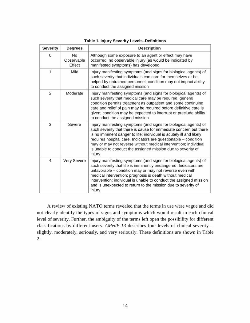
Table 1. Injury Severity Levels–Definitions
Severity Degrees Description
0 No Observable
Effect
Although some exposure to an agent or effect may have occurred, no observable injury (as would be indicated by manifested symptoms) has developed
1 Mild Injury manifesting symptoms (and signs for biological agents) of such severity that individuals can care for themselves or be helped by untrained personnel; condition may not impact ability to conduct the assigned mission
2 Moderate Injury manifesting symptoms (and signs for biological agents) of such severity that medical care may be required; general condition permits treatment as outpatient and some continuing care and relief of pain may be required before definitive care is given; condition may be expected to interrupt or preclude ability to conduct the assigned mission
3 Severe Injury manifesting symptoms (and signs for biological agents) of such severity that there is cause for immediate concern but there is no imminent danger to life; individual is acutely ill and likely requires hospital care. Indicators are questionable – condition may or may not reverse without medical intervention; individual is unable to conduct the assigned mission due to severity of injury
4 Very Severe Injury manifesting symptoms (and signs for biological agents) of such severity that life is imminently endangered. Indicators are unfavorable – condition may or may not reverse even with medical intervention; prognosis is death without medical intervention; individual is unable to conduct the assigned mission and is unexpected to return to the mission due to severity of injury
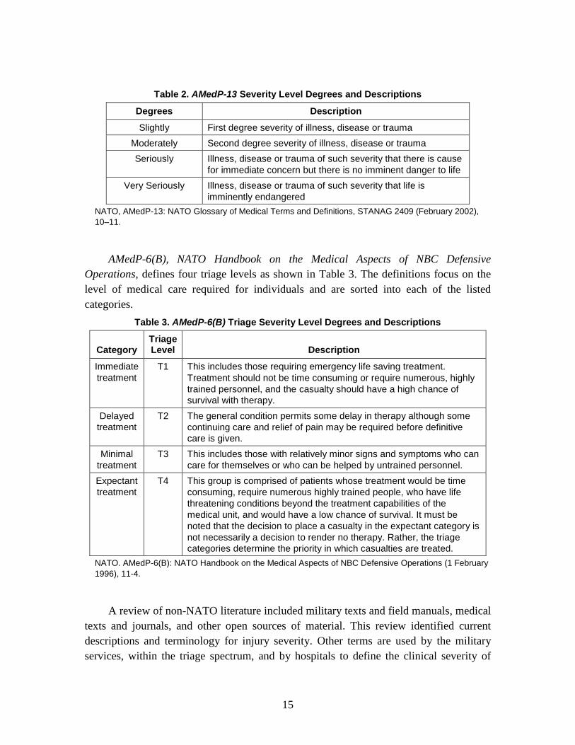
A review of existing NATO terms revealed that the terms in use were vague and did not clearly identify the types of signs and symptoms which would result in each clinical level of severity. Further, the ambiguity of the terms left open the possibility for different classifications by different users. AMedP-13 describes four levels of clinical severity—slightly, moderately, seriously, and very seriously. These definitions are shown in Table 2.
15
Table 2. AMedP-13 Severity Level Degrees and Descriptions
Degrees Description
Slightly First degree severity of illness, disease or trauma Moderately Second degree severity of illness, disease or trauma Seriously Illness, disease or trauma of such severity that there is cause
for immediate concern but there is no imminent danger to life Very Seriously Illness, disease or trauma of such severity that life is
imminently endangered NATO, AMedP-13: NATO Glossary of Medical Terms and Definitions, STANAG 2409 (February 2002),
10–11.
AMedP-6(B), NATO Handbook on the Medical Aspects of NBC Defensive Operations, defines four triage levels as shown in Table 3. The definitions focus on the level of medical care required for individuals and are sorted into each of the listed categories.
Table 3. AMedP-6(B) Triage Severity Level Degrees and Descriptions
Category Triage Level Description
Immediate treatment
T1 This includes those requiring emergency life saving treatment. Treatment should not be time consuming or require numerous, highly trained personnel, and the casualty should have a high chance of survival with therapy.
Delayed treatment
T2 The general condition permits some delay in therapy although some continuing care and relief of pain may be required before definitive care is given.
Minimal treatment
T3 This includes those with relatively minor signs and symptoms who can care for themselves or who can be helped by untrained personnel.
Expectant treatment
T4 This group is comprised of patients whose treatment would be time consuming, require numerous highly trained people, who have life threatening conditions beyond the treatment capabilities of the medical unit, and would have a low chance of survival. It must be noted that the decision to place a casualty in the expectant category is not necessarily a decision to render no therapy. Rather, the triage categories determine the priority in which casualties are treated.
NATO. AMedP-6(B): NATO Handbook on the Medical Aspects of NBC Defensive Operations (1 February 1996), 11-4.
A review of non-NATO literature included military texts and field manuals, medical texts and journals, and other open sources of material. This review identified current descriptions and terminology for injury severity. Other terms are used by the military services, within the triage spectrum, and by hospitals to define the clinical severity of
16
illness, but only a few of these terms help clarify the operational impacts also associated with the clinical disease severity.
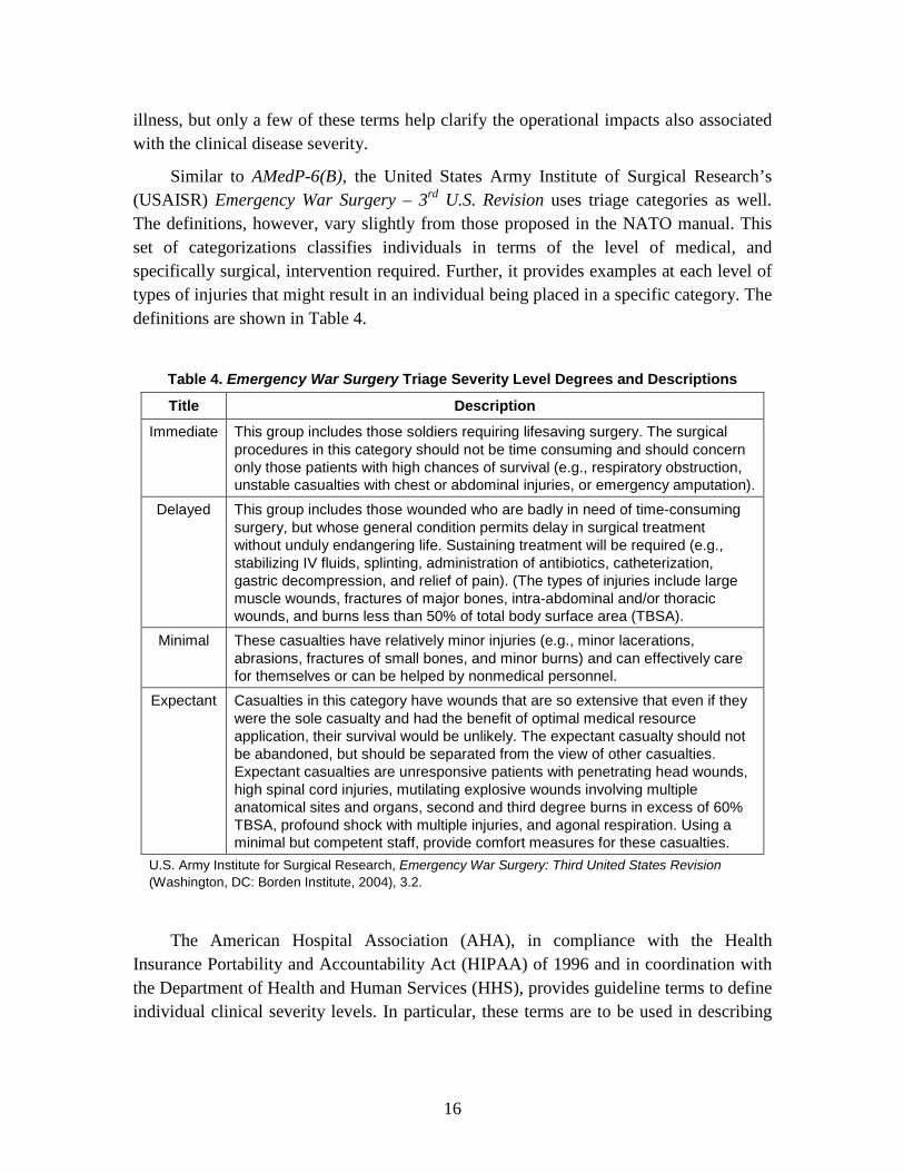
Similar to AMedP-6(B), the United States Army Institute of Surgical Research’s (USAISR) Emergency War Surgery – 3rd U.S. Revision uses triage categories as well. The definitions, however, vary slightly from those proposed in the NATO manual. This set of categorizations classifies individuals in terms of the level of medical, and specifically surgical, intervention required. Further, it provides examples at each level of types of injuries that might result in an individual being placed in a specific category. The definitions are shown in Table 4.
Table 4. Emergency War Surgery Triage Severity Level Degrees and Descriptions
Title Description
Immediate This group includes those soldiers requiring lifesaving surgery. The surgical procedures in this category should not be time consuming and should concern only those patients with high chances of survival (e.g., respiratory obstruction, unstable casualties with chest or abdominal injuries, or emergency amputation).
Delayed This group includes those wounded who are badly in need of time-consuming surgery, but whose general condition permits delay in surgical treatment without unduly endangering life. Sustaining treatment will be required (e.g., stabilizing IV fluids, splinting, administration of antibiotics, catheterization, gastric decompression, and relief of pain). (The types of injuries include large muscle wounds, fractures of major bones, intra-abdominal and/or thoracic wounds, and burns less than 50% of total body surface area (TBSA).
Minimal These casualties have relatively minor injuries (e.g., minor lacerations, abrasions, fractures of small bones, and minor burns) and can effectively care for themselves or can be helped by nonmedical personnel.
Expectant Casualties in this category have wounds that are so extensive that even if they were the sole casualty and had the benefit of optimal medical resource application, their survival would be unlikely. The expectant casualty should not be abandoned, but should be separated from the view of other casualties. Expectant casualties are unresponsive patients with penetrating head wounds, high spinal cord injuries, mutilating explosive wounds involving multiple anatomical sites and organs, second and third degree burns in excess of 60% TBSA, profound shock with multiple injuries, and agonal respiration. Using a minimal but competent staff, provide comfort measures for these casualties.
U.S. Army Institute for Surgical Research, Emergency War Surgery: Third United States Revision (Washington, DC: Borden Institute, 2004), 3.2.
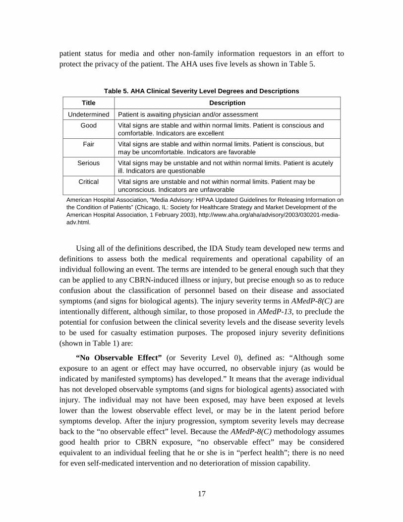
The American Hospital Association (AHA), in compliance with the Health Insurance Portability and Accountability Act (HIPAA) of 1996 and in coordination with the Department of Health and Human Services (HHS), provides guideline terms to define individual clinical severity levels. In particular, these terms are to be used in describing
17
patient status for media and other non-family information requestors in an effort to protect the privacy of the patient. The AHA uses five levels as shown in Table 5.
Table 5. AHA Clinical Severity Level Degrees and Descriptions
Title Description
Undetermined Patient is awaiting physician and/or assessment Good Vital signs are stable and within normal limits. Patient is conscious and
comfortable. Indicators are excellent Fair Vital signs are stable and within normal limits. Patient is conscious, but
may be uncomfortable. Indicators are favorable Serious Vital signs may be unstable and not within normal limits. Patient is acutely
ill. Indicators are questionable Critical Vital signs are unstable and not within normal limits. Patient may be
unconscious. Indicators are unfavorable American Hospital Association, “Media Advisory: HIPAA Updated Guidelines for Releasing Information on
the Condition of Patients” (Chicago, IL: Society for Healthcare Strategy and Market Development of the American Hospital Association, 1 February 2003), http://www.aha.org/aha/advisory/2003/030201-media-adv.html.
Using all of the definitions described, the IDA Study team developed new terms and definitions to assess both the medical requirements and operational capability of an individual following an event. The terms are intended to be general enough such that they can be applied to any CBRN-induced illness or injury, but precise enough so as to reduce confusion about the classification of personnel based on their disease and associated symptoms (and signs for biological agents). The injury severity terms in AMedP-8(C) are intentionally different, although similar, to those proposed in AMedP-13, to preclude the potential for confusion between the clinical severity levels and the disease severity levels to be used for casualty estimation purposes. The proposed injury severity definitions (shown in Table 1) are:
“No Observable Effect” (or Severity Level 0), defined as: “Although some exposure to an agent or effect may have occurred, no observable injury (as would be indicated by manifested symptoms) has developed.” It means that the average individual has not developed observable symptoms (and signs for biological agents) associated with injury. The individual may not have been exposed, may have been exposed at levels lower than the lowest observable effect level, or may be in the latent period before symptoms develop. After the injury progression, symptom severity levels may decrease back to the “no observable effect” level. Because the AMedP-8(C) methodology assumes good health prior to CBRN exposure, “no observable effect” may be considered equivalent to an individual feeling that he or she is in “perfect health”; there is no need for even self-medicated intervention and no deterioration of mission capability.

18
“Mild” (or Severity Level 1), defined as: “Injury manifesting symptoms (and signs for biological agents) of such severity that individuals can care for themselves or be helped by untrained personnel; condition may not impact ability to conduct the assigned mission.” Mild injury progression includes “nuisance” symptoms—the types of symptoms (and signs for biological agents) that might not prompt an individual to seek medical attention or miss work. These include symptoms for which an individual might self-medicate, including but not limited to: runny nose (rhinorrhea), slightly blurry vision, indigestion or heartburn, nausea, abdominal pain, and slight cough or tightness in the chest. These symptoms would not be expected to significantly impact an individual’s ability to accomplish most mission tasks. In the event of a known or suspected CBRN-event, these symptoms would indicate the potential for an injury progression of increasing severity, however, and therefore might be considered (depending on national or NATO policy) to be a basis for an individual’s removal from operations and transfer to the medical system.
“Moderate” (or Severity Level 2), defined as: “Injury manifesting symptoms (and signs for biological agents) of such severity that medical care may be required; general condition permits treatment as outpatient and some continuing care and relief of pain may be required before definitive care is given; condition may be expected to interrupt or preclude ability to conduct the assigned mission.” Moderate symptoms (and signs for biological agents) include those that might cause an individual to seek medical intervention or treatment as an outpatient. These have the potential to interrupt or otherwise impact an individual’s ability to complete assigned mission tasks. Symptoms of moderate severity level might include: sore skin or small blisters, vomiting, respiratory congestion (bronchorrhea) or difficulty breathing, ocular sensitivity to light, frequent diarrhea, difficulty concentrating, or trembling muscles.
“Severe” (or Severity Level 3), defined as: “Injury manifesting symptoms (and signs for biological agents) of such severity that there is cause for immediate concern but there is no imminent danger to life; individual is acutely ill and likely requires hospital care. Indicators are questionable – condition may or may not reverse without medical intervention; individual is unable to conduct the assigned mission due to severity of injury.” Severe symptoms may include some or all of the following, but are not limited to: large blisters, temporary blindness, extreme headache, hemoptysis, uncontrollable diarrhea, disorientation, and sporadic convulsions. These symptoms (and signs for biological agents) will impact an individual’s ability to perform assigned tasks and likely will result in a requirement for inpatient care for some duration. It is unclear, based solely on the symptoms, what an individual’s prognosis will be, although none of the symptoms, even in combination, may be expected to pose an imminent danger to life.
“Very Severe” (or Severity Level 4), defined as: “Injury manifesting symptoms (and signs for biological agents) of such severity that life is imminently endangered.
19
Indicators are unfavorable – condition may or may not reverse even with medical intervention; prognosis is death without medical intervention; individual is unable to conduct the assigned mission and is unexpected to return to the mission due to severity of injury.” The symptoms (and signs for biological agents) classified as “very severe”—paralysis, unconsciousness, prostration, or respiratory failure—will result in the death of an individual if allowed to continue for some period of time unabated and without medical intervention.31
b. Human Response Estimation
These symptoms will impact the individual’s ability to complete the assigned mission tasks and, in the event of death, will preclude any future mission capability.
“The human response estimation component is that portion of the casualty estimation methodology that determines the effects of CBRN exposures on individuals. It calculates the type and severity of illness or injury suffered by individuals, as well as their subsequent death or recovery.”32
c. Insult
The methodology does not anticipate the number of people who may seek medical assistance or the number who may be injured or killed indirectly (i.e., as a result of car accidents, dehydration, heart attacks, etc.).
An insult is defined as the agent or effect causing trauma, injury or illness.33
d. Symptom Progression
It is defined so as to be the nuclear equivalent of a chemical, biological, or radiological dose or dosage. Thus, exposure to nuclear effects produces a thermal or blast (static-overpressure or dynamic) insult, while exposure to other CBRN agents and effects produces a biological inhaled, chemical percutaneous liquid, or radiation whole-body or cutaneous dose or a chemical inhaled or percutaneous vapor dosage. The dose/dosage/insult, in turn, causes the human response and associated injury.
A symptom progression is the progression of symptom severity as a step-wise function of time for a specific physiological system. All of the physiological system symptom progressions for a particular chemical, radiological, or nuclear (CRN) agent or effect (and route of exposure) are combined to produce the injury profile.
31 For modeling purposes, SMEs agreed that remaining at Severity Level 4 as a result of exposure to
chemical, radiological, or nuclear (CRN) agents/effects and exhibiting very severe respiratory, muscular, neurological, or other symptoms for a period exceeding 15 minutes (without medical attention) would result in an individual becoming a fatality.
32 NATO, AMedP-8(C), GLOSSARY-2. 33 Dictionary.com Unabridged, Random House, Inc., s.v. “Insult,” www.dictionary.reference.com/
browse/insult.

20
e. Injury Profile An injury profile is a description of the injury in terms of the step-wise symptom
(and signs for exposure to biological agents) severity level changes over time.
f. Composite Injury Profile A composite injury profile is the combination of more than one injury profile, and
results in the description of the injury resulting from multiple, simultaneous routes of exposure or dose/dosage/insults in terms of the progression of step-wise injury severity level changes over time.
C. Assumptions, Limitations, and Rationale The AMedP-8(C) NATO Planning Guide includes a number of assumptions to
enable the utilization of data and concepts previously established for other models to be incorporated into the AMedP-8(C) methodology. Ideally, these assumptions also make the representations and estimation of casualties easier for the user to understand. This section is intended to elucidate some of the reasoning behind many of the assumptions and to further describe their effect on the casualty estimates output by the methodology. The assumptions and limitations, as stated in AMedP-8(C), are provided here as they appear in the NATO document, in their entirety. The associated rationale for each assumption and limitation is shown in italics.
1. General Assumptions and Limitations a. The methodology assumes that individuals are normally healthy. In other words, they have no pre-existing physiological injuries or physiological conditions that would be expected to increase susceptibility and alter human response or contribute increased risk factors. If casualty estimation is being done for populations which are already ill or susceptible to the CBRN agents or effects, then this assumption will result in an underestimation of casualties. In the same manner, this methodology may not be suitable for estimating casualties among civilian populations, since civilian populations may be more susceptible to CBRN agents or effects.
SMEs agreed that the AMedP-8(C) methodology should consider only individuals that are of normal health. The consideration of pre-existing physiological injuries or conditions would likely increase susceptibility, alter human response, contribute increased risk factors, and generally complicate the human response and casualty estimation.
b. For most CBRN agents and effects, the methodology does not model medical countermeasures. While certain medical countermeasures are available to most military individuals operating in a potential CBRN

21
environment—for example, atropine and oxime injectors for chemical exposure34
At this time, although policies on the use of medical countermeasures are standardized within NATO, the specific medications used vary from nation to nation. Further, data on how the use of those countermeasures would change the human response to a CBRN agent is not available in a form acceptable to all of the NATO Nations. Given this, NATO SMEs agreed that the use of medical countermeasures would not be included in AMedP-8(C), with the exception that prophylaxis may be considered for anthrax, plague, and smallpox.
—in most cases limited data are available to suggest how countermeasures might be employed or how general human response would change as a result of their application. In the current methodology, prophylaxis is considered only for three biological agents, as are discussed below. Future versions of this document may include additional forms of prophylaxis should the requisite information become available.
c. At the present time, the methodology does not include medical treatment. As a result, it provides estimates of the number of individuals who die of wounds in the absence of treatment. Were medical treatment considered, the number of individuals estimated to die of wounds (DOWs) would likely be reduced for many agents/effects. In the same manner, were medical treatment considered, the number of WIA casualties estimated at later time periods would likely be increased for many agents/effects.
NATO SMEs directed that medical treatment would not be considered in AMedP-8(C). The impact of medical treatment on human response is very much a function of the treatment protocol. At this time, there is no intent to standardize national medical CBRN treatment protocols. Without a standardized protocol to consider in the AMedP-8(C) methodology, it is left to each NATO Nation to consider the impact of medical treatment on casualty estimation.
d. The methodology does not estimate the number of individuals who recover or the time at which they would do so. Since the methodology does not consider medical countermeasures or treatment, duration of illness and time of recovery cannot be well-represented. While the methodology can be used to estimate recovery (and return to duty) in the absence of treatment, the NATO medical community decided this information was not a required output at this time.
For much the same reason that the AMedP-8(C) methodology does not consider medical treatment, NATO SMEs directed that recovery not be considered in AMedP-8(C). Recovery is primarily a function of the medical treatment provided, and there is no standardized NATO medical CBRN treatment protocol.
34 NATO, First-Aid Materiel for Chemical Injuries, STANAG 2871 (8 March 1989).

22
e. The methodology does not estimate battle stress (also commonly referred to as “psychological” or “psychological effects”) casualties. Planners should be aware that battle stress casualties may be expected to comprise a significant fraction of the total casualties and that a significant number of personnel suffering from battle stress may present themselves as requiring medical care.
NATO SMEs agreed that, at this time, due to the difficulty of estimating these casualties, battle stress casualties would not be included in AMedP-8(C).
f. Human response is assumed to begin after the completion of exposure; in other words, the exposed icon is assumed to have received its full dose prior to the selection of applicable dose ranges and injury profiles. This assumption implies that the duration of exposure is less than the latent period for acute radiation illness. This latent period varies from minutes (for very high doses) to hours or days (for low doses). Only at very high doses would this assumption tend to underestimate the time at which an individual becomes a casualty.
This is a simplifying assumption, to allow for a consistent interpretation of the time at which human response begins, and thus allows for a consistent interpretation of the time for casualties.
2. CRN Assumptions and Limitations The general and specific CRN assumptions and limitations were all agreed to by
NATO SMEs at the applicable human response SME review meetings35
a. For CRN agents and effects, the methodology models human response as agent/insult-related and time-dependent injury severity. In this methodology, human response is modeled by a series of injury profiles, which combine the time-dependent severities of symptoms as they are manifested in various physiological systems.
except as noted. As applicable, additional references and sources are also provided.
The concept of injury profiles as a time-dependent function of physiological system symptoms to describe human response and provide the basis for casualty estimation is a fundamental component of the prescribed methodology. This concept was briefed to and concurred with by NATO SMEs. 35 Julia K. Burr et al., Proceedings of the NATO Chemical Human Response Subject Matter Expert
Review Meeting, 21-22 April 2008, Munich, Germany, IDA Document D-3883 (Alexandria, VA: Institute for Defense Analyses, August 2009), 1–71; Julia K. Burr et al., Proceedings of the NATO Nuclear Human Response Subject Matter Expert Review Meeting, 23-25 June 2008, Albuquerque, New Mexico, United States of America, IDA Document D-3884 (Alexandria, VA: Institute for Defense Analyses, August 2009), 1–31; and Julia K. Burr et al., Proceedings of the NATO Radiological Human Response Subject Matter Expert Review Meeting, 26 June 2008, Albuquerque, New Mexico, United States of America, IDA Document D-3885 (Alexandria, VA: Institute for Defense Analyses, August 2009), 1–16.
23
b. The physiological systems from which the injury profiles were derived do not necessarily represent all systems that might be impacted by exposure to a CRN agent or effect. Rather, they represent those systems that would be expected to cause individuals to seek medical attention soonest—those that would be expected to manifest symptoms earliest and at the highest severity. There may be other symptoms of lesser medical significance or severity which are not described. Exclusion of these symptoms does not affect the casualty estimate.
CRN agents and effects result in complex symptomatology across numerous physiological systems. The physiological systems in which symptoms manifest were selected to represent the most likely symptoms and those that would be expected to result in symptom and injury severity requiring the affected individual to seek medical attention.36 Many of these systems were originally captured in the models done for previous versions of AMedP-8.37
c. The methodology also assumes for CRN agents and effects that the human response of individuals in each dose/dosage/insult range can be represented by the typical individual with the mid-range insult. Distributions of insult-related effects are not modeled in the CRN component of the methodology; an actual exposure may (and probably will) result in more or fewer casualties than the estimated number. At the same time, this assumption neglects variation in any exposed population, which is expected but impossible to precisely quantify. Thus, the modeling of typical individuals with mid-range insults is a reasonable compromise between practical application of the casualty estimation methodology and reality.
The previously represented symptoms/systems were modified, as necessary, to update the symptoms and severities to the current state of knowledge and to correlate the symptoms with the physiological systems in which they were expected to manifest. NATO SMEs reviewed and concurred with these system profiles.
When modeling any human population, individual differences may cause a response more or less severe than predicted for a given dose. Further, the expected response to the dose at the low end of the dose range may differ significantly from the dose at the high end of the range. These two variations from the expected response are minimized (but not eliminated) by a careful selection of the animal model for testing, and by a careful definition of the dose range. Since the authors did not perform any of the dose response research, but cited (to the extent available) references well accepted in the community, it is assumed that the animal models used were adequate to model the response of the 36 Additional detailed information on the injury manifestations and physiological systems modeled is
provided in Chapters 4-7 for the CRN agents and effects. 37 Deverill and Metz, DICE Chemical Insult Program; Levin, Effect of Combined Injuries; and Centers
for Disease Control and Prevention (CDC), “Cutaneous Radiation Injury (CRI): Fact Sheet for Physicians,” http://emergency.cdc.gov/radiation/criphysicianfactsheet.asp.

24
human population of interest. The dose ranges were explicitly selected to exclude extreme variation in response between the lower and upper bounds. Certainly, a sensitive individual with an exposure in the upper end of the dose range could have a much more extreme response than is expected. However, with a properly designed response model it should be equally likely that an exposure in that dose range would produce a response much milder than expected. If the exposure scenario results in a large number of persons exposed to a wide variety of doses, the variations in individual response will “average” out, and will result in the expected response among the population.
d. The final CRN assumption is that injury profiles induced by multiple routes of exposure or multiple insults are not synergistic. Although data exist that indicate that simultaneous injuries caused by multiple simultaneous insults may result in higher injury severity than would result from any single insult alone,38
Although it is known that the injury and resulting physiological system symptoms from multiple routes of exposure or multiple insults would be synergistic—the severity of symptoms and injury would likely be greater as a result of multiple routes of exposure or multiple insults—there is currently insufficient data to support modeling such effects. Further, capturing the synergism of multiple routes of exposure or multiple insults would make the human response model extremely complex. Therefore, SMEs agreed that the various routes of exposure and numerous, simultaneous insults could be modeled as resulting in independent, non-synergistic human response, symptom progressions, and injury profiles.
not enough information currently exists to determine the extent to which injury severity might be expected to change. As a result, when two or more injury profiles are combined, the resulting composite injury profile will follow the maximum severity level of the individual profiles at each point in time. This assumption may lead to an underestimate of the number and severity of casualties.
39
3. Chemical Assumptions and Limitations
a. For chemical agents, the methodology is based on toxicity data expressed in mass per kilogram and which assume exposure to a 70 kg man. This body weight may not be typical of most military personnel, who can be significantly heavier (or lighter) than 70 kg. Being heavier may result in a less severe injury from a specified dose or dosage, as the amount of agent is distributed in a larger mass of tissue. Conversely, being
38 Levin, Effect of Combined Injuries; and U.S. Army Nuclear and Chemical Agency (USANCA),
Personnel Risk and Casualty Criteria for Nuclear Weapons Effects (Springfield, VA: Training and Doctrine Command, June 1999), Appendix F.
39 Burr et al., Chemical Human Response SME Review Meeting, 1–71; Burr et al., Nuclear Human Response SME Review Meeting, 1–31; and Burr et al., Radiological Human Response SME Review Meeting, 1–16.
25
lighter than 70 kg may result in a more severe injury. Thus, this assumption may lead to either an over- or underestimate of the number and severity of casualties to a degree that is determined by the distribution of body weight among the population at risk.
The chemical toxicity data underlying the methodology are taken from the U.S. multiservice publication Potential Military Chemical/Biological Agents and Compounds, also published as U.S. Army Field Manual 3-11.9 (FM 3-11.9). As stated in that document, “In this manual, dosage is usually expressed as milligrams per kilogram (mg/kg) of body weight for liquid agents and as milligrams-minute per meter cubed (mg-min/m3) for vapor exposure. Dosages are given for a 70-kg man.”40
b. The toxicity data underlying the methodology for chemical agents assumes exposed individuals are breathing at a rate of 15 liters per minute, which is the rate associated with light exertion.
This assumption has been retained in order to use these data directly, but it should be noted that variations in body weight will affect the amount of agent needed to cause a specified physiological response.
41
The chemical toxicity data underlying the methodology are taken from FM 3-11.9. In that document, vapor exposure dosage estimates are expressed in milligrams-minute per meter cubed (mg-min/m3) for a defined minute volume and exposure duration. All estimates are presented for a defined minute volume of 15 liters/min, although the document notes that the relationship between minute volume and toxicity can be considered linear for minute volumes ranging from 10 to 50 liters/min.
If a breathing rate other than 15 liters per minute is chosen for individuals in the scenario, then an adjustment factor for inhaled doses can be applied as described in Chapter 2 [of AMedP-8(C)]. A related assumption is that all inhaled agent is retained. Although conservative, this assumption has negligible impact for chemical agents, since the mass of agent that would be exhaled and not retained is expected to be very small relative to the total mass of agent in the inhaled air.
42
c. The methodology uses Haber’s Law, which assumes that human response is a function of the dosage rate multiplied by the duration of exposure. Although battlefield chemical agent exposures are likely to be of varying lengths, the methodology assumes for chemical agents that all cumulative dosages and doses provide the same human response as would result from a two-minute exposure to the same amount of agent. This assumption neglects the repair and recovery mechanisms which naturally
40 Multiservice Publication, Potential Military Chemical/Biological Agents and Compounds, FM 3-
11.9/MCWP 3-37.1B/NTRP 3-11.32/AFTTP(I) 3-2.55 (Washington, DC: U.S. Government Printing Office, January 2005), II-4.
41 David W. Layton, “Metabolically Consistent Breathing Rates for Use in Dose Assessments,” Health Physics 64, no. 1 (January 1993): 30.
42 FM 3-11.9, II-5.
26
occur in the body and which are typically represented by employing a toxic load model.
The decision to ignore toxic load phenomena is based on several considerations. First, the initial step in the methodology for CRN agents and effects involves binning individuals by agent-specific dose/dosage ranges. In the current methodology, these ranges are constant for all doses and dosages of a given agent type. Use of a toxic load model for chemical agents, however, would require different ranges for each icon in a scenario to account for the variation in toxicity due to duration of exposure. Adding this step greatly complicates the methodology. Second, battlefield exposures will vary over time; at this time there are virtually no data to suggest the manner in which time-varying exposures affect toxic load. Third, battlefield exposures will tend to be relatively short, on the order of several minutes to, perhaps, an hour in duration. In these time frames, toxic load would not be anticipated to cause a significant change in the number of casualties. Finally, Haber’s Law is conservative; for estimating casualties at longer periods (using shorter duration toxicity estimates), it will tend to overestimate the number and severity of casualties, and the associated burden on the medical system.
Sufficient rationale is already provided in the quoted text. d. As the methodology always assumes that human response begins at the completion of exposure, it does not consider symptoms which may occur earlier as a consequence of partial exposure to chemical agents. Consequently, there may be a lag in the times at which various outputs of the methodology are reported for chemical agent exposures. Given the expected brevity of exposure duration, however, this lag should be very minor if it is observed at all.
There are currently insufficient data to support modeling of human response to partial dosages and the changes in human response as the dosage increases over time. Therefore, for ease of modeling, the human response and associated symptoms and injury had to be assumed to begin at the completion of exposure.
e. Nerve Agent GB Assumptions and Limitations
(1) Percutaneous GB doses/dosages due to both vapor and liquid are assumed to be negligible. The percutaneous vapor dosage required to impact human response is several orders of magnitude greater than the inhalation dosage required to produce similar effects.43
43 Gene E. McClellan, George H. Anno, and Leigh N. Matheson, Consequence Analytic Tools for NBC
Operations Volume 3: Chemical Agent Exposure and Casualty Estimation, DSWA-TR-97-61-V3 (Alexandria, VA: Defense Special Weapons Agency, 1998), 29–30.
Further, the liquid resulting from a GB attack, and thus the percutaneous liquid contribution

27
to dose, may be neglected due to the agent’s high volatility.44
Sufficient rationale is already provided in the quoted text.
This latter assumption may result in an underestimate of the number and severity of casualties.
f. Nerve Agent VX Assumptions and Limitations
(1) First, the percutaneous VX vapor contribution to human response is assumed to be negligible as compared to the contributions of inhaled VX vapor dosage and percutaneous VX liquid dose.45
Percutaneous VX vapor is accounted for in the toxicity values for VX inhalation dosage, which assumed a whole body exposure. The contribution of percutaneous VX vapor alone (i.e., after personal protective equipment is donned) is considered negligible as compared to inhaled VX vapor and percutaneous VX liquid.
This assumption may result in an underestimate of the number and severity of casualties.
46
(2) Second, the human responses due to inhaled VX vapor and percutaneous VX liquid are assumed to be independent of one another. Inhaled VX vapor induces human response in several physiological systems nearly instantaneously, including the ocular and respiratory systems. Human response resulting from percutaneous VX liquid takes longer to manifest and impacts physiological systems differently (e.g., the muscular system is the first system to manifest symptoms following percutaneous VX liquid exposure).
47
This is the same as assuming that exposure to inhaled VX vapor and percutaneous VX liquid are not synergistic. See the discussion of the fourth CRN assumption and limitation in section 2.C.2.d. on why this is assumed.
Thus, dosage and dose due to the two routes of exposure are represented by two separate injury profiles that are combined to generate a final composite VX injury profile, as described later in this document. It is possible that the interaction of human response resulting from exposure to inhaled VX vapor and percutaneous VX liquid may be synergistic; therefore, the assumption of the independence of human response given two routes of exposure may result in an underestimate of the number and severity of casualties.
44 Frederick R. Sidell, “Nerve Agents,” in Medical Aspects of Chemical and Biological Warfare, ed.
Frederick R. Sidell, Ernest T. Takafuji, and David R. Franz, Textbook of Military Medicine, Part 1: Warfare, Weaponry, and the Casualty (Washington, DC: Department of the Army, Office of the Surgeon General, Borden Institute, 1997), 141–42, Table 5-3.
45 Percutaneous VX vapor is accounted for in the toxicity values for VX inhalation dosage, which assumed a whole body exposure. The contribution of percutaneous VX vapor alone (i.e., after personal protective equipment is donned) is considered negligible as compared to inhaled VX vapor and percutaneous VX liquid.
46 Burr et al., Chemical Human Response SME Review Meeting, 10. 47 Sidell, “Nerve Agents,” 142–45; and U.S. Army Medical Research Institute of Chemical Defense
(USAMRICD), Medical Management of Chemical Casualties Handbook, 3rd ed. (Aberdeen Proving Ground, MD: International Medical Publishing, 2000), 111–17.

28
g. Blister Agent HD Assumptions and Limitations
(1) The human responses resulting from exposure to inhaled HD vapor, percutaneous HD vapor, and percutaneous HD liquid are assumed to be independent of one another and are represented by three separate injury profiles. Inhaled HD vapor results in an injury profile based on symptoms manifested in the respiratory and upper gastrointestinal systems. Percutaneous HD vapor and equivalent percutaneous HD vapor (the vapor dosage equivalent to the composite percutaneous HD vapor dosage and percutaneous HD liquid dose) result in injuries and symptoms manifested in the ocular system and skin respectively. It is possible that the interaction of human response resulting from exposure to inhaled HD and percutaneous HD may be synergistic; therefore, the assumption of the independence of human response given three routes of exposure may result in an underestimate of the number and severity of casualties.
This is the same as assuming that exposure to inhaled HD vapor, percutaneous HD vapor, and percutaneous HD liquid are not synergistic. See the discussion of the fourth CRN assumption and limitation above on why this is assumed.
4. Radiological Assumptions and Limitations a. The methodology assumes for radiological agents that external whole-body and cutaneous radiation doses continue to accumulate for as long as the individual remains within the radiation area. The radiation area is defined as the area within the boundaries of any radioactive cloud and/or within the boundaries of any contaminated area. Radiological inhalation is neglected in the estimation of radiological human response due to the negligible dose expected from inhalation relative to external radiation and the lack of information available to represent the injury profile associated with this route of exposure. These assumptions are reasonable for external exposure from radioactive material in the air (“cloudshine”) and exposure from radioactive material on the ground (“groundshine”). The assumption for cutaneous exposure also implies that contamination on the skin will be removed once the individual exits the radiation area. While this seems reasonable, if decontamination is not performed upon leaving the radiation area, this assumption may result in an underestimate of the number and severity of casualties.
Sufficient rationale is already provided in the quoted text. b. The methodology assumes that [radiological dispersal device] RDD and radioactive fallout events have different starting assumptions:
(1) For an RDD event, the exposed icons are assumed to be in the radiation area at the time of detonation or dispersal. This results in exposure due to cloudshine, groundshine, and cutaneous exposure.

29
Radiation from cloudshine and groundshine is considered in calculating the whole-body radiation dose. Cutaneous exposure in RDD scenarios includes radiation from cloudshine and groundshine and beta radiation from contamination on the skin. The deposition concentration on the skin is assumed to be the same as the ground concentration at the individual’s location.
This assumption can be restated as “Casualties are estimated for the personnel present at the time of the RDD event.” This is based upon the underlying assumption that if the RDD event has already occurred, personnel entering the area would be protected (suit and mask) from inhalation and skin contamination. To further underlay this assumption, personnel would not enter the RDD event contamination area until after the aerosolized radioactive material cloud has passed out of the area and some level of contamination control and exposure limitation had been established.
(2) For radioactive fallout, because air immersion is difficult to model, most hazard prediction models cannot account for the rapidly changing dose and dose rate as a function of the age of the fallout cloud. Individuals therefore are assumed to enter the radiation area only after all fallout has deposited on the ground, resulting in exposure due solely to groundshine and cutaneous exposure. This assumption limits the fallout scenarios for which this methodology can provide casualty estimates.48
c. For both RDD and fallout, the methodology assumes that only individuals dismounted and in the open (or, in the case of fallout, those who have acquired contaminant on bare skin) are exposed to beta radiation, all other individuals are fully shielded from this type of radiation.
Only radiation from groundshine is considered in calculating the whole-body radiation dose. Cutaneous exposure in fallout scenarios has two components: radiation from groundshine and beta radiation from possible contamination on the skin.
This assumption considers that the major component of the radiological cloud (and subsequent ground contamination from an RDD or fallout) is particulate, and not vapor. If individuals are inside a building or vehicle, it is a simple expedient to close windows and doors, shut down the ventilation system (or turn filters on), and remove the particulate exposure. It is recognized that contamination accumulating on horizontal surfaces (roof or ground) near the vehicle or building will contribute some dose to the
48 Alternatively, this assumption can be removed and scenarios examined prior to the removal of
cloudshine. However, because the contribution of cloudshine must still be neglected, due to the difficulties in calculating associated dose rates, the numbers and severity of casualties will be (in some cases significantly) underestimated. This, however, is a limitation of the existing hazard prediction models and not of the AMedP-8(C) methodology—if future hazard prediction tools are better able to model air immersion in fallout scenarios, then this limitation goes away.

30
occupants, but that should be insignificant; if individuals are in a building, the building provides significant shielding, and if they are in a vehicle, individuals can leave the area.
d. Dose protraction is included in the methodology as it pertains to the possible adjustment of lethality and time to death; it is not applied to the injury profiles and the determination of WIA. This assumption neglects the repair and recovery mechanisms which may naturally occur in the body. This assumption, therefore, may overestimate the number and severity of casualties, but by an amount which is probably insignificant in the timeframes considered on the battlefield.
For lethal exposures, changes in the time of death as a result of the body’s inherent repair mechanisms are accounted for by the use of a dose rate dependent correction factor. For sub-lethal exposures, the naturally occurring repair and recovery mechanisms generally occur over long time periods (30 days) relative to the time of exposure (hours), and do not change the time of the onset of symptoms. Since the AMedP-8(C) methodology does not consider recovery (see the discussion of the fourth general assumption in section 2.C.1.d.), this does not affect the casualty estimate.
e. The RDD scenario does not account for conventional casualties (i.e., from high explosives and fragmentation) that might result simultaneously in the event of a detonation. To account for conventional weapons effects, users are encouraged to develop a conventional casualty estimate in parallel with the RDD estimate. In lieu of conventional casualty estimation, this assumption may underestimate the number and severity of casualties.
This assumption clarifies the scope of this document - conventional casualties from high explosives and fragmentation are not considered in AMedP-8(C), and users should rely instead upon conventional casualty estimation tools.
5. Nuclear Assumptions and Limitations a. Since only the simultaneous prompt nuclear effects are modeled, it is assumed that human response for the entire exposed population begins simultaneously and immediately following the nuclear detonation. This assumption leads to a clear distinction between estimating casualties from prompt nuclear effects and estimating casualties due to fallout.
Sufficient rationale is already provided in the quoted text. b. Thermal Insult Assumptions and Limitations
(1) First, the thermal fluence associated with the nuclear environment can be translated to a percentage of body surface area burned, which is dependent on the type of uniform or clothing worn and the fit of the garment. The area included in the measurement of “body surface area
31
burned” is the area bounded by the partial-thickness (second degree) burn and may include areas of full-thickness (third degree) burns.49
The use of body surface area burned as a measure of thermal fluence for human response approximation is based on previous AMedP-8 models.
By not considering first degree burns in the measurement, this assumption may underestimate the number and severity of casualties, but is probably operationally insignificant on the battlefield.
50 SMEs agreed that this representation was appropriate for correlating thermal fluence to human response.51
(2) Second, the methodology assumes that thermal injury profiles are the same regardless of part of the body suffering burns; specifically, thermal burns to the face, hands, feet, or genitalia are assumed to produce injuries of the same severity as those elsewhere on the body. Although research suggests that absorption of thermal fluence by these specific parts of the anatomy significantly increases the hazard and severity of the resulting burns,
52
This is a simplifying assumption. The limited availability of data and the difficulty estimating which parts of the body are burned make it impractical to use a more sophisticated burn model that would account for these.
limited data exist to include the unique impacts of burns to these areas of the skin on the overall human response. This assumption may underestimate the number and severity of casualties.
(3) Third, individuals are either fully protected from or fully exposed to thermal fluence; partial exposure is not modeled. An icon can be separated into those individuals who are fully protected (i.e., receive no thermal exposure) and those individuals who are unprotected (i.e., receive the full thermal exposure). This assumption may under- or overestimate the number or severity of casualties.
Thermal shielding is different from radiation or blast shielding, or chemical protection, in that the shielding is typically either completely effective, or completely ineffective. Any solid, opaque material between a given object and the fireball will act as a shield and provide protection from thermal radiation.53 Objects that are shielded do not experience damage from thermal radiation. An exception to this is skin burns caused by the transmission of thermal energy through military uniforms,54
49 Levin, Effect of Combined Injuries, 23–24.
but that is considered separately in this document. This assumption presumes that there may be a certain
50 Anthony J. Baba et al., Incidence of Skin Burns Under Contemporary Army Uniforms Exposed to Thermal Radiation from Simulated Nuclear Fireballs, HDL-TR-2084 (Adelphi, MD: U.S. Army Laboratory Command, Harry Diamond Laboratories, December 1986), 8.
51 Burr et al., Chemical Human Response SME Review Meeting. 52 USANCA, Personnel Risk, D-2. 53 Samuel Glasstone and Philip J. Dolan, The Effects of Nuclear Weapons, 3rd ed. (Washington, D.C.:
U.S. Government Printing Office, 1977), para 7.18, 281. 54 Ibid., para 7.33, 286.

32
probability that an individual might be shielded, but if one is shielded, one is shielded completely.
(4) The effects of the thermal flash on the eyes (such as flash blindness) are not included in the methodology. These effects are highly dependent upon the orientation of the individual relative to the detonation as well as the presence of structures or other conditions which would mitigate or enhance the flash effects. This assumption may underestimate the number and severity of casualties.
Sufficient rationale is already provided in the quoted text.
6. Biological Assumptions and Limitations a. General Biological Assumptions and Limitations
(1) For each biological agent, the methodology assumes that exposure occurs via inhalation of the aerosolized agent.
Many of the biological agents considered in AMedP-8(C) can cause disease via a number of different routes of entry: inhalation, ingestion, ocular exposure, or via cuts and abrasions. Biological model parameter values generally vary by route of entry. For the agents considered, aerosol dissemination would have the greatest potential to cause large numbers of casualties and thus pose the greatest challenge to the medical system. For this reason, the parameter values associated with the inhalation route of entry were chosen.
(2) The methodology assumes that human response from exposure to biological agents can be modeled by looking at dose-dependent probabilities of illness and death and independent time-related distributions representing the period of incubation and the duration of symptomatic illness. The duration of illness distributions may differ for survivors and non-survivors. Furthermore, the methodology assumes that the period during which an individual is ill can be subdivided into one or more stages and that severity levels related to signs and symptoms can be associated with these stages. This set of assumptions allows for a simplification and generalization of complex disease processes and permits the practical estimation of the severity and time of biological casualties.
These concepts used to describe human response provide the basis for casualty estimation and are fundamental components of the AMedP-8(C) methodology. These concepts were briefed to and concurred with by NATO SMEs. The independent nature of the submodels within the methodology dictates that the incubation period and the various stages of illness may also be independent.
(3) The methodology assumes for biological agents that everyone who is “infected” will become symptomatic at some point. This assumption,
33
along with the correct definition of infectivity parameters, allows the planner to neglect those personnel who become (“subclinically”) infected but do not become symptomatic.
Sufficient rationale is already provided in the quoted text. (4) The biological agent methodology incorporates an infectivity submodel that describes the relationship between inhaled dose and the probability of illness. The dose parameters used in this submodel are characterized as “infective dose” for organisms and “effective dose” for toxins. The term “effective dose” for toxins is typically used to describe the dose at which some level of effect is observed; here the level of effect is considered to be the onset of signs and symptoms.
Sufficient rationale is already provided in the quoted text. (5) Physiological differences between animal and human respiratory systems and resultant impacts on deposited doses are not well enough understood to incorporate them into the process of extrapolating from animals to humans.
This assumption allows the human response to an inhaled agent to be modeled directly from animal data without an extrapolation or correction factor. At this time, there is insufficient data to quantitatively describe the variation in responses among species, so no variation is assumed. Future modeling efforts may incorporate an extrapolation factor to account for differences among species as data become available to support such a modification.
(6) For biological agents, the methodology does not allow for individual-level (or spatial) estimation of personnel status. In other words, it is not possible to estimate precisely which exposed icons will become ill and/or die. Only the total number of casualties, by time interval, can be estimated.
Because the biological agent human response methodologies rely on expected values of stochastic functions (vice the deterministic methodology employed for the CRN agents and effects), the results are captured over the entire population rather than on an individual basis.
(7) Prophylaxis is not generally considered in this methodology, with the exception of three diseases—anthrax, pneumonic plague, and smallpox—for which the user can elect to include or not include prophylaxis. For these diseases, prophylaxis (either pre-exposure vaccination or post-exposure, pre-symptom onset antibiotic prophylaxis) is assumed to be efficacious for a percentage of the population, independent of dose; there is no defeat dose beyond which the prophylaxis fails to be effective.55
55 Note that the use of prophylaxis may require a commitment of medical resources in advance of, or
during, the biological event. See AMedP-6 and AMedP-7 for the procedures for, and operational implications of, the use of prophylaxis.
This

34
assumption will tend to underestimate casualties in scenarios involving very high doses of the agents that cause these three diseases.
NATO SMEs agreed that, at this time, medical countermeasures would not be included in AMedP-8(C). Protocols, specific prophylaxis options, and efficacy information were available for the three agents for which medical prophylaxes are being considered. Even for these three agents, however, alternative medical prophylaxes are available and could be substituted into the methodology as discussed in Chapter 8 of this document.
While it is reasonable to assume that some defeat dose exists at which the medical prophylaxis may no longer be efficacious, limited human information exists on which to base this value. Therefore, at this time, for ease of modeling, defeat doses are not considered.
b. Non-Contagious Biological Agent Assumptions and Limitations
(1) Anthrax Assumptions and Limitations
(a) The methodology assumes that the disease resulting from inhalation of anthrax spores manifests as inhalation anthrax. The incidence of cutaneous and gastrointestinal (GI) anthrax is neglected. Because GI anthrax is not expected to occur after aerosolized spread of anthrax and because cutaneous anthrax is a milder disease, this assumption may result in a slight underestimation of the number of the casualties.
As stated above, all biological agents are assumed to act through the inhalation route of exposure only. Neglecting this route of exposure should only result in a slight underestimation of the number of the casualties, by not accounting for the (typically non-lethal) cutaneous anthrax cases.
(b) Untreated inhalation anthrax is assumed to be lethal in all cases. Therefore, the median infective dose (ID50) is assumed to equal the median lethal dose (LD50). Since mortality has been essentially 100% in the absence of appropriate treatment,56 this is a reasonable assumption which should not impact the casualty estimate.57
Sufficient rationale is already provided in the quoted text.
(2) Botulism Assumptions and Limitations
(a) Consistent with the assumptions made for chemical agents, the methodology assumes botulinum neurotoxin exposure to a 70 kg man. Since botulism is modeled as the result of inhalation of a biotoxin, then
56 Philip S. Brachman, "Inhalation Anthrax," Annals of the New York Academy of Sciences 353
(December 1980): 83–93; and Jon-Erik C. Holty et al., “Systematic Review: A Century of Inhalational Anthrax Cases from 1900 to 2005,” Annals of Internal Medicine 144, no. 4 (February 2006): 270–80.
57 Additional detailed information on the lethality rate and model used to describe the human response to anthrax is provided in Chapter 8.

35
(just as for chemical agents) this assumption may lead to an over- or underestimate of the number and severity of casualties.
The botulism lethality submodel incorporates data expressed in micrograms per kilogram of body weight. To maintain consistency with the assumptions that underlay the development of other human response models in AMedP-8(C), the botulism LD50 was calculated for a 70 kg man. Note that botulism is the only biological agent currently considered for which infectivity/effectivity data were expressed in this manner.
(b) Although there are seven different serotypes of the botulinum neurotoxin, the methodology assumes the disease is caused by botulinum neurotoxin serotype A. Serotype A neurotoxin is responsible for the plurality of human botulism cases and typically causes the most severe form of the disease.58
Sufficient rationale is already provided in the quoted text.
This assumption allows use of a broader array of case data in the development of the methodology than would be possible for other serotypes. It is also conservative, in that modeling botulism in its severest form would predict the greatest burden on the medical system.
(3) VEE Assumptions and Limitations
(a) For VEE, the methodology assumes that all inhaled agent is retained.
VEE is characterized (qualitatively) as very infectious, which is interpreted as meaning that any viable organism inhaled and retained in the lungs will result in an infection. The assumption that all inhaled agent is retained, combined with the infectivity model discussed in Chapter VIII, results in an estimate that inhalation of any viable organism will result in infection.
(b) VEE is assumed to be non-lethal in all cases, even without treatment. Cases of lethal encephalitis are sufficiently rare in adults (though more common in children) that they are considered negligible.59
Sufficient rationale is already provided in the quoted text.
It is anticipated that this assumption will not affect the number of DOW casualties from VEE in battlefield scenarios and may only result in a slight underestimation of such casualties in most other scenarios.
c. Contagious Biological Agent Assumptions and Limitations
(1) General Contagious Biological Agent Assumptions and Limitations
58 Bradley A. Woodruff et al., “Clinical and Laboratory Comparison of Botulism from Toxin Types A, B,
and E in the United States, 1975–1988,” The Journal of Infectious Diseases 166, no. 6 (December 1992): 1281.
59 Keith E. Steele et al., “Alphavirus Encephalitides,” in Medical Aspects of Biological Warfare, ed. Zygmunt F. Dembek, Textbook of Military Medicine (Washington, DC: Department of Defense, Office of the Surgeon General, U.S. Army, Borden Institute, 2007), 242.
36
(a) The population is assumed to be relatively large and unstructured. The first part of this assumption implies that the population is large enough to be modeled with parameters derived from real-world regional or metropolitan outbreaks. The second part requires that the entire population be modeled as a single unit, without ascribing different behaviors or conditions to any subset of the population. The populations used for casualty estimation should reflect this assumption; i.e., this may not be applicable to collections of geographically separated military units.
Sufficient rationale is already provided in the quoted text. (b) All population mixing is assumed to be homogeneous. This assumption follows, in part, from the second part of the assumption above. All persons have an equal likelihood of mixing with any other person – no subgroup is separated out as more or less likely to mix in the general population. Again, the populations used for casualty estimation should reflect this assumption. Including remote or isolated units with limited contact among the rest of the population (i.e., those entered into the medical system) may result in an overestimation of the number of casualties or an early estimation of when those casualties might occur.
Sufficient rationale is already provided in the quoted text. (c) Initial and transmission-caused infections are assumed to follow the same injury profile. This assumption allows for a simplification and generalization of complex disease processes and permits the practical estimation of the severity and time of biological casualties. Essentially, this assumption implies that the methodology does not consider possible variations in the presentation of a particular disease. However, since alternative presentations of a disease may be more or less severe than what is modeled, this assumption may result in an under- or overestimation of the severity of the casualties.
Sufficient rationale is already provided in the quoted text. (d) The SEIRP (Susceptible-Exposed and infected-Infectious-Removed-Prophylaxis efficacious) equations allow for utilization of a pre-exposure vaccination and/or a post-exposure antibiotic prophylaxis model.60
The SEIRP component of the AMedP-8(C) methodology extends the generally accepted Susceptible-Infected-Removed (SIR) methodology to separate out the “Exposed and infectious” cohort and to include the impact of the use of vaccination on the estimate of the spread of contagious diseases. The impact of vaccination is modeled on data from
60 The SEIRP methodology allows for the modeling of both pre-exposure and long-term post-exposure
prophylaxis as applicable: 1) vaccines, where available, may be used prior to exposure, and 2) antibiotic regimens, where available, may be begun immediately post-exposure and continued for some period post-exposure.
37
documented use of vaccination in the management of plague and smallpox. Consideration of vaccination is at the discretion of the methodology user.
(2) Plague Assumptions and Limitations
(a) The methodology assumes that the disease resulting from inhalation or contagious transmission of aerosolized plague bacteria manifests only as pneumonic plague. The incidence of bubonic and septicemic plague is neglected; ignoring bubonic and septicemic plague may underestimate the number of casualties and overestimate the severity.
As stated above, all biological agents are assumed to act through the inhalation route of exposure only. Bubonic plague is typically transmitted by the bite of an animal vector, often a flea. Septicemic plague may occur primarily or as a secondary complication of the onset of symptoms from an alternate form of plague.61 While pneumonic plague is typically the least common form of plague, it is anticipated that following an inhalation exposure, pneumonic plague will be the form of manifested injury.62
(b) Untreated pneumonic plague is assumed to be lethal in all cases. Therefore, the median infective dose (ID50) is assumed to equal the median lethal dose (LD50). Experimental data indicate that the case fatality rate is close to 100%; in animal experiments, all animals manifesting symptoms of pneumonic plague eventually die if untreated.
63
Sufficient rationale is already provided in the quoted text.
Therefore, this assumption should not impact the casualty estimate.
(c) Antibiotic prophylaxis, administered post-exposure, is assumed to be efficacious in both the “susceptible” and “exposed and infected” populations. This assumption provides a straightforward way to model the efficacy of antibiotics as prophylaxis.
Antibiotic prophylaxis regimens are recommended for those susceptible and those already “exposed and infected” to plague. Data suggest that the efficacy of prophylaxis
61 85–90% of naturally occurring human cases of plague manifest as bubonic plague; 10–15% manifest
as primary septicemic plague; and 1% manifest as pneumonic plague. Thomas W. McGovern and Arthur M. Friedlander, “Plague,” in Medical Aspects of Chemical and Biological Warfare, ed. Frederick R. Sidell, Ernest T. Takafuji, and David R. Franz, Textbook of Military Medicine, Part 1: Warfare, Weaponry, and the Casualty (Washington, D.C.: Department of the Army, Office of the Surgeon General, Borden Institute, 1997), 491.
62 Ibid., 499. 63 Raymond Gani and Steve Leach, “Epidemiological Determinants for Modeling Pneumonic Plague
Outbreaks,” Emerging Infectious Diseases 10, no. 4 (April 2004): 609; Wyndham W. Lathem et al., “Progression of Primary Pneumonic Plague: A Mouse Model of Infection, Pathology, and Bacterial Transcriptional Activity,” Proceedings of the National Academies of Science 102, no. 49 (December 2005): 17786–91; and Jacob L. Kool, “Risk of Person-to-Person Transmission of Pneumonic Plague,” Clinical Infectious Diseases 40, no. 8 (April 2005): 1166–72; Additional detailed information on the lethality rate and model used to describe the human response to plague is provided in Chapter 8.

38
is decreased in preventing the manifestation of symptoms and injuries when administered post-exposure in those already infected; however, there is still some potential for disease prevention if administered early enough post-exposure, prior to symptom onset.64
(3) Smallpox Assumptions and Limitations
(a) The methodology assumes that smallpox is manifested as “ordinary-type” (discrete) in all cases of illness. The incidence of other types of smallpox (modified, flat or hemorrhagic) is neglected; this may result in an under- or overestimation of the severity of casualties.
Although smallpox may manifest as one of four types—ordinary, modified, hemorrhagic, and flat—ordinary type smallpox was selected as representative of the incubation and illness durations, as well as the signs and symptoms of smallpox as it occurs most frequently. Approximately 88% of all the potential smallpox cases are ordinary type.65
(b) The methodology allows for consideration of the effects of pre-exposure and post-exposure, pre-symptom onset vaccination for smallpox. The case fatality rate for both methods of vaccination is assumed to be the same; post-exposure vaccination would be expected to have a higher case fatality rate. Use of the pre-exposure vaccination thereby leads to a worst-case scenario for planning purposes with more people remaining in the medical system. The use of the pre-exposure vaccination case fatality rate may result in an underestimation of the number of fatalities.
Ordinary type smallpox appears to be representative of the median injury profile; modified smallpox symptoms are milder, while hemorrhagic and flat smallpox symptoms are more severe.
Sufficient rationale is already provided in the quoted text.
64 McGovern and Friedlander, “Plague,” 498. Additional detailed information on the prophylaxis efficacy
and model used to describe the human response to plague is provided in Chapter 8. 65 A. R. Rao, Smallpox (Bombay, India: Kothari Book Depot, 1972).
39
3. Calculation of Dose/Dosage/Insult
A. Introduction Fundamental to the casualty estimation component of the AMedP-8(C) methodology
is the notion that the nature and severity of an individual’s response to CBRN agents or effects is a function of the amount of agent he or she receives. All of the human response models incorporated within the AMedP-8(C)NATO Planning Guide require as input the postulated quantity of agent or magnitude of effect received by individuals, defined and measured in a manner dependent on the specific agent or effect considered.
• Dose is the term used to represent the quantity of agent an individual receives via inhalation of biological agent, absorption of liquid chemical agent through the skin, and whole-body or skin absorption of radiation, and specifically refers to the quantity of agent or effect that enters the human body.
• Dosage is used to represent the quantity of agent an individual receives from chemical vapor, either inhaled or via absorption to the skin. However, dosage is a measure of the ambient amount of chemical vapor present in the environment, and does not directly refer to the quantity of agent that enters the body.
• Insult is used to represent the magnitude of external injury-causing effects of nuclear weapons, specifically burns from thermal fluence and trauma from blast.
The calculation of the environments, the first major component of the AMedP-8(C) methodology, then, describes how dose/dosage/insult can be calculated, both generally and in a manner that meets the specific requirements of each human response model. The calculation of dose/dosage/insult is described in AMedP-8(C) Chapter 2. It was designed specifically to accommodate the requirements of NATO nations for consideration of various factors that mitigate or exacerbate individual exposure to CBRN, including shielding, activity levels, and physical protection. However, the human response components of the AMedP-8(C) methodology can use estimates of dose/dosage/insult derived from other sources, as long as those estimates are provided in the appropriate units of measure. If necessary or desired, national methodologies or other means, such as
40
simply assigning values to individuals, can be substituted for this component of the AMedP-8(C) methodology.
The calculation of dose/dosage/insult begins with information on individual exposures, that is, the amount of agent or effect present in the environment and with which individuals interact. This exposure is then modified by various factors and translated into estimates of dose/dosage/insult, and, if applicable, further modified to account for multiple insult types and/or multiple routes of exposure.
This chapter is divided into three sections. Section A. describes the basic approach and discusses the derivation of the General Equation for calculating dose/dosage/insult. It provides possible alternatives and modification to the General Equation, to allow users to account for time-variability in various factors as desired. Finally, it discusses the required form for inputs and variables and suggests means by which these may be acquired or derived. Section B. provides agent- or insult-specific considerations that support the implementation of the dose/dosage/insult calculation for specific agents or effects. Section C. provides information on the selection and use of the suggested parameter values related to the calculation of dose/dosage/insult contained in Annex A of AMedP-8(C). As this document is considered a companion volume to AMedP-8(C), information available in that document has been omitted here.
B. Approach
1. Background Earlier versions of AMedP-8 were collections of tabular casualty estimates
developed using methodologies very similar in concept to that provided in AMedP-8(C). These methodologies began with the calculation of individual dose/dosage/insult, for all individuals within a unit. Agent-specific human response models then used the resulting set of calculated doses/dosages/insults to estimate the casualty status of individuals within the unit over time.
The calculations made in support of these earlier versions of AMedP-8 used a specific set of inputs and tools. AMedP-8(C) required something different: a formalized methodology flexible enough to allow Nations to calculate dose/dosage/insult using tools available to them and inputs that reflected their own objectives and capabilities. At the same time, the Nations requested the capability to consider various factors that could serve to mitigate or exacerbate an individual’s dose/dosage/insult. While earlier versions of AMedP-8 considered detection and physical protection, the Nations desired to expand the methodology to include activity levels and shielding from buildings and vehicles, and to do so in a way that allowed variations among personnel and over time. The methodology for calculating dose/dosage/insult provided in Chapter 2 of AMedP-8(C) is

41
derived from the process used to develop earlier versions of AMedP-8 but adds the formalism, flexibility, and factors needed to meet these new requirements.
The AMedP-8(C) concept for calculating dose/dosage/insult was initially presented to the member NATO nations at the AMedP-8(C) Custodial Meeting in Soesterberg, Netherlands in June 2007 and formally introduced in Study Draft 2 of AMedP-8(C) in advance of the 29th CBRN Medical Working Group Meeting in Brussels, Belgium in February 2008. Discussion at these meetings focused on issues related to the comprehensiveness of the methodology in addressing all parameters desired by the nations, and the level of detail or precision required in characterizing those parameters. Revisions to the original notation were made in subsequent versions of AMedP-8(C) in response to reviewer comments and to be consistent with the development of the human response component. The methodology itself, however, has remained largely unchanged since inception.
2. Derivation of the General Equation The methodology for calculating dose/dosage/insult is expressed in the form of the
General Equation, the results of which are then modified or combined to meet the requirements of agent-specific human response models. Several considerations were important in the development of this equation. It needed to be dimensionless, to account for variables expressed in different units of measure depending on the nature of the agent in the environment and on the requirements of the human response models. It needed to be applicable to multiple types of agents and effects, multiple routes of entry, and multiple types of inputs. It needed to be able to account for variability over time.
At the same time, the calculation of dose/dosage/insult needed to be straightforward and at a level of resolution commensurate with the purpose of the methodology and the confidence surrounding various inputs. For example, many Nations have developed extremely elaborate probabilistic models of deposition of chemical agents on the skin, as a function of ambient and body temperature, wind speed and direction, body size, weight and shape, clothing fabric and structure, etc. While such models are useful in evaluating chemical protective suits, they are less well suited to the casualty estimation methodology provided in AMedP-8(C) because 1) most of the parameters incorporated within them have highly variable and unpredictable values and 2) the AMedP-8(C) human response models require an absolute value as input. In consultation with the Nations at various Custodial meetings, the decision was made to capture the desired exposure modification factors, such as shielding and physical protection, as simple factors. This decision does not prohibit nations from using more elaborate models as the basis for developing the values associated with these factors, but it does require them to be expressed in a simple form.

42
As provided in the AMedP-8(C) methodology, the General Equation for dose/dosage/insult translates an individual’s environmental exposure to CBRN agents or effects into a dose/dosage/insult through the application of various factors:
, ,
0 ,
cum, , , cum, , ,
1 1, , ,
C EF C EFD
SF SF *PF
p n end n
p n
t tn t n t n t n t
nt t t tn t n t n t= + = +
∗ ∗= +
∑ ∑ (1)
where: n is the index number of the icon
Dn is the dose/dosage/insult at Icon n
Ccum,n,t is the cumulative agent or effect at Icon n, from time t-1 to t for t > t0
EFn,t is the exposure factor at Icon n from time t-1 to t for t > t0
SFn,t is the shielding factor at Icon n from time t-1 to t for t > t0
PFn,t is the physical protection factor at Icon n from time t-1 to t for t > tp,n
t0 is the beginning of the event that results in exposure
tend,n is the end of exposure time at Icon n (assumes tend,n ≥ tp,n + 1) and
tp,n is the time at which physical protection is implemented at Icon n.
The General Equation divides the time after the attack into two time periods: the time before physical protection is implemented and the time after physical protection is implemented. During both time periods, the cumulative agent or effect is modified by an exposure factor and a shielding factor. In addition, during the second time period, the cumulative agent or effect is further modified by a physical protection factor. All of these variables and the manner in which they are expressed are described below.
a. Icon The AMedP-8(C) methodology is designed to estimate casualties for a given tactical
scenario. While much of the required scenario information is likely to be generated externally, users of the methodology need to organize that information in a specified manner. The tactical laydown of forces within a scenario is one such set of inputs. Within the AMedP-8(C) methodology, these inputs are expressed in terms of icons, defined as groups of one or more individuals who share the same geospatial location over time.
The icon construct was initially conceived during the development of AMedP-8(A), Volume 1: Nuclear, where crew-served weapons were the smallest tactical unit considered within Janus, the force-on-force combat model used to calculate nuclear

43
insults.66
AMedP-8(C) requires each icon to be given a unique identifier, typically a number. The icon identifiers are defined as the variable n in the General Equation and serve as the means of indexing all scenario information and inputs to the dose/dosage/insult calculation. Since the calculation is done on an icon by icon basis, the icon identifiers also index the output dose/dosage/insult values, which in turn serve as inputs to the human response component of the AMedP-8(C) methodology. Each icon must also be assigned a number of individuals and a location on a user-defined x,y,z grid; if the icon location changes over the course of the scenario, this movement must be reflected in the assignment of new x,y,z grid locations at appropriate times. Note that the calculations done in support of earlier versions of AMedP-8 assumed icons arrayed on flat terrain, in which case the z dimension of the grid was constant and not overtly considered.
Since the chemical and biological volumes of AMedP-8 used the same set of tactical scenarios, the icon construct was retained. Within AMedP-8(C), it continues to be a useful means of organizing individuals within a scenario, since they are often collocated.
In addition to serving as the organizational focal point for information and calculation within the AMedP-8(C) methodology, icons also inherently define the geospatial resolution of the scenario. Grid spacing—the distance between grid points in the postulated scenario—is determined by the user of the methodology. Grid spacing can greatly influence the calculation of individual exposures. If grid spacing is relatively large, a cluster of individuals may be represented by a single icon and a single grid location, and assigned a single exposure value; if grid spacing is relatively small, that same cluster could be represented by multiple icons and multiple locations, with multiple exposure values. Selection of grid spacing will, in part, be determined by the resolution of environment information output from the user’s agent/effects propagation model, in part by the geographic size of the unit, and by the resolution inherent in the associated human response model. In selecting grid spacing, users may also consider their purpose in using the methodology and the associated resolution required in the outputs.
b. Time The concept of time plays a critical role within AMedP-8(C). The portrayal of
casualties and fatalities over time is a key feature of the methodology and, as described in the chapters that follow, relies on profiles of injury severity over time. In this portion of the methodology, consideration of time allows users to vary factors mitigating or
66 Carl Curling and Lusine Danakian, Documentation of Production: Allied Medical Publication 8
Planning Guide for the Estimation of Battle Casualties (Nuclear), IDA Paper P-4008 (Alexandria, VA: Institute for Defense Analyses, March 2005).

44
exacerbating dose/dosage/insult and thus consider behavioral changes—such as the donning of protective equipment—that could occur during the course of the attack.
As defined, t0 is the beginning of the event that results in exposure of individuals to CBRN agents or effects in their environment. This time origin is constant throughout the methodology; that is, the calculation of human response uses the same start time as the calculation of dose/dosage/insult. This time origin is also the same for all icons. Subsequently, time is considered as a series of steps, the size of which is user-defined. Within the General Equation, the value of the variable t is the integer value of the associated time step.
While the concentration of agents or effects in the environment occurs on a continuum, the factors that determine concentration at any given location are too many to allow it to be expressed as a continuous function. Thus the models used to approximate agent/effect concentrations provide outputs as integrated concentrations at discrete points in time. The use of time steps—versus a continuum—is inherent in the input information related to the CBRN environment and therefore is incorporated throughout the calculation of dose/dosage/insult.
The resolution of time steps is user-defined. The shorter the time steps, the more closely the CBRN environment information will approximate the (unknown) continuous function describing concentration over time, but the more data-intensive the calculation becomes. Users should establish time steps sufficient to capture time-dependent changes in agent/effect concentrations in the environment and to capture behavioral changes of individuals in the scenario. It is recommended that unless agents/effects persist for many hours or days, users select time steps of one minute.
In addition to t0, the General Equation defines two additional points in time: the time at which exposure at a given icon location ceases, tend,n, and the time at which physical protection is initiated, tp,n. From t0 through tp,n only exposure and shielding factors are considered, while from tp,n through tend,n protection factors are considered as well. The end result is the division of exposure time at an icon into two phases, before and after protection is initiated. Note, however, that the General Equation considers mitigating and exacerbating factors during each time step in both phases, allowing those factors to vary by time step and by icon.
Of course, not all CBRN agents or effects persist in the environment. Nuclear blast and thermal effects, for example, are virtually instantaneous. For these effects, t0 and tend,n are the same points in time. When calculating the resulting insults, constant values are assigned for the exposure, shielding, and protection factors for each icon, which cannot vary over time.
45
c. Cumulative Agent or Effect The CBRN environment is defined in AMedP-8(C) as the amount or intensity of
CBRN agent or effect present in the physical environment with which individuals are interacting following an attack with CBRN weapons. Within the General Equation, the variable Ccum,n,t is used to characterize the CBRN environment in the form of the amount of agent or effect accumulated at an icon’s location during a given time step.
To calculate dose/dosage/insult, users must provide input values for Ccum,n,t for all icons and all time periods from t0 through tend,n. These values can be simply postulated: for example, users could assume a range of doses that reflect some portion of the dose-response curve for the agent used in the scenario. Typically, though, these values would be derived from the outputs of a hazard prediction model.67
The methodology does not specify the use of any particular hazard prediction model; the only requirement is that the model provide outputs in a form that can be used by AMedP-8(C). The output from hazard prediction models is generally provided in the form of the amount or degree of cumulative agent or effect at various times (Ct) and locations (x,y) for a given altitude (z). When modeling hazards that persist over time, grid sizing is typically varied over time, to provide a spatial resolution adequate for capturing CBRN environment information as the hazards grow and change. Some hazard prediction models may allow users to derive Ct for user-specified locations and times, in which case the output may be used directly in the calculation of dose/dosage/input. Other models may report Ct on a grid and at times determined internally, in which case the required environment information must be derived via additional calculation. One simple way to do this is to overlay the environment model output grid on the icon grid and interpolate between points.
The icon grids used in the illustrative examples provided in Annex B of AMedP-8(C) use a constant vertical height of two meters—the altitude at which agent would be inhaled. This practice simplifies the derivation of Ccum,n,t by requiring hazard model outputs at a single altitude. However, if the icons vary in the z dimension—for example, if users wish to determine dose/dosage/insult to individuals on the roofs of buildings—it is possible to determine Ccum,n,t for more than one altitude.
From the General Equation, the units in which Ccum,n,t are expressed will determine the units of measure for dose/dosage/insult. The agent-specific human response models incorporated into the AMedP-8(C) methodology require dose/dosage/insult to be expressed in specific units; a list of those requirements is provided in Table 2-4 in AMedP-8(C). While hazard prediction models may well provide environment information
67 Examples of commonly used hazard prediction models include the Hazard Prediction and Assessment
Capability (HPAC) model or the Joint Effects Model (JEM).

46
in different units, this is acceptable as long as those units can be converted to those required by the human response models.
d. Exposure Factor An individual located within a CBRN environment will inhale, absorb, or otherwise
be affected by some portion of the agent or effect within that environment. The relationship between the amount of agent in the environment and the amount that affects an individual is defined in the methodology as an exposure factor, EFn,t. Exposure factors can vary by icon and time step.
The exposure factor is a function of the type of agent/effect and the associated route of entry. Chemical vapor and aerosol particulates enter the body via inhalation; for these types of agents, the exposure factor is measured as a function of breathing rate, or the volume of air inhaled by an individual over a defined period of time (typically one minute). Chemical agents, in both liquid and vapor forms, deposit on the skin and are absorbed or adsorbed by the body; for these types of agents, the exposure factor is measured as a function of body surface area. Flash burns resulting from the thermal effects of nuclear weapons likewise are a function of body surface area.
When calculating dose/dosage/insult, the exposure factor translates the amount of agents/effects in the environment to the amount of agents/effects that affect an individual as a very simple rate or fraction. As expressed in the General Equation, exposure factors must be less than or equal to 1. While AMedP-8(C) Annex A provides tables of exposure factor values that can be used for this calculation, users are free to select their own values from a member nation’s data or other sources.
e. Shielding Factor An individual’s acquisition of a CBRN dose/dosage/insult may be mitigated by
buildings, vehicles, or other types of barriers between that individual and his/her environment. Such barriers reduce the amount or degree of agent/effect in an individual’s immediate environment; the extent to which the barriers do so is captured in the methodology as a shielding factor, SFn,t. Shielding factors can vary by icon and time step.
The nature of shielding and the manner in which it is expressed are functions of the agent/effect type. Buildings and vehicles can shield individuals from aerosol, radiation, thermal, and blast effects. Clothing can shield individuals from skin contamination and thermal effects.
Like exposure factors, shielding factors are very simply represented in the General Equation as a single value representing the degree to which a given barrier reduces the amount of agent in the environment. As expressed in the General Equation, shielding factors must be greater than or equal to 1. While Annex A of AMedP-8(C) provides tables
47
of shielding factor values that can be used for this calculation, users are free to select their own values from a member nation’s data or other sources.
f. Protection Factor Modern military forces rely upon individual protective equipment and collectively
protected structures and vehicles to reduce or eliminate exposure to CBRN hazards. The extent to which individual dose/dosage/insult is mitigated by individual and collective protection is captured in the methodology as a protection factor, PFn,t. Protection factors can vary by icon and time step.
The methodology distinguishes protection from shielding: protection is an active response to an anticipated or ongoing attack, while shielding is a passive characteristic of the individuals within the scenario. Although protection and shielding perform largely the same function, the distinction serves two purposes. First, these are differentiable factors that must both be considered within the methodology. Separating them clarified this and makes consideration of these values more straightforward. Second, while both shielding and protection factors may vary over time, they are likely to do so at different times and for different reasons. Individual and collective protection may not be initiated until after the attack begins, that is, tp,n is likely to be greater than t0. In this case, there would be some number of time steps during which protection factors would not be applied. While shielding factors may also change over time with the movement of individuals into and out of structures and vehicles, these movements are more likely to be driven by the activities in which the individuals are engaged at the time of attack.
Like exposure and shielding factors, protection factors are very simply represented in the General Equation as a single value representing the degree to which a given type of protection mitigates an individual’s dose/dosage/insult. As expressed in the General Equation, protection factors must be greater than or equal to 1. While Annex A of AMedP-8(C) provides tables of protection factor values that can be used for this calculation, users are free to select their own values from a member nation’s data or other sources.
g. Dose/Dosage/Insult The output of the General Equation is a dose/dosage/insult value for each individual
within the scenario of interest, which in turn is input into the agent-specific human response models used to calculate injury severity over time. This value, however, is unique to a single form of agent/effect and to a single route of entry. Some agents/effects, however, are present in multiple forms in the environment. For example, agents such as HD have both vapor and liquid components. In this case, the calculation of dose/dosage/insult must be done separately for each form of agent. In addition, some agents/effects can cause injury through multiple routes of entry. For example, chemical

48
vapor can be both inhaled and absorbed through the skin. In this case, exposure, shielding, and protection factors may all vary by route of entry, and the calculation must be made separately for each.
The output of the General Equation is reported as a single, cumulative value, not a time-varying one. The agent-specific human response models incorporated within AMedP-8(C) do not currently consider toxic load or other effects of exposure time on injury severity, with the exception of considering ionizing radiation dose rate for radiological response. The models also begin the human response calculation at the time when accumulation of dose/dosage/insult ceases, using total dose/dosage/insult. They are not currently capable of associating human response with partial dose/dosage/insults during the period in which they are accumulated.
As noted, the outputs of the General Equation must be expressed in the units of measure required by the associated agent-specific human response model, or they must be amenable to conversion to those units. Table 2-4 of AMedP-8(C) provides the required units of measure for each agent-specific human response model considered in the methodology.
C. Agent-Specific Considerations The illustrative examples in Annex B of AMedP-8(C) used exposure, shielding, and
protection factor values for purposes of demonstrating the methodology for different types of agents and effects. The values acquired and used for this purpose are provided in Annex A of AMedP-8(C) as suggested parameter values. Further, some agents/effects exist in multiple forms or have multiple routes of entry into the human body. In such cases, the dose/dosage/insult calculated for each form or route of entry may need to be combined or further refined to accommodate the requirements of the agent-specific human response models. The processes for doing so are described in AMedP-8(C). The sections below describe the sources, derivation, and technical basis for these factors and processes as applied to specific routes of exposure, agents, or effects.
1. Exposure Factors
a. Exposure Factors for Inhaled Chemical and Biological Agents For agents that are inhaled, the exposure factor is defined as a breathing rate, or the
volume of air inhaled by an individual per unit time. Breathing rates in turn are a function of exertion. The methodology allows the user to assign each icon a breathing rate that corresponds to the activity level associated with the task the individuals in that icon are performing.
49
A brief survey of available literature provided various values for breathing rates associated with different activity levels. The results of this survey are shown in Table 6.
Table 6. Summary of Breathing Rates from Literature
Activity Level
Adult Male Breathing Rate (L/min)
Adult Female Breathing Rate (L/min)
Source 1 Source 2 Source 3 Source 1 Source 2 Source 3
Rest 7 N/A 9 5.4 N/A 6.4 Light Activity 15 14 26 12 8 20.8 Moderate Activity 30 41 N/A 24 26 N/A Heavy Activity 74 80 49.4 59 48 46.2
1 David W. Layton, “Metabolically Consistent Breathing Rates for Use in Dose Assessments,” Health Physics 64, no. 1 (January 1993): 23–36.
2 J. H. Overton and R. C. Graham, “Predictions of Ozone Absorption in Human Lungs from Newborn to Adult,” EPA-68-02-4450 (Research Triangle Park, NC: U.S. Environmental Protection Agency, 1989).
3 Jack Valentin, ed., “Basic Anatomical and Physiological Data for Use in Radiological Protection: Reference Values,” Annals of the ICRP Publication 89 32, no. 3–4 (2003).
Layton’s values (note 1 for Table 6) provided breathing rates for the widest range of activity levels, and the light activity value for adult males (15 liters/minute) is consistent with the default breathing rate used in many hazard prediction models. Hence these values were adapted for use in the development of the illustrative examples. For ease of computation, AMedP-8(C) used a value of 7.5 liters/minute for the “at rest” activity level, and 75 liters/minute for the heavy activity level.
As shown in Table 2-4 of AMedP-8(C), the biological human response models require inputs in the form of dose, meaning some number of organisms, plaque forming units (PFUs), colony forming units (CFUs), or quantity of mass. The environment information, Ccum,n,t, for aerosol particulates and chemical vapor are expressed in terms of some measured quantity of agent per minute per unit of volume—for example, mg-min/m3. Use of an exposure factor expressed as volume per minute will result in a calculated dose expressed in the appropriate units.
The chemical human response models, however, require inputs in the form of dosage, not dose. The chemical toxicity models that underlie the inhaled chemical vapor injury profiles express toxicity in terms of dosage, but use the assumption that individuals are breathing at a rate of 15 liters/minute,68
68 See Chapters 4 and 5 of this document for further discussion of the derivation of inhaled chemical
vapor injury profiles.
the light activity breathing rate shown in Table 6. To modify a chemical vapor Ccum,n,t to account for activity level while retaining

50
outputs in the appropriate units, exposure factors were simply scaled to the light activity level. In other words, the exposure factors for inhaled chemical vapor are simply the ratio of the breathing rate for the desired activity level to the assumed breathing rate of 15 liters/minute. Exposure factors of 0.5, 1, 2, and 5 were assigned based on this method for at rest, light, moderate, and heavy activity respectively.
b. Exposure Factor for Skin Absorption of Chemical Agents Chemical agents in both liquid and vapor forms pose a risk of exposure via
absorption through the skin. Liquid chemical hazards are output from hazard prediction models as deposition, measured in mass per square meter. The total average body surface area is typically assumed to be approximately 1.8 m2; in AMedP-8(C) the exposed skin surface area of a typical individual is assumed to be 1 m2 based on the assumption that liquid agent only deposits on approximately half of the body. The amount of liquid agent to which an individual is exposed, therefore, is equal to the mass of agent reported in the environment information, and the associated exposure factor is 1.
2. Shielding Factors
a. Radiation Shielding Initial ionizing radiation exposure occurs as external irradiation with gamma and
neutron radiation from the nuclear detonation or radiological dispersion event. This can be mitigated by the shelter/structure considered, which usually has different shielding factors for gamma or neutron radiation. The list of “Vehicle / Shelter Radiation Classes” in AMedP-8(C), Annex A, Table A-10 provides notional values for the neutron and gamma shielding factors appropriate to each class. These values are based on subject matter expert estimates of values appropriate to military vehicles and shelters.
b. Thermal Shielding Generally, thermal injury is expressed as a fraction (percent) of body surface area
(%BSA) burned. Since burns are mitigated differentially by the degree of thermal protection provided by the vehicle/shelter considered, and the amount and type of clothing worn, the intensity of the thermal fluence is not a direct measure of thermal injury. Given the thermal fluence, two calculations must be made: first, estimating what fraction of persons at each icon are exposed to the ambient thermal fluence, and second, estimating the extent of burn experienced by exposed personnel, expressed as %BSA. This section discusses the first calculation; the %BSA calculation is discussed in the section that follows.
Various vehicle/shelter types and associated thermal exposure probabilities for warned and unwarned postures are presented in Table 7. These thermal exposure
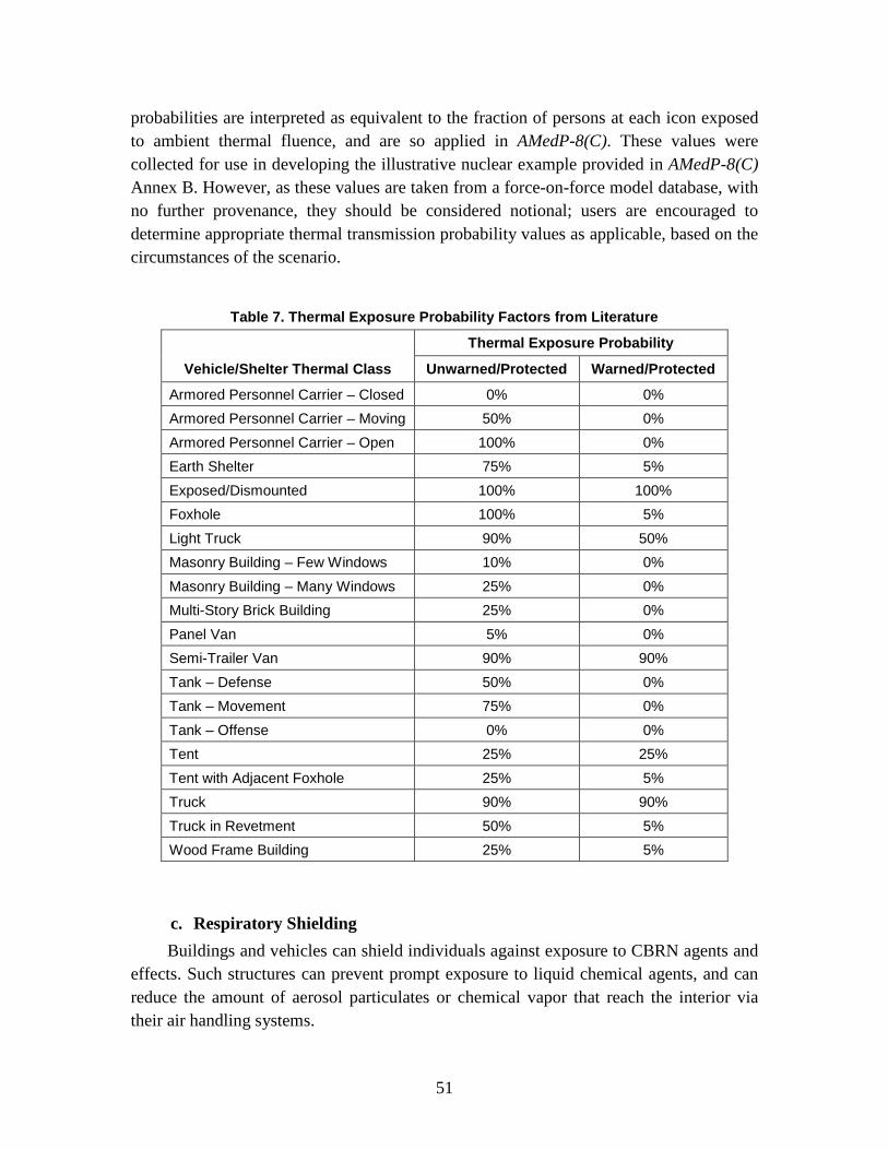
51
probabilities are interpreted as equivalent to the fraction of persons at each icon exposed to ambient thermal fluence, and are so applied in AMedP-8(C). These values were collected for use in developing the illustrative nuclear example provided in AMedP-8(C) Annex B. However, as these values are taken from a force-on-force model database, with no further provenance, they should be considered notional; users are encouraged to determine appropriate thermal transmission probability values as applicable, based on the circumstances of the scenario.
Table 7. Thermal Exposure Probability Factors from Literature
Vehicle/Shelter Thermal Class
Thermal Exposure Probability
Unwarned/Protected Warned/Protected
Armored Personnel Carrier – Closed 0% 0% Armored Personnel Carrier – Moving 50% 0% Armored Personnel Carrier – Open 100% 0% Earth Shelter 75% 5% Exposed/Dismounted 100% 100% Foxhole 100% 5% Light Truck 90% 50% Masonry Building – Few Windows 10% 0% Masonry Building – Many Windows 25% 0% Multi-Story Brick Building 25% 0% Panel Van 5% 0% Semi-Trailer Van 90% 90% Tank – Defense 50% 0% Tank – Movement 75% 0% Tank – Offense 0% 0% Tent 25% 25% Tent with Adjacent Foxhole 25% 5% Truck 90% 90% Truck in Revetment 50% 5% Wood Frame Building 25% 5%
c. Respiratory Shielding Buildings and vehicles can shield individuals against exposure to CBRN agents and
effects. Such structures can prevent prompt exposure to liquid chemical agents, and can reduce the amount of aerosol particulates or chemical vapor that reach the interior via their air handling systems.

52
The dynamics of air flow through buildings and the hazard mitigating effects of air handling systems are often considered with very sophisticated computational fluid dynamics models and the like. However, a simpler, more generic model, described by Blewett et al.69
( )resp, , -AER *Occupancy AER *(Duration Occupancy )
AER *DurationSFAER *Duration + n n n n n
n nn t
n n e e −=
−
was chosen for the purposes of developing the illustrative examples in AMedP-8(C). The advantages of Blewett’s model are that it is readily implemented using basic scenario and environment information and it will generate a single value that can be used as a shielding factor. In this model, the shielding afforded by any building or vehicle is determined by the structure’s air exchange rate (AER), the length of time it is enveloped in the hazard, and the length of time the building is occupied from the time the hazard arrives. The quantity of chemical vapor or aerosol particulates that enters and remains within a building or vehicle is a function of airflow, conventionally described as an air exchange rate, measured in air changes per hour (ACH). These variables combine in the calculation of a respiratory shielding factor as follows:
(2)
where: SFresp,n,t is the respiratory shielding factor at Icon n from time t-1 to t for t > t0,
AERn is the air exchange rate at Icon n [ACH],
Durationn is the length of time the hazard envelopes the vehicle/structure at Icon n [hr], and
Occupancyn is the length of time of vehicle/structure occupancy from the time of hazard arrival at Icon n [hr].
The value for Durationn is derived from the CBRN environment information used as inputs to the calculation of dose/dosage/insult. Since Ccum,n,t is provided for all t ≤ t end,n, users can determine the length of time that Ccum,n,t is greater than zero; this value is equal to Durationn. Occupancyn is more difficult to determine independent of the scenario. The scenario information may provide some guidance as to the expected movement of individuals into and out of buildings and vehicles during the postulated attack, depending on whether or not the attack is detected. Users may also make assumptions about Occupancyn using their own judgment. For occupancy times greater than the duration, the benefit of shielding is reduced, since for Occupancy ≥ Duration, the shielding factor takes on its largest value when Occupancy = Duration. The illustrative examples assume this is the case, in order to assume the greatest possible benefit from shielding.
69 William K. Blewett et al., Expedient Sheltering in Place: An Evaluation for the Chemical Stockpile
Emergency Preparedness Program (Edgewood, MD: Edgewood Research Development and Engineering Center, Aberdeen Proving Ground, June 1996): 14–20.

53
A brief survey of available literature produced widely varying values for air exchange rates associated with buildings and vehicles of various types. Table 8 summarizes these values; it also provides sample calculations of shielding factors based on the assumption that Durationn = Occupancyn = 0.25 hr.
Table 8. Summary of Air Exchange Rates from Literature
1 Ted Johnson, A Guide to Selected Algorithms, Distributions, and Databases used in Exposure Models
Developed by the Office of Air Quality Planning and Standards (Chapel Hill, NC: TRJ Environmental, Inc., 22 May 2002), http://www.epa.gov/ttn/fera/data/human/report052202.pdf. Accessed 8 January 2008.
2 J. H. Park et al., "Measurement of Air Exchange Rate of Stationary Vehicles and Estimation of In-Vehicle Exposure," Journal of Exposure Analysis & Environmental Epidemiology 8, no. 1 (January–March 1998):65-78.
In generating the illustrative examples, the building/vehicle types provided in Table 8 were mapped to the military structures and vehicles within the postulated scenario using SME judgment. The results of this process are provided in Table A-2 of AMedP-8(C).
3. Respiratory Protection Factors The illustrative examples consider two basic types of protection against inhalation
of chemical vapor or aerosol particulates: individual protective equipment (IPE) and collective protection. For purposes of illustration, notional values were selected as respiratory protection factors for these protection types. For IPE, a value of 1,667 was
2.00.250.256.4Residential Building (Windows Open)1
1.15.1-2.2
8.7-3.45.1-2.91.4-1.2
1.1
0.250.25
0.250.250.250.25
0.250.25
0.250.250.250.25
361.8-5.6
1.0-3.01.8-3.7
13.3-26.136.2-47.5
Vehicle1
Mass-Transit Vehicle1
Stationary Automobile2:Windows Closed/No VentilationWindows Closed/Fan On RecirculationWindows Open/No VentilationWindows Open/Fan On Fresh Air
6.927.3-2.7
0.250.25
0.250.25
1.2850.3-4.1
Nonresidential Building1
15.8100.7-3.2
0.250.25
0.250.25
0.530.08-3.24
Residential Building (Windows Closed)1
Shielding Factor
Time of Occupancy from
Cloud Arrival (hr.)
Time Building Is Exposed
(hr.)
Air Exchange
Rate (ACH)Building/ Vehicle Type
54
chosen based on an assumed capability of the standard issue U.S. M40 field protective mask.70
For collective protection, a value of 3,000 was selected on the assumption that collective protection would be equivalent to that provided by high efficiency particulate air (HEPA) filters. Since HEPA filters are designed to remove 99.97% of airborne particles measuring 0.3 microns or greater in diameter,
71
In developing the illustrative examples, it was assumed that IPE would be initiated via command decision given detection and warning of a CBRN attack. Collective protection, on the other hand, might be continuously operating or it might be initiated on warning, given the specific type of building. Table A-3 of AMedP-8(C) lists various structure types and notes whether or not they would have collective protection available and, if so, whether it would be always on or initiated on warning. This table was developed based on SME’s judgment for use in the illustrative examples.
this means approximately 1 in 3,000 particles would penetrate the system; alternatively, with HEPA filtration, 3,000 times as many particles would be required to result in a hazard equivalent to that experienced in the absence of filtration.
4. Dose/Dosage/Insult
a. HD Equivalent Dosage Skin injuries are a consequence of exposure to both vapor and liquid HD. Vapor and
liquid exposures are fundamentally different in that vapor dosages are expressed as a time-integrated concentration for a particular individual or group of individuals, but liquid doses are expressed as a mass of agent per 70 kilogram person. In order to evaluate the effects of vapor and liquid exposure to the skin, an “equivalent” dosage to the skin is calculated. The equivalent dosage is the vapor dosage that would be expected to produce the same human response—physiological system symptom progressions and injury profile—as the combined vapor and liquid exposure actually received.
This equivalent dosage is estimated by applying a conversion factor to the liquid percutaneous dose to determine the equivalent vapor percutaneous dosage. The conversion factor is calculated as the ratio of the vapor percutaneous ECt50 for severe effects to the liquid percutaneous ED50 for severe effects:
70 U.S. Army Chemical School, Protection Factor Requirement Analysis in Support of the Joint Service
General Purpose Mask (JSGPM) Operational Requirements Document (ORD) (Fort McClellan, AL: U.S. Army Chemical School, 13 August 1998), 2.
71 U.S. Department of Energy, DOE Standard: Specification for HEPA Filters Used by DOE Contractors, DOE-STD-3020-97 (Springfield, VA: U.S. Department of Commerce, Technology Administration, National Technical Information Service, January 1997), 7.
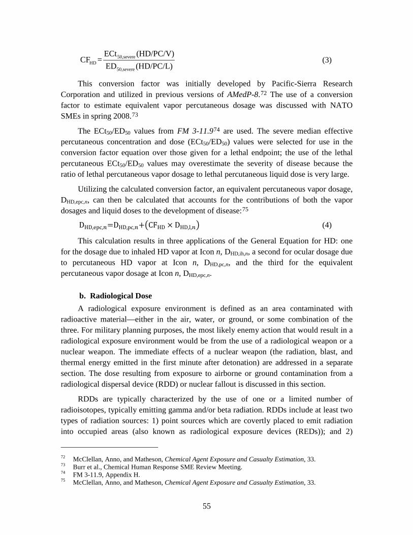
55
50,severeHD
50,severe
ECt (HD/PC/V)CF =
ED (HD/PC/L) (3)
This conversion factor was initially developed by Pacific-Sierra Research Corporation and utilized in previous versions of AMedP-8.72 The use of a conversion factor to estimate equivalent vapor percutaneous dosage was discussed with NATO SMEs in spring 2008.73
The ECt50/ED50 values from FM 3-11.9
74
Utilizing the calculated conversion factor, an equivalent percutaneous vapor dosage, DHD,epc,n, can then be calculated that accounts for the contributions of both the vapor dosages and liquid doses to the development of disease:
are used. The severe median effective percutaneous concentration and dose (ECt50/ED50) values were selected for use in the conversion factor equation over those given for a lethal endpoint; the use of the lethal percutaneous ECt50/ED50 values may overestimate the severity of disease because the ratio of lethal percutaneous vapor dosage to lethal percutaneous liquid dose is very large.
75
DHD,epc,𝑛=DHD,pc,𝑛+�CFHD × DHD,l,𝑛� (4)
This calculation results in three applications of the General Equation for HD: one for the dosage due to inhaled HD vapor at Icon n, DHD,ih,n, a second for ocular dosage due to percutaneous HD vapor at Icon n, DHD,pc,n, and the third for the equivalent percutaneous vapor dosage at Icon n, DHD,epc,n.
b. Radiological Dose A radiological exposure environment is defined as an area contaminated with
radioactive material—either in the air, water, or ground, or some combination of the three. For military planning purposes, the most likely enemy action that would result in a radiological exposure environment would be from the use of a radiological weapon or a nuclear weapon. The immediate effects of a nuclear weapon (the radiation, blast, and thermal energy emitted in the first minute after detonation) are addressed in a separate section. The dose resulting from exposure to airborne or ground contamination from a radiological dispersal device (RDD) or nuclear fallout is discussed in this section.
RDDs are typically characterized by the use of one or a limited number of radioisotopes, typically emitting gamma and/or beta radiation. RDDs include at least two types of radiation sources: 1) point sources which are covertly placed to emit radiation into occupied areas (also known as radiological exposure devices (REDs)); and 2)
72 McClellan, Anno, and Matheson, Chemical Agent Exposure and Casualty Estimation, 33. 73 Burr et al., Chemical Human Response SME Review Meeting. 74 FM 3-11.9, Appendix H. 75 McClellan, Anno, and Matheson, Chemical Agent Exposure and Casualty Estimation, 33.
56
radioactive material which is dispersed (mechanically or explosively) to spread contamination, resulting in casualties and denial of access to the zone of contamination. For point sources, it is a relatively simple matter to estimate the whole-body radiation dose, based on the amount of radioactivity, and the time, distance, and shielding of the scenario.76
Nuclear fallout includes the fission products, unfissioned bomb material, and activated materials in the air and soil that become particulates following the nuclear detonation. The specific radioisotopes, radiations emitted, and particle size distributions vary with time and distance from the point of detonation.
The sources of exposure from both RDDs and fallout include, potentially, four different types of radiation (gamma, beta, neutron, alpha) along four different routes of exposure (whole-body exposure (typically external), skin contamination, inhalation, ingestion). In order to practically describe a methodology for estimating casualties resulting from a military threat of RDDs or fallout, it is necessary to limit the consideration of these possible radiations and routes of exposure to those likely to result in battlefield casualties. Thus, inhalation and ingestion are not considered, because these are unlikely to result in casualties during the time frame of interest (typically within 30 to 60 days of exposure). Admittedly, there are credible scenarios wherein individuals inhale or ingest enough radioactive material to become ill within 60 days; these are just not regarded as likely to occur on a military battlefield. Whole-body radiation dose is considered, as a measure of the total contribution of radiation to the overall human response. Whole-body radiation dose can be characterized as the sum of the dose from radiation due to activity concentration in the air (cloudshine) and of the dose from radioactivity deposited on the ground (groundshine). Cutaneous (skin) radiation dose is also considered. Cutaneous dose is the dose to the skin due to beta and gamma radiation absorbed by the skin and is a function of several components—beta radiation due to contaminant on the skin, radiation from contamination deposited on the ground, and radiation from immersion in radioactive material suspended in the air.77
Similarly, alpha radiation is not considered because it can only cause casualties if it is inhaled or ingested, and that is regarded as unlikely. Neutron radiation is included, conceptually, in this methodology, but no isotope or mixture of isotopes which are significant neutron emitters are modeled. The isotopes that are included are those which
76 Michael G. Stabin, “External Dose Assessment,” Chap. 9 in Radiation Protection and Dosimetry: An
Introduction to Health Physics (New York, NY: Springer, 2008), 180–82. 77 Gamma and beta radiation from cloudshine is ignored for cutaneous dose because it will be negligible
compared to other sources for individuals in contaminated zones for extended periods of time.
57
have the potential for producing an acute radiation injury (overt symptoms within the time period of interest) and have a credible likelihood of battlefield exposure.78
For dispersed radioisotopes, estimates of radiological contamination are typically expressed in terms of activity per unit volume or activity per unit area. In order to estimate human response, these values must be translated to dose and provided as inputs to the human response estimation component of the AMedP-8(C) methodology. These calculations typically involve a dose conversion factor which translates activity (in becquerels (Bq)) into dose (in gray (Gy)). Most of the conversion factors are expressed in the literature using absorbed and equivalent doses. Such quantities modify the absorbed dose by incorporating radiation and tissue weighting factors to reflect the relative effectiveness of different radiations and vulnerabilities of different tissues specifically for late (stochastic) effects, principally cancer. They are used in routine occupational radiation protection and are consequently considered applicable at relatively low doses and dose rates. Since the radiation weighting factors for gamma and beta radiations are both unity (1), whole-body and cutaneous radiation dose factors are expressed as absorbed dose in units of gray, instead of dose equivalent with units of sievert, without altering the numerical values.
79
For calculating dose from RDDs or fallout, the original intent was to use international references to preclude any national bias. The ideal choice for this seemed to be the International Atomic Energy Agency’s (IAEA) TECDOC-1162,
80 but this reference did not provide estimates for all of the desired routes of exposure or all of the desired types of radiation of interest. The U.S. Environmental Protection Agency’s (EPA) Federal Guidance Report (FGR) 1281
• Whole body dose from exposure to ground contamination (Conversion factor CF3 from Table E-3)
did provide these, through the use of the “Tables of Dose Coefficients.” Specifically, the IAEA TECDOC provided tables which allowed for:
• Skin beta dose from material deposited onto skin (Conversion factor CF8 from Table E-5)
• Whole body dose from external exposure to γ-emitting radionuclides in a radioactive plume (Conversion factor CF9 from Table E-14)
EPA FGR No. 12, on the other hand, provided tables which allowed for: 78 Frederick T. Harper, Stephen V. Musolino, and William B. Wente, “Realistic Radiological Dispersal
Device Hazard Boundaries and Ramifications for Early Consequence Management Decisions,” Health Physics 93, no. 1 (July 2007): 1–16.
79 Glasstone and Dolan, Effects of Nuclear Weapons, 577. 80 International Atomic Energy Agency (IAEA), Generic Procedures for Assessment and Response
During a Radiological Emergency, IAEA-TECDOC-1162 (Vienna: IAEA, 2000). 81 Keith F. Eckerman and Jeffrey C. Ryman, External Exposure to Radionuclides in Air, Water, and Soil,
Federal Guidance Report No. 12, EPA-402-R-93-081 (Washington, DC: U.S. Environmental Protection Agency, September 1993).

58
• Whole body dose from exposure to ground contamination (“Effective” Column from Table III-3) (essentially the same as Conversion factor CF3 from Table E-3 of the IAEA TECDOC)
• Skin dose from exposure to ground contamination (“Skin” Column from Table III-3)
• Whole body dose from external exposure to all photons and electrons from radionuclides in a radioactive plume (“Effective” Column from Table III-1)
• Skin dose from external exposure to all photons and electrons from radionuclides in a radioactive plume (“Skin” Column from Table III-1)
The AMedP-8(C) methodology uses the EPA FGR No. 12 factors, combined with the skin beta dose from material deposited onto skin (conversion factor CF8) from IAEA TECDOC Table E-5, to comprehensively address the range of radiation types and routes of exposure of interest. When applying these factors to the General Equation for radiological agents, the methodology requires two different applications: one for the whole-body radiation [absorbed] dose and one for the cutaneous radiation dose (equivalent dose to the skin). The whole-body radiation dose comes from external radiation, while the cutaneous radiation dose can include contributions from both external radiation and skin contamination.
c. Body Surface Area Burned (%BSA) The equation for calculating %BSA used in AMedP-8(C) is derived from a U.S.
Defense Nuclear Agency (DNA) study conducted by Levin in the early 1990s.82
Under the assumption that there is equal probability that any side of the body will be facing a nuclear detonation, Levin used a cylindrical model of the body to estimate the effective area burned.
The variant used in AMedP-8(C) corrects a typographical error made in the original report, described below, and expands the equation to account for the percentage of body covered by a uniform and the percentage of body that is bare.
83
This underlying concept is shown in Figure 1.
82 Levin, Effect of Combined Injuries. 83 Ibid., 23.

59
Figure 1. Cylindrical Model for Man Used to Estimate Area Burned from Thermal Fluence
The corresponding equation, which calculates the area burned as a percent of the total area, is shown in Equation 5.
( )tarccos Q QA
pi= (5)
where: A = area burned, percent
Qt = the thermal fluence threshold value for a second degree burn (cal/cm2)
Q = the thermal fluence in cal/cm2 to which the cylinder is exposed
pi = 3.14159
The typographical error in Levin’s report was a transposition of Q and Qt. Because the argument of the arccosine function (expressed in radians) can never be greater than one, it is evident that the two terms (Q and Qt) are meant to be positioned as shown in Equation 5. A comparison of the numerical values provided by Levin to those calculated using the updated equation confirms that this is how he intended to write the equation and is, in fact, how he implemented it in his report.
The thermal fluence threshold value in Levin’s equation, Qt, varies as a function of clothing type and the extent to which it covers the body. Table A-13 in AMedP-8(C) Annex A provides thermal fluence threshold values corresponding to 50% incidence of second degree burns for various uniform types. The bare skin value in this table is taken from Levin’s report;84 and all others are taken from a 1986 report from Harry Diamond Labs.85
84 Ibid., 24.
Levin’s report contains thermal fluence threshold values for selected uniform types as well, and these values are consistent with those found in the Harry Diamond
85 Baba et al., Incidence of Skin Burns, Figure 1 and Table 4.

60
Labs report. Note that the values provided in AMedP-8(C) are expressed in kJ/m2 to be consistent with internationally recognized metric units.
In cases where the uniform type does not completely cover the body, the %BSA equation must account for both the differential injury to bare skin versus clothed skin. To do so, the %BSA equation given above must be calculated once using the bare skin threshold value and once using the uniform threshold value. The output of the equation generated with the bare skin threshold value is then multiplied by the percent of body surface area that is bare, while the output generated with the uniform type threshold value is multiplied by the percent of body surface area that is clothed. The results are summed to determine the total %BSA.
The resulting %BSA equation found in AMedP-8(C) is:
T,uniform T,bareskin
thermal,
Q Qarccosine arccosine
Q QD * % * %
n nuniform bareskinn P P
π π
= +
(6)
where: n is the index number of the icon,
Dthermal,n is the percent of body surface area burned for Icon n [%BSA],
QT,uniform is the thermal fluence threshold value for a specific uniform type for a partial-thickness (second degree) burn [kJ/m2],
QT,bareskin is the thermal fluence threshold value for bare skin for a partial-thickness (second degree) burn [kJ/m2],
Qn is the thermal fluence to which the body (cylinder) is exposed for Icon n [kJ/m2]
P%uniform is the percentage of the body covered by the uniform, and
P%bareskin is the percentage of the body uncovered or bare.

61
4. Chemical Human Response Review: Nerve Agents—Sarin and VX
A. Introduction Chemical nerve agents are among the most toxic chemical substances known; in
both vapor and liquid form, exposure can result in near-instantaneous symptoms and, at high enough doses, death. The objective of this chapter is to describe the human response methodologies for the nerve agents GB and VX as they have been incorporated into the AMedP-8(C) methodology.
B. Background Nerve agents GB and VX act through similar mechanisms of action—both inhibit
acetylcholinesterase reactions by binding at the enzyme receptor sites and blocking hydrolysis—but they differ in other respects. Because of its high volatility, for example, GB is a nonpersistent agent and evaporates quickly. As a result, GB vapor poses an inhalation hazard and a more-limited percutaneous hazard. On the other hand, VX is persistent and may pose a threat in the vicinity of an attack for longer periods of time. Because of the similarities in the mechanism of action and the resulting effects, both agents produce similar signs and symptoms, although the rate and severity of effect in relation to dose varies for each agent due to their different toxicities.
1. Agent Physiological Effects Chemical nerve agents cause disease by inhibiting the proper functioning of the
enzyme acetylcholinesterase in its interaction with acetylcholine. Acetylcholine is “the neurotransmitter of the neurons to skeletal muscle, of the preganglionic autonomic nerves, and of the post-ganglionic parasympathetic nerves.”86
86
In simple terms, acetylcholine passes messages to the skeletal muscles and through the nervous system, thereby stimulating the system’s reaction. The enzyme acetylcholinesterase breaks down (or hydrolyzes) the acetylcholine, ending the stimulation trigger and allowing the muscle to relax. Nerve agents inhibit acetylcholinesterase function by binding to the enzyme’s receptor sites, prohibiting the acetylcholine compounds from binding to these now-occupied sites. As a result, the enzyme is unable to hydrolyze the acetylcholine,
Sidell, “Nerve Agents,” 132.
62
precluding the termination of the nerve signal. Because the stimulation trigger remains, and even intensifies, as acetylcholine builds up in the system, the muscles remain constantly stimulated and prevented from relaxing. This effect can eventually lead to death via several routes, including: the failure of the central nervous system to stimulate respiratory drive, muscle fatigue leading to flaccid paralysis of the diaphragm, and asphyxiation due to constriction of the bronchial tubes combined with excessive secretions in the air passages. A brief summary of signs and symptoms follows to provide background material. More detailed discussions of these signs and symptoms are available in Sidell87 and McDonough.88
In addition to the respiratory system, several physiological organs and systems are affected, including the eye, nose, mouth, pulmonary tract, gastrointestinal tract, skin and sweat glands, muscular system, cardiovascular system, and central nervous system.
89 The severity of these effects is a function of dose or dosage: “The magnitude and duration of a particular physiological effect is highly dependent upon the level of agent exposure or dose of the drug.”90
Ocular effects are usually the first symptoms, as these occur at very low exposure levels. Ocular effects include miosis (constriction of the pupil), conjunctival injection (bloodshot eyes), eye pain, and dim or blurred vision. The duration and severity of these effects depends on the exposure dose.
91
In addition to ocular effects, nerve agent exposure causes an increased level of secretions from the nose and the sweat and salivary glands, as well as in the pulmonary and gastrointestinal systems. In the gastrointestinal tract, these may be accompanied by abdominal cramps, nausea, vomiting, and, in smaller segments of the population, diarrhea.
92
In the pulmonary tract, complaints may include cough, “tight chest,” and shortness of breath. As the dose increases, “respiration rapidly becomes gasping and irregular, and the victim can become cyanotic and totally apneic in a severe poisoning.”
93
87
Individuals exposed to low doses may begin to feel better shortly after moving to cleaner air environments and their respiratory complaints may resolve themselves without medical
Sidell, “Nerve Agents.” 88 John H. McDonough, “Performance Impacts of Nerve Agents and Their Pharmacological
Countermeasures,” Military Psychology 14, no. 2 (2002): 93–119. 89 Sidell, “Nerve Agents,” 145. 90 McDonough, “Performance Impacts of Nerve Agents,” 97. 91 Ibid., 98–99. 92 Ibid., 99–100; and Sidell, “Nerve Agents,”144–49. 93 McDonough, “Performance Impacts of Nerve Agents,” 100.

63
interventions. At higher doses, medical interventions are required to reduce the effects and possibly aid in ventilation.94
In the muscular system, the initial effects manifest as twitches, jerks, and fasciculations (visible contractions of small numbers of muscle fibers), resulting in muscle fatigue. Larger doses may result in seizures or larger muscle group contractions, causing flailing limbs or rigid hyperextension of the limbs or torso.
Psychological effects may also be present following nerve agent exposure; these may be of short or prolonged duration, depending on dose. Symptoms may include increased anxiety, tension, weakness, fatigue, forgetfulness, and irritability.
2. Toxicity Values Table 9 presents the GB and VX toxicity values (and respective probit slopes) for
the:
• Median ocular/mild dosage (ECt50,ocular/mild)—the amount of vapor agent expected to cause ocular or other mild effects (e.g., rhinorrhea) in 50% of an exposed, unprotected group of individuals;
• Median effective severe dosages and dose (ECt50,severe, ED50,severe)—the amount of vapor or liquid agent expected to cause severe effects in 50% of an exposed, unprotected group of individuals; and,
• Median lethal dosages and dose (LCt50, LD50)—the amount of vapor or liquid agent expected to kill 50% of an exposed, unprotected group of individuals.
Vapor exposures are expressed as dosages in milligram-minutes per cubic meter (mg-min/m3), while liquid exposures are expressed as doses in milligrams per 70 kilogram man (mg).
94 Ibid.; and Sidell, “Nerve Agents,” 148.
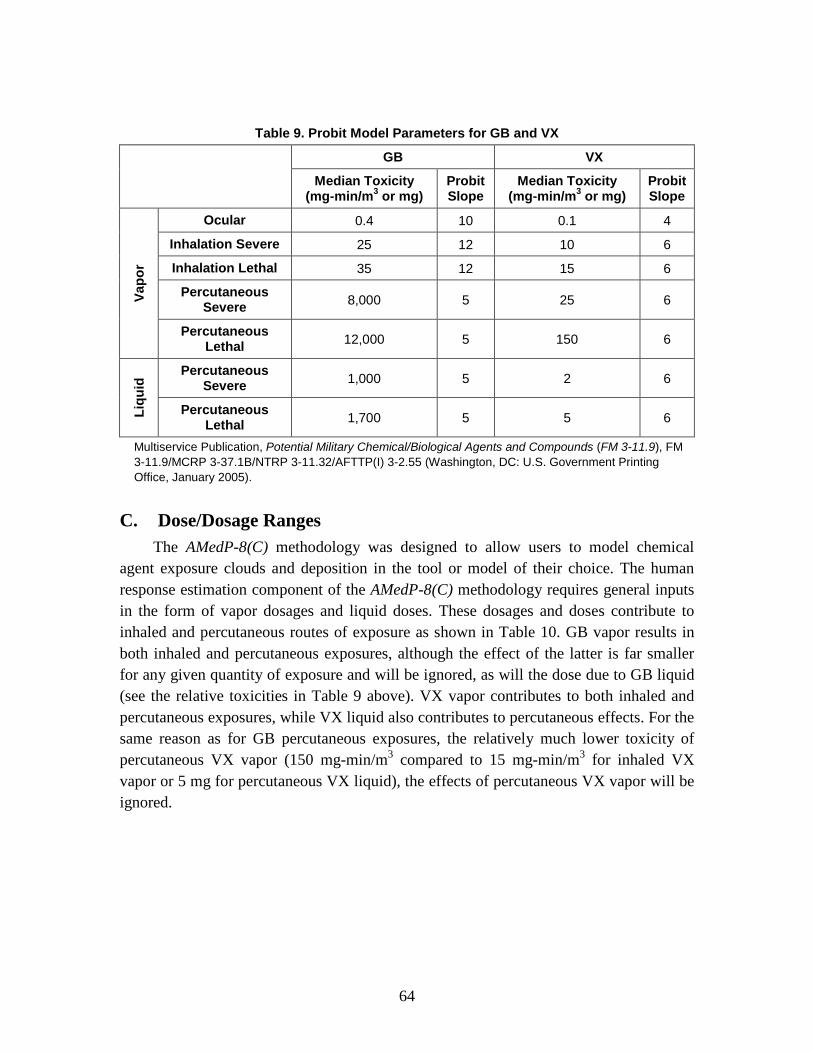
64
Table 9. Probit Model Parameters for GB and VX
GB VX
Median Toxicity (mg-min/m3 or mg)
Probit Slope
Median Toxicity (mg-min/m3 or mg)
Probit Slope
Vapo
r
Ocular 0.4 10 0.1 4
Inhalation Severe 25 12 10 6
Inhalation Lethal 35 12 15 6
Percutaneous Severe 8,000 5 25 6
Percutaneous Lethal 12,000 5 150 6
Liqu
id Percutaneous
Severe 1,000 5 2 6
Percutaneous Lethal 1,700 5 5 6
Multiservice Publication, Potential Military Chemical/Biological Agents and Compounds (FM 3-11.9), FM 3-11.9/MCRP 3-37.1B/NTRP 3-11.32/AFTTP(I) 3-2.55 (Washington, DC: U.S. Government Printing Office, January 2005).
C. Dose/Dosage Ranges The AMedP-8(C) methodology was designed to allow users to model chemical
agent exposure clouds and deposition in the tool or model of their choice. The human response estimation component of the AMedP-8(C) methodology requires general inputs in the form of vapor dosages and liquid doses. These dosages and doses contribute to inhaled and percutaneous routes of exposure as shown in Table 10. GB vapor results in both inhaled and percutaneous exposures, although the effect of the latter is far smaller for any given quantity of exposure and will be ignored, as will the dose due to GB liquid (see the relative toxicities in Table 9 above). VX vapor contributes to both inhaled and percutaneous exposures, while VX liquid also contributes to percutaneous effects. For the same reason as for GB percutaneous exposures, the relatively much lower toxicity of percutaneous VX vapor (150 mg-min/m3 compared to 15 mg-min/m3 for inhaled VX vapor or 5 mg for percutaneous VX liquid), the effects of percutaneous VX vapor will be ignored.

65
Table 10. Nerve Agent Routes of Exposure
GB VX
Vapor Liquid Vapor Liquid
Inhaled X X
Percutaneous X X X X Potential nerve agent routes of exposure include percutaneous vapor and liquid exposure; for GB, these
routes of exposure are neglected and therefore shown in red, as is the percutaneous vapor route for VX.
Dosage and dose ranges for GB and VX were selected to represent clinically differentiable injury profiles as a function of dosage or dose.
While the AMedP-8(C) nerve agent dosage range tables are derived from the original Injury Severity Category tables included in AMedP-8(A), some modification of those tables was needed for AMedP-8(C). Within AMedP-8(A), the GB and VX dosage ranges were selected using ocular/mild, severe, and lethal dosage values that have since been revised; as discussed below, to accommodate changes to toxicity values, reflected in Table 9. In addition, AMedP-8(A) used eight dosage ranges to represent both GB and VX, but discussions with the NATO CBRN Medical Working group indicated that this was too many ranges. Moreover, these discussions suggested that dosage ranges should ideally be clinically differentiable, and such was not the case with the ranges found in AMedP-8(A).
In order to modify the dosage ranges, the AMedP-8(C) methodology began by returning to the original DICE methodology.95
Using a similar methodological approach, the median, 10%, and 90% values for ocular, severe, and lethal inhalation effects and severe and lethal percutaneous effects due to liquid exposure for VX were plotted. Ranges were estimated to encompass some incidences and types of effect. For both inhaled GB and VX exposures, no inhalation “mild” toxicity value existed on which to base ranges 2 and 3. To derive these values, response curves were drawn from the values shown in Table 9; these curves were then scaled to allow for estimation of the ranges for use in the AMedP-8(C) methodology, as
The DICE methodology used the median ocular, severe, and lethal toxicity values along with probit curves for each agent to approximate the 10%, 50%, and 90% anticipated incidence of effect. The DICE methodology then drew ranges that encompassed some incidences and types of effect and associated symptoms with each range.
95 Deverill and Metz, DICE Chemical Insult Program, 8–23; and McClellan, Anno, and Matheson,
Chemical Agent Exposure and Casualty Estimation, 3–10.
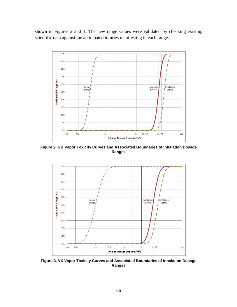
66
shown in Figures 2 and 3. The new range values were validated by checking existing scientific data against the anticipated injuries manifesting in each range.
Figure 2. GB Vapor Toxicity Curves and Associated Boundaries of Inhalation Dosage
Ranges
Figure 3. VX Vapor Toxicity Curves and Associated Boundaries of Inhalation Dosage
Ranges
0.2 6.5 12 25 30
Ocular (Mild)
Inhalation Severe
Inhalation Lethal
0.02 2 4
Ocular (Mild)
Inhalation Severe
Inhalation Lethal
0.3 13

67
The “no observable effect” range was added in place of the “no injury” range to indicate that below some dosage, although there may possibly be physiological effects, there will be no observable effects resulting from exposure. Although DICE had used a low incidence of occurrence equivalent to effects anticipated in 10% of the population as the lowest value of observable effects, SMEs recommended that an incidence of ocular injury in less than 1% of the population should provide the basis for a “no observable effects in majority of the population” range. Additionally, subject matter experts added the first observable effects range: “Miosis in 10% – 90%, rhinorrhea, transient tightness of the chest.”96
Separate dose ranges for percutaneous liquid VX exposure were derived for use in AMedP-8(C). Unlike for inhaled GB and VX, no previous dose ranges existed on which to base the new ranges, since percutaneous VX exposure was incorporated into the equivalent dosage calculation in the AMedP-8(A) methodology. As shown in Figure 4, ranges were selected using probit curves, similar to the approach used for the updated inhaled GB and VX ranges, although liquid toxicity data were limited to severe and lethal percutaneous effects.
Figure 4. VX Liquid Toxicity Curves and Associated Boundaries of Percutaneous Dose
Ranges
96 Conversations at the Institute for Defense Analyses with subject matter experts from Edgewood
Chemical and Biological Center, U.S. Army Medical Research Institute for Chemical Defense, and others, 11 March 2008.
0.8 3.9
Percutaneous Severe
Percutaneous Lethal
1.6

68
The range assignments with included incidences, for both the AMedP-8(A) methodology as conducted for DICE and the AMedP-8(C) methodology, are shown in Tables 11 and 12 for inhaled GB and VX respectively. The percutaneous VX liquid dose range assignments are shown in Table 13.
Table 11. Inhaled GB Dosage Range Derivation
AMedP-
8(A) AMedP-
8(C)*
Begin Dosage Range 1 0 0 End Dosage Range 1 – Begin Dosage Range 2 0.2 1% Ocular Injury (ocular/mild) 0.23 10% Ocular Injury (ocular/mild) 0.33 0.30 50% Ocular Injury (ocular/mild) 0.5 0.40 90% Ocular Injury (ocular/mild) 0.75 0.54 End Dosage Range 2 – Begin Dosage Range 3 1 1 ≈ ECt99 ocular End Dosage Range 3 – Begin Dosage Range 4 6.5 6.5 End Dosage Range 4 – Begin Dosage Range 5 14 12 < ECt01 severe 10% Severe Effects 23 19.55 50% Severe Effects 35 25 End Dosage Range 5 – Begin Dosage Range 6 35 25 = ECt50 severe 10% Lethal Effects 45 27.37
End Dosage Range 6 – Begin Dosage Range 7 50 30 ≈ ECt85 severe & LCt15
90% Severe Effects 54 31.97 50% Lethal Effects 70 35 90% Lethal Effects 107 44.76 *FM 3-11.9.

69
Table 12. Inhaled VX Dosage Range Derivation
AMedP-
8(A) AMedP-
8(C)*
Begin Dosage Range 1 0 0.00 0.02 1% Ocular Injury (ocular/mild) 0.03 10% Ocular Injury (ocular/mild) 0.06 0.05 50% Ocular Injury (ocular/mild) 0.09 0.10 90% Ocular Injury (ocular/mild) 0.14 0.21 End Dosage Range 1 – Begin Dosage Range 2 0.2 0.30 ≈ ECt99 ocular End Dosage Range 2 – Begin Dosage Range 3 2 End Dosage Range 3 – Begin Dosage Range 4 12 4 < ECt01 severe 10% Severe Effects 17 6.12 10% Lethal Effects 20 9.17 50% Severe Effects 25 10 End Dosage Range 4 – Begin Dosage Range 5 25 10 = ECt50 severe
End Dosage Range 5 – Begin Dosage Range 6 30 13 ≈ ECt85 severe & LCt15
90% Severe Effects 37 16.35 50% Lethal Effects 30 15 90% Lethal Effects 45 24.53 * FM 3-11.9.

70
Table 13. Percutaneous VX Liquid Dose Range Derivation
AMedP-8(C)* (all doses in mg) Begin Dosage Range 1 0.00 End Dosage Range 1 – Begin Dosage Range 2 0.8 < ED01 severe 1% Severe Effects 0.82 10% Severe Effects 1.22 End Dosage Range 2 – Begin Dosage Range 3 1.6 ≈ ED30 severe 50% Severe Effects 2 10% Lethal Effects 3.06 90% Severe Effects 3.27 End Dosage Range 4 – Begin Dosage Range 5 3.9 ≈ LD25 50% Lethal Effects 5 90% Lethal Effects 8.18
* FM 3-11.9.
Each range was then described with the associated symptoms. The resulting ranges are expressed in terms of the inhaled dosage value, in milligram-minutes per cubic meter, and the percutaneous dose, in milligrams (per 70 kilogram man). The ranges are shown in Tables 14 for inhaled GB and 15 and 16 for inhaled and percutaneous VX liquid exposures respectively.
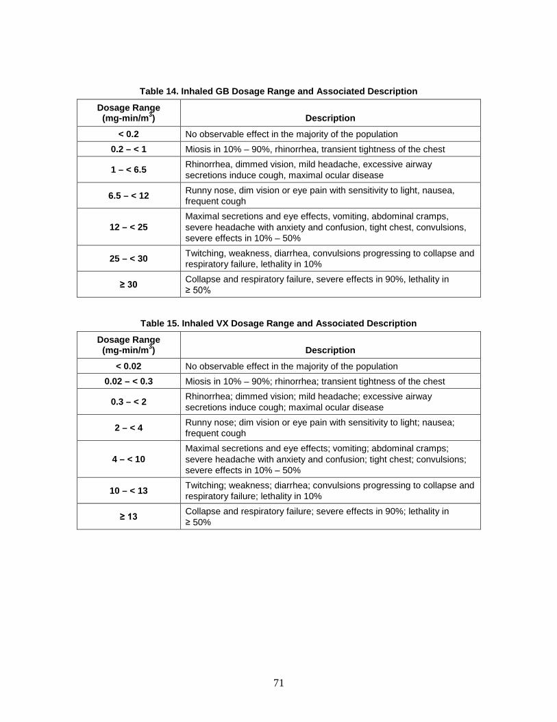
71
Table 14. Inhaled GB Dosage Range and Associated Description
Dosage Range (mg-min/m3) Description
< 0.2 No observable effect in the majority of the population 0.2 – < 1 Miosis in 10% – 90%, rhinorrhea, transient tightness of the chest
1 – < 6.5 Rhinorrhea, dimmed vision, mild headache, excessive airway secretions induce cough, maximal ocular disease
6.5 – < 12 Runny nose, dim vision or eye pain with sensitivity to light, nausea, frequent cough
12 – < 25 Maximal secretions and eye effects, vomiting, abdominal cramps, severe headache with anxiety and confusion, tight chest, convulsions, severe effects in 10% – 50%
25 – < 30 Twitching, weakness, diarrhea, convulsions progressing to collapse and respiratory failure, lethality in 10%
≥ 30 Collapse and respiratory failure, severe effects in 90%, lethality in ≥ 50%
Table 15. Inhaled VX Dosage Range and Associated Description
Dosage Range (mg-min/m3) Description
< 0.02 No observable effect in the majority of the population 0.02 – < 0.3 Miosis in 10% – 90%; rhinorrhea; transient tightness of the chest
0.3 – < 2 Rhinorrhea; dimmed vision; mild headache; excessive airway secretions induce cough; maximal ocular disease
2 – < 4 Runny nose; dim vision or eye pain with sensitivity to light; nausea; frequent cough
4 – < 10 Maximal secretions and eye effects; vomiting; abdominal cramps; severe headache with anxiety and confusion; tight chest; convulsions; severe effects in 10% – 50%
10 – < 13 Twitching; weakness; diarrhea; convulsions progressing to collapse and respiratory failure; lethality in 10%
≥ 13 Collapse and respiratory failure; severe effects in 90%; lethality in ≥ 50%

72
Table 16. Percutaneous VX Dose Range and Associated Description
Dose Range (mg) Description
< 0.8 No observable effect in the majority of the population
0.8 – < 1.6 Muscle twitching and fasciculation; chest tightness and shortness of breath; episodes of vomiting; severe effects in 10%
1.6 – < 3.9 Severe generalized trembling with possible convulsions; feelings of confusion and anxiety; respiratory congestion and bronchorrhea; severe effects in ≥ 50%; lethality in 10%
≥ 3.9 Unconsciousness; paralysis; breathing stops completely or struggling to breathe; lethality in ≥ 50%
D. Symptoms The basic concept of the AMedP-8(C) methodology is that an individual is
considered a casualty at the time of first onset of a specified injury severity level, based on specific symptoms resulting from exposure to the causative agent. The human response component of this methodology specifies an injury profile depicting injury severity level over time that is used to determine whether an individual is declared KIA, WIA, or DOW and thereby considered to be a casualty and, if so, at what point this would occur. The injury profile is derived from the symptom progressions, which show the severity level of symptoms in the system in which they manifest (as opposed to the causative system) over time. The severity level of the injury profile at any given time point corresponds to the worst severity level experienced in any of the representative physiological systems at that time. The nature of symptoms and their times of onset depend on the agent.
1. Severity Levels For GB and VX, the DICE methodology employed six sets of signs, symptoms, and
systems to represent the inhaled chemical nerve agent injury progression: upper gastrointestinal, lower gastrointestinal, respiratory, ocular, muscular, and mental. These symptoms were represented on a severity scale of 1–5.97
In an effort to ensure clarity and consistency, the symptoms and systems for the chemical nerve agents were correlated to six representative physiological systems—upper
97 George H. Anno et al., Predicted Performance on Infantry and Artillery Personnel Following Acute
Radiation or Chemical Agent Exposure, DNA-TR-93-174 (Washington, DC: Defense Nuclear Agency, November 1994), 8–13; McClellan, Anno, and Matheson, Chemical Agent Exposure and Casualty Estimation, 11–16; and Deverill and Metz, DICE Chemical Insult Program, 15–40.

73
gastrointestinal, lower gastrointestinal, respiratory, ocular, muscular, and neurological—in which symptoms would be expected to manifest following inhalation exposure to chemical agents. The same six systems were used to derive symptom progressions and injury profiles resulting from exposure to percutaneous liquid VX.
As previously described in Chapter 2 and summarized in Table 1, symptoms in the AMedP-8(C) methodology are expressed on a scale of 0–4, with 0 representing no observable effect and 4 representing very severe effects.
The DICE human response methodology correlated the severity levels for each of the six physiological systems to anticipated signs and symptoms; the severity levels were independent for each physiological system.98
In order to align the severities across the physiological systems and be able to draw useful injury profiles, the AMedP-8(C) methodology adjusted severity levels associated with each set of signs and symptoms. As a result, all six physiological systems begin with a “no observable effect” level, but each system has only the number of severity levels necessary to achieve the maximum severity at which signs and symptoms for that physiological system occur. For example, if a given physiological system was not expected to manifest symptoms greater in severity than level 3, then the scale for that system would range from 0 to 3. Moreover, the new severity levels are aligned so that, for instance, a Severity Level 3 ocular injury consists of signs and symptoms of equal severity to those found in Severity Level 3 for the respiratory system and Severity Level 3 for the muscular system. Again, these signs and symptoms are shown in the physiological system in which they manifest, rather than in the causative system.
For example, an ocular severity of 4 (described as “temporary blindness”) while operationally challenging, was not, however, equivalent to a respiratory severity of 4 (“breathing stops completely”) which could potentially kill an individual.
The AMedP-8(C) methodology symptom-severity level correlations are shown in Table 17. As both GB and VX are represented by the same six physiological systems, the severity levels described apply for both nerve agents.
98 These correlations are derived from those completed as part of the DICE methodology.

74
Table 17. GB and VX Symptoms Severity Levels
Severity Upper Gastrointestinal Lower Gastrointestinal Muscular
0 No observable effect No observable effect No observable effect
1
Upset stomach and nausea; watering mouth and frequent swallowing to avoid vomiting
Abdominal pain or cramps; occasional diarrhea and uncomfortable urge to defecate
Muscle twitching/ fasciculation; fatigue and weakness
2
Episodes of vomiting, possibly including dry heaves; severe nausea and possibility of continued vomiting
Frequent diarrhea and cramps; continuing defecation
Muscle trembling; lack of coordination; increased fatigue and weakness
3 Uncontrollable diarrhea and urination; painful cramps
Severe generalized twitching with or without convulsions
4 Flaccid paralysis
Table 17. continued
Severity Ocular Respiratory Neurological
0 No observable effect No observable effect No observable effect
1
Slightly blurred, dim (may be due to tearing), or possibly irritated (conjunctival erythema and/or edema) vision
Mild shortness of breath; tight chest, coughing, and runny nose
Feelings of anxiety, irritability or euphoria
2
Blurred vision due to dimming or difficulty opening eyes; eyes sensitive to light or puffy; potential for pressure behind the eyes, eye pain, or heavy tearing
Frank shortness of breath; difficult to breathe, wheezing breath, respiratory congestion, bronchorrhea
Difficulty in concentration
3 Functional blindness (possibly accompanied by extreme headache)
Breathing sporadically stops and starts, skin has a purple or blue color, hemoptysis
Aphasia; memory loss; disorientation
4 Breathing stops completely or struggling to breathe; prostration
Unconsciousness
75
2. Symptom Progression and Injury Profiles Each of the dosage or dose ranges previously described corresponds to a set of
symptom progressions through time. These symptom progressions are discontinuous with respect to dosage or dose; all dosages or doses within the specified range are represented by the same set of symptom progressions. The boundaries defining each dosage or dose range represent points in an exposure at which the expected progression of injury abruptly changes as the dosage or dose is increased. Moreover, the symptom progressions themselves are discontinuous and stepwise with respect to severity level; they are not smoothed or otherwise interpolated. In other words, moving along the time dimension of the symptom progression, the symptom severity changes instantaneously at specific points in time. For a given dosage or dose range, separate symptom progressions have been developed for each of the six physiological systems—upper gastrointestinal, lower gastrointestinal, respiratory, ocular, muscular, and neurological—illustrating the severity of the symptoms for a particular physiological system over time. Figures 5 through 10 and 11 through 16 present the symptom progressions by dosage range for inhaled GB and VX respectively, and Figures 17 through 19 present the symptom progressions by percutaneous dose range for liquid VX.99
The “no observable effect” dosage ranges are not shown; all severity levels in those dosage ranges would be 0 for the duration of time observed.
99 All of the symptom progressions and injury profiles are plotted using minutes along the logarithmic x-
axis.
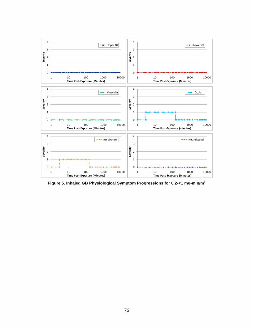
76
Figure 5. Inhaled GB Physiological Symptom Progressions for 0.2-<1 mg-min/m3
0
1
2
3
4
1 10 100 1000 10000
Seve
rity
Time Post-Exposure (Minutes)
Upper GI
0
1
2
3
4
1 10 100 1000 10000
Seve
rity
Time Post-Exposure (Minutes)
Lower GI
0
1
2
3
4
1 10 100 1000 10000
Seve
rity
Time Post-Exposure (Minutes)
Muscular
0
1
2
3
4
1 10 100 1000 10000
Seve
rity
Time Post-Exposure (minutes)
Ocular
0
1
2
3
4
1 10 100 1000 10000
Seve
rity
Time Post-Exposure (Minutes)
Respiratory
0
1
2
3
4
1 10 100 1000 10000
Seve
rity
Time Post-Exposure (Minutes)
Neurological

77
Figure 6. Inhaled GB Physiological Symptom Progressions for 1-<6.5 mg-min/m3
0
1
2
3
4
1 10 100 1000 10000
Seve
rity
Time Post-Exposure (Minutes)
Upper GI
0
1
2
3
4
1 10 100 1000 10000
Seve
rity
Time Post-Exposure (Minutes)
Lower GI
0
1
2
3
4
1 10 100 1000 10000
Seve
rity
Time Post-Exposure (Minutes)
Muscular
0
1
2
3
4
1 10 100 1000 10000
Seve
rity
Time Post-Exposure (Minutes)
Ocular
0
1
2
3
4
1 10 100 1000 10000
Seve
rity
Time Post-Exposure (Minutes)
Respiratory
0
1
2
3
4
1 10 100 1000 10000
Seve
rity
Time Post-Exposure (Minutes)
Neurological
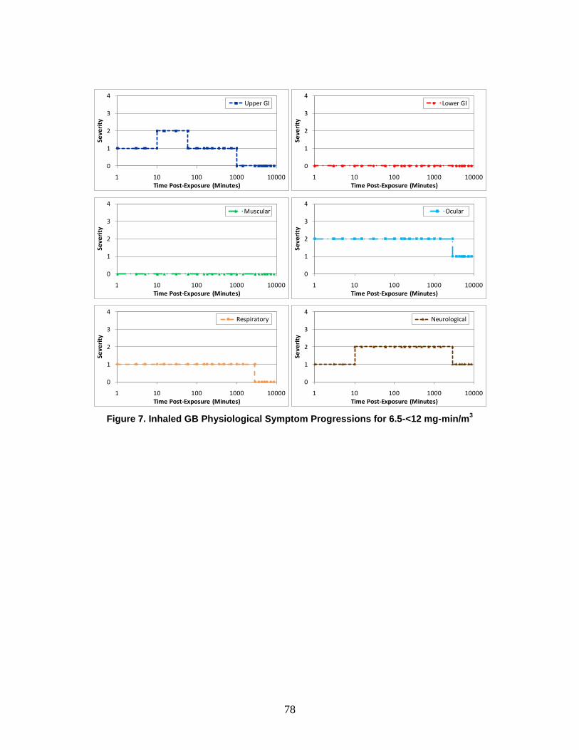
78
Figure 7. Inhaled GB Physiological Symptom Progressions for 6.5-<12 mg-min/m3
0
1
2
3
4
1 10 100 1000 10000
Seve
rity
Time Post-Exposure (Minutes)
Upper GI
0
1
2
3
4
1 10 100 1000 10000
Seve
rity
Time Post-Exposure (Minutes)
Lower GI
0
1
2
3
4
1 10 100 1000 10000
Seve
rity
Time Post-Exposure (Minutes)
Muscular
0
1
2
3
4
1 10 100 1000 10000
Seve
rity
Time Post-Exposure (Minutes)
Ocular
0
1
2
3
4
1 10 100 1000 10000
Seve
rity
Time Post-Exposure (Minutes)
Respiratory
0
1
2
3
4
1 10 100 1000 10000
Seve
rity
Time Post-Exposure (Minutes)
Neurological

79
Figure 8. Inhaled GB Physiological Symptom Progressions for 12-<25 mg-min/m3
0
1
2
3
4
1 10 100 1000 10000
Seve
rity
Time Post-Exposure (Minutes)
Upper GI
0
1
2
3
4
1 10 100 1000 10000
Seve
rity
Time Post-Exposure (Minutes)
Lower GI
0
1
2
3
4
1 10 100 1000 10000
Seve
rity
Time Post-Exposure (Minutes)
Muscular
0
1
2
3
4
1 10 100 1000 10000
Seve
rity
Time Post-Exposure (Minutes)
Ocular
0
1
2
3
4
1 10 100 1000 10000
Seve
rity
Time Post-Exposure (Minutes)
Respiratory
0
1
2
3
4
1 10 100 1000 10000
Seve
rity
Time Post-Exposure (Minutes)
Neurological
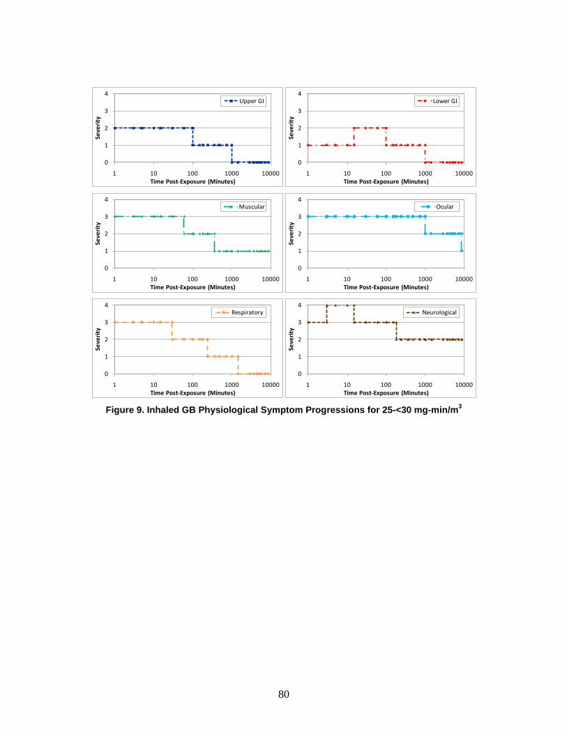
80
Figure 9. Inhaled GB Physiological Symptom Progressions for 25-<30 mg-min/m3
0
1
2
3
4
1 10 100 1000 10000
Seve
rity
Time Post-Exposure (Minutes)
Upper GI
0
1
2
3
4
1 10 100 1000 10000
Seve
rity
Time Post-Exposure (Minutes)
Lower GI
0
1
2
3
4
1 10 100 1000 10000
Seve
rity
Time Post-Exposure (Minutes)
Muscular
0
1
2
3
4
1 10 100 1000 10000
Seve
rity
Time Post-Exposure (Minutes)
Ocular
0
1
2
3
4
1 10 100 1000 10000
Seve
rity
Time Post-Exposure (Minutes)
Respiratory
0
1
2
3
4
1 10 100 1000 10000
Seve
rity
Time Post-Exposure (Minutes)
Neurological
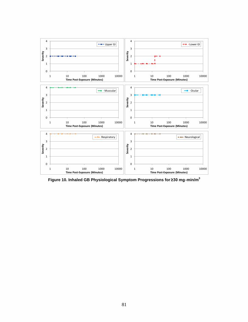
81
Figure 10. Inhaled GB Physiological Symptom Progressions for ≥30 mg -min/m3
0
1
2
3
4
1 10 100 1000 10000
Seve
rity
Time Post-Exposure (Minutes)
Upper GI
0
1
2
3
4
1 10 100 1000 10000
Seve
rity
Time Post-Exposure (Minutes)
Lower GI
0
1
2
3
4
1 10 100 1000 10000
Seve
rity
Time Post-Exposure (Minutes)
Muscular
0
1
2
3
4
1 10 100 1000 10000
Seve
rity
Time Post-Exposure (Minutes)
Ocular
0
1
2
3
4
1 10 100 1000 10000
Seve
rity
Time Post-Exposure (Minutes)
Respiratory
0
1
2
3
4
1 10 100 1000 10000
Seve
rity
Time Post-Exposure (Minutes)
Neurological

82
Figure 11. Inhaled VX Physiological Symptom Progressions for 0.02-<0.3 mg-min/m3
0
1
2
3
4
1 10 100 1000 10000
Seve
rity
Time Post-Exposure (Minutes)
Upper GI
0
1
2
3
4
1 10 100 1000 10000
Seve
rity
Time Post-Exposure (Minutes)
Lower GI
0
1
2
3
4
1 10 100 1000 10000
Seve
rity
Time Post-Exposure (Minutes)
Muscular
0
1
2
3
4
1 10 100 1000 10000
Seve
rity
Time Post-Exposure (minutes)
Ocular
0
1
2
3
4
1 10 100 1000 10000
Seve
rity
Time Post-Exposure (Minutes)
Respiratory
0
1
2
3
4
1 10 100 1000 10000
Seve
rity
Time Post-Exposure (Minutes)
Neurological

83
Figure 12. Inhaled VX Physiological Symptom Progressions for 0.3-<2 mg-min/m3
0
1
2
3
4
1 10 100 1000 10000
Seve
rity
Time Post-Exposure (Minutes)
Upper GI
0
1
2
3
4
1 10 100 1000 10000
Seve
rity
Time Post-Exposure (Minutes)
Lower GI
0
1
2
3
4
1 10 100 1000 10000
Seve
rity
Time Post-Exposure (Minutes)
Muscular
0
1
2
3
4
1 10 100 1000 10000
Seve
rity
Time Post-Exposure (Minutes)
Ocular
0
1
2
3
4
1 10 100 1000 10000
Seve
rity
Time Post-Exposure (Minutes)
Respiratory
0
1
2
3
4
1 10 100 1000 10000
Seve
rity
Time Post-Exposure (Minutes)
Neurological
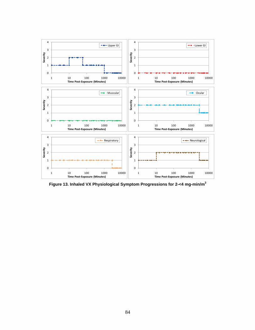
84
Figure 13. Inhaled VX Physiological Symptom Progressions for 2-<4 mg-min/m3
0
1
2
3
4
1 10 100 1000 10000
Seve
rity
Time Post-Exposure (Minutes)
Upper GI
0
1
2
3
4
1 10 100 1000 10000
Seve
rity
Time Post-Exposure (Minutes)
Lower GI
0
1
2
3
4
1 10 100 1000 10000
Seve
rity
Time Post-Exposure (Minutes)
Muscular
0
1
2
3
4
1 10 100 1000 10000
Seve
rity
Time Post-Exposure (Minutes)
Ocular
0
1
2
3
4
1 10 100 1000 10000
Seve
rity
Time Post-Exposure (Minutes)
Respiratory
0
1
2
3
4
1 10 100 1000 10000
Seve
rity
Time Post-Exposure (Minutes)
Neurological
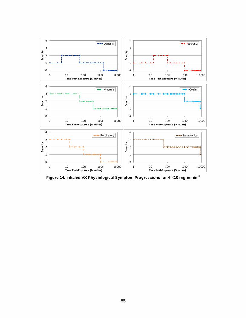
85
Figure 14. Inhaled VX Physiological Symptom Progressions for 4-<10 mg-min/m3
0
1
2
3
4
1 10 100 1000 10000
Seve
rity
Time Post-Exposure (Minutes)
Upper GI
0
1
2
3
4
1 10 100 1000 10000
Seve
rity
Time Post-Exposure (Minutes)
Lower GI
0
1
2
3
4
1 10 100 1000 10000
Seve
rity
Time Post-Exposure (Minutes)
Muscular
0
1
2
3
4
1 10 100 1000 10000
Seve
rity
Time Post-Exposure (Minutes)
Ocular
0
1
2
3
4
1 10 100 1000 10000
Seve
rity
Time Post-Exposure (Minutes)
Respiratory
0
1
2
3
4
1 10 100 1000 10000
Seve
rity
Time Post-Exposure (Minutes)
Neurological
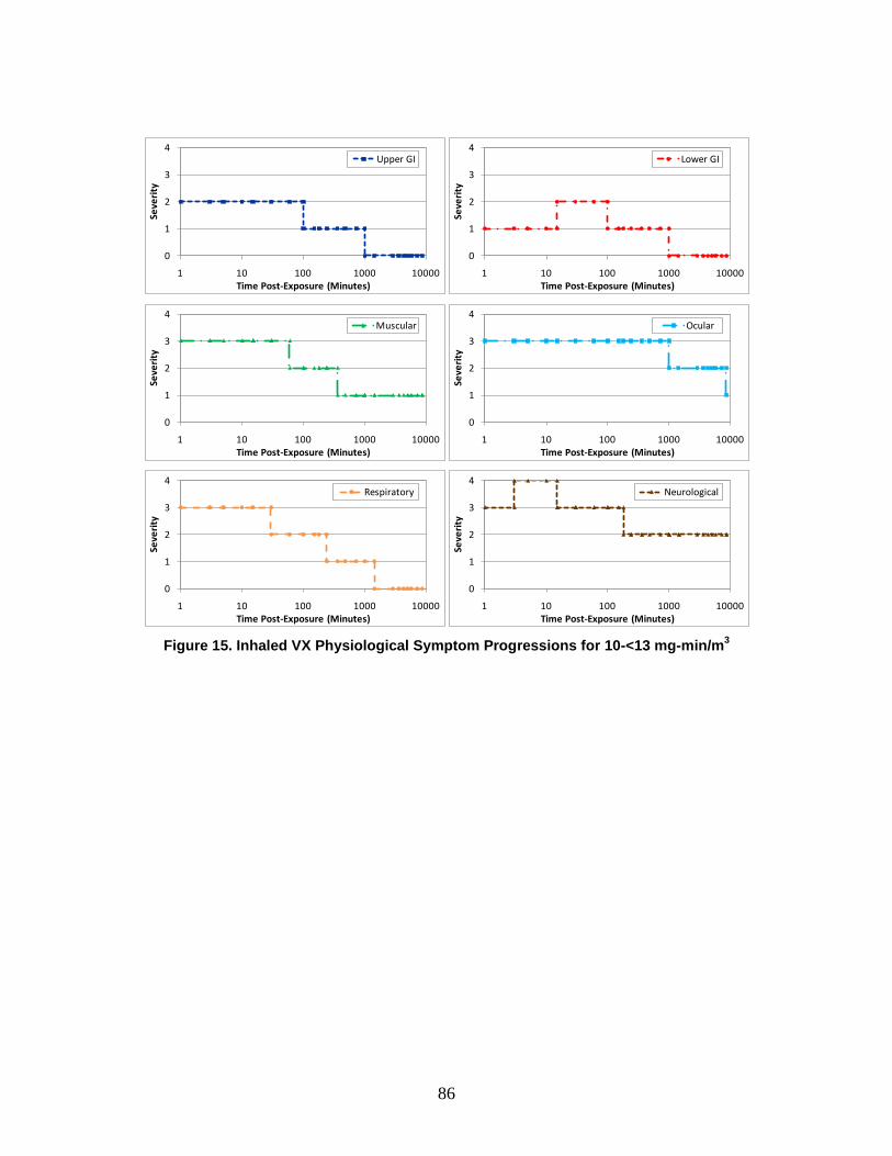
86
Figure 15. Inhaled VX Physiological Symptom Progressions for 10-<13 mg-min/m3
0
1
2
3
4
1 10 100 1000 10000
Seve
rity
Time Post-Exposure (Minutes)
Upper GI
0
1
2
3
4
1 10 100 1000 10000
Seve
rity
Time Post-Exposure (Minutes)
Lower GI
0
1
2
3
4
1 10 100 1000 10000
Seve
rity
Time Post-Exposure (Minutes)
Muscular
0
1
2
3
4
1 10 100 1000 10000
Seve
rity
Time Post-Exposure (Minutes)
Ocular
0
1
2
3
4
1 10 100 1000 10000
Seve
rity
Time Post-Exposure (Minutes)
Respiratory
0
1
2
3
4
1 10 100 1000 10000
Seve
rity
Time Post-Exposure (Minutes)
Neurological
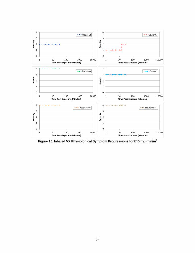
87
Figure 16. Inhaled VX Physiological Symptom Progressions for ≥13 mg-min/m3
0
1
2
3
4
1 10 100 1000 10000
Seve
rity
Time Post-Exposure (Minutes)
Upper GI
0
1
2
3
4
1 10 100 1000 10000
Seve
rity
Time Post-Exposure (Minutes)
Lower GI
0
1
2
3
4
1 10 100 1000 10000
Seve
rity
Time Post-Exposure (Minutes)
Muscular
0
1
2
3
4
1 10 100 1000 10000
Seve
rity
Time Post-Exposure (Minutes)
Ocular
0
1
2
3
4
1 10 100 1000 10000
Seve
rity
Time Post-Exposure (Minutes)
Respiratory
0
1
2
3
4
1 10 100 1000 10000
Seve
rity
Time Post-Exposure (Minutes)
Neurological

88
Figure 17. Percutaneous VX Physiological Symptom Progressions for 0.8-<1.6 mg/man
0
1
2
3
4
1 10 100 1000 10000
Seve
rity
Time Post-Exposure (Minutes)
Upper GI
0
1
2
3
4
1 10 100 1000 10000
Seve
rity
Time Post-Exposure (Minutes)
Lower GI
0
1
2
3
4
1 10 100 1000 10000
Seve
rity
Time Post-Exposure (Minutes)
Muscular
0
1
2
3
4
1 10 100 1000 10000
Seve
rity
Time Post-Exposure (Minutes)
Ocular
0
1
2
3
4
1 10 100 1000 10000
Seve
rity
Time Post-Exposure (Minutes)
Respiratory
0
1
2
3
4
1 10 100 1000 10000
Seve
rity
Time Post-Exposure (Minutes)
Neurological

89
Figure 18. Percutaneous VX Physiological Symptom Progressions for 1.6-<3.9 mg/man
0
1
2
3
4
1 10 100 1000 10000
Seve
rity
Time Post-Exposure (Minutes)
Upper GI
0
1
2
3
4
1 10 100 1000 10000
Seve
rity
Time Post-Exposure (Minutes)
Lower GI
0
1
2
3
4
1 10 100 1000 10000
Seve
rity
Time Post-Exposure (Minutes)
Muscular
0
1
2
3
4
1 10 100 1000 10000
Seve
rity
Time Post-Exposure (Minutes)
Ocular
0
1
2
3
4
1 10 100 1000 10000
Seve
rity
Time Post-Exposure (Minutes)
Respiratory
0
1
2
3
4
1 10 100 1000 10000
Seve
rity
Time Post-Exposure (Minutes)
Neurological

90
Figure 19. Percutaneous VX Physiological Symptom Progressions for ≥3.9 mg/man
It should be noted that, in the case of the uppermost ranges for both GB and VX, subject matter experts estimated that “very severe” effects manifested simultaneously in the respiratory, muscular, and neurological systems would result in rapid lethality (15 minutes or less). As such, these injury profiles and symptom progressions for these dosages are not shown beyond 30 minutes.
The symptom progressions provide the foundation for the injury profile, which illustrates the effect of the injury on the body overall by tracking the highest severity level across the six physiological systems at any moment in time. Using Figure 20 as an example, the physiological symptom progressions for an individual exposed to 20 mg-min/m3 of GB are shown.
0
1
2
3
4
1 10 100 1000 10000
Seve
rity
Time Post-Exposure (Minutes)
Upper GI
0
1
2
3
4
1 10 100 1000 10000
Seve
rity
Time Post-Exposure (Minutes)
Lower GI
0
1
2
3
4
1 10 100 1000 10000
Seve
rity
Time Post-Exposure (Minutes)
Muscular
0
1
2
3
4
1 10 100 1000 10000
Seve
rity
Time Post-Exposure (Minutes)
Ocular
0
1
2
3
4
1 10 100 1000 10000
Seve
rity
Time Post-Exposure (Minutes)
Respiratory
0
1
2
3
4
1 10 100 1000 10000
Seve
rity
Time Post-Exposure (Minutes)
Neurological

91
Figure 20. GB Signs and Symptoms Progressions for 20 mg-min/m3
The example in Figure 20 illustrates that, following exposure, symptoms begin at different severity levels. The neurological, ocular, respiratory, and muscular symptoms each begin at the “severe” level of severity (Severity Level 3). Respiratory symptoms show rapid improvement, within approximately 15 minutes. Neurological and muscular signs and symptoms begin to improve later (at approximately 1.5 hours post-exposure), while ocular symptoms take several hours longer.
Upper and lower gastrointestinal symptoms begin almost immediately as well, but at the “mild” level of severity (Severity Level 1). Both systems, however, soon increase in severity. Upper gastrointestinal symptoms increase to “moderate” severity (Severity Level 2) at approximately 5 minutes, while lower gastrointestinal symptoms take slightly longer but also increase to moderate. Both systems return to “mild” severity at a little longer than 1.5 hours.
Symptoms for each physiological system further decrease in severity as shown. At the end of the observed time period (approximately one week post-exposure), the upper and lower gastrointestinal and respiratory symptoms have returned to “no observable effect,” while the remaining symptoms have decreased to “mild” severity.
These symptoms can be summarized into an overall injury profile as shown in Figure 21. The injury profile tracks along with the maximum exhibited physiological symptoms at each point in time. As can be seen in Figure 20, ocular symptoms remain at “severe” severity for the longest period of time, approximately 1,000 minutes; consequently, the injury profile in Figure 21 also remains at “severe” severity for 1,000 minutes. The injury profile continues to follow the ocular and neurological progressions, both at “moderate” severity until the end of the observed period. Both physiological
0
1
2
3
4
1 10 100 1000 10000
Seve
rity
Time Post-Exposure (Minutes)
Upper GI Lower GI MuscularOcular Respiratory Neurological
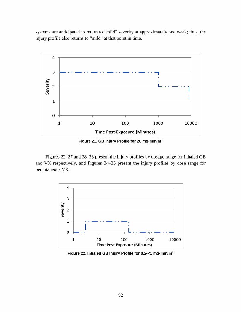
92
systems are anticipated to return to “mild” severity at approximately one week; thus, the injury profile also returns to “mild” at that point in time.
Figure 21. GB Injury Profile for 20 mg-min/m3
Figures 22–27 and 28–33 present the injury profiles by dosage range for inhaled GB and VX respectively, and Figures 34–36 present the injury profiles by dose range for percutaneous VX.
Figure 22. Inhaled GB Injury Profile for 0.2-<1 mg-min/m3
0
1
2
3
4
1 10 100 1000 10000
Seve
rity
Time Post-Exposure (Minutes)
0
1
2
3
4
1 10 100 1000 10000
Seve
rity
Time Post-Exposure (Minutes)

93
Figure 23. Inhaled GB Injury Profile for 1-<6.5 mg-min/m3
Figure 24. Inhaled GB Injury Profile for 6.5-<12 mg-min/m3
Figure 25. Inhaled GB Injury Profile for 12-<25 mg-min/m3
0
1
2
3
4
1 10 100 1000 10000
Seve
rity
Time Post-Exposure (Minutes)
0
1
2
3
4
1 10 100 1000 10000
Seve
rity
Time Post-Exposure (Minutes)
0
1
2
3
4
1 10 100 1000 10000
Seve
rity
Time Post-Exposure (Minutes)
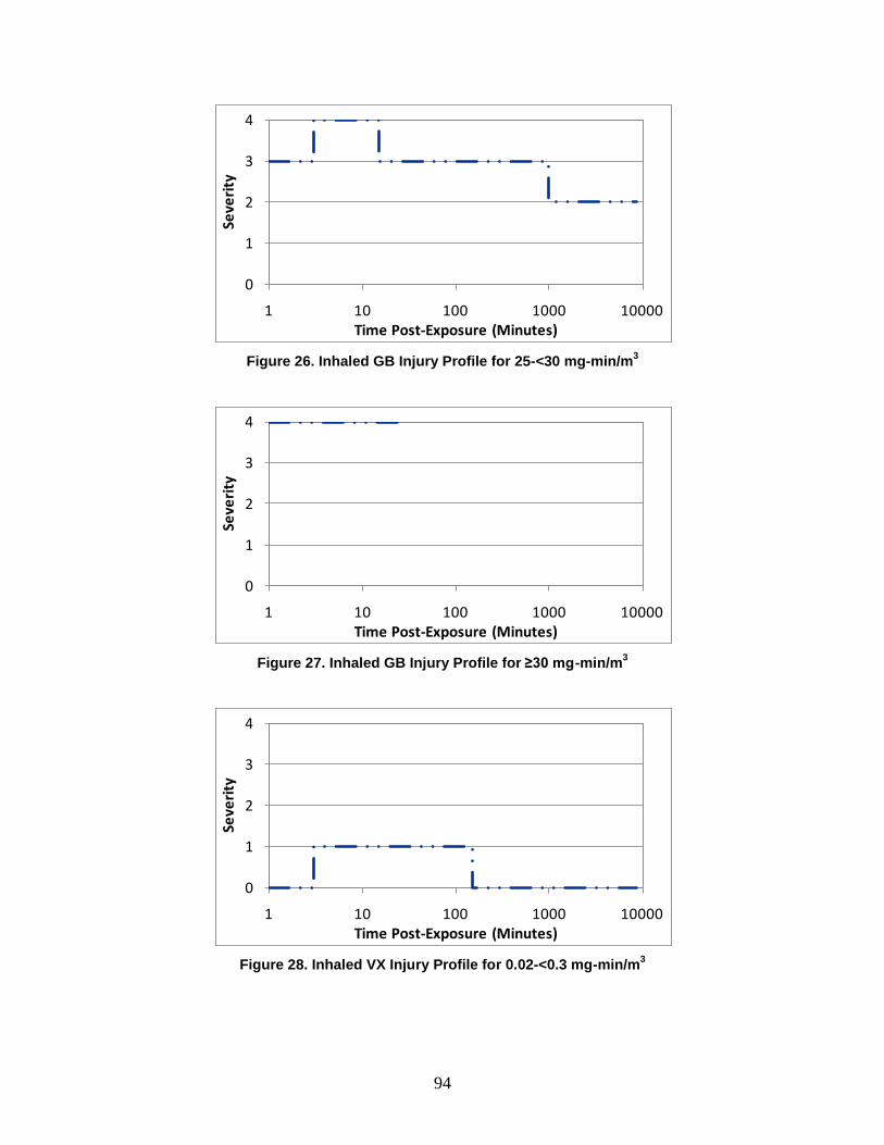
94
Figure 26. Inhaled GB Injury Profile for 25-<30 mg-min/m3
Figure 27. Inhaled GB Injury Profile for ≥30 mg-min/m3
Figure 28. Inhaled VX Injury Profile for 0.02-<0.3 mg-min/m3
0
1
2
3
4
1 10 100 1000 10000
Seve
rity
Time Post-Exposure (Minutes)
0
1
2
3
4
1 10 100 1000 10000
Seve
rity
Time Post-Exposure (Minutes)
0
1
2
3
4
1 10 100 1000 10000
Seve
rity
Time Post-Exposure (Minutes)

95
Figure 29. Inhaled VX Injury Profile for 0.3-<2 mg-min/m3
Figure 30. Inhaled VX Injury Profile for 2-<4 mg-min/m3
Figure 31. Inhaled VX Injury Profile for 4-<10 mg-min/m3
0
1
2
3
4
1 10 100 1000 10000
Seve
rity
Time Post-Exposure (Minutes)
0
1
2
3
4
1 10 100 1000 10000
Seve
rity
Time Post-Exposure (Minutes)
0
1
2
3
4
1 10 100 1000 10000
Seve
rity
Time Post-Exposure (Minutes)
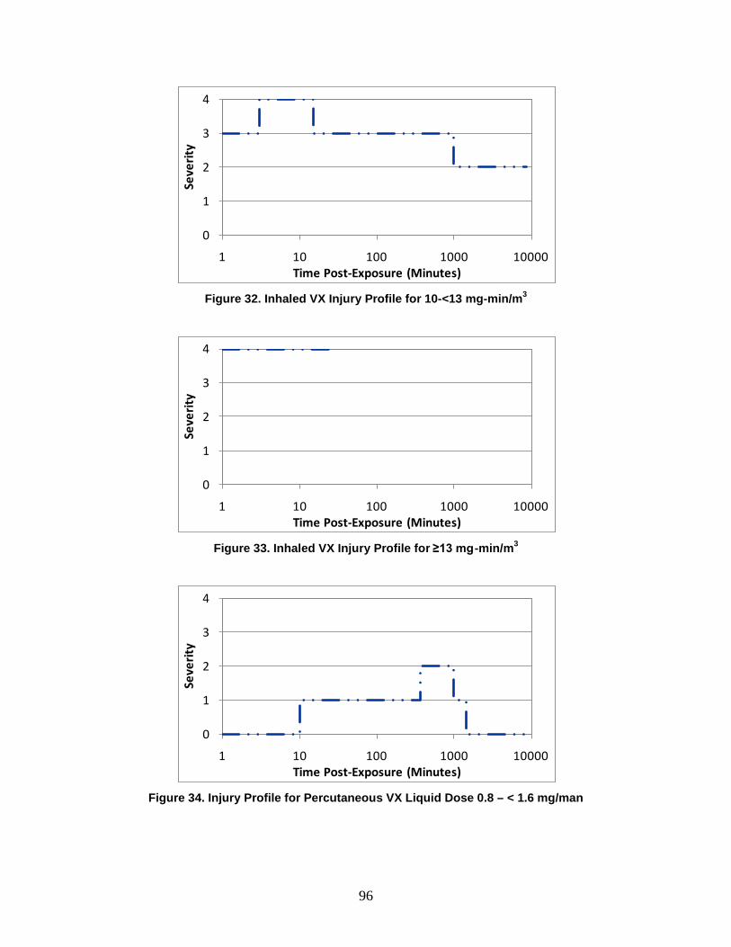
96
Figure 32. Inhaled VX Injury Profile for 10-<13 mg-min/m3
Figure 33. Inhaled VX Injury Profile for ≥13 mg-min/m3
Figure 34. Injury Profile for Percutaneous VX Liquid Dose 0.8 – < 1.6 mg/man
0
1
2
3
4
1 10 100 1000 10000
Seve
rity
Time Post-Exposure (Minutes)
0
1
2
3
4
1 10 100 1000 10000
Seve
rity
Time Post-Exposure (Minutes)
0
1
2
3
4
1 10 100 1000 10000
Seve
rity
Time Post-Exposure (Minutes)
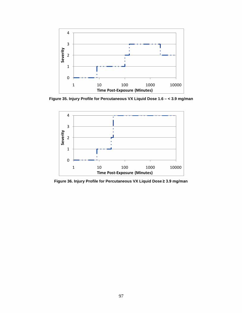
97
Figure 35. Injury Profile for Percutaneous VX Liquid Dose 1.6 – < 3.9 mg/man
Figure 36. Injury Profile for Percutaneous VX Liquid Dose ≥ 3.9 mg/man
0
1
2
3
4
1 10 100 1000 10000
Seve
rity
Time Post-Exposure (Minutes)
0
1
2
3
4
1 10 100 1000 10000
Seve
rity
Time Post-Exposure (Minutes)

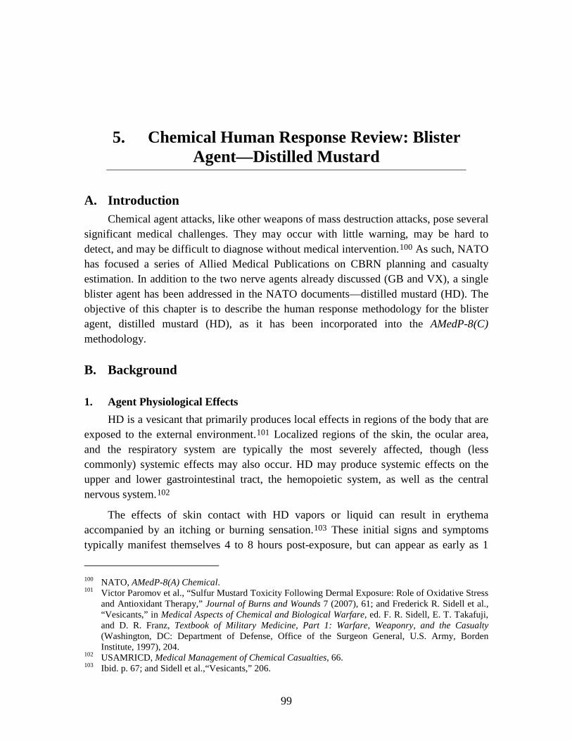
99
5. Chemical Human Response Review: Blister Agent—Distilled Mustard
A. Introduction Chemical agent attacks, like other weapons of mass destruction attacks, pose several
significant medical challenges. They may occur with little warning, may be hard to detect, and may be difficult to diagnose without medical intervention.100
B. Background
As such, NATO has focused a series of Allied Medical Publications on CBRN planning and casualty estimation. In addition to the two nerve agents already discussed (GB and VX), a single blister agent has been addressed in the NATO documents—distilled mustard (HD). The objective of this chapter is to describe the human response methodology for the blister agent, distilled mustard (HD), as it has been incorporated into the AMedP-8(C) methodology.
1. Agent Physiological Effects HD is a vesicant that primarily produces local effects in regions of the body that are
exposed to the external environment.101 Localized regions of the skin, the ocular area, and the respiratory system are typically the most severely affected, though (less commonly) systemic effects may also occur. HD may produce systemic effects on the upper and lower gastrointestinal tract, the hemopoietic system, as well as the central nervous system.102
The effects of skin contact with HD vapors or liquid can result in erythema accompanied by an itching or burning sensation.
103
100 NATO, AMedP-8(A) Chemical.
These initial signs and symptoms typically manifest themselves 4 to 8 hours post-exposure, but can appear as early as 1
101 Victor Paromov et al., “Sulfur Mustard Toxicity Following Dermal Exposure: Role of Oxidative Stress and Antioxidant Therapy,” Journal of Burns and Wounds 7 (2007), 61; and Frederick R. Sidell et al., “Vesicants,” in Medical Aspects of Chemical and Biological Warfare, ed. F. R. Sidell, E. T. Takafuji, and D. R. Franz, Textbook of Military Medicine, Part 1: Warfare, Weaponry, and the Casualty (Washington, DC: Department of Defense, Office of the Surgeon General, U.S. Army, Borden Institute, 1997), 204.
102 USAMRICD, Medical Management of Chemical Casualties, 66. 103 Ibid. p. 67; and Sidell et al.,“Vesicants,” 206.

100
hour and later than 48 hours post-exposure depending on the dose received.104 If the disease does not progress beyond this stage, then recovery can be expected within several days.105 At higher vapor doses and in cases where there is skin contact with liquid HD, the disease may progress to the formation of vesicles (fluid-filled blisters) on the skin beginning 2 to 18 hours after the initial manifestation of symptoms and continuing for several days.106 Contact with liquid HD can produce necrotic lesions that are surrounded by vesicles.107 Once the injury has progressed to this stage, recovery can be expected to require weeks to months.108 The magnitude of skin disease is highly dependent on the exposed location on the body, the presence of moisture on the skin, and the ambient temperature.109
The eyes are particularly sensitive to HD, and ocular effects produced by HD exposure are the most likely to incapacitate.
Areas of the body in which the skin is thin, moist, or warm are more susceptible to disease. As a result, the genitals, armpits, and neck are often the most severely affected.
110 The ocular signs and symptoms of HD exposure are usually present before the onset of skin effects.111 The initial ocular effects generally involve eye irritation with a concurrent reddening of the eye and photophobia.112 At high vapor doses and instances of liquid exposure, the eyes may develop severe conjunctivitis, blepharospasm (uncontrolled twitching of the eyelids), and corneal damage involving edema and scarring.113
Which regions within the pulmonary system are affected by the inhalation of HD vapors is dose-dependent.
114 Low-dose exposures may only cause irritation and erythema to the nose, sinuses, and pharynx.115 Other mild effects include runny nose, sneezing, nose bleed, and a dry unproductive cough.116
104 Sidell et al., “Vesicants,” 207; and USAMRICD, Medical Management of Chemical Casualties, 67.
At higher doses, areas that are lower in the respiratory tract become affected and result in laryngitis, sputum-producing cough, as well as a feeling of tightness in the chest. At even higher doses, the most severe
105 Sidell et al., “Vesicants,” 208. 106 Ibid., 207. 107 Sidell et al., “Vesicants”; and USAMRICD, Medical Management of Chemical Casualties, 68. 108 Sidell et al., “Vesicants,” 208. 109 Sidell et al., “Vesicants,” 205; USAMRICD, Medical Management of Chemical Casualties, 67; and
Sharon Reutter, “Hazards of Chemical Weapons Release During War: New Perspectives,” Environmental Health Perspectives 107, no. 12 (1999): 986.
110 USAMRICD, Medical Management of Chemical Casualties, 69; Sidell et al., “Vesicants,” 208; and S. Reutter, “Hazards of Chemical Weapons,” 986.
111 Sidell et al., “Vesicants,” 210; and USAMRICD, Medical Management of Chemical Casualties, 69. 112 Sidell et al., “Vesicants,” 210. 113 Ibid.; USAMRICD, Medical Management of Chemical Casualties, 70; and S. Reutter, “Hazards of
Chemical Weapons,” 986. 114 USAMRICD, Medical Management of Chemical Casualties, 68. 115 Sidell et al., “Vesicants,” 211. 116 USAMRICD, Medical Management of Chemical Casualties, 70.

101
symptoms involve dyspnea and sloughing of the airway’s epithelial tissue.117 This sloughed tissue and mucus can block airways resulting in atelectasis (collapse of the lung).118 Pulmonary edema does not often develop, but is sometimes seen in terminal cases accompanied by hemorrhaging.119
Upper gastrointestinal signs and symptoms are generally not severe at their onset, which often occurs around the time that the skin effects become apparent.
120 Nausea and vomiting are the most common symptoms and these usually last less than 24 hours, but may reappear several days later.121 Lower gastrointestinal effects such as diarrhea have been reported in laboratory animal experiments when HD is administered intravenously, but this is not an expected route of exposure in the event of a chemical warfare attack.122 Lower gastrointestinal effects are not common with human inhalation or percutaneous exposures.123 In fact, reports of lower gastrointestinal effects are often conflicting, with differing reports of both diarrhea and constipation.124
HD seems to affect the central nervous system rather mildly. Low-dose HD exposures may cause lethargy, apathy, and depression.
125 These effects on the central nervous system are mild. Although some laboratory animal experiments indicate that higher doses can cause hyperexcitability, abnormal muscular movements, and convulsions, there is little evidence of these more serious effects in human exposures.126
The most significant result of HD effects on the hemopoietic system is a decreased number of leucocytes.
127
There are three mechanisms for death as a result of HD exposure. Rapid deaths, in the first several minutes post-exposure, result from the extremely high doses of HD. These high doses produce an acetylcholinergic reaction in the body and effectively paralyze the respiratory system; individuals die of asphyxiation. Individuals could alternatively develop pneumonia and potentially die due to a combination of the infection in the lungs and sepsis at approximately 3–6 days post-exposure.
This reduces the ability to fight off the secondary infections that are likely to occur considering the damage to the skin and respiratory system.
128
117 Sidell et al., “Vesicants,” 211.
The last mechanism for death is also a result of internal sepsis: high percutaneous doses of liquid HD result in bone marrow suppression. Eventually, approximately 1 to 3 weeks post-exposure, the
118 Ibid. 119 Ibid., 212. 120 Ibid. 121 Ibid.; and USAMRICD, Medical Management of Chemical Casualties, 71. 122 Sidell et al., “Vesicants,” 212. 123 Ibid. 124 USAMRICD, Medical Management of Chemical Casualties, 71. 125 Sidell et al., “Vesicants,” 212; and USAMRICD, Medical Management of Chemical Casualties, 71. 126 Sidell et al., “Vesicants,” 212. 127 S. Reutter, “Hazards of Chemical Weapons,” 986. 128 USAMRICD, Medical Management of Chemical Casualties, 69.
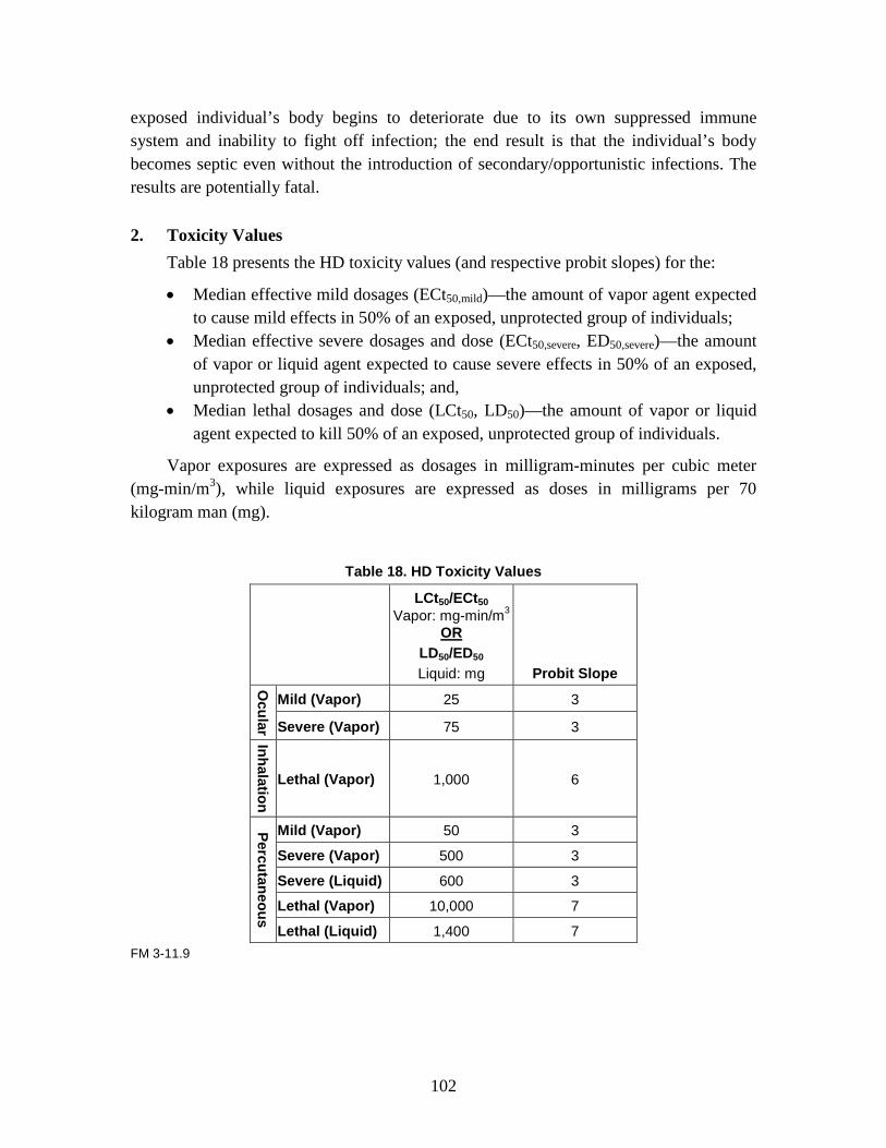
102
exposed individual’s body begins to deteriorate due to its own suppressed immune system and inability to fight off infection; the end result is that the individual’s body becomes septic even without the introduction of secondary/opportunistic infections. The results are potentially fatal.
2. Toxicity Values Table 18 presents the HD toxicity values (and respective probit slopes) for the:
• Median effective mild dosages (ECt50,mild)—the amount of vapor agent expected to cause mild effects in 50% of an exposed, unprotected group of individuals;
• Median effective severe dosages and dose (ECt50,severe, ED50,severe)—the amount of vapor or liquid agent expected to cause severe effects in 50% of an exposed, unprotected group of individuals; and,
• Median lethal dosages and dose (LCt50, LD50)—the amount of vapor or liquid agent expected to kill 50% of an exposed, unprotected group of individuals.
Vapor exposures are expressed as dosages in milligram-minutes per cubic meter (mg-min/m3), while liquid exposures are expressed as doses in milligrams per 70 kilogram man (mg).
Table 18. HD Toxicity Values
LCt50/ECt50 Vapor: mg-min/m3
LD50/ED50 OR
Liquid: mg Probit Slope
Ocular
Mild (Vapor) 25 3
Severe (Vapor) 75 3
Inhalation
Lethal (Vapor) 1,000 6
Percutaneous
Mild (Vapor) 50 3
Severe (Vapor) 500 3
Severe (Liquid) 600 3
Lethal (Vapor) 10,000 7
Lethal (Liquid) 1,400 7 FM 3-11.9

103
C. Dosage Ranges The AMedP-8(C) methodology is designed to allow users to model chemical agent
exposure clouds and deposition in the tool or model of their choice. The human response estimation component of the AMedP-8(C) methodology requires general inputs in the form of vapor dosages and liquid doses, which result in three routes of exposure for HD as shown in Table 19. (Vapor dosage and liquid dose are combined to estimate an equivalent percutaneous skin dosage.)
Table 19. HD Routes of Exposure
Vapor Liquid Inhaled X Percutaneous (ocular)
X
Percutaneous (skin)
X X
Dosage and dose ranges for HD were selected to represent clinically differentiable injury profiles as a function of dosage or dose. The physiological systems that can be affected by HD exposure differ in their sensitivity towards this agent. The differences in sensitivity necessitate that different dosage ranges be used for characterizing the progression of disease in different physiological systems.
The HD dosage ranges included in the older AMedP-8(A) were selected using since-revised ocular/mild, severe, and lethal dosage values and represented an equivalent dosage (the calculated inhaled vapor dosage producing similar effects to those produced by a combination of inhaled vapor dosage, percutaneous vapor dosage, and percutaneous liquid dose).
The new AMedP-8(C) dosage range tables are derived from the original Injury Severity Category tables included in AMedP-8(A). In those tables, HD was represented by four systems/areas impacted following exposure—eye, respiratory, systemic, and skin. Systemic effects were largely represented by upper gastrointestinal symptoms. Eye injuries were represented by four dosage ranges; respiratory and systemic injuries were represented by the same seven dosage ranges; skin injuries were represented by nine dosage ranges. Discussions with the NATO CBRN Medical Working group indicated that this was too many ranges. Moreover, these discussions suggested that dosage ranges should ideally be clinically differentiable, and such was not the case with the ranges found in AMedP-8(A).
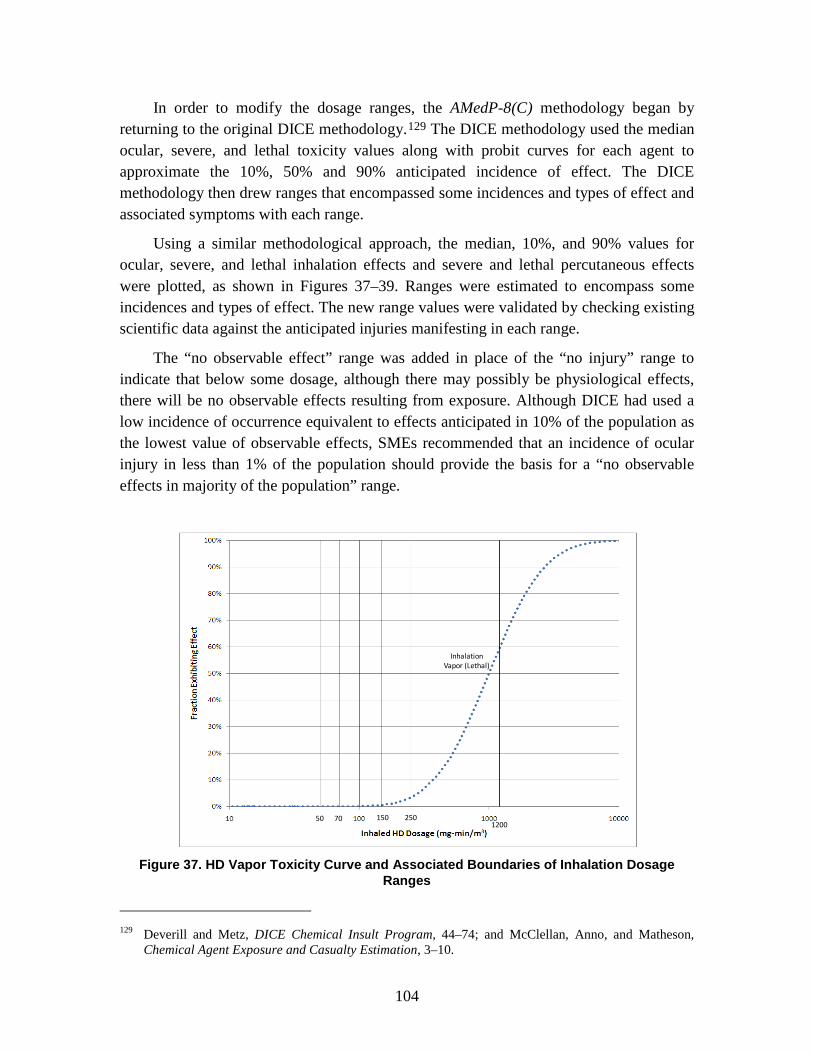
104
In order to modify the dosage ranges, the AMedP-8(C) methodology began by returning to the original DICE methodology.129
Using a similar methodological approach, the median, 10%, and 90% values for ocular, severe, and lethal inhalation effects and severe and lethal percutaneous effects were plotted, as shown in Figures 37–39. Ranges were estimated to encompass some incidences and types of effect. The new range values were validated by checking existing scientific data against the anticipated injuries manifesting in each range.
The DICE methodology used the median ocular, severe, and lethal toxicity values along with probit curves for each agent to approximate the 10%, 50% and 90% anticipated incidence of effect. The DICE methodology then drew ranges that encompassed some incidences and types of effect and associated symptoms with each range.
The “no observable effect” range was added in place of the “no injury” range to indicate that below some dosage, although there may possibly be physiological effects, there will be no observable effects resulting from exposure. Although DICE had used a low incidence of occurrence equivalent to effects anticipated in 10% of the population as the lowest value of observable effects, SMEs recommended that an incidence of ocular injury in less than 1% of the population should provide the basis for a “no observable effects in majority of the population” range.
Figure 37. HD Vapor Toxicity Curve and Associated Boundaries of Inhalation Dosage
Ranges
129 Deverill and Metz, DICE Chemical Insult Program, 44–74; and McClellan, Anno, and Matheson,
Chemical Agent Exposure and Casualty Estimation, 3–10.
50 150
Inhalation Vapor (Lethal)
701200
250
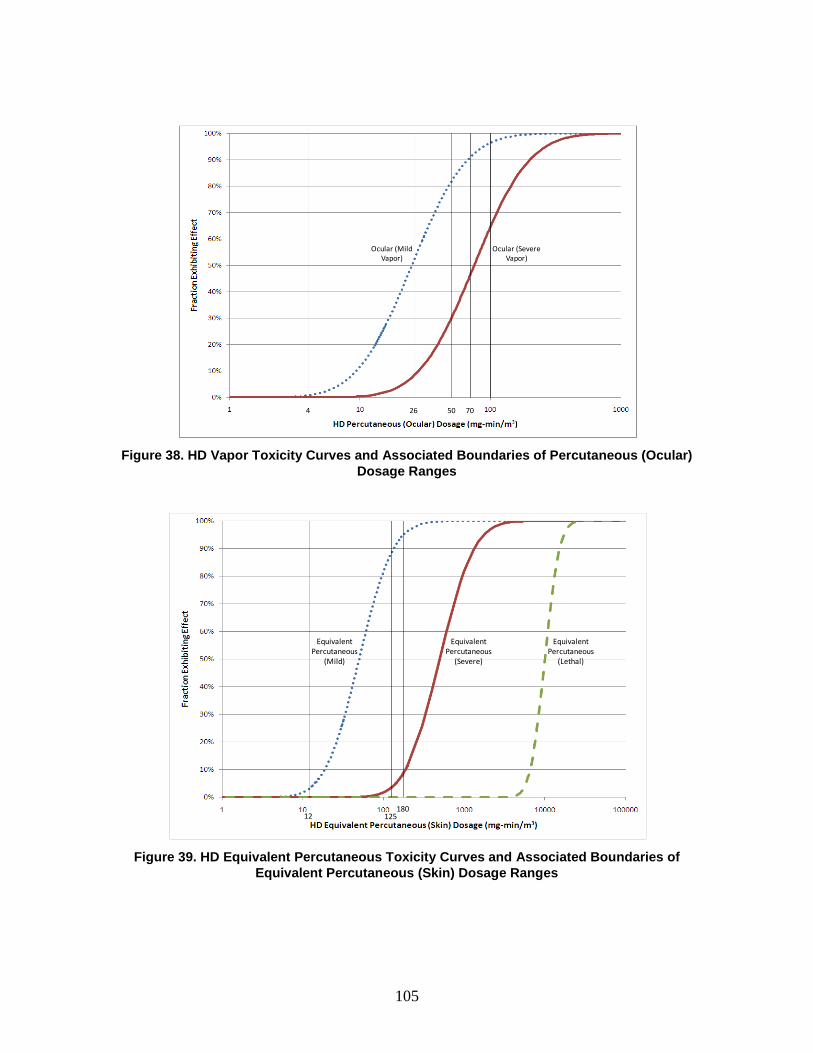
105
Figure 38. HD Vapor Toxicity Curves and Associated Boundaries of Percutaneous (Ocular)
Dosage Ranges
Figure 39. HD Equivalent Percutaneous Toxicity Curves and Associated Boundaries of
Equivalent Percutaneous (Skin) Dosage Ranges
4 50 70
Ocular (Mild Vapor)
Ocular (Severe Vapor)
26
12180
Equivalent Percutaneous
(Mild)
Equivalent Percutaneous
(Severe)
Equivalent Percutaneous
(Lethal)
125
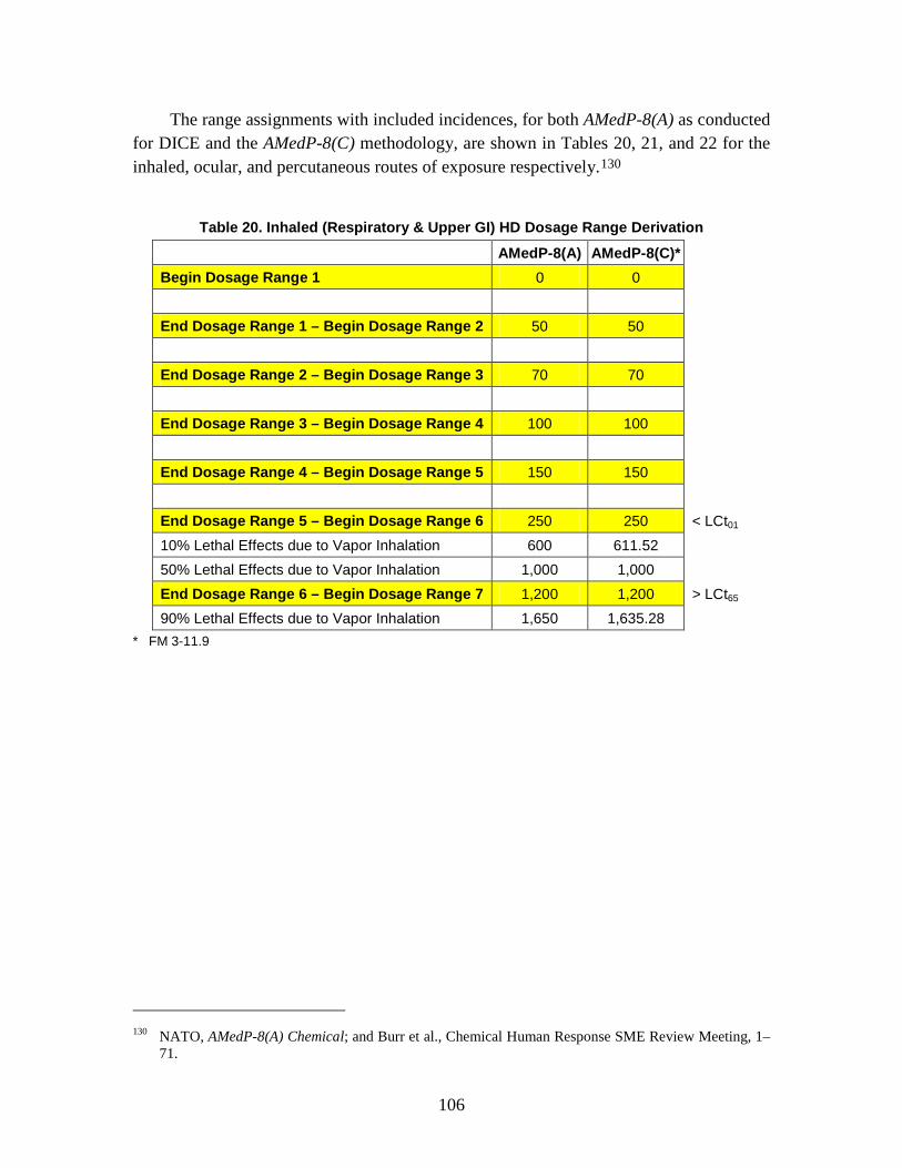
106
The range assignments with included incidences, for both AMedP-8(A) as conducted for DICE and the AMedP-8(C) methodology, are shown in Tables 20, 21, and 22 for the inhaled, ocular, and percutaneous routes of exposure respectively.130
Table 20. Inhaled (Respiratory & Upper GI) HD Dosage Range Derivation
AMedP-8(A) AMedP-8(C)* Begin Dosage Range 1 0 0 End Dosage Range 1 – Begin Dosage Range 2 50 50 End Dosage Range 2 – Begin Dosage Range 3 70 70 End Dosage Range 3 – Begin Dosage Range 4 100 100 End Dosage Range 4 – Begin Dosage Range 5 150 150 End Dosage Range 5 – Begin Dosage Range 6 250 250 < LCt01 10% Lethal Effects due to Vapor Inhalation 600 611.52 50% Lethal Effects due to Vapor Inhalation 1,000 1,000 End Dosage Range 6 – Begin Dosage Range 7 1,200 1,200 > LCt65 90% Lethal Effects due to Vapor Inhalation 1,650 1,635.28
* FM 3-11.9
130 NATO, AMedP-8(A) Chemical; and Burr et al., Chemical Human Response SME Review Meeting, 1–
71.

107
Table 21. Percutaneous Vapor (Ocular) HD Dosage Range Derivation
AMedP-8(A) AMedP-8(C)* Begin Dosage Range 1 0 0
End Dosage Range 1 – Begin Dosage Range 2 5 4 ≈ ECt01 ocular/mild
10% Ocular Injury (ocular/mild) 6.3 9.35 50% Ocular Injury (ocular/mild) 25 25
End Dosage Range 2 – Begin Dosage Range 3 50 26
≈ ECt50 ocular/mild < ECt10 ocular/severe
10% Ocular Injury (ocular/severe) 28.05
End Dosage Range 3 – Begin Dosage Range 4 70 50
> ECt80 ocular/mild ≈ ECt10 ocular/severe
10% Ocular Injury (ocular/severe) 81 90% Ocular Injury (ocular/mild) 96 66.85
End Dosage Range 4 – Begin Dosage Range 5 100 70
> ECt90 ocular/mild ≈ ECt45 ocular/severe
50% Ocular Injury (ocular/severe) 135 75
End Dosage Range 5 – Begin Dosage Range 6 150 100 > ECt60 ocular/severe
90% Ocular Injury (ocular/severe) 225 200.56 * FM 3-11.9

108
Table 22. Equivalent Percutaneous (Skin) HD Dosage Range Derivation
AMedP-8(A) AMedP-8(C)* Begin Dosage Range 1 0 0 End Dosage Range 1 – Begin Dosage Range 2 25 12 ≈ ECt03 mild 10% Threshold Effects - Vapor 30 18.70 50% Threshold Effects - Vapor 50 50 90% Threshold Effects - Vapor 82 End Dosage Range 2 – Begin Dosage Range 3 100 End Dosage Range 3 – Begin Dosage Range 4 250 125 ≈ ECt88 mild 90% Threshold Effects - Vapor 133.71 End Dosage Range 4 – Begin Dosage Range 5 500 End Dosage Range 5 – Begin Dosage Range 6 750 180 ≈ ECt09 severe 10% Severe Effects - Vapor 1,190 186.98 End Dosage Range 6 – Begin Dosage Range 7 1,500 300 ≈ ECt25 severe 50% Severe Effects - Vapor 2,000 500 90% Severe Effects - Vapor 3,300 1,337.07 End Dosage Range 7 – Begin Dosage Range 8 4,000 1,800 < LCt01 10% Lethal Effects - Vapor 6,500 6,560.26 50% Lethal Effects - Vapor 10,000 10,000 End Dosage Range 8 – Begin Dosage Range 9 12,000 12,000 > LCt70 90% Lethal Effects - Vapor 15,300 15,243.29
* FM 3-11.9
Each range was then described with the associated symptoms. The resulting ranges are expressed in terms of the dosage value, in milligram-minutes per cubic meter. The ranges are shown in Tables 23 through 25.
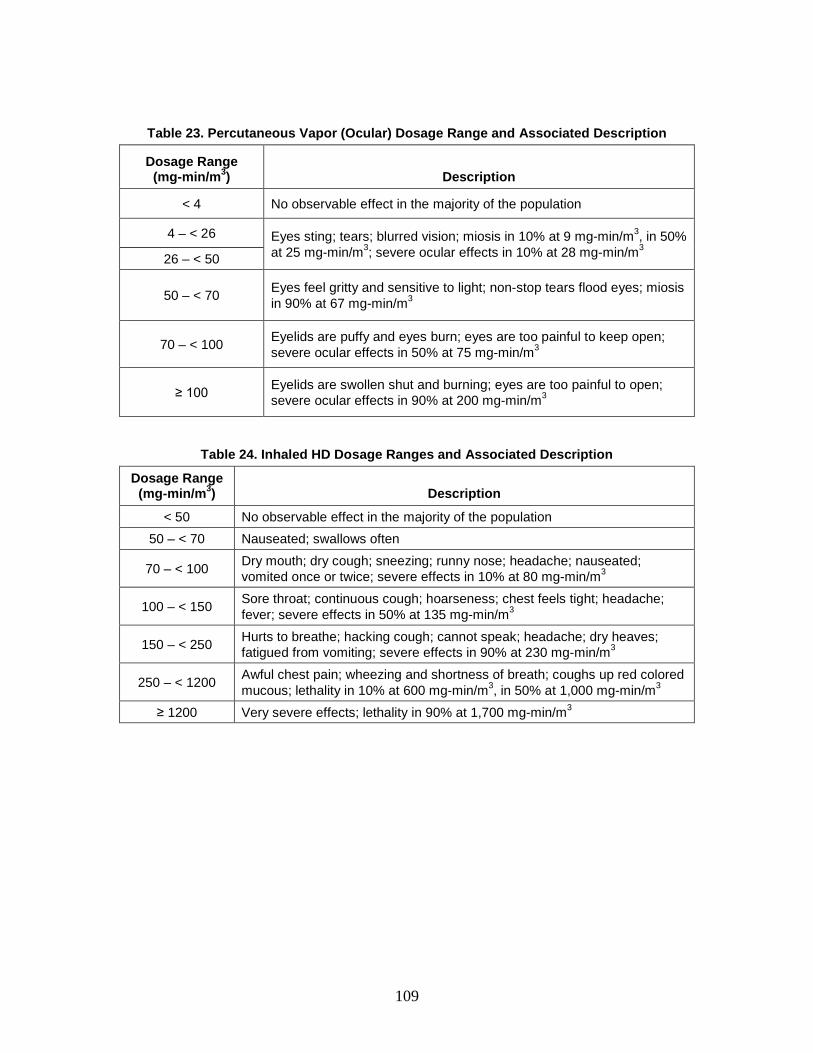
109
Table 23. Percutaneous Vapor (Ocular) Dosage Range and Associated Description
Dosage Range (mg-min/m3) Description
< 4 No observable effect in the majority of the population
4 – < 26 Eyes sting; tears; blurred vision; miosis in 10% at 9 mg-min/m3, in 50% at 25 mg-min/m3; severe ocular effects in 10% at 28 mg-min/m3 26 – < 50
50 – < 70 Eyes feel gritty and sensitive to light; non-stop tears flood eyes; miosis in 90% at 67 mg-min/m3
70 – < 100 Eyelids are puffy and eyes burn; eyes are too painful to keep open; severe ocular effects in 50% at 75 mg-min/m3
≥ 100 Eyelids are swollen shut and burning; eyes are too painful to open; severe ocular effects in 90% at 200 mg-min/m3
Table 24. Inhaled HD Dosage Ranges and Associated Description
Dosage Range (mg-min/m3) Description
< 50 No observable effect in the majority of the population 50 – < 70 Nauseated; swallows often
70 – < 100 Dry mouth; dry cough; sneezing; runny nose; headache; nauseated; vomited once or twice; severe effects in 10% at 80 mg-min/m3
100 – < 150 Sore throat; continuous cough; hoarseness; chest feels tight; headache; fever; severe effects in 50% at 135 mg-min/m3
150 – < 250 Hurts to breathe; hacking cough; cannot speak; headache; dry heaves; fatigued from vomiting; severe effects in 90% at 230 mg-min/m3
250 – < 1200 Awful chest pain; wheezing and shortness of breath; coughs up red colored mucous; lethality in 10% at 600 mg-min/m3, in 50% at 1,000 mg-min/m3
≥ 1200 Very severe effects; lethality in 90% at 1,700 mg-min/m3

110
Table 25. HD Equivalent Percutaneous (Skin) Dosage Range and Associated Description
Dosage Range
(mg-min/m3) Description
< 12 No observable effect in the majority of the population
12 – < 125 Skin sensitive to touch in tender areas (crotch, armpits, inside of elbow and knee); threshold effects in 10% at 19 mg-min/m3, in 50% at 50 mg-min/m3
125 – < 180 Skin sore in tender areas; painful when moving; redness of the skin; tiny blisters on hands and neck; threshold effects in 90% at 134 mg-min/m3
≥ 180
Skin peels off leaving open raw areas and painful ulcers in tender areas; severe effects in 10% at 187 mg-min/m3, in 50% at 500 mg-min/m3, in 90% at 1,337 mg-min/m3; lethality in 10% at 6,560 mg-min/m3, in 50% at 10,000 mg-min/m3, in 90% at 15,243 mg-min/m3
The DICE methodology did not account for very severe effects on the respiratory system due to hematopoietic system/bone marrow suppression and the resulting sepsis. Subject matter experts suggested the inclusion of such effects solely as the result of very high levels of percutaneous HD liquid exposure. In an effort to capture this effect, an additional respiratory dose range (≥ 1,400 mg to a 70 kilogram man) is included, which will be discussed in more detail in Chapter 9 of this document.
D. Symptoms The basic concept of the AMedP-8(C) methodology is that an individual is
considered a casualty at the time of first onset of a specified injury severity level, based on specific symptoms resulting from exposure to the causative agent. The human response component of the methodology specifies an injury profile depicting injury severity level over time that is used to determine whether an individual is declared killed in action (KIA), wounded in action (WIA), or died of wounds (DOW) and thereby considered to be a casualty and, if so, at what point this would occur. The injury profile is derived from the symptom progressions, which show the severity level of symptoms in the system in which they manifest (as opposed to the causative system) over time. The severity level of the injury profile at any given time point corresponds to the worst severity level experienced in any of the representative physiological systems at that time. The nature of symptoms and their times of onset depend on the agent.
111
1. Severity levels For HD, the DICE methodology employed four physiological systems to represent
the injury progression: systemic, respiratory, ocular, and skin. These symptoms were represented on a severity scale of 1–5.131
In an effort to ensure clarity and consistency, the symptoms and systems for the chemical blister agents were correlated to four representative physiological systems—upper gastrointestinal, respiratory, ocular, and skin—in which symptoms would be expected to manifest following exposure to chemical agents. The applicable systems are shown in Table 26.
Table 26. Blister Agent Route of Exposure Correlation to Representative Physiological
Systems
HD
Inhalation
HD Vapor Percutaneous
(Ocular)
HD Equivalent
Percutaneous Ocular X Respiratory X Skin X Upper Gastrointestinal X
As previously described in Chapter 2 and summarized in Table 1, symptoms in AMedP-8(C) are expressed on a scale of 0–4, with 0 representing “no observable effect” and 4 representing “very severe effects.”
The DICE human response methodology correlated the severity levels for each of the four physiological systems to anticipated signs and symptoms; the severity levels were independent for each physiological system.132
In order to align the severities across the physiological systems and be able to draw useful injury profiles, the AMedP-8(C) methodology adjusted severity levels associated with each set of signs and symptoms. As a result, all four physiological systems begin with a “no observable effect” level, but each system has only the number of severity levels necessary to achieve the maximum severity at which signs and symptoms for that
For example, an ocular severity of 4 (described as “temporary blindness”) while operationally challenging, was not, however, equivalent to a respiratory severity of 4 (“breathing stops completely”) which could potentially kill an individual.
131 Anno et al., Performance on Infantry and Artillery Personnel, 8–13; McClellan, Anno, and Matheson,
Chemical Agent Exposure and Casualty Estimation, 11–16; and Deverill and Metz, DICE Chemical Insult Program, 44–74.
132 These correlations are derived from those completed as part of the DICE methodology.

112
physiological system occur. For example, if a given physiological system was not expected to manifest symptoms greater in severity than level 3, then the scale for that system would range from 0 to 3. Moreover, the new severity levels are aligned so that, for instance, a Severity Level 3 ocular injury consists of signs and symptoms of equal severity to those found in Severity Level 3 for the respiratory system and Severity Level 3 for the muscular system. Again, these signs and symptoms are shown in the physiological system in which they manifest, rather than in the causative system. The AMedP-8(C) symptom-severity level correlations are shown in Table 27 for HD.
Table 27. HD Symptoms Severity Levels
Severity Ocular Respiratory
0 No observable effect No observable effect
1 Irritation with eye pain; conjunctival erythema and/or edema
Mild shortness of breath; tight chest, coughing, and runny nose
2
Eye pain and/or irritation with conjunctival erythema and/or edema; blepharospasm; difficulty opening the eyes; sensitivity to light
Frank shortness of breath; difficult to breathe, wheezing breath, respiratory congestion, bronchorrhea
3 Severe eye inflammation and pain leading to an inability to open the eyes Severe dyspnea
4 Breathing stops completely or struggling to breathe; prostration
Table 27. continued
Severity Skin Upper Gastrointestinal
0 No observable effect No observable effect
1 Skin sensitive to touch in crotch, armpits, and on inside of elbow and knee joints
Upset stomach and nausea; watering mouth and frequent swallowing to avoid vomiting
2
Skin sore in crotch, armpits, elbow and knee joints, and painful when moving, red swollen skin, tiny blisters on hands and neck
Episodes of vomiting, possibly including dry heaves; severe nausea and possibility of continued vomiting
3 Skin raw and painful in crotch, armpits, elbow and knee joints, red swollen body skin, large blisters on hands and neck
4 Skin sloughage after blisters or swollen skin
113
2. Symptom Progression and Injury Profiles Each of the dosage or dose ranges previously described corresponds to a progression
of symptoms through time. These progressions are discontinuous with respect to dosage or dose; all dosages or doses within the specified range are represented by the same symptom progression. The boundaries defining each dosage or dose band represent points in an exposure at which the expected progression of injury abruptly changes as the dosage or dose is increased. Moreover, the symptom progressions themselves are discontinuous and stepwise with respect to severity level; they are not smoothed or otherwise interpolated. In other words, moving along the time dimension of the symptom progression, the symptom severity changes instantaneously at specific points in time. For a given dosage or dose range, separate symptom progressions have been developed for each of the four physiological systems—upper gastrointestinal, respiratory, ocular, and skin—illustrating the severity of the symptoms for a particular physiological system over time. Figures 40 and 41 present the symptom progressions by dosage range for inhaled HD (upper GI and respiratory respectively). Figure 42 presents the symptom progressions by dosage range for ocular HD, and Figure 43 presents the symptom progressions by equivalent dosage range for percutaneous HD.133
The “no observable effect” progressions are not shown; all severity levels would be 0 for the duration of time observed.
133 All of the symptom progression and injury profiles are plotted using minutes along the logarithmic x-
axis.
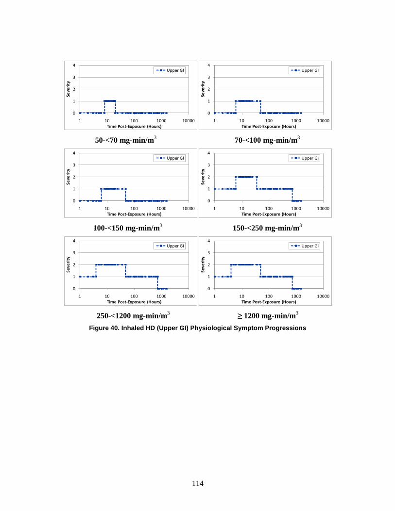
114
50-<70 mg-min/m3 70-<100 mg-min/m3
100-<150 mg-min/m3 150-<250 mg-min/m3
250-<1200 mg-min/m3 ≥ 1200 mg-min/m3
Figure 40. Inhaled HD (Upper GI) Physiological Symptom Progressions
0
1
2
3
4
1 10 100 1000 10000
Seve
rity
Time Post-Exposure (Hours)
Upper GI
0
1
2
3
4
1 10 100 1000 10000
Seve
rity
Time Post-Exposure (Hours)
Upper GI
0
1
2
3
4
1 10 100 1000 10000
Seve
rity
Time Post-Exposure (Hours)
Upper GI
0
1
2
3
4
1 10 100 1000 10000Se
veri
ty
Time Post-Exposure (Hours)
Upper GI
0
1
2
3
4
1 10 100 1000 10000
Seve
rity
Time Post-Exposure (Hours)
Upper GI
0
1
2
3
4
1 10 100 1000 10000
Seve
rity
Time Post-Exposure (Hours)
Upper GI

115
50-<70 mg-min/m3 70-<100 mg-min/m3
100-<150 mg-min/m3 150-<250 mg-min/m3
250-<1200 mg-min/m3 ≥ 1200 mg-min/m3
Figure 41. Inhaled HD (Respiratory) Physiological Symptoms Progressions
0
1
2
3
4
1 10 100 1000 10000
Seve
rity
Time Post-Exposure (Hours)
Respiratory
0
1
2
3
4
1 10 100 1000 10000
Seve
rity
Time Post-Exposure (Hours)
Respiratory
0
1
2
3
4
1 10 100 1000 10000
Seve
rity
Time Post-Exposure (Hours)
Respiratory
0
1
2
3
4
1 10 100 1000 10000Se
veri
ty
Time Post-Exposure (Hours)
Respiratory
0
1
2
3
4
1 10 100 1000 10000
Seve
rity
Time Post-Exposure (Hours)
Respiratory
0
1
2
3
4
1 10 100 1000 10000
Seve
rity
Time Post-Exposure (Hours)
Respiratory

116
4-<26 mg-min/m3 26-<50 mg-min/m3
50-<70 mg-min/m3 70-<100 mg-min/m3
≥ 100 mg-min/m3
Figure 42. Ocular HD Physiological Symptoms Progressions
0
1
2
3
4
1 10 100 1000 10000
Seve
rity
Time Post-Exposure (Hours)
Ocular
0
1
2
3
4
1 10 100 1000 10000
Seve
rity
Time Post-Exposure (Hours)
Ocular
0
1
2
3
4
1 10 100 1000 10000
Seve
rity
Time Post-Exposure (Hours)
Ocular
0
1
2
3
4
1 10 100 1000 10000Se
veri
ty
Time Post-Exposure (Hours)
Ocular
0
1
2
3
4
1 10 100 1000 10000
Seve
rity
Time Post-Exposure (Hours)
Ocular

117
12-<125 mg-min/m3 125-<180 mg-min/m3
≥ 180 mg-min/m3
Figure 43. Percutaneous HD Physiological Symptoms Progressions
The symptom progressions provide the foundation for the injury profile, which illustrates the effect of the injury on the body overall by tracking the highest severity level across the four physiological systems at any moment in time. Using Figure 44 as an example, the physiological symptom progressions for an individual exposed to an inhaled/ocular vapor dosage of 80 mg-min/m3 and a calculated equivalent percutaneous dosage of 200 mg-min/m3 are shown.
In this example, the ocular symptom progression corresponds to the dosage range containing dosages in the range of 70–100 mg-min/m3, the skin symptom progression corresponds to the dosage range containing dosages in the range of ≥ 180 mg -min/m3, and the upper gastrointestinal and respiratory symptom progressions correspond to the dosage range containing dosages in the range of 70–100 mg-min/m3.
0
1
2
3
4
1 10 100 1000 10000
Seve
rity
Time Post-Exposure (Hours)
Skin
0
1
2
3
4
1 10 100 1000 10000
Seve
rity
Time Post-Exposure (Hours)
Skin
0
1
2
3
4
1 10 100 1000 10000
Seve
rity
Time Post-Exposure (Hours)
Skin
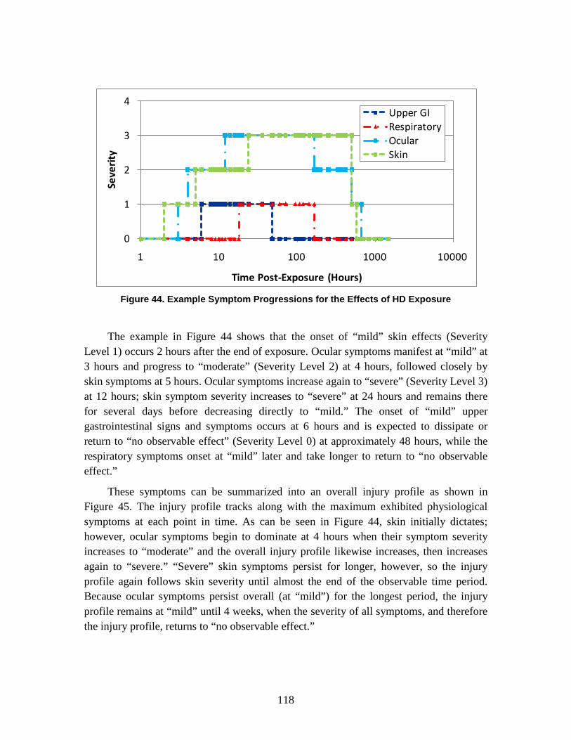
118
Figure 44. Example Symptom Progressions for the Effects of HD Exposure
The example in Figure 44 shows that the onset of “mild” skin effects (Severity Level 1) occurs 2 hours after the end of exposure. Ocular symptoms manifest at “mild” at 3 hours and progress to “moderate” (Severity Level 2) at 4 hours, followed closely by skin symptoms at 5 hours. Ocular symptoms increase again to “severe” (Severity Level 3) at 12 hours; skin symptom severity increases to “severe” at 24 hours and remains there for several days before decreasing directly to “mild.” The onset of “mild” upper gastrointestinal signs and symptoms occurs at 6 hours and is expected to dissipate or return to “no observable effect” (Severity Level 0) at approximately 48 hours, while the respiratory symptoms onset at “mild” later and take longer to return to “no observable effect.”
These symptoms can be summarized into an overall injury profile as shown in Figure 45. The injury profile tracks along with the maximum exhibited physiological symptoms at each point in time. As can be seen in Figure 44, skin initially dictates; however, ocular symptoms begin to dominate at 4 hours when their symptom severity increases to “moderate” and the overall injury profile likewise increases, then increases again to “severe.” “Severe” skin symptoms persist for longer, however, so the injury profile again follows skin severity until almost the end of the observable time period. Because ocular symptoms persist overall (at “mild”) for the longest period, the injury profile remains at “mild” until 4 weeks, when the severity of all symptoms, and therefore the injury profile, returns to “no observable effect.”
0
1
2
3
4
1 10 100 1000 10000
Seve
rity
Time Post-Exposure (Hours)
Upper GIRespiratoryOcularSkin

119
Figure 45. HD Injury Profile for Vapor Dosage of 80 mg-min/m3 and an Equivalent
Percutaneous Dosage of 200 mg-min/m3
Because each injury profile for HD depends on the combination of inhaled vapor dosage, ocular dosage, and equivalent percutaneous vapor dosage, and the respective physiological symptoms are manifested as a result of the individual dosages and doses, general injury profiles are not shown.
0
1
2
3
4
1 10 100 1000 10000
Seve
rity
Time Post-Exposure (Hours)


121
6. Ionizing Radiation Human Response Review: Radiological Agents
A. Introduction The adverse consequences of radioactivity and ionizing radiation to human health
were first recognized shortly after their discovery in the late 19th century.134 The intentional exposure of individuals to radiation may occur in a number of ways, including the deliberate use of ionizing radiation as a weapon and indirectly as a result of radioactive fallout following detonation of a nuclear device. One such tool for accomplishing the former task is a radiological dispersal device (RDD). An RDD may take one of many potential forms, so this document will not speculate about any particular design; instead, because it is assumed that the RDD can lead to human exposure via one or more pathways, this document will focus on the human response resulting from possible exposure.135 Though a variety of radioactive isotopes exist or can be produced, only a limited number possess the physical abundance, sufficiently long half-lives, and desirable energy characteristics suitable for use as radiological agents; prime candidates include 137Cs, 60Co, 90Sr, 131I, 241Am, and 192Ir.136
Another possible concern regarding exposure to radioactive materials on the battlefield is from fallout after the detonation of a nuclear weapon. This radioactive material includes the fission products, unfissioned nuclear material, and weapon residues, as well as soil which has been vaporized by the heat of the fireball. Radioactive fallout deposited on the ground may pose a hazard from external gamma and beta radiation exposure even to reasonably protected troops operating in the contaminated area.
The objective of this chapter is to describe the human response methodologies for radiological agents via specific pathways of exposure, as they have been incorporated into the AMedP-8(C) methodology.
134 Merril Eisenbud and Thomas Gesell, Environmental Radioactivity from Natural, Industrial, and
Military Sources, 4th ed. (San Diego: Academic Press, 1997), 4. 135 The term exposure in this paper does not refer, in any context, to the physical quantity commonly
measured in C/kg or Roentgen. 136 Harper, Musolino, and Wente, “Realistic Radiological Dispersal Device,” 1–16; and Burr et al.,
Radiological Human Response SME Review Meeting, 1–16.
122
B. Background For the purposes of this analysis, it is convenient to characterize radioactive isotopes
by radiation type, specifically alpha emitters, beta emitters, and gamma emitters (neutron emitters, though they exist, are sufficiently rare so as to preclude consideration as radiological agents). A particular isotope may emit some combination of these three radiation types. All types are capable, in large enough quantity and under the right circumstances, of inflicting lethal harm on humans. However, there are differences in the pathways by which this can occur.
1. Physiological Effects Nuclear radiation causes injury to a number of physiological systems through the
deposition of energy in the organ tissues—both electromagnetic (e.g., x-rays and gamma rays) and particulate radiation (e.g., beta particles, alpha particles, and neutrons). The deposition of energy produces free radicals which, in turn, interact with the body chemistry, causing damage to the cells and cellular material.137 The resulting damage is a function of a number of factors including the dose, the time post-exposure, and the sensitivity of the cellular material, among others.138 Thus, the higher the dose, the greater the resulting damage, the worse the anticipated injury severity, and the shorter the latent period before the injury manifests as symptoms, otherwise known as acute radiation syndrome (ARS).139
ARS is actually a combination of syndromes affecting multiple physiological systems, including the hematopoietic, gastrointestinal, and cerebrovascular systems.
140
In the hematopoietic syndrome, the deposited energy targets stem cells in the bone marrow. “A dose-dependent suppression of bone marrow may lead to marrow atrophy
Damage to a fourth organ system, the skin, may also result in casualties, if sufficient quantities of beta-emitting radioisotopes remain in contact with the skin for a long enough period of time. In each syndrome, the exposed individual would be expected to progress through four possible stages—prodromal, latent, manifest illness, and possible recovery. The length of each stage in a particular physiological syndrome, as well as the severity of injury in each stage, is a function of the dose received by the exposed individual.
137 Leonard A. Alt, C. Douglas Forcino, and Richard I. Walker, “Nuclear Events and Their
Consequences,” in Medical Consequences of Nuclear Warfare, ed. Richard I. Walker and T. Jan Cerveny, Textbook of Military Medicine, Part 1: Warfare, Weaponry, and the Casualty (Falls Church, VA: Department of the Army, Office of the Surgeon General, Borden Institute, 1996), 13–14.
138 Eric J. Hall, Radiobiology for the Radiologist, 5th ed. (Philadelphia, PA: Lippincott Williams & Wilkins, 2000), 17.
139 Ibid. 140 Donald Pizzarello and Richard Witcofski, Medical Radiation Biology, 2nd ed. (Philadelphia, PA: Lea
and Febiger, 1982), 136.

123
and pancytopenia. Prompt radiation doses of about 1–8 Gy may cause significant damage to the bone marrow.”141 A brief prodromal period—days—may have symptoms including nausea, vomiting, anorexia, diarrhea, fatigue, and weakness. At lower doses, the following latent period may last for weeks; at higher doses, however, the latent period may be days or shorter. The manifest illness stage may include moderate bleeding, fever, and ulceration; at the highest doses, platelet loss, anemia, hemorrhage, and infection as a result of pancytopenia from the bone marrow suppression may cause lethality.142
The gastrointestinal syndrome follows a similar, but shortened, course of illness. The prodromal stage may include nausea, vomiting, diarrhea, cramps, and resulting fatigue and weakness. The shorter latent period—days—may be the result of damage to mucosal lining. In a healthy individual the mucosal lining, which regenerates every 3–5 days, creates a barrier to the escape of mucosal flora and other materials from the gastrointestinal system; following radiation exposure, the mucosal lining sheds but does not regenerate. As a result, a potential pathway is opened from mucosal flora and other materials to escape the gastrointestinal system and enter the circulatory system. Further, this shedding of the mucosal layer alters the body’s ability to correctly absorb necessary nutrients. The manifest illness, therefore, will likely include similar symptoms to the prodromal period but may also include malnutrition, mucosal ulceration, and dehydration. At higher doses, sepsis, acute renal failure, anemia, and cardiovascular system collapse are also possible.
143
The cerebrovascular syndrome course of illness is more difficult to describe. Typically, this syndrome is observed in individuals with doses in excess of 20–30 Gy.
144
141 T. Jan Cerveny, Thomas J. MacVittie, and Robert W. Young, “Acute Radiation Syndrome in
Humans,” in Medical Consequences of Nuclear Warfare ed. Richard I. Walker and T. Jan Cerveny Textbook of Military Medicine, Part 1: Warfare, Weaponry, and the Casualty (Falls Church, VA: Department of the Army, Office of the Surgeon General, Borden Institute, 1996), 19.
Although the prodromal and latent period manifest similarly to the other syndromes, these symptoms appear quickly and may be accompanied by confusion and dizziness. The latent period, if it occurs at all, may be short—hours. The manifest illness stage includes vomiting, diarrhea, cardiac and respiratory distress, and central nervous system
142 Anno et al., “Symptomatology of Acute Radiation Effects,” 827–33; George H. Anno, D. B. Wilson, and S. J. Baum, Severity Levels and Symptom Complexes for Acute Radiation Sickness: Description and Quantification, PSR Report 1597 (Los Angeles, CA: Pacific Sierra Research Corporation, 30 November 1985), 6–17; and Cerveny, MacVittie, and Young, “Acute Radiation Syndrome in Humans,” 19–20.
143 Anno et al., “Symptomatology of Acute Radiation Effects,” 827–33; Anno, Wilson, and Baum, Severity Levels and Symptom Complexes, 6–17; Cerveny, MacVittie, and Young, “Acute Radiation Syndrome in Humans,”19–20; and Hall, Radiobiology for the Radiologist, 126–28.
144 Cardiovascular symptoms may occur at lower doses. Studies do not appear consistent regarding whether cardiovascular distress resulting from hypovolemia, which can occur at doses as low a 7.5 Gy, are considered part of the cardiovascular syndrome. Robert W. Young, “Acute Radiation Syndrome,” in Military Radiobiology, ed. James J. Conklin and Richard I. Walker (San Diego, CA: Academic Press, Inc., 1990), 167–71.

124
failure.145 Doses high enough to induce the cerebrovascular syndrome will result in death within hours of exposure. Incapacitation may result within minutes. However, only very unusual circumstances would lead to acute doses from a radiological agent capable of inducing the cerebrovascular syndrome. Examples of lethal exposures resulting in cerebrovascular syndrome have historically involved very sudden, short duration events, such as criticality accidents.146
If the lungs receive a large dose at a high dose-rate, a pulmonary syndrome may also develop. Because an external dose that might produce this effect will also induce the hematopoietic syndrome, the pulmonary syndrome and its associated symptoms are difficult to differentiate from hematopoietic syndrome symptoms.
147
The physiological effects of skin exposure to beta emitters are highly dose-dependent. Injury will likely not manifest for a week or more, except in the highest dose ranges. Redness, blisters, a sensation of heat, edema, ulceration and pain may occur once symptoms begin.
Additionally, limited data exist which specifically address the pulmonary syndrome. As such, this syndrome will not be examined further.
148
For the purposes of the AMedP-8(C) methodology, external exposures to gamma radiation from a radiological event are treated as whole-body exposure events. External exposure from beta particles is treated as a dose to skin only. Inhaled radioactive material behaves according to the relevant biokinetics; however, since the dose coefficients for inhaled radioactive material are in the 10-9 to 10-12 Gy/Bq range, it would require an inordinate amount of material of respirable quality to produce a noticeably acute affect. For this reason, internal dose from inhalation (and ingestion) will not be considered further.
A total body skin exposure at levels capable of producing such symptoms would likely be fatal; partial exposures at such levels may require amputation.
Relative to the nuclear bomb scenario, the ionizing radiation dose in the radiological scenario is delivered over a longer, but finite, period of time. The time period of minutes to hours, however, is considered short enough to treat the external radiation as effectively instantaneous. The role of dose-rate will not be taken into account when determining the potential for acute response, with the exception of its employment in calculating a whole-body dose protraction factor for use in determining the time to death under certain circumstances (see Chapter 9).
145 Cerveny, MacVittie, and Young, “Acute Radiation Syndrome in Humans,” 20–21; and Anno et al.,
“Symptomatology of Acute Radiation Effects,” 827–33. 146 Hall, Radiobiology for the Radiologist, 126. 147 Nuclear Regulatory Commission, Probabilistic Accident Uncertainty Consequence Analysis,
NUREG/CR-6545 (Brussels-Luxembourg: European Commission, 1997). 148 CDC, “Cutaneous Radiation Injury.”
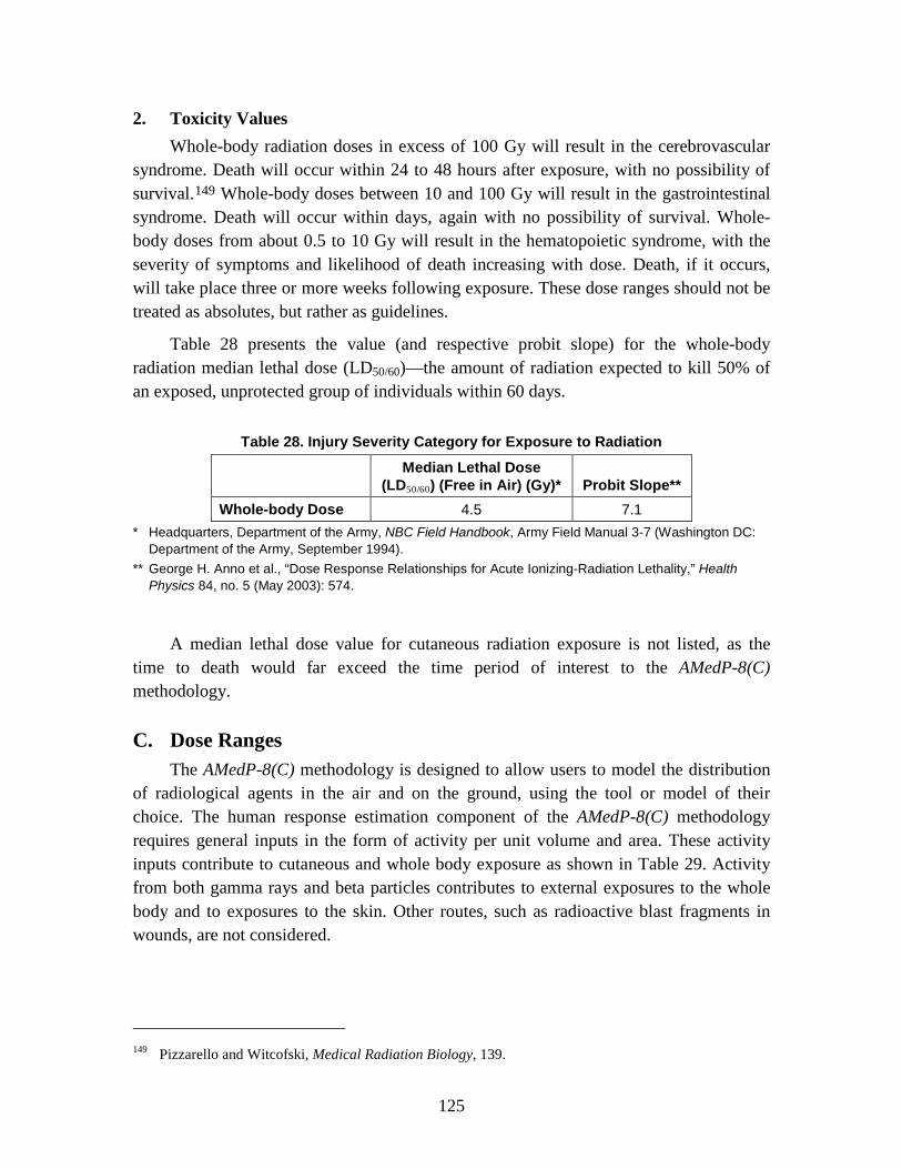
125
2. Toxicity Values Whole-body radiation doses in excess of 100 Gy will result in the cerebrovascular
syndrome. Death will occur within 24 to 48 hours after exposure, with no possibility of survival.149
Table 28 presents the value (and respective probit slope) for the whole-body radiation median lethal dose (LD50/60)—the amount of radiation expected to kill 50% of an exposed, unprotected group of individuals within 60 days.
Whole-body doses between 10 and 100 Gy will result in the gastrointestinal syndrome. Death will occur within days, again with no possibility of survival. Whole-body doses from about 0.5 to 10 Gy will result in the hematopoietic syndrome, with the severity of symptoms and likelihood of death increasing with dose. Death, if it occurs, will take place three or more weeks following exposure. These dose ranges should not be treated as absolutes, but rather as guidelines.
Table 28. Injury Severity Category for Exposure to Radiation
Median Lethal Dose (LD50/60) (Free in Air) (Gy)* Probit Slope**
Whole-body Dose 4.5 7.1 * Headquarters, Department of the Army, NBC Field Handbook, Army Field Manual 3-7 (Washington DC:
Department of the Army, September 1994). ** George H. Anno et al., “Dose Response Relationships for Acute Ionizing-Radiation Lethality,” Health
Physics 84, no. 5 (May 2003): 574.
A median lethal dose value for cutaneous radiation exposure is not listed, as the time to death would far exceed the time period of interest to the AMedP-8(C) methodology.
C. Dose Ranges The AMedP-8(C) methodology is designed to allow users to model the distribution
of radiological agents in the air and on the ground, using the tool or model of their choice. The human response estimation component of the AMedP-8(C) methodology requires general inputs in the form of activity per unit volume and area. These activity inputs contribute to cutaneous and whole body exposure as shown in Table 29. Activity from both gamma rays and beta particles contributes to external exposures to the whole body and to exposures to the skin. Other routes, such as radioactive blast fragments in wounds, are not considered.
149 Pizzarello and Witcofski, Medical Radiation Biology, 139.
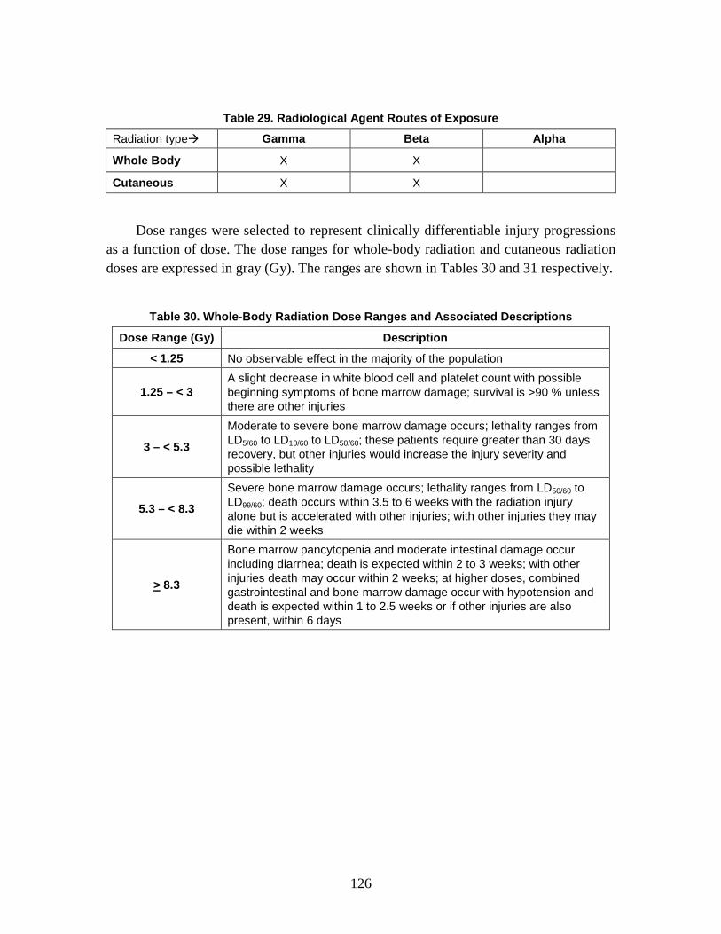
126
Table 29. Radiological Agent Routes of Exposure
Radiation type Gamma Beta Alpha
Whole Body X X
Cutaneous X X
Dose ranges were selected to represent clinically differentiable injury progressions as a function of dose. The dose ranges for whole-body radiation and cutaneous radiation doses are expressed in gray (Gy). The ranges are shown in Tables 30 and 31 respectively.
Table 30. Whole-Body Radiation Dose Ranges and Associated Descriptions
Dose Range (Gy) Description
< 1.25 No observable effect in the majority of the population
1.25 – < 3 A slight decrease in white blood cell and platelet count with possible beginning symptoms of bone marrow damage; survival is >90 % unless there are other injuries
3 – < 5.3
Moderate to severe bone marrow damage occurs; lethality ranges from LD5/60 to LD10/60 to LD50/60; these patients require greater than 30 days recovery, but other injuries would increase the injury severity and possible lethality
5.3 – < 8.3
Severe bone marrow damage occurs; lethality ranges from LD50/60 to LD99/60; death occurs within 3.5 to 6 weeks with the radiation injury alone but is accelerated with other injuries; with other injuries they may die within 2 weeks
> 8.3
Bone marrow pancytopenia and moderate intestinal damage occur including diarrhea; death is expected within 2 to 3 weeks; with other injuries death may occur within 2 weeks; at higher doses, combined gastrointestinal and bone marrow damage occur with hypotension and death is expected within 1 to 2.5 weeks or if other injuries are also present, within 6 days

127
Table 31. Cutaneous Radiation Dose Range and Associated Description
Dose Range (Gy) Description
< 2 No observable effect in the majority of the population
2 – < 15 12 hours to 5 weeks post exposure: erythema, slight edema, possible increased pigmentation; 6 to 7 weeks post exposure: dry desquamation
15 – < 40 Immediate itching; 1 to 3 weeks post exposure: erythema, edema; 5 to 6 weeks post exposure: subcutaneous tissue edema, blisters, moist desquamation; late effects (> 10 weeks)
40 – < 550 Immediate pain, tingling for 1 to 2 days; 1 to 2 weeks post exposure: erythema, blisters, edema, pigmentation, erosions, ulceration, severe pain; severe late effects (> 10 weeks)
> 550 Immediate pain, tingling, swelling; 1 to 4 days post exposure: blisters, early ischemia, substantial pain; tissue necrosis within 2 weeks, substantial pain
Source: CDC, Cutaneous Radiation Injury.
The whole-body dose ranges in Table 30 are based on and condensed from the original Injury Severity Category tables included in the nuclear volume of AMedP-8(A).150
In order to modify the whole-body dose ranges, the methodology began by returning to the original Intermediate Dose Program (IDP) methodology, where signs and symptoms progressions were prepared for four radiation doses—1.5 Gy, 3 Gy, 5 Gy, and 10 Gy.
In those tables, radiation injury severity was represented by eight dose ranges, but discussions with the NATO CBRN Medical Working group indicated that this was too many ranges. Moreover, these discussions suggested that dose ranges should ideally be clinically differentiable, and such was not clearly the case with the ranges found in AMedP-8(A).
151 These doses approximately correlate to the boundaries between the original AMedP-8(A), IDP, and AMedP-6(C) dose ranges with one exception; the uppermost value—10 Gy—was approximately the midpoint of the sixth dose range. Higher doses were anticipated to cause similar lethality in shorter time periods; these dose ranges were therefore correlated into a single representative range. The “no observable effect” range was extended slightly to correspond to the AMedP-6(C) value of 0.75 Gy; documentation suggests that less than 5% of the population would be expected to suffer mild nausea at doses in this range.152
150 NATO, AMedP-8(A) Nuclear, 3–9.
Thus, this would seem to indicate that, for most of the population, below this dose, there are no observable effects resulting from exposure.
151 Levin, Effect of Combined Injuries, A-2–A-5. 152 NATO, AMedP-6(C), Volume I: NATO Handbook on the Medical Aspects of NBC Defensive
Operations (Nuclear) (AMedP-6(C) Nuclear) (2005); and Armed Forces Radiobiology Research

128
The cutaneous radiation dose information in Table 31 is drawn from the CDC publication referenced in the table; AMedP-8(A) specifically addresses radiation resulting from a nuclear detonation and does not contain information related to cutaneous injury from skin contamination.
D. Symptoms The basic concept of the AMedP-8(C) methodology is that an individual is
considered a casualty at the time of first onset of a specified injury severity level, based on specific symptoms resulting from exposure to the causative agent. The human response component of this methodology specifies an injury profile depicting injury severity level over time that is used to determine whether an individual is declared KIA, WIA, or DOW and thereby considered to be a casualty and, if so, at what point this would occur. The injury profile is derived from the symptom progressions, which show the severity level of symptoms in the system in which they manifest (as opposed to the causative system) over time. The severity level of the injury profile at any given time point corresponds to the worst severity level experienced in any of the representative physiological systems at that time. The nature of symptoms and their times of onset depend on the agent or effect.
1. Injury Severity Levels For external whole-body radiation, the DNA IDP methodology employed six sets of
signs, symptoms, and systems to represent the injury progression: upper gastrointestinal, lower gastrointestinal, fatigability and weakness, infection and bleeding, hypotension, and fluid loss. These symptoms were represented on a severity scale of 1–5.153
In an effort to ensure clarity and consistency, the symptoms and systems for whole-body radiation were correlated to four representative physiological systems in which symptoms would be expected to manifest following exposure to nuclear radiation. These correlations are shown in Table 32. The new “cardiovascular” system encompasses hypotension and bleeding and the new “immune system” system encompasses infection (fluid loss was not considered in the AMedP-8(C) methodology).
Institute (AFRRI), Medical Management of Radiological Casualties, Second Edition (Bethesda, MD: AFRRI, April 2003), Table F-1.
153 Levin, Effect of Combined Injuries, 5–6; Anno et al., Performance on Infantry and Artillery Personnel, 6; and Sheldon G. Levin, Consolidated Human Response Nuclear Effects Model (CHRNEM), DNA-TR-93-45 (Alexandria, VA: Defense Nuclear Agency, 1993), 6–8.
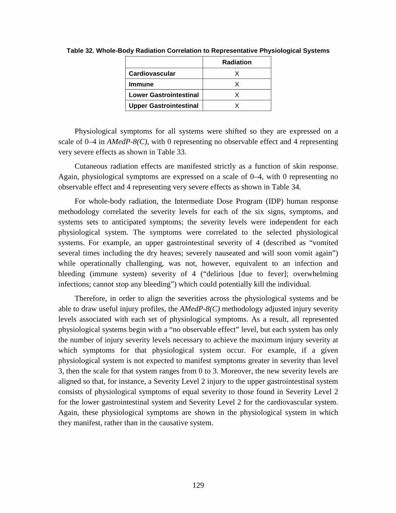
129
Table 32. Whole-Body Radiation Correlation to Representative Physiological Systems
Radiation
Cardiovascular X Immune X Lower Gastrointestinal X Upper Gastrointestinal X
Physiological symptoms for all systems were shifted so they are expressed on a scale of 0–4 in AMedP-8(C), with 0 representing no observable effect and 4 representing very severe effects as shown in Table 33.
Cutaneous radiation effects are manifested strictly as a function of skin response. Again, physiological symptoms are expressed on a scale of 0–4, with 0 representing no observable effect and 4 representing very severe effects as shown in Table 34.
For whole-body radiation, the Intermediate Dose Program (IDP) human response methodology correlated the severity levels for each of the six signs, symptoms, and systems sets to anticipated symptoms; the severity levels were independent for each physiological system. The symptoms were correlated to the selected physiological systems. For example, an upper gastrointestinal severity of 4 (described as “vomited several times including the dry heaves; severely nauseated and will soon vomit again”) while operationally challenging, was not, however, equivalent to an infection and bleeding (immune system) severity of 4 (“delirious [due to fever]; overwhelming infections; cannot stop any bleeding”) which could potentially kill the individual.
Therefore, in order to align the severities across the physiological systems and be able to draw useful injury profiles, the AMedP-8(C) methodology adjusted injury severity levels associated with each set of physiological symptoms. As a result, all represented physiological systems begin with a “no observable effect” level, but each system has only the number of injury severity levels necessary to achieve the maximum injury severity at which symptoms for that physiological system occur. For example, if a given physiological system is not expected to manifest symptoms greater in severity than level 3, then the scale for that system ranges from 0 to 3. Moreover, the new severity levels are aligned so that, for instance, a Severity Level 2 injury to the upper gastrointestinal system consists of physiological symptoms of equal severity to those found in Severity Level 2 for the lower gastrointestinal system and Severity Level 2 for the cardiovascular system. Again, these physiological symptoms are shown in the physiological system in which they manifest, rather than in the causative system.

130
Table 33. Symptoms Severity Levels Associated with Whole-Body Radiation
Severity Upper Gastrointestinal Lower Gastrointestinal
0 No observable effect No observable effect
1 Upset stomach and nausea: watering mouth and frequent swallowing to avoid vomiting
Abdominal pain or cramps; occasional diarrhea and uncomfortable urge to defecate
2
Episodes of vomiting, possibly including dry heaves; severe nausea and possibility of continued vomiting
Frequent diarrhea and cramps; continuing defecation
3 Protracted or continued vomiting, including dry heaves
Uncontrollable diarrhea and urination; painful cramps
4
Table 33. continued
Severity Cardiovascular Immune
0 No observable effect No observable effect 1 Slightly feeling of light headedness Slight fever and headache
2 Unsteadiness upon standing quickly; possible micro-hemorrhaging
Aching joints; fever; lack of appetite; sores in mouth/throat
3 Severe dizziness; faints upon standing quickly; may have difficulty stopping any bleeding
High fever results in shakes, chills and aches all over
4
Shock; rapid and shallow breathing; skin cold, clammy and very pale; difficulty or inability to stop any bleeding; crushing chest pain
Delirium from fever; overwhelming infections
Table 34. Severity Levels Associated with Cutaneous Effects
Severity Cutaneous Symptoms
0 No observable effect 1 Itching, sensation of heat, erythema, slight edema 2 Subcutaneous edema, blister formation, epilation 3 Ischemia, ulceration, substantial pain, possible skin necrosis 4
2. Injury Profiles Each of the dose bands previously described corresponds to a progression of injury
over time. These progressions are discontinuous with respect to dose; all insults within

131
the specified range are represented by the same injury progression. The boundaries defining each radiation exposure range represent points in an exposure at which the expected progression of injury abruptly changes as the exposure is increased. Moreover, the injury progressions themselves are discontinuous and stepwise with respect to severity level; they are not smoothed or otherwise interpolated. In other words, moving along the time dimension of the injury progression, the injury severity and the corresponding physiological symptoms change instantaneously at specific points in time.
In the case of whole-body radiation, for a given dose or insult range, separate injury progressions have been developed for each of the physiological systems—upper gastrointestinal, lower gastrointestinal, cardiovascular, immune, respiratory, and skin (thermal)—illustrating the severity of the physiological symptoms for a particular physiological system over time. Similarly, for a given cutaneous radiation dose range, separate injury progressions have been developed illustrating the severity of the physiological symptoms for the skin over time. Figures 46 through 53 present these injury progressions by insult range for whole-body and cutaneous radiation exposure.154
The “no observable effect” progressions are not shown; all injury severity levels on those would be 0 for the duration of time observed.
154 All of the injury progression and injury profiles are plotted using hours along the logarithmic x-axis.
The whole-body profiles are derived from those originally incorporated in the IDP and included in Levin, Effects of Combined Injuries, A-2–A-13. The cutaneous profiles are derived from those originally derived from CDC, “Cutaneous Radiation Injury.” Both sets of profiles have been further modified based on subject matter input and expertise as documented in Burr et al., Nuclear Human Response SME Review Meeting, 1–31; and Burr et al., Radiological Human Response SME Review Meeting, 1–16.
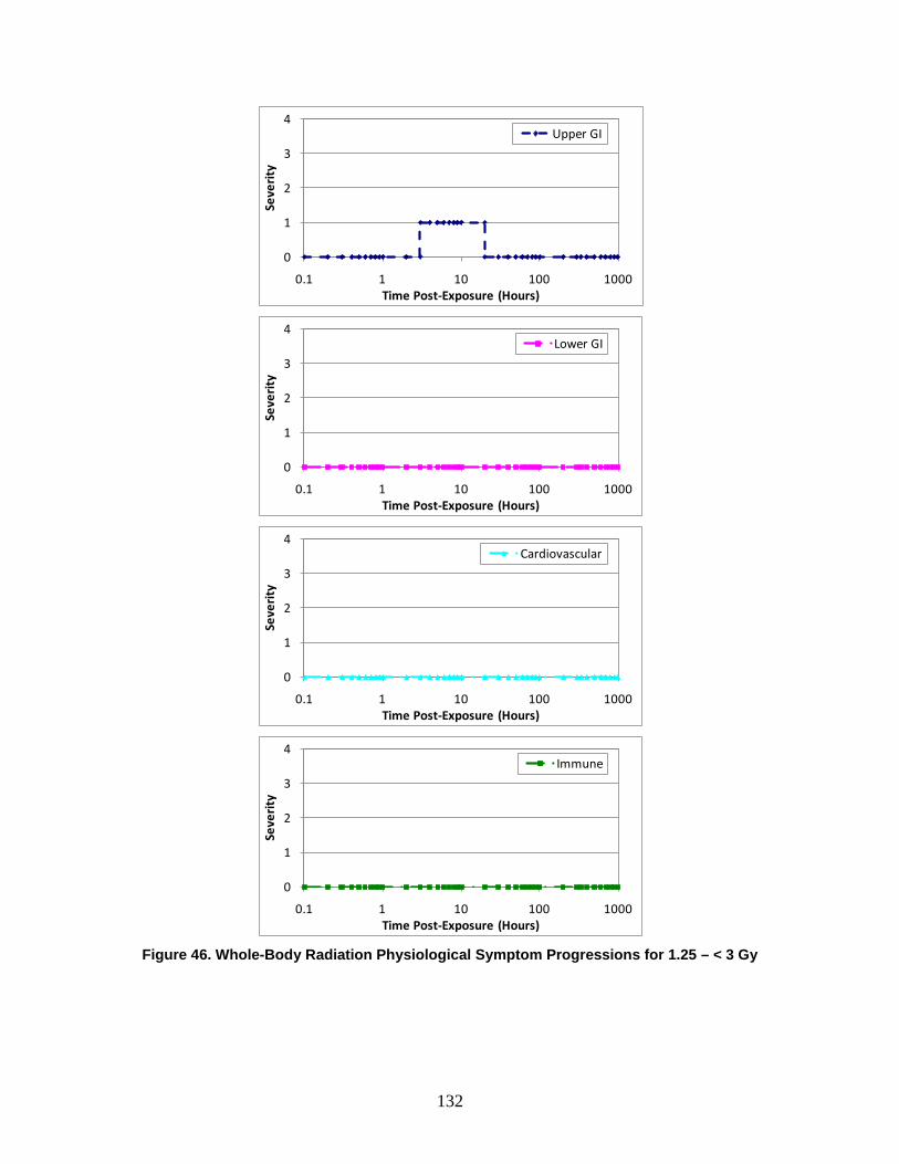
132
Figure 46. Whole-Body Radiation Physiological Symptom Progressions for 1.25 – < 3 Gy
0
1
2
3
4
0.1 1 10 100 1000Se
veri
ty
Time Post-Exposure (Hours)
Upper GI
0
1
2
3
4
0.1 1 10 100 1000
Seve
rity
Time Post-Exposure (Hours)
Lower GI
0
1
2
3
4
0.1 1 10 100 1000
Seve
rity
Time Post-Exposure (Hours)
Cardiovascular
0
1
2
3
4
0.1 1 10 100 1000
Seve
rity
Time Post-Exposure (Hours)
Immune

133
Figure 47. Whole-Body Radiation Physiological Symptom Progressions for 3 – < 5.3 Gy
0
1
2
3
4
0.1 1 10 100 1000Se
veri
ty
Time Post-Exposure (Hours)
Upper GI
0
1
2
3
4
0.1 1 10 100 1000
Seve
rity
Time Post-Exposure (Hours)
Lower GI
0
1
2
3
4
0.1 1 10 100 1000
Seve
rity
Time Post-Exposure (Hours)
Cardiovascular
0
1
2
3
4
0.1 1 10 100 1000
Seve
rity
Time Post-Exposure (Hours)
Immune

134
Figure 48. Whole-Body Radiation Physiological Symptom Progressions for 5.3 – < 8.3 Gy*
* As indicated by the “∫∫,” for doses > 5 Gy, time to death is calculated; the injury progression is followed as prescribed until time of death. Time of death may occur up to or later than 6 weeks.
0
1
2
3
4
0.1 1 10 100 1000Se
veri
ty
Time Post-Exposure (Hours)
Upper GI
∫∫
0
1
2
3
4
0.1 1 10 100 1000
Seve
rity
Time Post-Exposure (Hours)
Lower GI
∫∫
0
1
2
3
4
0.1 1 10 100 1000
Seve
rity
Time Post-Exposure (Hours)
Cardiovascular
∫∫
0
1
2
3
4
0.1 1 10 100 1000
Seve
rity
Time Post-Exposure (Hours)
Immune
∫∫
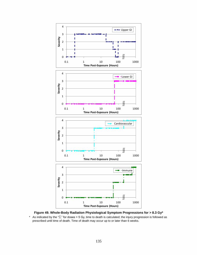
135
Figure 49. Whole-Body Radiation Physiological Symptom Progressions for > 8.3 Gy*
* As indicated by the “∫∫,” for doses > 5 Gy, time to death is calculated; the injury progression is followed as prescribed until time of death. Time of death may occur up to or later than 6 weeks.
0
1
2
3
4
0.1 1 10 100 1000Se
veri
ty
Time Post-Exposure (Hours)
Upper GI
∫∫
0
1
2
3
4
0.1 1 10 100 1000
Seve
rity
Time Post-Exposure (Hours)
Lower GI
∫∫
0
1
2
3
4
0.1 1 10 100 1000
Seve
rity
Time Post-Exposure (Hours)
Cardiovascular
∫∫
0
1
2
3
4
0.1 1 10 100 1000
Seve
rity
Time Post-Exposure (Hours)
Immune
∫∫

136
Figure 50. Cutaneous Injury Profile for 2 – < 15 Gy
Figure 51. Cutaneous Injury Profile for 15 – < 40 Gy
Figure 52. Cutaneous Injury Profile for 40 – < 550 Gy
0
1
2
3
4
0.1 1 10 100 1000Se
veri
ty
Time Post-Exposure (Hours)
Cutaneous
0
1
2
3
4
0.1 1 10 100 1000
Seve
rity
Time Post-Exposure (Hours)
Cutaneous
0
1
2
3
4
0.1 1 10 100 1000
Seve
rity
Time Post-Exposure (Hours)
Cutaneous
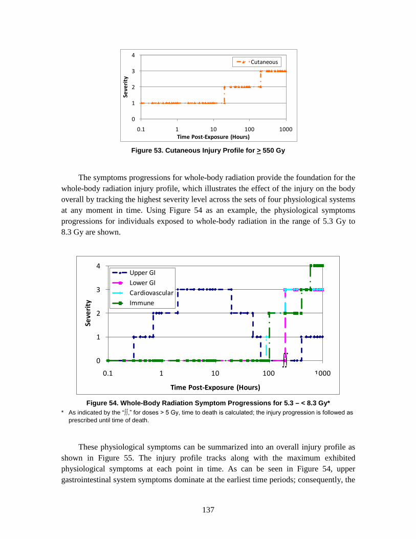
137
Figure 53. Cutaneous Injury Profile for > 550 Gy
The symptoms progressions for whole-body radiation provide the foundation for the whole-body radiation injury profile, which illustrates the effect of the injury on the body overall by tracking the highest severity level across the sets of four physiological systems at any moment in time. Using Figure 54 as an example, the physiological symptoms progressions for individuals exposed to whole-body radiation in the range of 5.3 Gy to 8.3 Gy are shown.
Figure 54. Whole-Body Radiation Symptom Progressions for 5.3 – < 8.3 Gy*
* As indicated by the “∫∫,” for doses > 5 Gy, time to death is calculated; the injury progression is followed as prescribed until time of death.
These physiological symptoms can be summarized into an overall injury profile as shown in Figure 55. The injury profile tracks along with the maximum exhibited physiological symptoms at each point in time. As can be seen in Figure 54, upper gastrointestinal system symptoms dominate at the earliest time periods; consequently, the
0
1
2
3
4
0.1 1 10 100 1000Se
veri
ty
Time Post-Exposure (Hours)
Cutaneous
0
1
2
3
4
0.1 1 10 100 1000
Seve
rity
Time Post-Exposure (Hours)
Upper GILower GICardiovascularImmune
∫∫
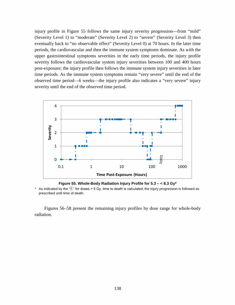
138
injury profile in Figure 55 follows the same injury severity progression—from “mild” (Severity Level 1) to “moderate” (Severity Level 2) to “severe” (Severity Level 3) then eventually back to “no observable effect” (Severity Level 0) at 70 hours. In the later time periods, the cardiovascular and then the immune system symptoms dominate. As with the upper gastrointestinal symptoms severities in the early time periods, the injury profile severity follows the cardiovascular system injury severities between 100 and 400 hours post-exposure; the injury profile then follows the immune system injury severities in later time periods. As the immune system symptoms remain “very severe” until the end of the observed time period—6 weeks—the injury profile also indicates a “very severe” injury severity until the end of the observed time period.
Figure 55. Whole-Body Radiation Injury Profile for 5.3 – < 8.3 Gy*
* As indicated by the “∫∫,” for doses > 5 Gy, time to death is calculated; the injury progression is followed as prescribed until time of death.
Figures 56–58 present the remaining injury profiles by dose range for whole-body radiation.
0
1
2
3
4
0.1 1 10 100 1000
Seve
rity
Time Post-Exposure (Hours)
∫∫
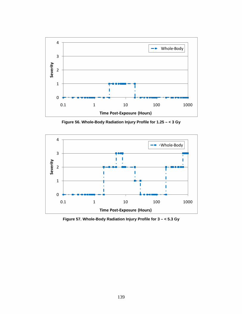
139
Figure 56. Whole-Body Radiation Injury Profile for 1.25 – < 3 Gy
Figure 57. Whole-Body Radiation Injury Profile for 3 – < 5.3 Gy
0
1
2
3
4
0.1 1 10 100 1000
Seve
rity
Time Post-Exposure (Hours)
Whole-Body
0
1
2
3
4
0.1 1 10 100 1000
Seve
rity
Time Post-Exposure (Hours)
Whole-Body
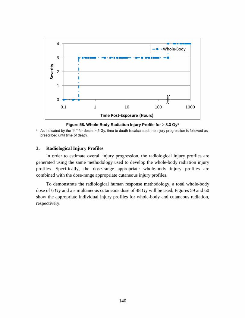
140
Figure 58. Whole-Body Radiation Injury Profile for ≥ 8.3 Gy*
* As indicated by the “∫∫,” for doses > 5 Gy, time to death is calculated; the injury progression is followed as prescribed until time of death.
3. Radiological Injury Profiles In order to estimate overall injury progression, the radiological injury profiles are
generated using the same methodology used to develop the whole-body radiation injury profiles. Specifically, the dose-range appropriate whole-body injury profiles are combined with the dose-range appropriate cutaneous injury profiles.
To demonstrate the radiological human response methodology, a total whole-body dose of 6 Gy and a simultaneous cutaneous dose of 48 Gy will be used. Figures 59 and 60 show the appropriate individual injury profiles for whole-body and cutaneous radiation, respectively.
0
1
2
3
4
0.1 1 10 100 1000
Seve
rity
Time Post-Exposure (Hours)
Whole-Body
∫∫

141
Figure 59. Whole-Body Radiation Injury Profile for 6 Gy*
* As indicated by the “∫∫,” for doses > 5 Gy, time to death is calculated; the injury progression is followed as prescribed until time of death.
Figure 60. Cutaneous Injury Profile for 48 Gy
The injury profiles are drawn together on a single plot. This is shown in Figure 61.
0
1
2
3
4
0.1 1 10 100 1000
Seve
rity
Time Post-Exposure (Hours)
Whole-Body
∫∫
0
1
2
3
4
0.1 1 10 100 1000
Seve
rity
Time Post-Exposure (Hours)
Cutaneous
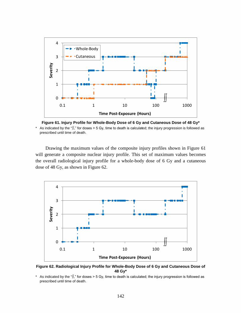
142
Figure 61. Injury Profile for Whole-Body Dose of 6 Gy and Cutaneous Dose of 48 Gy*
* As indicated by the “∫∫,” for doses > 5 Gy, time to death is calculated; the injury progression is followed as prescribed until time of death.
Drawing the maximum values of the composite injury profiles shown in Figure 61 will generate a composite nuclear injury profile. This set of maximum values becomes the overall radiological injury profile for a whole-body dose of 6 Gy and a cutaneous dose of 48 Gy, as shown in Figure 62.
Figure 62. Radiological Injury Profile for Whole-Body Dose of 6 Gy and Cutaneous Dose of
48 Gy* * As indicated by the “∫∫,” for doses > 5 Gy, time to death is calculated; the injury progression is followed as
prescribed until time of death.
0
1
2
3
4
0.1 1 10 100 1000
Seve
rity
Time Post-Exposure (Hours)
Whole-Body
Cutaneous
∫∫
0
1
2
3
4
0.1 1 10 100 1000
Seve
rity
Time Post-Exposure (Hours)
∫∫
143
7. Nuclear Human Response Review: Composite Nuclear Insults
A. Introduction Nuclear events are among the most damaging events possible; they result in injuries
and fatalities to exposed individuals, destruction of property, and long-term risks for both the populations exposed to the event and those exposed to its after-effects—e.g., the radioactive fallout. Nuclear events, like other weapons of mass destruction (WMD) events, pose several significant challenges. Nuclear events cause a combination of injuries due to the prompt nuclear effects—radiation, blast overpressure, and thermal energy—resulting from the detonation. Further, there are secondary effects (tumbling, missiling, and building collapse due to secondary, tertiary, and quaternary dynamic pressures) and indirect effects (flash blindness and burns due to secondary fires) which result from the detonation. Even with the experience of Hiroshima and Nagasaki, there is little information to facilitate the estimation of casualties. In part, this is due both to technological advances in the weapons and to differences in the environments in which they might be utilized.155
B. Background
As such, the AMedP-8(C) methodology estimates casualties based solely on prompt effects and does not consider secondary or indirect effects (with the exception of death due to tumbling). The objective of this chapter is to describe the human response component of the AMedP-8(C) methodology for estimating casualties resulting from the detonation of a nuclear weapon.
Nuclear events result in three prompt effects—initial radiation, primary overpressure (and some resulting dynamic pressure effects), and thermal energy. These prompt effects mobilize through different mechanisms of action, but often affect similar physiological systems. Radiation results in symptoms manifesting in the upper and lower gastrointestinal, cardiovascular, and immune systems. Static overpressure and the resulting primary blast injury also impact the upper and lower gastrointestinal and cardiovascular systems, as well as the respiratory system. Thermal injuries are most obvious in the flash burns which develop on the skin, but these injuries further affect the upper gastrointestinal, cardiovascular, and immune systems.
155 NATO, AMedP-8(A) Nuclear, 1-1–1-4.
144
1. Whole-Body Radiation Nuclear radiation causes injury to a number of physiological systems through the
deposition of energy in the organ tissues—both electromagnetic (e.g., x-rays and gamma rays) and particulate radiation (e.g., beta particles, alpha particles, and neutrons). The deposition of energy produces free radicals which, in turn, interact with the body chemistry causing damage to the cells and cellular material.156 The resulting damage is a function of a number of factors including the dose, the time post-exposure, and the sensitivity of the cellular material, among others. Thus, the higher the dose, the greater the resulting damage, the worse the anticipated injury severity, and the shorter the latent period before the injury manifests as symptoms, otherwise known as acute radiation syndrome (ARS).157
2. Blast
Within the first millisecond after a nuclear detonation, a fireball composed of the gaseous weapon residue and surrounding air is generated under extremely high pressures and temperature. The rapidly expanding fireball, in turn, compresses the air in front of it, generating a shock, or high-pressure blast, wave that travels radially outward from the center of the explosion. The main characteristic of this wave is a very rapid rise in peak static overpressure (i.e., the maximum pressure in excess of the ambient air pressure). The magnitude of the peak overpressure tends to decrease exponentially as it travels away from the detonation point. In addition, a dynamic pressure front, in the form of a blast wind, is generated by the blast wave and follows immediately behind it. The dynamic pressure is proportional to the density of air behind the shock wave and to the square of the wind velocity. Both the static overpressure and the dynamic pressure rapidly decrease to zero with time.158
At any point from the detonation, an ideal blast wave consists of a positive overpressure rapidly rising (near instantaneously) to its peak value, before decaying exponentially, followed by a less intense negative pressure phase (i.e., pressure less than the ambient air pressure). A key difference between conventional and nuclear explosions is the duration of the positive-pressure phase: for conventional explosives this time is measured in tens of milliseconds, while the positive phase for nuclear blasts lasts on the order of hundreds to thousands of milliseconds depending on yield.
159
156 Alt, Forcino, and Walker, “Nuclear Events and Their Consequences,” 13–14.
157 See Chapter VI for a more complete discussion of ARS. 158 Glasstone and Dolan, Effects of Nuclear Weapons, 80–83; and Alt, Forcino, and Walker, “Nuclear
Events and Their Consequences,” 5–6. 159 James H. Stuhmiller, Yancy Y. Phillips III, and Donald R. Richmond, “The Physics and Mechanisms
of Primary Blast Injury,” in Conventional Warfare: Ballistic, Blast, and Burn Injuries, ed. Ronald F. Bellamy and Russ Zajtchuk, Textbook of Military Medicine, Part I: Warfare, Weaponry, and the Casualty (Falls Church, VA: Department of the Army, Office of the Surgeon General, Borden Institute
145
Blast waves can reflect off of solid surfaces such as walls. The resulting combination of incident and reflected blast waves can be as much as twice the peak overpressure of the incident wave alone. Due to such factors as multiple reflections and time delays, more complex wave forms can be generated inside open structures (e.g., foxholes or open-sided buildings) or in enclosures with small openings. The potential and type of primary blast injuries are highly dependent upon the nature of the resulting complex waves.
The static overpressure is responsible for the primary blast effects and injuries, while dynamic pressure primarily produces secondary and tertiary blast effects and injuries. Each of these blast injuries will be discussed in turn.
a. Primary Blast Injuries In general, the probability of a direct, or primary, blast injury increases with the
duration of the blast wave’s positive-pressure phase for a given peak overpressure. The relationship between the duration of the positive phase and the potential for injury, however, only holds up to a certain time duration, beyond which the peak static overpressure alone plays a significant role. For expected yields and under most conditions, this time is exceeded for nuclear explosions; as a result, the potential for primary blast injuries is driven by the effective (i.e., the sum of incident and any reflected blast waves) peak static overpressure and the rapidity of its rise.
The pathology of the primary blast injuries is understood due to animal tests with nuclear and conventional explosives, and human data from military and terrorist conventional explosive events. The principal damage caused by the static overpressure is to air and gas-filled organs of the body: in particular the auditory system, the upper respiratory tract and lungs, and the upper and lower gastrointestinal tracts. Injuries to other organs typically are related to or caused by initial disruption to these organs. The organs have three characteristics in common: they mark areas of differing tissue density, they are filled with air or gas, and they assist in equilibrating air pressure within the body.
The auditory system is the most easily affected, with rupture of the tympanic membrane possible at fairly low static overpressures (around 34 kPa). However, in the AMedP-8(C) methodology, this injury is considered as a nuisance effect—it may or may not produce any pain and it may not lead to hearing loss. The blast wave may also
1998), 249; and Donald R. Richmond and Edward G. Damon, Primary Blast Injuries in the Open and in Foxholes Resulting from Nuclear Type Detonations, DNA-TR-90-212 (Los Alamos, NM: Technico Southwest, Inc., for the Defense Nuclear Agency, July 1991), 28.
146
damage the cochlea, leading to temporary or permanent hearing loss; in the absence of sufficient data, however, this injury too is neglected.160
Among the most serious primary effects of blast are injuries to the respiratory system, which tend to be hemorrhagic in nature. Pulmonary hemorrhages can range from a few pin-head sized petechiae to a concentration of petechiae on the surface of the lung, to confluent hemorrhaging entailing small areas of the lungs or encompassing entire lobes. Some evidence suggests that these blast forces may also produce pulmonary edema, though other research disputes this notion.
161 Under sufficiently high pressures, the lungs may rupture or be punctured by the jagged ends of fractured ribs. In the upper respiratory tract, the mucosal lining of the trachea, larynx, pharynx, and sinus may become bruised or, given sufficient static overpressure, even hemorrhage leading to constriction of the airways.162
More serious still, disruption to the alveoli in the lungs can lead to the introduction of air emboli into the circulatory system. Evidence suggests that the likelihood of significant embolism increases with the severity of the pulmonary hemorrhage.
163 Air emboli in the coronary vessels can lead to cardiac damage similar to a heart attack. Should these air bubbles reach the brain, they can lead to damage to the central nervous system and to stroke-like effects. Embolism is believed to be the leading cause of early death in primary blast injury victims.164
After the respiratory system, blast waves do the most damage to the gastrointestinal system. At low static overpressure, the damage can be limited to light contusions to the serosal tissue. As the static overpressure increases, injury can range from submucosal contusions, with or without rupture of the mucosal membrane, up to hemorrhages ranging from small petechiae to large hematomas within the intestinal or gastric walls. Finally, at high enough static overpressures, perforations of the intestinal wall can develop, emptying the contents of the gastrointestinal tract into the abdominal cavity and leading to peritonitis after several days.
165
160 Douglas D. Sharpnack, Anthony J. Johnson, and Yancy Y Phillips III, “The Pathology of Primary
Blast Injury,” in Conventional Warfare: Ballistic, Blast, and Burn Injuries, ed. Ronald F. Bellamy and Russ Zajtchuk, Textbook of Military Medicine, Part I: Warfare, Weaponry, and the Casualty 271–94 (Falls Church, VA: Department of the Army, Office of the Surgeon General, Borden Institute 1998), 290–92; and Richmond and Damon, Primary Blast Injuries, 24.
161 Sharpnack, Johnson, and Phillips, “The Pathology of Primary Blast Injury,” 279–80. 162 For more on the primary blast effects on the respiratory system, see Sharpnack, Johnson, and Phillips,
“The Pathology of Primary Blast Injury,” 273–83; Richmond and Damon, Primary Blast Injuries, 14; and Levin, Effect of Combined Injuries, 28–29.
163 Sharpnack, Johnson, and Phillips, “The Pathology of Primary Blast Injury,” 284–85. 164 Ibid., 284–86; and Richmond and Damon, Primary Blast Injuries, 25. 165 Sharpnack, Johnson, and Phillips, “The Pathology of Primary Blast Injury,” 288–89; Richmond and
Damon, Primary Blast Injuries, 21; and Levin, Effect of Combined Injuries, 29.
147
Other primary effects of blast may include contusions or hemorrhaging of solid organs, such as the heart, liver, spleen, and kidney. At very high pressures, these organs may rupture. In the case of the heart, these effects are most likely due to contact with the lungs as the latter are violently contorted by the blast wave. Similarly, the liver, spleen, and kidney are most likely damaged by coming into contact with the over-expanded gastrointestinal tract.166 Due to the absence of sufficient data, however, these effects are neglected in the AMedP-8(C) methodology. Orbital “blow-out” fractures have been reported in certain animal species at very high pressures (greater than 690 kPa), but their presence has not been reported in humans.167
Finally, the body is able to adjust (within limits) to relatively gradual changes in external air pressure. Thus, when individuals are in certain locations—such as open structures and enclosures—where the rise time of the static overpressure may be more gradual than that obtained in the open or in the presence of single reflective surfaces, organs may be able to sustain much higher total pressures than would be typical without sustaining significant damage.
Given the lack of data and the high pressures at which these injuries reportedly occur, this effect is ignored as well. Current research also suggests that pressures arising from conventional explosions may produce traumatic brain injury; but again, the lack of data currently prohibits the inclusion of this effect in the AMedP-8(C) methodology. However, any of the effects now excluded from the AMedP-8(C) methodology could easily be included given sufficient data.
168
b. Secondary Blast Injuries
Due to the uncertainties involved in the specifics of any given scenario, these situations are not included in the AMedP-8(C) methodology.
Secondary blast injuries result from the impact of debris energized by blast pressures, winds, ground shock, and gravity. Debris may include building and other structural fragments, as well as missiles generated from building material (e.g., glass fragments) or from the natural terrain (wood, stones, etc.). Secondary effects include both blunt and penetrating trauma. Resulting injuries can range from slight lacerations to perforating lesions to crushing injuries. The type and probability of secondary blast injuries are dependent upon a variety of factors, including: the size, shape, mass, density, and nature of the debris; the velocity of the debris; the angle at which impact occurs; the portion of the body involved in the impact; and whether the blow is piercing, penetrating, or nonpenetrating (i.e., crushing).169
166 Richmond and Damon, Primary Blast Injuries, 21.
In order to model secondary effects, much more
167 Ibid., 24–25; and Sharpnack, Johnson, and Phillips, “The Pathology of Primary Blast Injury,” 289. 168 Richmond and Damon, Primary Blast Injuries, 35; Clayton S. White, I. G. Bowen, and Donald R.
Richmond, A Comparative Analysis of Some of the Immediate Environmental Effects at Hiroshima and Nagasaki, CEX-63.7 (Washington, DC: U.S. Atomic Energy Commission, August 1964), 10–11.
169 Marvin K. Drake et al., An Interim Report on Collateral Damage, DNA 4734Z (LaJolla, CA: Science Applications, Inc., for the Defense Nuclear Agency, October 1978), 5-72.
148
detail regarding posture, orientation, environment, and many other factors would need to be provided for each scenario than is presently required for AMedP-8(C). Given the uncertainties involved in such factors as predicting the type and characteristics of debris, and in the absence of any generalized dynamic pressure threshold values for injury or death, secondary blast injuries are neglected in the AMedP-8(C) methodology.
c. Tertiary Blast Injuries Tertiary blast injuries result from whole body translation (i.e., individuals being
propelled through the air by the blast winds). Most of the damage resulting from tertiary blast effects occurs during the deceleration phase and is highly dependent on whether the individual’s movement is stopped abruptly by striking a solid object (e.g., a wall or the ground) or more gradually by tumbling along the open ground. Injuries can include contusions, abrasions, lacerations, fractures, damage to internal organs, and even death.170 The type and probability of tertiary blast injuries are dependent upon a number of factors including the yield of the nuclear weapon (which helps determine the duration of the blast wind), the posture of the individual (e.g., standing or prone), the orientation of the body to the blast (from perpendicular to parallel), the body’s final airborne velocity, the length of time the body is airborne, the hardness of the solid object struck (for abrupt deceleration), the angle of impact, and the organs impacted.171
3. Thermal Energy
Again, in order to model tertiary effects, much more detail would need to be provided for each scenario than is presently required for AMedP-8(C). Given the uncertainties involved in such factors as predicting the proximity of solid objects to impact against or the orientation of individuals to the blast wave, and in the absence of any generalized dynamic pressure threshold values for injury, tertiary blast injuries are largely neglected in the AMedP-8(C) methodology. However, a tertiary blast threshold for death due to tumbling is considered in the casualty estimation component of the AMedP-8(C) methodology and discussed in Chapter 9.
In the aftermath of a nuclear detonation, about one third of the explosive energy will dissipate as thermal energy. Thermal energy is output in two pulses. The first pulse, which is one percent of the total thermal energy, is short in duration, is ultraviolet, and does not contribute significantly to producing casualties. The second wave, which is comprised of ninety-nine percent of the thermal energy, is infrared, is invisible, and causes the majority of casualties—casualties exhibiting flash burns and interruption in
170 Alt, Forcino, and Walker, “Nuclear Events and Their Consequences,” 6. 171 Drake et al., Collateral Damage, 2-10; USANCA, Personnel Risk, C-2; and Glasstone and Dolan,
Effects of Nuclear Weapons, 553.
149
vision.172 Electromagnetic energy of the thermal pulse travels quickly and in a straight line, so the only possible protection is a barrier or clothing.173
a. Burn Injury
Burn injury severity is classified by the depth of the area burned: first, second, and third degree burns.
A first degree burn is characterized by damage to the epidermal layer of the skin, a skin depth of 100 nanometers. There is immediate pain and redness of skin similar to that from sunburn, and the damage is reversible. There is no loss of fluid.174
Second degree burns, or partial thickness burns, can damage the skin down to the dermal layer. Further differentiation of second degree burns are as follows: superficial (skin depth of 100–500 nanometers); mid-level (skin depths up to 1,000 nanometers); and deep (skin depths up to 2,000 nanometers). Second degree burns result in prolonged pain, skin redness, swelling, and blisters. An eschar (scab) will form within 6–24 hours post-exposure, and eventually full skin regeneration will occur. Second degree burns will generally heal in 1–3 weeks; as the percent body surface area burned (%BSA) increases, the healing time will increase as well.
Healing occurs within 2–3 days.
Third degree burns, or full thickness burns, are characterized by irreversible full thickness skin damage in skin depths of more than 2,000 nanometers. Skin will appear charred and may lose elasticity. Skin will not regenerate normally, therefore grafting is necessary. There is no pain at the site of the third degree burn because the nerve endings have been destroyed; however, there may be some pain in adjacent second degree burn areas. The incidence of infection is common. Healing of full thickness burns is extremely slow and always results in a scar unless new skin is grafted.175
In the post-burn period, specifically for second and third degree burns, there is fluid loss (hypovolemia) and electrolyte imbalance, which leads to a decrease in renal blood flow, followed by decreased cardiac output. As the blood pressure decreases, hemodynamic instability (shock) will occur. There is cell destruction in the burn area and a loss of red blood cells of 5 to 40 percent of the total red blood cell mass, depending on the area and depth of the burn. Lymphocytes are reduced and the immune system is
172 Levin, Effect of Combined Injuries, 20–21. 173 Alt, Forcino, and Walker, “Nuclear Events and Their Consequences,” 8. 174 Levin, Effect of Combined Injuries, 22. 175 Ibid.

150
compromised, resulting in an increased probability of infection.176 The severity of these symptoms varies depending on the type of burn, the burn location, and the %BSA.177
b. Eye Injury
Additionally, flash blindness and retinal burns are common thermal effects. Flash blindness is the depletion of photopigment from the retinal receptors. Flash blindness typically happens when the fireball is indirectly observed (e.g., via reflection). The result is temporary blindness, the duration of which is seconds in daylight and minutes in darkness. Retinal burns occur when the fireball is directly observed, causing a permanent blind spot on the retina. Nonetheless, as (at least partial) vision is restored in approximately the same amount of time in both cases, a retinal burn causes no more time loss to a mission than flash blindness.178
4. Combined Injury
Since these injuries are posture dependent (i.e., depend on the time of attack, direction the individual is facing, etc.), there are numerous uncertainties that make modeling these effects challenging. Further, since these injuries are seldom life threatening and are typically short lived, retinal burns and flash blindness are neglected in the AMedP-8(C) model.
Combined injury refers to the combination of physiological damage that results from exposure to both conventional trauma—pressure effects (e.g., static overpressure, dynamic pressure effects) and thermal burns—and radiation. Alone, each of these insults may cause severe injury and even lethality; in combination, the overall impact of the injuries may be magnified. The introduction of multiple sources of damage resulting from multiple insults would be expected to increase the severity of injury.
As a result, combined injuries increase the severity of individual radiation, blast and thermal injuries, and increase mortality. Traumatic injuries will manifest in each of the physiological systems previously discussed for blast and thermal energy insults—upper gastrointestinal, lower gastrointestinal, respiratory, auditory, skin, and ocular. Each of these, however, are complicated by the introduction of radiation, in part due to the cellular damage resulting from deposited radiation. Further, the body’s ability to heal
176 Marvin K. Drake and William A. Woolson, EM-1—Capabilities of Nuclear Weapons, Chapter 14—
Effects on Personnel, DNA-EM-1-CH-14 (San Diego, CA: Defense Nuclear Agency, March 1993), 14-5b.
177 Upper GI (UGI) is incorporated as a physiological system of thermal injury based on SME experience and input. The previous methodology also incorporates UGI as a physiological system. At this time, little documentation exists to support the incorporation of UGI.
178 Alt, Forcino, and Walker, “Nuclear Events and Their Consequences,” 7.
151
itself may be impeded by the suppression of the immune system and bone marrow which are derivative effects of the radiation.179
Due to the number of possible combinations of radiation, blast and thermal doses and ranges, it would be impossible to describe the combined injuries in detail. Additionally, limited human data exist detailing the magnifying effect of combined injuries. While some animal studies exist, these studies usually address a single conventional trauma—either pressure effects or thermal burns—in conjunction with radiation. Due to the lack of available data, combined injury is not explicitly addressed; rather, injuries resulting from each insult are modeled as non-synergistic.
C. Dose/Insult Ranges The AMedP-8(C) methodology is designed to allow users to model nuclear weapons
environments using the tool(s) or model(s) of their choice. The inputs to the nuclear composite human response methodology include prompt radiation, static blast overpressure, and thermal fluence; these values can be calculated using a variety of methodologies, equations, models, and tools. The resulting estimates of exposure—gray (Gy) of radiation, kilopascals (kPa) of blast overpressure, and percentage burn surface area (%BSA) derived from the thermal fluence expressed in kilo joules per square meter (kJ/m2)—are inputs to the human response methodology. These doses and insults are determined based on the distance from the point of detonation. Additionally, prior to input into the human response component of the AMedP-8(C) methodology, the doses and/or insults may have been modified at the discretion of the user by a variety of factors including shielding and protective measures which may be employed to minimize exposure.
Dose and insult ranges for each of the nuclear insults were selected to represent clinically differentiable injury progressions as a function of dose or insult. The dose and insult ranges for whole-body radiation are discussed and presented in Chapter 6. The insult ranges for static overpressure and body surface area burned are shown in Tables 35 and 36.
179 Gary J. Bowers, “The Combined Injury Syndrome,” in Military Radiobiology, ed. James J. Conklin
and Richard I. Walker (San Diego, CA: Academic Press, Inc., 1990), 191–217; and Doran M. Christensen et al., “Diagnosis and Medical Management of Radiation Injuries and Illnesses,” in Toxico-Terrorism: Emergency Response and Clinical Approach to Chemical, Biological, and Radiological Agents, ed. Robin B. McFee and Jerrold B. Leikin (New York City, NY: McGraw Hill Companies, Inc., 2008), 451–68.
152
Table 35. Blast Insult Ranges and Associated Description
Blast Insult Range (kPa) Descriptions
< 50 No observable effect
50 – < 140 50% eardrum rupture Threshold lung damage Threshold gastrointestinal damage
140 – < 240 50% burdening level (BD50) lung damage 90% burdening level (BD90) tympanic membrane rupture
240 – < 290 90% burdening level (BD90) lung damage 10% fatalities (LD10)
>290 50% fatalities (LD50)
Table 36. Thermal Insult Ranges and Associated Description*
Thermal Insult Range (%BSA)
Description
< 1 No observable effect** 1 – < 10 1st, 2nd and possible 3rd degree burns; electrolyte imbalance; pain 10 – < 20 Upper GI discomfort; 1st, 2nd and possible 3rd degree burns; electrolyte
imbalance; increased pain 20 – < 30 Upper GI discomfort; 1st, 2nd and possible 3rd degree burns; fluid loss;
decreased renal blood flow; compromise of the immune system; pain; lethality in 10%
≥ 30 Upper GI discomfort; 2nd and 3rd degree burns; hypovolemia; decreased renal blood flow; shock resulting from blood pressure decrease; cardiac distress; toxemia; multiple organ failure; lethality in ≥ 50%
* Estimation of burn lethality is approximate ** < 1 %BSA may include a larger area of 1st degree burns
The dose and insult ranges are based on and condensed from the original Injury Severity Category tables included in AMedP-8(A). In those tables, the various insult-driven injury severities was represented by a number of ranges—eight radiation dose ranges, eight static blast overpressure insult ranges, and eleven thermal insult ranges. Discussions with the NATO CBRN Medical Working group, however, indicated that this was too many ranges. Moreover, these discussions suggested that dose ranges should ideally be clinically differentiable, and such did not appear to clearly be the case with the ranges found in AMedP-8(A).
The development of the new blast insult ranges began by focusing only on effects due to static overpressure. The eight blast insult ranges from AMedP-8(A) were then condensed into five ranges based upon threshold injury-causing pressure values in the

153
auditory, upper gastrointestinal, and respiratory systems found in a variety of sources including: the original IDP methodology; a 1978 study prepared for the Defense Nuclear Agency by Drake, et al.; and input from NATO subject matter experts. In this manner, values were found for various levels of auditory, gastrointestinal, and respiratory damage (including, in some cases, burdening dose (BD) values) as well as for 50% (or median) incidence of lethal dose (LD50) at various postures and orientations of the body relative to the blast wave.180
Table 37. Symptoms by Blast Overpressure Values
Table 37 provides a description of effects at various overpressure values, accompanied by citations for each value and effect.
Exposure Value (kPa) Description
0 Begin Range 1 ~48 No observable GI tract injury (Drake, 1979; Richmond, 1991; Levin, 1993) 50 End Range 1 – Begin Range 2
~50 ~70
100–140
BD01 Tympanic membrane casualty (Drake, 1979) No observable lung injury (Drake, 1979; Richmond, 1991; Levin, 1993) BD50 Tympanic membrane casualty (Drake, 1979)
140 End Range 2 – Begin Range 3 ~160
~200
Moderate GI injury—small area submucosal contusions (Richmond, 1991; Levin 1993) Moderate lung injury—< 30% area confluent (Richmond, 1991; Levin, 1993)
240 End Range 3 – Begin Range 4 ~260
~260
Very severe GI injury—disruption of mucosal layer with perforation, hemorrhage or rupture (Richmond, 1991; Levin, 1993) LD50—perpendicular to blast wave (Bowen)
290 End Range 4 – Begin Range 5 ~290 ~290
~440
LD50 (PRCC, 1991) Very severe lung injury—> 60% lung area and/or entire lobes confluent (Richmond, 1991; Levin, 1993) LD50—prone and parallel to blast wave (Bowen)
Sources: Sheldon G. Levin, The Effect of Combined Injuries from a Nuclear Detonation on Soldier Performance, DNA-TR-92-134 (Alexandria, VA: Defense Nuclear Agency, June 1993); Donald R. Richmond and Edward G. Damon, Primary Blast Injuries in the Open and in Foxholes Resulting from Nuclear Type Detonations, DNA-TR-90-212 (Los Alamos, NM: Technico Southwest, Inc., for the Defense Nuclear Agency, July 1991); Marvin K. Drake et al., An Interim Report on Collateral Damage, DNA 4734Z (LaJolla, CA: Science Applications Inc., for the Defense Nuclear Agency, October 1978); U.S. Army Nuclear and Chemical Agency, Personnel Risk and Casualty Criteria for Nuclear Weapons Effects (Springfield, VA: Training and Doctrine Command, June 1999); and I. G. Bowen, E. R. Fletcher, and D. R. Richmond, Estimate of Man’s Tolerance to the Direct Effects of Air Blast, DASA 2113 (Washington, DC: Defense Atomic Support Agency, October 1968).
180 NATO, AMedP-8(C), 3-8; Levin, Effect of Combined Injuries, 30–32; and Drake et al., Collateral
Damage, 5-65–5-71.

154
The process for developing the thermal insult table required translation of thermal fluence to percentage of body surface area (%BSA) burned, shown in Table 38. AMedP-8(A) referenced the severity of thermal injury solely as a function of thermal fluence; the descriptions referenced the severity of burn as a function of uniform type. The %BSA, however, is what dictates the severity of injury. Changes in uniform type may be expected to alter the percentage of the body surface area burned—for example, bare skin has a significantly lower threshold for 2nd degree (partial thickness) burns (approximately 109 kJ/m2) than skin encased in a standard battle dress uniform (BDU) which fits loosely over a t-shirt (approximately 640 kJ/m2). Thus, physiological descriptions of anticipated injury progressions and symptoms associated with varying percentages of body surface area burned were used to derive the thermal insult table.181
181 Levin. Effect of Combined Injuries; AFRRI, Medical Management of Radiological Casualties; and
Baba et al., Incidence of Skin Burns.

155
Table 38. Thermal Ranges used in AMedP-8(A)182
Category Number
Exposure Range kJ/m2 (cal/cm2)
Description Abbreviation
1 0–105 (0.0–2.5)
No injury No Effects
2 105–168 (2.5–4.0)
First degree burn, bare skin Threshold 1° Bare Skin Burn
3 168–210 (4.0–5.0)
Second degree burn, bare skin Threshold 2° Bare Skin Burn
4 210–293 (5.0–7.0)
Third degree burn, bare skin Threshold 3° Bare Skin Burn
5 293–390 (7.0–9.3)
Skin burn, no uniform burn Extensive Bare Skin Burn
6 394–523 (9.3–12.5)
50 percent incidence second degree burn over 21 percent of the body in battle dress uniform (BDU) + T-shirt
2°, 21% BSA, BDU + T
7 523–787 (12.5–18.8)
50 percent incidence second degree burn over 21 percent of the body in battle dress overgarment (BDO)
2°, 21% BSA, BDO
8 787–842 (18.8–20.1)
50 percent incidence second degree burn over 21 percent of the body in BDU + T-shirt + spacer
2°, 21% BSA, BDU + T + Air
9 842–1,634 (20.1–39.0)
50 percent incidence second degree burn over 21 percent of the body BDO + spacer
2°, 21% BSA, BDO + Air
10 1,634–2,531 (39.0–60.4)
50 percent incidence second degree burn over 21 percent of the body in BDO + BDU + T-shirt
2°, 21% BSA, BDO + BDU + T
11 >2,531 (>60.4)
50 percent incidence second degree burn over 21 percent of the body in BDO + BDU + T-shirt + spacer
2°, 21% BSA, BDO + BDU + T + Air
The exposure range in Category 5 is 293–390 kJ/m2 and in Category 6 is 394–523 kJ/m2. Although this table is replicated exactly as it appears in AMedP-8(A), we believe that this difference is merely a typographical error and that the lower boundary of Category 6 should be 390 kJ/m2.
D. Symptoms The basic concept of the AMedP-8(C) methodology is that an individual is
considered a casualty at the time of first onset of a specified injury severity level, based on specific symptoms resulting from exposure to the nuclear effect (dose or insult). The human response component of this methodology specifies an injury profile depicting
182 NATO, AMedP-8(A) Nuclear, 3-8.
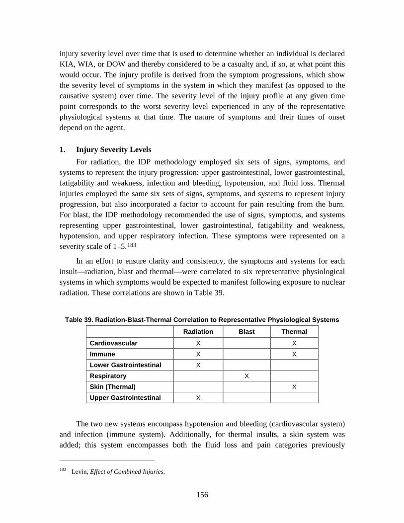
156
injury severity level over time that is used to determine whether an individual is declared KIA, WIA, or DOW and thereby considered to be a casualty and, if so, at what point this would occur. The injury profile is derived from the symptom progressions, which show the severity level of symptoms in the system in which they manifest (as opposed to the causative system) over time. The severity level of the injury profile at any given time point corresponds to the worst severity level experienced in any of the representative physiological systems at that time. The nature of symptoms and their times of onset depend on the agent.
1. Injury Severity Levels For radiation, the IDP methodology employed six sets of signs, symptoms, and
systems to represent the injury progression: upper gastrointestinal, lower gastrointestinal, fatigability and weakness, infection and bleeding, hypotension, and fluid loss. Thermal injuries employed the same six sets of signs, symptoms, and systems to represent injury progression, but also incorporated a factor to account for pain resulting from the burn. For blast, the IDP methodology recommended the use of signs, symptoms, and systems representing upper gastrointestinal, lower gastrointestinal, fatigability and weakness, hypotension, and upper respiratory infection. These symptoms were represented on a severity scale of 1–5.183
In an effort to ensure clarity and consistency, the symptoms and systems for each insult—radiation, blast and thermal—were correlated to six representative physiological systems in which symptoms would be expected to manifest following exposure to nuclear radiation. These correlations are shown in Table 39.
Table 39. Radiation-Blast-Thermal Correlation to Representative Physiological Systems
Radiation Blast Thermal
Cardiovascular X X Immune X X Lower Gastrointestinal X Respiratory X Skin (Thermal) X Upper Gastrointestinal X
The two new systems encompass hypotension and bleeding (cardiovascular system) and infection (immune system). Additionally, for thermal insults, a skin system was added; this system encompasses both the fluid loss and pain categories previously
183 Levin, Effect of Combined Injuries.
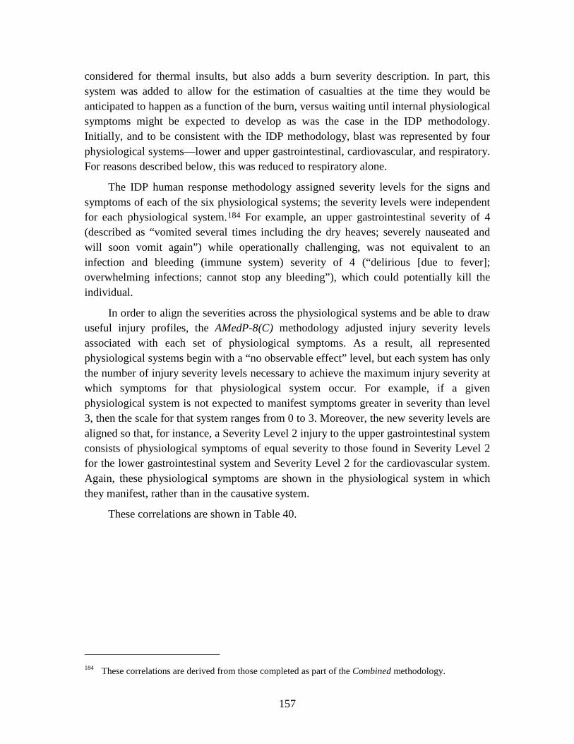
157
considered for thermal insults, but also adds a burn severity description. In part, this system was added to allow for the estimation of casualties at the time they would be anticipated to happen as a function of the burn, versus waiting until internal physiological symptoms might be expected to develop as was the case in the IDP methodology. Initially, and to be consistent with the IDP methodology, blast was represented by four physiological systems—lower and upper gastrointestinal, cardiovascular, and respiratory. For reasons described below, this was reduced to respiratory alone.
The IDP human response methodology assigned severity levels for the signs and symptoms of each of the six physiological systems; the severity levels were independent for each physiological system.184
In order to align the severities across the physiological systems and be able to draw useful injury profiles, the AMedP-8(C) methodology adjusted injury severity levels associated with each set of physiological symptoms. As a result, all represented physiological systems begin with a “no observable effect” level, but each system has only the number of injury severity levels necessary to achieve the maximum injury severity at which symptoms for that physiological system occur. For example, if a given physiological system is not expected to manifest symptoms greater in severity than level 3, then the scale for that system ranges from 0 to 3. Moreover, the new severity levels are aligned so that, for instance, a Severity Level 2 injury to the upper gastrointestinal system consists of physiological symptoms of equal severity to those found in Severity Level 2 for the lower gastrointestinal system and Severity Level 2 for the cardiovascular system. Again, these physiological symptoms are shown in the physiological system in which they manifest, rather than in the causative system.
For example, an upper gastrointestinal severity of 4 (described as “vomited several times including the dry heaves; severely nauseated and will soon vomit again”) while operationally challenging, was not equivalent to an infection and bleeding (immune system) severity of 4 (“delirious [due to fever]; overwhelming infections; cannot stop any bleeding”), which could potentially kill the individual.
These correlations are shown in Table 40.
184 These correlations are derived from those completed as part of the Combined methodology.

158
Table 40. Symptom Severity Levels
Severity Upper Gastrointestinal Lower Gastrointestinal
0 No observable effect No observable effect
1
Upset stomach and nausea: watering mouth and frequent swallowing to avoid vomiting
Abdominal pain or cramps; occasional diarrhea and uncomfortable urge to defecate
2
Episodes of vomiting, possibly including dry heaves; severe nausea and possibility of continued vomiting
Frequent diarrhea and cramps; continuing defecation
3 Protracted or continued vomiting, including dry heaves
Uncontrollable diarrhea and urination; painful cramps
4
Table 40. continued
Severity Cardiovascular Immune*
0 No observable effect No observable effect 1 Slightly feeling of light headedness Slight fever and headache**
2 Unsteadiness upon standing quickly; possible micro-hemorrhaging
Aching joints; fever; lack of appetite; sores in mouth/throat
3 Severe dizziness; faints upon standing quickly; may have difficulty stopping any bleeding
High fever results in shakes, chills and aches all over
4
Shock; rapid and shallow breathing; skin cold, clammy and very pale; difficulty or inability to stop any bleeding; crushing chest pain
Delirium from fever; overwhelming infections
* Immune symptoms are neglected in the Thermal ≥ 30%BSA Insult Range ** Level 1 Immune symptoms only apply to whole-body radiation

159
Table 40. continued
Severity Respiratory Skin (Thermal)
0 No observable effect No observable Effect
1
Mild shortness of breath Epidermal (1st degree) burns over small body surface area characterized by skin redness, swelling, and blistering; persistent pain at burn site
2
Frank shortness of breath, respiratory congestion, non-productive cough
Partial thickness (2nd degree) burns over large body surface area combined with some full thickness (3rd degree) burns; pain at sites of partial thickness burns; potential for fluid loss through burn sites
3
Air hunger; labored breathing; breathing sporadically stops and starts; hemoptysis
Partial (2nd degree) and full thickness (3rd degree) burns over up to 30% of the body surface area; limited pain due to nerve damage from 3rd degree burns; significant fluid loss through burn sites
4 Breathing stops completely or struggling to breathe; cyanosis; prostration
≥ 30 %BSA with partial (2nd degree) and full thickness (3rd degree) burns
2. Radiation, Blast, and Thermal Individual Insult Injury Profiles Each of the dose/insult ranges previously described corresponds to a progression of
injury through time. These progressions are discontinuous with respect to dose; all insults within the specified range are represented by the same injury progression. The boundaries defining each dose/insult range represent points in an exposure at which the expected progression of injury abruptly changes as the dose is increased. Moreover, the injury progressions themselves are discontinuous and stepwise with respect to severity level; they are not smoothed or otherwise interpolated. In other words, moving along the time dimension of the injury progression, the injury severity and the corresponding physiological symptoms change instantaneously at specific points in time. For a given dose or insult range, separate injury progressions have been developed for each of the physiological systems—upper gastrointestinal, lower gastrointestinal, cardiovascular, immune, respiratory, and skin (thermal)—illustrating the severity of the physiological symptoms for a particular physiological system over time.
As mentioned earlier, blast was originally represented by four physiological systems (upper and lower gastrointestinal, cardiovascular, and respiratory). However, following discussions with SMEs, it was decided to represent blast by the respiratory system alone

160
because the limited data that were available indicated that damage to the respiratory system was always more severe and rapid over any given set of blast ranges, as illustrated by Figures 63 through 66.
Figure 63. Blast Physiological Symptom Progressions for 50 – < 140 kPa
Figure 64. Blast Physiological Symptom Progressions for 140 – < 240 kPa
0
1
2
3
4
0.1 1 10 100 1000
Seve
rity
Time Post-Exposure (Hours)
Upper GI
0
1
2
3
4
0.1 1 10 100 1000
Seve
rity
Time Post-Exposure (Hours)
Lower GI
0
1
2
3
4
0.1 1 10 100 1000
Seve
rity
Time Post-Exposure (Hours)
Cardiovascular
0
1
2
3
4
0.1 1 10 100 1000
Seve
rity
Time Post-Exposure (Hours)
Respiratory
0
1
2
3
4
0.1 1 10 100 1000
Seve
rity
Time Post-Exposure (Hours)
Upper GI
0
1
2
3
4
0.1 1 10 100 1000
Seve
rity
Time Post-Exposure (Hours)
Lower GI
0
1
2
3
4
0.1 1 10 100 1000
Seve
rity
Time Post-Exposure (Hours)
Cardiovascular
0
1
2
3
4
0.1 1 10 100 1000
Seve
rity
Time Post-Exposure (Hours)
Respiratory

161
Figure 65. Blast Physiological Symptom Progressions for 240 – < 290 kPa
Figure 66. Blast Physiological Symptom Progressions for > 290 kPa
Chapter 6 presents the injury progressions by dose range for whole-body radiation. Figures 67 through 74 present the final injury progressions by insult range for blast and
0
1
2
3
4
0.1 1 10 100 1000
Seve
rity
Time Post-Exposure (Hours)
Upper GI
0
1
2
3
4
0.1 1 10 100 1000
Seve
rity
Time Post-Exposure (Hours)
Lower GI
0
1
2
3
4
0.1 1 10 100 1000
Seve
rity
Time Post-Exposure (Hours)
Cardiovascular
0
1
2
3
4
0.1 1 10 100 1000
Seve
rity
Time Post-Exposure (Hours)
Respiratory
0
1
2
3
4
0.1 1 10 100 1000
Seve
rity
Time Post-Exposure (Hours)
Upper GI
0
1
2
3
4
0.1 1 10 100 1000
Seve
rity
Time Post-Exposure (Hours)
Lower GI
0
1
2
3
4
0.1 1 10 100 1000
Seve
rity
Time Post-Exposure (Hours)
Cardiovascular
0
1
2
3
4
0.1 1 10 100 1000
Seve
rity
Time Post-Exposure (Hours)
Respiratory

162
thermal insults.185
The “no observable effect” progressions are not shown; all severity levels would be 0 for the duration of time observed.
Figure 67. Blast Physiological Symptom Progression for 50 – < 140 kPa
Figure 68. Blast Physiological Symptom Progression for 140 – < 240 kPa
Figure 69. Blast Physiological Symptom Progression for 240 – < 290 kPa
185 All of the injury progression and injury profiles are plotted using hours along the logarithmic x-axis.
These are derived from those originally incorporated in the IDP and included in Levin, Effect of Combined Injuries.
0
1
2
3
4
0.1 1 10 100 1000
Seve
rity
Time Post-Exposure (Hours)
Respiratory
0
1
2
3
4
0.1 1 10 100 1000
Seve
rity
Time Post-Exposure (Hours)
Respiratory
0
1
2
3
4
0.1 1 10 100 1000
Seve
rity
Time Post-Exposure (Hours)
Respiratory

163
Figure 70. Blast Physiological Symptom Progression for > 290 kPa
Figure 71. Thermal Physiological Symptom Progressions for 1 – < 10 %BSA
0
1
2
3
4
0.1 1 10 100 1000Se
veri
ty
Time Post-Exposure (Hours)
Respiratory
0
1
2
3
4
0.1 1 10 100 1000
Seve
rity
Time Post-Exposure (Hours)
Immune
0
1
2
3
4
0.1 1 10 100 1000
Seve
rity
Time Post-Exposure (Hours)
Cardiovascular
0
1
2
3
4
0.1 1 10 100 1000
Seve
rity
Time Post-Exposure (Hours)
Skin

164
Figure 72. Thermal Physiological Symptom Progressions for 10 – < 20 %BSA
0
1
2
3
4
0.1 1 10 100 1000
Seve
rity
Time Post-Exposure (Hours)
Immune
0
1
2
3
4
0.1 1 10 100 1000
Seve
rity
Time Post-Exposure (Hours)
Cardiovascular
0
1
2
3
4
0.1 1 10 100 1000
Seve
rity
Time Post-Exposure (Hours)
Skin
165
Figure 73. Thermal Physiological Symptom Progressions for 20 – < 30 %BSA
0
1
2
3
4
0.1 1 10 100 1000
Seve
rity
Time Post-Exposure (Hours)
Immune
0
1
2
3
4
0.1 1 10 100 1000
Seve
rity
Time Post-Exposure (Hours)
Cardiovascular
0
1
2
3
4
0.1 1 10 100 1000
Seve
rity
Time Post-Exposure (Hours)
Skin
166
Figure 74. Thermal Physiological Symptom Progressions for ≥ 30 %BSA
The symptoms progressions provide the foundation for the injury profile, which illustrates the effect of the injury on the body overall by tracking the highest severity level across the sets of physiological systems at any moment in time. Repeating the example used in Chapter 6 for whole-body radiation, the physiological symptoms progressions for an individual exposed to whole-body radiation in the range of 5.3 Gy to 8.3 Gy (from Figure 48) are shown in Figure 75.
0
1
2
3
4
0.1 1 10 100 1000
Seve
rity
Time Post-Exposure (Hours)
Cardiovascular
0
1
2
3
4
0.1 1 10 100 1000
Seve
rity
Time Post-Exposure (Hours)
Skin

167
Figure 75. Whole-Body Radiation Symptom Progressions for 5.3 – < 8.3 Gy*
* As indicated by the “∫∫,” for doses > 5 Gy, time to death is calculated; the injury progression is followed as prescribed until time of death.
These physiological symptoms can be summarized into an overall injury profile as shown in Figure 76. The injury profile tracks along with the maximum exhibited physiological symptoms at each point in time. As can be seen in Figure 75, upper gastrointestinal system symptoms dominate at the earliest time periods; consequently, the injury profile in Figure 76 follows the same injury severity progression—from “mild” (Severity Level 1) to “moderate” (Severity Level 2) to “severe” (Severity Level 3) then eventually back to “no observable effect” (Severity Level 0) at 70 hours. In the later time periods, the cardiovascular and then the immune system symptoms dominate. As with the upper gastrointestinal symptoms severities in the early time periods, the injury profile severity follows the cardiovascular system injury severities between 100 and 400 hours post-exposure; the injury profile then follows the immune system injury severities in later time periods. As immune system symptoms remains “very severe” until the end of the observed time period—6 weeks—the injury profile also indicates a “very severe” injury severity until the end of the observed time period.
0
1
2
3
4
0.1 1 10 100 1000
Seve
rity
Time Post-Exposure (Hours)
Upper GILower GICardiovascularImmune
∫∫
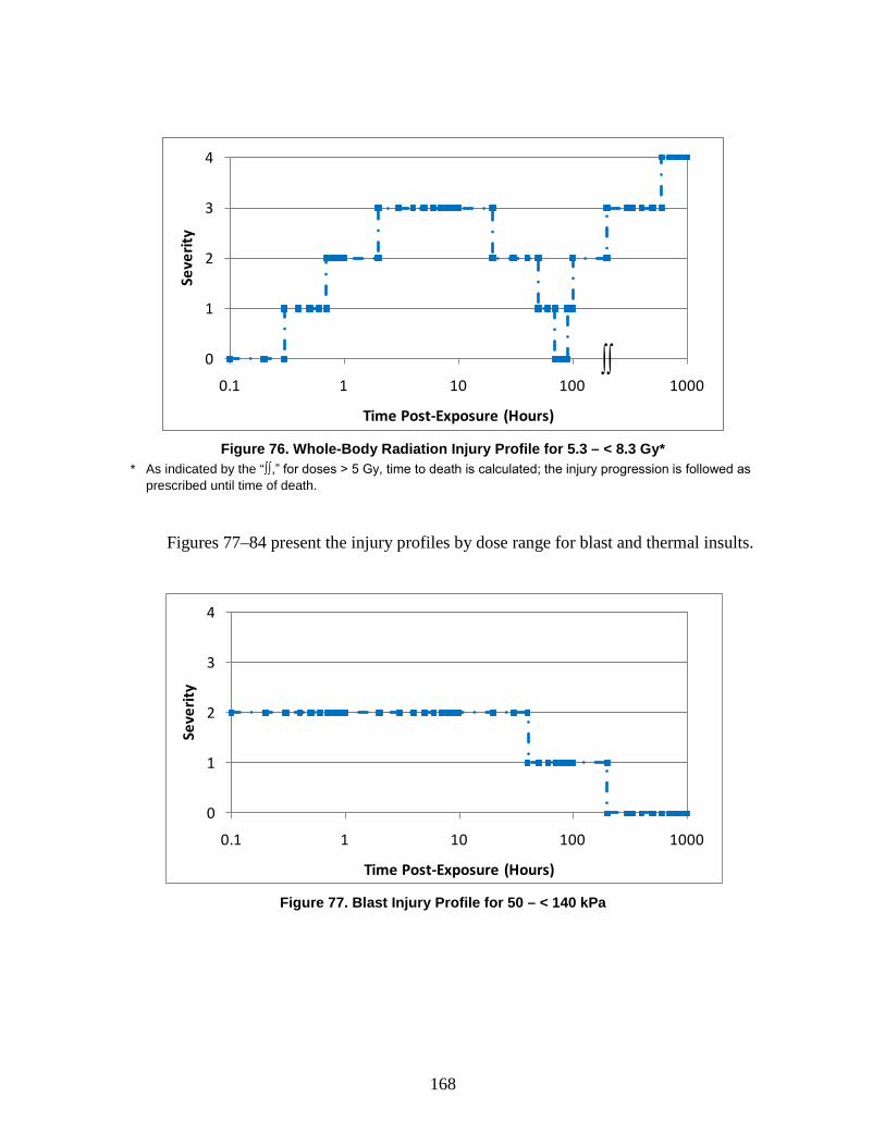
168
Figure 76. Whole-Body Radiation Injury Profile for 5.3 – < 8.3 Gy*
* As indicated by the “∫∫,” for doses > 5 Gy, time to death is calculated; the injury progression is followed as prescribed until time of death.
Figures 77–84 present the injury profiles by dose range for blast and thermal insults.
Figure 77. Blast Injury Profile for 50 – < 140 kPa
0
1
2
3
4
0.1 1 10 100 1000
Seve
rity
Time Post-Exposure (Hours)
∫∫
0
1
2
3
4
0.1 1 10 100 1000
Seve
rity
Time Post-Exposure (Hours)
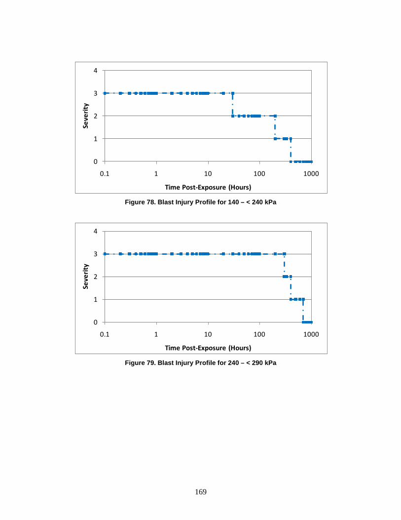
169
Figure 78. Blast Injury Profile for 140 – < 240 kPa
Figure 79. Blast Injury Profile for 240 – < 290 kPa
0
1
2
3
4
0.1 1 10 100 1000
Seve
rity
Time Post-Exposure (Hours)
0
1
2
3
4
0.1 1 10 100 1000
Seve
rity
Time Post-Exposure (Hours)
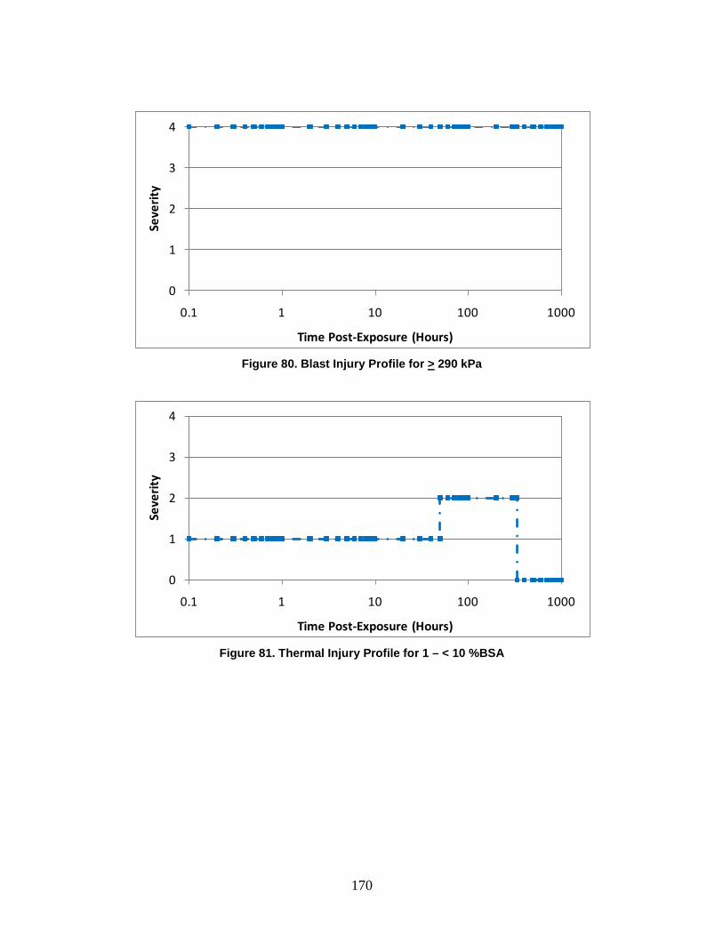
170
Figure 80. Blast Injury Profile for > 290 kPa
Figure 81. Thermal Injury Profile for 1 – < 10 %BSA
0
1
2
3
4
0.1 1 10 100 1000
Seve
rity
Time Post-Exposure (Hours)
0
1
2
3
4
0.1 1 10 100 1000
Seve
rity
Time Post-Exposure (Hours)
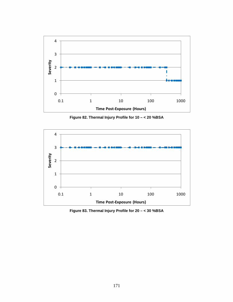
171
Figure 82. Thermal Injury Profile for 10 – < 20 %BSA
Figure 83. Thermal Injury Profile for 20 – < 30 %BSA
0
1
2
3
4
0.1 1 10 100 1000
Seve
rity
Time Post-Exposure (Hours)
0
1
2
3
4
0.1 1 10 100 1000
Seve
rity
Time Post-Exposure (Hours)
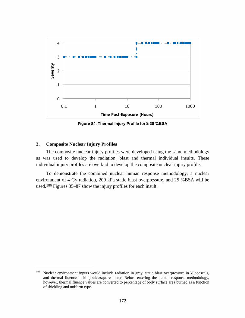
172
Figure 84. Thermal Injury Profile for ≥ 30 %BSA
3. Composite Nuclear Injury Profiles The composite nuclear injury profiles were developed using the same methodology
as was used to develop the radiation, blast and thermal individual insults. These individual injury profiles are overlaid to develop the composite nuclear injury profile.
To demonstrate the combined nuclear human response methodology, a nuclear environment of 4 Gy radiation, 200 kPa static blast overpressure, and 25 %BSA will be used.186
Figures 85–87 show the injury profiles for each insult.
186 Nuclear environment inputs would include radiation in gray, static blast overpressure in kilopascals,
and thermal fluence in kilojoules/square meter. Before entering the human response methodology, however, thermal fluence values are converted to percentage of body surface area burned as a function of shielding and uniform type.
0
1
2
3
4
0.1 1 10 100 1000
Seve
rity
Time Post-Exposure (Hours)
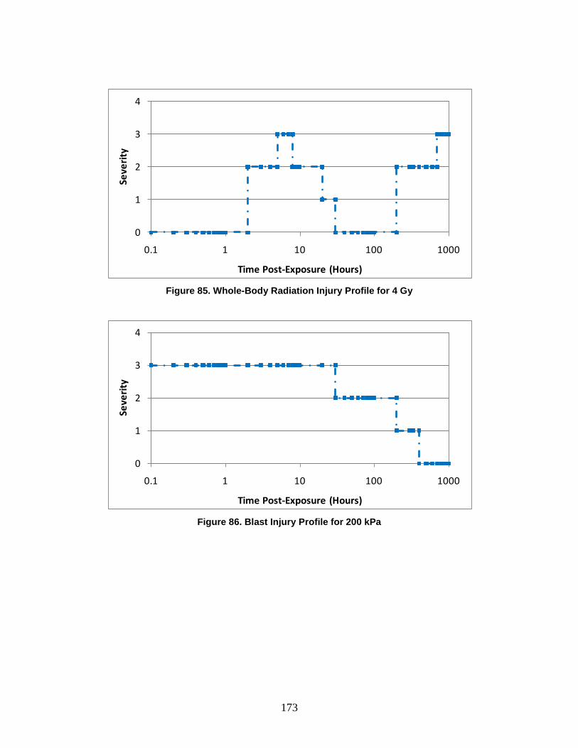
173
Figure 85. Whole-Body Radiation Injury Profile for 4 Gy
Figure 86. Blast Injury Profile for 200 kPa
0
1
2
3
4
0.1 1 10 100 1000
Seve
rity
Time Post-Exposure (Hours)
0
1
2
3
4
0.1 1 10 100 1000
Seve
rity
Time Post-Exposure (Hours)

174
Figure 87. Thermal Injury Profile for 25 %BSA
The injury profiles are drawn together on a single plot. This is shown in Figure 88.
Figure 88. Composite Nuclear Injury Profiles for 4 Gy, 200 kPa, and 25 %BSA
Drawing the maximum values of the overlaid radiation, blast, and thermal injury profiles shown in Figure 88, the composite nuclear injury profile can be obtained. This set of maximum values becomes the overall composite nuclear injury profile for 4 Gy, 200 kPa, and 25 %BSA, shown in Figure 89.
0
1
2
3
4
0.1 1 10 100 1000
Seve
rity
Time Post-Exposure (Hours)
0
1
2
3
4
0.1 1 10 100 1000
Seve
rity
Time Post-Exposure (Hours)
Radiation
Blast
Thermal

175
Figure 89. Composite Nuclear Injury Profile for 4 Gy, 200 kPa, and 25 %BSA
0
1
2
3
4
0.1 1 10 100 1000
Seve
rity
Time Post-Exposure (Hours)


177
8. Biological Agent Human Response Review: Non-Contagious and Contagious Diseases
A. Introduction The objective of this chapter is to describe the human response methodology for
biological agent-induced non-contagious diseases (anthrax, botulism, and Venezuelan equine encephalitis (VEE)) and contagious diseases (plague and smallpox) that have been incorporated into the AMedP-8(C) methodology.
B. Background Although a single term is used to categorize agents made of living organisms or
their toxic products, biological agents vary in many respects, including their infectivity or toxicity, mechanisms of action, and resulting symptoms and signs. AMedP-8(C) considers biological agents derived from two bacterial agents, two viral agents, and one toxin. Both non-contagious (anthrax, botulinum neurotoxin, and VEE) and contagious (plague and smallpox) agents are modeled.
Naturally occurring diseases resulting from these agents can occur via multiple routes of entry into the body, most commonly respiratory, ocular, oral, and cutaneous. Further, depending on the route of entry, naturally occurring diseases take multiple possible forms; each form has its own course of illness and associated signs and symptoms. For the purposes of AMedP-8(C), all biological agents were assumed to be weaponized and inhaled. Where available, information on the inhalation form of the disease was utilized to develop the human response methodology; when such information was not available, alternate disease forms were used as noted below.
For some agents, prophylaxis is considered, to include pre-exposure vaccination or antibiotic prophylaxis and post-exposure antibiotic prophylaxis. Injury profiles and descriptions do not consider the impact of medical treatment that occurs after symptom onset.
C. Methodology Development The biological agent human response for both non-contagious and contagious
biological agents is a sequential process. Prior to exposure, the population is susceptible to infection or intoxication. Following exposure, some fraction of the population has

178
received a sufficient dose so as to be expected to develop symptoms of the disease following some incubation or latent period. Each day a subset of this population develops symptoms and therefore is considered ill. For this population, the illness then runs its course and will end in either death or recovery, in proportions that are agent-dependent.
As for CRN agents or effects, the human response component for biological agents starts with an estimation of dose to an icon (or individual). Additionally, in both cases, personnel status is determined based on the time of first onset of a specified threshold injury severity level. The CRN and biological human response estimation processes, however, differ in that the former approach outputs icon-based estimates of injury severity over time while the estimates from the latter are population-based. In addition, the intermediate steps involved in deriving these population estimates for biological agents differ from those described above for CRN agents and effects. Further, the approach used to estimate human response for contagious biological agents varies from that used for non-contagious agents in order to consider the transmission of disease from person to person.
Both non-contagious and contagious biological agents human response approaches are derived from an underlying set of submodels characterizing various aspects of disease and describing disease progression—infectivity, incubation/latent period, lethality, injury profile, and duration of illness—as shown in Figure 90. Agents for which medical prophylaxis is available also include a prophylaxis efficacy submodel. As with CRN agents and effects, an infectivity submodel estimates the number of individuals who will become ill given their agent dose. Also similar to other agents within the AMedP-8(C) methodology, the injury profile submodels for biological agents describe clinically differentiable stages of disease and the severity of the associated symptoms and—for biological agents—signs over time. Two additional time-based submodels—incubation/latent period and duration of illness—estimate the duration of time before the initial onset of signs and symptoms and the length of time between the onset of symptoms and death or recovery. For modeling purposes, the duration of illness—and the duration of each stage of illness—is assumed to be independent of the incubation period. A lethality submodel estimates the number of ill individuals who are expected to die. Most submodels for the biological diseases are represented stochastically by a probability distribution to account for the variation in human response typically seen among individuals; some submodels may be estimated by threshold values.
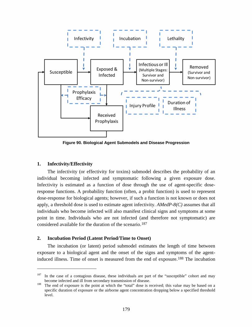
179
Figure 90. Biological Agent Submodels and Disease Progression
1. Infectivity/Effectivity The infectivity (or effectivity for toxins) submodel describes the probability of an
individual becoming infected and symptomatic following a given exposure dose. Infectivity is estimated as a function of dose through the use of agent-specific dose-response functions. A probability function (often, a probit function) is used to represent dose-response for biological agents; however, if such a function is not known or does not apply, a threshold dose is used to estimate agent infectivity. AMedP-8(C) assumes that all individuals who become infected will also manifest clinical signs and symptoms at some point in time. Individuals who are not infected (and therefore not symptomatic) are considered available for the duration of the scenario.187
2. Incubation Period (Latent Period/Time to Onset)
The incubation (or latent) period submodel estimates the length of time between exposure to a biological agent and the onset of the signs and symptoms of the agent-induced illness. Time of onset is measured from the end of exposure.188
187 In the case of a contagious disease, these individuals are part of the “susceptible” cohort and may
become infected and ill from secondary transmission of disease.
The incubation
188 The end of exposure is the point at which the “total” dose is received; this value may be based on a specific duration of exposure or the airborne agent concentration dropping below a specified threshold level.
SusceptibleExposed &Infected
Infectious or Ill(Multiple Stages:
Survivor andNon-survivor)
Removed(Survivor andNon-survivor)
ReceivedProphylaxis
Infectivity Incubation Lethality
Injury ProfileDuration of
Illness
ProphylaxisEfficacy
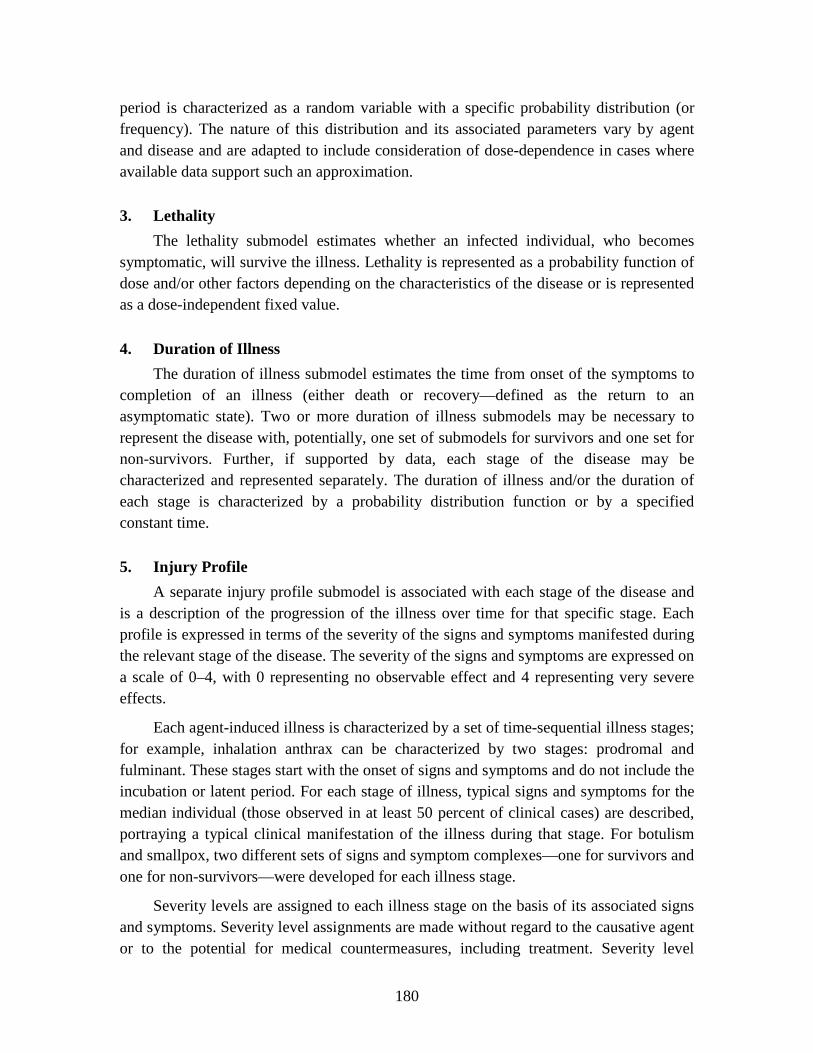
180
period is characterized as a random variable with a specific probability distribution (or frequency). The nature of this distribution and its associated parameters vary by agent and disease and are adapted to include consideration of dose-dependence in cases where available data support such an approximation.
3. Lethality The lethality submodel estimates whether an infected individual, who becomes
symptomatic, will survive the illness. Lethality is represented as a probability function of dose and/or other factors depending on the characteristics of the disease or is represented as a dose-independent fixed value.
4. Duration of Illness The duration of illness submodel estimates the time from onset of the symptoms to
completion of an illness (either death or recovery—defined as the return to an asymptomatic state). Two or more duration of illness submodels may be necessary to represent the disease with, potentially, one set of submodels for survivors and one set for non-survivors. Further, if supported by data, each stage of the disease may be characterized and represented separately. The duration of illness and/or the duration of each stage is characterized by a probability distribution function or by a specified constant time.
5. Injury Profile A separate injury profile submodel is associated with each stage of the disease and
is a description of the progression of the illness over time for that specific stage. Each profile is expressed in terms of the severity of the signs and symptoms manifested during the relevant stage of the disease. The severity of the signs and symptoms are expressed on a scale of 0–4, with 0 representing no observable effect and 4 representing very severe effects.
Each agent-induced illness is characterized by a set of time-sequential illness stages; for example, inhalation anthrax can be characterized by two stages: prodromal and fulminant. These stages start with the onset of signs and symptoms and do not include the incubation or latent period. For each stage of illness, typical signs and symptoms for the median individual (those observed in at least 50 percent of clinical cases) are described, portraying a typical clinical manifestation of the illness during that stage. For botulism and smallpox, two different sets of signs and symptom complexes—one for survivors and one for non-survivors—were developed for each illness stage.
Severity levels are assigned to each illness stage on the basis of its associated signs and symptoms. Severity level assignments are made without regard to the causative agent or to the potential for medical countermeasures, including treatment. Severity level
181
assignments do not consider the specific nature of the disease or the disease-based patient outlook and only refer to the severity of signs and symptoms at the time of observation. Consequently, severity of signs or symptoms is not a measure of the overall severity of disease, since the severity of signs and symptoms at the time they are observed is not necessarily commensurate with the underlying severity of disease.
6. Medical Countermeasures—Vaccination/Antibiotic Prophylaxis The consideration of prophylaxis—a subset of medical countermeasures—in a
human response model may alter the original model parameters discussed above, as well as introduce additional parameters, even in the absence of treatment.
For a given agent and medical countermeasure, three periods of prophylaxis administration are possible in the AMedP-8(C) methodology: before exposure, after exposure has occurred (but prior to developing symptoms), and both before and after exposure. Additional submodels were developed to account for prophylaxis in the human response models for anthrax, plague, and smallpox. The specific submodels and parameters depend on the agent of consideration, the type of prophylaxis (e.g., immunoprophylaxis, chemoprophylaxis), and time of administration (e.g., pre-exposure, post-exposure, or both). Prophylaxis efficacy may affect the numbers of susceptible individuals, the infectivity/effectivity of the agent, and the probability of survival.
7. Literature Review and Parameter Development In order to develop the model parameters for both contagious and non-contagious
biological agents, an extensive literature review was conducted. As much as possible, references were traced back to original sources and experimental or case study reports.189
189 Data in its rawest possible form was used when available in the scientifically published, academically
peer-reviewed literature. Data was not traced back beyond published sources (i.e., to laboratory notebooks).
Preference was given to scientifically published, academically peer-reviewed journal articles. When available, human data were preferred to animal data. In some cases, raw data were compiled from multiple sources to derive a specific parameter; for example, VEE incubation data were collected from two accidental exposures. When raw data were not available, published models (e.g., applicable cumulative distribution functions with associated parameters), derived by the authors of the study for which underlying data were not available, were selected. If neither raw data nor an accepted, published model were available, a general statement by the author of parameters was used. If no other information was available, a general data statement (i.e., a median lethal dose value without sources or underlying data) was chosen—whenever possible, this number was vetted with subject matter experts. The preference for data sources is shown in Figure 91.

182
Figure 91. Biological Literature Review Data Preference
When raw data were available, distributions were estimated using BestFit® software (part of Decision Tools 4.5 Professional Suite from Palisades Corp.). In addition, Microsoft Office Excel 2007 was used to collate data and conduct some analyses and graphing. The data used to determine these distributions are captured in the appropriate sections below.
The convolution process for non-contagious biological agents was conducted in MS Excel 2007 and validated through Monte Carlo simulations conducted in Wolfram Mathematica, version 6.0. The non-contagious and contagious biological examples were implemented in MS Excel 2007; the beta parameters were derived using Wolfram Mathematica, version 6.0.
8. Non-Contagious and Contagious Biological Agent Human Response
The combination of the submodels described above allows for a complete characterization of the human response to biological agents, but the application of that to the AMedP-8(C) methodology is challenging because of the complexity associated with integrating the multiple and varied submodels. Thus, two approaches are recommended: the convolution approach for non-contagious biological agents and the Susceptible-Exposed and infected-Infectious-Removed-Prophylaxis efficacious (SEIRP) approach for contagious biological agents.
Raw Human Data
Raw AnimalData
Derived DataModels
AuthorInterpretation
Of DataGeneral
Data Statement

183
D. Estimation of Non-Contagious Biological Agent Human Response The process shown in Figure 92 represents calculations which estimate the
population’s human response following exposure to a non-contagious biological agent. The infectivity submodel is used to calculate the number of individuals who are infected and expected to become ill. The lethality submodel is then used to calculate the number of people who are expected to die (non-survivors) and the number of people who are expected to survive (survivors).
Figure 92. Non-Contagious Biological Human Response Process
For some non-contagious biological agents, dose may be one factor determining the time to symptom onset. Thus, for those agents, individuals are binned by dose range to ease calculation. Rather than trying to track individuals, dose ranges and number of individuals within a dose range are input into the remainder of the human response calculation.
The incubation (or latent) period submodel is applied to the exposed and infected population to estimate the time of illness onset. The duration of illness submodel is applied to each stage of illness, as appropriate, to estimate the time after the onset of illness at which signs and symptoms of specified severity would be manifested. The injury profile descriptions dictate the severity level of each stage of disease. To account for the variation in the incubation/latent period and course of illness for non-contagious biological agents, these time periods are represented stochastically by probability distributions. Stochastic estimations, however, may be a time and computationally intensive process. In order to make the non-contagious human response methodology more accessible, the distributions are binned by day and presented in tabular form.
Infectivity and Lethality
Calculation
Casualties and Fatalities by Time Period Estimation
Dose Range Determination

184
The process used in AMedP-8(C) for combining various submodels within the non-contagious methodology is described in the next section. The parameters for use in the non-contagious biological agent submodels are described in the sections that follow.
A number of SMEs were consulted to determine the severity of symptoms which could be associated with each disease. Typically, SMEs were provided with a range of symptoms which could potentially manifest in a physiological system and asked to verify the expected severity level. Each physiological system was evaluated independently; although it is understood that a combination of signs and symptoms could produce a higher injury severity than each symptom experienced individually, due to the lack of available data, no synergism of symptoms was considered. Additionally, signs and symptom complexes (anticipated for the diseases under consideration but not correlated to them specifically) were provided to SMEs for their evaluation of the anticipated injury severity for each stage. These two approaches were compared with data from available literature to determine the final stage injury severity assignments.
1. Convolution Approach There are several methods available to combine the stochastic submodels to derive
mathematical representations of the time-course of illness. One process utilizes a Monte Carlo simulation190 which employs a number of random draws—taken from each distribution sequentially then summed—until the confidence interval (error bars) of the estimate converge to a sufficiently small number. Alternatively, this can be approximated through the use of a convolution algorithm wherein each distribution is represented by fractional values at discrete time steps to approximate the continuous function.191
For a given distribution (e.g., incubation period, duration of illness), the cumulative distribution function (CDF), denoted F(t), was evaluated to estimate the cumulative
These discrete distributions are then combined using matrix multiplication. Thus the time to the end of an illness stage is represented by numerically convolving (or performing matrix multiplication on) the fraction of population first manifesting symptoms by day (the incubation period submodel) with the fraction of population progressing from Stage 1 to Stage 2 of illness (the Stage 1 duration of illness submodel). Likewise, the time to death may be represented by convolving the incubation period submodel with all stages of the duration of illness submodel. This process, as implemented in AMedP-8(C), is described in detail below.
190 In general, the Monte Carlo method defines a domain of possible inputs, generates inputs randomly
from the domain using a certain specified probability distribution, performs a deterministic computation using the inputs, and aggregates the results of the individual computations into a final result.
191 E. Oran Brigham, The Fast Fourier Transform and Its Applications (Englewood Cliffs, NJ: Prentice Hall, 1988), 118.
185
percentage of individuals completing the corresponding stage of disease by time t. The percentage of individuals completing that disease stage in the span of time ∆t preceding t was then calculated using Equation 7.
F(t) − F(t − ∆t) (7)
More specifically, the percentage of individuals completing the incubation period in the ith time span of duration ∆t after becoming infected, denoted Inc(i), was estimated from the incubation period CDF, FInc, by evaluating Equation 8.
Inc(i) = FInc(i∆t)− FInc(i∆t − ∆t) (8)
Similarly, as shown in Equation 9, the percentage of individuals completing the first stage of illness in the jth time span of duration ∆t after completing the incubation period, denoted Stg1(j), was determined from the CDF of the duration of illness model for this stage, FStg1.
Stg1(j) = FStg1(j∆t)− FStg1(j∆t − ∆t) (9)
Given these two equations, it was possible to determine, at any given time, the percentage of individuals having completed both the incubation period and the first stage of illness. Consider the case where ∆t = 1 day and the percentage of individuals having completing both stages by day 3 (FIncStg1(3)) is sought. This is computed by summing the percentage finishing the incubation period in 1 day (Inc(1)) and the first stage of illness in 1 day (Stg1(1)), the percentage finishing the incubation period in 1 day (Inc(1)) and the first stage of illness in 2 days (Stg1(2)), and the percentage finishing the incubation period in 2 days (Inc(2)) and the first stage of illness in 1 day (Stg1(1)). Mathematically, this can be expressed as shown in Equation 10.
FIncStg1(3) = �Inc(1) × Stg1(1)� + �Inc(1) × Stg1(2)� + �Inc(2) × Stg1(1)� (10)
One shortcoming of using this technique when ∆t is limited to whole days is that no other combination of disease stage durations can result in individuals progressing through the first stage of disease in 3 days. Consequently, FIncStg1 is better approximated when ∆t is reduced, allowing individuals to spend fractions of a day in a given stage. Although ∆t may be as small as desired, in order to report results by day, it must divide evenly into 1 day; for the convolutions used in AMedP-8(C), ∆t = 0.01 days.
When described more generally, Equation 10 represents a numerical approximation of the CDF of the convolved distributions. This more general description, shown as Equation 11, was used to determine the percentage of individuals having progressed through both the incubation period and the first stage of illness by the end of the nth time span of duration ∆t after becoming infected.
FIncStg1(n) = ∑ �∑ Inc(y) ×x−1y=1 Stg1(x − y)�n
x=2 (11)

186
For reporting purposes, only the daily percentages of individuals finishing a given stage were needed. Thus, to determine the percentage of individuals finishing the first stage of illness on day D (after having already progressed through the incubation period), Equation 11 was evaluated at the two values of n corresponding to D and D − 1 and the difference between the two evaluations was taken, as shown in Equation 12, where x is defined as the number of time periods in 1 day (x∆t = 1).
GIncStg1(D) = FIncStg1(Dx) − FIncStg1�(D− 1)x� (12)
To similarly convolve the distributions of any subsequent stages of illness, the distributions were expressed as the difference between evaluations of the CDF at times separated by any arbitrary time span Δt. This is shown in Equation 13 for the convolved distribution approximated by Equation 11, where the percentage of individuals completing both the incubation period and the first stage of illness in the nth time span of duration ∆t after becoming infected is denoted IncStg1(n).
IncStg1(n) = FIncStg1(n) − FIncStg1(n − 1) (13)
Likewise, Equation 14 calculates Stg2(k), the percentage of individuals completing the second stage of illness in the kth time span of duration ∆t after completing the incubation period and stage 1 of illness, where FStg2 is defined as the CDF of the duration of illness model for this stage.
Stg2(k) = FStg2(k∆t) − FStg2(k∆t − ∆t) (14)
In this manner, discrete approximations of the distributions for each of the time-based submodels—incubation period and the duration of each stage of illness—were developed to define the fractions of the population experiencing various milestones in the course of illness on each day, as summarized in Table 41 for a disease of n stages.

187
Table 41. Convolutions Required to Estimate the Probability Density Functions (PDFs) for
Time to Each Illness Stage
To generate the PDF of the distribution characterizing the time
to enter each stage of illness: Convolve:
Stage 1 Incubation/Latent Period Submodel (no convolution required)
Stage 2 Incubation/Latent Period Submodel * Duration of Illness Stage 1 Submodel
Stage n
Incubation/Latent Period Submodel * Duration of Illness Stage 1 Submodel * … * Duration of Illness Stage n-1 Submodel
Death
Incubation/Latent Period Submodel * Duration of Illness Stage 1 Submodel * … * Duration of Illness Stage n Submodel
In particular, the following equations were used to determine the fractions of individuals entering each stage of illness:
Stage 1 of Illness: The incubation/latent period submodel dictates the duration of time for which the disease is incubating/latent, which is therefore the time it takes for symptoms to onset and some fraction of the population to enter stage 1. Equation 8 was evaluated with a time span of ∆t = 1 day for each day i to yield the fraction of individuals entering the first stage of illness.
Stage 2 of Illness: The incubation/latent period was convolved with the duration of illness stage 1 to determine the time it takes for symptoms to manifest and for some fraction of the population to progress through stage 1 of illness and begin to manifest symptoms in stage 2. Equation 12 was used to calculate the fraction of individuals entering the second stage of illness for each day D.
Stage 3 of Illness: Similarly, the incubation/latent period-duration of illness stage 1 results were convolved with the duration of illness stage 2 to determine the time at which symptoms for illness stage 3 manifest (for the three stage diseases—botulism and VEE). Equation 12 was modified as shown in Equation 15 to determine the fraction of individuals on day D entering the third stage of illness. The referenced function, a modified version of Equation 11, is defined in Equation 16.
GIncStg1Stg2(D) = FIncStg1Stg2(Dx) − FIncStg1Stg2�(D− 1)x� (15)
FIncStg1Stg2(n) = ∑ �∑ IncStg1(y) × Stg2(x − y)x−1y=1 �n
x=2 (16)

188
Time to Death/Recovery: For anthrax, which was modeled as a two stage disease, Equation 15 was used to determine the daily fractions of individuals dying or recovering. For botulism and VEE, the incubation/latent period-duration of illness stage 1-duration of illness stage 2 results were convolved with the duration of illness stage 3 to determine the time to death or time to recovery. Again, modified version of Equations 11 and 12 were used to determine the fraction of individuals finishing the last stage of illness, as shown in Equations 17 and 18.
GIncStg1Stg2Stg3(D) = FIncStg1Stg2Stg3(Dx) − FIncStg1Stg2Stg3�(D − 1)x� (17)
FIncStg1Stg2Stg3(n) = ∑ �∑ IncStg1Stg2(y) × Stg3(x − y)x−1y=1 �n
x=2 (18)
Monte Carlo simulations were used to validate the accuracy of these time-dependent population fraction effects. Wolfram Mathematica, version 6.0, software was employed to perform the Monte Carlo runs. Each time-based submodel distribution was defined in Mathematica. One thousand random draws were then performed; the results were distributed across the duration of illness. For symptom onset, the draws were a single step process using the incubation/latent period distribution; for other stages of illness, the draws were a multi-step process involving the summation of random draws from each of the applicable submodel distributions. The results were binned into day-long time periods and summed for the time period to provide the fraction of the population experiencing the particular effect on each day. This process was then repeated 1,000 times (1,000 draws, 1,000 times), resulting in 1,000 fractions for each effect on each day. Mathematica was also used to determine the mean value, 95% upper and lower confidence limits.
The final step of the validation was to do a pair-wise comparison of the discrete convolution-derived results and the Monte Carlo results for each day to determine if the values could be assumed to be drawn from the same distribution. Since 98% of the discrete approximations fell within the upper and lower bounds of the 95% confidence interval derived using Mathematica, this assumption appears to hold true. The discrete representations of the submodels and the convolved results are therefore included in AMedP-8(C).
2. Anthrax Anthrax is caused by Bacillus anthracis, a rod-shaped, gram-positive sporulating
organism, the spores of which constitute the usual infective form. Anthrax is a zoonotic disease, primarily infecting cattle, sheep, and horses, though other animals may be infected as well. Humans may contract the disease—typically in its cutaneous or gastrointestinal forms—by handling contaminated hair, wool, hides, flesh, blood, or excreta of infected animals and from manufactured products such as bone meal. The risk of person-to-person transmission is very low. The inhalation form of anthrax can be caused by the purposeful dissemination of aerosols containing spores. A summary of the

189
parameters characterizing each anthrax submodel in AMedP-8(C) is shown in Table 42 below, followed by more in-depth discussions of each submodel.
Table 42. Anthrax Model Parameters Summary Table
Submodel Type Parameters Infectivity Exponential distribution λ = 1.36x10⁻⁵
Incubation Period
Parametric lognormal distribution
M = α + βlog(dn) α = 10.3 β = –1.35
σ = γ + δlog(dn) γ = 0.804 δ = –0.079 dn = dose
Lethality, if Symptomatic
Rate 100%
Duration of Illness
Stage 1
Stage 2
Lognormal distribution
Lognormal distribution
Mean = 4.2 days Standard deviation = 2.3 days
Mean = 0.70 days
Standard deviation = 0.74 days
Prophylaxis Efficacy Rate 0.90
a. Infectivity Since untreated anthrax is lethal in nearly all cases, the endpoint of most studies was
lethality, which was accepted as a surrogate for infectivity. Despite reviewing numerous articles on anthrax lethality, the authors found that very little experimental data were published and that many of the studies referenced values that were eventually traced back to one of a limited number of studies. Unfortunately, much of the data on which most of these studies were based were not published or available for review.
A summary matrix of the available lethality estimates from this review is shown in Table 43. Original sources are listed in the first row and each source’s published study results are provided in the cell below. The authors of subsequent publications that cite the original sources are listed in the first column. The matrix elements consist of the lethality parameter values as given in the study identified in that row; the lethality parameter values are listed in the column of the cited reference found in the applicable column heading. If available, the experimental subjects—e.g., rhesus macaques (RM) or cynomolgus macaques (CM)—and the strain of anthrax are given in addition to the lethality parameters.
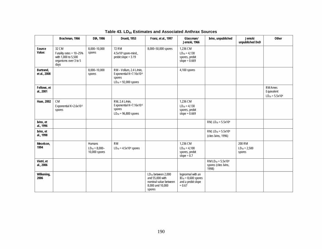
190
Table 43. LD50 Estimates and Associated Anthrax Sources Brachman, 1966 DIA, 1986 Druett, 1953 Franz, et al., 1997 Glassman/
Jemski, 1966 Ivins, unpublished Jemski
unpublished DoD Other
Source Value:
32 CM Fatality rates = 10–25% with 1,000 to 5,500 organisms over 3 to 5 days
8,000–10,000 spores
72 RM 4.5x10⁴ spore-min/L, probit slope = 3.19
8,000–50,000 spores 1,236 CM LD50 = 4,130 spores, probit slope = 0.669
Bartrand, et al., 2008
8,000–10,000 spores
RM – Vollum, 2.4 L/min, Exponential K=7.16x10⁻⁶ spores LD50 = 92,000 spores
4,100 spores
Fellows, et al., 2001
RM Ames Equivalent LD50 = 5.5x10⁴
Haas, 2002 CM Exponential K=2.6x10⁻⁵ spores
RM, 2.4 L/min, Exponential K=7.16x10⁻⁶ spores LD50 = 96,800 spores
1,236 CM LD50 = 4,130 spores, probit slope = 0.669
Ivins, et al., 1996
RM, LD50 = 5.5x10⁴
Ivins, et al., 1998
RM, LD50 = 5.5x10⁴ (cites Ivins, 1996)
Meselson, 1994
Humans LD50 = 8,000–10,000 spores
RM LD50 = 4.5x10⁴ spores
1,236 CM LD50 = 4,100 spores, probit slope = 0.7
200 RM LD50 = 2,500 spores
Vietri, et al., 2006
RM LD50 = 5.5x10⁴ spores (cites Ivins, 1998)
Wilkening, 2006
LD50 between 2,000 and 55,000 with nominal value between 8,000 and 10,000 spores
lognormal with an ID50 = 8,600 spores and a probit slope = 0.67

191
As mentioned, many of the estimates from these studies could not be validated due to the lack of published data. Glassman,192 for example, summarized the results of studies previously conducted by another researcher, Jemski. The purpose of the Jemski research was to expose cynomolgus monkeys to heterogeneously sized aerosols and determine the necessary retention periods for observing animals exposed to potentially lethal doses of anthrax spores. The studies incorporated 1,236 monkeys, which were watched for several months; one monkey died as late as 98 days after initial exposure to inhalation anthrax. Using the lethality data, a median lethal dose of 4,130 spores with a probit slope of 0.669 was derived. However, since the data on which this evaluation was based have not been published, the present authors chose to forego inclusion of these parameters in favor of published lethality data. Likewise, the Defense Intelligence Agency (DIA),193 Franz, et al.,194
Even when animal experiment results are available, some of the data cannot be clearly interpreted. For example, in Brachman’s industrial anthrax study conducted with cynomolgus monkeys exposed to anthrax aerosolized during the hair “picking” process in a goat hair mill, exposure to anthrax was discontinuous over long periods of time. As a result of the long duration and variable exposures, it is extremely difficult to determine the doses at which the monkeys became ill. For example, did a monkey manifesting symptoms late in the trial become ill due to an early exposure (and associated, relatively lower dose) with a long incubation period or did a late-trial exposure (cumulatively larger than earlier doses) cause the infection with a shorter incubation period? Therefore, although there are data presented, the results of this study are censored for research purposes as they do not provide (nor do the authors suggest) utility in determining anthrax infectivity values. The authors only suggest that the data may indicate a dose-fatality relationship of 10–25% from 1,000 to 5,500 spores over 3 to 5 days.
and Ivins studies were not included in the assessment of anthrax lethality because the underlying data were unavailable.
195
As the underlying data are not easily interpreted from Brachman’s study and are not available for the majority of the remaining studies shown in Table 43, these studies will not be considered further in this discussion. It should be noted that 8,000–10,000 spores is a value commonly cited as the median lethal dose for anthrax, as shown in Table 43. The authors, however, were not able to correlate this value to any published data or
192 Harold N. Glassman, “Industrial Inhalational Anthrax: Discussion,” Bacteriological Review 30 (1966):
658. 193 Defense Intelligence Agency, Soviet Biological Warfare Threat, DST-161OF-057-86 (Washington,
DC: Defense Intelligence Agency, 1986). 194 David R. Franz et al., “Clinical Recognition and Management of Patients Exposed to Biological
Warfare Agents,” Journal of the American Medical Association 278, no. 5 (August 1997): 399–411. 195 Philip S. Brachman, Arnold F. Kaufman, and Frederic G. Dalldorf, “Industrial Inhalation Anthrax,”
Bacteriological Reviews 30, no. 3 (1966): 655.

192
experimental result. Therefore, the authors turned to published experimental results to derive an infectivity value for anthrax.
In 1953, Druett, et al. conducted a study in which nine groups of eight rhesus macaques each were exposed to single-spore clouds of Bacillus anthracis for one minute. The lethality data for each of the nine groups are presented as a function of the dosage (concentration times exposure time) in units of spore-minutes/liter and are reproduced in Table 44.196
Table 44. Druett's Rhesus Macaque Exposure and Associated Mortality Rates
Dosage (spore-min/L)
Total Animals
Dead Animals Mortality
29,300 8 1 12.5% 32,100 8 4 50.0% 45,300 8 5 62.5% 57,300 8 6 75.0% 64,800 8 5 62.5% 67,000 8 3 37.5% 100,000 8 8 100.0% 125,000 8 7 87.5% 166,000 8 8 100.0%
From these data, Druett derived a median lethal dosage of 45,000 spore-min/L using a log-probit analysis; elsewhere in the article, he reports a breathing rate of 1.2 L/min, citing Gaddum.197
Two published evaluations of the Druett data have yielded an exponential probability distribution as the best model representation; both have also produced the same lambda value of 7.16x10⁻⁶. Using Druett’s original data, both authors multiplied the exposed concentration by a breathing rate of 2.4 L/min to arrive at the estimated doses shown in Table 45. No citation for this value is given, and it is unclear why it was chosen, although it is possible that the authors simply overlooked the breathing rate in Druett’s article and assumed another value. Even though they used the same data, shown in Table 45, the calculated median lethal value reported by the two studies differs: 96,800
By multiplying these two values, a median lethal dose for anthrax can be calculated as 54,000 spores. Druett provides a slightly different value of 53,000 spores, perhaps because an unrounded dosage value was used in the calculation.
196 H. A. Druett et al., “Studies on Respiratory Infection. I. The Influence of Particle Size on Respiratory
Infection with Anthrax Spores,” Journal of Hygiene 51, no. 3 (September 1953): 359–62. 197 Referenced by Druett to Gaddum, J. H. (1944). Pharmacology. London: Oxford University Press.

193
spores198 and 92,000 spores.199
The 92,000 value may simply be due to a rounding issue (or perhaps a transposition error in the decimals of the lambda value during the calculation).
Table 45. Haas and Bartrand's Interpreted Macaque Exposure and Associated Mortality Rates from Druett
Dosage (spore-min/L)
Estimated Dose (spores)*
Total Animals
Dead Animals Mortality
29,300 70,320 8 1 12.5% 32,100 77,040 8 4 50.0% 45,300 108,720 8 5 62.5% 57,300 137,520 8 6 75.0% 64,800 155,520 8 5 62.5% 67,000 160,800 8 3 37.5% 100,000 240,000 8 8 100.0% 125,000 300,000 8 7 87.5% 166,000 398,400 8 8 100.0%
* assumes a breathing rate of 2.4 L/min for one minute
It was determined that the exponential fit to the Druett data was a reasonable representation of the dose-response to anthrax, but the lack of evidence supporting a breathing rate of 2.4 L/min was problematic. The present authors consulted a 2007 study by Akata et al. on a new method for exposing non-human primates to aerosols, which measured the average minute volume of rhesus monkeys to be 1.108 L/min.200
Since this value was much closer to 1.2 L/min than 2.4 L/min, and since the average body weight of the four monkeys in Akata’s study (3.7 kg ≈ 8.2 lbs) was near the lower end of the weight range of the 7–14 pound animals used by Druett, it was decided that Druett’s original value of 1.2 L/min was the most reasonable value to use when converting dosage to dose.
198 Charles N. Haas, “On the Risk Analysis of Mortality to Primates Exposed to Anthrax Spores,” Risk
Analysis 22, no. 2 (2002): 190. 199 Timothy A. Bartrand, Mark H. Weir, and Charles N. Haas, “Dose-Response Models for Inhalation of
Bacillus anthracis Spores: Interspecies Comparisons,” Risk Analysis 28, no. 4 (August 2008): 1121. 200 Chrys J. Obot Akata et al., “Development of a Head-Out Plethysmograph System for Non-Human
Primates in an Animal Biosafety Level 3 Facility,” Journal of Pharmacological and Toxicological Methods 55 (2007): 101.

194
Table 46. AMedP-8(C) Interpretation of Macaque Exposure and Associated
Mortality Rates from Druett
Dosage (spore-min/L)
Estimated Dose (spores)*
Total Animals
Dead Animals Mortality
29,300 35,160 8 1 12.5% 32,100 38,520 8 4 50.0% 45,300 54,360 8 5 62.5% 57,300 68,760 8 6 75.0% 64,800 77,760 8 5 62.5% 67,000 80,400 8 3 37.5% 100,000 120,000 8 8 100.0% 125,000 150,000 8 7 87.5% 166,000 199,200 8 8 100.0%
* assumes a breathing rate of 1.2 L/min for one minute
The calculated dose values used in the AMedP-8(C) evaluation of Druett’s data are shown in Table 46. As seen in Figure 93, an exponential distribution was fit to the nine data points using the method of least squares and verified by maximizing the coefficient of determination (R2). The resulting exponential function can be described in terms of its cumulative distribution function (CDF):
F(x) = 1 − e−λx (19)
where the lambda value is 1.36 x 10⁻⁵ and x is the dose in spores. This corresponds to a mean value of approximately 73,500 spores and a median lethal dose (LD50) of approximately 51,000 spores, which is considerably below the estimates of Haas and Bartrand, but is close to the median lethal dose of 53,000 spores originally reported in the Druett article.

195
Figure 93. Exponential Fit to Druett Lethality Data with an Assumed Breathing Rate of 1.2
L/min for One Minute
b. Incubation Period There have been a limited number of human inhalation anthrax cases in the last
century. For these, only a limited amount of data exists regarding incubation. Because many of these cases followed inhalation exposure during wool or other animal hair processing, there is a lack of exact information about when exposure occurred. The largest U.S. outbreak occurred during the Amerithrax events of 2001; the exact period of exposure for most of those exposed, however, is unknown and therefore not useful for determining the duration of incubation.
The most notable exception to the general dearth of useful case data is the inhalation anthrax outbreak which occurred in Sverdlosk, Russia in 1979.201 It should be noted that even these data have been questioned; the source of the outbreak remains unclear—initially an ingestion-based outbreak was reported due to contaminated meat, but more recent statements indicate an unintentional release from a local factory.202
201 Ron Brookmeyer, Elizabeth Johnson, and Sarah Barry, “Modeling the Incubation Period of Anthrax,”
Statistics in Medicine 24, no. 4 (February 2005): 531–42.
In addition, the exact case reporting—including numbers of ill, population distribution, etc.—has been questioned.
202 Matthew Meselson et al., “The Sverdlovsk Anthrax Outbreak of 1979,” Science 266, no. 5188 (November 1994): 1202–8; and Dean A. Wilkening, “Sverdlosk Revisited: Modeling Human Inhalation Anthrax, Supporting Text.” Proceedings of the National Academy of Sciences of the Unites States of America 103, no. 20 (2006): supplement.
0%10%20%30%40%50%60%70%80%90%
100%
0 50,000 100,000 150,000 200,000
Perc
ent L
etha
lity
Dose (Spores)
Experimental Percent LethalityPredicted Percent Lethality

196
However, the few incubation period models that have been published utilize or have been compared to the data available from the Sverdlosk outbreak. Some models for the length of incubation period have tried to take into account the physiological processes, including the competing aspects of clearance and germination to describe the risk and likely durations associated with a dose-based anthrax exposure.203 Others employ simpler lognormal distributions or parametric, dose-based lognormal distributions of the incubation period.204
In 2006, Wilkening reviewed four different inhalation models utilizing the Sverdlosk data. Three of the reviewed models posited infectivity as a function of dose modeled as cumulative lognormal distributions with varying median infective doses and probit slopes. The fourth model used an exponential distribution based on the competing physiological aspects of the disease—clearance and germination.
205
The incubation period of anthrax has been assessed to be as short as 1 to 5 days
206
and as long as 2 to 60 days.207 The Sverdlosk data suggested a modal incubation period of 9 to 10 days with the longest incubation period being 43 days.208 Wilkening concluded that this information suggested dose-dependence of the incubation period. He then assumed a lognormal distribution, based on previous work by Sartwell.209 The result is a parametric, dose-based lognormal distribution, with parameters derived from Glassman.210 The CDF for the parametric lognormal distribution is given in the Supporting Text of Wilkening’s article, which can be found on the Proceedings of the National Academy of Sciences (PNAS) website:211
203 Brookmeyer, Johnson, and Barry, “Incubation Period of Anthrax.” 204 Ibid.; and Wilkening, “Sverdlosk Revisted,” 7589–94. 205 Wilkening, “Sverdlosk Revisted,” 7589–94. 206 Franz et al., “Clinical Recognition and Management,” 400–401; and Bret K. Purcell, Patricia L.
Worsham, and Arthur M. Friedlander, “Anthrax,” in Medical Aspects of Biological Warfare, ed. Zygmunt F. Dembek, Textbook of Military Medicine (Washington, DC: Department of Defense, Office of the Surgeon General, U.S. Army, Borden Institute, 2007), 74.
207 Virginia Department of Health, “Anthrax: Guidance for Health Care Providers” (2004) http://www.vdh.state.va.us/EPR/pdf/AnthraxGuidance12092004.pdf.
208 Meselson et al., “Sverdlovsk Anthrax Outbreak,” 1207. 209 Referenced by Wilkening to Sartwell, P. (1950) Am. J. Hyg. 51, 310–318. 210 Glassman, “Industrial Inhalation Anthrax,” 658. 211 Wilkening, “Sverdlosk Revisited,” supplement.

197
FInc−Anth(t) = � 1σ√2π
� ∫ �1x�t
0 exp �− �ln(x)−ln(M)�2
2σ2�dx (20)
where: FInc-Anth is the cumulative fraction of persons with anthrax who have completed the incubation period and entered Stage 1 of the disease at day t,
M = α + βlog(dose),
α = 10.3,
β = -1.35,
σ = γ + δlog(dose),
γ = 0.804, and
δ = -0.079.
Wilkening did not prescribe upper and lower dose thresholds for which the equation applied. Therefore, the equation allows for the calculation of estimated incubation periods even at extremely low doses. Referring back to the infectivity calculation, however, it becomes clear that 1.5% of the population or less is expected to become infected and ill at exposures below approximately 1,000 spores. Thus, only doses equal to or exceeding 1,000 spores were used when calculating the anthrax lookup tables in AMedP-8(C). Just as 1,000 spores is representative of all doses below that value in the lookup tables, 107 spores is recommended as the representative calculational value for all higher doses. Doses above this value (e.g., 108 spores) are beyond the limits of the equation and the duration of the incubation period cannot be predicted.
For the highest doses, specifically, the median incubation period for 106 spores is 2.2 days and for 107 spores is less than 1 day. For 95% of the population receiving such doses, the incubation period will end within 4 days or 2 days respectively. Although these durations seem short, they fall within the 1–5 day window of incubation typically cited, and without additional data, the use of a published, documented methodology—such as the one provided and evaluated by Wilkening—was deemed the most appropriate representation of anthrax incubation period.
The fraction of people progressing from the incubation period to the first stage of illness of anthrax on a given day t can be represented by the difference between F(t) and F(t–1), which is shown in AMedP-8(C) Table A-36. Table values were calculated using the upper dose specified in each column heading with the exception of the last column, which used 107 spores; each column is to be used for the range of doses specified in the column heading. Not all individuals exposed to anthrax via inhalation will develop

198
illness. The fractions by day listed refer only to the percentage of individuals who do actually develop illness after being exposed to a given spore dose.
The AMedP-8(C) Table A-36 values for the lowest dose (1,000 spores) are plotted in Figure 94 below with a smoothing function overlaid on top. These smoothed functions are shown in Figure 95 for all dose ranges in Table A-36, with the x axis truncated at 25 days for better visibility of the non-negligible values. Figure 95 shows that at low doses, the incubation may take several days, whereas at higher doses, the incubation time may be extremely short.
Figure 94. Fraction of People Ill with Anthrax Who Enter Stage 1 of Illness on Specified
Day for Dose of 1,000 Spores
0
0.02
0.04
0.06
0.08
0.1
0.12
0.14
0 5 10 15 20 25 30 35 40 45 50
Frac
tion
Man
ifest
ing
Sym
ptom
s by
Day
Incubation Period: Time from Exposure to Symptom Onset (Days)
10^3 spores

199
Figure 95. Fraction of People Ill with Anthrax Who Enter Stage 1 of Illness on Specified
Day for Several Doses
c. Injury Profile Anthrax is commonly modeled as a biphasic or two-stage disease, with the two
stages described as prodromal, or initial, and fulminant. Using descriptions from Brachman,212 Jernigan, et al.,213 Inglesby, et al.,214 and Holty, et al.,215
each stage of anthrax was associated with signs and symptoms and their associated severity as shown in Table 47. Depending on the dose and physiological manifestation of the disease, there may be a brief mitigation or even cessation of symptoms between these two periods (hours) that is not captured by the injury profile. Although treatment is not modeled in the AMedP-8(C) methodology, treatment considerations are included in Table 47 to help medical planners understand the implications of initiating treatment at different times of the illness, as this information may impact the policy which determines at what symptom level individuals are considered casualties.
212 Philip S. Brachman, “Inhalational Anthrax,” Annals of the New York Academies of Science 353
(December 1980): 85–92. 213 John A. Jernigan et al., “Bioterrorism-Related Inhalational Anthrax: The First 10 Cases Reported in the
United States,” Emerging Infectious Diseases 7, no. 6 (November–December 2001): 933–44. 214 Thomas V. Inglesby et al., “Anthrax as a Biological Weapon, 2002,” Journal of the American Medical
Association 287, no. 17 (May 2002): 2238–44. 215 Holty et al., “Systematic Review,” 272–75.
0
0.1
0.2
0.3
0.4
0.5
0.6
0.7
0.8
0 5 10 15 20 25
Frac
tion
Man
ifest
ing
Sym
ptom
s by
Day
Incubation Period: Time from Exposure to Symptom Onset (Days)
10^3 spores
10^4 spores
10^5 spores
10^6 spores
10^7 spores

200
Table 47. Inhalational Anthrax Non-Survivor Injury Profile
Stage 1 Stage 2
Signs and Symptoms
Flu-like symptoms including malaise, fatigue, drenching sweats, fever, headache, and chills; nausea and vomiting; nonproductive cough; mild chest discomfort and dyspnea; myalgia.
Persistent fever; sudden onset of increasing respiratory distress (increased chest pain, dyspnea, stridor, cyanosis, and diaphoresis) leading to respiratory failure and eventual death; tachycardia, tachypnea, hypotension, leading to cardiovascular collapse and death; altered neurological status (confusion, syncope, or coma) meningoencephalitis likely; edema of chest and neck may be present; pleural effusion and likely widening and edemas of the mediastinum.
Severity 2 (Moderate)
4 (Very Severe)
Outlook If treatment initiated in this stage, may still progress to Stage 2, but chances for survival are higher than if treatment initiated at any other stage. If untreated, will progress to Stage 2.
Even if treatment is initiated in this stage, will likely die of the disease.
d. Duration of Illness The work of Holty, et al. was chosen for use in modeling the duration of illness in
the AMedP-8(C) methodology because its descriptions of the two stages of illness were consistent with those in the AMedP-8(C) injury profile and because it provided specific quantitative estimates of the time spent in each stage based on a review of 2,500 journal articles.
During their review of human anthrax cases from 1900 to 2005, Holty, et al. extracted disease progression information for 82 patients, some of which had received antibiotic treatment. For those patients who received no antibiotics, the mean durations of illness were 3.8 days and 0.8 days for the prodromal and fulminant stages, respectively.216
Therefore, to account for this bias, Holty, et al. conducted maximum likelihood analyses using all cases for which time estimates were available, with cases considered to
However, the study authors felt that these data were skewed because patients with short prodromal stages were more likely to progress to the fulminant stage of illness without seeking medical treatment.
216 Ibid., W-52.
201
be right-censored if the progression of disease was halted by antibiotic intervention.217
The resulting lognormal maximum likelihood estimates for the mean time in the prodromal and fulminant stages are 4.2 (std. dev. = 2.3) and 0.7 (std. dev. = 0.74) days, respectively.218
e. Lethality
Table A-37 in AMedP-8(C) is derived by convolving the incubation period distribution with the stage 1 duration of illness distribution. The results of that convolution are then convolved with the stage 2 duration of illness distribution to produce the values shown in Table A-38 of AMedP-8(C).
To model the lethality of untreated inhalation anthrax, a 100% mortality rate is assumed. Evidence indicates that once infected and showing symptoms, individuals and animals that remain untreated will likely die. For instance, summarizing the results of several previous animal studies, Brachman219 reported that “[o]nce a sufficient level of toxin has been reached, death almost invariable follows…” Additional evidence from confirmed anthrax cases in the past century demonstrates that, even with medical intervention, if treatment is not initiated early, the mortality rate is extremely high.220
f. Vaccine Efficacy
A number of studies have been conducted on both human and animal subjects to determine the efficacy of the anthrax vaccine. The human efficacy study by Brachman, et al. tested the efficacy of a precursor to the currently licensed human anthrax vaccine, anthrax vaccine absorbed (AVA), on workers at four goat hair processing mills. Based on their results, the authors estimated the efficacy to be 0.925,221
To estimate the vaccine efficacy based on known lethal exposures, the authors consulted several studies conducted on rhesus monkeys, which are considered to be the most appropriate model for human inhalation anthrax.
although none of the workers were directly challenged with a known dose of Bacillus anthracis.
222
The combined data set consists of 71 rhesus monkeys from five studies, 60 of which survived (efficacy = 0.85). The obvious outlier in this data set was the one study in which
Even when not explicitly stated, the vaccine manufactured by the Michigan Department of Public Health (MDPH) and the currently licensed human vaccine, AVA, were assumed to be the same.
217 Ibid., W-44–W-45. 218 Ibid., W-52. 219 Brachman, “Inhalational Anthrax,” 85. 220 Holty et al., “Systematic Review,” 274. 221 Philip S. Brachman et al., “Field Evaluation of a Human Anthrax Vaccine,” American Journal of
Public Health 52, no. 4 (April 1962): 644. 222 M. L. Pitt et al., “Comparison of the Efficacy of Purified Protective Antigen and MDPH to Protect
Non-Human Primates from Inhalation Anthrax,” Special Supplement, Salisbury Medical Bulletin 87 (1996): 130.

202
only 2 of 10 monkeys survived; these monkeys were vaccinated only after exposure and therefore, for pre-exposure vaccination efficacy calculations, this data is discounted.223
Therefore, the data set is reduced to 61 monkeys, 58 of which survive (efficacy = 0.95). Of these 61 monkeys, all except those in one study were exposed to the Ames strain; the 20 monkeys in the remaining study224
were exposed to other strains of Bacillus anthracis. As demonstrated by the experimental data summarized in Table 48, the efficacy of anthrax vaccine against the Ames strain is approximately 100%. Against other strains of anthrax, the efficacy appears to be reduced, but not significantly. Based on these findings as well as providing a conservative estimate of prophylaxis efficacy in humans against multiple anthrax strains, a prophylaxis efficacy of 0.90 is recommended for use in the anthrax AMedP-8(C) methodology.
223 Arthur M. Friedlander et al., “Postexposure Prophylaxis against Experimental Inhalation Anthrax,”
Journal of Infectious Diseases 167, no. 5 (May 1993): 1239–43. 224 P. F. Fellows et al., “Efficacy of a Human Anthrax Vaccine in Guinea Pigs, Rabbits, and Rhesus
Macaques against Challenge by Bacillus anthracis Isolates of Diverse Geographical Origin,” Vaccine 19 (2001): 3241–47.

203
Table 48. Anthrax Vaccine Efficacy Studies Summary
Study Vaccine
B. anthracis
strain Subject Total
Subjects Subjects Protected Efficacy
Friedlander, et al., 1993 AVA Vollum 1B Rhesus
monkeys 10 2 0.2
Pitt, et al., 1996
MDPH (AVA) Ames Rhesus
monkeys 10 10 1
Ivins, et al., 1996
MDPH (8 weeks post-vaccination)
Ames Rhesus monkeys 10 10 1
MDPH (38 weeks post-vaccination)
Ames Rhesus monkeys 3 3 1
MDPH (100 weeks post-vaccination)
Ames Rhesus monkeys 8 7 0.875
Ivins, et al., 1998 AVA Ames Rhesus
monkeys 10 10 1
Fellows, et al., 2001 AVA
ASIL K7978/ Namibia
Rhesus monkeys 10 10 1
AVA
ASIL K9729/ Turkey
Rhesus monkeys 10 8 0.8
3. Botulism Botulinum toxins are a set of neurotoxins, serotypes A through G, produced by the
Clostridia botulinum bacteria. Exposure to the toxin via various pathways—ingestion, intramuscular injection, or inhalation—will cause the neuroparalytic disease botulism in humans. Botulism is most commonly caused by food borne ingestion of toxin serotypes A, B, and E; other types of naturally occurring botulism include infant botulism and wound botulism. The disease is often fatal if untreated. Time to onset, severity of illness, and probability of death vary by serotype of toxin. Serotype A was selected as the basis for AMedP-8(C) modeling of human response to botulism because serotype A is responsible for the plurality of human botulism cases reported in the United States and typically causes the most severe disease.225
Human data on inhalation exposure are very limited for botulism, although the few documented cases of inhalational botulism suggest characteristics of the disease—with
225 Woodruff et al., “Clinical and Laboratory Comparison,” 1281.

204
the exception of the gastrointestinal symptoms—are the same as that resulting from ingestion,226
for which significant information exists. Thus, given the available information, it is assumed that the inhalation and ingestion forms of the disease are similar in course, signs and symptoms, and severity. The parameters chosen to characterize each botulism submodel are shown in Table 49, and are described more fully in the subsequent sections.
Table 49. Botulism Model Parameters Summary Table
Submodel Type Parameters
Effectivity Log-probit distribution ED50 = 0.1 μg/man Probit slope = 12.5 probits/log dose
Latent Period Lognormal distribution Median = 1 day Lethality Log-probit distribution LD50 = 0.8 μg/man
Probit slope = 12.5 probits/log dose Duration of Illness
(survivor) Stage 1 Stage 2 Stage 3
Constant Constant Constant
1 day 2 weeks 6 months
Duration of Illness (non-survivor)
Stage 1 Stage 2 Stage 3
Exponential distribution
1/3 length 1/3 length 1/3 length
λ = 0.318
a. Effectivity Botulism effectivity is modeled as a log-probit function with a probit slope of 12.5
probits/log dose227 and a median effective dose (ED50) of 0.1 μg/man.228
A literature search was conducted to locate botulism effectivity data from human intoxication cases or animal studies. However, no published data were available for use
226 E. Holzer, “Botulism Caused by Inhalation,” Medizinische Klinik, 41 (1962) 1735–40 (German
language version), referenced in Zygmunt F. Dembek, Leonard A. Smith, and Janice M. Rusnak, “Botulism: Cause, Effects, Diagnosis, Clinical and Laboratory Identification, and Treatment Modalities,” Disaster Medicine and Public Health Preparedness 1, no. 2 (2007): 122–34.
227 Derived from data in Brunildo A. Herrero et al., “Experimental Botulism in Monkeys—A Clinical Pathological Study,” Experimental and Molecular Pathology 6, no. 1 (February 1967): 84–95.
228 In the absence of available data to estimate a median effective dose, NATO SMEs agreed to a value of 0.1 μg/man; see Julia Burr and Lusine Danakian, "Memorandum for the Record: Meeting Notes – NATO Biological Weapons Subject Matter Expert Human Response Review Meeting” (Alexandria, VA: Institute for Defense Analyses, 2008).
205
in determining the effective dose of botulinum toxin, so advice was sought during the NATO Subject Matter Expert Meeting in May 2008 (Madrid, Spain). Based on their experience with animal studies with botulism for vaccine development, the SMEs suggested using an ED50 of 0.1 μg/man.
In the absence of published data to calculate an effective dose-response curve, the effectivity submodel probit slope was assumed to be equivalent to the probit slope derived for the lethality submodel. This assumption was used, and later reviewed with SMEs, because steep dose-response curves have been observed in animal studies for both effectivity and lethality.
b. Latent Period The latent period of botulism is modeled as a random variable with a lognormal
probability distribution with parameters μ = 0, and σ = 0.84 based on a stated median value of 1 day. The CDF of the lognormal distribution is:
FLat−Bot(t) = 12
+ 12
erf �ln(x)−μσ√2
� (21)
where: FLat-Bot is the cumulative fraction of persons with botulism who have completed the latent period and entered Stage 1 of the disease,
t is the time post exposure [days],
μ is the mean of the natural logarithm of the incubation period [= 0], and
σ is the standard deviation of the natural logarithm of the incubation period [= 0.84].
A review by Woodruff, et al. of botulism cases in the United States between 1975 and 1988 concluded that there were 148 cases of type A botulism in this time period. Information on the incubation period duration existed for approximately 110 of these—76 illnesses associated with outbreaks and 34 illnesses associated with sporadic cases. Of these, 42 cases associated with outbreaks and 24 cases associated with sporadic intoxications had incubation periods of less than or equal to one day. From this, the study’s authors concluded “the median incubation period for all patients was 1 day (ranges: 0–7 days, type A; 0–5 days, type B; 0–2 days, type E).”229
Assuming that the median incubation period of 1 day described for all types of botulism is also the median time for Type A botulism and that the incubation times were lognormally distributed, a fit analysis was performed to estimate the parameters associated with a lognormal distribution with a median of 1 day and a range of 0–7 days. Such an approach is suggested by Walden and Kaplan for incubation periods described
229 Woodruff et al., “Clinical and Laboratory Comparison,” 1282.
206
only by a range of times.230 Since the median value of a lognormal distribution is defined as eµ, where the parameter μ is the mean of the natural logarithm of the observed random variables (in this case, the incubation periods),231
c. Lethality
μ is easily calculated (μ = ln(median) = ln(1) = 0). To account for the range of incubation period values, the second parameter of the lognormal distribution, σ, was manipulated until the CDF evaluated at 7 days was equal to 0.99, which was the case when σ = 0.84.
Lethality is modeled as a log-probit function with a probit slope of 12.5 probits/log dose and an LD50 of 0.8 μg/man.
The botulinum neurotoxin serotype A inhalation LD50 for rhesus monkeys has been demonstrated to be 300–400 mouse intraperitoneal median lethal doses (MIPLD50) per kilogram of body weight.232 Crystalline toxin assays indicate an average of 3.0x10¹⁰ MIPLD50 per gram of botulinum toxin.233 Assuming a 70 kg man, an average monkey inhalation LD50 dose of 350 MIPLD50/kg, and an assay of 3.0x10¹⁰ MIPLD50/g gives a human LD50 (directly translated from the rhesus monkey LD50) of 0.8 μg/man. This is consistent with the human inhalation LD50 of 0.7 to 0.9 μg estimated in Dembek, et al.234
To derive the lethal probit slope, dose-response data for intravenous administration of botulinum toxin in rhesus monkeys from Herrero, et al. were used. The Herrero data—provided for doses ranging from slightly below the calculated monkey LD50 to those where all monkeys died—are shown in Table 50,
235 although admittedly the lack of data at lower doses means this estimate can be improved with additional data. The probit slope was calculated according to the iterative procedure for probit analysis described by Tallarida.236
230 John Walden and Edward H. Kaplan, “Estimating Time and Size of Bioterror Attack,” Emerging
Infectious Diseases 10, no. 7 (July 2004): 1202.
The value of 12.5 probits/log dose was reached after five iterations of the prescribed calculations and all subsequent computational cycles produced the same result. A graph of the logarithm of dose versus percent mortality is shown in Figure 96.
231 Eckhard Limpert, Werner A. Stahel, and Markus Abbt, “Log-normal Distributions across the Sciences: Keys and Clues,” BioScience 51, no. 5 (May 2001): 344.
232 David R. Franz et al., “Efficacy of Prophylactic and Therapeutic Administration of Antitoxin for Inhalation Botulism,” in Botulinum and Tetanus Neurotoxins: Neurotransmission and Biomedical Aspects, ed. Bibhuti R. Dasgupta (New York, NY: Plenum Press, 1993), 473.
233 William C. Patrick III, “Analysis of Botulinum Toxin, Type A, as a Biological Warfare Threat,” May 1998.
234 Zygmunt F. Dembek, Leonard A. Smith, and Janice M. Rusnak, “Botulinum Toxin,” in Medical Aspects of Biological Warfare, ed. Zygmunt F. Dembek, Textbook of Military Medicine (Washington, DC: Department of Defense, Office of the Surgeon General, U.S. Army, Borden Institute, 2007), 340.
235 Herrero et al., “Experimental Botulism in Monkeys,” 92. 236 Ronald J. Tallarida, “Quantal Dose-Response Data: Probit and Logit Analysis,” in Drug Synergism
and Dose-Effect Data Analysis (Boca Raton, Florida: Chapman & Hall/CRC, 2000), 91–97.
207
Table 50. Botulinum Toxin Dose and Mortality Data from Herrero
Dose (MU/kg) Log(Dose)
Total Animals
Dead Animals Mortality
37.8 1.58 6 3 50.0% 44.0 1.64 6 2 33.3% 46.0 1.66 6 5 83.3% 52.0 1.72 6 5 83.3% 55.0 1.74 6 6 100.0% 55.0 1.74 6 6 100.0% 65.0 1.81 6 6 100.0%
208
Figure 96. Rhesus Monkey Mortality Data as a Function of Dose from Herrero
d. Duration of Illness and Injury Profile A literature search was conducted to find data and models that characterize the
duration of illness for survivors and non-survivors of botulism. Although human data exist from botulism outbreaks, all recorded cases had received some form of treatment, which could alter human response. Since AMedP-8(C) estimates the timing of casualties in the absence of treatment, these data could not be used. However, the literature search uncovered time to death data for rhesus monkeys exposed to varying levels of botulinum toxin serotype A, described in detail in Herrero, et al.237 and Oberst, et al.238
The two data sets were combined and the resulting 41 data points are shown in Table 51. Animals number 29, 32, and 45 from the Oberst study were excluded because the time of onset data was inadequate. To be consistent with the precision of the Herrero figures, the Oberst length of illness data were rounded to the nearest day before any analysis was performed.
237 Herrero et al., “Experimental Botulism in Monkeys.” 238 Fred W. Oberst et al., Botulinum Antitoxin as a Therapeutic Agent in Monkeys with Experimental
Botulism, CRDLR 3331 (Edgewood, MD: U.S. Army Edgewood Arsenal Chemical Research and Development Laboratories, October 1965).
0.00
0.20
0.40
0.60
0.80
1.00
1.60 1.70 1.80 1.90 2.00 2.10 2.20
Perc
ent
Mor
talit
y
Log(Dose)
Herrero DataPredicted
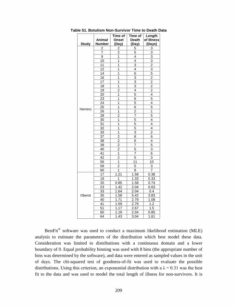
209
Table 51. Botulism Non-Survivor Time to Death Data
Study Animal Number
Time of Onset (Day)
Time of Death (Day)
Length of Illness
(Days)
Herrero
2 2 5 3 7 2 5 3 9 1 4 3 10 1 4 3 11 1 3 2 12 1 4 3 14 1 6 5 16 1 3 2 17 1 3 2 18 1 3 2 19 2 4 2 20 1 5 4 23 1 6 5 24 1 5 4 25 1 6 5 26 1 2 1 28 2 7 5 30 1 5 4 31 1 5 4 32 1 5 4 33 1 3 2 37 2 8 6 38 2 6 4 39 2 7 5 40 2 5 3 41 1 7 6 42 2 5 3 56 1 11 10 59 2 5 3 60 1 8 7
Oberst
17 1.21 1.58 0.38 19 1 1.33 0.33 20 0.85 1.58 0.74 23 1.42 2.04 0.63 33 1.64 2.04 0.4 35 1.58 5.42 3.83 40 1.71 2.79 1.08 41 1.59 2.79 1.2 51 1.17 2.67 1.5 60 1.19 2.04 0.85 64 1.43 3.04 1.61
BestFit® software was used to conduct a maximum likelihood estimation (MLE) analysis to estimate the parameters of the distribution which best model these data. Consideration was limited to distributions with a continuous domain and a lower boundary of 0. Equal probability binning was used with 8 bins (the appropriate number of bins was determined by the software), and data were entered as sampled values in the unit of days. The chi-squared test of goodness-of-fit was used to evaluate the possible distributions. Using this criterion, an exponential distribution with a λ = 0.31 was the best fit to the data and was used to model the total length of illness for non-survivors. It is
210
assumed that each of the three stages of illness has equal duration, so the length of each stage is modeled as 1/3 the total duration of illness.
No data were available on the duration of illness for untreated individuals who survive and recover. Thus, it is assumed that survivors of botulism will not begin to recover from their illness for several weeks after the onset of illness, and full recovery generally would take several months. Because the recovery period is so lengthy—and hence beyond the timelines of interest in AMedP-8(C)—and highly dependent on the individual and the treatment received, a stochastic model of recovery in the absence of treatment has not been developed for botulism. Rather, a deterministic illness time profile is suggested: individuals who are expected to survive botulism are assumed to spend 1 day in Stage 1, spend two weeks in Stage 2, and then remain for 6 months in Stage 3.239
Three stages of illness were chosen to capture the varying severity of the symptoms manifesting over time as shown in Tables 52 and 53. Symptom descriptions were compiled from Arnon, et al.,
240 Dembek, et al.,241 and Hughes, et al.242
Distinct injury profiles exist for survivors and non-survivors of botulism. Each injury profile characterizes the symptomatic period of illness and divides this period into three distinct stages. The signs and symptoms characterizing each stage as well as the corresponding sign/symptom severity level for each stage are described in Tables 52 and 53 for non-survivors and survivors respectively.
239 Dembek, Smith, and Rusnak. “Botulinum Toxin,” 341. 240 Stephen S. Arnon et al., “Botulinum Toxin as a Biological Weapon: Medical and Public Health
Management,” Journal of the American Medical Association 285, no. 8 (February 2001): 1059–70. 241 Dembek, Smith, and Rusnak. “Botulinum Toxin.” 242 James M. Hughes et al., “Clinical Features of Types A and B Food-borne Botulism,” Annals of
Internal Medicine 95, no. 4 (October 1981): 442–45.

211
Table 52. Botulism Non-Survivor Injury Profile
Stage 1 Stage 2 Stage 3
Signs and Symptoms
Fatigue; dry mouth; ptosis; diplopia; photophobia; dysphagia; dysarthria; dysphonia; facial paralysis.
Acute symmetrical descending flaccid paralysis: progressive muscle weakness in the head and neck, followed by upper extremities and lower extremities; dysphagia and loss of gag reflex; diplopia; dysarthria; dysphonia; fatigue.
Acute symmetrical descending flaccid paralysis: paralysis in respiratory muscles and upper and lower extremities; respiratory failure.
Severity 2 (Moderate)
3 (Severe)
4 (Very Severe)
Outlook Likelihoods for progression to Stage 2 and survival are uncertain and highly dependent on individual and dose. Treatment can significantly improve chances for survival.
Likelihoods for progression to Stage 3 and survival are uncertain and highly dependent on individual and dose. Treatment can significantly improve chances for survival.
Condition is lethal in the absence of treatment, but may survive with treatment.
Table 53. Botulism Survivor Injury Profile
Stage 1 Stage 2 Stage 3
Signs and Symptoms
Fatigue; dry mouth; ptosis; diplopia; photophobia; dysphagia; dysarthria; dysphonia; facial paralysis.
Acute symmetrical descending flaccid paralysis: progressive muscle weakness in the head and neck, followed by upper extremities and lower extremities; dysphagia and loss of gag reflex; diplopia; dysarthria; dysphonia; fatigue.
Gradual reversal of muscle paralysis.
Severity 2 (Moderate)
3 (Severe)
2 (Moderate)
Outlook Likelihoods for progression to Stage 2 and survival are uncertain and highly dependent on individual and dose. Treatment can significantly improve chances for survival.
Likelihoods for progression to Stage 3 and survival are uncertain and highly dependent on individual and dose. Treatment can significantly improve chances for survival.
Individual will likely recover.

212
e. Medical Countermeasures No medical countermeasures for botulism are modeled in AMedP-8(C).
4. Venezuelan Equine Encephalitis (VEE) The Venezuelan equine encephalitis (VEE) virus, first recognized in Venezuela in
1936, is an alphavirus, one of four genera making up the Togaviridae family. In nature, VEE is transmitted by arthropod vectors such as ticks, fleas, or mosquitoes, and has demonstrated high infectiousness in laboratory settings. Epizootic and enzootic strains of VEE can be found in nature, and both cause disease in humans.243
All subtypes of VEE are assumed to result in a similar disease progression for the purposes of modeling. Different routes of exposure are assumed to produce similar times of onset of symptoms and similar injury profiles for the purposes of data selection. All model parameters assume an absence of medical treatment. These parameters are provided in Table 54 and described more thoroughly in the sections that follow.
Table 54. VEE Model Parameters Summary Table
Submodel Type Parameters
Infectivity Threshold 1 PFU
Incubation Period
Weibull distribution Mean = 1.94 days
Standard deviation = 1.24 days
Lethality, if Symptomatic
Rate 0%
Duration of Illness
Stage 1
Stage 2
Stage 3
Discrete
Lognormal distribution
Lognormal distribution
x = {2, 3} p = {0.8, 0.2}
Mean = 3.47 days
Standard deviation = 2.80 days
Mean = 4.84 days
Standard deviation = 3.81 days
243 Steele et al., “Alphavirus Encephalitides,” 242.
213
a. Infectivity Assuming all inhaled agent is retained in the lungs, infectivity is modeled as a 100%
probability of infection if the inhaled dose is greater than or equal to 1 plaque forming unit (PFU); otherwise the probability is 0. A literature search was conducted to locate infectivity data from epidemiological and experimental studies. VEE is highly infectious by aerosol, based on a large number of observed laboratory infections.244
b. Incubation Period
In an attempt to capture the highly infectious nature of VEE, and in the absence of detailed dose-response information, a threshold response model with a threshold dose of 1 PFU is utilized in AMedP-8(C). Thus, 100% probability of infection (probability of becoming symptomatic) is modeled if exposure is ≥1 PFU. It is well understood that not all inhaled particles are retained. If one PFU deposited in the respiratory tract is all that is necessary to cause infection, then this may require that as many as five PFU be inhaled. Future versions of AMedP-8(C) should reconsider the assumption that all inhaled organisms are retained.
Data for the length of the incubation period for inhalational VEE were collected from published case reviews of accidental laboratory infections of VEE. A total of 36 incubation period data points (see Table 55) was used in a MLE analysis to estimate a distribution which would best fit this data. (The two cases reported by Casals, Curnen, and Thomas contained no information on the date of exposure and were not used in the analysis; they are included in the table because they were combined with some of the other cases in the table for use in the duration of illness submodel analysis described later.) The analysis was conducted using BestFit® software, and consideration was limited to distributions with a continuous domain and a lower boundary of 0. Equal probability binning was used with 7 bins (the appropriate number of bins was determined by the software), and data were entered as sampled values in the unit of days. The chi-squared test of goodness-of-fit was used to evaluate and select the most appropriate distribution.
The best fit to the data was a Weibull distribution with a mean and standard deviation of 1.94 and 1.24 days respectively. The CDF corresponding to this incubation period distribution is:
244 Venkat Rao et al., “Toxicity Assessment of Venezuelan Equine Encephalitis Virus Vaccine Candidate
Strain V3526,” Vaccine 24, no. 10 (March 2006): 1710–15; and Steele et al., “Alphavirus Encephalitides.”

214
FInc−VEE(t) = 1 − e−(t β⁄ )α (22)
where:
FInc-VEE is the cumulative fraction of persons with VEE who have completed the incubation period and entered Stage 1 of the disease,
t is the time post exposure [days],
α is the shape parameter [= 1.60], and
β is the scale parameter [= 2.16].245
245 Derived from data in H. Koprowski and H. R. Cox, “Human Laboratory Infection with Venezuelan
Equine Encephalitis Virus: Report of Four Cases,” New England Journal of Medicine 236, no. 18 (1947): 647–54; Edwin H. Lennette and Hilary Koprowski, “Human Infection with Venezuelan Equine Encephalomyelitis Virus: A Report of Eight Cases of Infection Acquired in the Laboratory,” Journal of the American Medical Association 123, no. 17 (December 1943), 1088–95; and A. N. Slepushkin, “An Epidemiological Study of Laboratory Infections with Venezuelan Equine Encephalitis,” Problems of Virology 4, (1959): 54–58.

215
Table 55. Summary of 38 Cases of VEE Human Inhalation Laboratory Infection
Event
Cas
e
Tim
e to
Ons
et
(in d
ays)
Ons
et o
f sy
mpt
oms
No
long
er
sym
ptom
atic
Num
ber o
f A
cute
day
s
Num
ber o
f M
oder
ate
days
Num
ber o
f M
ild d
ays
Tota
l Day
s of
Ill
ness
Casals, Curnen, and Thomas (CCT) no data on the date of exposure
CCT 1 No data 6-Nov 12-Nov 2 2 3 7
CCT 2 No data 7-Nov 10-Nov 2 1 2 5 Koprowski & Cox (KC) lab exposure Feb 1(assumed)
KC 1 1 2-Feb 14-Feb 2 4 6 12 KC 2 1 2-Feb 15-Feb 2 3 9 14 KC 3 1 2-Feb 12-Feb 2 3 5 10 KC 4 2 3-Feb 1-Mar 2 10 13 25
Lennette and Koprowski (LK) lab exposure June 28 (assumed)
LK 1 2 30-Jun 9-Jul 2 5 2 9 LK 2 3 1-Jul 8-Jul 2 2 4 8 LK 3 4 2-Jul 12-Jul 2 3 5 10 LK 4 4 2-Jul 6-Jul 3 1 1 5 LK 5 4 2-Jul 8-Jul 2 2 2 6 LK 6 7 5-Jul 10-Jul 2 1 2 5
Lennette and Koprowski (LK) lab exposure July 12 (assumed)
LK 7 1 13-Jul 24-Jul 3 3 5 11
LK 8 2 14-Jul 3-Aug 3 9 8 20
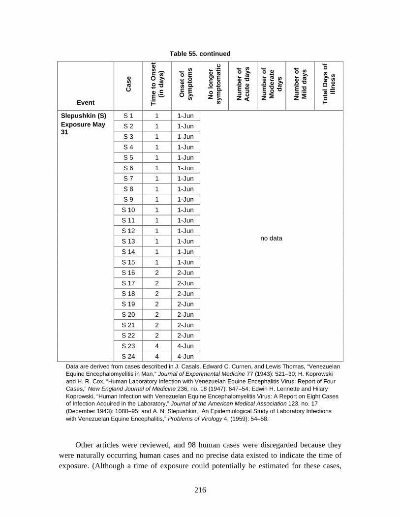
216
Table 55. continued
Event
Cas
e
Tim
e to
Ons
et
(in d
ays)
Ons
et o
f sy
mpt
oms
No
long
er
sym
ptom
atic
Num
ber o
f A
cute
day
s
Num
ber o
f M
oder
ate
days
Num
ber o
f M
ild d
ays
Tota
l Day
s of
Ill
ness
Slepushkin (S) Exposure May 31
S 1 1 1-Jun
no data
S 2 1 1-Jun S 3 1 1-Jun S 4 1 1-Jun S 5 1 1-Jun S 6 1 1-Jun S 7 1 1-Jun S 8 1 1-Jun S 9 1 1-Jun S 10 1 1-Jun S 11 1 1-Jun S 12 1 1-Jun S 13 1 1-Jun S 14 1 1-Jun S 15 1 1-Jun S 16 2 2-Jun S 17 2 2-Jun S 18 2 2-Jun S 19 2 2-Jun S 20 2 2-Jun S 21 2 2-Jun S 22 2 2-Jun S 23 4 4-Jun S 24 4 4-Jun
Data are derived from cases described in J. Casals, Edward C. Curnen, and Lewis Thomas, “Venezuelan Equine Encephalomyelitis in Man,” Journal of Experimental Medicine 77 (1943): 521–30; H. Koprowski and H. R. Cox, “Human Laboratory Infection with Venezuelan Equine Encephalitis Virus: Report of Four Cases,” New England Journal of Medicine 236, no. 18 (1947): 647–54; Edwin H. Lennette and Hilary Koprowski, “Human Infection with Venezuelan Equine Encephalomyelitis Virus: A Report on Eight Cases of Infection Acquired in the Laboratory,” Journal of the American Medical Association 123, no. 17 (December 1943): 1088–95; and A. N. Slepushkin, “An Epidemiological Study of Laboratory Infections with Venezuelan Equine Encephalitis,” Problems of Virology 4, (1959): 54–58.
Other articles were reviewed, and 98 human cases were disregarded because they were naturally occurring human cases and no precise data existed to indicate the time of exposure. (Although a time of exposure could potentially be estimated for these cases,
217
existing human cases with known times of exposure and incubation periods were used instead.)
The first ten excluded cases included a 15 year old boy who had been “frequently bitten” by insects—this case was not used for two reasons: the boy was a teen and not within the age considered in the methodology, and it was not possible to derive a time of onset since the boy was bitten over the course of several nights.246
Additionally, 88 officially reported human cases from July and August 1971 in two Texas counties were reviewed.
There were 9 other cases discussed in the article; 7 hospital charts and 2 chart summaries. Again, no onset data were available. Generally, the article discussed symptoms experienced by the patients.
247
c. Lethality
Of the 88 cases, only 79 had detailed case reports. Eleven of the 79 were reported to have been at one of two high risk beach areas—these cases were not considered because a time of exposure could not be determined. After examining “Table 2 – Estimated incubation periods of VEE in 11 persons with naturally acquired cases (Texas, 1971),” it was determined that the “estimated incubation period” was based loosely on times and dates of arrival, rather than the actual times of exposures. The exposure times would be hard to determine, since these 11 people could have been exposed to infected mosquitoes at any time after their arrival at the beach. There were not enough details given to estimate exposure time or incubation period for the remaining 68 cases.
Lethality is modeled as a rate of 0%, if symptomatic.
While VEE may be fatal in small percentages of children and the elderly, it is only very rarely fatal in adult cases (~0.05%). Only 0.5% of adult VEE cases manifest as fully-developed encephalitis cases, and of those, only 10% result in fatalities.248
d. Duration of Illness and Injury Profile
The fatality rate for untreated VEE is therefore assumed to be approximately 0% in healthy adults; as this assumption holds for the population of interest to AMedP-8(C), a 0% lethality rate for VEE is modeled.
The durations of illness for Stages 1–3 were determined from the data in Table 55. A total of 14 cases were considered (Casals, Curan, and Thomas (2), Koprowski and Cox 246 William H. Dietz, Pauline H. Peralta, and Karl M. Johnson, “Ten Clinical Cases of Human Infection
with Venezuelan Equine Encephalomyelitis Virus, Subtype I-D,” American Journal of Tropical Medicine and Hygiene 28, no.2 (1979): 329–34.
247 G. S. Bowen et al., “Clinical Aspects of Human Venezuelan Equine Encephalitis in Texas,” Bulletin of the Pan American Health Organization 10 (1976): 46–57.
248 Steele et al., “Alphavirus Encephalitides,” 252.
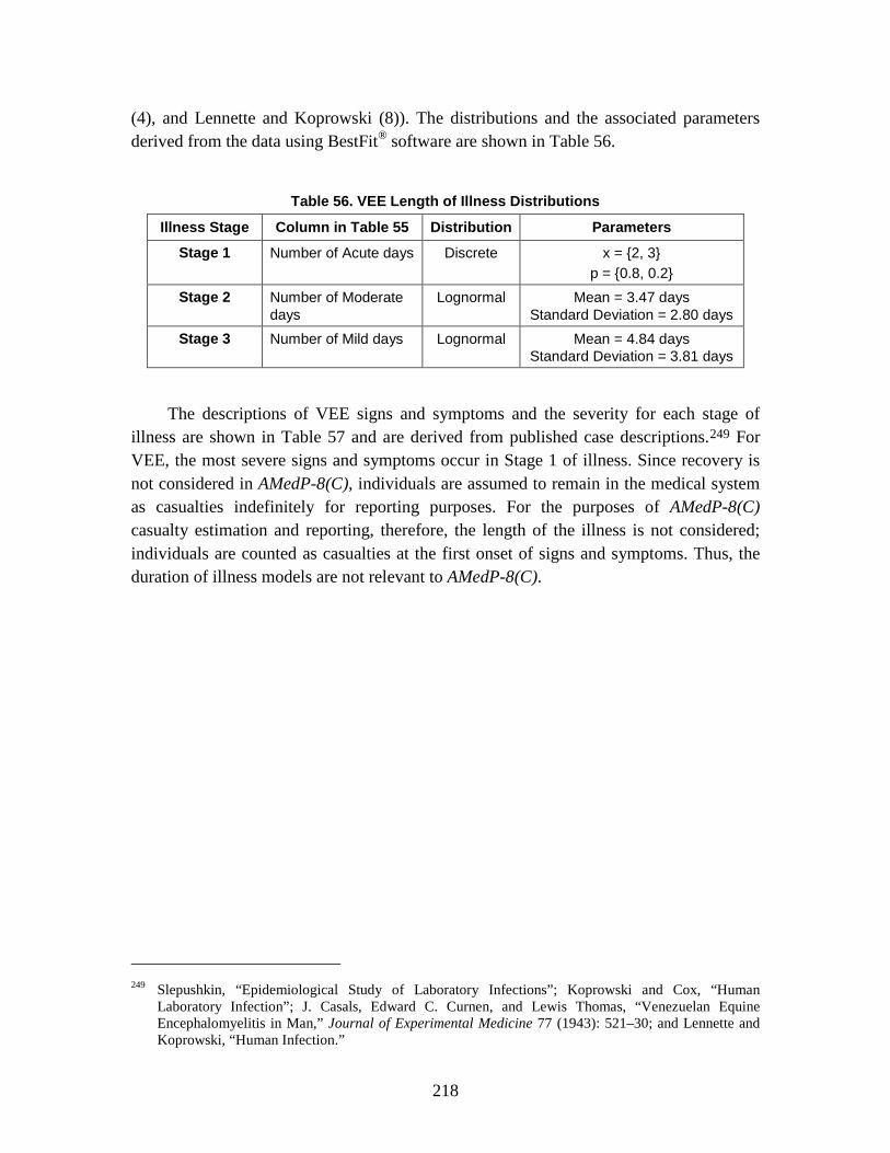
218
(4), and Lennette and Koprowski (8)). The distributions and the associated parameters derived from the data using BestFit® software are shown in Table 56.
Table 56. VEE Length of Illness Distributions
Illness Stage Column in Table 55 Distribution Parameters
Stage 1 Number of Acute days Discrete x = {2, 3} p = {0.8, 0.2}
Stage 2 Number of Moderate days
Lognormal Mean = 3.47 days Standard Deviation = 2.80 days
Stage 3 Number of Mild days Lognormal Mean = 4.84 days Standard Deviation = 3.81 days
The descriptions of VEE signs and symptoms and the severity for each stage of illness are shown in Table 57 and are derived from published case descriptions.249
For VEE, the most severe signs and symptoms occur in Stage 1 of illness. Since recovery is not considered in AMedP-8(C), individuals are assumed to remain in the medical system as casualties indefinitely for reporting purposes. For the purposes of AMedP-8(C) casualty estimation and reporting, therefore, the length of the illness is not considered; individuals are counted as casualties at the first onset of signs and symptoms. Thus, the duration of illness models are not relevant to AMedP-8(C).
249 Slepushkin, “Epidemiological Study of Laboratory Infections”; Koprowski and Cox, “Human
Laboratory Infection”; J. Casals, Edward C. Curnen, and Lewis Thomas, “Venezuelan Equine Encephalomyelitis in Man,” Journal of Experimental Medicine 77 (1943): 521–30; and Lennette and Koprowski, “Human Infection.”
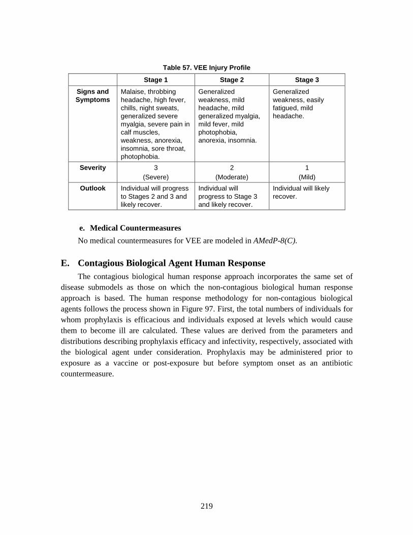
219
Table 57. VEE Injury Profile
Stage 1 Stage 2 Stage 3
Signs and Symptoms
Malaise, throbbing headache, high fever, chills, night sweats, generalized severe myalgia, severe pain in calf muscles, weakness, anorexia, insomnia, sore throat, photophobia.
Generalized weakness, mild headache, mild generalized myalgia, mild fever, mild photophobia, anorexia, insomnia.
Generalized weakness, easily fatigued, mild headache.
Severity 3 (Severe)
2 (Moderate)
1 (Mild)
Outlook Individual will progress to Stages 2 and 3 and likely recover.
Individual will progress to Stage 3 and likely recover.
Individual will likely recover.
e. Medical Countermeasures No medical countermeasures for VEE are modeled in AMedP-8(C).
E. Contagious Biological Agent Human Response The contagious biological human response approach incorporates the same set of
disease submodels as those on which the non-contagious biological human response approach is based. The human response methodology for non-contagious biological agents follows the process shown in Figure 97. First, the total numbers of individuals for whom prophylaxis is efficacious and individuals exposed at levels which would cause them to become ill are calculated. These values are derived from the parameters and distributions describing prophylaxis efficacy and infectivity, respectively, associated with the biological agent under consideration. Prophylaxis may be administered prior to exposure as a vaccine or post-exposure but before symptom onset as an antibiotic countermeasure.

220
Figure 97. Contagious Biological Human Response Process
1. Derivation of the Susceptible-Exposed and infected-Infectious-Removed-Prophylaxis efficacious (SEIRP) Approach Contagious disease modeling poses an additional challenge beyond non-contagious
disease modeling. Both contagious and non-contagious disease human response modeling may require, depending on the agent modeled, stochastic representations of infectivity, lethality, and the durations of incubation and illness. Contagious disease modeling adds the additional challenge of modeling the spread of disease among a susceptible population that did not develop the disease after the initial, possibly weaponized, exposure.
Epidemic models have historically been developed after a disease outbreak to explain the outbreak dynamics. In the late 1990’s, emergency and medical researchers and planners began using these epidemic models to attempt to predict the spread of disease using historical research to help define the likelihood of contagion spread in susceptible populations.
A number of approaches and variations on epidemic modeling, adjusted for planning purposes, exist. Among them, the Susceptible-Infected (SI), Susceptible-Infected-Removed (SIR), and the Susceptible-Exposed-Infectious-Removed (SEIR) models are relatively simple models where fractions of the population move linearly between cohorts depending on the state of their exposure and infection, as shown in Figure 98. Lekone and Finkenstadt described the SEIR model as a set of differential
Prophylaxis andInfectivity
Calculation
Casualties and Fatalities by Time Period Estimation
g g
Contagion (SEIRP)Calculation
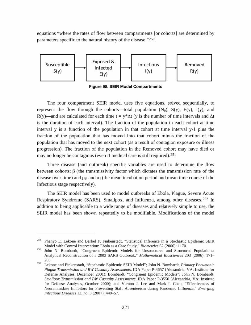
221
equations “where the rates of flow between compartments [or cohorts] are determined by parameters specific to the natural history of the disease.”250
Figure 98. SEIR Model Compartments
The four compartment SEIR model uses five equations, solved sequentially, to represent the flow through the cohorts—total population (N0), S(y), E(y), I(y), and R(y)—and are calculated for each time t = y*∆t (y is the number of time intervals and ∆t is the duration of each interval). The fraction of the population in each cohort at time interval y is a function of the population in that cohort at time interval y-1 plus the fraction of the population that has moved into that cohort minus the fraction of the population that has moved to the next cohort (as a result of contagion exposure or illness progression). The fraction of the population in the Removed cohort may have died or may no longer be contagious (even if medical care is still required).251
Three disease (and outbreak) specific variables are used to determine the flow between cohorts: β (the transmissivity factor which dictates the transmission rate of the disease over time) and µE and µI (the mean incubation period and mean time course of the Infectious stage respectively).
The SEIR model has been used to model outbreaks of Ebola, Plague, Severe Acute Respiratory Syndrome (SARS), Smallpox, and Influenza, among other diseases.252
250 Phenyo E. Lekone and Barbel F. Finkenstadt, “Statistical Inference in a Stochastic Epidemic SEIR
Model with Control Intervention: Ebola as a Case Study,” Biometrics 62 (2006): 1170.
In addition to being applicable to a wide range of diseases and relatively simple to use, the SEIR model has been shown repeatedly to be modifiable. Modifications of the model
251 John N. Bombardt, “Congruent Epidemic Models for Unstructured and Structured Populations: Analytical Reconstruction of a 2003 SARS Outbreak,” Mathematical Biosciences 203 (2006): 171–203.
252 Lekone and Finkenstadt, “Stochastic Epidemic SEIR Model”; John N. Bombardt, Primary Pneumonic Plague Transmission and BW Casualty Assessments, IDA Paper P-3657 (Alexandria, VA: Institute for Defense Analyses, December 2001); Bombardt, “Congruent Epidemic Models”; John N. Bombardt, Smallpox Transmission and BW Casualty Assessments, IDA Paper P-3550 (Alexandria, VA: Institute for Defense Analyses, October 2000); and Vernon J. Lee and Mark I. Chen, “Effectiveness of Neuraminidase Inhibitors for Preventing Staff Absenteeism during Pandemic Influenza,” Emerging Infectious Diseases 13, no. 3 (2007): 449–57.
SusceptibleS(y)
Exposed &Infected
E(y)
InfectiousI(y)
RemovedR(y)

222
have included the incorporation of structured populations,253 the incorporation of medical prophylaxes,254 and the incorporation of agent-based spatial representations.255
The basic, four-cohort SEIR model was modified four ways in AMedP-8(C) to allow for an accurate estimation of casualties as the result of multiple-stage injury profiles:
Incorporation of Prophylaxis Efficacious Cohort: This cohort allows for removal of a fraction of the population from the Susceptible and/or Exposed and Infected cohorts following the application of prophylaxis; prophylaxis can be administered either pre- or post-exposure. The efficacy afforded by the prophylaxis can be either semi-permanent or short-term, depending on the type of prophylaxis selected.
Use of Two Infectious Cohorts (Stage 1 & Stage 2): The use of two infectious cohorts allows for the differentiation of stages, and therefore, injury severity levels for each disease.
• Introduction of α, Infectivity of Stage 1: The use of two infectious cohorts requires the introduction of another variable α, the relative infectivity or the infectivity of Stage 1, which dictates the probability of transmitting the disease contagiously while in Stage 1 versus while in Stage 2 (1-α).
Introduction of Two Removed Sub-Cohorts: Two removed sub-cohorts—removed (fatality) and removed (medical) are included in the SEIRP model. Removed (fatality) allows for an estimation of the fraction of the population that becomes a fatality. Removed (medical) provides a holding cohort for the fraction of the population that is no longer infectious but may still require some medical care.
Introduction of Exposed and Infected Sub-Calculations: Although the SEIR model has an Exposed and Infected Cohort to account for incubation period, initial model versions did not allow for a minimum incubation time to be enforced. To include minimum incubation times, a set of two equations (depending on t in relation to the minimum incubation time) are performed to ensure that no fraction of the population manifests symptoms before the minimum incubation time has elapsed.
The SEIRP approach, the equations, and the agent-specific parameters are discussed in more detail in the following section.
253 Bombardt, “Congruent Epidemic Models”; and Lee and Chen, “Effectiveness of Neuraminidase
Inhibitors.” 254 D. Greenhalgh, “Hopf Bifurcation in Epidemic Models with a Latent Period and Nonpermanent
Immunity,” Mathematical and Computer Modelling 25, no. 2 (1997): 85–107. 255 Liliana Perez and Suzana Dragicevic, “An Agent-Based Approach from Modeling Dynamics of
Contagious Disease Spread,” International Journal of Health Geographics 8, no. 50 (2009): 1–17.
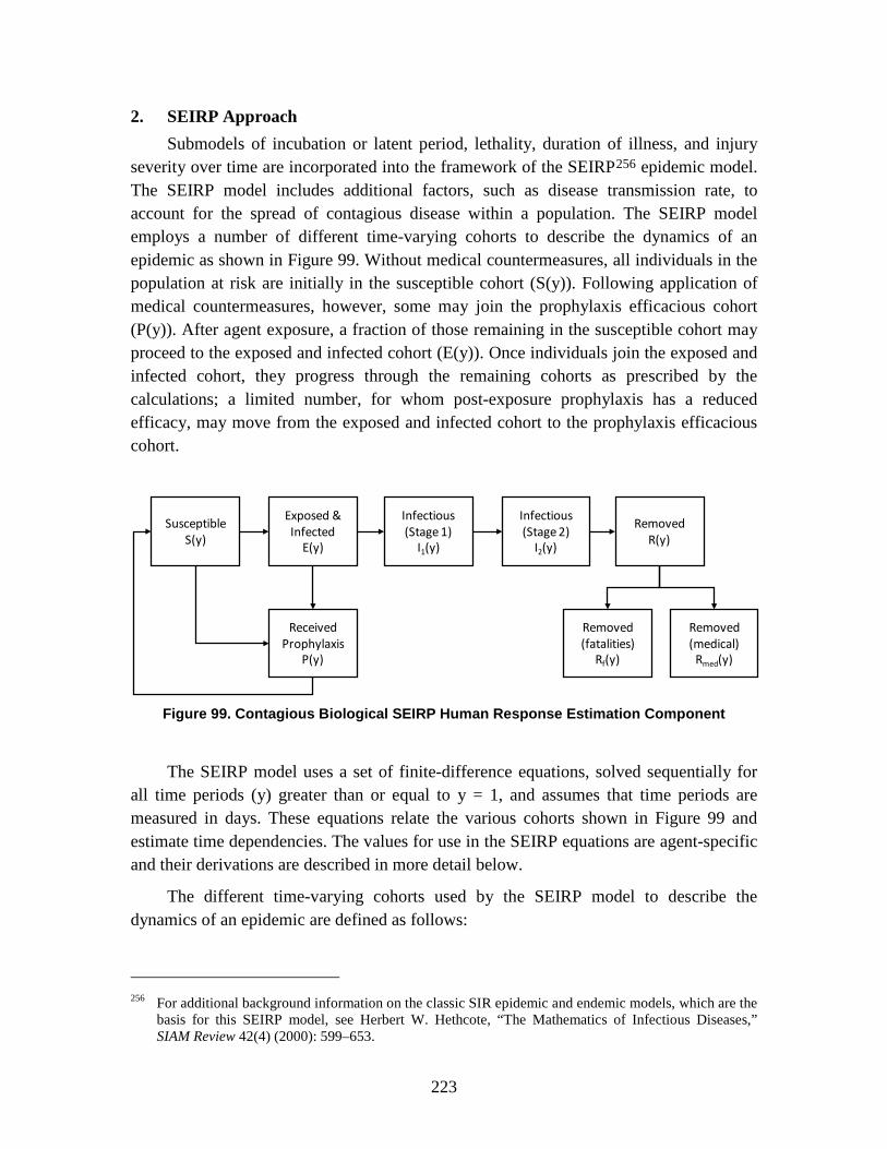
223
2. SEIRP Approach Submodels of incubation or latent period, lethality, duration of illness, and injury
severity over time are incorporated into the framework of the SEIRP256
epidemic model. The SEIRP model includes additional factors, such as disease transmission rate, to account for the spread of contagious disease within a population. The SEIRP model employs a number of different time-varying cohorts to describe the dynamics of an epidemic as shown in Figure 99. Without medical countermeasures, all individuals in the population at risk are initially in the susceptible cohort (S(y)). Following application of medical countermeasures, however, some may join the prophylaxis efficacious cohort (P(y)). After agent exposure, a fraction of those remaining in the susceptible cohort may proceed to the exposed and infected cohort (E(y)). Once individuals join the exposed and infected cohort, they progress through the remaining cohorts as prescribed by the calculations; a limited number, for whom post-exposure prophylaxis has a reduced efficacy, may move from the exposed and infected cohort to the prophylaxis efficacious cohort.
Figure 99. Contagious Biological SEIRP Human Response Estimation Component
The SEIRP model uses a set of finite-difference equations, solved sequentially for all time periods (y) greater than or equal to y = 1, and assumes that time periods are measured in days. These equations relate the various cohorts shown in Figure 99 and estimate time dependencies. The values for use in the SEIRP equations are agent-specific and their derivations are described in more detail below.
The different time-varying cohorts used by the SEIRP model to describe the dynamics of an epidemic are defined as follows:
256 For additional background information on the classic SIR epidemic and endemic models, which are the
basis for this SEIRP model, see Herbert W. Hethcote, “The Mathematics of Infectious Diseases,” SIAM Review 42(4) (2000): 599–653.
Removed(fatalities)
Rf(y)
Removed(medical)
Rmed(y)
SusceptibleS(y)
Exposed &Infected
E(y)
Infectious(Stage 1)
I1(y)
Infectious(Stage 2)
I2(y)
RemovedR(y)
ReceivedProphylaxis
P(y)

224
• Total population (N0) is the fixed total number of people in the population under attack at time 0.
• Susceptible (S(y)) is the total susceptible sub-population or the population at risk at time step y.
• Exposed and infected (E(y)) is the fraction of the population which is exposed to a contagious biological agent and will become infected following that exposure at time step y. Fractions enter the E(y) cohort either as initial infections (E(0)) or as transmission-caused infections due to contact with the infectious, or contagious, population. Individuals in this cohort remain here for the duration of the incubation period.
• Infectious stages (I1(y), I2(y), etc.) are the infectious sub-populations containing contagious people who manifest disease severity associated with a particular stage of disease (i.e., Stage 1, Stage 2, etc.) at time step y.
• Removed—There are two possible categories of removed: Removed (fatalities) and Removed (non-contagious medical). These two categories sum to the total number of individuals removed.
– Removed (fatalities) (Rf(y)) is the number of people who have died from the disease and are thereby removed as a source of infection from the model at time step y.
– Removed (non-contagious medical) (Rm(y)) is the number of people who are no longer infectious but remain in the medical system at time y; this fraction is not available for reinfection; therefore, they do not return to the susceptible population. Because the human response methodology does not account for recovery, these individuals remain in the medical system but can no longer infect susceptibles. This fraction will be counted as part of the casualty fraction.
• Prophylaxis efficacious (P(y)) is the number of people for whom prophylaxis is efficacious and are thereby protected against person-to-person disease transmission at time step y.
Individuals may move between S(y) and P(y) cohorts. Once an individual enters the E(y) cohort, however, they progress forward through the infectious stages until they are removed.
The SEIRP finite-difference equations relate the various cohorts and estimate time dependencies through the use of a relative infectivity (α), a prophylaxis efficacy (ρ), several mean dwell times for the various cohorts (µ), a time-varying disease transmission rate (β(y)), and two time-dependent prophylaxis parameters (prophylaxis on (ν on(y)) and prophylaxis off (νoff(y))).
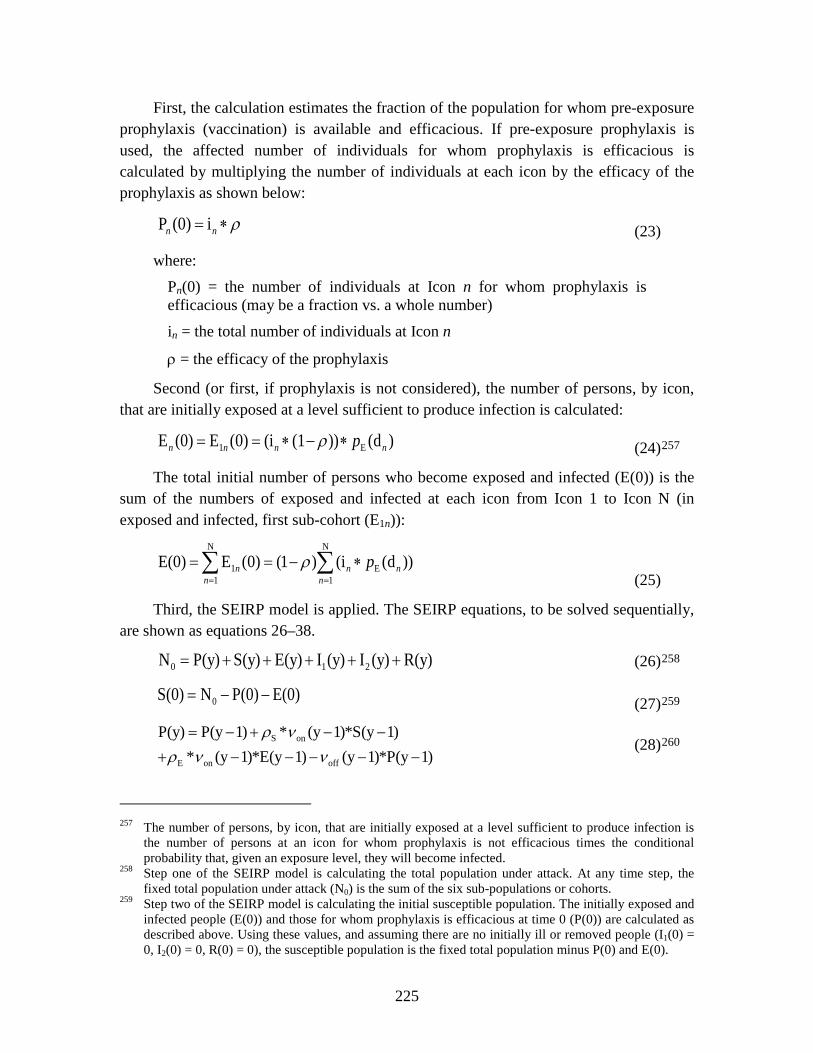
225
First, the calculation estimates the fraction of the population for whom pre-exposure prophylaxis (vaccination) is available and efficacious. If pre-exposure prophylaxis is used, the affected number of individuals for whom prophylaxis is efficacious is calculated by multiplying the number of individuals at each icon by the efficacy of the prophylaxis as shown below:
P (0) in n ρ= ∗ (23)
where: Pn(0) = the number of individuals at Icon n for whom prophylaxis is efficacious (may be a fraction vs. a whole number)
in = the total number of individuals at Icon n
ρ = the efficacy of the prophylaxis
Second (or first, if prophylaxis is not considered), the number of persons, by icon, that are initially exposed at a level sufficient to produce infection is calculated:
1 EE (0) E (0) (i (1 )) (d )n n n npρ= = ∗ − ∗ (24)257
The total initial number of persons who become exposed and infected (E(0)) is the sum of the numbers of exposed and infected at each icon from Icon 1 to Icon N (in exposed and infected, first sub-cohort (E1n)):
N N
1 E1 1
E(0) E (0) (1 ) (i (d ))n n nn n
pρ= =
= = − ∗∑ ∑ (25)
Third, the SEIRP model is applied. The SEIRP equations, to be solved sequentially, are shown as equations 26–38.
0 1 2N P(y) S(y) E(y) I (y) I (y) R(y)= + + + + + (26)258
0S(0) N P(0) E(0)= − −
(27)259
S on
E on off
P(y) P(y 1) * (y 1)*S(y 1)* (y 1)*E(y 1) (y 1)*P(y 1)
ρ νρ ν ν
= − + − −+ − − − − −
(28)260
257 The number of persons, by icon, that are initially exposed at a level sufficient to produce infection is
the number of persons at an icon for whom prophylaxis is not efficacious times the conditional probability that, given an exposure level, they will become infected.
258 Step one of the SEIRP model is calculating the total population under attack. At any time step, the fixed total population under attack (N0) is the sum of the six sub-populations or cohorts.
259 Step two of the SEIRP model is calculating the initial susceptible population. The initially exposed and infected people (E(0)) and those for whom prophylaxis is efficacious at time 0 (P(0)) are calculated as described above. Using these values, and assuming there are no initially ill or removed people (I1(0) = 0, I2(0) = 0, R(0) = 0), the susceptible population is the fixed total population minus P(0) and E(0).
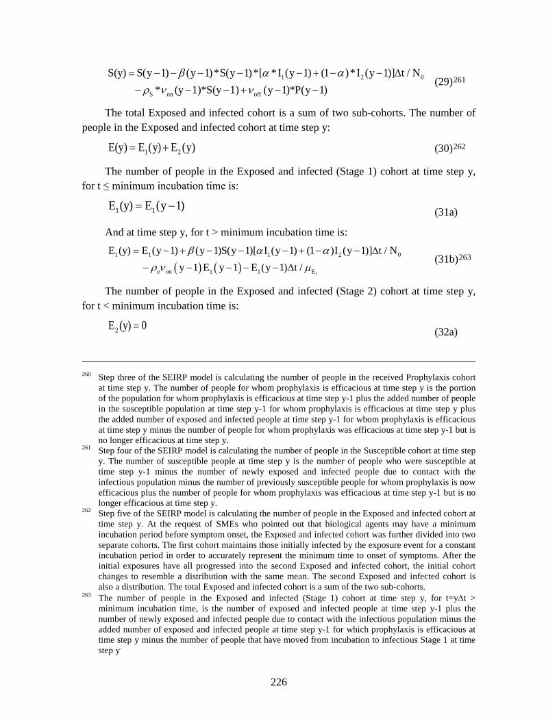
226
1 2 0
S on off
S(y) S(y 1) (y 1)*S(y 1)*[ *I (y 1) (1 )*I (y 1)] t / N * (y 1)*S(y 1) (y 1)*P(y 1)
β α αρ ν ν
= − − − − − + − − ∆− − − + − −
(29)261
The total Exposed and infected cohort is a sum of two sub-cohorts. The number of people in the Exposed and infected cohort at time step y:
1 2E(y) E (y) E (y) = + (30)262
The number of people in the Exposed and infected (Stage 1) cohort at time step y, for t ≤ minimum incubation time is:
1 1E (y) E (y 1) = − (31a)
And at time step y, for t > minimum incubation time is:
( ) ( )1
1 1 1 2 0
e on 1 1 E
E (y) E (y 1) (y 1)S(y 1)[ I (y 1) (1 )I (y 1)] t / N y 1 E y 1 E (y 1) t /
β α αρ ν µ
= − + − − − + − − ∆
− − − − − ∆ (31b)263
The number of people in the Exposed and infected (Stage 2) cohort at time step y, for t < minimum incubation time is:
2E (y) 0 = (32a)
260 Step three of the SEIRP model is calculating the number of people in the received Prophylaxis cohort
at time step y. The number of people for whom prophylaxis is efficacious at time step y is the portion of the population for whom prophylaxis is efficacious at time step y-1 plus the added number of people in the susceptible population at time step y-1 for whom prophylaxis is efficacious at time step y plus the added number of exposed and infected people at time step y-1 for whom prophylaxis is efficacious at time step y minus the number of people for whom prophylaxis was efficacious at time step y-1 but is no longer efficacious at time step y.
261 Step four of the SEIRP model is calculating the number of people in the Susceptible cohort at time step y. The number of susceptible people at time step y is the number of people who were susceptible at time step y-1 minus the number of newly exposed and infected people due to contact with the infectious population minus the number of previously susceptible people for whom prophylaxis is now efficacious plus the number of people for whom prophylaxis was efficacious at time step y-1 but is no longer efficacious at time step y.
262 Step five of the SEIRP model is calculating the number of people in the Exposed and infected cohort at time step y. At the request of SMEs who pointed out that biological agents may have a minimum incubation period before symptom onset, the Exposed and infected cohort was further divided into two separate cohorts. The first cohort maintains those initially infected by the exposure event for a constant incubation period in order to accurately represent the minimum time to onset of symptoms. After the initial exposures have all progressed into the second Exposed and infected cohort, the initial cohort changes to resemble a distribution with the same mean. The second Exposed and infected cohort is also a distribution. The total Exposed and infected cohort is a sum of the two sub-cohorts.
263 The number of people in the Exposed and infected (Stage 1) cohort at time step y, for t=y∆t > minimum incubation time, is the number of exposed and infected people at time step y-1 plus the number of newly exposed and infected people due to contact with the infectious population minus the added number of exposed and infected people at time step y-1 for which prophylaxis is efficacious at time step y minus the number of people that have moved from incubation to infectious Stage 1 at time step y.

227
At time step y, for t = minimum incubation time,
2 1E (y) E (y 1)= − (32b)
And at time step y, for t > minimum incubation,
1 22 2 1 E 2 EE (y) E (y 1) E (y 1) t / E (y 1) t /µ µ= − + − ∆ − − ∆ (32c)
21 1 2 E 1 1I (y) I (y 1) E (y 1) t / I (y 1) t /µ µ= − + − ∆ − − ∆ (33)264
2 2 1 1 2 2I (y) I (y 1) I (y 1) t / I (y 1) t /µ µ= − + − ∆ − − ∆
(34)265
2 2R(y) R(y 1) I (y 1) t / µ= − + − ∆
(35)266
f fR (y) *R(y)p=
(36)267
21,new 2 EI (y) E (y 1) t / µ= − ∆
(37a)
or
2,new 1 1I (y) I (y 1) t / µ= − ∆ (37b)268
f,new f 2 2R (y) *(I (y 1) t / )p µ= − ∆
(38)269
Calculations may be stopped at t = the day at which the transmission factor goes to zero plus the average time-course of disease (µE1 + µE2 + µ1 + µ2).
264 Step six of the SEIRP model is calculating the number of people in the Stage 1 Infectious cohort at
time step y. The number of people in infectious Stage 1 at time step y is the number of infectious people in Stage 1 at time step y-1 plus the number of people that have moved from incubation to infectious Stage 1 at time step y minus the number of people that have moved from infectious Stage 1 to infectious Stage 2 at time step y.
265 Step seven of the SEIRP model is calculating the number of people in the Stage 2 Infectious cohort at time step y. The number of people in infectious Stage 2 at time step y is the number of infectious people in Stage 2 at time step y-1 plus the number of people that have moved from infectious Stage 1 to infectious Stage 2 at time step y minus the number of people that have been removed at time step y.
266 Step eight of the SEIRP model is calculating the number of people in the Removed cohort at time step y. The total number of people removed at time step y is the number of people who were previously removed plus the number of people that have been removed at time step y.
267 To calculate Rf(y), multiply R(y) times the probability of death following disease transmission. 268 Step nine of the SEIRP model is calculating the number of new casualties at time step y. The number
of people who become new casualties at time step y is the number of exposed and infected people at time step y (or for a higher severity level—infectious in the previous stage at time step y) times the time period divided by the mean time of incubation (or infectiousness at Stage 1).
269 Step ten of the SEIRP model is calculating the number of new fatalities at time step y. The number of people who becomes new fatalities at time step y is the number of infectious people in Stage 2 at time step y times the time period divided by the mean time of infectiousness at Stage 2.
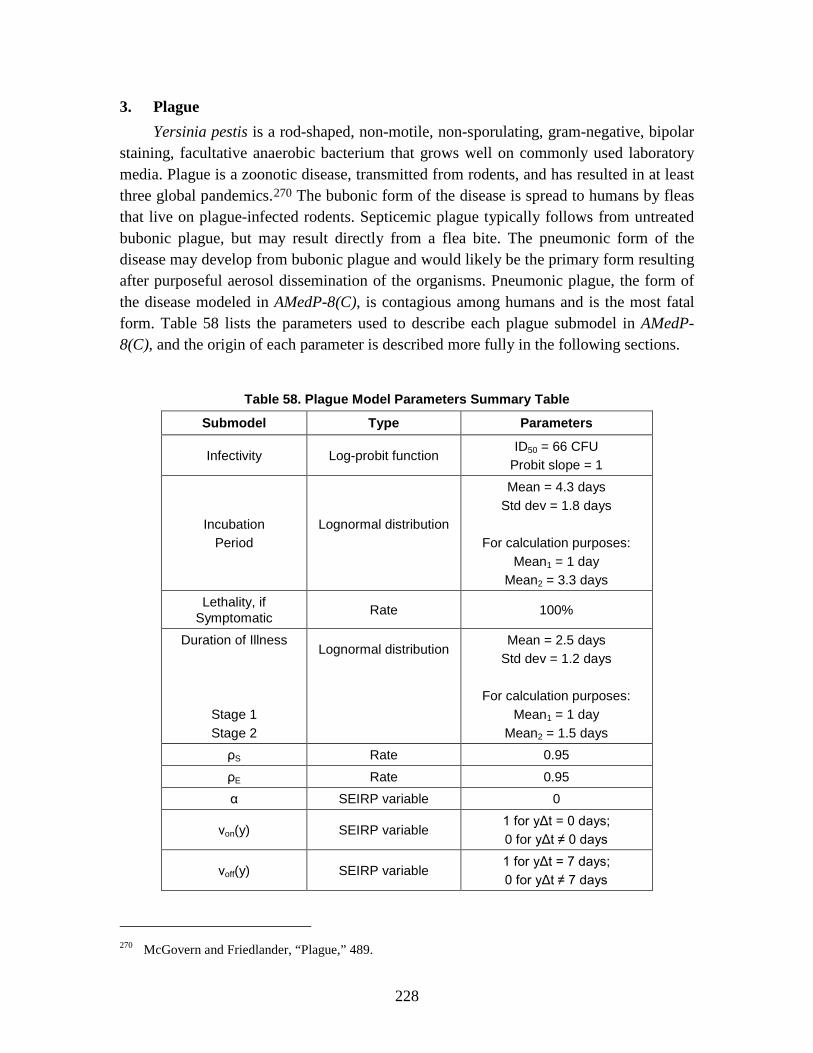
228
3. Plague Yersinia pestis is a rod-shaped, non-motile, non-sporulating, gram-negative, bipolar
staining, facultative anaerobic bacterium that grows well on commonly used laboratory media. Plague is a zoonotic disease, transmitted from rodents, and has resulted in at least three global pandemics.270
The bubonic form of the disease is spread to humans by fleas that live on plague-infected rodents. Septicemic plague typically follows from untreated bubonic plague, but may result directly from a flea bite. The pneumonic form of the disease may develop from bubonic plague and would likely be the primary form resulting after purposeful aerosol dissemination of the organisms. Pneumonic plague, the form of the disease modeled in AMedP-8(C), is contagious among humans and is the most fatal form. Table 58 lists the parameters used to describe each plague submodel in AMedP-8(C), and the origin of each parameter is described more fully in the following sections.
Table 58. Plague Model Parameters Summary Table
Submodel Type Parameters
Infectivity Log-probit function ID50 = 66 CFU
Probit slope = 1
Incubation Period
Lognormal distribution
Mean = 4.3 days Std dev = 1.8 days
For calculation purposes:
Mean1 = 1 day Mean2 = 3.3 days
Lethality, if Symptomatic Rate 100%
Duration of Illness
Stage 1 Stage 2
Lognormal distribution
Mean = 2.5 days Std dev = 1.2 days
For calculation purposes:
Mean1 = 1 day Mean2 = 1.5 days
ρS Rate 0.95
ρE Rate 0.95
α SEIRP variable 0
νon(y) SEIRP variable 1 for yΔt = 0 days; 0 for yΔt ≠ 0 days
νoff(y) SEIRP variable 1 for yΔt = 7 days; 0 for yΔt ≠ 7 days
270 McGovern and Friedlander, “Plague,” 489.
229
a. Infectivity The documented median infectious and lethal doses for plague vary widely, from
tens to tens of thousands. One median dose commonly cited in the literature is 2x10⁴ CFU, although this and other numbers are largely based on data that are 30 to 50 years old from experiments that were conducted in the monkey and murine models. 271 Current research, however, seems to suggest that some of these values may be far too high; cynomolgus macaque research indicates that the median lethal dose may be as low as 66272 to 75 CFU.273
Because the median lethal dose and the median infectious dose are roughly equivalent, plague research generally focuses on lethality. While additional infectivity and lethality values were recommended by SMEs and in the literature, the value recommended originally was 2x10⁴ CFU based on the work of several authors.
274 The value from Speck is 2x10⁴ inhaled cells for experiments on rhesus macaques (note, however, problems exist with the use of these data as noted below).275 Friedlander provides values from experiments conducted in two strains (Wild type CO92 and Java9) of Swiss mice: 2.3x10⁴ and 3.7x10⁴ CFUs respectively. These are aerosolized exposures.276
It should be noted that in the same document that Friedlander provides LD50 values for mice on the order of 104, he also says, “In some species like the mouse, the LD50 of <10 organisms suggests there is little or no intrinsic natural resistance to plague…”
277
271 R. S. Speck and H. Wolochow, “Studies on the Experimental Epidemiology of Respiratory Infections:
Experimental Pneumonic Plague in Macacus rhesus,” Journal of Infectious Diseases 100, no. 1 (1957): 58–99; Arthur M. Friedlander et al., “Relationship between Virulence and Immunity as Revealed in Recent Studies of F1 Capsule of Yersinia pestis,” Clinical Infectious Diseases 21, Supplement 2 (October 1995): S178–S181; and S. L. Welkos et al., “Studies on the Contribution of the F1 Capsule-Associated Plasmid pFra to the Virulence of Yersinia pestis,” Contributions to Microbiology and Immunology 13 (1995): 299–305.
It is unclear from this reading if this is meant to imply a ratio of organisms to CFU on the order of 1: several tens of thousands. According to Brubaker, the original citation of the
272 Roger Van Andel et al., “Clinical and Pathologic Features of Cynomolgus Macaques (Macaca fascicularis) Infected with Aerosolized Yersinia pestis,” Comparative Medicine 58, no. 1 (2009): 68–75.
273 R. C. Layton et al., “Comparison of Two Non Human Primate Pneumonic Plague Models,” Poster presented at the 6th Annual American Society for Microbiology Biodefense and Emerging Diseases Research Meeting (Albuquerque, NM: Lovelace Respiratory Research Institute, 2008).
274 Speck and Wolochow, “Experimental Pneumonic Plague”; Friedlander et al., “Virulence and Immunity”; and Welkos et al., “Contributions of the F1 Capsule.”
275 Speck and Wolochow, “Experimental Pneumonic Plague,” 59. 276 Friedlander et al., “Virulence and Immunity,” S179. 277 Ibid., S178.
230
<10 organisms value,278
Welkos reports the LD50 for CO92 strain in Swiss mice as 2.3x10⁴;
the median lethal dosage of <10 organisms is intended to refer to various routes of intravenous exposure.
279 however, it appears that this is not the result of a second study but rather a reiteration of the results from the same study published by Friedlander. If this is the case, then these are not separate references to the same value but one reference with a citation back to the original data. The Welkos data also include results from studies in African green monkeys; these data refer to tests with several different CO92 strains and indicate an LD50 one to two orders of magnitude higher than indicated by other studies, potentially, depending on the strain of CO92.280
In studies on the efficacy of vaccines and antibiotics, alone and in combination, for plague in rhesus macaques, researchers estimated the LD50 at 20,000 organisms; this number, however, may not be valid for use in a population with no medical countermeasures.
The respiratory LD50 of the 139L strain of Past. pestis [Yersinia pestis] for the rhesus monkey was estimated on a group size of 182, consisting of animals pooled from several titrations and from unvaccinated controls. They were tabulated with their individual dose and grouped into dose ranges…; the average dose and the survival rate for the animals within each group was calculated, this average dose then being taken as the dose for all animals within the group. An LD50 of 2.0x10⁴ inhaled cells was obtained…281
The problem is that the 182 monkeys for which this dose is estimated include vaccinated and unvaccinated animals. Therefore, this LD50 may not be applicable to the unvaccinated population of monkeys alone. If the vaccine was efficacious it would result in some inherent elevation of the LD50. Because the ratio of mortality in vaccinated monkeys to unvaccinated monkeys was 50% to 83%, it does appear that the vaccine was somewhat efficacious.
282
Log-probit distributions represented by median lethal/infective dose values and probit slopes are generally accepted methods of approximating infectivity for biological agents. None of the three studies cited, however, specifically refers to the use of a lognormal distribution; the studies only list the median lethal doses for aerosol exposure to plague.
278 Robert R. Brubaker, “Factors Promoting Acute and Chronic Diseases Caused by Yersiniae,” Clinical
Microbiology Reviews 4, no. 3 (July 1991): 312. 279 Welkos et al., “Contributions of the F1 Capsule.” 280 Ibid. 281 Speck and Wolochow, “Experimental Pneumonic Plague,” 59. 282 Ibid., 58–69.

231
Based on a recent symposium which recommended a thorough characterization of the cyomolgus macaque as an animal model for plague, researchers investigated the median infectious dose for these monkeys. Researchers exposed 22 Indonesian-origin cynomolgus macaques to doses ranging from 12 to 42,700 CFU of yersinia pestis. Seventeen developed plague; 2 of the 17 died with no premonitory signs or symptoms. The remaining 5 remained plague-free—with no bacteriologic, gross, or histologic evidence of plague infection—at doses less than 250 CFU. Using a logistic regression, the authors calculated the dose at which half of the macaques developed fever and clinical symptoms to be 66 CFU.283
For pneumonic plague, the median infectious dose is assumed to be equal to the median lethal dose (i.e., ID50 = LD50). For lack of additional data, a probit slope of 1 probit/log dose is assumed; this probit value assumes that 1 plague organism = 1 plague CFU. Thus, infectivity in AMedP-8(C) is modeled as a log-probit function with a probit slope of 1 probit/log dose and a median infectious dose of 66 CFU.
284
b. Incubation Period
The incubation period is assumed to be represented by a lognormal distribution with a mean of 4.3 days and a standard deviation of 1.8 days.285
For use in the SEIRP methodology, the incubation is further divided into two stages. The first stage represents the minimum time to symptom onset; for plague, this value is assumed to be 1 day. The second stage has a mean of the remaining 3.3 days.
Because the plague incubation period model is part of the SEIRP framework and the SEIRP distributions approximate exponential distributions, the lognormal mean of 4.3 days is assumed to be applicable for the SEIRP representation of the incubation period.
c. Lethality Evidence indicates that once infected, individuals who remain untreated will likely
die. “The reported case fatality rate is close to 100%.”286 Additional studies have shown similar results—all animals, either monkey or murine, showing symptoms of infection eventually die as a result of the infection if untreated.287
283 Van Andel et al., “Clinical and Pathologic Features.”
Thus, AMedP-8(C) models a 100% mortality rate for pneumonic plague.
284 Ibid., 68. 285 Gani and Leach, “Modeling Pneumonic Plague Outbreaks,” 608–9. 286 Ibid., 609. 287 Lathem et al., “Progression of Primary Pneumonic Plague”; and Kool, “Risk of Person-to-Person
Transmission.”
232
d. Duration of Illness and Injury Profile Plague is a biphasic disease, with the end of Stage 1 (the prodromal period) and the
beginning of Stage 2 marked by the onset of coughing.288 A literature search was conducted in search of duration of illness data from epidemiological studies and published models of such data. Recent analyses of epidemiological data give similar estimates of duration of illness for pneumonic plague. Gani and Leach derived a lognormal distribution with a mean of 2.5 days (std. 1.5 days) from eight outbreaks;289 Nishiura found a mean of 2.3 days (std. 1.7 days) using data from the Manchuria outbreak,290 while Bombardt derived a lognormal distribution with mean of 2.34 days (std. 1.07 days) from the Manchuria outbreak.291
Bombardt pointed out that in the cases of the 1965 Vietnam and 1997 Madagascar outbreaks, antibiotic treatments were employed, and he speculated that the range in means and standard deviations may be due in part to differences in sample size and Y. pestis strain. These differences could perhaps explain the difference in means between the estimates of Bombardt and Gani and Leach for overlapping data.
Based on the available literature, the total length of illness for plague is assumed to be represented by a lognormal distribution with a mean of 2.5 days and a standard deviation of 1.2 days. The plague length of illness model is part of the SEIRP framework. For the convenience of modeling, the lognormal mean of 2.5 days is assumed to be applicable for the SEIRP representation (as an exponential distribution) of the length of illness, and the means of Stage 1 and Stage 2 are assumed to be 1 day292
The course of illness is described by several as two distinct stages:
and 1.5 days respectively. The first stage of illness is assumed to be non-infective; during the second stage of illness, the patient is highly infectious.
…progresses rapidly from a febrile flu-like illness to an overwhelming pneumonia with coughing and the production of bloody sputum.293
[The prodromal period is] characterized by the sudden onset of severe headaches, chills, malaise, and increased respiratory and heart rates. Body temperature rises steadily during this initial stage…Generally cough [marking the onset of the second stage] develops after 20–24 h, and it is
288 Gani and Leach, “Modeling Pneumonic Plague Outbreaks,” 608–9. 289 Ibid., 609. 290 Hiroshi Nishiura et al., “Transmission Potential of Primary Pneumonic Plague: Time Inhomogeneous
Evaluation Based on Historical Documents of the Transmission Network,” Journal of Epidemiology Community Health 60 (2006): 643.
291 Bombardt, Primary Pneumonic Plague Transmission. 292 Thomas V. Inglesby et al., “Plague as a Biological Weapon: Medical and Public Health Management,”
Journal of the American Medical Association 283, no. 17 (May 2000): 2283–85. 293 Robert D. Perry and Jacqueline D. Fetherston, “Yersinia pestis—Etiologic Agent of Plague,” Clinical
Microbiology Reviews 10, no. 1 (January 1997): 58.

233
dry at first but becomes progressions productive…over time it becomes increasingly blood-stained and/or purulent. In the final stage (one to several hours before death), the patient produces copious amounts of bright red sputum…294
The onset of the disease is sudden and often marked by rigor. The first stage is characterized by the presence of general signs only; cough is most often still absent; when present, it is usually dry. The prominent symptoms during this period are severe headache, some nausea and vomiting, vertigo and general malaise. Both respiration and pulse show an increased rate; the pulse is early impaired in quality. The temperature, which is but slightly raised at the beginning of the illness, rises steadily during the first stage… The beginning of the second stage is manifested by the appearance of cough or—if this is already present—by that of expectoration. The cough is dry and seldom troublesome at first, but when continuous may exhaust the patient. The sputum shows at first no characteristic appearance, being mainly frothy. Soon, however, there is an admixture with blood, leading to a uniform bright pink or red hue. Now the sputum may be either thin, sometimes frothy or of more syrup-like consistency; but the degree of viscosity typical for croupous pneumonia is not reached. The quantity of bloody sputum varies greatly from mere streaks of red to ounces of deep red blood comparable to that seen in hemorrhage in phthisis (tuberculosis). During the first stage, few if any signs may be detected over the lungs; now symptoms of pneumonia become evident…Death occurs from heart failure. Sometimes there is a marked stage of agony characterized either by more or less protracted coma and symptoms of lung edema or by restlessness and active delirium.
295
The first stage of illness may include several symptoms including fever with cough and dyspnea, including bloody, watery, or purulent sputum as well as nausea, vomiting, and other gastrointestinal symptoms. The second stage closely resembles other late stage pneumonias.
296
An injury severity level of 2 has been assigned to the first stage of illness. Injury Severity Level 2 is moderate—effectively requiring the affected individual to seek medical attention as an outpatient. The first stage of illness is characterized by headache, general muscle pain, weakness, and possibly nausea and vomiting.
An injury severity level of 4 has been assigned to the second stage of illness. Injury Severity Level 4 is very severe—requiring intensive or critical care of the affected individual without which (and possibly following which) the individual would become a
294 Kool, “Risk of Person-to-Person Transmission,” 1167. 295 Lien-Teh Wu, A Treatise on Pneumonic Plague, C.H.474 (Geneva: League of Nations Health
Organization, May 1926). 296 Inglesby et al., “Plague as a Biological Weapon,” 2283–85.
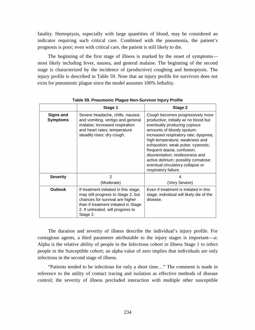
234
fatality. Hemoptysis, especially with large quantities of blood, may be considered an indicator requiring such critical care. Combined with the pneumonia, the patient’s prognosis is poor; even with critical care, the patient is still likely to die.
The beginning of the first stage of illness is marked by the onset of symptoms—most likely including fever, nausea, and general malaise. The beginning of the second stage is characterized by the incidence of (productive) coughing and hemoptysis. The injury profile is described in Table 59. Note that an injury profile for survivors does not exist for pneumonic plague since the model assumes 100% lethality.
Table 59. Pneumonic Plague Non-Survivor Injury Profile
Stage 1 Stage 2
Signs and Symptoms
Severe headache, chills, nausea and vomiting, vertigo and general malaise; increased respiration and heart rates; temperature steadily rises; dry cough.
Cough becomes progressively more productive, initially w/ no blood but eventually producing copious amounts of bloody sputum; increased respiratory rate; dyspnea; high temperature; weakness and exhaustion; weak pulse; cyanosis; frequent ataxia; confusion; disorientation; restlessness and active delirium; possibly comatose; eventual circulatory collapse or respiratory failure.
Severity 2 (Moderate)
4 (Very Severe)
Outlook If treatment initiated in this stage, may still progress to Stage 2, but chances for survival are higher than if treatment initiated in Stage 2. If untreated, will progress to Stage 2.
Even if treatment is initiated in this stage, individual will likely die of the disease.
The duration and severity of illness describe the individual’s injury profile. For contagious agents, a third parameter attributable to the injury stages is important—α. Alpha is the relative ability of people in the Infectious cohort in illness Stage 1 to infect people in the Susceptible cohort; an alpha value of zero implies that individuals are only infectious in the second stage of illness.
“Patients tended to be infectious for only a short time…” The comment is made in reference to the utility of contact tracing and isolation as effective methods of disease control; the severity of illness precluded interaction with multiple other susceptible

235
people and therefore likely only spread to those caring for the contagious individual.297 In the review of Manchurian epidemic cases, there appeared to be an early period of disease during which patients were non-contagious or “non-infective,” and that only after the late stage of the disease onset, did individuals become infectious.298
“Owing to the absence of cough and expectoration during the first stage of the disease, patients are practically non-infective.”
299
Summarizing Wu, Kool indicates that there is a ~24 hour non-infective period (assumed to roughly coincide with the first stage of illness), after which patients in the late-stage of illness could infect other people after prolonged and close contact.
300 Summarizing the research of Teague and Strong, Kool indicates that coughing appears to be the primary method by which aerosolized plague is spread; only a very limited fraction (1 of 39) of the sampled non-coughing patients respirated plague bacteria which could be captured and grown on a culture plate.301
Transmission apparently occurs through direct contact or through inhalation of airborne droplets expelled by coughing persons…Patients in the early stage of pneumonic plague (approximately the first 20–24 h) apparently pose little risk. This is likely because of the low counts of bacteria in their respiratory secretions and the general absence of coughing.
302
These results indicate that during the first stage of illness, an infected individual is unlikely to be infectious; only during the second stage of illness, when coughing and expectoration occur, is an individual likely to be infectious to other susceptible individuals. Thus, an alpha value of 0, indicating low likelihood of infectiousness during Stage 1 and high likelihood of infectiousness during Stage 2, is modeled, as shown in Table 60.
Table 60. Plague Alpha Value
α 0
297 Gani and Leach, “Modeling Pneumonic Plague Outbreaks,” 610. 298 Kool, “Risk of Person-to-Person Transmission,” 1167–68. Kool was citing Wu’s descriptions,
originally published in 1926. 299 Lien-Teh, Treatise on Pneumonic Plague. 300 Kool, “Risk of Person-to-Person Transmission,” 1167. 301 Ibid., 1170. 302 Ibid., 1171.

236
e. Medical Countermeasures The plague methodology utilizes an antibiotic prophylaxis model. Both the pre-
exposure methodology and the long-term equation used in the SEIRP model may be required to sufficiently model the application of plague prophylaxis: 1) plague vaccines, where available, may be used prior to exposure,303 and 2) antibiotic regimens may be begun immediately post-exposure and continued for some period post-exposure.304 According to the Blue Book,305
As antibiotic prophylaxis is recommended for individuals exposed to and potentially exposed to plague aerosol, the efficacy of antibiotic prophylaxis in those who are already exposed and will become infected with plague and in those who are susceptible to plague as a result of transmission-caused infections is assumed to be the same. The course of medication most commonly recommended within NATO nations is ciprofloxacin, which has been shown in multiple mouse studies, when administered up to 24 hours post-exposure, to prevent mortality due to plague; additional medications may be considered with similar or slightly reduced efficacy.
antibiotic prophylaxis should be provided to “persons possibly exposed to a plague aerosol (i.e., in a plague [biological warfare] BW attack).” Although there is not currently a known, approved plague vaccine, multiple nations are working on developing an F1-V antigen vaccine. At the time of the Medical Aspects of Biological Warfare publication, in 2007, the United Kingdom already had a vaccine in clinical trials. Therefore, no values are recommended for vaccine efficacy; however, the potential use of the pre-exposure prophylaxis model is retained for countries which either have or are considering vaccine employment.
306 The proposed antibiotic efficacy—95%—is based on additional, independent analysis of the Russell and Byrne data for ciprofloxacin conducted by Bombardt.307
303 Patricia L. Worsham et al., “Plague,” in Medical Aspects of Biological Warfare, ed. Zygmunt F.
Dembek, Textbook of Military Medicine (Washington, DC: Department of Defense, Office of the Surgeon General, U.S. Army, Borden Institute, 2007), 112–13; and Darling, Robert G., and Jon B. Woods, eds. USAMRIID’s Medical Management of Biological Casualties Handbook, 5th ed. (Ft. Detrick, MD: U.S. Army Medical Research Institute for Infectious Diseases, 2004), 44.
Further, although published studies indicate a 100% efficacy for ciprofloxacin, the recommended value of 95% efficacy accounts for the potential inclusion of other recommended antibiotics with slightly lower efficacy for use as plague post-exposure prophylaxis. The recommended efficacy, and start and stop days are listed in Table 61.
304 Worsham, et. al., “Plague,” 112–13. 305 Darling and Woods, Medical Management of Biological Casualties, 44. 306 P. Russell et al., “Doxycycline or Ciprofloxacin Prophylaxis and Therapy against Experimental
Yersinia pestis Infection in Mice,” Journal of Antimicrobial Chemotherapy 37 (1996): 769–74; P. Russell et al., “Efficacy of Doxycycline and Ciprofloxacin against Experimental Yersinia pestis Infection,” Journal of Antimicrobial Chemotherapy 41 (1998): 301–5; and William R. Byrne et al., “Antibiotic Treatment of Experimental Pneumonic Plague in Mice,” Antimicrobial Agents and Chemotherapy 42, no. 3 (March 1998): 675–81.
307 Bombardt, Primary Pneumonic Plague Transmission.

237
Table 61. Antibiotic Prophylaxis Efficacy and Course
ρS 0.95
ρE 0.95
νon(y) 1 for yΔt = 0 days; 0 for yΔt ≠ 0 days
νoff(y) 1 for yΔt = 7 days; 0 for yΔt ≠ 7 days
f. Transmission Rate The foregoing description of the SEIRP epidemic model presumes that a time-
varying disease transmission rate, β, is at the disposal of the modeler. The rate of disease transmission is essentially the product of (a) the conditional probability of infection (given an “adequate” contact) and (b) the number of adequate contacts per unit time. Both the conditional probability of infection and the rate of adequate contacts can change as an epidemic unfolds. For example, the conditional probability of infection can vary during an epidemic if the disease-causing microorganism mutates and becomes more or less able to overcome the host’s defensive mechanisms. Perhaps more importantly, the contact rate tends to fluctuate with day-to-day human activities, a growing public awareness of an ongoing outbreak, behavioral modifications due to this awareness, etc.
The time dependence of disease transmission is unknown a priori. But the epidemic curve (number of new cases per unit time) and other epidemiological information from a pertinent historical outbreak can be used in conjunction with an appropriate epidemic model to quantify the causative time-varying transmission rate. By assumption, such a derived historical transmission rate is representative of what could happen in a military population.
The 1946 outbreak of primary pneumonic plague in Mukden (now called Shenyang), China began when a man from another Russian-occupied district arrived in Mukden by train and began his stay with relatives on the 25th of February. He became ill on the 26th and died on the 27th of February. This fatal index case of primary pneumonic plague led to 35 other fatal cases and three non-fatal cases. Because this outbreak did not begin with a precursory case of bubonic plague and a secondary plague pneumonia, and because Mukden was free of plague for the previous 25 years, local medical practitioners did not recognize primary pneumonic plague and they attributed 8 deaths (over 10 days) to pneumonia. Even so, under difficult wartime conditions, a thorough (albeit delayed) program of traditional outbreak controls prevented the spread of disease beyond Mukden. In passing, note that a limited quantity of sulfadiazine became available to Mukden
238
physicians 12 days before the outbreak’s conclusion (on the 30th of March); all 3 survivors of primary pneumonic plague were recipients of that drug.308
Returning to the SEIRP epidemic model and the finite difference equation that defines E1, it is apparent that the number of new transmission-caused infections at time t = y*∆t is as follows:
1 2 0Q(y) (y 1)* (y 1)*[ *I (y 1) (1 )*I (y 1)]* t / NSβ α α= − − − + − − ∆ (39)
The epidemic curve for the 1946 primary pneumonic plague outbreak in Mukden and data describing the incubation period distribution are sufficient to directly quantify Q. A straightforward back-projection technique309
In deriving β for the historical outbreak of interest, the averaged Monte Carlo results for Q were first inserted into the SEIRP epidemic model (in the absence of prophylaxis) and then calculated to obtain the outbreak’s S, E, I and R cohorts over time. Quantified S, I1 and I2 cohorts, along with averaged Monte Carlo results for Q, were then utilized in the above equation in order to calculate the time-varying β. Table 62 indicates the derived time dependence of β.
and a Monte Carlo algorithm enable this direct quantification. Three basic steps characterize each Monte Carlo trial. First, obtain a random incubation or latent period for every onset of illness (i.e., every new case) that occurs on a given day of the historical outbreak (excluding the index case). Second, backtrack in time to identify when all infections began. And third, compile the total score for each time step. Averaging scores per day for a large number of Monte Carlo trials then yields a mean time-dependent number of new infections that is suitable for use in a deterministic or mean-field derivation of β.
308 Ibid. 309 Niels G. Becker and Xu Chao, “Dependent HIV Incidences in Back-Projection of AIDS Incidence
Data,” Statistics in Medicine 13 (1994): 1945–58.

239
Table 62. Plague Transmission Rate (Mukden, China)
Days after initial
exposures β value
Days after initial
exposures β value
0 0 21 0.250477
1 0 22 0.213678
2 1.399368 23 0.129681
3 2.114316 24 0.073931
4 3.924383 25 0.190478
5 4.323217 26 0.468109
6 3.461722 27 0.554607
7 1.027207 28 0.44357
8 1.27051 29 0.34088
9 2.046092 30 0.348683
10 2.311747 31 0.239461
11 2.272985 32 0.131417
12 1.955047 33 0.016763
13 1.639616 34 0
14 1.723586 35 0
15 1.751387 36 0
16 1.53121 37 0
17 1.120241 38 0
18 0.629848 39 0
19 0.375698 40 0
20 0.269083
4. Smallpox Smallpox is caused by the Orthopox virus, variola, which occurs in at least two
strains, variola major and variola minor. While poxviruses infect many zoonotic hosts, the variola virus is limited to humans. A global eradication campaign, combined with continued availability of vaccine, resulted in the disease’s eradication; the last naturally occurring case of smallpox was in Somalia in 1977. Despite this, the potential use of variola as a biological weapon continues to pose a military threat. This threat can be attributed to the aerosol infectivity of the virus, the relative ease of large-scale
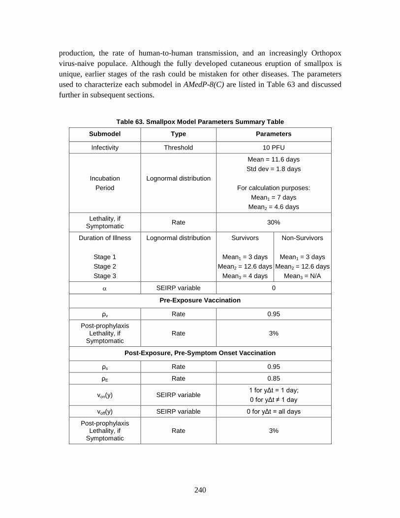
240
production, the rate of human-to-human transmission, and an increasingly Orthopox virus-naive populace. Although the fully developed cutaneous eruption of smallpox is unique, earlier stages of the rash could be mistaken for other diseases. The parameters used to characterize each submodel in AMedP-8(C) are listed in Table 63 and discussed further in subsequent sections.
Table 63. Smallpox Model Parameters Summary Table
Submodel Type Parameters
Infectivity Threshold 10 PFU
Incubation Period
Lognormal distribution
Mean = 11.6 days Std dev = 1.8 days
For calculation purposes:
Mean1 = 7 days Mean2 = 4.6 days
Lethality, if Symptomatic Rate 30%
Duration of Illness
Stage 1 Stage 2 Stage 3
Lognormal distribution
Survivors
Mean1 = 3 days Mean2 = 12.6 days
Mean3 = 4 days
Non-Survivors
Mean1 = 3 days Mean2 = 12.6 days
Mean3 = N/A
α SEIRP variable 0
Pre-Exposure Vaccination
ρv Rate 0.95
Post-prophylaxis Lethality, if
Symptomatic Rate 3%
Post-Exposure, Pre-Symptom Onset Vaccination
ρs Rate 0.95
ρE Rate 0.85
νon(y) SEIRP variable 1 for yΔt = 1 day; 0 for yΔt ≠ 1 day
νoff(y) SEIRP variable 0 for yΔt = all days
Post-prophylaxis Lethality, if
Symptomatic Rate 3%

241
Although smallpox may manifest as one of four types—ordinary, modified, hemorrhagic, and flat—ordinary type smallpox was selected as representative of the incubation and illness durations, as well as the signs and symptoms of smallpox as it occurs most frequently. Approximately 88% of all the potential smallpox cases are ordinary type.310
a. Infectivity
Ordinary type smallpox appears to be representative of the median injury profile; modified smallpox symptoms are milder, while hemorrhagic and flat smallpox symptoms are more severe.
There are few experimental data regarding smallpox infectivity. Because smallpox is specifically a human disease, it has, thus far, been impossible to develop an appropriate animal model for infectivity. Research suggests that a virus is a single particle and that individual particles, deposited in the correct location, can cause infection.311
Note that in planning for Dark Winter, a Top Officials Exercise, the infectious dose of smallpox was assumed to be low based on a 1999 article by Henderson, et al.
This single deposited particle must likely be one of a number of inhaled particles that are retained in the lungs.
312 Henderson cited a 1970 study of a smallpox epidemic in a Meschede, Germany hospital, saying, “The infectious dose is unknown but is believed to be only a few virions.”313 The cited article, however, makes no specific reference to infectious dose; rather, the low required infectious dose is likely inferred from the disease spread and a smoke experiment showing the spread through the hospital.314
The only cited values for smallpox infectivity that the authors were able to locate were those published in reference to clinical recognition and management of multiple biological agents. The document cites an “assumed low (10–100 organisms)” infectious dose.
315
With no published data to support or challenge the value cited by Franz, et al., infectivity is modeled as a threshold dose-response probability function: if the dose is greater than or equal to 10 PFU, an individual is considered exposed at sufficient dose
No specific reference is given for this value.
310 Rao, Smallpox. 311 Robert F. Parker, “Statistical Studies of the Nature of the Infectious Unit of Vaccine Virus,” Journal of
Experimental Medicine 67, no. 5 (1938): 726; and F. Fenner et al., Smallpox and its Eradication (Geneva, Switzerland: World Health Organization, 1988), 187–88.
312 Tara O’Toole, Michael Mair, and Thomas V. Inglesby, “Shining Light on ‘Dark Winter’,” Clinical Infectious Diseases 34, no. 7 (2002): 972–83.
313 Donald A. Henderson et al., “Smallpox as a Biological Weapon: Medical and Public Health Management,” Journal of the American Medical Association 281, no. 22 (June 1999): 2129.
314 P. F. Wehrle et al., “An Airborne Outbreak of Smallpox in a German Hospital and its Significance with Respect to Other Recent Outbreaks in Europe,” Bulletin of the World Health Organization 43, no. 5 (1970): 669–79.
315 Franz et al., “Clinical Recognition and Management,” 400–401.

242
that the individual will become infected (probability of infection is 1); if the dose is less than 10 PFU, it is not anticipated that the individual received a high enough dose to be considered exposed and infected, and therefore the individual will not develop the disease as a result of the inhalation exposure (the probability of infection is 0). The threshold infectious dose of smallpox is a conservative selection based on the assumed infectious dose range of 10–100 organisms.316
b. Incubation Period
Because smallpox is a contagious disease, and one not well-modeled by an existing animal model, it is difficult to determine an exact incubation period. Data collected from multiple outbreaks suggest that the typical incubation period for smallpox is 10–14 days but may be as short as 7 days or as long as 19 days.317
The incubation period length is derived from 232 cases of ordinary-type smallpox resulting from variola major exposure. These cases were compiled from two data sets. One set of data was prepared for the World Health Organization
318 and consisted of a study of 175 cases spread across Kosovo, Serbia, Voivodina, and Montenegro; the incubation period for 171 of these cases was captured. The second data set was compiled from 898 cases of both variola major and variola minor collected by multiple authors;319
the incubation period for 65—61 of which were unvaccinated—of these cases (variola major only) was captured as shown as shown in Table 64. Only unvaccinated cases were considered in the calculation of the incubation period.
316 Ibid. 317 Fenner et al., Smallpox and its Eradication, 188. 318 S. Litvinjenko, B. Arsic, and S. Borjanovic, “Epidemiologic Aspects of Smallpox in Yugoslavia in
1972,” Bulletin of the World Health Organization, WHO/SE/73.57 (1973). 319 A. W. Downie, “Incubation Period in Smallpox,” Bulletin of the World Health Organization,
WHO/SE/72.3 (1972).

243
Table 64. Incubation Period Data Collected in Literature
Length of incubation period (days)
Number of Cases
Litvinjenko Downie
7 1 0
8 5 3
9 20 3
10 26 3
11 39 5
12 39 12
13 27 18
14 6 9
15 7 7
16 1 0
17 0 1
Total Patients 171 61
Using these values, the incubation period is represented by a lognormal distribution with a mean of 11.6 days and a standard deviation of 1.8 days.320
For use in the SEIRP methodology, the incubation is further divided into two stages. The first stage represents the minimum time to symptom onset; for smallpox, this value is assumed to be 7 days.
Because the smallpox incubation period model is part of the SEIRP framework and the SEIRP distributions approximate exponential distributions, the lognormal mean of 11.6 days is assumed to be applicable for the SEIRP representation of the incubation period.
321
c. Lethality
The second stage has a mean of the remaining 4.6 days.
Lethality is modeled as rate of 30% if symptomatic of smallpox and unvaccinated. For individuals who are vaccinated and symptomatic, lethality is assumed to be 3%.322
These values are based on data collected during an outbreak in India; the data include 6,941 cases (shown in Table 65).
320 Gani and Leach, “Modeling Pneumonic Plague Outbreaks,” 608–9. 321 Fenner et al., Smallpox and its Eradication, 188; Martin I. Meltzer et al., “Modeling Potential
Responses to Smallpox as a Bioterrorist Weapon,” Emerging Infectious Diseases 7, no. 6 (2001): 959; and Litvinjenko, Arsic, and Borjanovic, “Epidemiologic Aspects of Smallpox,” 3.
322 Rao, Smallpox, 37–39; and Fenner et al., Smallpox and its Eradication, 40.

244
Table 65. Smallpox Case Fatality Rates (CFR) by Type and Vaccination Status
Vaccinal Status
Hemorrhagic Flat Ordinary Modified Total
Cases CFR Cases CFR Cases CFR Cases CFR Cases CFR
Unvaccinated 22 100 120 99.1 1296 36.9 15 0 1453 42.61%
Unsuccessfully vaccinated 59 96.6 88 96.6 1425 27.2 16 0 1588 33.35%
Primarily vaccinated after exposure to smallpox 4 100 28 96.4 426 20.6 44 0 502 23.65%
With primary vaccination scars only 111 94 45 66.7 2302 3.3 808 0 3266 6.44%
With primary and revaccination scars 4 100 0 0 75 0 53 0 132 3.03%
To calculate the unvaccinated and vaccinated case fatality rates, only ordinary smallpox was considered. Vaccinated status was indicated by the presence of the post-vaccination scar, while the unvaccinated category included all others (unvaccinated, unsuccessfully vaccinated (no scar), and vaccinated after primary exposure). These data are shown in Table 66 below.
Table 66. Smallpox Case Fatality Rates by Type and Vaccination Status
Vaccinal Status Ordinary
Unvaccinated Vaccinated
Cases Fatal
Cases CFR Cases Fatal
Cases CFR
Unvaccinated 1296 478 36.9
With primary vaccination scars only 2302 76 3.3
Unsuccessfully vaccinated 1425 388 27.2
With primary and revaccination scars 75 0 0
Primarily vaccinated after exposure to smallpox 426 88 20.6
Total 3147 954 30.30 Total 2377 76 3.20

245
The AMedP-8(C) methodology allows for consideration of the effects of pre-exposure and post-exposure, pre-symptom onset vaccination for smallpox (discussed below). The case fatality rate for both methods of vaccination is assumed to be the same, although post-exposure vaccination would be expected to have a higher case fatality rate. (The case fatality rate data in Table 66 from cases primarily vaccinated after exposure to smallpox was not used directly because it was not clear whether vaccination was administered before or after the onset of symptoms.) Use of the pre-exposure vaccination, therefore, leads to a worst-case scenario for planning purposes with more people remaining in the medical system. The use of the pre-exposure vaccination case fatality rate may result in an underestimation of the number of fatalities.
d. Length of Illness and Injury Profile Smallpox is described as a tri-phasic disease for survivors and a bi-phasic disease
for non-survivors as shown in Tables 67 and 68. Following the incubation period, both profiles begin with Stage 1—a prodromal, febrile period—then progress to Stage 2—the rash stage with the outbreak of the maculopapular rash. Survivors progress to Stage 3—the recovery stage with scab formation and eventual scab separation.323 A literature search was conducted to determine duration of illness data. Researchers and clinical reports typically indicate that the enanthem—or the beginning of the rash—which marks the transition from Stage 1 to Stage 2 occurs 1 to 3 days after symptom onset.324
The smallpox prodromal period begins with the onset of fever and ends with the onset of the rash. Historical cases suggest that the prodromal period duration is approximately the same, independent of whether an individual becomes a fatality or survives the disease and independent of smallpox type.
325 Reviewing data from several data sources and using temperature, versus enanthem, as the stage differentiator, Fenner reported that the prodromal stage lasts 3 days.326 Likewise, Bombardt calculated a 3 day mean prodromal period with a standard deviation of 0.95 days.327 Other mean prodromal duration values ranged from 2.49 days (with a standard deviation of 0.88 days)328
323 Franz et al., “Clinical Recognition and Management,” 404–5.
to 3
324 Ibid., 404; and Henderson et al., “Smallpox as a Biological Weapon,” 2129. 325 Henderson et al., “Smallpox as a Biological Weapon,” 2129 –30; Fenner et al., Smallpox and its
Eradication; Rao, Smallpox, 11–12; Peter B. Jahrling et al., “Smallpox and Related Orthopoxviruses,” in Medical Aspects of Biological Warfare, ed. Zygmunt F. Dembek, Textbook of Military Medicine (Washington, DC: Department of Defense, Office of the Surgeon General, U.S. Army, Borden Institute, 2007): 215–40.
326 Fenner et al., Smallpox and its Eradication, as cited by Meltzer et al., “Modeling Potential Responses to Smallpox,” 960.
327 Bombardt, Smallpox Transmission. 328 Martin Eichner and Klaus Dietz, “Transmission Potential of Smallpox: Estimates Based on Detailed
Data from an Outbreak,” American Journal of Epidemiology 158, no. 2 (2003): 113.
246
days.329 The actual duration of the prodromal stage is hard to determine exactly because it relies “in part on the ability of the physician or the patient to detect the first lesion.”330
The second stage of smallpox illness begins with the appearance of the first rash lesion and ends with death for non-survivors or scab formation and eventual scab separation for survivors. Eichner and Dietz estimated the mean duration of this stage as 16 days,
331 while Rao suggests a shorter duration of 12 to 14 days post-symptom onset, or 10 to 12 days post-Stage 1.332 Meltzer, et al., found the duration of the second stage to be between 10 to 15 days in length.333 Based on available literature and conversations with subject matter experts,334
Only survivors enter Stage 3. The duration of the third stage—from the time that scabs begin to form until scabs are separating—is assumed to be 4 days. Neither the first nor the third stage are infectious. For smallpox, in the SEIRP model, survivors entering Stage 3 are considered to have entered the Removed (medical) cohort.
the total length of the second stage is estimated to be 12.6 days.
The course of illness is described by several as two to three stages.
Dixon described two stages: pre-eruptive and eruption. The pre-eruptive stage is marked by the sudden onset of fever and malaise; symptoms similar to influenza may manifest in as little as an hour. Although unlikely, a small fraction of the population may exhibit a rash during this period. The rash begins in the mouth and throat, and then spreads to the body. It may spread uniformly or it may move downward from the face. The end result is a rash which “is more uniform in color than the rash of measles, has a centrifugal distribution, and quickly becomes papular.”335
During the first stage, the disease may be difficult to diagnose based on clinical symptoms which include fever and malaise, possibly accompanied by vomiting, muscle ache, and/or headache. The suddenness of onset is one mark of the disease, with patients progressing from feeling well to feeling flu-like within an hour.
336
329 Based on case studies collected by Justus Strom and Bo Zetterberg, Smallpox Outbreak and
Vaccination Problems in Stockholm, 1963 (Stockholm, Kungl. Boktryckeriet P.A. Norstedt & Soner, 1966), 45–56.
330 Meltzer et al., “Modeling Potential Responses to Smallpox,” 960. 331 Eichner and Dietz, “Transmission Potential of Smallpox,” 113. 332 Rao, Smallpox, 22. 333 Meltzer et al., “Modeling Potential Responses to Smallpox,” 960. 334 12.6 days based on disease progression as described by Fenner et al., Smallpox and its Eradication and
Rao, Smallpox and conversations with Dr. John Bombardt, May 2009. 335 C. W. Dixon et al., “Smallpox in Tripolitania, 1946: An Epidemiological and Clinical Study of 500
Cases, Including Trials of Penicillin Treatment,” The Journal of Hygiene 46, no. 4 (December 1948): 360–61.
336 Franz et al., “Clinical Recognition and Management,” 404.

247
The second stage of illness is marked by the formation or eruption of a macular rash; the exact onset of the second stage may be difficult to determine clinically because it requires identification of the earliest lesions which may form in the larynx or mouth and may not be easily visible. While most experts agree that the rash begins in the mouth and throat, there is disagreement about how the rash spreads. Some explain that it moves downward from the face to the trunk and hands and then the feet. Others state that the rash forms first at the extremities and moves inward towards the trunk. The rash is distinguished from measles and other pox virus rashes by the centrifugal pattern and near uniformity of the macules. As the disease progresses, the rash becomes papular and then pustular.337 Death, if it occurs, usually occurs in the second week of illness as a result of “toxemia associated with circulating immune complexes and soluble variola antigens.”338
“In the second week after onset, the pustules form scabs that leave depressed depigmented scars on healing,”
339
The first stage of illness may include several flu-like symptoms including fever, malaise, loss of appetite, and fatigue. The second stage is defined by the progression of the rash from macular to papular. The third stage, in survivors, involves the formation and eventual separation of scabs.
denoting survivors’ progression into the third stage of illness.
An injury severity level of 2 has been assigned to the first stage of illness. Injury Severity Level 2 is moderate—effectively requiring the affected individual to seek medical attention as an outpatient. The first stage of illness is characterized by fever and general flu-like symptoms, possibly with muscle or backache, headache, and vomiting.
In survivors, injury severity levels of 3 and 1 have been assigned to the second and third stages of illness respectively. Injury Severity Level 3 is Severe—requiring medical care as an inpatient. Injury Severity Level 1 is Mild—the manifestation of symptoms that may be considered “nuisance symptoms” and would usually only be anticipated to require self- or buddy-aid.
For non-survivors, an injury severity level of 4 has been assigned to the second stage of illness. Injury Severity Level 4 is very severe—requiring intensive or critical care of the affected individual without which (and possibly following which) the individual would become a fatality. The immune response during the early stages of the
337 Ibid. 338 Henderson et al., “Smallpox as a Biological Weapon,” 2130. 339 Franz et al., “Clinical Recognition and Management,” 404.
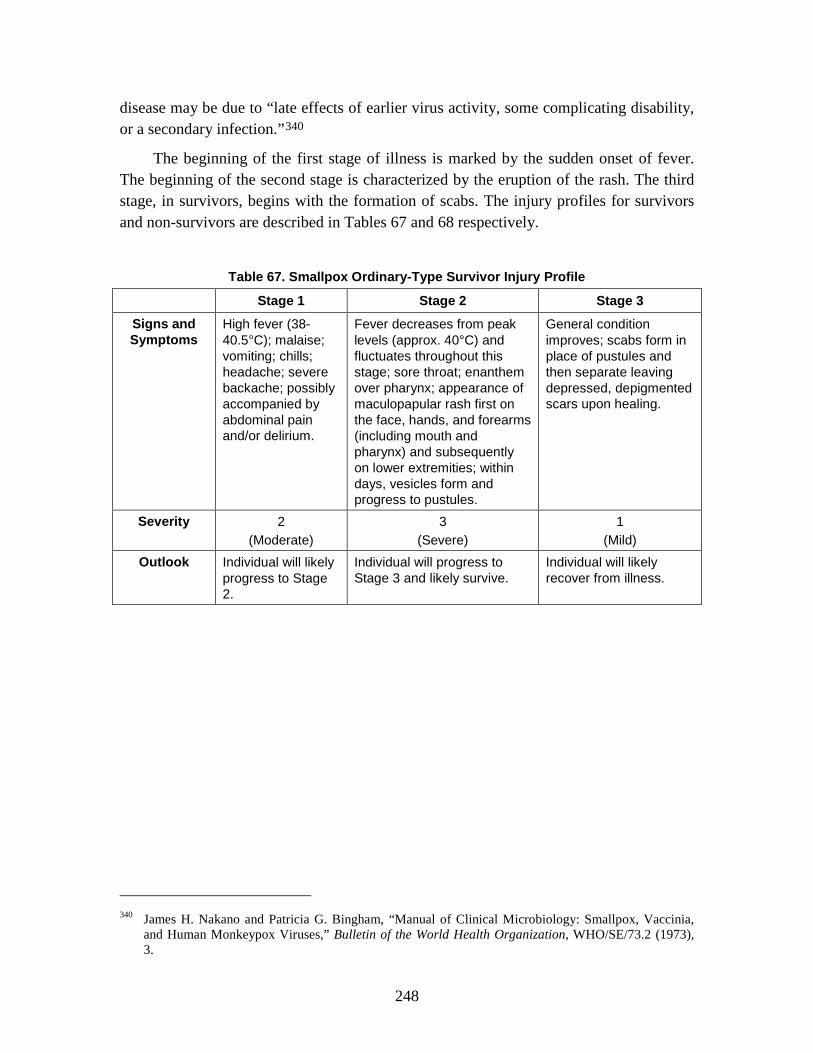
248
disease may be due to “late effects of earlier virus activity, some complicating disability, or a secondary infection.”340
The beginning of the first stage of illness is marked by the sudden onset of fever. The beginning of the second stage is characterized by the eruption of the rash. The third stage, in survivors, begins with the formation of scabs. The injury profiles for survivors and non-survivors are described in Tables 67 and 68 respectively.
Table 67. Smallpox Ordinary-Type Survivor Injury Profile
Stage 1 Stage 2 Stage 3
Signs and Symptoms
High fever (38-40.5°C); malaise; vomiting; chills; headache; severe backache; possibly accompanied by abdominal pain and/or delirium.
Fever decreases from peak levels (approx. 40°C) and fluctuates throughout this stage; sore throat; enanthem over pharynx; appearance of maculopapular rash first on the face, hands, and forearms (including mouth and pharynx) and subsequently on lower extremities; within days, vesicles form and progress to pustules.
General condition improves; scabs form in place of pustules and then separate leaving depressed, depigmented scars upon healing.
Severity 2 (Moderate)
3 (Severe)
1 (Mild)
Outlook Individual will likely progress to Stage 2.
Individual will progress to Stage 3 and likely survive.
Individual will likely recover from illness.
340 James H. Nakano and Patricia G. Bingham, “Manual of Clinical Microbiology: Smallpox, Vaccinia,
and Human Monkeypox Viruses,” Bulletin of the World Health Organization, WHO/SE/73.2 (1973), 3.
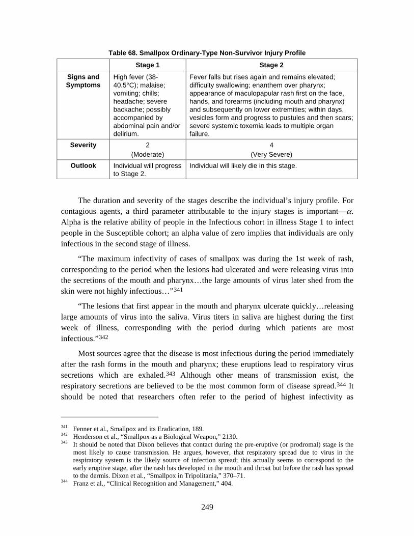
249
Table 68. Smallpox Ordinary-Type Non-Survivor Injury Profile
Stage 1 Stage 2
Signs and Symptoms
High fever (38-40.5°C); malaise; vomiting; chills; headache; severe backache; possibly accompanied by abdominal pain and/or delirium.
Fever falls but rises again and remains elevated; difficulty swallowing; enanthem over pharynx; appearance of maculopapular rash first on the face, hands, and forearms (including mouth and pharynx) and subsequently on lower extremities; within days, vesicles form and progress to pustules and then scars; severe systemic toxemia leads to multiple organ failure.
Severity 2 (Moderate)
4 (Very Severe)
Outlook Individual will progress to Stage 2.
Individual will likely die in this stage.
The duration and severity of the stages describe the individual’s injury profile. For contagious agents, a third parameter attributable to the injury stages is important—α. Alpha is the relative ability of people in the Infectious cohort in illness Stage 1 to infect people in the Susceptible cohort; an alpha value of zero implies that individuals are only infectious in the second stage of illness.
“The maximum infectivity of cases of smallpox was during the 1st week of rash, corresponding to the period when the lesions had ulcerated and were releasing virus into the secretions of the mouth and pharynx…the large amounts of virus later shed from the skin were not highly infectious…”341
“The lesions that first appear in the mouth and pharynx ulcerate quickly…releasing large amounts of virus into the saliva. Virus titers in saliva are highest during the first week of illness, corresponding with the period during which patients are most infectious.”
342
Most sources agree that the disease is most infectious during the period immediately after the rash forms in the mouth and pharynx; these eruptions lead to respiratory virus secretions which are exhaled.
343 Although other means of transmission exist, the respiratory secretions are believed to be the most common form of disease spread.344
341 Fenner et al., Smallpox and its Eradication, 189.
It should be noted that researchers often refer to the period of highest infectivity as
342 Henderson et al., “Smallpox as a Biological Weapon,” 2130. 343 It should be noted that Dixon believes that contact during the pre-eruptive (or prodromal) stage is the
most likely to cause transmission. He argues, however, that respiratory spread due to virus in the respiratory system is the likely source of infection spread; this actually seems to correspond to the early eruptive stage, after the rash has developed in the mouth and throat but before the rash has spread to the dermis. Dixon et al., “Smallpox in Tripolitania,” 370–71.
344 Franz et al., “Clinical Recognition and Management,” 404.

250
occurring during “the first week of illness.” This often coincides with the assumption that illness actually begins with rash formation and disregards the febrile symptoms observed during the prodromal period. Mack, Thomas, and Khan summarized this by stating, “in none [of the curves depicting disease transmission] is there a suggestion of significant transmission during the prodromal period.”345
These results indicate that during the prodromal or first stage of illness, an infected individual is unlikely to be infectious; only during the second stage of illness, when the rash in the mouth results in high virus titers and respiratory secretions result in exhalation of active virii, is an individual expected to be infectious to other susceptible individuals. Thus, an alpha value of 0, indicating low likelihood of infectiousness during Stage 1 and high likelihood of infectiousness during Stage 2, is modeled as indicated in Table 69.
Table 69. Smallpox Alpha Value
α 0
Data suggest that during the entire course of infection, the basic reproduction number, or the number of individuals that an infectious individual is likely to infect, is between approximately three and seven. That number increases to ten to twelve when hospital-associated cases are included; hospital-associated cases occurred as a result of hospitalization of early smallpox cases—prior to disease recognition—where infection-control measures had not yet been established.346
e. Medical Countermeasures
The smallpox vaccine contains vaccinia virus, a live poxvirus that induces protection against smallpox. The vaccine is currently licensed for pre-exposure use only; however, “vaccination administered within the first few days after exposure and perhaps as late as four days may prevent or significantly ameliorate subsequent illness.”347 Pre-exposure vaccination, often—but not always—combined with isolation and quarantine, played a crucial role in the control of historical outbreaks and eventual eradication of smallpox.348
345 Thomas M. Mack, David B. Thomas, and M. Muzaffar Khan, “Epidemiology of Smallpox in West
Pakistan: II. Determinants of Intravillage Spread Other than Acquired Immunity,” American Journal of Epidemiology 23, no. 2 (1972): 169–77.
346 Raymond Gani and Steve Leach, “Transmission Potential of Smallpox in Contemporary Populations,” Nature 414 (2001): 748–51.
347 Henderson et al., “Smallpox as a Biological Weapon,” 2132. 348 Fenner et al., Smallpox and its Eradication, 590.
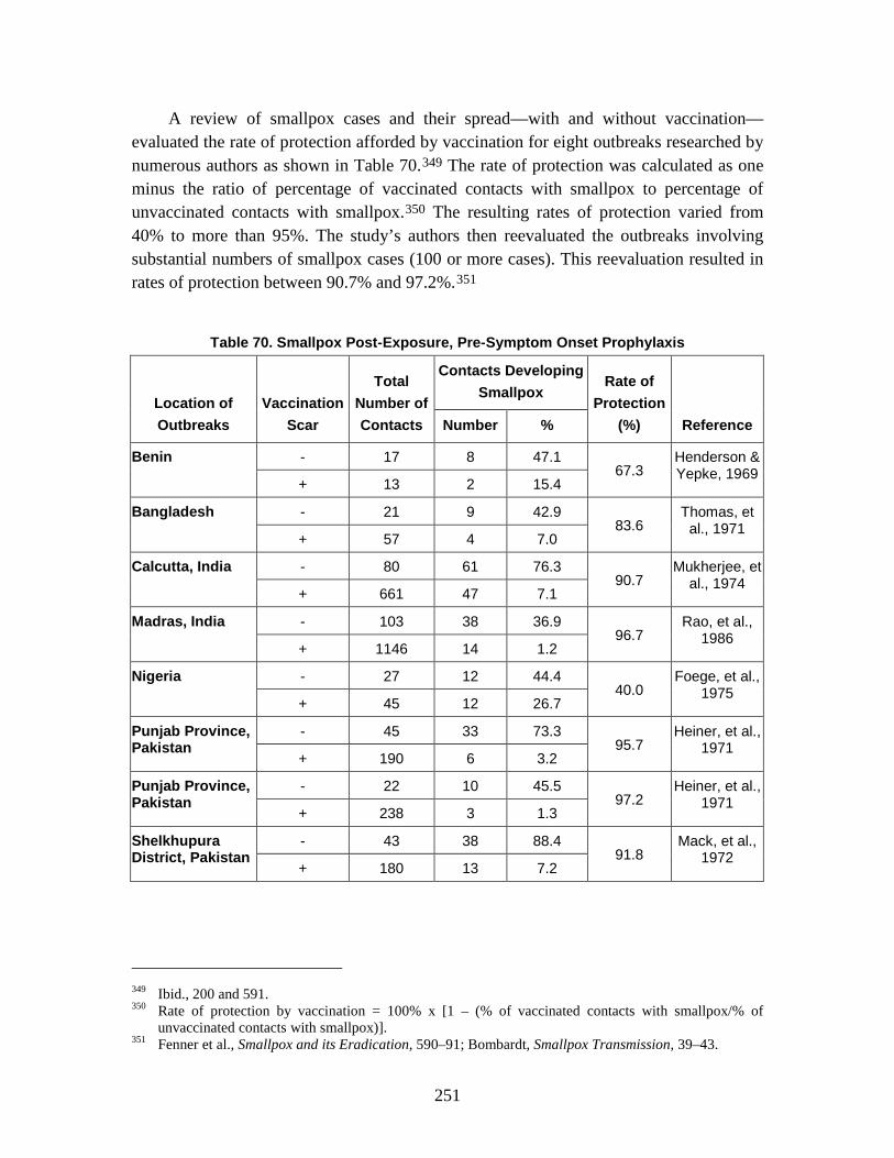
251
A review of smallpox cases and their spread—with and without vaccination—evaluated the rate of protection afforded by vaccination for eight outbreaks researched by numerous authors as shown in Table 70.349 The rate of protection was calculated as one minus the ratio of percentage of vaccinated contacts with smallpox to percentage of unvaccinated contacts with smallpox.350 The resulting rates of protection varied from 40% to more than 95%. The study’s authors then reevaluated the outbreaks involving substantial numbers of smallpox cases (100 or more cases). This reevaluation resulted in rates of protection between 90.7% and 97.2%.351
Table 70. Smallpox Post-Exposure, Pre-Symptom Onset Prophylaxis
Location of Outbreaks
Vaccination Scar
Total Number of Contacts
Contacts Developing Smallpox
Rate of Protection
(%) Reference Number %
Benin - 17 8 47.1 67.3
Henderson & Yepke, 1969
+ 13 2 15.4
Bangladesh - 21 9 42.9 83.6
Thomas, et al., 1971
+ 57 4 7.0
Calcutta, India - 80 61 76.3 90.7
Mukherjee, et al., 1974
+ 661 47 7.1
Madras, India - 103 38 36.9 96.7
Rao, et al., 1986
+ 1146 14 1.2
Nigeria - 27 12 44.4 40.0
Foege, et al., 1975
+ 45 12 26.7
Punjab Province, Pakistan
- 45 33 73.3 95.7
Heiner, et al., 1971
+ 190 6 3.2
Punjab Province, Pakistan
- 22 10 45.5 97.2
Heiner, et al., 1971
+ 238 3 1.3
Shelkhupura District, Pakistan
- 43 38 88.4 91.8
Mack, et al., 1972
+ 180 13 7.2
349 Ibid., 200 and 591. 350 Rate of protection by vaccination = 100% x [1 – (% of vaccinated contacts with smallpox/% of
unvaccinated contacts with smallpox)]. 351 Fenner et al., Smallpox and its Eradication, 590–91; Bombardt, Smallpox Transmission, 39–43.
252
The mean rate of protection afforded by vaccination—when only the outbreaks with 100 cases or greater were considered—was calculated to be 94.4%. For ease of calculation, a pre-exposure and susceptible vaccination efficacy of 95% is modeled in AMedP-8(C).
For vaccination in individuals already exposed and infected but not yet showing symptoms, vaccine efficacy one day post-exposure is assumed to be either 90% or 85%.352 An efficacy of 85% was selected for modeling in AMedP-8(C) to yield a conservative estimate of vaccine efficacy. Researchers disagree on the actual efficacy of vaccines given post-exposure. Vaccines given shortly post-exposure (within 4 days) are anticipated to confer some level of efficacy,353 but the longer the duration between exposure and vaccination, the lower the expected efficacy.354 Table 71 shows just a few examples of the variation of rates of protection as a function of duration between exposure and post-exposure vaccination.355 While the exact conditions associated with these values are not known, they do demonstrate that, consistently, some level of increased protection is afforded by vaccinating even after exposure. Further, although the model assumes that all cases manifest as ordinary type, one study author noted that there was an increased rate of modified (less severe) smallpox manifested (~9%) in vaccinated individuals who still manifested smallpox symptoms as compared with those who had never been vaccinated (~1%).356
352 Bombardt, Smallpox Transmission, 41. 353 Henderson et al., “Smallpox as a Biological Weapon,” 2132. 354 Dixon et al., “Smallpox in Tripolitania,” 370. 355 Fenner et al., Smallpox and its Eradication, 591. 356 Ibid.; and Rao, Smallpox, 143.
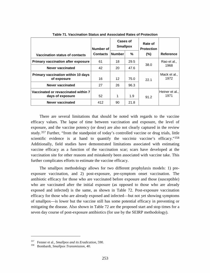
253
Table 71. Vaccination Status and Associated Rates of Protection
Vaccination status of contacts
Number of Contacts
Cases of Smallpox
Rate of Protection
(%) Reference Number %
Primary vaccination after exposure 61 18 29.5 38.0
Rao et al., 1968
Never vaccinated 42 20 47.6
Primary vaccination within 10 days of exposure 16 12 75.0 22.1
Mack et al., 1972
Never vaccinated 27 26 96.3
Vaccinated or revaccinated within 7 days of exposure 52 1 1.9 91.2
Heiner et al., 1971
Never vaccinated 412 90 21.8
There are several limitations that should be noted with regards to the vaccine efficacy values. The lapse of time between vaccination and exposure, the level of exposure, and the vaccine potency (or dose) are also not clearly captured in the review study.357 Further, “from the standpoint of today’s controlled vaccine or drug trials, little scientific evidence is at hand to quantify the vaccinia vaccine’s efficacy.”358
The smallpox methodology allows for two different prophylaxis models: 1) pre-exposure vaccination, and 2) post-exposure, pre-symptom onset vaccination. The antibiotic efficacy for those who are vaccinated before exposure and those (susceptible) who are vaccinated after the initial exposure (as opposed to those who are already exposed and infected) is the same, as shown in Table 72. Post-exposure vaccination efficacy for those who are already exposed and infected—but not yet showing symptoms of smallpox—is lower but the vaccine still has some potential efficacy in preventing or mitigating the disease. Also shown in Table 72 are the proposed start and stop times for a seven day course of post-exposure antibiotics (for use by the SEIRP methodology).
Additionally, field studies have demonstrated limitations associated with estimating vaccine efficacy as a function of the vaccination scar; scars have developed at the vaccination site for other reasons and mistakenly been associated with vaccine take. This further complicates efforts to estimate the vaccine efficacy.
357 Fenner et al., Smallpox and its Eradication, 590. 358 Bombardt, Smallpox Transmission, 40.

254
Table 72. Smallpox Post-Exposure, Pre-Symptom Onset Antibiotic Prophylaxis Efficacy and Course
Pre-Exposure Vaccination
ρv 0.95
Post-Exposure, Pre-Symptom Onset Vaccination
ρS 0.95
ρE 0.85
νon(y) 1 for yΔt = 1 day; 0 for yΔt ≠ 1 day
νoff(y) 0 for yΔt = all days
f. Transmission Rate The authors previously discussed the time dependence of the disease transmission
rate during an epidemic and we mentioned the fact that it is not known beforehand. On the other hand, the epidemic curve for a carefully-selected historical outbreak and additional epidemiological data can be coupled with an epidemic model to determine a driving time-dependent rate of disease transmission. And with regard to either primary pneumonic plague or smallpox, it is assumed that such an historical transmission rate is at least indicative of potential outbreak dynamics in a military population.
Of particular interest here is the 1972 smallpox outbreak in Yugoslavia.359
The derivation of a time-dependent β for an historical smallpox outbreak is essentially the same as that for an historical outbreak of primary pneumonic plague. One important common feature is the characterization of the incubation period distribution in Monte Carlo calculations. Random draws from a lognormal (or other familiar continuous) distribution may well yield unrealistic incubation periods: either shorter than the shortest observed period or longer than the longest observed period. To preclude unrealistic incubation periods in Monte Carlo calculations, the authors utilized a triangular
From 1932 to 1972, Yugoslavian health care systems did not have to deal with smallpox cases and this smallpox-free period of 40 years undoubtedly fostered a false sense of security. Even though vaccinations of Yugoslavian children continued unabated, the declining vaccinal state of Yugoslavia’s adult population was an important factor behind the 1972 outbreak, which began with a single index case and involved a total of 175 smallpox cases.
359 Bombardt, Smallpox Transmission.
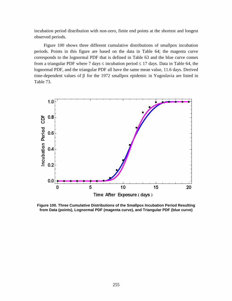
255
incubation period distribution with non-zero, finite end points at the shortest and longest observed periods.
Figure 100 shows three different cumulative distributions of smallpox incubation periods. Points in this figure are based on the data in Table 64; the magenta curve corresponds to the lognormal PDF that is defined in Table 63 and the blue curve comes from a triangular PDF where 7 days ≤ incubation period ≤ 17 days. Data in Table 64, the lognormal PDF, and the triangular PDF all have the same mean value, 11.6 days. Derived time-dependent values of β for the 1972 smallpox epidemic in Yugoslavia are listed in Table 73.
Figure 100. Three Cumulative Distributions of the Smallpox Incubation Period Resulting
from Data (points), Lognormal PDF (magenta curve), and Triangular PDF (blue curve)
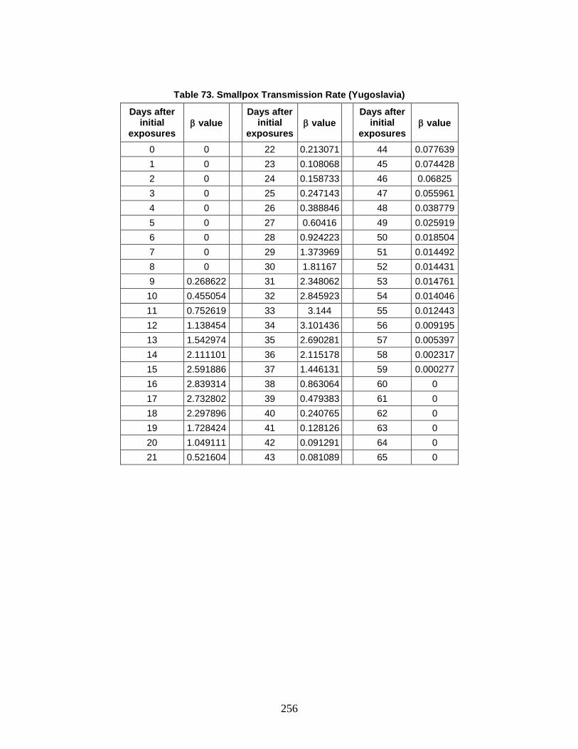
256
Table 73. Smallpox Transmission Rate (Yugoslavia)
Days after initial
exposures β value
Days after initial
exposures β value
Days after initial
exposures β value
0 0 22 0.213071 44 0.077639 1 0 23 0.108068 45 0.074428 2 0 24 0.158733 46 0.06825 3 0 25 0.247143 47 0.055961 4 0 26 0.388846 48 0.038779 5 0 27 0.60416 49 0.025919 6 0 28 0.924223 50 0.018504 7 0 29 1.373969 51 0.014492 8 0 30 1.81167 52 0.014431 9 0.268622 31 2.348062 53 0.014761 10 0.455054 32 2.845923 54 0.014046 11 0.752619 33 3.144 55 0.012443 12 1.138454 34 3.101436 56 0.009195 13 1.542974 35 2.690281 57 0.005397 14 2.111101 36 2.115178 58 0.002317 15 2.591886 37 1.446131 59 0.000277 16 2.839314 38 0.863064 60 0 17 2.732802 39 0.479383 61 0 18 2.297896 40 0.240765 62 0 19 1.728424 41 0.128126 63 0 20 1.049111 42 0.091291 64 0 21 0.521604 43 0.081089 65 0
257
9. Casualty Estimation
The outputs of the human response estimation component are used in the third and final step of the AMedP-8(C) methodology—the casualty estimation component—to determine casualty status as categorized by killed in action (KIA), wounded in action (WIA), and died of wounds (DOW). This chapter provides the rationale and sources for the recommended values and special procedures used in the casualty estimation component of the AMedP-8(C) methodology, which is described in Chapter 4 of the AMedP-8(C) NATO Planning Guide.
A. Estimation of Casualties: General Considerations
1. Recommended Time to Reach a Medical Treatment Facility Because the definitions of KIA and DOW rely on the casualty reaching a medical
treatment facility, the first step in the casualty estimation process is defining the time at which a medical treatment facility is available, measured relative to t0 (the beginning of the event that results in an exposure). In most cases, the time to reach a medical treatment facility is modeled as a fixed time and one that is the same for everyone in the scenario. The recommended value of 30 minutes was chosen based upon the consensus of NATO SMEs across the series of review meetings held for the purpose of developing the AMedP-8(C) methodology.360
2. Recommended Wounded in Action (WIA) Severity Level Threshold
An individual not already classified as a KIA is considered a WIA at the first time t at which the individual’s injury severity level is at or exceeds the user-defined severity level:
IF (NOT KIA) AND (Severity at time t User-Defined Severity Level)), THEN (WIA at time t)
≥ (40)
The first step in estimating WIA is defining the injury severity level at which individuals would be expected to become casualties—that is, the injury severity level that
360 Burr et al., Chemical Human Response SME Review Meeting, 1–71; Burr et al., Nuclear Human
Response SME Review Meeting, 1–31; and Burr et al., Radiological Human Response SME Review Meeting, 1–16.
258
would result in the individual becoming a loss to the unit. The recommended threshold value of WIA(1)—a criterion defining someone as a casualty at Severity Level 1 (“Mild”) or greater—was chosen based upon the consensus of NATO SMEs across the series of review meetings held for the purpose of developing the AMedP-8(C) methodology.361
3. Time at Severity Level 4 (“Very Severe”) to Determine Fatalities
At WIA(1), an individual exhibiting any symptoms is classified as a casualty. This level was chosen as it is the lowest severity level at which any symptoms appear and, therefore, includes the mildest type of casualties. Other, more severe, severity levels and types of casualties can be chosen at the user’s discretion.
For CRN agents, an individual is classified as a fatality if a severity level of 4 is achieved and maintained for fifteen minutes or more. According to the definition of Severity Level 4 (see Table 1 in Chapter 2), individuals at this level have an
[i]njury manifesting symptoms of such severity that life is imminently endangered. Indicators are unfavorable – condition may or may not reverse even with medical intervention; prognosis is death without medical intervention…
Examples of such symptoms include the cessation of breathing, stoppage of the heart, and other immediately life-threatening conditions. It was assumed that most individuals would be dead if they remained in these conditions for fifteen minutes or more. The consensus position of NATO SMEs across the series of review meetings held for the purpose of developing the AMedP-8(C) methodology agreed with this assumption.362
Two exceptions to this rule exist within the AMedP-8(C) methodology. First, since the time to death due to whole-body radiation insults is more sensitive to dose than can be shown in the injury profiles, the dose-dependent time to death value calculated using Equation 43 (discussed in the subsequent section) supersedes the time determined by the rule above for whole-body radiation injury profiles. Second, for biological agents, in order to account for the duration of a disease stage which ends in death, an individual, who is classified as a non-survivor, becomes a fatality when they reach the end of their expected duration of illness or time to death. This does mean they may be at severity level 4 for one or more days.
361 Burr et al., Chemical Human Response SME Review Meeting, 1–71; Burr et al., Nuclear Human
Response SME Review Meeting, 1–31; and Burr et al., Radiological Human Response SME Review Meeting, 1–16.
362 Burr et al., Chemical Human Response SME Review Meeting, 1–71; Burr et al., Nuclear Human Response SME Review Meeting, 1–31; and Burr et al., Radiological Human Response SME Review Meeting, 1–16.
259
B. Estimation of Casualties: Special Considerations
1. Chemical Blister Agent (HD): Percutaneous Liquid Dose and Internal Sepsis Large doses of percutaneous liquid HD damages bone marrow (bone marrow
suppression) and can cause eventual death, in excess of the injury described by the equivalent vapor percutaneous injury profiles. Approximately 1 to 3 weeks post-exposure, the exposed individual’s body begins to deteriorate due to its own suppressed immune system and inability to fight off infection. The individual’s body then becomes septic even without the introduction of secondary/opportunistic infections. The results are potentially fatal. To account for this injury, all icons exposed to percutaneous HD liquid in excess of 1,400 mg/man are estimated to die at 336 hours—the dose and time suggested and agreed to by NATO HD SMEs during the chemical review meeting held for the purpose of developing the AMedP-8(C) methodology.363
2. Radiological Agents: Whole-Body Radiation Dose and the Protracted Dose Calculation
There is evidence that radiation dose protraction (i.e., receiving the same total dose over a longer time period) will result in fewer deaths than if the entire dose is received over a very short period of time. For a given total whole-body radiation dose, the slower that dose is received (i.e., the lower the dose rate) the more time the body’s natural healing mechanisms have to combat its physiological effects. The result is that a lower dose rate will reduce the expected lethality of the total radiation dose. The following equation has been derived that allows for the calculation of a dose protraction correction factor, which, when multiplied by a lethal protracted dose, estimates the dose which, if absorbed nearly instantaneously (i.e., in 0.02 hours), would also result in death. This factor is used only in the estimation of the time to death, and is not used to estimate the altered human response to non-lethal protracted doses of radiation.
363 Burr et al., Chemical Human Response SME Review Meeting, 1–71.
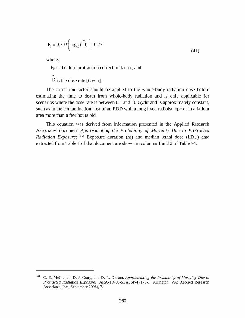
260
P 10F 0.20* log ( D) 0.77• = +
(41)
where:
FP is the dose protraction correction factor, and
D•
is the dose rate [Gy/hr].
The correction factor should be applied to the whole-body radiation dose before estimating the time to death from whole-body radiation and is only applicable for scenarios where the dose rate is between 0.1 and 10 Gy/hr and is approximately constant, such as in the contamination area of an RDD with a long lived radioisotope or in a fallout area more than a few hours old.
This equation was derived from information presented in the Applied Research Associates document Approximating the Probability of Mortality Due to Protracted Radiation Exposures.364
Exposure duration (hr) and median lethal dose (LD50) data extracted from Table 1 of that document are shown in columns 1 and 2 of Table 74.
364 G. E. McClellan, D. J. Crary, and D. R. Oldson, Approximating the Probability of Mortality Due to
Protracted Radiation Exposures, ARA-TR-08-SEASSP-17176-1 (Arlington, VA: Applied Research Associates, Inc., September 2008), 7.
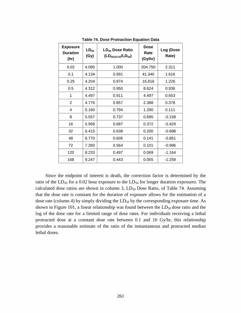
261
Table 74. Dose Protraction Equation Data
Exposure Duration
(hr)
LD50 (Gy)
LD50 Dose Ratio ([email protected]/LD50)
Dose Rate
(Gy/hr)
Log (Dose Rate)
0.02 4.095 1.000 204.750 2.311
0.1 4.134 0.991 41.340 1.616
0.25 4.204 0.974 16.816 1.226
0.5 4.312 0.950 8.624 0.936
1 4.497 0.911 4.497 0.653
2 4.776 0.857 2.388 0.378
4 5.160 0.794 1.290 0.111
8 5.557 0.737 0.695 -0.158
16 5.958 0.687 0.372 -0.429
32 6.415 0.638 0.200 -0.698
48 6.770 0.605 0.141 -0.851
72 7.260 0.564 0.101 -0.996
120 8.233 0.497 0.069 -1.164
168 9.247 0.443 0.055 -1.259
Since the endpoint of interest is death, the correction factor is determined by the ratio of the LD50 for a 0.02 hour exposure to the LD50 for longer duration exposures. The calculated dose ratios are shown in column 3, LD50 Dose Ratio, of Table 74. Assuming that the dose rate is constant for the duration of exposure allows for the estimation of a dose rate (column 4) by simply dividing the LD50 by the corresponding exposure time. As shown in Figure 101, a linear relationship was found between the LD50 dose ratio and the log of the dose rate for a limited range of dose rates. For individuals receiving a lethal protracted dose at a constant dose rate between 0.1 and 10 Gy/hr, this relationship provides a reasonable estimate of the ratio of the instantaneous and protracted median lethal doses.

262
Figure 101. Dose Protraction Correction Factor Derivation
The dose protraction correction factor equation is graphed in Figure 102.
Figure 102. Dose Protraction Correction Factor as a Function of Dose Rate
y = 0.20x + 0.77
0.000
0.200
0.400
0.600
0.800
1.000
1.200
-1.500 -1.000 -0.500 0.000 0.500 1.000 1.500 2.000 2.500
Dos
e Ra
tio
Log(Dose Rate)
0
0.1
0.2
0.3
0.4
0.5
0.6
0.7
0.8
0.9
1
0 1 2 3 4 5 6 7 8 9 10
Dos
e Pr
otra
ctio
n Co
rrec
tion
Fac
tor
Dose Rate (Gy/hr)

263
3. Radiological Agents and Radiation Insults: Whole-Body Radiation and the Time-to-Death Calculation Radiation is unique among agents or insults considered in the casualty estimation
methodology in that data exist to support modeling time-to-death as a function of whole-body radiation dose. This relationship has been well characterized in animal models and human experience, allowing for a deterministic calculation of a whole-body radiation dose-based time-to-death. In developing this approach, several possible methods for estimating radiation-induced time-to-death were considered. Specifically, three approaches were examined: 1) output from the Radiation Induced Performance Decrement (RIPD) methodology; 2) a meta-study conducted by Anno, et al. examining a number of radiation-induced effects, including time-to-death; and 3) a relatively simple straight-line log-log curve derived from the IDP.
The time of death, for the median individual, can be estimated using a formula derived for the RIPD code.365
tdeath = P1P2+(Dwb∗0.7∗100)P3 + P4
P5+(Dwb∗0.7∗100)P6 (42)
The functional form of the equation used to estimate time-to-death in RIPD is shown in the equation below:
where:
tdeath is the time to death in hours, Dwb is the free-in-air dose due to whole-body radiation in gray, and
the Pi values are empirically determined coefficients.
The curve which fits the RIPD data is shown in Figure 103.
365 G. H. Anno, G. E. McClellan, and M. A. Dore, Protracted Radiation-Induced Performance
Decrement, Vol. 1: Model Development, DNA-TR-95-117-V1 (Washington, DC: Defense Nuclear Agency, May 1996).

264
Figure 103. Radiation-Induced Time-to-Death: RIPD Curve
The values of the coefficients found to provide a good fit to the data are: P1 = 8.789 x 10⁸ P4 = 1.9866 x 10⁶
P2 = 1.923 x 10⁶ P5 = 5.8218 x 10³
P3 = 2.4489 P6 = 1.2
In a study conducted in 1989, George Anno, et al. examined multiple estimates of radiation-induced time-to-death and acute radiation syndromes.366
The work concluded that a good fit to the data was provided by a curve developed by Upton, which is shown in Figure 104 along with additional median lethal dose values plotted versus time-to-death.
366 Anno et al., “Symptomatology of Acute Radiation Effects,” 821–38.
1
10
100
1,000
10,000
100 1,000 10,000 100,000
Tim
e to
Dea
th (
Hou
rs)
Acute Radiation Dose - Free in Air (cGy FIA)
RIPD equation

265
Figure 104. Radiation-Induced Time-to-Death: “Upton Curve” and Additional Median Lethal
Dose Value Yields
Finally, the IDP methodology produced output relating time-to-death as a function of radiation dose. The U.S. Army Nuclear and Chemical Agency document, Personnel Risk and Casualty Criteria for Nuclear Weapons Effects, includes a graphical representation of this relationship, shown in Figure 105.367
367 USANCA, Personnel Risk, B-40.
1
10
100
1,000
10,000
100 1,000 10,000 100,000
Tim
e to
Dea
th (
Hou
rs)
Acute Radiation Dose - Free in Air (cGy FIA)
Anno et al 1989 Fig 2Various Sources

266
Figure 105. Radiation-Induced Time-to-Death: IDP Methodology Curve
This curve can be approximated by:
( ) 1.36death wbt 4.1x10 * D *100 −= (43)
where:
tdeath is the time to death in hours, and
Dwb is the free-in-air dose due to whole-body radiation in gray.
For comparison purposes, the three sets of curves are plotted together, along with various median lethal dose values in Figure 106.
1
10
100
1,000
10,000
100 1,000 10,000 100,000
Tim
e to
Dea
th (
Hou
rs)
Acute Radiation Dose - Free in Air (cGy FIA)
IDP Equation
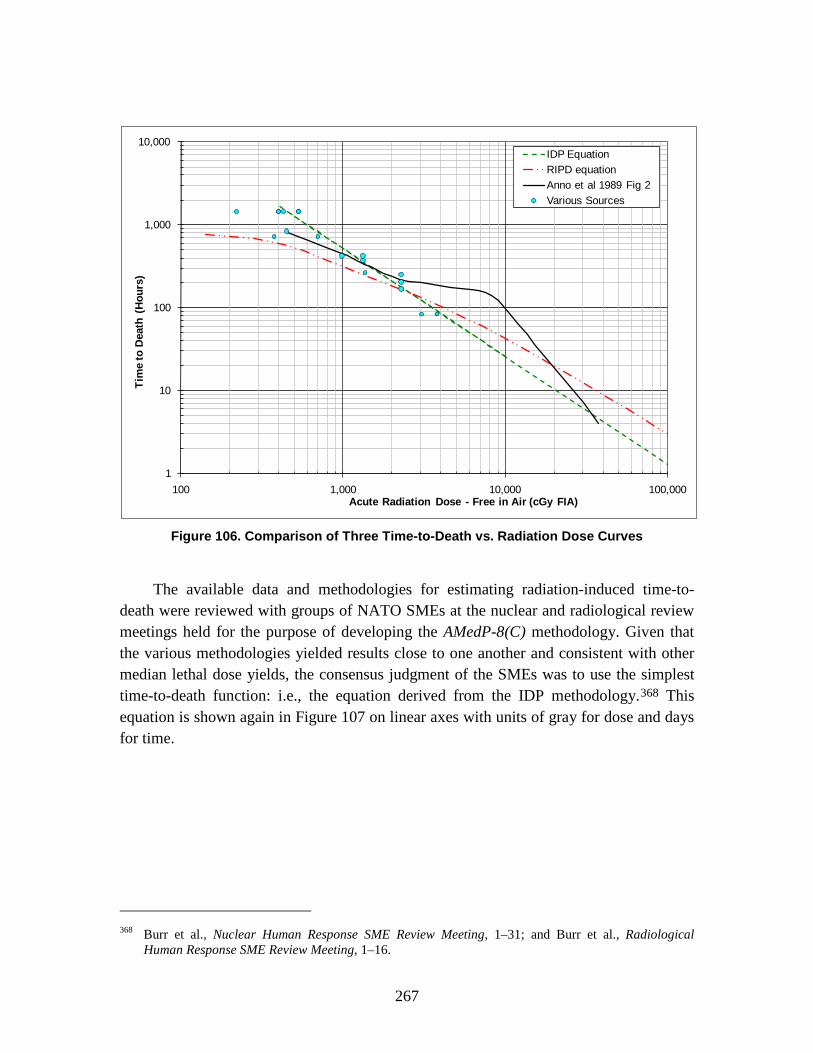
267
Figure 106. Comparison of Three Time-to-Death vs. Radiation Dose Curves
The available data and methodologies for estimating radiation-induced time-to-death were reviewed with groups of NATO SMEs at the nuclear and radiological review meetings held for the purpose of developing the AMedP-8(C) methodology. Given that the various methodologies yielded results close to one another and consistent with other median lethal dose yields, the consensus judgment of the SMEs was to use the simplest time-to-death function: i.e., the equation derived from the IDP methodology.368
This equation is shown again in Figure 107 on linear axes with units of gray for dose and days for time.
368 Burr et al., Nuclear Human Response SME Review Meeting, 1–31; and Burr et al., Radiological
Human Response SME Review Meeting, 1–16.
1
10
100
1,000
10,000
100 1,000 10,000 100,000
Tim
e to
Dea
th (
Hou
rs)
Acute Radiation Dose - Free in Air (cGy FIA)
IDP EquationRIPD equationAnno et al 1989 Fig 2Various Sources

268
Figure 107. Time-to-Death as a Function of Whole-Body Radiation Dose
4. Nuclear Blast Insults: Tertiary Blast Effects and Killed in Action (KIA) Dynamic pressure effects, such as missiling (secondary blast injury) or whole body
translation (tertiary blast injury), are difficult to model due to the large uncertainties in predicting the actual environment or the posture of exposed individuals. However, not including these effects underestimates casualties and fatalities. In order to partially account for these effects, for individuals in the open, the static overpressure can be used as an index for blast environment resulting in tertiary effects. With the association of static overpressure and tertiary effects, it is possible to estimate the KIAs from tertiary blast injury (specifically, decelerative tumbling) as a function of weapon yield.
The following data were derived from work described in Drake, et al.369
369 Drake et al., Collateral Damage, 5-90–5-106.
To begin, research suggested that the incidence of casualties and death could be described as a function of the velocity achieved by an individual picked up and thrown through the air by the winds, or dynamic pressures, generated by nuclear static overpressure (a tertiary blast effect known as “whole body translation”). Specifically, research indicated that 50% of individuals would become casualties (i.e., median burdening dose (BD50)) if thrown at an impact velocity of 4.7 meters/second, and 50% of individuals would die if thrown at an impact velocity of 10.7 meters/second. Impact velocity is dependent upon the amount of force (the strength of the winds, which is a function of overpressure) pushing on the individual and the length of time that this force acts on the individual; both values, in
0
10
20
30
40
50
60
0 20 40 60 80 100
Tim
e to
Dea
th (D
ays)
Whole-Body Radiation Dose (Gy)

269
turn, are highly dependent on the yield of the nuclear weapon. In addition, the impact velocity is dependent upon the posture of the individual at the time the dynamic pressure first strikes and upon the orientation of the body relative to the blast. Finally, the damage done to the body depends upon the manner in which its movement is stopped: stopping by striking a hard, “non-yielding” vertical surface will, all other things equal, cause more damage than decelerative tumbling. These factors were combined and examined by considering four combinations of target posture and environment: 1) a prone target, at a random orientation to the blast, impacting on a non-yielding surface, after traveling three meters; 2) a prone target, at a random orientation to the blast, undergoing decelerative tumbling across an open field; 3) a target standing, either oriented front- or back-on to the wind, impacting on a non-yielding surface, after traveling three meters; and 4) a target standing, either oriented front- or back-on to the wind, undergoing decelerative tumbling across an open field.
Based upon the minimum static overpressure versus yield required to cause a median casualty (BD50) and a median lethality (LD50) for each of these combinations of posture and environment provided in Drake, et al., the graphs shown in Figures 108 and 109 were generated for yields of interest.370 Additionally, Figure 108 displays the minimum overpressure required to achieve a casualty at Severity Level 2 (WIA(2)) and Severity Level 3 (WIA(3)) as indicated by the blast injury profiles.371
Likewise, the static overpressure value at which individuals reach Severity Level 4 (i.e., are declared dead—in this case KIA) is displayed in Figure 109. These graphs subsequently were provided to the NATO SMEs at the nuclear review meeting held for the purpose of developing the AMedP-8(C) methodology.
370 Ibid., 5-94. 371 Note that the blast injury profiles never go as low as severity level 1.
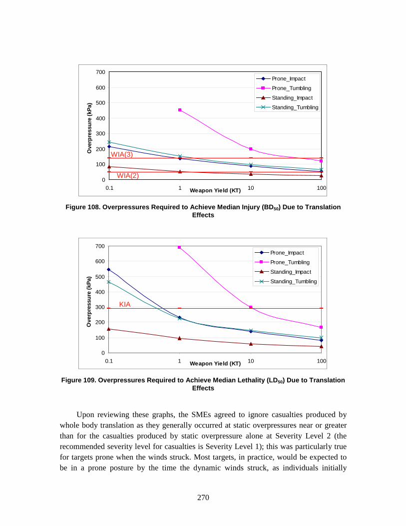
270
Figure 108. Overpressures Required to Achieve Median Injury (BD50) Due to Translation
Effects
Figure 109. Overpressures Required to Achieve Median Lethality (LD50) Due to Translation
Effects
Upon reviewing these graphs, the SMEs agreed to ignore casualties produced by whole body translation as they generally occurred at static overpressures near or greater than for the casualties produced by static overpressure alone at Severity Level 2 (the recommended severity level for casualties is Severity Level 1); this was particularly true for targets prone when the winds struck. Most targets, in practice, would be expected to be in a prone posture by the time the dynamic winds struck, as individuals initially
0
100
200
300
400
500
600
700
0.1 1 10 100Weapon Yield (KT)
Ove
rpre
ssur
e (k
Pa)
Prone_Impact
Prone_Tumbling
Standing_Impact
Standing_Tumbling
WIA(3)
WIA(2)0
100
200
300
400
500
600
700
0.1 1 10 100Weapon Yield (KT)
Ove
rpre
ssur
e (k
Pa)
Prone_Impact
Prone_Tumbling
Standing_Impact
Standing_Tumbling
WIA(3)
WIA(2)
0
100
200
300
400
500
600
700
0.1 1 10 100Weapon Yield (KT)
Ove
rpre
ssur
e (k
Pa)
Prone_Impact
Prone_Tumbling
Standing_Impact
Standing_Tumbling
KIA
0
100
200
300
400
500
600
700
0.1 1 10 100Weapon Yield (KT)
Ove
rpre
ssur
e (k
Pa)
Prone_Impact
Prone_Tumbling
Standing_Impact
Standing_Tumbling
KIA

271
standing at the time of a nuclear detonation would likely be knocked to the ground by a low-intensity precursor blast wave that oftentimes precedes the major pressure waves. Similar reasoning led the SMEs to consider only the prone posture for lethality effects. To simply the problem further, the SMEs agreed to consider only decelerative tumbling for the general casualty estimation process, although data are available to enable modelers to include prone “impact” cases as well.372
Therefore, in the AMedP-8(C) methodology, individuals at icons in the open are classified as KIAs if they are exposed to blast static overpressure exceeding the value required to achieve median lethality due to translation effects for the given weapon yield. Individuals inside some protective structure or vehicle (i.e., icons in vehicles, building structures, tents, or foxholes) are assumed to be shielded from tertiary effects.
5. Non-Contagious Biological Agents The biological casualty estimation approach (both non-contagious and contagious)
relies on the use of the injury profiles and the portion of the population at risk to which each injury profile is applicable at each point in time as determined by the human response approaches. The WIA and DOW status for biological casualties is therefore typically determined as a combination of the injury profile and the calculated times of disease progression. KIAs are not anticipated following exposure to biological agents due to the long incubation/latent period and the resultant time to develop symptoms being longer than the time required to reach a medical treatment facility.
For the non-contagious biological agents, the calculations associated with the times of injury progression have already been completed and compiled into tables (matrices) for ease of calculation. As described in Chapter 8, these tables were generated by convolving distributions of time to onset and duration of illness. Using the calculated number of non-survivors and survivors and the provided tables, the non-contagious biological casualty estimation methodology then determines, by day, the numbers expected to become ill at a (user-specified) severity level sufficient for them to be considered casualties. Depending upon the agent, either the total number of ill (the sum of non-survivors and survivors) or the specific number of non-survivors or survivors is multiplied by the matrix indicating the fraction of people who become ill or progress to a new disease stage (depending on the injury severity threshold selected by the user) as a function of time post-exposure. The calculated tables are then used to determine the number of people who manifest symptoms (the number of WIAs) and become casualties in Stage 1 (following the incubation/latent period) or become casualties as they enter Stage 2 (following the incubation/latent period convolved with duration of Stage 1) on each day.
372 Burr et al., Nuclear Human Response SME Review Meeting, 1–31.

272
Similarly, DOW status is calculated by again multiplying the total number of ill or the specific number of non-survivors (depending upon the agent) by the matrix indicating the fraction of people who die as a function of time post-exposure.
6. Contagious Biological Agents The contagious biological agents calculations associated with the times of disease
progression were completed as part of the contagious biological human response model, SEIRP. The outputs of this model—the number of individuals in each cohort (P(y), E(y), I1(y), I2(y), Rm(y), Rf(y)) and the number of new infectious casualties and fatalities each day (I1,new(y) or I2,new(y), Rf,new(y))—are used to estimate numbers of WIA and DOW over time. The process of assigning cohorts to the appropriate casualty category is shown in Figure 110. Because of the length of associated incubation periods, biological agent exposures are assumed to produce no KIAs.
Figure 110. Contagious Biological Agent Casualty Estimation Process
As with other agents/insults, for a contagious biological agent, an individual is considered to be a WIA at the first time at which the individual’s injury severity level is at or exceeds the user-defined severity level. For contagious biological agents, the number of individuals that become ill is distributed by day in the SEIRP model. Depending on the selected disease severity threshold level that characterizes a casualty, the applicable WIA cohorts are identified as follows:
The total number of WIAs on each day is the sum of the individuals in the earliest infectious stage cohort with a disease severity level equal to or
Removed(fatalities)
Rf(y)
Removed(medical)
Rmed(y)
Infectious(Stage 1)
I1(y)
Infectious(Stage 2)
I2(y)
RemovedR(y)
I1,new(y) I2,new(y)OR
Depending oncasualty severity
selected
WIA DOW
Rf,new(y)

273
greater than the selected threshold, any subsequent infectious stage cohort, and the Rm(y) cohort.
For each day, the number of new WIAs (I1,new(y) or I2,new(y)) is the number of individuals that enter the earliest infectious stage cohort with a disease severity level equal to or greater than the selected threshold.
Similarly, DOW status is based on the number of individuals entering the Rf(y) cohort over time and is identified as follows:
The total number of DOWs on each day is the sum of the individuals in the Rf(y) cohort.
For each day, the number of new DOWs (Rf,new(y)) is the number of individuals that enter the Rf(y) cohort.

275
10. Conclusions
The purpose of the AMedP-8(C) NATO Planning Guide is to:
...provide a methodology for estimating casualties uniquely occurring as a consequence of CBRN attacks against Allied targets… The methodology provides the capability to estimate the numbers of casualties over time as well as the incidence of injury by type and severity. These estimates assist planners, logisticians, and staff officers by allowing for more effective quantification of contingency requirements for medical personnel; medical materiel stockpiles; patient transport or evacuation capabilities; and facilities needed for patient decontamination, triage, treatment, and supportive care.373
This Technical Reference Manual (TRM) supplements AMedP-8(C) by documenting the development process, rationale, underlying data, and additional information utilized in the development of the calculation of the environments, and the human response and casualty estimation methodologies of the AMedP-8(C) methodology. The TRM includes descriptions of the sources, derivations, and rationale for definitions and methodology assumptions and limitations; details of the underlying symptomatology resulting from injuries caused by each agent or effect used in the methodology; and explanations of the equations and parameters employed in the environments calculations, human response, and casualty estimation methodologies. The goal of the TRM is to make the data underlying the casualty estimation component of the AMedP-8(C) methodology and the process through which it was developed as transparent as possible to enable other analysts and modelers to understand and replicate these results and procedures.
The definitions used, the assumptions made, and the limitations discussed in this document form the foundation of the AMedP-8(C) methodology. In most cases definitions from existing lexicons were used directly. The most significant exception to that was the definition of the symptom severity levels. While derived from a variety of sources that use similar terms, or terms in a similar manner, “Mild,” “Moderate,” “Severe,” and “Very Severe” were explicitly defined in order to allow for a consistent application of casualty criteria across the entire spectrum of CBRN injuries.
The assumptions used in AMedP-8(C) generally fall into one (or both) of two categories: “simplifying” or “directed.” The simplifying assumptions are made to keep 373 NATO, AMedP-8(C), 1-1.

276
the methodology from becoming too cumbersome for practical use throughout NATO. The directed assumptions were typically arrived at during custodial meetings held to review the technical aspects described in this document. When presented with a choice for specific aspects of the AMedP-8(C) methodology, the assembled nations typically directed the custodian to use one or another of the approaches or values presented.
The limitations of the AMedP-8(C) methodology, some of which are inherent to the casualty estimation process and some of which are imposed by the assumptions made, define the appropriate use of AMedP-8(C) method. Perhaps the most significant limitation is that the AMedP-8(C) methodology does not consider the impact of medical treatment on the casualty estimate. This is understandable and directed by the fact that there is no NATO standardized medical treatment protocol, but this limitation should be addressed at the national level as widely as possible, as it significantly impacts the use of the CBRN casualty estimate in planning for medical logistical requirements. As policies change and computational abilities improve, the definitions, assumptions, and limitations of AMedP-8(C) should be reviewed and revised to best meet NATO requirements for CBRN casualty estimation.
The IDA Study team devised a “general equation” to calculate the environments by converting an exposure environment to a dose, dosage, or insult and allows for the consideration of breathing rates, shielding, and personal protection among other factors. The AMedP-8(C) methodology is not dependent upon any specific model or tool for definition of the CBRN exposure environment, but does require that the dose, dosage, or insult be expressed in the appropriate units for consideration in the human response methodology. The environments calculation can be as complex or a simple as required for the use of the AMedP-8(C) casualty estimate.
The human response component of the AMedP-8(C) methodology employs injury profiles, represented as a function of changing injury severity over time, to describe the human response to agents and insults. This approach was actually an intermediate step in the earlier version of AMedP-8; in AMedP-8(C) it has been explicitly defined so that it can be applied across all CBRN injuries. This use, however, varies according to the type of agent being considered. Chemical, radiological, and nuclear agents and effects result in injuries that are deterministic, where the severity of the injury is (generally) proportional to the intensity of the dose, dosage, or insult. Biological agents, on the other hand, result in stochastic injuries (or illness). Whether an individual becomes ill may be dose dependent, while at the same time, the severity of the illness may be totally independent of the dose of the agent.
Defining the human response parameters for chemical, radiological, and nuclear agents and effects was typically a process of citing values clearly recognized and well accepted by the community of experts who research and describe CBRN human response. That process was not always feasible for selecting the human response

277
parameters for biological agents. Many of these parameters are subjects of current research, and accepted values often ranged widely. The approach taken for AMedP-8(C) and documented in this TRM was to use published dose response data, whenever possible, to define the necessary parameters. In those cases where data was not available, generally accepted values or expert estimates were used. With few exceptions, the human response parameters were discussed and accepted by panels of international subject matter experts prior to being included in AMedP-8(C).
The casualty estimation component of the AMedP-8(C) methodology utilizes the injury profile descriptions of the human response to agents and insults to estimate the resulting casualty status. As described, the AMedP-8(C) methodology allows the commander or planner using or developing the casualty estimate to establish casualty criteria appropriate to the urgency of the mission and capabilities of the units, without regard to the type of CBRN agent or effect being considered. Some exceptions to the use of the human response methodology are made to account for the special cases of internal sepsis from very large percutaneous doses of liquid HD, protracted whole-body radiation dose, the time-to-death for large doses of whole-body radiation, and prompt fatalities (KIAs) from tertiary blast effects. The final product of the AMedP-8(C) CBRN casualty estimation methodology is a tabulation of the estimated number of casualties, at specified injury severities and times of interest.
AMedP-8(C) is a significant change from earlier versions of AMedP-8, and is designed to be broader and more flexible to address the requirements of a commander and staff for a CBRN casualty estimate. It has limitations, some induced by NATO policy and doctrine, some by the limitations of current computational capabilities, and some by the current state of knowledge of CBRN agents and effects. As policies, capabilities, and knowledge change, AMedP-8(C) should be reviewed and revised to best respond to the commander’s requirements.

A-1
Appendix A. Abbreviations
Abbreviations AAP Allied Administration Publication
ACH Air changes per hour
AER Air exchange rate
AFMOA U.S. Air Force Medical Operations Agency
AFRRI Armed Forces Radiobiology Research Institute (U.S.)
AJP Allied Joint Publication
AHA American Hospital Association
AMedP Allied Medical Publication
ARS Acute Radiation Syndrome
AVA Anthrax vaccine absorbed
BD01 Dose resulting in burdening effects in 1% of exposed individuals
BD50 Median burdening dose; dose resulting in burdening effects in 50% of exposed individuals
BD90 Dose resulting in burdening effects in 90% of exposed individuals
BDO Battle dress overgarment
BDU Battle dress uniform
BUMED U.S. Navy Bureau of Medicine and Surgery
BW Biological warfare
CBRN Chemical, biological, radiological and nuclear
CDC Centers for Disease Control and Prevention
CDF Cumulative distribution function

A-2
CF Conversion factor
CFHSG-DHSO Canadian Forces Health Services Group, Defence Health Services Operations
CFU Colony forming unit
CHRNEM Consolidated Human Response Nuclear Effects Model
CM Cynomolgus macaques
ColPro Collective protection
CRI Cutaneous Radiation Injury
CRN Chemical, radiological and nuclear
CRSSA-MOD Centre de Recherches du Service Santé des Armées, Ministry of Defence (France)
Ct Concentration time
DIA U.S. Defense Intelligence Agency
DICE DNA Improvised Casualty Estimate
DNA U.S. Defense Nuclear Agency
DOE U.S. Department of Energy
DOW Died of wounds
DRDC Defence Research & Development Canada
DTRA Defense Threat Reduction Agency (U.S.)
ECt50 Effective median dosage (concentration time)
ECt50,severe Dosage of vapor required to produce severe effects in 50% of exposed individuals
ED50 Median effective dose; dose resulting in effects in 50% of exposed individuals
ED50,severe Dose of liquid required to produce severe effects in 50% of exposed individuals
EPA U.S. Environmental Protection Agency
ESG Elektroniksystem und Logistik-GmbH (Germany)

A-3
FBR Federal Guidance Report
FIA Free in air
GB Sarin
Gy Gray
HD Distilled mustard
HEPA High efficiency particulate air filter
HHS U.S. Department of Health and Human Services
HIPAA Health Insurance Portability and Accountability Act
HPAC Hazard Prediction and Assessment Capability
Hr Hour
IAEA International Atomic Energy Agency
ID50 Median infectious dose; dose resulting in infection and illness for 50% of exposed individuals
IDA Institute for Defense Analyses
IDP Intermediate Dose Program
IPE Individual protective equipment
J/cm2 Joule per square centimeter
JEM Joint Effects Model
JSGPM Joint Service General Purpose Mask
KAMI Knowledge Acquisition Matrix Instrument
KIA Killed in action
Kg Kilogram
kJ/m2 Kilojoule per square meter
kPa Kilopascal
LD10/60 Dose resulting in lethality in 10% of exposed individuals within 60 days
LD5/60 Dose resulting in lethality in 5% of exposed individuals within 60 days

A-4
LD50 Median lethal dose; dose resulting in lethality in 50% of exposed individuals
LD50/60 Dose resulting in lethality in 50% of exposed individuals within 60 days
LD99/60 Dose resulting in lethality in 99% of exposed individuals within 60 days
M Meter
MDPH Michigan Department of Public Health
Mg Milligram
Min Minute
MIHIE Military Institute of Hygiene and Epidemiology (Poland)
MIPLD Mouse intraperitoneal median lethal dose
MLE Maximum likelihood estimation
MODUK United Kingdom Ministry of Defense
N/A Not applicable
NATO North Atlantic Treaty Organization
NBC Nuclear, biological and chemical
N.O.E. No observable effect
ORD Operational requirements document
OTSG Office of The Surgeon General, U.S. Army
%BSA Percentage body surface area burned to second or third degree level
PDF Probability density function
PFU Plaque forming units
PNAS Proceedings of the National Academy of Sciences
PSR Pacific Sierra Research Corp.
RBE Relative biological effectiveness
R-B-T Radiation, blast and thermal
A-5
RED Radiological exposure device
RDD Radiological dispersal device
RIPD Radiation Induced Performance Decrement
RM Rhesus macaques
SARS Severe acute respiratory syndrome
SEB Staphylococcal enterotoxin B
SEIR Susceptible-Exposed-Infectious-Removed
SEIRP Susceptible-Exposed and infected-Infectious-Removed-Prophylaxis efficacious
SI Susceptible-Infected
SIR Susceptible-Infected-Removed
SME Subject matter expert
STANAG NATO standardization agreement
TNO The Netherlands Organization
UGI Upper Gastrointestinal
USAISR U.S. Army Institute of Surgical Research
USAMRICD U.S. Army Medical Research Institute of Chemical Defense
USAMRIID U.S. Army Medical Research Institute of Infectious Diseases
USANCA U.S. Army Nuclear and Chemical Agency
UTM Universal Transverse Mercator
VEE Venezuelan equine encephalitis
VLSTRACK Vapor, Liquid, and Solid Tracking
VX O-Ethyl-S-(2-diisopropylaminoethyl) methyl phosphonothiolate
WHO World Health Organization
WIA Wounded in action
WIA(1) Wounded in action (Severity Level 1 (“Mild”) or greater)
WIA(2) Wounded in action (Severity Level 2 (“Moderate”) or greater)

A-6
WIA(3) Wounded in action (Severity Level 3 (“Severe”) or greater)
WMD Weapons of Mass Destruction
Symbols In different sections of this document, the same symbol may be used to represent
different things, with the appropriate meaning either implied by the usage or explicitly stated in the surrounding text. If a symbol is not defined in the surrounding text, the following definitions should be assumed.
α Relative ability of people in the infectious cohort in illness Stage 1 to infect people in the susceptible cohort
AERn Air exchange rate at Icon n
β(y) Time-varying disease transmission rate
Bn Blast static overpressure at Icon n
Ccum,cld,n,r Activity concentration time integral in the cloud of the rth radioisotope at Icon n
Ccum,grd,n,r Ground activity deposition time integral of the rth radioisotope at Icon n
Ccum,n,t Cumulative agent or effect at Icon n, from time t-1 to t for t > t0
Ccum,s_fallout,n Cumulative concentration from fallout contamination on the skin for Icon n
Cgrd,n,r,j Average ground deposition output value for Icon n of the rth radioisotope at the jth time step
CFHD Percutaneous HD liquid to equivalent vapor conversion factor
CFs,r Skin contamination dose conversion factor
CFs,cld,r Skin cloudshine dose conversion factor for the rth radioisotope

A-7
CFs,grd,r Skin groundshine dose conversion factor for the rth radioisotope
CFs_fallout Dose conversion factor for fallout contamination on the skin at an epidermal thickness of 7 mg/cm2 for the time of interest after detonation
CFwb,cld,r Whole-body cloudshine dose conversion factor for the rth radioisotope
CFwb,grd,r Whole-body groundshine dose conversion factor for the rth radioisotope
s, ,C n r Skin activity deposition time integral of the rth radioisotope for Icon n
D•
Dose rate
Danthrax,n Anthrax spore dose for Icon n
Dblast,n Shielded static blast overpressure for Icon n
Dbotulism,n Botulinum neurotoxin dose for Icon n
Dcut,n Cutaneous radiation dose for Icon n
Dfallout_grd,γ,n Cumulative gamma radiation [absorbed] dose due to groundshine from fallout at Icon n
DGB,ih,n Inhaled GB vapor dosage for Icon n
DHD,epc,n Equivalent percutaneous HD vapor dosage for Icon n
DHD,ih,n Inhaled HD vapor dosage for Icon n
DHD,l,n Percutaneous HD liquid dose for Icon n
DHD,pc,n Percutaneous HD vapor dosage for Icon n
Dn / dn Dose/dosage/insult at Icon n (or in applicable non-contagious biological agent bin)

A-8
Dplague,n Plague dose for Icon n
Ds,cld,n Skin radiation [absorbed] dose due to radiation from cloudshine at Icon n
Ds,grd,n Skin radiation [absorbed] dose due to radiation from groundshine at Icon n
Dsmallpox,n Smallpox dose for Icon n
Dthermal,n Percent of body surface area burned for Icon n
DVEE,n VEE dose for Icon n
DVX,ih,n Inhaled VX vapor dosage for Icon n
DVX,pc,n Percutaneous VX liquid dose for Icon n
Dwb,cld,n Whole-body radiation [absorbed] dose due to radiation from cloudshine at Icon n
Dwb,grd,n Whole-body radiation [absorbed] dose due to radiation from groundshine at Icon n
Dwb,n Whole-body radiation dose for Icon n
Dwb,neutron,n Total (initial) whole-body radiation dose due to neutron radiation at Icon n
Dwb,γ,n Total (initial) whole-body radiation dose due to gamma radiation at Icon n
DRβ/γ_120 Beta-to-gamma dose ratio for bare skin at the approximate height of 120 cm above ground for the time of interest after detonation
Durationn Length of time the cloud envelopes the vehicle/structure at Icon n
E(y) Fraction of the population which is exposed to a contagious biological agent and will become infected following that

A-9
exposure at time step y
En(0) Initial number of exposed and infected individuals at Icon n
EFn,t Exposure factor at Icon n from time t-1 to t for t > t0
FInc Cumulative fraction of persons who have completed the incubation period and entered Stage 1 of the disease (agent specific)
FLat Cumulative fraction of persons who have completed the latent period and entered Stage 1 of the disease (agent specific)
FP Dose protraction correction factor
Hfallout,s,β,n Absorbed dose to the skin from beta radiation deposition on the ground from fallout for Icon n
Hs,β,n Absorbed dose to the skin from beta radiation contamination on the skin for Icon n
HD/PC/L HD percutaneous liquid
HD/PC/V HD percutaneous vapor
I1(y) Infectious sub-population containing contagious people who manifest symptoms of a selected severity associated with the first stage of disease at time step y
I2(y) Infectious sub-population containing contagious people who manifest symptoms of a selected severity associated with the second stage of disease at time step y
I1,new(y) Number of individuals who enter the first stage of disease at time step y
I2,new (y) Number of individuals who enter the second stage of disease at time step y
in Number of individuals at Icon n
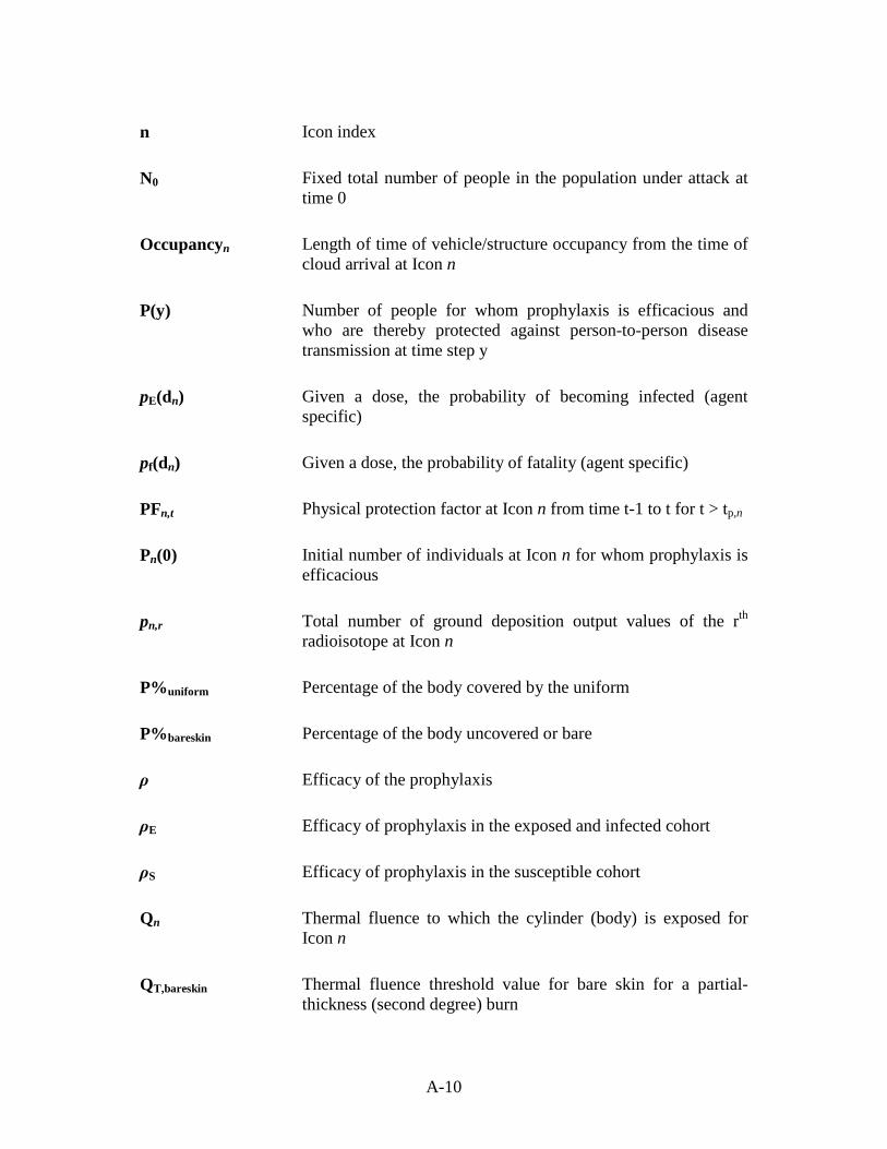
A-10
n Icon index
N0 Fixed total number of people in the population under attack at time 0
Occupancyn Length of time of vehicle/structure occupancy from the time of cloud arrival at Icon n
P(y) Number of people for whom prophylaxis is efficacious and who are thereby protected against person-to-person disease transmission at time step y
pE(dn) Given a dose, the probability of becoming infected (agent specific)
pf(dn) Given a dose, the probability of fatality (agent specific)
PFn,t Physical protection factor at Icon n from time t-1 to t for t > tp,n
Pn(0) Initial number of individuals at Icon n for whom prophylaxis is efficacious
pn,r Total number of ground deposition output values of the rth radioisotope at Icon n
P%uniform Percentage of the body covered by the uniform
P%bareskin Percentage of the body uncovered or bare
ρ Efficacy of the prophylaxis
ρE Efficacy of prophylaxis in the exposed and infected cohort
ρS Efficacy of prophylaxis in the susceptible cohort
Qn Thermal fluence to which the cylinder (body) is exposed for Icon n
QT,bareskin Thermal fluence threshold value for bare skin for a partial-thickness (second degree) burn

A-11
QT,uniform Thermal fluence threshold value for a specific uniform type for a partial-thickness (second degree) burn
R(y) Total number of individuals removed at time step y
Rf(y) Number of people who have died from the disease and who are thereby removed as a source of infection from the model at time step y
Rf,new(y) Number of people who enter the removed (fatalities) (Rf(y)) cohort at time step y
Rm(y) Number of people who are no longer infectious but remain in the medical system at time step y
S(y) Total susceptible sub-population or the population at risk at time step y
SFblast,n Blast shielding factor for Icon n
SFn,t Shielding factor at Icon n from time t-1 to t for t > t0
SFneutron,n Neutron radiation shielding factor for Icon n
SFvent,n,t Ventilation shielding factor for Icon n from time t-1 to t for t > t0
SFγ,n Gamma radiation shielding factor for Icon n
t0 Beginning of the event that results in exposure
tdeath,n Time to death for individuals at Icon n
tdur,n Duration of exposure for Icon n
tend,n End of exposure time at Icon n (assumes tend,n ≥ tp,n + 1)
tp,n Time at which physical protection is implemented at Icon n
μ1 Mean time individuals spend in the Stage 1 infectious cohort
A-12
μ2 Mean time individuals spend in the Stage 2 infectious cohort
μE Mean time individuals spend in the exposed and infected cohort
νoff(y) Binary prophylaxis parameter which dictates when prophylaxis is discontinued
νon(y) Binary prophylaxis parameter which dictates when prophylaxis is initiated
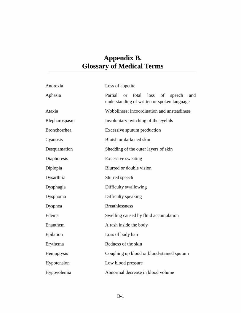
B-1
Appendix B. Glossary of Medical Terms
Anorexia Loss of appetite
Aphasia Partial or total loss of speech and understanding of written or spoken language
Ataxia Wobbliness; incoordination and unsteadiness
Blepharospasm Involuntary twitching of the eyelids
Bronchorrhea Excessive sputum production
Cyanosis Bluish or darkened skin
Desquamation Shedding of the outer layers of skin
Diaphoresis Excessive sweating
Diplopia Blurred or double vision
Dysarthria Slurred speech
Dysphagia Difficulty swallowing
Dysphonia Difficulty speaking
Dyspnea Breathlessness
Edema Swelling caused by fluid accumulation
Enanthem A rash inside the body
Epilation Loss of body hair
Erythema Redness of the skin
Hemoptysis Coughing up blood or blood-stained sputum
Hypotension Low blood pressure
Hypovolemia Abnormal decrease in blood volume

B-2
Insomnia Difficulty sleeping
Ischemia Inadequate blood circulation to a local area due to a blockage of blood vessels in the area; tissue turns white then dark
Maculopapular Slightly raised and discolored (refers to an area of skin)
Malaise Generalized discomfort or uneasiness
Meningoencephalitis An infection or inflammation of the meninges and the brain
Miosis Constriction of the pupil
Myalgia Muscle pain
Necrosis Death of living cells or tissues
Pancytopenia Shortage of all types of blood cells (red, white, platelets)
Photophobia Excessive sensitivity/aversion to light
Pleural effusion Accumulation of fluid between the layers of tissue that line the lungs and chest cavity
Prostration Total exhaustion or weakness; collapse
Ptosis Drooping eyelid
Rhinorrhea Runny nose
Stridor Abnormal, high-pitched breathing
Syncope Temporary loss of consciousness and posture
Tachycardia Rapid or accelerated heartbeat
Tachypnea Abnormally fast breathing
Toxemia Toxins in the blood
C-1
Appendix C. References
Chapter 1. Anno, George H., Siegmund J. Baum, H. Rodney Withers, and Robert W. Young.
“Symptomatology of Acute Radiation Effects in Humans After Exposure to Doses of 0.5 to 30 Gy.” Health Physics 56, no. 6 (June 1989): 821–38.
Anno, George H., and Arthur P. Deverill. Consequence Analytic Tools for NBC Operations Volume 1: Biological Agent Effects and Degraded Personnel Performance for Tularemia, Staphylococcal Enterotoxin B (SEB) and Q Fever. DSWA-TR-97-61-V1. Alexandria, VA: Defense Special Weapons Agency, October 1998.
Anno, George H., Michael Lockhart, Larry Karns, Gene E. McClellan, Gillian L. Rickmeier, Ronald M. Bloom, and Leigh N. Matheson. Biological Agent Exposure and Casualty Estimation: AMedP-8 (Biological) Methods Report. GS-35F-4923H. Fairfax, VA: General Dynamics Advanced Information Systems, 2005.
Deverill, Arthur P., and Dennis F. Metz. Defense Nuclear Agency Improved Casualty Estimation (DICE) Chemical Insult Program Acute Chemical Agent Exposure Effects. DNS-TR-93-162. Washington, DC: Defense Nuclear Agency, May 1994.
Levin, Sheldon G. The Effect of Combined Injuries from a Nuclear Detonation on Soldier Performance. DNA-TR-92-134. Alexandria, VA: Defense Nuclear Agency, June 1993.
North Atlantic Treaty Organization (NATO). AJMedP-1: Allied Joint Medical Planning Doctrine. STANAG 2542. 3 November 2009.
———. AJP-3.8(B): Allied Joint Doctrine for NBC Defence. STANAG 2451. 5 February 2004.
———. AJP-4.10(A): Allied Joint Medical Support Doctrine. STANAG 2228. 3 March 2006.
———. AMedP-7(D): Concept of Operations of Medical Support in Chemical, Biological, Radiological, and Nuclear Environments. STANAG 2873. 6 December 2007.
———. AMedP-8(A), Volume I: Medical Planning Guide for the Estimation of NBC Battle Casualties (Nuclear). STANAG 2475. April 2002.
———. AMedP-8(B), Volume II: Medical Planning Guide for the Estimation of CBRN Battle Casualties (Biological). STANAG 2476. December 2007.
C-2
———. AMedP-8(A), Volume III: Medical Planning Guide for the Estimation of NBC Battle Casualties (Chemical). STANAG 2477. 20 April 2005.
———. AMedP-8(C): NATO Planning Guide for the Estimation of CBRN Casualties Ratification Draft 1. DRAFT. February 2010.
Chapter 2. American Hospital Association. “Media Advisory: HIPAA Updated Guidelines for
Releasing Information on the Condition of Patients.” Chicago, IL: Society for Healthcare Strategy and Market Development of the American Hospital Association, 1 February 2003. http://www.aha.org/aha/advisory/2003/030201-media-adv.html.
Baba, Anthony J., Brian R. Schallhorn, Steward Share, and Susan M. Gaspar. Incidence of Skin Burns Under Contemporary Army Uniforms Exposed to Thermal Radiation from Simulated Nuclear Fireballs. HDL-TR-2084. Adelphi, MD: U.S. Army Laboratory Command, Harry Diamond Laboratories, December 1986.
Brachman, Philip S. "Inhalation Anthrax." Annals of the New York Academy of Sciences 353 (December 1980): 83–93.
Burr, Julia K., Carl A. Curling, Deena S. Disraelly, Preston J. Lee, Terri J. Walsh, and Robert A. Zirkle. Proceedings of the NATO Chemical Human Response Subject Matter Expert Review Meeting, 21-22 April 2008, Munich, Germany. IDA Document D-3883. Alexandria, VA: Institute for Defense Analyses, August 2009.
———. Proceedings of the NATO Nuclear Human Response Subject Matter Expert Review Meeting, 23-25 June 2008, Albuquerque, New Mexico, United States of America. IDA Document D-3884. Alexandria, VA: Institute for Defense Analyses, August 2009.
———. Proceedings of the NATO Radiological Human Response Subject Matter Expert Review Meeting, 26 June 2008, Albuquerque, New Mexico, United States of America. IDA Document D-3885. Alexandria, VA: Institute for Defense Analyses, August 2009.
Centers for Disease Control and Prevention. “Cutaneous Radiation Injury: Fact Sheet for Physicians.” http://emergency.cdc.gov/radiation/criphysicianfactsheet.asp.
Deverill, Arthur P., and Dennis F. Metz. Defense Nuclear Agency Improved Casualty Estimation (DICE) Chemical Insult Program Acute Chemical Agent Exposure Effects. DNS-TR-93-162. Washington, DC: Defense Nuclear Agency, May 1994.
Gani, Raymond, and Steve Leach. “Epidemiological Determinants for Modeling Pneumonic Plague Outbreaks.” Emerging Infectious Diseases 10, no. 4 (April 2004): 608–14.
Glasstone, Samuel, and Philip J. Dolan, eds. The Effects of Nuclear Weapons. 3rd ed. Washington, DC: U.S. Government Printing Office, 1977.
Holty, Jon-Erik C., Dena M. Bravata, Hau Liu, Richard A. Olshen, Kathryn M. McDonald, and Douglas K. Owens. “Systematic Review: A Century of Inhalational

C-3
Anthrax Cases from 1900 to 2005.” Annals of Internal Medicine 144, no. 4 (February 2006): 270–80.
Kool, Jacob L. “Risk of Person-to-Person Transmission of Pneumonic Plague.” Clinical Infectious Diseases 40, no. 8 (April 2005): 1166–72.
Lathem, Wyndham W., Seth D. Crosby, Virginia L. Miller, and William E. Goldman. “Progression of Primary Pneumonic Plague: A Mouse Model of Infection, Pathology, and Bacterial Transcriptional Activity.” Proceedings of the National Academy of Sciences of the United States of America 102, no. 49 (December 2005): 17786–91.
Layton, David W. “Metabolically Consistent Breathing Rates for Use in Dose Assessments.” Health Physics 64, no. 1 (January 1993): 23–36.
Levin, Sheldon G. The Effect of Combined Injuries from a Nuclear Detonation on Soldier Performance. DNA-TR-92-134. Alexandria, VA: Defense Nuclear Agency, June 1993.
McClellan, Gene E., George H. Anno, and Leigh N. Matheson. Consequence Analytic Tools for NBC Operations Volume 3: Chemical Agent Exposure and Casualty Estimation. DSWA-TR-97-61-V3. Alexandria, VA: Defense Special Weapons Agency, September 1998.
McGovern, Thomas W., and Arthur M. Friedlander. “Plague.” In Medical Aspects of Chemical and Biological Warfare, edited by Frederick R. Sidell, Ernest T. Takafuji, and David R. Franz, 479–502. Textbook of Military Medicine, Part 1: Warfare, Weaponry, and the Casualty. Washington, DC: Department of the Army, Office of the Surgeon General, Borden Institute, 1997.
Multiservice Publication. Potential Military Chemical/Biological Agents and Compounds. FM 3-11.9/MCRP 3-37.1B/NTRP 3-11.32/AFTTP(I) 3-2.55. Washington, DC: U.S. Government Printing Office, January 2005.
North Atlantic Treaty Organization (NATO). AAP-6: NATO Glossary of Terms and Definitions (English and French). STANAG 3680. 22 March 2010.
———. AAP-21(D): NATO Glossary of NBC Terms and Definitions. STANAG 2367. 2009.
———.AMedP-6(B): NATO Handbook on the Medical Aspects of NBC Defensive Operations. 1 February 1996.
———. AMedP-6(C), Volume I: NATO Handbook on the Medical Aspects of NBC Defensive Operations (Nuclear). STANAG 2461. 18 February 2005.
———. AMedP-6(C), Volume II: NATO Handbook on the Medical Aspects of NBC Defensive Operations (Biological). STANAG 2462. 11 May 2005.
———. AMedP-6(C), Volume III: NATO Handbook on the Medical Aspects of NBC Defensive Operations (Chemical). STANAG 2463. 14 December 2006.

C-4
———. AMedP-7(D): Concept of Operations of Medical Support in Chemical, Biological, Radiological, and Nuclear Environments. STANAG 2873. 6 December 2007.
———. AMedP-8(A), Volume III: Medical Planning Guide for the Estimation of NBC Battle Casualties (Chemical). STANAG 2477. 20 April 2005.
———. AMedP-8(C): NATO Planning Guide for the Estimation of CBRN Casualties Ratification Draft 1. DRAFT. February 2010.
———. AMedP-13: NATO Glossary of Medical Terms and Definitions. STANAG 2409. February 2002.
———. First-Aid Materiel for Chemical Injuries. STANAG 2871. 8 March 1989.
Rao A. R. Smallpox. Bombay, India: Kothari Book Depot, 1972.
Sidell, Frederick R. “Nerve Agents.” In Medical Aspects of Chemical and Biological Warfare, edited by Frederick R. Sidell, Ernest T. Takafuji, and David R. Franz, 130–79. Textbook of Military Medicine, Part 1: Warfare, Weaponry, and the Casualty. Washington, DC: Department of the Army, Office of the Surgeon General, Borden Institute, 1997.
Steele, Keith E., Douglas S. Reed, Pamela J. Glass, Mary Kate Hart, George V. Ludwig, William D. Pratt, Michael D. Parker, and Jonathan F. Smith. “Alphavirus Encephalitides.” In Medical Aspects of Biological Warfare, edited by Zygmunt F. Dembek, 241–70. Textbook of Military Medicine. Washington, DC: Department of Defense, Office of the Surgeon General, U.S. Army, Borden Institute, 2007.
U.S. Army Institute for Surgical Research. Emergency War Surgery: Third United States Revision. Washington, DC: Borden Institute, 2004.
U.S. Army Medical Research Institute of Chemical Defense. Medical Management of Chemical Casualties Handbook. 3rd ed. Aberdeen Proving Ground, MD: International Medical Publishing, 2000.
U.S. Army Nuclear and Chemical Agency. Personnel Risk and Casualty Criteria for Nuclear Weapons Effects. Springfield, VA: Training and Doctrine Command, June 1999. Unclassified.
Woodruff, Bradley A., Patricia M. Griffin, Loretta M. McCroskey, Joanne F. Smart, Robert B. Wainwright, Raymond G. Bryant, Lori C. Hutwagner, and Charles L. Hatheway. “Clinical and Laboratory Comparison of Botulism from Toxin Types A, B, and E in the United States, 1975–1988.” Journal of Infectious Diseases 166, no. 6 (December 1992): 1281–86.
Chapter 3. Baba, Anthony J., Brian R. Schallhorn, Steward Share, and Susan M. Gaspar. Incidence
of Skin Burns Under Contemporary Army Uniforms Exposed to Thermal Radiation from Simulated Nuclear Fireballs. HDL-TR-2084. Adelphi, MD: U.S. Army Laboratory Command, Harry Diamond Laboratories, December 1986.

C-5
Blewett, William K., Dennis W. Reeves, Victor J. Arca, David P. Fatkin, and Brenda D. Cannon. Expedient Sheltering in Place: An Evaluation for the Chemical Stockpile Emergency Preparedness Program. Edgewood, MD: Edgewood Research Development and Engineering Center, Aberdeen Proving Ground, June 1996.
Burr, Julia K., Carl A. Curling, Deena S. Disraelly, Preston J. Lee, Terri J. Walsh, and Robert A. Zirkle. Proceedings of the NATO Chemical Human Response Subject Matter Expert Review Meeting, 21-22 April 2008, Munich, Germany. IDA Document D-3883. Alexandria, VA: Institute for Defense Analyses, August 2009.
Curling, Carl, and Lusine Danakian. Documentation of Production: Allied Medical Publication 8 Planning Guide for the Estimation of Battle Casualties (Nuclear). IDA Paper P-4008. Alexandria, VA: Institute for Defense Analyses, March 2005.
Eckerman, Keith F., and Jeffrey C. Ryman. External Exposure to Radionuclides in Air, Water, and Soil. Federal Guidance Report No. 12. EPA-402-R-93-081. Washington, DC: U.S. Environmental Protection Agency, September 1993.
Glasstone, Samuel, and Philip J. Dolan, eds. The Effects of Nuclear Weapons. 3rd ed. Washington, DC: U.S. Government Printing Office, 1977.
Harper, Frederick T., Stephen V. Musolino, and William B. Wente. “Realistic Radiological Dispersal Device Hazard Boundaries and Ramifications for Early Consequence Management Decisions.” Health Physics 93, no. 1 (July 2007): 1–16.
International Atomic Energy Agency. Generic Procedures for Assessment and Response During a Radiological Emergency. IAEA-TECDOC-1162. Vienna: IAEA, 2000.
Johnson, Ted. A Guide to Selected Algorithms, Distributions, and Databases used in Exposure Models Developed by the Office of Air Quality Planning and Standards. Chapel Hill, NC: TRJ Environmental, Inc., May 2002. http://www.epa.gov/ttn/fera/data/human/report052202.pdf.
Layton, David W. “Metabolically Consistent Breathing Rates for Use in Dose Assessments.” Health Physics 64, no. 1 (January 1993): 23–36.
Levin, Sheldon G. The Effect of Combined Injuries from a Nuclear Detonation on Soldier Performance. DNA-TR-92-134. Alexandria, VA: Defense Nuclear Agency, June 1993.
McClellan, Gene E., George H. Anno, and Leigh N. Matheson. Consequence Analytic Tools for NBC Operations Volume 3: Chemical Agent Exposure and Casualty Estimation. DSWA-TR-97-61-V3. Alexandria, VA: Defense Special Weapons Agency, September 1998.
Multiservice Publication. Potential Military Chemical/Biological Agents and Compounds. FM 3-11.9/MCRP 3-37.1B/NTRP 3-11.32/AFTTP(I) 3-2.55. Washington, DC: U.S. Government Printing Office, January 2005.
North Atlantic Treaty Organization (NATO). AMedP-8(C): NATO Planning Guide for the Estimation of CBRN Casualties Ratification Draft 1. DRAFT. February 2010.

C-6
Overton, J. H., and R. C. Graham. “Predictions of Ozone Absorption in Human Lungs from Newborn to Adult.” EPA-68-02-4450. Research Triangle Park, NC: U.S. Environmental Protection Agency, 1989.
Park, J. H., J. D. Spengler, D. W. Yoon, T. Dumyahn, K. Lee, and H. Ozkaynak. “Measurement of Air Exchange Rate of Stationary Vehicles and Estimation of In-Vehicle Exposure.” Journal of Exposure Analysis & Environmental Epidemiology 8, no. 1 (January–March 1998): 65–78.
Stabin, Michael G. “External Dose Assessment.” Chap. 9 in Radiation Protection and Dosimetry: An Introduction to Health Physics. New York: Springer, 2008.
U.S. Army Chemical School. Protection Factor Requirement Analysis in Support of the Joint Service General Purpose Mask (JSGPM) Operational Requirements Document (ORD). Fort McClellan, AL: U.S. Army Chemical School, 13 August 1998.
U.S. Department of Energy. DOE Standard: Specification for HEPA Filters Used by DOE Contractors. DOE-STD-3020-97. Springfield, VA: U.S. Department of Commerce, Technology Administration, National Technical Information Service, January 1997.
Valentin, Jack, ed. “Basic Anatomical and Physiological Data for Use in Radiological Protection: Reference Values.” Annals of the ICRP Publication 89 32, no. 3–4 (2003).
Chapter 4. Anno, George H., Michael A. Dore, James T. Roth, Nils D. LaVine, and Arthur P.
Deverill. Predicted Performance on Infantry and Artillery Personnel Following Acute Radiation or Chemical Agent Exposure. DNA-TR-93-174. Washington, DC: Defense Nuclear Agency, November 1994.
Deverill, Arthur P., and Dennis F. Metz. Defense Nuclear Agency Improved Casualty Estimation (DICE) Chemical Insult Program Acute Chemical Agent Exposure Effects. DNS-TR-93-162. Washington, DC: Defense Nuclear Agency, May 1994.
McClellan, Gene E., George H. Anno, and Leigh N. Matheson. Consequence Analytic Tools for NBC Operations Volume 3: Chemical Agent Exposure and Casualty Estimation. DSWA-TR-97-61-V3. Alexandria, VA: Defense Special Weapons Agency, September 1998.
McDonough, John H. “Performance Impacts of Nerve Agents and Their Pharmacological Countermeasures.” Military Psychology 14, no. 2 (2002): 93–119.
Multiservice Publication. Potential Military Chemical/Biological Agents and Compounds. FM 3-11.9/MCRP 3-37.1B/NTRP 3-11.32/AFTTP(I) 3-2.55. Washington, DC: U.S. Government Printing Office, January 2005.
North Atlantic Treaty Organization (NATO). AMedP-8(A), Volume III: Medical Planning Guide for the Estimation of NBC Battle Casualties (Chemical). STANAG 2477. 20 April 2005.

C-7
———. AMedP-8(C): NATO Planning Guide for the Estimation of CBRN Casualties Ratification Draft 1. DRAFT. February 2010.
Sidell, Frederick R. “Nerve Agents.” In Medical Aspects of Chemical and Biological Warfare, edited by Frederick R. Sidell, Ernest T. Takafuji, and David R. Franz, 130–79. Textbook of Military Medicine, Part 1: Warfare, Weaponry, and the Casualty. Washington, DC: Department of the Army, Office of the Surgeon General, Borden Institute, 1997.
Chapter 5. Anno, George H., Michael A. Dore, James T. Roth, Nils D. LaVine, and Arthur P.
Deverill. Predicted Performance on Infantry and Artillery Personnel Following Acute Radiation or Chemical Agent Exposure. DNA-TR-93-174. Washington, DC: Defense Nuclear Agency, November 1994.
Burr, Julia K., Carl A. Curling, Deena S. Disraelly, Preston J. Lee, Terri J. Walsh, and Robert A. Zirkle. Proceedings of the NATO Chemical Human Response Subject Matter Expert Review Meeting, 21-22 April 2008, Munich, Germany. D-3883. Alexandria, VA: Institute for Defense Analyses, August 2009.
Deverill, Arthur P., and Dennis F. Metz. Defense Nuclear Agency Improved Casualty Estimation (DICE) Chemical Insult Program Acute Chemical Agent Exposure Effects. DNS-TR-93-162. Washington, DC: Defense Nuclear Agency, May 1994.
McClellan, Gene E., George H. Anno, and Leigh N. Matheson. Consequence Analytic Tools for NBC Operations Volume 3: Chemical Agent Exposure and Casualty Estimation. DSWA-TR-97-61-V3. Alexandria, VA: Defense Special Weapons Agency, September 1998.
Multiservice Publication. Potential Military Chemical/Biological Agents and Compounds. FM 3-11.9/MCRP 3-37.1B/NTRP 3-11.32/AFTTP(I) 3-2.55. Washington, DC: U.S. Government Printing Office, January 2005.
North Atlantic Treaty Organization (NATO). AMedP-8(A), Volume III: Medical Planning Guide for the Estimation of NBC Battle Casualties (Chemical). STANAG 2477. 20 April 2005.
———. AMedP-8(C): NATO Planning Guide for the Estimation of CBRN Casualties Ratification Draft 1. DRAFT. February 2010.
Paromov, Victor, Zacharias Suntres, Milton Smith, and William Stone. “Sulfur Mustard Toxicity Following Dermal Exposure: Role of Oxidative Stress, and Antioxidant Therapy.” Journal of Burns and Wounds 7 (2007): 60–85.
Reutter, Sharon. “Hazards of Chemical Weapons Release During War: New Perspectives.” Environmental Health Perspectives 107, no. 12 (December 1999): 985–90.
Sidell, Frederick R., John S. Urbanetti, William J. Smith, and Charles G. Hurst. “Vesicants.” In Medical Aspects of Chemical and Biological Warfare, edited by Frederick R. Sidell, Ernest T. Takafuji, and David R. Franz, 197–228. Textbook of
C-8
Military Medicine, Part 1: Warfare, Weaponry, and the Casualty. Washington, DC: Department of the Army, Office of the Surgeon General, Borden Institute, 1997.
U.S. Army Medical Research Institute of Chemical Defense. Medical Management of Chemical Casualties Handbook. 3rd ed. Aberdeen Proving Ground, MD: International Medical Publishing, 2000.
Chapter 6. Alt, Leonard A., C. Douglas Forcino, and Richard I. Walker. “Nuclear Events and Their
Consequences.” In Medical Consequences of Nuclear Warfare, edited by Richard I. Walker and T. Jan Cerveny, 1–14. Vol. 2 of Textbook of Military Medicine, Part I: Warfare, Weaponry, and the Casualty. Falls Church, VA: Department of the Army, Office of the Surgeon General, Borden Institute, 1996.
Anno, George H., Siegmund J. Baum, H. Rodney Withers, and Robert W. Young. “Symptomatology of Acute Radiation Effects in Humans After Exposure to Doses of 0.5 to 30 Gy.” Health Physics 56, no. 6 (June 1989): 821–38.
Anno, George H., Michael A. Dore, James T. Roth, Nils D. LaVine, and Arthur P. Deverill. Predicted Performance on Infantry and Artillery Personnel Following Acute Radiation or Chemical Agent Exposure. DNA-TR-93-174. Washington, DC: Defense Nuclear Agency, November 1994.
Anno, George H., D. B. Wilson, and S. J. Baum. Severity Levels and Symptom Complexes for Acute Radiation Sickness: Description and Quantification. PSR Report 1597. Los Angeles, CA: Pacific Sierra Research Corporation, 30 November 1985.
Anno, George H., R. W. Young, R. M. Bloom, and J. R. Mercier. “Dose Response Relationships for Acute Ionizing-Radiation Lethality.” Health Physics 84, no. 5 (May 2003): 565–75.
Armed Forces Radiobiology Research Institute. Medical Management of Radiological Casualties Handbook. 2nd ed. Bethesda, MD: AFRRI, April 2003.
Burr, Julia K., Carl A. Curling, Deena S. Disraelly, Preston J. Lee, Terri J. Walsh, and Robert A. Zirkle. Proceedings of the NATO Radiological Human Response Subject Matter Expert Review Meeting, 26 June 2008, Albuquerque, New Mexico, United States of America. IDA Document D-3885. Alexandria, VA: Institute for Defense Analyses, August 2009.
Centers for Disease Control and Prevention. “Cutaneous Radiation Injury: Fact Sheet for Physicians.” http://emergency.cdc.gov/radiation/criphysicianfactsheet.asp.
Cerveny, T. Jan, Thomas J. MacVittie, and Robert W. Young. “Acute Radiation Syndrome in Humans.” In Medical Consequences of Nuclear Warfare, edited by Richard I. Walker and T. Jan Cerveny, 15–36. Vol. 2 of Textbook of Military Medicine, Part I: Warfare, Weaponry, and the Casualty. Falls Church, VA: Department of the Army, Office of the Surgeon General, Borden Institute, 1996.
C-9
Eisenbud, Merril, and Thomas Gesell. Environmental Radioactivity: From Natural, Industrial, and Military Sources. 4th ed. San Diego: Academic Press, 1997.
Hall, Eric J. Radiobiology for the Radiologist. 5th ed. Philadelphia: Lippincott Williams & Wilkins, 2000.
Harper, Frederick T., Stephen V. Musolino, and William B. Wente. “Realistic Radiological Dispersal Device Hazard Boundaries and Ramifications for Early Consequence Management Decisions.” Health Physics 93, no. 1 (July 2007): 1–16.
Headquarters, Department of the Army. NBC Field Handbook. FM 3-7. Washington, DC: Department of the Army, September 1994.
Levin, Sheldon G. The Effect of Combined Injuries from a Nuclear Detonation on Soldier Performance. DNA-TR-92-134. Alexandria, VA: Defense Nuclear Agency, June 1993.
Levin, Sheldon G., and James W. Fulton. Consolidated Human Response Nuclear Effects Model (CHRNEM). DNA-TR-93-45. Alexandria, VA: Defense Nuclear Agency, September 1993.
North Atlantic Treaty Organization (NATO). AMedP-6(C), Volume I: NATO Handbook on Medical Aspects of NBC Defensive Operations (Nuclear). STANAG 2461. 18 February 2005.
———. AMedP-8(A), Volume I: Medical Planning Guide for the Estimation of NBC Battle Casualties (Nuclear). STANAG 2475. April 2002.
———. AMedP-8(C): NATO Planning Guide for the Estimation of CBRN Casualties Ratification Draft 1. DRAFT. February 2010.
Nuclear Regulatory Commission. Probabilistic Accident Uncertainty Consequence Analysis. NUREG/CR-6545. Brussels-Luxembourg: European Commission, 1997.
Pizzarello, Donald, and Richard Witcofski. Medical Radiation Biology. 2nd ed. Philadelphia: Lea and Febiger, 1982.
Young, Robert W. “Acute Radiation Syndrome.” In Military Radiobiology, edited by James J. Conklin and Richard I. Walker, 165–90. San Diego, CA: Academic Press, 1990.
Chapter 7. Alt, Leonard A., C. Douglas Forcino, and Richard I. Walker. “Nuclear Events and Their
Consequences.” In Medical Consequences of Nuclear Warfare, edited by Richard I. Walker and T. Jan Cerveny, 1–14. Vol. 2 of Textbook of Military Medicine, Part I: Warfare, Weaponry, and the Casualty. Falls Church, VA: Department of the Army, Office of the Surgeon General, Borden Institute, 1996.
Armed Forces Radiobiology Research Institute. Medical Management of Radiological Casualties Handbook. 2nd ed. Bethesda, MD: AFRRI, April 2003.
Baba, Anthony J., Brian R. Schallhorn, Steward Share, and Susan M. Gaspar. Incidence of Skin Burns Under Contemporary Army Uniforms Exposed to Thermal Radiation
C-10
from Simulated Nuclear Fireballs. HDL-TR-2084. Adelphi, MD: U.S. Army Laboratory Command, Harry Diamond Laboratories, December 1986.
Bowen, I. G., E. R. Fletcher, and D. R. Richmond. Estimate of Man’s Tolerance to the Direct Effects of Air Blast. DASA 2113. Washington, DC: Defense Atomic Support Agency, October 1968.
Bowers, Gary J. “The Combined Injury Syndrome.” In Military Radiobiology, edited by James J. Conklin and Richard I. Walker, 191–217. San Diego, CA: Academic Press, Inc., 1990.
Christensen, Doran M., Steve Sugarman, A. Seaton Garrett, Otis W. Jones, and Albert L. Wiley, Jr. “Diagnosis and Medical Management of Radiation Injuries and Illnesses.” In Toxico-Terrorism: Emergency Response and Clinical Approach to Chemical, Biological, and Radiological Agents, edited by Robin B. McFee and Jerrold B. Leikin, 451–68. New York City, NY: McGraw Hill Companies, Inc., 2008.
Drake, Marvin K., and William A. Woolson. EM-1 Capabilities of Nuclear Weapons, Chapter 14 – Effects on Personnel. DNA-EM-1-CH-14. San Diego, CA: Defense Nuclear Agency, March 1993.
Drake, Marvin K., M. P. Fricke, D. E. Groce, D. C. Kaul, C. J. Rindfleisch Jr., J. B. Swenson, and W. A. Woolson. An Interim Report on Collateral Damage. DNA 4734Z. LaJolla, CA: Science Applications, Inc., for the Defense Nuclear Agency, October 1978.
Glasstone, Samuel, and Philip J. Dolan, eds. The Effects of Nuclear Weapons. 3rd ed. Washington, DC: U.S. Government Printing Office, 1977.
Levin, Sheldon G. The Effect of Combined Injuries from a Nuclear Detonation on Soldier Performance. DNA-TR-92-134. Alexandria, VA: Defense Nuclear Agency, June 1993.
North Atlantic Treaty Organization (NATO). AMedP-8(A), Volume I: Medical Planning Guide for the Estimation of NBC Battle Casualties (Nuclear). STANAG 2475. April 2002.
———. AMedP-8(C): NATO Planning Guide for the Estimation of CBRN Casualties Ratification Draft 1. DRAFT. February 2010.
Richmond, Donald R., and Edward G. Damon. Primary Blast Injuries in the Open and in Foxholes Resulting from Nuclear Type Detonations. DNA-TR-90-212. Los Alamos, NM: Technico Southwest, Inc., for the Defense Nuclear Agency, July 1991.
Sharpnack, Douglas D., Anthony J. Johnson, and Yancy Y. Phillips III. “The Pathology of Primary Blast Injury.” In Conventional Warfare: Ballistic, Blast, and Burn Injuries, edited by Ronald F. Bellamy and Russ Zajtchuk, 271–94. Vol. 5 of Textbook of Military Medicine, Part I: Warfare, Weaponry, and the Casualty. Falls Church, VA: Department of the Army, Office of the Surgeon General, Borden Institute, 1998.
C-11
Stuhmiller, James H., Yancy Y. Phillips III, and Donald R. Richmond. “The Physics and Mechanisms of Primary Blast Injury.” In Conventional Warfare: Ballistic, Blast, and Burn Injuries, edited by Ronald F. Bellamy and Russ Zajtchuk, 241–70. Vol. 5 of Textbook of Military Medicine, Part I: Warfare, Weaponry, and the Casualty. Falls Church, VA: Department of the Army, Office of the Surgeon General, Borden Institute, 1998.
U.S. Army Nuclear and Chemical Agency. Personnel Risk and Casualty Criteria for Nuclear Weapons Effects. Springfield, VA: Training and Doctrine Command, June 1999. Unclassified.
White, Clayton S., I. G. Bowen, and Donald R. Richmond. A Comparative Analysis of Some of the Immediate Environmental Effects at Hiroshima and Nagasaki. CEX-63.7. Washington, DC: U.S. Atomic Energy Commission, August 1964.
Chapter 8. Akata, Chrys J. Obot, Lee F. Blair, Edward B. Barr, Steven Storch, Gilbert Vigil, and
Matthew J. Campen. “Development of a Head-Out Plethysmograph System for Non-Human Primates in an Animal Biosafety Level 3 Facility.” Journal of Pharmacological and Toxicological Methods 55 (2007): 96–102.
Arnon, Stephen S., Robert Schechter, Thomas V. Inglesby, Donald A. Henderson, John G. Bartlett, Michael S. Ascher, Edward Eitzen, et al. “Botulinum Toxin as a Biological Weapon: Medical and Public Health Management.” Journal of the American Medical Association 285, no. 8 (February 2001): 1059–70.
Bartrand, Timothy A., Mark H. Weir, and Charles N. Haas. “Dose-Response Models for Inhalation of Bacillus anthracis Spores: Interspecies Comparisons.” Risk Analysis 28, no. 4 (August 2008): 1115–24.
Becker, Niels G., and Xu Chao. “Dependent HIV Incidences in Back Projection of AIDS Incidence Data.” Statistics in Medicine 13 (1994): 1945–58.
Bombardt, John N. “Congruent Epidemic Models for Unstructured and Structured Populations: Analytical Reconstruction of a 2003 SARS Outbreak.” Mathematical Biosciences 203 (2006): 171–203.
Bombardt, John N. Primary Pneumonic Plague Transmission and BW Casualty Assessments. P-3657. Alexandria, VA: Institute for Defense Analyses, December 2001.
Bombardt, John N. Smallpox Transmission and BW Casualty Assessments. IDA Paper P-3550. Alexandria, VA: Institute for Defense Analyses, October 2000.
Bowen, G. S., Thomas R. Fashinell, Paul B. Dean, and Michael B. Gregg. “Clinical Aspects of Human Venezuelan Equine Encephalitis in Texas.” Bulletin of the Pan American Health Organization 10 (1976): 46–57.
Brachman, Philip S. “Inhalational Anthrax.” Annals of the New York Academy of Sciences 353 (December 1980): 83–93.
C-12
Brachman, Philip S., Herman Gold, Stanley A. Plotkin, F. Robert Fekety, Milton Werrin, and Norman R. Ingraham. “Field Evaluation of a Human Anthrax Vaccine.” American Journal of Public Health 52, no. 4 (April 1962): 632–45.
Brachman, Philip S., Arnold F. Kaufmann, and Frederic G. Dalldorf. “Industrial Inhalation Anthrax.” Bacteriological Reviews 30, no. 3 (September 1966): 646–59.
Bringham, E. Oran. The Fast Fourier Transform and Its Applications. Englewood Cliffs, NJ: Prentice Hall, 1988.
Brookmeyer, Ron, Elizabeth Johnson, and Sarah Barry. “Modeling the Incubation Period of Anthrax.” Statistics in Medicine 24, no. 4 (February 2005): 531–42.
Brubaker, Robert R. “Factors Promoting Acute and Chronic Diseases Caused by Yersiniae.” Clinical Microbiology Reviews 4, no. 3 (July 1991): 309–24.
Burr, Julia, and Lusine Danakian. “Memorandum for the Record: Meeting Notes – NATO Biological Weapons Subject Matter Expert Human Response Review Meeting.” Alexandria, VA: Institute for Defense Analyses, 16 December 2008.
Byrne, William R., Susan L. Welkos, M. Louise Pitt, Kelly J. Davis, Ralf P. Brueckner, John W. Ezzell, Gene O. Nelson, Joseph R. Vaccaro, Luann C. Battersby, and Arthur M. Friedlander. “Antibiotic Treatment of Experimental Pneumonic Plague in Mice.” Antimicrobial Agents and Chemotherapy 42, no. 3 (March 1998): 675–81.
Casals, J., Edward C. Curnen, and Lewis Thomas. “Venezuelan Equine Encephalomyelitis in Man.” Journal of Experimental Medicine 77 (1943): 521–30.
Darling, Robert G., and Jon B. Woods, eds. USAMRIID’s Medical Management of Biological Casualties Handbook. 5th ed. Ft. Detrick, MD: U.S. Army Medical Research Institute for Infectious Diseases, 2004.
Defense Intelligence Agency. Soviet Biological Warfare Threat. DST-161OF-057-86. Washington, DC: Defense Intelligence Agency, 1986.
Dembek, Zygmunt F., Leonard A. Smith, and Janice M. Rusnak. “Botulism: Cause, Effects, Diagnosis, Clinical and Laboratory Identification, and Treatment Modalities.” Disaster Medicine and Public Health Preparedness 1, no. 2 (2007) 122–34.
Dembek, Zygmunt F., Leonard A. Smith, and Janice M. Rusnak. “Botulinum Toxin.” In Medical Aspects of Biological Warfare, edited by Zygmunt F. Dembek, 337–53. Textbook of Military Medicine. Washington, DC: Department of Defense, Office of the Surgeon General, U.S. Army, Borden Institute, 2007.
Dietz, William H., Pauline H. Peralta, and Karl M. Johnson. “Ten Clinical Cases of Human Infection with Venezuelan Equine Encephalomyelitis Virus, Subtype I-D.” American Journal of Tropical Medicine and Hygiene 28, no. 2 (1979): 329–334.
Dixon, C. W., D. L. O., D. C. H., and D. P. H. “Smallpox in Tripolitania, 1946: An Epidemiological and Clinical Study of 500 Cases, Including Trials of Penicillin Treatment.” The Journal of Hygiene 46, no. 4 (December 1948): 351–77.
C-13
Downie, A. W. “Incubation Period in Smallpox.” Bulletin of the World Health Organization WHO/SE/72.3, 1972.
Druett, H. A., D. W. Henderson, L. Packman, and S. Peacock. “Studies on Respiratory Infection: I. The Influence of Particle Size on Respiratory Infection with Anthrax Spores.” Journal of Hygiene 51, no. 3 (September 1953): 359–71.
Eichner, Martin, and Klaus Dietz. “Transmission Potential of Smallpox: Estimates Based on Detailed Data from an Outbreak.” American Journal of Epidemiology 158, no. 2 (2003): 110–17.
Fellows, P. F., M. K. Linscott, B. E. Ivins, M. L. M. Pitt, C. A. Rossi, P. H. Gibbs, and A. M. Friedlander. “Efficacy of a Human Anthrax Vaccine in Guinea Pigs, Rabbits, and Rhesus Macaques against Challenge by Bacillus anthracis Isolates of Diverse Geographic Origin.” Vaccine 19 (2001): 3241–47.
Fenner, F., D. A. Henderson, I. Arita, Z. Ježek, and I. D. Ladnyi. Smallpox and its Eradication. Geneva, Switzerland: World Health Organization, 1988.
Franz, David R., Louise M. Pitt, Michael A. Clayton, Martha A. Hanes, and Kenneth J. Rose. “Efficacy of Prophylactic and Therapeutic Administration of Antitoxin for Inhalation Botulism.” In Botulism and Tetanus Neurotoxins: Neurotransmission and Biomedical Aspects, edited by Bibhuti R. Dasgupta, 473–76. New York: Plenum Press, 1993.
Franz, David R., Peter B. Jahrling, Arthur M. Friedlander, David J. McClain, David L. Hoover, W. Russell Bryne, Julie A. Pavlin, George W. Christopher, and Edward M. Eitzen Jr. “Clinical Recognition and Management of Patients Exposed to Biological Warfare Agents.” Journal of the American Medical Association 278, no. 5 (August 1997): 399–411.
Friedlander, Arthur M., S. L. Welkos, P. L. Worsham, G. P. Andrews, D. G. Heath, G. W. Anderson Jr., M. L. Pitt, J. Estep, and K. Davis. “Relationship between Virulence and Immunity as Revealed in Recent Studies of F1 Capsule of Yersinia pestis.” Clinical Infectious Diseases 21, Supplement 2 (October 1995): S178–S181.
Friedlander, Arthur M., Susan L. Welkos, Margaret L. M. Pitt, John W. Ezzell, Patricia L. Worsham, Kenneth J. Rose, Bruce E. Ivins, et al. “Postexposure Prophylaxis against Experimental Inhalation Anthrax.” Journal of Infectious Diseases 167, no. 5 (May 1993): 1239–43.
Gani, Raymond, and Steve Leach. “Epidemiological Determinants for Modeling Pneumonic Plague Outbreaks.” Emerging Infectious Diseases 10, no. 4 (April 2004): 608–14.
———. “Transmission Potential of Smallpox in Contemporary Populations.” Nature 414 (2001): 748–51.
Glassman, Harold N. “Industrial Inhalational Anthrax: Discussion.” Bacteriological Review 30 (1966): 657–59.
C-14
Greenhalgh, D. “Hopf Bifurcation in Epidemic Models with a Latent Period and Nonpermanent Immunity.” Mathematical and Computer Modelling 25, no. 2 (1997): 85–107.
Haas, Charles N. “On the Risk of Mortality to Primates Exposed to Anthrax Spores.” Risk Analysis 22, no. 2 (2002): 189–93.
Henderson, Donald A., T. V. Inglesby, J. G. Bartlett, M. S. Ascher, E. Eitzen, P. B. Jahrling, J. Hauer, et al. “Smallpox as a Biological Weapon: Medical and Public Health Management.” Journal of the American Medical Association 281, no. 22 (June 1999): 2127–37.
Herrero, Brunildo A., Allen E. Ecklung, C. Spencer Streett, Duane F. Ford, and John K. King. “Experimental Botulism in Monkeys—A Clinical Pathological Study.” Experimental and Molecular Pathology 6, no. 1 (February 1967): 84–95.
Hethcote, Herbert W. “The Mathematics of Infectious Diseases.” SIAM Review 42, no. 4 (December 2000): 599–653.
Holty, Jon-Erik C., Dena M. Bravata, Hau Liu, Richard A. Olshen, Kathryn M. McDonald, and Douglas K. Owens. “Systematic Review: A Century of Inhalational Anthrax Cases from 1900 to 2005.” Annals of Internal Medicine 144, no. 4 (February 2006): 270–80.
Holzer E. “Botulism Caused by Inhalation.” Medizinische Klinik 41 (1962): 1735–40.
Hughes, James M., Jeffrey R. Blumenthal, Michael H. Merson, George L. Lombard, Vulus R. Dowell Jr., and Eugene J. Gangarosa. “Clinical Features of Types A and B Food-borne Botulism.” Annals of Internal Medicine 95, no. 4 (October 1981): 442–45.
Inglesby, Thomas V., David T. Dennis, Donald A. Henderson, John G. Bartlett, Michael S. Ascher, Edward Eitzen, Anne D. Fine, et al. “Plague as a Biological Weapon: Medical and Public Health Management.” Journal of the American Medical Association 283, no. 17 (May 2000): 2281–90.
Inglesby, Thomas V., Tara O’Toole, Donald A. Henderson, John G. Bartlett, Michael S. Ascher, Edward Eitzen, Arthur M. Friedlander, et al. “Anthrax as a Biological Weapon, 2002.” Journal of the American Medical Association 287, no. 17 (May 2002): 2236–52.
Ivins, Bruce E., P. F. Fellows, M. L. M. Pitt, J. E. Estep, S. L. Welkos, P. L. Worsham, and A. M. Friedlander. “Efficacy of a Standard Human Anthrax Vaccine against Bacillus anthracis Aerosol Spore Challenge in Rhesus Monkeys.” Special Supplement, Salisbury Medical Bulletin 87 (1996): 125–26.
Ivins, Bruce E., M. L. M. Pitt, P. F. Fellows, J. W. Farchaus, G. E. Benner, D. M. Waag, S. F. Little, G. W. Anderson Jr., P. H. Gibbs, and A. M. Friedlander. “Comparative Efficacy of Experimental Anthrax Vaccine Candidates against Inhalational Anthrax in Rhesus Macaques.” Vaccine 16, no. 11/12 (1998): 1141–48.
Jahrling, Peter B., John W. Huggins, M. Sofi Ibrahim, James V. Lawler, and James W. Martin. “Smallpox and Related Orthopoxviruses.” In Medical Aspects of Biological

C-15
Warfare, edited by Zygmunt F. Dembek, 215–40. Textbook of Military Medicine. Washington, DC: Department of Defense, Office of the Surgeon General, U.S. Army, Borden Institute, 2007.
Jernigan, John A., David S. Stephens, David A. Ashford, Carlos Omenaca, Martin S. Topiel, Mark Galbraith, Michael Tapper, et al. “Bioterrorism-Related Inhalational Anthrax: The First 10 Cases Reported in the United States.” Emerging Infectious Diseases 7, no. 6 (November–December 2001): 933–44.
Kool, Jacob L. “Risk of Person-to-Person Transmission of Pneumonic Plague.” Clinical Infectious Diseases 40, no. 8 (April 2005): 1166–72.
Koprowski, H., and H. R. Cox. "Human Laboratory Infection with Venezuelan Equine Encephalitis Virus: Report of Four Cases." New England Journal of Medicine 236, no. 18 (1947): 647–54.
Lathem, Wyndham W., Seth D. Crosby, Virginia L. Miller, and William E. Goldman. “Progression of Primary Pneumonic Plague: A Mouse Model of Infection, Pathology, and Bacterial Transcriptional Activity.” Proceedings of the National Academy of Sciences of the United States of America 102, no. 49 (December 2005): 17786–91.
Layton, R. C., L. M. Myers, E. B. Barr, T. L. Brasel, R. L. Sherwood, and F. T. Koster. “Comparison of Two Non Human Primate Pneumonic Plague Models.” Poster presented at the 6th Annual American Society for Microbiology Biodefense and Emerging Diseases Research Meeting. Albuquerque, NM: Lovelace Respiratory Research Institute, 2008.
Lee, Vernon J., and Mark I. Chen. “Effectiveness of Neuraminidase Inhibitors for Preventing Staff Absenteeism during Pandemic Influenza.” Emerging Infectious Diseases 13, no. 3 (2007): 449–57.
Lekone, Phenyo E., and Barbel F. Findenstadt. “Statistical Inference in a Stochastic Epeidemic SEIR Model with Control Intervention: Ebola as a Case Study.” Biometrics 62 (2006): 1170–77.
Lennette, Edwin H., and Hilary Koprowski. “Human Infection with Venezuelan Equine Encephalomyelitis Virus: A Report on Eight Cases of Infection Acquired in the Laboratory.” Journal of the American Medical Association 123, no. 17 (December 1943): 1088–95.
Lien-Teh, Wu. A Treatise on Pneumonic Plague. C.H.474. Geneva: League of Nations Health Organization, May 1926.
Limpert, Eckhard, Werner A. Stahel, and Markus Abbt. “Log-normal Distributions across the Sciences: Keys and Clues.” BioScience 51, no. 5 (May 2001): 341–52.
Litvinjenko, S., B. Arsić, and S. Borjanović. “Epidemiologic Aspects of Smallpox in Yugoslavia in 1972.” Bulletin of the World Health Organization WHO/SE/73.57, 1973.
C-16
Mack, Thomas M., David B. Thomas, and M. Muzaffar Khan. “Epidemiology of Smallpox in West Pakistan: II. Determinants of Intravillage Spread Other than Acquired Immunity.” American Journal of Epidemiology 23, no. 2 (1972): 169–77.
McGovern, Thomas W., and Arthur M. Friedlander. “Plague.” In Medical Aspects of Chemical and Biological Warfare, edited by Frederick R. Sidell, Ernest T. Takafuji, and David R. Franz, 479–502. Textbook of Military Medicine, Part 1: Warfare, Weaponry, and the Casualty. Washington, DC: Department of the Army, Office of the Surgeon General, Borden Institute, 1997.
Meltzer, Martin I., Inger Damon, James W. LeDuc, and J. Donald Millar. “Modeling Potential Responses to Smallpox as a Bioterrorist Weapon.” Emerging Infectious Diseases 7, no. 6 (2001): 959–69.
Meselson, Matthew, Jeanne Guillemin, Martin Hugh-Jones, Alexander Langmuir, Ilona Popova, Alexis Shelokov, and Olga Yampolskaya. “The Sverdlovsk Anthrax Outbreak of 1979.” Science 266, no. 5188 (November 1994): 1202–8.
Nakano, James H., and Patricia G. Bingham. “Manual of Clinical Microbiology: Smallpox, Vaccinia, and Human Monkeypox Viruses.” Bulletin of the World Health Organization WHO/SE/73.2 (1973).
Nishiura, Hiroshi, Markus Schwehm, Masayuki Kakehashi, and Martin Eichner. “Transmission Potential of Primary Pneumonic Plague: Time Inhomogeneous Evaluation Based on Historical Documents of the Transmission Network.” Journal of Epidemiology and Community Health 60 (2006): 640–45.
North Atlantic Treaty Organization (NATO). AMedP-8(C): NATO Planning Guide for the Estimation of CBRN Casualties Ratification Draft 1. DRAFT. February 2010.
O’Toole, Tara, Michael Mair, and Thomas V. Inglesby. “Shining Light on ‘Dark Winter’.” Clinical Infectious Diseases 34, no. 7 (2002): 972–83.
Oberst, Fred W., Paul Cresthull, James W. Crook, and Michael J. House. Botulinum Antitoxin as a Therapeutic Agent in Monkeys with Experimental Botulism. CRDLR 3331. Edgewood, MD: U.S. Army Edgewood Arsenal Chemical Research and Development Laboratories, October 1965.
Parker, Robert F. “Statistical Studies of the Nature of the Infectious Unit of Vaccine Virus.” Journal of Experimental Medicine 67, no. 5 (1938): 725–38.
Patrick, William C. III. “Analysis of Botulinum Toxin, Type A, as a Biological Warfare Threat.” May 1998.
Perez, Liliana, and Suzana Dragicevic. “An Agent-Based Approach from Modeling Dynamics of Contagious Disease Spread.” International Journal of Health Geographics 8, no. 50 (2009): 1–17.
Perry, Robert D., and Jacqueline D. Fetherston. “Yersinia pestis—Etiologic Agent of Plague.” Clinical Microbiology Reviews 10, no. 1 (January 1997): 35–66.
Pitt, M. L. M., B. E. Ivins, J. E. Estep, J. Farchaus, and A. M. Friedlander. “Comparison of the Efficacy of Purified Protective Antigen and MDPH to Protect Non-Human
C-17
Primates from Inhalation Anthrax.” Special Supplement, Salisbury Medical Bulletin 87 (1996): 130.
Purcell, Bret K., Patricia L. Worsham, and Arthur M. Friedlander. “Anthrax.” In Medical Aspects of Biological Warfare, edited by Zygmunt F. Dembek, 69–90. Textbook of Military Medicine. Washington, DC: Department of Defense, Office of the Surgeon General, U.S. Army, Borden Institute, 2007.
Rao, A. R. Smallpox. Bombay, India: Kothari Book Depot, 1972.
Rao, Venkat, Matthew E. Hinz, Brian A. Roberts, and Donald Fine. “Toxicity Assessment of Venezuelan Equine Encephalitis Virus Vaccine Candidate Strain V3526.” Vaccine 24, no. 10 (March 2006): 1710–15.
Russell, P., S. M. Eley, D. L. Bell, R. J. Manchee, and R. J. Titball. “Doxycycline or Ciprofloxacin Prophylaxis and Therapy against Experimental Yersinia pestis Infection in Mice.” Journal of Antimicrobial Chemotherapy 37 (1996): 769–74.
Russell, P., S. M. Eley, M. Green, A. J. Stagg, R. R. Taylor, M. Nelson, R. J. Beedham, et al. “Efficacy of Doxycycline and Ciprofloxacin against Experimental Yersinia pestis Infection.” Journal of Antimicrobial Chemotherapy 41 (1998): 301–5.
Slepushkin, A. N. "An Epidemiological Study of Laboratory Infections with Venezuelan Equine Encephalitis.” Problems of Virology 4 (1959): 54–58.
Speck, R. S., and H. Wolochow. “Studies on the Experimental Epidemiology of Respiratory Infections: Experimental Pneumonic Plague in Macacus rhesus.” Journal of Infectious Diseases 100, no. 1 (1957): 58–69.
Steele, Keith E., Douglas S. Reed, Pamela J. Glass, Mary Kate Hart, George V. Ludwig, William D. Pratt, Michael D. Parker, and Jonathan F. Smith. “Alphavirus Encephalitides.” In Medical Aspects of Biological Warfare, edited by Zygmunt F. Dembek, 241–70. Textbook of Military Medicine. Washington, DC: Department of Defense, Office of the Surgeon General, U.S. Army, Borden Institute, 2007.
Strom, Justus, and Bo Zetterberg. Smallpox Outbreak and Vaccination Problems in Stockholm, 1963 (Stockholm, Kungl. Boktryckeriet P. A. Norstedt & Soner, 1966)
Tallarida, Ronald J. “Quantal Dose-Response Data: Probit and Logit Analysis.” Chap. 6 in Drug Synergism and Dose-Effect Data Analysis. Boca Raton, Florida: Chapman & Hall/CRC, 2000.
Van Andel, Roger, Robert Sherwood, Chris Gennings, C. Richard Lyons, Julie Hutt, Andrew Gigliotti, and Ed Barr. "Clinical and Pathologic Features of Cynomolgus Macaques (Macaca fascicularis) Infected with Aerosolized Yersinia pestis." Comparative Medicine 58, no. 1 (February 2008): 68–75.
Vietri, Nicholas J., Bret K. Purcell, James V. Lawler, Elizabeth K. Leffel, Pedro Rico, Christopher S. Gamble, Nancy A. Twenhafel, et al. “Short-Course Postexposure Antibiotic Prophylaxis Combined with Vaccination Protects against Experimental Inhalational Anthrax.” Proceedings of the National Academy of Sciences of the United States of America 103, no. 20 (May 2006): 7813–16.

C-18
Virginia Department of Health. “Anthrax: Guidance for Health Care Providers.” 2004. http://www.vdh.state.va.us/EPR/pdf/AnthraxGuidance12092004.pdf.
Walden, John, and Edward H. Kaplan. “Estimating Time and Size of Bioterror Attack.” Emerging Infectious Diseases 10, no. 7 (July 2004): 1202–5.
Wehrle, P. F., J. Posch, K. H. Richter, and D. A. Henderson. “An Airborne Outbreak of Smallpox in a German Hospital and its Significance with Respect to Other Recent Outbreaks in Europe.” Bulletin of the World Health Organization 43, no. 5 (1970): 669–79.
Welkos, S. L., K. M. Davis, L. M. Pitt, P. L. Worsham, and A. M. Friedlander. “Studies on the Contribution of the F1 Capsule-Associated Plasmid pFra to the Virulence of Yersinia pestis.” Contributions to Microbiology and Immunology 13 (1995): 299–305.
Wilkening, Dean A. “Sverdlovsk Revisited: Modeling Human Inhalation Anthrax.” Proceedings of the National Academy of Sciences of the United States of America 103, no. 20 (May 2006): 7589–94.
Woodruff, Bradley A., Patricia M. Griffin, Loretta M. McCroskey, Joanne F. Smart, Robert B. Wainwright, Raymond G. Bryant, Lori C. Hutwagner, and Charles L. Hatheway. “Clinical and Laboratory Comparison of Botulism from Toxin Types A, B, and E in the United States, 1975–1988.” Journal of Infectious Diseases 166, no. 6 (December 1992): 1281–86.
Worsham, Patricia L., Thomas W. McGovern, Nicholas J. Vietri, and Arthur M. Friedlander. “Plague.” In Medical Aspects of Biological Warfare, edited by Zygmunt F. Dembek, 91–119. Textbook of Military Medicine. Washington, DC: Department of Defense, Office of the Surgeon General, U.S. Army, Borden Institute, 2007.
Chapter 9. Anno, George H., Siegmund J. Baum, H. Rodney Withers, and Robert W. Young.
“Symptomatology of Acute Radiation Effects in Humans After Exposure to Doses of 0.5 to 30 Gy.” Health Physics 56, no. 6 (June 1989): 821–38.
Anno, George H., G. E. McClellan, and M. A. Dore. Protracted Radiation-Induced Performance Decrement, Vol. 1: Model Development. DNA-TR-95-117-V1. Washington, DC: Defense Nuclear Agency, May 1996.
Burr, Julia K., Carl A. Curling, Deena S. Disraelly, Preston J. Lee, Terri J. Walsh, and Robert A. Zirkle. Proceedings of the NATO Chemical Human Response Subject Matter Expert Review Meeting, 21-22 April 2008, Munich, Germany. D-3883. Alexandria, VA: Institute for Defense Analyses, August 2009.
———. Proceedings of the NATO Nuclear Human Response Subject Matter Expert Review Meeting, 23-25 June 2008, Albuquerque, New Mexico, United States of America. IDA Document D-3884. Alexandria, VA: Institute for Defense Analyses, August 2009.

C-19
———. Proceedings of the NATO Radiological Human Response Subject Matter Expert Review Meeting, 26 June 2008, Albuquerque, New Mexico, United States of America. IDA Document D-3885. Alexandria, VA: Institute for Defense Analyses, August 2009.
Drake, Marvin K., M. P. Fricke, D. E. Groce, D. C. Kaul, C. J. Rindfleisch Jr., J. B. Swenson, and W. A. Woolson. An Interim Report on Collateral Damage. DNA 4734Z. LaJolla, CA: Science Applications, Inc., for the Defense Nuclear Agency, October 1978.
McClellan, G. E., D. J. Crary, and D. R. Oldson. Approximating the Probability of Mortality Due to Protracted Radiation Exposures. ARA-TR-08-SEASSP-17176-1. Arlington, VA: Applied Research Associates, Inc., September 2008.
North Atlantic Treaty Organization (NATO). AMedP-8(C): NATO Planning Guide for the Estimation of CBRN Casualties Ratification Draft 1. DRAFT. February 2010.
U.S. Army Nuclear and Chemical Agency. Personnel Risk and Casualty Criteria for Nuclear Weapons Effects. Springfield, VA: Training and Doctrine Command, June 1999. Unclassified.
Chapter 10. North Atlantic Treaty Organization (NATO). AMedP-8(C): NATO Planning Guide for
the Estimation of CBRN Casualties Ratification Draft 1. DRAFT. February 2010.

D-1
Appendix D. Illustrations
Figures Figure 1. Cylindrical Model for Man Used to Estimate Area Burned from Thermal
Fluence ......................................................................................................................59
Figure 2. GB Vapor Toxicity Curves and Associated Boundaries of Inhalation Dosage Ranges .......................................................................................................................66
Figure 3. VX Vapor Toxicity Curves and Associated Boundaries of Inhalation Dosage Ranges .......................................................................................................................66
Figure 4. VX Liquid Toxicity Curves and Associated Boundaries of Percutaneous Dose Ranges .......................................................................................................................67
Figure 5. Inhaled GB Physiological Symptom Progressions for 0.2-<1 mg-min/m3 ........76 Figure 6. Inhaled GB Physiological Symptom Progressions for 1-<6.5 mg-min/m3 ........77
Figure 7. Inhaled GB Physiological Symptom Progressions for 6.5-<12 mg-min/m3 ......78
Figure 8. Inhaled GB Physiological Symptom Progressions for 12-<25 mg-min/m3 .......79 Figure 9. Inhaled GB Physiological Symptom Progressions for 25-<30 mg-min/m3 .......80
Figure 10. Inhaled GB Physiological Symptom Progressions for ≥30 mg-min/m3 ...........81 Figure 11. Inhaled VX Physiological Symptom Progressions
for 0.02-<0.3 mg-min/m3 ...........................................................................................82
Figure 12. Inhaled VX Physiological Symptom Progressions for 0.3-<2 mg-min/m3 ......83
Figure 13. Inhaled VX Physiological Symptom Progressions for 2-<4 mg-min/m3 .........84 Figure 14. Inhaled VX Physiological Symptom Progressions for 4-<10 mg-min/m3 .......85
Figure 15. Inhaled VX Physiological Symptom Progressions for 10-<13 mg-min/m3 .....86
Figure 16. Inhaled VX Physiological Symptom Progressions for ≥13 mg -min/m3 ..........87 Figure 17. Percutaneous VX Physiological Symptom Progressions
for 0.8-<1.6 mg/man ..................................................................................................88
Figure 18. Percutaneous VX Physiological Symptom Progressions for 1.6-<3.9 mg/man ..................................................................................................89
Figure 19. Percutaneous VX Physiological Symptom Progressions for ≥3.9 mg/man .....90 Figure 20. GB Signs and Symptoms Progressions for 20 mg-min/m3 ..............................91
Figure 21. GB Injury Profile for 20 mg-min/m3 ................................................................92
Figure 22. Inhaled GB Injury Profile for 0.2-<1 mg-min/m3 ............................................92 Figure 23. Inhaled GB Injury Profile for 1-<6.5 mg-min/m3 ............................................93
Figure 24. Inhaled GB Injury Profile for 6.5-<12 mg-min/m3 ..........................................93
Figure 25. Inhaled GB Injury Profile for 12-<25 mg-min/m3 ...........................................93

D-2
Figure 26. Inhaled GB Injury Profile for 25-<30 mg-min/m3 ...........................................94
Figure 27. Inhaled GB Injury Profile for ≥30 mg -min/m3 .................................................94 Figure 28. Inhaled VX Injury Profile for 0.02-<0.3 mg-min/m3 .......................................94
Figure 29. Inhaled VX Injury Profile for 0.3-<2 mg-min/m3 ............................................95
Figure 30. Inhaled VX Injury Profile for 2-<4 mg-min/m3 ...............................................95 Figure 31. Inhaled VX Injury Profile for 4-<10 mg-min/m3 .............................................95
Figure 32. Inhaled VX Injury Profile for 10-<13 mg-min/m3 ...........................................96
Figure 33. Inhaled VX Injury Profile for ≥13 mg-min/m3 .................................................96 Figure 34. Injury Profile for Percutaneous VX Liquid Dose 0.8 – < 1.6 mg/man ............96
Figure 35. Injury Profile for Percutaneous VX Liquid Dose 1.6 – < 3.9 mg/man ............97
Figure 36. Injury Profile for Percutaneous VX Liquid Dose ≥ 3.9 mg/man .....................97 Figure 37. HD Vapor Toxicity Curve and Associated Boundaries of Inhalation Dosage
Ranges .....................................................................................................................104
Figure 38. HD Vapor Toxicity Curves and Associated Boundaries of Percutaneous (Ocular) Dosage Ranges ..........................................................................................105
Figure 39. HD Equivalent Percutaneous Toxicity Curves and Associated Boundaries of Equivalent Percutaneous (Skin) Dosage Ranges .....................................................105
Figure 40. Inhaled HD (Upper GI) Physiological Symptom Progressions ......................114
Figure 41. Inhaled HD (Respiratory) Physiological Symptoms Progressions .................115 Figure 42. Ocular HD Physiological Symptoms Progressions ........................................116
Figure 43. Percutaneous HD Physiological Symptoms Progressions ..............................117
Figure 44. Example Symptom Progressions for the Effects of HD Exposure .................118 Figure 45. HD Injury Profile for Vapor Dosage of 80 mg-min/m3 and an Equivalent
Percutaneous Dosage of 200 mg-min/m3 ................................................................119
Figure 46. Whole-Body Radiation Physiological Symptom Progressions for 1.25 – < 3 Gy .....................................................................................................132
Figure 47. Whole-Body Radiation Physiological Symptom Progressions for 3 – < 5.3 Gy .......................................................................................................133
Figure 48. Whole-Body Radiation Physiological Symptom Progressions for 5.3 – < 8.3 Gy ....................................................................................................134
Figure 49. Whole-Body Radiation Physiological Symptom Progressions for > 8.3 Gy .............................................................................................................135
Figure 50. Cutaneous Injury Profile for 2 – < 15 Gy .......................................................136 Figure 51. Cutaneous Injury Profile for 15 – < 40 Gy .....................................................136
Figure 52. Cutaneous Injury Profile for 40 – < 550 Gy ...................................................136
Figure 53. Cutaneous Injury Profile for > 550 Gy ...........................................................137 Figure 54. Whole-Body Radiation Symptom Progressions for 5.3 – < 8.3 Gy ...............137
Figure 55. Whole-Body Radiation Injury Profile for 5.3 – < 8.3 Gy ..............................138
Figure 56. Whole-Body Radiation Injury Profile for 1.25 – < 3 Gy ...............................139 Figure 57. Whole-Body Radiation Injury Profile for 3 – < 5.3 Gy .................................139
Figure 58. Whole-Body Radiation Injury Profile for ≥ 8.3 Gy .......................................140 Figure 59. Whole-Body Radiation Injury Profile for 6 Gy ..............................................141
D-3
Figure 60. Cutaneous Injury Profile for 48 Gy ................................................................141
Figure 61. Injury Profile for Whole-Body Dose of 6 Gy and Cutaneous Dose of 48 Gy ..........................................................................................................142
Figure 62. Radiological Injury Profile for Whole-Body Dose of 6 Gy and Cutaneous Dose of 48 Gy ..........................................................................................................142
Figure 63. Blast Physiological Symptom Progressions for 50 – < 140 kPa ....................160
Figure 64. Blast Physiological Symptom Progressions for 140 – < 240 kPa ..................160 Figure 65. Blast Physiological Symptom Progressions for 240 – < 290 kPa ..................161
Figure 66. Blast Physiological Symptom Progressions for > 290 kPa ............................161
Figure 67. Blast Physiological Symptom Progression for 50 – < 140 kPa ......................162 Figure 68. Blast Physiological Symptom Progression for 140 – < 240 kPa ....................162
Figure 69. Blast Physiological Symptom Progression for 240 – < 290 kPa ....................162
Figure 70. Blast Physiological Symptom Progression for > 290 kPa ..............................163 Figure 71. Thermal Physiological Symptom Progressions for 1 – < 10 %BSA ..............163
Figure 72. Thermal Physiological Symptom Progressions for 10 – < 20 %BSA ............164
Figure 73. Thermal Physiological Symptom Progressions for 20 – < 30 %BSA ............165 Figure 74. Thermal Physiological Symptom Progressions for ≥ 30 %BSA ....................166
Figure 75. Whole-Body Radiation Symptom Progressions for 5.3 – < 8.3 Gy ...............167 Figure 76. Whole-Body Radiation Injury Profile for 5.3 – < 8.3 Gy ..............................168
Figure 77. Blast Injury Profile for 50 – < 140 kPa ..........................................................168
Figure 78. Blast Injury Profile for 140 – < 240 kPa ........................................................169 Figure 79. Blast Injury Profile for 240 – < 290 kPa ........................................................169
Figure 80. Blast Injury Profile for > 290 kPa ..................................................................170
Figure 81. Thermal Injury Profile for 1 – < 10 %BSA ....................................................170 Figure 82. Thermal Injury Profile for 10 – < 20 %BSA ..................................................171
Figure 83. Thermal Injury Profile for 20 – < 30 %BSA ..................................................171
Figure 84. Thermal Injury Profile for ≥ 30 %BSA ..........................................................172 Figure 85. Whole-Body Radiation Injury Profile for 4 Gy ..............................................173
Figure 86. Blast Injury Profile for 200 kPa......................................................................173
Figure 87. Thermal Injury Profile for 25 %BSA .............................................................174 Figure 88. Composite Nuclear Injury Profiles for 4 Gy, 200 kPa, and 25 %BSA ..........174
Figure 89. Composite Nuclear Injury Profile for 4 Gy, 200 kPa, and 25 %BSA ............175
Figure 90. Biological Agent Submodels and Disease Progression ..................................179 Figure 91. Biological Literature Review Data Preference ...............................................182
Figure 92. Non-Contagious Biological Human Response Process ..................................183
Figure 93. Exponential Fit to Druett Lethality Data with an Assumed Breathing Rate of 1.2 L/min for One Minute .......................................................................................195
Figure 94. Fraction of People Ill with Anthrax Who Enter Stage 1 of Illness on Specified Day for Dose of 1,000 Spores .................................................................................198
Figure 95. Fraction of People Ill with Anthrax Who Enter Stage 1 of Illness on Specified Day for Several Doses .............................................................................................199
D-4
Figure 96. Rhesus Monkey Mortality Data as a Function of Dose from Herrero ...........208
Figure 97. Contagious Biological Human Response Process ..........................................220 Figure 98. SEIR Model Compartments ...........................................................................221
Figure 99. Contagious Biological SEIRP Human Response Estimation Component .....223
Figure 100. Three Cumulative Distributions of the Smallpox Incubation Period Resulting from Data (points), Lognormal PDF (magenta curve), and Triangular PDF (blue curve) .......................................................................................................................255
Figure 101. Dose Protraction Correction Factor Derivation ............................................262
Figure 102. Dose Protraction Correction Factor as a Function of Dose Rate ..................262
Figure 103. Radiation-Induced Time-to-Death: RIPD Curve..........................................264 Figure 104. Radiation-Induced Time-to-Death: “Upton Curve” and Additional Median
Lethal Dose Value Yields ........................................................................................265
Figure 105. Radiation-Induced Time-to-Death: IDP Methodology Curve ......................266
Figure 106. Comparison of Three Time-to-Death vs. Radiation Dose Curves ...............267 Figure 107. Time-to-Death as a Function of Whole-Body Radiation Dose ....................268
Figure 108. Overpressures Required to Achieve Median Injury (BD50) Due to Translation Effects ......................................................................................................................270
Figure 109. Overpressures Required to Achieve Median Lethality (LD50) Due to Translation Effects ...................................................................................................270
Figure 110. Contagious Biological Agent Casualty Estimation Process .........................272
Tables Table 1. Injury Severity Levels–Definitions ......................................................................14 Table 2. AMedP-13 Severity Level Degrees and Descriptions ..........................................15
Table 3. AMedP-6(B) Triage Severity Level Degrees and Descriptions ...........................15
Table 4. Emergency War Surgery Triage Severity Level Degrees and Descriptions ........16 Table 5. AHA Clinical Severity Level Degrees and Descriptions.....................................17
Table 6. Summary of Breathing Rates from Literature .....................................................49
Table 7. Thermal Exposure Probability Factors from Literature .......................................51 Table 8. Summary of Air Exchange Rates from Literature ...............................................53
Table 9. Probit Model Parameters for GB and VX ............................................................64
Table 10. Nerve Agent Routes of Exposure ......................................................................65 Table 11. Inhaled GB Dosage Range Derivation...............................................................68
Table 12. Inhaled VX Dosage Range Derivation ..............................................................69
Table 13. Percutaneous VX Liquid Dose Range Derivation .............................................70 Table 14. Inhaled GB Dosage Range and Associated Description ....................................71
Table 15. Inhaled VX Dosage Range and Associated Description ...................................71 Table 16. Percutaneous VX Dose Range and Associated Description ..............................72
Table 17. GB and VX Symptoms Severity Levels ............................................................74

D-5
Table 18. HD Toxicity Values .........................................................................................102
Table 19. HD Routes of Exposure ...................................................................................103 Table 20. Inhaled (Respiratory & Upper GI) HD Dosage Range Derivation ..................106
Table 21. Percutaneous Vapor (Ocular) HD Dosage Range Derivation .........................107
Table 22. Equivalent Percutaneous (Skin) HD Dosage Range Derivation ......................108 Table 23. Percutaneous Vapor (Ocular) Dosage Range and Associated Description .....109
Table 24. Inhaled HD Dosage Ranges and Associated Description ................................109
Table 25. HD Equivalent Percutaneous (Skin) Dosage Range and Associated Description ............................................................................................110
Table 26. Blister Agent Route of Exposure Correlation to Representative Physiological Systems ....................................................................................................................111
Table 27. HD Symptoms Severity Levels........................................................................112
Table 28. Injury Severity Category for Exposure to Radiation .......................................125 Table 29. Radiological Agent Routes of Exposure ..........................................................126
Table 30. Whole-Body Radiation Dose Ranges and Associated Descriptions ................126
Table 31. Cutaneous Radiation Dose Range and Associated Description .......................127 Table 32. Whole-Body Radiation Correlation to Representative Physiological
Systems ....................................................................................................................129
Table 33. Symptoms Severity Levels Associated with Whole-Body Radiation .............130 Table 34. Severity Levels Associated with Cutaneous Effects........................................130
Table 35. Blast Insult Ranges and Associated Description .............................................152
Table 36. Thermal Insult Ranges and Associated Description ........................................152 Table 37. Symptoms by Blast Overpressure Values ........................................................153
Table 38. Thermal Ranges used in AMedP-8(A) .............................................................155
Table 39. Radiation-Blast-Thermal Correlation to Representative Physiological Systems .............................................................................................156
Table 40. Symptom Severity Levels ................................................................................158
Table 41. Convolutions Required to Estimate the Probability Density Functions (PDFs) for Time to Each Illness Stage .................................................................................187
Table 42. Anthrax Model Parameters Summary Table ...................................................189 Table 43. LD50 Estimates and Associated Anthrax Sources ............................................190
Table 44. Druett's Rhesus Macaque Exposure and Associated Mortality Rates .............192
Table 45. Haas and Bartrand's Interpreted Macaque Exposure and Associated Mortality Rates from Druett ....................................................................................................193
Table 46. AMedP-8(C) Interpretation of Macaque Exposure and Associated Mortality Rates from Druett ....................................................................................................194
Table 47. Inhalational Anthrax Non-Survivor Injury Profile ..........................................200
Table 48. Anthrax Vaccine Efficacy Studies Summary ..................................................203 Table 49. Botulism Model Parameters Summary Table ..................................................204
Table 50. Botulinum Toxin Dose and Mortality Data from Herrero ...............................207
Table 51. Botulism Non-Survivor Time to Death Data ...................................................209 Table 52. Botulism Non-Survivor Injury Profile .............................................................211
D-6
Table 53. Botulism Survivor Injury Profile .....................................................................211
Table 54. VEE Model Parameters Summary Table .........................................................212 Table 55. Summary of 38 Cases of VEE Human Inhalation Laboratory Infection .........215
Table 56. VEE Length of Illness Distributions ................................................................218
Table 57. VEE Injury Profile ...........................................................................................219 Table 58. Plague Model Parameters Summary Table ......................................................228
Table 59. Pneumonic Plague Non-Survivor Injury Profile ..............................................234
Table 60. Plague Alpha Value .........................................................................................235 Table 61. Antibiotic Prophylaxis Efficacy and Course ...................................................237
Table 62. Plague Transmission Rate (Mukden, China) ...................................................239
Table 63. Smallpox Model Parameters Summary Table .................................................240 Table 64. Incubation Period Data Collected in Literature ...............................................243
Table 65. Smallpox Case Fatality Rates (CFR) by Type and Vaccination Status ...........244
Table 66. Smallpox Case Fatality Rates by Type and Vaccination Status ......................244 Table 67. Smallpox Ordinary-Type Survivor Injury Profile ...........................................248
Table 68. Smallpox Ordinary-Type Non-Survivor Injury Profile ...................................249
Table 69. Smallpox Alpha Value .....................................................................................250 Table 70. Smallpox Post-Exposure, Pre-Symptom Onset Prophylaxis ...........................251
Table 71. Vaccination Status and Associated Rates of Protection ..................................253 Table 72. Smallpox Post-Exposure, Pre-Symptom Onset Antibiotic Prophylaxis Efficacy
and Course ...............................................................................................................254
Table 73. Smallpox Transmission Rate (Yugoslavia) .....................................................256
Table 74. Dose Protraction Equation Data ......................................................................261

Standard Form 298 Back (Rev. 8/98)
R E P O R T D O C U M E N TAT I O N PA G E Form Approved
OMB No. 0704-0188 Public reporting burden for this collection of information is estimated to average 1 hour per response, including the time for reviewing instructions, searching existing data sources, gathering and maintaining the data needed, and completing and reviewing this collection of information. Send comments regarding this burden estimate or any other aspect of this collection of information, including suggestions for reducing this burden to Department of Defense, Washington Headquarters Services, Directorate for Information Operations and Reports (0704-0188), 1215 Jefferson Davis Highway, Suite 1204, Arlington, VA 22202-4302. Respondents should be aware that notwithstanding any other provision of law, no person shall be subject to any penalty for failing to comply with a collection of information if it does not display a currently valid OMB control number. PLEASE DO NOT RETURN YOUR FORM TO THE ABOVE ADDRESS.
1 . R E P OR T D ATE (D D -M M - Y Y ) 2 . R E P OR T T YP E 3 . D ATE S C OV E R E D ( Fr om – To )
August 2010 Final 4 . T IT L E A N D S U B T I T LE 5 a . C O N TR A C T N O.
Technical Reference Manual: NATO Planning Guide for the Estimation of Chemical, Biological, Radiological, and Nuclear (CBRN), Allied Medical Publication-8(C)
DASW01-04-C-0003
5 b . GR A N T N O.
5 c . P R O G R AM E LE M E N T N O (S ) .
6 . A U TH O R ( S ) 5 d . P R O JE C T N O.
Carl A. Curling, Julia K. Burr, Lusine Danakian, Deena S. Disraelly, Lucas A. LaViolet, Terri J. Walsh, Robert A. Zirkle 5 e . TAS K N O.
CA-6-3079 5 f . W O R K U N I T N O.
7 . P E R F OR M IN G OR G A N I Z ATI O N N A M E (S ) A N D A D D R E S S ( E S ) Institute for Defense Analyses 4850 Mark Center Drive Alexandria, VA 22311-1882
8 . P E R F OR M IN G OR G A N I Z ATI O N R E P OR T N O . IDA D-4082
9 . S P O N S OR IN G / M O N I TOR IN G A GE N C Y N AM E ( S ) A N D A D D R E S S (E S ) 1 0 . S P O N S OR ’S / M ON I TO R ’ S A C R ON YM (S )
Office of the Army Surgeon General ATTN: DASG-HCO (MCOP-P) 5111 Leesburg Pike, Suite 401A Falls Church, VA 22041-3258
OTSG
11 . S P O N S OR ’S / M O N I TOR ’S R E P OR T N O (S ) .
1 2 . D IS T R I B U T IO N / AVA I L A B I L I T Y S TATE M E N T
Approved for public release; distribution unlimited. 1 3 . S U P P LE M E N TARY N O T E S
1 4 . A B S T R A C T
In 2010, a new version of the North Atlantic Treaty Organization (NATO) Allied Medical Publication 8 (i.e., AMedP-8(C), NATO Planning Guide for the Estimation of CBRN [Chemical, Biological, Radiological, and Nuclear] Casualties was distributed for ratification to the Allied Nations. This Technical Reference Manual (TRM) supplements the AMedP-8(C) by documenting the development process, rationales, underlying data, and additional information utilized to establish the calculation of the environments, and the human response and casualty estimation methodologies which comprise the AMedP-8(C) methodology. The IDA Study team devised a “General Equation” to calculate the environments by converting an exposure environment to a dose, dosage, or insult and allows for the consideration of breathing rates, shielding, and personal protection, among other factors. The human response and casualty estimation methodologies employ profiles of injury severity over time to describe the human response to agents and insults and then result in an estimate of the casualty’s status. The purpose of the TRM is to make the data underlying the components of the AMedP-8(C) methodology and the process through which it was developed as clear as possible and to enable analysts and modelers to understand and replicate these results and procedures.
1 5 . S U B JE C T TE R M S
Casualty estimation, CBRN, modeling, medical planning, AMedP-8, human response, technical reference manual
1 6 . S E C U R I T Y C L AS S I F IC AT IO N O F:
1 7 . L IM I TATI ON O F A B S T R A C T
UU
1 8 . N O . O F PA G E S
1 9a . N AM E O F R E S P ON S IB L E P E R S O N
a . R E P OR T b . A B S T R A C T c . TH IS PA GE 1 9 b . TE LE P H ON E N U M B E R ( I n c l u d e A r e a C o d e ) U U U


![STRATEGIC PLANNING€¦ · Definition of Strategic Planning “Strategic Planning [is] a deliberative, disciplined approach to producing fundamental decisions and actions that shape](https://img.pdfslide.net/doc/110x75/6002603e3eb8de35c83f8e57/strategic-planning-definition-of-strategic-planning-aoestrategic-planning-is-a.jpg)