TWO-SURFACE OPTICAL SYSTEMS WITH ZEROTHIRD-ORDER SPHERICAL ABERRATION

Item Type Technical Report

Authors Stavroudis, O. N.

Publisher Optical Sciences Center, University of Arizona (Tucson, Arizona)

Rights Copyright © Arizona Board of Regents

Download date 27/05/2018 13:01:14

Link to Item http://hdl.handle.net/10150/621631

QC '>51

A7 no. W

V' dÑ'ïl'ÌIÌiláiYdÑI'ÌI!V

TECHNICAL REPORT 37

TWO-SURFACE OPTICAL SYSTEMS

WITH ZERO THIRD-ORDER SPHERICAL ABERRATION

O. N. Stavroudis

15 April 1969

TWO- SURFACE OPTICAL SYSTEMS

WITH ZERO THIRD -ORDER SPHERICAL ABERRATION

O. N. Stavroudis

Optical Sciences Center Tucson, Arizona 85721

15 April 1969

ABSTRACT

This paper derives four one -parameter families of two -surface

optical systems having the property that, relative to a well- defined

pair of conjugate points, one finite and the other infinite, third -

order spherical aberration is zero. The two surfaces can be either

refracting or reflecting. Aperture planes are defined for which

third -order astigmatism is zero. An expression for coma is also de-

rived. Assuming that the systems will be constructible, a means of

defining domains for the free parameter is indicated. Possible ap-

plications of these results to optical design are included.

DESCRIPTORS: Aberrations, Geometrical optics, Lens design, Optical

systems, Ray tracing

CONTENTS

INTRODUCTION 1

Parameters 1

Method of solution 2

THE GENERAL CASE -- REFRACTING SYSTEMS 3

First -order calculations 3

Third -order calculations 5

The cubic 9

Coma and astigmatism 16

The concentric system 20

Parameter domains 21

REFLECTING SYSTEMS 29

CANONICAL OPTICAL PARAMETERS 32

CONCLUSION 33

REFERENCES 35

ACKNOWLEDGMENT 36

TABULATION OF SYMBOLS USED

to object distance, measured along axis of symmetry

c1 curvature of first surface

t1 lens thickness, measured along axis of symmetry

c2 curvature of second surface

No,N1,N2 indices of refractive media

y height of ray

u slope of ray

YO,uo ...on object plane Y1,111 ...on first refracting surface after refraction Y2,u2 ...on second refracting surface after refraction

it paraxial angle of incidence at first surface

i2 paraxial angle of incidence at second surface

ÿ,u,i quantities associated with principal rays

t distance from object point to entrance pupil plane

t' distance from second surface to exit pupil plane

B coefficient of third -order spherical aberration

F coefficient of third -order coma

C coefficient of third -order astigmatism

f a constraint on system parameters to keep system focal length constant as parameters vary; defined by Eq. (3)

q defined by Eq. (5)

S1,S2 auxiliary quantities associated with paraxial marginal ray; defined by Eqs. (15) and (16)

I Lagrange invariant

a,b,c,d defined by Eqs. (15')

H,K defined by Eqs. (16')

k a free parameter; defined by Eq. (30)

e2Tri /3 (a cube root of unity)

8 a free parameter; see Eq. (38)

C1,C2, To,T1, Q canonical optical parameters; defined on page 32

1

INTRODUCTION

This report concerns the derivation and description of a simple type

of optical system consisting of two spherical surfaces, either refracting

surfaces or reflecting surfaces, with the following properties: (1) One con-

jugate plane, which can be either an object plane or an image plane, is at

infinity, and (2) the third -order spherical aberration, relative to this pair

of conjugate planes, is zero. The report amplifies and extends work already

published on this subject.1,2,3

Parameters

The class of systems dealt with is shown schematically below:

The systems are described by an object distance to, a curvature c1,

a thickness tl, and a second curvature c2. Curvatures cl and c2 are associ-

ated with spherical refracting surfaces separating three media of refractive

indices No, N1, and N2. Rotational symmetry is assumed. Thickness tl, the

distance between the two refracting surfaces, is measured along the axis of

symmetry, as is object distance to.

2

Method of solution

We assume throughout the derivation portion of this paper that the

three refractive indices N0, N1 and N2 are fixed and that the four optical

parameters t0, c1, t1 and c2 are allowed to vary. Now, various requirements

on the system will result in various relations among the four optical param-

eters. If we require the image of the object point to be at infinity, then

a relation results among these four parameters. If we require that the fo-

cal length of the system remain constant as the optical parameters vary,

then a second relation results. Finally, if we require third -order spheri-

cal aberration to be zero, we have a third relation. Using all three re-

quirements together --image point at infinity, fixed focal length, and zero

third -order spherical aberration -- imposes three equations of constraint on

the four optical parameters. Under these constraints, a change in any one

parameter must be accompanied by corresponding changes in the other three,

dictated by the three equations of condition. In other words, by means of

the three constraining equations, any three of the optical parameters must

be considered as functions of the fourth.

The problem we set out to solve is that of finding these relations ex-

plicitly. However, the problem becomes considerably less unruly if we in-

troduce an additional parameter and express the four optical parameters as

functions of the new, nonoptical parameter, the nature of the functional

relationships being determined by the constraining conditions. We thus ob-

tain a one -parameter family of lenses meeting the required conditions. The

nonoptical parameter has no physical significance whatsoever; its role is

that of a lever to pry loose the solution we seek.

3

THE GENERAL CASE -- REFRACTING SYSTEMS

First -order calculations

First step in these calculations is to determine the equations which

assume that the first -order requirements are met. Throughout, we will make

use of the first and third order calculations of D. P. Feder,4 which are de-

rived from equations due to T. Smith.5

Cast in matrix form, the paraxial ray tracing equations for the first

surface are

Y1 1 -to Yo

(N1_N0c1 NO-(N1-N0)cito (ui) (uo

(1)

where yo and up represent the height and slope, respectively, of a ray on

the object plane; yl and ul represent the same quantities on the first re-

fracting surface after refraction. A similar expression is obtained for the

second surface by increasing all subscripts by unity. Combining these two

relations, using matrix multiplication, and eliminating yi and ul, yields

Y2 N1-(Ni-N0)c1t1 Nl

(u2) N1(N2-Ni)c2 +N1(N1-Np)c1 - (N2-Ni) (N1-N0)c2t1c1

N2N1

-Nof YO

(2) Np-(N1-Np)cltp - Npf(N2-N1)c2

u N2 0

where f Nit() + Not' - (N1-NO)ticlt0

N1Np (3)

4

and is related to the focal length of the system. Eq. (3) operates as a

constraint on the four optical parameters so that the focal length remains

constant as the optical parameters vary.

We now impose the condition that the second conjugate point be at

infinity, that the rays from the axial object point emerge from the system

parallel to the axis. In other words, we require that u2 = 0 whenever

yo = O. This requirement is satisfied whenever

No - (N1- No)clto - Nof(N2 -N1)c2 = 0. (4)

Next we define a parameter q,

q = No- (N1 -No) ceto ,

and solve Eqs. (3), (4), and (5) for c2, t1, cl, thus obtaining

c2 = q/(N2-N1)Nof

t1 = N1 (NOf-to)/q

cl = (No-q)/(N1-NO)to

}

When these are substituted into Eqs. (1) and (2), we obtain

and

u2/

1 -to

(No-q)/Nlto q/N1

No(to

Yo

uo

-NOf+fg)/tog -Nof Yo

1/N2f 0 uo

We see at once from Eq. (8) that Nof is the front focal length and that

N2f is the rear focal length.

(5)

(6)

(7)

(8)

5

The meaning of Eq. (6) is clear: Given any three refractive indices

N0, N1 and N2, and any three numbers q, f and to, these equations yield

c2, t1 and cl, which describe an optical system having the property that

the paraxial rays leaving a point located a distance to the left of the

first surface emerge from the system parallel to the axis.

Third -order calculations

Next we compute B, F and C, the coefficients of third -order spheri-

cal aberration, coma, and astigmatism, respectively. We must calculate

several auxiliary quantities first.

The paraxial angle of incidence at the first surface is given by

il = clYl - u0,

which, on application of Eqs. (6) and (7), becomes

il = ( (NNaNO of Y0

-( l - No l u0.

Similarly, the paraxial angle of incidence at the second surface is

i2 = c2y2 - ul,

which, on application of Eqs. (6), (7), and (8), becomes

(9)

i2

C

t(Nit() - fN2(No-q) luo (10) (N2-N1) ft0N1 (

N2q (N2-N1)

N1 /

At this point, we must discriminate between the paraxial marginal and

the paraxial principal ray. For the paraxial marginal ray, yo equals zero

and u0 represents the slope of the marginal ray leaving the object point.

This alters the expressions of Eqs. (7) through (10) considerably. Follow-

ing are all of the relevant equations:

6

Paraxial yl = -t0u0, marginal rays ul = quo /N1, 7;(11)

ìl = -(Nl-q)u0/(N1-No),

Y2 = -N0fu0,

u2 = 0,

i2 = -N2qu0/(N2-N1)N1.

The paraxial principal ray is defined as the ray from the edge of the

field and through the center of the entrance pupil. (We will denote quanti-

ties associated with the principal rays with a superior bar: ÿo, 50, etc.)

This imposes a linear relationship between Y0 and ü0. However, we will not

go into the matter of pupil and stop position, and we must, therefore, as-

sume this relationship without specifying it explicitly. The quantities

associated with the paraxial principal ray are as follows:

Paraxial principal rays

Y1 = Yo - t0u0

al = Y0(N0-q)/NltO + u0g/N1

11 = No-

q Y0 N1

q 0, (N1-N0)t0 N1 - N0

Y2 = Y0N0(t0-NOf+fq)/t0q - uoNOf,

52 = ÿ0/N2f, (14)

N t fN (N - q) - N q - O - 2 ? 12 (N2-N1)ft0N1 Yo - (N2-N1)N1 u0 _ L

We need now to calculate two additional auxiliary quantities associ-

ated with the paraxial marginal ray. These are

NJ-1 yJ (u)- iJ) (NJ- NJ-1) S. - J 2IN.

J

(j = 1,2)

where I is the Lagrange invariant. The Lagrange invariant does not enter

our calculations explicitly and will, therefore, be for the most part ig-

nored. Again using Eqs. (11) and (12), respectively, we obtain

Let

and

2 2 2

2IS1 = - uONOto(N1-NOg)/N1, (15)

2

2IS2 = - uoNpfg.

We can now calculate the aberration coefficients:

Spherical aberration

B = S112 S2i22

Coma F = S1i1i1 + S2i2i2

Astigmatism C = SII12 + S23.-2a.

No - q

a =

(N1-No)to

Nit() - fN2(No-q) c

N1 - q

b - Ñ1 - No

N2q

(N2-NO d

(N2-NI)N1

(16)

(15')

7

8

Then, from Eqs. (11) and (12)

il = bu0, i2 = duo

and from Eqs. (13) and (14)

i1 = an +bú0, i2 = cÿ0 +dú0.

Moreover, let

and

H = - NotO (N12 - Nog)/N12

K = - NOfg.

(16')

Then Eqs. (15) and (16) become

2IS1 = Huo2 , 2IS2 = Ku02 .

In these terms, Eq. (17), the third -order spherical aberration coefficient,

becomes

2IB = u04 [Hb2 + Kd2],

while Eq. (18), the coefficient for third -order coma, is

2IF = (Hu0 ) (buo) (aÿo +bú0) + (Kup ) (duo) (cY0 +dú0)

= u03 C (Hab + Kcd)Y0 + (Hb2 + Kd2)ú0]

and Eq. (19), that for third -order astigmatism, is

2IC = (Hu02) (aÿo +bú0) 2 + (Ku(? ) (cY0 +dú0) 2

(17')

(18')

(19')

= uoz C (Ha2 + Kc2)Y02 + 2 (Hab + Kcd)YOúo + (Hb2 + Kd2)úo2 ] .

9

The cubic

We are now in position to calculate B, the coefficient of third -order

spherical aberration given by Eq. (17),

B = S1i12 + S2i22 ,

which, from Eq. (17'), turns out to be equal to

2IB = ( u02 N0t0 (2 12 -NOg) 1 (

_ (N1-q)u0 j2 + (uo2Nofq) _ ( N2qu0

12` N1 J ` N1 -NO (N2-N1)N1 J

Setting this equal to zero gives us our condition for zero third -order spher-

ical aberration in the form of a cubic in q,

to(N2-N1)2(N12 - N0q) (N1-q)2 + N2 fg3(N1-N0)2 = 0, (20)

which when expanded and rearranged becomes

where

Aq3 + Bq2 + Cq + D = 0

A = N22f(N1-0)2 - N0t0(N2-N1)2

B = Nlto(N2-1)2(N1+2N0)

C = -N12t0(N2-N1)2(2N1+N0)

D = N14t0 (N2-N1)2

Hindsight tells us that we are better off if we let

q = 1/p

so that the cubic is transformed into

Dpi + Cp2 + Bp + A = 0.

} (21)

(22)

10

We proceed to solve this exactly using the method attributed to Cardano.6

We first form the reduced cubic by letting

p = x - C /3D, (23)

resulting in

27D3x3 - 9D(C2 - 3BD) x + (27AD2 - 9BCD + 2C3) - 0.

An additional transformation,

x = y /3D,

simplifies it still further, and

y3 - 3 (C 2 -3BD) y + (27AD2-9BCD + 2C 3) = O.

We next effect a final transformation,

y = CL -3BD (z + 1 /z),

which, after clearing of fractions, results in

(C2 -3BD) 3/2 z6 + (27AD2 -9BCD +3C3)z3 + (C2 -3BD) 3/2 = 0,

(24)

(25)

a quadratic in z3 which is easily solved, yielding

1

z+ = { - (27AD2 - 9BCD + 30) ± R }

,

(26)

2(C2- 3BD)3/2

where

R2 = (27AD2 - 9BCD + 3C 3) 2 - 4 (C2-3BD) 3 . (27)

First note that

27AD2 - 9BCD + 30 = 2C(C2 - 3BD) + 3D(9AD - BC).

Then from Eq. (21),

2 4 2 4 2 5 2 4 - 3BD = N1t0(N2-N1)(2N1+N0) - 3N1 C (N1+2N0)

4 2 4 2 = N1 t0 (N2-N1) C(2N1+N0) - 3N1(N1+2N0)]

4 2 4 2 = N1 t0 (N2-N1) (N1-N0) .

Also from Eq. (21)

9AD - BC = 9N14t0(N2-N1)2CN22f(N1-N0)2-NOtb(N2-Ni)2]

3 2 4 + N1 t0 (N2-N1) (N1+2N0)(2N1+N0)

= N13t0(N2-N1)2{9N1N22f(N1- N0)2

+ t0(N2-N1)2C(N1+2N0)(2N1+N0)-9N1N0]]

3t0(N2-N1 2 2 2 2 )(N1-N1) + 2t0(N2-N1) = N1 ].

Finally,

2 27AD2-9BCD + 3C2 = - 2Nit0(N2-N1)

2

[N1tp(N2-N1)4(N1-N0)21

(28)

11

+ 3Nitp(N2-N1) 2 N1t0(N2-N1)2(Ni-N0)2C9NiN2f+2t0(N2-N1)2]

6 2 4 2 2 2 = Nit0(N2-N1) (N1-N0) 3N1[9N1N2f+2t0(N2-Ni) ]

- 2tp(N2-N1)2(2N1+N0)]

6 2 4 2 2 2 2 = Nit0(N2-N1) (N1-N0) C27N1N2f + 2t0(N2-N1) (N1-N0)].

We are now in a position to calculate R in Eq. (27):

2 2 3 2 2 3 = (27AD - 9BCD + 3C - 4(C R

=SN6t0(N2-N1)4(N1-N0)2C27N1N2f+2t0(N2-N1)2(N1-N0)]2

4rNó - to (N2 -Ni) 6 (Ni -N0) 3} 2

12

= CN6itp(N2-N1)4(N1-N0)2]2fC27NiN2f+2tp(N2-141)2(Ni-No)]1

- 4[tp(N2-NI) 2(N1-N0)]2l

= CN6t2(N2-N1) -Np)2]2C27N1N2f]C27N1N2f+4tp(N2-N1)2(N1-N0)]

At this point we introduce a new parameter k defined by

27NiN2f + 4tp(N2-N1) 2(N1-Np) = (27NiN2f)k2 (30)

which, when substituted into the above, yields an expression for R2

which is a perfect square:

Thus,

R2 = CN6tp(N2-N1) 4(N1-Np)2]2(27NiN2f)2k2 .

8 2 2 R = 27N1N2tpf(N2-Ni) 4(N1-Np)2k.

Solving Eq. (30) for to yields

So that

to = 27NfNif (k2-1)

4(N2-N1)2(N1-N0)

R =

(27) 3

16 N12 N2f3(k2-1)2k.

Substituting Eq. (31) into Eq. (29) gives us

27AD2 - 9BCD + 3G2 = (32)3 N12N2f3(k2-1)2(k2+ 1).

(31)

(32)

(33)

Finally, substituting Eq. (31) into Eq. (28),

C 2- 3BD = (16)2 N1N2f2(k2 -1)2.

Substituting Eqs. (32), (33), and (34) into Eq. (26) gives

z+ = 1 S

l

(27) 3 N12N2f 3 (k2-1)2(k2+1)

(32) 3N N2f3 (k2-1)

32

_ (k) {(k2+1) ± 2k}

(k±1)2

(k2-1)

k±1 k1.

Finally,

k±l, 1 /3 z± - k*l) w

,

(27)

16 3 N2N26 f3 (k2 -

1)2k

(r = 0,1,2),

where w = e2Tri /3

is a cube root of unity.

Now set k+1)1/3 / _r

z k -1 wr , 1/z

= \k +

1)1 3 w (r = 0,1,2).

Substituting Eq. (35) into Eq. (25) and making use of Eq. (34),

27 N4N2f k2-1 [(k+1) 1/3 r k-1 1/3 _r I

. y = 4 1 2( ) (k-1) w (k+1) w

(34)

(35)

13

14

Applying this to Eq. (24) again, using Eq. (31) and the expression for

D in Eq. (21) :

_(N1-NO) f k+1 1/3 r k-1 1/3 -r] x

- 2 L(k-1) w + Ck+1) w

3N1

Next, substitute x into Eq. (23) using the expressions for C and D in Eq. (21).

r (k+l) 1/3 ¡k-1) 1/3 p = (2N1+N0) + (N1-N0) k-1 w + k+1 w J.

At long last we apply this final expression to Eq. (22) and obtain

the three solutions of Eq. (20), the original cubic:

3N12

qr

(36) (2N1+N0) +

(r = 0,1,2)

(N1-N0) k+1 1/3 r k-11 1/3

(k-1) w +

Ck+1J

r1 w

J

where w = e 27ri/3

a cube root of unity. For each value of r, any real

or complex value of k yields values of qr and t0 that satisfy Eq. (21).

Moreover, these solutions are exhaustive; there are no others.

However, we are interested only in those values of k which yield

real values of q and t0. We see from Eq. (21) that t0 will be real for

real values of k and when k is a pure imaginary. We must then consider

two cases.

15

k real. When k is real, q is real only when r =0. In this case,

Eq. (36) becomes

q

3N?

k+1 1/3 k - 1 1/3

(2N1+N0) - (N1-N0) [(k - 1) + (k +1 )

(37)

k imaginary. Let k = i tan 8, where 8 is a new free parameter. Then

Eq. (21) becomes

27 N22Nf- f sect 8

to = (38)

4(N2- N1)2(N1-N0)

Note that the sign of this expression is negative. If f is positive, we are

dealing with a virtual object point. Next,

Thus,

k +1 i tan 8 + 1 ei8 2i8 k - 1 i tan 8- 1 -i8 - e

(k +1)1/3 r - 1) 1/3 -r

k-1 w + k+1 w

Therefore, Eq. (36) becomes

qr

3N?

_ - (e

- 2 cos 3(8 +Trr) .

2i0/3 e2Trir/3 e-2i8/3 e-2Trir/3)

(2N1 +N0) + 2(N1-N0) cos 3 (8 + Trr)

(r = 0,1,2).

(39)

16

We have thus obtained one one -parameter family of solutions from the

case where k is real, given by Eq. (21) and Eq. (23), and three one -parameter

families of solutions from the case where k is imaginary, given by Eq. (24)

and Eq. (25). Either set of equations, combined with Eqs. (6), defines a

family of systems with zero third -order spherical aberration. It is important

to note that the vanishing of third -order spherical aberration is independent

of the choice of rays.

Coma and astigmatism

Now assume that we are dealing with one of the families for which third -

order spherical aberration is zero. Then, from Eq. (17'),

whence

H102 + Kd2 = 0,

K _ - Hb2/d2.

Substituting this into Eq. (18'), the expression for coma, we get

2IF = u03.0 Hb (ad -bc)/d , (40)

and, in like manner for astigmatism, Eq. (19'),

2IC = u02 H (ad- bc) [ (ad +bc)ÿ0 + 2bdü0] /d2. (41)

Note the common factor,

t0(N1-q) - fN2(N0-q) ad - bc = . (42)

(N2-N1) (N1-N0) t0 f

17

If it vanishes, then third -order coma and astigmatism are zero simultane-

ously for all rays. However, it turns out that this occurs only when the

system in question is concentric. The concentric configuration will be

discussed in detail in a separate paragraph.

If ad -bc does not vanish, then coma cannot be zero unless either

H or b is zero. If H is to be zero, then from Eq. (16')

Ni - Nog = 0,

which from Eq. (36) leads to

or

(k + 1)1/3 wr

2 + k +

- 1)1/3 I

1/3 w-r = 0

(k+1)2/3w2r + 2(k+1) wr + 1 = 0,

a perfect square which can be written

C\k w 1

k+1)1/3 r Ì2

= -1 + 0.

It is a simple matter to see that there are no nonzero values of k that

satisfy this equation. Thus H can never be zero.

If b is to be zero, then from Eq. (15')

N1 - q = O.

Making use of Eq. (36), we obtain

18

or

(k+1)113 k-1

+112/3

r

W

2r W

+ k+1 w

+1)1/3

-r

r W

+ 1

1

= 0 ,

k -1 /I (k

k -1 (k

a quadratic whose solution is

1/3

k ± 1

w = 1/2[1 ± irT]

the right member of which is the two complex cube roots of -1. The only so-

lution is therefore k =O. This is the only case where coma can be zero.

Astigmatism, on the other hand, is zero if from Eq. (41)

(ad +bc) yo + 2bd izo = 0

which is tantamount, as was noted previously, to selecting an appropriate

pupil position. If t represents the distance from the first conjugate point

to the entrance pupil, since the principal ray passes through the center of

the entrance pupil, then by Eq. (1)

Vo - t u0 = 0.

Thus, substituting this into the above equation,

t 2bd

ad +bc

or, using Eq. (15'),

2N2ftoq(N1-q) 2 (N0-q) (2q-N1) + N1t0 (N1-q) (43)

The distance t represents the distance from the object point to the

entrance pupil plane. We now calculate t', the distance from the second

surface to the exit pupil plane. These two planes are conjugate.

From Eq.

Y2

(8),

N0(to-Nof+fq)/t0q -N0f Yo

U2 1/N2f 0 u0

The coordinates of this ray on the entrance pupil plane are given by

Yo 1 -t Y

u0 0 1 (uoo

while the coordinates of the same ray on the exit pupil plane are

Y2 1 -t' Y2

ú2 0 1 u2

Combining these three equations results in

-t' No(to-Nof +fq) /toq -Nof

u2 0 1 1/N2f 0 0 1 üo

(..Q...(tQ_] O f +f q) N 2f toq (to-Nof+fq) Nof

N2f Y O

19

1/N 2 f t/N2f ú 0

For these two planes, the entrance pupil plane and the exit pupil plane, to

be conjugate, Y2 must vanish whenever yo is zero. This happens only if

Noto (t0 - Nof + fq) - Nof

toq

t t'

N2f = O.

Solving this for t' and substituting the value of t from Eq. (43) yields

-Nof Cto (N1 - 2N2) (N1 -q) + N2Nlf(N0 -0] (43')

2t0q(N1 -q)

20

The concentric system

A concentric system is defined as a system in which all of the refract-

ing or reflecting surfaces are spherical and have a common center. Applying

this definition to the kind of system under discussion, we see that it is

concentric if and only if

1

C1 = 1 + ti .

c2

Substituting for cl, c2 and t1 from Eqs. (6), we obtain

(N1-N0)t0 (N2-N1)N0f N1(N0f-t0)

No-q - q q

(44)

which reduces in several easy steps to

N2f(No-q) - to (Ni-q) = 0. (45)

On the other hand, if we compute ad -bc, which appears as a common

factor in Eqs. (40) and (41), using Eq. (15'), we obtain

ad -bc = N0-q -N2q - (N1-q) Nitc-fN2 (N0-q) (N1-N0)t0 (N2-N1)N1 N1-No (N2-N1)f

which reduces after a few steps to

ad -bc = -fN2 (N0-q) + to (N1-q)

t0f(N2-N1) (N1-N0) (46)

When we compare this with Eq. (45), it becomes obvious that our system is

concentric if and only if ad -bc = 0.

21

Parameter domains

It has been shown that each value of k in Eqs. (21) and (23) or each

value of 6 in Eqs. (24) and (25) yields values of q and to. When these are

substituted into Eqs. (6), we obtain the remaining optical parameters, cl,

t1 and c2. A functional relationship among the four optical parameters and

k or 6 therefore exists. Bounds placed on the optical parameters, important

in any practical application of these results, can therefore be interpreted

as being equivalent to the placing of bounds on the free parameters k and 6.

We begin by identifying critical values of the parameter k:

kp

=

(3N1 +2N0)1/3N1 -Np

3N1 N

(N1 +2N0) 4N1 -Np

3/3 N1 p

I 4 Np 1

27 Ni (N1+No)

4 (N1-N0) 3

1 +

27 Ni Np

(47)

(48)

4Np (N1-N0) (N2-N1) 2 = 1 + (49)

27 N22 N12

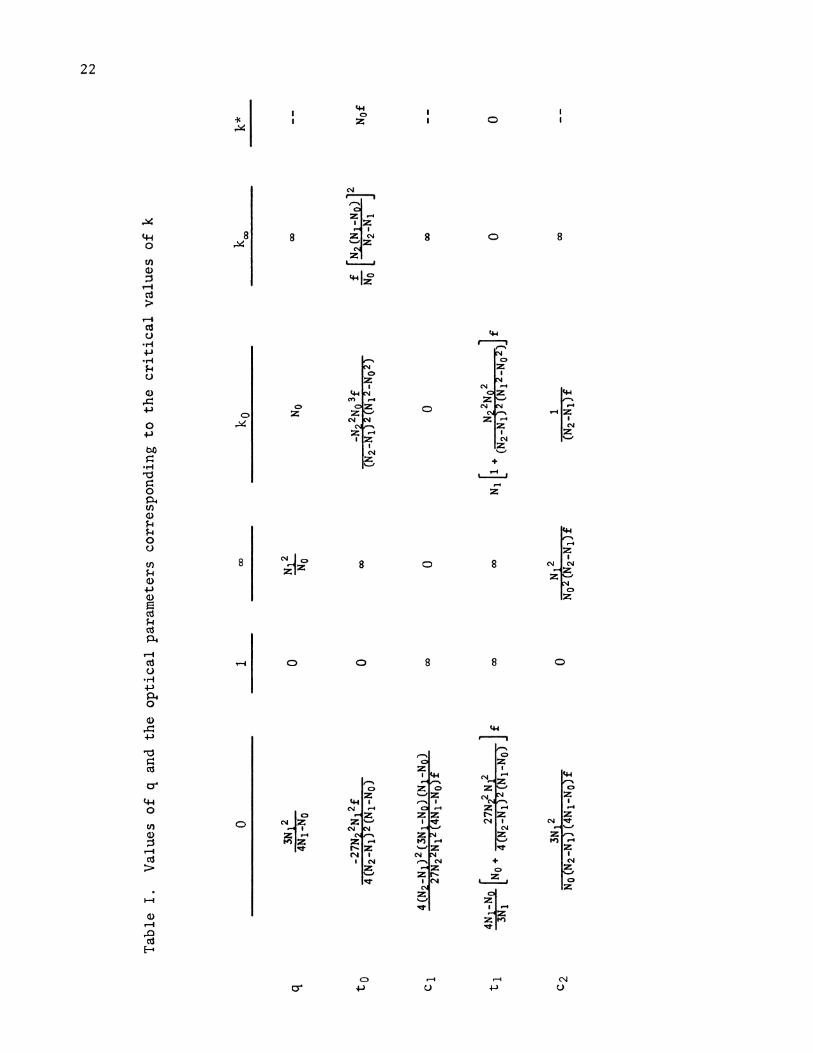
Table I on the following page gives the corresponding values of q and the op-

tical parameters for most cases. The importance of these critical values is

clear. For example, if N1 >N0 and if f >0, then to and t1 will both be pos-

itive only for values of k lying between k and k *. Table II gives similar

critical values for O.

q

Table I.

Values of q and the optical parameters corresponding to the critical values of k

3N12

4N1 -NO

-27NÊ2N12f

t

4(N2-N1) 2(N1-NO)

Cl t 1

e2

4(N2-N1)2(3N -N0) (N -N0)

27N22N12}4N1-NOf

4N1-N1

27N22 N

12

l 3N1

O

4(N2-N12(N1-No) J

3N12

N0(N2-N1)(4N1-N0)f

o

o

CO

CO

o

N12

No

CO

No

-N 2

2N

3f

(N2-Ni )2 12-NO2)

o o

N2N

2 00

N1

1 +

(N2-N1212-NO2) f

N12

1

No2(N2-N1)f

(N2-N1 f

00

f [N2 (N1-N0)12

No

N2-N1

J

00

CO

23

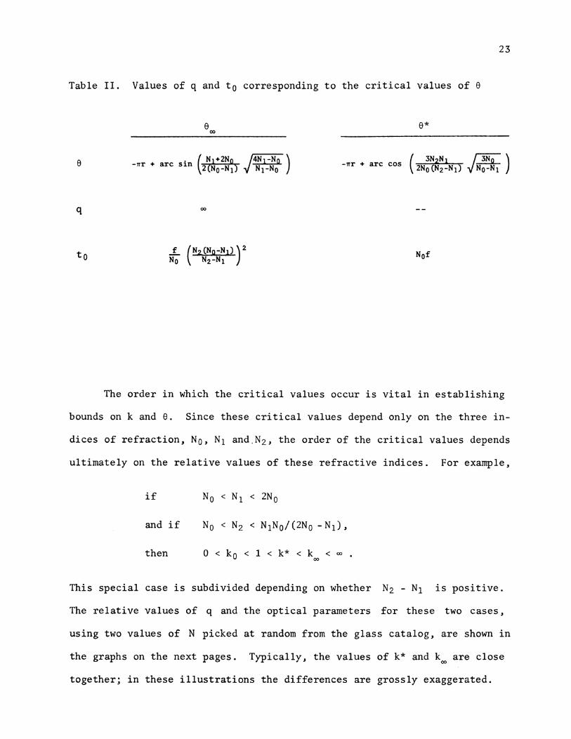
Table II. Values of q and to corresponding to the critical values of 0

0

q

to

0*

-nr + arc sin ( N1 o ) _nr + arc cos ( 3(221 3N- 2(No -N1 N1 -No J 2N0 (N2-N1) No -N1

00

f 12 Np N2-N1

Npf

The order in which the critical values occur is vital in establishing

bounds on k and 0. Since these critical values depend only on the three in-

dices of refraction, No, N1 and,N2, the order of the critical values depends

ultimately on the relative values of these refractive indices. For example,

if No < Ni < 2N0

and if ND < N2 < N1N0/(2N0 -N1),

then 0<ko <1<k* <k < This special case is subdivided depending on whether N2 - N1 is positive.

The relative values of q and the optical parameters for these two cases,

using two values of N picked at random from the glass catalog, are shown in

the graphs on the next pages. Typically, the values of k* and k00 are close

together; in these illustrations the differences are grossly exaggerated.

24

Values of q and the optical parameters as functions of k, showing the critical values of k.

q

to, ti

CI, C2

3.0 2.0 1.0

0

-1.0 -2.0 -3.0 -4.0

800 700 600 500 400 300 200 100

o -loo -200 -300 -400 -500 -600

40

30

20

Io

Io

tk hb ° °°ó °°N`ry\ti o K99999 g° oqó°O0°°°:oao°a°o ( ( ( ( ( ( ( ( « ( (((((

25

20 - - K

15o - tl

10- ti

- 5- t,

^IO

-15

N2 - N1 negative (NQ = 1, N1 = 1.9525, N2=1.5731)

5000 4000 3000 2000 1000

-1000 - 2000 -3000 -4000

2.0

1.0

0.0 -1.0 -2.0 -3.0 -4.0 -5.0 -6.0 -7.0 -8.0 -9.0

-10.0

o 0, A 6 e ( ( ( ( ( ( ( ' ( ( ( ( ( ( ( ( `(

K #04,6000 .00 o PO` 9 o ti b ó 5

a°P dP P 0 O A

4

K,

-10.0 -11.0

- 12.0

-13.0 -14.0 -15.0

30

25

K, 800 - 20 - 700 - 600 - \t1 15 - 500 - 400- \I0- 300 - 200 - 100 - 0

- 100

-200 -

-300 -400 --500 -600 -700 -

IO

-IO

-2-0

to

I I I

K. Km

- 5000 - 4000 - 3000 - 2000 - 1000

to

t1

tl

I I .10 I

8-

C2 6= C2

-2 -4 -6 -8

-10

N2 - N1 positive (0 = 1, N1 = 1.5731, N2 = 1.9525)

- 1000

-2000 - 3000 - 4000 -5000

25

26

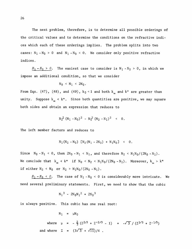
The next problem, therefore, is to determine all possible orderings of

the critical values and to determine the conditions on the refractive indi-

ces which each of these orderings implies. The problem splits into two

cases: N1 -N0 > 0 and N1 -N0 < O. We consider only positive refractive

indices.

N1 -No > O. The easiest case to consider is N1 -No > 0, in which we

impose an additional condition, so that we consider

N0 < N1 < 2N0.

From Eqs. (47), (48), and (49), k0 <1 and both k and k* are greater than

unity. Suppose k. < k *. Since both quantities are positive, we may square

both sides and obtain an expression that reduces to

N22 (N1 -N0)2 - NO2 (N2 -N1)2 < 0.

The left member factors and reduces to

N1(N2 -No) [N2 (N1 -2N0) + N1N07 < O.

Since No -N1 < 0, then 2N0 -N1 < N1, and therefore No < N1N0 /(2N0 -N1).

We conclude that k. < k* if N0 < N2 < N1N0 /(2N0 -N1). Moreover, k. > k*

if either N2 < No or N2 > N1N0 /(2N0 -N1).

N1 -No < O. The case of N1 -No < 0 is considerably more intricate. We

need several preliminary statements. First, we need to show that the cubic

N13 - 2N0N12 + 2NO3

is always positive. This cubic has one real root:

N1 = pNo

where u = - 4 (Z2/3 + Z -2/3 - 1) = -VT / (Z1 /3 + Z -1/3)

and where Z = (31/7r + ii1) /4 .

The cubic therefore factors into

(N1 -.iN0) [N12 + (u - 2)N1N0 + u(u - 2)NO2 J

The left factor is positive. The right factor can be written as

CN1 - N3 '71/3 + Z-L3) ]2 + N 2 (Z2/3 Z-2/3 ) 2 ,

which, as a sum of squares, is also positive. We have shown that

N13 - 2N0N12 + 2NO3 > 0 .

The next step in the preliminaries is to show that

Ñ1 ,/NO2 - N12 (N0 - }/NO2 - N12 ) <

2N01NN1 < N0.

The proof that N1N0 /(2N0 -N1) < N0 is analogous to the proof given for a

similar statement in the case of N1 -N0 > O. Next, start with

1

Ñ1 NO2 - N12 (N0 - NO2 - N12) <

and reduce it to

(N0 -Ni)/NO2 -N12 < NO2

.

Squaring both sides and rearranging terms yields

0 < Ni (N13 - 2N12 N0 + 2NO3 ) .

N1N0 2N0 -N1

We next write Eqs. (48) and (49) in a slightly different form,

kco = 1 4(N0 -N1)3 27N12N0

k* = 1/1 4N0(N0 -Ni) (N -N1)2 27N22N12 f

27

(48')

(49')

and note that k0, k. and k* are now all less than unity. We first prove

that k0 <k.. Squaring both sides and reducing yields

NO3 (N0 -N1)3 Ni +N0 No ,

which is equivalent to N1(N13 -2NON12 +2NO3) > O.

28

Next, suppose that k* <ko. By squaring and reducing we obtain

N1N22 + 2(1\102 - N12)N2 - (NO2 - N12)N1

which factors into

< 0,

N1 (N2

+

N0LN1N12 (No

+

,fNo2 _ N12))

(N2 - A2N1N12

(Np - Np2 -N12) < O.

Since the left -hand factor is always positive, this condition is equivalent to

2 N2 <

0 (No - ti/No2 - N12) if ko < k..

Moreover, if ko >k., the inequality sign in the above expression is reversed.

Next, if k* < k., then

NO2(N2 -N1)2 - N22(N0 -N1)2 > o

which, as we have seen, reduces to either N2 >0 or N2 <N1N0 /(2N0 -N1).

Finally, k <k* if N1N0 /(2N0 -N1) < N2 < No.

Summarizing all these facts gives the following:

For the case where N1 -N0 >0

N2 < No 0 < ko < 1 < k* < k < co

NO < N2 < N1N0/ (2N0 -N1) 0 <ko < 1 <k < k* <co

N1N0/(2NO -N1) < N2 0 < ko < 1 < k* < k < co

For the case where N1 -No <0

N2 < 02N1N12 (N0 - NO2 -N12)

2 2

0N1

N1 (N0 - VNo2 -N12) < N2 < 2Np1NÑ1

N1No 2N0 -N1

0 < k* <ko <k.< 1

0 < ko < k* < k < 1

0 < ko < k < k* < 1

No < N2 0 < ko < k* < k < 1

29

REFLECTING SYSTEMS

All that has been said so far applies, strictly speaking, to refract-

ing systems. To convert the above formulas to two -mirror systems in air,

all that is required is to set

No = N2 = 1

N1 = -1

(S0)

An additional proviso is required. In the discussion on refracting systems

it turned out that t1 had to be positive. For reflecting systems, however,

the value of t1 has to be negative for the systems to be constructible.

Applying Eq. (50) to Eqs. (31) and (37), we obtain the equations for

real k:

to = - 32 f (1(2 - 1) ,

q

-3

1-2 Ck+1 1/3

+

k-1 1/3l

\k-1

(k

J

(31')

(37')

Applying Eq. (50) to Eqs. (38) and (39) produces equations for the

case where k is imaginary,

to = 37

f sect 0, (38')

-3

q r (39') 1 + 4 cos 4(0+7r)

(r = 0, 1, 2)

30

Finally, applying Eq. (50) to Eqs. (6), we obtain the remaining optical

parameters,

c2 = q/2f

t1 = (to-f)/q

cl = (q-1)/2tp .

(6')

These equations provide, for each value of k or 8, values of t0, c2, t1, and

cl which give a reflecting system with the desired properties. A point at a

distance to from the first surface is imaged at infinity, and third -order

spherical aberration is zero.

Next, we refer to Eqs. (47), (48), and (49) giving the critical values

of k:

kp =

k* = k = 5 . Ignoring k* and k. for the moment, for the real case, given by Eqs.

(31') and (37'), we have only three critical values:

k --

k = 1

k = co

The values of the optical parameters at these values, obtained from

Table I, are given in Table III.

31

Table III. Optical parameters at critical values of k

k = 0 k = 1 k =

q -3/5 0 1

to 27f/32 0 co

cl -128/135f .0 0

ti 25f/96 co co

C2 3/10f 0 1/2f

Table III indicates that over the entire range of k, to and ti will always

have the same sign, indicating that to must be negative for every construct-

ible system conforming to this pattern. The finite conjugate point must

therefore be virtual. This general configuration resembles the Gregorian

telescope in which the mirror curvatures have opposite sign.

Next we turn to the case where k is imaginary. In this case we set

k = i tan 0. The imaginary critical values obtained for k* and k become real critical values for 0. Thus

tan(0. +Trr) = tan(0 * +Trr) = 5/27 .

This of course can be obtained directly from Table II by applying Eq. (55).

At this value of 0, ti changes sign and represents the point separating re-

gions in which the system is constructible from regions in which it is not.

The case where k is imaginary corresponds to Cassegranian telescopes

in which the two mirror curvatures have the same sign. It is only in this

case that the thickness ti is negative and the finite conjugate distance to

is positive, resulting in a constructible system.

32

CANONICAL OPTICAL PARAMETERS

It is sometimes useful to transform the optical parameters into a more

convenient form. Define

Also define

C2 = (N2-N1)fc2

C1 = (N1-N0)fc1

Q = g/No

Then Eqs. (6) are transformed into

C2 = Q

T1 = (1-T0)/Q

C1 = (1-Q)/T0

From Eq. (31)

T0 - 27N22N12 (k2 -1)

and from Eq. (36)

Qr

T1 = t1/N1f

T0 = t0/NOf. (51)

(52)

(53)

4N0(N2-N1)2(N1- N0) (54)

3N12 /N0

1/3

r

/3 1 (55)

(2N1+N0) - (N1-N0) [Ck+l) W + (k+1

w r

Note that these canonical optical parameters are independent of the

focal length and do not contain the refractive indices explicitly.

33

CONCLUSION

We have derived a set of algorithms for calculating two -surface optical

systems having the property that third -order spherical aberration is zero.

We have seen that these results are applicable to both refracting and reflect-

ing systems. For such systems we have obtained expressions for third -order

coma and astigmatism and have found the position of the entrance pupil which

corresponds to the vanishing of the latter. We have indicated regions in the

parameter domains where useful solutions might lie.

Some practical applications of these results have already been made.

The solutions for reflecting systems described above were applied to the de-

sign of four -mirror systems by combining any pair of solutions so that the

second conjugate point of the first coincided with the first conjugate point

of the second and so that prescribed first -order conditions were satisfied.

The resulting system had zero third -order spherical aberration as well as the

desired focal length. By changing the parameters associated with each of the

two solutions, the curvatures and separations were varied in concert without

changing the first -order properties of the system while maintaining a zero

value for third -order spherical aberration. Using a time - sharing computer,

the values of the parameters were altered while the values of the remaining

third -order aberrations were monitored. When these were reduced to small

enough values, rays were traced through the system. Small changes were made

on the parameters, and their effect on the rays was observed. A final design

was achieved by introducing a small amount of third -order spherical aberration,

to compensate for those uncorrected higher -order aberrations, by means of

Sutton's "generalized bending" equations, which also leave the first -order

properties of a lens invariant.

34

The method of applying the results to the design of complex refracting

systems is clear. These solutions can be considered as modules for forming

systems consisting of any number of refracting surfaces. These modules are

combined in such a way that the back and front foci of successive modules

coincide and so that the first -order properties of the system formed in this

way coincide with the prescribed requirements. Such a system would start

with zero third -order spherical aberration. At this point, perhaps, the lo-

cation of the stop could be specified, making use of Eq. (43), resulting in

the reduction of astigmatism. The parameters associated with the individual

modules can then be varied to optimize the design.

Before any real application of these techniques can be made, however,

a considerable amount of preliminary work has to be done. The parameter do-

mains corresponding to useful modules depend intimately on the refractive

indices chosen. We might guess that this dependence might prove useful in

the selection of glasses.

The results presented here appear to be applicable to the early stages

of the design process. The use of a conversational mode, time -sharing com-

puter, possibly in conjunction with the y,ÿ diagram described by Pegis et al.8

and improved by Shack, would appear to make best use of these results.

35

REFERENCES

1. 0. N. Stavroudis, "Two- mirror systems with spherical reflecting sur- faces," J. Opt. Soc. Am. 57(6):741 -748, 1967.

2. 0. N. Stavroudis, "Families of lenses with zero third -order spherical aberration" (abstr.), J. Opt. Soc. Am. 57(11): 1420, 1967.

3. 0. N. Stavroudis, "Two- surface refracting systems with zero third - order spherical aberration," J. Opt. Soc. Am. 59(3):288 -293, 1969.

4. D. P. Feder, "Optical calculations with automatic computing machinery," J. Opt. Soc. Am. 41(9): 630 -636, 1951.

5. T. Smith, in A Dictionary of Applied Physics, R. Glazebrook, Ed., London, Macmillan and Company, 1923, Vol. IV, p. 290.

6. L. E. Dickson, New First Course in the Theory of Equations, New York, John Wiley $ Sons, 1939, pp. 42 -45. See also G. A. Korn and T. M. Korn, Mathematical Handbook for Scientists and Engineers, ed. 2, New York, McGraw -Hill, 1968, p. 23.

7. L. E. Sutton, "A method for paraxial rays," Appl.

8. R. J. Pegis, T. P. Vogl, A.

generation of optical

localized variation of the paths of two Opt. 2(12): 1275 -1281, 1963.

K. Rigler, and R. Walters, "Semiautomatic prototypes," Appl. Opt. 6(5): 969 -973, 1967.

36

ACKNOWLEDGMENT

A portion of this work has been supported by Project THEMIS under

contract F44620 -69 -C -0024.