1

Technical Report: Analysis of Historical Land Cover

of the Nudo del Azuay using Aerial Photos (Stage 1 of 2, Orthophoto Generation)

Will Anderson, FCT GIS Specialist

July 2010

Executive Summary

The purpose of this technical report is to document the methods and results of the first of two stages of a

project that will use historical aerial photos (ranging from years 1956 to 2000) to analyze the historical land

cover in the Nudo del Azuay. This document should serve as a technical reference guide for FCT personnel and

their collaborators in any future work that stems from use of the resulting data.

This overall LULC classification project is comprised of two main stages: (1) Orthophoto Generation

(through use of geoprocessing and photogrammetric techniques), and (2) Land Cover/Use Layer Creation

(through manual digitization, using the orthophotos as primary visual aids). This report discusses the

methods and results of Stage 1, Orthophoto Generation.

The aim of the overall project is to create land cover vector layers for each year of our historical air

photos (including 1956, 1963, 1977, 1980-83, 1988-89, and 2000). The resulting vector layers will serve

as primary data sources in future studies identifying and studying priority habitat and ecosystem service

provision areas, and generally help direct the research and conservation efforts of FCT and its

collaborators.

The orthophoto generation process required: (1) scanning prints at high-resolution (600 dpi, resulting in

a 2.7 m cell size); (2) obtaining aerial camera calibration reports from the Instituto Geográfico Militar in

Quito for interior geometry; (3) creating the necessary data inputs using ESRI ArcGIS (ArcView) 9.3; and

(4) performing aerial triangulation, orthorectification, and mosaicking using ERDAS Imagine Leica

Photogrammetry Suite Project Manager 2010 software.

The main challenges of this stage centered on the poor and variable photo contrast and quality, a lack

of necessary fiducial marks in nearly half of the prints, and the general lack of reference data, including

geo-referenced imagery of an acceptable resolution. These issues were ultimately resolved.

Results: a total of 51 orthophotos of 2.75 m resolution were generated; they depict approximately

310,000 Ha of historical land cover in the NDA. Error estimation was within acceptable error

thresholds, and photos have excellent overall planimetric accuracy, as evidenced through their matching

existing vector layers of similar scale.

The second stage (Land Cover/Use Layer Creation) is already underway, and over half of the 1956 land

cover has been manually digitized using a mix of standard air photo interpretation techniques and ground-truthing.

2

Project Background

Fundación Cordillera Tropical (FCT) is an Ecuadorian conservation Non-Governmental Organization (NGO) that

focuses its efforts in the Nudo del Azuay, the mountainous region in the southern sector of Ecuador’s Parque

Nacional Sangay. The organization bases its environmental development and management work in civil society,

particularly with rural inhabitants, and sees them as forming a powerful tool in the protection and recuperation

of natural ecosystems.

Focus Area

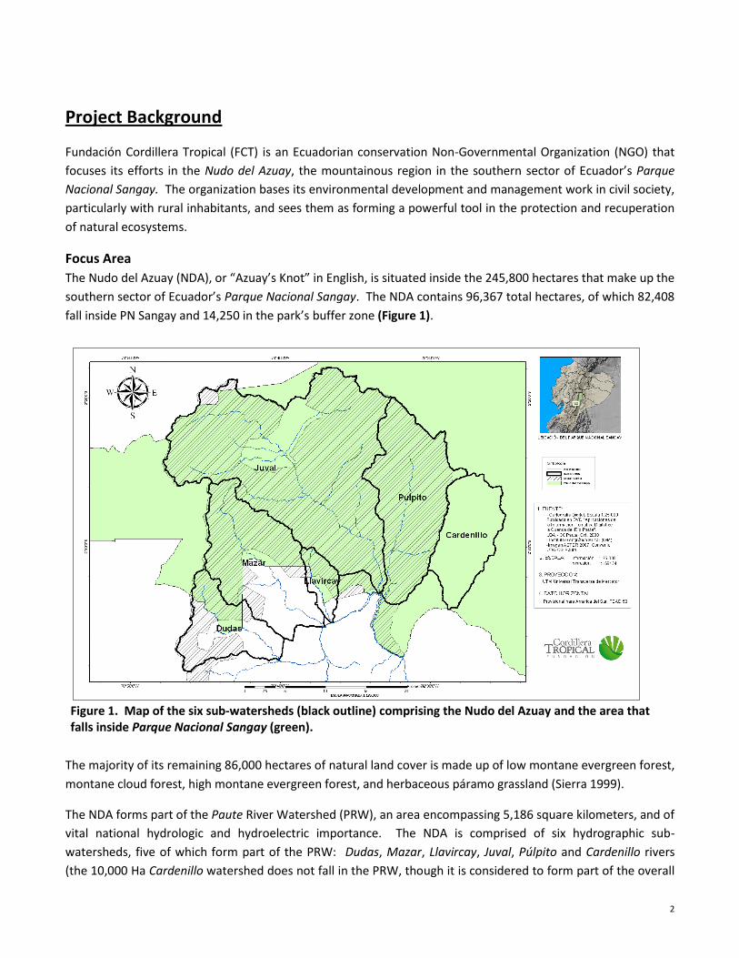
The Nudo del Azuay (NDA), or “Azuay’s Knot” in English, is situated inside the 245,800 hectares that make up the

southern sector of Ecuador’s Parque Nacional Sangay. The NDA contains 96,367 total hectares, of which 82,408

fall inside PN Sangay and 14,250 in the park’s buffer zone (Figure 1).

Figure 1. Map of the six sub-watersheds (black outline) comprising the Nudo del Azuay and the area that falls inside Parque Nacional Sangay (green).

The majority of its remaining 86,000 hectares of natural land cover is made up of low montane evergreen forest,

montane cloud forest, high montane evergreen forest, and herbaceous páramo grassland (Sierra 1999).

The NDA forms part of the Paute River Watershed (PRW), an area encompassing 5,186 square kilometers, and of

vital national hydrologic and hydroelectric importance. The NDA is comprised of six hydrographic sub-

watersheds, five of which form part of the PRW: Dudas, Mazar, Llavircay, Juval, Púlpito and Cardenillo rivers

(the 10,000 Ha Cardenillo watershed does not fall in the PRW, though it is considered to form part of the overall

3

unit of the NDA, for biological, climatic, and other reasons). The NDA’s highest point is Cerro Soroche

(4,730m/15,518 ft), and its elevation ranges from 1600 to 4730m (5,249 to 15,518 ft).

Ecosystem Services & Conservation Value

In addition to its diverse cultural landscapes and extreme natural beauty, the Nudo del Azuay also provides

important ecosystem services, primarily biodiversity, watershed/hydrological services, and carbon

sequestration. A comprehensive review of these services and other conservation value can be found in

Fundacíon Cordillera Tropical (2009), although a brief overview is provided here.

Biodiversity

The Nudo del Azuay contains the largest contiguous areas of native forest and páramo remaining in the Paute

river watershed (PRW), and serves as a biological transition zone between the northern and southern Andes

cordillera mountain range. It is also an Andes Hot Spot and area of high endemism. Both The Nature

Conservancy and EcoCiencia have identified it as being among the 10 ‘hottest’ Hot Spots of the Cordillera Real

Oriental, and the most biodiverse area in the PRW. The NDA is also home to populations of important

endangered mammals, including the tapir, Andean spectacled bear, condor, and puma. The area is also formally

recognized by Conservation International and BirdLife International, as it forms habitat for a great variety of

birds, including 195 registered species, 155 of which are only found in the upper Mazar sub-watershed.

Hydrology & Carbon

Five of the six watersheds of the NDA are tributaries of the length of the Paute river that flows into the Amaluza

reservoir and Daniel Palacios hydroelectric dam. Furthermore, the sub-watersheds fall within the Eastern

climatic region of the cordillera, and their peak flows occur in the driest months of the central and western

portions of the PRW. The topography of the five watersheds is extremely steep: 52% of the terrain has slope

greater than 50%.

The NDA’s large area of páramo ‘sponge’ ecosystem is integral to flow regulation for downstream irrigation

networks and potable water for growing urban populations. Although the processes are not entirely

understood, it is well-accepted that the high soil water retention capacity of páramo (due to high soil carbon) is

an invaluable contributor to year-round base-flow, particularly during the pronounced dry season, as Ecuador

enjoys only negligible snow or glacial melt each year, relative to other countries.

Páramo conservation has become the subject of national interest in the last decade or so. An increasingly visible

advancement of the agricultural frontier upland into the páramo, decreased flow, and increases in biological

contamination of streams, have helped raise concerns over future potable water provision for the country’s

growing downstream urban populations and irrigation networks.

Also, Ecuador relies heavily on hydroelectric power. Recent droughts and extended electrical black-outs

throughout the country have also raised awareness of the issue’s importance, particularly in light of projected

climate change. With the end of páramo conservation – including a focus primarily on preserving its

hydrological services - several new and innovative conservation initiatives have taken hold around the country,

including several compensation for ecosystem services (CES) programs. At the forefront of these is the national

government’s Socio Páramo (“Páramo Partner”) program launched in mid-2009 by the Ministerio del Ambiente,

where landowners enter into 20-year agreements to conserve their existing páramo in exchange for monetary

payments. Additionally, several of the country’s largest municipal water companies - including those of the

4

cities of Quito, Cuenca, and Loja - have implemented a water user conservation tax. Revenue will fund various

conservation programs aimed at protecting and regenerating páramo and other natural cover in their

surrounding watersheds. FCT also has plans in place for implementing a CES program in the Nudo del Azuay.

It is also worth noting that páramo and its high levels of soil carbon is spurring interest among the few countries

that have páramo (Costa Rica, Colombia, Ecuador, Peru, and Venezuela), to gain international funding through

the United Nations’ REDD-plus Programme and other global carbon markets. In fact, Ecuador’s long-term

national conservation strategy is predicated on gaining funding through these emerging markets.

Cultural Landscapes

The NDA’s cultural resources are also worthy of note. The area possesses rich and cultural landscapes, most

notably remnants of the Cañari, Puruhuá and Inca cultures that include terraces, roads, ceremonial sites, and

other archaeological artifacts. The area also possesses a rich contemporary culture, melded with traces of the

past, evident in local textiles, music, food and customs. The area’s population is estimated to be 4,000.

Threats

The primary threats to ecosystem service provision in the NDA include deforestation, agricultural activities

(primarily cultivation and overgrazing/over-burning for cattle), roads and infrastructure projects (including dams

and transmission lines), and weak state systems of protection and control. For a comprehensive report on

threats to the NDA, see Fundación Cordillera Tropical (2009).

When paired with the strong conservation value held by the Nudo del Azuay, this abundance of threats has

prompted several organizations (with Fundación Cordillera Tropical at the forefront) to focus on efforts to

conserve the area. However, because of the large area of focus (nearly 100,000 Ha), it is vital FCT and its

collaborators understand where to best focus their limited resources and conservation efforts.

Furthermore, understanding the historical land cover of the Nudo del Azuay is integral in creating a nexus

between desired land-use and ecosystem service provision (e.g. between conservation of forest and water flow,

or conservation of páramo and soil carbon content). Similarly, theories about the mechanisms that lay behind

ecosystem response to change are best developed and tested using data of a spatial and temporal nature

(Swetnam et al. 1999).

Finally, although the Paute river watershed is among the most studied in Ecuador from a hydrological

standpoint, there has been no scientific research that establishes a relation between vegetation cover type and

hydrological services in the five sub-watersheds of the NDA above the Amaluza reservoir. Similarly, although

there have been studies of flora and fauna of the NDA, conducted by UMACPA (the agency tasked with

managing the PRW), students of local universities, and other researchers, none have focused on the

consequences of the fragmentation or loss of habitat, the importance of corridors connecting contiguous forest

and páramo, nor the genetic consequences of isolation, which would indicate relationships between changes in

land use and biodiversity.

Project Motivation

Consequently, the goal of this project is to augment FCT’s current understandings of land-use-land-cover (LULC)

change in the NDA. Generally, LULC GIS data derived from high resolution remote sensing can serve as an

invaluable resource in guiding conservation interventions in any organization’s area of interest. Understanding

the spatial and temporal dynamics of LULC change is integral to orienting FCT’s overall conservation strategy in

5

the Nudo del Azuay, primarily by helping to prioritize areas of higher conservation value (e.g. older primary

montane forest and undisturbed páramo grassland), and to help optimize the use of limited organizational

resources in remote areas of limited accessibility. This includes where to direct FCT-managed park guards and

where to target the organization’s planned and existing environmental education and Compensation for

Ecosystem Service (CES) programs.

In the past, FCT has utilized Landsat and ASTER satellite imagery for gaining general understandings of the

classification and distribution of LULC in the NDA. However, the high cost, dubious classification accuracy,

coarse resolution (30m and 60m), and unavailability of imagery for years prior to the early 1980’s, prompted FCT

to seek alternative data sources that could provide a more precise understanding of historical LULC in the NDA,

and at a reasonable cost. To this end, FCT obtained historical grayscale aerial photos from Ecuador’s Instituto

Geográfico Militar (IGM) in 2008. The photos depicted the land cover of major portions of the NDA during the

years 1956 to 2000 (Figure 2).

Figure 2. Example of a block of overlapping aerial prints from 1956.

Unfortunately, FCT lacked the expertise and resources to incorporate the photos into its existing Geographic

Information System (GIS), so the prints were sporadically used in qualitative visual analysis on an ad hoc, site-

specific basis only. Not surprisingly, the cumbersome nature of the nearly 100 prints, as well as the varying

scale, often poor print quality, and systematic distortion inherent in aerial photography (particularly from the

extreme terrain differences contained in each photo), made for their difficult, imprecise, and generally

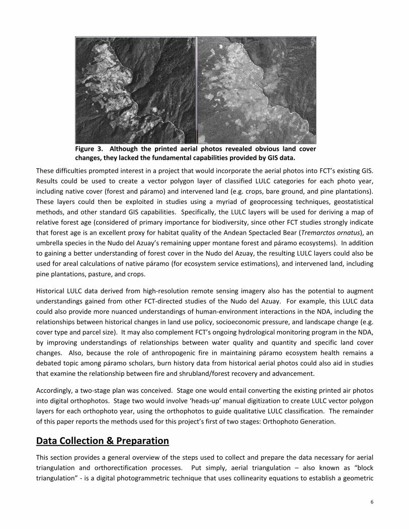
ineffective use. Although manual, visual analysis of the prints revealed obvious land cover changes, they

provided no possibility for accurate areal calculations or location in geographic space (Figure 3).

6

Figure 3. Although the printed aerial photos revealed obvious land cover changes, they lacked the fundamental capabilities provided by GIS data.

These difficulties prompted interest in a project that would incorporate the aerial photos into FCT’s existing GIS.

Results could be used to create a vector polygon layer of classified LULC categories for each photo year,

including native cover (forest and páramo) and intervened land (e.g. crops, bare ground, and pine plantations).

These layers could then be exploited in studies using a myriad of geoprocessing techniques, geostatistical

methods, and other standard GIS capabilities. Specifically, the LULC layers will be used for deriving a map of

relative forest age (considered of primary importance for biodiversity, since other FCT studies strongly indicate

that forest age is an excellent proxy for habitat quality of the Andean Spectacled Bear (Tremarctos ornatus), an

umbrella species in the Nudo del Azuay’s remaining upper montane forest and páramo ecosystems). In addition

to gaining a better understanding of forest cover in the Nudo del Azuay, the resulting LULC layers could also be

used for areal calculations of native páramo (for ecosystem service estimations), and intervened land, including

pine plantations, pasture, and crops.

Historical LULC data derived from high-resolution remote sensing imagery also has the potential to augment

understandings gained from other FCT-directed studies of the Nudo del Azuay. For example, this LULC data

could also provide more nuanced understandings of human-environment interactions in the NDA, including the

relationships between historical changes in land use policy, socioeconomic pressure, and landscape change (e.g.

cover type and parcel size). It may also complement FCT’s ongoing hydrological monitoring program in the NDA,

by improving understandings of relationships between water quality and quantity and specific land cover

changes. Also, because the role of anthropogenic fire in maintaining páramo ecosystem health remains a

debated topic among páramo scholars, burn history data from historical aerial photos could also aid in studies

that examine the relationship between fire and shrubland/forest recovery and advancement.

Accordingly, a two-stage plan was conceived. Stage one would entail converting the existing printed air photos

into digital orthophotos. Stage two would involve ‘heads-up’ manual digitization to create LULC vector polygon

layers for each orthophoto year, using the orthophotos to guide qualitative LULC classification. The remainder

of this paper reports the methods used for this project’s first of two stages: Orthophoto Generation.

Data Collection & Preparation

This section provides a general overview of the steps used to collect and prepare the data necessary for aerial

triangulation and orthorectification processes. Put simply, aerial triangulation – also known as “block

triangulation” - is a digital photogrammetric technique that uses collinearity equations to establish a geometric

7

relationship between the image, camera, and the ground at the time of exposure. Orthorectification is a pixel

resampling process that uses a Digital Elevation Model (DEM) to correct for terrain displacement (Figure 4).

Figure 4. The process of orthorectification uses a Digital Elevation Model (DEM) to resample image pixels (figure from ERDAS 2008).

Aerial triangulation and orthorectification are necessary to diminish the systematic error inherent in aerial

photographs, including differential and radial distortion. For a comprehensive explanation of orthorectification

and digital photogrammetric techniques, including aerial triangulation, see ERDAS (2008).

Data Needs The data necessary for aerial triangulation and orthorectification of aerial photos include the following:

A. Digital aerial image(s) with fiducial marks. Image may be captured by a digital camera or from a

scanned “analog” aerial print. The fiducial marks found at the image corners and/or sides act in concert

as an image x,y grid reference system that helps establish the print principal point of symmetry (image

center) where geometric radial distortion is zero but exponentially increases with distance radially

outward from that point.

B. Elevation (‘Z’) Source. This is usually a Digital Elevation Model (DEM) in the form of a raster grid.

Knowing elevation helps the triangulation process diminish differential distortion contained in an aerial

image and caused by terrain differences that cause some areas of the exposure – like mountain tops - to

be ‘closer’ to the aerial camera lens and thus appear larger than areas that are ‘farther away’ from the

lens and thus ‘smaller’, including areas covered by topographic features (e.g. river valleys).

C. Reference (X,Y) Source. The preferred X,Y reference source is typically a geo-referenced image of

similar resolution, although this was not an option in this case. The layer is used to establish a

relationship between known geographic coordinates of features contained in that imagery (e.g. road

intersections) – known as ground control points (GCPs) - and the aerial image to be geo-referenced.

D. Interior Parameters. These are variables that define the interior geometry of the camera lens and its

resulting image (Figure 5), and are obtained during periodic camera calibration in a laboratory

environment. They include:

a. Focal length: Measured as the distance from the center of the camera lens to the exposure

plate.

b. Principal Point: Coordinate measurements vis-à-vis the fiducial marks that identify the point on

the lens that –if extended through the image plane, would pass through the perspective center

of the image.

8

c. Radial Distortion: Results from flawed optics and lens wear-and-tear, but can be corrected, if

properly accounted for during block adjustment.

Figure 5. Internal geometry (figure from ERDAS 2010).

E. Exterior Parameters. These three rotation angles (omega, phi, and kappa) calculate the position and

angular orientation of an image at the time of exposure, which in turn define the relationship between

the ground coordinate system (X,Y) and the image (pixel) coordinate system (Figure 6). They are

calculated using established X,Y, and Z values and interior orientation variables during the actual

aerial/block triangulation process.

Figure 6. Exterior parameters include three rotation angles (omega, phi, and kappa) that define the position and angular orientation of the image at the time of exposure. These values – when paired with X, Y, and Z values and interior orientation parameters - establish the relationship between the ground coordinate system (X,Y) and image coordinate system (figure from ERDAS 2008).

9

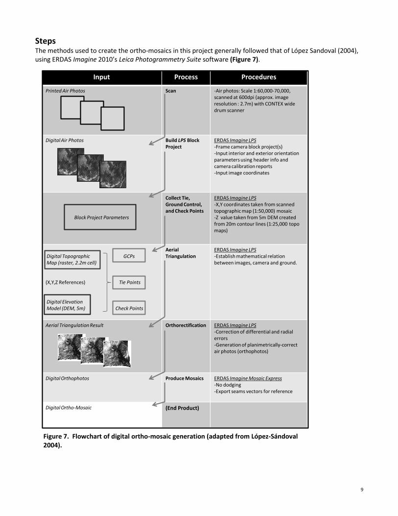
Steps The methods used to create the ortho-mosaics in this project generally followed that of López Sandoval (2004), using ERDAS Imagine 2010’s Leica Photogrammetry Suite software (Figure 7).

Input Process Procedures

Printed Air Photos Scan -Air photos: Scale 1:60,000-70,000, scanned at 600dpi (approx. image resolution : 2.7m) with CONTEX wide drum scanner

Digital Air Photos Build LPS Block Project

ERDAS Imagine LPS-Frame camera block project(s)-Input interior and exterior orientation parameters using header info and camera calibration reports-Input image coordinates

Block Project Parameters

Collect Tie, Ground Control,and Check Points

ERDAS Imagine LPS-X,Y coordinates taken from scanned topographic map (1:50,000) mosaic-Z value taken from 5m DEM created from 20m contour lines (1:25,000 topo maps)

Digital Topographic GCPsMap (raster, 2.2m cell)

(X,Y,Z References) Tie Points

Digital Elevation Model (DEM, 5m) Check Points

Aerial Triangulation

ERDAS Imagine LPS-Establish mathematical relation between images, camera and ground.

Aerial Triangulation Result Orthorectification ERDAS Imagine LPS-Correction of differential and radial errors-Generation of planimetrically-correct air photos (orthophotos)

Digital Orthophotos Produce Mosaics ERDAS Imagine Mosaic Express-No dodging-Export seams vectors for reference

Digital Ortho-Mosaic (End Product)

Figure 7. Flowchart of digital ortho-mosaic generation (adapted from López-Sándoval 2004).

10

1. Scan and Prepare Raw Aerial Images

Ninety-seven (97) aerial prints were available for this project, and were originally obtained from Ecuador’s

Instituto Geográfico Militar (IGM). Prints were 9 x 9 inch, panchromatic (grayscale), and 1:60,000 scale

(1cm=0.6km), although the fifteen 1956 prints were of 1:70,000 scale. Years of exposure included 1956, 1963,

1977, 1980-83, 1988, 1989, and 2000. Prints were scanned in January 2010 at San Diego State University’s

Department of Geography’s Center for Earth Systems Analysis and Research (CESAR) laboratory, as 8-bit, 256-

graytone images, using a calibrated 40-inch CONTEX wide-format drum scanner and accompanying scanning

software. Scan resolution was 600dpi, resulting in a cell/pixel size of approximately 2.7m for the majority

1:60,000 scale prints.

Because the print quality varied from year to year, brightness and contrast was improved using basic photo

editing software (Figure 8), although some of the poorer quality prints would require more advanced ‘dodging’

techniques after orthorectification.

Figure 8. Basic PC image editing software was first used to improve the brightness and contrast of features within the raw digital images.

Print Selection

Several problems were encountered at this point in the process, which ultimately led to the unfortunate

exclusion of nearly half of the prints. First, it was discovered that several fell well outside the NDA study area,

where reference data for aerial triangulation was unavailable. This was likely due to the fact that - at the time

FCT acquired the prints - ordering methods at the IGM in Quito required manual ‘eyeballing’ to discern which

prints were needed from any given film roll. (happily, IGM selection/ordering methods have since improved).

Second, sixteen of the aerial prints lacked fiducial marks, something necessary to accurately estimate the

interior geometry of each print prior to the block triangulation process. Finally, some prints were of such poor

quality (e.g. ‘gray-washed’) that – even after intensive editing to improve brightness and contrast - it became

apparent that any resulting orthorectified images would not have assisted in any subsequent land cover

classification via manual digitization. Consequently, of the 97 total prints available, 51 were selected as feasible

candidates for the aerial triangulation and orthorectification processes.

11

2. Create “Z” Source Digital Elevation Model (DEM)

Aerial triangulation and orthorectification are processes that require the use of elevation (“Z”) values in order to

remove the differential distortion inherent in aerial photos that cover areas containing relief differences. Put

simply, relief difference cause the scale in any given photo to vary, since some areas are inevitably closer to the

camera lens (e.g. mountain tops) than others (e.g. river valleys) and consequently occupy a larger area of the

photograph than is actually planimetrically correct (see Figure 9). As explained above, the NDA is a

mountainous region of extreme terrain differences of over 3000 meters. Although a 30m Digital Elevation

Model (DEM) was available in FCT’s GIS, it was decided that a DEM of finer-resolution would be required to

more optimally correct this differential distortion.

Figure 9. A “Z” value (elevation) source raster is required for orthorectification to reduce the effects of differential distortion, caused by an uneven terrestrial surface.

FCT did have access to a layer of 20m contour lines, vectorized from paper topographic maps (1:25,000, 1994)

by Omar Delgado Inga of the Universidad del Azuay, as part of a larger project aimed at digitizing geographic

information of the greater Paute River Watershed. ArcGIS 9.3’s 3-D Analyst was used to convert this contour

vector layer to a Triangulated Irregular Network (TIN) (Figure 10-A) and subsequent 5m DEM (Figure 10-B). The

resulting DEM – when displayed with a hillshade effect – would serve as an excellent visual reference during

Ground Control Point (GCP) extraction prior to aerial triangulation.

12

(A)

(B)

Figure 10. Results of steps taken to create DEM in ArcGIS 9.3 3-D Analyst: (A) Feature to TIN, and (B) TIN to Raster.

3. Create “ X,Y” Source Raster

In addition to a “Z” elevation value source raster, aerial triangulation also requires the use of a source of known

X,Y geographic coordinates. Although a variety of geo-referenced imagery – even of remote areas – is readily

available and often free of charge in industrialized countries like the United States, developing countries like

Ecuador constantly grapple with an acute shortage of geographic information in digital form. This is particularly

true for imagery of rural, mountainous areas like the Nudo del Azuay. Consequently, with the exception of a few

coarse resolution satellite images, FCT lacked access to any other geo-referenced imagery of the study area that

could be used a source of X,Y coordinates. In fact, with the exception of a 1:25,000-scale vector layer of rivers,

lakes, and the few roads that fall inside the more populated southern sector of the NDA, there were no X,Y

reference sources available.

Consequently, an original X, Y reference raster had to be created for the purpose. Although adequately fine-

scaled imagery was unavailable in digital form, FCT did possess several paper IGM topographic maps (1:50,000

13

scale) that covered the study area, which were ultimately generated into a workable X,Y reference raster, using

the following steps:

Scan:

The printed maps were scanned with an Epson Styles CX5600 desktop scanner at 600 dpi, resulting in a

pixel resolution of approximately 2.2m. The average area of each image was approximately 15,000 Ha,

with four images required to fully digitize each map.

Geo-reference:

Images were then geo-referenced (WGS 1984, UTM 17 South) in ArcGIS 9.3 by pairing their graticule

coordinate intersections with a custom-created vector layer comprised of a lattice of corresponding

points (Figure 11). The subsequent conversion process used a second-order polynomial operation and a

minimum of 25 ground control points (GCPs) per image. Overall, the process maintained a per-image

RMSE of less than 5.0 m.

Mosaic:

The resulting geo-referenced images were then mosaicked using ArcGIS 9.3 and resampled to 3.5m

(Figure 12). The resulting raster - when displayed semi-opaque over the hillshaded DEM with river, road

and lake vector layers (Figure 13) – served as an excellent visual reference and source of X,Y coordinates

for subsequent ground control point (GCP) collection process using ERDAS Imagine 2010 software.

Figure 11. Scanned topographic maps were geo-referenced using their graticule intersections (black lines) and a custom vector layer made of corresponding points of known X,Y coordinates (red points).

14

Figure 12. Overview of the result of scanning and geo-referencing paper topographic maps of 1:50,000 scale, the only sources of X,Y coordinates available at FCT.

Figure 13. The 3.5m topographic map mosaic would serve as an excellent visual reference and X,Y coordinate source for subsequent GCP collection, particularly when displayed semi-opaque over the hill-shaded 5m DEM (top) and draped with 1:25,000 river and lake layers. The result strongly resembled the raw digital prints (bottom).

15

Aerial Triangulation & Orthorectification

With the “X,Y”, and “Z” sources ready, the process of building interior and exterior orientation could begin.

1. Build Block Model Photos were imported by year groups into ERDAS Imagine’s LPS Project Manager software as Frame Camera

block projects. If a camera calibration report was available for the year (1983, 1988, 1989, and 2000 only), block

interior geometry was built using parameters provided in the report, including focal length (also provided in the

photo header), principal point, and radial distortion. If a report was unavailable (photos from 1956, 1963, and

1977), focal length was recorded from the photo header (if available, otherwise it was assumed to be the

standard 152.00mm), fiducial marks were manually measured, and the principal point was assumed to be an

idealized “0,0”, with zero overall radial distortion. No exterior orientation information was available for any

year. Procedures set forth in the LPS Guide (2010) were followed to record the image coordinates of the fiducial

marks, the RMSE of which did not exceed 1.0, except in a handful of cases, generally for images whose fiducial

coordinates had to be measured manually, in which case fiducial mark RMSE never exceeded 1.4, an acceptable

threshold under the circumstances.

2. Collect GCPs and Generate Tie Points Ground Control Points (GCPs) are points of known X,Y geographic coordinates (Figure 14). Tie Points have

coordinates in ‘image-‘ or ‘pixel-space’ (that is columns and rows, rather than latitude and longitude), and are

necessary to establish relations between overlapping images in ‘image-space’. Overall, GCPs are the key to

building a collinearity condition that accurately establishes the relationship between the image, the camera, and

the ground (hence the name aerial triangulation), and tie points help distribute the inherent radial error

throughout multiple overlapping images, via the block bundle adjustment process. This is the advantage of

block bundle adjustment, in that error is dispersed throughout several images, rather than concentrated in one

individual image.

Figure 14. Example of photogrammetric configuration of overlapping photos, showing Ground Control Points (GCPs) of X,Y coordinates, and tie points (using image/pixel coordinates), shared by images with overlapping geographic areas (ERDAS 2010).

In this project, GCPs were collected using the 3.5m X,Y reference raster (displayed with existing river, lake, and

road layers – see above), imported into each LPS block project, and manually assigned relative image-space

coordinates to each image. Where available, GCPs were taken at road intersections and switchbacks. In more

remote areas (the majority of the study area), GCPs were collected at prominent headlands and stream network

16

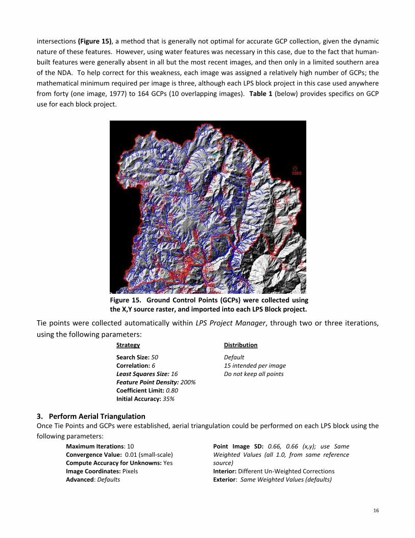
intersections (Figure 15), a method that is generally not optimal for accurate GCP collection, given the dynamic

nature of these features. However, using water features was necessary in this case, due to the fact that human-

built features were generally absent in all but the most recent images, and then only in a limited southern area

of the NDA. To help correct for this weakness, each image was assigned a relatively high number of GCPs; the

mathematical minimum required per image is three, although each LPS block project in this case used anywhere

from forty (one image, 1977) to 164 GCPs (10 overlapping images). Table 1 (below) provides specifics on GCP

use for each block project.

Figure 15. Ground Control Points (GCPs) were collected using the X,Y source raster, and imported into each LPS Block project.

Tie points were collected automatically within LPS Project Manager, through two or three iterations,

using the following parameters: Strategy

Search Size: 50 Correlation: 6 Least Squares Size: 16 Feature Point Density: 200% Coefficient Limit: 0.80 Initial Accuracy: 35%

Distribution

Default 15 intended per image Do not keep all points

3. Perform Aerial Triangulation Once Tie Points and GCPs were established, aerial triangulation could be performed on each LPS block using the

following parameters:

Maximum Iterations: 10 Convergence Value: 0.01 (small-scale) Compute Accuracy for Unknowns: Yes Image Coordinates: Pixels Advanced: Defaults

Point Image SD: 0.66, 0.66 (x,y); use Same Weighted Values (all 1.0, from same reference source) Interior: Different Un-Weighted Corrections Exterior: Same Weighted Values (defaults)

17

The block quality indicators of the nine LPS block projects and their resulting 51 othophotos are provided in

Table 1.

Table 1. Quality indicators of aerial triangulation per LPS photo block project.

Block Project (Year)

Aerial Photo ID

Image ID

Number of GCPs

Image Residuals of the Control Points (pixels)

Residuals of the Control Points (meters)

Accuracy of Object Points (meters)

2000 15331 15332 15333 15335 13725 13726 13727 13728

31 32 33 35 25 26 27 28

98 mx=1.121, my=1.915 mx=1.900, my=1.474 mx=2.720, my=3.132 mx=1.366, my=1.033 mx=1.819, my=2.468 mx=1.340, my=1.311 mx=1.545, my=1.790 mx=1.019, my=1.531

mX=3.2421 mY=3.2427 mZ=1.2889

amX=6.18 amY=5.18 amZ=12.28

1989 27716 27717 27718 27719

16 17 18 19

88 mx=1.324, my=1.535 mx=2.255, my=1.835 mx=2.158, my=2.186 mx=1.263, my=1.353

mX=2.0303 mY=1.9580 mZ=1.2054

amX=5.3852 amY=4.7548 amZ=11.3882

1988 25254 25255 25256

54 55 56

63 mx=1.395, my=0.619 mx=1.674, my=0.652 mx=2.307, my=1.889

mX=2.6922 mY=1.2758 mZ=0.8479

amX=5.9404 amY=5.7137 amZ=17.2136

1983 19084 19085 19086 19092 19093 19094 19095 19096 19097

84 85 86 92 93 94 95 96 97

112 mx=2.608, my=2.162 mx=2.539, my=1.669 mx=2.634, my=3.243 mx=0.687, my=0.641 mx=0.972, my=1.390 mx=2.295, my=1.530 mx=0.549, my=1.760 mx=1.107, my=1.107 mx=1.619, my=1.517

mX=2.8993 mY=2.5242 mZ=0.9358

amX=7.7990 amY=6.7893 amZ=16.9487

1980 13551 13552 13553 13554 13555

51 52 53 54 55

133 mx=1.203, my=1.458 mx=1.436, my=1.447 mx=1.658, my=1.559 mx=1.411, my=0.716 mx=2.612, my=1.421

mX=2.3699 mY=1.8008 mZ=0.9113

amX=5.3130 amY=4.5066 amZ=10.9766

1977 4121 4121 40 mx=2.862, my=2.115 mX=2.3541 mY=1.7254 mZ=0.8447

amX=4.1641 amY=4.1633 amZ=4.5247

1963 4509 4510 4530 4531 4532 3312 3313 3344 3345 3346

9 10 30 31 32 12 13 44 45 46

164 mx=1.265, my=1.838 mx=1.365, my=1.629 mx=0.569, my=1.641 mx=1.358, my=2.089 mx=1.657, my=1.769 mx=1.578, my=2.869 mx=1.888, my=1.330 mx=1.224, my=2.699 mx=0.868, my=1.017 mx=1.307, my=1.963

mX=2.4785 mY=3.5269 mZ=2.0494

amX=6.8118 amY=5.9231 amZ=15.7042

1956(a) 24080 24081 24082 24096 24097 24098 24099

80 81 82 96 97 98 99

106 mx=1.480, my=2.652 mx=2.727, my=1.447 mx=2.088, my=1.856 mx=1.979, my=2.598 mx=2.158, my=2.156 mx=2.542, my=2.577 mx=1.552, my=1.681

mX=3.5331 mY=3.5156 mZ=1.2516

amX=8.6826 amY=7.1298 amZ=20.6616

1956(b) 29814 29815 29816 29817

14 15 16 17

73 mx=2.304, my=0.755 mx=2.388, my=1.340 mx=2.715, my=3.001 mx=4.636, my=3.681

mX=4.3883 mY=3.0700 mZ=1.5871

amX=12.9594 amY=10.5442 amZ=25.4225

18

4. Perform Orthorectification Once aerial triangulation results were accepted, the images were orthorectified using the 5m DEM, and

resampled to a 2.75 m cell size (Figure 16).

Figure 16. Screenshots showing original image (left) and the resulting orthorectified image with differential and radial distortion removed (right).

Overall, error estimation of the aerial triangulation processes were within acceptable error thresholds, and

photos have excellent overall planimetric accuracy, as evidenced through their matching existing vector layers of

similar scale (Figure 17). When draped over the 5m DEM and rendered as a 3-dimensional terrain in ArcGlobe

9.3, the benefits and capabilities of the digital orthophotos is easy to discern (Figure 18).

Figure 17. Orthophotos have excellent ‘fit’ with existing vector layers of similar scale, including this 1:50,000 scale road layer (brown).

Finally, ERDAS Imagine 2010’s Mosaic Express was used to create image mosaics and vectors of image

seamlines, using a Nearest Neighbor sampling process (Figure 18). This was done primarily as a matter of

convenience for future cartographic applications. After all, given the variable contrast and image quality in the

corners (an unavoidable relic of original sub-par print quality), the process of manual digitization requires the

use of individual orthophotos, not mosaics.

19

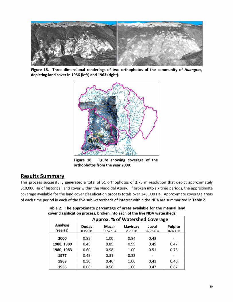
Figure 18. Three-dimensional renderings of two orthophotos of the community of Huangras, depicting land cover in 1956 (left) and 1963 (right).

Figure 18. Figure showing coverage of the orthophotos from the year 2000.

Results Summary This process successfully generated a total of 51 orthophotos of 2.75 m resolution that depict approximately

310,000 Ha of historical land cover within the Nudo del Azuay. If broken into six time periods, the approximate

coverage available for the land cover classification process totals over 248,000 Ha. Approximate coverage areas

of each time period in each of the five sub-watersheds of interest within the NDA are summarized in Table 2.

Table 2. The approximate percentage of areas available for the manual land cover classification process, broken into each of the five NDA watersheds.

Approx. % of Watershed Coverage

Analysis Year(s)

Dudas 8,452 Ha

Mazar 16,577 Ha

Llavircay 2,513 Ha

Juval 42,733 Ha

Púlpito 16,921 Ha

2000 0.85 1.00 0.84 0.43 -

1988, 1989 0.45 0.85 0.99 0.49 0.47

1980, 1983 0.60 0.98 1.00 0.51 0.73

1977 0.45 0.31 0.33 - -

1963 0.50 0.46 1.00 0.41 0.40

1956 0.06 0.56 1.00 0.47 0.87

20

Generally, the best coverage is available for the Mazar, Llavircay, and lower Dudas watersheds, although there is

also ample coverage for more than one analysis year in both the Púlpito and lower Juval. Obviously, the areal

coverage and locations where multiple years overlap will be of primary interest in any analysis carried out after

conclusion of the land cover classification process. That information will be provided later, in the results report

of that stage of the project.

Stage 2 Preparation: Land Cover Classification

The manual digitization process required to create the land cover vector layers for each othophoto is already

under way. The process requires a mix of standard air photo interpretation techniques (including the analysis of

tone, contrast, texture, pattern, context, association, etc.), local knowledge, and ground-truthing. Because the

orthophotos are panchromatic, the ability to distinguish between similar features will require the use of other

GIS reference layers (e.g. elevation bands that denote páramo’s lower local limit of 3200m, and a map of known

pine plantations). Also challenging will be the inherent dynamic nature of the rural landscape, and the ability to

distinguish between similar features within the páramo range (e.g. a recent páramo burn vs. an area plowed by

a tractor) and other areas (e.g. native forest vs. pine plantations) is imperative for a successful classification.

To that end, significant local knowledge of the area – particularly historical understandings – will also prove vital

in this process. In addition to valuable local knowledge held by FCT staff, Dr. Stuart White, local resident of over

25 years, and owner of the Mazar Wildlife Reserve in the southwest portion of the NDA, has created a valuable

annotated aerial print copy that identifies known native forest, páramo, pine plantations, cultivos, and other

disturbed areas, as well as notes on known burns, plowed areas, and secondary forest. These annotated prints

are being used as a guide not only for classification of the area included in the print, but also to guide further

visual classification in other areas. Finally, ground-truthing will inevitably be required for some areas.

End of Report

Will Anderson, FCT GIS Specialist

July 2010

21

Works Cited

Chapin, F.S., P.A. Matson, and H.A. Mooney (2002). Principles of Terrestrial Ecosystem Ecology Springer, New York.

ERDAS (2010). LPS User’s Guide. ERDAS, Inc. Norcross, GA.

ERDAS (2008). ERDAS Field Guide. ERDAS, Inc. Norcross, GA.

Fundación Cordillera Tropical (2009). Análisis de Amenazas y Priorización de Áreas Geográficas de Intervención, Nudo de Azuay, Zona sur del Parque Nacional Sangay, Ecuador. Cuenca, Ecuador (unpublished).

López Sándoval, M.F. (2004). Agricultural and Settlement Frontiers in the Tropical Andes: The Páramo Belt of Northern Ecuador, 1960-1990. Regensburger Geographische Schriften. Heft 37. Institut fur Geographie an der Universitat Regensburg, Germany. S

Sierra, R. (Ed.) (1999). Propuesta Preliminar de Un Sistema de Clasificación de Vegetación para El Ecuador Continental. Proyecto INEFAN/ GEF-BIRF y EcoCiencia. Quito, Ecuador.

Swetnam, T.W., C.D. Allen, and J.L. Betancourt. 1999. Applied historical ecology: Using the past to manage for the future. Ecological Applications 9 (1189-1206).