Embed Size (px)
Citation preview

Technical ReportNumber 261
Computer Laboratory
UCAM-CL-TR-261ISSN 1476-2986
Image resampling
Neil Anthony Dodgson
August 1992
15 JJ Thomson AvenueCambridge CB3 0FDUnited Kingdomphone +44 1223 763500
http://www.cl.cam.ac.uk/

c© 1992 Neil Anthony Dodgson
This technical report is based on a dissertation submitted bythe author for the degree of Doctor of Philosophy to theUniversity of Cambridge, Wolfson College.
Technical reports published by the University of CambridgeComputer Laboratory are freely available via the Internet:
http://www.cl.cam.ac.uk/TechReports/
ISSN 1476-2986
3
Summary
Image resampling is the process of geometrically transforming digital images. This dissertationconsiders several aspects of the process.
We begin by decomposing the resampling process into three simpler sub-processes: reconstructionof a continuous intensity surface from a discrete image, transformation of that continuous surface,and sampling of the transformed surface to produce a new discrete image. We then considerthe sampling process, and the subsidiary problem of intensity quantisation. Both these are wellunderstood, and we present a summary of existing work, laying a foundation for the central bodyof the dissertation where the sub-process of reconstruction is studied.
The work on reconstruction divides into four parts, two general and two specific:
1. Piecewise local polynomials: the most studied group of reconstructors. We examine these,and the criteria used in their design. One new derivation is of two piecewise local quadraticreconstructors.
2. Infinite extent reconstructors: we consider these and their local approximations, the problemof finite image size, the resulting edge effects, and the solutions to these problems. Amongstthe reconstructors discussed are the interpolating cubic B-spline and the interpolating Beziercubic. We derive the filter kernels for both of these, and prove that they are the same. Giventhis kernel we demonstrate how the interpolating cubic B-spline can be extended from a one-dimensional to a two-dimensional reconstructor, providing a considerable speed improvementover the existing method of extension.
3. Fast Fourier transform reconstruction: it has long been known that the fast Fourier transform(FFT) can be used to generate an approximation to perfect scaling of a sample set. DonaldFraser (in 1987) took this result and generated a hybrid FFT reconstructor which can beused for general transformations, not just scaling. We modify Fraser’s method to tackle twomajor problems: its large time and storage requirements, and the edge effects it causes inthe reconstructed intensity surface.
4. A priori knowledge reconstruction: first considering what can be done if we know how theoriginal image was sampled, and then considering what can be done with one particular classof image coupled with one particular type of sampling. In this latter case we find that exactreconstruction of the image is possible. This is a surprising result as this class of imagescannot be exactly reconstructed using classical sampling theory.
The final section of the dissertation draws all of the strands together to discuss transformationsand the resampling process as a whole. Of particular note here is work on how the quality ofdifferent reconstruction and resampling methods can be assessed.

4
About this document
This report is, apart from some cosmetic changes, the dissertation which I submitted for my PhDdegree. I performed the research for this degree over the period January 1989 through May 1992.
The page numbering is different in this version to versions prior to 2005 because I have been ableto incorporate many of the photographs which were previously unavailable in the online version.
Figures 1.4, 2.1, 2.2, 4.34, 7.9, and 7.10 are either incomplete or missing, owing to the way in whichthe original manuscript was prepared. Appendix C is also missing for the same reason.
Acknowledgements
I would like to thank my supervisor, Neil Wiseman, for his help, advice, and listening ear over thecourse of this research. I am especially grateful for his confidence in me, even when I had little ofmy own, and for reading this dissertation and making many helpful comments.
I would also like to thank David Wheeler and Paul Heckbert for useful discussions about imageresampling and related topics, which clarified and stimulated my research.
Over the last three and a third years several bodies have given me financial assistance. TheCambridge Commonwealth Trust paid my fees and maintenance for the first three years, for whichI am grateful. Wolfson College, through the kind offices of Dr Rudolph Hanka, and the ComputerLaboratory, have both contributed towards travel, conference, and typing expenses; and I amgrateful for these too. Finally, I am extremely grateful to my wife, Catherine Gibbs, for herfinancial support, without which that last third of a year would have been especially difficult.
This dissertation was typed in by four people, not a pleasant task. Many thanks go to LyndaMurray, Eileen Murray, Annemarie Gibbs, and Catherine Gibbs for taking this on, and winning!
The Rainbow graphics research group deserve many thanks for their support and friendship overmy time in Cambridge; they have made the research much more enjoyable. Thanks go to Olivia,Stuart, Jeremy, Heng, Alex, Adrian, Dan, Tim, Rynson, Nicko, Oliver, Martin, Jane, and Neil.Equal, if not more, thanks go to Margaret Levitt and Eileen Murray, who have helped to keep mesane; and also to the other inmates of Austin 4 and 5 for the interesting working environment theyprovide.
Final heartfelt thanks go to my parents and to Catherine, to whom this dissertation is dedicated.Their support, and encouragement, has been invaluable in getting me to this point.

Contents
Notation 8
Preface 9
1 Resampling 11
1.1 Introduction . . . . . . . . . . . . . . . . . . . . . . . . . . . . . . . . . . . . . . . . 11
1.2 Images . . . . . . . . . . . . . . . . . . . . . . . . . . . . . . . . . . . . . . . . . . . 11
1.3 Sources of discrete images . . . . . . . . . . . . . . . . . . . . . . . . . . . . . . . . 13
1.4 Resampling: the geometric transformation of discrete images . . . . . . . . . . . . 16
1.5 The practical uses of resampling . . . . . . . . . . . . . . . . . . . . . . . . . . . . 16
1.6 Optical image warping . . . . . . . . . . . . . . . . . . . . . . . . . . . . . . . . . . 18
1.7 Decomposition . . . . . . . . . . . . . . . . . . . . . . . . . . . . . . . . . . . . . . 18
1.8 How it really works . . . . . . . . . . . . . . . . . . . . . . . . . . . . . . . . . . . . 27
1.9 The literature . . . . . . . . . . . . . . . . . . . . . . . . . . . . . . . . . . . . . . . 29
1.10 Summary . . . . . . . . . . . . . . . . . . . . . . . . . . . . . . . . . . . . . . . . . 31
2 Sampling 33
2.1 Converting the continuous into the discrete . . . . . . . . . . . . . . . . . . . . . . 33
2.2 The problem of discrete intensities . . . . . . . . . . . . . . . . . . . . . . . . . . . 33
2.3 Producing a discrete image . . . . . . . . . . . . . . . . . . . . . . . . . . . . . . . 37
2.4 The sampling process . . . . . . . . . . . . . . . . . . . . . . . . . . . . . . . . . . 39
2.5 Area vs point sampling . . . . . . . . . . . . . . . . . . . . . . . . . . . . . . . . . . 43
2.6 Practical considerations . . . . . . . . . . . . . . . . . . . . . . . . . . . . . . . . . 46
2.7 Anti-aliasing . . . . . . . . . . . . . . . . . . . . . . . . . . . . . . . . . . . . . . . 48
2.8 Sampling which considers the reconstruction method . . . . . . . . . . . . . . . . . 49
2.9 Summary . . . . . . . . . . . . . . . . . . . . . . . . . . . . . . . . . . . . . . . . . 50
3 Reconstruction 52
3.1 Classification . . . . . . . . . . . . . . . . . . . . . . . . . . . . . . . . . . . . . . . 52
3.2 Skeleton reconstruction . . . . . . . . . . . . . . . . . . . . . . . . . . . . . . . . . 55
5

6 CONTENTS
3.3 Perfect interpolation . . . . . . . . . . . . . . . . . . . . . . . . . . . . . . . . . . . 58
3.4 Piecewise local polynomials . . . . . . . . . . . . . . . . . . . . . . . . . . . . . . . 59
3.5 What should we look for in a NAPK reconstructor? . . . . . . . . . . . . . . . . . 72
3.6 Cubic functions . . . . . . . . . . . . . . . . . . . . . . . . . . . . . . . . . . . . . . 87
3.7 Higher orders . . . . . . . . . . . . . . . . . . . . . . . . . . . . . . . . . . . . . . . 95
3.8 Summary . . . . . . . . . . . . . . . . . . . . . . . . . . . . . . . . . . . . . . . . . 96
4 Infinite Extent Reconstruction 98
4.1 Introduction to infinite reconstruction . . . . . . . . . . . . . . . . . . . . . . . . . 98
4.2 Edge effects . . . . . . . . . . . . . . . . . . . . . . . . . . . . . . . . . . . . . . . . 98
4.3 Sinc and other perfect interpolants . . . . . . . . . . . . . . . . . . . . . . . . . . . 117
4.4 Gaussian reconstructors . . . . . . . . . . . . . . . . . . . . . . . . . . . . . . . . . 123
4.5 Interpolating cubic B-spline . . . . . . . . . . . . . . . . . . . . . . . . . . . . . . . 125
4.6 Local approximations to infinite reconstructors . . . . . . . . . . . . . . . . . . . . 142
4.7 Summary . . . . . . . . . . . . . . . . . . . . . . . . . . . . . . . . . . . . . . . . . 144
5 Fast Fourier Transform Reconstruction 145
5.1 The reconstructed intensity surface . . . . . . . . . . . . . . . . . . . . . . . . . . . 145
5.2 DFT sample rate changing . . . . . . . . . . . . . . . . . . . . . . . . . . . . . . . . 148
5.3 FFT intensity surface reconstruction . . . . . . . . . . . . . . . . . . . . . . . . . . 154
5.4 Problems with the FFT reconstructor . . . . . . . . . . . . . . . . . . . . . . . . . 156
5.5 Summary . . . . . . . . . . . . . . . . . . . . . . . . . . . . . . . . . . . . . . . . . 169
6 A priori knowledge reconstruction 171
6.1 Knowledge about the sampler . . . . . . . . . . . . . . . . . . . . . . . . . . . . . . 171
6.2 Knowledge about the image content . . . . . . . . . . . . . . . . . . . . . . . . . . 174
6.3 One-dimensional sharp edge reconstruction . . . . . . . . . . . . . . . . . . . . . . 175
6.4 Two-dimensional sharp edge reconstruction . . . . . . . . . . . . . . . . . . . . . . 191
6.5 Summary . . . . . . . . . . . . . . . . . . . . . . . . . . . . . . . . . . . . . . . . . 210
7 Transforms & Resamplers 211
7.1 Practical resamplers . . . . . . . . . . . . . . . . . . . . . . . . . . . . . . . . . . . 211
7.2 Transform dimensionality . . . . . . . . . . . . . . . . . . . . . . . . . . . . . . . . 213
7.3 Evaluation of reconstructors and resamplers . . . . . . . . . . . . . . . . . . . . . . 215
7.4 Summary . . . . . . . . . . . . . . . . . . . . . . . . . . . . . . . . . . . . . . . . . 227
8 Summary & Conclusions 228
8.1 Major results . . . . . . . . . . . . . . . . . . . . . . . . . . . . . . . . . . . . . . . 228
8.2 Other results . . . . . . . . . . . . . . . . . . . . . . . . . . . . . . . . . . . . . . . 229

CONTENTS 7
8.3 Future work . . . . . . . . . . . . . . . . . . . . . . . . . . . . . . . . . . . . . . . . 229
A Literature Analysis 230
B Proofs 238
B.1 The inverse Fourier transform of a box function . . . . . . . . . . . . . . . . . . . . 238
B.2 The Fourier transform of the sinc function . . . . . . . . . . . . . . . . . . . . . . . 238
B.3 Derivation of a = −2 +√
3 . . . . . . . . . . . . . . . . . . . . . . . . . . . . . . . . 239
B.4 The Straightness Criteria . . . . . . . . . . . . . . . . . . . . . . . . . . . . . . . . 241
B.5 A signal cannot be bandlimited in both domains . . . . . . . . . . . . . . . . . . . 242
B.6 The Fourier transform of a finite-extent comb . . . . . . . . . . . . . . . . . . . . . 244
B.7 The not-a-knot end-condition for the B-spline . . . . . . . . . . . . . . . . . . . . . 245
B.8 Timing calculations for the B-spline kernel . . . . . . . . . . . . . . . . . . . . . . . 245
B.9 The error in edge position due to quantisation . . . . . . . . . . . . . . . . . . . . . 246
C Graphs 248
D Cornsweet’s figures 262
Glossary 266
Bibliography 268

Notation
There is little specialised notation in this thesis. We draw your attention to the following notationalconventions:
Spatial domain functions tend to be represented by lowercase letters, for example: g and f(x), orby lowercase words, for example: sinc(x). Frequency domain functions tend to be represented bythe equivalent uppercase letters, for example: G and F (ν), or by capitalised words, for example:Box(ν).
Domains are represented by calligraphic uppercase letters, for example: Z (the integers) and R(the real numbers). This non-standard notation is due to the inability of our typesetter to generatethe correct notation.
We use three functions which generate an integer from a real number: ceiling(x) gives the nearestinteger greater than, or equal to, x; floor(x) gives the nearest integer less than, or equal to, x;round(x) gives the nearest integer to x. These are represented in equations as shown below:
ceiling(x) = �x�floor(x) = �x�
round(x) = 〈x〉
Some of the derivations required the use of a book of tables. We used Dwight [1934]. References toDwight are written thus: [Dwight, 850.1], giving the number of the appropriate entry in Dwight’sbook.
The term continuous is used in this dissertation in a non-standard way: a continuous function is onethat is defined at all points in the real plane, but is not necessarily continuous in the mathematicalsense. A more rigourous description for this use of continuous would be everywhere defined. Theconcept of mathematical continuity is represented in this dissertation by the term C0-continuous.
There is a glossary of terms at the back of the dissertation, just before the bibliography.
8
Preface
Digital image resampling is a field that has been in existence for over two decades. However, whenwe began this research in 1989, all work on image resampling existed in conference proceedings,journals, and technical reports. Since that time, the subject has come more into the public eye.Heckbert’s Masters thesis, “Fundamentals of Texture Mapping and Image Warping” [Heckbert,1989], brought many of the ideas together, concentrating on two-dimensional geometric mappings(specifically affine, bilinear and projective) and on the necessary anti-aliasing filters.
Wolberg’s “Digital Image Warping” [Wolberg, 1990], is the first book on the subject. Its strengthis that it draws most of the published work together in one place. Indeed, it grew out of a surveypaper [Wolberg, 1988] on geometric transformation techniques for digital images. The book hasa computational slant to it, being aimed at people who need to implement image resamplingalgorithms.
The same year saw the publication of the long awaited successor to Foley and van Dam’s “Fun-damentals of Interactive Computer Graphics”, [1982]. Foley, van Dam, Feiner and Hughes [1990]contains a good summary of several image resampling concepts and techniques [ibid. pp.611, 614,617–646, 741–745, 758–761, 815–834, 851, 910, 976–979] in contrast with its predecessor whichdoes not mention resampling at all.
In the face of this flurry of publicity what can we say of image resampling. Certainly it has beenin use for over twenty years, and is now used regularly in many fields. Many of the problems havebeen overcome and the theory behind resampling has been more to the fore in recent years.
What place, then, is there for research in the field? Much: image resampling is a complicatedprocess. Many factors must be taken into account when designing a resampling algorithm. Aframework is required which can be used to classify and analyse resampling methods. Further,there are holes in the coverage of the subject. Certain topics have not been studied because theyare not perceived as important, because the obvious or naive answer has always been used, orbecause no-one has yet thought to study them.
In this dissertation we produce a framework which is useful for analysing and classifying resam-pling methods, and we fit the existing methods into it. We continue by studying the parts of theframework in detail, concentrating on the reconstruction sub-process. Thus we look at piecewisequadratic reconstructors, edge effects, the interpolating Bezier cubic, the kernel of the interpo-lating cubic B-spline, Fraser’s [1987, 1989a, 1989b] FFT method and its extensions, and a prioriknowledge reconstructors; whilst not ignoring the well-trod ground of, for example, piecewise cubicreconstructors and classical sampling theory.
The dissertation is divided into eight chapters, arranged as follows:
1. Resampling — we introduce the concepts of a digital image, a continuous image, and theresampling process. Resampling is decomposed into three sub-processes: reconstruction of acontinuous intensity surface from a discrete image, transformation of that continuous surface,and sampling of the transformed surface to produce a new discrete image. This decompositionunderpins the rest of the dissertation.
9

10
2. Sampling — the concepts of sampling are introduced, laying a foundation for the work onreconstruction and resampling as a whole. As a side issue we discuss the problem of intensityquantisation as it relates to image resampling.
3. Reconstruction — an introduction to reconstruction. Most of the chapter is given over toa discussion of piecewise local polynomial reconstructors, and the factors involved in theirdesign.
4. Infinite Extent Reconstruction — sinc, Gaussian, interpolating cubic B-spline, and interpo-lating Bezier cubic are all theoretically infinite. We discuss these, their local approximations,and the problem of a finite image. The latter problem applies to local reconstructors, as wellas infinite extent ones.
5. Fast Fourier Transform Reconstruction — a method of implementing an approximation tosinc reconstruction, developed by Donald Fraser [1987]. We describe his method, and thenpresent improvements which solve two of its major problems.
6. A priori knowledge reconstruction — in the preceding three chapters we assumed that wehad no a priori knowledge about how the image was sampled, or about its contents. In thischapter we briefly consider what can be achieved given a priori knowledge about how theimage was sampled. The bulk of this chapter, however, is an analysis of what can be achievedgiven a particular set of intensity surfaces (those with areas of constant intensity separatedby sharp edges) and one particular type of sampling (exact area sampling).
7. Transforms and Resamplers — where we consider transforms, and the resampling process asa whole. An important section in this chapter is the discussion of how to measure the qualityof a reconstructor and of a resampler.
8. Summary and Conclusions — where all our results are drawn into one place.

Chapter 1
Resampling
1.1 Introduction
Digital image resampling occupies a small but important place in the fields of image processing andcomputer graphics. In the most basic terms, resampling is the process of geometrically transformingdigital images.
Resampling finds uses in many fields. It is usually a step in a larger process, seldom an end initself and is most often viewed as a means to an end. In computer graphics resampling allowstexture to be applied to surfaces in computer generated imagery, without the need to explicitlymodel the texture. In medical and remotely sensed imagery it allows an image to be registeredwith some standard co-ordinate system, be it another image, a map, or some other reference. Thisis primarily done to prepare for further processing.
1.2 Images
There are two basic types of image: continuous and discrete. Continuous images have a realintensity at every point in the real plane. The image that is presented to a human eye or to avideo camera, before any processing is done to it, is a continuous image. Discrete images only haveintensity values at a set of discrete points and these intensities are drawn from a set of discretevalues. The image stored in a computer display’s frame buffer is a discrete image. The discretevalues are often called ‘pels’ or ‘pixels’ (contractions of ‘picture elements’).
There are intermediate types of image, which are continuous in some dimensions but discrete inothers. Wolberg [1990, p.12] gives two examples of these: where the image is continuous in space butdiscrete in intensity, or where it is continuous in intensity but discrete in space. A television signalis an interesting third case: it is continuous in intensity and in one spatial dimension (horizontally)but it is discrete in the other spatial dimension (vertically).
A digital computer, being a discrete device, can deal only with discrete images. What we perceivein the real world are invariably continuous images (which our eyes discretise for processing). Fora human to perceive a discrete image it must be displayed as a continuous image, thus alwaysputting us one step away from the data on which the computer operates. We must accept (andcompensate for) this limitation if we wish to use the power of digital computers to process images.
Binkley [1990] discusses some of the philosophical problems of digital imagery. He states that‘digital image’ is an oxymoron: “If a digital image is something one can see (by experiencingit with one’s eyes), one cannot compute it; but if one can apply mathematical operations to it,then it has no intrinsic visual manifestation.” Resampling is essentially a mathematical operation
11

12 CHAPTER 1. RESAMPLING
Figure 1.1: The same image represented in three different ways: (1) displayed on a monitor.
Figure 1.2: The same image represented in three different ways: (2) rendered in halftone by a laserprinter.
mapping one collection of numbers into another. The important point here is that what is seen bya human to be the input to and output from the resampling process are continuous representationsof the underlying discrete images. There are many different ways of reconstructing a continuousimage from a discrete one. We must be careful about the conclusions we draw from the continuousrepresentations of discrete images. Binkley’s figures 2 and 3 show how different two continuousrepresentations of the same discrete image can be. Figure 1.1 and figure 1.2 are based on Binkley’sfigures, and show that the same image can give rise to very different continuous representations.Figure 1.3 shows the discrete representation that is stored in the computer’s memory.
The images we deal with are thus discrete. In general any practical discrete image that we meetwill be a rectangular array of intensity values. Experimental and theoretical work is being doneon hexagonal arrays [Mersereau, 1979; Wuthrich, Stucki and Ghezal, 1989; Wuthrich and Stucki,1991] but, at present, all practical image resampling is performed on rectangular arrays.

1.3. SOURCES OF DISCRETE IMAGES 13
148 151 153 151 150 151 151 · · · 6 1 0 0 0 0149 148 151 152 151 149 147 · · · 0 0 0 3 7 5145 146 152 152 150 150 147 · · · 0 0 1 9 19 11145 144 148 149 149 149 148 · · · 4 0 1 14 26 15143 144 145 147 147 146 147 · · · 7 0 3 13 15 6144 146 144 147 146 147 146 · · · 0 0 4 13 13 5145 143 146 146 148 148 149 · · · 0 0 4 11 10 5139 141 144 143 149 148 144 · · · 0 0 2 18 14 5...
......
......
......
. . ....
......
......
...57 66 59 56 58 67 71 · · · 136 137 137 133 129 12731 38 42 36 37 53 60 · · · 138 138 136 134 128 12823 46 49 37 35 47 49 · · · 133 134 134 132 130 12740 64 53 38 45 54 70 · · · 131 127 129 126 125 126
Figure 1.3: The same image represented in three different ways: (3) the array of numbers held inthe computers memory.
���
���
���
���
���
���
���
���
���
�
�
�
�
�
(a)
(b)
(c)
Figure 1.4: The three ways of producing an image: (a) capturing a real world scene; (b) renderinga scene description; and (c) processing an existing image.
1.3 Sources of discrete images
There are three distinct ways of producing such a rectangular array of numbers for storage in acomputer. These can be succinctly described as capturing, rendering, or processing the discreteimage (figure 1.4):
Image capture is where some real-world device (for example: a video camera, digital x-ray

14 CHAPTER 1. RESAMPLING
Image
Description
�PatternRecognition
�
[Computer]Graphics
�� �Image Processing
Figure 1.5: Pavlidis [1982] figure 1.1, showing the relationship between image processing, patternrecognition (image analysis), and computer graphics.
Image
SceneDescription
�
ImageRendering
� �
� ��
ImageProcessing
�
�
Real-WorldImage
�Image Capture
Continuous World(real world)
Discrete World(in the computer)
Figure 1.6: The three sources of discrete imagery shown as processes.
scanner, or fax machine) is used to capture and discretise some real-world (continuous)image.
Image rendering is where some description of a scene is stored within the computer and thisdescription is converted into an image by a rendering process (for example: ray-tracing).The field of computer graphics is generally considered as encompassing all the aspects of thisrendering process.
Image processing is where a previously generated discrete image is processed in some way toproduce a new discrete image (for example: thresholding, smoothing, or resampling).
Pavlidis [1982] produced a simple diagram, reproduced in figure 1.5, showing the links betweendiscrete images and scene descriptions. Based on his diagram, we produce figure 1.6 which showsthe three sources of discrete imagery:
In order for us to evaluate digital imagery we must add ourselves into the picture (figure 1.7). Herewe see that, to perceive a discrete image, we need to display that image in some continuous form(be it on a cathode ray tube (CRT), on photographic film, on paper, or wherever) and then useour visual system on that continuous image.

1.3. SOURCES OF DISCRETE IMAGES 15
Image
SceneDescription
�
ImageRendering
� �
� ��
ImageProcessing
� �
� ��
SceneDescriptionProcessing
� �
� �
�
ImageAnalysis
�
�
�
�
�
Real-WorldImage
��
DisplayedImage
�
�
�
PerceivedImage
�
��
ImaginaryScene
�
Vision
Vision�
Image Display
Image Capture
‘Coding’
Perceptual World(in the mind)
Continuous World(real world)
Discrete World(in the computer)
Figure 1.7: The complete diagram, showing the connection between images in the discrete, con-tinuous, and perceptual worlds.
To complete the diagram, consider the scene description. Such a description could be generatedfrom an image by an image analysis process [see, for example, Rosenfeld, 1988]; or it could begenerated from another scene description (for example: by converting a list of solid objects into aset of polygons in preparation for rendering, as in the Silicon Graphics pipeline machines; or Bley’s[1980] cleaning of a ‘picture graph’ to give a more compact description of the image from whichthe graph was created). Mantas [1987] suggests that pattern recognition is partially image analysisand partially scene description processing. A third way of generating a scene description is for ahuman being to physically enter it into the computer, basing the description on some imaginedscene (which could itself be related to some perceived scene, a process not shown in the figures).Adding these processes to figure 1.6 gives us figure 1.7 which illustrates the relationships betweenthese processes and the various image representations.
To avoid confusion between continuous and discrete images in this dissertation, we have chosento call a continuous image an intensity surface. It is a function mapping each point in the realplane to an intensity value, and can be thought of as a surface in three dimensions, with intensitybeing the third dimension. We can thus take it that, when the word ‘image’ appears with noqualification, it means ‘discrete image’.

16 CHAPTER 1. RESAMPLING
Image
Image
DisplayedImage
DisplayedImage
PerceivedImage
PerceivedImage
�
�
�
�
� � �Vision
Vision
Display
Display
MentalTransform Transform Resample
Perceptual World Continuous World Discrete World
Figure 1.8: The relationship between the resampled and the original images. The two continuousversions must be perceived as transformed versions of one another.
1.4 Resampling: the geometric transformation of discreteimages
In image resampling we are given a discrete image and a transformation. The aim is to produce asecond discrete image which looks as if it was formed by applying the transformation to the originaldiscrete image. What is meant by ‘looks as if’ is that the continuous image generated from thesecond discrete image, to all intents and purposes, appears to be identical to a transformed versionof the continuous image generated from the first discrete image, as is illustrated in figure 1.8. Whatmakes resampling difficult is that, in practice, it is impossible to generate the second image bydirectly applying the mathematical transformation to the first (except for a tiny set of special casetransformations).
The similarity between the two images can be based on visual (perceptual) criteria or mathematicalcriteria, as we shall see in section 3.5. If based on perceptual criteria then we should consider theperceptual images, which are closely related to the continuous images. If based on mathematicalcriteria the perceptual images are irrelevant and we concentrate on the similarities between thecontinuous images and/or between the discrete images.
Whatever the ins and outs of how we think about image resampling, it reduces to a single problem:determining a suitable intensity value for each pixel in the final image, given an initial image anda transformation1.
1.5 The practical uses of resampling
Resampling initially appears to be a redundant process. It seems to beg the question: “why notre-capture or re-render the image in the desired format rather than resampling an already existingimage to produce a (probably) inferior image?”
Resampling is used in preference to re-capturing or re-rendering when it is either:
• the only available option; or
• the preferential option.
1c.f. Fiume’s definition of rendering, 1989, p.2.

1.5. THE PRACTICAL USES OF RESAMPLING 17
The first case occurs where it is impossible to capture or render the image that we require. In thissituation we must ‘make do’ with the image that we have got and thus use resampling to transformthe image that we have got into the image that we want to have.
The second case occurs where it is possible to capture or render the required image but it is easier,cheaper or faster to resample from a different representation to get the required image.
Various practical uses of image resampling are2:
• distortion compensation of optical systems. Fraser, Schowengerdt and Briggs [1985] give anexample of compensating for barrel distortion in a scanning electron microscope. Gardnerand Washer [1948] give an example of how difficult it is to compensate for distortion using anoptical process rather than a digital one (this example is covered in more detail in section 1.6).
• registration to some standard projection.
• registration of images from different sources with one another; for example registering thedifferent bands of a satellite image with one another for further processing.
• registering images for time-evolution analysis. A good example of this is recorded by Herbinet al [1989] and Venot et al [1988] where time-evolution analysis is used to track the healingof lesions over periods of weeks or months.
• geographical mapping; changing from one projection to another.
• photomosaicing; producing one image from many smaller images. This is often used to buildup a picture of the surface of a planet from many photographs of parts of the planet’s surface.A simpler example can be found in Heckbert [1989] figures 2.9 and 2.10.
• geometrical normalisation for image analysis.
• television and movie special effects. Warping effects are commonplace in certain types oftelevision production; often being used to enhance the transition between scenes. They arealso used by the movie industry to generate special effects. Wolberg [1990, sec. 7.5] discussesthe technique used by Industrial Light and Magic, the special effects division of Lucasfilm Ltd.This technique has been used to good effect, for example, in the movies: Willow3, IndianaJones and the Last Crusade4, and The Abyss5. Smith [1986, ch. 10] gives an overview ofIndustrial Light and Magic’s various digital image processing techniques.
• texture mapping; a technique much used in computer graphics. It involves taking an imageand applying it to a surface to control the shading of that surface in some way. Heckbert[1990b] explains that it can be applied so as to modify the surface’s colour (the more narrowmeaning of texture mapping), its normal vector (‘bump mapping’), or in a myriad of otherways. Wolberg [1990, p.3] describes the narrower sense of texture mapping as mapping atwo-dimensional image onto a three-dimensional surface which is then projected back on to atwo-dimensional viewing screen. Texture mapping provides a way of producing visually richand complicated imagery without the overhead of having to explicitly model every tiny feature
2Based on a list by Braccini and Marino, [1980, p.27].
3One character (Raziel) changes shape from a tortoise, to an ostrich, to a tiger, to a woman. Rather than simplycross-dissolve two sequences of images, which would have looked unconvincing, two sequences of resampled imageswere cross-dissolved to make the character appear to change shape as the transformation was made from one animalto another.
4The script called for a character (Donovan) to undergo rapid decomposition in a close-up of his head. In practice,three model heads were used, in various stages of decomposition. A sequence for each head was recorded and thenresampled so that, in a cross-dissolve, the decomposition appeared smooth and continuous.
5At one point in the movie, a creature composed of seawater appears. Image resampling was used in the generationof the effect of a semi-transparent, animated object: warping what could be seen through the object so that thereappeared to be a transparent object present.

18 CHAPTER 1. RESAMPLING
in the scene [Smith, 1986, p.208]. Image resampling, as described in this dissertation, can betaken to refer to texture mapping in its narrow sense (that of mapping images onto surfaces).The other forms of texture mapping described by Heckbert [1990b] produce different visualeffects and so the discussion will have little relevance to them.
1.6 Optical image warping
Image warping need not be performed digitally. The field of optical image warping has not beencompletely superseded by digital image warping [Wolberg, 1990, p.1]. However optical systems arelimited in control and flexibility. A major advantage of optical systems is that they work at thespeed of light. For example Chiou and Yeh [1990] describe an optical system which will producemultiple scaled or rotated copies of a source image in less than a millionth of a second. Theseimages can be used as input to an optical pattern recognition system. There is no way that suchimages could be digitally transformed this quickly, but there is a limited use for the output of thisoptical process.
The problems of using an optical system for correction of distortion in imagery are well illustratedby Gardner and Washer [1948]. In the early 1940s, Zeiss, in Germany, developed a lens with alarge amount of negative distortion, specifically for aerial photography. The negative distortionwas designed into the lens in order that a wide field of view (130◦) could be photographed withoutthe extreme loss of illumination which would occur near the edges of the field if no distortion werepresent in the lens.
A photograph taken with this lens will appear extremely distorted. To compensate, Zeiss developed(in parallel with the lens) a copying or rectifying system by which an undistorted copy of thephotograph could be obtained from the distorted negative.
For the rectification to be accurate the negative has to be precisely centred in the rectifying system.Further, and more importantly, the particular rectifying system tested did not totally correct thedistortion. Gardner and Washer suggest the possibility that camera lens and rectifier were designedto be selectively paired for use (that is: each lens must have its own rectifier, rather than beingable to use a general purpose rectifier) and that the lens and rectifier they tested may not havebeen such a pair. However, they also suggest that it would be difficult to actually make such alens/rectifier pair so that they accurately compensate for one another.
The advent of digital image processing has made such an image rectification process far simplerto achieve. Further, digital image processing allows a broader range of operations to be performedon images. One example of such processing power is in the Geosphere project, where satellitephotographs of the Earth, taken over a ten month period, were photomosaiced to produce acloudless satellite photograph of the entire surface of the Earth [van Sant, 1992]6.
1.7 Decomposition
Image resampling is a complex process. Many factors come into play in a resampling algorithm.Decomposing the process into simpler parts provides a framework for analysing, classifying, andevaluating resampling methods, gives a better understanding of the process, and facilitates thedesign and modification of resampling algorithms. One of the most important features of anyuseful decomposition is that the sub-processes are independent of one another. Independenceof the sub-processes allows us to study each in isolation and to analyse the impact of changingone sub-process whilst holding the others constant. In chapter 7 we will discuss the equivalence
6An interesting artifact is visible in the Antarctic section of this photomosaic: the Antarctic continent is sostretched by the projection used that resampling artifacts are visible there. However, the rest of the mosaic looksjust like a single photograph — no artifacts are visible.

1.7. DECOMPOSITION 19
Image IntensitySurface
Image� �Reconstruct Sample
Figure 1.9: A two part decomposition of resampling into reconstruction and sampling.
Reconstruct Sample
IntensitySurfaceImage
OriginalImage
Resampled
Figure 1.10: An example of a two-part decomposition (figure 1.9). The squares are the originalimage’s sample points which are reconstructed to make the intensity surface. The open circles arethe resampled images sample points which are not evenly spaced in the reconstructed intensitysurface, but are evenly spaced in the resampled image.
of resamplers; that is, how two dissimilar decompositions of a resampling method can produceidentical results.
The simplest decomposition is into two processes: reconstruction, where a continuous intensitysurface is reconstructed from the discrete image data; and sampling, where a new discrete im-age is generated by taking samples off this continuous intensity surface. Figure 1.9 shows thisdecomposition.
Mitchell and Netravali [1988] follow this view as a part of the cycle of sampling and reconstruc-tion that occurs in the creation of an image. Take, for example, a table in a ray-traced image,texture-mapped with a real wooden texture. First, some wooden texture is sampled by an imagecapture device to produce a digital texture image. During the course of the ray-tracing this imageis reconstructed and sampled to produce the ray-traced pixel values. The ray-traced image is sub-sequently reconstructed by the display device to produce a continuous image which is then sampledby the retinal cells in the eye. Finally, the brain processes these samples to give us the perceivedimage, which may or may not be continuous depending on quite what the brain does. These manyprocesses may be followed in figure 1.7, except that image resampling is a single process there,rather than being decomposed into two separate ones.
This decomposition into reconstruction and sampling has also been proposed by Wolberg [1990,p.10], Ward and Cok [1989, p.260], Parker, Kenyon and Troxel [1983, pp.31–32], and Hou andAndrews [1978, pp.508–509]. It has been alluded to in many places, for example: by Schreiber andTroxel [1985].
It is important to note that all of these people (with the exception of Wolberg) used only singlepoint sampling in their resampling algorithms. This decomposition becomes complicated whenmore complex methods of sampling are introduced and Wolberg introduces other decompositionsin order to handle these cases, as explained below. Figure 1.10 gives an example of a resamplingdecomposed into these two sub-processes.
A second simple decomposition into two parts is that espoused by Fraser, Schowengerdt and Briggs[1985, pp.23–24] and Braccini and Marino [1980, p.130]; it is also mentioned by Foley, van Dam,Feiner and Hughes [1990, pp.823–829] and Wolberg [1990]. The first part is to transform thesource or destination pixels into their locations in the destination or source image (respectively).The second part is to interpolate between the values of the source pixels near each destinationpixel to provide a value for each destination pixel. This decomposition is shown in figure 1.11.

20 CHAPTER 1. RESAMPLING
Image Image Image� �Transform Interpolate
Figure 1.11: A two part decomposition into transformation and interpolation.
The interpolation step could be thought of as a reconstruction followed by a point sample at the(transformed) destination pixel, but this further decomposition is not explicit in this model ofresampling7. Note that point sampling is assumed in the model of the resampling process and thusany more complicated sampling method cannot easily be represented.
Both of these two part models are valid and useful decompositions of resampling. However, bothcontain the implicit assumption that only single point sampling will be used. Many resamplingprocesses do exclusively use single point sampling. However, those which do not will not fit intothese models. A more general model of resampling is required if we are to use it to classify andanalyse all resampling methods.
It may not be immediately apparent why these models cannot embrace other sampling methods.In the case of the second decomposition, there is no place for any other sampling method. Singlepoint sampling is built into the model. The sampling is performed as part of the interpolationstep, and the assumption is that interpolation is done at a single point from each sample value. Itis possible to simulate other forms of sampling by modifying the interpolation method, but suchmodification is transform-specific and thus destroys the independence of the two sub-processes inthe model.
The first decomposition can be expanded to include other sampling methods, but there are difficul-ties. To illustrate this let us look at exact-area sampling using a square kernel the size of one pixel.This resampling model (figure 1.9) has the transform implicitly built into the sampling stage. Thisworks well with point sampling. A transformed point is still a point. With area sampling we havetwo choices: either we transform the centre of the pixel and apply the area sampler’s kernel ‘asis’ (as in figure 1.12(a)) or we transform the whole area and apply the transformed kernel (as infigure 1.12(b)).
The former method is equivalent to changing the reconstructor8 in a transformation-independentway and then using point sampling. This is not what is desired. We would get the same resultsby retaining point sampling and using a different reconstructor.
The latter method is what is wanted, the whole area is warped by the transformation. Unfortu-nately, the sampler is now transform-dependent (remember that transforming a point produces apoint, so a point sampler is transform-independent: although the positions of the point sampleschange, the shape of the sampling kernel (a point) does not; in area sampling, the position andshape of the kernel change and thus the area sampler is transform-dependent). Therefore, neithermethod of expanding the reconstruct/sample decomposition is particularly helpful.
To produce an all-encompassing decomposition we need to split resampling into three parts.
1.7.1 A three-part decomposition
Fiume [1989, pp.36-38; 1986, pp.28-30] discusses texture mapping using a continuous texture func-tion defined over a texture space [see p.37 of Fiume, 1989]. He comments: “In practice, texturemapping consists of two distinct (but often interleaved) parts: the geometric texture mappingtechnique itself. . . and rendering”. Rendering is a sampling process (Fiume discusses rendering in
7The ‘interpolation’ need not be a true interpolation but may be an ‘approximation’, that is a function whichdoes not interpolate the data points but still produces an intensity surface which reflects the shape implied by thedata points.
8A reconstructor is a reconstruction method.

1.7. DECOMPOSITION 21
(a) (b)
Figure 1.12: Two ways of extending two-part decomposition to cope with area sampling. Thesquares are the original image’s pixels on a regular grid. The open circles are the resampledimage’s pixels at the locations they would be if they were generated by taking point samples offthe intensity surface (figure 1.10). As an example, we have taken a square area sampler centred atthis point. This can be implemented in two ways: (a) transform-independent sampling, the samplefilter shape does not change; (b) transform-dependent sampling, the sample filter shape changes.
IntensitySurface
IntensitySurface
Image� �Transform Render(Sample)
Figure 1.13: Fiume’s [1989] decomposition of resampling. He does not, however, start with animage, but with an intensity surface. Some extra process is required to produce the intensitysurface from an image.
great detail in his chapter 3 [Fiume, 1989, pp.67-121]). Figure 1.13 shows Fiume’s decomposition.Compare this with Mitchell and Netravali’s ‘reconstruct/sample’ decomposition (figure 1.9).
These two decompositions do not have the same starting point. Fiume is interested in the gen-eration of digital images from scene specifications (the rendering process in figure 1.13(b)), thushe starts with some continuous intensity surface. He states that this continuous intensity surfacecould itself be generated procedurally from some scene specification or it could be generated froma digital image but gives no further comment on the process required to generate a continuousintensity surface from a digital image. The required process is reconstruction, as found in Mitchelland Netravali’s decomposition. Fiume, however, splits Mitchell and Netravali’s sampling step intotwo parts: the geometric transformation and the sampling, where ‘sampling’ can be any type ofsampling, not just single point sampling. He comments: “The failure to distinguish between these[two] parts can obscure the unique problems that are a consequence of each.”
The three part decomposition thus developed from these two-part decompositions is shown infigure 1.14.
1.7.2 Description of the parts
A discrete image, consisting of discrete samples, is reconstructed in some way to produce a contin-uous intensity surface. The actual intensity surface that is produced depends solely on the imagebeing reconstructed and on the reconstruction method. There are many different reconstructionmethods so a given image can give rise to many different intensity surfaces.
This intensity surface is then transformed to produce another intensity surface. This is a well-understood and simple idea, but it is the heart of resampling. Resampling itself, the geometric

22 CHAPTER 1. RESAMPLING
Image IntensitySurface
IntensitySurface
Image� � �Reconstruct Transform Sample
Figure 1.14: The three part decomposition of resampling into reconstruction, transformation, andsampling.
Image IntensitySurface
IntensitySurface
IntensitySurface
Image� � � �Reconstruct Transform PrefilterSingle Point
Sample
Figure 1.15: Smith’s [1982] four part decomposition of resampling.
transformation of one digital image into another (or, rather the illusion of such a transformation,as described in section 1.4) is a complex process. The transformation stage in this decompositionis applying that geometric transform to a continuous intensity surface, and is a much simpler idea.
Mathematically an intensity surface can be thought of as a function, I(x, y), defined over thereal plane. The function value I(x, y) is the intensity at the point (x, y). When we say that theintensity surface is transformed we mean that every point, (x, y), in the real plane is transformedand that the intensity values move with the points. Thus a transform τ will move the point (x, y)to τ(x, y) and the transformed intensity surface, Iτ (x, y) will bear the following relation to theoriginal intensity surface:
Iτ (τ(x, y)) = I(x, y)
This holds for one-to-many and one-to-one transforms. For many-to-one transforms some arbiteris needed to decide which of the many points mapping to a single point should donate its intensityvalue to that point (or whether there should be some sort of mixing of values). Catmull and Smith[1980] call this the ‘foldover’ problem because it often manifests itself in an image folding overon top of itself, perhaps several times. An example of such a transform is mapping a rectangularimage of a flag into a picture of a flag flapping in the breeze.
Whatever the transform, the end result is a new intensity surface, Iτ (x, y). The final stage in thisdecomposition is to sample off this new surface to produce a new, resampled image. Any samplingmethod can be used, whether it is single point, multiple point, or area (filtered) sampling.
This decomposition is general. All three parts are essential to a resampling method. It is ourhypothesis that virtually any resampling method can be decomposed into these three stages. Ap-pendix A lists the resamplers discussed in around fifty of the resampling research papers, anddecomposes them into these three parts.
It is, however, possible to decompose resampling further. The two four-part decompositions whichhave been proposed are described in the following section.
1.7.3 Further decomposition
The two decompositions discussed here have more parts than those discussed above and are notas general as the three-part decomposition. They can each be used to classify only a subset of allresamplers, although in the first case this subset is large.
Smith and Heckbert’s four part decomposition
Smith [1982] proposed this decomposition in the early eighties and Heckbert [1989, pp.42–45]subsequently used it with great effect in his development of the idea of a ‘resampling filter’.

1.7. DECOMPOSITION 23
Image IntensitySurface
IntensitySurface
Image Image� � � �Reconstruct TransformPoint
Sample Postfilter
Figure 1.16: The super-sampling, or postfiltering decomposition.
Smith’s decomposition is shown in figure 1.15. It arose out of sampling theory where it is considereddesirable to prefilter an intensity surface before point sampling to remove any high frequencieswhich would alias in the sampling process.
The two stages of prefilter and single point sample replace the single sample stage in the three-partdecomposition. Not all samplers can be split up easily into a prefilter followed by single pointsampling. Such a split is appropriate for area samplers, which Heckbert [1989] uses exclusively[ibid., sec. 3.5.1]. For multiple point samplers this split is inappropriate, especially for such asjittered sampling [Cook, 1986] and the adaptive super-sampling method.
Heckbert [1989 pp.43–44] slightly alters Smith’s model by assuming that the reconstruction is onethat can be represented by a filter. The majority of reconstructors can be represented as recon-struction filters, but a few cannot and so are excluded from Heckbert’s model. Two examples ofthese exceptions are the sharp edge reconstruction method described in section 6.4, and Olsen’s[1990] method for smoothing enlarged monochrome images. However, the idea of a reconstruc-tion filter and a prefilter are important ones in the development of the concept of a resamplingfilter. This decomposition is useful for those resamplers where the filter idea is appropriate. Seesection 1.8.2 for a discussion of resampling filters.
The super-sampling or postfiltering decomposition
This decomposition is only appropriate for resamplers which use point sampling. It consists of thesame reconstruction and transformation stages as the three-part decomposition with the samplingstage replaced by point sampling at a high resolution and then postfiltering the high resolutionsignal to produce a lower resolution output [Heckbert, 1989, pp.46–47]. This is illustrated infigure 1.16.
This can be considered to be a decomposition in two separate resampling processes. In the first, thetransformed intensity surface is sampled at high resolution, while in the second (the postfiltering)this high resolution image is resampled to a low resolution image.
Area sampling does not fit into this model, although high resolution single point sampling andpostfiltering is used as an approximation to area sampling. As the number of points tends toinfinity, point sampling plus postfiltering tends towards area sampling, but using an infinite numberof point samples is not a practicable proposition. Certain types of multi-point sampling do notfit into this model either, notably adaptive super-sampling. Therefore this decomposition, whileuseful for a subset of resampling methods, is not useful as a general decomposition.
1.7.4 Advantages of the three-part decomposition
Our view is that the three-part decomposition is the most useful general decomposition for thestudy of resampling. This is justified below. Accordingly this thesis is divided in much the sameway with chapters associated with each of the three parts.
This decomposition is fairly intuitive to a person taking an overview of all resampling methods,but is not explicitly stated elsewhere. Wolberg [1990, p.6] mentions “the three components thatcomprise all geometric transformations in image warping: spatial transformations, resampling andantialiasing”; but these are not the three parts we have described, and it is odd that ‘resampling’(the whole process) is considered to be a part of the whole by Wolberg. Foley et al [1990, p.820],
24 CHAPTER 1. RESAMPLING
on the other hand, describe a decomposition as follows: “we wish to reconstruct the abstractimage, to translate it, and to sample this translated version.” This is our three-part decomposition(figure 1.14), but for translation rather than general transformation. Other transforms naturallyfollow, Foley et al discuss these without explicitly generalising the decomposition.
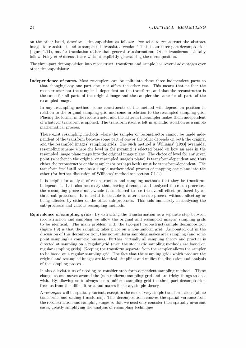
The three-part decomposition into reconstruct, transform and sample has several advantages overother decompositions:
Independence of parts. Most resamplers can be split into these three independent parts sothat changing any one part does not affect the other two. This means that neither thereconstructor nor the sampler is dependent on the transform, and that the reconstructor isthe same for all parts of the original image and the sampler the same for all parts of theresampled image.
In any resampling method, some constituents of the method will depend on position inrelation to the original sampling grid and some in relation to the resampled sampling grid.Placing the former in the reconstructor and the latter in the sampler makes them independentof whatever transform is applied. The transform itself is left in splendid isolation as a simplemathematical process.
There exist resampling methods where the sampler or reconstructor cannot be made inde-pendent of the transform because some part of one or the other depends on both the originaland the resampled images’ sampling grids. One such method is Williams’ [1983] pyramidalresampling scheme where the level in the pyramid is selected based on how an area in theresampled image plane maps into the original image plane. The choice of level for any givenpoint (whether in the original or resampled image’s plane) is transform-dependent and thuseither the reconstructor or the sampler (or perhaps both) must be transform-dependent. Thetransform itself still remains a simple mathematical process of mapping one plane into theother (for further discussion of Williams’ method see section 7.1.1.)
It is helpful for analysis of reconstruction and sampling methods that they be transform-independent. It is also necessary that, having discussed and analysed these sub-processes,the resampling process as a whole is considered to see the overall effect produced by allthree sub-processes. It is useful to be able to alter one sub-process without affecting orbeing affected by either of the other sub-processes. This aids immensely in analysing thesub-processes and various resampling methods.
Equivalence of sampling grids. By extracting the transformation as a separate step betweenreconstruction and sampling we allow the original and resampled images’ sampling gridsto be identical. The main problem with the two-part reconstruct/sample decomposition(figure 1.9) is that the sampling takes place on a non-uniform grid. As pointed out in thediscussion of this decomposition, this non-uniform sampling makes area sampling (and somepoint sampling) a complex business. Further, virtually all sampling theory and practice isdirected at sampling on a regular grid (even the stochastic sampling methods are based onregular sampling grids). Keeping the transform separate from the sampler allows the samplerto be based on a regular sampling grid. The fact that the sampling grids which produce theoriginal and resampled images are identical, simplifies and unifies the discussion and analysisof the sampling process.
It also alleviates us of needing to consider transform-dependent sampling methods. Thesechange as one moves around the (non-uniform) sampling grid and are tricky things to dealwith. By allowing us to always use a uniform sampling grid the three-part decompositionfrees us from this difficult area and makes for clear, simple theory.
A resampler will be spatially-variant, except in the case of very simple transformations (affinetransforms and scaling transforms). This decomposition removes the spatial variance fromthe reconstruction and sampling stages so that we need only consider their spatially invariantcases, greatly simplifying the analysis of resampling techniques.

1.7. DECOMPOSITION 25
Image
Image
IntensitySurface
IntensitySurface
�
�
� �Sample
Reconstruct
Transform Resample
Continuous World Discrete World
Figure 1.17: The original image (at top) is reconstructed to give an intensity surface. This is thentransformed to produce the transformed intensity surface, which is sampled, giving the resampledimage. In a digital computer the entire process is performed in the discrete world, shown by thedotted arrow in this figure.
Separation of format conversion. Reconstruction and sampling are opposites. Reconstructionconverts a discrete image into a continuous intensity surface. Sampling converts a continuousintensity surface into a discrete image.
Resampling is the complex process of geometrically transforming one digital image to pro-duce another (see figure 1.8). This decomposition replaces that transformation with theconceptually much simpler transformation from one continuous intensity surface to another,and it adds processes to convert from the discrete image to the continuous intensity surface(reconstruction) and back again (sampling). Thus the decomposition separates the formatconversion (discrete to continuous, and continuous to discrete) from the transform (the coreof the process). This whole process is illustrated in figure 1.17.
Generality of the decomposition. Almost all resamplers can be split into these three parts,but decomposing resampling into more parts limits the types of resamplers that can berepresented, as illustrated in section 1.7.3. Appendix A lists many of the resamplers thathave been discussed in the literature and decomposes them into these three parts.
1.7.5 One-dimensional and multi-pass resampling
Multi-pass resampling can mean a sequence of two-dimensional resampling stages to produce thedesired result. An example of this is the decomposition in figure 1.16 which can be thought of asone resampling followed by another. Such methods fit easily into our framework by consideringthem to be a sequence of resamplings with each resampling being decomposed individually into itsthree component stages.
Multi-pass resampling, however, usually refers to a sequence of two or more one-dimensional re-samplings. For example, each horizontal scan-line in the image may be resampled in the firstpass and each vertical scan-line in the second. The overall effect is that of a two-dimensionalresampling. Catmull and Smith [1980] deal with this type of resampling; other researchers havesuggested three- [Paeth, 1986, 1990] and four- [Weiman, 1980] pass one-dimensional resampling.

26 CHAPTER 1. RESAMPLING
Image Image�Resample
Image Image�Resampleall horizontal
scan lines
Image�Resampleall verticalscan lines
For each scan line:
Scan Line IntensityCurve
IntensityCurve Scan Line�Reconstruct �Transform �Sample
��
��
���
��
���
��
���
�������������������
Figure 1.18: The decomposition of resampling for a two-pass one-dimensional resampler. Thewhole resampling decomposes into two sets of resamplings, one resampling per scan line. Thesethen decompose into the three parts, as before.
To include such resampling methods in our framework we note that the overall resampling consistsof two or more resampling stages. In each of these stages each one of a set of scan-lines undergoesa one-dimensional resampling which can be decomposed into reconstruction, transformation andsampling. An example of this decomposition for a two-pass resampling is given in figure 1.18. Thusthe decomposition is quite valid for multi-pass one-dimensional resampling methods. Indeed, manytwo-dimensional reconstructors are simple extrapolations of one-dimensional ones (for example: seesection 3.4.2).
Multi-pass, one-dimensional resampling tends to be faster to implement than the same two-dimensional resampling. In general, though, the one-dimensional version produces a more degradedresampled image than the two-dimensional one. Fraser [1989b] and Maisel and Morden [1981] areamongst those who have examined the difference in quality between one-pass, two-dimensional andmulti-pass, one-dimensional resampling.
1.7.6 Three dimensions and mixed dimensional cases
Resampling theory can be simply extended to three or more dimensions (where an intensity vol-ume or hyper-volume is reconstructed). There are still the same three sub-processes. Multi-passresampling also generalises: three dimensional resampling, for example, can be performed as amulti-pass one-dimensional process [Hanrahan, 1990].
Finally, some resamplers involve the reconstruction of an intensity surface (or volume) of higher di-mension than the image. One example is the 11
2 -dimensional reconstruction of a one-dimensionalimage, discussed in section 7.2. Another is Williams’ [1983] resampler: reconstructing a threedimensional intensity volume from a two dimensional image. This is discussed in detail in sec-tion 7.1.1.

1.8. HOW IT REALLY WORKS 27
SampleTransformReconstruct
TransformedIntensity Surface
ReconstructedIntensity Surface
Original Image Resampled Image
ReconstructionCalculation
InverseTransform
Figure 1.19: How resampling is implemented when it involves point sampling. For each pointsample required in the process, the point is inverse transformed into the original image’s spaceand a reconstruction calculation performed for the point from the original image’s samples in theregion of the inverse transformed point.
1.8 How it really works
The theory is that a digital image is reconstructed to a continuous intensity surface, which istransformed, and then sampled on a regular grid to produce a new digital image (figure 1.14).In practice resampling cannot be done this way because a digital computer cannot contain acontinuous function. Thus practical resampling methods avoid the need to contain a continuousfunction, instead calculating values from the original image’s data values only at the relevantpoints.
Conceptually, the usual method of implementation is to push the sampling method back throughthe transformation so that no continuous surface need be created. Whilst this process is conceptu-ally the same for an area sampler as for a point sampler, the former is practically more complicatedand so we will discuss the two cases separately.
1.8.1 The usual implementation of a point sampler
Each point sample that must be taken is taken at a single point on the transformed intensitysurface. This point usually corresponds to exactly one point on the original intensity surface.Remember that for many-to-one transformations some arbiter must be included to decide whichone of the many takes priority, or to decide how to mix the many reconstructed intensities toproduce a single intensity9.
The value of the intensity surface at this point (or points) in the original image can then becomputed from the original image’s data values. This process is illustrated in figure 1.19.
For a single point sampler this value is assigned to the appropriate pixel in the final image. For amulti-point sampler, several such samples are combined in some way to produce a pixel value.
Thus to get the value of a point sample the following process is used:
1. Inverse transform the location of the point from the final image’s space to the original image’sspace.
2. Calculate the value of the intensity surface at this point in the original image’s space.
9The situation where a final intensity surface point has no corresponding original intensity surface point isdiscussed in the section on edge effects (section 4.2).

28 CHAPTER 1. RESAMPLING
SampleTransformReconstruct
TransformedIntensity Surface
ReconstructedIntensity Surface
Original Image Resampled Image
InverseTransform
ReconstructionCalculation
Figure 1.20: How resampling is implemented when it involves area sampling. For each area samplerequired in the process, the area is inverse transformed into the original image’s space and areconstruction calculation performed for the whole area from the original image’s samples in theregion of the inverse transformed area.
Image IntensitySurface
IntensitySurface
Image� � �
Reconstructionfilter
Inversetransformed
prefilter
Inverse transformedsingle pointsampling
Figure 1.21: An equivalent decomposition of an area sampler. Rather than use a transform-invariant area sampler, here we use an inverse transformed prefilter, followed by inverse transformedsingle point sampling. These two steps combine to produce the same effect as a transform followedby area sampling.
1.8.2 The usual implementation of an area sampler
Analogous to the point sampling case, the area of the sample is inverse transformed (taking withit, of course, the weighting information for every point in the area). This inverse transformed areawill now be spatially-variant as it is now transformation-dependent. The same shaped area indifferent parts of the final image’s space will inverse transform to differently shaped areas in theoriginal image’s space.
Somehow this spatially-variant area sampler is combined with the spatially-invariant reconstructorto produce a calculation which will give a single value for each final image pixel. The process isillustrated in figure 1.20.
Heckbert [1989] explains how this combination can be achieved in the case where the reconstructorcan be represented as a filter:
Heckbert’s resampling filter
An area sampler can be thought of as a filter (called a ‘prefilter’) followed by single point sampling.Thus the three-part decomposition becomes four part (see figure 1.15). If both sampling stages arepushed back through the transform we get the situation shown in figure 1.21. The space-invariantreconstruction filter can now be convolved with the generally space-variant inverse transformedprefilter to produce what Heckbert calls the resampling filter, shown in figure 1.22. The righthand process is a point sampler and so the intensity surface values need only be generated at thosepoints — in a similar way to the point sampling case. Thus the area sampling resampler can beimplemented as a point sampling resampler.

1.9. THE LITERATURE 29
Image IntensitySurface
Image� �
Resamplingfilter
Inverse transformedsingle pointsampling
Figure 1.22: Heckbert’s [1989] resampling filter. The whole resampling is decomposed into twostages for implementation: a resampling filter composed of the convolution of the reconstructionfilter and the inverse transformed prefilter, and inverse transformed single point sampling.
1.8.3 Comparison
The major difference between a point and an area sampling process is that the calculation toproduce a value is space-invariant in the former case and generally space-variant in the latter. Onlyin the case of an affine transform will the area-sampling case produce a space-invariant calculation[Heckbert, 1989, p.46, sec. 3.4.4]. The added complexity of space-variance makes area samplingmuch more difficult to implement than point sampling. This disadvantage must be weighed againstthe advantages of area sampling.
1.8.4 Other implementations
Whilst those shown here are the most common implementations, it is possible to generate others.For those, relatively rare, reconstructors which cannot be represented as filters, Heckbert’s ‘resam-pling filter’ is not a viable implementation. Some other way of combining the reconstructor andarea sampler would need to be found if such a reconstructor were to be used with an area sampler(the alternative is that this reconstructor could only ever be used with point sampling methods).
On a different tack, resamplers could be found for which the following implementation would provepossible:
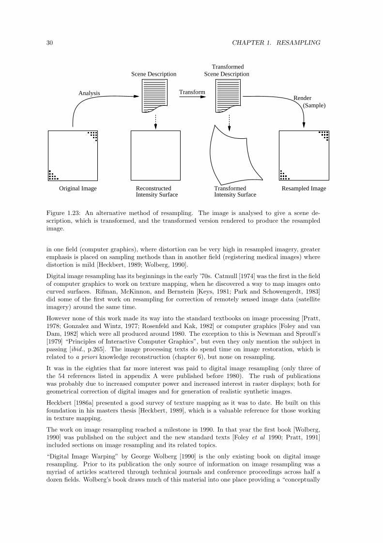
The original digital image is analysed to produce a digital ‘image description’ which de-scribes an intensity surface. This image description is transformed, producing anotherimage description which describes the transformed intensity surface. This image de-scription can then be rendered, potentially by any sampler, to produce the final image(see figure 1.23).
Such reconstruction methods are discussed in chapter 6.
1.8.5 Comments
However we think of a particular resampling process: whether as a single process; as a resamplingfilter that is point sampled; as reconstruction followed by sampling; or as reconstruct, transform,sample; it is the same resampler producing the same results. The implementation may appeartotally different to the theoretical description, but the results are the same.
1.9 The literature
Digital image resampling is useful in many fields and so the literature relating to it is in many dis-parate places. Medical imaging, remote sensing, computer vision, image processing and computergraphics all make use of resampling. The practitioners in the various fields all have their own viewson the subject, driven by the uses to which they put resampling. Thus we find, for example, that
30 CHAPTER 1. RESAMPLING
TransformedIntensity Surface
ReconstructedIntensity Surface
Original Image Resampled Image
Transform
Scene Description Scene DescriptionTransformed
AnalysisRender
(Sample)
Figure 1.23: An alternative method of resampling. The image is analysed to give a scene de-scription, which is transformed, and the transformed version rendered to produce the resampledimage.
in one field (computer graphics), where distortion can be very high in resampled imagery, greateremphasis is placed on sampling methods than in another field (registering medical images) wheredistortion is mild [Heckbert, 1989; Wolberg, 1990].
Digital image resampling has its beginnings in the early ’70s. Catmull [1974] was the first in the fieldof computer graphics to work on texture mapping, when he discovered a way to map images ontocurved surfaces. Rifman, McKinnon, and Bernstein [Keys, 1981; Park and Schowengerdt, 1983]did some of the first work on resampling for correction of remotely sensed image data (satelliteimagery) around the same time.
However none of this work made its way into the standard textbooks on image processing [Pratt,1978; Gonzalez and Wintz, 1977; Rosenfeld and Kak, 1982] or computer graphics [Foley and vanDam, 1982] which were all produced around 1980. The exception to this is Newman and Sproull’s[1979] “Principles of Interactive Computer Graphics”, but even they only mention the subject inpassing [ibid., p.265]. The image processing texts do spend time on image restoration, which isrelated to a priori knowledge reconstruction (chapter 6), but none on resampling.
It was in the eighties that far more interest was paid to digital image resampling (only three ofthe 54 references listed in appendix A were published before 1980). The rush of publicationswas probably due to increased computer power and increased interest in raster displays; both forgeometrical correction of digital images and for generation of realistic synthetic images.
Heckbert [1986a] presented a good survey of texture mapping as it was to date. He built on thisfoundation in his masters thesis [Heckbert, 1989], which is a valuable reference for those workingin texture mapping.
The work on image resampling reached a milestone in 1990. In that year the first book [Wolberg,1990] was published on the subject and the new standard texts [Foley et al 1990; Pratt, 1991]included sections on image resampling and its related topics.
“Digital Image Warping” by George Wolberg [1990] is the only existing book on digital imageresampling. Prior to its publication the only source of information on image resampling was amyriad of articles scattered through technical journals and conference proceedings across half adozen fields. Wolberg’s book draws much of this material into one place providing a “conceptually
1.10. SUMMARY 31
unified, interdisciplinary survey of the field” [Heckbert, 1991a].
Wolberg’s book is not, however, the final word on image resampling. His specific aim was toemphasise the computational techniques involved rather than any theoretical framework [Wolberg,1991]. “Digital Image Warping” has its good points [McDonnell, 1991] and its bad [Heckbert,1991b] but as the only available text it is a useful resource for the study of resampling (for a reviewof the book see Heckbert [1991a]; the discussion sparked by this review may be found in Wolberg[1991], McDonnell [1991] and Heckbert [1991b]).
The most recent standard text, Foley, van Dam, Feiner and Hughes [1990] “Computer Graphics:Principles and Practice”, devotes some considerable space to image resampling and its relatedtopics. Its predecessor [Foley and van Dam, 1982] made no mention at all of the subject. Thisreflects the change in emphasis in computer graphics from vector to raster graphics over thepast decade. The raster display is now the most common ‘soft-copy’ output device [Sproull,1986; Fournier and Fussell,1988], cheap raster displays having been developed in the mid nineteen-seventies as an offshoot of the contemporary television technology [Foley and van Dam, 1982].Today it is true to say that “with only a few specialised exceptions, line [vector] graphics has beensubsumed by... raster graphics” [Fiume, 1986, p.2].
A number of the myriad articles on resampling are analysed in appendix A. The resamplers ineach article have been decomposed into their three constituent parts, which are listed in the tablethere. This produces some insights into research in resampling. Over half the articles consideronly single point sampling, concentrating instead on different reconstructors or transforms. Manyarticles examine only one of the three parts of the decomposition, keeping the other two constant.There are a significant number which consider only a scaling transform and single point sampling.There are others which concentrate on the transforms. It is only a minority that consider theinteraction between all parts of the resampler, and these are mostly in the computer graphics fieldwhere distortions tend to be highest and hence the resampler has to be better (the higher thedistortion the harder it is to resample well).
Most of the resamplers surveyed fit neatly into our three part decomposition, having three inde-pendent parts. A few fit less neatly, in that the three parts cannot be made independent. Thislatter set of resamplers are those in which area sampling is approximated. They depend on anapproximation in original image space to an area in resampled image space transformed back intooriginal image space. Because of the approximation either the reconstructor or the sampler mustbe transformation-dependent. Only one of the resamplers in appendix A does not fit well into thedecomposition. This is Namane and Sid-Ahmed’s [1990] method of binary image scaling. Theirmethod cannot be said to produce any kind of continuous intensity surface and has thus provendifficult to fit into the three-part decomposition.
One ‘resampler’ not listed in the table is Kornfeld’s [1985, 1987] image prism. This device only per-forms a limited set of orthogonal transformations which exactly map pixels onto pixels. Thereforeno resampling is required.
In the following chapters many of these articles will be referred to in the discussion of the threeparts of resampling. At the end we will draw the strands together and consider resampling as awhole.
1.10 Summary
The concept of digital image resampling has been introduced. It is a process which find uses inmany fields. We have seen how it fits into the larger framework of operations on images, and howthe continuous image we view differs from the discrete image that the computer operates on.
Several decompositions of resampling have been considered. We favour the three-part decompo-sition into reconstruction, transformation, and sampling. The remainder of this dissertation is

32 CHAPTER 1. RESAMPLING
organised around this decomposition.
We concluded the chapter by considering how a resampler can be implemented, and by brieflylooking at the history and literature of digital image resampling.
We now go on to consider the third of the sub-processes: sampling.

Chapter 2
Sampling
Sampling is the process of converting a continuous intensity surface into a discrete representation.As well as being the third sub-process of resampling, it is the process by which the original image isgenerated. Thus sampling is important in its own right as a sub-process, and also in how it it affectsthe original image and subsequent reconstruction from that image. Conventional sampling theorydeals with a regular grid of point samples, with each sample in the image being generated by asingle one of these point samples. In this dissertation ‘sampling’ refers to many sampling methodsbesides this single point sample method. In this chapter we discuss these sampling methods andtheir applicability to various sampling tasks.
2.1 Converting the continuous into the discrete
Sampling takes a continuous signal, one defined over all space, and produces a discrete signal, onedefined over only a discrete set of points. In practice the two signals are only defined within aregion of interest. Discussion of what lies outside this region is left until chapter 4. In our case,the continuous signal is an intensity surface; that is: a three-dimensional function with two spatialdimensions and one intensity dimension where each point in the spatial plane has a single intensity.When dealing with colour, the number of dimensions increases, typically to three colour dimensions(but still only two spatial dimensions). When dealing with one or three spatial dimensions thesituation also changes but the underlying principle is the same: for every spatial point there is asingle intensity or colour. An intensity surface is a many-to-one mapping from a spatial domaininto an intensity (or colour) domain.
The discrete signal in our case is an image. It has the same number of spatial and intensity (colour)dimensions as the intensity surface but is discrete in the spatial domain. A digital computer cannotrepresent a continuous quantity and so the image will be discrete in intensity as well. In practicewe find that spatial discreteness is central to the resampling problem, whilst intensity discretenessis a peripheral problem which can, for the most part, be safely ignored. Why this is so is discussedin the next section.
2.2 The problem of discrete intensities
Ideally, infinite precision in recorded intensity is desirable, no errors would then arise from slightlyimprecise intensity values. In practice, intensities are recorded to finite precision which leads toerrors in the reconstructed intensity surface, whether on the screen or in the resampling process.
These errors are most noticeable when only a few discrete intensity levels are available, and most
33

34 CHAPTER 2. SAMPLING
Pratt [1991]fig. 2.3–1(a)
Figure 2.1: The minimum noticeable intensity difference (∆I/I) as a function of intensity (I)[Pratt, 1991, fig. 2.3–1(a)]. It is 2% for much of the range, rising to higher values for very dark orvery light intensities.
image processing texts include an example showing the effect on a displayed image of allowing alarger or smaller number of intensity levels [see, for example, Rosenfeld and Kak, 1982, pp.107–8figs. 14 and 15; Gonzalez and Wintz, 1977, fig. 2.8]. The extreme case is where there are only twolevels: black and white. Such an image takes comparatively little storage (one bit per pixel) buthas a limited usefulness. With digital half-toning techniques it can be made to simulate a widerange of grey shades, but, for resampling, it is preferable to have true shades of grey rather thansimulated ones.
The general case, then, is one where a significant number of discrete intensity levels are used torepresent a continuous range of intensities. But how many intensity levels are sufficient?
The minium necessary number of intensity levels
The human visual system is limited in how small an intensity change it can detect. Researchsuggests that, for two large areas of constant intensity, a two percent difference can be just detected[Crow, 1978, p.4]. The minimum difference that can be detected rises to a higher value for verydark or very bright areas [Pratt, 1978, pp.17–18] (see figure 2.1). It also rises when comparingsmall areas of constant intensity [ibid., pp.18–19, fig. 2.5]. When dealing with colour images theminimum noticeable differences for pure colour information (that is with no intensity component)are much larger than those for intensity information, hence broadcast television has an intensitychannel with high spatial resolution and two channels carrying the colour information at low spatialresolution [NMFPT, 1992]. Here, we shall consider only intensity. The number of intensity levelsrequired to produce a faithful representation of an original intensity surface depends on the imageitself [Gonzalez and Wintz, pp.27-28] and on the type of reconstruction.
If we wish to display any image on a ‘reasonable’ display device then how many levels are required?Many researchers have answered this question and their results are given below. We are workingwith binary digital computers and so, sensibly, most of the answers are powers of two.
Crow [1978, p.4] says that between six and eight bits (64 to 256 intensity levels) are required,depending on the quality of the display. He also calculates that the typical display would needabout 162 intensity levels. This calculation is reproduced and explained later.
Gonzalez and Wintz [1977, pp.19 and 26] suggest that 64 levels (six bits) may be sufficient in somecases but say that “to obtain displays that will appear reasonably smooth to the eye for a largeclass of image types, a range of over 100 intensity levels is generally required.”
Rosenfeld and Kak [1982, p.106] also suggest that more than 100 levels may be needed for someapplications.
Finally, Foley and van Dan [1982, p.594] and Pavlidis [1982, p.39] both agree that 64 levels aregenerally adequate but that 256 levels may be needed for some images (Pavlidis hints that 256
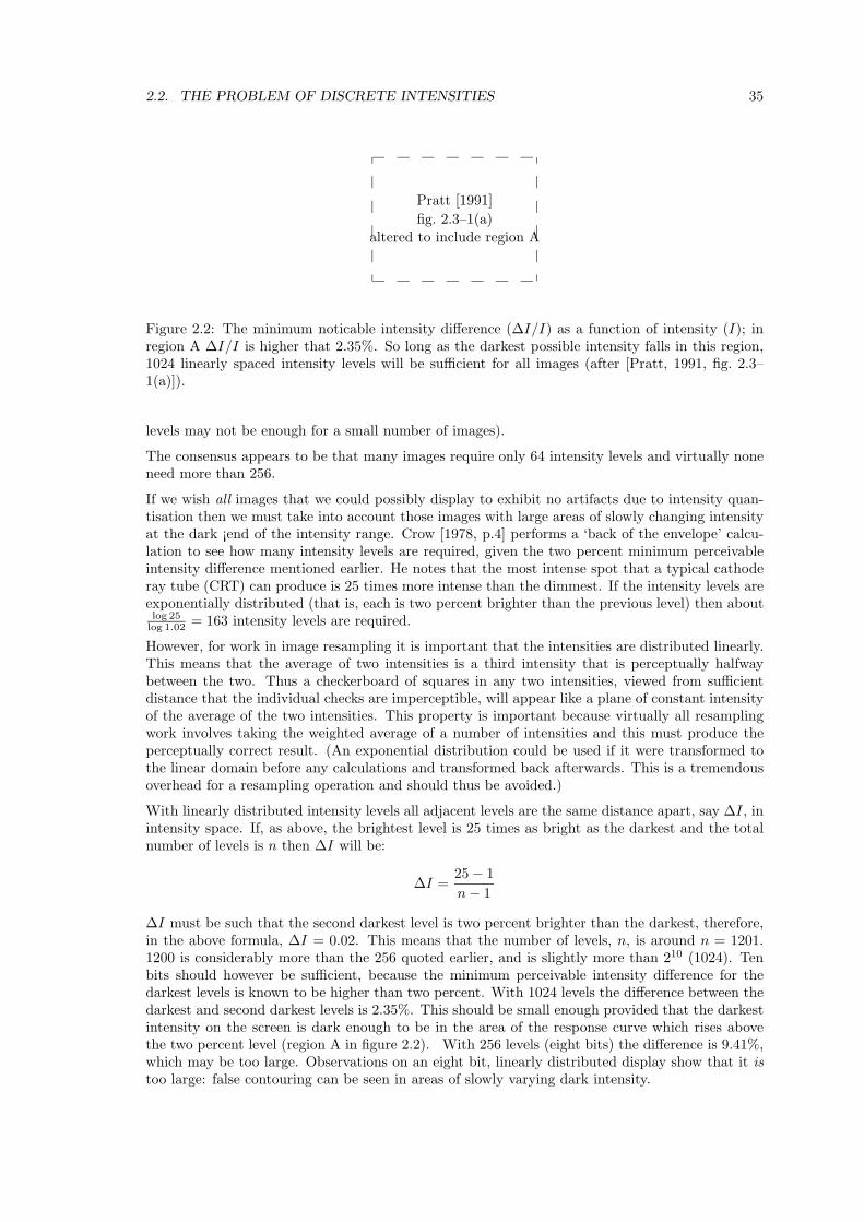
2.2. THE PROBLEM OF DISCRETE INTENSITIES 35
Pratt [1991]fig. 2.3–1(a)
altered to include region A
Figure 2.2: The minimum noticable intensity difference (∆I/I) as a function of intensity (I); inregion A ∆I/I is higher that 2.35%. So long as the darkest possible intensity falls in this region,1024 linearly spaced intensity levels will be sufficient for all images (after [Pratt, 1991, fig. 2.3–1(a)]).
levels may not be enough for a small number of images).
The consensus appears to be that many images require only 64 intensity levels and virtually noneneed more than 256.
If we wish all images that we could possibly display to exhibit no artifacts due to intensity quan-tisation then we must take into account those images with large areas of slowly changing intensityat the dark ¡end of the intensity range. Crow [1978, p.4] performs a ‘back of the envelope’ calcu-lation to see how many intensity levels are required, given the two percent minimum perceivableintensity difference mentioned earlier. He notes that the most intense spot that a typical cathoderay tube (CRT) can produce is 25 times more intense than the dimmest. If the intensity levels areexponentially distributed (that is, each is two percent brighter than the previous level) then aboutlog 25
log 1.02 = 163 intensity levels are required.
However, for work in image resampling it is important that the intensities are distributed linearly.This means that the average of two intensities is a third intensity that is perceptually halfwaybetween the two. Thus a checkerboard of squares in any two intensities, viewed from sufficientdistance that the individual checks are imperceptible, will appear like a plane of constant intensityof the average of the two intensities. This property is important because virtually all resamplingwork involves taking the weighted average of a number of intensities and this must produce theperceptually correct result. (An exponential distribution could be used if it were transformed tothe linear domain before any calculations and transformed back afterwards. This is a tremendousoverhead for a resampling operation and should thus be avoided.)
With linearly distributed intensity levels all adjacent levels are the same distance apart, say ∆I, inintensity space. If, as above, the brightest level is 25 times as bright as the darkest and the totalnumber of levels is n then ∆I will be:
∆I =25 − 1n − 1
∆I must be such that the second darkest level is two percent brighter than the darkest, therefore,in the above formula, ∆I = 0.02. This means that the number of levels, n, is around n = 1201.1200 is considerably more than the 256 quoted earlier, and is slightly more than 210 (1024). Tenbits should however be sufficient, because the minimum perceivable intensity difference for thedarkest levels is known to be higher than two percent. With 1024 levels the difference between thedarkest and second darkest levels is 2.35%. This should be small enough provided that the darkestintensity on the screen is dark enough to be in the area of the response curve which rises abovethe two percent level (region A in figure 2.2). With 256 levels (eight bits) the difference is 9.41%,which may be too large. Observations on an eight bit, linearly distributed display show that it istoo large: false contouring can be seen in areas of slowly varying dark intensity.
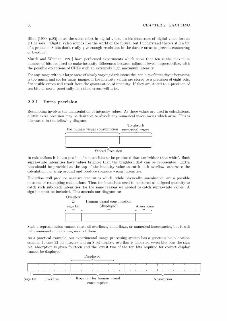
36 CHAPTER 2. SAMPLING
Blinn [1990, p.85] notes the same effect in digital video. In his discussion of digital video formatD1 he says: “Digital video sounds like the world of the future, but I understand there’s still a bitof a problem: 8 bits don’t really give enough resolution in the darker areas to prevent contouringor banding.”
Murch and Weiman [1991] have performed experiments which show that ten is the maximumnumber of bits required to make intensity differences between adjacent levels imperceptible, withthe possible exceptions of CRTs with an extremely high maximum intensity.
For any image without large areas of slowly varying dark intensities, ten bits of intensity informationis too much, and so, for many images, if the intensity values are stored to a precision of eight bits,few visible errors will result from the quantisation of intensity. If they are stored to a precision often bits or more, practically no visible errors will arise.
2.2.1 Extra precision
Resampling involves the manipulation of intensity values. As these values are used in calculations,a little extra precision may be desirable to absorb any numerical inaccuracies which arise. This isillustrated in the following diagram:
For human visual consumption︷ ︸︸ ︷To absorb
numerical errors︷ ︸︸ ︷︸ ︷︷ ︸
Stored Precision
In calculations it is also possible for intensities to be produced that are ‘whiter than white’. Suchsupra-white intensities have values brighter than the brightest that can be represented. Extrabits should be provided at the top of the intensity value to catch such overflow, otherwise thecalculation can wrap around and produce spurious wrong intensities.
Underflow will produce negative intensities which, while physically unrealisable, are a possibleoutcome of resampling calculations. Thus the intensities need to be stored as a signed quantity tocatch such sub-black intensities, for the same reasons we needed to catch supra-white values. Asign bit must be included. This amends our diagram to:
Overflow&
sign bit︷ ︸︸ ︷Human visual consumption
(displayed)︷ ︸︸ ︷Absorption︷ ︸︸ ︷
Such a representation cannot catch all overflows, underflows, or numerical inaccuracies, but it willhelp immensely in catching most of them.
As a practical example, our experimental image processing system has a generous bit allocationscheme. It uses 32 bit integers and an 8 bit display: overflow is allocated seven bits plus the signbit, absorption is given fourteen and the lowest two of the ten bits required for correct displaycannot be displayed:
︸ ︷︷ ︸ ︸ ︷︷ ︸Sign bit Overflow
︸ ︷︷ ︸Required for human visual
consumptionAbsorption
Displayed︷ ︸︸ ︷

2.3. PRODUCING A DISCRETE IMAGE 37
Reconstruct
Generate
Render
Resample
Capture
Continuousdomain
Discretedomain
Project
planeonto a 2D
Real WorldScene
SceneDescription
3D continuousscene
Transform SampleIntensitySurface
ImageImageIntensitySurface
Map onto a surfacein the scene
Project
planeonto a 2D
Discretedomain
Figure 2.3: The three image creation processes subdivided. On the right is the image that iscreated. In each case it is generated from an intensity surface by a sampling sub-process. Thisintensity surface is generated in a different way for each creation process.
To conclude: with these precautions it can be seen that little, if any, visible errors or artifactswill arise from intensity quantisation. Thus the fact that the intensity values are quantised can belargely ignored in our discussion. We may now proceed to discuss the more important problem ofspatial discreteness.
2.3 Producing a discrete image
Sampling occurs in three distinct processes: image capture, image rendering and image resampling.These are the three image creation processes described in section 1.3. In each of these a continuousintensity surface is sampled to produce a discrete image. The continuous intensity surface isgenerated in a different way in each process but the sampling is fundamentally the same in allthree cases, as illustrated in figure 2.3.
In image capture some physical device is used to sample a real world scene. Such devices includevideo cameras, scanners and fax machines. Figure 2.3 divides the image capture process into twoparts. This subdivision can be thought of in two ways:
(a) the theoretical two-dimensional intensity surface is generated by the optics of the capturedevice and occurs immediately in front of the light sensors (figure 2.4(a));
(b) the theoretical two-dimensional intensity surface exists just in front of the entire capture deviceand the entire device, optics and light sensors included, form part of the sampling process(figure 2.4(b)).
Some capture devices have no optics, in which case (a) and (b) are identical.
(b) has the disadvantage that depth effects caused by the optics of the system cannot be modelledas pointing the capture device at a two-dimensional intensity surface because depth effects (for
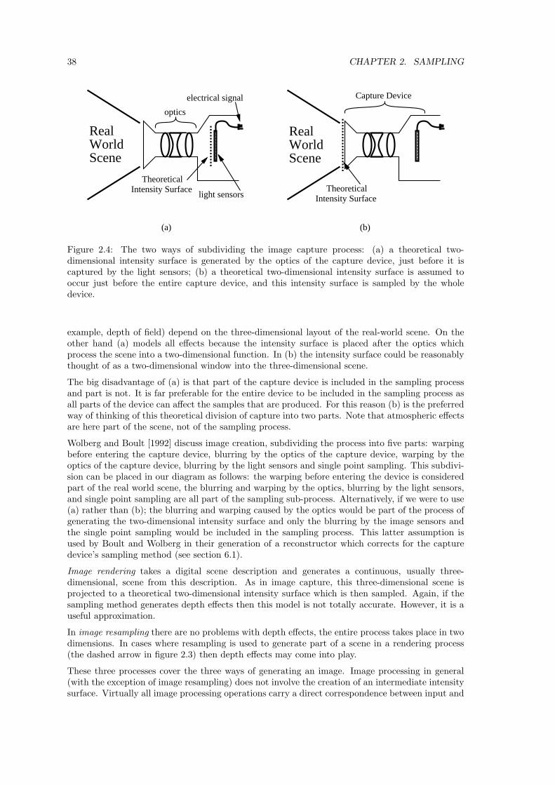
38 CHAPTER 2. SAMPLING
RealWorldScene
optics
electrical signal
light sensors
TheoreticalIntensity Surface
RealWorldScene
TheoreticalIntensity Surface
Capture Device
(a) (b)
Figure 2.4: The two ways of subdividing the image capture process: (a) a theoretical two-dimensional intensity surface is generated by the optics of the capture device, just before it iscaptured by the light sensors; (b) a theoretical two-dimensional intensity surface is assumed tooccur just before the entire capture device, and this intensity surface is sampled by the wholedevice.
example, depth of field) depend on the three-dimensional layout of the real-world scene. On theother hand (a) models all effects because the intensity surface is placed after the optics whichprocess the scene into a two-dimensional function. In (b) the intensity surface could be reasonablythought of as a two-dimensional window into the three-dimensional scene.
The big disadvantage of (a) is that part of the capture device is included in the sampling processand part is not. It is far preferable for the entire device to be included in the sampling process asall parts of the device can affect the samples that are produced. For this reason (b) is the preferredway of thinking of this theoretical division of capture into two parts. Note that atmospheric effectsare here part of the scene, not of the sampling process.
Wolberg and Boult [1992] discuss image creation, subdividing the process into five parts: warpingbefore entering the capture device, blurring by the optics of the capture device, warping by theoptics of the capture device, blurring by the light sensors and single point sampling. This subdivi-sion can be placed in our diagram as follows: the warping before entering the device is consideredpart of the real world scene, the blurring and warping by the optics, blurring by the light sensors,and single point sampling are all part of the sampling sub-process. Alternatively, if we were to use(a) rather than (b); the blurring and warping caused by the optics would be part of the process ofgenerating the two-dimensional intensity surface and only the blurring by the image sensors andthe single point sampling would be included in the sampling process. This latter assumption isused by Boult and Wolberg in their generation of a reconstructor which corrects for the capturedevice’s sampling method (see section 6.1).
Image rendering takes a digital scene description and generates a continuous, usually three-dimensional, scene from this description. As in image capture, this three-dimensional scene isprojected to a theoretical two-dimensional intensity surface which is then sampled. Again, if thesampling method generates depth effects then this model is not totally accurate. However, it is auseful approximation.
In image resampling there are no problems with depth effects, the entire process takes place in twodimensions. In cases where resampling is used to generate part of a scene in a rendering process(the dashed arrow in figure 2.3) then depth effects may come into play.
These three processes cover the three ways of generating an image. Image processing in general(with the exception of image resampling) does not involve the creation of an intermediate intensitysurface. Virtually all image processing operations carry a direct correspondence between input and

2.4. THE SAMPLING PROCESS 39
output pixels and can work by a discrete convolution process [see for example, Fang, Li and Ni,1989, for a discussion of discrete and continuous convolution]. Image resampling, by comparison,does not have this direct correspondence and some process is required so that output pixels canbe positioned anywhere, in relation to the input pixels. In our three-part model this process isprovided by reconstructing an intensity surface, transforming this, and sampling the transformedversion to produce a new image.
We have seen that sampling is a very similar process for the three distinct operations of image cap-ture, image rendering, and image resampling. It is thus important for its part in image resamplingand for its part in creating the images that are resampled. We now go on to discuss this samplingprocess.
2.4 The sampling process
The aim of sampling is to generate pixel values so that they “best represent” the two-dimensionalintensity surface. [Foley et al, 1990, p.619]. This is a good concept but what is meant by ‘bestrepresent’? To some it may mean that the samples obey classical sampling theory. To others itmay mean that the resulting image, when displayed on a certain device, is visually as similar aspossible to the two-dimensional intensity surface. These two ideas are not necessarily the samething. In the subsequent sections we discuss both of these ideas and the tension between them.
2.4.1 Classical sampling theory
The roots of sampling theory go back to 1915, with Whittaker’s work on interpolation of a setof equispaced samples. However, most people attribute the sampling theorem to Shannon [1949],who acknowledges a debt to many others in its development. Attribution of the theorem has beenjointly given to Whittaker and Shannon [Gonzalez and Wintz, 1977, p.72] Shannon and Nyquist[Turkowski, 1986], and to Shannon, Kotel’nikof and Whittaker [Petersen and Middleton, 1962,p.279]. Shannon’s statement of the sampling theorem is1:
If a function f(t) contains no frequencies higher that W cps it is completely deter-mined by giving its ordinates at a series of points spaced 1
2W seconds apart.[Shannon, 1949, Theorem 1] 2.
Mathematically, the sampling process is described as the product of f(t) with the comb function:
comb(t) =∞∑
n=−∞δ(t − nT )
where δ(t) is the Dirac delta-function3. This gives the sampled function:
f(t) =
( ∞∑n=−∞
δ(t − nT )
)f(t)
1The theory laid out by Shannon [1949] and others is for one dimensional sampling only. Petersen and Middleton[1962] extended Shannon’s work to many dimensions.
2cps = cycles per seconds ≡ Hertz
3The Dirac delta function is zero everywhere except at t = 0. The area under the function is unity, that is∫ ∞−∞ δ(t) dt = 1. One definition of the Dirac delta function is:
δ(t) = lima→∞
√a e−aπx2

40 CHAPTER 2. SAMPLING
νx
f( x) F ( ν )
νx
f( x) comb(x)x F ( ν ) Comb(ν )∗
Spatial Domain Frequency Domain
(a)
(b)
12T
-12T
T-T 1T
-1T
Figure 2.5: The sampling process: (a) the continuous spatial domain function, f(x), has a Fouriertransform, F (ν), bandlimited to below half the sampling frequency, 1
2T ; (b) when it is sampled(f(x)×comb(x)) its Fourier transform is convolved with Comb(ν) producing replicas of the originalFourier transform at a spacing of 1
T .
=∞∑
n=−∞(δ(t − nT )f(t − nT )) (2.1)
This is not the same as:fn = f(nT ) (2.2)
Equation 2.1 is a continuous function which consists of an infinite sum of weighted, shifted Diracdelta functions and is zero everywhere except at t = nT, n ∈ Z. Equation 2.2 is a discrete functionwhich is defined on the set n ∈ Z. The values of the discrete function are the weights on the deltafunctions that make up the continuous function, that is:
f(t) =∞∑
n=−∞fn δ(t − nT )
In a computer we, of course, store the discrete version; but mathematically and theoretically wedeal with the continuous one. The sampling theorem can be justified by considering the functionin the frequency domain.
The continuous spatial domain function, f(t), is bandlimited. That is it contains no frequencieshigher than νb (W in the statement of Shannon’s theorem above). Its Fourier transform, F (ν) isthus zero outside the range (−νb, νb). Sampling involves multiplying f(t) by comb(t). The equiva-lent operation in the frequency domain is to convolve F (ν) by Comb(ν), the Fourier transform ofcomb(t). Comb(ν) is composed of Dirac delta-functions at a spacing of 1
T (for a proof of this seeMarion [1991, pp.31–32]). Convolving this with F (ν) produces replicas of F (ν) at a spacing of 1
T .Figure 2.5 illustrates this process.
If T < 12νb
then the copies of F (ν) will not overlap and the original F (ν) can be retrieved bymultiplying F (ν) by a box function:
Box(ν) ={
1, |ν| < νb
0, otherwise
This removes all the copies of the original except for the copy centred at ν = 0. As this isthe original frequency domain function, F (ν), the spatial domain function will also be perfectlyreconstructed.

2.4. THE SAMPLING PROCESS 41
ν
ν
F ( ν )
F ( ν ) Comb(ν )∗
Frequency Domain
(a)
(b)
12T
-12T
1T
-1T
Figure 2.6: An example of sampling at too low a frequency. Here we see the frequency domainrepresentations of the functions. The original function, (a), is not bandlimited to within half thesampling frequency and so when it is sampled, (b), the copies overlap and add up producing thefunction shown by the dark line. It is impossible to recover the original function from this aliasedversion.
Multiplying by a box function in the frequency domain is equivalent to convolving in the spatialdomain by the box’s inverse Fourier transform, s(x). This can be shown to be s(x) = 2νbsinc(2νbx),where sinc(x) = sin(πx)
πx (a proof of this can be found in appendix B.1). The sinc function isdiscussed in sections 3.3 and 4.3.
If T ≥ 12νb
then the copies of F (ν) will overlap (figure 2.6). The overlapping parts sum to produceF (ν). There is no way that this process can be reversed to retrieve F (ν) and so f(t) cannotbe perfectly reconstructed. If F (ν) is multiplied by the box function (the perfect reconstructor)then the resulting function is as if F (ν) had been folded about the frequency 1
2T and summed(figure 2.7). For this reason ν = 1
2T is known as the folding frequency. The effect of thisfolding is that the high frequencies in F (ν) alias into low frequencies. This causes artifacts inthe reconstructed image which are collectively known as ‘aliasing’. In computer graphics the termaliasing is usually incorrectly used to refer to both aliasing and rastering artifacts [Pavlidis, 1990].This point is picked up in section 2.7. Figure 2.8 gives an example of aliasing. It normally manifestsas unsightly ripples, especially near sharp changes in intensity.
To avoid aliasing we must ensure that the sampled intensity surface is bandlimited to below thefolding frequency. If it is not then it can be prefiltered to remove all information above thisfrequency. The procedure here is to multiply the intensity surface’s Fourier transform by a boxfunction, a process known as bandlimiting the intensity surface. Foley et al [1990, fig. 14.29] givean example of this procedure. This prefiltering followed by point sampling is equivalent to an areasampling process, as is explained later.
These procedures are mathematically correct and produce an image free of aliasing. However theyhave their drawbacks. Firstly, if an intensity surface has to be prefiltered then the image does notrepresent the original intensity surface but rather the filtered one. For certain applications thismay be undesirable. To represent a flat or linearly sloped intensity surface, infinite frequencies arerequired. Bandlimiting prevents such surfaces from being perfectly represented, and so any ‘flat’part of a bandlimited image will be ripply. An example of this effect is that any discontinuityin a band-unlimited intensity surface will have a 9% overshoot either side if it is bandlimited, nomatter what the bandlimit is [Lynn and Fuerst, 1989, p.145]; ripples will also propagate out fromthe discontinuity, reducing in magnitude as they get farther away. Thus a bandlimited intensity
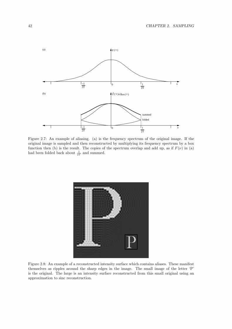
42 CHAPTER 2. SAMPLING
F ( ν )
ν12Τ2Τ
−1 0
(a)
ν12Τ2Τ
−1 0
summed
folded
(b) F ( ν )^ ( ν )x Box
Figure 2.7: An example of aliasing. (a) is the frequency spectrum of the original image. If theoriginal image is sampled and then reconstructed by multiplying its frequency spectrum by a boxfunction then (b) is the result. The copies of the spectrum overlap and add up, as if F (ν) in (a)had been folded back about 1
2T and summed.
Figure 2.8: An example of a reconstructed intensity surface which contains aliases. These manifestthemselves as ripples around the sharp edges in the image. The small image of the letter ‘P’is the original. The large is an intensity surface reconstructed from this small original using anapproximation to sinc reconstruction.

2.5. AREA VS POINT SAMPLING 43
surface is, by its very nature, ripply. This can be seen in figure 2.12(a); there is no aliasing inthis figure, the intensity surface is inherently ripply due to being bandlimited. The human visualsystem abhors ripples, they seriously degrade an image. If however, the ripples in the reconstructedintensity surface are undetectable by the human eye then the surface looks very good. These pointsare picked up in chapter 7.
More importantly, it is practically impossible to achieve perfect prefiltering and so some aliasingwill creep in. In an image capture device, some (imperfect) prefiltering will occur; that is: the imagecapture device does not perform perfect prefiltering. Fraser [1987] asserts that most people dependon this prefiltering to bandlimit the intensity surface enough that little aliasing occurs. In thedigital operations of rendering and resampling, perfect prefiltering is simply impossible, ensuringthat some aliasing always occurs. This is because perfect prefiltering involves either continuousconvolution by an infinite sinc function or multiplication of the continuous Fourier transform by abandlimiting function. Both of these operations are impossible in a discrete computer.
Finally, perfect reconstruction is also practically impossible because it requires an infinite image.Thus, whilst it would be theoretically possible to exactly recreate a bandlimited intensity surfacefrom its samples, in practice it is impossible. In fact, most display devices reconstruct so badlythat correct sampling can be a liability. Sampling which takes into account the reconstructionmethod is the topic of section 2.8.
Before discussing this, however, we need to examine the various types of sampling. These fall intotwo broad categories: area samplers and point samplers.
2.5 Area vs point sampling
Any sampling method will fall into one of these two categories. Area sampling produces a samplevalue by taking into account the values of the intensity surface over an area. These values areweighted somehow to produce a single sample value. Point sampling takes into account the valuesof the intensity surface only at a finite set of distinct points4. If the set contains more than onepoint then these values must be combined in some way to produce a single sample value. This isnot the usual description of point sampling, because ‘point sampling’ is usually used in its narrowsense: to refer to single point sampling. Fiume [1989, section 3.2.4] studied the various samplingtechniques, the following sections draw partly on his work.
2.5.1 Area sampling
Exact-area sampling
The assumptions behind exact-area sampling are that each pixel has a certain area, that everypart of the intensity surface within that area should contribute equally to the pixel’s sample value,and that any part of the intensity surface outside that area should contribute nothing. Hence,if we make the common assumption that pixels are abutting squares then for a given pixel thesample value produced by the exact area sampler will be the average intensity of the intensitysurface within that pixel’s square (figure 2.9(a)) Alternately, we could assume that pixels areabutting circles [Durand, 1989] or overlapping circles [Crow, 1978] and produce the average valueof the intensity surface over the relevant circular area (figure 2.9(b) and (c)). Obviously otherassumptions about pixel shape are possible.
Exact-area sampling is very common, and is discussed again when we look at sampling methodswhich take into account how the image will be reconstructed (section 2.8).
4Fiume [1989, p.82] states that the set of point samples should be countable, or more generally, a set of measurezero.

44 CHAPTER 2. SAMPLING
(a) (b) (c)
Figure 2.9: Three common assumptions about pixel shape: (a) abutting squares, (b) abuttingcircles, and (c) overlapping circles.
General area sampling
The general case for area sampling is that some area is chosen, inside which intensity surface valueswill contribute to the pixel’s sample value. This area is usually centred on the pixel’s centre. Someweighting function is applied to this area and the pixel’s value is the weighted average over thearea. Exact-area sampling is obviously a special case of this.
Equivalence to prefiltering
Area sampling is equivalent to prefiltering followed by single point sampling. In area sampling, aweighted average is taken over an area of the intensity surface. With prefiltering a filter is convolvedwith the intensity surface and a single point sample is taken for each pixel off this filtered intensitysurface. To be equivalent the prefilter will be the same function as the area sample weightingfunction. The two concepts are different ways of thinking about the same process. Looking back tochapter 1, Heckbert [1989] proposed that the sampling sub-process be decomposed into prefilteringand single point sampling. Whilst this is entirely appropriate for all area samplers, not all pointsamplers can be represented in this way, because some point samplers cannot be represented byfilters. Specific examples are adaptive super-samplers and stochastic point samplers, discussedbelow.
2.5.2 Point sampling
Unlike an area-sampling process, a point-sampler ignores all but a countable set of discrete pointsto define the intensity value of a pixel. Point sampling comes in two flavours: regular and irregular(or stochastic) point sampling. Wolberg [1990, sections 6.2 and 6.3] summarises the various typesof point sampling; here we only outline them.
Single point sampling
In single point sampling, the samples are regularly spaced and each pixel’s sample value is producedby a single point. In fact this is exactly the method of sampling described in classical samplingtheory (section 2.4.1). All other point sampling methods are attempts to approximate area sam-pling methods or attempts to reduce artifacts in the reconstructed intensity surface (often theyattempt to be both).
Super-sampling
As in single point sampling, the samples are arranged in a regular fashion, but more that onesample is used per pixel. The pixel’s intensity value is produced by taking a weighted average ofthe sample values taken for that pixel. This can be seen as a direct approximation to area sampling.

2.5. AREA VS POINT SAMPLING 45
Fiume [1989, p.96, theorem 6] proves that, given a weighting function, a super-sampling methodusing this weighting function for its samples converges, as the number of samples increases, towardan area sampling method using the same weighting function.
Such a super-sampling technique can be represented as a prefilter followed by single point sampling;on the other hand, the adaptive super-sampling method cannot.
Adaptive super-sampling
Adaptive super-sampling is an attempt to reduce the amount of work required to produce thesamples. In order to produce a good quality image, many super-samples need to be taken inareas of high intensity variance but a few samples would give good results in areas of low intensityvariance. Ordinary super-sampling would need to take many samples in all areas to produce agood quality image, because it applies the same sampling process for every pixel. Adaptive super-sampling takes a small number of point samples for a pixel and, from these sample values, ascertainswhether more samples need to be taken to produce a good intensity value for that pixel. In thisway fewer samples need to be taken in areas of lower intensity variance and so less work needs tobe done.
Stochastic sampling
Stochastic, or irregular, sampling produces a sample value for each pixel based on one or morerandomly placed samples. There are obviously some bounds within which each randomly placedsample can lie. For example it may be constrained to lie somewhere within the pixel’s area,or within a third of a pixel width from the pixel’s centre. The possible locations may also beconstrained by some probability distribution so that, say, a sample point has a greater chance oflying near the pixel centre than near its edge. Stochastic methods cannot be represented as aprefilter followed by single point sampling, because of this random nature of the sample location.
Stochastic sampling is in favour amongst the rendering community because it replaces the regularartifacts which result from regular sampling with irregular artifacts. The human visual systemfinds these irregular artifacts far less objectionable than the regular ones and so an image of equalquality can be achieved with fewer stochastic samples than with regularly spaced samples (seeCook [1986] but also see Pavlidis’ [1990] comments on Cook’s work).
Fiume [1989, p.98, theorem 7] proves that the choice of point-samples stochastically distributedaccording to a given probability distribution will converge to the analagous area-sampling processas the number of points taken increases, a result similar to that for super-sampling.
2.5.3 Summary
Area sampling yields mathematically precise results, if we are attempting to implement someprefilter (section 2.4.1). However, in digital computations it may be impossible, or difficult toperform area sampling because it involves continuous convolution. In resampling it is possible toimplement some area samplers, at least approximately, but a general area sampler is practicallyimpossible. The point sampling techniques have been shown to be capable of approximatingthe area sampling methods. Such approximations are necessary in cases where area sampling isimpracticable [Fiume, 1989, p.102].

46 CHAPTER 2. SAMPLING
Figure 2.10: Two very similar images: (a) on the left, was generated by summing the first twenty-nine terms of the Fourier series representation of the appropriate square wave; (b) on the right,was generated by super-sampling a perfect representation of the stripes.
Figure 2.11: The Fourier transforms of the images in figure 2.10. (a) on the left and (b) on theright. The Fourier transforms are shown on a logarithmic scale. Note that the background is black(zero) in (a) but has non-zero, but small, magnitude in (b).
2.6 Practical considerations
An image capture device always implements some area sampling process. There is usually somesmall change that can be made in the area sampler by, for example, changing the focus of thelenses or inserting a mask. Major changes involve the expensive process of designing a new device.
Rendering and resampling occur in a digital computer and, for rendering, most area samplingtechniques are analytically impossible and/or computationally intractable [Fiume, 1989, p.102].Thus they cannot be implemented. The complexity of scenes in image rendering means that areasampling, where possible, can be extremely expensive to compute. Image rendering therefore makesalmost exclusive use of point-sampling techniques.

2.6. PRACTICAL CONSIDERATIONS 47
Figure 2.12: The two images of figure 2.10 reconstructed using as near perfect reconstruction aspossible. (a) on the left and (b) on the right. This figure shows part of the reconstructed intensitysurface. Aliasing artifacts occur in (b) only
Figure 2.13: The two images of figure 2.10 reconstructed using as nearest-neighbour reconstruction.(a) on the left and (b) on the right. This figure shows part of the reconstructed intensity surface.(a) contains only rastering atifacts, while (b) contains a combination of rastering and aliasingartifacts.

48 CHAPTER 2. SAMPLING
Image resampling involves a simpler ‘scene’ and so both the computationally possible area samplersand the point samplers can be used. Heckbert [1989, sec. 3.5.1] dismisses point sampling techniqueson the grounds that they do not eliminate aliasing. A super-sampling method shifts the foldingfrequency higher, but band-unlimited signals are common in texture mapping [ibid., p.47], and so,while super-sampling will reduce aliasing, it will not eliminate all aliases, no matter how manysuper-samples are taken. Heckbert thus considers only area sampling techniques.
This argument is certainly valid for the surface texture mapping application discussed by Heck-bert. However stochastic point sampling methods have done much to eliminate aliasing artifacts(by replacing them with less-objectionable noise artifacts) and many people do use point samplingmethods in preference to area sampling methods simply because they are easier to implement.Further, in rendering work, it is often expedient to treat all samples identically and so, if texturemapping (a form of resampling) occurs in the scene, the samples will be taken in the same way assamples are taken in the rest of the scene: almost invariably by some point sampling technique.Wolberg [1990] covers the stochastic sampling methods, drawing on the rendering literature. How-ever, Heckbert [1991a] found this material out of place in Wolberg’s book. We think that it isnecessary because such methods are used for resampling work.
Finally it is useful to realise that many practitioners in resampling use single point sampling.It appears to be the default method. We believe that this is because single point sampling is(a) simple to implement; (b) the obvious sampling method; and (c) all that is required if the imageneed only undergo a mild transformation.
This latter point draws on the fact that the aliasing (and other) artifacts, which more sophisticatedsampling methods suppress, do not manifest themselves very much under a mild transformation(that is, scale changes of ±20% at most). Some applications of resampling only require such mildtransformations, (for example the medical image registration system developed by Venot et al[1988] and Herbin et al [1989]) while others require more violent transforms (for example texturemapping) and thus require more advanced sampling, especially in cases of image shrinking wherethe sampling method dominates the resampler (see chapter 7).
2.7 Anti-aliasing
The purpose of all sampling, other than single-point sampling, is ostensibly to prevent any artifactsfrom occuring in the image. In fact it is usually used to prevent any artifacts from occuring in theintensity surface reconstructed from the image by the display device. This prevention is generallyknown in computer graphics as anti-aliasing. This is something of a misnomer as many of theartifacts do not arise from aliases. The perpetuation of the incorrect terminology is possibly dueto the fact that the common solution to cure aliasing also alleviates rastering, the other mainsource of artifacts in images [Pavlidis, 1990, p.234].
Crow [1977] was the first to show that aliasing (sampling a signal at too low a rate) was the causeof some of the artifacts in digital imagery. He also notes [ibid., p.800] that some artifacts are dueto failing to reconstruct the signal properly. This latter problem he termed ‘rastering’. ‘Aliasing’,however, became the common term for both of these effects, with some subsequent confusion, andit is only recently that the term ‘rastering’ has reappeared [Foley et al, 1990, p.641]. Mitchelland Netravali [1988] do discuss the two types of artifact as distinct effects but perpetuate theterminology by naming aliasing and rastering, pre-aliasing and post-aliasing respectively.
Sampling has thus been used to alleviate both types of artifact. This has an inbuilt problem that,to correct for reconstruction artifacts (rastering), one needs to know the type of reconstructionthat will be performed on the image. Most images are displayed on a CRT, and all CRTs havea similar reconstruction method, so this is not too big a problem. However, when displayed on adifferent device (for example a film recorder) artifacts may appear which were not visible on theCRT because the reconstruction method is different. Further, an image used for resampling which

2.8. SAMPLING WHICH CONSIDERS THE RECONSTRUCTION METHOD 49
has been ‘anti-aliased’ for use on a CRT may not be particularly amenable to the reconstructionmethod used in the resampling algorithm.
Figures 2.10 through 2.13 illustrate the distinction between aliasing artifacts and reconstructionartifacts. Two images are shown of alternate dark and bright stripes. These images were speciallydesigned so that no spurious information due to edge effects would appear in their discrete Fouriertransforms (that is: the Fourier transforms shown here are those of these simple patterns copiedoff to infinity so as to fill the whole plane).
Figure 2.10(a) was generated by summing the first twenty-nine terms of the Fourier series repre-sentation of the appropriate square wave as can be seen by its Fourier transform (figure 2.11(a)).Figure 2.10(b) was generated by one of the common anti-aliasing techniques. It was renderedusing a 16 × 16 super-sampling grid on each pixel with the average value of all 256 super-samplesbeing assigned to the pixel. Figure 2.11(b) shows its Fourier transform. It is similar in form tofigure 2.11(a) but the aliasing can be clearly seen in the wrap around effect of the line of majorcomponents, and also in that the other components are not zero, as they are in the unaliased case.
When these are reconstructed using as near-perfect reconstruction as possible we get the intensitysurfaces shown in figure 2.12. The ripples in figure 2.12(a) are not an aliasing artifact but thecorrect reconstruction of the function; it is, after all, a sum of sine waves. The ripply effect infigure 2.12(b)is due to aliasing. The intensity surface that was sampled had constant shaded stripeswith infinitely sharp transitions between the dark and light stripes. The perfectly reconstructedintensity surface shown here perfectly reconstructs all of the aliases caused by sampling the originalintensity surface.
By contrast, figure 2.13 shows the intensity surfaces which result from an imperfect reconstructor:the nearest-neighbour interpolant. The artifacts in figure 2.13(a) are entirely due to rastering (theimage contains no aliasing). This is the familiar blocky artifact so often attributed, incorrectly, toaliasing. The artifacts in figure 2.13(b) are due to a combination of aliasing and rastering. Oddly,it is this latter intensity surface which we tend to find intuitively preferable. This is probablydue to the areas perceived as having constant intensity in figure 2.10(b) retaining this constantintensity in figure 2.13(b).
How these intensity surfaces are perceived does depend on the scale to which they are reconstructed.The ‘images’ in figure 2.10 are of course intensity surfaces but are reconstructed to one eighth thescale of those in figure 2.12 and figure 2.13. If one stands far enough back from these larger-scalefigures then they all look identical.
It is fascinating that the intensity surface with both types of artifact in it appears to be the preferedone. This is possibly due to the facts that (a) the human visual system is good at detectingintensity changes, hence rippling is extremely obvious; and (b) most scenes consist of areas ofconstant intensity or slowly varying intensity separated by fairly sharp edges, hence representingthem as a bandlimited sum of sinusoids will produce what we perceive as an incorrect result: mostvisual scenes simply do not contain areas of sinsoidally varying intensity.
Thus there is a tension between the sampling theory and the visual effect of the physical reconstruc-tion on the display device. Indeed many researchers, instead of turning to the perfect samplingtheory method of sampling, turn instead to methods which take the reconstruction process intoaccount.
2.8 Sampling which considers the reconstruction method
In such sampling the reconstruction is usually onto a display device, rather than to any theoreticalintensity surface. Several models of the display device have been used in the design of samplingmethods.
The common assumption is that each pixel represents a finite area on the screen and therefore

50 CHAPTER 2. SAMPLING
should be area sampled from that area. This leads to the exact area sampling method givenin section 2.5.1. Such an assumption can be found in many papers on resampling, for exampleWeiman [1980], Paeth [1986], Fant [1986], and Durand and Faguy [1990] all assume square (orrectangular) abutting pixels. Paeth [1990, pp.194-5] later revised his earlier work to allow for moresophisticated sampling methods. Durand [1989] used abutting circular pixels, which seems a lessobvious choice, particularly as parts of the sampled intensity surface are not included in the sumfor any pixel. His reasoning was to reduce the number of calculations in his resampling method(compared with abutting rectangular pixels). This assumption can also be found in Kiryati andBruckstein [1991] but they are modelling a physical sampling device, not a physical reconstruction.
Foley et al [1990, pp.621-3] show that this exact area sampling method is inadequate for sequencesof images. They suggest weighted area sampling functions which cover a larger area than the pixel(for example: a circularly symmetric tent function centred at the pixel centre).
Finally, it is well known that a CRT display reconstructs an image by first convolving it witha nearest-neighbour function (the effect of the digital to analogue converter) and then with aGaussian (the effect of the spot in the CRT tube) [Blinn, 1989b]. Crow [1978] used this type ofmodel in his sampling method. He says that: “A properly adjusted digital raster display consistsof regularly spaced dots which overlap by about one-half.” His conclusion was that a pixel sampledover such an area with a weighting function that peaked in the centre and fell off to the edges gavereasonable results.
We thus find that these methods are motivated by the reconstruction method rather than anysampling theory. Fortunately, they fit neatly into the sampling theory concept of prefiltering (thatis: area sampling). A final important class of samplers are those which take into account the verylimited range of intensity levels of a particular image format or display device. Examples of suchsamplers are those which perform half-toning (for example: the PostScript half-toning algorithm,illustrated in figure 1.2) and those which use dithering to reduce quantisation error effects. Thesemethods are catering for devices with a small number of intensity levels and so do not produceimages for which the assumption made in section 2.2 will hold. Reconstructing an intensity surfacefrom such an image can produce bizarre results unless intelligence is built into the reconstructionalgorithm, but they are useful where the target of the resampling is a device with a limited rangeof intensity levels. The PostScript image command [Adobe, 1985a, p.170, pp.72-83] essentiallyimplements an image resampling process which uses a nearest-neighbour reconstruction techniqueand a half-toning sampling technique to decide which pixels are white and which are black in theimage in the printer’s memory. This resampled image is then reconstructed by the printer when itproduces the picture on paper.
2.9 Summary
Sampling is the process of converting a continuous intensity surface into a discrete image. Samplingis used in all three processes (capturing, rendering, and resampling) which generate a discreteimage, and is fundamentally the same in all three cases. Quantisation of intensity does not pose aproblem, provided enough quantisation levels are available.
There are two basic types of sampling: area, where a sample’s value is determined from the intensitysurface’s values over some non-zero area; and point, where a sample’s value is determined from theintensity surface’s values at only a finite set of points.
The main artifact caused by sampling is aliasing, not to be confused with the rastering artifactcaused by reconstruction.

2.9. SUMMARY 51
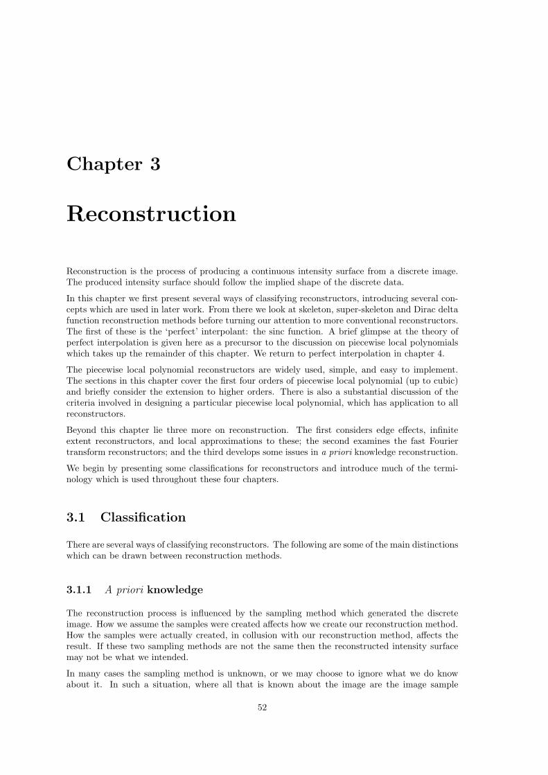
Chapter 3
Reconstruction
Reconstruction is the process of producing a continuous intensity surface from a discrete image.The produced intensity surface should follow the implied shape of the discrete data.
In this chapter we first present several ways of classifying reconstructors, introducing several con-cepts which are used in later work. From there we look at skeleton, super-skeleton and Dirac deltafunction reconstruction methods before turning our attention to more conventional reconstructors.The first of these is the ‘perfect’ interpolant: the sinc function. A brief glimpse at the theory ofperfect interpolation is given here as a precursor to the discussion on piecewise local polynomialswhich takes up the remainder of this chapter. We return to perfect interpolation in chapter 4.
The piecewise local polynomial reconstructors are widely used, simple, and easy to implement.The sections in this chapter cover the first four orders of piecewise local polynomial (up to cubic)and briefly consider the extension to higher orders. There is also a substantial discussion of thecriteria involved in designing a particular piecewise local polynomial, which has application to allreconstructors.
Beyond this chapter lie three more on reconstruction. The first considers edge effects, infiniteextent reconstructors, and local approximations to these; the second examines the fast Fouriertransform reconstructors; and the third develops some issues in a priori knowledge reconstruction.
We begin by presenting some classifications for reconstructors and introduce much of the termi-nology which is used throughout these four chapters.
3.1 Classification
There are several ways of classifying reconstructors. The following are some of the main distinctionswhich can be drawn between reconstruction methods.
3.1.1 A priori knowledge
The reconstruction process is influenced by the sampling method which generated the discreteimage. How we assume the samples were created affects how we create our reconstruction method.How the samples were actually created, in collusion with our reconstruction method, affects theresult. If these two sampling methods are not the same then the reconstructed intensity surfacemay not be what we intended.
In many cases the sampling method is unknown, or we may choose to ignore what we do knowabout it. In such a situation, where all that is known about the image are the image sample
52

3.1. CLASSIFICATION 53
values (and their relative positions), we must use a reconstructor which only takes those valuesinto consideration. We call such a reconstructor a ‘no a priori knowledge’ (NAPK) reconstructor.That is, no knowledge is utilised except for the image sample values. Such a reconstructor canthus be applied to any image.
If we have some a priori knowledge about the image (that is knowledge that is separate from theimage data itself) then we can potentially produce a better reconstructed intensity surface than aNAPK reconstructor could. Such a priori knowledge could be about the sampling method used,the content of the image, or both. A reconstructor which uses such knowledge we call an ‘a prioriknowledge’ (APK) reconstructor. APK reconstruction is discussed in chapter 6.
3.1.2 Reconstruction filters
Reconstruction methods can be classified as to whether or not they can be represented by a filter.Many reconstruction methods can be expressed as filters. A filter is some continuous functionwhich is convolved with the sample values to produce the continuous intensity surface.
In dealing with images it is important to remember that there are two ways of thinking aboutthem. The first is to think of an image as it is stored in the computer: as a finite array of intensityvalues, fi,j , where (i, j) is the co-ordinate of the pixel with value fi,j . The second way is to considerthe image to be a continuous function consisting of an infinite sum of equispaced, weighted Diracdelta functions. For a square pixel array, for example:
ι(x, y) =∞∑
i=−∞
∞∑j=−∞
fi,j δ(x − i, y − j)
ι(x, y) is a continuous function which is non-zero only at integer locations1. It is this latter,continuous, function with which the reconstruction filter, h(x, y), is convolved to produce thecontinuous intensity surface:
f(x, y) = h(x, y) ∗ ι(x, y)
h(x, y) is referred to as the filter’s impulse response, the filter’s kernel, or sometimes simply as thefilter itself.
A problem with this is that the mathematical image function, ι(x, y), is infinite in extent whilstthe discrete function, fi,j , is finite in extent. This means that all of the weights in ι(x, y) whichlie beyond the edges of the discrete image have an indeterminate value. The solutions to this edgeeffect problem, how to determine these unknown values, are discussed in chapter 4.
Throughout the following chapters two different functions will be used in analysing reconstructionfilters: the filter itself, h(x, y), and the intensity surface produced by that filter, f(x, y). In thecase of a reconstruction method that cannot be represented by a filter, only the intensity surface,f(x, y), can be used.
3.1.3 Skeleton vs continuous reconstruction
The skeleton reconstructors do not generate a continuous intensity surface, instead they generatea surface which only has a defined value at certain points and is elsewhere undefined. Such asurface cannot be represented by a filter. However, a similar idea can be, that is: a surface whichis non-zero and finite at certain points and is elsewhere zero. A related idea to this is the Dirac
1It is a simplification to assume that the samples occur at integer locations in the real plane. But here we canmake this simplification without loss of generality, because any rectangular sampling grid can be converted to onewhere the samples occur at integer locations. For example, if the samples are at (x, y) = (x0 + i∆x, y0 + j∆y), then
they can be put at integer locations by changing the coordinate system: x′ = x−x0∆x
and y′ = y−y0∆y

54 CHAPTER 3. RECONSTRUCTION
delta function surface, described above, which consists of an infinite sum of weighted, shifted Diracdelta functions.
Both the skeleton and Dirac delta function reconstructors are discussed under the general headingof ‘skeleton reconstruction’ (section 3.2) although a Dirac delta function surface can be consideredcontinuous for area sampling processes. All other reconstructors produce a continuous intensitysurface. As this is the norm, no special section is required to discuss continuous reconstruction.
3.1.4 Interpolating or approximating
There are two broad categories of reconstructor: the interpolants and the approximants. Theinterpolants (interpolating reconstructors) generate intensity surfaces which pass through all ofthe sample data points; the approximants (approximating reconstructors) generate surfaces whichdo not have to do this, but an approximant may generate an intensity surface which may passthrough any number of the points.
If we have no a priori knowledge, then we are best advised to use an interpolant. This is be-cause we know nothing about how the image was captured, so we must make an assumption. Thesimplest, and generally accepted, assumption is that the samples are single point samples of anoriginal intensity surface and thus the original surface interpolates the sample points. Lacking anyfurther information we assume that it is this intensity surface that we ideally wish to reconstruct,and thus the reconstructed intensity surface should interpolate the points. The concept of interpo-lating rather than the more general reconstruction is so strong that many authors assume that areconstructor is an interpolant (Mitchell and Netravali [1988], for example, discuss approximantsbut use the word ‘interpolation’ to describe all reconstructors).
If, however, we have some a priori knowledge, or some such knowledge can be extracted from theimage then we will probably find that our reconstructor is an approximant, as it is well knownthat no captured images are produced by single point sampling owing to limited resolution andbandwidth in the sampling process. Few rendered images are produced by single point samplingeither, because more sophisticated sampling methods are used to prevent artifacts occurring inthe images. Thus the samples do not necessarily lie on the original intensity surface, and sointerpolating through them will not produce the original intensity surface.
3.1.5 Finite or infinite; local or non-local
Some reconstructors are formally infinite; they depend on an infinite number of sample points.Put another way, they have reconstruction filters of infinite support (assuming they have filters).Other reconstructors are finite; they depend on only a finite number of sample points to producethe value at any given point on the intensity surface.
A finite reconstructor may be local or non-local. This is a less sharp division. Local reconstructorsbase the value of the intensity surface at any point on only local data points. Typically thismeans data points no more than a few pixel widths away from the point being calculated. Non-local reconstructors depend on data farther away (as well as the local data). An infinite-extentreconstructor could be considered the limiting case of non-local reconstructors.
Most practical reconstructors are finite. Some infinite reconstructors can be implemented so thatthe calculation take finite time, but the vast majority cannot. Infinite-extent reconstructors andthe finite-extent approximations to them are discussed in chapter 4.
Localness is an important consideration when implementing a reconstructor. In general, the morelocal a reconstructor, the faster the value of the intensity surface can be calculated at an arbitrarypoint. Localness is also an important consideration in stream processing: the fewer points neededat any one time, the better. It is discussed in more detail in section 3.5.5.

3.2. SKELETON RECONSTRUCTION 55
Figure 3.1: Each grid (solid lines) represents part of an infinite array of square pixels. On the leftare the reflection lines (dashed lines) for those reflections which exactly map pixel centres into pixelcentres. On the right are the rotation centres (dotted circles) for the 180n◦ and 90n◦ rotationswhich map pixel centres to pixel centres.
3.1.6 Other classifications
There are other ways of classifying reconstructors:
• is it a polynomial or not?
• does it have a strictly positive kernel or not? (see section 3.5.7)
• does it approximate some other function? If so, which? For example, approximations to thesinc function or to a Gaussian function are common.
In this dissertation several families of reconstructors are discussed. They are certainly not mutuallyexclusive. The family of piecewise local polynomials are examined later in this chapter. There,many of the criteria used in the design of reconstructors are evaluated. These criteria can also beused to classify reconstructors. Whilst the discussion there is focussed on piecewise local polyno-mials, it is applicable to all reconstructors. Thus, we leave discussion of these other classificationsuntil then (section 3.5).
We now turn to the slightly odd families of skeleton and Dirac delta function reconstructors.
3.2 Skeleton reconstruction
The question arises as to whether a continuous intensity surface is actually required. In somecircumstances it is only necessary to have the value of the intensity surface at the sample pointsthemselves. Elsewhere the intensity surface is undefined (some may prefer to say that it is zero,which is not the same thing). Such a bare bones reconstruction is called skeleton reconstruction.
Skeleton reconstruction is only useful with a limited set of transformations and samplers. Forexample, with single point sampling, the set of transformations is that where the transformationsexactly map pixel centres to pixel centres. This set includes (for a square pixel grid) rotation by90n◦ (n ∈ Z); mirroring about certain horizontal, vertical and 45◦ diagonal lines; and translationsby an integral number of pixels in the horizontal and vertical directions (see figure 3.1 and alsoKornfeld [1985, 1987]). For one bit per pixel images, Fiume [1989, section 4.6] proves that these

56 CHAPTER 3. RECONSTRUCTION
Figure 3.2: Shear distortion — the image on the left is sheared to produce that on the right. Thepixel centres in the right hand image are still in the same square grid orientation. However thepixels themselves are distorted. This leads to distortions in the output image if only pixel centresare considered in the resampling from one image to the other.
transformations are the only ones which can be performed on a square pixel grid without degradingthe image. For many bit per pixel images the questions of whether there are other transformationsthat lose no information is an open one.
As well as these, there are lossy transformations which map pixel centres to pixel centres. Theseinclude scaling by a factor of 1
N , N ∈ Z, N �= 0, about certain points (generally pixel centres).This maps some pixel centres to pixel centres and is a digital sub-sampling operation. Guibasand Stolfi [1982] propose this form of image shrinking in their bitmap calculus. It gives the leastpleasing result of all shrinking methods and is only applicable to shrinking by integral factors( 1
N , N ∈ Z, N �= 0)2.
A further set of transformations which map pixel centres to pixel centres is the set of shears, byan integral number of pixels. However, these transformations produce distortions if done in thissimplistic way. These distortions occur because, while pixel centres do map to pixel centres, thepixel areas do not map onto pixel areas. Figure 3.2 shows the distortion for square pixels shearedby one pixel distance 3.
Skeleton reconstruction does not produce a continuous intensity surface because the value of the‘intensity surface’ is undefined except at the sample points. But a surface can be designed whichproduces similar results to those described. The method described above has an intensity surfacewhich takes the sample values at the sample points and is undefined at all other points. ‘Undefined’is a difficult concept to express mathematically, so to generate a filter kernel which describes thisskeleton reconstruction we replace ‘undefined’ with ‘zero’ and get the kernel:
h(x, y) ={
1, x = 0 and y = 00, otherwise
The properties of an intensity surface reconstructed by this kernel are:
• it has non-zero values only at the sample points;
• it will produce a sensible result only if it is point sampled at only these points;
2For shrinking by a factor of 1R
, R ∈ R, |R| ≥ 1, you need at least some form of reconstruction or a moresophisticated sampling method. Heckbert [1989] says that for R � 1 it is only necessary to reconstruct using aDirac delta function reconstructor, but that a good area sampler is required.
3Interestingly enough, many other reconstruction methods will produce as bad a result in this case unless amore sophisticated sampling method is employed. This is because the value of the intensity surface at the pixelcentres under interpolation methods is exactly the sample value at that pixel centre before interpolation and sopoint sampling at these points produces exactly the same value as if we had used skeleton reconstruction.

3.2. SKELETON RECONSTRUCTION 57
• a point sample anywhere else will produce the value zero;
• an area sampling method will not work at all.
This last point is due to the fact that any area sampler’s prefilter applied to this surface willproduce the filtered surface g(x, y) = 0, ∀x, y ∈ R. Thus all the sample values from the areasampler will be zero.
This reconstructor is different to the Dirac delta function reconstructor discussed by Heckbert[1989, p.51], and it produces different results. The Dirac delta function produces a very differentkind of intensity surface. Its filter is defined as:
h(x, y) = δ(x, y)
and it has the following properties:
• it is the identity function, that is: it has the following effect on the continuous image function:
f(x, y) = δ(x, y) ∗ ι(x, y)= ι(x, y)
• it is zero everywhere except at pixel centres where it tends to infinity;
• for some small ε, less than the distance between pixels:∫ i+ε
i−ε
∫ j+ε
j−ε
f(x, y) dy dx = fi,j
• it only works with area sampling methods because using a point sampling method couldresult in the product of two Dirac delta functions, the value of such a product is undefined;
• not all area samplers produce a good result, only those for which a large number of deltafunctions fall within the area of the sampler for each sample taken.
The notable difference is that the Dirac delta function works with area samplers, but not pointsamplers, whilst the skeleton reconstructor works with point samplers but not area ones.
There are other reconstructors which produce a similar effect to skeleton reconstruction, the dif-ference being that their set of defined points is not limited to the sample points. They are able toproduce a finite number of new points between the existing data points. However they cannot bepractically used to find the value of the surface at an arbitrary point. Such a reconstructor can bedubbed ‘super-skeleton’ by analogy to ‘sampling’ and ‘super-sampling’.
The best example of a super-skeleton method is the fast Fourier transform (FFT) scaling method[Fraser, 1987, 1989a, 1989b; Watson, 1986] (section 5.1). This method produces a finite number ofequispaced samples between existing samples but cannot be used to produce samples at arbitrarypoints. Fraser’s implementation allows for x × 2n, n ∈ Z points from x original sample points.Watson’s method allows us to produce an arbitrary number of points in place of our original x(these figures are quoted for one-dimensional signals, they need to be squared for two dimensions).To produce a continuous surface would require an infinite number of points and hence infinite time;so whilst theoretically possible it is hardly practicable. In this method, all the points have to begenerated before you can use them for further processing, they cannot be generated one at a time.
This FFT method reconstructs a surface, which, as before, has non-zero values only at a set ofpoints and is elsewhere undefined (alternatively, zero). There is no way of stating the methodas a reconstruction filter. It is however, a perfectly valid reconstruction method. Again, on itsown, it is only useful for a limited number of applications, most notably for scaling the image.

58 CHAPTER 3. RECONSTRUCTION
However, as part of a more powerful reconstruction method it has great utility, as we shall seelater (section 5.3).
A super-skeletal intensity surface, like a skeletal surface, has defined values only at certain points,and is undefined elsewhere. The values at these points are finite. An analagous procedure couldbe followed to produce a ‘super-delta function’ reconstructor with extra delta functions occurringbetween the ones at the pixel centres. Which is chosen depends on the use that is being made ofthe intensity surface. The former is useful for point sampling; the latter for area sampling. Againonly a limited set of transformations and samplers can be used with these reconstruction methods.
We now turn our attention to those reconstruction processes which do produce a continuous inten-sity surface in the more usual sense. We begin by looking at the theory of perfect interpolation.
3.3 Perfect interpolation
For any set of finitely spaced sample points there exist an infinite number of interpolating func-tions. Which of these functions is the one that we want? Whittaker posed this question in 1915and produced the possibly unexpected result that through any set of finite-value, finite-spacedpoints there exists a single interpolating function which is everywhere finite valued and has nospatial frequencies greater than one half the sample frequency4. This function Whittaker calledthe cardinal function of the infinite set of functions through these sample points.
This result was also discovered empirically in signal processing work. Shannon [1949] states thatboth Nyquist (in 1928) and Gabor (in 1946) had pointed out that “approximately 2TW numbersare sufficient” to represent a one-dimensional function limited to the bandwidth W and the timeinterval T . Mitchell and Netravali [1988] note that Mertz and Gray (in 1934) had established thesame principle as a rule of thumb for processing images (two-dimensional signals).
However, it was in 1949 that Shannon first formalised what we now call ‘the sampling theorem’described in section 2.4.1. His contribution was to prove it as an exact relation, not just anapproximate one. Shannon’s theorem can be seen as a restatement of Whittaker’s result, in differentlanguage. Given a set of samples of some function, one can reconstruct this cardinal function byconvolving the samples with a sinc function (see section 2.4.1). The theory behind this can be foundin both Whittaker [1915] and Shannon [1949] but perhaps more understandably in Wolberg [1990]or Foley et al [1990, section 14.10]. The sinc function has also been called the ‘cardinal function’,[Petersen and Middleton, 1962, p.292], the ‘cardinal sine’ [Marion, 1991, p.24], and some call itthe ‘cardinal spline’ [Maeland, 1988 p.213]. However the term ‘cardinal spline interpolation’ isoften used in a wider sense to mean any interpolation. Schoenberg [1973] uses the term to describeinterpolants which fall between the sinc interpolant and linear interpolation in complexity.
Other perfect interpolation reconstructors exist for other classes of signal, but, for a square pixelgrid, a two-dimensional sinc function perfectly reconstructs all signals band-limited to |νx|, |νy| < 1
2T .
To use this ‘perfect interpolation’ one of the following two methods must be used: either (a)convolve the original image samples with the appropriate sinc function, or (b) do the appropriateprocessing in the continuous frequency domain. The latter method, being continuous, is impossiblein a digital computer; the FFT method discussed in chapter 5 is, however, a digital approximationto it. The former method has drawbacks which will be discussed in more detail in section 4.3.At this point all we need know is that the ‘perfect’ interpolation method does have drawbacks;notably it is painfully slow, and for non-bandlimited images it reconstructs aliases (manifestingmainly as ripples in the intensity surface).
Because of these drawbacks other interpolating and approximating reconstruction methods havebeen used over the years. We begin our discussion of these with one very important family ofreconstruction methods: the piecewise local polynomials.
4Equivalently “no periodic constituents of period less than twice the sampling period” [Whittaker, 1915, p.187].

3.4. PIECEWISE LOCAL POLYNOMIALS 59
3.4 Piecewise local polynomials
The piecewise local polynomials are a very useful and commonly used family of reconstructors.Before looking at them in detail we discuss the general form in one dimension and its extensionto two or more dimensions. This is followed by a section on each order from the first to the third;the third being used as a case study of the design of such reconstructors. The case study leadsus into a discussion of the factors involved in the design of piecewise local polynomial (and, moregenerally, all) reconstructors. In the final major part of this section we discuss the fourth order,finishing with a brief look at higher orders. At this juncture we need to point out that the orderof a polynomial is one more than its highest degree term. Thus a quadratic is a second degreepolynomial, but a third order one.
3.4.1 The general case in one dimension
The piecewise local polynomial curve consists of polynomial pieces, each one sample width wide.Every piece of the curve depends on the m nearest sample points. Thus, if m is even, each piecestarts and ends at adjacent sample points; if m is odd, each piece starts and ends halfway betweenadjacent data points. This is important and is elaborated on in section 3.4.6.
The general form of the piecewise local polynomial is:
f(x) =b∑
i=−a
ci(x) fα+i
a and b depend on m:
a =⌊
m − 12
⌋b =
⌊m
2
⌋They can be shown to obey the property a + b = m − 1. Thus there are m terms in the sum.
α is an integer dependent on x:
α =
⌊x − x0
∆x
⌋, m even⟨
x − x0
∆x
⟩, m odd
The samples are assumed to be equispaced at a spacing of ∆x. Sample zero has value f0 and is atlocation x0 (figure 3.3).
ci(x) is a polynomial function of order n. Its general form is:
ci(x) =n−1∑j=0
ki,j tj
where: t =x − xα
∆x
For m even: 0 ≤ t < 1. For m odd: − 12 ≤ t < 1
2 .
x is thus split into two parameters: an integer part, α, and a fractional part, t. The relationshipbetween them is:
x = x0 + (α + t)∆x
= xα + t ∆x

60 CHAPTER 3. RECONSTRUCTION
x-3
f-3
x-2
f-2
x-1
f-1
x0
f0
x1
f1
x2
f2
x3
f3
x4
f4
x5
f5
∆x
Figure 3.3: The relationship between xi, fi and ∆x. The xi are equispaced along the x-axis witha spacing of ∆x. The value of the sample at xi is fi.
The whole general form can be represented as the single equation:
f(x) =b∑
i=−a
n−1∑
j=0
ki,jtj
fα+i (3.1)
where:
a =⌊
m − 12
⌋α =
⌊x − x0
∆x
⌋, m even⟨
x − x0
∆x
⟩, m odd
b =⌊m
2
⌋t =
x − xα
∆x
Note that the formula has m × n degrees of freedom (ki,j values). The larger m × n, the morecomputation is required. The smaller m × n, the less the reconstructor can achieve. A balancemust be found, choosing m and n to give the best result. In normal use m = n; the reasonsfor this are given in section 3.5.5. Figure 3.4 gives some examples of piecewise local polynomialreconstructors.
3.4.2 Extending to two dimensions
The standard way of extending this to more than one dimension is to use the same one-dimensionalpolynomial along each axis of the co-ordinate system (assuming the usual rectangular co-ordinatesystem). In two dimensions this thus gives:
f(x, y) =b∑
i=−a
n−1∑
j=0
ki,jtj
b∑
p=−a
(n−1∑q=0
kp,qsq
)fα+i,β+p
=b∑
i=−a
b∑p=−a
n−1∑j=0
n−1∑q=0
Ki,j,p,qtjsqfα+i,β+p (3.2)
where:
Ki,j,p,q = ki,j × kp,q

3.4. PIECEWISE LOCAL POLYNOMIALS 61
n = 4m = 4(f)
n = 4m = 4(g)
n = 3m = 3(d)
n = 3m = 3(e)
n = 4m = 2(c)
n = 2m = 2(b)
n = 1m = 1(a)
Figure 3.4: Some piecewise local polynomial reconstructed curves, showing the number of pointseach segment is based on (m) and the order of the piecewise curve (n). (a) Nearest-neighbour; (b)linear; (c) two point cubic; (d) interpolating quadratic; (e) approximating quadratic; (f) Catmull-Rom cubic; and (g) approximating cubic B-spline.

62 CHAPTER 3. RECONSTRUCTION
a =⌊
m−12
⌋b =
⌊m2
⌋
α =
{ ⌊x−x0∆x
⌋, m even⟨
x−x0∆x
⟩, m odd
β =
⌊y−y0∆y
⌋, m even⟨
y−y0∆y
⟩, m odd
t = x−xα
∆x s = y−yβ
∆y
Whilst this is only the product of two functions of the form of equation 3.1 it appears considerablymore complex. Because the two-dimensional form is unwieldy we use the one-dimensional form inour work. We keep in mind that, in real image resampling, the equivalent two-dimensional form isused. The extension is similar for three or more dimensions.
It is possible to extend from one to many dimensions in a different way. This is very seldom donebut one such extension method is discussed in section 3.4.5.
It is also possible to use different m and n values in each dimension, although it is difficult toconceive of a situation that would warrant it. Perhaps a spatio-temporal resampling would requirea different reconstructor in the temporal dimension to that used in the spatial dimensions.
3.4.3 Why are they so useful?
The piecewise local polynomials are easy to understand, simple to implement, and quick to evaluate.The localness is especially useful in stream processing applications. The family contains manyreconstructors which have been studied over the years: some in their own right and some asapproximations to more complex functions.
Having examined the general form of the family we now move on to discuss the first, second, andthird order sub-families.
3.4.4 Nearest-neighbour
The simplest reconstruction method of all is the nearest-neighbour method which assigns to eachpoint the intensity of the sample at the sample point nearest to that point. It is the first orderpiecewise linear polynomial. The parameters, m and n, are set to m = n = 1. The single degree offreedom is given the value 1 so that the function interpolates the sample points. The function is:
f(x) = fα
where:
α =⟨
x − x0
∆x
⟩and its kernel is the box function:
h(s) ={
1, |s| < 12
0, otherwise (3.3)
Thus the value of f(x) at any point is based on just a single sample value. An example of nearest-neighbour reconstruction is shown in figure 3.4(a).
This reconstructor produces an intensity surface which is, in general, discontinuous. It is the worstof the common methods, but it has been widely used because of the speed with which it can beimplemented and its sheer simplicity. Improvements in computer power have meant that it hasbeen replaced in many applications although it is still the dominant method in one area: framebuffer hardware zoom functions [Wolberg, 1990, p.127]. It is only recently that hardware hasbecome available for real-time hardware magnification using more sophisticated algorithms [TRW,1988, chip TMC2301].

3.4. PIECEWISE LOCAL POLYNOMIALS 63
This reconstructor is the first order member of the family of B-splines. Each member of this familyis generated by convolving a number of box functions to produce the filter kernel [Andrews andPatterson, 1976]. The first order member’s filter (equation 3.3) is a single box function. Convolvingtwo of these together produces the second order member: linear interpolation.
3.4.5 Linear interpolation
This is, perhaps, the most used reconstruction method. In one dimension it involves the two closestsample points to each point. The general form of a second-order piecewise linear polynomial withm = n = 2 is (from equation 3.1):
f(x) = (at + b)fα
+ (ct + d)fα+1
where:
α =⌊
x − x0
∆x
⌋t =
x − xα
∆x
If we wish this to be an interpolating method then the four degrees of freedom are completelyspecified to give:
f(x) = (1 − t)fα + tfα+1
It is basically a ‘join the dots with straight lines’ method and it is hard to think of any other usefulvalues for the degrees of freedom. The filter kernel for this function is the convolution of two boxfunctions (equation 3.3), producing a ‘tent’ function:
h(s) =
1 + s, −1 < s < 01 − s, 0 ≤ s < 10, otherwise
An example of this type of reconstruction is shown in figure 3.4(b).
There are two ways of extending this to two dimensions. The first is as described in section 3.4.2and produces possibly non-planar, bilinear patches bounded by four sample points. The otherdivides each square bound by four adjacent sample points into two triangles and produces a planarpatch in each triangle (figure 3.5) [Pratt, 1978, pp.114–116]. The two methods generally do notproduce the same result and the latter method can produce different results depending on how thesquare is split into triangles. We will consider only the former as it is better, is more amenable tomathematical analysis, and is by far the most used.
Linear interpolation produces an intensity surface which is guaranteed continuous; however, it isdiscontinuous in its first derivative. It is one of the most widely used reconstruction algorithmand is recommended by Andrews and Patterson [1976] in their study of interpolating B-splines,of which it is the second order member. It produces reasonable, but blurry, results at a moderatecost [Wolberg 1990, p.128]. However, often a higher fidelity is required and so we go on to higherorders of polynomials.
3.4.6 Quadratic functions
The quadratic functions have m = n = 3; each section is thus a quadratic curve based on threepoints. This family of reconstructors does not appear to have been studied. Hence we make thequadratics a case study in the design of reconstructors. We begin with the general case, addingmore and more criteria to the function until we have used all of the degrees of freedom to producethe best possible quadratic reconstructor.

64 CHAPTER 3. RECONSTRUCTION
(a) (b) (c)
Figure 3.5: Two ways of extending linear interpolation to two dimensions. (a) shows the bilin-ear approach, which we recommend. (b) and (c) show the subdivision into two planar trianglesapproach. Notice that this can lead to different results depending on how the square is split intotriangles (after Pratt [1978] fig. 4.3–6).
Before doing so, however, we must clear up a misunderstanding in the literature. Wolberg [1990]says that third order polynomials are inappropriate because it has been shown that their filters arespace-variant with phase-distortions and, further, that these problems are shared by all polynomialreconstructors of odd order. This result is attributed to the fact that the number of sampling pointson each side of the reconstructed point always differs by one. Wolberg thus does not consider anypolynomials of odd order.
He bases his conclusion on the work of Schafer and Rabiner [1973] who show this result given certainassumptions (perhaps their work explains why no-one has considered quadratic reconstruction).However, as will be shown, if we replace one of Schafer and Rabiner’s initial assumptions withanother we can produce quadratic polynomials whose filters are space-invariant and which produceno phase-distortion.
It should also be noted that nearest-neighbour (first order) reconstruction is an odd order methodand that Wolberg (and many others) do consider this without considering the fact that the numberof sampling points on each side of the reconstructed point always differs by one (zero on one sideand one on the other). This lack of consistency seems to be because nearest-neighbour is so simplethat it has linear phase anyway, and so produces no phase distortions.
Parker et al [1983], who also consider the nearest-neighbour interpolant, say that using three pointsfor reconstruction (that is: quadratic reconstruction) would result in two points on one side of thereconstructed point and only one point on the other side. They believe that this is a bad thingand therefore conclude that the next logical reconstruction function (after linear reconstruction)would use the two nearest points in each direction, that is: cubic reconstruction.
It is true that quadratic reconstruction requires that there be two points on one side of the recon-structed point and only one on the other but our assertion is that if these three points are the threepoints closest to the reconstructed point then a space-invariant, non-phase-distorted, perhaps evenuseful, reconstruction method can be created.
It is this assumption that the three points used for quadratic reconstruction are the three closestto the reconstructed point that distinguishes our work from that of Schafer and Rabiner [1973].They assume that each piecewise segment of the curve must start and end at sample points.This leads to an unbalanced situation (figure 3.6). In half of each piecewise segment there is afourth sample point that is closer to the reconstructed point than one of the sample points that is

3.4. PIECEWISE LOCAL POLYNOMIALS 65
P
QR
S
α
γ
Figure 3.6: An unbalanced situation with a quadratic piece starting and ending at sample locations.The piece depends on three points: Q, R, and S. It is defined over the range α, to start and endat points Q and R. Thus for half the range, that is for range γ, point P is closer to the points onthe reconstructed curve than point S, although it is point S which is used to calculate values.
s-1 0 1 2
h(s)
0.5
1
Figure 3.7: The kernel of one of Schafer and Rabiner’s quadratic interpolants. This kernel doesnot have linear phase, as can be readily seen from the fact that the kernel has no vertical line ofsymmetry.
used to calculate the reconstructed value. Schafer and Rabiner prove that a quadratic Lagrangeinterpolating function based on this assumption does not have linear phase (that is: it producesphase distortion in the reconstructed intensity surface) and, hence, is useless as a reconstructor.It can be shown that any quadratic reconstructor based on this assumption will not have linearphase (see section 3.5.1 for a discussion of linear phase).

66 CHAPTER 3. RECONSTRUCTION
∆ x
2∆ x
Figure 3.8: Each piece of a quadratic local polynomial starts and ends halfway between samplepoints.
The filter kernel for the continuous version of one of Schafer and Rabiner’s quadratic Lagrangeinterpolants is shown in figure 3.7. It is defined as:
h(s) =
12s2 + 3
2s + 1, −1 < s ≤ 0−s2 + 1, 0 < s ≤ 112s2 − 3
2s + 1, 1 < s ≤ 20, otherwise
(3.4)
The other possible Lagrange interpolant’s kernel is this mirrored in the line s = 0.
It is obvious from this that the interpolant does not have linear phase. A reconstructor with linearphase obeys the rule that h(s− s′) = h(−(s− s′)) for some constant s′. That is to say the functionis symmetric about the line s = s′. For zero phase s′ = 0 and h(s) = h(−s).
The effect of linear phase is to translate the zero phase intensity surface in the spatial domain.Thus we can, without loss of generality, concentrate on the zero phase situation. The idea of linear,rather than zero phase comes from work in the time domain where a reconstructed point can onlybe output after all of the sample points which affect its value have been input. In a real-timesystem there must thus be some delay between points going into and points coming out of thesystem when data occurring after the time of the required output point affects that output point’svalue. Linear phase is necessary in such cases. In our case we have all of the data points availableat once and so need only concern ourselves with the zero phase case. Should we need to shift thespatial domain filter later then we can be assured that it will have linear phase if we simply leth′(s) = h(s − s′) for some constant s′.
We will start by looking at the general quadratic reconstructor in the spatial domain. Its intensitysurface will be made up of a piecewise quadratic curve. Every point on the curve will depend onthe three sample points closest to that point. Thus each quadratic piece will start and end halfwaybetween samples (figure 3.8). The equation is
f(x) = (at2 + bt + c)fα−1
+ (dt2 + et + f)fα
+ (gt2 + ht + i)fα+1
(3.5)
where α =⟨
x − x0
∆x
⟩and t =
x − xα
∆x
We want this function to have zero phase. This applies the restriction that the function’s filterkernel, h(s), is real and even. For f(x) above, the kernel is:
h(s) =
gs2 + (h + 2g)s + (i + h + g), − 32 ≤ s ≤ − 1
2
ds2 + es + f, − 12 ≤ s ≤ 1
2
as2 + (b − 2a)s + (c − b + a), 12 ≤ s ≤ 3
2
0, otherwise

3.4. PIECEWISE LOCAL POLYNOMIALS 67
For this to be real and even, we require h(s) = h(−s). This gives us the values of four parameters,say e, g, h, and i, in terms of the other five:
e = 0, g = a, h = −b, i = c
Thus reducing equation 3.5 to:
f(x) = (at2 + bt + c)fα−1
+ (dt2 + f)fα
+ (at2 − bt + c)fα+1
(3.6)
We now have a system with five degrees of freedom, compared to the original nine. What we usethese degrees of freedom for depends on what features we would like our function to have.
Looking back we can see that nearest-neighbour interpolation does not produce a continuous curve,whilst linear interpolation does. So the first ‘desirable feature’ (after zero phase) is to constrainthe curve to be continuous (this is called C0-continuity: continuity of the function itself). Wedo this by making sure that all the pieces join up at the ‘knots’. If f(x) = f(α, t) (that is:f(x) = f(xα + t∆x)), then we want f(α, 1
2 ) = f(α + 1,− 12 ):
( 14a + 1
2b + c)fα−1 + (14d + f)fα + (1
4a − 12b + c)fα+1
= (14a − 1
2b + c)fα + (14d + f)fα+1 + (1
4a + 12b + c)fα+2
Which gives us two parameters in terms of the other three (say, c = − 12b− 1
4a and d = −4(b+ f)).This reduces equation 3.6 to:
f(x) = (at2 + bt + (− 12b − 1
4a))fα−1
+ (−4(b + f)t2 + f)fα
+ (at2 − bt + (− 12b − 1
4a))fα+1
(3.7)
Leaving us with the three degrees of freedom: a, b and f .
We can use these in an attempt to make the piecewise quadratic interpolate the points. Thisrequires that f(xα) = fα:
fα = f(xα) = (− 12b − 1
4a))fα−1
+ (f)fα
+ (− 12b − 1
4a))fα+1
Giving us a and f , say, in terms of the one remaining parameter: a = −2b and f = 1.
We are thus left with one degree of freedom: b. Equation 3.7 can now be rewritten as:
f(x) = (−2bt2 + bt)fα−1
+ (−4(b + 1)t2 + 1)fα
+ (−2bt2 − bt)fα+1
(3.8)
Thus far our function is doing no more than linear interpolation; it is: zero phase, C0-continuousand interpolating.
Let us add to this list: continuous in the first derivative (that is C1-continuous). This requires:
f ′ (α, 12
)= f ′ (α + 1,− 1
2
)(3.9)
Substituting this into equation 3.8 we get:
(−b)fα−1 + (−4b − 4)fα + (−3b)fα+1
= (3b)fα + (4b + 4)fα+1 + (b)fα+2

68 CHAPTER 3. RECONSTRUCTION
Giving us the two conditions that:b = 0 and b = − 4
7
This is an inconsistency and so we cannot have a zero-phase, C1-continuous, interpolating, piece-wise quadratic reconstructed surface.
If we now remove the criterion that the curve be interpolating and enforce the criterion that it beC1-continuous we can apply equation 3.9 to equation 3.7 giving, say, b and f in terms of the oneremaining parameter: b = −a and f = 3
2a. Again we can rewrite equation 3.7:
f(x) = (at2 − at + 14a)fα−1
+ (−2at2 + 32a)fα
+ (at2 + at + 14a)fα+1
Factoring a out of this we get:
f(x) = a[ (t2 − t + 14 )fα−1
+ (−2t2 + 32 )fα
+ (t2 + t + 14 )fα+1]
(3.10)
So we now have two families of curves: zero-phase, C0-continuous and interpolating, as given inequation 3.8; and: zero-phase, C1-continuous and approximating as given in equation 3.10. Thesetwo families are plotted in figures 3.9 and 3.10, respectively, acting on a sample data set designedto illustrates some of their properties.
Given these families, what criterion can we use to pick the best reconstructor? Chu [1990], in apaper on the use of splines in CAD, uses the criteria that, if several of the points lie in a straightline then the interpolating function should give a straight line. This makes sense in an image, inas much as if several adjacent sample points have the same intensity then the intensity surfacebetween those points should be that constant intensity (except possibly near the end of the runof constant intensity sample points). Look at it this way: we are producing a quadratic segmentbased on the nearest three sample points. If these three points lie in a straight line then the onlysensible shape for that quadratic segment is to lie on that straight line. The only informationavailable for the segment is those three points: if they lie in a straight line then the segment musttoo; there is no more available information for it to do anything else.
Applying this criteria to our two families, we find that, for the C0-continuous interpolant: b = − 12 .
For the C1-continuous approximant: a = 12 . Examining figures 3.9 and 3.10, we see that these two
curves are the ones which appear to most nearly match the implied shape of the data. These finaltwo curves are shown in figure 3.11. Their equations are:
C0-continuous, interpolating quadratic:
f(x) = (t2 − 12 t)fα−1
+ (−2t2 + 1)fα
+ (t2 + 12 t)fα+1
(3.11)
C1-continuous, approximating quadratic
f(x) = (12 t2 − 1
2 t + 18 )fα−1
+ (−t2 + 34 )fα
+ (12 t2 + 1
2 t + 18 )fα+1
(3.12)
Perhaps the most important thing to notice about both functions is that they are constrained topass through the midpoints of the segments joining each pair of adjacent data points; that is theymust pass through the points : (
xα + xα+1
2,fα + fα+1
2
)

3.4. PIECEWISE LOCAL POLYNOMIALS 69
b = -1.25
b = -1.00
b = -0.75
b = -0.50
b = -0.25
b = 0.00
b = +0.25
Figure 3.9: The one parameter family of C0-continuous interpolating quadratics (equation 3.8)acting on a one-dimensional image.
Formally this constraint is a direct result of imposing the C0-continuity and straightness criteriaon f(x). Intuitively the reasoning is that any two adjacent parabolic segments must meet at apoint midway between the two sample points (that is: at x = xα+xα+1
2 ) and that, at this point,the value of f(x) can only depend on the two sample points common to both segment definitions.Thus, the only sensible value of f(x) lies on the line segment connecting those two points; andtherefore f(x) is constrained to pass through the midpoint of this line segment.
This problem will occur, in some form, for all odd order, piecewise polynomials, because, in eachcase, the segments meet midway between sample points rather than at sample points (which iswhere they meet in even order, piecewise polynomials).
The C0-continuous interpolant (equation 3.11) does no more than the linear interpolant (sec-tion 3.4.5). They have the same features (zero-phase, C0-continuity, interpolating and straight-ness); they achieve the same thing in different ways. With linear interpolation each segment isthe single straight line segment between two adjacent data points; while with the quadratic inter-polant each segment is the single parabolic segment through a data point and the two adjacentmidpoints. In both cases the piecewise curve is exactly defined by the only possible pieces thatcan pass through the controlling points.
The C0-continuous interpolant can be shown to be a linear blend of two linear functions, asillustrated in figure 3.12. This is analagous to Brewer and Anderson’s [1977] Overhauser cubicfunction which they derived as a linear blend of two interpolating parabolas. This fourth orderfunction is better known as the Catmull-Rom cubic [Catmull and Rom, 1974]. Our third order

70 CHAPTER 3. RECONSTRUCTION
a = -0.50
a = -0.25
a = 0.00
a = +0.25
a = +0.50
a = +0.75
a = +1.00
a = +1.25
Figure 3.10: The one parameter family of C1-continuous approximating quadratics (equation 3.10)acting on a one-dimensional image.

3.4. PIECEWISE LOCAL POLYNOMIALS 71
(a)
(b)
Figure 3.11: The two piecewise local quadratic reconstructors acting on a one-dimensional im-age: (a) the C0-continuous interpolant (equation 3.11), (b) the C1-continuous approximant (equa-tion 3.12).
p r( )
t=0r=0
s=0r=1
t=1
f1
x1
f2
x3
f3
x2
q s( )
c t( )
s=1s=0.5
t=0.5r=0.5
Figure 3.12: The C0-continuous quadratic interpolant as a linear blend of two linear functions. p(r)and q(s) are straight lines passing through the data points as shown. c(t) is a linear blend of these,producing a quadratic function which passes through the central data point, and the midpoints ofthe two lines. c(t) is calculated from p(r) and q(s) as: c(t) = (1 − t)p(t + 1
2 ) + (t)q(t − 12 )

72 CHAPTER 3. RECONSTRUCTION
function is one of the general set of Catmull-Rom curves described in section 3.6.2.
The C1-continuous approximant (equation 3.12) is also constrained to pass through the midpointsbut not through the sample points. It seems counter-intuitive to have a function which is con-strained to pass through non-sample points and yet does not, in general, pass through the samplepoints themselves. However, this function is of good lineage, being the third order B-spline. It canbe generated by convolving three box functions (equation 3.3).
Having looked at these two quadratic reconstruction methods, we can see that both have detrac-tions. The C0-continuous interpolant can be said to do little more than linear interpolation (infact, it can be viewed as adding a small ‘correction’ to linear interpolation, [Press et al, 1988,chapter 3]), whilst the C1-continuous approximant is constrained to interpolate a set of pointsthat are not the sample points (but are derived from them).
3.4.7 Visual evaluation
While the above comments are valid from an inspection of the equations, an important test of thequality of any reconstructor is a visual inspection of the intensity surface that it produces. We saidin section 3.4.5 that the linear interpolant produces a blurry intensity surface. Comparing the twoquadratic reconstructors to linear interpolation we find that the approximant generates a blurriersurface than linear, and the interpolant generates a less blurry surface.
If we now compare these quadratics to similar cubic reconstructors, we find that the quadraticapproximant is almost as blurry as the approximating cubic B-spline. The surprising result is thatthe intensity surface reconstructed by the quadratic interpolant is practically indistinguishable fromthat generated by the Catmull-Rom cubic interpolant, which is the best of the cubic interpolants(section 3.6.2).
As the quadratic can be evaluated in approximately 60% of the time of the cubic, this quadraticwould appear to offer a faster way of achieving similar visual quality to the Catmull-Rom cubic.
3.4.8 Summary
We have shown that third order, zero-phase reconstructors exist. We have not disproved Schaferand Rabiner’s [1973] proof that such a reconstructor does not exist, given certain initial assump-tions; rather we have changed one of the initial assumptions and thus been able to consider adifferent family of functions.
From the family of third order, zero-phase reconstructors we have found two interesting membersby progressively applying fruitful criteria to the general third order, zero-phase reconstructor.Both of these bear the straightness and C0-continuity criteria. One is also C1-continuous and canbe shown to be the third order B-spline. The other is interpolating and only C0-continuous. Itcan be shown to be a linear blend of two linear functions, and gives similar visual quality to theCatmull-Rom cubic discussed in section 3.6.
The derivation of these third order reconstructors has brought out the important issue of whatcriteria a reconstruction method should include. The next section considers the various criteriawhich could be incorporated in a reconstructor.
3.5 What should we look for in a NAPK reconstructor?
There are many factors which could be taken into consideration when designing a ‘no a prioriknowledge’ reconstructor. In this section we will discuss these factors, with specific reference topiecewise local polynomials.

3.5. WHAT SHOULD WE LOOK FOR IN A NAPK RECONSTRUCTOR? 73
(b)
(a)
(c)
Figure 3.13: The effects of a non-linear phase reconstructor. (a) and (b) are the same data set,one the reverse of the other. They have both been reconstructed by the same non-linear phasereconstructor (equation 3.4 was used). (c) is (a) reversed so as to allow easy comparison with (b).The two curves are obviously different.
3.5.1 No phase distortion
The first need is for linear phase. This idea was introduced in section 3.4.6. It basically ensuresthat the signal will not be distorted by its frequency components having their phases shifted bynon-linear amounts (shifting them by linear amounts is equivalent to moving the entire signal inthe spatial domain [see page 66]; shifting them by non-linear amounts produces distortion in thespatial domain). Practically, linear phase implies that the reconstruction filter’s kernel is real andevenly symmetric about some point. In filter design we can, without loss of generality, use thezero phase situation. With zero-phase the kernel is real and even (symmetric about the origin).In general, it would seem that a spatial filter can always have zero phase, while a temporal filterneeds linear phase in the cases where a zero phase filter would be non-causal.
A very basic reason behind the need for zero or, at most, linear phase is for the intensity surfaceto be the same whether the data is presented forward or backward. With a non-linear phasereconstructor the orientation of the data affects the shape of the intensity surface, while with alinear phase reconstructor the orientation of the data has no bearing on the shape of the intensitysurface. An example of this is given in figure 3.13.
The practical outworking of having linear phase is that, if there are an odd number of pointscontrolling each section then the sections will start and end midway between sample points. If

74 CHAPTER 3. RECONSTRUCTION
there are an even number of points then the sections will start and end at sample points.
Other factors
While a linear phase reconstructor ensures that we will get no spatial distortion due to phase shiftsin the frequency domain, our reconstructor still needs many more constraints in order that thespatial domain intensity surface is a good approximation to the original intensity surface. Whatis meant by ‘good approximation’ tends to depend on who you ask: are we trying to approximatethe cardinal function through the sample points?, a Gaussian reconstructed surface?, or the realoriginal function? Are we trying to make the intensity surface mathematically nice? (that is: obeysome predefined mathematical criteria of goodness) or visually nice? (that is: look right). In thisentire section we consider both mathematical and visual criteria for correctness.
Whatever the effect we are trying to achieve, from now on we can only affect magnitudes in thefrequency domain, because we have already constrained our reconstructor to have zero (or at mostlinear) phase. Thus, if ever we need to look at the frequency response of a linear phase filter weknow that we need only consider the magnitude of the frequency response.
3.5.2 Continuity
Continuity is arguably the most important criterion for our intensity surfaces, after linear phase.There are several grades of continuity. We met the first two in section 3.4.6. C0-continuity issimply continuity of the intensity surface. C1-continuity is C0-continuity plus continuity of thefirst derivative of the intensity surface. In general, Cn-continuity is C0-continuity plus continuityof all derivatives of the intensity surface up to and including the nth.
The degree of continuity required depends on the application. In Computer-Aided Design (CAD),where design curves are being ‘reconstructed’ from control points, a minimum of C2-continuity isgenerally desirable [Chu, 1990, p.283].
For our application (reconstructing intensity surfaces) we have seen that a reconstructor withno continuity (the nearest-neighbour interpolant) is in frequent use and that the most commonreconstructor (linear) has only C0-continuity. Thus the stringent requirements of CAD are notessential here.
How much continuity is required for intensity surface reconstruction? Nearest-neighbour interpola-tion is not good enough for many purposes and has been replaced by linear and other methods. Thehuman eye is very sensitive to intensity differences [Pratt, 1977] and so C0-continuity is desirable.
It is true that the original intensity surface may have had C0-discontinuities (that is: edges5),but it is extremely unlikely that the nearest-neighbour reconstructed intensity surface has C0-discontinuities in the same place. The human eye is so sensitive to discontinuities that addingincorrect ones produces very visible rastering artifacts (for example: the familiar blocky effect dueto nearest-neighbour interpolation; see figure 2.13).
C0-continuity is thus highly desirable because of the human eye’s ease of picking out C0-discontinuities.Can we stop at C0-continuity? In the design of our quadratic reconstructors we attempted to en-force C1-continuity. How much continuity is required?
Keys [1981] in his development of a cubic interpolant constrains it to be zero-phase, interpolating,and C1-continuous, but gives no reason for doing so [Keys, 1981, p.1154] except to say that C1-discontinuities are not normally desirable [ibid., p.1159]. Mitchell and Netravali [1988, p.223], intheir study of cubic filters, insist that the filter should be smooth in the sense that its value and firstderivative are continuous everywhere (that is: C1-continuous). Their reason is that discontinuities
5‘C0-discontinuity’ is not a term defined in the literature. We define ‘Cn-discontinuity’ to mean “discontinuousin the nth derivative but continuous in all derivatives from 0 . . . n − 1”.

3.5. WHAT SHOULD WE LOOK FOR IN A NAPK RECONSTRUCTOR? 75
in the function lead to high-frequency leakage in the frequency response of the filter which can allowaliasing. Chu [1990, p.283] states that, for CAD applications, the curves should have C2-continuity(that is: continuity of curvature). Foley, van Dam, Feiner and Hughes [1990, p.479] say that thereare applications, such as the aerodynamic design of cars and aeroplanes, where it is important tocontrol higher-derivatives than the second; so we can assume that C3- or even C4-continuity isrequired here. However, we are dealing with an intensity surface rather than with a curve thatwill be seen as a wiggly line. A gradient, or a discontinuity in intensity is perceived differently toa gradient or a discontinuity in a line, for example in a CAD curve. For this reason the criteriaused for continuity in CAD applications are probably irrelevant.
The visual evidence favours C0-continuity — even though this intensity surface will never be seen(it must go through at least one sample-and-reconstruct cycle before it is consumed visually); lackof C0-continuity can cause visual problems which propagate through this cycle.
Unfortunately, it is not true that C0-continuity is desirable in all cases. If a C0-discontinuity inthe intensity surface matches a C0-discontinuity in the original surface then the result is what wewant (assuming that the sampling method is chosen intelligently). A good example of this is usingnearest-neighbour interpolation to reconstruct a certain type of checkerboard image. The edgesin the original image fell along pixel edges and so the nearest-neighbour interpolated image is anexact reconstruction of the original (figure 7.9). Such cases are, however, rare. All we can sayfrom visual evidence is that introducing C0-discontinuities in the reconstructed intensity surfacein places where they did not exist in the original intensity surface is a bad idea. With no a prioriknowledge we cannot know where any C0-discontinuities could have been in the original image andso C0-continuity is a good criterion to use if there is no a priori knowledge about the placementof C0-discontinuities.
The visual evidence favouring C1-continuity is much weaker than that for C0-continuity becausethe visual response to a C1-discontinuity is much weaker than the response to a C0-discontinuity.There is evidence that the human visual system cannot detect C2-, or higher, discontinuitiesin intensity, and there exists little contrary evidence in favour of human ability to detect thesehigher order discontinuities. Mach [1865] does suggest that the Mach band effect is related tothe value of the second derivative of intensity and hence the visual system is slightly sensitive toC2-discontinuities. It seems unlikely that we are affected by C2-discontinuities in the reconstructedintensity surface, especially as there is at least one cycle of sampling and reconstruction betweenthis intensity surface and the intensity surface that is displayed and, hence, viewed by a human. Onthe other hand, if humans could be slightly sensitive to it, we should take this into consideration.
Turning to the mathematical evidence for requiring continuity we find much stronger arguments.Any discontinuity in a spatial function requires high, up to infinite, frequencies in the frequencydomain. To minimise aliasing artifacts, high frequencies must be minimised, thus discontinuitiesshould be avoided.
The biggest problems in reconstructed intensity surfaces arise from C0-discontinuities; however,C1-discontinuities are enough of a problem that Mitchell and Netravali [1988, p.223] cite thisas the reason for requiring C1-continuity. C2-discontinuities seem to cause few problems andC2-continuity can be considered an optional extra: it is nice to have but not at the expense ofother, more important criteria. Above C2-continuity, other problems start to creep in because ofthe number of degrees of freedom required to produce higher orders of continuity. The intensitysurface may oscillate wildly to allow for Cn-continuity (n > 2) and this is a visually undesirableeffect.
The recommendations for continuity are:
• C0-continuity is a very high priority;
• C1-continuity is a medium priority (it makes for smooth changes and there is evidence thathumans detect C1-discontinuities);
• C2-continuity is a low priority, it need only be pursued when more important criteria have

76 CHAPTER 3. RECONSTRUCTION
been met;
• any higher continuity is a very low priority, it may actually be counter-productive to insiston higher continuity in a piecewise local polynomial as a lot of degrees of freedom, andhence a high order, are required to allow for it. Forcing a higher order of continuity maycause undesirable rippling artifacts in the reconstructed intensity surface. However, from afrequency domain point of view, the higher n in the Cn-continuity, the better the frequencyresponse should be, all other things being equal.
Having decided, for a given reconstructor, that Cn-continuity is desired, it is enforced by ensuringthat the piecewise function is Cn-continuous across the joins, or knots, between the pieces. Eachpiece is infinitely differentiable along its length by its very nature; it is only the ends that need tobe matched up.
3.5.3 Straightness
This property can be interpreted in two ways, one of which includes the other. The first is that,for a piecewise function where each piece depends on the m nearest points; if, for a given piece,the sample value at all m points is the same, then the piece should have that value along itsentire length. In other words, if the samples controlling a piece have a constant value then thereconstruction for that piece is a flat constant signal, producing a visually correct result.
Mitchell and Netravali [1988, p.223] explain the need for this criterion in a different way: itremoves any sample frequency ripple. If you look back to figure 3.9 you will see that, for everyreconstructed function except the one which meets this criterion (b = − 1
2 ) there is a periodic rippleat the sample frequency. By insisting on this straightness criterion, this ripple is designed out of thereconstruction. Mitchell and Netravali [1988] illustrate this in their figure 8 using an unnormalisedGaussian filter. They say that sample frequency ripple can be shown to be aliasing of the image’sDC (‘direct current’ or ‘zero frequency’) component in the frequency domain. Designing samplefrequency ripple out of the filter ensures that its frequency response will be zero at all integermultiples of the sampling frequency (except zero), thus eliminating all extraneous replicas of theDC component. Parker, Kenyon and Troxel [1983, p.36] say that the straightness criterion alsoforces the reconstructor to have a DC amplification of one. This means that the average intensityof the intensity surface is the same as that of the image.
The mathematical expression of this constraint is that:
∞∑m=−∞
h(s − m) = 1, ∀s ∈ R
Looking at it another way, for any order of reconstructor as given in equation 3.1, for the casewhere all the points affecting the piece have the same value (fi = fα, i ∈ [α − a, α + b]) we have:
f(x) = fα
b∑i=−a
n−1∑j=0
ki,jtj
We would like:
fα = fα
b∑i=−a
n−1∑j=0
ki,jtj , ∀t ∈ T
T ={
[0, 1), m even[− 1
2 , 12 ), m odd

3.5. WHAT SHOULD WE LOOK FOR IN A NAPK RECONSTRUCTOR? 77
which implies that:b∑
i=−a
ki,j = 0, ∀j ∈ {1, 2, . . . , n − 1}
b∑i=−a
ki,0 = 1
(3.13)
These two conditions enforce the straightness criterion.
The second interpretation of straightness goes farther than this and insists that, for any set of msample points in a straight line, the reconstructor produces that straight line for the appropriatepolynomial piece. It is easy to show that, to ensure this, two constraints must be added to the twoin equation 3.13 (the derivation of these equations is given in appendix B.4):
b∑i=−a
iki,j = 0, ∀j ∈ {0, 2, 3, . . . , n − 1}
b∑i=−a
iki,1 = 1
(3.14)
The first two constraints (equation 3.13) ensure that, for sample points lying on a first order curve(that is: a horizontal straight line) the reconstructed function also lies on that first order curve.The second pair of constraints (equation 3.14) ensure that, for sample points, lying on a secondorder curve (that is: on an arbitrary straight line) the reconstructed function also lies on thatsecond order curve. It is also possible to extend this criterion to third order curves, in which casethe points lie not on a straight line but on a parabola.
The first order constraint allows us to select functions with no sample frequency ripple (as infigure 3.9) and also with the correct multiplicative constant (as in figure 3.10) because it constrainsthe function to be both flat (no sample frequency ripple [Mitchell and Netravali, 1988, p.223]) andinterpolative (correct multiplicative constant [Parker et al, 1983, p.36]) when the m points all havethe same sample value.
For both interpolants and approximants this constraint ensures that, given m sample points withthe same sample value, the piece controlled by those points will be flat, constant and interpolating.This is obviously desirable for an interpolant. A few moments thought and a glance at figure 3.10will show that it is also the only sensible choice for an approximant; basically the m data pointsreduce to a single piece of information (the common sample value) and so the approximant can dono better than be flat, constant and interpolating.
Obviously, the criterion can be extended to higher orders but it is the first order that is important.Only the first order constraints (equation 3.13) are required to enforce the straightness criterionas it is needed for reconstructing intensity surfaces.
3.5.4 Interpolating or approximating
If we assume that our sample points are perfect point samples then we should use an interpolatingfunction, because the sample points are constrained to lie on the original intensity surface.
In an ideal world that would be the end of the matter, however, it is well known that the intensitysamples in captured imagery cannot be perfect point samples and often do not approximate pointsamples at all well. In rendered imagery, perfect point samples are possible, but they are notcommon in good quality rendered images. Given this, an approximant is a valid reconstructor.
In order to produce a useful approximant, however, some a priori knowledge is required abouthow the samples are produced and/or about the type of image sampled. In the discussion inthis section we are restricting ourselves to the case where we have no a priori knowledge. In this

78 CHAPTER 3. RECONSTRUCTION
case we assume, as mentioned earlier (section 3.1.4), that the samples are perfect point samples,and reconstruct the surface represented by those samples as best we can. It can be argued that,because we know that we have not got perfect point samples, it is better to make some assumptionof non-perfection. The problem is that we do not know what assumption to make. It would bepossible to make a guess as to how the samples were formed, or it may be possible to derivesuch information from the image. Here we make the guess that they are single point samples,which is the commonest assumption. Other assumptions could throw us into the world of APKreconstructors, considered in chapter 6, where reconstruction is done on the basis of knowledgeabout the sampling process.
Given the assumption of single point sampling, is there a use for any approximant? The answeris yes. In order to make a piecewise curve of a certain order interpolate, we have to use some ofits degrees of freedom. If we remove the interpolation constraint then we release these degrees offreedom. They can then be used to constrain the piecewise polynomial to meet other criteria. Thisis exactly what was done in the case of the quadratic in section 3.4.6; the interpolation criterionwas dropped, releasing two degrees of freedom which were used to meet the C1-continuity criterion.Thus an approximant is useful where criteria other than interpolation are considered more desirablethan interpolation.
3.5.5 Localisation
This is not a criterion applied to our general form (equation 3.1) but is more fundamental, relatingto how that formula was derived. The question is: which sample points are used to calculate theintensity at any given point? In our examples so far we have used the rule that, for a piecewisereconstructor of order n, the function value at any point is based solely on the n nearest samplepoints to that point.
This leads to several questions:
• Why use the sample points directly?
• Why n points?
• Why the nearest points?
The first question is profound. Our general formula for a piecewise polynomial reconstructor isgiven in equation 3.1. This is, however, a specific form of the more general:
f(x) =b∑
i=−a
n−1∑
j=0
ki,jtj
gα+i (3.15)
where:
a =⌊
m − 12
⌋α =
{ ⌊x−x0∆x
⌋, m even⟨
x−x0∆x
⟩, m odd
b =⌊m
2
⌋t =
x − xα
∆x
The difference here is that gα+i is used in place of fα+i The gα are coefficients calculated from thefα plus, in some cases, other fixed conditions. Equation 3.1 is a special case of equation 3.15 withgα = fα.
A well known example of equation 3.15 is the interpolating cubic B-spline. Wolberg [1990, pp.136-137] gives an example of this showing that one method of calculating the gα from the fα is by the

3.5. WHAT SHOULD WE LOOK FOR IN A NAPK RECONSTRUCTOR? 79
following matrix equation (assuming N sample points):
f0
f1
f2
...fN−2
fN−1
=
4 11 4 1 0
1 4 1
1. . . 11 4 1
0 1 4
×
g0
g1
g2
...gN−2
gN−1
That is, F = KG.
Inverting the tridiagonal matrix, K, gives its inverse, K−1, giving us G = K−1F . We thus get afunction for each gα:
gα =N−1∑l=0
K−1α,lfl
where K−1i,j is the element in the ith row and jth column of the matrix K−1. The nature of K−1
(it contains no zeros) means that every gα depends on every fα. Thus every point, f(x), on theintensity surface depends on all the fα sample values. In general, for almost all such methods, eachgα value is a function of all of the fα values, and so the conclusions from this specific interpolatingB-spline example can be generalised.
Thus, from equation 3.15:
f(x) =b∑
i=−a
n−1∑
j=0
ki,j tj
N−1∑
l=0
K−1α+i,l fl
=N−1∑l=0
b∑
i=−a
n−1∑j=0
ki,j K−1α+i,l tj
fl
=N−1∑l=0
n−1∑
j=0
κα,j,l tj
fl (3.16)
where:
κα,j,l =b∑
i=−a
ki,jK−1α+i,l
The κα,j,l values can be precalculated in the same way that the ki,j values are for equation 3.1.Indeed equation 3.16 is almost equation 3.1 with m = N , but note that here κ depends on α while,in equation 3.16, the equivalent k is independent of α.
By using such a method every point on the intensity surface will, in general, depend on all thesample points. Finding the intensity value, f(x), for any point will thus involve a lot of calculation.The great advantage of using only the local sample points (the n nearest) is that the calculationis fast. If, as in many resampling situations, there is a need for quick computation or for fastarbitrary sampling off the intensity surface, localisation is a good idea and therefore equation 3.1is preferable to equation 3.16.
It is feasible to precalculate all of the gα coefficients for use in equation 3.15; and this is generallywhat is done in any real system. This gives the same speed advantage in the actual resamplingas using equation 3.1. Instead of calculating intensity values from local sample values they arecalculated from local, pre-computed, gα coefficients.
The disadvantage here is that the precomputation still has to be done and is different for eachimage6. If we want a quick reconstructor we may not be willing to pay the price of the precompu-
6whilst the ki,j values are the same for all images, and the κα,j,l for all images of the same size.

80 CHAPTER 3. RECONSTRUCTION
tation. Further, if the data is being processed as a stream, as in scan-line algorithms, it may beimpractical to read and store a whole scanline, calculate the coefficients and produce the outputsamples. In this case an algorithm requiring this precomputation of coefficients will be impractical.
The advantage of using precomputed coefficients is that they allow all of the data to be taken intoaccount at each sample point rather than just the local data. This should, arguably, make possiblea more accurate reconstructor.
In chapter 4 we look at such non-local reconstructors and their advantages. For now we willconcentrate on the simplicity of local reconstructors. That is reconstructors where gα = fα. Itis possible to conceive a way of calculating the gα values which makes f(x) dependent only onlocal fα values. For example, gα = 1
4fα−1 + 12fα + 1
4fα+1. Such a reconstructor can, however, beeasily recast in the terms of equation 3.1 by changing the ki,j values. Another local possibility isa non-linear manipulation of the fα values, for example gα = log(fα). We do not consider suchfunctions here because non-linear manipulations of the intensity values are not useful in resamplingwork, section 2.2 points out the necessity of the intensity surface being a linear function of theinput image data.
This still leaves two questions:
• Why n points?
• Why the nearest points?
Why do we use n points when reconstructing with an nth order piecewise polynomial?
A polynomial of order n can be expressed as
f(x) =n−1∑i=0
cixi
That is, it has n coefficients. These n coefficients can be uniquely determined from n data values.For example, in a piecewise polynomial function each piece is a function of the form:
f(t) =n−1∑j=0
cjtj
where cj =b∑
i=−a
ki,jfα+i (this is simply a reformulation of equation 3.1).
Note that a + b = n − 1, thus there are n fα+i values involved in calculating the ci co-efficients.
But why use exactly n data points when wanting an order n function? Approaching the problemfrom the other end: given m data points why limit ourselves to a function of order m? There aretwo alternatives: either use a function with order less than m or use a function with order greaterthan m.
A function of order less than m has fewer than m coefficients and thus cannot take all the availabledata into account. With an order n function (n < m) the effective result will be that m − ndata points will be irrelevant in calculating the function values, that is: m independent variablesare used to calculate n values therefore the potential of m − n values are ‘lost’. Given that mpoints have the expressive power to produce m independent coefficients [Foley et al, pp.478–479]it seems ludicrous to limit the function to any order less than m. The counter to this observationis that a good reconstructor, the interpolating cubic B-spline, has m � n. The m data values arecombined to give n coefficients for each segment of the curve, producing a better result than canbe obtained from just n data values. Another example of m > n is given by Keys [1981, pp.1159-60]. He presents a cubic function based on six data points which has an O(h4) convergence rate

3.5. WHAT SHOULD WE LOOK FOR IN A NAPK RECONSTRUCTOR? 81
to the Taylor series expansion of the function being interpolated, as compared to O(h3) for theCatmull-Rom spline.
The use of a function of order n greater than m, is very tempting. While the data can onlydetermine m independent coefficients the extra n − m coefficients give more degrees of freedomwith which to satisfy more criteria (note that with a function of order n, and m data points youget m × n degrees of freedom).
Unfortunately, the problem here is that the coefficients are underconstrained and have to createdata items to define themselves on. There is simply not enough data available to fully definethe function and so the extra criteria that are imposed (using the extra degrees of freedom) force‘default data values’ to be accepted — for example a quintic function (n = 6) based on m = 4data points has a potential for two extra data values. As these are not supplied the criteria forcethese extra data values to some value, which may be constant for all pieces. For example, in thiscase, it may be that the value of the second derivative at each end of the segment is zero. Thus wenow have six data values to base the six coefficients on, the m = 4 real data points plus the twoconstant data values that f ′′(α, 0) = 0 and f ′′(α, 0) = 0.
The following example will help to clarify this.
Previously we produced the standard linear interpolant (m = n = 2) when deriving a reconstructorfor the two point case. Now let m = 2 and n = 4. Thus we will produce a piecewise cubic functionwhere each piece depends on two data points:
f(x) = (at3 + bt2 + ct + d)fα + (et3 + ft2 + gt + h)fα+1
If we now impose the criteria met by the piecewise linear function in section 3.4.5 and use theextra freedom given by the cubic function to also enforce C1-continuity we get:
f(x) = f(α, t) = (2t3 − 3t2 + 1)fα + (−2t3 + 3t2)fα+1 (3.17)
Thus function’s kernel is:
h(s) =
−2s3 − 3s2 + 1, −1 ≤ s ≤ 02s3 − 3s2 + 1, 0 ≤ s ≤ 10, otherwise
This is a member of the one parameter family of cubics described by Wolberg [1990, pp.129-131]and many others (equation 3.20). To produce this particular member the parameter, a, is set tozero.
Analysis of this function in the spatial domain shows that, for any α: f ′(α, 0) = 0 and f ′(α, 1) = 07.Thus the two extra data points required by the cubic are provided by these two ‘default data points’;the first derivatives of the function at xα and xα+1 default to zero. This gives the interpolatedfunction the form shown in figure 3.14.
The extra C1-continuity provided by the cubic function means that its frequency response issmoother; it does, however, produce a rather odd looking interpolant.
Maeland [1988] claims, from frequency domain evidence, that this piecewise cubic interpolantproduces a much better quality of interpolation than the simple linear interpolation. In contrast,Fraser [1989b, p.272–3] claims that it produces much the same quality. Our visual evaluation showsthat it is less blurry than linear interpolation but has a blocky (anisotropic) artifact, similar tonearest-neighbour, but not as obvious8.
7f ′(α, t) = f ′(xα + t∆x)
8Mitchell and Netravali’s [1988] subjective evaluation also shows that the dominant artifact in this reconstructoris anisotropy.

82 CHAPTER 3. RECONSTRUCTION
Figure 3.14: The two point cubic operating on an image. Notice that the slope of the curve ateach data point is zero.
Using a function of order higher than m allows more constraints to be met by the reconstructor atthe expense of every piece being partly controlled by these ‘default data values’.
Given that a piecewise function of order n can be used to meet up to n independent data itemsthe most sensible course of action is to take those n items to be n real data points from the setof data available, rather than force n − m (m < n) of these items to be default data values, mostlikely the same value for every piece. We conclude that m = n is the ideal case but that bothm < n and m > n are useful.
Why the nearest points?
The simple answer is that, to find the value of the function at a given point, the data points whichare most relevant are those nearest to the point. The farther apart two points are, the weaker therelation between their function values. Thus if you are going to use m data points to calculate thevalue at some point, then it is logical to use the m nearest data points.
Thus we should use the nearest sample points to define the pieces of a local polynomial piecewisefunction. This gives us simplicity and localisation of data references in implementations. No datapoint beyond the local neighbourhood of the point we are interested in is used in the calculation ofthe function value at that point; unlike methods with precalculation where every data point tendsto be involved in calculating the function value at every point.
3.5.6 Approximating sinc, approximating Gaussian, or neither
One measure of the quality of a reconstructor is how closely it approximates some other, moredesirable, reconstructor. The reasons for not implementing this more desirable reconstructor couldbe many; most often we are looking for a good local approximation to a non-local reconstructor.
Mathematically the sinc reconstructor is the most desirable. Much effort can be expended indesigning a local filter to match the sinc function as closely as possible [Schafer and Rabiner1973]. This work is usually undertaken in the frequency domain where the frequency response isdesigned to be as close to a box function as possible. For example, Reichenbach and Park [1989]analyse the two parameter family of cubics (equation 3.19) in the frequency domain to find thebest approximation to sinc reconstruction. Another example is Wolberg’s [1990, sec.5.4.7] tanhfilter which has an approximate box function frequency response composed of the product of twotanh functions.
Visually, the sinc function may not necessarily be the best function to use (figures 2.10–2.13). TheCatmull-Rom function is considered to be a local approximation to the sinc function [Wolberg 1990,sec.5.4.3] yet both Mitchell and Netravali [1988], and Ward and Cok [1989] claim that visually theCatmull-Rom cubic produces a better reconstructed intensity surface than the sinc function. Whatreasons can be put forward to explain this apparent inconsistency?
Ward and Cok [1989] suggest that this is due to the original signal not being bandlimited and

3.5. WHAT SHOULD WE LOOK FOR IN A NAPK RECONSTRUCTOR? 83
thus sinc reconstruction causing ripples near edges because of the aliased high spatial frequencies.However, we saw in section 2.7 that even a perfectly bandlimited image can display objectionableripples in its sinc reconstructed intensity surface. The sinc reconstructed intensity surface of anyimage will contain ripples, although, if the image is bandlimited to well below the Nyquist limit,then the ripples will almost certainly be visually acceptable.
Ward and Cok’s theory is that the sharp cutoff in the frequency domain of the sinc reconstruction(infinitely sharp, it is a box function) causes the rippling and that passing some frequency informa-tion above the Nyquist limit is beneficial, producing visually nicer results, especially near edges.They believe that linear interpolation makes the picture too blurry (and thus must pass too muchinformation above Nyquist and too little below) whilst the Catmull-Rom cubic interpolant givesabout the right balance.
Taking their argument and developing it further we postulate the following frequency domainexplanation for the perceived differences in intensity surface quality arising from sinc and Catmull-Rom reconstructions:
Almost any image of interest will have a frequency spectrum which is not bandlimited; this spec-trum will usually peak near zero and fall off rapidly at higher intensities, as shown in figure 3.15(a).When sampled without perfect prefiltering, as is usual, the resulting spectrum contains aliases, asillustrated in figure 3.15(b). Reconstructing this using sinc perfectly reproduces these aliases(figure 3.15(c)). Comparing figure 3.15(c) with figure 3.15(a) shows what is wrong with the re-constructed intensity surface: the frequencies just below the Nyquist frequency have too large amagnitude, whilst those just above have too small. Catmull-Rom cubic reconstruction, on theother hand, produces a reconstructed surface closer to the original. Figure 3.15(d) shows thatthe frequency domain representations of the original and the reconstructed surfaces match muchbetter than with sinc reconstruction. Those extra high frequencies prevent the offensive ripplingartifacts.
These diagrams, look quite convincing but how realistic are they? Firstly, many images do exhibitthis distribution of frequencies: a high peak near zero and a long tail off to infinity. Certainlythe images we looked at had frequency responses that dropped as they approached the Nyquistfrequency, but they did not fall all the way to zero, which indicates the presence of aliases. Theeffect of sampling such a signal will be as illustrated in figure 3.15(b): the frequencies near zeroundergoing little change whilst the frequencies near Nyquist exhibit large changes.
However, these diagrams show only the effect on magnitudes. The effect of phase in all this has notbeen mentioned. The phases of the frequency components of the reconstructed intensity surfacesnear and above Nyquist will bear little relationship to those in the original intensity surface, becausethe phases of the correct component and the aliased component will be added together, producingan incorrect result. The aliased component has a large magnitude relative to the correct componentaround the Nyquist frequency, so causing the largest errors in phase around this frequency. Thismay turn out to be unimportant, but it throws doubt on this explanation of why we observe thatthe Catmull-Rom cubic is better that the sinc function at image reconstruction.
The ripples caused by sinc reconstruction are certainly caused by the limited frequency domainspectrum; that is there are no spatial frequencies greater than the Nyquist frequency. The out-working of this is that no change can occur in the intensity surface faster than a distance of 1
2νN
(the sampling spacing) and that any change is accompanied by subsidiary ripples on either side.
To explain the good results from Catmull-Rom interpolation we can consider the results in thespatial domain. Here we note several features of this reconstruction:
• like sinc, no changes can occur faster than 12νN
(the sample spacing);
• the side lobe sharpening effect (one ripple either side of an edge) is used to make edges appearsharper, and is thus not perceived as a ripple but as a sharper edge;
• unlike sinc, no distracting extra ripples are produced;

84 CHAPTER 3. RECONSTRUCTION
νF( )
ννN
νN- 0
νF( )
ννN
νN- 0
νF( )
ννN
νN- 0
νF( )
ννN
νN- 0
(a)
(b)
(c)
(d)
Figure 3.15: The effects, in the frequency domain, of sampling and subsequent reconstructionby sinc and Catmull-Rom reconstructors: (a) the original intensity surface’s Fourier transform,note that it has frequencies higher than the sampling frequency νN ; (b) the sampled image’sFourier transform after sampling at frequency νN , the dotted line is the curve from (a), aliasinghas occurred (c) the Fourier transform of the sinc reconstructed image; the Fourier transform ofthe sinc reconstructor is shown by the dotted line; (d) the Fourier transform of the Catmull-Romreconstructed image; the Fourier transform of the Catmull-Rom reconstructor is shown by thedotted line.

3.5. WHAT SHOULD WE LOOK FOR IN A NAPK RECONSTRUCTOR? 85
• large, near constant, areas can be reproduced with no visible internal rippling.
Basically the Catmull-Rom cubic panders to our visual system’s predilections, whilst the sincfunction panders to our desire for mathematical correctness. We are good at recognising sharpedges; the Catmull-Rom cubic sharpens edges. We object to extra ripples in ‘flat shaded’ areas,which sinc reconstruction produces in abundance; the Catmull-Rom cubic produces none.
Other approximations
The other function to which a good local approximation is frequently sought is the Gaussian. TheGaussian is infinite in extent, like sinc, and it falls off to zero as it goes to infinity, also like sinc.There the similarities stop. Sinc is an oscillatory function whilst a Gaussian is strictly positive.The Gaussian is the limit of the B-spline family. It can be generated by convolving an infinitenumber of boxes together. All members of the B-spline family are approximations to the Gaussian.
The Gaussian tends to produce a blurry intensity surface (as do most B-splines) but is prizedbecause it is strictly positive and has other nice analytical properties [Turkowski, 1990, p.150].These other properties are irrelevant when designing an approximation as they will not be presentin the approximation. The strict positiveness is an important property which is discussed in thenext section.
The sinc and Gaussian are by far the most approximated functions. There appears to be no workon approximating other functions. Keys [1981] chooses his cubic function by finding the member ofthe family of cubics which produces an intensity surface which matches the Taylor series expansionfor the original intensity surface to as many terms as possible . This criterion is not makingthe reconstruction filter approximate some other filter, but is making the reconstructed intensitysurface approximate the original intensity surface in a well defined mathematical way.
The final option is to approximate no particular function at all. This means that the reconstructoris designed based on the other criteria discussed in this chapter and judged on its own merits, noton its closeness to some more ‘desirable’ reconstructor. Any resulting resemblance to some otherreconstructor is thus purely coincidental.
3.5.7 Negative lobes vs strictly positive
These terms refer to the shape of the reconstruction filter. All reconstruction filters are mostlypositive (to ensure that the average intensity of the intensity surface is the same as that of theimage from which it is reconstructed, the integrated area under the whole reconstruction filtermust be unity). The debate is over whether the filter should be all positive or whether negativelobes are permissable. The problem with negative lobes is that they introduce the possibility thatsome parts of the intensity surface may have intensity values brighter than the brightest whitein the image, or, worse still, darker than black. The former can be dealt with, as it is always(theoretically) possible to produce a brighter white. The latter is a major problem, there is nosuch thing as negative light, there is no intensity ‘blacker than black’ and so such intensities cannotbe displayed9. Blinn [1989b] says that clamping these values to zero (black) is about the best youcan do, but is not ideal. This issue is taken up in section 4.5.2.
Because of this problem of negative light some have advocated using only a strictly positive kernel.Unfortunately, such reconstructors tend to produce blurry intensity surfaces. Further this makesit difficult to produce a good interpolating reconstruction. Blinn [1989b, p.87] asserts that anydecent approximation to a low-pass filter, for either sampling or reconstruction, has negative lobes.
9Negative light is an interesting concept. A negative light bulb, for example, would be very useful: if you areworking nights and have to sleep during the day, just turn on your negative light bulb, flooding the room withnegative light and there you have it, a darkened room. It can’t do anything about traffic noise though.

86 CHAPTER 3. RECONSTRUCTION
It is the negative lobes in the Catmull-Rom cubic, for example, that generate the desirable edgesharpening effect.
Thus we are faced with a simple choice: either allow negative lobes and cope with any negativeintensities which arise; or reject negative lobes and accept a certain amount of blurriness in theintensity surfaces.
3.5.8 Computational considerations
In all this we have given little consideration to the length of time required to generate actual valuesof the intensity at arbitrary points. Keys [1981, p.1153] remarks “Because of the [large] amountof data associated with digital images, an efficient interpolation algorithm is essential.” Obviouslysome housekeeping calculations are common to all piecewise local polynomials (for example, findingα and t) but there is part of the calculation which depends on m and n. To calculate a single valueusing equation 3.1 (the one-dimensional version) requires m(n + 1) multiplications (plus (n − 2)to find all the tj values for t ∈ {2, 3, . . . , n − 1}) and (mn − 1) additions. Thus it is an O(mn)process. For computational efficiency we therefore need to keep m × n as small as possible.
Small m also means that there need to be less of the image in memory at once, an important pointfor stream processing: the fewer input points that need to be operated on for each output point,the better. Speed of computation, which is a function of m×n, not just m, is also very importantin stream processing.
So we find a tension here: on the one hand the larger m × n the more criteria the reconstructioncan meet; on the other hand the smaller m × n, the faster the resampling can be performed.
This generalises to other reconstructors; computational cost is related to ‘M ’, the number of inputpoints used to produce one output point, and ‘N ’, the amount of processing required for each ofthe ‘M ’ input points.
In general, the more criteria a reconstructor has, and the more input points required to generateone output point, the longer it takes to evaluate.
3.5.9 No extra knowledge
Finally it should be noted that there is no knowledge about the image besides the data points andthus any reconstruction method must be based solely on information in the data points. Indeed,this is what is meant by ‘no a priori knowledge’.
Later we will look at what can be achieved when more knowledge is available. For example,Mitchell and Netravali [1988] show that a much better cubic reconstruction can be produced ifboth intensity and first derivative of intensity values are available at each sample point.
3.5.10 Summary
Chu [1990] gives a list of the five features which a good interactive interpolation procedure forCAD should possess. While providing a good starting point for investigating features which agood reconstructor should possess, the use of the resulting curve dictates different priorities.
The features which a good NAPK reconstructor should possess are:
• Linear phase.
• C0-continuity, C1-continuity if possible, higher orders of continuity if desirable (a generalrule is that the higher the order the better the frequency response, all other things beingequal).

3.6. CUBIC FUNCTIONS 87
• First order straightness, so that the intensity surface does not exhibit sample frequency ripple.
• Maximum use of the available information — a practical outworking of this is if we restrictourselves to an order n function then we should use the same number of data points (n) andthe most relevant ones (the closest).
• Reasonable computational effort.
3.6 Cubic functions
We now turn back to considering specific functions. The cubic piecewise functions are amongstthe most studied group of reconstructors. The general form is:
f(x) = (k−1,3t3 + k−1,2t
2 + k−1,1t + k−1,0)fα−1
+ (k0,3t3 + k0,2t
2 + k0,1t + k0,0)fα
+ (k1,3t3 + k1,2t
2 + k1,1t + k1,0)fα+1
+ (k2,3t3 + k2,2t
2 + k2,1t + k2,0)fα+2
or, more compactly:
f(x) =2∑
i=−1
3∑
j=0
ki,jtj
fα+i (3.18)
where
α =⌊
x − x0
∆x
⌋, t =
x − xα
∆x
Given these 16 degrees of freedom (ki,j) we agree with Mitchell and Netravali [1988] in imposingthe following criteria:
• Linear phase (Mitchell and Netravali do not explicitly state this but it is implicit in theirformulations of the function as a symmetric cubic filter with only eight degrees of freedom,the other eight are required to ensure linear phase).
• C0-continuity
• C1-continuity
• Straightness (which they call designing “the problem of sample-frequency ripple” out of thefilter).
With these constraints, which, from our discussion in section 3.5, are not contentious, the degreesof freedom in equation 3.18 are reduced from sixteen to two10.
The function is now as follows:
f(x) = ( (− 16B − C)t3 + (1
2B + 2C)t2 + (− 12B − C)t + (1
6B) )fα−1
+ ( (2 − 32B − C)t3 + (−3 + 2B + C)t2 + (1 − 1
3B) )fα
+ ( (−2 + 32B + C)t3 + (3 − 5
2B − 2C)t2 + (12B + C)t + (1
6B) )fα+1
+ ( (16B + C)t3 + (−C)t2 )fα+2
(3.19)where B and C are the two remaining degrees of freedom as used by Mitchell and Netravali [1988,p.223].
10The only bone of contention here could be whether the C1-continuity is necessary. As we decided in section 3.5.2that C1-continuity is desirable, if possible, and as there are quite enough degrees of freedom to allow C1-continuitythen it is sensible to include it as a criterion here.

88 CHAPTER 3. RECONSTRUCTION
If we add the C2-continuity criterion then the equation above reduces to the case where B = 1 andC = 0. This C2-continuous cubic is the approximating cubic B-spline (which is not interpolating).
If we impose the interpolating criterion (and do not impose the C2-continuity criterion) thenwe get: B = 0 with C still a free parameter. This one-parameter family of interpolating cubicfunctions have been extensively studied [Keys, 1981; Park and Schowengerdt, 1983; to a lesserextent: Maeland, 1988 and Parker et al., 1983].
Keys [1981] uses the parameter a (a = −C) while Park and Schowengerdt [1983] use the parameterα (α = a). Whatever the name of the parameter, it is the same family of cubics. Its general formis:
f(x) = ( (a)t3 + (−2a)t2 + (a)t )fα−1
+ ( (2 + a)t3 + (−3 − a)t2 + 1 )fα
+ ( (−2 − a)t3 + (3 + 2a)t2 + (−a)t )fα+1
+ ( (−a)t3 + (a)t2 )fα+2
(3.20)
Various members of this family have been advanced as useful:
−3 ≤ a ≤ 0 because between these limits the parametric cubic is a local approximation to thesinc interpolant [Wolberg, 1990, p.130].
a = −1 because the slope of the kernel, h(s) at s = ±1 is then equal to the slope of the sincfunction kernel at s = ±1 [Parker et al, p.36].
a = − 34 to make the function C2-continuous at s = ±1; it is still C2-discontinuous at s = ±2 [see
Maeland, 1988].
a = − 12 to make the interpolation function agree with the Taylor series expansion of the function
being interpolated to as many terms as possible [Keys, 1981]. In this case this means thatthe interpolation function can exactly reproduce a quadratic (second-order) function. Parkand Schowengerdt [1983] propose this value also, their argument being that a = − 1
2 givesthe best frequency response in that it provides the best low frequency approximation to theideal reconstruction filter (sinc) and is also particularly effective at suppressing aliasing [ibid.,p.265]. Therefore, they state that it is the optimal value of a in the image-independent case.
a = 0 is recommended by Maeland [1988] as a strictly-positive two-point cubic reconstructor andis, in fact, the two-point cubic that we derived in section 3.5.5.
“a dependent on the image energy spectrum”. This idea, from Park and Schowengerdt [1983], isthat the value of a is tailored to the energy spectrum of the image that is to be resampled.They show that, in typical cases, this value should lie in the range − 3
4 ≤ a ≤ − 12 .
3.6.1 Other criteria
Mitchell and Netravali [1988] performed an experiment to find the combination of values for Band C which gave the best subjective results. They concluded that the reconstructor defined byB = 1
3 , C = 13 in equation 3.19 is subjectively the best (based on nine experts’ opinions). This is
neither interpolating nor C2-continuous but a curious blend of two-thirds Catmull-Rom spline (seebelow) plus one-third approximating cubic B-spline. This reconstructor will exactly reproduce afirst-order function as will any reconstructor for which 2C + B = 1 [Mitchell and Netravali, 1988,p.244], reconstructors for which 2C + B �= 1 can only exactly reproduce zeroth-order functionsand the reconstructor C = 1
2 , B = 0 (Catmull-Rom spline) can (as mentioned already) exactlyreproduce a quadratic function.
Mitchell and Netravali [1988] propose a further reconstructor, B = 32 , C = − 1
4 which very stronglysuppresses rastering artifacts but also blurs the image.

3.6. CUBIC FUNCTIONS 89
3.6.2 The Catmull-Rom spline
The reconstructor for which B = 0, C = 12 is commonly known as the Catmull-Rom spline. The
name derives from a 1974 paper by Catmull and Rom in which they propose a large family offunctions defined by the weighted blending of other (usually simpler) functions. Their generalform, translated into our notation, is:
f(x) =∑
i gi(x)wi(x)∑i wi(x)
(3.21)
where the gi(x) are the original functions, the wi(x)∑iwi(x)
are the weighting or blending functions,
and f(x) is the resulting function. Note that in this model functions are blended together, ratherthan sample values as in our model (equation 3.1).
While there are many reconstructors that can be defined using Catmull and Rom’s method, onespecific example in their paper has become widely known as the Catmull-Rom spline. It is generatedas follows:
The gi(x) are defined to be the set of straight lines passing through adjoining points:
gi(x) = fi
(1 − x − xi
∆x
)+ fi+1
(x − xi
∆x
)
The wi(x) are defined to be offset third order B-splines:
wi(x) = B3
(x − xi
∆x− 1
2
)where:
B3(s) =
12s2 − 3
2s + 98 , 1
2 ≤ s ≤ 32
−s2 + 34 , − 1
2 ≤ s ≤ 12
12s2 + 3
2s + 98 , − 3
2 ≤ s ≤ − 12
(Note that B3(s) is also the kernel of one of our quadratic reconstructors — see equation 3.12.)
This produces the Catmull-Rom spline, which was also chosen by Keys [1981] and Park andSchowengerdt [1983] as the best member of the family of parametric cubics which they were study-ing.
There is yet another way of deriving the Catmull-Rom reconstructor. It can be generated by takinga linear blend of two parabolic functions. This process is explained by Brewer and Anderson [1977]who base their derivation on earlier work by Overhauser [1968]. It is illustrated in figure 3.16.
The unique quadratic through the three points (xα−1, fα−1), (xα, fα) and (xα+1, fα+1) can beshown to be:
qα(s) = (12s2 − 1
2s)fα−1
+ (−s2 + 1)fα
+ (12s2 + 1
2s)fα+1
where s = x−xα
∆x . In figure 3.16, p(r) = q2(r) and q(s) = q3(s).
From this we can easily derive the cubic, cα(t):
cα(t) = (1 − t)qα(t) + tqα+1(t − 1)
Which is the Catmull-Rom spline yet again (in figure 3.16, c(t) = cα(t)).
Brewer and Anderson [1977] call this spline the ‘Overhauser Curve’ after the original inventor ofthe parabolic blending method. However Overhauser’s [1968] statement of the method (and Rogers
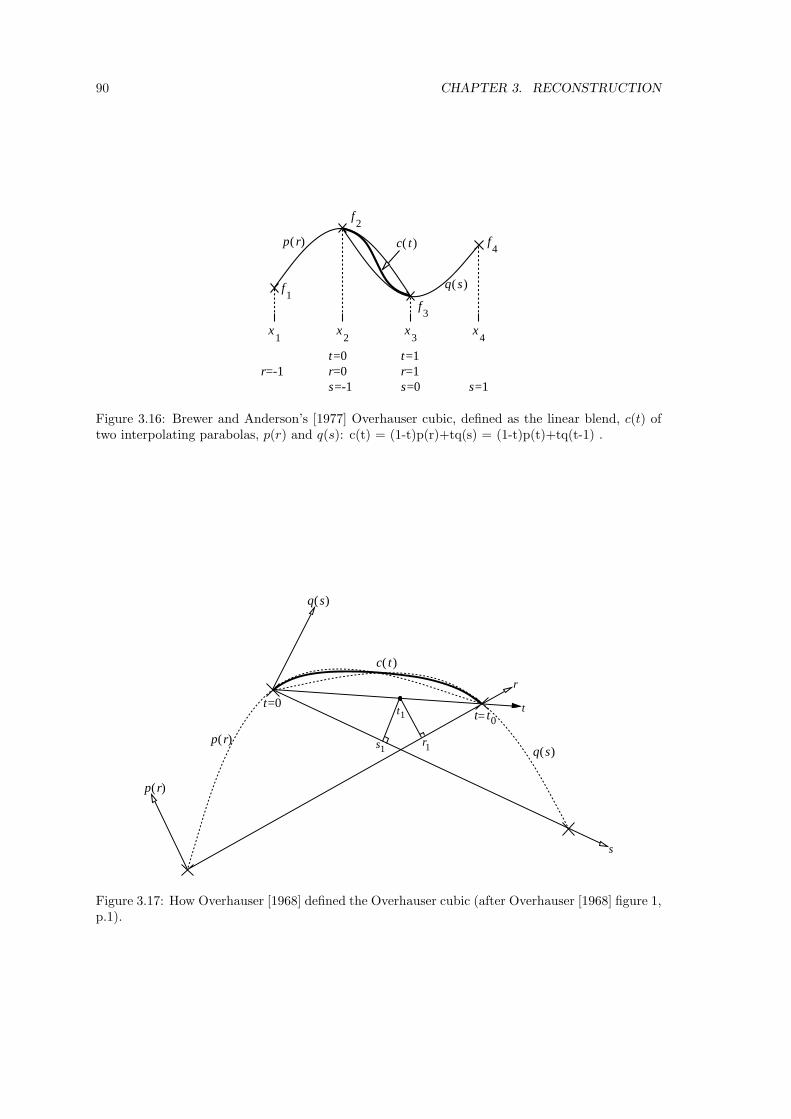
90 CHAPTER 3. RECONSTRUCTION
p r( )
r=-1t=0r=0s=-1 s=0
r=1t=1
f1
x1
f2
x3
f4
f3
x2
q s( )
c t( )
x4
s=1
Figure 3.16: Brewer and Anderson’s [1977] Overhauser cubic, defined as the linear blend, c(t) oftwo interpolating parabolas, p(r) and q(s): c(t) = (1-t)p(r)+tq(s) = (1-t)p(t)+tq(t-1) .
s
t
r
t1
s1r1
t t= 0
p(r)
p(r)
t=0
q(s)
q(s)
c( t)
Figure 3.17: How Overhauser [1968] defined the Overhauser cubic (after Overhauser [1968] figure 1,p.1).

3.6. CUBIC FUNCTIONS 91
and Adams’ [1975, pp.133–138] subsequent restatement) uses a slightly different derivation. Hisderivation uses a local coordinate system for each of the two parabolas, as illustrated in figure 3.17.c(t) is then linearly blended from the two functions, as before, by:
c(t) =(
1 − t
t0
)p(r) +
(t
t0
)q(s)
To make sense of this it is necessary to have r and s as functions of t. Overhauser chose to definethese two functions by dropping a perpendicular from the point t, on the t-axis, to the r- or s-axis,as illustrated by the points t1, s1 and r1 in figure 3.17. Unfortunately, this makes the resultingalgebra extremely complex. So much so that it is not worth following for our use11.
Thus, while Brewer and Anderson [1977] do produce a curve in the spirit of Overhauser, it is notthe same curve as that developed by Overhauser [1968].
Brewer and Anderson’s ‘Overhauser Curve’ can be fitted into Catmull and Rom’s formalism bydefining:
gi(t) = qi(t)wi(x) = B2(x − i)
where B2(s) =
1 + s, −1 ≤ s ≤ 01 − s, 0 ≤ s ≤ 10, otherwise
B2(s) is a linear blending function. It is the same function as the linear interpolation kernel andthe second order B-spline.
We have now seen that the same spline has been derived independently in four different ways. ToCatmull and Rom [1974] it was the quadratic B-spline blend of three linear functions; to Brewer andAnderson [1977] it was the linear blend of two quadratics; to Keys [1981] it was the C1-continuousinterpolating cubic which matched a Taylor’s series expansion to the highest order and to Parkand Schowengerdt [1983] it was the C1-continuous interpolating cubic with the best frequencyresponse. As if this were not enough, there is a fifth derivation of the same cubic, which canbe found in the next section. The fact that the same cubic has been independently put forwardas somehow ‘the best’ cubic by two separate methods, and is also the end result of three otherderivations would seem to be heavy evidence in favour of adopting the Catmull-Rom spline as thebest all-round cubic interpolant. Mitchell and Netravali’s [1988] subjective analysis backs this up;the Catmull-Rom spline falls near the middle of the region of ‘satisfactory’ subjective behaviour.
Whether the Catmull-Rom spline is the best all-round cubic reconstructor is another question.Mitchell and Netravali would say no, the reconstructor defined by B = 1
3 , C = 13 in equation 3.19 is
subjectively better, while Reichenbach and Park [1989] in their critique of Mitchell and Netravali’s[1988] paper claim that, from a frequency domain analysis, yes, the Catmull-Rom spline is thebest. Their criterion for ‘best’ is closeness of the reconstructor’s frequency response to that of theperfect reconstructor: sinc. Wolberg [1990, p.132] points out that this disagreement brings intoquestion whether Reichenbach and Parks’ criterion for ‘best’ is useful, as it does not equate to thesubjective ‘best’ and, for pictures for human consumption, it is subjective quality that is important.On the other hand Mitchell and Netravali’s experiment involved scaling and sampling as part ofthe resampling process; so their results judge the subjective quality of the whole resampling, notjust the reconstruction. This theme is picked up in chapter 7.
For a given application, it may be desirable to use a different interpolant. In particular, if astrictly positive interpolating kernel is required, then the cubic interpolant with parameter a = 0can be used [Maeland, 1988, pp.215-216]. If an interpolant is required that perceptually sharpensthe picture then the cubic interpolant with a = −1 can be used [Parker et al., 1983, pp.36, 39].
11However, it should be noted that Overhauser’s use (CAD) is very different in its requirements to ours.

92 CHAPTER 3. RECONSTRUCTION
However, Mitchell and Netravali [1988] claim that this interpolant introduces too much ringinginto the reconstructed intensity surface. An interpolant with properties midway between thissharpening interpolant and the Catmull-Rom interpolant can be obtained by using a = − 3
4 [Parkeret al., 1983, p.36].
3.6.3 Other cubic methods
There are many methods for generating cubic reconstructors in the literature. Some fit into ourformalism and some do not. Cubic polynomials are the most often used polynomials because lowerorder polynomials give too little flexibility and higher order polynomials can introduce unwantedwiggles (and require more computation) [Foley et al., 1990, p.478, sec. 11.2]. Their usefulnesshas lead to a large body of knowledge about them — mostly about their usefulness for describingsurfaces in computer aided design (CAD) and its related fields.
It is useful to briefly scan through these methods to see if they shed any more light on usefulmethods for intensity surface reconstruction. Foley et al. [1990] give a summary of the mostcommon of these. We will consider the utility of each one.
Hermite
The Hermite form of a cubic is determined from two endpoints and tangents (first derivatives) atthose endpoints. The formula for a piecewise Hermite is: [Foley and van Dam, 1982, p.516]:
f(x) = [ t3 t2 t 1 ]
2 −2 1 1−3 3 −2 −1
0 0 1 01 0 0 0
fα
fα+1
f ′α
f ′α+1
= (2t3 − 3t2 + 1)fα
+ (−2t3 + 3t2)fα+1
+ (t3 − 2t2 + t)f ′α
+ (t3 − t2)f ′α+1
where α =⌊
x − x0
∆x
⌋and t =
x − xα
∆xas usual.
Here fi are the sample values, as before, and f ′i are the tangents of the sampled function at the
sample points12.
We will not, in general, have these tangent values as we are dealing with NAPK reconstructors.However, Mitchell and Netravali [1988] show that, if these tangent values are available (as, forexample, is possible with some artificially generated images), then the Hermite form produces abetter result than the best cubic reconstruction based only on the sample values.
In the absence of explicit tangent information, it is common to approximate the tangent by thedifference between adjacent sample values. That is:
f ′i ≈ (∆x)
∆fi
∆x= ∆fi = fi+1 − fi
12N.B. f ′i = df
dt
∣∣x=xi
because the equation is in terms of t rather than x:
f ′i =
df
dt
∣∣∣x=xi
=df
dx
dx
dt
∣∣∣x=xi
= (∆x)dx
dt
∣∣∣x=xi

3.6. CUBIC FUNCTIONS 93
P
P
P
P
α,1
α+1,−1
α
α+1
P
P
α
α+1
’
’
Figure 3.18: How the Bezier and Hermite cubics are related: the Hermite form of the curve iscontrolled by the two data points, Pα and Pα+1 and by the two derivative vectors P′
α and P′α+1;
the Bezier form is controlled by the two data points, Pα and Pα+1 and by two other control points,Pα,1 and Pα+1,−1. The relationship between these is given in equations 3.22 and 3.23.
The approximation f ′i ≈ fi−fi−1 is equally valid and it is the average of these two approximations
that is generally taken:
f ′i ≈
∆fi + ∆fi−1
2where ∆fj = fj+1 − fj .
If this approximation is used in the Hermite cubic then resulting function is the Catmull-Romspline. This is the fifth derivation of the Catmull-Rom spline (mentioned in section 3.6.2). Re-ichenbach and Park [1989] independently discovered this derivation of the spline.
Bezier
The Bezier form of the cubic is related to the Hermite. It uses four control points for each piece:two endpoints plus two other points to control the shape of the curve. If we take the two endpointsto be (xα, fα) and (xα+1, fα+1) and the two control points to be (xα,1, fα,1) and (xα+1,−1, fα+1,−1).The location of these two control points is linked to the Hermite form by the formula: [see Foleyand van Dam, 1982, p.519].
Pα,1 = Pα +13P′
α (3.22)
Pα+1,−1 = Pα+1 −13P′
α+1 (3.23)
This relationship is illustrated in figure 3.18.
The Bezier form can be used in two ways: either by defining the control points in some way, or byusing the existing data points as control points. The former method presents us with a situationsimilar to that with the Hermite: how do we define these extra points? If we have the derivativevalues then we can use equations 3.22 and 3.23 to calculate the positions of the control points andthus produce a Hermite cubic as before.
Rasala [1990] shows how the positions of the control points can be computed from all the availabledata13, this is discussed in section 4.5.1. However, his first approximations to this globally con-
13Theoretically all of the available data should be used. In practice it is only necessary to use the 12 to 16 nearestpoints, still rather more than the four nearest points we are using here.
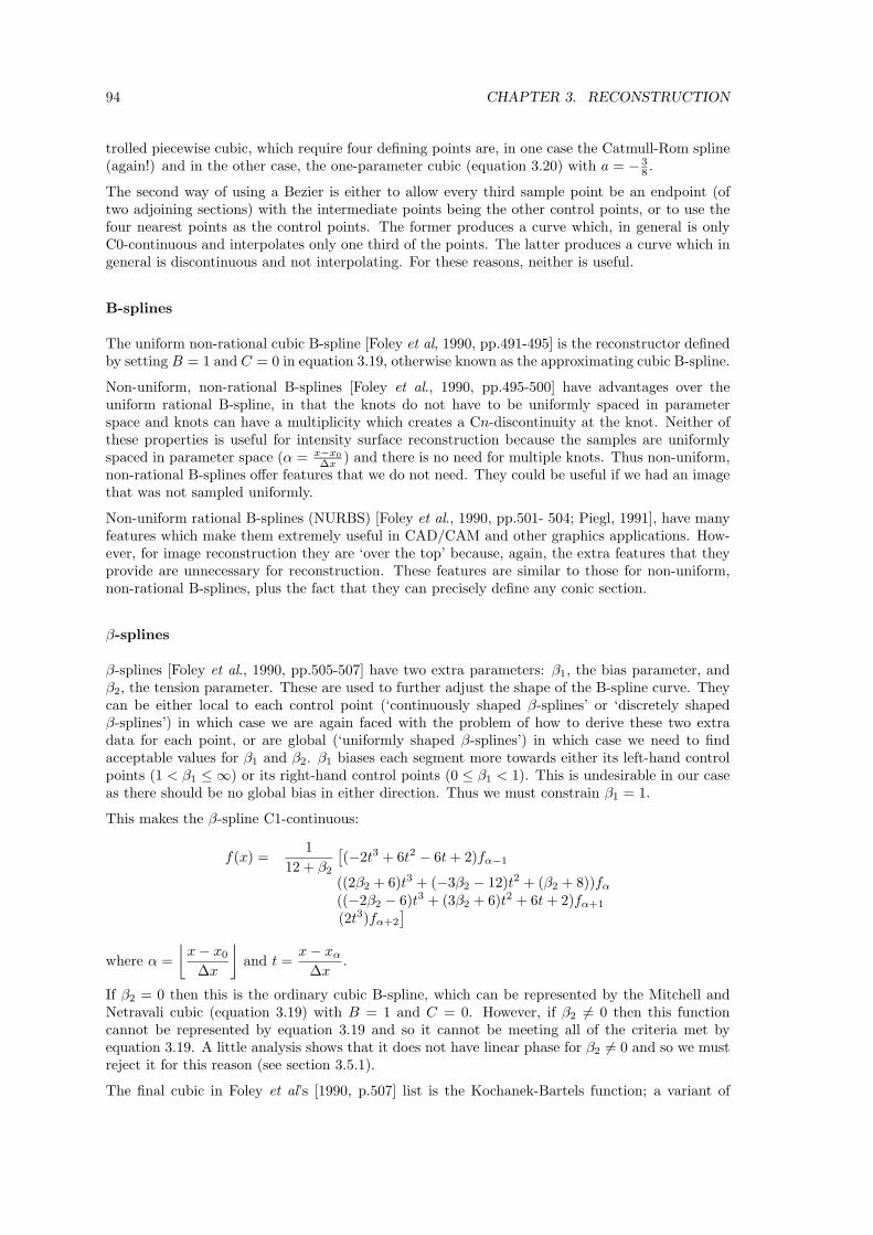
94 CHAPTER 3. RECONSTRUCTION
trolled piecewise cubic, which require four defining points are, in one case the Catmull-Rom spline(again!) and in the other case, the one-parameter cubic (equation 3.20) with a = − 3
8 .
The second way of using a Bezier is either to allow every third sample point be an endpoint (oftwo adjoining sections) with the intermediate points being the other control points, or to use thefour nearest points as the control points. The former produces a curve which, in general is onlyC0-continuous and interpolates only one third of the points. The latter produces a curve which ingeneral is discontinuous and not interpolating. For these reasons, neither is useful.
B-splines
The uniform non-rational cubic B-spline [Foley et al, 1990, pp.491-495] is the reconstructor definedby setting B = 1 and C = 0 in equation 3.19, otherwise known as the approximating cubic B-spline.
Non-uniform, non-rational B-splines [Foley et al., 1990, pp.495-500] have advantages over theuniform rational B-spline, in that the knots do not have to be uniformly spaced in parameterspace and knots can have a multiplicity which creates a Cn-discontinuity at the knot. Neither ofthese properties is useful for intensity surface reconstruction because the samples are uniformlyspaced in parameter space (α = x−x0
∆x ) and there is no need for multiple knots. Thus non-uniform,non-rational B-splines offer features that we do not need. They could be useful if we had an imagethat was not sampled uniformly.
Non-uniform rational B-splines (NURBS) [Foley et al., 1990, pp.501- 504; Piegl, 1991], have manyfeatures which make them extremely useful in CAD/CAM and other graphics applications. How-ever, for image reconstruction they are ‘over the top’ because, again, the extra features that theyprovide are unnecessary for reconstruction. These features are similar to those for non-uniform,non-rational B-splines, plus the fact that they can precisely define any conic section.
β-splines
β-splines [Foley et al., 1990, pp.505-507] have two extra parameters: β1, the bias parameter, andβ2, the tension parameter. These are used to further adjust the shape of the B-spline curve. Theycan be either local to each control point (‘continuously shaped β-splines’ or ‘discretely shapedβ-splines’) in which case we are again faced with the problem of how to derive these two extradata for each point, or are global (‘uniformly shaped β-splines’) in which case we need to findacceptable values for β1 and β2. β1 biases each segment more towards either its left-hand controlpoints (1 < β1 ≤ ∞) or its right-hand control points (0 ≤ β1 < 1). This is undesirable in our caseas there should be no global bias in either direction. Thus we must constrain β1 = 1.
This makes the β-spline C1-continuous:
f(x) =1
12 + β2
[(−2t3 + 6t2 − 6t + 2)fα−1
((2β2 + 6)t3 + (−3β2 − 12)t2 + (β2 + 8))fα
((−2β2 − 6)t3 + (3β2 + 6)t2 + 6t + 2)fα+1
(2t3)fα+2
]where α =
⌊x − x0
∆x
⌋and t =
x − xα
∆x.
If β2 = 0 then this is the ordinary cubic B-spline, which can be represented by the Mitchell andNetravali cubic (equation 3.19) with B = 1 and C = 0. However, if β2 �= 0 then this functioncannot be represented by equation 3.19 and so it cannot be meeting all of the criteria met byequation 3.19. A little analysis shows that it does not have linear phase for β2 �= 0 and so we mustreject it for this reason (see section 3.5.1).
The final cubic in Foley et al’s [1990, p.507] list is the Kochanek-Bartels function; a variant of

3.7. HIGHER ORDERS 95
the Hermite cubic where each segment depends on the four nearest control points and three extraparameters specific to that segment. As with the Hermite curve the problem with using thisfunction is that we have no way of generating these extra parameters.
This completes the list of cubics given by Foley et al [1990]. Others do exist and some families havebeen given names which have not been mentioned here, for example the Mitchell and Netravalicubics with C = 0 are Duff’s tensioned B-splines [see Mitchell and Netravali, 1988, p.223]. Most ofthese functions have been primarily designed for CAD; few of them are applicable to reconstruction.The aims of the two fields are different, there tends to be more data available for describing the curvein CAD than in resampling (for example: derivative values), thus allowing these more complexforms, and CAD has greater need of weird and wonderful properties in its curves than resampling(for example: discontinuities at some sample points, and not at others). However, this section has,at least, considered the utility of these functions. The approximating cubic B-spline has alreadybeen met as a case of equation 3.19. The interpolating cubic B-spline and interpolating Beziercubic are discussed in chapter 4.
3.6.4 Summary
It would appear that the all-round best cubic interpolant is the Catmull-Rom spline. There is lessconsensus on the all-round best cubic reconstructor, but Mitchell and Netravali’s results wouldindicate that it is some linear blend of the Catmull-Rom spline and the cubic B-spline:
f(x) = (1 − ζ)CatRom(x) + ζBSpline(x)
with ζ closer to zero than one. Mitchell and Netravali [1988] recommend ζ = 13 , while Reichenbach
and Park [1989] recommend ζ = 0.
3.7 Higher orders
In section 3.5.10 we saw the multitude of conditions which it would be useful to get a reconstructorto obey. It would be almost impossible to meet all these conditions. If we look at the Catmull-Romspline, it does meet most of the conditions but fails in that it is not C2-continuous and its frequencyresponse, while the closest to the perfect frequency response of any cubic [Reichenbach and Park,1989], is still not particularly close to it (Note that the approximating cubic B-spline is the onlyC2-continuous cubic, and it is not an interpolant. It produces a rather blurry intensity surface.)The solution to this problem could be to go to a higher-order.
Parker et al [1989, p.39] state that “although the length [cubic function, 4 data points] for inter-polating functions is adequate for many tasks, additional improvement in performance could bemade by including more points in the calculation. The same criteria used for selecting interpolatingfunctions used in this paper — frequency responses, phase shift and gain — would also be usefulin selecting between functions with a longer extent.”
Keys [1981, pp.1159-60] six point cubic function has an O(h4) convergence rate to the Taylorseries expansion of the function being interpolated. As cubics can give at most O(h4) accuracy, itimmediately follows that higher order convergence rates require higher order piecewise polynomials.
However, Mitchell and Netravali [1988, p.225] believe that no simple filter (such as a piecewise localpolynomial) will be found that will improve much on the cubic filters they have derived. They thussuggest that other avenues of research would be more fruitful. Further, Foley and van Dam [1982]note that higher order polynomials can introduce unwanted wiggles in the reconstructed function.
Quadratics and cubics allow a single lobe, or ripple, either side of an edge, which perceptuallysharpens the edge (section 4.5.2). Quartics, and higher orders, allow more ripples either side,which can perceptually degrade the image. Hence it may be counter-productive to go to higherorders than cubic.
96 CHAPTER 3. RECONSTRUCTION
We have done little work on fifth, and higher, order piecewise polynomials and so cannot giveevidence as to the validity of these arguments. It should be fairly simple, though, to extend ouranalysis to higher orders. We leave this for future work. However, there seems to be little roomfor significant improvement, and so, perhaps, the subject of piecewise local polynomials should beclosed.
3.8 Summary
We have seen several ways of classifying reconstructors, including local vs non-local, and skeletonvs continuous. Skeleton reconstruction describes a situation where the intensity surface is definedonly at specific points, and is undefined elsewhere. Delta function reconstruction is a similar idea.
The bulk of this chapter was devoted to piecewise local polynomials. There are, by far, the moststudied group of local reconstructors. They are easily understood, quickly implemented, and fastto evaluate. We proved that zero-phase piecewise local quadratics do exist, and derived two newquadratic reconstructors. One of these provides similar visual quality to the Catmull-Rom cubic,with faster evaluation.
The study of quadratics led into an examination of the factors involved in the design of recon-structors. This in turn brought us to a discussion of piecewise local cubics. Here we saw that theevidence indicates that the Catmull-Rom cubic is the best all-round cubic interpolant, and that it,or some linear mix of it and the cubic B-spline, is the best all-round cubic reconstructor.

3.8. SUMMARY 97
Chapter 4
Infinite Extent Reconstruction
In the previous chapter we discussed the most studied group of reconstructors, the piecewise localpolynomials. We now turn our attention to other classes of reconstructor:
1. the infinite reconstructors
2. the local approximations to the infinite reconstructors
3. the a priori knowledge reconstructors.
The first two are discussed in this chapter. The final class we leave until chapter 6.
4.1 Introduction to infinite reconstruction
Into this class fall all the reconstructors which use all of the sample points in the image. We willconcentrate on these four:
• sinc interpolant
• Gaussian approximant
• interpolating cubic B-spline
• interpolating Bezier cubic
All these methods are based on a theory of an infinite image; that is: the theory does not take theimage’s edges into account. In a practical situation the image has edges and these must be dealtwith if we are to use an infinite reconstructor. Edge effects and the edge extension solutions arediscussed in the next section.
4.2 Edge effects
While the finite size of real images is a readily apparent problem for infinite extent reconstructors,the problem exists to a lesser extent for finite-extent reconstructors, such as those discussed inthe previous chapter. It is feasible that a certain transformation, reconstructor, and sampler maycombine to produce a resampling which never needs to access data beyond the edge of the image,but in general, we have to answer the question: what is out there?
98

4.2. EDGE EFFECTS 99
The simple answer is that nothing is out there, we know absolutely nothing about the intensityvalues beyond the edges of our finitely sized image. This is unfortunately of little use in caseswhere we need to know the value of a sample beyond the edge of the image.
There are at least eight ways of specifying the values of the pixels beyond the image’s edge; thusproducing an infinite image from a finite one. These are:
1. Undefined
2. Error Limits
3. Constant
4. Extrapolation
5. Replication
6. Reflection
7. Transparent
8. Special Cases
The last one requires special knowledge about the reconstructor involved and must be tailored tosuit. The others are independent of the reconstructor.
There are two types of occurrence which require information about pixel values beyond the edgeof the image: (a) when we require the value of the intensity surface at some point within the finiteimage’s edges, but, to calculate the value at that point, the reconstructor needs pixel values frombeyond the edge of the image; and (b) when we require the value of the intensity surface at somepoint outside the finite image’s edges. Figure 4.1 gives an example of both these types of pixel. Itis possible to use a different method to generate intensity surface values of type (a) from that usedfor type (b). For example, type (a) could be generated by some edge extension method while type(b) is given a constant value. In most situations, these two cases collapse nicely into the singlecase: ‘when the reconstructor requires the value of a pixel beyond the image’s edges’.
In figure 4.1 the shaded band shows the area near the edge of the image where the reconstructorneeds values beyond the image’s edge to produce intensity surface values. For an infinite extentreconstructor this shaded area extends over the whole image, but for finite extent reconstructorsit is a band, usually a few pixels wide, around the edge of the image. It is non-existent only fornearest-neighbour, skeleton, and Delta-function reconstruction.
The necessity of edge extension depends on the reconstructor, transformer, and sampler used. Ifthey form a resampling where the required portion of the intensity surface lies within the innerregion in figure 4.2 (region A) then no image extension is required, and no edge effects will occur.An example is shown in figure 4.3(a). However, many resampling applications require values of theintensity surface in region B (the band) and often also in region C (the outer region). An exampleis shown in figure 4.3(b). In these cases we must decide how to perform edge extension and howto minimise the resulting edge effects.
There are two possible ways of defining edge extension. One is to assign values to the unknownpixels and use the reconstruction method on these assigned sample values to generate the intensitysurface. The other method may give values to some, or all, of these unknown pixels but it alsooverrides the reconstruction method by explicitly defining part of the intensity surface, usuallyregion C in figure 4.2.
Little work has been done on the edge extension problem. The usual assumption that is made isthat any pixel outside the image has the intensity zero [Fiume, 1989, p.78, definition 16; Pratt,1978, ch.9]. Two other common assumptions are that the image is repeated (that is: it tiles theplane), or that it is mirrored and repeated. These are illustrated later in the chapter. White and

100 CHAPTER 4. INFINITE EXTENT RECONSTRUCTION
(a)
(b)
Figure 4.1: The two types of destination pixel for which edge effects are important. The image onthe left is rotated (dashed line on right) to produce a new image (solid line on right). The shadedarea in the left hand image represents that part of the reconstructed intensity surface whose valuesdepend on samples outside the image’s edges. Pixel (a) in the final image lies within the originalimage’s edges but its value depends on sample values outside those edges. Pixel (b) lies within thefinal image’s edges but outside the original image’s edges.
A B C
image edge
Figure 4.2: The three areas of an image: A: the intensity surface in this area depends only on pixelvalues within the image’s edges. B: the intensity surface in this area depends on pixel values bothinside and outside the image’s edges. C: the intensity surface in this area lies outside the image’sedges.

4.2. EDGE EFFECTS 101
(a)
(b)
Figure 4.3: Two examples of transforms, one requiring edge extension and one not. (a) all intensitysurface values in the final image (right) lie within region A (figure 4.2) in the original image, so noedge extension is required. (b) Intensity surface values in the final image lie in all three regions ofthe original image, so some edge extension is required.
Brzakovic [1990] present two novel methods of image extension but, otherwise, there appears to belittle published on it. These, and other, methods of edge extension are discussed in detail below.
4.2.1 The methods of edge extension
Edge extension is fundamentally the process of producing pixel values outside the image’s edgesfor the reconstructor to operate on, thus producing an intensity surface of infinite extent. It alsoincludes those methods which explicitly define part of the intensity surface to have values indepen-dent of the reconstructor. The ensuing discussion covers the eight methods of edge extension.
(1) Undefined
Our opinion is that this is the philosophically correct value to give to those pixels which lie beyondthe image’s edges. We don’t know what these values are and so they should remain undefined.Furthermore, if the value ‘undefined’ occurs in the definition of the intensity surface’s value at anypoint then that intensity surface value is also undefined.
The practical upshot of this is that the only part of the intensity surface which is defined is thatwhich lies within the inner boundary of the shaded area in figure 4.2 (region A). So, if we have anN ×N image, and a reconstructor which requires an L pixel wide boundary, the resulting intensitysurface will be defined over only (N − 2L) × (N − 2L) pixels. This assumption is often used inother image processing operations, where the loss of a few pixels is unimportant. For example, seeFang, Li and Ni’s [1989] discussion of two dimensional convolution.

102 CHAPTER 4. INFINITE EXTENT RECONSTRUCTION
In resampling, however, this solution is unworkable. Firstly, if we use an infinite extent reconstruc-tor, practically the entire intensity surface will be undefined1. Secondly, and more importantly: inmost cases, some of the destination pixels will have an undefined value. It is impossible to display‘undefined’ as it is not a real intensity value.
We could decide that a pixel with an undefined value is displayed with some constant intensitybut, if we do this, undefined pixels cannot be distinguished from pixels which really have thatintensity. Further, if undefined values are stored as this constant value then errors will occur ifthe destination image is the source for further processing unless we also keep note of which storedpixels are defined and which are not.
The problem has a simple solution in Fang, Li and Ni’s case. Their destination image is simplysmaller than the source, and there are no undefined pixels within the destination’s edges. In ourgeneral resampling case we cannot guarantee this, and, if we do display an image which containsundefined pixels we must display them with some intensity other than ‘undefined’. We cannothave undefined pixels and display them too!
This particular solution to the edge problem, while philosophically sound, is unsatisfactory forpractical purposes. We must look to other solutions.
(2) Error bounds
In the previous case we assumed that we knew nothing about the value of the pixels beyond theimage’s edges. This is untrue, in that we will, in general, know the bounds within which thesepixel values are constrained to lie. If we are dealing with an image representation which boundsall pixel values between two extrema, then we can assume that all the unknown pixel values mustlie between them also.
Having defined bounds within which the unknown pixel values can lie, it is possible to calculatebounds within which the intensity surface must lie, as illustrated in figure 4.4. Thus, for everydestination pixel, it is possible to give an upper and a lower bound to the pixel’s value. For somedestination pixels (under some reconstructors) these two bounds will be equal to one another andfor some they will be equal to the extrema, or even beyond them, as in figure 4.4(Catmull-Romcubic).
It may be thought that the error bounds of source pixels just beyond an image edge should beless separated than those well beyond the edge. That is: the error bounds should increase as onemoves away from the edge until they reach the extrema (figure 4.5(b)). Unfortunately, this is notthe case. Theorem 1 gives the lie to the scenario in figure 4.5(b) for a general image.
Theorem 1 The first unknown pixel beyond an image’s edge can take any value between the ex-trema.
Proof: Whittaker [1915] proves that, for any set of equispaced samples,
F∞ = {(xi, fi) : i ∈ Z, xi = x0 + i∆x}
there exists a unique function, f(x), through those sample points such that f(x) is bandlimited tobelow 1
2∆x (later named the folding frequency2).
1‘practically’ because, for example, a sinc reconstructed intensity surface would be undefined everywhere exceptat the sample points, where it would be equal to the sample value at that point.
2note that the Nyquist frequency of f(x) will be less than or equal to the folding frequency [see Lynn and Fuerst,1989, p.11]

4.2. EDGE EFFECTS 103
Two-point cubic Approximating cubic B-spline Catmull-Rom cubic
(a)
(b)
(c)
Figure 4.4: Error bounds on intensity surface values. The crosses mark known pixel values, thedotted vertical lines unknown pixel values, bounded above and below. The shaded area showsthe range of values within which the intensity surface can lie. Here we show three local piecewisepolynomial reconstructors operating on three situations: (a) constant intensity; (b) oscillatingintensity; (c) slowly varying intensity.
image edge
(a)
image edge
(b)
Figure 4.5: Two possible scenarios for error bounds on unknown pixels. (a) all unknown pixels cantake any value between the extrema; (b) pixels close to the image edge are more tightly boundedthan those farther away. Theorem 1 gives the lie to the scenario in (b).

104 CHAPTER 4. INFINITE EXTENT RECONSTRUCTION
Now, our image is of finite extent:
Fa,b = {(xi, fi) : i ∈ [a, b], xi = x0 + i∆x}
and we have assumed that we do not know the values fi, i �∈ [a, b]. By assigning values to these,an infinite number of infinite sets, F∞, can be created; each containing the set Fa,b. Thus, fromWhittaker’s result, we see that there are an infinite number of bandlimited functions which passthrough any finite set of sample points.
Therefore the first unknown pixel (fa−1 or fb+1) can take any value and there will still be abandlimited function through the set of samples. If all the samples are constrained to lie betweentwo extrema then these first unknown pixels will be able to take any value between them. QED.
If we know that the image is bandlimited to below the folding frequency then we may be able todefine tighter bounds than the extrema for unknown pixels close to the image’s edge. In general,we do not have this a priori knowledge, therefore all unknown pixels are bounded between theextrema.
This solution to the edge problem has much the same drawbacks as the previous solution: (1) itis impossible to display a range of intensities for a single pixel; (2) an infinite extent reconstructorwill contain some uncertainty at practically every point. For example, the sinc reconstructor wouldproduce bounds at the extrema for all but the known sample points.
A solution to this problem would be to display the mean of all possible values at each point.However, calculating this mean is not a simple matter. An approximation to the mean couldbe obtained by setting all unknown values to the mean of the two extrema and calculating theintensity surface from these. This collapsing of the error bounds onto a single value takes us to athird solution: the constant value.
(3) Constant
The solution most often adopted is to set all unknown pixels to be a constant value. By commonconsent it appears that this value is invariably chosen to be zero, which nearly always representsblack.
Zero, at first glance, is a sensible value. Any multiplications involving zero evaluate to zero andthus need not be performed. Thus, for any reconstructor that can be represented by a filter, nounknown values need to be taken into consideration when producing the intensity surface becausethey contribute nothing to the evaluation of the surface values.
However, the identification of zero with black3 is unfortunate. Black is at one end of the spectrumof possible intensity values. We are thus setting all unknown pixels to one of the two extremevalues. In other applications, for example sound and electrical current, zero is an average value.The signal can fluctuate to positive or negative. With intensity, zero is a minimum value — youcannot have negative light. While it is sensible to set zero intensity to be absence of light (in asimilar way to zero mass being absence of mass) and setting unknown values to be zero can bejustified (an identification of ‘nothing’ with ‘nil’), the combination of the two produces a problem,in that it can cause excessive ringing artifacts, and negative intensities near the image’s edges.
The previous edge extension method contains the seed of a better constant value: the value halfwaybetween the two extrema; a mid-grey. Using mid-grey in place of any unknown value minimisesthe maximum discrepancy between the last known value and the first unknown value on eitherside of an edge (see figure 4.6).
Purists may balk at the idea of using any value but zero to replace the unknown values. A simplesolution to this objection is to subtract the mid-grey value from all pixels in the image, set unknownpixels to zero, resample the image and then add back the mid-grey value. However, this only works
3or, in some rare cases, with the brightest white, for much the same effect.

4.2. EDGE EFFECTS 105
(a) (b)
Figure 4.6: Minimising the maximum discrepancy between pixel values and the constant value.(a) using a mid-grey constant, the maximum discrepancy is half the full range; (b) using a blackconstant, the maximum discrepancy is the full range.
for resamplings in which the final pixel values are linear combinations of the original pixel values,which, fortunately, are the great majority of resamplings (see section 2.2).
Another candidate constant value is the average value of all the known image pixels. One motiva-tion behind this choice is that it retains the DC component of the frequency spectrum: the DFTof the finite image and the FT of the infinite extended image have the same DC component. Inmost cases this average value would be close to the suggested mid-grey value. For the minority ofcases in which the image is unusually dark or unusually light, this average value is a better choicethan the mid-grey. For the rare situations with a dark centre and bright edge (or vice-versa) it isconceivable that this average would be a worse choice than the mid-grey.
Though, overall it would appear that the average value would be slightly preferable to the mid-greyvalue, this advantage must be offset against the need to calculate the average. Taking this intoconsideration, there is little to choose between the two values.
Use of a constant intensity beyond the edges of the image is simple and efficient. It requires littlecomputational effort (except when the average intensity of the known image values needs to becalculated, but even that need only be done once per resampling). When a destination pixel fallswell outside the edge of the transformed source image it will, in general, be given a value close tothe constant value. However, just inside and just outside the source image edge, the reconstructedsurface will display ‘edge effects’. The severity of these effects depends partly on the differencebetween the pixel values just inside the edge and the constant value assigned to the unknown pixelsjust outside the edge. It also depends on the reconstructor used. The sinc interpolant producesmany obvious artifacts, while a very local reconstructor, such as linear interpolation, displaysvirtually no artifacts at all (see figure 4.7).
We can attempt to reduce this edge effect problem by extrapolating more ‘sensible’ values off theedge of the image rather than simply setting all the unknown pixels to a constant.
(4) Extrapolation
Extrapolation out from the edge of the image is an attempt to make what is beyond the edge bearsome relation to what is inside the edge. It cannot create any extra information, but the hope isthat the available information can be used to produce sensible values for the unknown pixels.
Extrapolation is considerably more hazardous than interpolation [Press et al, 1988, p.85]. A typicalinterpolating function (which is perforce an extrapolating function) will tend to go berserk at adistance beyond the image edge greater than the inter-pixel spacing [ibid., p.88]. We must becareful how we extrapolate.
One advantage we have over general extrapolation is our knowledge of the bounds within whichthe values must lie. These can be used to prevent the values from going berserk and reachingvalues way beyond the bounds.
The simplest extrapolation method is to copy the final row of pixels to infinity. This is illustratedin figure 4.9 which shows the images in figure 4.8 extrapolated by this method. White andBrzakovic [1990] modify this idea by assigning a virtually constant intensity to each unknown

106 CHAPTER 4. INFINITE EXTENT RECONSTRUCTION
Figure 4.7: The effect of a constant zero edge extension on two reconstructors. On the left is theintensity surface reconstructed by sinc interpolation, notice the ripples near the image edges (bothinside and outside of the edges), caused by the sharp fall off to zero. On the right is the intensitysurface reconstructed by linear interpolation. The only edge effect is a slight fading off at the veryedge of the image. The right hand image is quite blurry, but this is a property of the reconstructor,not an edge effect.
Figure 4.8: The original images used in the extrapolation examples.
Figure 4.9: Extrapolation by copying the final row of pixels off to infinity. This process is appliedto the two images in figure 4.8
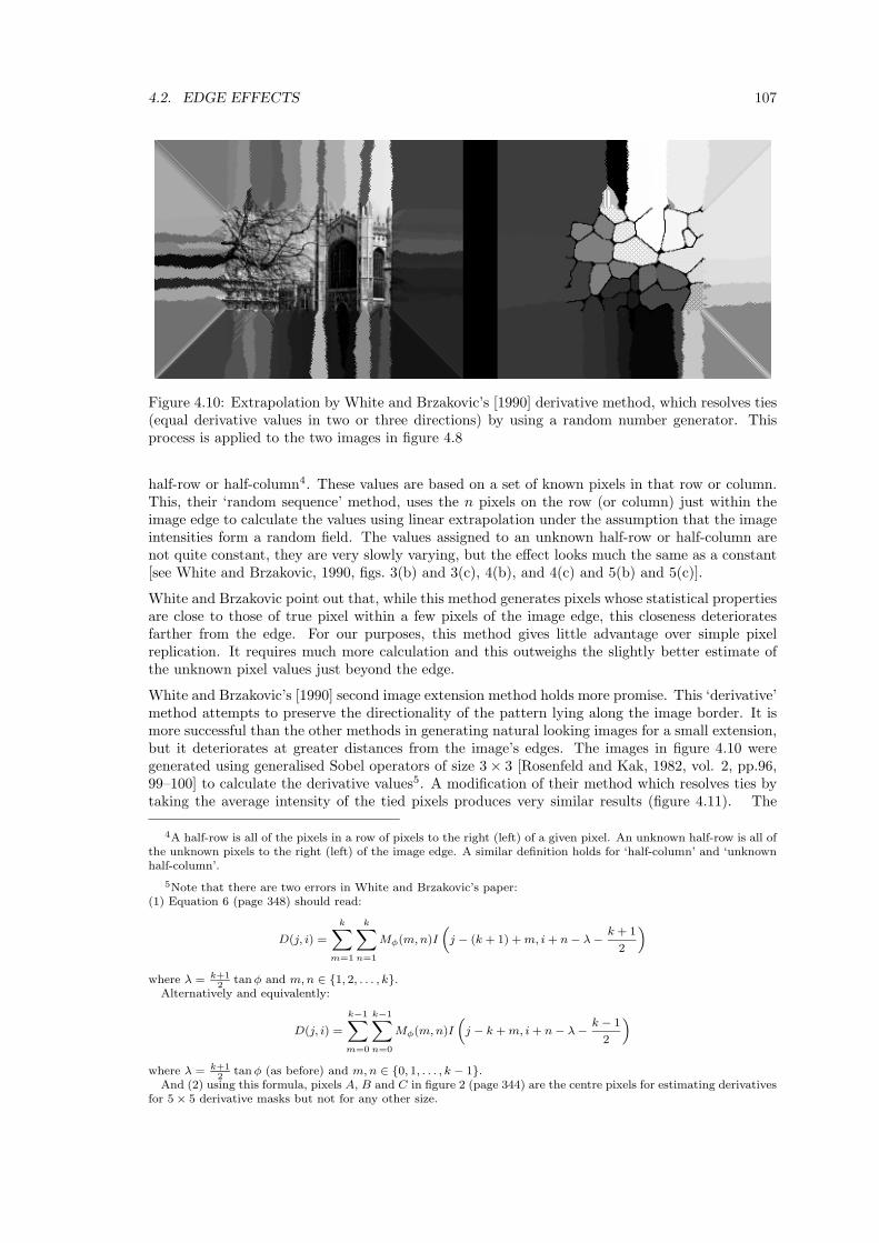
4.2. EDGE EFFECTS 107
Figure 4.10: Extrapolation by White and Brzakovic’s [1990] derivative method, which resolves ties(equal derivative values in two or three directions) by using a random number generator. Thisprocess is applied to the two images in figure 4.8
half-row or half-column4. These values are based on a set of known pixels in that row or column.This, their ‘random sequence’ method, uses the n pixels on the row (or column) just within theimage edge to calculate the values using linear extrapolation under the assumption that the imageintensities form a random field. The values assigned to an unknown half-row or half-column arenot quite constant, they are very slowly varying, but the effect looks much the same as a constant[see White and Brzakovic, 1990, figs. 3(b) and 3(c), 4(b), and 4(c) and 5(b) and 5(c)].
White and Brzakovic point out that, while this method generates pixels whose statistical propertiesare close to those of true pixel within a few pixels of the image edge, this closeness deterioratesfarther from the edge. For our purposes, this method gives little advantage over simple pixelreplication. It requires much more calculation and this outweighs the slightly better estimate ofthe unknown pixel values just beyond the edge.
White and Brzakovic’s [1990] second image extension method holds more promise. This ‘derivative’method attempts to preserve the directionality of the pattern lying along the image border. It ismore successful than the other methods in generating natural looking images for a small extension,but it deteriorates at greater distances from the image’s edges. The images in figure 4.10 weregenerated using generalised Sobel operators of size 3 × 3 [Rosenfeld and Kak, 1982, vol. 2, pp.96,99–100] to calculate the derivative values5. A modification of their method which resolves ties bytaking the average intensity of the tied pixels produces very similar results (figure 4.11). The
4A half-row is all of the pixels in a row of pixels to the right (left) of a given pixel. An unknown half-row is all ofthe unknown pixels to the right (left) of the image edge. A similar definition holds for ‘half-column’ and ‘unknownhalf-column’.
5Note that there are two errors in White and Brzakovic’s paper:(1) Equation 6 (page 348) should read:
D(j, i) =
k∑m=1
k∑n=1
Mφ(m, n)I
(j − (k + 1) + m, i + n − λ − k + 1
2
)where λ = k+1
2tan φ and m, n ∈ {1, 2, . . . , k}.
Alternatively and equivalently:
D(j, i) =
k−1∑m=0
k−1∑n=0
Mφ(m, n)I
(j − k + m, i + n − λ − k − 1
2
)where λ = k+1
2tan φ (as before) and m, n ∈ {0, 1, . . . , k − 1}.
And (2) using this formula, pixels A, B and C in figure 2 (page 344) are the centre pixels for estimating derivativesfor 5 × 5 derivative masks but not for any other size.

108 CHAPTER 4. INFINITE EXTENT RECONSTRUCTION
Figure 4.11: Extrapolation by a modification of White and Brzakovic’s [1990] derivative method.This modification resolves ties by taking the average of the intensities in the tied directions. Thisprocess is applied to the two images in figure 4.8
original method resolves ties in two or three directions by the use of a random number generator.
Extrapolation is a risky business. Even these moderately sophisticated methods only succeed fora small distance out from the image edge. This is good for small kernel operators, those whichonly need information up to a few pixels out (for example: a local reconstructor calculating valuesjust inside the image’s edges and needing some pixel values from just outside). But they are notuseful for infinite operators nor for large kernel operators (although White and Brzakovic [1990]imply that they need to use kernels up to size 47 × 47, an edge extension of 23 pixels). Nor arethey particularly useful for finding a pixel value when the destination pixel maps to a source pixelwell outside the image’s edge (case (b) in figure 4.1). Because extrapolation is inaccurate at largedistances from the pixel edge we propose the following ‘hybrid’ solution:
For any pixel farther outside the image edge than a given distance, the pixel’s value isa given constant. Between this region’s boundary and the image edge the pixels aregiven extrapolated values such that they match up neatly with both the image and theconstant at the respective edges.
Figure 4.12 illustrates this concept.
There are still questions to be answered: what constant to use, how wide the extrapolated regionshould be, how to perform the extrapolation. However, this solution holds promise in that: (a) ithas not got the sharp changes in intensity at the image edge that the constant solution has, and (b)it does not tend to produce bad results at great distances from the image edge, as straightforwardextrapolation can do.
Our discussion in the previous section gives us guidance as to which constant value to use. Thethree useful possibilities are:
• zero (usually black), because of the simplification this can make to the calculation of intensitysurface values;
• half-way between the minimum and maximum intensities (a mid-grey), because this min-imises the maximum possible difference between the intensity of an edge pixel and the con-stant intensity6;
6an ‘edge pixel’ is the last known pixel, on a row or column, just within the image’s edge.

4.2. EDGE EFFECTS 109
Image
Constant Region
(a)
ImageExtrapolation ExtrapolationConstant Constant
(b)
Extrapolated Region
Figure 4.12: Extrapolation to a constant. (a) shows the basic idea: the image is surrounded byan area that is extrapolated, beyond this area the pixel values are set to a constant; (b) shows theidea for a single scanline.
• the average intensity of the known pixels in the image (usually a mid-grey7), because thiskeeps the average intensity of the infinite image the same as that of the finite image.
Once a constant value is chosen, the other problems remain to be tackled. How wide should theextrapolated region be? It must be wide enough that we do not get any untoward effects in theintensity surface near the image edges. A zero width gives the equivalent of the constant solutionin the previous section. This is obviously too small a width as it is the edge effects caused bythat solution which led us to consider other solutions. The minimum acceptable width of theextrapolated region is a subjective judgement, depending partly on the type of image and theconstant value chosen.
On the other hand, the extrapolated region cannot be too wide. If it is allowed to be too widethen the problem of the extrapolation being inaccurate rears its head once more. A width of eightor sixteen pixels would seem to be practical. A width of four pixels may be acceptable.
Given this band of unknown values, how do we extrapolate sensible values? There are some obvioussimple methods of interpolating between the edge pixels and the constant pixels. For example,simple linear interpolation between the edge pixel and the first constant pixel (figure 4.13) or cubicinterpolation through two edge pixels and the first constant pixel, ensuring that the first derivativeof the interpolated curve is zero at the first constant pixel (figure 4.14). Such methods, and thelike, produce results similar to that shown in figure 4.15. More complex methods, which take intoaccount more of the context of each extrapolated pixel, could be employed.
However, there is a simple method of ensuring that the extrapolated values fade off to the correctvalue. That is to extrapolate using any of the existing methods and then window the resultingdata. Figure 4.16 illustrates this idea. Windowing allows such methods as the windowed, deriva-tive method illustrated in figure 4.17. Compare this with figure 4.10 (the unwindowed derivative
7not exactly half-intensity grey like the previous value, but usually close to this.
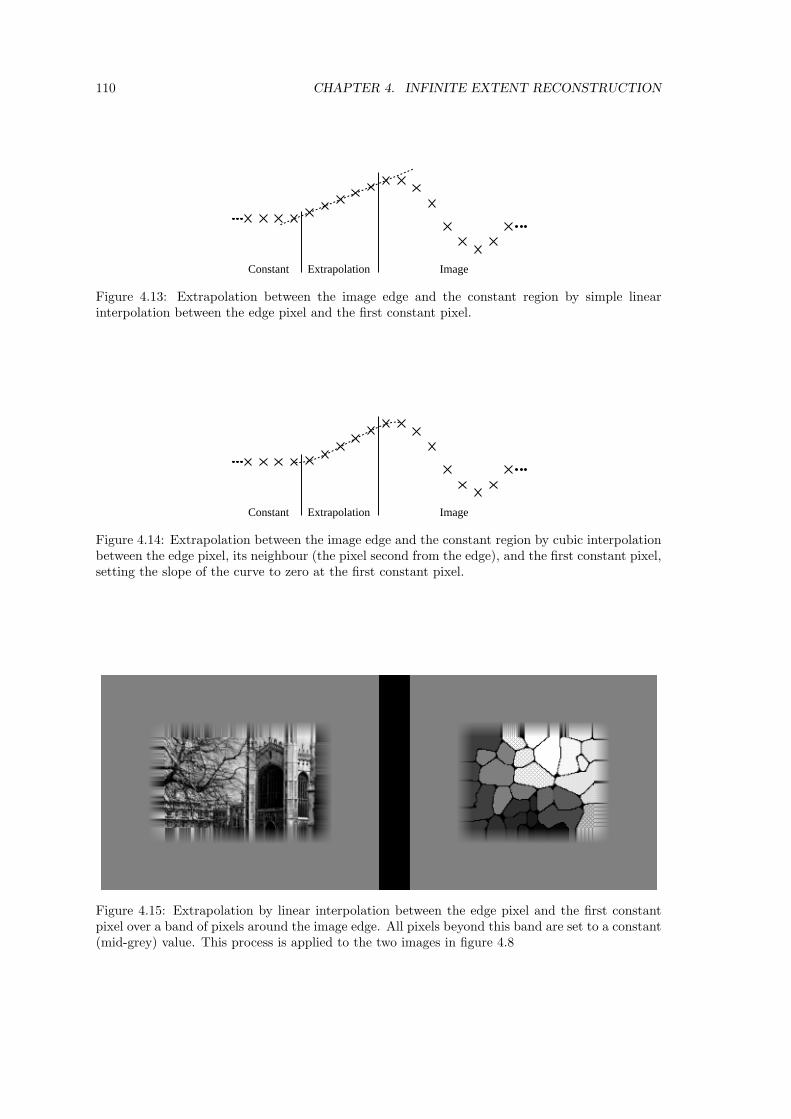
110 CHAPTER 4. INFINITE EXTENT RECONSTRUCTION
ImageExtrapolationConstant
Figure 4.13: Extrapolation between the image edge and the constant region by simple linearinterpolation between the edge pixel and the first constant pixel.
ImageExtrapolationConstant
Figure 4.14: Extrapolation between the image edge and the constant region by cubic interpolationbetween the edge pixel, its neighbour (the pixel second from the edge), and the first constant pixel,setting the slope of the curve to zero at the first constant pixel.
Figure 4.15: Extrapolation by linear interpolation between the edge pixel and the first constantpixel over a band of pixels around the image edge. All pixels beyond this band are set to a constant(mid-grey) value. This process is applied to the two images in figure 4.8

4.2. EDGE EFFECTS 111
ImageExtrapolation Extrapolation
Window
(a)
(b)
Figure 4.16: Windowed extrapolation. (a) shows the image extrapolated, (b) shows this windowedso that the pixels outside the window are constant, the image pixels are unchanged, and the pixelsin between are smoothly windowed off to the constant value.
Figure 4.17: Extrapolation by derivative method (as in figure 4.10) windowed using a piecewiselinear window. This process is applied to the two images in figure 4.8

112 CHAPTER 4. INFINITE EXTENT RECONSTRUCTION
(a)
Constant ConstantExtrapolated ExtrapolatedImage
(b)
Constant ConstantExtrapolated ExtrapolatedImage
Figure 4.18: Two simple windows: (a) piecewise linear; (b) cosine half-bells in the extrapolatedregion. Both windows have value one inside the image and zero in the constant region.
method) and figure 4.15 (linear extrapolation to a constant).
Windowing, in this context, has some non-standard features. Firstly, the window does not neces-sarily fade the function to zero, but to the constant intensity. This can be achieved by using theformula:
i′(x) = W (x) × (i(x) − c) + c
where i(x) and i′(x) are the unwindowed and windowed intensity functions respectively, W (x) isthe windowing function in the range zero to one, and c is the constant intensity to which i′(x)fades. Secondly, the window function should be unity for all pixels within the finite image. Thisrestriction is to prevent corruption of the existing, and presumably correct, intensity values.
The shape of the window is probably of little importance, given that the extrapolated values arethemselves approximations. A piecewise linear function, as in figure 4.18(a); or cosine half-bell(figure 4.18(b)) are two simple windows. The cosine half-bell is the better of these two, as it isC1-continuous.
An extension of this idea is to window the known pixel values and thus remove the need for anyextrapolation. All unknown pixels are set to the constant value. Pixels just within the imageedge are windowed, while the central portion of the image remains unaffected. Fraser [1989b] usessuch a method to fade the image to zero at the edges. However, he is quick to point out thatsuch windowing, while a good technique for other signal types (for example, sound), causes anundesirable effect, vignetting, when applied to images. Figure 4.19 gives an example of vignetting.
(5) Replication
This is a simple method, often used in texture mapping applications. The image is simply replicatedan infinite number of times to completely tile the plane. Glassner [1990b] uses this as the simplestway of generating an infinite texture from a finite ‘texture cell’. When using the fast Fouriertransform (FFT), (section 5.4.1), this is the method of edge extension implicit in the algorithm.This property of the FFT has important ramifications, as we shall see in chapter 5.
Hall [1989] used this method in his pipelined binary image processor, where he dealt with blacktext on a white background. His assumption was that the image would be all white near the edgesand so there would be no untoward edge effects (as the edges, being all white, would exactly matchup). In his later work, Hall [1991] rejected this assumption and altered his algorithm (to a constantedge extension) in order to avoid the errors it could conceivably cause.

4.2. EDGE EFFECTS 113
Figure 4.19: An example of vignetting. The image on the left is the original, on the right it isvignetted: it fades off towards its edges. This is almost always an undesirable effect.
Replicating the image in this way is a valid image extension method, and works well for certaintexture mapping applications (for example, generating wallpaper). However, in other areas it hasa major flaw. Except in fortuitous cases, the intensity values at one edge of the image bear norelation to those at the opposite edge. Yet, in replication, these unrelated pixels are placed nextto one another. This causes edge effects similar to those caused by the constant extension method,as illustrated in figure 4.20. In general, this method is not recommended except for specialistapplications such as the texture mapping operation mentioned above.
Along with simple copying, Glassner [1990b] explains that many different textures can be generatedby rotating, reflecting and/or offsetting the texture cell before copying. This is basically using thetexture cell as the unit cell for one of the wallpaper groups [Martin, 1982]. Some of these areillustrated in figure 4.21.
While this is extremely useful for generating repetitive textures (so long as the textures are carefullychosen), it is not generally useful for edge extension. The one wallpaper group that is useful isthat illustrated in figure 4.21 (W 2
2 (pmm)) where the image is reflected about its edges.
(6) Reflection
This, as well as being one of the methods of generating a wallpaper pattern, has been widelyused as an inexpensive method of image extension [White and Brzakovic, 1990, p.343]. It isinexpensive because there is no need to generate any additional values, the only overhead is thesimple one of evaluating which of the existing image values to use. It is widely used because of theexpectation that, by reflecting, the pixels just outside the edge will bear a good relation to thosejust inside, hence minimising edge effects. This method is implicit in the discrete cosine transform(DCT) variation of the FFT method described in section 5.4.1, greatly improving the edge effectperformance over the FFT’s implicit replication method.
White and Brzakovic [1990] use this method as the standard against which they compare theirnew methods. They conclude that this method leads to good results only in cases of highlytextured regions or regions of uniform intensity. However, this method is certainly better thaneither copying or using a constant and is certainly cheaper than explicitly extrapolating. One ofWhite and Brzakovic’s complaints is that this method fails dismally for highly directional images.Figure 4.22 illustrates how the various other methods cope with such a situation. Note that

114 CHAPTER 4. INFINITE EXTENT RECONSTRUCTION
Figure 4.20: An example of edge effects caused by the replication edge extension method. Thetop photograph shows an image replicated, notice how the edges of the image do not match up,causing a large intensity difference where the replicas meet. The bottom photograph shows anintensity surface reconstructed from this image by sinc reconstruction. Notice the ripples in theimage near the edges, similar to those in figure 4.7(left) for a constant edge extension method.

4.2. EDGE EFFECTS 115
W22
W1 W13Cell W4 (p4) (pmm)(p1) (pg)
Figure 4.21: Some of the possible textures that can be generated by replicating a square texturecell with no rotational or reflectional symmetry of its own. On the left is the texture cell, the fourwallpaper groups shown here are: W1, simple replication of the cell; W4, a replication that hascentres of four-fold rotation; W 2
2 , replication by reflection in both horizontal and vertical reflectionlines; and W 3
1 replication with glide reflections. All except W4 could also be used with a rectangulartexture cell. The notation used here is that used by Martin [1982]. That in brackets is the commonabbreviated form of the International Union of Crystallography.
Figure 4.22: How the edge extension methods cope with a pathological case. At top left is theoriginal which consists of diagonal lines at 22.5◦ (left half) and 45◦ (right half). Bottom left isextrapolated by copying, this fails for either case as it extrapolates horizontally or vertically. Topright is White and Brzakovic’s [1990] derivative method (figure 4.10), and bottom right is ourmodification of that method (figure 4.11). Both of these perform excellent extrapolation of the 45◦features, but fail for the 22.5◦ features, extending them horizontally, vertically, or at 45◦.
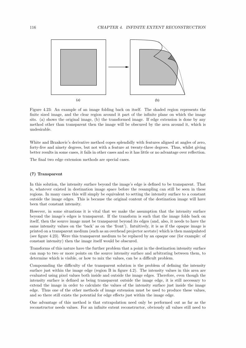
116 CHAPTER 4. INFINITE EXTENT RECONSTRUCTION
(a) (b)
Figure 4.23: An example of an image folding back on itself. The shaded region represents thefinite sized image, and the clear region around it part of the infinite plane on which the imagesits. (a) shows the original image, (b) the transformed image. If edge extension is done by anymethod other than transparent then the image will be obscured by the area around it, which isundesirable.
White and Brzakovic’s derivative method copes splendidly with features aligned at angles of zero,forty-five and ninety degrees, but not with a feature at twenty-three degrees. Thus, whilst givingbetter results in some cases, it fails in other cases and so it has little or no advantage over reflection.
The final two edge extension methods are special cases.
(7) Transparent
In this solution, the intensity surface beyond the image’s edge is defined to be transparent. Thatis, whatever existed in destination image space before the resampling can still be seen in theseregions. In many cases this will simply be equivalent to setting the intensity surface to a constantoutside the image edges. This is because the original content of the destination image will havebeen that constant intensity.
However, in some situations it is vital that we make the assumption that the intensity surfacebeyond the image’s edges is transparent. If the transform is such that the image folds back onitself, then the source image must be transparent beyond its edges (and, also, it needs to have thesame intensity values on the ‘back’ as on the ‘front’). Intuitively, it is as if the opaque image isprinted on a transparent medium (such as an overhead projector acetate) which is then manipulated(see figure 4.23). Were this transparent medium to be replaced by an opaque one (for example: ofconstant intensity) then the image itself would be obscured.
Transforms of this nature have the further problem that a point in the destination intensity surfacecan map to two or more points on the source intensity surface and arbitrating between them, todetermine which is visible, or how to mix the values, can be a difficult problem.
Compounding the difficulty of the transparent solution is the problem of defining the intensitysurface just within the image edge (region B in figure 4.2). The intensity values in this area areevaluated using pixel values both inside and outside the image edges. Therefore, even though theintensity surface is defined as being transparent outside the image edge, it is still necessary toextend the image in order to calculate the values of the intensity surface just inside the imageedge. Thus one of the other methods of image extension must be used to produce these values,and so there still exists the potential for edge effects just within the image edge.
One advantage of this method is that extrapolation need only be performed out as far as thereconstructor needs values. For an infinite extent reconstructor, obviously all values still need to

4.3. SINC AND OTHER PERFECT INTERPOLANTS 117
be available. But, for a piecewise cubic reconstructor, a band two pixels wide outside the imageedge is all that need be generated by extension.
Such situations as these lead to the final solution to the edge extension problem.
(8) Special cases
In situations where the intensity surface beyond the edge of the image is defined to be a constant,or transparent, or some other case that does not depend on the reconstructor, then a small-kernel reconstructor can use a special case extension method to produce the necessary pixel valuesbeyond the image edge. These methods are not the general extension methods discussed earlierbut methods specific to particular reconstructors which may only be valid for an extension of oneor two pixels beyond the image edge.
For local piecewise polynomials (chapter 3) the only documented extension method of this natureis Keys’ [1981] single pixel extension method for the Catmull-Rom interpolant. Keys derives theinterpolant by insisting that the cubic agree with the Taylor’s series expansion of the originalfunction to as many terms as possible. He then [ibid., p.1155] develops a formula to approximateone pixel value beyond the image edge in order to maintain this agreement. This extension canbe used for pixels farther out from the edge but it was developed specifically for the first pixel outand specifically for the Catmull-Rom reconstructor.
The cubic B-spline interpolant, discussed later in this chapter (section 4.5) is theoretically of infiniteextent. In order to use this in a practical (finite) situation, end conditions have to be specified.In this instance we do not require the values of pixels beyond the image edge, but other edgeconditions. For example, the ‘natural cubic spline’ criterion requires that the second derivative ofthe intensity surface at the edge points is zero [Press et al, 1988, p.96]. Wolberg [1990, p.136], onthe other hand, implicitly assumes that the pixels just outside the image edge have intensity zerowhen he uses the cubic B-spline interpolant.
A final category of special case extension methods includes the a priori method described insection 6.4. The analysis done by this method can be used to generate an infinite image byextending the edges found to infinity. Alternatively the pixels outside the image edge can be leftundefined and the final image have an implicit extra edge around the outside. The intensity surfacebeyond the image edge can then be undefined, constant or transparent as required.
Summary
All these methods fail in certain cases. The best option for general image extension would appearto be either reflection for quick processing, or a good extrapolation windowed to a constant. Suchan extrapolation would need to give good results out to the extent of the window8. If extremely fastprocessing is required, a constant value may be used. For resampling work, it is usually desirableto use these methods of edge extension when generating pixel values of type (a) in figure 4.1, andto use a constant value (for example: zero, mid-grey, transparent) for pixels of type (b).
4.3 Sinc and other perfect interpolants
The theory of perfect interpolation is straightforward. If the original intensity surface is band-limited and the sampling rate is high enough then the samples in the image contain all the in-formation necessary to exactly reconstruct the original intensity surface. The reconstructors thatcan perform this exact reconstruction are the ‘perfect interpolants’. When we introduced perfect
8In fact it need not be good quite all the way as any strange effects at the limits would be rendered practicallynegligible by the windowing.

118 CHAPTER 4. INFINITE EXTENT RECONSTRUCTION
νx
νy
νx
νy
νxN
νyN
νyN
−
−
νxN
(a) (b)
νx
νy
(c)
νrN
νrN
−νrN
−νrN
Figure 4.24: Examples of the ranges over which an image’s Fourier transform can be non-zero.(a) an example of the non-zero area of a bandlimited image’s Fourier transform, (b) a rectangularpassband, with Nyquist frequencies: νxN and νyN , (c) a circular passband, with Nyquist frequency:νrN .
interpolation, in section 3.3, we only looked at the sinc function, but other perfect interpolantsexist.
An infinite extent intensity surface, s(x, y), in the spatial domain can be represented equally wellin the frequency domain by its Fourier transform:
S(νx, νy) =∫ ∞
−∞
∫ ∞
−∞s(x, y)e−i2π(xνx+yνy) dy dx
This frequency domain function, if bandlimited, will have a certain range over which it is non-zero,shown in figure 4.24 (a).
Point sampling on a regular grid in the spatial domain equates to regularly replicating in thefrequency domain (section 2.4.1) as illustrated in figure 4.25.
To reconstruct a continuous spatial function from this we need an interpolation filter with a fre-quency response which is unity for the original bandlimited area (shaded in figure 4.25) and zerofor all the replicas. Obviously such a filter cannot exist if the replicas overlap the original in anyway, so the samples need to be sufficiently close that the replicas are separated.
However, the filter does not need to take any specific value between the replicas because the Fouriertransform of the sampled image is zero in these regions. So, if the replicas do not tile the plane,there are an infinite number of perfectly reconstructing filters for a given intensity surface.
If the bandlimited area can be bounded by a circle (figure 4.24 (c)) then a perfect interpolationfilter is one which is unity within the circle and zero outside it. In the spatial domain this filteris a first order Bessel function [Pratt, 1978; Heckbert, 1989]. Mersereau’s [1979] results allowus to derive the spatial domain equation for a perfect hexagonal filter, useful when processinghexagonally sampled images. However, except for a few experimental cases [Wuthrich, Stucki andGhezal, 1989; Wuthrich and Stucki, 1991], all images are sampled on a rectangular grid.
For a given sampling rate there is a single function that can perfectly reconstruct any function thatis bandlimited at or below half that rate. If we take the largest rectangular area in the frequencydomain which can be replicated without overlap (figure 4.21(b)), then the perfect interpolationfilter must be unity inside this area and zero outside it, because the replicas tile the plane. In thespatial domain this filter is a two dimensional sinc function. For bandlimits of νxN and νyN in thefrequency domain, the spatial domain function is:
h(x, y) = 4νxNνyNsinc(2xνxN)sinc(2yνyN) (4.1)
This is the function which is generally used as the perfect interpolant, because it perfectly interpo-lates all rectangularly bandlimited images. This function’s spatially separability is advantageous

4.3. SINC AND OTHER PERFECT INTERPOLANTS 119
νx
νy
Figure 4.25: The example frequency spectrum of figure 4.24(a) replicated infinitely many times.This is caused by sampling in the spatial domain. The original copy is shown shaded, the othersare left white.
when implementing it. If rotational invariance is more desirable then the first-order Bessel functionmay be used, though it is a more difficult function to evaluate.
The most common complaint levelled against the sinc function (and is equally valid against theother perfect interpolants) is that it produces unsightly ripples in the reconstructed intensity surface[Mitchell and Netravali, 1988; Ward and Cok, 1989]. Another commonly mentioned problem isthat the sinc function can produce negative values in the intensity surface [Pratt, 1978; Blinn,1989b] (section 3.5.7).
In answer to these two criticisms, it is necessary to point out that a perfect interpolant perfectlyreconstructs a sufficiently bandlimited intensity surface. If the original intensity surface is suffi-ciently bandlimited then it will contain no negative values (negative light being impossible) andany ripples in it are supposed to be there. The sinc function cannot introduce any negative lightor extra ripples because it exactly reconstructs the original surface.
These complaints about the sinc interpolator come from attempting to apply it to an image sampledfrom an intensity surface which is not bandlimited within the limits required. In such a case,aliasing will occur and the sinc interpolator will perfectly reconstruct an aliased version of theoriginal intensity surface, possibly with negative values and unsightly ripples, rather than theoriginal surface itself. Using the sinc function with an intensity surface that is not sufficientlybandlimited is fraught with difficulties.
Opinion is divided in the literature about how many real images are sampled from intensity surfaceswhich are bandlimited within tight enough limits to prevent aliasing. Any real world intensitysurface will be bandlimited before sampling by the physical device used to capture the image,because no real-world device has an infinite bandwidth [Wolberg, 1990, p.99]. Fraser [1987] believesthat people, often unwittingly, rely on the physical device to sufficiently bandlimit the signal sothat either minimal or no aliasing occurs.
Artificially generated intensity surfaces can contain infinite frequencies due to discontinuities in thesurfaces. Such surfaces are not bandlimited and will always generate images that contain aliases. If

120 CHAPTER 4. INFINITE EXTENT RECONSTRUCTION
such a surface is filtered before point sampling then it may, depending on the filter, be bandlimitedsufficiently.
From the images we have seen, it would appear that most images are not bandlimited sufficientlyto prevent the sinc interpolant from producing ripples around quick intensity changes; Wolberg[1990, p. 108] is of the same opinion.
This is not the end of the problems with the sinc interpolant. As discussed earlier, a practicalimage must be finite. When using sinc interpolation the only sensible edge extension methods arethose which fall off to zero (including the constant method which sets all values outside the edgesto zero). The following formula can be used to calculate the value of the interpolated surface atthe point (x, y):
f(x, y) =∞∑
i=−∞
∞∑j=−∞
sinc(x − i)sinc(y − j)fi,j (4.2)
where the sample points are located at integer locations in the xy-plane and fi,j is the samplelocated at (i, j). If the sample values, fi,j , in the image are zero outside certain bounds then thisinfinite (and hence impossible to do) sum reduces to a finite (do-able) one. This is why definingall samples outside certain limits to be zero is the only sensible method of edge extension. Sincreconstruction is a linear process, and so we could use the trick described in section 4.2.1 to allowany constant value, not just zero, and still require only a finite sum9.
Unfortunately, by insisting that the image be zero outside a finite boundary, the sampled intensitysurface cannot be bandlimited. While this result is not intuitive, we have found a proof of it, whichis given in theorem 2.
Theorem 2 An image that is only non-zero within finite bounds must contain aliases.
Proof: an infinite bandlimited, intensity surface is sampled by an infinite extent comb function.The resulting function (a continuous representation of an image (section 2.4.1)), is clamped to zerooutside finite limits. This is equivalent to multiplying the sampled function by a box function.Multiplication is commutative and so we could have got the same result by first multiplying by abox function and then multiplying by the comb sampling function. The function that is sampledis thus the product of the original intensity surface and a box function. It is thus of finite extentin the spatial domain. A function cannot be simultaneously of finite extent in both the spatialdomain and the frequency domain (a detailed proof of this statement is given in appendix B.5),and so this function cannot be bandlimited, and therefore the sampled version must contain aliasesQED.
The most obvious effect of this aliasing is rippling around the edges — this is the reason why wewent from the constant edge solution in section 4.2.1 to the ‘extrapolation to a constant’ edgesolutions in the following subsection. However, even this latter edge solution produces aliasingeffects, although not as badly.
Pratt [1978] shows another way of looking at this finite-extent sampling process. This is that a finiteextent sampling grid can be generated by multiplying the box and comb functions and applyingthe product to the continuous intensity surface. The product is simply a truncated (finite-extent)comb function. In the same way that sampling using an infinite extent comb is equivalent toconvolving with the comb’s Fourier transform in the frequency domain, sampling using this finiteextent comb is equivalent to convolving with this function’s Fourier transform in the frequencydomain. This Fourier transform is fairly simple to evaluate. With limits (±bx∆x,±by∆y), for a
9The ensuing discussion applies equally to those cases as the effect of the trick in the frequency domain isto modify only the DC component, then to do the same processing as for the zero case (leaving the modifiedDC component unchanged) and finally to reset the DC component to its original value (leaving the rest of thecomponents unchanged).

4.3. SINC AND OTHER PERFECT INTERPOLANTS 121
(a)
(b)
Figure 4.26: The Fourier transform of a finite extent comb function. (a) the Fourier transform ofa comb function with 8 teeth, (b) the Fourier transform of a comb function with 32 teeth.
comb of spacing (∆x,∆y), it can be shown to be:
D(νx, νy) =sin(2πνx(bx − 1
2 )∆x)sin(πνx∆x)
×sin(2πνy(by − 1
2 )∆y)sin(πνy∆y)
(4.3)
The derivation of this can be found in appendix B.6. This function is illustrated in figure 4.26. Ithas a similar but nonetheless different effect to convolving with a comb, with the results describedearlier.
4.3.1 Richards’ positive perfect interpolant
Pratt [1978, p.98] points out that a sinc-reconstructed function can be considered to be the super-position of an infinite number of weighted translated sinc functions. Because each of the functionsin the sum has negative lobes, it is impossible to optically create the image by superposition be-cause negative light does not exist. Pratt then points to Richards’ [1966] discovery of a family ofperfect interpolants that are positive in regions in which their magnitude is large, and hence canbe used for sequential optical interpolation. In resampling, we can add the intensities up inside acomputer, and so negative addends are not a problem. Nevertheless, it is instructive to look atRichards’ function.
Richards’ interpolants are interesting in that he generates them in a similar way to the Bezier andB-spline interpolants discussed later (section 4.5). He effectively defines a set of coefficients:
hn = fn − α × (fn−1 + fn+1) (4.4)
which he convolves with a kernel, g(x), such that:
h ∗ g = f ∗ sinc
g(x) can be evaluated from this equation and shown to be [Richards, 1966, equation 4]:
g(x) =1√
1 − 4α2
sinπx
πx
[1 − 2x2
∞∑n=1
(−β)n
n2 − x2
]
where β = 1−√
1−4α2
2α . Figure 4.27 shows this kernel graphed for two different values of α.
While this kernel is indeed positive over a significant range, when combined with the kernel. . . , 0, 0,−α, 1,−α, 0, 0, . . . operating on h(x) (equation 4.4) it is exactly equivalent to the sincfunction and so is simply another way of writing sinc convolution. This situation is analogous

122 CHAPTER 4. INFINITE EXTENT RECONSTRUCTION
-8 -7 -6 -5 -4 -3 -2 -1 0 1 2 3 4 5 6 7 8
Figure 4.27: Richards’ [1966] kernel, for α = 0.2875 (lower curve) and α = 0.4 (upper curve).
to that with the B-spline and Bezier interpolants discussed in section 4.5. In those cases, a localkernel operates on coefficients, gn, derived from the data values, fn. However, the overall kernelwhich operates on the fn values is not local. In a similar manner, the Richards kernel is positiveover its central region and operates on a set of coefficients, hn, derived from the data values, fn.However, the sinc kernel which operates directly on the fn data values is not positive over such awide region.
Pratt was attracted to Richards’ kernel because it is positive in regions where its magnitude is large.This, he claimed, allows it to be employed for sequential optical interpolation. Unfortunately thisclaim is only true if all of the hn coefficients are non-negative. It is true that all of the data values,fn, must be non-negative, because negative light does not exist. So applying a Richards kernel tothese values would have the effect desired by Pratt. However, the Richards kernel is applied tothe hn coefficients. Thus, sequentially generating an image using a Richards kernel can only beachieved if all the hn are non-negative. A coefficient, hi, is non-negative if, and only if:
fi ≥ α × (fi−1 + fi+1) (4.5)
For the Richards kernel to be positive in the region |x| < 5 (this is the significant range used byRichards [1966, fig. 1]) then we must have α ≥ 0.34222888± 5× 10⁻⁹ (rather than Richards’ valueof α > 0.2875). This curve is shown in figure 4.28. With α in this range, many images willcontain at least one location where equation 4.5 will not be satisfied. This unfortunately meansthat the Richard’s kernel can not be used for sequential optical interpolation of these images. Foran image that is bandlimited well below the folding frequency, equation 4.5 should be satisfied atall locations and, in these cases, it can be used for sequential optical interpolation.

4.4. GAUSSIAN RECONSTRUCTORS 123
-8 -7 -6 -5 -4 -3 -2 -1 0 1 2 3 4 5 6 7 8
Figure 4.28: Richards’ [1966] kernel, for α = 0.342229. For α greater than this value the kernel ispositive in the range |x| < 5.
4.4 Gaussian reconstructors
The Gaussian filter is of the form:
h(s) = 1σ√
2πe−s2/2σ2
(4.6)
for a standard deviation of σ with unit area under the curve.
The Gaussian has many interesting features:
• it will never produce negative values, unlike the sinc function.
• it falls to zero much faster than the sinc function and so can be truncated with little loss ofquality, unlike the sinc function [Heckbert, 1989, p.41]. See section 4.6 for more details.
• it is both circularly symmetric and separable (the only function that is), properties thatare useful in implementing the filter, for example: in Greene and Heckbert’s [1986] ellipticalweighted average filter [see also Heckbert, 1989, sec 3.5.8 and 3.5.9].
• it is an approximant, as opposed to sinc which is an interpolant.
Whilst its properties make it useful, it produces a blurrier intensity surface than, say, the Catmull-Rom spline.
When using a Gaussian we must decide what value of σ to use. For reconstruction of unit spacedsamples, Heckbert [1989, p.41] recommends a standard deviation of about σ = 1
2 . Ratzel [1980],and subsequently Schreiber and Troxel [1985], use σ = 0.52 (see footnote 10 for details of where thisvalue comes from, as it is not the value which they report). Turkowski [1990] uses two Gaussianfunctions, expressed in the form:
h(x) = 2−x2/τ2
where τ = 1√2
or τ = 12 . Some consider this form to be more convenient than equation 4.6 [Wolberg,
1990]. This form is not normalised, but when it is (by multiplying by the correct constant) thesetwo values of τ correspond to σ ≈ 0.600561 and σ ≈ 0.424661 respectively.

124 CHAPTER 4. INFINITE EXTENT RECONSTRUCTION
-8 -7 -6 -5 -4 -3 -2 -1 0 1 2 3 4 5 6 7 8
Figure 4.29: The sharpened Gaussian kernel.
4.4.1 The sharpened Gaussian
This was developed by Ratzel [1980] to improve on the sharpness of a Gaussian reconstructedintensity surface. The Gaussian’s kernel is10:
hg(s) =1
0.52√
2πe−s2/2(0.52)2 (4.9)
The sharpened Gaussian kernel is the weighted sum of three of these functions, two of them offsetfrom the origin:
hsg(s) =15
(7hg(s) − hg(s − 1) − hg(s + 1)) (4.10)
This is graphed in figure 4.29. The single side-lobe each side of the central lobe perceptuallysharpens the picture, as discussed in section 4.5.2.
The sharpened Gaussian can be considered to be the convolution of two simpler functions:
hsg(s) = hg(s) ∗ m
where m is a discrete function: m0 = 75 ; m1 = − 1
5 ; mn = 0, n ≥ 2; and m−n = mn.
Thus, a sharpened Gaussian intensity surface can be generated by precomputing a set of coefficients,g = m ∗ f , and then applying the simple Gaussian (equation 4.9) to these coefficients:
f(x) = hg(s) ∗ g
This is computationally more efficient than the straightforward f(x) = hsg(s) ∗ f , especially forthe two-dimensional version of the reconstructor [Schreiber and Troxel, 1985].
10Ratzel claims to have used this Gaussian [Ratzel, 1980, p.68]:
hg(s) =1
2.6√
2πe−n2/2(2.6)2 (4.7)
where n is an integer and s = n5. This is equation 4.6 with σ = 2.6. However, converting this to normal co-ordinates
gives:
hg(s) =1
2.6√
2πe−s2/2(0.52)2 (4.8)
which is not normalised; to normalise it requires us to use equation 4.6 with σ = 0.52, which is equation 4.9. If oneexamines Ratzel’s hand-tuned approximation this is, in fact, the function that he used, rather than the virtuallyidentical one (equation 4.7) he claims to have used. The only difference is the normalising coefficient. This is aminor correction, but it makes a difference to the results in table 4.5 (section 4.6).
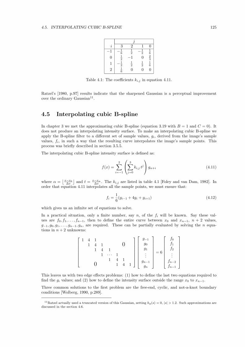
4.5. INTERPOLATING CUBIC B-SPLINE 125
ji 3 2 1 0
−1 − 16
12 − 1
216
0 12 −1 0 2
3
1 − 12
12
12
16
2 16 0 0 0
Table 4.1: The coefficients ki,j in equation 4.11.
Ratzel’s [1980, p.97] results indicate that the sharpened Gaussian is a perceptual improvementover the ordinary Gaussian11.
4.5 Interpolating cubic B-spline
In chapter 3 we met the approximating cubic B-spline (equation 3.19 with B = 1 and C = 0). Itdoes not produce an interpolating intensity surface. To make an interpolating cubic B-spline weapply the B-spline filter to a different set of sample values, gi, derived from the image’s samplevalues, fi, in such a way that the resulting curve interpolates the image’s sample points. Thisprocess was briefly described in section 3.5.5.
The interpolating cubic B-spline intensity surface is defined as:
f(x) =2∑
i=−1
3∑
j=0
ki,j tj
gα+i (4.11)
where α =⌊
x−x0∆x
⌋and t = x−xα
∆x . The ki,j are listed in table 4.1 [Foley and van Dam, 1982]. Inorder that equation 4.11 interpolates all the sample points, we must ensure that:
fi =16(gi−1 + 4gi + gi+1) (4.12)
which gives us an infinite set of equations to solve.
In a practical situation, only a finite number, say n, of the fi will be known. Say these val-ues are f0, f1, . . . , fn−1, then to define the entire curve between x0 and xn−1, n + 2 values,g−1, g0, g1, . . . , gn−1, gn, are required. These can be partially evaluated by solving the n equa-tions in n + 2 unknowns:
1 4 11 4 1 0
1 4 11 · · · 1
1 4 10 1 4 1
g−1
g0
g1
...gn−1
gn
= 6
f0
f1
f2
...fn−2
fn−1
This leaves us with two edge effects problems: (1) how to define the last two equations required tofind the gi values; and (2) how to define the intensity surface outside the range x0 to xn−1.
Three common solutions to the first problem are the free-end, cyclic, and not-a-knot boundaryconditions [Wolberg, 1990, p.289].
11Ratzel actually used a truncated version of this Gaussian, setting hg(s) = 0, |s| > 1.2. Such approximations arediscussed in the section 4.6.
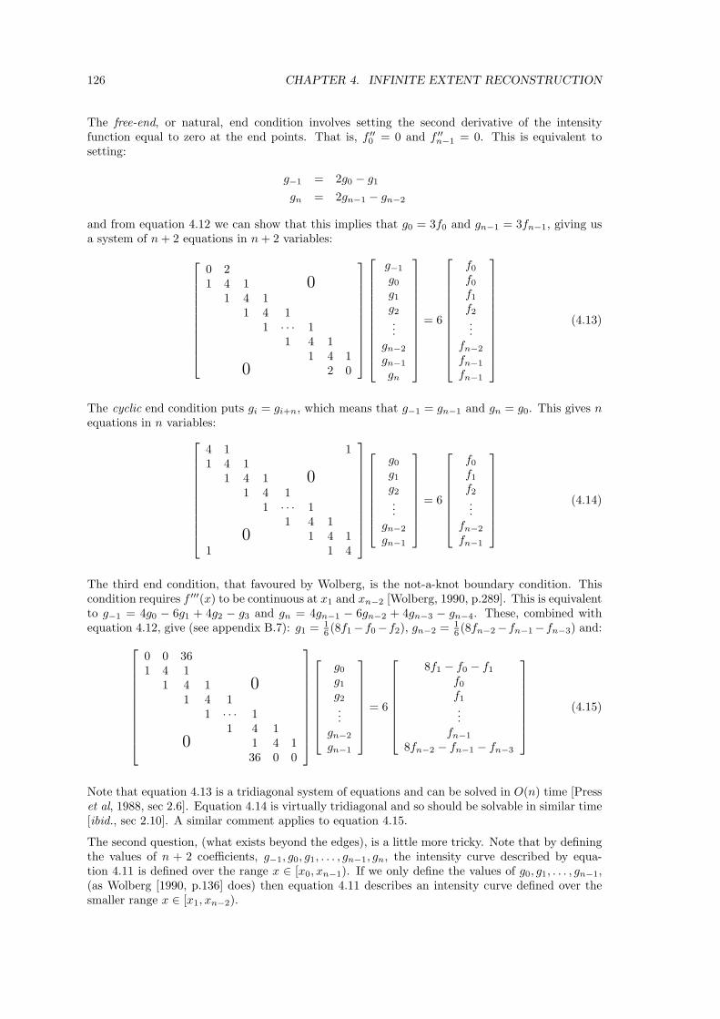
126 CHAPTER 4. INFINITE EXTENT RECONSTRUCTION
The free-end, or natural, end condition involves setting the second derivative of the intensityfunction equal to zero at the end points. That is, f ′′
0 = 0 and f ′′n−1 = 0. This is equivalent to
setting:
g−1 = 2g0 − g1
gn = 2gn−1 − gn−2
and from equation 4.12 we can show that this implies that g0 = 3f0 and gn−1 = 3fn−1, giving usa system of n + 2 equations in n + 2 variables:
0 21 4 1 0
1 4 11 4 1
1 · · · 11 4 1
1 4 10 2 0
g−1
g0
g1
g2
...gn−2
gn−1
gn
= 6
f0
f0
f1
f2
...fn−2
fn−1
fn−1
(4.13)
The cyclic end condition puts gi = gi+n, which means that g−1 = gn−1 and gn = g0. This gives nequations in n variables:
4 1 11 4 1
1 4 1 01 4 1
1 · · · 11 4 1
0 1 4 11 1 4
g0
g1
g2
...gn−2
gn−1
= 6
f0
f1
f2
...fn−2
fn−1
(4.14)
The third end condition, that favoured by Wolberg, is the not-a-knot boundary condition. Thiscondition requires f ′′′(x) to be continuous at x1 and xn−2 [Wolberg, 1990, p.289]. This is equivalentto g−1 = 4g0 − 6g1 + 4g2 − g3 and gn = 4gn−1 − 6gn−2 + 4gn−3 − gn−4. These, combined withequation 4.12, give (see appendix B.7): g1 = 1
6 (8f1−f0−f2), gn−2 = 16 (8fn−2−fn−1−fn−3) and:
0 0 361 4 1
1 4 1 01 4 1
1 · · · 11 4 1
0 1 4 136 0 0
g0
g1
g2
...gn−2
gn−1
= 6
8f1 − f0 − f1
f0
f1
...fn−1
8fn−2 − fn−1 − fn−3
(4.15)
Note that equation 4.13 is a tridiagonal system of equations and can be solved in O(n) time [Presset al, 1988, sec 2.6]. Equation 4.14 is virtually tridiagonal and so should be solvable in similar time[ibid., sec 2.10]. A similar comment applies to equation 4.15.
The second question, (what exists beyond the edges), is a little more tricky. Note that by definingthe values of n + 2 coefficients, g−1, g0, g1, . . . , gn−1, gn, the intensity curve described by equa-tion 4.11 is defined over the range x ∈ [x0, xn−1). If we only define the values of g0, g1, . . . , gn−1,(as Wolberg [1990, p.136] does) then equation 4.11 describes an intensity curve defined over thesmaller range x ∈ [x1, xn−2).

4.5. INTERPOLATING CUBIC B-SPLINE 127
Outside these ranges, the intensity curve is undefined, because the necessary gi coefficients areundefined. One solution is to set the intensity curve to a constant value outside this range, thusmaking it unnecessary to specify any of these unknown coefficient values.
The cyclic boundary condition automatically defines all the coefficients by the formula gi = gi+n.This gives a result identical to the ‘replication’ solution in section 4.2.1.
For the other boundary conditions we could specify the unknown fi values, the unknown gi values,or the value of the intensity curve outside the defined area, as described above. Specifying theunknown fi values would allow us to find the gi values by the impossible task of solving an infinitesystem of equations. It would be possible to specify the unknown fi values only in the region whichwill actually be seen in the output, making it possible to calculate all the necessary gi values.
Specifying the unknown gi values directly is perhaps a more tempting solution, and certainlyrequires far less computation. This extrapolation can be achieved by any of the edge solutions insection 4.2.1, although we are no longer working with the image samples but with equation 4.11’scoefficients. Wolberg [1990, p.136] seems to assume that gi = 0, i �∈ {0, 1, 2, . . . , n − 1}.The interpolating cubic B-spline has been praised as being of higher quality than the Catmull-Romcubic spline [Keys, 1981]. It has also been recommended as being a strictly positive interpolant,which it certainly is not. This confusion arises from the fact that the cubic B-spline function,which is applied to the gi coefficients, is a strictly positive function. However, the function thatis applied to the fi values is not strictly positive [Maeland, 1988]. The kernel of the interpolatingcubic B-spline actually oscillates in a manner similar to the sinc interpolant’s kernel.
The interpolating cubic B-spline’s kernel
The kernel of the interpolating cubic B-spline can be analytically derived if we ignore boundaryconditions . Equation 4.11 can now be written as a discrete convolution:
f = h ∗ g (4.16)
where f = . . . , f−2, f−1, f0, f1, f2, . . ., likewise for h and g. Further, h is defined as: h−1 = 16 ;
h0 = 46 ; h1 = 1
6 ; hn = 0, n �∈ {−1, 0, 1}.In the frequency domain equation 4.16 is equivalent to:
F = H × G (4.17)
where, for unit spaced samples, H can be shown to be:
H(ν) =46
+26
cos 2πν
To find g in terms of f , we invert equation 4.17:
G =1H
× F
= L × F
where L is:L(ν) =
1H(ν)
=3
2 + cos 2πν
and by judicious use of Dwight [417.2] we get:
L(ν) =32× 1 + a2
1 − a2
1 +
∞∑j=1
2aj cos 2jπν
(4.18)

128 CHAPTER 4. INFINITE EXTENT RECONSTRUCTION
where a = −2 +√
3. A little algebra shows that 32 × 1+a2
1−a2 =√
3.
Transferring this back to the discrete spatial domain we get:
g = l ∗ f
where l is the inverse Fourier transform of L:
ln =√
3an
l−n = ln
}n ≥ 0 (4.19)
Thus each gi is dependent on all of the fi values.
Numerical verification of the values of li can be achieved by running a modified version of Sedgewick’s[1988, p.549] algorithm for finding interpolating B-spline coefficients. On a dataset of 32 samples,this gave values (for the middle region of the data, where edge effects are minimised) for the li tothree significant figures of:
l0 = 1.732 ±0.001l−1 = l1 = −0.464 ±0.001l−2 = l2 = 0.124 ±0.001l−3 = l3 = −0.033 ±0.001l−4 = l4 = 0.009 ±0.001l−5 = l5 = −0.002 ±0.001
n ≥ 5 : l−n = ln = 0.000 ±0.001
In agreement with the theoretically derived formula.
The creation of an intensity curve can be written as:
i = b ∗ g
where b is the approximating cubic B-spline kernel. This is equivalent to:
i = b ∗ (l ∗ f)= (b ∗ l) ∗ f
The approximating B-spline kernel, b, is graphed in figure 4.30, and the interpolating B-splinekernel, b ∗ l, is graphed in figure 4.31. Note that b ∗ l has negative lobes.
This derivation roughly parallels that given by Maeland [1988]. Maeland’s formula for the cubicB-spline kernel [p.214, equation 8] is, however, wrong. It is:
BMaeland(s) =
34 |s|3 −
32 |s|2 + 1, 0 ≤ |s| < 1
− 14 |s|3 + 1
2 , 1 ≤ |s| < 20, otherwise
Compare this with the correct version (equation 4.21) provided by Parker et al [1983, p.35] andWolberg [1990, p.135, equation 5.4.18]. Maeland’s conclusions are still valid, but the details areslightly incorrect.
The interpolating cubic B-spline is often cited as being better than the Catmull-Rom spline (orother cubics which fit Mitchell and Netravali’s [1988] formula (equation 3.19)) [Keys, 1981; Mae-land, 1988]. This is due to the fact that this interpolant considers a wider range of data thanthese other cubics. Further it is sinc-like in form; with the advantages that negative lobes bring(section 3.5.7). However, it has an advantage over the sinc function in that, while the sinc kernelonly has a 1
x decay, the interpolating B-spline exhibits an exponential decay (see section 4.6).

4.5. INTERPOLATING CUBIC B-SPLINE 129
-8 -7 -6 -5 -4 -3 -2 -1 0 1 2 3 4 5 6 7 8
2/3
Figure 4.30: The approximating cubic B-spline kernel, b.
-8 -7 -6 -5 -4 -3 -2 -1 0 1 2 3 4 5 6 7 8
1.0
Figure 4.31: The interpolating cubic B-spline kernel, b ∗ l.

130 CHAPTER 4. INFINITE EXTENT RECONSTRUCTION
Qi
Ri
Pi P
Qi
Pi P
Ri
i+1
i+1
Figure 4.32: A Bezier cubic curve is defined by four points: its two endpoints, Pi and Pi+1, andtwo control points, Qi and Ri.
The interpolating B-spline kernel can be used directly on the image data values, fi. In this caseboundary effects would be handled by one of the methods in section 4.2.1. The interpolatingB-spline kernel is analytically defined as:
h(s) =∞∑
j=−∞B4(j − s)
√3a|j|, a = −2 +
√3 (4.20)
where B4(s) is the approximating B-spline kernel:
B4(s) =
12 |s|3 − |s|2 + 2
3 , 0 ≤ |s| < 1− 1
6 |s|3 + |s|2 − 2|s| + 43 , 1 ≤ |s| < 2
0, otherwise(4.21)
This equation looks as if it is uncomputable because of the infinite sum. However, for any givenvalue of s, only four of the terms in the sum will be non-zero: those for which j ∈ {�s�−1, �s� , �s�+1, �s� + 2}.
4.5.1 Bezier cubic interpolation
Bezier cubic interpolation is related to cubic B-spline interpolation in that a particular cubicfunction is applied to a set of coefficients derived from the data points. We briefly discussed theBezier cubic in section 3.6.3. The Bezier cubic form is described by Foley and van Dam [1982,sec. 13.5.2] and the Bezier cubic interpolation formula is presented by Rasala [1990]. The cubicform is:
P (x) = [t3 t2 t 1]
−1 3 −3 13 −6 3 0
−3 3 0 01 0 0 0
Pα
Qα
Rα
Pα+1
(4.22)
Where α =⌊
x−x0∆x
⌋, t = x−xα
∆x , and P (x) = (xα, fα) is a point in space rather than simply afunction value. This equation produces a cubic curve which passes through its end points (Pα
and Pα+1) and whose shape is controlled by the endpoints and by the control points as shown infigure 4.32.
Given a set of points, {Pi : i ∈ Z}, we can generate a set of control points, {(Qi, Ri) : i ∈ Z},such that the piecewise Bezier cubic defined by the points is C2-continuous. Rasala [1990] givesthe conditions required to generate the control points as:
Pi − Ri−1 = Qi − Pi (4.23)Pi − 2Ri−1 + Qi−1 = Ri − 2Qi + Pi (4.24)

4.5. INTERPOLATING CUBIC B-SPLINE 131
Given equation 4.23, a difference vector can be defined:
Di = Pi − Ri−1 (4.25)= Qi − Pi (4.26)
Equations 4.24, 4.25, and 4.26 can be combined to produce a recurrence relation between the Di
and the Pi:Di+1 + 4Di + Di−1 = Pi+1 − Pi−1
Rasala produces the following result for a closed loop of n points (that is: Pi = Pi−n):
Di =m∑
k=1
ak(Pi+k − Pi−k) (4.27)
where:ak = − fm−k
fm
fj = −4fj−1 − fj−2, j ≥ 2
for n even m = n−22 , f0 = 1, f1 = −3
for n odd m = n−12 , f0 = 1, f1 = −4
For the infinite case (that is: a non-repeating infinite set of points) it can be shown that:
an = −(a)n
where a = −2 +√
3 (see appendix B.3 for details).
This is the same constant as that used in the B-spline case (equation 4.20) and, indeed, the samesequence of coefficients (an). This is unsurprising as both situations involve the 1–4–1 kernel.Note, however, that these values are used in different ways.
If we let Di =[
εi
δi
]then Qi = (xi + εi, fi + δi), Ri = (xi+1 − εi+1, fi+1 − δi+1).
Taking equation 4.27 for the infinite case, and splitting it into two parts we get:
εi =∞∑
k=1
ak(xi+k − xi−k) (4.28)
δi =∞∑
k=1
ak(fi+k − fi−k) (4.29)
With the sample points equispaced (xi+1 = xi + ∆x) equation 4.28 becomes:
εi = −∞∑
k=1
(a)k × 2k ∆x
= −2∆x
∞∑k=1
k(a)k
= −2∆x a1
(1 − a)2[Dwight 9.06]
=13
∆x
Thus the four control points are equispaced over the unit distance, at xi, xi + 13∆x, xi + 2
3∆x, andxi+1. Further, δi (equation 4.29) can be expressed as:
δi = −k=∞∑k=1
(a)k (fi+k − fi−k)

132 CHAPTER 4. INFINITE EXTENT RECONSTRUCTION
-8 -7 -6 -5 -4 -3 -2 -1 0 1 2 3 4 5 6 7 8
1.0
Figure 4.33: The Bezier interpolating cubic’s filter kernel.
Substituting this into equation 4.22 we get:
f(x) = (−t3 + 3t2 − 3t + 1)fα
+ (3t3 − 6t2 + 3t)(fα −
∑∞k=1 ak(fα+k − fα−k)
)+ (−3t3 + 3t2)
(fα+1 −
∑∞k=1 ak(fα+1+k − fα+1−k)
)+ (t3)fα+1
(4.30)
From this we can evaluate this interpolant’s kernel:
h(s) =
ai+1(3x3 + (−9i − 3)x2
+ (9i2 + 6i)x + (−3i3 − 3i2))+ ai(3x3 + (−9i − 6)x2
+ (9i2 + 12i + 3)x + (−3i3 − 6i2 − 3i)), i ≥ 1, i = �x�i ≤ x < i + 1
a(3x3 − 3x2)+ 2x3 − 3x2 + 1, 0 ≤ x < 1
a(−3x3 − 3x2)− 2x3 − 3x2 + 1, −1 ≤ x < 0
ai−1(−3x3 + (−9i + 3)x2
+ (−9i2 + 6i)x + (−3i3 + 3i2))+ ai(−3x3 + (−9i + 6)x2
+ (−9i2 + 12i − 3)x + (−3i3 + 6i2 − 3i)), i ≥ 2, i = −�x�−i ≤ x < −i + 1
(4.31)
This kernel is shown in figure 4.33. Comparing figures 4.33 and 4.31 it may be suspected thatthis Bezier kernel may be identical to the interpolating cubic B-spline kernel (equation 4.20) inthe same way that several paths led to the Catmull-Rom. This suspicion is in fact true: a goodlyamount of algebra will show that equations 4.31 and 4.20 are identical.
An image to which Bezier/B-spline reconstruction is to be applied can be edge extended in any ofthe usual ways (section 4.2.1). Rasala’s [1990] paper, rather than discussing the general methodpresented here, gives the exact Bezier reconstruction for two special cases: the case of a ‘closedloop’, that is the replication edge extension method, where the image edges, in effect, wrap round

4.5. INTERPOLATING CUBIC B-SPLINE 133
Brown [1969]p.252, fig. 8
Figure 4.34: Brown’s [1969] figure 8. Images were reconstructed using a filter with first and secondside lobes. The second side lobe height was set at 2% of the central lobe’s height. This graphshows the subjective score for two images, one live and one still, against the height of the firstside lobe as a percentage of the height of the central lobe. The best subjective quality occurs at aheight of around 12%.
to meet one another; and the case of an ‘open curve’. In this latter case, one specifies the tangentvalues of the curve at the end points and reflects the curve about its endpoints. This is a specialcase edge extension, similar, but not equal to, the reflection edge extension method.
The B-spline/Bezier kernel has the properties of oscillating about zero and of decaying exponen-tially to zero. It thus has negative lobes. The first negative lobe is by far the biggest, and hencecontributes most to any sub-black or supra-white value, the second and subsequent negative lobescontribute a negligible amount to the final intensity surface values.
The Catmull-Rom spline has these properties also. It has been suggested that the interpolatingcubic B-spline is a good interpolant because it is continuous in its second derivative, while theCatmull-Rom spline, which is not as good [Keys, 1981] has only first derivative continuity. However,the discussion in section 3.5.2 indicates that the presence or absence of C2-continuity has littleeffect on the visual fidelity of the interpolation. It appears that it is the sharpening effect causedby the negative lobes is the important factor here.
4.5.2 The sharpening effect of negative lobes
A reconstruction filter which has a negative side lobe, such as the Catmull-Rom or B-spline/Bezier,produces a visually sharper intensity surface than reconstructors without such lobes. Schreiber andTroxel [1985] noted this effect in their sharpened Gaussian filter. They point out that the overshootcaused by the negative lobes appears to be a defect but actually is the feature responsible for thebetter tradeoff between sharpness and sampling structure.
However, ringing, when there is more than one lobe either side of the central lobe, is perceived tobe a bad effect. Brown [1969] carried out a test to discover the subjective effects of these side lobes.Brown’s results show that the presence of the first side lobe increases subjective picture quality,provided the second lobe is non-existent or at least small. The subjective quality was measuredon a scale of 0–4 by seven observers and the average value plotted in figure 4.34. A value of 1indicates no improvement; less than 1 is degradation. A value of 3 indicates that the image issubjectively as good as an image of twice the test bandwidth. The best improvements occur for alobe of height 10–14% of the height of the intensity change (in our filters this means a first sidelobe of height 10–14% of the central lobe height). Brown’s results for the second lobe show that it

134 CHAPTER 4. INFINITE EXTENT RECONSTRUCTION
Reconstructor Sinc Catmull-Rom B-Spline/Bezier Sharpened GaussianFirst side lobe 22% 7.4% 14% 8.4%Second side lobe 13% 0% 3.7% 0%
Table 4.2: The heights of the side lobes of four reconstructor’s filters, given as a percentage of theheight of the central lobe.
causes subjective degradation of the image but that, for a height of 4% or less this degradation isnot significant compared to the enhancing attributes of the first lobe.
Table 4.2 contains the size of the first two side lobes of each of the reconstructors with a negativefirst side lobe. The figures are given as percentages of the height of the central lobe. This tableindicates that sinc will produce a visually degraded intensity surface. This result is well knownfrom simply viewing sinc reconstructed and enlarged images [Mitchell and Netravali, 1988; Wardand Cok, 1989]; see figures 2.8, 2.12, and 4.20 for examples of this degradation.
The B-spline/Bezier interpolant should produce a result which is about right, whilst both theCatmull-Rom and sharpened Gaussian, appear to have a first side lobe that is slightly small forbest effect.
Brown states [p.252] that, for moving pictures, with a signal to noise ratio of 40dB, the best heightfor the first side lobes is reduced. He found that moving the ideal value from 12% (noiseless) to6% (noisy) gave the best results. Thus the Bezier/B-spline reconstructor would be expected to dobadly with noisy images while the other two would be better.
This effect does not account for all subjective quality, as it only improves the sharpness of theimage. However it does give an important pointer to why some reconstructors appear better thanothers. Other factors, though also come into play.
The sinc and Bezier/B-spline kernels are both oscillatory. The reason the sinc kernel causes ringingartifacts while the B-spline tends not to is that sinc has a much slower fall off to zero than theB-spline. Thus sinc has much more prominent side lobes than the B-spline. This is picked up insection 4.6.
The Mach band effect
One possible explanation of this sharpening is that it is due to the Mach band effect. Thisphysiological effect was first described by Mach [1865] and is described in detail by Ratliff [1965](Ratliff’s book also includes translations of Mach’s papers on this and related effects). The basiceffect, as it concerns our work, is that the bright side of an edge appears brighter than its surroundsand the dark side appears darker. The stimulus presented to the eye by a sharp edge, and thesensation passed by the eye to the brain, are illustrated in figure 4.35.
The sharper the edge, the more pronounced the effect [Ratliff, 1965, p.89]. The importance ofthis effect is that, if the eye is presented with a different intensity distribution which produces asensation similar to the sensation curve in figure 4.35 then the visual system will interpret it as thestimulus curve in the same figure. Thus, to give the appearance of a sharp edge, it is not necessaryto present the eye with an actual sharp edge. It is sufficient to present a sloping edge with a lobeat either end, producing a very similar sensation curve to that given by a sharp edge. Cornsweet[1970] presents an interesting illustration of two different stimuli producing the same sensation.This is shown in appendix D.
The response function of the human visual system is known to be shaped something like thatshown in figure 4.36 [Ratliff, 1965]. This shape, with a single prominent negative side lobe isvery like that of the Catmull-Rom, sharpened Gaussian, and B-spline/Bezier kernels. Thus thesekernels will produce an intensity curve, around an edge in the image, similar to the eye’s responseto a sharp edge. This may fool the eye into seeing a sharp edge at that point. This phenomenon

4.5. INTERPOLATING CUBIC B-SPLINE 135
Stimulus
Sensation
Intensity
Position
Figure 4.35: The Mach band effect, showing the stimulus presented to the eye and the sensationpassed by the eye to the brain. The sensation curve has bumps either side of the edge which makethe intensity appear slightly darker on the dark side and slightly lighter on the light side.
Figure 4.36: The response function of the human visual system, similar in shape to the kernels ofthe Catmull-Rom, sharpened Gaussian, and B-spline/Bezier reconstructors.
could account in part for the success of these kernels as reconstructors, that is: they are perceivedto be good because they take advantage of a physiological effect of the eye.
The problem of negative intensities
A final note here is that there is some debate as to whether negative lobes are desirable (sec-tion 3.5.7). The main argument against negative lobes is that they can produce negative pixelvalues. Blinn [1989b] states “there is no such thing as negative light and clamping these negativevalues to zero is about all you can do, but it is not ideal”. Clamping will, in fact, destroy the lobeswe are using to sharpen the edge.
An alternative to clamping is to rescale the values so that the lowest and highest intensities arephysically realisable [Wolberg, 1990, p.131]. This maintains the intensity changes required toproduce the desired effect. However, the unfortunate consequence is that the image’s contrast isreduced, which is undesirable.
If we consider Blinn’s [1989b, p.87] statement that clamping negative values to zero is about all youcan do, it appears that something could be achieved when we examine the visual phenomena shownin appendix D. There, Cornsweet’s [1970] figures indicate that a third solution, that of locallyrescaling intensity values, could produce desirable results. Cornsweet shows that two different

136 CHAPTER 4. INFINITE EXTENT RECONSTRUCTION
(a) (b)
(c) (d)
Figure 4.37: A possible solution to the problem of generating negative intensity values. (a) showsthe curve we would like to simulate: a sharp edge. (b) shows the stimulus we would like to presentto the eye to fool the brain into seeing the sharp edge. (c) shows this stimulus clamped to zero,thus destroying the illusion of a sharp edge. (d) shows a possible solution: locally modifying theintensities so that the stimulus is still there at the dark side of the edge, and gently blending thisinto the dark area to the left.
intensity distributions produce identical visual response for two different cases.
This, and other, evidence indicate that local intensity changes are far more important than slow(non-local) changes and absolute intensity values. Thus, if we could ‘raise’ a region of negativelight into positive values and gently blend this raised region in with the surrounding areas then theresulting visual response should be closer to the desired response than simply clamping negativevalues to zero, and it would not have the undesirable characteristics of globally reducing imagecontrast. The basic idea is shown in figure 4.37.
Some way of implementing a function of this nature needs to be found. This is not a simple processas the correction applied at any one point can depend on a large neighbourhood around that point,on the distance to the ‘centre’ of the nearest negative trough, and on the depth of that trough.It is difficult to decide if such a ‘correction’ can be performed. If it can, then a decision must bemade as to whether it is worth the effort. Further work on this solution is required.
4.5.3 The two-dimensional interpolating cubic B-spline
The B-spline interpolant has been presented in a one-dimensional form. When using filters, such asthe sinc or Gaussian, it is simple to extrapolate from the one- to the two-dimensional filter kernelby convolving two one-dimensional filter kernels, perpendicular to one another. This is illustratedin figures 4.38, 4.39, and 4.40.
This two dimensional kernel can be directly convolved with the sample points. The B-spline kernelcould also be treated like this. However, the usual way of producing a B-spline curve is to evaluatethe coefficients, gi and then use a simple, local B-spline kernel on these. The standard way ofextending this to two dimensions is to evaluate the coefficients for each scan-line in one direction,then, for each point for which a value is required, the coefficients must be evaluated for the line,passing through the point, perpendicular to those scan lines; and hence the value at that pointcalculated (see figure 4.41). This is a very time consuming process.
In practice, this limits the B-spline interpolant’s usefulness to scan-line algorithms rather than 2-Dalgorithms. However, if we treat the B-spline as a filter (equation 4.20), rather than as a calculation

4.5. INTERPOLATING CUBIC B-SPLINE 137
Figure 4.38: The sinc kernel aligned along the x-axis.
Figure 4.39: The sinc kernel aligned along the y-axis.

138 CHAPTER 4. INFINITE EXTENT RECONSTRUCTION
Figure 4.40: The two-dimensional sinc kernel, generated by convolving the two one-dimensionalkernels shown in figures 4.38 and 4.39.
Figure 4.41: The traditional extension of the one-dimensional interpolating cubic B-spline to two-dimensional interpolation. Coefficients are calculated for each scan-line in the horizontal direction,then to find the value at any one point we need to calculate a complete set of coefficients in thevertical direction — a time-consuming process, because in general, the required points can beanywhere in the plane, and so these vertical coefficients will not be used for more than one point.

4.5. INTERPOLATING CUBIC B-SPLINE 139
of coefficients, followed by a simpler filter, the two dimensional version is easy to construct fromtwo one-dimensional versions, as in figures 4.38 through 4.40:
h(x, y) = h(x) × h(y)
where h(x, y) is the two-dimensional kernel and h(s) is the one-dimensional kernel.
The question now arises, is it possible to generate a two-dimensional set of coefficients and applya simple local kernel (for example: the two-dimensional approximating cubic B-spline) to them toproduce the same result as applying the complicated non-local kernel to the image sample values?
If we assume an image of infinite extent, then equation 4.20 is the one-dimensional filter kernel forthe interpolating B-spline:
h(s) = b(s) ∗ l(s)
where b(s) is the cubic B-spline kernel and l(s) is the discrete kernel which is convolved with thedata-values, fi, to produce the coefficients, gi.
The two one-dimensional versions of h(s) are:
hx(x, y) ={
h(x), y = 00, otherwise
hy(x, y) ={
h(y), x = 00, otherwise
These can be convolved to produce the two-dimensional interpolating cubic B-spline kernel:
h(x, y) = hx(x, y) ∗ hy(x, y)
Expanding this out and rearranging terms we get:
h(x, y) = bx(x, y) ∗ lx(x, y) ∗ by(x, y) ∗ ly(x, y)= bx(x, y) ∗ by(x, y) ∗ lx(x, y) ∗ ly(x, y)= b(x, y) ∗ l(x, y)
where b(x, y) is the two-dimensional approximating cubic B-spline kernel and l(x, y) can be shownto be a discrete function with values: lx,y = lx× ly, x, y ∈ Z (ln is defined in equation 4.19). Thus:
lx,y = 3a|x|+|y|, x, y ∈ Z
Now if we perform the discrete convolution:
gx,y = lx,y ∗ fx,y
then the two-dimensional B-spline kernel, b(x, y) applied to the gx,y coefficients will produce anintensity surface which interpolates the fx,y data values.
lx,y is an infinitely wide filter. Its values, however, decrease exponentially as |x| + |y| increases(this rapid decrease is noted by Rasala [1990, p.584] in his discussion of the Bezier interpolant).This means that an excellent approximation to lx,y can be obtained by only considering values ofx and y for which |lx,y| is greater than some constant. For example, if we consider all values suchthat |lx,y| ≥ 10−4 (an adequate lower bound for our purposes) then we need only consider valuesof x and y for which |x| + |y| ≤ 7. This gives a diamond of lx,y coefficients to consider, with adiagonal length of 15 coefficients (total, 113 coefficients). This can be used to calculate all the gx,y
coefficients. There are the usual edge effect problems near the image edges but these can be solvedby any of the standard edge solutions in section 4.2.1.
This method of producing the coefficients differs from the standard method. The standard methodinvolves the solution of a one-dimensional system of equations for each scan-line. This system has

140 CHAPTER 4. INFINITE EXTENT RECONSTRUCTION
special end conditions (because scan-lines are finite in length) and thus cannot be represented asa digital filter12. The special end-conditions cause a problem in that they mean that a solutioncannot easily be found to a two-dimensional system of equations, and so we must resort to thetime-consuming method shown in figure 4.41. A two-dimensional system of equations could begenerated based on the fact that:
fx,y =136
(gx−1,y−1 +4gx−1,y +gx−1,y+1 +4[gx,y−1 +4gx,y +gx,y+1]+gx+1,y−1 +4gx+1,y +gx+1,y+1)
End conditions could be imposed for the edge values. This would produce a system of (N + 2)2
equations in (N + 2)2 unknowns. This two-dimensional system does not have the tridiagonalproperty of its one-dimensional counterpart and so would take O(N6) time to solve [Press et al,1988]. It may be possible to reduce this order with a specially designed algorithm [ibid., sec. 2.10],but this possibility has yet to be investigated.
The coefficients resulting from the method of figure 4.41 are virtually identical to those generatedby the filter method except near the image edges. Near the edges, the different results are due tothe different edge solutions employed by the two methods.
4.5.4 Using the two-dimensional interpolating B-spline
We have developed three different ways of producing an intensity surface using the interpolatingcubic B-spline. To evaluate the usefulness of each method, assume that the original image containsN × N sample values and that we need to evaluate the intensity surface at M × M points. Thatis: the reconstructor forms part of a resampler which also includes some sort of point sampler.
The first of the three methods is to convolve the two dimensional interpolating B-spline kernel,h(x, y), directly with the fx,y data values. Given these assumptions, resampling using this firstmethod is an O(M2) process.
The second method is to precalculate the gx,y coordinates using the lx,y filter on the fx,y datavalues. The local B-spline kernel, b(x, y), can then be applied to these. The precalculation is anO(N2) process and the intensity surface evaluation is an O(M2) process. Thus, overall this is anO(M2) process (N is of order O(M)).
The third method is that illustrated in figure 4.41. It involves precalculating one-dimensionalcoefficients for each scan-line and then, for each point evaluated, calculating a perpendicular setof one-dimensional coefficients and then using these to evaluate the value of the intensity surfaceat the point. The precalculation here is O(N2), but the evaluation of the intensity surface valuesis O(NM2), except in certain special cases where it can be reduced to only O(M2). This makesthe overall process O(M3) (except in those special cases).
Thus, either of the first two cases reduces the time from O(M3) (for the third, traditional, method)to O(M2). Which of these two is faster depends on the actual timings of the two, and on the valuesof N and M .
As a rough guide, let us say that the execution time of the two methods can be written as follows:
T1 ≈ k1M2
T2 ≈ cN2 + k2M2
Now, for each intensity surface value evaluated by the first method, 113 numbers have to becomputed and summed (assuming we adopt the diamond-shaped kernel of page 139); while thetotal for the second method is only 16. Thus k1 ≈ 7k2. For the second method to be faster than
12Remember that we originally produced the filter version by assuming an infinitely long scan-line, and thereforeno end conditions.

4.5. INTERPOLATING CUBIC B-SPLINE 141
Method Precalculation Calculation1. Direction convolution — O(M)2. Filter precalculation O(N) O(M)3. Traditional method O(N) O(M)
Table 4.3: The orders of the operations involved in each of the three ways of calculating theone-dimensional, interpolating cubic B-spline.
Operation k1 k2 k3 c2 c3
Multiplies 62 18 18 15 1Divides — — — — 3Adds 74 15 15 14 5Table lookups 60 16 16 15 —Function value lookups 15 — — 15 3
Table 4.4: The operations involved in calculating a value for each constant in timing equations foreach of the three ways of calculating the one-dimensional, interpolating cubic B-spline.
the first thus requires:
cN2 <67k1M
2
It can be shown that k1 is between 2 and 3 times c (see appendix B.8) and thus, for T2 > T1, werequire:
N2 < 2M2
Therefore, so long as the destination image has the same or a greater number of pixels as the sourceimage, the second method should be noticeably faster. On the other hand if the destination hassignificantly less pixels than the source (say M2 ≤ 1
4N2), then the first method will be noticeablyfaster. The third method, being O(M3) will be slower than both, except, perhaps, for very smallM .
4.5.5 Using the one-dimensional interpolating B-spline
While this O(M3) behaviour makes the traditional method unsuitable for two-dimensional recon-struction, it suffers no such problem in one-dimension. Do these new methods of evaluating theinterpolating B-spline offer any advantages in one-dimensional reconstruction?
Again, assume that the one-dimensional source ‘image’ contains N sample values and the destina-tion, M sample values. Table 4.3 gives the time complexities of the three methods. They are all ofthe same order. To get some idea of how they compare, we will again produce some approximatetimings.
Assume:
T1 ≈ k1M
T2 ≈ c2N + k2M
T3 ≈ c3N + k3M
The number of operations involved in each of these constants is shown in table 4.4. This shows thatk2 = k3 (the process is identical for both methods), k1 ≈ 4k2, and c2 ≈ k2. Thus, for the secondmethod to be faster than the first requires N < 3M , that is the source image is at most threetimes the length of the destination. The second and third methods are identical for calculatingthe destination image values. Comparing their times for precalculating the coefficients dependson how long a divide operation takes compared to a multiply. If a divide is about five times the

142 CHAPTER 4. INFINITE EXTENT RECONSTRUCTION
length of a multiply the two methods take about the same time; if less then the third is faster; ifmore then the second is faster.
Tests on one particular machine (a DEC Decstation 5400 running Ultrix 3.1 and X11R4) indicatedthat a divide was about five times the length of a multiply. This indicates that both methods areas fast as each other, although the second method uses less storage than the third.
Thus, for shrinking a one-dimensional image by a factor smaller than a third, the first methodis fastest. For other cases there is little to choose between the second and the third (traditional)method. However, as we have seen, for two-dimensional images the third method is considerablyslower than either of the two new methods.
4.6 Local approximations to infinite reconstructors
The infinite extent reconstructors are good theoretical devices. With appropriate edge solutionsthey can be used in a real situation, operating on an entire image. In practice, however, resamplingis a faster operation if a smaller local reconstructor is used. Thus we seek local approximations tothese non-local reconstructors.
These are two basic types of approximation: either a windowed version of the infinite reconstructor,or a local polynomial approximation, matching the shape of the infinite reconstructor. We havealready discussed several members of this latter class. In particular, the one-parameter familyof cubics (equation 3.20) was originally developed by Rifman [Keys, 1981, p.1153] as an efficientapproximation to the sinc reconstructor [Park and Schowengerdt, 1983, p.260; Wolberg 1990,p.129]. As such, Rifman set the parameter a = −1 in order to match the slope of the sinc functionat s = ±1. Since then, Keys [1981] and Park and Schowengerdt [1983] have shown that a = − 1
2(the Catmull-Rom spline) is a better choice. It is still, of course, a valid approximation to asinc function. The local B-splines, on the other hand, are local approximations to the Gaussian[Heckbert, 1989, p.41]. The approximating cubic B-spline is the most used member of this family.
The other form of approximation to an infinite function is a windowed version of that infinitefunction. Windowing is a simple process where the infinite function’s kernel is multiplied by aneven, finite-extent window kernel. The simplest window function is a box, which has the valueone within certain bounds and zero outside. Windowing by a box function is commonly calledtruncation.
Truncation’s effectiveness depends on the nature of the infinite function being truncated. If theinfinite function’s values are negligible outside the truncation bounds then the effect of truncationon the function will also be negligible. However, if the function’s values outside these bounds arenot negligible then truncation will have a noticeable, usually deleterious, effect on the reconstructor.
Table 4.5 gives the bounds beyond which the listed functions’ magnitudes remain below each ofthe listed limit values. Note that all the functions are normalised so that the area under the curveis one. This especially relates to the the two 2−kx2
Gaussians, which are usually presented in theirunnormalised form. (Note that the Gaussians chosen by the different researchers are all similar invalue with standard deviations, ranging between σ = 0.42 and σ = 0.61.)
All of the tabulated functions, except for the sinc function, decay exponentially. All of the expo-nential methods’ kernel values become negligible within at most ten sample spaces. The fact thatthese reconstructor kernels become negligible so quickly means that they can be truncated locallywith negligible loss of quality [Heckbert, 1989 p.41; Wolberg, 1990, pp.143–146].
Examples of such truncation include Ratzel’s [1980, p.68] truncation of his Gaussian to |x| < 1.3and of the sharpened Gaussian to |x| < 2.3 [ibid., p.69]. This truncation limit on the Gaussianwould appear to be a little low.
Turkowski [1990, pp.153–154] truncates his 2−2x2filter to |x| < 2 and his 2−4x2
filter to |x| < 1.5.

4.6. LOCAL APPROXIMATIONS TO INFINITE RECONSTRUCTORS 143
LimitsFunction ±0.01 ±0.001 ±0.0001 Source√
8ln22π 2−4x2
1.280 1.571 1.816 Gaussian; Turkowski [1990],Wolberg [1990]
10.5×
√2π
e− 1
2x2
(0.5)2 1.480 1.828 2.119 Gaussian; Heckbert [1989, p.41]
10.52×
√2π
e− 1
2x2
(0.52)2 1.532 1.895 2.199 Gaussian; Ratzel [1980],Schreiber and Troxel [1985]√
4ln22π 2−2x2
1.740 2.165 2.520 Gaussian; Turkowski [1990],Wolberg [1990]
Sharpened Gaussian 2.212 2.650 2.992 Ratzel [1980], Schreiber andTroxel [1985]
tanh, k = 4 1.81 2.79 3.76 Wolberg [1990, pp.145–146]Interpolating B-spline 2.855 4.804 6.735 section 4.5tanh, k = 10 3.77 6.52 8.68 Wolberg [1990, pp.145–146]sinc(x) ≈ 31.5 ≈ 318.5 ≈ 3183.0 section 4.3
Table 4.5: The functions on the left are all normalised. The table shows the minimum value of xabove which the functions value never goes outside the listed limits. All values are given to 3 or 4significant digits. On the right are the sources for each function.
His basic assumption appears to be that three decimal places are sufficient accuracy for his purposes[see ibid., figures 9, 10, 13, and 14]. These limits are close approximations to the 0.001 limits intable 4.5.
Wolberg [1990, p.146] reports that the tanh filter yields excellent results when truncated to |s| ≤ 3.The numbers in table 4.5 confirm this for the k = 4 filter, truncated to the 0.001 limit, but throwdoubt on it for the k = 10 filter. Wolberg does not make it clear which of the two filters thistruncation limit is applied to, presumably it is the k = 4 version.
In section 4.5.3 we truncated the interpolating B-spline to |s| ≤ 7, that is to the 0.0001 level.Judging from the other results, this is a little conservative. Limiting at the 0.001 level, say |s| ≤ 5,seems to be adequate, and agrees with Rasala’s [1990, p. 584] estimation of the truncation limit.(Rasala estimates that for practical purposes a point is affected by values up to seven samplesaway on either side. However, he comments that this estimate is pessimistic and that given certainlimits [met by our application] only values up to five samples away need be considered).
4.6.1 Sinc
The sinc function decays as 1x . Table 4.5 shows that the practical outworking of this is that sinc
cannot be truncated locally without severely affecting its quality. Here, ‘locally’ means within atmost a dozen sample spaces.
Ratzel [1980, p. 69] used a sinc truncated to |x| ≤ 10. He found that it performed poorly. Whilefor a Gaussian this truncation limit is adequate, even excessive, for a sinc it is nowhere near bigenough to make the truncation errors negligible.
A solution to this problem is to multiply the sinc function by a better window function, one whichfalls off smoothly to zero. Wolberg [1990, pp. 137-143] and Smith [1981, 1982] describe the commonwindowing functions used with the sinc interpolant. These windows were all originally derived foruse in one-dimensional signal processing such as sound or radar signals. Visual signals tend to bea little different (see section 2.7) and so we should not expect the results from these types of signalto necessarily hold for images [Blinn, 1989a].
Unfortunately, any window, except a very local one, will leave the resulting reconstructor with

144 CHAPTER 4. INFINITE EXTENT RECONSTRUCTION
large side lobes beyond the first. These will produce ringing artifacts in the reconstructed intensitysurface. Of the very local reconstructors, the best appears to be the Lanczos-3 window [Turkowski,1990; Wolberg, 1990; Blinn, 1989b], which is:
Lanczos3(s) ={
sinc( s3 ), |s| < 3
0, otherwise
This gives a windowed function:
S(s) ={
sinc(s) sinc( s3 ), |s| < 3
0, otherwise
However, a window this local produces a function which is quite different to the original sincfunction. Hence, neither type of windowing is ideal for the sinc function.
4.7 Summary
We have discussed the problem of edge effects and the methods of edge extension. The best edgeextension solutions are windowed extrapolation, and reflection. Constant edge extension is thefastest to evaluate.
Several of the infinite extent reconstructors have been examined. Sinc and Gaussian are well-knownreconstructors, and we briefly examined these and some of their variants.
We have derived the kernels of the interpolating cubic B-spline and the interpolating Bezier cubic.These have been shown to be identical, and the kernel has allowed us to implement an efficienttwo-dimensional version of the interpolating cubic B-spline.
Finally, we save that all of the common infinite reconstructors can be locally truncated withpractically no loss of quality, except for the sinc reconstructor. Any non-local windowing of sincwill not remove the problem of ripply artifacts, where as a local windowing will. However, thelocal windowing will also significantly change the reconstructor.
We now go on to consider a way of implementing an approximation to sinc reconstruction whichimplicitly uses the replication edge extension method.

Chapter 5
Fast Fourier TransformReconstruction
The theoretically perfect reconstructed intensity surface is generated by convolving the image witha sinc function. Whatever the advantages and disadvantages of this reconstruction method, itis sometimes necessary to implement it. Sinc reconstruction is, however, extremely expensive toimplement. We saw in section 4.6.1 that the sinc function cannot be truncated to produce a localreconstructor without severe artifacts; windowing gives better results but is still not ideal. Toimplement ideal sinc reconstruction for use with point sampling and constant edge extension willbe an O(N2) process for every sample point for an N × N image. Thus resampling an N × Nimage to another N × N image with single point sampling will be an O(N4) process.
Fraser [1987, 1989a, 1989b] presents a method which uses the fast Fourier transform (FFT) toproduce practically identical results to sinc reconstruction in O(N2 log N) time. This chapterdiscusses his method and presents two variations on it: one to improve its accuracy near imageedges; the other to increase its speed and reduce its memory requirements.
5.1 The reconstructed intensity surface
The fast Fourier transform techniques are fast ways of implementing the discrete Fourier transform(DFT). The DFT transforms a finite-length discrete image into a finite-length discrete frequencyspectrum. The intensity surface generated by DFT reconstruction is the periodic function describedby a Fourier series consisting of the DFT coefficients below the Nyquist frequency and zeros aboveit [Fraser, 1987]. No doubt this statement requires some explanation.
Given a one-dimensional sequence of N samples, fj , the DFT produces N frequency values, Fk
[Lynn and Fuerst, 1989, p.212]:
Fk =N−1∑j=0
fj e−i2πjk/N , k ∈ {0, 1, . . . , N − 1}
These two discrete series, fj and Fk, each form the weights of periodic weighted comb functions:
ι(x) =∞∑
j=−∞fj δ(x − j
N), fj = fj−N
I(ν) =∞∑
k=−∞Fk δ(ν − k), Fk = Fk−N
145

146 CHAPTER 5. FAST FOURIER TRANSFORM RECONSTRUCTION
fj
j0 1 2 3 4 5 6 7
Fk
k0 1 2 3 4 5 6 7
ι(x)
x0 1 2
I( ν )
ν0 1 2 3 4 5 6 7-1-2-3 8 9 10 11 12 13 14 15 16 17 18 19
DFT
FT
(a) (b)
(c)
(d)
Figure 5.1: The relationship between the discrete and continuous representations of a sampledfunction. (a) shows the discrete samples, which can be discrete Fourier transformed to give (b)the DFT of (a). (c) shows ι(x), the continuous version of (a), it consists of an infinite periodic setof Dirac delta functions. Its Fourier transform, (d), is also an infinite periodic set of Dirac deltafunctions and is the continuous representation of (b).
(a) (b) (c)
Figure 5.2: The three possible forms of the box function:
(a) b1(x) =
{1, |x| < m
2
0, |x| ≥ m2
(b) b2(x) =
1, |x| < m2
12 , |x| = m
2
0, |x| > m2
(c) b3(x) =
{1, |x| ≤ m
2
0, |x| > m2
Watson [1986] shows that these two comb functions are Fourier transforms of one another. Therelationship is illustrated in figure 5.1.
Now, to perfectly reconstruct f(x) from ι(x) we convolve it with Nsinc(Nx). This is equivalentto multiplying I(ν) in the frequency domain by a box function, suppressing all periods except thecentral one between ν = −N/2 and ν = N/2.
An important question here is what happens at the discontinuities of the box function? Figure 5.2gives the three plausible answers to this: the value at the discontinuity can be zero, a half, or one.In continuous work it does not matter particularly which version is used. Here, however, we are
dealing with a weighted comb function. If this comb has a tooth at the same place as the boxfunction’s discontinuity then it makes a good deal of difference which version of the box functionis used. Fraser [1987, p.122] suggests that the central version be used (where b2(N
2 ) = 12 ). His
reasoning is that all components of the Fourier sequence appear once in the box windowed function

5.1. THE RECONSTRUCTED INTENSITY SURFACE 147
but the component at the Nyquist frequency occurs twice (once at each end) and so must be givena weight of one half relative to the other components.
A more rigorous reason can be found from taking the Fourier transform of the spatial domain sincfunction:
B(ν) =∫ ∞
−∞Nsinc(Nx)e−i2πνx dx, N > 0
This can be shown (appendix B.2) to be:
B(ν) =
1, |ν| < N2
12 , |ν| = N
2
0, |ν| > N2
(5.1)
Thus we see that the middle version of the box function is the mathematically correct one to use1.
Applying the box function (equation 5.1) to the function I(ν) gives a non-periodic weighted combfunction, V (ν):
V (ν) = I(ν) ∗ B(ν)
=∞∑
k=−∞Vk δ(ν − k)
Vk =
Fk, 0 ≤ k < N2
FN−k, −N2 < k < 0
12FN/2, |k| = N
2
0, |k| > N2
Note that there will only be coefficients at |k| = N2 when N is even.
The coefficients of V (ν) form a Fourier series which describes a continuous function in the spatialdomain [Lynn and Fuerst, 1989, p.338]:
f(x) =∞∑
k=−∞Vk ei2πkx (5.2)
This is the intensity surface reconstructed by DFT reconstruction. The whole process is illustratedin figures 5.3 and 5.4.
This same sequence of events can be seen in Watson [1986, figs 2 and 4] except that Watson usesthe third version of the box function (b3(N
2 ) = 1) rather than the second.
The reconstructed intensity surface is thus perfectly reconstructed from the samples by theoreticallyconvolving it with a sinc function and, in practice, using the DFT method. The significant factabout this surface is that it is periodic. Edge extension has been done by replication and thus theinfinite convolution of ι(x) by Nsinc(Nx) can be performed in finite time: the value at any pointon the surface can be found by evaluating the sum of N or N + 1 terms in equation 5.2, althoughthis method of evaluation is as expensive as sinc convolution of the spatial domain samples.
The edge extension implicit in the DFT method is different from that which must be used for sincinterpolation (section 4.3). There we saw that all pixels beyond the image edges must be giventhe value zero (or somehow be faded off to zero). Here edge extension is by copying, which meansthat edge effects will be visible in the intensity surface unless we get a fortuitous case where theedges match [Fraser, 1989a, pp.667–668] (section 4.2.1).
1Any of the versions, when Fourier transformed, gives the sinc function, but the inverse transform gives themiddle version of the box function.

148 CHAPTER 5. FAST FOURIER TRANSFORM RECONSTRUCTION
ι(x)
x0 1 2
x0 1 2
f( x)
x0 1 2
8
(a)
(b)
(c)
sinc(8 x)8
Figure 5.3: The spatial domain representation of FFT reconstruction. The sampled function,ι(x) is shown in (a). It is Fourier transformed to give figure 5.4(a). This Fourier transform ismultiplied by a box function (figure 5.4(b)) to give a finite extent function (figure 5.4(c)) in thefrequency domain. This is inverse Fourier transformed to give the continuous function (c) here.Multiplication by a box in the frequency domain is equivalent to convolving by a sinc function,(b), in the spatial domain.
5.2 DFT sample rate changing
The DFT can be used to change the sample rate of the image, that is: to scale the image. Theseed of this idea can be found in Schafer and Rabiner [1973]. The idea itself was developed byPrasad and Satyanarayana [1986] and modified slightly by Fraser [1989a] to use the correct boxfunction. Their implementation only allows for magnification by an integer power of two. Watson[1986] independently developed the idea, though he does not use the correct box function in part ofhis implementation. His algorithm allows for scaling by a rational factor such that, if the originalsequence is N samples and the final L samples, then scaling is by a factor L/N . Watsons’ algorithmcan thus be used to scale from any whole number of samples to any other whole number of sampleswhilst Fraser’s can only scale from N to 2nN, n ∈ N .
5.2.1 How it works
The following explanation is based on Watson’s [1986] work, with the modification that the correctbox function is used in the first multiplication (Watson already uses it in the second stage so it issurprising that he is inconsistent). We first present the algorithm in the continuous domain, thenexplain how it can be implemented digitally. Again the one-dimensional case is used for clarity.
The continuous version of the DFT sample rate changing process is illustrated in figure 5.6 (mini-fication) and figure 5.7 (magnification). Our image sample values represent the weights on oneperiod of a periodic, weighted comb function (figure 5.6(a)). This is Fourier transformed to giveanother periodic weighted comb function (figure 5.6(b)). The Fourier transform is then correctly

5.2. DFT SAMPLE RATE CHANGING 149
I( ν )
ν0 1 2 3 4 5 6 7-1-2-3 8 9 10 11 12 13 14 15 16 17
B( ν )
ν0 1 2 3 4 5 6 7-1-2-3 8 9 10 11 12 13 14 15 16 17-4
-4
V( ν )
ν0 1 2 3 4 5 6 7-1-2-3 8 9 10 11 12 13 14 15 16 17-4
(a)
(b)
(c)
1
Figure 5.4: The frequency domain representation of FFT reconstruction. See the caption of fig-ure 5.3.
(a)
(c)
(e)
(b)
(d)
(f)
Figure 5.5: Critical sampling. The sine waves in (a), (c), and (e) are sampled at exactly twicetheir frequencies. The perfectly reconstructed versions are shown in (b), (d), and (f) respectively.The function is only correctly reconstructed when the samples are in exactly the right place.

150 CHAPTER 5. FAST FOURIER TRANSFORM RECONSTRUCTION
Spatial Domain
-0.5 0 0.5 1 1.5
(a)
-0.5 0 0.5 1 1.5
(c)
-0.5 0 0.5 1 1.5
(e)
-0.5 0 0.5 1 1.5
(g)
Frequency Domain
-5 -4 -3 -2 -1 0 1 2 3 4 5 6 7 8 9 10
(b)
FT
-5 -4 -3 -2 -1 0 1 2 3 4 5 6 7 8 9 10
(d)
FT
-5 -4 -3 -2 -1 0 1 2 3 4 5 6 7 8 9 10
(f)
FT
-5 -4 -3 -2 -1 0 1 2 3 4 5 6 7 8 9 10
(h)
FT
Figure 5.6: An example of ‘perfect’ minification. The sampled spatial function (a) is transformedto give (b), this is multiplied by a box function producing (d) [and thus generating a continuousfunction (c) in the spatial domain]. (d) is multiplied by another box function to band-limit it[filtering the spatial domain function (e)], and then sampling is performed to replicate the frequencyspectrum (h) and produce a minified image in the spatial domain (g).
box filtered (figure 5.6(d)) which gives a continuous intensity surface in the spatial domain (fig-ure 5.6(c)). To resample this intensity surface at a different frequency (equivalent to scaling it andthen sampling it at the same frequency) we first perfectly prefilter it, using another correct boxfunction in the frequency domain. If we are enlarging the image this makes no difference to theimage (figure 5.7(f)), if reducing it then the higher frequency teeth in the comb function are setto zero and any component at the new Nyquist frequency is halved (figure 5.6(f)). We can thenpoint sample at the new frequency, which produces periodic replication in the frequency domain.Figure 5.6(h) shows this for reduction and figure 5.7(h) for enlargement.
Notice that the first multiplication with a box is redundant for reduction and the second is re-dundant for enlargement. So, in either case only one multiplication by a box function is required.Note also that the periodic copies move farther apart in enlargement, as if they had been pushedapart at the Nyquist frequency (and its copies); and they have been pushed closer together inreduction, hence the need to prefilter to prevent overlap and thus aliasing. The overlap at theNyquist frequency (and its copies at (2N +1)νN , N ∈ Z) appears to be acceptable [Watson, 1986].Here the negative and positive Nyquist frequencies add together (hence, again, the need for thebox function to have half values at the Nyquist frequencies). With a real spatial domain functionthis will mean that the even component at this frequency will be doubled and the odd componentwill cancel itself. So, if the original spectrum is non-zero at the Nyquist frequency then samplesat the sampling frequency preserve only the even portion of this component. This is known ascritical sampling [Watson, 1986, p.4]. Figure 5.5 shows three sine waves sampled at twice their ownfrequency, and the perfectly reconstructed version of these: only the even component survives.

5.2. DFT SAMPLE RATE CHANGING 151
Spatial Domain
-0.5 0 0.5 1 1.5
(a)
-0.5 0 0.5 1 1.5
(c)
-0.5 0 0.5 1 1.5
(e)
-0.5 0 0.5 1 1.5
(g)
Frequency Domain
-5 -4 -3 -2 -1 0 1 2 3 4 5 6 7 8 9 10
(b)
FT
-5 -4 -3 -2 -1 0 1 2 3 4 5 6 7 8 9 10
(d)
FT
-5 -4 -3 -2 -1 0 1 2 3 4 5 6 7 8 9 10
(f)
FT
-5 -4 -3 -2 -1 0 1 2 3 4 5 6 7 8 9 10
(h)
FT
Figure 5.7: An example of ‘perfect’ magnification. See the caption of figure 5.6 for a description ofthe processes. Note that multiplying (d) by the appropriate box function to give (f) has no effecton the function in this magnification case.
Whilst this theoretical explanation clearly shows that a continuous intensity surface is generatedand resampled, as a practical reconstruction method a super-skeleton surface is generated, becausesamples can only be produced at regularly spaced points, not at any arbitrary point. To be able tosample at any point there would need to be an infinite number of points generated in each period,and hence an infinite length of time to evaluate all the points (they must all be evaluated in asingle operation using this method).
5.2.2 Practical implementation
This algorithm is implemented using the discrete Fourier transform (normally its fast version: thefast Fourier transform (section 5.2.4)). The process mirrors that shown in figure 5.6 and figure 5.7.In this section we consider first the case of discrete reduction and then that of enlargement. Inboth cases we use even length sequences in our examples. We consider the differences betweeneven and odd length sequences in the next section.
For reduction, the image (figure 5.8(a)) is discrete Fourier transformed (figure 5.8(b)). Notice thatthis transform has only one Nyquist component (here shown at the negative end of the spectrum).The periodic nature of the continuous equivalent means that the other Nyquist component, and allthe other copies of this component, have the same value. The transformed data are then multipliedby a box function the same width as the new sample sequence. For an even length sequence, thiscreates a sequence of length one more that the new sample sequence, with a Nyquist frequencycomponent at each end (figure 5.8(c)). These two components are added together to give a singleNyquist component, here shown at the negative end of the period (figure 5.8(d)). Compare thiswith figure 5.6(f) and (h) where sampling in the spatial domain causes the copies of the spectrum
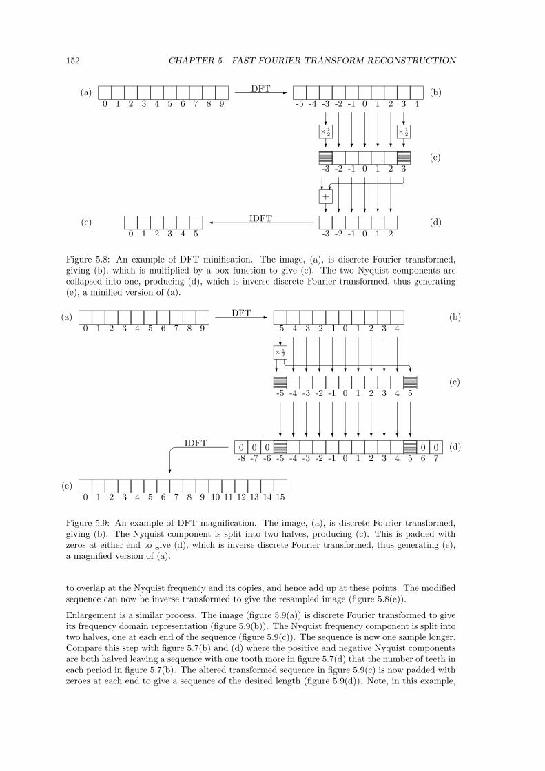
152 CHAPTER 5. FAST FOURIER TRANSFORM RECONSTRUCTION
0 1 2 3 4 5 6 7 8 9 -5 -4 -3 -2 -1 0 1 2 3 4
0 1 2 3 4 5
-3 -2 -1 0 1 2 3
-3 -2 -1 0 1 2
�DFT
� IDFT
� � � � �
� � � � �
× 12
�
�× 1
2
�
�
+�
��� �
(a) (b)
(c)
(d)(e)
Figure 5.8: An example of DFT minification. The image, (a), is discrete Fourier transformed,giving (b), which is multiplied by a box function to give (c). The two Nyquist components arecollapsed into one, producing (d), which is inverse discrete Fourier transformed, thus generating(e), a minified version of (a).
0 1 2 3 4 5 6 7 8 9 -5 -4 -3 -2 -1 0 1 2 3 4
-5 -4 -3 -2 -1 0 1 2 3 4 5
-8 -7 -6 -5 -4 -3 -2 -1 0 1 2 3 4 5 6 70 0 0 0 0
0 1 2 3 4 5 6 7 8 9 10 11 12 13 14 15
�DFT
�
IDFT
� � � � � � � � �
� � � � � � � � � � �
× 12
�
�
� �
(a) (b)
(c)
(d)
(e)
Figure 5.9: An example of DFT magnification. The image, (a), is discrete Fourier transformed,giving (b). The Nyquist component is split into two halves, producing (c). This is padded withzeros at either end to give (d), which is inverse discrete Fourier transformed, thus generating (e),a magnified version of (a).
to overlap at the Nyquist frequency and its copies, and hence add up at these points. The modifiedsequence can now be inverse transformed to give the resampled image (figure 5.8(e)).
Enlargement is a similar process. The image (figure 5.9(a)) is discrete Fourier transformed to giveits frequency domain representation (figure 5.9(b)). The Nyquist frequency component is split intotwo halves, one at each end of the sequence (figure 5.9(c)). The sequence is now one sample longer.Compare this step with figure 5.7(b) and (d) where the positive and negative Nyquist componentsare both halved leaving a sequence with one tooth more in figure 5.7(d) that the number of teeth ineach period in figure 5.7(b). The altered transformed sequence in figure 5.9(c) is now padded withzeroes at each end to give a sequence of the desired length (figure 5.9(d)). Note, in this example,

5.2. DFT SAMPLE RATE CHANGING 153
(a)
(b)
0 1 2 3 4 5 6 7 8 9
-5 -4 -3 -2 -1 0 1 2 3 4
� � � � �
� � � � �� � � � �� � � � �
Figure 5.10: Comparison of the usual FFT output order and the DFT output order used infigure 5.8 and figure 5.9. At the top is the usual FFT output order. The Nyquist component isnumber 5. This can be easily converted to our DFT output order, shown at the bottom. TheNyquist component here is −5.
that one more zero is added at the negative end than at the positive end because we are assumingthat the Nyquist component is at the negative end of the spectrum. The discrete spectrum isfinally inverse discrete Fourier transformed to produce the desired enlarged image (figure 5.9(e)).
5.2.3 Odd vs even length sequences
All of the examples, up to this point, have used even length sequences. The processing requiredfor an odd length sequence is slightly different and slightly easier. This is due to the fact thatthere is no frequency component at the Nyquist limit in an odd length sequence. Refer back tothe continuous case in figure 5.6(a) and (b). In general, for a sequence of length L, there are Lsamples (teeth) in a unit distance in the spatial domain. Each period in the frequency domainis L units long, with the teeth of the comb function at integer locations. The Nyquist frequencyis at ±L
2 . For an even length sequence there are components (teeth) at these frequencies; foran odd length sequence there are no components at these frequencies because they are not atinteger locations. There are therefore no special case frequencies to consider when dealing with anodd-length sequence, because there is no Nyquist component.
5.2.4 Implementation using the FFT
Implementing this algorithm using a fast Fourier transform is straightforward. Two transforms arerequired, one of the original length and one of the final length. Provided an FFT algorithm canbe implemented for both lengths the whole algorithm can be implemented. All FFT algorithmsdecompose the DFT into a number of successively shorter, and simpler DFTs [Lynn and Fuerst,1989, p.221]. Thus an FFT of length 2n, n ∈ N is well known and widely used. Decomposition ofother, non-prime length DFTs is less widely used. Finally, FFTs for prime length DFTs or lengthswith large prime factors are most difficult, because the DFT has to be split into pieces of unequallength.
One important implementation issue is that most FFT algorithms produce N coefficients in thefrequency domain ranging from ν = 0 to ν = 2νN − 1. The examples shown here in figures 5.8 and5.9 show them ranging from ν = −�νN� to ν =
⌊νN − 1
2
⌋. This is no great problem as the values
generated are exactly the same because the sequence is periodic with period 2νN (see figure 5.1).Figure 5.10 shows the equivalence. So long as this is borne in mind in implementation, noproblems will arise.

154 CHAPTER 5. FAST FOURIER TRANSFORM RECONSTRUCTION
5.3 Using the FFT to produce a continuous reconstructedintensity surface
As pointed out in section 3.2, the FFT method is a super-skeleton reconstruction method. As itstands it is only useful for scaling and a limited set of other transforms.
Fraser [1987, 1989a, 1989b] takes this FFT method and extends it to produce a continuous intensitysurface, which is thus useful for any transform. Fraser’s idea is to use the FFT method to generateseveral extra points between the existing sample points. If the FFT method is used to scaleby a factor of M (an integer) then M − 1 extra sample points will be generated between eachadjacent pair of original sample points. A local interpolant is then used to interpolate betweenthese points, which all lie on the theoretically perfect intensity surface (equation 5.2). The FFTenlargement eliminates the majority of the rastering artifacts that would arise from applying thelocal interpolant to the original samples.
In practice Fraser [1987, p.122] scales the image by a factor of four or eight using the FFTmethod and then employs the Catmull-Rom cubic interpolant to produce the intensity surface.It is profitable to compare interpolation by the sinc function, the Catmull-Rom cubic and theFFT/Catmull-Rom interpolant. Ignoring edge effects, figure 5.11 compares these three inter-polants in the frequency domain. The sinc function preserves the central copy of the signal, asis required for perfect interpolation. The Catmull-Rom interpolant attenuates some frequenciesbelow the Nyquist frequency and passes some above it, thus the reconstructed signal is a distortedversion of the ‘perfectly’ reconstructed signal.
The FFT/Catmull-Rom method consists of two steps. The first, the FFT step, produces a spectrumwhich has copies of the original spectrum at four or eight times the spacing in the sampled signal,with gaps between them of three or seven times the sampling frequency respectively. In the secondstep, where the Catmull-Rom interpolant is convolved with the FFT scaled signal, the centralcopy is almost perfectly preserved and the other copies are almost completely suppressed. Thusthe FFT/Catmull-Rom method produces a nearly perfect reconstructed surface.
5.3.1 Implementation
There are two distinct steps in this process, as illustrated in figure 5.12. First the image is ‘enlarged’by a factor of, say, four and then this intermediate image is reconstructed using the Catmull-Romcubic to give the continuous intensity surface.
The FFT process requires a large amount of extra storage for the intermediate image. The in-termediate image is generated in its entirety by a single FFT and cannot be generated a piece ata time on demand (but see section 5.4.2). Further, storage must be provided for the frequencydomain representation of the image. This can be stored in the same location as the images if anin-place FFT is used [Lynn and Fuerst, 1989]. However the image data is real while the frequencydomain data is complex; hence the frequency domain data requires twice the storage space of theimage data if a naive FFT algorithm is used.
Two features of the process enable it to be implemented more efficiently than a general FFT.Firstly, the image data is real, so the frequency domain data exhibits conjugate symmetry; thatis: Fk = F ∗
−k. This symmetry enables us to halve the number of operations required for both theforward and inverse fast Fourier transforms [Watson, 1989, p.15] and halve the storage requiredfor the frequency domain data. Secondly, there are a large number of zero values in the frequencydomain image that is to be inverse transformed. Operations on these zeros are unnecessary becausethe FFT consists of several multiply and add stages. Multiplying by zero and adding the productgives the same result as doing nothing. Some savings can be made by implementing a specialversion of the FFT which does not perform the unnecessary operations. Smit, Smith and Nichols[1990] discuss precisely this version of the FFT. They show that, for scaling an image of size N by

5.3. FFT INTENSITY SURFACE RECONSTRUCTION 155
F( ν )
ν
F( ν )
ν
νN
νN
−
νN
νN
−
F( ν )
νν
Nν
N−
F( ν )
νν
Nν
N− ν
Nν
N−
(old)(new) (old) (new)
F( ν )
νν
Nν
N−
(a)
(b)
(c)
(d)
(e)
Figure 5.11: A comparison of sinc, Catmull-Rom, and FFT/Catmull-Rom reconstruction. (a)shows the Fourier transform of the sampled function; (b) is the sinc reconstructed function, thereare no aliases in this function; (c) is the Catmull-Rom reconstructed function, it contains aliases.(d) is the FFT scaled function, which has the effect of pushing the components farther apart (inthis figure they are moved twice as far apart). When (d) is reconstructed using a Catmull-Romfunction, fewer aliases are produced (e). In a real situation the components will be moved fartherapart than shown here, reducing the errors further.

156 CHAPTER 5. FAST FOURIER TRANSFORM RECONSTRUCTION
Image Image IntensitySurface
� �FFT
Scale ×4Catmull-Romreconstruction
Figure 5.12: FFT/Catmull-Rom reconstruction is a two-stage process, requiring production of anintermediate (scaled) image. The scaling can be ×4 or ×8.
a factor of M , a reduction in time of around log2 N/ log2 MN can be achieved when M and N areboth powers of two.
Combining both savings, a 512 sample one-dimensional sequence magnified by a factor of fourtakes just over 40% of the time that a naive FFT implementation would take. The saving for a512 × 512 two-dimensional image is the same.
5.4 Problems with the FFT reconstructor
There are two major problems with the FFT reconstructor. Firstly, edge effects appear in theintensity surface to a considerable distance from the edges. Secondly, the process is both time andmemory intensive. We tackle these two problems separately and draw them together at the end.
5.4.1 Edge effects
Inherent in the FFT reconstructor is the assumption that edge extension is done by replicating(copying) the image. Looking back to section 5.1 we can see this in the explanation of FFT scaling.Except in exceptional cases, there will be a sharp change in intensity along the edges of the imagewhere the replicas join. Figure 4.20(top) gives an example of this.
From section 4.2.1 we know that perfect reconstruction causes unsightly ripples for some distancearound such sharp changes. The FFT method implements perfect reconstruction and so there willbe ripples visible around the ‘edge’ of the intensity surface. Figure 4.20(bottom) gives an exampleof these ripples.
Visual examination of images with large intensity differences at the edges indicates that theseripples can extend twelve to sixteen original sample spacings from the edge. This means thataround twelve percent of a 512 × 512 image is degraded by this process. A larger proportion isdegraded in smaller images.
Solving the edge effect problem
Fraser [1989a, p.668] noted the errors due to edge effects, and that low errors occur when thereare “fortuitous end-around effects”, that is: when the intensities at opposite edges are very close.We simply cannot depend on good fortune to always provide images with nice end-around effects.Indeed, most images do not fall into this category.
Fraser [1989a, p.669; figs. 3, 4; 1989b, p.269 & fig. 1] avoided the edge effects in his experimentalmeasurements by considering only the central portion of the image, remote from the edges andany edge effects. In resampling work, however, it is usually necessary to use the entire image andso the edge effect problem cannot be avoided.

5.4. PROBLEMS WITH THE FFT RECONSTRUCTOR 157
The solution is to produce a situation where the intensities at opposite edges of the image matchbefore the image is transformed. There are several ways to do this:
1. window the image;
2. extend the image so that the edges match;
3. linearise the image;
4. use reflection in place of replication.
(1) Window the image
Fraser [1989a, pp.671–3] solves the edge effect problem by end-windowing the image. He appliescosine half-bells to each end of each row and column in the image to form a new image whoseintensities fall off smoothly to zero at the edges. Fraser showed that only a small amount ofwindowing can significantly affect the result. A window covering only four sample spacings (twoat each end) reduces the distance from the edge that errors are noticeable to around a sixth of thedistance without windowing, in the cases where the ripples are most noticeable.
The problem with this method is that it causes a different visual artifact, known as vignetting.This effect is illustrated in figure 4.19. Windowing reduces the rippling artifact near the edges ofthe image at the expense of introducing the vignetting artifact. In places where the rippling wasless noticeable, the vignetting may cause larger errors than the ripples would have. That is: it ispossible for the vignetting to be more objectionable than the rippling.
(2) Extend the image so that the edges match
This is similar to the windowing idea. The image is left unchanged in this case and a few extralines of pixels added around the outside to ‘fade off’ to some constant value. A more sophisticatedalgorithm than simple fading could be tried (section 4.2.1). Once the image has been enlarged bythe FFT method the extra lines can be discarded.
A simple algorithm can be developed which fades each row and column to a constant value withina few pixels. A problem with this method is that many FFT algorithms are designed for sequencesof length 2n, n ∈ N , and many images have heights and widths which are also powers of two.Extending an image by a few pixels before transforming will be extremely inconvenient in thesecases. Extending an image to twice its width and height (with mostly some constant value in theextension) would be more convenient (figure 5.13).
(3) Linearisation
The idea behind linearisation is to remove a linear trend from the data, so that the two ends matchin intensity, then do the processing, and finally add the trend back in. This process, illustrated infigure 5.14, can be described for one dimension as follows:
Given a set of N data points, fn, subtract a linear trend from the data to give a new sequence gn:
gn = fn − sn
where: s =fN−1 − f0
N
Expand gn by a factor Z, using the FFT method, to give hn. This can be converted back to anexpansion of fn by adding back the linear trend:
in = hn + sn
Z

158 CHAPTER 5. FAST FOURIER TRANSFORM RECONSTRUCTION
Image
Constant Value
ImageImage
Windowedregion
Extrapolatedregion
Extrapolatedregion
(a) (b) (c)
Figure 5.13: Three ways of coping with edge effects in FFT expansion of an image. (a) windowingthe image, shaded area affected; (b) extending the image; and (c) extending the image to twice itssize in both dimensions. In all three cases the resulting image (larger in (b) and (c)) is extendedby replication by the FFT.
(d)
(c)
(b)
(a)
Figure 5.14: An example of linearisation. (a) shows the original samples and a linear trend throughthem; (b) shows the same samples with the linear trend removed; (c) is the FFT expanded versionof (b); (d) is (c) with the linear trend added back in.

5.4. PROBLEMS WITH THE FFT RECONSTRUCTOR 159
Analysing this method shows that it removes the edge ripples from the resulting image.
The transform of the original image, f , is F :
Fk =N−1∑n=0
fn e−i2πkn/N
This can be expanded by the FFT method to give J , the Fourier transform of the expanded image,j:
Jk =ZN−1∑n=0
jn e−i2πkn/ZN
In general j will contain edge ripples.
On the other hand, the transform of the linearised image, g, is G:
Gk =N−1∑n=0
gn e−i2πkn/N
=N−1∑n=0
fn e−i2πkn/N − sN−1∑n=0
n e−i2πkn/N
= Fk − sEk
This can be expanded to give H:Hk = Jk − sE′
k
Inverse transforming H gives the image, h, which then has the linear trend added back in to givethe final image, i:
in = jn − se′n + sn
Z
The difference between the latter two terms is an edge ripple which cancels out the edge ripple inj.
Extending to two dimensions
It is a simple matter to linearise a two dimensional image so that either the horizontal or thevertical edges match. This is achieved by linearising each column or row individually. It is possibleto linearise every row and then linearise every column in the row-linearised image (this can beshown to leave every row and every column linearised). However, after FFT enlargement theimage cannot be de-linearised because new rows and columns have been generated, between theexisting rows and columns, for which no linearisation information exists.
It is impossible to linearise the image as a two dimensional whole so, if we wish to apply thelinearisation process to a two-dimensional image we must think of some other way to performthe operation. To do this we alter the two-dimensional FFT expansion. A two dimensional FFTis performed by applying the FFT to every row in the image and then to every column in therow-transformed image. The FFT expansion expands the resulting frequency domain image andthen two-dimensionally inverse transforms it. As noted above, this process is not amenable tolinearisation. However, if the process is altered so that the rows are expanded first and the columnsof the row-expanded image are expanded as a separate step, then linearisation is possible. Thestandard method and this new two-stage method are illustrated in figures 5.15 and 5.16. It is notimmediately obvious that both methods should produce the same result (without linearisation).Experiments on several images have shown that they are equivalent (to within the numericalaccuracy of the computer on which the operations were performed).

160 CHAPTER 5. FAST FOURIER TRANSFORM RECONSTRUCTION
I
I’’
T’form
Rows
T’form
Cols.
Inv.T’form
Rows
T’form
Cols.
Inv.
Rows & Cols.
Expand
Figure 5.15: The standard way of performing two-dimensional FFT expansion of an image. Thismethod is not amenable to linearisation.
IT’form
Rows
I’’
Inv.T’form
Cols.
I’
Inv.T’formRows
T’formCols.
ExpandRows
ExpandCols.
Figure 5.16: The two-stage method of performing two-dimensional FFT expansion of an image.This method is amenable to linearisation of each of the two stages.

5.4. PROBLEMS WITH THE FFT RECONSTRUCTOR 161
(a) (b) (c)
Figure 5.17: Two ways of reflecting an image to produce an image of twice the size in eachdimension. (a) the original image; (b) reflected with the original in a corner; (c) reflected with theoriginal in the centre.
Applying the linearisation to each of the two stages suppresses the edge ripples which wouldotherwise result. Obviously linearisation is applied to the rows in the row-expansion stage and tothe columns in the column expansion stage2.
(4) Using reflection in place of replication
In chapter 4 we saw that reflection is a better extension method than replication. Reflection ensuresthat the edges match. Reflection can be implemented in the FFT expansion stage by using animage twice the size in both dimensions and filling the extra three quarters with reflected versionsof the image as illustrated in figure 5.17. Once this image is enlarged, using FFT expansion,only the appropriate quarter of the expanded image need be used in the ensuing Catmull-Romreconstruction.
This method quadruples the computation required to perform the FFT expansion. Fortunatelythere is a way to compute the expansion in the same time as the basic FFT method; that is to usethe discrete cosine transform (DCT), in place of the DFT.
Discrete cosine transform expansion
The discrete cosine transform of a sequence fn, n ∈ {0, 1, . . . , N − 1}, is [Ahmed, Natarajan andRao, 1974]:
F0 =√
2N
N−1∑n=0
fn
Fk =2N
N−1∑n=0
fn cos(2n + 1)kπ
2N, k ∈ {1, 2, . . . , N − 1}
The special case for F0 can be combined into the general form as illustrated in the two-dimensionalDCT [Chen and Pratt, 1984]:
Fk,l =4C(k)C(l)
MN
M−1∑m=0
N−1∑n=0
fm,n cos(2m + 1)kπ
2Mcos
(2n + 1)lπ2N
2Linearisation is a good word to play that game where you try to get as many words as possible from a singlelong word. For example: line, arise, ear, rise, is, at, on, in, ate, note, not, near, rest, least, sat, sate, nation, sir, sire,sit, sits, tin, tins, linear, salt, real, role, sole, aerial, nil, sale, rail, tail, tale, notion, elation, eat, eats, nit, trial, etc.[Gibbs, 1992]

162 CHAPTER 5. FAST FOURIER TRANSFORM RECONSTRUCTION
2N
N(a)
(b)
Figure 5.18: The implicit periodicity of (a) the discrete Fourier transform, and (b) the discretecosine transform (after Rabbani and Jones [1991], figure 10.4).
k ∈ {0, 1, . . . ,M − 1}l ∈ {0, 1, . . . , N − 1}
C(j) =
{1√2, j = 0
1, otherwise(5.3)
The DCT expresses the image as a sum of cosinusoidal terms [Chen and Pratt, 1984]:
f(m,n) =M−1∑k=0
N−1∑l=0
C(k)C(l)Fk,l cos(2m + 1)kπ
2Mcos
(2n + 1)lπ2N
Compare this with the DFT decomposition into a sum of complex exponential terms (equation 5.2).The two transforms have different implicit periodicities (figure 5.18). As we have seen the DFTassumes a replicated periodic image whilst the DCT assumes a reflected periodic image [Rabbaniand Jones, 1991, pp.108-111]. Expansion of the DCT can be performed in much the same way asfor the DFT. But there turns out to be a slight catch to DCT expansion, which we now explain.
Working in one dimension for clarity, given an image fn, n ∈ {0, 1, . . . , N −1}, the DCT is definedas:
Fk =2C(k)MN
N−1∑n=0
fn cos(2n + 1)kπ
2N, k ∈ {0, 1, . . . , N − 1} (5.4)
where C(k) is defined in equation 5.3.
This can be expanded by a factor Z to Gk:
Gk ={
Fk, k < N0, otherwise , k ∈ {0, 1, . . . , ZN − 1}
Note that, unlike the DFT expansion, there is no special (Nyquist) frequency component, nor arethere any negative frequencies.
G can now be inverse transformed to give an expanded image, g:
gn =ZN−1∑k=0
C(k)Gk cos(2n + 1)kπ
2ZN, n ∈ {0, 1, . . . , ZN − 1} (5.5)

5.4. PROBLEMS WITH THE FFT RECONSTRUCTOR 163
Here lies the catch: with the DFT every Zth member of the expanded image would be in the originalimage, with Z − 1 new image samples between every adjacent pair. That is: gZn = fn. With theDCT, as it stands, this is not the case and a small correction must be made to equation 5.5 tomake it the case. To explain what happens we see that:
fn =N−1∑k=0
C(k)Fk cos(2n + 1)kπ
2N, n ∈ {0, 1, . . . , N − 1} (5.6)
this is simply the inverse of equation 5.4. Equation 5.5 can be rewritten as:
gn =N−1∑k=0
C(k)Fk cos(2n + 1)kπ
2ZN, n ∈ {0, 1, . . . , ZN − 1} (5.7)
The differences between these two equations are the factor of 1Z in the cosine’s argument, and that
there are Z times as many gn as there are fn. We require:
gZn = fn, n ∈ {0, 1, . . . , N − 1}
We can rewrite equation 5.7 for gZn as:
gZn =N−1∑k=0
C(k)Fk cos(2n + 1
Z )kπ
2N, n ∈ {0, 1, . . . , N − 1} (5.8)
The only difference between equation 5.6 and equation 5.8 is that the (2n + 1) in equation 5.6 isreplaced by (2n + 1
Z ) in equation 5.8. The net result is that there is a linear phase shift in the gn
with respect to the fn.
This can be simply corrected by either:(a) altering equation 5.5 to:
gn =ZN−1∑k=0
C(k)Gk cos(2n + Z)kπ
2ZN
or:(b) correcting for the linear phase shift in the subsequent small kernel interpolation. That is:instead of sample gn being at location x = x0 + n∆x
Z it is shifted slightly to be at:
x = x0 +(n −
(12 − 1
2Z
)) ∆x
Z
Thus the DCT can be successfully used as an expansion method which does not produce edgeripple effects.
Expansion using other transforms
The DFT and DCT are only two of many types of image transform. We have seen that both ofthese can be used for image expansion. In general, any transform can be used for image expansionprovided that N of the basis functions of the expanded version are identical to the N basis functionsof the smaller version, except for a scale factor and possibly a linear phase shift, n′ = sn + c. TheDFT and DCT are examples of such transforms. For the DFT the basis functions are:
{e−i2πkn/N , k ∈ {−N2 ,−N
2 + 1, . . . , 0, 1, . . . , N2 − 1}, n ∈ {0, 1, 2, . . . , N − 1}} (5.9)
Expanding this by a factor Z we find the basis functions for k ∈ {−N2 ,−N
2 +1, . . . , 0, 1, . . . , N2 −1}
are:{e−i2πkn′/ZN} (5.10)

164 CHAPTER 5. FAST FOURIER TRANSFORM RECONSTRUCTION
Setting n′ = Zn gives N functions from equation 5.10 which are equal to the N in equation 5.9.Thus it is possible to expand an image using the DFT.
Likewise for the DCT the basis functions are:
{ 1√2, cos
(2n + 1)kπ
2N, k ∈ {1, 2, . . . , N − 1}, n ∈ {0, 1, 2, . . . , N − 1}} (5.11)
Expanding by a factor of Z we find that the lowest N basis function of the new sequence are:
{ 1√2, cos
(2n′ + 1)kπ
2ZN, k ∈ {1, 2, . . . , N − 1}} (5.12)
Setting n′ = Zn + (12 − 1
2Z ) makes N functions in equation 5.12 equal to those in equation 5.11and so the DCT can also be used for image expansion.
Such an expansion is carried out by taking the coefficients of the basis functions in the originalsequence and allocating them to the equivalent basis function in the expanded sequence. Allother coefficients in the expanded sequence are set to zero. The DFT is a bit of a special case asthe Nyquist component in the original sequence has two matching components in the expandedsequence with half its coefficient being given to each.
To illustrate this principle for other transforms take two square wave transforms: the Walsh-Hadamard transform and the Haar transform, both considered for N,Z ∈ {2n, n ∈ N}. The basisfunction for both transforms are square-like waves. The first sixteen Walsh-Hadamard basis func-tion are shown in figure 5.19(a) and the first sixteen Haar basis function are shown in figure 5.19(b).Enlarging either by a factor of Z leaves the first N basis functions scaled but otherwise unchangedand thus either can be used for image expansion.
This can be implemented so that there is no phase shift or so that there is the same phase shift asin the DCT. For both transforms, this latter case produces identical results to nearest-neighbourexpansion of the image, which would be considerably quicker to implement. The former produces ashifted version of this nearest-neighbour expansion. Therefore, while theoretically possible, neitherof these transforms provide a particularly efficient way of achieving this type of expansion.
5.4.2 Speed and storage requirements
These image expansion methods are extremely time and memory intensive. Transform expansionfor an N × N image is O(N2 log N), thus increasing rapidly as image size increases. An N × Nimage expanded by a factor Z requires Z2N2 complex numbers to be stored for a straight forwardFFT expansion, a quarter of this for an optimised FFT expansion, and Z2N2 real numbers for theother transforms discussed in the previous section. For example, a DCT expansion of a 256 × 256image by a factor of four would typically require 4MB of storage. Experience on the ComputerLaboratory’s workstations has shown that they tend to fail when asked to allocate these hugequantities of memory to an image processing program. On occasion processes have required over50MB of memory to expand a large image by a factor of eight, and such quantities seem wellbeyond the capability of the machines. Even where large quantities of memory are available mostof it will tend to be in virtual memory, incurring an extra time cost as data is paged in and out ofrandom access memory. In order to speed up the algorithm and reduce the need for large quantitiesof quickly accessible storage we can tile the image (figure 5.20). Tiling is used in image coding toreduce the time and memory cost of the coding algorithm and because image tend to be locallysimilar and globally dissimilar. The JPEG image compression method, for example, splits theimage into 8 × 8 pixel non-overlapping tiles [Rabbani and Jones, 1991, p.114].
In image extension we will use relatively large tiles (32 × 32 pixels is a good size), and they willoverlap. Processing is done on each tile separately and so, if they did not overlap, the edges of thetiles would be obvious. Overlapping the tiles places each tile in its local context. That is: a tile isexpanded but only the central portion is used, as illustrated in figure 5.21.

5.4. PROBLEMS WITH THE FFT RECONSTRUCTOR 165
Walsh-Hadamard(a)
0
1
2
3
4
5
6
7
8
9
10
11
12
13
14
15
(b)
0
1
2
3
4
5
6
7
8
9
10
11
12
13
14
15
Haar
Figure 5.19: (a) the first sixteen Walsh-Hadamard basis functions; (b) the first sixteen Haarbasis functions (after Hall [1979, pp.138–145]), these remain the same, no matter how many morecoefficients there are.
Figure 5.20: An image (shaded) divided into tiles.

166 CHAPTER 5. FAST FOURIER TRANSFORM RECONSTRUCTION
Discrete Fourier Transform
Add zeros
Inverse
Transform
Place central portionin expanded image
to expand image
Figure 5.21: Using a tiled DFT expansion. Each tile is individually expanded, within its localcontext, and the appropriate expanded portion put into the expanded image.

5.4. PROBLEMS WITH THE FFT RECONSTRUCTOR 167
02
4
6
8
10
Window Size
3230
28
26
24
22
Central Portion Size
5101520
50100150200
Error Intensity
Figure 5.22: The values in table 5.1. Error intensity is the height of the largest ripple in intensityvalues, ranging from 0 to 255. This is graphed on a logarithmic scale. Only values for whichCentral Portion Size + Window Size ≤ 32 were evaluated.
As with the untitled version, if we use a DFT expansion, we are faced with edge effects. The DFTof a tile implicitly assumes that the infinite image is that tile replicated to infinity. The centralquarter of the expanded tile will probably be unaffected by these edge effects but transforming animage twice the size of the useful portion in both dimensions is quite an overhead. It would bebetter if the useful portion was a larger proportion of the whole tile.
Here the edge effects solutions come into play. We could apply a DCT, or linearisation and a DFTto the tile, both of which would markedly increase the size of the usable inner portion of the tile.Further, windowing is a viable proposition here because the windowed pixels will be in the unusedouter portion of the tile. An experiment has been performed to ascertain the best size of windowand central portion given a tile size of 32× 32 pixels. A completely black image was enlarged withwindowing designed to fade the image off to white. Thus any artifacts in the expanded image willbe extremely obvious as non-black pixels. This experiment gives a feel for the maximum errorslikely due to windowing. In practice windowing should be done to a mid-grey, halving these errors;but many people prefer to window off to an extreme, usually black, and so it is necessary to recordthese maximum errors.
The results of this experiment are tabulated in table 5.1 and graphed in figure 5.22. The windowsize refers to the number of pixels in a row (or column) that are windowed. Half this number arewindowed at each end of a row or column.
Any combination which has an intensity error less than three produces no visible artifacts. Ifwindowing is done to a mid-grey than any combination with an intensity error under six producesno visible artifacts. Therefor any combination of an n× n central portion in a 32× 32 tile is goodprovided n ≤ 26 and the window width is greater than 2 and less than 32−n. Besides requiring novisible artifacts we also require the largest possible central portion relative to the tile size. Thus
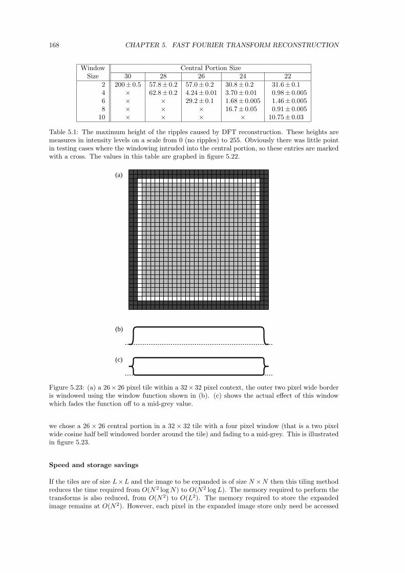
168 CHAPTER 5. FAST FOURIER TRANSFORM RECONSTRUCTION
Window Central Portion SizeSize 30 28 26 24 22
2 200± 0.5 57.8± 0.2 57.0± 0.2 30.8± 0.2 31.6± 0.14 × 62.8± 0.2 4.24± 0.01 3.70± 0.01 0.98± 0.0056 × × 29.2± 0.1 1.68± 0.005 1.46± 0.0058 × × × 16.7± 0.05 0.91± 0.005
10 × × × × 10.75± 0.03
Table 5.1: The maximum height of the ripples caused by DFT reconstruction. These heights aremeasures in intensity levels on a scale from 0 (no ripples) to 255. Obviously there was little pointin testing cases where the windowing intruded into the central portion, so these entries are markedwith a cross. The values in this table are graphed in figure 5.22.
(a)
(b)
(c)
Figure 5.23: (a) a 26× 26 pixel tile within a 32× 32 pixel context, the outer two pixel wide borderis windowed using the window function shown in (b). (c) shows the actual effect of this windowwhich fades the function off to a mid-grey value.
we chose a 26 × 26 central portion in a 32 × 32 tile with a four pixel window (that is a two pixelwide cosine half bell windowed border around the tile) and fading to a mid-grey. This is illustratedin figure 5.23.
Speed and storage savings
If the tiles are of size L×L and the image to be expanded is of size N ×N then this tiling methodreduces the time required from O(N2 log N) to O(N2 log L). The memory required to perform thetransforms is also reduced, from O(N2) to O(L2). The memory required to store the expandedimage remains at O(N2). However, each pixel in the expanded image store only need be accessed

5.5. SUMMARY 169
once in the expansion process, whilst each element in the transform memory must be accessed.2+2 log2 L times (for an untiled transform L = N). There is also the possibility that the expandedimage could be generated a few tiles at a time, as required, rather than as a whole, which is whatthe untiled version must do.
The tiled version of the algorithm thus makes a big difference to the amount of transform memoryrequired for the transform. With a 256× 256 pixel image split in to 32× 32 tiles, a sixty-fourth ofthe memory is required, reducing the required 4MB of random access memory quoted on page 164to 64kB.
If the whole operation can be carried out in random access memory then little difference is madeto the time taken to expand the image. In the example in the previous paragraph the time isreduced by thirty percent if 32× 32 non-overlapping tiles are used and increased by nine percent ifa 26× 26 pixel central portion is used in a 32× 32 tile. However, if the untiled version is swappingin and out of virtual memory then the tiled version can run considerably faster.
Implementation in hardware
Fraser [1989a] notes that the FFT is a time-intensive process, which perhaps explains why thismethod of reconstruction has been neglected. However the advent of very fast FFT hardwaremeans that FFT interpolation is feasible.
As an example, dataβ produce a dedicated FFT processor which can perform a 1024 point FFTevery 700µs [Data Beta, 1992]. To enlarge a 256 × 256 image to 1024 × 1024 using this processorwould take 753ms. Using 32 × 32 non-overlapping tiles would take 525ms, and using overlapping32 × 32 tiles with a 26 × 26 pixel central portion would take 819ms.
Theoretical ramifications of tiling
By tiling the image we destroy the theoretical basis behind applying the DFT or DCT to thewhole image as a way of performing sinc reconstruction. Applying the DFT or DCT to a tilegives an approximation to this reconstruction. The untiled version gives an approximate sincreconstruction based on all of the information in the image, the tiled version gives an approximatesinc reconstruction based on local information only. We can consider the entire image to be a largetile taken from an infinite, non-repeating picture. In this scenario the tiled version of the processis a scaled-down version of the untiled version with the advantage that most of the tiles can beplaced in some sort of context.
In spite of this it is surprising that the tiled and untiled algorithms give virtually identical results.This observation lends weight to the hypothesis that it is local information that is important indetermining the intensity surface’s values, rather than any globally encoded intensity information.
5.5 Summary
We have seen how DFT expansion can be used, with a local piecewise polynomial reconstructor,to generate a near perfect sinc reconstructed intensity surface in O(N2 log N) time.
We have examined two areas where improvements can be made to the existing method. The first,the edge effect problem, has several solutions, one of which led to the use of the DCT in place ofthe DFT, with better intensity surface quality near edges. This also laid the foundation for theuse of any transform in performing the necessary expansion. The second, the need for time andspace savings, led to a tiling solution, which dramatically reduces the amount of memory requiredto perform the transforms and, where virtual memory must be used for a non-tiled version, canlead to speed improvements also.

170 CHAPTER 5. FAST FOURIER TRANSFORM RECONSTRUCTION

Chapter 6
A priori knowledge reconstruction
If we have some a priori knowledge about the image we are resampling then we may be able toreconstruct a better intensity surface than we could without this knowledge.
A priori knowledge comes in two forms:
1. Knowledge about how the image was sampled;
2. Knowledge about the image’s content.
The majority of this chapter is concerned with finding an exact reconstruction of the image in oneparticular case where both these are known. Before progressing to this we look at what can beachieved when only the first is known.
6.1 Knowledge about the sampler
Most images are captured by some physical device. Knowledge of that device’s sampling processgives the potential to invert the process and restore what would have been produced by single pointsampling the original intensity surface, or at least a closer approximation to it than that producedby the device. The closer an image is to the single point sampled image, the better many of theNAPK reconstructors discussed in the previous three chapters will work.
Much effort has been expended over the years on image restoration, the attempt to produce abetter image from a less good one. Such a process could be applied to an image which could thenbe reconstructed using a NAPK method.
Referring back to figure 2.3 we can add this restoration process to the figure, and add also thetheoretically equivalent path of single point sampling, as shown in figure 6.1. This inversion of thecapture process could be built into the reconstructor, giving an APK reconstructor by combininga restorer and a NAPK reconstructor.
6.1.1 Inverting the sampling filter
All capture devices implement some form of area sampling. This sampling can be thought ofas convolving the intensity surface with a sampling filter, followed by single point sampling theresulting intensity surface (section 2.5.1). If this sampling filter can be inverted, and the inversionimplemented, then it can be used for image restoration and hence APK reconstruction. Thisprocess is illustrated in figure 6.2, in the frequency domain.
171
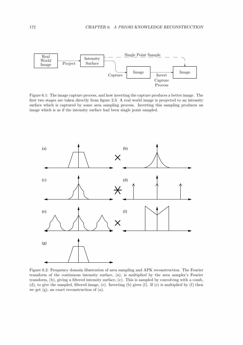
172 CHAPTER 6. A PRIORI KNOWLEDGE RECONSTRUCTION
RealWorldImage
IntensitySurface
Image Image
�
� � �
Project
Capture InvertCaptureProcess
�
Single Point Sample
Figure 6.1: The image capture process, and how inverting the capture produces a better image. Thefirst two stages are taken directly from figure 2.3. A real world image is projected to an intensitysurface which is captured by some area sampling process. Inverting this sampling produces animage which is as if the intensity surface had been single point sampled.
(a)
(c)
(e)
(g)
(b)
(d)
(f)
Figure 6.2: Frequency domain illustration of area sampling and APK reconstruction. The Fouriertransform of the continuous intensity surface, (a), is multiplied by the area sampler’s Fouriertransform, (b), giving a filtered intensity surface, (c). This is sampled by convolving with a comb,(d), to give the sampled, filtered image, (e). Inverting (b) gives (f). If (e) is multiplied by (f) thenwe get (g), an exact reconstruction of (a).
6.1. KNOWLEDGE ABOUT THE SAMPLER 173
If the sampling filter has frequency spectrum S(ν) then the inverted filter could be given thespectrum I1(ν) = 1
S(ν) . If S(ν) extends beyond the folding frequency then this will have theundesirable effect of amplifying copies of the central component of the image’s spectrum. So, thedesired form of this inverted filter is:
I2(ν) =B1(ν)S(ν)
That is: the ideal filter’s spectrum, B1(ν), multiplied by the inverted sampling filter’s spectrum,1
S(ν) . I2(ν) can be implemented as convolution in the spatial domain, if the inverse filter’s kernelcan be determined. Or it can be approximated using the DFT, with the inverse filtering beingperformed in the frequency domain and an appropriate NAPK reconstruction method applied tothe resulting image. The DFT reconstruction methods of the previous chapter could be combinedwith this DFT restoration to produce an improved reconstructed intensity surface.
The problem with this method is that all practical sampling filters fall off as they move away fromzero. Thus the inverse filter amplifies those frequencies near the folding frequency. It is thesefrequencies in the image which have the smallest amplitudes and which are most affected by noiseand any aliasing which may occur. The frequencies near zero, which are least amplified by theinverse filter, are those which are at least affected by these two problems. Therefore inverse filteringamplifies any noise and aliasing artifacts present in an image. It is thus unsuitable for all imagesexcept those with very low noise and practically no aliasing.
6.1.2 Modified inverted sampling filter
Oakley and Cunningham [1990] have considered the problem of finding the best reconstructionfilter given the sampling function. They develop an error measure which they claim is a goodapproximation to the visual quality of the reconstructed images [ibid., p.191]. By minimisingthis measure over all images they produce a formula for the optimal reconstruction filter. In onedimension it is:
I(ν) =K(ν)S∗(ν)
1∆x
∞∑n=−∞
∣∣S (ν + n
∆x
)∣∣2 (6.1)
where S∗(ν) is the complex conjugate of S(ν); ∆x is the sample spacing in the spatial domain;and K(ν) is the Fourier transform of the ideal reconstruction filter. Here ‘ideal reconstructionfilter’ means the filter you would like to convolve the original intensity surface with to produce thereconstructed intensity surface. Several such functions are of interest:
1. K(ν) = 1; that is: the reconstructed intensity surface should be as close as possible to theoriginal intensity surface. Oakley and Cunningham [1990] call this a restoration case. Thisreconstruction filter is highly sensitive to noise [ibid., p.180]. Note that, if the samplingfilter is bandlimited to below the folding frequency then the reconstruction filter generatedby equation 6.1 is equal to both I1(ν) and I2(ν), except for a multiplicative constant. Asecond restoration filter is where K(ν) is the statistically optimal Wiener filter for the con-tinuous image formation case. This produces an implementation of the Wiener filter whichis corrected for the effects of sampling.
2. K(ν) is a low-pass filter. Here the reconstructed intensity surface approximates as closely aspossible the original intensity surface convolved with the low pass filter. Of special interestis the case where K(ν) = B1(ν). The reconstructed intensity surface will approximate aperfectly low-pass filtered version of the original intensity surface. It is instructive to notethat the sum of the squares in the denominator of equation 6.1 is the sampling filter squaredin the frequency domain, then sampled in the spatial domain and transformed into the

174 CHAPTER 6. A PRIORI KNOWLEDGE RECONSTRUCTION
frequency domain. Thus the function:
S∗(ν)∞∑
n=−∞
∣∣S (ν + n
∆x
)∣∣2is closely related to 1
S(ν) with some modification to take into account the fact that the imageis sampled, not just an intensity surface filtered by S(ν). If S(ν) is bandlimited to below thefolding frequency then
S∗(ν)∞∑
n=−∞
∣∣S (ν + n
∆x
)∣∣2 =1
S(ν)
3. K(ν) = S(ν). The reconstructed intensity surface here is the original surface convolved bythe sampling filter — thus producing the theoretical surface generated just before single pointsampling occurred. Oakley and Cunningham [1990, p.181] call this “matched reconstruction”or the “interpolating case”. If S(ν) is bandlimited to below the folding frequency than theresampling filter is a box function: I(ν) = ∆xB1(ν). This means that the reconstructedintensity surface is the same as that produced by convolving the image with the sinc function.
Both Oakley and Cunningham [1990] and Boult and Wolberg [1992] have generated implementa-tions of matched reconstructions filters. These filters have been based on rectangular and hexago-nally sampled Gaussian filters [Oakley and Cunningham, 1990] and on box and cubic B-spline filters[Boult and Wolberg, 1992]. Both claim that their derived reconstruction filters perform better thanthe best NAPK reconstructors, notably better than the Catmull-Rom cubic interpolant.
6.2 Knowledge about the image content
It is possible that a better reconstruction can be achieved if we know something about the image’scontent. This is true for image restoration; Oakley and Cunningham [1990, p.180] state that:
“In general, successful image restoration relies not only on correct linear processing,but on the the exploitation of prior knowledge about the image source.”
In the image resampling field itself, Ward and Cok [1989, p.264] hypothesise:
“If there is sufficient a priori knowledge of the content of an image, the visual qualitycan be improved by using interpolation functions that use this a priori information.For example, if the original image is known to consist of uniform areas and edges,interpolated pixels can be constrained by some rule to be close in value to some of theneighbouring pixels.”
This is an interesting idea but Ward and Cok do not take it any farther.
In the fields of image understanding and computer vision much work has, and is, been done ontrying to extract features from a digital image. If an accurate list of features could be extractedthen it could be used to drive a renderer which would generate a transformed image. This processis illustrated in figure 6.3. This is analagous to the reconstruct–transform–sample decompositionin figure 1.14, the difference being that the intensity surfaces are replaced by scene descriptions.Unfortunately, the generation of a detailed enough scene description is extremely difficult for eventhe simplest scenes and so this process would appear to be impractical for image resampling, exceptin the case of very limited sets of images.

6.3. ONE-DIMENSIONAL SHARP EDGE RECONSTRUCTION 175
Image SceneDescription
SceneDescription Image� � �
ExtractFeatures Transform Render
Figure 6.3: A three stage decomposition for a resampler which analyses an image into a scenedescription, transforms this and then renders it. Compare figure 1.14.
xa
xa
xa
xa
xa+1 +2 +3 +4
ga g
a+1
ga+2
ga+3
ga+4
ga-1
g( x)
x
Figure 6.4: The general intensity curve input to one-dimensional sharp edge reconstruction. Itconsists of areas of constant intensity separated by sharp discontinuities.
To illustrate the type of algorithm that could be developed we will consider a simple case. In thiscase we limit the class of images to those which consist of areas of constant intensity bounded byinfinitely sharp edges. These images will be sampled using an exact-area sampler on a square pixelgrid.
We begin by considering the one-dimensional case before progressing to the two-dimensional case.
6.3 One-dimensional sharp edge reconstruction
The general intensity curve in the one-dimensional case consists of a series of plateaux of constantintensity separated by sharp discontinuities. Such an image is shown in figure 6.4. It can bedescribed mathematically as:
g(x) = gc, xc ≤ x < xc+1 (6.2)
where (. . . , (x−1, g−1), (x0, g0), (x1, g1), . . .) is an ordered set of ordered pairs of position and in-tensity information. The pairs are ordered on position values: xc < xc+1, and the intensity valuesfall in the range 0 ≤ gc ≤ 1.
6.3.1 The black and white case
To simplify matters we begin by considering only the black and white case where gc = 0 or gc = 1.Zero is taken to be black, and one, white. We start by looking at the simplest case: a singleedge between a black area and a white area (see figure 6.5). This can be represented as the set((−∞, 0), (x1, 1), (∞, φ)) where φ is an arbitrary value which is never used.
Without loss of generality we can consider sampling with unit spacing, and with position x1
between zero and one (0 ≤ x1 < 1). If the samples are represented as {gn, n ∈ Z} then sample gn
is taken at point x = n + 12 [Heckbert, 1990a]. This disparity between continuous and discrete
coordinates, illustrated in figure 6.6, greatly simplifies many of the calculations on them.

176 CHAPTER 6. A PRIORI KNOWLEDGE RECONSTRUCTION
x1
g( x)
x
1
0
Figure 6.5: The black and white case with a single edge. The edge is at x1. To the left the intensitycurve is blank (0), and to the right, (1).
x0 1 2-1-2
sample 0 sample 1sample -1sample -2
Figure 6.6: The positions of the discrete samples relative to the continuous coordinate system[after Heckbert, 1990a, fig 1]
If the function shown in figure 6.5 is point sampled then the sample values will be:
gn = 0, n < 0
g0 ={
0, x1 < 12
1, x1 ≥ 12
gn = 1, n > 0
The information about the discontinuity’s position is lost here. It is only possible to say where theedge occurred to within ± 1
2 .
However, we want to use exact-area sampling which is equivalent to convolving with a box filterfollowed by point sampling (section 2.5.1). Convolving the intensity curve with this box filterproduces the function in figure 6.7.
Point sampling this function produces the sample values:
gn = 0, n < 0g0 = 1 − x1
gn = 1, n > 0
The information about the position of the discontinuity is now encoded in g0. It can be exactlyreconstructed from that value:
x1 = 1 − g0 (6.3)
A similar situation holds in the case where g(x) = 1, x < x1 and g(x) = 0, x ≥ x1, shown infigure 6.8. Here the sample values will be:
gn = 0, n < 0g0 = x1
gn = 1, n > 0
And the discontinuity can be reconstructed exactly as being at:
x1 = g0 (6.4)
Thus, in either case, we can exactly reconstruct the curve from the image.

6.3. ONE-DIMENSIONAL SHARP EDGE RECONSTRUCTION 177
x0 1-1 2
g*b1
x1
0.5
1
0
Figure 6.7: The intensity curve of figure 6.5 convolved with a box filter of width one.
x0 x
1
1
g( x)
0
Figure 6.8: The other single edge black and white case, white to the left of the discontinuity andblack to the right.
Black and white case — many edges
If we extend this to a situation where there are many edges alternating the intensity between blackand white then we can apply the above result in the following way. The original function, g(x),is represented by its exact-area samples {. . . , g−1, g0, g1, . . .}. The function that is reconstructedfrom these samples is, gr(x). gr(x) can be generated in a piecewise manner as follows:
Algorithm 1For every pixel, a:
If ga = 0 then gr(x) = 0, a ≤ x < a + 1
If ga = 1 then gr(x) = 1, a ≤ x < a + 1
If 0 < ga < 1 then
if limx→a−
gr(x) = 0 or limx→(a+1)+
gr(x) = 1 then
gr(x) ={
0, a ≤ x < a + 1 − ga
1, a + 1 − ga ≤ x < a + 1
if limx→a−
gr(x) = 1 or limx→(a+1)+
gr(x) = 0 then
gr(x) ={
1, a ≤ x < a + ga
0, a + ga ≤ x < a + 1

178 CHAPTER 6. A PRIORI KNOWLEDGE RECONSTRUCTION
(a)
(b)
Figure 6.9: Two ways of interpreting the sample sequence 0.5, 1.0, 0.7, if each pixel is allowed tocontain one edge. Only (b) is possible if edges are constrained to be at least one sample spaceapart.
This algorithm will not give an exact reconstruction for all possible g(x). In theorem 3 we seewhat restrictions must be put on g(x) for gr(x) to be an exact reconstruction, that is: to ensurethat gr(x) = g(x). The last part of this algorithm shows that, in addition to the intensity level ofthe edge pixel, one extra bit of information is required to uniquely determine the location of theedge. This bit is the orientation of the edge: whether it is rising from zero to one, or falling fromone to zero. The orientation can be ascertained from the orientation of the reconstructed functionin either of the adjacent pixels. A single zero or one pixel is required in the entire infinite sequenceto fix the orientation for all edges. This information can then be propagated through the sequenceto produce gr(x).
An alternative representation of gr(x) would be to find the values (. . . , (x−1, g−1), (x0, g0), (x1, g1), . . .)which define g(x) (equation 6.2). This can be done from gr(x), as produced by algorithm 1. Analgorithm to directly generate the (xc, gc) pairs must be constructed so as to take into account thepossibility of edges which fall exactly at pixel boundaries. Here the pixels either side of the edgewill have sample values zero and one indicating the discontinuity, rather than a single pixel witha value between zero and one indicating it1. Notice that algorithm 1 implicitly deals with thissituation in its first two cases.
Theorem 3 Algorithm 1 exactly reconstructs gr(x) = g(x) if adjacent edges in g(x) are spacedmore than one sample space apart. That is: xc+1 − xc > 1,∀c.
Proof: if xc+1 − xc > 1,∀c then:
1. No pixel can contain more than one edge, thus ensuring that any grey pixel codes the positionof one, and only one, edge. This edge can be reconstructed using orientation informationand equation 6.3 or 6.4.
2. Any edge occurring at a pixel boundary generates a zero sample value on one side and a onesample value on the other. This ensures that no dichotomies arise in the reconstruction. Forexample, if we imposed the lesser restriction that each pixel could only contain a single edge(but that the edges could be any distance apart) then the sample sequence . . . , 0.5, 1, 0.7, . . .could be interpreted in two different ways, as can be seen in figure 6.9, whereas the tighterrestriction imposed here permits the unique interpretation in figure 6.9(b).
3. Orientation information can be generated by any pair of adjacent pixels. If their sample
1The assumption that the samples on either side will have values zero and one is valid if the conditions intheorem 3 are adhered to.

6.3. ONE-DIMENSIONAL SHARP EDGE RECONSTRUCTION 179
values are gc and gc+1 then the following table gives the orientation information:
gc gc+1 limx→(c+1)−
gr(x) limx→(c+1)+
gr(x)
0 − 0 −1 − 1 −− 0 − 0− 1 − 1α β > 1 − α 1 1α β < 1 − α 0 0
where 0 < α, β < 1. We can never have a situation where β = 1−α because this would meanthat two edges were exactly one sample space apart which is not allowed.
From this information we can produce an algorithm which generates the exact reconstruction,gr(x) from local information, rather than depending on some global method to propagate theorientation information back and forth along the number line. Such an algorithm is essentialfor the reconstruction of a finite length sequence of samples because it is possible to conceive of asituation where no zero or one samples would occur within a finite length to provide the orientationinformation for algorithm 1. The improved algorithm, for a sequence of infinite length, is:
Algorithm 2For every pixel, c:
If gc = 0: gr(x) = 0, c ≤ x < c + 1
If gc = 1: gr(x) = 1, c ≤ x < c + 1
If 0 < gc < 1:
If gc−1 < 1 − gc: gr(x) ={
0, c ≤ x < c + 1 − gc
1, c + 1 − gc ≤ x < c + 1
If gc−1 > 1 − gc: gr(x) ={
1, c ≤ x < c + gc
0, c + gc ≤ x < c + 1
An algorithm to find the ordered pairs that define g(x) is:
Algorithm 31. For every pixel, c:
If gc = 0 and gc−1 = 1: output (c, 0)
If gc = 1 and gc−1 = 0: output (c, 1)
If 0 < gc < 1:
If gc−1 < 1 − gc: output (c + 1 − gc, 1)
If gc−1 > 1 − gc: output (c + gc, 0)
2. Sort the ordered pairs, (xi, gi), which have been output, into an ordered set on their x-values.

180 CHAPTER 6. A PRIORI KNOWLEDGE RECONSTRUCTION
Finite-length black and white functions
A finite length function can be defined as
g(x) = gc, xc ≤ x < xc+1, c ∈ {0, 1, 2, ..., N} (6.5)
where: ((−∞, g0), (x1, g1), (x2, g2), . . . , (xN , gN ), (+∞, φ)) is an ordered set of ordered pairs, xc <xc+1 − 1. gN+1 = φ is irrelevant, as its value is never used.
g(x) is defined over all real numbers; a finite length version of g(x) must be defined over at leastx ∈ [�x1� − 1, �xN� + 1) giving at least samples g�x1�−1, g�x1�, . . . , g�xN−1, g�xN. The reason forthese limits is to ensure that even an edge at x1 = �x1� or xN = �xN� can be detected.
The algorithms to reconstruct g(x) from its samples are very similar to algorithm 2 and algorithm 3.The main difference is that the first pixel is a special case. Note that the algorithms given belowonly work if there are at least two samples in the sample set. Edge effects are avoided by assumingthat the intensity value at either end of the sequence continues to infinity. This is explicit in thedefinition of g(x) (equation 6.5).
Algorithm 4To reconstruct gr(x) from samples ga, ga+1, . . . , gb−1, gb:For every value c ∈ {a, a + 1, . . . , b − 1, b}:
If gc = 0: gr(x) = 0, c ≤ x < c + 1
If gc = 1: gr(x) = 1, c ≤ x < c + 1
If 0 < gc < 1:
If c = a:
If gc+1 > 1 − gc: gr(x) ={
0, c ≤ x < c + 1 − gc
1, c + 1 − gc ≤ x < c + 1
If gc+1 < 1 − gc: gr(x) ={
1, c ≤ x < c + gc
0, c + gc ≤ x < c + 1
If c �= a:
If gc−1 < 1 − gc: gr(x) ={
0, c ≤ x < c + 1 − gc
1, c + 1 − gc ≤ x < c + 1
If gc−1 > 1 − gc: gr(x) ={
1, c ≤ x < c + gc
0, c + gc ≤ x < c + 1
This algorithm exactly reconstructs the values of g(x) over the range a ≤ x < b, given the followingconditions:
1. xc < xc+1 − 1, ∀c ∈ {0, 1, ..., N} (that is: all adjacent edges are greater than one samplespace apart);
2. a < b (that is: at least two samples)
3. a ≤ �x1�− 1 and b ≥ �xN� (that is: enough information to adequately reconstruct the edgesat both ends).
The last contstraint allows us to exactly reconstruct the intensity surface over the entire numberline. If we only need the values of g(x) for a ≤ x < b, they can be relaxed to:
a ≤ �x1� and b ≥ �xN� − 1

6.3. ONE-DIMENSIONAL SHARP EDGE RECONSTRUCTION 181
(a) (b)
Figure 6.10: The two possible interpretations of a grey pixel value for a single pixel.
The need for constraint 1 was determined in theorem 3, and the need for constraint 2 is implicitin algorithm 4 requring two adjacent pixels to ascertain the edge position in certain cases. Ifthere is only one pixel then we cannot extract the orientation information and thus there are twopossiblities for a grey pixel, as illustrated in figure 6.10.
The finite length algorithm to find the edge positions (that is: the (xc, gc) pairs) is similar toalgorithm 3. To exactly reconstruct g(x) it requires constraints 1, 2, and 3 as given above.
Algorithm 5To reconstruct gr(x) from samples ga, ga+1, . . . , gb−1, gb:
1. Set n ← 0, x0 ← −∞
2. If ga = 0: g0 ← 0If ga = 1: g0 ← 1If 0 < ga < 1:
(a) n ← 1
(b) If ga+1 < 1 − ga: g0 ← 1, x1 ← a + ga, g1 ← 0If ga+1 > 1 − ga: g0 ← 0, x1 ← a + 1 − ga, g1 ← 1
3. For c = a + 1 to b:If gc = 0 and gc−1 = 1:
(a) n ← n + 1
(b) gn ← 0, xn ← c
If gc = 1 and gc−1 = 0:
(a) n ← n + 1
(b) gn ← 1, xn ← c
If 0 < gc < 1:
(a) n ← n + 1
(b) If gn−1 = 0: gn ← 1, xn ← c + 1 − gc
If gn−1 = 1: gn ← 0, xn ← c + gc
4. xn+1 ← ∞, gn+1 ← φ
5. gr(x) = gz, xz ≤ x < xz+1, z ∈ {0, 1, 2, . . . , n}
We now present an example of how algorithm 5 works:
Let ((x0, g0), (x1, g1), (x2, g2), (x3, g3), (x4, g4), (x5, g5))= ((−∞, 0), (0.4, 1), (2.2, 0), (3.4, 1), (5, 0), (∞, φ)) (6.6)
This defines g(x) as illustrated in figure 6.11

182 CHAPTER 6. A PRIORI KNOWLEDGE RECONSTRUCTION
g( x)
x
1
0
-1 0 1 2 3 4 5 6
0 1 2 3 4 5
0.6 1 0.2 0.6 1 0
(a)
(b)
Figure 6.11: The intensity curve used in the example on page 181 is shown in (a). It is defined byequation 6.6 and equation 6.5. The finite image sampled from this intensity curve is shown in (b).
Taking gn, n ∈ {0, 1, 2, 3, 4, 5} we get:
g0 = 0.6, g1 = 1, g2 = 0.2, g3 = 0.6, g4 = 1, g5 = 0
Stepping through algorithm 5:
Step Actions1. n ← 0, x0 ← −∞2. (a) n ← 1
(b) g0 ← 0, x1 ← 0.4, g1 ← 13.(c = 1)3.(c = 2) (a) n ← 2
(b) g2 ← 0, x2 ← 2.23.(c = 3) (a) n ← 3
(b) g3 ← 1, x3 ← 3.43.(c = 4)3.(c = 5) (a) n ← 4
(b) g4 ← 0, x4 ← 54. x5 ← ∞, g5 ← φ
In step 5, gr(x) is specified by the ordered set of ordered pairs:
((−∞, 0), (0.4, 1), (2.2, 0), (3.4, 1), (5, 0), (∞, φ))
which is identical to the specification of the original intensity curve, g(x) (equation 6.6).
6.3.2 The grey level case
The extension to grey levels immediately increases the amount of information required to locatean edge’s position. In the black and white case we require the intensity value of the pixel in whichthe edge falls (hereafter called the ‘edge pixel’) plus one bit of orientation information to ascertainwhether the edge is a rise from zero to one or a fall from one to zero. In the grey level case, wherethe original function is defined in equation 6.2, we require three pieces of information to exactlylocate an edge. These three are the intensity of the edge pixel and the intensities of the greylevel plateaux on either side of the edge. In the absence of any other information we assume thatthese latter two values are provided by the two pixels immediately adjacent to the edge pixel. Thissituation is illustrated in figure 6.12.

6.3. ONE-DIMENSIONAL SHARP EDGE RECONSTRUCTION 183
xc
a +2a+1a-1a
gl
gr
ga-1
^ ga+1
ga
^Samplevalues:
Figure 6.12: An edge in the grey level case. The intensity to the left of the edge is gl, to the right,gr. The three sample values are: ga−1 = gl, ga = gr + (xc − a)(gl − gr), and ga+1 = gr.
0.40.1 0.2 0.3 0.5 0.6 0.7 0.8
0.4
0.1
0.2
0.30.5
0.6
0.7
0.8
insufficientinformation
insufficientinformation
(a)
(b)
(c)
Figure 6.13: Two possible ways of reconstructing the same finite-length sequence of pixel values.(a) shows a sequence of pixel values. (b) and (c) show the two possible ways of reconstructingthese values. Note that each case has one pixel in which there is insufficient information to decidewhat happens within that pixel. Also, it is every second pixel that contains an edge.
We can find the position of the edge from the three sample values as:
xc = a +ga+1 − ga
ga+1 − ga−1(6.7)
and the value of the plateau in the intensity curve immediately to the right of this edge as gc = ga+1.Therefore, to exactly reconstruct an edge, there must be a single edge within the edge pixel andno edges within the two adjacent pixels. We will assume that this is the case for all edges in theintensity curve, thus no edge pixel will be adjacent to any other edge pixel.
How then do we ascertain which are edge pixels and which are not? For simplicity consideronly the cases where no edges occur at pixel boundaries (we will shortly examine the specialcase where they do occur here). The problem is that we cannot determine from an individualsample’s value whether it is an edge pixel or not. In the black and white case it is simple: an edgepixel has a value between zero and one, whilst a non-edge pixel has a value of either zero or one(remember, we are not considering edges that occur at pixel boundaries). In this grey-scale caseit is simple to invent a finite-length sequence which is ambiguous. For example the set of samples0.1, 0.2, 0.3, 0.4, 0.5, 0.6, 0.7, 0.8 can be reconstructed in two possible ways, shown in figure 6.13.
It proves to be easiest to identify pixels which do not contain edges and to ascertain from thesewhich pixels do contain edges. There are two cases where a pixel can be definitely said not tocontain an edge:
1. if an adjacent pixel has the same value as this pixel then neither can contain an edge;
2. if both adjacent pixels have different values to this pixel and they are either both greater orboth lesser values than this pixel’s value, then this pixel does not contain an edge.
If a pixel’s value is zero or one, then one of these two cases will always be true.

184 CHAPTER 6. A PRIORI KNOWLEDGE RECONSTRUCTION
α βα β γ βα β
a-2a -1a +2a+1a a-2a -1a +2a+1a
(a) (b)
Figure 6.14: The arrangement required to identify an edge at a pixel boundary is shown in (a): twopixels either side of the edge with the same intensity. (b) shows a situation that can be interpretedwrongly. If γ < α < β then an edge will be found in the α pixel rather than an edge at x = a andone in the γ pixel, as occurred in the original intensity curve.
0 1 2 3 4
0 1 2 3Pixel number:
x
Pixel value: 0g
1g
2g
3g
4g
-1g
Figure 6.15: The situation for a four-pixel sequence.
Having found a single non-edge pixel, the entire infinite length becomes an unambiguous encodingof g(x). The only case where no non-edge pixel could be identified using the above rules is wherethe sample values continuously ascend or descend, never reaching one or zero at either end.
Let us now consider the case of an edge at a pixel boundary. Equation 6.7 can still be used to findthe edge position. But, to prevent ambiguity, there must be two samples of equal value on eitherside of the edge, giving a sequence of four samples with the edge in the middle of the sequence.Figure 6.14 shows the ambiguity which arises if this constraint is not obeyed.
This constraint, and the constraint that the two pixels adjacent to an edge pixel may not be edgepixels, can be drawn into a single rule: that any two edges in the original image must be fartherthan two sample spaces apart. That is, in equation 6.2:
xa+1 − xa > 2 (6.8)
It is debatable whether this equation should have ≥ rather than >. With the black and whitecase we found that the greater than without the equality allowed us to unambiguously reproducethe reconstructed surface from any pair of sample values. Proceeding on that precedent, we willattempt to find some unambiguous reconstruction from a finite-length set of contiguous samples,assuming that equation 6.8 holds.
Is there an unambiguous reconstruction from a four-pixel sequence?
The shortest length which can contain two potential pairs of edges is four pixels long. If these fourpixels contain either of the two situations described on page 183 then the original function canbe unambiguously reconstructed over at least the central two pixels (the outer two may requireone extra pixel of information in order for us to apply equation 6.7). In the cases where neithersituation occurs the four sample values will be either increasing or decreasing. Without loss ofgenerality we can take the increasing case with the left-most pixel being pixel zero, as illustratedin figure 6.15.
We know the values of g0, g1, g2, g3. They are related by:
0 < g0 < g1 < g2 < g3 < 1
The values of g−1 and g4 are unknown, but are used in some of the intermediate formulae.
There are two possibilities: either edges occur in pixels 0 and 2 or in pixels 1 and 3. We want tofind some way of distinguishing between these two. The only constraint on the original function

6.3. ONE-DIMENSIONAL SHARP EDGE RECONSTRUCTION 185
Possible edge pixels Number of cases Percent of cases0 and 2 1,167,877 29.8%1 and 3 1,092,634 27.9%Both 793,406 20.2%Neither 867,308 22.1%Total 3,921,225 100.0%
Table 6.1: The results for a four pixel long sequence, with pixels having values of 0.01n, n ∈{1, 2, . . . , 99}. The table shows the number of cases in which edges could occur in pixels 0 and 2only, pixels 1 and 3 only, either of these cases, or neither of them.
is that any two edges must be more than two sample spaces apart. Therefore we need to find thepotential edge locations, x0;x2 and x1;x3, and the distances between these pairs of edges ∆0,2 and∆1,3. The edge locations can be found using equation 6.7 and the distance between edges thusbecome:
∆0,2 = 2 +g3 − g2
g3 − g1− g1 − g0
g1 − g−1(6.9)
∆1,3 = 2 +g4 − g3
g4 − g2− g2 − g1
g2 − g0(6.10)
The distance between edges must be greater than two, so, to ensure unambiguous reconstructioneither ∆0,2 > 2 or ∆1, 3 > 2. If both inequalities are true, then either case could hold andreconstruction is ambiguous. A problem with finding when these inequalities hold is that theunknown value g−1 appears in equation 6.9 and g4 in equation 6.10. If we set the former to 0 andthe latter to 1, we maximise the values of ∆0,2 and ∆1,3. We need to know these maxima in orderto ascertain if unambiguous reconstruction can be achieved given just the values g0, g1, g2, andg3. Setting these two values to these extrema gives us the following conditions:
1. For it to be possible for edges to be located in pixels 0 and 2, we require:
g3 − g2
g3 − g1− g1 − g0
g1> 0 (6.11)
2. For it to be possible for edges to be located in pixels 1 and 3, we require:
1 − g3
1 − g2− g2 − g1
g2 − g0> 0 (6.12)
It can easily be shown that both conditions can be true for some combinations of sample values,for example: g0 = 1
20 , g1 = 220 , g2 = 4
20 , and g3 = 920 produces, in equation 6.11: 3
14 > 0, and inequation 6.12: 1
48 > 0.
To give some idea of what is going on, an experiment was performed using all possible values ofg0, g1, g2, g3 ∈ {0.01, 0.02, 0.03, . . . , 0.98, 0.99}. This gave the results shown in table 6.1. In nearly26% of the cases where one of the edge cases is possible, the other is possible too. Therefore theinequalities in equation 6.9 and equation 6.10 do not effectively arbitrate between the two cases.
Longer sequences
An obvious extension to this idea is to use a larger context to determine where the edges fall.Rather than explicitly extend to a five pixel context, then to a six pixel context, and so on, wepresent the general case, for an n pixel context.

186 CHAPTER 6. A PRIORI KNOWLEDGE RECONSTRUCTION
Possible edge pixels Number of cases Percent of casesEven only 9,349,562 12.4%Odd only 35,036,048 46.5%Either 2,624,600 3.5%Neither 28,277,310 37.6%Total 75,287,520 100.0%
Table 6.2: The results for a five pixel long sequence, with pixels having values of 0.01n, n ∈{1, 2, . . . , 99}. The table shows the number of cases in which edges could occur in the even numberedpixels only, the odd numbered pixels only, either even or odd, or neither even nor odd.
Possible edge pixels Number of cases Percent of casesEven only 189,397,344 15.9%Odd only 179,280,225 15.0%Either 8,826,079 0.74%Neither 814,548,752 68.3%Total 1,192,052,400 100.0%
Table 6.3: The results for a six pixel long sequence, with pixels having values of 0.01n, n ∈{1, 2, . . . , 99}. The table shows the number of cases in which edges could occur in the even numberedpixels only, the odd numbered pixels only, either even or odd, or neither even nor odd.
Given n consecutive pixel values: g0, g1, . . . , gn−1, such that 0 < ga < 1 and ga < ga+1, and giventhat any two edges will be greater than two sample spaces apart:
1. For it to be possible for the edges to the edges to be in the even numbered pixels, we require:
δ0,2 > 0, δ2,4 > 0, . . . ,
{δn−3,n−1 > 0, n oddδn−4,n−2 > 0, n even
2. For it to be possible for the edges to occur in the odd numbered pixels, we require:
δ1,3 > 0, δ3,5 > 0, . . . ,
{δn−3,n−1 > 0, n evenδn−4,n−2 > 0, n odd
where:δa−1,a+1 =
ga+2 − ga+1
ga+2 − ga− ga − ga−1
ga − ga−2
and the two required but unknown pixel values are set to:
g−1 = 0gn = 1
When n = 5, both cases are possible for, for example: g0 = 0.2, g1 = 0.3, g2 = 0.4, g3 = 0.5, andg4 = 0.7. With these values: δ0,2 = 1
6 , δ1,3 = 16 , and δ2,4 = 1
10 .
When n = 6, both cases are still possible. For example, with g0 = 0.01, g1 = 0.02, g2 = 0.03,g3 = 0.05, g4 = 0.1, and g5 = 0.3: δ0,2 = 1
6 , δ1,3 = 314 , δ2,4 = 2
15 , and δ3,5 = 463 .
For n = 5 and n = 6 similar experiments were performed to that for n = 4. The results of theseare shown in tables 6.2 and 6.3. For the case of n = 6 we would expect an equal number of casesfor even only and odd only. The difference in table 6.3 is most likely due to bias in the particular1.2 billion samples we took.
Obviously the proportion of situations where either case could be true declines as n increases from4 to 6; but the fact that there are still situations where either case is possible means that we cannotuse these inequalities to arbitrate between the cases.

6.3. ONE-DIMENSIONAL SHARP EDGE RECONSTRUCTION 187
We have been unable to find a proof which shows that, for any length, there are always situationswhere both cases are possible, or that there is a length for which it is possible to unambiguouslyarbitrate between the two cases. However the series of sample values: ga = ln(ca + k), withsuitable choices for c and k, appears to provide situations where either case could be true forvery large n. For example: c = 0.001, k = 1.001 provides a situation where both cases are truefor any n, n ≤ 1717. To discover if a logarithmic sequence can produce a situation where bothcases are true for arbitrarily large n seems an insoluble problem in itself. For example, computercalculations show that c = 10−4 and k = 1+10−4 gives a situation where either case could be truefor n ≤ 17, 181, whilst c = 10−6 and k = 1 + 10−6 does not give such a situation for any n.
In the face of this failure to find an unambiguous reconstruction from a finite-length sequence,what can we say?
Firstly, with n = 6, only about 2.3% of the situations where one case could be true can alsorepresent the other cases. Thus, we could use n = 6 and, in ambiguous situations, depend onpixels beyond these six to provide sufficient contextual information to unambiguously reconstruct.This option would succeed almost always, but, as we have seen, even with a very long sequenceof samples there exist situations which are ambiguous over the entire sequence. Secondly, thesecalculations have been based on the assumption that any two adjacent edges are greater than twosample spaces apart (equation 6.8). We could increase this limit. The simplest way to ensureunambiguous reconstruction for a finite-length sequence is to have one known non-edge pixel inthe sequence. Non-edge pixels can be identified using one of the two rules on page 183. Pixelsobeying the second rule are impossible to ensure for any length of sequence with any minimumlimit on the distance between adjacent edges. It is possible to ensure that at least one non-edgepixel can be identified using the first rule, provided that:
xa+1 − xa > 2 +1⌊
n−12
⌋ (6.13)
for a sequence of n pixels.
This condition ensures that, in most cases, there are adjacent pixels in the sequence of n pixelswhich can be identified as non-edge pixels using the first rule on page 183. In the remaining cases,where no two adjacent pixels have the same value, we can be sure that the pixels at the extremeends of the sequence are both non-edge pixels. This latter situation only occurs when n is odd,The limiting value can obviously be made closer to two by increasing the length of the sequence.
6.3.3 Practical reconstruction
To perfectly reconstruct a function from a sequence of samples we need to convert the above resultsto a practical algorithm. One such algorithm considers sequences of three pixels, thus requiringall edges to be greater than three sample spaces apart. By considering longer sequences a smallerminimum distance can be used, and by considering all N samples a distance very close to twocould be achieved for large enough N .
The algorithm for three pixel sequences is:
Algorithm 6Given a sequence of samples: ga, ga+1, . . . , gb, generated from a function g(x), where g(x) is de-scribed by equation 6.2, and the ordered set of pairs is ((−∞, g0), (x1, g1), . . . , (xm, gm), (∞, φ)).Then an exact reconstruction, gr(x), can be made from the samples in the range x ∈ [a + 1, b), if:
1. b − a ≥ 2 (at least three samples);
2. xc+1 − xc > 3, ∀c ∈ {1, 2, . . . ,m − 1} (all adjacent edges greater than three sample spacesapart).

188 CHAPTER 6. A PRIORI KNOWLEDGE RECONSTRUCTION
gr(x) is generated piecewise as follows:
For every value c ∈ {a + 1, a + 2, . . . , b − 2, b − 1}:
If gc−1 = gc or gc+1 = gc
then gr(x) = gc, c ≤ x < c + 1
If gc−1 �= gc and gc+1 �= gc
then gr(x) ={
gc−1, c ≤ x < c + εgc+1, c + ε ≤ x < c + 1 where ε = gc+1−gc
gc+1−gc−1
If ga = ga+1
then gr(x) = ga, a ≤ x < a + 1otherwise gr(x) is undefined for a ≤ x < a + 1
If gb = gb−1
then gr(x) = gb, b ≤ x < b + 1otherwise gr(x) is undefined for b ≤ x < b + 1
You will note that this algorithm perfectly reconstructs the original function in the range x ∈[a + 1, b). It is undefined in the range x ∈ [a, a + 1) and x ∈ [b, b + 1) if there are edges in pixelsa and b respectively. This is a manifestation of the edge effect problem — there is not enoughinformation to exactly reconstruct the function in these two end pixels. An equivalent algorithmto find the (xi, gi) pairs will be unable to ascertain the values at the extreme ends of the range ofpixels in the same situations.
An alternative strategy is to allow adjacent edges to be closer together but insist that no edgeoccur in either of the pixels at the extreme ends of the sample sequence. These changes to thecriteria would enable us to always exactly reconstruct an intensity curve.
This final, one-dimensional algorithm, exactly reconstructs the entire original function, providedthat the original function obeys the given criteria.
Algorithm 7Given a set of samples: ga, ga+1, . . . , gb−1, gb generated from a function g(x), an exact reconstruc-tion, gr(x), of g(x) can be generated by this algorithm provided:
• g(x) is generated by equation 6.2 from the ordered set of ordered pairs:((−∞, g0), (x1, g1), (x2, g2), . . . , (xm, gm), (∞, φ)) where xc < xc+1, ∀c ∈ {1, 2, . . . ,m − 1};
• xc+1 − xc > 2, ∀c ∈ {1, 2, . . . ,m − 1};
• a + 1 ≤ x1;
• xm < b.
gr(x) is generated by:
1. m ← 0x0 ← −∞g0 ← ga
previous ← NotEdge
2. For c ← a + 1 to b − 1:If gc �= gc−1 and previous = NotEdgethen:
(a) m ← m + 1
6.3. ONE-DIMENSIONAL SHARP EDGE RECONSTRUCTION 189
(b) gm ← gc+1,xm ← c + gc+1−gc
gc+1−gc−1,
previous ← Edge
otherwise:previous ← NotEdge
3. xm+1 ← ∞, gm+1 ← φ
4. gr(x) = ge, xe ≤ x < xe+1, e ∈ {0, 1, 2, . . . ,m}
For an infinite length sequence all that need be done is to identify a single non-edge pixel andapply this algorithm forward toward positive infinity and a slightly modified version of it backwardtoward negative infinity. Thus, provided that there is a single identifiable non-edge pixel in theinfinite image, a perfect reconstruction can be generated. As equation 6.8 must be true in thisalgorithm, an identifiable non-edge pixel will almost certainly appear in an infinitely long sequence.
6.3.4 Use in resampling
If we are resampling functions of the type described by equation 6.2 then the above algorithms givean exact reconstruction of the original function. This is better than any of the NAPK methodscould do with this particular set of original functions, and even better than the APK methodsdisscussed in section 6.1, because neither the sampling kernal nor the original function are bandlimited. The band-unlimited nature of these functions is discussed in the next section.
The final algorithm in the previous section (algorithm 7) generates a description of the functionwhich can be transformed and the new description rendered as illustrated by figure 6.3. Thusthe resampled version is as accurate as it could possibly be, having been rendered from an exactdescription of the function.
6.3.5 Relationship to sampling theory
It is well known that any function, f(x), can be exactly reconstructed from single point samples,fi, provided that the highest spatial freqency in f(x) has wavelength longer than two samplespacings (section 2.4.1). If, without loss of generality, we take the sample spacing to be one, thenthis condition is that the highest spatial frequency is less than one half. Perfect reconstruction isperformed by convolving the samples by an appropriate sinc function.
The algorithms given in this chapter have shown that any function, g(x), which can be definedby equation 6.2 can be exactly reconstructed from its exact-area samples gi, provided that anytwo edges in the image are greater than two sample spaces apart and that there is at least oneidentifiable non-edge pixel in the sample set. Perfect reconstruction in this case is performed byalgorithm 7 modified for an infinite set of samples, as explained on page 189.
The sets of functions which can be exactly reconstructed by these two methods are disjoint exceptfor the trivial case f(x) = g(x) = K, a constant. This can be proven by noting that, except for thetrivial case, g(x) always contains sharp edges, which require infinite frequencies to generate whilstf(x) must always be bandlimited.
Classical sampling theory produces criteria for perfect reconstruction based on Fourier transformtheory [Shannon, 1949]. The resulting method of perfect reconstruction is a simple mathematicalprocess: convolution of the samples by a sinc function. The method of perfect reconstructionpresented here, on the other hand, consists of an algorithm which generates a description of theoriginal function.
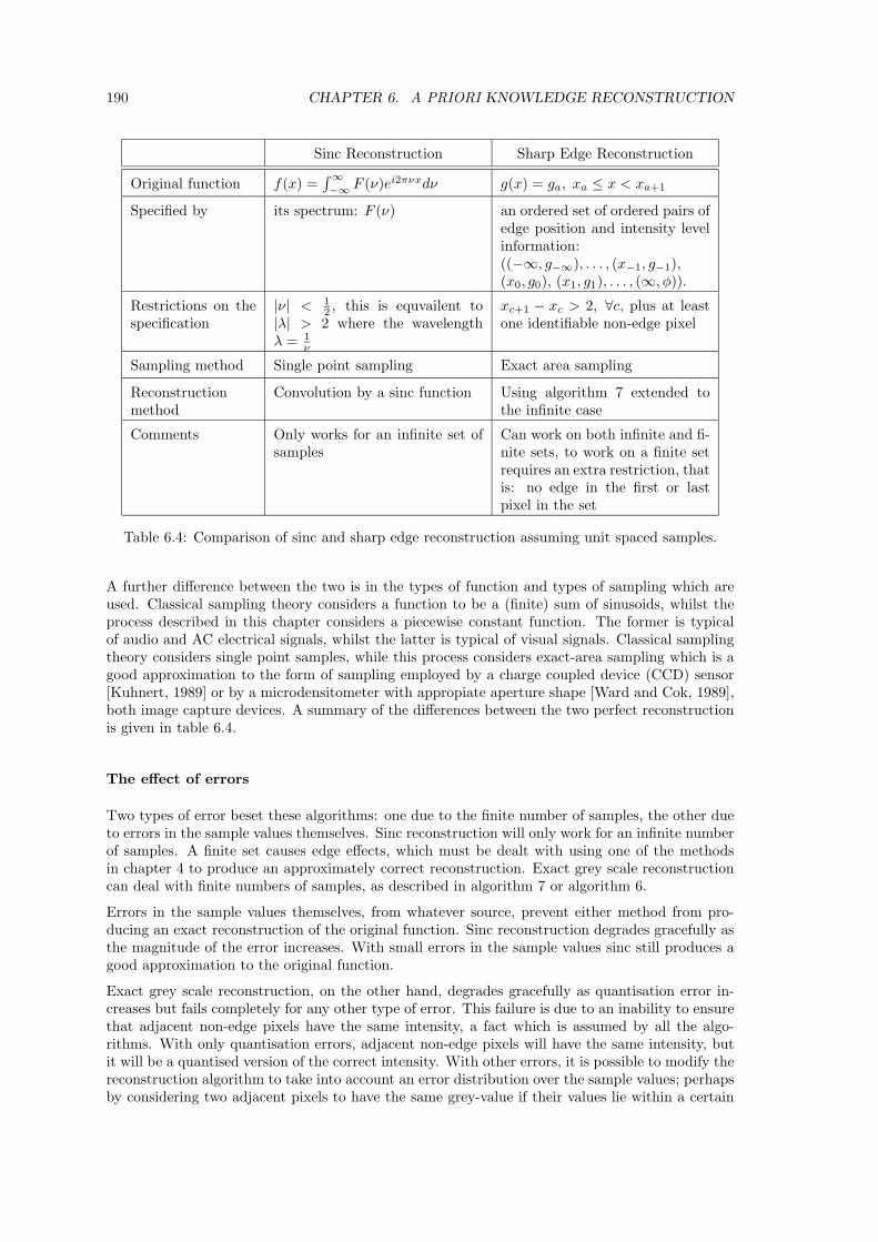
190 CHAPTER 6. A PRIORI KNOWLEDGE RECONSTRUCTION
Sinc Reconstruction Sharp Edge Reconstruction
Original function f(x) =∫∞−∞ F (ν)ei2πνxdν g(x) = ga, xa ≤ x < xa+1
Specified by its spectrum: F (ν) an ordered set of ordered pairs ofedge position and intensity levelinformation:((−∞, g−∞), . . . , (x−1, g−1),(x0, g0), (x1, g1), . . . , (∞, φ)).
Restrictions on thespecification
|ν| < 12 , this is equvailent to
|λ| > 2 where the wavelengthλ = 1
ν
xc+1 − xc > 2, ∀c, plus at leastone identifiable non-edge pixel
Sampling method Single point sampling Exact area sampling
Reconstructionmethod
Convolution by a sinc function Using algorithm 7 extended tothe infinite case
Comments Only works for an infinite set ofsamples
Can work on both infinite and fi-nite sets, to work on a finite setrequires an extra restriction, thatis: no edge in the first or lastpixel in the set
Table 6.4: Comparison of sinc and sharp edge reconstruction assuming unit spaced samples.
A further difference between the two is in the types of function and types of sampling which areused. Classical sampling theory considers a function to be a (finite) sum of sinusoids, whilst theprocess described in this chapter considers a piecewise constant function. The former is typicalof audio and AC electrical signals, whilst the latter is typical of visual signals. Classical samplingtheory considers single point samples, while this process considers exact-area sampling which is agood approximation to the form of sampling employed by a charge coupled device (CCD) sensor[Kuhnert, 1989] or by a microdensitometer with appropiate aperture shape [Ward and Cok, 1989],both image capture devices. A summary of the differences between the two perfect reconstructionis given in table 6.4.
The effect of errors
Two types of error beset these algorithms: one due to the finite number of samples, the other dueto errors in the sample values themselves. Sinc reconstruction will only work for an infinite numberof samples. A finite set causes edge effects, which must be dealt with using one of the methodsin chapter 4 to produce an approximately correct reconstruction. Exact grey scale reconstructioncan deal with finite numbers of samples, as described in algorithm 7 or algorithm 6.
Errors in the sample values themselves, from whatever source, prevent either method from pro-ducing an exact reconstruction of the original function. Sinc reconstruction degrades gracefully asthe magnitude of the error increases. With small errors in the sample values sinc still produces agood approximation to the original function.
Exact grey scale reconstruction, on the other hand, degrades gracefully as quantisation error in-creases but fails completely for any other type of error. This failure is due to an inability to ensurethat adjacent non-edge pixels have the same intensity, a fact which is assumed by all the algo-rithms. With only quantisation errors, adjacent non-edge pixels will have the same intensity, butit will be a quantised version of the correct intensity. With other errors, it is possible to modify thereconstruction algorithm to take into account an error distribution over the sample values; perhapsby considering two adjacent pixels to have the same grey-value if their values lie within a certain

6.4. TWO-DIMENSIONAL SHARP EDGE RECONSTRUCTION 191
distance of each other. Such a modification is left for future work.
An analysis of the algorithm’s performance for quantisation errors shows that, if the two greylevels either side of an edge quantise to the same qunatisation level, then that edge cannot bereconstructed at all: it ‘dissappears’. All other edges will tend to move slightly. The smaller thedifference in grey level either side of the edge, the larger the maximum possible difference in edgeposition between the original and the reconstructed functions, but the less visible the edge to theeye and so possibly, the less the eye will care about the shift. For N quantisation levels, when ∆g,the difference between adjacent grey levels, is ∆g � 1
N−1 ; this maximum shift in edge position isapproximately ± 1
∆g (N−1) . See appendix B.9 for details.
We have demonstrated that, in an error-free system, a class of intensity curves can be exactlyreconstructed by sharp edge reconstruction, which cannot be exactly reconstructed by classicalsampling theory methods. We now consider if such a class exists for two-dimensional intensitysurfaces.
6.4 Two-dimensional sharp edge reconstruction
The original intensity surface in this case consists of areas of constant intensity bound by sharpedges. The image is produced by taking exact-area samples off this intensity surface. We willconsider a square pixel grid and, without loss of generality, unit spaced samples. Thus if theoriginal function is g(x, y), then gi,j is taken over the area i ≤ x < i + 1, j ≤ y < j + 1; that is:
gi,j =∫ i+1
i
∫ j+1
j
g(x, y) dy dx
A good deal of research has been done on locating the positions of edges in images. These tend tobe developed for and tested on real, noisy images, and give approximate locations of edges in theimage. By constrast we are here assuming a perfectly sampled, perfect intensity surface — thus noerrors appear in the sample values. The aim is to ascertain whether, in the absence of any errors,perfect reconstruction is possible. If so, what criteria must the original intensity surface obey forperfect reconstruction to be possible.
6.4.1 Single point sampling case
Before looking at exact-area sampling, we examine how much information we can extract from asingle point sampled image. Here a pixel’s sample value is the value of the intensity surface atthe pixel’s center. An edge will thus be identifiable as being close to where adjacent pixels havedifferent intensities.
In the one-dimensional case the edge occurs in a single pixel, and thus the error in edge positionis ± 1
2 sample spaces. In the two dimensional case, an infinitely long edge will pass through aninfinite number of pixels. Thus there is potential to extract accurate information about the line’sslope and position by considering more of the evidence than a single pixel’s worth.
Theorem 4 If we have an intensity surface containing a single, infinitely long straight edge, singlepoint sampled over all Z2, then the slope of that edge can be exactly determined, whilst its positionmay have some inaccuracy.
Proof: Consider only edges with a slope between zero and one:
y = mx + c, 0 ≤ m ≤ 1
where the area below the edge is white and above it is black. All other cases can be transformedinto this case by rotation of 90n◦, n ∈ Z and/or reflection in the line y = 0.

192 CHAPTER 6. A PRIORI KNOWLEDGE RECONSTRUCTION
KeyPixel centre
Position of edge
Black pixel
White pixel
01 1 1 0 1 0 1hi
Figure 6.16: An example of a single point sampled single edge. The hi are a Rothstein code forthe edge.
For every integer x-coordinate we define a number hi, which is either one or zero, depending on thevalues of the pixels near the edge. To ascertain the value of hi we first find j such that gi,j �= gi,j+1,then:
hi ={
1, gi−1,j �= gi,j
0, gi−1,j = gi,j
Part of an edge is illustrated in figure 6.16, with the hi values given underneath. A value of 1indicates that this column contains the first white pixel on a row, a value 0 indicates that it doesnot.
. . . , h−1, h0, h1, h2, . . . is a Rothstein code describing the line [Weiman, 1980; Rothstein and Weiman,1976]. The slope of the line is the number of 1s in the sequence divided by the total number ofdigits in the sequence:
m = limk→∞
k∑i=−k
hi
k∑i=−k
1
(6.14)
If the sequence of hi values is aperiodic then equation 6.14 converges on the real value of m[Rothstein and Weiman, 1976, p.123]. A finite length fragment gives an approximation to the realslope [ibid., p.110]. These statements are also true for a periodic sequence of hi values, but in thiscase the value of m is rational. If the length of a period is q and each period contains p 1s thenthe slope is [ibid., p.109]:
m =p
q
Thus the slope of the edge can be exactly determined, in all cases, because we have an infinitenumber of hi values.
If hi is periodic (that is: m is rational) then the position, c, can only be determined to withinsome error bounds. If the slope is expressed as m = p
q with p and q relatively prime then c
can be determined with an error of ± 12q . This is illustrated in figure 6.17. The truth of this
error bound can be seen by finding the y-intercepts, yi, of the edge with each of the samplinglines; y = i + 1
2 , i ∈ Z. The fractional parts of these values repeat with period q, and within aperiod they are evenly spaced. Thus, if the fractional part of yi is ei = yi − �yi�, then, becauseyi+1 = yi + p
q , we can write, for some en:
en = o +np mod q
q(6.15)
where n is chosen so that en < 1q and thus o, the offset from zero, is such that o < 1
q .

6.4. TWO-DIMENSIONAL SHARP EDGE RECONSTRUCTION 193
KeyPixel centre
Position of edge
Black pixel
White pixel
1q
Figure 6.17: The error bounds on the position of a line of rational slope, in this case the slopem = p
q = 35 . The line can be positioned anywhere over a vertical distance of 1
q .
The values of ei are periodic, with period q. They are also evenly distributed. The minimumdifference between any two different values of ei is 1
q . Thus o can range over values up to 1q apart
and yet the same sample values will be generated. The error in the position, c, is plus or minushalf this number, that is ± 1
2q .
If we wish to know the positional error in the direction perpendicular to the edge, rather thanalong the y-axis then, given that the error along the y-axis is εy = ± 1
2q , then the positional errorperpendicular to the edge is:
ε⊥ = ± 1
2√
p2 + q2
If the sequence hi is aperiodic (that is: m is irrational), then we can condider the situation as qgoes to infinity:
limq→∞
ε⊥ = 0
Therefore, there exists only one possible position for a line of irrational slope, and c can be exactlydetermined in this case. QED.
For a finite length edge the slope can only be determined approximately. When a sequence of mhi values are available, h1, h2, . . . , hn, then the slope is approximated by:
m =
n∑i=1
hi
n
We can see that a good approximation to the line’s slope and position can be obtained from thesingle point sample case. Can the exact-area sample case improve on these results?
6.4.2 Exact area sampling — black and white case, single edge
Given an image, area sampled from an intensity surface consisting of a single edge between anarea of constant intensity zero and an area of constant intensity one, what can we say? Firstly theposition of the edge can be approximately determined from the location of the grey pixels in theimage. The edge must pass through all these grey pixels in the image. We call such pixels ‘edgepixels’. Secondly, the exact slope and positions of the edge should be determinable from a finitenumber of pixel values. (In the single point sample case an infinite number of pixel values wererequried to exactly determine the slope, and there existed situations where the position could notbe exactly determined).

194 CHAPTER 6. A PRIORI KNOWLEDGE RECONSTRUCTION
θρ
x
y
Figure 6.18: The (ρ, θ) parameterisation of a straight line. θ is the angle the line makes with thepositive x-axis, ρ is the perpendicular distance from the line to the origin.
Hypothesis: The position and slope of a single, infinitely long, straight edge between an area ofconstant intensity zero and an area of constant intensity one can be exactly determined from twoexact-area sample values.
This hypothesis has its foundation in the recognition that only two numbers are required to exactlyspecify a straight line. In section 6.3.1 we saw that a single number specified the position of a sharpedge in one dimension and that this positional information was coded in a single pixel values (plusone extra bit of orientation information which could be derived from a neighbouring pixel). Herewe will see that the slope and direction of a straight line are indeed coded in the sample valuesof two adjacent edge pixels plus some extra bits of orientation information, which can be derivedfrom neighbouring pixels. Because of the need for this orientation information, the hypothesis isincorrect, but it is not far from the truth.
The equation of a straight line
Three parameterisation of a straight line, which prove useful when determining the position of anedge, are:
1. y = mx + c, the standard equation of the line, using the slope, m, and y-intercept c, as theparameters. This equation for a straight line has problems in that a vertical line cannot berepresented and a small change in m makes a large difference in the line when m is smalland a small difference in the line when m is large, meaning that an error measure on m (oron c which has a similar problem) is difficult.
2. x = t cos θ + ρ sin θ, y = t sin θ − ρ cos θ, using parameters ρ and θ. ρ is the perpendiculardistance from the line to the origin, and θ is the angle the line makes with the positivex-axis (figure 6.18). These two parameters are better than m and c in that they render auniform description for any position and orientation (error bounds will be the same for allorientations and positions) and have no special case (such as the vertical lines in the previouscase) [Kitchen and Malin, 1987]. However, they can also make the algebra more difficult.
3. x = x0t, y = y0(1− t). The two parameters x0 and y0 are the x- and y-intercepts of the lineas shown in figure 6.19(a). This parameterisation can represent any line except one for whichx0 = y0 = 0, or a vertical or a horizontal line which does not pass through the origin. Analternative parameterisation using the same philosophy is that shown in figure 6.19(b) usingy0 and y1, the y-intercepts of the line at x = 0 and x = 1 respectively. This gives: x = t,y = (1 − t)y0 + ty1. This parameterisation cannot represent vertical lines.
Neither of these parameterisations renders a uniform description for all positions and orien-tations. In the former, for example, when either parameter is close to zero, a small changein the other will cause a large change in the line. However, both of these very similarparametrisations prove useful in the ensuing work.

6.4. TWO-DIMENSIONAL SHARP EDGE RECONSTRUCTION 195
x
y
x0
y0
x
y
y0
y1
x=1
(a) (b)
Figure 6.19: Two intercept parameterisations of a straight line. (a) in terms of its x- and y-axisintercepts, x0 and y0. (b) in terms of two y-intercepts, y0 and y1.
value = 0.25
value = 0.5
value = 0.75
0o 26.6o 45oθ
Figure 6.20: A single edge pixel’s value can represent an edge at any orientation. Here we see threepixel values (0.25, 0.5, and 0.75) each with five of the many possible edges that could pass throughthe pixel.
All three parameterisations completely determine the position and slope of a line in two parameters.It is therefore not unreasonable to expect that two pixel values will also completely determine theposition and slope of the edge.
What can one pixel value tell us?
To again simplify matters we consider only an edge with slope between zero and one, and withblack (intensity zero) above it and white (intensity one) below it. All other possible situations canbe transformed into this set of situations by reflection and/or rotation. The single edge pixel willhave a grey value between zero and one. Its value reduces the set of possible edges through thepixel from an infinite set to a smaller, but still infinite, set. Examples are shown in figure 6.20. Theambiguity in the line’s slope and position can be removed by considering the value of an adjacentedge pixel.
Before doing this we classify edge pixels into three groups based on how the edge passes throughthe pixel. Type I pixels have the edge passing through their bottom and right sides (figure 6.21(a)).Type II have the edge passing through the left and right sides (figure 6.21(b)), and Type III havethe edge passing through the left and top sides (figure 6.21(c)). No other combination of sidescan occur for an edge with slope between zero and one. Edges passing through the bottom-left ortop-right corner can be considered to be of any appropriate type.
If we now apply a local coordinate system to the pixel, with the origin at the bottom left cornerand the pixel of size 1 × 1 (figure 6.21(a)), then we can describe the edge simply using the thirdof our three parameterisations of a straight line on page 194. These descriptions are shown infigure 6.21(b), (c), and (d).

196 CHAPTER 6. A PRIORI KNOWLEDGE RECONSTRUCTION
x
y
1
0 1x
y
1
0 1
x
y
1
0 1x
y
1
0 1
1x
0x
1y
y0
1y y
0
(a) (b)
(c) (d)
Figure 6.21: The coordinate system for a pixel and the three types of pixel. (a) Local coordinatesystem for the pixel. (b) Type I pixel, parameterised by x0 and y1. (c) Type II pixel, parameterisedby y0 and y1. (d) Type III pixel, parameterised by y0 and x1.
Case Third intercept calculationI.II y2 = y1(1 + 1
1−x0)
I.III x2 = 1 + 1−y1y1
(1 − x0)
II.II y2 = 2y1 − y0
II.III x2 = 1−y0y1−y0
III.I y2 = y0 + 1−y0x1
Table 6.5: How the third intercept is calculated from the first two in all five possible cases.
The sample value, A, for each type of pixel can easily be determined using these simple formulae:
AI =12(1 − x0)y1 (6.16)
AII =12(y0 + y1) (6.17)
AIII = 1 − 12x1(1 − y0) (6.18)
The information that can be gathered from two adjacent edge pixels
Given an edge pixel we will consider also the next edge pixel to the right, or, if this is not an edgepixel, then the next edge pixel above. This gives the five possible situations shown in figure 6.22.No other situations are possible given the restrictions we have placed on edge orientation. In eachcase the third intercept is given the subscript 2 in order to save confusion and unify the notationfor all cases. This third intercept can be derived from the other two, because the first two uniquelydefine the lines. These derivations are shown in table 6.5.
Given the two pixel values, call the left one, A, and the right, B, it is possible to recover the values

6.4. TWO-DIMENSIONAL SHARP EDGE RECONSTRUCTION 197
1y
2x
0x
y0
2x
1y
2y
0x
1y
1xy
0
2y
y0
2y
1y
I.II
I.III
II.II
II.III
III.I
Figure 6.22: The five possible arrangements of two adjacent edge pixels for a line of slope betweenzero and one. Each is named by the types of the two pixels ordered from left to right, or bottomto top. The origin is always considered to be at the bottom left corner of the bottom left pixel.
of the first and second intercepts, thus uniquely determining the edge position and slope from thetwo pixels’ values.
Case II.II
This is the simplest case. The pixel values are given by:
A =12(y0 + y1)
B =12(y1 + y2)
=12(3y1 − y0)
where the last step is produced by replacing y2 with its equivalent equation in table 6.5.
Some fairly simple algebra leads to the results:
y0 =12(3A − B)
y1 =12(A + B)
From these, and table 6.5, we can also find y2:
y2 =12(3B − A)
The other four cases are not as simple as this. Rather than show the working here we present onlythe start and end of the algebraic manipulation.

198 CHAPTER 6. A PRIORI KNOWLEDGE RECONSTRUCTION
Case I.II
The equations for the pixel values are:
A =12(1 − x0)y1
B =12(y1 + y2)
= y1 +y1
2(1 − x0)
which produce these equations for the intercepts:
y1 = −2A + 2√
A2 + AB
x0 = 1 − 2A
−2A + 2√
A2 + AB
For the denominator to be zero in the latter equation requires A = B = 0, which means that theedge passes along the lower boundary, rather than intercepting it, so the value of x0 is undefined.Such a situation should be considered as case II.II, not case I.II.
Case I.III
The equations for the pixel values are:
A =12(1 − x0)y1
B = 1 − 12(x2 − 1)(1 − y1)
= 1 − 12
(1 − y1)2
y1(1 − x0)
which produce these equations for the intercepts:
y1 =√
A√A +
√1 − B
x0 = 1 − 2A − 2√
A(1 − B)
For the denominator to be zero in the equation for y1 requires A = 0 and B = 1, which impliesthat the slope of the line is greater than one. Therefore this situation cannot arise.
Case II.III
The equation for the pixel values are:
A =12(y0 + y1)
B = 1 − 12(1 − y1)(x2 − 1)
= 1 − 12(1 − y1)
(1 − y0
y1 − y0− 1
)which produce these equations for the intercepts:
y1 = 1 + 2(1 − B) − 2√
(1 − B)2 + (1 − A)(1 − B)
y0 = 1 − 2(1 − A) − 2(1 − B) + 2√
(1 − B)2 + (1 − A)(1 − B)

6.4. TWO-DIMENSIONAL SHARP EDGE RECONSTRUCTION 199
III.I I.III I.II II.III II.II II.IIy0 2 − x2 x0 2 − x2 y0 1 − y2
x1 1 − y1 y1 1 − y1 y1 1 − y1
y2 2 − x0 y2 1 − y0 y2 1 − y0
A B A 1 − B A 1 − BC A B 1 − A B 1 − A
Table 6.6: The equivalences between the various cases. Note that II.II is equivalent to itself.Substituting the values in the right hand column in the place of those in the left hand column inthe left hand case’s equations will produce the right hand case’s equations.
Case III.I
This is different from the other four cases in that it uses the pixel above pixel A, rather than tothe right. We will identify this pixel’s value as C. The pixel to the right has value B = 1. Theequations for the pixel values are:
A = 1 − 12(1 − y0)x1
C =12(1 − x1)(y2 − 1)
=12
(1 − x1)2
x1(1 − y0)
which produce these equations for the intercepts:
x1 =√
1 − A√1 − A +
√C
y0 = 1 − 2(1 − A) − 2√
(1 − A)C
For the denominator to be zero in the equation for x1 requires A = 1 and C = 0, which meansthat the edge passes along the boundary between the two pixels, rather than intercepting it, sothe value of x1 is undefined. Such a situation should be considered as case II.II, not case III.I.
Equivalences between cases
In figure 6.22 we can see that cases I.II and II.III are very similar. By a substitution of variablesone case can be made equivalent to the other, thus linking the sets of equations for the two cases.The same is true of cases I.III and III.I. The equivalences are shown in table 6.6. Substituting thevalues in the right hand column in the place of those in the left hand column in the left hand case’sequations will produce the right hand case’s equations.
Identifying the case
Given the edge pixel, of value 0 < A < 1, if the next pixel to the right is not an edge pixel (that is:B = 1) then we know that we have case III.I. The pixel, of value C, above pixel A is used in thecalculation. If C = 0 and B = 1 then the edge passes through the top right corner of the pixel.Case III.I still calculates the intercepts correctly; they are:
x1 = 1y0 = 2A − 1
If 0 < B < 1 then we could be dealing with any of the other four cases. Fortunately the values Aand B uniquely identify which to apply.

200 CHAPTER 6. A PRIORI KNOWLEDGE RECONSTRUCTION
A B
C
Figure 6.23: The arrangement of pixels A, B, and C.
I.II I.III II.II II.III0 ≤ x0 ≤ 1 0 ≤ x0 ≤ 1 0 ≤ y0 ≤ 1 0 ≤ y0 ≤ 10 ≤ y1 ≤ 1 0 ≤ y1 ≤ 1 0 ≤ y1 ≤ 1 0 ≤ y1 ≤ 10 ≤ y2 ≤ 1 1 ≤ x2 ≤ 2 0 ≤ y2 ≤ 1 1 ≤ x2 ≤ 2
Table 6.7: The restrictions on the values of the parameters in the four cases which use pixels Aand B.
Possible values of A and B are restricted to lie in the square:
0 ≤ A ≤ 1
0 ≤ B ≤ 1
Further restrictions are produced by making the slope of the edge lie between zero and one: aminimum slope of zero means that
A ≤ B
A maximum slope of one affects only case, I.III, where it implies that x2 − x1 ≥ 1 (in the otherthree cases the slope can never exceed one). Working through the algebra of this gives us therestriction:
B ≤ 12− A +
√2A, 0 ≤ A ≤ 1
2
These four restrictions define the boundary in figure 6.24 within which A and B must lie. Theother lines in figure 6.24 are set by restricting the values of the intercepts in each case to lie withinthe boundaries listed in table 6.7. These lines bound the areas with which each case deals.
Some involved algebraic manipulation or a dense sampling of A,B pairs will determine whichareas within the boundary are dealt with by each case. Figure 6.25 shows these areas. They donot overlap and completely fill the area within the boundary. The boundaries between the variousareas are where the edge passes through the corner of one of the pixels. These are illustrated infigure 6.26, along with the situations that occur at the boundaries of the whole area.
These results are all well and good for edges with a slope between zero and one, allowing usto exactly reconstruct the line from two adjacent sample values. It leaves the question of howto identify the orientation of a general edge so that it can be transformed to this case and itsintercepts determined.
Identifying the orientation
Given two edge pixels A and B, arranged as shown in figure 6.23, the orientation of the edge canbe determined to one of two octants. This is shown in figures 6.27 and 6.28. A similar diagram canbe drawn for edge pixels A and C arranged as in figure 6.23. Examples are given in figure 6.29.To determine which of these two choices is correct we require more information than supplied bythe two pixel values.

6.4. TWO-DIMENSIONAL SHARP EDGE RECONSTRUCTION 201
A0 0.25 0.5 1
B
0
0.5
075
1
boun
dary
L
L
L
L
1
2
3
4
Figure 6.24: The restrictions on A and B values for the various cases, this figure shows the boundinglines of the areas covered by each case. The light line shows the boundary within which A,B pairsmust lie, the equations defining this boundary are given in the text. The other four lines aregenerated by imposing the restrictions in table 6.7. They are:
L1: B = 2 − A − 14A
L2: A = (B− 12 )2
1−B
L3: B = 1 − 13 (1 − A)
L4: B = 3A

202 CHAPTER 6. A PRIORI KNOWLEDGE RECONSTRUCTION
I.II II.II
I.III II.III
I.II
II.IIII.III
II.II
Figure 6.25: The four disjoint areas covered by the four cases.
(a) (b) (c)
(d) (e)
(f) (g)
(h) (i) (j)
(k) (l) (m)
Figure 6.26: The special cases, on boundaries in figure 6.25. They are defined by their locationsin (A,B) space. (a) (0, 1
2 ), the point on the left boundary where I.II meets I.III; (b) (14 , 3
4 ), thepoint in the middle where all four regions meet; (c) (1
2 , 1), the point on the top boundary whereI.III and II.III meet; (d) (0, 0), the bottom left corner; (e) (1, 1), the top right corner; (f) movingalong the boundary line A = B from (0, 0) to (1, 1); (g) moving around the boundary from (0, 1
2 )to (1
2 , 1); (h) moving along the top boundary from (12 , 1) to (1, 1); (i) moving along L3 from (1
4 , 34 )
to (1, 1); (j) moving along L2 from (0, 12 ) to (1
4 , 34 ); (k) moving up the left boundary from (0, 0) to
(0, 12 ); (l) moving along L4 from (0, 0) to (1
4 , 34 ); (m) moving along L1 from ( 1
4 , 34 ) to (1
2 , 1).

6.4. TWO-DIMENSIONAL SHARP EDGE RECONSTRUCTION 203
α
β
γ
δ0
0.5
1
0 0.5 1
B
A
Figure 6.27: These are four areas of A,B space: corresponding to four pairs of octants. We havebeen considering area β. An edge in any area can be identified to be in either of two possiblelocations, shown in figure 6.28.
octant 2octant 7
αCase octant 1
octant 4
Case β
octant 5
octant 8Case γ
octant 3octant 6
δCase
Figure 6.28: The four areas in figure 6.27 can identify an edge to be one of just two possibilities.In each case these two edges lie in two different quadrants. Examples are shown here for each case.
13
23
(a)(i)
(a)(ii)
(a)(iii)
18
78
(b)(i) (b)(ii) (b)(iii)
Figure 6.29: Two examples of the two possibilities for a given pair of adjacent grey pixel values.(a)(i) can represent either (a)(ii) or (a)(iii), (b)(i) can represent either (b)(ii) or (b)(iii).
µ ν
A B
κ C λ
Figure 6.30: The 3 × 3 context of the edge pixel A, with the pixel labels used in the text.

204 CHAPTER 6. A PRIORI KNOWLEDGE RECONSTRUCTION
Exclusion
Zone
4 samplespacings
4 samplespacings
Figure 6.31: To ensure that every edge generates at least one edge pixel at the centre of a 3 × 3context through which no other edge passes, there must be at least one edge point on every edgesuch that no other edge passes through a 4 × 4 sample spacing ‘exclusion zone’ cantered on thatedge point.
If we pick a single edge pixel and use the 3× 3 pixel region around it we can be certain to get theorientation right. The 3 × 3 region is illustrated in figure 6.30. If the 3 × 3 region is rotated andreflected so that κ ≤ λ ≤ µ ≤ ν then we can be certain that the edge is in the first octant. We canthen apply our equations to A and B (or A and C, if B = 1) and then transform the results backto the correct octant. Note that, after rotation and reflection, κ = 0 and ν = 1.
6.4.3 Extension to grey scale — single edge
A single edge, where the intensity on either side may have any value, can be exactly reconstructedas easily as a black and white edge. Taking a 3× 3 area, as in figure 6.30. Again rotate and reflectit so that κ ≤ λ ≤ µ ≤ ν. Then, if A �= κ and A �= ν, A is an edge pixel. All values in the 3 × 3square can be modified so that κ = 0 and ν = 1. Taking o to be the old pixel value and m, themodified pixel value, the modification is simply
m =o − κ
ν − κ
for each pixel value. The edge can now be found in the same way as for the black and white case.
6.4.4 Extension to many edges
Many edges in an intensity surface means that it consists of areas of constant intensity separatedby sharp edges. Provided every edge generates at least one edge pixel at the centre of a 3×3 blockof pixels through which no other edges run, then the method of the previous section can be usedto find the slope and position of all the edges in the image.
To ensure that every edge generates at least one block of pixels of this type there must be atleast one position along the edge such that no other line passes inside a square of side four samplespacings centred at that point. An example is given in figure 6.31. A 4 × 4 region is requiredbecause we do not necessarily know where the pixel edges are going to fall, but we can be surethat there will be a 3× 3 pixel block inside this 4× 4 exclusion zone, and that the central pixel ofthis block will contain this edge point, thus this central pixel will be an edge pixel.

6.4. TWO-DIMENSIONAL SHARP EDGE RECONSTRUCTION 205
Potential edge pixel
Potential area pixel
Pixel that has beenidentified as both apotential edge and apotential area pixel
An edge
Key
Figure 6.32: The algorithm discussed in the text would classify the pixels as shown for this com-bination of edges.
Figure 6.33: No edge can generate three edge pixels of the same intensity in any of these L-shapedarrangements.
How edge pixels are found
This restriction on the original intensity surface ensures that there will be at least one 3 × 3 pixelblock for every edge through which no other edge passes. This allows us to calculate the slope andposition of the edge. The problem is now to separate those 3 × 3 blocks which contain a singleedge from those which contain no edges or which contain two or more edges.
One solution to this problem is to first find all of the four-connected areas of constant intensityand mark all of the eight-connected neighbours of this area as potential edge pixels. An exampleis shown in figure 6.32. The second step is to apply our equations to the 3 × 3 region aroundeach potential edge pixel (and any pixels which were not identified as either potential edge pixelsor area pixels). The edge information is only retained for those regions for which it is consistentwith the pixel values. This gives us the position and slope of all edges in the image.
These two steps need some fleshing out. The first step, area-finding, is achieved by a singleobservation and a modification of a well-known algorithm. The observation is that no single edgecan generate three edge-pixels of the same intensity in an L-shaped arrangement (those illustratedin figure 6.33). Such an arrangement of three pixels can thus be assumed to be part of an areaor caused by a combination of several edges. In the first case none of the three pixels is an edgepixel, in the latter, none is at the centre of a 3 × 3 block containing only a single edge. Thus nopixel identified by this method need be passed to the second step.
A pixel from an L-shaped block of three of the same intensity can be used as the seed to a flood-fillalgorithm [Foley et al, pp.979–982]. Every pixel in the filled area is identified as a possible areapixel and every pixel not in, but eight-connected to, the area is identified as a possible edge pixel.This process is repeated until all identifiable areas have been flood-filled. If an L-shaped block isgenerated by multiple edges the whole algorithm should still work, because neither these pixels,nor any pixel of the same intensity four-connected to them, will uniquely identify a single edge.

206 CHAPTER 6. A PRIORI KNOWLEDGE RECONSTRUCTION
Note that some pixels may be identified as both possible edge pixels and possible area pixels (forexample: when an edge falls on a pixel boundary), this is not a problem and, for the next stage,these pixels should be treated as possible edge pixels.
In the second step every possible edge pixel is processed individually. All pixels that have not beenidentified as possible edge or possible area pixels must also be processed. Such pixels may arise ina small single pixel wide area with no L-shaped group of pixels in it.
An attempt is made to rotate and reflect the 3×3 region centred on each pixel so that κ ≤ λ ≤ µ ≤ νin figure 6.30. If this is impossible then we can be certain that more than one edge pixel passesthrough this region, otherwise we apply our equations to generate a slope and direction for anedge, along with the intensity on either side of the edge. These four values can then be used togenerate pixel values for all nine pixels in the region. If these match the true pixel values thenthere is only one edge in the region and we can output the edge parameters and the grey valueseither side of the edge, otherwise we ignore these values. This will generate the parameters for allof the edges in the image (duplicate sets of parameters can be discarded).
This process gives us the slope and positions of all the edges in the image, because every edgehas at least one pixel in a 3 × 3 area which will uniquely identify it. As a byproduct the processgives us the intensities of the areas either side of each edge. What it does not give us are the endpoints of the edges. However, for a scene to be consistent all areas must be of constant intensityand bound by straight edges. Hence it should be possible for an algorithm to be devised whichgenerates the end points of all the edges given the image, the slopes and positions of all the edges,and the grey values either side of each edge; all of which can be derived from the above methodsand equations. Such an algorithm has not been developed, it is left for future work. Some idea ofhow if could operate is given below:
Every edge’s edge pixels are rendered assuming that it is the only edge in the image.The values produced are compared with the values in the image and all correct valuesnoted as being pixels through which this edge is likely to be the only edge. The pixels ateither end of a run of such edge pixels are likely to contain two or more edges. Such endpixels can be rendered using all suitable edges in the description. If the correct value isgenerated it is likely that the edges used pass through the pixel. Intersections betweenedges must be found to render these pixel values and these intersections are likely tobe the ends of lines. When three or more edges pass through a pixel all combinationsof intersections may need to be tried to find the correct one.
Without designing such an algorithm it is impossible to say whether or not any extra restrictionsmust be placed on the input intensity surface to allow for exact reconstruction.
6.4.5 Discussion
Whether or not extra restrictions are required, this work shows that there exists a class of two-dimensional intensity surface which can be exactly reconstructed from their exact-area sampledimages. Apart from the trivial, constant intensity surface, no member of this class can be exactlyreconstructed from its single point sampled image using classical sampling theory.
Such an exact reconstruction would be extremely useful in resampling as it allows the resamplingto produce the best possible resulting image. However, the class of intensity surfaces that can beexactly reconstructed by this method is extremely limited.
Real images
Several types of real image could potentially be exactly reconstructed by these methods. Forexample: printed matter (text and diagrams) and especially cartographic documents (maps) may
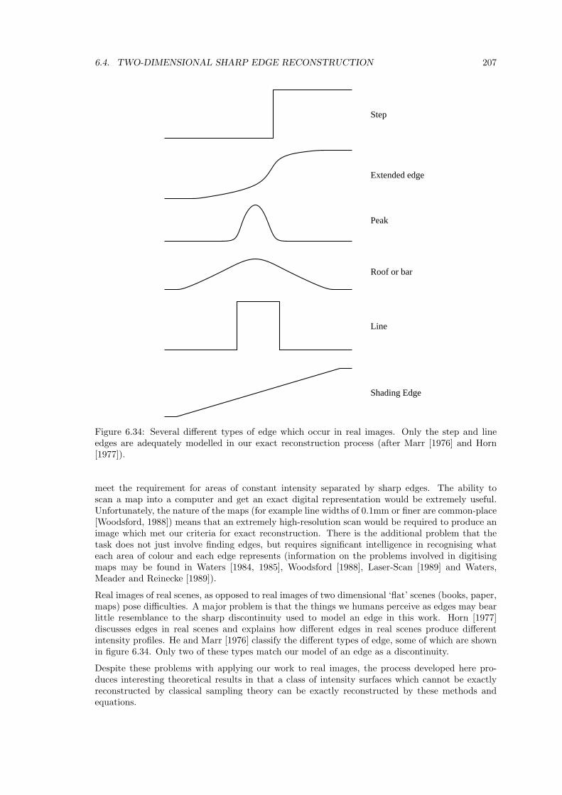
6.4. TWO-DIMENSIONAL SHARP EDGE RECONSTRUCTION 207
Step
Extended edge
Peak
Roof or bar
Line
Shading Edge
Figure 6.34: Several different types of edge which occur in real images. Only the step and lineedges are adequately modelled in our exact reconstruction process (after Marr [1976] and Horn[1977]).
meet the requirement for areas of constant intensity separated by sharp edges. The ability toscan a map into a computer and get an exact digital representation would be extremely useful.Unfortunately, the nature of the maps (for example line widths of 0.1mm or finer are common-place[Woodsford, 1988]) means that an extremely high-resolution scan would be required to produce animage which met our criteria for exact reconstruction. There is the additional problem that thetask does not just involve finding edges, but requires significant intelligence in recognising whateach area of colour and each edge represents (information on the problems involved in digitisingmaps may be found in Waters [1984, 1985], Woodsford [1988], Laser-Scan [1989] and Waters,Meader and Reinecke [1989]).
Real images of real scenes, as opposed to real images of two dimensional ‘flat’ scenes (books, paper,maps) pose difficulties. A major problem is that the things we humans perceive as edges may bearlittle resemblance to the sharp discontinuity used to model an edge in this work. Horn [1977]discusses edges in real scenes and explains how different edges in real scenes produce differentintensity profiles. He and Marr [1976] classify the different types of edge, some of which are shownin figure 6.34. Only two of these types match our model of an edge as a discontinuity.
Despite these problems with applying our work to real images, the process developed here pro-duces interesting theoretical results in that a class of intensity surfaces which cannot be exactlyreconstructed by classical sampling theory can be exactly reconstructed by these methods andequations.

208 CHAPTER 6. A PRIORI KNOWLEDGE RECONSTRUCTION
(a) (b) (c)
Figure 6.35: Layout of CCD sensors. The solid lines show the receptive area of each pixel’s sensor.(a) common CCD sensor, (b) advanced CCD sensor, (c) ideal CCD sensor. (After Kuhnert [1989]fig 3.)
Errors
As in the one-dimensional case, the introduction of errors causes problems. Again, quantisationerror introduces an inaccuracy into the calculated edge parameters, while other errors requireparameter calculations based on probabilities rather than being deterministic as they have been inthe above discussion.
The advantage here over the one-dimensional case is that every line has many edge pixels andeach pair of these can be used to estimate the slope and position of the line (note that not onlyadjacent pairs of edge pixels can be used, but any two edge pixels provided we know their types(I, II, or III) and their relative position). Also the position of all the edge pixels in the pixel gridgives bounds on the slope and position of the line, because the line has to pass through all of itsedge pixels. Therefore we can expect to be able to generate a fairly accurate approximation froma noisy image provided that none of the edges are very short.
Other published work
Klassman [1975] considered the case of thick lines. These can be considered as two parallel edgesbetween which lies a black region and outside which lie two white regions. Klassman’s resultsindicated that, even with no errors in the pixel values, there will always be an error in the estimatedposition of the line no matter how thick it is. Our process, on the other hand, would be able toexactly find the position the line provided its width is such that the 4×4 exclusion zone constraintis satisfied for some point on each edge.
Kuhnert [1989] considers rectangular pixels as used in a CCD device, he gives three types of CCDcell, shown in figure 6.35. We have been using an ideal CCD-sensor layout (figure 6.35(c)). Kuhnertuses the advanced layout (figure 6.35(b)). He considers an edge between two areas of constantintensity but concludes that his model of the sensor does not permit a unique conclusion on theposition and slope of the edge. He says that this is unsurprising given that the original intensitysurface violates the sampling theorem. However, we have seen here that exact reconstruction ofsuch an intensity surface is possible, given exact-area sampling.
Hyde and Davis [1983] consider a similar situation to ours: a single edge, of finite length, betweentwo areas of constant intensity. They use two least-squares edge estimation techniques, assumingsome noise in the image. The first step, which they assume is done for them, is to identify the edgepixels. Then, one technique gives the least-squares edge fitted to the centres of the edge pixels,that is: no intensity information is utilised. This is similar to the black and white case discussedin section 6.4.1. The second technique gives a least-squares fit based on the intensity values of theedge pixels. The sum of the squares of the difference between the true intensity values and theestimated intensity values, is minimised.
Their conclusion is that the differences between the two techniques are not significant enough towarrant the use of the second, more costly technique. That is: taking the intensity values intoconsideration gives little advantage over simply using the position of all the edge pixels to calculatethe edge’s parameters. Compare this with our method which gives the exact position of an edge,
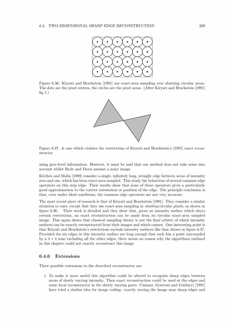
6.4. TWO-DIMENSIONAL SHARP EDGE RECONSTRUCTION 209
Figure 6.36: Kiryati and Bruckstein [1991] use exact-area sampling over abutting circular areas.The dots are the pixel centres, the circles are the pixel areas. (After Kiryati and Bruckstein [1991]fig 1.)
Figure 6.37: A case which violates the restrictions of Kiryati and Bruckstein’s [1991] exact recon-structor.
using grey-level information. However, it must be said that our method does not take noise intoaccount whilst Hyde and Davis assume a noisy image.
Kitchen and Malin [1989] consider a single, infinitely long, straight edge between areas of intensityzero and one, which has been exact-area sampled. This study the behaviour of several common edgeoperators on this step edge. Their results show that none of these operators gives a particularlygood approximation to the correct orientation or position of the edge. The principle conclusion isthat, even under ideal conditions, the common edge operators are not very accurate.
The most recent piece of research is that of Kiryati and Bruckstein [1991]. They consider a similarsituation to ours, except that they use exact-area sampling in abutting circular pixels, as shown infigure 6.36. Their work is detailed and they show that, given an intensity surface which obeyscertain restrictions, an exact reconstruction can be made from its circular exact-area sampledimage. This again shows that classical sampling theory is not the final arbiter of which intensitysurfaces can be exactly reconstructed from their images and which cannot. One interesting point isthat Kiryati and Bruckstein’s restrictions exclude intensity surfaces like that shown in figure 6.37.Provided the six edges in this intensity surface are long enough that each has a point surroundedby a 4 × 4 zone excluding all the other edges, there seems no reason why the algorithms outlinedin this chapter could not exactly reconstruct this image.
6.4.6 Extensions
Three possible extensions to the described reconstructor are:
1. To make it more useful this algorithm could be altered to recognise sharp edges betweenareas of slowly varying intensity. Then exact reconstruction could be used at the edges andsome local reconstructor in the slowly varying parts. Cumani, Grattoni and Guiducci [1991]have tried a similar idea for image coding: exactly storing the image near sharp edges and

210 CHAPTER 6. A PRIORI KNOWLEDGE RECONSTRUCTION
storing very little information in the slowly varying areas between regions. Such an ideacould be tried with resampling where the intensity surface in the slowly varying regions isreconstructed differently to that near the edges.
2. A straight edge can be represented by two parameters. A circle by three. An extension couldbe made to find a circle’s parameters from three pixel values on the circle’s edge. Preliminaryresults show that the algebra involved in these computations is considerably more involvedthan that for straight edges.
3. Two problems with images that have been enlarged using good NAPK reconstructors are:(1) the straight edges become blurry; and (2) textured areas do not reveal any finer texture(for example, enlarging a tree produces a blurry tree, you do not see more of the tree’sstructure). Kajiya and Kay [1989] call this effect ‘the painter’s illusion’. The image gives theimpression that more detail is there at the sub-pixel level than is actually present. When theimage is enlarged this lack of fine detail becomes readily apparent. The work in this sectionhas attempted to solve the first of the two problems. An extension would be to tackle thesecond: how to reconstruct, or resample, a textured region so that the resampled image isvisually acceptable.
6.5 Summary
We have seen that, given knowledge about how an image was sampled, a better reconstructedintensity surface can be generated. The bulk of this chapter dealt with sharp edge reconstruction.We have proven that, for a certain set of one-dimensional intensity curves, exact reconstruction ispossible from the exact area sampled image of an intensity curve in the set. We have also givenstrong evidence that a similar result holds in two dimensions.
The significance of this result is two-fold. Firstly, it shows that classical sampling theory is notthe final word on which intensity surfaces can be exactly reconstructed from images. Secondly,it indicates that a good reconstruction of this particular class of real intensity surface may bepossible.

Chapter 7
Transforms & Resamplers
In this chapter we draw together the threads of reconstruction, sampling, and transformation. Wediscuss the overall resampler, the measurement of quality, and some points about transforms ingeneral.
The transform is at the heart of the resampling. The other two sub-processes can be consideredas simply format converters (chapter 1) allowing the transform to be performed in the continuousdomain, where it is simple, rather than in the discrete domain, where it is complicated. In generalthe transform moves intensity information around but neither loses nor adds any information.Reconstruction and sampling, on the other hand, tend to be lossy operations.
Thus, it is the choice of reconstructor and sampler which determines the quality of the overallresampler. These should therefore be the best possible, regardless of the transform. For certainclasses of images there are perfect reconstruction and sampling processes, but, for the averageimage, such perfect processes do not exist. So we must content ourselves with the best imperfectresampler that we can implement.
Before we continue we need to note that, in chapter 1, a resampler consisted of a specific recon-structor, transform, and sampler. Often however, we will wish to discuss the same reconstructorand sampler coupled with many different transforms, or some class of transforms. In these caseswe still speak of a resampler but it is one in which the transform can be any of a set of transformsor sometimes any transform at all, whilst the reconstructor and sampler remain fixed.
7.1 Practical resamplers
In general the better the reconstructor or sampler, the more difficult it is to implement and so weneed to trade off between a good reconstructor or sampler and an easily implemented one. We needto make as many simplifications as possible, with the least effect on quality in order to produce aquick, practical, and good resampler.
For certain transforms it transpires that changing the reconstructor or changing the sampler makeslittle difference on the overall result of the resampling, while changing the other can make a greatdifference. Heckbert [1989, pp.51–52] shows that, for large magnifications, the reconstructionmethod dominates the resampler and the sampler is irrelevant, so it may as well be a single pointsampler for simplicity. He also shows that for large minification the sampling method dominates,and the reconstructor is irrelevant. In this case we can use a simple reconstructor with much thesame effect as a complex one.
For a resampler which may have to cope with both large magnifications and large minifications,we require either a good reconstructor and a good sampler, or some sort of combination where a
211
212 CHAPTER 7. TRANSFORMS & RESAMPLERS
switch is made from a good magnification resampler to a good minification resampler as the scalefactor passes through one [Heckbert, 1989, p.52].
Near a scale factor of one, the evidence indicates that changing the sampler makes little or nodifference to the quality of the resampled image1, and that there is little to choose between thequality offered by the better reconstructors. With a magnification factor near one, reconstructionby nearest-neighbour produces noticeable artifacts and reconstruction by linear interpolation oftengives a blurry result, but other methods produce few, if any artifacts (see section 7.3.2 whichdiscusses the effect of reconstructors at large scale factors compared with their effect at a scalefactor of one). Therefore, good samplers are required for minification, and good reconstructorsrequired for same-scale operations and magnification.
7.1.1 Restricted resamplers
While theoretical resamplers can be applied to any transform, a practical resampling method mayonly be applicable to a limited set of transforms. A resampler employing point sampling can beused with any invertible transform provided that the reconstructor can give the value of the originalintensity surface at an arbitrary point. An invertible transform here is one for which any outputpoint can be mapped, by the computer program, to a point in the input intensity surface. Manytransforms are covered by this restriction. Those which are not can be closely approximated bytransforms which are.
Practical resamplers which employ area sampling tend to be more restricted in the types of trans-forms they can be used with. This restriction is due to their implementation, discussed in sec-tion 1.8.2. Greene and Heckbert [1986], for example, consider a resampler composed of a Gaussianreconstructor and a Gaussian area sampler. This resampler only works with affine transforms.However, a local affine approximation to the true transform can be used, allowing the recon-structor to approximate the correct results for a wide range of transforms. Other area samplingresamplers give a transform-dependent approximation to a transform-independent sampler. Suchresamplers include those developed by Crow [1984], Glassner [1986], and Fournier and Fiume [1988].Their starting point in algorithm development is a transform-independent area sampler. The finalalgorithm has a transform-dependent area sampler in order to be practical.
Williams [1983] has an interesting approach to approximating a nearest-neighbour reconstruc-tion/exact area sampling resampler. If we look at his entry in appendix A, we see that his methodis equivalent to point sampling off a three-dimensional reconstructed volume. The first two dimen-sions are the usual spatial coordinates whilst the third dimension, d, is related to the size of theoutput pixel projected back onto original image space. The volume is created by first minifyingthe image several times (by a nearest-neighbour reconstruction/exact area sampling resampler) togenerate an image pyramid. Each image in the pyramid is then reconstructed by linear interpo-lation and the whole volume filled in by linear interpolation between the intensity planes in thepyramid (figure 7.1).
7.1.2 Resampler equivalences
The implementation of an area sampler, described in section 1.8.2, is possible because of the equiv-alence of two different decompositions. In general, any resampler can be decomposed in manydifferent ways; the transform remaining the same but the reconstructor and sampler being dif-ferent. As an example, consider a resampler consisting of nearest-neighbour reconstruction, a
1The evidence, indicating this result for samplers, is in the papers which discuss resampling for geometric cor-rection of images. Such correction does not require large scale changes and none of these papers discuss any formof sampling other than single point. Our own observations indicate that an exact area sampler makes no appre-ciable difference in near-same scale transforms, compared with single point sampling, unless a nearest-neighbourreconstructor is used.

7.2. TRANSFORM DIMENSIONALITY 213
Image Pyramid Intensity Surfaces Intensity Volume
d=0
=1d
=2d
=3d
=4d
xy
xyd
LinearInterpolation
LinearInterpolation
Figure 7.1: Williams’ [1983] reconstructor. An image pyramid is formed by nearest-neighbour/exact area scaling by a factor of two, several times. Each level of the pyramid is thenenlarged by linear interpolation, and then the third dimension is filled in by linear interpolationbetween the resulting intensity surfaces.
Reconstruction Filter Transform Sampling Filter
(a) translation
(b) ���� translation �
(c) � translation ����
Figure 7.2: Three equivalent decompositions of the same reconstructor: (a) nearest-neighbour/exact area, (b) linear/single point, and (c) delta-function/triangle filter.
translation, and exact area sampling. This same resampler can be decomposed into linear interpo-lation and single point sampling; or into Dirac delta function reconstruction and triangle filteredarea sampling. These three decompositions are illustrated in figure 7.2, for one dimensional sig-nals. If we now change the transform, these three decompositions are no longer equivalent. Forexample: take a resampler with nearest-neighbour reconstruction, scaling transform, and exactarea sampling. Its equivalent decomposition with point sampling is shown in figure 7.3. The re-constructor depends on the scale of the transform. This equivalence can lead to confusion. Durandand Faguy [1990] for example, mistakenly equate scaling using nearest-neighbour reconstructionand exact area sampling with scaling using linear intepolation and single point sampling, whenthis equivalence is only correct for a scale factor of one.
For a general transform using transform-independent reconstruction and area sampling, the equiva-lent decomposition with single point sampling will have a reconstructor that is transform-dependent.We hypothesise that, given a transform-independent reconstructor, an arbitrary transform, and atransform-independent sampler, any equivalent resampler will have a transform-dependent recon-structor and/or a transform-dependent sampler. This hypothesis shows why area sampling resam-plers are so much more difficult to implement than point sampling ones. It is because, in the methodof section 1.8.2, the area sampler has to be converted to a point sampler to be implementable, andso the reconstructor in the equivalent point sampling resampler is transform-dependent, and hencedifficult to implement.
7.2 Transform dimensionality
Resampling has been applied to one-, two-, and three-dimensional images. One use of resamplingis in texture mapping where a two-dimensional image is mapped onto a three-dimensional surfacewhich is then projected onto a two-dimensional plane, giving an overall 2D to 2D transform. Imagewarping and rectification are also generally 2D to 2D transforms.
For any dimensionality the theory is much the same. However, resamplings where a many di-

214 CHAPTER 7. TRANSFORMS & RESAMPLERS
Reconstruction Filter Transform Sampling Filter
(a)�
�1
�� 1
scale ×k�
�1
�� 1
(b)
k < 1
�� 1 � �1� �1 + 1
k
�
�k
k = 1 ��
���
�� �2
�
�1
k > 1 ��� �
��
� �1k
�� 1k� �1 + 1
k
�
�1
scale ×k �1
Figure 7.3: Two equivalent decompositions of the same reconstructor: (a) nearest-neighbour/exactarea, (b) a transform-dependent reconstructor combined with point sampling. A third decomposi-tion could be generated with delta-function reconstruction and a transform-dependent sampler.
& Shear
Nearestneighbourreconstruct
Exact-areasample
& Shear
Nearestneighbourreconstruct Exact-area
sample
(a)
(b)
In two dimensions
For eachscan line
Figure 7.4: A shear transform, with nearest-neighbour reconstruction and exact area sampling.(a) The 2D resampling; (b) the 11
2D resampling process for a single scanline.
mensional transform is split into two or more one-dimensional passes are a special case (see sec-tion 1.7.5). There are two types of one-dimensional resampling used in such multipass algorithmson two-dimensional images. We have choosen to call these 1D resampling and 11
2D resampling.
In 1D resampling each scan-line is treated as a one-dimensional resampling problem. That is: thescan-line has length but not breadth [Euclid, 300BC]. It is thus easy to use the one-dimensionaltheory to develop resamplers for this case. In 11
2D resampling each scan-line is considered to be onepixel wide, and the transform applied to it does not necessarily have to be the same across the entirewidth of the line, it is thus a restricted two-dimensional resampling. An example of 11
2D resamplingis given by Paeth [1990], where he implements rotation as three shears. Each shear is implementedas a one-dimensional resampling on each row or column of the image (figure 7.4). Paeth takesthis exact 1 1
2D resampling and approximates it by a 1D nearest-neighbour reconstruction/exactarea sampling resampler.
This idea can be extended to, for example, three dimensions. With one-dimensional resampling,in 3D, we can either have a breadth-less 1D resampling, or a volume with cross-section of size a

7.3. EVALUATION OF RECONSTRUCTORS AND RESAMPLERS 215
Image IntensitySurface
IntensitySurface
ImageDisplayedIntensitySurface
� � � �Reconstruct MagnifySingle Point
Sample Display
Figure 7.5: The reconstruction process we want to evaluate is on the left, we would like to viewthe intensity surface that it produces. The other three processes are needed for us to be able toview an approximation to the reconstructed intensity surface on a physical display device.
pixel width by a pixel width. This could be called 123D resampling.
7.3 Evaluation of reconstructors and resamplers
In chapter 3 we said that reconstructors are evaluated either on their visual results or on theirmathematical properties. But how do we visually evaluate a reconstructor? It produces an intensitysurface which cannot be represented inside the computer and cannot be displayed directly unless apiece of hardware is built which takes the discrete image as input and produces the reconstructedintensity surface in a form that can be viewed directly by the eye. In general, such a piece ofhardware would be impossible, or at best, expensive and difficult to build.
The usual way to visually assess reconstructors is to resample an image using the appropriatereconstructor, a magnification, and single point sampling, and then display this much larger imageon an ordinary CRT [Andrews and Patterson, 1976; Schreiber and Troxel, 1985; Mitchell andNetravali, 1988; Wolberg, 1990; Boult and Wolberg, 1992]. The process involved is shown infigure 7.5. The intensity surface we are evaluating is therefore not the intensity surface which weview, but is separated from it by a sampling and another (probably dissimilar) reconstruction.
How valid are the results of this type of evaluation? We can conclude that they are adequate ifthe effects of the sampling and the display reconstruction are small compared to the effects of thereconstructor we are studying. Such a situation will arise under a significant magnification of theintensity surface and when the displayed intensity surface is viewed from sufficient distance thatthe display’s reconstruction effects are not noticeable (see the discussion in section 7.3.1 on theeffect of viewing distance on the perceived intensity surface).
The former point about significant magnification is justified because of two results of insufficientmagnification. The first is that, under low magnification, the sampling significantly affects theresult. For small magnification the combination of a reconstructor and sampler can produce verydifferent results to those expected from considering the reconstructor alone. This happens becausethe combination of reconstructor and sampler generate a discrete reconstructor with differentproperties to the continuous one. The solution is to either magnify by a large factor (for example:×8), which ameliorates this problem; or to magnify by an irrational factor (for example: ×e or×π), which randomly distributes errors across the magnified image rather than producing a regularerror pattern. The latter solution is not preferred because the error is still there, it is just not asobvious because it is random [Cook, 1986].
The second reason for using a large magnification factor is so that the reconstruction filter is largecompared to the display reconstruction filter. This means that the display reconstruction filterhas little effect on the overall filter, and so what we see is very similar to the reconstruction filterwhich we are trying to evaluate. If we assume that the display reconstructs using a typical Gaussianconvolved with a box filter2, then the overall reconstruction filter viewed is shown in figure 7.6 forvarious magnification factors of a linear interpolant.
Thus, for our results to be valid we need large magnification. A factor of four is the minimum
2the box filter is the nearest-neighbour reconstruction used in most display drivers, and the Gaussian is the blurcaused by the phosphor spot on a CRTs surface.

216 CHAPTER 7. TRANSFORMS & RESAMPLERS
(a)
(b)
(c)
(d)
(e)
(f)
(g)
Figure 7.6: The effect of magnification factor on displaying a reconstructors results. On the left isthe linear interpolation filter, (a), whose effects we are trying to view. After sampling this becomes(b) for magnification by 2, (c) for magnification by 4, and (d) for magnification by 8. Reconstructionby the display’s Gaussian∗box reconstructor gives an overall reconstructor shown in (e), (f) and(g). As the magnification factor increases, so the overall reconstructor better approximates (a),the reconstructor we are trying to evaluate.
that will be useful, eight is better. Andrews and Patterson [1976] used a factor of 16, which is thelargest factor recorded in the literature.
Whilst useful for evaluating reconstructors, enlargement of this nature is not a particularly usefulfunction of resampling. By enlarging a function to, say, four times its size in both dimensions, we arebasically using the original as a compressed version of the resampled image. It is possible to achievemuch higher quality reproduction, using the same number of bits of information, by using a bettercompression method than sampling at one quarter of the frequency and reproducing the original byresampling. However, Reed, Algazi, Ford and Hussain [1992] have used such resampling as part ofa more complex compression method. First, the image is subsampled at an eighth the resolution ineach dimension, and this minified image encoded and transmitted. Secondly the difference betweenthe original image and this small image enlarged by cubic interpolation is quantised, encoded andtransmitted. At the receiver, the minified image is decoded and enlarged by the same resamplingmethod, and the difference image is decoded and added back to the enlarged image.
Resampling cannot create extra information. So reconstruction is the process of arranging theavailable information in the best possible way. By enlarging an image we stretch the availableinformation over a wide area and the artifacts of the reconstruction method become readily ap-parent. This is why we use enlargement to subjectively study reconstruction methods, it is a wayof getting a handle on what the reconstructed surface actually looks like. However, in practicalapplications, it is desirable to have as much information as possible available. Thus, if we knowbeforehand the range to which we may have to transform our original image, then we should ensurethat the original contains as many, if not more, samples than the final image will require. Thisensures that we will be discarding information rather than having to ‘fill in the gaps’, and thus

7.3. EVALUATION OF RECONSTRUCTORS AND RESAMPLERS 217
our final image will contain the maximum amount of information possible. This is a tall orderbecause often we do not know what transformations will have to be performed on an image whenit is captured. However, if the choice exists between recapturing the image at higher resolution orresampling it to higher resolution, then recapturing it is by far more preferable from the point ofview of image quality.
It is interesting to consider an application where the size of the final image is roughly knownbefore the original is captured. Venot et al [1988] and Herbin et al [1989] describe a system for theregistration of medical images. The normal process is that two or more images are captured overthe period of treatment and registered with one another to track the progress of healing. The firstimage to be captured is the standard. Subsequent images are then taken over a period of weeksand are registered against the standard. Venot et al [1988, p.300] give their default range of scalefactors to be 0.8 to 1.2. This implies that they expect subsequent images to be at roughly the samescale as the first. This is a sensible assumption: too much larger than the original and excessiveprocessing would be required to reduce it down to size and, more importantly, with a fixed sizeimage some of the necessary parts of the second image could be lost off the edges (for example: theedge of a region of scar tissue could fall outside the image’s edge). Much smaller than the originaland there would be insufficient detail in the second image, it would need to be enlarged too much,and of course no extra information would be available.
Our recommendation is that, ideally, the second image should be a little larger than the first toallow for some information loss during the resampling process. Some information is bound to belost in this process, so having more than enough to start with will partly compensate for the qualitydegradation due to the resampling.
7.3.1 Display artifacts
Now, consider the effect of the display reconstructor on the resampled image. Pavlidis [1990]and Blinn [1989b] both say that it is the display reconstructor which causes at least some of therastering effects in the continuous intensity surfaces that we view. This is certainly true. Pavlidis[1990] suggests that we could improve the performance of our graphics displays by using a betterreconstructor between the digital image and the displayed intensity surface. Such an idea meritsconsideration, but there are two factors which may make it impractical or unnecessary.
The first is that this idea cannot be implemented easily with CRT technology. A better recon-structor than the box convolved with a Gaussian that is currently used could be designed forreconstruction along a raster scan line, by altering the digital to analogue converter used to drivethe CRT. But it is difficult to see how it could be made to work between scan lines, because thereconstruction method in this direction is inherent in the CRT and cannot be altered by changingthe process which drives the display. Perhaps extra scan lines could be used between the true ones?
The second is that, regardless of the reconstruction method, from a great enough distance, thereconstructed image looks the same. Using nearest-neighbour, linear, Catmull-Rom and FFTreconstruction we found that the four magnified versions were indistinguishable when a singlepixel subtended a visual angle of less than about 2 minutes. Thus, provided the CRT is alwaysviewed from at least this distance (50–60cm for a typical display), rastering effects caused by thedisplay should be undetectable. As we cannot guarantee that the display will always be viewedfrom at least this distance, there is value in Pavlidis’ suggestion, although it may require non-CRTdisplay technology to implement.
As to worries about evaluating resampled images on an imperfect display device: (1), the imagewill always have to be displayed somehow, so that it may be a good thing to evaluate it on a typicaldisplay; (2), if we are worried about it, we can enlarge the image using any reconstructor we thinkdesirable, and then view the image on the display from a much greater distance, ameliorating theeffects of the display reconstructor, as discussed earlier.

218 CHAPTER 7. TRANSFORMS & RESAMPLERS
Figure 7.7: Two images rotated by 5◦ using four reconstructors and single point sampling. In bothcases: top left: nearest-neighbour; top right: linear interpolation; bottom left: Catmull-Rom cubicinterpolation; bottom right: FFT interpolation.
7.3.2 Judging a resampler by its reconstructor’s quality
Resamplers are evaluated visually by examining the displayed resampled image and comparingit with the displayed original image (as in figure 1.8). They are evaluated mathematically bycomparing the original and resampled images in some way, or by considering the mathematicalfeatures of the whole resampler.
Resamplers are often evaluated by considering only their reconstructors and assuming that thequality of the resampler depends solely on the quality of the reconstructor. We have already seenthat this is not necessarily a valid assumption.
One practical example of this error of reasoning, occurred in the following situation. Four recon-struction methods, nearest-neighbour, linear, Catmull-Rom and an FFT method, were used withsingle point sampling. Three different transformations were used: magnification by a factor of four,and rotation by five and forty-five degrees. The first transformation is a standard way of assessingthe quality of different reconstructors [Mitchell and Netravali, 1988; Andrews and Patterson, 1976].The results from the magnification (figures 7.9 and 7.10) indicated that the FFT method is inferiorto the Catmull-Rom method. The nearest-neighbour and linear methods are inferior also3.
The results from the rotation by 5 degrees (figure 7.7) however, indicate that the FFT method isas good as the Catmull-Rom method. The nearest-neighbour and linear methods are still inferior4.
However, when rotating by forty-five degrees, all four methods produce virtually identical results(figure 7.8). The trained eye can pick up some blurriness in the linear version and some minordefects in the nearest-neighbour version but these are almost negligible.
The point here is that a resampling method cannot be judged on its reconstructor alone, as someare wont to do, but rather on the reconstructor, transform, and sampler. Here we see that recon-structors of widely differing quality can produce resamplers of similar quality because the transformand sampler are such that the differences in reconstructor quality are negligible in the overall re-sampler. Obviously, from this, there are situations where a low quality reconstructor will be justas effective as a high quality one. The best example of this is in minification, where the quality of
3The main problems with the reconstructors are: blockiness (nearest-neighbour), blur (linear) and ringing (FFT).
4Nearest-neighbour produces a lot of obvious ‘jaggies’, linear produces a slightly blurry image.

7.3. EVALUATION OF RECONSTRUCTORS AND RESAMPLERS 219
Figure 7.8: Two images rotated by 45◦ using four reconstructors and single point sampling. Inboth cases: top left: nearest-neighbour; top right: linear interpolation; bottom left: Catmull-Romcubic interpolation; bottom right: FFT interpolation.
the sampler is important, and the quality of the reconstructor is practically irrelevant.
7.3.3 Artifacts in resampled images
Mitchell and Netravali [1988] consider several artifacts which can occur in a resampled image:sample frequency ripple, anisotropic effects, ringing, blurring, and aliasing. If we are comparingdifferent type of resampler, (for example: linear against cubic against FFT reconstructors), ratherthan searching for, say, the best cubic reconstructor, then we can assume that the first two problemshave been designed out of the resampler. These two tend to be easy to remove early on in resamplerdesign. If they do occur, the solution is to use a better reconstructor. This leaves us with severalartifacts which may occur in an image, Mitchell and Netravali’s latter three plus an additional few.They all have their causes and most can be corrected for:
• Aliasing — caused by bad sampling. May be corrected by sampling well, or may be desirablein certain cases (for example: the exact reconstruction method in chapter 6 required analiased image as input).
• Ringing — caused by a combination of aliasing and near ‘perfect’ reconstruction. May becorrected by using a less than perfect reconstructor (for example: Catmull-Rom cubic, ratherthan sinc) or by not using aliased images. May also be caused by a well sampled image andnear perfect reconstruction giving a result that is exactly correct, but which we conceive tobe very wrong (see section 2.7).
• Rastering — an artifact caused by bad reconstruction. Most noticeable with nearest-neighbourreconstruction where it produces the well-known ‘jaggy’ effect (for example, figure 7.10(topleft)). The solution is to use a better reconstructor.
• Blurring — caused by certain types of reconstruction. Notably, all strictly positive recon-structors produce blurred results. The solution is to use a reconstructor with negative lobes,or an exact reconstructor, as in chapter 6. The former solution can lead to negative inten-sities. There is a trade-off here, between removing blur and wanting to be certain of alwayshaving positive intensities.

220 CHAPTER 7. TRANSFORMS & RESAMPLERS
PhotographChecks 1 and 2
The image file for this photograph is unavailable
PhotographChecks 3 and 4
The image file for this photograph is unavailable
Figure 7.9: A checkerboard image enlarged fourfold using four reconstructors and single pointsampling. Top left: nearest-neighbour; top right: linear interpolation; bottom left: Catmull-Romcubic interpolation; bottom right: FFT interpolation. For this particular image the nearest-neighbour method gives an exact reconstruction, an unusual occurrence.

7.3. EVALUATION OF RECONSTRUCTORS AND RESAMPLERS 221
PhotographKings 1 and 2
The image file for this photograph is unavailable
PhotographKings 3 and 4
The image file for this photograph is unavailable
Figure 7.10: A captured image enlarged fourfold using four reconstructors and single point sam-pling. Top left: nearest-neighbour; top right: linear interpolation; bottom left: Catmull-Rom cubicinterpolation; bottom right: FFT interpolation.

222 CHAPTER 7. TRANSFORMS & RESAMPLERS
• Missing detail — this was mentioned at the end of chapter 6. It occurs when a texturedregion is enlarged and no extra detail becomes apparent. There is no obvious solution to thisproblem.
• Blurry edges — occur, under magnification, even with good reconstructor. They are due toa lack of information about edge position. One solution to this was developed in chapter 6.
These last two artifacts are due to the original image being a representation at a specific scale of anintensity surface. Magnifying the image reveals the lack of underlying detail in this representation.(‘the painter’s illusion’ [Kajiya and Kay, 1989]). There are certain methods which try to produceunderlying detail. One is the exact reconstructor of chapter 6 which can reconstruct straight edges.Another is the fractal compression technique [Sloan, 1992] which represents an image as a set offractal definitions. This allows an image to be magnified and produce finer detail than was in theoriginal. There is of course, no guarantee that this fine detail will be accurate. In general, wecannot access any underlying detail and so must content ourselves with the information that existsin the original image.
7.3.4 Quality measures
One very useful tool in the evaluation of resamplers would be a single number which could becalculated from an image, or images, which would indicate the quality of the resampling. Forexample, say we had a quality measure which we could apply to a single image. When we generateseveral resampled images from the same original, using the same transform but different resamplers,we could calculate this measure for them. Ideally, the measure should order the resampled imagesin order of increasing visual quality.
In practice, subjective visual judgements are often used. For example, Mitchell and Netravali[1988] used subjective visual judgement by experts to assess image quality. Vogt [1986] and Fiume[1989] both bemoan the lack of a formal measure of goodness, which thus leaves it up to a humanto make arbitrary statements about how good an image is. Vogt especially comments that it isdifficult to compare more than four images at one time without losing judgement.
Pratt [1978] discusses qualitative measures of image quality. He says that they are desirablebecause:
• they form a basis for the design and evaluation of imaging systems;
• they eliminate the cumbersome, and often inaccurate efforts of image rating by human ob-servers;
• they can form the framework for the optimisation of image processing systems.
He goes on to comment that, unfortunately, developing such quantitative measures is tricky andthat, while much progress has been made, the measures that have been developed are not per-fect. Counter-examples can often be generated that possess a high quality rating but that aresubjectively poor in quality and vice-versa. He claims that the key to the formulation of betterimage quality measures is a better understanding of the human visual system. At the present time,Pratt states that the most common and reliable judgement of image quality is subjective ratingby human observers.
Nagioff [1991] discussed the problem for comparing image compression techniques. She concludedthat the best way of judging image quality, to date, is root mean square difference between com-pressed and original versions combined with visual inspection, but that neither on its own is asufficiently good quality measure.
The image quality measures that have been developed, can be divided into two classes [Pratt,1978]:

7.3. EVALUATION OF RECONSTRUCTORS AND RESAMPLERS 223
• bivariate — a numerical comparison between two images;
• univariate — a numerical rating assigned to a single image based upon measurements onthat image.
Many bivariate measures have been used. One such is the root mean square difference. In imageresampling we are faced with the problem that we cannot use difference measures of this typebecause the original and resampled images are not aligned. A solution to this problem is to resamplethe image and then resample the resampled image to realign it with the original. Hammerin andDanielsson [1991] and Parker et al [1983] do this to get mean square differences for rotated images.The argument here is that the degradation in both rotations is roughly the same and so the meansquare difference is a valid measure of the quality of a single rotation.
Unfortunately, this argument fails when the transform involves a scale change. Magnifying an imageand reducing an image are very different operations and an algorithm that is good at one can behopeless at the other. For example, we performed an experiment in which an image was magnifiedand reduced, and the root mean square difference between the original and the doubly resampledimage calculated. This was done for a range of magnifications and a number of resamplers. Theresults are shown in appendix C. The worst resampler (nearest-neighbour reconstruction/singlepoint sampling) performed the best in this test because it allows the original image to be exactlyreproduced for any magnification factor greater than one, yet it produces the worst magnifiedimage. The better resamplers produced worse numerical results on this test, but better visualresults in the magnified images. Thus the root mean square difference between an image and itsdoubly resampled version is not a good measure of quality for transforms involving any sort ofscale change.
What is required is a univariate quality measure, one which can be calculated for a single image.Such a measure is likely to be very hard to find. Pratt [1978 pp.175-176] only gives one trueunivariate measure, the ‘equivalent rectangular passband measure’, and he says that this has notproven to be well correlated with subjective testing. One possible candidate is the mean intensitylevel. However, this should be constant for all images resampled from the same source, and so isunlikely to be a good discriminator between resamplers.
Oakley and Cunningham [1990, p.191] claim that their accuracy metric is closely related to thevisual quality of the results. They propose to present a future paper discussing the relationshipbetween the theoretical and visual performance of the optimal reconstruction filter generated usingthis accuracy metric.
To give some idea of the relative merits of various possible measures, we performed experiments,comparing five different quality measures, on six different images, using four different resamplers,over a range of rotations from zero to forty-five degrees.
The first quality measure was root mean square difference between a doubly rotated image and theoriginal; it is a valid measure here because there is no scale change in the transform. The otherfour were calculated from the central portion of a single, resampled image. These were determinedas follows:
Three were measures of image entropy. One was the entropy itself, defined as:
H = −N−1∑i=0
pilnpi
where pi is the probability that a pixel will have intensity i and N is the number of intensity levels.
Entropy was chosen because it is often proposed as a measure of the amount of information inan image. It is debatable how well this information measure relates to image quality. What itdoes measure is the minimum number of bits per pixel required to encode the image, with norelationships between adjacent pixels taken into consideration.

224 CHAPTER 7. TRANSFORMS & RESAMPLERS
Figure 7.11: The six images used in the quality measure experiment. See text for a description ofthe images.
The other two entropy measures do take adjacent pixel values into consideration. One of these wasthe entropy of the differences between a pixel’s intensity and each of its four-connected neighbours’intensities. This we termed the ‘difference entropy’. The third entropy measure was second orderentropy which uses the probability that a pixel will be a certain intensity given the intensity ofone of its four-connected neighbours.
The hypothesis in choosing these measures is that it is not so much the absolute intensity of eachpixel that is important in image quality, but the relative intensities; the eye being more sensitiveto intensity differences (for example: edges), than to absolute intensities.
The fifth potential quality measure that was tested was developed based on the same hypothesis.The concept behind this is to take the weighted root mean square of the difference between eachpixel and every other pixel:
I =
√√√√√√√√∑
i
∑j �=i
(fi − fj)2 × wi,j
∑i
∑j �=i
wi,j
The weights, wi,j , were set to be the inverse square of the distance between the two pixels. Themeasure we actually implemented in our experiment is an approximation to this, which considersonly a pixel’s eight-connected neighbours. A low value of this measure should indicate a smoothimage and a high value a heavily corrugated one.
Figure 7.11 shows the six images used in the experiment. Images 1 and 6 have only two intensitylevels (a dark and a light grey, not black and white) and hence very low entropies. Images 2and 3 are extracts from natural images, one of a log cabin and one of a woman with some partydecorations in the background. Image 4 is extracted from a piece of computer art with many greylevels and some patterned areas. Image 5 is a computer generated sine wave, sampled very closeto its Nyquist limit. It is thus a pathological case for which we would expect any resampler to failexcept one using sinc reconstruction.
Four resamplers were tested, all using single point sampling. The reconstructors involved werenearest-neighbour, linear interpolation, Catmull-Rom cubic interpolation, and FFT/Catmull-Rominterpolation, which approximates sinc reconstruction. The results of the experiments are graphedin appendix C.

7.3. EVALUATION OF RECONSTRUCTORS AND RESAMPLERS 225
The visual evidence indicates that the Catmull-Rom and FFT methods give similar results, bothproducing acceptable resampled (rotated) images, the linear interpolant often gives blurry resultsand the nearest-neighbour gives results which usually contain obvious jaggy artifacts, most notice-able along edges.

226 CHAPTER 7. TRANSFORMS & RESAMPLERS
Analysis of the results in appendix C gives some interesting information about these resamplersand the images they produce:
1. Apart from pathological image 5, the RMS difference between original and doubly resampledimages remains almost constant for the linear, Catmull-Rom, and FFT methods for all imagesat all rotation angles. This indicates that there is something inherent in these methods whichcauses the differences, rather than an angle-dependent factor. For nearest-neighbour the RMSdifference climbs as the angle increases. This indicates that, as the angle increases, more andmore pixels are being lost or moved to the wrong location by this method.
2. The nearest-neighbour method preserves all the entropy measures, some extremely precisely,even in cases where the other methods produce widely different values. This is presumablydue to the fact that nearest-neighbour does not produce any new (interpolated) pixel values,merely moves the old ones to new locations, and adjacent pixels in the original image usuallyremain adjacent in the resampled image.
3. The other three methods increase the entropy of the image. Image 1 is an interesting casehere. In order to produce a visually acceptable resampled image, the resamplers produce animage with far more entropy than the original. The Catmull-Rom and FFT methods dependon the side lobe sharpening effect to produce sharp edges, requiring a far larger range of pixelvalues than the original which simply had sharp edges. Two very different ways of producingthe same visual result.
This data implies that more ‘information’ is required to represent a resampled image thanis required to represent the original. This is not an intuitive result as no resampling processcan increase the amount of real information in an image, in fact they tend to lose informa-tion. This data could thus mean that a resampler compensates for this lost information byproducing an image which generates the correct visual stimulus in a more complex way thanthe original.
4. The other two entropy measures also increase with the linear, Catmull-Rom, and FFT meth-ods. The exceptions to this are the two natural images (2 and 3) with linear interpolation,where the entropy reduces. This may be due to linear interpolation’s tendency to blur(smooth) an image, reducing the differences between adjacent pixels, but, if this is so, whyis the same effect not apparent in the artificial images?
5. Of all the entropy measures, the FFT result is always higher than the linear result exceptin the case of image 5’s second order entropy and the Catmull-Rom result is higher thanlinear in all but image 3’s entropy, where they are the same. The FFT and Catmull-Rommethods are not as consistently ordered: in images 2, 3, 4 and 6 the FFT value is alwayshigher than Catmull-Rom’s. In images 1 and 5 it is not. Quite how this relates to subjectiveimage quality has yet to be tested. We suspect that there is a relation but a probabilisticrather than a consistent one.
6. The final ‘smoothness’ measure gives interesting insights. The nearest-neighbour methodproduces a less smooth (higher value) or similarly smooth image to the original. Linear andCatmull-Rom give smoother images, perhaps indicating that they blur the original in the re-sampling. Linear consistently produces a smoother image than Catmull-Rom. Catmull-Rom,in turn, consistently produces a smoother image than the FFT method. The most surprisingresult is that the FFT method gives almost exactly the same value for the resampled image asfor the original in three of the six images. The consistent ordering provided by this measure,except for the nearest neighbour case, gives some hope that it may be a step toward a usefulquality measure. Further work is required to confirm or contradict this view.
While these results are interesting, they have not given us a conclusive quality measure. It mayyet prove possible to find a good univariate measure.

7.4. SUMMARY 227
7.4 Summary
In a resampler, it is the reconstructor and sampler which cause degradation in the image. Fortransforms which minify the image, good sampling is required; for transforms which magnify,good reconstruction is required; and for same-scale transforms, the quality of both reconstructorand sampler have little effect on the overall quality of the resampler, except that skeleton, deltafunction, or nearest-neighbour reconstruction cause obvious degradation.
If the required transform is known before the original image is captured, then it should be capturedslightly larger than the final image will be in order to ensure that no magnification is required.This will maximise the information in the resampled image.
When subjectively evaluating visual reconstructor quality, the image should be magnified usingthat reconstructor, before displaying it on a display device. This minimises the effect of the samplerand the display on the displayed intensity surface.
Subjective image quality is difficult to evaluate mathematically, especially as a univariate measureis required for measurements on any resampler which involves a scale change. We experimentedwith four univariate measures, and commented on our results. However, we could draw no defi-nite conclusions. Further work is required on these measures, especially on the last ‘smoothness’measure, in order to discover their true utility.
Chapter 8
Summary & Conclusions
We have examined many facets of digital image resampling, concentrating on the reconstructionsub-process. In this final chapter we summarise the main results and conclusions, briefly mentionother results, and end with three suggestions for future research.
8.1 Major results
In the area of piecewise local polynomials we have shown that zero-phase, piecewise local quadraticscan be derived. Of the two that we did derive, one gives practically identical visual quality to theCatmull-Rom cubic interpolant, which is the best all-round piecewise local cubic interpolant. Thisquadratic can be evaluated in about 60% of the time of the cubic, giving a significant time savingin situations where we require the Catmull-Rom’s visual quality.
Moving to non-local reconstructors, we have derived the kernels of the interpolating cubic B-splineand interpolating Bezier cubics, and shown them to be the same. This kernel has allowed usto create an efficient way of extending the one-dimensional cubic B-spline to a two-dimensionalreconstructor.
For edge extension, we concluded that replication or windowed extrapolation are the best meth-ods, with constant extension the fastest. With sinc reconstruction: constant edge extension, orwindowed extrapolation, are the only practicable edge extension methods, giving an O(N4) re-sampling time for an N × N image. However, FFT reconstruction reduces this to O(N2 log N),with replication edge extension. We have provided solutions to two major problems with FFTreconstruction: (1) Edge effects, for which four solutions were presented. The fourth, DCT re-construction, uses reflection edge extension and paves the way for us to show when and how ageneral transform can be used for image reconstruction. (2) Time and storage requirements, forwhich a tiling solution was developed. The tiled version greatly reduces the memory required forperforming the transform, and, when the untiled version must be executed using virtual memory,the tiled version can reduce the time requirement as well. The fact that the tiled version givesvery similar visual results to the untiled version gives weight to the hypothesis that local, ratherthan global information is important in image reconstruction.
In a priori knowledge reconstruction, we considered one particular set of one-dimensional intensitycurves, coupled with one particular type of sampling. Here we proved that, given certain conditionson the original intensity curve, it can be exactly reconstructed from its exact area samples. Theseintensity curves cannot be exactly reconstructed using classical sampling theory. For the two-dimensional case the evidence strongly suggests that a similar proof can be found.
Finally, drawing the strands together, we show that the quality of the resampler is not dependentsolely on the quality of its reconstructor, but on all three sub-processes. We have performed
228

8.2. OTHER RESULTS 229
some experimental work on measuring the quality of an image, which is a step in the search for aunivariate quality measure for images.
8.2 Other results
An analysis of the factors involved in designing piecewise local polynomials has been given, showingthat it is very difficult to include all of the desirable factors in a single piecewise local polynomialreconstructor.
An analysis of several infinite reconstructors has shown that all decay exponentially, except sinc,allowing them to be truncated locally with negligible loss of quality. Sinc can be windowed locally,greatly changing its nature, or non-locally, which does not solve the problem of undesirable ripplesbeing generated near edges in non-bandlimited images. We have proven the result that no finiteimage can be bandlimited.
The three-part decomposition developed in chapter 1 has underpinned all of the other work in thisdissertation. We believe it has shown its utility throughout all this work.
8.3 Future work
We could extend the work on piecewise local polynomials to fifth and higher orders, to ascertainwhether such extension is worthwhile. Our opinion is that there is probably little to gain fromsuch extension, and that, to achieve better reconstruction, methods other that piecewise localpolynomials must be considered.
The work on the two-dimensional sharp edge reconstructor in section 6.4 has stopped short of aworking implementation. Development of such an implementation, following the outline given insection 6.4, is a necessary piece of future work.
Finally, more analysis of the quality measures examined in section 7.3.4 is required. Specialattention should be paid to the ‘smoothness’ measure to ascertain its utility.

Appendix A
Literature Analysis
Many resamplers have been considered over the years. This appendix contains a table of theresamplers considered in many of the papers in the field. Each set of resamplers is decomposedinto its three constituent parts, as described in chapter 1 (figure 1.14). We have deliberatelyomitted the books and surveys on the subject as these consider a very large number of resamplersand draw heavily on the papers listed here. Specifically omitted are Heckbert [1986a], Heckbert[1989], Wolberg [1990] and Foley et al [1990].
230

Reference Reconstructors Transforms SamplersAndrews andPatterson [1976]
Nearest-neighbour; linear;approximating quadratic B-spline;approximating cubic B-spline;four-piece piecewise linear.
Scaling ×16. Further experiments withnearest-neighbour and linearreconstruction only: scaling ×8, ×4,×2 and ×1.
Single point.
Bier and Sloan [1986] Don’t say. Mapping a two-dimensional imageonto a three-dimensional surface viaan intermediate simplethree-dimensional surface (plane, box,cylinder, or sphere).
Don’t say.
Blinn [1989b] Nearest-neighbour; linear; Gaussian;sinc; Lanczos windowed sinc.
None (frequency domain analysis ofreconstructors).
None (frequency domain analysis ofreconstructors).
Boult and Wolberg[1992]
Linear; interpolating cubic B-spline;Catmull-Rom; cubic interpolant(a = −1); quadratic APKreconstructor based on rectangularand Gaussian area samplers; two piececubic APK reconstructor based onrectangular area sampler.
Scaling by 8. Single point.
Braccini and Marino[1980]
Nearest-neighbour. Rotation; scaling; general affine;non-affine; four-point transformations.
Single point.
Catmull and Smith[1980]
Don’t say (but see e.g. Smith [1981,1982]).
Two-pass, one-dimensional rotation;rational linear; bilinear.
Don’t say (but see e.g. Smith [1981,1982]).
Crow [1984] Linear. Arbitrary. Exact area sampling over a rectanglein the original image space, this areabased on the size and position of thefinal pixel inverse mapped into originalimage space.

Reference Reconstructors Transforms SamplersDurand [1989] Nearest-neighbour on an abutting
circular pixel grid, zero between thecircles.
Rotation. Exact area on an abutting circularpixel grid.
Durand and Faguy[1990]
Nearest-neighbour; quadratic andcubic B-splines.
Scaling by a rational factor. Exact area.
Fant [1986] Nearest-neighbour;nearest-neighbour/linear crossbred.
Arbitrary 1D transforms in multi-passoperations.
Exact area.
Feibush, Levoy andCook [1980]
Linear. Perspective. Single point, exact area, Gaussian.
Fournier and Fiume[1988]
Piecewise polynomials (and arbitraryreconstructors).
Conformal; perspective. Piecewise polynomial approximationsto various sampling filters; specificallyGaussian, sinc and difference ofGaussian.
Fraser [1987, 1989a,1989b]
FFT/Catmull-Rom with and withoutwindowing; Catmull-Rom; cubicinterpolation with a = 0 and a = −1;linear.
Rotation (one pass 2D and two pass1D).
Single point; sinc filtering.
Fraser, Schowengerdtand Briggs [1985]
Nearest-neighbour; Catmull-Rom. Two-pass, one-dimensional, separableoperations: specifically rotation andthird-order polynomial warping. Alsothe transpose operation requiredbetween the two passes.
Single point.
Frederick andSchwartz [1990]
see Williams [1983]. Conformal mapping. Either(a) directly (if the mapping isinvertible), or (b) approximately viatriangulation and two-dimensionallinear interpolation over the triangles.
see Williams [1983].
Glassner [1986] Nearest-neighbour. Arbitrary (none specifically analysed). An approximation to exact areasampling.

Reference Reconstructors Transforms SamplersGoshtasby [1989] Nearest-neighbour. Correction of image deformation using
a Bezier patch method (local scaling is×0.97–×1.03 (±3%), thus little changein scale; shearing is also involved butno transformation is of highmagnitude).
Single point.
Greene and Heckbert[1986]
Gaussian. Perspective. Gaussian.
Hammerin andDanielsson [1991]
Linear; 2-, 4- and 8-point cubic splines. One-pass (2D), two-pass (1D) andthree-pass (1D) rotation.
Single point
Hanrahan [1990] Catmull-Rom cubic interpolation (butdiscusses the theory of perfectreconstruction).
Three-dimensional affinetransformations (but discussestwo-dimensional and more complexthree-dimensional transformations).
Single point (but discussespre-filtering).
Heckbert [1986b] Linear. Arbitrary. Various area samplers over a rectanglein the original image space, this areabased on the size and position of thefinal pixel inverse mapped into originalimage space.
Herbin et al [1988] see Venot et al [1989]Hou and Andrews[1978]
Cubic B-splines. Also briefly mentionsnearest-neighbour, linear, quadraticB-splines, polynomial interpolationand sinc interpolation. Comparesnearest-neighbour, linear, interpolatingcubic B-spline and approximatingcubic B-spline for magnification.Compares cubic B-spline with sinc forminification.
Scaling ×r, r ∈ R (in software).Scaling ×M
N , M,N ∈ Z (in hardware).Single point.
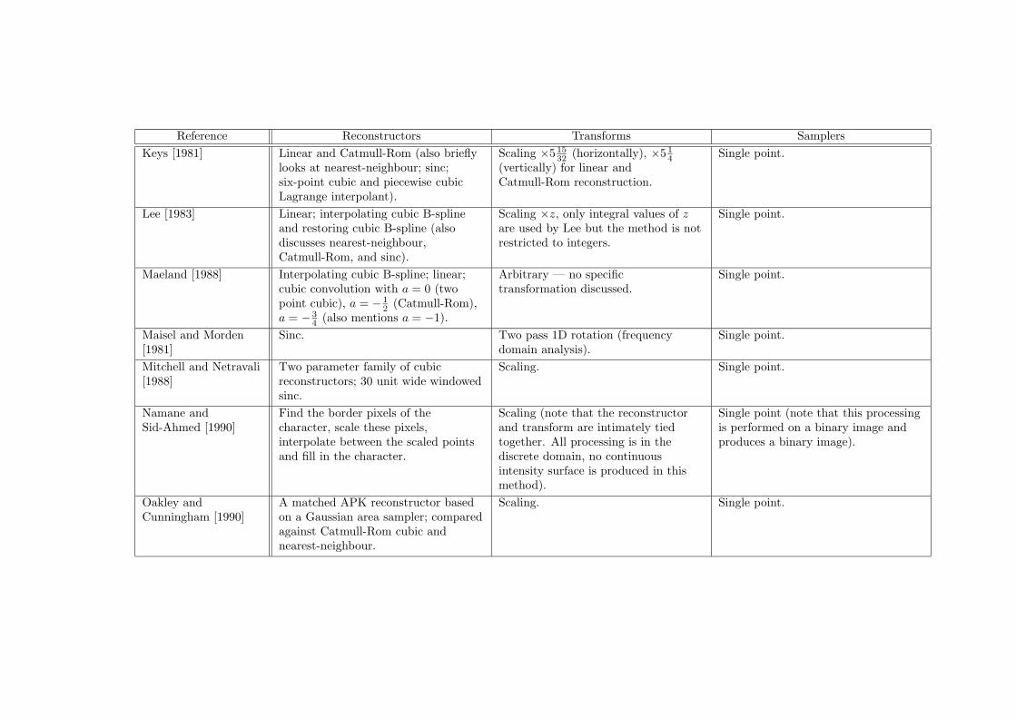
Reference Reconstructors Transforms SamplersKeys [1981] Linear and Catmull-Rom (also briefly
looks at nearest-neighbour; sinc;six-point cubic and piecewise cubicLagrange interpolant).
Scaling ×5 1532 (horizontally), ×5 1
4(vertically) for linear andCatmull-Rom reconstruction.
Single point.
Lee [1983] Linear; interpolating cubic B-splineand restoring cubic B-spline (alsodiscusses nearest-neighbour,Catmull-Rom, and sinc).
Scaling ×z, only integral values of zare used by Lee but the method is notrestricted to integers.
Single point.
Maeland [1988] Interpolating cubic B-spline; linear;cubic convolution with a = 0 (twopoint cubic), a = − 1
2 (Catmull-Rom),a = − 3
4 (also mentions a = −1).
Arbitrary — no specifictransformation discussed.
Single point.
Maisel and Morden[1981]
Sinc. Two pass 1D rotation (frequencydomain analysis).
Single point.
Mitchell and Netravali[1988]
Two parameter family of cubicreconstructors; 30 unit wide windowedsinc.
Scaling. Single point.
Namane andSid-Ahmed [1990]
Find the border pixels of thecharacter, scale these pixels,interpolate between the scaled pointsand fill in the character.
Scaling (note that the reconstructorand transform are intimately tiedtogether. All processing is in thediscrete domain, no continuousintensity surface is produced in thismethod).
Single point (note that this processingis performed on a binary image andproduces a binary image).
Oakley andCunningham [1990]
A matched APK reconstructor basedon a Gaussian area sampler; comparedagainst Catmull-Rom cubic andnearest-neighbour.
Scaling. Single point.

Reference Reconstructors Transforms SamplersOka, Tsutsui, Ohba,Kurauchi and Tago[1987]
Nearest-neighbour. Block affine approximation to generaltransformation.
Minimum enclosing rectangle of pixelpreimage (approximating exact areaarea sampling).
Paeth [1986, 1990] Nearest-neighbour. Three pass 1D rotation. Approximation to exact area (both 1Dand 11
2D); triangle and higher ordersampling filters.
Park andSchowengerdt [1982]
Nearest-neighbour; linear; cubic witha = −1; sinc.
None (frequency domain analysis ofreconstructors).
None (frequency domain analysis ofreconstructors).
Park andSchowengerdt [1983]
Nearest-neighbour; linear; cubicinterpolating piecewise polynomials(including Catmull-Rom); sinc.
None (frequency domain analysis ofreconstructors).
None (frequency domain analysis ofreconstructors).
Parker, Kenyon andTroxel [1983]
Nearest-neighbour, linear,approximating cubic B-spline, cubicconvolution with a = − 1
2(Catmull-Rom) and a = −1 (alsomentions a = − 3
4 ).
General two-dimensionaltransformations. Specific examplesused are rotation and subpixeltranslation. Applied to imageregistration.
Single point.
Ratzel [1980] See Schreiber and Troxel [1985].Reichenbach and Park[1982]
Mitchell and Netravali’s [1988] twoparameter family of cubics.
None (frequency domain analysis ofreconstructors).
None (frequency domain analysis ofreconstructors).
Schafer and Rabiner[1973]
Digital filters: Lagrange interpolation;linear interpolation; optimum FIRinterpolation.
Scaling ×MN , M,N ∈ Z. Single point.
Schreiber and Troxel[1985] (based onRatzel [1980])
Nearest-neighbour; linear; truncatedGaussian; truncated sharpenedGaussian; truncated sinc;approximating cubic B-spline; twotypes of sharpened cubic B-spline.
Scaling ×5 (also scaling by otherfactors to find best sharpenedGaussian prefilter and best sharpenedGaussian reconstructor).
Single point.
Smit, Smith andNichols [1990]
FFT; FFT with ARMA algorithm;nearest-neighbour.
Scaling ×2k, k ∈ Z (with potential totruncate result to a sub-image).
Single point.

Reference Reconstructors Transforms SamplersSmith [1981] Sinc. Scaling. Single point; sinc filtered sampling.Smith [1982] Catmull-Rom; approximating cubic
B-spline; various windowed sincs.Scaling and arbitrary. None (discussion of reconstruction and
transforms only).Smith [1987] Not stated (but see e.g. Smith [1981,
1982]).Two-pass; one-dimensionalsuperquadric; bi-cubic andbi-quadratic warps.
Not stated (but see e.g. Smith [1981,1982]).
Trussell et al [1988] Inverse sinc. Correction of one-dimensional sampleposition errors.
Single point.
Turkowski [1990] Nearest-neighbour; linear; twoGaussians; two Lanczos windowedsincs.
Scaling ×2, 3, 4;× 12 , 1
3 , 14 . Single point.
Venot et al [1988],Herbin et al [1989]
Don’t say. Registration of two-dimensionalimages. Translation, rotation, scaling,included in a general transform whichalso allows for grey-scale manipulation.
Don’t say.
Ward and Cok [1989] Linear; Catmull-Rom (with andwithout coefficient bins); Hammingwindowed sinc.
Scaling × 32 , ×2 and ×4 (all three
reconstructors). Non-seperable andseperable rotation (Catmull-Romonly).
Single point.
Watson [1986] FFT Scaling. FFTWeiman [1980] Nearest-neighbour. Rotation, scaling, shearing by
multi-pass 1D algorithms.Exact area.

Reference Reconstructors Transforms SamplersWilliams [1983] A three-dimensional intensity volume
is produced. It is generated by linearinterpolation between two-dimensionalintensity planes. Each plane isgenerated by two-dimensional linearinterpolation between sample pointscreated by a two-dimensionalnearest-neighbour/exact arearesampling (minification by2n, n ∈ {0, 1, 2, 3, . . .}) of the originalimage.
General. Any transformation althoughones with highly non-symmetrix(non-square) pixel preimages do notwork well.
Single point sampling into thethree-dimensional volume using spatial(x and y) coordinates and a “depth”coordinated wich is related to the sizeof the destination pixel mapped ontothe original image.
Wolberg and Boult[1989]
see Fant [1986]. Arbitrary two-pass 1D transformationsspecified by spatial lookup tables.
see Fant [1986].

Appendix B
Proofs
B.1 The inverse Fourier transform of a box function
(section 2.4.1)
s(x) =∫ ∞
−∞Box(ν)ei2πνx dν
=∫ νb
−νb
ei2πνx dν
=1
i2π xei2πνx
∣∣∣∣νb
−νb
=1
i2π x
(ei2πνbx − e−i2πνbx
)=
1i2π x
(cos(2πνbx) + i sin(2πνbx) − (cos(2πνbx) − i sin(2πνbx)))
=1
i2π x(2i sin(2πνbx))
=sin(2πνbx)
πx= 2νbsinc(2νbx)
sinc(x) is defined in the literature as either sinc(x) = sin(x)x or as sinc(x) = sin(πx)
πx . In this thesiswe will stick with the latter.
B.2 The Fourier transform of the sinc function
(section 5.1)
The sinc function is defined as:
h(x) = NsinπNx
πNx, N > 0
It’s Fourier transform is:
H(ν) =∫ ∞
−∞h(x)e−i2πνx dx
238

B.3. DERIVATION OF A = −2 +√
3 239
=∫ ∞
−∞N
sin(πNx)πNx
[cos(2πνx) − i sin(2πνx)]
=1π
∫ ∞
−∞
sin(πNx) cos(2πνx)x
dx − i
π
∫ ∞
−∞
sin(πNx) sin(2πνx)x
dx
=1π
A(x, ν) − i
πB(x, ν)
Let y = πNx. Thus: x = yπN and dy
dx = 1πN .
A(x, ν) =∫ ∞
−∞
sin(πNx) cos(2πνx)x
dx
=∫ ∞
−∞
sin(y) cos(2y/N)y
dy
sin is an odd function, 1y is an odd function, and cos is an even function, therefore the function
that is being integrated is even, and so:
A(x, ν) = 2∫ ∞
0
sin(y) cos(2y/N)y
dy
=
0,∣∣ 2ν
N
∣∣ > 1π2 ,
∣∣ 2νN
∣∣ = 1π,
∣∣ 2νN
∣∣ < 1
[Dwight 858.9]
B(x, ν) =∫ ∞
−∞
sin(πNx) sin(2πνx)x
dx
=12
∫ ∞
−∞
cos(π(N − 2ν)x)x
dx − 12
∫ ∞
−∞
cos(π(N + 2ν)x)x
dx
[Dwight 401.07]
Now, cos is an even function and 1x is an odd function, so the equation inside each of the integrals
is odd, meaning that each integral equates to zero (∫ 0
−∞cos kx
x dx = −∫∞0
cos kxx dx).
Thus:B(x, ν) = 0
and therefore:
H(ν) =
1, |ν| < N2
12 , |ν| = N
2
0, |ν| > N2
B.3 Derivation of a = −2 +√
3
(section 4.5.1)
From Rasala [1990] we know that:
ak = −fm−k
fm
where fi = −4fi−1 − fi−2, f0 = 1, f1 = −3 or − 4.

240 APPENDIX B. PROOFS
For i very large:
fi−1
fi=
fi−1
(−4fi−1 − fi−2)
= − 1
4 + fi−2fi−1
= − 14 − 1
4+fi−3fi−2
= − 14 − 1
4− 14− 1
. . .
From this we can see that:
limi→∞
(fi−1
fi− fi−2
fi−1
)= 0
and so,
limm→∞
a1 = limm→∞
−fm−1
fm
= limm→∞
1
4 − fm−2fm−1
= limm→∞
1
4 − fm−1fm
=1
4 − limm→∞
a1
which implies that the limit of a1 as m goes to infinity is: a1 = 2 ±√
3.
Now, the value of a2 as m goes to infinity can be defined in terms of this limit of a1:
a2 = −fm−2
fm
= a1 ×fm−2
fm−1
= −a21 (m → ∞)
A similar argument for the general case as m goes to infinity is:
an = −fm−n
fm
= −fm−1
fm× fm−2
fm−1· · · × fm−n
fm−n+1
= −(−a1)n
= −(a)n (m → ∞)
where a = −a1 = −2 ∓√
3.
The case a = −2 −√
3 gives a divergent series of ai values, while the case a = −2 +√
3 gives aconverging series. Thus:
a = −2 +√
3

B.4. THE STRAIGHTNESS CRITERIA 241
B.4 The Straightness Criteria
(Section 3.5.3)
For first order continuity:
Given m sample points, fα−a, fα−a+1, . . . , fα, . . . , fα+b, all having the same value, fα, we want thereconstructed segment dependent on these m values to be f(x) = fα.
Thus:
fx = fα
b∑i=−a
n−1∑j=0
ki,jtj
= fα, ∀t ∈ T
T ={
[0, 1), m even[− 1
2 , 12 ), m odd
where: α =⌊
x − x0
∆x
⌋and t =
x − xα
∆x.
This implies that:b∑
i=−a
n−1∑j=0
ki,jtj = 1
which gives us the result that:
b∑i=−a
ki,j = 0, ∀j ∈ {1, 2, . . . , n − 1}
b∑i=−a
ki,0 = 1
which is equation 3.13.
For second order continuity:
Given m sample points, fα−a, fα−a+1, . . . , fα, . . . , fα+b, having value fα+i = fα + iδ, we want thereconstructed segment dependent on these m values to be f(x) = fα + tδ.
Thus:
f(x) =b∑
i=−a
n−1∑j=0
ki,jtj(fα + iδ)
= fα + tδ, ∀t ∈ T
T ={
[0, 1), m even[− 1
2 , 12 ), m odd
where: α =⌊
x − x0
∆x
⌋and t =
x − xα
∆x, as before.
This implies that:
fα + tδ = fα
b∑i=−a
n−1∑j=0
ki,jtj + δ
b∑i=−a
n−1∑j=0
iki,jtj
and so:
fα = fα
b∑i=−a
n−1∑j=0
ki,jtj (B.1)

242 APPENDIX B. PROOFS
tδ = δb∑
i=−a
n−1∑j=0
iki,jtj (B.2)
Equation B.1 is the same as for first order straightness, and so equation 3.13 holds for second orderstraightness as well. Equation B.2 reduces to the following results:
b∑i=−a
iki,j = 0, ∀j ∈ {0, 2, 3, . . . , n − 1}
b∑i=−a
iki,1 = 1
which is equation 3.14.
B.5 Proof that a signal cannot be simultaneously of finiteextent in both the frequency domain and the spatialdomain
(section 4.3)
Assume that f(x) and F (ν) are a Fourier transform pair. Further assume that f(x) is real, offinite extent, and infinitely piecewise differentiable:
f(x) ∈ R
f(x) = 0, |x| > xK
and that F (ν) is bandlimited:F (ν) = 0, |ν| > νN
F (ν) =∫ ∞
−∞f(x)e−i2πνx dx
=∫ xK
−xK
f(x)e−i2πνx dx
=f(x)e−i2πνx
−i2πν
∣∣∣∣+xK
−xK
− 1(−i2πν)
∫ xK
−xK
f ′(x)e−i2πνx dx
[Dwight, 79]
=f(x)e−i2πνx
−i2πν
∣∣∣∣+xK
−xK
− f ′(x)e−i2πνx
(−i2πν)2
∣∣∣∣+xK
−xK
+1
(−i2πν)2
∫ xK
−xK
f ′′(x)e−i2πνx dx
= eiax
(f(x)ia
− f ′(x)(ia)2
+f ′′(x)(ia)3
− f ′′′(x)(ia)4
+ · · ·)∣∣∣∣xK
−xK
, a = −2πν
= (cos(ax) + i sin(ax))(
f(x)(ia)
− f ′(x)(ia)2
+f ′′(x)(ia)3
− f ′′′(x)(ia)4
+ · · ·)∣∣∣∣xK
−xK
= cos(ax)(
f ′(x)a2 − f ′′′(x)
a4 + · · ·)∣∣∣xK
−xK
+ sin(ax)(
f(x)a − f ′′(x)
a3 + · · ·)∣∣∣xK
−xK
+ i cos(ax)(− f(x)
a + f ′′(x)a3 − · · ·
)∣∣∣xK
−xK
+ i sin(ax)(
f ′(x)a2 − f ′′′(x)
a4 + · · ·)∣∣∣xK
−xK

B.5. A SIGNAL CANNOT BE BANDLIMITED IN BOTH DOMAINS 243
= cos(ax)φ(a, x)|xK
−xK
+ sin(ax)χ(a, x)|xK
−xK
+ i cos(ax)(−χ(a, x))|xK
−xK
+ i sin(ax)φ(a, x)|xK
−xK
= cos(axK)(φ(a, xK) − φ(a,−xK))+ sin(axK)(χ(a, xK) + χ(a,−xK))+ i cos(axK)(−χ(a, xK) + χ(a,−xK))+ i sin(axK)(φ(a, xK) + φ(a,−xK))
(B.3)
Where:
φ(a, x) =(
f ′(x)a2
− f ′′′(x)a4
+ · · ·)
and:
χ(a, x) =(
f(x)a
− f ′′(x)a3
+ · · ·)
Now, if we set equation B.3 to be zero outside the bandlimit of F (ν) (as we assumed) and rememberthat f(x) is a real function, then we find that:
φ(a, xK) = −φ(a,−xK), |a| > νN/2π
φ(a, xK) = φ(a,−xK), |a| > νN/2π
χ(a, xK) = −χ(a,−xK), |a| > νN/2π
χ(a, xK) = χ(a,−xK), |a| > νN/2π
These four equations show that:
φ(a, xK) = 0, |a| > νN/2π (B.4)φ(a,−xK) = 0, |a| > νN/2π
χ(a, xK) = 0, |a| > νN/2π
χ(a,−xK) = 0, |a| > νN/2π
Taking equation B.4 as an example:
φ(a, xK) =(
f ′(xK)a2
− f ′′′(xK)a4
+f (V )(xK)
a6− · · ·
)= 0, |a| > νN/2π
which gives the following equalities:
f ′(xK) = 0,f ′′′(xK) = 0,
f (V )(xK) = 0...
This gives us the result:φ(a, xK) = 0, ∀a
A similar argument holds for φ(a,−xK), χ(a, xK) and χ(a,−xK). From these and equation B.3 itcan be seen that:
F (ν) = 0, ∀ν
which implies that:f(x) = 0, ∀x
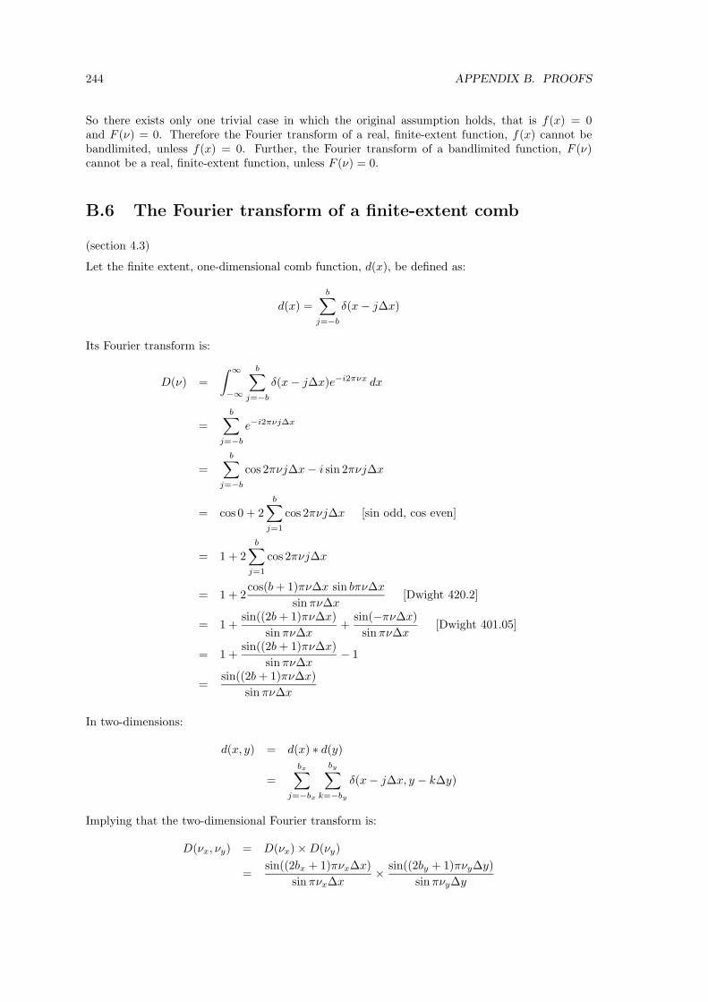
244 APPENDIX B. PROOFS
So there exists only one trivial case in which the original assumption holds, that is f(x) = 0and F (ν) = 0. Therefore the Fourier transform of a real, finite-extent function, f(x) cannot bebandlimited, unless f(x) = 0. Further, the Fourier transform of a bandlimited function, F (ν)cannot be a real, finite-extent function, unless F (ν) = 0.
B.6 The Fourier transform of a finite-extent comb
(section 4.3)
Let the finite extent, one-dimensional comb function, d(x), be defined as:
d(x) =b∑
j=−b
δ(x − j∆x)
Its Fourier transform is:
D(ν) =∫ ∞
−∞
b∑j=−b
δ(x − j∆x)e−i2πνx dx
=b∑
j=−b
e−i2πνj∆x
=b∑
j=−b
cos 2πνj∆x − i sin 2πνj∆x
= cos 0 + 2b∑
j=1
cos 2πνj∆x [sin odd, cos even]
= 1 + 2b∑
j=1
cos 2πνj∆x
= 1 + 2cos(b + 1)πν∆x sin bπν∆x
sinπν∆x[Dwight 420.2]
= 1 +sin((2b + 1)πν∆x)
sin πν∆x+
sin(−πν∆x)sinπν∆x
[Dwight 401.05]
= 1 +sin((2b + 1)πν∆x)
sin πν∆x− 1
=sin((2b + 1)πν∆x)
sin πν∆x
In two-dimensions:
d(x, y) = d(x) ∗ d(y)
=bx∑
j=−bx
by∑k=−by
δ(x − j∆x, y − k∆y)
Implying that the two-dimensional Fourier transform is:
D(νx, νy) = D(νx) × D(νy)
=sin((2bx + 1)πνx∆x)
sinπνx∆x× sin((2by + 1)πνy∆y)
sin πνy∆y

B.7. THE NOT-A-KNOT END-CONDITION FOR THE B-SPLINE 245
B.7 The not-a-knot end-condition for the B-spline
(section 4.5)
The cubic B-spline function (equation 4.11) is:
f(x) =2∑
i=−1
3∑
j=0
ki,j tj
gα+i
The third derivative of this is:
f ′′′(x) = 62∑
i=−1
ki,3 gα+i
= −gα−1 + 3gα − 3gα+1 + gα+2
The not-a-knot condition requires f ′′′(x) to be continuous at x1 and xn−2. At x1:
−g−1 + 3g0 − 3g1 + g2 = −g0 + 3g1 − 3g2 + g3
⇒ g−1 − 4g0 + 6g1 − 4g2 + g3 = 0 (B.5)
We know that (equation 4.12):
fi =16(gi−1 + 4gi + gi+1)
For f0 we can write 6f0 = g−1 + 4g0 + g1. Subtracting this from equation B.5 gives:
−8g0 + 5g1 − 4g2 + g3 = −6f0 (B.6)
For f2 we can write 6f2 = g1 + 4g2 + g3. Subtracting this from equation B.6 produces:
−8g0 + 4g1 − 8g2 = −6f0 − 6f2 (B.7)
And for f1 we can write 48f1 = 8g0 + 32g1 + 8g2. Adding this to equation B.7 gives:
36g1 = 48f1 − 6f0 − 6f2 (B.8)
Making equation B.8 a function of g1 gives us:
g1 =16(8f1 − f0 − f2)
QED
A similar derivation holds for gn−2.
B.8 Timing calculations for the B-spline kernel
(section 4.5.4)
In the first method we need to sum 113 terms (assuming we adopt the diamond shaped kerneldiscussed on page 139). Each term is of the form:
ViWjfx−i,y−j
Where 15 Vi and 15 Wj values must be precalculated as follows:
Vi = vi,3r3 + vi,2r
2 + vi,1r1 + vi,0
Wi = wj,3t3 + wj,2t
2 + wj,1t1 + wj,0

246 APPENDIX B. PROOFS
Operation Method 1 Method 2 M1/M2Multiplies 320 113 3×Adds 202 112 2×Table lookups 120 113 1×Function value lookups 113 113 1×
Table B.1: Timing calculations for the two ways of implementing the interpolating cubic B-spline.
where i and j range from -7 to 7, vi,n and wj,n are retrieved from a table, and the rn and tn termsare precalculated.
From this we find that we require 320 multiples, 202 adds, 120 table lookups and 113 functionvalue lookups for each intensity surface value calculation.
Using the second method, each coefficient is calculated by summing 113 products of a table lookup(a|i|+|j|) and a function value lookup (fx−i,y−j). This makes the requirement 113 multiples, 112adds, 113 table lookups and 113 function value lookups, per coefficient.
These values are laid out in table B.1, from which we can conclude that the first method’s calcu-lation is 2 to 3 times as long as the second method’s, thus 2c < k1 < 3c.
B.9 The error in edge position due to quantisation
section 6.3.5
The edge’s position is given by:
xm = c +gc+1 − gc
gc+1 − gc−1
(equation 6.7).
Without loss of generality, take c = 0:
xm =g1 − g0
g1 − g−1(B.9)
With quantisation, the values of g−1, g0, and g1 in equation B.9 are quantised:
g−1 = Q(gl)g0 = Q(gr + ε(gl − gr))g1 = Q(gr)
The quantisation function is:
Q(g) =1
N − 1〈(N − 1)g〉
The error caused by this is ± 12(N−1) , so:
Q(g) = g ± 12(N − 1)
(B.10)
Substituting equation B.10 into equation B.9 gives:
xm =gr ± 1
2(N−1) − (gr + ε(gl − gr) ± 12(N−1) )
gr ± 12(N−1) − gl ± 1
2(N−1)

B.9. THE ERROR IN EDGE POSITION DUE TO QUANTISATION 247
=ε(gr − gl) ± 1
(N−1)
gr − gl ± 1(N−1)
=ε(∆g) ± 1
(N−1)
∆g ± 1(N−1)
(B.11)
where: ∆g = gr − gl.
If ∆g � 1N−1 then equation B.11 becomes:
xm ≈ε(∆g) ± 1
(N−1)
∆g
= ε ± 1∆g(N − 1)
As xm is an approximation to ε, the error in xm is ± 1∆g(N−1) provided ∆g � 1
N−1 .

Appendix C
Graphs
The graphs are unavailable in this online version of the report owing to the way inwhich they were produced.
This appendix contains the results used in section 7.3.4. There are two sets of experimental results.The first consists of three graphs showing the root mean square difference between an image andits doubly resampled image, for a range of magnification factors (each image is magnified by thisfactor and then minified by the inverse of the factor). The three images used are reproduced infigure C.1.
The second set of results consists of thirty graphs. There are five sets of graphs, one for each ofthe quality measures investigated. Each set contains six graphs, one for each of the six imagesinvolved in the experiments. These images are reproduced in figure 7.11.
Note that the fifth measures, called ‘smoothness’ in section 7.3.4 is here called ‘bumpiness’.
Figure C.1: The three images used in the first experiment.
248
Appendix D
Cornsweet’s figures
This appendix should have contained two photocopies of Cornsweet’s [1970] figures 11.2 and 11.3.Unfortunately, we were unable to get permission to copy these figures before the dissertation wasbound. Instead we present approximations to Cornsweet’s figures, which attempt to illustrate thesame effect. The two images in each photograph (figures D.1 and D.3) are generated from differentintensity distributions (shown in figure D.2), but, in each case, they give approximately the samevisual sensation.
249

250 APPENDIX D. CORNSWEET’S FIGURES
Figure D.1: Two intensity curves which produce roughly the same response from the human visualsystem. The profiles of the edges in the two images are shown in figure D.2(a) and (b) (left andright images respectively). Note that, in the right hand image, the intensity at the centre of thestripe is the same as the intensity at the left and right edges of the image. (After Cornsweet [1970]fig 11.2).
(a)
(b)
(c)
(d)
Figure D.2: The intensity profiles of the edges (a) and (b) in figure D.1; (c) and (d) in figure D.3.
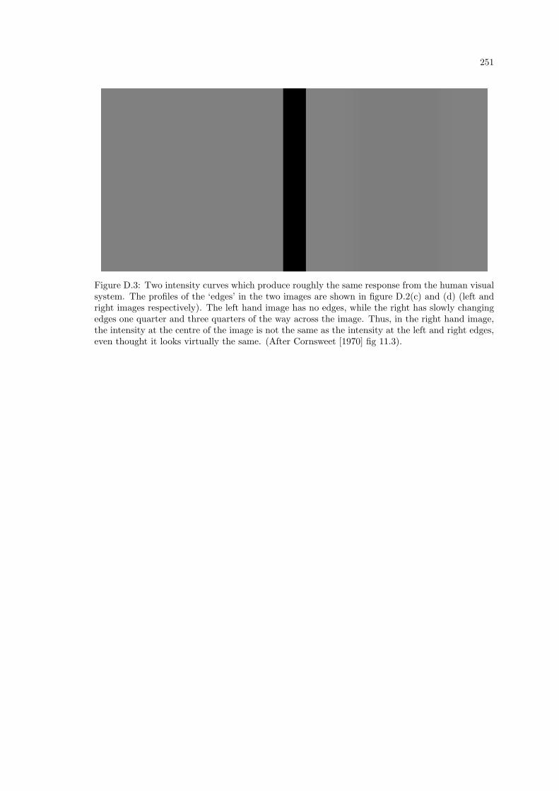
251
Figure D.3: Two intensity curves which produce roughly the same response from the human visualsystem. The profiles of the ‘edges’ in the two images are shown in figure D.2(c) and (d) (left andright images respectively). The left hand image has no edges, while the right has slowly changingedges one quarter and three quarters of the way across the image. Thus, in the right hand image,the intensity at the centre of the image is not the same as the intensity at the left and right edges,even thought it looks virtually the same. (After Cornsweet [1970] fig 11.3).

252 APPENDIX D. CORNSWEET’S FIGURES

Glossary
Approximant a reconstructor that does not necessarily interpolate the image samples. Compareinterpolant.
Area sampler a sampler which uses intensity surface values over some area to provide a valuefor each pixel in the image. Compare point sampler.
Decomposition dividing a process into sub-processes in order to better understand the process.In this dissertation decomposition is applied to the image resampling process, notably de-composing it into three sub-processes: reconstruction, transform, and sampling.
Destination image the image that is output by a resampling process, also called resampled imageor final image.
Filter in an area sampler there is an equivalence that allows us to represent the sampler as a filtercombined with single point sampling, such that the filter is the function that is convolved withthe intensity surface before single point sampling the filtered surface. Some point samplerscan also be represented in this way. Some reconstructors can be represented by filters, sothat the reconstructed intensity surface that they produce is the convolution of the filter withthe image. Also called kernel or ‘filter kernel’.
Final image the image that is output by a resampling process, also called destination image orresampled image.
Final intensity surface the intensity surface generated by transforming the original intensitysurface. The final image is generated from it by sampling.
Hedgehog an omnivorous mammal renowned for its prickliness.
Image in this dissertation ‘image’ almost exclusively refers to a discrete image. A continuousimage is known as an intensity surface.
Image samples the sample values that make up a discrete image. Also called pixels or pixelvalues.
Intensity surface a continuous surface in three dimensions, with two spatial dimensions andone intensity dimension. There is a many-to-one mapping from two-dimensional spatialcoordinates to intensity values. Can be extrapolated to an intensity volume (three spatialdimensions and one intensity dimension) or to a colour surface (where colour dimensionsreplace the single intensity dimension). Also known as ‘continuous image’.
Interpolant a reconstructor that interpolates the image samples. Compare approximant.
Kernel an abbreviation of ‘filter kernel’ (see filter).
Original image the image that is input to the resampling process, also called source image.
Original intensity surface the intensity surface generate from the original image by reconstruc-tion.
253

254
Pixel (a) a single sample value in an image; (b) the theoretical area represented by such a samplevalue in an intensity surface which generates, or is generated by, that image. Also called‘pel’.
Point sampler a sampler which only uses intensity surface values at a countable set of points toprovide a value for each pixel in the image. Compare area sampler.
Reconstruction applying a reconstructor to an image to produce an intensity surface.
Reconstructor a process which reconstructs a continuous intensity surface from a discrete image.
Resample to take a discrete image and produce another image which appears to be a spatiallytransformed version of the first.
Resampled image the image that is output by a resampling process, also called final image ordestination image.
Resampler a process which performs image resampling.
Sampler a process which produces a discrete image from a continuous intensity surface.
Sampling applying a sampler to an intensity surface to produce an image.
Single point sampler a point sampler which uses a single intensity surface value to provide avalue for each pixel.
Source image the image that is input to a resampling process, also called original image.
Sub-process a process that forms part of a larger process. Sub-processes are generated by de-composition of some process. Also called: a ‘part’ or ‘stage’ of the larger process.
Transform a process which takes a continuous intensity surface and produces another, trans-formed, intensity surface from it.
Warp a synonym for resample, used more in computer graphics work; whilst ‘resample’ is usedmore in signal processing work.

Bibliography
The reference style used in this dissertation follows these rules:
1. A reference is given by the author’s name, or authors’ names, followed by the date of pub-lication and sometimes extra information as to the location within the quoted work of theparticular item referenced.
2. If the context requires a direct reference to the paper then the name(s) are placed in thetext, with the other material placed in square brackets immediately after the name(s). If anindirect reference is required then all the information appears inside square brackets.
3. A work with three or more authors should be referenced by all the authors’ names the firsttime it is referred to. Subsequent references use the first author’s name followed by “et al”in place of all the other names.
This last rule has been bent in the case of Venot, Devaux, Herbin, Lebruchec, Dubertret, Rauloand Roucayrol [1988] and Herbin, Venot, Devaux, Walter, Lebruchec, Dubertret and Roucayrol[1989]. These are always referred to as Venot et al [1988] and Herbin et al [1989] respectively.
To aid those working at the University of Cambridge, there is a reference mark at the end ofmany of the entries in this bibliography which shows where the referenced work may be found.Abbreviations used in these references are:
CLL Computer Laboratory LibrarySPL Scientific Periodicals LibraryUL University Library
Adobe, [1985a] PostScript Language Reference Manual, Addison-Wesley, Reading, Massachusetts,USA, ISBN 0–201–10174–2.
Ahmed, N., Natarajan, T. and Rao, K.R. [1974] “Discrete cosine transform”, IEEE Trans-actions on Computers, Vol. C–23, No. 1, Jan, 1974, pp.90–93. CLL
Andrews, H.C. and Patterson, C.L. (III) [1976] “Digital interpolation of discrete images”,IEEE Transactions on Computers, Vol. C–25, No. 2, Feb, 1976, pp.197–202. CLL
Bier, E.A. and Slone, K.R.(Jr) [1986] “Two-part texture mappings”, IEEE Computer Graph-ics and Applications, Sept, 1986, pp.40–53. CLL
Binkley, T. [1990] “Digital dilemmas”, LEONARDO, Digital Image—Digital Cinema Supple-mental Issue, 1990, pp.13–19. CLL
Bley, H. [1980] “Digitization and segmentation of circuit diagrams”, Proceedings of the FirstScandanavian Comference on Image Analysis, Studentlitteratur, Lund, Sweden, 1980, pp.264–269. UL 348:8.c.95.1213
255

256
Blinn, J.F. [1989a] “What we need around here is more aliasing”, IEEE Computer Graphicsand Applications, Jan, 1989, pp.75–79. CLL
Blinn, J.F. [1989b] “Return of the jaggy”, IEEE Computer Graphics and Applications, Mar,1989, pp.82–89. CLL
Blinn, J.F. [1990] “Wonderful world of video”, IEEE Computer Graphics and Applications,Vol. 10, No. 3, May, 1990, pp.83–87. SPL E0.2.96
Boult, T.E. and Wolberg, G. [1992] “Local image reconstruction and sub-pixel restorationalgorithms”, CVGIP: Image Understanding, in press.
Braccini, C. and Marino, G. [1980] “Fast geometrical manipulations of digital images”, Com-puter Graphics and Image Processing, Vol. 13, 1980, pp.127–141. SPL E0.2.13
Brewer, J.A. and Anderson, D.C. [1977] “Visual interaction with Overhauser curves and sur-faces”, Computer Graphics, Vol. 11, No. 2, Summer, 1977, pp.132–137.
Brown, E.F. [1969] “Television: the subjective effects of filter ringing transients”, Journal ofthe Society of Motion Picture and Television Engineers (SMPTE), Vol. 78, No. 4, Apr, 1969,pp.249–255. SPL E0.2.24
Catmull, E. [1974] “Computer display of curved surfaces”, Proceedings of the Conference onComputer Graphics, Pattern Recognition and Data Structure, Los Angeles, California, May14–16, 1974, IEEE, New York, 1975, IEEE Catalogue Number 75CHO981–1C, pp.11–17.Also reprinted as: Tutorial and Selected Readings in Interactive Computer Graphics, H.Freeman (ed), IEEE, 1980, IEEE Catalogue Number EHO 156–0, pp.309–315.
Catmull, E. and Rom, R. [1974] “A class of local interpolating splines”, Computer Aided Ge-ometric Design, R.E. Barnhill and R.F. Riesenfeld (eds.), Academic Press, New York, ISBN0–12–079050–5, pp.317–326.
Catmull, E. and Smith, A.R. [1980] “3-D transformations of images in scanline order”, Com-puter Graphics, Vol. 14, No. 3, 1980, pp.279–285.
Chen, W-H. and Pratt, W.K. [1984] “Scene adaptive coder”, IEEE Transactions on Com-munications, Vol. COM–32, No. 3, Mar, 1984, pp.255–232. CLL
Chiou, A.E.T. and Yeh, P. [1990] “Scaling and rotation of optical images using a ring cavity”,Applied Optics, Vol. 29, No. 11, 10th Apr, 1990, pp.1584–1586. SPL F1.2.3
Chu, K-C. [1990] “B3-splines for interactive curve and surface fitting”, Computers and Graph-ics, Vol. 14, No. 2, 1990, pp.281–288. SPL E0.1.34
Cook, R.L. [1986] “Stochastic sampling in computer graphics”, ACM Transactions on Graphics,Vol. 5, No. 1, Jan, 1986, pp.51–72. CLL
Cornsweet, T.N. [1970] Visual Perception, Academic Press, 1970, Library of Congress Cata-logue Card No. 71–107570.Physiological Lab. Library C6.143A
Crow, F.C. [1977] “The aliasing problem in computer-generated shaded images”, Communica-tions of the ACM, Vol. 20, No. 11, Nov, 1977, pp.799–805 CLL
Crow, F.C [1978] “The use of grayscale for improved raster display of vectors and characters”,Computer Graphics, Vol. 12, No. 3, Aug, 1978, pp.1–5. CLL
Crow, F.C. [1984] “Summed-area tables for texture mapping”, Computer Graphics, Vol. 18,No. 3, Jul, 1984, pp.207–212. CLL

257
Cumani, A., Grattoni, P. and Guiducci, A. [1991] “An edge-based description of colour im-ages”, CVGIP: Graphical Models and Image Processing, Vol. 53, No. 4, Jul, 1991, pp.313–323.CLL
Data Beta [1992] Product Description; Data Beta Ltd, Unit 7, Chiltern Enterprise Centre,Theale, Berkshire, United Kingdom RG7 4AA.
Durand, C.X. [1989] “Bit map transformations in computer 2-D animation”, Computers andGraphics, Vol. 13, No. 4, 1989, pp.433–440. SPL E0.1.34
Durand, C.X. and Faguy, D. [1990] “Rational zoom of bit maps using B-spline interpolationin computerized 2-D animation”, Computer Graphics Forum, Vol. 9, No. 1, Mar, 1990, pp.27–37 CLL
Dwight, H.B. [1934] Tables of Integrals and other Mathematical Data, The MacMillan Com-pany, New York, 1934. CLL X14
Euclid [300BC] Elements.
Fang, Z., Li, X. and Ni, L.M. [1989] “On the communication complexity of generalised 2-Dconvolution on array processors”, IEEE Transactions on Computers, Vol. 38, No. 2, Feb,1989, pp.184–194. CLL
Fant, K.M. [1986] “A non-aliasing, real-time spatial transform technique”, IEEE ComputerGraphics and Applications, Jan, 1986, pp.71–80. SPL E0.2.96
Fiume, E.L. [1986] “A mathematical semantics and theory of raster graphics”, PhD thesis, tech-nical report CSRI–185, Computer Systems Research Group, University of Toronto, Toronto,Canada M5S 1A1 CLL V106–669Published, with minor additions, as Fiume [1989].
Fiume, E.L. [1989] The Mathematical Structure of Raster Graphics, Academic Press, San Diego,1989, ISBN 0–12–257960–7.Based on Fiume [1986].
Feibush, E.A., Levoy, M. and Cook, R.L. [1980] “Synthetic texturing using digital filters”,Computer Graphics, Vol. 14, 1980, pp.294–301.
Foley, J.D. and van Dam. A. [1982] Fundamentals of Interactive Computer Graphics, Addison-Wesley, Reading, Massachusetts, USA, 1982, ISBN 0–201–14468–9.
Foley, J.D., van Dam, A., Feiner, S.K. and Hughes, J.F. [1990] Computer Graphics: Prin-ciples and Practice (‘second edition’ of Foley and van Dam [1982]), Addison-Wesley, Reading,Massachusetts, USA, 1990, ISBN 0–201–12110–7.
Fournier, A. and Fiume, E.L. [1988] “Constant-time filtering with space-variant kernels”, Com-puter Graphics, Vol. 22, No. 4, Aug, 1988, pp.229–238. CLL
Fournier, A. and Fussell, D. [1988] “On the power of the frame buffer”, ACM Transactionson Graphics, Vol. 7, No. 2, Apr, 1988, pp.103–128. CLL
Fraser, D. [1987] “A conceptual image intensity surface and the sampling theorem”, AustralianComputer Journal, Vol. 19, No. 3, Aug, 1987, pp.119–125. SPL E0.13.3
Fraser, D. [1989a] “Interpolation by the FFT revisited — an experimental investigation”, IEEETransactions on Acoustics, Speech and Signal Processing, Vol. 37, No. 5, May, 1989, pp.665–675. SPL E0.2.34
Fraser, D. [1989b] “Comparison at high spatial frequencies of two-pass and one-pass geomet-ric transformation algorithms”, Computer Vision, Graphics and Image Processing, Vol. 46,No. 3, Jun, 1989, pp.267–283. SPL E0.2.34

258
Fraser, D., Schowengerdt, R.A. and Briggs, I. [1985] “Rectification of multichannel imagesin mass storage using image transposition”, Computer Vision, Graphics and Image Process-ing, Vol. 29, No. 1, 1985, pp.23–56. SPL E0.2.13
Fredrick, C. and Schwartz, E.L. [1990] “Conformal image warping”, IEEE Computer Graph-ics and Applications, Vol. 10, No. 2, Mar, 1990, pp.54–61. SPL E0.2.96
Gardner, I.C. and Washer, F.E [1948] “Lenses of extremely wide angle for airplane map-ping”, Journal of the Optical Society of America, Vol. 38, No. 5, May, 1948, pp.421–431.SPL F1.2.1
Gibbs, A.R. [1992] Personal communication.
Glassner, A. [1986] “Adaptive precision in texture mapping”, Computer Graphics, Vol. 20,No. 4, Aug, 1986, pp.297–306. CLL
Glassner, A.S. [1990b] “Interpretation of texture map indices”, Graphics Gems, A.S. Glassner(ed.), Academic Press Ltd, San Diego, California, USA, 1990, ISBN 0–12–286165–5.
Gonzalez, R.C. and Wintz, P. [1977] Digital Image Processing, Addison-Wesley, 1977, ISBN0–201–02596–5. CLL U135
Goshtasby, A. [1989] “Correction of image deformation from lens distortion using Bezier patches”,Computer Vision, Graphics and Image Processing, Vol. 47, 1989, pp.385–394. SPL E0.2.13
Greene, N. and Heckbert, P.S. [1986] “Creating raster omnimax images from multiple per-spective views using the elliptical weighted average filter”, IEEE Computer Graphics andApplications, Vol. 6, No. 6, Jun, 1986, pp.21–27. CLL
Guibas, L.J. and Stolfi, J. [1982] “A language for bitmap manipulation”, ACM Transactionson Graphics, Vol. 1, No. 3, Jul, 1982, pp.191–214.
Hall, A.D. [1989] “Pipelined logical convolvers for binary picture processing”, Electronics Let-ters, Vol. 25, No. 15, 20 Jul, 1989, pp.961–963. SPL E0.1.36
Hall, A.D. [1991] Personal communication.
Hall, E.L. [1979] Computer image processing and recognition, Academic Press, New York, USA,1979, ISBN 0–12–318850–4. CLL 1Y88
Hammerin, M. and Danielsson, P-E. [1991] “High accuracy rotation of images”, Contribu-tions to the SSAB symposium, March, 1991, Report No. LiTH–ISY–I–1161, Department ofElectrical Engineering, Linkoping University, S–58183 Linkoping, Sweden; pp.1–4.
Hanrahan, P. [1990] “Three-pass affine transforms for volume rendering”, Computer Graphics,Vol. 24, No. 5, Nov, 1990, pp.71–78. CLL
Heckbert, P.S. [1986a] “Survey of texture mapping”, IEEE Computer Graphics and Applica-tions, Nov, 1986, pp.56–67. CLL
Heckbert, P.S. [1986b] “Filtering by repeated integration”, Computer Graphics, Vol. 20, No. 4,1986, pp.315–321. CLL
Heckbert, P.S. [1989] “Fundamentals of texture mapping and image warping”, Master’s the-sis, report number UCB/CSD 89/516, Computer Science Division (EECS), University ofCalifornia, Berkeley, California 94720, USA; June, 1989.
Heckbert, P.S. [1990a] “What are the coordinates of a pixel?”, Graphics Gems, A.S. Glassner(ed.), Academic Press, 1990, ISBN 0–12–28616–5, pp.246–248.

259
Heckbert [1990b] “Texture mapping”, lecture presented to the ACM/BCS International Sum-mer Institute, “State of the art in computer graphics”, 2–6 July, 1990, Edinburgh, U.K.
Heckbert, P.S. [1991a] “Review of ‘Digital Image Warping’ [Wolberg, 1990]”, IEEE ComputerGraphics and Applications, Jan, 1991, pp.114–116. CLL
Heckbert, P.S. [1991b] Response to Wolberg [1991] and McDonnell’s [1991] replies to Heck-bert’s [1991a] review of Wolberg’s [1990] book (“Letters to the Editor” column), IEEE Com-puter Graphics and Applications, May, 1991, p.5. CLL
Herbin, M., Venot, A., Devaux, J.Y., Walter, E., Lebruchec, J.F., Dubertret, L. andRoucayrol, J.C. [1989] “Automated registration of dissimilar images: application to med-ical imagery”, Computer Vision, Graphics and Image Processing, Vol. 47, No.1, Jul, 1989,pp.77–88. SPL E0.2.13
Horn, B.K.P. [1977] “Understanding image intensities”, Readings in Computer Vision, M.A.Fischler and O. Fischler (eds.), Morgan Kaufmann Publishers Inc., 95 First Street, LosAltos, California 94022, USA, 1987, ISBN 0–934613–33–8.Originally in Artificial Intelligence, Vol.8, No.2, 1977, pp.201–231.
Hou, H.S. and Andrews, H.C. [1978] “Cubic splines for image interpolation and digital fil-tering”, IEEE Transactions on Acoustics, Speech and Signal Processing, Vol. ASSP–26, No. 6,Dec, 1978, pp.508–517. SPL E0.2.34
Hyde, P.D. and Davis. L.S. [1983] “Subpixel edge estimation”, Pattern Recognition, Vol. 16,No. 4, 1983, pp.413–420. SPL E0.0.1
Kajiya, J.T. and Kay, T.L. [1989] “Rendering fur with three-dimensional textures”, ComputerGraphics, Vol. 23, No. 3, Jul, 1989, pp.656–657. CLL
Keys, R.G. [1981] “Cubic convolution interpolation for digital image processing”, IEEE Trans-actions on Acoustics, Speech and Signal Processing, Vol. ASSP–29, No. 6, Dec, 1981, pp.1153–1160. SPL E0.2.34
Kiryati, N. and Bruckstein, A. [1991] “Gray levels can improve the performance of binaryimage digitizers”, CVGIP: Graphical Models and Image Processing, Vol. 53, No. 1, Jan,1991, pp.31–39. CLL
Kitchen, L.J. and Malin, J.A. [1989] “The effect of spacial discretization on the magnitudeand direction response of simple differential operators on a step edge”, Computer Vision,Graphics and Image Processing, Vol. 47, No.2 , Aug, 1989, pp.234–258. SPL E0.2.13
Klassman, H. [1975] “Some aspects of the accuracy of the approximated position of a straightline on a square grid”, Computer Graphics and Image Processing, Vol. 4, No. 3, Sept, 1975,pp.225–235. SPL E0.2.13
Kornfeld, C.D. [1985] “Architectural elements for bitmap graphics”, PhD thesis, technical re-port CSL–85–2, June, 1985, Xerox Corporation, Palo Alto Research Center, 3333 Coyote HillRoad, Palo Alto, California 94304, USA, 1985. CLL V106–900
Kornfeld, C. [1987] “The image prism: a device for rotating and mirroring bitmap images”,IEEE Computer Graphics and Applications, Vol. 7, No. 5, 1987, pp.21–30. CLL
Kuhnert, K-D. [1989] “Sensor modelling as a basis of subpixel image processing”, Proceedingsof the SPIE, Vol. 1135, “Image Processing III”, chair and editor: J.F. Duverney; 27–28 April,1989, Paris, France, pp.104–111. SPL F1.2.6
Laser-Scan, [1989] “VTRAK”, Laser-Scan Laboratories Ltd, Software Product Specification,Jan 12, 1989, issue 1.2. Laser-Scan, Science Park, Milton Rd, Cambridge, CB4 4FY.

260
Lee, C-H. [1983] “Restoring spline interpolation of CT images”, IEEE Transactions on MedicalImaging, Vol. MI–2, No. 2, Sept, 1983, pp.142–149.
Lynn, P.A. and Fuerst, W. [1989] Introductory digital signal processing with computer appli-cations, John Wiley and Sons, Ltd, Chichester, 1989, ISBN 0–471–91564–5.
Mach, E. [1865] “On the visual sensations produced by intermittent excitations of the retina”,Philosophical Magazine, Vol. 30, No. 2, Fourth Series, 1865, pp.319–320. SPL A0.1.2
Maeland, E. [1988] “On the comparison of the interpolation methods”, IEEE Transactions onMedical Imaging, Vol. 7, No. 3, Sept, 1988, pp.213–217. SPL E0.2.103
Maisel, J.E. and Morden, R.E [1981] “Rotation of a two-dimensional sampling set using one-dimensional resampling”, IEEE Transactions on Acoustics, Speech and Signal Processing,Vol. ASSP–29, No. 6, Dec, 1981, pp.1218–1222. SPL E0.2.34
Mantas, J. [1987] “Methodologies in patternrecognition and image analysis — a brief survey”,Pattern Recognition, Vol. 20, No. 1, 1987, pp.1–6. SPL E0.0.1
Marion, A. [1991] An introduction to image processing, Chapman and Hall, 2–6 Boundary Row,London, 1991, ISBN 0–412–37890–6.
Marr, D. [1976] “Early processing of visual information”, Philosophical Transactions of theRoyal Society of London, Vol. 257, Series B, 1976, pp.483–524.
Martin, G.E. [1982] Transformation Geometry, Springer-Verlag, New York, USA, 1982, ISBN0–387–90636–3.
McDonnell, M. [1991] “Response to Heckbert’s [1991a] review of Wolberg’s [1990] book”, “Let-ters to the Editor” column, IEEE Computer Graphics and Applications, May, 1991, p.4–5.
Mersereau, R.M [1979] “The processing of hexagonally sampled two-dimensional signals”, Pro-ceedings of the IEEE, Vol. 67, No. 6, Jun, 1979, pp.930–949. CLL
Mitchell, D.P. and Netravali, A.N. [1988] “Reconstruction filters in computer graphics”, Com-puter Graphics, Vol. 22, No. 4, Aug, 1988, pp.221–288. CLL
Murch, G.M. and Weiman, N. [1991] “Gray-scale sensitivity of the human eye for differentspacial frequencies and display luminance levels”, Proceedings of the Society for InformationDisplay, Vol. 32, No. 1, 1991, pp.13–17.
Nagioff, O. [1991] Personal communication.
Namane, A. and Sid-Ahmed, M.A. [1990] “Character scaling by contour method”, IEEETransactions on Pattern Analysis and Machine Intelligence, Vol. 12, No. 6, Jun, 1990,pp.600–606. SPL E0.2.98
Newman, W. and Sproull, R. [1979] Principles of Interactive Computer Graphics (second edi-tion), McGraw-Hill, 1979, ISBN 0–07–046338–7.
NMFPT, [1992] National Museum of Film, Photography, and Television, Bradford, West York-shire, personal communication.
Oakley, J.P. and Cunningham, M.J. [1990] “A function space model for digital image sam-pling and its application in image reconstruction”, Computer Graphics and Image Processing,Vol. 49, No. 2, Feb, 1990, pp.171–197. SPL E0.2.13
Oka, M., Tsutsui, K., Ohba, A., Kurauchi, Y. and Tago, T. [1987] “Real-time manipula-tion of texture-mapped surfaces”, Computer Graphics, Vol. 21, No. 4, Jul, 1987, pp.181–188.CLL

261
Olsen, J. [1990] “Smoothing enlarged monochrome images”, Graphics Gems, A.S. Glassner,(ed.),Academic Press Ltd, San Diego, CA, 1990, ISBN 0–12–286165–5, pp.166–170.
Oskoui-Fard, P. and Stark, H. [1988] “Tomographic image reconstruction using the theoryof convex projections”, IEEE Transactions on Medical Imaging, Vol. 7, No. 1, Mar, 1988,pp.45–58. SPL E0.2.103
Overhauser, A.W. [1968] “Analystical definition of curves and surfaces by parabolic blend-ing”, Mathematical and Theoretical Sciences Department, Scientific Laboratory, Ford MotorCompany, Report No. SL–68–40, 1968.
Paeth, A.W. [1986] “A fast algorithm for general raster rotation”, Proceedings, Graphics Inter-face ’86/Vision Interface’86, 26–30 May, 1986, pp.77–81. CLL 1Y712
Paeth, A.W. [1990] “A fast algorithm for general raster rotation”, Graphic Gems, A.S. Glassner(ed.), Academic Press, 1990, ISBN 0–12–286165–5.
Park, S.K. and Schowengerdt, R.A. [1982] “Image sampling, reconstruction and the effectof sample scene phasing”, Applied Optics, Vol. 21, No. 17, 1 Sept, 1982, pp.3142–3151. SPLF1.2.3
Park, S.K. and Schowengerdt, R.A. [1983] “Image reconstruction by parametric cubic con-volution”, Computer Vision, Graphics and Image Processing, Vol. 23, No. 3, Sept, 1983,pp.258–272. SPL E0.2.13
Parker, J.A., Kenyon, R.V. and Troxel, D.E. [1983] “Comparison of interpolation meth-ods for image resampling”, IEEE Transactions on Medical Imaging, Vol. MI–2, No. 1, Mar,1983, pp.31–39.
Pavlidis, T. [1982] Algorithms for Graphics and Image Processing, Springer-Verlag, 1982. CLL1Y138
Pavlidis, T.[1990] “Re: Comments on ‘Stochastic Sampling in Computer Graphics’ [Cook, 1986]”,Letter to the Editor, ACM Transactions on Graphics, Vol. 9, No. 2, Apr, 1990, pp.233–326.CLL
Petersen, D.P. and Middleton, D. [1962] “Sampling and reconstruction of wave-number-limitedfunctions in N -dimensional Euclidean spaces”, Information and Control, Vol. 5, No. 4, Dec,1962, pp.279–323. SPL E0.2.121
Pettit, F. [1985] Fourier Transforms in Action Chartwell-Bratt (Publishing and Training) Lim-ited, 1985, ISBN 0–86238–088–X. CLL 1Y505
Piegl, L. [1991] “On NURBS: a survey”, IEEE Computer Graphics and Applications, Jan, 1991,pp.55–71. CLL
Prasad, K.P. and Satyanarayana, P. [1986] “Fast interpolation algorithm using FFT”, Elec-tronics Letters, Vol. 22, No. 4, 13 Feb, 1986, pp.185–187. SPL E0.1.36
Pratt, W.K [1978] Digital Image Processing, John Wiley and Sons, New York, USA, 1978, ISBN0–471–01888–0. UL 9428.c.3814
Pratt, W.K [1991] Digital Image Processing (second edition), John Wiley and Sons, New York,USA, 1991, ISBN 0–471–85766–0.
Press, W.H., Flannery, B.P., Teukolsky, S.A. and Vetterling, W.T. [1988] Numerical Recipesin C: The Art of Scientific Computing, Cambridge University Press, Cambridge, 1988, ISBN0–521–35465–X.
262
Rabbani, M. and Jones, P.W. [1991] Digital Image Compression Techniques, SPIE — TheSociety of Photo-Optical Instrumentation Engineers, P.O. Box 10, Bellingham. Washington,USA, 1991, ISBN 0–8194–10648–1.
Rasala. R. [1990] “Explicit cubic spline interpolation formulas”, Graphic Gems, A.S. Glassner(ed.), Academic Press, 1990, ISBN 0–12–286165–5.
Ratliff, F. [1965] Mach Bands: Quantitative studies on neural networks in the retina, Holden-Day Inc, San Francisco, USA, 1965.Psychology Lab. Library: C.6.68A
Ratzel, J.N. [1980] “The discrete representation of spatially continuous images”, PhD thesis,Department of Electrical Engineering and Computer Science, Massachusetts Institute ofTechnology, Cambridge, Massachusetts, USA, Aug, 1980.
Reed, T.R., Algazi, V.R., Ford, G.E. and Hussain, I. [1992] “Perceptually based codingof monochrome and color still images”, Proceedings of the Data Compression Conference,March 24–27, 1992, Snowbird, Utah, USA; J.A. Storer and M. Cohn (eds.), IEEE ComputerSociety Press, Los Alamitos, California, USA; ISBN 0–8186–2717–4 (case bound); pp.142–151.
Reichenbach, S.E. and Park, S.K. [1989] “Two-parameter cubic convolution for image re-construction”, Proceedings of the SPIE, Vol. 1199, “Visual Communications and Image Pro-cessing IV (1989)”, pp.833–840.
Richards, P.I. [1966] “Sampling positive functions”, Proceedings of the IEEE (Letters), Vol. 54,No. 1, Jan, 1966, pp.81–82. CLL
Robertson, P.K. [1987] “Fast perspective views of images using one-dimensional operations”,IEEE Computer Graphics and Applications, Vol. 7, No. 2, Feb, 1987, pp.47–56. SPL E0.2.96
Rogers, D.F. and Adams, J.A. [1976] Mathematical Elements for Computer Graphics, McGraw-Hill, 1976, ISBN 0–07–053527–2.
Rosenenfeld, A. [1988] “Computer vision: basic principles”, Proceedings of the IEEE, Vol. 76,No. 8, Aug, 1988, pp.863–868. CLL
Rosenfeld, A. and Kak, A.C. [1982] Digital Picture Processing (second edition, two volumes),Academic Press, Orlando, Florida, USA, 1982, ISBN 0–12–597301–2. CLL 1Y213
Rothstein, J. and Weiman, C. [1976] “Parallel and sequential specification of a context sen-sitive language for straight lines on grids”, Computer Graphics and Image Processing, Vol. 5,No. 1, Mar, 1976, pp.106–124. SPL E0.2.13
van Sant, T. [1992] “The Earth/From Space”, a satellite composite view of Earth, c©Tom vanSant/The Geosphere Project, Santa Monica, California, USA, 800 845–1522.Reproduced in Scientific American, Vol. 266, No. 4, April, 1992, p.6.
Schafer, R.W. and Rabiner, L.R. [1973] “A digital signal processing approach to interpola-tion”, Proceedings of the IEEE, Vol. 61, No. 6, Jun, 1973, pp.692–702.
Schoenberg, I.S. [1973] “Cardinal spline interpolation”, Regional Conference Series in AppliedMathematics, Society for Industrial and Applied Mathematics, (SIAM), Philadelphia, Penn-sylvania, USA, Vol. 12, 1973.
Schreiber, W.F. and Troxel, D.E. [1985] “Transformation between continuous and discreterepresentations of images: a perceptual approach”, IEEE Transactions on Pattern Analysisand Machine Intelligence, Vol. PAMI–7, No. 2, Mar, 1985, pp.178–186. SPL

263
Sedgewick, R. [1988] Algorithms (second edition), Addison-Wesley, Reading, Massachusetts,USA, 1988, ISBN 0–201–06673–4.
Shannon, C.E. [1949] “Communication in the presence of noise”, Proceedings of the IRE, Vol. 37,No. 1, Jan, 1949, pp.10–21. SPL E0.2.17
Sloan, A.D. [1992] “Fractal image compression: a resolution independent representation fromimagery”, Proceedings of the NASA Space and Earth Science Data Compression Workshop,March 27, 1992, Snowbird, Utah, USA; J.C. Tilton and S. Dolinar (eds.); NASA ConferencePublications; to appear.
Smit, T., Smith, M.R. and Nichols, S.T. [1990] “Efficient sinc function interpolation tech-nique for centre padded data”, IEEE Transactions on Acoustics, Speech and Signal Process-ing, Vol. 38, No. 9, Sept, 1990, pp.1512–1517 SPL E0.2.34
Smith, A.R. [1981] “Digital filtering tutorial for computer graphics”, Technical Memo, Lucas-film Ltd, (available from PIXAR, 1001 West Cutting Richmond, CA 94804, USA). TechnicalMemo No. 27, 1981.
Smith, A.R. [1982] “Digital filtering tutorial, part II”, Technical Memo, Lucasfilm Ltd, (avail-able from PIXAR, 1001 West Cutting Richmond, CA 94804, USA). Technical Memo No. 44,10 May, 1982.
Smith, A.R. [1987] “Planar 2-pass texture mapping and warping”, Computer Graphics, Vol. 21,No. 4, Jul, 1987, pp.263–272. CLL
Smith, T.G. [1986] Industrial Light and Magic: the art of special effects, Virgin Publishing, 338Ladbroke Grove, London, UK, 1986, ISBN 0–86287–142–5.
Sproull, R.F. [1986] “Frame-buffer display architectures”, Annual Review of Computer Science,Vol. 1, 1986, pp.19–46. SPL A0.2.39
Trussell, H.J., Ardner, L.L., Moran, P.R. and Williams, R.C. [1988] “Corrections for non-uniform sampling distributions in magnetic resonance imagery”, IEEE Transactions on Med-ical Imaging, Vol. 7, No. 1, Mar, 1988, pp.32–44. SPL E0.2.103
TRW, [1988] , Data Book: Data Converters — DSP Products, TRW LSI Products Inc., P.O.Box 2472, La Jolla, California 92038, USA, 1988.
Turkowski, K. [1986] “Anti-aliasing in topological color spaces”, Computer Graphics, Vol. 20,No. 4, Aug, 1986, pp.307–314. CLL
Turkowski, K. [1990] “Filters for common resampling tasks”, Graphics Gems, A.S. Glassner(ed.), Academic Press, 1990, ISBN 0–12–286165–5.
Venot, A., Devaux, J.Y., Herbin, M., Lebruchec, J.F., Dubertret, L., Raulo, Y. andRoucayrol, J.C. [1988] “An automated system for the registration and comparison ofphotographic images in medicine”, IEEE Transactions on Medical Imaging, Vol. 7, No. 4,Dec, 1988, pp.298–303. SPL E0.2.103
Vogt, R.C. [1986] “Formalised approaches to image algorithm development using mathematicalmorphology”, Environmental Research Institute of Michigan, Ann Arbor, Michigan, USA;personal communication, 1986.
Ward, J. and Cok, D.R. [1989] “Resampling algorithms for image resizing and rotation”, Pro-ceedings of SPIE, Vol.1075, “Digital Image Processing Applications”, 17–20 Jan, 1989, Y-W.Lin and R. Srinivason (eds.), Los Angeles, California, USA.Also available: (with colour plates)as: Technical Report 24800H, Hybrid Imaging SystemsDivision (PRL-PPG), Kodak Research Laboratories, Eastman Kodak Company, Rochester,New York, 14650–2018, USA. SPL F1.2.6.

264
Waters, R. [1984] “Automated digitising: the ‘remaining’ obstacles”, presented to “CopmputerGraphics in Mapping and Exploration”, Computer Graphics ’84, Wembley, London, Oct 11,1984. Laser-Scan, Science Park, Milton Rd, Cambridge, CB4 4FY.
Waters, R. [1985] “LASERTRAK: a vector scanner”, presented at AM/FM Keystone Confer-ence, Aug, 1985. Laser-Scan, Science Park, Milton Rd, Cambridge, CB4 4FY.
Waters, R., Meader, D., and Reinecke, G. [1989] “Data Capture for the Nineties: VTRAK”,Laser-Scan, 12343F Sunrise Valley Drive, Reston, Virginia 22091, USA.
Watson, A.B. [1986] “Ideal shrinking and expansion of discrete sequences”, NASA TechnicalMemorandum 88202, Jan, 1986, NASA, Ames Research Center, Moffett Field, California94035, USA.
Weiman, C.F.R. [1980] “Continuous anti-aliased rotation and zoom of raster images”, Com-puter Graphics, Vol. 14, No. 3, 1980, pp.286–293. SPL
White, B. and Brzakovic, D. [1990] “Two methods of image extension”, Computer Vision,Graphics and Image Processing, Vol. 50, No. 3, Jun, 1990, pp.342–352. SPL E0.2.13
Whittaker, E.T. [1915] “On the functions which are represented by the expansions of the inter-polation theory”, Proceedings of the Royal Society of Edinburgh, Vol. 35, Part 2, 1914–1915session (issued separately July 13, 1915), pp.181–194. SPL A1.1.10
Williams, L.[1983] “Pyramidal parametrics”, Computer Graphics, Vol. 17, No. 3, Jul, 1983,pp.1–11. CLL
Wolberg, G. [1988] “Geometric tranformation techniques for digital images: a survey”, De-partment of COmputer Science, Columbia University, New York, New York 10027, USA;Technical Report CUCS–390–88, Dec, 1988.
Wolberg, G. [1990] Digital Image Warping, IEEE Computer Society Press Monograph, IEEEComputer Society Press, 10662 Los Vaqueros Circle, P.O.Box 3013, Los Alamitos, CA 90720–1264, USA, 1990, ISBN 0–8186–8944–7 (case bound).
Wolberg, G. [1991] “Response to Heckbert’s [1991a] review of Wolberg’s [1990] book”, “Lettersto the Editor” column, IEEE Computer Graphics and Applications, May, 1991, p.4. CLL
Wolberg, G. and Boult, T.E [1989] “Separable image warping with spatial lookup tables”,Computer Graphics, Vol. 23, No. 3, Jul, 1989, pp.369–378. CLL
Woodsford, P.A. [1988] “Vector scanning of maps”, Proceesings of IGC Scanning Conference,Amsterdam, 1988. Laser-Scan, Science Park, Milton Rd, Cambridge, CB4 4FY.
Wuthrich, C.A. and Stucki, P. [1991] “An algorithmic comparison between square and hexag-onal based grids”, CVGIP: Graphical Models and Image Processing, Vol. 53, No. 4, Jul, 1991,pp.324–339. CLL
Wuthrich, C.A., Stucki, P. and Ghezal, A. [1989] “A frequency domain analysis of square-and hexagonal-grid based images”, Raster Imaging and Digital Typography, Proceedingsof the International Conference, Ecole Polytechnique Federale, Lausanne, October, 1989;Andre, J. and Hersch, R.D. (eds.); Cambridge University Press, UK, 1989; ISBN 0–521–37490–1, pp.261–270


![On the approximability of Dodgson and Young electionscmh/dodgson.aij.pdf · 2012-09-10 · A Dodgson winner isany alternative witha minimum Dodgson score. Young[45]raisedasecondoption:measuringthedistancebyagents.Specifically,the](https://img.pdfslide.net/doc/110x75/5e7a38741f4ab12d650dff75/on-the-approximability-of-dodgson-and-young-elections-cmh-2012-09-10-a-dodgson.jpg)