Embed Size (px)
Citation preview

Electric Power Research Institute 3420 Hillview Avenue, Palo Alto, California 94304-1338 • PO Box 10412, Palo Alto, California 94303-0813 USA
800.313.3774 • 650.855.2121 • [email protected] • www.epri.com
Electric Power Research Institute 3420 Hillview Avenue, Palo Alto, California 94304-1338 • PO Box 10412, Palo Alto, California 94303-0813 USA
800.313.3774 • 650.855.2121 • [email protected] • www.epri.com
Place Image Here
Fossil Plant High-Energy Piping Damage: Theory and Practice Volume 1: Piping Fundamentals


EPRI Project Manager K. Coleman
ELECTRIC POWER RESEARCH INSTITUTE 3420 Hillview Avenue, Palo Alto, California 94304-1338 • PO Box 10412, Palo Alto, California 94303-0813 • USA
800.313.3774 • 650.855.2121 • [email protected] • www.epri.com
Fossil Plant High-Energy Piping Damage: Theory and Practice Volume 1: Piping Fundamentals
1012201
Interim Report, June 2007

DISCLAIMER OF WARRANTIES AND LIMITATION OF LIABILITIES
THIS DOCUMENT WAS PREPARED BY THE ORGANIZATION(S) NAMED BELOW AS AN ACCOUNT OF WORK SPONSORED OR COSPONSORED BY THE ELECTRIC POWER RESEARCH INSTITUTE, INC. (EPRI). NEITHER EPRI, ANY MEMBER OF EPRI, ANY COSPONSOR, THE ORGANIZATION(S) BELOW, NOR ANY PERSON ACTING ON BEHALF OF ANY OF THEM:
(A) MAKES ANY WARRANTY OR REPRESENTATION WHATSOEVER, EXPRESS OR IMPLIED, (I) WITH RESPECT TO THE USE OF ANY INFORMATION, APPARATUS, METHOD, PROCESS, OR SIMILAR ITEM DISCLOSED IN THIS DOCUMENT, INCLUDING MERCHANTABILITY AND FITNESS FOR A PARTICULAR PURPOSE, OR (II) THAT SUCH USE DOES NOT INFRINGE ON OR INTERFERE WITH PRIVATELY OWNED RIGHTS, INCLUDING ANY PARTY'S INTELLECTUAL PROPERTY, OR (III) THAT THIS DOCUMENT IS SUITABLE TO ANY PARTICULAR USER'S CIRCUMSTANCE; OR
(B) ASSUMES RESPONSIBILITY FOR ANY DAMAGES OR OTHER LIABILITY WHATSOEVER (INCLUDING ANY CONSEQUENTIAL DAMAGES, EVEN IF EPRI OR ANY EPRI REPRESENTATIVE HAS BEEN ADVISED OF THE POSSIBILITY OF SUCH DAMAGES) RESULTING FROM YOUR SELECTION OR USE OF THIS DOCUMENT OR ANY INFORMATION, APPARATUS, METHOD, PROCESS, OR SIMILAR ITEM DISCLOSED IN THIS DOCUMENT.
ORGANIZATION(S) THAT PREPARED THIS DOCUMENT
Structural Integrity Associates, Inc.
NOTE
For further information about EPRI, call the EPRI Customer Assistance Center at 800.313.3774 or e-mail [email protected].
Electric Power Research Institute, EPRI, and TOGETHER…SHAPING THE FUTURE OF ELECTRICITY are registered service marks of the Electric Power Research Institute, Inc.
Copyright © 2007 Electric Power Research Institute, Inc. All rights reserved.
iii
CITATIONS
This report was prepared by
Structural Integrity Associates, Inc. 3315 Almaden Expressway, Suite 24 San Jose, CA 95118-1557
Principal Investigators S. Rau C. Krause M. Clark Y. Krampfner K. Bezzant
This report describes research sponsored by the Electric Power Research Institute (EPRI).
This report is a corporate document that should be cited in the literature in the following manner:
Fossil Plant High-Energy Piping Damage: Theory and Practice, Volume 1: Piping Fundamentals. EPRI, Palo Alto, CA: 2007. 1012201.


v
PRODUCT DESCRIPTION
Condition assessment programs for high-energy piping systems are often a major aspect of a fossil utility’s inspection and maintenance program. In the past 30 years, a number of major failures of fossil high-energy piping have been associated with flow-accelerated corrosion of feedwater piping, creep failures of longitudinal seam-welded hot reheat and main steam piping, and corrosion fatigue failures of cold reheat steam piping. In addition to these well-documented failures, most utilities experience failures of support systems, branch lines, instrumentation and inspection connections, and even circumferential weld cracking. Although considerable literature is available to describe the more notable and catastrophic failure mechanisms, many of the more frequent but generally less catastrophic failures are less well documented, and the understanding of these failures has been garnered through experience and utility participation in industry-sponsored seminars and user groups.
Results and Findings High-energy fossil piping systems include the main steam, hot and cold reheat, feedwater, and extraction steam piping. These systems can be subjected to a number of damage mechanisms, including creep, fatigue, thermal fatigue, creep-fatigue, microstructural instability, and flow-accelerated corrosion. An effective in-service inspection program anticipates the occurrence of damage and provides for a cost-effective inspection program to identify this damage during an early stage of development to allow for budgeted repair or replacement. This report presents an overview of the design and fabrication of high-energy piping systems, common damage mechanisms, inspection techniques, and condition assessment approaches.
Challenges and Objectives
As utilities’ technical personnel continue to mature and retire, there is often little opportunity for less senior technical staff to glean information from these individuals. This report gathers, in a single resource, an overview of the design, fabrication, common failure mechanisms, inspection techniques, and condition assessment tools associated with fossil utility high-energy piping systems.
Boiler and turbine manufacturers provide an in-depth resource for condition assessment programs associated with their components. In contrast, much of the technical expertise associated with the design and construction of fossil high-energy piping systems was distributed through a large number of medium to large architect-engineering or engineering-construction firms. With the decrease in new construction, most of these firms have gone through restructuring and downsizing, resulting in a significant loss of centralized piping design and fabrication experience. At the same time, most utilities have experienced similar reductions in

vi
their technical staff. Concurrent with the loss of available technical resources, the U.S. fleet of fossil power plants continue to age, the potential for the development of long-term damage mechanisms increases, and a need for the appropriate level of condition assessment continues.
The objective of this report is to provide a guidance document that facilitates the development and implementation of a comprehensive, programmatic approach to life management of fossil generation piping systems.
Applications, Value, and Use Utilities can use the information in this report to develop and implement a comprehensive high-energy piping inspection program with an emphasis on safety, system reliability, optimized inspection costs and timing, and outage planning.
EPRI Perspective Although the more notable and catastrophic failure mechanisms are well documented in industry literature, the more frequent but generally less catastrophic failures are less well documented. The understanding of these less catastrophic failures has been garnered through experience and utility participation in industry-sponsored seminars and user groups. This report compiles information from a variety of sources to describe the design, fabrication, common failure mechanisms, inspection techniques, and condition assessment tools associated with fossil utility high-energy piping systems.
Approach
This report will be produced in three volumes.
This first volume, Volume 1: Piping Fundamentals, provides an overview of the design and fabrication of high-energy piping systems. Volume 1 also describes common damage mechanisms, inspection techniques, and condition assessment approaches.
Volume 2: Performance of Steam Piping will provide a more in-depth perspective associated with the materials and fabrication methods used in high-energy fossil steam piping. It will also cover common damage mechanisms and describe how to develop a condition assessment program to identify these mechanisms.
Volume 3: Performance of High-Energy Water Piping will provide information similar to that provided in Volume 2, but it will focus on high-energy water piping systems.
Keywords Condition assessment Creep-fatigue Damage mechanisms Design Flow-accelerated corrosion Nondestructive examination
vii
CONTENTS
1 INTRODUCTION ....................................................................................................................1-1
2 DESIGN ..................................................................................................................................2-1 Introduction ...........................................................................................................................2-1 The Design Process..............................................................................................................2-1
Fundamental Questions ...................................................................................................2-1 Material Selection .............................................................................................................2-2 Support Locations.............................................................................................................2-2 Stress Analysis .................................................................................................................2-2
Design Codes and Regulations.............................................................................................2-3 ASME Codes ....................................................................................................................2-4
Design Life ............................................................................................................................2-6 System Loads .......................................................................................................................2-7
Dead Weight Loads .....................................................................................................2-7 Pressure Loads............................................................................................................2-8 Wind Loads..................................................................................................................2-9 Seismic Loads ...........................................................................................................2-10 Pressure Relief Loads ...............................................................................................2-10 Expansion Loads .......................................................................................................2-11
System Supports, Design, and Function .............................................................................2-12 Basic Design Steps ........................................................................................................2-12
Flow Considerations and Modeling .....................................................................................2-16 Flow-Related Dynamic Load Events ..............................................................................2-16 Flow-Accelerated Corrosion ...........................................................................................2-17
Inspection Methods....................................................................................................2-19 Assessment Approaches ...........................................................................................2-20
Attemperator Design and Function......................................................................................2-20 References..........................................................................................................................2-22
viii
3 METALLURGY OF STEELS ..................................................................................................3-1 Introduction ...........................................................................................................................3-1 Comparison of Material Standards........................................................................................3-1 Historical Perspective on Material Changes in the American Power Piping Standards ........3-7 Steel Metallurgy ....................................................................................................................3-9
Iron-Carbon Systems........................................................................................................3-9 Nonequilibrium Cooling of Steels ...................................................................................3-12 Continuous Cooling Transformations .............................................................................3-13
Effects of Composition on Microstructure and Properties ...................................................3-18 Elemental Effects............................................................................................................3-18
Mechanical Properties.........................................................................................................3-21 Strength ..........................................................................................................................3-21 Fatigue............................................................................................................................3-21 Creep..............................................................................................................................3-22 Creep Crack Growth.......................................................................................................3-23 Creep-Fatigue.................................................................................................................3-23
Classification of Steels Used in Power Plant Applications ..................................................3-23 Carbon and Low-Alloy Steels .........................................................................................3-25 Ferritic and Advanced Ferritic Boiler Steels ...................................................................3-27 Austenitic Steels .............................................................................................................3-30
Carbon Steels......................................................................................................................3-32 Microstructure.................................................................................................................3-33 Mechanical Properties ....................................................................................................3-35 Allowable Stress Values .................................................................................................3-38 Creep Properties ............................................................................................................3-40 Aging Effects ..................................................................................................................3-41
Chromium-Molybdenum Steels ...........................................................................................3-43 Microstructure.................................................................................................................3-46 Mechanical Properties ....................................................................................................3-47 Allowable Stress Values .................................................................................................3-47 Creep Properties ............................................................................................................3-48 Aging Effects ..................................................................................................................3-50
Carbide Changes and Coarsening.............................................................................3-50 Carbide Embrittlement ...............................................................................................3-52 Temper Embrittlement ...............................................................................................3-53
ix
Austenitic Steels..................................................................................................................3-54 Microstructure.................................................................................................................3-55 Allowable Stress Values .................................................................................................3-55 Creep Properties ............................................................................................................3-55 Aging Behavior ...............................................................................................................3-58
Sigma Phase .............................................................................................................3-59 Sensitization ..............................................................................................................3-60 Grain Growth .............................................................................................................3-62
Advanced Ferritic Steels .....................................................................................................3-62 Microstructure.................................................................................................................3-65 Mechanical Properties ....................................................................................................3-67 Allowable Stress Values .................................................................................................3-67 Creep Strength ...............................................................................................................3-68 Aging Behavior ...............................................................................................................3-69
References..........................................................................................................................3-70
4 WELDING FUNDAMENTALS ................................................................................................4-1 Introduction ...........................................................................................................................4-1 Welding Processes ...............................................................................................................4-1
Shielded Metal Arc Welding .............................................................................................4-2 Gas Tungsten Arc Welding...............................................................................................4-3 Submerged Arc Welding...................................................................................................4-4
Process Description.....................................................................................................4-4 Consumables...............................................................................................................4-5
Gas Metal Arc Welding.....................................................................................................4-7 Spray Transfer .............................................................................................................4-8 Short Circuiting Arc Transfer........................................................................................4-8 Globular Transfer .........................................................................................................4-9 Pulsed-Arc Spray Transfer.........................................................................................4-10
Flux Cored Arc Welding..................................................................................................4-10 Weld Design........................................................................................................................4-11 Microstructural Development...............................................................................................4-15
Solidification Structure ...............................................................................................4-15 Buoyancy and Electromagnetic Effects .....................................................................4-15 Surface Tension.........................................................................................................4-16
x
Inclusion Formation....................................................................................................4-21 Microstructure of the Heat Affected Zone ..................................................................4-22
Welding Defects ..................................................................................................................4-23 Cracks ............................................................................................................................4-25 Incomplete Fusion ..........................................................................................................4-26 Incomplete Joint Penetration ..........................................................................................4-27 Inclusions........................................................................................................................4-27 Porosity...........................................................................................................................4-27 Undercut .........................................................................................................................4-27
References..........................................................................................................................4-28
5 MANUFACTURE, FABRICATION, AND ERECTION............................................................5-1 Introduction ...........................................................................................................................5-1 Piping ....................................................................................................................................5-2
Historical Perspective on Piping Codes—Boiler Proper, Boiler External, and Power Piping................................................................................................................................5-4
Development of ASME B31.1 ......................................................................................5-4 Fabrication of Piping Components ...................................................................................5-5 Seamless Pipe..................................................................................................................5-6
Pierce and Pilger Rolling Process................................................................................5-6 Plug Rolling Process....................................................................................................5-7 Pierce and Draw Process ............................................................................................5-9 Extrusion Process......................................................................................................5-10 Forged and Bored......................................................................................................5-10 Centrifugally Cast ......................................................................................................5-10
Welded Pipe ...................................................................................................................5-10 Pipe Bends .....................................................................................................................5-11
Furnace Bending .......................................................................................................5-12 Incremental Bending..................................................................................................5-12 Induction Bending ......................................................................................................5-12 Ram Bending .............................................................................................................5-14 Rotary Draw Bending.................................................................................................5-14 Roll Bending ..............................................................................................................5-15
Pipe Fittings....................................................................................................................5-16 References..........................................................................................................................5-16
xi
6 OPERATION...........................................................................................................................6-1
7 DAMAGE MECHANISMS AND MODELS .............................................................................7-1 Introduction ...........................................................................................................................7-1 Creep ....................................................................................................................................7-5
Introduction.......................................................................................................................7-5 Crack Initiation..................................................................................................................7-7 Crack Growth....................................................................................................................7-8 Analytical Techniques.......................................................................................................7-8
Creep Deformation—Life Models.................................................................................7-8 Creep Crack Growth Models......................................................................................7-10 Damage Accumulation Rules.....................................................................................7-12 Commercially Available Modeling Packages .............................................................7-15
Example..........................................................................................................................7-15 Fatigue ................................................................................................................................7-18
Introduction.....................................................................................................................7-18 Crack Initiation................................................................................................................7-20 Crack Growth..................................................................................................................7-20 Analytical Techniques.....................................................................................................7-22
Introduction ................................................................................................................7-22 Nominal Stress Approaches—Goodman Diagram and Modified Goodman Diagram .....................................................................................................................7-23 The Local Strain Approach to Fatigue .......................................................................7-25 Miner’s Rule for Calculation of Fatigue Life-Fraction .................................................7-27 Fracture Mechanics Approaches to Crack Growth by Fatigue ..................................7-29
Example..........................................................................................................................7-31 Creep-Fatigue .....................................................................................................................7-34
Introduction.....................................................................................................................7-34 Crack Initiation................................................................................................................7-36 Crack Growth..................................................................................................................7-37 Analytical Techniques.....................................................................................................7-37
Life Prediction Techniques ........................................................................................7-37 Crack Growth Under Creep-Fatigue Loading ............................................................7-40 Comparison of Analytical Techniques for Creep, Fatigue, and Creep-Fatigue..........7-43
Example..........................................................................................................................7-44
xii
Flow-Accelerated Corrosion................................................................................................7-46 Introduction.....................................................................................................................7-46 Operational Conditions ...................................................................................................7-47
Oxidation-Reduction Potential ...................................................................................7-48 Water pH....................................................................................................................7-48 Temperature ..............................................................................................................7-48 Flow Velocity..............................................................................................................7-49 Mass Transfer ............................................................................................................7-49 Geometry ...................................................................................................................7-49
Materials Influences........................................................................................................7-49 Analysis Techniques.......................................................................................................7-50 Examples........................................................................................................................7-50
Other Potential Damage Mechanisms.................................................................................7-52 Microstructural Degradation and Embrittlement .............................................................7-52
Spheroidization ..........................................................................................................7-53 Graphitization.............................................................................................................7-55 Temper Embrittlement ...............................................................................................7-57
Corrosion ........................................................................................................................7-59 Stress Corrosion Cracking and Corrosion Fatigue .........................................................7-61 Erosion ...........................................................................................................................7-61 Cavitation........................................................................................................................7-62
Material Selection Considerations.......................................................................................7-63 References..........................................................................................................................7-64
8 PROGRAMMATIC APPROACHES TO LIFE MANAGEMENT OF PIPING SYSTEMS ........8-1 Introduction ...........................................................................................................................8-1 Three-Level, Phased Approach to Assessment ....................................................................8-3
Level I ...............................................................................................................................8-4 Level II ..............................................................................................................................8-7 Level III .............................................................................................................................8-9
Advantages and Disadvantages of the Phased Approach to Assessment .........................8-12 Currently Available Prediction Tools ...................................................................................8-14
Introduction.....................................................................................................................8-14 BLESS (Boiler Life Evaluation and Simulation System) .................................................8-14

xiii
Inputs .........................................................................................................................8-14 Material Properties.....................................................................................................8-15 Calculational Methods ...............................................................................................8-15
OmegaPipe Software .....................................................................................................8-16 Overview....................................................................................................................8-16 Piping Stress Analysis ...............................................................................................8-18 Local Weld Stresses ..................................................................................................8-19 Life Assessment ........................................................................................................8-19
CHECWORKS™ and CHECUP™ Programs.................................................................8-20 European Programs .......................................................................................................8-22
References..........................................................................................................................8-22
9 PIPING SYSTEM SURVEYS..................................................................................................9-1 Introduction and Background ................................................................................................9-1
Support System Design....................................................................................................9-1 Types of Hanger Supports................................................................................................9-3
Flexible Supports .........................................................................................................9-4 Rigid Supports .............................................................................................................9-5 Snubbers and Sway Braces.........................................................................................9-6 Dampers ......................................................................................................................9-7
Support Attachments (Pipe Side) .....................................................................................9-7 Evaluation of Hanger and Support Performance...................................................................9-8
What to Look for in a Hanger Support Evaluation ............................................................9-8 When a Hanger Support Problem Has Been Identified ....................................................9-9 Replacing a Hanger Support ............................................................................................9-9 Addressing Chronic Hanger Support Problems..............................................................9-10 In Situ Hanger Testing....................................................................................................9-10 Sagging and Skews in Critical Piping .............................................................................9-10
Hot and Cold Hanger Walkdown Inspections......................................................................9-11 Preparation .....................................................................................................................9-11 Inspection Equipment and Documentation Aids.............................................................9-13 Documentation of the Hanger Walkdown .......................................................................9-14 Summary of Hanger Walkdown Documentation Requirements .....................................9-15
System Survey Checklist.....................................................................................................9-15
xiv
General Hanger Observations ...................................................................................9-15 Constant Load Support Observations........................................................................9-15 Variable Load Support Observations .........................................................................9-16 Rigid Support Observations.......................................................................................9-16 Sway Brace Support Observations............................................................................9-16 Snubber and Shock Suppressors Support Observations ..........................................9-16 General Piping Observations.....................................................................................9-17
References..........................................................................................................................9-17
10 NONDESTRUCTIVE TESTING ..........................................................................................10-1 Introduction .........................................................................................................................10-1
Assessment Objective (Macro/Micro).............................................................................10-2 Access and Required Surface Preparation ....................................................................10-4
No Surface Preparation .............................................................................................10-4 Surface Debris and Scale Removal ...........................................................................10-5 Access Limitations .....................................................................................................10-6
Visual Testing......................................................................................................................10-6 Overview.........................................................................................................................10-6 Application in Piping Systems ........................................................................................10-6 Advantages and Disadvantages.....................................................................................10-7
Advantages................................................................................................................10-7 Disadvantages ...........................................................................................................10-7
Magnetic Particle Testing ....................................................................................................10-7 Overview.........................................................................................................................10-7 Application in Piping Systems ........................................................................................10-8 Advantages and Disadvantages.....................................................................................10-8
Advantages................................................................................................................10-8 Disadvantages ...........................................................................................................10-9
Dye Penetrant Testing.........................................................................................................10-9 Overview.........................................................................................................................10-9 Application in Piping Systems ......................................................................................10-10 Advantages and Disadvantages...................................................................................10-10
Advantages..............................................................................................................10-10 Disadvantages .........................................................................................................10-10
xv
Eddy Current Testing ........................................................................................................10-11 Overview.......................................................................................................................10-11 Application in Piping Systems ......................................................................................10-11 Advantages and Disadvantages...................................................................................10-12
Advantages..............................................................................................................10-12 Disadvantages .........................................................................................................10-12
Conventional Ultrasonic Testing........................................................................................10-12 Overview.......................................................................................................................10-12 Application in Piping Systems ......................................................................................10-14 Advantages and Disadvantages...................................................................................10-15
Advantages..............................................................................................................10-15 Disadvantages .........................................................................................................10-15
Advanced Ultrasonic Testing.............................................................................................10-15 Time-of-Flight Diffraction ..............................................................................................10-15
Overview..................................................................................................................10-15 Application in Piping Systems..................................................................................10-19 Advantages/Disadvantages .....................................................................................10-19
Advantages .........................................................................................................10-19 Disadvantages ....................................................................................................10-19
Phased Array Ultrasonic Testing ..................................................................................10-20 Overview..................................................................................................................10-20 Application in Piping Systems..................................................................................10-21 Advantages and Disadvantages ..............................................................................10-21
Advantages .........................................................................................................10-21 Disadvantages ....................................................................................................10-21
Acoustic Emission Crack Detection...................................................................................10-22 Overview.......................................................................................................................10-22 Application in Piping Systems ......................................................................................10-22 Advantages and Disadvantages...................................................................................10-22
Advantages..............................................................................................................10-22 Disadvantages .........................................................................................................10-22
Pulsed Eddy Current Testing ............................................................................................10-23 Overview.......................................................................................................................10-23 Application in Piping Systems ......................................................................................10-23
xvi
Advantages and Disadvantages...................................................................................10-23 Advantages..............................................................................................................10-23 Disadvantages .........................................................................................................10-23
Radiographic Testing ........................................................................................................10-24 Overview.......................................................................................................................10-24 Application in Piping Systems ......................................................................................10-24 Advantages and Disadvantages...................................................................................10-25
Advantages..............................................................................................................10-25 Disadvantages .........................................................................................................10-25
Guided Wave Ultrasonic Testing.......................................................................................10-25 Overview.......................................................................................................................10-25 Application in Piping Systems ......................................................................................10-26 Advantages and Disadvantages...................................................................................10-26
Advantages..............................................................................................................10-26 Disadvantages .........................................................................................................10-26
11 METALLURGICAL EXAMINATION AND ANALYSIS AND MATERIAL CHARACTERIZATION............................................................................................................11-1
Introduction .........................................................................................................................11-1 Material Sampling................................................................................................................11-3
Large-Sample Collection Methods .................................................................................11-3 Boat Sampling ...........................................................................................................11-4 Plug Sampling............................................................................................................11-4
Small-Sample Collection Methods..................................................................................11-4 Small Cone Sampling ................................................................................................11-4 Sample Removal by Drilling.......................................................................................11-5 Surface Sampling System .........................................................................................11-5
Remediation ...................................................................................................................11-6 Hardness Testing ................................................................................................................11-6
Overview.........................................................................................................................11-6 Advantages and Disadvantages.....................................................................................11-7 Application in Piping Systems ........................................................................................11-9
Alloy Identification .............................................................................................................11-10 Manufacturer’s Identification.........................................................................................11-10 Qualitative Alloy Identification.......................................................................................11-11
xvii
Quantitative Alloy Identification ....................................................................................11-11 Material Testing.................................................................................................................11-12
Mechanical Testing.......................................................................................................11-12 Metallographic Examination .........................................................................................11-13
Metallurgical Replication ...................................................................................................11-15 Overview.......................................................................................................................11-15 Casting Replication.......................................................................................................11-15 Metallurgical Replication...............................................................................................11-16 Application in Piping Systems ......................................................................................11-17 Advantages and Disadvantages...................................................................................11-17
Advantages..............................................................................................................11-17 Disadvantages .........................................................................................................11-18
Accelerated Creep-Rupture Testing..................................................................................11-18 References........................................................................................................................11-19
12 INSTRUMENTATION AND MONITORING ........................................................................12-1 Introduction .........................................................................................................................12-1 Thermocouples....................................................................................................................12-1 Strain Gauges .....................................................................................................................12-3 Creep-FatiguePro On-Line Damage Monitoring..................................................................12-4 Acoustic Emission On-Line Damage Monitoring .................................................................12-6 Water Chemistry..................................................................................................................12-7 Dimensional Measurements................................................................................................12-8 References..........................................................................................................................12-9
13 DATA STORAGE, RETRIEVAL, AND EVALUATION.......................................................13-1 Introduction .........................................................................................................................13-1 Traditional Methods.............................................................................................................13-2 PC-Based Applications........................................................................................................13-2 Web-Based Applications .....................................................................................................13-3
System Isolation and Security ........................................................................................13-3 Software Changes, Patches, and Upgrades ..................................................................13-3 Data Collection Periods ..................................................................................................13-3 Remote Access ..............................................................................................................13-4 System Capacity.............................................................................................................13-4
xviii
14 REPAIR AND REPLACEMENT .........................................................................................14-1 Introduction .........................................................................................................................14-1 Governing Codes ................................................................................................................14-1 Type and Extent of Repair ..................................................................................................14-1
Permanent Repairs.........................................................................................................14-2 Temporary Repairs.........................................................................................................14-2
Piping System Support or Restraint ....................................................................................14-3 Repair Design .....................................................................................................................14-3
Pipe or Component Replacement ..................................................................................14-3 Complete Weld Removal—Through-Wall Weld Repairs ................................................14-5 Non-Through-Wall Weld Repairs....................................................................................14-6
Circumferential Repairs .............................................................................................14-7 Localized Repairs ......................................................................................................14-8 Through-Wall Defects ................................................................................................14-9 Base Metal Repairs ...................................................................................................14-9 Plug Sample Repairs ...............................................................................................14-11 Radiographic Plugs..................................................................................................14-11 Other Repair Designs ..............................................................................................14-11
Repair Considerations.......................................................................................................14-12 Flaw Excavation ...........................................................................................................14-12
Fit-up, Tack Welding, and Temporary Attachments ..........................................................14-12 Fit-Up............................................................................................................................14-12 Cleaning .......................................................................................................................14-12 Alignment......................................................................................................................14-13 Tack Welding................................................................................................................14-13 Temporary Attachments ...............................................................................................14-13 Preheating and Post-Weld Heat Treatment..................................................................14-14
General ....................................................................................................................14-14 Preheat ....................................................................................................................14-14 Post-Weld Heat Treatment ......................................................................................14-15
Prerequisites .......................................................................................................14-15 Temperature Measurement.................................................................................14-15 Post-Weld Heat Treatment Procedure ................................................................14-16 Resistance Heating Pad Installation ...................................................................14-17
xix
Post-Weld Heat Treatment Schedule..................................................................14-17 Nondestructive Evaluation Following Completion of Post-Weld Heat Treatment............................................................................................................14-17
Alternatives to Post-Weld Heat Treatment...............................................................14-18 Component Replacement..................................................................................................14-18
Like-for-Like..................................................................................................................14-18 Upgrading by Design or Material Improvement ............................................................14-18
References........................................................................................................................14-18

xxi
LIST OF FIGURES
Figure 2-1 Configuration of a Constant Load Support .............................................................2-15 Figure 2-2 Cross Section of a Variable Load Support Using a Single Coil Spring...................2-15 Figure 2-3 Contact Type (Spray) Attemperator Showing General Configuration.....................2-21 Figure 3-1 The Iron Carbon Equilibrium Diagram Showing How the Phases Change with
Temperature and Carbon Composition............................................................................3-10 Figure 3-2 Detail of the Iron Carbon Diagram, Illustrating Microstructures Formed During
Equilibrium Cooling ..........................................................................................................3-11 Figure 3-3 Dimensional Changes That Occur on Heating and Cooling through the
Temperature Range in Which Microstructural Transformations Take Place....................3-14 Figure 3-4 Continuous Cooling Transformation Diagram for Carbon Steel .............................3-15 Figure 3-5 Continuous Cooling Transformation Diagram for 2-1/4 Cr 1 Mo Steel ...................3-16 Figure 3-6 Peak Temperature Variations in the Weld and Heat-Affected Zone Result in a
Range of Prior Austenite Grain Sizes ..............................................................................3-17 Figure 3-7 Changes That Occur in the Precipitates Present in Cr Mo Low-Alloy Steels
with Exposure to Elevated Temperatures ........................................................................3-25 Figure 3-8 Historical Background of the Development of Power Plant Steels .........................3-26 Figure 3-9 Variation in Strength and Ductility for New 9 wt% and 12 wt% Cr Steels as a
Function of C + N and Chromium Equivalent (Based on Irving) ......................................3-27 Figure 3-10 Development of High-Strength Boiler Steels ........................................................3-29 Figure 3-11 Development of High-Strength Boiler Steels ........................................................3-32 Figure 3-12 Typical Micrographs of Carbon Steel, Showing (a) Predominantly Ferrite
with Approximately 10% Pearlite and (b) Detail of the Pearlitic Microstructure................3-35 Figure 3-13 Changes in Strength and Ductility with Increasing Carbon Levels for a
Simple Carbon Steel ........................................................................................................3-36 Figure 3-14 The Influence of Increasing Carbon Level on Charpy Impact Tests for
Carbon Steels ..................................................................................................................3-37 Figure 3-15 Variation of Microstructural Changes Resulting from Spheroidization and
Graphitization with Time at Elevated Temperature ..........................................................3-42 Figure 3-16 Effect of Spheroidization on the Rupture Strength of Carbon-Molybdenum
Steel (0.17 C 0.88 Mn 0.20 Si 0.42 Mo)...........................................................................3-44 Figure 3-17 Differences in Fatigue Behavior for Carbon Steels with a Pearlitic or a
Spheroidized Microstructure ............................................................................................3-45 Figure 3-18 Variation of Creep Strength with Chromium Content for a Series of Low-
Alloy Steels ......................................................................................................................3-45
xxii
Figure 3-19 Continuous Cooling Transformation Diagram for 2-1/4 Cr 1 Mo Steel .................3-46 Figure 3-20 Typical Weld Microstructures in Cr Mo Low-Alloy Steel Shown in (a)
Macrosection, (b) with Details of Typical Microstructures in the Weld Metal, and (c) Heat-Affected Zone ..........................................................................................................3-47
Figure 3-21 Variation of Allowable Stress Values for Grade 11, 1-1/4 Cr Mo Steel at Different Metal Temperatures ..........................................................................................3-48
Figure 3-22 Variation of the Larson-Miller Parameter with Creep Stress for 2-1/4 Cr 1 Mo Steel .................................................................................................................................3-49
Figure 3-23 Optical Micrograph Showing Precipitate Coarsening of P22 Material ..................3-50 Figure 3-24 Progressive Changes in the Microstructure of 1 Cr Mo Steel...............................3-51 Figure 3-25 Variation in Creep Strength of 1 Cr Mo Steel Samples as Microstructural
Aging Progresses.............................................................................................................3-52 Figure 3-26 Charpy Impact Transition Curves for 2-1/4 Cr 1 Mo Steel....................................3-53 Figure 3-27 Stress Rupture Curves for a Weak Heat (Heat A) and an Average Heat
(Heat B) of Type 304 Stainless Steel Tubing Material .....................................................3-56 Figure 3-28 Etched Surface of a Service-Degraded Type 304H Stainless Steel Tube
Sample .............................................................................................................................3-57 Figure 3-29 Microstructural Changes That Occurred in 321H Stainless Steel After
Exposure at Elevated Temperatures for Different Times .................................................3-58 Figure 3-30 Microstructural Changes That Occurred in 347H Stainless Steel After
Exposure at Elevated Temperatures for Different Times .................................................3-59 Figure 3-31 The Development of Sigma Phase for Different Austenitic Stainless Steels
Exposed at 1292°F (700°C) .............................................................................................3-60 Figure 3-32 When Austenitic Stainless Steels Are Exposed to Prolonged Exposure to
Temperatures in the Range of 805°F–1650°F (430°C–900°C), Chromium Carbides Form on the Grain Boundaries.........................................................................................3-61
Figure 3-33 Typical Micrographs of Grade 91 Martensitic Steel Shown in (a) an Optical Micrograph and (B) a Transmission Electron Micrograph................................................3-62
Figure 3-34 Continuous Cooling Transformation Results for Grade 91 Steel..........................3-66 Figure 3-35 Ferrite and Coarse Carbides Formed in Grade 91 Steel ......................................3-66 Figure 3-36 Comparison of the Creep Strength of Grade 91 with P22 and X20......................3-68 Figure 3-37 Summary of the Microstructural Changes Noted During Long-Term Aging of
Grade 91 Material at 1112°F (600°C) ..............................................................................3-69 Figure 3-38 Results of Postexposure Testing on Grade 91 Material, Showing the
Decrease in Strength Compared to Unexposed Material.................................................3-70 Figure 4-1 Schematic of Shielded Metal Arc Welding Process..................................................4-2 Figure 4-2 Schematic of Gas Tungsten Arc Welding Process...................................................4-3 Figure 4-3 Schematic of Submerged Arc Welding Process.......................................................4-5 Figure 4-4 Schematic of Gas Metal Arc Welding Process .........................................................4-7 Figure 4-5 Schematic of Short Circuit Cycle in Gas Metal Arc Welding.....................................4-9 Figure 4-6 Pulsed-Spray Arc Welding Current Characteristic..................................................4-10
xxiii
Figure 4-7 Schematic of Flux Cored Arc Welding Process......................................................4-11 Figure 4-8 Standard 37-1/2° Weld Bevel .................................................................................4-12 Figure 4-9 J-Bevel Weld End Preparation ...............................................................................4-12 Figure 4-10 Compound Bevel Weld End Preparation..............................................................4-13 Figure 4-11 Allowable Weld End Transition for Components With Different Wall
Thickness or Outside Diameter ........................................................................................4-14 Figure 4-12 Weld Metal Fluid Flow as a Result of Buoyancy Effects.......................................4-16 Figure 4-13 Weld Metal Fluid Flow as a Result of Electromagnetic Force ..............................4-16 Figure 4-14 Weld Metal Fluid Flow as a Result of the Variation of Surface Tension of (a)
Iron and (b) Surface Active Elements (Such As Sulfur and Oxygen) As a Function of Temperature.....................................................................................................................4-17
Figure 4-15 Weld Metal Fluid Flow Along the Direction of Welding.........................................4-17 Figure 4-16 Different Solidification Processes in an Iron Base Alloy .......................................4-18 Figure 4-17 Two-Dimensional Appearance of the Weld Pool Showing the Columnar
Grain Development ..........................................................................................................4-19 Figure 4-18 Schematic Illustration of Location of Inclusions in the Microstructure of a
Weld Solidifying As (a) δ-Ferrite and (b) Austenite ..........................................................4-20 Figure 4-19 Transmission Electron Microscopy Images of Weldment Oxides Exhibiting
MnS Caps on the Surface of the Oxide............................................................................4-22 Figure 4-20 Schematic Diagram of the Various Subzones of the Heat-Affected Zone
Approximately Corresponding to a Carbon Steel Containing 0.15 Wt% Carbon .............4-23 Figure 4-21 Classification Scheme For Cracks in Steam Pipe Weldments .............................4-26 Figure 5-1 Pilger Mill Process for Seamless Pipe Manufacture.................................................5-7 Figure 5-2 Plug Rolling Process for Seamless Pipe Manufacture .............................................5-8 Figure 5-3 Pierce and Draw Process for Seamless Pipe Manufacture......................................5-9 Figure 5-4 Induction Bending ...................................................................................................5-13 Figure 5-5 Ram Bending Process............................................................................................5-14 Figure 5-6 Rotary Draw Bending Process ...............................................................................5-14 Figure 5-7 Roll Bending Process .............................................................................................5-15 Figure 5-8 Cold Bending Ranges.............................................................................................5-15 Figure 7-1 Typical Creep Curve Showing the Three Steps of Creep (Curve A, Constant
Load Test; Curve B, Constant Stress Test)........................................................................7-6 Figure 7-2 Use of a Parametric Method (the Larson-Miller Parameter) to Estimate the
Remaining Life of Service-Damaged Material..................................................................7-10 Figure 7-3 Flowchart of the Time-Dependent Fracture Mechanics Analysis Approach to
Determining the Remaining Life in Creep and Creep-Fatigue Assessments ...................7-12 Figure 7-4 Comparison Between Life Estimates Based on the Life-Fraction Rule and the
Observed Life in Postexposure Accelerated Tests ..........................................................7-14 Figure 7-5 Remaining Life-Fraction from Postexposure Accelerated Tests Versus
Expended Life Under Service Conditions ........................................................................7-15 Figure 7-6 Schematic Drawing Illustrating the Location and Extent of Cracking .....................7-16
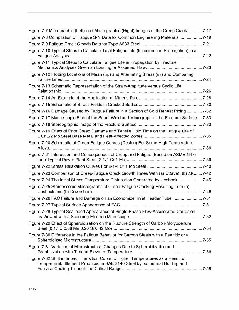
xxiv
Figure 7-7 Micrographic (Left) and Macrographic (Right) Images of the Creep Crack ............7-17 Figure 7-8 Compilation of Fatigue S-N Data for Common Engineering Materials ...................7-19 Figure 7-9 Fatigue Crack Growth Data for Type A533 Steel ...................................................7-21 Figure 7-10 Typical Steps to Calculate Total Fatigue Life (Initiation and Propagation) in a
Fatigue Analysis...............................................................................................................7-22 Figure 7-11 Typical Steps to Calculate Fatigue Life in Propagation by Fracture
Mechanics Analyses Given an Existing or Assumed Flaw...............................................7-23 Figure 7-12 Plotting Locations of Mean (σM) and Alternating Stress (σA) and Comparing
Failure Lines.....................................................................................................................7-24 Figure 7-13 Schematic Representation of the Strain-Amplitude versus Cyclic Life
Relationship .....................................................................................................................7-26 Figure 7-14 An Example of the Application of Miner’s Rule.....................................................7-28 Figure 7-15 Schematic of Stress Fields in Cracked Bodies.....................................................7-30 Figure 7-16 Damage Caused by Fatigue Failure in a Section of Cold Reheat Piping .............7-32 Figure 7-17 Macroscopic Etch of the Seam Weld and Micrograph of the Fracture Surface ....7-33 Figure 7-18 Stereographic Image of the Fracture Surface ......................................................7-33 Figure 7-19 Effect of Prior Creep Damage and Tensile Hold Time on the Fatigue Life of
1 Cr 1/2 Mo Steel Base Metal and Heat-Affected Zones .................................................7-35 Figure 7-20 Schematic of Creep-Fatigue Curves (Design) For Some High-Temperature
Alloys................................................................................................................................7-36 Figure 7-21 Interaction and Consequences of Creep and Fatigue (Based on ASME N47)
for a Typical Power Plant Steel (2-1/4 Cr 1 Mo)...............................................................7-39 Figure 7-22 Stress Relaxation Curves For 2-1/4 Cr 1 Mo Steel ..............................................7-40 Figure 7-23 Comparison of Creep-Fatigue Crack Growth Rates With (a) Ct(ave), (b) ΔK.......7-42 Figure 7-24 The Initial Stress-Temperature Distribution Generated by Upshock ....................7-45 Figure 7-25 Stereoscopic Macrographs of Creep-Fatigue Cracking Resulting from (a)
Upshock and (b) Downshock ...........................................................................................7-46 Figure 7-26 FAC Failure and Damage on an Economizer Inlet Header Tube .........................7-51 Figure 7-27 Typical Surface Appearance of FAC ....................................................................7-51 Figure 7-28 Typical Scalloped Appearance of Single-Phase Flow-Accelerated Corrosion
as Viewed with a Scanning Electron Microscope.............................................................7-52 Figure 7-29 Effect of Spheroidization on the Rupture Strength of Carbon-Molybdenum
Steel (0.17 C 0.88 Mn 0.20 Si 0.42 Mo)...........................................................................7-54 Figure 7-30 Difference in the Fatigue Behavior for Carbon Steels with a Pearlitic or a
Spheroidized Microstructure ............................................................................................7-55 Figure 7-31 Variation of Microstructural Changes Due to Spheroidization and
Graphitization with Time at Elevated Temperature ..........................................................7-56 Figure 7-32 Shift in Impact Transition Curve to Higher Temperatures as a Result of
Temper Embrittlement Produced in SAE 3140 Steel by Isothermal Holding and Furnace Cooling Through the Critical Range...................................................................7-58
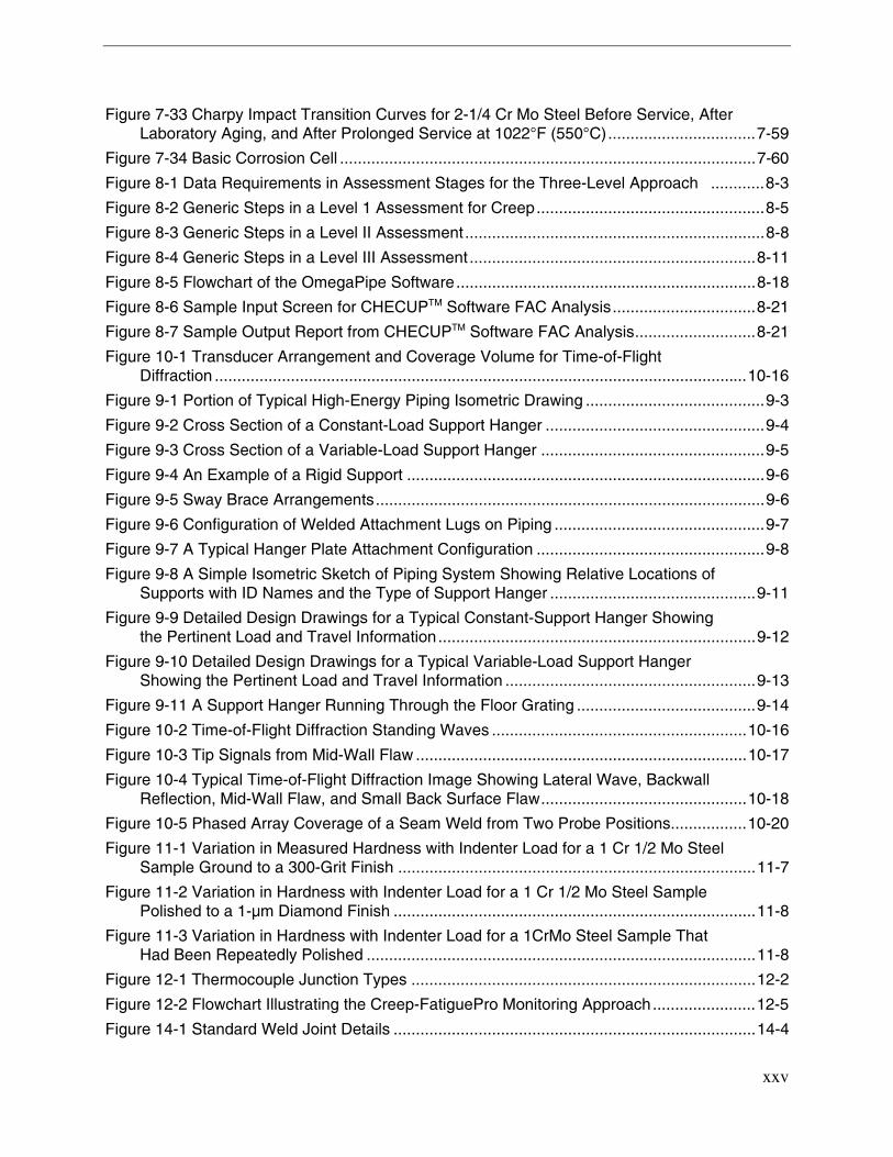
xxv
Figure 7-33 Charpy Impact Transition Curves for 2-1/4 Cr Mo Steel Before Service, After Laboratory Aging, and After Prolonged Service at 1022°F (550°C).................................7-59
Figure 7-34 Basic Corrosion Cell .............................................................................................7-60 Figure 8-1 Data Requirements in Assessment Stages for the Three-Level Approach ............8-3 Figure 8-2 Generic Steps in a Level 1 Assessment for Creep...................................................8-5 Figure 8-3 Generic Steps in a Level II Assessment...................................................................8-8 Figure 8-4 Generic Steps in a Level III Assessment................................................................8-11 Figure 8-5 Flowchart of the OmegaPipe Software...................................................................8-18 Figure 8-6 Sample Input Screen for CHECUPTM Software FAC Analysis................................8-21 Figure 8-7 Sample Output Report from CHECUPTM Software FAC Analysis...........................8-21 Figure 10-1 Transducer Arrangement and Coverage Volume for Time-of-Flight
Diffraction .......................................................................................................................10-16
Figure 9-1 Portion of Typical High-Energy Piping Isometric Drawing ........................................9-3
Figure 9-2 Cross Section of a Constant-Load Support Hanger .................................................9-4
Figure 9-3 Cross Section of a Variable-Load Support Hanger ..................................................9-5
Figure 9-4 An Example of a Rigid Support ................................................................................9-6
Figure 9-5 Sway Brace Arrangements.......................................................................................9-6
Figure 9-6 Configuration of Welded Attachment Lugs on Piping ...............................................9-7
Figure 9-7 A Typical Hanger Plate Attachment Configuration ...................................................9-8
Figure 9-8 A Simple Isometric Sketch of Piping System Showing Relative Locations of Supports with ID Names and the Type of Support Hanger ..............................................9-11
Figure 9-9 Detailed Design Drawings for a Typical Constant-Support Hanger Showing the Pertinent Load and Travel Information.......................................................................9-12
Figure 9-10 Detailed Design Drawings for a Typical Variable-Load Support Hanger Showing the Pertinent Load and Travel Information ........................................................9-13
Figure 9-11 A Support Hanger Running Through the Floor Grating ........................................9-14
Figure 10-2 Time-of-Flight Diffraction Standing Waves .........................................................10-16
Figure 10-3 Tip Signals from Mid-Wall Flaw ..........................................................................10-17 Figure 10-4 Typical Time-of-Flight Diffraction Image Showing Lateral Wave, Backwall
Reflection, Mid-Wall Flaw, and Small Back Surface Flaw..............................................10-18 Figure 10-5 Phased Array Coverage of a Seam Weld from Two Probe Positions.................10-20 Figure 11-1 Variation in Measured Hardness with Indenter Load for a 1 Cr 1/2 Mo Steel
Sample Ground to a 300-Grit Finish ................................................................................11-7 Figure 11-2 Variation in Hardness with Indenter Load for a 1 Cr 1/2 Mo Steel Sample
Polished to a 1-μm Diamond Finish .................................................................................11-8 Figure 11-3 Variation in Hardness with Indenter Load for a 1CrMo Steel Sample That
Had Been Repeatedly Polished .......................................................................................11-8 Figure 12-1 Thermocouple Junction Types .............................................................................12-2 Figure 12-2 Flowchart Illustrating the Creep-FatiguePro Monitoring Approach.......................12-5 Figure 14-1 Standard Weld Joint Details .................................................................................14-4

xxvi
Figure 14-2 Typical Counterbore Design .................................................................................14-5 Figure 14-3 Weld Buttering to Reestablish Pipe or Component Length After Removal of
Heat-Affected Zone ..........................................................................................................14-6 Figure 14-4 Typical Non-Through-Wall, Full-Circumferential Weld Repair Detail....................14-7 Figure 14-5 Typical Non-Through-Wall, Local Weld Repair Detail ..........................................14-8 Figure 14-6 Typical Base Metal Excavation Details...............................................................14-10 Figure 14-7 Plug Sample Repair Methods.............................................................................14-11
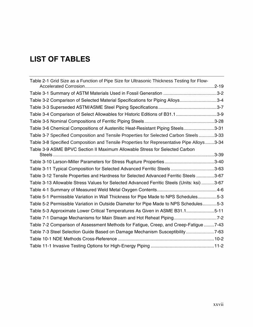
xxvii
LIST OF TABLES
Table 2-1 Grid Size as a Function of Pipe Size for Ultrasonic Thickness Testing for Flow-Accelerated Corrosion......................................................................................................2-19
Table 3-1 Summary of ASTM Materials Used in Fossil Generation ..........................................3-2 Table 3-2 Comparison of Selected Material Specifications for Piping Alloys.............................3-4 Table 3-3 Superseded ASTM/ASME Steel Piping Specifications..............................................3-7 Table 3-4 Comparison of Select Allowables for Historic Editions of B31.1................................3-9 Table 3-5 Nominal Compositions of Ferritic Piping Steels.......................................................3-28 Table 3-6 Chemical Compositions of Austenitic Heat-Resistant Piping Steels........................3-31 Table 3-7 Specified Composition and Tensile Properties for Selected Carbon Steels ............3-33 Table 3-8 Specified Composition and Tensile Properties for Representative Pipe Alloys .......3-34 Table 3-9 ASME BPVC Section II Maximum Allowable Stress for Selected Carbon
Steels ...............................................................................................................................3-39 Table 3-10 Larson-Miller Parameters for Stress Rupture Properties .......................................3-40 Table 3-11 Typical Composition for Selected Advanced Ferritic Steels ..................................3-63 Table 3-12 Tensile Properties and Hardness for Selected Advanced Ferritic Steels ..............3-67 Table 3-13 Allowable Stress Values for Selected Advanced Ferritic Steels (Units: ksi) ..........3-67 Table 4-1 Summary of Measured Weld Metal Oxygen Contents...............................................4-6 Table 5-1 Permissible Variation in Wall Thickness for Pipe Made to NPS Schedules...............5-3 Table 5-2 Permissible Variation in Outside Diameter for Pipe Made to NPS Schedules...........5-3 Table 5-3 Approximate Lower Critical Temperatures As Given in ASME B31.1......................5-11 Table 7-1 Damage Mechanisms for Main Steam and Hot Reheat Piping..................................7-2 Table 7-2 Comparison of Assessment Methods for Fatigue, Creep, and Creep-Fatigue ........7-43 Table 7-3 Steel Selection Guide Based on Damage Mechanism Susceptibility ......................7-63 Table 10-1 NDE Methods Cross-Reference ............................................................................10-2 Table 11-1 Invasive Testing Options for High-Energy Piping ..................................................11-2

1-1
1 INTRODUCTION
The objective of this three-volume report is to provide a guidance document that facilitates the development and implementation of a comprehensive, programmatic approach to life management of fossil generation piping systems. This first volume presents an overview of general issues that relate to all piping systems, including the following:
• Design fundamentals
• Design of piping support systems
• Materials
• Fabrication
• Damage mechanisms
• Inspection methods
• Programmatic approaches to life management
• Considerations for repair versus replacement
High-energy fossil piping systems are normally considered to include the main steam, reheat (both hot and cold), feedwater, and extraction steam piping. These systems can be subjected to a number of damage mechanisms, including creep, fatigue, thermal fatigue, creep-fatigue, microstructural instability, and flow-accelerated corrosion (FAC). An effective in-service inspection program anticipates the occurrence of damage and provides for a cost-effective program to identify this damage during an early stage of development in order to allow for budgeted repair or replacement.
Unlike boiler tubes, high-energy piping has no expected design life. When in service, this equipment undergoes continuous damage; however, the design margins established in the fabrication codes are such that the anticipated damage rate was not expected to result in a failure of major components during the economic life of a unit. When failure occurs, it is normally the result of inadequate design as a result of overestimation of material strength (for example, 1-1/4 Cr 1/2 Mo has been derated over the years), an incomplete understanding of the metallurgical impact of fabrication variables (creep cavitation damage in submerged arc welds), or a significant change in operating practices (excessive temperatures or a change from base load to cyclic operation).
Introduction
1-2
Although repair of selected locations (such as circumferential welds) might be required throughout the life of the unit, the need for complete replacement of the piping system is unusual and not expected. In addition, when major modifications are necessary, there is typically no expectation of performance improvement. Therefore, the goal of a critical piping program is to ensure personnel safety and to limit expenditures associated with forced outages resulting from failure.
Historically, the assessment of high-energy fossil piping systems primarily consisted of regular monitoring and adjustment of the piping support systems and nondestructive examination (NDE) of a limited number of select circumferential welds. However, following the catastrophic failure of seam-welded hot reheat (HRH) pipe at two power stations in 1985 and 1986, the U.S. electric power industry embarked on an aggressive inspection and evaluation effort to minimize the risk associated with operating seam-welded high-energy piping. As a result of these inspections, a significant number of failures and major cracking occurrences have been identified in seam-welded HRH and main steam piping.
Similarly, recent occurrences of circumferential weld damage have frequently developed in nontraditional locations and, in many cases, have initiated subsurface, increasing the difficulty of detection. Historically, critical piping inspection programs have considered a stress-biased approach that focused attention on the calculated highest-stress welds with the expectation that these welds would develop damage first and then serve as indicators for the overall system condition. However, recent experience has shown that many industry failures and severe cracking events have developed in lower-stress welds, demonstrating that stress is only one of several critical factors that must be considered in developing a comprehensive inspection plan.
Finally, the catastrophic failure of a seam-welded cold reheat pipe in 2003 resulting from corrosion fatigue and the periodic occurrence of FAC damage failures in feedwater and extraction steam piping demonstrate potential for damage occurrence in fossil piping systems operating outside the normal creep regime.
These experiences demonstrate the need for a comprehensive understanding of the design and fabrication of high-energy piping systems, the identification of probable damage mechanisms, and the tools available for developing and implementing a comprehensive high-energy piping program with the following objectives and benefits:
• Safety. Personnel safety is the highest priority. Although it is impossible to remove all risk, the goal of an effective high-energy piping program should be to lower the risk of failure to a level that is reflective of risks to which employees are normally exposed and that the employees readily accept. For example, an acceptable level of risk could be comparable to the level of risk that employees expose themselves to during their daily commute to work.
• System reliability. An additional objective of the high-energy piping program is to reduce the financial impact associated with forced outages resulting from failure. This can be accomplished by using state-of-the-art inspection techniques to identify damage in sufficient time to effect mitigation or any required repair and replacement during scheduled maintenance overhauls. Although early detection of service-induced damage by inspection is
Introduction
1-3
necessary to limit the risk of forced outages, it is equally important to reduce the occurrence of damage through proper maintenance of piping supports and to identify system operating conditions that adversely impact component life. For a given operating history, a properly implemented program will anticipate damage associated with known damage mechanisms and will schedule periodic inspections to identify components for repair or replacement during routine scheduled maintenance outages.
• Optimized inspection costs. An effective high-energy fossil piping program can minimize inspection costs through the following methods:
– Proper documentation. Documentation of weld locations, materials of construction, fabrication practices, and previous inspection results can help reduce inspection costs.
Many of the risk factors associated with circumferential weld failures are associated with material properties and fabrication practices. For example, submerged arc welds (SAW) are more susceptible to the development of subsurface-initiated Type IV creep damage than shielded metal arc welds (SMAW). Similarly, the presence of a repair to a weld (longitudinal or circumferential) greatly increases the probability of damage initiating in the weld. Minor compositional variables can also be a significant factor in determining the susceptibility of a weld to failure, and it is not uncommon to find welds in a piping system fabricated with an incorrect filler metal.
When possible, fabrication practices should be documented, and compositional information should be gathered. When available, construction records can be used to identify fabrication practices and the compositional make-up of a component. However, in most cases these detailed records will not be available. When detailed fabrication records are not available, welding methods (for example, SAW versus SMAW) can be inferred from the appearance of the weld, and the occurrence of a weld repair can be ascertained by noting a disruption of the weld bead pattern in the finished weld. Limited compositional information can be obtained by nondestructive alloy analysis.
– Optimal inspection timing. Using the best inspection technology and documenting the inspection results can prevent premature or unnecessary reinspection.
• Outage planning. Program costs can be minimized only through complete and effective forecasting of inspection and repair requirements. Forecasting inspection and repair activities can enable a utility to schedule and budget for inspection, repair, and replacement costs and to coordinate these activities with concurrent outage activities.

2-1
2 DESIGN
Introduction
The initial design of a piping system is established by the functional requirements of transporting a fluid from one point to another. The detailed design is affected by such criteria as the type of fluid being transported, the allowable pressure drop, the pumping requirements, the desired velocity, and the available materials.
In the design of a piping system and its supports, the factors that must be considered are predicated by the type of plant in which the system will be used. Clearly, piping systems are a major component (and expense) in power stations. Other than in nuclear applications, where environmental hazard potential is the prime factor, power plant designs are affected by economic considerations. Aside from the functional aspects of piping system design, the system supports require significant engineering effort (design, fabrication, and installation) to ensure that the piping system operates at stress levels within the levels prescribed by codes and provides reliable operation for a prescribed time period.
This section describes a typical design process, the role of codes and regulations in the formulation of a design, the primary parameters that affect the design, and the relationship of the design process to other disciplines.
The Design Process
Fundamental Questions
The fundamental function of a high-energy piping system is to transport fluid (water or steam) from a source to a delivery point. The characteristics of the piping system are developed to achieve this goal. The fundamental design requirement is to deliver the required fluid volume at the specified conditions and in compliance with the governing code. In the United States, the governing codes are the American Society of Mechanical Engineers (ASME) Boiler and Pressure Vessel Code (BPVC), Section I, Power Boilers, and ASME B31.1, Code for Pressure Piping Standards: Power Piping [2-1, 2-2]. These documents are examples of design-by-rule codes wherein simplified equations are used to determine characteristic stress values that are then compared with allowable stresses. Therefore, after the piping diameter is determined (to meet flow requirements), wall thickness requirements can be determined from the code rules based on the specified fluid conditions and the selected materials of construction.
Design
2-2
Material Selection
For the most part, material selection is governed by cost and availability. However, there are other indirect effects of material selection that might not be readily apparent. For example, selection of a high-chromium alloy steel instead of a low-alloy steel can result in a significantly thinner wall requirement for a given pressure and temperature according to the code allowable. A thinner pipe results in less dead weight, which could allow the use of smaller pipe supports and lighter structural steel. Each potential selection has both beneficial and less beneficial points. The difficult part is arriving at the optimum balance of cost, functionality, and safety. A more in-depth description of the material selection process can be found in the EPRI report Metallurgical Guidebook for Fossil Power Plant Boilers (1004509) [2-3].
Support Locations
After the pipe sizes are established, a routing plan can be developed to get from the source to the delivery point. Because most high-energy piping is large (greater than 10 in. [25.4 cm]) diameter, cost considerations dictate that run geometry be kept simple with as few directional changes as possible. Specification of support types and locations is critical. For this process, detailed drawings of the proposed pipe routing, structural steel drawings, and location of other piping and equipment in the proposed run area are required.
With all the geometric data collected, the next step is to define initial support locations. This is accomplished by establishing characteristic support spans for each pipe diameter based on dead weight loading (vertical support span) and, if applicable, seismic and wind loadings (lateral support span). It is advantageous to use one span that satisfies both criteria, thereby allowing a combination of directional support at one location.
With the characteristic spans determined, superimposing the piping drawings over the structural steel layouts should allow identification of candidate support locations. These locations should be near, or coincident with, structural steel or other convenient points of attachment, and the distance between locations should be consistent with the characteristic spans. When available structure is not present to maintain the determined spans, it is usually preferable to shorten the span between supports as opposed to constructing a more complicated attachment. It is also important to review drawings from other systems and equipment to avoid physical interference.
Stress Analysis
After the initial support locations are selected, stress analysis of the system is performed to determine the support characteristics required to prevent piping overstress according to the code requirements. In this design phase, a balance between required support and flexibility for thermal expansion must be obtained. A design that provides the minimum number of supports with locations and functions that minimize resistance to thermal expansion, within the code allowable stresses, will be the best.
Design
2-3
By analysis, support function (constant load, variable load, or restraint) and required load capability can be determined through the combination of individual load cases. These load cases include dead weight (DW), thermal expansion (Th), seismic loading (EQ), and wind loading. From these load cases, the following combinations should be considered:
• DW + Th + (EQ + Wind)
• DW + Th - (EQ + Wind)
• DW + (EQ + Wind)
• DW - (EQ + Wind)
The maximum loading in each direction determined from these load combinations should be used to design the support.
Design Codes and Regulations
In the interest of public protection, numerous international, federal, state, and local government regulations have been created and enacted. In the United States, these are typically associated with the ASME BPVC and ASME B31 [2-1, 2-2] . The ASME BPVC Section I, Power Piping, for power boilers was issued in 1914. Today the ASME BPVC includes eleven sections, and it is mandatory in most states. The ASME B31 code collection (B31.1 through B31.9) is not mandatory in the United States, although it has been adopted as a legal requirement with the minimum design requirements being accepted by the power industry as a standard for all piping outside the jurisdiction of the ASME BPVC.
In response to these regulations and with the intent of simplifying their interpretation, several professional societies have published guidelines, codes, and standards. However, some confusion exists as a result of the number of such documents. The following generally accepted definitions are used in this volume:
• Codes. The collections of rules or systematic standards for design, materials, fabrication, installation, or inspection prepared in a way that they can be adopted by a legal jurisdiction and made into law.
• Standards. Documents prepared by a professional group describing requirements that are good and proper engineering practices and that are written with mandatory requirements (use the verb “shall”).
• Recommended practices. Documents prepared by a professional group specifying good engineering practices, the application of which is optional.
• Guidelines. Documents prepared by agencies, organizations, or committees describing engineering methods that are considered good practice but have no specific recommendation or requirement.

Design
2-4
For the purposes of system design, it is important that designers remain current regarding changes to the applicable codes. The codes and standards applicable to a given design are those that are in effect at the time that the system or component purchase order is awarded.
Typically, changes to any of these documents are identified as addenda, errata sheets, or new editions. When a code requirement is questioned and an interpretation is requested, a Code Case is assigned. The resulting committee response can result in the relaxation of a specific requirement. Code Cases do not signify a revision to the code; designers who use Code Cases should be sure that they apply to their situation. Code changes are typically not retroactive; they become mandatory six months after they are issued, unless otherwise indicated.
ASME Codes
The ASME BPVC, Section III, Rules for Construction of Nuclear Power Plant Components, Subsections NC (Class 2 Components) and ND (Class 3 Components), and the ASME B31 codes, which are applicable to the majority of piping systems, use the maximum principal stress theory to assess component failure [2-4, 2-2]. This theory states that yielding occurs when the magnitude of any of the three principal stresses exceeds the material yield strength. More detailed evaluations of stress combined with the maximum shear stress theory are allowed for Section III, Subsection NB (Class 1) components.
Piping stresses are categorized by the following three types:
• Primary stresses are developed by applied mechanical loads. Primary stresses are not self-limiting. Failure modes are plastic deformation and bursting.
• Secondary stresses are developed as a result of constraint of the system against displacement such as thermal expansion or imposed displacements. Secondary stresses are self-limiting and can be relieved by deformation of the system. Failure modes are plastic instability and buckling.
• Peak stresses are developed locally, and they typically do not result in distortion of the system. Peak stresses form as the result of thermal gradients or stress concentrations. Failure mode is fatigue failure from cyclic loading.
Stress limits within a fossil piping system designed under ASME B31.1 criteria must meet the following limits:
• Sustained-load stresses from pressure, weight, and other mechanical loads must satisfy Equation 2-1.
(English Units) hA
n
O SZiM
tPD 0.175.04
≤+
(SI Units) hA
n
O SZ
Mit
PD 0.1)75.0(10004
≤+ Eq. 2-1

Design
2-5
Where:
P is the internal design pressure (psi or kPa).
DO is the outside diameter of the pipe (in. or mm).
tn is the nominal wall thickness of the pipe (in. or mm).
MA is the resultant moment on the cross section from sustained loads (in-lb or mm-N).
Z is the section modulus of the cross section (in3 or mm3).
i is the stress intensification factor (a dimensionless parameter).
Sh is the material allowable stress at maximum temperature from the stress tables in the ASME BPVC, Section II, Part D (psi or kPa) [2-5].
• Occasional-load stresses from pressure, weight, other mechanical loads, and occasional loads (including earthquake) must satisfy Equation 2-2.
(English Units) hBA
n
O kSZiM
ZiM
tPD
≤++75.075.0
4
(SI Units) hBA
n
O kSZ
MiZ
Mit
PD≤++
)75.0(1000)75.0(10004
Eq. 2-2
Where:
k is 1.15 for occasional loads acting less than 10% of the operating time, and 1.2 for occasional loads acting less than 1% of the operating time.
MB is the resultant moment on the cross section from sustained loads (in-lb or mm-N).
• Expansion-load stresses, the effects of thermal expansion loads, must satisfy Equation 2-3.
(English Units) )( LhAC
E SSfSZ
iMS −+≤=
(SI Units) )()(1000LhA
CE SSfS
ZiMS −+≤= Eq. 2-3
Where:
MC is the range of moments on the cross section from thermal expansion (in-lb or mm-N).
SA is the allowable stress range for thermal expansion stresses = f(1.25SC + 0.25Sh).
SC is the material allowable stress at minimum temperature from the stress tables.
Design
2-6
f is the stress range reduction factor for cyclic conditions.
SL is the sustained stress calculated in Equation 2-1.
Design Life
The determination of design life for high-energy piping, as for any component, can be made only based on an in-depth understanding of the properties of the construction materials and the service conditions that will be experienced. The guidelines contained in the ASME BPVC, Section I, and ASME B31.1 have demonstrated that they provide adequate margins in establishing these values for the majority of high-energy system components [2-1, 2-2]. As with any complex system, identification of all factors and their respective application ranges is not possible. As a consequence, neither code defines a specific design life.
ASME B31.1 states in its Foreword, “this Code is more conservative than some other piping codes, reflecting the need for long service life and maximum reliability in power plant installations” [2-2]. The Foreword of the ASME BPVC section states that “the objective of the rules is to afford reasonably certain protection of life and property and to provide a margin for deterioration in service so as to give a reasonably long, safe period of usefulness” [2-1]. Clearly, “long service life” and “reasonably long, safe period of usefulness” are not specific design lives. Therefore, it is the designer’s responsibility to be aware of those factors that affect component or system life and to establish the design life for a component or system that also meets code rules. Recognizing that not all factors are covered in the code, the designer must be ready to go beyond the code rules to ensure the target design life.
Although the codes do not explicitly define a design life, examination of the bases used in development of the allowable stress tables can provide some general insight. In the design-by-rule method, the basis for design of pressure components is the comparison of a singular calculated stress value with the allowable stresses provided in the code. In general, values in the stress tables have been established to prevent the following:
• Rupture of the pressure boundary, independent of temperature
• General yielding during short-term loading at temperatures below the creep range
• Large strains (>1%) for components with extended service at temperatures in the creep range.
To prevent pressure boundary rupture, design stresses at temperature are limited to 0.314 of the material tensile strength at temperature. In the creep range, design stresses are limited to the lower of a secondary creep rate of 1% per 100,000 hours or 80% of the 100,000-hour creep rupture stress.
For general yielding of most materials, the primary stress values are limited to two-thirds of the yield strength at temperature. For some more-ductile materials, as much as 90% of the yield strength at temperature is allowed. For long-term exposure in the creep range, allowable stresses produce an average secondary creep rate of 1% per 100,000 hours exposure.
Design
2-7
Therefore, for components that operate at temperatures below the creep range of the constituent materials, it is reasonable to presume that—barring faulty fabrication, material degradation with time, out of specified operation, or fatigue—extended lives will be realized. For components that operate in the creep range, the factors described in this section indicate a minimum design life of 100,000 hours.
System Loads
All piping codes followed in the United States were developed from the American Standards Association (ASA) B31, Code for Pressure Piping, which was first published in 1935. As a consequence of this common source, today’s codes share a common terminology regarding the classification of loads experienced by piping systems. Specifically, loads are classified as the following three types:
• Sustained loads are those loads caused by forces that are present throughout normal operation, such as pipe weight and internal pressure.
• Occasional loads, as the name implies, are those that do not occur on a regular basis but do happen during operation. Examples of occasional loads are wind, seismic events, fault events, and valve relief.
• Expansion loads are the result of pipe displacements typically caused by pipe thermal expansion and terminal point displacements from thermal expansion or foundation settlement.
Regardless of the type of load, the system supports must be able to transmit that load to the building structure. To ensure that the supports are able to perform this function for the life of the plant, the loads applied must be determined and combined to develop a set of design loads for the system. The following subsections describe how to estimate or calculate design loads for a system.
Dead Weight Loads
All systems must be designed for dead weight loading. This load type is not self-relieving; therefore, supports must be provided to prevent collapse of the system from its own weight. Because this load is present throughout the operating cycle of a system, it is a sustained load.
The load at a support from system weight must include the weight of the pipe, insulation, fluid, attached components, and support hardware. Dead weight loads establish the initial spacing of supports so that bending stresses on the pipe cross section do not exceed code allowables. Support spacing should also consider other load contributions; therefore, dead weight loads frequently do not by themselves determine the final spacings in a design.
Design
2-8
Considering the span of piping between supports as a beam, the maximum bending moments and end loads on the cross section as a function of the span (L), assumed end conditions (pinned or fixed), and material densities (ρ) are determined using strength of materials formulas (Equation 2-4 for pinned-end conditions, and Equation 2-5 for fixed-end conditions).
Pinned-end conditions Mmax = (1/2)WL2 and FEnd = 1/2WL Eq. 2-4
Fixed-end conditions Mmax = (1/12)WL2 and FEnd = 1/2WL Eq. 2-5
Where:
W is the combined weight per unit length of pipe, insulation, and other materials.
L is the length of pipe between span ends.
FEND is the vertical reaction load at each end of the section.
In application, the actual conditions at a support fall between the fixed and pinned conditions. Consequently, bending moments at supports are best approximated in the range of WL2/4 to WL2/7, depending on the support type.
For a given W for a section of piping, support spacing is determined by using the allowable stress at temperature from the stress tables for the specified material, as shown in Equation 2-6, applying the best approximation formulation for bending stress.
Lmax = (10ZSALL/W)1/2 Eq. 2-6
Where:
L is the overall length of the span for which you are determining the support spacing.
Z is the section modulus of the pipe cross section or the outside radius/moment of inertia.
SALL is the allowable stress at the operating temperature for the specified material from the applicable code stress table.
W is the combined weight per unit length of pipe, insulation, and other materials.
Pressure Loads
Internal pressure from the water or steam being transported is another sustained load. This pressure does not typically result in loads on the supports other than at terminal points or where the pipe wall is not continuous (for example, at bellows or slip joints). However, it certainly is a main contributor to the stress state in a section of piping.
Design
2-9
At a terminal point or discontinuous pipe-wall location, the load (F) developed from internal pressure is determined from the magnitude of the pressure (P) multiplied by the cross-sectional flow area (DFlow), as shown in Equation 2-7.
4FlowDPF π
= Eq. 2-7
Where:
F is the load.
P is the pressure.
DFlow is the cross-sectional flow area.
Wind Loads
Wind loads are classified as occasional loads. Any section of a piping system that is outdoors could be subjected to external pressure forces (horizontal, vertical, or both) from wind. To develop the potential contribution from wind loading, the maximum anticipated wind velocity over the life of the system must be determined. Wind velocity maps and mean and peak velocity data as a function of location and elevation are published by several organizations and should be cited in the system design documentation.
The load applied by wind is typically modeled as uniform, acting over the projected area of the pipe, parallel to the wind direction. The force generated per unit length, FWind, is calculated using Equation 2-8 (based on Bernoulli’s equation for fluid flow over a body).
gDqC
F DragWind = Eq. 2-8
Where:
CDrag is the drag coefficient for the pipe (dimensionless).
D is the pipe and insulation outside diameter.
g is the gravitational constant.
q is the dynamic pressure exerted by the wind, calculated as 1/2ρV2 for the air density (ρ) in mass/length3 and wind velocity (V) in length/s.
The drag coefficient, CDrag, is a function of the body shape and flow velocity evaluated using the Reynolds number. Values for CDrag for piping are found in tables available in many references.
Design
2-10
Seismic Loads
Safety-related nonnuclear piping must be designed to withstand seismic loads. Accurate evaluation of seismic loads is complex, whether by modal or time-history analysis, and it requires numerical analysis that is typically performed on a computer. In those instances where less accuracy is acceptable, static analyses can be performed.
The first step in the process is to establish the seismic potential in the area in which the piping system is located. The Uniform Building Code provides one source of damage potential based on a four-tiered zone ranking system. After the area-based seismic characteristics (particularly magnitude and duration) are determined, they are converted into loads using Equation 2-9.
ZKCWFSeismic = Eq. 2-9
Where:
Z is a factor based on the seismic zone.
K is a factor based on the type of structure, typically 0.67 to 3.0.
C is 0.5/T1/2 for T, the fundamental period of the system (s)
W is the weight of the piping system, including insulation and support hardware (lb or kg).
Pressure Relief Loads
All high-energy piping systems must have the capability to relieve internal pressure to prevent boundary ruptures. This is accomplished by placing pressure-sensitive valves in the piping system. When a pressure relief valve opens, the resulting stream of fluid causes a jet force that must be resisted by the pipe and its supports. The magnitude of the relief force is typically supplied by the valve manufacturer. If it is not provided, it can be calculated for those instances in which the pipe is vented directly to the atmosphere, as shown in Equation 2-10.
⎥⎦
⎤⎢⎣
⎡+= PA
gMVFF
cDynamicRelief Eq. 2-10
Where:
FDynamic is a dynamic load factor included to account for the increased load applied as a result of the rapid application of the relief force, typically in the range of 1.1 to 2.0.
M is the mass flow rate from the valve.
gc is the gravitational constant.
V is the fluid exit velocity.
P is the fluid pressure.
A is the discharge flow area.

Design
2-11
Expansion Loads
The more supports provided in a system, the more effectively restrained it will be for dead weight and occasional loads. However, with increased temperatures during operation, the pipe will expand. A system that is too constrained will resist this expansion, resulting in locations of increased stress. Ideally, the piping support system need only support the weight of the piping and fluid and provide no additional restraints. Complete lack of restraint is not possible, and some expansion forces will be developed at restrained locations. The most comprehensive evaluation of expansion loads is accomplished by using numerical methods implemented through several currently available computer programs.
Besides evaluating an entire system using a computer, there are simplified methods for determining expansion loads. The primary concern regarding thermal expansion is in the direction parallel to the pipe axis. The amount of thermal expansion, ΔThermal, in a given section of pipe can be determined by Equation 2-11.
TLThermal Δ=Δ α Eq. 2-11
Where:
α is the pipe material coefficient of thermal expansion.
L is the pipe length.
ΔT is the difference in temperature.
For typical piping materials, the value of α is temperature dependent. Mean values for the expansion coefficient are provided in the code for application over temperature ranges starting at 70°F (21°C).
After the magnitude of the expansion is determined, the loads created by that expansion on the supports can be approximated by assuming that the expansion must be absorbed by bending of the piping that is perpendicular to the expansion. Then, treating each perpendicular leg as a cantilever beam, the moment (M) and force (P) at each end of the expansion length can be determined from beam theory, as shown in Equation 2-12.
26
LEIM ThermalΔ
= and 312
LEIP ThermalΔ
= Eq. 2-12
Where:
E is the pipe modulus of elasticity.
I is the pipe cross-section moment of inertia.
L is the leg length perpendicular to the expansion direction.
ΔThermal is the change in length as a result of the difference in temperature.
Design
2-12
The expansion accommodated by each leg is inversely proportional to the ratio of the leg stiffness to the sum of all leg stiffnesses absorbing the expansion. This method is only approximate because the leg intersections provide some rotation capability and thereby redistribute the developed moment. Consequently, in most cases, the calculated moments should be conservative.
To alleviate the development of excessive expansion loads, most high-temperature systems are designed with expansion loops. This term is not to be taken literally, but instead represents the introduction of run directional changes and reduced numbers of rigid supports to provide additional system flexibility. This flexibility allows for the accommodation of thermal expansion without the penalty of added loads. The downside is that as a system becomes more flexible, it is less able to handle occasional loads without additional supports.
System Supports, Design, and Function
The design of high-energy piping system supports is a nontrivial task with no set method of accomplishment. The design process, from initial conceptual drawings of support locations and calculations to final construction, involves many steps performed in series and in parallel. Each project must be individually tailored to the specifics of the plant.
As a result of the inherent flexibility of large-volume, long-run piping systems, supports are available in a variety of types and styles, each designed for a specific function and location. Regardless of the size and shape of the supports, their functions remain the same, as follows:
• To support the dead weight of the piping, insulation, and attached components from the available structure
• To allow thermal expansion of the piping, yet provide weight support and minimize load transfer at terminal points
• To provide vibration, fault, and seismic event displacement control
A detailed description of system support design is outside the scope of this report. However, having a general understanding of the design process and those factors that influence a design will facilitate the treatment of support problems if and when they occur.
Basic Design Steps
The basic steps followed in support system design are the following:
1. Determine the support locations to meet the applicable code pipe stress requirements.
2. Determine the loads carried by each support.
3. Determine the thermal movement of the piping at each support location.
Design
2-13
4. Select the support types (that is, constant, variable, rigid, and so on) to meet the requirements of steps 2 and 3.
5. Check the clearances between the support components and nearby piping, cable trays, ducts, and so on.
Each basic step contains several steps and requirements that must be met for a given design to perform adequately. The following paragraphs describe those steps and requirements.
Support Locations. Determination of support locations within a system depends on several factors, including pipe size, piping configuration, the location of heavy valves and fittings, and the structure available for support. There are no set rules or limits that positively fix support locations. However, suggested characteristics that have performed well are the following:
• Published tables of recommended piping spans between hangers based on diameter and carried product (straight runs only) should be used.
• For concentrated loads (such as valves and wyes), supports should be located as close as possible to the load to minimize bending stresses.
• When practical, supports should be located adjacent to any change in direction of the piping.
• When changes in direction occur between supports, span lengths should be less than 75% of comparable straight-run lengths.
• The load carried by a hanger in a vertical section should be selected such that the elevation of the support is above the midpoint of the length of pipe supported. This eliminates a tendency for the piping to rotate about the support.
Support Loads. For high-energy piping systems, the loads carried by the supports are created primarily by the weight of the piping, insulation, valves, fittings, and support hardware. Wind, seismic, and fault condition loads typically define the capacity (but not the size) of the support and its attachment structure. During normal operation, the job of the majority of supports is to support the weight of the system while allowing unrestricted thermal expansion. It is this aspect of support operation (the combination of structural support and motion) that complicates support design.
Through the use of static equilibrium equations, estimates of the load applied to a support can be determined. The procedure requires that you divide the system into sections, constructing a “free-body” diagram of each section. When the weights and locations of the components in each section with respect to the section end points are known, the equations for static equilibrium within the section can be written (see Equation 2-13), where Mi and Vi are moment and force values in each orthogonal direction.
∑Mi = 0 and ∑Vi = 0 for i = x, y, and z directions Eq. 2-13
Combining the equations from each free-body diagram will result in a series of equations that will allow determination of the load at each support. As a final check, the total weight of the piping, insulation, valves, and so on should be equal to the total load carried by all of the hangers plus the load supported by the terminal points.
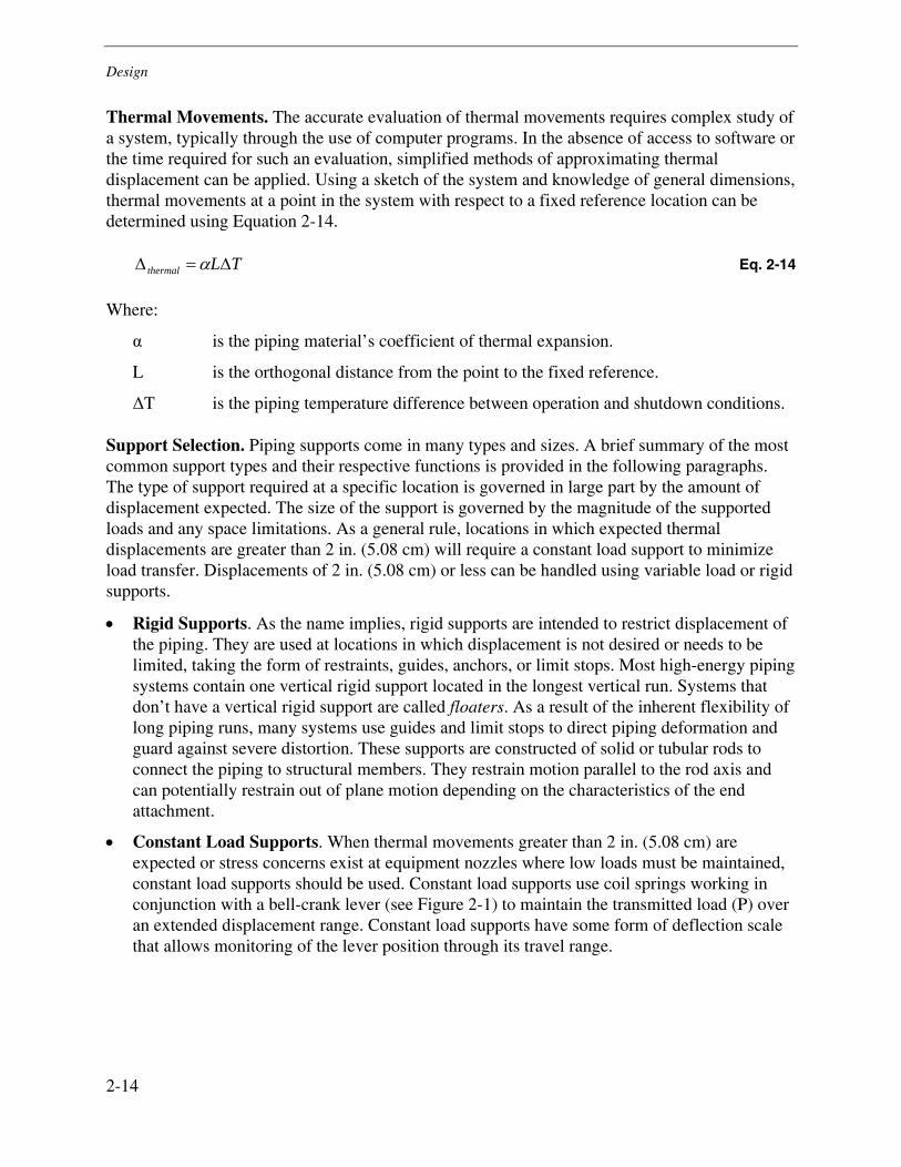
Design
2-14
Thermal Movements. The accurate evaluation of thermal movements requires complex study of a system, typically through the use of computer programs. In the absence of access to software or the time required for such an evaluation, simplified methods of approximating thermal displacement can be applied. Using a sketch of the system and knowledge of general dimensions, thermal movements at a point in the system with respect to a fixed reference location can be determined using Equation 2-14.
TLthermal Δ=Δ α Eq. 2-14
Where:
α is the piping material’s coefficient of thermal expansion.
L is the orthogonal distance from the point to the fixed reference.
ΔT is the piping temperature difference between operation and shutdown conditions.
Support Selection. Piping supports come in many types and sizes. A brief summary of the most common support types and their respective functions is provided in the following paragraphs. The type of support required at a specific location is governed in large part by the amount of displacement expected. The size of the support is governed by the magnitude of the supported loads and any space limitations. As a general rule, locations in which expected thermal displacements are greater than 2 in. (5.08 cm) will require a constant load support to minimize load transfer. Displacements of 2 in. (5.08 cm) or less can be handled using variable load or rigid supports.
• Rigid Supports. As the name implies, rigid supports are intended to restrict displacement of the piping. They are used at locations in which displacement is not desired or needs to be limited, taking the form of restraints, guides, anchors, or limit stops. Most high-energy piping systems contain one vertical rigid support located in the longest vertical run. Systems that don’t have a vertical rigid support are called floaters. As a result of the inherent flexibility of long piping runs, many systems use guides and limit stops to direct piping deformation and guard against severe distortion. These supports are constructed of solid or tubular rods to connect the piping to structural members. They restrain motion parallel to the rod axis and can potentially restrain out of plane motion depending on the characteristics of the end attachment.
• Constant Load Supports. When thermal movements greater than 2 in. (5.08 cm) are expected or stress concerns exist at equipment nozzles where low loads must be maintained, constant load supports should be used. Constant load supports use coil springs working in conjunction with a bell-crank lever (see Figure 2-1) to maintain the transmitted load (P) over an extended displacement range. Constant load supports have some form of deflection scale that allows monitoring of the lever position through its travel range.
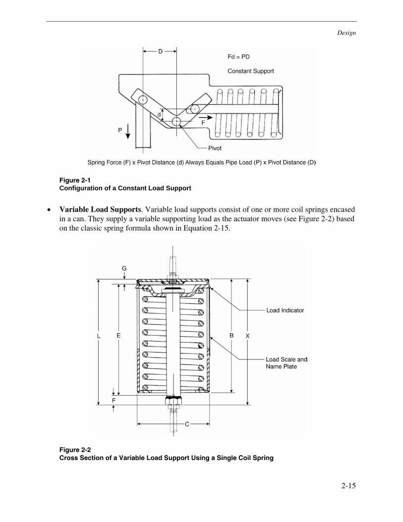
Design
2-15
Figure 2-1 Configuration of a Constant Load Support
• Variable Load Supports. Variable load supports consist of one or more coil springs encased in a can. They supply a variable supporting load as the actuator moves (see Figure 2-2) based on the classic spring formula shown in Equation 2-15.
Figure 2-2 Cross Section of a Variable Load Support Using a Single Coil Spring
Design
2-16
Δ+= KFF InitialSupport Eq. 2-15
Where:
FInitial is the starting load on the support.
K is the spring stiffness.
Δ is the actuator displacement from the as-installed position or the anticipated thermal movement.
With this type of support, the direction of motion controls whether the support load increases or decreases. Supports of this type will also have a displacement or load scale to facilitate monitoring of support loads.
As dictated by design practice, the supported load, FSupport, is the hot load; therefore, in Equation 2-15, FInitial is the cold load, or more appropriately, the installed load. In general practice, it is desirable to limit the load variability from cold to hot conditions to a maximum of 25%. Because the hot condition load and thermal movement are established by the piping design, load variability can be controlled only by changing the spring stiffness (K) of the support.
Flow Considerations and Modeling
As a result of the high flow velocities and volumes present in power generation steam and feedwater piping systems, the potential exists for significant dynamic loads. For steam lines, flow-related damage can occur from safety valve operation, steam hammer, condensate buildup, and inside diameter (ID) erosion. In feedwater piping, FAC and water hammer can occur. Generally, for steam hammer, water hammer, and other dynamic load events, adherence to standard design practices and recommended operating methods and procedures will alleviate these events and their causative effects. For FAC mechanisms, some form of monitoring or predictive assessment is required to ensure the identification of affected components and assessment of long-term effects.
Flow-Related Dynamic Load Events
Flow-related dynamic loads occur in steam piping from safety valve operation, steam hammer, and condensate buildup. The opening of safety relief valves produces a jet force that must be accommodated by the piping and support system in the vicinity of the valve. The magnitude of the force created will be function of the fluid pressure, exhaust conditions, and valve flow capacity. According to ASME B31.1, the discharge force, F, can be calculated as shown in Equation 2-16 [2-2].
⎟⎟⎠
⎞⎜⎜⎝
⎛+= PA
gMVDF
cf Eq. 2-16
Design
2-17
Where:
Df is a dynamic load factor with a range of 1.1 to 2.0, depending on the rigidity of the valve support and its opening time.
M is the mass flow rate from the valve.
V is the steam exit velocity.
gc is the gravitational constant.
P is the discharge pressure.
A is the discharge flow area.
During startup and low-load operation, conditions can exist in which condensate will collect in the piping system. This condition is exacerbated by inadequate or nonoperating drains. The velocity of the steam flowing over the condensate causes ripples in the water. Turbulence builds up until the water forms a solid mass, or slug, that fills the pipe cross section. This slug of condensate travels at the speed of the steam until it impacts the first change in flow direction (for example, an elbow or bend) with significant force, resulting in dynamic loading of the piping. The impact force is a function of the flow velocity and the mass of the slug.
During fault events, the rapid closure of stop or control valves can produce a significant shock wave that propagates upstream through the piping system as a result of the fluid momentum change (steam hammer). The magnitude of the shock wave is a function of steam velocity, enthalpy, and valve closure time. Because this is a momentum change, forces are applied at each change in direction of the piping, staggered according to the shock wave velocity.
Flow-Accelerated Corrosion
Service-related damage in low-temperature piping systems predominantly occurs as a result of fatigue, corrosion fatigue, or erosion-corrosion (commonly referred to as flow-accelerated corrosion or FAC). FAC is a significant degradation mechanism that occurs in low-temperature piping systems and has resulted in a number of failures in both nuclear and fossil-fueled power plants. Thermal or mechanical fatigue cracking can occur in feedwater and other low-temperature piping systems that are exposed to significant thermal shock events, water hammer, or deficient pipe support conditions. These are localized events that occur as a result of unit- or operations-specific conditions, as opposed to generic problems.
FAC refers to material wall loss that occurs in piping systems through dissolution of the protective oxide layer (magnetite or hematite) by localized turbulence from flowing water or wet steam. A number of FAC-related failures have occurred in low-temperature piping systems of fossil-fueled power plants over the years. As was the case with longitudinal seam-welded failures occurring in high-temperature HRH piping systems, the occurrence of these failures resulted in
Design
2-18
various EPRI and other industry-sponsored studies of the FAC damage mechanism [2-6–2-8]. From these studies, the following major factors influencing FAC susceptibility have been identified:
• Material composition. FAC has been found to be highly dependent on levels of trace elements such as chromium, molybdenum, and copper. Chromium (Cr) content, in particular, offers significantly improved resistance to FAC. In general, FAC is active in piping systems containing 0%–0.20% Cr with increased susceptibility in systems containing only 0%–0.05% Cr content.
• Temperature. FAC is generally active at temperatures ranging from 200°F–550°F (93°C–288°C) with increased susceptibility occurring at 260°F–400°F (127°C–288°C).
• Oxygen content. The presence of dissolved oxygen (O2) in the feedwater system promotes formation of the protective oxide layer, in turn reducing the susceptibility to FAC. FAC is generally active at dissolved O2 levels of ≤40 ppb with increased susceptibility at O2 levels of ≤5 ppb.
• pH level. FAC is generally active at cold pH levels of 7.0–9.5, with increased susceptibility at levels of 7.0–8.0. FAC is primarily a function of the hot pH, but this is usually difficult to measure and is usually inferred from the cold pH.
• Fluid velocity. FAC is generally active at fluid velocities greater than 10 ft/s (3.05 m/s), with increased susceptibility occurring at rates greater than 17–20 ft/s (5.2–6.1 m/s).
• Fluid quality. FAC is generally active in water or wet steam systems, with increased susceptibility occurring in a two-phase flow that is 30%–80% steam.
• Flow geometry. FAC can occur in any piping location; areas of flow turbulence—tees, elbows, reducers, valves, orifices, or other flow control devices—are particularly susceptible.
Piping systems that should be evaluated for potential FAC damage based on the above parameters include the following:
• Feedwater and economizer inlet lines
• Condensate lines
• Feedwater drips and drains
• Wet steam extraction lines
Piping systems that can be considered immune to FAC (for the most part) include the following:
• Stainless steel piping systems or low-alloy systems with nominal specified chromium content of 1% or greater
• Superheated steam systems with no moisture content
• Raw water systems not subject to strict water chemistry limits, such as service water piping where dissolved oxygen content is typically high (greater than 1 ppm)
• Single-phase flow systems that operate at temperatures <200°F (93°C).
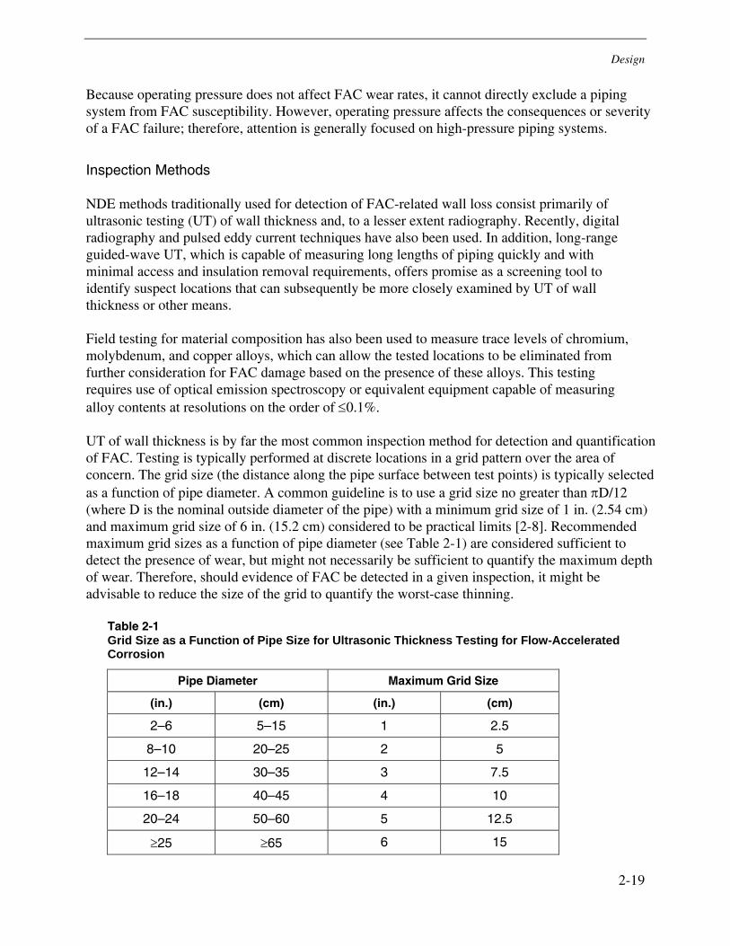
Design
2-19
Because operating pressure does not affect FAC wear rates, it cannot directly exclude a piping system from FAC susceptibility. However, operating pressure affects the consequences or severity of a FAC failure; therefore, attention is generally focused on high-pressure piping systems.
Inspection Methods
NDE methods traditionally used for detection of FAC-related wall loss consist primarily of ultrasonic testing (UT) of wall thickness and, to a lesser extent radiography. Recently, digital radiography and pulsed eddy current techniques have also been used. In addition, long-range guided-wave UT, which is capable of measuring long lengths of piping quickly and with minimal access and insulation removal requirements, offers promise as a screening tool to identify suspect locations that can subsequently be more closely examined by UT of wall thickness or other means.
Field testing for material composition has also been used to measure trace levels of chromium, molybdenum, and copper alloys, which can allow the tested locations to be eliminated from further consideration for FAC damage based on the presence of these alloys. This testing requires use of optical emission spectroscopy or equivalent equipment capable of measuring alloy contents at resolutions on the order of ≤0.1%.
UT of wall thickness is by far the most common inspection method for detection and quantification of FAC. Testing is typically performed at discrete locations in a grid pattern over the area of concern. The grid size (the distance along the pipe surface between test points) is typically selected as a function of pipe diameter. A common guideline is to use a grid size no greater than πD/12 (where D is the nominal outside diameter of the pipe) with a minimum grid size of 1 in. (2.54 cm) and maximum grid size of 6 in. (15.2 cm) considered to be practical limits [2-8]. Recommended maximum grid sizes as a function of pipe diameter (see Table 2-1) are considered sufficient to detect the presence of wear, but might not necessarily be sufficient to quantify the maximum depth of wear. Therefore, should evidence of FAC be detected in a given inspection, it might be advisable to reduce the size of the grid to quantify the worst-case thinning.
Table 2-1 Grid Size as a Function of Pipe Size for Ultrasonic Thickness Testing for Flow-Accelerated Corrosion
Pipe Diameter Maximum Grid Size
(in.) (cm) (in.) (cm)
2–6 5–15 1 2.5
8–10 20–25 2 5
12–14 30–35 3 7.5
16–18 40–45 4 10
20–24 50–60 5 12.5
≥25 ≥65 6 15
Design
2-20
Assessment Approaches
Assessment approaches for FAC can be classified as preinspection or postinspection activities. Preinspection evaluations include quantitative predictive modeling to predict FAC wear rates or otherwise identify FAC-susceptible locations, as well as other relative ranking methodologies that are performed to similarly identify and prioritize locations for inspection. Postinspection evaluations essentially entail the assessment of pipe wall thickness measurements relative to nominal or minimum wall thickness specifications in order to determine serviceability (run, replace, or reinspect).
The CHEC™ software series developed by EPRI is one of the more common analytical tools used to predict FAC susceptibility and wear rates. These programs, which use the Chexal-Horowitz FAC model, were first developed for nuclear plants in response to the Surry plant failure in 1986. The initial version of the software, called CHEC, was developed in 1987. Incremental modifications to the software resulted in later versions such as CHECMATE™ and CHECWORKS™. CHECUP™ is a version of the software that was specifically developed for fossil plants to rank piping locations based on predicted FAC wall loss.
The CHEC software programs require input related to water chemistry (pH, dissolved oxygen, and water treatment), hydrodynamic variables (fluid velocity, pipe diameter, temperature, steam quality, and flow path geometry) and materials composition. As with the application of any predictive tool, the results should be supplemented by engineering judgment and field experiences when selecting inspection sites. For more information about the CHEC software series, refer to the EPRI reports Recommendations for an Effective Flow-Accelerated Corrosion Program (1011838) and CHECWORKS™ Fossil Plant Application, Version 1.0 (TR-103198-P5R1) [2-7, 2-9].
Attemperator Design and Function
Attemperation is the primary means for controlling the degree of superheat in a superheated boiler. Attemperation is the process of removing steam enthalpy by either the controlled injection of water into the superheated steam flow or the direct removal of heat from the steam. The degree of superheat present in the steam flow depends on the steam load and the heat available in the boiler, given the design of the superheater. The degree of superheat of the final exiting steam is generally not subject to wide variation because the design of downstream processes requires consistency. To achieve control of the steam temperature (amount of superheat), an attemperator is used.
The attemperator is typically located in one of three places in the steam generation process: between the saturated steam outlet and the superheater, between sections of the superheater, or at the outlet of the superheater. Attemperators are classified as one of two types: surface or direct contact. In surface attemperators (called shell or drum attemperators), the steam is isolated from the cooling medium by a heat-transfer surface. In direct contact attemperators, which are more common, the superheated steam is mixed with water; this is typically accomplished by the use of sprays, as shown in Figure 2-3 [2-10]. Water is introduced into the steam line through spray
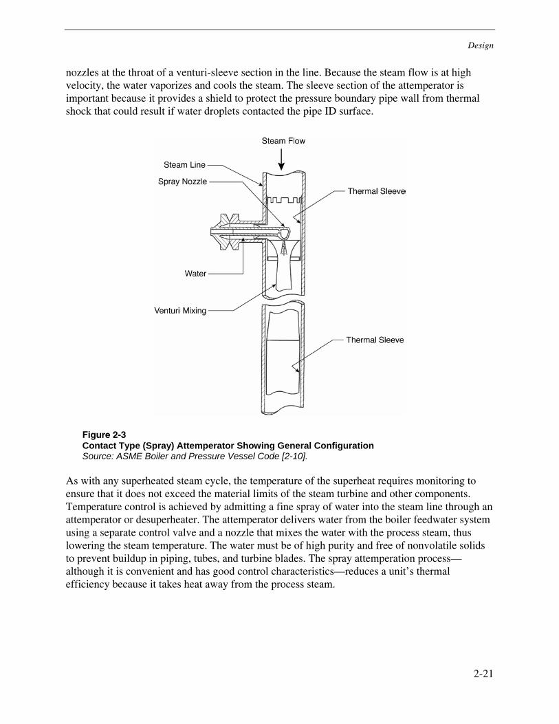
Design
2-21
nozzles at the throat of a venturi-sleeve section in the line. Because the steam flow is at high velocity, the water vaporizes and cools the steam. The sleeve section of the attemperator is important because it provides a shield to protect the pressure boundary pipe wall from thermal shock that could result if water droplets contacted the pipe ID surface.
Figure 2-3 Contact Type (Spray) Attemperator Showing General Configuration Source: ASME Boiler and Pressure Vessel Code [2-10].
As with any superheated steam cycle, the temperature of the superheat requires monitoring to ensure that it does not exceed the material limits of the steam turbine and other components. Temperature control is achieved by admitting a fine spray of water into the steam line through an attemperator or desuperheater. The attemperator delivers water from the boiler feedwater system using a separate control valve and a nozzle that mixes the water with the process steam, thus lowering the steam temperature. The water must be of high purity and free of nonvolatile solids to prevent buildup in piping, tubes, and turbine blades. The spray attemperation process—although it is convenient and has good control characteristics—reduces a unit’s thermal efficiency because it takes heat away from the process steam.
Design
2-22
In most coal-fired power plants, the reheat attemperator is installed in the cold reheat piping between the outlet of the high-pressure turbine and the reheat inlet header. A feedback control scheme tied back to the spray water control valve is used to control the temperature of the HRH steam. In combined-cycle plants, the reheat attemperator is usually installed between passes in the reheat section; the most common installation point is between the two sets of reheater tube banks.
When attemperator water comes from the boiler feedwater, provision for it must be made in calculating system flows. The calculation is based on heat balance. The total enthalpy (heat content) of the final superheat steam must be the mass-weighted sum of the enthalpies of the initial superheat steam and the attemperation water.
References
2-1. ASME Boiler and Pressure Vessel Code, Section I, Power Boilers. American Society of Mechanical Engineers, New York. 2004.
2-2. ASME B31.1, Code for Pressure Piping Standards: Power Piping. American Society of Mechanical Engineers, New York. 2004.
2-3. Metallurgical Guidebook for Fossil Power Plant Boilers. EPRI, Palo Alto, CA:2005. 1004509.
2-4. ASME Boiler and Pressure Vessel Code, Section III, Rules for Construction of Nuclear Power Plant Components. American Society of Mechanical Engineers, New York. 2004.
2-5. ASME Boiler and Pressure Vessel Code, Section II, Materials. American Society of Mechanical Engineers, New York. 2004.
2-6. Flow-Accelerated Corrosion in Power Plants. EPRI, Palo Alto, CA: 1998. TR-106611-R1.
2-7. Recommendations for an Effective Flow-Accelerated Corrosion Program (NSAC-202L-R3). EPRI, Palo Alto, CA: 2006. 1011838.
2-8. Acceptance Criteria for Structural Evaluation of Erosion-Corrosion Thinning in Carbon Steel Piping. EPRI, Palo Alto, CA:1988. NP-5911M.
2-9. CHECWORKS™ Fossil Plant Application, Version 1.0. EPRI, Palo Alto, CA: 1998. TR-103198-P5R1.
2-10. ASME Boiler and Pressure Vessel Code. American Society of Mechanical Engineers, New York. 2004.
3-1
3 METALLURGY OF STEELS
Introduction
Because of their availability, range of mechanical and physical properties, and ease of fabrication, steel and steel alloys are the most widely used materials of construction for high-energy piping systems in fossil generation. This section provides an overview and general background on the classification, microstructure, and mechanical properties of steels, including those of carbon, low-alloy, creep-strength-enhanced ferritic, and stainless steels. In addition, a list of the most widely used standard specifications for steel products in the United States is presented along with comparisons to many of the international standards.
The majority of this chapter was adapted from Section 5 of the EPRI report Metallurgical Guidebook for Fossil Power Plant Boilers (1011912) [3-1]. To complement the information contained in EPRI report 1011912, a series of stand-alone handbooks is being prepared. These handbooks provide details on the fabrication, microstructure, and performance of key individual alloys and should be referred to for details regarding microstructures and properties of these specific alloys. In addition, a large number of publications are available describing various aspects of ferrous metallurgy [3-2–3-9]. These documents should be referred to as necessary.
Comparison of Material Standards
The standard specifications of ASTM International (formerly the American Society for Testing and Materials) are the most widely used specifications for steel products in the U.S. electric power generation industry (see summary in Table 3-1). The ASTM standards are complete specifications suitable for procurement purposes and include such items as requirements for composition, manufacturing methods, heat treatment, mechanical properties, testing, marking, ordering information, and dimensional tolerances. The majority of the ASTM specifications are based on performance characteristics, such as the mechanical properties, with considerable latitude in compositional requirements.
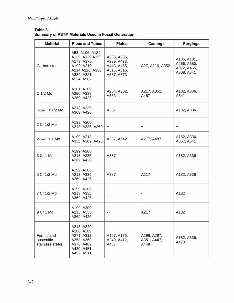
Metallurgy of Steels
3-2
Table 3-1 Summary of ASTM Materials Used in Fossil Generation
Material Pipes and Tubes Plates Castings Forgings
Carbon steel
A53, A106, A134, A135, A139,A155, A178, A179, A192, A210, A214,A226, A333, A334, A381, A524, A587
A283, A285, A299, A433, A443, A455, A515, A516, A537, A573
A27, A216, A352
A105, A181, A266, A350, A372, A465, A508, A541
C 1/2 Mo A161, A209, A250, A335, A369, A426
A204, A302, A533
A217, A352, A487
A182, A336, A541
1-1/4 Cr 1/2 Mo A213, A335, A369, A426 A387 _ A182, A336
2 Cr 1/2 Mo A199, A200, A213, A335, A369 _ _ _
2-1/4 Cr 1 Mo A199, A213, A335, A369, A426 A387, A542 A217, A487 A182, A336,
A357, A541
3 Cr 1 Mo A199, A200, A213, A335, A369, A426
A387 - A182, A336
5 Cr 1/2 Mo A199, A200, A213, A335, A369, A426
A387 A217 A182, A336
7 Cr 1/2 Mo A199, A200, A213, A335, A369, A426
_ - A182
9 Cr 1 Mo A199, A200, A213, A335, A369, A426
- A217 A182
Ferritic and austenitic stainless steels
A213, A249, A268, A269, A271, A312, A358, A362, A376, A409, A430, A451, A452, A511
A167, A176, A240, A412, A457
A296, A297, A351, A447, A448
A182, A336, A473

Metallurgy of Steels
3-3
ASME has adopted many of the ASTM standards with little or no modification. The ASME material specifications are included in the ASME BPVC, Section II, Materials, and are differentiated from the ASTM standards with an “S” prefix to the ASTM designation (for example, the ASME counterpart to ASTM A182 is SA182) [3-10].
Alternative U.S. alloy designations include those of the American Iron and Steel Institute (AISI), Society of Automotive Engineers (SAE), and the Aerospace Materials Specifications (AMS). The AISI and SAE standards are essentially equivalent for most compositions. These specifications primarily address compositional requirements and are frequently used by equipment manufacturers who must procure a material of known composition, machine or otherwise manufacture a component part, and then heat treat the component to the required mechanical properties. Many of the AISI and SAE grades have been incorporated into ASTM standards.
Although ASTM and ASME specifications are the most widely used standard specifications for steel products in the United States, there are also many international standards. For details on any particular standard, refer to articles, reports, and other documents that describe the applicable national or international standard. Some European and Japanese designation systems are the following:
• DIN standards are developed by Deutsches Institut für Normung in the Federal Republic of Germany. All West German steel specifications begin with the uppercase letters DIN followed by an alphanumeric or numeric code. The latter code, known as the Werkstoff number, uses only numbers, with a decimal point after the first digit.
• JIS standards are developed by the Japanese Industrial Standards Committee, which is part of the Ministry of International Trade and Industry in Tokyo. The JIS steel specifications begin with the uppercase letters JIS followed by an uppercase letter (G in the case of carbon and low-alloy steels) designating the division (product form) of the standard. This letter is followed by a series of numbers and letters that indicate the specific steel.
• British standards (BS) are developed by the British Standards Institute in London, England. Similar to the JIS standards, each British designation includes a product form and an alloy code.
• AFNOR standards are developed by the Association Française de Normalisation in Paris, France. The correct format for reporting AFNOR standards is as follows: the uppercase letters NF, a code consisting of an uppercase letter, a series of digits, and an alphanumeric sequence.
• UNI standards are developed by the Ente Nazionale Italiano di Unificazione in Milan, Italy. Italian standards begin with the uppercase letters UNI followed by a four-digit product form code, followed by an alphanumeric alloy identification.
• Swedish standards (SS) are prepared by the Swedish Standards Institution in Stockholm. Designations begin with the letters SS, followed by the number 14 (all Swedish carbon and low-alloy steels are covered by SS14), followed by a four-digit numerical sequence similar to the German Werkstoff number.
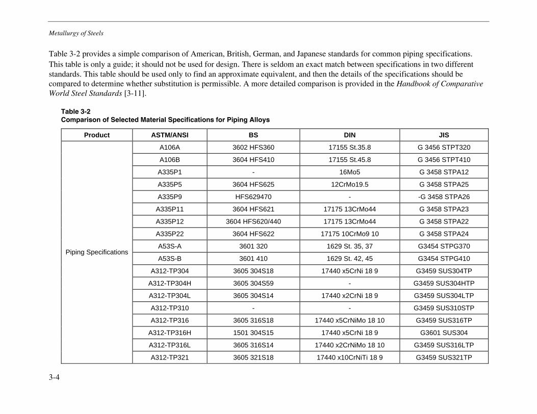
Metallurgy of Steels
3-4
Table 3-2 provides a simple comparison of American, British, German, and Japanese standards for common piping specifications. This table is only a guide; it should not be used for design. There is seldom an exact match between specifications in two different standards. This table should be used only to find an approximate equivalent, and then the details of the specifications should be compared to determine whether substitution is permissible. A more detailed comparison is provided in the Handbook of Comparative World Steel Standards [3-11].
Table 3-2 Comparison of Selected Material Specifications for Piping Alloys
Product ASTM/ANSI BS DIN JIS
A106A 3602 HFS360 17155 St.35.8 G 3456 STPT320
A106B 3604 HFS410 17155 St.45.8 G 3456 STPT410
A335P1 - 16Mo5 G 3458 STPA12
A335P5 3604 HFS625 12CrMo19.5 G 3458 STPA25
A335P9 HFS629470 - -G 3458 STPA26
A335P11 3604 HFS621 17175 13CrMo44 G 3458 STPA23
A335P12 3604 HFS620/440 17175 13CrMo44 G 3458 STPA22
A335P22 3604 HFS622 17175 10CrMo9 10 G 3458 STPA24
A53S-A 3601 320 1629 St. 35, 37 G3454 STPG370
A53S-B 3601 410 1629 St. 42, 45 G3454 STPG410
A312-TP304 3605 304S18 17440 x5CrNi 18 9 G3459 SUS304TP
A312-TP304H 3605 304S59 - G3459 SUS304HTP
A312-TP304L 3605 304S14 17440 x2CrNi 18 9 G3459 SUS304LTP
A312-TP310 - - G3459 SUS310STP
A312-TP316 3605 316S18 17440 x5CrNiMo 18 10 G3459 SUS316TP
A312-TP316H 1501 304S15 17440 x5CrNi 18 9 G3601 SUS304
A312-TP316L 3605 316S14 17440 x2CrNiMo 18 10 G3459 SUS316LTP
Piping Specifications
A312-TP321 3605 321S18 17440 x10CrNiTi 18 9 G3459 SUS321TP
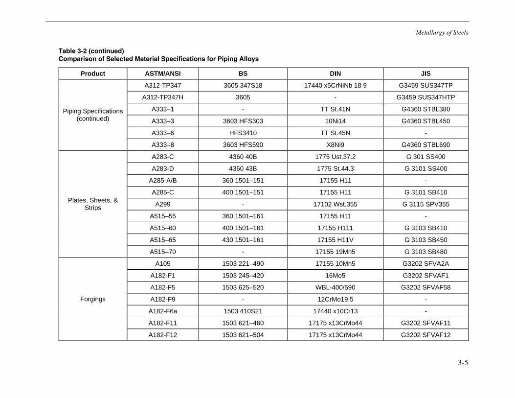
Metallurgy of Steels
3-5
Table 3-2 (continued) Comparison of Selected Material Specifications for Piping Alloys
Product ASTM/ANSI BS DIN JIS
A312-TP347 3605 347S18 17440 x5CrNiNb 18 9 G3459 SUS347TP
A312-TP347H 3605 - G3459 SUS347HTP
A333–1 - TT St.41N G4360 STBL380
A333–3 3603 HFS303 10Ni14 G4360 STBL450
A333–6 HFS3410 TT St.45N -
Piping Specifications (continued)
A333–8 3603 HFS590 X8Ni9 G4360 STBL690
A283-C 4360 40B 1775 Ust.37.2 G 301 SS400
A283-D 4360 43B 1775 St.44.3 G 3101 SS400
A285-A/B 360 1501–151 17155 H11 -
A285-C 400 1501–151 17155 H11 G 3101 SB410
A299 - 17102 Wst.355 G 3115 SPV355
A515–55 360 1501–161 17155 H11 -
A515–60 400 1501–161 17155 H111 G 3103 SB410
A515–65 430 1501–161 17155 H11V G 3103 SB450
Plates, Sheets, & Strips
A515–70 - 17155 19Mn5 G 3103 SB480
A105 1503 221–490 17155 10Mn5 G3202 SFVA2A
A182-F1 1503 245–420 16Mo5 G3202 SFVAF1
A182-F5 1503 625–520 WBL-400/590 G3202 SFVAF58
A182-F9 - 12CrMo19.5 -
A182-F6a 1503 410S21 17440 x10Cr13 -
A182-F11 1503 621–460 17175 x13CrMo44 G3202 SFVAF11
Forgings
A182-F12 1503 621–504 17175 x13CrMo44 G3202 SFVAF12
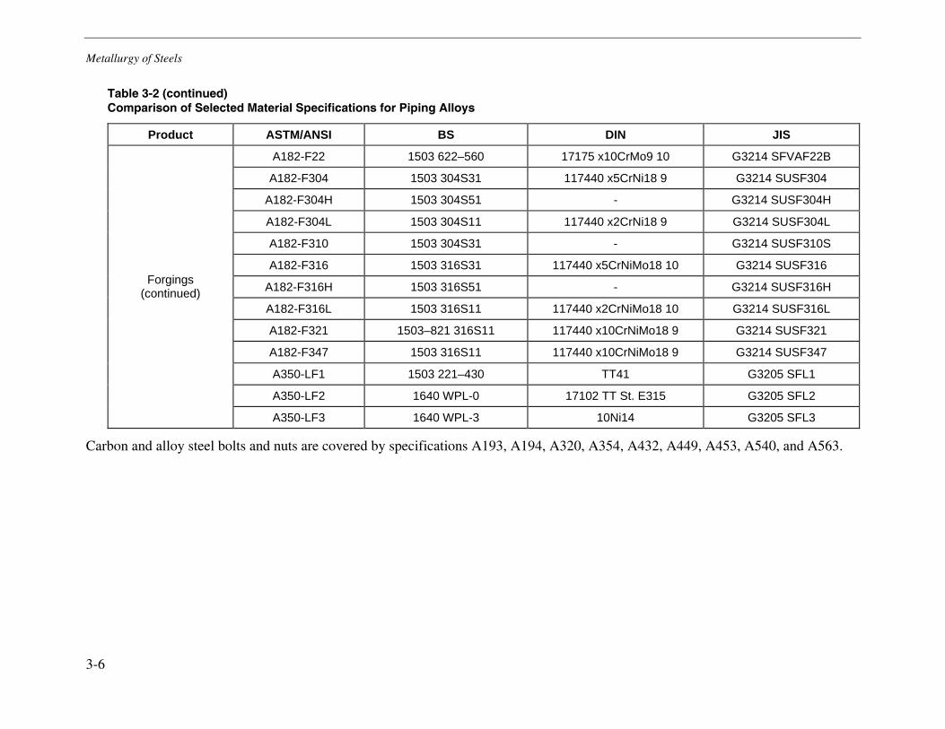
Metallurgy of Steels
3-6
Table 3-2 (continued) Comparison of Selected Material Specifications for Piping Alloys
Product ASTM/ANSI BS DIN JIS
A182-F22 1503 622–560 17175 x10CrMo9 10 G3214 SFVAF22B
A182-F304 1503 304S31 117440 x5CrNi18 9 G3214 SUSF304
A182-F304H 1503 304S51 - G3214 SUSF304H
A182-F304L 1503 304S11 117440 x2CrNi18 9 G3214 SUSF304L
A182-F310 1503 304S31 - G3214 SUSF310S
A182-F316 1503 316S31 117440 x5CrNiMo18 10 G3214 SUSF316
A182-F316H 1503 316S51 - G3214 SUSF316H
A182-F316L 1503 316S11 117440 x2CrNiMo18 10 G3214 SUSF316L
A182-F321 1503–821 316S11 117440 x10CrNiMo18 9 G3214 SUSF321
A182-F347 1503 316S11 117440 x10CrNiMo18 9 G3214 SUSF347
A350-LF1 1503 221–430 TT41 G3205 SFL1
A350-LF2 1640 WPL-0 17102 TT St. E315 G3205 SFL2
Forgings (continued)
A350-LF3 1640 WPL-3 10Ni14 G3205 SFL3
Carbon and alloy steel bolts and nuts are covered by specifications A193, A194, A320, A354, A432, A449, A453, A540, and A563.

Metallurgy of Steels
3-7
Historical Perspective on Material Changes in the American Power Piping Standards
In 1916, the Power Piping Society developed and published the first standard specifications for power piping to meet industry needs. Then in 1924, the Ohio Society of Safety Engineers completed a draft of Rules for Power Plant Steam and Water Piping. This was followed by a draft Code for Safety Rules and Regulations Covering the Installation of High and Low Pressure Steam Piping.
In March of 1926, project B31, Code for Pressure Piping, was initiated by the ASA at the request of ASME. This work became the American Tentative Standard Code for Pressure Piping (B31.1) in 1935 [3-12]. This code contained sections on power piping systems, air and gas piping, oil piping, district heating piping, fabrication details, and materials.
To bring uniformity between sections and to eliminate divergent requirements and discrepancies, a revision to this code was started in 1937. Final approval of this revision was given in November of 1942, and it was subsequently designated the American Standard Code for Pressure Piping [3-13].
Since 1942, this code has grown to meet industry changes in materials development, fabrication techniques, and inspection techniques. New editions to ASME B31.1 are issued every three years, with addenda issued annually. These revisions are developed and voted on by the Sectional Committee B31. This committee comprises members from some 30–40 engineering societies, government bureaus, trade associations, and various institutes with one or more representatives plus members at large to represent general interests. Code activities are subdivided according to the scope of the several sections and chapters, with general direction resting with the sectional committee officers and an executive committee.
Concurrent with the evolution and development of the Power Piping code, several of the original material specifications have been superseded by newer specifications. Table 3-3 shows a representations of some of the more common ASTM/ASME steel specifications that have been superseded and the steel specifications with which they have been replaced.
Table 3-3 Superseded ASTM/ASME Steel Piping Specifications
ASTM/ASME Superseded Specification
Description of Superseded Specification
ASTM/ASME Current Specification
Description of Current Specification
ASTM A53 (see note)
Pipe, welded, and seamless for coiling, bending and other special uses
A53/SA53 Pipe, steel, black, hot-dipped, zinc-coated, welded, and seamless
ASTM A105 Material for forged and bored carbon-steel pipe
A105/SA105 Carbon steel forgings for piping applications
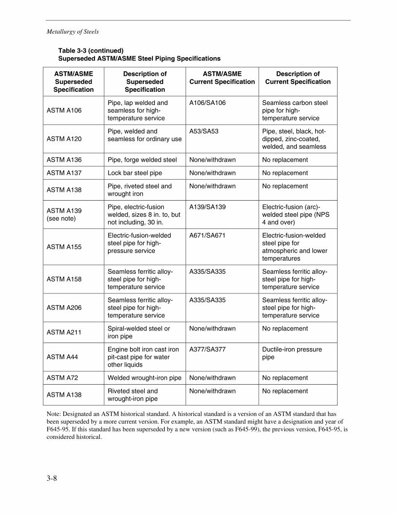
Metallurgy of Steels
3-8
Table 3-3 (continued) Superseded ASTM/ASME Steel Piping Specifications
ASTM/ASME Superseded Specification
Description of Superseded Specification
ASTM/ASME Current Specification
Description of Current Specification
ASTM A106 Pipe, lap welded and seamless for high-temperature service
A106/SA106 Seamless carbon steel pipe for high-temperature service
ASTM A120 Pipe, welded and seamless for ordinary use
A53/SA53 Pipe, steel, black, hot-dipped, zinc-coated, welded, and seamless
ASTM A136 Pipe, forge welded steel None/withdrawn No replacement
ASTM A137 Lock bar steel pipe None/withdrawn No replacement
ASTM A138 Pipe, riveted steel and wrought iron
None/withdrawn No replacement
ASTM A139 (see note)
Pipe, electric-fusion welded, sizes 8 in. to, but not including, 30 in.
A139/SA139 Electric-fusion (arc)-welded steel pipe (NPS 4 and over)
ASTM A155
Electric-fusion-welded steel pipe for high-pressure service
A671/SA671 Electric-fusion-welded steel pipe for atmospheric and lower temperatures
ASTM A158 Seamless ferritic alloy-steel pipe for high-temperature service
A335/SA335 Seamless ferritic alloy-steel pipe for high-temperature service
ASTM A206 Seamless ferritic alloy-steel pipe for high-temperature service
A335/SA335 Seamless ferritic alloy-steel pipe for high-temperature service
ASTM A211 Spiral-welded steel or iron pipe
None/withdrawn No replacement
ASTM A44 Engine bolt iron cast iron pit-cast pipe for water other liquids
A377/SA377 Ductile-iron pressure pipe
ASTM A72 Welded wrought-iron pipe None/withdrawn No replacement
ASTM A138 Riveted steel and wrought-iron pipe
None/withdrawn No replacement
Note: Designated an ASTM historical standard. A historical standard is a version of an ASTM standard that has been superseded by a more current version. For example, an ASTM standard might have a designation and year of F645-95. If this standard has been superseded by a new version (such as F645-99), the previous version, F645-95, is considered historical.
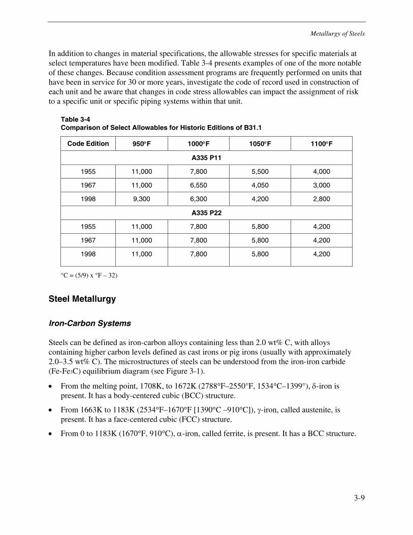
Metallurgy of Steels
3-9
In addition to changes in material specifications, the allowable stresses for specific materials at select temperatures have been modified. Table 3-4 presents examples of one of the more notable of these changes. Because condition assessment programs are frequently performed on units that have been in service for 30 or more years, investigate the code of record used in construction of each unit and be aware that changes in code stress allowables can impact the assignment of risk to a specific unit or specific piping systems within that unit.
Table 3-4 Comparison of Select Allowables for Historic Editions of B31.1
Code Edition 950°F 1000°F 1050°F 1100°F
A335 P11
1955 11,000 7,800 5,500 4,000
1967 11,000 6,550 4,050 3,000
1998 9,300 6,300 4,200 2,800
A335 P22
1955 11,000 7,800 5,800 4,200
1967 11,000 7,800 5,800 4,200
1998 11,000 7,800 5,800 4,200
°C = (5/9) x °F – 32)
Steel Metallurgy
Iron-Carbon Systems
Steels can be defined as iron-carbon alloys containing less than 2.0 wt% C, with alloys containing higher carbon levels defined as cast irons or pig irons (usually with approximately 2.0–3.5 wt% C). The microstructures of steels can be understood from the iron-iron carbide (Fe-Fe3C) equilibrium diagram (see Figure 3-1).
• From the melting point, 1708K, to 1672K (2788°F–2550°F, 1534°C–1399°), δ-iron is present. It has a body-centered cubic (BCC) structure.
• From 1663K to 1183K (2534°F–1670°F [1390°C –910°C]), γ-iron, called austenite, is present. It has a face-centered cubic (FCC) structure.
• From 0 to 1183K (1670°F, 910°C), α-iron, called ferrite, is present. It has a BCC structure.
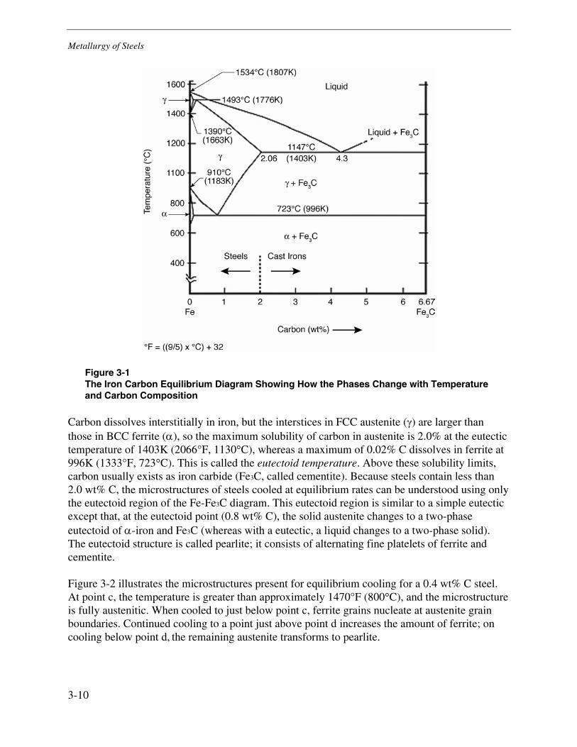
Metallurgy of Steels
3-10
Figure 3-1 The Iron Carbon Equilibrium Diagram Showing How the Phases Change with Temperature and Carbon Composition
Carbon dissolves interstitially in iron, but the interstices in FCC austenite (γ) are larger than those in BCC ferrite (α), so the maximum solubility of carbon in austenite is 2.0% at the eutectic temperature of 1403K (2066°F, 1130°C), whereas a maximum of 0.02% C dissolves in ferrite at 996K (1333°F, 723°C). This is called the eutectoid temperature. Above these solubility limits, carbon usually exists as iron carbide (Fe3C, called cementite). Because steels contain less than 2.0 wt% C, the microstructures of steels cooled at equilibrium rates can be understood using only the eutectoid region of the Fe-Fe3C diagram. This eutectoid region is similar to a simple eutectic except that, at the eutectoid point (0.8 wt% C), the solid austenite changes to a two-phase eutectoid of α-iron and Fe3C (whereas with a eutectic, a liquid changes to a two-phase solid). The eutectoid structure is called pearlite; it consists of alternating fine platelets of ferrite and cementite.
Figure 3-2 illustrates the microstructures present for equilibrium cooling for a 0.4 wt% C steel. At point c, the temperature is greater than approximately 1470°F (800°C), and the microstructure is fully austenitic. When cooled to just below point c, ferrite grains nucleate at austenite grain boundaries. Continued cooling to a point just above point d increases the amount of ferrite; on cooling below point d, the remaining austenite transforms to pearlite.
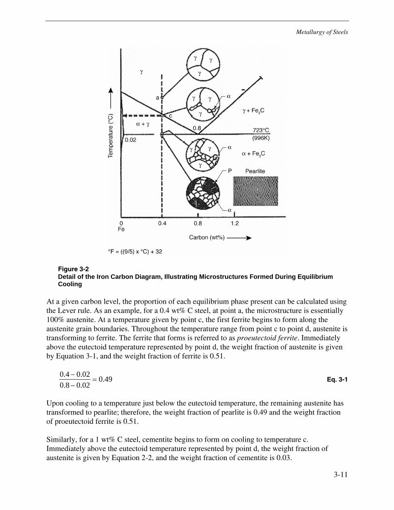
Metallurgy of Steels
3-11
Figure 3-2 Detail of the Iron Carbon Diagram, Illustrating Microstructures Formed During Equilibrium Cooling
At a given carbon level, the proportion of each equilibrium phase present can be calculated using the Lever rule. As an example, for a 0.4 wt% C steel, at point a, the microstructure is essentially 100% austenite. At a temperature given by point c, the first ferrite begins to form along the austenite grain boundaries. Throughout the temperature range from point c to point d, austenite is transforming to ferrite. The ferrite that forms is referred to as proeutectoid ferrite. Immediately above the eutectoid temperature represented by point d, the weight fraction of austenite is given by Equation 3-1, and the weight fraction of ferrite is 0.51.
49.002.08.002.04.0
=−−
Eq. 3-1
Upon cooling to a temperature just below the eutectoid temperature, the remaining austenite has transformed to pearlite; therefore, the weight fraction of pearlite is 0.49 and the weight fraction of proeutectoid ferrite is 0.51.
Similarly, for a 1 wt% C steel, cementite begins to form on cooling to temperature c. Immediately above the eutectoid temperature represented by point d, the weight fraction of austenite is given by Equation 2-2, and the weight fraction of cementite is 0.03.
Metallurgy of Steels
3-12
97.08.067.60.167.6=
−−
Eq. 3-2
This is referred to as proeutectoid cementite. Upon cooling to a temperature just below the eutectoid temperature, the remaining austenite transforms to pearlite; therefore, the weight fraction of pearlite is 0.97 and the weight fraction of proeutectoid cementite is 0.03.
Nonequilibrium Cooling of Steels
It is the existence of the austenite-to-ferrite transformation, combined with the marked change in carbon solubility, that accounts for the enormous range of microstructures and properties possible in steels. Equilibrium slow cooling from the austenitic range results in microstructures containing either ferrite or cementite, together with pearlite.
Because ferrite is soft and ductile, whereas cementite is hard and brittle, the hardness and the strength increase (but the ductility and the toughness decrease) with increasing carbon content as the proportion of cementite increases. Unlike slow cooling from the austenite range (called annealing), air cooling is called normalizing. Normalizing allows less than the equilibrium proportions of ferrite or cementite to separate from the austenite, resulting in a higher proportion of pearlite with decreased platelet size and spacing. With even more severe cooling procedures, the eutectoid transformation can be suppressed; that is, quenching from the austenite range can produce two entirely different types of structures: bainite and martensite.
Bainite is formed when austenite is quenched to temperatures around 356°F–800°F (180°C–425°C) and held at the quench temperature for some time (or frequently, by quenching into oil). Bainite consists of a fine submicroscopic dispersion of Fe3C particles in a highly strained α matrix.
Martensite is formed following rapid quenching to lower temperatures than those involved in forming bainite. In this case, the severe quench retains carbon in solid solution in a distorted body-centered tetragonal iron lattice. Martensite is hard and brittle, but the toughness can be improved with a corresponding reduction in hardness by tempering—that is, heating martensite to 392°F–1330°F (200°C–720°C) allows transformation to a structure consisting of very small Fe3C particles or precipitates in ferrite. The size and spacing of these cementite particles increase with increasing tempering times and temperatures, giving a progressively softer but less brittle product. Heat treatment of steels by quenching and tempering therefore offers a means of optimizing strength and toughness.
The transformation of austenite to pearlite (at the eutectoid point, 0.77 wt% C) and the transformation of austenite to bainite (at any carbon content) occur by diffusion-controlled processes of nucleation and growth of the new phases so that, on quenching austenite to temperatures that allow these transformations, some time elapses before the transformations begin, and further time is needed before the transformations are complete. In contrast, the transformation of austenite to martensite is diffusionless and almost instantaneous.
Metallurgy of Steels
3-13
Continuous Cooling Transformations
Continuous cooling transformations (CCTs) are distinct from isothermal transformations in that the time at temperature is dictated by the cooling rate that a sample has experienced. Welding is a typical process in which an understanding of transformation behavior is important because the practicalities of welding mean that isothermal transformations cannot be applied and weld and heat-affected zone (HAZ) microstructures are thus a function of the time at peak temperature and the subsequent cooling rate. The use of preheating can assist in controlling the cooling rate, and the required conditions for given alloys are specified in applicable codes.
CCT diagrams show the transformations that take place in a continuously cooled sample of material. These diagrams can predict the microstructure of a sample at any cooling rate covered by the diagram.
CCT diagrams are generated from controlled heating and cooling experiments carried out while monitoring the physical dimensions (diameter or length) of the sample. Because there will be a change in dimensions when transformation from BCC ferrite-type microstructures to FCC austenite occurs, the heating curve shows inflection points allowing the AC1 and AC3 temperatures to be determined. Similarly, the dimensional changes on cooling allow the specific transformation temperatures to be determined so that the transformation behavior can be established by conducting a set of experiments on a selected alloy. The effect of heating and cooling cycles on specimen dimensions is illustrated in Figure 3-3, with the CCT curves measured for carbon and 2-1/4 Cr 1 Mo steel shown in Figures 3-4 and 3-5, respectively [3-7, 3-14, 3-15]. The additional alloying elements present in 2-1/4 Cr 1 Mo steel increase hardenability, allowing bainite and martensite to form at slower cooling rates than for carbon steel.
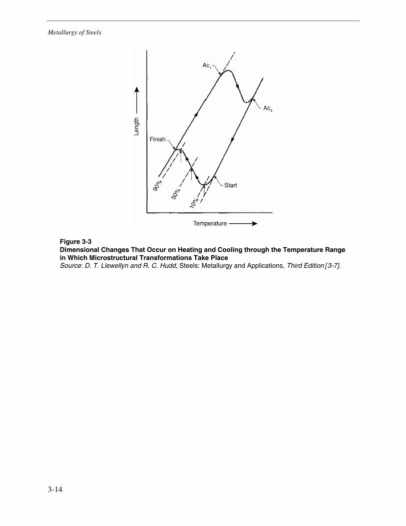
Metallurgy of Steels
3-14
Figure 3-3 Dimensional Changes That Occur on Heating and Cooling through the Temperature Range in Which Microstructural Transformations Take Place Source: D. T. Llewellyn and R. C. Hudd, Steels: Metallurgy and Applications, Third Edition [3-7].
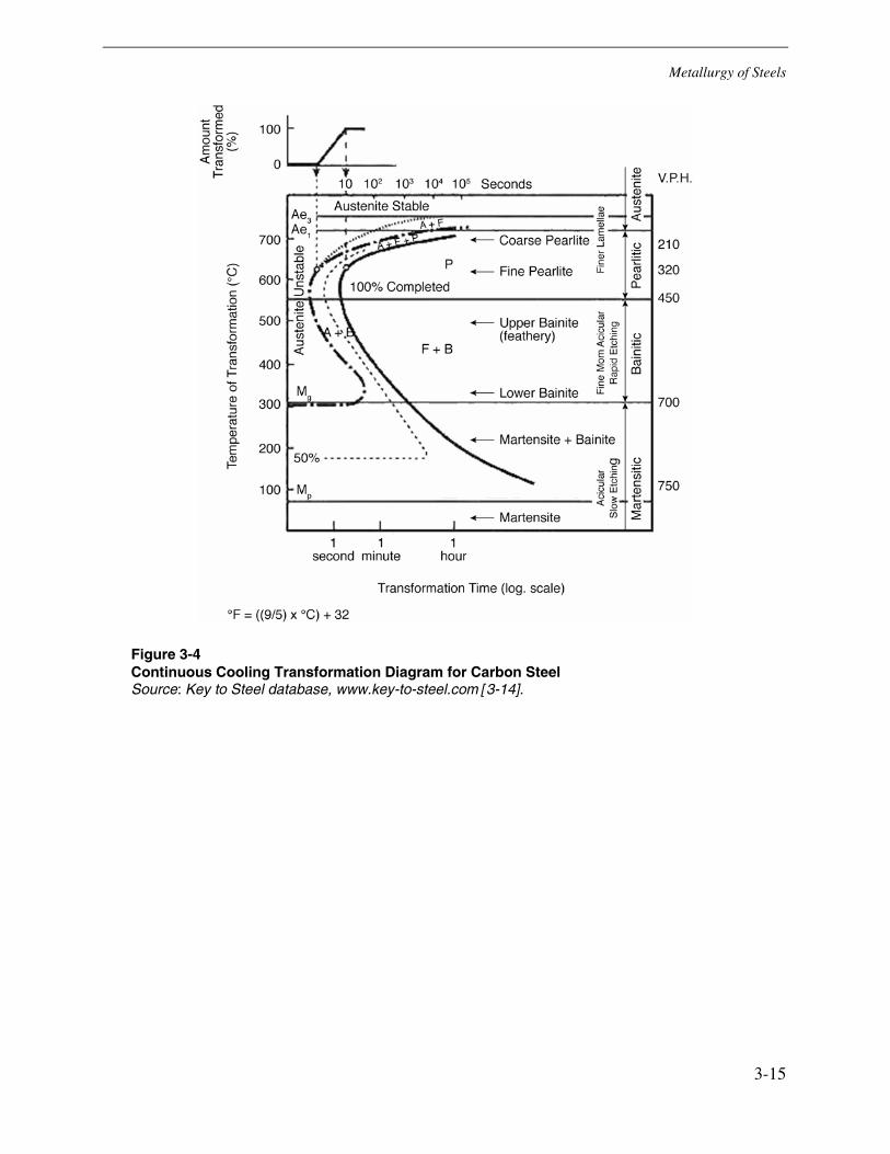
Metallurgy of Steels
3-15
Figure 3-4 Continuous Cooling Transformation Diagram for Carbon Steel Source: Key to Steel database, www.key-to-steel.com [3-14].
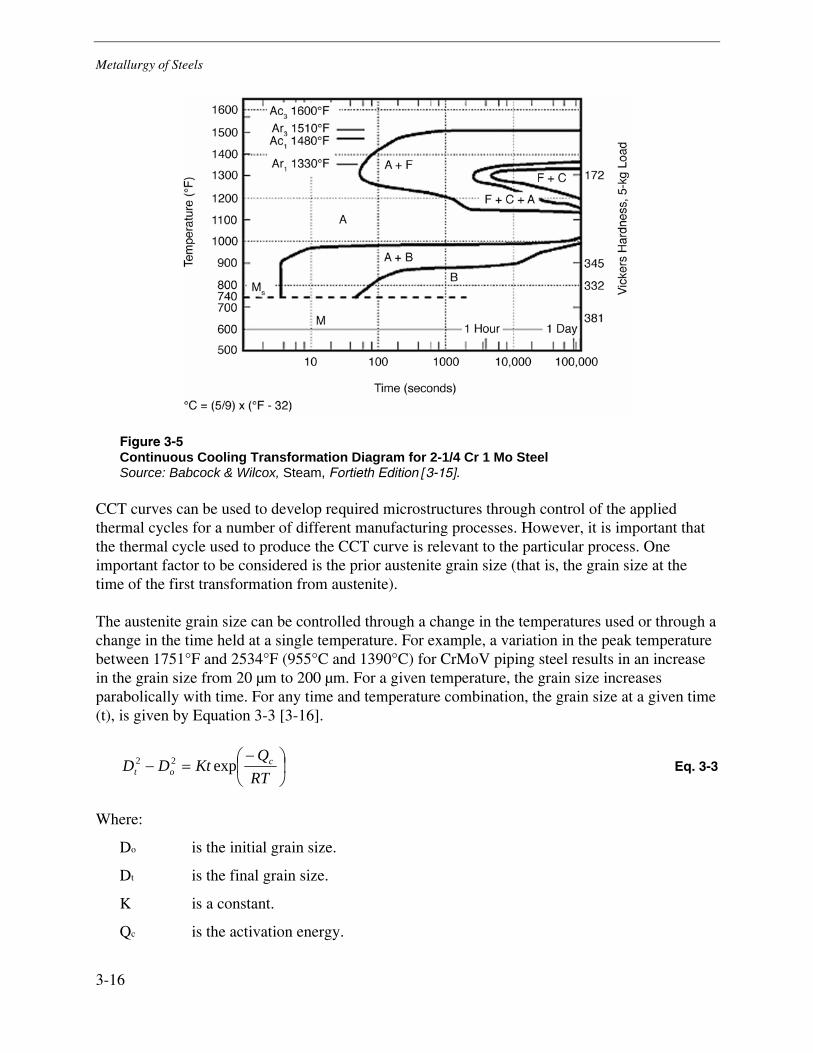
Metallurgy of Steels
3-16
Figure 3-5 Continuous Cooling Transformation Diagram for 2-1/4 Cr 1 Mo Steel Source: Babcock & Wilcox, Steam, Fortieth Edition [3-15].
CCT curves can be used to develop required microstructures through control of the applied thermal cycles for a number of different manufacturing processes. However, it is important that the thermal cycle used to produce the CCT curve is relevant to the particular process. One important factor to be considered is the prior austenite grain size (that is, the grain size at the time of the first transformation from austenite).
The austenite grain size can be controlled through a change in the temperatures used or through a change in the time held at a single temperature. For example, a variation in the peak temperature between 1751°F and 2534°F (955°C and 1390°C) for CrMoV piping steel results in an increase in the grain size from 20 μm to 200 μm. For a given temperature, the grain size increases parabolically with time. For any time and temperature combination, the grain size at a given time (t), is given by Equation 3-3 [3-16].
⎟⎠⎞
⎜⎝⎛ −=−
RTQ
KtDD cot exp22 Eq. 3-3
Where:
Do is the initial grain size.
Dt is the final grain size.
K is a constant.
Qc is the activation energy.
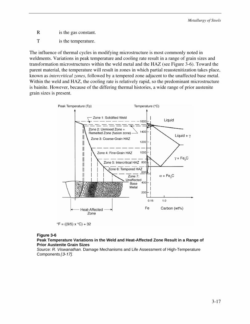
Metallurgy of Steels
3-17
R is the gas constant.
T is the temperature.
The influence of thermal cycles in modifying microstructure is most commonly noted in weldments. Variations in peak temperature and cooling rate result in a range of grain sizes and transformation microstructures within the weld metal and the HAZ (see Figure 3-6). Toward the parent material, the temperature will result in zones in which partial reaustenitization takes place, known as intercritical zones, followed by a tempered zone adjacent to the unaffected base metal. Within the weld and HAZ, the cooling rate is relatively rapid, so the predominant microstructure is bainite. However, because of the differing thermal histories, a wide range of prior austenite grain sizes is present.
Figure 3-6 Peak Temperature Variations in the Weld and Heat-Affected Zone Result in a Range of Prior Austenite Grain Sizes Source: R. Viswanathan. Damage Mechanisms and Life Assessment of High-Temperature Components [3-17].

Metallurgy of Steels
3-18
Effects of Composition on Microstructure and Properties
This section provides background regarding the influence of composition on the microstructure and mechanical properties of steel. This information is followed by general comments describing selected physical and mechanical properties relevant to engineering issues in boilers and piping.
Elemental Effects
Classification of alloying elements according to their effect in the steel is difficult, because the influence varies so widely with each addition, depending on the quantity used and other elements present. A useful approach to grouping is based on the effect of the element on the stability of carbides and the stability of austenite. With this approach, alloying elements are classified as follows:
1. Elements that tend to form carbides: chromium, tungsten, titanium, columbium, vanadium, molybdenum, and manganese. The mixture of complex carbides is often referred to as cementite.
2. Elements that tend to graphitize the carbide: silicon, cobalt, aluminum, and nickel. Only a small proportion of these elements can be added to the steel before graphite forms during processing, with attendant ruin of the properties of the steel, unless elements from group 1 are added to counteract the effect.
3. Elements that tend to stabilize austenite: manganese, nickel, cobalt, and copper. These elements alter the critical points of iron in a way similar to carbon by raising the A4 point and lowering the A3 point, thus increasing the range in which austenite is stable, and they also tend to retard the separation of carbides. They have a crystal lattice (FCC) similar to that of γ-iron, in which they are more soluble than they are in α-iron.
4. Elements that tend to stabilize ferrite: chromium, tungsten, molybdenum, vanadium, and silicon. These elements are more soluble in α-iron than in γ-iron. They diminish the amount of carbon soluble in the austenite and thus tend to increase the volume of free carbide in the steel for a given carbon content. On the binary equilibrium diagram of these elements with pure iron, the A4 point is lowered and the A3 point is raised (although it might be lowered initially), until the two points merge to form a closed gamma loop. Thus, with a certain amount of each of these elements, the austenite phase disappears and ferrite exists from the melting point down to room temperature. Adding elements from group 3 of the periodic table, however, can counteract this effect. For example, 2% nickel is added to the 18 wt% chromium stainless steel to enable it to be refined by normal heat treatment; carbon has the same effect. Aluminum has the reverse effect in 12 wt% chromium steel.
Metallurgy of Steels
3-19
The microstructure and properties of steels are determined primarily by composition and heat treatment. Applicable references should be studied for detailed information regarding the microstructure and properties of a specific alloy or alloy type. The general effects of individual elements are summarized as follows:
• Aluminum (Al) is used to deoxidize steel and control grain size. Grain size control is achieved by forming a fine dispersion with nitrogen and oxygen, which restricts austenite grain growth. Aluminum is also an extremely effective nitride former in nitriding steels.
• Antimony (Sb) and arsenic (As) are trace elements that are believed to reduce ductility through temper embrittlement.
• Boron (B) is added between 0.0005% and 0.003% to significantly increase hardenability, especially for low-carbon steels. It does not affect the strength of ferrite, thus not sacrificing ductility, formability, or machinability in the annealed state.
• Calcium (Ca) is used to control the shape, size, and distribution of oxide and sulfide inclusions. Benefits of having fine, well-distributed inclusions include improved toughness and machinability.
• Carbon (C) is the most important alloying element and is essential for the formation of cementite, pearlite, bainite, and iron-carbon martensite. Compared to steels with similar microstructures, the properties of strength, hardness, hardenability, and ductile-to-brittle transition temperature are increased with increasing carbon content. Toughness and ductility of pearlitic steels are decreased with increasing carbon content. The significant increase in hardenability with increasing carbon content results in decreased weldability.
• Chromium (Cr) influences hardenability and is a carbide former and stabilizer. It is used in low-alloy steels to increase the following:
– Resistance to corrosion and oxidation
– High-temperature strength
– Hardenability
– Abrasion resistance in high-carbon alloys
Straight chromium steels are susceptible to temper embrittlement and can be brittle, so steels for elevated-temperature service tend to contain both chromium and molybdenum. At composition levels of approximately 9% to 13% Cr, the increased hardenability is such that, for normal cooling rates, martensite is formed. In the absence of nickel, high-chromium steels (above approximately 18% Cr) are fully ferritic and are used where high resistance to corrosion is required.
• Copper (Cu) is detrimental to hot workability and subsequent surface quality, and it can reduce creep ductility. It is used in certain steels to improve resistance to atmospheric corrosion.
• Lead (Pb) improves machinability. It does not dissolve in steel but is present as metallic globules. Environmental concerns are resulting in a decreased usage of lead in the steel industry.
Metallurgy of Steels
3-20
• Manganese (Mn) is important because it controls transformation kinetics on cooling from austenite, it deoxidizes the melt, and it facilitates hot working of the steel by reducing the susceptibility to hot shortness caused by the presence of free sulfur—that is, it combines with sulfur to form MnS inclusions. Manganese increases the tendency for trace elements to cause temper embrittlement.
• Molybdenum (Mo) increases hardenability of steels and helps to maintain a specified hardness. Even in small amounts (0.1% to 0.5%), molybdenum increases high-temperature tensile and creep strengths, and it acts to reduce the effects of trace elements such as phosphorus in causing temper embrittlement.
• Nickel (Ni) is used in low-alloy steels to reduce the sensitivity of the steel to variations in heat treatment and to distortion and cracking on quenching. It also improves low-temperature toughness and hardenability. In stainless steels, at levels above approximately 8% Ni, the austenite is stabilized to room temperature.
• Niobium (Nb), also known as columbium (Cb), forms stable carbides that increase strength at elevated temperatures and, by providing a finer grain size, lowers the fracture transition temperature. Is added to austenitic stainless steels to form carbides in stabilized grades to reduce risk of sensitization.
• Nitrogen (N) increases the strength, hardness, and machinability of steel, but it decreases the ductility and toughness. In aluminum-killed steels, nitrogen combines with the aluminum to provide grain size control, thereby improving both toughness and strength. Nitrogen can reduce the effect of boron on the hardenability of steels.
• Phosphorus (P) is generally restricted to levels below 0.04 wt% to minimize its detrimental effect on ductility and toughness. Certain steels can contain higher levels to enhance machinability, strength, and atmospheric corrosion resistance.
• Silicon (Si) is one of the principal deoxidizers, with the amount used dependent on the deoxidization practice. Silicon can increase high-temperature strength and reduce the amount of surface scale formed during exposure to high temperature, but it has been shown to increase temper embrittlement caused by segregation of trace elements in low-alloy steels.
• Sulfur (S) is detrimental to fracture strength, so manganese must be added to form inclusions. These manganese sulfide stringers can reduce transverse strength and impact resistance, and fine inclusions on grain boundaries can facilitate the formation of creep cavities.
• Tin (Sn) is a trace element that is believed to increase temper embrittlement and has been shown to reduce creep ductility and accelerate creep damage development.
• Titanium (Ti) is added to steels containing boron because it combines preferentially with oxygen and nitrogen, thus allowing the boron to increase hardenability. Titanium, as titanium nitride, also provides grain size control at elevated temperatures.
• Tellurium (Te) can be added to modify sulfide-type inclusion size, morphology, and distribution. The resulting sulfide-type inclusions are finer and remain ellipsoidal in shape following hot working, thereby improving transverse fracture properties.
Metallurgy of Steels
3-21
• Tungsten (W) increases hardenability and forms carbides. It acts in a similar manner to molybdenum.
• Vanadium (V) additions of up to 0.05% increase hardenability, whereas larger amounts tend to reduce hardenability because of extensive carbide formation. The presence of vanadium carbides or carbonitrides improves elevated strength, provides resistance to tempering and hydrogen attack, and inhibits grain growth during heat treatment. Proper application leads to improved strength and toughness of hardened and tempered steels; however, excessive strengthening can lead to reheat cracking associated with welds.
Mechanical Properties
The mechanical properties of a metal determine the range of usefulness of the metal and establish the service that can be expected from it. They are of vital interest to the performance of components and the associated welds because the weld must provide mechanical properties in the same order as the base metals being joined. The performance of a welded joint depends on whether it provides properties equal to or exceeding those of the metals being joined. The following paragraphs explain why specific properties are important in the selection and assessment of component performance.
Strength
Strength is often the primary consideration when manufacturing a component because it is essential that loads are limited to a safe fraction of the material yield point. If the yield point is exceeded, plastic deformation will be introduced. Tensile strength considerations ensure against failure by plastic collapse. Other potential failure modes require consideration of different material properties—for example, for a cyclically loaded structure, fatigue properties must be taken into account; at high temperatures, creep performance might be important. Ductility refers to the ability of an alloy to withstand plastic deformation without failure. Data are normally presented as elongation for a standard gauge length in a laboratory tensile test (typically 2 in. [5 cm]) or as a reduction in cross-sectional area. For many components and welds, a key property is fracture toughness because toughness is a major factor in establishing critical crack size and thus whether components will be subject to sudden brittle fracture. In the majority of cases, as strength increases, ductility is reduced. In general, superior performance is achieved with alloys that exhibit an appropriate balance between strength and ductility—that is, alloys that have excellent toughness.
Fatigue
Fatigue is the phenomenon of damage accumulation caused by cyclic or fluctuating stresses. Generally, it is manifested as the initiation and stable propagation of a crack. Final failure in a component subjected to fatigue ensues when a critical crack size is reached and failure occurs by fracture or by overload. In some situations in which crack growth is very rapid, failure can be defined by the initiation of a crack. Fatigue depends on the frequency and magnitude of the stress
Metallurgy of Steels
3-22
cycles and is generally independent of stress duration. However, at high temperatures at which creep-fatigue interactions become important, the damage level depends on stress duration. Stress cycling can be induced mechanically or thermally.
High-cycle fatigue consists of crack initiation or fracture brought about by fluctuating stresses of low amplitude; it is generally defined as requiring more than 10,000 stress cycles to failure. The examination of high-cycle fatigue fracture surfaces will usually reveal a relatively smooth, flat surface with beach marks. In contrast, with low-cycle fatigue, in which failure occurs after fewer than 10,000 stress cycles of higher amplitude, the fracture surface is somewhat rougher. Beach marks can also be evident in low-cycle fatigue, depending on the range of stress intensity at the crack tip. Fatigue cracks are usually transgranular.
The metallurgical variables having the most pronounced effects on the fatigue behavior of carbon and low-alloy steels are strength level, ductility, cleanliness of the steel, residual stresses, surface conditions, and aggressive environments. At least partly because of the characteristic scatter of fatigue-testing data, it is difficult to distinguish the direct effects of other variables such as composition on fatigue from their effects on the strength level of steel. For most steels with hardness values below approximately 400 HB (excluding precipitation hardening steels), the fatigue limit is approximately half the ultimate tensile strength. Thus, any heat treatment or alloying addition that increases the strength (or hardness) of a steel can be expected to increase its fatigue limit.
Creep
Creep is a time-dependent deformation and fracture that takes place at elevated temperatures under the application of a load. For common engineering steels, creep becomes a significant concern only at temperatures exceeding approximately 0.4 Tm, where Tm is the absolute melting point. For the stress levels encountered in most power generating or petrochemical plants, creep is not a concern for low-alloy steels below 752°F (400°C) and for austenitic alloys below 1000°F (538°C).
The creep strain versus time curves have traditionally been described using three stages: primary, secondary, and tertiary. Each stage can be characterized in terms of creep rate (the change in strain with time). Primary creep is a period of relatively high but decreasing creep rate with time, during which the material’s creep resistance increases by work hardening (that is, in the primary stage, the strain rate is continuously changing). Secondary creep is a period of essentially constant creep rate. Tertiary creep is a period of increasing creep rate, at the end of which the material ultimately fails. Increasing creep rate can be a result of microstructural aging, void development, or a combination of the two effects. Microstructural changes that occur during creep in chromium-molybdenum steels include precipitation and growth of chromium and molybdenum carbides (spheroidization). Low-strain failures are the result of the coalescence of grain boundary microvoids into grain boundary cracks. Eventually, voids link up to form microcracks. Local fracture occurs when the microcracks link to form macrocracks. For most thick section components, the existence of even a macrocrack does not necessarily constitute the end of life because a period of stable crack growth usually occurs until a critical crack size is reached, which then leads to rapid failure.
Metallurgy of Steels
3-23
Creep Crack Growth
In thick section components, such as main steam piping and secondary superheater headers, the initiation of a crack is normally followed by a period of stable crack growth. Significant effort has been expended toward understanding the factors that determine crack growth rate and developing procedures for predicting behavior. Under the special conditions in which second-stage creep deformation is widespread in the body, a parameter known as C* describes the crack tip region. C* is an energy-rate line integral that is the creep analogue of the J-integral, in which strain rates and displacement rates have been substituted for strains and displacements. C* can be calculated by finite-element methods and used as a parameter to predict creep crack growth.
For the more general case in which significant creep strains occur only in the localized region near the crack tip, at least in the beginning stages of crack growth, a parameter Ct has been proposed. In the limit of widespread creep deformation, Ct = C*. These concepts have been confirmed by applying them to explain the observed creep lifetime of cracked components such as superheater outlet headers.
Creep-Fatigue
During elevated-temperature operation, components can be subjected to both creep and cyclic loading. This condition is termed creep-fatigue, and the effects can be either interactive (they can cause component damage to accumulate significantly faster than would be expected by considering each mechanism separately) or simply additive.
The problem of material degradation under the combination of cyclic loading and high temperatures is currently under intensive study in many laboratories. Increasing numbers of components must operate under creep-fatigue conditions because power generating systems are seeking maximum flexibility from available generating plants.
Classification of Steels Used in Power Plant Applications
In addition to containing carbon, all commercial steels contain varying amounts of manganese, silicon, sulfur, phosphorus, gases, and other trace impurities that are present as a result of the methods used during steel production. Consequently, steels are defined as plain carbon even when they contain 1% or more manganese, up to 0.3 wt% Si, 0.06 wt% P and S, and so on. However, the structure and properties of plain carbon steels depend not only on composition but also on the heat treatment and on the hot and cold working operations before or after heat treatment. Consequently, specifying only the composition is insufficient to provide an adequate description of properties. Although there is no universally agreed system of steel specifications, for most general purposes, plain carbon steels are grouped as follows:
• Low-carbon or mild steels (<0.25 wt% C)
• Medium-carbon steels (0.25–0.6 wt% C)
• High-carbon or plain carbon tool steels (>0.6 wt% C)
Metallurgy of Steels
3-24
The low-carbon grades are used for sheet and strip manufacture for cans, pressings, and so on, in which ductility and toughness combined with reasonable strength are required. The stronger mild steels (0.2 wt% C) are used as weldable structural steels. Medium-carbon steels are chosen for casting, forging, and so on of axles, gears, wire ropes, and springs. The hardness and strength of high-carbon steels result in their selection for tools, ball bearings, and dies.
With plain carbon steels, the critical cooling rate needed to form martensite depends on the carbon content; with less than 0.3 wt% C, even water-quenching austenite does not produce a fully hard martensitic product. Even with higher carbon levels, the critical cooling rates are high, which limits hardenability—that is, because of the relatively low thermal conductivities of steels, there is a maximum section thickness that can be hardened from surface to center. With plain carbon steel, this hardening depth is not more than approximately 1 in. (2–3 cm); with rapid quenching, the volume change accompanying the austenite-martensite transformation can cause severe distortion and cracking of higher-carbon steels.
Although plain carbon steels are perfectly satisfactory for most applications, there are distinct limits to the combination of strength and toughness attainable, to the section sizes that can be fully hardened, and to the temperatures at which even high-carbon steels can operate without softening. These property limitations can be alleviated, and new property ranges introduced, by alloying. No classification system is universally accepted for alloy steels, but excluding steels for electrical and magnetic applications and certain other special products, it is possible to consider the following three broad categories of alloy or special steels:
• Low-alloy structural steels are grades for which strength is a major criterion for selection. The amount of any alloying element present is usually less than 2%, except that nickel can be up to 4 wt%. The elements nickel, chromium, molybdenum, and vanadium improve strength and toughness, hardenability, and so on; therefore, stronger but lighter components and structures can be made without sacrificing some of the most desirable features of plain carbon steels, such as easy workability, weldability, and cost.
• Tool and die steels must maintain strength and hardness at temperature, so elements such as chromium, tungsten, tantalum, and vanadium are added to provide hard, stable carbide dispersions in the steel. For example, a typical high-speed tool steel can contain 18 wt% W, 4 wt% Cr, l wt% V, 5 wt% Co, and 0.75 wt% C. The low diffusion rates of elements such as tungsten, chromium, and vanadium in the iron alloy matrix minimize strength loss at high temperatures.
• Corrosion- and heat-resistant steels usually rely on additions of chromium to provide protection—for example, chromium oxidizes form a protective coating on the steel. This category is dominated by the stainless steels. For example, austenitic stainless steels, which combine corrosion resistance and ductility, usually contain 16–23 wt% Cr, 6–22 wt% Ni, and 0.03–0.2 wt% C. (It is the nickel that stabilizes the FCC structure so that austenite is present at room temperature.) Martensitic stainless steels suitable for valves, turbine blades, and bolts, which combine hardness and corrosion resistance, have compositions in the range of 12–18 wt% Cr and 0.15–1.2 wt% C.
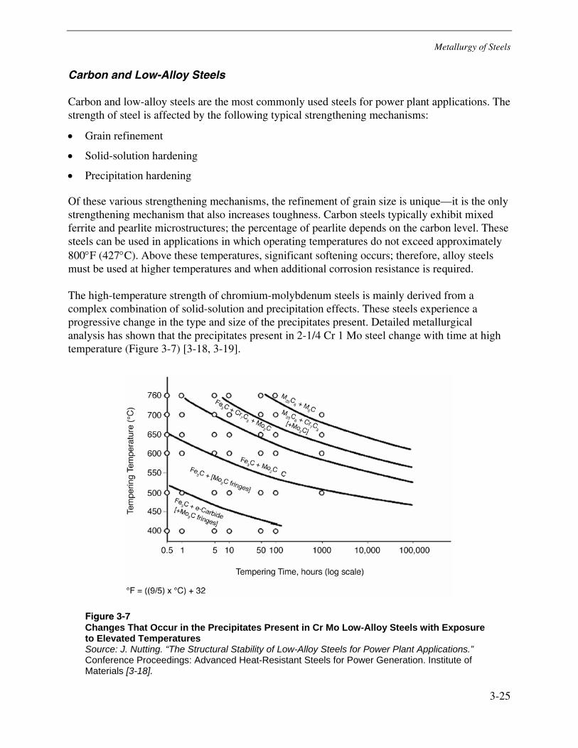
Metallurgy of Steels
3-25
Carbon and Low-Alloy Steels
Carbon and low-alloy steels are the most commonly used steels for power plant applications. The strength of steel is affected by the following typical strengthening mechanisms:
• Grain refinement
• Solid-solution hardening
• Precipitation hardening
Of these various strengthening mechanisms, the refinement of grain size is unique—it is the only strengthening mechanism that also increases toughness. Carbon steels typically exhibit mixed ferrite and pearlite microstructures; the percentage of pearlite depends on the carbon level. These steels can be used in applications in which operating temperatures do not exceed approximately 800°F (427°C). Above these temperatures, significant softening occurs; therefore, alloy steels must be used at higher temperatures and when additional corrosion resistance is required.
The high-temperature strength of chromium-molybdenum steels is mainly derived from a complex combination of solid-solution and precipitation effects. These steels experience a progressive change in the type and size of the precipitates present. Detailed metallurgical analysis has shown that the precipitates present in 2-1/4 Cr 1 Mo steel change with time at high temperature (Figure 3-7) [3-18, 3-19].
Figure 3-7 Changes That Occur in the Precipitates Present in Cr Mo Low-Alloy Steels with Exposure to Elevated Temperatures Source: J. Nutting. “The Structural Stability of Low-Alloy Steels for Power Plant Applications.” Conference Proceedings: Advanced Heat-Resistant Steels for Power Generation. Institute of Materials [3-18].
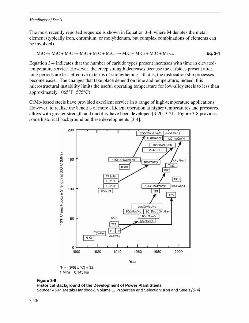
Metallurgy of Steels
3-26
The most recently reported sequence is shown in Equation 3-4, where M denotes the metal element (typically iron, chromium, or molybdenum, but complex combinations of elements can be involved).
M3C → M3C + M2C → M3C + M2C + M7C3 → M2C + M7C3 + M6C + M23C6 Eq. 3-4
Equation 3-4 indicates that the number of carbide types present increases with time in elevated-temperature service. However, the creep strength decreases because the carbides present after long periods are less effective in terms of strengthening—that is, the dislocation slip processes become easier. The changes that take place depend on time and temperature; indeed, this microstructural instability limits the useful operating temperature for low-alloy steels to less than approximately 1065°F (575°C).
CrMo-based steels have provided excellent service in a range of high-temperature applications. However, to realize the benefits of more efficient operation at higher temperatures and pressures, alloys with greater strength and ductility have been developed [3-20, 3-21]. Figure 3-8 provides some historical background on these developments [3-4].
Figure 3-8 Historical Background of the Development of Power Plant Steels Source: ASM. Metals Handbook, Volume 1, Properties and Selection: Iron and Steels [3-4].
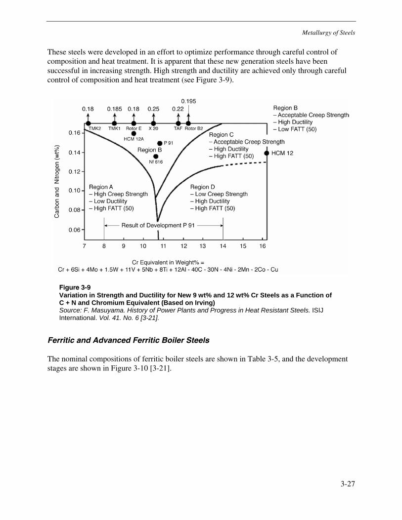
Metallurgy of Steels
3-27
These steels were developed in an effort to optimize performance through careful control of composition and heat treatment. It is apparent that these new generation steels have been successful in increasing strength. High strength and ductility are achieved only through careful control of composition and heat treatment (see Figure 3-9).
Figure 3-9 Variation in Strength and Ductility for New 9 wt% and 12 wt% Cr Steels as a Function of C + N and Chromium Equivalent (Based on Irving) Source: F. Masuyama. History of Power Plants and Progress in Heat Resistant Steels. ISIJ International. Vol. 41. No. 6 [3-21].
Ferritic and Advanced Ferritic Boiler Steels
The nominal compositions of ferritic boiler steels are shown in Table 3-5, and the development stages are shown in Figure 3-10 [3-21].
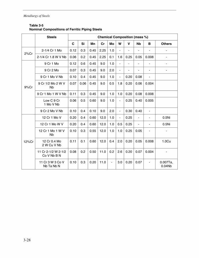
Metallurgy of Steels
3-28
Table 3-5 Nominal Compositions of Ferritic Piping Steels
Chemical Composition (mass %) Steels
C Si Mn Cr Mo W V Nb B Others
2-1/4 Cr 1 Mo 0.12 0.3 0.45 2.25 1.0 - - - - - 2%Cr
2-1/4 Cr 1.8 W V Nb 0.06 0.2 0.45 2.25 0.1 1.6 0.25 0.05 0.008 -
9 Cr 1 Mo 0.12 0.6 0.45 9.0 1.0 - - - - -
9 Cr 2 Mo 0.07 0.3 0.45 9.0 2.0 - - - - -
9 Cr 1 Mo V Nb 0.10 0.4 0.45 9.0 1.0 - 0.20 0.08 -
9 Cr 1/2 Mo 2 W V Nb
0.07 0.06 0.45 9.0 0.5 1.8 0.20 0.06 0.004
9 Cr 1 Mo 1 W V Nb 0.11 0.3 0.45 9.0 1.0 1.0 0.20 0.08 0.008
Low C 9 Cr 1 Mo V Nb
0.06 0.5 0.60 9.0 1.0 - 0.25 0.40 0.005
9%Cr
9 Cr 2 Mo V Nb 0.10 0.4 0.10 9.0 2.0 - 0.30 0.40 -
12 Cr 1 Mo V 0.20 0.4 0.60 12.0 1.0 - 0.25 - - 0.5Ni
12 Cr 1 Mo W V 0.20 0.4 0.60 12.0 1.0 0.5 0.25 - - 0.5Ni
12 Cr 1 Mo 1 W V Nb
0.10 0.3 0.55 12.0 1.0 1.0 0.25 0.05 - -
12 Cr 0.4 Mo 2 W Cu V Nb
0.11 0.1 0.60 12.0 0.4 2.0 0.20 0.05 0.008 1.0Cu
11 Cr 2-1/2 W 2-1/2 Co V Nb B N
0.08 0.2 0.50 11.0 0.2 2.6 0.20 0.07 0.004 -
12%Cr
11 Cr 3 W 3 Co V Nb Ta Nb N
0.10 0.3 0.20 11.0 - 3.0 0.20 0.07 - 0.007Ta, 0.04Nb
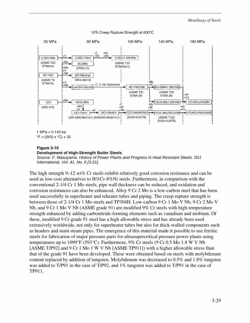
Metallurgy of Steels
3-29
Figure 3-10 Development of High-Strength Boiler Steels Source: F. Masuyama. History of Power Plants and Progress in Heat Resistant Steels. ISIJ International. Vol. 41. No. 6 [3-21].
The high strength 9–12 wt% Cr steels exhibit relatively good corrosion resistance and can be used as low-cost alternatives to l8%Cr-8%Ni steels. Furthermore, in comparison with the conventional 2-1/4 Cr 1 Mo steels, pipe wall thickness can be reduced, and oxidation and corrosion resistances can also be enhanced. Alloy 9 Cr 2 Mo is a low-carbon steel that has been used successfully in superheater and reheater tubes and piping. The creep rupture strength is between those of 2-1/4 Cr 1 Mo steels and TP304H. Low-carbon 9 Cr 1 Mo V Nb, 9 Cr 2 Mo V Nb, and 9 Cr 1 Mo V Nb (ASME grade 91) are modified 9% Cr steels with high-temperature strength enhanced by adding carbonitride-forming elements such as vanadium and niobium. Of these, modified 9 Cr grade 91 steel has a high allowable stress and has already been used extensively worldwide, not only for superheater tubes but also for thick-walled components such as headers and main steam pipes. The emergence of this material made it possible to use ferritic steels for fabrication of major pressure parts for ultrasupercritical pressure power plants using temperatures up to 1099°F (593°C). Furthermore, 9% Cr steels (9 Cr 0.5 Mo 1.8 W V Nb [ASME T/P92] and 9 Cr 1 Mo 1 W V Nb [ASME TP911]) with a higher allowable stress than that of the grade 91 have been developed. These were obtained based on steels with molybdenum content replaced by addition of tungsten. Molybdenum was decreased to 0.5% and 1.8% tungsten was added to T/P91 in the case of T/P92, and 1% tungsten was added to T/P91 in the case of TP911.

Metallurgy of Steels
3-30
Of the 12% Cr steels, 12 Cr 1 Mo V (DIN X20CrMoV121) is used extensively in Europe for superheater tubes, steam pipes, and so forth, and has a large amount of service experience. However, because this steel has a carbon content as high as 0.2%, weldability is relatively poor, and because high-temperature strength is not satisfactorily high, this material is hardly ever used in Japan or in the United States. However, improved 12% Cr steels for boiler applications, for example 12 Cr 1 Mo 1 W V Nb and 12 Cr 0.4 Mo 2 W Cu V Nb (ASME T122), have been developed with improved performance.
Austenitic Steels
Chemical compositions of austenitic heat-resistant steels are shown in Table 3-6, and development stages are presented in Figure 3-11 [3-21]. Because 18%Cr-8%Ni steels are used for the highest-temperature boiler components, various improvements have been made to enhance corrosion resistance while maintaining high creep strength. In addition, new steels with chromium content of 20% or more have been developed for the purpose of improving creep strength and corrosion resistance. The 18% Cr-8% Ni steels such as TP304H, TP32IH, TP316H, and TP347H are still used for fossil-fired power plants operating under conventional steam conditions. Steel TP347H, which has the highest allowable stress among these four types of steels, has been produced with a fine-grained structure (ASTM grain size 8 and finer) for improved steam oxidation resistance and creep strengthening; this alloy is designated as TP347HFG by ASME. This steel is very useful for improved performance in superheater tubes for ultrasupercritical pressure power plants operating at temperatures up to 1099°F (593°C).
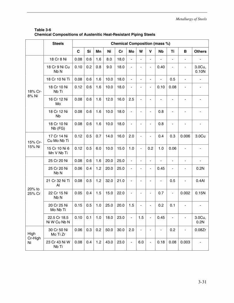
Metallurgy of Steels
3-31
Table 3-6 Chemical Compositions of Austenitic Heat-Resistant Piping Steels
Chemical Composition (mass %) Steels
C Si Mn Ni Cr Mo W V Nb Ti B Others
18 Cr 8 Ni 0.08 0.6 1.6 8.0 18.0 - - - - - - -
18 Cr 9 Ni Cu Nb N
0.10 0.2 0.8 9.0 18.0 - - - 0.40 - - 3.0Cu, 0.10N
18 Cr 10 Ni Ti 0.08 0.6 1.6 10.0 18.0 - - - - 0.5 - -
18 Cr 10 Ni Nb Ti
0.12 0.6 1.6 10.0 18.0 - - - 0.10 0.08 - -
16 Cr 12 Ni Mo
0.08 0.6 1.6 12.0 16.0 2.5 - - - - - -
18 Cr 12 Ni Nb
0.08 0.6 1.6 10.0 18.0 - - - 0.8 - - -
18% Cr-8% Ni
18 Cr 10 Ni Nb (FG)
0.08 0.6 1.6 10.0 18.0 - - - 0.8 - - -
17 Cr 14 Ni Cu Mo Nb Ti
0.12 0.5 0.7 14.0 16.0 2.0 - - 0.4 0.3 0.006 3.0Cu
15% Cr-15% Ni 15 Cr 10 Ni 6
Mn V Nb Ti 0.12 0.5 6.0 10.0 15.0 1.0 - 0.2 1.0 0.06 - -
25 Cr 20 Ni 0.08 0.6 1.6 20.0 25.0 - - - - - - -
25 Cr 20 Ni Nb N
0.06 0.4 1.2 20.0 25.0 - - - 0.45 - - 0.2N
21 Cr 32 Ni Ti Al
0.08 0.5 1.2 32.0 21.0 - - - - 0.5 - 0.4Al
22 Cr 15 Ni Nb N
0.05 0.4 1.5 15.0 22.0 - - - 0.7 - 0.002 0.15N
20 Cr 25 Ni Mo Nb Ti
0.15 0.5 1.0 25.0 20.0 1.5 - - 0.2 0.1 - -
20% to 25% Cr
22.5 Cr 18.5 Ni W Cu Nb N
0.10 0.1 1.0 18.0 23.0 - 1.5 - 0.45 - - 3.0Cu, 0.2N
30 Cr 50 Ni Mo Ti Zr
0.06 0.3 0.2 50.0 30.0 2.0 - - - 0.2 - 0.08Zr High Cr-High Ni 23 Cr 43 Ni W
Nb Ti 0.08 0.4 1.2 43.0 23.0 - 6.0 - 0.18 0.08 0.003 -
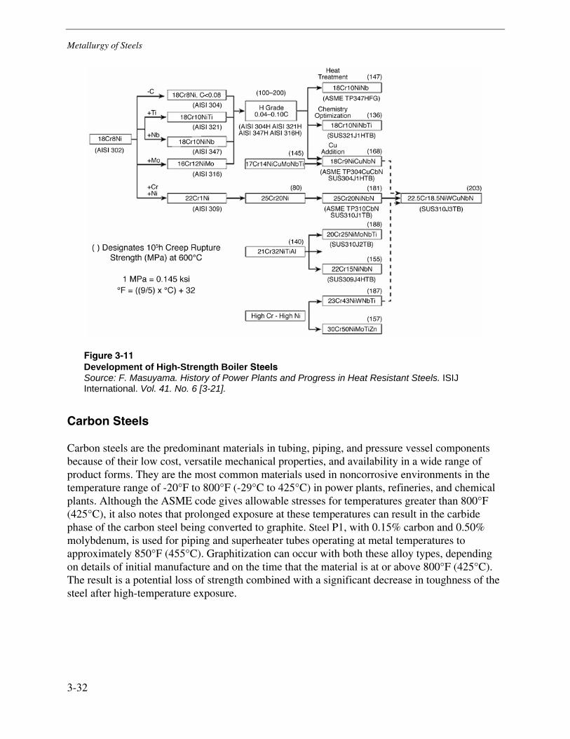
Metallurgy of Steels
3-32
Figure 3-11 Development of High-Strength Boiler Steels Source: F. Masuyama. History of Power Plants and Progress in Heat Resistant Steels. ISIJ International. Vol. 41. No. 6 [3-21].
Carbon Steels
Carbon steels are the predominant materials in tubing, piping, and pressure vessel components because of their low cost, versatile mechanical properties, and availability in a wide range of product forms. They are the most common materials used in noncorrosive environments in the temperature range of -20°F to 800°F (-29°C to 425°C) in power plants, refineries, and chemical plants. Although the ASME code gives allowable stresses for temperatures greater than 800°F (425°C), it also notes that prolonged exposure at these temperatures can result in the carbide phase of the carbon steel being converted to graphite. Steel P1, with 0.15% carbon and 0.50% molybdenum, is used for piping and superheater tubes operating at metal temperatures to approximately 850°F (455°C). Graphitization can occur with both these alloy types, depending on details of initial manufacture and on the time that the material is at or above 800°F (425°C). The result is a potential loss of strength combined with a significant decrease in toughness of the steel after high-temperature exposure.
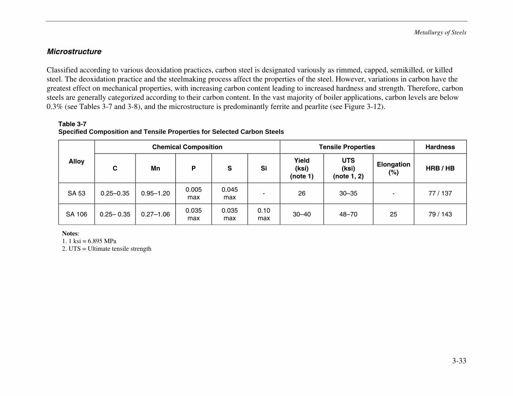
Metallurgy of Steels
3-33
Microstructure
Classified according to various deoxidation practices, carbon steel is designated variously as rimmed, capped, semikilled, or killed steel. The deoxidation practice and the steelmaking process affect the properties of the steel. However, variations in carbon have the greatest effect on mechanical properties, with increasing carbon content leading to increased hardness and strength. Therefore, carbon steels are generally categorized according to their carbon content. In the vast majority of boiler applications, carbon levels are below 0.3% (see Tables 3-7 and 3-8), and the microstructure is predominantly ferrite and pearlite (see Figure 3-12).
Table 3-7 Specified Composition and Tensile Properties for Selected Carbon Steels
Chemical Composition Tensile Properties Hardness
Alloy C Mn P S Si
Yield (ksi)
(note 1)
UTS (ksi)
(note 1, 2)
Elongation (%)
HRB / HB
SA 53 0.25–0.35 0.95–1.20 0.005 max
0.045 max
- 26 30–35 - 77 / 137
SA 106 0.25– 0.35 0.27–1.06 0.035 max
0.035 max
0.10 max
30–40 48–70 25 79 / 143
Notes: 1. 1 ksi = 6.895 MPa 2. UTS = Ultimate tensile strength
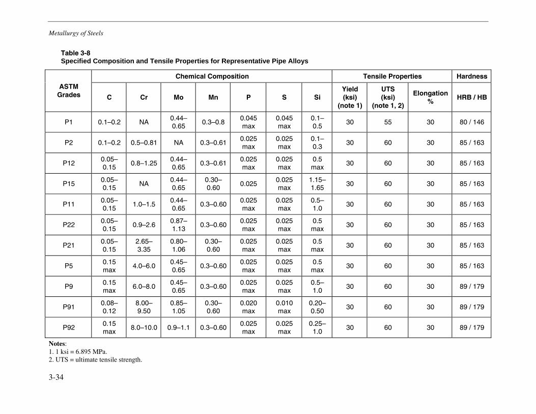
Metallurgy of Steels
3-34
Table 3-8 Specified Composition and Tensile Properties for Representative Pipe Alloys
Chemical Composition Tensile Properties Hardness
ASTM Grades C Cr Mo Mn P S Si
Yield (ksi)
(note 1)
UTS (ksi)
(note 1, 2)
Elongation %
HRB / HB
P1 0.1–0.2 NA 0.44–0.65
0.3–0.8 0.045 max
0.045 max
0.1–0.5
30 55 30 80 / 146
P2 0.1–0.2 0.5–0.81 NA 0.3–0.61 0.025 max
0.025 max
0.1–0.3
30 60 30 85 / 163
P12 0.05–0.15
0.8–1.25 0.44–0.65
0.3–0.61 0.025 max
0.025 max
0.5 max
30 60 30 85 / 163
P15 0.05–0.15
NA 0.44–0.65
0.30–0.60
0.025 0.025 max
1.15–1.65
30 60 30 85 / 163
P11 0.05–0.15
1.0–1.5 0.44–0.65
0.3–0.60 0.025 max
0.025 max
0.5–1.0
30 60 30 85 / 163
P22 0.05–0.15
0.9–2.6 0.87–1.13
0.3–0.60 0.025 max
0.025 max
0.5 max
30 60 30 85 / 163
P21 0.05–0.15
2.65–3.35
0.80–1.06
0.30–0.60
0.025 max
0.025 max
0.5 max
30 60 30 85 / 163
P5 0.15 max
4.0–6.0 0.45–0.65
0.3–0.60 0.025 max
0.025 max
0.5 max
30 60 30 85 / 163
P9 0.15 max
6.0–8.0 0.45–0.65
0.3–0.60 0.025 max
0.025 max
0.5–1.0
30 60 30 89 / 179
P91 0.08–0.12
8.00–9.50
0.85–1.05
0.30–0.60
0.020 max
0.010 max
0.20–0.50
30 60 30 89 / 179
P92 0.15 max
8.0–10.0 0.9–1.1 0.3–0.60 0.025 max
0.025 max
0.25–1.0
30 60 30 89 / 179
Notes: 1. 1 ksi = 6.895 MPa. 2. UTS = ultimate tensile strength.
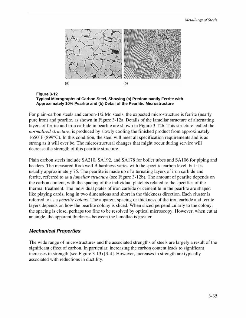
Metallurgy of Steels
3-35
Figure 3-12 Typical Micrographs of Carbon Steel, Showing (a) Predominantly Ferrite with Approximately 10% Pearlite and (b) Detail of the Pearlitic Microstructure
For plain-carbon steels and carbon-1/2 Mo steels, the expected microstructure is ferrite (nearly pure iron) and pearlite, as shown in Figure 3-12a. Details of the lamellar structure of alternating layers of ferrite and iron carbide in pearlite are shown in Figure 3-12b. This structure, called the normalized structure, is produced by slowly cooling the finished product from approximately 1650°F (899°C). In this condition, the steel will meet all specification requirements and is as strong as it will ever be. The microstructural changes that might occur during service will decrease the strength of this pearlitic structure.
Plain carbon steels include SA210, SA192, and SA178 for boiler tubes and SA106 for piping and headers. The measured Rockwell B hardness varies with the specific carbon level, but it is usually approximately 75. The pearlite is made up of alternating layers of iron carbide and ferrite, referred to as a lamellar structure (see Figure 3-12b). The amount of pearlite depends on the carbon content, with the spacing of the individual platelets related to the specifics of the thermal treatment. The individual plates of iron carbide or cementite in the pearlite are shaped like playing cards, long in two dimensions and short in the thickness direction. Each cluster is referred to as a pearlite colony. The apparent spacing or thickness of the iron carbide and ferrite layers depends on how the pearlite colony is sliced. When sliced perpendicularly to the colony, the spacing is close, perhaps too fine to be resolved by optical microscopy. However, when cut at an angle, the apparent thickness between the lamellae is greater.
Mechanical Properties
The wide range of microstructures and the associated strengths of steels are largely a result of the significant effect of carbon. In particular, increasing the carbon content leads to significant increases in strength (see Figure 3-13) [3-4]. However, increases in strength are typically associated with reductions in ductility.
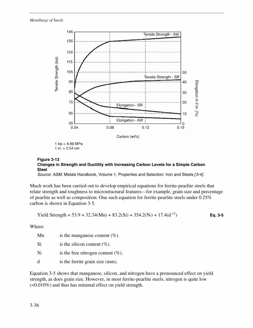
Metallurgy of Steels
3-36
Figure 3-13 Changes in Strength and Ductility with Increasing Carbon Levels for a Simple Carbon Steel Source: ASM. Metals Handbook, Volume 1, Properties and Selection: Iron and Steels [3-4].
Much work has been carried out to develop empirical equations for ferrite-pearlite steels that relate strength and toughness to microstructural features—for example, grain size and percentage of pearlite as well as composition. One such equation for ferrite-pearlite steels under 0.25% carbon is shown in Equation 3-5.
Yield Strength = 53.9 + 32.34(Mn) + 83.2(Si) + 354.2(Nf) + 17.4(d-1/2) Eq. 3-5
Where:
Mn is the manganese content (%).
Si is the silicon content (%).
Nf is the free nitrogen content (%).
d is the ferrite grain size (mm).
Equation 3-5 shows that manganese, silicon, and nitrogen have a pronounced effect on yield strength, as does grain size. However, in most ferrite-pearlite steels, nitrogen is quite low (<0.010%) and thus has minimal effect on yield strength.
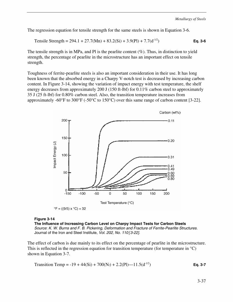
Metallurgy of Steels
3-37
The regression equation for tensile strength for the same steels is shown in Equation 3-6.
Tensile Strength = 294.1 + 27.7(Mn) + 83.2(Si) + 3.9(Pl) + 7.7(d-1/2) Eq. 3-6
The tensile strength is in MPa, and Pl is the pearlite content (%). Thus, in distinction to yield strength, the percentage of pearlite in the microstructure has an important effect on tensile strength.
Toughness of ferrite-pearlite steels is also an important consideration in their use. It has long been known that the absorbed energy in a Charpy V-notch test is decreased by increasing carbon content. In Figure 3-14, showing the variation of impact energy with test temperature, the shelf energy decreases from approximately 200 J (150 ft-lbf) for 0.11% carbon steel to approximately 35 J (25 ft-lbf) for 0.80% carbon steel. Also, the transition temperature increases from approximately -60°F to 300°F (-50°C to 150°C) over this same range of carbon content [3-22].
Figure 3-14 The Influence of Increasing Carbon Level on Charpy Impact Tests for Carbon Steels Source: K. W. Burns and F. B. Pickering, Deformation and Fracture of Ferrite-Pearlite Structures. Journal of the Iron and Steel Institute, Vol. 202, No. 110 [3-22].
The effect of carbon is due mainly to its effect on the percentage of pearlite in the microstructure. This is reflected in the regression equation for transition temperature (for temperature in °C) shown in Equation 3-7.
Transition Temp = -19 + 44(Si) + 700(Nf) + 2.2(Pl)—11.5(d-1/2) Eq. 3-7

Metallurgy of Steels
3-38
It can be seen in all these relationships that ferrite grain size is an important parameter in improving both strength and toughness. Although pearlite is beneficial for increasing tensile strength, and nitrogen is beneficial for increasing yield strength, both are harmful to toughness.
Allowable Stress Values
The allowable stress values according to the ASME Boiler and Pressure Vessel Code, Section II, Materials, are presented in Table 3-9 [3-10]. At lower temperatures, these allowable stresses are based on the tensile properties; therefore, no variation of allowable stress is recommended. However, above approximately 700°F (371°C) for the carbon steels and approximately 750°F (399°C) for the carbon-1/2 Mo steel, diffusion processes begin to become significant, and the allowable stress is reduced. With further increases in temperature, the allowable stress is further reduced, as creep damage development becomes the dominant process.
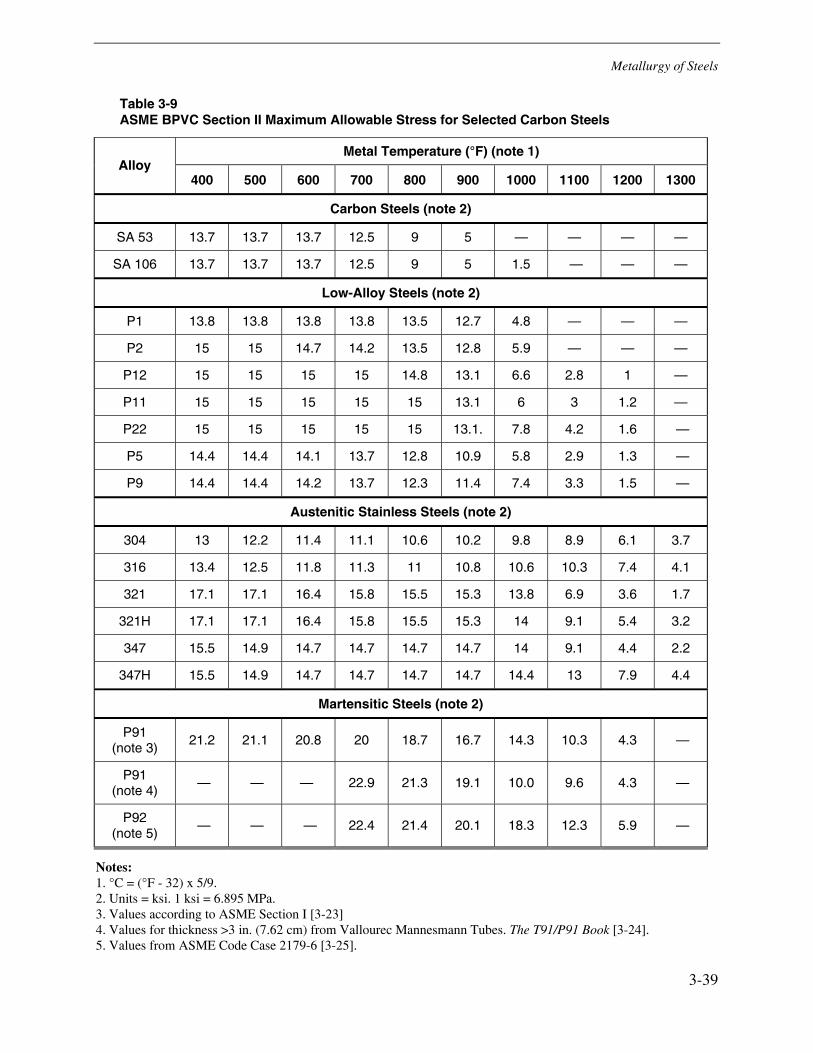
Metallurgy of Steels
3-39
Table 3-9 ASME BPVC Section II Maximum Allowable Stress for Selected Carbon Steels
Metal Temperature (°F) (note 1) Alloy
400 500 600 700 800 900 1000 1100 1200 1300
Carbon Steels (note 2)
SA 53 13.7 13.7 13.7 12.5 9 5 — — — —
SA 106 13.7 13.7 13.7 12.5 9 5 1.5 — — —
Low-Alloy Steels (note 2)
P1 13.8 13.8 13.8 13.8 13.5 12.7 4.8 — — —
P2 15 15 14.7 14.2 13.5 12.8 5.9 — — —
P12 15 15 15 15 14.8 13.1 6.6 2.8 1 —
P11 15 15 15 15 15 13.1 6 3 1.2 —
P22 15 15 15 15 15 13.1. 7.8 4.2 1.6 —
P5 14.4 14.4 14.1 13.7 12.8 10.9 5.8 2.9 1.3 —
P9 14.4 14.4 14.2 13.7 12.3 11.4 7.4 3.3 1.5 —
Austenitic Stainless Steels (note 2)
304 13 12.2 11.4 11.1 10.6 10.2 9.8 8.9 6.1 3.7
316 13.4 12.5 11.8 11.3 11 10.8 10.6 10.3 7.4 4.1
321 17.1 17.1 16.4 15.8 15.5 15.3 13.8 6.9 3.6 1.7
321H 17.1 17.1 16.4 15.8 15.5 15.3 14 9.1 5.4 3.2
347 15.5 14.9 14.7 14.7 14.7 14.7 14 9.1 4.4 2.2
347H 15.5 14.9 14.7 14.7 14.7 14.7 14.4 13 7.9 4.4
Martensitic Steels (note 2)
P91 (note 3)
21.2 21.1 20.8 20 18.7 16.7 14.3 10.3 4.3 —
P91 (note 4)
— — — 22.9 21.3 19.1 10.0 9.6 4.3 —
P92 (note 5)
— — — 22.4 21.4 20.1 18.3 12.3 5.9 —
Notes: 1. °C = (°F - 32) x 5/9. 2. Units = ksi. 1 ksi = 6.895 MPa. 3. Values according to ASME Section I [3-23] 4. Values for thickness >3 in. (7.62 cm) from Vallourec Mannesmann Tubes. The T91/P91 Book [3-24]. 5. Values from ASME Code Case 2179-6 [3-25].
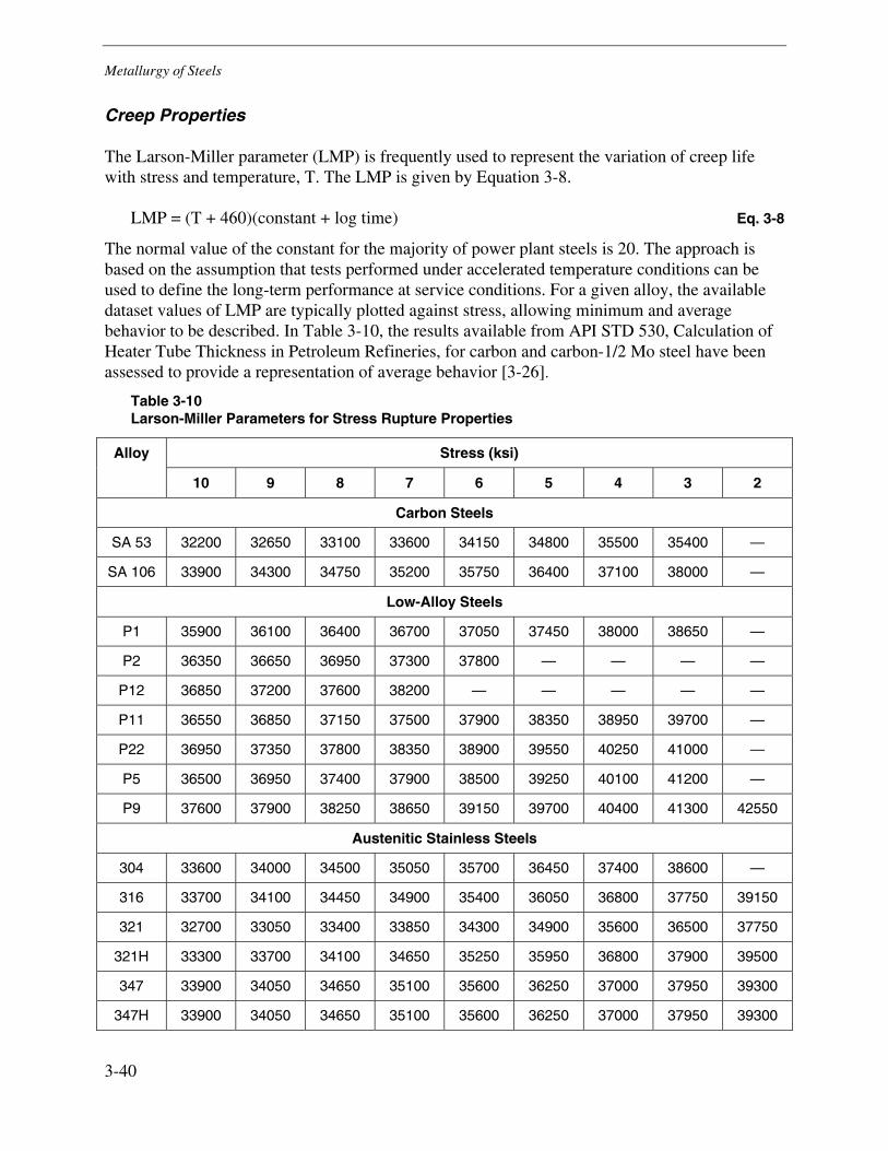
Metallurgy of Steels
3-40
Creep Properties
The Larson-Miller parameter (LMP) is frequently used to represent the variation of creep life with stress and temperature, T. The LMP is given by Equation 3-8.
LMP = (T + 460)(constant + log time) Eq. 3-8
The normal value of the constant for the majority of power plant steels is 20. The approach is based on the assumption that tests performed under accelerated temperature conditions can be used to define the long-term performance at service conditions. For a given alloy, the available dataset values of LMP are typically plotted against stress, allowing minimum and average behavior to be described. In Table 3-10, the results available from API STD 530, Calculation of Heater Tube Thickness in Petroleum Refineries, for carbon and carbon-1/2 Mo steel have been assessed to provide a representation of average behavior [3-26].
Table 3-10 Larson-Miller Parameters for Stress Rupture Properties
Stress (ksi) Alloy
10 9 8 7 6 5 4 3 2
Carbon Steels
SA 53 32200 32650 33100 33600 34150 34800 35500 35400 —
SA 106 33900 34300 34750 35200 35750 36400 37100 38000 —
Low-Alloy Steels
P1 35900 36100 36400 36700 37050 37450 38000 38650 —
P2 36350 36650 36950 37300 37800 — — — —
P12 36850 37200 37600 38200 — — — — —
P11 36550 36850 37150 37500 37900 38350 38950 39700 —
P22 36950 37350 37800 38350 38900 39550 40250 41000 —
P5 36500 36950 37400 37900 38500 39250 40100 41200 —
P9 37600 37900 38250 38650 39150 39700 40400 41300 42550
Austenitic Stainless Steels
304 33600 34000 34500 35050 35700 36450 37400 38600 —
316 33700 34100 34450 34900 35400 36050 36800 37750 39150
321 32700 33050 33400 33850 34300 34900 35600 36500 37750
321H 33300 33700 34100 34650 35250 35950 36800 37900 39500
347 33900 34050 34650 35100 35600 36250 37000 37950 39300
347H 33900 34050 34650 35100 35600 36250 37000 37950 39300

Metallurgy of Steels
3-41
Table 3-10 (continued) Larson-Miller Parameters for Stress Rupture Properties
Stress (ksi) Alloy
10 9 8 7 6 5 4 3 2
Martensitic Steels
P91 — — — — — — — — —
P92 — — — — — — — — —
Note: 1 ksi = 6.895 MPa.
Aging Effects
At temperatures above approximately 800°F (427°C), the plate-like shape of the pearlite is unstable and will change to a sphere-like shape. Changing its shape to a sphere reduces the internal energy of the carbide. The excess surface energy is the driving force for the change. The process that leads to the new shape is known as spheroidization. Another factor in addition to temperature that will promote spheroidization is high stress. For plain carbon (SA53, SA106) steels, the iron carbide itself is unstable and will transform to graphite and ferrite. Thus, a further step in the microstructural changes is the formation of graphite particles within the steel, a process known as graphitization. Graphitization is a well-known phenomenon; in fact, the ASME Boiler and Pressure Vessel Code, Section II, Materials, Part D, Table 1A warns of the change in iron carbide to graphite for plain carbon steels and carbon-1/2 Mo steels.
Spheroidization and graphitization are competing processes (see Figure 3-15) [3-27]. At temperatures above approximately 1000°F (538°C), graphite will appear after spheroidization. At temperatures below approximately 1000°F (538°C), graphitization occurs before the steel is fully spheroidized.
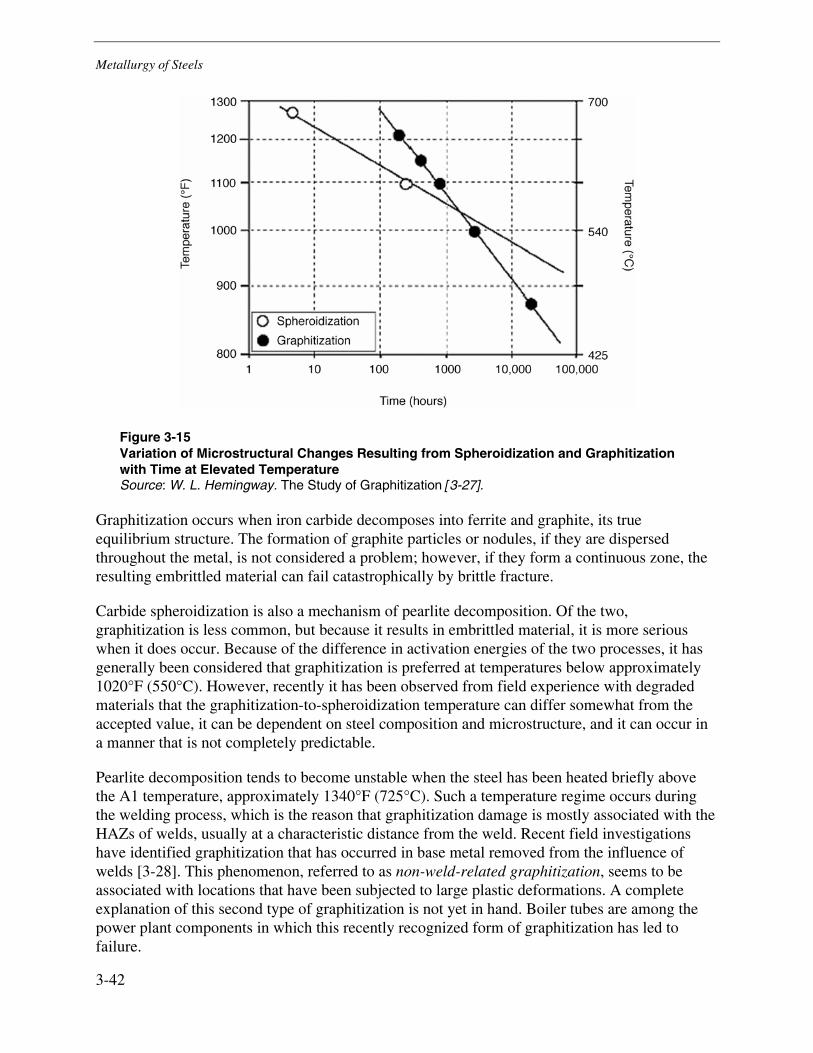
Metallurgy of Steels
3-42
Figure 3-15 Variation of Microstructural Changes Resulting from Spheroidization and Graphitization with Time at Elevated Temperature Source: W. L. Hemingway. The Study of Graphitization [3-27].
Graphitization occurs when iron carbide decomposes into ferrite and graphite, its true equilibrium structure. The formation of graphite particles or nodules, if they are dispersed throughout the metal, is not considered a problem; however, if they form a continuous zone, the resulting embrittled material can fail catastrophically by brittle fracture.
Carbide spheroidization is also a mechanism of pearlite decomposition. Of the two, graphitization is less common, but because it results in embrittled material, it is more serious when it does occur. Because of the difference in activation energies of the two processes, it has generally been considered that graphitization is preferred at temperatures below approximately 1020°F (550°C). However, recently it has been observed from field experience with degraded materials that the graphitization-to-spheroidization temperature can differ somewhat from the accepted value, it can be dependent on steel composition and microstructure, and it can occur in a manner that is not completely predictable.
Pearlite decomposition tends to become unstable when the steel has been heated briefly above the A1 temperature, approximately 1340°F (725°C). Such a temperature regime occurs during the welding process, which is the reason that graphitization damage is mostly associated with the HAZs of welds, usually at a characteristic distance from the weld. Recent field investigations have identified graphitization that has occurred in base metal removed from the influence of welds [3-28]. This phenomenon, referred to as non-weld-related graphitization, seems to be associated with locations that have been subjected to large plastic deformations. A complete explanation of this second type of graphitization is not yet in hand. Boiler tubes are among the power plant components in which this recently recognized form of graphitization has led to failure.
Metallurgy of Steels
3-43
The propensity toward graphitization damage has also been considered to depend on the steelmaking practice used. Aluminum-killed steels, once in common usage, have been shown to be more susceptible than steels deoxidized with silicon or titanium, unless the aluminum content is restricted to <0.025%.
The use of carbon-molybdenum steel has been largely discontinued for higher temperatures because of problems associated with graphitization. Chromium-containing steels are highly resistant to graphitization and are therefore preferred for service above 850°F (455°C).
The effect of spheroidization on the rupture strength of a typical carbon-molybdenum steel containing 0.17% C and 0.42% Mo, at 900°F and 1000°F (480°C and 540°C), is shown in Figure 3-16 for several initial metallurgical structures (normalized or annealed). In these tests, the structure of the steel affected the rupture strength; for example, the stress for failure of a spheroidized structure in a given time was sometimes only half that of a normalized structure [3-29].
At 900°F (480°C), a coarse-grain normalized structure was the strongest for both short-time and long-time tests. The spheroidized structures were weaker than the normalized or annealed structures for short-time tests at both 900°F and 1000°F (480°C and 540°C). As the test time increased, the rupture values for all the structures tended to approach a common value.
Although the spheroidized structure is weaker than the normalized pearlitic microstructure, a greater life in cyclic fatigue loading has been observed (see Figure 3-17) [3-4]. This is because the platelets of cementite in pearlite are relatively brittle and therefore offer planes of relatively rapid fracture within the pearlitic microstructure.
Chromium-Molybdenum Steels
Chromium-molybdenum heat-resistant steels encompass a number of different alloys that contain between approximately 0.5%–10% chromium and 0.5%–1.2% molybdenum. The carbon content is usually below 0.2%. The specified alloy compositions for selected steels within the classification are given in Table 3-6. The chromium provides improved oxidation and corrosion resistance, and the molybdenum increases strength at elevated temperatures. These alloys are generally supplied in the normalized and tempered, quenched and tempered, or annealed condition. Chromium-molybdenum steels are widely used in the oil and gas industries and in fossil-fuel and nuclear power plants. The greatest creep strength is found in 2-1/4 Cr 1 Mo steels (see Figure 3-18) [3-30]. However, the resistance to oxidation increases with increasing chromium level.
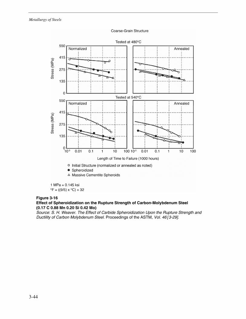
Metallurgy of Steels
3-44
Figure 3-16 Effect of Spheroidization on the Rupture Strength of Carbon-Molybdenum Steel (0.17 C 0.88 Mn 0.20 Si 0.42 Mo) Source: S. H. Weaver. The Effect of Carbide Spheroidization Upon the Rupture Strength and Ductility of Carbon Molybdenum Steel. Proceedings of the ASTM, Vol. 46 [3-29].
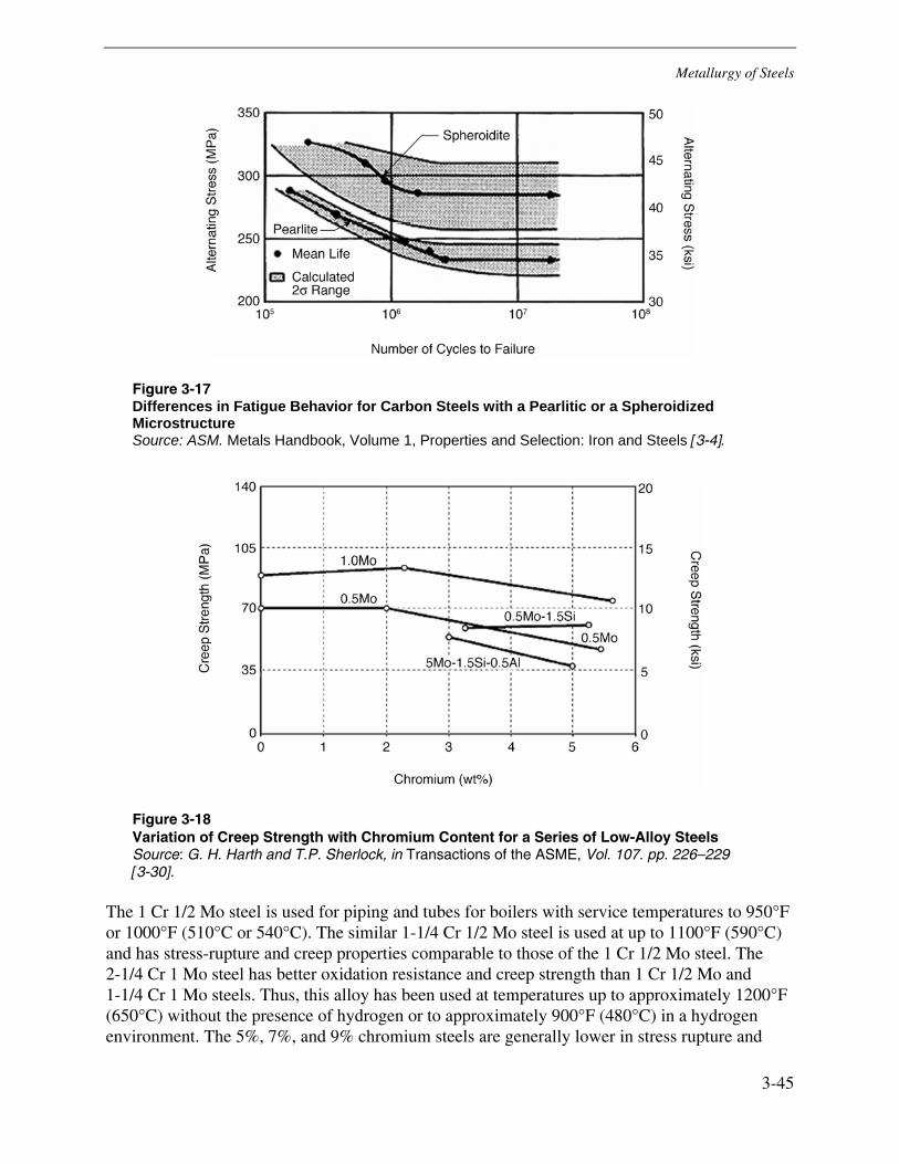
Metallurgy of Steels
3-45
Figure 3-17 Differences in Fatigue Behavior for Carbon Steels with a Pearlitic or a Spheroidized Microstructure Source: ASM. Metals Handbook, Volume 1, Properties and Selection: Iron and Steels [3-4].
Figure 3-18 Variation of Creep Strength with Chromium Content for a Series of Low-Alloy Steels Source: G. H. Harth and T.P. Sherlock, in Transactions of the ASME, Vol. 107. pp. 226–229 [3-30].
The 1 Cr 1/2 Mo steel is used for piping and tubes for boilers with service temperatures to 950°F or 1000°F (510°C or 540°C). The similar 1-1/4 Cr 1/2 Mo steel is used at up to 1100°F (590°C) and has stress-rupture and creep properties comparable to those of the 1 Cr 1/2 Mo steel. The 2-1/4 Cr 1 Mo steel has better oxidation resistance and creep strength than 1 Cr 1/2 Mo and 1-1/4 Cr 1 Mo steels. Thus, this alloy has been used at temperatures up to approximately 1200°F (650°C) without the presence of hydrogen or to approximately 900°F (480°C) in a hydrogen environment. The 5%, 7%, and 9% chromium steels are generally lower in stress rupture and
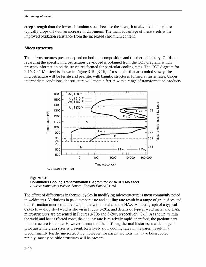
Metallurgy of Steels
3-46
creep strength than the lower-chromium steels because the strength at elevated temperatures typically drops off with an increase in chromium. The main advantage of these steels is the improved oxidation resistance from the increased chromium content.
Microstructure
The microstructures present depend on both the composition and the thermal history. Guidance regarding the specific microstructures developed is obtained from the CCT diagram, which presents information on the structures formed for particular cooling rates. The CCT diagram for 2-1/4 Cr 1 Mo steel is shown in Figure 3-19 [3-15]. For samples that are cooled slowly, the microstructure will be ferrite and pearlite, with bainitic structures formed at faster rates. Under intermediate conditions, the structure will contain ferrite with a range of transformation products.
Figure 3-19 Continuous Cooling Transformation Diagram for 2-1/4 Cr 1 Mo Steel Source: Babcock & Wilcox, Steam, Fortieth Edition [3-15].
The effect of differences in thermal cycles in modifying microstructure is most commonly noted in weldments. Variations in peak temperature and cooling rate result in a range of grain sizes and transformation microstructures within the weld metal and the HAZ. A macrograph of a typical CrMo low-alloy steel weld is shown in Figure 3-20a, and details of typical weld metal and HAZ microstructures are presented in Figures 3-20b and 3-20c, respectively [3-1]. As shown, within the weld and heat-affected zone, the cooling rate is relatively rapid; therefore, the predominant microstructure is bainite. However, because of the differing thermal histories, a wide range of prior austenite grain sizes is present. Relatively slow cooling rates in the parent result in a predominantly ferritic microstructure; however, for parent sections that have been cooled rapidly, mostly bainitic structures will be present.
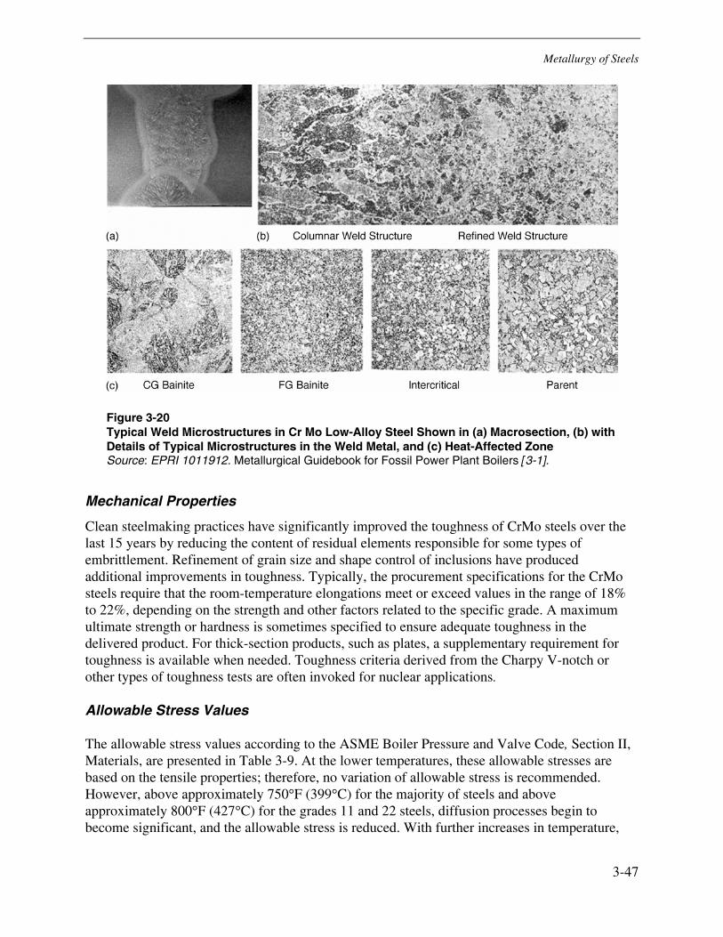
Metallurgy of Steels
3-47
Figure 3-20 Typical Weld Microstructures in Cr Mo Low-Alloy Steel Shown in (a) Macrosection, (b) with Details of Typical Microstructures in the Weld Metal, and (c) Heat-Affected Zone Source: EPRI 1011912. Metallurgical Guidebook for Fossil Power Plant Boilers [3-1].
Mechanical Properties
Clean steelmaking practices have significantly improved the toughness of CrMo steels over the last 15 years by reducing the content of residual elements responsible for some types of embrittlement. Refinement of grain size and shape control of inclusions have produced additional improvements in toughness. Typically, the procurement specifications for the CrMo steels require that the room-temperature elongations meet or exceed values in the range of 18% to 22%, depending on the strength and other factors related to the specific grade. A maximum ultimate strength or hardness is sometimes specified to ensure adequate toughness in the delivered product. For thick-section products, such as plates, a supplementary requirement for toughness is available when needed. Toughness criteria derived from the Charpy V-notch or other types of toughness tests are often invoked for nuclear applications.
Allowable Stress Values
The allowable stress values according to the ASME Boiler Pressure and Valve Code, Section II, Materials, are presented in Table 3-9. At the lower temperatures, these allowable stresses are based on the tensile properties; therefore, no variation of allowable stress is recommended. However, above approximately 750°F (399°C) for the majority of steels and above approximately 800°F (427°C) for the grades 11 and 22 steels, diffusion processes begin to become significant, and the allowable stress is reduced. With further increases in temperature,
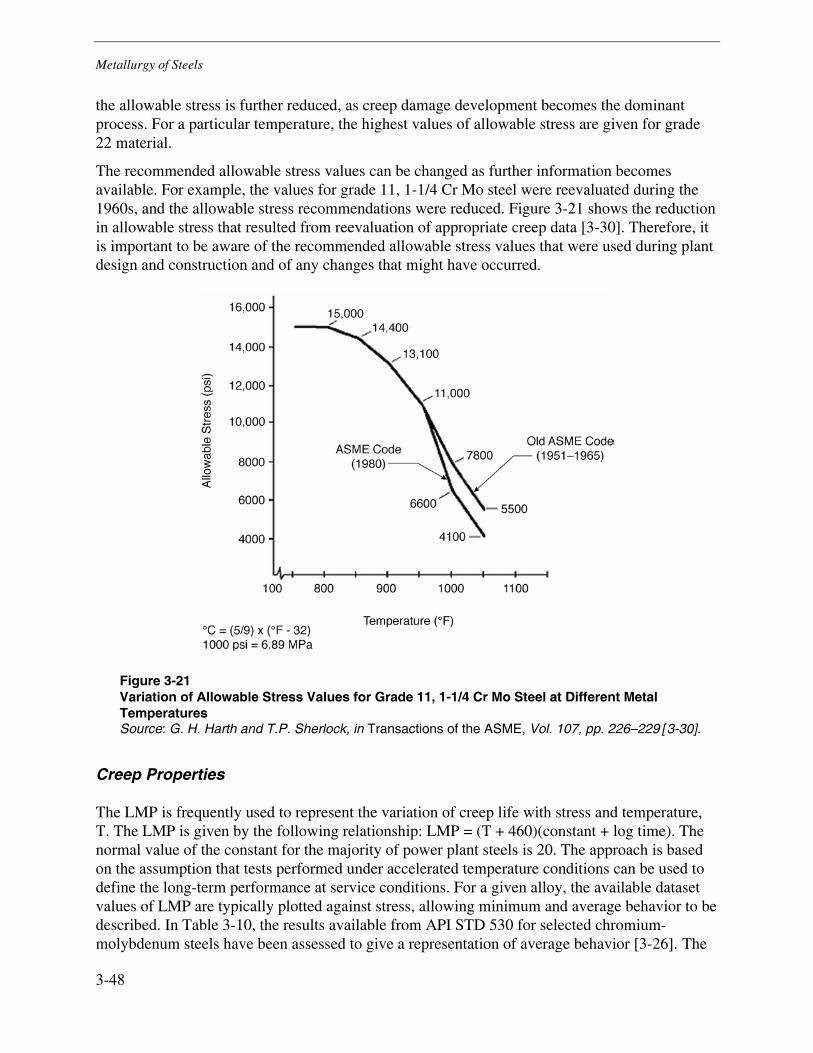
Metallurgy of Steels
3-48
the allowable stress is further reduced, as creep damage development becomes the dominant process. For a particular temperature, the highest values of allowable stress are given for grade 22 material.
The recommended allowable stress values can be changed as further information becomes available. For example, the values for grade 11, 1-1/4 Cr Mo steel were reevaluated during the 1960s, and the allowable stress recommendations were reduced. Figure 3-21 shows the reduction in allowable stress that resulted from reevaluation of appropriate creep data [3-30]. Therefore, it is important to be aware of the recommended allowable stress values that were used during plant design and construction and of any changes that might have occurred.
Figure 3-21 Variation of Allowable Stress Values for Grade 11, 1-1/4 Cr Mo Steel at Different Metal Temperatures Source: G. H. Harth and T.P. Sherlock, in Transactions of the ASME, Vol. 107, pp. 226–229 [3-30].
Creep Properties
The LMP is frequently used to represent the variation of creep life with stress and temperature, T. The LMP is given by the following relationship: LMP = (T + 460)(constant + log time). The normal value of the constant for the majority of power plant steels is 20. The approach is based on the assumption that tests performed under accelerated temperature conditions can be used to define the long-term performance at service conditions. For a given alloy, the available dataset values of LMP are typically plotted against stress, allowing minimum and average behavior to be described. In Table 3-10, the results available from API STD 530 for selected chromium-molybdenum steels have been assessed to give a representation of average behavior [3-26]. The
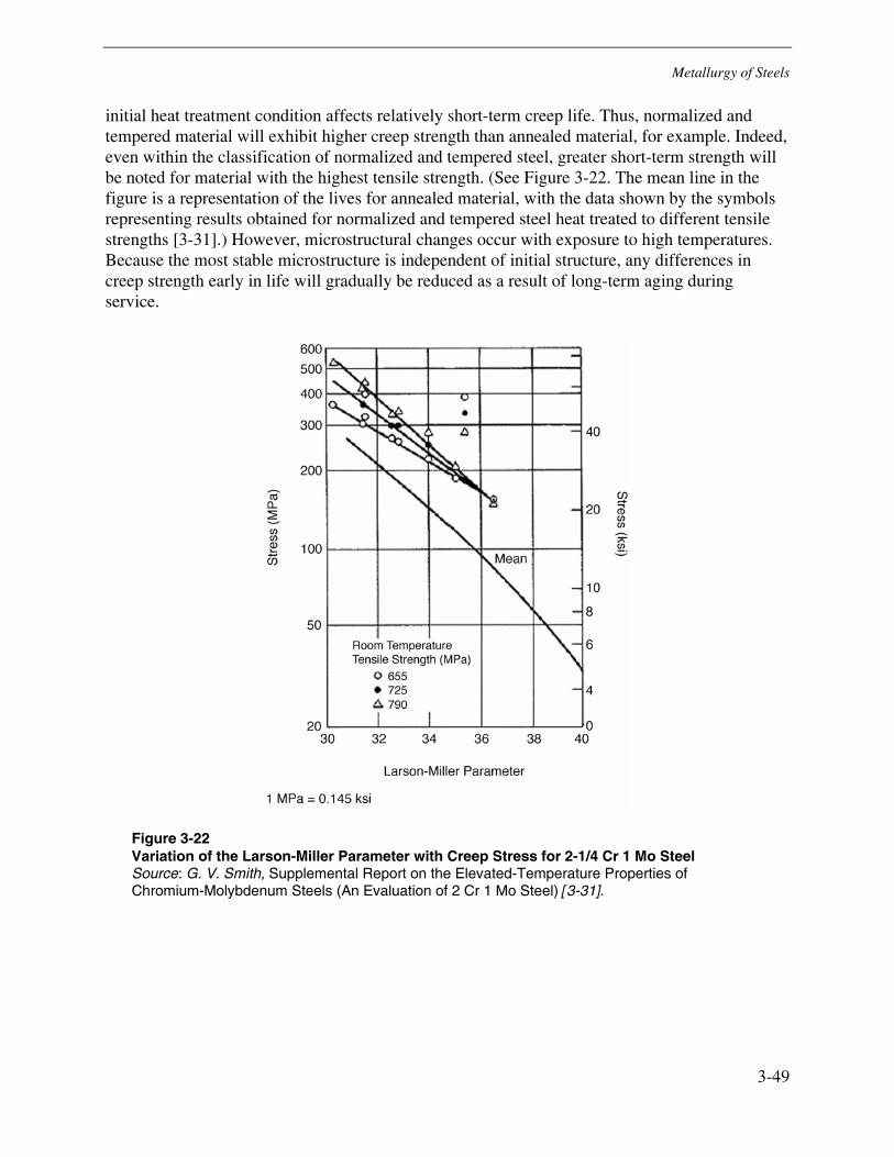
Metallurgy of Steels
3-49
initial heat treatment condition affects relatively short-term creep life. Thus, normalized and tempered material will exhibit higher creep strength than annealed material, for example. Indeed, even within the classification of normalized and tempered steel, greater short-term strength will be noted for material with the highest tensile strength. (See Figure 3-22. The mean line in the figure is a representation of the lives for annealed material, with the data shown by the symbols representing results obtained for normalized and tempered steel heat treated to different tensile strengths [3-31].) However, microstructural changes occur with exposure to high temperatures. Because the most stable microstructure is independent of initial structure, any differences in creep strength early in life will gradually be reduced as a result of long-term aging during service.
Figure 3-22 Variation of the Larson-Miller Parameter with Creep Stress for 2-1/4 Cr 1 Mo Steel Source: G. V. Smith, Supplemental Report on the Elevated-Temperature Properties of Chromium-Molybdenum Steels (An Evaluation of 2 Cr 1 Mo Steel) [3-31].
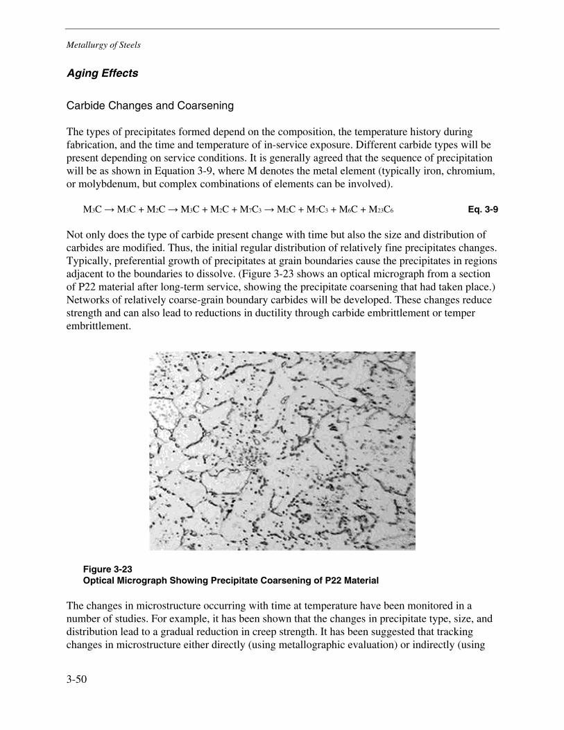
Metallurgy of Steels
3-50
Aging Effects
Carbide Changes and Coarsening
The types of precipitates formed depend on the composition, the temperature history during fabrication, and the time and temperature of in-service exposure. Different carbide types will be present depending on service conditions. It is generally agreed that the sequence of precipitation will be as shown in Equation 3-9, where M denotes the metal element (typically iron, chromium, or molybdenum, but complex combinations of elements can be involved).
M3C → M3C + M2C → M3C + M2C + M7C3 → M2C + M7C3 + M6C + M23C6 Eq. 3-9
Not only does the type of carbide present change with time but also the size and distribution of carbides are modified. Thus, the initial regular distribution of relatively fine precipitates changes. Typically, preferential growth of precipitates at grain boundaries cause the precipitates in regions adjacent to the boundaries to dissolve. (Figure 3-23 shows an optical micrograph from a section of P22 material after long-term service, showing the precipitate coarsening that had taken place.) Networks of relatively coarse-grain boundary carbides will be developed. These changes reduce strength and can also lead to reductions in ductility through carbide embrittlement or temper embrittlement.
Figure 3-23 Optical Micrograph Showing Precipitate Coarsening of P22 Material
The changes in microstructure occurring with time at temperature have been monitored in a number of studies. For example, it has been shown that the changes in precipitate type, size, and distribution lead to a gradual reduction in creep strength. It has been suggested that tracking changes in microstructure either directly (using metallographic evaluation) or indirectly (using
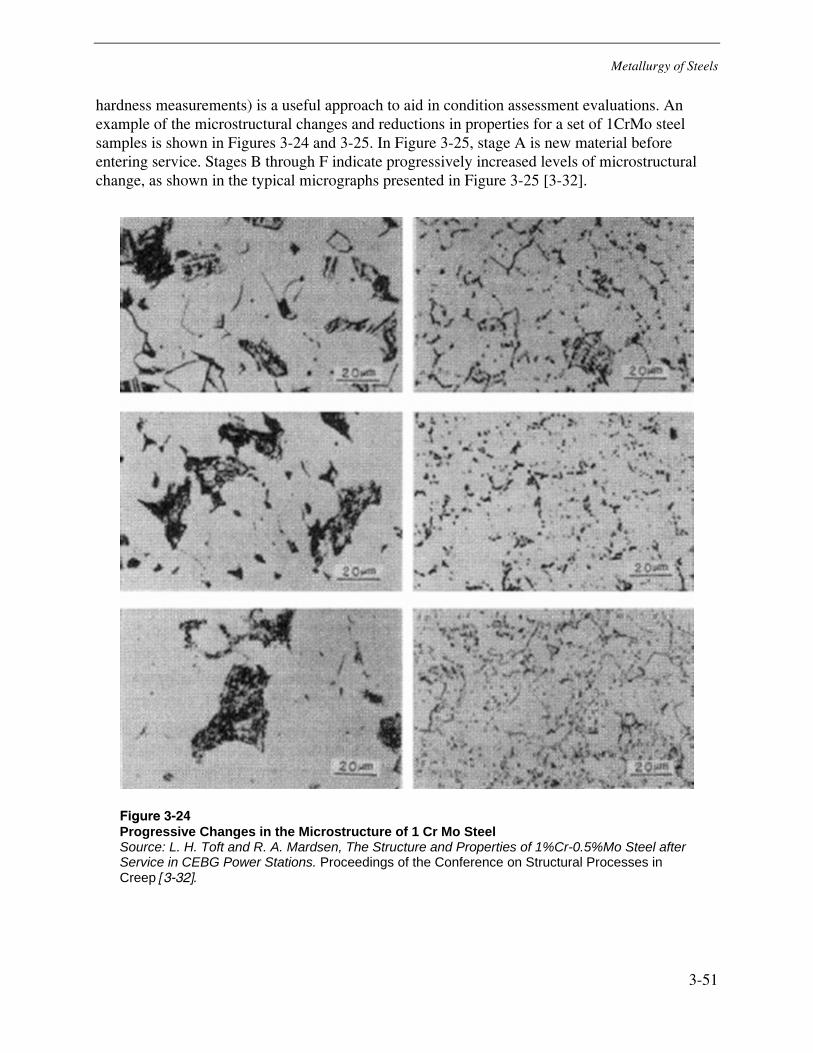
Metallurgy of Steels
3-51
hardness measurements) is a useful approach to aid in condition assessment evaluations. An example of the microstructural changes and reductions in properties for a set of 1CrMo steel samples is shown in Figures 3-24 and 3-25. In Figure 3-25, stage A is new material before entering service. Stages B through F indicate progressively increased levels of microstructural change, as shown in the typical micrographs presented in Figure 3-25 [3-32].
Figure 3-24 Progressive Changes in the Microstructure of 1 Cr Mo Steel Source: L. H. Toft and R. A. Mardsen, The Structure and Properties of 1%Cr-0.5%Mo Steel after Service in CEBG Power Stations. Proceedings of the Conference on Structural Processes in Creep [3-32].
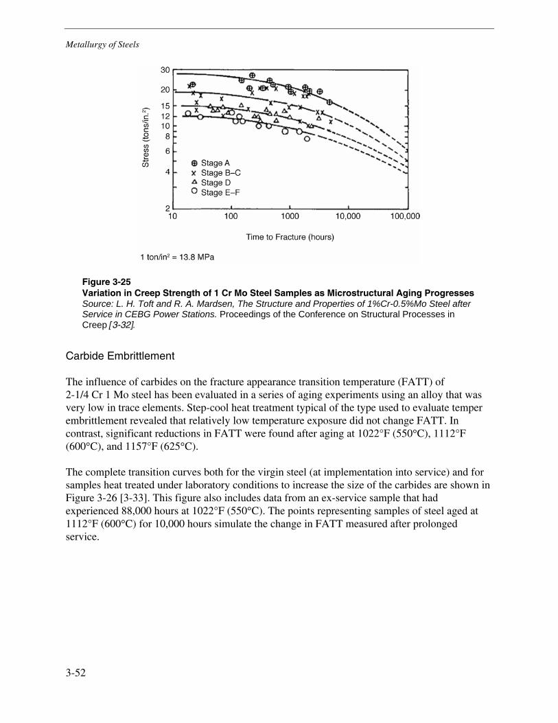
Metallurgy of Steels
3-52
Figure 3-25 Variation in Creep Strength of 1 Cr Mo Steel Samples as Microstructural Aging Progresses Source: L. H. Toft and R. A. Mardsen, The Structure and Properties of 1%Cr-0.5%Mo Steel after Service in CEBG Power Stations. Proceedings of the Conference on Structural Processes in Creep [3-32].
Carbide Embrittlement
The influence of carbides on the fracture appearance transition temperature (FATT) of 2-1/4 Cr 1 Mo steel has been evaluated in a series of aging experiments using an alloy that was very low in trace elements. Step-cool heat treatment typical of the type used to evaluate temper embrittlement revealed that relatively low temperature exposure did not change FATT. In contrast, significant reductions in FATT were found after aging at 1022°F (550°C), 1112°F (600°C), and 1157°F (625°C).
The complete transition curves both for the virgin steel (at implementation into service) and for samples heat treated under laboratory conditions to increase the size of the carbides are shown in Figure 3-26 [3-33]. This figure also includes data from an ex-service sample that had experienced 88,000 hours at 1022°F (550°C). The points representing samples of steel aged at 1112°F (600°C) for 10,000 hours simulate the change in FATT measured after prolonged service.
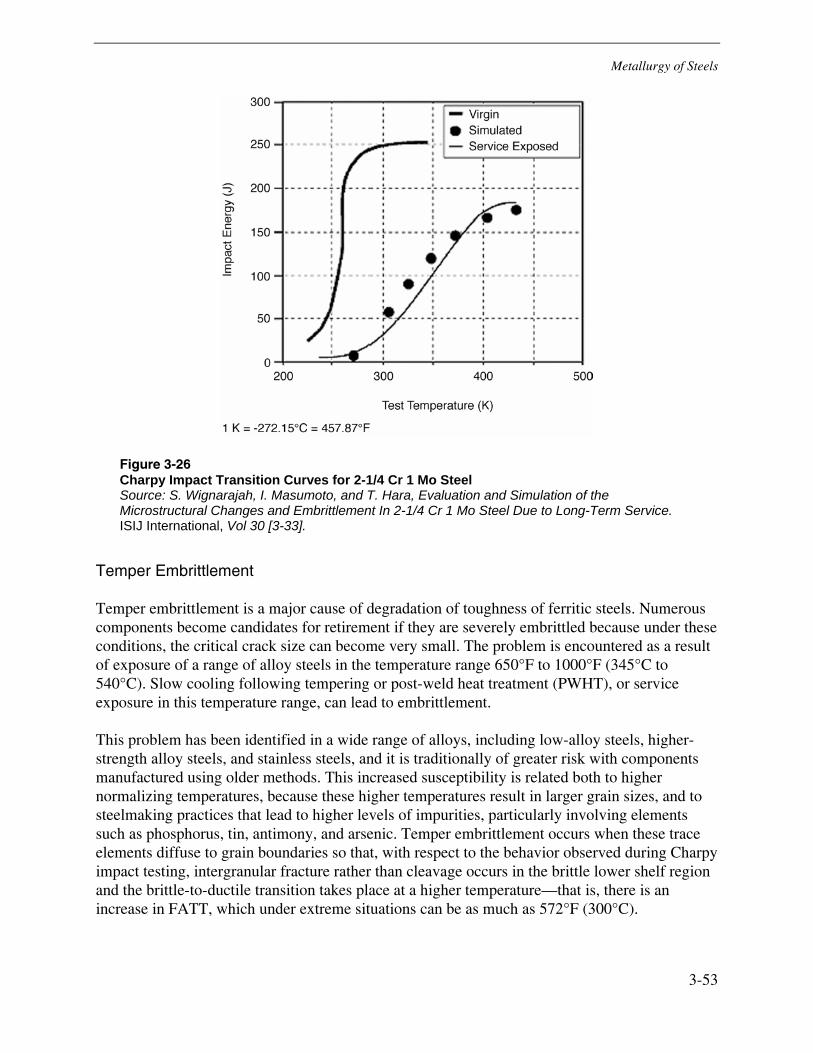
Metallurgy of Steels
3-53
Figure 3-26 Charpy Impact Transition Curves for 2-1/4 Cr 1 Mo Steel Source: S. Wignarajah, I. Masumoto, and T. Hara, Evaluation and Simulation of the Microstructural Changes and Embrittlement In 2-1/4 Cr 1 Mo Steel Due to Long-Term Service. ISIJ International, Vol 30 [3-33].
Temper Embrittlement
Temper embrittlement is a major cause of degradation of toughness of ferritic steels. Numerous components become candidates for retirement if they are severely embrittled because under these conditions, the critical crack size can become very small. The problem is encountered as a result of exposure of a range of alloy steels in the temperature range 650°F to 1000°F (345°C to 540°C). Slow cooling following tempering or post-weld heat treatment (PWHT), or service exposure in this temperature range, can lead to embrittlement.
This problem has been identified in a wide range of alloys, including low-alloy steels, higher-strength alloy steels, and stainless steels, and it is traditionally of greater risk with components manufactured using older methods. This increased susceptibility is related both to higher normalizing temperatures, because these higher temperatures result in larger grain sizes, and to steelmaking practices that lead to higher levels of impurities, particularly involving elements such as phosphorus, tin, antimony, and arsenic. Temper embrittlement occurs when these trace elements diffuse to grain boundaries so that, with respect to the behavior observed during Charpy impact testing, intergranular fracture rather than cleavage occurs in the brittle lower shelf region and the brittle-to-ductile transition takes place at a higher temperature—that is, there is an increase in FATT, which under extreme situations can be as much as 572°F (300°C).
Metallurgy of Steels
3-54
Austenitic Steels
Austenitic steels have excellent corrosion resistance and excellent high-temperature tensile and creep strength. However, because of their susceptibility to halide stress corrosion cracking, these alloys are not commonly used for piping applications at temperatures above approximately 150°F (66°C). In contrast, austenitic steels have been used in superheaters and reheaters for approximately 35 years and have provided excellent performance.
For high-temperature boiler applications, three general grades—304, 321, and 347—are the most widely used. Within these classifications are other grades, designated by a following capital letter, L (low carbon, C ≤ 0.035%) or H (high carbon, C 0.04–0.10%). The differences lie only in the carbon content. For use at temperatures above 1000°F (538°C), the ASME Boiler and Pressure Vessel Code, Section II, Part D requires a minimum of 0.04% carbon for adequate creep strength [3-10]. For superheater and reheater applications, the H grade is preferred, as this ensures the proper carbon content and solution heat treatment for use at temperatures where creep strength is the important design consideration. There are two other grades, 304N and 304LN. The N indicates a nitrogen content of 0.10%–0.16% (for improved strength), and the L again signifies a maximum carbon content of 0.035%. The 304, 321, and 347 grades are all in the classification of 18% chromium and 8% nickel, with some slight variations in the range of these alloying elements.
There are different ASME specifications, depending on the form in which the material is used. Tubes are covered in SA213, pipes are covered in SA376, and plates are covered in SA240. Each product form has a slightly different composition range.
Other differences among these three grades are the addition of titanium in 321 and the addition of columbium and tantalum in grade 347. For 321, the titanium is 0.60% maximum, and for 347, the columbium plus tantalum cannot exceed 1.0%. There are other requirements for the minimum amount of these alloying elements, based on the carbon content. There are also some other minor differences in the nickel range, depending on the product form. However, except for these relatively minor differences, they all fall within the broad classification of the 18-8 austenitic stainless steels.
The material specification requires all of these materials to be provided in the solution-annealed condition. That is, the final heat treatment is performed at a temperature of 1900°F–2000°F (1038°C–1093°C), depending on the particular grade. For the 321H grade, there is a further requirement: a grain size of ASTM No.7 or coarser is specified to ensure adequate creep strength. A solution anneal at 2000°F (1093°C) minimum is usually sufficient to meet this specification requirement.
Metallurgy of Steels
3-55
Microstructure
After the high-temperature solution anneal, the microstructure will be equiaxed austenite. The word equiaxed means that the dimensions of an individual austenite grain will be essentially the same, regardless of orientation or direction. The material is in the fully annealed condition and is a single-phased material with only some nonmetallic inclusions, which are inherent to steelmaking, apparent within the microstructure.
Unlike the ferritic steels, which have dramatic microstructural changes depending on the peak operational or failure temperature, there are no abrupt microstructural changes in the austenitic stainless steels. The microstructural changes that do occur take place at high temperature. The austenitic grades will form chromium carbides along the austenite grain boundaries. The formation of these carbides reduces the chromium content of the austenite grains at the boundary and therefore reduces the local corrosion resistance along the grain boundaries.
To prevent sensitization, additions of titanium to make the alloy 321 and additions of columbium and tantalum to make the alloy 347 were introduced. If these alloys are given a second heat treatment, called a stabilization anneal, at 1600°F–1650°F (871°C–899°C) after the solution anneal, titanium carbide or columbium-tantalum carbide will form preferentially to chromium carbide. With all of the carbon removed as innocuous carbides, no chromium carbide can form. There is no loss of chromium at the grain boundaries, no loss of corrosion resistance, and thus no sensitization. However, because 321 and 347 in boiler applications are not given a stabilization anneal, these two alloys will sensitize just the same as 304.
Allowable Stress Values
The allowable stress values according to the ASME BPVC, Section II, are presented in Table 3-9 [3-10]. Even at the relatively low temperatures at which the allowable stresses are based on the tensile properties, there is a gradual decrease in recommended stress. This gradual decrease occurs because the microstructure of austenitic alloys is FCC; with this crystallographic structure, as temperature increases, there is a gradual loss of strength. However, above approximately 1000°F (540°C), diffusion processes begin to become significant, and the allowable stress is reduced dramatically as creep damage development becomes the dominant process.
Creep Properties
The LMP is frequently used to represent the variation of creep life with stress and temperature, T. The LMP is given by the following relationship: LMP = (T + 460)(constant + log time). The normal value of the constant for the majority of power plant steels is 20. The approach is based on the assumption that tests performed under accelerated temperature conditions can be used to define the long-term performance at service conditions. For a given alloy, the available dataset values of LMP are typically plotted against stress, allowing minimum and average behavior to be described. In Table 3-10, the results available from API STD 530 for selected austenitic stainless steels have been assessed to give a representation of average behavior [3-26].
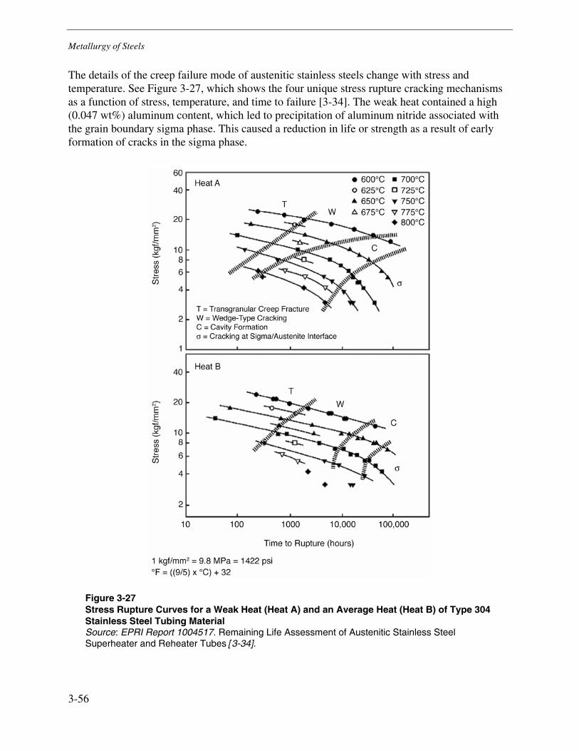
Metallurgy of Steels
3-56
The details of the creep failure mode of austenitic stainless steels change with stress and temperature. See Figure 3-27, which shows the four unique stress rupture cracking mechanisms as a function of stress, temperature, and time to failure [3-34]. The weak heat contained a high (0.047 wt%) aluminum content, which led to precipitation of aluminum nitride associated with the grain boundary sigma phase. This caused a reduction in life or strength as a result of early formation of cracks in the sigma phase.
Figure 3-27 Stress Rupture Curves for a Weak Heat (Heat A) and an Average Heat (Heat B) of Type 304 Stainless Steel Tubing Material Source: EPRI Report 1004517. Remaining Life Assessment of Austenitic Stainless Steel Superheater and Reheater Tubes [3-34].
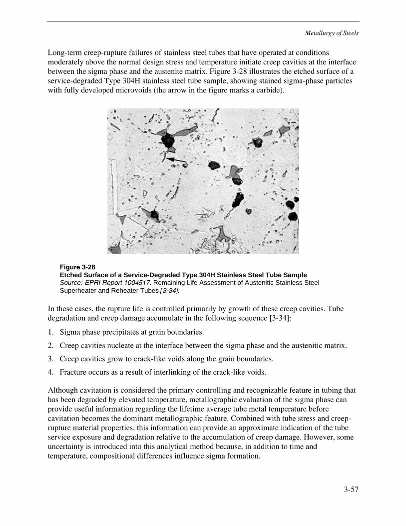
Metallurgy of Steels
3-57
Long-term creep-rupture failures of stainless steel tubes that have operated at conditions moderately above the normal design stress and temperature initiate creep cavities at the interface between the sigma phase and the austenite matrix. Figure 3-28 illustrates the etched surface of a service-degraded Type 304H stainless steel tube sample, showing stained sigma-phase particles with fully developed microvoids (the arrow in the figure marks a carbide).
Figure 3-28 Etched Surface of a Service-Degraded Type 304H Stainless Steel Tube Sample Source: EPRI Report 1004517. Remaining Life Assessment of Austenitic Stainless Steel Superheater and Reheater Tubes [3-34].
In these cases, the rupture life is controlled primarily by growth of these creep cavities. Tube degradation and creep damage accumulate in the following sequence [3-34]:
1. Sigma phase precipitates at grain boundaries.
2. Creep cavities nucleate at the interface between the sigma phase and the austenitic matrix.
3. Creep cavities grow to crack-like voids along the grain boundaries.
4. Fracture occurs as a result of interlinking of the crack-like voids.
Although cavitation is considered the primary controlling and recognizable feature in tubing that has been degraded by elevated temperature, metallographic evaluation of the sigma phase can provide useful information regarding the lifetime average tube metal temperature before cavitation becomes the dominant metallographic feature. Combined with tube stress and creep-rupture material properties, this information can provide an approximate indication of the tube service exposure and degradation relative to the accumulation of creep damage. However, some uncertainty is introduced into this analytical method because, in addition to time and temperature, compositional differences influence sigma formation.
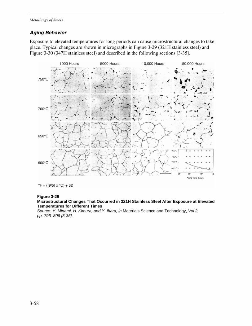
Metallurgy of Steels
3-58
Aging Behavior
Exposure to elevated temperatures for long periods can cause microstructural changes to take place. Typical changes are shown in micrographs in Figure 3-29 (321H stainless steel) and Figure 3-30 (347H stainless steel) and described in the following sections [3-35].
Figure 3-29 Microstructural Changes That Occurred in 321H Stainless Steel After Exposure at Elevated Temperatures for Different Times Source: Y. Minami, H. Kimura, and Y. Ihara, in Materials Science and Technology, Vol 2, pp. 795–806 [3-35].
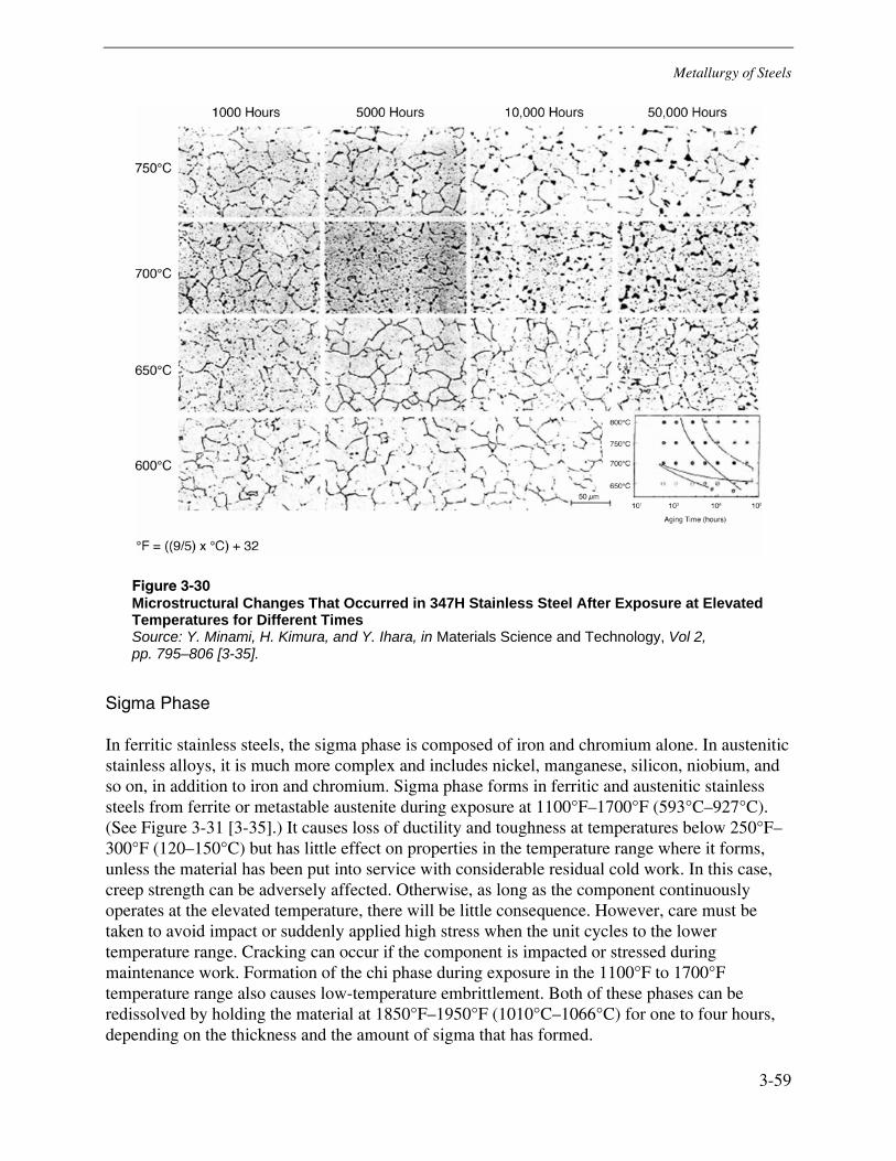
Metallurgy of Steels
3-59
Figure 3-30 Microstructural Changes That Occurred in 347H Stainless Steel After Exposure at Elevated Temperatures for Different Times Source: Y. Minami, H. Kimura, and Y. Ihara, in Materials Science and Technology, Vol 2, pp. 795–806 [3-35].
Sigma Phase
In ferritic stainless steels, the sigma phase is composed of iron and chromium alone. In austenitic stainless alloys, it is much more complex and includes nickel, manganese, silicon, niobium, and so on, in addition to iron and chromium. Sigma phase forms in ferritic and austenitic stainless steels from ferrite or metastable austenite during exposure at 1100°F–1700°F (593°C–927°C). (See Figure 3-31 [3-35].) It causes loss of ductility and toughness at temperatures below 250°F–300°F (120–150°C) but has little effect on properties in the temperature range where it forms, unless the material has been put into service with considerable residual cold work. In this case, creep strength can be adversely affected. Otherwise, as long as the component continuously operates at the elevated temperature, there will be little consequence. However, care must be taken to avoid impact or suddenly applied high stress when the unit cycles to the lower temperature range. Cracking can occur if the component is impacted or stressed during maintenance work. Formation of the chi phase during exposure in the 1100°F to 1700°F temperature range also causes low-temperature embrittlement. Both of these phases can be redissolved by holding the material at 1850°F–1950°F (1010°C–1066°C) for one to four hours, depending on the thickness and the amount of sigma that has formed.
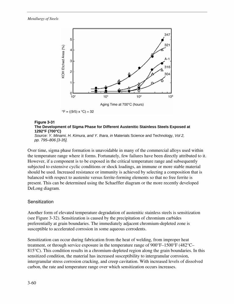
Metallurgy of Steels
3-60
Figure 3-31 The Development of Sigma Phase for Different Austenitic Stainless Steels Exposed at 1292°F (700°C) Source: Y. Minami, H. Kimura, and Y. Ihara, in Materials Science and Technology, Vol 2, pp. 795–806 [3-35].
Over time, sigma phase formation is unavoidable in many of the commercial alloys used within the temperature range where it forms. Fortunately, few failures have been directly attributed to it. However, if a component is to be exposed in the critical temperature range and subsequently subjected to extensive cyclic conditions or shock loadings, an immune or more stable material should be used. Increased resistance or immunity is achieved by selecting a composition that is balanced with respect to austenite versus ferrite-forming elements so that no free ferrite is present. This can be determined using the Schaeffler diagram or the more recently developed DeLong diagram.
Sensitization
Another form of elevated temperature degradation of austenitic stainless steels is sensitization (see Figure 3-32). Sensitization is caused by the precipitation of chromium carbides preferentially at grain boundaries. The immediately adjacent chromium-depleted zone is susceptible to accelerated corrosion in some aqueous corrodents.
Sensitization can occur during fabrication from the heat of welding, from improper heat treatment, or through service exposure in the temperature range of 900°F–1500°F (482°C–815°C). This condition results in a chromium-depleted region along the grain boundaries. In this sensitized condition, the material has increased susceptibility to intergranular corrosion, intergranular stress corrosion cracking, and creep cavitation. With increased levels of dissolved carbon, the rate and temperature range over which sensitization occurs increases.
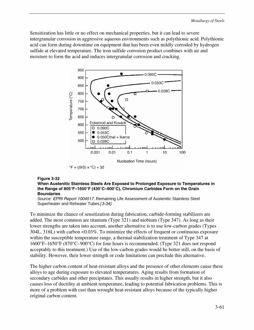
Metallurgy of Steels
3-61
Sensitization has little or no effect on mechanical properties, but it can lead to severe intergranular corrosion in aggressive aqueous environments such as polythionic acid. Polythionic acid can form during downtime on equipment that has been even mildly corroded by hydrogen sulfide at elevated temperature. The iron sulfide corrosion product combines with air and moisture to form the acid and induces intergranular corrosion and cracking.
Figure 3-32 When Austenitic Stainless Steels Are Exposed to Prolonged Exposure to Temperatures in the Range of 805°F–1650°F (430°C–900°C), Chromium Carbides Form on the Grain Boundaries Source: EPRI Report 1004517. Remaining Life Assessment of Austenitic Stainless Steel Superheater and Reheater Tubes [3-34].
To minimize the chance of sensitization during fabrication, carbide-forming stabilizers are added. The most common are titanium (Type 321) and niobium (Type 347). As long as their lower strengths are taken into account, another alternative is to use low-carbon grades (Types 304L, 316L) with carbon <0.03%. To minimize the effects of frequent or continuous exposure within the susceptible temperature range, a thermal stabilization treatment of Type 347 at 1600°F–1650°F (870°C–900°C) for four hours is recommended. (Type 321 does not respond acceptably to this treatment.) Use of the low-carbon grades would be better still, on the basis of stability. However, their lower strength or code limitations can preclude this alternative.
The higher carbon content of heat-resistant alloys and the presence of other elements cause these alloys to age during exposure to elevated temperatures. Aging results from formation of secondary carbides and other precipitates. This usually results in higher strength, but it also causes loss of ductility at ambient temperature, leading to potential fabrication problems. This is more of a problem with cast than wrought heat-resistant alloys because of the typically higher original carbon content.
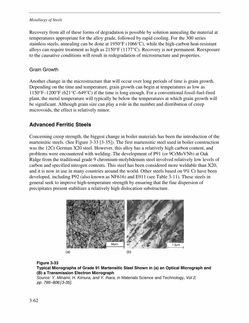
Metallurgy of Steels
3-62
Recovery from all of these forms of degradation is possible by solution annealing the material at temperatures appropriate for the alloy grade, followed by rapid cooling. For the 300 series stainless steels, annealing can be done at 1950°F (1066°C), while the high-carbon heat-resistant alloys can require treatment as high as 2150°F (1177°C). Recovery is not permanent. Reexposure to the causative conditions will result in redegradation of microstructure and properties.
Grain Growth
Another change in the microstructure that will occur over long periods of time is grain growth. Depending on the time and temperature, grain growth can begin at temperatures as low as 1150°F–1200°F (621°C–649°C) if the time is long enough. For a conventional fossil-fuel-fired plant, the metal temperature will typically be below the temperatures at which grain growth will be significant. Although grain size can play a role in the number and distribution of creep microvoids, the effect is relatively minor.
Advanced Ferritic Steels
Concerning creep strength, the biggest change in boiler materials has been the introduction of the martensitic steels. (See Figure 3-33 [3-35]). The first martensitic steel used in boiler construction was the 12Cr German X20 steel. However, this alloy has a relatively high carbon content, and problems were encountered with welding. The development of P91 (or 9CrMoVNb) at Oak Ridge from the traditional grade 9 chromium-molybdenum steel involved relatively low levels of carbon and specified nitrogen contents. This steel has been considered more weldable than X20, and it is now in use in many countries around the world. Other steels based on 9% Cr have been developed, including P92 (also known as NF616) and E911 (see Table 3-11). These steels in general seek to improve high-temperature strength by ensuring that the fine dispersion of precipitates present stabilizes a relatively high dislocation substructure.
Figure 3-33 Typical Micrographs of Grade 91 Martensitic Steel Shown in (a) an Optical Micrograph and (B) a Transmission Electron Micrograph Source: Y. Minami, H. Kimura, and Y. Ihara, in Materials Science and Technology, Vol 2, pp. 795–806 [3-35].
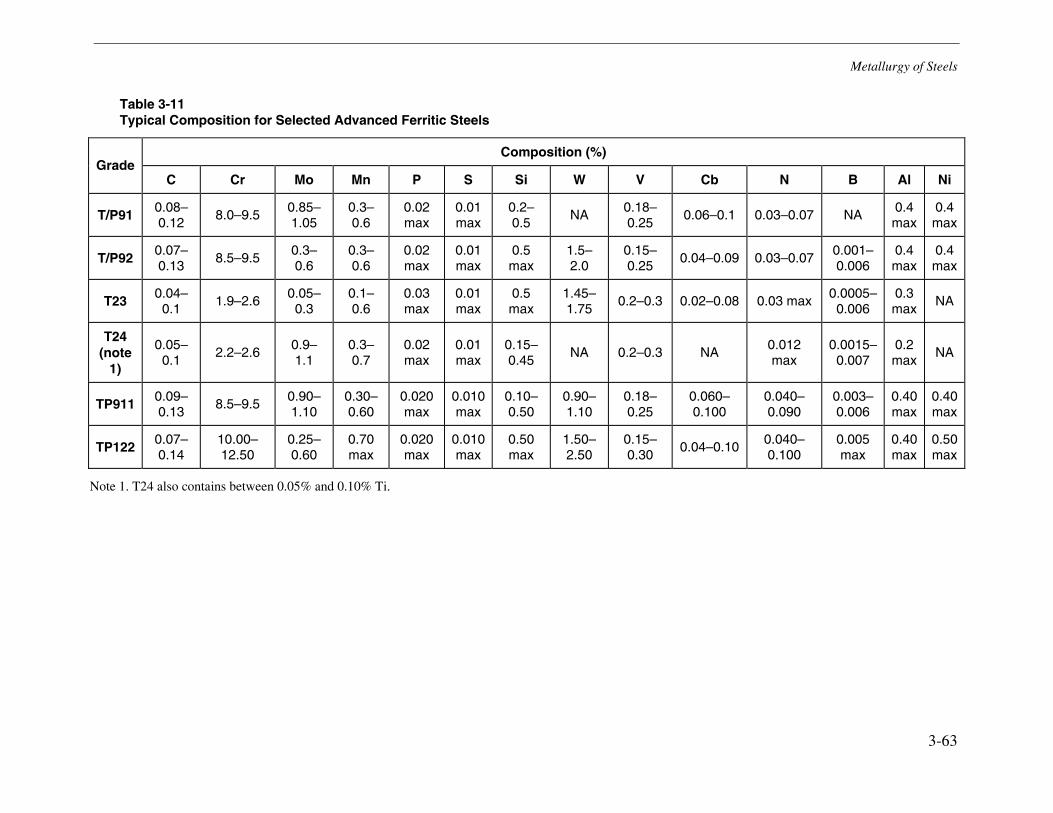
Metallurgy of Steels
3-63
Table 3-11 Typical Composition for Selected Advanced Ferritic Steels
Composition (%) Grade
C Cr Mo Mn P S Si W V Cb N B Al Ni
T/P91 0.08–0.12
8.0–9.5 0.85–1.05
0.3–0.6
0.02 max
0.01 max
0.2–0.5
NA 0.18–0.25
0.06–0.1 0.03–0.07 NA 0.4 max
0.4 max
T/P92 0.07–0.13
8.5–9.5 0.3–0.6
0.3–0.6
0.02 max
0.01 max
0.5 max
1.5–2.0
0.15–0.25
0.04–0.09 0.03–0.07 0.001–0.006
0.4 max
0.4 max
T23 0.04–
0.1 1.9–2.6
0.05–0.3
0.1–0.6
0.03 max
0.01 max
0.5 max
1.45–1.75
0.2–0.3 0.02–0.08 0.03 max 0.0005–0.006
0.3 max
NA
T24 (note
1)
0.05–0.1
2.2–2.6 0.9–1.1
0.3–0.7
0.02 max
0.01 max
0.15–0.45
NA 0.2–0.3 NA 0.012 max
0.0015–0.007
0.2 max
NA
TP911 0.09–0.13
8.5–9.5 0.90–1.10
0.30–0.60
0.020 max
0.010 max
0.10–0.50
0.90–1.10
0.18–0.25
0.060–0.100
0.040–0.090
0.003–0.006
0.40 max
0.40 max
TP122 0.07–0.14
10.00–12.50
0.25–0.60
0.70 max
0.020 max
0.010 max
0.50 max
1.50–2.50
0.15–0.30
0.04–0.10 0.040–0.100
0.005 max
0.40 max
0.50 max
Note 1. T24 also contains between 0.05% and 0.10% Ti.
Metallurgy of Steels
3-64
Welding consumables have been developed for P91, and data have been accumulated, but difficulties have been encountered with the following:
• The fabrication of welds between new grade 91 material and previously exposed chromium-molybdenum steel.
• Cracking near the weld fusion line in welds that did not have PWHT immediately after welding.
• Creep-related problems known as Type IV cracking, which can reduce the cross-weld properties to approximately 60% of that of the parent. The actual cross-weld strength varies with material and temperature; it is also believed to vary from weld to weld. This type of failure occurs at the rear of the visibly transformed HAZ and is associated with a region of reduced hardness.
Both P92 and E911 also exhibit Type IV cracking. There is considerable debate about the advantages and disadvantages of these alloys. Both show parent properties better than P91, but P92 has higher design stresses than does E911.
An additional difficulty that has been encountered with grade 91 tubing is the corrosion and oxidation resistance. As the operating temperature of the tube wall increases, so does its oxidation rate. For the 9% Cr steels, evidence has accumulated that at higher temperatures the rate of oxidation in steam can lead to problems. Essentially, the temperature of a heat transfer component such as a superheater or reheater tube is controlled by the rate at which the fluid (in this case, steam) within the tube can absorb the heat being absorbed by the tube from the boiler gases. As the internal oxide on the steam side of the tube increases in thickness, it acts as a barrier to heat flow, increasing the tube temperature. This in turn increases the rate of oxide growth, giving a runaway effect. In practice, the problem is more complex, involving scale exfoliation potentially leading to tube blockage, turbine damage, and tube thinning.
Two advanced ferritic steels that are variants of 2-1/4 Cr 1 Mo steel have been developed (see Table 3-11). Microalloying systems capable of increasing the creep strength of steels have been extensively used in the development of the martensitic (9%–12% Cr) steels. The addition of similar microalloying to the base 2-1/4 Cr 1 Mo system has led to considerable increases in the creep strength of the materials; therefore, TP23 and TP24 now approach the strength values of the martensitic steels at lower temperatures. P23 was developed in Japan. It was originally designated as HCM2S and is still widely identified by this name. P24 is a European steel, originally designated as 7CrMoVTiB 9 10, developed by Mannesmann. Of the two alloys, only TP23 is presently approved for ASME Boiler and Pressure Vessel Code, Section I, Power Boilers, Code Case 2199 [3-36].
For boiler manufacturers, the real importance of these steels lies in their relatively low chromium content and hardenability. These factors will allow thinner wall components to be designed, for example in membrane waterwalls, and then to be fabricated without PWHT. For supercritical boiler designs, where temperatures at the top of the boiler wall can reach 1112°F (600ºC), this offers a commercially viable route for membrane wall manufacture.

Metallurgy of Steels
3-65
Microstructure
As illustrated in Figure 3-34, the microstructure of the 9%–12% Cr alloys developed following normal cooling rates will be martensite [3-24]. To overcome the severe brittleness associated with martensitic microstructure, heat treatment must be carried out to temper the structure and thereby improve ductility. Under normal conditions, the microstructure of grade 91 steel consists of tempered martensite, with carbide precipitates present on the prior austenite grain boundaries and within the grains. Typically, this microstructure will exhibit a hardness of approximately 250 HV. Problems with the heat treatment can lead to a range of problems, including the following:
• Very slow cooling, leading to the formation of relatively coarse carbides in a ferrite matrix (see Figure 3-35). This microstructure is soft and significantly weaker than the hardness and strength achieved for the normal tempered martensitic microstructure.
• Reheating above the A1 temperature during either tempering or PWHT. Exceeding A1 leads to partial transformation back to austenite and then retransformation upon cooling. Again, the properties are inferior to normal strength and ductility.
• Failure to cool below the MF temperature so that significant fractions of austenite are retained.
Aging produces no obvious changes in microstructure that could be determined from optical microscopy. To monitor microstructural changes, the higher resolution of electron optics must be used.
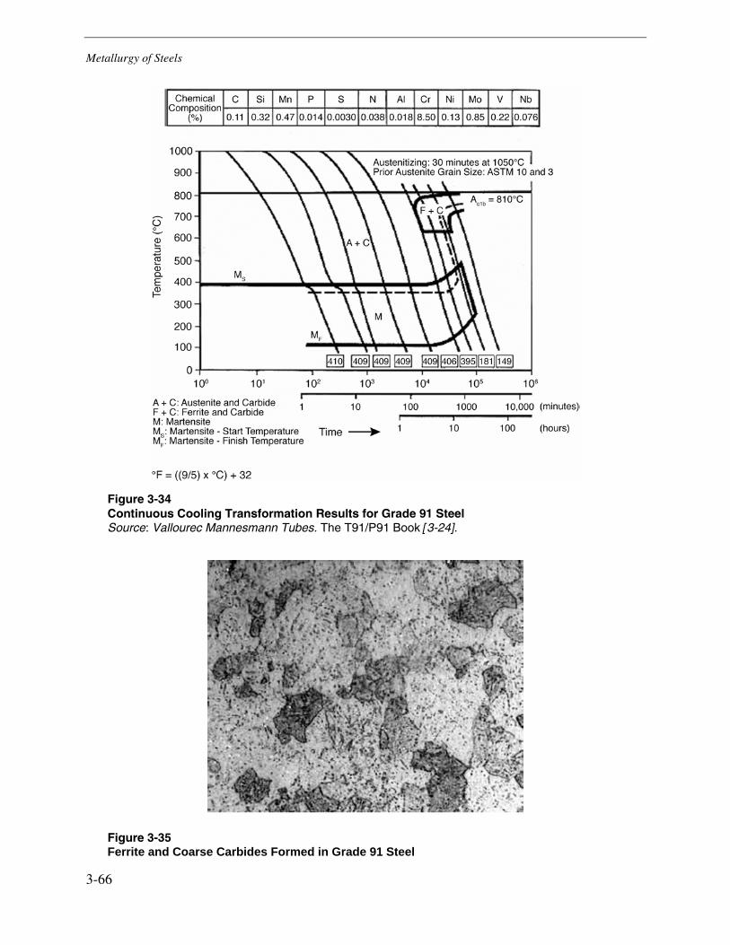
Metallurgy of Steels
3-66
Figure 3-34 Continuous Cooling Transformation Results for Grade 91 Steel Source: Vallourec Mannesmann Tubes. The T91/P91 Book [3-24].
Figure 3-35 Ferrite and Coarse Carbides Formed in Grade 91 Steel
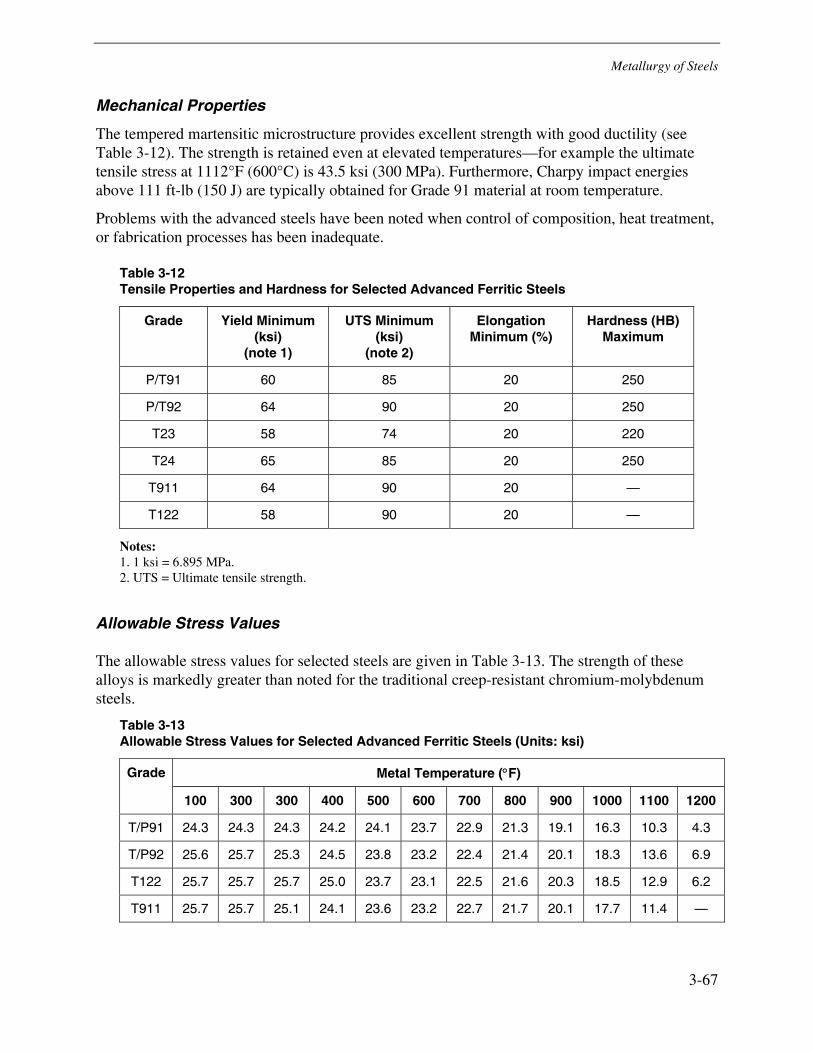
Metallurgy of Steels
3-67
Mechanical Properties
The tempered martensitic microstructure provides excellent strength with good ductility (see Table 3-12). The strength is retained even at elevated temperatures—for example the ultimate tensile stress at 1112°F (600°C) is 43.5 ksi (300 MPa). Furthermore, Charpy impact energies above 111 ft-lb (150 J) are typically obtained for Grade 91 material at room temperature.
Problems with the advanced steels have been noted when control of composition, heat treatment, or fabrication processes has been inadequate.
Table 3-12 Tensile Properties and Hardness for Selected Advanced Ferritic Steels
Grade Yield Minimum (ksi)
(note 1)
UTS Minimum (ksi)
(note 2)
Elongation Minimum (%)
Hardness (HB) Maximum
P/T91 60 85 20 250
P/T92 64 90 20 250
T23 58 74 20 220
T24 65 85 20 250
T911 64 90 20 —
T122 58 90 20 —
Notes: 1. 1 ksi = 6.895 MPa. 2. UTS = Ultimate tensile strength.
Allowable Stress Values
The allowable stress values for selected steels are given in Table 3-13. The strength of these alloys is markedly greater than noted for the traditional creep-resistant chromium-molybdenum steels.
Table 3-13 Allowable Stress Values for Selected Advanced Ferritic Steels (Units: ksi)
Metal Temperature (°F) Grade
100 300 300 400 500 600 700 800 900 1000 1100 1200
T/P91 24.3 24.3 24.3 24.2 24.1 23.7 22.9 21.3 19.1 16.3 10.3 4.3
T/P92 25.6 25.7 25.3 24.5 23.8 23.2 22.4 21.4 20.1 18.3 13.6 6.9
T122 25.7 25.7 25.7 25.0 23.7 23.1 22.5 21.6 20.3 18.5 12.9 6.2
T911 25.7 25.7 25.1 24.1 23.6 23.2 22.7 21.7 20.1 17.7 11.4 —
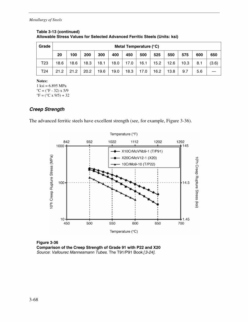
Metallurgy of Steels
3-68
Table 3-13 (continued) Allowable Stress Values for Selected Advanced Ferritic Steels (Units: ksi)
Metal Temperature (°C) Grade
20 100 200 300 400 450 500 525 550 575 600 650
T23 18.6 18.6 18.3 18.1 18.0 17.0 16.1 15.2 12.6 10.3 8.1 (3.6)
T24 21.2 21.2 20.2 19.6 19.0 18.3 17.0 16.2 13.8 9.7 5.6 —
Notes: 1 ksi = 6.895 MPa °C = (°F - 32) x 5/9 °F = (°C x 9/5) + 32
Creep Strength
The advanced ferritic steels have excellent strength (see, for example, Figure 3-36).
Figure 3-36 Comparison of the Creep Strength of Grade 91 with P22 and X20 Source: Vallourec Mannesmann Tubes. The T91/P91 Book [3-24].
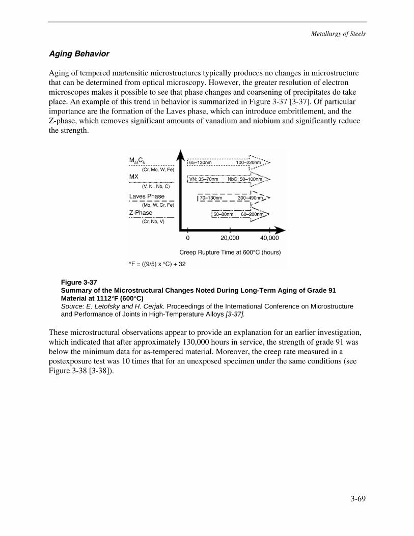
Metallurgy of Steels
3-69
Aging Behavior
Aging of tempered martensitic microstructures typically produces no changes in microstructure that can be determined from optical microscopy. However, the greater resolution of electron microscopes makes it possible to see that phase changes and coarsening of precipitates do take place. An example of this trend in behavior is summarized in Figure 3-37 [3-37]. Of particular importance are the formation of the Laves phase, which can introduce embrittlement, and the Z-phase, which removes significant amounts of vanadium and niobium and significantly reduce the strength.
Figure 3-37 Summary of the Microstructural Changes Noted During Long-Term Aging of Grade 91 Material at 1112°F (600°C) Source: E. Letofsky and H. Cerjak. Proceedings of the International Conference on Microstructure and Performance of Joints in High-Temperature Alloys [3-37].
These microstructural observations appear to provide an explanation for an earlier investigation, which indicated that after approximately 130,000 hours in service, the strength of grade 91 was below the minimum data for as-tempered material. Moreover, the creep rate measured in a postexposure test was 10 times that for an unexposed specimen under the same conditions (see Figure 3-38 [3-38]).
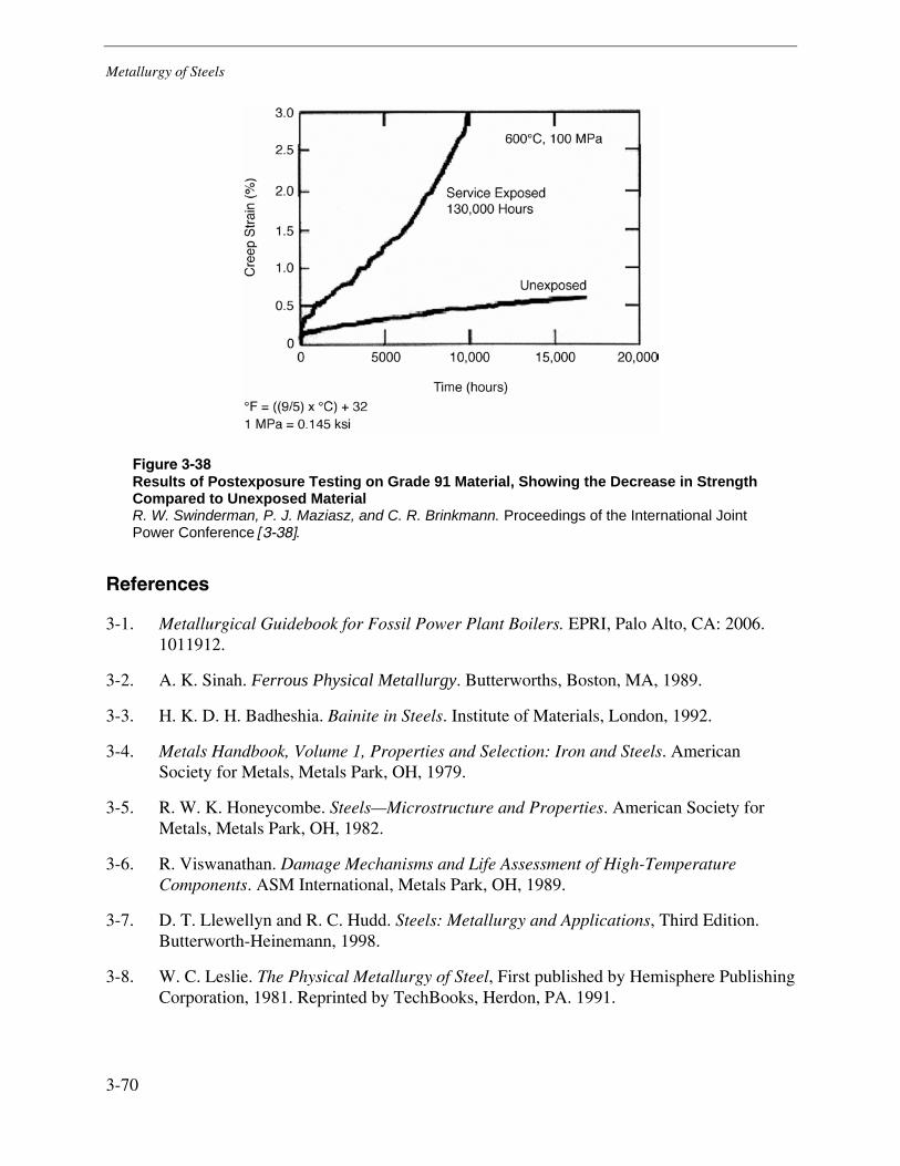
Metallurgy of Steels
3-70
Figure 3-38 Results of Postexposure Testing on Grade 91 Material, Showing the Decrease in Strength Compared to Unexposed Material R. W. Swinderman, P. J. Maziasz, and C. R. Brinkmann. Proceedings of the International Joint Power Conference [3-38].
References
3-1. Metallurgical Guidebook for Fossil Power Plant Boilers. EPRI, Palo Alto, CA: 2006. 1011912.
3-2. A. K. Sinah. Ferrous Physical Metallurgy. Butterworths, Boston, MA, 1989.
3-3. H. K. D. H. Badheshia. Bainite in Steels. Institute of Materials, London, 1992.
3-4. Metals Handbook, Volume 1, Properties and Selection: Iron and Steels. American Society for Metals, Metals Park, OH, 1979.
3-5. R. W. K. Honeycombe. Steels—Microstructure and Properties. American Society for Metals, Metals Park, OH, 1982.
3-6. R. Viswanathan. Damage Mechanisms and Life Assessment of High-Temperature Components. ASM International, Metals Park, OH, 1989.
3-7. D. T. Llewellyn and R. C. Hudd. Steels: Metallurgy and Applications, Third Edition. Butterworth-Heinemann, 1998.
3-8. W. C. Leslie. The Physical Metallurgy of Steel, First published by Hemisphere Publishing Corporation, 1981. Reprinted by TechBooks, Herdon, PA. 1991.
Metallurgy of Steels
3-71
3-9. G. Krauss. Steels Heat Treatment and Processing Principles. American Society for Metals, Metals Park, OH, 1990.
3-10. ASME Boiler and Pressure Vessel Code, Section II, Materials. American Society of Mechanical Engineers, New York.
3-11. John E. Bringas, Ed. Handbook of Comparative World Steel Standards, Third Edition. ASTM International, West Conshohocken, PA, 2004. DS67B.
3-12. ASA B31.1, American Tentative Standard Code for Pressure Piping. American Standards Association, 1935.
3-13. ASA B31.1, American Standard Code for Pressure Piping. American Standards Association, 1942.
3-14. Key to Metals Group. Key to Steel database. http://www.key-to-steel.com.
3-15. Steam, Fortieth Edition. Babcock & Wilcox, Barberton, OH, 1992.
3-16. P. J. Alberry and W. K. C. Jones, “Diagram for the Prediction of Weld Heat Affected Zone Microstructure,” Metals Technology, Vol. 4, No. 4, pp. 360–364 (1977).
3-17. R. Viswanathan. Damage Mechanisms and Life Assessment of High-Temperature Components. ASM International, Metals Park, OH, 1989
3-18. J. Nutting, “The Structural Stability of Low-Alloy Steels for Power Plant Applications.” Conference Proceedings: Advanced Heat-Resistant Steels for Power Generation. Institute of Materials, London, 1999, pp. 12–30.
3-19. N. Fujita and H. K. D. H. Badheshia, “Modelling Simultaneous Alloy Carbide Sequences in Power Plant Steels,” ISIJ International, Vol. 42, No.7, pp. 760–769 (2002).
3-20. Materials for Ultra Supercritical Fossil Power Plants. EPRI, Palo Alto, CA: 2000. TR-114750.
3-21. F. Masuyama, “History of Power Plants and Progress in Heat Resistant Steels,” ISIJ International, Vol. 41, No. 6, pp. 612–625 (2001).
3-22. K. W. Burns and F. B. Pickering, “Deformation and Fracture of Ferrite-Pearlite Structures,” Journal of the Iron and Steel Institute, Vol. 202, No. 110, pp. 899–906.
3-23. ASME Boiler and Pressure Vessel Code, Section I, Power Boilers. American Society of Mechanical Engineers, New York, 2004.
3-24. The T91/P91 Book. Vallourec Mannesmann Tubes, 2002.
3-25. ASME Code Case 2179-6. Seamless 9Cr-2W Material, Section I and Section VIII, Division I. American Society of Mechanical Engineers. Case 2179-5. 2006.
Metallurgy of Steels
3-72
3-26. API STD 530. Calculation of Heater Tube Thickness in Petroleum Refineries. American Petroleum Institute. 2003.
3-27. W. L. Hemingway. The Study of Graphitization. Edwards Valve Co., 1952.
3-28. J. R. Foulds and R. Viswanathan, “Graphitization of Steels in Elevated Temperature Service,” in Microstructures and Mechanical Properties of Aging Materials. The Minerals, Metals, & Materials Society, Warrendale, PA, 1993, pp. 61–69.
3-29. S. H. Weaver, “The Effect of Carbide Spheroidization Upon the Rupture Strength and Ductility of Carbon Molybdenum Steel,” Proceedings of the ASTM, Vol. 46, pp. 856–866 (1946).
3-30. G. H. Harth and T. P. Sherlock, in Transactions of the ASME, Vol. 107, pp. 226–229 (1985).
3-31. G. V. Smith, Supplemental Report on the Elevated-Temperature Properties of Chromium-Molybdenum Steels (An Evaluation of 2Cr-1Mo Steel), American Society for Testing and Materials, March 1971. DS6S2.
3-32. L. H. Toft and R. A. Mardsen, “The Structure and Properties of 1%Cr-0.5%Mo Steel after Service in CEGB Power Stations,” Proceedings of the Conference on Structural Processes in Creep. JISI, JIM (London), 1963, p. 275.
3-33. S. Wignarajah, I. Masumoto, and T. Hara, “Evaluation and Simulation of the Microstructural Changes and Embrittlement in 2-1/4 Cr 1 Mo Steel Due to Long-Term Service,” ISIJ International, Vol. 30, 1990, pp. 58–63.
3-34. Remaining Life Assessment of Austenitic Stainless Steel Superheater and Reheater Tubes. EPRI, Palo Alto, CA: 2002. 1004517.
3-35. Y. Minami, H. Kimura, and Y. Ihara, in Materials Science and Technology, Vol. 2, pp. 795–806 (1986).
3-36. ASME Code Case 2199. 2.25Cr-1.6W-V-Cb Material, Section I. American Society of Mechanical Engineers. Case 2199-3. 2006.
3-37. E. Letofsky and H. Cerjak, in Proceedings of the International Conference on Microstructure and Performance of Joints in High-Temperature Alloys. Institute of Materials, London, 2002.
3.38. R. W. Swinderman, P. J. Maziasz, and C. R. Brinkmann, in Proceedings of the International Joint Power Conference, ASME, 2000, pp. 1–4.

4-1
4 WELDING FUNDAMENTALS
Introduction
A variety of joining methods are allowed for use in the fabrication of fossil piping systems, including the following:
• Flanged joints
• Threaded joints
• Flared, flareless, and compression joints (for tube sizes ≤2 in. [50 mm] outside diameter [OD])
• Brazed and soldered joints
However, the most common method for joining high-energy fossil piping systems is welding. ASME B31.1 allows the use of butt welds, socket welds, and fillet welds as long as they comply with the additional restrictions listed within the standard. Seal welds can be used to avoid joint leakage but shall not be considered as contributing any strength to the joint.
Welding Processes
Several welding processes can be used in the fabrication and erection of fossil piping systems, including the following:
• Shielded metal arc welding (SMAW)
• Gas tungsten arc welding (GTAW)
• Submerged arc welding (SAW)
• Gas metal arc welding (GMAW)
• Flux cored arc welding (FCAW)
ASME B31.1 does not place a restriction on the selection of welding process, as long as it is qualified in accordance with the requirements of the ASME Boiler and Pressure Vessel Code, Section IX, Welding and Brazing Qualifications [4-1] However, from a practical standpoint, most welding is accomplished using SMAW, GTAW, and SAW processes. SAW is primarily limited to shop welding; GTAW and SMAW welding can be used for both field and shop applications. Although GMAW and FCAW welding can be used in both field and shop applications, the increased equipment requirements associated with these processes inhibit widespread field application.
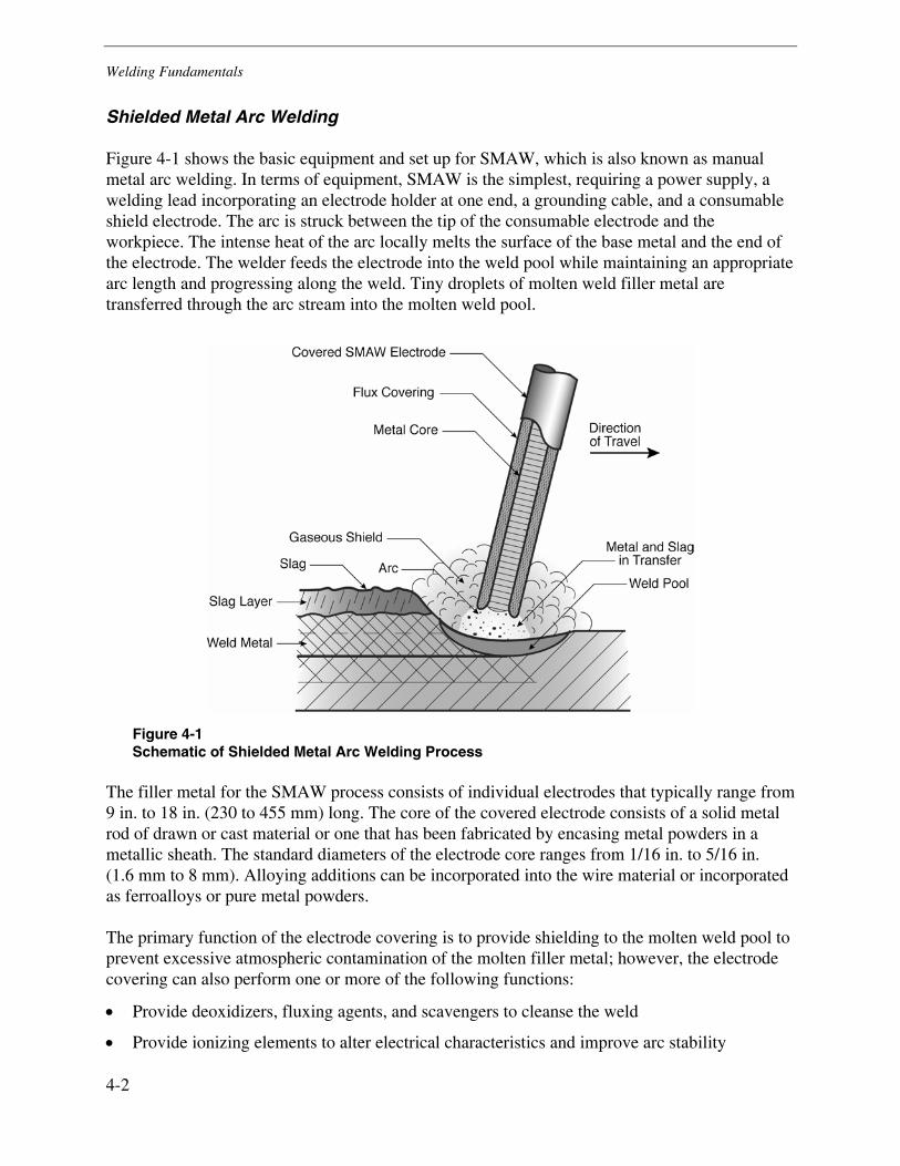
Welding Fundamentals
4-2
Shielded Metal Arc Welding
Figure 4-1 shows the basic equipment and set up for SMAW, which is also known as manual metal arc welding. In terms of equipment, SMAW is the simplest, requiring a power supply, a welding lead incorporating an electrode holder at one end, a grounding cable, and a consumable shield electrode. The arc is struck between the tip of the consumable electrode and the workpiece. The intense heat of the arc locally melts the surface of the base metal and the end of the electrode. The welder feeds the electrode into the weld pool while maintaining an appropriate arc length and progressing along the weld. Tiny droplets of molten weld filler metal are transferred through the arc stream into the molten weld pool.
Figure 4-1 Schematic of Shielded Metal Arc Welding Process
The filler metal for the SMAW process consists of individual electrodes that typically range from 9 in. to 18 in. (230 to 455 mm) long. The core of the covered electrode consists of a solid metal rod of drawn or cast material or one that has been fabricated by encasing metal powders in a metallic sheath. The standard diameters of the electrode core ranges from 1/16 in. to 5/16 in. (1.6 mm to 8 mm). Alloying additions can be incorporated into the wire material or incorporated as ferroalloys or pure metal powders.
The primary function of the electrode covering is to provide shielding to the molten weld pool to prevent excessive atmospheric contamination of the molten filler metal; however, the electrode covering can also perform one or more of the following functions:
• Provide deoxidizers, fluxing agents, and scavengers to cleanse the weld
• Provide ionizing elements to alter electrical characteristics and improve arc stability
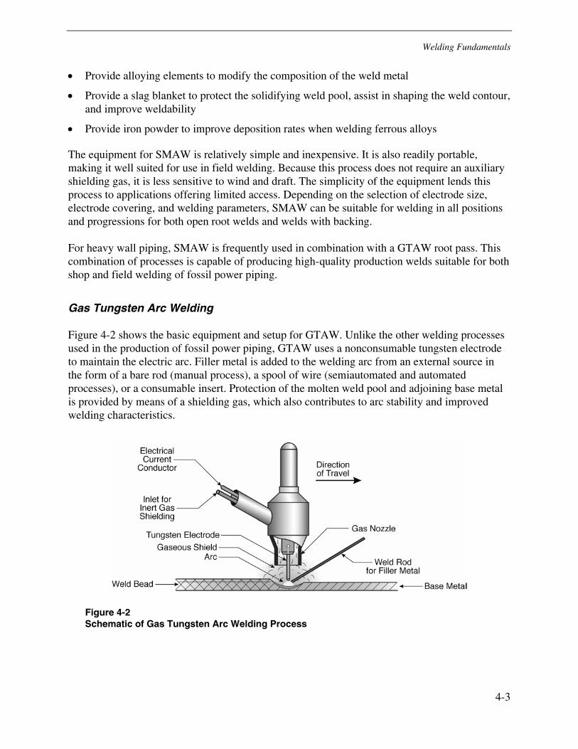
Welding Fundamentals
4-3
• Provide alloying elements to modify the composition of the weld metal
• Provide a slag blanket to protect the solidifying weld pool, assist in shaping the weld contour, and improve weldability
• Provide iron powder to improve deposition rates when welding ferrous alloys
The equipment for SMAW is relatively simple and inexpensive. It is also readily portable, making it well suited for use in field welding. Because this process does not require an auxiliary shielding gas, it is less sensitive to wind and draft. The simplicity of the equipment lends this process to applications offering limited access. Depending on the selection of electrode size, electrode covering, and welding parameters, SMAW can be suitable for welding in all positions and progressions for both open root welds and welds with backing.
For heavy wall piping, SMAW is frequently used in combination with a GTAW root pass. This combination of processes is capable of producing high-quality production welds suitable for both shop and field welding of fossil power piping.
Gas Tungsten Arc Welding
Figure 4-2 shows the basic equipment and setup for GTAW. Unlike the other welding processes used in the production of fossil power piping, GTAW uses a nonconsumable tungsten electrode to maintain the electric arc. Filler metal is added to the welding arc from an external source in the form of a bare rod (manual process), a spool of wire (semiautomated and automated processes), or a consumable insert. Protection of the molten weld pool and adjoining base metal is provided by means of a shielding gas, which also contributes to arc stability and improved welding characteristics.
Figure 4-2 Schematic of Gas Tungsten Arc Welding Process
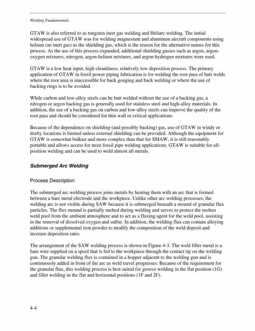
Welding Fundamentals
4-4
GTAW is also referred to as tungsten inert gas welding and Heliarc welding. The initial widespread use of GTAW was for welding magnesium and aluminum aircraft components using helium (an inert gas) as the shielding gas, which is the reason for the alternative names for this process. As the use of this process expanded, additional shielding gasses such as argon, argon-oxygen mixtures, nitrogen, argon-helium mixtures, and argon-hydrogen mixtures were used.
GTAW is a low heat input, high cleanliness, relatively low deposition process. The primary application of GTAW in fossil power piping fabrication is for welding the root pass of butt welds where the root area is inaccessible for back gouging and back welding or where the use of backing rings is to be avoided.
While carbon and low-alloy steels can be butt welded without the use of a backing gas, a nitrogen or argon backing gas is generally used for stainless steel and high-alloy materials. In addition, the use of a backing gas on carbon and low-alloy steels can improve the quality of the root pass and should be considered for thin wall or critical applications.
Because of the dependence on shielding (and possibly backing) gas, use of GTAW in windy or drafty locations is limited unless external shielding can be provided. Although the equipment for GTAW is somewhat bulkier and more complex than that for SMAW, it is still reasonably portable and allows access for most fossil pipe welding applications. GTAW is suitable for all-position welding and can be used to weld almost all metals.
Submerged Arc Welding
Process Description
The submerged arc welding process joins metals by heating them with an arc that is formed between a bare metal electrode and the workpiece. Unlike other arc welding processes, the welding arc is not visible during SAW because it is submerged beneath a mound of granular flux particles. The flux mound is partially melted during welding and serves to protect the molten weld pool from the ambient atmosphere and to act as a fluxing agent for the weld pool, assisting in the removal of dissolved oxygen and sulfur. In addition, the welding flux can contain alloying additions or supplemental iron powder to modify the composition of the weld deposit and increase deposition rates.
The arrangement of the SAW welding process is shown in Figure 4-3. The weld filler metal is a bare wire supplied on a spool that is fed to the workpiece through the contact tip on the welding gun. The granular welding flux is contained in a hopper adjacent to the welding gun and is continuously added in front of the arc as weld travel progresses. Because of the requirement for the granular flux, this welding process is best suited for groove welding in the flat position (1G) and fillet welding in the flat and horizontal positions (1F and 2F).
Welding Fundamentals
4-5
Figure 4-3 Schematic of Submerged Arc Welding Process
While single electrode welding is the most common, multiple electrodes (two or three) can be used to increase deposition rates. However, the microstructural effects of the higher heat input and coarse solidification structure should be considered. For ferrous alloys, deposition rates can also be increased by adding iron powder to the flux. In practice, supplemental filler metal is generally used only in welding mild carbon steel because the recovery of alloying elements can be greatly affected by variations within welding parameters.
Consumables
During SAW, flux and electrode wire feed simultaneously to the joint. The flux shields, cleans, and shapes the weld bead. The electrode wire is the main component of the weld metal; however, supplemental filler metal can be included with the flux.
The welding electrode is a bare wire that is provided on spools or in drums for a continuous wire feed. The electrode diameter ranges from 1/16 in. to 1/4 in. (1.6 mm to 6.4 mm). Alloy additions can be incorporated through the use of an alloy wire or through a cored wire consisting of a low-carbon metal sheath surrounding a core of alloy material. SAW fluxes are classified as fused or bonded, active or neutral, and acidic or basic.
To manufacture a fused flux, the raw materials are melted together and cooled to produce a glassy flux that is crushed and screened for size. Fused fluxes have good chemical homogeneity, have low moisture pickup during storage and use, and can be readily recycled and reused without a significant change in particle size or composition.
Welding Fundamentals
4-6
Bonded fluxes are manufactured by dry-mixing powders of the various raw materials and bonding them with either potassium silicate, sodium silicate, or a mixture of the two. After bonding, the wet mix is palletized and baked. Finally the backed and bonded flux is broken up and screened to size. An advantage to bonded flux is the ability to easily add deoxidizers and alloying elements. However the disadvantages to bonded flux include possible change in flux composition due to segregation, possible gas evolution from the molten slag, and a tendency for some fluxes to absorb moisture from the atmosphere.
The basicity of the SAW flux plays an important role in governing the composition of the weld metal. The basicity of a flux (BI) is given by the ratio of the sum of the weight percentages of basic oxides to the sum of the weight percentages of the acidic oxides, as shown in Equation 4-1.
( )
( )22322
2222
21
21
ZrOTiOOAlSiO
FeOMnOSrOBaOOLiONaOKMgOCaFCaOBI
+++
+++++++++= Eq. 4-1
BI typically has values ranging from 0.5 to 3.0. Fluxes with a basicity index greater than 1.5 are considered basic, while those less than 1.0 are considered acid. The basicity index is essentially an estimate of the oxygen content of the weld metal, and it has an impact on the weld composition and total inclusion content. Basic weld fluxes tend to produce welds with lower oxygen content, a finer grain structure, and improved impact toughness. Acid fluxes have higher oxygen content, increased numbers of oxide inclusions, and a coarser microstructure. Typical weld metal oxygen contents for various welding processes are shown in Table 4-1.
Table 4-1 Summary of Measured Weld Metal Oxygen Contents Source: Ø. Gröng, Metallurgical Modeling of Welding [4-2].
Welding Process Material Oxygen Content (ppm)
SMAW—basic electrode Low-alloy steel 250–440
SMAW—rutile electrodes Low-alloy steel 500–1300
SMAW—acid electrodes Low-alloy steel 700–1400
GTAW—Ar or He Shielding Low-alloy steel 50–100
GMAW—Ar-O2 mixtures Low-alloy steel 200–1300
GMAW—CO2 Low-alloy steel 500–800
FCAW—self shielded cored wire Low-alloy steel 130–200
SAW—calcium silicate flux (acid) Low-alloy steel 450–2600
SAW—basic fluxes Low-alloy steel 180–350
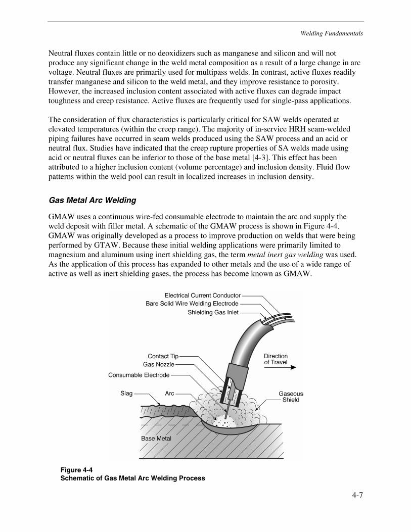
Welding Fundamentals
4-7
Neutral fluxes contain little or no deoxidizers such as manganese and silicon and will not produce any significant change in the weld metal composition as a result of a large change in arc voltage. Neutral fluxes are primarily used for multipass welds. In contrast, active fluxes readily transfer manganese and silicon to the weld metal, and they improve resistance to porosity. However, the increased inclusion content associated with active fluxes can degrade impact toughness and creep resistance. Active fluxes are frequently used for single-pass applications.
The consideration of flux characteristics is particularly critical for SAW welds operated at elevated temperatures (within the creep range). The majority of in-service HRH seam-welded piping failures have occurred in seam welds produced using the SAW process and an acid or neutral flux. Studies have indicated that the creep rupture properties of SA welds made using acid or neutral fluxes can be inferior to those of the base metal [4-3]. This effect has been attributed to a higher inclusion content (volume percentage) and inclusion density. Fluid flow patterns within the weld pool can result in localized increases in inclusion density.
Gas Metal Arc Welding
GMAW uses a continuous wire-fed consumable electrode to maintain the arc and supply the weld deposit with filler metal. A schematic of the GMAW process is shown in Figure 4-4. GMAW was originally developed as a process to improve production on welds that were being performed by GTAW. Because these initial welding applications were primarily limited to magnesium and aluminum using inert shielding gas, the term metal inert gas welding was used. As the application of this process has expanded to other metals and the use of a wide range of active as well as inert shielding gases, the process has become known as GMAW.
Figure 4-4 Schematic of Gas Metal Arc Welding Process
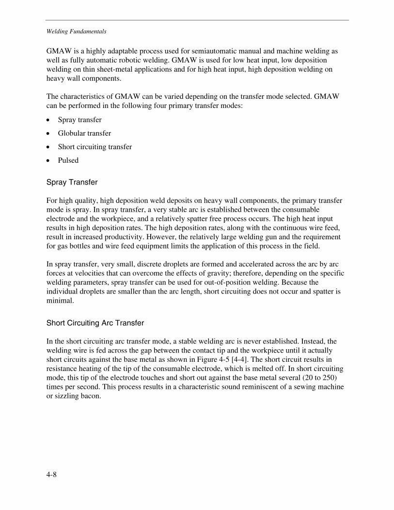
Welding Fundamentals
4-8
GMAW is a highly adaptable process used for semiautomatic manual and machine welding as well as fully automatic robotic welding. GMAW is used for low heat input, low deposition welding on thin sheet-metal applications and for high heat input, high deposition welding on heavy wall components.
The characteristics of GMAW can be varied depending on the transfer mode selected. GMAW can be performed in the following four primary transfer modes:
• Spray transfer
• Globular transfer
• Short circuiting transfer
• Pulsed
Spray Transfer
For high quality, high deposition weld deposits on heavy wall components, the primary transfer mode is spray. In spray transfer, a very stable arc is established between the consumable electrode and the workpiece, and a relatively spatter free process occurs. The high heat input results in high deposition rates. The high deposition rates, along with the continuous wire feed, result in increased productivity. However, the relatively large welding gun and the requirement for gas bottles and wire feed equipment limits the application of this process in the field.
In spray transfer, very small, discrete droplets are formed and accelerated across the arc by arc forces at velocities that can overcome the effects of gravity; therefore, depending on the specific welding parameters, spray transfer can be used for out-of-position welding. Because the individual droplets are smaller than the arc length, short circuiting does not occur and spatter is minimal.
Short Circuiting Arc Transfer
In the short circuiting arc transfer mode, a stable welding arc is never established. Instead, the welding wire is fed across the gap between the contact tip and the workpiece until it actually short circuits against the base metal as shown in Figure 4-5 [4-4]. The short circuit results in resistance heating of the tip of the consumable electrode, which is melted off. In short circuiting mode, this tip of the electrode touches and short out against the base metal several (20 to 250) times per second. This process results in a characteristic sound reminiscent of a sewing machine or sizzling bacon.
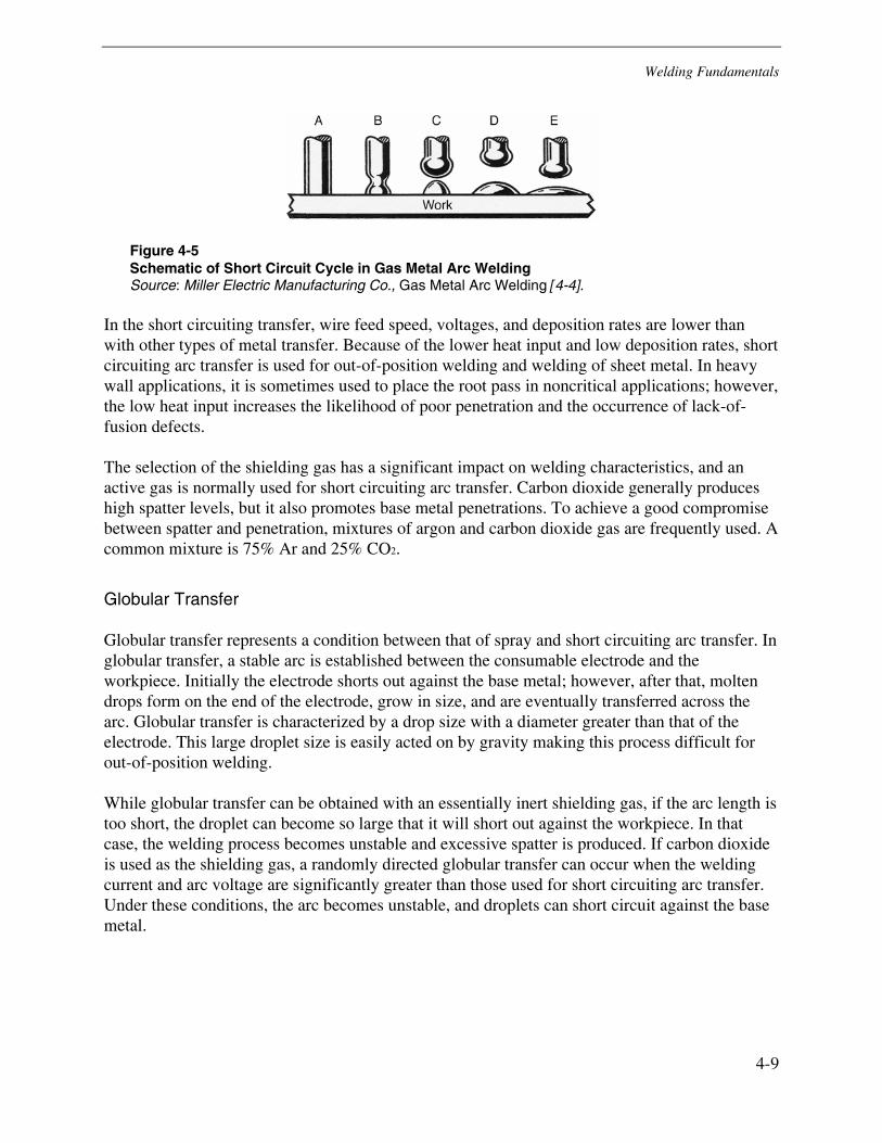
Welding Fundamentals
4-9
Figure 4-5 Schematic of Short Circuit Cycle in Gas Metal Arc Welding Source: Miller Electric Manufacturing Co., Gas Metal Arc Welding [4-4].
In the short circuiting transfer, wire feed speed, voltages, and deposition rates are lower than with other types of metal transfer. Because of the lower heat input and low deposition rates, short circuiting arc transfer is used for out-of-position welding and welding of sheet metal. In heavy wall applications, it is sometimes used to place the root pass in noncritical applications; however, the low heat input increases the likelihood of poor penetration and the occurrence of lack-of-fusion defects.
The selection of the shielding gas has a significant impact on welding characteristics, and an active gas is normally used for short circuiting arc transfer. Carbon dioxide generally produces high spatter levels, but it also promotes base metal penetrations. To achieve a good compromise between spatter and penetration, mixtures of argon and carbon dioxide gas are frequently used. A common mixture is 75% Ar and 25% CO2.
Globular Transfer
Globular transfer represents a condition between that of spray and short circuiting arc transfer. In globular transfer, a stable arc is established between the consumable electrode and the workpiece. Initially the electrode shorts out against the base metal; however, after that, molten drops form on the end of the electrode, grow in size, and are eventually transferred across the arc. Globular transfer is characterized by a drop size with a diameter greater than that of the electrode. This large droplet size is easily acted on by gravity making this process difficult for out-of-position welding.
While globular transfer can be obtained with an essentially inert shielding gas, if the arc length is too short, the droplet can become so large that it will short out against the workpiece. In that case, the welding process becomes unstable and excessive spatter is produced. If carbon dioxide is used as the shielding gas, a randomly directed globular transfer can occur when the welding current and arc voltage are significantly greater than those used for short circuiting arc transfer. Under these conditions, the arc becomes unstable, and droplets can short circuit against the base metal.
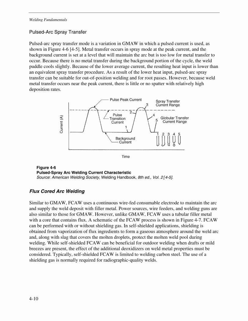
Welding Fundamentals
4-10
Pulsed-Arc Spray Transfer
Pulsed-arc spray transfer mode is a variation in GMAW in which a pulsed current is used, as shown in Figure 4-6 [4-5]. Metal transfer occurs in spray mode at the peak current, and the background current is set at a level that will maintain the arc but is too low for metal transfer to occur. Because there is no metal transfer during the background portion of the cycle, the weld puddle cools slightly. Because of the lower average current, the resulting heat input is lower than an equivalent spray transfer procedure. As a result of the lower heat input, pulsed-arc spray transfer can be suitable for out-of-position welding and for root passes. However, because weld metal transfer occurs near the peak current, there is little or no spatter with relatively high deposition rates.
Figure 4-6 Pulsed-Spray Arc Welding Current Characteristic Source: American Welding Society, Welding Handbook, 8th ed., Vol. 2 [4-5].
Flux Cored Arc Welding
Similar to GMAW, FCAW uses a continuous wire-fed consumable electrode to maintain the arc and supply the weld deposit with filler metal. Power sources, wire feeders, and welding guns are also similar to those for GMAW. However, unlike GMAW, FCAW uses a tubular filler metal with a core that contains flux. A schematic of the FCAW process is shown in Figure 4-7. FCAW can be performed with or without shielding gas. In self-shielded applications, shielding is obtained from vaporization of flux ingredients to form a gaseous atmosphere around the weld arc and, along with slag that covers the molten droplets, protect the molten weld pool during welding. While self-shielded FCAW can be beneficial for outdoor welding when drafts or mild breezes are present, the effect of the additional deoxidizers on weld metal properties must be considered. Typically, self-shielded FCAW is limited to welding carbon steel. The use of a shielding gas is normally required for radiographic-quality welds.
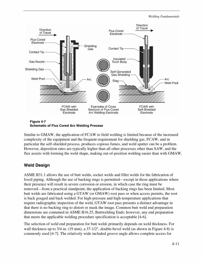
Welding Fundamentals
4-11
Figure 4-7 Schematic of Flux Cored Arc Welding Process
Similar to GMAW, the application of FCAW to field welding is limited because of the increased complexity of the equipment and the frequent requirement for shielding gas. FCAW, and in particular the self-shielded process, produces copious fumes, and weld spatter can be a problem. However, deposition rates are typically higher than all other processes other than SAW, and the flux assists with forming the weld shape, making out-of-position welding easier than with GMAW.
Weld Design
ASME B31.1 allows the use of butt welds, socket welds and fillet welds for the fabrication of fossil piping. Although the use of backing rings is permitted—except in those applications where their presence will result in severe corrosion or erosion, in which case the ring must be removed—from a practical standpoint, the application of backing rings has been limited. Most butt welds are fabricated using a GTAW (or GMAW) root pass or when access permits, the root is back gouged and back welded. For high-pressure and high-temperature applications that require radiographic inspection of the weld, GTAW root pass presents a distinct advantage in that there is no backing ring to distort or mask the image. Common butt weld end preparation dimensions are contained in ASME B16.25, Buttwelding Ends; however, any end preparation that meets the applicable welding procedure specification is acceptable [4-6].
The selection of weld end preparation for butt welds primarily depends on weld thickness. For wall thickness up to 3/4 in. (19 mm), a 37-1/2°, double-bevel weld (as shown in Figure 4-8) is commonly used [4-7]. The relatively wide included groove angle allows complete access for
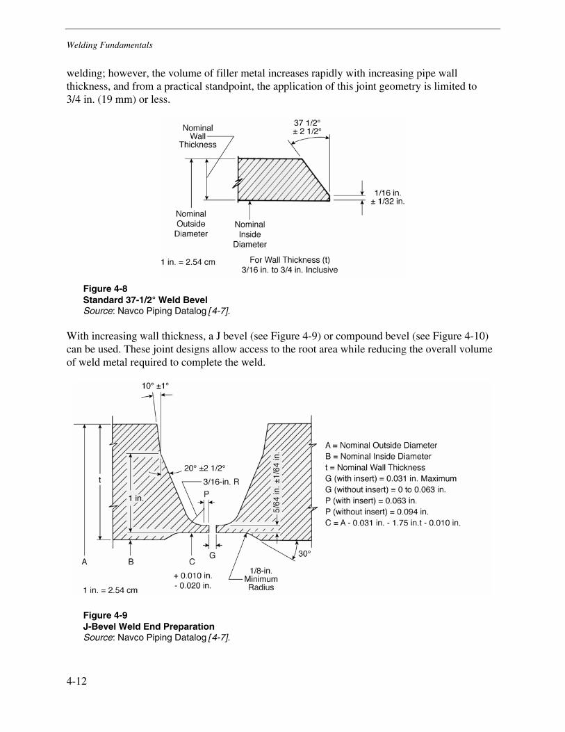
Welding Fundamentals
4-12
welding; however, the volume of filler metal increases rapidly with increasing pipe wall thickness, and from a practical standpoint, the application of this joint geometry is limited to 3/4 in. (19 mm) or less.
Figure 4-8 Standard 37-1/2° Weld Bevel Source: Navco Piping Datalog [4-7].
With increasing wall thickness, a J bevel (see Figure 4-9) or compound bevel (see Figure 4-10) can be used. These joint designs allow access to the root area while reducing the overall volume of weld metal required to complete the weld.
Figure 4-9 J-Bevel Weld End Preparation Source: Navco Piping Datalog [4-7].
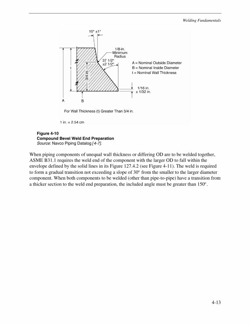
Welding Fundamentals
4-13
Figure 4-10 Compound Bevel Weld End Preparation Source: Navco Piping Datalog [4-7].
When piping components of unequal wall thickness or differing OD are to be welded together, ASME B31.1 requires the weld end of the component with the larger OD to fall within the envelope defined by the solid lines in its Figure 127.4.2 (see Figure 4-11). The weld is required to form a gradual transition not exceeding a slope of 30° from the smaller to the larger diameter component. When both components to be welded (other than pipe-to-pipe) have a transition from a thicker section to the weld end preparation, the included angle must be greater than 150°.
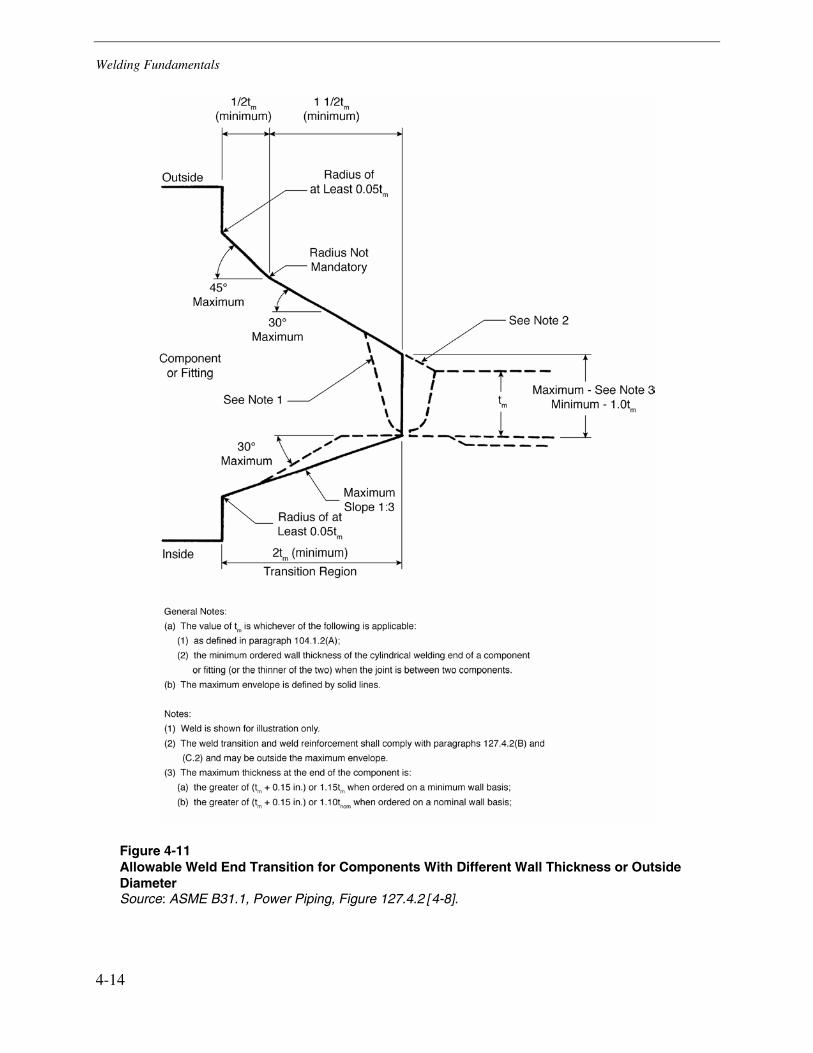
Welding Fundamentals
4-14
Figure 4-11 Allowable Weld End Transition for Components With Different Wall Thickness or Outside Diameter Source: ASME B31.1, Power Piping, Figure 127.4.2 [4-8].
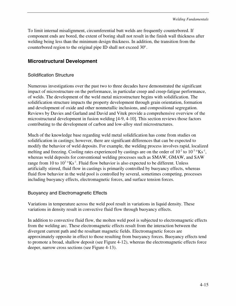
Welding Fundamentals
4-15
To limit internal misalignment, circumferential butt welds are frequently counterbored. If component ends are bored, the extent of boring shall not result in the finish wall thickness after welding being less than the minimum design thickness. In addition, the transition from the counterbored region to the original pipe ID shall not exceed 30°.
Microstructural Development
Solidification Structure
Numerous investigations over the past two to three decades have demonstrated the significant impact of microstructure on the performance, in particular creep and creep-fatigue performance, of welds. The development of the weld metal microstructure begins with solidification. The solidification structure impacts the property development through grain orientation, formation and development of oxide and other nonmetallic inclusions, and compositional segregation. Reviews by Davies and Garland and David and Vitek provide a comprehensive overview of the microstructural development in fusion welding [4-9, 4-10]. This section reviews those factors contributing to the development of carbon and low-alloy steel microstructures.
Much of the knowledge base regarding weld metal solidification has come from studies on solidification in castings; however, there are significant differences that can be expected to modify the behavior of weld deposits. For example, the welding process involves rapid, localized melting and freezing. Cooling rates experienced by castings are on the order of 10-2 to 10-3 °Ks-1, whereas weld deposits for conventional welding processes such as SMAW, GMAW, and SAW range from 10 to 103 °Ks-1. Fluid flow behavior is also expected to be different. Unless artificially stirred, fluid flow in castings is primarily controlled by buoyancy effects, whereas fluid flow behavior in the weld pool is controlled by several, sometimes competing, processes including buoyancy effects, electromagnetic forces, and surface tension forces.
Buoyancy and Electromagnetic Effects
Variations in temperature across the weld pool result in variations in liquid density. These variations in density result in convective fluid flow through buoyancy effects.
In addition to convective fluid flow, the molten weld pool is subjected to electromagnetic effects from the welding arc. These electromagnetic effects result from the interaction between the divergent current path and the resultant magnetic fields. Electromagnetic forces are approximately opposite in effect to those resulting from buoyancy forces. Buoyancy effects tend to promote a broad, shallow deposit (see Figure 4-12), whereas the electromagnetic effects force deeper, narrow cross sections (see Figure 4-13).
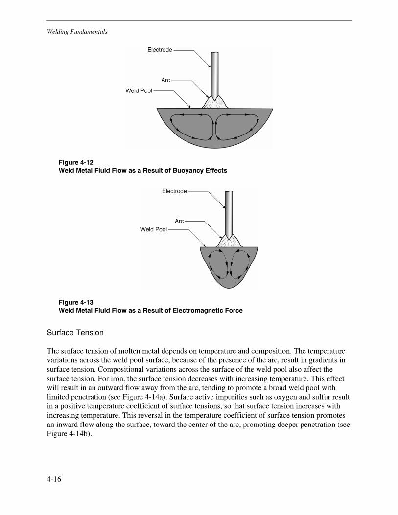
Welding Fundamentals
4-16
Figure 4-12 Weld Metal Fluid Flow as a Result of Buoyancy Effects
Figure 4-13 Weld Metal Fluid Flow as a Result of Electromagnetic Force
Surface Tension
The surface tension of molten metal depends on temperature and composition. The temperature variations across the weld pool surface, because of the presence of the arc, result in gradients in surface tension. Compositional variations across the surface of the weld pool also affect the surface tension. For iron, the surface tension decreases with increasing temperature. This effect will result in an outward flow away from the arc, tending to promote a broad weld pool with limited penetration (see Figure 4-14a). Surface active impurities such as oxygen and sulfur result in a positive temperature coefficient of surface tensions, so that surface tension increases with increasing temperature. This reversal in the temperature coefficient of surface tension promotes an inward flow along the surface, toward the center of the arc, promoting deeper penetration (see Figure 4-14b).
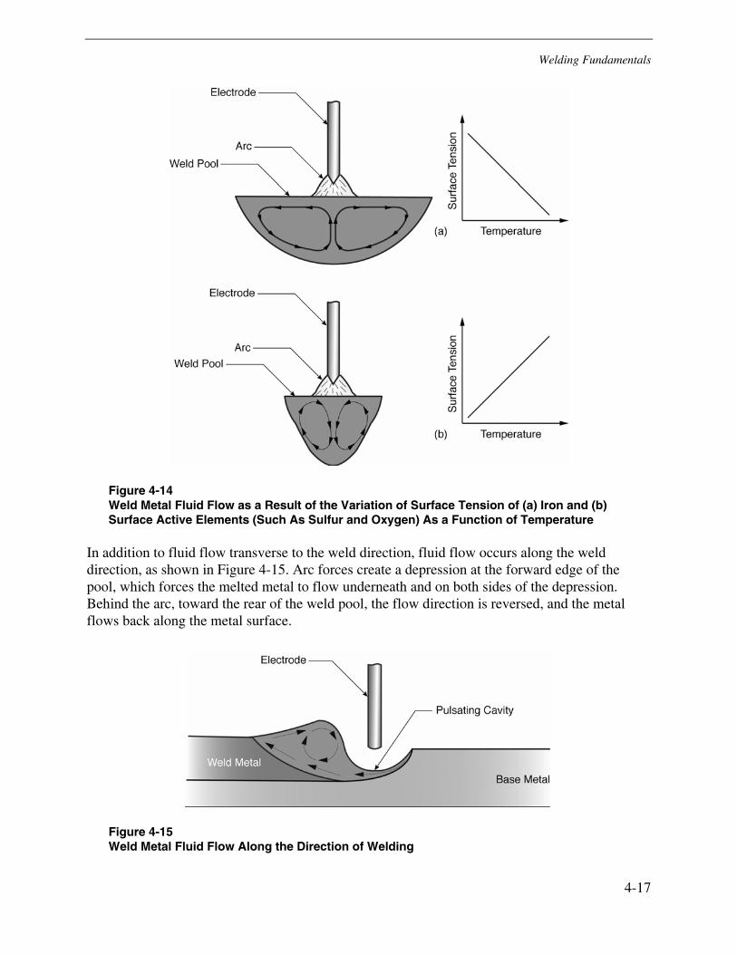
Welding Fundamentals
4-17
Figure 4-14 Weld Metal Fluid Flow as a Result of the Variation of Surface Tension of (a) Iron and (b) Surface Active Elements (Such As Sulfur and Oxygen) As a Function of Temperature
In addition to fluid flow transverse to the weld direction, fluid flow occurs along the weld direction, as shown in Figure 4-15. Arc forces create a depression at the forward edge of the pool, which forces the melted metal to flow underneath and on both sides of the depression. Behind the arc, toward the rear of the weld pool, the flow direction is reversed, and the metal flows back along the metal surface.
Figure 4-15 Weld Metal Fluid Flow Along the Direction of Welding
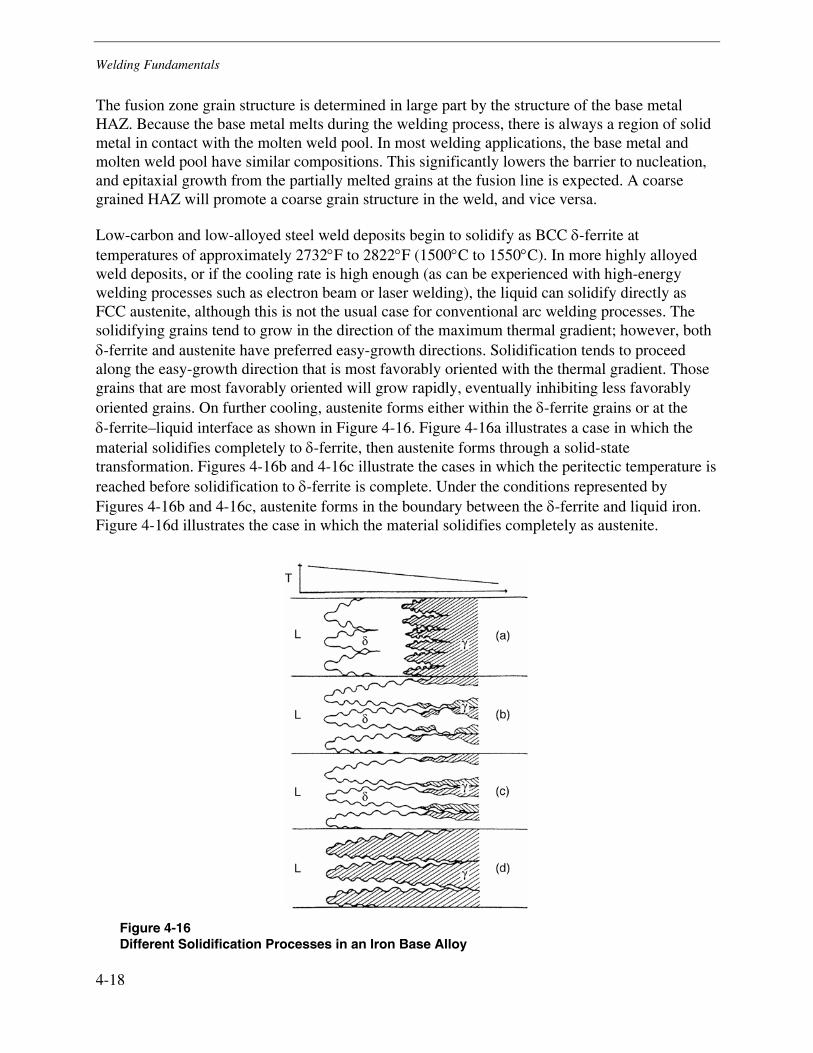
Welding Fundamentals
4-18
The fusion zone grain structure is determined in large part by the structure of the base metal HAZ. Because the base metal melts during the welding process, there is always a region of solid metal in contact with the molten weld pool. In most welding applications, the base metal and molten weld pool have similar compositions. This significantly lowers the barrier to nucleation, and epitaxial growth from the partially melted grains at the fusion line is expected. A coarse grained HAZ will promote a coarse grain structure in the weld, and vice versa.
Low-carbon and low-alloyed steel weld deposits begin to solidify as BCC δ-ferrite at temperatures of approximately 2732°F to 2822°F (1500°C to 1550°C). In more highly alloyed weld deposits, or if the cooling rate is high enough (as can be experienced with high-energy welding processes such as electron beam or laser welding), the liquid can solidify directly as FCC austenite, although this is not the usual case for conventional arc welding processes. The solidifying grains tend to grow in the direction of the maximum thermal gradient; however, both δ-ferrite and austenite have preferred easy-growth directions. Solidification tends to proceed along the easy-growth direction that is most favorably oriented with the thermal gradient. Those grains that are most favorably oriented will grow rapidly, eventually inhibiting less favorably oriented grains. On further cooling, austenite forms either within the δ-ferrite grains or at the δ-ferrite–liquid interface as shown in Figure 4-16. Figure 4-16a illustrates a case in which the material solidifies completely to δ-ferrite, then austenite forms through a solid-state transformation. Figures 4-16b and 4-16c illustrate the cases in which the peritectic temperature is reached before solidification to δ-ferrite is complete. Under the conditions represented by Figures 4-16b and 4-16c, austenite forms in the boundary between the δ-ferrite and liquid iron. Figure 4-16d illustrates the case in which the material solidifies completely as austenite.
Figure 4-16 Different Solidification Processes in an Iron Base Alloy
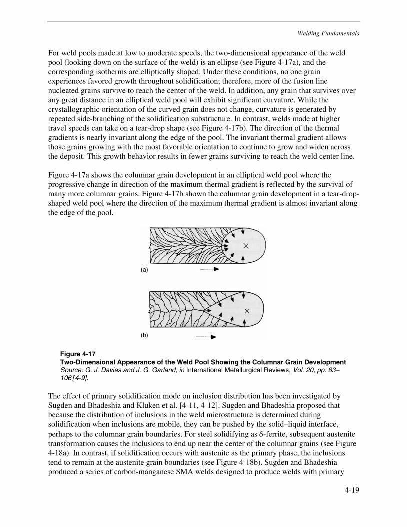
Welding Fundamentals
4-19
For weld pools made at low to moderate speeds, the two-dimensional appearance of the weld pool (looking down on the surface of the weld) is an ellipse (see Figure 4-17a), and the corresponding isotherms are elliptically shaped. Under these conditions, no one grain experiences favored growth throughout solidification; therefore, more of the fusion line nucleated grains survive to reach the center of the weld. In addition, any grain that survives over any great distance in an elliptical weld pool will exhibit significant curvature. While the crystallographic orientation of the curved grain does not change, curvature is generated by repeated side-branching of the solidification substructure. In contrast, welds made at higher travel speeds can take on a tear-drop shape (see Figure 4-17b). The direction of the thermal gradients is nearly invariant along the edge of the pool. The invariant thermal gradient allows those grains growing with the most favorable orientation to continue to grow and widen across the deposit. This growth behavior results in fewer grains surviving to reach the weld center line.
Figure 4-17a shows the columnar grain development in an elliptical weld pool where the progressive change in direction of the maximum thermal gradient is reflected by the survival of many more columnar grains. Figure 4-17b shown the columnar grain development in a tear-drop-shaped weld pool where the direction of the maximum thermal gradient is almost invariant along the edge of the pool.
Figure 4-17 Two-Dimensional Appearance of the Weld Pool Showing the Columnar Grain Development Source: G. J. Davies and J. G. Garland, in International Metallurgical Reviews, Vol. 20, pp. 83–106 [4-9].
The effect of primary solidification mode on inclusion distribution has been investigated by Sugden and Bhadeshia and Kluken et al. [4-11, 4-12]. Sugden and Bhadeshia proposed that because the distribution of inclusions in the weld microstructure is determined during solidification when inclusions are mobile, they can be pushed by the solid–liquid interface, perhaps to the columnar grain boundaries. For steel solidifying as δ-ferrite, subsequent austenite transformation causes the inclusions to end up near the center of the columnar grains (see Figure 4-18a). In contrast, if solidification occurs with austenite as the primary phase, the inclusions tend to remain at the austenite grain boundaries (see Figure 4-18b). Sugden and Bhadeshia produced a series of carbon-manganese SMA welds designed to produce welds with primary
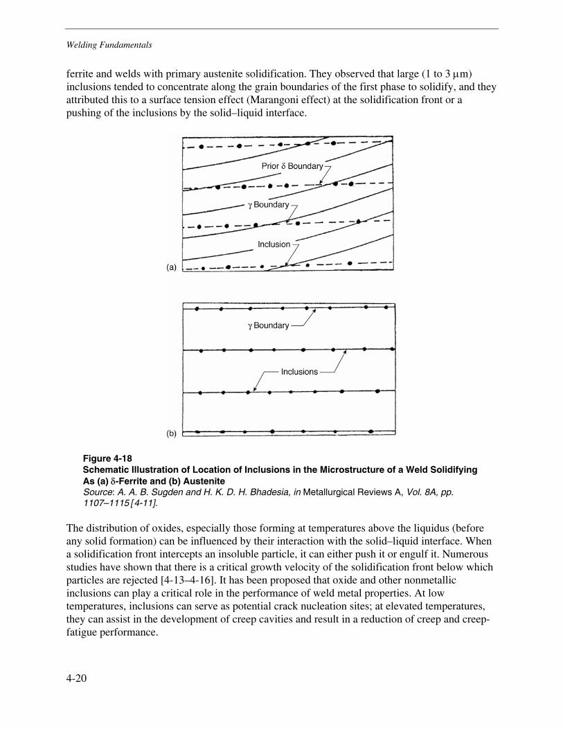
Welding Fundamentals
4-20
ferrite and welds with primary austenite solidification. They observed that large (1 to 3 μm) inclusions tended to concentrate along the grain boundaries of the first phase to solidify, and they attributed this to a surface tension effect (Marangoni effect) at the solidification front or a pushing of the inclusions by the solid–liquid interface.
Figure 4-18 Schematic Illustration of Location of Inclusions in the Microstructure of a Weld Solidifying As (a) δ-Ferrite and (b) Austenite Source: A. A. B. Sugden and H. K. D. H. Bhadesia, in Metallurgical Reviews A, Vol. 8A, pp. 1107–1115 [4-11].
The distribution of oxides, especially those forming at temperatures above the liquidus (before any solid formation) can be influenced by their interaction with the solid–liquid interface. When a solidification front intercepts an insoluble particle, it can either push it or engulf it. Numerous studies have shown that there is a critical growth velocity of the solidification front below which particles are rejected [4-13–4-16]. It has been proposed that oxide and other nonmetallic inclusions can play a critical role in the performance of weld metal properties. At low temperatures, inclusions can serve as potential crack nucleation sites; at elevated temperatures, they can assist in the development of creep cavities and result in a reduction of creep and creep-fatigue performance.
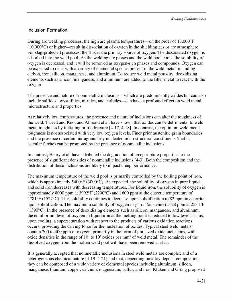
Welding Fundamentals
4-21
Inclusion Formation
During arc welding processes, the high arc plasma temperatures—on the order of 18,000°F (10,000°C) or higher—result in dissociation of oxygen in the shielding gas or arc atmosphere. For slag-protected processes, the flux is the primary source of oxygen. The dissociated oxygen is adsorbed into the weld pool. As the welding arc passes and the weld pool cools, the solubility of oxygen is decreased, and it will be removed as oxygen-rich phases and compounds. Oxygen can be expected to react with a variety of elemental species present in the weld metal, including carbon, iron, silicon, manganese, and aluminum. To reduce weld metal porosity, deoxidizing elements such as silicon, manganese, and aluminum are added to the filler metal to react with the oxygen.
The presence and nature of nonmetallic inclusions—which are predominantly oxides but can also include sulfides, oxysulfides, nitrides, and carbides—can have a profound effect on weld metal microstructure and properties.
At relatively low temperatures, the presence and nature of inclusions can alter the toughness of the weld. Tweed and Knot and Almond et al. have shown that oxides can be detrimental to weld metal toughness by initiating brittle fracture [4-17, 4-18]. In contrast, the optimum weld metal toughness is not associated with very low oxygen levels. Finer prior austenitic grain boundaries and the presence of certain intragranularly nucleated microstructural constituents (that is, acicular ferrite) can be promoted by the presence of nonmetallic inclusions.
In contrast, Henry et al. have attributed the degradation of creep rupture properties to the presence of significant densities of nonmetallic inclusions [4-3]. Both the composition and the distribution of these inclusions are likely to impact creep performance.
The maximum temperature of the weld pool is primarily controlled by the boiling point of iron, which is approximately 5400°F (3000°C). As expected, the solubility of oxygen in pure liquid and solid iron decreases with decreasing temperatures. For liquid iron, the solubility of oxygen is approximately 8000 ppm at 3992°F (2200°C) and 1600 ppm at the eutectic temperature of 2781°F (1527°C). This solubility continues to decrease upon solidification to 82 ppm in δ-ferrite upon solidification. The maximum solubility of oxygen in γ-iron (austenite) is 28 ppm at 2534°F (1390°C). In the presence of deoxidizing elements such as silicon, manganese, and aluminum, the equilibrium level of oxygen in liquid iron at the melting point is reduced to low levels. Thus, upon cooling, a supersaturation with respect to the products of various oxidation reactions occurs, providing the driving force for the nucleation of oxides. Typical steel weld metals contain 200 to 400 ppm of oxygen, primarily in the form of μm-sized oxide inclusions, with oxide densities in the range of 107 to 108 oxides per mm3 of weld metal. The remainder of the dissolved oxygen from the molten weld pool will have been removed as slag.
It is generally accepted that nonmetallic inclusions in steel weld metals are complex and of a heterogeneous chemical nature [4-19–4-21] and that, depending on alloy deposit composition, they can be composed of a wide variety of elemental species including aluminum, silicon, manganese, titanium, copper, calcium, magnesium, sulfur, and iron. Kluken and Gröng proposed
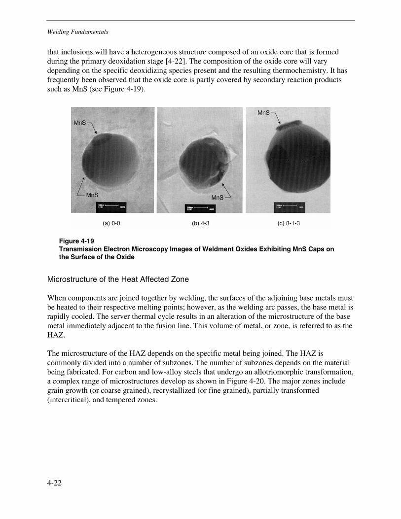
Welding Fundamentals
4-22
that inclusions will have a heterogeneous structure composed of an oxide core that is formed during the primary deoxidation stage [4-22]. The composition of the oxide core will vary depending on the specific deoxidizing species present and the resulting thermochemistry. It has frequently been observed that the oxide core is partly covered by secondary reaction products such as MnS (see Figure 4-19).
Figure 4-19 Transmission Electron Microscopy Images of Weldment Oxides Exhibiting MnS Caps on the Surface of the Oxide
Microstructure of the Heat Affected Zone
When components are joined together by welding, the surfaces of the adjoining base metals must be heated to their respective melting points; however, as the welding arc passes, the base metal is rapidly cooled. The server thermal cycle results in an alteration of the microstructure of the base metal immediately adjacent to the fusion line. This volume of metal, or zone, is referred to as the HAZ.
The microstructure of the HAZ depends on the specific metal being joined. The HAZ is commonly divided into a number of subzones. The number of subzones depends on the material being fabricated. For carbon and low-alloy steels that undergo an allotriomorphic transformation, a complex range of microstructures develop as shown in Figure 4-20. The major zones include grain growth (or coarse grained), recrystallized (or fine grained), partially transformed (intercritical), and tempered zones.
Welding Fundamentals
4-23
Figure 4-20 Schematic Diagram of the Various Subzones of the Heat-Affected Zone Approximately Corresponding to a Carbon Steel Containing 0.15 Wt% Carbon Source: K. Easterling, Introduction to the Physical Metallurgy of Welding [4-23].
Each of the microstructural zones within the HAZ can be expected to exhibit mechanical properties specific to that zone. In addition, the constraint affects from surrounding microstructures will affect the composite performance of the joint.
Welding Defects
Welding is subject to a wide range of discontinuities, including the following:
• Slag inclusions
• Porosity
• Incomplete fusion or lack of fusion
• Lack of penetration
• Cracks
• Undercut
• Underfill
Welding Fundamentals
4-24
These discontinuities can occur within the weld metal or in the base metal adjacent to the weld (in particular the HAZ). Most discontinuities develop during the welding process; however, certain forms of cracking can develop a significant period of time after completion of the weld (hydrogen cold cracking) or during heat treatment after welding (reheat cracking).
In the strictest sense, all materials (including weldments) contain intrinsic defects. These intrinsic defects include grain boundaries, dislocations, substitutional and interstitial alloying elements, and nonmetallic inclusions. In fact, the free surface of a part is a defect in the structure of the metal. However, in a macro sense, the term defect is used to identify imperfections or discontinuities that exceed an established acceptance criteria or that otherwise impair the function of the component.
Each industry uses specific codes or standards that identify the acceptable limits for discontinuities. Typically, these codes and standards are adopted by and enforced by local jurisdictions. After the acceptance criteria are exceeded, the discontinuity is classified as a defect.
For fossil power piping systems in the United States, inspection methods and acceptance criteria are established in ASME B31.1. Similar criteria exist in equivalent EN, BS, DIN, and JIS standards.
Most code-based acceptance criteria are not deterministic (stress and fracture mechanics-based); they are developed empirically, and they represent a quality standard. When the early fabrication codes (ASME BPVC and B31.1) were first developed, NDE methods such as liquid penetrant, magnetic particle, radiography, eddy current, and ultrasonic testing were not available. Proof testing (hydrostatic testing) and visual inspection were the only tests required; however, with agreement between the purchaser and the contractor, early versions of B31.1 allowed the following:
…welded joints may be given a hammer or impact test where such a test is feasible. This hammer or impact test shall consist of striking the pipe at 6-in. intervals on both sides of the welded joint. The weight of the hammer in pounds shall be approximately equal to the thickness of the pipe wall in tenths of an inch, but shall not exceed 10 lb.
In addition, although the concept of fracture-tolerant designs are based on the initial work of C. E. Inglis in 1913 and A. A. Griffith in 1920, modern analytical fracture mechanics methods did not enter into code design until the early 1970s. Therefore, most code acceptance criteria (including those of B31.1) represent a quality standard based on the philosophy that a qualified welder using a qualified welding procedure is capable of producing a weld meeting the intended design. The primary purpose of NDE is to ensure that the welder continues to produce a quality weld.
Welding Fundamentals
4-25
Cracks
Cracks (and crack-like indications) are considered the most detrimental of all weld discontinuities and are generally unacceptable. Cracks are characterized as linear, with sharp ends. Cracks are described by their primary length direction with respect to the longitudinal axis or the weld. Those lying parallel to the longitudinal axis are referred to as longitudinal cracks, and those lying perpendicular to the longitudinal axis of the weld are called transverse cracks.
Cracks that form as a result of fabrication in either the weld metal or the HAZ can be the result of a number of mechanisms. The key cracking mechanisms are the following:
• Solidification cracking (hot cracking). Solidification cracks most often occur in the weld metal, although a similar mechanism called liquation cracking can occur in the HAZ of some materials. Solidification cracks occur near the end of the weld and are the result of residual stress development during solidification before the weld metal obtains sufficient strength to resist the stress. A weld metal with a wide solidification range or that contains sulfur or phosphorous promotes solidification cracking. If there is insufficient filler metal to compensate for shrinkage in the terminal weld pool, a form of hot cracking referred to as crater cracking can result. Crater cracking can be eliminated by using a welding technique that backfills the terminal weld pool.
• Hydrogen cracking (cold cracking). The presence of hydrogen can promote the formation of cracking in the weld metal or HAZ. Hydrogen cracking can be either transgranular or intergranular, although intergranular fracture along the prior austenitic grain boundaries is the most common. Hydrogen cracking can be transverse or longitudinal to the weld axis; the direction is determined by the combined effect of the highest stress and the most susceptible microstructure. While the specific mechanism has been the subject of extensive research, no single mechanism adequately describes the process and the observed characteristics. A state-of-the-art review of the mechanism’s damage is provided in “Hydrogen Trapping in Steel Weld Metal,” an International Materials Review paper by Maroef and Olson [4-24]. In order for hydrogen cracking to occur, monatomic hydrogen must first diffuse the crack site. Depending on the total amount of available diffusible hydrogen, the residual stress, and ambient temperature, this form of cracking can take more than 72 hours to develop; however, it generally occurs within 8 hours. Susceptibility to hydrogen cracking increases with increasing hardness, constraint, and hydrogen levels. The use of low-hydrogen welding practices greatly reduce the likelihood of hydrogen cracking. These low hydrogen practices include proper filler metal control, adequate preheat, and cleanliness of the weld preparation.
• Reheat cracking. Reheat cracking develops during stress relief or when heating the weldment after welding. This mechanism is most prevalent in austenitic steels, creep-enhanced ferritic steels, and certain microalloyed steels. The phenomenon tends be more associated with the HAZ and is thought to be closely related to creep rupture.
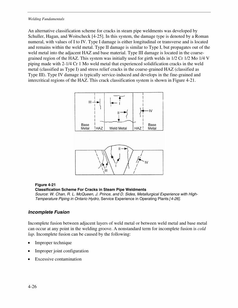
Welding Fundamentals
4-26
An alternative classification scheme for cracks in steam pipe weldments was developed by Schuller, Hagan, and Woitscheck [4-25]. In this system, the damage type is denoted by a Roman numeral, with values of I to IV. Type I damage is either longitudinal or transverse and is located and remains within the weld metal. Type II damage is similar to Type I, but propagates out of the weld metal into the adjacent HAZ and base material. Type III damage is located in the coarse-grained region of the HAZ. This system was initially used for girth welds in 1/2 Cr 1/2 Mo 1/4 V piping made with 2-1/4 Cr 1 Mo weld metal that experienced solidification cracks in the weld metal (classified as Type I) and stress relief cracks in the coarse-grained HAZ (classified as Type III). Type IV damage is typically service-induced and develops in the fine-grained and intercritical regions of the HAZ. This crack classification system is shown in Figure 4-21.
Figure 4-21 Classification Scheme For Cracks in Steam Pipe Weldments Source: W. Chan, R. L. McQueen, J. Prince, and D. Sides, Metallurgical Experience with High-Temperature Piping in Ontario Hydro, Service Experience in Operating Plants [4-26].
Incomplete Fusion
Incomplete fusion between adjacent layers of weld metal or between weld metal and base metal can occur at any point in the welding groove. A nonstandard term for incomplete fusion is cold lap. Incomplete fusion can be caused by the following:
• Improper technique
• Improper joint configuration
• Excessive contamination
Welding Fundamentals
4-27
Incomplete Joint Penetration
Incomplete joint penetration is a discontinuity associated only with groove welds, in which the weld metal does not extend entirely through the joint thickness. It is located adjacent to the weld root. Several nonstandard terms for incomplete joint penetration are inadequate penetration or IP and lack of penetration or LP. Incomplete joint penetration can be caused by the same conditions that result in incomplete fusion.
Inclusions
Inclusions are foreign solid material entrapped in the weld. Inclusions could be slag, flux, tungsten, or oxide; they can be either metallic or nonmetallic. Slag inclusions can result only when the welding process uses some type of flux shielding, such as the SMAW process. They are caused by improper manipulation of the welding electrode and insufficient cleaning between weld passes.
Tungsten inclusions are almost always associated with the GTAW process, which uses a tungsten electrode to produce an arc. The tungsten electrode makes contact with the weld puddle, the arc is interrupted, and molten metal solidifies around the tip of the electrode. The tip of the electrode breaks off and remains embedded in the final weld.
Porosity
Porosity can occur on or near the surface of the weld. It is characterized by a rounded or elongated shape resulting from gas being entrapped during solidification of the weld. Porosity is typically classified as follows:
• Scattered porosity—randomly or uniformly scattered throughout the weld
• Cluster porosity—cavities grouped together
• Linear porosity—cavities that are grouped in a straight line
Porosity is normally caused by contaminants or moisture on the surface to be welded or in the welding consumables. In the extreme temperature of the arc, these contaminants decompose and are absorbed into the weld metal. The solubility of gasses is much greater in liquid metals than in solid metals; therefore, the weld solidifies the excess dissolved gasses and can form porosity in the weld. Porosity is normally considered to be the least detrimental discontinuity because of the characteristically spherical shape and the lack of sharp end conditions.
Undercut
Undercut consists of a groove melted into the base metal adjacent to the weld toe. Undercut is generally the result of improper welding technique or parameters, although the complete elimination of undercut can be difficult.
Welding Fundamentals
4-28
References
4-1. ASME Boiler and Pressure Vessel Code, Section IX, Welding and Brazing Qualifications. American Society of Mechanical Engineers, New York. 2004.
4-2. Ø. Gröng. Metallurgical Modeling of Welding. The Institute of Materials, London, 1994.
4-3. J. F. Henry, F. V. Ellis, and C. D. Lundin. “The Effect of Inclusions, as Controlled by Flux Composition, on the Elevated Temperature Properties of Submerged-Arc Weldments,” WELDTECH 88, International Conference on Weld Failures, London, November 1988.
4-4. Gas Metal Arc Welding. Miller Electric Manufacturing Co., Appleton, WI, 1994.
4-5. R. L. O’Brien, ed. Welding Handbook, Vol. 2: Welding Processes, 8th ed., American Welding Society, Miami, 1991. p. 116
4-6. ASME B16.25, Buttwelding Ends. American Society of Mechanical Engineers, New York, 2004.
4-7. Navco Piping Datalog, Ed. 11-1984. National Valve and Manufacturing Co., Pittsburgh, PA. Ed.11-1984. BASIC-PSA, Inc., Construction Trades Press, Clinton, NC, 1984.
4-8. ASME B31.1, Code for Pressure Piping Standards: Power Piping. American Society of Mechanical Engineers, New York, 2004.
4-9. G. J. Davies and J. G. Garland, in International Metallurgical Reviews. Vol. 20, pp. 83–106 (1975).
4-10. S. A. David and J. M. Vitek, in International Materials Reviews. Vol. 34, No. 5, pp. 213–245. (1989)
4-11. A. A. B. Sugden and H. K. D. H. Bhadeshia, in Metallurgical Transactions A. Vol. 19A, pp. 669–674 (March 1988).
4-12. A. O. Klueken, Ø. Gröng, and G. Rorvik, in Metallurgical Transactions A. Vol. 21A, pp. 2047–2058 (July 1990).
4-13. J. Cisse and G. F. Bolling, in Journal of Crystal Growth, Vol. 10, pp. 67–76 (1971).
4-14. G. F. Bolling and H. Cisse, in Journal of Crystal Growth, Vol. 10, pp. 56–66 (1971).
4-15. J. Cisse and G. F. Bolling, in Journal of Crystal Growth, Vol. 11, pp. 25–28 (1971).
Welding Fundamentals
4-29
4-16. D. R. Uhlmann and B. Chalmers, in Journal of Applied Physics, Vol. 35, No. 10, pp. 2986–2993 (October 1964).
4-17. J. H. Tweed and J. F. Knott, in Metal Science, Vol. 17, pp. 45–54 (February 1983).
4-18. E. A. Almond, D. H. Timbres, and J. D. Embury. “Influence of Second Phase Particles on Brittle Fracture,” Proceedings of the Second International Conference on Fracture, Brighton, April 1969, pp. 253–264.
4-19. B. R. Keville. Welding Journal, Welding Research Supplement, Vol. 62, pp. 253s-260s (1983).
4-20. A. R. Mills, G. Thewlis, and J. A. Whiteman, in Materials Science and Technology, Vol. 3, pp. 1051–1061 (December 1987).
4-21. J. M. Dowling, J. M. Corbett, and H. W. Kerr, in Metallurgical Transactions A, Vol. 17A, pp. 1611–1623 (September 1986).
4-22. A. O. Klueken and Ø. Gröng, in Metallurgical Transactions A, Vol. 20A, pp. 1335–1349 (August 1989).
4-23. K. Easterling. Introduction to the Physical Metallurgy of Welding, 2nd ed. Linacre House, Jordan Hill, Oxford. 1992.
4-24. I. Maroef, D. L. Olson, M. Eberhart, and G. R. Edwards, “Hydrogen Trapping in Steel Weld Metal,” International Materials Review, Vol. 47, No. 4, pp. 199–223 (August 2002).
4-25. H. J. Schulleer, L. Hagan, and A. Woitscheck, “Cracking in the Weld Region of Shaped Components in Hot Steam Pipe Lines—Materials Investigations,” Der Masinenschaden, Vol. 47, pp. 97–105 (1991).
4-26. W. Chan, R. L. McQueen, J. Prince, and D. Sidey, D. “Metallurgical Experience with High Temperature Piping in Ontario Hydro,” Service Experience in Operating Plants, ASME, New York, pp. 97–105 (1991).

5-1
5 MANUFACTURE, FABRICATION, AND ERECTION
Introduction
Fabrication applies to the cutting, threading, bending, forming, and welding of individual materials into integral pieces of piping (spool pieces) ready for assembly. Fabrication can be performed in the shop or in the field. Commercial pipe fabrication shops generally have specialized equipment for bending and heat treatment; that equipment is not readily available in the field. In addition, certain welding processes, such as submerged arc welding (SAW) and many automated processes, require a fixed-position application and are more suitable for shop fabrication. As a rule, piping systems smaller than nominal pipe size (NPS) 2 are frequently field-fabricated and erected whereas piping systems NPS 2-1/2 and larger are shop-fabricated into subassemblies for field erection.
Assembly applies to the joining of piping components into their installed location as specified by the engineering design. Erection refers to the complete installation of a piping system; it consists of field assembly, fabrication, testing, and inspection.
A variety of materials are used in the construction of fossil piping systems, including pipe, forged fittings (such as Weldolet and Sockolet fittings), flanges, valves, elbows, tees, wyes, laterals, sweeps (3D/5D bends). These materials can be forged, cast, or fabricated by welding. Historically, there has been a preference to use seamless pipe and components for high-pressure and high-temperature service; however ASME B31.1 does not have a penalty associated with the allowable stress for the use of seam-welded piping or fittings. With larger-diameter piping (typically larger than 24-in. (61-cm) diameter) and as the result of scheduling impacts associated with obtaining seamless piping during construction, seam-welded piping was regularly used for the HRH system and occasionally for the main steam link piping (boiler external piping) from the 1960s into the early 1980s.
Many substitutions of seam-welded piping for the specified seamless piping occurred during construction of units, and this change might not have been reflected on the original engineering documents. Therefore, positive confirmation by etching or other means of positive verification of the use of seamless components is recommended, even when engineering drawings indicate seamless piping was used.
Manufacture, Fabrication, and Erection
5-2
Piping
Piping materials are commonly produced in standard schedules that are defined in ASME standards B36.10 and B36.19 [5-1, 5-2]. Although standard schedule pipe is frequently used for small-diameter application, for large-diameter heavy wall applications, such as main steam and HRH piping, special wall pipe is frequently used. The general requirements for pipe are contained in ASME specifications SA-530 (for carbon and alloy steel) and SA-999 (for alloy and stainless steel) [5-3, 5-4]. NPS ranges from 1/8 to 80. For NPS 14 and larger, the outside diameter in inches is equivalent to the nominal pipe size. For pipe sizes up to and including NPS 12, the outside diameter is larger than the nominal pipe size, in accordance with B36.10. For example, NPS 8 has a nominal outside diameter of 8.625 in. (219.1 mm).
Two systems are commonly used to describe standard wall thicknesses. The first system uses the following designations:
• STD, standard
• XS, extra strong (also called extra heavy)
• XXS, double extra strong (also called double extra heavy)
The second system developed from an attempt to establish a set of schedules (Sch) from Sch 5 to Sch 160. From Sch 10 through Sch 40, the schedules increase in increments of 10; from Sch 40 through Sch 160, the schedules increase in increments of 20. Each schedule corresponds to a specific wall thickness for each pipe size so the pressure-carrying capacity (pressure stress) is the same, regardless of size.
Standard wall and Sch 40 are the same through NPS 10. For sizes NPS 12 and greater, standard wall thickness is 3/8 in. (9.5 mm) and Sch 40 wall thickness increases with diameter. Extra strong and Sch 80 are the same wall thickness for pipe sizes through NPS 8. For pipe sizes greater than NPS 8, extra strong pipe has a wall thickness of 1/2 in. (12.7 mm) and Sch 80 wall thickness increases with diameter.
Functionally, pipe and tube are equivalent, and most codes allow the design of either to be selected by the sizing equation of choice by the designer. The major distinctions between pipe and tube are in the method of specifying the outside diameter, wall thickness, and tolerances.
Possibly the greatest difference between the two product forms is the magnitude of the tolerance for wall thickness. For pipes, the tolerance applies to a nominal wall thickness; for tubes, it applies to a minimum wall thickness. For ASTM/ASME piping materials, the permissible variation in wall thickness for pipe is shown in Table 5-1. Because the designer must use the minimum specified wall thickness to ensure conservatism, for seamless pipe and pipe fabricated by welding the under-tolerance always controls the selection of wall thickness. These broad tolerances can also allow pipes to be produced with poor concentricity or with multiple lobes on the ID. These geometric anomalies are more prevalent for thick-walled pipe than for thin-walled pipe.
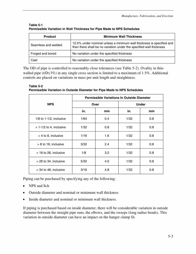
Manufacture, Fabrication, and Erection
5-3
Table 5-1 Permissible Variation in Wall Thickness for Pipe Made to NPS Schedules
Product Minimum Wall Thickness
Seamless and welded 12.5% under nominal unless a minimum wall thickness is specified and then there shall be no variation under the specified wall thickness
Forged and bored No variation under the specified thickness
Cast No variation under the specified thickness
The OD of pipe is controlled to reasonably close tolerances (see Table 5-2). Ovality in thin-walled pipe (t/D≤3%) in any single cross section is limited to a maximum of 1.5%. Additional controls are placed on variations in mass per unit length and straightness.
Table 5-2 Permissible Variation in Outside Diameter for Pipe Made to NPS Schedules
Permissible Variations In Outside Diameter
Over Under NPS
in. mm in. mm
1/8 to 1-1/2, inclusive 1/64 0.4 1/32 0.8
> 1-1/2 to 4, inclusive 1/32 0.8 1/32 0.8
> 4 to 8, inclusive 1/16 1.6 1/32 0.8
> 8 to 18, inclusive 3/32 2.4 1/32 0.8
> 18 to 26, inclusive 1/8 3.2 1/32 0.8
> 26 to 34, inclusive 5/32 4.0 1/32 0.8
> 34 to 48, inclusive 3/16 4.8 1/32 0.8
Piping can be purchased by specifying any of the following:
• NPS and Sch
• Outside diameter and nominal or minimum wall thickness
• Inside diameter and nominal or minimum wall thickness.
If piping is purchased based on inside diameter, there will be considerable variation in outside diameter between the straight pipe runs, the elbows, and the sweeps (long radius bends). This variation in outside diameter can have an impact on the hanger clamp fit.

Manufacture, Fabrication, and Erection
5-4
Historical Perspective on Piping Codes—Boiler Proper, Boiler External, and Power Piping
Piping in fossil power plants can be divided into four distinct sections: boiler proper piping, boiler external piping, nonboiler external piping, and turbine piping.
Piping that is integral with the boiler, such as downcomers, risers, and piping between headers, is classified as boiler proper piping.
Boiler external piping refers to the piping that begins where the boiler proper terminates at any of the following points:
• The first circumferential joint for welding end connections
• The face of the first flange in bolted flanged connections
• The first threaded joint in that type of connection
It extends up to and including the code-required valves, which for the main steam piping system, is the steam isolation valve or, in the absence of an isolation valve, the turbine stop valves. Historically ASME Section I maintained responsibility for the boiler proper and boiler external piping and made no distinction regarding these two portions of piping; all of it was just treated as piping. However, Section I never developed sophisticated design rules associated with piping flexibility analyses and hanger design. These additional considerations were the responsibility of the boiler manufacturer, who was free to use design approaches based on experience and good engineering practices. In the late 1960s, it became apparent the piping rules of ASME Section I were no longer adequate to cover the design of modern steam piping systems. In 1972, the responsibility of most aspects of the construction of boiler external piping was transferred to ASME B31.1.
Nonboiler external piping (piping from the boiler to the Section I code boundary) is designed and fabricated in accordance with ASME B31.1. The primary difference between boiler external and nonboiler external piping is that the quality control requirements (including authorized inspection and stamping) of Section I still apply to boiler external piping. For additional differences, refer to the specific codes.
Turbine piping is generally limited in scope, but it is the design and fabrication responsibility of turbine manufacturers as a portion of the mechanical equipment supplied by them.
Development of ASME B31.1
In July 1935, the American Tentative Standard Code for Pressure Piping (B31.1) was published. This code contained sections on power piping systems, gas and air piping, oil piping, and district heating piping. In 1942, the American Standard Code for Pressure Piping (ASA B31.1) [5-5, 5-6] was first published. Since 1942, this code has grown to meet industry changes in materials development, fabrication techniques, and inspection techniques. Revisions to this code are typically issued every three years (early editions were not issued on this schedule). The
Manufacture, Fabrication, and Erection
5-5
American National Standards Institute (ANSI) coordinates the development and use of voluntary consensus standards in the United States, including B31.1. However, the responsibility for this standard rests with the American Society of Mechanical Engineers (ASME).
Throughout the history of B31.1, materials acceptance, design, fabrication, and inspection have evolved to reflect changes, while still setting forth the minimum engineering requirements deemed necessary for safe design and construction of pressure piping. As technology has advanced, so has this standard. In particular, changes in materials or improved understanding of material properties have necessitated the inclusion of these new materials or changes in allowables for existing materials.
There have also been significant advances in the choice and availability of NDE techniques. In the American Tentative Standard Code for Pressure Piping (B31.1) issued in 1935, testing of welds consisted of a hydrostatic test at twice the normal service pressure and visual examination. If there was any reasonable doubt of the satisfactory quality of a weld, the weld could be checked by trepanning out a coupon large enough to show a clear cross section of the weld. In contrast, inspection of welds under the current edition of ASME B31.1 might require radiography, liquid penetrant, and magnetic particle testing, in addition to the specified hydrostatic test and visual examination. The specific testing methods are established based on weld type (butt weld, branch connection, or fillet weld) and service conditions (temperature and pressure).
Fabrication of Piping Components
Section 3 of this report provides an overview of the applicable material specifications for piping and piping system components. ASME B31.1 references numerous ASTM specifications and a limited number of American Petroleum Institute (API) and American Water Works Association (AWWA) standards. ASTM standards are listed as “A” (such as A335) for ferrous materials and “B” (such as B167) for nonferrous materials. ASME Section II lists “SA” and “SB” counterparts to many of the ASTM specifications. Similar material standards have been published by various international organizations such as DIN, JIS, and BSI. Specific fabrication methods are listed within these reference standards; however, this section provides a summary of fabrication methods.
ASME Section I and B31.1 draw a distinction between boiler external and nonboiler external piping [5-7, 5-8]. Both the boiler external and nonboiler external piping are fabricated in accordance with ASME B31.1; however, for boiler external piping, only materials approved for use by Section I, all of which appear in B31.1 as their ASTM counterparts, can be applied.
Boiler external piping is defined by ASME B31.1 as the piping that begins where the boiler proper terminates at any of the following points [5-8]:
• The first circumferential joint for welding end connections
• The face of the first flange in bolted flanged connections
• The first threaded joint in that type of connection
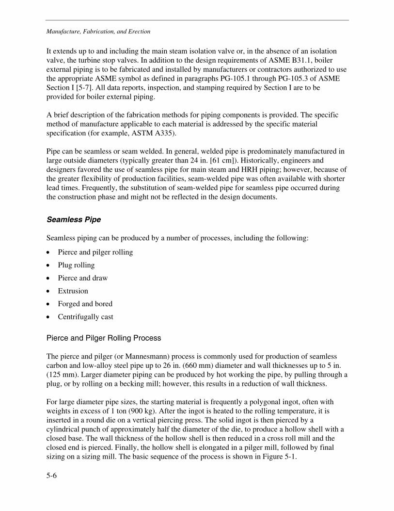
Manufacture, Fabrication, and Erection
5-6
It extends up to and including the main steam isolation valve or, in the absence of an isolation valve, the turbine stop valves. In addition to the design requirements of ASME B31.1, boiler external piping is to be fabricated and installed by manufacturers or contractors authorized to use the appropriate ASME symbol as defined in paragraphs PG-105.1 through PG-105.3 of ASME Section I [5-7]. All data reports, inspection, and stamping required by Section I are to be provided for boiler external piping.
A brief description of the fabrication methods for piping components is provided. The specific method of manufacture applicable to each material is addressed by the specific material specification (for example, ASTM A335).
Pipe can be seamless or seam welded. In general, welded pipe is predominately manufactured in large outside diameters (typically greater than 24 in. [61 cm]). Historically, engineers and designers favored the use of seamless pipe for main steam and HRH piping; however, because of the greater flexibility of production facilities, seam-welded pipe was often available with shorter lead times. Frequently, the substitution of seam-welded pipe for seamless pipe occurred during the construction phase and might not be reflected in the design documents.
Seamless Pipe
Seamless piping can be produced by a number of processes, including the following:
• Pierce and pilger rolling
• Plug rolling
• Pierce and draw
• Extrusion
• Forged and bored
• Centrifugally cast
Pierce and Pilger Rolling Process
The pierce and pilger (or Mannesmann) process is commonly used for production of seamless carbon and low-alloy steel pipe up to 26 in. (660 mm) diameter and wall thicknesses up to 5 in. (125 mm). Larger diameter piping can be produced by hot working the pipe, by pulling through a plug, or by rolling on a becking mill; however, this results in a reduction of wall thickness.
For large diameter pipe sizes, the starting material is frequently a polygonal ingot, often with weights in excess of 1 ton (900 kg). After the ingot is heated to the rolling temperature, it is inserted in a round die on a vertical piercing press. The solid ingot is then pierced by a cylindrical punch of approximately half the diameter of the die, to produce a hollow shell with a closed base. The wall thickness of the hollow shell is then reduced in a cross roll mill and the closed end is pierced. Finally, the hollow shell is elongated in a pilger mill, followed by final sizing on a sizing mill. The basic sequence of the process is shown in Figure 5-1.
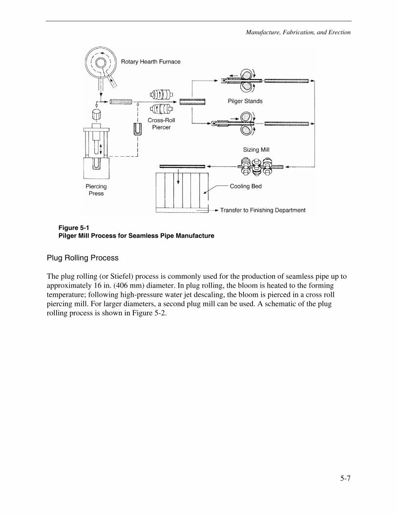
Manufacture, Fabrication, and Erection
5-7
Figure 5-1 Pilger Mill Process for Seamless Pipe Manufacture
Plug Rolling Process
The plug rolling (or Stiefel) process is commonly used for the production of seamless pipe up to approximately 16 in. (406 mm) diameter. In plug rolling, the bloom is heated to the forming temperature; following high-pressure water jet descaling, the bloom is pierced in a cross roll piercing mill. For larger diameters, a second plug mill can be used. A schematic of the plug rolling process is shown in Figure 5-2.
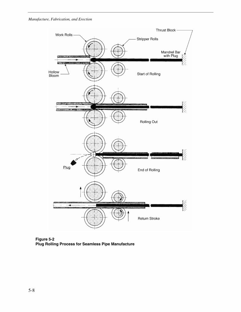
Manufacture, Fabrication, and Erection
5-8
Figure 5-2 Plug Rolling Process for Seamless Pipe Manufacture
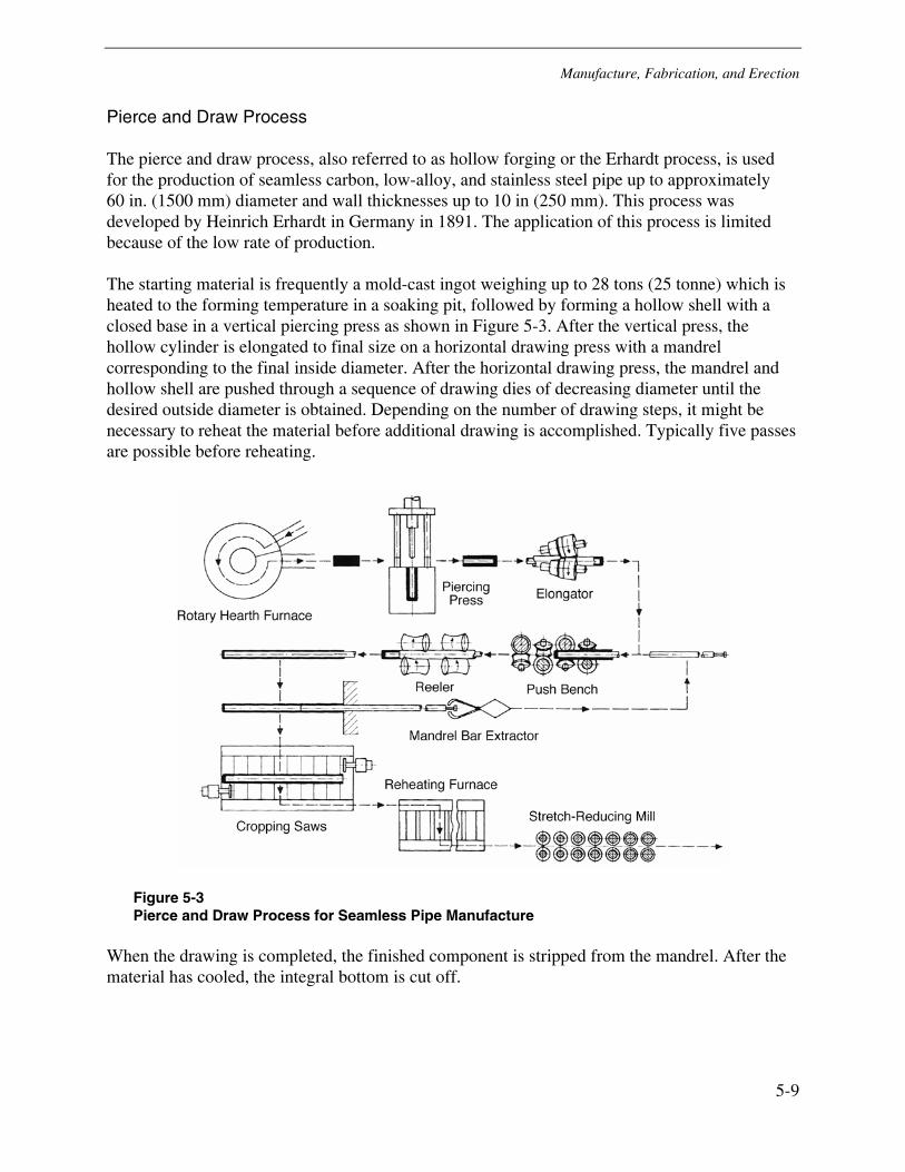
Manufacture, Fabrication, and Erection
5-9
Pierce and Draw Process
The pierce and draw process, also referred to as hollow forging or the Erhardt process, is used for the production of seamless carbon, low-alloy, and stainless steel pipe up to approximately 60 in. (1500 mm) diameter and wall thicknesses up to 10 in (250 mm). This process was developed by Heinrich Erhardt in Germany in 1891. The application of this process is limited because of the low rate of production.
The starting material is frequently a mold-cast ingot weighing up to 28 tons (25 tonne) which is heated to the forming temperature in a soaking pit, followed by forming a hollow shell with a closed base in a vertical piercing press as shown in Figure 5-3. After the vertical press, the hollow cylinder is elongated to final size on a horizontal drawing press with a mandrel corresponding to the final inside diameter. After the horizontal drawing press, the mandrel and hollow shell are pushed through a sequence of drawing dies of decreasing diameter until the desired outside diameter is obtained. Depending on the number of drawing steps, it might be necessary to reheat the material before additional drawing is accomplished. Typically five passes are possible before reheating.
Figure 5-3 Pierce and Draw Process for Seamless Pipe Manufacture
When the drawing is completed, the finished component is stripped from the mandrel. After the material has cooled, the integral bottom is cut off.
Manufacture, Fabrication, and Erection
5-10
Extrusion Process
The extrusion process, also referred to as the Ugine Sejournet extrusion process, is used for high-alloy pipe. In this process, a descaled billet is heated to the forming temperature and placed in a vertical press with an extrusion die at its bottom. The billet is pressed with a hydraulic ram and then pierced with a mandrel to produce a cylinder. Finally a ram is activated to apply pressure to the billet and extrude it through the annulus formed between the mandrel and the die. This process can be used to produce heavy wall pipe with diameters up to approximately 48 in. (1220 mm) with wall thicknesses up to approximately 6 in (152 mm).
Forged and Bored
In the forged and bored process, a billet is heated to the forging temperature and forged to make a hollow shell using heavy presses or forging hammers. The ID and OD of this forging will be slightly smaller and larger, respectively, than the finished dimensions. The rough forged cylinder is then lathe turned to the desired OD, and the ID is bored to the specified inside dimension.
At least one major boiler manufacturer frequently lathe turned the OD of seam-welded pipe used for link (boiler external) piping. Because forged and bored piping is also lathe turned, the presence of turn marks on the OD surface of the pipe might not be sufficient to indicate the pipe is seam welded.
Centrifugally Cast
Centrifugally cast pipe is made by pouring molten metal into a rotating mold and continuing to spin the mold as the metal cools and solidifies. Subsequently the pipe is machined on both the inner and outer surfaces.
Welded Pipe
Welded pipe is produced by forming a cylinder from a plate and fusion welding the seam. The earliest method of pipe production was forge welding, which was originally patented by James Whitehouse in 1825. In forge welding, the cylinder is formed, the mating edges are heated and mechanically brought together in a draw bench. With the development and improvement of electric arc welding following World War II, these processes quickly gained acceptance and became widely used for the production of large diameter pipe. A number of welding processes can be used in the production of seam-welded pipe, including GTAW and GMAW; however, the primary welding process for heavy wall power piping is SAW.
The production of seam-welded pipe starts with the formation of a cylinder from plate. The forming can be accomplished using a C-ing press, U-ing and O-ing press, or a three-roll bending process. The U-ing and O-ing presses are the most common for large-diameter heavy wall pipe.
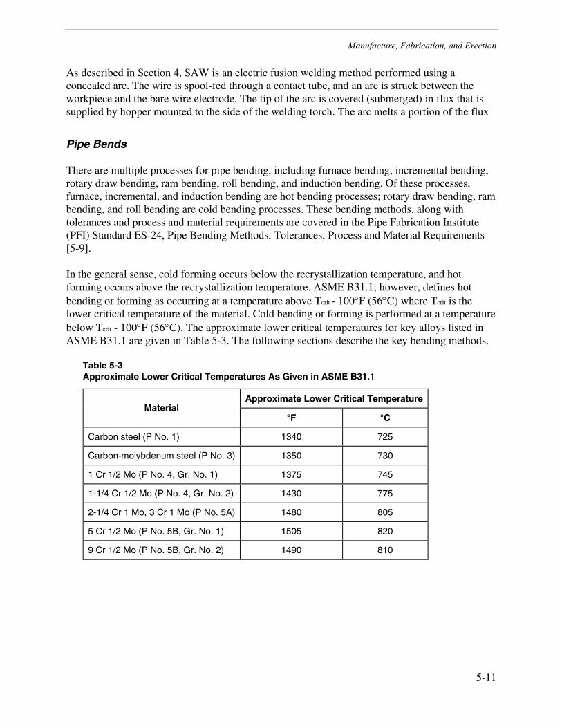
Manufacture, Fabrication, and Erection
5-11
As described in Section 4, SAW is an electric fusion welding method performed using a concealed arc. The wire is spool-fed through a contact tube, and an arc is struck between the workpiece and the bare wire electrode. The tip of the arc is covered (submerged) in flux that is supplied by hopper mounted to the side of the welding torch. The arc melts a portion of the flux
Pipe Bends
There are multiple processes for pipe bending, including furnace bending, incremental bending, rotary draw bending, ram bending, roll bending, and induction bending. Of these processes, furnace, incremental, and induction bending are hot bending processes; rotary draw bending, ram bending, and roll bending are cold bending processes. These bending methods, along with tolerances and process and material requirements are covered in the Pipe Fabrication Institute (PFI) Standard ES-24, Pipe Bending Methods, Tolerances, Process and Material Requirements [5-9].
In the general sense, cold forming occurs below the recrystallization temperature, and hot forming occurs above the recrystallization temperature. ASME B31.1; however, defines hot bending or forming as occurring at a temperature above Tcrit - 100°F (56°C) where Tcrit is the lower critical temperature of the material. Cold bending or forming is performed at a temperature below Tcrit - 100°F (56°C). The approximate lower critical temperatures for key alloys listed in ASME B31.1 are given in Table 5-3. The following sections describe the key bending methods.
Table 5-3 Approximate Lower Critical Temperatures As Given in ASME B31.1
Approximate Lower Critical Temperature Material
°F °C
Carbon steel (P No. 1) 1340 725
Carbon-molybdenum steel (P No. 3) 1350 730
1 Cr 1/2 Mo (P No. 4, Gr. No. 1) 1375 745
1-1/4 Cr 1/2 Mo (P No. 4, Gr. No. 2) 1430 775
2-1/4 Cr 1 Mo, 3 Cr 1 Mo (P No. 5A) 1480 805
5 Cr 1/2 Mo (P No. 5B, Gr. No. 1) 1505 820
9 Cr 1/2 Mo (P No. 5B, Gr. No. 2) 1490 810
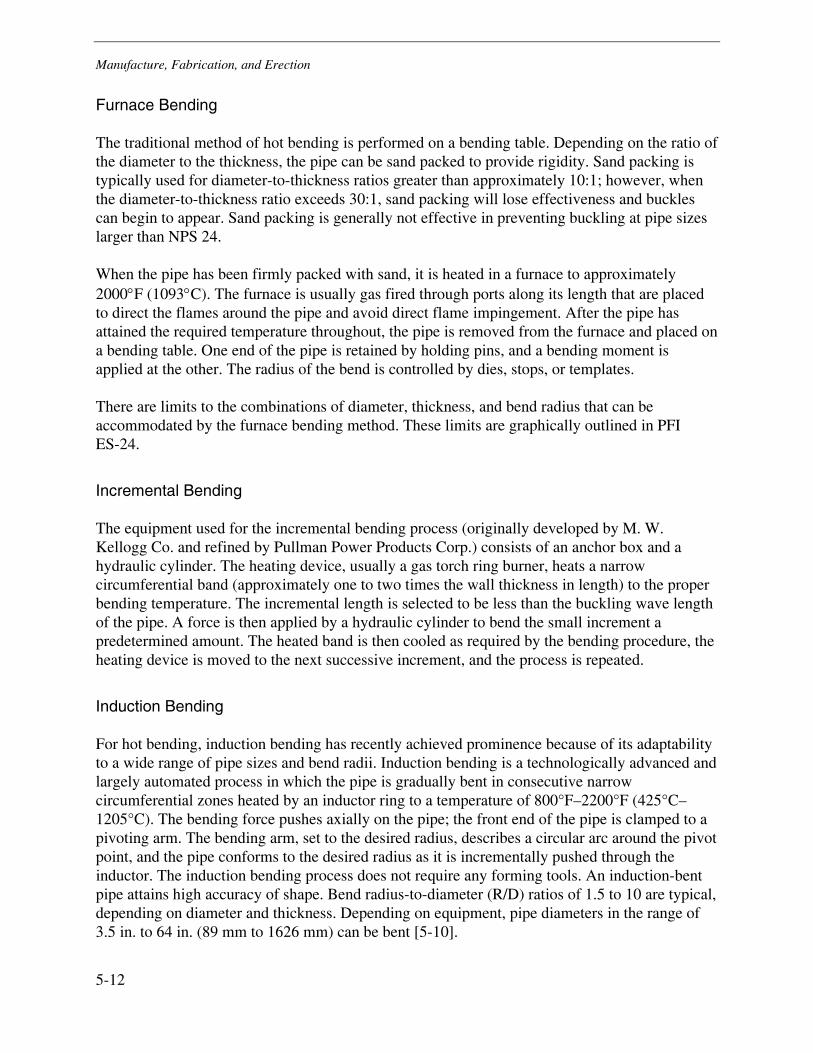
Manufacture, Fabrication, and Erection
5-12
Furnace Bending
The traditional method of hot bending is performed on a bending table. Depending on the ratio of the diameter to the thickness, the pipe can be sand packed to provide rigidity. Sand packing is typically used for diameter-to-thickness ratios greater than approximately 10:1; however, when the diameter-to-thickness ratio exceeds 30:1, sand packing will lose effectiveness and buckles can begin to appear. Sand packing is generally not effective in preventing buckling at pipe sizes larger than NPS 24.
When the pipe has been firmly packed with sand, it is heated in a furnace to approximately 2000°F (1093°C). The furnace is usually gas fired through ports along its length that are placed to direct the flames around the pipe and avoid direct flame impingement. After the pipe has attained the required temperature throughout, the pipe is removed from the furnace and placed on a bending table. One end of the pipe is retained by holding pins, and a bending moment is applied at the other. The radius of the bend is controlled by dies, stops, or templates.
There are limits to the combinations of diameter, thickness, and bend radius that can be accommodated by the furnace bending method. These limits are graphically outlined in PFI ES-24.
Incremental Bending
The equipment used for the incremental bending process (originally developed by M. W. Kellogg Co. and refined by Pullman Power Products Corp.) consists of an anchor box and a hydraulic cylinder. The heating device, usually a gas torch ring burner, heats a narrow circumferential band (approximately one to two times the wall thickness in length) to the proper bending temperature. The incremental length is selected to be less than the buckling wave length of the pipe. A force is then applied by a hydraulic cylinder to bend the small increment a predetermined amount. The heated band is then cooled as required by the bending procedure, the heating device is moved to the next successive increment, and the process is repeated.
Induction Bending
For hot bending, induction bending has recently achieved prominence because of its adaptability to a wide range of pipe sizes and bend radii. Induction bending is a technologically advanced and largely automated process in which the pipe is gradually bent in consecutive narrow circumferential zones heated by an inductor ring to a temperature of 800°F–2200°F (425°C–1205°C). The bending force pushes axially on the pipe; the front end of the pipe is clamped to a pivoting arm. The bending arm, set to the desired radius, describes a circular arc around the pivot point, and the pipe conforms to the desired radius as it is incrementally pushed through the inductor. The induction bending process does not require any forming tools. An induction-bent pipe attains high accuracy of shape. Bend radius-to-diameter (R/D) ratios of 1.5 to 10 are typical, depending on diameter and thickness. Depending on equipment, pipe diameters in the range of 3.5 in. to 64 in. (89 mm to 1626 mm) can be bent [5-10].
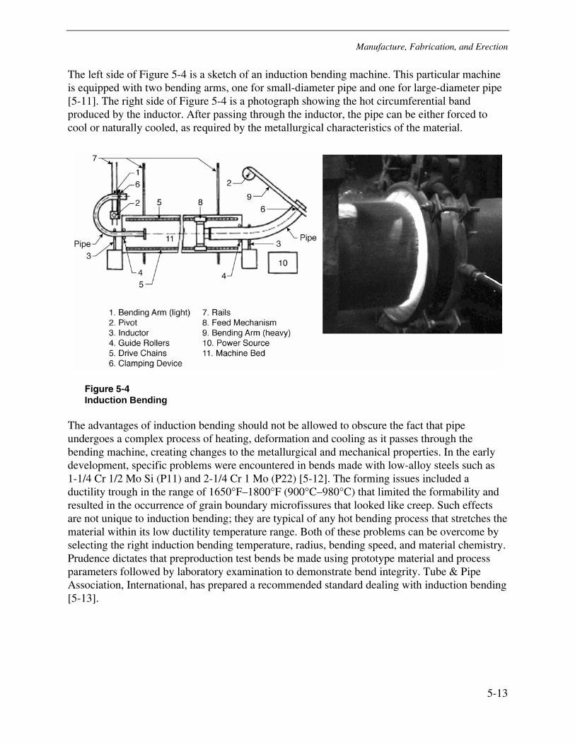
Manufacture, Fabrication, and Erection
5-13
The left side of Figure 5-4 is a sketch of an induction bending machine. This particular machine is equipped with two bending arms, one for small-diameter pipe and one for large-diameter pipe [5-11]. The right side of Figure 5-4 is a photograph showing the hot circumferential band produced by the inductor. After passing through the inductor, the pipe can be either forced to cool or naturally cooled, as required by the metallurgical characteristics of the material.
Figure 5-4 Induction Bending
The advantages of induction bending should not be allowed to obscure the fact that pipe undergoes a complex process of heating, deformation and cooling as it passes through the bending machine, creating changes to the metallurgical and mechanical properties. In the early development, specific problems were encountered in bends made with low-alloy steels such as 1-1/4 Cr 1/2 Mo Si (P11) and 2-1/4 Cr 1 Mo (P22) [5-12]. The forming issues included a ductility trough in the range of 1650°F–1800°F (900°C–980°C) that limited the formability and resulted in the occurrence of grain boundary microfissures that looked like creep. Such effects are not unique to induction bending; they are typical of any hot bending process that stretches the material within its low ductility temperature range. Both of these problems can be overcome by selecting the right induction bending temperature, radius, bending speed, and material chemistry. Prudence dictates that preproduction test bends be made using prototype material and process parameters followed by laboratory examination to demonstrate bend integrity. Tube & Pipe Association, International, has prepared a recommended standard dealing with induction bending [5-13].
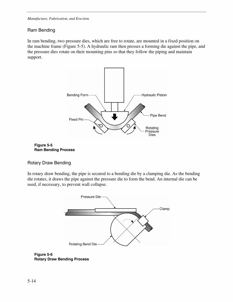
Manufacture, Fabrication, and Erection
5-14
Ram Bending
In ram bending, two pressure dies, which are free to rotate, are mounted in a fixed position on the machine frame (Figure 5-5). A hydraulic ram then presses a forming die against the pipe, and the pressure dies rotate on their mounting pins so that they follow the piping and maintain support.
Figure 5-5 Ram Bending Process
Rotary Draw Bending
In rotary draw bending, the pipe is secured to a bending die by a clamping die. As the bending die rotates, it draws the pipe against the pressure die to form the bend. An internal die can be used, if necessary, to prevent wall collapse.
Figure 5-6 Rotary Draw Bending Process
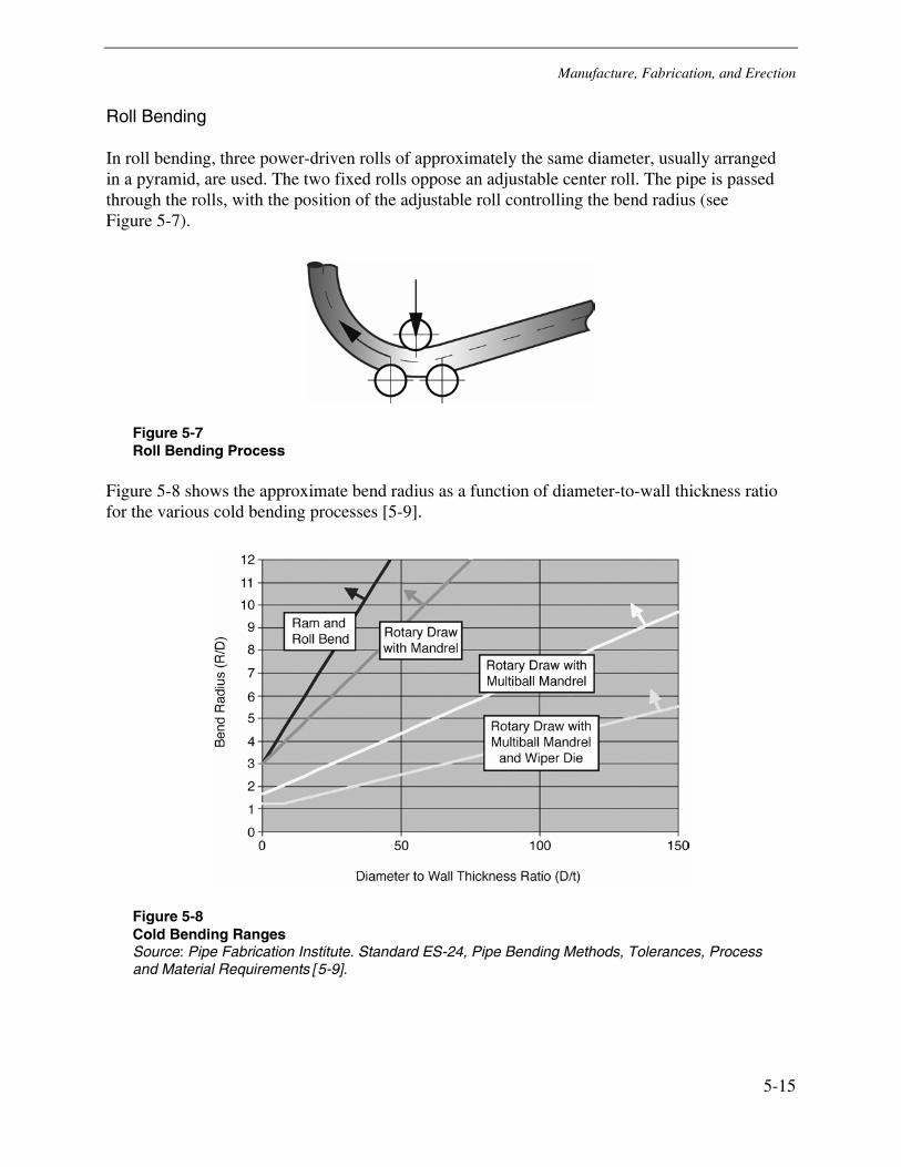
Manufacture, Fabrication, and Erection
5-15
Roll Bending
In roll bending, three power-driven rolls of approximately the same diameter, usually arranged in a pyramid, are used. The two fixed rolls oppose an adjustable center roll. The pipe is passed through the rolls, with the position of the adjustable roll controlling the bend radius (see Figure 5-7).
Figure 5-7 Roll Bending Process
Figure 5-8 shows the approximate bend radius as a function of diameter-to-wall thickness ratio for the various cold bending processes [5-9].
Figure 5-8 Cold Bending Ranges Source: Pipe Fabrication Institute. Standard ES-24, Pipe Bending Methods, Tolerances, Process and Material Requirements [5-9].
Manufacture, Fabrication, and Erection
5-16
Pipe Fittings
Fittings for pipe can be wrought (seamless and welded construction), forged, or cast. Fittings can include short radius elbows, bifurcations (wyes), laterals, and tees.
Forgings are typically manufactured in accordance with ASME/ASTM SA182/A182. This standard covers carbon-molybdenum and chromium-molybdenum low-alloy steels as well as martensitic, ferritic, duplex, and austenitic stainless steels. Depending on the grade, post-forging heat treatment can consist of annealing, normalizing and tempering, or solution treating and quenching. Carbon steel forgings are manufactured in accordance with ASME/ASTM SA105/A105. Depending on the application, carbon steel forgings can be left as forged or can be heat treated by annealing, normalizing, normalizing and tempering, or quenching and tempering.
Wrought fittings are typically manufactured in accordance with ASME/ASTM SA234/A234. This standard covers carbon, carbon-molybdenum, and chromium-molybdenum alloy steels. Wrought austenitic stainless steel fittings are manufactured in accordance with ASME/ASTM SA403/A403. The material for fittings can consist of forgings, bars, plates, and seamless or fusion-welded tubular products. Welded tubular products can contain one or two welds depending on the method of manufacture. Clam-shell elbows contain a seam weld along both the extrados and intrados of the elbow. If seam-welded pipe was used, it might contain only a single weld. For elbows, this weld is typically located along the intrados, but there are no specific requirements specifying this location, and the weld can be located at any position circumferentially. Depending on the grade, post-forming heat treatment can consist of hot-formed, annealed, normalized, normalized and tempered, subcritically stress relieved, or solution annealed.
References
5-1. ANSI B36.10, Welded and Seamless Wrought Iron Pipe. American National Standards Institute. Washington, DC.
5-2. ANSI B36.19, Stainless Steel Pipe. American National Standards Institute. Washington, DC.
5-3. ASME SA530, ASME Standard Specification for General Requirements for Specialized Carbon and Alloy Steel Pipe. American Society of Mechanical Engineers. New York.
5-4. ASME SA999, General Requirements for Alloy and Stainless Steel Pipe, American Society of Mechanical Engineers. New York.
5-5. ASA B31.1, American Tentative Standard Code for Pressure Piping. American Standards Association, 1935.
5-6. ASA B31.1, American Standard Code for Pressure Piping. American Standards Association, 1942.
Manufacture, Fabrication, and Erection
5-17
5-7. ASME Boiler and Pressure Vessel Code, Section I, Power Boilers. American Society of Mechanical Engineers, New York. 2004.
5-8. ASME B31.1, Code for Pressure Piping Standards: Power Piping. American Society of Mechanical Engineers, New York, 2004.
5-9. PFI ES-24, Pipe Bending Methods, Tolerances, Process and Material Requirements. Pipe Fabrication Institute, New York, 2003.
5-10. M. L. Nayyar. Piping Handbook. Seventh Edition, McGraw-Hill, 2000.
5-11. B. Hahn, B. Vandenberghe, J. C. Valliant, and W. Bendick. The WB 36 Book (15NiCuMo) for Feedwater Systems. Vallourec & Mannesmann Tubes, 2002.
5-12. John Reason, “Watch Materials Properties During Induction Bending.” Power Magazine, December 1987, pp. 33-34.
5-13. Recommended Standards for Induction Bending of Pipe and Tube. Tube & Pipe Association, International, Rockford, IL, 1998.


6-1
6 OPERATION
This section will be included in a future update.

7-1
7 DAMAGE MECHANISMS AND MODELS
Introduction
In general, high-energy piping service experience indicates that damage development and cracking have been encountered at specific base metal locations and at weldments. Indeed, several examples of catastrophic rupture have been recorded in which fracture has resulted in widespread damage. Fortunately, the number of catastrophic failures is relatively small. However, in many other cases, damage development has resulted in steam leaks, or significant cracking has been found during plant inspections. In some situations, these problems have been related to deficiencies during welding or manufacture. However, in the majority of cases, damage developed as a result of long-term, in-service mechanisms.
The obvious goal for the electric generation industry as a whole is to predict and prevent failures before they occur. The fundamental step in predicting a component’s effective lifespan and preventing failures is to develop a comprehensive understanding of the potential damage mechanisms affecting the component. With an estimate of current damage, rules for damage accumulation, and failure criteria, the remaining life of a component can be assessed. However, for both the dispositioning of defects and the assessment of damage accumulation, it is important to identify the mechanism responsible for damage and, if possible, to determine the root cause of the damage. A root cause analysis is significantly more than simply identifying the mechanism. Root cause analysis should establish the reasons for the accelerated damage, so that appropriate remedial action can be undertaken to minimize the risk of future problems.
Which damage mechanisms are active depends on the component, the local operating conditions, and the materials and methods used in fabrication. Frequently, two or more damage mechanisms are at work simultaneously on a component. Table 7-1 lists common damage mechanisms for various components and locations.
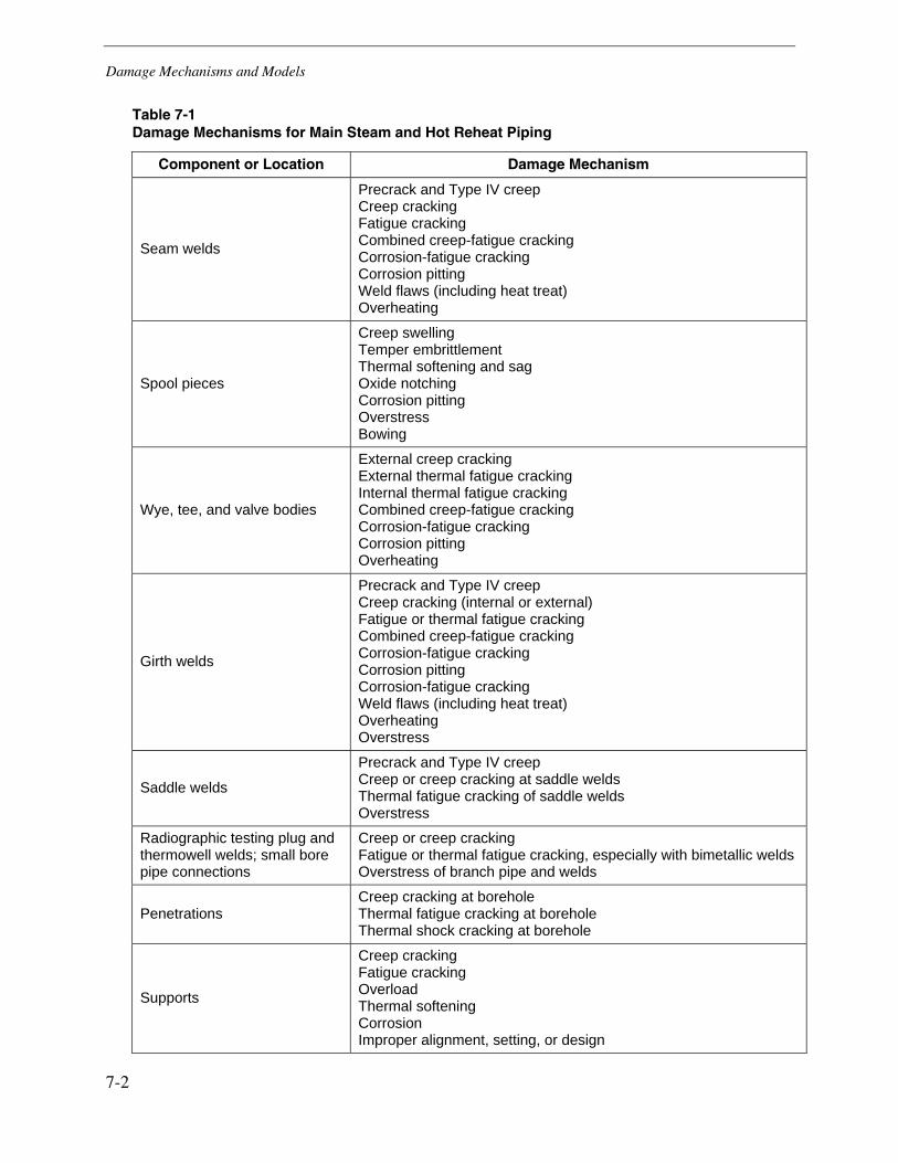
Damage Mechanisms and Models
7-2
Table 7-1 Damage Mechanisms for Main Steam and Hot Reheat Piping
Component or Location Damage Mechanism
Seam welds
Precrack and Type IV creep Creep cracking Fatigue cracking Combined creep-fatigue cracking Corrosion-fatigue cracking Corrosion pitting Weld flaws (including heat treat) Overheating
Spool pieces
Creep swelling Temper embrittlement Thermal softening and sag Oxide notching Corrosion pitting Overstress Bowing
Wye, tee, and valve bodies
External creep cracking External thermal fatigue cracking Internal thermal fatigue cracking Combined creep-fatigue cracking Corrosion-fatigue cracking Corrosion pitting Overheating
Girth welds
Precrack and Type IV creep Creep cracking (internal or external) Fatigue or thermal fatigue cracking Combined creep-fatigue cracking Corrosion-fatigue cracking Corrosion pitting Corrosion-fatigue cracking Weld flaws (including heat treat) Overheating Overstress
Saddle welds
Precrack and Type IV creep Creep or creep cracking at saddle welds Thermal fatigue cracking of saddle welds Overstress
Radiographic testing plug and thermowell welds; small bore pipe connections
Creep or creep cracking Fatigue or thermal fatigue cracking, especially with bimetallic weldsOverstress of branch pipe and welds
Penetrations Creep cracking at borehole Thermal fatigue cracking at borehole Thermal shock cracking at borehole
Supports
Creep cracking Fatigue cracking Overload Thermal softening Corrosion Improper alignment, setting, or design

Damage Mechanisms and Models
7-3
Because damage depends on factors specific to a generating unit (design, operating modes, water chemistry, and fuel characteristics), each unit and its components must be treated individually to obtain realistic life assessments. Determining the degree of damage to a component typically requires the application of one or more inspection methods. Assessing the rate of damage accumulation implies that the process of monitoring damage will be performed repeatedly or be ongoing. Determining the degree of damage required to cause failure requires the use of one or more analytical or experimental techniques. In some cases, it is advisable to adopt a conservative approach. A component can be considered to have failed when it is more sensible economically to repair or replace it rather than continuing to operate with a high risk of catastrophic failure.
Depending on the active damage mechanism, several techniques and software programs can be used to predict the remaining life for a component. The lifetime of any high-energy piping component is a complex function of factors such as operating conditions (stresses, temperatures, and environment), geometry (piping layout, support placement, wall thickness), material, and damage type. The uncertainties associated with life assessment such as actual material properties, fabrication tolerances, and stress states make it extremely difficult to determine actual component life, even with good analysis techniques. As a result, life assessment is often focused on helping to set inspection intervals and is used as input to deciding whether to repair or replace a component.
For those conditions in which crack initiation alone constitutes failure (or is a substantial portion of the useful life of a component), conventional NDE methods and fracture mechanics analysis are not helpful. This primarily occurs in very thin section components, in highly stressed components, or in materials that have rapid crack growth rates or that are highly embrittled. Techniques used for these conditions include calculations based on history, extrapolations of failure statistics, strain measurements, accelerated mechanical testing, microstructural evaluations, oxide scale growth, hardness measurements, and advanced NDE techniques.
In most instances of cracking in high-energy piping sections, the critical crack size at failure is sufficiently large that NDE for crack sizing along with crack growth analysis for life assessment is appropriate. This is then followed by periodic monitoring of the progression of damage and benchmarking of analysis results against field observations. In these cases, cracks are tolerated, crack initiation can occur early in the total life of the component (10%–20%), and retirement is based on the economics of repeated repairs and the growth of a crack to critical size. In this case, excessive concern with refining the damage rules is unwarranted. There are at least two exceptions to the general observation, however. If a material has suffered severe embrittlement, crack initiation approaches are important. A second exception is in Type IV cracking (creep cracking), in which cracks that form along the fusion line of the weld–base metal interface are hard to detect and can link up to grow rapidly.
Damage Mechanisms and Models
7-4
A survey of U.S. repair technologies and practices for headers, high-temperature piping, and turbine casings has been reported [7-1, 7-2]. The results for life assessment showed the following:
• Over half of the utilities indicated that they used some form of in-house life assessment. However, only two used computer software for life assessment.
• The level of damage (for example, creep cavitation, embrittlement, and so forth) at which a component is considered nonrepairable varied considerably. Slightly more than 30% of the utilities indicated that some minimum level of metallurgical damage was established. However, 30% of utilities indicated that cost or economics often took priority over metallurgical or technical considerations in their decision making.
• Factors included in repair or replace decisions included the following:
– Contract cost of repair versus cost of replacement
– Requirements for analysis and testing
– Estimated remaining life of component before and after repairs
– Trade-offs among cost, safety, risk, and availability
A few other general observations about life assessment are the following:
• The critical crack size to cause failure is not a constant in high-energy piping but will decrease with service exposure as embrittlement occurs. The use of conventional NDE techniques (see Section 10) is based on the premise that a detectable crack will form and grow slowly enough to permit periodic inspection, repair, or retirement before a crack grows to a critical size.
• The failure scenario must be understood. In thick-section components, cracks can grow by creep or creep-fatigue at high temperature, but failure can occur by brittle fracture at low temperatures during startup and shutdown sequences. Hydrostatic tests are often found to be the limiting condition for fracture. Ductile tearing or plastic collapse at operating conditions can also determine the limiting flaw size.
• Weld-related cracking in high-energy piping requires attention from a life assessment viewpoint because the deterioration in susceptible locations often precedes deterioration in the piping base material. Damage in welds can thus serve as an precursor index to damage and remaining life in the base metal.
• The validity of any damage approach must be evaluated with reference to the material and service conditions. As a result, tailored, case-specific approaches should be used rather than relying on generalized laboratory results.
• A considerable amount of materials data has been accumulated from service-exposed material. In the absence of component-specific data, the ex-service property databases are very useful for life assessment.
Damage Mechanisms and Models
7-5
The following subsections outline information about specific damage mechanisms that can affect high-energy piping. Additional information regarding these topics and applicable assessment methods can be found in the following EPRI reports [7-3–7-9]:
• Boiler Tube Failure Metallurgical Guide, Volumes 1–2 (TR-102433)
• Boiler Tube Failure: Theory and Practice, Volumes 1–3 (TR-105261)
• Condition Assessment Guidelines for Fossil Fuel Power Plant Components (GS-6724)
• Guidelines for Controlling Flow-Accelerated Corrosion in Fossil and Combined Cycle Plants (1008082)
• Life Assessment of Boiler Pressure Parts, Volumes 1–5 (TR-103377)
• Metallurgical Guidebook for Fossil Plant Boilers (1004509)
• Remaining Life Assessment of Austenitic Stainless Steel Superheater and Reheater Tubing (1004517)
Creep
Introduction
Creep is a time-dependent deformation and fracture of metal components that takes place at elevated temperatures under the application of a load. Typical loading in a high-energy piping system can include the weight of the pipe and the operating pressure stress. For common engineering steels, creep becomes a significant concern only at temperatures exceeding approximately half of the absolute melting point. For the stress levels encountered in most power generating plants, creep is not a concern for low-alloy steels below approximately 700°F (370°C), and for austenitic alloys below approximately 1000°F (538°C).
Curves that plot creep strain versus time have traditionally been described using three stages of creep: primary, secondary, and tertiary (see Figure 7-1). Each stage can be characterized in terms of creep rate (the change in strain with time). Primary creep is a period of relatively high but decreasing creep rate during which the material’s creep resistance increases by work hardening; the strain rate is continuously changing. No observable microstructural changes occur during the primary period, and there is no mechanical degradation of the material. Secondary creep is a period of essentially constant creep rate. Tertiary creep is a period of increasing creep rate; the material fails at the end of this period.
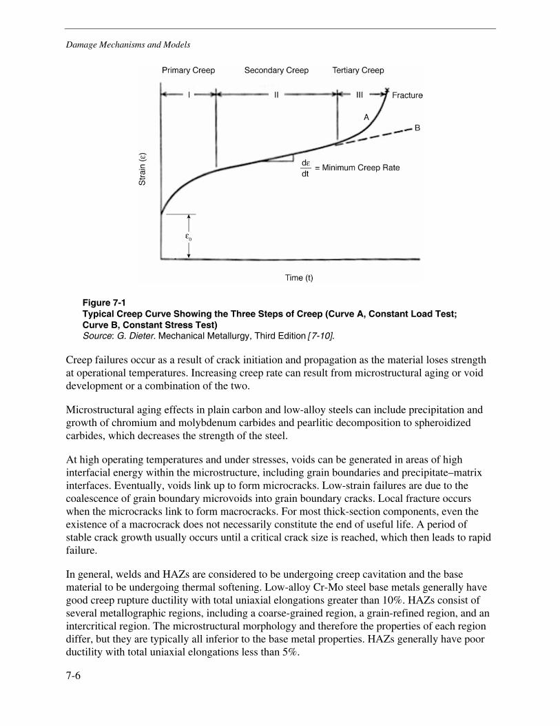
Damage Mechanisms and Models
7-6
Figure 7-1 Typical Creep Curve Showing the Three Steps of Creep (Curve A, Constant Load Test; Curve B, Constant Stress Test) Source: G. Dieter. Mechanical Metallurgy, Third Edition [7-10].
Creep failures occur as a result of crack initiation and propagation as the material loses strength at operational temperatures. Increasing creep rate can result from microstructural aging or void development or a combination of the two.
Microstructural aging effects in plain carbon and low-alloy steels can include precipitation and growth of chromium and molybdenum carbides and pearlitic decomposition to spheroidized carbides, which decreases the strength of the steel.
At high operating temperatures and under stresses, voids can be generated in areas of high interfacial energy within the microstructure, including grain boundaries and precipitate–matrix interfaces. Eventually, voids link up to form microcracks. Low-strain failures are due to the coalescence of grain boundary microvoids into grain boundary cracks. Local fracture occurs when the microcracks link to form macrocracks. For most thick-section components, even the existence of a macrocrack does not necessarily constitute the end of useful life. A period of stable crack growth usually occurs until a critical crack size is reached, which then leads to rapid failure.
In general, welds and HAZs are considered to be undergoing creep cavitation and the base material to be undergoing thermal softening. Low-alloy Cr-Mo steel base metals generally have good creep rupture ductility with total uniaxial elongations greater than 10%. HAZs consist of several metallographic regions, including a coarse-grained region, a grain-refined region, and an intercritical region. The microstructural morphology and therefore the properties of each region differ, but they are typically all inferior to the base metal properties. HAZs generally have poor ductility with total uniaxial elongations less than 5%.
Damage Mechanisms and Models
7-7
The following subsections describe the various stages of creep failure, including crack initiation and crack growth, as well as current creep modeling efforts.
Crack Initiation
All engineering metals are essentially composed of many metallic crystals, which are three-dimensional matrices of atoms following the repetitive order of the primary alloying element (that is, iron for steels). When a stress is applied, the crystalline atomic matrix of any material has the following three basic options to respond to the stress:
• The matrix can elastically deform. That is, the atoms in the matrix stretch to accommodate the applied stress. This occurs at low values of applied stress.
• If the applied stress exceeds the ability of the atoms to stretch, then the crystal can plastically deform (change shape) by moving atoms from one location to another.
• If the applied stress exceeds the ability of the atoms to stretch or to change the crystal shape, the atoms can break their bonds, separate, and form two new surfaces. This is commonly called cracking.
Which option the atoms of the metallic crystals follow depends on the inherent strength of the alloy, the amount of stress applied, how quickly that stress is applied, and the operational temperature.
Creep is time-dependent deformation that occurs at relatively constant stress levels but at elevated temperatures. Increases in operational temperature produce several key microstructural changes that decrease the strength of the alloy and its ability to resist applied stresses, including the following:
• Metallic atom matrices become more energized, and it becomes easier for the atoms to move and therefore easier for the crystal to change shape to accommodate the applied stress. Therefore, the strength (which is the ability of the crystal to resist deformation) decreases as the temperature increases.
• Many high-temperature alloys depend on precipitated particles for their strength. Precipitates are second-phase particles (a separate atomic matrix) within the basic atomic matrix of the crystal. They are formed when a sufficient number of alloying atoms of the nonprimary element collect to form a new local matrix that differs from the overall crystal matrix. The nonprimary alloying elements do not truly fit into the primary element atomic matrix. The new matrix accommodates the size and electronic difference of the nonprimary alloying elements. Because diffusion of atoms is easier, it is easier for nonprimary alloying elements to collect and precipitate second-phase particles at elevated temperatures. The particles grow as more atoms collect at the particles’ interfaces. Small particles become larger particles by collecting the atoms of other smaller particles—the larger particles get larger, and the smaller particles dissolve. It is harder to move atoms through a “forest” of many small particles than it is to
Damage Mechanisms and Models
7-8
move them through a lower number of large particles. (As an analogy, imagine how much harder it is to walk through a dense forest of small-diameter trees versus walking through a sparsely populated forest of large-diameter trees.) Therefore as the particles coarsen at elevated temperatures, the metallic crystals lose strength.
• Many of the phase constituents that give steel higher strength—such as like pearlite, bainite, or martensite—are metastable phases that will reorganize themselves into lower-strength microstructural constituents if given a sufficient amount of time at a diffusion-activated temperature.
These microstructural changes can lead to losses in high-temperature strength. As a tensile load is applied to the weakened microstructure, voids can be created at phase interfaces (that is, grain boundaries, second-phase particle boundaries, phase boundaries), which are areas with the lowest cohesive forces. The number and size of the voids depend on the amount of load, the amount of thermal energy, the number of void initiation sites, and the strength of the microstructural interfaces. The formation of voids and the interlinking of these voids (microvoid coalescence) is the fundamental crack initiation mechanism for creep degradation. Therefore, creep cracks form where the microvoids initiate and coalesce.
Crack Growth
Cracks typically grow under tensile loading. When a large enough microcrack has been initiated (no longer just a few coalesced voids), it acts as a sharp stress concentrator. The stress at the very tip of the crack is amplified to levels significantly higher than the average applied stress (several orders of magnitude higher), and therefore it generally takes less stress energy to extend a crack than to plastically deform the material. Thus, when a crack is initiated, it tends to grow under continued applied loading. The rate of crack growth depends on the level of loading and the material’s inherent resistance to crack extension, which in turn depends on the material’s microstructural morphology, and specifically can be related to the strength and fracture toughness of the material. Because it can take time for a crack to propagate through the material, the presence of a crack does not necessarily mean the end of useful component life.
Analytical Techniques
Creep Deformation—Life Models
Several mathematical models can be used to predict the operational creep life for a component under specific operating conditions (time at temperature). The models vary in complexity. For a variety of alloys, there is a simple relationship between minimum creep rate, ε, and time to rupture, tr, termed the Monkman-Grant correlation, shown in Equation 7-1 [7-11].
log tr = m log ε Eq. 7-1
Damage Mechanisms and Models
7-9
In Equation 7-1, m is a constant. For most materials, m has a value approaching unity, so that the equation can be rewritten as shown in Equation 7-2.
ε tr = constant Eq. 7-2
Estimates of rupture life can be obtained with this equation for components removed from service, given creep rate from dimensional measurements, or from short-term laboratory tests (isostress tests), to give estimates of rupture life. Extrapolation to determine the probable time to rupture at service temperatures is then typically performed. The most common accelerated test for creep is the creep-to-failure test, in which engineering stress (load normalized by initial specimen dimensions) is plotted against the logarithm of time to rupture, tr. The result is a series of curves similar to the S-N curve for fatigue. For steady-state conditions, the stress rupture curves provide reliable design lifetimes.
There are several alternative parametric extrapolations that allow short-term creep test results to be extrapolated to long exposure times typical of power plant applications. These include the LMP, the theta projection concept, and various others [7-12–7-14].
The LMP is the most commonly used, is easy to understand and use, and has been proven to be at least as accurate as, if not more accurate than, any of the other parameters [7-12, 7-14]. The LMP can be derived from the stress and temperature dependence of the creep rate or time to rupture. The resulting equation relates stress, temperature, and time, as shown in Equation 7-3.
)(log)( 1CtTfLMP r +== σ Eq. 7-3
Where:
T = temperature in absolute units
tr = time to rupture, at temperature (h)
C1 = a constant that ranges from 10 to 40 depending on the material; 20 is commonly used for 1-1/4 Cr 1/2 Mo and 2-1/4 Cr 1 Mo, and 30 is commonly used for P91.
The LMP can be used to estimate remaining life at a given service temperature and stress and to set reinspection intervals. Figure 7-2 shows the curve relating stress to LMP. It is generated from test data or from literature values. The service stress level (σ*) can be entered to read off the service LMP. A knowledge of expected operating temperature can then be used to predict remaining life.
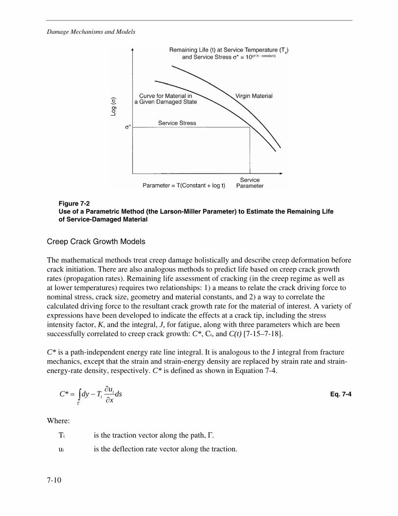
Damage Mechanisms and Models
7-10
Figure 7-2 Use of a Parametric Method (the Larson-Miller Parameter) to Estimate the Remaining Life of Service-Damaged Material
Creep Crack Growth Models
The mathematical methods treat creep damage holistically and describe creep deformation before crack initiation. There are also analogous methods to predict life based on creep crack growth rates (propagation rates). Remaining life assessment of cracking (in the creep regime as well as at lower temperatures) requires two relationships: 1) a means to relate the crack driving force to nominal stress, crack size, geometry and material constants, and 2) a way to correlate the calculated driving force to the resultant crack growth rate for the material of interest. A variety of expressions have been developed to indicate the effects at a crack tip, including the stress intensity factor, K, and the integral, J, for fatigue, along with three parameters which are been successfully correlated to creep crack growth: C*, Ct, and C(t) [7-15–7-18].
C* is a path-independent energy rate line integral. It is analogous to the J integral from fracture mechanics, except that the strain and strain-energy density are replaced by strain rate and strain-energy-rate density, respectively. C* is defined as shown in Equation 7-4.
dsxuTdyC i
i∫Γ ∂
∂−=* Eq. 7-4
Where:
Ti is the traction vector along the path, Γ.
ui is the deflection rate vector along the traction.
Damage Mechanisms and Models
7-11
ds is a length element along the path.
W* is the strain rate density, which is defined as shown in Equation 7-5.
∫=ij
ijijdWε
εσ0
* Eq. 7-5
Where:
σij = the stress tensor
εij = the strain tensor
C* addresses the steady-state (large-scale) creep crack growth regime under the special conditions in which second-stage creep deformation is widespread in the body. C* can be related to the crack tip stress and strain fields. Where elastic strains are dominant, the expressions reduce to those for the stress distribution ahead of a crack tip as a function of the stress intensity. C* can be directly measured in laboratory tests on cracked specimens in which the creep deflection is measured. Also, C* can be estimated from J integral expressions and from estimates of the J integral [7-14]. Therefore, C* can be calculated by finite-element methods and used as a parameter to predict creep-crack growth.
Ct and C(t) are ways to extend the C* concept to small-scale creep conditions. For the more general case in which significant creep strains occur only in the localized region near the crack tip, at least in the beginning stages of crack growth, a parameter Ct has been proposed. In the limit of widespread creep deformation, Ct = C*. The use of Ct has been shown to have some advantages over the other two parameters. C* is not defined as path-independent in small-scale and transition creep regions; therefore, its use is confined to extensive creep. C(t) is the near crack tip value of C* and is therefore useful for small-scale and transition creep regions. However, in these regimes, C(t) cannot be measured at the load point; it can only be calculated. Ct can be used in all regimes, and can be both measured and calculated at the load point. It has been shown that creep crack growth rate data for a wide range of conditions correlate with Ct.
These concepts have been confirmed by applying them to explain the observed creep lifetime of cracked components, such as superheater outlet headers and high-temperature rotors, after they have been removed from service. Figure 7-3 diagrams the typical fracture mechanics approach to estimating life after creep cracks are detected.
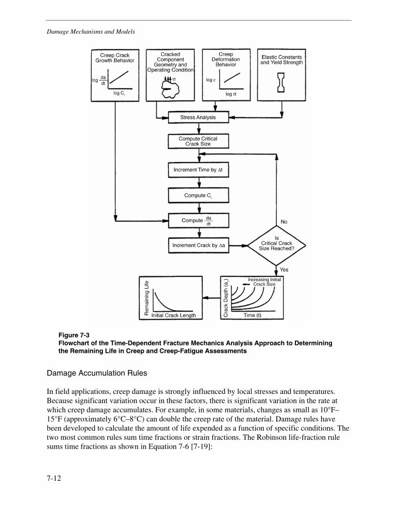
Damage Mechanisms and Models
7-12
Figure 7-3 Flowchart of the Time-Dependent Fracture Mechanics Analysis Approach to Determining the Remaining Life in Creep and Creep-Fatigue Assessments
Damage Accumulation Rules
In field applications, creep damage is strongly influenced by local stresses and temperatures. Because significant variation occur in these factors, there is significant variation in the rate at which creep damage accumulates. For example, in some materials, changes as small as 10°F–15°F (approximately 6°C–8°C) can double the creep rate of the material. Damage rules have been developed to calculate the amount of life expended as a function of specific conditions. The two most common rules sum time fractions or strain fractions. The Robinson life-fraction rule sums time fractions as shown in Equation 7-6 [7-19]:
Damage Mechanisms and Models
7-13
∑=ri
i
ttD Eq. 7-6
Where:
ti is the time spent under condition i.
tri is the time to rupture under condition i.
Strains are summed in the strain-fraction rule as shown in Equation 7-7 [7-20]:
∑=ri
iDεε
Eq. 7-7
Where:
εi= the strain accumulated under condition i
εri= the strain to rupture under condition i
The Robinson life-fraction rule is analogous to the Palmgren-Miner rule in fatigue analysis. As with fatigue, the Robinson rule assumes that each fractional expenditure of life is independent of all others. It is frequently called, incorrectly, a linear damage rule; there is no requirement for linearity, only for uniqueness of damage to life-fraction [7-21]. The original formulation was for temperature changes only. Damage induced by variable temperature but constant stress is uniquely related to life-fraction. Temperature changes do not result in sequence effects, and therefore life expenditures in each segment of time at temperature are simply additive. In contrast, problems developed with Robinson’s rule when it was applied assuming that stress changes were uniquely related to life-fraction; they are not [7-21]. Robinson’s rule has been successfully applied to analyzing power plant components.
There has been a considerable amount of evaluation of the accuracy of the life-fraction rules [7-22–7-24]. Some current views toward using these damage rules are the following:
• Linear damage summation rules have been found to be just as accurate and useful as any other rule in the specific context that they are used [7-25].
• Life-fraction rules have been shown to be generally valid for temperature changes and not for stress changes [7-24].
• Cumulative life-fraction at failure has been shown to be greater than, equal to, or less than unity, depending on the nature of the prior degradation, the ductility of the material, and the order in which stress changes and temperature changes are imposed [7-24]. For example, Figures 7-4 and 7-5 show the correspondence between the actual life and remaining life-fraction for a ferritic 1/2 Cr 1/2 Mo 1/4 V pipe steel (MG) and a bainitic, low ductility cast version (FW) based on the life-fraction rule (LFR). Results show that for ductile materials, cumulative life-fraction is >1 and for brittle material life-fraction is <1.
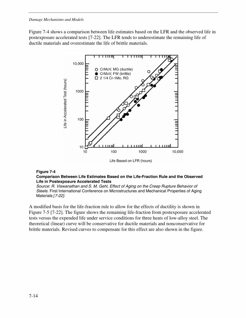
Damage Mechanisms and Models
7-14
Figure 7-4 shows a comparison between life estimates based on the LFR and the observed life in postexposure accelerated tests [7-22]. The LFR tends to underestimate the remaining life of ductile materials and overestimate the life of brittle materials.
Figure 7-4 Comparison Between Life Estimates Based on the Life-Fraction Rule and the Observed Life in Postexposure Accelerated Tests Source: R. Viswanathan and S. M. Gehl, Effect of Aging on the Creep Rupture Behavior of Steels. First International Conference on Microstructures and Mechanical Properties of Aging Materials [7-22].
A modified basis for the life-fraction rule to allow for the effects of ductility is shown in Figure 7-5 [7-22]. The figure shows the remaining life-fraction from postexposure accelerated tests versus the expended life under service conditions for three heats of low-alloy steel. The theoretical (linear) curve will be conservative for ductile materials and nonconservative for brittle materials. Revised curves to compensate for this effect are also shown in the figure.
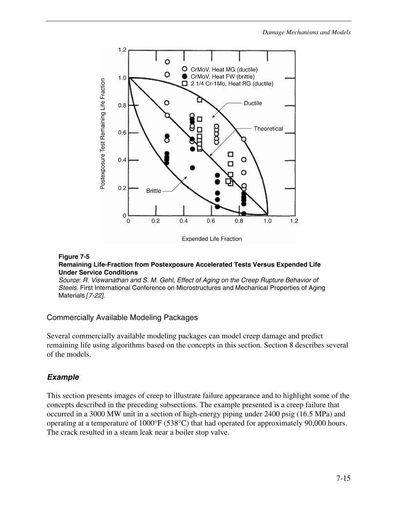
Damage Mechanisms and Models
7-15
Figure 7-5 Remaining Life-Fraction from Postexposure Accelerated Tests Versus Expended Life Under Service Conditions Source: R. Viswanathan and S. M. Gehl, Effect of Aging on the Creep Rupture Behavior of Steels. First International Conference on Microstructures and Mechanical Properties of Aging Materials [7-22].
Commercially Available Modeling Packages
Several commercially available modeling packages can model creep damage and predict remaining life using algorithms based on the concepts in this section. Section 8 describes several of the models.
Example
This section presents images of creep to illustrate failure appearance and to highlight some of the concepts described in the preceding subsections. The example presented is a creep failure that occurred in a 3000 MW unit in a section of high-energy piping under 2400 psig (16.5 MPa) and operating at a temperature of 1000°F (538°C) that had operated for approximately 90,000 hours. The crack resulted in a steam leak near a boiler stop valve.
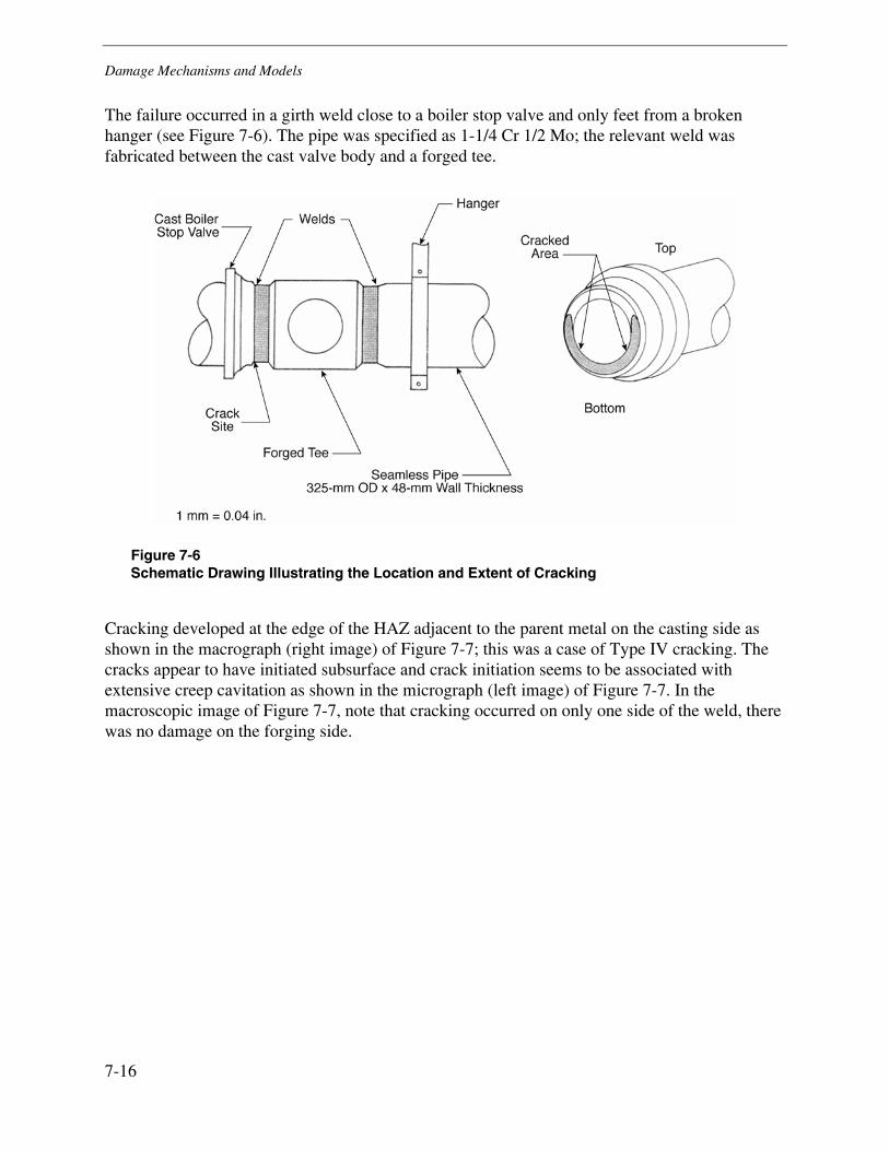
Damage Mechanisms and Models
7-16
The failure occurred in a girth weld close to a boiler stop valve and only feet from a broken hanger (see Figure 7-6). The pipe was specified as 1-1/4 Cr 1/2 Mo; the relevant weld was fabricated between the cast valve body and a forged tee.
Figure 7-6 Schematic Drawing Illustrating the Location and Extent of Cracking
Cracking developed at the edge of the HAZ adjacent to the parent metal on the casting side as shown in the macrograph (right image) of Figure 7-7; this was a case of Type IV cracking. The cracks appear to have initiated subsurface and crack initiation seems to be associated with extensive creep cavitation as shown in the micrograph (left image) of Figure 7-7. In the macroscopic image of Figure 7-7, note that cracking occurred on only one side of the weld, there was no damage on the forging side.
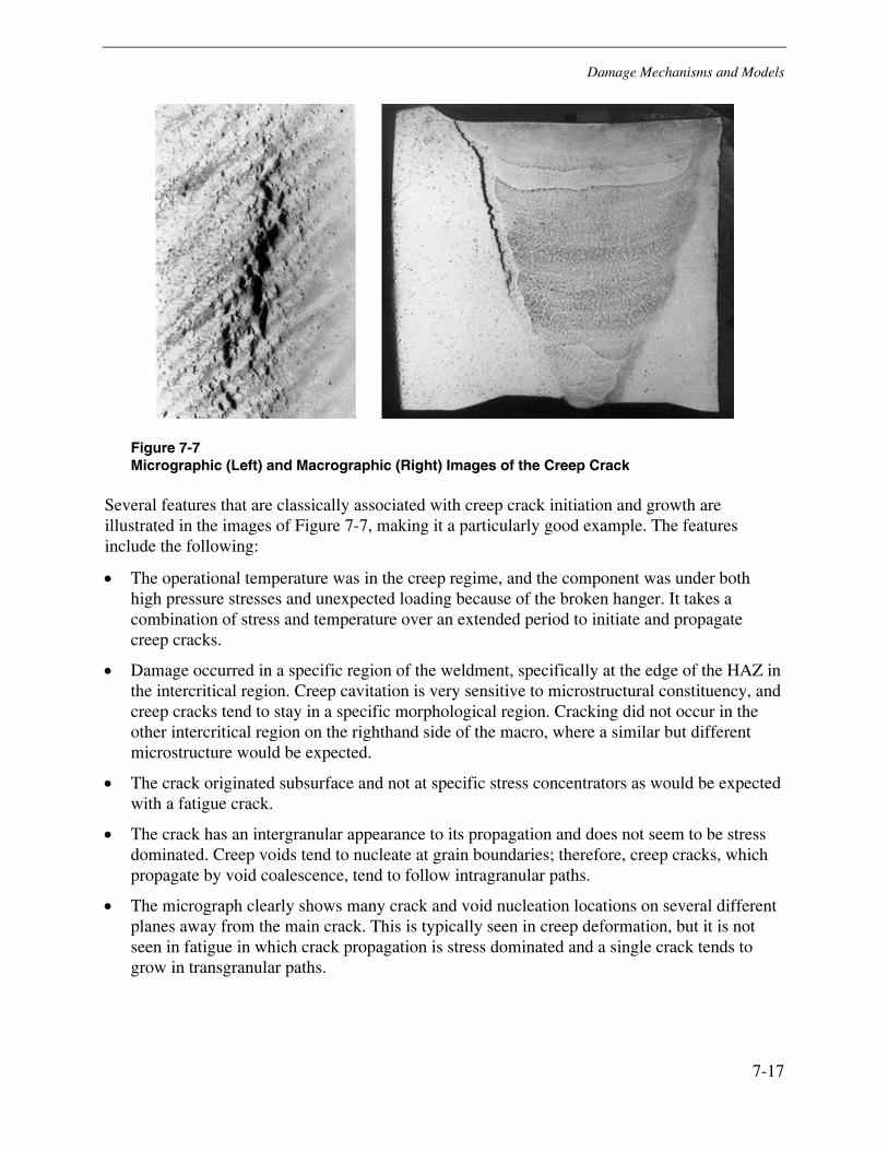
Damage Mechanisms and Models
7-17
Figure 7-7 Micrographic (Left) and Macrographic (Right) Images of the Creep Crack
Several features that are classically associated with creep crack initiation and growth are illustrated in the images of Figure 7-7, making it a particularly good example. The features include the following:
• The operational temperature was in the creep regime, and the component was under both high pressure stresses and unexpected loading because of the broken hanger. It takes a combination of stress and temperature over an extended period to initiate and propagate creep cracks.
• Damage occurred in a specific region of the weldment, specifically at the edge of the HAZ in the intercritical region. Creep cavitation is very sensitive to microstructural constituency, and creep cracks tend to stay in a specific morphological region. Cracking did not occur in the other intercritical region on the righthand side of the macro, where a similar but different microstructure would be expected.
• The crack originated subsurface and not at specific stress concentrators as would be expected with a fatigue crack.
• The crack has an intergranular appearance to its propagation and does not seem to be stress dominated. Creep voids tend to nucleate at grain boundaries; therefore, creep cracks, which propagate by void coalescence, tend to follow intragranular paths.
• The micrograph clearly shows many crack and void nucleation locations on several different planes away from the main crack. This is typically seen in creep deformation, but it is not seen in fatigue in which crack propagation is stress dominated and a single crack tends to grow in transgranular paths.
Damage Mechanisms and Models
7-18
Fatigue
Introduction
Fatigue is damage accumulation caused by cyclic or fluctuating stresses that typically lie below the yield stress of the material and generally manifest as the initiation and stable propagation of a crack. Final failure in a component subjected to fatigue occurs in one of two ways: either 1) a critical crack size is reached and unstable rapid crack propagation leads to a through-component fracture or 2) losses in cross-sectional area as a result of crack propagation lead to stress overload. In cases of rapid crack growth, failure can be defined by the initiation of a crack. In many cases, however, cracks grow for many stress cycles and the initiation of a crack does not necessarily mean the end of useful life for the component.
Fatigue crack propagation depends on the frequency and magnitude of applied stress cycles and is generally independent of stress duration (at high temperatures in which creep-fatigue becomes the dominant mechanism, there is a dependence on stress duration). Stress cycling can be induced mechanically or thermally. Figure 7-8 shows experimental results of fatigue testing for several commonly used engineering materials, in which a cyclical stress (alternating tensile stress, in this case) is applied to a component until it fails. In Figure 7-8, the ordinate variable (Y axis) is the applied cyclical strain and the abscissa variable (X axis) is the number of applied cycles. Although cyclic stress range is typically plotted on the ordinate axis, stress and strain are interchangeable because fatigue testing is normally performed in the elastic region of the stress-strain curve. At a high strain range (stress level), fatigue failure can occur in less than 100 cycles. As the strain (stress) is lowered, the number of cycles to fracture increases dramatically and asymptotically. Ultimately, there is a strain range (stress range) below which the component can be cycled indefinitely without failure. This level is commonly called the endurance limit of the material.
Fatigue damage is commonly grouped into two categories—low-cycle fatigue and high-cycle fatigue. It is the magnitude of applied stress that dictates the number of cycles to failure (see Figure 7-8). High-cycle fatigue is usually thought to occur in 106 or more cycles, and low cycle fatigue usually occurs in 10,000 or fewer cycles of applied stress. Whether a fatigue fracture is of a high-cycle or low-cycle nature is important in analyzing the failure and providing information to the designer to correct the problem.
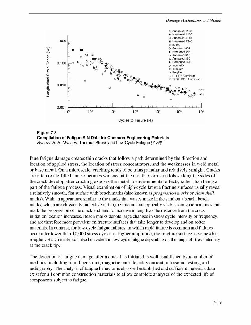
Damage Mechanisms and Models
7-19
Figure 7-8 Compilation of Fatigue S-N Data for Common Engineering Materials Source: S. S. Manson. Thermal Stress and Low Cycle Fatigue [7-26].
Pure fatigue damage creates thin cracks that follow a path determined by the direction and location of applied stress, the location of stress concentrators, and the weaknesses in weld metal or base metal. On a microscale, cracking tends to be transgranular and relatively straight. Cracks are often oxide-filled and sometimes widened at the mouth. Corrosion lobes along the sides of the crack develop after cracking exposes the metal to environmental effects, rather than being a part of the fatigue process. Visual examination of high-cycle fatigue fracture surfaces usually reveal a relatively smooth, flat surface with beach marks (also known as progression marks or clam shell marks). With an appearance similar to the marks that waves make in the sand on a beach, beach marks, which are classically indicative of fatigue fracture, are optically visible semispherical lines that mark the progression of the crack and tend to increase in length as the distance from the crack initiation location increases. Beach marks denote large changes in stress cycle intensity or frequency, and are therefore more prevalent on fracture surfaces that take longer to develop and on softer materials. In contrast, for low-cycle fatigue failures, in which rapid failure is common and failures occur after fewer than 10,000 stress cycles of higher amplitude, the fracture surface is somewhat rougher. Beach marks can also be evident in low-cycle fatigue depending on the range of stress intensity at the crack tip.
The detection of fatigue damage after a crack has initiated is well established by a number of methods, including liquid penetrant, magnetic particle, eddy current, ultrasonic testing, and radiography. The analysis of fatigue behavior is also well established and sufficient materials data exist for all common construction materials to allow complete analyses of the expected life of components subject to fatigue.
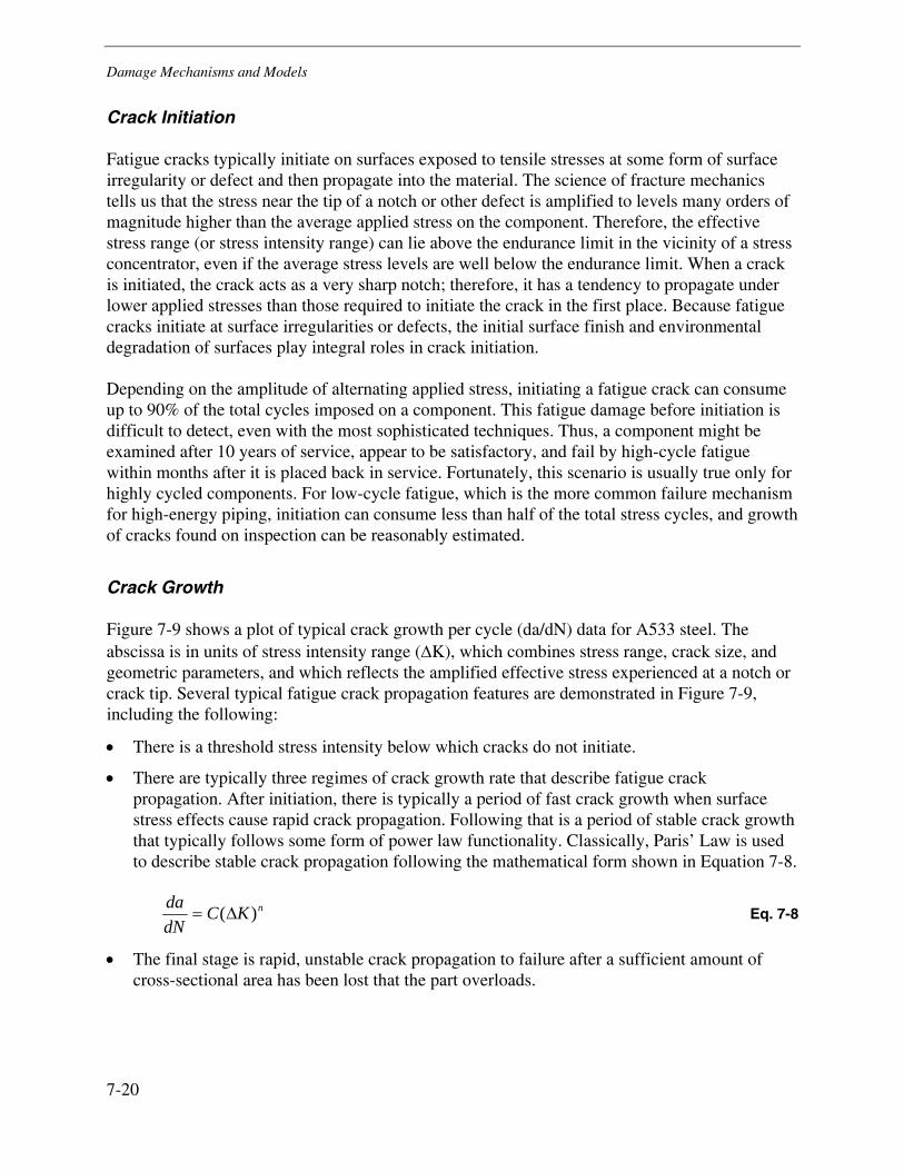
Damage Mechanisms and Models
7-20
Crack Initiation
Fatigue cracks typically initiate on surfaces exposed to tensile stresses at some form of surface irregularity or defect and then propagate into the material. The science of fracture mechanics tells us that the stress near the tip of a notch or other defect is amplified to levels many orders of magnitude higher than the average applied stress on the component. Therefore, the effective stress range (or stress intensity range) can lie above the endurance limit in the vicinity of a stress concentrator, even if the average stress levels are well below the endurance limit. When a crack is initiated, the crack acts as a very sharp notch; therefore, it has a tendency to propagate under lower applied stresses than those required to initiate the crack in the first place. Because fatigue cracks initiate at surface irregularities or defects, the initial surface finish and environmental degradation of surfaces play integral roles in crack initiation.
Depending on the amplitude of alternating applied stress, initiating a fatigue crack can consume up to 90% of the total cycles imposed on a component. This fatigue damage before initiation is difficult to detect, even with the most sophisticated techniques. Thus, a component might be examined after 10 years of service, appear to be satisfactory, and fail by high-cycle fatigue within months after it is placed back in service. Fortunately, this scenario is usually true only for highly cycled components. For low-cycle fatigue, which is the more common failure mechanism for high-energy piping, initiation can consume less than half of the total stress cycles, and growth of cracks found on inspection can be reasonably estimated.
Crack Growth
Figure 7-9 shows a plot of typical crack growth per cycle (da/dN) data for A533 steel. The abscissa is in units of stress intensity range (ΔK), which combines stress range, crack size, and geometric parameters, and which reflects the amplified effective stress experienced at a notch or crack tip. Several typical fatigue crack propagation features are demonstrated in Figure 7-9, including the following:
• There is a threshold stress intensity below which cracks do not initiate.
• There are typically three regimes of crack growth rate that describe fatigue crack propagation. After initiation, there is typically a period of fast crack growth when surface stress effects cause rapid crack propagation. Following that is a period of stable crack growth that typically follows some form of power law functionality. Classically, Paris’ Law is used to describe stable crack propagation following the mathematical form shown in Equation 7-8.
nKCdNda )(Δ= Eq. 7-8
• The final stage is rapid, unstable crack propagation to failure after a sufficient amount of cross-sectional area has been lost that the part overloads.
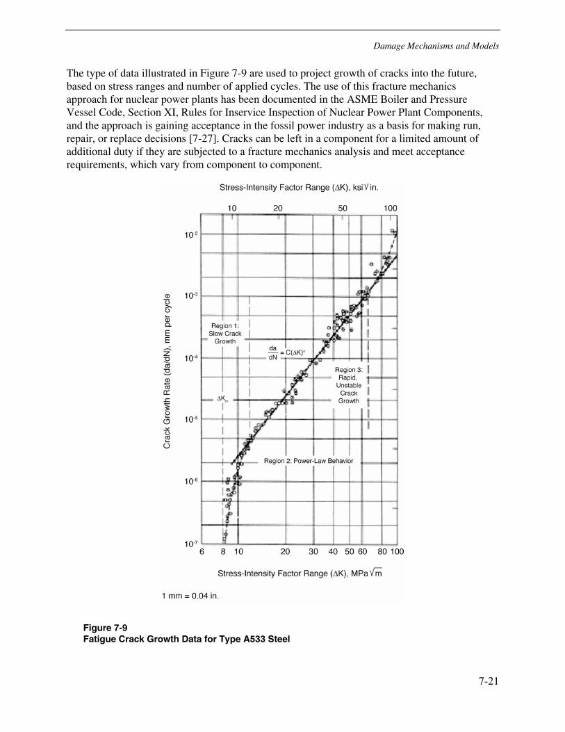
Damage Mechanisms and Models
7-21
The type of data illustrated in Figure 7-9 are used to project growth of cracks into the future, based on stress ranges and number of applied cycles. The use of this fracture mechanics approach for nuclear power plants has been documented in the ASME Boiler and Pressure Vessel Code, Section XI, Rules for Inservice Inspection of Nuclear Power Plant Components, and the approach is gaining acceptance in the fossil power industry as a basis for making run, repair, or replace decisions [7-27]. Cracks can be left in a component for a limited amount of additional duty if they are subjected to a fracture mechanics analysis and meet acceptance requirements, which vary from component to component.
Figure 7-9 Fatigue Crack Growth Data for Type A533 Steel
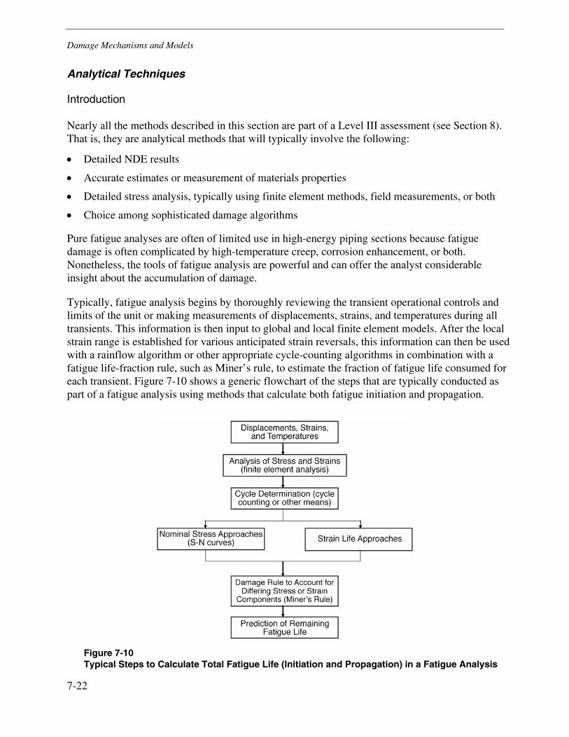
Damage Mechanisms and Models
7-22
Analytical Techniques
Introduction
Nearly all the methods described in this section are part of a Level III assessment (see Section 8). That is, they are analytical methods that will typically involve the following:
• Detailed NDE results
• Accurate estimates or measurement of materials properties
• Detailed stress analysis, typically using finite element methods, field measurements, or both
• Choice among sophisticated damage algorithms
Pure fatigue analyses are often of limited use in high-energy piping sections because fatigue damage is often complicated by high-temperature creep, corrosion enhancement, or both. Nonetheless, the tools of fatigue analysis are powerful and can offer the analyst considerable insight about the accumulation of damage.
Typically, fatigue analysis begins by thoroughly reviewing the transient operational controls and limits of the unit or making measurements of displacements, strains, and temperatures during all transients. This information is then input to global and local finite element models. After the local strain range is established for various anticipated strain reversals, this information can then be used with a rainflow algorithm or other appropriate cycle-counting algorithms in combination with a fatigue life-fraction rule, such as Miner’s rule, to estimate the fraction of fatigue life consumed for each transient. Figure 7-10 shows a generic flowchart of the steps that are typically conducted as part of a fatigue analysis using methods that calculate both fatigue initiation and propagation.
Figure 7-10 Typical Steps to Calculate Total Fatigue Life (Initiation and Propagation) in a Fatigue Analysis
Damage Mechanisms and Models
7-23
A corresponding flowchart that examines the steps for propagation only (given an existing flaw found by inspection or a flaw of assumed size) is shown in Figure 7-11.
Figure 7-11 Typical Steps to Calculate Fatigue Life in Propagation by Fracture Mechanics Analyses Given an Existing or Assumed Flaw
Nominal Stress Approaches—Goodman Diagram and Modified Goodman Diagram
The basic method for presenting fatigue life information is the S-N curve, which is a plot of the number of cycles, N, to failure against the stress range. N is usually the number of cycles to complete specimen fracture and the S-N curve does not distinguish between crack initiation and crack propagation. The number of cycles to failure at a given stress level is termed the fatigue life for that stress. S-N curves are constructed using fully reversed loading on smooth fatigue specimens. A number of variables—including mean stress, temperature, environment, specimen size, specimen surface condition, and stress concentrations—can impact the measurement of fatigue life. A safety factor is typically applied to the S-N curve in design of components, partly to account for the effects of these variables.
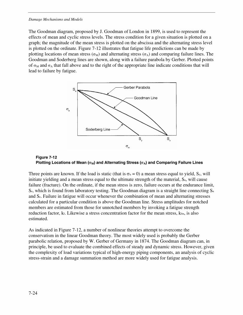
Damage Mechanisms and Models
7-24
The Goodman diagram, proposed by J. Goodman of London in 1899, is used to represent the effects of mean and cyclic stress levels. The stress condition for a given situation is plotted on a graph; the magnitude of the mean stress is plotted on the abscissa and the alternating stress level is plotted on the ordinate. Figure 7-12 illustrates that fatigue life predictions can be made by plotting locations of mean stress (σM) and alternating stress (σA) and comparing failure lines. The Goodman and Soderberg lines are shown, along with a failure parabola by Gerber. Plotted points of σM and σA that fall above and to the right of the appropriate line indicate conditions that will lead to failure by fatigue.
Figure 7-12 Plotting Locations of Mean (σM) and Alternating Stress (σA) and Comparing Failure Lines
Three points are known. If the load is static (that is σa = 0) a mean stress equal to yield, Sy, will initiate yielding and a mean stress equal to the ultimate strength of the material, Su, will cause failure (fracture). On the ordinate, if the mean stress is zero, failure occurs at the endurance limit, Se, which is found from laboratory testing. The Goodman diagram is a straight line connecting Su and Se. Failure in fatigue will occur whenever the combination of mean and alternating stresses calculated for a particular condition is above the Goodman line. Stress amplitudes for notched members are estimated from those for unnotched members by invoking a fatigue strength reduction factor, kf. Likewise a stress concentration factor for the mean stress, kfm, is also estimated.
As indicated in Figure 7-12, a number of nonlinear theories attempt to overcome the conservatism in the linear Goodman theory. The most widely used is probably the Gerber parabolic relation, proposed by W. Gerber of Germany in 1874. The Goodman diagram can, in principle, be used to evaluate the combined effects of steady and dynamic stress. However, given the complexity of load variations typical of high-energy piping components, an analysis of cyclic stress-strain and a damage summation method are more widely used for fatigue analysis.
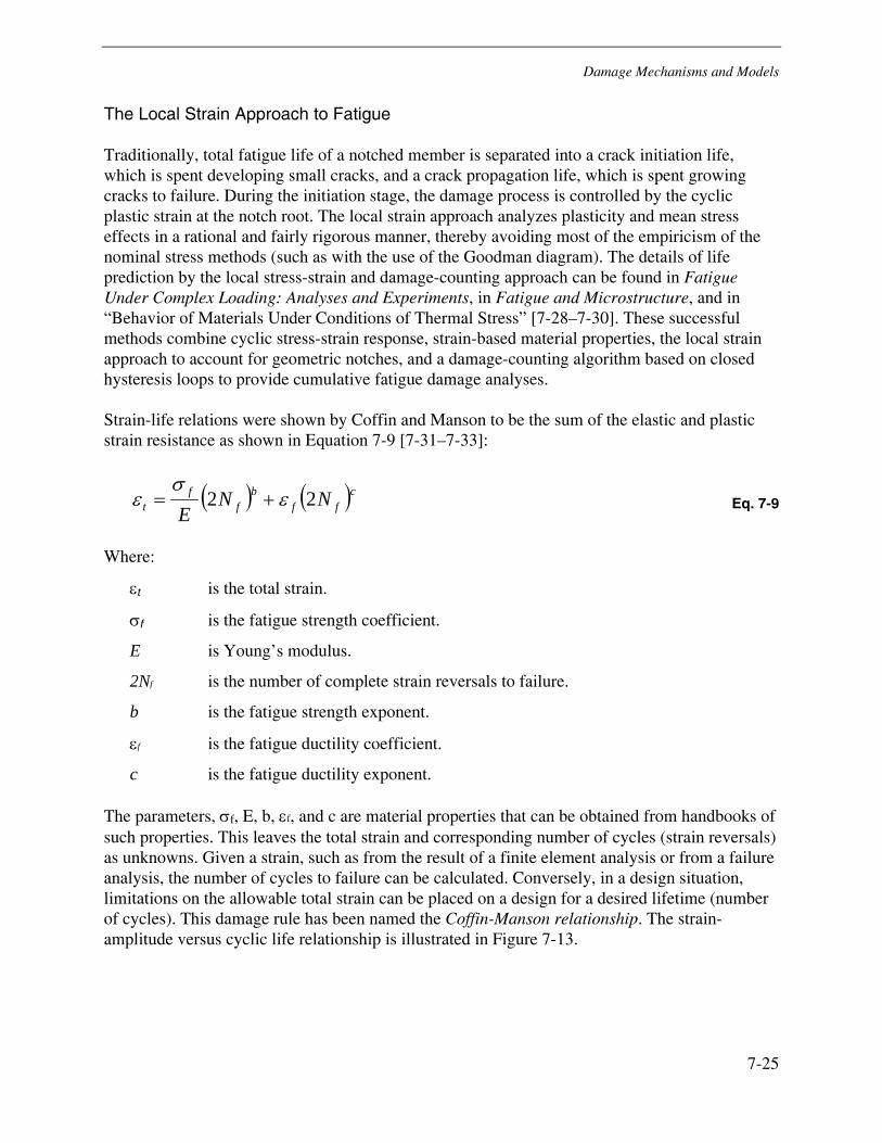
Damage Mechanisms and Models
7-25
The Local Strain Approach to Fatigue
Traditionally, total fatigue life of a notched member is separated into a crack initiation life, which is spent developing small cracks, and a crack propagation life, which is spent growing cracks to failure. During the initiation stage, the damage process is controlled by the cyclic plastic strain at the notch root. The local strain approach analyzes plasticity and mean stress effects in a rational and fairly rigorous manner, thereby avoiding most of the empiricism of the nominal stress methods (such as with the use of the Goodman diagram). The details of life prediction by the local stress-strain and damage-counting approach can be found in Fatigue Under Complex Loading: Analyses and Experiments, in Fatigue and Microstructure, and in “Behavior of Materials Under Conditions of Thermal Stress” [7-28–7-30]. These successful methods combine cyclic stress-strain response, strain-based material properties, the local strain approach to account for geometric notches, and a damage-counting algorithm based on closed hysteresis loops to provide cumulative fatigue damage analyses.
Strain-life relations were shown by Coffin and Manson to be the sum of the elastic and plastic strain resistance as shown in Equation 7-9 [7-31–7-33]:
( ) ( )cff
bf
ft NN
E22 ε
σε += Eq. 7-9
Where:
εt is the total strain.
σf is the fatigue strength coefficient.
E is Young’s modulus.
2Nf is the number of complete strain reversals to failure.
b is the fatigue strength exponent.
εf is the fatigue ductility coefficient.
c is the fatigue ductility exponent.
The parameters, σf, E, b, εf, and c are material properties that can be obtained from handbooks of such properties. This leaves the total strain and corresponding number of cycles (strain reversals) as unknowns. Given a strain, such as from the result of a finite element analysis or from a failure analysis, the number of cycles to failure can be calculated. Conversely, in a design situation, limitations on the allowable total strain can be placed on a design for a desired lifetime (number of cycles). This damage rule has been named the Coffin-Manson relationship. The strain-amplitude versus cyclic life relationship is illustrated in Figure 7-13.
Damage Mechanisms and Models
7-26
Figure 7-13 Schematic Representation of the Strain-Amplitude versus Cyclic Life Relationship
The fractional damage under varying strain range conditions are estimated using standard εt (total strain range) versus Nf (cycles to failure) curves and are summed up using the Miner rule (see the next subsection) to determine the total life-fraction consumed. In the absence of εt versus Nf
curves, the method of universal slopes proposed by Manson can be used to estimate fatigue curves based on a knowledge of the tensile strength and ductility of the material [7-34]. The equation is shown in Equation 7-10.
6.06.012.05.3 −− +⎟⎠⎞
⎜⎝⎛=Δ ff
ut NDN
Eσε Eq. 7-10
Where:
σu is the ultimate tensile strength (ksi).
E is Young’s modulus (ksi).
D is ductility, defined as D = ln [100/(100-RA)] where RA is the reduction of area in (%).
The implication of this equation is that in the elastic region, fatigue strength is governed by tensile strength, and at large cyclic strains, it is governed by ductility. The knowledge of cyclic strains can be either measured or calculated by finite element methods. If the temperature-dependent strength modulus and ductility are used, the universal slope equations can be used to estimate fatigue life at any desired service temperature.

Damage Mechanisms and Models
7-27
Miner’s Rule for Calculation of Fatigue Life-Fraction
Actual service spectra almost always show an irregular variation with time. Realistic life predictions must account for irregular load histories in fatigue or irregular stress histories from other degradations. Traditionally, the method of analyzing nonconstant fatigue loading is a life-fraction rule (termed Miner’s rule or Palmgren-Miner rule), which states that life is exhausted when the sum of life-fractions in each load or stress regime reaches unity [7-35]. See Equation 7-11.
∑=
=m
i i
f
Nn
D1
Eq. 7-11
Where:
D is the fatigue damage fraction.
Ni is the number of cycles to failure for cycle i.
ni is the number of applied stress-strain loops of this amplitude.
m is the number of stress-strain loops of various amplitudes within the load block.
To calculate the time to failure for a spectrum of loads, it is necessary to add the incremental damage per cycle.
Figure 7-14 shows a simple example of how the rule is applied [7-36]. Here the assumed strain-time history consists of three strain cycles of strain range Δε1, two cycles of strain range Δε2, and four cycles of strain range Δε3. The increment of fatigue damage attributable to cycling at any one of the strain ranges is defined as the number of applied cycles, n, of that strain range divided by the allowable number of cycles, N, at that strain range. The allowable number of cycles is determined from a fatigue curve of log strain range versus log cycles to failure.
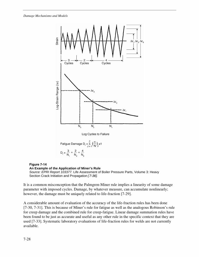
Damage Mechanisms and Models
7-28
Figure 7-14 An Example of the Application of Miner’s Rule Source: EPRI Report 103377. Life Assessment of Boiler Pressure Parts, Volume 3: Heavy Section Crack Initiation and Propagation [7-36].
It is a common misconception that the Palmgren-Miner rule implies a linearity of some damage parameter with imposed cycles. Damage, by whatever measure, can accumulate nonlinearly; however, the damage must be uniquely related to life-fraction [7-29].
A considerable amount of evaluation of the accuracy of the life-fraction rules has been done [7-30, 7-31]. This is because of Miner’s rule for fatigue as well as the analogous Robinson’s rule for creep damage and the combined rule for creep-fatigue. Linear damage summation rules have been found to be just as accurate and useful as any other rule in the specific context that they are used [7-33]. Systematic laboratory evaluations of life-fraction rules for welds are not currently available.

Damage Mechanisms and Models
7-29
Fracture Mechanics Approaches to Crack Growth by Fatigue
Fracture mechanics analyses can be invoked in situations where a crack is known to exist or is assumed to exist (sized just below the detection limits of an NDE technique, for example). Fracture mechanics assumes that there is no initiation; that is, the analysis begins with the assumption of a sharp crack in the part and determines the time for that crack to grow to a critical size. However, in damage-tolerant design, assumed initial flaw sizes can be unduly conservative, in part because no credit is taken for the crack initiation life of the component. The optimal approach is to consider both crack initiation and crack growth in design or life prediction. Initiation lives from strain life curves to a specific crack size can be combined with crack growth lives that start at the crack size at which initiation ended. One difficulty in combining initiation and propagation is how to choose the crack size that can be considered the end of the initiation phase.
In linear elastic fracture mechanics (LEFM) analyses, the component is assumed to behave as a perfectly elastic material. A stress intensity is calculated that specifies the stress state at the tip of a crack. In general, the stress intensity is a function of the applied and residual stress fields, the existing crack size, and a factor that accounts for crack and specimen geometry, as shown in Equation 7-12.
aAK σ1= Eq. 7-12
Where:
K is the stress intensity.
A1 is a crack and specimen geometry factor.
σ is applied stress.
a is crack size.
For cyclic stresses, the same equation is applicable and provides the cyclic stress intensity factor (stress intensity range), ΔK = Kmax - Kmin. The incremental crack growth can be expressed as a function of applied stress intensity range, as shown in Equation 7-13, where C and n are empirical constants derived from laboratory test data.
( )nΔKCdNda
= Eq. 7-13
The coefficient C depends on the temperature, the mean stress or strain, the material, the configuration of the design or weld detail, the thickness of the member subjected to cyclic loading, the surface roughness, and the weld quality. The exponent n is typically in the range from 2.0 to 5.0. For a wide range of weld configurations and weld materials, the exponent has been found to be approximately 3 [7-37].
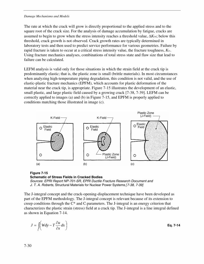
Damage Mechanisms and Models
7-30
The rate at which the crack will grow is directly proportional to the applied stress and to the square root of the crack size. For the analysis of damage accumulation by fatigue, cracks are assumed to begin to grow when the stress intensity reaches a threshold value, ΔKTH; below this threshold, crack growth is not observed. Crack growth rates are typically determined in laboratory tests and then used to predict service performance for various geometries. Failure by rapid fracture is taken to occur at a critical stress intensity value, the fracture toughness, KIC. Using fracture mechanics analyses, combinations of total stress state and flaw size that lead to failure can be calculated.
LEFM analysis is valid only for those situations in which the strain field at the crack tip is predominantly elastic; that is, the plastic zone is small (brittle materials). In most circumstances when analyzing high-temperature piping degradation, this condition is not valid, and the use of elastic-plastic fracture mechanics (EPFM), which accounts for plastic deformation of the material near the crack tip, is appropriate. Figure 7-15 illustrates the development of an elastic, small plastic, and large plastic field caused by a growing crack [7-38, 7-39]. LEFM can be correctly applied to images (a) and (b) in Figure 7-15, and EPFM is properly applied to conditions matching those illustrated in image (c).
Figure 7-15 Schematic of Stress Fields in Cracked Bodies Sources: EPRI Report NP-701-SR, EPRI Ductile Fracture Research Document and J. T. A. Roberts, Structural Materials for Nuclear Power Systems [7-38, 7-39]
The J-integral concept and the crack-opening-displacement technique have been developed as part of the EPFM methodology. The J-integral concept is relevant because of its extension to creep conditions through the C* and Ct parameters. The J-integral is an energy criterion that characterizes the plastic strain (stress) field at a crack tip. The J-integral is a line integral defined as shown in Equation 7-14.
∫Γ
⎟⎠⎞
⎜⎝⎛
∂∂
−= dsxuTWdyJ Eq. 7-14

Damage Mechanisms and Models
7-31
Where:
Γ is the counterclockwise contour around a crack tip.
T is the traction vector defined according to the outward normal n along Γ (that is, Ti = σijnj).
u is the displacement vector acting along the integration path.
ds is an increment of length along the integration path.
W = ∫ε
εσ0
ijij , where σij and εij are the components of stress and strain.
The J-integral can be used as a fracture criterion. There is a value of J, termed JIC, that is the critical value for the onset of fast crack propagation and is analogous to KIC for the linear elastic case. Test methods are available for the measurement of JIC [7-40]. The J-integral is applied in two different ways [7-7]. First, J expressions can be directly applied where they have been developed for the particular component geometry. Secondly, the equivalence of J and K has been established (see Equations 7-15 and 7-16), and this equivalence can be invoked to allow the use of more common K solutions.
( )22
1 υ−=E
KJ ICIC for plane strain conditions Eq. 7-15
EKJ C
C
2
= for plane stress conditions Eq. 7-16
Several commercially available fracture mechanics programs an be used to evaluate the accumulation of damage by the crack-like mechanisms—fatigue, stress corrosion cracking, and corrosion fatigue. International standards such as the R6 procedure developed by the former Central Electricity Generating Board provide methods to analyze structures containing flaws [7-41, 7-42].
Example
This section presents images of fatigue to illustrate failure appearance and to highlight some of the concepts described in the preceding subsections. The example presented is a catastrophic fatigue failure that occurred in a section of cold reheat piping. During the explosive failure event, sections of collapsed metal piping were projected out of the plant’s building and into an employee parking lot. The left image in Figure 7-16 shows the extent of damage caused by the ultimate failure. The right image shows piping debris that was flung into the employee parking lot by the explosion associated with the catastrophic failure.
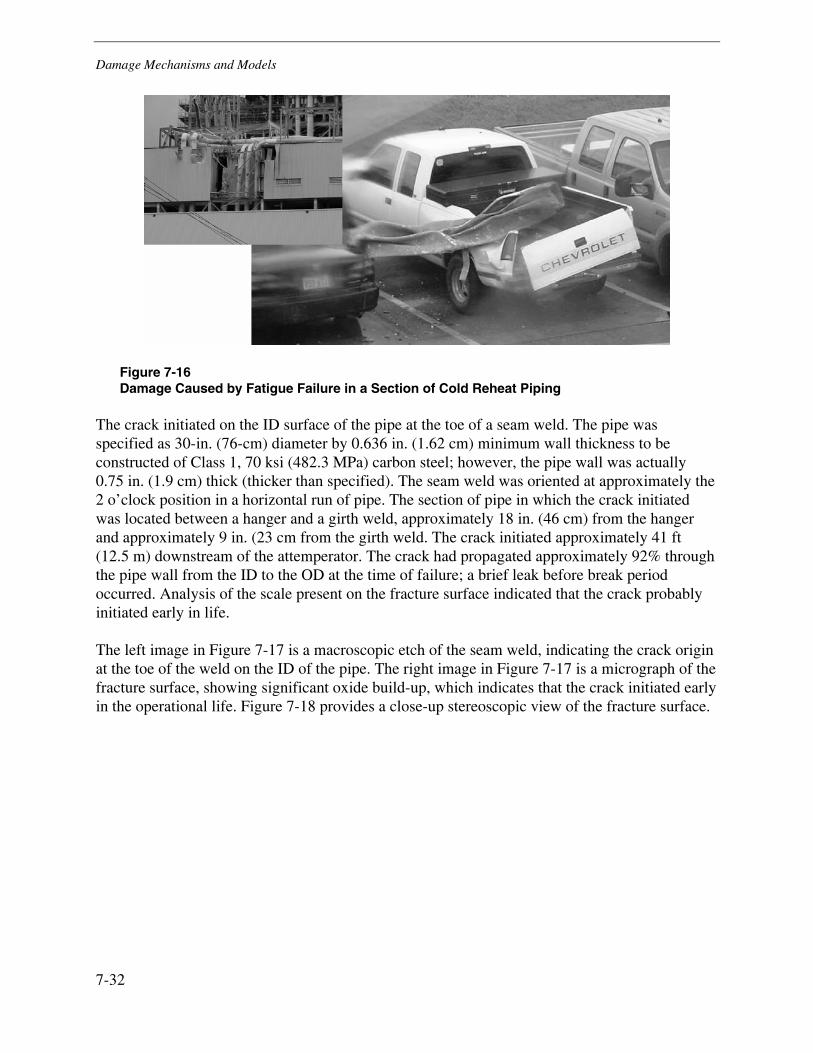
Damage Mechanisms and Models
7-32
Figure 7-16 Damage Caused by Fatigue Failure in a Section of Cold Reheat Piping
The crack initiated on the ID surface of the pipe at the toe of a seam weld. The pipe was specified as 30-in. (76-cm) diameter by 0.636 in. (1.62 cm) minimum wall thickness to be constructed of Class 1, 70 ksi (482.3 MPa) carbon steel; however, the pipe wall was actually 0.75 in. (1.9 cm) thick (thicker than specified). The seam weld was oriented at approximately the 2 o’clock position in a horizontal run of pipe. The section of pipe in which the crack initiated was located between a hanger and a girth weld, approximately 18 in. (46 cm) from the hanger and approximately 9 in. (23 cm from the girth weld. The crack initiated approximately 41 ft (12.5 m) downstream of the attemperator. The crack had propagated approximately 92% through the pipe wall from the ID to the OD at the time of failure; a brief leak before break period occurred. Analysis of the scale present on the fracture surface indicated that the crack probably initiated early in life.
The left image in Figure 7-17 is a macroscopic etch of the seam weld, indicating the crack origin at the toe of the weld on the ID of the pipe. The right image in Figure 7-17 is a micrograph of the fracture surface, showing significant oxide build-up, which indicates that the crack initiated early in the operational life. Figure 7-18 provides a close-up stereoscopic view of the fracture surface.
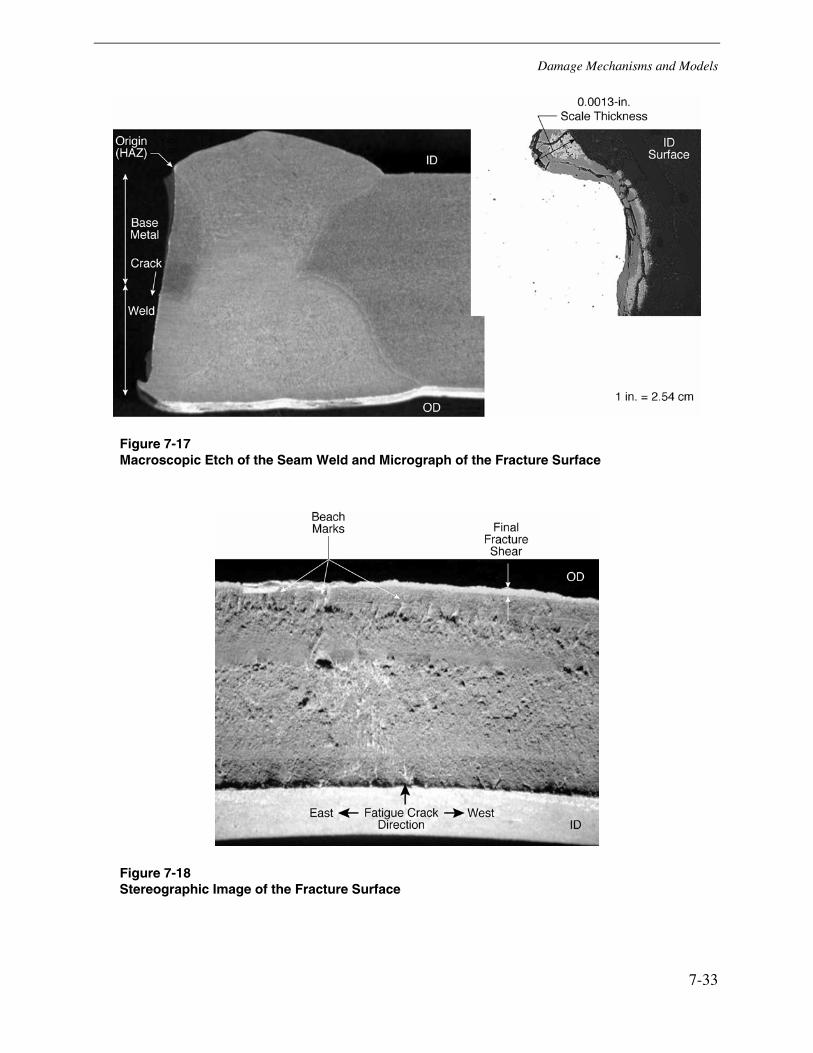
Damage Mechanisms and Models
7-33
Figure 7-17 Macroscopic Etch of the Seam Weld and Micrograph of the Fracture Surface
Figure 7-18 Stereographic Image of the Fracture Surface
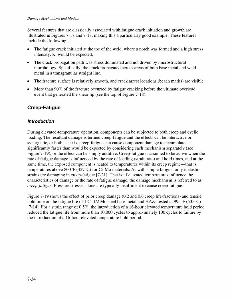
Damage Mechanisms and Models
7-34
Several features that are classically associated with fatigue crack initiation and growth are illustrated in Figures 7-17 and 7-18, making this a particularly good example. These features include the following:
• The fatigue crack initiated at the toe of the weld, where a notch was formed and a high stress intensity, K, would be expected.
• The crack propagation path was stress dominated and not driven by microstructural morphology. Specifically, the crack propagated across areas of both base metal and weld metal in a transgranular straight line.
• The fracture surface is relatively smooth, and crack arrest locations (beach marks) are visible.
• More than 90% of the fracture occurred by fatigue cracking before the ultimate overload event that generated the shear lip (see the top of Figure 7-18).
Creep-Fatigue
Introduction
During elevated-temperature operation, components can be subjected to both creep and cyclic loading. The resultant damage is termed creep-fatigue and the effects can be interactive or synergistic, or both. That is, creep-fatigue can cause component damage to accumulate significantly faster than would be expected by considering each mechanism separately (see Figure 7-19), or the effect can be simply additive. Creep-fatigue is assumed to be active when the rate of fatigue damage is influenced by the rate of loading (strain rate) and hold times, and at the same time, the exposed component is heated to temperatures within its creep regime—that is, temperatures above 800°F (427°C) for Cr-Mo materials. As with simple fatigue, only inelastic strains are damaging in creep-fatigue [7-21]. That is, if elevated temperatures influence the characteristics of damage or the rate of fatigue damage, the damage mechanism is referred to as creep-fatigue. Pressure stresses alone are typically insufficient to cause creep-fatigue.
Figure 7-19 shows the effect of prior creep damage (0.2 and 0.6 creep life-fractions) and tensile hold time on the fatigue life of 1 Cr 1/2 Mo steel base metal and HAZs tested at 995°F (535°C) [7-14]. For a strain range of 0.5%, the introduction of a 16-hour elevated temperature hold period reduced the fatigue life from more than 10,000 cycles to approximately 100 cycles to failure by the introduction of a 16-hour elevated temperature hold period.
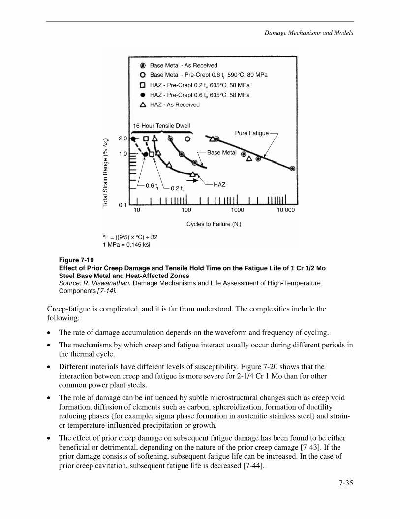
Damage Mechanisms and Models
7-35
Figure 7-19 Effect of Prior Creep Damage and Tensile Hold Time on the Fatigue Life of 1 Cr 1/2 Mo Steel Base Metal and Heat-Affected Zones Source: R. Viswanathan. Damage Mechanisms and Life Assessment of High-Temperature Components [7-14].
Creep-fatigue is complicated, and it is far from understood. The complexities include the following:
• The rate of damage accumulation depends on the waveform and frequency of cycling.
• The mechanisms by which creep and fatigue interact usually occur during different periods in the thermal cycle.
• Different materials have different levels of susceptibility. Figure 7-20 shows that the interaction between creep and fatigue is more severe for 2-1/4 Cr 1 Mo than for other common power plant steels.
• The role of damage can be influenced by subtle microstructural changes such as creep void formation, diffusion of elements such as carbon, spheroidization, formation of ductility reducing phases (for example, sigma phase formation in austenitic stainless steel) and strain- or temperature-influenced precipitation or growth.
• The effect of prior creep damage on subsequent fatigue damage has been found to be either beneficial or detrimental, depending on the nature of the prior creep damage [7-43]. If the prior damage consists of softening, subsequent fatigue life can be increased. In the case of prior creep cavitation, subsequent fatigue life is decreased [7-44].
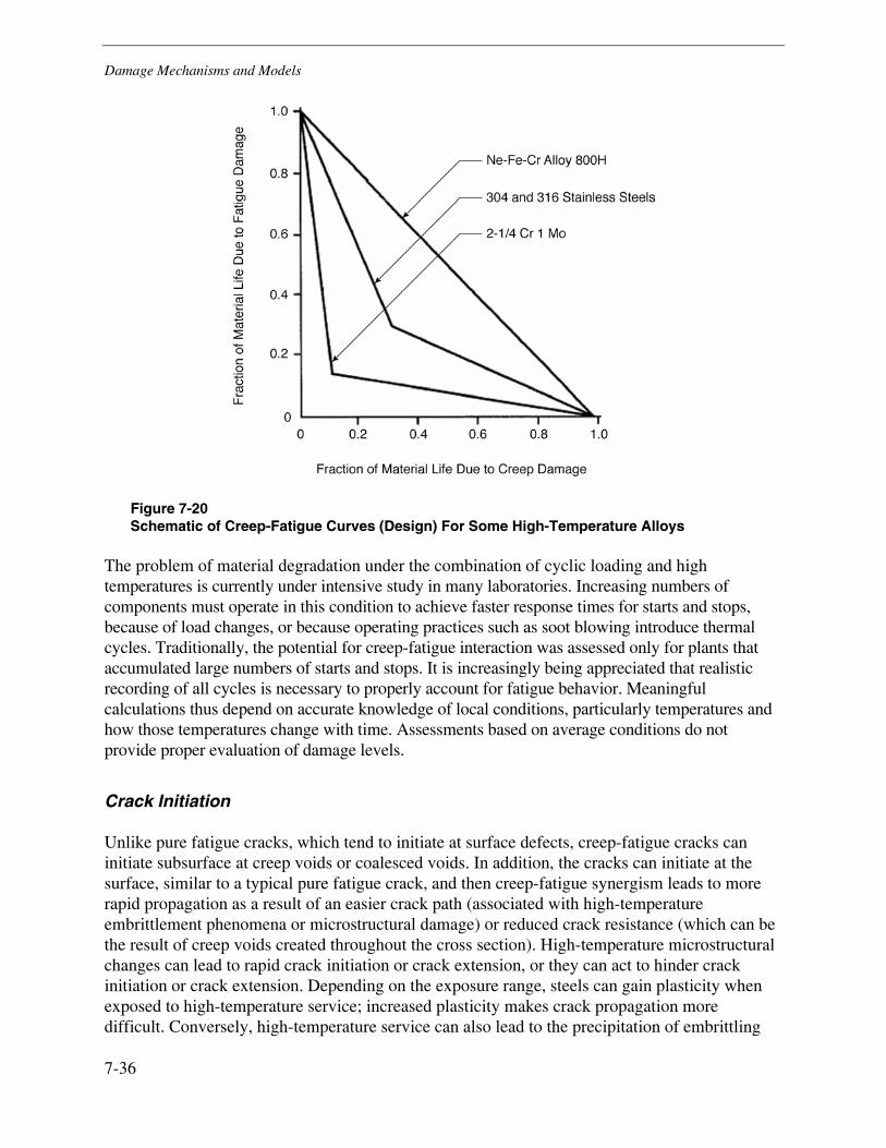
Damage Mechanisms and Models
7-36
Figure 7-20 Schematic of Creep-Fatigue Curves (Design) For Some High-Temperature Alloys
The problem of material degradation under the combination of cyclic loading and high temperatures is currently under intensive study in many laboratories. Increasing numbers of components must operate in this condition to achieve faster response times for starts and stops, because of load changes, or because operating practices such as soot blowing introduce thermal cycles. Traditionally, the potential for creep-fatigue interaction was assessed only for plants that accumulated large numbers of starts and stops. It is increasingly being appreciated that realistic recording of all cycles is necessary to properly account for fatigue behavior. Meaningful calculations thus depend on accurate knowledge of local conditions, particularly temperatures and how those temperatures change with time. Assessments based on average conditions do not provide proper evaluation of damage levels.
Crack Initiation
Unlike pure fatigue cracks, which tend to initiate at surface defects, creep-fatigue cracks can initiate subsurface at creep voids or coalesced voids. In addition, the cracks can initiate at the surface, similar to a typical pure fatigue crack, and then creep-fatigue synergism leads to more rapid propagation as a result of an easier crack path (associated with high-temperature embrittlement phenomena or microstructural damage) or reduced crack resistance (which can be the result of creep voids created throughout the cross section). High-temperature microstructural changes can lead to rapid crack initiation or crack extension, or they can act to hinder crack initiation or crack extension. Depending on the exposure range, steels can gain plasticity when exposed to high-temperature service; increased plasticity makes crack propagation more difficult. Conversely, high-temperature service can also lead to the precipitation of embrittling
Damage Mechanisms and Models
7-37
phases, which reduce plasticity and increase the likelihood of crack initiation or easy crack extension. The steel’s initial chemistry and microstructural morphology are critical variables that determine a component’s resistance to creep-fatigue crack initiation or crack extension. During failure analysis, creep-fatigue cracks are differentiated from pure creep and pure fatigue cracks because morphological characteristics of both phenomena are observed.
As with most high-energy piping defects, the most susceptible, and therefore probable, locations for cracking are weldments because of their microstructural inhomogeneity.
Crack Growth
Like both pure fatigue cracks and creep cracks, creep-fatigue cracks typically experience a period of stable crack growth. Crack extension rates depend on the temperature of service, the amplitude and period of the applied stress range, the mean stress level, the rate of strain application, and the complex interactions of microstructural changes at high temperatures. Both high-cycle fatigue behavior and low-cycle fatigue behavior can be experienced. Because microstructural embrittlement caused by high-temperature exposure is a time-dependent phenomenon, crack initiation and rapid fatigue crack propagation (classically associated with low-cycle fatigue) are possible after years of operation. In this case, crack initiation can be defined as component failure. The more common scenario is stable creep-fatigue crack propagation at definable and measurable rates, which can be used to predict useful component life.
Several methods exist to enable the use of crack measurements made with NDE to predict remaining component life. Even if cracks are not detected, calculational methods can be used to ensure safe operation until the next inspection cycle. A fracture mechanics approach can be used in which the maximum crack size that cannot be detected is postulated, and calculations are performed to predict when the postulated crack will reach a size that will induce rupture or failure. This type of approach can be used to justify continued operation and determine appropriate reinspection intervals to ensure safe operation. The next subsection describes several calculation techniques in more detail.
Analytical Techniques
Life Prediction Techniques
There are numerous rules and methods for estimating creep-fatigue damage, including the following:
• A linear summation of Miner’s and Robinson’s rule
• Frequency-modified Coffin-Manson relationship [7-45]
• Strain range partitioning method [7-46]
• Ostergren damage function [7-47]

Damage Mechanisms and Models
7-38
• Ductility exhaustion method [7-48]
• Bicego’s energy criterion [7-49]
• Ductility normalized inelastic strain range [7-50]
• Damage rate method [7-51]
• General damage function [7-52]
The various damage rules for creep-fatigue have been compared by many investigators, and there is a wide divergence of opinion about which rule provides the most accurate life prediction [7-14, 7-53]. One consistent finding is that even the most accurate rule is useful only to within a factor of 2 or 3 on remaining life prediction. It has been suggested that further tuning of the damage rules themselves, which represent only the first step in the life assessment process, is not expected to be fruitful [7-54].
The most common approach to life estimation based on creep-fatigue damage, particularly in the United States, is the linear superposition of fatigue and creep damage (see Equation 7-17).
∑ ∑+=rf tt
NND Eq. 7-17
Where:
D is cumulative life.
N/Nf is the cyclic portion of the life-fraction.
N is the number of cycles at a given strain range.
Nf is the pure fatigue life at that strain range.
t/tr is the time-dependent creep fraction.
t is the time at a given stress.
tr is the time to rupture at that stress.
The stress relaxation period is divided into time blocks during which an average constant stress occurs, and then t/tr is computed and summed for each time block. Creep damage occurring under constant stress after stress relaxation is also included in the creep fraction. This approach is the basis of the inelastic route described by Viswanathan in “Life Prediction of Turbine Generator Rotors” [7-25]. An alternative approach, the elastic route, incorporates the stress relaxation damage into the fatigue term by using fatigue curves that incorporate the effect of long hold times.
The solid line in Figure 7-21 shows the safe design limit as a fraction of creep life and fatigue life for 2-1/4 Cr 1 Mo steel. The figure indicates the relative reductions in life for various levels of two-shift operation relative to the original, primarily base load operation. This methodology is highly conservative [7-55].
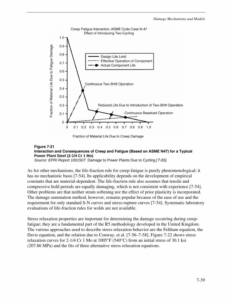
Damage Mechanisms and Models
7-39
Figure 7-21 Interaction and Consequences of Creep and Fatigue (Based on ASME N47) for a Typical Power Plant Steel (2-1/4 Cr 1 Mo) Source: EPRI Report 1001507. Damage to Power Plants Due to Cycling [7-55].
As for other mechanisms, the life-fraction rule for creep-fatigue is purely phenomenological; it has no mechanistic basis [7-54]. Its applicability depends on the development of empirical constants that are material-dependent. The life-fraction rule also assumes that tensile and compressive hold periods are equally damaging, which is not consistent with experience [7-54]. Other problems are that neither strain softening nor the effect of prior plasticity is incorporated. The damage summation method, however, remains popular because of the ease of use and the requirement for only standard S-N curves and stress-rupture curves [7-54]. Systematic laboratory evaluations of life-fraction rules for welds are not available.
Stress relaxation properties are important for determining the damage occurring during creep-fatigue; they are a fundamental part of the R5 methodology developed in the United Kingdom. The various approaches used to describe stress relaxation behavior are the Feltham equation, the Davis equation, and the relation due to Conway, et al. [7-56–7-58]. Figure 7-22 shows stress relaxation curves for 2-1/4 Cr 1 Mo at 1005°F (540°C) from an initial stress of 30.1 ksi (207.86 MPa) and the fits of three alternative stress relaxation equations.
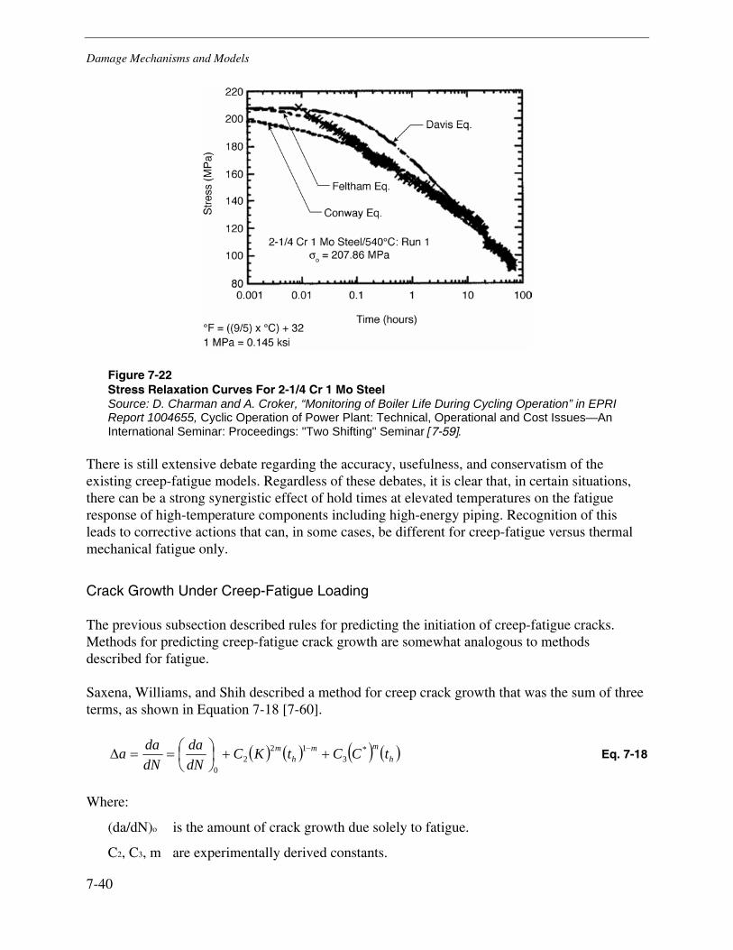
Damage Mechanisms and Models
7-40
Figure 7-22 Stress Relaxation Curves For 2-1/4 Cr 1 Mo Steel Source: D. Charman and A. Croker, “Monitoring of Boiler Life During Cycling Operation” in EPRI Report 1004655, Cyclic Operation of Power Plant: Technical, Operational and Cost Issues—An International Seminar: Proceedings: "Two Shifting" Seminar [7-59].
There is still extensive debate regarding the accuracy, usefulness, and conservatism of the existing creep-fatigue models. Regardless of these debates, it is clear that, in certain situations, there can be a strong synergistic effect of hold times at elevated temperatures on the fatigue response of high-temperature components including high-energy piping. Recognition of this leads to corrective actions that can, in some cases, be different for creep-fatigue versus thermal mechanical fatigue only.
Crack Growth Under Creep-Fatigue Loading
The previous subsection described rules for predicting the initiation of creep-fatigue cracks. Methods for predicting creep-fatigue crack growth are somewhat analogous to methods described for fatigue.
Saxena, Williams, and Shih described a method for creep crack growth that was the sum of three terms, as shown in Equation 7-18 [7-60].
( ) ( ) ( ) ( )hmm
hm tCCtKC
dNda
dNdaa *
312
20
++⎟⎠⎞
⎜⎝⎛==Δ −
Eq. 7-18
Where:
(da/dN)o is the amount of crack growth due solely to fatigue.
C2, C3, m are experimentally derived constants.

Damage Mechanisms and Models
7-41
K is the elastic stress intensity.
th is the hold time.
C* is the crack tip driving force in creep.
The first term is the pure fatigue contribution with no effect of hold time; it corresponds to crack growth behavior at short hold times and high frequencies. The second term is the creep-fatigue interaction term. It has a nonlinear dependence of crack growth rate on hold time and pertains to intermediate hold times and frequencies in which the creep-fatigue interaction is present. The third term is for pure creep occurring during long hold times and low frequencies. A plot of da/dN versus t shows three regimes of crack growth rates that correspond to the terms in the equation. The crack growth rate is a continuous function of frequency, even though the mechanism varies from transgranular fatigue at one end of the spectrum to intergranular creep at the other end of the spectrum [7-61].
A more recent model has been proposed, combining the second and third terms into a single term, as shown in Equations 7-19 through 7-21 [7-62].
( ) hm
avetn
Total
tbCKCdN
daa +Δ=⎟⎟⎠
⎞⎜⎜⎝
⎛=Δ Eq. 7-19
Ct(ave) is expressed by Equation 7-20.
( ) ∫=ht
th
avet dtCt
C0
1 Eq. 7-20
Ct(ave) was observed to correlate well with average crack growth rate during the hold time, expressed as shown in Equation 7-21.
⎥⎦
⎤⎢⎣
⎡⎟⎠⎞
⎜⎝⎛−⎟
⎠⎞
⎜⎝⎛=⎟
⎠⎞
⎜⎝⎛=⎟
⎠⎞
⎜⎝⎛
0
11dNda
dNda
tdNda
tdtda
Totalhholdhave
Eq. 7-21
Figure 7–23 shows creep-fatigue crack growth data for a 1-1/4 Cr 1/2 Mo steel at various hold times from 10 seconds to 24 hours [7-61].
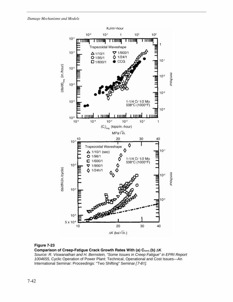
Damage Mechanisms and Models
7-42
Figure 7-23 Comparison of Creep-Fatigue Crack Growth Rates With (a) Ct(ave), (b) ΔK Source: R. Viswanathan and H. Bernstein, “Some Issues in Creep Fatigue” in EPRI Report 1004655, Cyclic Operation of Power Plant: Technical, Operational and Cost Issues—An International Seminar: Proceedings: "Two Shifting" Seminar [7-61].
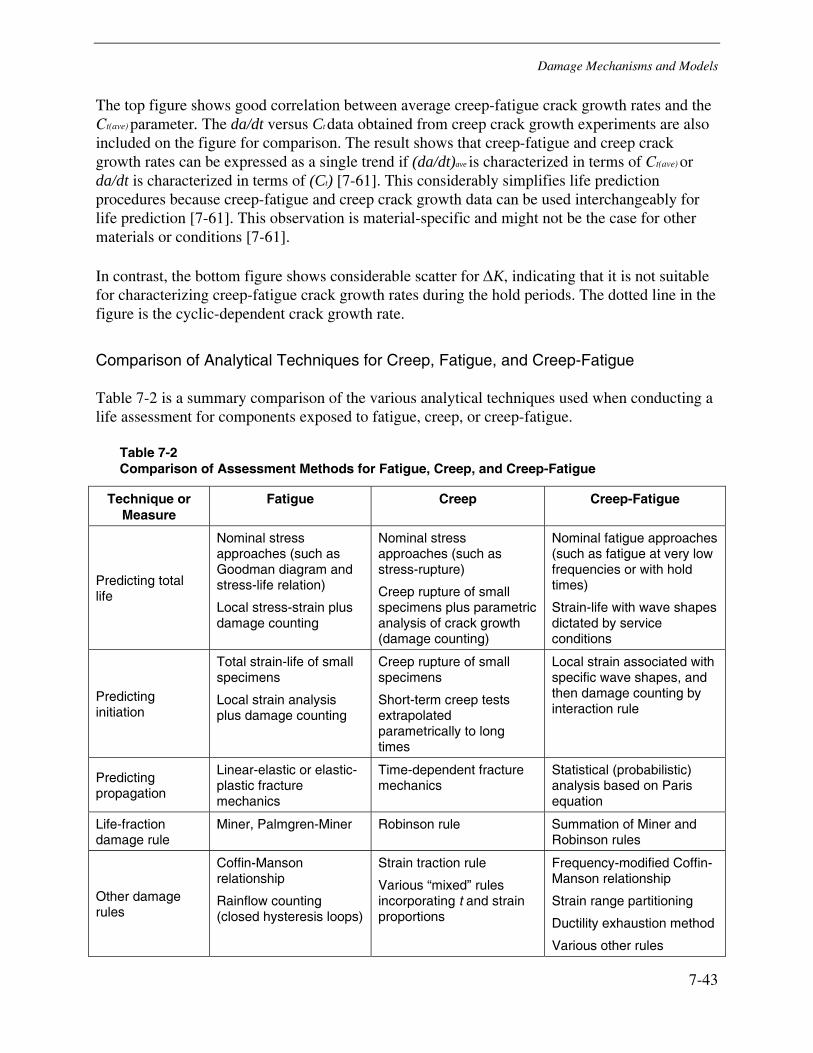
Damage Mechanisms and Models
7-43
The top figure shows good correlation between average creep-fatigue crack growth rates and the Ct(ave) parameter. The da/dt versus Ct data obtained from creep crack growth experiments are also included on the figure for comparison. The result shows that creep-fatigue and creep crack growth rates can be expressed as a single trend if (da/dt)ave is characterized in terms of Ct(ave) or da/dt is characterized in terms of (Ct) [7-61]. This considerably simplifies life prediction procedures because creep-fatigue and creep crack growth data can be used interchangeably for life prediction [7-61]. This observation is material-specific and might not be the case for other materials or conditions [7-61].
In contrast, the bottom figure shows considerable scatter for ΔK, indicating that it is not suitable for characterizing creep-fatigue crack growth rates during the hold periods. The dotted line in the figure is the cyclic-dependent crack growth rate.
Comparison of Analytical Techniques for Creep, Fatigue, and Creep-Fatigue
Table 7-2 is a summary comparison of the various analytical techniques used when conducting a life assessment for components exposed to fatigue, creep, or creep-fatigue.
Table 7-2 Comparison of Assessment Methods for Fatigue, Creep, and Creep-Fatigue
Technique or Measure
Fatigue Creep Creep-Fatigue
Predicting total life
Nominal stress approaches (such as Goodman diagram and stress-life relation)
Local stress-strain plus damage counting
Nominal stress approaches (such as stress-rupture)
Creep rupture of small specimens plus parametric analysis of crack growth (damage counting)
Nominal fatigue approaches (such as fatigue at very low frequencies or with hold times)
Strain-life with wave shapes dictated by service conditions
Predicting initiation
Total strain-life of small specimens
Local strain analysis plus damage counting
Creep rupture of small specimens
Short-term creep tests extrapolated parametrically to long times
Local strain associated with specific wave shapes, and then damage counting by interaction rule
Predicting propagation
Linear-elastic or elastic-plastic fracture mechanics
Time-dependent fracture mechanics
Statistical (probabilistic) analysis based on Paris equation
Life-fraction damage rule
Miner, Palmgren-Miner Robinson rule Summation of Miner and Robinson rules
Other damage rules
Coffin-Manson relationship
Rainflow counting (closed hysteresis loops)
Strain traction rule
Various “mixed” rules incorporating t and strain proportions
Frequency-modified Coffin-Manson relationship
Strain range partitioning
Ductility exhaustion method
Various other rules
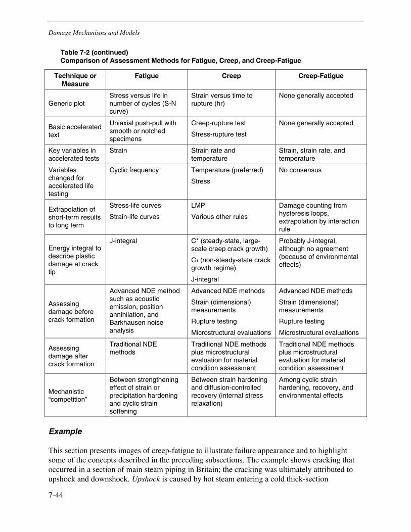
Damage Mechanisms and Models
7-44
Table 7-2 (continued) Comparison of Assessment Methods for Fatigue, Creep, and Creep-Fatigue
Technique or Measure
Fatigue Creep Creep-Fatigue
Generic plot Stress versus life in number of cycles (S-N curve)
Strain versus time to rupture (hr)
None generally accepted
Basic accelerated text
Uniaxial push-pull with smooth or notched specimens
Creep-rupture test
Stress-rupture test
None generally accepted
Key variables in accelerated tests
Strain Strain rate and temperature
Strain, strain rate, and temperature
Variables changed for accelerated life testing
Cyclic frequency Temperature (preferred)
Stress
No consensus
Extrapolation of short-term results to long term
Stress-life curves
Strain-life curves
LMP
Various other rules
Damage counting from hysteresis loops, extrapolation by interaction rule
Energy integral to describe plastic damage at crack tip
J-integral C* (steady-state, large-scale creep crack growth)
C1 (non-steady-state crack growth regime)
J-integral
Probably J-integral, although no agreement (because of environmental effects)
Assessing damage before crack formation
Advanced NDE method such as acoustic emission, position annihilation, and Barkhausen noise analysis
Advanced NDE methods
Strain (dimensional) measurements
Rupture testing
Microstructural evaluations
Advanced NDE methods
Strain (dimensional) measurements
Rupture testing
Microstructural evaluations
Assessing damage after crack formation
Traditional NDE methods
Traditional NDE methods plus microstructural evaluation for material condition assessment
Traditional NDE methods plus microstructural evaluation for material condition assessment
Mechanistic “competition”
Between strengthening effect of strain or precipitation hardening and cyclic strain softening
Between strain hardening and diffusion-controlled recovery (internal stress relaxation)
Among cyclic strain hardening, recovery, and environmental effects
Example
This section presents images of creep-fatigue to illustrate failure appearance and to highlight some of the concepts described in the preceding subsections. The example shows cracking that occurred in a section of main steam piping in Britain; the cracking was ultimately attributed to upshock and downshock. Upshock is caused by hot steam entering a cold thick-section
Damage Mechanisms and Models
7-45
component, causing the inner part of the wall to warm faster than the outer. The instantaneous result can be compressive yielding of the inside surface. The stress-temperature profile is illustrated in Figure 7-24.
Figure 7-24 The Initial Stress-Temperature Distribution Generated by Upshock
When the through-wall temperature gradient has dissipated, a local tensile residual stress remains at the pipe bore, which in turn acts as a stress riser. The residual stress creeps out during service, but is regenerated at the next start-up. Resultant cracking occurs by intermittent creep at the operating temperature. The reverse condition, downshock, is caused by rapid steam cooling on a hot component, causing the inner part of the wall to cool faster than the outer. This gives rise to a transient tensile stress at the bore. Resultant cracking occurs by fatigue at a temperature close to the cooled steam temperature. In this specific main steam piping, the base metal was CrMoV low-alloy steel, and the weld metal was 2-1/4 Cr 1 Mo. British plants tend to operate at higher temperatures than their U.S. counterparts; in this case, the main steam temperature was 1050°F (565°C), which is well within the creep range.
Figure 7-25 illustrates several features that are classically associated with creep-fatigue crack initiation and propagation, making this a good example. Both images in Figure 7-25 are stereoscopic macrographs of creep-fatigue cracking that occurred in two different longitudinal seam weldments in the same main steam piping. The left image shows creep-fatigue cracking from upshock; the right image shows creep-fatigue cracking from downshock.
Damage Mechanisms and Models
7-46
Figure 7-25 Stereoscopic Macrographs of Creep-Fatigue Cracking Resulting from (a) Upshock and (b) Downshock
Creep-fatigue is differentiated from pure fatigue or pure creep because the cracking has features of both damage mechanisms. The upshock cracking shown in the left image of Figure 7-25 was initiated at the stress concentrators on either side of the weldments and was generated by repeated thermal shock loading cycles; both of these characteristics are classically associated with fatigue cracking. However, the crack is Type IV, it tends to follow the intercritical region of the HAZ, and it does not follow the stress path or propagate transgranularly; these behaviors are classically associated with creep cracking. Because these cracks demonstrate both fatigue and creep behavior, they are classified as creep-fatigue cracks.
In a similar but different way, the crack shown in the image on the right side of Figure 7-25 is also classified as creep-fatigue. In both images, the cracks occur in the creep regime, which is a necessary condition for creep-fatigue. In the right-side image, the crack initiates at a stress concentrator toward the center of the weldment, it propagates transgranularly, and the propagation seems to be stress dominated—these are all classically associated with fatigue cracking. Again, both creep and fatigue factors and behaviors are present; therefore, the crack is classified as creep-fatigue.
Flow-Accelerated Corrosion
Introduction
The phenomenon of FAC is well understood. It is a process in which the normally protective magnetite (Fe3O4) layer on carbon steel dissolves in a stream of flowing water (single phase) or wet steam (two phase). Under normal conditions, the oxide growth and removal processes are approximately equal. However, abnormal conditions can reduce or eliminate the protective oxide
Damage Mechanisms and Models
7-47
layer and lead to a rapid removal of the base material. In the worst cases, metal loss continues until the pipe or tube bursts. The rate of metal loss depends on a complex interplay of many parameters including the following:
• The feedwater chemistry, including oxidation-reduction potential (ORP), oxygen and reducing agents, and pH
• The material composition, in particular the levels of Cr, Cu, and Mo
• The other materials in the feedwater system
• The fluid hydrodynamics, such as velocity, geometry, steam quality, temperature, and mass transfer
The FAC process can lead to rapid rates of metal loss; wall thinning rates as high as 0.120 in./yr (3mm/yr) have occurred. Thus, it is important to implement effective FAC prevention programs. See the EPRI report Guidelines for Controlling Flow-Accelerated Corrosion in Fossil and Combined Cycle Plants (1008082) for details [7-6].
The feedwater system in fossil plants can consist of all-ferrous materials or a mixture of copper-containing feedwater tubes and ferrous piping (known as a mixed metallurgical system). The specific configuration has important ramifications on the choice of feedwater chemistry and hence on FAC. The two possible all-ferrous systems are those containing carbon steel piping and tubing, and those with stainless steel tubing and carbon steel piping.
Based on the seriousness of previously reported failures the most susceptible situation for FAC is one in which all the feedwater heater tubing (both low-pressure and high-pressure tubing) is stainless steel and the water chemistry is all-volatile treatment (AVT) reducing.
Mixed metallurgical systems can use only AVT-reducing chemistry because the reducing environment is necessary to protect the copper-based tubing. Wall loss has been observed in ferrous parts of these systems, but the rate of damage is not as severe. This apparent anomaly is explained by the fact that the copper alloys and oxides act as a catalyst for the reaction between the reducing agent (hydrazine) and dissolved oxygen in the feedwater. However, even with these systems, it is still advisable to operate with a rigorous monitoring system.
High-energy piping can contain single-phase (water) fluid flow or two-phase (wet steam) fluid flow, or both, depending on the temperature and pressure conditions. FAC mechanisms differ for the two conditions; therefore, it is important to differentiate between the two and explore them individually. The underlying mechanisms for single-phase flow are explored first.
Operational Conditions
The critical factors influencing FAC include the following:
• ORP
• Water pH
Damage Mechanisms and Models
7-48
• Temperature
• Flow velocity
• Mass transfer
• Geometry
The following sections describe these factors.
Oxidation-Reduction Potential
ORP (or redox) is by far the most important factor for single-phase FAC. In fossil and heat recovery steam generator (HRSG) plants, the ORP is usually reported as a voltage versus that of an Ag/AgCl (sat. KCl) reference electrode. ORP reflects the balance between various conjugate redox systems and must not be confused with the corrosion potential. However, it does provide a useful indicator of the corrosivity of the flowing water. ORP is sensitive to the materials of construction and to the temperature because of the effects of temperature on the redox reactions. ORP also changes with pH, partial pressure of oxygen in the flowing water, mass transport properties, and flow rates; therefore, ORP cannot be compared from unit to unit. Not only does ORP control the surface oxide that forms in feedwater or evaporator water—AVT reducing (AVT[R]) or AVT oxygenating (AVT[O]) or oxygenating treatment (OT)—but as the ORP becomes more reducing, the possibility for FAC increases. Changing to AVT(O) by eliminating the reducing agent or by adding oxygen (OT) essentially reduces the possibility of dissolution into the flowing water to low values, even in areas where FAC was severe with AVT(R).
Water pH
Water pH is the second most important factor because it affects the solubility of the surface Fe3O4. Generally, a higher pH reduces the amount of corrosion and FAC. FAC is directly related to the pH of the fluid in contact with the oxide surface at the hot operating temperature, not the cold pH as measured in the feedwater or HRSG evaporator.
Temperature
Temperature is important because it influences several fluid properties: the pH of the water or wet steam, the solubility of the oxide layer, the rates of the oxidation and reduction reactions, and the variables related to mass transfer (Reynolds, Schmidt, and Sherwood numbers; fluid density and viscosity; steam quality and void fraction). Laboratory data and field experience indicate that FAC tends to peak at temperatures in the range of 300°F–350°F (150°C–180°C).
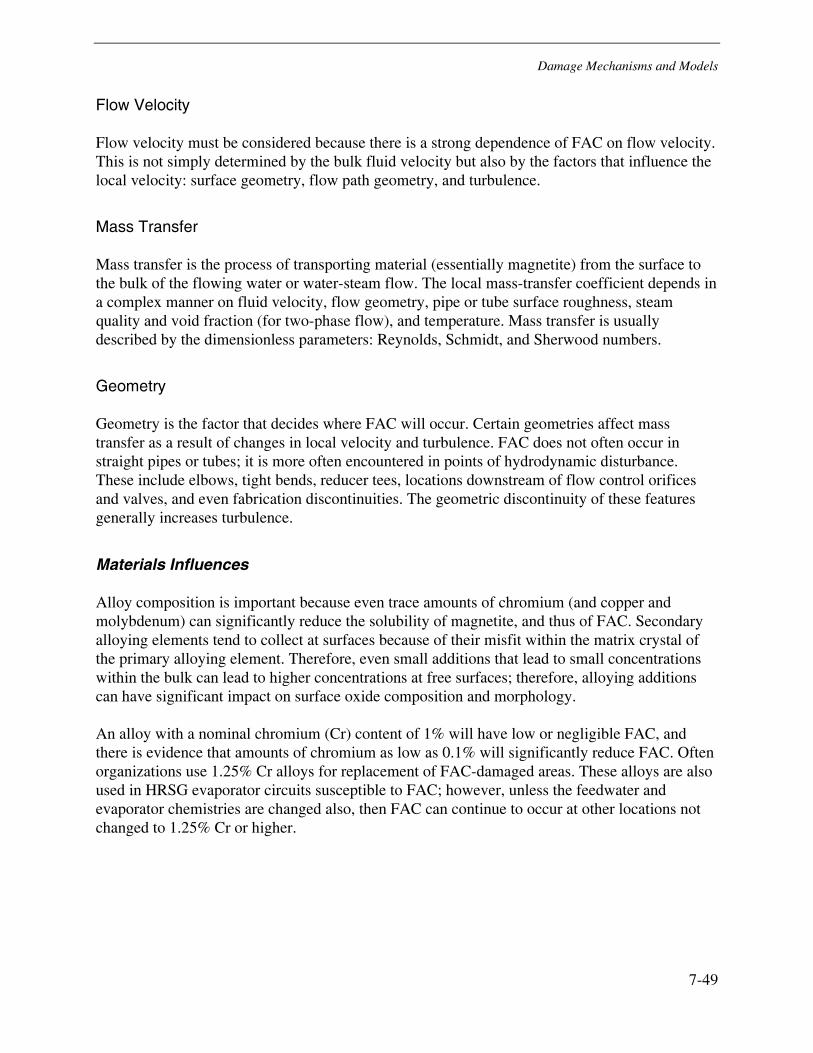
Damage Mechanisms and Models
7-49
Flow Velocity
Flow velocity must be considered because there is a strong dependence of FAC on flow velocity. This is not simply determined by the bulk fluid velocity but also by the factors that influence the local velocity: surface geometry, flow path geometry, and turbulence.
Mass Transfer
Mass transfer is the process of transporting material (essentially magnetite) from the surface to the bulk of the flowing water or water-steam flow. The local mass-transfer coefficient depends in a complex manner on fluid velocity, flow geometry, pipe or tube surface roughness, steam quality and void fraction (for two-phase flow), and temperature. Mass transfer is usually described by the dimensionless parameters: Reynolds, Schmidt, and Sherwood numbers.
Geometry
Geometry is the factor that decides where FAC will occur. Certain geometries affect mass transfer as a result of changes in local velocity and turbulence. FAC does not often occur in straight pipes or tubes; it is more often encountered in points of hydrodynamic disturbance. These include elbows, tight bends, reducer tees, locations downstream of flow control orifices and valves, and even fabrication discontinuities. The geometric discontinuity of these features generally increases turbulence.
Materials Influences
Alloy composition is important because even trace amounts of chromium (and copper and molybdenum) can significantly reduce the solubility of magnetite, and thus of FAC. Secondary alloying elements tend to collect at surfaces because of their misfit within the matrix crystal of the primary alloying element. Therefore, even small additions that lead to small concentrations within the bulk can lead to higher concentrations at free surfaces; therefore, alloying additions can have significant impact on surface oxide composition and morphology.
An alloy with a nominal chromium (Cr) content of 1% will have low or negligible FAC, and there is evidence that amounts of chromium as low as 0.1% will significantly reduce FAC. Often organizations use 1.25% Cr alloys for replacement of FAC-damaged areas. These alloys are also used in HRSG evaporator circuits susceptible to FAC; however, unless the feedwater and evaporator chemistries are changed also, then FAC can continue to occur at other locations not changed to 1.25% Cr or higher.
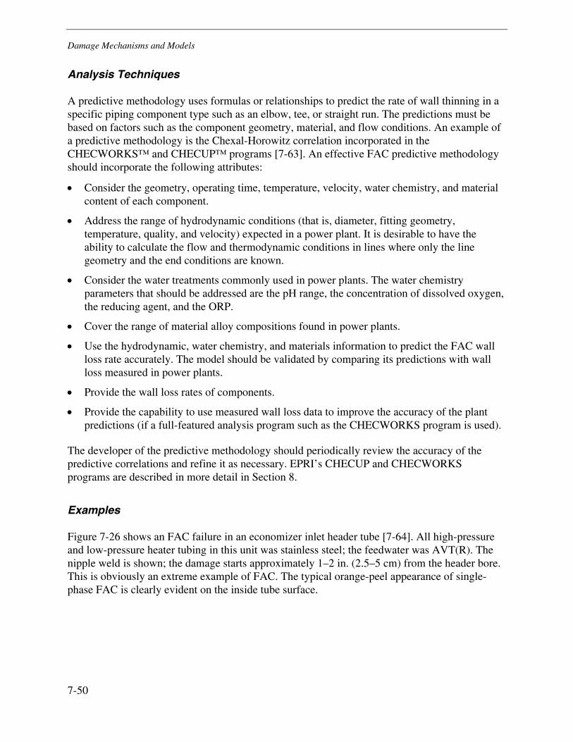
Damage Mechanisms and Models
7-50
Analysis Techniques
A predictive methodology uses formulas or relationships to predict the rate of wall thinning in a specific piping component type such as an elbow, tee, or straight run. The predictions must be based on factors such as the component geometry, material, and flow conditions. An example of a predictive methodology is the Chexal-Horowitz correlation incorporated in the CHECWORKS™ and CHECUP™ programs [7-63]. An effective FAC predictive methodology should incorporate the following attributes:
• Consider the geometry, operating time, temperature, velocity, water chemistry, and material content of each component.
• Address the range of hydrodynamic conditions (that is, diameter, fitting geometry, temperature, quality, and velocity) expected in a power plant. It is desirable to have the ability to calculate the flow and thermodynamic conditions in lines where only the line geometry and the end conditions are known.
• Consider the water treatments commonly used in power plants. The water chemistry parameters that should be addressed are the pH range, the concentration of dissolved oxygen, the reducing agent, and the ORP.
• Cover the range of material alloy compositions found in power plants.
• Use the hydrodynamic, water chemistry, and materials information to predict the FAC wall loss rate accurately. The model should be validated by comparing its predictions with wall loss measured in power plants.
• Provide the wall loss rates of components.
• Provide the capability to use measured wall loss data to improve the accuracy of the plant predictions (if a full-featured analysis program such as the CHECWORKS program is used).
The developer of the predictive methodology should periodically review the accuracy of the predictive correlations and refine it as necessary. EPRI’s CHECUP and CHECWORKS programs are described in more detail in Section 8.
Examples
Figure 7-26 shows an FAC failure in an economizer inlet header tube [7-64]. All high-pressure and low-pressure heater tubing in this unit was stainless steel; the feedwater was AVT(R). The nipple weld is shown; the damage starts approximately 1–2 in. (2.5–5 cm) from the header bore. This is obviously an extreme example of FAC. The typical orange-peel appearance of single-phase FAC is clearly evident on the inside tube surface.
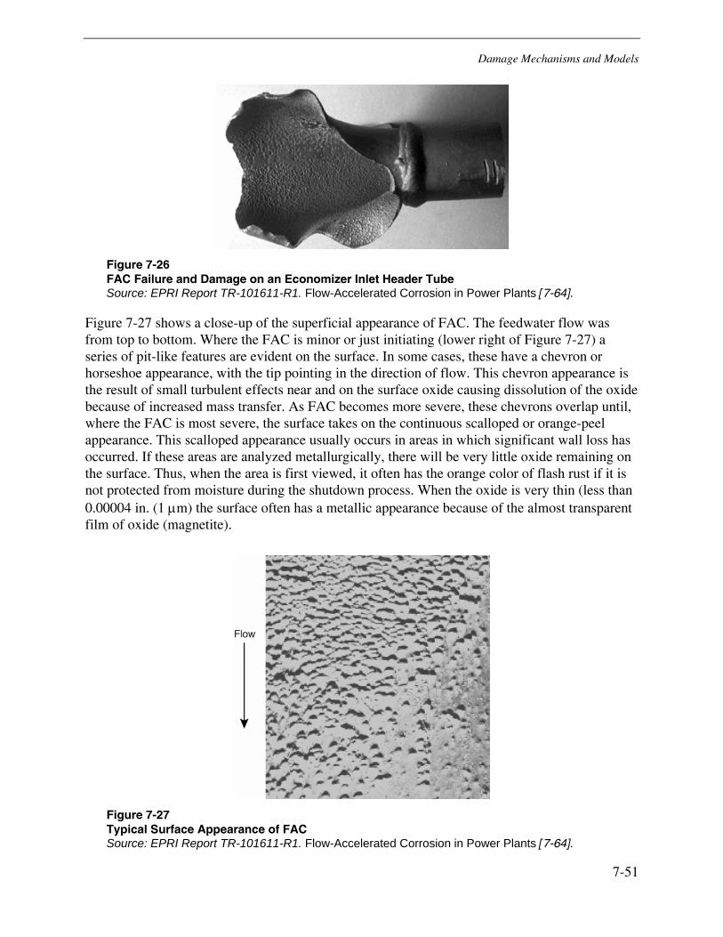
Damage Mechanisms and Models
7-51
Figure 7-26 FAC Failure and Damage on an Economizer Inlet Header Tube Source: EPRI Report TR-101611-R1. Flow-Accelerated Corrosion in Power Plants [7-64].
Figure 7-27 shows a close-up of the superficial appearance of FAC. The feedwater flow was from top to bottom. Where the FAC is minor or just initiating (lower right of Figure 7-27) a series of pit-like features are evident on the surface. In some cases, these have a chevron or horseshoe appearance, with the tip pointing in the direction of flow. This chevron appearance is the result of small turbulent effects near and on the surface oxide causing dissolution of the oxide because of increased mass transfer. As FAC becomes more severe, these chevrons overlap until, where the FAC is most severe, the surface takes on the continuous scalloped or orange-peel appearance. This scalloped appearance usually occurs in areas in which significant wall loss has occurred. If these areas are analyzed metallurgically, there will be very little oxide remaining on the surface. Thus, when the area is first viewed, it often has the orange color of flash rust if it is not protected from moisture during the shutdown process. When the oxide is very thin (less than 0.00004 in. (1 μm) the surface often has a metallic appearance because of the almost transparent film of oxide (magnetite).
Figure 7-27 Typical Surface Appearance of FAC Source: EPRI Report TR-101611-R1. Flow-Accelerated Corrosion in Power Plants [7-64].
Damage Mechanisms and Models
7-52
Figure 7-28 shows a higher-magnification view of the surface of an active FAC site that shows the microscopic scalloped appearance.
Figure 7-28 Typical Scalloped Appearance of Single-Phase Flow-Accelerated Corrosion as Viewed with a Scanning Electron Microscope Source: EPRI Report TR-101611-R1. Flow-Accelerated Corrosion in Power Plants [7-64].
Other Potential Damage Mechanisms
The most relevant forms (that is, those that have the highest rate of occurrence) of degradation in high-energy piping are creep, fatigue, creep-fatigue, and FAC. There are, however, other degradation mechanisms that either are partially responsible for overall material damage or occur much less frequently than the four primary mechanisms. Several other potential degradation mechanisms are briefly described below.
Microstructural Degradation and Embrittlement
Alloy composition, thermomechanical processing, and heat treatment determine what microstructural components are present in a metal component. The microstructure determines the mechanical properties. The thermodynamic stability of all microstructural components is sensitive to operating temperature. At the higher operating temperatures of fossil plant high-energy piping, many microstructural components change, sometimes detrimentally, and therefore affect the mechanical properties of the component. Several degradation and embrittlement phenomena relevant to high-temperature piping are described in the following subsections.
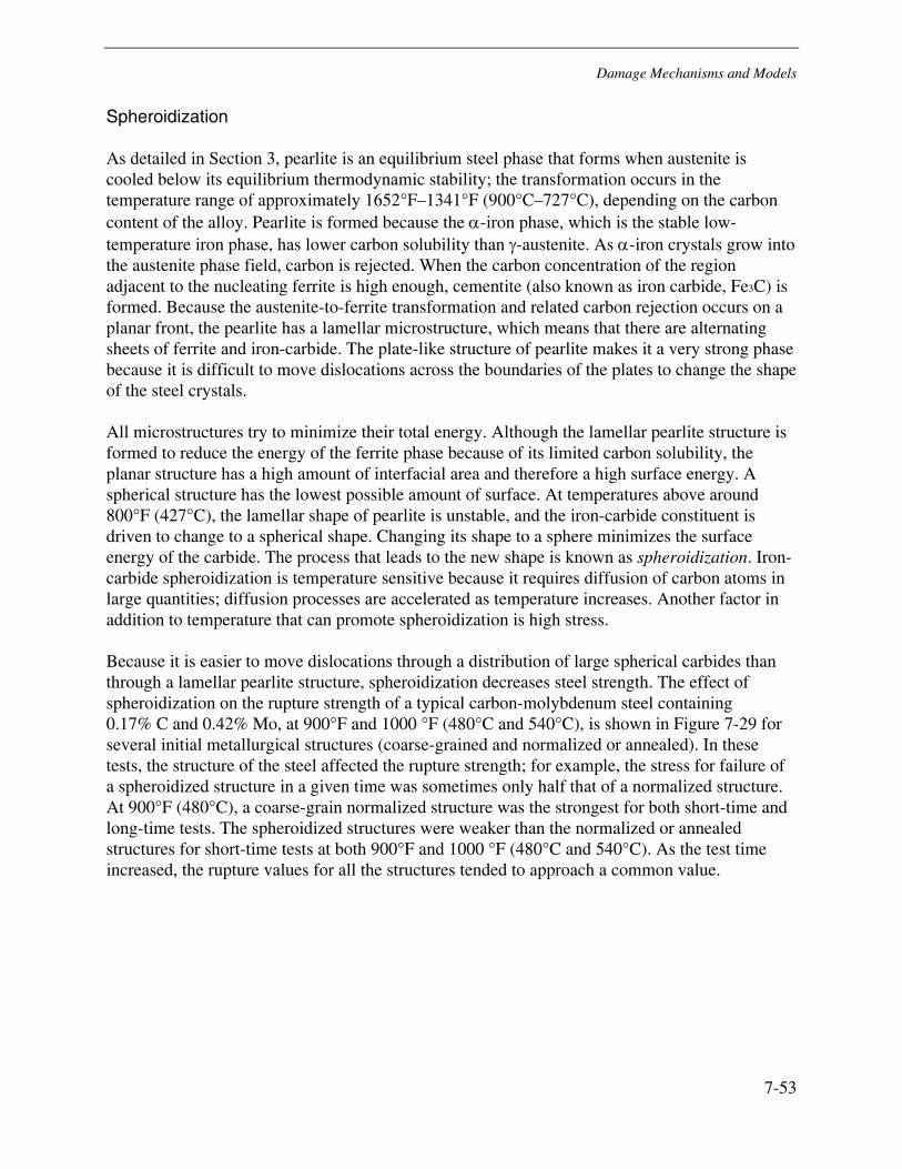
Damage Mechanisms and Models
7-53
Spheroidization
As detailed in Section 3, pearlite is an equilibrium steel phase that forms when austenite is cooled below its equilibrium thermodynamic stability; the transformation occurs in the temperature range of approximately 1652°F–1341°F (900°C–727°C), depending on the carbon content of the alloy. Pearlite is formed because the α-iron phase, which is the stable low-temperature iron phase, has lower carbon solubility than γ-austenite. As α-iron crystals grow into the austenite phase field, carbon is rejected. When the carbon concentration of the region adjacent to the nucleating ferrite is high enough, cementite (also known as iron carbide, Fe3C) is formed. Because the austenite-to-ferrite transformation and related carbon rejection occurs on a planar front, the pearlite has a lamellar microstructure, which means that there are alternating sheets of ferrite and iron-carbide. The plate-like structure of pearlite makes it a very strong phase because it is difficult to move dislocations across the boundaries of the plates to change the shape of the steel crystals.
All microstructures try to minimize their total energy. Although the lamellar pearlite structure is formed to reduce the energy of the ferrite phase because of its limited carbon solubility, the planar structure has a high amount of interfacial area and therefore a high surface energy. A spherical structure has the lowest possible amount of surface. At temperatures above around 800°F (427°C), the lamellar shape of pearlite is unstable, and the iron-carbide constituent is driven to change to a spherical shape. Changing its shape to a sphere minimizes the surface energy of the carbide. The process that leads to the new shape is known as spheroidization. Iron-carbide spheroidization is temperature sensitive because it requires diffusion of carbon atoms in large quantities; diffusion processes are accelerated as temperature increases. Another factor in addition to temperature that can promote spheroidization is high stress.
Because it is easier to move dislocations through a distribution of large spherical carbides than through a lamellar pearlite structure, spheroidization decreases steel strength. The effect of spheroidization on the rupture strength of a typical carbon-molybdenum steel containing 0.17% C and 0.42% Mo, at 900°F and 1000 °F (480°C and 540°C), is shown in Figure 7-29 for several initial metallurgical structures (coarse-grained and normalized or annealed). In these tests, the structure of the steel affected the rupture strength; for example, the stress for failure of a spheroidized structure in a given time was sometimes only half that of a normalized structure. At 900°F (480°C), a coarse-grain normalized structure was the strongest for both short-time and long-time tests. The spheroidized structures were weaker than the normalized or annealed structures for short-time tests at both 900°F and 1000 °F (480°C and 540°C). As the test time increased, the rupture values for all the structures tended to approach a common value.
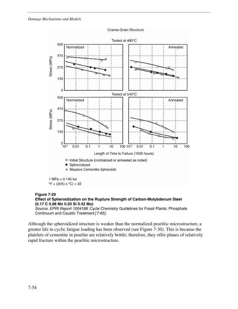
Damage Mechanisms and Models
7-54
Figure 7-29 Effect of Spheroidization on the Rupture Strength of Carbon-Molybdenum Steel (0.17 C 0.88 Mn 0.20 Si 0.42 Mo) Source: EPRI Report 1004188. Cycle Chemistry Guidelines for Fossil Plants: Phosphate Continuum and Caustic Treatment [7-65].
Although the spheroidized structure is weaker than the normalized pearlitic microstructure, a greater life in cyclic fatigue loading has been observed (see Figure 7-30). This is because the platelets of cementite in pearlite are relatively brittle; therefore, they offer planes of relatively rapid fracture within the pearlitic microstructure.
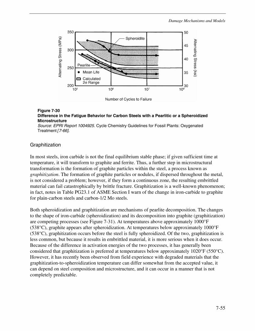
Damage Mechanisms and Models
7-55
Figure 7-30 Difference in the Fatigue Behavior for Carbon Steels with a Pearlitic or a Spheroidized Microstructure Source: EPRI Report 1004925. Cycle Chemistry Guidelines for Fossil Plants: Oxygenated Treatment [7-66].
Graphitization
In most steels, iron carbide is not the final equilibrium stable phase; if given sufficient time at temperature, it will transform to graphite and ferrite. Thus, a further step in microstructural transformation is the formation of graphite particles within the steel, a process known as graphitization. The formation of graphite particles or nodules, if dispersed throughout the metal, is not considered a problem; however, if they form a continuous zone, the resulting embrittled material can fail catastrophically by brittle fracture. Graphitization is a well-known phenomenon; in fact, notes in Table PG23.1 of ASME Section I warn of the change in iron-carbide to graphite for plain-carbon steels and carbon-1/2 Mo steels.
Both spheroidization and graphitization are mechanisms of pearlite decomposition. The changes to the shape of iron-carbide (spheroidization) and its decomposition into graphite (graphitization) are competing processes (see Figure 7-31). At temperatures above approximately 1000°F (538°C), graphite appears after spheroidization. At temperatures below approximately 1000°F (538°C), graphitization occurs before the steel is fully spheroidized. Of the two, graphitization is less common, but because it results in embrittled material, it is more serious when it does occur. Because of the difference in activation energies of the two processes, it has generally been considered that graphitization is preferred at temperatures below approximately 1020°F (550°C). However, it has recently been observed from field experience with degraded materials that the graphitization-to-spheroidization temperature can differ somewhat from the accepted value, it can depend on steel composition and microstructure, and it can occur in a manner that is not completely predictable.
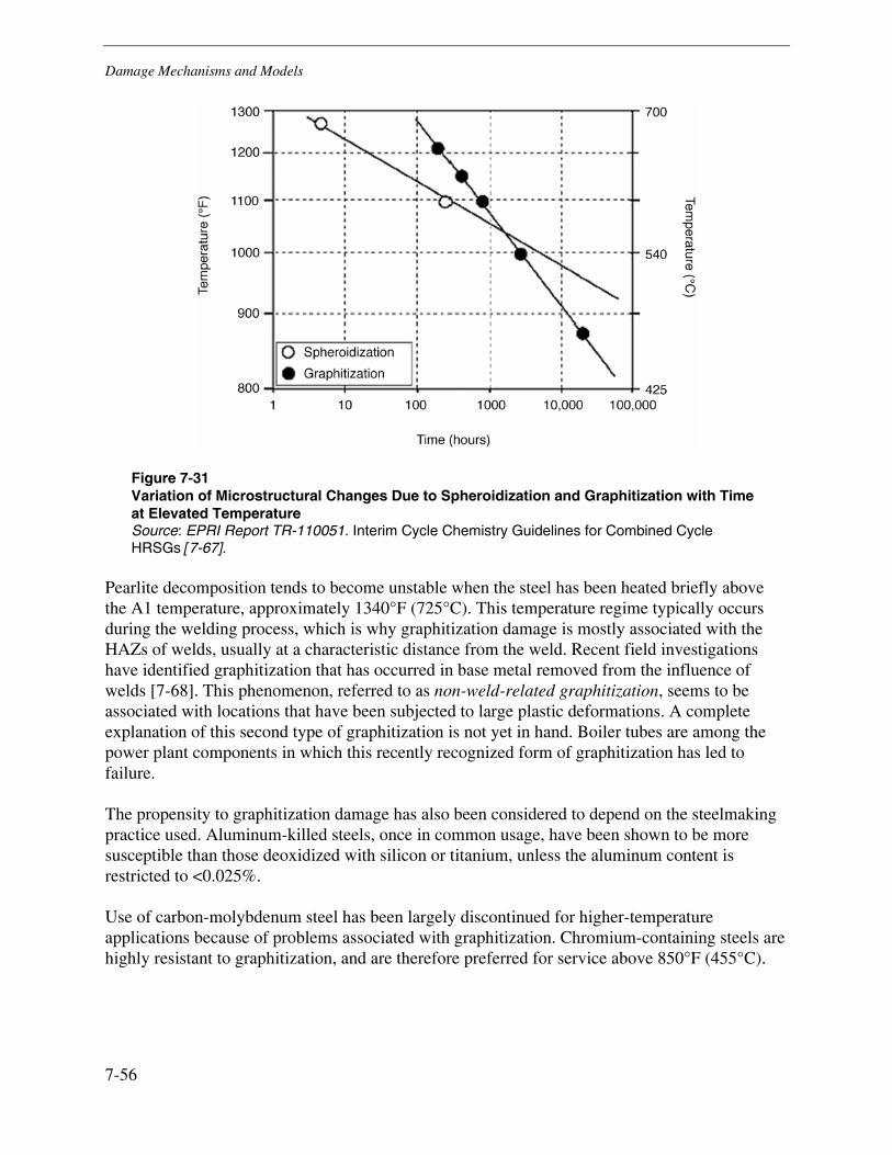
Damage Mechanisms and Models
7-56
Figure 7-31 Variation of Microstructural Changes Due to Spheroidization and Graphitization with Time at Elevated Temperature Source: EPRI Report TR-110051. Interim Cycle Chemistry Guidelines for Combined Cycle HRSGs [7-67].
Pearlite decomposition tends to become unstable when the steel has been heated briefly above the A1 temperature, approximately 1340°F (725°C). This temperature regime typically occurs during the welding process, which is why graphitization damage is mostly associated with the HAZs of welds, usually at a characteristic distance from the weld. Recent field investigations have identified graphitization that has occurred in base metal removed from the influence of welds [7-68]. This phenomenon, referred to as non-weld-related graphitization, seems to be associated with locations that have been subjected to large plastic deformations. A complete explanation of this second type of graphitization is not yet in hand. Boiler tubes are among the power plant components in which this recently recognized form of graphitization has led to failure.
The propensity to graphitization damage has also been considered to depend on the steelmaking practice used. Aluminum-killed steels, once in common usage, have been shown to be more susceptible than those deoxidized with silicon or titanium, unless the aluminum content is restricted to <0.025%.
Use of carbon-molybdenum steel has been largely discontinued for higher-temperature applications because of problems associated with graphitization. Chromium-containing steels are highly resistant to graphitization, and are therefore preferred for service above 850°F (455°C).
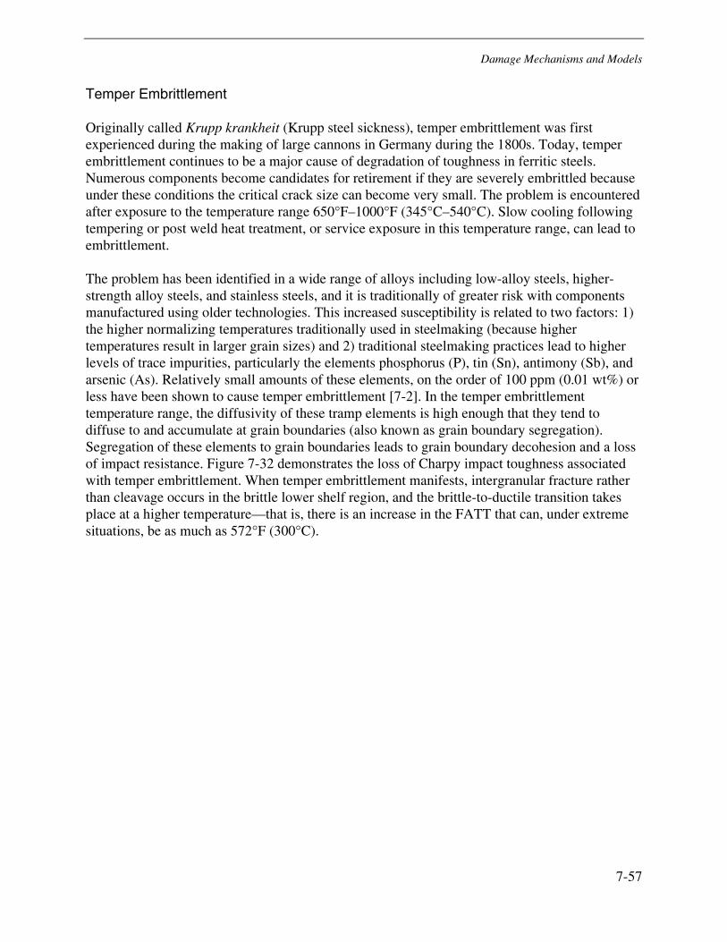
Damage Mechanisms and Models
7-57
Temper Embrittlement
Originally called Krupp krankheit (Krupp steel sickness), temper embrittlement was first experienced during the making of large cannons in Germany during the 1800s. Today, temper embrittlement continues to be a major cause of degradation of toughness in ferritic steels. Numerous components become candidates for retirement if they are severely embrittled because under these conditions the critical crack size can become very small. The problem is encountered after exposure to the temperature range 650°F–1000°F (345°C–540°C). Slow cooling following tempering or post weld heat treatment, or service exposure in this temperature range, can lead to embrittlement.
The problem has been identified in a wide range of alloys including low-alloy steels, higher-strength alloy steels, and stainless steels, and it is traditionally of greater risk with components manufactured using older technologies. This increased susceptibility is related to two factors: 1) the higher normalizing temperatures traditionally used in steelmaking (because higher temperatures result in larger grain sizes) and 2) traditional steelmaking practices lead to higher levels of trace impurities, particularly the elements phosphorus (P), tin (Sn), antimony (Sb), and arsenic (As). Relatively small amounts of these elements, on the order of 100 ppm (0.01 wt%) or less have been shown to cause temper embrittlement [7-2]. In the temper embrittlement temperature range, the diffusivity of these tramp elements is high enough that they tend to diffuse to and accumulate at grain boundaries (also known as grain boundary segregation). Segregation of these elements to grain boundaries leads to grain boundary decohesion and a loss of impact resistance. Figure 7-32 demonstrates the loss of Charpy impact toughness associated with temper embrittlement. When temper embrittlement manifests, intergranular fracture rather than cleavage occurs in the brittle lower shelf region, and the brittle-to-ductile transition takes place at a higher temperature—that is, there is an increase in the FATT that can, under extreme situations, be as much as 572°F (300°C).
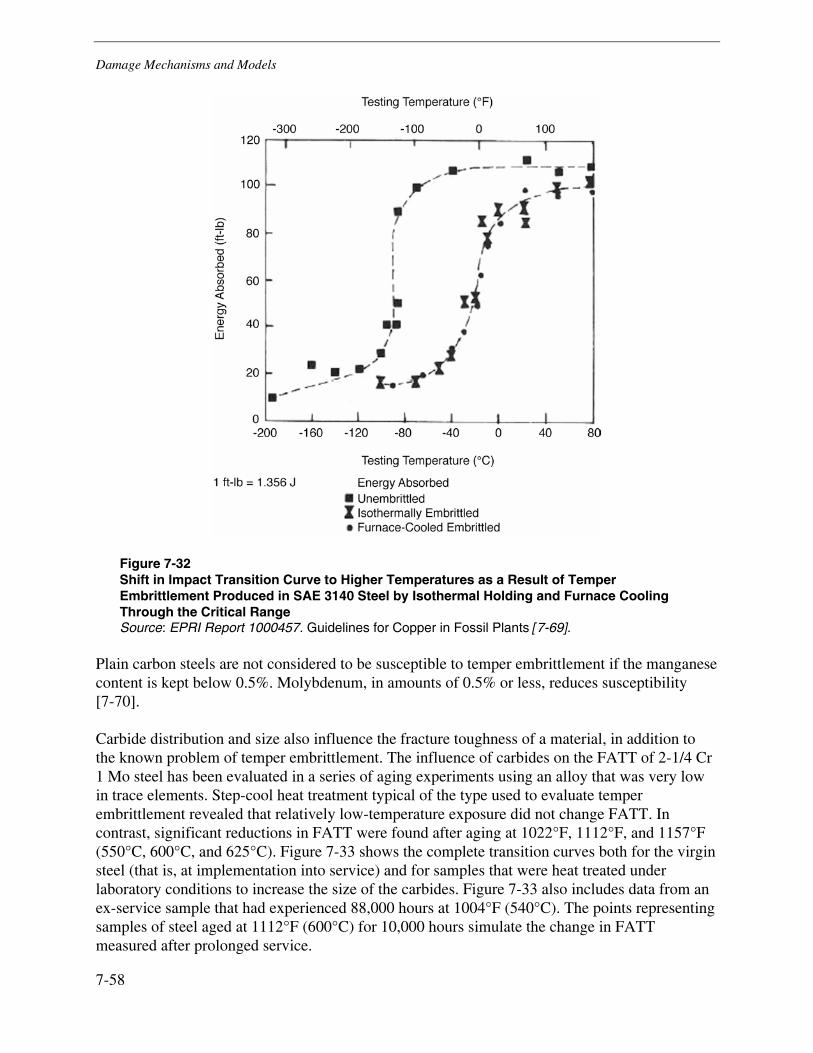
Damage Mechanisms and Models
7-58
Figure 7-32 Shift in Impact Transition Curve to Higher Temperatures as a Result of Temper Embrittlement Produced in SAE 3140 Steel by Isothermal Holding and Furnace Cooling Through the Critical Range Source: EPRI Report 1000457. Guidelines for Copper in Fossil Plants [7-69].
Plain carbon steels are not considered to be susceptible to temper embrittlement if the manganese content is kept below 0.5%. Molybdenum, in amounts of 0.5% or less, reduces susceptibility [7-70].
Carbide distribution and size also influence the fracture toughness of a material, in addition to the known problem of temper embrittlement. The influence of carbides on the FATT of 2-1/4 Cr 1 Mo steel has been evaluated in a series of aging experiments using an alloy that was very low in trace elements. Step-cool heat treatment typical of the type used to evaluate temper embrittlement revealed that relatively low-temperature exposure did not change FATT. In contrast, significant reductions in FATT were found after aging at 1022°F, 1112°F, and 1157°F (550°C, 600°C, and 625°C). Figure 7-33 shows the complete transition curves both for the virgin steel (that is, at implementation into service) and for samples that were heat treated under laboratory conditions to increase the size of the carbides. Figure 7-33 also includes data from an ex-service sample that had experienced 88,000 hours at 1004°F (540°C). The points representing samples of steel aged at 1112°F (600°C) for 10,000 hours simulate the change in FATT measured after prolonged service.
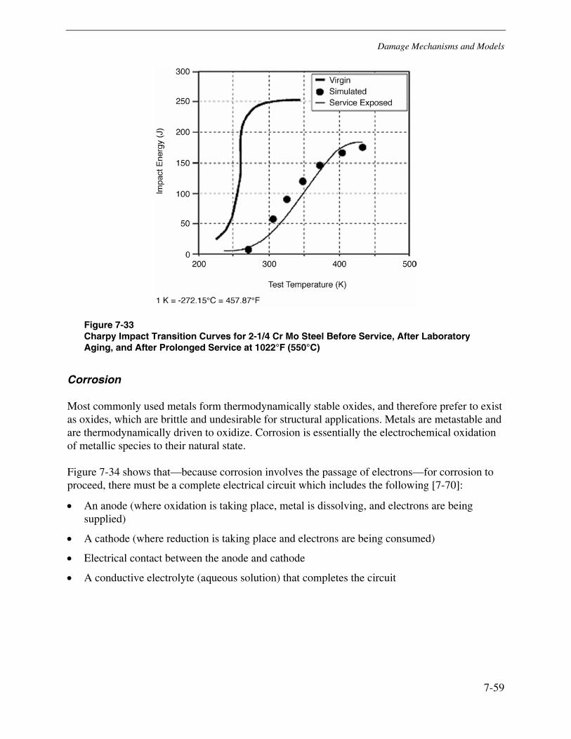
Damage Mechanisms and Models
7-59
Figure 7-33 Charpy Impact Transition Curves for 2-1/4 Cr Mo Steel Before Service, After Laboratory Aging, and After Prolonged Service at 1022°F (550°C)
Corrosion
Most commonly used metals form thermodynamically stable oxides, and therefore prefer to exist as oxides, which are brittle and undesirable for structural applications. Metals are metastable and are thermodynamically driven to oxidize. Corrosion is essentially the electrochemical oxidation of metallic species to their natural state.
Figure 7-34 shows that—because corrosion involves the passage of electrons—for corrosion to proceed, there must be a complete electrical circuit which includes the following [7-70]:
• An anode (where oxidation is taking place, metal is dissolving, and electrons are being supplied)
• A cathode (where reduction is taking place and electrons are being consumed)
• Electrical contact between the anode and cathode
• A conductive electrolyte (aqueous solution) that completes the circuit
Damage Mechanisms and Models
7-60
Figure 7-34 Basic Corrosion Cell
If any one of these components is not present, the circuit is not complete, and corrosion will not occur. At higher temperatures, there are fewer impediments to oxidation reactions, and the primary limiting factor is the availability of oxygen to form oxide; therefore, an even layer of oxide is typically formed on the surface of metal exposed to oxidizing conditions, and low-temperature aqueous corrosion is not a concern.
In a high-energy piping system, corrosive processes become a concern only during lay-ups and maintenance activities where local pools of water can exist in places that catch water. Specifically, the concern is localized corrosion. Localized corrosion involves stationary electrodes; that is, one area of the metal surface becomes a fixed anode and another area becomes a fixed cathode. Under these conditions, corrosion will continue unfettered at the anodic site. There are many forms of localized corrosion, including crevice corrosion, pitting corrosion, and under-deposit corrosion. The nature of localized corrosion tends to produce metal loss at ever-increasing rates as the environment within the pit or electrochemical crevice is isolated from the bulk environment, and the localized environment becomes acidified and enriched in damaging ions such as chlorides and sulfates.
Pitting is the most common form of localized corrosion damage in high-energy piping. It is also one of the most destructive and insidious forms of localized corrosion because it can cause equipment failures as a result of perforation with essentially no weight loss of the component. It is often difficult to detect pits because of their small size and because they are often covered by corrosion product. Like crevice corrosion, pitting most often occurs in stagnant environments. Pitting is typically characterized by an extended initiation period followed by an autocatalytic (snowballing) propagation. The relative probability of identifying a pit of a given depth is a function of the area—the larger the surface area, the deeper the pits. Therefore, laboratory tests cannot be readily used to predict the pitting depths on an actual component. Extreme value statistics can be used to make pitting prediction extrapolations.
Damage Mechanisms and Models
7-61
Because of the thickness of high-energy piping, it is unlikely that pitting can lead to through-wall perforation. However, depending on its aspect ratio, a pit can act as a very effective stress concentrator and therefore become an initiation location for cracking (either fatigue, corrosion fatigue, stress corrosion cracking, or creep-fatigue).
Stress Corrosion Cracking and Corrosion Fatigue
As with creep-fatigue, the imposition of cyclic stresses in a corrosive environment (aqueous, steam, or air) can cause greater damage than the effect of either corrosion or fatigue independently. Two types of environmentally assisted cracking are distinguished here, stress-corrosion cracking and corrosion fatigue.
Stress corrosion cracking is the initiation and growth of cracks in a susceptible material by simultaneous exposure to stress and an adverse chemical environment. Stress corrosion cracks can be either intergranular or transgranular. The level of concentration of corrodents can be high in stress corrosion cracks. These concentrations are caused by thermodynamic and mechanical factors that combine to collect contaminants in steam or water into relatively small regions. As a result of these concentration levels, stress corrosion cracking can take place at stress levels significantly below the yield strength of the material. Cracks initiated by stress corrosion can subsequently grow by other mechanisms or a combination of mechanisms.
Corrosion fatigue is the initiation and growth of a crack brought about by the combined action of fluctuating stresses and a corrosive environment. It results in a shorter life than would be characteristic of either the cyclic stresses (fatigue) or the corrosive environment alone. Typically, in corrosion fatigue processes, the tip of the crack becomes an anodic region where metal dissolution occurs and can accelerate either crack initiation rates, crack propagation rates, or both. After cracks have initiated, corrosion fatigue is essentially indistinguishable from stress-corrosion cracking if the maximum applied stress-intensity factor (Kmax) is greater than KISCC. KjSCC is the stress-intensity factor below which stress-corrosion cracks do not propagate in static loading. The stress intensity factor is a description of the stress field at the tip of a crack, which is usually much greater than the stress applied to the overall component. Fatigue-crack propagation rates are increased by corrosive environments both above and below KISCC; however, below K1SCC, there is a critical frequency (for each material) at which crack growth rate is a maximum. Corrosion fatigue is sensitive to the rate of cycling because most corrosion processes are dependent on both macroscopic diffusion of aqueous ionic species and diffusion of chemical species within the metallic microstructure. Because diffusion processes take time (diffusion rates depend on temperature), fast cycling loads can propagate a crack by standard fatigue processes without allowing any form of anodic dissolution at the crack tip.
Erosion
Erosion is the degradation of material resulting from severe fluid flow, impingement of steam or fluid directly on a surface, or impingement of solid particles borne by fluid or gas flow.
Damage Mechanisms and Models
7-62
Solid particle erosion is a common problem; for example, in turbine blading, erosion is caused by impingement of steam-borne oxide particles on the blades. Various explanations for the mechanism of damage through solid particle erosion have been proposed. Regimes of damage and rate of attack have been found to be a function of a number of parameters, including angle of impingement, particle size, shape, hardness, velocity, and the material properties of the target. In blading, for example, one mechanism in effect is ductile shearing resulting from impingement of particles at small angles to the surface.
Internal erosion is usually attributed to the removal of protective surface films on a metal. Accelerated corrosion rates can occur as the protective film is removed. The combined process is referred to as erosion-corrosion. Higher alloy steels, nickel-based alloys, and stainless steels are generally considered resistant to erosion-corrosion. Another example of erosion is the degradation of blade airfoil materials caused by water droplets carried by the steam in a turbine. Erosion damage can predispose sites for damage from other mechanisms such as fatigue. More commonly, however, erosion continues to remove material until there is no longer sufficient area for the component to carry the steady load to which it is subjected, at which time failure occurs by an overload mechanism.
The next subsection describes the operational conditions and mechanisms that lead to erosion in high-energy piping.
Cavitation
Cavitation occurs in two distinct forms in power plant equipment. Although the same word is used to describe both phenomena, they are distinctively different. For clarity, they are defined in the following paragraphs.
Creep cavitation is the formation of microscopic holes or voids in a structure subjected to high temperatures and stresses; it is a volumetric phenomenon that affects steels operating above 700ºF (370ºC). The creep process is a slow, time-dependent mechanism that causes permanent deformation of the component, the very early stages of which are characterized by the formation of internal voids in the structure as a result of migration of atoms under stress. Grain boundaries are the preferred sites for the formation of these cavities, and replication techniques are used to determine their existence. Creep cavitation in itself is not harmful to the structure, but is a precursor of more severe damage.
Cavitation or cavitation pitting occurs in components such as pumps and hydraulic turbines where water is compressed and decompressed for transport purposes. As the absolute pressure of the water changes with respect to the vapor pressure, bubbles can form and eventually collapse as the pressure rises and falls. When the bubbles collapse, there is a localized water hammer-type implosion, which can produce a high local stress on the surface of the component. The continuous action of multiple implosions can cause the surface material to crack and eventually disintegrate locally, resulting in the formation of minute pits. These pits can eventually grow by continued cavitation or by other means, and can eventually weaken the structure to the point at which failure occurs. In a high-energy piping system, cavitation or cavitation pitting is a concern only in the immediate vicinity of pumps where bubbles can be created and entrained in the fluid flow.
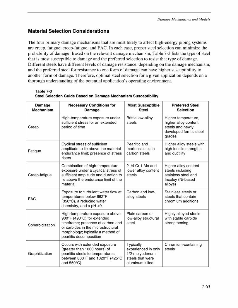
Damage Mechanisms and Models
7-63
Material Selection Considerations
The four primary damage mechanisms that are most likely to affect high-energy piping systems are creep, fatigue, creep-fatigue, and FAC. In each case, proper steel selection can minimize the probability of damage. Based on the relevant damage mechanism, Table 7-3 lists the type of steel that is most susceptible to damage and the preferred selection to resist that type of damage. Different steels have different levels of damage resistance, depending on the damage mechanism, and the preferred steel for resistance to one form of damage can have higher susceptibility to another form of damage. Therefore, optimal steel selection for a given application depends on a thorough understanding of the potential application’s operating environment.
Table 7-3 Steel Selection Guide Based on Damage Mechanism Susceptibility
Damage Mechanism
Necessary Conditions for Damage
Most Susceptible Steel
Preferred Steel Selection
Creep
High-temperature exposure under sufficient stress for an extended period of time
Brittle low-alloy steels
Higher temperature, higher alloy content steels and newly developed ferritic steel grades
Fatigue
Cyclical stress of sufficient amplitude to lie above the material endurance limit; presence of stress risers
Pearlitic and martensitic plain carbon steels
Higher alloy steels with high tensile strengths and ductility
Creep-fatigue
Combination of high-temperature exposure under a cyclical stress of sufficient amplitude and duration to lie above the endurance limit of the material
21/4 Cr 1 Mo and lower alloy content steels
Higher alloy content steels including stainless steel and Incoloy (Ni-based alloys)
FAC
Exposure to turbulent water flow at temperatures below 662°F (350°C), a reducing water chemistry, and a pH <9
Carbon and low-alloy steels
Stainless steels or steels that contain chromium additions
Spheroidization
High-temperature exposure above 900°F (490°C) for extended timeframe; presence of carbon and or carbides in the microstructural morphology; typically a method of pearlitic decomposition
Plain carbon or low-alloy structural steel
Highly alloyed steels with stable carbide strengthening
Graphitization
Occurs with extended exposure (greater than 1000 hours) of pearlitic steels to temperatures between 800°F and 1020°F (425°C and 550°C)
Typically experienced in only 1/2-molybdenum steels that were aluminum killed
Chromium-containing steels
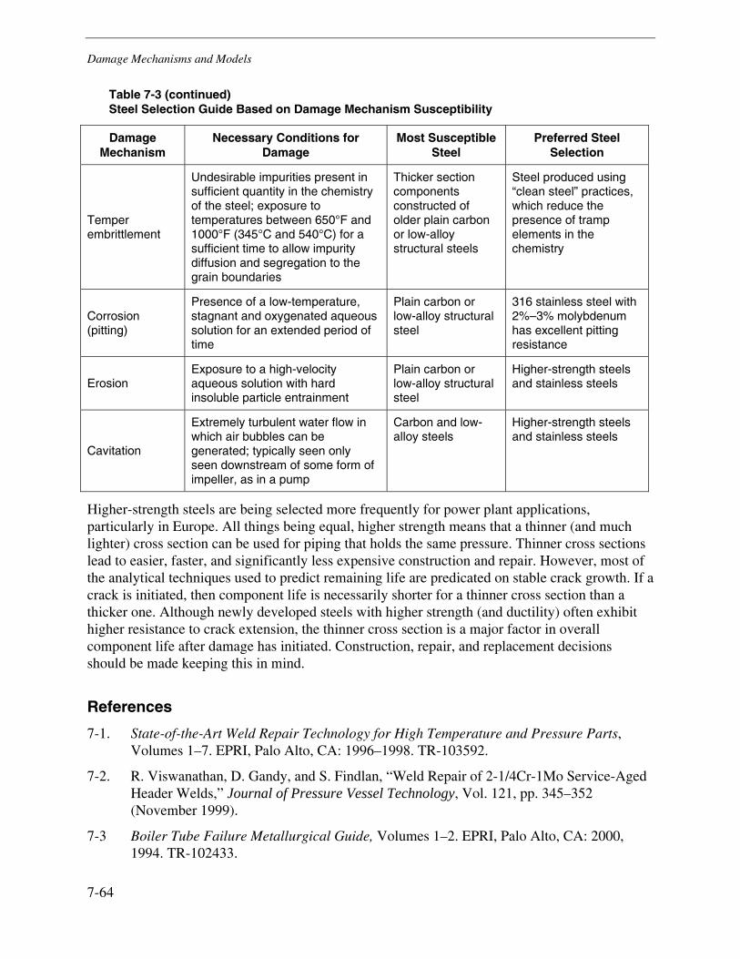
Damage Mechanisms and Models
7-64
Table 7-3 (continued) Steel Selection Guide Based on Damage Mechanism Susceptibility
Damage Mechanism
Necessary Conditions for Damage
Most Susceptible Steel
Preferred Steel Selection
Temper embrittlement
Undesirable impurities present in sufficient quantity in the chemistry of the steel; exposure to temperatures between 650°F and 1000°F (345°C and 540°C) for a sufficient time to allow impurity diffusion and segregation to the grain boundaries
Thicker section components constructed of older plain carbon or low-alloy structural steels
Steel produced using “clean steel” practices, which reduce the presence of tramp elements in the chemistry
Corrosion (pitting)
Presence of a low-temperature, stagnant and oxygenated aqueous solution for an extended period of time
Plain carbon or low-alloy structural steel
316 stainless steel with 2%–3% molybdenum has excellent pitting resistance
Erosion Exposure to a high-velocity aqueous solution with hard insoluble particle entrainment
Plain carbon or low-alloy structural steel
Higher-strength steels and stainless steels
Cavitation
Extremely turbulent water flow in which air bubbles can be generated; typically seen only seen downstream of some form of impeller, as in a pump
Carbon and low-alloy steels
Higher-strength steels and stainless steels
Higher-strength steels are being selected more frequently for power plant applications, particularly in Europe. All things being equal, higher strength means that a thinner (and much lighter) cross section can be used for piping that holds the same pressure. Thinner cross sections lead to easier, faster, and significantly less expensive construction and repair. However, most of the analytical techniques used to predict remaining life are predicated on stable crack growth. If a crack is initiated, then component life is necessarily shorter for a thinner cross section than a thicker one. Although newly developed steels with higher strength (and ductility) often exhibit higher resistance to crack extension, the thinner cross section is a major factor in overall component life after damage has initiated. Construction, repair, and replacement decisions should be made keeping this in mind.
References
7-1. State-of-the-Art Weld Repair Technology for High Temperature and Pressure Parts, Volumes 1–7. EPRI, Palo Alto, CA: 1996–1998. TR-103592.
7-2. R. Viswanathan, D. Gandy, and S. Findlan, “Weld Repair of 2-1/4Cr-1Mo Service-Aged Header Welds,” Journal of Pressure Vessel Technology, Vol. 121, pp. 345–352 (November 1999).
7-3 Boiler Tube Failure Metallurgical Guide, Volumes 1–2. EPRI, Palo Alto, CA: 2000, 1994. TR-102433.
Damage Mechanisms and Models
7-65
7-4 Boiler Tube Failure: Theory and Practice, Volumes 1–3. EPRI, Palo Alto, CA: 1996. TR-105261.
7-5 Condition Assessment Guidelines for Fossil Fuel Power Plant Components. EPRI, Palo Alto, CA: 1990. GS-6724.
7-6 Guidelines for Controlling Flow-Accelerated Corrosion in Fossil and Combined Cycle Plants. EPRI, Palo Alto, CA: 2005. 1008082.
7-7 Life Assessment of Boiler Pressure Parts, Volumes 1–5. EPRI, Palo Alto, CA: 1990. TR-103377.
7-8 Metallurgical Guidebook for Fossil Plant Boilers. EPRI, Palo Alto, CA: 2005. 1004509.
7-9 Remaining Life Assessment of Austenitic Stainless Steel Superheater and Reheater Tubing. EPRI, Palo Alto, CA: 2002. 1004517.
7-10. G. Dieter, Mechanical Metallurgy, Third Edition, McGraw-Hill, 1986.
7-11. F. C. Monkman and N. J. Grant, “An Empirical Relationship Between Rupture Life and Minimum Creep Rate in Creep Rupture Tests,” Proceedings of the ASTM, Vol. 56, p. 593 (1956).
7-12. F. R. Larson and J. Miller, “A Time-Temperature Relationship for Rupture and Creep Stresses,” Transactions of the ASME, Vol. 34, pp. 765–771 (1952).
7-13. R. W. Evans, J. D. Parker, and B. Wilshire, “An Extrapolation Procedure for Long-Term Creep Strain and Creep Life Prediction,” in B. Wilshire and D. R. J. Owen (eds.), Recent Advances in Creep and Fracture of Engineering Materials and Structures, Pineridge Press, Swansea, 1982, pp. 135–184.
7-14. R. Viswanathan, Damage Mechanisms and Life Assessment of High-Temperature Components, ASM International, Metals Park, OH, 1989.
7-15. J. D. Landes and J. A. Begley, in Mechanics of Crack Growth, ASTM STP 590, American Society for Testing and Materials, Philadelphia, PA, 1976, pp. 128–148.
7-16. A. Saxena, in Fracture Mechanics: Twelfth Conference, ASTM STP 700, American Society for Testing and Materials, Philadephia, PA, 1980, pp. 131–135.
7-17. A. Saxena, in Fracture Mechanics: Seventeenth Volume, ASTM STP 905, American Society for Testing and Materials, Philadelphia, PA, 1986, pp. 185–201.
7-18. H. Riedel, Fracture at High Temperatures, Springer-Verlag, Berlin, 1987.
7-19. E. L. Robinson, “Effect of Temperature Variation on the Creep Strength of Steels,” Transactions of the ASME, Vol. 60, pp. 253–259 (1938).
7-20. Y. Lieberman, “Relaxation, Tensile Strength, and Failure of E1 512 and Kh1 F-L Steels,” Metalloved. Term. Obrabotka Metal, Vol. 4, pp. 6–13 (1962).
7-21. R. H. Richman and W. P. McNaughton, An Analysis of Accelerated Life Testing, Final Report, Research Project 2812-4, EPRI, Palo Alto, CA: May 1988. Unpublished.
Damage Mechanisms and Models
7-66
7-22. R. Viswanathan and S. M. Gehl, “Effect of Aging on the Creep Rupture Behavior of Steels,” in P. K. Liaw, et al (eds.), First International Conference on Microstructures and Mechanical Properties of Aging Materials, TMS, Warrendale, PA, 1992, pp. 35–41.
7-23. Accelerated Stress Rupture Testing Guidelines for Remaining Creep Life Prediction. EPRI, Palo Alto, CA: 1997. TR-106171.
7-24. R. Viswanathan and J. Foulds, “Accelerated Stress Rupture Testing for Creep Life Prediction—Its Value and Limitations,” Journal of Pressure Vessel Technology, Vol. 120, American Society of Mechanical Engineers, pp. 105–115 (1998).
7-25. R. Viswanathan and C. H. Wells, “Life Prediction of Turbine Generator Rotors,” Technology for the Nineties, American Society of Mechanical Engineers, New York, 1993.
7-26. S. S. Manson, Thermal Stress and Low Cycle Fatigue, McGraw-Hill, 1966.
7-27 ASME Boiler and Pressure Vessel Code, Section XI, Rules for Inservice Inspection of Nuclear Power Plant Components. American Society of Mechanical Engineers, New York, 2004.
7-28. N. E. Dowling, W. R. Brose, and W. K. Wilson, “Notched Member Fatigue Life Predictions by the Local Strain Approach,” in Fatigue Under Complex Loading: Analyses and Experiments, Vol. AE-6, Society of Automotive Engineers, Warrendale, PA, pp. 55–84 (1977).
7-29. R. W. Landgraf, R. D. Richards, and N. R. LaPointe, “Fatigue Life Predictions for a Notched Member Under Complex Load Histories,” in Fatigue Under Complex Loading: Analyses and Experiments, Vol. AE-6, Society of Automotive Engineers, Warrendale, PA, pp. 95–106 (1977).
7-30. M. R. Mitchell, “Fundamentals of Modern Fatigue Analysis for Design,” in M. Meshii (ed.), Fatigue and Microstructure, American Society for Metals, Metals Park, OH, 1979, pp. 385–437.
7-31. S. S. Manson, “Behavior of Materials Under Conditions of Thermal Stress,” NACA-TN-2933, National Advisory Committee for Aeronautics, 1953.
7-32. S. S. Manson, and M. H. Hirschberg, “Fatigue Behavior in Strain Cycling in the Low- and Intermediate-Cycle Range,” in J. J. Burke and V. Weiss (eds.) Fatigue—An Interdisciplinary Approach, Proceedings of the 10th Sagamore Army Research Conference, Syracuse University Press, Syracuse, NY, 1964, pp. 138–178.
7-33. L. F. Coffin Jr., “A Study of the Effects of Cyclic Thermal Stresses on a Ductile Material,” Transactions of the ASME, Vol. 76, p. 923 (1954).
7-34. S. S. Manson, “Fatigue: A Complex Subject—Some Simple Approximations,” Experimental Mechanics, Vol. 5, No. 7, pp. 193–226 (1965).
7-35. M. A. Miner, “Cumulative Damage in Fatigue,” Trans. ASME Journal of Applied Mechanics, Series E, Vol. 67, pp. A159–164 (1945).
Damage Mechanisms and Models
7-67
7-36. Life Assessment of Boiler Pressure Parts, Volume 3: Heavy Section Crack Initiation and Propagation, EPRI, Palo Alto, CA: 1993. TR-103377-V3.
7-37. T. R. Gurney and S. J. Maddox, “A Re-Analysis of Fatigue Data for Welded Joints in Steel,” Welding Research International, Vol. 3, No. 4 (1973).
7-38. EPRI Ductile Fracture Research Review Document. EPRI, Palo Alto, CA:1978. NP-701-SR. (Out of print and unavailable.)
7-39. J. T. A. Roberts, Structural Materials for Nuclear Power Systems, Plenum Press, New York, 1981.
7-40. ASTM Standard E813-85, Standard Test Method for JIC, A Measure of Fracture Toughness, 1985 Annual Book of ASTM Standards, American Society for Testing and Materials, Philadelphia, PA, 1985.
7-41. I. Milne, R. A. Ainsworth, A. R. Dowling, and A. T. Stewart, “Assessment of the Integrity of Structures Containing Defects,” Report R/H/R6-Rev. 3, CEGB, London, 1986. Also, International Journal of Pressure Vessels and Piping, Vol. 32, p. 196 (1988).
7-42. G. G. Chell, Application of the CEGB Failure Assessment Procedure, R6, to Surface Flaws, ASTM STP 1074-1990, American Society for Testing and Materials, Philadelphia, PA, 1990.
7-43. R. Viswanathan, “Life Management of High-Temperature Piping and Tubing in Fossil Power Plants,” Journal of Pressure Vessel Technology, Vol. 122, pp. 305–316 (August 2000).
7-44. R. Viswanathan and H. Bernstein, “Some Issues in Creep-Fatigue Life Prediction in Fossil Power Plants,” in W. Barnford (ed.), Service Experience and Design in Pressure Vessels and Piping, PVP-Vol. 335, American Society of Mechanical Engineers, pp. 99–109 (1996).
7-45. L. F. Coffin, “Prediction Parameters and Their Application to High Temperature Low Cycle Fatigue,” in Proceedings of the 2nd International Conference on Fracture, Brighton, London, Chapman-Hall, 1969, pp. 643–654.
7-46. S. S. Manson, in Fatigue at Elevated Temperatures, ASTM STP 520, American Society for Testing and Materials, Philadelphia, PA, 1973, pp. 744–782.
7-47. W. J. Ostergren, “A Damage Function and Associated Failure Equations for Predicting Hold Time and Frequency Effects in Elevated Temperature Low Cycle Fatigue,” Journal of Testing and Evauation, Vol. 4, No. 5, American Society for Testing and Materials, pp 327–339 (1976).
7-48. R. H. Priest, D. J. Beauchamp, and E. G. Ellison, “Damage During Creep-Fatigue,” in Advances in Life Prediction Models, ASME Conference, Albany, NY, 1983, pp. 115–122.
7-49. V. Bicego, C. Fossati, and S. Rafazzoni, “An Energy Based Criterion for Low Cycle Fatigue Damage Evaluations,” in Y. Yamada, R. L. Roche, and F. L. Cho (eds.), Material
Damage Mechanisms and Models
7-68
Behavior At Elevated Temperatures and Component Analysis, Book No. H00217 PVP Vol. 60, American Society of Mechanical Engineers, New York, NY, 1982.
7-50. K. Yamaguchi, S. Nishijima, and K. Kanazawa, “Prediction and Evaluation of Long Term Creep Life, in International Conference on Creep, Tokyo, April 1986, pp. 47–52.
7-51. S. Majumdar and P. S. Maiya, “A Damage Equation for Creep-Fatigue Interactions” in ASME-MPC Symposium on Creep-Fatigue Interaction, MPC-3, Metal Properties Council, 1976, p. 323.
7-52. G. A. Cincotta, et al., Gas Turbine Life Management System, General Electric Company, EPRI Project RP-2421-2, February 1988.
7-53. D. A. Miller, R. H. Priest, E. G. Ellison, “Review of Material Response and Life Prediction Techniques Under Fatigue-Creep Loading Conditions,” High Temperature Material Processes., Vol. 6, No. 3 and 4, pp. 115–194 (1984).
7-54. R. Viswanathan, “Creep-Fatigue Life Prediction of Fossil Plant Components,” in Y. S. Garud (ed.), Creep, Fatigue, Flaw Evaluation and Leak-Before-Break Assessment, PVP Vol. 266, American Society of Mechanical Engineers, pp. 33–50 (1993).
7-55. Damage to Power Plants Due to Cycling, EPRI, Palo Alto, CA: 2001. 1001507.
7-56. P. Feltham, “Stress Relaxation in Copper & Alpha-Brasses at Low Temperatures,” Journal of the Institute of Metals, Vol.89, pp. 210–214.
7-57. E. A. Davis, “Creep and Relaxation of Oxygen-Free Copper,” Journal of Applied Mechanics, Vol. 65, p. A-101.
7-58. J. B. Conway, R. H. Stentz, and J. T. Berling, “Fatigue, Tensile and Relaxation Behavior of Stainless Steels,” USAEC, TID-26135, pp. 228–262.
7-59. D. Charman and A. Croker, “Monitoring of Boiler Life During Cycling Operation,” in I. A. Shibli, F. Starr, R. Viswanathan, and D. Gray (eds.), International Seminar on Cyclic Operation of Power Plant—Technical, Operational and Cost Issues, pp. 4–3-1 through 4–3-11. EPRI, Palo Alto, CA: 2001. 1004655.
7-60. A. Saxena, R. S. Williams, and T. T. Shih, “A Model for Representing and Predicting the Influence of Hold Times on Fatigue Crack Growth Behavior at Elevated Temperatures,” in Fracture Mechanics: Thirteenth Conference, ASTM STP 743, American Society for Testing and Materials, Philadelphia, PA, 1981, pp. 86–99.
7-61. R. Viswanathan and H. Bernstein, “Some Issues in Creep-Fatigue,” in I. A. Shibli, F. Starr, R. Viswanathan, and D. Gray (eds.), An International Seminar on Cyclic Operation of Power Plant—Technical, Operational and Cost Issues. pp. S2–1-1 through S2–1-23. EPRI, Palo Alto: CA, 2001. 1004655.
7-62. K. B. Yoon, A. Saxena, and P. K. Liaw, “Characterization of Creep-Fatigue Crack Growth Behavior under Trapezoidal Waveshape Using Ct Parameter,” International Journal of Fracture, Vol. 59, pp. 95–102 (1993).

Damage Mechanisms and Models
7-69
7-63. CHECWORKS™ Fossil Plant Application, Version 1.0. EPRI, Palo Alto, CA: 1998. TR-103198-P5R1.
7-64. Flow-Accelerated Corrosion in Power Plants. EPRI, Palo Alto, CA: 1998. TR-106611-R1.
7-65. Cycle Chemistry Guidelines for Fossil Plants: Phosphate Continuum and Caustic Treatment. EPRI, Palo Alto, CA: 2004. 1004188.
7-66. Cycle Chemistry Guidelines for Fossil Plants: Oxygenated Treatment. EPRI, Palo Alto, CA: 2005. 1004925.
7-67. Interim Cycle Chemistry Guidelines for Combined Cycle HRSGs. EPRI, Palo Alto, CA: 1998. TR-110051.
7-68. G. Krauss, Steels: Heat Treatment and Processing Principles, 4th Printing, ASM International, 1995.
7-69. Guidelines for Copper in Fossil Plants, EPRI, Palo Alto, CA: 2000. 1000457.
7-70. J. J. Moore, Chemical Metallurgy, Second Edition, Butterworths, 1990, p. 333.

8-1
8 PROGRAMMATIC APPROACHES TO LIFE MANAGEMENT OF PIPING SYSTEMS
Introduction
Condition assessment of critical components is essential to ensure safe and reliable operation of fossil-fueled power plants. In the most extreme case, accurate condition assessment would necessitate inspection of all the components in a system. However, in view of the large number of components in a commercial generating plant, it is not practical or even possible to perform inspection at all possible degradation locations. Such a task would be completely impractical because of the excessive costs and time that would be involved.
Traditionally, therefore, inspections have been performed in stages with a full system evaluation requiring years to complete, or assessments have been carried out on a “random” sample of locations. However, both of these approaches have serious drawbacks. Although the systematic, staged inspection eventually covers the whole system, the locations at greatest risk are not necessarily inspected first. Furthermore, because the information regarding condition is obtained in increments, judgment about the most appropriate maintenance action cannot consider an overall evaluation. In the worst-case scenario, costly repairs are carried out on different sections of the piping system during each maintenance period. Even when all the repairs are complete, the system is not new because the integrity of repair welds is a significant variable, yet the total cost of the multiple repair programs is usually far greater than the cost of complete replacement. Conversely, the approach based on selective examination is usually not completely random because criteria such as ease of access are frequently taken into account when selecting inspection locations. Unfortunately, locations that are readily accessible are not always those of highest risk of failure.
The most effective approach is therefore to adopt a methodology that permits a relatively simple yet conservative assessment of the plant as a whole. This should allow a realistic knowledge of all major sections of a facility. Initially, therefore, the general condition of all aspects should be established so that maintenance work can be focused in plant areas most in need, without compromising safety.
Moreover, in a balanced approach, the level of analysis performed will vary for different plant components and the selection of specific methods should be based on the consequences of local component failure. Thus, recent methodologies for maintenance planning have advocated that components are identified as either critical or influence. A critical component is defined as one in
Programmatic Approaches to Life Management of Piping Systems
8-2
which failure would have significant safety or financial consequences. Typically, such components are high-energy pressure vessels and piping or turbine generator rotors. In these cases, initial failure would be life threatening, the cost of replacement components is high, and the long lead times for replacement would, in many situations, result in high costs for the associated losses in output.
Conversely, an influence component is defined as one in which failure would not normally be life threatening and a single failure does not have a major impact on cost. An example of an influence component would be tubing in a boiler or heat exchanger. Here, it is unlikely that a single failure would lead to personal injury or major repair costs. However, if failures occur over a period of time with an increasing rate, eventually the rate of failure will be unacceptably high and remedial action must be taken. In general, the level of failures considered unacceptable depend on the economics of a particular plant. Thus, for a particularly high efficiency unit, more than one or two failures per year can be considered excessive, whereas for a low merit plant, when there is sufficient spare capacity, relatively high rates of failure can be tolerated.
In general, this approach provides for specific actions based on the risk of failure, where risk can be defined as the product of failure probability, P(F), and failure severity, S, as shown in Equation 8-1.
Risk = P(F) x S Eq. 8-1
The simplest approach to assess risk is to extrapolate from an experience base. This approach is frequently adopted for tubing failures because there is usually a statistically significant sample size available and the risk of underestimating performance and having one or two failures is usually not catastrophic. However, this approach cannot usually be adopted for critical components. First, there are much lower populations for analysis; and second, without understanding the details of the relevant damage processes, failure can occur without warning. Thus, assessment programs for critical components must be capable of answering key questions such as the following:
• Where to look
• What to look for
• Which techniques to use
• At what frequency to carry out evaluations
If these questions can be answered, a realistic condition assessment program will be achieved. Furthermore, if the costs of specific technical programs can be balanced with the costs of replacement and the costs of failure, then run, repair, or replacement decisions will be optimized from both economic and technical standpoints.
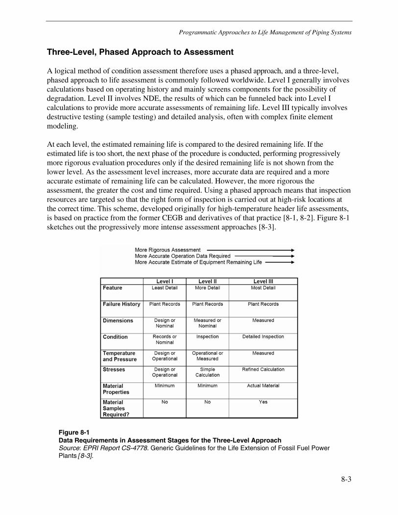
Programmatic Approaches to Life Management of Piping Systems
8-3
Three-Level, Phased Approach to Assessment
A logical method of condition assessment therefore uses a phased approach, and a three-level, phased approach to life assessment is commonly followed worldwide. Level I generally involves calculations based on operating history and mainly screens components for the possibility of degradation. Level II involves NDE, the results of which can be funneled back into Level I calculations to provide more accurate assessments of remaining life. Level III typically involves destructive testing (sample testing) and detailed analysis, often with complex finite element modeling.
At each level, the estimated remaining life is compared to the desired remaining life. If the estimated life is too short, the next phase of the procedure is conducted, performing progressively more rigorous evaluation procedures only if the desired remaining life is not shown from the lower level. As the assessment level increases, more accurate data are required and a more accurate estimate of remaining life can be calculated. However, the more rigorous the assessment, the greater the cost and time required. Using a phased approach means that inspection resources are targeted so that the right form of inspection is carried out at high-risk locations at the correct time. This scheme, developed originally for high-temperature header life assessments, is based on practice from the former CEGB and derivatives of that practice [8-1, 8-2]. Figure 8-1 sketches out the progressively more intense assessment approaches [8-3].
Figure 8-1 Data Requirements in Assessment Stages for the Three-Level Approach Source: EPRI Report CS-4778. Generic Guidelines for the Life Extension of Fossil Fuel Power Plants [8-3].
Programmatic Approaches to Life Management of Piping Systems
8-4
The application of the phased approach provides those responsible for plant maintenance with a logical progression to decision making. With this approach, assessments are based on established engineering guidelines, with appropriate actions specified at each stage. Thus, the final decision must be either to continue operation for a given time under specified operating conditions or to repair or replace the component. Moreover, this methodology is amenable to the application of computer codes. Successful systems are already available that perform the following:
• Store all relevant information regarding the plant in a logical manner
• Allow sorting and retrieval of data so that required analyses can be performed accurately and efficiently
• Ensure that procedures are such that documentation, analyses, and inspections are fully verified by appropriate quality assurance procedures
• Provide consistency and continuity for all activities undertaken
In this way, the multiplicity of potential maintenance decisions facing a plant operator can be reduced with information supplied rapidly in an appropriate format. The following subsections detail the three levels of phased approach.
Level I
The initial, or Level I, evaluation examines design or overall service parameters to ascertain whether, on the basis of the most conservative considerations, the component has a remanent life greater than the anticipated service life. It is possible to carry out this assessment without reference to plant-specific measurements provided that operating parameters do not exceed design. However, it is normal even at this stage to consider the results of component-specific instrumentation. Care must be exercised with this approach because instrumentation, which monitors average conditions, might not identify regions where extremes are present. Nevertheless, by considering relevant industry experience, it is usually possible to ensure that the data used are conservative. When implementing the methodology, if doubt exists regarding the conservatism of the data available, the more complex evaluations of Level II should be implemented.
Each level of analysis can be conducted considering a specific degradation mechanism. Figure 8-2 shows the generic steps in a Level I assessment for creep damage [8-4]. The Level I analysis is a preliminary or screening assessment of component condition based on maintenance history, relevant experience, a piping survey, and a preliminary life-fraction. The information gathered in Level I will be required for more detailed analyses of later levels; therefore, investigators should start with Level I, even if damage has been found in the component. However, in that case, it will almost always be necessary to determine the extent of damage, which is a Level II activity, and to determine its significance, which in many cases will invoke at least some analytical techniques that are part of Level III.
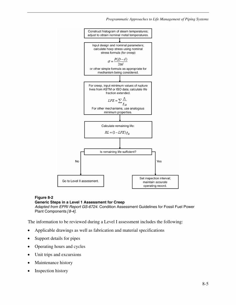
Programmatic Approaches to Life Management of Piping Systems
8-5
Figure 8-2 Generic Steps in a Level 1 Assessment for Creep Adapted from EPRI Report GS-6724. Condition Assessment Guidelines for Fossil Fuel Power Plant Components [8-4].
The information to be reviewed during a Level I assessment includes the following:
• Applicable drawings as well as fabrication and material specifications
• Support details for pipes
• Operating hours and cycles
• Unit trips and excursions
• Maintenance history
• Inspection history
Programmatic Approaches to Life Management of Piping Systems
8-6
• History of failures, details of failure analyses performed, maintenance actions taken
• Design parameters, including temperatures and pressures
• Steam temperature records
For specific damage mechanisms, there will be an emphasis on different data. For example, creep evaluation will involve design pressure, design temperature, and operating hours. Creep-fatigue of attachment welds will also include an analysis of unit cycling and survey of header attachments and supports. A hot walkdown survey for attachments to, and in the vicinity of, the subject pipe should be conducted to assess the magnitude of system loads that would influence the accumulation of damage at the attachment welds. The purpose is to benchmark the piping systems and attachments in the hot conditions so that the systems can be checked from hot to cold to determine actual deflections. These deflections can then be checked against those predicted by stress analysis.
Supports and attachments should be reviewed for the following:
• Compatibility between analyzed (design) and as-built (present) configurations
• Unacceptable vibrations
• Interference problems
• Signs of physical damage
• Operability of drains
Supports should be surveyed for the following:
• Operation within the travel range
• Actual and design support location consistency
• Proper installation and sizing of supports according to the design
• Support movements in agreement with design and analysis displacement
• Signs of transient and impact loads on pins and other devices
• Operability of any special supports, guides, or restraints
• Proper clearances and gaps
The survey is combined with a review of the piping stress analysis, if available, to determine whether the attachment welds are high stress areas. In the absence of a piping analysis, hanger and pipe support information will qualitatively indicate whether the attachment junctions are potentially subject to significant damage from system loads.
Programmatic Approaches to Life Management of Piping Systems
8-7
For high-temperature components, a preliminary life-fraction analysis should be performed. It will typically use minimum materials properties, design stresses, design or actual service temperatures, and a life-fraction rule. Typical analyses might include the following:
• Piping. Creep rupture analysis using operating pressure, temperature, and minimum base metal properties.
• Longitudinal seam welds. Creep rupture analysis. Properties to be used are a fraction of those for the base metal. The appropriate values to be used can be obtained from the methodology outlined in the EPRI report Guidelines for the Evaluation of Seam-Welded High Energy Piping (TR-104631) [8-5].
• Attachment welds (base and weld metal). Creep and fatigue analysis. See EPRI report TR-104631 for the value of material properties to use for considering the weld and HAZ [8-5].
• Other welds. Creep rupture evaluation can be performed. Stress analysis will generally be required. However, a preliminary creep rupture evaluation can be performed using code allowable stresses and operating temperature with properties as defined in EPRI report TR-104631 [8-5].
Historically, Level 1 analysis provided only gross estimates of damage as a result of inaccuracies in the assumed history of stresses and temperatures, material properties, and the life-fraction rule. As a result, such calculations have been most useful for determining key locations to be evaluated more rigorously, for scheduling maintenance outages, and screening for when inspections for damage should occur.
The complexity and variability of damage precludes a definitive quantitative guideline for triggering a Level II assessment from Level I results. Some Level II triggers are the following:
• The life-fraction consumed, as calculated by the analyses described above, exceeds 50%.
• The visual inspection performed during the hot walkdown indicates piping or piping support damaged.
• There is other evidence of known damage to the piping.
• There have been repairs (except the most trivial) to the piping, seam welds, girth welds, or attachment welds in the past (other than during initial installation).
Level II
The basic steps in a generic Level II assessment are shown in Figure 8-3 [8-4]. Level II assessments require that specific plant examinations be performed. It is the role of the initial evaluation to screen and identify the components that are at highest risk of failure and to select specific locations to be examined. The particular methods involved in these examinations will depend on the component and the type of operation. In general, the inspections should provide information regarding condition through NDE. Level II can also involve the use of thermocouples to refine operating temperature estimates, although some care in this regard is required when extrapolating the current temperature backward over significant periods of
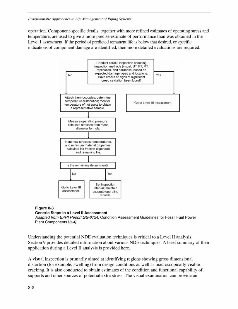
Programmatic Approaches to Life Management of Piping Systems
8-8
operation. Component-specific details, together with more refined estimates of operating stress and temperature, are used to give a more precise estimate of performance than was obtained in the Level I assessment. If the period of predicted remanent life is below that desired, or specific indications of component damage are identified, then more detailed evaluations are required.
Figure 8-3 Generic Steps in a Level II Assessment Adapted from EPRI Report GS-6724. Condition Assessment Guidelines for Fossil Fuel Power Plant Components [8-4].
Understanding the potential NDE evaluation techniques is critical to a Level II analysis. Section 9 provides detailed information about various NDE techniques. A brief summary of their application during a Level II analysis is provided here.
A visual inspection is primarily aimed at identifying regions showing gross dimensional distortion (for example, swelling) from design conditions as well as macroscopically visible cracking. It is also conducted to obtain estimates of the condition and functional capability of supports and other sources of potential extra stress. The visual examination can provide an
Programmatic Approaches to Life Management of Piping Systems
8-9
indication of high-temperature locations for more detailed inspection (or sampling as a part of a Level III assessment). Locating the longitudinal seam welds, if any, should also be part of the visual inspection.
All major welds should be inspected by magnetic particle testing (MT) and dye penetrant testing (PT). If flaws or cracks can be present at locations away from the accessible surface, then angel beam UT or another volumetric method should be applied. Macrocracking associated with the inspected welds will thus be identified. All indications should be mapped and sized, if possible. Specialized techniques such as time-of-flight diffraction or linear phased array UT might be required.
High-priority locations for further inspection will be identified by the results of the Level I assessment and the Level II visual, MT, PT, and UT examinations. Further inspection will include replication, chemical analysis, and hardness measurements. Replication of weldments can provide an indication of the severity of creep cavitation damage in the weld metal and HAZs. Nominal compositions of piping base metal and surface weld beads can be verified with an alloy analyzer in situ, or alternatively, material can be removed using a clean tungsten carbide burr or other means. These samples can then be analyzed using relevant laboratory test methods.
In general, a preliminary qualitative estimate of remaining life of the weldments can be made from the results of the replication, based on the appearance of the creep cavities. (See Section 10 for more information.) For the base metal at stress concentrations, simple estimates of remaining life based on the level of damage observed are more difficult.
Level III
Figure 8-5 lists the generic steps in a Level III assessment [8-4]. This level is triggered by the need to ascertain remaining life more precisely on the basis of Level II results. The Level III assessment should be based on detailed knowledge of operating conditions and specific materials properties. Thus, sophisticated instrumentation and analysis procedures are required to document local operating conditions. The effort at this level is relatively involved and is aimed at determining actual material properties and loads, along with more detailed analytical techniques for a more precise life assessment. However, experience suggests that even with precise knowledge of stress and temperature parameters, the scatter in standard material properties will introduce unacceptable uncertainties in life estimates. Probabilistic analysis methods have been introduced to reduce the overall conservatism of performance assessment based on lower bound properties. However, these methods are still limited because many of the steels used in steam plants are susceptible to changes in material properties with time. Thus, even if distributions of materials data are available for relevant alloys before service, changes in properties as a result of operation can be established only by postexposure testing.
The type of testing required for a Level III assessment will vary with component type and degradation susceptibility. Thus, for example, if the component is at risk of creep failure, tests are performed to evaluate creep strength and ductility. Conversely, defect assessments are usually based on material toughness so that testing must establish fracture toughness. In general, condition

Programmatic Approaches to Life Management of Piping Systems
8-10
assessments will frequently be limited by the ability to characterize accurately the nature and extent of defects present and the uncertainty regarding component properties. These limitations will be significantly reduced if techniques can be applied to remove material samples for laboratory testing.
A Level III assessment will typically consist of the following elements:
• More detailed NDE to fully characterize defect dimensions.
• More detailed microstructural evaluation by more careful examination of the results of replication.
• A refined analysis of all loads and stress analysis by finite element or other methods to identify and quantify the highly stressed regions.
• A refined analysis of creep, creep-fatigue, fatigue, or corrosion-fatigue (depending on the situation) expected life.
• Sampling of piping and weld material for testing to establish the actual properties of the material. This is particularly applicable to creep rupture or creep-fatigue properties in high-temperature components. See Section 10 for more information on accelerated testing and the use of miniature specimens.
• More detailed or specific on-line monitoring for specific variables of interest. It can also require more complete acquisition of information to characterize the extent of damage, depending on what was conducted during Level II. For example, if an inspection of the main steam seam welds indicated some significant damage, an extension of the inspection to nearby regions might be indicated.
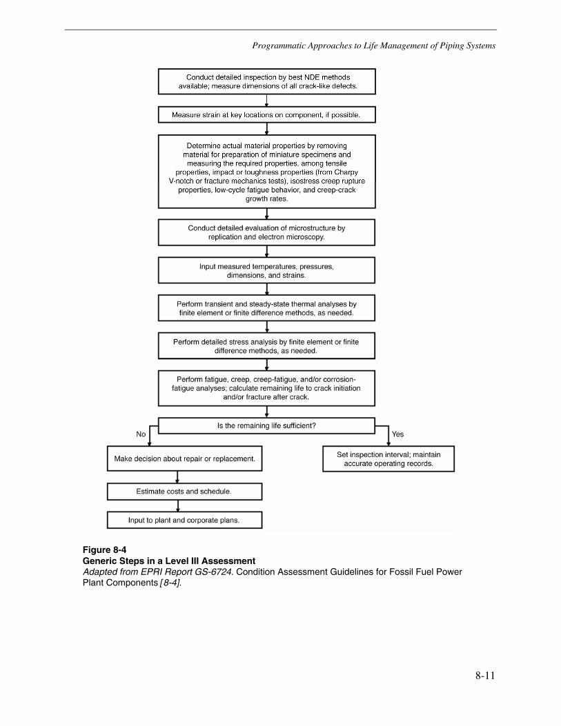
Programmatic Approaches to Life Management of Piping Systems
8-11
Figure 8-4 Generic Steps in a Level III Assessment Adapted from EPRI Report GS-6724. Condition Assessment Guidelines for Fossil Fuel Power Plant Components [8-4].
Programmatic Approaches to Life Management of Piping Systems
8-12
The detailed Level III assessment can be quite expensive and might require cost justification, for example, when the alternative is replacement or significant repair. In most cases, if significant damage is found and repair or replacement is not chosen, a Level III assessment will be required to ensure that the component can be operated in a safe manner, even for a short period of time.
Advantages and Disadvantages of the Phased Approach to Assessment
Several key points can summarize the role of component condition assessment in continued plant operations [8-4].
• In general, a multilevel approach offers a logical and resource-effective way to evaluate most components. If thorough documentation of historical practice and current operations is in hand, some components and damage types can be evaluated with only a Level I assessment.
• Component assessment is normally described in terms of multiple levels of evaluation. Clearly some types of components and damage are more amenable to the general methodology than others. Modification of the methods to suit the demands of or resources available to a particular utility application might be required.
• The multilevel approach can be modified when common sense dictates that some activities that are generally applied later in the sequence should be moved to earlier roles. Certain critical components are more likely to demand such foresight for reasons of safety, time constraints, access, cost constraints, or overall impact on scheduling. For example, it is often expeditious to perform analyses to identify critical flaw sizes or locations (such analysis methods are generally considered a Level III activity) before embarking on certain inspection programs. This might be necessary when the expected time to evaluate any indications is expected to take longer than is allowed by the constraints of the outage. Hence, knowledge of what level of damage will necessitate a replace or repair option might be necessary for cost effectiveness, even before the inspection outage is started.
• Phased levels of assessment interface with ongoing plant operation. Planned maintenance outages can be aligned with required inspection and sampling projects for detailed component assessment.
• At each level of analysis, the calculated remaining life is compared to the desired component life. The choice of an acceptable remaining life (or alternatively a safety factor on the calculation) will depend on a number of factors specific to each utility. These can typically include the unit plan, ease of repair or replacement in case of failure, lead time on component procurement, and safety implications of component failure.
• The final event in the assessment sequence is the decision about whether to run the component as is, to refurbish by repair or upgrade, or to replace. After that decision is made, it is appropriate to attach a reevaluation period to the result. For any of the options, a periodic inspection and reevaluation will be appropriate.
Programmatic Approaches to Life Management of Piping Systems
8-13
• Before replacing a damaged component, it is crucial to determine the cause of the damage and to estimate the probable damage accumulation rate. Damage found in a component after 20 years should not simply be assumed to have developed over the entire service life. This could lead to a replacement of like with like and the assumption that it should provide a further 20 years of service. However, close examination of the damage and unit history can indicate that in fact damage has developed in the recent past and a policy of straightforward replacement offers significantly less service. (This is a typical problem with change of service from base load to cycling.). Damage can be found to have been caused by operating practice that has not been properly controlled. If the root cause is identified, often operation can be modified to improve service performance without major cost or inconvenience.
• The completion of assessment of a particular component is also an excellent time to determine the nature of inspection, monitoring, and future record keeping that would make the reevaluation easier the next time. It might also be a time to examine operating procedures and routine aspects of maintenance to fine-tune them for longer life as well as for increased performance.
Application of the progressive damage assessment scheme described depends on the ability to assess the degree of damage in the component, the rate of accumulation of additional damage, and the degree of damage necessary to cause failure. Most of the required methods and techniques to make these determinations are well established; however, some continue to see improvements with time, as evidenced by the large and growing literature of life assessment techniques.
In addition, each method (and Level) has inherent problems. For example, accurate knowledge of local component stress values is often complex. For Level I, the use of design stresses can in certain cases allow a realistic bounding analysis to be performed. More often, for all but the simplest cases, complications such as residual stresses, system loads, geometric discontinuities, and so on, will mandate more detailed methods typical of Level III analysis. Even in Level III, uncertainties will be present in the methods used.
The same observation pertains to other aspects of the assessment methods. First, the amount of damage (or size of flaw depending on the type of damage) can be hard to measure. More often, issues such as whether the worst damage was detected, where to look, and what was overlooked are inherent in trying to answer the question about the amount of damage in the component. Second, the actual material properties can be difficult to evaluate, particularly without destroying the components. As with inspection, the issue of identifying locally inferior material and the choices of sampling schemes make the application of the assessment methods more difficult. Finally, in some cases there is insufficient historical information, so that any form of Level I methods is immediately rejected.
These drawbacks are, for the most part, inherent in any method of condition assessment; they are not specific to a multilevel approach. Further, they do not detract from the efficacy of the process for components that are appropriate. The point is made to emphasize the requirement for good judgment along with an understanding of the advantages and drawbacks of the various assessment methods.

Programmatic Approaches to Life Management of Piping Systems
8-14
Currently Available Prediction Tools
Introduction
A number of currently available software packages can be used to perform the different level analyses for high-energy piping life assessments. This subsection introduces both the available American programs and those used in Europe, evaluates their effectiveness, and describes some operational details.
BLESS (Boiler Life Evaluation and Simulation System)
When analyzing for creep and creep-fatigue, developing a complete analytical technique from first principles and applying it to the field situation can be an extremely daunting task. This subsection describes BLESS, an analytical tool that has been developed to incorporate the key aspects of high-temperature damage analysis. BLESS is available to utilities from EPRI. The description of its capabilities also highlights some of the key considerations for those who build their own analytical tools.
The primary focus of the EPRI BLESS code is an estimation of the initiation and propagation of ligament cracking in high-temperature headers [8-6–8-8]. But a secondary (and relevant) application is the initiation and propagation of girth and longitudinal seam weld cracking in headers and straight runs of steam piping. The primary use for the BLESS code is to establish component inspection schedules.
The code facilitates analysis of high-temperature component life by eliminating the requirement for finite element stress analysis and thermal analysis. The BLESS code can be used to make either deterministic or probabilistic estimates of remaining life. BLESS can also be used to evaluate alternative, new high-temperature component designs. The program calculates the time to initiation and time to failure for a specific design.
For component seam welds, the one-dimensional model is adequate without empirical modifications. For component girth welds, although stresses from attached components and support loads are important, they are not calculated. The restraint of thermal expansion stresses by piping systems dominates the stress state at girth welds; these are not included in BLESS calculations [8-9]. Restraint of thermal expansion stresses as well as deadweight stresses and bending moments must be calculated outside of the BLESS code and then used to define equivalent load-controlled membrane stress inputs to BLESS.
Inputs
Operating conditions and header geometry are input to the program.
Programmatic Approaches to Life Management of Piping Systems
8-15
Material Properties
All material properties required for analysis are contained in the program. BLESS uses nonlinear creep-fatigue crack growth rates. Material properties are best-estimate values, and therefore produce a best estimate for lifetime. Materials included in the code include P11, P22, and P91. The constitutive relationships consider primary and secondary creep and use functional forms provided by Riedel in Fracture at High Temperatures, which are briefly described in “BLESS: Boiler Life Evaluation and Simulation System, A Computer Code for Reliability Analysis of Headers and Piping” [8-10, 8-8]). Additional information can be found in the following documents:
• Properties for P11 are reviewed in “BLESS: Boiler Life Evaluation and Simulation System, A Computer Code for Reliability Analysis of Headers and Piping” [8-8].
• Properties for P22 are summarized in the EPRI report Life Assessment of Boiler Pressure Parts, Volume 4: BLESS Code User’s Manual and Life Assessment Guidelines (TR-103377-V4) [8-7].
• The creep rupture properties are based on the ASTM compilation, “Supplemental Report on the Elevated-Temperature Properties of Chromium-Molybdenum Steels (An Evaluation of 2-1/4 Cr 1 Mo Steel)” [8-11].
• The creep and fatigue crack growth properties are described in Chapter 5, “Probabilistic Fracture Mechanics,” of the Probabilistic Structural Mechanics Handbook [8-12].
The BLESS program incorporates the effect of aging on material properties. For components already in service, the program permits adjusting the key inputs—including current crack sizes, material ultimate tensile strength and hardness, and oxide crack depth—to perform a sensitivity analysis of assumptions and to attempt to match the estimated flaw size or growth with what has been actually observed.
Calculational Methods
The program performs both thermal and pressure stress analysis of a high-temperature component. The BLESS code allows for life assessment of components without the use of finite element thermal and stress analysis. The simplification is made possible by using a one-dimensional model (through-wall variation only) based on a simple thick-walled cylinder model to calculate transient temperatures and stresses. The simplified model provides reasonable values for stress distributions in areas removed from geometric discontinuities, such as boreholes. The model is modified to account for specific geometries with closed-form empirical equations based on detailed three-dimensional linear finite element analyses. Details about how this was done can be found in the EPRI report Life Assessment of Boiler Pressure Parts, Volume 1: Executive Summary (TR-103377-V1) [8-13].
The BLESS code can be used either probabilistically or deterministically. The probabilistic functions of the code use a Monte Carlo simulation consisting of repetitive deterministic lifetime calculations [8-13]. The repetitive calculations use varying input values randomly sampled from their distribution. The results of the simulations are combined into a histogram of results that is the probability of failure as a function of time.
Programmatic Approaches to Life Management of Piping Systems
8-16
BLESS incorporates two alternative approaches for predicting crack initiation [8-4]. The first involves inelastic linear damage summation. It includes a damage fraction rule that consists of two parts—a rate-dependent creep portion based on Robinson’s rule and a rate-independent fatigue part based on Miner’s rule. The second approach involves repeated cracking of oxide scale and oxide notching. After a crack is initiated, growth from creep and fatigue is calculated using nonlinear fracture mechanics using the Ct(ave) parameter. Elastic deformation with primary creep and secondary creep are considered. The creep-fatigue interaction uses Robinson’s rule for creep and Miner’s rule for fatigue.
After a crack has initiated, growth can occur by fatigue, by creep, or by continued oxide notching. BLESS allows for calculation of propagation by all of these mechanisms. When both fatigue and creep occur together, the resulting creep-fatigue is covered by BLESS. If either of the two constituent modes is not present, the value calculated for the contribution from that mechanism is negligible. The crack driving force for fatigue is considered to be the cyclic stress intensity factor (ΔK) and for creep, the Ct parameter. These are evaluated from the analogous fully plastic J-integral solution. After (ΔK) and Ct(ave) are calculated, crack growth can be calculated from Equations 8-2 and 8-3, where nfat, Cl, and q are constants determined from curve fit data.
timecycle dNda
dNda
dNda
⎟⎠⎞
⎜⎝⎛+⎟
⎠⎞
⎜⎝⎛= Eq. 8-2
( ) ( )( ) hq
avetln
fat tCCKCdNda fat +Δ= Eq. 8-3
Cracks can grow in an axial or circumferential direction, and from surface penetration to surface penetration, or from component ID to OD.
OmegaPipe Software
Overview
All of the information in this subsection was extracted and modified from the following two documents:
• T. L. Anderson, OmegaPipe Version 2.6 User’s Manual, The Materials Properties Council, Inc., 2002 [8-14].
• T. L. Anderson, Life Assessment of Long Seam Piping, as Implemented in the OmegaPipe Software, Structural Reliability Technology, 2001 [8-15].
Programmatic Approaches to Life Management of Piping Systems
8-17
The OmegaPipe software was developed by Dr. Ted L. Anderson of Structural Reliability Technology, Inc., for the High-Energy Piping Project of the Materials Properties Council. (The Materials Properties Council is a nonprofit corporation founded in 1966 by the American Society of Mechanical Engineers, ASM International, ASTM, and the Engineering Foundation. It is supported by industry, technical organizations, codes and standards developers, and government agencies.)
The software package performs stress analysis, life assessment, and remaining life predictions for seam-welded steam piping systems that operate at elevated temperatures (high-energy piping). Using a template provided in the software, the user creates a piping model that corresponds to the system of interest, and then OmegaPipe performs a global stress analysis. The user can then select a portion of the piping system (for example, elbow, sweep, or run) for which the software can probabilistically estimate the remaining life for that specific piping detail.
The OmegaPipe software includes the following four main modules:
• A Windows-based physical modeling editor, which allows users to create a three-dimensional, geometrically correct, graphical piping system model that incorporates dimensional, material, and support data. The modeling editor displays an isometric view of the piping system on screen.
• A finite element analysis module, which performs a global stress analysis of the piping system models.
• A library of parametric equations, which relate stresses in the pipe wall (obtained from the global stress analysis) to local stresses at the fusion boundary of a seam weld or girth weld. Unlike most piping stress analysis programs, OmegaPipe software also models creep relaxation in the system.
• A life assessment module for long seam welds and girth welds, which uses the local stresses computed in the other modules to predict remaining life in specific sections of pipe. The life prediction module combines a void growth failure model with the Omega creep crack growth equations. Two versions of a cavity growth model are incorporated into the software; one model is used for life assessment of normalized weld metal, and the other pertains to Type IV cracking in the HAZ.
The flowchart in Figure 8-1 illustrates the various modules and file types used in the OmegaPipe software [8-14]. More detail is provided below on several special features of OmegaPipe software that add to its utility in high-energy piping analysis.
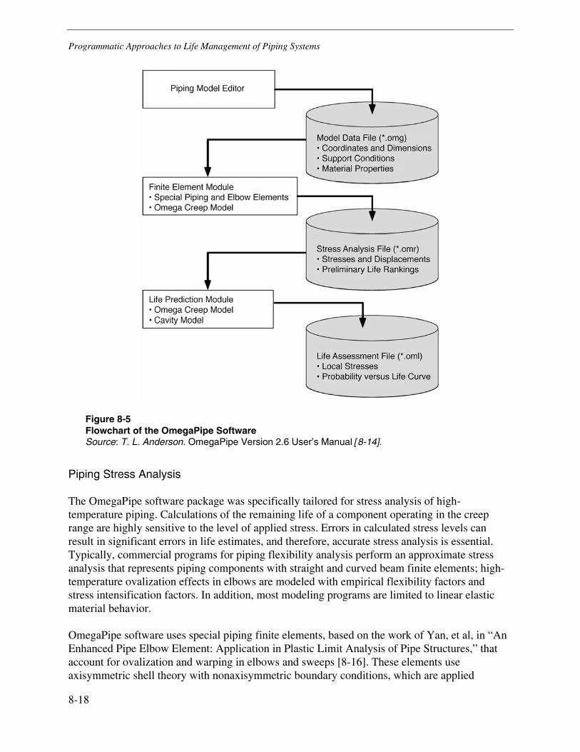
Programmatic Approaches to Life Management of Piping Systems
8-18
Figure 8-5 Flowchart of the OmegaPipe Software Source: T. L. Anderson. OmegaPipe Version 2.6 User’s Manual [8-14].
Piping Stress Analysis
The OmegaPipe software package was specifically tailored for stress analysis of high-temperature piping. Calculations of the remaining life of a component operating in the creep range are highly sensitive to the level of applied stress. Errors in calculated stress levels can result in significant errors in life estimates, and therefore, accurate stress analysis is essential. Typically, commercial programs for piping flexibility analysis perform an approximate stress analysis that represents piping components with straight and curved beam finite elements; high-temperature ovalization effects in elbows are modeled with empirical flexibility factors and stress intensification factors. In addition, most modeling programs are limited to linear elastic material behavior.
OmegaPipe software uses special piping finite elements, based on the work of Yan, et al, in “An Enhanced Pipe Elbow Element: Application in Plastic Limit Analysis of Pipe Structures,” that account for ovalization and warping in elbows and sweeps [8-16]. These elements use axisymmetric shell theory with nonaxisymmetric boundary conditions, which are applied
Programmatic Approaches to Life Management of Piping Systems
8-19
through harmonic analysis. During stress analysis, these elements can account for the relaxation and redistribution of stresses that occurs during creep. During analysis, the Material Properties Counsel’s Omega material model is used to characterize creep behavior at elevated temperatures.
Local Weld Stresses
The complex piping finite elements that OmegaPipe software uses do not account for the presence of seam or girth welds, and therefore the stresses computed pertain only to seamless piping. Although the presence of seam welds does not have a significant effect on the global stiffness or relaxation of the piping system, the stress distribution in a piping system’s weldments is very important because welds are the locations of highest susceptibility to damage. The weld metal in a normalized weld creeps faster than the base metal. In this case, the physical constraint of the base metal creates a triaxial stress state in the weld metal, which increases the probability of cracking. Moreover, the weld cusp in a double-V joint creates a local stress concentration, which also increases the probability of cracking. In the alternative case of a weld that is not normalized, the HAZ is softer than the surrounding base metal and weld metal, and therefore local deformation and triaxiality make the HAZ susceptible to Type IV cracking.
OmegaPipe software is designed to account for the effects of welds on actual stress distributions. A series of parametric equations, which were developed through complex finite element analysis and curve fitting, are used to relate stresses obtained from the seamless piping stress analysis to the local stress state at the weld fusion lines [8-15, 8-17]. At a given location around the circumference in a straight pipe or bend, OmegaPipe software’s stress analysis module reports five stress values (calculated through the thickness), which are averaged to give equivalent membrane hoop and axial stresses at the location of interest.
Life Assessment
OmegaPipe software includes subroutines that predict the remaining life in welded components exposed to high temperatures based on the analyses performed. The local stresses, which were calculated at weld fusion lines, are used to estimate prior damage and predict the remaining life at the location of interest. Upon completion of the piping stress analysis, the program conducts a deterministic life assessment on each element in the model at the seam weld location. If the seam weld location was not identified for a given element, the life assessment is performed at the 12 o’clock position around the piping circumference.
OmegaPipe software reports its individual component life estimates with a relative life ranking system, from the shortest predicted lifespan to the longest. Within the ranking methodology, the location at which the shortest life is computed is assigned an index of 10, and all other locations are scaled relative to that location. For example, a life index of 1.0 would be expected to have a life 10 times greater than that of the worst location. As noted in the OmegaPipe literature, the relative life ranking should be used with caution because this ranking does not account for possible random and unpredictable metallurgical variations throughout the piping system, nor does it account for local variations in geometry, such as pipe peaking or out-of-roundness [8-15].
Programmatic Approaches to Life Management of Piping Systems
8-20
The life assessment model considers the combined effect of creep and cavity growth. The same model is used for both normalized welds and Type IV cracking in nonnormalized HAZs. The OmegaPipe software treats the difference between the two failure mechanisms with variations in local stress state and material properties (for example, relative creep rates and initial cavity size and spacing).
The OmegaPipe software can also perform a Monte Carlo probabilistic life assessment for specific locations, which creates a plot of probability of failure versus remaining life.
CHECWORKS™ and CHECUP™ Programs
Using the Chexal-Horowitz correlation incorporated in the CHECWORKS™ and CHECUP™ programs, EPRI’s CHECUP technology was developed specifically for fossil, co-generation, and industrial steam plants to rank the amount of wall loss that might have occurred at various piping locations due to FAC [8-18]. It can also be used for the feedwater piping of HRSG units, but not for economizer or evaporator tubing. CHECWORKS increases the confidence of plant owners and operators that the most damaged components will be identified, inspected, and repaired or replaced long before a rupture might occur. For the large number of piping runs and components that are potentially susceptible to FAC damage, CHECUP provides a technical basis for selecting higher FAC risk locations for inspection from among the many possibilities. This provides a cost benefit in reducing the number of inspections required to characterize the level of FAC damage for a specific unit. Material and chemistry conditions drive the FAC mechanism with the hydrodynamics setting the rate of damage; CHECUP provides an analysis basis for the hydrodynamic factors.
CHECUP predicts the wall loss of single-phase piping segments and components since plant startup. A piping segment is a portion of a line that has the same size, material, and operating conditions. Input data for a segment include the material, pipe size, operating temperature, flow rate, system identification, dissolved oxygen, water treatment, condensate cold pH, and number of operating hours since plant startup. Provision is made for selecting component types from a library of previously analyzed geometries. A typical input screen for CHECUP is shown in Figure 8-5. Output data include the predicted wear of common types of piping components with some parametric variations of uncertainties. as shown in Figure 8-6.
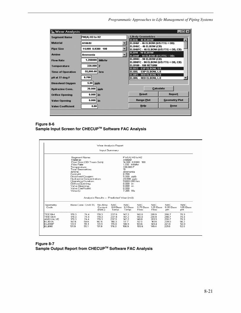
Programmatic Approaches to Life Management of Piping Systems
8-21
Figure 8-6 Sample Input Screen for CHECUPTM Software FAC Analysis
Figure 8-7 Sample Output Report from CHECUPTM Software FAC Analysis
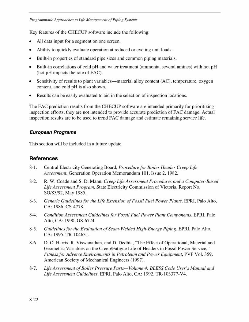
Programmatic Approaches to Life Management of Piping Systems
8-22
Key features of the CHECUP software include the following:
• All data input for a segment on one screen.
• Ability to quickly evaluate operation at reduced or cycling unit loads.
• Built-in properties of standard pipe sizes and common piping materials.
• Built-in correlations of cold pH and water treatment (ammonia, several amines) with hot pH (hot pH impacts the rate of FAC).
• Sensitivity of results to plant variables—material alloy content (AC), temperature, oxygen content, and cold pH is also shown.
• Results can be easily evaluated to aid in the selection of inspection locations.
The FAC prediction results from the CHECUP software are intended primarily for prioritizing inspection efforts; they are not intended to provide accurate prediction of FAC damage. Actual inspection results are to be used to trend FAC damage and estimate remaining service life.
European Programs
This section will be included in a future update.
References
8-1. Central Electricity Generating Board, Procedure for Boiler Header Creep Life Assessment, Generation Operation Memorandum 101, Issue 2, 1982.
8-2. R. W. Coade and S. D. Mann, Creep Life Assessment Procedures and a Computer-Based Life Assessment Program, State Electricity Commission of Victoria, Report No. SO/85/92, May 1985.
8-3. Generic Guidelines for the Life Extension of Fossil Fuel Power Plants. EPRI, Palo Alto, CA: 1986. CS-4778.
8-4. Condition Assessment Guidelines for Fossil Fuel Power Plant Components. EPRI, Palo Alto, CA: 1990. GS-6724.
8-5. Guidelines for the Evaluation of Seam-Welded High-Energy Piping. EPRI, Palo Alto, CA: 1995. TR-104631.
8-6. D. O. Harris, R. Viswanathan, and D. Dedhia, “The Effect of Operational, Material and Geometric Variables on the Creep/Fatigue Life of Headers in Fossil Power Service,” Fitness for Adverse Environments in Petroleum and Power Equipment, PVP Vol. 359, American Society of Mechanical Engineers (1997).
8-7. Life Assessment of Boiler Pressure Parts—Volume 4: BLESS Code User’s Manual and Life Assessment Guidelines. EPRI, Palo Alto, CA: 1992. TR-103377-V4.

Programmatic Approaches to Life Management of Piping Systems
8-23
8-8. D. O. Harris, C. H. Wells, J. M. Bloom, C. C. Schultz, H. J. Grunloh, R. H. Ryder, and R. Viswanathan, “BLESS: Boiler Life Evaluation and Simulation System: A Computer Code for Reliability Analysis of Headers and Piping,” Reliability and Risk in Pressure Vessels and Piping, PVP Vol. 251, American Society of Mechanical Engineers, New York, pp. 17–26 (1993).
8-9. Inherently Reliable Boiler Component Design: Interim Report. EPRI, Palo Alto, CA: 2002. 1003990.
8-10. H. Riedel, Fracture at High Temperatures, Springer-Verlag, Berlin, 1987.
8-11. G. V. Smith, “Supplemental Report on the Elevated-Temperature Properties of Chromium-Molybdenum Steels (An Evaluation of 2-1/4 Cr 1 Mo Steel),” ASTM Data Series DS6S2, American Society for Testing and Materials, Philadephia, PA, 1971.
8-12. D. O. Harris, “Probabilistic Fracture Mechanics,” in C. Sundararajan (ed.), Probabilistic Structural Mechanics Handbook, Chapman & Hall, New York, , 1995, pp. 106–145.
8-13. Life Assessment of Boiler Pressure Parts—Volume 1: Executive Summary. EPRI, Palo Alto, CA: 1993. TR-103377-V1.
8-14. T. L. Anderson, OmegaPipe® Version 2.6 User’s Manual, The Materials Properties Council, Inc., 2002.
8-15. T. L. Anderson, Life Assessment of Long Seam Piping, as Implemented in the OmegaPipe Software, Structural Reliability Technology, Boulder, CO, 2001.
8-16. A. M. Yan, R. J. Jospin, and D. H. Nguyen, “An Enhanced Pipe Elbow Element: Application in Plastic Limit Analysis of Pipe Structures.” International Journal for Numerical Methods in Engineering, Vol. 46, pp. 409–431 (1999).
8-17. G. V. Thorwald and T. L. Anderson, Finite Element Case Study of Local Stress Effects in Long Seam Welded Pipe. Structural Reliability Technology, Boulder, CO, 2001.
8-18. CHECWORKS™ Fossil Plant Application, Version 1.0. EPRI, Palo Alto, CA: 1998. TR-103198-P5R1.


9-1
9 PIPING SYSTEM SURVEYS
Introduction and Background
Pipe support systems are a critical component of properly operating high-energy piping systems. Their primary function is to maintain the system stresses while the unit is in the on-line (hot) and off-line (cold) positions. Hanger support systems are designed to accomplish the following:
• Support the dead weight of the piping, the insulation, the contained fluid, and the weight of other attached components.
• Allow for thermal expansion of the piping and still provide weight support, while minimizing the load transfer at the terminal points (the boiler header and turbine connection).
• Provide support and displacement control for wind and seismic loads.
• Provide support for other dynamic load situations such as vibration and water or steam hammer.
Considerable stresses can be created in the piping and in the terminal point connections (boiler header and turbine) if the support system is not designed properly to accommodate thermal expansion differences or if the hanger supports malfunction. These elevated stresses can eventually lead to distortion of the steam piping or premature failure of the girth, seam, or other attachment welds.
This section provides a brief background of the various types of high-energy piping hanger supports and how they operate. It includes guidelines on evaluating the hanger and support performance and describes problems that can arise from hanger malfunctions. It also describes how to conduct a thorough hot and cold walkdown of a system. Finally, it provides system survey checklists that can assist in the hanger system evaluation.
Support System Design
The method of determining hanger support locations that will allow the pipe to meet the code stress requirements is primarily based on the pipe’s diameter, the overall configuration of the line (including the span of the horizontal and vertical pipe runs), the location of heavy valves and fittings, and the structures available for support. Because the location of the supports is different for each piping system, several considerations can help to create a successful hanger support system. For areas with valves, wyes, or other exceptionally heavy loads within the piping run, the hangers should be located as close as possible to the load to minimize bending stresses. If the
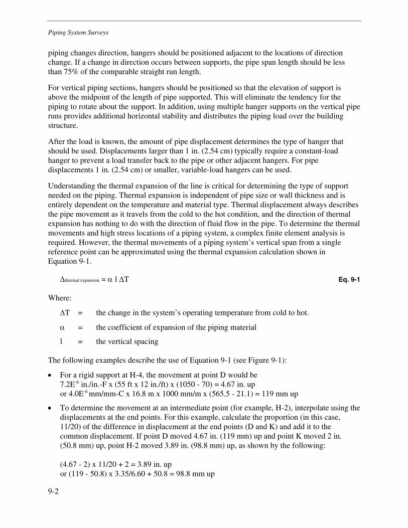
Piping System Surveys
9-2
piping changes direction, hangers should be positioned adjacent to the locations of direction change. If a change in direction occurs between supports, the pipe span length should be less than 75% of the comparable straight run length.
For vertical piping sections, hangers should be positioned so that the elevation of support is above the midpoint of the length of pipe supported. This will eliminate the tendency for the piping to rotate about the support. In addition, using multiple hanger supports on the vertical pipe runs provides additional horizontal stability and distributes the piping load over the building structure.
After the load is known, the amount of pipe displacement determines the type of hanger that should be used. Displacements larger than 1 in. (2.54 cm) typically require a constant-load hanger to prevent a load transfer back to the pipe or other adjacent hangers. For pipe displacements 1 in. (2.54 cm) or smaller, variable-load hangers can be used.
Understanding the thermal expansion of the line is critical for determining the type of support needed on the piping. Thermal expansion is independent of pipe size or wall thickness and is entirely dependent on the temperature and material type. Thermal displacement always describes the pipe movement as it travels from the cold to the hot condition, and the direction of thermal expansion has nothing to do with the direction of fluid flow in the pipe. To determine the thermal movements and high stress locations of a piping system, a complex finite element analysis is required. However, the thermal movements of a piping system’s vertical span from a single reference point can be approximated using the thermal expansion calculation shown in Equation 9-1.
Δthermal expansion = α l ΔT Eq. 9-1
Where:
ΔT = the change in the system’s operating temperature from cold to hot.
α = the coefficient of expansion of the piping material
l = the vertical spacing
The following examples describe the use of Equation 9-1 (see Figure 9-1):
• For a rigid support at H-4, the movement at point D would be 7.2E-6 in./in.-F x (55 ft x 12 in./ft) x (1050 - 70) = 4.67 in. up or 4.0E-6 mm/mm-C x 16.8 m x 1000 mm/m x (565.5 - 21.1) = 119 mm up
• To determine the movement at an intermediate point (for example, H-2), interpolate using the displacements at the end points. For this example, calculate the proportion (in this case, 11/20) of the difference in displacement at the end points (D and K) and add it to the common displacement. If point D moved 4.67 in. (119 mm) up and point K moved 2 in. (50.8 mm) up, point H-2 moved 3.89 in. (98.8 mm) up, as shown by the following: (4.67 - 2) x 11/20 + 2 = 3.89 in. up or (119 - 50.8) x 3.35/6.60 + 50.8 = 98.8 mm up
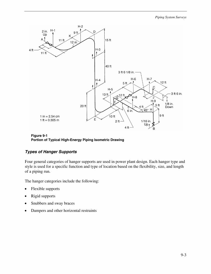
Piping System Surveys
9-3
Figure 9-1 Portion of Typical High-Energy Piping Isometric Drawing
Types of Hanger Supports
Four general categories of hanger supports are used in power plant design. Each hanger type and style is used for a specific function and type of location based on the flexibility, size, and length of a piping run.
The hanger categories include the following:
• Flexible supports
• Rigid supports
• Snubbers and sway braces
• Dampers and other horizontal restraints
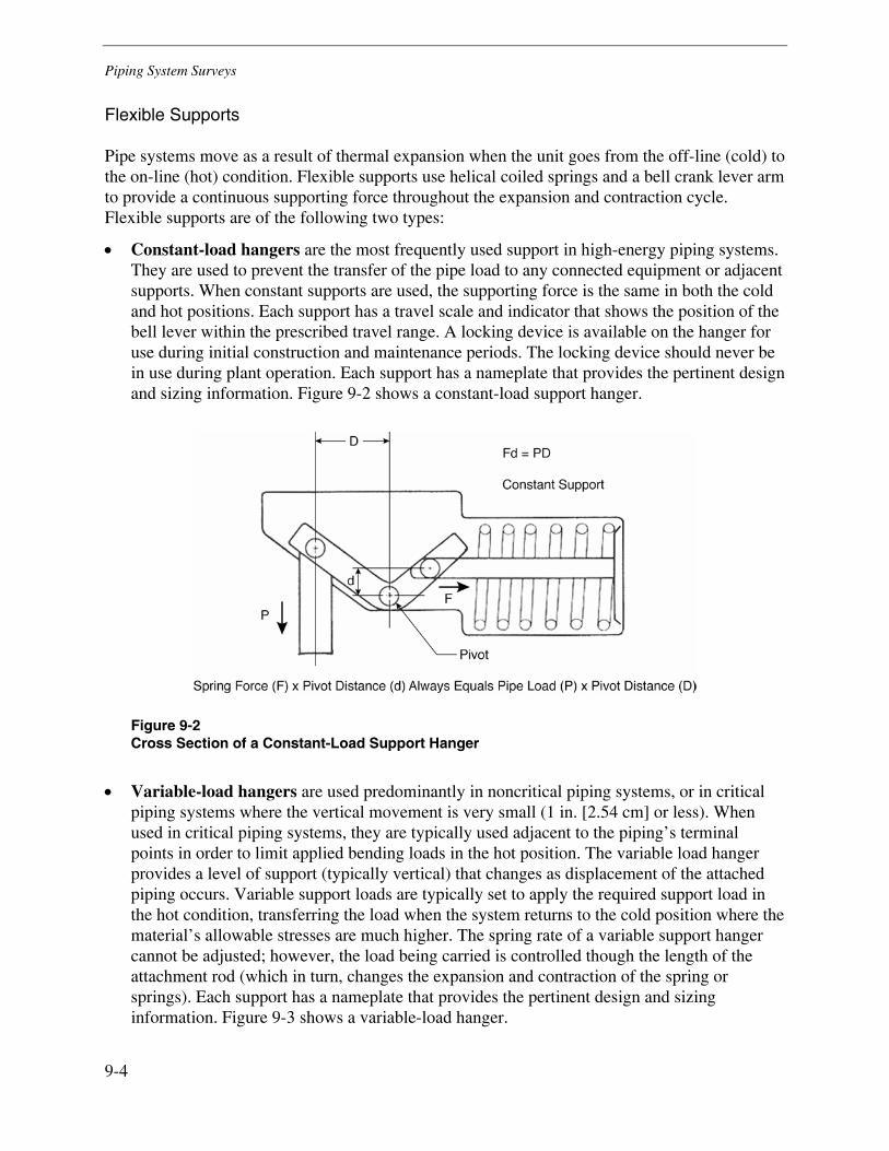
Piping System Surveys
9-4
Flexible Supports
Pipe systems move as a result of thermal expansion when the unit goes from the off-line (cold) to the on-line (hot) condition. Flexible supports use helical coiled springs and a bell crank lever arm to provide a continuous supporting force throughout the expansion and contraction cycle. Flexible supports are of the following two types:
• Constant-load hangers are the most frequently used support in high-energy piping systems. They are used to prevent the transfer of the pipe load to any connected equipment or adjacent supports. When constant supports are used, the supporting force is the same in both the cold and hot positions. Each support has a travel scale and indicator that shows the position of the bell lever within the prescribed travel range. A locking device is available on the hanger for use during initial construction and maintenance periods. The locking device should never be in use during plant operation. Each support has a nameplate that provides the pertinent design and sizing information. Figure 9-2 shows a constant-load support hanger.
Figure 9-2 Cross Section of a Constant-Load Support Hanger
• Variable-load hangers are used predominantly in noncritical piping systems, or in critical piping systems where the vertical movement is very small (1 in. [2.54 cm] or less). When used in critical piping systems, they are typically used adjacent to the piping’s terminal points in order to limit applied bending loads in the hot position. The variable load hanger provides a level of support (typically vertical) that changes as displacement of the attached piping occurs. Variable support loads are typically set to apply the required support load in the hot condition, transferring the load when the system returns to the cold position where the material’s allowable stresses are much higher. The spring rate of a variable support hanger cannot be adjusted; however, the load being carried is controlled though the length of the attachment rod (which in turn, changes the expansion and contraction of the spring or springs). Each support has a nameplate that provides the pertinent design and sizing information. Figure 9-3 shows a variable-load hanger.
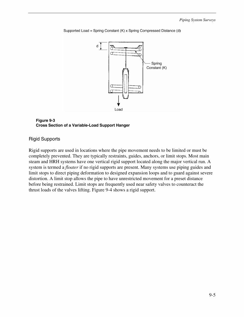
Piping System Surveys
9-5
Figure 9-3 Cross Section of a Variable-Load Support Hanger
Rigid Supports
Rigid supports are used in locations where the pipe movement needs to be limited or must be completely prevented. They are typically restraints, guides, anchors, or limit stops. Most main steam and HRH systems have one vertical rigid support located along the major vertical run. A system is termed a floater if no rigid supports are present. Many systems use piping guides and limit stops to direct piping deformation to designed expansion loops and to guard against severe distortion. A limit stop allows the pipe to have unrestricted movement for a preset distance before being restrained. Limit stops are frequently used near safety valves to counteract the thrust loads of the valves lifting. Figure 9-4 shows a rigid support.
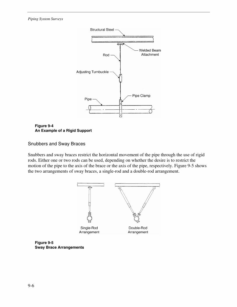
Piping System Surveys
9-6
Figure 9-4 An Example of a Rigid Support
Snubbers and Sway Braces
Snubbers and sway braces restrict the horizontal movement of the pipe through the use of rigid rods. Either one or two rods can be used, depending on whether the desire is to restrict the motion of the pipe to the axis of the brace or the axis of the pipe, respectively. Figure 9-5 shows the two arrangements of sway braces, a single-rod and a double-rod arrangement.
Figure 9-5 Sway Brace Arrangements
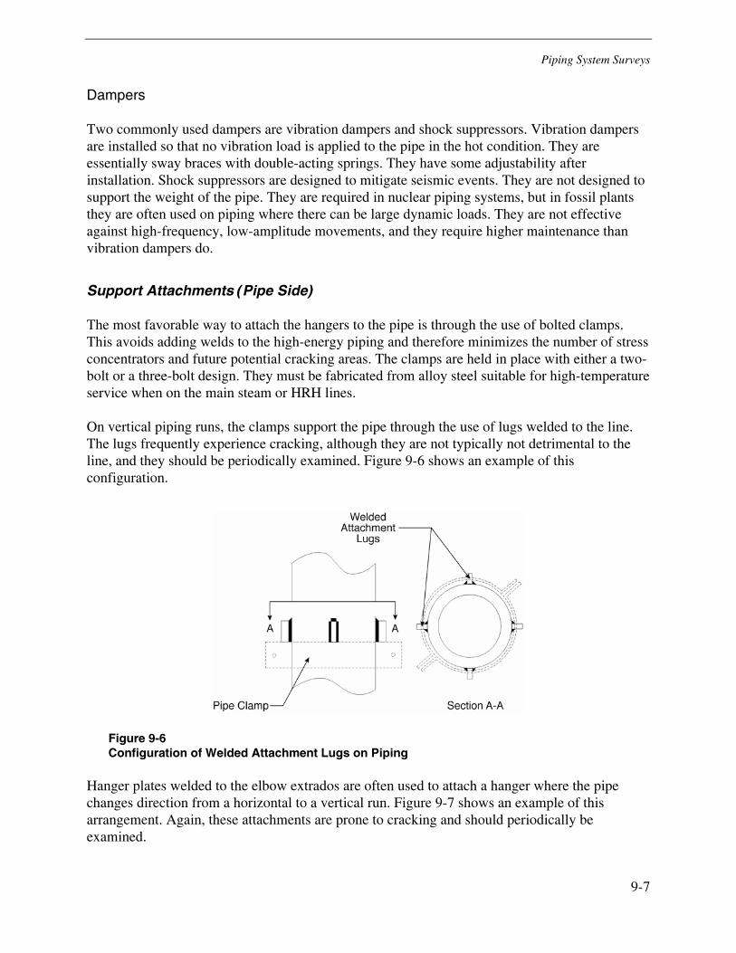
Piping System Surveys
9-7
Dampers
Two commonly used dampers are vibration dampers and shock suppressors. Vibration dampers are installed so that no vibration load is applied to the pipe in the hot condition. They are essentially sway braces with double-acting springs. They have some adjustability after installation. Shock suppressors are designed to mitigate seismic events. They are not designed to support the weight of the pipe. They are required in nuclear piping systems, but in fossil plants they are often used on piping where there can be large dynamic loads. They are not effective against high-frequency, low-amplitude movements, and they require higher maintenance than vibration dampers do.
Support Attachments (Pipe Side)
The most favorable way to attach the hangers to the pipe is through the use of bolted clamps. This avoids adding welds to the high-energy piping and therefore minimizes the number of stress concentrators and future potential cracking areas. The clamps are held in place with either a two-bolt or a three-bolt design. They must be fabricated from alloy steel suitable for high-temperature service when on the main steam or HRH lines.
On vertical piping runs, the clamps support the pipe through the use of lugs welded to the line. The lugs frequently experience cracking, although they are not typically not detrimental to the line, and they should be periodically examined. Figure 9-6 shows an example of this configuration.
Figure 9-6 Configuration of Welded Attachment Lugs on Piping
Hanger plates welded to the elbow extrados are often used to attach a hanger where the pipe changes direction from a horizontal to a vertical run. Figure 9-7 shows an example of this arrangement. Again, these attachments are prone to cracking and should periodically be examined.
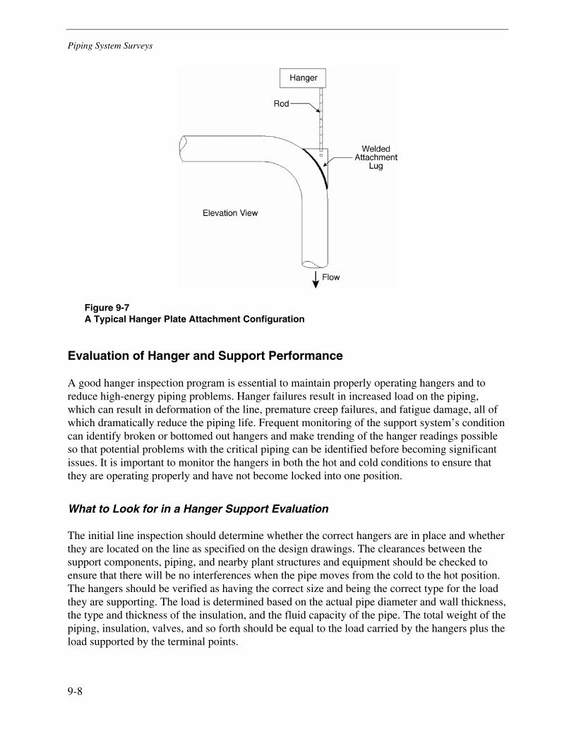
Piping System Surveys
9-8
Figure 9-7 A Typical Hanger Plate Attachment Configuration
Evaluation of Hanger and Support Performance
A good hanger inspection program is essential to maintain properly operating hangers and to reduce high-energy piping problems. Hanger failures result in increased load on the piping, which can result in deformation of the line, premature creep failures, and fatigue damage, all of which dramatically reduce the piping life. Frequent monitoring of the support system’s condition can identify broken or bottomed out hangers and make trending of the hanger readings possible so that potential problems with the critical piping can be identified before becoming significant issues. It is important to monitor the hangers in both the hot and cold conditions to ensure that they are operating properly and have not become locked into one position.
What to Look for in a Hanger Support Evaluation
The initial line inspection should determine whether the correct hangers are in place and whether they are located on the line as specified on the design drawings. The clearances between the support components, piping, and nearby plant structures and equipment should be checked to ensure that there will be no interferences when the pipe moves from the cold to the hot position. The hangers should be verified as having the correct size and being the correct type for the load they are supporting. The load is determined based on the actual pipe diameter and wall thickness, the type and thickness of the insulation, and the fluid capacity of the pipe. The total weight of the piping, insulation, valves, and so forth should be equal to the load carried by the hangers plus the load supported by the terminal points.

Piping System Surveys
9-9
ASME B31.1 recommends that the hangers be periodically examined to look for changes both in the piping and in the hangers [9-1]. Hangers can become inoperable as a result of creep deformation of the piping, a dynamic event in the line such as a water or steam hammer, or deterioration of the spring and other components. For constant-support and variable-load hangers, the code recommends that hanger readings be obtained both in the fully hot position and when the unit is off-line in the cold position. The hanger readings should be recorded and permanently stored. The temperature of the pipe at the time of observations should also be noted.
Hanger load and travel adjustments might be necessary over the life of a critical piping system. As a result of relaxation in the material, the piping rarely returns to its exact original position after operating in the hot condition. Also, as high-energy piping ages, creep deformation results in permanent shifting throughout the system. Careful monitoring of the hanger loads will result in a better-balanced system and less permanent deformation.
When a Hanger Support Problem Has Been Identified
For the majority of hanger problems that are identified, an immediate shutdown of the plant for repairs is not necessary; however, a timely response is important. Engineering must assess the effect of the hanger failure on the unit’s continued operation. In addition, they must determine the cause of the hanger failure. Typically, a flexible support hanger failure is the result of the support exceeding its limit. The damage imposed on the piping as a result of the malfunctioning hanger is cumulative. High stresses can lead to either premature creep failure or fatigue cracks. Without a stress analysis, it is difficult to determine where damage will occur in the piping; it is not always in the proximity of the failed hanger.
If the flexible support’s limits have been exceeded, adjustments should be made with the system on-line in the hot condition. This will ensure that the necessary loads are supported when the unit is most susceptible to creep degradation. (The allowable stress is much higher, and therefore the piping is more tolerant to high stresses, in the cold condition.) To ensure that the proper adjustments and maintenance have been performed on the hanger, the support’s readings in both the hot and cold positions should be taken over the next few months of operation.
Replacing a Hanger Support
If the hanger support is not repairable, then the entire hanger or the affected parts must be replaced. Hanger replacements typically occur with the unit off-line. Before removing the hanger, at least one support upstream and downstream of the affected support should be pinned, and the piping at the hanger should be supported. Lateral support might also be required. If a detached support (as in the case of a broken hanger rod) is being reconnected, the piping run must be brought back to the appropriate elevation and slope before attaching and setting the support.
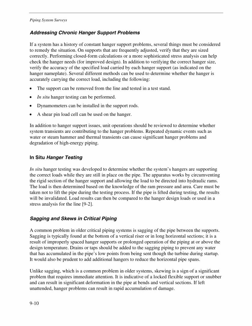
Piping System Surveys
9-10
Addressing Chronic Hanger Support Problems
If a system has a history of constant hanger support problems, several things must be considered to remedy the situation. On supports that are frequently adjusted, verify that they are sized correctly. Performing closed-form calculations or a more sophisticated stress analysis can help check the hanger needs (for improved design). In addition to verifying the correct hanger size, verify the accuracy of the specified load carried by each hanger support (as indicated on the hanger nameplate). Several different methods can be used to determine whether the hanger is accurately carrying the correct load, including the following:
• The support can be removed from the line and tested in a test stand.
• In situ hanger testing can be performed.
• Dynamometers can be installed in the support rods.
• A shear pin load cell can be used on the hanger.
In addition to hanger support issues, unit operations should be reviewed to determine whether system transients are contributing to the hanger problems. Repeated dynamic events such as water or steam hammer and thermal transients can cause significant hanger problems and degradation of high-energy piping.
In Situ Hanger Testing
In situ hanger testing was developed to determine whether the system’s hangers are supporting the correct loads while they are still in place on the pipe. The apparatus works by circumventing the rigid section of the hanger support and allowing the load to be directed into hydraulic rams. The load is then determined based on the knowledge of the ram pressure and area. Care must be taken not to lift the pipe during the testing process. If the pipe is lifted during testing, the results will be invalidated. Load results can then be compared to the hanger design loads or used in a stress analysis for the line [9-2].
Sagging and Skews in Critical Piping
A common problem in older critical piping systems is sagging of the pipe between the supports. Sagging is typically found at the bottom of a vertical riser or in long horizontal sections; it is a result of improperly spaced hanger supports or prolonged operation of the piping at or above the design temperature. Drains or taps should be added to the sagging piping to prevent any water that has accumulated in the pipe’s low points from being sent though the turbine during startup. It would also be prudent to add additional hangers to reduce the horizontal pipe spans.
Unlike sagging, which is a common problem in older systems, skewing is a sign of a significant problem that requires immediate attention. It is indicative of a locked flexible support or snubber and can result in significant deformation in the pipe at bends and vertical sections. If left unattended, hanger problems can result in rapid accumulation of damage.
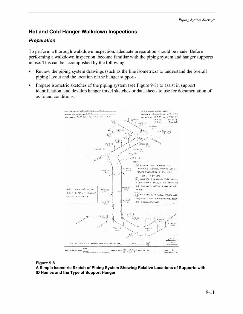
Piping System Surveys
9-11
Hot and Cold Hanger Walkdown Inspections
Preparation
To perform a thorough walkdown inspection, adequate preparation should be made. Before performing a walkdown inspection, become familiar with the piping system and hanger supports in use. This can be accomplished by the following:
• Review the piping system drawings (such as the line isometrics) to understand the overall piping layout and the location of the hanger supports.
• Prepare isometric sketches of the piping system (see Figure 9-8) to assist in support identification, and develop hanger travel sketches or data sheets to use for documentation of as-found conditions.
Figure 9-8 A Simple Isometric Sketch of Piping System Showing Relative Locations of Supports with ID Names and the Type of Support Hanger
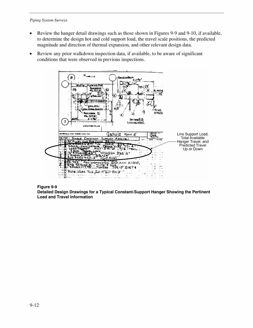
Piping System Surveys
9-12
• Review the hanger detail drawings such as those shown in Figures 9-9 and 9-10, if available, to determine the design hot and cold support load, the travel scale positions, the predicted magnitude and direction of thermal expansion, and other relevant design data.
• Review any prior walkdown inspection data, if available, to be aware of significant conditions that were observed in previous inspections.
Figure 9-9 Detailed Design Drawings for a Typical Constant-Support Hanger Showing the Pertinent Load and Travel Information
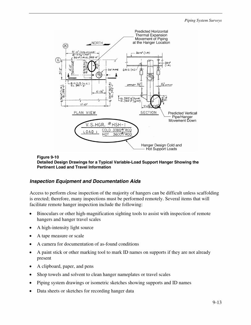
Piping System Surveys
9-13
Figure 9-10 Detailed Design Drawings for a Typical Variable-Load Support Hanger Showing the Pertinent Load and Travel Information
Inspection Equipment and Documentation Aids
Access to perform close inspection of the majority of hangers can be difficult unless scaffolding is erected; therefore, many inspections must be performed remotely. Several items that will facilitate remote hanger inspection include the following:
• Binoculars or other high-magnification sighting tools to assist with inspection of remote hangers and hanger travel scales
• A high-intensity light source
• A tape measure or scale
• A camera for documentation of as-found conditions
• A paint stick or other marking tool to mark ID names on supports if they are not already present
• A clipboard, paper, and pens
• Shop towels and solvent to clean hanger nameplates or travel scales
• Piping system drawings or isometric sketches showing supports and ID names
• Data sheets or sketches for recording hanger data
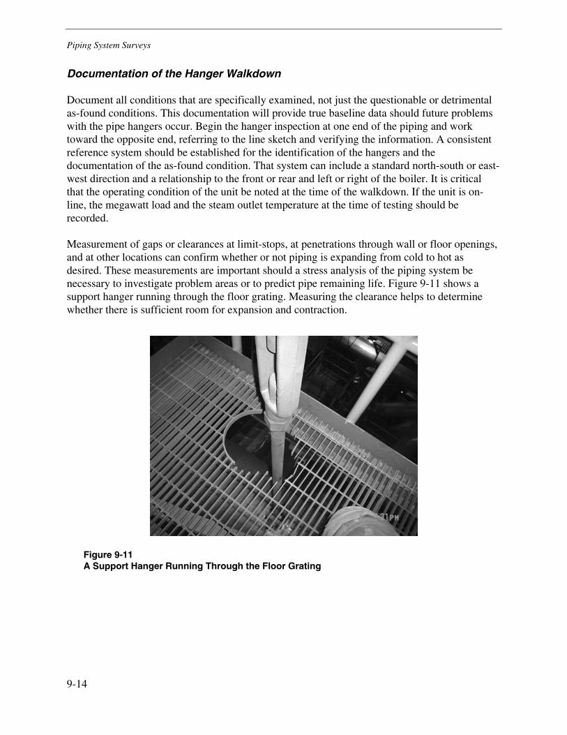
Piping System Surveys
9-14
Documentation of the Hanger Walkdown
Document all conditions that are specifically examined, not just the questionable or detrimental as-found conditions. This documentation will provide true baseline data should future problems with the pipe hangers occur. Begin the hanger inspection at one end of the piping and work toward the opposite end, referring to the line sketch and verifying the information. A consistent reference system should be established for the identification of the hangers and the documentation of the as-found condition. That system can include a standard north-south or east-west direction and a relationship to the front or rear and left or right of the boiler. It is critical that the operating condition of the unit be noted at the time of the walkdown. If the unit is on-line, the megawatt load and the steam outlet temperature at the time of testing should be recorded.
Measurement of gaps or clearances at limit-stops, at penetrations through wall or floor openings, and at other locations can confirm whether or not piping is expanding from cold to hot as desired. These measurements are important should a stress analysis of the piping system be necessary to investigate problem areas or to predict pipe remaining life. Figure 9-11 shows a support hanger running through the floor grating. Measuring the clearance helps to determine whether there is sufficient room for expansion and contraction.
Figure 9-11 A Support Hanger Running Through the Floor Grating
Piping System Surveys
9-15
Summary of Hanger Walkdown Documentation Requirements
The documentation requirements for a hanger walkdown include the following:
• Date and unit status (off-line or on-line, unit load or nominal steam outlet temperature) at the time of the inspection
• Hanger nameplate design information (hanger manufacturer, hanger size or figure number, design cold and hot load, design travel and direction, total available travel)
• Hanger travel or load scale configuration (such as 10 travel scale divisions with 0 at the top of the travel scale and 10 at the bottom)
• Hanger design cold and hot travel scale positions as indicated by stamps, if present, on the travel scale (typically H and C stamps or red and white markers)
• Current hanger travel scale position, including a note for any hangers that are topped or bottomed out
• Details of any other observed detrimental conditions (such as loose support rods, corroded or impacted spring hanger assemblies, or deformed structural steel members)
System Survey Checklist
The following list can be used as a checklist for observations that should be made during a hanger support evaluation.
General Hanger Observations
• Check whether the supports are located where they are supposed to be according to the design drawings.
• Check whether the supports are the right size and type for the load they are carrying.
• Check whether the supports are free to move with the pipe.
• Check for any structural restrictions.
• Check for damaged insulation adjacent to the hanger area.
Constant Load Support Observations
• Look for loose, bent or broken support rods.
• Examine the springs, pivots, and cases for broken parts.
• Look for signs of corrosion on the springs.
• Check for foreign matter such as fly ash or other debris in the springs that could restrict its movement.
Piping System Surveys
9-16
• Document the hanger travel scale position (if the hanger scale position is not legible, then estimate the position from 0 at the bottom or lowermost scale position and 10 at the top or uppermost travel position.
• Note any hanger that is topped or bottomed out.
• Ensure that the locking devices are not engaged.
• Note the hanger design information from the hanger nameplate.
Variable Load Support Observations
• Look for loose, bent, or broken support rods.
• Examine the springs, pivots, and cases for broken parts.
• Look for signs of corrosion on the springs.
• Check for foreign matter such as fly ash or other debris in the springs that could restrict its movement.
• Document the hanger load scale position.
• Note any hanger that is topped or bottomed out.
• Ensure that the locking devices are not engaged.
• On vertical piping runs, examine the pipe-side hanger attachment lugs for cracking.
• Note the hanger design information from the hanger nameplate.
Rigid Support Observations
• Look for loose, bent, or broken support rods.
• Check pipe-side lugs for deformation.
• Look for signs of lateral interference with the surrounding structure.
Sway Brace Support Observations
• Look for loose, bent, or broken support rods.
• Examine the pivot to ensure it is in proper working order
Snubber and Shock Suppressors Support Observations
• Stroke snubbers and shock suppressors to verify that they are not locked up and acting as rigid supports.
• Ensure that the hanger is not bearing the pipe’s weight.
• Check that the fluid reservoirs are filled to the manufacturer’s recommended level.

Piping System Surveys
9-17
General Piping Observations
• Examine horizontal and vertical piping runs for sags, skews, or other anomalies.
• Examine the insulation on the piping for interference or tight clearances between the piping and any adjacent piping, surrounding structures, other equipment, floor gratings, and so on.
• Check for missing, loose, or damaged pipe insulation or lagging.
• Look for damage or deformation of the structural steel at or near the pipe support attachment points.
• Measure and document the pipe location at position indicators, limit stops supports, or other locations where the pipe location can be measured relative to a fixed, permanent reference.
References
9-1. ASME B31.1, Code for Pressure Piping Standards: Power Piping. American Society of Mechanical Engineers, New York. 2004.
9.2 G. May, “The Need for in situ Pipe Support Testing,” Proceedings of ASME Power 2004, POWER2004-52031. March 2004, Baltimore, MD.


10-1
10 NONDESTRUCTIVE TESTING
Introduction
The status of fossil power plant condition assessment has changed dramatically over the past several decades. Previously, the problem was a lack of inspection and life assessment tools; now, the problem centers on the vast array of options available to the planner. The list of components recommended for inspection has grown dramatically, as have the available NDE approaches for component inspection. Even within the limitations of a single component, the planner often finds an extensive range of available inspection technologies, each having its own inherent capabilities, reliabilities, and level of maturity.
The problem that the planner must currently address has evolved to the selection of appropriate inspection technologies and inspection scope to meet specific conditions and objectives in the most economic way. Reinspection interval extension is one way of reducing maintenance costs that is currently receiving significant attention. Although this approach is perfectly valid, it places additional emphasis on selection of appropriate NDE and life assessment technologies to ensure that the component will operate through a longer cycle with acceptable risk.
Power utility NDE planners or purchasers must often make decisions based on limited information and without sufficient time and support to perform a comprehensive cost-benefit analysis. All too often, decisions are made purely on the basis of inspection cost without due consideration of the true cost, which should include the impact of decisions on potential repairs or replacements, reinspection intervals, possible forced outages, and other indirect expenses associated with the inspection capabilities.
At the other end of the spectrum, decisions are also based on the best available technology for the application. Depending on the particular circumstances, less exhaustive (and therefore generally less expensive) options can be more than adequate and therefore appropriate.
This situation has increased the need for a single document that presents NDE information in a concise format. The fossil power utility planner can then access and retrieve comprehensive information quickly and use the information in developing a condition assessment strategy.
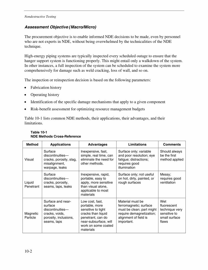
Nondestructive Testing
10-2
Assessment Objective (Macro/Micro)
The procurement objective is to enable informed NDE decisions to be made, even by personnel who are not experts in NDE, without being overwhelmed by the technicalities of the NDE technique.
High-energy piping systems are typically inspected every scheduled outage to ensure that the hanger support system is functioning properly. This might entail only a walkdown of the system. In other instances, a full inspection of the system can be scheduled to examine the system more comprehensively for damage such as weld cracking, loss of wall, and so on.
The inspection or reinspection decision is based on the following parameters:
• Fabrication history
• Operating history
• Identification of the specific damage mechanisms that apply to a given component
• Risk-benefit assessment for optimizing resource management budgets
Table 10-1 lists common NDE methods, their applications, their advantages, and their limitations.
Table 10-1 NDE Methods Cross-Reference
Method Applications Advantages Limitations Comments
Visual
Surface discontinuities— cracks, porosity, slag, misalignment, warpage, leaks
Inexpensive, fast, simple, real time, can eliminate the need for other methods.
Surface only; variable and poor resolution; eye fatigue; distractions; requires good illumination
Should always be the first method applied
Liquid Penetrant
Surface discontinuities—cracks, porosity, seams, laps, leaks
Inexpensive, rapid, portable, easy to apply, more sensitive than visual alone, applicable to most materials
Surface only; not useful on hot, dirty, painted, or rough surfaces
Messy; requires good ventilation
Magnetic Particle
Surface and near-surface discontinuities—cracks, voids, porosity, inclusions, seams, laps
Low cost, fast, portable, more sensitive to tight cracks than liquid penetrant, can do near-subsurface, will work on some coated materials
Material must be ferromagnetic; surface must be clean; part might require demagnetization; alignment of field is important.
Wet fluorescent technique very sensitive to small surface flaws
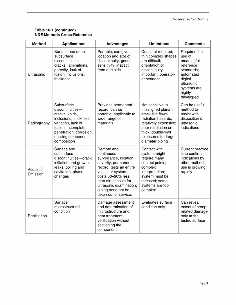
Nondestructive Testing
10-3
Table 10-1 (continued) NDE Methods Cross-Reference
Method Applications Advantages Limitations Comments
Ultrasonic
Surface and deep subsurface discontinuities—cracks, laminations, porosity, lack of fusion, inclusions, thickness
Portable, can give location and size of discontinuity, good sensitivity, inspect from one side
Couplant required; thin complex shapes are difficult; orientation of discontinuity important; operator-dependent
Requires the use of meaningful reference standards; automated digital ultrasonic systems are highly developed
Radiography
Subsurface discontinuities—cracks, voids, inclusions, thickness variation, lack of fusion, incomplete penetration, corrosion, missing components, composition
Provides permanent record, can be portable, applicable to wide range of materials
Not sensitive to misaligned planar, crack-like flaws; radiation hazards; relatively expensive; poor resolution on thick, double-wall exposures for large diameter piping
Can be useful method to assist with disposition of ultrasonic indications
Acoustic Emission
Surface and subsurface discontinuities—crack initiation and growth, leaks, boiling and cavitation, phase changes
Remote and continuous surveillance, location, severity; permanent record; tests an entire vessel or system; costs 50–90% less than direct costs for ultrasonic examination; piping need not be taken out of service.
Contact with system; might require many contact points; complex interpretation; system must be stressed; some systems are too complex
Current practice is to confirm indications by other methods; use is growing rapidly
Replication
Surface microstructural condition
Damage assessment and determination of microstructure and heat treatment verification without sectioning the component.
Evaluates surface condition only
Can reveal extent of creep-related damage only at the tested surface

Nondestructive Testing
10-4
Access and Required Surface Preparation
Preparation of various power plant component surfaces for inspection is governed by many variables, including the following:
• NDE techniques to be used
• Type of NDE procedures to be applied
• Sequence of NDE techniques to be used
• Materials involved
• Component size and portability
• Costs of various surface preparation techniques
• Time required, including scaffolding, access, and so forth
• Interference with other projects in the plant
Planning of the overall outage and inspections and coordination between the NDE personnel and contractors are critical to minimizing the cost and time involved in surface preparation, as well as the impact on other parallel plant projects being performed during the outage.
No Surface Preparation
It is often recommended that a walkdown of the equipment be conducted with no surface preparation of the components because signs of unusual operation of the unit can often provide valuable evidence of the abnormal condition and aid in subsequent inspections and overall condition assessment. Signs of steam or water leakage, aggressive air penetration, or local overheating can be detected quickly and visually by experienced personnel during the walkdown, before any cleaning is conducted. Deposits in the turbine stages can provide critical evidence of past exposure to contaminants for future use, and samples should be collected before being contaminated with cleaning media. Heat patterns in generator rotors or stators can be indicative of insulation breakdown. Similarly, dusting or greasing of insulation components can provide valuable information relative to looseness between mating parts, rubs, vibration, and so on. Patterns of coal ash deposition in superheater, reheater, or economizer sections can provide critical information regarding flow balance across the boiler. Damage to insulation and sagging can indicate hanger or support problems in piping systems. One of the first questions to be asked after the unit is scheduled to be brought down is, “What information might I lose by cleaning component surfaces?”
Most inspection techniques require that a clean surface be obtained for inspection. However, this is not always the case. Some exceptions can include electromagnetic acoustic transducer or focused beam UT of boiler tubes (particularly in gas-fired units) and internal inspection of heat exchanger tubing by eddy current testing (ET), which can be performed with no surface preparation unless deposits and debris accumulation are excessive. Magnetic flux leakage inspections and even some general UT techniques can be performed with no surface preparation,
Nondestructive Testing
10-5
depending on the as-found component surface condition, the criticality of the inspection, and other factors. Infrared thermography and radiographic test (RT) inspections can often be done with no surface preparation. The need to perform any cleaning operations should be verified with the appropriate NDE personnel before proceeding with any cleaning operation.
Surface Debris and Scale Removal
One of the most popular surface preparation techniques is grit or sand blasting. Large areas can be cleaned quickly and, with proper air pressure and media density, little damage is done to the surface. For smaller areas requiring inspection, local wire brushing, needle gunning, or light grinding might be preferred because of their portability. There is a possibility that some small, shallow cracks will be peened over with these latter techniques. Particular care is recommended for thin or soft materials to ensure that small cracks do not go undetected. The use of such surface preparation methods can lead to severe inspection limitations when certain surface inspections are to be conducted, particularly for PT and to a lesser degree MT and ET. The materials involved should also be considered when considering appropriate cleaning methods. Some material, for example, cannot be exposed to chemicals and must be cleaned using purely mechanical means. Other components must be cleaned using chemicals because of surface finish requirements or dimensional tolerances that cannot be disturbed. Consequently, it is important to coordinate the type of surface preparation to be performed with the appropriate NDE personnel and materials specialists to make certain that the selected cleaning means is compatible with the NDE methods and techniques to be applied and with the materials involved.
Local, state, or federal regulations might dictate that cleaning techniques that cause potential airborne contamination in confined spaces (grit blasting of boiler tubes is a good example) require monitoring during and after the cleaning cycle. In these cases, the NDE personnel might be required to wear protective breathing apparatus, which can slow down the inspection cycle. This can be a particular problem when cleaning surfaces from which asbestos insulation has just been removed.
For parts or components that can be moved, cleaning is often accomplished in a confined area, such as an erected tent. This limits the export of cleaning media or the import of airborne contaminants into the cleaning environment, which can be important for cleaning parts with tight fit-ups and clearances that must be disassembled for inspection. In addition, the use of cleaning and inspection enclosures can often be required as a means of controlling ambient light, for example for the performance of fluorescent MT or PT inspections. For some components, such as certain generator retaining rings, temperature and humidity control is very important. Often the same enclosures used for cleaning provide suitable environmental protection for the inspection and for storage of the components until ready for return to service.
Nondestructive Testing
10-6
Access Limitations
Internal inspections of boiler components, water and steam lines, assembled turbine and generators, heat exchangers, and so on can require considerable modifications to gain access. If the component is to be inspected frequently, consideration should be given to designing and implementing a convenient means of access that can be reused, thus eliminating cutting and rewelding at each outage. Modifications to provide access should include consideration for both personnel and equipment and can involve larger access doors on boilers, new or larger manways in turbine casings, heat exchangers, and so on. When modifications are required to perform certain inspections, permanent modification can pay for themselves many times over because improved access usually results in more timely maintenance, inspection, and repair cycles during future outages.
Visual Testing
Overview
Quality visual testing (VT) is one of the least appreciated and possibly the most demanding NDE activity currently used in power plant inspection. Whereas VT once consisted of looking over a component, by current standards VT typically involves a great deal of training and practical experience before one is qualified for this inspection method. Qualified VT inspectors must have a good working knowledge of a vast array of plant components, metallurgy, potential flaw types for various components, failure mechanisms, and so forth. They must be able to recognize the presence of different damage forms and classify the damage in terms of severity and implications relative to ongoing operation of the component, based solely on what normally is very limited visual evidence. The American Society for Nondestructive Testing (ASNT) currently recognizes VT as a specific inspection discipline, and the requirements for acquiring certification are extremely demanding.
Although it is not an NDE technique in itself, debris removal is often a substantial part of a visual inspector’s job. It is common for items such as screwdrivers, grippers, welding rods, or nuts and bolts to drop into a component during maintenance operations. If not removed, they could cause considerable damage when the plant is brought back to power. Various devices and attachments have been developed to facilitate this task.
Application in Piping Systems
VT can be applied to any component in which the damage manifests itself at accessible surfaces to a degree that permits detection by visual means. Considerable ingenuity can often be exercised to produce a viewing and transport system for most plant components. VT should always be the first method applied.
Nondestructive Testing
10-7
Advantages and Disadvantages
Advantages
The advantages of VT include the following:
• Inexpensive (excluding video borescope techniques)
• Fast and simple
• Real-time examination
• A permanent record can be produced when using video-based systems
• Can eliminate the need for other methods
Disadvantages
The disadvantages of VT include the following:
• Limited to accessible surfaces
• Variable quality; dependent on human factors (for example, eye fatigue and distractions)
• Typically poor resolution
• Requires good illumination
• Does not lend itself to automation
Magnetic Particle Testing
Overview
MT is a fairly simple inspection method that is useful for the detection of surface-connected and near-surface discontinuities in ferromagnetic material. The method is applicable to a variety of components, including raw materials as well as finished components.
When a ferromagnetic material test piece is magnetized by bringing the poles of a magnet (either permanent or electromagnet) into contact or into close proximity, the magnetic flux lines that flow from one pole of the magnet to the other will now travel within a surface layer of the test piece. The presence of a discontinuity that intercepts the magnetic flux lines will result in flux leakage, which, in turn, will attract small magnetic or ferromagnetic particles that will indicate the location of such discontinuity. Tight discontinuities, such as cracks, will be best detected when oriented in a perpendicular position to the flux lines; tight cracks that are parallel to the flux are poorly detected or not detected at all.

Nondestructive Testing
10-8
In practice, the magnetic particles (commonly fine iron filings) are applied as a powder (or liquid suspension of a powder); these are either colored to contrast with the test surface under visible light or coated with a fluorescent material that glows under ultraviolet (UV) light. Fluorescent particles are used for increased visibility and better sensitivity of detection. The test piece is magnetized by the use of permanent magnets or an electromagnet yoke or by wrapping a length of electrical cable around the test section to form a coil that is then energized with a power supply that results in the magnetization of the wrapped zone. With the exception of the permanent magnet, a yoke or a coil can be energized either with ac or dc in order to obtain the needed mix of sensitivity and penetration.
Application in Piping Systems
MT is one of the most frequently used of the NDE methods applied in power stations for routine inspection. MT can be applied essentially to any exposed surface of any ferromagnetic material. Surface preparation is not as demanding as for dye penetrant inspection, and reasonable sensitivity can be achieved, particularly with the wet fluorescent method. MT can even be applied over thin surface coatings such as paint, although surface finish can affect both mobility and retention of the particles.
A special type of magnetic particle inspection that is useful for inspection of tight spaces that otherwise cannot be inspected with this method involves the use of rubber compounds for the suspension medium. The process, called rubber-mag, is one in which particles are mixed into a rubber compound that is in a liquid state. Magnetization is accomplished by the most appropriate technique to produce directional magnetization for optimum detection of the prevalent flaw orientation, and the magnetic particles are applied through the rubber suspension. The rubber compound used must have very specific properties to maintain particle mobility while in the liquid state and to provide a contrasting background to the particles. When set, the molded rubber is removed and viewed for indications of the surface.
Advantages and Disadvantages
Advantages
The advantages of MT are the following:
• Relatively inexpensive
• Fast and simple
• Requires only minimal surface preparation
• Better surface preparation and the use of liquid fluorescent particles improves sensitivity
• Real-time examination
• A permanent record can be produced by photography
Nondestructive Testing
10-9
Disadvantages
The disadvantages of MT are the following:
• Limited to accessible surfaces
• Variable quality; dependent on human factors (for example, eye fatigue or distractions)
• Requires good illumination for visible particles, or a darkened location for fluorescent
• Does not lend itself to automation
Dye Penetrant Testing
Overview
PT is a nondestructive method for finding discontinuities that are open to the surface. Indications open to the inspection surface can generally be found regardless of the flaw size (above the detection threshold), configuration, or orientation. As a result of capillary action, penetrant materials are drawn into various types of surface imperfections, making the method well suited for detecting most imperfections in both ferrous and nonferrous metals, provided the flaws are open to the inspection surface. PT can be applied to a variety of components including raw materials as well as finished components. The inspection of complex geometries is possible if the surfaces are accessible and the surface geometry complexity does not preclude complete removal of excess penetrant.
The theoretical basis of penetrant inspection is relatively simple. A liquid penetrant containing a visible liquid (also called color-contrast) or fluorescent compound is applied to the inspection surface. The penetrant is allowed to remain on the inspection surface for sufficient time to be drawn into the openings of the surface discontinuity by capillary action. Excess penetrant material is then removed, and a developer is applied to the test surface (applied as a thin layer of white powder by a quick-drying propellant or suspension). The developer absorbs the residual penetrant material held in the surface discontinuities and draws the penetrant to the exposed surface, providing both an indication of the presence of a surface discontinuity and a contrasting background which makes the indication more apparent under visual observation of the surface. Fluorescent dyes require the use of UV light and a darkened location for viewing.
Penetrant inspection can be broadly classified by the following types of penetrants:
• Water-washable penetrant, which contains an emulsifier and therefore can be directly removed using water as the cleaning agent
• Post-emulsifiable penetrant, which requires application of an emulsifier (liquid that combines with the penetrant to make it water-washable) before water cleaning
• Solvent-removable penetrant, which can be removed adequately only by using the appropriate solvent
Nondestructive Testing
10-10
Application in Piping Systems
Although PT can be applied to essentially any exposed surface, it is not used as frequently as MT for NDE of piping systems. This is mostly because it requires more extensive surface preparation than MT, yet results in only minimal increase of sensitivity. Also, unlike MT, it is not able to detect near-subsurface discontinuities because the penetrating dye requires a path to the discontinuity that is open to the surface.
More commonly for piping systems, PT is used by default for surface inspections of non-ferromagnetic materials, such as austenitic stainless steels, where it is not possible to apply MT.
Advantages and Disadvantages
Advantages
The advantages of PT are the following:
• Inexpensive
• Fast and simple
• Better surface preparation and the use of liquid fluorescent dyes improves sensitivity
• Real-time examination
• A permanent record can be produced by photography
Disadvantages
The disadvantages of PT are the following:
• Limited to accessible surfaces
• Variable quality; dependent on human factors
• Requires good surface preparation and care to prevent laps that close off surface discontinuities
• Complete cleaning and removal of the dye is not always possible
• Requires good illumination for visible dye penetrants or a darkened location for fluorescent
• Does not lend itself to automation
Nondestructive Testing
10-11
Eddy Current Testing
Overview
ET is used to inspect the surface or near-surface of electrically conducting materials. The test probe, typically with a coil-like construction, induces an electrical current into the near-surface volume of the test area adjacent to it. When a discontinuity is present in the test volume under the probe, it distorts the electromagnetic field that was created by the probe. Such distortion is detected by the probe, and its indication on the instrument screen can be interpreted by the expert analyst as to the type, size, location, or any other parameter of the discontinuity that was incorporated into the calibration process.
The theoretical depth of the surface region that can be inspected is governed by three parameters: frequency of the excitation current, the electrical conductivity of the test piece, and the relative magnetic permeability of the test material. The other parameters that affect depth of penetration and sensitivity are the probe size and type; these are determined mostly empirically. Because the relative permeability of nonferromagnetic materials is 1, and the electrical conductivity is a material constant, the depth of penetration, for a simplistic model, can be varied by the selection of the test frequency.
When applying ET to ferromagnetic materials (for example, carbon and alloy steels) the relative magnetic permeability does not equal 1 and could vary across the surface as a result of compositional and heat treatment nonuniformities. The eddy currents induced into such test pieces would be affected mostly by limiting the depth of penetration and the ability to measure crack depth by the phase angle shift method. Still, the ability to detect cracks is not diminished, but rather enhanced, by the effect of the permeability being greater than 1, and the ability to detect surface-connected cracks that go below the calculated skin depth is not affected. However, when the parameters of interest are affected by permeability, it is possible to negate the effect by magnetically saturating (fully or partially) the test location next to the probe.
Electromagnetic NDE techniques for ferromagnetic materials include remote field eddy current, flux leakage, and partial saturation.
Application in Piping Systems
Conventional ET is not often used for the inspection of piping systems. Mostly, it is applied for the detection of seam welds where there is no visual indication of the weld’s presence or location. Otherwise, ET can be used in lieu of other surface techniques, replacing MT or PT, but at a greater cost. Advanced ET techniques, such as remote field and flux leakage, are more commonly used for the inspection of boiler tubes rather than for large-diameter piping systems.
Nondestructive Testing
10-12
Advantages and Disadvantages
ET is limited to inspecting the surfaces of conducting materials; it is an alternative technique to MT and PT inspection.
Advantages
The advantages of ET are the following:
• Probes can be constructed to be very small so they can enter components that are inaccessible to other techniques.
• There is little need for surface preparation. In many cases it is possible to inspect through surface layers such as paint.
• There is no need for dyes and developers, making ET attractive in applications where waste and contamination must be minimized. Similarly, no contact is necessary between the test probe and the examined surface, as long as the probe proximity can be precisely controlled during scanning
• A permanent record can be created by the instrumentation
• ET can be easily automated.
Disadvantages
The disadvantages of ET are the following:
• The signals produced on the instrument screen can be complex, they require a higher level of training and experience to interpret, and the equipment is relatively expensive. However, much recent work has been aimed at developing equipment that can assist with data interpretation and flaw classification that minimize such concerns.
• The presence of geometric features and discontinuities near the region where flaws are expected can complicate the examination. The selection of proper test coils for such cases can reduce or eliminate the problem.
• A careful assessment by an expert is required in order to make the proper inspection technique selection.
Conventional Ultrasonic Testing
Overview
UT technology encompasses a wide range of applications that vary dramatically in technological sophistication, complexity, required equipment, implementation constraints, speed of application, detection reliability, sizing accuracy, requisite operator skills, and so forth. The
Nondestructive Testing
10-13
technology has evolved to a point at which very few components are inspected according to generic procedures. That is, specific techniques and application procedures designed to address certain desired performance characteristics are used for most components. What is optimum for one application simply might not be adequate, or in some cases even possible, for another. Consequently, it is difficult to provide guidance that is concise and easy to understand and yet provide sufficient detail for educated decisions.
UT is generally described as the introduction of high-frequency sound waves—generally in the range of 0.5 MHz to 50 MHz—into a component, part, or structure for the purpose of determining some characteristic of the material from which the component, part, or structure is made. Material characteristics that can be and have been determined ultrasonically include such items as material structure, stress (both residual and applied), hardness, anisotropy, and others. However, for fossil power plant inspection, ultrasonic inspection is used primarily for flaw detection, classification, and sizing, and for dimensional measurement (thickness). Other applications are possible and should be considered along with other competing or complementing technologies for the objective of determining other material characteristics.
UT, as used for flaw detection and thickness measurement, is analogous to active sonar. A short-duration pulse of sound is generated in the part by a transmitter, immediately following which the ultrasonic instrumentation is switched to a listening mode. Any detected return signal indicates the presence at some point in the sound field of a reflector that has redirected the propagating wave in the direction of the receiver.
Flaw detection and thickness measurement applications of ultrasound operate on two fundamental principles. First, for a specific propagation mode, sound travels in a given material at a constant velocity. Therefore, a precise measurement of the propagation time between initiation of the pulse and detection of a signal at the receiver provides the basis for calculating the position of the reflector relative to the transmitter and receiver positions. Second, the response from a reflector is a function of characteristics of the transmitted beam, the material through which it propagates, and certain characteristics of the reflector that causes the response. If ultrasonic practitioners can extract, or deconvolve, those characteristics of the response that are attributable to the beam and propagation material, they are left with a response that is characteristic of the reflector. If they can further extract from this remaining reflector response the information that is related most directly to the feature of interest, for example flaw size, then they might have a reasonable chance of estimating that feature.
Flaw sizing, flaw classification, and extraction of other useful information are described later in this section. However, at this point, it is more important to concentrate on basic inspection approaches, displays, and other factors that will be found in use throughout the power plant.
The traditional ultrasonic implementation means and display were developed on the basis of the two fundamental principles—that time and amplitude are the main features of interest. Short-duration sound pulses are used such that the instrumentation can quickly be switched to the listening mode for the detection of reflectors located close to the transducers, therefore having short propagation paths and correspondingly small propagation times. A cathode ray tube (CRT)
Nondestructive Testing
10-14
display is used where the horizontal axis of the display represents time, increasing from left to right, and the vertical axis represents intensity, increasing from the base level to saturation. The listening interval is set at sufficient duration to allow the wave to propagate to the maximum inspection depth and back to the receiver before the next pulse is generated. Because propagation velocities are typically in the range up to 1 in./μs (2.54 cm/μs), pulse repetition rates in the hundreds or even thousands of pulses per second are achievable for most materials and typical material thicknesses, while still providing sufficient listening time. By synchronizing the CRT sweep with the pulse rate such that each sweep represents a new pulse, at such high pulse rates the CRT display appears as continuous without perceptible flicker. In more modern, computer-based ultrasonic systems, these same features (and others) are converted to graphical displays that present responses in spatially correlated images, thereby adding position to the presented time and amplitude information.
Application in Piping Systems
Probably 75% of all UT performed in power plants involves conventional S-wave or L-wave techniques. The term conventional is used as a descriptive term for pulse-echo or pitch-catch testing (pitch-catch only when the transducer elements are operated on the same surface in close proximity to each other) using broad beams whose beam characteristics are controlled only by transducer size and frequency and the inherent material considerations.
However, these techniques have been found to be unsuitable for certain applications—in some cases even for detection, but more often because of unacceptable sizing error. In certain instances, flaw detection is inadequate because sufficient beam intensity cannot be produced in a conventional inspection mode to detect the flaw of interest. This is normally attributable to flaw orientation relative to the achievable beam angle or simply because detection requirements are beyond the detection capabilities of this type of inspection, as affected by certain material characteristics including material attenuation. To a degree, the design of a particular inspection approach can affect detection capabilities. Careful selection of transducer size and frequency to optimize detection over the required depth range (for example by moving the peak beam intensity point, or near field limit, to the appropriate depth) and properly control the beam spread can have a significant effect. Material attenuation is a function of test frequency, with higher frequency being more susceptible to attenuation than lower frequencies. In addition, basic detection capabilities, as dictated by physics, improve (that is, smaller flaws are theoretically more readily detected) with increased test frequency. Consequently, optimum test design often involves a compromise among basic detection sensitivity, attenuation, near field limit, and beam spread, as controlled by transducer size and frequency.
Flaw sizing is even more variable than detection when using conventional ultrasonic approaches in all but very limited cases for very specifically defined flaws. The measured parameters are limited to time and amplitude, where time is generally used to determine reflector location and amplitude is the basis of size estimates. Response amplitude is affected by a number of parameters, some of which are attributable to the beam (including the material effects such as attenuation) and others are attributable to the flaw. Beam characteristics, primarily the beam shape and intensity at the flaw, can be either removed using deconvolution algorithms or at least
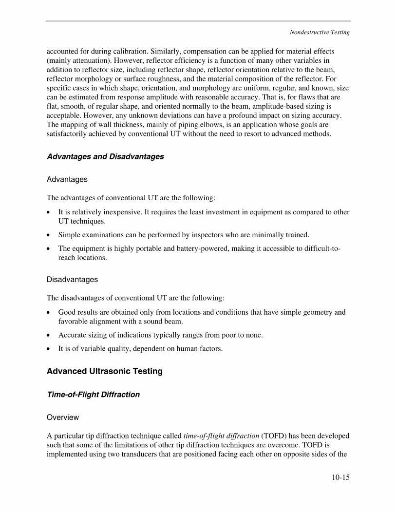
Nondestructive Testing
10-15
accounted for during calibration. Similarly, compensation can be applied for material effects (mainly attenuation). However, reflector efficiency is a function of many other variables in addition to reflector size, including reflector shape, reflector orientation relative to the beam, reflector morphology or surface roughness, and the material composition of the reflector. For specific cases in which shape, orientation, and morphology are uniform, regular, and known, size can be estimated from response amplitude with reasonable accuracy. That is, for flaws that are flat, smooth, of regular shape, and oriented normally to the beam, amplitude-based sizing is acceptable. However, any unknown deviations can have a profound impact on sizing accuracy. The mapping of wall thickness, mainly of piping elbows, is an application whose goals are satisfactorily achieved by conventional UT without the need to resort to advanced methods.
Advantages and Disadvantages
Advantages
The advantages of conventional UT are the following:
• It is relatively inexpensive. It requires the least investment in equipment as compared to other UT techniques.
• Simple examinations can be performed by inspectors who are minimally trained.
• The equipment is highly portable and battery-powered, making it accessible to difficult-to-reach locations.
Disadvantages
The disadvantages of conventional UT are the following:
• Good results are obtained only from locations and conditions that have simple geometry and favorable alignment with a sound beam.
• Accurate sizing of indications typically ranges from poor to none.
• It is of variable quality, dependent on human factors.
Advanced Ultrasonic Testing
Time-of-Flight Diffraction
Overview
A particular tip diffraction technique called time-of-flight diffraction (TOFD) has been developed such that some of the limitations of other tip diffraction techniques are overcome. TOFD is implemented using two transducers that are positioned facing each other on opposite sides of the
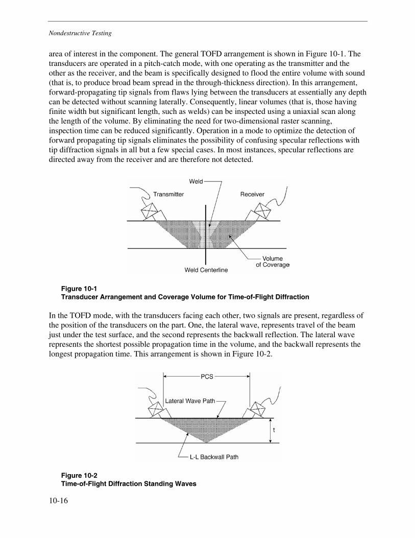
Nondestructive Testing
10-16
area of interest in the component. The general TOFD arrangement is shown in Figure 10-1. The transducers are operated in a pitch-catch mode, with one operating as the transmitter and the other as the receiver, and the beam is specifically designed to flood the entire volume with sound (that is, to produce broad beam spread in the through-thickness direction). In this arrangement, forward-propagating tip signals from flaws lying between the transducers at essentially any depth can be detected without scanning laterally. Consequently, linear volumes (that is, those having finite width but significant length, such as welds) can be inspected using a uniaxial scan along the length of the volume. By eliminating the need for two-dimensional raster scanning, inspection time can be reduced significantly. Operation in a mode to optimize the detection of forward propagating tip signals eliminates the possibility of confusing specular reflections with tip diffraction signals in all but a few special cases. In most instances, specular reflections are directed away from the receiver and are therefore not detected.
Figure 10-1 Transducer Arrangement and Coverage Volume for Time-of-Flight Diffraction
In the TOFD mode, with the transducers facing each other, two signals are present, regardless of the position of the transducers on the part. One, the lateral wave, represents travel of the beam just under the test surface, and the second represents the backwall reflection. The lateral wave represents the shortest possible propagation time in the volume, and the backwall represents the longest propagation time. This arrangement is shown in Figure 10-2.
Figure 10-2 Time-of-Flight Diffraction Standing Waves
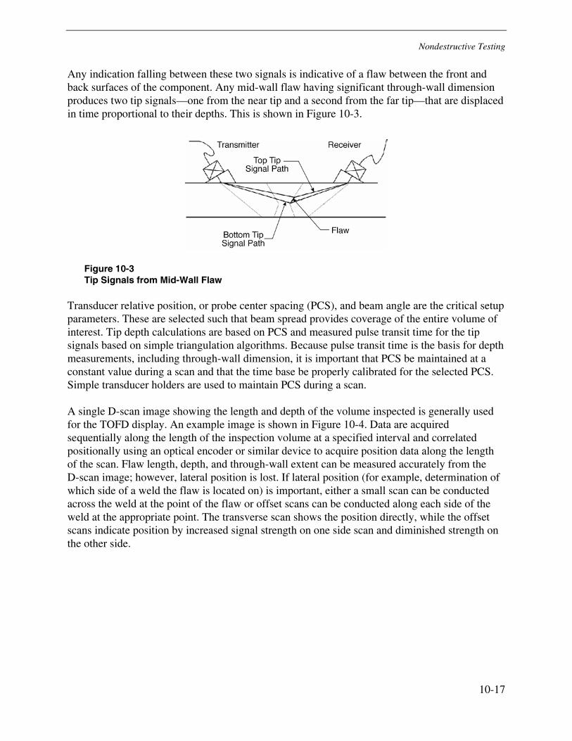
Nondestructive Testing
10-17
Any indication falling between these two signals is indicative of a flaw between the front and back surfaces of the component. Any mid-wall flaw having significant through-wall dimension produces two tip signals—one from the near tip and a second from the far tip—that are displaced in time proportional to their depths. This is shown in Figure 10-3.
Figure 10-3 Tip Signals from Mid-Wall Flaw
Transducer relative position, or probe center spacing (PCS), and beam angle are the critical setup parameters. These are selected such that beam spread provides coverage of the entire volume of interest. Tip depth calculations are based on PCS and measured pulse transit time for the tip signals based on simple triangulation algorithms. Because pulse transit time is the basis for depth measurements, including through-wall dimension, it is important that PCS be maintained at a constant value during a scan and that the time base be properly calibrated for the selected PCS. Simple transducer holders are used to maintain PCS during a scan.
A single D-scan image showing the length and depth of the volume inspected is generally used for the TOFD display. An example image is shown in Figure 10-4. Data are acquired sequentially along the length of the inspection volume at a specified interval and correlated positionally using an optical encoder or similar device to acquire position data along the length of the scan. Flaw length, depth, and through-wall extent can be measured accurately from the D-scan image; however, lateral position is lost. If lateral position (for example, determination of which side of a weld the flaw is located on) is important, either a small scan can be conducted across the weld at the point of the flaw or offset scans can be conducted along each side of the weld at the appropriate point. The transverse scan shows the position directly, while the offset scans indicate position by increased signal strength on one side scan and diminished strength on the other side.
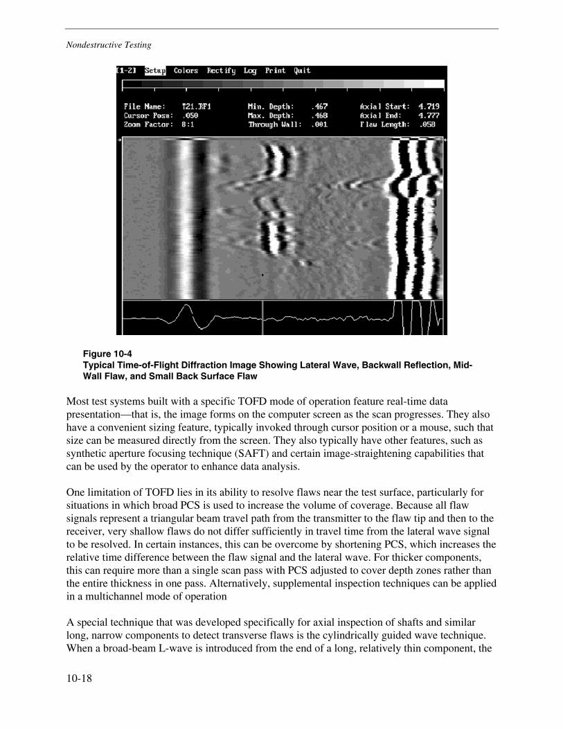
Nondestructive Testing
10-18
Figure 10-4 Typical Time-of-Flight Diffraction Image Showing Lateral Wave, Backwall Reflection, Mid-Wall Flaw, and Small Back Surface Flaw
Most test systems built with a specific TOFD mode of operation feature real-time data presentation—that is, the image forms on the computer screen as the scan progresses. They also have a convenient sizing feature, typically invoked through cursor position or a mouse, such that size can be measured directly from the screen. They also typically have other features, such as synthetic aperture focusing technique (SAFT) and certain image-straightening capabilities that can be used by the operator to enhance data analysis.
One limitation of TOFD lies in its ability to resolve flaws near the test surface, particularly for situations in which broad PCS is used to increase the volume of coverage. Because all flaw signals represent a triangular beam travel path from the transmitter to the flaw tip and then to the receiver, very shallow flaws do not differ sufficiently in travel time from the lateral wave signal to be resolved. In certain instances, this can be overcome by shortening PCS, which increases the relative time difference between the flaw signal and the lateral wave. For thicker components, this can require more than a single scan pass with PCS adjusted to cover depth zones rather than the entire thickness in one pass. Alternatively, supplemental inspection techniques can be applied in a multichannel mode of operation
A special technique that was developed specifically for axial inspection of shafts and similar long, narrow components to detect transverse flaws is the cylindrically guided wave technique. When a broad-beam L-wave is introduced from the end of a long, relatively thin component, the
Nondestructive Testing
10-19
portions of the beam that reach the side walls are mode-converted to shear. They then travel at S-wave velocity, with reflections and additional mode conversions occurring as they travel down the component, arriving at the receiver later in time than the primary L-wave because of the longer travel path and travel at least partially in the slower S-wave mode. The display shows a series of subsidiary signals following the L-wave. Analysis of this portion of the presentation by a trained operator provides information on the presence of side-wall flaws that are not obvious if one is looking only for direct L-wave reflections. This technique has proven useful for the inspection of shafts and other long components, for example for fatigue cracks that initiate at the outer surface in a transverse direction due to cyclic bending, where the outer surfaces are covered with other components or are otherwise inaccessible for inspection by more conventional surface NDE methods.
Application in Piping Systems
TOFD is generally applicable to the inspection of a volume with a relatively simple and uniform geometry. However, it is primarily used for the examination of seam welds and circumferential welds in piping systems.
Advantages/Disadvantages
Advantages
The advantages of TOFD are the following:
• It provides both detection and sizing capabilities in a single scan.
• Data analysis can be performed off-line, which speeds up the acquisition process.
• The scan data are saved as a digital image, which provides for a permanent record and a baseline for future monitoring.
Disadvantages
• It requires highly trained inspection and analysis personnel.
• The equipment is costly.
• It is not applicable to highly attenuative materials (for example, austenitic and cast microstructures) or thick sections.
• It is not easily adapted to sections with complex geometry.
• The image does not provide the lateral position of indications, only their depth and the location along the scan line.
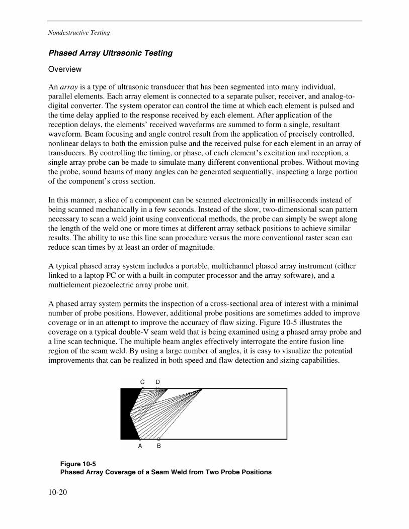
Nondestructive Testing
10-20
Phased Array Ultrasonic Testing
Overview
An array is a type of ultrasonic transducer that has been segmented into many individual, parallel elements. Each array element is connected to a separate pulser, receiver, and analog-to-digital converter. The system operator can control the time at which each element is pulsed and the time delay applied to the response received by each element. After application of the reception delays, the elements’ received waveforms are summed to form a single, resultant waveform. Beam focusing and angle control result from the application of precisely controlled, nonlinear delays to both the emission pulse and the received pulse for each element in an array of transducers. By controlling the timing, or phase, of each element’s excitation and reception, a single array probe can be made to simulate many different conventional probes. Without moving the probe, sound beams of many angles can be generated sequentially, inspecting a large portion of the component’s cross section.
In this manner, a slice of a component can be scanned electronically in milliseconds instead of being scanned mechanically in a few seconds. Instead of the slow, two-dimensional scan pattern necessary to scan a weld joint using conventional methods, the probe can simply be swept along the length of the weld one or more times at different array setback positions to achieve similar results. The ability to use this line scan procedure versus the more conventional raster scan can reduce scan times by at least an order of magnitude.
A typical phased array system includes a portable, multichannel phased array instrument (either linked to a laptop PC or with a built-in computer processor and the array software), and a multielement piezoelectric array probe unit.
A phased array system permits the inspection of a cross-sectional area of interest with a minimal number of probe positions. However, additional probe positions are sometimes added to improve coverage or in an attempt to improve the accuracy of flaw sizing. Figure 10-5 illustrates the coverage on a typical double-V seam weld that is being examined using a phased array probe and a line scan technique. The multiple beam angles effectively interrogate the entire fusion line region of the seam weld. By using a large number of angles, it is easy to visualize the potential improvements that can be realized in both speed and flaw detection and sizing capabilities.
Figure 10-5 Phased Array Coverage of a Seam Weld from Two Probe Positions
Nondestructive Testing
10-21
In addition to improved coverage, the automated phased array technique offers a much simpler means of analyzing the resultant data. Even with automated UT techniques, the analysis of conventional ultrasonic data generally takes longer than the acquisition of the data, especially if many flaws are detected. Using phased array technology, the data analysis process tends to be simpler, faster, and more reliable than conventional data analysis. By reviewing the B-scan images of the different beam angles, a flaw can be very clearly identified.
Application in Piping Systems
Phased array technology is most beneficial in locations that have limited probe scanning space and complex geometries. Typical examples are inspection of header ligaments and pipe welds (mostly circumferential welds) where geometrical limitations to TOFD favor the use of phased arrays.
Advantages and Disadvantages
The advantages of phased array UT are the following:
Advantages
• By virtue of dynamic focusing and beam sweeping, volume coverage at complex geometries can be achieved with minimal or no probe movement.
• Both detection and sizing information can be gleaned from a single image.
• Data analysis is simpler than for other UT techniques and can be performed off-line, which speeds up the acquisition process.
• The test data can be saved as a digital image, which provides a permanent record and a baseline for future monitoring.
Disadvantages
The disadvantages of phased array UT are the following:
• It requires highly trained inspection and analysis personnel.
• The equipment is costly.

Nondestructive Testing
10-22
Acoustic Emission Crack Detection
Overview
Acoustic emission crack detection (AECD) is based on the theory that a growing crack will emit energy in the form of sound waves, which can be detected by piezoelectric sensors attached to the component. In order to propagate the crack, the component must be stressed when the sensors are attached, and one of the most common methods of stressing components is by a hydro test. An array of sensors is usually used, so that the signals from a growing crack can be collected by sophisticated computers and the location of the crack can be identified by triangulation.
Application in Piping Systems
Currently, AECD is used primarily to monitor seam-welded HRH lines.
Advantages and Disadvantages
Advantages
The advantages of AECD include the following:
• A large volume of material can be tested very rapidly.
• The data can be stored digitally for future recall.
• Sensors can be used in conjunction with waveguides that transmit the sound waves (usually through a stainless steel rod) to the sensor. For insulated structures, only enough insulation must be removed to enable installation of the waveguides. It is this advantage of AECD that makes it attractive to utilities with long runs of insulated high-energy piping. Insulation removal and reinstallation represents a major portion of the cost of inspecting a high-energy line using conventional techniques such as MT, PT, and UT.
Disadvantages
The disadvantages of AECD include the following:
• It is sometimes difficult to separate the signal noise from background, even with the use of the most advanced (and expensive) instrumentation.
• Source location can be very difficult in complex geometries.
• If transient conditions are required to activate the source, a very narrow window of opportunity might exist to detect the flaw(s).

Nondestructive Testing
10-23
Pulsed Eddy Current Testing
Overview
Pulsed eddy current testing (pulsed ET) technology is showing promise for measuring pipe wall thicknesses without the requirement to remove the thermal insulation first. This provides the opportunity to perform inspections while the plant is on load when it might be more convenient logistically, and it also reduces or eliminates the costs of insulation removal and reinstatement.
Conventional ET generally uses a single high-frequency excitation to inspect the near surface of a component. Pulsed ET, on the other hand, uses a burst of low-frequency excitation. The progress of the generated currents and their reciprocal effect on the probe coil are measured as a function of time. In this way, changes in the decay of the interaction can be converted into measurements of the thickness of the component.
Application in Piping Systems
The primary use for pulsed ET is to measure wall thickness reductions caused by FAC. In this case, the metal loss is on the inner surface of the pipe, but the technique works equally well when the wastage is on the OD. Therefore, it can also be used to find corrosion underneath insulation.
Advantages and Disadvantages
Advantages
The advantage of pulsed ET is the following:
• It eliminates the high cost of insulation removal and restoration by making the wall thickness measurement through the insulation and the thin aluminum cladding.
Disadvantages
The disadvantages of pulsed ET are the following:
• It is not as accurate as UT wall thickness measurement techniques.
• Its spatial resolution is much coarser than UT; thickness values represent an average of a relatively large area.
• The equipment is expensive and highly dedicated; it cannot be applied to perform other ET work.
Nondestructive Testing
10-24
Radiographic Testing
Overview
Radiography, or radiographic testing (RT), has been a primary weld inspection technique for many years. This technique passes gamma radiation through the component and records the exiting backside radiation by either photographic or electronic means. The gamma radiation can be produced either by a radioactive source or by an X-ray machine.
Radioactive sources commonly use the radioisotope iridium-192 for activity up to 370 E10 bq (100 Ci), and cobalt-60 for higher activity levels. X-ray machines produce gamma radiation by bombarding a metallic target with fast electrons in a vacuum. Whether an X-ray machine or a radioactive source is appropriate for a particular inspection depends on a number of factors, including the following:
• X-ray machines produce a directional radiation field that is concentrated in a smaller area. This tends to reduce the peripheral shielding and safety requirements associated with the test, as well as limiting the size of the area that is inspected.
• X-ray machines of sufficient power to inspect large, thick-walled components are usually stationary. This means that the component must be brought to the X-ray machine. Normally, material handling equipment associated with the X-ray machine is used to rotate or otherwise move the component to allow a complete inspection. A common example is a circumferential weld in a pressure vessel. To inspect this weld using an X-ray machine, the vessel can be rotated. The stationary X-ray machine makes successive readings through the rotating weld until the entire weld has been inspected.
• Radioactive sources produce an omnidirectional radiation field, which must be limited by careful design of the source container or the use of auxiliary shielding, or both. Generally, safety requirements such as area evacuation during the test can be more restrictive for the use of radioactive sources than for X-ray machines.
• The radioactive source can be transported to the component, so it is usually superior to X-ray machines for field inspections.
• The omnidirectional radiation field provided by a radioactive source can be used to inspect large areas quickly. A common example is inspecting a circumferential weld in a pressure vessel. The source can be placed at the center of the vessel, and the outside of the circumferential weld can be wrapped with X-ray film. If the radioactive source is then triggered, the entire weld is inspected at the same time. Unlike the X-ray machine, no component rotation is required.
Application in Piping Systems
Generally, radiography is used to inspect welds. The most common use in power plants is for inspecting repair welds in boiler tubes. It is ideal for detecting macroscopic defects that are common to welds, such as porosity or slag inclusion.
Nondestructive Testing
10-25
Advantages and Disadvantages
Advantages
The advantages of RT include the following:
• It is a nondestructive method.
• A permanent film record of each inspection is available for archiving and later review.
• In the United States, radiography is the most commonly recognized method for inspecting numerous types of welds.
Disadvantages
The disadvantages of RT include the following:
• There are significant safety requirements. The test procedure must protect personnel from radiation exposure, and radioactive sources must be handled properly by qualified personnel.
• It is nonquantitative; defects cannot be located (depth) or sized precisely.
• Results for components with complicated, nonuniform section thickness can be difficult to interpret.
Guided Wave Ultrasonic Testing
Overview
In guided wave UT, the ultrasonic wave propagates in the axial (longitudinal) direction in the test specimen. The test probe is typically a flexible strip or belt equipped with multiple transducers along its length. This belt is wrapped around the outer surface of the pipe using an inflatable bladder, which forces the transducers to form a tight contact with the OD surface of the pipe. The guided wave transmitted from the sensors propagates in the axial direction of the pipe, and when it encounters an anomaly (for example, wall loss, a bracket, or a t-branch) a transmitted wave is reflected back to the sensor. The distance from the sensor to the location of the anomaly is measured by recording the round-trip travel time of the guided wave.
The nature and magnitude of the anomaly can be deducted from an analysis of the detected waveform of the returning echo. Interpretation of the data is also aided by drawings of the pipeline that show the location of welds, branches, valves, and any other feature that deviates from the smooth pipe configuration. The reach of the guided wave can extend to several hundred feet from the location of the sensor belt. Actual effective length of coverage depends on the contact that the pipe is making with other media on the ID and OD sides (for example, whether the pipe is insulated or not, whether it is full of water or empty, or whether it is in contact with wet, compacted soil or just loose gravel).
Nondestructive Testing
10-26
Application in Piping Systems
Guided wave UT applies most commonly to the inspection of buried or otherwise inaccessible pipelines; therefore, it is used to inspect service water lines. Because of its versatility, guided wave UT can also be applied to monitoring loss of wall of insulated lines with only minimal removal of insulation.
Advantages and Disadvantages
Advantages
The advantages of guided wave UT include the following:
• It allows the inspection of buried or otherwise inaccessible pipes from a small, exposed location.
• It allows the inspection of insulated lines without complete the removal of the insulation.
• The data acquisition step is very rapid and minimally invasive.
Disadvantages
The disadvantages of guided wave UT include the following:
• It is not as accurate as conventional UT wall thickness measurement techniques.
• Its spatial resolution is much coarser than conventional UT; measured thickness values represent an average of full circumference at the location of the anomaly.
• It requires highly trained inspection and analysis personnel.
11-1
11 METALLURGICAL EXAMINATION AND ANALYSIS AND MATERIAL CHARACTERIZATION
Introduction
Postexposure characterization of fossil plant materials is commonly conducted in two instances: 1) after a failure has occurred, material analysis is typically performed during a root-cause investigation, and 2) if a proactive Level III investigation and prediction of remaining life is being conducted, quantitative knowledge of the current material condition is required, which often necessitates destructive sampling, laboratory analysis, and property determinations.
Destructive sampling of exposed material can be used as part of a comprehensive assessment program to determine the current actual accumulation of material degradation. Often laboratory analysis of piping material can provide more accurate degradation assessment and engineering design detail on the existing condition of the component than can be obtained through NDE techniques alone. However, there are several drawbacks to material sampling, including the following:
• Material sampling is expensive and time consuming, and it typically requires some form of repair or remediation
• Repair or remediation activities can often lead to a more damage-susceptible section of piping.
• The most susceptible materials can be difficult to reach, which can make sampling difficult, expensive, and sometimes dangerous.
• Statistically meaningful material sampling can be difficult to achieve, and material that shows limited damage can be collected for analysis within 2 ft (61 cm) of an area with extensive degradation, which can result in false life estimation.
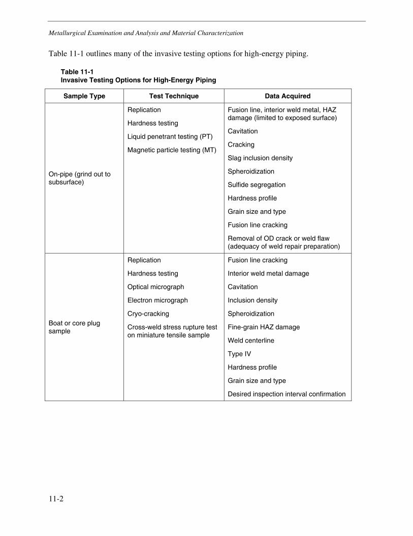
Metallurgical Examination and Analysis and Material Characterization
11-2
Table 11-1 outlines many of the invasive testing options for high-energy piping.
Table 11-1 Invasive Testing Options for High-Energy Piping
Sample Type Test Technique Data Acquired
On-pipe (grind out to subsurface)
Replication
Hardness testing
Liquid penetrant testing (PT)
Magnetic particle testing (MT)
Fusion line, interior weld metal, HAZ damage (limited to exposed surface)
Cavitation
Cracking
Slag inclusion density
Spheroidization
Sulfide segregation
Hardness profile
Grain size and type
Fusion line cracking
Removal of OD crack or weld flaw (adequacy of weld repair preparation)
Boat or core plug sample
Replication
Hardness testing
Optical micrograph
Electron micrograph
Cryo-cracking
Cross-weld stress rupture test on miniature tensile sample
Fusion line cracking
Interior weld metal damage
Cavitation
Inclusion density
Spheroidization
Fine-grain HAZ damage
Weld centerline
Type IV
Hardness profile
Grain size and type
Desired inspection interval confirmation
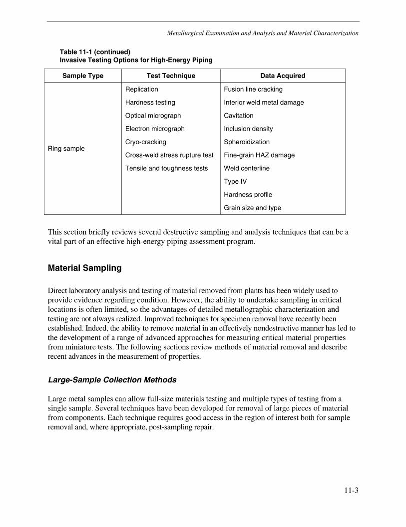
Metallurgical Examination and Analysis and Material Characterization
11-3
Table 11-1 (continued) Invasive Testing Options for High-Energy Piping
Sample Type Test Technique Data Acquired
Ring sample
Replication
Hardness testing
Optical micrograph
Electron micrograph
Cryo-cracking
Cross-weld stress rupture test
Tensile and toughness tests
Fusion line cracking
Interior weld metal damage
Cavitation
Inclusion density
Spheroidization
Fine-grain HAZ damage
Weld centerline
Type IV
Hardness profile
Grain size and type
This section briefly reviews several destructive sampling and analysis techniques that can be a vital part of an effective high-energy piping assessment program.
Material Sampling
Direct laboratory analysis and testing of material removed from plants has been widely used to provide evidence regarding condition. However, the ability to undertake sampling in critical locations is often limited, so the advantages of detailed metallographic characterization and testing are not always realized. Improved techniques for specimen removal have recently been established. Indeed, the ability to remove material in an effectively nondestructive manner has led to the development of a range of advanced approaches for measuring critical material properties from miniature tests. The following sections review methods of material removal and describe recent advances in the measurement of properties.
Large-Sample Collection Methods
Large metal samples can allow full-size materials testing and multiple types of testing from a single sample. Several techniques have been developed for removal of large pieces of material from components. Each technique requires good access in the region of interest both for sample removal and, where appropriate, post-sampling repair.
Metallurgical Examination and Analysis and Material Characterization
11-4
Boat Sampling
Boat samples are removed from the surface of components by the cutting action of a slightly concave, circular saw blade. Two adjacent cuts are made into the surface and the sample released resembles that of a boat hull. Significant amounts of material can be removed in this way with sample lengths typically in the range of 1–4 in. (25–100 mm). However, it is usually necessary to weld repair the sampled location.
Uncertainties regarding the effects of local weld repair on future component performance usually limit the use of boat sampling to regions where extensive damage has been detected and major repairs are known to be required. In this case, the boat samples are used to characterize the damage present. In situations where samples of this type have been removed to evaluate the condition of undamaged components, experience shows that the repair of the sampled region can itself develop cracks if the repair process is not carefully controlled.
Plug Sampling
Cylindrical plug samples have been removed from header and piping components. With this approach, a hole saw is passed through the component wall to remove a through-thickness section of material. Where no component feature is present to establish the orientation of the plug, the component should be marked before sampling to allow sectioning and laboratory investigations to be performed with reference to selected component directions. Samples of approximately 1–3 in. (25–75 mm) in diameter have been removed. Repair procedures usually involve capping the hole with a blank, oversized stub or socket-welding a purpose-made section of material into the hole. This approach has been successfully used to provide metallographic information and specimens for postexposure testing. The method is limited to locations where good access is available for both sample removal and repair.
Small-Sample Collection Methods
Often, large sample removal either is not practical because it will require significant material repair or there is limited access, or is not possible because there is insufficient material available for large sample removal. In recent years, small-sample analysis techniques that can be correlated to standard test results have increased the viability of small sample removal. Several small-sample collection methods are described in the following paragraphs.
Small Cone Sampling
Small cone samples of approximately 0.2 in. (5 mm) base diameter and 0.2 in. (5 mm) height have been removed using a device based on the air abrasive technique used for hole cutting during residual strain measurement. A cutting head was developed that holds the nozzle of the abrasive jet at the correct angle and distance from the selected location and permits orbital movement such that a cone-shaped sample can be removed. The cutting head and its driving motor are secured to the component by mechanical clamps, and sample removal is achieved by bombarding the surface with a stream of abrasive particles. The samples can be used to examine the material microstructure using optical or electron microscopy.
Metallurgical Examination and Analysis and Material Characterization
11-5
Laboratory trials were performed to optimize the operating parameters of air pressure, powder type and flow, nozzle orbital rate, and nozzle distance to the component. Although these trials were successful in overcoming a number of difficulties, problems of nozzle erosion were reported. In addition, having successfully removed the conical specimen, the sampled region must be blended to minimize stress concentrations.
Sample Removal by Drilling
A method for removing shallow, prismatic samples of material from headers using a chain drilling rig has been developed. With this method, the rig is attached to the component using straps and then a series of drilling operations are carried out. When the drilling operations are complete, a section of material approximately 0.8 in. (20 mm) in length and 0.4 in. (10 mm) in depth is removed. This material could be subjected to a range of metallographic studies, but the particular application reported was to machine a blank cylinder approximately 0.1 in. (3 mm) in diameter by 0.6 in. (15mm) in length. This cylinder was then used to manufacture a miniature test sample for postexposure creep testing. The method was developed primarily to extract material from thick-section components where excavations of approximately 0.5 in. (12 mm) could be blended without the need for repair. By modifying the drilling jig, it is possible to remove larger samples. However, in this case, repair of the component would usually be required.
Surface Sampling System
The surface sampling (SSAM) system was developed to remove material from the surface of plant components without introducing thermal or mechanical damage to the sample removed or the component [11-1]. Thus, no post-sampling treatment is required before further operation.
A sample, approximately disc shaped, is removed by the action of a hemispherical shell cutter. The cutter is a hardened steel, hemispherical shell that is 2 in. (5.1 cm) in diameter and 0. 01 in. (0.25 mm) thick. The cutting surface consists of cubic boron nitride grit applied to the edge of the shell. This shell is spun about its axis of symmetry at over 4000 RPM and rotated about an orthogonal axis through the material being sampled.
The sample thickness depends on the depth to which the spherical cutter is set before beginning the cut, and the width depends on the depth of the cut, the cutter radius, and the contour of the sampled surface. Typical depths are from 0.03 to 0.1in. (0.76 to 2.5 mm), with widths varying up to 1 in. (2.5 cm).
The machine that drives the cutter is designed for operation in confined spaces as small as 3 in. (76 mm) in diameter. Thus, the equipment can be used inside relatively narrow tubes and pipes or inside the bores of turbine rotors. The device is positioned by the use of a rod coupled to the rear trunnion. In general, the sampling location is identified by visual examination or surface NDE. After the device has been located, a clamping shoe is actuated by an air cylinder that engages the upper surface. Cutter drive-motor current and cutter feed position information are provided to the operator. The feed rate is controllable to accommodate the very shallow entry angle that the cutter makes with the part and to maintain a constant cutting torque throughout the cut.
Metallurgical Examination and Analysis and Material Characterization
11-6
The cutter is mounted on a spindle and trunnion that is rotated to feed the cutter into the work. This feed motion is controlled by a stepper motor, gear train, and lead screw mechanism to maintain a desired load on the cutter. The cutter is driven through a flexible shaft to accommodate the feed rotation.
Coolant is delivered to the inner diameter of the shell, where it flows outward along the cutter shell as a result of centrifugal force, clearing the cutter swarf and cooling the process. Coolant is recovered through a suction tube and is recycled. When the cut is complete, a magnet attached to the underside of the cutter trunnion captures the sample. Deactivation of the clamp allows the device to rise up on its suspension, so that the cutter is clear of the interior surface. The device, with the sample, is then removed.
Remediation
Following any sampling program, remediation of the damage caused by sampling is often necessary to maintain structural integrity in the component. Remediation of sampling damage can include repair welding buildup with filler material, repair welding overlays with weld metal, repair welding with pad overlay, welding of material plugs into extraction holes, pipe cutout and replacement, and so on. In all cases, it is important that proper welding procedures with post- and preweld heat treatments be performed to minimize the variation in materials properties from the base metal to the weldment. Weldments are always more sensitive to a variety of degradation mechanisms, and the repair weld can become a preferential location for future damage. Post-repair inspection is important, and special attention should be paid to remediated areas. It is also important to understand the nature of the damage that is being removed and repaired. Cracks will often continue to propagate into a newly welded region; therefore, material removal does not always guarantee defect elimination.
Hardness Testing
Overview
Hardness is defined as the resistance of a metal to indentation, scratching, cutting, and so forth. When hardness is measured by pressing a very hard ball or diamond point into the metal under restrained conditions, the depth of penetration can be correlated with the material’s tensile strength. This process is conducted with hardness testing machines or indenting equipment on scales including Rockwell, Brinell, Knoop or Vickers, which differ in the type, size, and geometry of indenter as well as the level of indentation force. There are other types of hardness measurements; for example, Equotip testers use a spring-loaded impact body that is propelled against a test piece. The ratio of impact to rebound velocity is compared to a Leeb scale to determine material hardness.
Portable indention or impact hardness testers come in many varieties and are useful as NDE tools because they can indicate hard or soft spots in components, which can be indicative of component damage. Because the microstructural changes that are created during high-temperature exposure affect tensile strength, theoretically they should also impact hardness.
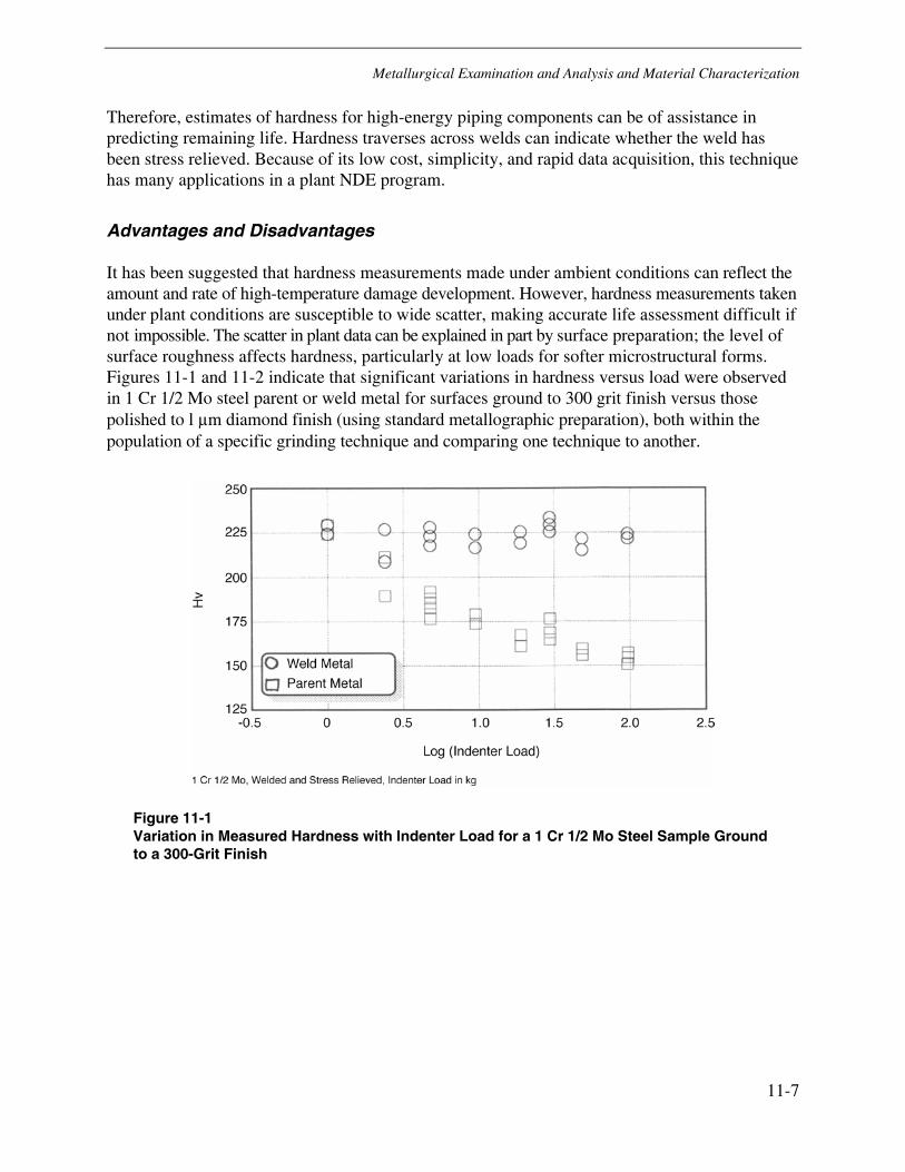
Metallurgical Examination and Analysis and Material Characterization
11-7
Therefore, estimates of hardness for high-energy piping components can be of assistance in predicting remaining life. Hardness traverses across welds can indicate whether the weld has been stress relieved. Because of its low cost, simplicity, and rapid data acquisition, this technique has many applications in a plant NDE program.
Advantages and Disadvantages
It has been suggested that hardness measurements made under ambient conditions can reflect the amount and rate of high-temperature damage development. However, hardness measurements taken under plant conditions are susceptible to wide scatter, making accurate life assessment difficult if not impossible. The scatter in plant data can be explained in part by surface preparation; the level of surface roughness affects hardness, particularly at low loads for softer microstructural forms. Figures 11-1 and 11-2 indicate that significant variations in hardness versus load were observed in 1 Cr 1/2 Mo steel parent or weld metal for surfaces ground to 300 grit finish versus those polished to l µm diamond finish (using standard metallographic preparation), both within the population of a specific grinding technique and comparing one technique to another.
Figure 11-1 Variation in Measured Hardness with Indenter Load for a 1 Cr 1/2 Mo Steel Sample Ground to a 300-Grit Finish
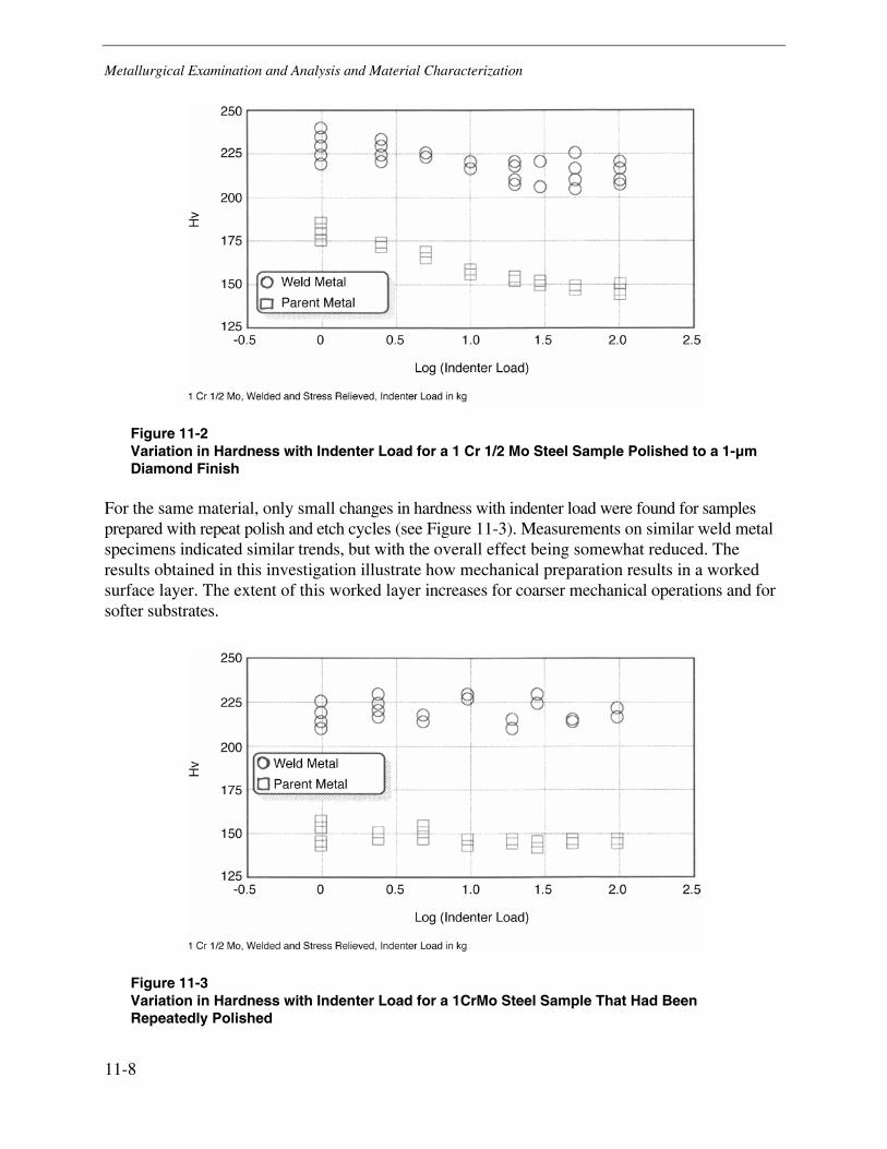
Metallurgical Examination and Analysis and Material Characterization
11-8
Figure 11-2 Variation in Hardness with Indenter Load for a 1 Cr 1/2 Mo Steel Sample Polished to a 1-μm Diamond Finish
For the same material, only small changes in hardness with indenter load were found for samples prepared with repeat polish and etch cycles (see Figure 11-3). Measurements on similar weld metal specimens indicated similar trends, but with the overall effect being somewhat reduced. The results obtained in this investigation illustrate how mechanical preparation results in a worked surface layer. The extent of this worked layer increases for coarser mechanical operations and for softer substrates.
Figure 11-3 Variation in Hardness with Indenter Load for a 1CrMo Steel Sample That Had Been Repeatedly Polished
Metallurgical Examination and Analysis and Material Characterization
11-9
It has been suggested that the following factors that will influence hardness values for a given material:
• Surface preparation
• Number of measurements
• Workmanship
• Wall thickness
• Degree of surface flatness
• Measuring orientation
• Type of tester
• Indenter load
• Oxidation or decarburization of the surface
Application in Piping Systems
A number of evaluations have examined the changes in hardness that occur with aging at elevated temperature. In several cases, the decrease in hardness with increased tempering is sensible. Therefore, hardness can be described using a time and temperature factor in a similar manner to the LMP, using equations of the form shown in Equations 11-1 and 11-2.
HV = A - B * P Eq. 11-1
where A and B are material constants and P is calculated from
P = T (20 +log f) Eq. 11-2
Thus, if proper care is taken in preparing the surface and making the measurements, it is apparent that hardness data can be used to differentiate between hot and cold regions of a component. Moreover, where repeat measurements have been taken at different times at a given location, the data should allow a reasonable estimate of the equivalent operating temperature.
To use hardness measurements to estimate remaining life, one must ignore the well-known fact that hardness is affected by factors other than precipitate size and distribution (for example, grain size) and make simplifying assumptions regarding the relationship of hardness with interparticle spacing. Where large databases have been developed for widely used alloys, analysis indicates that trends in behavior can be identified. Thus, for 2-1/4 Cr 1 Mo steel, it appears that it is possible to apply a lower bound criterion to provide a realistic minimum remaining life indicator. Although this approach can be used as a guide to remaining life in some situations, it should not be applied when accurate estimates of condition are required.
Metallurgical Examination and Analysis and Material Characterization
11-10
Alloy Identification
Identifying component alloy chemistry is critical to predicting material degradation and predicting life. With time, documentation of materials of construction can be lost, necessitating alloy identification. In addition, accidental substitution of materials occurs and can have catastrophic results in critical applications should a lower grade of material be mistakenly substituted for the properly specified material. Field identification or verification of the materials of construction for fossil power plant components consists of various techniques, some of which can be performed in situ.
The three primary methods are manufacturer’s identification, qualitative field identification, and quantitative field identification. The manufacturer method relies on the use of documentation and physical markings on components to identify or verify the materials of construction. Qualitative field techniques include analysis of materials through tests other than chemical analysis. Quantitative identification is performed through the use of chemical analysis (in situ or otherwise). Most field methods are nondestructive, so that the removal of a material sample is unnecessary; however; a minimal amount of surface preparation is required.
Manufacturer’s Identification
Manufacturer’s identification relies on the use of documentation and physical markings on the actual components. In general, manufacturers provide material certifications with critical components. These certifications include certificates of heat analysis (or mill certs), which provide a chemical analysis of an ingot or billet that was used as the starting point in the fabrication of a component, and certificates of product analysis, which provide a chemical analysis of the actual component after fabrication. Materials specifications contained in materials lists, design drawings, owners manuals, and so forth should not be used interchangeably with certificates of analysis. Furthermore, the use of manufacturer’s identification necessitates an absolute correlation of the analysis certificate with the actual component. This correlation is typically carried out through the use of physical markings.
Physical identification of materials includes the use of symbols or markings that provide a code to the material identification of a component. These symbols or markings include foundry marks embossed on the exterior of castings, color coding or stenciling of new materials, and stampings or embossing on forged components. Foundry markings on castings can provide information on the ASTM grade, foundry name or logo, heat number, and alloy type. Additional information such as design pressure and temperature rating can also be included. Similar information on ASTM grade, forge shop name, heat number, and design pressure and temperature rating can be found in the stampings on forged components. When foundry or forging markings are not identifiable or are questionable, in situ alloy identification using qualitative or quantitative methods can be used.
Metallurgical Examination and Analysis and Material Characterization
11-11
Qualitative Alloy Identification
Qualitative techniques include analysis of materials through tests other than chemical analysis. These methods use the physical properties of the material—including metal color, magnetic behavior, density measurements, spark testing, chemical spot testing, thermoelectric testing, metallographic examinations, and optical emission spectroscopy—in the identification process,. The use of metal color is a method to sort different alloy groups that exhibit unique color differences (such as dark yellow bronzes from reddish coppers or silvery white aluminums) but not to sort alloys within a group. Magnetic behavior can be used as a simple test to separate magnetic materials from nonmagnetic materials. Even more sophisticated alloy identification techniques based on ET are available.
Quantitative Alloy Identification
Quantitative field techniques sort and identify material by actual chemical analysis of the component at one or more locations. Although in situ chemical analysis techniques do not typically analyze for all elements present in a material, they are typically comprehensive enough to identify unknown materials and provide certain compositional data with a high degree of accuracy. These techniques are based on X-ray fluorescence spectroscopy (XRF). In XRF, an X-ray beam impinging on the surface of an unknown material causes the surface atoms of specific chemical elements in the material to emit fluorescent X-rays. These fluorescent X-rays have unique energy levels and wavelengths that are characteristic of the specific chemical elements in the unknown material. These characteristic X-rays are passed through detectors to measure either the energy level or the wavelengths. Typically, the measurements are analyzed by a microprocessor that compares the percentages of the chemical elements present in the unknown material to programmed compositions of specific alloys. The instrument then identifies the alloy, if the measured composition matches a programmed alloy, and displays the percentages of the measured elements.
Many instruments used for this method of alloy identification are very portable for field applications and provide quantitative analysis results in an efficient and timely manner. In addition, a range of instruments exist. The selection of which instrument to use depends on time constraints, number of elements to be analyzed, and precision required from the measurements. In general, the accuracy of measurements depends on the specific instrument and the surface conditions at the test location. Typically, some degree of surface preparation is required for the effective use of these instruments. Specifically, a test location must be selected that is representative of the bulk of the component because the fluorescent X-rays are obtained from only a comparatively thin layer of the material. Also, the test area should be sufficiently large for the particular instrument. Surface curvature and irregularities should be minimized, and all extraneous surface materials (scale, oxide, deposits, coatings, paints, oils, or greases) must be removed. In addition, the surface finish must be controlled through the use of grinding unless the test location is a finished or machined surface.
Metallurgical Examination and Analysis and Material Characterization
11-12
Material Testing
Several forms of destructive materials testing techniques can reveal not only the mechanical properties of a material but also the fundamentally microstructural constituency that is producing those properties. The following subsections describe various forms of mechanical testing and metallographic examination.
Mechanical Testing
Structural alloys are selected by and used for their combination of strength, ductility, and crack resistance. Therefore, there must be ways of measuring and categorizing material behavior in a laboratory that will indicate mechanical performance in service. Many standard laboratory mechanical tests can determine the mechanical properties of a material, including tensile testing, toughness testing, creep testing, fatigue testing, and fracture mechanics testing. The most relevant of these are described in the following paragraphs.
• Tensile Testing. Basic strength properties—including yield strength, ultimate tensile strength, elongation, and reduction in cross-sectional area—are determined with a tensile test. Tensile tests can be performed with a variety of round or flat specimen geometries. During the test, a uniaxial tensile load is applied continuously until the test specimen fails; the applied load and change in gauge length are measured. Engineering stress and strain are calculated by dividing the applied load by the original cross-sectional area and the specimen extension by the original gauge length.
• Toughness Testing. Toughness is the ability of a material to absorb energy in the form of plastic deformation without fracturing. The toughness of steels is directly related to the rate at which energy is imparted to the material and the temperature at which the testing is conducted. Most steels go through a ductile-to-brittle transition at low temperatures (near 32°F [0°C] depending on several factors), in which the steel loses the ability to absorb impact-type energy and becomes brittle. Toughness can be evaluated by either measuring the ductile-to-brittle transition temperature through a Charpy V-notch or other impact testing method or by using fracture toughness tests such as crack opening displacement testing. An extensive description of toughness testing for high-temperature components can be found in Damage Mechanisms and Life Assessment of High Temperature Components [11-2]. A small punch test can be used to determine the fracture appearance transition temperature (FATT) of service-exposed material [11-3]. The method relies on empirical correlations developed between the transition temperature (the temperature range over which the ductile-brittle-transition occurs) measured on small punch tests to the Charpy FATT values acquired on standard sized Charpy specimens.
• Creep Testing. Creep testing measures the high-temperature response of a material to tensile loading. Creep properties can be measured by creep, creep relaxation, and creep rupture tests. The measured creep rate response can be used directly in life estimations or indirectly in time-dependent stress analyses or creep crack growth analyses. Creep tests measure deformation of a metal as a function of a constant load (typically a uniaxial dead weight) and temperature. Creep relaxation tests, of less interest for power plant steels, are similar except that the load is continually decreased during testing instead of remaining constant. In both
Metallurgical Examination and Analysis and Material Characterization
11-13
cases, strain is measured during the testing. Stress-rupture and time-to-failure tests are similar to creep and creep rupture tests, except that no strains are measured. Accelerated creep-rupture testing has become a common method for determination of the remaining life of components subject to creep damage; it is described in detail in the “Accelerated Creep-Rupture Testing” subsection of this section.
For the most part, testing can be conducted in a laboratory with postexposure material if sufficient material is available to make standard specimen sizes. In all cases, mechanical properties are directly related to microstructural morphology. Because steel morphology changes with exposure to time at temperature, mechanical properties change, as well. If the original mechanical properties (in the as-delivered condition) are known, then comparison to postexposure properties can indicate the amount of microstructural damage and remaining life can be estimated. Weldments are often the primary locations of interest because their inherent morphological variation and resultant property inhomogeneity make them susceptible to many degradation mechanisms. Considering the material volume requirements for standard testing, the difficulties in obtaining statistically meaningful representative samples, and the focus on welds, it can be difficult to obtain a sufficient amount of postexposure material for accurate laboratory testing. With relatively large samples, laboratory evaluation can be performed using normal practices. Intermediate-sized samples are amenable to metallographic evaluation, but postexposure testing normally requires the fabrication of sub-sized specimens.
Metallographic Examination
Metallography first gained prominence in the 1800s, when the first modern metallurgists discovered that if a metal surface was properly prepared and attacked with acid, the fundamental “cell” structure (actually the crystal structure) could be revealed. Metallographic sample preparation became an art form; it includes the following three basic steps:
1. Grinding. The first step in metallographic preparation is to grind a metal surface to a fine finish by using abrasives of decreasing coarseness. Typically, sand paper of increasing grit size (decreasing coarseness) is used to grind grooves of finer and finer indentation on the surface of the metal at different angles for each grit size. The surface is ground until the grooves from the previous grit size are no longer evident. Depending on the hardness of the metal being examined, metallographers will start with 200 grit paper and reduce to a final paper size of approximately 800 grit.
2. Polishing. The second step is to take the finely ground surface and polish it to a mirror finish by using abrasive solutions of decreasing particle size. Typically slurries of diamond or alumina particles of a common particle size distribution (mesh size) are produced in colloidal suspensions. The fluids are dispersed on a mechanically rotating polishing wheel that has been covered with some form of paper or cloth, which collects and holds the polishing medium while preventing contamination of other sized hard particles that could scratch the surface. Again, depending on the hardness of the material being polished, a cascading order of decreasing particle size starting around 9 μm and finishing around 0.05 μm is used to continually decrease the size of the abrasive polishing marks until a mirror finish is achieved.

Metallurgical Examination and Analysis and Material Characterization
11-14
Ultimately, the goal of the grinding and polishing process is to create a perfectly flat surface that reflects light.
3. Etching. The final step is to attack the perfectly flat surface with an acid and create controlled surface relief. Each of the various phases and microstructural constituents within a polycrystalline structure has a different level of internal energy. Grain boundaries (borders between crystals) and other discontinuities within the crystalline matrix have higher energy levels than the surrounding perfect crystal. When an acid is applied, the first locations to become anodes and corrode are the high-energy locations. As specific locations on the perfectly flat, polished surface corrode preferentially, the surface begins to have areas of surface relief that scatter and reflect light. When the etched surface is examined under a light microscope, the preferentially etched areas show as darker than the surrounding untouched matrix, which still reflects all of the light back like a mirror. In this way, the various microstructural features can be seen on a pseudo-two-dimensional plane.
The type, size, and distribution (known as morphology) of microstructural constituents determine the macroscopic mechanical properties of any structural alloy. Because all microstructural constituents have varying thermodynamic stability, which depends on exposure time to a specific temperature (amount of input energy), microstructural morphology can and does change during high-temperature service exposure. In fact, there is a well-defined series of microstructural evolutional changes as a function of time at operational temperature. Therefore, microstructural examination can indicate 1) the effective service temperatures of a specific component, and 2) where the component is currently with respect to overall property degradation.
For example, many of the steels used in high-temperature service derive their creep resistance from a dispersion of second-phase precipitates. Despite the fact that most of these steels typically enter service in the normalized and tempered condition, aging occurs during operation. In the majority of cases, this aging reduces the strength of the component. Attempts have been made to link the size and distribution of precipitates present with thermal history. While in most cases the uncertainties present render direct life assessment inaccurate, success has been achieved linking aging characteristics to an equivalent operating temperature. Thus, in circumstances where a representative value of operating temperature is required for calculation purposes, these estimates are valuable.
Initial work in this area involved microstructural assessment using optical metallography with the microstructures classified using a simple assessment of the degree of spheroidization. Five categories were established and related to creep strength by conducting laboratory tests. Although this was a reasonable approach where extreme aging had taken place (for example where overheating occurred in tubing), in general, it does not provide sufficient detail for acceptable operational performance.
Detailed assessment of changes in the precipitates present requires the application of electron optics (which have higher resolution than light metallographic sample preparations). Thus, assessment of carbides in metallic samples removed from a plant or by undertaking specialist replication procedures allows assessment of coarsening behavior through application of an equation of the form shown in Equation 11-3.
d3t-d3
0=Kt Eq. 11-3
Metallurgical Examination and Analysis and Material Characterization
11-15
Where:
do is the initial carbide size.
dt is the average carbide size after time, t.
K is a temperature-dependent constant for a given alloy.
For a particular component, the value of K can be determined by repeated sampling. Comparison with values obtained from laboratory aging studies then allows the effective temperature to be determined. Alternatively, an assessment of the remaining component life can be made by assuming the average particle size to give failure, df, by using Equation 11-4.
d3f -d3
t = K tf Eq. 11-4
Where:
tf is the failure time.
An average particle size of 330 nm has been measured at failure in 1/2 Cr 1/2 Mo 1/4 V pipe material in laboratory tests conducted above 1112°F (600°C). No information is available for tests under typical service conditions.
Metallurgical Replication
Overview
Replication is an in situ nondestructive method for reproducing the surface topography from a component. Similar to the metallographic techniques described in the previous subsection, the replication process can reproduce spatial geometry and orientation as well as morphological details comparable to those from optical metallography and in some case electron optics. Examination of replicas using either optical or scanning electron microscopy is useful for evaluating and characterizing the microstructural morphological characteristics of the surface material of the component. Replication can be performed using a wide range of materials and procedures depending on the features to be reproduced and evaluated. The most commonly referred to replication method is the reproduction of microstructural features using metallurgical replication; however, casting replicas are also commonly used in the assessment of component condition.
Casting Replication
Quantitative assessment of macroscopic surface geometry is often a necessary step in the evaluation of numerous damage mechanisms that cause macroscopic changes. Silicon rubber or acetate castings (replicas) can be made of components for laboratory examination of features associated with erosion, corrosion, dimensional changes, and cracking. In addition, castings can be sectioned to provide direct measurements of feature dimensions. However, it must be realized
Metallurgical Examination and Analysis and Material Characterization
11-16
that the dimensional accuracy retained in a casting replica is highly dependent on the replication material used, curing times and temperatures, and local environmental factors.
This form of replication is also routinely used as an effective method for the removal and preservation of surface deposits or contaminates for subsequent chemical analysis and identification. In addition, these replicas provide archival evidence of the dimensions and morphology of a surface condition or feature against which future results can be compared to establish specific rates of change.
Metallurgical Replication
Metallurgical replication is a field-implemented technique that allows for NDE of material microstructure and metallurgical condition. It is the most commonly used form of replication in the condition assessment of fossil power plant components. In lieu of replicas, a metallurgical evaluation of material condition or an identification of relevant damage mechanisms requires the destructive removal of material samples from a component, submittal of the samples to a metallurgical laboratory, preparation and analysis of the sample, and repair of the sampled location—all tasks that require significant time and expense to complete. Metallurgical replication allows metallurgical analysis of large numbers of locations in a timely manner without requiring repair, provided that the surface of examination is accessible.
Metallurgical replication is performed following standard metallographic techniques used in a laboratory; however, replication is performed in situ on the component under examination. Specifically, portable equipment is used for the grinding stages to prepare the surface for subsequent polishing. As with grinding, polishing is carried out in progressively finer steps to remove scratches and the deformed surface layer that can interfere with detailed microstructural interpretation. After polishing is completed, the surface is etched with a suitable etchant solution to reveal the microstructural features of interest. When preparation is complete, a thin piece of acetate film is moistened in acetone and applied to the prepared surface. The acetate conforms to the surface, duplicating the surface features (although in reverse). When the acetate film is dry, it is removed from the component and placed on a slide for analysis using a standard metallograph or portable microscope. Following proper procedures, replicas can be produced that can be interpreted using optical microscopes at magnifications up to 1000X or scanning electron microscopes with up to 5000X magnifications.
The characterization of microstructures, with emphasis on identifying fabrication history (forging, casting, or welded construction), heat-treatment (annealed or as-fabricated), and typical structures (decarburization, quenched structures, spheroidization, and graphitization) can be carried out on-site with the use of replication. Characterization can also include the separation and identification of benign fabrication-induced defects (laminations, forging laps, slag, porosity, or liquation cracking) from deleterious service-induced damage. Service-induced damage mechanisms could include spheroidization, graphitization, creep, fatigue (mechanical or thermal), hydrogen cracking, stress corrosion cracking, and corrosion. Each mechanism can be identified so that only the appropriate remedial actions are undertaken, which minimizes unnecessary maintenance efforts.
Metallurgical Examination and Analysis and Material Characterization
11-17
Metallurgical replication is used extensively for the evaluation of microstructural degradation (such as thermal softening, spheroidization, precipitation, graphitization, and decarburization) that occur due to long term exposure elevated temperatures. It must be realized that these changes can affect critical properties (such as creep ductility and strength) of the material, and thus affect the service life. When these microstructural changes are observed, they can affect the materials properties selected in subsequent analytical assessments. Therefore, replication can provide assistance in the selection of critical material properties in the analytical prediction of crack growth or remaining life.
Application in Piping Systems
Historically, the most important use for metallurgical replication in the fossil power industry has been in the assessment and prediction of useful life of components subject to creep damage, and specifically high-energy piping systems. Creep is a progressive damage mechanism that begins as isolated grain boundary cavities. (See Section 7, Damage Mechanisms and Models, for details.) As damage progresses, the density of cavities increases until microcracks form. Microcrack development is followed by macrocrack formation and propagation. Creep damage detected through replication can be described using qualitative or quantitative approaches, such as the Neubauer system and A-parameter method, respectively [11-4, 11-5].
The Neubauer system allows rapid (however, subjective) classification of creep cavitation and cracking that, when used with generalized correlations of life-fraction, allows for the qualitative development of reinspection intervals and serves as a baseline to estimate damage rates based on subsequent inspection results.
In the A-parameter method, quantitative metallography is performed on each creep-damaged microstructural zone (that is, base metal, fine-grained HAZ, coarse-grained HAZ, or weld metal) to statistically correlate the number of damaged grain boundaries with the particular zone. Although the A-parameter method requires more evaluation effort and thus increases replication costs, it provides an objective approach for classifying creep damage, minimizes differences in classification among different examiners, and provides for a quantitative measure of change in creep damage between inspections.
Advantages and Disadvantages
Like all material assessment techniques, metallurgical replication has both strengths and weaknesses associated with its implementation.
Advantages
Replication has the following advantages:
• Replication is nondestructive.
• Replication can be performed in situ.
Metallurgical Examination and Analysis and Material Characterization
11-18
• Replication can provide rapid analysis to enable repair or replace decisions to be made in a short time and without requiring samples to be evaluated at a laboratory.
• When taken to a laboratory, replication samples can provide extensive and timely metallographic or scanning electron microscope information regarding microstructural evolution or damage.
• Replication is a much less expensive technique than destructive sample collection and analysis.
Disadvantages
Replication is technique sensitive and includes the following disadvantages:
• Replication provides microstructural morphological information comparable to standard metallographic techniques, but only to limited magnifications.
• Replication does not provide information on chemical makeup of phase constituents or second-phase particles.
• Replication does not provide information on the measurable mechanical properties of the component.
• Replication provides information on only the surface material of the component. The microstructure can vary through the thickness of the pipe as a result of a number of fabrication, stress, and temperature factors. Replication does not record this variation and can under-predict the level of degradation below the surface replicated.
• Unlike many other NDE techniques that allow remote collection of data, replication can be performed only at locations that are easily accessible to personnel.
• It requires the transport and use of hazardous materials (etchants, alcohol, and solvents).
• Replication is extremely technique dependent; it must be performed by highly skilled inspectors with specific expertise and extensive experience.
Accelerated Creep-Rupture Testing
Accelerated creep-rupture testing has become a common method for determination of the remaining life of components subject to creep damage. Because creep degradation follows an Arrhenius functionality (that is, the degradation rate is an exponential function of temperature), constant-load testing at temperatures higher than actual in-service temperatures can lead to ruptures that occur in useful timeframes (typically in-service ruptures occur after many years of exposure). The specimen is stressed under a constant tensile load at a constant temperature until separation occurs. The resultant data from multiple tests are plotted on a temperature versus time-to-rupture plot. Extrapolation to the service temperature is then used to estimate the remaining life of the component. Stress rupture as a measure of component life is used mainly because the tests are relatively easy to perform.
Metallurgical Examination and Analysis and Material Characterization
11-19
High-temperature design is generally based on the stress to cause rupture (rupture strength) of a laboratory specimen in 100,000 hours. For example, the ASME BPVC, Section II, Part D allowable stress is usually 67% of the average or 80% of the minimum stress to cause rupture in 100,000 hours at the design temperature.
Stress rupture does not require measurement of creep strain during the test; it simply measures the time to specimen failure. This is in contrast to the more difficult job of measuring strain conducted in creep testing.
However, the extrapolation of accelerated stress rupture testing data to service conditions is far from straightforward [11-6]. There are a number of reasons for this, including the following:
• There is uncertainty about actual field stresses.
• The tests are uniaxial, whereas the service stress state is almost always multiaxial.
• Cyclic loads are often present in the service condition that can considerably shorten life, but they are not accounted for in creep-rupture testing.
• Welds are particularly problematic, including the issues of stress redistributions, inhomogeneous materials properties, stress concentrations, and general inability of tests to simulate the locations or causes of field failures.
A first consideration before embarking on accelerated creep-rupture testing is to make sure that the component life is indeed limited by creep and creep rupture. Rupture testing is largely irrelevant in components where life is controlled by environmental degradation or where lifetime is controlled by crack growth rate. In the latter case, where localized cracking is the majority of the lifetime, rupture testing is mostly limited to helping characterize the crack initiation portion of the total life.
Two major problems arise with the use of literature creep-rupture data for remaining life prediction [11-6]. First, the use of worst-case creep-rupture data results in extremely conservative life prediction. Second, the considerable scatter in the literature data results in large uncertainties in remaining life predictions. Testing of actual service-aged material can reduce the uncertainty in life predictions. Postexposure testing provides a direct measure of creep or creep-fatigue life remaining in a component.
References
11-1. L. H. Bisbee, J. D. Parker and D. Mercaldi, “SSAM—A System for Non-Destructive Material Removal,” Condition Monitoring and Diagnostic Engineering Management, Adam Hilger, 1991, pp. 520–524.
11-2. R. Viswanathan, Damage Mechanisms and Life Assessment of High Temperature Components, ASM International, 1989.

Metallurgical Examination and Analysis and Material Characterization
11-20
11-3. J. Foulds and R. Viswanathan, “Small Punch Testing for Determining the Material Toughness of Low Alloy Steel Components in Service,” Journal of Engineering Materials and Technology, Vol. 116, 1994, pp. 457–464 (1994).
11-4. B. Neubauer and U. Wedel, “Rest Life Estimation of Creeping Components by Means of Replicas,” in Advances in Life Prediction Methods, D. A. Woodford and J. R. Whitehead (eds.), American Society of Mechanical Engineers, New York, 1983, pp. 307–314.
11-5. B. J. Cane and M. Shammas, “A Method for Remanent Life Estimation by Quantitative Assessment of Creep Cavitation on Plant,” CEGB report TPRD/L/2645/N84, 1984.
11-6. Metallurgical Guidebook for Fossil Power Plant Boilers. EPRI, Palo Alto, CA: 2006. 1011912.

12-1
12 INSTRUMENTATION AND MONITORING
Introduction
Efficient operation of high-energy piping systems and components requires the monitoring of several critical operational characteristics such as fluid pressure, temperature, and flow, as well as steam quality and purity. Instruments that provide measurements of these characteristics are required to provide accurate readings (of adequate quality) over an extended period of time. Instrumentation packages for units constructed through the 1980s utilized strip and circular charts to record operating data. With the introduction of digital data acquisition and recording methods, significant improvements in instrument accuracy and data availability have been realized.
The high-energy piping system characteristics that are most frequently monitored are associated with physical displacements of the piping. Measurements are typically performed at the support locations, but it is not uncommon for specific displacement pointers to be installed in areas of concern. This section describes selected instruments and techniques that provide the required data inputs for any comprehensive piping management effort.
Thermocouples
Two types of temperature-measuring instruments are most frequently used in power piping applications: thermocouples and electrical-resistance thermometers. Both instruments are based on the relationship between temperature and the subject material’s electrical properties. Of these two instruments, the thermocouple is by far the most widely used because of its ruggedness, versatility, rapid response time, and ease of use.
A thermocouple consists of two dissimilar metal conductors joined at their ends to form an electrical circuit. Based on the Seebeck effect, if one junction is heated or cooled with respect to the other, a voltage gradient and, therefore, a current is produced. The magnitude of the current is a function of the temperature difference and the materials used in the junction. For a calibrated circuit, if one junction is maintained at a known temperature, the temperature of the other junction can be determined by measurement of the circuit current produced.
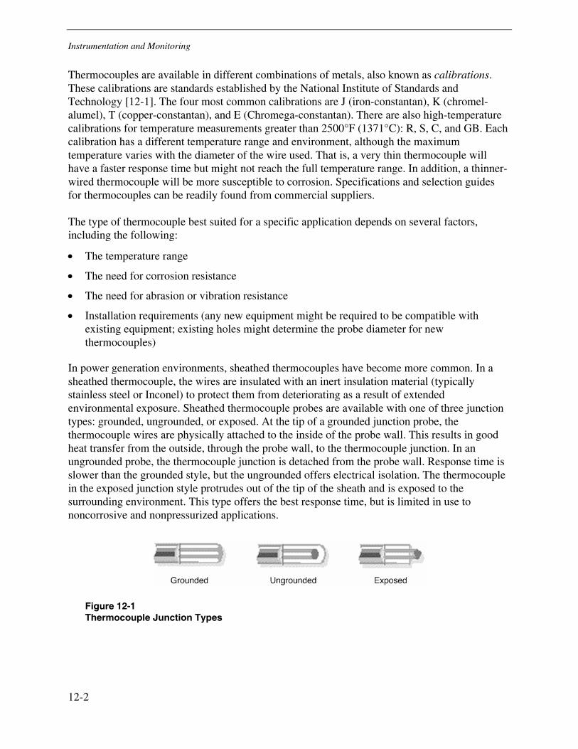
Instrumentation and Monitoring
12-2
Thermocouples are available in different combinations of metals, also known as calibrations. These calibrations are standards established by the National Institute of Standards and Technology [12-1]. The four most common calibrations are J (iron-constantan), K (chromel-alumel), T (copper-constantan), and E (Chromega-constantan). There are also high-temperature calibrations for temperature measurements greater than 2500°F (1371°C): R, S, C, and GB. Each calibration has a different temperature range and environment, although the maximum temperature varies with the diameter of the wire used. That is, a very thin thermocouple will have a faster response time but might not reach the full temperature range. In addition, a thinner-wired thermocouple will be more susceptible to corrosion. Specifications and selection guides for thermocouples can be readily found from commercial suppliers.
The type of thermocouple best suited for a specific application depends on several factors, including the following:
• The temperature range
• The need for corrosion resistance
• The need for abrasion or vibration resistance
• Installation requirements (any new equipment might be required to be compatible with existing equipment; existing holes might determine the probe diameter for new thermocouples)
In power generation environments, sheathed thermocouples have become more common. In a sheathed thermocouple, the wires are insulated with an inert insulation material (typically stainless steel or Inconel) to protect them from deteriorating as a result of extended environmental exposure. Sheathed thermocouple probes are available with one of three junction types: grounded, ungrounded, or exposed. At the tip of a grounded junction probe, the thermocouple wires are physically attached to the inside of the probe wall. This results in good heat transfer from the outside, through the probe wall, to the thermocouple junction. In an ungrounded probe, the thermocouple junction is detached from the probe wall. Response time is slower than the grounded style, but the ungrounded offers electrical isolation. The thermocouple in the exposed junction style protrudes out of the tip of the sheath and is exposed to the surrounding environment. This type offers the best response time, but is limited in use to noncorrosive and nonpressurized applications.
Figure 12-1 Thermocouple Junction Types
Instrumentation and Monitoring
12-3
Strain Gauges
When external forces are applied to a stationary component, stress and strain result. Either the component can elastically absorb the applied energy or it can plastically deform to accommodate the applied energy. Stress is defined as the component’s internal shape-change resisting forces, and strain is defined as the displacement and deformation (elastic and plastic) that occurs. For a uniform distribution of internal shape-change resisting forces, stress can be calculated by dividing the force (F) applied by the unit area (A). Strain is defined as the amount of deformation per unit length when a load is applied. Strain is calculated by dividing the total change in length by the original length. For material stressed in the elastic range, typical values for strain are less than 0.002 in./in. (0.002 cm/cm). Strain can be compressive or tensile, and it is typically measured by strain gages. It was Lord Kelvin who first reported in 1856 that metallic conductors subjected to mechanical strain exhibit a change in their electrical resistance. This phenomenon was first put to practical use in the 1930s.
Fundamentally, all strain gages are designed to convert mechanical motion into an electronic signal. A change in capacitance, inductance, or resistance is proportional to the strain experienced by the sensor. If a wire is held under tension, it gets slightly longer and its cross-sectional area is reduced. This changes its resistance (R) in proportion to the strain sensitivity (S) of the wire’s resistance. When a strain is introduced, the strain sensitivity or gage factor (GF) is given by Equation 12-1.
StrainRR
GF
Δ
= Eq. 12-1
The ideal strain gage changes resistance only as a result of the deformations of the surface to which the sensor is attached. However, in real applications, temperature, material properties, the bonding media, and stability of the metal all affect the detected change in resistance. Because most materials do not have the same properties in all directions, knowledge of the axial strain alone might be insufficient for a complete analysis. Poisson, bending, and torsional strains might also require measurement.
The first bonded, metallic wire-type gages consisted of a grid of wire filament (a resistor) bonded directly to the strained surface by a thin layer of epoxy resin. The foil diaphragm and the adhesive bonding agent work together to transmit the strain data, and the adhesive also serves as an electrical insulator between the foil grid and the surface.
When selecting a strain gage, one must consider not only the strain characteristics of the sensor but also its stability and temperature sensitivity. Regrettably, in power plant applications, component temperatures greater than 400°F (204°C) are common; the most desirable strain gage materials are sensitive to temperature variations and tend to change resistance as they age. For short-duration tests, this variation might not be a concern; however, for continuous measurement, temperature and drift compensation must be considered.
Instrumentation and Monitoring
12-4
Each gage wire material has its own characteristic gage factor, resistance, temperature coefficient of gage factor, thermal coefficient of receptivity, and stability. Typical materials used for strain gauges include constantan (copper-nickel alloy), Nichrome V (nickel-chrome alloy), platinum alloys (usually tungsten), nickel-iron alloys, or nickel-chrome alloy wires, foils, or semiconductor materials. The most popular alloys used for strain gages are copper-nickel alloys and nickel-chromium alloys.
For high-temperature applications in the range of typical main steam and HRH system operation (approximately 1000°F [538°C]) free filament or weldable gages are typically used. In free filament gages, the sensor wires are not encapsulated but instead are bonded directly to the subject component by flame spraying or with ceramic cement. In weldable gages, the sensors are usually prebonded to a superalloy shim stock using ceramic materials and are subsequently attached to the component using spot welds around the periphery of the shim stock.
Creep-FatiguePro On-Line Damage Monitoring
The principal degradation mechanisms affecting the long-term reliability of high-energy piping systems are creep and fatigue. The accumulation of material damage during the course of power generation operations eventually leads to crack initiation and propagation. It is not a question of whether it will occur, but rather a matter of when. In extreme cases, the growth of these cracks can lead to leakage or rupture. The monitoring and prediction of the rate of accumulation of creep-fatigue damage is, therefore, essential in developing an effective life assessment strategy for any component or system.
Current methods of life assessment use sophisticated stress and defect initiation and propagation analysis methods to determine current damage levels and predict rates of future accumulation. Both calculations are based on a review of past operating data (such as number of starts and time of operation) that is used to assemble a history of operational experience and assist in projecting current operating experience into future performance. Typically, the analyst makes conservative assumptions regarding service history characteristics (frequency of occurrence, magnitude, and duration) to provide confidence that the analysis results are conservative. Clearly, the implication is that by providing more accurate and current operating data, less conservatism will be included and a more cost-effective evaluation will result.
To address this issue, EPRI sponsored the development and implementation of two stand-alone Windows software-based computer programs: Fatigue Pro for nuclear applications (components subjected to only fatigue damage) and Creep-FatiguePro for fossil plant applications with components operating in the creep range [12-2, 12-3]. Both programs have the ability to access and process actual, real-time, plant operating data to track fatigue and creep-fatigue damage accumulation, respectively.
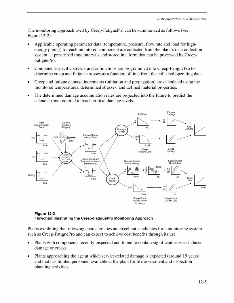
Instrumentation and Monitoring
12-5
The monitoring approach used by Creep-FatiguePro can be summarized as follows (see Figure 12-2):
• Applicable operating parameter data (temperature, pressure, flow rate and load for high-energy piping) for each monitored component are collected from the plant’s data collection system at prescribed time intervals and stored in a form that can be processed by Creep-FatiguePro.
• Component-specific stress transfer functions are programmed into Creep-FatiguePro to determine creep and fatigue stresses as a function of time from the collected operating data.
• Creep and fatigue damage increments (initiation and propagation) are calculated using the monitored temperatures, determined stresses, and defined material properties.
• The determined damage accumulation rates are projected into the future to predict the calendar time required to reach critical damage levels.
Figure 12-2 Flowchart Illustrating the Creep-FatiguePro Monitoring Approach
Plants exhibiting the following characteristics are excellent candidates for a monitoring system such as Creep-FatiguePro and can expect to achieve cost benefits through its use.
• Plants with components recently inspected and found to contain significant service-induced damage or cracks.
• Plants approaching the age at which service-related damage is expected (around 15 years) and that has limited personnel available at the plant for life assessment and inspection planning activities.
Instrumentation and Monitoring
12-6
• Plants currently operating under, or contemplating a shift to, load-following or on-off cyclic operation. In this case, plants can expect acceleration of component life consumption rates compared to that of base-load operation.
On-line monitoring is the best alternative for tracking remaining useful life and equipment wear and tear, which is one of the most difficult costs of unit cycling to quantify. Monitoring tools such as Creep-FatiguePro allow plants to develop economic models that convert monitoring results into plant cycling costs.
To date, more than 30 power plants are using Creep-FatiguePro or its nuclear counterpart, FatiguePro. Each plant has realized considerable cost reduction through lengthened inspection intervals, reduction in unnecessary component replacement, changes to operating procedures, and avoidance of in-service component failures.
In the cost-competitive deregulated environment, accurate and timely information on component condition is vital for input to repair or replacement decisions and outage planning and scheduling. Through automation of damage accumulation and remaining life computation, in addition to basing calculations on actual operating conditions, Creep-FatiguePro offers the following benefits:
• By accounting for periods of low-stress operation, more accurate damage predictions than those based on maximum design or operating conditions are obtained. This enables decreased inspection frequency and extension of the predicted life of critical components.
• Advanced data trending and analysis tools allow users to identify and adjust operating procedures to minimize creep and fatigue damage at monitored locations. In addition, the effects of potential operation revisions can be evaluated before implementation.
• Automated tracking of damage in critical components eliminates the need for manual remaining life calculations.
Acoustic Emission On-Line Damage Monitoring
As a corollary to the quantitative analytical tracking of damage development and progression provided by a system such as Creep-FatiguePro, acoustic emission (AE) technology has been applied in high-energy piping systems by several utilities to act as an “early warning system” for damage development.
Acoustic emissions are the audible stress waves produced by the sudden internal stress redistribution of a material, created by changes in its internal structure. Possible causes of internal structure changes include crack initiation and growth, crack opening and closure, dislocation movement, twinning and phase transformation in crystalline materials, and fiber breakage and fiber-matrix debonding in composites. Most sources of AE are damage-related; therefore, the detection and monitoring of these emissions are commonly used to predict material failure.

Instrumentation and Monitoring
12-7
AE has been demonstrated as a viable technique in the detection of defect initiation and propagation through fatigue [12-4]. In high-temperature applications associated with high-energy piping, the goal has been the detection of the formation of creep cavities. No documented validation of the detection of creep void formation through the use of AE currently exists. Research in this technology continues, sponsored by EPRI and others.
The difference between AE and other NDE methods is that AE detects changes occurring inside the material while they are occurring, while other NDE methods examine the internal structure of the material (in whatever state it is in at the time of inspection). AE needs only the input of one or more sensors on the surface of the component being examined. AE systems are designed to monitor acoustic emissions during system operation.
One of the disadvantages of AE is that commercial systems typically estimate only qualitatively how much damage is present in the material at the time acoustic emissions are detected, and no historical information is acquired. Therefore, other NDE methods are needed to provide more quantitative results. In high-energy piping applications, service environments are generally noisy, and the AE signals are usually weak. Therefore, signal discrimination and noise reduction are difficult challenges, yet they are extremely important for successful acoustic signal interpretation.
Over the past five years AE instruments have transitioned to digital signal processing. This has opened up a new range of technical capabilities for the AE method—the frequency domain. The ability to capture full waveforms allows advanced post-test analysis; previously, real-time wave form analysis was performed on a small set of features that were measured with bulky electronic circuits.
Water Chemistry
Water cleanliness is important to all waterside boiler and steam transport components. Water impurities can lead to boiler tube failures and carryover of solids in the steam, which in turn can result in superheater tubing problems and turbine blade deposits. Flushing of loose debris from the feedwater system and boiler in combination with the use of high-quality water must supplement waterside surface cleaning efforts.
Water sources used to provide feedwater to a boiler are never 100% pure. They always contain varying amounts of suspended and dissolved materials. Clearly, the type and amount of materials present will depend on the water source (river, lake, and so on). Aside from organic material that might be present, water contains solids that are either dissolved or suspended. Suspended solids are those that do not dissolve in water and can be removed or separated by filtration; these types of solids include mud, silt, clay, and metallic oxides. Dissolved solids are those that are present in solution, and therefore cannot be removed by filtration; the primary dissolved solids in most waters include iron, silica, calcium, magnesium, and sodium.
Instrumentation and Monitoring
12-8
Chemistry control begins with treatment of the feedwater to the boiler. To minimize corrosion, feedwater and condensate must be maintained at the proper pH and ORP levels and free of dissolved carbon dioxide and oxygen gases. In general, plants maintain water pH between 8.0 and 9.5. High pH levels can lead to foaming, and consequently an increase in the amount of carryover solids. The optimal pH level for a given unit will be the one that results in the least amount of iron and copper corrosion products.
Because corrosion of steel typically involves the reduction of dissolved oxygen in water, oxygen gas dissolved in solution increases corrosion rates of waterside surfaces, typically through pitting. Therefore, the best defense is to maintain an airtight system. Deaerators are used to capture and expel gases, while chemical treatments with sodium sulfite (up to 1800 psi [12.411 MPa]) or hydrazine act to scavenge oxygen that is dissolved in solution.
Water chemistry control for drum-type boilers is typically performed by one of four chemical additions:
• Phosphate-hydroxide
• Coordinated phosphate
• Chelant
• Volatile
The choice of chemical is usually governed by the pressure range in the unit. Phosphate-hydroxide (<1000 psi [<6895 kPa]) and coordinated phosphate (all pressures) methods target water pH and precipitate calcium and magnesium compounds so they can be removed in blowdown. Chelants (<1000 psi [<6895 kPa]) are complex acids that are added to react with metal ions, calcium, magnesium, and iron to form soluble complexes that can be removed during continuous blowdown. During volatile treatment (all pressures), no solid chemicals are added—only amines, typically ammonia. Volatile treatment is sensitive to water hardness (because no phosphates are used) and condenser leaks. All methods use either sulfite or hydrazine to control free oxygen.
Dimensional Measurements
One of the basic characteristics of a high-energy piping system is its physical size. This consists of not only the outside diameters and wall thicknesses of the constituent piping but also the run lengths and elevation points that define the overall geometry of a system. The long-term temperature and stress exposure of the piping material results in inelastic, permanent deformation of the system (through creep). It is not a question of whether it will occur, but when and how much. Monitoring the position of selected points in a system and the magnitude of motion that occurs in a system when transitioning from ambient to operating conditions can provide indication of support malfunction and help identify those locations that are most susceptible to damage.
Instrumentation and Monitoring
12-9
Recording the hot and cold dimensions of a piping system is an integral part of any piping management program. As-built, construction, and design drawings in many instances might not reflect the current configuration of a system. This becomes more evident as systems age and exposure time increases. To ensure a correspondence between the system geometry and the drawing record, selected system dimensions should be checked.
With the intent of tracking the general deformation of a system, selected locations should be monitored to periodically record the pipe position in space. In its basic form, this monitoring is accomplished by performing periodic walkdowns, recording support indicator readings, and correlating those readings with the travel range of the support. When more accurate positioning is required at a position not coincident with a support, pointers or other indicators can be fixed to the piping and used as reference points for collecting position data.
In addition to positional measurements, spool diameters and wall thicknesses should be measured as accurately as possible to provide a basis to monitor swelling and assist in stress evaluations. Swelling of the pipe cross section can occur as a result of overpressure or extensive creep deformation. Pipe OD measurements can be performed with outside calipers or PI tape measures, which provide ample accuracy to detect swelling strains in excess of 2%. For wall thickness measurements, ultrasonic methods should be used. Pipe spools are ordered to a specified minimum thickness. Actual thicknesses of delivered spools are typically thicker than the specified minimum diameter (usually by 10%). Knowledge of the actual wall thickness of a pipe segment allows more accurate modeling of the piping by eliminating the assumption of minimum wall thickness.
References
12-1. G. W. Burns, M. G. Scroger, G. F. Strouse, M. C. Croarkin, and W. F. Guthrie, Temperature-Electromotive Force Reference Functions and Tables for the Letter-Designated Thermocouple Types Based on the ITS-90, National Institute of Standards and Technology. Monograph 175 (1993).
12-2. FatiguePro: On-Line Fatigue Usage Transient Monitoring System. EPRI, Palo Alto, CA: 1988. NP-5835-SP.
12-3. Creep-FatiguePro: On-Line Creep-Fatigue Damage and Crack Growth Monitoring System. EPRI, Palo Alto, CA: 1992. TR-100907.
12-4. J. E. Coulter, T. P. Sherlock, et al, “Acoustic Emission Monitoring or Fossil Power Plants,” Paper presented at the Third EPRI Conference on Incipient Failure Detection in Power Plants, Philadelphia, PA (March 1987).


13-1
13 DATA STORAGE, RETRIEVAL, AND EVALUATION
Introduction
Implementation of an effective piping management program involves the integration of several key elements, including the following:
• Materials. Identification of damage mechanisms allowing application of appropriate initiation and propagation models
• NDE. Detection and quantitative characterization of damage
• Engineering analysis. Projections of damage development related to specific operating practices. Basis development for safe operating periods and expected remaining life
• Monitoring. Verification of prediction inputs, identify damage-producing operating modes and optimize component operation
• Repair technology. Should be designed and implemented to have minimal impact on continued degradation and maximum serviceability
• Inspection, repair, and replacement planning. The combination of engineering analyses and financial and safety consequences in light of unit availability targets
Another key element missing from this list but essential to the effective implementation of any program is data management. Institution of consistent data gathering and structured cataloging and storage of information provides the foundation for analyses and evaluations required by the key elements. Data management provides the unifying line among the elements. Data must be stored in useable format that is easily queried for analysis. Storing large volumes of data that nobody can access is not useful. Having large volumes of data is insufficient; after they are stored, data must be trended and analyzed to detect trends and issues before they become problems. Effective data collection, storage, retrieval and analysis are the lifeblood of any optimally operating process.
How many times have you heard someone say, “I wish I knew then what I know now”? Utility experience (with respect to data collection, storage, and review) in many cases implies that this statement be reworded to say, “I wish I knew now what I knew then.” The underlying meaning of this last statement is that without good historical records you will receive minimal value from collecting further data.

Data Storage, Retrieval, and Evaluation
13-2
Advancing technology, shifts in management philosophy and personnel changes collectively influence how data (and knowledge) are collected, used, and archived. This section describes the evolution of data storage and analysis as it relates to high-energy piping and provides guidance concerning the criteria for its management.
Traditional Methods
Before the proliferation of computer technology in the 1980s, data collection was, of necessity, a manual task resulting in the generation of hardcopy records. Hardcopy records required significant personnel and physical space commitments for their organization and storage. As a consequence, a large percentage of information was not analyzed to assess its meaning regarding component reliability. In many instances, recordkeeping was locally driven by plant personnel responsible for specific equipment, and program overviews were not developed.
Regardless of the specific methods used to secure plant data, it is essential that the information be available from some central location to facilitate its distribution and analysis. Traditional methods of data analysis involve plotting information and identifying trends. Evaluation methods from hardcopy data are usually less quantitative because more assumptions are made during interpretation of written data. In addition, failure to centralize data places an unnecessary burden on staff to actively search for information pertinent to the problem at hand.
PC-Based Applications
The increase in computer applications for both data acquisition and analysis has greatly expanded the volume of information available, creating the potential for data overload. Computers can store all forms of information—records, documents, images, sound recordings, videos, scientific data, and so on—but the basic problem of managing the information and putting it to good use remains.
Many PC-based software tools have been developed to facilitate the management and analysis of piping data. Spreadsheet programs and database applications such as Microsoft Excel and Microsoft Access provide platforms for the collection of component information. Analysis tools provide plant personnel with the ability to perform comprehensive quantitative evaluations of component and system life. Planning software is available to help evaluate multiple inspection and replacement scenarios and view the problem from a financial perspective.
Aside from the ability to collect more data and perform sophisticated evaluations, logistical problems—specifically, maintaining current software versions and ensuring their compatibility with operating system changes—exist.

Data Storage, Retrieval, and Evaluation
13-3
Web-Based Applications
The next generation of data management systems is already in use, using the Internet to eliminate the need for local software. The only requirements are Internet access and a web browser. It should be the goal of each station to have the ability to use real-time information to track and evaluate components and systems. To achieve this goal requires involvement of information technology (IT) personnel to ensure rapid data transmittal, data integrity, and security. Areas that should be addressed when developing a web-based data management system are described in the following subsections.
System Isolation and Security
The control system must be isolated by an effective firewall and traffic must be monitored by intrusion detection sensors. Only specific traffic should be allowed into the system network, such as supplemental data for the historian, virus protection definitions, and remote support. Virtual Private Network (VPN) encryption technology and managed routing should be used as part of a security plan for remote support.
Periodic security evaluations by an expert third party should be performed to ensure that effective security protections, policies, and procedures are in place to protect the system. Your IT department should also conduct corporate security assessments at periodic intervals.
Software Changes, Patches, and Upgrades
In many instances, web-based systems take advantage of readily available computing components and operating systems. The disadvantage of this open system is the increased vulnerability to hacking and virus attacks. Increased costs associated with the use of proprietary systems force many users to accept this increased risk. The trade-off for using a nonproprietary system is the increased frequency of operating system patches and security upgrades. This forces hardware upgrades and increases maintenance. Installation of patches and updates should be approached with caution.
Data Collection Periods
The time period over which data is maintained should be decided. It is suggested that—as a minimum—two to three years of information should be directly accessible on the system. A procedure for archiving data that exceeds the established limits should be developed.

Data Storage, Retrieval, and Evaluation
13-4
Remote Access
While security is the primary concern, the benefits of remote access to the system for data review or support should be considered. By using Virtual Private Network connections and specific transmission control protocol/Internet protocol (TCP/IP) ports, a firewall can allow the connection of defined users for remote console control.
System Capacity
Depending on the architectures selected for a production system, the amount and frequency of data collection and the techniques used to meet the other requirements (system isolation and security; software changes, patches, and upgrades; data collection periods; and remote access), additional system capacity might be required. To ensure adequate system performance, IT personnel should be part of station meetings regarding data collection, project planning, and support.
14-1
14 REPAIR AND REPLACEMENT
Introduction
As a result of either regular inspection protocols or an unanticipated occurrence, damage can be detected in piping systems that requires repair or replacement of the component to ensure continued safe operation. Damage can occur at any point in the piping system, but is most frequently associated with high constraint regions including valves, wyes, tees, or attachment welds. Specific damage mechanisms associated with each piping system within a fossil generating station will be described in Volume 2, Performance of Steam Piping, and Volume 3, Performance of High-Energy Water Piping, of this report.
When damage is identified, a decision for repair or replacement will be based on a number of technical, financial, and risk factors. Technical factors include the type, location, extent, and severity of the damage. Financial factors include unit availability requirements, timing of the repair or replacement, availability of craft labor, and availability of replacement material. Risk factors include the time to predicted failure, consequence of a failure, and impact of a failure on surrounding equipment.
Based on these competing factors, consideration must be given to the type of repair to be performed. Before any decision of repair or replacement is made or undertaken, it is necessary to fully characterize the location, type, and extent of damage. Section 9, Piping System Surveys, of this volume describes available inspection techniques, and Volumes 2 and 3 provide specific guidance regarding the best-suited NDE techniques for each damage mechanism associated with specific piping systems, as well as suggestions for ongoing damage assessment.
Governing Codes
The design codes address fabrication and erection of new piping systems. These codes generally serve to provide guidance for any repair or replacement. However, after the piping system has been commissioned, alteration and repair of the piping systems are generally performed under the National Board Inspection Code NB-23 [14-1]. The applicability of NB-23 or the original fabrication code depends on implementation by the local jurisdiction.
Type and Extent of Repair
Repairs can be considered long term or temporary. Temporary repairs can be performed to allow operation of the generating unit until a more permanent repair can be affected; however, a
Repair and Replacement
14-2
thorough understanding of the extent of damage, impact of the repair on the progression of damage, and a conservative estimate of the service life of the temporary repair must be made and communicated to responsible individuals.
Whenever damage is detected, consideration should be given to the inspection of similar locations on the affected unit or other units in the fleet that are operating under similar conditions. After the cause and extent of damage have been quantified, the need to incorporate an inspection protocol for similar damage into an overall condition assessment program should be evaluated.
Permanent Repairs
Permanent repairs normally require complete removal of the defect. If damage remains after the repair, the remaining service life should be quantified; if it is determined to extend beyond the remaining life of the facility, periodic reinspections should be performed to assess damage progression within a timeframe based on a conservative calculation of damage accumulation. Available life prediction tools are described in this volume; however, repairs can impart unanticipated stresses that can be difficult to quantify, and repair techniques can locally modify the microstructure and thus the performance characteristics of the material.
Defect removal typically involves grinding or machining to either remove the defect or reduce the defect to an acceptable size. The use of thermal processes such as arc gouging should be restricted because the localized heat input can cause an existing defect to run. If thermal processes are used, complete removal of the heat-affected material is recommended. NDE should be performed to confirm removal of the defect. If the defect is eliminated by localized removal of material, the depth and extent of the excavation must be quantified. If the minimum wall thickness has not been violated, the excavation area can be blended into the surrounding material and no further repair might be required. If the minimum wall thickness has been violated, a local thin area calculation should be performed to determine whether sufficient reinforcement is provided by adjoining material; if it is not, weld repair is required.
For more extensive damage, material or component replacement might be required. The need for redesign to eliminate the reoccurrence of damage should be evaluated.
Temporary Repairs
In some instances, temporary repairs can be performed to allow operation of the unit until a permanent repair can be designed and implemented. Often replacement components are not readily available and require extensive lead times to procure. When considering the appropriateness of a temporary repair, the consequence of the failure of the repair must be considered. The use of temporary repairs should be limited to only those applications that are considered safe with limited exposure to consequential damage.
When temporary repairs are implemented, the life of the repair should be established by analysis or experience, and this life should be communicated to responsible individuals. It is
Repair and Replacement
14-3
recommended that systems be established to ensure that a permanent repair or replacement is effected in a timely manner. Particular attention should be given to the repair of longitudinal seam welds because of long-term serviceability issues and the risk of catastrophic failure.
Piping System Support or Restraint
Before any repair is performed, the component should be properly supported and restrained. To prevent weld cracking and limit additional creep damage from the stresses imposed by welding and PWHT, it is necessary to eliminate or minimize stresses in the repair area until PWHT has been completed. This can require the use of temporary supports. The supports and restraints will also support the component during the required PWHT and prevent sagging or movement of the piping system.
Small-diameter, light-wall piping systems typically can be adequately supported and restrained by using mechanical means (chain falls or come-alongs) and by pinning adjacent hangers. Limited input from the system design engineer is required for the repair of small diameter piping systems.
For large-diameter or heavy-wall piping systems, greater care must be taken to ensure that adequate restraint and support are provided during the repair operation. Involvement of the system design engineer is often required, particularly if the system was designed and installed with significant cold spring. Heavy rigging and the installation of temporary structural steel will often be required to support and restrain a large-diameter, heavy-wall piping system during a repair.
Repair Design
Depending on the nature of the repair, a number of alternative repair designs can be considered. A brief description of these options is included in this section. The designs represent typical repairs that can be encountered, and they contain applicable cautions. If these repair approaches cannot be performed as shown, or if the specific repair approach is not addressed within the text of this procedure, than a more detailed analysis is required to ensure the structural integrity of the repair.
Pipe or Component Replacement
When a pipe or component is to be replaced, a standard weld joint design should be used (Figure 14-1). When reestablishing the weld bevel on a pipe or component that will be reused, it is recommended that the original HAZ be removed. This can typically be accomplished by machining back into the base metal approximately 1/4 in. (6.4 mm) from the original weld toe.
Caution: Because the HAZ has been removed, the pipe or component will be shorter than originally installed. A stress analysis can be performed to determine whether the additional stresses that are introduced into the system are acceptable. Alternatively, the length of pipe removed can be made up in the replacement pipe or component.
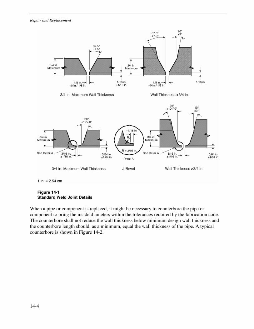
Repair and Replacement
14-4
Figure 14-1 Standard Weld Joint Details
When a pipe or component is replaced, it might be necessary to counterbore the pipe or component to bring the inside diameters within the tolerances required by the fabrication code. The counterbore shall not reduce the wall thickness below minimum design wall thickness and the counterbore length should, as a minimum, equal the wall thickness of the pipe. A typical counterbore is shown in Figure 14-2.
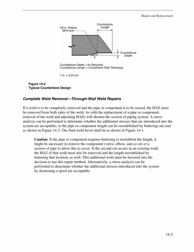
Repair and Replacement
14-5
Figure 14-2 Typical Counterbore Design
Complete Weld Removal—Through-Wall Weld Repairs
If a weld is to be completely removed and the pipe or component is to be reused, the HAZ must be removed from both sides of the weld. As with the replacement of a pipe or component, removal of the weld and adjoining HAZs will shorten the section of piping system. A stress analysis can be performed to determine whether the additional stresses that are introduced into the system are acceptable, or the pipe or component length can be reestablished by buttering one end as shown in Figure 14-3. The final weld bevel shall be as shown in Figure 14-1.
Caution: If the pipe or component requires buttering to reestablish the length, it might be necessary to remove the component (valve, elbow, and so on) or a section of pipe to allow this to occur. If the second cut occurs in an existing weld, the HAZ of that weld must also be removed and the length reestablished by buttering that location, as well. This additional weld must be factored into the decision to use this repair method. Alternatively, a stress analysis can be performed to determine whether the additional stresses introduced into the system by shortening a spool are acceptable.
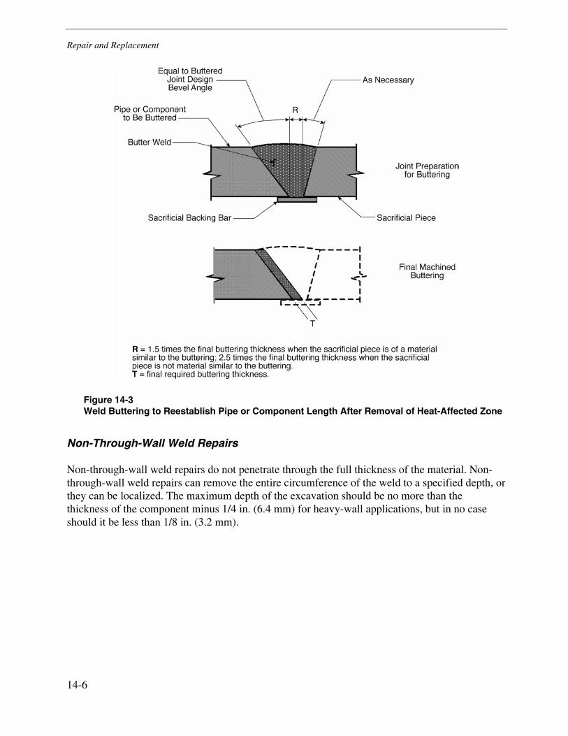
Repair and Replacement
14-6
Figure 14-3 Weld Buttering to Reestablish Pipe or Component Length After Removal of Heat-Affected Zone
Non-Through-Wall Weld Repairs
Non-through-wall weld repairs do not penetrate through the full thickness of the material. Non-through-wall weld repairs can remove the entire circumference of the weld to a specified depth, or they can be localized. The maximum depth of the excavation should be no more than the thickness of the component minus 1/4 in. (6.4 mm) for heavy-wall applications, but in no case should it be less than 1/8 in. (3.2 mm).
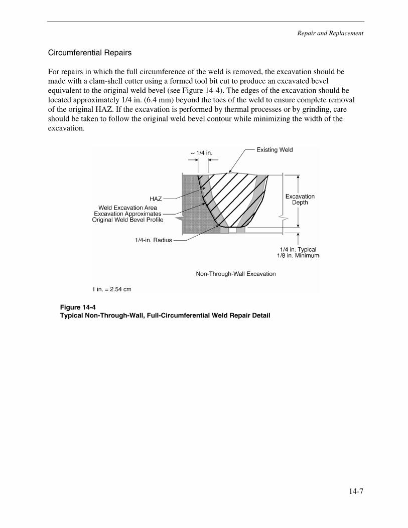
Repair and Replacement
14-7
Circumferential Repairs
For repairs in which the full circumference of the weld is removed, the excavation should be made with a clam-shell cutter using a formed tool bit cut to produce an excavated bevel equivalent to the original weld bevel (see Figure 14-4). The edges of the excavation should be located approximately 1/4 in. (6.4 mm) beyond the toes of the weld to ensure complete removal of the original HAZ. If the excavation is performed by thermal processes or by grinding, care should be taken to follow the original weld bevel contour while minimizing the width of the excavation.
Figure 14-4 Typical Non-Through-Wall, Full-Circumferential Weld Repair Detail
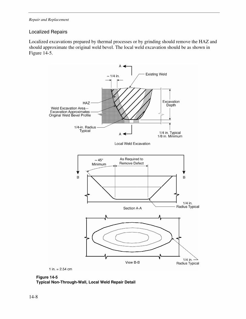
Repair and Replacement
14-8
Localized Repairs
Localized excavations prepared by thermal processes or by grinding should remove the HAZ and should approximate the original weld bevel. The local weld excavation should be as shown in Figure 14-5.
Figure 14-5 Typical Non-Through-Wall, Local Weld Repair Detail
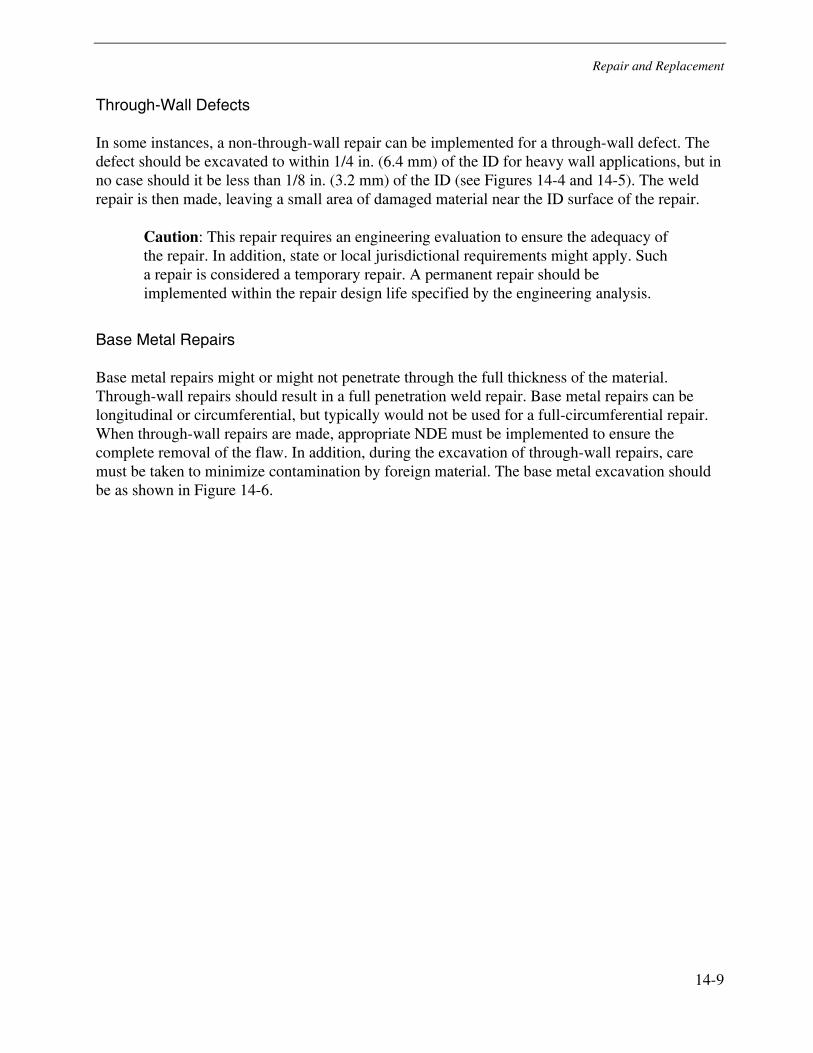
Repair and Replacement
14-9
Through-Wall Defects
In some instances, a non-through-wall repair can be implemented for a through-wall defect. The defect should be excavated to within 1/4 in. (6.4 mm) of the ID for heavy wall applications, but in no case should it be less than 1/8 in. (3.2 mm) of the ID (see Figures 14-4 and 14-5). The weld repair is then made, leaving a small area of damaged material near the ID surface of the repair.
Caution: This repair requires an engineering evaluation to ensure the adequacy of the repair. In addition, state or local jurisdictional requirements might apply. Such a repair is considered a temporary repair. A permanent repair should be implemented within the repair design life specified by the engineering analysis.
Base Metal Repairs
Base metal repairs might or might not penetrate through the full thickness of the material. Through-wall repairs should result in a full penetration weld repair. Base metal repairs can be longitudinal or circumferential, but typically would not be used for a full-circumferential repair. When through-wall repairs are made, appropriate NDE must be implemented to ensure the complete removal of the flaw. In addition, during the excavation of through-wall repairs, care must be taken to minimize contamination by foreign material. The base metal excavation should be as shown in Figure 14-6.
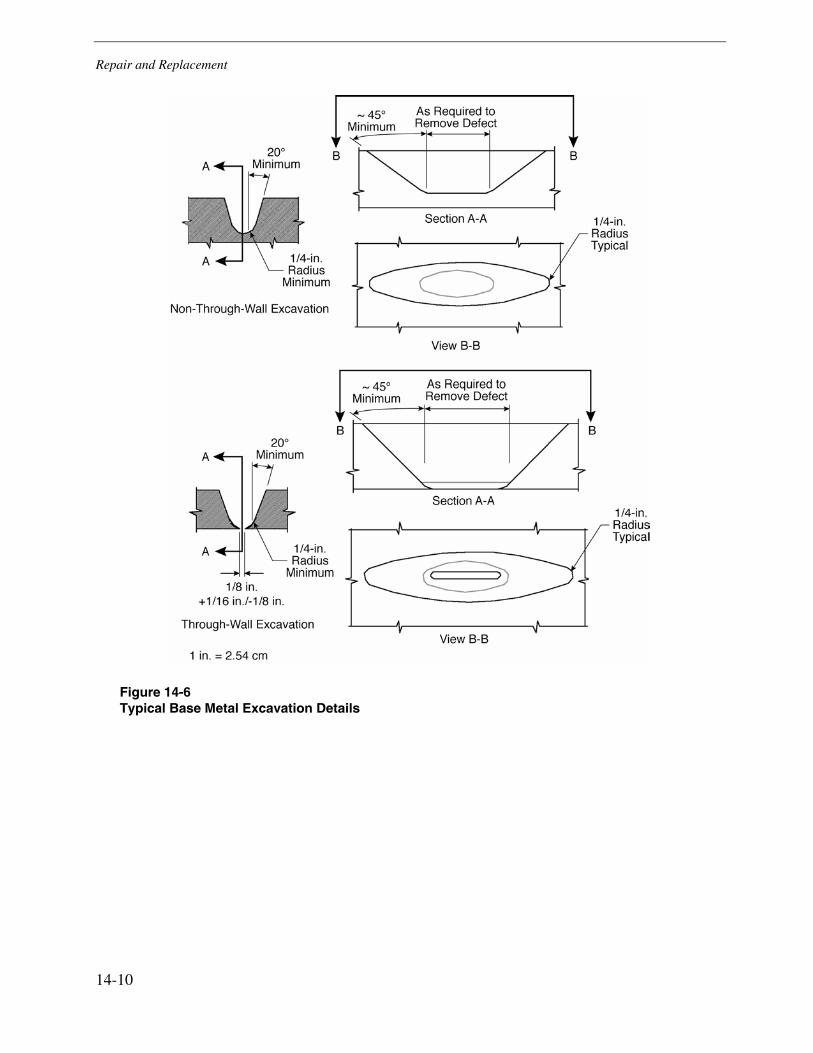
Repair and Replacement
14-10
Figure 14-6 Typical Base Metal Excavation Details
Repair and Replacement
14-11
Plug Sample Repairs
When plug samples are removed, the remaining hole can be repaired by installing a radiographic plug or a capped Weldolet or Sockolet style boss, as shown in Figure 14-7.
Figure 14-7 Plug Sample Repair Methods
Radiographic Plugs
Radiographic plugs must be designed and installed according to the requirements of PFI ES-16, Access Holes, Bosses, and Plugs for Radiographic Inspection of Pipe Welds [14-2].
The plug material should be fabricated from a material similar to the base metal and must be listed in the applicable code of construction (see Figure 14-7). To minimize the risk associated with oxidation of the thread profile and the resulting loss of strength, the use of nonthreaded gamma plugs should be considered.
A plugged or capped Weldolet or Sockolet style boss must be designed and fabricated to the applicable code requirements. The materials used should be similar to the base metal and must be listed in the applicable code of construction (see Figure 14-7).
Other Repair Designs
In addition to the repair designs highlighted in this section, other types of repairs, such as structural weld overlays, might be suitable for temporary or permanent repairs. These repair designs require an engineering analysis to ensure the structural integrity of the repair and establish a design life for the repair.
Repair and Replacement
14-12
Repair Considerations
Flaw Excavation
Flaw excavation can be by machining, grinding or air carbon arc gouging. Machining is the preferred method because it does not affect the material properties. In addition, machining allows flaw excavation and weld bevel preparation to be carried out in one operation.
The use of carbon arc gouging is generally discouraged. Thermal stresses from the arc gouging process can propagate the crack, and the temperature of the process can adversely affect the surrounding material. In addition, it can be more difficult to follow the defect and ensure complete removal during arc gouging than is possible when grinding. If air carbon arc gouging is used for flaw excavation, preheat should be established and maintained during the gouging process. The preheat temperature should be as specified by the applicable welding procedure to be used in the repair. Gouged surfaces should be cleaned back to bright metal.
If grinding is used for flaw excavation and weld bevel preparation, care should be taken not to overheat the base metal. If the ID of the component will not be accessible after flaw excavation, care must be taken to ensure that foreign material does not enter the system during cavity excavation. When the excavation has been completed, complete removal of the flaw or the reduction of an acceptable size should be verified by appropriate NDE or metallographic methods.
Fit-up, Tack Welding, and Temporary Attachments
Fit-Up
Before and during welding, parts to be joined might require being fit, aligned, or restrained in position. Tolerances for fit-up should meet the requirements of the fabrication code and qualified welding procedure.
Cleaning
Before fit-up, surfaces to be welded should be cleaned to bright metal. Adjacent internal and external surfaces should be cleaned to bright metal for a minimum of 1/2 in. (12.8 mm) back from the surface to be welded. The cleaned areas should be free of oil, dirt, moisture, rust, scale, and any coating or contaminant. On vertical sections of line, surfaces above the weld should be cleaned of loose contaminants (such as scale or dirt) for 2 in. (51 mm) above the joint.
Areas to be welded must be free of moisture. Typically, preheat will remove any residual moisture. If welding will be done outdoors, an appropriate shelter should be erected to protect the weld area from inclement weather. If welding processes incorporating shielding gasses are used for repair, the work area should be protected from direct exposure to wind such that any wind at the joint should not exceed 15 mph (24 kph).
Repair and Replacement
14-13
Alignment
Weld joint alignment should be as specified in the applicable fabrication code. Any misalignment, within the allowable tolerance, should be faired to at least a 3:1 taper over the width of the weld. Additional weld metal can be added to improve the transition. When tolerances for diameter, wall thickness, or out-of-roundness exceed fabrication code allowables, counterboring should be used to provide an adequate alignment.
Tack Welding
Tack welds should be made by qualified welders using a qualified weld procedure. A sufficient number of tack welds should be made to maintain alignment; in no case should tack welds be less than 1/2 in. (12.8 mm) in length The ends of the tack welds should be feathered to allow proper tie-in. Any tack weld that is not incorporated into the final weld should be removed by grinding. Tack welds should, as a minimum, be visually inspected and should be of a quality equivalent to the root pass. Any cracked or otherwise defective weld should be repaired before root pass welding.
Temporary Attachments
Temporary attachments are plates, bars, strong backs, lifting lugs, and similar items that are welded to the component to assist in fit-up and alignment of the weld joint. Items such as insulation pins used to hold resistant heating pads in place are also considered temporary attachments. Tack welds that will be incorporated into the weld, clamps, or other mechanical means are preferred over temporary attachments.
Temporary attachments should be made from material with a similar chemical composition to the base metal and should be welded to the component with an approved welding procedure by a qualified welder. Temporary attachments can be made of mild steel if all areas that will contact the base material or will be welded to the base metal are first buttered with a filler material matching the base metal composition. The temporary attachments can then be welded to the component with an approved welding procedure. If PWHT is required for the base metal, temporary attachments should be made only in areas that will be included in the PWHT of the repair.
Temporary attachments should be removed, unless otherwise specified. Temporary attachments can be removed by grinding, machining, or thermal cutting. Removal of temporary attachments by hammering or otherwise breaking the attachment away from the base metal is not allowed. If the temporary attachments are removed by thermal cutting, the temporary attachment should be cut no closer than 1/8 in. (3.2 mm) from the surface of the component, and the remaining material should be removed by grinding until flush with the surrounding base metal. The location from which temporary attachments were removed should be inspected by MT or PT before and after PWHT.
Repair and Replacement
14-14
Preheating and Post-Weld Heat Treatment
General
Proper application and control of heating operations is critical when making welded repairs. Rigorous control of preheat, interpass, and PWHT operations is necessary to avoid cracking and to ensure that the desired toughness and creep resistance are developed and maintained. Preheat and post-bake operations can be performed using oxy-fuel torches, electric resistance, or electric induction heaters.
Caution: The use of oxy-fuel torches is not recommended for preheat or post-bake operations except for very thin sections or under tightly controlled conditions. On heavy sections, there is a tendency for the surface of the work area to reach the required temperature while the temperature below the surface remains significantly below the required preheat temperature.
When oxy-fuel torches are used for preheating, extra care must be taken to prevent localized overheating of the material. One to two minutes should be allowed to elapse after removal of the flame and before the preheat temperature is measured. This will determine whether the material is uniformly heated through the entire thickness.
For PWHT, only electric resistance or induction heating is recommended. Localized oxy-fuel heating is not acceptable for PWHT. An exception would be PWHT of components in a temperature-controlled oxy-fuel furnace.
Preheat
Preheat should be uniformly applied to the joint including a minimum of 2 in. (50.8 mm) on either side of the weld, before any welding begins. After it is initiated, preheat should be maintained until all welding is complete. If preheat is interrupted for any reason, the weld should be inspected by MT before the resumption of welding.
Accurate temperature monitoring of preheat is critical for successful repairs. For preheat during welding operations, temperature-indicating crayons, contact or infrared pyrometers, or direct-reading thermocouples can be used. If temperature-indicating crayons are used, a crayon for the minimum preheat temperature and a crayon for the maximum interpass temperature must be in possession of the welder at all times. The preheat and interpass temperatures should be checked regularly on the base metal adjacent to the weld groove to ensure uniform heating. To avoid contaminating the weld, temperature readings should not be taken in the weld groove. If contact or infrared pyrometers are used, the preheat and interpass temperatures should be checked regularly on the base metal adjacent to the weld groove to ensure uniform heating. Direct-reading thermocouples attached to a strip chart recorder are the preferred method for temperature monitoring. Thermocouples should be attached on both sides of the weld in sufficient locations to ensure uniform heating.

Repair and Replacement
14-15
The preheat and interpass temperatures should be as specified on the Welding Procedure Specification. An increase in preheat temperature of 100°F–200°F (38°C–93°C) above that specified might be required for highly restrained repairs, but in no case should the preheat exceed the maximum interpass temperature.
Post-Weld Heat Treatment
For many repair or replacements activities, PWHT will be required by the governing code or can be used to enhance the material properties. PWHT should follow the requirements of the governing code with additional consideration given to the recommendations in the remainder of this subsection.
Prerequisites
• PWHT should be performed using electric resistance or induction heaters. PWHT with oxy-fuel gas is typically not allowed unless the PWHT is being performed in a temperature-controlled oven.
• PWHT should be limited to one weld at a time in any straight run of pipe unless the pipe is free to expand lengthwise.
• All weld repairs and required inspections should be completed before PWHT.
• The area to be treated by PWHT should be clean and free of all foreign materials and the component should be free of fluids and drafts on the ID.
Temperature Measurement
It is recommended that PWHT temperatures be monitored and controlled using chromel-alumel (ISA type K) thermocouples, extension wires, and corresponding strip chart recorders. Thermocouple wire can be high-temperature glass insulated or sheathed types. The recommended wire size is AWG20. Heavier wire is not recommended because it is less responsive to temperature change.
Thermocouples, extension wires, and connectors should be checked before use, including the following:
• Verify that screws are tightened at the terminal connections.
• Verify that the thermocouple extension wire polarity is correct; red is negative (alumel, slightly magnetic), and yellow is positive (chromel, nonmagnetic).
• Verify that the insulation is not damaged and the connectors are tight.
• Verify the function of thermocouple extension wire and strip chart recorder.

Repair and Replacement
14-16
Thermocouples should be attached directly to the component using a low energy (125 W/s maximum) capacitive discharge welder. The thermocouple junction ends must be less than 1/4 in. (6.4 mm) apart. Other methods of thermocouple attachment are not recommended. The hot junction end of each thermocouple wire should be protected from radiant heat by ceramic putty or a small piece of insulation. Thermocouple wires should be insulated from each other and from any metal surface, except at the hot junction. Thermocouple wires should be run along the component in a uniformly heated area for at least 2 in. (50.8 mm) before being routed out of the insulation.
The heat treatment cycle should be monitored and recorded on a strip chart recorder. The temperature should be monitored when the temperature exceeds 200°F (93°C) on heating and is above 600°F (316°C) on cooling.
Post-Weld Heat Treatment Procedure
Careful control of the PWHT operations is necessary to avoid cracking and to ensure that the desired toughness and creep-resistance is developed and maintained. For this reason, a detailed PWHT procedure should be prepared and reviewed by a qualified individual before the start of the repair. The procedure, as a minimum, should address all of the following items:
• Maximum PWHT temperature. The PWHT temperature should be as specified by the governing code and as specified in the applicable welding procedure specification. PWHT temperature should not exceed the lower critical temperature of the material; for normalized and tempered materials, the PWHT temperature is typically maintained 50°F (10°C) below the original tempering temperature.
• Support and restraint. The support and restraint of the repair weld should be evaluated to ensure adequate support and minimum loading on the weld to be PWHT.
• Thermocouple placement. Thermocouple placement is critical to performing an acceptable PWHT. Thermocouples should be attached near the centerline of the weld and on each side of the required heating band and at least in the following locations:
– In each separate heating zone.
– For pipes or components of 10 in. (254 mm) diameter or less, thermocouples should be located at the 6 o’clock and 12 o’clock positions.
– For pipes or components greater than 10 in. (254 mm) diameter, thermocouples should be placed at the 12 o’clock, 3 o’clock, 6 o’clock, and 9 o’clock positions.
– In the anticipated hottest and coldest locations. This is of particular importance when significant thickness transitions occur in the heating band zone.
– For thick components, thermocouples should be attached on the ID if it is accessible.
– A spare thermocouple wire should be attached at each location in the event the primary thermocouple fails. All thermocouples and extension wires should be clearly labeled as to their location on the component.

Repair and Replacement
14-17
Resistance Heating Pad Installation
Heating pads should extend completely around the circumference of the component. The width of the area heated should be as specified by the applicable fabrication code, along with the following guidelines:
• When the axis of the component is within ±15° of horizontal and over 10 in. (254 mm) diameter, it is recommended the heating pads be placed to allow the top and bottom of the component to be heated separately.
• When the axis of the component is within ±15° of vertical, it might be necessary to offset the heating pads toward the lower half to compensate for convection heat loss. Alternatively, separately controlled heating pads can be placed above and below the weld.
• When component wall thickness varies by more than 25% or 3/8 in. (9.5 mm), whichever is greater, separately controlled heating pads should be placed on each side of the weld.
Heating pads should be brought into tight contact with the pipe or component. Particular attention should be given to thickness transition areas. Failure to maintain a tight contact could prevent areas of the repair from reaching minimum PWHT temperature.
Post-Weld Heat Treatment Schedule
The PWHT cycle should begin by heating to 400°F (204°C) and holding for 15 minutes. During the hold time, the setup should be checked for uniform heating and proper operation of the heaters, thermocouples, strip chart recorder, and control equipment.
To minimize thermal stresses, at no time during the heat up, hold, or cold down cycle should any two thermocouples within the heat band have a temperature difference of more than 100°F (38°C). If this temperature differential is approached, the rate of heating or cooling should be slowed. If any temperature difference cannot be corrected, the component should be cooled to 200°F (93°C), and the PWHT setup should be reevaluated.
During the PWHT, if the maximum hold temperature is exceeded, the repair weld will require further evaluation to determine suitability for service after completion of the PWHT. This evaluation, as a minimum, would include replication and hardness testing to assess the metallurgical condition of the weld.
Nondestructive Evaluation Following Completion of Post-Weld Heat Treatment
When the pipe or component has cooled to room temperature, the weld should be inspected according to code requirements. In addition, it is recommended that all thermocouple removal areas and temporary attachment removal areas be inspected by MT or PT.
Repair and Replacement
14-18
Alternatives to Post-Weld Heat Treatment
In some situations, it might not be advisable or even possible to perform PWHT to the requirements of the original fabrication code. In such cases, alternatives to PWHT—such as temper bead welding and the alternative heat treatment rules given in the National Board Inspection Code—can be considered and can provide an acceptable repair [14-1]. Application of these alternative methods must meet the requirements of the applicable code (including qualification of welding procedures) and should include an engineering evaluation to determine whether they are appropriate for the intended service. In addition, such alternative methods must be acceptable to the applicable jurisdictions and, if required, be approved by a National Board-authorized inspector.
Component Replacement
When components are replaced, consideration should be given to the cause of the failure and whether changes in material or design are required to provide a satisfactory repair or to extend the life of the component.
Like-for-Like
Like-for-like replacements are made when the anticipated service life of the repair meets or exceeds that of the piping system. In such cases, no additional engineering work is required. Like-for-like replacements can also be used as a stopgap method to provide the necessary time to procure upgrade material or complete an improved design.
Upgrading by Design or Material Improvement
If a material has proven unsatisfactory for the intended service or if the anticipated life of a repair is deemed unacceptable, a change in material or design can be considered. Material changes can include changing to a higher alloy or different heat treat condition. Such improvement must meet all the applicable code requirements and be evaluated for the service condition.
Examples of design improvements include changes to the support systems or changes in the operating temperature or pressure of the system. As with material changes, any such change must meet the applicable code requirements and be suitable for the intended service.
References
14-1. National Board Inspection Code: NBIC NB-23. National Board of Boiler and Pressure Vessel Inspectors. Columbus, OH. 2004.
14-2. PFI ES-16, Access Holes, Bosses, and Plugs for Radiographic Inspection of Pipe Welds. Pipe Fabrication Institute, New York, 2004.

Electric Power Research Institute 3420 Hillview Avenue, Palo Alto, California 94304-1338 • PO Box 10412, Palo Alto, California 94303-0813 USA
800.313.3774 • 650.855.2121 • [email protected] • www.epri.com
The Electric Power Research Institute (EPRI), with major
locations in Palo Alto, California; Charlotte, North Carolina; and
Knoxville, Tennessee, was established in 1973 as an independent,
nonprofit center for public interest energy and environmental
research. EPRI brings together members, participants, the Institute’s
scientists and engineers, and other leading experts to work
collaboratively on solutions to the challenges of electric power. These
solutions span nearly every area of electricity generation, delivery,
and use, including health, safety, and environment. EPRI’s members
represent over 90% of the electricity generated in the United States.
International participation represents nearly 15% of EPRI’s total
research, development, and demonstration program.
Together...Shaping the Future of Electricity
Export Control Restrictions
Access to and use of EPRI Intellectual Property is granted with the
specific understanding and requirement that responsibility for ensur-
ing full compliance with all applicable U.S. and foreign export laws
and regulations is being undertaken by you and your company. This
includes an obligation to ensure that any individual receiving access
hereunder who is not a U.S. citizen or permanent U.S. resident is
permitted access under applicable U.S. and foreign export laws and
regulations. In the event you are uncertain whether you or your com-
pany may lawfully obtain access to this EPRI Intellectual Property, you
acknowledge that it is your obligation to consult with your company’s
legal counsel to determine whether this access is lawful. Although
EPRI may make available on a case-by-case basis an informal as-
sessment of the applicable U.S. export classification for specific EPRI
Intellectual Property, you and your company acknowledge that this
assessment is solely for informational purposes and not for reliance
purposes. You and your company acknowledge that it is still the ob-
ligation of you and your company to make your own assessment
of the applicable U.S. export classification and ensure compliance
accordingly. You and your company understand and acknowledge
your obligations to make a prompt report to EPRI and the appropriate
authorities regarding any access to or use of EPRI Intellectual Prop-
erty hereunder that may be in violation of applicable U.S. or foreign
export laws or regulations.
© 2007 Electric Power Research Institute (EPRI), Inc. All rights reserved. Electric Power Research Institute, EPRI, and TOGETHER...SHAPING THE FUTURE OF ELECTRICITY are registered service marks of the Electric Power Research Institute, Inc.
PrintedonrecycledpaperintheUnitedStatesofAmerica
Electric Power Research Institute 3420 Hillview Avenue, Palo Alto, California 94304-1338 • PO Box 10412, Palo Alto, California 94303-0813 USA
800.313.3774 • 650.855.2121 • [email protected] • www.epri.com
Program:
Boiler Life and Availability Improvement Program
1012201