Embed Size (px)
Citation preview

TECHNICAL REPORT SfANDARD TIILE PAGE
1. Report No. 2. Government Accession No. 3. Recipient'. Catalog No.
FHWA/TX-93-1177-1F 4. Title and Subtitle
RESIUENT MODULUS OF ASPHALT CONCRETE
7. Author(s)
D.N. Little, W.W. Crockford, V,KR. Gaddam
9. Performing Organization Name and Address
Texas Transportation Institute The Texas A&M University System College Station, TX 77843-3135
12. Sponsoring Agency Name and Address
Texas Department of Transportation Division of Transportation Planning P.O. Box 5051 Austin, TX 78763
15. Supplementary Note.
S. Report Date
November 1991; revised April 1992
6. Performing Organization Code
8. Performing Organization Report No.
Research Report 1177-1F
10. Wod< Unit No.
11. Contract or Grant No.
Study No. 2/3-10-8-89/0-1177 13. Type ot Report and Period Covered
Final: March 1989 - August 1991 14. Sponsoring Agency Code
Research performed in cooperation with the Texas Department of Transportion and the U.S. Department of Transportation, Federal Highway Administration. Research Study Title: Development of Routine Resilient Modulus Testing for Use with the New AASHTO Pavement Design Guide
16. Abstract
The 1986 AASHTO Guide for Design of Pavement Structures incorporates the resilient modulus of pavements into the procedure. This parameter is analogous to one of the two constants used for linear elastic models of material behavior. Mechanistic models that incorporate parameters such as the modulus are being explored in current major research efforts that may replace the AASHTO Guide in the future.
At present, the Texas Department of Transportation does not routinely perform resilient modulus tests. Several approaches to measurement of the modulus of asphalt concrete have been developed in this study to provide the Department with the capability to perform this test in support of both design activities and corroboration of nondestructive field testing. Techniques were developed that can be modified easily to incorporate new research findings and procedures oriented toward mechanistic design methods.
17. Key Words
Resilient Modulus, Asphalt Concrete
19. Seeurity Classif. (oC this report)
Unclassified
18. Distribution Statement
No restrictions. This document is available to the public through NTIS: National Technical Information Service 5285 Port Royal Road Springfield, Virginia 22161
20. Security Classif. (of this page) 21. No. of Page. 22. Price
Unclassified 152


RESILIENT MODULUS OF ASPHALT CONCRETE
by
Dallas N. Little William W. Crockford
Venkata Krishna Reddy Gaddam
Research Report 1177-1F
Development of Routine Resilient Modulus (MR) Testing for Asphalt Bound Materials
Conducted for
The Texas Department of Transportation in cooperation with the U.S. Department of Transportation,
Federal Highway Administration
by the
TEXAS TRANSPORTATION INSTITUTE Texas A&M University
College Station, Texas 77843-3135
November 1991; revised April 1992


SUMMARY
The 1986 AASHTO Guide for Design of Pavement Structures incorporates the resilient modulus of the pavements into the procedure. This parameter is analogous to one of the two constants used for linear elastic models of material behavior. Mechanistic models that incorporate parameters such as the modulus are being explored in current major research efforts that may replace the AASHTO Guide in the future.
At present, the Texas Department of Transportation does not routinely perform resilient modulus tests. Several approaches to measurement of the modulus of asphalt concrete have been developed in this study to provide the Department with the capability to perform this test in support of both design activities and corroboration of nondestructive field testing. A production testing technique was attempted, as well as techniques that can be modified easily to incorporate new research findings and procedures oriented toward mechanistic design methods.
Two test configurations were selected for development. The uniaxial compression test with sinusoidal loading can be used with a wide range of materials and stress conditions. A procedure was developed that can be used for relatively short field cores. The diametral indirect tension test can be conducted very quickly on short (two inches) specimens of dense graded asphalt concrete. In both test configurations, the capability to measure Poisson's ratio in addition to the resilient modulus has been provided.
iii
IMPLEMENTATION
Test methodology developed in this study will provide expedient and flexible testing to quantify moduli for asphalt concrete surface courses and other asphalt bound materials. These moduli can be used together with nondestructive back-calculation techniques in pavement design and maintenance and will provide materials data necessary as input to the 1986 AASHTO Guide.
The benefits are that Texas Department of Transportation personnel would be able to use the new AASHTO Pavement Design Guide to its fullest extent, thus improving the methodology used in the design of Texas Highways. In addition, the results of this study can be utilized in future refinements of mechanistic pavement design procedures with minor modifications.
A proposed test procedure is presented in Appendix B of the report. The testing equipment has been delivered to the Department for evaluation and implementation.
iv

CREDITS AND DISCLAIMERS
This report has been prepared in cooperation with the U. S. Department of Transportation, Federal Highway Administration.
The contents of this report reflects the views of the authors who are responsible for the opinions, findings, and conclusions presented herein. The contents do not necessarily reflect the official views or policies of the Federal Highway Administration or the Texas Department of Transportation. This report does not constitute a standard, specification, or regulation, nor is it intended for construction, bidding, or permit purposes.
Some of the devices described in Appendix D were first conceived or reduced to practice during the course of this contract and may be patentable under the patent laws of the United States of America or a foreign country.
No warranty is made by the Texas Department of Transportation, the Federal Highway Administration, the Texas Transportation Institute, or the authors as to the accuracy, completeness, reliability, usability, or suitability of the testing equipment and its associated data and documentation. No responsibility is assumed by the above parties for incorrect results or damages resulting from use of the equipment.
The engineer in charge of the study was Dallas N. Little, Jr., PhD, PE 40392.
v

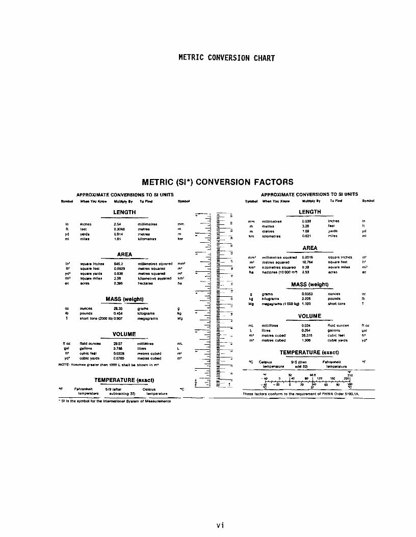
METRIC CONVERSION CHART
METRIC (51*) CONVERSION FACTORS
APPROXIMATE CONVERSIONS TO 51 UNITS APPROXIMATE CONVERSIONS TO SI UNITS
Symbol _VouK!tow "'ultiply 8, To find Symbol S,- _VouK!tow "'oII'ply By To And Sy .. ""
LENGTH LENGTH
mm mUUmetres 0.0311 inches in In Inches 2.54 mlillmel"'. mm 3.28 , ... , 't
It 'eet m metres
0.3048 1'tm1res m 1.09 yards
yd yards 0.91. m metres yo
metres m km kilometres 0.821 miles ml
ml miles 1.81 kilometres km
AREA AREA
mm' millimetres squared 0.0016 square: Inches Inl
In' ""uarelnch" &45.2 mllilmelr ... squared mm' m' metres squated 10.754 square teet f1'
It' squiNt feet 0.0929 metres squared m' km' il:ilomet,..s squared 0.311 square miles m,'
yd' aqu .... yards 0.836 metres squared m' b. Metor .. (10000 m'l 2.53 acres ac
ml' ""uor. miles 2.59 kilometres squared km' eo acr .. 0.395 _taras ha MASS (weight)
g grams 0.0353 ounce' oz
MASS (weight) kg kilograms 2.205 pounds Ib Mg mev-grams (1 000 kgt 1.103 short tons T
oz ounees 28.35 grams 11 Ib pounds 0..c54 kilograms kg
VOLUME T short tons (2OOIllbi 0.!)()7 megagrams. Mg
mL milUUtres 0.034 fluid ounees 110l
VOLUME L lUres 0.254 gaUOtIs gal
m' metres cubed 35.315 cubiC feet fI' m' metres cubed 1.308 cubic yard$ yd'
lIoz ffuld cunc ... 29.57 mllllllt_ ml gal gal'ons 3.785 IIt,..s L ft' cubic faa' 0.0328 metres cubed m' TEMPERATURE (exact) yd' oUbic y ... ds 0.0785 metres cubed m'
NOTE: Volumes greater than 1000 l. shan be $hown In m"'. "C CelsIus 915 (Ihan FaJuenht't 'F
temperatwe _32) temperature
Of "F 32 9U 212
TEMPERATURE (exact) -f· ,. '~"'I"'!"'bo""', ',':'l", ,,2?"J _AD i -to I 0 20' '60 80 100
Of' Fan"'nhilil 519(811 ... cefalul 'C 'C 37 'C
t.m~rature sub1rAQUno 32) temP4rature these f&(:tors conform to the reqt,liremenl 0' FHWA Order 5190_1A .
.. 51 te the symbol for the Internatlonat SYlt(tfl1 of Meuuremtmts
vi


TABLE OF CONTENTS
SUMMARY . . . . . . . . . . . . IMPLEMENTATION . . . . . . . . . . . . . CREDITS AND DISCLAIMERS . . . . . . METRIC CONVERSION CHART . . . . . . . . TABLE OF CONTENTS . LIST OF FIGURES . . LIST OF TABLES . .
· iii iv v
. . . . vi · vii
ix xi
I. INTRODUCTION . • . . . . . .. .... 1 I I . BACKGROUND . . . . . . . . . . . . 2
A. Terminology. . . . • . . . . . . . . . . . . . 2 B. Overview of Existing Testing Methods 4
Indirect Tension Devices . • .. .... 5 Predictive Models . . . . . . . . . . . 5 Nondestructive Methods . . . . 6
C. Materi a 1 Behavi or . . . . . . . 7 Temperature . . . . . . . . . . . .. 8 Component and Mix Properties 8 App 1 i ed Load . . . . . . . . . . . . 11 Specimen Type . • . . . • . . . . . . . .. 14 Test Type . . . . . . . . . . ..... 14
D. AAMAS. . . . • . . . . . . . . . . . . . . . . . . .. .... 16 Role of Resilient Modulus Testing in AAMAS . . . . . . . . . .. 21 Performance Evaluation Schemes in the Mixture Analysis Phase of
AAMAS . . . . . . . . . . . . . . . . . . . . . . . . . 23 Testing Procedures in AAMAS for Diametral Resilient Modulus. 27 Resilient Modulus as the AASHTO Design Parameter . . . 31 Relation of Resilient Modulus to Pavement Performance 37
III. APPARATUS DEVELOPMENT. . . . . . . . . .. ..... 39 A. Axial Loading Apparatus. . . . . . . . . 39 B. Indirect Tension (Diametral) Devices . . . . . . ... 42
Generalized Indirect Tension Device . . . . . 42 Rapid Diametral Testing Device . . .. ....... .... 45
IV. EMPIRICAL STUDY . . . . . . . . . . . . . . . . . . . 49 A. Experiment Design . . . . . . . . . . . . . . 49 B. Materi a 1 s and Methods . . . . . . . . 50
General Procedure for Axial Tests . . . . . . . . . . 53 General Procedure for Diametral Indirect Tension Tests 55
C. Test Results . . . . . . . . . . . . . . . . . . . . . . 60 Comparison of Diametral Devices . . . . . . . . . . . 60 Comparison of Axial versus Di~metral Resilient Moduli .... 64
V. CONCLUSIONS.. 69 VI. RECOMMENDATIONS...... . . . .. .... 71 VII. ACKNOWLEDGEMENT. . . . . 72 VI I I. REFERENCES . . . . . . . . . . . . . . . .. 72
APPENDIX A: DERIVATION OF DIAMETRAL RESILIENT MODULUS EQUATION APPENDIX B: TEST PROCEDURE . . . ... . APPENDIX C: USE OF TEST RESULTS .... . APPENDIX D: SUMMARIZED DATA . . APPENDIX E: MACHINE DRAWINGS . .
vii
75 77 97
· 104 124

Figure 1.
Figure 2.
Figure 3.
LIST OF FIGURES
Components of asphalt concrete material response as a function of temperature/frequency . . . . . . . . • .
Schematic of modulus versus temperature: (upper) polymer, (lower) asphalt .............. .
Variation of Poisson's ratio with temperature for an asphalt concrete ................. .
Figure 4. Schematic of phase relationships for asphalt concrete
Figure 5.
Figure 6.
Time dependent material response: (a) Step function loading, (b) response to step function loading, (c) haversine type loading normally used in resilient modulus testing. . ...................... .
Schematic of possible stress states to be applied in the laboratory to refine asphalt concrete constitutive models .......................... .
Figure 7. Conceptual flow chart illustrating the AAMAS procedure ..
Figure 8. Flow chart for the design of dense-graded asphalt concrete mixtures. . ....... .
Figure 9. Flow chart for the AAMAS procedure
Figure 10.
Figure 11.
Chart for estimating structural layer coefficient of dense graded asphalt concrete based on the elastic (resilient) modulus ................. .
Minimum tensile failure strains required for the mix as a function of resilient modulus ........... .
Figure 12. Chart for total resilient modulus versus temperature using indirect tensile loading conditions ..
Figure 13.
Figure 14.
Estimation of the fatigue factor to determine an equivalent annual resilient modulus ...... .
Typical deformation (horizontal or vertical) versus time relationship for repeated-load indirect tensile using a 'haversine' wave form with a rest period ........ .
Figure 15. Comparison of test results between unconfined compression
7
9
10
12
13
15
17
19
20
21
22
24
25
28
and indirect tensile tests ... . . . • . . . . . . . . . . .. 32
Figure 16. Comparison of resilient modulus measured on cores using different specimen holding devices and test equipment (Texas versus Baladi) ................ .
viii
33
Figure 17. Comparison of resilient moduli measured on cores using different specimen holding devices and test equipment (Texas versus Retsina) •....... . . . • . . . . . • . • • 33
Figure 18. Comparison of coefficient of variation for resilient moduli measured on cores using different specimen holding devi ces and test equi pment . . • . . . . . . 34
Figure 19. Thickness and modular influence on structural layer coefficient . . . . . . . . . . . . . . . . . . . . · . . . . 38
Figure 20. Axial measurement devices: (top) contact vertical LVOTs and remotely mounted noncontact radial transducers, (lower) contact sensors all directions.
Figure 21. Universal loading head for diametral test.
Figure 22. Gluing fixture for diametral loading strips.
Figure 23. Specimen with loading/gauging strips mounted.
Figure 24. Comparison of horizontal deflection measurements in the diametral test .................. .
Figure 25. Specimen centering and loading strip alignment device.
Figure 26. Installing specimen in yoke/centering device assembly.
Figure 27. Centering device with yokes and specimen in place.
Figure 28. Complete assembly of previous figure in testing machine with static seating load applied ........... .
Figure 29. Centering device removed and specimen and yoke assembly ready for testing. . ................ .
Figure 30. Theoretical stress distribution used for the diametral
·
·
41
· · · · 42
43
44
46
47
47
48
· · · · 48
· · · · 48
indirect tension test for Mr . . . . . . . . 57
Figure 31. Frequency dependence on field cores (Mopac, 77°F). . .... 65
Figure 32. Frequency dependence (Crushed limestone t AAM-1 AC20, Type Ct 77°F) ..................................... .
Figure 33. Comparison of axial resilient (dynamic) modulus with diametral resilient modulus means with 95 percent
66
confidence intervals. . . . . . . . . . . . . . . . . . . . . . . 66
Figure 34. Relationship between sample size and error tolerance (Type C, CLS, AAM-l AC-20) .................... 68
ix

Tabl e 1.
Table 2.
Table 3.
Table 4.
Table 5.
LIST OF TABLES
Summary of the approximate time required for the laboratory compaction, conditioning, and testing of asphalt concrete mixtures using AAMAS ...... .
Data acquisition - minimum response characteristics for resilient modulus tests ............... .
Summary of resilient modulus variations measured using different testing/holding devices .......... .
Summary of the difference between the instantaneous and total resilient modulus at different test temperatures.
Summary of indirect tensile test results for the field cores recovered immediately after construction ...
·
·
·
·
Table 6.
Table 7.
Summary of levels of aggregate and asphalt factors ....
Gradation requirements for Type 'e' coarse graded surface
Table 8.
Table 9.
course ..
Gradation requirements for Type '0' fine graded surface course ..
Device codes ......... .
Table 10. Analysis of variance for pneumatic versus hydraulic loading systems. . ... .
Table 11. ANOVA for lOT devices and mixtures ... .
Table 12. Analysis of variance for axial and diametral tests.
x
· · ·
· · ·
· · ·
· · ·
·
·
·
·
18
31
34
35
36
50
51
52
60
61
63
67


I. INTRODUCTION
The 'resilient modulus' of asphalt concrete is a single number that is used to describe material behavior and to predict pavement performance in many pavement design procedures. It is analogous to Young's modulus in the small strain theory of elasticity, which is one of two parameters needed to fully characterize a linear elastic, rate-independent material. The second parameter is Poisson's ratio.
Several techniques exist for determining resilient modulus. The most common methods are dynamic laboratory tests and nondestructive field tests (NDT). Both laboratory and field tests have limitations that include instrumentation problems, deviation of the actual procedure from the theory upon which the procedure is based, and wave propagation anomalies.
A rapid and consistent laboratory testing method should address these problems and should complement the field testing and evaluation program in pavement design and evaluation. New devices for laboratory testing were developed during this project to address the laboratory needs of the AASHTO Guide and to corroborate NDT results. They are intended for use primarily in the determination of the resilient modulus, but provisions for measurement of Poisson's ratio have been made as well.
This area of research is undergoing considerable change at the present time with the SHRP and AAMAS programs in the final stages of development. The developments in this project have been directed toward short term implementation and production, while maintaining long term flexibility to cope with new research findings.
1

II. BACKGROUND
An understanding of stress-strain behavior of the materials in a pavement structure is required for the prediction of stresses, strains, and deflections occurring under vehicle wheel loads. A portion of this behavior is expressed in terms of a quantity known as the resilient modulus of the material. This material property is used to characterize roadbed soil and asphalt bound materials for flexible and composite (asphalt concrete overlay on portland cement concrete slab) pavements in the AASHTO Pavement Design Guide (AASHTO 1986). Since a wide range of 'modulus' numbers exist in engineering, the next section is devoted to clarification of the modulus numbers and other terminology as used in this report.
A. Terminology
Chord modulus The slope of a line between any two points on a stress-strain curve.
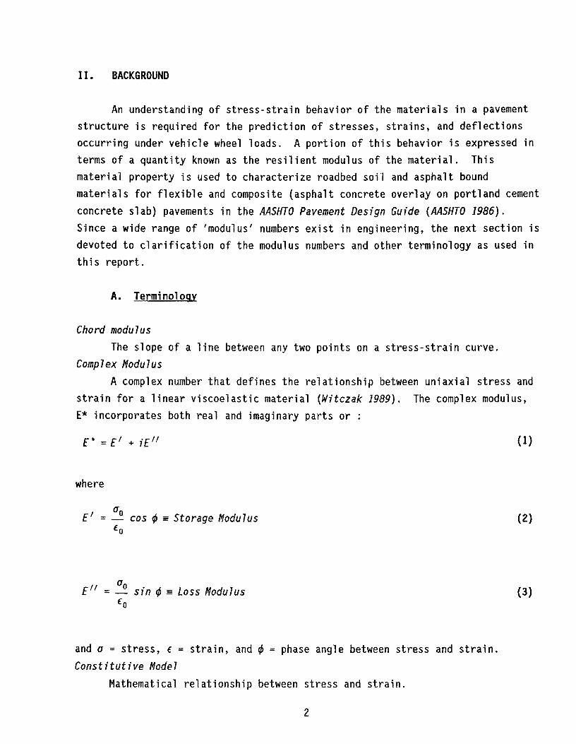
Complex Modulus A complex number that defines the relationship between uniaxial stress and
strain for a linear viscoelastic material (Witczak 1989). The complex modulus, E* incorporates both real and imaginary parts or :
£* = £' + i£"
where
0'0 £' = -- cos ~ = Storage Modulus
Eo
0'0 - -- sin ¢ = Loss Modu7us
Eo
and 0' = stress, E' = strain, and ~ = phase angle between stress and strain. Constitutive Model
Mathematical relationship between stress and strain.
2
(I)
(2)
(3)

Dilatant material A material that exhibits a change in volume when subjected only to simple
shear stress. Microcracking or very high Poisson's ratios and nonlinear stressstrain curves are often associated with this type of material. Dynamic Modulus
The magnitude of the complex modulus that defines the elastic properties of a linear viscoelastic material subjected to a sinusoidal loading, IE*I. Linear Material
A material whose stress to strain ratio is 'independent of the loading stress applied. Nonlinear material
A material whose stress-strain response is not linear. Plastic behavior
Material behavior in which some or all of the strain can not be recovered after unloading. Pulsed Loading
This loading is similar to the sinusoidal loading with introduction of a rest period after each load application as shown. Resilient Modulus
The resilient modulus MR is a dynamic test response defined as the ratio of the repeated axial deviator stress ad to the recoverable axial strain fa in a test involving uniaxial loading (Yoder & Witczak 1975). This is mathematically represented by the following equation.
ad E =-
ra E a
(4)
For uniaxial loading, this interpretation is essentially equivalent to the dynamic modulus. For the indirect tension case, the resilent modulus is the value obtained from the solution of the generalized Hooke's law for the loading and geometry used in the testing. In this case, the modulus is dependent on Poisson's ratio, v, and the deflection, as shown below.
~ = P(v + O. 732)/t5 (5)
3

Secant modulus The slope of a line between the origin and any other point on a stress
strain curve. Sinusoidal Loading
Load application from one stress level to another along a path that can be described by a simple sine function. Tangent modulus
The slope of a line tangent to the stress-strain curve at any point. Viscoelastic material
A material whose stress-strain response is nonlinear due to time dependent factors (e.g. viscous fluid flow).
B. Overview of Existing Testing Methods
The resilient modulus can be used directly in the design of flexible pavements. The AASHTO Pavement Design Guide suggests the use of the resilient modulus to characterize the materials in various pavement layers to estimate the values of the layer coefficients. Direct laboratory test procedures used to determine this property include, but are not limited to: (a) Direct Tension, (b) Beam Flexure, (c) Indirect Tension, (d) Triaxial Compression. Among the moduli resulting from these various test procedures are: (1) elastic or Young's, (2) shear, (3) bulk, (4) complex, (5) dynamic, (6) resilient, (7) double-punch, (8) flexural, (9) creep and (10) Shell nomograph moduli. Much research has focused upon simplification and refinement of the diametral and triaxial resilient modulus testing devices for use in material characterization {Brickman 1989}. These two types of devices are used in this research as well.
Each modulus and test procedure has different assumptions and limitations, and the real dilemma is how to determine which modulus to use in characterizing asphalt concrete structural pavement layers in various modes of pavement behavior (e.g. flexural, compressive, tensile). For example, layered elastic modeling of flexible pavements is widely used as a pavement design tool and as a pavement analysis tool. However, the results of multilayered elastic analyses are highly sensitive to the modulus used to characterize the asphalt concrete. Since the value of these moduli vary greatly even when evaluating the same material, the results of the multilayered design or analysis will also vary greatly depending on which modulus was used for characterization (Mam7ouk & Sarafin 1988).
4

Ind;rect Tens;on Dev;ces The indirect tension method of testing pavement cores has been in use for
some time. It has been used for both strength testing and resilient modulus testing of bound materials. Both types of test are basically the same geometry, and only the shape of the loading function is different.
Baladi (1990) designed an indirect tensile appartus that is capable of measuring deformations in three directions (along the vertical diameter, the horizontal direction, and the along thickness of the material of the specimen).
Schmidt (1972) developed a practical method for measuring resilient modulus of asphalt-treated mixtures. This method is rapid and economical. During the course of the test, dynamic load and total horizontal deformation are recorded. The resilient modulus is calculated using the following equation:
f\ = P(v + 0.273)/t6 (6)
A range of values for Poisson's ratio were assumed based on Sayegh's (1967) sonic experiments.
Maupin (1972) related results of indirect tensile tests to asphalt fatigue. The diametral device adopted by Maupin has a transducer to measure strain over a I-in gauge length. The maximum tensile strain is at the center of the specimen.
Hudson & Kennedy (1968) have summarized the advantages and disadvantages of several methods and used the indirect tensile test to characterize the strength of stabilized materials. Results of this test were utilized to evaluate the effects of such factors as composition and width of the loading strip, testing temperature, and loading rate on the parameters of strength, vertical failure deformation, and a modulus based on load and vertical deformation for asphalt stabilized materials. It was recommended by Hudson & Kennedy that the test be conducted utilizing a 1.0 in. wide stainless steel loading strip, loading rate of 2 in/min, and a test temperature of 77°F.
Predictive Models The predictive equation for lEI developed by Witczak (1989) is based upon
measured laboratory tests following the ASTM 03497 procedure for dynamic modulus. The equation is based upon over 20 years of cumulative laboratory test studies.
The method developed by the Shell Oil Company to determine the modulus of
5

an asphalt mix is based upon over 20 years of laboratory work. Nomographic solutions are used to obtain the properties of the bitumen. Several equations are used to convert these properties to the stiffness of the asphalt mix. The bitumen properties are dependent on origin, hardness, temperature susceptibility, temperature at the load condition, duration of load and rate of loading (Huekelom 1966, Van der Poe7 1965).
Nondestructive Methods Several nondestructive techniques are used in evaluating pavement systems.
The method developed by Heisley et a7. (1982) evaluates the moduli of the various materials in existing pavement systems, but seems to be best suited for measurements of the properties of the surface layer. Elastic waves are generated by steady-state vibrations or transient impulses, and they propagate through individual layers and/or the entire pavement structure. Frequency and phase content of the surface waves generated by the source are collected with spectral analysis equipment. Moduli and thicknesses are calculated from the velocities of the surface waves.
The Benkelman beam is one of the simpler nondestructive methods. A truck having an 18-kip load on the rear axle with dual tires (70-80 psi tire pressure) is normally used to load the pavement when using this device. Other vehicles with known wheel loads can be used for the test. In this method, rebound deflections of the pavements are measured when the truck moves away from the testing point.
The Road Rater is an electro-hydraulic vibrator capable of generating harmonic loads up to 8 kips (peak to peak) at driving frequencies between 6 and 60 Hz. A static preload of 5 kips is applied through 12-in circular loading plate while a vibrator is set at the testing point. The desired peak-to-peak load is then generated at a preselected driving frequency, and peak-to-peak deflections are recorded with velocity transducers (geophones).
The FWD (Falling-Weight Deflectometer) operates on impulse-loading principle. There are on the order of four types of FWD's presently in use (Bentsen et aT. 1989). Each FWD operates under the same basic loading principle and uses similar data collection techniques. A weight is raised mechanically and dropped on a set of rubber cushions, and the force is transmitted to the pavement through a steel plate. The resulting pavement movement is monitored with either velocity transducers or seismometers. The load pulse generally has a time period on the order of 20-100 milliseconds, depending on load level and the design of the device.
6

c. Material Behavior
The resilient modulus is a property that is similar in concept to the modulus of elasticity. Along with Poisson's ratio, it defines a portion of an elastic stress-strain relationship. However, results of many different types of tests indicate that the behavior of asphalt mixtures is influenced by factors such as temperature and other environmental conditions, loading frequency, mix properties, applied load and triaxial stress state, specimen type, and type of test. The reason for the dependency on the various factors is that asphalt concrete often exhibits a combination of elastic, time dependent, and plastic behavior in response to loading at in-service temperatures. The temperature and/or loading frequency controls the balance of what percentage of the response is elastic, what percentage is time dependent, and what percentage is plastic. The temperature and/or frequency also controls what portion of the failure mode can be described as brittle cracking and what portion of the failure can be attributed to higher degrees of ductile behavior. This can be illustrated schematically as in Figure 1 (Lytton 1991 unpublished).
MICROCAACK DAMAGE
Percent of SO Response
----o~~---+--~--~--~~~--+_-=~~ G~assy -2()OC -10°C aGe moe 200C 40°C sOGe
Temperature Stress-Free
-ercafl! grogale
P Ag B In
reakage Tension
Temperature
100 -..... ~
~i~ 0
low Temperature Cracktng Ductile Load Fatigue Separation
Tllermal Cooling I
Rutting I Thermal
\ Fatlguo
Fi gure 1. Components of asphalt concrete materi a 1 response as a function of temperature/frequency (after Lytton, unpublished).
7

Temperature Asphalts can be classed as thermoplastic materials because they gradually
liquefy when heated and become solid again on cooling. Their behavior is dependent on temperature. In this respect, asphalts are quite similar to many polymers. The thermoplastic property of the asphalt binder has a significant influence on the resilient modulus of asphaltic mixtures (Schmidt 1974). The dependency of the storage modulus on temperature for a polymer as compared to the resilient modulus of an asphalt material can be illustrated schematically as shown in Figure 2. The curve drawn for asphalt in part (b) of this figure corresponds roughly to the region labeled 'leathery' on the schematic for a polymer in part (a) of the figure. As the temperature decreases, the asphalt curve just begins to level off on the left side of Figure 2{b) which corresponds to the 'glassy' region at short loading times (or cold temperatures) in part (a), and there appears to be a very slight change toward the 'rubbery' shelf as the temperature increases in part (b) of the figure. Other studies at TTl have indicated that the rubbery shelf may be very small or nonexistent for most asphalt mixtures on the hot side and that the transition from the leathery region to the glassy region is not very well defined on the cold side.
The temperature effect extends to Poisson's ratio as can be seen in Figure 3. The theoretical limit of Poisson's ratio is 0.5. At temperatures above approximately 90°F, the figure indicates that Poisson's ratios greater than the theoretical limit are observed. This can be interpreted to be an indication of dilation and indicates that aggregate particle interaction becomes an important factor as the Viscosity of the asphalt decreases with increasing temperature.
Component and Mix Properties PhYSical and chemical properties of asphalt, aggregate, and composite
mixture have a vital influence on the dynamic response of asphalt concrete. The grade of asphalt is critical to the dynamic behavior of asphalt treated mixtures (Roque et al. 1987). Asphalt consistency is related to the type of asphalt. Consistency is a qualitative term used to describe viscosity or degree of fluidity (Penetration) at any particular temperature (TAl 1989). The high viscosity (low penetration) asphalts are called 'hard' asphalts because the material is relatively stiff (high modulus).
8

Glassy
9
6
5 Liquid L-____________________________________ -L __ __
log t
I
~" " ~,
"
i~ ~
\
" ", " ",
" "-" lXlO It " I .....
r
,
5S 70 100 litO
TEMPERATURE, of
Figure 2. Schematic of modulus versus temperature: (upper) polymer (Hertzberg 1983), (lower) asphalt (Nair et a7. 1972)
9

0.6
0 0.5 .... Eo<
~ !J)
:z: 0 !J) O.lt !J) .... 0 Q.
"'" Eo<
~ .... 0.3 >< 0 ~
V' Q. Q. « /
0.2
0.1 40
/' /'
/; I-'
;
55 70
.",..""'" ~--/
... /
100
TEMPERATURE, of
-- ----
140
Figure 3. Variation of Poisson's ratio with temperature for an asphalt concrete (Nair et a7. 1972)
10

When asphalt cement is exposed to air in thin films at elevated temperatures (e.g. during mixing with the aggregate), the asphalt tends to harden. Field measurements show higher viscosity values due to increased state of hardness. This effect is due to chemical and mechanical processes {e.g. oxidative hardening that occurs during mixing, laydown, and upon exposure to environmental conditions (Bell et a7. 1990, Goode & Owings 1961».
The gradation of the aggregate has a significant influence on the mix properties (Gemayel & Mamlouk 1988, Ishai & Gelber 1982). The type of aggregate (macro texture, crushed versus rounded, geologic source) often has a slightly less pronounced effect when compared to gradation. However, surface texture and particle angularity are often extremely important as well.
Other important mix property parameters are amount of asphalt and air voids. Amount of asphalt is expressed by weight or volume percentages. Generally as the asphalt content increases, the modulus of the mix decreases (taking other parameters into account). The percent asphalt and air voids in a mix are inversely related (Gemayel & Mam70uk 1988). As the percentage of asphalt content increases, the percentage of air voids decreases. During the process of mixing and compacting, a portion of asphalt is aborbed by the mineral aggregates. This absorption is less influential than the properties at the asphalt-aggregate interface and the asphalt film on the physical response of the mix. Illustrated in Figure 4 is a schematic of the relationship between percent air voids and percent asphalt content.
Applied Load One of the most important factors affecting the modulus of the asphalt
treated materials is duration of applied dynamic load. It is observed that, at constant mix conditions (temperature, confining pressure and magnitude of load), the modulus of the mix decreases with the increase of the duration of applied dynamic load. This characteristic of the asphalt treated mixtures makes it necessary to estimate the loading time applied by vehicles to be simulated in the laboratory. Alternatively, a complete frequency spectrum characterization may be undertaken. To see why the load duration makes such a difference, Figure 5 should be consulted. Part (a) of the figure shows a square pulse stress application. The strain response to this loading for a typical polymer or asphalt concrete is shown in part (b) of the figure in which E indicates the elastic part of the response, P is the plastic part of the response, and V
indicates a time dependent ('visco-f) effect. Finally, part (c) of Figure 5 illustrates the two most common waveforms used in resilient modulus testing. The
11

waveforms shown in part (c) of the figure will not induce a response like that illustrated in part (b) of the figure; instead, they will induce a response similar to that shown later in the report (see Figure 14).
~ Air { t Va
As J I J t ~ Vr phalt r b
Vba
t Vmb
Aggregate -oj Vsb Vse Vmm
" V ma Volume of voids in mineral aggregate and effective asphalt V mb Volume of compacted specimen V mm Voidless volume of paving mix Va = Volume of air voids Vb Volume of asphalt Vba Volume of absorbed asphalt Vbe :0 Volume of effective asphalt V sb = Volume of aggregate (by bulk specific gravity) V se = Volume of aggregate (by effective specific gravity) Wb Weight of asphalt W s = Weight of aggregate y w Unit weight of water 1.0 g/cm3 (62.4 Ib/ft3)
Gmb = Bulk specific gravity of compacted paving mixture sample
Figure 4. Schematic of phase relationships for asphalt concrete (TAl 1990).
12

.!;; 'JE 0 + ... (i) lIP
E+P
E
! f
\IE
! f
vp+p
(0)
~
Time
(b)
~
Time
~
Time
(c)
Figure 5. Time dependent material response: (a) Step function loading, (b) response to step function loading, (c) haversine type loading normally used in resilient modulus testing.
13

The type of truck {vehicle} affects the load duration as well as the rest period between loadings. Wheel spacing affects the relaxation time in the application of pulsed loading. There is a stress overlap between wheel loads on dual wheel and tandem axle truck configurations.
Specimen Type The geometry of the specimen and the mode of compaction can have a
significant impact on the dynamic response of the asphalt materials. Often, there are differences associated with the method of compaction (impact, rolling wheel, kneading compactor and Texas gyratory) used in the laboratory and specimens cored from field sites (Consuegra et a7. 1989).
The specimen geometry governs the analysis procedure. The dimensions associated with each geometry are governed by the maximum size of the aggregate. Normal practice in the laboratory is to limit the maximum size of the aggregates to 1 inch for a 4 inch diameter specimen. This 4:1 ratio is used to try to avoid adverse effects from the mold during the compaction process (i.e. hindrance of effective densification) and to avoid altering the true failure mechanism during testing. The 4:1 ratio is somewhat smaller than that normally used in geotechnical circles, but the asphalt mix is usually stiffer than soils, and the size distribution is also important in the decision. In fact, if the smallest dimension is used to specify the size ratio, the ratio becomes 2:1 for the indirect tension test.
Test Type The most popular techniques in practice are direct compression and indirect
tension. Results from the previous research show that moduli obtained from direct compression and direct tension are equal if the stress level is sufficiently low. These tests are generally conducted on 4 inch diameter by 8 inch tall specimens. However, many pavements are not 8 inches thick, and those that are at least that thick are almost never homogeneous through the thickness. One solution to this problem is to test short cores using a 'brush platen' type loading surface as described in Appendix B of this report. Another successful approach is to take a large diameter core from the pavement and then core the specimen again, along the diameter this time.
In some instances, confining pressure is applied during the test to develop relationships that cover a wide range of stress states on Mohr's diagram as illustrated schematically in Figure 6. These relationships are then used to refine the constitutive models in mathematical pavement design and evaluation computer programs.
14

Shear
\ Normal Stress
Figure 6. Schematic of possible stress states to be applied in the laboratory to refine asphalt concrete constitutive models.
15
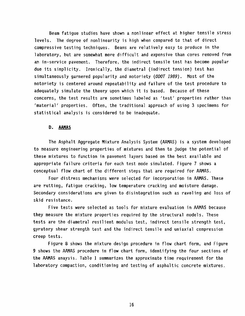
Beam fatigue studies have shown a nonlinear effect at higher tensile stress levels. The degree of nonlinearity is high when compared to that of direct compressive testing techniques. Beams are relatively easy to produce in the laboratory, but are somewhat more difficult and expensive than cores removed from an in-service pavement. Therefore, the indirect tensile test has become popular due its simplicity. Ironically, the diametral (indirect tension) test has simultaneously garnered popularity and notoriety (ODOT 1989). Most of the notoriety is centered around repeatability and failure of the test procedure to adequately simulate the theory upon which it is based. Because of these concerns, the test results are sometimes labeled as 'test' properties rather than 'material' properties. Often, the traditional approach of using 3 specimens for statistical analysis is considered to be inadequate.
D. AAMAS
The Asphalt Aggregate Mixture Analysis System (AAMAS) is a system developed to measure engineering properties of mixtures and then to judge the potential of these mixtures to function in pavement layers based on the best available and appropriate failure criteria for each test mode simulated. Figure 7 shows a conceptual flow chart of the different steps that are required for AAMAS.
Four distress mechanisms were selected for incorporation in AAMAS. These are rutting, fatigue cracking, low temperature cracking and moisture damage. Secondary considerations are given to disintegration such as raveling and loss of skid resistance.
Five tests were selected as tools for mixture evaluation in AAMAS because they measure the mixture properties required by the structural models. These tests are the diametral resilient modulus test, indirect tensile strength test, gyratory shear strength test and the indirect tensile and uniaxial compression creep tests.
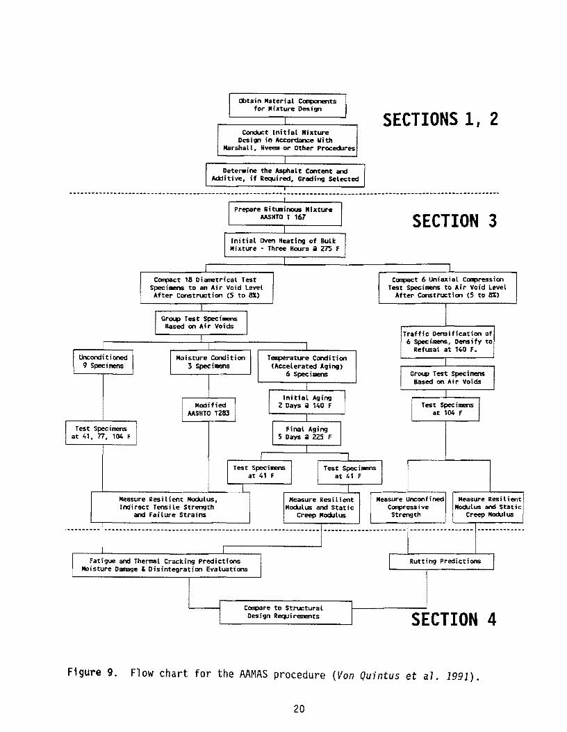
Figure 8 shows the mixture design procedure in flow chart form, and Figure 9 shows the AAMAS procedure in flow chart form, identifying the four sections of the AAMAS anaysis. Table 1 summarizes the approximate time requirement for the laboratory compaction, conditioning and testing of asphaltic concrete mixtures.
16

STRUCTURAL DESIGN OF ASPHALT CONCRETE PAVEMENTS
PERFORMANCE FUNCTIONS OF MODELS TO PREDICT CRITICAL MATERIAL PROPERTIES AND PARAMETERS FOR MIX DESIGN
REDESIGN . STRUCTURE
USING RESULTS FROM
LABORATORY
FATIGUE CRACKING RUTTING
low-TEMP CRACKING
MOISTURE DAMAGE
SET CRITERIA FOR MIX DESIGN PARAMETERS
SAMPLE PREPARATION/CONDITIONING
TEST PROCEDURES TO MEASURE THOSE CRITICAL PARAMETERS
MODIFY MIX (USE ADDITIVES)
Figure 7. Conceptual flow chart illustrating the AAMAS procedure.
17
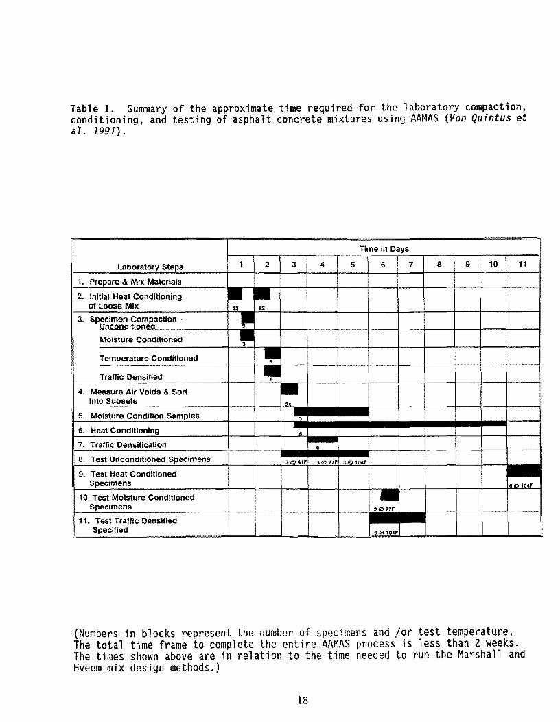
Table 1. Summary of the approximate time required for the laboratory compaction, conditioning, and testing of asphalt concrete mixtures using AAMAS (Von Quintus et aT. 1991).
Time in Days
La .. ',".UUI y Steps 1 2 3 4 5 6 7 8 9 10 11
1, r '''' ..... ' '" & Mix Materials
2. Initial Heat Conditioning of Loose Mix 12 12
'" _ .. ._0' 3, ''''0: '.:" .-
Moisture Conditioned
Temperature Conditioned
Traffic Densified
4. Measure Air Voids & Sort Into Subsets
?4~ 5, Moisture Condition Samples
6. Heat Conditioning "
7, Traffic Densification II
8, Test Unconditioned Specimens 3 t1i) 41f --9. Test Heat Conditioned ...... "' ... " It::U~ ISla) 104F
10. Test Moisture Conditioned
~ Specimens
11. Test Traffic Densified Specified
(Numbers in blocks represent the number of specimens and jor test temperature. The total time frame to complete the entire AAMAS process is less than 2 weeks. The times shown above are in relation to the time needed to run the Marshall and Hveem mix design methods.)
18

Sample & ObUin Material Components for r- Mixture Des Ign f-
Asphalt. Aggregate. Minerai Filler. Additive,
Measure & Define the Physical Measure & DefIne the Physical Characteristics of the Characteristics of the
Aggregates, as Required by Asphalt. as Required by the the Specifications Specifications I
~ SELECT INITIAL AGGREGATELJ BLEND & RANGE OF ASPHALT CONTENTS
I Prepare e Iturninous Mixtures I at Each Selected Alpha 1t Content
I I INITIAL AGING OF LOOSE MIXTURE I
I Compact ion of Three To Hlne
Specimens at Se lected Aspha It Content
I ; Measure All" Voids. lInlt \leight, I
VHA, and Other Propert les
I Tratf Ic Dens if Ication of I Spec lmen! to Refu!a I
RESISTANCE TO I RESISTANCE TO RESISTANCE TO FRACTURE SHEAR DISPLACEMENT UNIAXIAL DEFORMATION
Indirect Tensile Tests Gyratory Testing Machin. Unconfined Uniaxial
" 71 F " 140 F Canpress ion Tests II 104 F
Resi Hent Modulus, Strength Gyratory Shear Stress Res I 11ene IIOdu Ius, Compress I ve and Failure Strains and Strains Strength and Fl\lure StraIns.
and Creep Modulus
Measure All" Voids, ...... Unit Weight, VMA, and Other r-Properties
-{SELECT DESIGN ASPHALT CONTENT ~
Figure 8. Flow chart for the design of dense-graded asphalt concrete mixtures (Von Quintus et a7. 1991).
19
I Unconditioned I 9 Spec j mens
I Test Specimens I at 41, 77, 104 F
I Obtain Material Camponents I for Mixture Design
I Conduct Initial Mixture
Design in Accordance Vith Marshall, Hveem"or Other Procedures
I I DeterMine the Asphalt COntent and I I Additive, if Ret?Jired, Grading ~lec:ted
I Prepare BitUlinous Mixture / MSHTO T 167
I Initial OVen Heating of Bulk I Mixture - Three Hours a 275 F
I compact 18 Diametrical Test
Specimens to an Air Void Level After Construction (5 to ax)
I
/ Group Test Specimens Based on Air Voids
/
I I I I Moisture Condition Temperature Condition
3 Specimens (Aceelerated Aging) 6 Spec: imens
I
I Initial Aging
I I Modified I 2 Days a 140 f MSHTO T283
I Final Aging
I 5 Days a 225 F
I I I
SECTIONS 1, 2
SECTION 3
I Compact 6 Uniaxial Coq:Iression
Test Specimens to Air Void level After Construction (5 to ax)
Traffic Densification of 6 Spec:illlel"lS, Density to
Refusal at 140 F.
I Group Test Spec: i mens Based on Air Voids
I
I Test Specimens I
at 104 f
I Test specimens I at 41 F
l Test Specimens / at 41 F
l I Measure Res it i ent Modulus, Measure Resilient Measure Unconfined Measure Resil ient Indirect Tensile Strength Modulus and Static CoII1>ress i ve Modulus and Static
and Failure Strains Creep Modulus Strength Creep Modulus
. __ ....... ---- ---------------------------------------------------------/---------------------- ----.-.. ~--- ..... -- ........ _----- ..........
L
I Fatigue and Thermal Cracking Predietions
I I Rutting Predictions I Moisture Damage & Disintegration Evaluations
I Compare to Structural I
I Design Ret?Jirements I SECTION 4
Figure 9. Flow chart for the AAMAS procedure (Von Quintus et a7. 1991).
20

Since this report is concerned with the development of a resilient modulus test procedure and accompanying equipment to reliably measure resilient moduli of densely graded asphalt concrete mixtures, the resilient modulus testing phase of AAMAS is of concern only. Therefore, the role of resilient modulus testing in AAMAS and the pertinent findings from resilient modulus evaluation during the AAMAS procedural development at Brent Rauhut Engineering and Texas A&M University will be discussed here.
Role of Resilient Modulus Testing in AAMAS AAMAS is divided into two broad segments: mixture design and mixture
evaluation. In the mixture design segment of testing, the role of the resilient modulus test is to provide an approximation of the AASHTO structural layer coefficient and to provide an approximation of the fatigue charactersitics of the mixture.
The AASHTO 1986 Guide for the Design of Pavement Structures provides a relationship between resilient modulus and structural layer coefficient of the asphalt concrete to be used as the surface course and the structural layer coefficient. This relationship is shown in Figure 10.
0.5
0.0
I I I I I
I- V"-../'
/ I- / -
- / -
I- -
-I l I I J I
, o 100.000 200,000 300.000 400.000 500,000
Elastic Modulus, EAC (psi). of Asphalt Concrete (at 68 0 F)
Figure 10. Chart for estimating structural layer coefficient of dense graded asphalt concrete based on the elastic (resilient) modulus (Von Quintus et aI. 1991).
21

Ironically, this relationship was developed based on the uniaxial resilient modulus (Van TiT et aT., 1972), but the 1986 Design Guide requires the diametral resilient modulus (ASTM D 4123). These two approaches are similar to Method C and Method B, respectively, of the proposed test procedure in Appendix B of this report. Since the Guide requires the indirect test approach for input to Figure 10, Method B would be the corresponding procedure. Appendix C contains more discussion on this topic. An acceptable mixture design in this phase of AAMAS is based on the asphalt content, or mixture components in general, that produce the minimum acceptable AASHTO structural layer coefficient.
In the mixture design phase of AAMAS, the total diametral resilient modulus is used in conjunction with the strain at failure in the indirect tensile test to predict fatigue potential. Figure 11 is used to plot the relationship between indirect tensile total resilient modulus and indirect tensile strain at failure for each asphalt concrete mixture design. Those asphalt contents that fall above the minimum design relationship are assumed to meet the minimum fatigue cracking criteria.
40
30
-A :0 ~
~
~ ~
~
< ~ 10 ~ ~
8
~ ~ ~
~
~ z 4 ~ ~
3 -
2
.6 .3 1 2 4 6 8 10 20 40 60
LOG TOTAL RESILIENT MODULUS, psi x 105
Figure 11. Minimum tensile failure strains required for the mix as a function of resilient modulus (Von Quintus et a7. 1991).
22

In the mixture analysis phase of AAMAS, diametral resilient modulus testing is used to predict mixture performance acceptability based on unconditioned specimens, moisture conditioned specimens, and temperature conditioned specimens.
Unconditioned specimens are tested at 41, 77 and 104°F in accordance with ASTM 0 4123. The specimens are preconditioned by applying a repeated 'haversine' load to the specimen without impact using a loading frequency of 1 Hz for a minimum period sufficient to obtain uniform deformation readout (less than two percent deviation). A preconditioning time of of 25 to 45 seconds is sufficient in most cases.
The fixed load to be used in the diametral repeated load resilient modulus test for each test temperature can be selected by using elastic layer theory to calculate the tensile stress and strain at the bottom of the asphalt concrete layer. For those conditions where the asphalt concrete layer is in compression (i.e. asphalt concrete overlays), the fixed load applied to the specimen should be of a sufficient magnitude to result in a horizontal deformation greater than 0.0001 inches. In most cases, the load established by these criteria wlll induce a tensile stress in the specimen in the range of 5 to 20 percent of the indirect tensile strength.
Following preconditioning, the total resilient modulus is measured in accordance with ASTM 0 4123 along two orthogonal axes at a loading frequency of 1 Hz. The lower value of resilient modulus is to be used. After the resilient modulus of the unconditioned specimens is determined at each temperature, the indirect tensile strength is measured at a loading rate of 2 inches per minute. The values of resilient modulus and indirect tensile strength are used in Figure 11 to determine the fatigue cracking potential (or acceptability) of the mixtures evaluated.
Resilient modulus testing is used following moisture and temperature conditioning. The primary purpose of resilient modulus testing following moisture conditioning is to identify the critical axis for testing in order to determine the indirect tensile strength which, in turn, is used to determine the tensile strength ratio. Testing following temperature conditioning in the resilient modulus mode is used primarily to identify the low temperature cracking and fatigue cracking potential of mixtures at the low test temperature of 41°F.
~erformance Evaluation Schemes in the Mixture Analysis Phase of AAMAS Four performance evaluation scheme.s are included in the mixture analysis
phase of AAMAS which employ the diametral resilient modulus test. The procedural schemes include: the fatigue evaluation (Figure 11), the resilient modulus versus
23

temperature accepability analysis (Figure 12), the weighted average structural layer coefficient analysis (Figure 13) and the thermal fracture analysis.
The flexural fatigue anlysis is essentially the same as that discussed in the mixture design section (Figure 8). Figure 12 is used to ascertain if the relationship between the diametral resilient modulus and temperature is within the band deemed to be acceptable. If the modulus is above the upper limit of this band, then the mixture is too stiff and fatigue and/or thermal cracking may be a problem. If the mixture is too soft and the resilient modulus versus temperature relationship plots below the lower limit, then the mix is deemed too soft and hence does not adequately protect the underlying layers or may be succeptable to deformation.
1.0 o
100.0
0.4
a ~e nt Mod.ulus b too
.............. High
""'" r-... r--........ '" ~
i'.... "" ......
"' '\. I'\.. " "\. " " '-.
'\ ............. '-
Area,~ tl.ere the ~ Total ellillent '-. Modul\ ~ is Too
F I I I
o 20 40 60 80 100 120
Temperature, F
Figure 12. Chart for total resilient modulus versus temperature using indirect tensile loading conditions (Von Quintus et a7. 1991).
24

Figure 13 is used to calculate the weighted annual structural layer coefficient. One technique that can be used to evaluate the environmental effects on the structural design is to consider seasonal fatigue damage. From the annual damage, an equivalent asphaltic concrete resilient modulus can be calculated by the following equation:
(7)
where ERE is the equivalent resilient modulus based on a fatigue damage approach, ERt is the total resilient modulus as measured in accordance with ASTM D 4123 at the pavement temperature for season i and FF is the fatigue factor obtained from Figure 13.
100
IQ C
'" H I'-.. iii ~ ~ Ii' :::I '3 '" 0
~ .........
"'- t'-.... ::. .... ~ CD a IIQ CD 10 ~
"'f'-.
~ r---... 'il .... '-
r"": 0 .....
E-< CD I I r-.
== a CD
E-<
I I ~ ............
i'..... .... 0 tl
~ S
~ r-.... f,.. ~r-.
1 0.010 , 0.100 1.000
Fatigue Factor
~
"r-.
10.000
Figure 13. Estimation of the fatigue factor to determine an equivalent annual resilient modulus (Von Quintus et a7. 1991)
25

Equation 7 includes only the damage associated with fatigue cracking and ignores any damage caused by permanent deformation and disintegration. Through the use of the fatigue factor, the equation allows seasonal and environmental effects to be used in estimating the AASHTO structual layer coefficient.
The step-by-step procedure that can be used to ensure that the asphaltic concrete mixture meets or exceeds the layer coefficient assumed during structural design is as follows:
* Obtain the seasonal average pavement temperature (for each season).
* Determine the total resilient modulus at each seasonal temperature.
* Obtain the fatigue factor for each seasonal resilient modulus from Figure 13.
* Calculate the equivalent resilient modulus using equation 7.
This equivalent resilient modulus should equal or exceed the modulus value used to estimate the AASHTO structural layer coefficient used for design.
The tendency of a mixture to fracture due to thermal fluctuations in the AAMAS process is evaluated by means of the following relationship:
(8)
where T is the critical change in temperature at which cracking occurs, Ect(T i )
is the indirect tensile creep modulus measured at temperature Ti' Eo is a regression constant, tr is the relaxation time, aA is the thermal coefficient of volume change, Eo(Ti) is the intercept of the indirect tensile creep curve at temperature Ti' nc is the slope of the indirect tensile creep relationship and nt
is the slope of the relationship between indirect tensile strength and total resilient modulus of the mixture at temperatures of 41, 77 and 104°F (unconditioned). Therefore, the indirect tensile resilient modulus (ASTM D ¢123)
26

is of significant importance as the relationship presented in equation 8 is quite sensitive to the slope of the relationship between resilient modulus and indirect tensile strength of the mixture at the three test temperatures.
Testing Procedures in AAMAS for Diametral Resilient Modulus The general testing procedure in AAMAS for samples tested for resilient
modulus in the indirect tensile mode is discussed in the following paragraphs. Place the test specimen in the loading apparatus, position as stated in
Test Method ASTM D 4123, adjust and balance the electronic measuring system, as necessary.
Precondition the specimen by applying a repeated haversine (or other suitable wave form) to the specimen without impact, using a loading frequency of 1 cps (O.l-sec load duration and O.g-sec rest period) for a minimum period sufficient to obtain uniform deformation readout (less than 2 percent deviation). In most cases, a preconditioning time of 25 to 45 sec is sufficient (25 to 45 loading cycles). The fixed load applied to the specimen is that which will result in a horizontal deformation greater than 0.0001 in. {0.00254 mm}. Normally, the load established by this criterion will induce a tensile stress in the range of 5 to 20 percent of the indirect tensile strength.
After preconditioning, measure the total and instantaneous resilient deformations for the next three loading cycles along each of two previously marked orthogonal axes. A loading frequency of 1 cps (O.l-sec load duration and 0.9-sec rest period) shall be used. The total resilient modulus is the parameter used for mixture design. The instantaneous resilient modulus is used for information purposes only. The total resilient horizontal deformation shall be measured in accordance with ASTM 0 4123. The instantaneous resilient horizontal deformation shall be measured at the time defined as twice the time interval from load application (or horizontal movement) to peak horizontal movement {see Figure 14}.
For each specimen tested, calculate the total resilient modulus, ERT , for the last 3 cycles after preconditioning. The instantaneous resilient modulus can be calculated for information purposes, if needed.
(9)
27
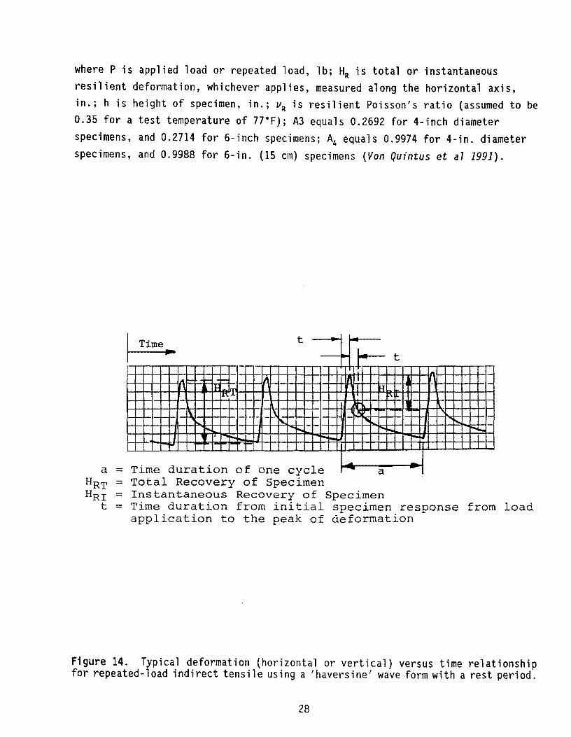
where P is applied load or repeated load, lb; HR is total or instantaneous resilient deformation, whichever applies, measured along the horizontal axis, in.; h is height of specimen, in.; vR is resilient Poisson's ratio (assumed to be 0.35 for a test temperature of 77°F); A3 equals 0.2692 for 4-inch diameter specimens, and 0.2714 for 6-inch specimens; A4 equals 0.9974 for 4-in. diameter specimens, and 0.9988 for 6-;n. (15 cm) specimens (Von Quintus et a7 1991).
a HRT HRI
t
= = = =
Time duration of one cycle a Total Recovery of Specimen Instantaneous Recovery of Specimen Time duration from initial specimen response from load application to the peak of deformation
Figure 14. Typical deformation (horizontal or vertical) versus time relationship for repeated-load indirect tensile using a 'haversine' wave form with a rest period.
28

A general description of the apparatus required for resilient modulus testing in accordance with the AAMAS guidelines is discussed in the following paragraphs.
Any loading machine capable of providing a repetitive sinusoidal or square type compression load of fixed cycle and duration can be used. Typically, a cam and switch or timer control of solenoid valves operating a pneumatic air piston, or a closed-loop electrohydraulic system is used. Pneumatic systems are the simplest, while closed-loop electrohydraulic systems allow more versatility {variable wave forms, higher loads, and higher frequency response}. Generally, a haversine wave form is characteristic of closed-looped electrohydraulic equipment, while rectangular wave forms are used with pneumatically operated loading equipment. Both wave forms can be used for the resilient modulus test. The two waveforms will give similar results if the load level and duration of loading are sufficiently small and the duration of the rest period is sufficiently long that the effects of time dependent and plastic behavior do not overshadow the approximation of the elastic response in the analysis. It is often the case that a pneumatic system that is being commanded to deliver a square wave will actually deliver something between a square wave and a sine wave anyway (at the loading frequencies typically used for resilient modulus testing). A loading frequency of 1 cycle per second has been found to be satisfactory for most applications. With a pneumatic loading system, a square wave form with a load duration of 0.1 second and a rest period of 0.9 seconds is recommended.
The resilient modulus, creep modulus and indirect tensile strength tests require deformation transducers with a sufficient range to cover the cumulative deformation during the test and also a high resolution for the smallest resilient strains to be measured. The linear variable differential transformer (LVOT) is generally considered to be the most suitable deformation transducer for the test. Table 2 provides the required accuracy of the axial deformation measurement device.
LVOT Clamps are used to hold the LVOTs in place during indirect tensile testing. There are different sample holding devices that can be used in the test program. One such device is described in ASTM 0 4123, and another in Federal Highway Administration Report No. FHWA/RO-88/118. Either of these devices can be used provided that the specimen has smooth surfaces, and is centered under the axial load (i.e., no load eccentricity). For uniaxial compression loading, LVOT clamps are not required if a friction reducing material is placed between the specimen and top and bottom platens. Thin teflon tape can be used as a friction
29

reducing material. The axial load measuring device is an electronic load cell. The load may
be measured by placing the load cell between the specimen cap and the loading piston. The total load capacity of the load transducer (load cell) should be of the proper order of magnitude with respect to the maximum total loads to be applied to the test specimen. Generally, its capacity should be no greater than five times to the total maximum load applied to the test specimen to ensure that the necessary measurement accuracy is achieved. The minimum performance characteristics of the load cell are presented in Table 2. The axial loadmeasuring device shall be capable of measuring the axial load to an accuracy within 1 percent of the applied axial load.
Specimen behavior is evaluated from continuous time records of applied load and specimen deformation. Commonly, these parameters are recorded on a multichannel strip-chart recorder. Analog to digital data acquisition systems may be used provided that data can be converted later into a convenient form for data analysis and interpretation. Fast recording system response is essential if accurate specimen performance is to be monitored. It is recommended that the response characteristics in Table 2 be satisfied.
For analog strip-chart recording equipment, the load and deformation recorder trace must be of sufficient amplitude and time resolution to enable accurate data reduction. Resolution of each variable should be better than 2 percent of the maximum value being measured. To take advantage of recorder accuracy and for subsequent data analysis, 2 to 4 cycles per inch of recording paper is acceptable. The clarity of the trace with respect to the background should provide sufficient contrast and minimum trace width, so that the minimum resolution of 2 percent of the maximum value of the recorded parameter is maintained, and the trace should be included in the reports.
For uniaxial compression testing, the number of recording channels can be reduced by wiring the leads from the LVDTs so that only the average or total signal from a pair is recorded. For indirect tensile loadings, the signal from each LVDT shall be recorded separately. This permits observation of individual lVDT readings, rather than an average or total signal, to determine if significant differences are being recorded between the two lVDTs. If the differences between LVDTs is large, the specimen shall be repositioned.
30

Table 2. Data acquisition - minimum response characteristics for resilient modulus tests (Von Quintus et al. 1991).
Analog Records
Recording Speeds: 0.5 to 50 cm/sec (0.2 to 20 in./sec) System Accuracy (include linearity and hysteresis); 0.5%'
Fre~uency Response: 100Hz
Measurement Transducers
Minimum Sensitivity, mv/v
Nonlinearity, % Full Scale
Hysteresis, % Full Scale
Repeatability, % Full Scale
Thermal Effects on Zero Shift or sensitivity, % of Full Scale /F(c)
Maximum Deflection at Full Rated Value in Inches (mm)
Load Cell
2
+0.25
+0.25
+0.10
+0.005 (+0.025)
0.005 (0.125)
Displacement2
0.2 mv/0.25 mm/v (AC LVDT)
(5mv/0.025 mm/v) (DC LVDT)
+0.25
+0.0
+0.01
1 System frequency response, sensitivity, and linearity are functions of the electronic system interfacing, the performance of the signal conditioning system used, and other factors. It is, therefore, a necessity to check and calibrate the above parameters as a total system and not on a component basis.
2 lVDTs, unlike strain gauges, cannot be supplied with meaningful calibration data. System sensitivity is a function of excitation frequency, cable loading, amplifier phase characteristics, and other factors. It is necessary to calibrate each lVDT-cable-instrument system after installation, using a known input standard.
Resilient Modulus as the AASHTO Design Parameter In the 1986 AASHTO Pavement Design Guide, the resilient modulus at 68°F is
used to estimate the AASHTO layer coefficient for pavement thickness design. The chart used to approximate the structural layer coefficient in the 1986 Design Guide was actually based on the resilient modulus determined on cylindrical samples tested in compression in accordance with ASTM D 3497. However, the 1986 Design Guide allows for the determination of resilient modulus in either the compressive or diametral (ASTM D 4123) mode. This is unusual, since there can be substantial differences between moduli measured in the compressive and diametral directions (especially if loading is carried past the level at which strains are
31
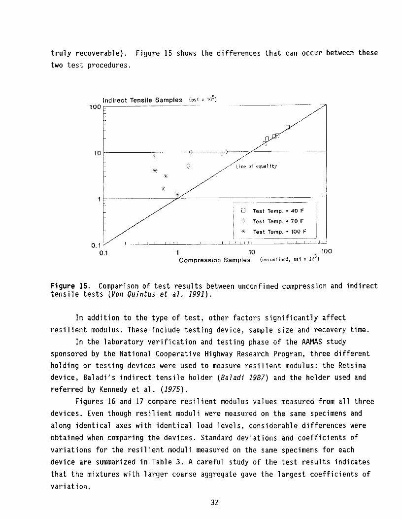
truly recoverable). Figure 15 shows the differences that can occur between these two test procedures.
Indirect Tensile Samples (psi x 105
)
100 -----...... ~-
10~--------~*------~-----.~--~/----------J
* o
* . Line of equality
Test Temp .• 40 F
Test Temp .• 70 F
Test Temp .• 100 F
O. 1 .-L--_L_ ... ~I--L--'--'-I .-'-1--,-1 ..LI .1.-1 __ '----L-I L ... L ... L...L.L .. LI __ ~---L---L..-L-.L' ...L' .J.....W
0.1 1 10 100 Compression Samples (unconfined, Dsi x 10
5)
Figure 15. Comparison of test results between unconfined compression and indirect tensile tests (Von Quintus et a7. 1991).
In addition to the type of test, other factors significantly affect resilient modulus. These include testing device, sample size and recovery time.
In the laboratory verification and testing phase of the AAMAS study sponsored by the National Cooperative Highway Research Program, three different holding or testing devices were used to measure resilient modulus: the Retsina device, Baladi's indirect tensile holder (8aladi 1987) and the holder used and referred by Kennedy et al. (1975).
Figures 16 and 17 compare resilient modulus values measured from all three devices. Even though resilient moduli were measured on the same specimens and along identical axes with identical load levels, considerable differences were obtained when comparing the devices. Standard deviations and coefficients of variations for the resilient moduli measured on the same specimens for each device are summarized in Table 3. A careful study of the test results indicates that the mixtures with larger coarse aggregate gave the largest coefficients of variation.
32

Resilient Modulus - Baladi's Holder, ksi 500~------------------------------------------------~
X 400 -
S 0
300 I-
X 200 '- * X *X*O
* * * 100 I-
X
** 0
*
o
* Wyoming
o Virginia
X Colorado
I 0 Michigan
O~ __ ~I ____ ~i _____ ~I __ ~I _____ ~i __ ~ ____ ~ ____ ~i _____ ~I __ __
o 50 100 150 200 250 300 350 400 450 500 Resilient Modulus - Texas Holder, ksi
Figure 16. Comparison of resilient modulus measured on cores using different specimen holding devices and test equipment (Texas versus Baladi, after Von Quintus et a7. 1991)
Res. Modulus-Retsina Device, ksi 1200.-----------------------------------------------~
1000 -
800 I-~ .
600 1--
400 i-~~~.
* 200 l-
0 0 100
o
*x
* X o 0 **<>* ~
I
200 300
0
(5
400 500
* Wyoming
o Virginia
o Colorado
X Michigan
J J
600 700
Resilient Modulus - Texas Holding Device (ksi) 800
Figure 17. Comparison of resilient moduli measured on cores using different specimen holding devices and test equipment (Texas versus Retsina, after Von Quintus 1991)
33

Table 3. Summary of resilient modulus variations measured using different testing/holding devices (Von Quintus et aI. 1991)
Testing Device Mixture Average Value
Standard Saladi Retsina
CO-0009 Std. Deviation 107 224 220 Coefficient of Variation, % 40 37 48
MI-0021 Std. Deviation 1 14 73 Coefficient of Variation, % 0.3 4.0 23
VA-0621 Std. Deviation 103 1 72 Coefficient of Variation, % 33 0.6 37
WY-0080 Std. Deviation 39 25 114 Coefficient of Variation, % 20 14 58
Figure 18 provides an illustration of the coefficients of variation for resilient moduli measured on cores using the different holding devices and test equipment.
Coef. of Variation-Other Devices, % 70~------------~----------~*---------------------'
60
50
40
30
X 20
10
* 0
0
x x
* *
10 20 30
Note: One pOlllble reason 'or the large COY's Is discussed In the text;
x x X
*
*
,---------,
* Baladl's
X Retsina
40
* 50
Coefficient of Variation - Texas Holder, %
Figure 18. Comparison of coefficient of variation for resilient moduli measured on cores using different specimen holding devices and test equipment (Von Quintus et a7. 1991)
34

A separate study on the effects of nominal size of the aggregate within the sample was completed in the AAMAS laboratory study. The study determined the existence of a significant effect of the ratio of nominal aggregate size to specimen size on the value of resilient modulus measured. As the sample size to aggregate diameter ratio increases, the resilient modulus decreases substantially. In addition, as the sample diameter decreased in relation to aggregate size, the variation in test results increased.
In the ASTM D 4123 test procedure, two equations are presented for the calculation of the resilient modulus. One value relates to the instantaneous resilient modulus and the other to the total value of the resilient modulus. Complete load-deformation time traces were recorded during repeated resilient modulus testing; both of these values were calculated for selected samples. Table 4 summarizes the differences between resilient moduli obtained from each equation. As shown, larger differences occurred at 104°F; and smaller differences were found at 41°F because of the difference in creep and recovery properties between these two temperatures. The total resilient modulus was selected in the AAMAS guide. The variability of resilient modulus testing is considerable. Table 5 summarizes the resilient modulus test-jog of five sets of field cores tested in the AAMAS laboratory study.
Tab 1 e 4. Summary of the difference between the instantaneous and total res il i ent modul us at di fferent test temperatures (Von Quintus 1991).
Modulus Ratio*, ERt/ERI Mixture
4lF 77F I04F
CO-0009 .88 .71 .67
MI -0021 .82 .65 .58
TX-0021 .90 .81 .60
VA-0621 .88 .78 .58
WY-0080 .92 .82 .65
* Modulus Ratio = ERt/ERI ERI = Instantaneous Resilient Modulus, as defined by ASTM D 4123 ERt = Total Resilient Modulus, as defined by ASTM D 4123
Modulus E ** k' Ratio rp , S 1
ERP **/ERI
255 .44
216 .67
173 .27
137 .27
234 .35
** ERp = Total Resilient Modulus at a Test Temperature of 77f, as Defined by ASTM 0 4123, but Measured After the Permanent Deformation Testing
35

Table 5. Summary of indirect tensile test results for the field cores recovered immediately after construction (Von Quintus et a7. 1991).
Statel Temperature Test Air Indirect Res il i ent Strain at Project of Section Voids % Tensile Modulus, ksi Failure
Strength, psi Mil s/in. Mean COy Mean COy Mean COy
Colorado 4·1 I-VB 7.56 361 1.8 1625 6.4 1.30 20.0 CO-0009 2-PB 8.41 295 0.5 1991 66.8 1.80 23.4
77 I-VD 8.30 90 10.2 583 11.2 15.40 15.7 2-PB 8.67 88 4.7 460 14.9 13.17 2.2
104 I-VB 7.92 30 23.6 329 31.3 16.38 47.2 2-PB 9.63 27 37.5 15.40 13.9
Michigan 41 I-VB 3.42 347 8.1 1473 29.0 6.40 12.8 MI-0021 2-PB 4.17 382 5.5 2379 8.9 4.51 24.0
77 I-VB 3.87 84 7.0 420 11.1 15.17 16.6 2-PB 4.15 90 8.9 456 9.2 14.56 18.9
104 I-VB 3.50 23 9.2 161 10.8 18.89 39.8 2-PB 4.25 34 20.8 168 16.8 13.70 9.6
Texas 41 I-SB 9.27 316 5.6 4480 43.7 1. 21 24.8 TX-0021 2-VB 9.58 291 14.9 1189 21.4 1.31 16.3
77 I-SB 9.15 119 3.7 1287 11.0 9.01 12.0 2-VB 10.88 106 29.6 709 29.1 11.23 30.5
104 I-SB 9.16 33 3.5 242 1.5 11.01 5.5 2-VB 10.50 32 17 .3 267 19.8 16.12 19.0
Virginia 41 I-VB 6.91 424 11.3 3449 17 .4 2.38 82.1 VA-0621 2-SB 7.25 407 11.9 1509 26.7 3.35 41.7
77 I-VB 5.57 224 7.3 925 22.9 6.96 5.2 2-SB 7.68 184 5.5 504 28.4 11. 51 27.2
104 I-VB 5.75 99 6.6 252 39.3 3.45 17.3 2-SB 7.29 70 31.3 246 39.9 10.75 22.9
Wyoming 41 I-VB 6.06 398 27.0 2062 74.2 0.95 15.7 WY-0080 2-PB 8.07 446 11.6 1877 36.1 1.04 70.7
77 I-VB 6.03 143 3.7 707 28.0 6.40 28.3 2-PB 9.84 103 9.3 197 11.2 5.29 14.2
104 I-VB 6.61 56 21.5 204 24.9 10.14 3.6 2-PB 9.12 42 2.4 260 24.1 10.92 33.1
36

Relation of Resilient Modulus to Pavement Performance The familiar and widely used AASHTO performance equation is based on the
concept of serviceability. In this performance equation, the influence of the structural pavement layers on overall performance is defined by the structural number term. The structural number (SN) is defined as the sum of the products of the structural layer coefficient and the thickness of the corresponding layer:
where a j is the structual layer coefficient of layer i, and OJ is the thickness of layer i. National Cooperative Highway Research (NCHRP) report 128 (1972) discusses the variability of the layer coefficients derived from various layers and in different climatic periods of the AASHTO Road Test.
The structual layer coefficient is not a material property or even an engineering property of the pavement layer in question. Instead it is a regression constant that is selected by statistical regression techniques to reduce the variability between the preformance equation and actual data. Consequently one would expect the layer coefficient to be highly sensitive to the pavement structure and the pavement environmental conditions, especially temperature.
The influence of thickness of the asphalt concrete surface (OJ) and the subgrade modulus (£3) is presented in Figure 19. This sensitivity analysis was performed by Van Til et al. (1972).
The results of the Van Til et al. study (1972) clearly demonstrate that the layer coefficients are not constant and that it would be difficult, if not impossible, to develop a sliding scale for layer coefficients which appropriately consider the many important influencing factors. The findings of Van Til et al. (1972) have been further developed by Little and Epps (1980). Until a more realistic and interactive method can be developed, a simple sliding scale concept for prediction of the structural layer coefficient, ai' must be used.
The sliding scale for determination of ai from the NCHRP 128 study uses resilient modulus as the determining factor for the selection of the structural layer coefficient. This was accomplished by using layered elastic analysis techniques and modeling the various pavement cross sections at the Road Test. Pavement subgrade deflections measured at the Road Test were found to relate well with deterioration in serviceability. By calculating the subgrade deflection using layered elastic theory in the computer modelled sections, it was possible
37

to develop a link between the resilient modulus of the asphalt concrete surface and the contribution of the surface layer to the serviceability of the pavement. Figure 10 is the chart used to calculate the design a1 from the diametral resilient modulus evaluation of the
determined at 68°F. This chart was developed from the effect of the modulus
pavement serviceability accomplished in
0.70r---~r---------r-----------~-----------r----1
~ote: Based on equal values for vertical compressive s train for sub~rade.
;z w
u
::: "' o u
of the asphalt concrete NCHRP report 128.
surface on
0.70.---~r---------~--------~----------'---~
30,000 PSI
0.56
E2 ' IS,OOO PSI
0.42 -' 0.42 :. ., ~
u :>
'" ~ '" "' ~ w '" '-' Z o u
o a
.... 0.14 -' « J:
~ <l.
(a)
(c)
30,000 PSI
EI 150,000 PSI
5', 3,0(:;) pSI
2-4 6-8 8-10
01' INCHES
SlrlIcI/lral la~'er coefjiciellt as a fllllClioll of D,.
o v
< o
~ . 3
0.11
~H«q 0(\ totl""! ~&J~, for ''''rti(.ll <:01III)f"'IlIII,,'t ~t rain fer <;"bltr"~~.
~-----~----------~
E1 :: iOQ,OOO
£1 H,Oaf)
) ,000 ], ;0(1
!J' PSI
1\,(.,
A
• • •
TkI{I(I4ESS. ". ,., h, ,., 5-10
Asphaltic coltcrcte struclllral la~'er coeljirklll as " fU1H'liOIl of subgrade modulus (E,) and aspilaltic COllcrete ""rfacil1g thickness.
O.IS
!<late!
2-4
EI = 600,000 PSI
ES = 3,000 PSI
Based on equal values fOT vertical cOm?ressive strain for subltrade.
.-6 6-8
01' INCHES
8-10
Si/"llctliral laye]" coefjicient as a fUllction of D,. (b)
~ v
~ ~ 0
~
· ~ · « ~
... ~ · ~ ~ ~ «
~
~
I).I!}
o. so
0.1+2
1}.28
I), l~
'lote"
lS.~OO
" ' I NeMES ___ 2_it
----- ....
Asphaltic COllcrele stfllctuml layer coe/ficiell{ as a fUl/ctiOIl 0/ base modulus (E,), surface course moduIllS (E,). alld swjace COllrse {hick""ss (D,) wilell E. :3.000 psi.
(d)
Figure 19. Thickness and modular influence on structural layer coefficient (Van TiT et a7. 1972).
38


III. APPARATUS DEVELOPMENT
Three new devices were designed and fabricated during the course of this study. Machine drawings for the critical components of the devices can be found in Appendix D. The use of the three devices is described in Part II of the suggested test procedure presented in Appendix B. Two of the devices that were developed are indirect tension test devices and the remaining device is for axial loading. The primary objectives in the design of the axial loading device were to obtain more complete instrumentation coverage of the specimen, provide instrumentation for measurement of Poisson's ratio/dilation, and suggest some approaches for solving the problem of axial loading of short pavement cores. This device is not necessary for routine Department use unless Method C of the the suggested test procedure found in Appendix B is to be used. Cases in which Method C might be particularly useful include elevated temperature testing, investigation of effects of confining pressure at elevated temperature, and detailed investigation of the various components of time dependent behavior. The goals of the development of the diametral resilient modulus apparatus were to overcome problems associated with mounting sensors and specimen alignment with respect to the loading axis. A capability for measurement of Poisson's ratio was desired while maintaining the maximum speed and simplicity possible. Overall, the common goal of the development of the devices and test procedures was to provide the Department of Transportation with laboratory test procedures that can be used in conjunction with the 1986 AASHTO Guide and nondestructive testing to. improve design and evaluation. Although the devices provide the necessary capability for current design procedures and NOT evaluation procedures, they should also maintain their utility for the foreseeable future as new design and evaluation tools are developed.
A. Axial Loading Apparatus
The axial loading apparatus is a simple modification of existing equipment. The emphasis in the development was put on on-sample measurements. This approach was required because remotely mounted sensors are usually inadequate if the specimen translates (tilts or slides horizontally) during loading or if there is considerable slack in the loading system. Specimens cored from an in-service pavement will almost always have ends that are not parallel. These ends are very
39

difficult to saw parallel, so capping compounds must be used. This technique is acceptable for length to diameter ratios greater than two, but the practice restricts the movement of the ends on shorter cores. For this reason, short cores are not capped, and load application almost always results in some specimen translation.
To ensure that a reasonable average of vertical displacements is available, three vertical Linear Variable Differential Transformers {LVDTs} are glued to the surface of the specimen using small mounting fixtures. A simple positioning jig is used to make sure the fixtures are placed every 120 0 around the diameter and at a specified gauge length {usually 2-4 inches for an 8 inch tall specimen, 1.5 inches for a 3 inch specimen}. To ensure that a reasonable integrated picture of the radial strain is available, a circumference measurement device is positioned around the specimen at mid-height between the vertical sensor gauge points. Both the non-contact, externally mounted sensor system and the circumferential measurement device are illustrated in Figure 20. The non-contact system shown in Figure 20 illustrates a radial displacement sensor every 120 0 around the specimen. If specimen translation (tilting or sliding) is anticipated, the sensor configuration should be changed to a 180 0 spacing in order to simplify the cancellation of the translational effects in the data analysiS procedure.
The axial configuration can be used with confining pressure to extend the range of stress states that can be applied. For relatively low confining pressures and fast cycle times, a membrane is not used. For slower rates and higher confinement, the specimen should be placed in an impermeable membrane. Generally, the specimen in this test configuration is loaded with a sine wave frequency spectrum to obtain the 'dynamic' modulus. As will be shown later in the report, the results from loading at a frequency equal to that applied in the indirect tensile configuration will generate results that are not statistically different from one procedure to the other.
40

Figure 20. Axial measurement devices: (top) contact vertical LVOTs and remotely mounted noncontact radial transducers, (lower) contact sensors all directions.
41

B. Indirect Tension (Diametral) Devices
Two devices were developed. The first device allows the measurement of Poisson's ratio. The second device was developed for speed only, does not include a capability for measuring Poisson's ratio, and does not function properly at this time. Both devices use a universal loading head that incorporates a removable loading strip. The loading head is illustrated in Figure 21.
Figure 21. Universal loading head for diametral test.
Generalized Indirect Tension Device The measurement of Poisson's ratio in the diametral test has been met with
mixed reviews. Many of the reviews are not complimentary. The reason for this is that, unless the applied load levels are very small and/or the temperatures very low, a plastic zone develops in the vicinity of the loading strip where it contacts the specimen. The development of this plastic zone can cause erroneous vertical deformation readings. This is especially true if the loading strips are not aligned with each other along the diameter of the specimen.
42

In the new device, the loading strips are glued to the specimen in an alignment frame as shown in Figure 22. This frame insures that the strips are located on the diameter and that the specimen will be loaded through the center. The glue stiffness should be reasonably well matched to the specimen stiffness. A hot glue appears to work reasonably well for this application as long as the testing is conducted at a sufficiently low temperature and the glue film thickness is kept to a minimum. The device allows for control of both vertical and horizontal alignment of the diametral resilient modulus specimen. After the strips have been glued to the specimen, the assembly is as shown in Figure 23.
Figure 22. Gluing fixture for diametral loading strips.
43

Figure 23. Specimen with loading/gauging strips mounted.
The dual purpose loading/gauging strips have been designed to accomodate four spring loaded sensors. The four loading strips are positioned perpendicular to the face of the specimen and 90° apart from each other. Two sensors are positioned on each side of the specimen such that they can measure both vertical and horizontal displacements. The surface of the strip glued to the specimen is machined to the nominal specimen radius.
Schlumberger/Sangamo AGIO.S spring loaded gauging transducers have been used to measure the horizontal and vertical displacements. Selected features of these spring loaded sensors include:
44

a. a linear stroke of 0.5 mm; b. an acceptable temperature range of -40°C to 100°C; c. AC powered and perform very well when there is vibration or wide temperature variations; and d. accurate linear movement of the shaft assured by a linear bearing and antirotation guide.
Two important properties of these 'gage head' type LVDTs must be recognized. The first is that the standard spring may be too strong for this application at high temperature if the hot glue begins to soften. The standard spring can be removed quite easily and replaced with a weaker spring if desired. The second property is that the core of the LVDT is not free to move completely through the body of the device. Therefore the vertical LVDTs should be carefully set and monitored throughout the test so that they are not damaged by a compressive load. External signal conditioning for these LVDTs is provided by a CAH series carrier card. The original cards contained some inferior chips which were replaced after results from a portion of the testing revealed inconsistent and significant noise problems.
Rapid Diametral Testing Device The Texas Department of Transportation reviewed the generalized indirect
tension testing device and determined that a method having a shorter setup time was needed. Several devices were studied to determine their acceptability. The disadvantages of existing devices were that many of the devices had large sensor support structures mounted on the specimen or mounted on a rigid base that did not move with the specimen as it moved under loading. Some of the devices have a yoke that is held to the specimen by four screws. This concept was extended to the design of the accelerated testing device. Instead of using screws to hold an instrumentation support structure; spring loaded, grooved, linear bearing shafts were used to mount a yoke system to the specimen. The pressure points were then used as the gauge points for displacement measurements. The difference between the approaches is shown in Figure 24. The spring pressure should be adjusted if necessary as a function of the temperature to make up for the changing stiffness of the specimen. Since the horizontal displacement measurement is not taken across the full diameter, an integration must be performed to determine the formula for the horizontal strain. This derivation is carried out in Appendix A. The reader can easily demonstrate that the formula reduces to the more familiar form when the gauge length is made equal to the diameter and substituted into the final equation.
45

The yoke system was designed to be light, yet stiff. The weight of the yokes acts through the contact pOints parallel to the gravity vector. The springs are removed from the LVDTs in this application. The entire system comprises a specimen centering and loading strip aligning device, and the yoke system. In Figures 25 through 29, the components of this device are illustrated. Unfortunately, this system does not function properly and yields smaller strains than expected probably because of the slack in the yoke bearings, the LVDT bearings, or bulging of the specimen.
Gauge length (Method A) K ~
8 8 " "
" " r " " " " ,
...I.
Gauge length (Method B) I )1
Figure 24. Comparison of horizontal deflection measurements in the diametral test.
46

Figure 25. Specimen centering and loading strip alignment device.
Figure 26. Installing specimen in yoke/centering device assembly.
47

Figure 27. Centering device with yokes and specimen in place.
Figure 28. Complete assembly of previous figure in testing machine with static seating load applied.
Figure 29. Centering device removed and specimen and yoke assembly ready for testing.
48

IV. EMPIRICAL STUDY
As the testing devices were being developed, a small test program was conducted to evaluate the equipment. In the initial test series, only the axial loading device with noncontact radial measurement transducers and the generalized indirect tension apparatus were used. Over 30 tests were conducted in the initial series. After development of the accelerated indirect tension device, over 650 additional tests were conducted to compare and refine all three devices and to develop a test procedure for the Department.
A. Experiment Design
An analysis was undertaken to evaluate the ability of the new diametral resilient modulus testing device to measure the various asphalt mixtures. The sensitivity analysis was based on a partial factorial analysis of mixture and procedural variables including the following.
(I) Asphalt Grade: Two asphalt types were used. (2) Aggregate Type: limestone. (3) Aggregate Gradation: Type D and Type C (4) Percent Passing the No. 200 Sieve Size: Percentage ranging from 0 to 8
were considered. (5) Frequency of Loading or Time of Duration of loading:
Frequencies from 1 to 16 Hz were considered. (6) Temperatures considered: 0 to 140°F
In the first series of tests, Type C and 0 mixtures were used. An AC-IO and an AC-20 asphalt were used in the mix. A crushed limestone (ClS) aggregate was used. Tests were conducted at 77 and 104°F.
In the second series, only the type C mix was used. An AC-IO from two different sources, and an AC-20 from two different sources were used in the mix. A crushed limestone and a crushed, rounded river gravel (chert, RL) were used for aggregate. Tests in this series were conducted at 50, 77, and 104°F at four different load levels. The factor level combinations are listed in Table 6. In addition to the mixtures listed in the table, four cores were obtained from an in-service pavement. These cores were taken at the northbound off-ramp from Mopac to Highway 183 in Austin. The cores were relatively short and were approximately 3.75 inches in diameter.
49

Table 6. Summary of levels of aggregate and asphalt factors.
ASPHALT AGGREGATE
AAM-I AC20 CLS Texaco AC20 CLS Witco ACIO CLS Shamrock ACIO CLS Shamrock ACIO RL
B. Materials and Methods
The mixtures were designed in accordance with SDHPT Bulletin C-I4 and Test Method Tex-204-F to conform with the requirements therein. This procedure provides a means to determine the proper proportions of approved aggregates and asphalt which, when combined, will produce a mixture that will satisfy the specification requirements. In this method, the mix is designed both by weight and by volume. If the determined values for the design by weight vary by 0.300
or more, the mix design is done by the volumetric method (Test Method Tex-204-F, Part II).
The design should produce an acceptable mixture at optimum density. Acceptability is determined by the following laboratory density and stability requirements.
Min 95
Density Max 99
Percent Optimum
97
Stability, Percent Not less than 35 unless otherwise specified
Paving mixtures consist of a mixture of coarse aggregate, fine aggregate and asphalt materials. Mineral filler, and/or additive may also be required. When properly proportioned, the aggregate gradation will conform to the limitations for master grading given in Tables 7 and 8 for the type specified. The gradation is determined in accordance with Test Method Tex-204-F (Dry Sieve Analysis) and shall be based on aggregate only. The percentage or quantity of asphaltic material shall conform to the limitations shown for the paving type specified. Texas gyratory compaction was used for diametral test specimens and kneading compaction was used for taller specimens.
50

Table 7. Gradation requirements for Type 'e' coarse graded surface course.
Type HCH (Coarse Graded Surface Course): Percent Aggregate by
Weight or Volume
Passing 7/811 sieve 100
Passing 5/8" sieve 95 to 100
Passing 5/8" sieve, retained on 3/8" sieve 16 to 42
Passing 3/8" sieve, retained on No.4 sieve 11 to 37
Passign No.4 sieve, retained on No.10 sieve 11 to 32
Total retained on No.lO sieve 54 to 74
Passing No.lO sieve, retained on No.40 sieve 6 to 32
Passing No.40 sieve, retained on No.80 sieve 4 to 27
Passing No.80 sieve, retained on No.200 sieve 3 to 27
Passing No. 200 sieve 1 to 8
The asphaltic material shall form from 3.5 to 7 percent of the mixture by weight or from 8 to 16 percent of the mixture by volume, unless otherwise specified.
The AAM-l asphalt used in the experiment had viscosities of 1992 poises and 569 cSt at 140 and 275°F, respectively. After thin film oven testing, the viscosities at the two temperatures were 3947 poises and 744 cSt. The original asphalt penetration at 77°F was 64. The ring and ball softening occurred at 125°F. Asphaltenes made up 3.9 percent of the material.
The RL aggregate had a bulk specific gravity of 2.59. It had a flakiness index of 14.4 percent and an L.A. Abrasion value of 20.2 percent.
51

Table 8. Gradation requirements for Type '0' fine graded surface course.
Type HOH ( Fine Graded Surface Course) Percent Aggregate by
Weight or Volume
Passi ng 1/211 sieve 100
Passing 3/8" sieve 85 to 100
Passing 3/8 11 sieve, retained on No.4 sieve 21 to 53
Passing No.4 sieve, retained on No.IO sieve 11 to 32
Total retained on No.IO sieve 54 to 74
Passing No.IO sieve, retained on No.40 sieve 6 to 32
Passing No.40 sieve, retained on No.80 sieve 4 to 27
Passing No.80 sieve, retained on No.200 sieve 3 to 27
Passing No.200 sieve 1 to 8
The asphaltic material shall form from 4 to 8 percent of the mixture by weight or from 9 to 19 percent of the mixture by volume, unless otherwise specified.
To determine an appropriate aggregate grading Cooper et aI. (1985) have formulated the following relationship:
p = (100 - F) (d n - 0.075n
) + F
(On -0.07sn)
where P = Percentage passing a sieve of size d (mm) o = Maximum aggregate size (mm) F = Percentage passing a 0.075 mm sieve
(10)
In this study, the gradation used in laboratory specimen preparation was obtained by setting F equal to a value between 0 and 8 percent and setting 0 to the maximum size specified for the mix type. Minor adjustments of the value of F in the vicinity of 5 percent were made to produce a smooth gradation curve that fell within the specified band for the mix type.
52

General Procedure for Axial Tests The resilient modulus of most of the materials in flexible pavements can be
determined by a repeated load triaxial compression test. The term triaxial is interpreted loosely in this terminology since it is actually an axisymmetric problem and not a true three dimensional one. The 'unconfined' compression test is a triaxial test in which the confining pressure is simply the ambient atmospheric pressure (approximately 14.7 psi). The specimen size used for dense graded asphalt mixtures is normally 4 inches in diameter by 8 inches high.
Triaxial tests often employ monotonically applied stresses to failure in order to characterize the strength of the material. The inherent stability of a material can be represented by the general (linear) Coulomb equation:
s = c + a tan ¢> (11)
The use of the Coulomb equation to represent internal stability is predicated on the assumption that material behavior is a function of shearing resistance due to internal friction. It is further assumed that cohesion and internal friction may be combined in a single expression for shearing stress. A nonlinear interpretation of the Coulomb equation presented above is illustrated by the dashed line in Figure 6.
The resilient modulus of a material is determined using a cyclic application of stresses that are usually well below those attained in monotonic failure tests. The cyclic stress states can be illustrated by the Mohr's circles in Figure 6 which are well below the failure envelope. In a triaxial resilient modul us test, the specimen is subjected to a repeated axi a 1 stress, ad (=0'1 - 0'3)
and, if desired, a confining pressure, ac (=0'3)' In Figure 6, the first circle on the right side of the origin (compression) ;s usually interpreted to be the unconfined compression case (atmospheric pressure is usually considered to be the zero reference point). Other confining pressures would give circles farther toward the right in the figure.
The recoverable axial strain , fa' is determined by measuring the recoverable deformations across a known length ('gauge length') on the specimen. The resilient modulus is calculated from the following equation:
53

(12)
With the application of the first deviator stress in a resilient modulus test, there is an immediate deformation that can be followed by a plastic deformation. When the load is removed, there is a partial recovery or rebound. Similar deformations occur with the application of successive loads; but the rate of accumulation of total deformation since the start of the test generally decreases with additional load applications (depending on load level, specimen integrity, and temperature), tends toward a constant value (preferably as close to zero rate of accumulation as possible), and then increases again as failure conditions are approached. The resilient deformation should remain approximately constant over the period of loading. The results of tests conducted during this study indicate that measurements taken in the range of 45-50 cycles will be in the stable region of the deformation curve where the rate of change of the total deformation is small. The test procedure in Appendix B recommends 50 cycles for the test.
The repeated axial (deviator) stress is calculated from the following equation:
where, P = repeated load A = cross-sectional area
The axial strain is calculated using the output of displacement transducers according to the following equation:
where 0 = axial deformation Lg = original gauge length
(13)
(14)
Poisson's ratio is calculated from the measurement of radial as well as axial deformations of the specimen which are then converted to strains. The following
54

equation is used to calculate Poisson's ratio from the strains:
where fr is radial strain and fa is the axial strain. The resilient moduli obtained in a repeated load triaxial test are
expressed by the equation of the form
M - K 8c R -
where K and c = experimental constants 8 = bulk stress
General Procedure for Diametral Indirect Tension Tests
(15)
(16)
The resilient modulus of asphalt-treated materials can also be determined by means of the diametral resilient modulus (MR) device. This test is generally used because of the simplicity of the equipment and because it is possible to test asphalt specimens similar in size to those used for the widely known Marshall and Hveem tests.
To determine the resilient modulus of an asphalt concrete specimen, horizontal deformations are measured with displacement transducers such as linear variable differential transformers (LVDT). These LVDT's are mounted on the specimen. If Poisson's ratio is to be determined, an additional set of LVDTs must be mounted so as to measure deformation in the vertical direction. It is preferable that the vertical measurement be taken over a gauge length that is shorter than the diameter. However, the practice has usually been to take the measurement between the loading strips (i.e. with a gauge length equal to the specimen diameter) because of the logistical problems involved in any other approach. The material properties of the test specimen (i.e., resilient modulus and Poisson's ratio) are calculated with the following equation
MR = (~) (v + 0.27) Ht
where MR resilient modulus P = repeated load H total recoverable horizontal deformation
55
(17)

t = thickness of the specimen v = Poisson's ratio
The tensile strain at the center of the specimen is given by
f t = [ O. 16 + O. 48v] H 0.27 + v
where f t = tensile strain at the center (microstrain, ~)
and
v =
v = Poisson's ratio calculated from vertical and horizontal deformations
-3.50 -D.27 (V/H)
0.063 + (V/H)
where V = total recoverable vertical deflection
(18)
(19)
The theoretical distribution of stresses in a disk of idealized elastic material subjected to a concentrated (line) load is shown in Figure 30. This is the theory upon which the diametral indirect tension test is based. The obvious objection to the f"inite width strip used in the test procedure is that the two halves of a failed specimen can support a load if the load is applied with a finite width strip, but a line load can not be supported once failure occurs. Of course, there is the practical argument against the line load because the stress concentration is very high at the contact point, which can cause a wide array of problems when the material being tested is a thermoplastic, nonhomogeneous composite instead of a perfectly homogeneous, elastic solid.
The equations presented in Figure 30 can be manipulated to derive the formula for the modulus to be used with test measurement input.
Horizontal diametral:
56
(20)

(21)
(22)
y
(Ix. TenSion =
. - 2P [4d2
] (Iy. Compression = -d -.-2- 1
• 7rt d<+4x
y
(I •• TensIOn = = Constant
(Iy. Com pre ;sion = - 2P [ 2 1]
1I"t d - 2) d
Figure 30. Theoretical stress distribution used for the diametral indirect tension test for Mr (Frocht 1957, Yoder & Witczak 1975).
57

Vertical diametral:
2P (J = - = Constant
x 1ftd
Uy = - !~ [ (d ~2Y) + (d :2Y) - ! 1
where P = total applied load (lb) t = specimen thickness (in) d = specimen diameter (in.) x,y = coordinate values from center of specimen
The above equations are presented by Frocht (1957) for an idealized elastic solid. Assuming that plane stress conditions are applicable {(Jz = 0) the resultant strain Ex is given by
(23)
(24)
(25)
(26)
The deformation across the full distance of the horizontal diameter (at y = 0) may be found by integrating the last equation above between x = - d/2 and x = d/2. This results in the horizontal deformation being equal to:
58

(27)
Hence, for an applied dynamic load of P in which the resulting horizontal dynamic deformation is measured, the modulus or MR value is:
M. = P(v + 0.2734) R to
h
(28)
A more general solution for the modulus as a function of the gauge length along the diameter (for applications in which the gauge length is less than the diameter) is given in Appendix A. For a configuration in which a 4-inch diameter specimen is used and a 3-inch gauge length is used, the solution for the modulus is as shown below.
M = P(O.36 + 1.27v) R to (29)
When no vertical measurements are taken, a value of Poisson's ratio at 77°F for asphaltic material is v = 0.35 is often used as input to these equations. At other temperatures, values are sometimes taken from Figure 3. When more instrumentation is available and a volume change can be measured, an approximate relationship for the Poisson's ratio can be used. This method is illustrated in the equation below in which fa is the strain along the axis parallel to the load vector.
where ~V = change in volume, V = original volume.
59
(30)

For diametral specimens, the ASTM test procedure 04123 uses the following equation to calculate Poisson's ratio:
AHT "RT =3.59 - -0.27
AVT
where AHT = total recoverable horizontal deformation, AVT = total recoverable vertical deformation.
C. Test Results
(31)
The ASTM 04123 equation has been used to compute Poisson's ratio from the results of the diametral resilient modulus tests conducted during this study. Resilient modulus was calculated as shown in Appendices A and B as appropriate for the test procedure being conducted. Summaries of the data from the tests are given in Appendix C. Table 9 shows the codes used to identify the different devices. Table 9. Device codes.
Code Device/Sensors Testing Machine
0 Retsina Pneumatic 1 Retsina Hydraulic
2 Accelerated IDT method/LVDTs Hydraulic 3 Generalized IDT/2 horizontal LVDTs only Hydraulic 4 Generalized lOT/both horizontal & vertical Hydraulic
5 Axial: lab mix, 4 LVDTs Hydraulic 6 Axial: field core, 4 LVDTs Hydraulic
Comparison of Diametral Devices A series of tests was conducted to evaluate the differences between various
diametral devices. The commercially produced Retsina device was used as the reference. The approach was to conduct tests with each device on a given set of specimens. Twenty limestone aggregate test specimens were compacted in the gyratory compactor with three different asphalts (total of 60 specimens). Ten companion 4-inch diameter by 8-inch tall specimens were compacted with a kneading compactor (total of 30 specimens). An additional 10 gyratory specimens and 5
60

kneading specimens were compacted using the RL aggregate. from a 1 pound seating load with a 10 pound cyclic load to load and a 200 pound cyclic load.
Load levels ranged a 15 pound seating
Poisson's ratios calculated from the early portion of the testing program were larger for AC-I0 mixtures than for AC-20 mixtures having the same type aggregate and gradation. This trend was expected because of the lower viscosity of the AC-I0 binder.
Since none of the other diametral devices could measure Poisson's ratio, no comparisons among devices can be made. However, comparisons can be made with respect to resilient modulus computation. The first comparison to be made is to compare the results of tests using a pneumatic actuator with the results of tests conducted using an hydraulic actuator. These tests have device codes of a and 1. Since the transducers used in the Retsina device (device code 0) were sufficiently portable to move from one loading system to another, a direct comparison could be made between the pneumatic and the hydraulic loading system. An analysis of variance showed that no statistically significant difference was found between the two types of load actuators using the materials and load levels applied in this portion of the study. This conclusion is documented in Table 10.
Table 10. Analysis of variance for pneumatic versus hydraulic loading systems.
One-Way Analysis of Variance
Data: MR
Level codes: Loading Method (pneumatic versus hydrauLic
Means plot: Conf. Int. Confidence level: 95 Range test: Bonferroni
Analysis of variance
Source of variation Sum of Squares d.f. Mean square F-ratio Si9. level
Between groups Within groups
Total (corrected)
1.7269E0010 1 1.7269E0010 1.0474E0013 349 3.0012E0010
1.0492E0013 350
.575 .4567
The data for all tests at various temperatures for all the mixtures were combined to perform an ANOVA (analysis of variance) for the overall experiment, the results of which are presented in Table 11. Contributing to the variability were the following factors: (a) the load level was not taken into account, (b) the use of more than one untrained technician was not taken into account, (c) the
61

experiment was unbalanced with unequal cell sizes. Air voids and temperature were used as covariates in the analysis. For
qualitative discussion purposes, a covariate may be considered to be similar to a pre-existing condition or an independent regression variable. In the upper portion of Table 11, the overall results of the ANOVA are presented. At the 10 percent significance level ('sig. level' less than O.IOOO), the main effects (device type and mixture) are significant variables, and the temperature covariate is significant. For this experiment and this ANOVA model, the air void content was not significant (i.e. the modulus was not sensitive to air voids in the range of air voids tested).
In the middle and lower portions of Table 11, a test was performed concerning the differences among means. Consider the middle portion of Table 11. The first column (level) lists the device codes included in the analysis (from Table 9). The second column (count) is the number of tests in the level. The third column is the 'least squares' mean (LS mean) which is a mean for the level that would be expected for a balanced design with the covariates held at their mean value. Considering the mean and variance, a test called Tukey's studentized range test was conducted to identify differences among the testing devices. A formal test is necessary because simply taking the mean (average) of the moduli for each level will result in different mean values in most cases, but there is no proof that the differences are real and statistically sound unless the variances are considered. In the fourth column (homogeneous groups), the results of this test are presented. The levels associated with the 'X's that are in the same column and that overlap are not statistically different. Using this logiC, it can be seen that levels 3 and 4 are not statistically different while levels 1 and 2 are significantly different. The accelerated device gives moduli that are approximately 2.35 times the values obtained with the Retsina device. It is assumed that the accelerated device is incorrect and that the deflections are not being measured accurately (i.e. deflections are too small) with this device. This could be caused by roughness in the LVDT bearings (least lik~ly), slipping of the contact points, or slack in the linear bearings in the yoke assembly (most likely). It is also possible that correction factors for specimen bulging must be developed. These factors were found to be important by Roque & Butt7ar (1992) with their device which is similar to the accelerated device (device code 2 of Table 9), except that their device uses a much shorter gauge length, and the device that holds the LVDT is actually glued to the specimen, which is a more time consuming process.
62

Tukey's test also found a difference in mixture types as shown in the lower portion of Table 11. The difference was found between an AC-I0 and an AC 20. The same aggregate and gradation were used in these two mixes, so it can be concluded that the diametral test is sensitive to asphalt type.
Table 11. ANOVA for lOT devices and mixtures.
Analysis of Variance for Modulus - Type III Sums of Squares
Source of variation Sum of Squares d.f. Mean square F-ratio Sig. level
COVARIATES Air voids 4.1215E0012 4.1215E0012 1.361 .2440 Terrperature 7.4287£0014 7.4287E0014 245.268 .0000
MAIN EFFECTS Device 7.7545E0013 3 2.5848E0013 8.534 .0000 Mixture 3.2200E0013 5 6.4400E0012 2.126 .0612
RESIDUAL 1.4023E0015 463 3.0288E0012
TOTAL (CORRECTED) 2.5704E0015 473
All F-ratios are based on the residual mean square error.
Multiple range analysis for Modulus by Device
Method: 95 Percent Tukey HSD Level Count LS Mean Homogeneous Groups
193 677446.1 X Retsina + hydraulic
3 30 844371.8 XX Generalized lOT + hydraulic
4 9 864674.4 XX Generalized lOT + hydraulic
2 242 1595251.2 X Accelerated lOT + hydraulic
Multiple range analysis for Modulus by Mix type
Method: 95 Percent Tukey HSD Level Count lS Mean Homogeneous Groups
S4 55 340122.9 X Shamrock AC-10 + ClS RL 42 954201.0 XX Shamrock AC-10 + RL S3 123 1092195.6 XX Witco AC-10 + ClS S2 82 1125543.0 XX Texaco AC-20 + CLS S1 166 1207830.7 X MM-1 AC-20 + ClS MO 6 1252722.1 XX Mopac field cores
63

Comparison of Axial versus Diametral Resilient Moduli In the diametral test, the specimen is loaded and unloaded within 0.1
seconds, and then a rest period of 0.9 seconds is allowed prior to the succeeding load pulse. In the axial test, the load is cycled continuously. Because of the complex time dependent nature of the strain response of this material, it is not certain that the axial loading test can produce the same results as the diametral test. The period of the loading pulse is expected to be the most important factor. In an effort to determine which loading frequency in the axial test simulates the conditions in the diametral test (and to demonstrate frequency dependence), the following study was undertaken.
Specimens of lab mix and field mix were tested using the axial loading test. After the completion of the test, the center 2 inches was cut from each specimen and tested in the diametral device. This procedure made it absolutely certain that any differences detected by the analysis of data from the two test procedures would be due to differences in the test procedures and not due to extraneous factors such as variations in the air voids and particle distribution in the test specimens.
In Figures 31 and 32, the dependency of the materials on frequency is illustrated. The Mopac specimens were taken in 1991 in an area near that tested by Roesset et al. (1990) using spectral analysis of surface waves (SASW) approximately one to two years earlier. In that study, the researchers found the modulus to be approximately 1.94 x 10⁶ psi at a frequency of approximately 15 kHz at 88°F. Cyclic torsional tests by those researchers indicated modulus values in the range of 521 ksi at 10 Hz down to 278 ksi at 1Hz. The results of the current study are shown in Figure 31 and indicate that the material tested in this study are slightly higher than the SASW results. This can be verified by substituting the appropriate frequency in the simplified regression equation shown in Figure 31, £=460,146 fO.270806 (where f is frequency in Hz and £ is modulus in psi). For example, at 10 Hz, the predicted modulus in Figure 31 is 858,424 psi. However, this is quite a reasonable agreement in the results, given that the pavement was only 4 days old when the SASW measurements were taken, but had been exposed to over a year of traffic and aging prior to the axial laboratory testing in this study. The Mopac specimens used in this study were approximately 3.75 inches in diameter and had been trimmed to a height near 4 inches. Laboratory specimens of a type C mix were tested in a similar fashion as the Mopac specimens. The results of these tests are shown in Figure 32.
64

1E7
Mopac
E 460,146 f A D.270806 ,..--.,
VI 0.. '---'
VI 1E6 _---""lE _-------- lIE ----- - ..lE
:::;
U 0 :2
-------* ------lIoO----
1000[10
Frequency (Hz)
Figure 31. Frequency dependence on field cores (Mopac, 77°F).
After the field and laboratory specimens were cut down and tested in the diametral device, the data was analyzed to determine if results from tests with the axial device could be interchanged with diametral test results. The 'mix type' variable defines the response as being the result of a test on either a Mopac specimen or a laboratory mix. The 'frequency' variable identifies the frequency as 1 or 10 Hz from the axial test, or the 0.1 second load pulse with 0.9 second rest used in the indirect tension test (lOT). The analysis of variance (ANOVA) table indicates that all treatments are significant and the least significant difference (LSD) analysis indicates that the response at the 1 Hz frequency in the axial test is significantly different from the 10 Hz response in the same test and that the mix types are significantly different. The more important result is that the LSD procedure indicates that there does not appear to be a significant difference between the 10 Hz axial test results and the diametral resilient modulus test results. A means plot with 95 percent confidence intervals to accompany the ANOVA in Table 12 is presented in Figure 33.
65

(J)
Q.
1E6
100000
Lab mix (AAM1 AC20 Crushed Limestone Type C)
E = 145,089 f A O,264963
----------------------------------- -----------------------------------Frequency (Hz)
---' liE ---
10
Figure 32. Frequency dependence (Crushed limestone, AAM-I AC20, Type C, 77°F)
(X 10000) r--------------r------------,-----------~----------~
74 I- -
I 64 I-
""" (J)
Q. 54 I-'--' I
-
(J)
:::::;
:::; 44 l- -v 0 :2
34 f- -
-I 24 I-
lOT 1 10
Frequency (Hz)
Figure 33. Comparison of axial resilient (dynamic) modulus with diametral resilient modulus means with 95 percent confidence intervals.
66

Table 12. Analysis of variance for axial and diametral tests.
Analysis of Variance for MR - Type III Sums of Squares --------------------------------------------------------------------------------Source of variation Sum of Squares d.f. Mean square F-ratio Sig. level
MAIN EFFECTS Frequency 4.5132E0011 2 2.2566E0011 17.275 Mix type 5.5680E0011 1 5.5680E0011 42.625
I NTERACTI ONS f x mix 2.5676E0011 2 1.2838E0011 9.828
RESIDUAL 1. 9594E0011 15 1.3063E0010
TOTAL (CORRECTED) 1.4531E0012 20
All F-ratios are based on the residual mean square error.
Multiple range analysis for MR by frequency
Method: 95 Percent LSD Level Count LS Mean Homogeneous Groups
1 10
lOT
contrast lOT - 1 lOT - 10
1 - 10
7 7 7
309329.29 X 572428.96 X 657234.25 X
difference +/-347905. 84805.3
-263100.
limits 131597. * 131597. 131597. *
* denotes a statistically significant difference.
Multiple range analysis for MR by Mix type
Method: 95 Percent LSD Level Count LS Mean Homogeneous Groups
Lab Mopac
contrast Lab - Mopac
9 12
348477.67 X 677517.33 X
difference +/- limits -329040. 107448. *
* denotes a statistically significant difference.
.0001
.0000
.0019
In general, the summarized data shown in Appendix C indicates the expected trend with respect to identifying differences in mixtures and temperature conditions. Poisson's ratio appears to be larger for the AC-IO mixtures than for the AC-20 mixtures with the same type of aggregate, and the resilent modulus values indicate the reversed trend. Increasing the test temperature always increases Poisson's ratio and decreases the resilient modulus.
The data sets for the 77°F tests for selected mixtures were analyzed to provide some indication of how many specimens would be recommended for replicate testing as a function of the allowable error. The equation used to define the
67
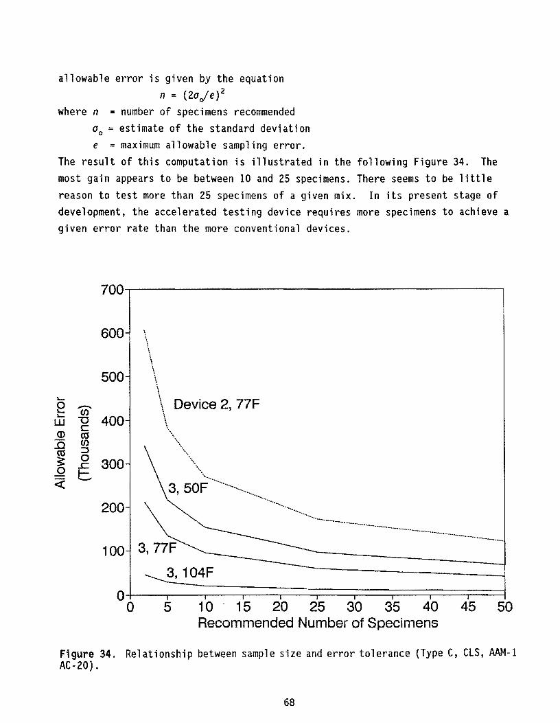
all owab 1 e error is gi ven by the equation n = (2aje}2
where n = number of specimens recommended ao = estimate of the standard deviation e = maximum allowable sampling error.
The result of this computation is illustrated in the following Figure 34. The most gain appears to be between 10 and 25 specimens. There seems to be little reason to test more than 25 specimens of a given mix. In its present stage of development, the accelerated testing device requires more specimens to achieve a given error rate than the more conventional devices.
700~----------------------------------------~
600
500
400
300
200
100
3,104F
5 10 . 15 20 25 30 35 40 45 50 Recommended Number of Specimens
Figure 34. Relationship between sample size and error tolerance (Type C, CLS, AAM-l AC-20).
68

v. CONCLUSIONS
(1) A procedure was developed for the measurement of both resilient modulus and Poisson's ratio. The draft recommended procedure is presented in Appendix B of the report. During the course of the procedural development, new hardware was developed and tested for both axially loaded and diametrally loaded specimens. The new devices can be used to cover a wide range of testing conditions. Two different diametral devices were constructed, one of which is capable of measuring Poisson's ratio in addition to the resilient modulus, and the other of which allows very rapid testing to be accomplished for high volume testing requirements. Although the rapid testing device meets the objective of maximizing the speed of testing quite well, its development was initiated too late in the project for its deficiencies (i.e. the measured strains are apparently less than the actual specimen strains) to be corrected prior to the end of the project. The time estimates for testing with these devices are listed in items 2 through 4 below. The estimates assume that all the necessary components and the specimen are at the desired temperature before starting the instrumentation mounting process.
(2) The minimum time required for specimen preparation and testing in the diametral test that incorporates both horizontal and vertical measurements is approximately 9-10 minutes.
(3) The minimum time required for specimen preparation and testing in the diametral test that incorporates only horizontal measurements with spring-loaded contact points is approximately 2-4 minutes.
(4) The minimum time required for specimen preparation and testing in the the fully instrumented unconfined axial test is appoximately 20-40 minutes, depending on the drying time of the adhesives used. The confined test setup and take down would require an additional time period (e.g. 30 minutes).
(5) The test procedure is capable of distinguishing among important mix variables.
(6) Axial testing at a continuous frequency of 10 Hz corresponds well to the diametral test. This frequency corresponds to the frequency of the load pulse portion of the diametral wave form. The result also compares favorably with extrapolations (to corresponding temperatures and frequencies) of SASW test results.
(7) The qualitative features of the expected temperature and frequency dependent response to loading was observed with the new equipment.
69
(8) No statistically significant difference was observed between loading with a pneumatic actuator and loading with an hydraulic actuator.
(9) Commercially available LVDTs and signal conditioning equipment can provide the required sensitivity for resilient modulus testing. However, the equipment should be checked using an oscilloscope to verify that the individual unit to be used has an adequately small noise level and that any relatively large noise signals do not appear at frequencies to be used in the test.
(10) The materials tested apparently dilated slightly, especially at the higher temperatures and load levels.
(11) Tests to corroborate nondestructive field testing results should be conducted at the temperature (and as close to the frequency as possible) that was used in the field test.
(12) A significant desirable drop in the error rate can be obtained with as few as 5 specimens of a given mix. Up to 25 specimens of a given mix may be required to reach an optimum practical error rate. Fewer specimens may be tested if the consequent error rate is acceptable to the engineer. The number can also be reduced by using extraordinary care in the control of mixture properties such as gradation and air voids, and in the control of specimen testing temperature. The number of specimens needed ;s also a function of the testing device, temperature, and mix homogeneity.
70

VI. RECOMMENDATIONS
(1) The testing devices were delivered to the Department in November 1991. The devices should be used in conjunction with the test procedure given in Appendix B. The procedure should be reviewed by the Department and revised as necessary to keep pace with AAMAS methodology and emerging SHRP testing and design and evaluation procedures.
(2) The clamping apparatus on the accelerated testing device should be evaluated for possible improvement. Decreasing the weight of the instrumentation yoke would be a small improvement. A more important improvement would be to replace the Thomson super ball bushing bearings (Delrin cage) with instrument quality or adjustable diameter linear bearings that are more rigid, and to place the lVDT on the clamping shafts closer to the specimen. This would help to correct the apparent underestimation of strains. The use of standard LVDTs with a separate core and body could also be evaluated to replace the gauging type LVDTs currently being used. If specimen bulging occurs, the gauging type LVDTs could restrict movement since their core shaft is guided by a precision bearing that does not allow any misalignment that would be associated with specimen bulging. The standard LVDT can tolerate a small degree of misalignment. Until these deficiencies can be corrected, Method A of Part II of the test procedure in Appendix B should not be used.
(3) Consideration should be given to using the concept of the yoke system on the accelerated device for a vertical measurement application. If this technique could be perfected, the resulting vertical measurement could be designed with a sufficiently short gauge length. Then St. Venant's principle could be used to virtually eliminate the concerns about localized plastic deformations in the vicinity of the loading strips causing erroneous measurement of Poisson's ratio. However, the short gauge length may require a correction factor for specimen bulging and measurements may be affected by aggregate size.
71


VII. ACKNOWLEDGEMENT
Mr. S.G. Phillips designed most of the equipment for the generalized indirect tension device and performed much of the electronic troubleshooting. Mr. Crockford designed the accelerated test apparatus and a portion of the generalized indirect tension device. Machine work was done by Mr. Bill Ray and his staff. The signal conditioning system was built by Mr. Carl Fredericksen.
VIII. REFERENCES
AASHTO Guide for Design of Pavement Structures. American Association of State Highway and Tranportation Officials, Washington, D. C., 1986.
Annual Book of ASTM Standards. Road and Paving Materia7s, Trave7ed Surface Characteristics, Vol. 04.03, American Society for Testing and Materials, Philadelphia, 1988, pp. 406-407.
Baladi, G. V., Harichandran, R. and Defoe, J. H. "The Indirect Test - A New Apparatus. 1I Interim Report prepared for the Federal Highway Administration, Michigan State University, 1987.
Baladi, G. V. "Integrated Material and Structural Design Method for Flexible Pavements, Volume 3 - Laboratory Design GUide. 1I Report No. FHWA/RD-88/118, Federal Highway Administration, 1988.
Baladi, G.V., and M. B. Snyder. Highway Pavements, Vol II, Prepared for U.S. Dept. of Transportation, Publication No. FHWA-HI-90-027, May 1990, pp. 6-141.
Bell, C.A., V. Abwahab, and M. E. CristL "Laboratory Aging of Asphalt-aggregate Mixtures," ASCE, Boston Society of Civil Engineers, Boston, 1990, pp. 254-262.
Bentsen, R.A., S. Nazarian, and J.A. Harrison. Reliability Testing of Seven Nondestructive Pavement Testing Devices, Nondestructive Testing of Pavements and Backca7culating Moduli, ASTM STP 1026, 1989, pp. 41-58
Brickman, A.M. "An Overview of Resilient Modulus Test Systems," Proceedings, Workshop on Resilient Modulus Testing, Corvallis, Oregon, 1989.
Consuegra, A., D. N. Little, H. Von Quintus, and J. Burati. "Comparative Evaluation of Laboratory Compaction Devices Based on their Ability to Produce Mixtures with Engineering Properties Similar to those Produced in the Field," Transportation Research Record 1228, Transportation Research Board, National Research Council, Washington, D. C., 1989, pp. 80-87.
Cooper, K.E., S. F. Brown, and G. R. Pooley, "The Design of Aggregate Gradings for Asphalt Basecourses," Proc., Association of Asphalt Paving Technologists, San Antonio, Texas, 1985.
72

Elliott, R.P. and S. I. Thornton. "Resilient Modulus and AASHTO Pavement Design," Transportation Research Record 1196, Transportation Research Board, National Research Council, Washington, D.C., 1988.
Frocht, M.M., Photoe7asticity, Vol. 2, John Wiley and Sons, New York, 1957.
Gemayel, C.A., and M. S. Mamlouk. "Characterization of Hot-mixed Open-Graded Asphalt Mixtures," Transportation Research Record ll7l, Transportation Research Board, National Research Council, Washington, D. C., 1988, pp. 184-192.
Goode, J.F., and E. P. Owings. "A Laboratory - Field Study of Hot Asphalt Concrete Wearing Course Mixtures,1I Public Roads, Vol. 31, No. 11. Bureau of Public Roads, Washington, D. C., 1961.
Ishai, I., and H. Gelber. "Effect of Geometric Irregularity of Aggregates on the Properties and Behavior of Bituminous Concrete, Asphalt Paving Technology," Proc., AAPT, Vol. 51, University of Minnesota, Minneapolis, 1982, pp. 494-521.
Hadley, W.O., W. R. Hudson, and T. W. Kennedy, "Evaluation and Prediction of the Tensile Properties of Asphalt-Treated Materials," Highway Research Board Annual Meeting, Washington, D.C., 1971.
Heisey, J.S., K. H. Stokoe II, and A. H. Meyer. "Moduli of Pavement Systems from Spectral Analysis of Surface Waves," Transportation Research Record 852, Transportation Research Board, National Research Council, Washington, D. C., 1982, pp. 22-31.
Hertzberg, R.W., Deformation and Fracture Mechanics of Engineering Materials, J. Wiley & Sons, N.Y.
Huekelom, W. "Observations on the Rheology and Fracture of Bitumens and Asphalt Mixes," Shell Bitumen Reprint No. 19, Shell Laboratorium-Koninklijke, 1966.
Kennedy, T.W. and W. R. Hudson. "Application of the Indirect Tensile Test to Stabilized Materials," Highway Research Board Annual Meeting, Washington, D.C., 1968.
Kennedy, T. W., G. Gonzaliz, and J.N. Anagnos. "Evaluation of the Resilient Elastic Characteristics of Asphalt Mixtures Using the Indirect Tensile Test." Research Report 183-6, Center for Transportation Research, The University of Texas at Austin, 1975.
Little, D. N. and J.A. Epps. "Evaluation of Certain Structural Characteristics of Recycled Pavement Materials." Proceedings of the Association of Asphalt Paving Technologists, Vol.49, 1980.
Mamlouk, M.S., and R. T. Sarofin. "Modulus of Asphalt Mixtures - An Unresolved Dilemma," Transportation Research Record 1171, Transportation Research Board, National Research Council, Washington, D. C., 1988.
Maupin, G.W., Jr. "Results of Indirect Tensile Tests Related to Asphalt Fatigue," Highway Research Record 404, Highway Research Board, National Research Council, Washington, D. C., 1972, pp. 1-7.
73

Nair, K., W.S. Smith, and C-Y Chang. Characterization of Asphalt Concrete and Cement-treated Granular Base Course, Final Report, contract FH-11-7319, FHWA, 1972.
ODOT. Proceedings of the Workshop on Resilient Modulus Testing - State of the Practice, March 28-30, 1989, Corvallis, Oregon, Oregon DOT.
Roesset, J.M., D-W. Chang, K.H. Stokoe, and M. Aouad. "Modulus and Thickness of the Pavement Surface Layer from SASW Tests," Paper presented at the 1990 annual meeting of the Transportation Research Board.
Roque, R. and W.G. Buttlar. "The Development of a Measurement and Analysis System to Accurately Determine Asphalt Concrete Properties Using the Indirect Tensile Mode," Draft submitted to the Association of Asphalt Paving Technologists for the 1992 Annual Meeting, Charleston, South Carolina.
Roque, R., M. Tia, and B. E. Ruth. "Asphalt Rheology to Define the Properties of Asphalt Concrete Mixtures and the Performance of Pavements," Special Technical Pub7ication 941, ASTM, Philadelphia, 1987, pp. 3-27.
Sayegh, G. Proceedings, 2nd Internationa7 Conference on Structural Design of Pavements, 1967, p. 743.
Schmidt, R.J. "A Practical Method for Measuring the Resilient Modulus of Asphalt-Treated Mixes," Highway Research Record 404, Highway Research Board, National Research Council, Washington, D. C., 1972, pp. 22-29.
Schmidt, R. J. "Effect of Temperature, Freeze-Thaw, And Various Moisture conditions on the resilient modulus of Asphalt-treated Mixes," Transportation Research Record 515, Transportation Research Board, National Research Council, Washington, D. C., 1974, pp. 27-39.
The Asphalt Institute Handbook, Manual Series No.4, Asphalt Institute, College Park, Maryland, 1989, pp. 33.
Van der Poel, C. "A General System Describing the Visco-elastic Properites of Bitumens and Its Relation to Routine Test Data," Strasse und Antobahn, Vol. 35, 1965.
Van Til, C. J., B.F. McCullough, B.A. Vallerga, and R.G. Hicks. Eva7uation of AASHO Interim Guides for Design of Pavement Structures, NCHRP report 128, 1972.
Von Quintus, H. L., J.A. Scherocman, C.S. Hughes and T.W. Kennedy. AsphaltAggregate Mixture Analysis System (AAMAS), NCHRP report 338.
Witczak, M.W. The Universal Airport Pavement Design System, University of Maryland Technical Report, College Park, Maryland, 1989.
Yoder, E.J. and M. W. Witczak. Principles of Pavement Design, John Wiley & Sons, Inc., New York, 1975.
74


APPENDIX A
DERIVATION OF DIAMETRAL RESILIENT MODULUS EQUATION
xz
J Ex dx = J ! dx = ! (X2 - X1) x x1
75

Let x2 = Ld, x1 = -Ld, O~L~O.5
where
L = [Gage ~ength 1 Diameter
=> E = ~ f[2L - Tan-'(2L) + Tan-'(-2L)](1 - 1/) + 4(1 + II} 1 6t1l'[ L (1+4L2)
Case 1: Let L = ~ 2
,. E = :t ~ + V-I]
Case 2: Let L = (3/2) 4
[! - Tan-1
P => E =-ot
3 - -8
[!] + Tanl!]] (1 - II) 4(1 + II)
+
[3;) • [1 + 4 [:4)]
76

Scope
APPENDIX B TEST PROCEDURE
Texas Department of Transportation Materials and Tests Division
Test Method Tex-2XX-F November 1991
RESILIENT MODULUS OF ASPHALT CONCRETE
This procedure is used for characterization of the elastic properties of asphalt concrete materials. The three part procedure provides methods suitable for the characterization of a wide range of mix types. Parts I and II are mandatory. Part III is optional. In Part II, three methods are provided, only one of which is necessary to perform. The choice of which method to use rests with the laboratory engineer. Method A is a rapid test useful for high production output. Method B allows computation of Poisson's ratio in an indirect tension test. Method C allows computation of Poisson's ratio in a direct compression test and can be used to control applied stress paths to a limited degree. The preferred test temperature for the indirect testing is in the 40-60°F range because the assumptions made in the development of the equations for computation of modulus rapidly lose credibility above these temperatures for many asphalt concretes. However, most of the testing in this procedure is performed at a temperature of 77±2°F primarily because (a) the temperature is easily controlled within the specified tolerance by a standard room thermostat, and this feature implies the availability of large storage areas for specimens, and (b) this temperature is closer to the average pavement temperature for much of the year in a large portion of the state. However, it is necessary to conduct testing at other temperatures which require environmental chambers (e.g. refrigerators and ovens) in cases involving corroboration of field testing and in cases requiring a full temperature sensitivity characterization. Part III of the test procedure describes the full temperature sensitivity characterization.
This standard may involve hazardous materials, operations, and equipment.
77

This procedure does not purport to address all of the safety problems associated with its use. It is the responsibility of the user of this procedure to establish appropriate safety and health practices and to determine the applicability of regulatory limitations prior to use. Related Documents Tex-226-F ASTM 02493 ASTM 03497 ASTM 04123
Research Report 1177
Definitions
Indirect Tensile Strength Test Viscosity-Temperature Chart for Asphalts Dynamic Modulus of Asphalt Mixtures Indirect Tension Test for Resilient Modulus of Bituminous Mixtures Routine Resilient Modulus Testing
Chord modulus-the slope of a line between any two points on a stress-strain curve.
Complex modulus-a complex number that defines the relationship between stress and strain for a linear viscoelastic material, E*. The Storage Modulus and the Loss Modulus are components of the complex modulus.
Dilatant materia7-a material that exhibits a change in volume when subjected only to simple shear stress. Microcracking or very high Poisson's ratios and nonlinear stress-strain curves are often associated with this type of material.
Dynamic modulus-the magnitude of the complex modulus that defines the elastic properties of a linear viscoelastic material subjected to a sinusoidal load i ng , I E* I .
Linear materia7-a material whose stress to strain ratio is independent of the loading stress applied.
Nonlinear material-a material whose stress-strain response is not linear.
Plastic behavior-material behavior in which some or all of the strain can not be recovered after unloading.
Resilient modulus-ratio of the recovered stress to the recovered strain in a repeated load test. For the purposes of this test procedure, the recovered strain is the maximum difference in strain during the time period between the maximum load in the cycle and the start of the following loading cycle.
Secant modulus-the slope of a line between the origin and any other point on a stress-strain curve.
Tangent modulus-the slope of a line tangent to the stress-strain curve at any point.
Viscoelastic material-a material whose stress-strain response is nonlinear due to time dependent factors (e.g. viscous fluid flow).
78

Apparatus
PART I STRENGTH TESTING
1. Loading press capable of applying a compressive load at a controlled deformation rate of 2 inches per minute.
2. Even though the theory upon which the strength equation is based assumes a line load, finite width loading strips are used to apply the load. Loading strips consisting of 1/2-inch by 1/2-inch square steel bars which have one surface (surface in contact with specimen) machined to the curvature of the specimen should be used when testing 4-inch diameter specimens. When testing 6-inch diameter specimens, a 3/4-inch width loading strip should be used.
Test Record Forms
See Figure B.1.
Preparation of Test Specimen
1. Prepare laboratory-molded specimens in accordance with Test Method Tex-206-F. The specimens should have a height of at least 2 in. (51 mm) and a minimum diameter of 4 in. (102 mm) for aggregate up to 1 in. (25 mm) maximum size, and a height of at least 3 in. (76 mm) and a minimum diameter of 6 in (152 mm) for aggregate up to 1.5 in. (38 mm) maximum size.
2. If field cores are being used, trim the cores so that the thickness is 1.875-2.000 inches and so that the core is a right circular cylinder with parallel ends. If the core shows evidence of core bit "wobble" greater than 0.075 inch, if the core has been damaged during shipping, or if the core has been taken at an angle so severe that it can not be corrected by trimming, discard the core without testing. Cores should conform to the height and diameter requirements specified for laboratory specimens.
Procedure
1. Determine the height and diameter of the test specimen.
2. Place the test specimen in the constant temperature apparatus long enough to insure a consistent temperature of 77 ± 2°F throughout the test specimen.
3. Align the specimen and loading strips in accordance with Part II, Method A or Method B of this procedure.
4. Slowly move the actuator so as to apply approximately 10 pounds load on the specimen while maintaining proper loading strip alignment and
79


parallelism. (The 10 pound load can be adjusted upward or downward slightly depending on the material strength).
5. Apply the load at a controlled deformation rate of 2 inches per minute and determine the total vertical load at failure of the specimen. Optionally, the specimen may be instrumented as in Part II, Method B of this procedure for acquisition of data that enables computation of Poisson's ratio and strain energy density.
Calculations
Where: ST P d h
Calculations of tensile strength:
=
= =
s =~ T 1£dh
Indirect tensile strength, in psi Total applied vertical load at failure (lbs) Specimen diameter (inches) Height of specimen, in inches
80

INDIRECT TENSILE STRENGTH TEST
Test Method Tex-2XX-F November 1991
Lab. No. ____________________________ ___ Date _______________ _
Specimen Number
Specimen Diameter (4" if no entry)
Specimen Height
Total Vertical Load (Lbs.)
Indirect Tensile Strength (psi)
Average Value
Remarks: _________________________________________________________ _
Where: ST P d h
= == =
=
2P ST =
'1£dh
Indirect tensile strength, in psi Total applied vertical load at failure (lbs) Specimen diameter (inches) Height of specimen, in inches
Figure B.1. Test record form.
81


Introduction
PART II RECOVERABLE RESPONSE ,
Asphalt concrete often exhibits a combination of elastic, time dependent, and plastic behavior in response to loading at in-service temperatures. For this reason, Part II of the test procedure allows engineering judgement to be used in the selection of loading frequencies and environmental conditions (e.g. temperatures, moisture conditions) at which the test will be conducted. Frequencies and temperatures specified in this Part are to be used in the event that no engineering considerations indicate a need for additional temperatures and frequencies.
METHOD A: ACCELERATED TEST (Note: See Recommendation number 2, Part VI of this report)
Summary of Method
The repeated-load indirect tension test for determining resilient modulus of bituminous mixtures is conducted by applying compressive loads with an offset sine wave (commonly, but incorrectly termed a 'haversine') followed by a rest period that has a long duration in relation to the duration of the sinusoidal pulse. The load is applied vertically in the vertical diametral plane of a cylindrical specimen of asphalt concrete (Figure A.2). The resulting horizontal deformation of the specimen is measured and, with an assumed Poisson's ratio, is used to calculate a modulus based on the recovery portion of the stress-strain curve.
The total resilient modulus is calculated using the total recoverable deformation which includes both the instantaneous recoverable and the timedependent continuing recoverable deformation during the unloading and rest-period portion of one cycle. (The instantaneous value obtained from calculations using only the recoverable deformation from the peak load to the start of the rest period is not used in this procedure.)
Apparatus
Testing Machine - The testing machine must have the capability of applying a load pulse over a range of frequencies, load durations, and load levels. As a minimum, the machine must be able to apply a load sufficient to break the specimen and must be able to apply 50 cycles of a 0.1 second duration offset sine pulse with a 0.9 second rest period between each pulse.
Temperature-Control System - The temperature-control system should be capable of maintaining a temperature of 77±2°F.
Measurement and Recording System - The measurement and recording system should include sensors for measuring and recording horizontal deformation. The
82

mlnlmum acceptable system should be capable of measuring horizontal deformations in the range of 0.00001 in (0.00025 mm) of deformation. The linear variable differential transformers (LVDT's) and their associated signal conditioning system must meet this resolution requirement. Loads should be measured with a minimum precision of 1 percent of the maximum load.
Data Acquisition - The measuring or recording devices should be independent of frequency for tests conducted up to 10.0 Hz. Digital data acquisition systems must have a sampling rate of at least 100 Hz.
Loading Strips - Use loading strips as specified in Part I of this procedure. For specimens with rough textures, a thin hard rubber membrane attached to the loading strip can reduce stress concentration effects, but should be used only when vertical deformations are not measured.
Alignment Fixture - Use the alignment fixture illustrated in Figure B.2. Machine drawings for the fixture are presented in Research Report 1177.
Figure B.2. Accelerated test fixture (Method A).
83

Procedure
1. Prepare specimens as noted in Part I of this procedure.
2. Place the test specimens in a controlled-temperature environment at 77°F for at least 24 hours prior to testing.
3. Place a specimen into the alignment fixture and adjust and balance the electronic measuring system as necessary.
4. Place the fixture and specimen in the testing machine as a unit by aligning the slot in the fixture with the bottom loading strip. Bring the upper strip into contact with the specimen by moving the testing machine actuator. Put a static load of 10-20 pounds (but not more than 20% of the average failure load applied to similar mixes as determined in Part I of this procedure) on the specimen. Maintain the static load on the specimen, and gently remove the alignment fixture without disturbing the displacement measuring transducers.
5. Recheck the transducers. If the voltage is out of range or if it is likely that it will go out of range during the testing, remove the specimen and return to step 3 above.
6. Adjust the static load to 15 pounds (or 20% of the average failure load for the mix, whichever is less), and begin the cyclic test. The waveform to be applied is a sine wave with an amplitude of 40% of the average failure load of the mix found in Part I of this procedure applied over a period of 0.1 second followed by a rest period (i.e. unload to the static load level) of 0.9 second. A total of 50 cycles of loading is to be applied to each specimen.
7. Each test should be completed within 5 min from the time the specimens are removed from the temperature-control cabinet if the specimen temperature is different from the temperature of its environment during the test.
8. As a minimum, load and deflection data must be acquired for cycles 42 through 49 of the test.
9. Remove the specimen from the testing apparatus and remove the displacement measurement assembly from the specimen. If the specimen is to be discarded, conduct the test specified in Part I of this procedure prior to disposing of the specimen. If the specimen is to be retained for future testing, store it in an appropriate environment.
Calculations
Calculate the elastic modulus, E, in pounds-force per square inch (or megapascals) as shown below. Assume Poisson's ratio is 0.35 unless other sources of information indicate otherwise.
where:
84

E = ~ f[2L - tan-1(2L) + tan-1( -2L)] (1 - II) + 4(1 + II) 1
6t1f [L (1 +4L2)
E = Modulus
P = Vertical load
t = Specimen thickness (height)
6 = Horizontal deflection
II = Poisson's ratio
L = (Gauge length/2)/specimen diameter
For a 3.0 inch gauge length and a 4.0 inch specimen diameter, the previous equation reduces to:
E = :t (O.359+1.271v)
If the temperature is greater than 40°F, Poisson's ratio may be estimated with the following equation (Note: this equation is based on a steeper slope than that presented by Nair et aI. and predicts a value of 0.38 for Poisson's ratio at T=77°F). Use a Poisson's ratio of 0.15 for temperatures below 40°F. Until such time as dilation can be adequately described by theory, use a Poisson's ratio of 0.499 for temperatures above 112°F.
II = O.3120311nT - 0.97432
85
METHOD B: GENERALIZED INDIRECT TENSION TEST
Summary of Method
The repeated-load indirect tension test for determining resilient modulus of bituminous mixtures is conducted by applying compressive loads with an offset sine wave (commonly, but incorrectly termed a 'haversine') followed by a rest period that has a long duration in relation to the duration of the sinusoidal pulse. The load is applied vertically in the vertical diametral plane of a cylindrical specimen of asphalt concrete (Figure B.3). The resulting horizontal and vertical deformations of the spec"imen are measured and subsequently used to calculate a modulus and Poisson's ratio based on the recovery portion of the stress-strain curve.
The total resilient modulus and Poisson's ratio are calculated using the total recoverable deformation, which includes both the instantaneous recoverable and the time-dependent, continuing recoverable deformation during the unloading and rest-period portion of one cycle. (The instantaneous value obtained from calculations using only the recoverable deformation from the peak load to the start of the rest period is not used in this procedure.)
Apparatus
Testing Machine - The testing machine must have the capability of applying a load pulse over a range of frequencies, load durations, and load levels. As a minimum, the machine must be able to apply a load sufficient to break the specimen and must be able to apply 50 cycles of a 0.1 second duration offset sine pulse with a 0.9 second rest period between each pulse.
Temperature-Control System - The temperature-control system should be capable of maintaining a temperature of 77±2°F.
Measurement and Recording System - The measurement and recording system should include sensors for measuring and recording horizontal deformation. The minimum acceptable system should be capable of measuring horizontal deformations in the range of 0.00001 in (0.00025 mm) of deformation. The linear variable differential transformers (LVDT's) and their associated signal conditioning system must meet this resolution requirement. Loads should be measured with a minimum precision of 1 percent of the maximum load.
Data Acquisition - The measuring or recording devices should be independent of frequency for tests conducted up to 10.0 Hz. Digital data acquisition systems must have a sampling rate of at least 100 Hz.
Loading Strips and Specimen Alignment - Specimen alignment is automatically provided by the loading strips. The loading strips are aligned with a gluing jig and glued in place with hot glue. Epoxy or other adhesives may be substituted as desired. Hot glue should not be used for tests conducted at temperatures above its softening pOint. Machine drawings for the fixture are presented in Research Report 1177.
86

Gauge length (Method A) K ~
" " " " r " " "
"
I( Gauge length (Method B) I
)l
Figure B.3. Generalized indirect tension test fixture (Method 8).
87

Procedure
1. Prepare specimens as noted in Part I of this procedure.
2. Place the test specimens in a controlled-temperature environment at 77°F for at least 24 hours prior to testing.
3. Place the loading strips in a 140°F or hotter oven. Turn on the hot glue gun.
4. Place a specimen into the load strip alignment fixture, and glue each loading strip in place.
5. Install, adjust and balance the electronic measuring system as necessary.
6. Place the instrumented specimen in the testing machine as a unit. Manually align the specimen with the central axis of the actuator. Move the testing machine actuator to put a static load of 10-20 pounds (but not more than 20% of the average failure load applied to similar mixes as determined in Part I of this procedure) on the specimen.
7. Recheck the transducers. If the voltage is out of range or if it is likely that it will go out of range during the testing, remove the specimen and return to step 5 above.
8. Adjust the static load to 15 pounds (or 20% of the average failure load for the mix, whichever is less) and begin the cyclic test. The waveform to be applied is a sine wave with an amplitude of 40% of the average failure load of the mix found in Part I of this procedure applied over a period of 0.1 second followed by a rest period (i.e. unload to the static load level) of 0.9 second. A total of 50 cycles of loading is to be applied to each specimen.
9. Each test should be completed within 10 min. from the time the specimens are removed from the temperature-control cabinet if the specimen temperature is different from the temperature of its environment during the test.
10. As a minimum, load and deflection data must be acquired for cycles 42 through 49 of the test.
11. Test each specimen for resilient modulus twice: Following the first test, rotate the specimen 90°, and repeat the test starting at Step 5.
12. Remove the specimen from the testing apparatus, and remove the displacement measurement assembly from the specimen. If the specimen is to be discarded, conduct the test specified in Part I of this procedure prior to disposing of the specimen (Note: If gauge head type transducers are being used, remove the vertical sensors before performing the strength test). If the specimen is to be retained for future testing, remove the sensors from the loading strips, and store the specimen in an appropriate environment.
88

Calculations
Calculate Poisson's ratio and the elastic modulus as shown below. If Poisson's ratio is measured to be greater than 0.5, use 0.499 in the calculation of the modulus and make a note of the change in the report.
ERT
P(VRT + 0.27) =
t!J.HT
VRT
3. 59!J.HT = !J.VT - 0.27
where:
ERT = total resilient modulus of elasticity, psi,
VRT = Poisson's ratio
P = repeated load, lbf,
t = thickness of specimen, in,
!J.HT ::: total recoverable horizontal deformation, in, and
!J.Vt = total recoverable vertical deformation, in.
89

METHOD C: GENERALIZED AXIAL COMPRESSION TEST
Summary of Method
A sinusoidal axial compressive stress is applied to a specimen of asphalt concrete at a given temperature and loading frequency. The resulting recoverable axial strain response of the specimen is measured and used to calculate resilient modulus.
Apparatus
Testing Machine - The testing machine must have the capability of applying a load pulse over a range of frequencies, load durations, and load levels. As a minimum, the machine must be able to apply a load sufficient to break the specimen and must be able to apply multiple cycles of an offset sine wave at frequencies of 0.1 to 20 Hz with or without a rest period.
Temperature-Control System - The temperature-control system should be capable of maintaining a temperature of 77±2°F.
Measurement and Recording System - The measurement and recording system should include sensors for measuring and recording horizontal deformation. The system should be capable of measuring horizontal deformations in the range of 0.00001 in (0.00025 mm) of deformation. The linear variable differential transformers (LVDT's) and their associated signal conditioning system must meet this resolution requirement. Loads should be measured with a minimum precision of 1 percent of the maximum load.
Data Acquisition - The measuring or recording devices should be independent of frequency for tests conducted up to 20.0 Hz. Digital data acquisition systems must have a sampling rate of at least 100 Hz. Apparatus
Loading Platens - The steel loading platens should incorporate a spherical seat so that imperfect specimens can be tested. Two rubber sheets with a lubricant such as silicone grease should be prepared and placed between the ends of the specimen and the loading platens.
Instrumentation - Two to three vertical LVDTs and one circumferential lVDT (or two radial non-contact transducers or contact LVDTs if necessary) should be mounted on the specimen. A schematic of the circumferential measurement device and photographs of specimens instrumented for testing are shown in Figure 8.4.
90

Specimen
CircumferentiOI wire
/ LVOT ho lde, assemblv (spring loaded. piVolOble)
Figure 8.4. Axial testing apparatus (Method C): (top) schematic of circumference measurement device, (center) instrumented specimen with circumference measurement device, (bottom) instrumented specimen with non-contact transducers .
91

Laboratory Molded Specimens - In general, laboratory molded specimens will not be prepared for this test since the Department does not currently mold tall asphalt specimens. However, some gyratory compaction machines can be pushed to their limits to prepare 3 inch tall specimens which can be used in this test procedure. Alternatively, large specimens can be compacted in the large gyratory (soils) press, and a smaller diameter core can be taken from the large specimen. Preferably, the specimens should have a height-to-diameter ratio of 2 to 1, a minimum diameter of 4 in. (101.6 mm) and a diameter four or more times the maximum nominal size of aggregate particles. However, a 4 inch diameter, 3 inch tall specimen geometry will be allowed for this procedure as the minimum acceptable size.
Pavement Cores - A minimum of six cores from an in-service pavement is required for testing. If possible, obtain cores having a minimum height-todiameter ratio of 2 to 1 and with diameters not less than two times the maximum nominal size of an aggregate particle. Select cores to provide a representative sample of the pavement section being studied. If the core shows evidence of core bit "wobble" greater than 0.075 inch, if the core has been damaged during shipping, or if the core has been taken at an angle so severe that it can not be corrected by trimming, discard the core without testing. Do not cap the cores. Trim the ends to parallel (within ±0.030 inches of a plane parallel to a flat surface used as a height measurement reference taken at the ends of the diameter). Cores should conform to the height and diameter requirements specified for laboratory specimens.
Procedure
1. Prepare specimens as noted in Part I of this procedure.
2. Glue the LVDT mounting hardware to the specimen. (If a membrane is being used for triaxial testing, the membrane must be glued to the specimen at the contact point, and the LVDT mounts must be glued to the membrane at the contact point so that positive contact with the specimen is maintained).
3. Place the test specimens in a controlled-temperature environment at 77°F for at least 24 hours prior to testing.
4. Install the LVDTs, and adjust and balance the electronic measuring system as necessary.
5. Place the instrumented specimen in the testing machine as a unit. Move the testing machine actuator to put a static load of 10-20 pounds (but not more than 20% of the average failure load applied to similar mixes as determined in Part I of this procedure) on the specimen. (If confining pressure is to be applied, the pressure vessel must be secured and the desired pressure applied).
6. Recheck the transducers. If the voltage is out of range or if it is likely that it will go out of range during the testing, remove the specimen and return to step 4 above.
7. Adjust the static load to 15 pounds (or 20% of the average failure load for the mix, whichever is less) and begin the cyclic test. The waveform to
92

be applied is a sine wave with an amplitude of 40% of the average failure load of the mix found in Part I of this procedure applied at 10 Hz for 1 minute.
8. Each test should be completed within 10 min from the time the specimens are removed from the temperature-control cabinet if the specimen temperature is different from the temperature of its environment during the test.
9. As a minimum, load and deflection data must be acquired for the last 5 cycles of the test.
10. If desired, conduct a monotonic load compressive strength test (to failure) after the completion of the cyclic test using a loading rate of 2 inches per minute. Use caution to avoid damage to the transducers if the strength test is performed. Remove the specimen from the testing apparatus and remove the displacement measurement assembly from the specimen.
Calculations
Measure the average amplitude of the load and the recoverable strains over the last 5 loading cycles. Calculate dynamic modulus, IE*I; as follows:
where:
Dynamic modulus = ualfa
ua = axial loading stress, pSi, ( = load/specimen cross sectional area) and fa = recoverable axial strain, in/in ( = displacement/gage length)
and compute Poisson's ratio, v, as follows:
v = -f /f r a
where: fr is the radial strain (sign is opposite that of the axial strain).
If the circumferential measurement device is used, additional factors enter into the computation of the radial strain. Assuming that the difference between a circular line segment and the path of the wire between two bracelet inserts is negligible, and that the included angle between the tangent points of the wire/bracelet contacts remains constant during testing, the following formula can be used for computation of the radial engineering strain:
o E = --::---:::~--:::-:-
r 2r(1t-6+tan6)
where fr = radial strain, r = radius to the center of the wire resting in a bracelet insert groove, 0 = LVDT displacement, and 8 = one half of the total included angle defined by the two tangent points of the wire and the central axis of the specimen.
93

PART III FUll TEMPERATURE SENSITIVITY CHARACTERIZATION
In order to fully characterize asphalt concrete materials, a modulustemperature and/or modulus-frequency relationship should be developed. In general (i.e. for thermorheologically simple materials), cold temperature performance can be predicted from high frequency tests and vice versa. In general, the range of temperatures for a full characterization that would cover pavement conditions in almost all of the climatic regions of the country is 0-60°C. A range of loading frequencies between 0.01 and 20 Hz will cover the simulation of many traffic situations.
The use of a single specimen for multiple tests (i.e. at different temperatures and frequencies) is permitted in this procedure. However, the order of testing is important in this case. Testing should begin with the lowest temperature, shortest load duration, and smallest load. Subsequent testing on the same specimen should be for conditions producing progressively lower moduli. Bring the specimens to the specified temperature before each test.
Part II, Method A or B may be used from 50°F (10°C) up to 104°F (40°C). At high temperature, specialized adhesives for the loading/gauging strips may be required for Method B. Below 10°C, Method B is recommended. Method A can be used, but a stronger spring may be necessary to keep the gauge paints from sliding on the specimen surface. Method C can be used for all temperatures (within the temperature limits of the measurement transducers as specified by the manufacturer).
Choice of Testing Frequencies
Six frequencies of load duration are suggested for use in a full frequency characterization. In order of application, they are: 20 Hz for 50 cycles, 10 Hz for 50 cycles, 5 Hz for 50 cycles, 1 Hz for 50 cycles, 0.1 Hz for 10 cycles, and 0.01 Hz for 5 cycles. The procedures in Part II must be adjusted in terms of duration of the cyclic loading (Method C) or number of cycles (Methods A and B) so that the test can be completed in a reasonable period of time while maintaining a sufficient number of cycles to obtain stable readings. The rest period used in Methods A and B can be deleted if desired for this test, but a note should be made to that effect in the report.
Choice of Testing Temperatures
Testing at six temperatures should be accomplished for full temperature characterization. An arbitrary choice of temperatures that covers the desired range of response for most materials is: 0, 4, 10, 25, 40, 50 and 60°C. Alternatively, a more objective method for temperature selection may be desired. This method is based on the viSCOSity of the asphalt.
Obtain the viscosity of the asphalt used in the mixture by testing in accordance with AASH10 1201 and AASH10 1202. Perform the appropriate tests at
94

temperatures of 40, 60, and 135°C. Obtain the specific gravity of the asphalt in accordance with AASHTO T228. Convert kinematic viscosities to absolute viscosities according to the following formula:
absolute viscosity in poises = (kinematic viscosity in stokes)(specific gravity)
where I Stoke = 100 cSt.
After converting all viscosities to units of poise, plot the data on the viscosity-temperature chart in Figure B.5 and draw a smooth line through the points. The chart coordinates are the logarithm of the logarithm of viscosity in centipoise as the ordinate and logarithm of absolute temperature in degrees Rankine (degrees Fahrenheit +459.7) as the abscissa. However, viscosity in poises and the temperature in degrees Fahrenheit are shown in the chart for convenience. Some asphalts have viscosity-temperature relationships too complex to be represented by only three points. In this case determine the viscosity at sufficient temperatures to produce a curve adequate for the purpose intended.
Once the viscosity-temperature relationship has been established, the temperatures for resilient modulus testing can be determined. It is suggested that modulus testing be conducted at temperatures corresponding to at least three of the following viscosities of the asphalt binder: 5 x 10⁹
, I X 109 ,Ix 108, 2
X 107, 2 X 10⁶ , 1 X 10⁵ , 2 X 10⁴, and 4 x 10³ . Alternatively, tests may be
conducted at three temperatures that cover the range of temperatures expected at the site of interest. These test results can then be used to generate a plot of the relationship between resilient modulus and temperature similar to that illustrated in Figure C.l in Appendix C of Report 1177.
95
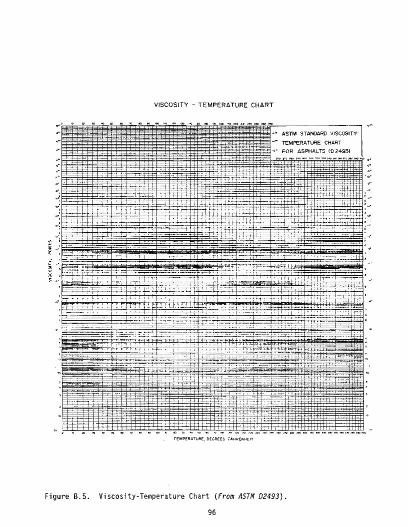
<II .... <II (5 o· ~
.; ... "' iii 0 u V> :;; O·
4'
Figure B.S.
VISCOSITY - TEMPERATURE CHART
TEMPERATURE, DEGREES FAHRENHEIT
ASTM STANDARD VISCOSITY
TEMPERATURE CHART
FOR
Viscosity-Temperature Chart (from ASTM 02493).
96
'0'
'0"
,0"
.,'
",'


APPENDIX C
USE OF TEST RESULTS
INTRODUCTION
This Appendix illustrates the usage of the resilient modulus in quality control, analysis and design. In order to obtain the full benefit of the design and analysis problems, the user must obtain a copy of the 1986 AASHTO Guide for the Design of Pavement Structures, the TFPS computer program, and Research Reports 455-1 and 455-2 to accompany the TFPS program. This Appendix is not meant to duplicate or take precedence over those documents or the TFPS computer program. The examples given in this Appendix are hypothetical in nature. However, test results from the research conducted during this research study are used in the illustrations. The examples include the design of the surface course thickness on a new flexible pavement using the 1986 AASHTO Guide for the Design of Pavement Structures, an overlay design using the TFPS computer program, and a brief suggestion of how to use the test results in quality control. The examples are not intended to suggest least cost, or optimal structure solutions. They only serve to illustrate the use of the modulus test results.
PAVEMENT DESIGN AND ANALYSIS - 1986 AASHTO GUIDE
The first problem to be discussed is the solution of a design problem in which everything is given except for the thickness of the asphalt concrete surface layer. The situation is one of new construction. Volume I of the 1986 AASHTO Guide is divided into four parts designated with Roman numerals (e.g. 1-IV). Volume 2 consists of several Appendices designated with two letters (e.g. AA, BB, etc.) In the discussion below, references to Volume I include the appropriate Roman numeral and the paragraph, Table, or Figure number. References to Volume 2 begin with the appropriate Appendix letters.
The following parameters are given:
General Materials
APSI;4.2-2.7=1.5 (11-2.2.1) Granular Base: O2=10 inches Standard Deviation, So=0.44 (1-4.3) £8s=25,000 psi Reliability, R=80% (II-Table 2.2) No Subbase Total 18kip ESALs=IO,OOO,OOO Subgrade: M~=10,000psi
Assume that the drainage is good and that the pavement structure is exposed to moisture levels approaching saturation from 1-5% of the time. This results in a quality of drainage factor, mz' of about 1.20 (II-Table 2.4). (Note: research study 1173 set forth guidelines for computing MR from Texas triaxial test results, presented further details on drainage, and developed computer program subroutines to solve the nomograph equation in II-Figure 3.1 of the Guide) Using II-Figure 2.6, the layer coefficient of the base course, az' is approximately 0.12.
97

Find: the required thickness of an asphalt concrete surface course to meet the design requirements of the given conditions using mix 51 from the study (AAM1, AC20, crushed limestone, Type C).
For flexible pavements, the structural number (5N) equation is used in thickness design. For this problem with two layers, the equation has two terms on the right hand side:
SN = a,01 + a202m2
where 'a' is a layer coefficient, '0' is the layer thickness, and 'm' is the drainage factor {II-2.4.1}. Using the table of known information, it is seen that all of the second layer parameters have been given. The solution is 0,. Therefore, 5N and at remain to be found. Refer back to Figure 10 in the boay of this report. This 1S the same figure as II-Figure 2.5 in the AASHTO Guide. If it can be assumed that the figure is based on the 10 Hz response from the uniaxial test, Figure 33 of the body of this report indicates that either the lOT type test results or the uniaxial test results may be used in II-Figure 2.5. For this problem, the lOT type test results (device code 3 of Table 9 in the body of this report) will be used. However, note that II-Figure 2.5 requires the modulus at 68°F and test results on the 51 mix are only available at 50, 77, and 104°F (see Appendix 0 of this report). Therefore the full temperature sensitivity characterization of Part III of the test procedure in Appendix B of this report must be extended one step further. Figure C.I illustrates how the modulus at a temperature of 68°F is obtained with the existing data.
Although not a rigorous form for the theoretical relationship, the following regression model adequately captures the trend in the area of interest:
E = e (12.211195 ... O.056374F - O.000619F2)
where F is the temperature in OF, and e or exp is the exponential function (the base of natural logarithms). Entering a temperature of 68°F into this equation results in a modulus of approximately 531,000 psi. Assuming that the fatigue factor from Figure 13 of the body of this report is approximately 1.0, the 531,000 psi modulus presents a problem for use in II-Figure 2.5. One must extrapolate the curve out beyond 500,000 to obtain a value for the layer coefficient. However, Figure GG.7 of Volume 2 of the Guide extends to 600,000 psi and results in a value of approximately 0.48 for a,.
The structural number equation can now be expressed as follows:
0, = {SN-I.44)/0.48
The nomograph II-Figure 3.1 in the AASHTO Guide solves for SN. Enter the graph on the left side an proceed toward the right side. Draw a straight line from the reliability of 80% through the overall standard deviation of 0.44 to the first turning line (T~). Draw a second straight line from the first turning line through the estlmated number of 18kip ESALs of 10,000,000 to the second turning line. Draw a third straight line from this turning line through the effective roadbed soil resilient modulus of 10,000 psi to the left border of the design serviceability loss box. Proceed horizontally to intercept the APSI of 1.5. Then proceed vertically downward to read the design structural number of
98

1E7
Lab mix (AAM1 AC20 Crushed Limestone Type c)
E exp (12.211195 + 0.056374 F - 0000619 FA 2) ,-.,
U1 lE6 * 0..
it '--' *
* U1
:::J
:::J U 100000 0
10000
50 60 70 80 90 100 110
Temperature (FJ
Figure C.l. Change of modulus with temperature.
approximately 4.4. It is now a simple matter to solve for the thickness, D,.
D1 = (4.4-1.44)/0.48 = 6.2 inches of mix 51
PAVEMENT DESIGN AND ANALYSIS - TFPS
In its present form, the TFPS computer program allows entry of, but does not make use of, resilient modulus values of the asphalt mix in new pavement construction. It is only in the case of overlays that the modulus of the asphalt mix is used. In the case of overlays, the resilient modulus of the existing asphalt layers can be entered into the program and the entered value will override the normal procedure used for computing the modulus from mixture characteristics. The program automatically adjusts the modulus for each District in accordance with the climatological temperature and environmental conditions in the District. A fictitious example was formulated using the resilient modulus of the Mopac specimens tested in this study. An approximate modulus of 677,517 psi at 77°F obtained from the lower portion of Table 12 in the body of this report was used in the analysiS. Since the program automatically takes care of the test temperature, there is no need to perform the full temperature sensitivity characterization that is required for the AASHTO procedure. Data files for the example are illustrated below.
99
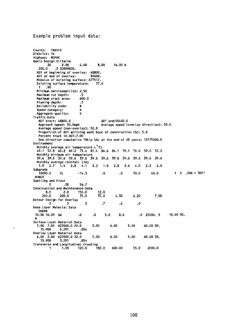
Example problem input data:
County: TRAVIS District: 14 Highway: MOPAC Basic Design Criteria
20 2.00 4.00 8.00 200.0 .2 20000000.
ADT at beginning of overlay: 48800. ADT at end of overlay: 90400. Modulus of existing surface: 677517. Existing surface temperature: 77.0 1 .90
Minimum serviceability: 2.50 Maximum rut depth: .5 Maximum crack area: 600.0 Planing depth: .5 Reliability code: A Speed category: H Aggregate quality: H
Traffic Data
16.00 N
ADT end:90400.0 ADT start: 48800.0 Approach speed: 50.~ Average speed (overlay direction): 20.0 Average speed (non-overlay): 50.0 Proportion of ADT arriving each hour of construction (%): 5.0 Percent truck in ADT:7.00 One direction cumulative 18kip SAL at the end of 20 years: 13175000.0
Environment Monthly average air temperature (oF) 49.1 52.8 60.2 69.2 75.4 81.4 84.6 84.1 79.1 70.0 59.0 52.2 Monthly minimum air temperature 39.6 39.6 39.6 39.6 39.6 39.6 39.6 39.6 39.6 39.6 39.6 39.6 Monthly average rainfall (in)
1.9 2.7 1.5 2.8 4.1 3.3 1.8 2.8 3.6 4.0 2.3 2.0 Subgrade
10000.0 CL -14.3 .0 .0 30.0 40.0 DONEO
Swelling and Frost 0 .00 56.7
Construction and Maintenance Data 8.0 2.0 150.0 12.0
200.0 200.0 75.0 75.0 4.30 4.20 7.00 Detour Design for Overlay
3 2 3 .7 .4 .0 Base Layer Material Data
OGRAN 10.00 10.00 GW • 0 .0 5.0 8.0 .0 25000. 5 N
Surface Layer Material Data 7.00 7.00 622000.0 20.0 5.00 6.00 5.00 60.00 30.
15.900 3.291 .854 Overlay Layer Material Data
6.00 2.00 622000.0 20.0 5.00 6.00 5.00 60.00 30. 15.900 3.291 .854
Transverse and Longitudinal Cracking 1 1.00 120.0 182.0 600.00 55.0 2000.0
100
y 5
10.00 30 •
.OON > 30FT


Example problem output data:
EXISTING CONSTRUCTION T( 1)= 7.00 T(2): 10.00 T(3)= .00 H SPEED
MICRO CRACKING DAMAGE CRACKING RUT RUTTING CUMULATIVE YR MTH STRAIN DAMAGE VARIANCE LAYER1 LAYER2 DEPTH VARIANCE EPSR 18KSAL 0 0 .OOE+OO .OOE+OO .OOE+OO O. O. .OOE+OO .5SE-03 4.30 .OOOE+OO o 10 .20E+03 .65E-02 .17E-02 O. O. • 13E+00 .54E-02 3.65 .392E+06 1 10 .20E+03 .20E-01 .17E-01 1. O. .18E+00 .78E-02 3.43 .88OE+06 2 10 .20E+03 .21E-01 • 18E-01 16. O • .21E+00 .92E-02 3.24 .139E+07 3 10 .20E+03 .22E-01 .19E-01 54. O. • 24E+00 .10E-01 3.08 .192E+07
CODE=5 ANALYSIS PERIOD OF 20 YEARS IS NOT REACHED OVERLAY NO. 1
T(1 )= 2.00 T(2): 6.50 T(3)= 10.00 H SPEED A REl LEVel
MICRO CRACKING DAMAGE CRACKING RUT RUTTING CUMULATIVE YR MTH STRAIN DAMAGE VARIANCE LAYER1 LAYER2 DEPTH VARIANCE EPSR 18KSAL 0 0 .OOE+OO .OOE+OO .OOE+OO O. 200. .12E-01 .11E-02 4.20 .OOOE+OO o 10 .OOE+OO .OOE+OO .OOE+OO 25. 225. .92E-01 .31E-02 3.74 .595E+06 1 10 .OOE+OO .OOE+OO .OOE+OO 53. 253. .12E+00 .39E-02 3.57.134E+07 2 10 • OOE+OO .OOE+OO • OOE+OO 83 • 283 • .14E+00 .44E-02 3.47 .211E+07 3 10 • 42E+01 .21E-06 • 14E-11 114 • 314 • .15E+00 .47E-02 3.39 .~91E+07 4 10 • 13E+02 .93E-05 .22E-08 145. 345. .16E+00 .49E-02 3.32 .374E+07 5 10 • 23E+02 .62E-04 .11E-06 176. 376. .17E+00 .51E-02 3.26 .46OE+07 6 10 • 34E+02 .23E-03 .16E-05 207. 407. .19E+00 .55E-02 3.19 .549E+07 7 10 .46E+02 .67E-03 .14E-04 238. 438. .22E+00 .69E-02 3.04 .641E+07 8 10 .60E+02 .16E-02 .82E-04 268. 468. • 24E+00 .81E-02 2.91 .736E+07 9 10 .75E+02 .34E-02 .38E-03 297. 497. • 27E+00 .93E-02 2.81 .834E+07
10 10 .91E+02 .66£-02 .15E-02 325. 525. • 29E+00 .10E-01 2.71 .935E+07 11 10 .11E+03 .12E-01 • 52E-02 353. 553 • .32E+00 .11E-01 2.62 .104E+08 12 10 • 13E+03 .21E-01 .16E-01 379. 579. .34E+00 .12E-01 2.55 .115E+08 13 10 • 15E+03 .35E-01 .46E-01 409. 603. .36E+00 .13E-01 2.47.126E+08 FAILURE MODE IS SERVICEABILITY CODE=5 ANALYSIS PERIOD OF 16 YEARS IS NOT REACHED OVERLAY NO. 2
T(1 )= 2.00 T(2)= 8.00 T(3)= 10.00 H SPEED A REL LEVEL
MICRO CRACKING DAMAGE CRACKING RUT RUTTING CUMULATIVE YR MTH STRAIN DAMAGE VARIANCE LAYER1 LAYER2 DEPTH VARIANCE EPSR 18KSAL 13 9 .OOE+OO .OOE+OO .OOE+OO O. 603. .18E·01 .11E-02 4.20 .125E+08 13 10 • 17E+02 .10E-04 • 29E-08 1. 604. .91E-01 .90E-02 3.36 .126E+08 14 10 • 19E+02 .39E-04 .41E-07 12. 616. .15E+00 .12E-01 3.09 .137E+08 15 10 .20E+02 .49E-04 .65E-07 23. 627. • 18E+00 .14E-01 3.00 .148E+08 CODE=6 THIS DESIGN MEETS ALL THE DESIGN CRITERIA
*********************************************************************************
STATE OF TEXAS NEW FLEXIBLE PAVEMENT SYSTEM
NAME OF ENGINEER : PROB O[ST. COUNTY M-4 14 TRAVIS
CONT. SECT. JOB HIGHWAY DATE PAGE 0113 13 1 MOPAC 1/29/91 1
================================-==============================================
GRANULAR BL-BASE TIME PAVEMENT BASE SURFACE OVERLAY OF
SYSTEM THICKNESS THICKNESS OVERLAY (in.) (in.) (in.) (in.) (yr.)
1 5 10.00 1 5 10.00
.00
.00 7.00 8.50
2.00 2.00
3.6 13.6
TIME OVERLAY FAILED CODE (yr.)
13.8 5 16.0 6
Code 1= Thick pavement, Max. time to first overlay exceeded Code 2= Thin pavement, Min. time to first overlay not reached Code 3= Thick pavement, Max. time between overlays exceeded Code 4= Thin overlay, Min. time between overlays not exceeded Code 5= Analysis period not reached within overlay Code 6= All design criteria met.
SEAL COATS ADDED
No Seal Coat No Seal Coat
*********************************************************************************
101

NAME OF ENGINEER PROB DIST. COUNTY M-4 14 TRAVIS
STATE OF TEXAS NEW FLEXIBLE PAVEMENT SYSTEM
LIST OF FEASIBLE DESIGN ALTERNATIVES
CONT. SECT. JOB HIGHWAY 0113 13 1 MOPAC
DATE PAGE 1/29/91 1
==:================================================================================================ SYSTEM : 1 1 5
OVERLAY HooE
EXISTING CONSTRUCTION Granular Base :10.00 Black Base .00 Asphalt Surface 7.00
inches inches inches
Asphalt OVerlay 2.00 inches
SWELLING SOILS Not analyzed
OVERLAY # 1 fAILED - 13 YRS Asphalt Overlay: 2.00 inches Mill Depth .50 inches
PAVEMENT PARAMETERS AT YEAR CONDITION : PSI
: Cracked Area : Rut Depth
TRAFfIC .192E+0718kSAL
9 MNTHS- SERVICEABILITY CONDITiON PSI
Cracked Area Rut Depth :
TRAFFIC .126E+0818kSAL
OVERLAY # 2 MET DESIGN CRITERIA 16 Years Asphalt Overlay 2.00 inches CONDITION Hill Depth .50 inches
TRAfFIC
LIFE CYCLE COSTS (in present value)
PSI Cracked Area Rut Depth
.151E+08 18kSAL
Initial Construction .00 Overlay Constr. Routine Maintenance .36 Seal Coats
4.00 3.08 54. .24
2.47 409.
.36
2.99 24. .18
User Costs .51 Salvage Value
3.86 .00
-.68 TOTAL
102
4.05

POTENTIAL USE FOR QUALITY CONTROL
If quality control is to be based on resilient modulus values, the checks must be made with the understanding that there must be a sufficient number of tests conducted so that the allowable error in the test procedure does not exceed the tolerance specified for the construction. For instance, consider Figure 34 of the body of this report. A figure such as this can be generated for each device and mix of interest. As an example, choose an S1 mix with a standard deviation of 133,019 psi and a mean of 412,824 psi. If the modulus of the material in place is specified on the plans as 300,000 psi minimum at 77°F, the maximum allowable sampling error could be estimated as 112,824 psi (the difference between the specification and the mean value). Using the equation in the body of the report
it is found that the minimum number of specimens necessary for testing to determine compliance is six (since n=5.56 in this case). The same type of approach can be taken to determine the uniformity of the quality of the mix. Note that, in general, between 10 and 25 specimens must be tested at the outset so that a good estimate of the standard deviation can be obtained for the computation of n. If laboratory compacted specimens are used, the air voids should match the expected voids in the field. While the test results may be useful in the quality control area, the engineer should be cautious when attempting to make judgmental inferences about distress based solely on resilient modulus, since the test and the current methods of interpretation of test results do not characterize adequately the failure mechanisms involved.
103


APPENDIX D
SUMMARIZED DATA
Poisson's ratios at 77°F and 104°F. (Type "C" aggregate with AC-IO)
7rF
Cycle PI P2 P (avg)
I 0.541 0.533 0.538
2 0.547 0.534 0.542
3 0.550 0.536 0.545
4 0.555 0.543 0.550
!> 0.558 0.546 0.553
6 0.556 0.548 0.553
7 0.556 0.550 0.554
8 0.563 0.562 0.562
9 0.566 0.568 0.567
1U 0.569 0.569 0.569
Where,
PI = Poisson's ratio in direction I P2 = Poisson's ratio in direction 2
(after rotating sample by 90°) P(avg) = average Poisson's ratio. Mean Poisson's ratio at 77°F is 0.553 Mean Poisson's ratio at 104 c F is 0.709
104
104°F
PI P2 P (avg)
0.622 0.725 0.673
0.656 0.735 0.695
0.658 0.709 0.683
0.664 0.7 .700
0.680 0.725 0.702
0.704 0.720 0.712
0.721 0.715 0.718
0.726 0.727 0.738
0.730 0.746 0.738
.714 0.737 0.739
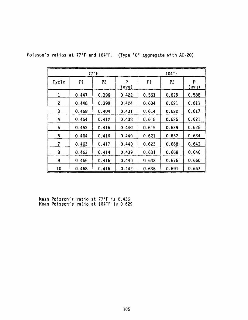
Poisson's ratios at 77°F and 104"F. (Type "C" aggregate with AC-20)
77°F
Cycle PI P2 P 1avg)
1 0.447 0.396 0.422
2 0.448 0.399 0.424
3 0.458 0.404 0.431
4 0.464 0.412 0.438
5 0.463 0.416 0.440
6 0.464 0.416 0.440
7 0.463 0.417 0.440
8 0.463 0.414 0.439
9 0.466 0.415 0.440
10 0.468 0.416 0.442
Mean Poisson's ratio at 77°F is 0.436 Mean Poisson's ratio at 104°F is 0.629
105
104"F
PI P2 P (avg)
0.561 0.629 0.588
0.604 0.621 0.611
0.614 0.622 0.617
0.618 0.625 0.621
0.615 0.639 0.625
0.621 0.652 0.634
0.623 0.668 0.641
0.631 0.668 0.646
0.633 0.675 0.650
0.635 0.691 0.657
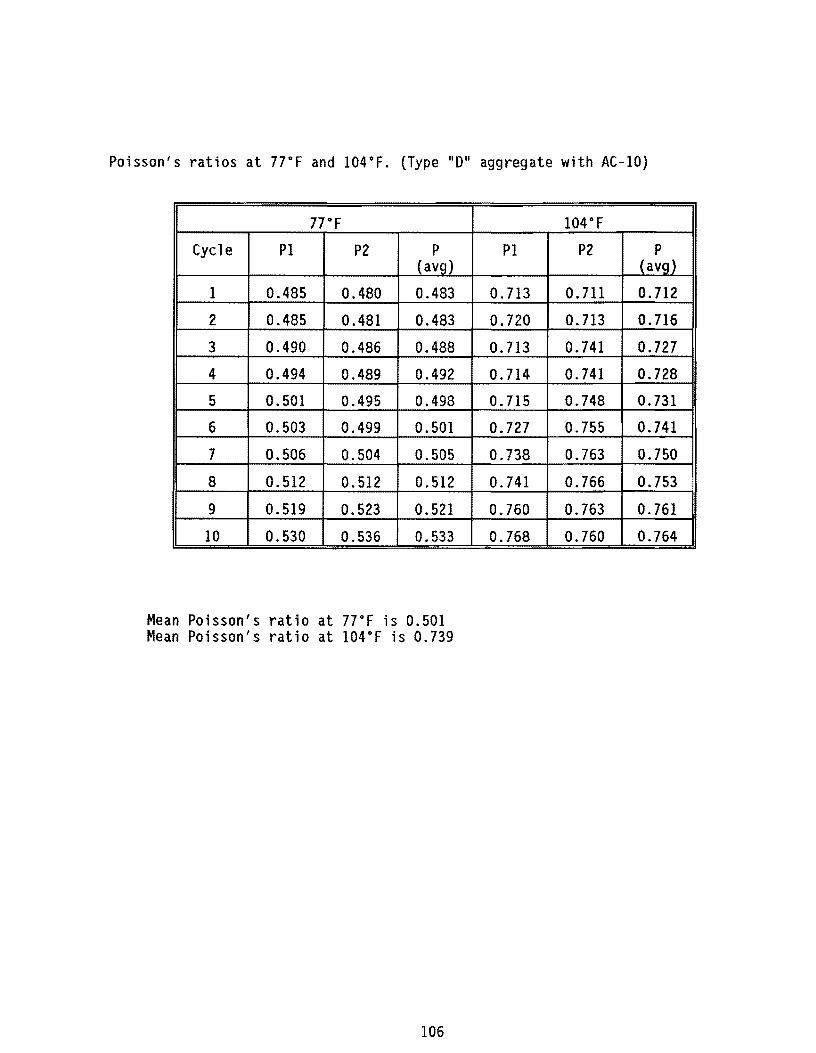
Poisson's ratios at 7rF and 104°F. (Type nOli aggregate with AC-I0)
77°F
Cycle PI P2 P (avg)
1 0.485 0.480 0.483
2 0.485 0.481 0.483
3 0.490 0.486 0.488
4 0.494 0.489 0.492
5 0.501 0.495 0.498
6 0.503 0.499 0.501
7 0.506 0.504 0.50S
8 0.512 0.512 0.S12
9 0.S19 0.S23 0.S21
10 0.530 0.536 0.533
Mean Poisson's ratio at 77°F is 0.501 Mean Poisson's ratio at 104°F is 0.739
106
104°F
PI P2 P (avg)
0.713 0.711 0.712
0.720 0.713 0.716
0.713 0.741 0.727
0.714 0.741 0.728
0.715 0.748 0.731
0.727 0.755 0.741
0.738 0.763 0.750
0.741 0.766 0.753
0.760 0.763 0.761
0.768 0.760 0.764

Poisson's ratios at 7rF and 104°F. (Type "Oil aggregate with AC-I0)
7rF
Cycle PI P2 P (avg)
1 0.420 0.434 0.427
2 0.425 0.443 0.434
3 0.433 0.449 0.441
4 0.447 0.463 0.455
5 0.471 0.486 0.478
6 0.475 0.492 0.483
7 0.492 0.503 0.498
8 0.509 0.518 0.514
9 0.513 0.520 0.517
10 0.516 0.526 0.521
Mean Poisson's ratio at 77°F is 0.470 Mean Poisson's ratio at 104°F is 0.723
107
104°F
PI P2 P (avg)
0.680 0.719 0.700
0.705 0.719 0.712
0.695 0.735 0.715
0.691 0.745 0.718
0.682 0.770 0.726
0.678 0.754 0.716
0.701 0.771 0.736
0.716 0.777 0.747
0.705 0.762 0.734
0.703 0.761 0.732

Resilient moduli at 77°F and 104°F. (Type "C II aggregate with AC-I0 )
7rF
Cycle E1 E2 E (avg)
1 303542 271939 290900
2 293361 268795 283534
3 284475 264959 276669
4 276659 257636 269049
I~: 270102 254167 263727
7 247347 258873
7 i:::t)i:::t)..:s5 244096 255219
8 253855 234329 246045
9 247023 228668 239681
10 240272 226964 234949
Where, El = Resilient modulus in direction 1 (psi) E2 = Resilient modulus in direction 2 (psi)
( after rotating sample by 90°) E(avg) = average resilient modulus. Mean resilient modulus at 77°F is 261865 psi. Mean resilient modulus at 104°F is 124994 psi.
108
104°F
E1 E2
175426
156026 139002
150584 136362
143475 117852
132981 113583
123524 109400
117892 107026
115698 101488
114284 95762 I 110676 94924
E (avg)
159677
147513
143473
130664
123282
116462
112459
108593
105023
'''' .;c.ovv

Resilient moduli at 7rF and 104°F. (Type "C" aggregate with AC-20 )
7rF
Cycle El E2 E (avg)
1 430994 432371 431683
2 420848 419478 420163
3 393004 400800 396903
4 375880 376820 376350
5 371514 367640 369577
6 366960 364846 365903
7 364081 359121 361601
8 357208 359207 358207
9 350595 354982 352788
10 343415 352353 347884
Mean resilient modulus at 77°F is 378106 psi. Mean resilient modulus at 104°F is 119359 psi.
109
104°F
El E2
167835 136184
137777 132271
131099 125289
126624 120962
122247 110714
118307 104507
116166 96917
111806 95407
110817 93526
109638 89721
E (avg)
155174
135575
128775
124359
117633
112787
108466
105246
103900
101671

Resilient moduli at 7rF and 104°F. (Type "0" aggregate with AC-10 )
7rF
Cycle El E2 E (avg)
1 280372 278339 279356
2 276925 273190 275058 .. 267222 265813 266517
4 259642 259186 259414
5 249637 251209 250423
6 244821 245054 244937
7 238932 237585 238259
8 230602 226494 228548
9 220922 215067 217995
10 210089 204463 207276
Mean resilient modulus at 77°F is 224344 psi. Mean resilient modulus at 104°F is 70815 psi.
110
104°F
El E2 E (avg)
88772 94722 91747
86063 93939 90001
84089 83790 83939
82817 83052 82934
80267 78200 79234
76311 76666 76488
72834 74519 73676
69464 70626 70045
65505 67007 66256
63746 65539 ~

Resilient moduli at 77°F and 104°F. (Type "DIt aggregate with AC-20 )
7rF Cycle E1 E2 E
(avg)
1 609122 545874 577498
2 585885 517400 551642
3 545919 490144 518032
4 498718 447169 472944
5 437826 396141 416983
6 426619 382145 404382
7 389163 361243 375203
8 358611 337834 348223
9 349457 332613 341035
10 339133 324502 33181
Mean resilient modulus at 77°F ;s 433776 psi. Mean resilient modulus at 104°F is 117573 psi.
III
104°F
El E2
165118 151894
144493 148406
132266 131905
122584 121260
118647 111997
115353 107317
106459 97862
99636 94013
99016 94094
96798 92351
E (avg)
158506
146449
132085
121922
115322
111335
102160
96825
96555
94574

DATA COLUMN ORDER: Device code (see Table 9), Mix code (see Table 11), Air Voids, Load level (% of strength), Temperature (F), Last cycle contributing data to the analysis, 5pecimen orientation (degrees) or frequency (for axial specimens), Resilient modulus
o RL 5.11 13.4 77 .0 5 0 . 1125940E+06 o RL 5.09 16.3 77 .0 5 0 . 1183540E+06 o RL 5.40 13.7 77 .0 5 0 . 1108260E+06 o RL 4.88 12.1 77 .0 5 0 .1028820E+06 o RL 5.08 13.1 77.0 5 0 . 1216000E+06 o RL 5.35 14.8 77.0 5 0 .9057100E+05 o RL 4.81 14.3 77.0 5 0 .9292060E+05 o RL 4.84 14.2 77 .0 5 0 .1032740E+06 o RL 5.29 12.5 77.0 5 0 .5107440E+05 o 51 2.72 6.9 77 .0 5 0 . 2348300E+06 o 51 2.44 3.5 77 .0 5 0 .2592820E+06 o 51 3.09 16.1 77 .0 5 0 .2383940E+06 o 51 2.21 15.3 77 .0 5 0 .2756380E+06 o 51 2.82 16.8 77 .0 5 0 .2806510£+06 o 51 2.29 15.7 77 .0 5 0 .2626110£+06 o 51 3.04 13.6 77 .0 5 0 .2679610E+06 o Sl 2.46 6.6 77.0 5 0 . 2892300E+06 o Sl 2.59 6.6 77 .0 5 0 . 2794620E+06 o 51 2.53 6.6 77.0 5 0 . 2494050E+06 o 51 2.59 6.6 77 .0 5 0 . 2992680E+06 o 51 2.25 7.5 77 .0 5 0 .2899570E+06 o 51 2.00 6.6 77 .0 5 0 . 2949880E+06 o 51 2.34 7.6 77 .0 5 0 . 2536800E+06 o 51 2.79 7.4 77 .0 5 0 . 2929440E+06 o 51 2.72 8.5 77 .0 5 0 .2246370E+06 o 51 2.77 5.1 77 .0 5 0 .2637030E+06 o 51 2.89 4.5 77 .0 5 0 .2692370E+06 o 51 2.48 3.4 77.0 5 0 .2876620E+06 o 51 2.70 3.5 77 .0 5 0 .3134920E+06 o 52 3.26 6.8 77 .0 5 0 .2514340£+06 o 52 2.50 6.8 77.0 5 0 .2485340E+06 o 52 2.72 6.9 77.0 5 0 .2035350E+06 o 52 2.23 7.2 77 .0 5 0 .2148280E+06 o 52 2.56 6.6 77 .0 5 0 .2311570E+06 o 52 2.28 6.3 77 .0 5 0 .2641630E+06 o 52 2.58 6.4 77 .0 5 0 .3259770E+06 o 52 2.71 6.8 77 .0 5 0 .2044990E+06 o 52 2.00 6.8 77 .0 5 0 . 2420490E+06 o 52 2.85 6.8 77 .0 5 0 .2551680£+06 o 52 2.55 6.8 77 .0 5 0 . 2472270E+06 o 52 2.27 6.3 77 .0 5 0 .2674570£+06 o 52 2.90 6.8 77 .0 5 0 .2216530£+06 o 52 2.84 7.4 77.0 5 0 .2452120£+06 o 52 2.58 7.0 77.0 5 0 .2447260E+06 o 52 2.95 6.9 77 .0 5 0 .2993490E+06 o 52 2.24 6.1 77 .0 5 0 .2505990E+06 o 52 2.44 6.8 77 .0 5 0 .2348690E+06 o 52 2.09 8.4 77 .0 5 0 .2160750E+06
112

o S2 1.87 6.8 77.0 5 0 .2782140E+06 o S3 2.38 5.4 77 .0 5 0 . 1843550E+06 o S3 2.17 4.7 77.0 5 0 .2937460£+06 o S3 2.10 4.5 77 .0 5 0 .2639360£+06 o S3 1. 75 4.6 77 .0 5 0 .2881820£+06 o S3 2.93 4.0 77 .0 5 0 .3784490E+06 o S3 2.64 4.7 77 .0 5 0 .3134810E+06 o S3 2.92 5.1 77 .0 5 0 .2311620£+06 o S3 1. 54 4.8 77 .0 5 0 .2744340E+06 o S3 3.22 4.8 77.0 5 0 .2703520E+06 o S3 2.81 4.8 77 .0 5 0 .2894550£+06 o S3 2.63 4.8 77 .0 5 0 . 2966950E+06 o S3 3.20 4.5 77 .0 5 0 .2692110E+06 o 53 2.71 4.8 77.0 5 0 .3127280£+06 o 53 3.38 4.7 77 .0 5 0 .2856590£+06 o 53 2.26 4.9 77.0 5 0 . 2682040E+06 o 53 7.49 6.2 77 .0 5 0 .2718160£+06 o S3 3.03 4.4 77 .0 5 0 .2811640E+06 o S3 2.88 4.9 77 .0 5 0 . 2839760E+06 o S3 2.63 5.1 77 .0 5 0 .2763520£+06 o S3 3.27 4.9 77 .0 5 0 .2813490E+06 o S4 2.39 11.9 77 .0 5 0 .1926510£+06 o S4 1.84 9.7 77 .0 5 0 .2003920E+06 o 54 2.80 12.6 77.0 5 0 .2037610E+06 o S4 2. 48 11. 0 77 .0 5 0 .2346320E+06 o S4 2.94 10.6 77 .0 5 0 .2005350£+06 o 54 2.88 10.7 77 .0 5 0 .2013660E+06 o 54 2.65 10.9 77 .0 5 0 .2020350E+06 o S4 1. 93 10.1 77.0 5 0 .2217200E+06 o S4 2.56 10.5 77.0 5 0 . 2399290E+06 o S4 2.95 9.9 77 .0 5 0 .2114760E+06 o RL 5.11 13.4 77 .0 5 90 .9160220E+05 o RL 5.09 16.3 77 .0 5 90 .9801960E+05 o RL 5.40 13.7 77.0 5 90 .9012660E+05 o RL 4.88 12.1 77 .0 5 90 . 9289490E+05 o RL 5.08 13.1 77 .0 5 90 .8782220E+05 o RL 5.35 14.8 77 .0 5 90 . 9233880E+05 o RL 4.81 14.3 77 .0 5 90 .1018510£+06 o RL 4.84 14.2 77 .0 5 90 .4542200£+05 o RL 5.29 12.5 77 .0 5 90 .4595490£+05 o SI 2.72 6.9 77 .0 5 90 .2646780£+06 o SI 2.44 3.5 77 .0 5 90 .2618490£+06 o SI 3.09 16.1 77 .0 5 90 .2643580£+06 o SI 2.21 15.3 77 .0 5 90 .2859420£+06 o SI 2.82 16.8 77.0 5 90 .2495560E+06 o SI 2.29 15.7 77 .0 5 90 . 2283350E+06 o S1 3.04 13.6 77 .0 5 90 .3031780E+06 o SI 2.46 6.6 77.0 5 90 . 2508360E+06 o SI 2.59 6.6 77 .0 5 90 .2432350E+06 o SI 2.53 6.6 77.0 5 90 . 2831780E+06 o SI 2.59 6.6 77.0 5 90 .3152170E+06 o SI 2.25 7.5 77 .0 5 90 .2770120E+06 o SI 2.00 6.6 77 .0 5 90 . 2742870E+06 o SI 2.34 7.6 77 .0 5 90 .2671150£+06 o SI 2.79 7.4 77 .0 5 90 . 2646780E+06
113

o 51 2.72 8.5 77 .0 5 90 .2330010E+06 o 51 2.77 5.1 77.0 5 90 .2773510E+06 o 51 2.89 4.5 77.0 5 90 .2411560E+06 o SI 2.48 3.4 77 .0 5 90 .2418260E+06 o 51 2.70 3.5 77 .0 5 90 . 2666570E+06 o S2 3.26 6.8 77 .0 5 90 . 2490620E+06 o S2 2.50 6.8 77 .0 5 90 . 2174680E+06 o 52 2.72 6.9 77 .0 5 90 .2011400E+06 o S2 2.23 7.2 77 .0 5 90 .2167490E+06 o S2 2.56 6.6 77 .0 5 90 . 2465680E+06 o S2 2.28 6.3 77 .0 5 90 .2241170E+06 o S2 2.58 6.4 77.0 5 90 . 2264680E+06 o S2 2.71 6.8 77 .0 5 90 . 1878540E+06 o S2 2.00 6.8 77.0 5 90 .2349000E+06 o S2 2.85 6.8 77.0 5 90 . 2433540E+06 o S2 2.55 6.8 77 .0 5 90 .2425180E+06 o S2 2.27 6.3 77 .0 5 90 . 2277080E+06 o 52 2.90 6.8 77 .0 5 90 .2299070E+06 o 52 2.84 7.4 77 .0 5 90 .2168190E+06 o 52 2.58 7.0 77 .0 5 90 .2395730E+06 o S2 2.95 6.9 77 .0 5 90 .2720580E+06 o 52 2.24 6.1 77 .0 5 90 .2330130E+06 o 52 2.44 6.8 77 .0 5 90 . 2577080E+06 o S2 2.09 8.4 77 .0 5 90 .3249500£+06 o S2 1.87 6.8 77 .0 5 90 . 2838350E+06 o 53 2.38 5.4 77 .0 5 90 . 2263820E+06 o 53 2.17 4.7 77.0 5 90 . 2861790E+06 o 53 2.10 4.5 77 .0 5 90 . 2603530E+06 o S3 1. 75 4.6 77 .0 5 90 .2931940E+06 o 53 2.93 4.0 77 .0 5 90 .3660410E+06 o 53 2.64 4.7 77 .0 5 90 .2773100E+06 o 53 2.92 5.1 77.0 5 90 .2311620E+06 o 53 1.54 4.8 77 .0 5 90 . 2848880E+06 o 53 3.22 4.8 77 .0 5 90 .2755020E+06 o 53 2.81 4.8 77 .0 5 90 • 2704860E+06 o 53 2.63 4.8 77 .0 5 90 . 2745600E+06 o 53 3.20 4.5 77 .0 5 90 . 3438340E+06 o S3 2.71 4.8 77 .0 5 90 .2636580E+06 o 53 3.38 4.7 77 .0 5 90 . 2908060E+06 o 53 2.26 4.9 77 .0 5 90 .2730370£+06 o 53 7.49 6.2 77 .0 5 90 .2538450E+06 o 53 3.03 4.4 77.0 5 90 .2811640£+06 o 53 2.88 4.9 77 .0 5 90 .3008450E+06 o 53 2.63 5.1 77 .0 5 90 . 2478750E+06 o 53 3.27 4.9 77 .0 5 90 .2721300E+06 o 54 2.39 11.9 77.0 5 90 . 1964010E+06 o 54 1.84 9.7 77 .0 5 90 . 1857860E+06 o 54 2.80 12.6 77 .0 5 90 . 1907230E+06 o 54 2.48 11. 0 77 .0 5 90 . 2479580E+06 o S4 2.94 10.6 77 .0 5 90 . 1966780E+06 o S4 2.88 10.7 77.0 5 90 .2066080E+06 o 54 2.65 10.9 77.0 5 90 . 1668630E+06 o 54 1. 93 10. 1 77 .0 5 90 .2157480E+06 o 54 2.56 10.5 77 .0 5 90 .2230110E+06 o 54 2.95 9.9 77 .0 5 90 . 9708980E+05
114

1 RL 5.11 1.3 77.0 49 0 .3543025E+06 1 RL 5.11 1.3 77 .0 49 90 .3383428E+06 2 RL 5.11 15.7 73.5 49 0 .3837983E+06 2 RL 5.11 21.4 50.0 49 0 .3849804E+07 3 RL 5. 11 15 . 8 77.0 49 0 . 1928452E+06 1 RL 5.09 1.6 77.0 49 0 . 1316981E+05 1 RL 5.09 1.7 77.0 49 90 . 1320484E+05 2 RL 5.09 19.3 73.5 49 0 .3169815E+06 2 RL 5.09 26.3 50.0 49 0 .6299903E+07 3 RL 5.09 19.3 77.0 49 0 . 5328842E+06 1 RL 5.40 1.4 77.0 49 0 .2262142E+06 1 RL 5.40 1.4 77.0 49 90 .2272977E+06 2 RL 5.40 16.2 74.0 49 0 .3661066E+06 2 RL 5.40 22.0 50.0 49 0 .8532349E+07 3 RL 5.40 16.1 77.0 49 0 . 1891613E+06 1 RL 4.88 1.1 77.0 49 0 .3179594E+06 1 RL 4.88 1.4 77.0 49 90 . 2865596E+06 2 RL 4.88 14.2 74.0 49 0 .4149122E+06 2 RL 4.88 19.2 50.0 49 0 . 1959285E+07 3 RL 4.88 14.1 77.0 49 0 .7841474E+05 1 RL 5.08 1.3 77.0 49 0 . 5283424E+04 1 RL 5.08 1.3 77 .0 49 90 . 5245606E+04 2 RL 5.08 15.4 74.0 49 0 .3262963E+06 2 RL 5. 08 21. 0 50.0 49 0 .2079370E+07 3 RL 5.08 15.4 77 .0 49 0 . 1206847E+06 1 RL 5.35 1.5 77 .0 49 0 . 1956423E+05 1 RL 5.35 1.6 77.0 49 90 . 1894441E+05 2 RL 5.35 17.4 74.0 49 0 . 2947038E+06 2 RL 5.35 23.6 50.0 49 0 .2529423E+07 1 RL 4.81 1.4 77 .0 49 0 .3837160E+06 1 RL 4.81 1.4 77 .0 49 90 .3093868E+06 1 RL 4.81 1.5 77 .0 49 90 .3535486E+06 2 Rl 4.81 17.0 74.0 49 0 .3901578E+06 2 Rl 4.81 23.2 50.0 49 0 .3654024E+07 1 RL 4.84 1.3 77.0 49 0 . 8287588E+05 1 RL 4.84 1.5 77 .0 49 90 .7911053E+05 2 RL 4.84 16.6 74.5 49 0 .3210151E+06 2 RL 4.84 22.5 50.0 49 0 .4097944E+07 1 RL 5.29 1.3 77.0 49 0 .8727991E+05 1 RL 5.29 1.3 77.0 49 90 .8701302E+05 2 RL 5.29 14.9 74.5 49 0 .4272198E+06 2 RL 5.29 20.4 50.0 49 0 .5810917E+07 1 SI 2.44 .4 77 .0 49 0 .1745954[+06 1 SI 2.44 .4 77.0 49 90 . 1710033E+06 1 51 2.44 .4 77 .0 49 90 .9192366E+05 2 51 2.44 .4 77 .0 49 0 .5817746E+06 2 51 2.44 .4 77.0 49 90 .6811778E+06 2 51 2.44 5.6 50.0 49 0 .8181931E+07 2 SI 2.44 4.1 76.0 49 0 .5364120E+06 3 51 2.44 4.1 50.0 49 0 .1058954E+07 1 SI 3.09 1.8 77.0 49 0 .7096139E+05 1 51 3.09 1.6 77 .0 49 90 .7082949E+05 1 51 3.09 -.1 77.0 49 90 . 2253236E+04 2 51 3.09 1.8 77 .0 49 0 .7162053E+06 2 51 3.09 1.7 77 .0 49 90 .4577086E+06
115

2 51 3.09 26.1 50.0 49 0 .5054760E+07 2 51 3.09 19.1 76.0 49 0 .6525362E+06 3 51 3.09 19.2 104.0 49 0 .7667447E+05 1 51 2.21 1.6 77 .0 49 0 .5520251E+04 1 51 2.21 1.6 77 .0 49 90 .5511247E+04 1 51 2.21 1.6 77 .0 49 90 .5516701E+04 2 51 2.21 1.7 77 .0 49 0 .5740653E+06 2 51 2.21 1.6 77 .0 49 90 . 5882709E+06 2 51 2.21 24.9 50.0 49 0 . 5846503E+07 2 51 2.21 18.2 76.0 49 0 . 7379270E+06 3 51 2.21 18.2 104.0 49 0 .9109372E+05 1 51 2.82 1.7 77 .0 49 0 .6184303E+04 1 51 2.82 1.8 77 .0 49 90 .6138346E+04 1 51 2.82 1.8 77 .0 49 90 .3886579E+04 2 51 2.82 1.8 77 .0 49 0 .6753943E+06 2 51 2.82 1.8 77 .0 49 90 .5304117E+06 2 51 2.82 27.4 50.0 49 0 . 1154605E+08 2 51 2.82 20.0 76.0 49 0 .4983449E+06 3 51 2.82 20.0 104.0 49 0 .6025263E+05 1 51 2.29 1.6 77.0 49 0 .4094261E+04 1 51 2.29 1.6 77 .0 49 90 .4116030E+04 1 51 2.29 1.6 77 .0 49 90 .4078483E+04 2 51 2.29 1.7 77 .0 49 0 .7242779E+06 2 51 2.29 1.8 77 .0 49 90 .5222106E+06 2 51 2.29 25.8 50.0 49 0 .4711780E+07 2 51 2.29 18.8 76.0 49 0 .5128413E+06 3 51 2.29 18.9 104.0 49 0 . 1452985E+06 1 51 3.04 1.4 77 .0 49 0 .5983976E+06 1 51 3.04 1.4 77 .0 49 90 .4666536E+06 1 51 3.04 -.1 77 .0 49 90 .3980943E+05 2 51 3.04 1.5 77 .0 49 0 . 4738348E+06 2 51 3.04 1.5 77 .0 49 90 . 5992128E+06 2 51 3.04 21.9 50.0 49 0 .5140659E+07 2 51 3.04 16.1 76.0 49 0 .7824416E+06 3 51 3.04 16.0 104.0 49 0 .8515600E+05 1 51 2.46 .7 77 .0 49 0 .5815061E+04 1 51 2.46 .7 77 .0 49 90 .5812254E+04 1 51 2.46 .7 77 .0 49 90 .5848192E+04 2 51 2.46 .7 77 .0 49 0 .3217447E+06 2 51 2.46 .7 77.0 49 90 . 5887439E+06 2 51 2.46 10.7 50.0 49 0 .7058055£+07 2 51 2.46 7.8 76.0 49 0 . 5890604E+06 1 51 2.59 .7 77 .0 49 0 .3129524E+05 1 51 2.59 .7 77 .0 49 90 .3110688E+05 1 51 2.59 .7 77.0 49 90 .3106508E+05 2 51 2.59 .7 77 .0 49 0 . 5136690E+06 2 51 2.59 .7 77 .0 49 90 .6256152E+06 2 51 2.59 10.7 50.0 49 0 .6114496E+07 2 51 2.59 7.9 76.0 49 0 .8262382E+06 1 51 2.53 .7 77.0 49 0 .2596821E+06 1 51 2.53 .7 77 .0 49 90 . 2578209E+06 2 51 2.53 .7 77 .0 49 0 . 5596634E+06 2 51 2.53 .7 77 .0 49 90 . 5360674E+06 2 51 2.53 10.8 50.0 49 0 .3547992E+07 2 51 2.53 7.9 76.0 49 0 .6055251E+06
116

1 SI 2.59 .7 77 .0 49 0 .3142269E+05 1 SI 2.59 .7 77 .0 49 90 .3207549E+05 2 SI 2.59 .7 77.0 49 0 .5607271E+06 2 SI 2.59 .7 77.0 49 90 . 5206898E+06 2 SI 2.59 .0 77.0 49 90 .2196537E+05 2 SI 2.59 10.7 50.0 49 0 . 1407320E+08 2 SI 2.59 7.9 76.0 49 0 .3125442E+07 1 51 2.72 .7 77 .0 49 0 .1776158£+06 1 SI 2.72 .7 77 .0 49 90 .1773458E+06 1 SI 2.72 .7 77 .0 49 90 . 1781307E+06 2 SI 2.72 .7 77 .0 49 0 .6531184E+06 2 51 2.72 .7 77 .0 49 90 . 5330737E+06 2 51 2.72 11.2 60.0 49 0 . 4329094E+07 2 51 2.72 8.3 76.0 49 a .6165729E+06 3 51 2.72 8.2 77 .0 49 a . 6247886E+06 3 51 2.72 8.1 77.0 49 90 .3009461E+06 1 SI 2.00 .7 77 .0 49 0 .2077065E+05 1 51 2.00 .7 77 .0 49 90 .2071920E+05 2 51 2.00 .7 77.0 49 0 .7450471E+06 2 51 2.00 .7 77 .0 49 90 .6535619E+06 2 SI 2.00 10.8 50.0 49 a .4420187£+07 2 SI 2.00 7.9 76.0 49 a .1124787£+07 1 51 2.25 .8 77 .0 49 a .1018334£+06 1 51 2.25 .8 77 .0 49 90 .1016887£+06 1 51 2.25 .8 77 .0 49 90 .1006402£+06 2 SI 2.25 .8 77 .0 49 a . 5757432E+06 2 51 2.25 .8 77 .0 49 90 .6662541E+06 2 51 2.25 12.3 58.1 49 a .9390627E+07 2 51 2.25 9.1 76.0 49 a .5797542E+06 3 SI 2.25 9.0 77 .0 49 a .5409041E+06 3 SI 2.25 9.1 77 .0 49 90 .4878820E+06 1 51 2.34 .8 77 .0 49 0 . 5744724E+05 1 51 2.34 .8 77 .0 49 90 . 5693011E+05 1 SI 2.34 .0 77 .0 49 90 .3100130E+04 2 51 2.34 .8 77 .0 49 0 .5795162E+06 2 51 2.34 .8 77 .0 49 90 . 559.7887E+06 2 51 2.34 12.4 59.0 49 0 .3735401E+07 2 SI 2.34 9.0 76.0 49 0 .5813706E+06 3 SI 2.34 9.1 77 .0 49 0 .3869435E+06 3 SI 2.34 9.1 77 .0 49 90 .3431294E+06 1 SI 2.79 .8 77 .0 49 0 . 4582926E+06 1 51 2.79 .8 77 .0 49 90 .4618140E+06 1 51 2.79 .8 77 .0 49 90 .4593199E+06 2 51 2.79 .8 77 .0 49 0 .5797931E+06 2 51 2.79 .8 77.0 49 90 . 5848629E+06 2 51 2.79 8.8 76.0 49 0 .5860803£+06 2 51 2.79 12.0 55.9 49 0 .7326244E+07 3 SI 2.79 8.8 77 .0 49 0 .5680655£+06 3 51 2.79 8.8 77 .0 49 90 .3563321E+06 1 51 2.72 .9 77 .0 49 0 .5095625E+06 1 SI 2.72 .9 77 .0 49 90 .5146912E+06 1 SI 2.72 .9 77 .0 49 90 . 5302909E+06 2 SI 2.72 .9 77 .0 49 0 .6132560E+06 2 SI 2.72 .9 77 .0 49 90 .5597137£+06 2 51 2.72 10.2 76.0 49 0 .5152994E+06
117

2 SI 2.72 13.9 55.0 49 0 .2678762£+07 3 SI 2.72 10.2 77 .0 49 0 .2583741E+06 3 SI 2.72 10.2 77.0 49 90 .2608724£+06 1 51 2.77 .5 77.0 49 0 .2695538£+06 1 51 2.77 .5 77.0 49 90 .3012834E+06 1 SI 2.77 .0 77.0 49 90 . 1547784E+05 2 51 2.77 .6 77.0 49 0 . 6967685E+06 2 51 2.77 .5 77.0 49 90 .5219307£+06 2 51 2.77 8.3 54.8 49 0 .3364223E+07 2 SI 2.77 6.0 76.0 49 0 .1204764£+07 3 SI 2.77 6.0 50.0 49 0 .4431780£+06 1 SI 2.89 .5 77 .0 49 0 .3070155£+05 1 SI 2.89 .5 77.0 49 90 .3060478£+05 1 SI 2.89 .5 77.0 49 90 .3011204E+05 2 SI 2.89 .5 77.0 49 0 .4891834E+06 2 SI 2.89 .5 77.0 49 90 .5140673E+06 2 SI 2.89 7.5 56.0 49 0 . 2296808E+07 2 SI 2.89 5.4 76.0 49 0 .4503529E+06 3 SI 2.89 5.4 50.0 49 0 .5804808£+06 1 SI 2.48 .3 77 .0 49 0 .3641535E+05 1 SI 2.48 .3 77 .0 49 90 .3602049E+05 1 SI 2.48 .0 77.0 49 90 .2043669E+04 2 51 2.48 .4 77.0 49 0 . 5957550E+06 2 51 2.48 .4 77.0 49 90 .4466191E+06 2 SI 2.48 5.5 52.0 49 0 . 9823620E+07 2 SI 2.48 4.0 76.0 49 0 .9366881£+06 3 SI 2.48 4.0 50.0 49 0 .8125164E+06 1 SI 2.70 .4 77 .0 49 0 .9888850£+05 1 SI 2.70 .4 77.0 49 90 .9751270E+05 1 SI 2.70 .0 77 .0 49 90 . 5445463E+04 2 SI 2.70 .4 77 .0 49 0 .5027858E+06 2 SI 2.70 .4 77.0 49 90 .5020404E+06 2 SI 2.70 5.6 50.0 49 0 . 3885993E+07 2 SI 2.70 4.1 76.0 49 0 .9206761E+06 3 SI 2.70 4.2 50.0 49 0 .8575858E+06 1 S2 2.50 .7 77 .0 49 0 .5658363E+05 1 S2 2.50 .7 77 .0 49 90 .5634427E+05 1 S2 2.50 .7 77.0 49 0 .4835442E+06 2 S2 2.50 8.2 76.0 49 0 .5055760£+06 2 S2 2.72 8.4 76.0 49 0 .3795205E+06 1 S2 2.23 .7 77.0 49 0 .3083064E+06 1 52 2.23 .7 77 .0 49 90 .3093133E+06 1 S2 2.23 .7 77.0 49 0 .4789467E+06 2 S2 2.23 8.4 76.0 49 0 .3803274£+06 1 S2 2.56 .7 77.0 49 0 .3979262E+06 1 S2 2.56 .7 77 .0 49 90 .3976125E+06 1 S2 2.56 .7 77.0 49 0 . 8408747E+06 2 S2 2.56 7.8 76.0 49 0 .1177261£+07 1 S2 2.28 .7 77 .0 49 0 .8099173E+05 1 S2 2.28 .6 77.0 49 90 . 7906539E+05 1 S2 2.28 .7 77 .0 49 0 . 5646444E+06 2 S2 2.28 7.5 76.0 49 0 .7838217E+06 1 S2 2.58 .7 77 .0 49 0 . 5524885E+05 1 S2 2.58 .6 77 .0 49 90 .5415757E+05 1 S2 2.58 .7 77 .0 49 0 .6756910E+06
118

2 52 2.58 7.7 76.0 49 0 .8684561E+06 1 52 2.71 .7 77.0 49 0 .6803026E+05 1 52 2.71 .7 77 .0 49 90 .6805834[+05 1 52 2.71 .7 77.0 49 0 . 5748438E+06 2 52 2.71 8.2 76.0 49 0 .4473150[+06 1 52 2.00 .7 77 .0 49 0 . 3418428E+06 1 52 2.00 .7 77.0 49 90 .3430802E+06 1 52 2.00 .7 77.0 49 0 .6487898[+06 2 52 2.00 8.1 76.0 49 0 .5920256[+06 1 S2 2.85 .7 77 .0 49 0 .9616686E+05 1 S2 2.85 .7 77 .0 49 90 .9566350E+05 1 S2 2.85 .7 77 .0 49 0 .9275845E+06 2 S2 2.85 8.1 76.0 49 0 .5286954[+06 1 S2 2.55 .7 77.0 49 0 .2842798E+05 1 52 2.55 .7 77.0 49 90 • 2802847E+05 1 S2 2.55 .7 77 .0 49 0 . 7940963E+06 2 S2 2.55 8.1 76.0 49 0 .7461261E+06 1 S2 3.26 .7 77 .0 49 0 .3875432E+05 1 S2 3.26 .7 77.0 49 90 .3891110[+05 1 S2 3.26 .7 77.0 49 0 . 6394080E+06 2 S2 3.26 8.2 76.0 49 0 .4310756E+06 1 S2 2.90 .7 77 .0 49 0 .5148438E+06 1 S2 2.90 .7 77 .0 49 90 . 4773535E+06 1 S2 2.90 .7 77.0 49 0 .6711596E+06 2 52 2.90 8.0 76.0 49 0 .4223982E+06 1 S2 2.27 .7 77 .0 49 0 .2287336E+05 1 S2 2.27 .7 77.0 49 90 .2263199E+05 1 S2 2.27 .7 77.0 49 0 .5710485E+06 2 S2 2.27 7.6 76.0 49 0 .4710996[+06 I S2 2.84 .8 77 .0 49 0 .3940372E+06 I S2 2.84 .8 77 .0 49 90 .3890626E+06 1 52 2.84 .8 77 .0 49 0 .5904648[+06 2 S2 2.84 8.8 76.0 49 0 .3945552E+06 1 S2 2.58 .8 77 .0 49 0 .2052498E+05 1 S2 2.58 .7 77 .0 49 90 .2049218E+05 1 S2 2.58 .8 77.0 49 0 .5193309E+06 2 52 2.58 8.4 76.0 49 0 .8461245E+06 1 S2 2.95 .7 77.0 49 0 .4634244E+05 1 52 2.95 .7 77 .0 49 90 . 4626288E+05 1 S2 2.95 .7 77 .0 49 0 .5632020E+06 2 S2 2.95 8.2 76.0 49 0 .6785474E+06 1 S2 2.24 .6 77 .0 49 0 .3597707E+05 1 S2 2.24 .6 77 .0 49 90 .3600471 E +05 1 S2 2.24 .6 77.0 49 0 . 5668020E+06 2 S2 2.24 7.3 76.0 49 0 .1021960E+07 1 S2 2.44 .7 77.0 49 0 .5692132E+05 1 S2 2.44 .7 77 .0 49 90 . 5805244E+05 1 S2 2.44 .7 77.0 49 0 .5789505E+06 2 S2 2.44 8.1 76.0 49 0 .6298004E+06 1 52 2.09 .9 77.0 49 0 .7422543E+05 1 52 2.09 .8 77.0 49 90 .7219969E+05 1 S2 2.09 .9 77 .0 49 0 .8332285E+06 2 S2 2.09 9.7 76.0 49 0 .5202231E+06 1 S2 1.87 .7 77 .0 49 0 .2797113E+05 I S2 1.87 .7 77 .0 49 90 . 2796699E+05
119

1 S2 1.87 .7 77.0 49 0 . 7929496E+06 2 S2 1.87 8.1 76.0 49 0 .5259201E+06 1 S3 2.17 .5 77.0 49 0 . 3828253E+06 1 S3 2.17 .5 77 .0 49 90 .3845255E+06 2 S3 2.17 .5 77 .0 49 0 .4316392E+06 2 S3 2.17 .5 77.0 49 90 .4594425E+06 2 S3 2.17 5.7 78.4 49 0 . 7223392E+06 2 S3 2.17 7.7 50.0 49 0 .5746152E+07 1 S3 2.10 .5 77 .0 49 0 .. 1250658E+06 1 S3 2.10 .5 77 .0 49 90 . 1245293E+06 2 S3 2.10 .5 77 .0 49 0 .5196389E+06 2 S3 2.10 .5 77 .0 49 90 .5561484E+06 2 S3 2.10 5.5 78.4 49 0 . 1967568E+07 2 S3 2.10 7.4 50.0 49 0 . 1354045E+08 1 S3 1. 75 .5 77.0 49 0 .5812381E+06 1 S3 1. 75 .5 77.0 49 90 .5214740E+06 2 S3 1. 75 .5 77 .0 49 0 . 5573079E+06 2 S3 1. 75 .5 77 .0 49 90 .5435102E+06 2 S3 1. 75 5.8 78.4 49 0 .2933203E+07 2 S3 1. 75 7.9 50.0 49 0 .3480314E+07 1 S3 2.93 .4 77 .0 49 0 . 5714898E+06 1 S3 2.93 .4 77 .0 49 90 • 5693834E+06 2 S3 2.93 .4 77.0 49 0 .5470696E+06 2 S3 2.93 .4 77 .0 49 90 .5863992E+06 2 S3 2.93 4.8 78.4 49 0 .9550630E+06 2 S3 2.93 6.6 50.0 49 0 .3660110E+07 1 S3 2.64 .5 77 .0 49 0 . 1591579E+06 1 S3 2.64 .5 77 .0 49 90 . 1562478E+06 2 S3 2.64 .5 77 .0 49 0 .6851122E+06 2 S3 2.64 .5 77 .0 49 90 .5086768E+06 2 S3 2.64 5.7 78.4 49 0 .7287140E+06 2 S3 2.64 7.8 50.0 49 0 .6089917E+07 1 S3 2.92 .5 77.0 49 0 .1427479E+06 1 S3 2.92 .6 77 .0 49 90 .1416255E+06 2 S3 2.92 .6 77 .0 49 0 .4816639E+06 2 S3 2.92 .5 77 .0 49 90 .3870220E+06 2 S3 2.92 6.2 78.4 49 0 .9445182E+06 2 S3 2.92 8.3 50.0 49 0 .3146136E+07 1 S3 1.54 .5 77 .0 49 0 .7819211E+05 1 S3 1.54 .5 77 .0 49 90 .7841094E+05 2 S3 1.54 .5 77 .0 49 0 .6706206E+06 2 S3 1.54 .5 77 .0 49 90 .4662844E+06 2 S3 1.54 5.8 78.4 49 0 .7427929E+06 2 S3 1. 54 7.9 50.0 49 0 .3966491E+07 1 S3 3.22 .5 77 .0 49 0 .6677149E+06 1 S3 3.22 .5 77.0 49 90 .5670127E+06 2 S3 3.22 .5 77 .0 49 0 .6224754E+06 2 S3 3.22 .5 77 .0 49 90 . 4860664E+06 2 S3 3.22 5.8 78.4 49 0 .9489715E+06 2 S3 3.22 7.8 50.0 49 0 .6284725E+07 1 S3 2.81 .5 77.0 49 0 . 1108064E+06 1 S3 2.81 .5 77 .0 49 90 . 1116624E+06 2 S3 2.81 .5 77 .0 49 0 .6023310E+06 2 S3 2.81 .5 77 .0 49 90 .4892139E+06 2 S3 2.81 5.8 78.4 49 0 . 1275569E+07
120

2 S3 2.81 7.8 50.0 49 0 .2301662E+07 1 S3 2.63 .5 77 .0 49 0 .9163496£+05 1 S3 2.63 .5 77.0 49 90 .9142943£+05 2 S3 2.63 .5 77.0 49 0 .5034391E+06 2 S3 2.63 .5 77 .0 49 90 .5831722£+06 2 S3 2.63 5.8 78.4 49 0 .1028773E+07 2 S3 2.63 7.9 50.0 49 0 .1117128E+08 1 53 2.38 .6 77.0 49 0 . 1277833E+06 1 S3 2.38 .6 77.0 49 90 . 1292506E+06 2 S3 2.38 .6 77 .0 49 0 .5399819£+06 2 S3 2.38 .6 77 .0 49 90 .6269112£+06 2 S3 2.38 6.6 78.4 49 0 . 5727989E+06 2 53 2.38 8.9 50.0 49 0 .6213740E+07 1 53 2.71 .5 77.0 49 0 .5715282E+06 1 S3 2.71 .5 77.0 49 90 . 5667384E+06 2 S3 2.71 .5 77 .0 49 0 . 5548177E+06 2 S3 2.71 .5 77.0 49 90 . 5508350E+06 2 S3 2.71 5.7 78.4 49 0 .6737906E+06 2 53 2.71 7.7 50.0 49 0 .3531340E+07 1 53 3.20 .5 77.0 49 0 .8327861E+05 1 53 3.20 .5 77 .0 49 90 .8365178E+05 2 S3 3.20 .5 77 .0 49 0 .4554405E+06 2 53 3.20 .5 77.0 49 90 .5123742E+06 2 53 3.20 5.3 78.4 49 0 .1079342E+07 2 53 3.20 7.3 50.0 49 0 .1082637E+08 1 S3 3.38 .5 77 .0 49 0 . 1638601E+06 1 S3 3.38 .4 77.0 49 90 . 1632269E+06 2 53 3.38 .5 77 .0 49 0 .5381142E+06 2 S3 3.38 .5 77 .0 49 90 . 4280230E+06 2 S3 3.38 5.6 78.4 49 0 .6935560E+06 2 S3 3.38 7.6 50.0 49 0 .4905091E+07 1 S3 2.26 .5 77.0 49 0 . 1695510E+06 1 S3 2.26 .5 77 .0 49 90 . 1729100E+06 2 S3 2.26 .5 77 .0 49 0 .5298577£+06 2 S3 2.26 .5 77.0 49 90 . 5760089E+06 2 S3 2.26 6.0 78.4 49 0 .6242090E+06 2 53 2.26 8.1 50.0 49 0 . 9842480E+07 1 S3 7.49 .6 77 .0 49 0 .3246204£+06 1 S3 7.49 .6 77 .0 49 90 .3245894E+06 2 S3 7.49 7.0 78.4 49 0 . 8929986E+06 2 S3 7.49 9.4 50.0 49 0 .3014713E+07 1 S3 3.03 .5 77 .0 49 0 . 6548827E+06 1 53 3.03 .5 77 .0 49 90 . 5965449E+06 2 S3 3.03 .5 77 .0 49 0 .4876096E+06 2 S3 3.03 .5 77 .0 49 90 .5136793E+06 2 S3 3.03 5.2 78.4 49 0 .8370071E+06 2 S3 3.03 7.1 50.0 49 0 .4852545E+07 1 53 2.88 .5 77.0 49 0 . 2455486E+06 1 53 2.88 .5 77.0 49 90 .2474191E+06 2 S3 2.88 .5 77.0 49 0 .5139581 E+06 2 53 2.88 .5 77.0 49 90 .5786173E+06 2 S3 2.88 5.9 78.4 49 0 . 6965660E+06 2 S3 2.88 8.0 50.0 49 0 .7001482E+07 1 S3 2.63 .5 77 .0 49 0 .3827245E+06 1 S3 2.63 .5 77 .0 49 90 .3812211£+06
121

2 S3 2.63 .6 77.0 49 0 . 5444030E+06 2 S3 2.63 .5 77.0 49 90 .5232147E+06 2 S3 2.63 6.2 78.4 49 0 . 7809796E+06 2 S3 2.63 8.4 SO.O 49 0 . 9263164E+07 1 S3 3.27 .S 77.0 49 0 . 1221608E+06 1 S3 3.27 .S 77.0 49 90 . 1235177E+06 2 S3 3.27 .5 77.0 49 0 .S427057E+06 2 53 3.27 .5 77.0 49 90 .5429874E+06 2 53 3.27 5.8 78.4 49 0 .6414763E+06 2 53 3.27 8.0 SO.O 49 0 .4270572E+07 1 54 1.84 1.0 77.0 49 0 .4408307E+06 1 54 1.84 1.0 77.0 49 90 .4292S05E+06 2 54 1.84 1.1 74.0 49 0 .5550108E+06 2 54 1. 84 11. 6 73.5 49 0 .4085517E+06 2 54 1. 84 15. 9 50.0 49 0 .S831398E+07 1 54 2.39 1.2 77.0 49 0 .7812226E+05 1 54 2.39 1.2 77.0 49 90 . 7764730E+05 2 54 2.39 1.3 74.0 49 0 .6107139E+06 2 54 2.39 14.S 73.0 49 0 .3126438E+06 2 54 2.39 19.6 50.0 49 0 . 1411363E+07 3 54 2.39 14.2 77.0 49 0 . 1325495E+06 1 54 2.80 1.3 77 .0 49 0 .8910477E+04 1 54 2.80 1.3 77 .0 49 90 . 8929724E+04 2 54 2.80 1.3 74.0 49 0 . 1678641E+05 2 54 2.80 15.1 73.0 49 0 . 1229402E+07 2 54 2.80 20.6 50.0 49 0 . 4820069E+07 3 54 2.80 15.1 77.0 49 0 . 1336610E+06 1 54 2.48 1.1 77 .0 49 0 .9213428E+04 1 54 2.48 1.1 77 .0 49 90 .9110179E+04 2 54 2.48 1.2 74.0 49 0 .3281607E+06 2 54 2.48 13.1 73.0 49 0 .337952SE+06 2 54 2.48 17.7 SO.O 49 0 .4861296E+07 3 54 2.48 13.0 77 .0 49 0 . 1821064E+06 1 54 2.94 1.1 77 .0 49 0 . 1381875E+05 1 54 2.94 1.1 77.0 49 90 . 1408407E+05 2 54 2.94 1.1 74.0 49 0 . 5953891E+06 2 54 2.94 12.6 73.0 49 0 .3716452E+06 2 54 2.94 17.1 SO.O 49 0 . 1467068E+07 3 54 2.94 12.7 77 .0 49 0 .1038781E+06 1 54 2.88 1.1 77 .0 49 0 .20004S5E+05 1 54 2.88 1.1 77 .0 49 90 .2015146E+05 2 54 2.88 1.1 74.0 49 0 .648103SE+06 2 54 2.88 12.7 73.0 49 0 .3000656E+06 2 54 2.88 17.3 50.0 49 0 .3497053E+07 3 54 2.88 12.6 77 .0 49 0 .8633680E+OS 1 54 2.65 1.1 77.0 49 0 .4056472E+06 1 54 2.65 1.2 77 .0 49 90 .3726065E+06 2 54 2.65 1.2 74.0 49 0 . 5307248E+06 2 54 2.65 13.0 73.0 49 0 .2802855E+06 2 54 2.65 17.7 SO.O 49 0 .4037691E+07 1 54 1. 93 1.0 77 .0 49 a .2103355E+06 1 54 1. 93 1.0 77 .0 49 90 .2143711E+06 2 54 1. 93 1.1 74.0 49 0 . 5993254E+06 2 54 1.93 12.2 73.0 49 0 .3730099E+06 2 54 1.93 16.5 50.0 49 0 .7867520E+07
122

1 54 2.56 1.1 1 S4 2.56 1.1 2 S4 2.56 1.1 2 S4 2.56 12.5 2 S4 2. 56 17.0 1 S4 2.95 1.0 1 S4 2.95 I. 0 2 S4 2.95 1.0 2 S4 2.95 11.8 2 S4 2.95 16.1 2 S3 2 S3 2 S3 2 S3 2 S3 2 SI 2 SI 2 SI 2 SI 2 SI 2 S2 2 S2 2 S2 2 S2 2 S2 4 SI 4 SI 4 SI 4 MO 4 MO 4 MO 4 MO 4 MO 4 MO 5 SI 5 SI 5 SI 5 SI 5 SI 5 SI 5 MO 5 MO 5 MO 5 MO 5 MO 5 MO 5 MO 5 MO
77.0 49 0 77.0 49 90 74.0 49 0 73.5 49 0 50.0 49 0 77.0 49 0 77.0 49 90 74.0 49 0 73.5 49 0 50.0 49 0 77.0 49 0 77.0 49 0 77.0 49 0 77.0 49 0 77.0 49 0 77.0 49 0 77.0 49 0 77.0 49 0 77.0 49 0 77.0 49 0 77.0 49 0 77.0 49 0 77.0 49 0 77.0 49 0 77.0 49 0 77.0 49 0 77.0 49 0 77.0 49 0 77.0 49 0 77.0 49 90 77.0 49 0 77.0 49 0 77.0 49 90 77.0 49 0 77 295 10 77 25 1 77 295 10 77 25 1 77 295 10 77 25 1 77 295 10 77 25 1 77 295 10 77 25 1 77 295 10 77 25 1 77 295 10 77 25 1
. 1121421E+06
. 1134156E+06
.5743219E+06
.4373664E+06
.2478875E+07
.4483075E+06
. 4440684E+06
.5005893E+06
.5857819E+06
.3470512E+07
.3992424E+07
. 1389817E+07
. 1207817E+07
. 1808305E+07
. 1528150E+07
. 5626839E+07
. 1997406E+08
.1042294E+08
. 1133729E+08
. 1111965E+07
.6847390E+07
.2263566E+07
. 5139264E+07
.2040848E+07
.9209164E+07
. 5203378E+06
.7494407E+06
.6171371E+06
.6831201E+06
. 6352284E+06
.7160513E+06
.6912169E+06
. 6956720E+06
.6515983E+06 212140.9 124291. 2 293334.7 155416.7 306076.7 158121.8 1111877 648882.9 656884.1 349675.7 804949 407921.1 923647.9 484380.7
123

ACCELERATED DEVICE
APPENDIX D
MACHINE DRAWINGS
Alignment fixture assembly
Rotation alignment marks
Load strip alignment ~
Lineor bearing
Gage length
Alignment taper (centering)
Alignment plate
124
LVDT
Support yoke
Point of contact can be fixed or free. Fixed was used in this study.

Alignment plate Material: Aluminum Quantity: 1
I
6.0 (approx) )[
4.0625
4.000 (+.000 -.025)
• •
K
3.000
r~ 0
0.500
L{)
r--. n
io + 0
f~ 0
3.000
Milled slots with alignment pins --~ for yokes & LVDT slot
125
,.,-...
X-0 I-a. a. 0 ~
0 N

Yoke assembly
Spring loaded grooved linear bearing shaft
Specimen -----."
Support yoke
Note: Moments acting at vertical moment arms caused by LVDT spring forces exactly cancel.
-,
A small horizontal shear stress at the contact disk due to the spring and a small vertical shear stress at the disk due to the weight of the support yoke assembly must be resisted by friction at the disk/asphalt interface. The LVDT springs were removed during the test program to decrease the horizontal shear stresses.
126
LVDT

0 0 l,()
0
Yoke Material: Aluminum Quantity: 2
I 0'
: o I I~ 0.500 0.375 0.500 I(---)j ~ ~
I \ t t :0 r - -4--, , I I I
- - - -,- + I(---)j J
I
0.5001 I( )oj
0 N
1 .q-I ~
0.375 I} 1 foE-)j I
, I·' f __ -----'
I
I 0
\ 0 r 0 1 I I I l,() , I - - - - - - - _,_ l.
0
!oHoI
0.250
01 I~ I
I
: 0
127
I l,() r---n 0
0.375 ~
0.750 I( )oj
0
0
I l,()
r---n 0

GENERALIZED DEVICE
LOADING,!GAUGING STRIP (LONG)
TOPVIE\I
BOTTOM VIEW
o..Sil2S" DlA ~ I----.~. 1 --~ 0.1875"' DEE? ~ I .• - .Gli.# I
I '0 0 I 11------ 50S- --------+-1
MATERIAl.; STAINLESS S"I"EEL QUANTITY; 4
128

TllP VIE\l CROSS SE.C110N A-A ac: a-a
rc.:5 Ec.:m"
, 2.G Radius
#6-32 DRIll. TO
1 Q.2S- DEEP 0.187S- DEEP niREADS
0.15625- OIA BOTTOM VlEYi
0.1875· DEEP END VIEW
[ Q3'1;'''
D J L.,. I
..a"
M6IERlAl.: STAINlESS STEEL QU6NJlIY: 4
129

, "J
10 ~f
DRILL FOR # [0-24 BOLT THRU
(Q.1875'")
. 0
GAUGING/LOADING STRIP AUGNMENT FRAME
TOP Pu\ TE (TOP VIEW)
. - 025" DRILL FOR /18-32
;- BOLT THRU r:)~
ad Cl '"\
""- .25-O.!325"~
-0 0
- r- 0.25"
6.Ci
.n 00
L3.5' 7.Ci
ALL BOLTS ARE ALLEN HEAD AND RECESSED INTO TOP SIDE OF PLATE
MATERIAL: I/'L ALUMINUM SHEET
130
3. 5"
0 0
3.
oj
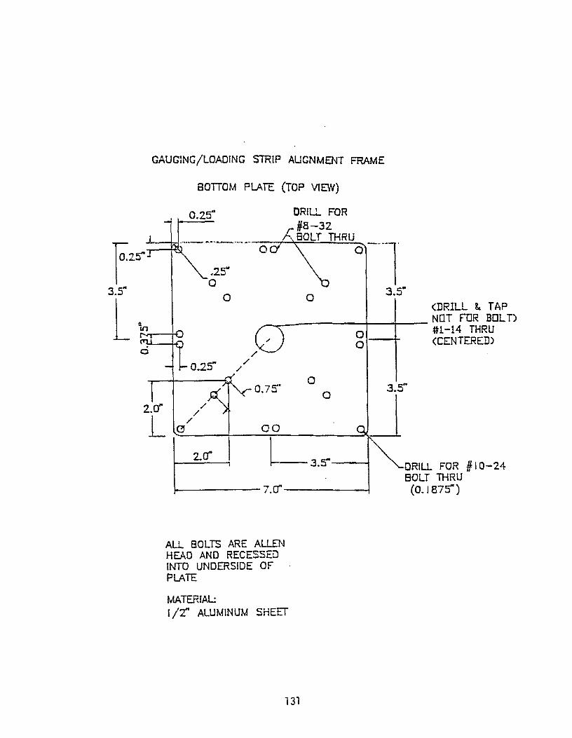
GAUGJNG!LOADING STRIP AUGNMENT FRAME
BonOM PLATE (TOP VIEW)
0.25'"
.25" o
o
a
ORILL FOR 1/8-32 BOLT THRU
o 3.5-
I (DRILL ~ TAP __ -----+---i---- NOT fOR BOLT)
#1-14 THRU (CENTERED)
0.25"
0.7:;' o
o
ai_-+a
z.O'" //
~ ~G~/ ____ ~ ____ O~O __________ ~
L305'------4 2.0'"
~------7.C1'-------1
ALL BOLTS ARE ALLEN HEAD AND RECESSED INTO UNDERSIDE OF PLATE
MATERIAL: 1/2" ALUMINUM SHEET
131
ORILL FOR 1/10-24 BOLT THRU
(0. J 875'")

T 0.1857
I
(SIDE VIEWS)
DRILL & TAP #6-32 (CENTERED)
r---L __ _
0.1875" --t 0.5'"
DRILL & TAP /14-40 lHRU (CENTERED)
L:- l. 1875"" ------
(1/4-" 0 SS ROO)
O. 1875" --\ \.2: . KNURL
MATI..: STAINLESS STEEL ROD QUANIIIY; 4 OF EACH
132
DRILL & TAP #4-40 (C~EO)
(3/1 fj ~ SS ROD)
o. J 25"
I I 0.375"
~~
0.1875" ~ ~ (3/8'" ¢ SS ROO)

OOT CLAM P /HOLDER
SIDE VIEW
t-- 1.25" ---I . r-L_
staT cur I.rt' IN lENGTH TO EKmOJ.I OF HOl£
..... '-....,... DRfU. &Ii: TAP .P$ ,4-40 1t{RU
SEr SCREW
~ STAINLESS STEEl. (lIZ' ~ ROD) Oummy: ...
RETAINER RING
0.0825
Tt)p VIEW
..,............;;__ staT (APPOX 0.25'" WID£)
0.5'"
BarTOM VIal
~. ORIU. &: TAP FOR
\ '6-32 ~, 31 I S- OEE?
SET SREW
(To be sholdered over clamp/holder before drilling &; tapping /14-40 set screw)
SIDE VIEW
t 0.6875'''
I 0.1875 ~ MATL: 5S ROO
133
TOP VI'2N
60" -~
A
0.09375#
#4-40 SET SCREW
MATCH SECTION A-A

rO.2~
LOADING BLOCK
SIDE VlF:W
--.t o.2!j -~I \: ---,.,? I I
"ll--_ 3.(j--11-° 1"-1 3.0'"
SPHERICAL HOLE (CENTERED)
TOP VIEW
¢O.8750
01.et
END VI EN
. ~0.375a
0.375" ~ iJ .
I.et I
MATL: I 1/4"X I 1/4" STAINLESS ~ 8AR
SWIVEL ATIACHMENT
#5/8"-18 THREAD
SiDE VIf:N
t- 1.125"--,
CYUNDRICAL E:XT8-JSION
I O.B7!) 1.0"
SPERlCAL HOLE (CENTERED)
MArl: I 1/4" STAINLESS STEEL HEX 8AR
134


DRILL THRU (CENTERED)
1/8-32 CENTERED
COLl.!lR
SIDE VIal
~ l- 0.375'"
MAIL: 1.5' OR 2.0" ¢ 55 ROD
TOP VlF::N
135
QUANTITY: 2
DRILL &: TAP THRU /18-32 (120'

GAUGING IAUGNMENT PINS
THREADED SHAFT
. SIDE VIEW
SHAFT 0 TO AT #12-24 TIiREAD
L O.12S-~ O.12S-
NO THREADS
l PARALLEL SIDES
TAPER END TO FIT BOTIOM OF DRILLED HOlES IN LOADING/GAUGING STRIPS
MATL: 3/1 b 0 5S ROD QUANTITY: 8
t\UGNMENT PIN COLLAR
SIDE VlF::N
THREAD OUTSIDE 1/3/8- f 6 ¢ TO FiT ~~'7"'!J"'r;..,.,...,....---------,
DRILL &: TAP THRU FOR #: 12-24 (CENTERED)
MAll: 3/'0 0 5S ROD QUANT1TY: 8
136

HEIGHT ADJUSIMENT TIiREADED SHAFT
SIDE Vlf}N .
__ ~IJ~.,~ THREAD
~ 2.S' I
MA TL: [/2" ¢ SS ROO
LOCK NUT
SIDE VIEW FRONT VIEW
1.0"
O.S'
~ ~O.25' DRILL & TAP THRU
KNURL FOR # 1/2-20 SHAFT (CENTERED)
MAR: 1.0" c,z) SS ROO QUANTITY; 2
137

HEIGHT ADJUSTMENT TIiREADED COlLAR'
SIDE VIF:N
THREAD OUTSIDE # I - [4 ({ll TO FIT)
...-------rrh'7"7"i-~
DRILL & TAP THRU 111/2-20 (CENTERED)
MATI..: 1.0'" ¢ SS ROD
FRONT VIEW
DRILL &; TAP # f 2-24 TIiRU (CENTERED)
KNURlED KNOB
SIDE VIEW
(.0'" ¢
J
-t ~O.2S-KNURL
MATL: 1.0'" ¢ Stainless steel rod
QUANTITY: a
138

0.125' RAD
0.125" ] I 0.25"" ~
I
SPECIMEN BASE PlATIEN
BOTTOM VIEW
"".---- ". '-/ . '" ¢ 3,,75'"
DRILL &: TAP #1/2-20 0.5: DEEP (CENTERED)
MATI.: 3/4" THICK Al SHEET
SUDE PLATE
TOP VIEW
1.2'5' .. 1
T
DRILL THRU FOR D4-4C (ALLEN HEAD BOLT RECESSED INTO PLATE)
MATI.; 1/4" THICK AL SHEET .QUANTITY: 4
139

ALIGNMENT REFERENCING SUDE
GUIDE BAR FRONT VIE.W
DRILL & TAP FOR 114-40 (CENTERED ACROSS MATERIAL THICKNESS
--r--~---------~ ___ [ 0.125
ft
• 0.5" 
AUGNMENT SUPPO~T BLOCK
,0.5" I
0.375"
SIDE V:EW
# 1/4ft
-20 DRILL &: TAP
#8-32 DRILL & TAP
----+-r-' r
0.375" I I I I
J I I f
0.375"..1 l 0.375"
l~--- ! .5··---....-;J
141
MAIL; 1/217
THICK AL SHEET
QUANllTY:4

SUPpORT" RODS
SIDE VIEW DRILL & TAP FOR # 10-24 (CENTERED) -1 ~ 0.375" /- BOLT
(j d·O~5. ~I----------------~I 1-.... ------ 8.0" --------1.
PIN REFERENCE SUPPORTS
FRONT VI'fW
MATERIAL:. 3/8'" ~ Stc.irlks£ steel rod QUANTITY: 4
DRILL &: TAP FOR 13/8-16 THRU
0.375· r--.... ---------...,...::..---C.....,---r-
=- 3.375"-....;,- 1.7'S'-, 0.37'S'
l-I-------8.0··-----~
NOTE:
ALL HOLES CENTERED ACROSS MATERIAL THICKNESS
142
O.7'S'
DRIll &: TAP FOR #8-32 BOLT
MAR: 1/2" THICK AL SHEET
QUANTJT(:4